BioMed CentralBMC Bioinformatics

ss

Open AcceResearch articleEvaluation of time profile reconstruction from complex two-color microarray designsAna C Fierro1,2,3, Raphael Thuret1,2, Kristof Engelen4, Gilles Bernot3, Kathleen Marchal*4 and Nicolas Pollet1,2,3

Address: 1CNRS UMR 8080, Laboratoire Développement et Evolution, Bat 445, F-91405 Orsay, France, 2Univ Paris Sud, F-91405 Orsay, France, 3Programme d'Epigenomique – Genopole, Univ Evry, Tour Evry-2, Place des terrasses, 91000 Evry, France and 4Dep Microbial and Molecular Sciences, K.U.Leuven, Kasteelpark Arenberg 20, 3001 Leuven, Belgium

Email: Ana C Fierro - carolina.fierro@gmail.com; Raphael Thuret - raphael.thuret@u-psud.fr; Kristof Engelen - kristof.engelen@biw.kuleuven.be; Gilles Bernot - bernot@epigenomique.genopole.fr; Kathleen Marchal* - Kathleen.Marchal@biw.kuleuven.be; Nicolas Pollet - Nicolas.Pollet@u-psud.fr

* Corresponding author

AbstractBackground: As an alternative to the frequently used "reference design" for two-channelmicroarrays, other designs have been proposed. These designs have been shown to be moreprofitable from a theoretical point of view (more replicates of the conditions of interest for thesame number of arrays). However, the interpretation of the measurements is less straightforwardand a reconstruction method is needed to convert the observed ratios into the genuine profile ofinterest (e.g. a time profile). The potential advantages of using these alternative designs thus largelydepend on the success of the profile reconstruction. Therefore, we compared to what extentdifferent linear models agree with each other in reconstructing expression ratios andcorresponding time profiles from a complex design.

Results: On average the correlation between the estimated ratios was high, and all methodsagreed with each other in predicting the same profile, especially for genes of which the expressionprofile showed a large variance across the different time points. Assessing the similarity in profileshape, it appears that, the more similar the underlying principles of the methods (model and inputdata), the more similar their results. Methods with a dye effect seemed more robust against arrayfailure. The influence of a different normalization was not drastic and independent of the methodused.

Conclusion: Including a dye effect such as in the methods lmbr_dye, anovaFix and anovaMixcompensates for residual dye related inconsistencies in the data and renders the results morerobust against array failure. Including random effects requires more parameters to be estimatedand is only advised when a design is used with a sufficient number of replicates. Because of this, webelieve lmbr_dye, anovaFix and anovaMix are most appropriate for practical use.

Published: 3 January 2008

BMC Bioinformatics 2008, 9:1 doi:10.1186/1471-2105-9-1

Received: 19 March 2007Accepted: 3 January 2008

This article is available from: http://www.biomedcentral.com/1471-2105/9/1

© 2008 Fierro et al; licensee BioMed Central Ltd. This is an Open Access article distributed under the terms of the Creative Commons Attribution License (http://creativecommons.org/licenses/by/2.0), which permits unrestricted use, distribution, and reproduction in any medium, provided the original work is properly cited.

Page 1 of 14(page number not for citation purposes)

BMC Bioinformatics 2008, 9:1 http://www.biomedcentral.com/1471-2105/9/1

BackgroundMicroarray experiments have become an important toolfor biological studies, allowing the quantification of thou-sands of mRNA levels simultaneously. They are being cus-tomarily applied in current molecular biology practice.

In contrast to the Affymetrix based technology, for thetwo-channel microarray technology assays, mRNAextracted from two conditions is hybridised simultane-ously on a given microarray. Which conditions to pair onthe same array is a non trivial issue and relates to thechoice of the "microarray design". The most intuitivelyinterpretable and frequently used design is the "referencedesign" in which a single, fixed reference condition is cho-sen against which all conditions are compared. Alterna-tively, other designs have been proposed (e.g. a loopdesign). From a theoretical point of view, these alternativedesigns usually offer, at the same cost, more balancedmeasurements in the number of replicates per conditionthan a common reference design. They are thus, based ontheoretical issues, potentially more profitable [1,2]. Forinstance, a loop design would outperform the commonreference design when searching for differentiallyexpressed genes [3]. However, the drawback of such alter-native design is that the interpretation of the measure-ments becomes less straightforward. More complexanalysis procedures are needed to reconstruct the factor ofinterest (genes being differentially expressed between twoparticular conditions, a time profile, etc.), so that the prac-tical usefulness of a design depends mainly on how wellanalysis methods are able to retrieve this factor of interestfrom the data. Such analysis would require removing sys-tematic biases from the raw data by the appropriate nor-malization steps and combining replicate values toreconstruct the factor of interest.

When focusing on profiling the changes in gene expres-sion over time, the factor of interest is the time profile[1,2]. For such time series experiments, the "referencedesign", where, for instance, time point zero is chosen asthe common reference has a straightforward interpreta-tion: for each array, the genes' mean ratio between repli-cates readily represents the changes in expression of thatgene relative to the first time point. However, when usingan alternative design, such as an interwoven design, meanratios represent the mutual comparison between distinct(sometimes consecutive) time points. A reconstructionprocedure is needed to obtain the time profile from theobserved ratios [3-5].

Several profile reconstruction methods are available forcomplex designs. They all rely on linear models, and forthe purpose of this study, we subdivided them in "gene-specific" and "two-stage" methods. Gene-specific profilereconstruction methods apply a linear model to each gene

separately. The underlying linear model is usually onlydesigned for reconstructing a specific gene profile from acomplex design, but not for normalizing the data. As aresult, normalized log-ratios are used as input to thesemethods (see 'Methods'). Examples of these methods aredescribed by Vinciotti, et al. (2005) [3] and Smyth, et al.(2004) (Limma) [4]. Two-stage profile reconstructionmethods on the other hand, first apply a single linearmodel to all data simultaneously, i.e. the model is fittedto the dataset as a whole. These models use the separatelog-intensity values for each channel, as spot effects areexplicitly incorporated. They return normalized absoluteexpression levels for each channel separately, which canthen be used to reconstruct the required time profile by asecond-stage gene-specific model. An example of suchtwo-stage method is implemented in the MAANOVApackage [6].

So far, comparative studies focused on the ability of differ-ent methods to reconstruct "genes being differentiallyexpressed" from different two-color array based designs[7-9] or the ratio estimation between two particular con-ditions [5]. In this study, we aimed at performing a com-parative study focusing on the time profile as the factor ofinterest to be reconstructed from the data.

We compared to what extent five existing profile recon-struction methods (lmbr, lmbr_dye, limmaQual, ano-vaFix, and anovaMix; see 'Methods' for details) were ableto reconstruct similar profiles from data obtained by twochannel microarrays using either a loop design or an inter-woven design. We assessed similarities between the meth-ods, their sensitivity towards using alternativenormalizations and their robustness against array failure.A spike-in experiment was used to assess the accuracy ofthe ratio estimates.

ResultsAssessing the influence of the used methodology on the profile reconstructionWe compared to what extent the different methods agreedwith each other in 1) estimating the changes in geneexpression relative to the first time point (i.e. the log-ratios of each single time point and the first time point)and 2) in estimating the overall gene-specific profileshapes. Results were evaluated using two test sets, each ofwhich represents a different complex design.

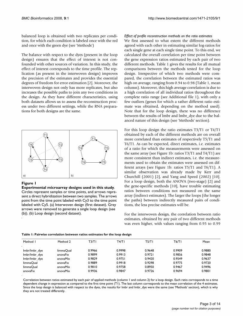
The first dataset was a time series experiment consisting of6 time points measured on 9 arrays using an interwovendesign (Figure 1a). This design resulted in three replicatemeasurements for each time point, with alternating dyes.As a second test, a smaller loop design was derived from theprevious dataset by picking the combination of five arraysthat connect five time points in a single loop (Figure 1b). A

Page 2 of 14(page number not for citation purposes)

BMC Bioinformatics 2008, 9:1 http://www.biomedcentral.com/1471-2105/9/1

balanced loop is obtained with two replicates per condi-tion, for which each condition is labeled once with the redand once with the green dye (see 'Methods')

The balance with respect to the dyes (present in the loopdesign) ensures that the effect of interest is not con-founded with other sources of variation. In this study, theeffect of interest corresponds to the time profile. The rep-lication (as present in the interwoven design) improvesthe precision of the estimates and provides the essentialdegrees of freedom for error estimation [2]. Moreover, theinterwoven design not only has more replicates, but alsoincreases the possible paths to join any two conditions inthe design. As they have different characteristics, usingboth datasets allows us to assess the reconstruction proc-ess under two different settings, while the RNA prepara-tions for both designs are the same.

Effect of profile reconstruction methods on the ratio estimatesWe first assessed to what extent the different methodsagreed with each other in estimating similar log-ratios foreach single gene at each single time point. To this end, wecalculated the overall correlation per time point betweenthe gene expression ratios estimated by each pair of twodifferent methods. Table 1 gives the results for all mutualcomparisons between the methods tested for the loopdesign. Irrespective of which two methods were com-pared, the correlation between the estimated ratios washigh on average, ranging from 0.94 to 0.98 (Table 1, meancolumn). Moreover, this high average correlation is due toa high correlation of all individual ratios throughout thecomplete ratio range (see Additional file 1), with only afew outliers (genes for which a rather different ratio esti-mate was obtained, depending on the method used).Note that for the loop design, there was no differencebetween the results of lmbr and lmbr_dye due to the bal-anced nature of this design (see 'Methods' section).

For this loop design the ratio estimates T3/T1 or T4/T1obtained by each of the different methods are on overallmore correlated than estimates of respectively T5/T1 andT6/T1. As can be expected, direct estimates, i.e. estimatesof a ratio for which the measurements were assessed onthe same array (see Figure 1b: ratios T3/T1 and T4/T1) aremore consistent than indirect estimates, i.e. the measure-ments used to obtain the estimates were assessed on dif-ferent arrays (see Figure 1b: ratios T5/T1 and T6/T1). Asimilar observation was already made by Kerr andChurchill (2001) [2], and Yang and Speed (2002) [10].For a loop design, both the ANOVA (two-stage) [2] andthe gene-specific methods [10], have trouble estimatingratios between conditions not measured on the samearray (indirect estimates). The larger the loops (the longerthe paths) between indirectly measured pairs of condi-tions, the less precise estimates will be.

For the interwoven design, the correlation between ratioestimates, obtained by any pair of two different methodswas even higher, with values ranging from 0.95 to 0.99

Experimental microarray designs used in this studyFigure 1Experimental microarray designs used in this study. Circles represent samples or time points, and arrows repre-sent a direct hybridization between two samples. The arrows point from the time point labeled with Cy3 to the time point labeled with Cy5. (a) Interwoven design (first dataset). Grey arrows were removed to generate a single loop design (see (b)). (b) Loop design (second dataset).

T1

T2

T3

T4

T6

T5

a) b)

T1

T3

T5T6

T4

Table 1: Pairwise correlation between ratios estimates for the loop design

Method 1 Method 2 T3/T1 T4/T1 T5/T1 T6/T1 Mean

lmbr/lmbr_dye limmaQual 0.9966 0.9998 0.9648 0.9909 0.9880lmbr/lmbr_dye anovaFix 0.9899 0.9913 0.9721 0.9856 0.9848lmbr/lmbr_dye anovaMix 0.9829 0.9751 0.9420 0.9549 0.9637limmaQual anovaFix 0.9889 0.9918 0.9298 0.9775 0.9720limmaQual anovaMix 0.9810 0.9758 0.8950 0.9467 0.9496anovaFix anovaMix 0.9936 0.9847 0.9726 0.9694 0.9801

Correlation between ratios estimated by each pair of applied methods (column 1 and column 2) for a loop design. Each ratio corresponds to a time dependent change in expression as compared to the first time point (T1). The last column corresponds to the mean correlation of the 4 estimates. Since the loop design is balanced with respect to the dyes, the results for lmbr and lmbr_dye were the same (see 'Methods' section), which is why they are not treated differently.

Page 3 of 14(page number not for citation purposes)

BMC Bioinformatics 2008, 9:1 http://www.biomedcentral.com/1471-2105/9/1

(see Additional file 2). For this unbalanced design, theratio estimates for the lmbr_dye and the lmbr methodswere no longer exactly the same. The difference in consist-ency between direct and indirect ratio estimates was notobviously visible for this design.

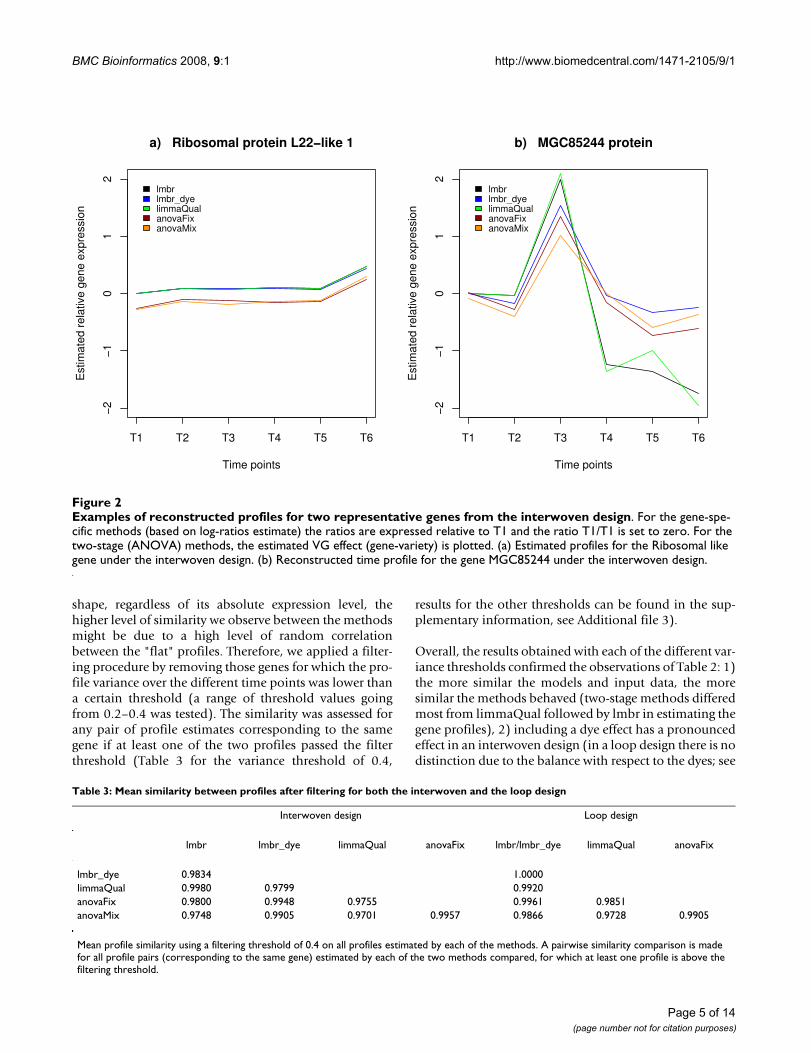
Effect of profile reconstruction methods on the profile shapeA high average correlation between the ratio estimatesobtained by the different methods at each single timepoint is a first valuable assessment. However, it is biolog-ically more important that gene-specific profiles recon-structed by the different methods exhibit the sametendency over time. Therefore, we also compared to whatextent profile shapes estimated by each of the methodsdiffered from each other. This was done by computing themean similarity between profile estimates obtained byany combination of two methods (Table 2).

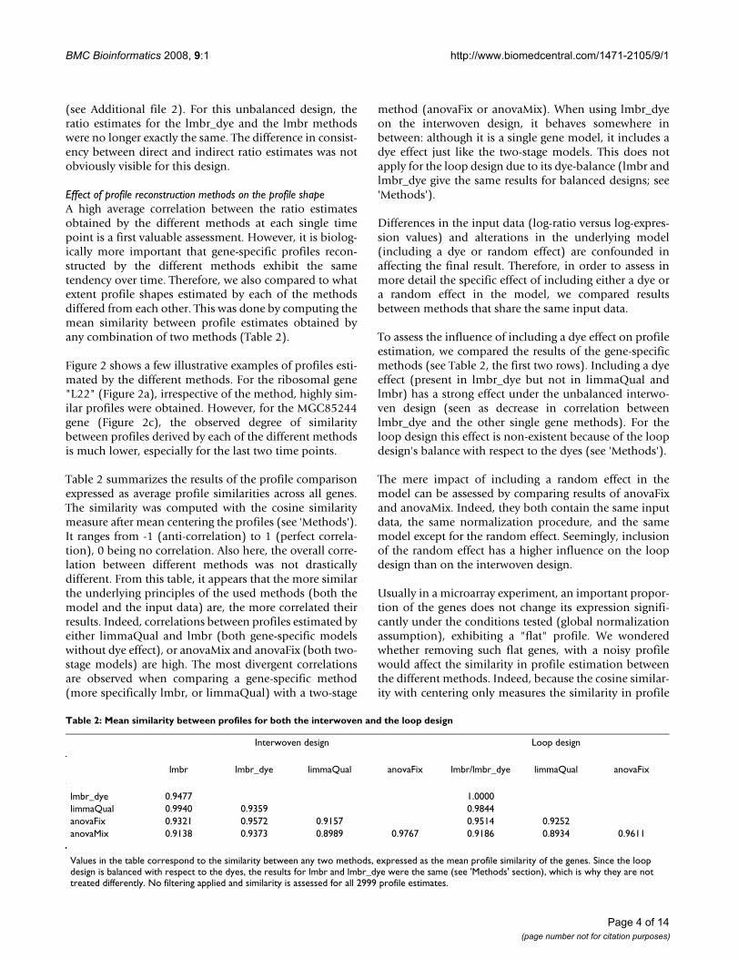
Figure 2 shows a few illustrative examples of profiles esti-mated by the different methods. For the ribosomal gene"L22" (Figure 2a), irrespective of the method, highly sim-ilar profiles were obtained. However, for the MGC85244gene (Figure 2c), the observed degree of similaritybetween profiles derived by each of the different methodsis much lower, especially for the last two time points.

Table 2 summarizes the results of the profile comparisonexpressed as average profile similarities across all genes.The similarity was computed with the cosine similaritymeasure after mean centering the profiles (see 'Methods').It ranges from -1 (anti-correlation) to 1 (perfect correla-tion), 0 being no correlation. Also here, the overall corre-lation between different methods was not drasticallydifferent. From this table, it appears that the more similarthe underlying principles of the used methods (both themodel and the input data) are, the more correlated theirresults. Indeed, correlations between profiles estimated byeither limmaQual and lmbr (both gene-specific modelswithout dye effect), or anovaMix and anovaFix (both two-stage models) are high. The most divergent correlationsare observed when comparing a gene-specific method(more specifically lmbr, or limmaQual) with a two-stage

method (anovaFix or anovaMix). When using lmbr_dyeon the interwoven design, it behaves somewhere inbetween: although it is a single gene model, it includes adye effect just like the two-stage models. This does notapply for the loop design due to its dye-balance (lmbr andlmbr_dye give the same results for balanced designs; see'Methods').

Differences in the input data (log-ratio versus log-expres-sion values) and alterations in the underlying model(including a dye or random effect) are confounded inaffecting the final result. Therefore, in order to assess inmore detail the specific effect of including either a dye ora random effect in the model, we compared resultsbetween methods that share the same input data.

To assess the influence of including a dye effect on profileestimation, we compared the results of the gene-specificmethods (see Table 2, the first two rows). Including a dyeeffect (present in lmbr_dye but not in limmaQual andlmbr) has a strong effect under the unbalanced interwo-ven design (seen as decrease in correlation betweenlmbr_dye and the other single gene methods). For theloop design this effect is non-existent because of the loopdesign's balance with respect to the dyes (see 'Methods').

The mere impact of including a random effect in themodel can be assessed by comparing results of anovaFixand anovaMix. Indeed, they both contain the same inputdata, the same normalization procedure, and the samemodel except for the random effect. Seemingly, inclusionof the random effect has a higher influence on the loopdesign than on the interwoven design.

Usually in a microarray experiment, an important propor-tion of the genes does not change its expression signifi-cantly under the conditions tested (global normalizationassumption), exhibiting a "flat" profile. We wonderedwhether removing such flat genes, with a noisy profilewould affect the similarity in profile estimation betweenthe different methods. Indeed, because the cosine similar-ity with centering only measures the similarity in profile

Table 2: Mean similarity between profiles for both the interwoven and the loop design

Interwoven design Loop design

lmbr lmbr_dye limmaQual anovaFix lmbr/lmbr_dye limmaQual anovaFix

lmbr_dye 0.9477 1.0000limmaQual 0.9940 0.9359 0.9844anovaFix 0.9321 0.9572 0.9157 0.9514 0.9252anovaMix 0.9138 0.9373 0.8989 0.9767 0.9186 0.8934 0.9611

Values in the table correspond to the similarity between any two methods, expressed as the mean profile similarity of the genes. Since the loop design is balanced with respect to the dyes, the results for lmbr and lmbr_dye were the same (see 'Methods' section), which is why they are not treated differently. No filtering applied and similarity is assessed for all 2999 profile estimates.

Page 4 of 14(page number not for citation purposes)

BMC Bioinformatics 2008, 9:1 http://www.biomedcentral.com/1471-2105/9/1

shape, regardless of its absolute expression level, thehigher level of similarity we observe between the methodsmight be due to a high level of random correlationbetween the "flat" profiles. Therefore, we applied a filter-ing procedure by removing those genes for which the pro-file variance over the different time points was lower thana certain threshold (a range of threshold values goingfrom 0.2–0.4 was tested). The similarity was assessed forany pair of profile estimates corresponding to the samegene if at least one of the two profiles passed the filterthreshold (Table 3 for the variance threshold of 0.4,

results for the other thresholds can be found in the sup-plementary information, see Additional file 3).

Overall, the results obtained with each of the different var-iance thresholds confirmed the observations of Table 2: 1)the more similar the models and input data, the moresimilar the methods behaved (two-stage methods differedmost from limmaQual followed by lmbr in estimating thegene profiles), 2) including a dye effect has a pronouncedeffect in an interwoven design (in a loop design there is nodistinction due to the balance with respect to the dyes; see

Table 3: Mean similarity between profiles after filtering for both the interwoven and the loop design

Interwoven design Loop design

lmbr lmbr_dye limmaQual anovaFix lmbr/lmbr_dye limmaQual anovaFix

lmbr_dye 0.9834 1.0000limmaQual 0.9980 0.9799 0.9920anovaFix 0.9800 0.9948 0.9755 0.9961 0.9851anovaMix 0.9748 0.9905 0.9701 0.9957 0.9866 0.9728 0.9905

Mean profile similarity using a filtering threshold of 0.4 on all profiles estimated by each of the methods. A pairwise similarity comparison is made for all profile pairs (corresponding to the same gene) estimated by each of the two methods compared, for which at least one profile is above the filtering threshold.

Examples of reconstructed profiles for two representative genes from the interwoven designFigure 2Examples of reconstructed profiles for two representative genes from the interwoven design. For the gene-spe-cific methods (based on log-ratios estimate) the ratios are expressed relative to T1 and the ratio T1/T1 is set to zero. For the two-stage (ANOVA) methods, the estimated VG effect (gene-variety) is plotted. (a) Estimated profiles for the Ribosomal like gene under the interwoven design. (b) Reconstructed time profile for the gene MGC85244 under the interwoven design.

a) Ribosomal protein L22−like 1

Time points

Est

imat

ed r

elat

ive

gene

exp

ress

ion

T1 T2 T3 T4 T5 T6

−2

−1

01

2

lmbrlmbr_dyelimmaQualanovaFixanovaMix

b) MGC85244 protein

Time points

Est

imat

ed r

elat

ive

gene

exp

ress

ion

T1 T2 T3 T4 T5 T6−

2−

10

12

lmbrlmbr_dyelimmaQualanovaFixanovaMix

Page 5 of 14(page number not for citation purposes)

BMC Bioinformatics 2008, 9:1 http://www.biomedcentral.com/1471-2105/9/1

'Methods'), 3) including a random effect has most influ-ence on the loop design. In addition, it seems that, themore flat profiles are filtered from the dataset, the moresimilar the results obtained by each of the different meth-ods become.

The effect of array failure on the profile reconstructionIn practice, when performing a microarray experimentsome arrays might fail with their measurements fallingbelow standard quality. When these bad measurementsare removed from the analysis, the complete design andthe results inferred from it will be affected. Here we eval-uated this issue experimentally by simulating arraydefects. In a first experiment, the interwoven design (data-set 1) was considered as the original design without fail-ure. We tested 9 different possible situations of failure, byeach time removing a single array from the design, result-ing in 9 reduced datasets. The same test was performedwith the loop design (dataset 2).

We compared for each of the different profile reconstruc-tion methods the mean similarity between the ratiosobtained either with the full dataset or with each of thereduced datasets (9 comparisons). Table 4 summarizesthe results for the interwoven design, and Table 5 for theloop design.

For the interwoven design (Table 4), it appears that ingeneral removing one array from the original design didnot really affect the ratio reconstruction. For all methods,ratio estimates tend to be more affected when an arraymeasuring the reference time point was removed (T1)(Table 4). Overall the two-stage methods, and in particu-lar anovaMix, seemed most robust against array failure,while limmaQual was most sensitive (Table 4). Methodsincluding a dye effect were more robust against array fail-ure. Similar results were obtained when the effect of array

failure was assessed on the similarity in profiles (see Addi-tional file 4).

For the loop design, the situation was quite different(Table 5). Note that here, the lmbr_dye and limmaQualmethods were not used for profile reconstruction as thereduced datasets did not contain sufficient informationfor estimating all the model parameters. For bothlmbr_dye and limmaQual, the linear models lose theirmain differing characteristics compared to lmbr (see'Methods' section). For all remaining methods removingone array from the design affected the results considerablymore than was the case for the interwoven design. Two-stage methods were the most robust, but in this designanovaMix performs slightly worse than anovaFix. Thelmbr method turned out to be very sensitive to array fail-ure, giving a mean profile similarity around 0.2, indicat-ing no correlation between profiles estimated with andwithout array failure (see Additional file 5).

Note that overall, all methods seem to be more robust toarray failure under the interwoven design than under theloop design. This is to be expected as the latter design con-tains more replicates.

Consistency of the methods under different normalization proceduresIn the previous section we compared profiles and ratioestimates obtained by the different methods after apply-ing default normalization steps. However, other normali-zation strategies are possible, and could potentially affectthe outcome. To assess the influence of using alternativenormalization procedures, we compared profiles recon-structed from data normalized with 1) print tip Loesswithout additional normalization step (the default settingfor anovaMix and anovaFix as used throughout thispaper), 2) print tip Loess with a scale-based normaliza-

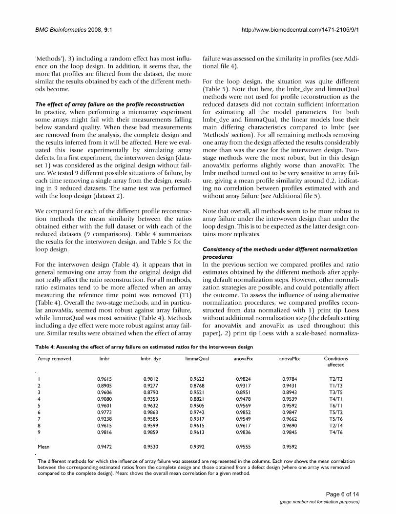
Table 4: Assessing the effect of array failure on estimated ratios for the interwoven design

Array removed lmbr lmbr_dye limmaQual anovaFix anovaMix Conditions affected

1 0.9615 0.9812 0.9623 0.9824 0.9784 T2/T32 0.8905 0.9277 0.8768 0.9317 0.9431 T1/T33 0.9606 0.8790 0.9521 0.8951 0.8943 T3/T54 0.9080 0.9353 0.8821 0.9478 0.9539 T4/T15 0.9601 0.9632 0.9505 0.9569 0.9592 T6/T16 0.9773 0.9863 0.9742 0.9852 0.9847 T5/T27 0.9238 0.9585 0.9317 0.9549 0.9662 T5/T68 0.9615 0.9599 0.9615 0.9617 0.9690 T2/T49 0.9816 0.9859 0.9613 0.9836 0.9845 T4/T6

Mean 0.9472 0.9530 0.9392 0.9555 0.9592

The different methods for which the influence of array failure was assessed are represented in the columns. Each row shows the mean correlation between the corresponding estimated ratios from the complete design and those obtained from a defect design (where one array was removed compared to the complete design). Mean: shows the overall mean correlation for a given method.

Page 6 of 14(page number not for citation purposes)

BMC Bioinformatics 2008, 9:1 http://www.biomedcentral.com/1471-2105/9/1

tion between arrays [11], and 3) print tip Loess with aquantile-based between array normalization [12,13] (thedefault normalization for lmbr, lmbr_dye, and lim-maQual as used throughout this paper).

Table 6 shows, for each of the different methods, themean similarity between reconstructed profiles derivedfrom differently normalized datasets. Overall, the influ-ence of the normalization was not drastic. More impor-tantly, the influence of the additional normalization stepsseemed independent of the method used (similar influ-ences were observed for all methods). When assessing thesimilarity in ratio estimates instead of profile estimates,similar results were obtained (data not shown).

Accuracy of estimationSo far we only assessed to what extent changes in the usedmethodologies or normalization steps affected theinferred profiles. This, however, does not give any infor-mation on the accuracy of the methods, i.e., which of

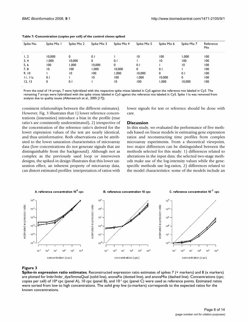
these methods is able to best approximate the true timeprofiles. Assessing the accuracy is almost impossible asusually the true underlying time profile is not known.However, datasets that contain external controls (spikes)could prove useful in this regard. Spikes are added to thehybridisation solution in known quantities, so that wehave a clear view of their actual profile. In the followinganalysis, we used a publicly available spike-in experimentin attempt to assess the accuracy of each of the profilereconstruction methods [14]. For the technical details ofthis dataset we refer to 'Methods' and Table 7.

As lmbr and lmbr_dye and limmaQual gave exactly thesame results using this balanced design, we furtherassessed to what extent lmbr, anovaFix and anovaMixagreed with each other. Fig. 3 shows the effect of using dif-ferent spike concentrations as reference points for ratioestimation. Panels A through C reflect decreasing refer-ence concentrations. The choice of reference has littleeffect on the shape of the profile (as indicated by

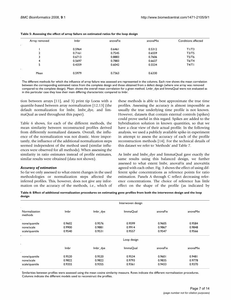
Table 6: Effect of additional normalization procedures on estimating gene profiles from both the interwoven design and the loop design

Interwoven design

Normalization methods

lmbr lmbr_dye limmaQual anovaFix anovaMix

none/quantile 0.9602 0.9576 0.9599 0.9605 0.9584none/scale 0.9900 0.9881 0.9914 0.9867 0.9848scale/quantile 0.9540 0.9531 0.9557 0.9547 0.9566

Loop design

lmbr lmbr_dye limmaQual anovaFix anovaMix

none/quantile 0.9520 0.9520 0.9534 0.9601 0.9481none/scale 0.9822 0.9822 0.9793 0.9835 0.9778scale/quantile 0.9355 0.9355 0.9361 0.9433 0.9370

Similarities between profiles were assessed using the mean cosine similarity measure. Rows indicate the different normalization procedures. Columns indicate the different models used to reconstruct the profiles.

Table 5: Assessing the effect of array failure on estimated ratios for the loop design

Array removed lmbr anovaFix anovaMix Conditions affected

1 0.5964 0.6461 0.5312 T1/T32 0.7161 0.7545 0.6559 T3/T53 0.6713 0.8883 0.7606 T5/T64 0.5697 0.7883 0.6637 T6/T45 0.4359 0.6042 0.5534 T4/T1

Mean 0.5979 0.7363 0.6330

The different methods for which the influence of array failure was assessed are represented in the columns. Each row shows the mean correlation between the corresponding estimated ratios from the complete design and those obtained from a defect design (where one array was removed compared to the complete design). Mean: shows the overall mean correlation for a given method. Lmbr_dye and limmaQual were not evaluated as in this particular case they lose their main differing characteristic compared to lmbr.

Page 7 of 14(page number not for citation purposes)

BMC Bioinformatics 2008, 9:1 http://www.biomedcentral.com/1471-2105/9/1

consistent relationships between the different estimates).However, Fig. 3 illustrates that 1) lower reference concen-trations (intensities) introduce a bias in the profile (trueratio's are consistently underestimated), 2) irrespective ofthe concentration of the reference ratio's derived for thelower expression values of the test are nearly identical,and thus uninformative. Both observations can be attrib-uted to the lower saturation characteristics of microarraydata (low concentrations do not generate signals that aredistinguishable from the background). Although not ascomplex as the previously used loop or interwovendesigns, the spiked-in design illustrates that this lower sat-uration effect, an inherent property of microarray data,can distort estimated profiles: interpretation of ratios with

lower signals for test or reference should be done withcare.

DiscussionIn this study, we evaluated the performance of five meth-ods based on linear models in estimating gene expressionratios and reconstructing time profiles from complexmicroarray experiments. From a theoretical viewpoint,two major differences can be distinguished between themethods selected for this study: 1) differences related toalterations in the input data: the selected two-stage meth-ods make use of the log-intensity values while the gene-specific methods use log-ratios, 2) differences related tothe model characteristics: some of the models include an

Spike-in expression ratio estimatesFigure 3Spike-in expression ratio estimates. Reconstructed expression ratio estimates of spikes 7 (+ markers) and 8 (x markers) are plotted for lmbr/lmbr_dye/limmaQual (solid line), anovaFix (dotted line), and anovaMix (dashed line). Concentrations (cpc; copies per cell) of 104 cpc (panel A), 10 cpc (panel B), and 10-1 cpc (panel C) were used as reference points. Estimated ratios were sorted from low to high concentrations. The solid grey line (o-markers) corresponds to the expected ratios for the known concentrations.

Table 7: Concentration (copies per cell) of the control clones spiked

Spike No. Spike Mix 1 Spike Mix 2 Spike Mix 3 Spike Mix 4 Spike Mix 5 Spike Mix 6 Spike Mix 7 Reference Mix

1, 2 10,000 0 0.1 1 10 100 1,000 1003, 4 1,000 10,000 0 0.1 1 10 100 1005, 6 100 1,000 10,000 0 0.1 1 10 1007, 8 10 100 1,000 10,000 0 0.1 1 1009, 10 1 10 100 1,000 10,000 0 0.1 10011, 11a 0.1 1 10 100 1,000 10,000 0 10012, 13 0 0.1 1 10 100 1,000 10,000 100

From the total of 14 arrays, 7 were hybridized with the respective spike mixes labeled in Cy5 against the reference mix labeled in Cy3. The remaining 7 arrays were hybridized with the spike mixes labeled in Cy3 against the reference mix labeled in Cy5. Spike 11a was removed from analysis due to quality issues (Allemeersch et al., 2005 [17]).

Page 8 of 14(page number not for citation purposes)

BMC Bioinformatics 2008, 9:1 http://www.biomedcentral.com/1471-2105/9/1

explicit dye effect (lmbr_dye, anovaFix and anovaMix) oran explicit random effect (anovaMix).

Although Kerr [5] assumed that observed differences inestimates obtained by different models are due to the dif-ferences in model characteristics, rather than to the inputdata, we cannot clearly make this distinction. Indeed, theway the error-term is modeled influences the statisticalinference and hence the use of log-intensities or log-ratiosdoes cause a difference between models [5]. However,when focusing on results obtained between methods withsimilar input data, we can assess, to some extent, the effectof different model specificities. In the following sections,some of these effects are discussed more in detail.

The inclusion of the dye effectIn general we observed that, gene-specific methods with-out dye effects, and two-stage models with dye effectbehaved more similar with each other than when theywere compared among each other. Lmbr_dye (a gene-spe-cific model with dye effect) is situated somewhere inbetween when the design is unbalanced with respect tothe dyes. Indeed, the gene-specific models lmbr and lim-maQual contain a combination of log-ratios plus an errorterm. However, when adding a dye effect to these modelsas is the case of lmbr_dye, the formulations and estima-tions converge with those of the two-stage ANOVA mod-els for unbalanced designs.

Originally, Vinciotti, et al. (2005) [3] and Wit, et al.(2005) [15] added the dye effect for purposes of data nor-malization when one is working with non-normalizeddata. From our results, we also noted a practical advantageof including a dye effect even with normalized data. Thefact that adding a dye effect showed pronounced differ-ences for a dye-unbalanced design indicates that, despitethe data being normalized, there are still dye-relatedinconsistencies in the data that might -partially- be com-pensated for by including a dye effect. Moreover, modelswith dye effects seemed more robust in estimating log-ratios from a design disturbed by array failure. Therefore,when working with unbalanced designs, it is advisable toinclude a dye effect, not only for the two-stage ANOVAmodels, as was also suggested by Wolfinger (2001) [16],Kerr (2003) [5], and Kerr and Churchill (2001) [2], butalso for gene-specific models based on log-ratios.

Mixed models versus Fixed modelsSeveral studies advise the users to model the spot-gene orarray-gene effects as random variables [9,16]. Weobserved that under the loop design (with 5 arrays), pro-files estimated by anovaMix and anovaFix diverged. Wealso noticed that, for the loop design anovaMix had alower capacity than anovaFix to handle array failures. Forthe interwoven design with 9 arrays these effects were less

pronounced. The loop design used in our study does notcontain a sufficient number of replicates to allow for reli-able estimation of the spot-gene effect when using amixed ANOVA model. As a result, ratios and time profilesestimated by anovaMix than anovaFix are less reliable foran experiment with few replicates

The effect of using alternative normalization steps on the methods' performanceWe tested the influence of using additional normalizationsteps. Differently normalized data give different results,but the effects were not dramatic. Moreover, they had thesame influence on all methods, indicating that allmethods were equally sensitive to changes in thenormalization.

Accuracy of estimated ratiosBased on spike-in experiments for two-channel microar-rays, we could also assess to what extent the estimatedratios approximated the true ratios (i.e., the accuracy ofthe estimated ratios). We observed that all five tested lin-ear methods generated biased estimations, consistentlyoverestimating changes in expression relative to a refer-ence with low mRNA-concentration. These results wereindependent of the method used (gene-specific or two-stage) or of the number of effects included the model.

ConclusionOn average the correlation between the estimated ratioswas high, and all methods more or less agreed with eachother in predicting the same profile. The similarity in pro-file estimation between the different methods improvedwith an increasing variance of the expression profiles.

We observed that when dealing with unbalanced designs,including a dye effect, such as in the methods lmbr_dye,anovaFix and anovaMix, seems to compensate for residualdye related inconsistencies in the data (despite an earliernormalization step). Adding a dye effect also renders theresults more robust against array failure. Including ran-dom effects requires more parameters to be estimated andis only advised when a design is used with a sufficientnumber of replicates.

Conclusively, because of their robustness against imbal-ances in the design and array failure, we believe lmbr_dye,anovaFix and anovaMix are most appropriate for practicaluse (given a sufficient number of replicates in case of thelatter).

MethodsMicroarray dataThe first dataset used in this study was a temporal Xenopustropicalis expression profiling experiment. The array usedconsisted of 2999 oligos of 50 mers, corresponding to

Page 9 of 14(page number not for citation purposes)

BMC Bioinformatics 2008, 9:1 http://www.biomedcentral.com/1471-2105/9/1

2898 unique X. tropicalis gene sequences and negativecontrol spots (Arabidopsis thaliana probes, blanks andempty buffer controls). Each oligo was spotted in dupli-cate on each array in two separated grids. On each grid,oligonucleotides were spotted in 16 blocks of 14 × 14spots. Pairs of duplicated oligo's on the two grids of thesame gene sequence were treated as replicates during anal-ysis, corresponding to a total of 2999 different duplicatedmeasurements (a few oligos were spotted multiple timeson the arrays). MWG Biotech performed oligonucleotidedesign, synthesis and spotting. X. tropicalis gene sequenceswere derived from the assembly of public and in-houseexpressed sequence tags. The temporal expression of X.tropicalis during metamorphosis was profiled at 6 timepoints, using an experimental design consisting of 9arrays. Each time point was measured three times, withalternating dyes as shown in Figure 1a. This interwovendesign was used as a first test set.

From this original design a second test set containing asmaller loop design was derived by picking the combina-tions of five arrays that connect five time points in a singleloop (Figure 1b) and with the first time point as a refer-ence. This results in a balanced loop design

A publicly available spike-in experiment [17] was used asa third test set. This dataset contains 13 spikes-in, or con-trol clones spiked with known concentrations. The con-trol clones were spiked at different concentrations for eachof the 7 conditions (Table 7).

The microarray design used for the spike-in experimentwas a common reference design, with dye swap for eachcondition, and the concentrations of spikes ranges from 0to 10,000 copies per cellular equivalent (cpc), assumingthat the total RNA contained 1% poly(A) mRNA and thata cell contained on average 300,000 transcripts. This con-centration range covered all biologically relevant tran-script levels.

Probes preparation and microarray hybridization10 μg of total RNA were used to prepare probes. Labelingwas performed with the Invitrogen SuperScript™ IndirectcDNA labeling system (using polyA and random hexam-ers primers) using the Amersham Cy3 or Cy5 monofunc-tional reactive dyes. Probe quality was assessed on anagarose minigel and quantified with a Nanodrop ND-1000 spectrophotometer. Dye quantities were equili-brated for hybridization by the amount of fluorescenceper ng of cDNA. The arrays were hybridized for 20 h at45°C according to the manufacturers protocol (QMT ref).Washing was performed in 2× SSC 0.1% SDS at 42°C for5' and then twice at room temperature in 1× SSC, 0.5×SSC each time for 5'. Arrays were scanned using a GenePixAxon scanner.

Microarray normalizationThe raw intensity data were used for further normaliza-tion. No background subtraction was performed. Datawere log-transformed and the intensity dependent dye orcondition effects were removed by using a local linear fitloess on these log-transformed data (Printtiploess com-mand with default settings as implemented in the limmaBioConductor package [18]). As this loess fit not only nor-malizes the data but also linearizes them, applying itbefore profile reconstruction is a prerequisite as all linearmodels used for profile reconstruction assume non linear-ities to be absent from the data.

For the gene-specific methods (lmbr, lmbr_dye and lim-maQual), Loess corrected log-ratios (per print tip) weresubjected to an additional quantile normalization step[4,12] as suggested by Vinciotti et al. (2005) [3] in orderto improve the intercomparability between arrays. Itequalizes the distribution of probe intensities for eacharray in a set of arrays. For the two-stage profile recon-struction methods (anovaFix and anovaMix), correctedlog-intensities for the red (RCORR) and green (GCORR) chan-nels were calculated from the Loess corrected log-ratios(MCORR; no additional quantile normalization was donefor the two-stage methods) and mean absolute intensities(A) as follows: RCORR = (A + MCORR)/2, and GCORR = (A -MCORR)/2.

Used profile reconstruction methodsAvailable R implementations (BioConductor [19]) of thepresented methods were used to perform the analyses.

Gene-specific methods based on log-ratiosGene-specific profile reconstruction methods apply a lin-ear model on each gene separately. The goal is to estimatethe true expression differences between the mRNA ofinterest and the reference mRNA, from the observed log-ratios. The presented models assume that the expressionvalues have been appropriately pre-processed and nor-malized [3,20]. The three selected gene-specific modelsfor this study are:

1) lmbr, the linear model described by Vinciotti et al. (2005)[3]:

An observation yjk is the log-ratio of condition j and con-dition k. For each gene a vector of n observations y =(y1,...,yn) can be represented as

y = X +

where X is the design matrix defining the relationshipbetween the values observed in the experiment and a set

of independent parameters = ( 12, 13,..., 1T representing

Page 10 of 14(page number not for citation purposes)

BMC Bioinformatics 2008, 9:1 http://www.biomedcentral.com/1471-2105/9/1

true expression differences, and is a vector of errors. The

parameters in are arbitrarily chosen this way for estima-tion purposes; all expression differences between otherconditions i and k can be calculated from these parame-

ters as ik = 1k - 1i. The goal is to obtain estimates of the true

expression differences separately for each gene. Giventhe assumptions behind the linear model, the least

squares estimator for is [3]

2) lmbr_dye, an extension of lmbr including a general dyeeffect:

The previous model can be extended to include a gene-specific dye effect [3]

y = X + D +

where D is a vector of n times a constant value representingthe gene-specific dye effect . Alternatively, one could writey = XD D + where XD is the design matrix X with an extra col-umn of ones, and = ( 12, 13,..., 1T, ). Note that in the caseof dye-balanced designs, the addition of a dye effect willnot yield any different estimators for the contrasts of inter-est. In a balanced design, each column of X will have anequal amount of 1's and -1's. I.e. the ith column of X, cor-responding to the true expression difference 1i, reflects howcondition i was measured an equal number of times withboth dyes. As such, the positive and negative influences ofthe dye effect will cancel each other out in the estimation oftrue expression differences. The use of lmbr_dye will thusonly render different results compared to lmbr when usingit to analyze unbalanced experiments.

In order to estimate all parameters, the matrix XD must beof full rank. If the column representing the dye effect isnot linearly independent, the matrix is rank deficient. Thissituation occurs for example when an array is removedfrom the loop design used in this paper. In this case, thereare an infinite number of possible least squares parameterestimates. Since we expect a single set of parameters, aconstraint must be applied (this is done on the dye effect)in which case the true expression estimates are the same asfor lmbr.

Lmbr and lmbr_dye were implemented in the R languageusing the function 'lm' for linear least squares regression.

3) limmaQual, the Limma model [4,20,21] including anarray quality adjustment:

The quality adjustment assigns a low weight to poor qual-ity arrays, which can be included in the inference. The

approach is based on the empirical reproducibility of thegene expression measures from replicated arrays, and itcan be applied to any microarray experiment. The linearmodel is similar to the model describes by Vinciotti et al.,(2005) but the variance of the observations y includes theweight term. In this case, the weighted least squares esti-

mator of is [20]:

where Σ is the diagonal matrix of weights.

The weights in the limmaQual model are the inverse ofestimated array variances, down weighting the observa-tions of lower quality arrays in order to decrease thepower to detect differential expression. The method isrestricted for use on data from experiments that include atleast two degrees of freedom. When testing the array fail-ure in case of the loop design, there is no array level repli-cation for two of the conditions so the array qualityweights can not be estimated: the Limma function returnsa perfect quality for all the arrays (in this case Σ is a diag-onal matrix of 1's).

The fit is by generalized least squares allowing for correla-tion between duplicate spots or related arrays, imple-mented in an internal function (gls.series) of the Limmapackage.

Two-stage methods based on the log-intensity valuesThe selected methods correspond to ANOVA (Analysis ofvariance) models. They can normalize microarray dataand provide estimates of gene expression levels that arecorrected for potential confounding effects.

Since the global methods are computationally time-con-suming, we selected two-stage methods that apply a firststage on all data simultaneously and a second stage on agene by gene level. These models use partially normalizeddata as input (i.e., the separate log-intensity values foreach channel), as spot effects are explicitly incorporated.They return normalized absolute expression levels foreach channel separately (i.e. no ratios), which can then beused to reconstruct the required time profile.

4) anovaFix, two-stage ANOVA with fixed effects [6]:

We denote the loess-normalized log-intensity data by yijkgrthat represents the measurement observed in the array i,labeled with the dye j, representing the time point k, fromgene g and spot r. The first stage is the normalizationmodel:

yijkgr = + Ai + Dj + ADij + rijkgr

μ̂

ˆ ( )μ = −X X X yt t1

μ̂

ˆ ( )μ = ∑ ∑− − −X X X yt t1 1 1

Page 11 of 14(page number not for citation purposes)

BMC Bioinformatics 2008, 9:1 http://www.biomedcentral.com/1471-2105/9/1

where the term captures the overall mean. The otherterms capture the overall effects due to arrays (A), dyes(D) and labelling reactions (AD). This step is called "nor-malization step" and it accounts for experiment system-atic effects that could bias inferences made on the datafrom the individual genes. The residual of the first stage isthe input for the second stage, which models the gene-specific effects:

rijkgr = G + SGr + DGj + VGk + ijkgr

Here G captures the average effect of the gene. The SGeffect captures the spot-gene variation and we used itinstead of the more global AG array-gene effect. The use ofthis effect obviates the need for intensity ratios. DG cap-tures specific dye-gene variation and VG (variety-gene) isthe effect of interest, the effects due to the time pointmeasured. The MAANOVA fixed model computes leastsquares estimators for the different effects.

5) anovaMix, two-stage ANOVA with mixed effects [6,16]:

The model applied is exactly the same as anovaFix, but inthis case the SG effect was treated as a random variable,meaning that if the experiment were to be repeated, therandom spot effects would not be exactly reproduced, butthey would be drawn from a hypothetical population. Amixed model, where some variables are treated as ran-dom, allows for including multiple sources of variation.

We used the default method to solve the mixed modelequation, the REML (restricted maximum likelihood)method. Duplicated spots were treated as independentmeasurements of the same gene. For MAANOVA andLimma packages the option to do so is available, for lmbrand lmbr_dye duplicated spots were taken into accountby the design matrix.

Profile reconstructionApplying the gene-specific methods mentioned aboveresults in estimated differences in log-expression between atest and a reference condition or in log-ratios. To recon-struct from the different designs a time profile, the first timepoint was chosen as the reference. A gene-specific recon-structed profile thus consists of a vector which contains asentries ratios of the measured expression level of that geneat each time point except the first, relative to its expressionvalue at the first time point. For instance, for the loopdesign shown in Table 1 the profile contains 4 ratios.

In contrast to the gene-specific methods, two-stage meth-ods estimate the absolute gene expression level for eachtime point rather than log-ratios. In this case, for the loopdesign shown in Table 1, the profile contains 5 geneexpression levels.

Comparison of profile reconstructionTo assess the influence of using different methodologieson the profile reconstruction, the following similaritymeasures were used to compare the consistency in recon-structing profiles for the same gene between the comparedmethods:

1. Overall similarity in the estimated ratios: we assessedthe similarity between the estimations of each single ratioof the time profile generated by two methods using thePearson correlation. Since two-stage methods estimategene expression levels (variety-gene effect in the model)instead of log-ratios, we converted these absolute valuesinto log-ratios by subtracting from the absolute expres-sion levels estimated for each of the conditions the esti-mated level of the first time point (the reference).

2. Profile shape similarity: the profile shape reflects theexpression behaviour of a gene over time. For each singlegene, we computed the mutual similarity between profileestimates obtained by any combination of two methods.To make profiles consisting of log-ratios obtained by thegene-specific methods comparable with the profiles esti-mated by the two-stage methods, we extended the log-ratios profile by adding as a first time point a zero. Thisrepresents the contrast between the expression value ofthe first time point against itself in log-scale (Figure 2).

Profile SimilarityThe mutual similarity was computed as the cosine similar-ity, which corresponds to the angle between two vectorsrepresenting genes i and j with profiles Pi and Pj.

All profiles were mean centered, i.e. data have been shiftedby the mean of the profile ratios to have an average of zerofor each gene, prior to computing the cosine similarity.With centered data, the cosine similarity can also be viewedas the correlation coefficient, and it ranges between -1(opposite shape) and 1 (similar shape), 0 being no correla-tion. The cosine similarity only considers the angle betweenthe vectors focusing on the shape of the profile. As a result,it ignores the magnitude of ratios of the profiles, resultingin relatively high similarities for false positives (i.e. "flatprofiles", genes that do not change their expression profileover time, but for which the noise profile corresponds bychance to other gene profiles).

No variance normalization was performed on the profilesto preserve their shape. Instead of normalizing by the vari-ance, the profiles were filtered using the standard deviation.

cos( , )P PPi PjPi Pji j =

⋅

Page 12 of 14(page number not for citation purposes)

BMC Bioinformatics 2008, 9:1 http://www.biomedcentral.com/1471-2105/9/1

Filtering flat profilesConstitutively expressed genes or genes for which theexpression did not significantly change over the condi-tions were filtered by removing genes of which the vari-ance in expression over different conditions was lowerthan a fixed threshold (the following range of thresholdswas tested: 0.1, 0.2, 0.4). A pair wise similarity compari-son was made for all profile estimates (corresponding tothe same gene) that were above the filtering threshold inat least one of the two methods compared. Similar resultswere obtained when applying as a filter that all profileestimates had to be above the filtering threshold in bothmethods compared (data not shown).

Authors' contributionsAF performed the analysis and wrote the manuscript. RTand NP were responsible for the microarray hybridiza-tion. NP and GB critically read the draft. KE contributed tothe analysis. KM coordinated the work and revised themanuscript. All authors read and approved the final man-uscript.

Additional material

AcknowledgementsWe thank Dr. Filip Vandenbussche for his comments on earlier versions of this manuscript. AF was partially supported by a grant French embassy – CONICYT Chili. This work was also partially supported by 1) IWT: SBO-BioFrame, 2) Research Council KULeuven: EF/05/007 SymBioSys, IAP BioMagnet.

References1. Glonek GF, Solomon PJ: Factorial and time course designs for

cDNA microarray experiments. Biostatistics (Oxford, England)2004, 5(1):89-111.

2. Kerr MK, Churchill GA: Experimental design for gene expres-sion microarrays. Biostatistics (Oxford, England) 2001, 2(2):183-201.

3. Vinciotti V, Khanin R, D'Alimonte D, Liu X, Cattini N, Hotchkiss G,Bucca G, de Jesus O, Rasaiyaah J, Smith CP, Kellam P, Wit E: Anexperimental evaluation of a loop versus a reference designfor two-channel microarrays. Bioinformatics (Oxford, England)2005, 21(4):492-501.

4. Smyth GK: Linear models and empirical bayes methods forassessing differential expression in microarray experiments.Stat Appl Genet Mol Biol 2004, 3:Article3.

5. Kerr MK: Linear models for microarray data analysis: hiddensimilarities and differences. J Comput Biol 2003, 10(6):891-901.

6. MAANOVA software [http://www.jax.org/staff/churchill/labsite/software/anova]

7. Tsai CA, Chen YJ, Chen JJ: Testing for differentially expressedgenes with microarray data. Nucleic acids research 2003,31(9):e52.

8. Marchal K, Engelen K, De Brabanter J, Aert S, De Moor B, Ayoubi T,Van Hummelen P: Comparison of different methodologies toidentify differentially expressed genes in two-sample cDNAmicroarrays. J Biological Systems 2002, 10(4):409-430.

9. Cui X, Churchill GA: Statistical tests for differential expressionin cDNA microarray experiments. Genome biology 2003,4(4):210.

10. Yang YH, Speed T: Design issues for cDNA microarray experi-ments. Nature reviews 2002, 3(8):579-588.

Additional file 1Plot of corresponding ratios estimated by two linear methods. Comparison of corresponding ratios estimated by lmbr and anovaMix using the loop design. The line indicates the identity between both methods and most of the points are situated near this identity line.Click here for file[http://www.biomedcentral.com/content/supplementary/1471-2105-9-1-S1.pdf]

Additional file 2Pairwise correlation between ratios estimated for the interwoven design. The table shows the pairwise correlation between ratios estimated by each pair of methods (columns 1 and 2) for the interwoven design. The ratios correspond to the change in expression compared to the first time point. The last column corresponds to the mean correlation of the 5 estimations.Click here for file[http://www.biomedcentral.com/content/supplementary/1471-2105-9-1-S2.pdf]

Additional file 3Mean similarity between profiles using different filtering thresholds. Val-ues in the table correspond to the similarity between any two methods, expressed as the mean profile similarity of the genes. Results are shown for both the interwoven and loop design using different filtering thresholds. Since the loop design is balanced with respect to the dyes, the results for lmbr and lmbr_dye were the same (see 'Methods' section), which is why they are not treated differently. A) No filtering applied, similarity is assessed for all 2999 profile estimates, B) a filtering threshold (SD) is used on all profiles estimated by each of the methods, a pairwise similarity comparison is made for all profile pairs (corresponding to the same gene) estimated by each of the two methods compared, for which at least one pro-file is above the filtering threshold (SD >0.1, 0.2, 0.4 respectively).Click here for file[http://www.biomedcentral.com/content/supplementary/1471-2105-9-1-S3.pdf]

Additional file 4Effect of array failure for the interwoven design. The table shows the effect of array failure in reconstructing profiles from an interwoven design. Pro-file similarities were assessed using the cosine similarity. The different methods for which the influence of the failure was assessed are represented in the columns. Each row shows the mean cosine similarity between the corresponding profiles estimated from the complete design and those obtained from a defect design (where one array was removed compared to the complete design). Mean: shows the overall mean similarity for a given method.Click here for file[http://www.biomedcentral.com/content/supplementary/1471-2105-9-1-S4.pdf]

Additional file 5Effect of array failure for the loop design. The table shows the effect of array failure in reconstructing profiles from a loop design. Profile similar-ities were assessed using the cosine similarity. The different methods for which the influence of the failure was assessed are represented in the col-umns. Each row shows the mean cosine similarity between the correspond-ing profiles estimated from the complete design and those obtained from a defect design (where one array was removed compared to the complete design). Mean: shows the overall mean similarity for a given method.Click here for file[http://www.biomedcentral.com/content/supplementary/1471-2105-9-1-S5.pdf]

Page 13 of 14(page number not for citation purposes)

BMC Bioinformatics 2008, 9:1 http://www.biomedcentral.com/1471-2105/9/1

Publish with BioMed Central and every scientist can read your work free of charge

"BioMed Central will be the most significant development for disseminating the results of biomedical research in our lifetime."

Sir Paul Nurse, Cancer Research UK

Your research papers will be:

available free of charge to the entire biomedical community

peer reviewed and published immediately upon acceptance

cited in PubMed and archived on PubMed Central

yours — you keep the copyright

Submit your manuscript here:http://www.biomedcentral.com/info/publishing_adv.asp

BioMedcentral

11. Smyth GK, Speed T: Normalization of cDNA microarray data.Methods (San Diego, Calif 2003, 31(4):265-273.

12. Yang YH, Thorne NP: Normalization for two-color cDNAmicroarray data. Science and Statistics: A Festschrift for Terry Speed,IMS Lecture Notes-Monograph Series 2003, 40:403-418.

13. Bolstad BM, Irizarry RA, Astrand M, Speed TP: A comparison ofnormalization methods for high density oligonucleotidearray data based on variance and bias. Bioinformatics (Oxford,England) 2003, 19(2):185-193.

14. Hilson P, Allemeersch J, Altmann T, Aubourg S, Avon A, Beynon J,Bhalerao RP, Bitton F, Caboche M, Cannoot B, Chardakov V, Cognet-Holliger C, Colot V, Crowe M, Darimont C, Durinck S, Eickhoff H, deLongevialle AF, Farmer EE, Grant M, Kuiper MT, Lehrach H, Leon C,Leyva A, Lundeberg J, Lurin C, Moreau Y, Nietfeld W, Paz-Ares J, Rey-mond P, Rouze P, Sandberg G, Segura MD, Serizet C, Tabrett A,Taconnat L, Thareau V, Van Hummelen P, Vercruysse S, Vuylsteke M,Weingartner M, Weisbeek PJ, Wirta V, Wittink FR, Zabeau M, SmallI: Versatile gene-specific sequence tags for Arabidopsis func-tional genomics: transcript profiling and reverse geneticsapplications. Genome research 2004, 14(10B):2176-2189.

15. Wit E, Nobile A, Khanin R: Near-optimal designs for dual-chan-nel microarray studies. Applied Statistics 2005, 54(5):817-830.

16. Wolfinger RD, Gibson G, Wolfinger ED, Bennett L, Hamadeh H,Bushel P, Afshari C, Paules RS: Assessing gene significance fromcDNA microarray expression data via mixed models. J Com-put Biol 2001, 8(6):625-637.

17. Allemeersch J, Durinck S, Vanderhaeghen R, Alard P, Maes R, SeeuwsK, Bogaert T, Coddens K, Deschouwer K, Van Hummelen P, Vuyl-steke M, Moreau Y, Kwekkeboom J, Wijfjes AH, May S, Beynon J,Hilson P, Kuiper MT: Benchmarking the CATMA microarray.A novel tool for Arabidopsis transcriptome analysis. Plantphysiology 2005, 137(2):588-601.

18. Yang YH, Dudoit S, Luu P, Lin DM, Peng V, Ngai J, Speed TP: Nor-malization for cDNA microarray data: a robust compositemethod addressing single and multiple slide systematic vari-ation. Nucleic acids research 2002, 30(4):e15.

19. Gentleman RC, Carey VJ, Bates DM, Bolstad B, Dettling M, Dudoit S,Ellis B, Gautier L, Ge Y, Gentry J, Hornik K, Hothorn T, Huber W,Iacus S, Irizarry R, Leisch F, Li C, Maechler M, Rossini AJ, Sawitzki G,Smith C, Smyth G, Tierney L, Yang JY, Zhang J: Bioconductor: opensoftware development for computational biology and bioin-formatics. Genome biology 2004, 5(10):R80.

20. Ritchie ME, Diyagama D, Neilson J, van Laar R, Dobrovic A, HollowayA, Smyth GK: Empirical array quality weights in the analysis ofmicroarray data. BMC bioinformatics 2006, 7:261.

21. Smyth GK, Michaud J, Scott HS: Use of within-array replicatespots for assessing differential expression in microarrayexperiments. Bioinformatics (Oxford, England) 2005,21(9):2067-2075.

Publish with BioMed Central and every scientist can read your work free of charge

"BioMed Central will be the most significant development for disseminating the results of biomedical research in our lifetime."

Sir Paul Nurse, Cancer Research UK

Your research papers will be:

available free of charge to the entire biomedical community

peer reviewed and published immediately upon acceptance

cited in PubMed and archived on PubMed Central

yours — you keep the copyright

Submit your manuscript here:http://www.biomedcentral.com/info/publishing_adv.asp

BioMedcentral

Page 14 of 14(page number not for citation purposes)