EVALUATION OF THE IMPACT OF BACKYARD GARDENS ON HOUSEHOLD

INCOMES IN SOUTHERN DISTRICT, BOTSWANA

SEKGOPA KEALEBOGA TABOKA

A Thesis submitted to the Graduate School in partial fulfilment of the requirements for the

award of a Master of Science Degree in Agricultural and Applied Economics of Egerton

University

EGERTON UNIVERSITY

DECEMBER, 2016

ii

DECLARATION AND APPROVAL

Declaration

This thesis is my original work and has not been submitted for an award of any degree in any

other University.

Signature………………… Date………………...

Sekgopa Kealeboga Taboka

KM17/13568/14

Approval

This thesis has been submitted with our approval as university supervisors.

Signature………………… Date………………...

Prof. Job-Kibiwot Lagat (PhD)

Associate Professor in the Department of Agricultural Economics and Agribusiness

Management, Egerton University

Signature………………… Date………………...

Dr. Nelson Motlapele Tselaesele (PhD)

Lecturer in the department of Agricultural Economics, Education and Extension, Botswana

University of Agriculture and Natural Resources

iii

COPYRIGHT

Sekgopa Kealeboga Taboka © 2016

All rights reserved for this thesis. No part of this thesis may be reproduced, stored in any

retrieval system or transmitted in any form, electronic, mechanical, photocopying, and recording

or otherwise without prior written permission of the author or Egerton University on behalf.

All rights reserved

iv

DEDICATION

This work is dedicated to my family.

v

ACKNOWLEDGEMENT

I give my sincere gratitude to the German Academic Exchange Service – Deutscher

Akadamischer Austauscdienst (DAAD) for providing me with a scholarship through the African

Economic Research Consortium (AERC)/ Collaborative Master of Science in Agricultural and

Applied Economics (CMAAE) at Egerton University, Kenya. I would also like to thank my

supervisors Professor J.K Lagat and Dr N.M Tselaesele for tirelessly supervising the whole

research work, the guidance and support is highly appreciated. I gratefully acknowledge the

support I got from members of staff of Botswana University of Agriculture and Natural

Resources (BUAN) and Ms Mokime from Ministry of Agriculture (Poverty Eradication Office)

for their invaluable support and their various contributions to the success of this work. The staff

from Office of the President in Botswana is herewith acknowledged.

vi

ABSTRACT

Botswana is classified as an upper middle income country and despite having attained

such economic growth, the country still faces socio-economic challenges such as poverty. The

current poverty rate is 20.7% while rural poverty is 24.7% which is relatively higher for an upper

middle income country. In order to address this problem, the government introduced the Poverty

Eradication Programme. This study therefore, sought to assess the income, expenditure and

consumption dimensions of households that have benefited from backyard gardens which form

part of the Poverty Eradication Programme in Southern district of Botswana. The study areas

were three sub-districts of Southern district, Botswana whereby cross-sectional data was used to

evaluate the effects of backyard gardens on household incomes. The objectives were to:

characterize households with and without backyard gardens: evaluate the factors that influenced

the gross margin of backyard gardens, and evaluate the impact of backyard gardens on rural

household consumption expenditure. A structured questionnaire was used to collect data from

beneficiaries and non-beneficiaries of the backyard gardens program. Multi-stage sampling

technique was employed to acquire proportionate sample of 247 respondents. Data was analysed

using descriptive statistics, gross margin analysis, regression analysis and propensity score

matching. Results showed that gardens were a viable activity as gardens had positive gross

margins. Gross margins were affected by a number of factors including fertilizer application,

market availability and area planted. Even though, backyard gardens were viable they are

affected by a various production and marketing constraints and the major constraints were pests

and diseases, lack of water, lack of market and poor prices. Propensity score matching revealed

that average consumption expenditure of backyard garden program beneficiaries was P934.02

which was 8.07 % higher than that of non-beneficiaries (P841.34) of the backyard gardens

indicating that backyard garden program has improved the livelihoods of rural households. Thus,

the government can invest more on the program as one of the extreme poverty reduction tools

and encourage beneficiaries to put more effort into making the gardens successful. This could be

possible if the program leaders could develop policies aimed at enhancing productivity of

backyard gardens through provision of workshops and seminars whereby beneficiaries would

acquire more training on vegetable production. Therefore, it can be concluded that backyard

garden program plays a crucial role in improving the living standards of Batswana.

vii

TABLE OF CONTENTS

DECLARATION AND APPROVAL .......................................................................................... ii

COPYRIGHT ............................................................................................................................... iii

DEDICATION.............................................................................................................................. iv

ACKNOWLEDGEMENT ............................................................................................................ v

ABSTRACT .................................................................................................................................. vi

TABLE OF CONTENTS ........................................................................................................... vii

LIST OF TABLES ........................................................................................................................ x

LIST OF FIGURES ..................................................................................................................... xi

ACRONYMS AND ABBREVIATIONS ................................................................................... xii

CHAPTER ONE ........................................................................................................................... 1

INTRODUCTION......................................................................................................................... 1

1.1 Background Information ....................................................................................................... 1

1.2 Statement of the Problem ...................................................................................................... 2

1.3 Objectives of the Study ......................................................................................................... 3

1.3.1 General Objective ........................................................................................................... 3

1.3.2 Specific Objectives ......................................................................................................... 3

1.4 Research Questions ............................................................................................................... 3

1.5 Justification of the Study ....................................................................................................... 3

1.6 Scope and Limitations ........................................................................................................... 3

1.7 Definition of Terms ............................................................................................................... 5

CHAPTER TWO .......................................................................................................................... 6

LITERATURE REVIEW ............................................................................................................ 6

2.0 Concept of Backyard Gardens............................................................................................... 6

2.1 Backyard Gardens in Botswana ............................................................................................ 7

2.2 Benefits of Backyard Gardening in the Community ............................................................. 8

2.2.1 Ecological Benefits of Backyard Gardens ...................................................................... 8

2.2.2 Psychological and Cultural Aspects of Backyard Gardens ............................................ 8

2.2.3 Physical Health Benefits from Backyard Gardens ......................................................... 8

2.2.4 Economic Benefits of Backyard Gardens ..................................................................... 10

2.3 Impact of Backyard Gardens on Household Welfare.......................................................... 11

viii

2.4 Theoretical Framework ....................................................................................................... 12

2.4 Conceptual Framework ....................................................................................................... 14

CHAPTER THREE .................................................................................................................... 16

METHODOLOGY ..................................................................................................................... 16

3.1 Study Area ........................................................................................................................... 16

3.2 Sampling Procedure ............................................................................................................ 17

3.3 Sample Size ......................................................................................................................... 18

3.4 Data Collection Instrument ................................................................................................. 18

3.5 Data Analysis Techniques ................................................................................................... 19

CHAPTER 4 ................................................................................................................................ 27

RESULTS AND DISCUSSION ................................................................................................. 27

4.1 Socio-economic Dimensions of Beneficiaries and Non-beneficiaries of the Backyard

Garden Programme ................................................................................................................... 27

4.1.1 Demographic Characteristics of Households ............................................................... 27

4.1.2 Gender and Marital Status ............................................................................................ 28

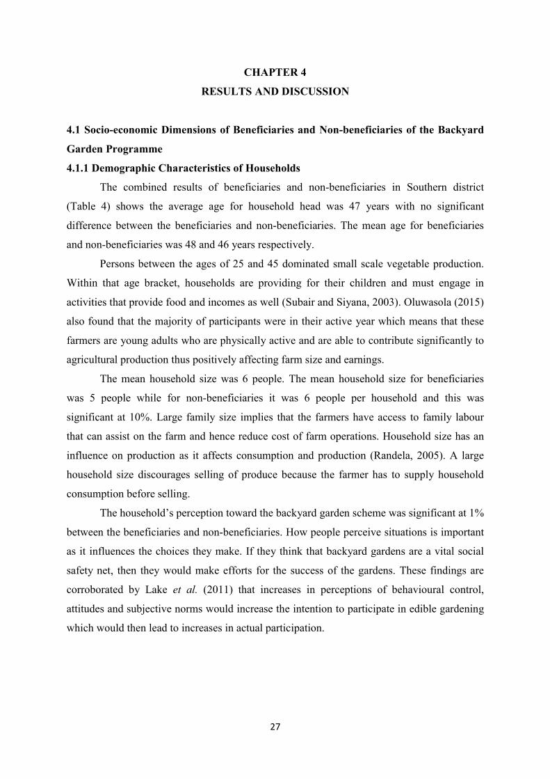
4.1.3 Educational Level ......................................................................................................... 29

4.1.4 Asset Ownership ........................................................................................................... 30

4.2 Backyard Gardening Response rate .................................................................................... 31

4.3 Backyard Garden Productivity ............................................................................................ 32

4.3.1 Garden Income Share Ratio .......................................................................................... 32

4.3.2 Gross Margin Analysis ................................................................................................. 33

4.3.3 Factors Affecting Gross Margin per Hectare ............................................................... 34

4.3.4 Analysis of Production Constraints for Rural Beneficiary Households ....................... 36

4.3.5 Analysis of Marketing Constraints ............................................................................... 38

4.4 Impact of Backyard Gardens and Factors that Affect Consumption Expenditure .................. 39

4.4.1 Factors Affecting Household Consumption Expenditure ................................................ 40

4.4.2 Impact of Backyard Gardens on Farm Household Consumption Expenditure ................ 42

4.4.3 Average Treatment Effects on Consumption Expenditure .............................................. 44

CHAPTER 5 ................................................................................................................................ 47

SUMMARY, CONCLUSION AND RECOMMENDATIONS .............................................. 47

5.1 Summary ............................................................................................................................. 47

ix

5.2 Conclusion ........................................................................................................................... 47

5.2 Recommendations ............................................................................................................... 48

5.3 Areas for Future Research ................................................................................................... 49

REFERENCES ............................................................................................................................ 50

APPENDIX .................................................................................................................................. 58

x

LIST OF TABLES

Table 1: Household Population and Sample Size for Study Areas ............................................... 18

Table 2: Description of the independent variables used in the productivity model ...................... 20

Table 3: Variables used in the logistic regression ........................................................................ 24

Table 4: Demographic Characteristics of Beneficiaries and Non-beneficiaries of Backyard

Gardens ......................................................................................................................................... 28

Table 5: Summary Statistics of the Garden Income Share Ratio .................................................. 33

Table 6: Gross Margin Analysis of Garden Crops ........................................................................ 33

Table 7: Factors affecting gross margin per hectare ..................................................................... 34

Table 8: Factors Affecting Consumption Expenditure ................................................................. 40

Table 9: Psmatch2 Logit Results .................................................................................................. 42

Table 10: Average Treatment Effects on Household Consumption Expenditure ......................... 45

Table 11: Region of Common Support ......................................................................................... 45

Table 12: Ps-test for Covariates .................................................................................................... 46

xi

LIST OF FIGURES

Figure 1: Conceptual Framework .............................................................................................. 185

Figure 2: Map of Study Area ..................................................................................................... 187

Figure 3: Distribution of Households by Gender and Marital Status .......................................... 29

Figure 4: Educational Level ......................................................................................................... 30

Figure 5: Household Assets ......................................................................................................... 31

Figure 6: Response Rate .............................................................................................................. 32

Figure 7: Production Constraints ................................................................................................. 38

Figure 8: Marketing Constraints .................................................................................................. 39

xii

ACRONYMS AND ABBREVIATIONS

BCWIS Botswana Core Welfare Indicator Survey

CEDA Citizen Entrepreneurship Development Agency

EA Enumeration Areas

FAO Food and Agriculture Organization

GDP Gross Domestic Product

GM Gross Margin

SDG Sustainable Development Goals

MLGRD Ministry of Local Government and Rural Development

MOA Ministry of Agriculture

MOPA PA Ministry of Presidential Affairs and Public Administration

PEP Poverty Eradication Programmme

RDA Rural Development Areas

SB Statistics Botswana

SHHA Self Help Housing Agency

SPSS Statistical Package for Social Sciences

STATA General Purpose Statistical Software Package

TVC Total Variable Cost

1

CHAPTER ONE

INTRODUCTION

1.1 Background Information

Botswana was classified as one of the ten poorest countries at the time of

independence in 1966 and currently it is classified as an upper middle income country

(Maipose, 2008). Though it has attained such economic growth, the country still faces socio

economic challenge of poverty among others. The spread of poverty is geographical with

some areas more profoundly affected than others. Results from the Botswana Core Welfare

Indicator Survey (BCWIS) of 2009/10, revealed that poverty headcount rate stood at 20.7 %

which is relatively high for an upper middle income country. Botswana’s aspiration is to

surpass the Sustainable Development Goal target of reducing extreme poverty by half by

2030 (Ministry of Presidential Affairs and Public Administration, 2015).

In order to achieve this goal, the government has introduced several initiatives aimed

at improving the livelihoods of Batswana by addressing all aspects of poverty. These include

among others the policy on environment such as the Environment Impact Assessment Act of

2005, Strategic Framework for Community Development in Botswana of 2010 and the

establishment of sustainable economic empowerment projects under Young farmers CEDA

fund which was established in 2004, Local Enterprise Authority established by the Small

Business Act number 7 of 2004 and the Economic Diversification Drive (2010). Others

include programs for orphans and destitute persons which falls under the Revised National

Policy on Destitute Persons (2002), subsidized Self Help Housing Agency (SHHA) which

falls under the National Policy on Housing (2000) and agricultural schemes which are under

the National Policy for Agricultural Development of 1991 (MOPAPA, 2015). In addition to

the above initiatives, a Poverty Eradication Programme that would aid in attaining food

security and minimum sustainable livelihoods amongst disadvantaged individuals and/or

families was introduced. The packages in the Poverty Eradication Programme include: Food

items include; Jam, pickles, food catering, food packaging, backyard garden, bakery, small

stock, poultry and bee keeping and non-food items include; kiosk, home based laundry,

leather works, textiles, tent hire, landscaping, hair salon, backyard tree nursery, upholstery,

handy crafts (basketry, wood carving, pottery), arts, craft, traditional dance and song.

The backyard garden program was introduced towards the end of 2009, as a

government initiative through which individuals were identified and funded for a backyard

garden (Basimane, 2014). Beneficiaries are given inputs such as irrigation systems (water

2

tank, drip irrigation pipes), seeds, fertilizer, tools (spade, garden fork, and rake), gum tree

poles and net shade (Botlhoko, 2012; Keakabetse, 2013).

According to Torimiro et al. (2015) the types of vegetables that are mostly grown in

the gardens are spinach (Spinacea oleracea L.), onion (Allium cepa L.), beetroot (Beta

vulgaris L.), carrot (Daucus carota L.), rape (Brassica napus L.), chomolia (Brassica

oleracea L.), green pepper (Capsicum annum L.) and tomato (Solanum lycopersicum L.).

Challenges that backyard garden owners reported to face include lack of water, lack of

finance, lack of market, pests and diseases, lack of technical knowledge on vegetable

production and preservation and lack of encouragement from extension workers (Subair and

Siyana, 2003; Torimiro et al., 2015).

Backyard farming contributes to food security by assuring the provision of food in

fresh form to satisfy the immediate calorie and nutritional needs of the household (Ojo,

2009). They are small pieces of land measuring approximately 30m by 10m in a residential

area which is used to guarantee that the needs of immediate household members (Ojo, 2009).

According to Ditedu (2015) backyard gardens were started with the aim of making sure that

households were self-sufficient in fresh vegetables and they sell the surplus to their

neighbours or through wet markets. Mostly these wet markets are found in front of retail

supermarkets and the fresh vegetables are sold for a price lower than what the supermarket is

offering for the same product.

1.2 Statement of the Problem

At the inception of the backyard gardening program, the government argued that these

gardens would help poor households achieve food security and enhanced incomes through

direct food provision and would enable households to earn income through sale of surplus

produce. Though many households have been recruited into the program since its inception,

the impact of these backyard gardens on household welfare have not been evaluated.

Consequently evidence as to whether the socio-economic status of households that benefitted

from backyard gardening has improved is largely unavailable. Likewise, direct impact of the

program on access to food and household incomes remain largely un-documented. This study

therefore sought to assess the income, expenditure and consumption dimensions of the

backyard gardening program of households in Southern District of Botswana.

3

1.3 Objectives of the Study

1.3.1 General Objective

The aim is to contribute to improved household welfare of backyard gardens beneficiaries

and food security in Southern District, Botswana.

1.3.2 Specific Objectives

i. To characterize households with and without backyard gardens as per their socio

economic indicators in Southern district, Botswana.

ii. To evaluate the gross margins of the backyard gardens and factors that influence the

gross margins of backyard gardens in Southern district, Botswana.

iii. To evaluate the impact of backyard gardens on rural household consumption

expenditure.

1.4 Research Questions

i. What are the socio-economic characteristics of households in the study area?

ii. Is there any difference in the gross margins of the backyard gardens?

iii. What is the impact of backyard gardens on household consumption expenditure?

1.5 Justification of the Study

Considering the effort that the government is putting in making sure the programme is

a success, there is need to assess how the backyard gardens are performing in terms of

contributing to the standards of living of small scale vegetable farmers. Therefore the results

will provide empirical evidence of the contribution of backyard gardens.

Secondly, findings will contribute towards the development of short and long term

policy interventions aimed at fostering eradication of extreme poverty in the country. It will

also add literature on the analysis of backyard gardens and poverty linkages specifically for

smallholder farmers.

1.6 Scope and Limitations

The study used backyard gardens that are in the rural areas and are part of the poverty

eradication programme. The limitation that this study had was that data collection was done

during the period when most respondents were at the fields as it was harvesting time. To

overcome this, the researcher made arrangements to interview the respondents in their

preferred environment. Other respondents were unwilling to be interviewed no matter the

level of assurance of anonymity and to address this limitation, those respondents were

skipped. Most of the respondents did not keep records so they were not sure about some of

4

the feedback that they were giving therefore to overcome this limitation, follow up questions

were asked to ascertain the answers given.

5

1.7 Definition of Terms

Backyard garden - is a small piece of land (10m by 10m, 20m by 10m or 30m by 10m)

cultivated around the dwelling place which have been funded by the Botswana government.

Gross margin - compares the performance of enterprises that have similar requirements for

capital and labour. It is given by total income less the variable costs associated with that

enterprise.

Productivity – is a measure of efficiency in which inputs are utilized in production. It is the

ratio of agricultural outputs to agricultural inputs.

Small scale vegetable farmer - refers to the beneficiary of the backyard garden scheme as

funded by the government.

Welfare - this is the improvement in the household income level and livelihoods which leads

to increase in consumption expenditure.

6

CHAPTER TWO

LITERATURE REVIEW

2.0 Concept of Backyard Gardens

Home gardens are found in both rural and urban areas in primarily small-scale

subsistence agricultural systems (Nair, 1993). The very beginning of modern agriculture can

be dated back to subsistence production systems that arose in small garden plots near the

household. These gardens have tirelessly bore the test of time and continue to play an

important role in providing food and income for the family (Marsh, 1998). Since the early

studies of home gardens in the 1930s by the Dutch scholars Osche and Terra(1934) on mixed

gardens in Java, Indonesia there have been comprehensive contributions to the subject

amalgamating definitions, species inventories, functions, structural characteristics,

composition, socio-economic, and cultural relevance. Home gardens are defined in multiple

ways highlighting various aspects based on the context or emphasis and objectives of the

research (Hoogerbrugge and Fresco, 1993).

Relying on research and observations on home gardens in developing and developed

countries in five continents, (Nifiez, 1984) formulated the following definition: The

household garden is a small-scale production system furnishing plant and animal

consumption and utilitarian items either not obtainable, affordable, or enthusiastically

available through retail markets, field cultivation, hunting, gathering, fishing, and wage

earning. Household gardens tend to be situated nearby the dwelling place for security,

convenience, and special care. They inhabit land marginal to field production and labor

marginal to major household economic activities (ibid). Including ecologically adapted and

complementary species, household gardens are marked by low capital input and simple

technology (ibid).

Generally, home gardening refers to the farming of a small portion of land which may

be around the household or within walking distance from the family home (Odebode, 2006).

Home gardens can be described as a mixed cropping system that includes vegetables, fruits,

plantation crops, spices and herbs, ornamental and medicinal plants as well as livestock that

can serve as a supplementary source of food and income. While Kumar and Nair (2004),

acknowledge that there was no standard definition for 'a home garden', they summarized the

shared view by referring to it as 'an intimate, multi-story permutations of various trees and

crops, sometimes in association with domestic animals, around homesteads', and added that

7

home garden cultivation is fully or partially dedicated for vegetables, fruits, and herbs

primarily for domestic consumption.

Adding to this, Eyzaguirre and Linares, (2010); Sthapit et al. (2004) and Krishna,

(2006) have defined a home garden as a well-defined, multi-storied and multi-use area near

the family dwelling that serves as a small-scale supplementary food production system

maintained by the household members, and one that encompasses a diverse array of plant and

animal species that mimic the natural eco-system.

Home gardens are normally established on lands that are marginal or not suitable for

field crops or forage cultivation because of their size, topography, or location (Hoogerbrugge

and Fresco, 1993). The specific size of a home garden varies amongst households and

normally their average size is less than that of the arable land owned by the household.

However, this may not hold true for those families that do not own agricultural land and for

the landless. New innovations and techniques have made home gardening possible even for

the families that have very little land or no land at all (Ranasinghe, 2009). The home gardens

may be delimited by physical demarcations such as live fences or hedges, fences, ditches or

boundaries established through mutual understanding.

2.1 Backyard Gardens in Botswana

The backyard garden scheme was introduced towards the end of 2009, as a

government initiative through which individuals are identified and funded for a backyard

garden (Basimane, 2014). The Ministry of Presidential Affairs and Public Administration is

the driver of the poverty eradication programme with the Ministry of Agriculture

implementing the gardens after the Social and Community Development have identified

people who qualify to benefit (MOA, 2008). The aims of backyard gardens are to

economically empower individuals and/or families and enhance the self-esteem of

beneficiaries.

To date, there are 3078 funded gardens nationwide; of which 1698 are operational,

1100 gardens are non-operational, 98 have failed and 182 are success stories (Ditedu, 2015).

The maximum grants for backyard gardens is P12, 500 (P= Pula, Botswana currency P1=

0.096 USD). Torimiro et al. (2015) found out that small scale production beneficially

impacted lives of respondents with increased profit margins, that is, for spinach (Spinacea

oleracea L.) (P1, 140), onion (Allium cepa L.) (P276) and tomato (Solamun lycopersicum L.)

(P684).

8

2.2 Benefits of Backyard Gardening in the Community

2.2.1 Ecological Benefits of Backyard Gardens

Private backyard gardens in cities, both food producing and non-food producing, have

the ability to boost ecological function and connectivity (Byers, 2009). One study conducted

in backyard gardens in Toronto found that natural conscription by all organisms was

significant in 20 backyard study sites (Sperling and Lortie, 2010). Another study conducted

in the United Kingdom found that the approximately 15 million gardens across the country

performed as bio-havens for wildlife and played a substantial role in the preservation of

biodiversity (Ryall and Hatherell, 2003).

2.2.2 Psychological and Cultural Aspects of Backyard Gardens

Lewis (1993) described gardens as a work of, and an expression of culture by being a

purely human paradigm with intrinsic value for the gardener and can be viewed as a

diagnostic artefact, reflecting the characteristics of the gardener. For example, the food plants

within a garden reflect the gardener’s cultural traits and culinary preferences. Kiesling and

Manning (2010) noted that gardening lies at the juncture of nature and culture, personal

values and public expectation. Gardens are products of social, physical and symbolic ordering

of private living space (Kimber, 2004) and any place where people garden, be it associated

with a house or a community garden, is a place of social, cultural and religious significance

(Francis and Hester, 1990; Kimber, 2004; Sinclair, 2005).

Food gardening provides a number of personal and cultural benefits and uses. Local

food production benefits cities by: 1) providing socio-educational functions, 2) contributing

to urban employment, and 3) reducing social inequality (Aubry et al., 2012). Wilhelm (1975)

studied gardening within a southern black community in USA and found that residents

identified both the tangible (trees, flowers, fruits and vegetables) and intangible (a connection

with the land) benefits from their dooryard gardens. Study participants identified curiosity,

personal satisfaction, social recognition, beauty and amazement by the mysteries of nature as

some reasons for gardening. Although intangible benefits were important, gardening was

done primarily to raise the homeowner’s standard of living and to provide food. Essential to

gardening success and passage to younger generations, local plant experts played an

esteemed role within the community.

2.2.3 Physical Health Benefits from Backyard Gardens

As the number of people living in cities continues to increase, dependency on large-

scale and distant agriculture will only grow. With the increasing population densities,

community leaders have identified food insecurity and food deserts, places where little fresh

9

or quality food is available for purchase, as growing problems in inner-city neighbourhoods.

In these areas, access to healthy and affordable food can be limited. Inadequate access to

fresh and nutritious food has been linked to higher rates of diabetes, obesity, cardiovascular

disease, certain types of cancers and chronic illnesses (Aubry et al., 2012; Corrigan, 2011;

Mccormack et al., 2010). Hendrickson et al. (2006) summarized the many definitions of

“food desert” used by different researchers. These varied definitions share the common idea

that a food desert is a condition where people living in poor urban communities have few or

no choices to purchase affordable, healthy food because of a lack of money, a lack of retail

outlets or the low nutritional quality of food offerings (Koh and Caples, 1979; Lang and

Rayner, 2002; Hendrickson et al., 2006). Because people living in food deserts may have

inadequate diets, they have a higher risk for health problems (Resnicow et al., 2001).

Unfortunately, the availability of affordable and quality fresh fruits and vegetables is a

problem in some communities, particularly in inner-city and minority neighbourhoods.

In a study of low-income residents living in urban and rural Minnesota communities,

the price of fresh fruits and vegetables were significantly higher in markets in poor areas, and

selection and quality were lower (Hendrickson et al., 2006). These conditions reduce

residents’ access to fresh, healthy and nutritious food. Besides food deserts, another problem

that affects many city dwellers is food insecurity. Anderson (1990) described food insecurity

as the inadequate availability of nutritional and safe food to meet the person’s needs, or the

uncertain or limited ability to acquire food in socially acceptable ways. Factors that

contribute to food insecurity include limited income, lack of home ownership and education,

ethnicity and household size (Eikenberry and Smith, 2005; Nord and Brent, 2002; Rose,

1999). Urban agriculture, such as community and backyard gardens, offers an inexpensive

means to alleviate some of the problems of food deserts and food insecurity by positioning

food production in the areas of greatest need.

Numerous studies examined the relationship between the availability of fresh

vegetables, vegetable consumption and attitudes toward eating fresh vegetables. Several

studies found that convenience, as related to the ease of obtaining fresh vegetables, was

related to the amount consumed (Nijmeijer et al., 2004; Steptoe et al., 1995; Worsley and

Skrzypiec, 1998). Household participation in a community garden may increase fruit and

vegetable consumption among urban adults. For example, Alaimo et al. (2008) found that

adults with a household member who participated in a community garden consumed fruits

and vegetables 1.4 more times per day than those who did not participate, and they were 3.5

times more likely to consume fruits and vegetables at least 5 times daily.

10

Studies have suggested that the presence of farmers markets, community gardens and

backyard gardens improve community nutrition and diet (Mccormack et al., 2010). This

could be related to a greater ease of obtaining fresh fruits and vegetables, as suggested by

Steptoe et al. (1995), Worsley and Skrzypiec (1998) and Nijmeijer et al. 2004).

2.2.4 Economic Benefits of Backyard Gardens

The economic benefits of home gardens go beyond food and nutritional security and

subsistence, especially for resource-poor families. Bibliographic evidence suggests that home

gardens contributed to income generation, improved livelihoods, and household economic

welfare as well as promoting entrepreneurship and rural development (Calvet-mir et al.,

2012; Trinh et al., 2003).

Through the review of a number of case studies, Mitchell and Hanstad (2004) assert

that home gardens can contribute to household economic well-being in several ways: garden

products can be sold to earn additional income (Ezygguire and Linares 2010, Torquebiau

1992and Ninez 1985); gardening activities can be developed into a small cottage industry and

earnings from the sale of home garden products and the savings from consuming home-

grown food products can lead to more disposable income that can be used for other domestic

purposes.

Studies from Nepal, Cambodia, and Papua New Guinea report that the income

generated from the sale of home garden fruits, vegetables, and livestock products allowed

households to use the proceeds to purchase additional food items as well as for savings,

education, and other services (Iannotti et al., 2009 and Vasey 1985). Families in mountain

areas of Vietnam were able to generate more than 22 % of their cash income through home

gardening activities (Trinh et al., 2003).

Home gardens are widely promoted in many countries as a mechanism to avert

poverty and as a source of income for subsistence families in developing countries. Although

home gardens are viewed as subsistence-low production systems, they can be structured to be

more efficient commercial enterprises by growing high-value crops and animal husbandry

(Torquebiau, 1992). A number of research studies have focused on evaluating the potential or

real economic contribution to the household and local economy as well as social development

(Kehlenbeck and Maass, 2004). A study from South-eastern Nigeria reported that tree crops

and livestock produced in home gardens accounted for more than 60 % of household income

(Okigbo, 1990). In many cases the sale of produce from home gardens improves the financial

status of the family providing additional income, while contributing social and cultural

amelioration (Wilson, 1995). The fact that home production is less cost-intensive and requires

11

fewer inputs and investment is extremely important for resource-poor families that have

limited access to production inputs. It has been assessed that moderately rigorous crop and

livestock production in home gardens can generate as much revenue per unit area as field

crop production (Marsh, 1998 and Danoesastro, 1980). Where land constraints exist,

innovative tools have been used to make efficient use of limited space (Ranasinghe, 2009).

Also, livestock housed in gardens diversify risk due to crop losses and provide a cash buffer

and asset to the household (Devendra and Thomas, 2002).

2.3 Impact of Backyard Gardens on Household Welfare

Torimiro et al. (2015) in a study conducted in Kweneng District of Botswana found

that the participants of backyard gardens either moderately or highly benefited from small

scale vegetable production. Food, income, payment of bills, purchase of clothing and

furniture were identified as benefits derived and this is supported by observations made by

Rahman et al. (2008) that homestead vegetable production can play an important role in

changing social and livelihood issues. The increased purchasing power can be used for non-

vegetable food items. Subair and Siyana (2003) concluded in study done in Mochudi village

in Botswana that the joy derived from backyard gardening and the physical exercises

involved could help to keep the body in shape.

Batchelor et al. (1994) concurred with Rahman et al. (2008) that gardening has the

potential to improve the household welfare by providing continuous supply of vegetables

throughout the dry season and years of drought. Gardens offer crop security as compared to

field crops as they are prone to drought. Yields in gardens are high and farmers are able to

produce three crops in a year thus giving a relative high income as crops grown in gardens

are high value crops hence this can increase the income of communal farmers. Gardens can

significantly increase household income (Rahman et al., 2008).

Produce from backyard gardens can be used for household consumption or for sale.

Income from the sale of garden produce provides for other household needs as well. The fact

that small but steady income comes from gardens, they are considered as dependable socio-

economic safety nets for household food security and other requirements (Chirinda et al.,

2002).

Qualitative impact assessments have shown that the encouragement of vegetable

gardens in particular keyhole gardens to improve access to a variety of food, even during the

winter months, attests to being successful (FAO, 2000). Participating households noted the

increase in the availability of food, wider diversity of their diet and surplus in vegetables,

12

which they are able to sell to generate income. Thus, households that participate in vegetable

production are able to reduce both the direct and trade entitlements failures. According to

Mwabumba (2015), direct entitlement failures refer to a situation where the food producers

fail to produce enough and are unable to feed themselves either by self-supply or by trade.

Irrigated farming can create economic backward and forward linkages (FAO, 2000).

A backward linkage takes the form of creating and enhancing business activities for those

dealing in farm inputs. This is because of the fact that the crops grown under irrigation rely

heavily on recommendations of improved purchased inputs. Forward linkages occur if

irrigation leads to cash cropping. This will promote the growth of the agro- industry.

2.4 Theoretical Framework

The theory adapted in this study is the theory of agricultural household model. The

model of household behaviour presented below describes a semi-commercial family farm

with a competitive labour market (Singh et al., 1986). It has been noted that the major part of

world agriculture is consistent with this genre of model which is located intermediately on a

continuum between a wholly commercial farm employing only hired labour and marketing all

output and a pure subsistence farm using only family labour and producing no marketed

surplus. Further, there is an active labor market for agricultural and other types of labor and

all households participate in the labor market either as buyers or sellers of labor. Thus the use

of labor time and the disposal of output are determined with reference to market wages and

prices, and the average farm is aptly described as semi-commercial. Finally we note that land

is rented by means of fixed charges and there are no sharecropping or other contractual

arrangements which might lead to non-standard profit maximizing conditions.

With these points in mind, the household model can be formulated as follows:

� = �(�, �, �; ��), � = 1…………………………………………………………………….. 1

� = �(�, ��; �), � = 1………………………………………………………………………... 2

� = � + � + �...................................................................................................................…... 3

And

�� + �� = �� + � + �� − ∑����………………………………………………………... 4

Where L = leisure, C = own-consumption of agricultural output, M = consumption of market-

purchased goods, ai= household characteristics (for example, number of dependents), F

13

=total output of C, D = total labor input (both family and hired) used in i; production,

dj =other variable inputs used in F production, A =area of land used in F production, T =

total household time available for labour, H =net quantity of labor time sold if H ~0 and

net quantity of labor time purchased if H < 0, R =non-wage, non-crop net other income, q

=price of M, p =price of C, w = wage- rate, and Wj = prices of other variable factors.

The household is assumed to maximise its utility function [eq. (l)] subject to a

production function [eq. (2)] and time and income constraints [eq. (3) and (4)]. The planning

horizon is assumed to be one agricultural cycle. As a result, decisions relating to the

total supply of household factors of production are treated as given. Thus migration,

which affects total available household labor supply, is omitted from the analysis, as is the

rent decision, which affects the total available household land supply. Land may, therefore,

be treated as a fixed factor. Rent payments or receipts, however, are captured in the definition

of R, non-wage, non-crop net other income. Other long term decisions are also omitted from

the analysis. In particular, it is assumed that the household has already made some

decision about its desired level of saving and that this quantity is included in the

definition of R. Finally, the analysis ignores risk, again on the grounds that, while risk may

play a crucial role in the migration decision or the rent decision, it plays a less important role

in the short term when it may be assumed that the longer term decisions have already been

made and the household is, at least to some extent, committed to a fairly well-defined course

of action for the duration of the agricultural cycle.

Maximising eq. (1) subject to eqn (2) through (4) and eliminating the Langrangian

multipliers, yields the following first order equations:

��

��=

�

�…………………………………………………………….………………………… 5

��

��=

�

�……………………………………………………………...…...…………………... 6

��� = �………………………………………………………………………………………7

��� = ��, � = 1……………………………………………………………………………….8

and

�� + �� + �� = � + � + ��………………………………………………………………9

where,

14

� = ��(�) − �� − ∑����……………………………………………………………….... 10

Eqs. (5) and (6) express the traditional first-order condition of welfare

economics: that is, the marginal rate of substitution in consumption must equal the

marginal rate of transformation in production. Eqs. (7) and (8) are the profit-

maximising conditions for the allocation of labor and 01-3 x variable factors. Eq. (9)

combines the income and time constraints as well as the technological constraint

described by the production function. The left- hand side of eq. (9) includes the

‘expenditure’ on leisure and the right-hand side is an augmented version of Becker’s

(1965) concept of ‘full income’ which in this case includes the net profit (π) from

household production.

Labor is singled out for separate treatment in eq. (7) to emphasize that the level of

labor input is determined solely by the profit maximizing condition. In the absence of labor

market participation the dichotomy between the production and consumption side would

not be as complete. In this cast the quantity of labor used in production would be affected

directly by the subjective evaluation of work to the household. However, with an active labor

market the subjective evaluation of work determines the level of labor supplied by the

household but not the household’s total demand for labor in production. Instead total labor

demand is determined by the profit maximizing condition and the production and

consumption segments of the model can be estimated separately.

Given an independent estimate of the production function, eqn. (7) and (8) can be

used to determine the variable inputs into F production, and since the land input is determined

exogenously, the total output of F. The solutions for the variable inputs and F can then be

used to derive π, net farm profit. Eqn. (7) and (8), therefore, represent the production side of

the model, and the impact of production on the consumption side is then transmitted through

the value of π in the income constraint. Turning to the consumption segment, if we assume

that the second order conditions are satisfied, eqn. (5), (6) and (9) can be solved for demand

functions for the three consumption goods, C, M and L, in terms of the three prices, q, p and

w, the household characteristics, ai, and total household expenditure, E, which is defined as

the sum of π, R and wT.

2.4 Conceptual Framework

The conceptual framework adapted in this study is built on the relationship between

backyard gardening and an improvement in farm household welfare. The production decision

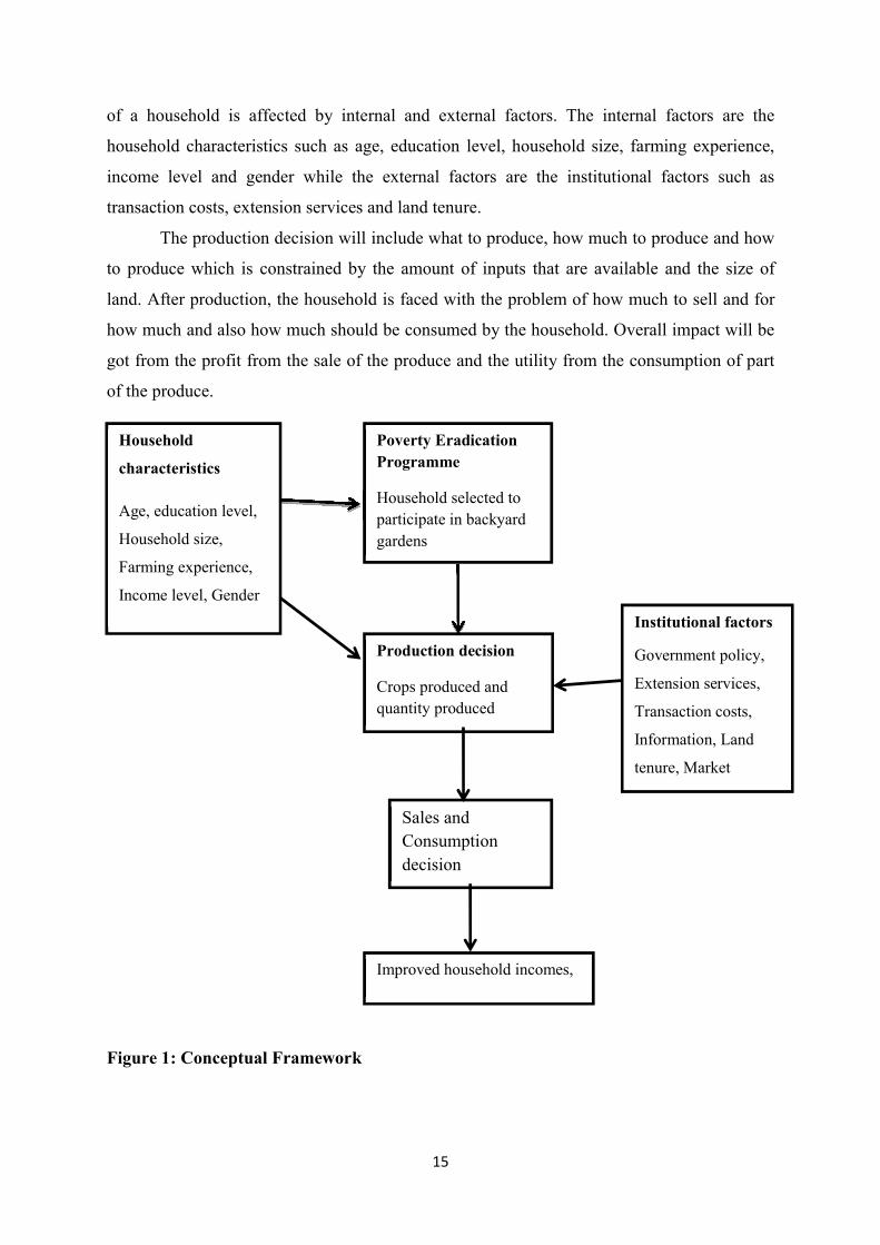
15

of a household is affected by internal and external factors. The internal factors are the

household characteristics such as age, education level, household size, farming experience,

income level and gender while the external factors are the institutional factors such as

transaction costs, extension services and land tenure.

The production decision will include what to produce, how much to produce and how

to produce which is constrained by the amount of inputs that are available and the size of

land. After production, the household is faced with the problem of how much to sell and for

how much and also how much should be consumed by the household. Overall impact will be

got from the profit from the sale of the produce and the utility from the consumption of part

of the produce.

Figure 1: Conceptual Framework

Poverty Eradication

Programme

Household selected to

participate in backyard

gardens

Household

characteristics

Age, education level,

Household size,

Farming experience,

Income level, Gender

Institutional factors

Government policy,

Extension services,

Transaction costs,

Information, Land

tenure, Market

Production decision

Crops produced and

quantity produced

Sales and

Consumption

decision

Improved household incomes,

16

CHAPTER THREE

METHODOLOGY

This chapter describes the study area, the sampling procedure and determination of

the sample size from the target population. The section on the method of data collection

explains the tools that were used.

3.1 Study Area

This study was conducted in Southern District in Botswana because this is where the

largest number of backyard gardens is found. The district is bordered by the North West

Province of South Africa in the South, South East district in the East, Kweneng district in the

North and Kgalagadi district in the South-west. Figure 2 below shows the Southern district

which lies approximately between latitudes 24° and 25° South and longitudes 24° and 25°

East. Southern district has an area of 28470 km2 with a population of 186 831 and the

population density of 6.6/ km2 (Statistics Botswana, 2011). The capital of Southern District

Kanye Village and the other large villages in the district are Moshupa and Goodhope.

17

Figure 2: Map of Study Area

Source: Google maps

3.2 Sampling Procedure

The study targeted beneficiaries of the backyard garden program and non-

beneficiaries who have the same characteristics as the beneficiaries. In order to control

selection errors, an up-to date population source list was obtained from the Office of the

President and the local extension officer in the department of Crops.

Multi-stage sampling was used to select the sample whereby in the first stage:- the

region was purposively divided into three sub-districts which are Ngwaketse Enumeration

Area (EA) (10617), Ngwaketse West Enumeration Area (10618) and Barolong sub-district

Enumeration Area (10619). In the second stage, the population was stratified into two groups

(beneficiaries and non-beneficiaries) and then random sampling was used to get a

representative sample size from each strata.

18

3.3 Sample Size

Yamane (1973) suggested that since the population number (number of targeted

population) is known in the study area, the following can best provide the required sample

size for this study.

n=

)(2

1 eN

N

…………………………….………………………………………… (1)

Where n is the desired sample size, N is the population size and e is the allowable margin of

error (level of precision) ranging from 0.05 to 0.1. Margin of error shows the percentage at

which the opinion or behaviour of the sample deviates from the total population. The smaller

the margin of error the more the sample is representative to the population at a given

confidence interval. Therefore, for this study allowing the smallest possible margin of error

(e= 0.05), the total sample size became:

n= 648

1 + 648(0.05)�= 247 respondents

The proportions to size sample for each enumeration area are given in Table 1.

Table 1: Household Population and Sample Size for Study Areas

Enumeration Area

code

Enumeration area Number of

households

Sample size

10617 Ngwaketse EA 323 123

10618 Ngwaketse- West EA 54 21

10619 Barolong EA 271 103

Total 648 247

3.4 Data Collection Instrument

A structured questionnaire was used to collect data. The kind of information required

was on the socio-economic characteristics such as age, gender of the respondent, education

level, household size and farming experience, consumption expenditure of households and

amount of time allocated to garden work. However, pre-testing of the questionnaire was done

on 25 respondents with similar characteristics in Kweneng District before data was collected

in order to test the validity and reliability of the questionnaire and a final questionnaire was

prepared using responses from the respondents. Pre-testing revealed that the economic

19

benefits of the backyard program were missing in the first questionnaire and should therefore

be included in the final questionnaire.

To support the data collected from the field, secondary data which was collected from

different published and non-published research journals and reports of Poverty Eradication

Programme office were used.

3.5 Data Analysis Techniques

3.5.1 Characterizing Households With and Without Backyard Gardens as per their

Socio-economic Indicators

Descriptive statistics was applied where mean, standard deviation, frequency

distribution, and percentages were used to compare participants and non-participants of

backyard garden scheme.

Variables included garden size, employment, age, marital status and gender of family

head, education level of household head and possession of durable goods (variables obtained

from the Botswana Core Welfare Indicators Survey, 2010).

3.5.2 Evaluating the Gross Margin of the Backyard Gardens and Factors Influencing

the Gross Margins of the Backyard Gardens

Households are involved in various livelihood activities. These activities contribute to

the income and food security status of a household. In this section the productivity and

viability of the gardening activities were calculated. Gross margin analysis was used to

determine the viability of the gardening activities. Gross margin is the difference between the

value of output and the total variable costs. It is used to evaluate the performance of different

enterprises.

Gross margin analysis was carried out for the garden crops; leafy vegetables, green

pepper, tomatoes, and onions. This was used to test the hypothesis that gardening activities

are profitable. The model for calculating the gross margin can be specified as:

�� = ���� − �����…………………………………...……………………………………. (2)

Where GM is the gross margin, Qi is the quantity of output of crop i produced, Pi is

the price of output, Xi amount of input i used and Pxi price of input i.

Even though the gross margin is an important analytic tool to assess the profitability

of different farming enterprises, it has a number of disadvantages (Forestry, 2009). These are:

i. There is no inclusion of fixed costs in the analysis. This incomplete analysis may lead

to wrong conclusions.

20

ii. Gross margin analysis does not take into account the possible environmental and

social effects that may arise due to different types of technology or crops grown.

iii. The results of a gross margin analysis are valid for the season under consideration;

therefore, they may be not useful for other recommendations.

The ratio of income from backyard gardening to total income was calculated to get the

contribution of gardening to the total household incomes. A regression analysis was run to

relate the profitability of the gardens to the different socio- economic characteristics.

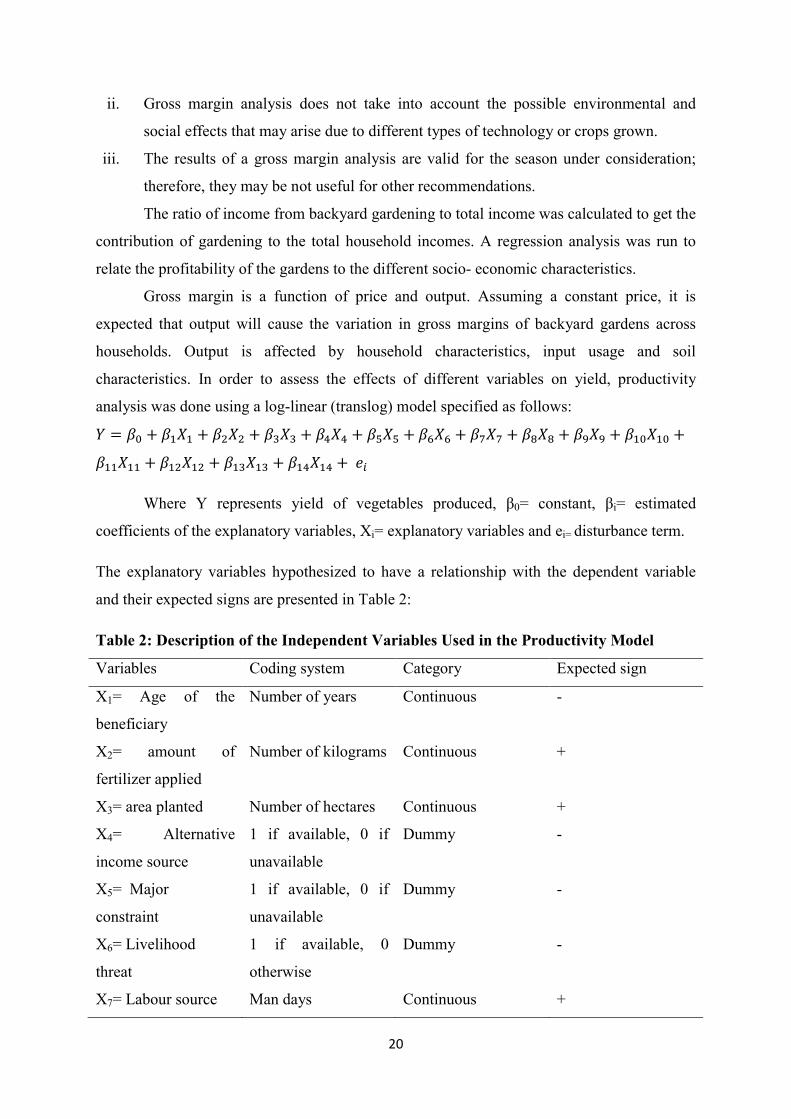
Gross margin is a function of price and output. Assuming a constant price, it is

expected that output will cause the variation in gross margins of backyard gardens across

households. Output is affected by household characteristics, input usage and soil

characteristics. In order to assess the effects of different variables on yield, productivity

analysis was done using a log-linear (translog) model specified as follows:

� = �� + ���� + ���� + ���� + ���� + ���� + ���� + ���� + ���� + ���� + ������ +

������ + ������ + ������ + ������ + ��

Where Y represents yield of vegetables produced, β0= constant, βi= estimated

coefficients of the explanatory variables, Xi= explanatory variables and ei= disturbance term.

The explanatory variables hypothesized to have a relationship with the dependent variable

and their expected signs are presented in Table 2:

Table 2: Description of the Independent Variables Used in the Productivity Model

Variables Coding system Category Expected sign

X1= Age of the

beneficiary

Number of years Continuous -

X2= amount of

fertilizer applied

Number of kilograms Continuous +

X3= area planted Number of hectares Continuous +

X4= Alternative

income source

1 if available, 0 if

unavailable

Dummy -

X5= Major

constraint

1 if available, 0 if

unavailable

Dummy -

X6= Livelihood

threat

1 if available, 0

otherwise

Dummy -

X7= Labour source Man days Continuous +

21

X8= Market

constraint

1 if available, 0

otherwise

Dummy -

X9= Production

constraint

1 if available, 0

otherwise

Dummy -

X10= Market

availability

1 if available, 0

otherwise

Dummy +

X11= Garden size Number of hectares Continuous +

X12= Education level

of the beneficiary

1 if literate, 0 if

illiterate

Dummy +

X13= Household size

(family labour)

Man days Continuous +

X14= Problem index 1 if available, 0

otherwise

Dummy -

Increase in the farmer’s age was expected to negatively affect the profitability of

vegetable production. Nwaru and Iwuji (2005) stated that entrepreneurship gradually

becomes less as age of the entrepreneur increases because creativity and confidence of the

entrepreneur as well as his mental capacity to cope with challenges of his business activities

decrease with age. Education is thought to be important as it informs farmers on how best to

strategize and adapt to better marketing conditions therefore a positive relationship was

expected between education and profitability.

The amount of land cultivated under vegetables was expected to be positively allied

with profitability, because the more land put under production, the higher would be the

profitability of the crop because of possible economies of scale. Garden size was assumed to

have a positive relationship with profitability as the bigger the garden, the more land

household have to plant more vegetables hence increasing their profits. Market constraint and

production constraint were set as dummy variables, where a farmer either having marketing

and production constraints took the value one or no constraint took a value of zero. Both

marketing and production constraints were assumes to have a negative influence on

profitability of backyard gardens.

Distance between the production area and the market is expected to reduce the

probability of households in participating in commercial vegetable production hence poor

profits because of associated high transport costs. Therefore it is expected that market

availability would positively affect profitability. Household size is assumed to have a positive

22

relationship with profitability because households with large family sizes may cultivate more

land. This is because family labour that is cheap is guaranteed therefore labour constraints

will not be a problem.

Fertilizer quantity was measured in kilograms and was anticipated to positively affect

the profitability of backyard gardening. It was assumed that the more fertilizer applied on

vegetable crops up to a certain level, the more the quantity of vegetables produced. Problem

index was assumed to have a negative relationship with profitability and this is because a

household would spend more in-order to solve the problems that they are facing hence cutting

the amount of profits realized.

Availability of alternative sources of income is also another factor that may affect the

profitability of backyard gardens thus was given a value of one is alternative sources of

income are available and zero otherwise. Therefore a negative relationship is expected

between availability of alternative sources of income and profitability of the gardens. Major

constraint to improving livelihood and threats to livelihood of the household were given

value of one if they are available and zero if unavailable. Therefore, a negative relationship is

expected between major constraint to improving livelihood, threats to livelihood and

profitability.

3.5.3 Evaluating the Impact of Backyard Gardens on Household Consumption

Expenditure

In order to evaluate the impact, the outcome variable that was used was consumption

expenditure per day per adult equivalent. The average change in the outcome variable was

estimated using Propensity Score Matching (PSM). PSM method improves on the ability of

regression to generate accurate causal estimates by virtue of its non-parametric approach of

balancing of covariates between the “treatment” and “control” group.

When usual methods of assessing the impact of an intervention using “with” and

“without” method, has been hindered by a problem of missing data, the impact of

intervention cannot be accurately estimated by simply comparing the outcome of the

treatment groups with the outcomes of control groups (Heckman et al., 1998). Rosenbaum

and Rubin (1985) developed an alternative technique to assess the impact of discrete

treatment on an outcome by using propensity score matches. This was achieved by grouping

households from treated individuals and non-treated individuals which show a high similarity

in their explanatory variables. Thus, to support results obtained from regression analysis the

impact of having a backyard garden on household consumption expenditure was examined

using econometric PSM method.

23

This study considered households that participate in backyard gardens as the

treatment group and the non-participants as the control group. Ideally, the aim is to compare

the level consumption expenditure, socio-economic and institutional factors of the backyard

gardens participants to that of the non-participants. This ensures that the average treatment

effect or effect of choice to participate in the backyard gardens on household consumption

expenditure can be accurately estimated.

First, logistic regression of treatment status (1 if a household participate in backyard

gardens, 0 if a household is a non-participant) was specified. This was run for the households

on observables and exogenous variables that included: gender, level of education, household

size, distance to market, price of output, price of information, farming experience, crops

quantity output and extension services.

The major concern of this regression was to predict the probability of a household

participating in backyard gardens. That is, to predict propensity scores based on which, the

treatment and control groups of households was matched using the matching algorithms. As

such according to Gujarati (1995), the functional form of logit model is specified as follows:

�� = �(� = 1 ��) =⁄�

����(�������) …………………………………..……..…………… (3)

Equation (4) can also be written as:

�� =�

������………………………………………..……………………………………..…. (4)

The probability that a given household participates in backyard gardens is expressed

by (5) while, the probability for non-participants in backyard gardens scheme is given by:

1 − �� =�

�����………………………..………………………..…………………………… (5)

Therefore it can be written that:

��

����=

�����

������……………………………………………………………………………. (6)

��

���� is the odds ratio in favour of participating in backyard gardens that is, the ratio of

the probability of participating in backyard gardens to that of the probability of not

participating in backyard gardens. Lastly, taking the natural logarithms of equation (7) we

obtained:

�� = ln ���

����� = �� = �� + ���� + ⋯ + ����……………………………………. (7)

Where Pi is probability of participating in backyard garden scheme and it ranges from

0 to 1 and Zi is a function of n explanatory variables (Xi) which is expressed as:

�� = �� + ���� + ⋯ + ����………………………………………………………… (8)

24

Where �� is intercept, ��, … , �� are the slope parameters in the model, �� is the log of

the odds ratio, which is not only linear in X but also linear in parameters and �� is vector of

the relevant sampled household’s characteristics. If the disturbance term �� is introduced to

the logit model it will become:

�� = �� + ���� + ⋯ + ���� + ��………………………………………………….. (9)

Table 3: Variables used in the logistic regression

Code Variable Variable Measurement of variable Expected sign

Dependent variable BGPART Independent Variables Age Gender EducL HHsz FrmE MrktI MrktD OutputP OutputQ ExtS

Household choice to Participate in export market Age of household head Gender of household head Education Level of household head Household size Farming experience Market information Market Distance Output Price Output Quantity Extension Services

(1=participants, 0=non-participants) In years (Continuous) Dummy (1=Male, 0=Female) (1=No education, 2=Primary, 3=Secondary, 4=Tertiary) Size of the household (Continuous) In years(continuous) Dummy (yes=1, No=0) Kilometers Pula In kilograms (continuous) Number of contacts with extension

+ + +/- + + + +/- +/- + +/- +/-

However, estimation of the propensity score is not enough to estimate the ATT of

interest. This is due to the fact that propensity score is a continuous variable and the

probability of observing two units with exactly the same propensity score is, in principle,

zero. Therefore, after obtaining the predicted probability values on the observable covariates

(the propensity scores) from the binary estimation, matching was done using a matching

algorithm that is selected based on the data at hand. Some of the various matching algorithms

that have been proposed in literature differ from each other with respect to the weights they

attribute to the selected controls when estimating the counterfactual outcome of the treated.

However, they all provide consistent estimates of the Average effect of treatment on the

25

Treated (ATT) under the Conditional Independence Assumption (CIA) and the overlap

condition (Caliendo and Kopeinig, 2008).

Nearest Neighbour matching (NNM): Here an individual from a comparison group is

chosen as a matching partner for a treated individual that is closest in terms of propensity

score (Caliendo and Kopeinig, 2008). It can be done with or without replacement options.

The problem this technique faces is that where the treatment and comparison units are very

different, finding a satisfactory match by matching without replacement can be very

problematic (Dehejia and Wahba, 2002).

Checking overlap and common support

Imposing a common support condition ensures that any combination of characteristics

observed in the treatment group can also be observed among the control group (Bryson et al.,

2002). The common support region is thus the area which will contain the minimum and

maximum propensity scores of treatment and control group households, respectively.

However, comparing the incomparable must be avoided. This can be avoided by checking the

overlap and the region of common support between treatment and comparison group. One

way of determining the region of common support more precisely is by comparing the

minima and maxima of the propensity score in both groups. The basic criterion of this

approach is to delete all observations whose propensity score is smaller than the minimum

and larger than the maximum in the opposite group. As such, observations which lie outside

this region are discarded from analysis (Caliendo and Kopeinig, 2008).

Impact of backyard garden participation on household consumption expenditure

The impact of farmer’s participation in backyard gardens on household consumption

expenditure were further investigated by letting ��� and ��

� be the amount of consumption

expenditure for participants and non-participants respectively. As such the difference in

outcome between treated and control groups can be seen from the following mathematical

equation:

�� = ��� − ��

�………………………………………………………………………….. (10)

Where TiY = Outcome of treatment (income of thi household, when they participate in

backyard garden scheme), C

iY = Outcome of the untreated individuals (income of thi

household, when they do not participate in backyard garden scheme) and i = Change in

outcome as a result of treatment or change in consumption expenditure for participating in

backyard gardens.

26

Equation (11) is then expressed in causal effect notational form, by assigning �� =

1as a treatment variable taking the value 1 if individual received the treatment (participates in

backyard garden) and 0 otherwise. Then the Average Treatment Effect of an individual i can

be written as:

��� = �(������ = 1) − �(��

�|�� = 0)………………………………………………….. (11)

Where ATE, Average Treatment Effect: is the effect of treatment on household consumption

expenditure, E (YT |Di=1): Average outcomes for individuals with treatment, if they choose to

participate in the backyard garden, (Di=1) and E (YC | Di = 0): average outcome of the

untreated individual, when they do not choose the backyard garden is (Di =0). Furthermore,

the Average Effect of Treatment on the Treated (ATT) for the sample can be expressed as:

��� = ����� − ��

��� = 1� = �(����� = 1) − �(��

�|� = 1)…………………………… (12)

27

CHAPTER 4

RESULTS AND DISCUSSION

4.1 Socio-economic Dimensions of Beneficiaries and Non-beneficiaries of the Backyard

Garden Programme

4.1.1 Demographic Characteristics of Households

The combined results of beneficiaries and non-beneficiaries in Southern district

(Table 4) shows the average age for household head was 47 years with no significant

difference between the beneficiaries and non-beneficiaries. The mean age for beneficiaries

and non-beneficiaries was 48 and 46 years respectively.

Persons between the ages of 25 and 45 dominated small scale vegetable production.

Within that age bracket, households are providing for their children and must engage in

activities that provide food and incomes as well (Subair and Siyana, 2003). Oluwasola (2015)

also found that the majority of participants were in their active year which means that these

farmers are young adults who are physically active and are able to contribute significantly to

agricultural production thus positively affecting farm size and earnings.

The mean household size was 6 people. The mean household size for beneficiaries

was 5 people while for non-beneficiaries it was 6 people per household and this was

significant at 10%. Large family size implies that the farmers have access to family labour

that can assist on the farm and hence reduce cost of farm operations. Household size has an

influence on production as it affects consumption and production (Randela, 2005). A large

household size discourages selling of produce because the farmer has to supply household

consumption before selling.

The household’s perception toward the backyard garden scheme was significant at 1%

between the beneficiaries and non-beneficiaries. How people perceive situations is important

as it influences the choices they make. If they think that backyard gardens are a vital social

safety net, then they would make efforts for the success of the gardens. These findings are

corroborated by Lake et al. (2011) that increases in perceptions of behavioural control,

attitudes and subjective norms would increase the intention to participate in edible gardening

which would then lead to increases in actual participation.

28

Table 4: Demographic Characteristics of Beneficiaries and Non-beneficiaries of

Backyard Gardens

Variables Beneficiaries Non-beneficiaries Total t test p-value

Mean SD Mean SD Mean SD

Age 47.45 13.00 46.28 13.06 46.75 13.02 -0.70 0.488

Household Size 5.41 3.24 6.15 3.59 5.85 3.47 1.65 0.100*

Perception

index

6.52 2.33 4.31 2.94 5.19 2.92 -6.34 0.000***

Note, *, **, ***: refers to significance at 10%, 5% and 1% respectively while SD denotes

standard deviation.

4.1.2 Gender and Marital Status

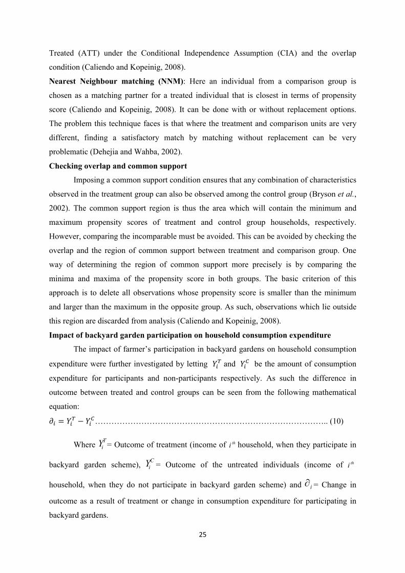
Results in Figure 3 show that about 28 % of the households were male headed and

72% female headed for combined households. However, when the two groups were

separated, 71% of beneficiary households were headed by females compared to 72% for non-

beneficiaries. Female headed households dominated those participating in the program as

they are responsible for their household food security and this is also a deliberate policy

action by the government to make sure that more women are participating in the backyard

gardens as they are the more vulnerable to food insecurity than men. Samantaray et al. (2009)

established that vegetable cultivation is dominated by women and that they manage the

vegetable production system up to harvesting and marketing stage.

When compared to non-beneficiaries, single parents (57%) dominate the program.

This might be because they do not have a partner to help them support their families such that

all responsibilities befall them. Widowed and divorced people accounted for 23% and 1%

respectively and this might be because they take a long time to remarry and sometimes they

do not have that opportunity thus they are responsible for their household welfare. Married

people accounted for 19% and they were mature adults saddled with marital responsibilities

hence their involvement in backyard gardening. These were regarded to have more labour

force compared the unmarried. This is corroborated by Oladele ( 2011) that farm labour

required by the married vegetable farmers was supplied by their spouses.

29

Figure 3: Distribution of Households by Gender and Marital Status

4.1.3 Educational Level

In this study, the level of education was included to ascertain the farmers’ ability to

use and interpret information than those who have less education or no education at all

(Marther and Aldelzadeh, 1998). The results (figure 4) show that 25% of the households had

no formal education at all whilst 75% had formal education. For those who had formal

education, 47% had gone up to primary level whilst 16 % attained junior secondary school,

9% had senior secondary school and 3% had tertiary education. These findings are supported

by those of Subair and Siyana (2003) that most of the participants of backyard gardens have

primary education and little to no skills to perform optimally in backyard gardens. Such

farmers are imbued with the ability to access and appreciate the use of improved technology

and best practices in their enterprises.

0 20 40 60 80

Female

Male

Single

Married

Divorced

WidowedG

ende

rM

arit

al s

tatu

s

% of respondents

Non-beneficiaries

Beneficiaries

25%

47%

16%

9%

3%

never attended

primary school

junior secondary

BGCSE

tertiary

30

Figure 4: Educational Level

4.1.4 Asset Ownership

Asset ownership is an indicator of welfare in the sense that the households which

owns such assets are assumed to be better in terms of poverty level as compared to those who

cannot afford to purchase such items (Statistics Botswana, 2003). Results in Figure 5 reflect

ownership of durable assets for production such as tractors, handhoes and ox drawn ploughs.

Assets for production were handhoe, ox plough and wheelbarrows. Compared to non-

beneficiaries where 70% had wheelbarrows, 80% of the beneficaries had the equipment.

About 48% of the beneficiaries had hand hoes compared to 46.7% of the non-beneficiaries

while 10% of the beneficiaries had an ox plough compared to 6.7% of the non-beneficiary

households. These are the most commonly used implements in backyard gardens.

Rural households for beneficiares that had tractors was 4% compared to 3.3% for non-

beneficiaries. This might be because of the fact that tractors are expensive to purchase, own

and run. The low numbers of farmers using tractors was because they are expensive to hire

and run and not readily available ( Betek and Jumbam, 2016). About 10% of the beneficiaries

had bicycles when compared to 6% of the non-beneficiaries. This is because they are a

convinient way of easily accesing input and output markets in the village given the lack of

transport due to poor roads. However, bicycles are not efficient as farmers spent most of their

time and energy riding it to the market instead of utilizing that time for production (Phanith

and Phnom, 2011).

There was no distinct difference in cellphone ownership since 82% of beneficiaries

and 81% non-benefeciaries had them. Both groups indicated that they used the cellphone to

keep in touch with the outside world. Rural beneficiary household indicated that they needed

the cellphone in order to communicate with the suppliers of manure and also their customers.

Krone et al. (2014) found that the increasing use of mobile phones resulted in positive

contributions to the economic activities of horticultural farmers as it it facilitated a diversified

knowledge access and led to better informed farmers.

When compared to non-beneficiary households, beneficiary households had a higher

number of fridges (26%) to 17.3% for non-beneficiaries. Majority of the both groups

indicated that they did not have fridges because they do not have access to electricity.

However, for beneficiary households that had fridges they indicated that they have fridges so

as to store some of their left over produce to be sold the next day.

31

A good number (52%) of beneficiaries owned radios when compared to 40.7% non-

beneficiaries and about 38% of the beneficiaries compared to 28% of the non-beneficiaries

had televisions. They indicated that they needed the radios and televisions to access

information on better crop production techniques and major inputs such as high-yielding

seeds and pesticides so that they can improve their gardens. These results are substantiated by

Ali (2011) that the use of mass media (radios and television) methods of information transfer

has the potential to greatly help the farming community.

Figure 5: Household Assets

4.2 Backyard Gardening Response rate

Backyard gardening is a government program as such most beneficiaries and non-

beneficiaries were unwilling to respond to the questionnaire. Despite the impact that

backyard gardens might be having towards improving the incomes of rural households, the

uptake of the program remains low in some places such as Southern District. Out of the total

sampled respondents, about 39% were beneficiaries of the backyard garden program while

61% were non-beneficiaries of the program and this is presented in Figure 6.

0

10

20

30

40

50

60

70

80

90

Per

cen

tage

Beneficiaries

Non-beneficiaries

32

Figure 6: Response rate

4.3 Backyard Garden Productivity

Apart from outputs from gardens, farmers would also be interested in producing crops

that would minimize cost of production to save on the limited financial resources they have.

Therefore gross margin analysis was used to analyse the returns beneficiary rural households

were getting from the different garden crops.

4.3.1 Garden Income Share Ratio

The study also analysed the contribution of gardening activities to household income.

Since gardening seemed to be the main livelihood activity in the area, there was an interest to

what proportion of the household incomes was coming from the gardening activities. To

analyse the contribution of gardening income to the household, the garden income share ratio

was used. The proportion of the income from the garden was calculated from the household

income.

In order to calculate the garden share ratio the following formulae was used;

������ ������ �ℎ��� ����� = ������ ���� ������ �����

����� ℎ����ℎ��� ������

The summary of the garden income share ratio is presented in Table 5. On average,

the income from gardening activities of beneficiary households was contributing about 36%

of the total household income. Twenty five percent of the households had 18% or less of their

income from gardening activities which might be of little significance to the welfare of the

household. About 75% of the households had income from the garden contributing 49% or

less to the total household income. This analysis shows that the income from the gardening

activities is relatively small as compared to the whole household income. This can reveal that

households had other sources of income besides gardening.

Beneficiaries (87 households),39%

Non-beneficiaries (138 households),

61%

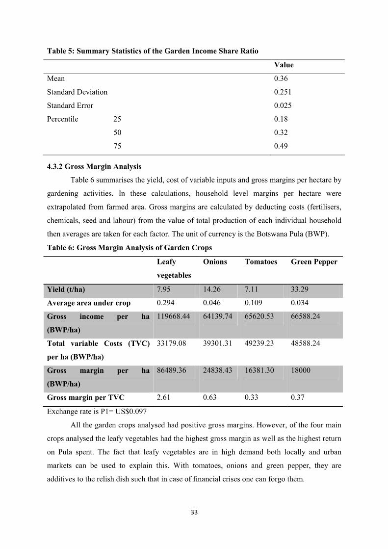
33

Table 5: Summary Statistics of the Garden Income Share Ratio

Value

Mean 0.36

Standard Deviation 0.251

Standard Error 0.025

Percentile 25 0.18

50 0.32

75 0.49

4.3.2 Gross Margin Analysis

Table 6 summarises the yield, cost of variable inputs and gross margins per hectare by

gardening activities. In these calculations, household level margins per hectare were

extrapolated from farmed area. Gross margins are calculated by deducting costs (fertilisers,

chemicals, seed and labour) from the value of total production of each individual household

then averages are taken for each factor. The unit of currency is the Botswana Pula (BWP).

Table 6: Gross Margin Analysis of Garden Crops

Leafy

vegetables

Onions Tomatoes Green Pepper

Yield (t/ha) 7.95 14.26 7.11 33.29

Average area under crop 0.294 0.046 0.109 0.034

Gross income per ha

(BWP/ha)

119668.44 64139.74 65620.53 66588.24

Total variable Costs (TVC)

per ha (BWP/ha)

33179.08 39301.31 49239.23 48588.24

Gross margin per ha

(BWP/ha)

86489.36 24838.43 16381.30 18000

Gross margin per TVC 2.61 0.63 0.33 0.37

Exchange rate is P1= US$0.097

All the garden crops analysed had positive gross margins. However, of the four main

crops analysed the leafy vegetables had the highest gross margin as well as the highest return

on Pula spent. The fact that leafy vegetables are in high demand both locally and urban

markets can be used to explain this. With tomatoes, onions and green pepper, they are

additives to the relish dish such that in case of financial crises one can forgo them.

34

From the results, gardening is viable as indicated by the gross margins. The mean

gross margin per hectare for the leafy vegetables was P86489.36 or US$ 8380.78, onions was

P24838.43 or US$ 2406.83 and P16381.30 or US$ 1587.34 for tomatoes. On average, the

area under leafy vegetables was 0.294 whilst for onions it was 0.0458 and 0.1091 for

tomatoes. Larger areas could significantly increase the contribution of income from the

garden to the total household income.

4.3.3 Factors Affecting Gross Margin per Hectare

Gross margin is a function of price and yield. Assuming a constant price, it is

expected that yield will cause the variation in the gross margins across rural beneficiary

households. Yield is affected by household characteristics, input usage and garden size

among other factors. The results of log-linear analysis of these relationships are presented in

Table 7.

Table 7: Factors Affecting Gross Margin per Hectare

Variable Coefficient Std. Err. t p>|t|

Age -0.07 0.30 -0.23 0.753

Fertilizer applied 0.70 0.14 5.10 0.000***

Area planted 0.34 0.18 1.87 0.066*

Income source -0.03 0.05 -1.70 0.484

Livelihood constraint -0.08 0.07 -1.30 0.196

Livelihood threat 0.003 0.03 0.09 0.931

Labour source 0.001 0.63 -0.00 0.998

Market constraint 0.05 0.03 1.31 0.195

Production constraint 0.17 0.06 3.06 0.003***

Market availability 0.63 0.22 2.79 0.007***

Education level 0.11 0.11 1.06 0.295

Household size -0.05 0.03 -1.79 0.078*

Problem index -0.29 0.27 -1.11 0.273

Constant 0.50 1.97 0.25 0.801

Number of obs = 83

R-squared = 0.5456

Adjusted r-squared = 0.4521

*, **, ***: refers to significance at 10 %, 5 % and 1 % level, respectively

35

Out of the 14 factors that were hypothesized to have an effect on the household gross

margin, three (fertilizer, production constraint and market) had a significant effect on gross

margin.

The amount of fertilizer applied was significant at 1%. Fertilizer is an agent for

increasing yields and when optimum levels are applied, more output is realized and thus

gross margins. Results showed that a one unit increase of fertilizer raises yield of vegetables

by 70%. This is corroborated by Chellemi and Pierce (2002) that supplemental use of

fertilizers an significantly impact marketable yields as fertilizer application increased the

marketable yield of the first harvest.

The head of a household is assumed to be responsible for the coordination of the

household activities therefore, age of the household head is often indicative of farming

experience as well as the ability to comprehend new technologies. The results in Table 6

show that age has a negative relationship with vegetable yields. When the age of the

household head increases by one unit then yield will be reduce by 7%. This is because the

innovativeness, buoyancy of the farmer and mental abilities to deal with challenges that arise

decreases with age. The age of the head of the household is also important since it determines

whether the household benefits from the experience of an older person, or has to base its

decisions on the risk-taking attitude of a young farmer (Makhura, 2001).

Market availability has to be determined by the farmers before they start production

so as to answer the question of what to plant, how much to plant, where and to whom the

produce will be sold to. Nichols and Hilmi (2009) found that availability of market research

enables smallholder farmers to become more knowledgeable about prices, what vegetables

are wanted and the quantities of the vegetables markets require. Availability of the market

was significant at 1% and the positive coefficient can be construed to mean when farmers

have a particular preference they get motivated to increase yields and thus increasing profits.

There is often preference for retail markets because they tend to provide higher prices as

observed by Oxouzi and Papanagiotou (2010).

The results suggest a positive relationship between the yield and area devoted to

vegetable production due to economies of scale. Area planted was significant at 10% which

can be inferred to mean that a unit increase in the area planted will increase yield and

consequently gross margins by 34%. Given good management practices, increase in area

under vegetable production would increase output. Erbaugh et al. (2008) found that farm size

negatively influenced gross margins and this contrasted the results found by Sulumbe et al.

(2010) who found positive relationships between gross margins and farm size.

36

The alternative income source of a household is another factor that was found to

affect profitability of the gardens negatively. When a household has an alternative source of

income, it reduces gross margins by 3%. With existence of other sources of income, there is

tendency of less concentration on the gardens leading to lower yields assuming constant

prices, low output leads to low margins.

A large household size indicates availability of labour to garden activities and thus

labour constraints would not be a problem. In addition a large household size could be an

indication of a household’s ability to have several sources of information that might have a

positive impact on yield. Even though the source of labour dummy was not significant in

explaining the observed gross margins, household size was significant at 10% and showed a

negative relationship between household size and yield. The observed relationship may be

due to the fact that in some instances, despite the relatively large household size, most

members spend their time on other activities and thus may not represent a readily available

labour source. Despite a large household size, profitability may be negatively impacted in

that some family members may not take part in production activities or due to diminishing

marginal returns to labour (Ahuja, 2000).

4.3.4 Analysis of Production Constraints for Rural Beneficiary Households

Farmers were asked using Focus Group Discussion (FGD) about main limitations

they face during farming operations. Households were requested to list the three most

important constraints they face in the gardens. Figure 6 shows the strength of each constraint

in the garden. Pests and diseases seem to be the greatest challenge that 27.7 % of households

were facing. Farmers indicated that the problematic pests were aphids thus they were using

soapy water to control them. Soapy water does not always work so households that can afford

to buy pesticides were using Malathion. Households indicated that they rely on the

government to supply them with pesticides but often, there are delays which leads to a build-

up of pests. This is substantiated by Ellis-Jones et al. (2008) that pests and diseases have been

identified as major constraints to vegetable production as they cause both economic and

health problems for vegetable farmers.

A small number of households (4.3 %) had insufficient knowledge on what to produce

and when to produce for higher returns. However farmers pointed out that they grow leafy

vegetables because they are perennial in nature and easy to manage. It is possible for farmers

to get information by their own effort but they are facing problems due to absence of market

information as most of the time they become aware of the price upon arrival at the market.

Farmer’s know-how of product sorting, grading, packing and transporting is traditional,

37

which severely affects the quality of horticultural products supplied to the market (Kiros,

2008).

Lack of water is also a major production constraint that 23 % of the farmers were

facing as most of them rely on rain water. Since the gardens were situated in places where

access to piped water is not available, government supplies using bowsers and sometimes

they go for a month without water thus disrupting vegetable production. For farmers (4 %)

who pointed out that they use piped water for irrigation, their water bills exponentially

increased and they could not afford to pay the bill hence their water was be disconnected.

Rahman et al. (2008) identified shortage of irrigation water in the dry season, lack of quality

seeds, lack of knowledge on vegetable production and preservation, insect/pest problems on

vegetables as major constraints to homestead vegetable production for sale.

Damage of gardens by domestic animals affected 3.3 % of the farmers. Goats and

donkeys could damage the net shading and eat the vegetables inside. As a way of preventing

animals from damaging their gardens, farmers have put up fences to surround the gardens.

About 2.3 % of the farmers had a problem of vandalism and crime as their gardens were

destroyed and the thieves took the poles thus leaving the net shading sagging. These findings

are supported by Chowdhuri et al. (2014) that farmers pointed out they have a problem of

vegetable damage by domestic animals and loss of production due to theft.

Low quality of materials supplied (variable inputs included) was identified by 15.7 %

of the farmers as a production constraint. For example, farmers indicated that they were given

pipes for drip irrigation that were blocked and were never checked thus the farmers have

never used them and some were given leaking water tanks so they could not store water in

them until they could fix the leaks. The farmers indicated that though they would like to fix

the leaks themselves it is not possible as they cannot afford to do so. Chowdhuri et al. (2014)

found that inadequate supply of good quality seeds was also a vegetable production problem

faced by farmers.

Transport was a production constraint to 2 % of the farmers as they did not have

reliable transport to the market or even to places where they can purchase inputs they needed.

(Kiros, 2008) found that the issue of transport brings into focus the inadequacy of farm roads

and the poor condition of existing ones as most of the production sites are in rural areas.

Because soil testing was not done before the farmer was given the backyard gardens, 4.3 % of

the farmers indicated that where the gardens were constructed was not suitable for growing

vegetables and thus gardens failed. Soil properties and its water permeability should be

38

known as they are important aspects of vegetable growth and quality (Nichols and Hilmi,

2009).

Figure 7: Production constraints

4.3.5 Analysis of Marketing Constraints

Results of marketing constraints facing backyard gardens are presented in Figure 7. In

marketing of horticultural produce, lack of market was identified by the majority (26%) as

the main constraint. The primary markets for various vegetable products from the gardens

were neighbourhood households who buy for consumption. Likewise, vendors who bought in

bulk for re-sale in open markets served as another outlet. Xaba and Masuku (2013) found out

that some vegetables produced by farmers in Swaziland were spoiled due to lack of markets.

Lack of storage facilities was a problem faced by 11 % of the farmers as sometimes

they produced excess vegetables which they could not consume. Large amounts of vegetables

were lost due to wastage as farmers had no technical knowledge of preservation and lack of

facilities. This led to high post-harvest losses because of large amounts of left overs. Lack of

market facility was identified by 20 % of the farmers as a constraint because they sold their

vegetables in the local market as they were dependent on word of mouth to market their

gardens. As a result, they did not get good prices. Poor prices were encountered by 15.7 % of

the farmers. The main cause is that farmers produce at the same time leading to low demand

because there might not be enough market to sell (Antwi and Seahlodi, 2011; Kiros, 2008).

Salami et al. (2010) stated that road systems are the most serious infrastructural

bottleneck facing agricultural development. The results in figure 7 further show that about

0 5 10 15 20 25 30

pests and disease

insufficient knowledge

lack of water

poor soils

vandalism & crime

low quality materials supplied

transport

water disconnection

animals

percentage

39

4.7% of farmers were constrained by the lack or poor access roads. These may have limited

transportation of vegetables to better or other markets. However, it may have also delayed

quick distribution of produce after harvesting hence the vegetables deteriorated. Lack of rural

roads impedes the marketing of agricultural commodities, preventing farmers from selling

their produce at reasonable prices and leads to spoilage of farm produce (Oluwasola, 2015).

Access to transport by farmers plays a significant role in their ability to access

markets. Since vegetables are highly perishable, there is a sense of urgency in marketing

these products as quickly and efficiently as possible in order to maintain their farm fresh

value. About 6.7 % of the farmers did not have access to convenient modern transportation

system to ship their products to the market thus they were forced to hire transport from other

people or use public transport. This findings are supported by Louw et al. (2004) that most

small scale farmers have no means of transport to carry their produce to markets, therefore,

transportation problems results in loss of quality and late delivery, which in turn lead to lower

prices and this is the greatest problem faced by emerging farmers. The problem of marketing

constraints arise due to many factors such as limited knowledge, lack of access to reliable

markets and lack of appropriate and affordable means of transport (Chanimuka et al., 2008).

Figure 8: Marketing constraints

4.4 Impact of Backyard Gardens and Factors that Affect Consumption Expenditure

Prior to discussion of the impact of backyard gardens on household consumption

expenditure, it was imperative to explain the factors that affect consumption expenditure.

0 5 10 15 20 25 30

lack of market

lack of transport

poor prices

poor roads

lack of/poor market facility

lack of storage facilities

Percentage

40

Factors that affect consumption expenditure explain why some household spend more than

others.

4.4.1 Factors Affecting Household Consumption Expenditure

The OLS model results of factors affecting household consumption expenditure are

presented in Table 8. The dependent variable was average household expenditure and

variable of interest were household size, marital status, education, gender, age, perception

index, income perceptions, source of income, threats to livelihoods constraint to improving

livelihoods, number of meals a household has each day and total income.

The results in Table 8 show that the significant variable were gender and education

level of household head, income perception, total income, threats to household livelihood,

number of meals the household have each day and income source were found to be

significant.

Table 8: Factors Affecting Consumption Expenditure

Average expenditure Coefficient SE t p>|t|

Age 1.63 2.50 0.65 0.514

Gender -145.74 66.84 -2.18 0.030**

Marital status 9.67 25.87 0.37 0.709

Household size 1.27 8.64 0.15 0.883

Education level 108.28 31.58 3.43 0.001***

Farming experience 0.13 9.46 0.01 0.989

Livestock ownership 0.004 0.003 1.18 0.239

Perception index -8.74 10.30 -0.85 0.397

Income perception 61.98 15.55 3.99 0.000***

Total income 0.07 0.03 2.21 0.028**

Livelihood threat -17.04 7.31 -2.33 0.021**

Major constraint -6.56 16.75 -0.39 6.696

No of meals 157.76 47.35 3.35 0.001***

Income source -35.09 12.16 -2.88 0.004***

Kanye -8.97 61.22 -0.14 0.885

Mabutsane -22.16 107.15 -0.21 0.836

_Const -11.22 218.50 -0.05 0.959

Number of obs = 238

Prob> F = 0.0000

R- squared = 0.3347

Adjusted R-squared = 0.2766

**, ***: refers to significant level at 5 and 1% level, respectively

The relationship between gender of the respondent and consumption expenditure was

negative. It implies that being male reduces the consumption expenditure by BWP145.74.

41

This is explained by the fact that men tend to spend the income on non-household items like

alcohol and tobacco. This is corroborated by Muriithi (2015) who found that a significant

share of income managed by men was used to purchase adults goods such as beer and other

expenditures that do not benefit the family.

Education level had a positive relationship with consumption expenditure as a unit

increase in the level of education of the household head by one year will increase the

consumption expenditure of that household by BWP 108.28 and was significant at 1%. This

is because household heads are the decision makers in matters concerning expenditure and

education exposes them to a wide range of consumer possibilities. Mignouna et al. (2015)

found that farm households expenditure increases with education which suggests that the

more educated the household head are, the higher their household expenditure when

compared to their less educated counterparts.

Money increases the willingness of households to consume more. Therefore a

household that perceives more income will increase its consumption expenditure. Results in

Table 7 show a positive relationship between income perception and consumption

expenditure. This results are supported by Jappelli and Pistaferri (2010) who found that a one

dollar anticipated rise in income increases non-durable consumption by approximately 20

cents. There is a positive relationship between total income that the household has and

consumption expenditure. This is because it expected that the rich will spend more than the

poor hence rural households that are rich will consume more goods and services than their

counterparts. Ruel et al. (2005) found that income growth contributed to greater consumption

in the long run.

The major threat to livelihoods that rural households were facing was

drought/irregular rains and prolonged dry spells. This might lead to a severe loss of

employment as 80% of rural population is engaged in agriculture and allied activities

(Udmale et al., 2014). The results in Table 7 show that rural households that are faced with

this threat toward their livelihoods would reduce their consumption expenditure by 17%.

There is a positive relationship between the number of meals per day that a household

consumes and the consumption expenditure. This might be because the more meals per day a

household consumes, the more they have to spend on buying food to take care of their dietary

needs. Therefore, if there are concerns by households about job security and future expected

income, they will reduce their consumption expenditure. Results in Table 7 show that when

households are worried about their income source, their consumption expenditure reduces by

35.1%.

42

4.4.2 Impact of Backyard Gardens on Farm Household Consumption Expenditure

Table 9 presents the logit model results which were used to create the counterfactuals

for matching and the outcome variable was consumption per equivalent adult. Matching of

beneficiaries to non-beneficiaries was based on household size, marital status, education,

gender, age, perceptions, income perceptions, source of income, threats to livelihoods and

constraint to improving livelihoods. These are the variables which both groups had similar

characteristics suitable for matching. The average treatment effect of the program was then

calculated as the mean difference in outcomes between these two groups.

The results in Table 9 show that the significant variables were perception index,

income perception, source of income, major threat to livelihood of the household, major

constraint to improving household livelihood, household size, being located in Mabutsane

and farming experience.

Table 9: Psmatch2 Logit Results

Variable Coefficient Std. Err. Z P>|Z|

Age -0.003 0.003 -1.00 0.320

Gender -0.010 0.092 -0.11 0.910

Marital status 0.048 0.350 1.36 0.172

Household size -0.021 0.011 -1.87 0.061*

Education 0.005 0.043 0.11 0.915

Farming experience 0.136 0.078 1.74 0.082*

Livestock 0.014 0.010 1.37 0.172

Perception index 0.069 0.015 4.57 0.000***

Income perception 0.072 0.025 2.90 0.004***

Total income -0.057 0.045 -1.29 0.198

Livelihood threat -0.025 0.011 -2.27 0.023**

Major Constraint -0.047 0.024 -2.00 0.046**

No of meals -0.039 0.065 -0.61 0.545

Income source -0.069 0.017 -4.04 0.000***

Kanye 0.052 0.085 0.61 0.543

Mabutsane -0.170 0.101 -1.69 0.090*

Constant -1.077 1.956 -0.55 0.528

Number of obs = 225

LR chi2 = 78.48

43

Prob> chi2 = 0.0000

Pseudo R2 = 0.2614

Log likelihood = -110.885

*, **, ***: refers to significance at 10, 5 and 1% level, respectively

Perception index is important because when one’s overall perception increases, the

probability of participating in the backyard garden scheme increased by 6.9 %. This findings

are supported by Sirivongs and Tsuchiya (2012) who found that there is a strong relationship

between positive perceptions, attitudes and participation. The resident’s positive perceptions

affected their attitudes while positive attitudes strongly influenced their participation.

Money increases the willingness of the households to participate in programs that they

perceive to give higher returns. Therefore a household that perceives backyard gardening as

an income source and also has alternative source of income has a 7.3% chance of

participating in gardening. Northrop et al. (2013) found that several consumers perceived

store-bought organic foods as high-priced and therefore, they preferred to have gardens as an

affordable means of obtaining organic food.

The severe threat that households indicated to be facing was drought/irregular rains

and prolonged dry spells. This might lead to a reduction in crop production and a severe loss

of employment as 80% of rural population is engaged in agriculture and allied activities

(Udmale et al., 2014). The results in Table 8 show that rural households that are faced with

this threat toward their livelihoods, the chances of them participating in the backyard gardens

are reduced by 2.5 %.

Production constraint was the most serious problem that households faced to

improving the household livelihoods as it reduced the probability of the household

participating in backyard gardens by 4.7%. This might be because vegetable production as a

livelihood strategy is a distress-push because its share in total earnings reduces as income

increases. The almost constant income share of off farm income activity may be taken as an

indication of a stagnant off farm economy therefore, farmers should integrate on-farm with

off farm activities especially those that have complementarity with farming activities and also

adopt a livelihood diversification strategy that combines multiple portfolios (Udmale et al.,

2014).

Household size in this context was used to describe the dependency of the household

rather than labour availability. An increase in the number of household members was

negatively related to the probability of that household participating in the backyard garden

44

scheme. This may be because household size is not a good indicator of labour availability as

it includes not only active and inactive members of the household but the number of mouths

to be fed. This is supported by Mustafa-Msukwa et al. ( 2011) who found that an increase in

the number of household members was negatively related to the adoption of compost manure

in Malawi therefore having a large family per se does not necessarily mean all family

members are available for the farm work.

If a farmer increased farming experience by one year then the probability of them

participating in backyard gardens would increase 13.6%. This might be because the

experience of farmers in vegetable production is positively associated with net income from

vegetable farming. As farmer’s experience in vegetable production increases, their efficiency

at utilizing resources to achieve higher levels of output increases as they understand the

dynamics in demand and pricing of vegetables to be able to take full advantage in order to

increase earnings and/or minimize loss (Oluwasola, 2015).

A person from Mabutsane has a probability of 17% that they might participate in the

backyard garden scheme when compared to the person from Goodhope. This is because of

the location. Mabutsane is a remote village without proximity to any urban area and therefore

if a household was to participate in backyard gardens, they were likely to be running a

profitable small scale vegetable production unit. The reason is that the anticipated customers

will not be willing to travel long distances to the nearest town to buy garden produce.

4.4.3 Average Treatment Effects on Consumption Expenditure

To identify the impact of backyard gardens on consumption expenditure, the average

monthly consumption expenditure was compared for beneficiaries and non-beneficiaries. The

result obtained are presented in Table 10 and indicate that, there was no significant difference

(p<0.73) between the consumption expenditure of the beneficiaries and non-beneficiaries but

the average monthly consumption expenditure of backyard garden scheme beneficiary

household was P934.02 which is equivalent to US$90.60, was higher than non-beneficiaries,

P841.34 or US$81.61. This implies that backyard garden scheme increases the per capita

consumption expenditure of scheme members by P92.69 or by 9.9 %. This agrees with Beshir

(2012) who found that households who are members of irrigation scheme for vegetable

gardens have better annual incomes when compared to non-members and this extra income

allows households to meet daily expenses.

45

Table 10: Average Treatment Effects on Household Consumption Expenditure

Variable Sample Treated Controls Difference S.E T-stat

Consumption expenditure

Unmatched 934.02 766.52 167.52 67.76 2.47

ATT 934.02 841.34 92.69 127.13 0.73

Region of common support ensures that treatment observations have comparison

observations nearby in the propensity score distribution (Heckman et al., 1998). Results in

Table 11 indicate that there were no cases that were out of the region of support. (Bryson et

al., 2002) noted that when the proportion of lost individuals is small, this poses few

problems. Therefore, this means that only individuals between the treatment and control

group in terms of observed characteristics unaffected by participation were compared as only

in the area of common support can inferences be made about causality.

Table 11: Region of Common Support

Treatment assignment Off support On support Total

Untreated 0 138 138

Treated 0 87 87

Total 0 225 225

After matching, the covariate imbalance was checked and a ps-test command was

used. The ps-test shows the percentage reduction in bias which is the standardised biased. A

good bias reduction is supposed to be below 5 %, however 10 % is also reasonable

(Rosenbaum and Rubin, 1985). The variables after matching are not supposed to be

significant. Results in Table 12 indicate that after matching there was less bias in the

covariates which were below 10 %. U represents unmatched and M represents matched.

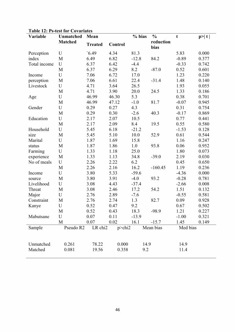
46

Table 12: Ps-test for Covariates Variable Unmatched

Matched Mean % bias %

reduction bias

t p>| t |

Treated Control

Perception index

U `6.49 4.34 81.3 84.2

5.83 0.000 M 6.49 6.82 -12.8 -0.89 0.377

Total income U 6.37 6.42 -4.4 -87.0

-0.33 0.742 M 6.37 6.29 8.2 0.52 0.601

Income perception

U 7.06 6.72 17.0 -31.4

1.23 0.220 M 7.06 6.61 22.4 1.48 0.140

Livestock U 4.71 3.64 26.5 24.5

1.93 0.055 M 4.71 3.90 20.0 1.33 0.186

Age U 46.99 46.30 5.3 81.7

0.38 0.701 M 46.99 47.12 -1.0 -0.07 0.945

Gender U 0.29 0.27 4.3 40.3

0.31 0.754 M 0.29 0.30 -2.6 -0.17 0.869

Education U 2.17 2.07 10.5 19.5

0.77 0.441 M 2.17 2.09 8.4 0.55 0.580

Household size

U 5.45 6.18 -21.2 52.9

-1.53 0.128 M 5.45 5.10 10.0 0.61 0.544

Marital status

U 1.87 1.69 15.8 93.8

1.16 0.247 M 1.87 1.86 1.0 0.06 0.952

Farming experience

U 1.33 1.18 25.0 -39.0

1.80 0.073 M 1.33 1.13 34.8 2.19 0.030

No of meals U 2.26 2.22 6.2 -160.45

0.45 0.650 M 2.26 2.16 16.2 1.19 0.236

Income source

U 3.80 5.33 -59.6 93.2

-4.36 0.000 M 3.80 3.91 -4.0 -0.28 0.781

Livelihood Threat

U 3.08 4.43 -37.4 54.2

-2.66 0.008 M 3.08 2.46 17.2 1.51 0.132

Major Constraint

U 2.76 2.89 -7.6 82.7

-0.55 0.581 M 2.76 2.74 1.3 0.09 0.928

Kanye U 0.52 0.47 9.2 -98.9

0.67 0.502 M 0.52 0.43 18.3 1.21 0.227

Mabutsane U 0.07 0.11 -13.9 -15.7

-1.00 0.321 M 0.07 0.02 16.1 1.45 0.149

Sample Pseudo R2 LR chi2 p>chi2 Mean bias Med bias

Unmatched Matched

0.261 0.081

78.22 19.56

0.000 0.358

14.9 9.2

14.9 11.4

47

CHAPTER 5

SUMMARY, CONCLUSION AND RECOMMENDATIONS

This section presents summary of the major findings in the study, conclusions drawn

and recommendations.

5.1 Summary

The main aim of this study was to assess the impact of backyard gardening on

household incomes. To select respondents for the study, Southern District was selected

because this is where the largest number of backyard gardens was found. Accordingly,

primary data was collected from 247 respondents of which 100 where beneficiaries and 147

where non-beneficiaries of the backyard garden program.

In order to examine the impact of backyard gardening on household income, the study

assessed gross margins of backyard gardens, factors affecting gross margins, factors affecting

consumption expenditure and the impact of backyard gardens on household consumption

expenditure. Descriptive statistics were also employed for analysis. During analysis, different

software’s such as SPSS and Stata were used.

In relation to gross margins of the backyard gardens, the results revealed that

backyard gardening was viable as leafy vegetables had gross margins of P86 489.36, onions

had P240838.43, tomatoes had P16 381.30 and green pepper had P18 000. Factors that affect

gross margins were fertilizer application, market availability, area planted, household size

and production constraint. Household size negatively influenced gross margins while the

remaining four factors influenced gross margins positively. The gender of household head,

education level, income perception, total household income, livelihood threat, income source

and number of meals per day had significantly influenced the average consumption

expenditure of both the beneficiary and non-beneficiary households. Propensity score

matching revealed that backyard gardening increased beneficiary household’s monthly

average consumption expenditure by P92.69.

5.2 Conclusion

Although gardening was prominent in the area, some households were seasonal

gardeners, some did very little gardening because of water challenges. The income from the

garden was not contributing much to the total household income and this would affect the

amount of effort households are willing to put into gardening. In order to generate income,

the rural households must also incur costs, which may be a heavier burden in the first few

years. Beneficiaries should have been informed that their gardens may not be profitable for

48

the first few years and therefore they should maintain their other forms of employment if

possible.

Farmers faced various production and marketing constraints but the major constraints

were pests and diseases, lack of water, low quality materials supplied, lack of market, lack of

storage facilities, lack of market facilities and poor prices. Government should have a

comprehensive value chain for backyard gardens so as to avoid some of the production and

marketing challenges that the beneficiaries are facing. As for the lack of water constraint, it is

important that another source of water be identified and used instead of relying on rainfall.

Unreliable rainfall and insufficient water for crop production is a major constraint to

improving the welfare of households as it results in low productivity. The uncertainty of rain

fed agriculture results in low yields, thus most of the households might fail to meet their

minimum food requirement.

Based on the results many households in Southern district are operating and selling

their produce locally as gross margin analysis of the different garden crops revealed that

gardening activity is viable. The impact of the backyard garden in terms of consumption

expenditure of households was higher for beneficiaries indicating a positive impact of the

backyard garden program towards their incomes.

Hence it can be concluded that backyard garden program plays a crucial role in

improving the living standards of Batswana as it has the potential to increase household

incomes.

5.2 Recommendations

There is need for the government to re-design the backyard garden program in

Botswana due to the significant contribution of this program in alleviating extreme poverty

especially the consumption expenditure of the households who are beneficiaries of the

program. As part of re-designing the backyard garden program, beneficiaries should be taught

about rain water harvesting technology and be encouraged to form groups in order to access

financing for drilling boreholes because irrigation is an alternative way to improve and

sustain food production hence consumption expenditure of rural households.

Program leaders must recognize the production and marketing constraints themselves

as well as plan for the possibility that continual financial support may be necessary

particularly in the first few years of operation as beneficiaries may need assistance for

purchasing inputs and for garden upkeep. Even though there was increase in consumption

expenditure, there is dire need for setting up a comprehensive structure to engage all

stakeholders to improve the implementation of the program. This could start with identifying

49

the aims of the program because as of yet it is not clear what the aims of the program are and

stakeholders should be identified and they could be potential beneficiaries, social workers,

dikgosi, councillors, extension officers, office of the president officers and ministry of

agriculture officers.

Program leaders should come up with policies that would improve productivity of

small scale vegetable farmers through provision of seminars and workshops where farmers

would acquire more training on vegetable production. This would enable them to increase the

average yield of vegetables produced per hectare, hence profitability.

There is an urgent need to develop a complete value chain for produce from backyard

gardens. This policy will ensure a wholistic approach of rural development in the agricultural

sector.

5.3 Areas for Future Research

The conclusions drawn in this study were based on the cross-sectional data of the year

2015/2016. However, the impact of the currently significant variables as well as the non-

significant variables should also be checked using time series data. It is also recommended

that a study should be conducted on market analysis for the community so that the

community can be able to plan their cropping programs effectively such that issues of market

flooding are avoided. There is also a need for a study which will focus on the sustainability of

all backyard gardens in Botswana.

Another issue to be looked at would be opportunities for exploring other markets as

well as value addition of the produce before going to the markets. Finally it is recommended

for future researchers to consider SWOT analysis of the backyard garden program as it was

introduced without carrying out SWOT analysis and also interrogate how Agricultural

Extension Agents can assist beneficiaries of the program.

50

REFERENCES

Ahuja, G. (2000). The duality of collaboration. Strategic Management Journal, 21(3): 317–

343.

Alaimo, K., Packnett, E., Miles, R. A., and Kruger, D. J. (2008). Fruit and Vegetable Intake

among Urban Community Gardeners. Journal of Nutrition Education and Behavior,

40(2): 94–101.

Ali, J. (2011). Adoption of mass media information for decision-making among vegetable

growers in Uttar Pradesh. Indian Journal of Agricultural Economiccs, 66(2): 241–254.

Anderson, S. A. (1990). Core indicators of nutritional state for difficult-to-sample

populations. The Journal of Nutrition, 11(120): 1559–600.

Antwi, M., and Seahlodi, P. (2011). Marketing Constraints Facing Emerging Small-Scale Pig

Farmers in Gauteng Province , South Africa. Journal of Human Ecology, 36(1): 37–42.

Aubry, C., Ramamonjisoa, J., Dabat, M., Rakotoarisoa, J., Rakotondraibe, J., and

Rabeharisoa, L. (2012). Land Use Policy Urban agriculture and land use in cities: An

approach with the multi-functionality and sustainability concepts in the case of

Antananarivo ( Madagascar ). Land Use Policy, 29(2): 429–439.

Basimane, I. (2014). Backyard gardening: Just what the doctor ordered. Retrieved from

www.kutlwano.gov.bw/kut-article-teaser-detail.Php ? aid = 54andcid=26andmid=60

Batchelor, C. H., Lovell, C. J., and Sernple, A. J. (1994). Garden irrigation for improving

agricultural sustainability in dryland areas. Land Use Policy, 11(4): 286–293.

Becker, S.O. and Ichino, A. (2002). Estimation of average treatment effects based on

Propensity Scores. The Stata Journal, 2(4): 1-19.

Beshir, H. (2012). Poverty and food security analysis at farm household level in South Wollo

, Ethiopia: propensity score matching approach. Unpublished Phd thesis. Haramaya

University.

Betek, C. K. E., and Jumbam, N. D. (2015). Transactions of the Royal Society of South

Africa Small scale vegetable production: a case study of Port St Johns , Eastern Cape

Province. Transactions of the Royal Society of South Africa, 70(1): 41–45.

Botlhoko, P. (2012). Batswana take up backyard gardening in numbers. Retrieved from

http://www.mmegi.bw/index.php?sid=1andaid=336anddir=2012/August/ Wednesday8.

Bryson, A., Dorsett, R., and Purdon, S. (2002). The use of propensity score matching in the

evaluation of active labour market policies. Working paper No.4, Department for Work

and Pensions.

Byers, K. (2009). The Psycho-social Benefits of Backyard and Community Gardening Among

51

Immigrants. Unpublished Masters Thesis. University of Georgia.

Caliendo, M., and Kopeinig, S. (2008). Some practical guidance for the implementation of

propensity score matching. Journal of Economic Surveys, 22(1): 31–72.

Calvet-mir, L., Gómez-baggethun, E., and Reyes-garcía, V. (2012). Beyond food production :

Ecosystem services provided by home gardens. A case study in Vall Fosca , Catalan

Pyrenees , Northeastern Spain. Ecological Economics, 74: 153–160.

Chanimuka, P., Senyolo, G. M., Makhura, M. N., and Belete, A. (2008). A factor analysis of

access to and use of service infrastructure amongst emerging farmers in South Africa.

Agrekon, 47(3): 37–41.

Chellemi, D. O., and Pierce, F. (2002). Effect of organic fertilizer applications on growth ,

yield and pests of vegetable crops. Florida State Horticultural Society, 115(1): 315–321.

Chirinda, N., Muusha, M., Manyange, E., and Mbetu, J. (2002). Contribution of palustrine

wetlands on livelihoods in semi-arid masvingo district of zimbabwe.Unpublished paper.

Masvingo State University.

Chowdhuri, N. Y., Haque, S., Shammi, S. A., Jannat, A., and Sannyashi, P. R. (2014).

Profitability analysis of winter vegetables production in a selected area of narshingdi

district in Bangladesh. Progressive Agriculture, 25: 47–53.

Corrigan, M. P. (2011). Growing what you eat: Developing community gardens in Baltimore

, Maryland. Applied Geography, 31(4): 1232–1241.

Dehejia, R. H., and Wahba, S. (2002). Propensity Score Matching Methods for Non-

experimental Casual Studies. The Review of Economics and Statistics, 84(1): 151–161.

Devendra, C., and Thomas, D. (2002). Smallholder farming systems in Asia. Agricultural

Systems, 71: 17–25.

Danoesastro, H. (1980). The Role of Home gardens as a Source of Additional Daily Income.

Bandung, Indonesia: Paper presented at the Seminar on the Ecology of

Homegardens III.

Eikenberry, N., and Smith, C. (2005). Attitudes , beliefs , and prevalence of dumpster diving

as a means to obtain food by Midwestern , low-income , urban dwellers. Agriculture and

Human Values, 22: 187–202.

Ellis-Jones, J., J. Stenhouse, H. Gridley, J. Hellaand, and M. Onim. 2008. Baseline study on

vegetable production and marketing. Vegetable breeding and seed systems for poverty

reduction in Africa.

Erbaugh, D. (2008). Profitability analysis of sorghum framing and its influence on sorghum

value chain in Tanzania: A case study of Singida and Simanjaro. Tanzania.

52

Eyzaguirre, P.B. and Linares, O.F. (2010). Introduction: In home gardens and Agro

biodiversity. Edited by Eyzaguirre, P.B. and Linares, O.F. Washington DC, USA:

Smithsonian Books.

Food and Agriculture Organisation, (2000). Socio-economic impact of smallholder irrigation

development in Zimbabwe: Case study of ten irrigation schemes, FAO, SAFR, Harare.

Forestry, A. F. (2009). Farm Gross margins. State Governemnt of Victoria.

Francis, M. and Hester, Jr., R.T. (1990). The meaning of gardens. Cambridge, MA: The MIT

Press.

Gujarati, D.N. (1995). Basic econometrics, Third Edition. McGraw Hill Inc, New York.

Heckman, J. J., Ichimura, H., and Todd, P. (1998). Matching As An Econometric Evaluation

Estimator. Review of Economic Studies, 65: 261–294.

Hendrickson, D., Smith, C., and Eikenberry, N. (2006). Fruit and vegetable access in four

low-income food deserts communities in Minnesota. Agriculture and Human Values,

23: 371–383.

Hoogerbrugge, I., and Fresco, L. O. (1993). Homegarden Systems : Agricultural

Characteristics And Challenges.International Institute for Environment and

Development, Gatekeeper series no. 39, London.

Iannotti, L., Cunningham, K., and Ruel, M. (2009). Improving Diet Quality and

Micronutrient Nutrition Homestead Food Production in Bangladesh. Washington D.C:

USA.

Jappelli, T., & Pistaferri, L. (2010). The Consumption Response to Income Changes. Annual

Review of Economics, 2(1): 479–506.

Keakabetse, B. (2013). Over 7000 backyard underway. Retrieved from

http://botswanaonlinenews.com/over-7000-backyard-gardens-underway/.

Kehlenbeck, K., and Maass, B. L. (2004). Crop diversity and classification of homegardens in

Central Sulawesi , Indonesia. Agroforestry Systems, 63: 53–62.

Kiesling, F. M., and Manning, C. M. (2010). How green is your thumb? Environmental

gardening identity and ecological gardening practices. Journal of Environmental

Psychology, 30(3): 315–327.

Kimber, C. T. (2004). Gardens and Dwelling: People in Vernacular Gardens. Geographical

Review, 94(3): 263–283.

Kiros, A. (2008). Opportunities and Challenges of Vegetable Marketing in Kilte-Awlaelo

Woreda. Unpublished Masters Thesis. Mekelle University.

53

Koh, E.T. and Caples, V. (1979). Frequency of selection of food groups by low-income

families in south-western Mississippi. Journal of the American Dietetic Association,

74(6): 660-664.

Krishna, G.C. (2006). Home Gardening as a Household Nutrient Garden. Pokhara, Nepal;

local initiatives for biodiversity Research and Development, Biodiversity international

and Swiss Agency for development and cooperation: 48-52.

Krone, M., Schumacher, K. P., and Dannenberg, P. (2014). The impact of mobile phones on

knowledge access and transfer of small-scale horticultural farmers in Tanzania.

Geographical Society of Berlin, 145(3): 158–161.

Kumar, B. ., and Nair, P. K. . (2004). Tropical Homegardens: A Time-Tested Example Of

Sustainable Agroforestry. Agroforestry system, 61: 135-152.

Lake, B., Milfont, T. L., and Gavin, M. (2011). The Relative Influence of Psycho-Social

Factors on Urban Edible Gardening. New Zealand Journal of Psychology, 40(3): 50–59.

Lang, T. and Rayner, G. (2002). Why health is the key to the future of food and farming.

Issues 202: 222-0749.

Lewis, P. (1993). The making of vernacular taste: The case of Sunset and Southern Living. In

J. D. Hunt and J. Wolschke-Bulmahn (Eds.), The vernacular garden. Washington, DC:

Dumbarton Oaks.

Louw, A., Madevu, H., Jordaan, D. and Vermeulen, H. (2004). Regoverning markets:

Securing small producer participation in restructured national and regional agri-food

systems. London: International Institute for Environment and Development (IIED).

Maipose, G. S. (2008). Policy and Institutional Dynamics of Sustained Development in

Botswana. The Commision of Growth and Development No. 35.

Makhura, M. T. (2001). Overcoming Transaction Costs Barriers To Market Participation

Participation of Smallholder Farmers in the Northern Province of South Africa. PhD

thesis. University of Pretoria, South Africa.

Marsh, R. (1998). Building on traditional gardening to improve household food security.

Food Nutrition and Agriculture, 22: 4–14.

Mccormack, L. A., Laska, M. N., Larson, N. I., and Story, M. (2010). Review of the

Nutritional Implications of Farmers’ Markets and community Gardens: A call for

Evaluation and Research Efforts. Journal of the American Dietetic Association, 110:

399–408.

Mignouna, D. B., Abdoulaye, T., Alene, A., Manyong, V. M., Donstop, P. N., Ainembabazi,

J. H., & Asiedu, R. (2015). A Microeconometric anlaysis of household consumption

54

expenditure determinants in Yam-growing areas of Nigeria and Ghana. Journal of

Tropicultura, 33(3): 226–237.

Ministry of Agriculture (2008). Backyard gardens guidelines. Gaborone, Botswana.

Ministry of presidential affairs and public administration (2015) state of the nation address by

his Excellency. Gaborone, Botswana. (http://www.gov.bw/en/News/N1_News_211/)

Mitchell, R., and Hanstad, T. (2004). Small homegarden plots and sustainable livelihoods for

the poor. Working paper 11. Rome, Italy.

Muriithi, B. (2015). Smallholder horticultural commercialization: Gender roles and

implications for household well-being in Kenya. In Proceedings of 29th Annual

Conference, International Conference of Agricultural Economists. Milan, Italy.

Mustafa-Msukwa, A. ., Mutimba, J. ., Masangano, C., and Edriss, A. (2011). An Assessment

of the Adoption of Compost Manure By. South African Journal of Agricultural

Extension, 39(1): 17–25.

Mwabumba, M. (2015). Agricultural and Rural Development lecture Notes. University of

Pretoria CMAAE, Programme.

Nair, R. (1993). An Introduction to Agroforestry An Introduction to Agroforestry. Dordrecht,

The Netherlands: Kluwer Academic Publishers.

Nichols, M., and Hilmi, M. (2009). Growing vegetables for home and market. Diversification

booklet 11, Rome.

Nifiez, V. K. (1984). Household gardens: Theoretical considerations on an old survival

strategy. Unpublished Manuscript.

Niñez, V.K. (1985). Working at half-potential: constructive analysis of home garden

programme in the Lima slums with suggestions for an alternative approach. Food

Nutrition Bulletin, 7(3):6-13.

Nijmeijer, M., Worsley, A., and Astill, B. (2004). An exploration of the relationships between

food lifestyle and vegetable. British Food Journal, 106(7): 520–533.

Nord, B. M., and Brent, C. P. (2002). Food Insecurity in Higher Income Households.

Washington, D.C.

Northrop, M. D., Wingo, B. C., and Ard, J. D. (2013). The Perceptions of Community

Gardeners at Jones Valley Urban Farm and the Implications for Dietary Interventions.

The Qualitative Report, 18(53): 1–11.

Nwaru, J. C. (2004). Rural Credit Markets and Resource Use in Arable Crop Production in

Imo State of Nigeria. Unpublished Doctorate Dissertation. Department of Agricultural

Economics, Michael Okpara University of Agriculture, Umudike, Nigeria.

55

Ochse, J.J. and Terra, G.J.A. (1934). Research on the Economic and Agricultural Condition

and Food Consumption in Koetowinangoen. Landbouw. The Netherlands: Publisher

unknown.

Odebode, O.S. (2006). Assessment of home gardening as a potential source of household

income in Akinyele Local Government Area of Oyo State. Nigeria Journal of

Horticulture Science, 2:47-55.

Ojo, S. O. (2009). Backyard Farming: A Panacea for Food Security in Nigeria. Journal of

Human Ecology, 28(2): 127–133.

Okigbo, B. (1990). Home Gardens in Tropical Africa. In Tropical Home Gardens. Edited by

Landauer K, Brazil M. Tokyo, Japan: United Nations University Press.

Oladele, O. I. (2011). Contribution of indigenous vegetables and fruits to poverty alleviation

in Oyo State, Nigeria. Journal of Human Ecology-New Delhi, 34(1): 1-6.

Oluwasola, O. (2015). Vegetable Production, Livelihood Diversification and Employment

Generation in Oyo State, Nigeria. Journal of Agricultural Science, 7(8): 165–174.

Oxouzi, E., and Papanagiotou, E. (2010). Comparative analysis of organic and conventional

farmers and their farming systems. Where does the difference lie? Bulgarian Journal of

Agricultural Science, 16(2): 135–142.

Phanith, C., and Phnom, P. (2011). Market intergration of local farmers: case study of

vegetable trade in Sourt Nikom District, Cambodia. Unpublished Masters Thesis.

Swedish University of Agricultural Sciences.

Rahman, F. M. M., Rahman, M. G. G. M. M. T., and Rokonuzzaman, M. (2008). Food

security through homestead vegetable production in the smallholder agricultural

improvement project ( SAIP ) area. J. Bangladesh Agril. Univ., 6(2): 261–269.

Ranasinghe, T. T. (2009). Manual of Low Space/No-space Agriculture cum-Family Business

Gardens. The Netherlands: RUAF Foundation.

Randela, R. (2005). Integration of emerging cotton farmers into the commercial agricultural

economy. Unpublished PhD thesis, University of the Free State, Bloemfontein.

Resnicow, B. K., Wang, T., Dudley, W. N., Jackson, A., Ahluwalia, J. S., Braithwaite, R. L.,

… Rl, B. (2001). Risk Factor Distribution Among Sociodemographically Diverse

African American Adults. Journal of Urban Health, 78(1): 125–40.

Rose, D. (1999). Economic Derterminants and Dietary Consequences of Food Insecurity in

the United States. The Journal of Nutrition, 129(2): 517–520.

Rosenbaum, P. R., and Rubin, D. B. (1985). Constructing a Control Group Using

Multivariate Matched Sampling Methods That Incorporate the Propensity Score.

56

American Statistical Association, 39(1): 33-38.

Ruel, M. T., Minot, N., and Smith, L. (2005). Patterns and determinants of fruit and vegetable

consumption in Sub-Saharan frica: a multicountry comparison. International Food

Policy Resserach Institute, 1(1): 1–45.

Ryall, C., and Hatherell, P. (2003). A Survey of Strategies Adopted by UK Wildlife Trusts in

the Promotion of Gardening for Wildlife. The Environmentalist, 23: 81–87.

Salami, A., Kamara, A. B., Abdul, B., and John, C. (2010). Smallholder Agriculture in East

Africa : Trends , Constraints and Opportunities. Working papers series No. 105. African

Development Bank, Tunis, Tunisia.

Samantaray, S. K., Prusty, S., and Raj, R. K. (2009). Constraints in Vegetable Production-

Experiences of Tribal Vegetable Growers. Indian Research Journal for Extension

Education, 9(3): 32–34.

Samboko, C. P. (2011). An Asssessment of Factors Influencing the Profitability of Bean

Production in Zambia. Unpublished Masters Thesis. University of Zambia.

Sinclair, D. (2005). The spirituality of gardening. Kelowna, BC, Canada: Northstone

Publishers.

Singh, I., L. Squire and J. Strauss (1986). The basic model: Theory, Empirical results, and

policy conclusions. In Agricultural Household Models: Extensions, Applications, and

Policy. ed. in Singh, L. Squire and J. Strauss, pp.17-47. The Johns Hopkins University

Press, Baltimore, USA.

Sirivongs, K., and Tsuchiya, T. (2012). Forest Policy and Economics Relationship between

local residents ’ perceptions , attitudes and participation towards national protected

areas : A case study of Phou Khao Khouay National Protected Area , central Lao PDR.

Forest Policy and Economics, 21: 92–100.

Sperling, C. D., and Lortie, C. J. (2010). The importance of urban backgardens on plant and

invertebrate recruitment : A field microcosm experiment. Journal of Urban Ecologist,

(13): 223–235.

Steptoe, A., Pollard, T. M., and Wardle, J. (1995). Development of a Measure of the Motives

Underlying the Selection of Food : the Food Choice Questionnaire Department of

Psychology , St George ’ s Hospital Medical School , London. Appetite, 25: 267–284.

Statistics Botswana (2003). Household Income and Expenditure Survey (2002-2003).

Government printer. Gaborone. Botswana

Statistics Botswana (2010). Botswana Core Welfare Indicators Survey (2009-2010).

Government printer. Gaborone. Botswana

57

Sthapit, B.R., Rana, R.B., Hue, N.N. and Rijal, D.R. (2004).The diversity of taro and sponge

gourds in traditional home gardens in Nepal and Vietnam. In Home Gardens and

agrobiodiversity. Edited by Eyzaguirre PB, Linares OF. Washington DC, USA:

Smithsonian Books:234-254.

Subair, S. K., and Siyana, M. (2003). Attitude T oward Backyard Gardening in Botswana. In

Proceedings of 19th Annual Conference, Association for International Agricultural and

Extension Education (pp. 612–622). Raleigh, NC.

Sulumbe MI, Iheanacho AC, Mohammed ST (2010). Profitability Analysis of cotton

production Under Sole-cropping system In Adamawa State, Nigeria. Journal of

Sustainable Development Agriculture Environment, 5 (1): 7-13.

Torimiro, D. O., Tselaesele, N. T., Seven, K., Ramorathudi, M. V., and Hulela, K. (2015).

Vulnerable Groups’ Involvement in Small-scale Vegetable Production: A Panacea for

Poverty and Food Insecurity? International Journal of Vegetable Science, 1–23.

Torquebiau, E. (1992). Are tropical agroforestry home gardens sustainable ? Agriculture,

Ecosystem and Environmennt, 41: 189–207.

Trinh, L. N., Watson, J. W., Hue, N. N., De, N. N., Minh, N. V, Chu, P., … Eyzaguirre, P. B.

(2003). Agrobiodiversity conservation and development in Vietnamese home gardens.

Agriculture Ecosystems and Environment, 97: 317–344.

Udmale, P., Ichikawa, Y., Manandhar, S., Ishidaira, H., and Kiem, A. S. (2014). International

Journal of Disaster Risk Reduction Farmers ’ perception of drought impacts , local

adaptation and administrative mitigation measures in Maharashtra. International Journal

of Disaster Risk Reduction, 1–20.

Vasey, D.E. (1985). Household gardens and their niche in Port Moresby, Papua New Guinea.

Food Nutrition Bulletin, 7(3):37-43.

Wilhelm, G. (1975). American Geographical Society Dooryard Gardens and Gardening in the

Black Community of Brushy , Texas. Geographical Review, 65(1): 73–92.

Wilson, R.T. (1995). Livestock Production Systems. London, UK: Macmillan.

Worsley, A., and Skrzypiec, G. (1998). Do attitudes predict red meat consumption among

young people ?. Ecology of Food and Nutrition, 37(2): 163–195.

Xaba, B. G., and Masuku, M. B. (2013). Factors Affecting the Productivity and Profitability

of Vegetables Production in Swaziland. Journal of Agricultural Studies, 1(2): 37-52.

Yamane, T. (1973). Statistics: An Introductory Analysis, 2nd Ed., New York: Harper and

Row.

58

APPENDIX HOUSEHOLD QUESTIONNAIRE

A questionnaire for research titled: Evaluation of the role of backyard gardens on household

incomes in Southern District, Botswana.

My name is Taboka Kealeboga Sekgopa, a master’s student from Egerton University.

The purpose of this questionnaire is to collect data that will assist me in my research

objective (goal), so your participation is vital. The outcome of this research will enhance

knowledge on the role that backyard gardens play in improving household incomes thus

contributing to household welfare.

I would appreciate it if you could please assist me by answering the following questions. I

assure you that your information will be kept confidential as your name will not be

documented in any of the pages of this questionnaire.

Household level survey: Questionnaire for Farmers

1. Enumerator____________________________

2. Date of interview_______________________

3. Sub-district____________________________

4. Village_______________________________

5. Time started:______________ Time finished:__________________

A. GENERAL INFORMATION

[The respondent must be the head or de-facto head of the household]

1. Gender of respondent:

1. Male [ ]

2. Female [ ]

2. Age of respondent

1. 21 – 25 [ ]

2. 26 – 30 [ ]

3. 31 – 35 [ ]

4. 36 – 40 [ ]

5. Above 41[ ]

3. Marital status

1. Single [ ]

2. Married [ ]

3. Divorced [ ]

59

4. Widowed [ ]

4.Educational level

5. Never attended [ ]

1. Primary school [ ]

2. Junior secondary [ ]

3. BGCSE [ ]

4. Tertiary [ ]

5. Other(specify)____________

5.Household size (number of people living and eating together)__________________

6. Farming experience

1. < 9 months [ ]

2. 9 – 12 months [ ]

3. > 12 months [ ]

B. HOUSEHOLD RESOURCES

(We would like to know a little bit about the resources your household owns)

7. What type of dwelling do you live in?

1. Mud hut and grass thatch roof [ ]

2. Mud hut and asbestos/iron roof [ ]

3. Brick house and grass thatch roof[ ]

4. Brick house and asbestos/iron roof[ ]

5. Block house and grass thatch roof[ ]

6. Block house and asbestos/iron roof[ ]

7. Pole and dagga and grass thatch [ ]

8. Other(specify)____________

8. Family household assets

ASSETS NO. OWNED

CURRENTLY

UNIT VALUE NET VALUE

Chickens

Goats

Draft animals

Total livestock

Car

Tractor

Hand hoe

Trailer

Truck

60

Animal scotch cart

Animal plough

Wheel barrow

Bicycle

Urban house

Fridge

Television

Radio

Telephone-landline

Cell phone

Other(specify)

C. AGRICULTURAL GARDEN PRODUCTION AND MARKETING ACTIVITIES

9. Are you part of the backyard garden scheme? (If YES continue to question 10, if NO go to

question 23)

1. Yes [ ]

2. No [ ]

10. What is the total size of the garden you have/own?

1. 100m2 [ ]

2. 200m2 [ ]

3. 300m2 [ ]

11. What is the source of water for your garden?

1. Stand pipe [ ]

2. Borehole [ ]

3. River [ ]

4. Shallow well [ ]

5. Other (specify)…………………..

12. What type of fence is around your garden?

1. Wire [ ]

2. Branches [ ]

3. live fencing [ ]

4. Grass fencing [ ]

5. Net shading [ ]

6. Other (specify) ………..

13. Who are the main people involved in the gardening activities in your household?

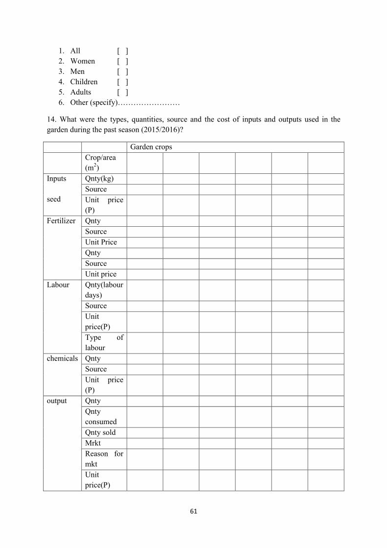
61

1. All [ ]

2. Women [ ]

3. Men [ ]

4. Children [ ]

5. Adults [ ]

6. Other (specify)……………………

14. What were the types, quantities, source and the cost of inputs and outputs used in the

garden during the past season (2015/2016)?

Garden crops

Crop/area

(m2)

Inputs

seed

Qnty(kg)

Source

Unit price

(P)

Fertilizer Qnty

Source

Unit Price

Qnty

Source

Unit price

Labour

Qnty(labour

days)

Source

Unit

price(P)

Type of

labour

chemicals Qnty

Source

Unit price

(P)

output Qnty

Qnty

consumed

Qnty sold

Mrkt

Reason for

mkt

Unit

price(P)

62

Types of garden crops[1]-Leaf vegetables [2]-Tomatoes [3]-Onions [4]-Carrots [5]-

green beans [6]-peas [7]-cucumber [8] - other(specify)

Source input [1]-local shop [2] - town [3] - other

Market type code [1]- local [2]-roadside [3] -middlemen [4]-horticultural companies [5]

other _______(specify)

Reason for that choice of market? 1- Near 2- high prices 3- cheap transport 4-variety of

customers 5- other

Labour source [1]- hired [2]- family [3] other- specify

Type of labour [1] –family [2] - hired [3]- seasonal [4] - contract [5] - permanent

[6]-other- specify

15. What are the 3 main production constraints limiting productivity in the garden

i .……………………………………

ii …………………………………...

iii …………………………………..

Production Constraint [1]pests and diseases [2]high temperatures [3]insufficient knowledge

of small scale production [4]insufficient financial support [5] no water [6] poor soils [7]

vandalism and crime [8] low quality materials supplied [9] transport [10] water

disconnection [11] animals [12] other (specify)

16. List the 3 main constraints you face when marketing the horticulture produce?

i………………………………………………

ii ……………………………………………

iii……………………………………………

Marketing constraint [1] lack of market [2]lack of competition/few traders [3]poor

transport [5]poor prices [6]unreliable traders [7]poor roads [8]lack of/poor market

structures [9]lack of storage facilities [10] inadequate communication[11]lack of marketing

institutions [12] other (specify)

17. How do you handle the produce that fails to sell on the market?

1. Process it [ ]

2. Throw it away [ ]

3. Give it away [ ]

4. Other (specify)…………..

63

18. Would you classify the following problems as either major or minor in association with

your garden? Tick the correct answer

Problem

1. Major 2. Minor

Pests and diseases

High temperature

Insufficient knowledge of

small scale production

Insufficient financial support

Lack of market

No water

Poor soils

Vandalism and crime

Low quality materials

supplied

Transport

Water disconnection

Animals

Lack of support from

extension services

Competition

D: SOCIAL IMPACTS OF THE BACKYARD GARDEN PROGRAMME

19. Please indicate how your participation in the backyard programme has affected you in the

following social aspects

Social impact Experienced change

Your way of life 1 2 3 4 5 6 7

How you live

64

How you work

How you play

How you interact with other people

Your culture

Your beliefs

Your customs

Your values

Your language

Your community

Its cohesion

Its stability

Its character

Its services

Its facilities

Your political systems

The extent to which you participate in decisions that

affect your life

The level of democratization that is taking place

The resources provided for this democratization

Your environment

The quality of air you breathe

The quality of the water you use

The availability of the food you eat

The quality of the food you eat

The level of hazard or risk you are exposed to

The level of noise you are exposed to

The adequacy of sanitation

Your physical safety

Your access to resources

Your control over resources

Your health and wellbeing

Physical well being

Mental well being

Social well being

Spiritual well being

The absence of disease or infirmity

Your personal and property rights

Whether you are economically affected

Whether you experience personal disadvantage

Your fears and aspirations

Your perceptions about your safety

Your fears about the future of your community

65

Your aspirations for your future

The future of your children

1= extreme negative 2=moderate negative 3=slight negative 4=no impact 5=slight

positive 6=moderate positive 7=extreme positive

ECONOMIC IMPACTS OF THE BACKYARD GARDEN PROGRAMME

20. Please indicate how the backyard garden programme has affected your community in the

following aspects

Basic economic indicator Experienced change

1 2 3 4 5 6 7 Unemployment level

The quantity of jobs in a community

The quality of jobs in a community

Income level

Wealth level

Poverty level

The presence of major industrial sectors

The level of business activity

Aesthetic quality of the community

Secure livelihoods

Self-reliance

Economic diversification

Access to finance

1= extreme negative 2=moderate negative 3=slight negative 4=no impact 5=slight

positive 6=moderate positive 7=extreme positive

ATTITTUDE TOWARDS THE BACKYARD GARDEN PROGRAMME

21. State whether you agree or disagree with the statements below

Statement regarding backyard garden programme Rating of extent of

agreement with the

statement

1 2 3 4 5 The backyard garden programme is effective in alleviating poverty

The backyard garden programme is okay as it is designed currently

The backyard garden programme should be reviewed

The backyard garden programme is sustainable

The backyard programme helps the poor people

The backyard programme is a source of employment

The backyard garden programme wastes national resources

The backyard garden programme should be terminated

The backyard garden programme is a vital social safety net

66

The backyard garden programme should be continued

1=strongly disagree 2=disagree 3=undecided 4=agree 5=strongly agree

22. What changes can be made to improve the effectiveness of the backyard garden

programme?

___________________________________________________________________________

___________________________________________________________________________

___________________________________________________________________________

___________________________________________________________________________

___________________________________________________________________________

_______________________________________________________________________

E: Monthly food requirements, Income and Expenditure requirements for the family

23. How important are the following sources of income to your household on the following

scale?

SCALE

1not important

2 less important

3 neutral

4 important

5 very important

Source of income Importance

1-Field crop sales

2-Garden sales

3-Petty trading

4-Formal employment

5-Casual farm work

6-Self-employment

7-Other(specify)

24. Sources of income 2015/2016 season

Category Amount (P) Category Amount (P)

Crops (grains/seeds)

sales

Self-employment

Garden sales Remittances

Petty trading Other (specify)

Formal employment

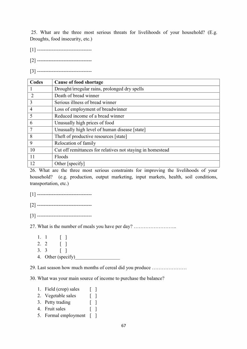
67

25. What are the three most serious threats for livelihoods of your household? (E.g.

Droughts, food insecurity, etc.)

[1] ---------------------------------

[2] ---------------------------------

[3] ---------------------------------

Codes Cause of food shortage

1 Drought/irregular rains, prolonged dry spells

2 Death of bread winner

3 Serious illness of bread winner

4 Loss of employment of breadwinner

5 Reduced income of a bread winner

6 Unusually high prices of food

7 Unusually high level of human disease [state]

8 Theft of productive resources [state]

9 Relocation of family

10 Cut off remittances for relatives not staying in homestead

11 Floods

12 Other [specify]

26. What are the three most serious constraints for improving the livelihoods of your

household? (e.g. production, output marketing, input markets, health, soil conditions,

transportation, etc.)

[1] ---------------------------------

[2] ---------------------------------

[3] ---------------------------------

27. What is the number of meals you have per day? ……………………..

1. 1 [ ]

2. 2 [ ]

3. 3 [ ]

4. Other (specify)__________________

29. Last season how much months of cereal did you produce …………………

30. What was your main source of income to purchase the balance?

1. Field (crop) sales [ ]

2. Vegetable sales [ ]

3. Petty trading [ ]

4. Fruit sales [ ]

5. Formal employment [ ]

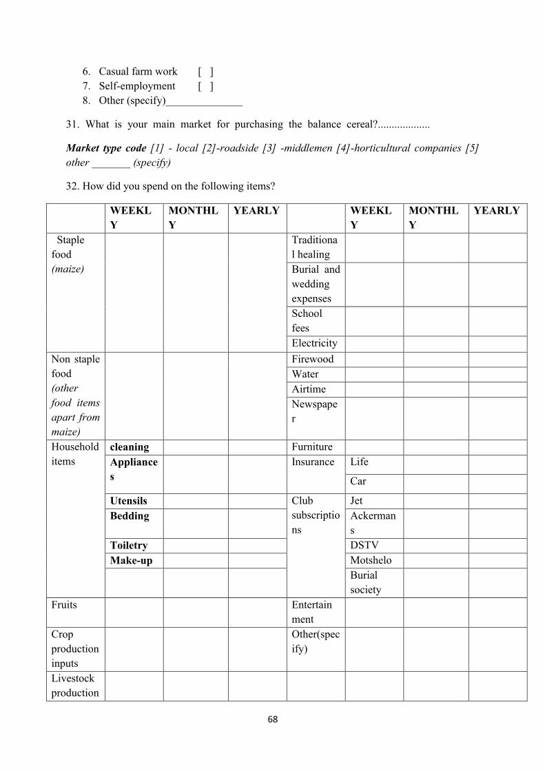
68

6. Casual farm work [ ]

7. Self-employment [ ]

8. Other (specify)______________

31. What is your main market for purchasing the balance cereal?...................

Market type code [1] - local [2]-roadside [3] -middlemen [4]-horticultural companies [5]

other _______ (specify)

32. How did you spend on the following items?

WEEKL

Y

MONTHL

Y

YEARLY WEEKL

Y

MONTHL

Y

YEARLY

Staple

food

(maize)

Traditiona

l healing

Burial and

wedding

expenses

School

fees

Electricity

Non staple

food

(other

food items

apart from

maize)

Firewood

Water

Airtime

Newspape

r

Household

items

cleaning Furniture

Appliance

s

Insurance Life

Car

Utensils Club

subscriptio

ns

Jet

Bedding Ackerman

s

Toiletry DSTV

Make-up Motshelo

Burial

society

Fruits Entertain

ment

Crop

production

inputs

Other(spec

ify)

Livestock

production

69

inputs

Transport

Clothes Men

Women

Children

Beer and

tobacco

Hospital

bills and

Medical

Aid

33. Are there any chronically ill people in the household?

1. Yes [ ]

2. No [ ]

34. In the past 3 months has there been a death in the family?

1. Yes [ ]

2. No [ ]

35. If yes what was the cause of the death? ………….

Thank you for your cooperation!!