Evaluation and optimization of ASM1 parameters using large ...
17
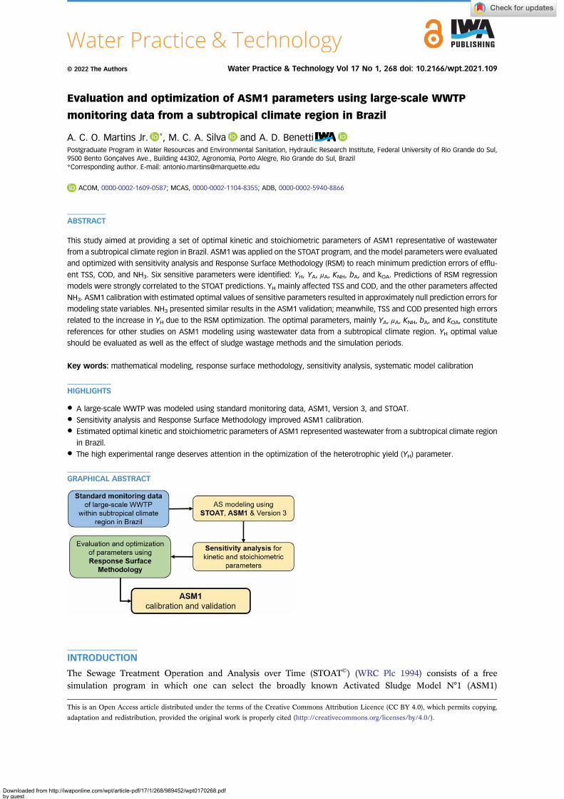
Evaluation and optimization of ASM1 parameters using large-scale WWTP monitoring data from a subtropical climate region in Brazil A. C. O. Martins Jr. * , M. C. A. Silva and A. D. Benetti Postgraduate Program in Water Resources and Environmental Sanitation, Hydraulic Research Institute, Federal University of Rio Grande do Sul, 9500 Bento Gonçalves Ave., Building 44302, Agronomia, Porto Alegre, Rio Grande do Sul, Brazil *Corresponding author. E-mail: [email protected] ACOM, 0000-0002-1609-0587; MCAS, 0000-0002-1104-8355; ADB, 0000-0002-5940-8866 ABSTRACT This study aimed at providing a set of optimal kinetic and stoichiometric parameters of ASM1 representative of wastewater from a subtropical climate region in Brazil. ASM1 was applied on the STOAT program, and the model parameters were evaluated and optimized with sensitivity analysis and Response Surface Methodology (RSM) to reach minimum prediction errors of efflu- ent TSS, COD, and NH 3 . Six sensitive parameters were identified: Y H , Y A , μ A , K NH , b A , and k OA . Predictions of RSM regression models were strongly correlated to the STOAT predictions. Y H mainly affected TSS and COD, and the other parameters affected NH 3 . ASM1 calibration with estimated optimal values of sensitive parameters resulted in approximately null prediction errors for modeling state variables. NH 3 presented similar results in the ASM1 validation; meanwhile, TSS and COD presented high errors related to the increase in Y H due to the RSM optimization. The optimal parameters, mainly Y A , μ A , K NH , b A , and k OA , constitute references for other studies on ASM1 modeling using wastewater data from a subtropical climate region. Y H optimal value should be evaluated as well as the effect of sludge wastage methods and the simulation periods. Key words: mathematical modeling, response surface methodology, sensitivity analysis, systematic model calibration HIGHLIGHTS • A large-scale WWTP was modeled using standard monitoring data, ASM1, Version 3, and STOAT. • Sensitivity analysis and Response Surface Methodology improved ASM1 calibration. • Estimated optimal kinetic and stoichiometric parameters of ASM1 represented wastewater from a subtropical climate region in Brazil. • The high experimental range deserves attention in the optimization of the heterotrophic yield (Y H ) parameter. GRAPHICAL ABSTRACT INTRODUCTION The Sewage Treatment Operation and Analysis over Time (STOAT © )(WRC Plc 1994) consists of a free simulation program in which one can select the broadly known Activated Sludge Model N°1 (ASM1) This is an Open Access article distributed under the terms of the Creative Commons Attribution Licence (CC BY 4.0), which permits copying, adaptation and redistribution, provided the original work is properly cited (http://creativecommons.org/licenses/by/4.0/). © 2022 The Authors Water Practice & Technology Vol 17 No 1, 268 doi: 10.2166/wpt.2021.109 Downloaded from http://iwaponline.com/wpt/article-pdf/17/1/268/989452/wpt0170268.pdf by guest on 26 January 2022
-
Upload
khangminh22 -
Category
Documents
-
view
1 -
download
0
Transcript of Evaluation and optimization of ASM1 parameters using large ...
Downloaded from http://iwby gueston 26 January 2022
Evaluation and optimization of ASM1 parameters using large-scale WWTP
monitoring data from a subtropical climate region in Brazil
A. C. O. Martins Jr. *, M. C. A. Silva and A. D. BenettiPostgraduate Program in Water Resources and Environmental Sanitation, Hydraulic Research Institute, Federal University of Rio Grande do Sul,9500 Bento Gonçalves Ave., Building 44302, Agronomia, Porto Alegre, Rio Grande do Sul, Brazil*Corresponding author. E-mail: [email protected]
ACOM, 0000-0002-1609-0587; MCAS, 0000-0002-1104-8355; ADB, 0000-0002-5940-8866
© 2022 The Authors Water Practice & Technology Vol 17 No 1, 268 doi: 10.2166/wpt.2021.109
ABSTRACT
This study aimed at providing a set of optimal kinetic and stoichiometric parameters of ASM1 representative of wastewater
from a subtropical climate region in Brazil. ASM1 was applied on the STOAT program, and the model parameters were evaluated
and optimized with sensitivity analysis and Response Surface Methodology (RSM) to reach minimum prediction errors of efflu-
ent TSS, COD, and NH3. Six sensitive parameters were identified: YH, YA, μA, KNH, bA, and kOA. Predictions of RSM regression
models were strongly correlated to the STOAT predictions. YH mainly affected TSS and COD, and the other parameters affected
NH3. ASM1 calibration with estimated optimal values of sensitive parameters resulted in approximately null prediction errors for
modeling state variables. NH3 presented similar results in the ASM1 validation; meanwhile, TSS and COD presented high errors
related to the increase in YH due to the RSM optimization. The optimal parameters, mainly YA, μA, KNH, bA, and kOA, constitute
references for other studies on ASM1 modeling using wastewater data from a subtropical climate region. YH optimal value
should be evaluated as well as the effect of sludge wastage methods and the simulation periods.
Key words: mathematical modeling, response surface methodology, sensitivity analysis, systematic model calibration
HIGHLIGHTS
• A large-scale WWTP was modeled using standard monitoring data, ASM1, Version 3, and STOAT.
• Sensitivity analysis and Response Surface Methodology improved ASM1 calibration.
• Estimated optimal kinetic and stoichiometric parameters of ASM1 represented wastewater from a subtropical climate region
in Brazil.
• The high experimental range deserves attention in the optimization of the heterotrophic yield (YH) parameter.
GRAPHICAL ABSTRACT
INTRODUCTION
The Sewage Treatment Operation and Analysis over Time (STOAT©) (WRC Plc 1994) consists of a freesimulation program in which one can select the broadly known Activated Sludge Model N°1 (ASM1)
This is an Open Access article distributed under the terms of the Creative Commons Attribution Licence (CC BY 4.0), which permits copying,
adaptation and redistribution, provided the original work is properly cited (http://creativecommons.org/licenses/by/4.0/).
aponline.com/wpt/article-pdf/17/1/268/989452/wpt0170268.pdf
Water Practice & Technology Vol 17 No 1, 269
Downloaded from http://iwby gueston 26 January 2022
(Henze et al. 1987) to model an activated sludge (AS) process. STOAT and ASM1 may be used with scarce datasets available from standard monitoring of large-scale Wastewater Treatment Plants (WWTP) for setting up afacility and modeling the performance of AS under steady-state conditions (Andraka et al. 2018).
The calibration is one of the most critical steps in the modeling procedure to provide reliable predictions accord-ingly with the specific conditions of AS process (Rieger et al. 2013). ASM1 modeling and calibration depend onwastewater composition fractionation and model parameters determination, respectively. Such fractionation anddetermination may need extra laboratory analysis, which is not commonly viable for some plants (Borzooei et al.2019). In some cases, typical ratios of municipal wastewater may be used for fractionation (Henze & Comeau2008, p. 36), and kinetic and stoichiometric ASM1 parameters calibration on trial and error procedure may beadopted. However, this calibration procedure is not appropriate due to the importance of prioritizing methods
that guarantee as much information as possible to form a suitable parameter combination (Petersen et al. 2003).Alternatively, some authors have proposed a systematic calibration approach to find optimal parameters for
ASMs. The strategy comprises modeling in association with sensitivity analysis for parameter selection, and
design of experiments and Response Surface Methodology (RSM) for parameter evaluation and optimization(Kim et al. 2009; Lim et al. 2012; Ahn et al. 2014).
Most studies on the evaluation and optimization of ASM1 parameters were developed in Europe, North Amer-
ica, and Asia (Hauduc et al. 2011). Furthermore, ASM1 presents default values of parameters for Europeanwastewater characteristics (Ahn et al. 2014). Thus, applications in other regions are relevant due to the variationof model parameters correspondingly to wastewater composition through space and time (Von Sperling et al.2020).
The geographic expansion may also contribute to evaluating ASM1 modeling using STOAT in other climateregions. That program is broadly used in the temperate climate of the United Kingdom and was validated in tro-pical climate conditions in India, where the microorganisms’ growth rate is higher than the temperate climate
conditions (Sarkar et al. 2010).Particularly in Brazil, AS modeling is essential to improve wastewater treatment. The country presents 354
WWTPs with such treatment process (10% of the total) (ANA 2020), and more than half of the population
lack wastewater treatment (Brasil 2019). Some authors have used ASM1 and STOAT to model a WWTP usingmonitoring data of domestic wastewater treatment from a subtropical climate region in Brazil (Pistorello 2018;Baptista 2020). However, to the best of our knowledge, no studies have performed an estimation of optimalASM1 parameters associating the use of monitoring data of a large-scale WWTP within a subtropical climate
region with sensitivity analysis and RSM.Therefore, this study aimed at providing a set of optimal kinetic and stoichiometric parameters of ASM1 repre-
sentative of wastewater from a subtropical climate region in Brazil. Thus, these optimal values may compose the
references of ASM1 parameters and be effective on AS modeling using the STOAT program and monitoring dataof large-scale WWTP in the same climate conditions.
METHODS
WWTP of study
The research was conducted on domestic wastewater generated from São João Navegantes WWTP in PortoAlegre, Brazil, located in a subtropical climate region (29°59029″S; 51°11043.5″W). The average raw-waterflow is 0.44 m3/s, corresponding to 150 thousand inhabitants. The wastewater system comprises extended aera-
tion activated sludge (Figure 1).
Data collection and reconciliation
The following wastewater characteristics were determined: flow, temperature, total suspended solids (TSS),
chemical oxygen demand (COD), ammonia (NH3), and pH. Influent and effluent means of these variableswere considered after treating missing and censored data, as well as outliers of the WWTP monitoring dataset, as described in von Sperling et al. (2020). Annual means of those variables of 2018 and 2019 were used
for ASM1 calibration and validation, respectively (Table 1).
Activated sludge modeling
TheASM1 andVersion 3models were used, respectively, for the aeration and secondary sedimentation tanks. Bothmodels are available on the STOAT© simulation program and the guidelines of Rieger et al. (2013) and WRC PLC
aponline.com/wpt/article-pdf/17/1/268/989452/wpt0170268.pdf

Figure 1 | The treatment system of the São João Navegantes WWTP.
Table 1 | Means of wastewater composition for modeling periods
Influent Effluent
Variable/Year 2018 2019 2018 2019
TSS (mg/l) 119 170 30 21
COD (mg/l) 297 359 52 45
NH3 (mg/l) 45.5 39.5 4.4 3.7
pH 7.2 7.2 6.9 7
Temperature (°C) 22.6 23.8 22.9 24.1
¼ Treated flow (m3/s) – – 0.077 0.076
Water Practice & Technology Vol 17 No 1, 270
Downloaded from http://iwby gueston 26 January 2022
(1994) were considered for modeling conduction. Modeling was developed for one of the four parallels flows of the
treatment plant. Information on tank sizes and operational data were provided by the WWTP (Table 2).On Version 3, the wastage method selected was fixed-rate (0.00153 m3/s) over variable time (0–8 h) to maintain
a specific Mixed-Liquor Suspended Solids (MLSS) set-point (3,000 mg/l). By assuming extended aeration corre-
lation, sewage calibration data for the same model considered Stirred Sludge Volume Index (SSVI) (3.5 g/l) equalto 100 ml/g (average for fair sludge sedimentation) (von Sperling 1994).
AS Solids Retention Time (SRT) was estimated using Equation (1) (Tchobanoglous et al. 2014), according to
the WWTP monitoring data (Table 2). V is the volume of the aeration tank, X is the MLSS concentration, QW
is the sludge wastage flow (0.00153 m3/s considering a pump run time of 8 h), and XR is the sludge TSS. Thefirst simulation period was assumed as 3 SRT (60 d) (Rieger et al. 2013).
SRT � VXQWXR
(1)
The influent profile assumed on STOAT was the sinusoidal pattern. Thus, the following conditions wereselected for most wastewater variables (Table 1): 0 h for phase, 30% for amplitude, and frequency equal to
0.261799 (representing daily fluctuations). Specifically for temperature, the frequency was 7.27E-4 (annual fluc-tuations), and amplitude was 0% for the same variable and pH. Typical ratios of municipal wastewater wereapplied at the fractionation of TSS, COD, and N contents (Table 3).
The modeling state variables were the mean effluent concentrations of TSS, COD, and NH3 (Table 1). The fol-lowing runs started from the end of the first simulation.
ASM1 parameters and respective default values are presented in Table 4. Some kinetic parameters displaydifferent units on STOAT; that is, h�1 for 15 °C (P15°C). By using the temperature coefficients (θ) provided on
aponline.com/wpt/article-pdf/17/1/268/989452/wpt0170268.pdf
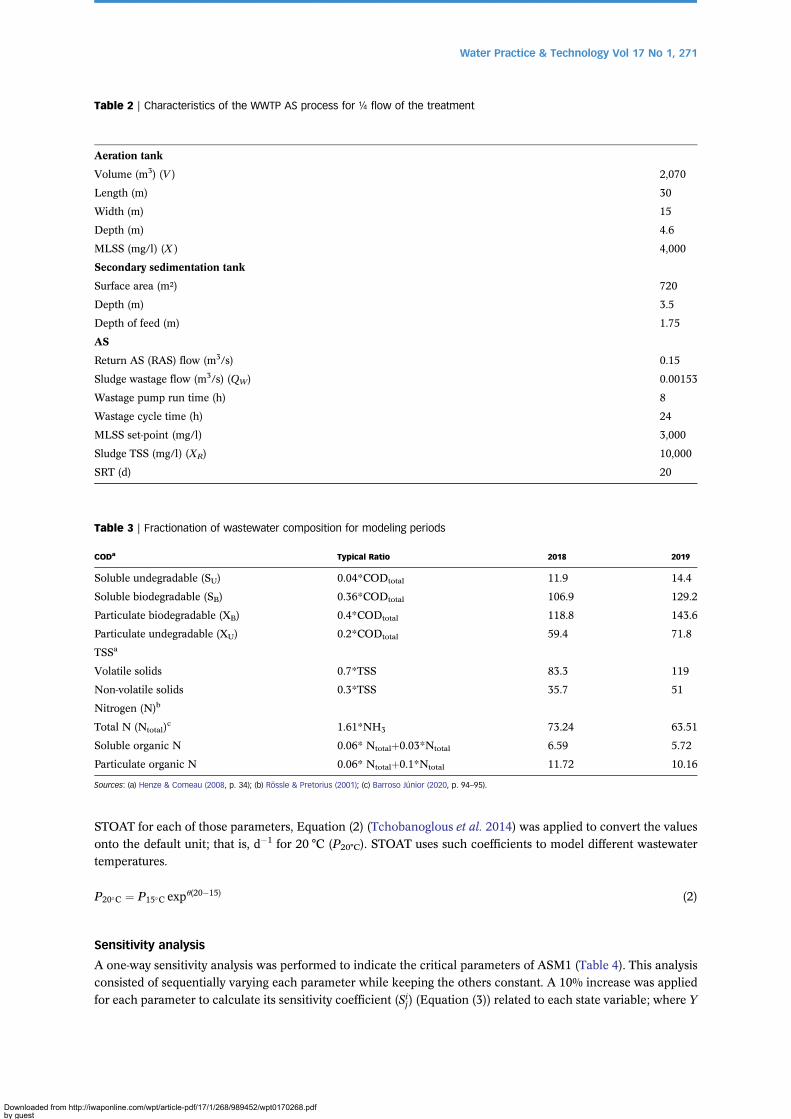
Table 2 | Characteristics of the WWTP AS process for ¼ flow of the treatment
Aeration tank
Volume (m3) (V ) 2,070
Length (m) 30
Width (m) 15
Depth (m) 4.6
MLSS (mg/l) (X ) 4,000
Secondary sedimentation tank
Surface area (m²) 720
Depth (m) 3.5
Depth of feed (m) 1.75
AS
Return AS (RAS) flow (m3/s) 0.15
Sludge wastage flow (m3/s) (QW) 0.00153
Wastage pump run time (h) 8
Wastage cycle time (h) 24
MLSS set-point (mg/l) 3,000
Sludge TSS (mg/l) (XR) 10,000
SRT (d) 20
Table 3 | Fractionation of wastewater composition for modeling periods
CODa Typical Ratio 2018 2019
Soluble undegradable (SU) 0.04*CODtotal 11.9 14.4
Soluble biodegradable (SB) 0.36*CODtotal 106.9 129.2
Particulate biodegradable (XB) 0.4*CODtotal 118.8 143.6
Particulate undegradable (XU) 0.2*CODtotal 59.4 71.8
TSSa
Volatile solids 0.7*TSS 83.3 119
Non-volatile solids 0.3*TSS 35.7 51
Nitrogen (N)b
Total N (Ntotal)c 1.61*NH3 73.24 63.51
Soluble organic N 0.06* Ntotalþ0.03*Ntotal 6.59 5.72
Particulate organic N 0.06* Ntotalþ0.1*Ntotal 11.72 10.16
Sources: (a) Henze & Comeau (2008, p. 34); (b) Rössle & Pretorius (2001); (c) Barroso Júnior (2020, p. 94–95).
Water Practice & Technology Vol 17 No 1, 271
Downloaded from http://iwby gueston 26 January 2022
STOAT for each of those parameters, Equation (2) (Tchobanoglous et al. 2014) was applied to convert the values
onto the default unit; that is, d�1 for 20 °C (P20°C). STOAT uses such coefficients to model different wastewatertemperatures.
P20�C ¼ P15�C expu(20�15) (2)
Sensitivity analysis
A one-way sensitivity analysis was performed to indicate the critical parameters of ASM1 (Table 4). This analysisconsisted of sequentially varying each parameter while keeping the others constant. A 10% increase was applied
for each parameter to calculate its sensitivity coefficient (Sij) (Equation (3)) related to each state variable; where Y
aponline.com/wpt/article-pdf/17/1/268/989452/wpt0170268.pdf

Table 4 | Kinetic and stoichiometric parameters of ASM1
Stoichiometric Symbol Unit Default (20 °C)a Literature
Heterotrophic yield YH g cell COD formed(g COD oxidized)�1
0.67 0.62–0.67b
Autotrophic yield YA g cell COD formed(g N oxidized)�1
0.24 0.07–0.28c
Fraction of biomass yielding particulateproducts
fP Dimensionless 0.08 –
Mass N/Mass COD in biomass iXB g N (g COD)�1 in biomass 0.086 0.079–0.086b
Mass N/Mass COD in products frombiomass
iXP g N (g COD)�1 in endogenousbiomass
0.06 –
Kinetic
Heterotrophic maximum specific growthrate
μH d�1 6 (0.1768 h�1)d 5.7–6b
Half-saturation coefficient (hsc) forheterotrophs
KS g COD.m�3 20 5–225c
Oxygen hsc for heterotrophs KOH g O2.m�3 0.2 0.01–0.2c
Nitrate hsc for denitrifying heterotrophs KNO g NO3-N.m�3 0.5 0.1–0.5c
Heterotrophic decay rate bH d�1 0.62(0.0147 h�1)d
0.05–1.6c
Autotrophic maximum specific growth rate μA d�1 0.8 (0.0207 h�1)d 0.2–1c
Ammonia hsc for autotrophs KNH g NH3-N.m�3 1 0.75–1b
Oxygen hsc for autotrophs KOA g O2.m�3 0.4 0.4–2c
Autotrophic decay rate bA d�1 0.15(0.0036 h�1)d
0.05–0.15a
Correction factor for anoxic growth ofheterotrophs
ηg Dimensionless 0.8 0.6–1c
Ammonification rate kA m3(g COD d)�1 0.08(0.0024 h�1)d
0.07–0.08b
Maximum specific hydrolysis rate Kh g slowly biodeg.(g cell COD d)�1 3 (0.0722 h�1)d 2.2–3b
Hsc for hydrolysis of slowly biodegradablesubstrate
KX g slowly biodeg.(g cell COD d)�1 0.03(0.0173 h�1)d
–
Correction factor for anoxic hydrolysis ηh Dimensionless 0.4 0.4–0.5b
Sources: (a) Henze et al. (1987); (b) Hauduc et al. (2011); (c) Ahn et al. (2014); (d) value displayed on STOAT for 15 °C.
Water Practice & Technology Vol 17 No 1, 272
Downloaded from http://iwby gueston 26 January 2022
is the state variable output, P is the ASM1 parameter value, and the subscripts 0 e 1 stand for the default and the
changed values, respectively. A parameter is considered sensitive if Sij � 0:25 (Liwarska-Bizukojc et al. 2011;Andraka et al. 2018; Chen et al. 2020). Herein, the period of each simulation was equivalent to the estimatedSRT (Table 2).
Sij ¼Yi1 � Yi0
Yi0Pj1 � Pj0
Pj0
(3)
Parameters optimization
Sensitive kinetic and stoichiometric parameters of ASM1 were optimized aiming at minimum prediction errors
for state variables on simulations, according to the WWTP monitoring data (Lim et al. 2012). Response SurfaceMethodology (RSM) and Central Composite Design (CCD) were conducted using Minitab Statistical Software(Version 20.2), whose input consisted of the difference between the observed data recorded by the WWTP
(Table 1) and the result of simulation.
aponline.com/wpt/article-pdf/17/1/268/989452/wpt0170268.pdf
Water Practice & Technology Vol 17 No 1, 273
Downloaded from http://iwby gueston 26 January 2022
Regression models were created for each modeling state variable, and ANOVA and standardized effects wereused to evaluate the influence of changes in sensitive parameters on prediction errors of effluent TSS, COD, andNH3. Regression models’ adequacy was verified using the Lack-of-fit test. Also, the correlation between results of
simulations on STOAT and predictions of the regression models was analyzed, as well as the RMSE (Equation(4)) of each regression model (Kim Rao & Yoo 2009; Lim et al. 2012; Ahn et al. 2014).
RMSE ¼
ffiffiffiffiffiffiffiffiffiffiffiffiffiffiffiffiffiffiffiffiffiffiffiffiffiffiffiffiPni¼1
(Xi � Yi)2
n� 1
vuuut(4)
X is the simulation prediction using STOAT, Y is the regression prediction via RSM, and n is the number of
simulations designed by CCD.In the multiple optimization, the desirability function based on a target value was used to estimate optimal
values for sensitive parameters, which would lead to minimum prediction errors of effluent TSS, COD, and
NH3 (Kim Rao & Yoo 2009; Lim et al. 2012). According to the modeling objective, a range of minimum predic-tion error for each state variable was assumed: +5 mg/l for TSS and COD, and +1 mg/l for NH3 (Rieger et al.2013).
Finally, optimized parameters of ASM1 were applied on simulations on STOAT for model calibration and vali-
dation. It was verified whether or not the results complied with the previous range of prediction errorsdetermined for each state variable. The period of each run for parameter optimization was also the estimatedSRT (Table 2).
RESULTS AND DISCUSSION
Sensitive parameters of ASM1
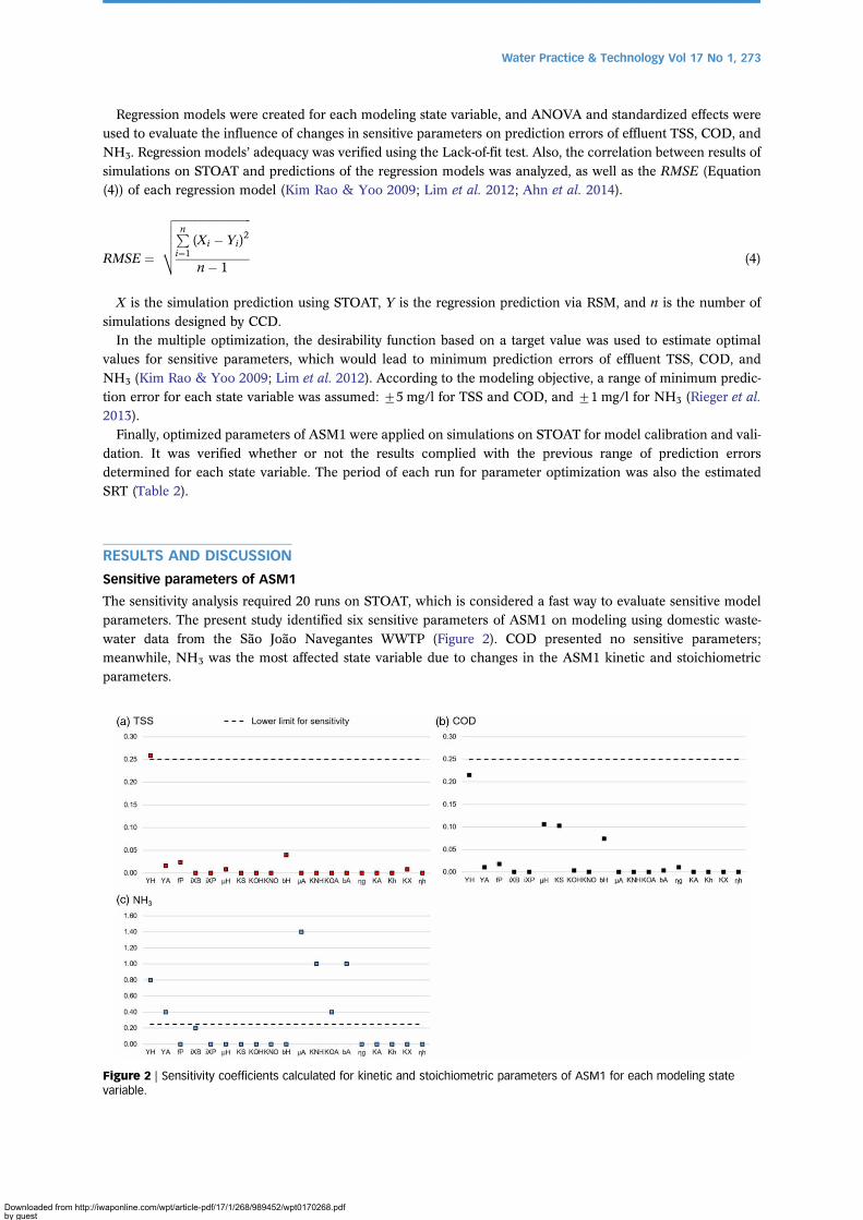
The sensitivity analysis required 20 runs on STOAT, which is considered a fast way to evaluate sensitive modelparameters. The present study identified six sensitive parameters of ASM1 on modeling using domestic waste-
water data from the São João Navegantes WWTP (Figure 2). COD presented no sensitive parameters;meanwhile, NH3 was the most affected state variable due to changes in the ASM1 kinetic and stoichiometricparameters.
Figure 2 | Sensitivity coefficients calculated for kinetic and stoichiometric parameters of ASM1 for each modeling statevariable.
aponline.com/wpt/article-pdf/17/1/268/989452/wpt0170268.pdf
Water Practice & Technology Vol 17 No 1, 274
Downloaded from http://iwby gueston 26 January 2022
YH was sensitive for the TSS and NH3 outputs. Although the same parameter was not sensitive for COD, itpresented a coefficient of 0.22, indicating an effect on that state variable. Lim et al. (2012) observed similar resultsand commented that the relationship between YH and the state variables TSS and COD are related to sludge pro-
duction. The heterotrophic yield also depends upon the nature of the substrate and the population ofmicroorganisms performing degradation (Henze et al. 1987).
Other sensitive parameters only affected NH3 predictions. In particular, the sensitivity coefficients of μA, KNH,and bA presented high values (�1), characterizing a substantial effect on the NH3 outputs of the WWTP AS pro-
cess modeling. Contrarily, μA also affected effluent TSS in another study (Lim et al. 2012). Nevertheless, the highsensitivity of μA may be related to elevated ammonia loads and to a lack of complete nitrification (Levy 2007).This parameter is the most critical one for characterizing the growth of the autotrophic biomass and is influenced
by many environmental factors, such as pH and temperature (Henze et al. 1987). On the other hand, the value ofbA is considered difficult to measure and may be assumed (Levy 2007), as well as the values of YA and KOA thatalso affected effluent NH3 (Figure 2(c)). KNH and YH are recommended to be evaluated for each type of waste-
water (Henze et al. 1987).It is noteworthy that 13 parameters of ASM1 were not sensitive for the predictions of effluent TSS, COD, and
NH3 of the São João Navegantes WWTP, regarding the specific modeling conditions. It meant that fewer par-
ameters need to be evaluated, which sped up the ASM1 calibration. However, even though the parametersIXB, μH, kS, and bH were not considered sensitive, they deserved attention as long as they affected COD andNH3 predictions (Figure 2(b) and 2(c)).
Half of the six sensitive parameters identified (YH, μA, and bA) were also subject to change in another study that
used ASM1 modeling results of 18 WWTPs in Europe, three in Asia, and one in North America (Hauduc et al.2011). Other authors have confirmed the relevance of YH, μA, KNH, and KOA for either steady-state or dynamic ASsimulation conditions (Petersen et al. 2003). Furthermore, sensitive parameters determined for steady-state
conditions can significantly support the dynamic calibration (Liwarska-Bizukojc et al. 2011). Therefore, theresults of the present study indicate a set of sensitive parameters of ASM1, which besides being representativeof a subtropical climate region, may be used in dynamic modeling practices.
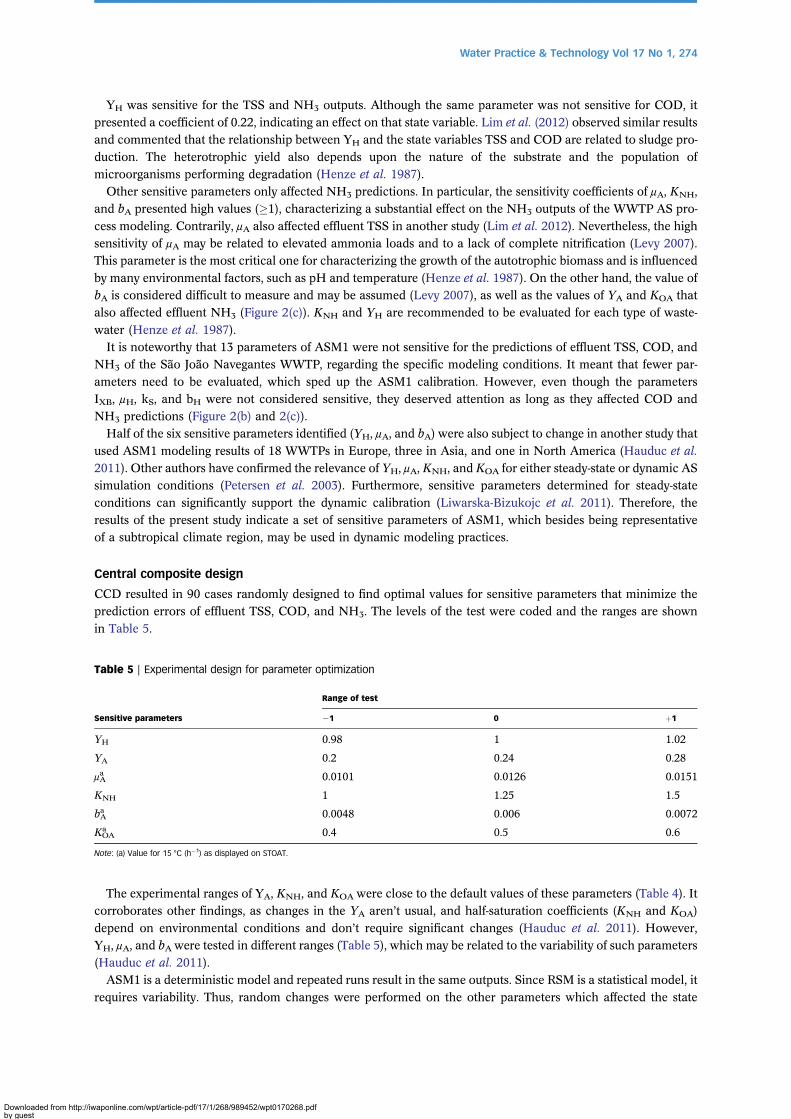
Central composite design
CCD resulted in 90 cases randomly designed to find optimal values for sensitive parameters that minimize theprediction errors of effluent TSS, COD, and NH3. The levels of the test were coded and the ranges are shown
in Table 5.
Table 5 | Experimental design for parameter optimization
Sensitive parameters
Range of test
�1 0 þ1
YH 0.98 1 1.02
YA 0.2 0.24 0.28
μAa 0.0101 0.0126 0.0151
KNH 1 1.25 1.5
bAa 0.0048 0.006 0.0072
KOAa 0.4 0.5 0.6
Note: (a) Value for 15 °C (h�1) as displayed on STOAT.
The experimental ranges of YA, KNH, and KOA were close to the default values of these parameters (Table 4). Itcorroborates other findings, as changes in the YA aren’t usual, and half-saturation coefficients (KNH and KOA)
depend on environmental conditions and don’t require significant changes (Hauduc et al. 2011). However,YH, μA, and bA were tested in different ranges (Table 5), which may be related to the variability of such parameters(Hauduc et al. 2011).
ASM1 is a deterministic model and repeated runs result in the same outputs. Since RSM is a statistical model, it
requires variability. Thus, random changes were performed on the other parameters which affected the state
aponline.com/wpt/article-pdf/17/1/268/989452/wpt0170268.pdf
Water Practice & Technology Vol 17 No 1, 275
Downloaded from http://iwby gueston 26 January 2022
variables but were not considered sensitive by the 0.25 limit (Figure 2) to provide such variability. These changeswere made in 13 out of 14 repeated cases designed by CCD, and the parameters changes were iXB, bH, μH, and KS
(Table 6).
Table 6 | Alternate parameters changes to provide variability in repeated cases of CCD
Case (run) iXB bH μH KS
78 0.0825 Default Default 40
79 0.075 Default Default Default
80 0.075 Default 0.1179 40
81 0.09 Default 0.1179 Default
82 0.09 Default Default 60
83 0.085 Default 0.1179 Default
84 0.0825 0.0237 Default Default
85 0.075 0.0237 Default Default
86 0.08 Default Default Default
87 0.08 Default 0.1179 40
88 0.0825 Default 0.1179 60
89 0.09 Default 0.1179 60
90 0.085 Default 0.1179 40
Note: default values are presented in Table 4.
Regression models
The prediction errors of effluent TSS, COD, and NH3 were calculated from the results of runs designed byCCD, which means the difference between the observed data recorded by the WWTP and the STOAT simu-
lation’s prediction. Such prediction errors were input onto RSM to generate the regression models for eachstate variable. The regression coefficients estimated by RSM are presented in Table 7. The respective non-
Table 7 | Regression models coefficients of modeling state variables generated by RSM
Term TSS COD NH3
Constant 3.270 6.085 �0.047
YH 10.062 11.973 �0.1021
YA 0.703 0.835 0.5201
μA 0.342 0.405 �3.1580
KNH �0.055 �0.065 0.4933
bA �0.256 �0.303 2.4448
KOA �0.061 �0.073 0.5749
YH*YH 1.3441 0.9401 –
YA*YA 0.3216 �0.3249 –
μA*μA 0.1966 �0.4742 1.1151
KNH*KNH 0.3278 �0.3180 –
bA*bA 0.2816 �0.3724 0.3826
KOA*KOA 0.3241 �0.3224 –
YA*μA – – �0.2970
μA*bA – – �1.2083
μA*KOA – – �0.2789
bA*KOA – – 0.2458
aponline.com/wpt/article-pdf/17/1/268/989452/wpt0170268.pdf
Water Practice & Technology Vol 17 No 1, 276
Downloaded from http://iwby gueston 26 January 2022
significant quadratic relationships and interactions between parameters weren’t considered to simplify theregression models.
ANOVA showed similar results for TSS and COD. Changes in most sensitive parameters affected TSS and
COD predictions (p, 0.001). Only KNH e kOA didn’t affect those state variables (TSS: F(1,89)¼ 0.22; p¼ 0.639and F(1,89)¼ 0.28; p¼ 0.598, respectively; COD: F(1,89)¼ 0.36; p¼ 0.552 and F(1,89)¼ 0.45; p¼ 0.505, respect-ively). All quadratic relationships also influenced TSS and COD, especially YH*YH for both variables (F(1,89)¼197.60 and 109.12, respectively; p, 0.001). However, interactions between sensitive parameters weren’t statisti-
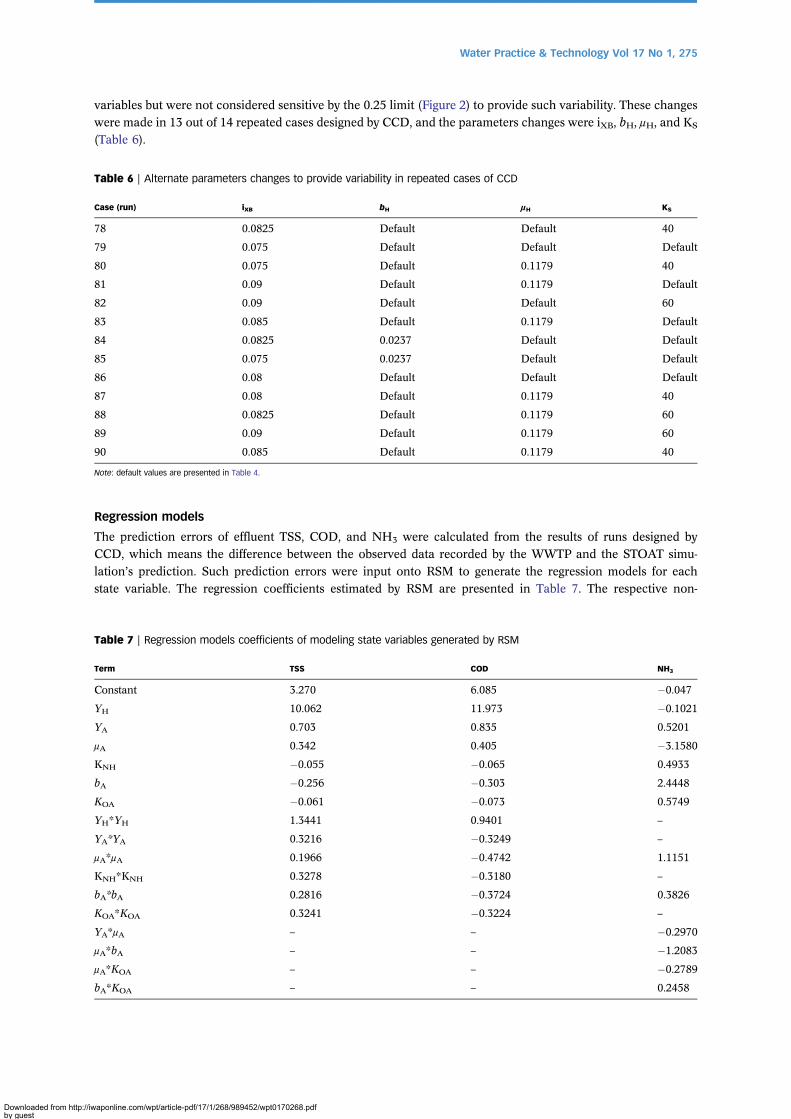
cally significant for TSS and COD and were disregarded in their regression models (Table 7).The ANOVA of the NH3 regression model showed that YH was the only sensitive parameter that did not affect
the predictions of such state variable (F(1,89)¼ 1.69; p¼ 0.198). Although only quadratic relationships of μA and bAwere statistically significant in that regression model (F(1,89)¼ 303.27 and 35.70, respectively; p, 0.001), fourinteractions between parameters affected effluent NH3 prediction errors: YA*μA; μA*bA; μA*KOA and bA*KOA
(Table 7). Response surfaces of these significant interactions are shown in Figure 3.
Figure 3 | Response surfaces of significant interactions between sensitive parameters in the regression model for NH3 pre-diction errors: (a) μA*bA; (b) YA*μA; (c) μA*KOA; and (d) bA*KOA.
The relevant impact of μA*bA interaction (F(1,89)¼ 189.17; p, 0.001) indicates the many combinations that
may be assumed for such parameters to estimate minimum prediction errors for effluent NH3 (Figure 3(a)).Hauduc et al. (2011) highlighted the variability of values for those parameters. Such a relationship is usuallyinversely proportional, as reduction of μA and bA increases and decreases, respectively, ammonia effluent concen-
tration. Also, an increase in bA may inhibit cell growth and replace nutrients in the system, elevating NH3
concentration. However, the effect of bA is not the most important for effluent NH3 control (Levy 2007).In the interactions of YA*μA (F(1,89)¼ 11.43; p¼ 0.001) and μA*KOA (F(1,89)¼ 10.08; p¼ 0.002), the prediction
errors of effluent NH3 generated by the regression models were null for higher tested values of μA (Figure 3(b) and3(c)). Changes in YA and KOA on such interactions didn’t show a distinct effect on prediction errors, as observedby other authors (Petersen et al. 2002).
Finally, the interaction between bA*KOA (F(1,89)¼7.83; p¼0.006) was the less significant in the NH3 regressionmodel. In that relationship, the whole experimental range tested for KOA was suitable to obtain minimum effluentNH3 prediction errors (Figure 3(d)), though only lower values adopted for bA worked appropriately.
aponline.com/wpt/article-pdf/17/1/268/989452/wpt0170268.pdf
Water Practice & Technology Vol 17 No 1, 277
Downloaded from http://iwby gueston 26 January 2022
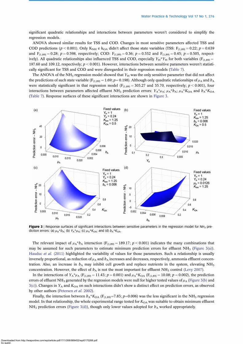
The standardized effects of the regression models pointed out the influence of YH on TSS (87%) and COD(109%) prediction errors (Figure 4(a) and 4(b)). Linear and quadratic relationships of other parameters presentedeffects lower than 15%, even though they were significant in the ANOVA results.
Figure 4 | Standardized effects of RSM regression models for modeling state variables (α¼0.05).
For NH3 prediction errors, μA and bA stood out and indicated contrary effects on responses: �40 and 31%,
respectively (Figure 4(c)). This situation is also shown in Figure 3(a).The lack-of-fit tests showed that p-values were not statistically significant for regression models of TSS and
COD, which means that the alternative hypothesis that indicates the lack of fit of those regression models
wasn’t selected. On the other hand, the NH3 regression model presented opposite results, revealing that sucha model didn’t show the goodness of fit (Table 8).
Table 8 | Measures of the regression model’s adequacy
TSS COD NH3
Lack-of-fit test F(64,89)¼0.06; p¼1 F(64,89)¼0.11; p¼1 F(64,89)¼15.51; p,0.001
R² 0.9902 0.9938 0.977
RMSE 0.97 0.91 0.65
For that specific case, to correct the lack of fit of the regression model, the original variable predicted on simu-lation using STOAT was used (prediction of NH3 effluent concentration instead of the prediction error). Then, it
aponline.com/wpt/article-pdf/17/1/268/989452/wpt0170268.pdf
Water Practice & Technology Vol 17 No 1, 278
Downloaded from http://iwby gueston 26 January 2022
was expected to obtain only positive values, which could be transformed to improve the fit of the regressionmodel. However, it didn’t show different results, and the first regression model was maintained (Table 7).
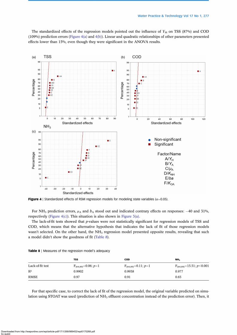
The estimated prediction errors of all state variables provided by RSM were compared with those predicted
using STOAT. Such relationships presented a strong correlation (R² .0.97), as shown in Figure 5. Thus, theregression models explain at least 97% of the variations in prediction errors of effluent TSS, COD, and NH3.The statistical error via RMSE presented lower values; that is, close to 0, indicating that there wasn’t a discre-pancy between prediction errors estimated by RSM and predicted via STOAT. Those results are similar to the
findings of other authors (Kim et al. 2009; Ahn et al. 2014).
Figure 5 | Correlation between prediction errors via RSM and prediction errors via STOAT for modeling state variables.
Parameter optimization
The generated regression models of RSM were used to estimate optimal values for the sensitive parameters to beapplied on the calibration and validation of ASM1. The target value onto the desirability function in the optim-ization procedure was zero to estimate parameters to reach minimum prediction errors of effluent TSS, COD, and
NH3.RSM optimization generated the output shown in Figure 6. The optimal values for the sensitive parameters are
displayed in red within a specific range. The optimal prediction errors for each state variable are in blue. The ver-tical lines in red show the optimal parameters within the experimental range of CCD (Table 5).
Figure 6 also presents the relationships between each parameter and the modeling state variables. Changes inYH mainly affected prediction errors of effluent TSS and COD. Variations in the values of the other sensitive par-ameters affected NH3 prediction errors. It’s important to emphasize the effect of μA and bA, whose interaction
was the most significant in the ANOVA results of the NH3 regression model. Nonetheless, μA showed two opti-mal points, on the central and upper regions of the parameter experimental range. The first one was moreprominent and consisted of the optimal value determined for the parameter. That situation may be related to
the great importance of μA for the NH3 predictions (Petersen et al. 2002), as shown in Figure 3(a)–3(c).The single value of D, which lies between zero and one, is the overall desirability of the combined response
levels. D close to one means that the balance of the properties becomes more feasible. On the other hand, Dclose to zero indicates that one of the response variables is unacceptable (Lim et al. 2012). The composite desir-
ability showed D¼0.9181, pointing out a balance among the responses regarding the optimal values estimated for
aponline.com/wpt/article-pdf/17/1/268/989452/wpt0170268.pdf
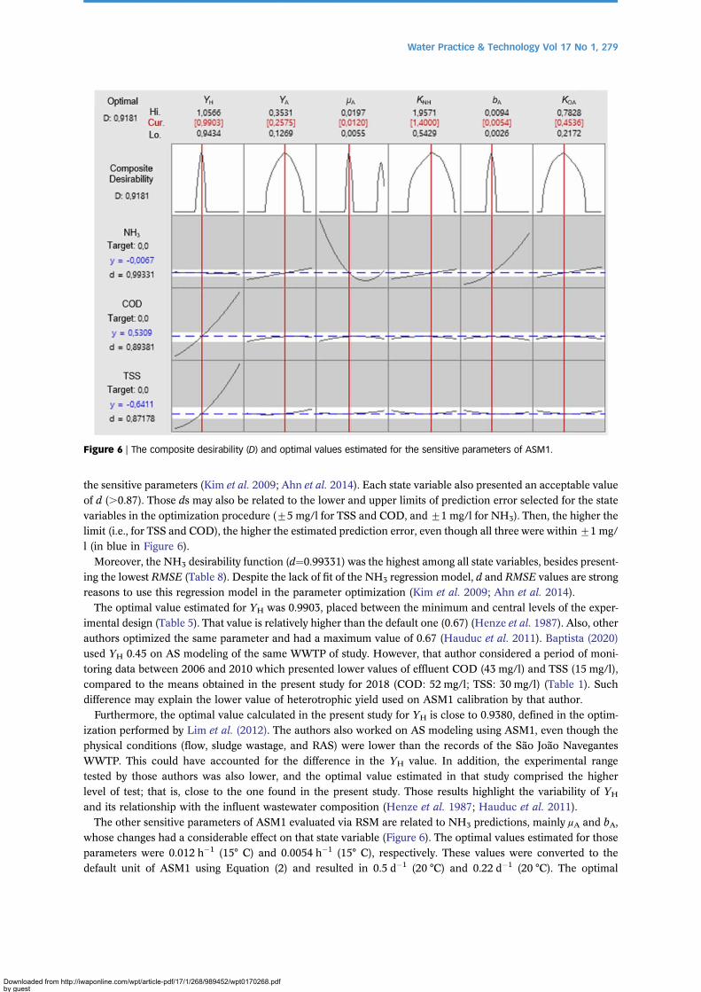
Figure 6 | The composite desirability (D) and optimal values estimated for the sensitive parameters of ASM1.
Water Practice & Technology Vol 17 No 1, 279
Downloaded from http://iwby gueston 26 January 2022
the sensitive parameters (Kim et al. 2009; Ahn et al. 2014). Each state variable also presented an acceptable valueof d (.0.87). Those ds may also be related to the lower and upper limits of prediction error selected for the state
variables in the optimization procedure (+5 mg/l for TSS and COD, and +1 mg/l for NH3). Then, the higher thelimit (i.e., for TSS and COD), the higher the estimated prediction error, even though all three were within+1 mg/l (in blue in Figure 6).
Moreover, the NH3 desirability function (d¼0.99331) was the highest among all state variables, besides present-ing the lowest RMSE (Table 8). Despite the lack of fit of the NH3 regression model, d and RMSE values are strongreasons to use this regression model in the parameter optimization (Kim et al. 2009; Ahn et al. 2014).
The optimal value estimated for YH was 0.9903, placed between the minimum and central levels of the exper-imental design (Table 5). That value is relatively higher than the default one (0.67) (Henze et al. 1987). Also, otherauthors optimized the same parameter and had a maximum value of 0.67 (Hauduc et al. 2011). Baptista (2020)
used YH 0.45 on AS modeling of the same WWTP of study. However, that author considered a period of moni-toring data between 2006 and 2010 which presented lower values of effluent COD (43 mg/l) and TSS (15 mg/l),compared to the means obtained in the present study for 2018 (COD: 52 mg/l; TSS: 30 mg/l) (Table 1). Suchdifference may explain the lower value of heterotrophic yield used on ASM1 calibration by that author.
Furthermore, the optimal value calculated in the present study for YH is close to 0.9380, defined in the optim-ization performed by Lim et al. (2012). The authors also worked on AS modeling using ASM1, even though thephysical conditions (flow, sludge wastage, and RAS) were lower than the records of the São João Navegantes
WWTP. This could have accounted for the difference in the YH value. In addition, the experimental rangetested by those authors was also lower, and the optimal value estimated in that study comprised the higherlevel of test; that is, close to the one found in the present study. Those results highlight the variability of YH
and its relationship with the influent wastewater composition (Henze et al. 1987; Hauduc et al. 2011).The other sensitive parameters of ASM1 evaluated via RSM are related to NH3 predictions, mainly μA and bA,
whose changes had a considerable effect on that state variable (Figure 6). The optimal values estimated for those
parameters were 0.012 h�1 (15° C) and 0.0054 h�1 (15° C), respectively. These values were converted to thedefault unit of ASM1 using Equation (2) and resulted in 0.5 d�1 (20 °C) and 0.22 d�1 (20 °C). The optimal
aponline.com/wpt/article-pdf/17/1/268/989452/wpt0170268.pdf
Water Practice & Technology Vol 17 No 1, 280
Downloaded from http://iwby gueston 26 January 2022
value estimated for μA remained in the usual range presented in the literature (0.2–1) (Ahn et al. 2014). For bA, theoptimal estimative was higher than the maximum value observed (0.05–0.15) (Henze et al. 1987).
The optimal values of YA 0.2575 and KOA 0.4536 (Figure 6) were similar to the default values of such par-
ameters: 0.24 and 0.4, respectively (Ahn et al. 2014). On the other hand, KNH 1.4 also showed a higher valuethan the usual range of 0.75–1 (Hauduc et al. 2011).
Table 9 shows the comparison of observed data, default results, and verification of parameter optimizationresults. Prediction error ranges and prediction errors estimated by RSM and via simulations on STOAT are
also presented.
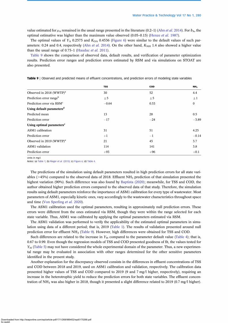
Table 9 | Observed and predicted means of effluent concentrations, and prediction errors of modeling state variables
TSS COD NH3
Observed in 2018 (WWTP)a 30 52 4.4
Prediction error rangeb +5 +5 +1
Prediction error via RSMc �0.64 0.53 0
Using default parametersd
Predicted mean 13 28 0.5
Prediction error �17 �24 �3.89
Using optimal parametersc
ASM1 calibration 31 51 4.25
Prediction error þ1 �1 �0.14
Observed in 2019 (WWTP)a 21 45 3.7
ASM1 validation 114 141 3.8
Prediction error þ93 þ96 þ0.1
Units in mg/l.
Notes: (a) Table 1; (b) Rieger et al. (2013); (c) Figure 6; (d) Table 4.
The predictions of the simulation using default parameters resulted in high prediction errors for all state vari-ables (.45%) compared to the observed data of 2018. Effluent NH3 prediction of that simulation presented thehighest variation (90%). Such difference was also found by Baptista (2020); meanwhile, for TSS and COD, the
author obtained higher prediction errors compared to the observed data of that study. Therefore, the simulationresults using default parameters reinforce the importance of ASM1 calibration for every type of wastewater. Mostparameters of ASM1, especially kinetic ones, vary accordingly to the wastewater characteristics throughout spaceand time (Von Sperling et al. 2020).
The ASM1 calibration used the optimal parameters, resulting in approximately null prediction errors. Theseerrors were different from the ones estimated via RSM, though they were within the range selected for eachstate variable. Thus, ASM1 was calibrated by applying the optimal parameters estimated via RSM.
The ASM1 validation was performed to verify the applicability of the estimated optimal parameters in simu-lation using data of a different period; that is, 2019 (Table 1). The results of validation presented around nullprediction error for effluent NH3 (Table 9). However, high differences were obtained for TSS and COD.
Such differences are related to the increase in YH compared to the parameter default value (Table 4); that is,0.67 to 0.99. Even though the regression models of TSS and COD presented goodness of fit, the values tested forYH (Table 5) may not have considered the whole experimental domain of the parameter. Thus, a new experimen-
tal range may be evaluated in association with other ranges determined for the other sensitive parametersidentified in the present study.
Another explanation for the discrepancy observed consists in the differences in effluent concentrations of TSSand COD between 2018 and 2019, used on ASM1 calibration and validation, respectively. The calibration data
presented higher values of TSS and COD compared to 2019 (9 and 7 mg/l higher, respectively), requiring anincrease in the heterotrophic yield to reduce the prediction errors for both state variables. The effluent concen-tration of NH3 was also higher in 2018, though it presented a slight difference related to 2019 (0.7 mg/l higher).
aponline.com/wpt/article-pdf/17/1/268/989452/wpt0170268.pdf
Water Practice & Technology Vol 17 No 1, 281
Downloaded from http://iwby gueston 26 January 2022
The increase in YH raises the COD transformation efficiency, determining the biomass concentration in thereactor. Hence, it has a high effect on the microbial growth rates and on the sludge production (Petersen et al.2002; Levy 2007; Chen et al. 2020). Therefore, adjustments in the sludge wastage method may lead to obtaining
a suitable YH value for ASM1 calibration and validation, aiming at minimum prediction errors of TSS and CODfor the specific modeling conditions of the present study.
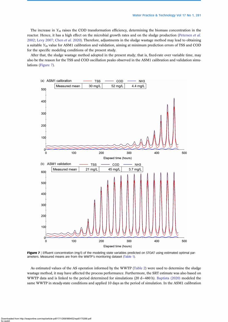
After that, the sludge wastage method adopted in the present study; that is, fixed-rate over variable time, mayalso be the reason for the TSS and COD oscillation peaks observed in the ASM1 calibration and validation simu-
lations (Figure 7).
Figure 7 | Effluent concentration (mg/l) of the modeling state variables predicted on STOAT using estimated optimal par-ameters. Measured means are from the WWTP’s monitoring dataset (Table 1).
As estimated values of the AS operation informed by the WWTP (Table 2) were used to determine the sludge
wastage method, it may have affected the process performance. Furthermore, the SRT estimate was also based onWWTP data and is linked to the period determined for simulations (20 d¼480 h). Baptista (2020) modeled thesame WWTP in steady-state conditions and applied 10 days as the period of simulation. In the ASM1 calibration
aponline.com/wpt/article-pdf/17/1/268/989452/wpt0170268.pdf
Water Practice & Technology Vol 17 No 1, 282
Downloaded from http://iwby gueston 26 January 2022
of the present study, the oscillation peaks were at the end of the period; hence, after 10 days of simulation(Figure 7(a)). Although in the ASM1 validation the peaks started after 100 hours (Figure 7(b)); that is, lessthan 10 days of simulation, the SRT estimate may have been overrated. Therefore, accurate AS operation data
would aid in improving process performance on modeling. Also, other methods of sludge wastage (constant orfixed time over variable rate), and changes in operational parameters of ASM1 and Version 3 may contributeto control predictions of effluent TSS and COD.
Moreover, such peaks always happened when the YH upper level of test was chosen in the simulations per-
formed via CCD (Table 5) (see Results of CCD simulations in Supplementary Material). Then, those peaks arealso related to the increase of YH and its influence on the biomass concentration in the treatment process(Levy 2007).
The heterotrophic yield sensitivity is highlighted in optimizing ASM1 parameters (Hauduc et al. 2011). It’simportant to determine the value of such parameter for every type of wastewater, as YH is commonly changedin ASM1 modeling (Henze et al. 1987) and each WWTP should be modeled assuming specific conditions related
to its reality and challenges (Borzooei et al. 2019). Then, the wastewater physical and chemical composition,especially temperature, may have influenced YH hence the predictions of effluent TSS and COD on STOATusing the optimal value estimated for the parameter. Also, the results of the present study support that attention
should be dedicated to the calibration of YH.Otherwise, in addition to the high variation of NH3 prediction in the simulation using default parameters
(Table 9), all six sensitive parameters affected this state variable (Figure 2(c)). Five of these parameters are relatedto the autotrophic microorganisms (YA), N content, and specifically to ammonia (μA, KNH, bA, and kOA). The opti-
mal values estimated for all of them were appropriate for both calibration and validation of ASM1, and the NH3
prediction errors were lower than 1 mg/l. Therefore, such parameters are related to wastewater concerning sub-tropical climate conditions being a reference for other applications.
CONCLUSIONS
AS process of a large-scale WWTP within a subtropical climate region in Brazil was modeled using standardmonitoring data set, the ASM1 model, and the STOAT program.
With sensitive analysis, six parameters of ASM1 were identified as sensitive to effluent TSS, COD, and NH3
predictions: two stoichiometric (YH and YA) and four kinetic (μA, KNH, bA, and kOA). Sensitive parameterswere evaluated and optimized via RSM aiming at minimum prediction errors for modeling state variables. YH
mainly affected TSS and COD predictions; meanwhile, NH3 predictions were influenced by changes in the
other sensitive parameters.Estimated optimal parameters were used on ASM1 calibration resulting in approximately null prediction errors
for effluent TSS, COD, and NH3. In the ASM1 validation, the same was obtained for NH3, even though high pre-
diction errors were observed for TSS and COD. Such errors are related to an increase in YH through parameteroptimization that highlights the sensitivity of this parameter on ASM1 modeling.
The parameters optimized in the present study, mainly YA, μA, KNH, bA, and kOA, whose optimal values were
appropriate for effluent NH3 predictions in the ASM1 calibration and validation, constitute references for otherstudies on modeling using wastewater data from a subtropical climate region. In particular, those optimal par-ameters may be effective on either steady-state or dynamic AS modeling using the STOAT program andmonitoring data of large-scale WWTP in the mentioned climate conditions.
The quantity and quality of the WWTP monitoring data set used to characterize the AS process and waste-water, and the typical ratios adopted at influent fractionation restrict the application of the optimizedparameters. Also, factors related to the sinusoidal simulation pattern and the sludge wastage method consist of
specific modeling conditions and deserve attention.The optimal value estimated for YH needs to be evaluated considering tests on a new experimental range and/
or adjustments in the sludge wastage method.
The optimal parameters may be tested on a ASM1 cross-calibration/validation; that is, data of validation (2019)for calibration and calibration (2018) for validation; on dynamic modeling studies; and applied at the modeling ofsimilar WWTPs. It is recommended to use the optimal parameters for evaluating the simulation period and differ-
ent sludge wastage methods on ASM1 and STOAT modeling. Furthermore, it’s important to assess and optimize
aponline.com/wpt/article-pdf/17/1/268/989452/wpt0170268.pdf
Water Practice & Technology Vol 17 No 1, 283
Downloaded from http://iwby gueston 26 January 2022
Version 3 parameters and other operational parameters of AS process on modeling using the estimated optimalASM1 parameters to improve the removal of TSS, COD, and NH3.
ACKNOWLEDGEMENTS
The authors appreciate the support of the DMAE/Porto Alegre, the NAE/UFRGS, the community WRc STOATas Freeware, and the financial aid of the CAPES/Brazil.
DATA AVAILABILITY STATEMENT
All relevant data are included in the paper or its Supplementary Information.
REFERENCES
Ahn, J. Y., Chu, K. H., Yoo, S. S., Mang, J. S., Sung, B. W. & Ko, K. B. 2014 Determination of optimal operating factors viamodeling for livestock wastewater treatment: comparison of simulated and experimental data. InternationalBiodeterioration and Biodegradation 95(PA), 46–54. https://doi.org/10.1016/j.ibiod.2014.04.014.
ANA – AGÊNCIA NACIONALDE ÁGUAS 2020 Atlas Esgotos – Atualização da Base de Dados de Estações de Tratamento deEsgotos no Brasil (Wastewater Treatment Plants of Brazil Data Set Update). Brasília, p. 44. Available from: https://www.snirh.gov.br/portal/centrais-de-conteudos/central-de-publicacoes/encarteatlasesgotos_etes.pdf/view (accessed 31 May2021).
Andraka, D., Piszczatowska, I. K., Dawidowicz, J. & Kruszynski, W. 2018 Calibration of activated sludge model with scarcedata sets. Journal of Ecological Engineering 19(6), 182–190. https://doi.org/10.12911/22998993/93793.
Baptista, M. T. 2020 Avaliação dos modelos matemáticos ASM1 e ASM3 calibrados com dados de monitoramento padrão deum sistema de lodos ativados (Evaluation of the ASM1 and ASM3Models Calibrated with Standard Monitoring Data of anActivated Sludge System). Thesis (Master in Water Resources and Environmental Sanitation), Hydraulic Research Institute,Federal University of Rio Grande do Sul, Porto Alegre, p. 96. Available from: https://lume.ufrgs.br/handle/10183/217074(accessed 8 February 2021)
Barroso Júnior, J. C. A. 2020 Avaliação de lagoas de tratamento com presença de macrófitas flutuantes e microalgas aplicadasao pós-tratamento de esgoto sanitário em condições de clima subtropical (Evaluation of Lagoons Presenting FloatingMacrophytes Applied at Domestic Wastewater Post-Treatment in Subtropical Climate Conditions). Thesis (PhD in WaterResources and Environmental Sanitation), Hydraulic Research Institute, Federal University of Rio Grande do Sul, PortoAlegre, p. 165. Available from: https://lume.ufrgs.br/handle/10183/211282 (accessed 14 April 2021)
Borzooei, S., Amerlinck, Y., Abolfathi, S., Panepinto, D., Nopens, I., Lorenzi, E., Meucci, L. & Zanetti, M. C. 2019 Data scarcityin modelling and simulation of a large-scale WWTP: stop sign or a challenge. Journal of Water Process Engineering 28,10–20. https://doi.org/10.1016/j.jwpe.2018.12.010.
Brasil. Ministério do Desenvolvimento Regional. Secretaria Nacional de Saneamento – SNS 2019 Sistema Nacional deInformações sobre Saneamento (National System of Sanitation Information): 25° Diagnóstico dos Serviços de Água eEsgotos. Brasília, p. 183. Available from: http://www.snis.gov.br/diagnosticos (accessed 30 July 2021)
Chen, W., Dai, H., Han, T., Wang, X., Lu, X. & Yao, C. 2020 Mathematical modeling and modification of a cycle operatingactivated sludge process via the multi-objective optimization method. Journal of Environmental Chemical Engineering8(6), 104470. https://doi.org/10.1016/j.jece.2020.104470.
Hauduc, H., Rieger, L., Ohtsuki, T., Shaw, A., Takács, I., Winkler, S., Héduit, A., Vanrolleghem, P. A. & Gillot, S. 2011Activated sludge modelling: development and potential use of a practical applications database. Water Science andTechnology 63(10), 2164–2182. https://doi.org/10.2166/wst.2011.368.
Henze, M. & Comeau, Y. 2008 Wastewater Characterisation. In: Biological Wastewater Treatment: Principles, Modelling andDesign, Vol. 7 (Henze, M., Van Loosdrecht, M. C. M., Ekama, G. A. & Brdjanovic, D., eds.). IWA Publishing, London, pp.33–52.
Henze, C., Grady Jr, C. P. L., Gujer, W., Marais, G. V. R. & Matsuo, T. 1987 Activated Sludge Model No1. InternationalAssociation on Water Pollution Research and Control, London, p. 33.
Kim, M., Rao, A. S. & Yoo, C. 2009 Dual optimization strategy for N and P removal in a biological wastewater treatment plant.Industrial and Engineering Chemistry Research 48(13), 6363–6371. https://doi.org/10.1021/ie801689t.
Levy, A. L. L. 2007 Modelagem e análise de sensibilidade do processo de tratamento de lodo ativado com reciclo (Modeling andSensitivity Analysis of the Activated Sludge Process Treatment with Return Sludge). Thesis (Master in Science in ChemicalEngineering), Federal University of Rio de Janeiro, Rio de Janeiro, p. 140. Available from: http://portal.peq.coppe.ufrj.br/index.php/dissertacoes-de-mestrado/2007-1/ (accessed 28 April 2021)
Lim, J. J., Kim, M. H., Kim, M. J., Oh, T. S., Kang, O. Y., Min, B., Rao, A. S. & Yoo, C. K. 2012 A systematic model calibrationmethodology based on multiple errors minimization method for the optimal parameter estimation of ASM1. KoreanJournal of Chemical Engineering 29(3), 291–303. https://doi.org/10.1007/s11814-011-0178-2.
Liwarska-Bizukojc, E., Olejnik, D., Biernacki, R. & Ledakowicz, S. 2011 Calibration of a complex activated sludge model forthe full-scale wastewater treatment plant. Bioprocess and Biosystems Engineering 34(6), 659–670. https://doi.org/10.1007/s00449-011-0515-1.
aponline.com/wpt/article-pdf/17/1/268/989452/wpt0170268.pdf
Water Practice & Technology Vol 17 No 1, 284
Downloaded from http://iwby gueston 26 January 2022
Petersen, B., Gernaey, K., Henze, M. & Vanrolleghem, P. A. 2002 Evaluation of an ASM1 model calibration procedure on amunicipal-industrial wastewater treatment plant. Journal of Hydroinformatics 4(1), 15–38. https://doi.org/10.2166/hydro.2002.0003.
Petersen, B., Gernaey, K., Henze, M. & Vanrolleghem, P. A. 2003 Calibration of Activated Sludge Models: A Critical Review ofExperimental Designs. In: Biotechnology for the Environment: Wastewater Treatment and Modeling (Agathos, S. N. &Reineke, W., eds.), Waste Gas Handling. 3C ed. Springer, Dordrecht, pp. 101–186. https://doi.org/10.1007/978-94-017-0932-3_5
Pistorello, J. 2018 Simulação do co-tratamento de resíduo de tanque séptico em Estação de Tratamento de Esgoto Doméstico(Simulation of Septic Tank Waste co-Treatment in Domestic Wastewater Treatment Plant). Thesis (Master in WaterResources and Environmental Sanitation), Hydraulic Research Institute, Federa University of Rio Grande do Sul, PortoAlegre, p. 123. Available from: https://lume.ufrgs.br/handle/10183/174129 (accessed 8 February 2021)
Rieger, L., Gillot, S., Langergraber, G., Ohtsuki, T., Shaw, A., Takács, I. & Winkler, S. 2013 Guidelines for Using ActivatedSludge Models. IWA Publishing, London, p. 281. Available from: https://www.iwapublishing.com/books/9781843391746/guidelines-using-activated-sludge-models (accessed 25 November 2020)
Rössle, W. H. & Pretorius, W. A. 2001 A review of characterisation requirements for in-line prefermenters paper 1: wastewatercharacterisation. Water SA 27(3), 405–412. https://doi.org/10.4314/wsa.v27i3.4985.
Sarkar, U., Dasgupta, D., Bhattacharya, T., Pal, S. & Chakroborty, T. 2010 Dynamic simulation of activated sludge basedwastewater treatment processes: case studies with Titagarh Sewage Treatment Plant, India. Desalination 252(1–3),120–126. https://doi.org/10.1016/j.desal.2009.10.014.
Tchobanoglous, G., Burton, F. L. & Stensel, H. D. 2014 Wastewater Engineering: Treatment and Resource Recovery, 5th edn.McGraw-Hill Higher Education, New York, p. 2018.
Von Sperling, M. 1994 A new unified solids flux-based approach for the design of final clarifiers: description and comparisonwith traditional criteria. Water Science and Technology 30(4), 57–66. https://doi.org/10.2166/wst.1994.0157.
Von Sperling, M., Verbyla, M. E. & Oliveira, S. M. A. C. 2020 Assessment of Treatment Plant Performance and Water QualityData: A Guide for Students, Researchers and Practitioners. IWA Publishing, London, UK, p. 644.
WRC PLC 1994 WRC STOAT: Tutorials Guide. Swindon, UK, p. 74. Available from: https://www.wrcplc.co.uk/ps-stoat(accessed 10 February 2021)
First received 5 September 2021; accepted in revised form 25 October 2021. Available online 5 November 2021
aponline.com/wpt/article-pdf/17/1/268/989452/wpt0170268.pdf