Evaluating the Performability of Systems with Background Jobs∗

Qi Zhang1, Alma Riska2, Ningfang Mi1, Erik Riedel2, and Evgenia Smirni1

1Computer Science Dept., College of William and Mary, Williamsburg, VA 23187.1{qizhang, ningfang, esmirni}@cs.wm.edu

2Seagate Research, 1251 Waterfront Place, Pittsburgh, PA 15222.1{alma.riska, erik.riedel}@seagate.com

Abstract

As most computer systems are expected to remain opera-tional 24 hours a day, 7 days a week, they must completemaintenance work while in operation. This work is in ad-dition to the regular tasks of the system and its purposeis to improve system reliability and availability. Nonethe-less, additional work in the system, although labeled asbest effort or low priority, still affects the performance offoreground tasks, especially if background/foreground workis non-preemptive. In this paper, we propose an analyticmodel to evaluate the performance trade-offs of the amountof background work that a storage system can sustain. Theproposed model results in a quasi-birth-death (QBD) pro-cess that is analytically tractable. Detailed experimenta-tion using a variety of workloads shows that under depen-dent arrivals both foreground and background performancestrongly depends on system load. In contrast, if arrivals offoreground jobs are independent, performance sensitivityto load is reduced. The model identifies dependence in thearrivals of foreground jobs as an important characteristicthat controls the decision of how much background load thesystem can accept to maintain high availability and perfor-mance gains.

Keywords: Foreground/background jobs; storage systems;idle periods; Markov Modulated Poisson Process, QBD.

∗This work was partially supported by the National Science Founda-tion under grants CCR-0098278, ACI-0090221, and ITR-0428330, and bySeagate Research.

1 Introduction

Nowadays, computer systems are rarely taken off-line formaintenance. Even simple workstations, are in operation24 hours a day, 7 days a week. Consequently, most sys-tems schedule necessary maintenance that intends to assesssystem status and predict/avoid reliability and availabilityissues as background tasks [1, 2, 12, 17]. Very often, back-ground activity is also associated with approaches that aimat enhancing system performance [4, 21, 3].

Although background activity is critical to system opera-tion, it often has lower priority than foreground work, i.e.,the work requested by the system users. Therefore, it isof paramount importance for system designers to better un-derstand the trade-offs between minimizing the foregroundperformance degradation and maximizing completion ofbackground tasks so that system reliability, availability, andperformance are improved in the long-run and without com-promising the short-term performance of foreground work.While facilitating and supporting background activity in asystem is a general concept [20], its applicability differsamong systems, i.e., distributed and clustered systems, stor-age systems, and communication systems. Consequently,efforts for utilizing idle time to improve reliability or per-formance are often system specific and are either based onprototyping and measurements [3, 1, 4, 21] or analytic mod-els [2, 12, 13, 15].

In this paper, we propose an analytic model that ad-dresses performance trade-offs between foreground andbackground work at the disk drive level of a storage system.There are numerous cases where storage systems and diskdrives deal with background jobs1. One widely acceptedbackground task is data integrity check or media scrubbingin disk drives [17]. Disk scrubbing is a periodic checking

1The terms “task” and “job” are used interchangeably.

Proceedings of the 2006 International Conference on Dependable Systems and Networks (DSN’06) 0-7695-2607-1/06 $20.00 © 2006 IEEE

Authorized licensed use limited to: Seagate Technology. Downloaded on November 25, 2008 at 11:32 from IEEE Xplore. Restrictions apply.

of disk media to detect unaccessible sectors. If a sectoris not accessible then it is reported up to the file system fordata recovery and it is remapped elsewhere on the disk. An-other background activity in disk drives is the RAID rebuildprocess [19, 12], which happens when one disk in a RAIDarray fails and its data is reconstructed in a spare disk usingthe data in the remaining disks of the array. Other exam-ples of background activities include flushing of write-backcaches, prefetching, and replication [19].

Background tasks in a storage system may be periodic suchas disk scrubbing, or may span over a long period of time,such as the RAID rebuild. Yet there are tasks where thebackground jobs have the same service demands as the fore-ground ones. For example, disk WRITE verification incursone extra READ to detect any disk WRITE error. This pro-cess, known as READ-after-WRITE, degrades disk perfor-mance substantially and is not feasible if running in fore-ground, but is attractive as a low priority background activ-ity. Nevertheless, its successful completion is tightly relatedto the reliability and consistency of the data.

In this paper, we propose a model, which consists of an infi-nite Markov chain with repetitive structure that captures thedisk or storage system behavior under the background ac-tivity whose service demands are similar to the foregroundactivity. It differs from similar models proposed for storagesystems [2] because it allows for bursty and autocorrelatedarrivals, which are the case in storage systems [16]. The so-lution of the proposed model is tractable and can be solvedusing the well-known matrix-geometric method [10]. Themodel establishes that the relative performance of fore-ground and background jobs is similar for either indepen-dent or dependent arrivals. However, the saturation underdependent arrivals is very fast (for small changes in fore-ground workload), which actually effects more completionrate of background jobs rather than the latency of the fore-ground ones. For example, the non-preemptive backgroundjobs delay in the worst case only 20% of all foregroundjobs, with most delays remain below 5%. However, un-der highly correlated arrivals and medium load the com-pletion of background tasks is minimal (close to zero), anon-desirable outcome when background activity intendsto enhance long-term reliability, such as the case of WRITEverification.

This paper is organized as follows. Section 2 presents re-lated work. Section 3 gives an overview of storage systemsunder background jobs. The proposed model is presented inSection 4. Performance evaluation results that are derivedusing the analytic model are presented in Section 5. Con-clusions and directions for future work are given in Sec-tion 6.

2 Related Work

Multiple sources [4, 3, 16] indicate that computer sys-tem resources operate under bursty arrivals and while theyhave periods of high utilization, they may also have longstretches of idleness. For example, in average disk drivesare only 20% utilized [16]. Given that a system operates inlow utilization, a myriad of approaches have been proposedaiming at utilizing idle time to improve performance [4, 3],fault tolerance [1], and reliability [17]. The goal is to sched-ule performance/availability enhancing activities as low pri-ority and minimize their impact on user performance [3].

The motivation of our work stems from storage systems,where traditionally a variety of tasks, mostly aiming at en-hancing data reliability, are treated as background activ-ity [2]. Storage system background functions that addressreliability, availability, and consistency typically includedata reconstruction [12], data replication [13], disk scrub-bing [17], and WRITE verification [2]. Background jobsmay also address storage performance issues including datareplication in a cluster to improve throughput or data reor-ganization to minimize disk arm movement [4, 21].

Because background activity has often low priority, its ser-vice is completed only when there is no foreground activityin the system, i.e., at the end of a busy period. Vacationmodels have been proposed for the general performanceanalysis of systems where foreground/background jobs co-exist [20, 15, 15, 22, 23]. To the best of our knowledge,vacation models that are applied in storage systems or diskdrives have been considered only in [2]. However the mod-els in [2] attempt to model a system whose arrival processis strictly exponential and the background task results fromsequential scanning of the data on a disk or part of it. In thispaper, we explicitly model the performance effects of de-pendence (be it short range or long range) in the arrival pro-cess of background/foreground jobs on the disk, which hasbeen detected in [7, 16, 5]. We examine the effects of bothvariability and dependence in the arrivals. We further as-sume that background and foreground jobs are drawn fromthe same distribution because we are interested in the set ofbackground activities such as WRITE verification that havethe same service demands as the user requests.

3 Storage System

In this section, we first identify the salient characteristics ofIO workloads and we give an overview of the operation ofthe system with foreground and background tasks.

Proceedings of the 2006 International Conference on Dependable Systems and Networks (DSN’06) 0-7695-2607-1/06 $20.00 © 2006 IEEE

Authorized licensed use limited to: Seagate Technology. Downloaded on November 25, 2008 at 11:32 from IEEE Xplore. Restrictions apply.

3.1 Workload Parameterization

In storage systems and disk drives the arrival process isbursty or self-similar [7, 16]. Here, we look at traces mea-sured in different storage systems [16] that show high inter-dependence in the arrival streams of requests. Throughoutthis paper, we use the autocorrelation function (ACF) as ametric of the dependence structure of a time series and thecoefficient of variation (CV) as a metric of variability. Con-sider a stationary time series of random variables {Xn},where n = 0, . . . ,∞, in discrete time. The autocorrelationfunction (ACF) ρX(k) and the coefficient of variation (CV)are defined as follows

ρX(k) = ρXt,Xt+k=

E[(Xt − µ)(Xt+k − µ)]δ2

, CV =δ

µ,

where µ is the mean and δ2 is the common variance of{Xn}. The argument k is called the lag and denotes thetime separation between the occurrences Xt and Xt+k. Thevalues of ρX(k) may range from -1 to 1. If ρX(k) = 0, thenthere is no autocorrelation at lag k. If ρX(k) = 0 for allk > 0 then the series is independent, i,e., uncorrelated. Inmost cases ACF approaches zero as k increases. The ACF’sdecay rate distinguishes processes as short-range dependent(SRD) or long-range dependent (LRD).

Figure 1 presents the autocorrelation function (ACF) of theinter-arrival times of three traces that have been collected inthree different systems, each supporting an e-mail server,a software development server, and user accounts server,respectively. These traces consist of a few hundred thou-sands entries each and are measured over a 12 to 24 hourperiod. As expected, for different applications the depen-dence structure of the arrivals is different and it is a resultof multiple factors including the architecture of the storagesystem, the file system running on top of the storage sys-tem, and the I/O path hierarchy together with the resourcemanaging policies at all levels of the I/O path. Nonetheless,independently of all these factors, all measurements showthat arrivals at the storage system exhibit some amount ofautocorrelation. The table in Figure 1 shows the mean andcoefficient of variation (CV) for the inter-arrival times andthe service times of all requests in the trace. The three tracesrepresent systems under different loads. Specifically, the“User Accounts” trace comes from a lightly loaded system(only 2% utilized), while the “E-mail” and “Software De-velopment” traces come from systems with modest utiliza-tions also (“E-mail’ is 8% utilized and “Software Develop-ment” 6% utilized). These cases of underutilized systemsnaturally indicate that an opportunity exists for schedulinglow priority jobs in the system and treating them as back-ground work. Additionally, the low utilization levels in theabove measurement traces allow to assume that the mea-sured job response times are a close approximation of the

0

0.05

0.1

0.15

0.2

0.25

0.3

0 200 400 600 800 1000

E−mailUser Accounts

AC

F

Lag (k)

Software Dev.

Inter arrival times Service times Utili-mean CV mean CV zation

E-mail 56.93 9.01 5.59 0.75 8%Soft. Dev. 88.06 12.38 6.34 0.84 6%User Accs, 246.65 3.85 6.1 0.74 2%

Figure 1. ACF of inter-arrival times of threetraces, the respective mean (in ms) and CVof the inter-arrival and service times.

workload service times. Because all storage systems in Fig-ure 1 consist of similar hardware, the service process is sim-ilar across all traces and it actually has low variability, i.e.,CV values are less than 1.

We propose models of the arrival and service processes ina storage system that reflect the characteristics of the var-ious traces illustrated in Figure 1. We model the serviceprocess via an exponential distribution with mean servicetime of 6 ms. For the arrival process, we use a two-stateMarkovian Modulated Poisson Process (MMPP) [8, 11].2

MMPPs are processes whose events are guided by the tran-sitions of an underlying finite absorbing continuous timeMarkov chain and are described by two square matrices D0

and D1, with dimensions equal to the number of transientstates in the Markov chain. D0 captures the transitions be-tween transient states and the variability in the stochasticprocess while D1 is a diagonal matrix that captures the de-pendence structure.

Let πMMPP be the stationary probability vector of the under-lying Markov chain for an MMPP, i.e., πMMPP(D1 + D0) =0, πMMPPe = 1, where 0 and e are vectors of zeros and onesof the appropriate dimension. A variety of performancemeasures are computed using πMMPP , D0, and D1, such asthe mean arrival rate, the squared coefficient of variation,and the lag-k of its autocorrelation function ACF [14]:

λ = πMMPPD1e, (1)

2MMPP can capture various ACF levels and inter-arrival times vari-abilities. Additionally, by using a 2-state MMPP for the arrival processand exponential service times, the resulting queuing system can be ana-lyzed with matrix-analytic methods [10].

Proceedings of the 2006 International Conference on Dependable Systems and Networks (DSN’06) 0-7695-2607-1/06 $20.00 © 2006 IEEE

Authorized licensed use limited to: Seagate Technology. Downloaded on November 25, 2008 at 11:32 from IEEE Xplore. Restrictions apply.

CV 2 =E[X2]

(E[X ])2− 1 (2)

= 2λπMMPP(−D0)−1e− 1,

ACF (k) =E[(X0 − E[X ])(Xk − E[X ])]

Var[X ](3)

=λπMMPP((−D0)−1D1)k(−D0)−1e− 1

2λπMMPP(−D0)−1e− 1,

where X0 and Xk denote two inter-event times k lags apart.

We parameterize our MMPP models, using a simple mo-ment matching approach that follows from the Eqs.(1), (2),and (3). The two 2 × 2 matrices of the MMPP model, D0

and D1, have four parameters, i.e., v1, v2, l1, and l2 asshown in Eq. (4).

D0 =[ −(l1 + v1) v1

v2 −(l2 + v2)

],

D1 =[

l1 00 l2

]. (4)

Our moment matching technique has one degree of free-dom. We decide to set l1 as the free parameter and adjust itto let the analytic model have the same mean response timeas the real system. We parameterize three different MMPPsto model separately the three different arrival processes ofour traces. The MMPPs are labeled as “E-mail”, “User Ac-counts”, and “Software Development” and are used as inputto the analytic model that we develop here. We stress thatthese MMPP models do not represent an exact fitting of thetraces in Figure 1, they only match the first two momentsof the trace and provide a range of different ACF functions.Workload fitting such that the ACF is matched exactly, isoutside the scope of this paper. In Figure 2, we show theACF of the three MMPPs used here and their full parame-terization.

3.2 Background Tasks in Storage Systems

We model a simple storage system with one service center,where foreground jobs are served in a first-come first-serve(FCFS) fashion. We assume that the amount of availablebuffer space is always large enough to store all data asso-ciated with waiting foreground tasks in the queue. There-fore, the above system is approximated by an infinite-bufferqueue.

Foreground jobs consists of user arrivals only. Upon com-pletion, a foreground job may either leave the system withprobability (1− p), or generate a new background job withprobability p, i.e., background tasks are only a portion offoreground tasks and have service demands with the samestochastic characteristics as the foreground jobs. Think ofWRITE verification; only a portion of all user requests are

0

0.1

0.2

0.3

0.4

0.5

0 200 400 600 800 1000

E−Mail

Soft. Dev.User Accounts

AC

F

Lag (k)v1 v2 l1 l2

E-mail 0.31e-5 0.69e-6 0.09 0.35e-3Soft. Dev. 0.90e-6 0.19e-5 0.10e-3 0.35e-1User Accs, 0.36e-4 0.13e-5 0.10e-1 0.49e-3

Figure 2. ACF of our 2-state MMPP models forthe interarrival times of the three traces andtheir parameterization.

WRITEs and they need to be verified once they are servicedby the disk. Background tasks are served in a “best-effort”manner: a background job will get served only if there isno foreground job waiting in the queue, i.e., during idle pe-riods. Consequently, background tasks will ordinarily havelonger waiting times than foreground tasks.

Neither foreground nor background tasks are preemptive,which is consistent with the nature of work in disk drives,where the service process consist of three distinct opera-tions, i.e., seek to the correct disk track, position to the cor-rect sector, and transfer data. The “seek” portion of theservice time accounts in average for 50% of the servicetime and is a non-preemptive operation [9, 18]. Becauseof the non-preemptive nature of seeks, background activityinevitably impacts foreground work performance: if a back-ground task starts service, then this precludes the existenceof any foreground task in the system, but if a foreground jobarrives during the service of a background job, it will haveto wait in the queue and on the average experience longerdelay than the delay it would have experienced if the systemwas not serving background tasks. To minimize this effect,background tasks do not start service immediately after theend of a foreground busy period, but after the system hasbeen idle for some pre-specified period of time, which werefer to as “idle wait”.

Background jobs, similarly to the foreground ones, requirebuffer space. Because the buffer is reserved for foregroundjobs, background buffer is limited. As a result, some ofbackground tasks will be dropped because the buffer is full.A practical setting in a disk drive would be to allocate 0.5-1MB of buffer space for background activity, which cor-responds to approximately 50 background jobs of averagesize. Throughout the paper, we assume a buffer that stores a

Proceedings of the 2006 International Conference on Dependable Systems and Networks (DSN’06) 0-7695-2607-1/06 $20.00 © 2006 IEEE

Authorized licensed use limited to: Seagate Technology. Downloaded on November 25, 2008 at 11:32 from IEEE Xplore. Restrictions apply.

������������������������������������������������������������������������������������������������������������������������������������������������������������������������������������������������������������������������

������������������������������������������������������������������������������������������������������������������������������������������������������������������������������������������������������������������������

������������������������������������������������������������������������������������������������������������������������������������������������������������������������������������������������������������������������

������������������������������������������������������������������������������������������������������������������������������������������������������������������������������������������������������������������������

������������������������������������������������������������������������������������������������������������������������������������������������������������������������������������������������������������������������������������������������������������������������������������������������������������������������������������������������������������������������������������������������������������������������������������������������������������������������������������������������������������������������������������������������������������������������������������������������������������������������������������������������������������������������������������������������������������������������������������������������������������������������������������

������������������������������������������������������������������������������������������������������������������������������������������������������������������������������������������������������������������������������������������������������������������������������������������������������������������������������������������������������������������������������������������������������������������������������������������������������������������������������������������������������������������������������������������������������������������������������������������������������������������������������������������������������������������������������������������������������������������������������������������������������������������������������������

0, 0

1, 0

0, 1

1, 1

1’, 1

0, 2

1, 2

1’, 2

0, 3

1, 3

1’, 3

0, 4

2’, 1 2’, 2

2, 1 2, 2

(1−p)µ (1−p)µ (1−p)µ (1−p)µ

(1−p)µ (1−p)µ(1−p)µ

(1−p)µ (1−p)µ

pµpµ

pµ pµ pµpµ1’, 0

2’, 0pµ

2, 0

...

...

...

...

...

x’, y

y: # foreground jobsx’: # background jobsis in servicebackground job

x, y

is in servicex: # background jobsy: # foreground jobs

foreground job

x, 0

idle waiting statex: # background jobs

λ λ λ

µ µ

λ λ

λ

µµ µ

λ λ

λ

λ

λ

λ

α

µλ

µ

λ

α

Figure 3. The Markov chain of the queue-ing system with infinite buffer size for fore-ground tasks and a buffer size of 2 for back-ground tasks.

maximum of 50 background jobs. We also examined buffersizes for up to 250 background jobs. Results are qualita-tively same as those with buffer size 50 and are omitted dueto lack of space.

4 The Markov Chain

In this section, we describe a Markov chain that modelsthe queueing system with foreground/background activityas described in the previous section. To simplify the defi-nition of the state space as well as transitions among states,we first assume exponential inter-arrival and service timeswith mean rates λ and µ, respectively. Later, in Subsec-tion 4.1, we show how the exponential inter-arrival processis replaced by the 2-stage MMPP process. The Markovchain of the foreground/background activity is depicted inFigure 3. Because foreground jobs use an infinite buffer andthe background jobs use only a finite one, the Markov chainis infinite in one dimension only. For presentation sim-plicity, Figure 3 shows the instance where the backgroundbuffer can store up to 2 background jobs only.

The state space is defined by a 2-tuple (x, y), where x indi-cates the number of background tasks in the system (wait-ing or in service) and y indicates the number of foregroundtasks in the system (waiting or in service). There are twosets of 2-tuples in Figure 3: (x, y) and (x′, y). States (x, y)indicate that a foreground job is being served. States (x′, y)show that a background job is being served. The “idle wait”is represented by states (x, 0), where x > 0 means that thebackground jobs wait for a time period, which is exponen-tially distributed with mean 1/α, before starting. We definelevels in this Markov chain such that level j consists of the

set of states S(j) defined as

S(j) = {(x, y) and (x′, y) |0 ≤ x ≤ j, 0 ≤ y ≤ j, x + y = j}. (5)

Let the maximum buffer size of the background jobs be X .Until there are X tasks in the system, the Markov chainhas a tree-like structure. Beyond that point, the backgroundbuffer could be full and the levels of the Markov chainform a repetitive pattern. The form of the chain is that ofa Quasi-Birth-Death process (QBD) which can be solvedusing matrix-analytic methods [10].

4.1 Modeling Dependence in the ArrivalProcess

Here, we enhance the simple Markov chain model to cap-ture arrival streams with high variability and various de-grees of dependence in their inter-arrival structure using a2-state Markov Modulated Poisson Process (MMPP). Eachstate in the Markov chain of Figure 3 is now replaced bya set of sub-states, and scalars λ, µ and α are replaced bymatrices F, B, and W, respectively. An additional matrixL0 is used to describe transitions within a set of sub-states.Assume that D(A)

0 and D(A)1 describe an A-state MMPP.

Then L0, F, B, and W are A × A matrices computed bythe following equations.3

F = D(A)1 , B = IA×µ, W = IA×α, L0 = (D(A)

0 )(∗),(6)

where IA is an A × A unit matrix and (D(A)0 )(∗) is equal

to D(A)0 except that diagonal elements are all 0. Therefore,

we construct a new Markov chain and its corresponding in-finitesimal generator Q by replacing each state in Figure 3with a set of A sub-states and use F, B, W, and L0 to de-scribe its state transitions. The resulting Markov chain isalso a QBD process.

Figure 4(A) illustrates the transitions between the sub-statescorresponding to states (x, y), (x, y + 1) and (x + 1′, y) inFigure 3. If we do not draw the detailed state transitions,but simply substitute λ, µ and α in Figure 3 with matricesF, B and W, and add L0 to describe the local state transi-tions, we obtain the matrix-based transitions in Figure 4(B).According to Eq. (6), F, B, W, and L0 of a system withtwo-state MMPP arrivals are computed as follows:

F =[

l1 00 l2

], B =

[µ 00 µ

],

W =[

α 00 α

], L0 =

[0 v1

v2 0

], (7)

3Note that the service time and the idle waiting time are exponentiallydistributed in our model. However, a similar method and Kronecker prod-ucts can be used to generate the auxiliary matrices F, B, W, and L0 whenuse a MMPP (or MAP) for the service and idle waiting processes.

Proceedings of the 2006 International Conference on Dependable Systems and Networks (DSN’06) 0-7695-2607-1/06 $20.00 © 2006 IEEE

Authorized licensed use limited to: Seagate Technology. Downloaded on November 25, 2008 at 11:32 from IEEE Xplore. Restrictions apply.

where v1, v2, l1, and l2 are the parameters of the 2-stateMMPP model in Eq. (4). One can easily show the equiv-alence of state transitions in Figure 4(A) and Figure 4(B).The infinitesimal generator Q of this new Markov chain can

������������������������������������������������������������������������������������������������������������������������

������������������������������������������������������������������������������������������������������������������������

������������������������������������������������������������������������������������������������������������������������

������������������������������������������������������������������������������������������������������������������������

������������������������������������������������������������������������������������������������������������������������

������������������������������������������������������������������������������������������������������������������������

������������������������������������������������������������������������������������������������������������������������

������������������������������������������������������������������������������������������������������������������������

������������������������������������������������������������������������������������������������������������������������

������������������������������������������������������������������������������������������������������������������������

������������������������������������������������������������������������������������������������������������������������

������������������������������������������������������������������������������������������������������������������������

(1−p)µ

(1−p)µ

l2

v2v1v1 v2

v2v1

l1

(x, y+1)(x, y)

(x+1’, y)

µ

µ

(A)

B

L0

L0

L0

F(x, y+1)(x, y)

B(x+1’, y)

(B)

(1−p)

Figure 4. Changes in the Markov chain of Fig-ure 3 when the arrival process is a 2-stateMMPP.

be obtained from Figure 3. For each level i correspondingto the (i + 1)th column in Figure 3, the stationary stateprobabilities are given by the following vectors:

π(i) = [π(i)(0,i), π

(i)(1′,i−1), π

(i)(1,i−1), · · · , π(i)

(i′,0), π(i)(i,0)],

for 0 ≤ i ≤ X,

π(i) = [π(i)(0,i), π

(i)(1′,i−1), π

(i)(1,i−1), · · · , π(i)

(X′,i−X), π(i)(X,i−X)],

for i > X.

π(i)(x,y) or π

(i)(x′,y) is a row vector of size A that corre-

sponds to a set of sub-states under the MMPP arrivalprocess. Then, πQ = 0 and πe = 1 where π =(π(0), π(1), · · · , π(X), π(X+1), · · ·).We solve the QBD using the matrix geometric solution [10].The state space is partitioned into boundary states andrepetitive states. Boundary states in the QBD of Figure 3are the union of all levels i for 0 ≤ i ≤ X . We use π[0]

to denote the stationary probability vector of these states,i.e., π[0] = (π(0), π(1), · · · , π(X)). Each level i for i > Xrepresents a repetitive set of states. Key to the matrix geo-metric solution is that a geometric relation holds among thestationary probabilities of the repetitive states, i.e.,

∀i > X, π(i) = π(X+1) ·Ri−1. (8)

Here the matrix R is a squared matrix of dimension equalto the cardinality of repetitive levels, and can be computed

using an iterative numerical algorithm [10]. By computingπ[0] and π(X+1) as in [10] one can easily generate the entireinfinite stationary probability vector for the QBD. Thanksto the geometric relationship in Eq. (8), several metrics canbe computed in closed form formulas.

Let e(i) be a column vector of 0’s with appropriate dimen-sion except the (2i ·A+1)th to the (2i ·A+A)th elementsthat are equal to 1, and let e(i′) be another column vector of0’s except the ((2i−1) ·A+1)th to the ((2i−1) ·A+A)thelements that are equal to 1, for i ≥ 0. Note that all the ele-ments of e(0′) are equal to 0. Both e(i) and e(i′) are of sizeA, where A is the order of the arrival MMPP process. Theaverage queue length of the foreground jobs QLENFG, thecompletion rate (or admission rate) of the background jobsCompBG, and the percentage of foreground jobs waitingbehind background jobs WaitPFG can be calculated as fol-lows.

QLENF G =

X∑i=1

i−1∑j=0

((i − j) ∗ (π(i)

(j,i−j) + π(i)

(j′,i−j))e)

+

X∑i=0

(X + 1 − i)π(X+1)(I −R)−2(e(i) + e(i′)) ,

CompBG = 1 − π(X+1)(I− R)−1e(X)

1 −X∑

i=0

π(i)

(0,i)e − π(X+1)(I− R)−1e(0)

,

WaitPF G =

X∑i=2

i−1∑j=1

π(i)

(j′,i−j) +

X∑i=1

π(X+1)(I− R)−1e(i′)

1 −X∑

i=0

(π(i)

(i,0)+ π

(i)

(i′,0))e

.

5 Performance Evaluation Results

Here we use the analytic model to analyze the performanceof a storage system that serves foreground and backgroundjobs, as described in the previous section. The model isparameterized using the E-mail and Software Developmenttraces (see Figure 1). This parameterization results in theMMPPs of Figure 2 which have different mean, CV, anddependence structure, and we consider representative.4

We evaluate the general performance of the system as afunction of system load.5 Foreground load is a function ofthe mean of the arrival process in the system (i.e., the mean

4The User Account trace performs qualitatively the same as the E-mailtrace because of its strong ACF structure. Results are not reported heredue to lack of space.

5In this section we use interchangeably the terms “load” and “utiliza-tion”.

Proceedings of the 2006 International Conference on Dependable Systems and Networks (DSN’06) 0-7695-2607-1/06 $20.00 © 2006 IEEE

Authorized licensed use limited to: Seagate Technology. Downloaded on November 25, 2008 at 11:32 from IEEE Xplore. Restrictions apply.

of the MMPPs in Figure 2) while background load is a func-tion of p, i.e., the probability that a foreground generates abackground job upon its completion. We scale the mean ofthe two MMPPs in Figure 2 to obtain different foregroundutilizations. We also scale the value of p between 0.1 and0.9 to obtain different background loads. The mean “idlewait” time for a background job before starting service dur-ing an idle period is equal to the mean service time, unlessotherwise stated. The background buffer size is 50.

5.1 Performance of foreground jobs

First, we report on the performance of foreground jobs.Figure 5 presents the average queue length of foregroundjobs, which sharply increases as a function of foregroundload. This increase is nearly insensitive to different p val-ues, showing that foreground load determines overall sys-tem performance. Note that for long-range dependent ar-rivals (“E-mail” MMPP) the saturation is reached muchfaster than for arrivals with short-range dependence (“Soft-ware Development” MMPP). We will return to the ques-tion of how intensity in the dependence structure of the ar-rival process affects system performance later in this sec-tion. Figure 6 shows the percentage of foreground jobs that

10 15 20 25 30 35 0.01 0.1

1 10

100 1000

0 5Foreground utilization (%)

(b) Software Dev. − Low ACF

4 6 8 10 14 12 16 18 20

1000 100 10 1

0.1 0.01

(a) E−mail − High ACF

Foreground utilization (%)

p = 0 p = 0.1 p = 0.3 p = 0.6 p = 0.9

Fg Q

LE

N

Fg Q

LE

N

Figure 5. Average queue length of fore-ground jobs for the Email (a) and SoftwareDev. (b) traces as a function of foregroundload.

are delayed because of background jobs. As backgroundload increases, the portion of foreground jobs that are de-layed increases, but as foreground load increases the por-tion of foreground jobs that are delayed decreases. In theworst case scenario that we present here, i.e., for p = 0.9,only 20% of foreground jobs are delayed, which shows thatmost foreground jobs maintain their expected performance.The most interesting point in Figure 6 is that when the (to-tal) load increases beyond a certain point then the portionof foreground jobs that are affected decreases dramatically,which is explained by background jobs performance in thenext subsection.

4 6 8 10 12 14 16 18 20−5 0 5

10 15 20 25

(a) E−mail − High ACF

Foreground utilization (%) 0 5 10 15 20 25 30 35

25 20 15 10 5 0

−5

Foreground utilization (%)

(b) Software Dev. − Low ACF

p = 0 p = 0.1 p = 0.3 p = 0.6 p = 0.9

Perc

. of

Fg b

ehin

d bg

Perc

. of

Fg b

ehin

d bg

Figure 6. Portion of foreground jobs delayedby a background job for the Email (a) andSoftware Dev. (b) traces as a function of fore-ground load.

5.2 Performance of background jobs

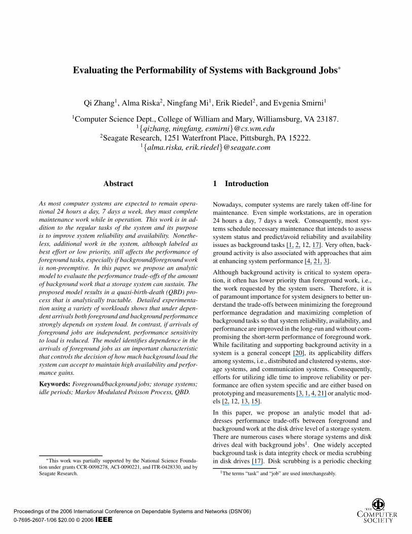
We measure the performance of background jobs by theportion of background tasks that complete. This metricis directly related to reliability (or long term performancebenefits) of background activity. Results are given in Fig-ure 7, which shows that as load increases, the completionrate decreases to zero, independent of load or dependencestructure. For arrivals with a strong dependence structure,(i.e., of “E-mail”), this point comes sooner than for arrivalswith weak dependence structure, (i.e., the “Software Devel-opment”), see the range of the x-axis in Figure 7. Note thatthe completion rate of the background activity relates to theprobability of the background buffer being full, which sup-ports the observation that the strong dependence structurein arrivals increases the queue length of background jobs,as illustrated in Figure 8. Figure 8 shows the average queue

100 80 60 40 20

0 0 10 5 15 20 25 30 35

Foreground utilization (%)

(b) Software Dev. − Low ACF

p = 0 p = 0.1 p = 0.3 p = 0.6 p = 0.9

0 20 40 60 80

100

4 6 8 10 12 14 16 18 20

(a) E−mail − High ACF

Foreground utilization (%)

Bg

com

plet

ion

rate

Bg

com

plet

ion

rate

Figure 7. Completion rate for backgroundjobs for the Email (a) and Software Dev. (b)traces as a function of foreground load.

length of background jobs. Consistent with results in Fig-ure 7, Figure 8 shows a similar qualitative behavior acrossthe two workloads. Quantitatively, the average queue lengthof the long-range dependent workload is smaller than thatof the short-range dependent workload because more back-ground jobs are dropped.

Proceedings of the 2006 International Conference on Dependable Systems and Networks (DSN’06) 0-7695-2607-1/06 $20.00 © 2006 IEEE

Authorized licensed use limited to: Seagate Technology. Downloaded on November 25, 2008 at 11:32 from IEEE Xplore. Restrictions apply.

18 16 14 12 10 8 6 4 2 0

0 5 10 15 20 25 30 35Foreground utilization (%)

(b) Software Dev. − Low ACF

0 2 4 6 8 10

4 6 8 10 12 14 16 18 20

(a) E−mail − High ACF

Foreground utilization (%)

p = 0.1 p = 0.3 p = 0.6 p = 0.9

Bg

QL

EN

Bg

QL

EN

Figure 8. Average queue length of back-ground jobs in the workloads Email (a) andSoftware Dev. (b) as a function of foregroundload.

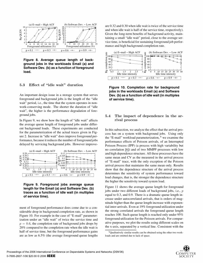
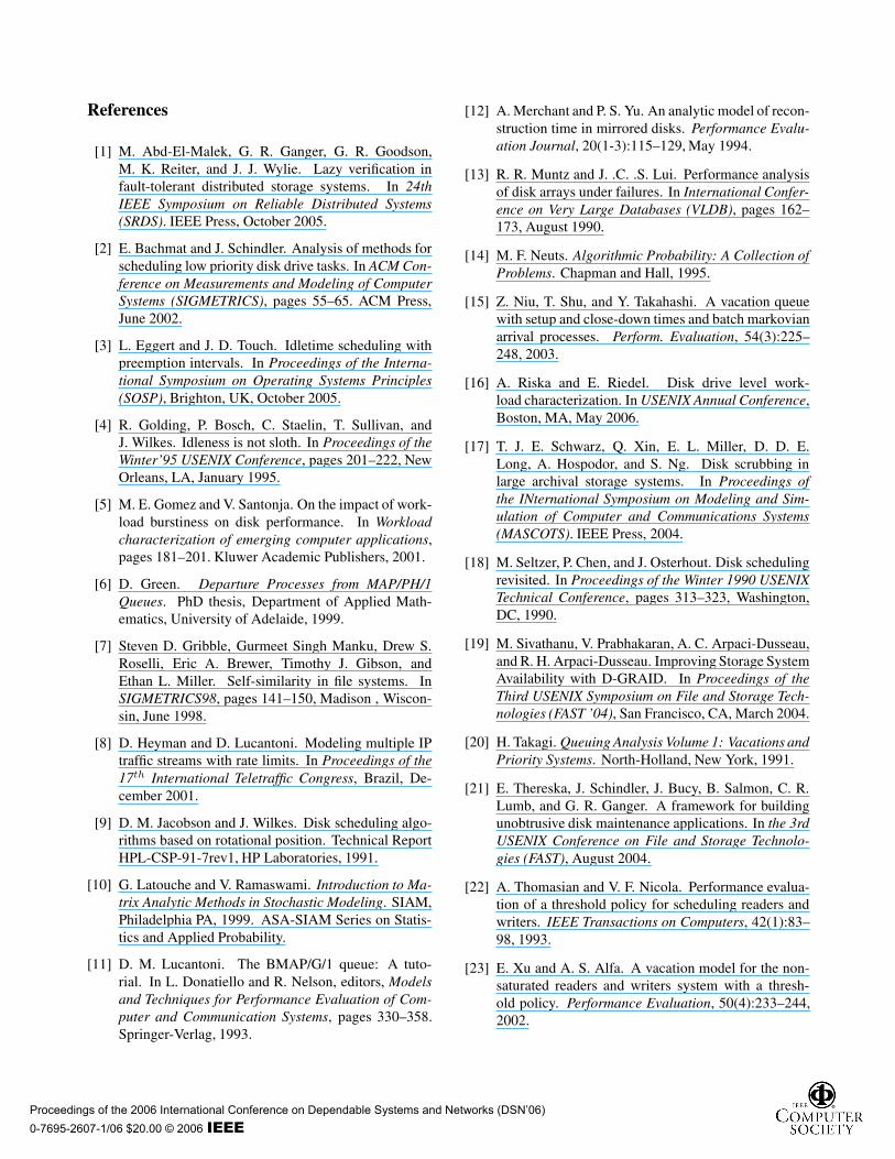
5.3 Effect of “idle wait” duration

An important design issue in a storage system that servesforeground and background jobs is the length of the “idlewait” period, i.e., the time that the system operates in non-work-conserving mode. The shorter the duration of “idlewait”, the higher is the performance degradation of fore-ground jobs.

In Figure 9, we show how the length of “idle wait” affectsthe average queue length of foreground jobs under differ-ent background loads. These experiments are conductedfor the parameterization of the actual traces given in Fig-ure 2. Increase in “idle wait” does improve foreground per-formance, because it reduces the number of foreground jobsdelayed by servicing background jobs. However improve-

0.5 1 1.5 2 2.5 3

0.38 0.36 0.34 0.32 0.3

0.28 0.26 0.24

(a) E−mail − High ACF

Idle time intensity 0 5 10 15 20 25 30 35 40

0.080.085 0.090.095 0.1

0.105 0.11

Idle time intensity

(b) Software Dev. − Low ACF

p = 0.1 p = 0.3 p = 0.6 p = 0.9

Fg Q

LE

N

Fg Q

LE

N

Figure 9. Foreground jobs average queuelength for the Email (a) and Software Dev. (b)traces as a function of idle wait (in multiplesof service time).

ment of foreground performance does come due to a con-siderable drop in background completion rate, as shown inFigure 10. For example in the case of “E-mail” parameter-ization under an “idle wait” of twice the service time andp = 0.6, the completion rate of background jobs drops by20% compared to the completion rate when the idle wait ishalf of service time, but the foreground performance gainsare as low as 6.5% (the average foreground queue lengths

are 0.32 and 0.30 when idle wait is twice of the service timeand when idle wait is half of the service time, respectively).Given the long-term benefits of background activity, main-taining a small “idle wait” period, close to the average ser-vice time, is beneficial for sustaining foreground job perfor-mance and high background completion rate.

Idle time intensity

(a) E−mail − High ACF (b) Software Dev. − Low ACF

Idle time intensity

p = 0.1 p = 0.3 p = 0.6 p = 0.9

100 80 60 40 20 0

100 80 60 40 20 0

0.5 1 1.5 2 2.5 3 0 5 10 15 20 25 30 35 40Bg

com

plet

ion

rate

Bg

com

plet

ion

rate

Figure 10. Completion rate for backgroundjobs in the workloads Email (a) and SoftwareDev. (b) as a function of idle wait (in multiplesof service time).

5.4 The impact of dependence in the ar-rival process

In this subsection, we analyze the effect that the arrival pro-cess has on a system with background jobs. Using onlythe “E-mail” workload parameterization, 6 we examine theperformance effects of Poisson arrivals, of an InterruptedPoisson Process (IPP) (a process with high variability butno correlation [6]) and of two MMPP processes with lowand high dependence structure. All these processes have thesame mean and CV as the measured in the arrival processof “E-mail” trace, with the only exception of the Poissonarrival process that maintains the same mean only. Resultsshow that the dependence structure of the arrival processdetermines the sensitivity of system performance towardload changes, that is, the stronger the dependence structurethe higher the sensitivity toward system load.

Figure 11 shows the average queue length for foregroundjobs under two different loads of background jobs, i.e., pequal to 0.3, and 0.9. There is a dramatic queue length in-crease under autocorrelated arrivals, that is orders of mag-nitude higher than the queue length increase with exponen-tial inter-arrivals. Even at 19% foreground utilization underthe strong correlated arrivals the foreground queue lengthreaches 100. Such queue length is reached only under 95%foreground utilization for the Poisson arrivals. For compar-ative purposes, we plot the results using different scales onthe x-axis, separated by a vertical line. Consistent with the

6Qualitatively similar results can be obtained using the other two work-loads and are omitted due to lack of space.

Proceedings of the 2006 International Conference on Dependable Systems and Networks (DSN’06) 0-7695-2607-1/06 $20.00 © 2006 IEEE

Authorized licensed use limited to: Seagate Technology. Downloaded on November 25, 2008 at 11:32 from IEEE Xplore. Restrictions apply.

results in Figure 5, high foreground load rather than back-ground load determines overall foreground performance. In

0 5 10 15 20 40 60 80 100Foreground utilization (%)

0.01

0.1

10

100

1000(a) E−mail p = 0.3

0 5 10 15 20 40 60 80 100Foreground utilization (%)

0.01

0.1

1

10

100

1000(b) E−mail p = 0.9

High ACF Low ACF IIP Expo

1

Fg Q

LE

N

Fg Q

LE

N

Figure 11. Average queue length for fore-ground jobs for the “E-mail” workload as afunction of foreground load in the system.

Figure 12, we show completion rates for background jobsas a function of foreground load. There are cases whenunder high foreground load, there is nearly a 100% differ-ence in performance between exponential and correlated ar-rivals. The system simply saturates faster under correlatedarrivals and does not have the capacity to serve backgroundtasks. Therefore, under correlated arrivals light backgroundload should be sustained to ensure acceptable backgroundcompletion rates. Finally, Figure 13 shows the percentage

High ACF Low ACF IIP Expo

100

80

60

40

20

0 0

20

40

60

80

100

0 5 10 15 20 40 60 80 100 0 5 10 15 20 40 60 80 100Foreground utilization (%) Foreground utilization (%)

(a) E−mail p = 0.3 (b) E−mail p = 0.9

Bg

com

plet

ion

rate

Bg

com

plet

ion

rate

Figure 12. Completion rate of backgroundjobs for the “E-mail” workload as a functionof foreground load in the system.

of foreground jobs delayed by background jobs as a func-tion of foreground load. Interestingly, the figure shows thatthe worst impact on foreground jobs is contained within alimited range which is reached faster under highly corre-lated arrivals than independent arrivals. In a dynamicallychanging environment with correlated arrivals, the systemregulates itself faster to sustain foreground job performancethan under independent arrivals.

To summarize, the results of this section indicate that, in-dependent of workload characteristics, the non-preemptivebackground jobs minimally impact performance of fore-ground jobs. However sustained foreground performanceunder worst case scenarios is a result of low backgroundcompletion rates, which suggests that background loadmust be kept modest to benefit system reliability or per-

25

20

15

10

5

0 0 5 10 15 20 40 60 80 100

Foreground utilization (%)

(a) E−mail p = 0.3 25

20

15

10

5

0 0 5 10 15 20 40 60 80 100

Foreground utilization (%)

(b) E−mail p = 0.9

High ACF Low ACF IIP Expo

Perc

. of

Fg b

ehin

d bg

Perc

. of

Fg b

ehin

d bg

Figure 13. Portion of foreground jobs delayedby a background job for the “E-mail” work-load as a function of foreground load in thesystem.

formance in the long-term. This sensitivity toward systemchanges, in particular for the background completion rate,is significantly higher for correlated than for independentarrivals, which indicates that workload burstiness is an im-portant factor that should determine the amount of back-ground work in the system.

6 Conclusions and Future Work

In this paper, we presented an analytic model for the eval-uation of disk drives or storage systems with backgroundjobs. Because of the non-preemptive nature of work (i.e.,seeks) in disks, background work inevitably affects perfor-mance of foreground work. The proposed model allows toevaluate the trade-offs between foreground and backgroundactivities. Our model incorporates most important charac-teristics in storage systems workloads, including burstinessand dependence in the arrival process. The model resultsin a Markov chain of a QBD form that is solved using thematrix-geometric method.

Experiments show that system behavior can be qualitativelysimilar for independent or correlated arrivals, albeit for dif-ferent utilization levels. This sensitivity to the system uti-lization levels strongly depends on the dependence structurein the arrival process. Although foreground performanceis sustained at acceptable levels, the background comple-tion rate suffers when background load is high under corre-lated arrivals. Our results suggest that the amount of back-ground work is paramount for reliability and performancegains, and must be a function of the degree of dependenceor burstiness in the arrival process. Currently, we are work-ing on model extensions that capture more than one job pri-ority level, i.e., different classes of background jobs.

Proceedings of the 2006 International Conference on Dependable Systems and Networks (DSN’06) 0-7695-2607-1/06 $20.00 © 2006 IEEE

Authorized licensed use limited to: Seagate Technology. Downloaded on November 25, 2008 at 11:32 from IEEE Xplore. Restrictions apply.

References

[1] M. Abd-El-Malek, G. R. Ganger, G. R. Goodson,M. K. Reiter, and J. J. Wylie. Lazy verification infault-tolerant distributed storage systems. In 24thIEEE Symposium on Reliable Distributed Systems(SRDS). IEEE Press, October 2005.

[2] E. Bachmat and J. Schindler. Analysis of methods forscheduling low priority disk drive tasks. In ACM Con-ference on Measurements and Modeling of ComputerSystems (SIGMETRICS), pages 55–65. ACM Press,June 2002.

[3] L. Eggert and J. D. Touch. Idletime scheduling withpreemption intervals. In Proceedings of the Interna-tional Symposium on Operating Systems Principles(SOSP), Brighton, UK, October 2005.

[4] R. Golding, P. Bosch, C. Staelin, T. Sullivan, andJ. Wilkes. Idleness is not sloth. In Proceedings of theWinter’95 USENIX Conference, pages 201–222, NewOrleans, LA, January 1995.

[5] M. E. Gomez and V. Santonja. On the impact of work-load burstiness on disk performance. In Workloadcharacterization of emerging computer applications,pages 181–201. Kluwer Academic Publishers, 2001.

[6] D. Green. Departure Processes from MAP/PH/1Queues. PhD thesis, Department of Applied Math-ematics, University of Adelaide, 1999.

[7] Steven D. Gribble, Gurmeet Singh Manku, Drew S.Roselli, Eric A. Brewer, Timothy J. Gibson, andEthan L. Miller. Self-similarity in file systems. InSIGMETRICS98, pages 141–150, Madison , Wiscon-sin, June 1998.

[8] D. Heyman and D. Lucantoni. Modeling multiple IPtraffic streams with rate limits. In Proceedings of the17th International Teletraffic Congress, Brazil, De-cember 2001.

[9] D. M. Jacobson and J. Wilkes. Disk scheduling algo-rithms based on rotational position. Technical ReportHPL-CSP-91-7rev1, HP Laboratories, 1991.

[10] G. Latouche and V. Ramaswami. Introduction to Ma-trix Analytic Methods in Stochastic Modeling. SIAM,Philadelphia PA, 1999. ASA-SIAM Series on Statis-tics and Applied Probability.

[11] D. M. Lucantoni. The BMAP/G/1 queue: A tuto-rial. In L. Donatiello and R. Nelson, editors, Modelsand Techniques for Performance Evaluation of Com-puter and Communication Systems, pages 330–358.Springer-Verlag, 1993.

[12] A. Merchant and P. S. Yu. An analytic model of recon-struction time in mirrored disks. Performance Evalu-ation Journal, 20(1-3):115–129, May 1994.

[13] R. R. Muntz and J. .C. .S. Lui. Performance analysisof disk arrays under failures. In International Confer-ence on Very Large Databases (VLDB), pages 162–173, August 1990.

[14] M. F. Neuts. Algorithmic Probability: A Collection ofProblems. Chapman and Hall, 1995.

[15] Z. Niu, T. Shu, and Y. Takahashi. A vacation queuewith setup and close-down times and batch markovianarrival processes. Perform. Evaluation, 54(3):225–248, 2003.

[16] A. Riska and E. Riedel. Disk drive level work-load characterization. In USENIX Annual Conference,Boston, MA, May 2006.

[17] T. J. E. Schwarz, Q. Xin, E. L. Miller, D. D. E.Long, A. Hospodor, and S. Ng. Disk scrubbing inlarge archival storage systems. In Proceedings ofthe INternational Symposium on Modeling and Sim-ulation of Computer and Communications Systems(MASCOTS). IEEE Press, 2004.

[18] M. Seltzer, P. Chen, and J. Osterhout. Disk schedulingrevisited. In Proceedings of the Winter 1990 USENIXTechnical Conference, pages 313–323, Washington,DC, 1990.

[19] M. Sivathanu, V. Prabhakaran, A. C. Arpaci-Dusseau,and R. H. Arpaci-Dusseau. Improving Storage SystemAvailability with D-GRAID. In Proceedings of theThird USENIX Symposium on File and Storage Tech-nologies (FAST ’04), San Francisco, CA, March 2004.

[20] H. Takagi. Queuing Analysis Volume 1: Vacations andPriority Systems. North-Holland, New York, 1991.

[21] E. Thereska, J. Schindler, J. Bucy, B. Salmon, C. R.Lumb, and G. R. Ganger. A framework for buildingunobtrusive disk maintenance applications. In the 3rdUSENIX Conference on File and Storage Technolo-gies (FAST), August 2004.

[22] A. Thomasian and V. F. Nicola. Performance evalua-tion of a threshold policy for scheduling readers andwriters. IEEE Transactions on Computers, 42(1):83–98, 1993.

[23] E. Xu and A. S. Alfa. A vacation model for the non-saturated readers and writers system with a thresh-old policy. Performance Evaluation, 50(4):233–244,2002.

Proceedings of the 2006 International Conference on Dependable Systems and Networks (DSN’06) 0-7695-2607-1/06 $20.00 © 2006 IEEE

Authorized licensed use limited to: Seagate Technology. Downloaded on November 25, 2008 at 11:32 from IEEE Xplore. Restrictions apply.