EVALUATING AND IMPROVING COLLECTION TREE PROTOCOL

IN

MOBILE WIRELESS SENSOR NETWORK

By

Dixit Sharma

A Thesis Submitted in Partial Fulfillment

Of the Requirements for the Degree of

Master of Applied Science

In

Electrical and Computer Engineering Program

Faculty of Engineering and Applied Science

University of Ontario Institute of Technology (UOIT)

Oshawa, Ontario, Canada

July, 2011

© Dixit Sharma, 2011

ii

ABSTRACT

There has been growing interest in the Mobile WSN applications where mobility is

the fundamental characteristic of the sensor nodes. Mobility poses many challenges

to the routing protocols used in such applications. In this thesis we evaluate the

performance of Collection Tree Protocol as applied in mobile WSN scenarios. The

simulation study shows CTP performs poorly in mobile scenario because of the

frequent tree re-generation resulting from node movements.

We compare Collection Tree Protocol with reactive ad hoc network routing

protocols. The simulation results show that collection tree protocol performs better

than reactive MANET protocols in terms of data delivery ratio and control

overhead under low traffic rates. The end-to-end delay obtained in case of reactive

protocols is also higher compared to that obtained when using CTP, which is due to

their route discovery process.

This thesis presents an improved data collection protocol Fixed Node Aided CTP

based on the analysis of CTP. The protocol introduces the concept of fixed aided

routing into CTP.

It is shown that our enhanced CTP outperforms CTP in terms of data delivery ratio

and control overhead chosen as performance metrics.

iii

ACKNOWLEDGEMENT

At this point, I would like to thank Dr. Ramiro Liscano and Dr. Shahram S. Heydari

for advising, supervising and correcting my work. I would like to thank them for

their help, patience and time invested in our research meetings.

I deeply thank my mother and sister back home for their infinite support and love.

iv

Table of Contents

ABSTRACT ................................................................................................................................ ii

ACKNOWLEDGEMENT ......................................................................................................... iii

List of Abbreviations………………………………………………………………………….vii

LIST OF Figures ...................................................................................................................... viii

LIST OF TABLES ....................................................................................................................... x

Chapter 1: Introduction ................................................................................................................ 2

1.1 Wireless Sensor Networks ........................................................................................... 2

1.2 Routing in Wireless Sensor Networks .......................................................................... 5

1.2.1 MANET vs. WSN ................................................................................................ 5

1.2.2 Routing Protocols in WSN ................................................................................... 6

1.3 Mobile Wireless Sensor Networks Characteristics and Applications .......................... 9

1.4 Performance Evaluation Metrics ................................................................................ 12

1.5 The Problem ............................................................................................................... 14

1.6 Objectives ................................................................................................................... 14

1.7 Approach .................................................................................................................... 15

1.8 Thesis Contributions .................................................................................................. 16

1.9 Thesis Outline ............................................................................................................ 16

Chapter 2: Background and Related Work................................................................................. 18

Chapter 3: CTP Design Overview .............................................................................................. 24

3.1 Collection Tree Protocol’s key challenges ................................................................. 25

3.2 Link estimation and adaptive beaconing in CTP ........................................................ 25

v

Chapter 4: Network Modeling and Simulation .......................................................................... 29

4.1 Modelling and Simulation Cycle ................................................................................ 29

4.2 System Description and Assumptions ........................................................................ 31

4.3 Traffic Model ............................................................................................................. 32

4.4 Radio Propagation Basics ........................................................................................... 33

4.5 Wireless Channel Models ........................................................................................... 34

4.6 MAC Layer Model ..................................................................................................... 35

4.7 Mobility Models ......................................................................................................... 35

Chapter 5: CTP Performance in Mobile and Static WSN .......................................................... 38

5.1 SIMULATION SETUP .............................................................................................. 38

5.2 RESULTS AND ANALYSIS .................................................................................... 40

Chapter 6: Comparison of CTP with Reactive Ad Hoc Routing Protocol ................................. 45

6.1 AODV SIMULATION RESULTS ............................................................................ 46

6.1.1 Average end to end delay ................................................................................... 46

6.1.2 Packet delivery ratio ........................................................................................... 47

6.1.3 Control Overhead ............................................................................................... 47

6.1.4 Dropped Packets ................................................................................................. 48

6.2 Analysis of AODV and CTP Performance ................................................................. 51

6.2.1 Average end to end delay ................................................................................... 51

6.2.2 Packet delivery ratio ........................................................................................... 51

6.2.3 Control Overhead ............................................................................................... 52

Chapter 7: Fixed Node Aided Collection Tree Protocol for Mobile WSN ................................ 53

7.1 APPROACH............................................................................................................... 53

7.2 PROPOSED ALGORITHM ...................................................................................... 55

vi

7.2.1 Link Quality Estimation in FNA CTP ................................................................ 55

7.2.2 Route Discovery and Forwarding ....................................................................... 58

7.3 Modifications to CTP in CASTALIA ........................................................................ 60

7.4 Simulation Evaluation ................................................................................................ 61

7.4.1 Experiment Results ............................................................................................ 62

7.4.2 Analysis of Results ............................................................................................. 64

Chapter 8: Conclusion and Future Work .................................................................................... 66

REFERENCES ......................................................................................................................... 68

vii

LIST OF ABBREVIATIONS

ACK: Acknowledgement Packet

ADV: Advertisement Packet

AODV: Ad hoc on demand Distance Vector

CBR: Constant Bit Rate

CTP: Collection Tree Protocol

CSMA/CA: Carrier Sense Medium Access/Collision Avoidance

FNA: Fixed Node Aided

GEAR: Geographical and Energy-Aware Routing

LEACH: Low Energy Adaptive Clustering Hierarchy

MAC: Medium Access Control

PEGASIS: Power Efficient Gathering in Sensor Information

Systems

REQ: Request Packet

SPIN: Sensor Protocol for Information via Negotiation

TEEN: Threshold sensitive Energy Efficient Sensor Network

Protocol

WSN: Wireless Sensor Network

viii

LIST OF FIGURES

Figure 1: Wireless Sensor Network Architecture ......................................................................... 3

Figure 2: Sensor node architecture ............................................................................................. 12

Figure 3: Architecture of ELQR ................................................................................................. 21

Figure 4: Simulation and modeling cycle ................................................................................... 30

Figure 5: snapshot of the sensor field ......................................................................................... 31

Figure 6: Six point random waypoint movement ....................................................................... 36

Figure 7: CTP Data delivery ratio in mobile and static WSN scenario ...................................... 41

Figure 8: CTP Control packets received in mobile and static wsn scenario .............................. 41

Figure 9: CTP Control packets transmitted in mobile and static wsn scenario .......................... 42

Figure 10: CTP Latency in mobile and static wsn scenario ....................................................... 42

Figure 11: CTP Duplicate packets in mobile and static wsn scenario........................................ 43

Figure 12: CTP Failures at the radio level in mobile wsn scenario ............................................ 43

Figure 13: AODV-CTP AVERAGE END TO END DELAY COMPARISON ........................ 46

Figure 14: AODV-CTP Packet Delivery Ratio Comparison ..................................................... 47

Figure 15: AODV-CTP Control Overhead Comparison ............................................................ 48

Figure 16: AODV Dropped Packets ........................................................................................... 49

Figure 17: AODV RREQ Packets Dropped due to TTL expiry ................................................. 50

Figure 18: Number of Duplicate RREQ Packets Received ........................................................ 50

Figure 19 : FNA CTP Sink Node Link Quality Estimation Process .......................................... 56

Figure 20: FNA CTP Sensor Node Link QUality Estimate ....................................................... 57

Figure 21: Route Discovery and FOrwarding in FNA CTP ....................................................... 59

Figure 22: FNA CTP Control Packet Format ............................................................................. 60

Figure 23: FNA CTP Toplogy Diagram..................................................................................... 62

Figure 24: FNA CTP data delivery ratio .................................................................................... 63

ix

Figure 25: FNA CTP Control packets transmitted ..................................................................... 64

x

LIST OF TABLES

Table 1: CTP Simulation Parameters…………………………………………………. 39

Table 2: AODV Simulation Parameters………………………………………………. 45

2

Chapter 1: Introduction

1.1 Wireless Sensor Networks A Wireless Sensor Network (WSN) is an ad hoc network with a number of sensors

deployed across a wide geographical area. The sensor nodes have sufficient

intelligence to communicate with each other over wireless channels and are capable of

performing signal processing and routing of data. The WSN nodes are examples of

energy and computation constrained devices as the sensor devices have limited

memory and processing power. A WSN is an ideal solution for collecting data in a

variety of environments. WSNs are widely used for environmental monitoring, outdoor

industrial process and military surveillance.

Many of the WSN applications share some basic characteristics. Typically in a WSN

application there are two types of nodes: source node – the node which actually sense

and collect data – and sink node – the node to which the collected data is sent. The

sinks can be part of the network or outside the wireless sensor networks. Usually, there

is more number of source nodes than sink nodes. In most of the general WSN

applications the sink node does not concern itself with the identification of the source

nodes but only about the collected data except in situations where it is required to

authenticate the sources.

3

FIGURE 1: WIRELESS SENSOR NETWORK ARCHITECTURE

The interaction pattern between the source and the sink varies depending upon the

application. Typically, the source nodes report to the sink nodes when they detect the

occurrence of a specific event (for e.g. if the temperature threshold is exceeded). In

multihop communication between two end nodes, the intermediate nodes function to

relay the information from one point to another. When the source and the sink are at a

multi-hop distance, the nodes other than the source and sink act as passive forwarding

nodes in the network to deliver the collected data to the sink. Some nodes can act as

both active source nodes and routers. This is in fact what makes a sensor network so

interesting that some nodes can take on both roles. In certain applications, the source

nodes are required to report the collected data periodically to the sink at an application

specific sampling rate.

4

A WSN has a wide variety of deployment options ranging from a uniform fixed node

deployment as utilized in machinery performance detection and random deployments

where a large number of sensors are spread across a region as utilized in military

surveillance or sensors dropped from the aircraft over a forest fire. An Environmental

Observation and Forecasting System (EOFS) [1] is another application of sensor

networks where a large system of widely distributed nodes span across various

geographical areas and is used to monitor, model and forecast physical processes like

environment pollution and flooding. Sometimes, depending upon the application, the

sensor nodes may have to be deployed for prolonged time. In such cases, the

maintenance of sensor nodes would prove to be problematic.

This poses a challenge in designing efficient WSN as the sensor nodes are

microelectronic devices with a limited power source ((<0.5 Ah, 1.2 V) [2] and

processing capabilities. A solitary WSN design is unlikely to ensure effective handling

of a wider range of applications. Thus, the researchers and designers have to think

about every aspect of the application like the lifetime of the network, energy supply

and quality of service needed. Regard must be paid to how fault tolerant the network

needs to be, maintenance options, scalability, programmability of the nodes when the

network is functioning and density of the network. However, there are common

characteristics in a variety of WSN application and the most important amongst them is

data collection. It must be noted that maximum energy consumption in WSN happens

during the communication process. Direct communication between the source node and

sink node over a long distance is not practical as it would need high transmission

power which quickly reduces the lifetime of the network. Hence, the intermediate

5

nodes act as relays to deliver the data and the most common type of communication in

WSN is multi-hop.

In traditional communication networks, the data transfer is centered between 2 devices

with specific network addresses and is called address-centric communications. In many

WSN applications with redundant deployments of sensors to protect against a node

failure or compensate for low sensing capabilities of a single sensor node, the network

address of the node is irrelevant and only the data is important. Thus, WSN designers

have to look for data centric communication protocols.

1.2 Routing in Wireless Sensor Networks

1.2.1 MANET vs. WSN

There are several Mobile Ad hoc Networks (MANET) routing protocols designed for

various ad hoc network applications for both static and mobile scenarios. However, the

same routing techniques cannot be applied in WSN applications as the two networks

differ greatly on the following aspects [3]:

• WSNs are mainly used for the purpose of data collection whereas

MANETs are designed for distributed computing.

• A WSN utilises a larger number of nodes than MANET

• The sensor nodes in WSN use broadcast communication where as in

MANETs nodes mainly use point-to-point communication.

• In WSN, the data flows from the source nodes towards the sink or

conversely but in MANET the data flows are irregular.

6

• Power resources of a WSN are limited as the nodes are left unattended

while in operation and cannot be recharged as frequently as in MANET.

Finally, the computational and communication power of WSN nodes are very limited

as compared to the MANET devices.

1.2.2 Routing Protocols in WSN

There are several energy-aware routing techniques which have been proposed for

Wireless Sensor Networks. These routing techniques can be classified in to three

categories: Data Centric, Hierarchical Cluster based and Location based routing.

In data centric routing protocols, the name schemes of the gathered data are used to

query for data. There are two such routing protocols in place: SPIN (Sensor Protocol

for Information via Negotiation) [4] and Directed Diffusion [5]. In SPIN, the nodes use

a name scheme to create meta-data to describe the collected data. Instead of traditional

flooding it sends an ADV (advertise) message to its neighbours to probe if they are

interested in the data. If the neighbour has not received the data before it send the REQ

message back and then the data is sent to it by the source node. This process is repeated

by all the nodes until everyone has a copy of the data. This protocol reduces the

redundant data in the network to great extent and minimizes the energy dissipation

which occurs in traditional flooding mechanism. However, the mobility of nodes will

challenge the speed and adaptability of the SPIN model. Furthermore, the SPIN

algorithm does not guarantee the delivery of data for example in case of tracking a

moving object upon receiving the REQ when the target goes out of range.

In Directed Diffusion, the sink requests the data from the sensor nodes by broadcasting

a request message for example “give me the temperature in a particular region” and

7

this interest diffuses throughout the network going from one node to another in a multi-

hop fashion and hence every node in the sensor area knows of the request. As the

interest diffuses down the network the node maintains a gradient to the node from

which it received the interest. Hence, after the sensing, the data can be sent back and

there might be a case when a node receives the same interest from multiple neighbours

and then it will have multiple paths to send the data back to the sink. In this case it can

use some metric like least-delay to choose the best path. The intermediate nodes also

perform some in network processing like aggregating the data based on name and

attributes value and hence performing some energy saving here. In this case the in

network processing done to perform the data aggregation uses time synchronisation

which consumes a lot of processing power.

The problem with a data centric approach is that it works well for static nodes, but are

not designed to handle the mobility. Also it cannot handle complex queries and are not

suitable for large sensor networks as they are not scalable and aggregation leads to

overhead.

In Cluster based routing protocols, the sensor nodes are grouped and the one with the

highest residual energy is chosen as the cluster head. More efficient energy distribution

can be achieved in this case. Some of the cluster based protocols proposed are: Low

Energy Adaptive Clustering Hierarchy (LEACH) [6], Power-Efficient Gathering in

Sensor Information Systems (PEGASIS) [7], Threshold sensitive Energy Efficient

sensor Network protocol (TEEN) [8]. LEACH is one of the first cluster based routing

protocols where data is collected in a very elegant way as the small number or clusters

are formed in self organised manner. The cluster head collects and combines the data

8

collected from the nodes in its cluster and transmits the data to the base station.

LEACH uses randomization to select the cluster heads, balance the energy dissipation

among the sensor nodes and increases the lifetime of the sensor network. The

PEGASIS protocol is a near-optimal chain based protocol which is an improvement

over LEACH. In PEGASIS, each node communicates with only one neighbour at a

time and take turns to communicate with the base station. When all the nodes have

communicated with the base station a new round starts. This approach saves power

consumption with every round. TEEN protocol forms clusters in a similar way as

LEACH. It defines two thresholds, soft and hard. When the sensed value of the

attribute differs from the current value by an amount greater or equal to the soft

threshold or the sensed value is above the hard threshold the nodes transmits the data to

the cluster head for forwarding to the base station.

The advantage of using the cluster approach is that these protocols are scalable and

easy to manage routes. The problem with these routing protocols is they are designed

for static WSN and cannot handle mobility. In mobile scenarios the cluster heads are

also moving and hence it requires frequent computation of the cluster head when they

move out of a group’s communication range. Also most of the protocols are designed

based on the LEACH assumptions and hence suffer from the same disadvantages as

LEACH. For instance, what to do if the cluster head has no other cluster head in its

communication range. They are also not suited for time-critical applications as it takes

time in computing the cluster heads.

In location-aided routing (LAR) [9], the location information of the sensor nodes is

used to perform the energy efficient routing. Many protocols have been proposed based

9

on this approach and the most well known of them are Minimum Energy

Communication Network (MECN), Geographic Adaptive Fidelity (GAF), Geographic

and Energy Aware Routing (GEAR). A sensor network application might be interested

in knowing “what is the temp in region x in time y”. The efficient way to disseminate

the geographical query to the specified region is to leverage the location information in

the query and direct the query directly to the region of interest instead of flooding it

everywhere.

One of the most promising data collection protocols for such WSNs is the Collection

Tree Protocol (CTP) [10]. It is a tree based collection protocol whose main objective is

to provide a best effort any cast datagram communication to one of the collection roots

node in the network. It falls in the category of data centric protocols. Collection tree is

an address free protocol where a node chooses its root implicitly by selecting the next

hop based on a routing gradient. It is a state of the art data collection protocol for WSN

and finds its first implementation in TinyOS. A detailed description of its working is

given in chapter 3.

Since there cannot be one realisation of WSN design which will cater the needs of

various applications they have been applied to, specific requirements have to be taken

into consideration when selecting the routing protocol.

1.3 Mobile Wireless Sensor Networks Characteristics and

Applications Sensor networks have the potential to revolutionize the field of medical, disaster

response and vehicular ad hoc networks (VANET) [10] amongst others. In tracking

applications the source of the event can be mobile (e.g. intruder in surveillance

10

scenarios) and WSN may be required to report the source’s speed and direction to the

sink. These requirements can change dynamically and a different interaction pattern

between the source and sink would exist. However, there is a significant gap between

the present sensor network technologies and the special needs of such applications -

one of them is handling mobility of nodes. The application of WSN in medical care

[11] and disaster relief calls for pondering over the re-design of the current protocols to

make them better suited to adapt to the mobility of nodes. Most of the current routing

protocols in WSN’s were designed assuming that all the nodes in the network are

stationary and CTP is one of them. This assumption is no longer valid in today’s

scenario and hence there is a need to come up with protocol designs which will

function as nearly well in mobile scenarios as they do in static. In WSN’s the mobility

patterns can be classified into three categories:

• Source Node Mobility – The wireless sensor network source nodes can be

mobile. In the environmental control application such mobility should not

happen but in applications like livestock surveillance (e.g. sensors attached to

the cattle) it is a normal phenomenon. When mobility comes into picture the

network has to be able to frequently able to re organize itself in order to

function properly. Obviously there will be some tradeoffs between the

frequency and speed of the nodes and the energy needed to maintain an

acceptable level of functionality.

• Sink Node Mobility – This is special case of mobility when the information

sinks are mobile. An example is an application where the information sink is

not part of the network (e.g. a user with a PDA walking in an intelligent

11

building). The user communicates with one source node at a time and after

completing the interaction with that node moves to the next one. Many

researchers have developed protocols allowing for sink mobility [12] in order to

reduce the communication cost resulting from multihop communication when

the source of the information is far off from the sink node. The sink nodes are

allowed to move in between the sensor region and interact with certain nodes to

collect the information.

• Event Mobility – In tracking and event detection applications the source of the

event can be mobile. In such cases a group of sensors around the event object

wake up and report the activity a remote sink. As the source of the event moves

through the region the sensor nodes wake up report the event and go back to the

sleep state. An example of it is in a forest when an elephant movement is being

monitored.

For Mobile WSN applications different mobility models have been proposed which

imitate the real mobility patterns of nodes when they change their speed and direction

in a given time slot. The mobility models [13] are classified in four major categories:

• Models with temporal dependency: as an example is the Gauss-Markov model

• Models with spatial dependency: such as Reference point group model

• Models with geographic restrictions: such as Pathway mobility model

• Random models: such as the Random waypoint model

These mobility models have been used extensively to study the performance of

difference WSN applications using simulations. The mobility models help in

determining probability distributions for link connected and disconnected durations

12

between two moving nodes in the network. Designing and testing of a network

protocol for a mobile WSN application requires considering appropriate mobility

model which will depict the movement of nodes as closely as possible.

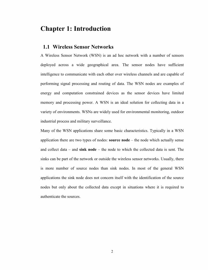
1.4 Performance Evaluation Metrics

In this section the most important evaluation metrics are presented that will be used to

evaluate a collection routing protocol in wireless sensor networks. The key evaluation

metrics of interest for this work in wireless sensor networks are network life time,

response time, and reliability, quality of links, node density and communication

overhead.

FIGURE 2: SENSOR NODE ARCHITECTURE

Packet loss probability, throughput, optimal buffer size of nodes and end to end delay

are also important when evaluating the performance of a routing technique in wireless

sensor network.

Network life time has many definitions, it can be considered to be the time until the

network is fully functional (none of the node has died) or when the first node runs out

13

of energy. Determining the energy consumption for each operation of node is

important. This metric is very important for periodic monitoring applications.

Maximum energy consumption happens during communication and hence for any

protocol to be efficient it has to have minimum control overhead. By control overhead

we refer to the amount of packet traffic which flows through the network to get the

collected data value to the information sink. In a collection tree protocol the sink node

is the root of the tree and the source nodes choose the best path or the least cost path to

the tree and send the data over this path. The control packets which establish the

cost/quality of links are the control overhead flowing in the network.

The latency of the data communication from the source nodes to the sink nodes has a

critical impact on the performance of alarm based applications. The delay and energy

overhead is an interesting topic as in some cases high energy consumption can be

justified giving more importance to the fast reporting of urgent events.

Link quality estimation is a main part of a collection tree protocol as one wants to send

the data over best possible link with least cost. How much control overhead it involves

to calculate the link quality of the links to neighboring nodes and how often it is done

is something which must be considered while designing a link estimation engine for an

application?

Node buffer size is a very important design parameter as it tells how many packets a

node can handle which in turn has an impact on congestion and packet loss in the

network.

14

1.5 The Problem With the rapid application of wireless sensor networks, mobile wireless sensor

networks are going to become common. These mobile wireless sensor networks have

many nodes which are moving and hence the network topology keeps changing

frequently. It is very important to have a routing protocol that could minimize the

energy dissipation in such networks and correctly and reliably transmit data to the sink

information node.

Collection tree protocol (CTP) [14]is one of the most promising data collection tree

protocol. CTP has been shown to be a very efficient data collection routing protocol

and has wide applications in static (non-mobile) WSN [15]. CTP was selected over

other routing protocols in WSN for the study as many applications in WSN involve

only data collection rather than peer to peer communication. The intention is to show

that CTP would function better than other routing protocols when put in data collection

scenarios in mobile wireless sensor networks.

1.6 Objectives The overall objective of this research is to evaluate and identify the performance

challenges for collection tree protocol for mobile WSN applications against the set of

qualitative performance metrics relevant for any routing protocol. Furthermore, a

comparison of CTP’s performance in mobile WSN applications with other relevant

routing techniques in WSN will be provided. At the end changes to CTP are proposed

to make it more efficient in handling mobility of nodes in WSN.

The specific goals of this research include:

• To identify the factors affecting the performance of routing protocols in WSN

15

• To implement Random Way point mobility model in the simulator used for the

study

• To simulate CTP in mobile WSN scenario against performance metrics

• To analyze the results of the simulation against performance metrics in mobile

and static scenarios

• To simulate other relevant routing protocols in the same mobile WSN scenario

and compare their performance with CTP

• To analyse the suitability of the protocols for mobile WSN applications based

on the findings

• Finally draw conclusion of the research by presenting outcomes and proposing

changes to the existing design and algorithmic aspects of CTP to make it

suitable for functioning in mobile WSN applications

1.7 Approach

In the literature survey a detailed study of the background of WSN was carried out for

relevant data gathering. The study involved exploring the state of the art routing

techniques in WSN, mobile WSN applications, performance metrics of interest and

finally choosing a state of the art routing protocol CTP for our study in mobile WSN.

For Performance evaluation Castalia 3.0 [16] was used which is an OMNET-based [17]

network simulator with CTP implementation. Qualnet network simulator was used to

compare CTP against other relevant routing protocols. Random way point mobility

model was implemented in Castalia to test CTP in mobile scenarios.

The network model was designed for the simulation study with different network

entities and different application classes. The routing protocol was simulated for

16

evaluation against selected metrics. The network model used is described later in

chapter 4.

1.8 Thesis Contributions

• Identify through literature review the key drawbacks of the current CTP

implementation that prevents it from being suitable for mobile WSNs

deployment and confirm these findings through simulations.

• Design an enhanced CTP protocol to address these drawbacks and demonstrate

by simulations its effectiveness in handling mobile WSNs scenarios.

1.9 Thesis Outline

This thesis is organized into seven chapters. The first chapter gives introduction and

background to the problem, motivation for this research, research objectives, and

methodology used.

The second chapter gives an overview of the related work directly related to the

research. In the third chapter a design overview and implementation details of

collection tree protocol are presented.

The fourth chapter discusses the network model used for simulations throughout the

thesis.

Performance evaluation of CTP in mobile WSN is presented in chapter 5 and a

comparative study of CTP’s performance in mobile WSN with other related routing

protocols is presented in chapter 6.

In chapter 7 an algorithm is proposed to make CTP better at handling mobility in

WSN.

17

Finally, chapter 8 states the conclusion and the future work.

18

Chapter 2: Background and Related Work

There has not been any work on testing CTP for mobile applications. However, lot of

researchers have tried and used MANET protocols in mobile wireless sensor network

applications.

This simulation study makes use of CTP implementation in Castalia 3.0 [18]. A brief

overview of their work in this section is given as well as some other routing techniques

used in mobile wireless sensor network applications.

Santini et al [18] implemented CTP in the Castalia 3.0 [16] wireless sensor

network simulator, which is based on OMNET [19]. Castalia offers advanced channel

model based on empirically measured data and advanced radio model based on real

radios for low-power communication. The authors gave a comprehensive explanation

of the implementation details in Castalia and how the implementation is different from

the actual design of CTP. The underlying MAC module in Castalia is T-MAC

(Tunable-MAC) which does not offer all the features for CTP so the implementation in

Castalia has made modifications to the MAC to make it similar to the TinyOS

implementation. The main modifications include changes to the queue length, adding

snooping mechanism, link layer acknowledgements and changes to backoff timers. The

backoff timer values determine the delay in transmitting the packet for the first time

and when the channel is busy. It is an important design parameter as a very small value

of the timer would cause too many retransmissions and a high value results in queue

fill up.

The performance of CTP was evaluated through a set of important metrics for a

WSN application including data delivery ratio, control overhead, hopcount and the

19

number of duplicate packets. The simulation study showed that as the number of nodes

sending data packets increases for a particular network configuration the delivery ratio

decreases. This is because of the collisions happening as the number of packets

travelling the network increases. Another interesting note was the effect of network

topology on reliability of packet delivery. As the distance between the sink node from

the source or from the relay node approaches the node’s transmission range a

significant performance hit is observed. This is because of the re-transmissions that are

needed in such cases for successful delivery of a packet. The packets waiting to be

delivered can fill up the buffers quickly so no new incoming packets are accepted and

are therefore dropped. Their simulation study also showed that the control overhead

which is the ratio between data traffic control traffic (beacons sent throughout the

network to maintain the tree) decreases as the probability of the number of nodes

sending data at a time in the network increases. This is because additional data packets

travelling in the network would reduce the number of control packets that have to be

sent to maintain the routing tree. In case of a cluster of nodes disconnected from the

rest of the network (but within the transmission range high control) overhead was

observed as the remote nodes frequently exchange control packets with the sink node.

The hop count and even the duplicate packets number are higher when more nodes are

active in the network. This is due to the number of data packets being sent in the

network which results in congestion, packet drops and lost acknowledgements, and

significantly affects the performance of CTP.

The energy consumption and route changes are most important features in the design of

mobile sensor routing protocol. However, so far the research on CTP has focused on

20

static scenarios only, mainly on reducing energy consumption of the nodes and thus

increasing the life time of the network.

Sridharan et al [20] proposed ELQR as an energy aware link quality estimator, which

takes into account the residual energy as one of the factor before selecting the route. In

CTP the node with better link quality is selected as parent most of the time and is the

one which is involved in most of the communication, which drains out such good link

quality nodes and results in network disconnection. In order to avoid this problem, a

routing protocol is proposed to balance the traffic load among the possible routes. This

is done by having residual energy as a decision factor in the routing tables and this

information is exchanged between the neighbouring nodes. The aim is to select the sub

optimal routes but increase the lifetime of the network. The challenge in ELQR is how

to measure the energy metric. There is no hardware supported energy measurement so

the only way to do is to use software measures and calculate the time spent by devices

like microcontroller, LED, radio, sensor and memory in each mode to calculate energy

spent and use the energy budget of the mote given in the manual to calculate the

residual energy at run time. This residual energy value of each node gets updated

dynamically in the routing tables. This algorithm was simulated in TOSSIM [21]which

is a simulator for TinyOS networks and showed increased network lifetime comparing

to CTP. But the PRR (Packet Reception Rate) is less as compared to CTP as it takes

longer to converge when there is a route change. This work also dealt with testing CTP

only in static scenarios.

21

FIGURE 3: ARCHITECTURE OF ELQR

This work is the first step towards testing CTP for mobile WSN applications and

studying its functioning and proposing changes to its design and working so that it can

handle mobility in wireless sensor networks efficiently.

In [22] the authors propose a new architecture for better handling mobility in wireless

sensor networks. They propose a hierarchical network architecture having a low level

sensing layer with mobile sensor nodes and a high level routing layer with fixed

routing nodes. The nodes in the sensing layer are mobile and they send their sensed

data to the static routing nodes in the routing layer which are at a one hop distance

from them. The static routing nodes then further process and forward the data to the

sink. This is a good solution for such a scenario where we can have fixed nodes at the

side with enough processing, storage and communication capabilities and the mobile

nodes are only one hop distance away from these fixed nodes like a vehicular ad hoc

network. But still this is not a solution to multihop communication between mobile

sensor nodes. Even in case of the VANET’s the distance between the moving sensor

nodes and the fixed routing nodes can be more than the transmission range of the low

power radios of the sensor nodes and hence it will require them to have a multihop

22

communication between the other mobile sensor nodes to get their collected data value

to the base station.

Many researchers have proposed to use the wireless ad hoc network protocols to be

used in wireless sensor networks. Some of them are proactive like Destination

Sequenced Distance Vector (DSDV) [23] and designed for static networks. Some are

reactive like Dynamic Source Routing [24] and Ad hoc On Demand Distance Vector

(AODV) [25]. As mentioned in the previous section these protocols are not designed

for low power, battery enabled sensor nodes. In [26] authors performed the simulation

study on AODV’s performance in wireless sensor networks and it is shown that it gives

around 70% delivery ratio in a static scenario. As they used 802.11 as the MAC layer It

would be interested and more relevant to investigate AODV’s performance using

802.15.4 MAC in a mobile wireless sensor network application.

Hierarchical routing schemes [27] have also been tested to prove that they cannot

support mobility in wireless sensor network applications. The flat based multihop

routing techniques for wireless sensor networks [28] also lack the capability to support

mobility. The frequent link breakages due to node movements cannot be handled fast

enough by their routing mechanism to provide reliable performance.

LEACH-Mobile [29] protocol supports mobility in wireless sensor networks and is

better than LEACH protocol. In LEACH-Mobile each sensor uses a two way

communication mechanism to become part of a cluster. The cluster head sends a

message to the sensor nodes in its cluster and if it does not hear from a sensor node it is

assumed to have moved out of the cluster. When a node does not hear from the cluster

23

head, it tries to connect to other clusters. This protocol also suffers from high packet

losses and energy consumption because of its cluster membership mechanism.

24

Chapter 3: CTP Design Overview

CTP is a tree based collection protocol whose main objective is to provide best effort

anycast datagram communication to one of the collection roots node in the network. At

the start of the network some of the nodes advertise themselves as the root nodes. The

root node is also called the sink node. As there can be multiple root nodes in the

network, the data is delivered to one with the minimum cost. The rest of the nodes use

the root advertisements to connect to the collection tree. When a node collects a data

value, it is sent up the tree. CTP is an address free protocol so a node does not send the

packet to a particular node but chooses its next hop based on a routing gradient. The

node also acts as a relay to forward the data packets from the other nodes in the tree.

The routing gradient used is called expected transmission value (ETX) [30]. One hop

ETX is determined by calculating the number of transmission it takes for a node to

send a unicast packet to its neighbor whose acknowledgement is successfully received.

ETX (root) = 0 and ETX (node) = ETX (parent) + ETX (link to parent)

CTP chooses the route with the lowest ETX value.

The CTP implementation consists of three software modules: link estimation, routing

engine and forwarding engine.

25

3.1 Collection Tree Protocol’s key challenges

1. Routing loops: - Loops occur when a node chooses a new route with higher

ETX value than its old one. This may occur in response to losing connectivity

with a candidate parent. Now if the new route contains a node which was a

descendant earlier, then a loop occurs.

2. Packet duplicates: - Duplication occurs when a node receives a data frame and

transmits an ACK but the ACK is not received. The sender sends the packet

again and the receiver receives it twice. This effect increases over number of

hops as the duplication is exponential (If the first hop produces two duplicates

the second produces four and the third eight and so on). The duplicate

suppression can get really complicated as if the node only suppresses the

duplicates based on source address and sequence number as the packet in

routing loop may also be discarded.

3. Link dynamics: An efficient link quality estimation technique is vital for the

performance of a collection protocol.

3.2 Link estimation and adaptive beaconing in CTP

Link estimation in CTP design is used for determining the communication link quality

between the neighbors. The bidirectional link estimate value ETX is computed by

using both routing beacons and unicast data packets.

The routing packets are sent periodically to calculate the bidirectional link quality

between the neighbors. This value fills the link estimator neighbor table. The CTP

make use of the data transmissions as well to calculate the outbound link quality which

26

is then combined with the control packets link estimate. In a stable network data

packets are used to keep track of any link quality changes and therefore the number of

control packets is reduced. After the transmission of n number of data packets new

outbound quality estimate is performed, where n is implementation dependent. The

outbound quality estimate value is the ratio of number of data packets transmitted to

the number of acknowledgements received. The MAC layer gives the

acknowledgement information to the forwarding engine. The forwarding engine

removes the data packet from its send cache and informs the link estimator engine

about the acknowledgement.

The CTP implementation in [15] uses adaptive beaconing. In a stable network

with less dynamics (link breakages) the frequency of routing packets sending is

reduced over time using the Trickle algorithm [31]. In case of topology update the

nodes find themselves disconnected and with no route to sink. This results in resetting

of the routing packet intervals to adapt to the change and refresh the routing tables and

to calculate the link estimator neighbor table. This is a very important part of the

design of the protocol as more frequent routing packets result in cost and absence for

long result in stale topology information and hence affecting the protocol performance.

Studies have shown that most of the periodic overhead occurs because of the periodic

link quality estimation used in CTP i.e. the ETX metric. Whenever the link dynamics

change or the topology changes due to node mobility the CTP does not respond fast

enough and result in packet losses. So because of the overhead and the unstable

wireless links there are always some significant losses.This limitation of CTP

27

motivates to come up with a better routing algorithm to promise better delivery ratios

and fact recovery mechanism in case of faulty links.

To give an account of the communication overhead involved in CTP a numerical

analysis of the link quality estimation in CTP is presented here. Suppose there is a

wireless sensor network of N nodes, and each node periodically sends x routing

beacons for link quality estimate and one broadcast message is required for each node

to respond to the incoming routing beacons.

Hence the number of packets to be sent comes out to be: (x + 1)*N

Also suppose the CTP implementation sends p number of packets and then again

calculate the link quality and it takes s number of transmissions for a successful

delivery of the packet. The total packet overhead per packet comes out to be:

Packet overhead: ((x+1)*N + p*s)/p (2)

(x+1)*N*T + s where (T = 1/p, frequency of outbound link quality estimation)

Now the (x+1)*N*T is the periodic link quality estimate per packet and is depending

on N which is number of nodes in the sensor network and T which is the frequency of

link estimation. Now if T fairly small value there can be many numbers of

retransmissions and deliver the packets but analysis of some simulation results of

previous studies suggest that it does not promise good delivery ratios and also results in

more power consumption. This is because if a node’s link to its neighbour is

permanently broken (in case neighbour runs out of battery) retransmission of data

packets over the same link results in packet drops and wastage of energy in

28

transmission. Therefore the link quality estimation must happen frequently enough to

keep only valid routes in the neighbour table.

29

Chapter 4: Network Modeling and Simulation This chapter introduces the models used for various components of a wireless sensor

network in this research. First the concept of network modelling is defined and various

phases in modelling and simulation of a network are presented. Communications is the

most important aspect of wireless sensor networks. In the second subsection some

basics on the radio propagation and wireless channel modelling are presented which

are necessary to understand the wireless sensor network models along with a

description of the wireless channel model used. The performance of a routing protocol

in mobile wireless sensor networks depends greatly on the mobility model used. This

chapter describes how the node mobility is modelled, presents various mobility models

in ad hoc networks and explains the working of random way point mobility model used

for this work. As the models parameters are variable, we specify them in chapter 5, 6

and 7 for different simulation configurations run.

4.1 Modelling and Simulation Cycle

The simulator software tools are very handy when dealing with network design and

optimization considering the complex network scenarios, architectures, protocols and

dynamic topologies in them. It relieves the designer from the burden of “hit and trial”

errors in hardware implementations. Usually the network simulators provide the

programmer with the multi thread control and inter communication abstraction. The

events and protocols are represented by finite state machine or the simulator native

programming code or both. The simulators usually come with pre defined modules and

graphical user interfaces. Qualnet is an example of a discrete event simulator which

provides a very friendly GUI and also the support for visualization and animation.

30

Qualnet is used for AODV (ad hoc on demand distance vector) simulations in chapter

6. Castalia is another simulator which specializes in simulating wireless sensor

networks and body area networks. Given the modular structure implementing new

distributed algorithms in Castalia is very convenient. It also provides one of the most

realistic wireless channel and radio propagation models.

FIGURE 4: SIMULATION AND MODELING CYCLE

31

4.2 System Description and Assumptions

FIGURE 5: SNAPSHOT OF THE SENSOR FIELD

In this work the WSN is modelled as a system consisting of N identical sensor nodes.

The sensor nodes are randomly distributed in a rectangular region. It is assumed that

the sink node collecting all the information sensed and collected by the source nodes is

located at (0, 0) location of the topology graph. An example of the network topology is

given in the Figure 5. All the sensor nodes are assumed to have the same radio range r

and they are equipped with omnidirectional antennas.

The phenomena sensed by the sensor nodes are stored as data units of fixed size in the

buffer at the sensor. The buffer is modeled as FIFO queue and its length is a design

32

parameter and implementation dependent. It must be noted that the sensors are half-

duplex as they cannot receive and transmit a message at the same time. The time is

divided into unit durations and reception/transmission can occur for only one data unit

at one time slot. Further details on the traffic pattern, wireless channel model used, and

mobility models are given below.

4.3 Traffic Model

A simple data traffic scenario is considered which is very typical of wireless sensor

network applications. The physical phenomenon used is the same as the one in [18].It

is important to address Time synchronisation [32]in multihop and ad hoc wireless

networks like sensor networks. In several WSN applications the sensor nodes need to

cooperate and collaborate to achieve a sensing task. For example, in Vehicular Ad hoc

Networks (VANET) the sensor nodes report the time and location of the vehicle to the

sink node which further combines this information to estimate the location of the

vehicle. If the nodes are not synchronised the estimate will be incorrect. For this

purpose, it is assumed that the nodes in the network are synchronised so that their wake

and sleep cycles are easily scheduled. The nodes are required to provide “snapshots” of

the values of a physical phenomenon at regular time intervals. The sampling frequency

Fs remains fixed from the start and is same for all the nodes in the network. The sensor

source nodes wake up at every Ts = 1 / Fs seconds, sample the phenomenon (for e.g.

Gather the temperature value at that instant), send the data to the sink node and go back

to sleep. After waking up, in order to send the data to the sink node the network

establishes a data collection tree using the CTP protocol. The sequence sleep-wake up-

sleep is called a round and is repeated during the network operation.

33

4.4 Radio Propagation Basics

For understanding the wireless channel models there are certain terms and definitions

one needs to know related to radio propagation.

Path Loss – It is defined as a decrease of signal power from the effects of free space,

attenuation and scattering. Free space loss means the diminishing of the signal power

as a result of the spreading of the wave front. Free space loss is hence solely dependent

on the distance of the receiver from the transmitter. Also when taking obstacles into

account one needs to consider the signal attenuation. Attenuation occurs when the

signal has to pass through solids like chairs, tables or walls.

Fading – It is the variation of the power of the signal at the receiver side. Fading

results from the addition of phase delayed signals at the receiving side which may

result in the signal to be completely useless. The signal from the transmitter to the

receiver takes on different paths and the addition of the signal following the direct path

to the longer path results in this problem.

Signal to Noise Ratio – The signal suffers from degradation during the propagation

because of fading and path loss. This signal quality also varies over time with

dynamics on the way like people moving etc. The SNR is the ratio of received

meaningful information to the noise in the background. This is used to estimate if the

received frame is correct or not.

34

4.5 Wireless Channel Models

There are a number of radio propagation models. The two most common path loss

models are free space model and two-ray ground reflection model. The free space

model is one of the most basic path loss models. It assumes the receiving and

transmitting antennas are ‘floating in space’. It assumes there is no obstacle or ground

in the path and there is only one direct path between the transmitter and receiver. It

means the received signal power is only a function of distance and the transmitted

signal power. The problem with this model is that even far off nodes can hear the

transmitted packets which can result in wrong decisions of routing algorithms in ad hoc

networks. Two ray ground reflection models is an improvement over the free space

model as it assumes the reflection of the signal on ground. Hence there exists two

paths, the direct path and the path reflected from the ground. The heights of the

antennas are also considered while calculating the received signal power in this model.

But still it suffers from the same limitation as the previous model as they both do not

consider any real obstacles in the signals way.

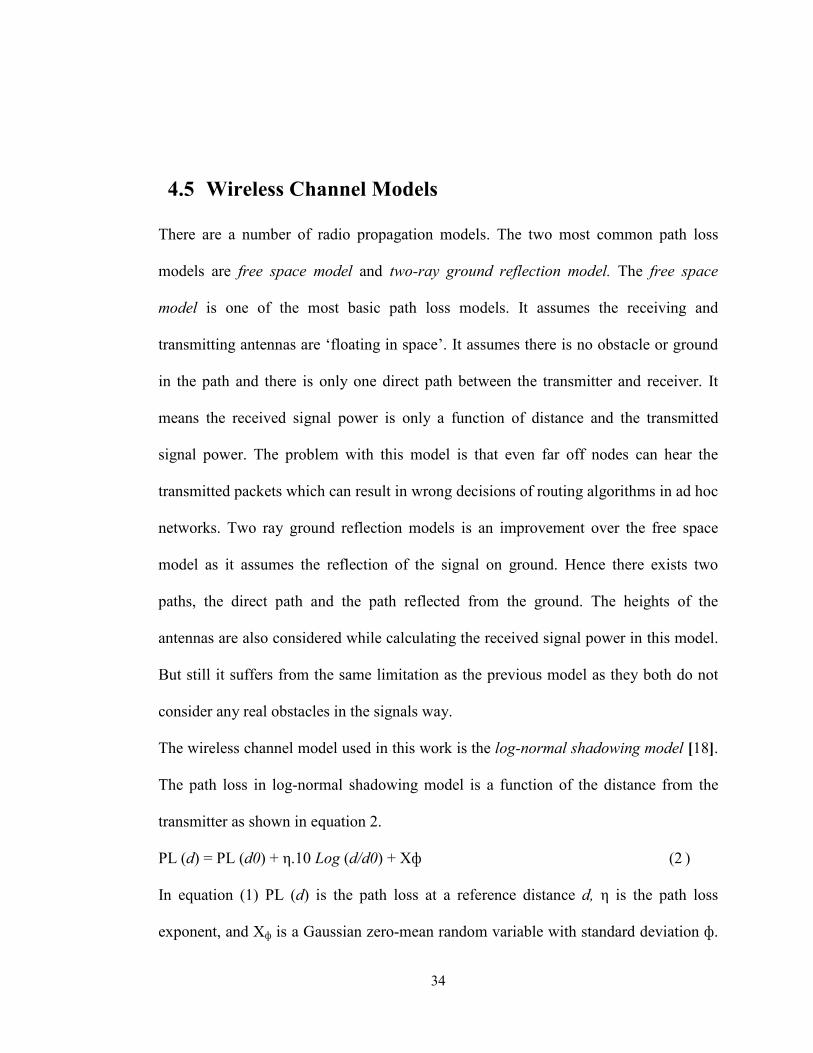
The wireless channel model used in this work is the log-normal shadowing model [18].

The path loss in log-normal shadowing model is a function of the distance from the

transmitter as shown in equation 2.

PL (d) = PL (d0) + η.10 Log (d/d0) + Xф (2 )

In equation (1) PL (d) is the path loss at a reference distance d, η is the path loss

exponent, and Xф is a Gaussian zero-mean random variable with standard deviation ф.

35

This is a more realistic channel model than the previous two as it takes in to account

the obstructions and tries to disturb the ideal propagation circle. It also models the

complicated path loss and fading effects by using a probabilistic approach.

4.6 MAC Layer Model

The network models we assume that the multihop wireless communication MAC layer

is CSMA – based and the physical layer for our network model supports burst-mode

(packetized), coded communications. The general framework used for this work

applies to 802.15.4 and 802.11 mesh networks. The evaluation of CTP performance is

done in Castalia. The modified Tunable MAC is used by Castalia because it imitates

very closely the MAC functions of the CTP implementation in TinyOS which is an

open source operating system designed for low power wireless devices like the ones

used in sensor networks and is widely used and supported by the academia [33].

4.7 Mobility Models

A number of mobility patterns of nodes exist which can be classified as: pedestrian,

vehicles, robot and dynamic medium. A few of most common mobility models used

are:

1. Random Waypoint Model

2. Random Walk Model

3. Gauss-Markov Model

4. Reference Point Group Model

5. Pathway Mobility Model

36

For some mobility models, the mobility pattern is affected by their history. These are

models with temporal dependency such as Gauss-Markov model. In some models the

movement is in a correlated manner such as in Reference Point Group model. The

pathway mobility model’s mobility pattern is restricted by the boundaries of the region

they travelling in [34].

It is important to choose the mobility models that emulate the mobility pattern of the

nodes in the real life applications as closely as possible. Trace based-mobility pattern is

a way to construct realistic mobility patterns but they have not been implemented and

deployed in MANETs. This makes it challenging to obtain realistic mobility traces.

FIGURE 6: SIX POINT RANDOM WAYPOINT MOVEMENT

One of the frequently used mobility model in MANET’s is Random mobility model.

Their simplicity makes them one of the favourite choices for the mobility model in

simulations. In the Random Waypoint Mobility Model the mobile node moves a

distance d in a direction randomly chosen from (0,2π). The distance is exponentially

distributed. The node moves from its current position for a randomly selected

move_time with speed varying between [min_speed, max_speed]. The node bounces

back into the test region when it hits a boundary. At the end of the move_time it pauses

37

for pause_time. The pause_time is randomly picked like move_time based on random

variable and the process is repeated. Random Way point model is used over others

because if a data collection protocol can give good results in this mobility pattern then

it can be assumed that it will give better results in cases where we have linear or more

predictable mobility pattern.

38

Chapter 5: CTP Performance in Mobile and

Static WSN Mobility poses many challenges to the routing protocols used in Wireless Sensor

Networks. In this section the performance of the Collection Tree Protocol is evaluated

when used in a mobile wireless sensor network scenario through simulations. The

simulation experiments have been performed using a CTP implementation in Castalia

3.1 [18].

5.1 SIMULATION SETUP

The purpose of this simulation is to study the effect of mobility on CTP and identify

the key design, implementation and algorithmic features of its current implementation

which causes a deviation from its performance in static scenario.

In this simulation setup there are 40 nodes randomly spread in a rectangular field of

100m x 100m. The network has a fixed data sink at position (0, 0) meters. The sensor

nodes sample the physical phenomenon at regular intervals. Every time the nodes wake

up they establish a data collection tree using CTP to transport the collected data to the

data sink. The simulation assumptions, parameters and their values are given in the

Table 1.

39

Parameter Value Units

Topology

Cx 100 meters

Cy 100 meters

Nnodes 40 -

(xs, ys) (0,0) Sink coordinates

Radio Model

d0 1 meters

PL(d0) 54.2247 dB

η 2.4

Xσ 0

Tx 50 meters

Data Traffic

Source data pattern .333 packets/ second

Random Waypoint Mobility Model

Minimum Velocity 0 meter/seconds

Maximum Velocity 15 meter/seconds

Pause Time 10 seconds

General

Simulation Time 300 seconds

Nrounds 50 -

TABLE 1: CTP SIMULATION PARAMETERS

40

The following performance metrics are used for the study of CTP’s performance under

mobile scenarios:

1. Data delivery ratio: This is the ratio between the numbers of data packets

successfully delivered to the sink to those sent by the source nodes.

2. Control traffic: This is the traffic resulting from routing beacons in the network for

establishing and maintaining the tree.

3. Application level packet latency: It is the time taken for a packet to travel from the

source node to the sink node.

5.2 RESULTS AND ANALYSIS

Figure 7 shows the data delivery ratio for the static and mobile scenario. The average

data delivery ratio was around 94% in static case with confidence interval of 92% and

47% for the mobile scenario with confidence interval of 79%. The control overhead is

the number of routing packets to deliver the data packets to the sink. Figure 8 and Figure

9 show that the control packets received and transmitted in the case of the mobile

scenario is around three times more than in the case of static nodes. The confidence

interval in the case of mobile WSN scenario for both transmitted and received control

packets is around 77% and for static WSN scenario it is around 91 %. The nodes may

receive control packets from number of neighbours. This implies that overhead of

using CTP for mobile applications can be very significant.

41

FIGURE 7: CTP DATA DELIVERY RATIO IN MOBILE AND STATIC WSN SCENARIO

FIGURE 8: CTP CONTROL PACKETS RECEIVED IN MOBILE AND STATIC WSN SCENARIO

42

FIGURE 9: CTP CONTROL PACKETS TRANSMITTED IN MOBILE AND STATIC WSN SCENARIO

FIGURE 10: CTP LATENCY IN MOBILE AND STATIC WSN SCENARIO

The end to end delay or latency is also an important performance metric for sensor

networks. It was noticed that around 30% of packets take more than 1000 milliseconds

to get to the sink. This is the case when a packet does not receive acknowledgements

for the first time it sends the packet and a couple of retransmissions are required for the

0

10

20

30

40

50

60

70

80

90

100

1 3 5 7 9 11 13 15 17 19 21 23 25 27 29 31 33 35 37 39

Control pkts transm

itted

Node

Mobile

Static

43

successful delivery. This happens at multiple hops on its path to the sink node which

adds to the delay. The results also showed that the average delay increased with the

increase in node mobility. The packets delivered include the duplicate packets as well.

In terms of duplicate packets there were on average 8% of duplicate packets with

confidence interval 84% in the network for the mobile scenario case and 3.4% for the

static scenario with confidence interval 93% (we believe these are due to lost link level

acknowledgements.) The results of this experiment are shown in Figure 11.

FIGURE 11: CTP DUPLICATE PACKETS IN MOBILE AND STATIC WSN SCENARIO

FIGURE 12: CTP FAILURES AT THE RADIO LEVEL IN MOBILE WSN SCENARIO

44

A good analysis for determining why there is so much overhead can be done by

looking at how packets failed at the radio level. Figure 12 shows a histogram

breakdown of 6 packet failures at the radio level.� The received packet breakdown

show that most of the packets failed because the signal was below the receiver’s

sensitivity level. This occurs when the node moves out of the transmission range of the

receiver. There is also a large number of packet drops occurring because of packet

interference.

The purpose of studies in this section was to identify important factors that contribute

the most to the degradation of CTP performance in mobile environment. It was noticed

from the simulation results that mobility significantly affects the reliability of the

protocol. The mobility causes frequent topology changes which result in more frequent

tree re-generation. In order to setup the tree again more beacons are sent throughout the

network. Many packets were discarded from the queue because the queue would fill up

with control packets. It can be concluded from the results that the path metric

estimation makes CTP unsuitable for areas involving mobility. Even when there are

nodes close enough for communication this result in more channel interference and

therefore temporary disconnection of the link. This again triggers the re-construction of

a portion of the tree. These temporary tree disconnections cause loops and hence

congestion in the network. The loss of acknowledgements result in more duplicate

packets sent. The control overhead increases significantly in this case.

Latency was another parameter that was computed. Latency in the case of a static

scenario was more than 300 ms for one third of the nodes. This could be a crucial

factor in some time constraint real time applications for sensor networks.

45

Chapter 6: Comparison of CTP with Reactive

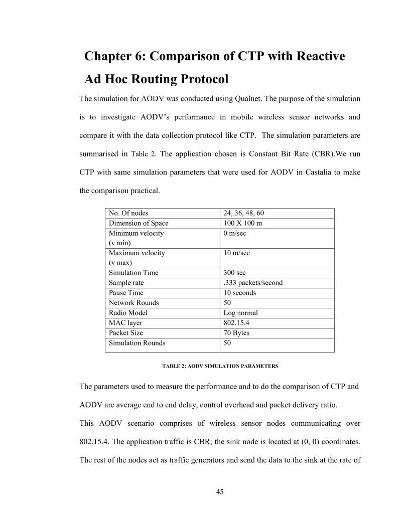
Ad Hoc Routing Protocol The simulation for AODV was conducted using Qualnet. The purpose of the simulation

is to investigate AODV’s performance in mobile wireless sensor networks and

compare it with the data collection protocol like CTP. The simulation parameters are

summarised in Table 2. The application chosen is Constant Bit Rate (CBR).We run

CTP with same simulation parameters that were used for AODV in Castalia to make

the comparison practical.

The parameters used to measure the performance and to do the comparison of CTP and

AODV are average end to end delay, control overhead and packet delivery ratio.

This AODV scenario comprises of wireless sensor nodes communicating over

802.15.4. The application traffic is CBR; the sink node is located at (0, 0) coordinates.

The rest of the nodes act as traffic generators and send the data to the sink at the rate of

No. Of nodes 24, 36, 48, 60 Dimension of Space 100 X 100 m Minimum velocity (v min)

0 m/sec

Maximum velocity (v max)

10 m/sec

Simulation Time 300 sec Sample rate .333 packets/second Pause Time 10 seconds Network Rounds 50 Radio Model Log normal MAC layer 802.15.4 Packet Size 70 Bytes Simulation Rounds 50

TABLE 2: AODV SIMULATION PARAMETERS

46

one packet every three seconds for the total duration of the simulation. The channel

model, the radio range and the energy model is the same as that used for the CTP

simulations in the previous section.

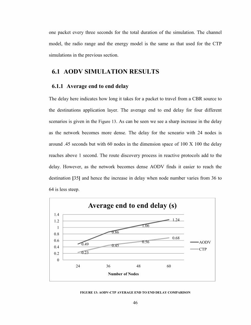
6.1 AODV SIMULATION RESULTS

6.1.1 Average end to end delay

The delay here indicates how long it takes for a packet to travel from a CBR source to

the destinations application layer. The average end to end delay for four different

scenarios is given in the Figure 13. As can be seen we see a sharp increase in the delay

as the network becomes more dense. The delay for the scneario with 24 nodes is

around .45 seconds but with 60 nodes in the dimension space of 100 X 100 the delay

reaches above 1 second. The route discovery process in reactive protocols add to the

delay. However, as the network becomes dense AODV finds it easier to reach the

destination [35] and hence the increase in delay when node number varies from 36 to

64 is less steep.

FIGURE 13: AODV-CTP AVERAGE END TO END DELAY COMPARISON

0.49

0.86

1.061.24

0.23

0.450.56

0.68

0

0.2

0.4

0.6

0.8

1

1.2

1.4

24 36 48 60

Number of Nodes

Average end to end delay (s)

AODV

CTP

47

6.1.2 Packet delivery ratio

Packet delivery ratio is the total number of data packets received by the destination

node to the actual number of data packets generated by the CBR. It is also an indicator

of the packet loss ratio which bounds the throughput of the network. As shown in the

Error! Reference source not found. delivery ratio for a network of 24 nodes is

around 40% and for a denser network with 60 nodes it is noticably low and is only

around 15%.

FIGURE 14: AODV-CTP PACKET DELIVERY RATIO COMPARISON

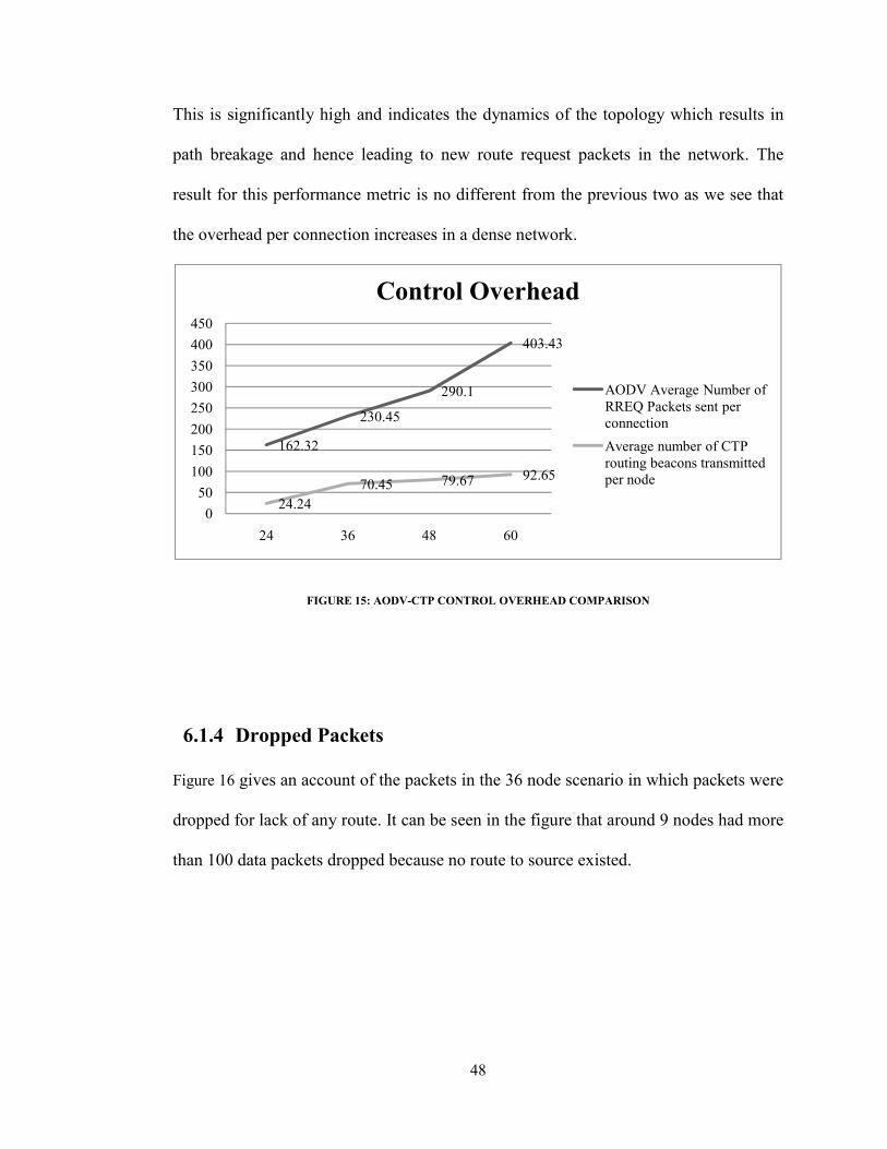
6.1.3 Control Overhead

The overhead in this section involves the control packets sent by AODV to find a path.

In the figure we present the number of route requests per connection against the

number of nodes in the network. The RREQ packets sent during path establishment is

metric to find the communication overhead involved in sending the data packets to the

destination. The more number of control packets result in more power consumption as

the sensor nodes spend maximum energy during transmission. The results show that on

average there are around 150 route request packets sent in case of 24 node network.

40.8

27.121.34

12.67

48 45.4 47.1 43

0102030405060

24 36 48 60

Number of nodes

Packet Delivery Ratio %

AODV

CTP

48

This is significantly high and indicates the dynamics of the topology which results in

path breakage and hence leading to new route request packets in the network. The

result for this performance metric is no different from the previous two as we see that

the overhead per connection increases in a dense network.

FIGURE 15: AODV-CTP CONTROL OVERHEAD COMPARISON

6.1.4 Dropped Packets

Figure 16 gives an account of the packets in the 36 node scenario in which packets were

dropped for lack of any route. It can be seen in the figure that around 9 nodes had more

than 100 data packets dropped because no route to source existed.

162.32

230.45

290.1

403.43

24.2470.45 79.67 92.65

050

100150200250300350400450

24 36 48 60

Control Overhead

AODV Average Number of RREQ Packets sent per connection

Average number of CTP routing beacons transmitted per node

49

FIGURE 16: AODV DROPPED PACKETS

Figure 17 shows the number of route request (RREQ) packets which are dropped due to TTL

(time to live) expiry. Now the main reason for this dropping of packets is mobility. Because of

the mobility pattern the last route stored in AODV cache becomes invalid and hence more and

more packets die due to the TTL expiry. Also it was observed during the simulations that with

more numbers of nodes the hop count for the packet traversal increases which also adds to TTL

expiry of packets. The TTL threshold used was 7 in this case.

Figure 18 shows the number of duplicate RREQ packets in the network. The RREQ packets

are retransmitted because a lot of packets are lost due to the TTL expiry.

50

FIGURE 17: AODV RREQ PACKETS DROPPED DUE TO TTL EXPIRY

FIGURE 18: NUMBER OF DUPLICATE RREQ PACKETS RECEIVED

51

6.2 Analysis of AODV and CTP Performance

6.2.1 Average end to end delay

Due to the reactive approach followed by AODV the average end to end delay

compared to a tree collection protocol is quite high. The mobility in the network causes

frequent RREQ packets to be sent to rediscover the route and if no route reply message

is received (RREP) the packet delivery delay increases. However, the delay in CTP

does not increase exponentially like it does in the case of AODV as the number of

nodes is increased.

6.2.2 Packet delivery ratio

The Figure 14shows the comparison between the packet delivery ratio between AODV

and CTP. A good packet delivery ratio means a reliable routing protocol. The results

for AODV slides sharply with number of nodes in the network increasing. This is

because of the packet losses due to no routes, ttl expiry, channel congestion and

collisions in a more dense network. In case of CTP surprisingly there is not much

difference in the data delivery ratio with increasing nodes and one can say it almost

remains constant with slight changes The result for CTP are not so great as well but are

comparatively better than AODV which reinforces are belief that a collection tree

protocol should be more suited for typical data collection scenarios in mobile wireless

sensor networks. The confidence interval for AODV in this case was 71 % and for CTP

around 88 %.

52

6.2.3 Control Overhead

The per node control overhead in case of CTP is much less as compared to the AODV.

As the control overhead is directly related to power consumption, congestion and hence

collisions in the network, AODV is not as well suited for mobile applications in

wireless sensor networks. CTP adopts a hybrid approach to find routes. It proactively

fills its neighbour table by sending control packets and also reacts to the topology

changes by recomputing the link quality of its neighbouts. CTP which is a tree protocol

appears to be a better solution if its link quality estimation engine can be modified the

control overhead can be decreased further which will result in better overall

performance. In the next chapter modifications to CTP are proposed in order to make it

better for mobile WSN applications. Confidence interval for AODV over different

simulation rounds was 67 % and for CTP 92 %. In AODV simulation in Qualnet there

was significant difference in results for different random seeds used.

53

Chapter 7: Fixed Node Aided Collection Tree

Protocol for Mobile WSN This chapter presents a solution to the problems identified earlier in using a collection

tree routing protocol in mobile wireless sensor network scenario. Based on the analysis

of CTP’s performance in mobile scenarios it is concluded that the current adaptive

beaconing mechanism implemented in CTP is not fast enough to adapt to the too

frequent topology changes introduced by the mobile nodes. There is a trade-off here

because in order to achieve high delivery ratio one needs to tune the design parameters

of the adaptive beaconing mechanism to timer values small enough to react to the

changing topology. But in doing a lot of control overhead is introduced which is not

acceptable in resource constrained wireless sensor networks.

The algorithm proposed in this section achieves higher delivery ratio with reduced

control overhead than CTP as shown by the simulation results as well.

7.1 APPROACH

Fixed Node Aided CTP’s basic primitive is simple: Every deployment of WSN has a

few static sensor nodes distributed in the network region. These fixed wireless sensor

nodes are distributed over the network region using an effective and an optimal

coverage function [36] and they have higher radio transmission range higher than the

other active nodes to cover most of the network region. The fixed nodes deployment is

optimized to cover the maximum area of interest using minimum number of fixed

nodes. All the other mobile source nodes in the network will be in the transmission

range of at least one of the fixed nodes. Depending on the area of the network the

54

number of fixed nodes and their transmission range is selected. The working of the

CTP remains the same except that now every mobile node will have at least one fixed

node’s ETX entry in its link estimation neighbour table and routing table in which

fixed node will be identified by a special flag bit set. It is assumed that after every

unicast data transmission if the source node does not receive an acknowledgement back

it will forward the packet to the fixed static node. This is unlike CTP in which a

significant performance hit is observed when CTP keeps calculating the link quality to

determine the new parent for its neighbours in response to no routes to its current

parent. The link quality estimation happens in a periodic fashion only using the

adaptive beaconing mechanism except for that now the beacon interval is not set to the

minimum value for the mobile sensor nodes after detecting lost acknowledgements.

The fixed node upon receiving the unicast data packet schedules it to be forwarded to

its parent which can be a mobile node. The procedure is repeated until the packet gets

to the sink node. The advantage of this mechanism is that it improves the packet

delivery ratio with minimal control overhead; it still uses the link quality estimation

mechanism of CTP benefiting from the multihop communication rather than forcing

the packets to be delivered to the sink through fixed sensor nodes over long

communication distances. The fixed nodes provide a back up infrastructure to the

network. They increase the reliability of the network in mobile scenarios as packets are

not dropped for not finding the route due to ever changing topology due to the

movement of nodes. This scheme is different from the standard clustering algorithm as

it does not involve the computation of cluster heads. The clustering algorithms are not

suitable for sparse networks and in cases when the nodes do not follow a group

55

mobility pattern. In mobile scenarios the cluster head candidate is also moving and

often nodes have to spend energy in computing new cluster heads.

7.2 PROPOSED ALGORITHM

The same network model is used as in previous chapters having a static sink node and

number of mobile sensor nodes scattered randomly in the network region, with the

addition of pre-defined number of fixed nodes distributed in the area with full coverage

of the network. Each mobile sensor node has the same transmission range and can

communicate with the nodes within its range. There are two main processes in the

original CTP:

1. Link Quality Estimation of Neighbour Nodes

2. Route Discovery and Forwarding

This section presents the changes made to these two processes in Fixed Node Aided

CTP (FNA CTP) and it also gives the key assumptions made.

7.2.1 Link Quality Estimation in FNA CTP

The tree establishment is same as in CTP; the sink node broadcasts the routing beacons

with ETX value 0. The nodes receiving this broadcast attach themselves to the tree

with sink node as tree root and calculate the inbound link quality ETX value to fill up

the link estimator neighbour table during the bootstrap mechanism. These nodes further

broadcast the routing beacons with their cost value to the sink node and using this

broadcasting of routing beacons the nodes maintain the link estimator tables with ETX

value of its neighbours. In FNA CTP the fixed nodes act as just any other sensor node

in the network except that the routing beacons broadcast by them have a special flag

56

called Fixed bit set. The nodes receiving the broadcast messages from the fixed node

create an entry in their neighbour table for the fixed node with its ETX value. As in the

network model fixed nodes cover most of the network region because of their higher

transmission range each node will have a fixed node entry in its neighbour table. A

flow chart of this link quality establishment process is presented in Figure 19 and Figure

20.

FIGURE 19 : FNA CTP SINK NODE LINK QUALITY ESTIMATION PROCESS

57

Sensor Node

No Yes

No

Yes

We only present those algorithmic aspects of our algorithm which are different from CTP.

Receives Routing beacons from sink;

Calculate Link quality of the link to Sink node and create the neighbour table

Is sensor node = fixed node?

Broadcast routing beacons to neighbours with fixed bit set

Send original CTP routing beacons

Received Routing beacon with fixed bit set?

Create a special entry in neighbour table for this fixed node with ETX value of the link

Regular Neighbour table entry with ETX value

FIGURE 20: FNA CTP SENSOR NODE LINK QUALITY ESTIMATE

58

7.2.2 Route Discovery and Forwarding

Route Discovery, forwarding and reaction to failed data deliveries is where FNA CTP

differs from CTP. Route discovery happens after the one hop link estimator table has

been used to fill the routing table entries. As mentioned earlier every link estimator

table and routing table has at least one entry for the fixed node. The unicast data is

forwarded after look up in the routing table to find the next hop with minimum ETX

value. If the fixed node has the minimum ETX value the packet is forwarded to it. In

case it is a mobile sensor node with minimum ETX value, the packet is forwarded to it

but only two attempts are made to get the data delivered else we choose the fixed node

as the next hop distance. No adaptive beaconing is applied to the mobile sensor nodes

to react to failures. The mobile sensor nodes find routes only periodically after a fixed

time interval, 20 seconds in this implementation. The packet received at the fixed node

is forwarded to the node in its neighbor table with minimum ETX value. In case of lost

acknowledgements the fixed node uses the adaptive beaconing method to react to lost

links. The fixed node has a larger queue size and is made to keep the packet for some

time until it is successfully delivered. The packet is dropped if no success is achieved

in that time.

A buffer management process at the fixed nodes is required as it may happen in case

with mobile sensors with very high degree of mobility that they keep sending packets

to the fixed node and the fixed nodes suffer from buffer overflow and start dropping

packets. In this implementation it is assumed that the buffer sizes of fixed nodes are

fairly large enough so that no packets are dropped because of buffer overflow. In

sparse networks however the buffer management should not be much of a problem as

59

in dense networks. Figure 21 is flow chart for the route discovery and forwarding

mechanism in FNA CTP.

Yes

No

No

Yes

Mobile Node Routing Table Look up

Next hop = Fixed Node?

Forward the packet to the fixed node

Send the packet to

mobile Node and wait

Ack received?

Successful delivery, remove packet from the send cache

Retransmit the packet two times and if no acknowledgement received choose fixed node entry as the next hop

FIGURE 21: ROUTE DISCOVERY AND FORWARDING IN FNA CTP

60

The routing table lookup for fixed node remains same as in the original CTP. In that

the adaptive beaconing mechanism resets the beaconing interval to its minimum value

to react to a packet failure.

The next subsection gives detail about the implementation modifications made to CTP

in Castalia to mimic this algorithm as much as possible.

7.3 Modifications to CTP in CASTALIA

In FNA CTP the control packet format of the fixed nodes has a special bit called fixed

bit for their unique identification in the network. The packet format is given in figure

27 with fixed bit field added to it.

P C Fixed Reserved Parent Parent ETX ETX

FIGURE 22: FNA CTP CONTROL PACKET FORMAT

ü P (Routing pull)

ü C (Congestion notification)

ü Fixed (Fixed node identifier)

ü Parent – nodes current parent

ü ETX-nodes current routing metric value.

The frequency of beacon sending at the fixed node follows the Trickle based algorithm

[31] with minimum beacon interval of 128 milliseconds and a maximum beacon

interval of 250 seconds but for the mobile nodes in FNA CTP unlike CTP the beacons

are send periodically after an interval of every 15 seconds to find the neighbors and

calculate the link qualities.

61

Maximum transmission retries for mobile nodes is reduced to 2 from the original CTP

implementation. Maximum transmission retries for fixed node remains 30. We have

fixed nodes with increased buffer size of 24 packets and the send cache of 8 packets.

7.4 Simulation Evaluation

This section presents several simulations that were run to evaluate the performance of

the proposed algorithm. To prove the efficiency of this algorithm the simulations were

run with different number of fixed nodes in the network and the results were compared

with the original CTP in same scenario.

40 identical mobile sensor nodes were randomly deployed on a rectangular region of

100 m X 100 m with sink node located at (50, 100). The nodes move in the region

according to a random waypoint mobility model []. Each node selects a random

direction ([0,2π]) and a speed in the range of [0, 10] m/s then goes in the direction for

randomly selected duration. When the move duration ends the same process is repeated

with new direction, speed and move duration. The simulations were run for three

different scenarios with varying number of fixed nodes k in the network. The

transmission range of the mobile nodes and the sink node is set at R = 10 m. Since our

goal is to cover most of the network region within the radio range of fixed nodes we set

their transmission range at Rf = 30 m. The rest of the parameters remain the same as

given in Table 1. 50 Simulation rounds are run for each configuration and the results

are averaged.

62

FIGURE 23: FNA CTP TOPLOGY DIAGRAM

Figure 23 shows that the mobile nodes are deployed according to a uniform distribution

in the field and the fixed nodes are deployed using grid topology covering most of the

network region with their transmission power. It must be noted that the range of the

fixed nodes does not go as far as the other fixed nodes because not one fixed node can

cover the entire network area with its limited transmission power.

7.4.1 Experiment Results

The important parameters from the perspective of the comparison done between FNA

CTP and CTP are data delivery ratio and control overhead. Figure 24 shows the data

delivery ratio for CTP and FNA CTP with three different values of varying number of

fixed k. The number of mobile nodes remains the same in all the configurations. The

CTP gives a data delivery ratio of 52.6 % in the mobile scenario where as we see a

significant improvement in data delivery ratio when the routing protocol used is FNA

CTP. The data delivery ratio is increased to 83.7 % in case of FNA CTP with 9 fixed

63

nodes aiding in the routing process. As we increased the number of fixed nodes in the

network for k=12 the delivery ratio was 84.2 % and for k=15 it was 88.8 %. The results

were very promising as it improved the reliability of the data collection tree protocol in

mobile WSN.

FIGURE 24: FNA CTP DATA DELIVERY RATIO

Another important metric for any routing protocol is the communication overhead or

the cost to get the data sampled to the sink. The control overhead for CTP was

compared with FNA CTP in three scenarios with different number of fixed nodes. The

average number of control packets or routing beacons transmitted per node over 50

simulation runs is given. For CTP all the nodes in the network except the sink node are

mobile and their average number of transmitted control packets was 87 per node. For

the FNA CTP the average number of control packets transmitted per mobile node was

around 47 for all three scenarios of different values of k. But the average number of

control packets per fixed node decreased with the increase in the number of fixed

nodes in the network. FNA CTP with 9 fixed nodes transmitted 78.4 control packets

52.6

83.7 84.288.8

0

10

2030

40

50

60

70

8090

100

CTP FNA CTP (k=9) FNA CTP (k=12) FNA CTP (k=15)

Data delivery ratio %

64

over the simulation run, with k=12 68.7 and for k=15 the number of control packets

transmitted was 55.7.

FIGURE 25: FNA CTP CONTROL PACKETS TRANSMITTED

The total control overhead is clearly a lot less in case of FNA CTP given its data

delivery ratio. If we assume to have the fixed nodes with increased battery life the

increased delivery ratio at the expense of high control packet transmission by fixed

nodes can be acceptable. The confidence interval was above 85% for both the metrics.

7.4.2 Analysis of Results

The simulation results show that our proposed algorithm outperforms CTP in reliability

and control overhead. The delivery ratio is increased by having more fixed nodes.

Some packets were dropped because of the fixed node’s queue getting filled with

unacknowledged packets. When the source node is at a distance from the fixed node

which is equal to its transmission range the data packet sent may get dropped and it

87

47.4

78.4

47.2

68.7

47.555.7

0102030405060708090

100

Control pkts Tx per node

Control pkts Tx per node

65

may have to retransmit the data packets a few times before successful delivery. This

can be avoided by having a higher transmission range than the 30 m use in our

scenario. The duplicate packets were higher in case of FNA CTP with 12 fixed nodes.

The reason is that there are some situations when a packet is delivered to the fixed

nodes and no acknowledgement is received and the packet is forwarded again. This

redundancy in the network increased with increased number of fixed nodes. For the

sake of brevity we do not plot the percentage of duplicate packets on the graph. The

control packets by the mobile nodes were programmed to be sent periodically only so

they remained consistent and every time mobile node lost connectivity with its mobile

parent it sent the packet to the fixed node. Most of the time when a fixed node sends a

packet to its parent node which can be mobile it does not receive an acknowledgement

back due to the mobility and hence losing connection. This triggers the adaptive

beaconing timer and causes the fixed node to broadcast routing beacons to update its

neighbor table fast enough to adapt to the topology change and get the data delivered.

However, the reliability achieved by adding few fixed nodes at the cost of control

overhead is acceptable when the fixed nodes have higher battery life and do not risk

dying out causing network disconnectivity.

66

Chapter 8: Conclusion and Future Work

In this work, the effect of mobility on the performance of CTP was studied. It is

believed that this is the first kind of comprehensive analysis and evaluation of CTP

under mobile scenario. The results showed that the performance of CTP significantly

decreases in mobile scenario. The movement of nodes results in frequent topology

changes and more frequent evaluation of the link metrics. The link estimation results in

many control packets traveling in the network causing congestion and packets dropped

by the filled queues. The nodes moving get disconnected from their parents and their

route to the neighbors becomes invalid. This causes frequent tree re-generation. The

changes due to node movement cause looping, which briefly result in queue discards.

The data delivery ratio was around 50% only which is way below what would be an

acceptable performance.

A comparative study on the performance of a reactive ad hoc network protocol AODV

with CTP in the mobile wireless sensor network scenarios was performed. CTP

outperforms AODV in terms of reliability, control overhead and the average end to end

delay. The results conclude that a hybrid approach like CTP is better for typical

wireless sensor network applications involving data collection and hence collection

tree protocols are more promising than reactive MANET protocols like AODV.

Finally, motivated by the idea of having static nodes assisting in routing as given in

[37] Fixed Node Aided Collection Tree Protocol was proposed. The key assumptions

made were that there are a few fixed numbers of nodes with enhanced battery life,

transmission power and increased buffer size. These nodes act as a backup when the

mobile nodes are not able to deliver the packets to their parents due to the dynamics of

67

a mobile scenario. The results showed that our algorithm gives improved data delivery

ratio with reduced control overhead. The algorithm make use of the multihop

communication as much as it can and only revert to the fixed nodes for data

communication if it the nodes do not achieve the successful delivery after a few

attempts. Forcibly enforcing a tree topology is avoided using the fixed nodes as we do

not want a packet to travel a longer distance to fixed node when a moving node is in its

proximity and not out of range yet. The work is especially suitable for applications like

VANET’s where vehicles speed vary depending on the traffic so at the intersection or a

congested road one can use the multihop communication with stable links as nodes are

not moving. Even at a slow speed the multihop communication dominates. It is only

when there is high degree of mobility fixed node infrastructure plays a part and

provides the desired reliability.

Although in the simulations we have used Random Waypoint Mobility Model other

more realistic mobility models can be used yielding similar results. Also with linear

mobility models which are more close to vehicle mobility pattern the advantage of our

protocol can be more pronounced since the node mobility is predictable to some extent.

As a future work we plan on extending the study of our algorithm in more realistic

scenarios such as for example changing the deployment strategy or topology, higher

sampling rate and the density of the network. We plan to study the VANET application

specific parameters and provide a guideline on protocol design parameters

optimization. We plan on implementing an effective and efficient coverage control

mechanism for the fixed infrastructure in our protocol.

68

REFERENCES

[1] Antonio Baptista, Dylan McNamee, Calton Pu, and Jonathan Walpole David C. Steere,

"Research Challenges in Environmental Observation and Forecasting Systems," in

MobiCom '00 Proceedings of the 6th annual international conference on Mobile

computing and networking, Beijing, 2000, pp. 292-299.

[2] S., Aravinda, B., Nalini, L., Venugopal, K.R., Patnaik, L.M. Tarannum, "Routing Protocol

for Lifetime Maximization of Wireless Sensor Networks," in Advanced Computing and

Communications, 2006. ADCOM 2006. International Conference, Surathkal, 2006, pp.

401-406.

[3] W. Su, Y. Sankarasubramaniam, and E. Cayirci I. Akyildiz, "A survey on Sensor

Networks," IEEE communications Magazine, vol. 40, 2002.

[4] J. Kulik, and H. Balakrishnan W. Heinzelman, "Negotiation-based Protocols for

Disseminating Information in Wireless Sensor Networks," in 5th Annual ACM/IEEE

International Conf. on Mobile Computing and Networking, Seattle, 1999.

[5] R. Govindan, D. Estrin, J. Heidemann, and F. Silva C. Intanagonwiwat, "Directed

Diffusion for Wireless Sensor Networking," vol. 11, 2003.

[6] A. Chandrakasan, and H. Balakrishnan W. Heinzelman, "Energy efficient Communication

Protocol for Wireless Micro Sensor Networks," in 33rd Annual Hawaii International

Conf. on System Sciences, Washington, 2000.

[7] S. Lindsey and C. Raghavendra, "PEGASIS: Power-Efficient Gathering in Sensor

Information Systems," in Aerospace Conference Proceedings, 2002, vol. 3, 2002, pp. 3-

69

1125 - 3-1130.

[8] Dharma P. Agrawal Arati Manjeshwar, "TEEN: A Routing Protocol for Enhanced

Efficiency in Wireless Sensor Networks," in 15th International Parallel and Distributed

Processing Symposium (IPDPS'01) Workshops, vol. 3, 2001, p. pp.30189a.

[9] Young-Bae and Vaidya, Nitin H. Ko, "Location-aided routing (LAR) in mobile ad hoc

networks," Wireless Networks, vol. 6, pp. 307--321, 2000.

[10] Omprakash Gnawali and Rodrigo Fonseca and Kyle Jamieson and David Moss and Philip

Levis, "Collection Tree Protocol," in Proceedings of the 7th ACM Conference: Embedded

Networked Sensor Systems, New York, NY, USA, 2009, pp. 1-14.

[11] Xia-Miao Li Sun Xi, "Study of the Feasibility of VANET and its Routing Protocols," in

Wireless Communications, Networking and Mobile Computing, 2008. WiCOM '08. 4th

International Conference, Dalian, China, 2008.

[12] Victor and Chen, Bor-rong and Lorincz, Konrad and Jones, Thaddeus R. F. Fulford and

Welsh, Matt Shnayder, "Sensor networks for medical care," in Proceedings of the 3rd

international conference on Embedded networked sensor systems, San diego, 2005.

[13] Hubaux, J.-P. Jun Luo, "Joint Sink Mobility and Routing to Maximize the Lifetime of

Wireless Sensor Networks: The Case of Constrained Mobility," IEEE/ACM Transactions

on Networking, vol. 18, pp. 871-884, 2009.

[14] J.,Filali, F.,Bonnet, C Harri, "Mobility models for vehicular ad hoc networks: a survey and

taxonomy," Communications Surveys & Tutorials, IEEE, vol. 11, pp. 19-41, 2009.

[15] Omprakash Gnawali, Kyle Jamieson, and Philip Levis Rodrigo Fonseca. TinyOS wiki

70

TEP119-collection. [Online]. http://www.tinyos.net/tinyos-2.x/doc/txt/tep123.txt

[16] Athanassios Boulis et al. Castalia: A Simulator for Wireless Sensor Networks. [Online].

http://castalia.npc.nicta.com.au/

[17] Scalable Network Technologies. [Online]. http://www.scalable-

networks.com/products/qualnet/

[18] Silvia Santini Ugo Colesanti, "A Performance Evaluation Of The Collection Tree Protocol

Based On Its Implementation For The," Department of Computer Science ETH, Zurich,

2010.

[19] OMNeT++ User Manual (Version 3.2). [Online].

www.omnetpp.org/doc/omnetpp33/manual/usman.html

[20] K. Pavai, D. Sridharan, S.A.V. Satya Murty A. Sivagami, "Energy and Link Quality

Based Routing for Data Gathering Tree in Wireless Sensor Networks Under TINYOS -

2.X," International Journal of Wireless & Mobile Networks, vol. 2, no. 2, pp. 47-60, 2010.

[21] N. Lee, M. Welsh, and D. Culler P. Levis, "TOSSIM: accurate and scalable simulation of

entire TinyOS applications," in Proceedings of the 1st international conference on

Embedded networked sensor systems, New York, 2003, pp. 126-137.

[22] Xuhui Chen and Peiqiang Yu, "Research on hierarchical mobile wireless sensor network

architecture with mobile sensor nodes," in Biomedical Engineering and Informatics

(BMEI), 2010 3rd International Conference, Yantai, China, 2010.

[23] Charles E. and Bhagwat, Pravin Perkins, "Highly dynamic Destination-Sequenced

Distance-Vector routing (DSDV) for mobile computers," in Proceedings of the conference

71

on Communications architectures, protocols and applications, London, UK, 1994, pp.

234-244.

[24] D.B. Johnson, D.A. Maltz, "Dynamic Source Routing in Ad Hoc Wireless Networks," in

Mobile Computing, 1996, pp. 153-181.

[25] E. B. Royer, and S. Das C. E. Perkins. (2003) Ad hoc On-demand Distance Vector

(AODV) Routing, IETF RFC 3561. [Online].

http://www3.ietf.org/proceedings/05mar/RFCs/rfc3561.txt

[26] Khan, Rizwan Ahmed and Khan, Shoab A., "Performance evaluation of AODV and DSR

for wireless sensor networks," in Proceedings of the 10th WSEAS international conference

on Communications, Athens, 2006, pp. 268-273.

[27] J.J., Hosseinzadeh, M.,Alguliev, R.M Lotf, "Hierarchical routing in wireless sensor

networks: a survey," in Computer Engineering and Technology (ICCET), 2010 2nd

International Conference, Chengdu, 2010, pp. V3-650 - V3-654.

[28] S. R. Sawant, R. R. Mudholkar, V.C.Patil Rajashree.V.Biradar, "Multihop Routing In

Self-Organizing Wireless Sensor," IJCSI International Journal of Computer Science, vol.

8, no. 1, 2011.

[29] G., V Paul, M.V.,P Jacob, K. S Kumar, "Mobility Metric based LEACH-Mobile

Protocol," in Advanced Computing and Communications, 2008. ADCOM 2008. 16th

International Conference, 2009.

[30] D. S. J . De Couto, D. Aguayo, J . Bicket, and R. Morris, “A

high-throughput path metric for multi-hop wireless routing,”

72

in Proceedings of the 9th annual International Conference on

Mpbi l e Computing nnd Networking. ACM Press, 2003, pp.

134146

[31] P. Levis, N. Patel, D. Culler, and S. Shenker, "Trickle: A Self-Regulating Algorithm for

Code Propagation and Maintenance in Wireless Sensor Networks," EECS Department,

University of California, Berkeley, 2003.

[32] F., Yener, B. Sivrikaya, "Time synchronization in sensor networks: a survey," Network,

IEEE, vol. 18, no. 4, pp. 45-50, July-Aug 2004.

[33] Robert Szewczyk, Alec Woo, Seth Hollar, Jason Hill. TinyOS. [Online].

http://www.tinyos.net/

[34] T Camp, J Boleng, Vanessa Davies, "A Survey of Mobility Models for Ad Hoc Network

Research," WIRELESS COMMUNICATIONS & MOBILE COMPUTING (WCMC):

SPECIAL ISSUE ON MOBILE AD HOC NETWORKING: RESEARCH, TRENDS AND

APPLICATIONS, vol. 2, pp. 483-502, 2002.

[35] Huda Al, Mehran, Wysocki, Tadeusz A, "Scalability of MANET routing protocols for

heterogeneous and homogenous networks," Comput. Electr. Eng., vol. 36, no. 4, pp. 752-

765, July 2010.

[36] J. Kanno, J. Buchart, and N. Richardson R. Selmic, "Quadratic optimal control of wireless

sensor network deployment," in Cyberspace Research Workshop, Shreveport, Louisiana,

2007.

[37] Yong, Wang, Chen, Xiao, Li Ding, "A static-node assisted adaptive routing protocol in

73

vehicular networks," in Proceedings of the fourth ACM international workshop on

Vehicular ad hoc networks, Montreal, 2007, pp. 59-68.

[38] Ioannis and Kinalis, Athanasios and Nikoletseas, Sotiris Chatzigiannakis, "Sink Mobility

Protocols for Data Collection in Wireless Sensor Networks," , vol. Proceedings of the 4th

ACM international workshop on Mobility management and wireless access,

Terromolinos, Spain, 2006.