European trend Atlas of extreme temperature and precipitation
183
Transcript of European trend Atlas of extreme temperature and precipitation

European Trend Atlas of Extreme Temperature and Precipitation Records

Deliang Chen • Alexander Walther Anders Moberg • Phil Jones • Jucundus Jacobeit David Lister
European Trend Atlas of Extreme Temperature and Precipitation Records

ISBN 978-94-017-9311-7 ISBN 978-94-017-9312-4 (eBook)DOI 10.1007/978-94-017-9312-4
Library of Congress Control Number: 2014953837
Springer Dordrecht Heidelberg New York London© Springer Science+Business Media Dordrecht 2015This work is subject to copyright. All rights are reserved by the Publisher, whether the whole or part of the material is concerned, specifically the rights of translation, reprinting, reuse of illustrations, recitation, broadcasting, reproduction on microfilms or in any other physical way, and transmission or information storage and retrieval, electronic adaptation, computer software, or by similar or dissimilar methodology now known or hereafter developed.The use of general descriptive names, registered names, trademarks, service marks, etc. in this publication does not imply, even in the absence of a specific statement, that such names are exempt from the relevant protective laws and regulations and therefore free for general use.The publisher, the authors and the editors are safe to assume that the advice and information in this book are believed to be true and accurate at the date of publication. Neither the publisher nor the authors or the editors give a warranty, express or implied, with respect to the material contained herein or for any errors or omissions that may have been made.
Printed on acid-free paper
Springer is part of Springer Science+Business Media (www.springer.com)
Deliang ChenDepartment of Earth SciencesUniversity of GothenburgGothenburgSweden
Alexander WaltherDepartment of Earth SciencesUniversity of GothenburgGothenburgSweden
Anders MobergDepartment of Physical Geography and Quaternary GeologyStockholm UniversityStockholmSweden
Phil JonesUniversity of East AngliaNorwichUnited Kingdom
Jucundus JacobeitDepartment of GeographyUniversity of AugsburgAugsburgGermany
David ListerUniversity of East AngliaNorwichUnited Kingdom
v
Preface
Climate change not only includes changes in mean conditions, but also covers changes in extremes. For impact on society, extreme climatic conditions are often much more important than mean climate. Thus adaptation to climate change needs to take historical changes in the extreme climatic conditions into account. Europe is one of a few places in the world where the longest instrumental meteorological records exist, which provides an important opportunity to reveal long term changes in the extremes. Over the past decade, several research projects at the European level have dealt with changes in extreme climatic conditions in Europe.
One of these projects is EMULATE (European and North Atlantic daily to MULtidecadal climATE variability) that was supported by the European Commission under the Fifth Frame-work Programme. The project contributed to the implementation of the Key Action “Global change, climate and biodiversity” within the Environment, Energy and Sustainable Develop-ment. It was coordinated by Prof. Phil Jones, Climatic Research Unit at the University of East Anglia, UK and had eight participating institutions across Europe. One of the outcomes of the EMULATE project was a systematic mapping of the observed trends of 64 temperature and precipitation indices based on daily instrumental records in Europe. The majority of the indi-ces describe extreme climatic conditions.
In 2006, this systematic mapping was published as an internal report at the University of Gothenburg, which was one of the participating organizations of EMULATE. However, given the nature of the report, the accessibility is limited. Over recent years, needs for information about past changes in extreme climatic conditions have significantly increased. This is par-ticularly true for really extreme conditions and for extended time perspectives. This in 2012, the authors of the report decided to publish an atlas of those indices that represent the most extreme conditions of climate in Europe. This idea resulted in an atlas attempting to show a subset of all the EMULATE indices to a much wider audience than the internal report does.
This atlas presents information in the form of maps, time series and tables for a selection of 27 indices. Four of them represent mean climate conditions while the remaining indices represent climate extremes. All indices were derived from daily temperature and precipitation data at European meteorological stations with records starting before 1901. Since the updating of the daily records for the stations after 2000 has not been finished, this atlas was prepared by using the trends only until 2000 for all the stations. Seasonal trends of the indices during three periods (1801–2000, 1851–2000, and 1901–2000) were shown and their significance was tested. The stations for 1901–2000 were also grouped into three regions (Northern, Central, and Southern Europe) and regional means were calculated. The trend which this atlas provides is an easy way to show spatial patterns for a given time period, region, season, and index. There is strong evidence that climate in Europe has changed during the three periods analyzed, such that the occurrence and intensity of warm temperature extremes have increased. Precipi-tation extremes have also changed, but with a less clear pattern compared to the temperature extremes.

vi Preface
The atlas should be interesting to and useful for researchers who are from or interested in Earth and Environmental Sciences and practitioners from many sectors in society who are concerned with climate changes in the mean and extreme conditions in Europe.
On behalf of the writing team, I would like to express our thanks to the European Commis-sion for their financial support to EMULATE with the contract EVK2-CT-2002-00161. The Swedish Research Council and the Swedish Rescue Services Agency are thanked for their support and grants. Dr. Elodie J. Tronche and Mariëlle Klijn from Springer are acknowledged for their support and understanding throughout the preparation of the atlas.
Gothenburg Deliang ChenOctober 2013
vii
Contents
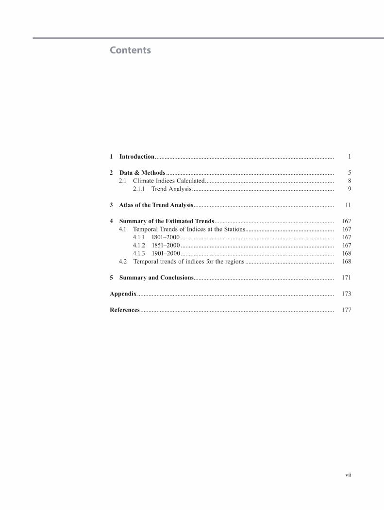
1 Introduction ............................................................................................................... 1
2 Data & Methods ........................................................................................................ 52.1 Climate Indices Calculated ................................................................................ 8
2.1.1 Trend Analysis ........................................................................................ 9
3 Atlas of the Trend Analysis ....................................................................................... 11
4 Summary of the Estimated Trends .......................................................................... 1674.1 Temporal Trends of Indices at the Stations ....................................................... 167
4.1.1 1801 –2000 ............................................................................................... 1674.1.2 1851 –2000 ............................................................................................... 1674.1.3 1901–2000 ............................................................................................... 168
4.2 Temporal trends of indices for the regions ....................................................... 168
5 Summary and Conclusions....................................................................................... 171
Appendix .......................................................................................................................... 173
References ........................................................................................................................ 177
1
Introduction
© Springer Science+Business Media Dordrecht 2015D. Chen et al., European Trend Atlas of Extreme Temperature and Precipitation Records, DOI 10.1007/978-94-017-9312-4_1
The impact of climate change on society is of fundamental importance for future planning and management. Statistics of extreme events is considered as a part of the climate, and their changes often have much higher impact on society than changes in the mean climate. As the mean climate changes, the characteristics of extremes may also change (e.g. Tren-berth 1999; Easterling et al. 2000; Beniston and Stephenson 2004). For many impact applications and decision support systems, extreme events are much more important than the mean climate (e.g. Mearns et al. 1984; WISE 1999). Changes in extremes may be due to changes in the mean (Wigley 1985), changes in the variance (Katz and Brown 1992), or a combination of both factors (e.g. Brown and Katz 1995; Beniston 2004).
Extreme climate events can be defined as events that occur with extraordinary low frequency during a certain period of time (rarity), events with high magnitude (intensity) or dura-tion, and events causing sizeable impacts such as direct dam-ages to assets, cultural heritage, ecosystem service and loss of human lives. According to The Intergovernmental Panel on Climate Change (IPCC) (IPCC 2001, p. 790), “An ex-treme weather event is an event that is rare within its statisti-cal reference distribution at a particular place. Definitions of ‘rare’ vary, but an extreme weather event would normally be as rare as or rarer than the 10th or 90th percentile. By defini-tion, the characteristics of what is called extreme weather may vary from place to place. An extreme climate event is an average of a number of weather events over a certain period of time, an average which itself is extreme (e.g. rainfall over a season).” This definition has also been used in the fourth IPCC report published in 2007 (IPCC 2007).
Indices have been developed to measure the degree of exceedance of specific thresholds (which define the rarity of such an event) for maxima/minima during specific time-periods (Jones et al. 1999). Examples are the number of very warm and very cold days for the time of year, the number of heavy rainfall days, and number of frost days (Frich et al. 2002). Some extremes are defined by natural thresholds, while the majority of extremes are determined by the dataʼs
own distribution. The majority of indices relate to counts of individual daily extremes, but a few are determined by spells of exceptionally warm/cold temperatures or wet/dry periods or the first/last occurrence of an event during a season (like spring/autumn frosts, beginning/end of the summer dry sea-son etc.). With respect to temperature and rainfall, spells of extreme weather generally have large societal and economic impacts. Examples of short-lived extremes that may cause extensive damage are windstorms, hailstorms and extensive and heavy snowfall.
Recently, there has been an international effort towards developing a suite of standardized indices so that research-ers around the world can calculate the indices in exactly the same manner. This is important for detecting and monitoring changes in the extreme climates and allows for comparison of observations and model simulations at the global scale. These analyses can then be combined into the regional and global perspectives (Karl and Easterling 1999; Peterson et al. 2001; Frich et al. 2002). However, the definition of several of the suggested indices is somewhat cumbersome and some of the indices still exist in various forms. Consequently, dif-ferent software may produce slightly different results. Sev-eral EU research projects either use the indices in the Euro-pean Climate Assessment (Klein-Tank et al. 2002a; Klein-Tank and Können 2003) or a program developed within the STARDEX project (STAtistical and Regional dynamical Downscaling of EXtremes for European regions; Haylock and Goodess (2004)). In this atlas we use the extremes in-dices software developed within EMULATE (European and North Atlantic daily to MULtidecadal climATE variability; Moberg et al. (2006)).
While some of the climatic extremes are well described by meteorological variables/indices, others may not be easily defined with data for a single meteorological variable only. This is true when the combined impact is involved (Pellikka and Järvenpää 2003). For example, freezing rain is a special combination of low temperature and rain that produces major damages through ice loading on wires and structures. Other examples are snow damage on forests (Solantie 1994) and
1
2 1 Introduction
the occurrence of landslides that are known to be caused by heavy rains (e.g. Schuster 1996). However, geological and geomorphologic settings may also play an important role here (Brunsden 1999). Yet another type of climate extreme is that some weather conditions, which may seem more or less normal from a purely anthropocentric perspective, nev-ertheless could induce a strong impact on some other spe-cies. Thus, such ecological climate extremes may not be easy to identify as climate extremes. The dependence on factors other than meteorological data makes it difficult to disentan-gle the specific contribution of weather/climate in producing the impacts and to describe the combination of extremes. A possible solution to this problem is interactions with affected and interested groups and individuals, such as the insurance industry and design engineers.
Damage reports from (re)insurance companies may also be useful. Nevertheless, since there is no long-term homo-geneous data yet in this regard, the use of this approach in climate change studies is not feasible at this point. Therefore, this atlas will not discuss these kinds of extremes. Rather, the focus will emphasize a set of indices well defined by meteorological data that are available for relatively long time periods, i.e. temperature and precipitation.
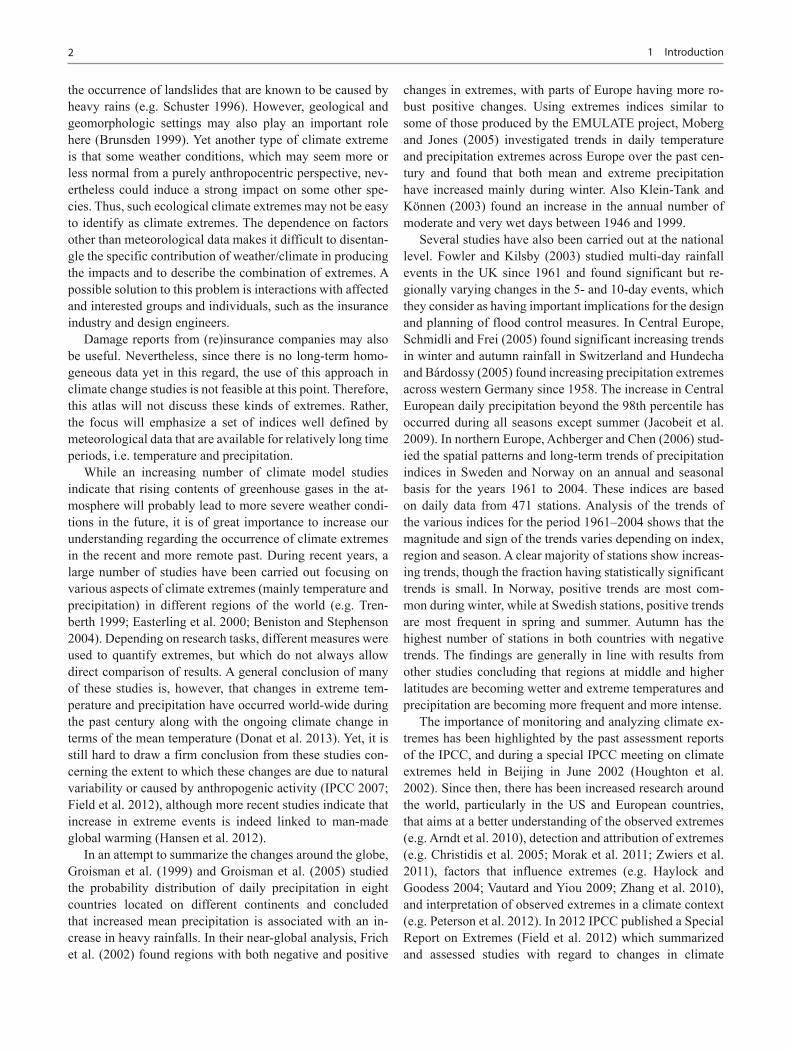
While an increasing number of climate model studies indicate that rising contents of greenhouse gases in the at-mosphere will probably lead to more severe weather condi-tions in the future, it is of great importance to increase our understanding regarding the occurrence of climate extremes in the recent and more remote past. During recent years, a large number of studies have been carried out focusing on various aspects of climate extremes (mainly temperature and precipitation) in different regions of the world (e.g. Tren-berth 1999; Easterling et al. 2000; Beniston and Stephenson 2004). Depending on research tasks, different measures were used to quantify extremes, but which do not always allow direct comparison of results. A general conclusion of many of these studies is, however, that changes in extreme tem-perature and precipitation have occurred world-wide during the past century along with the ongoing climate change in terms of the mean temperature (Donat et al. 2013). Yet, it is still hard to draw a firm conclusion from these studies con-cerning the extent to which these changes are due to natural variability or caused by anthropogenic activity (IPCC 2007; Field et al. 2012), although more recent studies indicate that increase in extreme events is indeed linked to man-made global warming (Hansen et al. 2012).
In an attempt to summarize the changes around the globe, Groisman et al. (1999) and Groisman et al. (2005) studied the probability distribution of daily precipitation in eight countries located on different continents and concluded that increased mean precipitation is associated with an in-crease in heavy rainfalls. In their near-global analysis, Frich et al. (2002) found regions with both negative and positive
changes in extremes, with parts of Europe having more ro-bust positive changes. Using extremes indices similar to some of those produced by the EMULATE project, Moberg and Jones (2005) investigated trends in daily temperature and precipitation extremes across Europe over the past cen-tury and found that both mean and extreme precipitation have increased mainly during winter. Also Klein-Tank and Können (2003) found an increase in the annual number of moderate and very wet days between 1946 and 1999.
Several studies have also been carried out at the national level. Fowler and Kilsby (2003) studied multi-day rainfall events in the UK since 1961 and found significant but re-gionally varying changes in the 5- and 10-day events, which they consider as having important implications for the design and planning of flood control measures. In Central Europe, Schmidli and Frei (2005) found significant increasing trends in winter and autumn rainfall in Switzerland and Hundecha and Bárdossy (2005) found increasing precipitation extremes across western Germany since 1958. The increase in Central European daily precipitation beyond the 98th percentile has occurred during all seasons except summer (Jacobeit et al. 2009). In northern Europe, Achberger and Chen (2006) stud-ied the spatial patterns and long-term trends of precipitation indices in Sweden and Norway on an annual and seasonal basis for the years 1961 to 2004. These indices are based on daily data from 471 stations. Analysis of the trends of the various indices for the period 1961–2004 shows that the magnitude and sign of the trends varies depending on index, region and season. A clear majority of stations show increas-ing trends, though the fraction having statistically significant trends is small. In Norway, positive trends are most com-mon during winter, while at Swedish stations, positive trends are most frequent in spring and summer. Autumn has the highest number of stations in both countries with negative trends. The findings are generally in line with results from other studies concluding that regions at middle and higher latitudes are becoming wetter and extreme temperatures and precipitation are becoming more frequent and more intense.
The importance of monitoring and analyzing climate ex-tremes has been highlighted by the past assessment reports of the IPCC, and during a special IPCC meeting on climate extremes held in Beijing in June 2002 (Houghton et al. 2002). Since then, there has been increased research around the world, particularly in the US and European countries, that aims at a better understanding of the observed extremes (e.g. Arndt et al. 2010), detection and attribution of extremes (e.g. Christidis et al. 2005; Morak et al. 2011; Zwiers et al. 2011), factors that influence extremes (e.g. Haylock and Goodess 2004; Vautard and Yiou 2009; Zhang et al. 2010), and interpretation of observed extremes in a climate context (e.g. Peterson et al. 2012). In 2012 IPCC published a Special Report on Extremes (Field et al. 2012) which summarized and assessed studies with regard to changes in climate
3Introduction
Extremes and their Impacts on the natural physical environ-ment and human systems and ecosystems, as well as manag-ing the risks from climate extremes at the Local Level round the world.
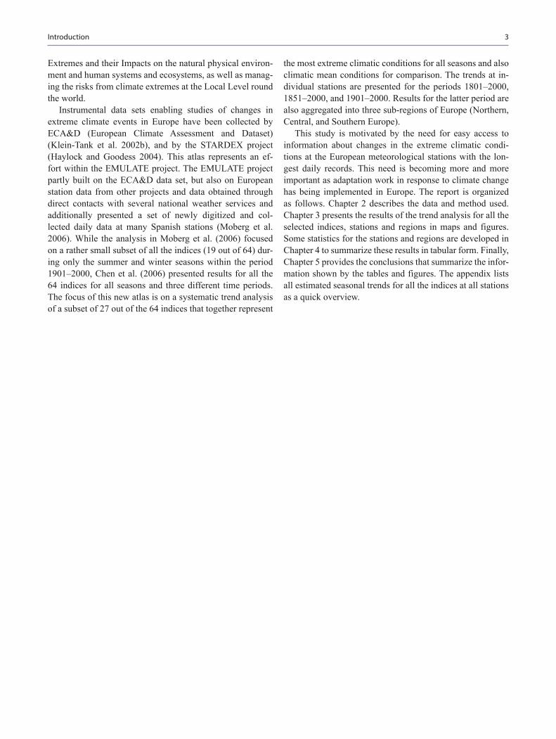
Instrumental data sets enabling studies of changes in extreme climate events in Europe have been collected by ECA&D (European Climate Assessment and Dataset) (Klein-Tank et al. 2002b), and by the STARDEX project (Haylock and Goodess 2004). This atlas represents an ef-fort within the EMULATE project. The EMULATE project partly built on the ECA&D data set, but also on European station data from other projects and data obtained through direct contacts with several national weather services and additionally presented a set of newly digitized and col-lected daily data at many Spanish stations (Moberg et al. 2006). While the analysis in Moberg et al. (2006) focused on a rather small subset of all the indices (19 out of 64) dur-ing only the summer and winter seasons within the period 1901–2000, Chen et al. (2006) presented results for all the 64 indices for all seasons and three different time periods. The focus of this new atlas is on a systematic trend analysis of a subset of 27 out of the 64 indices that together represent
the most extreme climatic conditions for all seasons and also climatic mean conditions for comparison. The trends at in-dividual stations are presented for the periods 1801–2000, 1851–2000, and 1901–2000. Results for the latter period are also aggregated into three sub-regions of Europe (Northern, Central, and Southern Europe).
This study is motivated by the need for easy access to information about changes in the extreme climatic condi-tions at the European meteorological stations with the lon-gest daily records. This need is becoming more and more important as adaptation work in response to climate change has being implemented in Europe. The report is organized as follows. Chapter 2 describes the data and method used. Chapter 3 presents the results of the trend analysis for all the selected indices, stations and regions in maps and figures. Some statistics for the stations and regions are developed in Chapter 4 to summarize these results in tabular form. Finally, Chapter 5 provides the conclusions that summarize the infor-mation shown by the tables and figures. The appendix lists all estimated seasonal trends for all the indices at all stations as a quick overview.
5
Data & Methods
© Springer Science+Business Media Dordrecht 2015D. Chen et al., European Trend Atlas of Extreme Temperature and Precipitation Records, DOI 10.1007/978-94-017-9312-4_2,
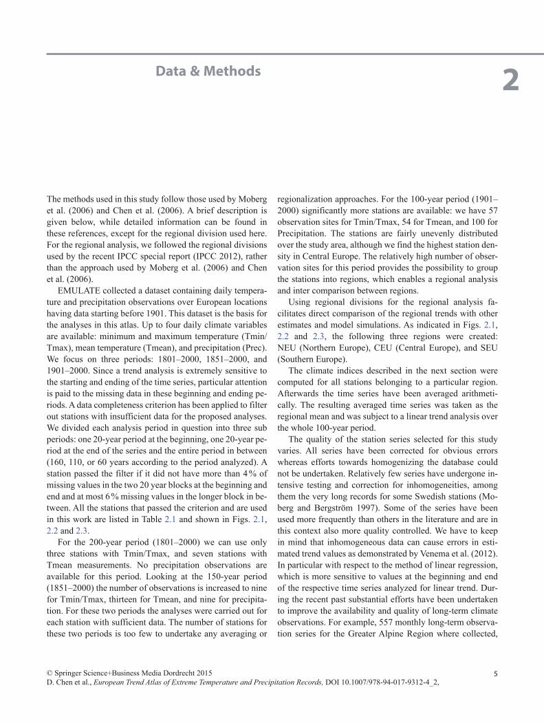
The methods used in this study follow those used by Moberg et al. (2006) and Chen et al. (2006). A brief description is given below, while detailed information can be found in these references, except for the regional division used here. For the regional analysis, we followed the regional divisions used by the recent IPCC special report (IPCC 2012), rather than the approach used by Moberg et al. (2006) and Chen et al. (2006).
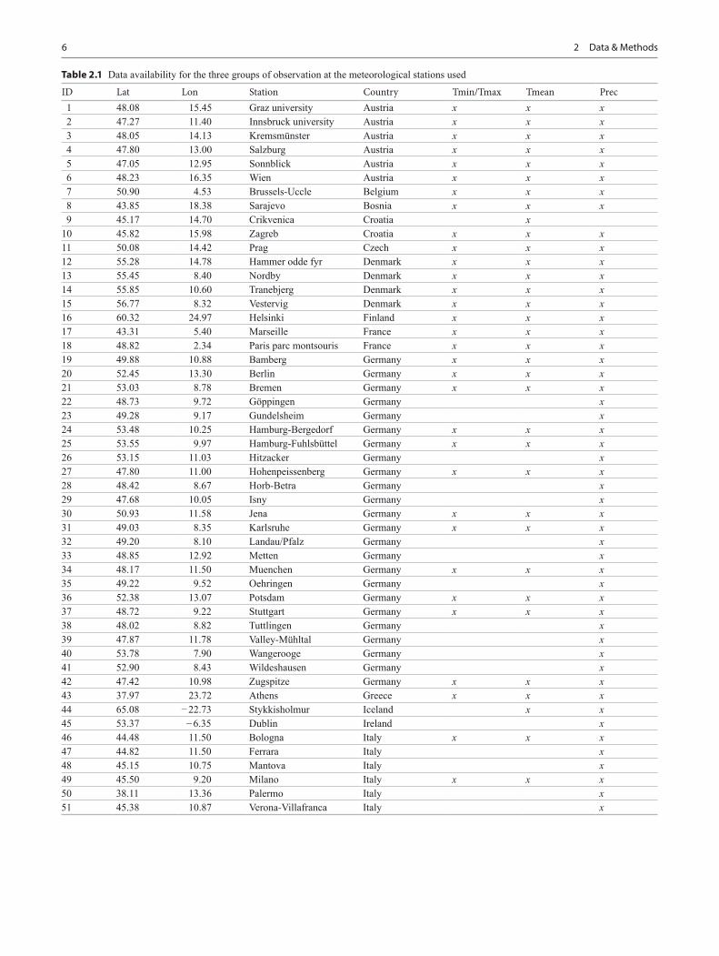
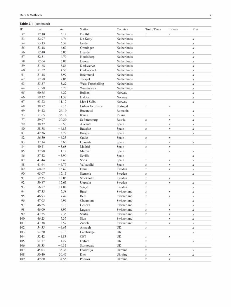
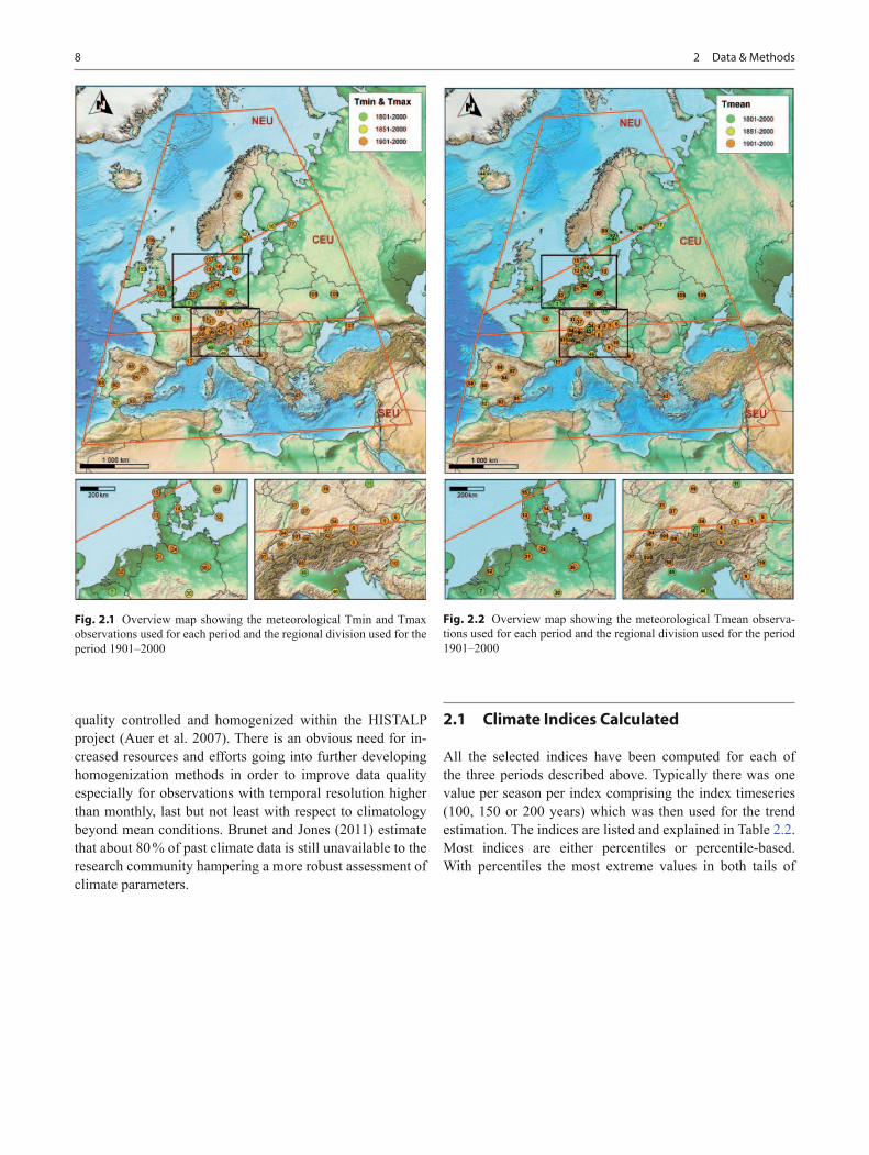
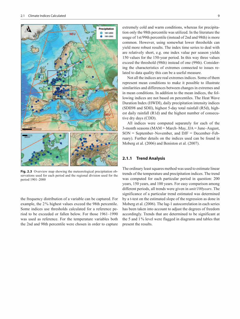
EMULATE collected a dataset containing daily tempera-ture and precipitation observations over European locations having data starting before 1901. This dataset is the basis for the analyses in this atlas. Up to four daily climate variables are available: minimum and maximum temperature (Tmin/Tmax), mean temperature (Tmean), and precipitation (Prec). We focus on three periods: 1801–2000, 1851–2000, and 1901–2000. Since a trend analysis is extremely sensitive to the starting and ending of the time series, particular attention is paid to the missing data in these beginning and ending pe-riods. A data completeness criterion has been applied to filter out stations with insufficient data for the proposed analyses. We divided each analysis period in question into three sub periods: one 20-year period at the beginning, one 20-year pe-riod at the end of the series and the entire period in between (160, 110, or 60 years according to the period analyzed). A station passed the filter if it did not have more than 4 % of missing values in the two 20 year blocks at the beginning and end and at most 6 % missing values in the longer block in be-tween. All the stations that passed the criterion and are used in this work are listed in Table 2.1 and shown in Figs. 2.1, 2.2 and 2.3.
For the 200-year period (1801–2000) we can use only three stations with Tmin/Tmax, and seven stations with Tmean measurements. No precipitation observations are available for this period. Looking at the 150-year period (1851–2000) the number of observations is increased to nine for Tmin/Tmax, thirteen for Tmean, and nine for precipita-tion. For these two periods the analyses were carried out for each station with sufficient data. The number of stations for these two periods is too few to undertake any averaging or
regionalization approaches. For the 100-year period (1901–2000) significantly more stations are available: we have 57 observation sites for Tmin/Tmax, 54 for Tmean, and 100 for Precipitation. The stations are fairly unevenly distributed over the study area, although we find the highest station den-sity in Central Europe. The relatively high number of obser-vation sites for this period provides the possibility to group the stations into regions, which enables a regional analysis and inter comparison between regions.
Using regional divisions for the regional analysis fa-cilitates direct comparison of the regional trends with other estimates and model simulations. As indicated in Figs. 2.1, 2.2 and 2.3, the following three regions were created: NEU (Northern Europe), CEU (Central Europe), and SEU ( Southern Europe).
The climate indices described in the next section were computed for all stations belonging to a particular region. Afterwards the time series have been averaged arithmeti-cally. The resulting averaged time series was taken as the regional mean and was subject to a linear trend analysis over the whole 100-year period.
The quality of the station series selected for this study varies. All series have been corrected for obvious errors whereas efforts towards homogenizing the database could not be undertaken. Relatively few series have undergone in-tensive testing and correction for inhomogeneities, among them the very long records for some Swedish stations (Mo-berg and Bergström 1997). Some of the series have been used more frequently than others in the literature and are in this context also more quality controlled. We have to keep in mind that inhomogeneous data can cause errors in esti-mated trend values as demonstrated by Venema et al. (2012). In particular with respect to the method of linear regression, which is more sensitive to values at the beginning and end of the respective time series analyzed for linear trend. Dur-ing the recent past substantial efforts have been undertaken to improve the availability and quality of long-term climate observations. For example, 557 monthly long-term observa-tion series for the Greater Alpine Region where collected,
2
6 2 Data & Methods
ID Lat Lon Station Country Tmin/Tmax Tmean Prec1 48.08 15.45 Graz university Austria x x x2 47.27 11.40 Innsbruck university Austria x x x3 48.05 14.13 Kremsmünster Austria x x x4 47.80 13.00 Salzburg Austria x x x5 47.05 12.95 Sonnblick Austria x x x6 48.23 16.35 Wien Austria x x x7 50.90 4.53 Brussels-Uccle Belgium x x x8 43.85 18.38 Sarajevo Bosnia x x x9 45.17 14.70 Crikvenica Croatia x
10 45.82 15.98 Zagreb Croatia x x x11 50.08 14.42 Prag Czech x x x12 55.28 14.78 Hammer odde fyr Denmark x x x13 55.45 8.40 Nordby Denmark x x x14 55.85 10.60 Tranebjerg Denmark x x x15 56.77 8.32 Vestervig Denmark x x x16 60.32 24.97 Helsinki Finland x x x17 43.31 5.40 Marseille France x x x18 48.82 2.34 Paris parc montsouris France x x x19 49.88 10.88 Bamberg Germany x x x20 52.45 13.30 Berlin Germany x x x21 53.03 8.78 Bremen Germany x x x22 48.73 9.72 Göppingen Germany x23 49.28 9.17 Gundelsheim Germany x24 53.48 10.25 Hamburg-Bergedorf Germany x x x25 53.55 9.97 Hamburg-Fuhlsbüttel Germany x x x26 53.15 11.03 Hitzacker Germany x27 47.80 11.00 Hohenpeissenberg Germany x x x28 48.42 8.67 Horb-Betra Germany x29 47.68 10.05 Isny Germany x30 50.93 11.58 Jena Germany x x x31 49.03 8.35 Karlsruhe Germany x x x32 49.20 8.10 Landau/Pfalz Germany x33 48.85 12.92 Metten Germany x34 48.17 11.50 Muenchen Germany x x x35 49.22 9.52 Oehringen Germany x36 52.38 13.07 Potsdam Germany x x x37 48.72 9.22 Stuttgart Germany x x x38 48.02 8.82 Tuttlingen Germany x39 47.87 11.78 Valley-Mühltal Germany x40 53.78 7.90 Wangerooge Germany x41 52.90 8.43 Wildeshausen Germany x42 47.42 10.98 Zugspitze Germany x x x43 37.97 23.72 Athens Greece x x x44 65.08 − 22.73 Stykkisholmur Iceland x x45 53.37 − 6.35 Dublin Ireland x46 44.48 11.50 Bologna Italy x x x47 44.82 11.50 Ferrara Italy x48 45.15 10.75 Mantova Italy x49 45.50 9.20 Milano Italy x x x50 38.11 13.36 Palermo Italy x51 45.38 10.87 Verona-Villafranca Italy x
Table 2.1 Data availability for the three groups of observation at the meteorological stations used
7Data & Methods
ID Lat Lon Station Country Tmin/Tmax Tmean Prec52 52.10 5.18 De Bilt Netherlands x x53 52.97 4.76 De Kooy Netherlands x54 53.13 6.58 Eelde Netherlands x55 53.18 6.60 Groningen Netherlands x56 52.40 6.05 Heerde Netherlands x57 52.31 4.70 Hoofddorp Netherlands x58 52.64 5.07 Hoorn Netherlands x59 51.68 3.86 Kerkwerve Netherlands x60 51.57 4.53 Oudenbosch Netherlands x61 51.18 5.97 Roermond Netherlands x62 52.88 7.06 Terapel Netherlands x63 53.37 5.22 West-Terschelling Netherlands x64 51.98 6.70 Winterswijk Netherlands x65 60.65 6.22 Bulken Norway x66 59.12 11.38 Halden Norway x67 63.22 11.12 Lien I Selbu Norway x68 38.72 − 9.15 Lisboa Geofísica Portugal x x69 44.42 26.10 Bucuresti Romania x73 51.65 36.18 Kursk Russia x x77 59.97 30.30 St Petersburg Russia x x x79 38.37 − 0.50 Alicante Spain x x x80 38.88 − 6.83 Badajoz Spain x x x81 42.36 − 3.72 Burgos Spain x82 36.50 − 6.23 Cadiz Spain x x83 37.14 − 3.63 Granada Spain x x x84 40.41 − 3.68 Madrid Spain x x85 37.98 − 1.12 Murcia Spain x x x86 37.42 − 5.90 Sevilla Spain x87 41.44 − 2.48 Soria Spain x x x88 41.64 − 4.77 Valladolid Spain x x x89 60.62 15.67 Falun Sweden x x x90 65.07 17.15 Stensele Sweden x x91 59.35 18.05 Stockholm Sweden x x92 59.87 17.63 Uppsala Sweden x x x93 56.87 14.80 Växjö Sweden x x94 47.55 7.58 Basel Switzerland x x x95 46.93 7.42 Bern Switzerland x x x96 47.05 6.99 Chaumont Switzerland x97 46.25 6.13 Geneva Switzerland x x x98 46.00 8.97 Lugano Switzerland x x x99 47.25 9.35 Säntis Switzerland x x x
100 46.23 7.37 Sion Switzerland x x101 47.38 8.57 Zurich Switzerland x x x102 54.35 − 6.65 Armagh UK x x103 52.20 0.13 Cambridge UK x104 52.42 − 1.83 CET UK x x105 51.77 − 1.27 Oxford UK x x106 58.33 − 6.32 Stornoway UK x107 45.03 35.38 Feodosija Ukraine x x108 50.40 30.45 Kiev Ukraine x x x109 49.60 34.55 Poltava Ukraine x x
Table 2.1 (continued)
8 2 Data & Methods
quality controlled and homogenized within the HISTALP project (Auer et al. 2007). There is an obvious need for in-creased resources and efforts going into further developing homogenization methods in order to improve data quality especially for observations with temporal resolution higher than monthly, last but not least with respect to climatology beyond mean conditions. Brunet and Jones (2011) estimate that about 80 % of past climate data is still unavailable to the research community hampering a more robust assessment of climate parameters.
2.1 Climate Indices Calculated
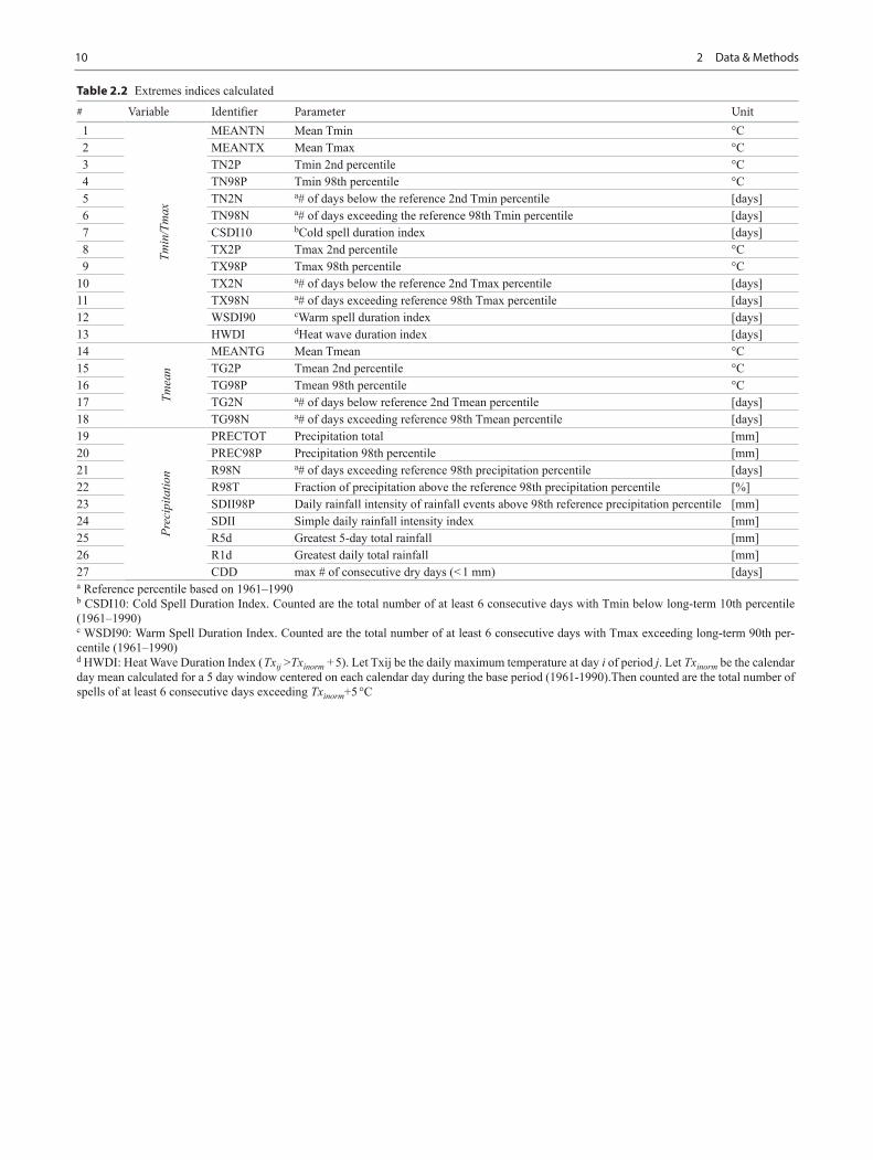
All the selected indices have been computed for each of the three periods described above. Typically there was one value per season per index comprising the index timeseries (100, 150 or 200 years) which was then used for the trend estimation. The indices are listed and explained in Table 2.2. Most indices are either percentiles or percentile-based. With percentiles the most extreme values in both tails of
Fig. 2.1 Overview map showing the meteorological Tmin and Tmax observations used for each period and the regional division used for the period 1901–2000
Fig. 2.2 Overview map showing the meteorological Tmean observa-tions used for each period and the regional division used for the period 1901–2000
92.1 Climate Indices Calculated
the frequency distribution of a variable can be captured. For example, the 2 % highest values exceed the 98th percentile. Some indices use thresholds calculated for a reference pe-riod to be exceeded or fallen below. For those 1961–1990 was used as reference. For the temperature variables both the 2nd and 98th percentile were chosen in order to capture
extremely cold and warm conditions, whereas for precipita-tion only the 98th percentile was utilized. In the literature the usage of 1st/99th percentile (instead of 2nd and 98th) is more common. However, using somewhat lower thresholds can yield more robust results. The index time series to deal with are relatively short, e.g. one index value per season yields 150 values for the 150-year period. In this way three values exceed the threshold (98th) instead of one (99th). Consider-ing the characteristics of extremes connected to issues re-lated to data quality this can be a useful measure.
Not all the indices are real extremes indices. Some of them represent mean conditions to make it possible to illustrate similarities and differences between changes in extremes and in mean conditions. In addition to the mean indices, the fol-lowing indices are not based on percentiles. The Heat Wave Duration Index (HWDI), daily precipitation intensity indices (SDII98 and SDII), highest 5-day total rainfall (R5d), high-est daily rainfall (R1d) and the highest number of consecu-tive dry days (CDD).
All indices were computed separately for each of the 3-month seasons (MAM = March–May, JJA = June–August, SON = September–November, and DJF = December–Feb-ruary). Further details on the indices used can be found in Moberg et al. (2006) and Beniston et al. (2007).
2.1.1 Trend Analysis
The ordinary least squares method was used to estimate linear trends of the temperature and precipitation indices. The trend was computed for each particular period in question: 200 years, 150 years, and 100 years. For easy comparison among different periods, all trends were given in unit/100years. The significance of a particular trend estimated was determined by a t-test on the estimated slope of the regression as done in Moberg et al. (2006). The lag-1 autocorrelation in each series has been taken into account to adjust the degrees of freedom accordingly. Trends that are determined to be significant at the 5 and 1 % level were flagged in diagrams and tables that present the results.
Fig. 2.3 Overview map showing the meteorological precipitation ob-servations used for each period and the regional division used for the period 1901–2000
10 2 Data & Methods
Table 2.2 Extremes indices calculated
# Variable Identifier Parameter Unit1
Tmin
/Tm
ax
MEANTN Mean Tmin °C2 MEANTX Mean Tmax °C3 TN2P Tmin 2nd percentile °C4 TN98P Tmin 98th percentile °C5 TN2N a# of days below the reference 2nd Tmin percentile [days]6 TN98N a# of days exceeding the reference 98th Tmin percentile [days]7 CSDI10 bCold spell duration index [days]8 TX2P Tmax 2nd percentile °C9 TX98P Tmax 98th percentile °C
10 TX2N a# of days below the reference 2nd Tmax percentile [days]11 TX98N a# of days exceeding reference 98th Tmax percentile [days]12 WSDI90 cWarm spell duration index [days]13 HWDI dHeat wave duration index [days]14
Tmea
n
MEANTG Mean Tmean °C15 TG2P Tmean 2nd percentile °C16 TG98P Tmean 98th percentile °C17 TG2N a# of days below reference 2nd Tmean percentile [days]18 TG98N a# of days exceeding reference 98th Tmean percentile [days]19
Prec
ipita
tion
PRECTOT Precipitation total [mm]20 PREC98P Precipitation 98th percentile [mm]21 R98N a# of days exceeding reference 98th precipitation percentile [days]22 R98T Fraction of precipitation above the reference 98th precipitation percentile [%]23 SDII98P Daily rainfall intensity of rainfall events above 98th reference precipitation percentile [mm]24 SDII Simple daily rainfall intensity index [mm]25 R5d Greatest 5-day total rainfall [mm]26 R1d Greatest daily total rainfall [mm]27 CDD max # of consecutive dry days (< 1 mm) [days]a Reference percentile based on 1961–1990b CSDI10: Cold Spell Duration Index. Counted are the total number of at least 6 consecutive days with Tmin below long-term 10th percentile (1961–1990)c WSDI90: Warm Spell Duration Index. Counted are the total number of at least 6 consecutive days with Tmax exceeding long-term 90th per-centile (1961–1990)d HWDI: Heat Wave Duration Index ( Txij >Txinorm + 5). Let Txij be the daily maximum temperature at day i of period j. Let Txinorm be the calendar day mean calculated for a 5 day window centered on each calendar day during the base period (1961-1990).Then counted are the total number of spells of at least 6 consecutive days exceeding Txinorm+5 °C
11
3Atlas of the Trend Analysis
© Springer Science+Business Media Dordrecht 2015D. Chen et al., European Trend Atlas of Extreme Temperature and Precipitation Records, DOI 10.1007/978-94-017-9312-4_3
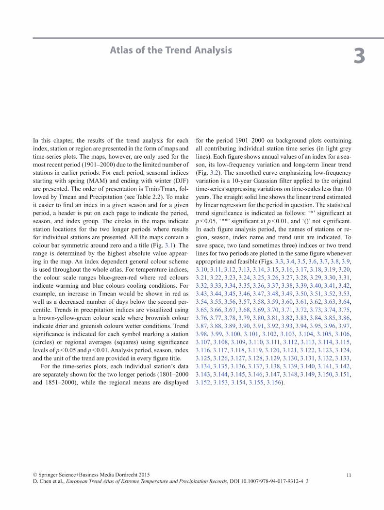
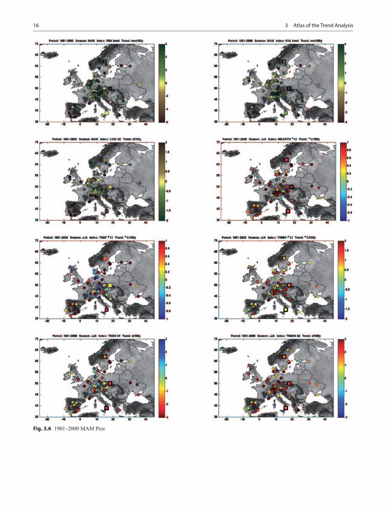
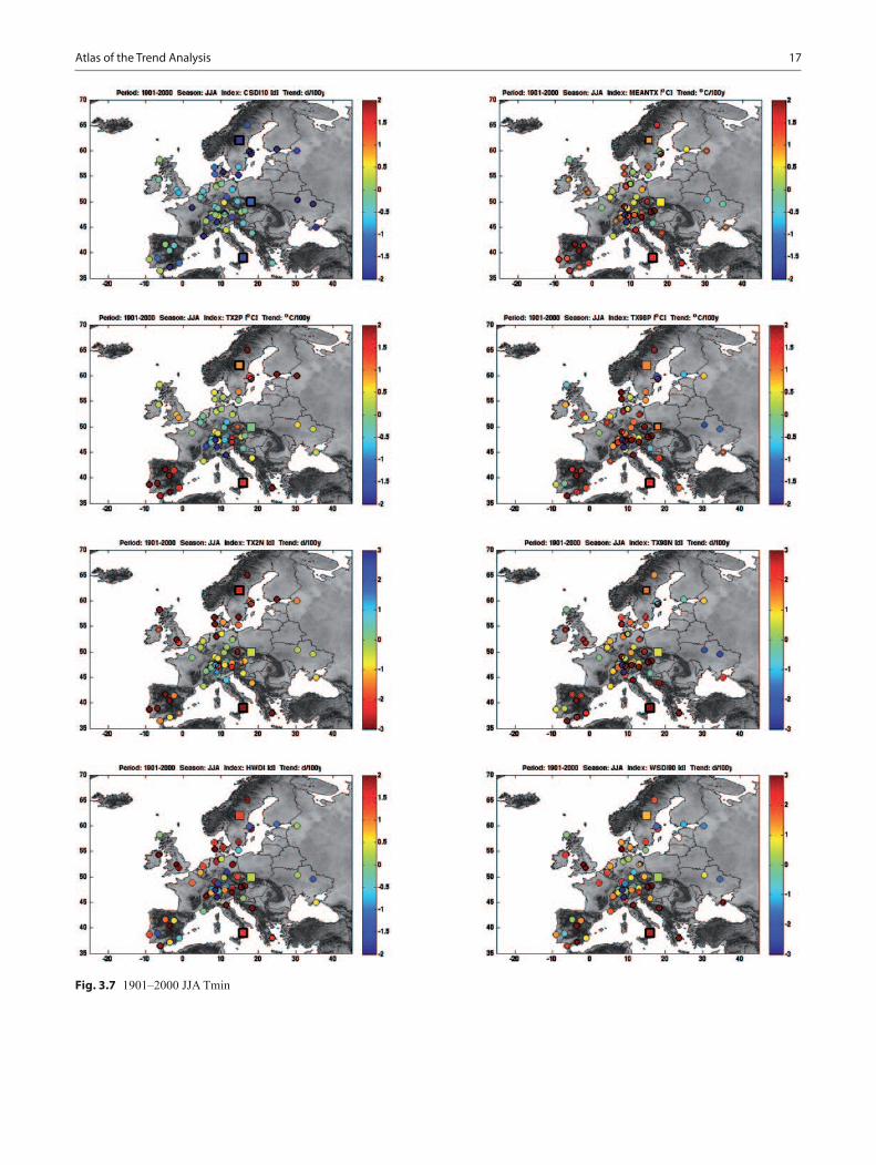
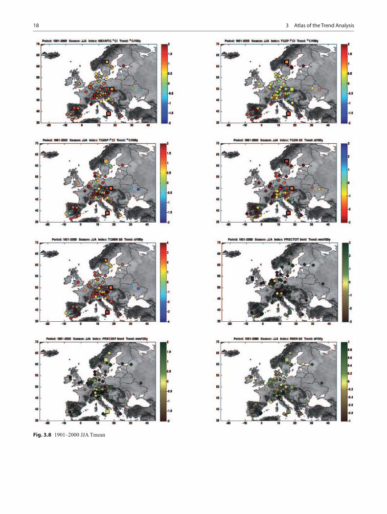
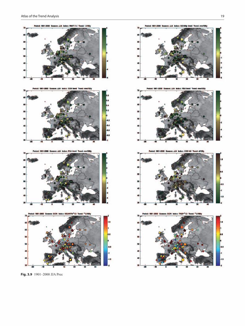
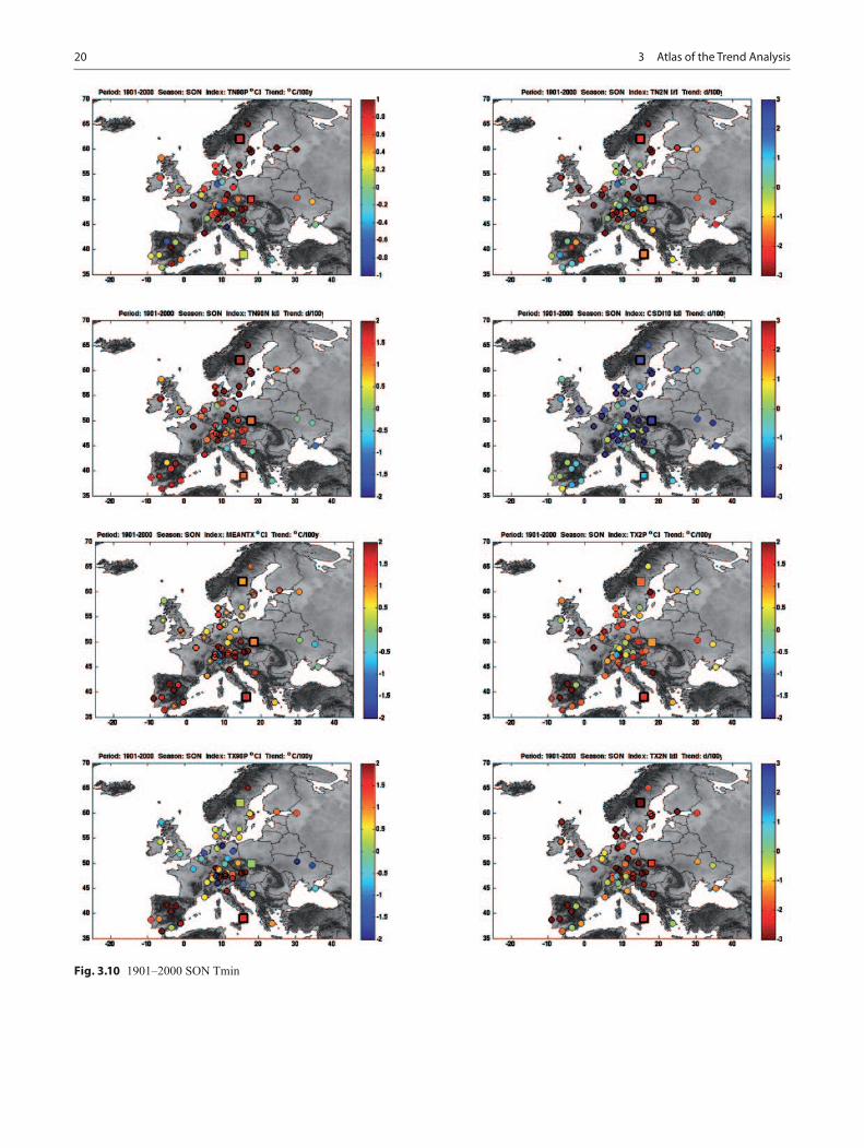
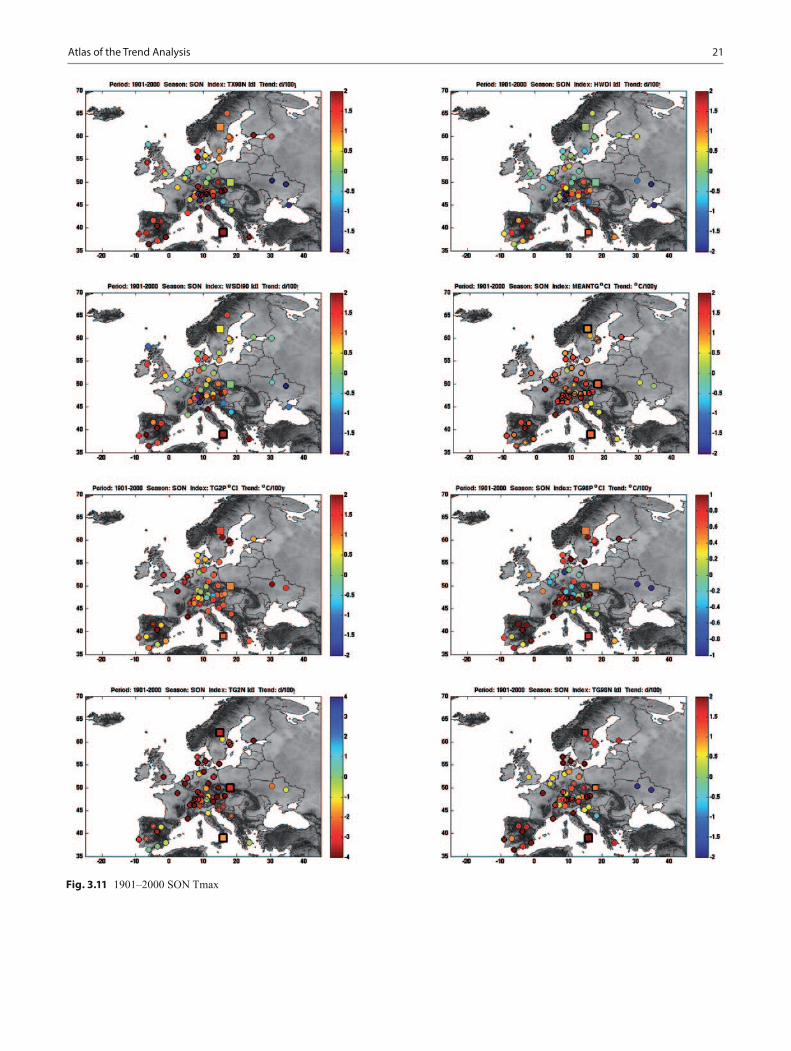
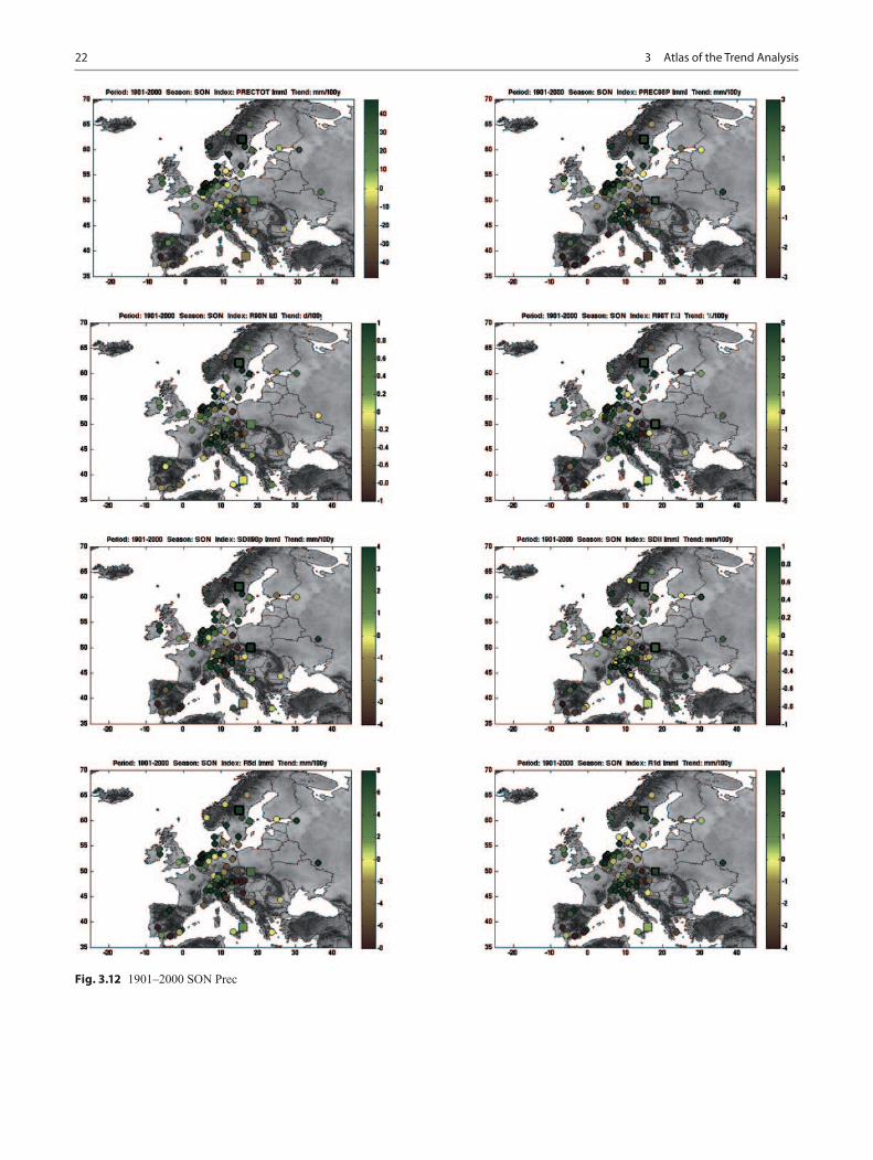
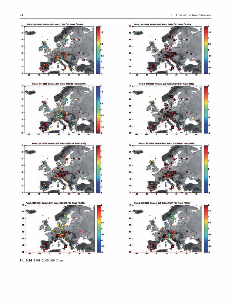
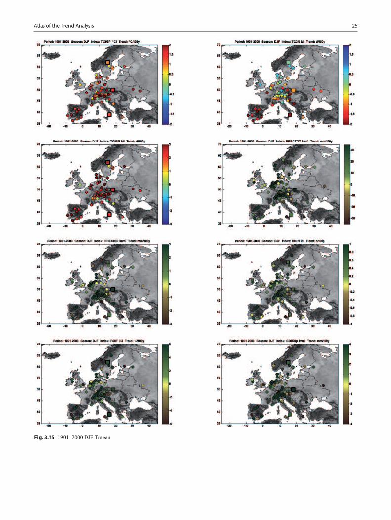
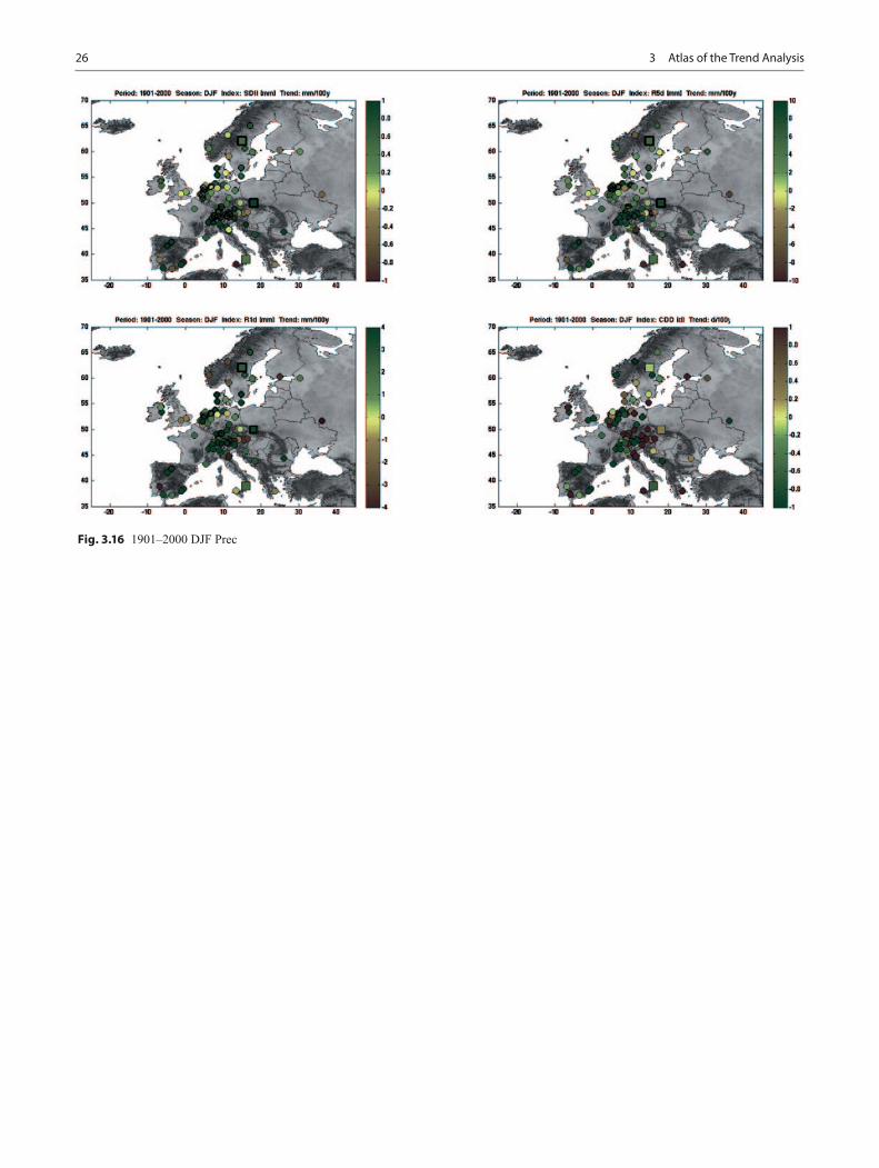
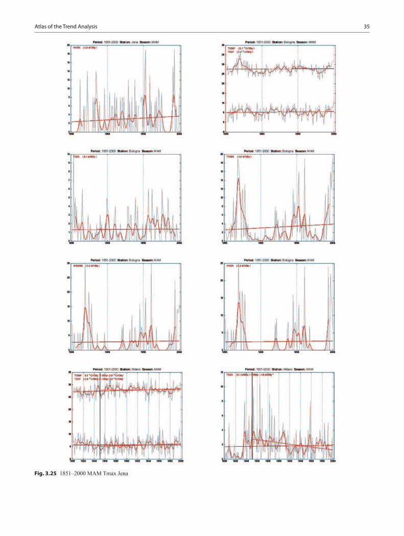
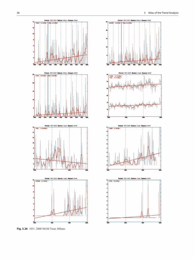
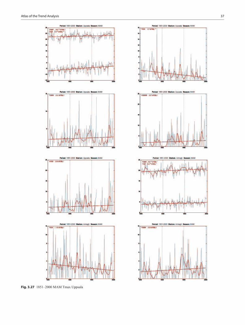
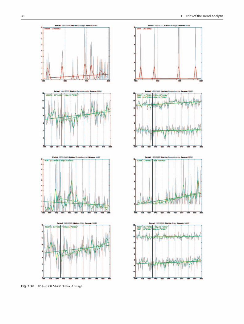
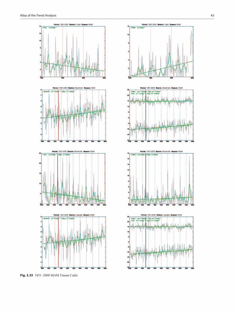
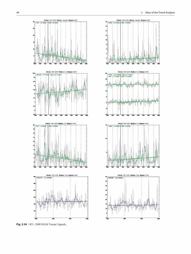
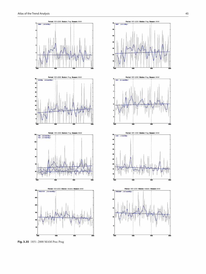
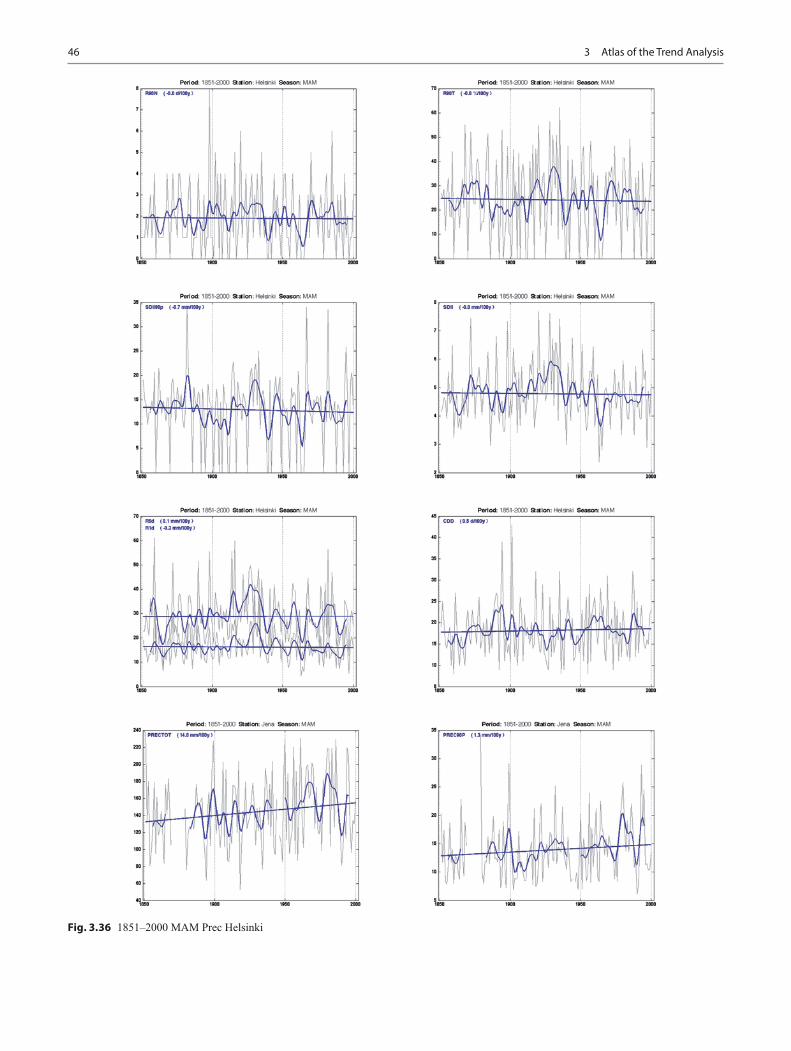
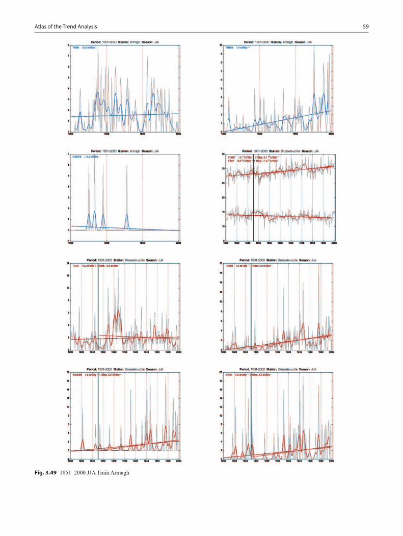
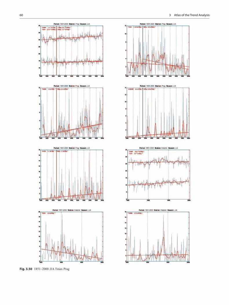
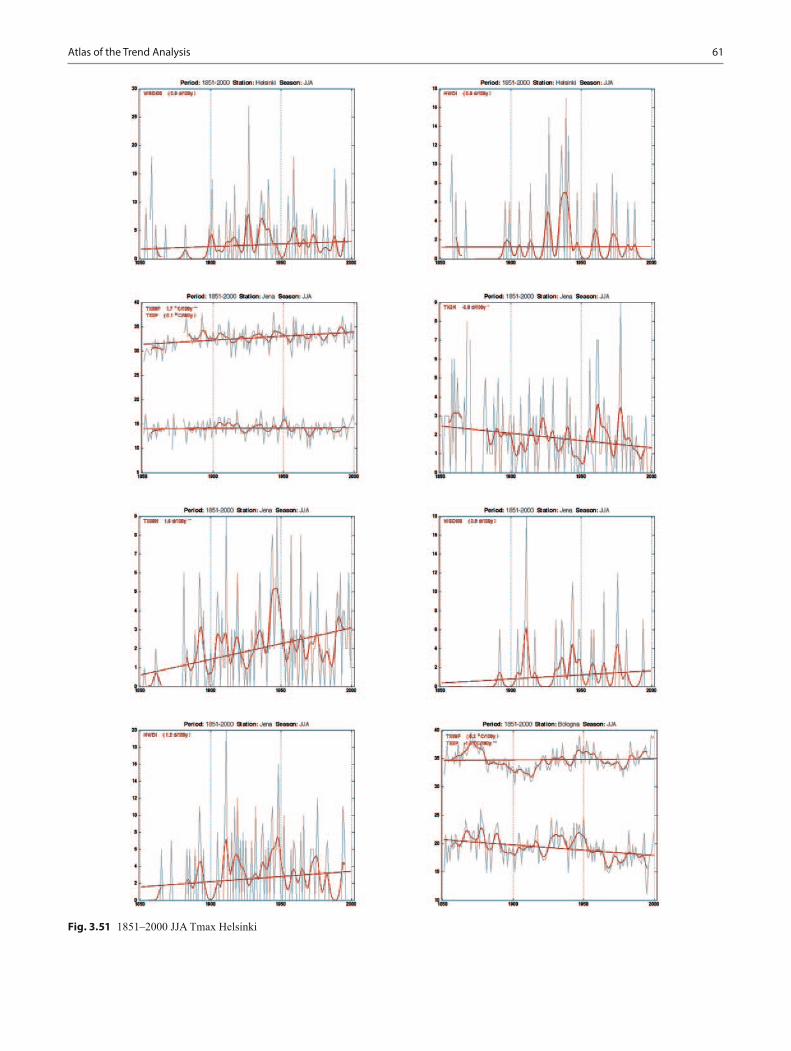
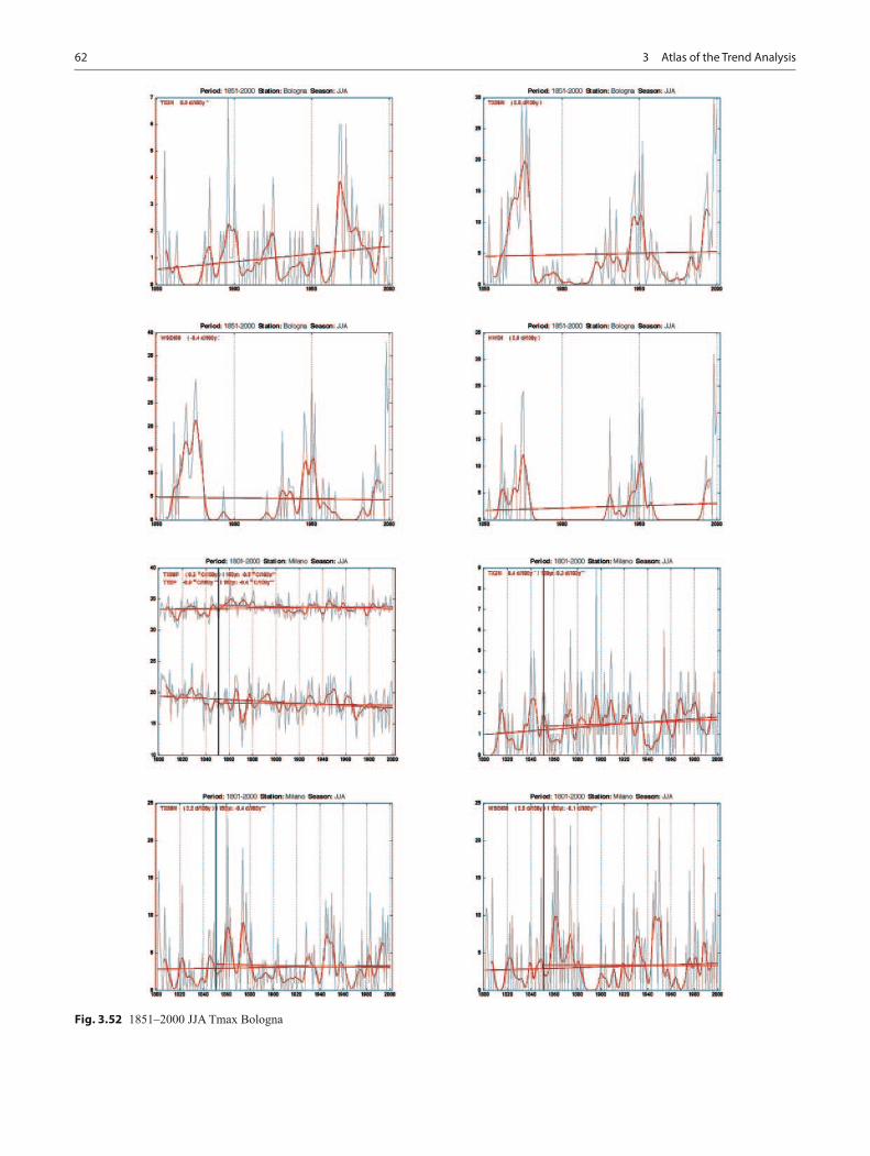
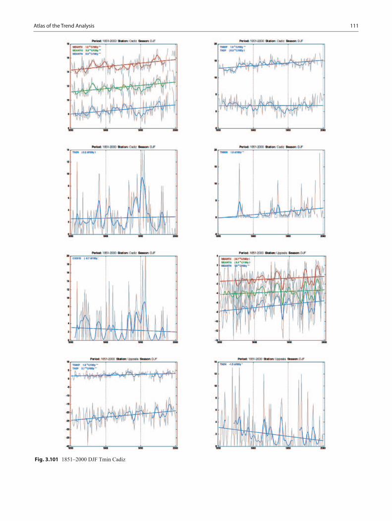
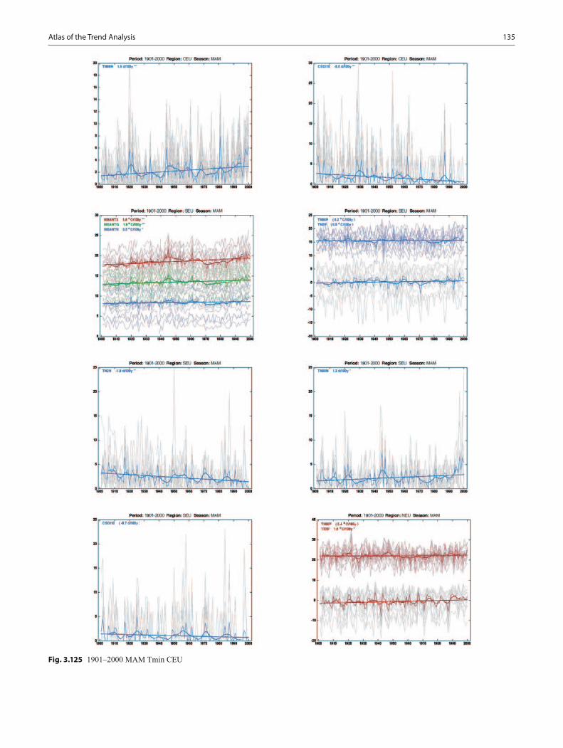
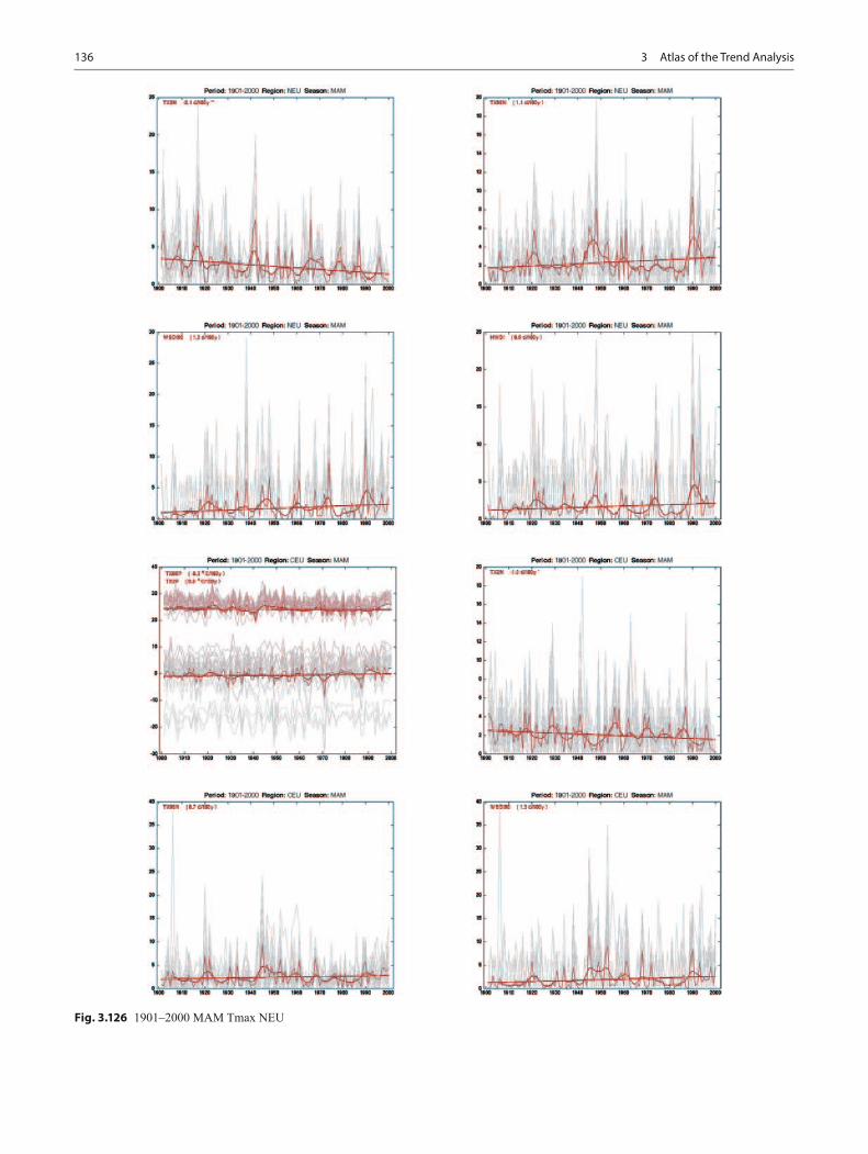
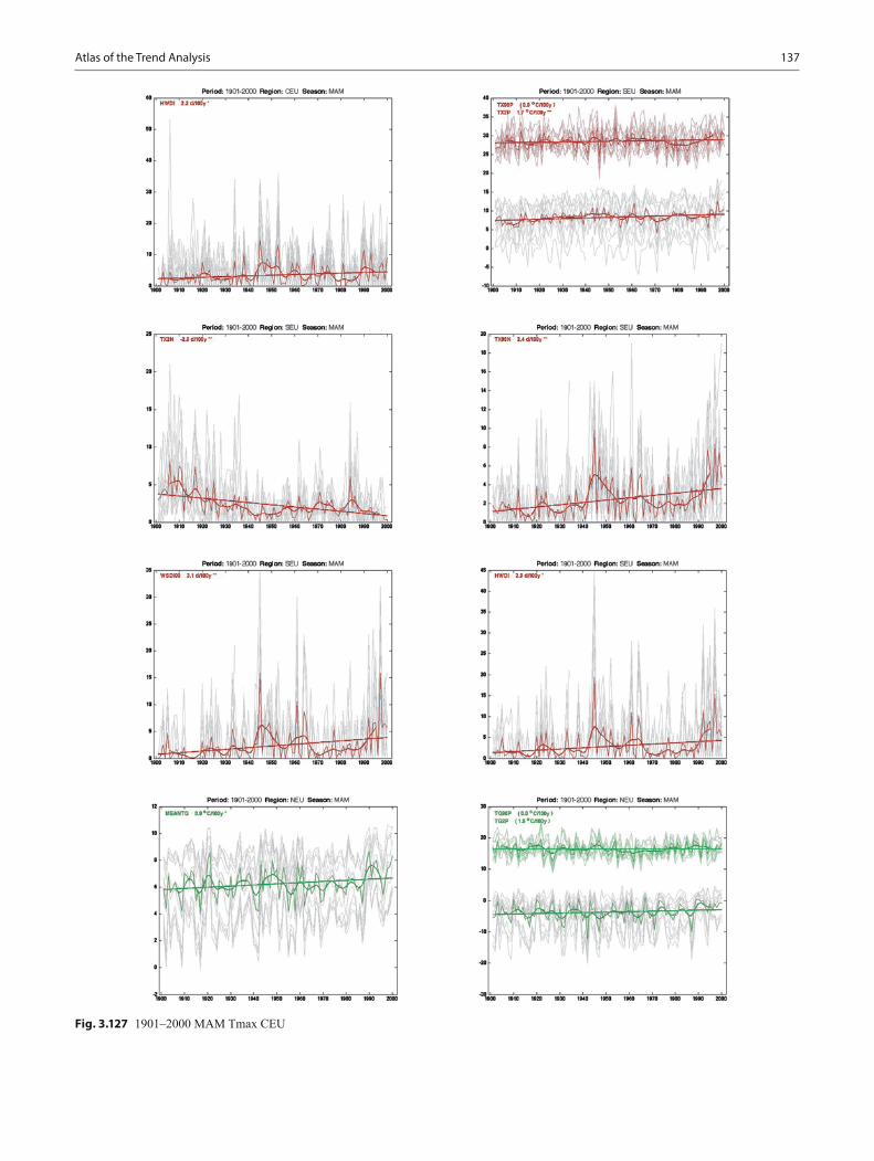
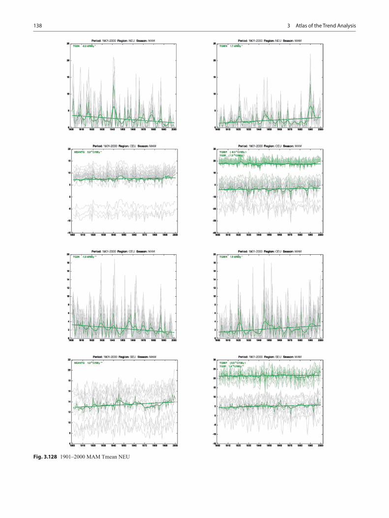
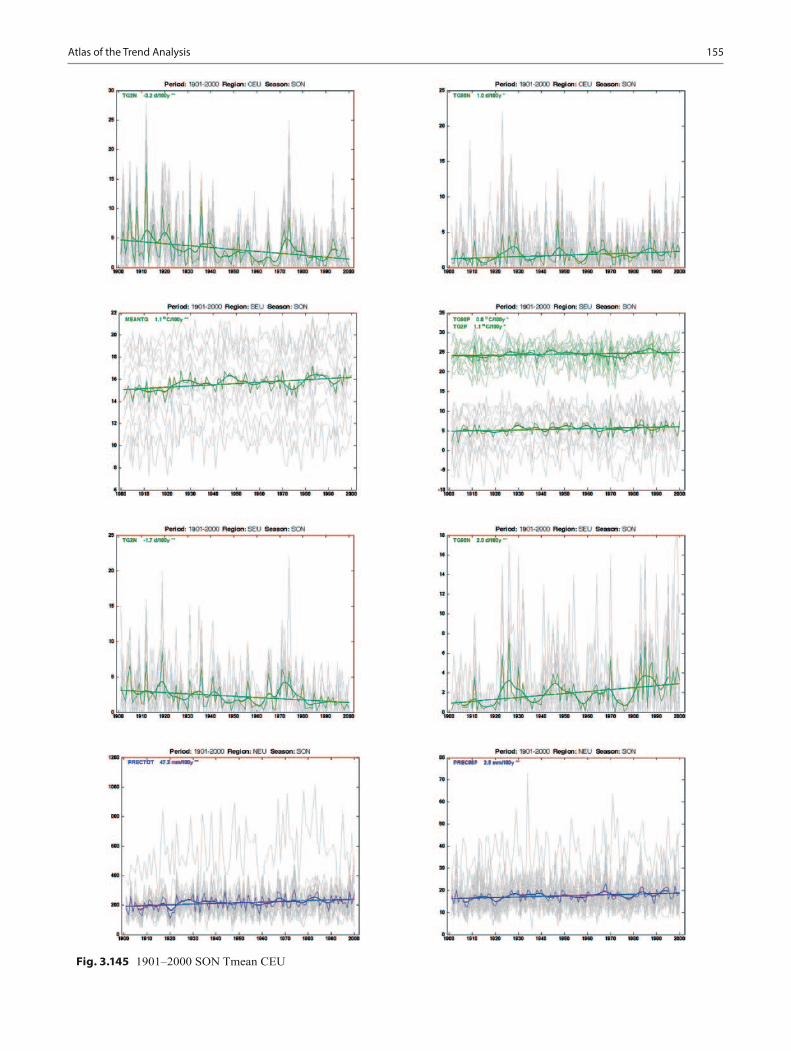
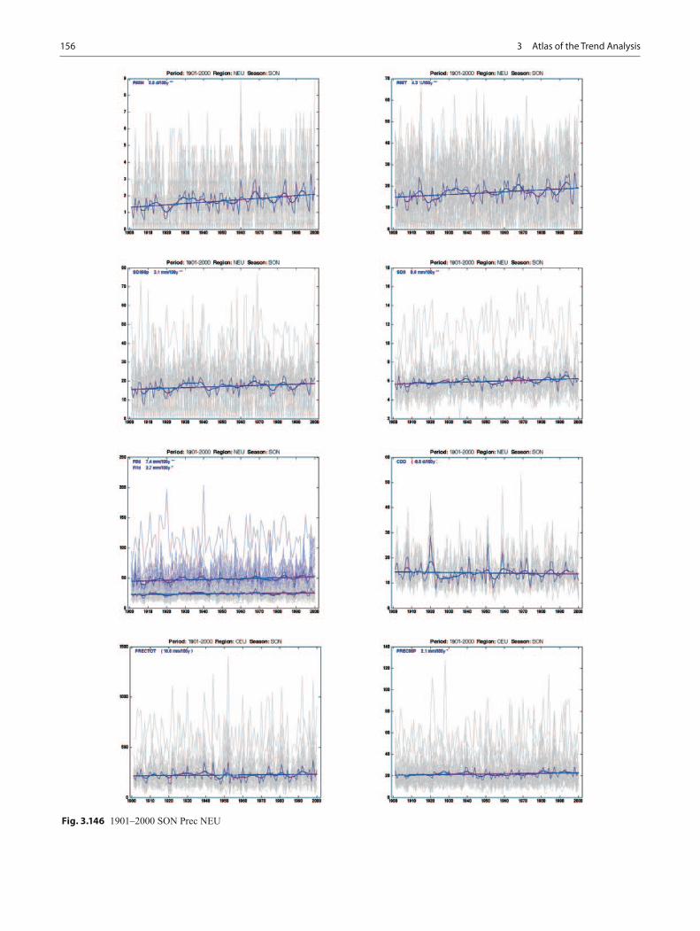
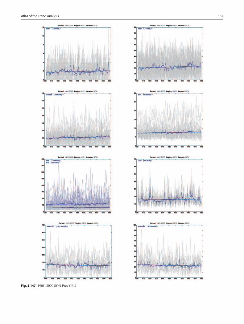
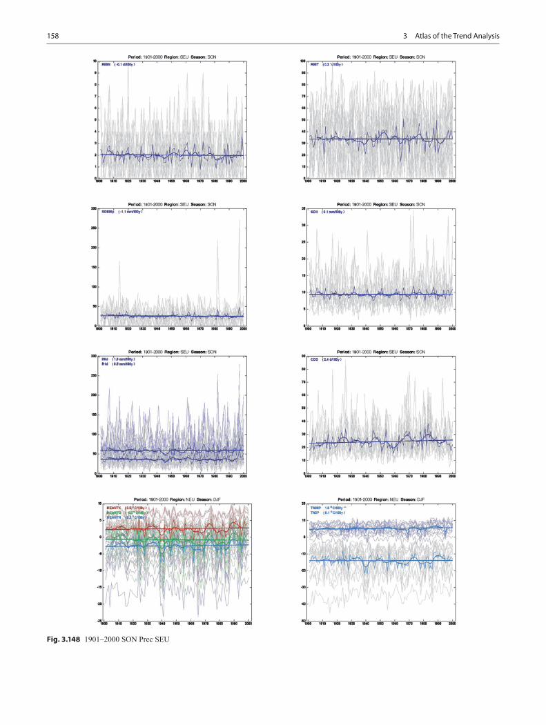
In this chapter, the results of the trend analysis for each index, station or region are presented in the form of maps and time-series plots. The maps, however, are only used for the most recent period (1901–2000) due to the limited number of stations in earlier periods. For each period, seasonal indices starting with spring (MAM) and ending with winter (DJF) are presented. The order of presentation is Tmin/Tmax, fol-lowed by Tmean and Precipitation (see Table 2.2). To make it easier to find an index in a given season and for a given period, a header is put on each page to indicate the period, season, and index group. The circles in the maps indicate station locations for the two longer periods where results for individual stations are presented. All the maps contain a colour bar symmetric around zero and a title (Fig. 3.1). The range is determined by the highest absolute value appear-ing in the map. An index dependent general colour scheme is used throughout the whole atlas. For temperature indices, the colour scale ranges blue-green-red where red colours indicate warming and blue colours cooling conditions. For example, an increase in Tmean would be shown in red as well as a decreased number of days below the second per-centile. Trends in precipitation indices are visualized using a brown-yellow-green colour scale where brownish colour indicate drier and greenish colours wetter conditions. Trend significance is indicated for each symbol marking a station (circles) or regional averages (squares) using significance levels of p < 0.05 and p < 0.01. Analysis period, season, index and the unit of the trend are provided in every figure title.
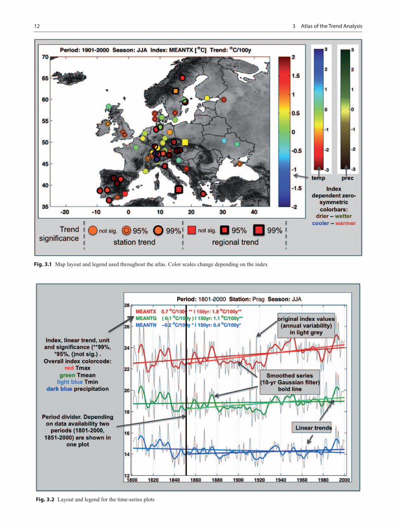
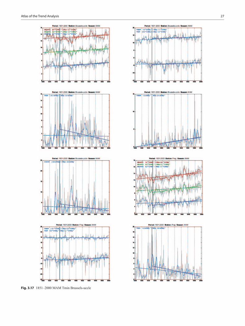
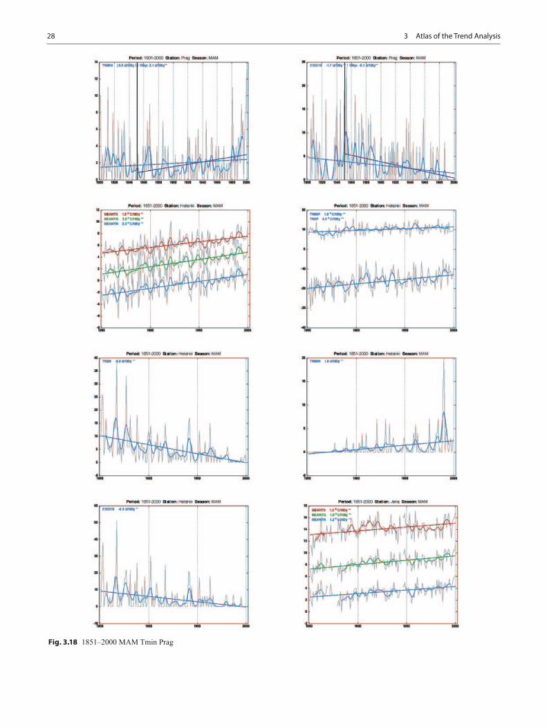
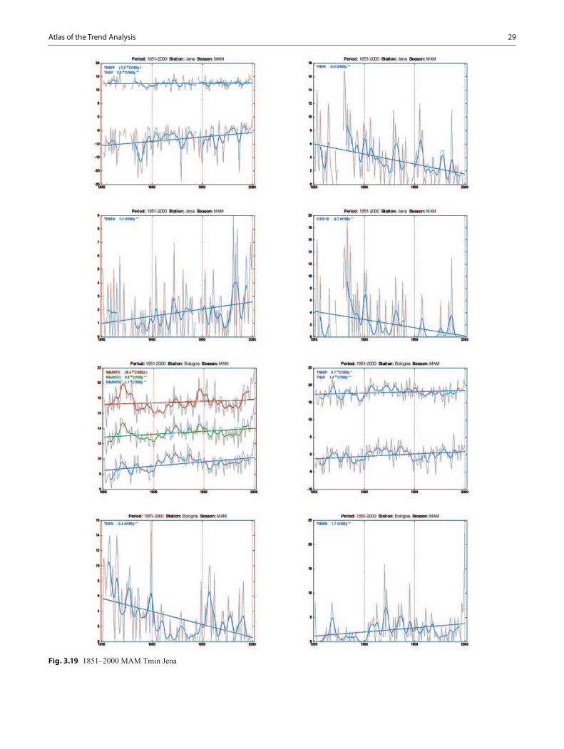
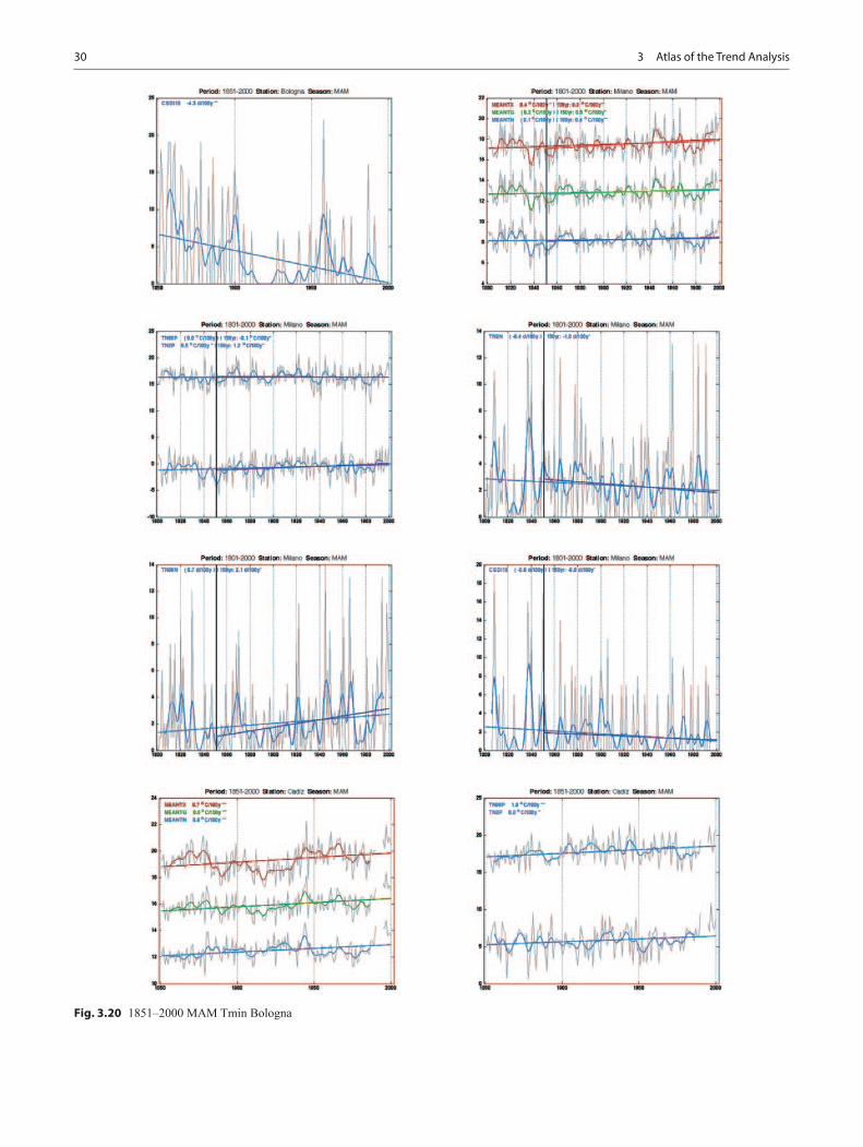
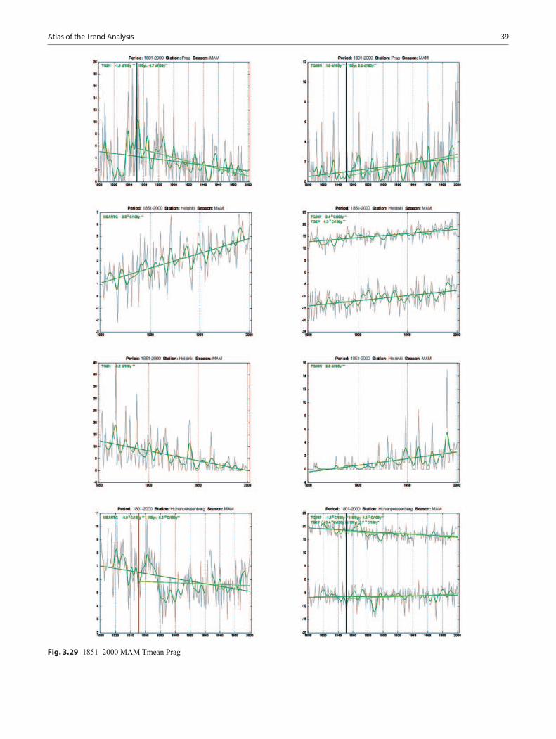
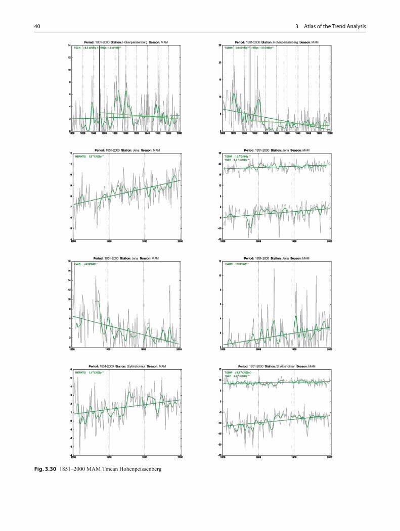
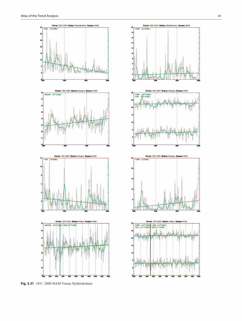
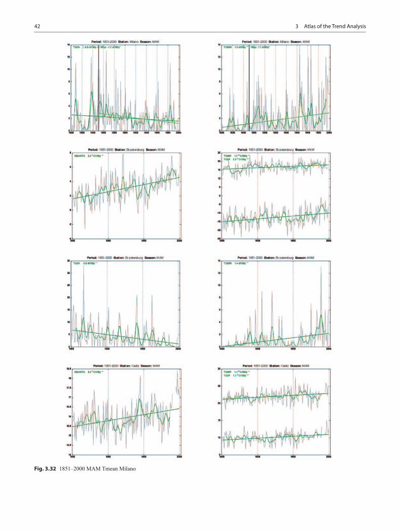
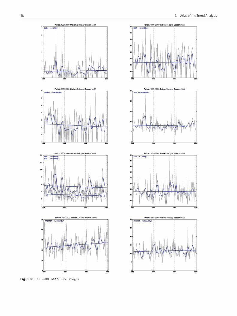
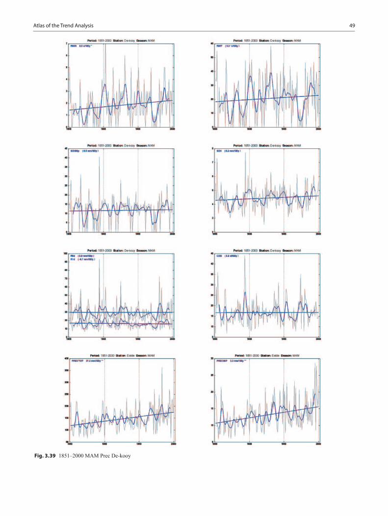
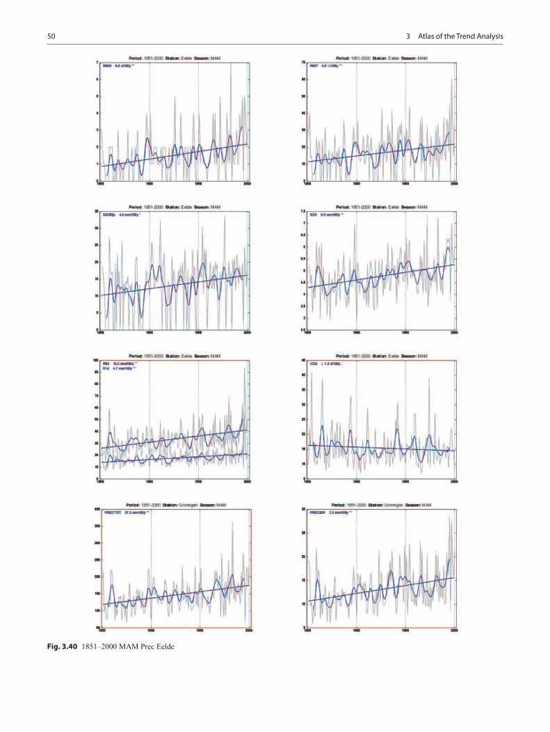
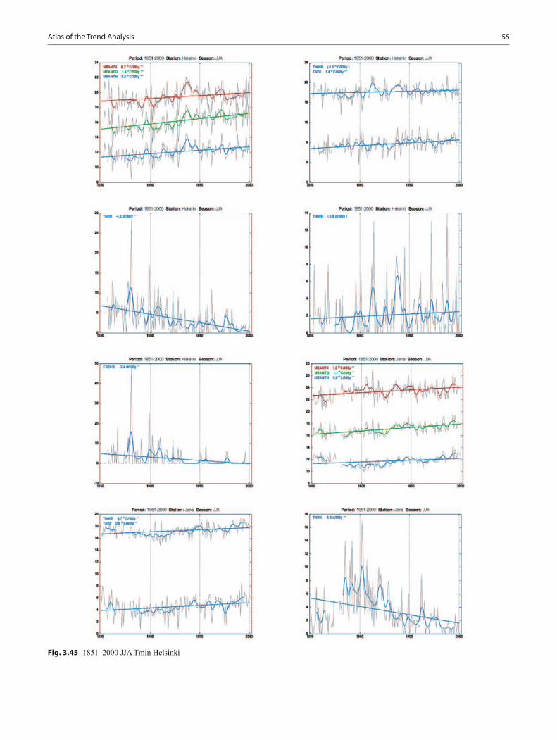
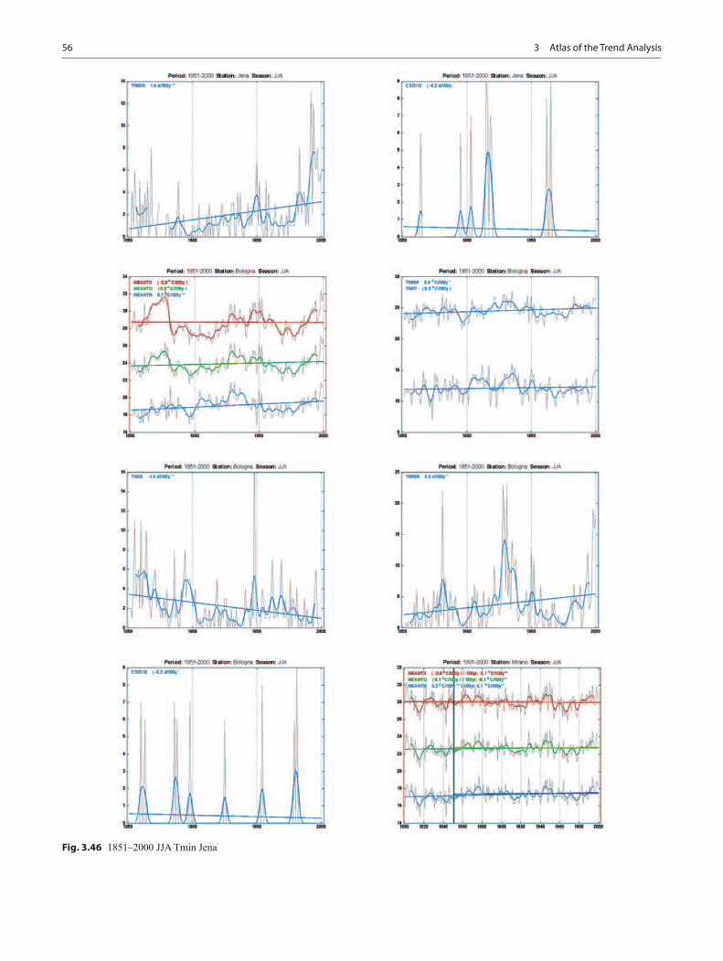
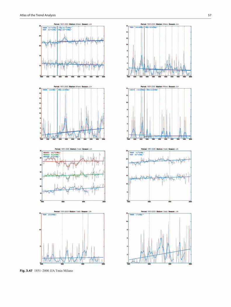
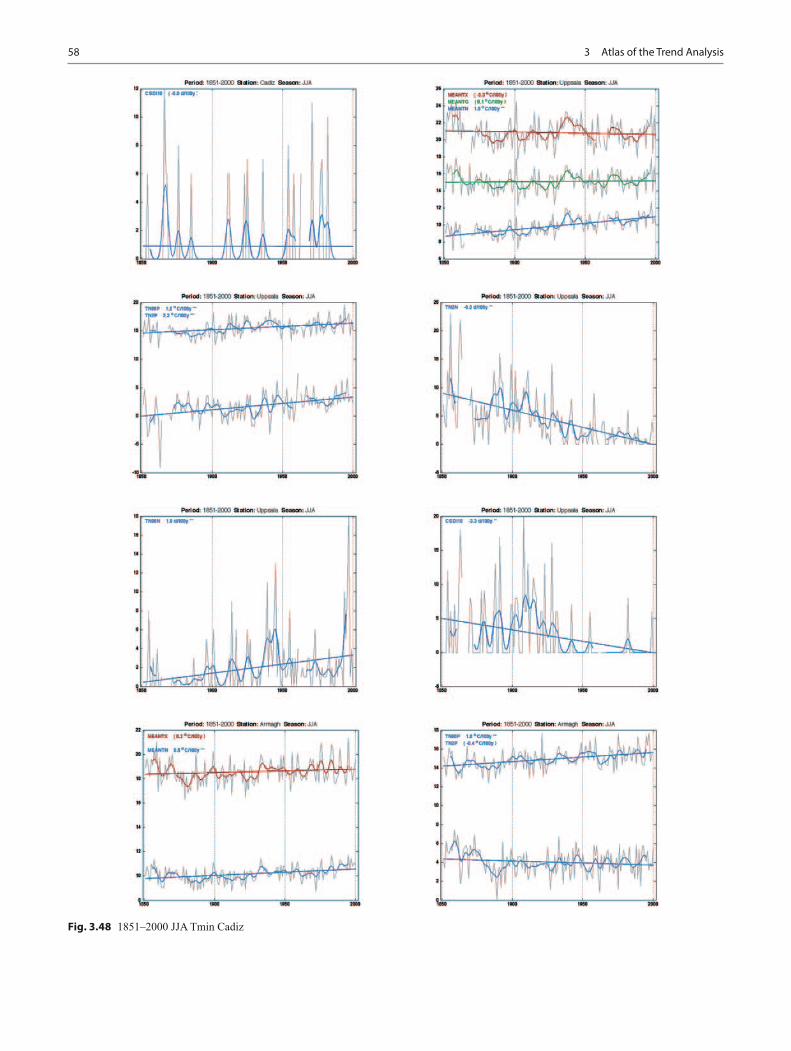
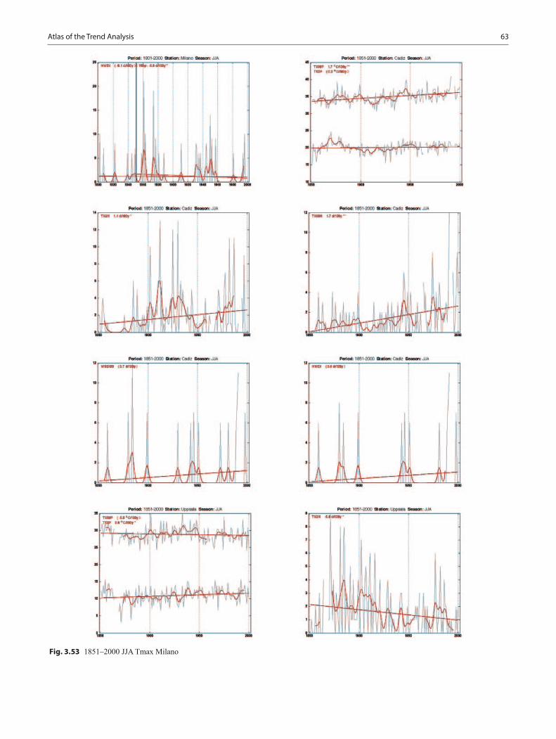
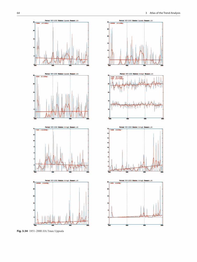
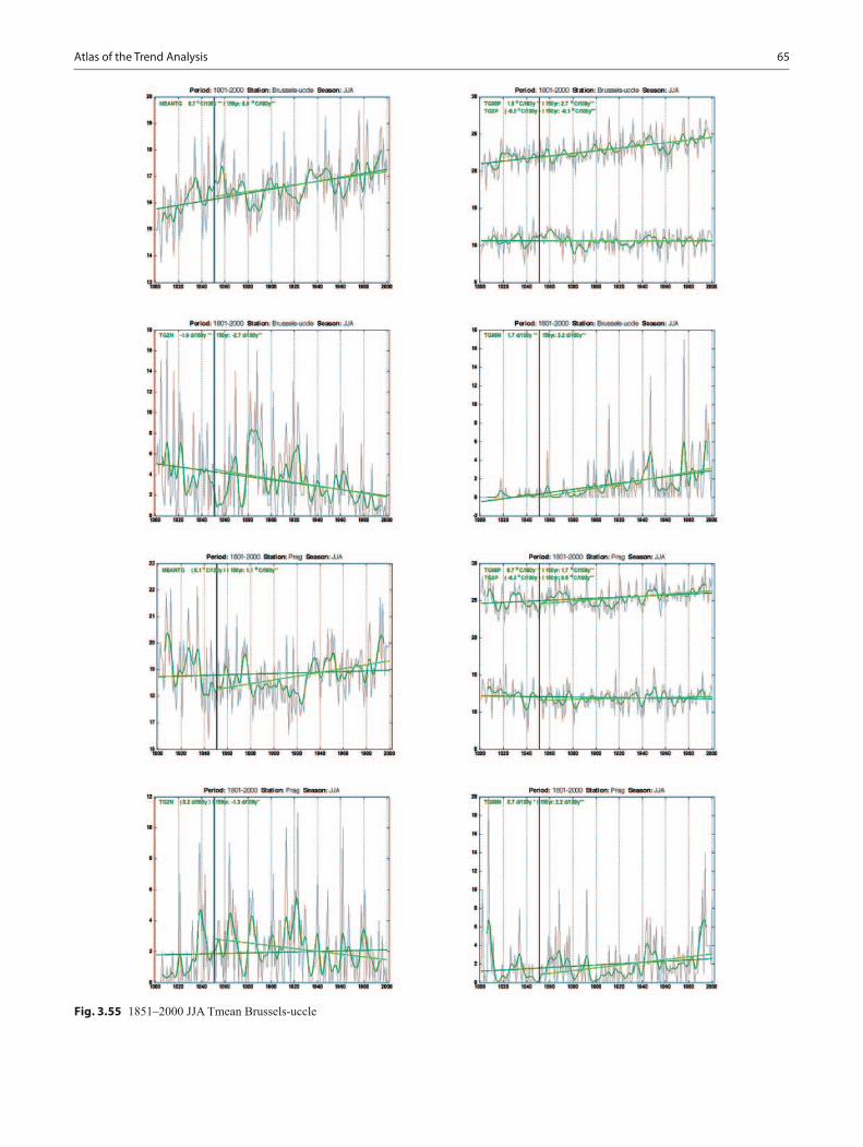
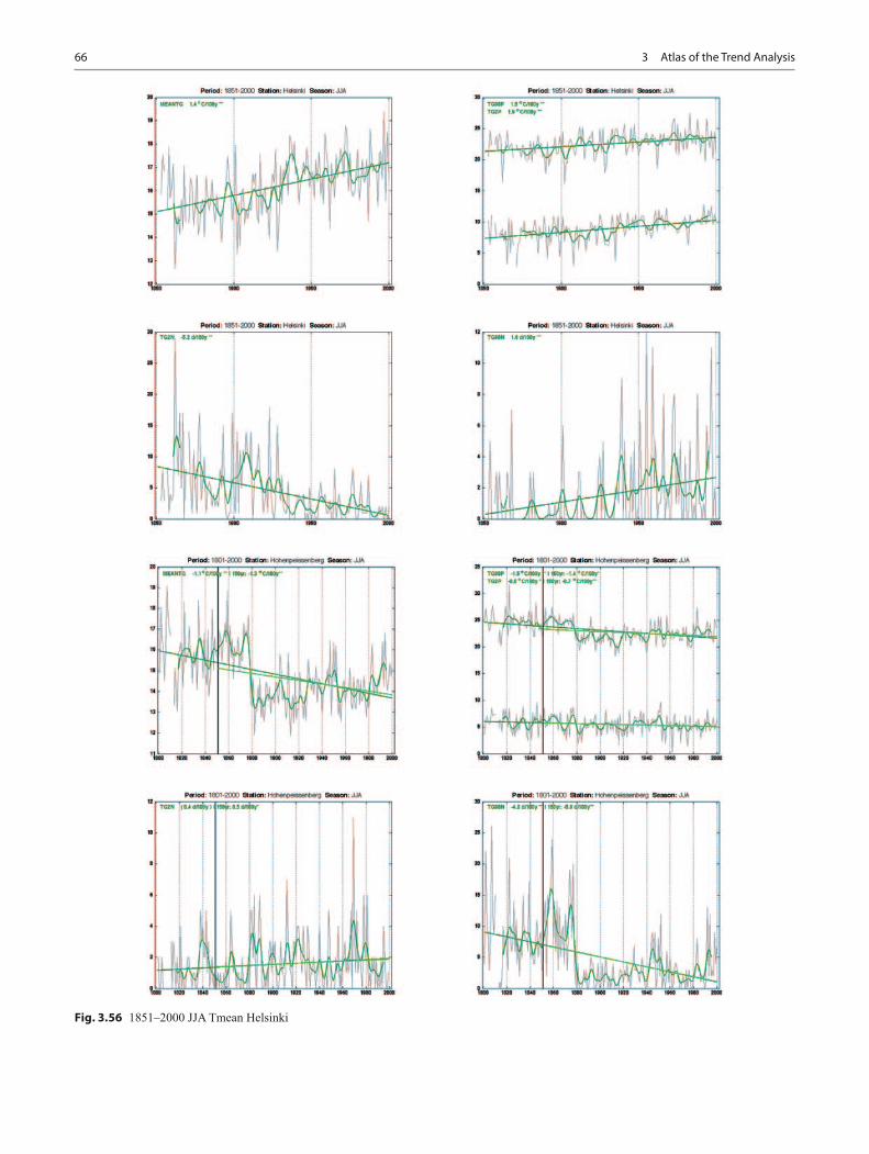
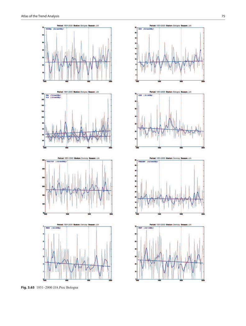
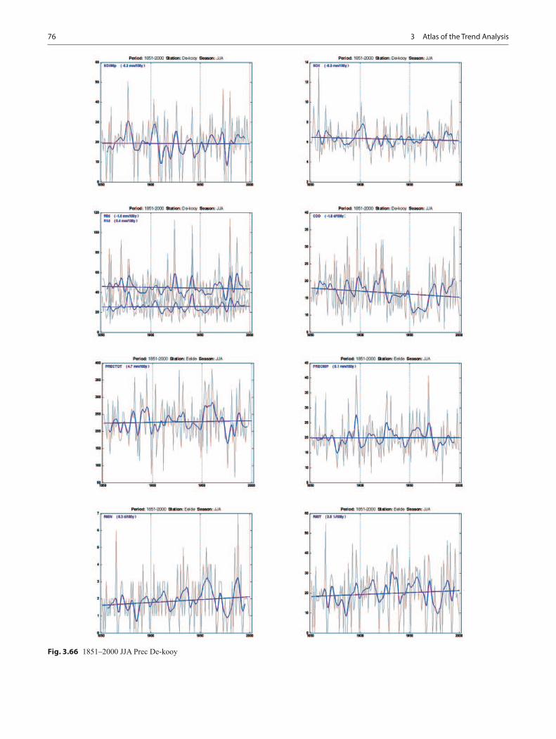
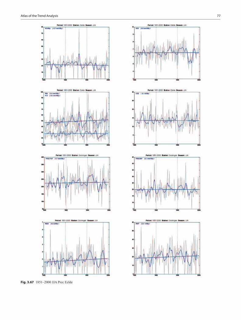
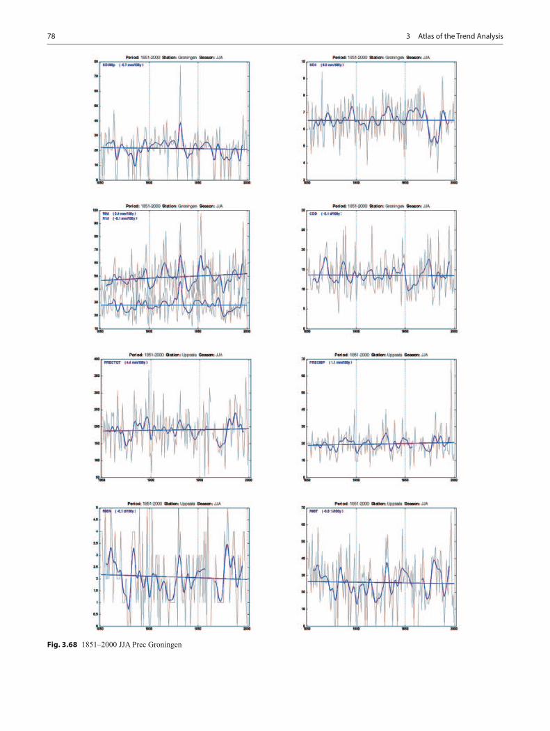
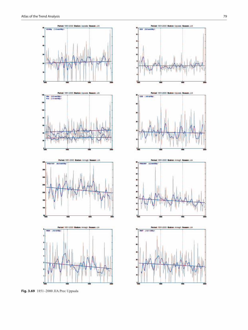
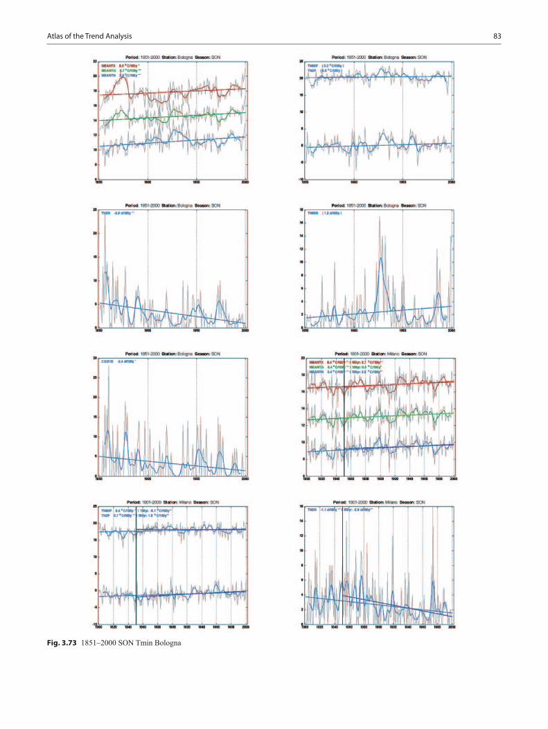
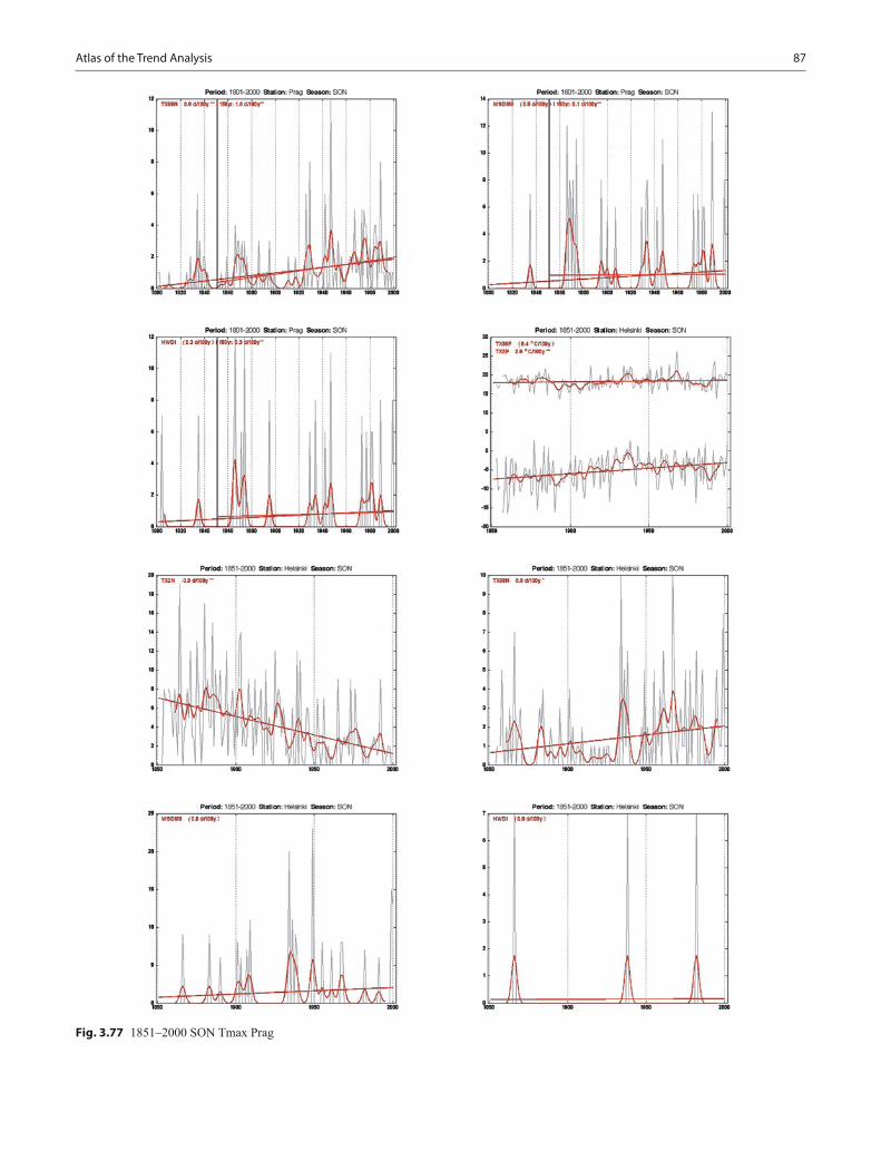
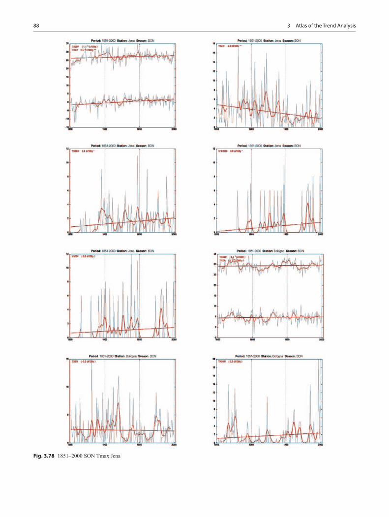
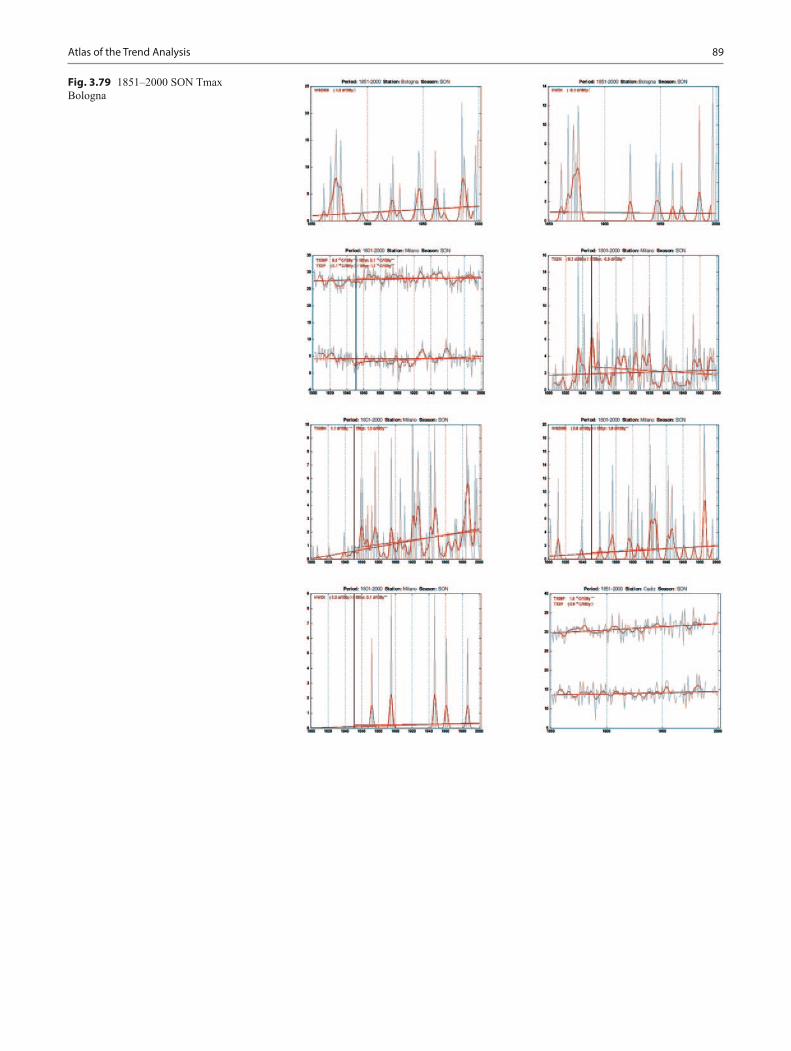
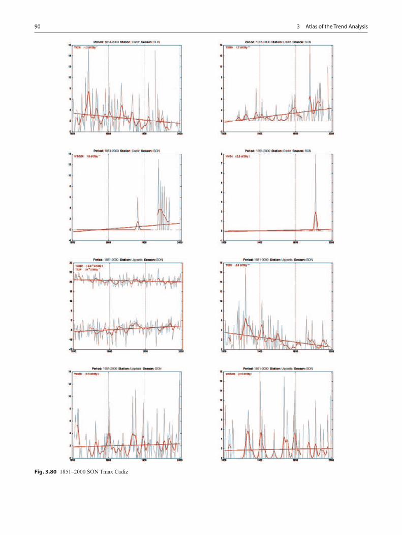
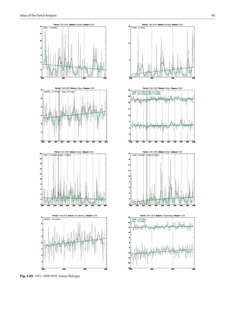
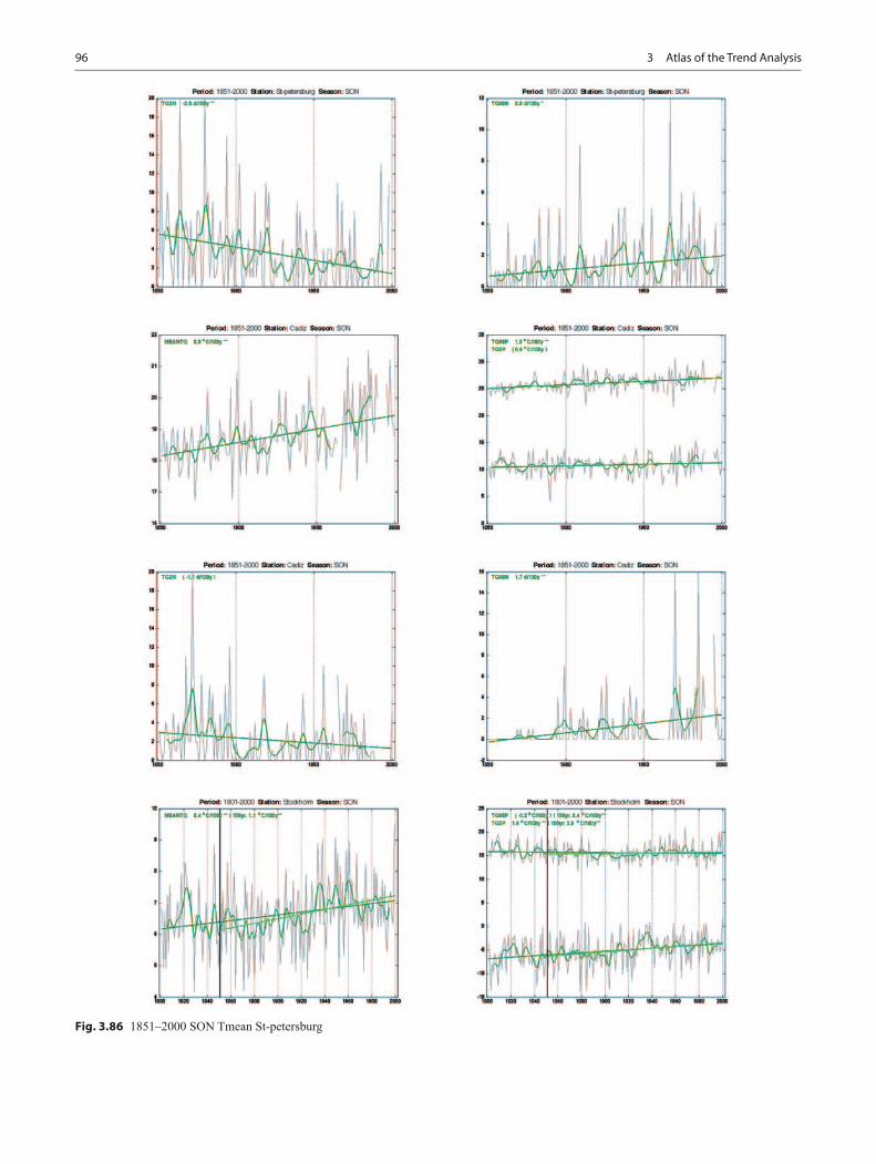
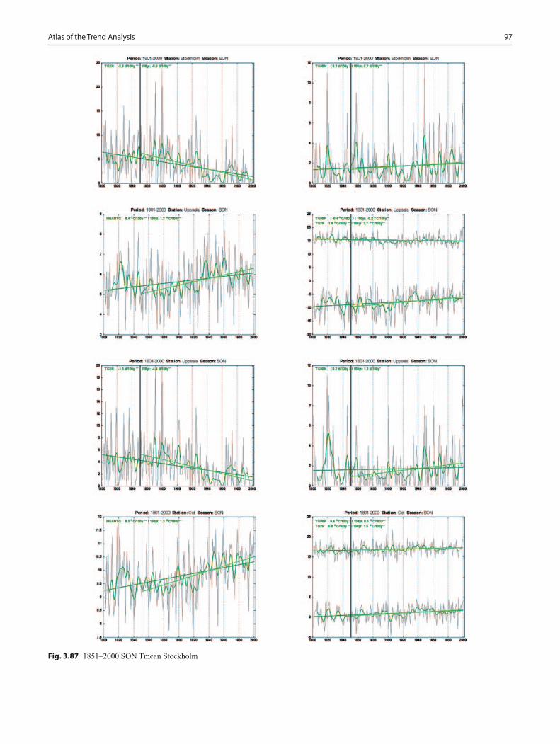
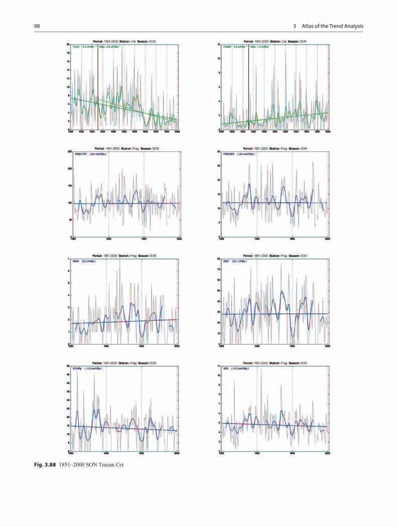
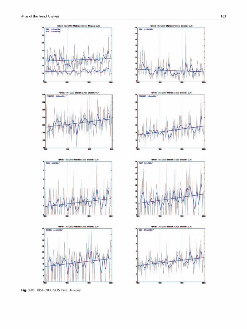
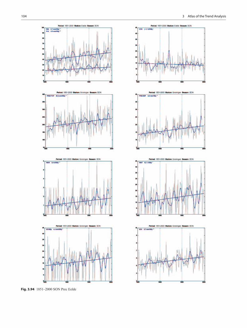
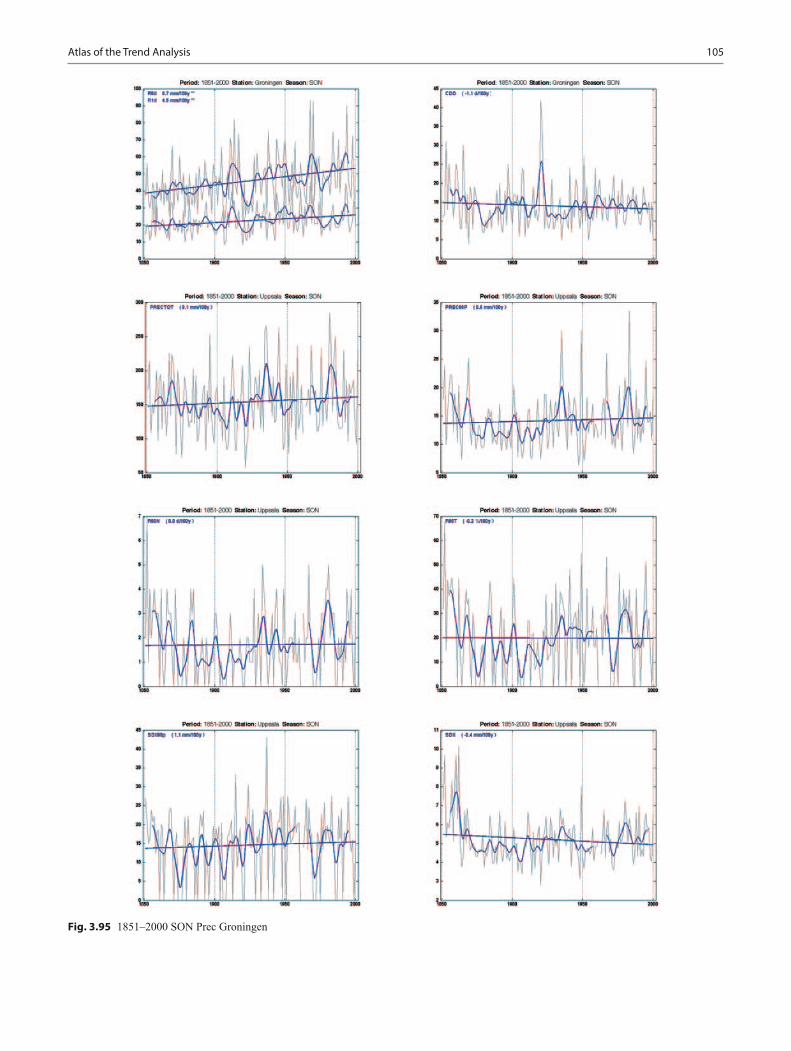
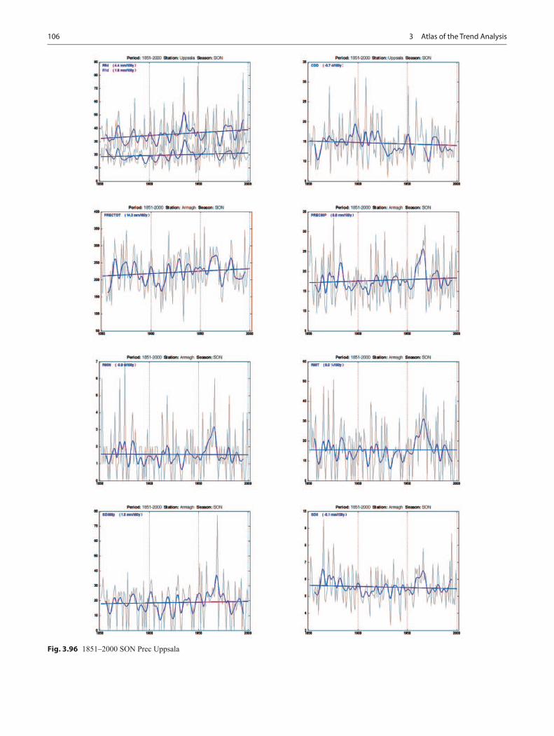
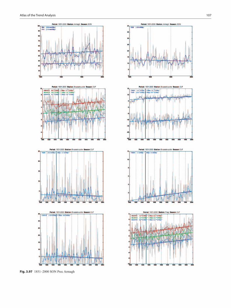
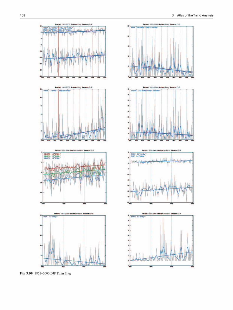
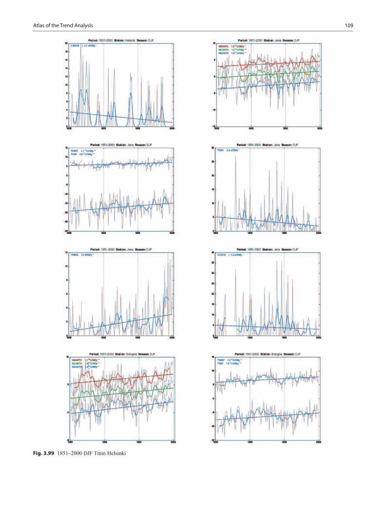
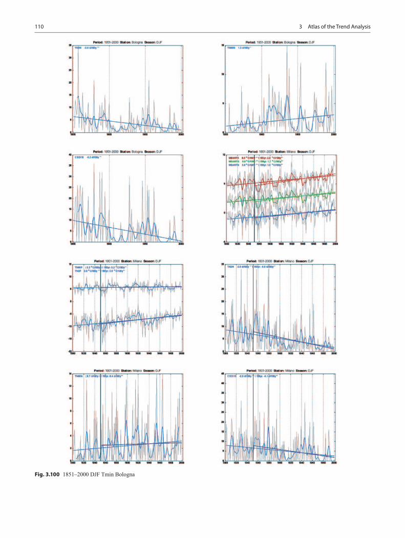
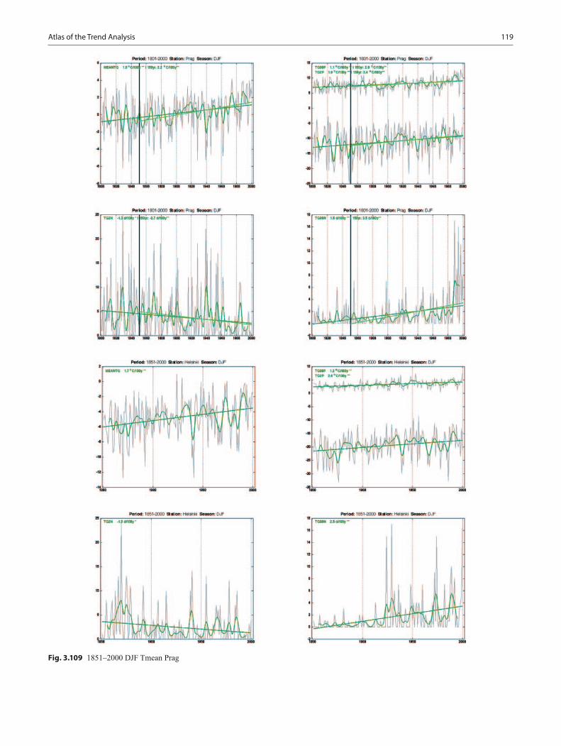
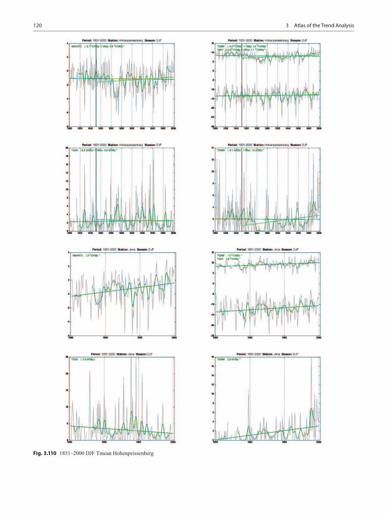
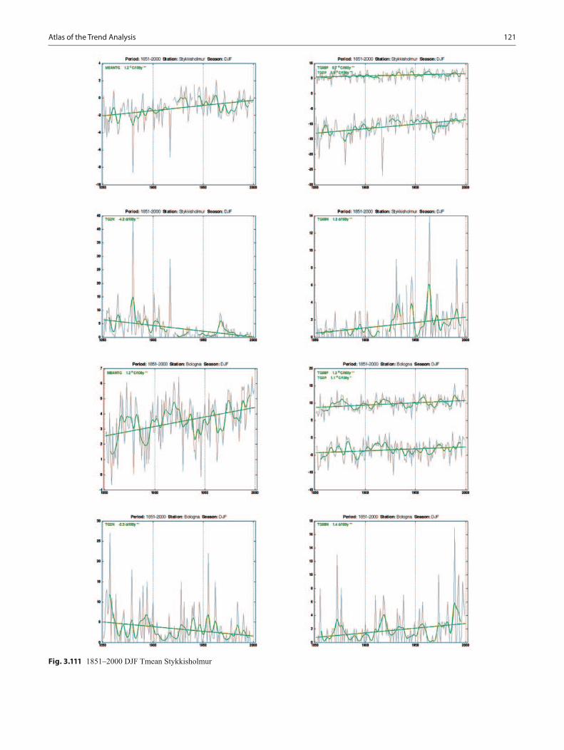
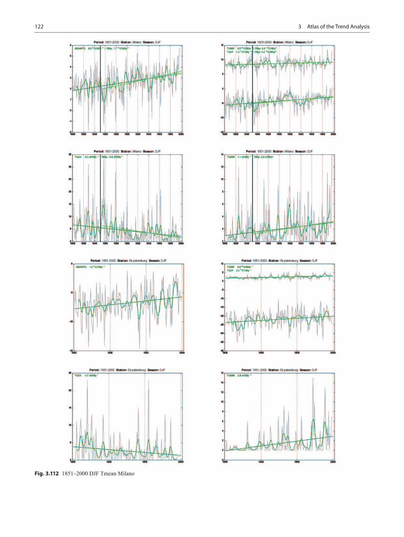
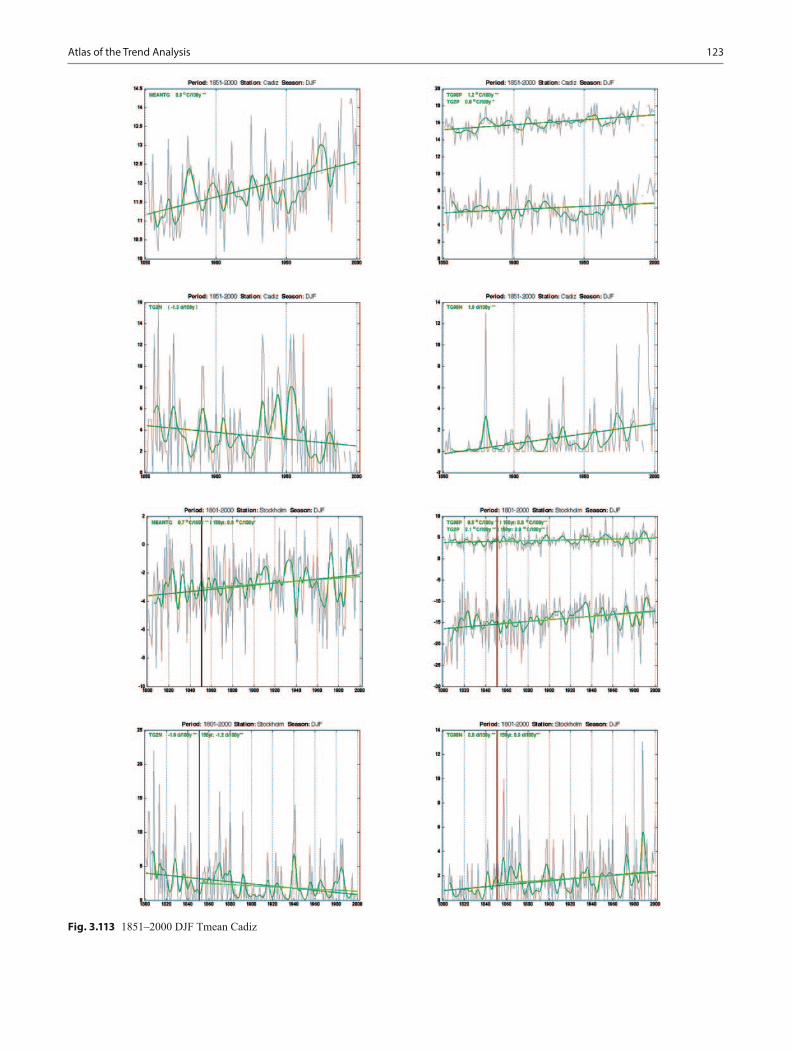
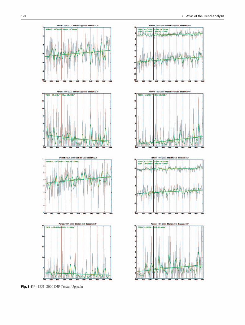
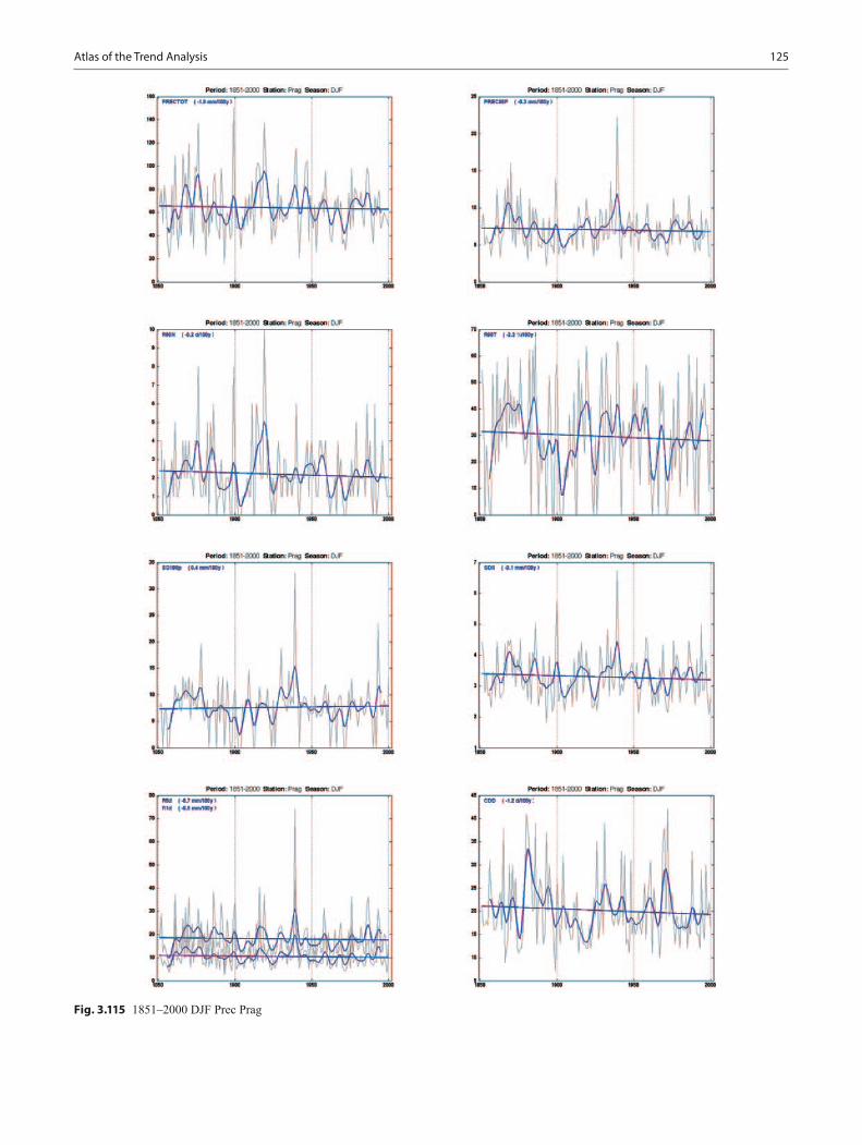
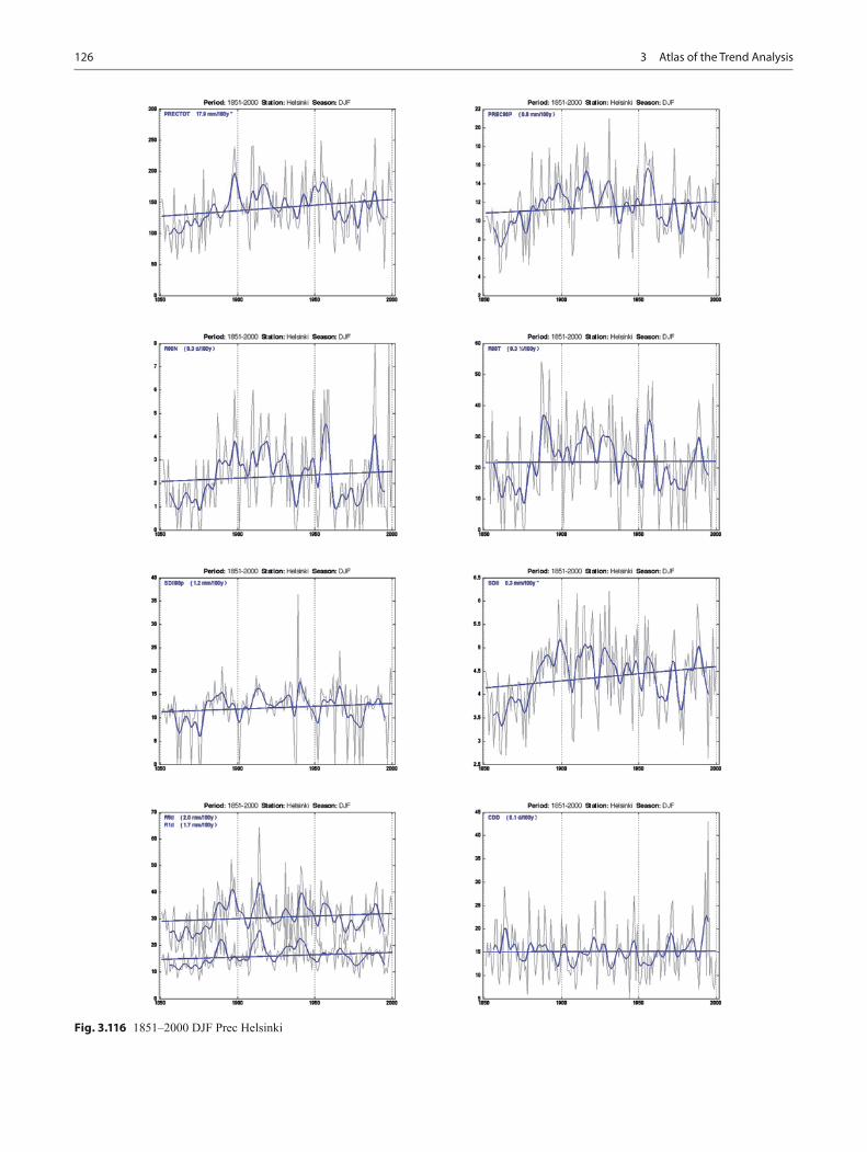
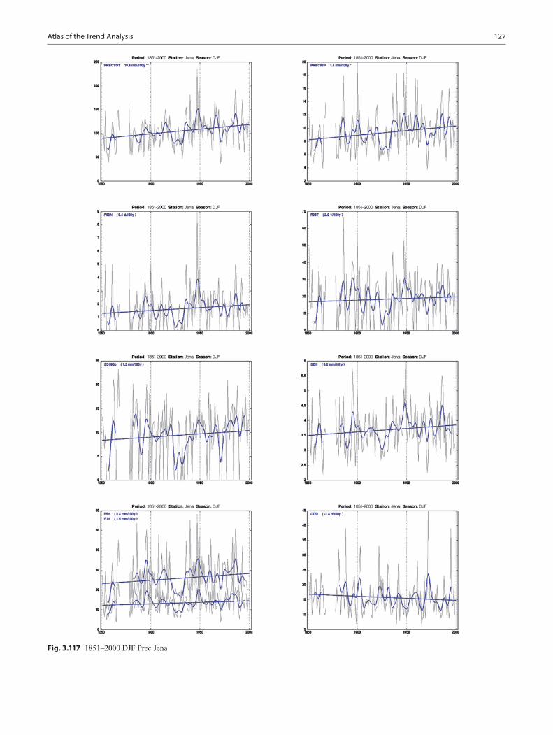
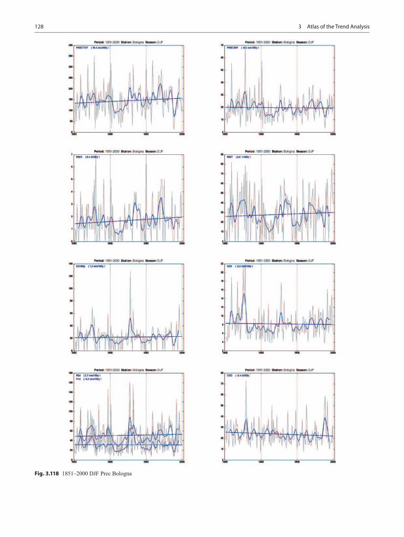
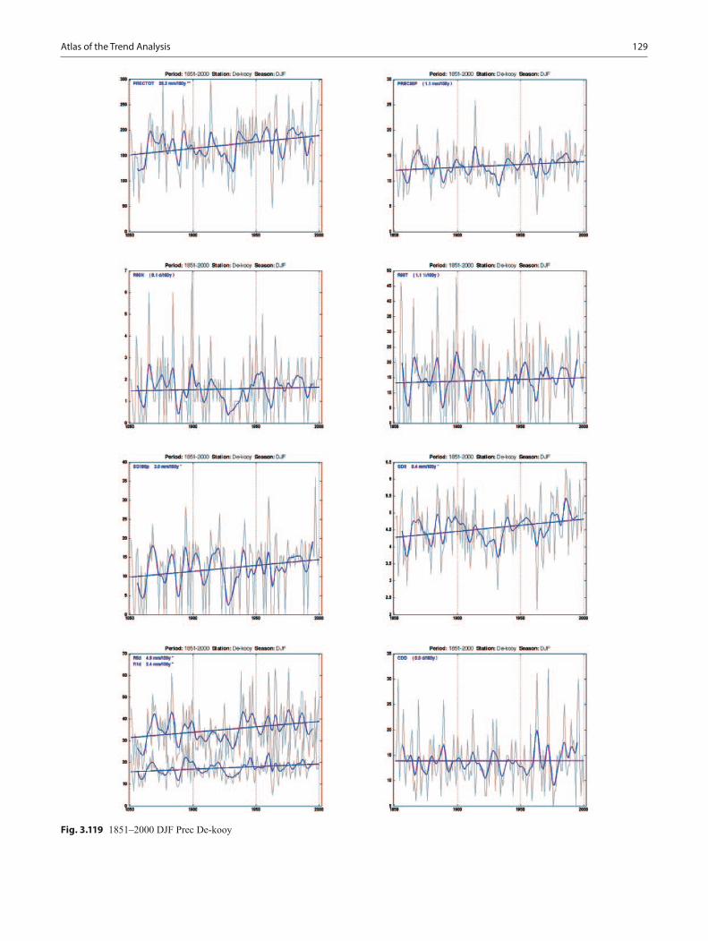
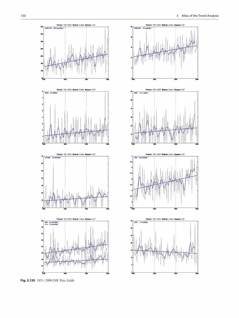
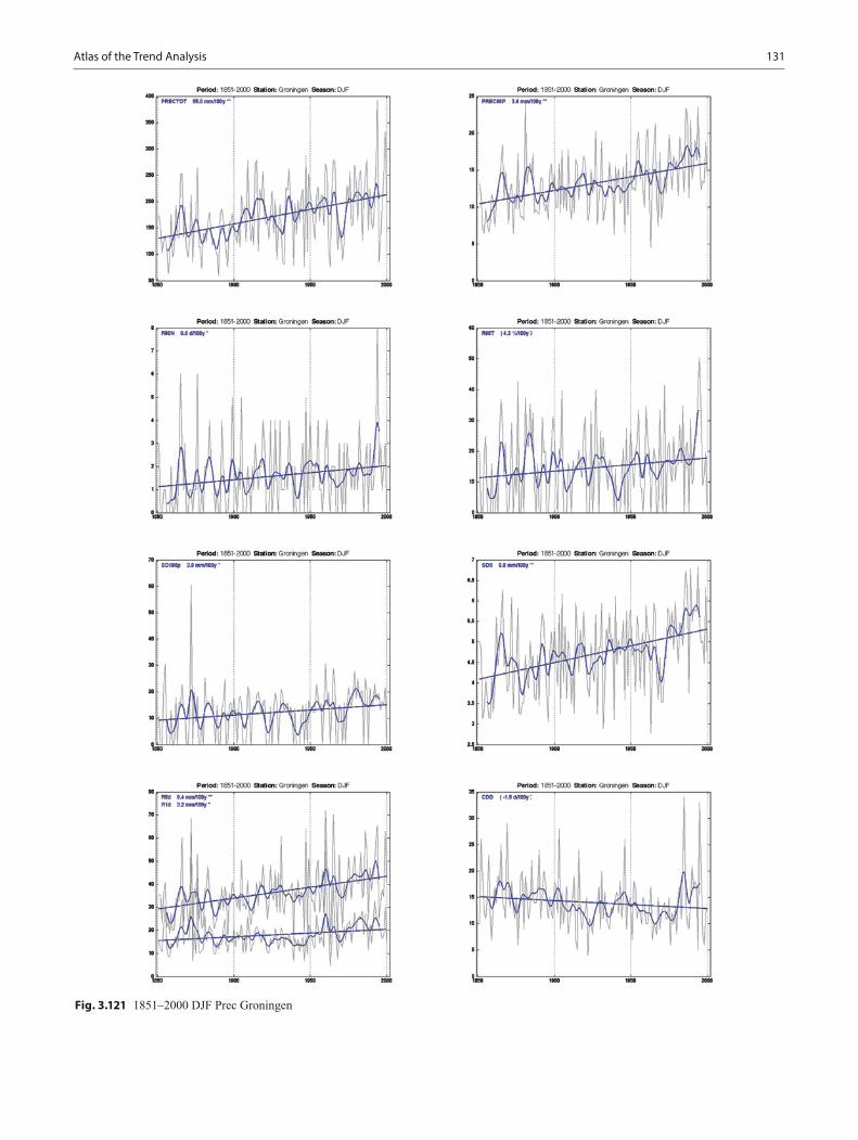
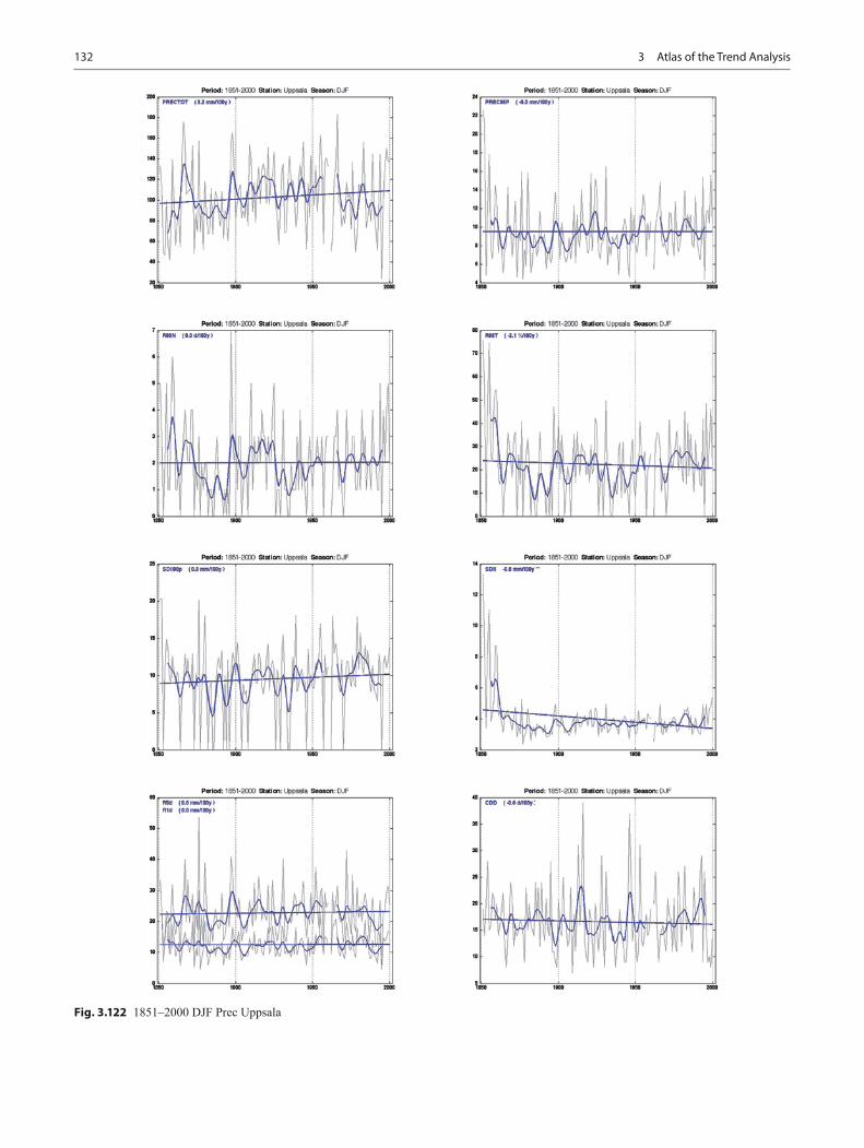
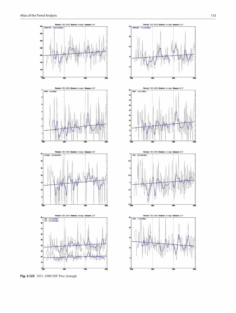
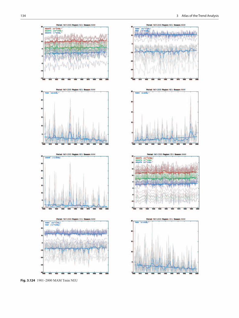
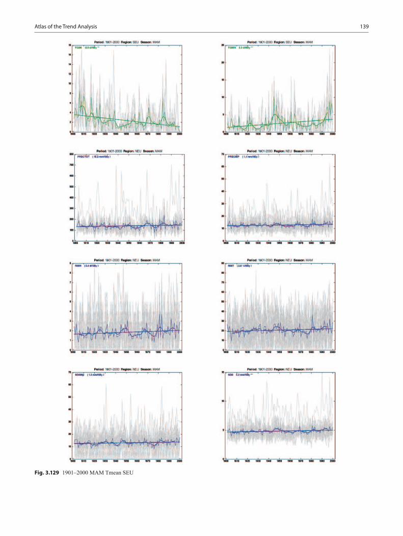
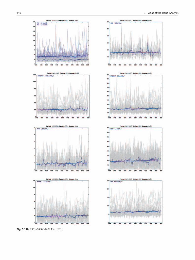
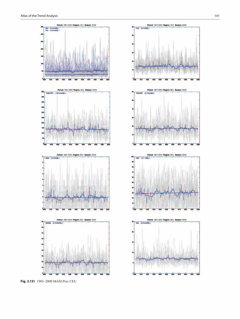
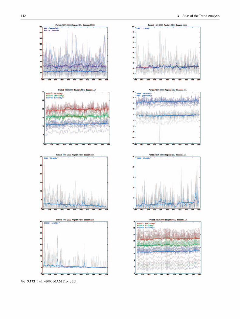
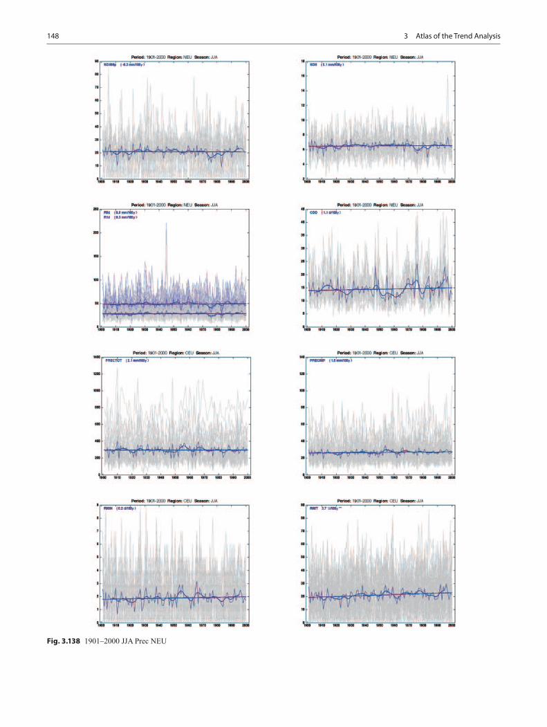
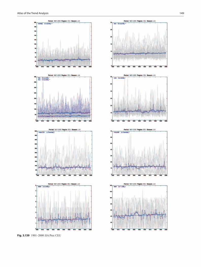
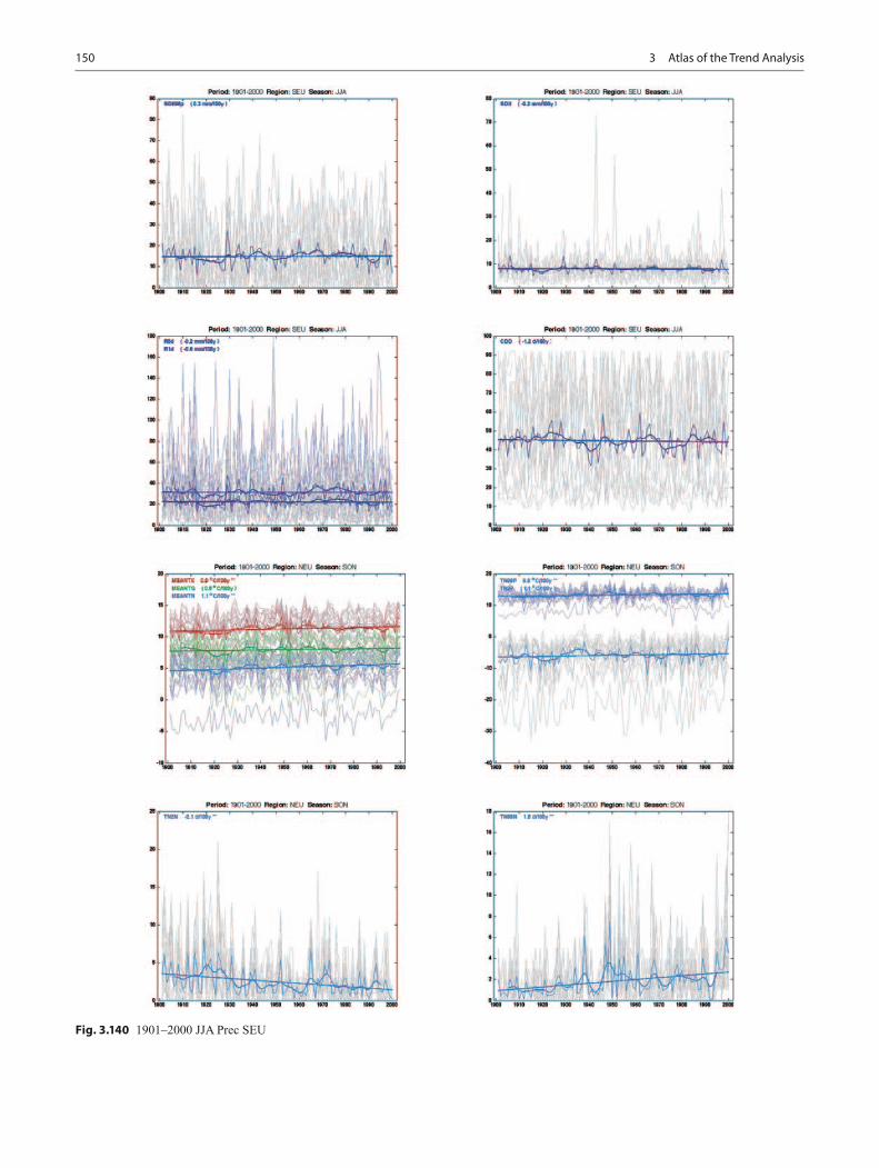
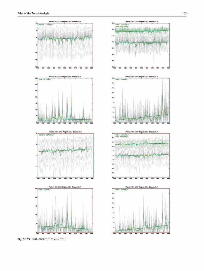
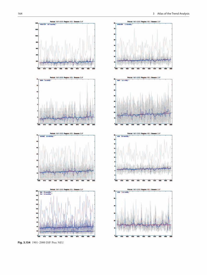
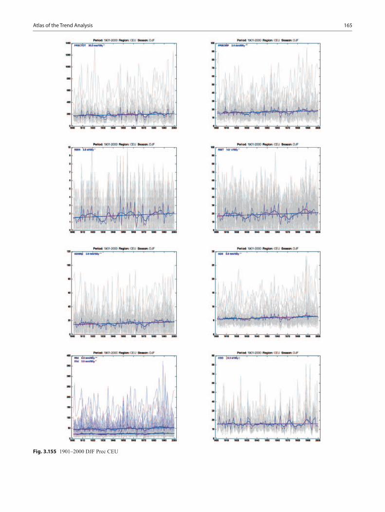
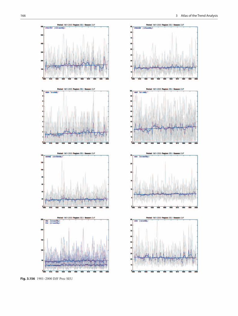
For the time-series plots, each individual station’s data are separately shown for the two longer periods (1801–2000 and 1851–2000), while the regional means are displayed
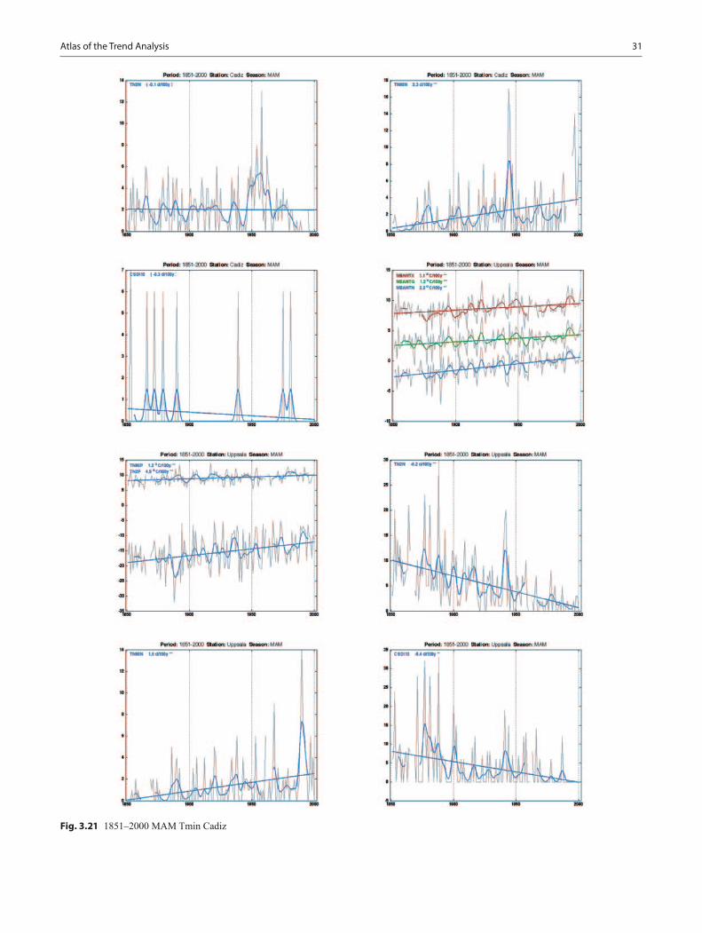
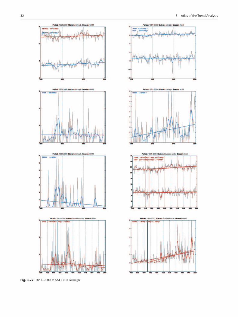
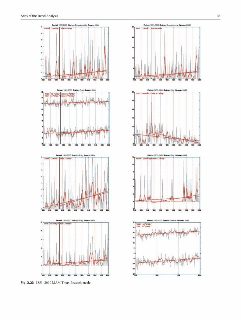
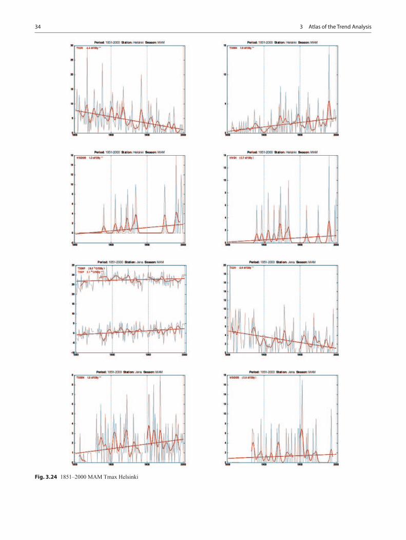
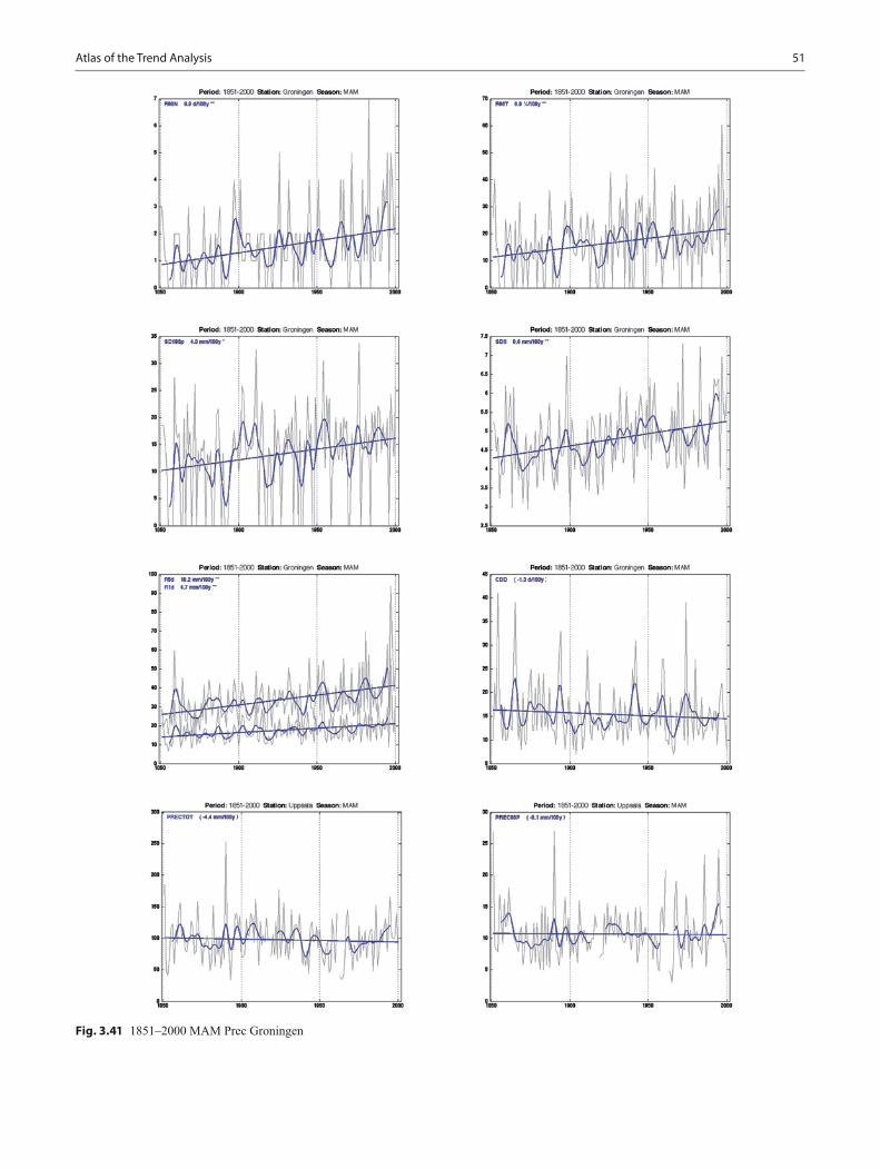
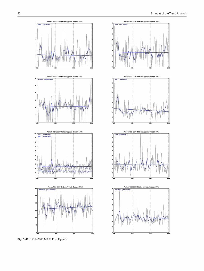
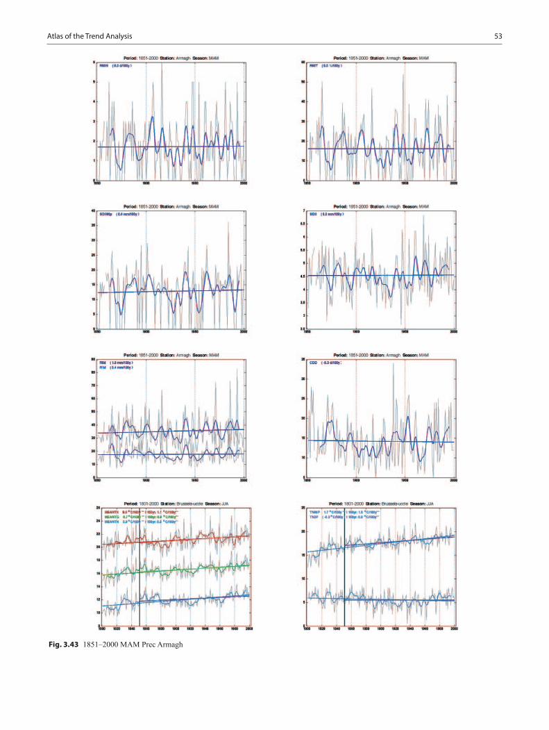
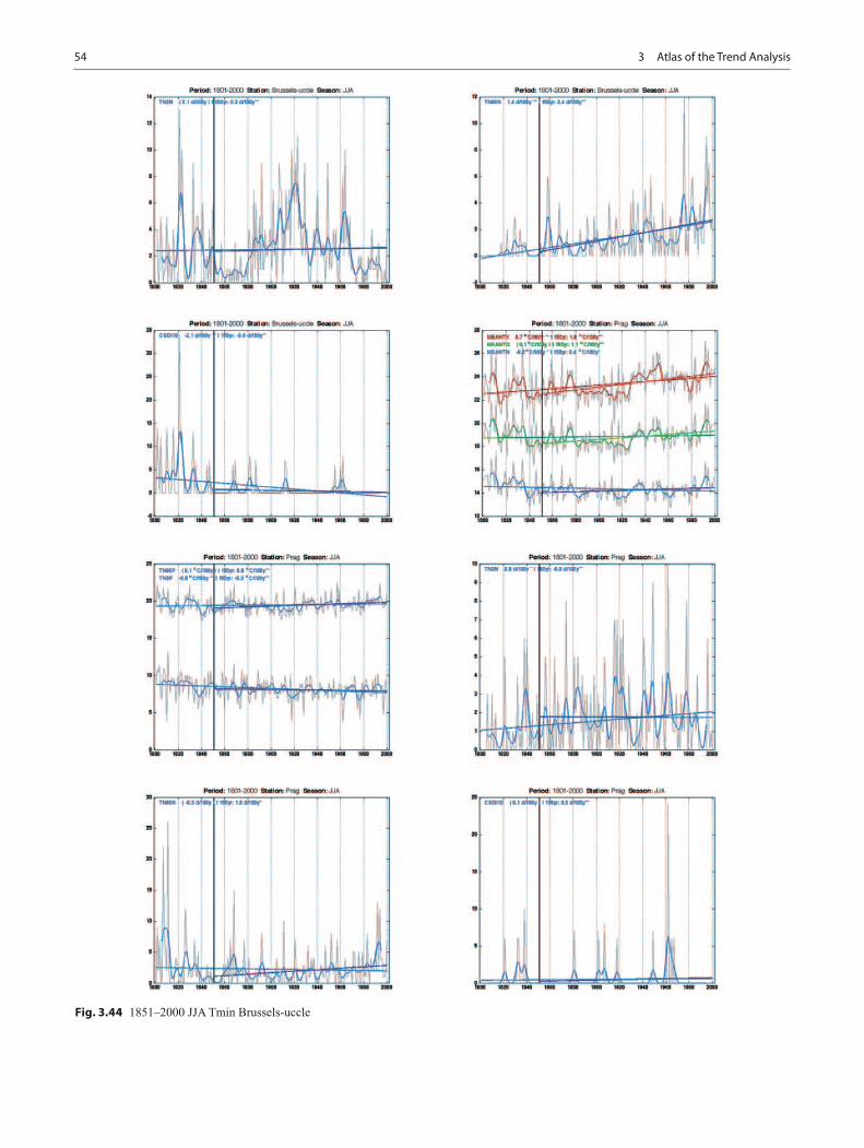
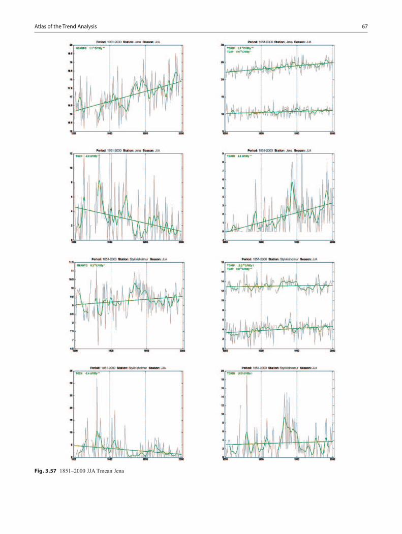
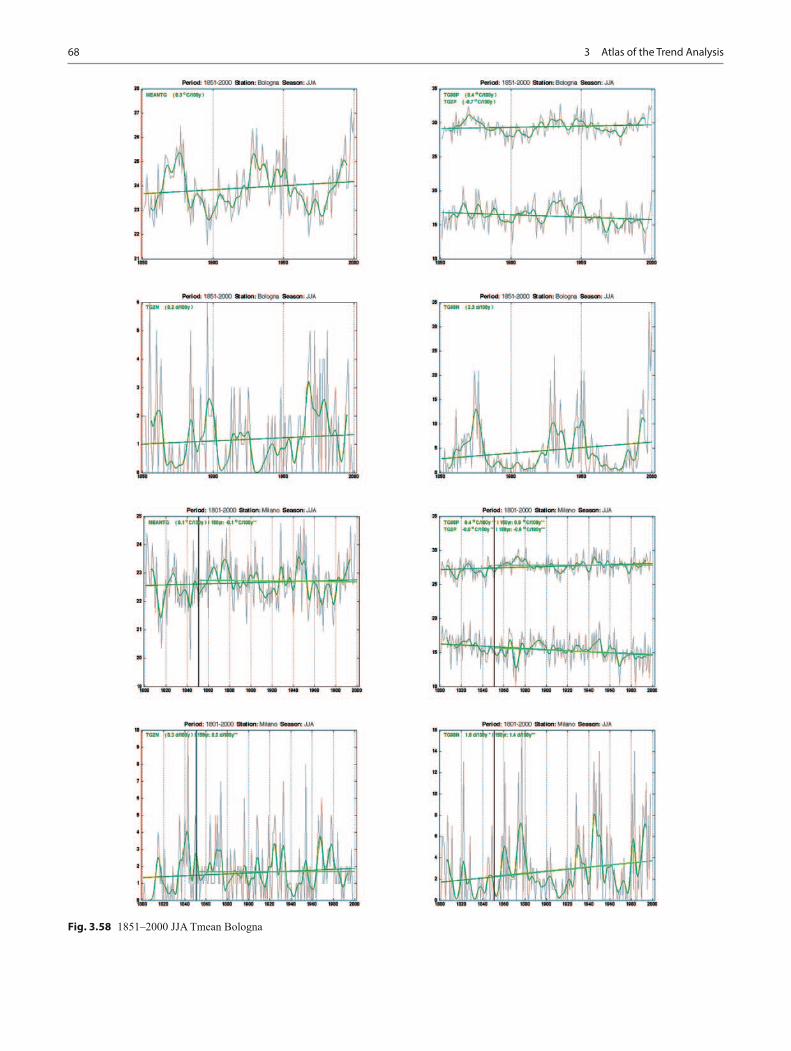
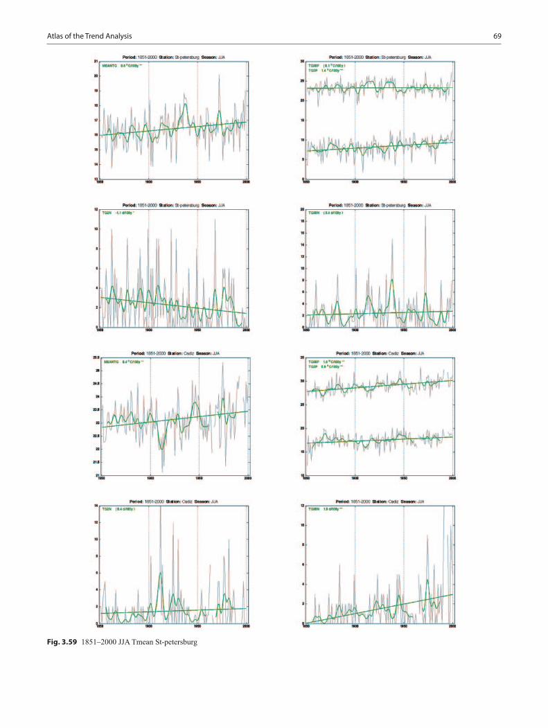
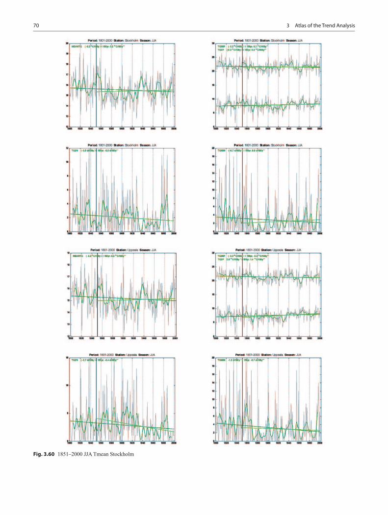
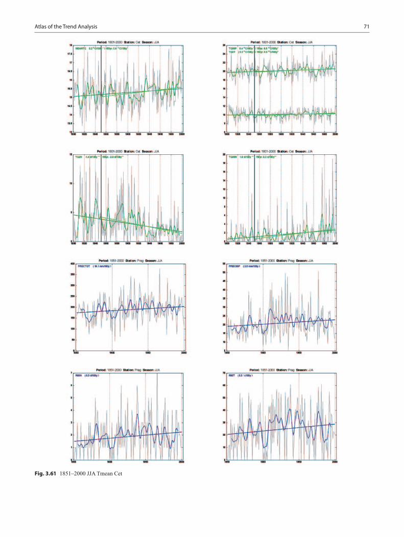
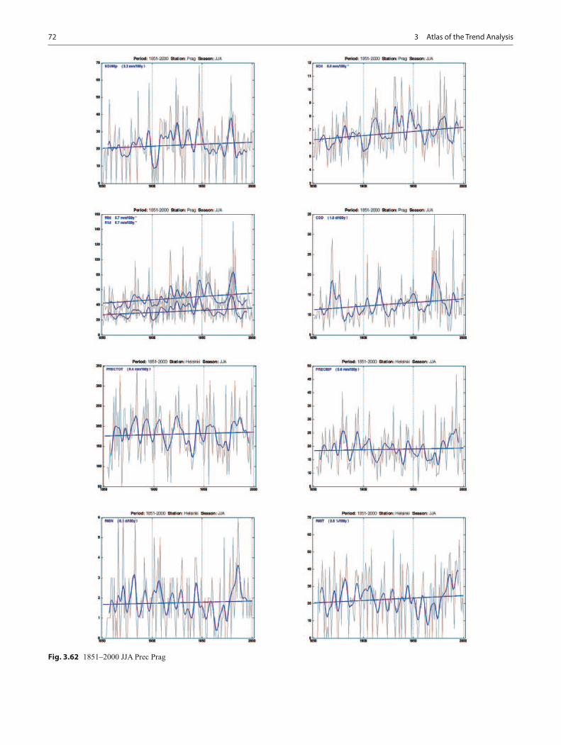
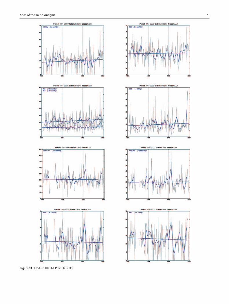
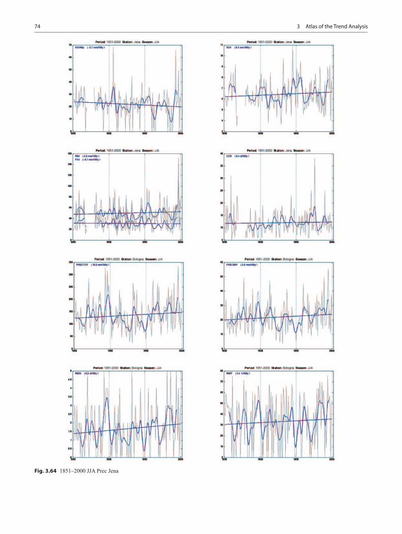
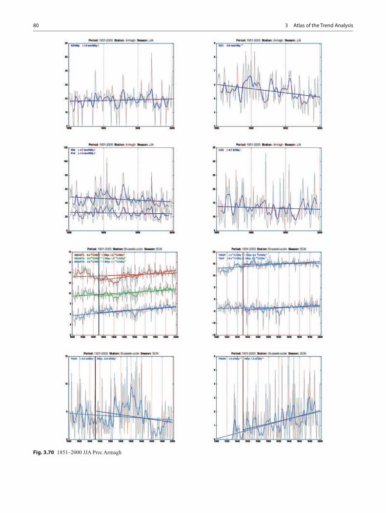
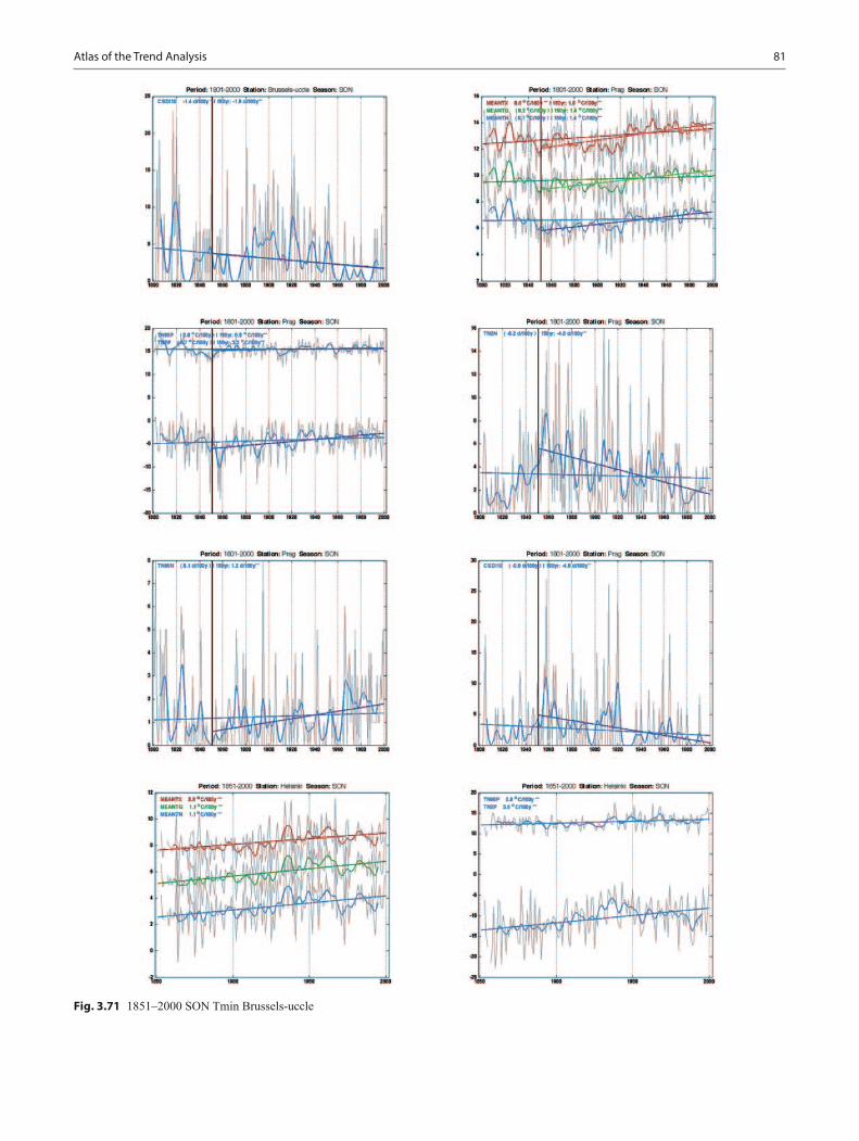
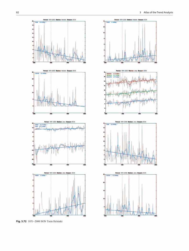
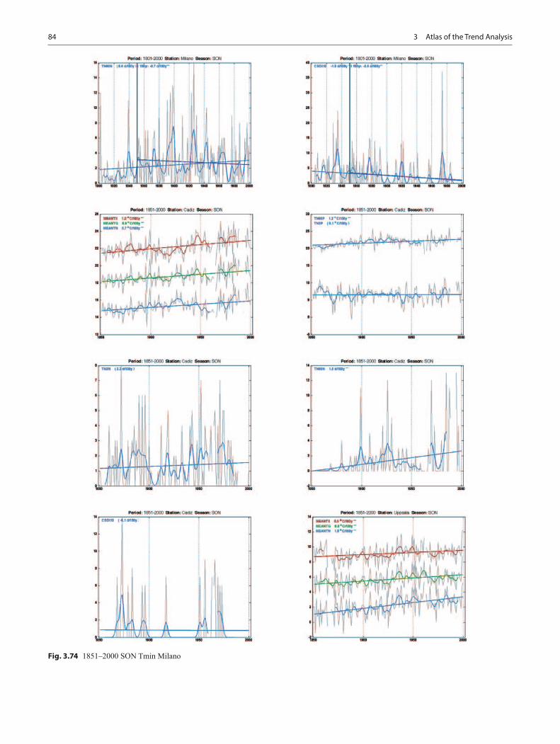
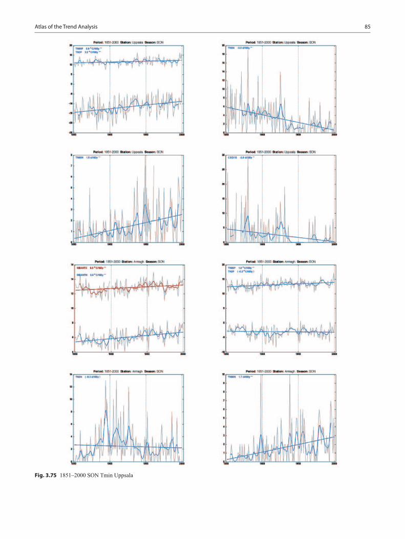
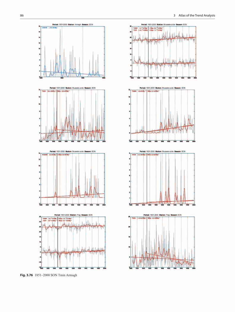
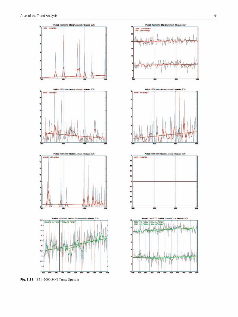
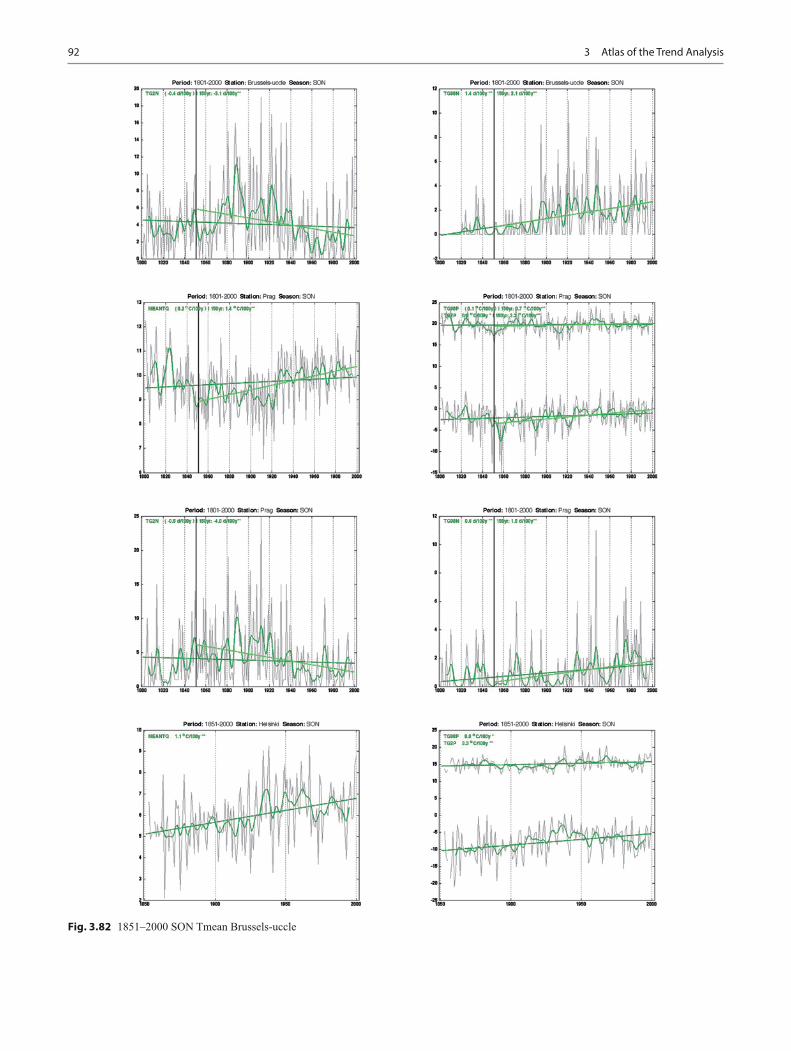
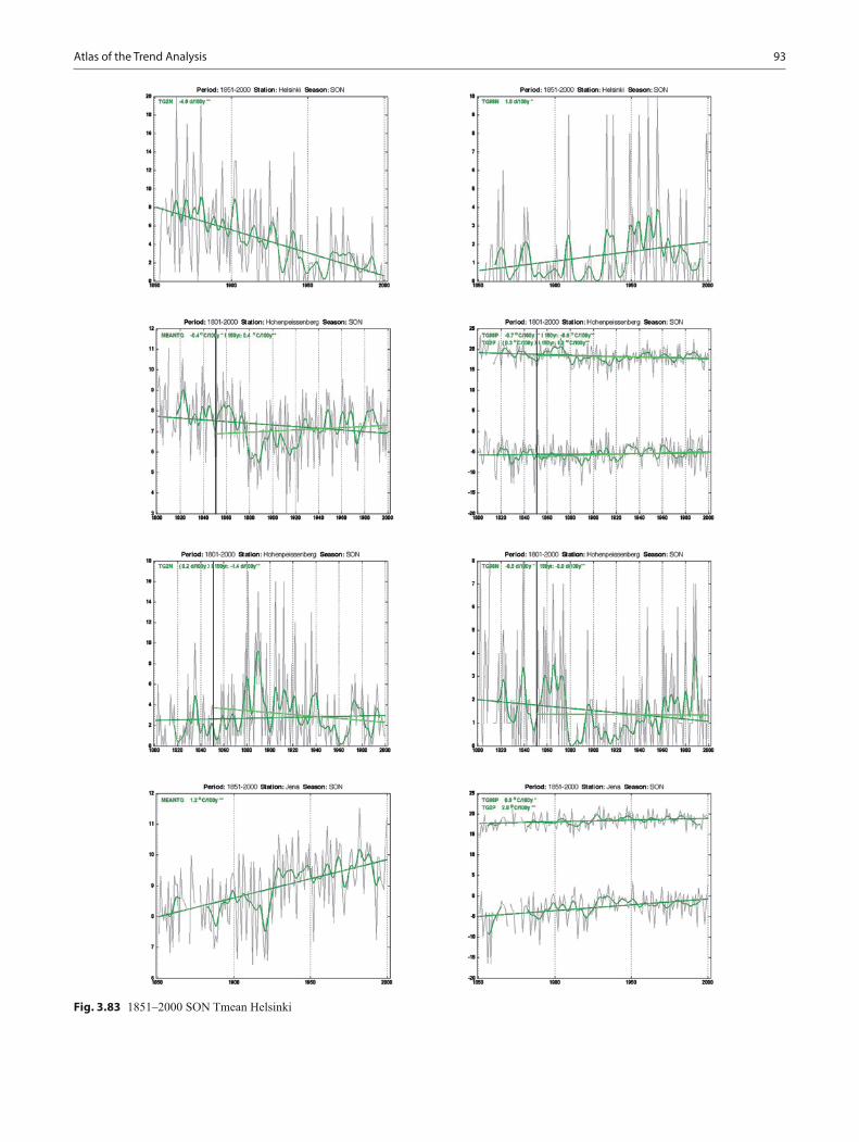
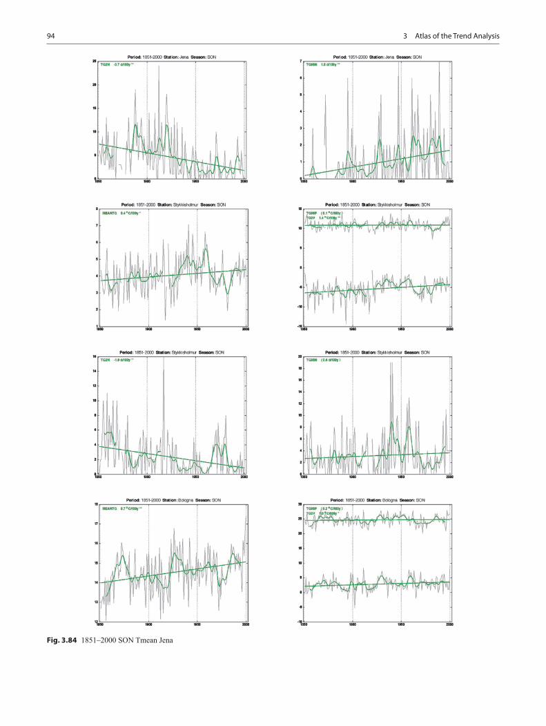
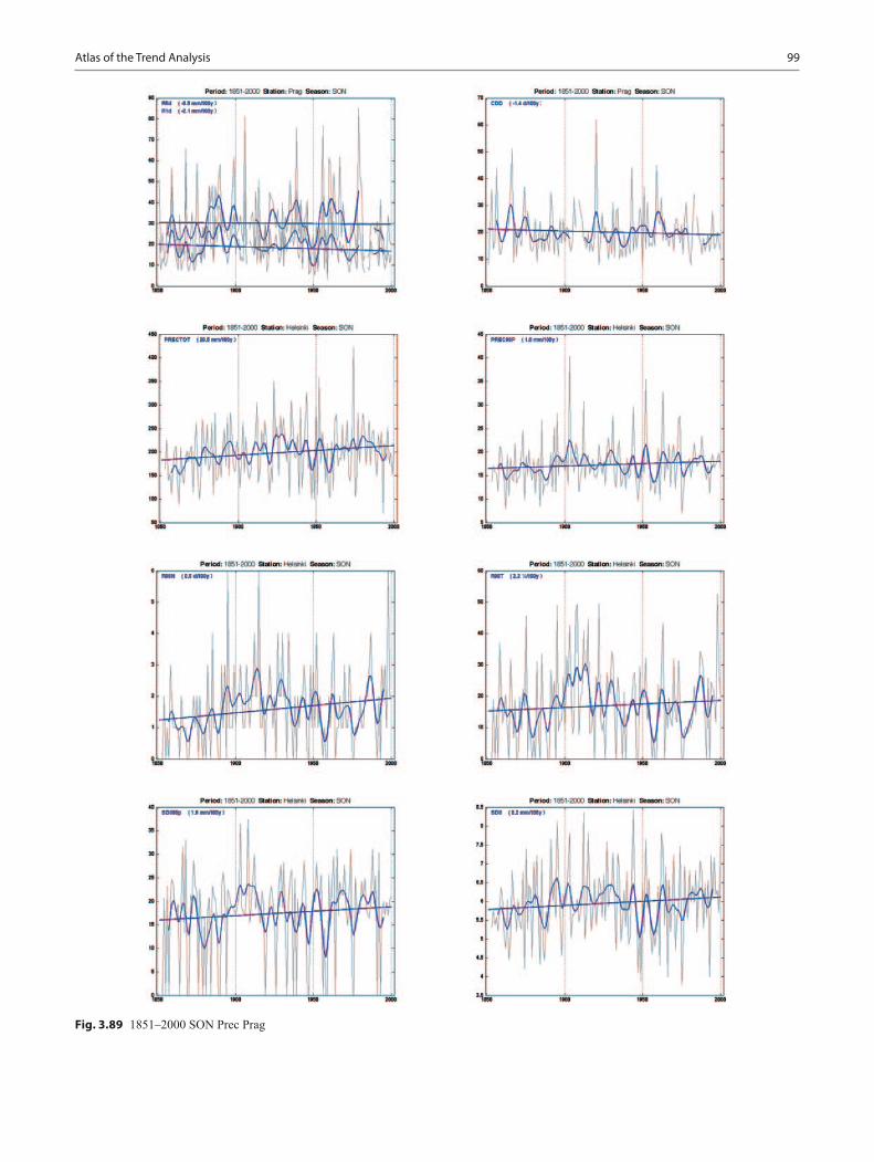
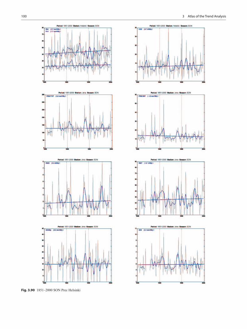
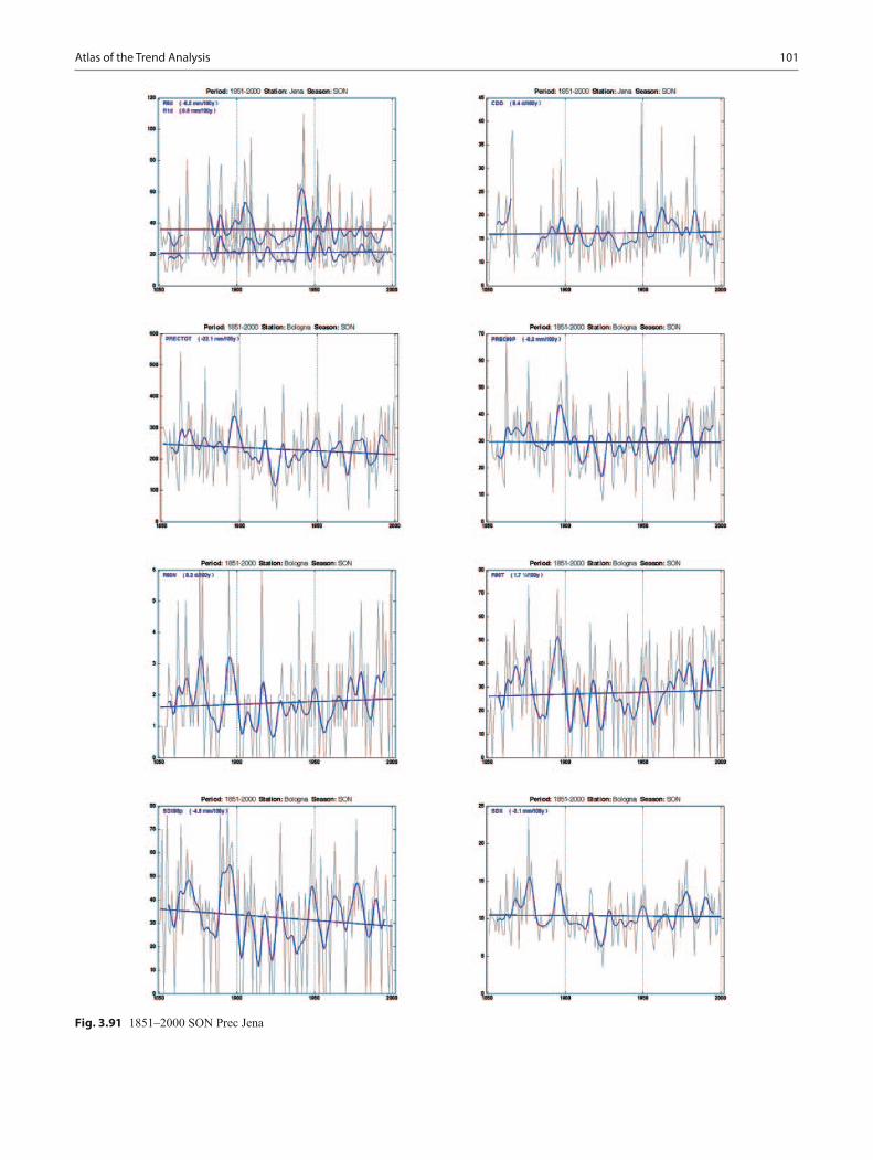
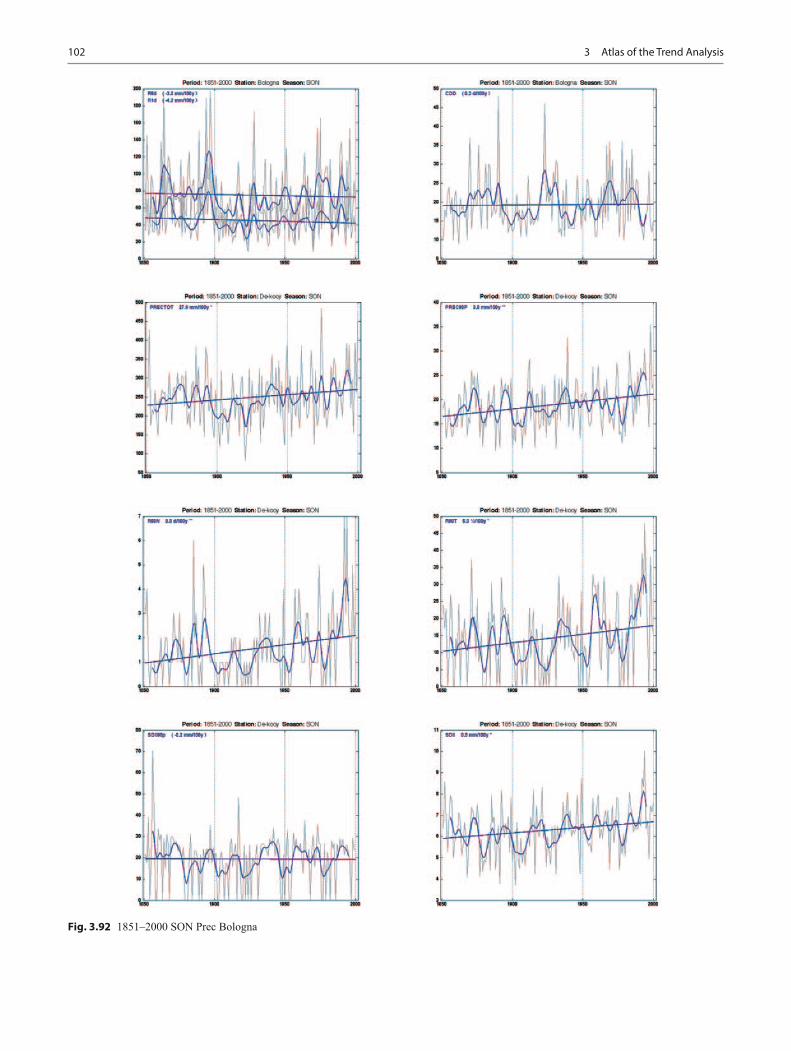
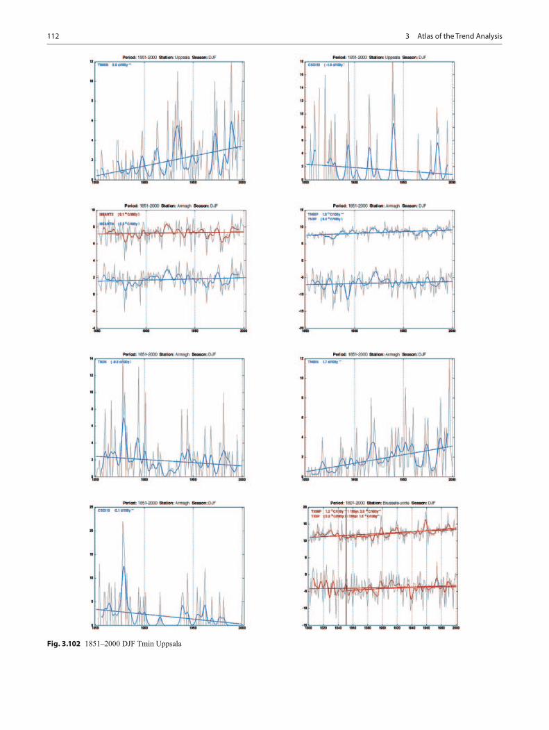
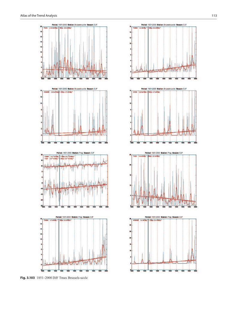
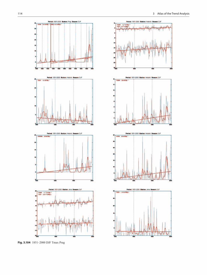
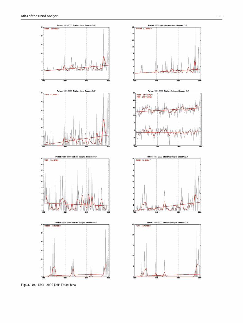
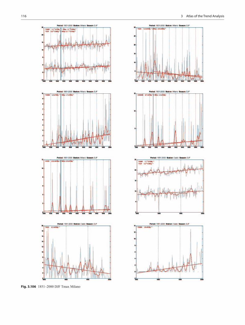
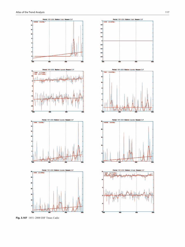
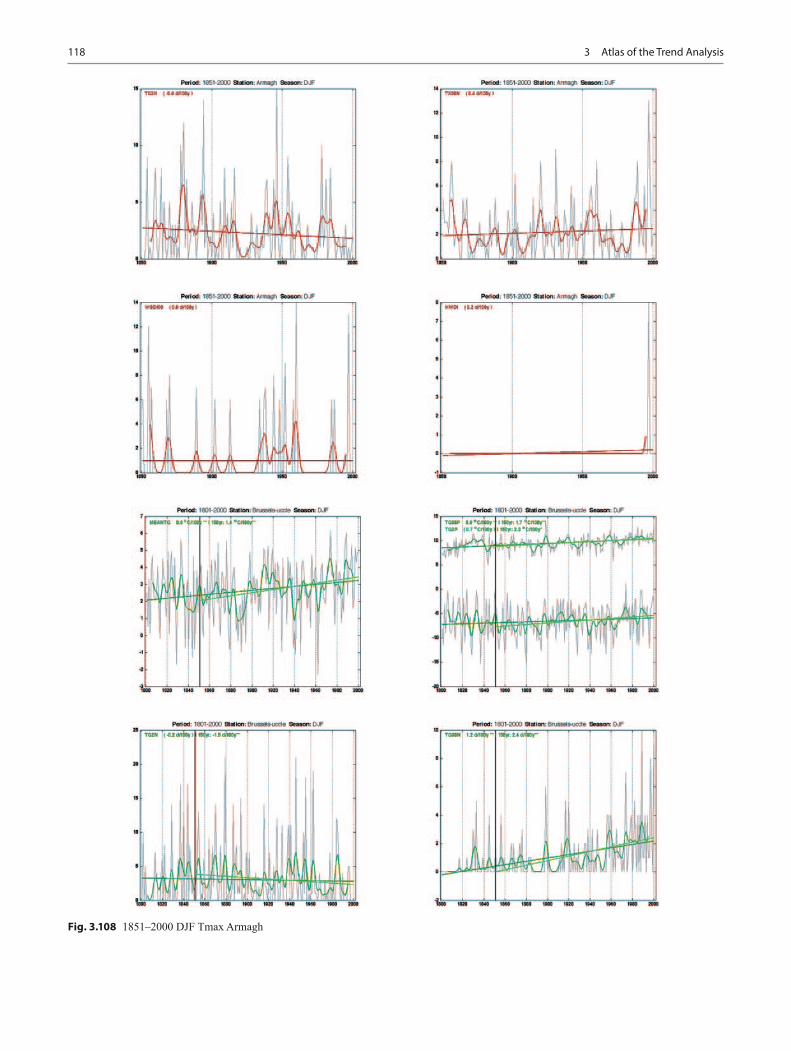
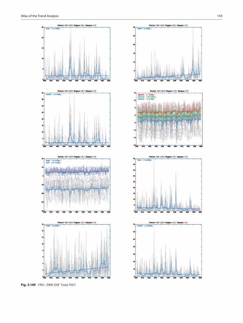
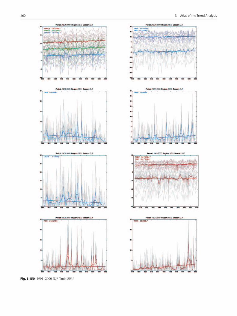
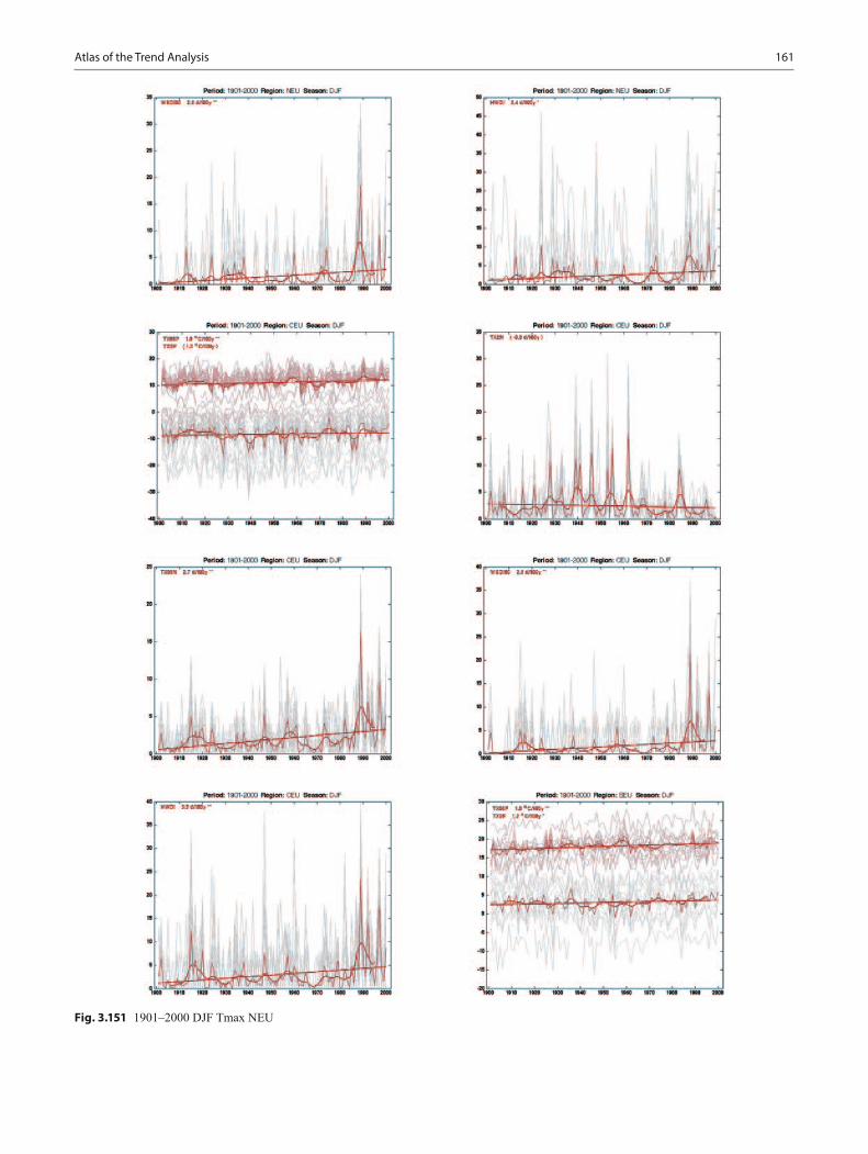
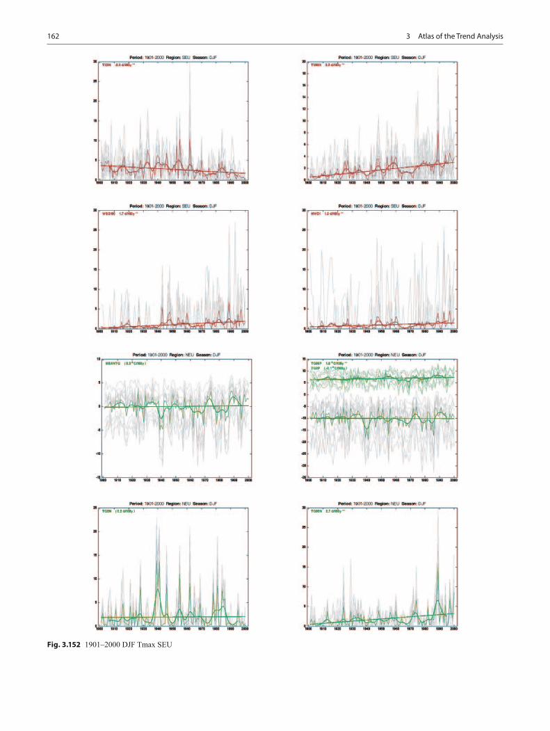
for the period 1901–2000 on background plots containing all contributing individual station time series (in light grey lines). Each figure shows annual values of an index for a sea-son, its low-frequency variation and long-term linear trend (Fig. 3.2). The smoothed curve emphasizing low-frequency variation is a 10-year Gaussian filter applied to the original time-series suppressing variations on time-scales less than 10 years. The straight solid line shows the linear trend estimated by linear regression for the period in question. The statistical trend significance is indicated as follows: ‘*’ significant at p < 0.05, ‘**’ significant at p < 0.01, and ‘()’ not significant. In each figure analysis period, the names of stations or re-gion, season, index name and trend unit are indicated. To save space, two (and sometimes three) indices or two trend lines for two periods are plotted in the same figure whenever appropriate and feasible (Figs. 3.3, 3.4, 3.5, 3.6, 3.7, 3.8, 3.9, 3.10, 3.11, 3.12, 3.13, 3.14, 3.15, 3.16, 3.17, 3.18, 3.19, 3.20, 3.21, 3.22, 3.23, 3.24, 3.25, 3.26, 3.27, 3.28, 3.29, 3.30, 3.31, 3.32, 3.33, 3.34, 3.35, 3.36, 3.37, 3.38, 3.39, 3.40, 3.41, 3.42, 3.43, 3.44, 3.45, 3.46, 3.47, 3.48, 3.49, 3.50, 3.51, 3.52, 3.53, 3.54, 3.55, 3.56, 3.57, 3.58, 3.59, 3.60, 3.61, 3.62, 3.63, 3.64, 3.65, 3.66, 3.67, 3.68, 3.69, 3.70, 3.71, 3.72, 3.73, 3.74, 3.75, 3.76, 3.77, 3.78, 3.79, 3.80, 3.81, 3.82, 3.83, 3.84, 3.85, 3.86, 3.87, 3.88, 3.89, 3.90, 3.91, 3.92, 3.93, 3.94, 3.95, 3.96, 3.97, 3.98, 3.99, 3.100, 3.101, 3.102, 3.103, 3.104, 3.105, 3.106, 3.107, 3.108, 3.109, 3.110, 3.111, 3.112, 3.113, 3.114, 3.115, 3.116, 3.117, 3.118, 3.119, 3.120, 3.121, 3.122, 3.123, 3.124, 3.125, 3.126, 3.127, 3.128, 3.129, 3.130, 3.131, 3.132, 3.133, 3.134, 3.135, 3.136, 3.137, 3.138, 3.139, 3.140, 3.141, 3.142, 3.143, 3.144, 3.145, 3.146, 3.147, 3.148, 3.149, 3.150, 3.151, 3.152, 3.153, 3.154, 3.155, 3.156).
12 3 Atlas of the Trend Analysis
Fig. 3.1 Map layout and legend used throughout the atlas. Color scales change depending on the index
Fig. 3.2 Layout and legend for the time-series plots
13Atlas of the Trend Analysis
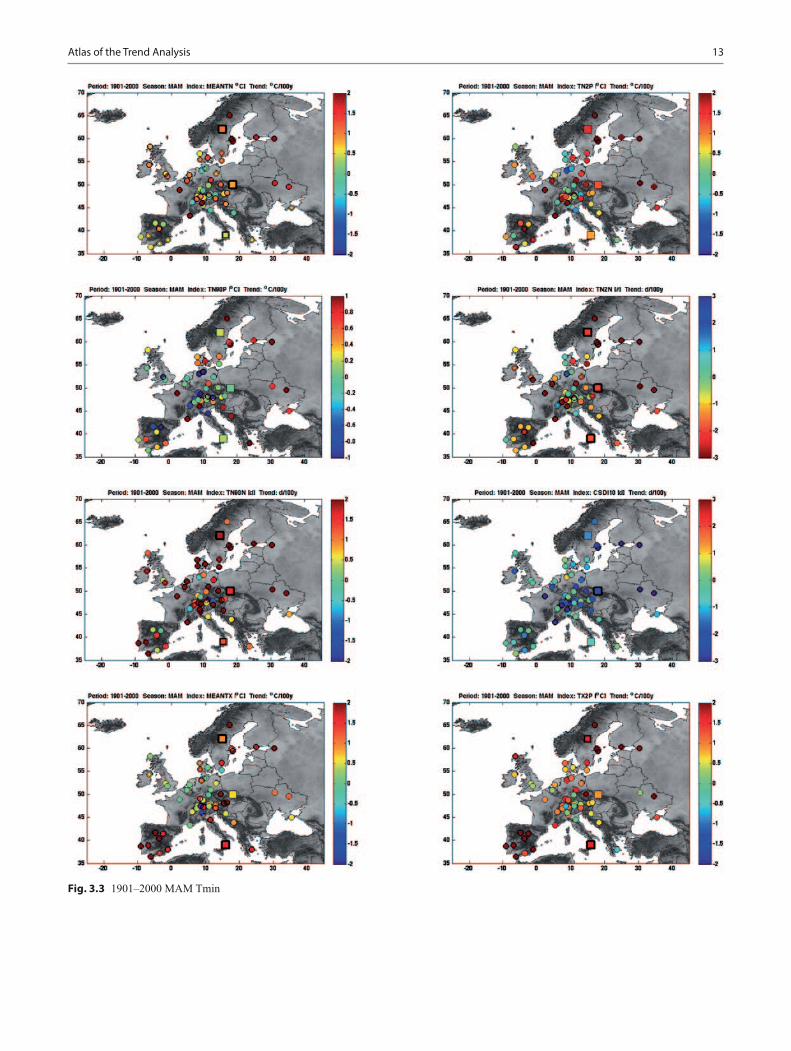
Fig. 3.3 1901–2000 MAM Tmin
14 3 Atlas of the Trend Analysis
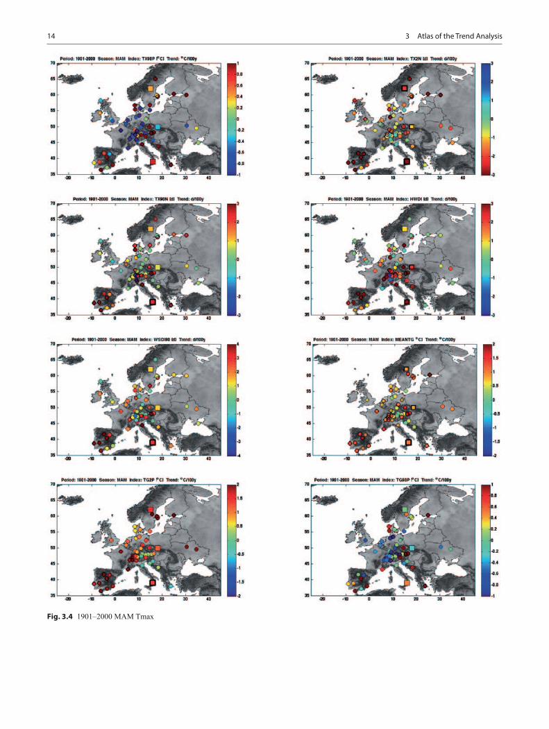
Fig. 3.4 1901–2000 MAM Tmax
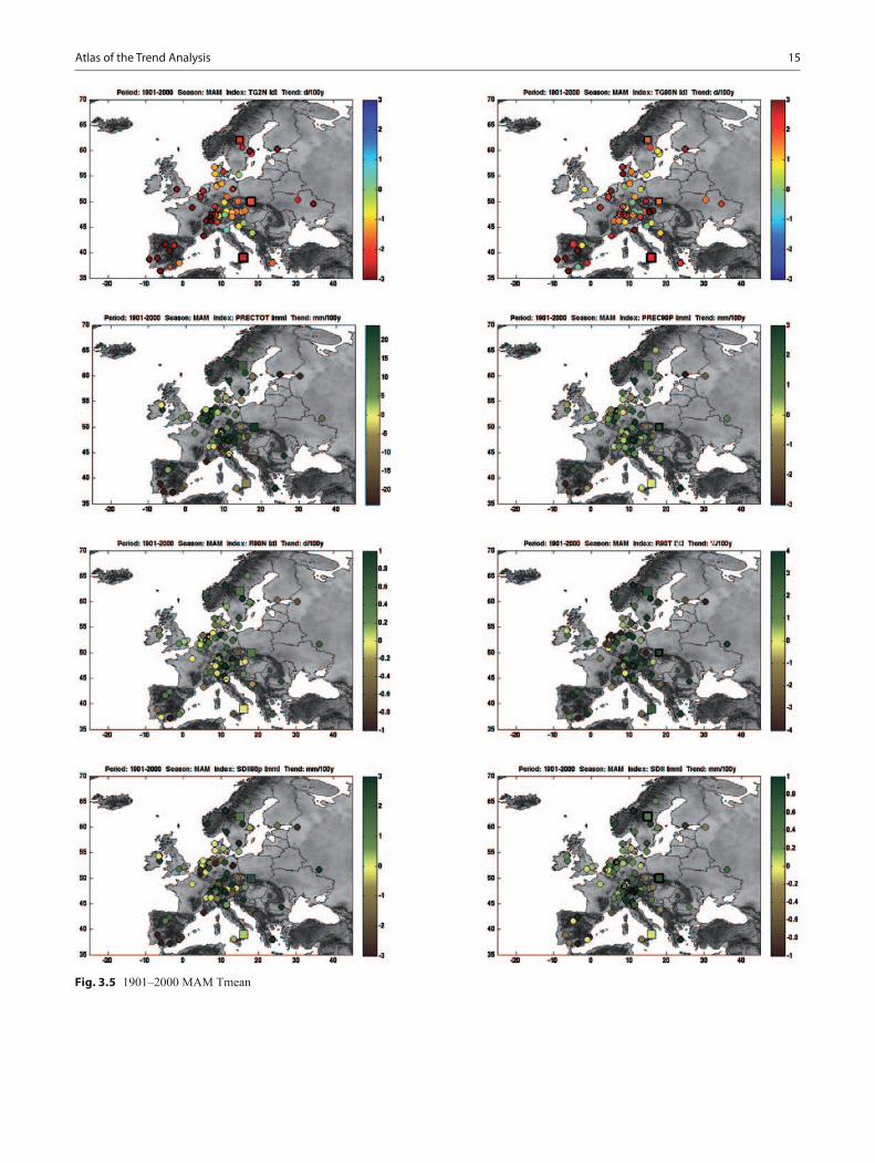
15Atlas of the Trend Analysis
Fig. 3.5 1901–2000 MAM Tmean
16 3 Atlas of the Trend Analysis
Fig. 3.6 1901–2000 MAM Prec
17Atlas of the Trend Analysis
Fig. 3.7 1901–2000 JJA Tmin
18 3 Atlas of the Trend Analysis
Fig. 3.8 1901–2000 JJA Tmean
19Atlas of the Trend Analysis
Fig. 3.9 1901–2000 JJA Prec
20 3 Atlas of the Trend Analysis
Fig. 3.10 1901–2000 SON Tmin
21Atlas of the Trend Analysis
Fig. 3.11 1901–2000 SON Tmax
22 3 Atlas of the Trend Analysis
Fig. 3.12 1901–2000 SON Prec
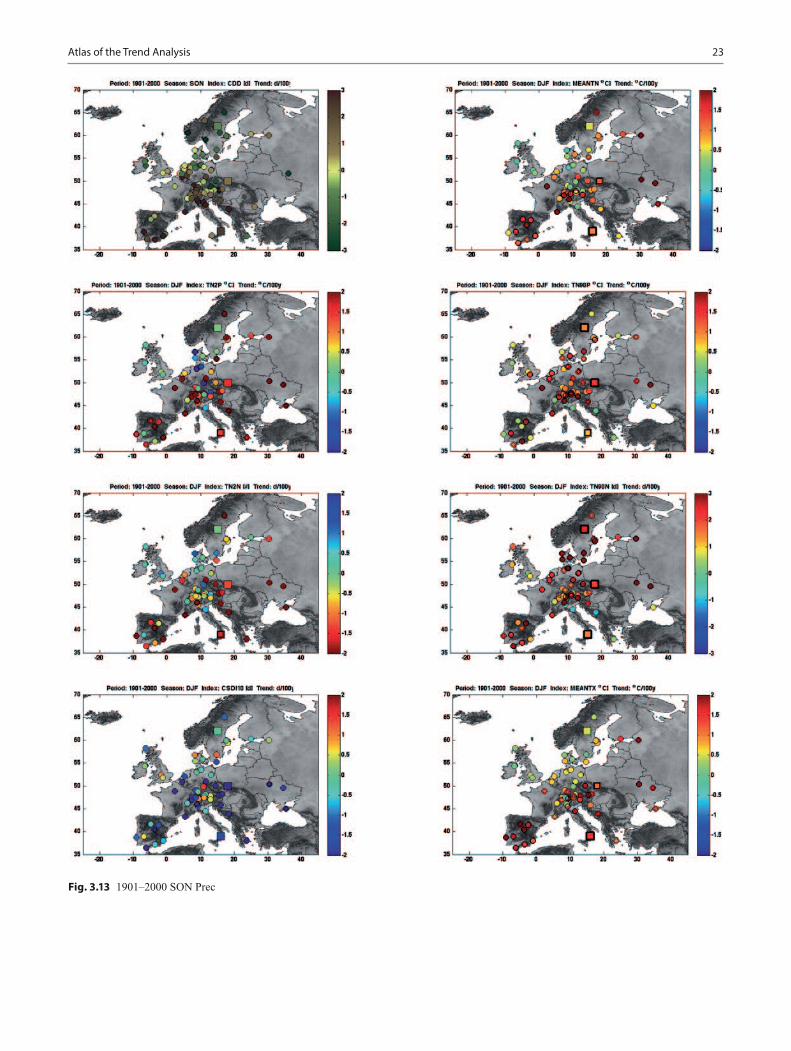
23Atlas of the Trend Analysis
Fig. 3.13 1901–2000 SON Prec
24 3 Atlas of the Trend Analysis
Fig. 3.14 1901–2000 DJF Tmax
25Atlas of the Trend Analysis
Fig. 3.15 1901–2000 DJF Tmean
26 3 Atlas of the Trend Analysis
Fig. 3.16 1901–2000 DJF Prec
27Atlas of the Trend Analysis
Fig. 3.17 1851–2000 MAM Tmin Brussels-uccle
28 3 Atlas of the Trend Analysis
Fig. 3.18 1851–2000 MAM Tmin Prag
29Atlas of the Trend Analysis
Fig. 3.19 1851–2000 MAM Tmin Jena
30 3 Atlas of the Trend Analysis
Fig. 3.20 1851–2000 MAM Tmin Bologna
31Atlas of the Trend Analysis
Fig. 3.21 1851–2000 MAM Tmin Cadiz
32 3 Atlas of the Trend Analysis
Fig. 3.22 1851–2000 MAM Tmin Armagh
33Atlas of the Trend Analysis
Fig. 3.23 1851–2000 MAM Tmax Brussels-uccle
34 3 Atlas of the Trend Analysis
Fig. 3.24 1851–2000 MAM Tmax Helsinki
35Atlas of the Trend Analysis
Fig. 3.25 1851–2000 MAM Tmax Jena
36 3 Atlas of the Trend Analysis
Fig. 3.26 1851–2000 MAM Tmax Milano
37Atlas of the Trend Analysis
Fig. 3.27 1851–2000 MAM Tmax Uppsala
38 3 Atlas of the Trend Analysis
Fig. 3.28 1851–2000 MAM Tmax Armagh
39Atlas of the Trend Analysis
Fig. 3.29 1851–2000 MAM Tmean Prag
40 3 Atlas of the Trend Analysis
Fig. 3.30 1851–2000 MAM Tmean Hohenpeissenberg
41Atlas of the Trend Analysis
Fig. 3.31 1851–2000 MAM Tmean Stykkisholmur
42 3 Atlas of the Trend Analysis
Fig. 3.32 1851–2000 MAM Tmean Milano
43Atlas of the Trend Analysis
Fig. 3.33 1851–2000 MAM Tmean Cadiz
44 3 Atlas of the Trend Analysis
Fig. 3.34 1851–2000 MAM Tmean Uppsala
45Atlas of the Trend Analysis
Fig. 3.35 1851–2000 MAM Prec Prag
46 3 Atlas of the Trend Analysis
Fig. 3.36 1851–2000 MAM Prec Helsinki
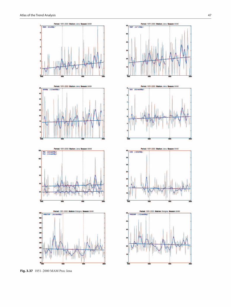
47Atlas of the Trend Analysis
Fig. 3.37 1851–2000 MAM Prec Jena
48 3 Atlas of the Trend Analysis
Fig. 3.38 1851–2000 MAM Prec Bologna
49Atlas of the Trend Analysis
Fig. 3.39 1851–2000 MAM Prec De-kooy
50 3 Atlas of the Trend Analysis
Fig. 3.40 1851–2000 MAM Prec Eelde
51Atlas of the Trend Analysis
Fig. 3.41 1851–2000 MAM Prec Groningen
52 3 Atlas of the Trend Analysis
Fig. 3.42 1851–2000 MAM Prec Uppsala
53Atlas of the Trend Analysis
Fig. 3.43 1851–2000 MAM Prec Armagh
54 3 Atlas of the Trend Analysis
Fig. 3.44 1851–2000 JJA Tmin Brussels-uccle
55Atlas of the Trend Analysis
Fig. 3.45 1851–2000 JJA Tmin Helsinki
56 3 Atlas of the Trend Analysis
Fig. 3.46 1851–2000 JJA Tmin Jena
57Atlas of the Trend Analysis
Fig. 3.47 1851–2000 JJA Tmin Milano
58 3 Atlas of the Trend Analysis
Fig. 3.48 1851–2000 JJA Tmin Cadiz
59Atlas of the Trend Analysis
Fig. 3.49 1851–2000 JJA Tmin Armagh
60 3 Atlas of the Trend Analysis
Fig. 3.50 1851–2000 JJA Tmax Prag
61Atlas of the Trend Analysis
Fig. 3.51 1851–2000 JJA Tmax Helsinki
62 3 Atlas of the Trend Analysis
Fig. 3.52 1851–2000 JJA Tmax Bologna
63Atlas of the Trend Analysis
Fig. 3.53 1851–2000 JJA Tmax Milano
64 3 Atlas of the Trend Analysis
Fig. 3.54 1851–2000 JJA Tmax Uppsala
65Atlas of the Trend Analysis
Fig. 3.55 1851–2000 JJA Tmean Brussels-uccle
66 3 Atlas of the Trend Analysis
Fig. 3.56 1851–2000 JJA Tmean Helsinki
67Atlas of the Trend Analysis
Fig. 3.57 1851–2000 JJA Tmean Jena
68 3 Atlas of the Trend Analysis
Fig. 3.58 1851–2000 JJA Tmean Bologna
69Atlas of the Trend Analysis
Fig. 3.59 1851–2000 JJA Tmean St-petersburg
70 3 Atlas of the Trend Analysis
Fig. 3.60 1851–2000 JJA Tmean Stockholm
71Atlas of the Trend Analysis
Fig. 3.61 1851–2000 JJA Tmean Cet
72 3 Atlas of the Trend Analysis
Fig. 3.62 1851–2000 JJA Prec Prag
73Atlas of the Trend Analysis
Fig. 3.63 1851–2000 JJA Prec Helsinki
74 3 Atlas of the Trend Analysis
Fig. 3.64 1851–2000 JJA Prec Jena
75Atlas of the Trend Analysis
Fig. 3.65 1851–2000 JJA Prec Bologna
76 3 Atlas of the Trend Analysis
Fig. 3.66 1851–2000 JJA Prec De-kooy
77Atlas of the Trend Analysis
Fig. 3.67 1851–2000 JJA Prec Eelde
78 3 Atlas of the Trend Analysis
Fig. 3.68 1851–2000 JJA Prec Groningen
79Atlas of the Trend Analysis
Fig. 3.69 1851–2000 JJA Prec Uppsala
80 3 Atlas of the Trend Analysis
Fig. 3.70 1851–2000 JJA Prec Armagh
81Atlas of the Trend Analysis
Fig. 3.71 1851–2000 SON Tmin Brussels-uccle
82 3 Atlas of the Trend Analysis
Fig. 3.72 1851–2000 SON Tmin Helsinki
83Atlas of the Trend Analysis
Fig. 3.73 1851–2000 SON Tmin Bologna
84 3 Atlas of the Trend Analysis
Fig. 3.74 1851–2000 SON Tmin Milano
85Atlas of the Trend Analysis
Fig. 3.75 1851–2000 SON Tmin Uppsala
86 3 Atlas of the Trend Analysis
Fig. 3.76 1851–2000 SON Tmin Armagh
87Atlas of the Trend Analysis
Fig. 3.77 1851–2000 SON Tmax Prag
88 3 Atlas of the Trend Analysis
Fig. 3.78 1851–2000 SON Tmax Jena
89Atlas of the Trend Analysis
Fig. 3.79 1851–2000 SON Tmax Bologna
90 3 Atlas of the Trend Analysis
Fig. 3.80 1851–2000 SON Tmax Cadiz
91Atlas of the Trend Analysis
Fig. 3.81 1851–2000 SON Tmax Uppsala
92 3 Atlas of the Trend Analysis
Fig. 3.82 1851–2000 SON Tmean Brussels-uccle
93Atlas of the Trend Analysis
Fig. 3.83 1851–2000 SON Tmean Helsinki
94 3 Atlas of the Trend Analysis
Fig. 3.84 1851–2000 SON Tmean Jena
95Atlas of the Trend Analysis
Fig. 3.85 1851–2000 SON Tmean Bologna
96 3 Atlas of the Trend Analysis
Fig. 3.86 1851–2000 SON Tmean St-petersburg
97Atlas of the Trend Analysis
Fig. 3.87 1851–2000 SON Tmean Stockholm
98 3 Atlas of the Trend Analysis
Fig. 3.88 1851–2000 SON Tmean Cet
99Atlas of the Trend Analysis
Fig. 3.89 1851–2000 SON Prec Prag
100 3 Atlas of the Trend Analysis
Fig. 3.90 1851–2000 SON Prec Helsinki
101Atlas of the Trend Analysis
Fig. 3.91 1851–2000 SON Prec Jena
102 3 Atlas of the Trend Analysis
Fig. 3.92 1851–2000 SON Prec Bologna
103Atlas of the Trend Analysis
Fig. 3.93 1851–2000 SON Prec De-kooy
104 3 Atlas of the Trend Analysis
Fig. 3.94 1851–2000 SON Prec Eelde
105Atlas of the Trend Analysis
Fig. 3.95 1851–2000 SON Prec Groningen
106 3 Atlas of the Trend Analysis
Fig. 3.96 1851–2000 SON Prec Uppsala
107Atlas of the Trend Analysis
Fig. 3.97 1851–2000 SON Prec Armagh
108 3 Atlas of the Trend Analysis
Fig. 3.98 1851–2000 DJF Tmin Prag
109Atlas of the Trend Analysis
Fig. 3.99 1851–2000 DJF Tmin Helsinki
110 3 Atlas of the Trend Analysis
Fig. 3.100 1851–2000 DJF Tmin Bologna
111Atlas of the Trend Analysis
Fig. 3.101 1851–2000 DJF Tmin Cadiz
112 3 Atlas of the Trend Analysis
Fig. 3.102 1851–2000 DJF Tmin Uppsala
113Atlas of the Trend Analysis
Fig. 3.103 1851–2000 DJF Tmax Brussels-uccle
114 3 Atlas of the Trend Analysis
Fig. 3.104 1851–2000 DJF Tmax Prag
115Atlas of the Trend Analysis
Fig. 3.105 1851–2000 DJF Tmax Jena
116 3 Atlas of the Trend Analysis
Fig. 3.106 1851–2000 DJF Tmax Milano
117Atlas of the Trend Analysis
Fig. 3.107 1851–2000 DJF Tmax Cadiz
118 3 Atlas of the Trend Analysis
Fig. 3.108 1851–2000 DJF Tmax Armagh
119Atlas of the Trend Analysis
Fig. 3.109 1851–2000 DJF Tmean Prag
120 3 Atlas of the Trend Analysis
Fig. 3.110 1851–2000 DJF Tmean Hohenpeissenberg
121Atlas of the Trend Analysis
Fig. 3.111 1851–2000 DJF Tmean Stykkisholmur
122 3 Atlas of the Trend Analysis
Fig. 3.112 1851–2000 DJF Tmean Milano
123Atlas of the Trend Analysis
Fig. 3.113 1851–2000 DJF Tmean Cadiz
124 3 Atlas of the Trend Analysis
Fig. 3.114 1851–2000 DJF Tmean Uppsala
125Atlas of the Trend Analysis
Fig. 3.115 1851–2000 DJF Prec Prag
126 3 Atlas of the Trend Analysis
Fig. 3.116 1851–2000 DJF Prec Helsinki
127Atlas of the Trend Analysis
Fig. 3.117 1851–2000 DJF Prec Jena
128 3 Atlas of the Trend Analysis
Fig. 3.118 1851–2000 DJF Prec Bologna
129Atlas of the Trend Analysis
Fig. 3.119 1851–2000 DJF Prec De-kooy
130 3 Atlas of the Trend Analysis
Fig. 3.120 1851–2000 DJF Prec Eelde
131Atlas of the Trend Analysis
Fig. 3.121 1851–2000 DJF Prec Groningen
132 3 Atlas of the Trend Analysis
Fig. 3.122 1851–2000 DJF Prec Uppsala
133Atlas of the Trend Analysis
Fig. 3.123 1851–2000 DJF Prec Armagh
134 3 Atlas of the Trend Analysis
Fig. 3.124 1901–2000 MAM Tmin NEU
135Atlas of the Trend Analysis
Fig. 3.125 1901–2000 MAM Tmin CEU
136 3 Atlas of the Trend Analysis
Fig. 3.126 1901–2000 MAM Tmax NEU
137Atlas of the Trend Analysis
Fig. 3.127 1901–2000 MAM Tmax CEU
138 3 Atlas of the Trend Analysis
Fig. 3.128 1901–2000 MAM Tmean NEU
139Atlas of the Trend Analysis
Fig. 3.129 1901–2000 MAM Tmean SEU
140 3 Atlas of the Trend Analysis
Fig. 3.130 1901–2000 MAM Prec NEU
141Atlas of the Trend Analysis
Fig. 3.131 1901–2000 MAM Prec CEU
142 3 Atlas of the Trend Analysis
Fig. 3.132 1901–2000 MAM Prec SEU
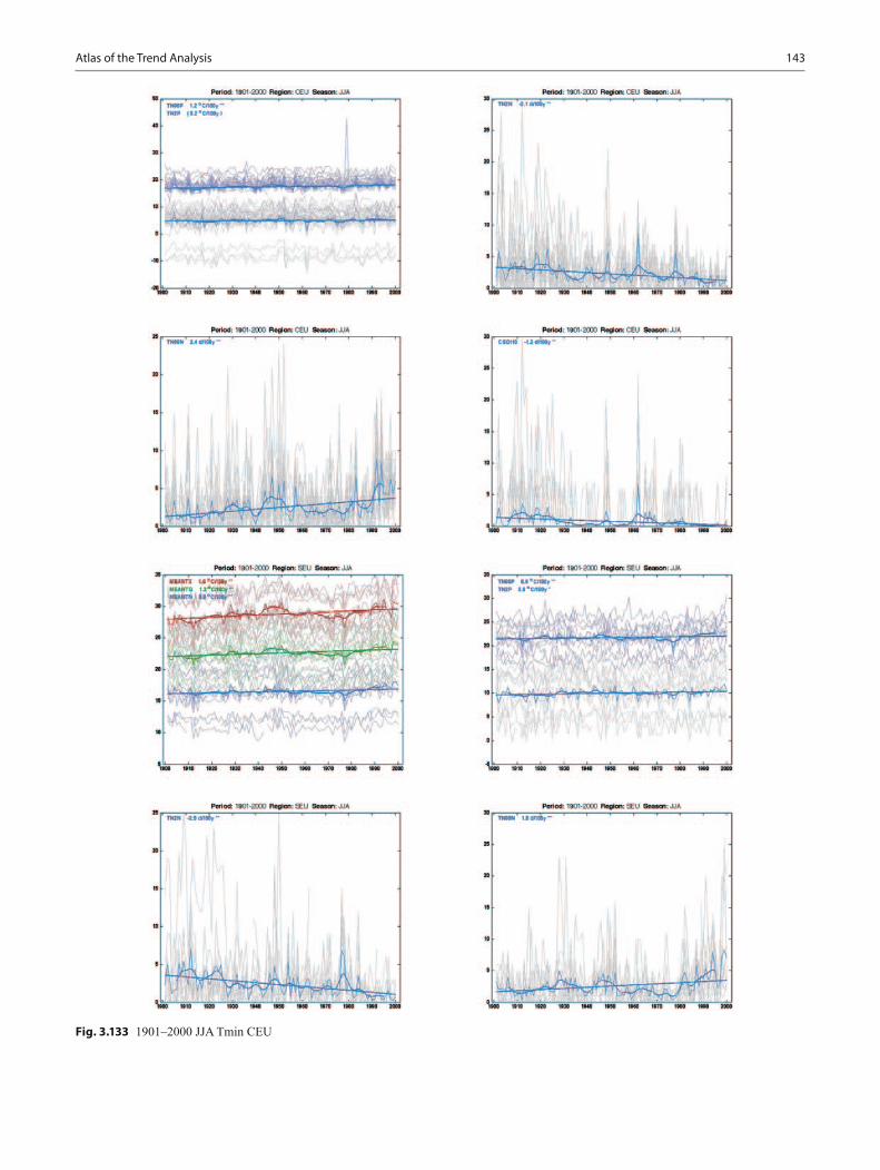
143Atlas of the Trend Analysis
Fig. 3.133 1901–2000 JJA Tmin CEU
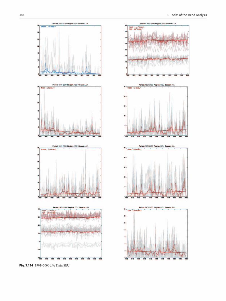
144 3 Atlas of the Trend Analysis
Fig. 3.134 1901–2000 JJA Tmin SEU
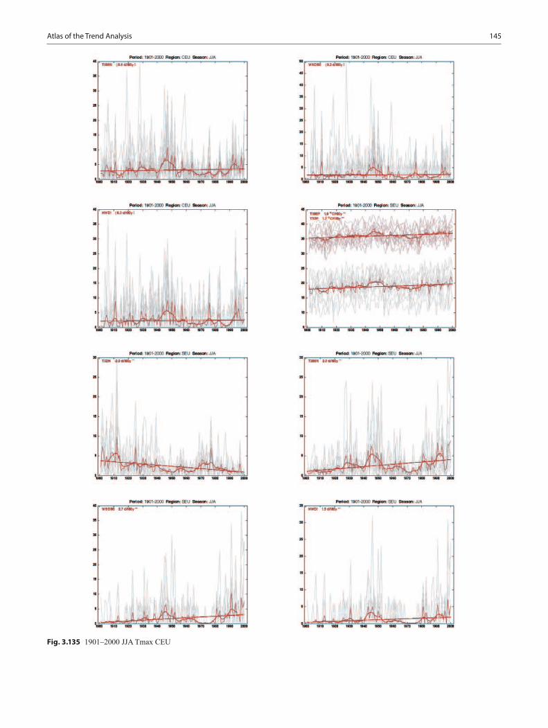
145Atlas of the Trend Analysis
Fig. 3.135 1901–2000 JJA Tmax CEU
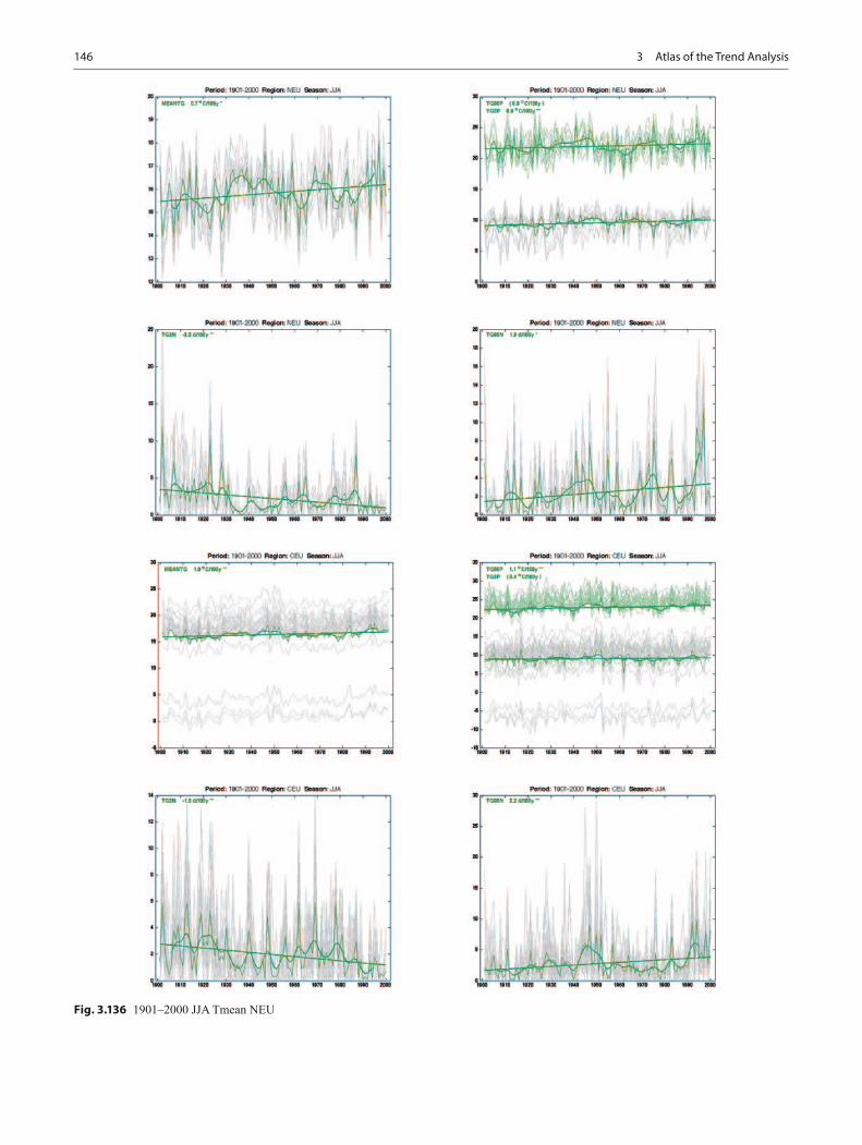
146 3 Atlas of the Trend Analysis
Fig. 3.136 1901–2000 JJA Tmean NEU
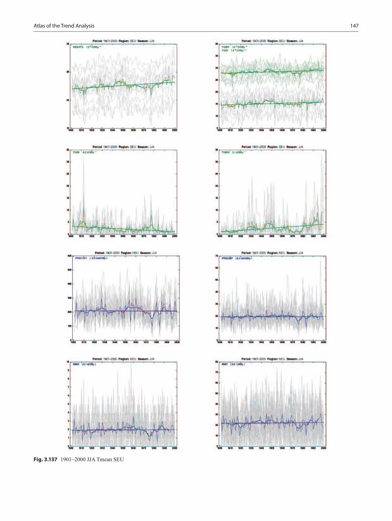
147Atlas of the Trend Analysis
Fig. 3.137 1901–2000 JJA Tmean SEU
148 3 Atlas of the Trend Analysis
Fig. 3.138 1901–2000 JJA Prec NEU
149Atlas of the Trend Analysis
Fig. 3.139 1901–2000 JJA Prec CEU
150 3 Atlas of the Trend Analysis
Fig. 3.140 1901–2000 JJA Prec SEU
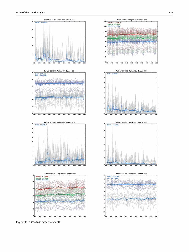
151Atlas of the Trend Analysis
Fig. 3.141 1901–2000 SON Tmin NEU
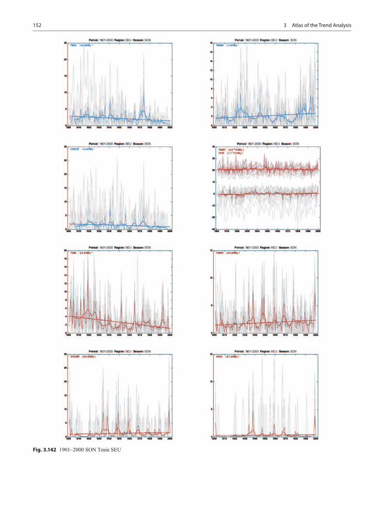
152 3 Atlas of the Trend Analysis
Fig. 3.142 1901–2000 SON Tmin SEU
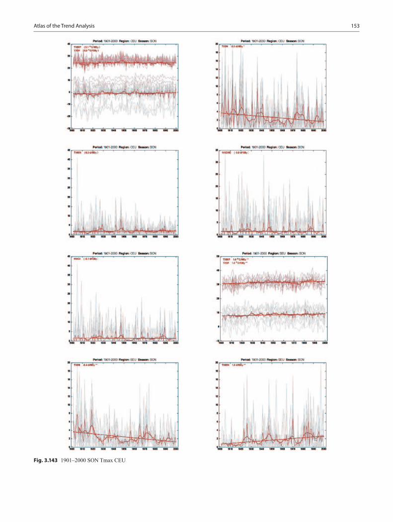
153Atlas of the Trend Analysis
Fig. 3.143 1901–2000 SON Tmax CEU
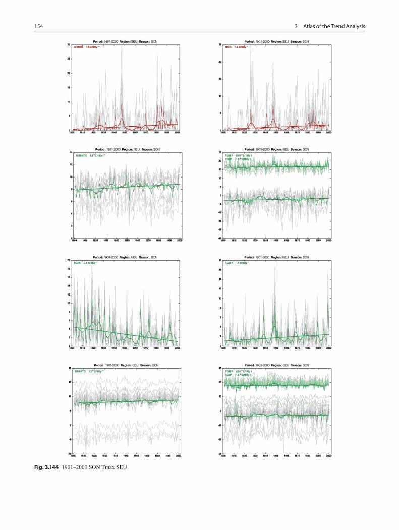
154 3 Atlas of the Trend Analysis
Fig. 3.144 1901–2000 SON Tmax SEU
155Atlas of the Trend Analysis
Fig. 3.145 1901–2000 SON Tmean CEU
156 3 Atlas of the Trend Analysis
Fig. 3.146 1901–2000 SON Prec NEU
157Atlas of the Trend Analysis
Fig. 3.147 1901–2000 SON Prec CEU
158 3 Atlas of the Trend Analysis
Fig. 3.148 1901–2000 SON Prec SEU
159Atlas of the Trend Analysis
Fig. 3.149 1901–2000 DJF Tmin NEU
160 3 Atlas of the Trend Analysis
Fig. 3.150 1901–2000 DJF Tmin SEU
161Atlas of the Trend Analysis
Fig. 3.151 1901–2000 DJF Tmax NEU
162 3 Atlas of the Trend Analysis
Fig. 3.152 1901–2000 DJF Tmax SEU
163Atlas of the Trend Analysis
Fig. 3.153 1901–2000 DJF Tmean CEU
164 3 Atlas of the Trend Analysis
Fig. 3.154 1901–2000 DJF Prec NEU
165Atlas of the Trend Analysis
Fig. 3.155 1901–2000 DJF Prec CEU
166 3 Atlas of the Trend Analysis
Fig. 3.156 1901–2000 DJF Prec SEU
167
Summary of the Estimated Trends
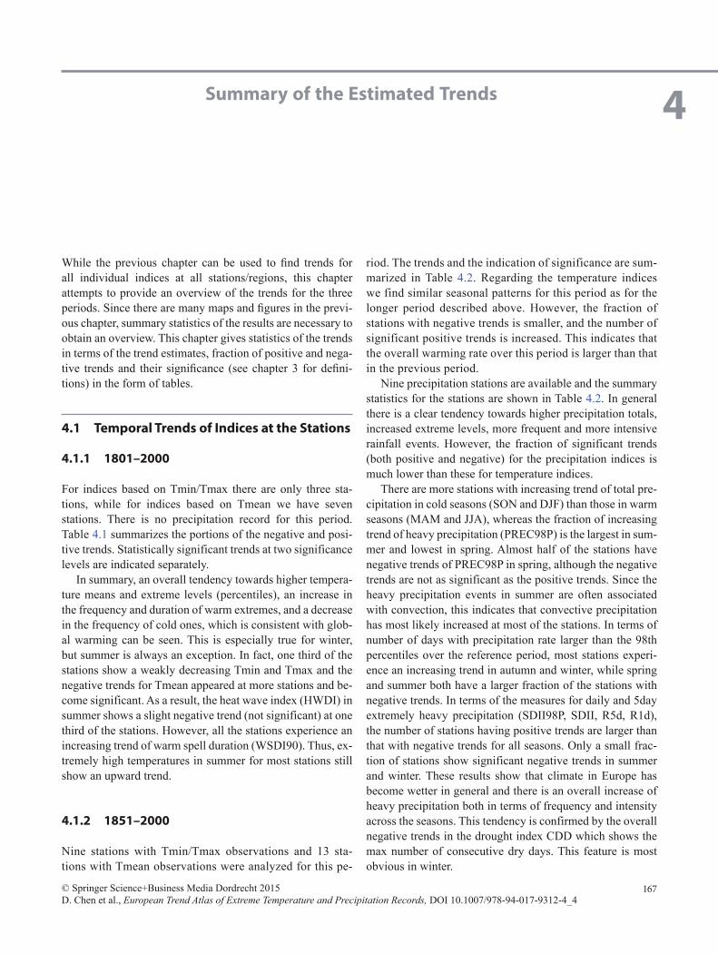
While the previous chapter can be used to find trends for all individual indices at all stations/regions, this chapter attempts to provide an overview of the trends for the three periods. Since there are many maps and figures in the previ-ous chapter, summary statistics of the results are necessary to obtain an overview. This chapter gives statistics of the trends in terms of the trend estimates, fraction of positive and nega-tive trends and their significance (see chapter 3 for defini-tions) in the form of tables.
4.1 Temporal Trends of Indices at the Stations
4.1.1 1801 –2000
For indices based on Tmin/Tmax there are only three sta-tions, while for indices based on Tmean we have seven stations. There is no precipitation record for this period. Table 4.1 summarizes the portions of the negative and posi-tive trends. Statistically significant trends at two significance levels are indicated separately.
In summary, an overall tendency towards higher tempera-ture means and extreme levels (percentiles), an increase in the frequency and duration of warm extremes, and a decrease in the frequency of cold ones, which is consistent with glob-al warming can be seen. This is especially true for winter, but summer is always an exception. In fact, one third of the stations show a weakly decreasing Tmin and Tmax and the negative trends for Tmean appeared at more stations and be-come significant. As a result, the heat wave index (HWDI) in summer shows a slight negative trend (not significant) at one third of the stations. However, all the stations experience an increasing trend of warm spell duration (WSDI90). Thus, ex-tremely high temperatures in summer for most stations still show an upward trend.
4.1.2 1851 –2000
Nine stations with Tmin/Tmax observations and 13 sta-tions with Tmean observations were analyzed for this pe-
riod. The trends and the indication of significance are sum-marized in Table 4.2. Regarding the temperature indices we find similar seasonal patterns for this period as for the longer period described above. However, the fraction of stations with negative trends is smaller, and the number of significant positive trends is increased. This indicates that the overall warming rate over this period is larger than that in the previous period.
Nine precipitation stations are available and the summary statistics for the stations are shown in Table 4.2. In general there is a clear tendency towards higher precipitation totals, increased extreme levels, more frequent and more intensive rainfall events. However, the fraction of significant trends (both positive and negative) for the precipitation indices is much lower than these for temperature indices.
There are more stations with increasing trend of total pre-cipitation in cold seasons (SON and DJF) than those in warm seasons (MAM and JJA), whereas the fraction of increasing trend of heavy precipitation (PREC98P) is the largest in sum-mer and lowest in spring. Almost half of the stations have negative trends of PREC98P in spring, although the negative trends are not as significant as the positive trends. Since the heavy precipitation events in summer are often associated with convection, this indicates that convective precipitation has most likely increased at most of the stations. In terms of number of days with precipitation rate larger than the 98th percentiles over the reference period, most stations experi-ence an increasing trend in autumn and winter, while spring and summer both have a larger fraction of the stations with negative trends. In terms of the measures for daily and 5day extremely heavy precipitation (SDII98P, SDII, R5d, R1d), the number of stations having positive trends are larger than that with negative trends for all seasons. Only a small frac-tion of stations show significant negative trends in summer and winter. These results show that climate in Europe has become wetter in general and there is an overall increase of heavy precipitation both in terms of frequency and intensity across the seasons. This tendency is confirmed by the overall negative trends in the drought index CDD which shows the max number of consecutive dry days. This feature is most obvious in winter.
© Springer Science+Business Media Dordrecht 2015D. Chen et al., European Trend Atlas of Extreme Temperature and Precipitation Records, DOI 10.1007/978-94-017-9312-4_4
4
168 4 Summary of the Estimated Trends4 Summary of the Estimated Trends
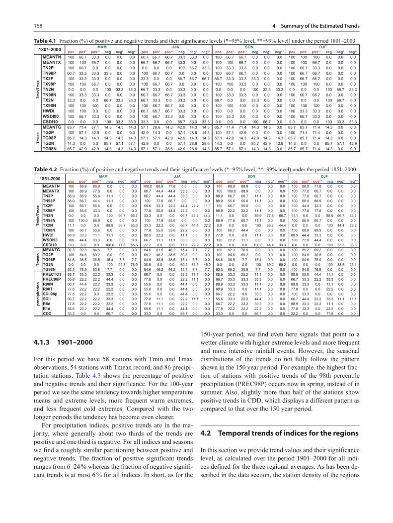
4.1.3 1901–2000
For this period we have 58 stations with Tmin and Tmax observations, 54 stations with Tmean record, and 86 precipi-tation stations. Table 4.3 shows the percentage of positive and negative trends and their significance. For the 100-year period we see the same tendency towards higher temperature means and extreme levels, more frequent warm extremes, and less frequent cold extremes. Compared with the two longer periods the tendency has become even clearer.
For precipitation indices, positive trends are in the ma-jority, where generally about two thirds of the trends are positive and one third is negative. For all indices and seasons we find a roughly similar partitioning between positive and negative trends. The fraction of positive significant trends ranges from 6–24 % whereas the fraction of negative signifi-cant trends is at most 6 % for all indices. In short, as for the
150-year period, we find even here signals that point to a wetter climate with higher extreme levels and more frequent and more intensive rainfall events. However, the seasonal distributions of the trends do not fully follow the pattern shown in the 150 year period. For example, the highest frac-tion of stations with positive trends of the 98th percentile precipitation (PREC98P) occurs now in spring, instead of in summer. Also, slightly more than half of the stations show positive trends in CDD, which displays a different pattern as compared to that over the 150 year period.
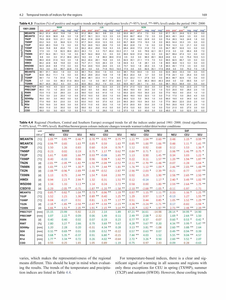
4.2 Temporal trends of indices for the regions
In this section we provide trend values and their significance level, as calculated over the period 1901–2000 for all indi-ces defined for the three regional averages. As has been de-scribed in the data section, the station density of the regions
Table 4.1 Fraction (%) of positive and negative trends and their significance levels (*=95% level, **=99% level) under the period 1801–2000
pos pos* pos** neg neg* neg** pos pos* pos** neg neg* neg** pos pos* pos** neg neg* neg** pos pos* pos** neg neg* neg**MEANTN 100 88.9 88.9 0.0 0.0 0.0 100.0 88.9 77.8 0.0 0.0 0.0 100 88.9 88.9 0.0 0.0 0.0 100 88.9 77.8 0.0 0.0 0.0MEANTX 100 88.9 77.8 0.0 0.0 0.0 66.7 44.4 44.4 33.3 0.0 0.0 100 100.0 88.9 0.0 0.0 0.0 100 77.8 66.7 0.0 0.0 0.0TN2P 88.9 88.9 55.6 11.1 0.0 0.0 66.7 44.4 44.4 33.3 0.0 0.0 88.9 66.7 66.7 11.1 0.0 0.0 100 77.8 66.7 0.0 0.0 0.0TN98P 88.9 66.7 44.4 11.1 0.0 0.0 100 77.8 66.7 0.0 0.0 0.0 88.9 55.6 55.6 11.1 0.0 0.0 100 88.9 88.9 0.0 0.0 0.0TX2P 100 66.7 55.6 0.0 0.0 0.0 55.6 33.3 22.2 44.4 22.2 11.1 100 66.7 55.6 0.0 0.0 0.0 100 44.4 33.3 0.0 0.0 0.0TX98P 100 55.6 33.3 0.0 0.0 0.0 77.8 55.6 44.4 22.2 0.0 0.0 88.9 22.2 22.2 11.1 0.0 0.0 100 77.8 77.8 0.0 0.0 0.0TN2N 0.0 0.0 0.0 100 66.7 66.7 33.3 0.0 0.0 66.7 44.4 44.4 11.1 0.0 0.0 88.9 77.8 66.7 11.1 0.0 0.0 88.9 66.7 33.3TN98N 100 100.0 88.9 0.0 0.0 0.0 100 77.8 55.6 0.0 0.0 0.0 88.9 77.8 66.7 11.1 0.0 0.0 100 88.9 66.7 0.0 0.0 0.0TX2N 11.1 0.0 0.0 88.9 66.7 55.6 33.3 22.2 0.0 66.7 44.4 22.2 0.0 0.0 0.0 100 66.7 44.4 0.0 0.0 0.0 100 44.4 22.2TX98N 100 66.7 55.6 0.0 0.0 0.0 77.8 55.6 55.6 22.2 0.0 0.0 100 66.7 44.4 0.0 0.0 0.0 100 88.9 88.9 0.0 0.0 0.0HWDI 88.9 33.3 11.1 11.1 0.0 0.0 88.9 22.2 0.0 11.1 0.0 0.0 77.8 0.0 0.0 11.1 0.0 0.0 88.9 44.4 33.3 0.0 0.0 0.0WSDI90 100 44.4 33.3 0.0 0.0 0.0 66.7 11.1 11.1 33.3 0.0 0.0 100 22.2 11.1 0.0 0.0 0.0 100 77.8 44.4 0.0 0.0 0.0CSDI10 0.0 0.0 0.0 100.0 77.8 55.6 22.2 0.0 0.0 77.8 22.2 22.2 0.0 0.0 0.0 100.0 44.4 33.3 0.0 0.0 0.0 100 33.3 33.3MEANTG 92.3 92.3 84.6 7.7 0.0 0.0 84.6 61.5 46.2 15.4 7.7 7.7 100 92.3 76.9 0.0 0.0 0.0 100 69.2 69.2 0.0 0.0 0.0TG2P 100 84.6 69.2 0.0 0.0 0.0 69.2 46.2 38.5 30.8 0.0 0.0 100 84.6 69.2 0.0 0.0 0.0 100 84.6 30.8 0.0 0.0 0.0TG98P 84.6 38.5 38.5 15.4 7.7 7.7 84.6 38.5 38.5 15.4 7.7 0.0 84.6 38.5 7.7 15.4 0.0 0.0 100 84.6 76.9 0.0 0.0 0.0TG2N 0.0 0.0 0.0 100 92.3 76.9 30.8 0.0 0.0 69.2 61.5 46.2 0.0 0.0 0.0 100 69.2 69.2 0.0 0.0 0.0 100 38.5 23.1TG98N 92.3 76.9 53.8 7.7 0.0 0.0 84.6 46.2 46.2 15.4 7.7 7.7 92.3 69.2 30.8 7.7 0.0 0.0 100 84.6 76.9 0.0 0.0 0.0PRECTOT 66.7 33.3 22.2 33.3 0.0 0.0 66.7 0.0 0.0 33.3 11.1 0.0 88.9 33.3 22.2 11.1 0.0 0.0 88.9 55.6 44.4 11.1 0.0 0.0PREC98P 55.6 22.2 22.2 44.4 0.0 0.0 77.8 0.0 0.0 22.2 11.1 0.0 66.7 33.3 33.3 33.3 0.0 0.0 66.7 33.3 22.2 33.3 0.0 0.0R98N 66.7 44.4 22.2 33.3 0.0 0.0 55.6 0.0 0.0 44.4 0.0 0.0 88.9 33.3 33.3 11.1 0.0 0.0 88.9 33.3 0.0 11.1 0.0 0.0R98T 77.8 22.2 22.2 22.2 0.0 0.0 55.6 0.0 0.0 44.4 0.0 0.0 88.9 33.3 0.0 11.1 0.0 0.0 77.8 0.0 0.0 22.2 0.0 0.0SDII98p 77.8 22.2 0.0 22.2 0.0 0.0 55.6 0.0 0.0 44.4 0.0 0.0 66.7 22.2 0.0 33.3 0.0 0.0 100 33.3 0.0 0.0 0.0 0.0SDII 66.7 22.2 22.2 33.3 0.0 0.0 77.8 11.1 0.0 22.2 11.1 11.1 55.6 33.3 22.2 44.4 0.0 0.0 66.7 44.4 22.2 33.3 11.1 11.1R5d 77.8 22.2 22.2 22.2 0.0 0.0 77.8 11.1 0.0 22.2 0.0 0.0 66.7 22.2 22.2 33.3 0.0 0.0 88.9 33.3 22.2 11.1 0.0 0.0R1d 55.6 22.2 22.2 44.4 0.0 0.0 55.6 11.1 0.0 44.4 0.0 0.0 77.8 22.2 22.2 22.2 0.0 0.0 77.8 33.3 0.0 22.2 0.0 0.0CDD 33.3 0.0 0.0 66.7 0.0 0.0 33.3 0.0 0.0 66.7 0.0 0.0 33.3 0.0 0.0 66.7 0.0 0.0 22.2 0.0 0.0 77.8 0.0 0.0
DJF
Tmin
/Tm
ax
1851-2000
Tmea
npr
ecip
itatio
n
MAM JJA SON Table 4.2 Fraction (%) of positive and negative trends and their significance levels (*=95% level, **=99% level) under the period 1851–2000
1694.2 Temporal trends of indices for the regions
varies, which makes the representativeness of the regional means different. This should be kept in mind when evaluat-ing the results. The trends of the temperature and precipita-tion indices are listed in Table 4.4.
For temperature-based indices, there is a clear and sig-nificant signal of warming in all seasons and regions with only three exceptions for CEU in spring (TX98P), summer (TX2P) and autumn (HWDI). However, these cooling trends
unit
100 yr-1
MEANTN [°C] 1.09 ** 0.85 ** 0.46 * 0.70 ** 0.92 ** 0.75 ** 1.11 ** 1.04 ** 0.60 ** 0.48 1.19 * 0.99 **
MEANTX [°C] 0.94 ** 0.65 1.63 ** 0.85 * 0.59 1.63 ** 0.85 ** 1.00 ** 1.66 ** 0.48 1.11 * 1.41 **TN2P [°C] 1.50 1.26 0.83 0.60 0.24 0.76 * 1.12 0.92 0.68 0.12 1.53 1.36 *TN98P [°C] 0.23 0.02 0.19 0.75 * 1.17 ** 0.62 ** 0.84 ** 0.71 * 0.17 0.98 ** 1.46 ** 0.75 *TX2P [°C] 1.61 * 0.89 1.66 ** 0.93 ** -0.08 1.65 ** 1.13 0.90 1.45 ** 0.34 1.03 1.22 *TX98P [°C] 0.40 -0.33 0.86 0.96 0.98 * 1.62 ** 0.22 0.11 1.57 ** 1.20 ** 1.94 ** 1.87 **TN2N [d] -2.01 ** -2.05 ** -1.82 ** -1.50 ** -2.09 ** -2.52 ** -2.11 ** -2.70 ** -1.48 ** -0.07 -1.28 -1.64 *TN98N [d] 1.83 ** 1.57 ** 1.30 * 1.71 ** 2.44 ** 1.81 ** 1.76 ** 1.12 ** 1.09 * 2.46 ** 2.03 ** 1.48 **TX2N [d] -2.08 ** -0.96 * -2.89 ** -2.48 ** -0.52 -2.87 ** -2.96 ** -2.03 * -2.39 ** -0.21 -0.77 -1.97 **
TX98N [d] 1.13 0.75 2.44 ** 1.54 * 0.64 2.93 ** 0.92 0.29 1.90 ** 2.58 ** 2.69 ** 2.50 **
HWDI [d] 0.94 2.21 * 2.94 * 1.32 0.31 1.51 ** 0.12 -0.14 1.17 * 2.40 * 3.49 ** 1.02 **
WSDI90 [d] 1.34 1.33 3.13 ** 1.14 0.24 2.72 ** 0.58 0.00 1.80 ** 2.59 ** 2.64 ** 1.75 **
CSDI10 [d] -1.29 -2.05 ** -0.75 -1.87 ** -1.20 ** -1.58 ** -2.10 ** -2.68 ** -1.05 * -0.11 -1.97 -1.71MEANTG [°C] 0.85 * 0.82 * 1.04 ** 0.73 * 0.96 ** 1.19 ** 0.97 ** 1.15 ** 1.11 ** 0.33 1.16 * 1.25 **TG2P [°C] 1.52 1.21 1.36 ** 0.89 ** 0.40 1.25 ** 1.29 0.97 1.13 * -0.13 1.27 1.55 **TG98P [°C] 0.04 -0.27 0.51 0.81 1.15 ** 1.17 ** 0.51 0.44 0.85 * 1.05 ** 1.52 ** 1.29 **TG2N [d] -2.18 * -1.85 ** -2.50 ** -2.47 ** -1.59 ** -2.23 ** -3.38 ** -3.24 ** -1.71 ** 0.17 -0.82 -1.94 *TG98N [d] 1.66 * 1.51 * 2.35 ** 1.91 * 2.15 ** 3.14 ** 1.35 * 1.02 * 1.97 ** 2.73 ** 2.48 ** 2.39 **PRECTOT [mm] 15.15 23.99 -5.92 -2.23 2.14 1.89 47.21 ** 16.61 -14.98 28.14 * 34.99 * 14.90PREC98P [mm] 1.07 2.22 * 0.09 0.06 1.49 0.11 2.49 ** 2.08 * -2.32 1.69 * 2.64 ** 1.50R98N [d] 0.40 0.40 0.02 0.07 0.19 0.23 0.77 ** 0.37 -0.07 0.60 * 0.53 * 0.42 *R98T [%] 2.80 3.27 * 2.66 0.79 3.69 ** 5.67 4.28 ** 3.67 ** 0.20 4.34 ** 3.99 * 5.47 **SDII98p [mm] 1.20 2.28 0.20 -0.31 4.34 ** 0.28 3.13 ** 3.81 ** -1.08 2.60 ** 3.88 ** 2.64SDII [mm] 0.32 ** 0.69 ** 0.01 0.09 0.52 ** -0.22 0.57 ** 0.63 ** 0.07 0.49 ** 0.94 ** 0.39R5d [mm] 3.68 * 5.35 * -0.37 0.91 6.80 * -0.15 7.44 ** 4.03 1.52 5.55 ** 9.04 ** 4.57R1d [mm] 1.77 * 3.34 ** 0.72 0.26 4.02 ** -0.64 2.72 * 3.26 * 0.50 2.60 ** 3.52 * 2.07CDD [d] 0.55 0.25 1.65 1.05 0.89 -1.19 -0.75 0.97 2.43 -0.09 0.28 -0.63
SEUMAM JJA SON DJF
NEU CEU SEU NEU CEU SEU NEU CEU SEU NEU CEU
Table 4.4 Regional (Northern, Central and Southern Europe) averaged trends for all the indices under period 1901–2000. (trend significance *=95% level, **=99% level). Red/blue/brown/green colours indicate changes towards warmer/colder/drier/wetter conditions
pos pos* pos** neg neg* neg** pos pos* pos** neg neg* neg** pos pos* pos** neg neg* neg** pos pos* pos** neg neg* neg**MEANTN 84.2 61.4 45.6 15.8 1.8 0.0 91.2 68.4 56.1 8.8 3.5 3.5 93.0 66.7 47.4 7.0 0.0 0.0 87.7 35.1 24.6 12.3 0.0 0.0MEANTX 91.2 50.9 36.8 8.8 3.5 1.8 87.7 56.1 33.3 12.3 3.5 3.5 93.0 66.7 45.6 7.0 3.5 0.0 96.5 49.1 24.6 3.5 0.0 0.0TN2P 78.9 22.8 10.5 21.1 0.0 0.0 68.4 31.6 22.8 31.6 7.0 5.3 77.2 24.6 14.0 22.8 0.0 0.0 75.4 26.3 14.0 24.6 1.8 0.0TN98P 63.2 14.0 3.5 36.8 12.3 7.0 87.7 54.4 43.9 12.3 0.0 0.0 80.7 36.8 17.5 19.3 1.8 0.0 96.5 54.4 33.3 3.5 0.0 0.0TX2P 93.0 26.3 15.8 7.0 0.0 0.0 70.2 24.6 19.3 29.8 7.0 3.5 98.2 22.8 7.0 1.8 0.0 0.0 78.9 12.3 5.3 21.1 0.0 0.0TX98P 54.4 15.8 8.8 45.6 7.0 3.5 84.2 40.4 29.8 15.8 5.3 3.5 68.4 24.6 17.5 31.6 7.0 3.5 94.7 80.7 52.6 5.3 0.0 0.0TN2N 17.5 3.5 1.8 82.5 38.6 26.3 26.3 7.0 5.3 73.7 40.4 33.3 21.1 1.8 0.0 78.9 42.1 35.1 31.6 0.0 0.0 68.4 8.8 7.0TN98N 87.7 54.4 35.1 12.3 1.8 0.0 94.7 54.4 36.8 5.3 0.0 0.0 86.0 52.6 31.6 14.0 0.0 0.0 94.7 68.4 47.4 5.3 0.0 0.0TX2N 8.8 0.0 0.0 91.2 38.6 26.3 14.0 3.5 1.8 86.0 38.6 31.6 3.5 0.0 0.0 96.5 49.1 36.8 24.6 0.0 0.0 75.4 10.5 5.3TX98N 86.0 43.9 31.6 14.0 3.5 1.8 84.2 40.4 28.1 15.8 3.5 3.5 82.5 35.1 21.1 17.5 7.0 5.3 96.5 82.5 66.7 3.5 0.0 0.0HWDI 84.2 22.8 8.8 15.8 0.0 0.0 73.7 21.1 10.5 26.3 3.5 1.8 64.9 5.3 1.8 28.1 3.5 1.8 89.5 36.8 12.3 5.3 0.0 0.0WSDI90 82.5 24.6 8.8 17.5 0.0 0.0 75.4 24.6 10.5 24.6 3.5 3.5 73.7 14.0 1.8 26.3 3.5 1.8 96.5 49.1 17.5 3.5 0.0 0.0CSDI10 19.3 0.0 0.0 80.7 22.8 7.0 28.1 0.0 0.0 71.9 19.3 14.0 17.5 0.0 0.0 82.5 35.1 17.5 29.8 0.0 0.0 70.2 7.0 1.8MEANTG 98.1 61.1 44.4 1.9 0.0 0.0 98.1 70.4 55.6 1.9 0.0 0.0 98.1 75.9 63.0 1.9 0.0 0.0 92.6 38.9 33.3 5.6 0.0 0.0TG2P 92.6 35.2 11.1 7.4 0.0 0.0 85.2 29.6 20.4 14.8 1.9 1.9 96.3 20.4 5.6 3.7 0.0 0.0 77.8 24.1 9.3 20.4 0.0 0.0TG98P 48.1 7.4 7.4 51.9 7.4 1.9 88.9 48.1 33.3 11.1 1.9 0.0 72.2 22.2 11.1 27.8 0.0 0.0 96.3 66.7 42.6 1.9 0.0 0.0TG2N 3.7 0.0 0.0 96.3 51.9 38.9 9.3 1.9 0.0 90.7 57.4 38.9 3.7 0.0 0.0 96.3 68.5 46.3 29.6 0.0 0.0 68.5 5.6 3.7TG98N 90.7 44.4 35.2 9.3 0.0 0.0 92.6 59.3 35.2 7.4 0.0 0.0 92.6 40.7 24.1 7.4 0.0 0.0 98.1 83.3 64.8 0.0 0.0 0.0PRECTOT 68.0 14.0 4.0 32.0 3.0 2.0 48.0 6.0 4.0 52.0 3.0 2.0 67.0 21.0 12.0 33.0 3.0 0.0 78.0 27.0 10.0 22.0 2.0 1.0PREC98P 80.0 7.0 1.0 20.0 2.0 0.0 60.0 9.0 5.0 40.0 4.0 1.0 66.0 19.0 9.0 34.0 3.0 1.0 72.0 20.0 8.0 28.0 2.0 1.0R98N 72.0 11.0 3.0 28.0 2.0 2.0 59.0 13.0 6.0 41.0 1.0 1.0 65.0 22.0 10.0 35.0 2.0 0.0 77.0 18.0 8.0 23.0 1.0 1.0R98T 75.0 5.0 2.0 25.0 1.0 0.0 67.0 14.0 5.0 33.0 1.0 0.0 68.0 18.0 10.0 32.0 1.0 0.0 71.0 17.0 5.0 29.0 4.0 0.0SDII98p 56.0 8.0 3.0 44.0 0.0 0.0 58.0 11.0 3.0 42.0 1.0 0.0 66.0 12.0 5.0 34.0 1.0 0.0 66.0 19.0 6.0 34.0 0.0 0.0SDII 77.0 19.0 8.0 23.0 3.0 0.0 63.0 14.0 9.0 37.0 4.0 2.0 66.0 24.0 15.0 34.0 5.0 1.0 77.0 38.0 22.0 23.0 2.0 1.0R5d 70.0 10.0 3.0 30.0 3.0 0.0 67.0 11.0 4.0 33.0 1.0 1.0 67.0 20.0 8.0 33.0 2.0 1.0 79.0 20.0 10.0 21.0 2.0 1.0R1d 65.0 11.0 3.0 35.0 0.0 0.0 59.0 8.0 5.0 41.0 0.0 0.0 67.0 13.0 6.0 33.0 1.0 0.0 73.0 21.0 9.0 27.0 3.0 0.0CDD 58.0 5.0 0.0 42.0 1.0 0.0 71.0 1.0 1.0 29.0 1.0 1.0 57.0 1.0 0.0 43.0 3.0 0.0 48.0 0.0 0.0 52.0 2.0 0.0
DJF
Tmin
/Tm
ax
1901-2000
Tmea
npr
ecip
itatio
n
MAM JJA SON Table 4.3 Fraction (%) of positive and negative trends and their significance levels (*=95 % level, **=99% level) under the period 1901–2000

170 4 Summary of the Estimated Trends4 Summary of the Estimated Trends
are very small and not statistically significant. As a result, generally more significant positive trends are found in south-ern Europe than in the other two regions. This is especially true for summer. With respect to seasonal differences, spring shows the negligible regional differences.
For precipitation indices of all the regions and seasons, there is an overall increasing trend for all heavy rainfall events indicated by the green colour, although there are a few
exceptions. The exceptions are concentrated in SEU; how-ever, none of these negative trends are statistically signifi-cant. Interestingly, the only index for dry condition (CDD) shows more drying events than wetting ones, indicating a likely shift of rainfall towards heavy ones. Most significant positive trends appear in cold seasons for NEU and CEU. In summer only CEU experiences significant changes. In gen-eral, SEU experiences only a few significant changes.
171
Summary and Conclusions
© Springer Science+Business Media Dordrecht 2015D. Chen et al., European Trend Atlas of Extreme Temperature and Precipitation Records, DOI 10.1007/978-94-017-9312-4_5
The selected 27 indices are based on daily temperature and precipitation data at some European climate stations (ranging from 3 to 86 depending on period and variable), which have among the most extensive climate records in the world. The stations used here are required to have daily records start-ing before 1901. Seasonal linear trends of the indices dur-ing three periods (1801–2000, 1851–2000, and 1901–2000) were estimated by simple regression. The significance of the trends was determined by a t-test (see earlier) of the esti-mated trend. For the most data-rich period 1901–2000, the stations are grouped into three regions (northern, central and southern Europe) and regional means are calculated as an arithmetic mean of all the stations in each region. The long term trends of the temperatures and precipitation at these sta-tions are shown in figures and tables which provide valuable information for past extreme climatic condition based on reliable instrumental records over Europe.
In summary, the estimated trends for the temperature in-dices indicate a shift in the frequency distribution of tem-perature. Higher frequency and greater amplitude of warm and hot extremes were detected for all the three periods. At the same time, cold extremes have become rarer. A large number of these trends are found to be statistically signifi-cant at the 5 % level. On the other hand, the pattern of the trends is much more heterogeneous and less significant for the precipitation indices than for the temperature ones. Nevertheless, a tendency towards increased precipitation intensity, not necessarily combined with increased precipi-tation totals, was established. There is strong evidence that climate in Europe has changed during the three periods analyzed, such that the occurrence and intensity of warm temperature extremes have increased. Precipitation extremes have also changed with a likely shift of the rainfall moving towards higher precipitation rate.
Based on the summary statistics of the estimated trends, the following conclusions can be highlighted:• The majority of the trends estimated for temperature
indices over all the three periods is positive and a large part of these positive trends are statistically significant. In terms of regional difference, SEU stands out as a region which experiences higher and more significant warming trends, particularly in summer.
• The increased/decreased frequency and intensity of high/low temperature extremes are associated with increased mean temperatures. Extremely cold days and nights have become fewer whereas extremely warm and hot days and nights occurred more often.
• The majority of the trends for precipitation indices suggest increased rainfall amount, increased extreme level and frequency, although there are large regional differences. There are also some differences in the trends of the indices among the three time periods. Over the recent 100 years, NEU has most significant increases, especially in autumn, while there is practically no significant change in SEU. In terms of seasonal distribution, cold seasons (SON and DJF) show more significant changes than those of warm seasons (MAM and JJA).
• Generally, similar patterns of trends with regard to season for all indices over different periods of time are established. This is particularly true for the temperature indices. The trends for the last 100 years are often higher and more significant than the two longer time periods, indicating higher speed of change over the most recent 100 years.
5
173
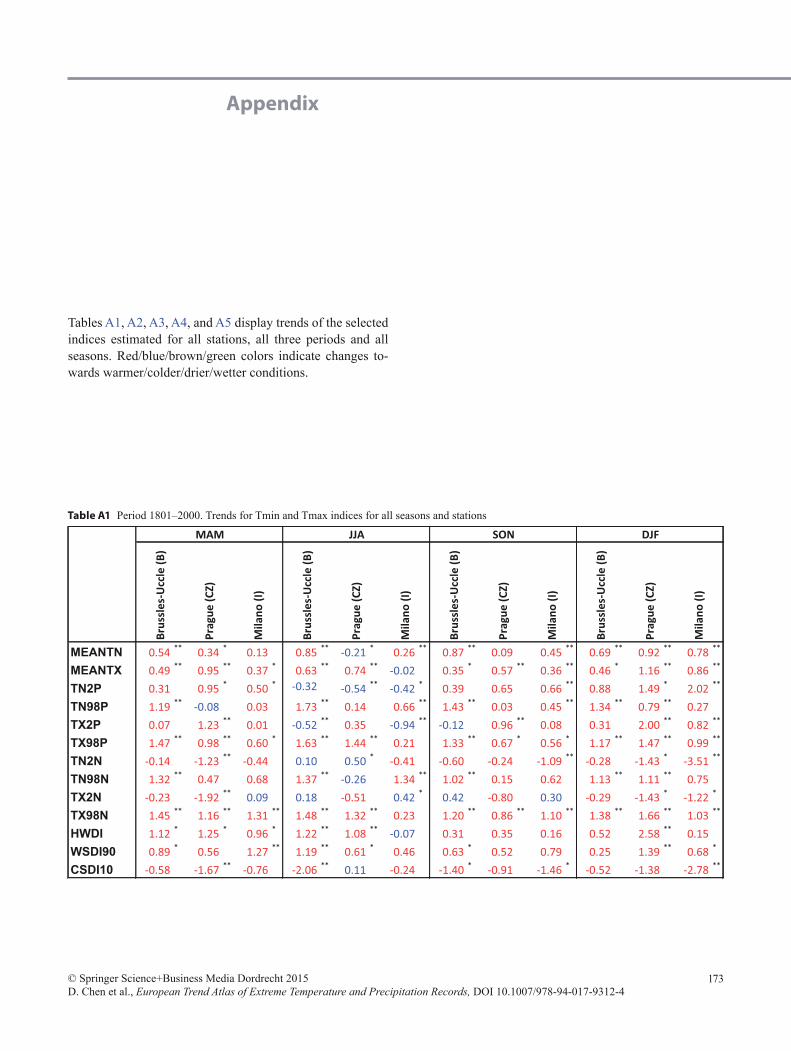
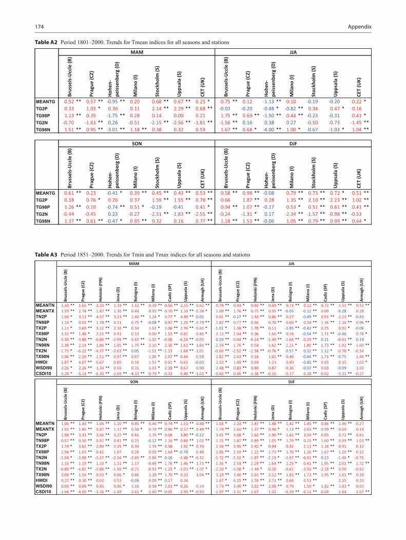
Tables A1, A2, A3, A4, and A5 display trends of the selected indices estimated for all stations, all three periods and all seasons. Red/blue/brown/green colors indicate changes to-wards warmer/colder/drier/wetter conditions.
Appendix
© Springer Science+Business Media Dordrecht 2015D. Chen et al., European Trend Atlas of Extreme Temperature and Precipitation Records, DOI 10.1007/978-94-017-9312-4
MEANTN 0.54 ** 0.34 * 0.13 0.85 ** -0.21 * 0.26 ** 0.87 ** 0.09 0.45 ** 0.69 ** 0.92 ** 0.78 **
MEANTX 0.49 ** 0.95 ** 0.37 * 0.63 ** 0.74 ** -0.02 0.35 * 0.57 ** 0.36 ** 0.46 * 1.16 ** 0.86 **
TN2P 0.31 0.95 * 0.50 * -0.32 -0.54 ** -0.42 * 0.39 0.65 0.66 ** 0.88 1.49 * 2.02 **
TN98P 1.19 ** -0.08 0.03 1.73 ** 0.14 0.66 ** 1.43 ** 0.03 0.45 ** 1.34 ** 0.79 ** 0.27
TX2P 0.07 1.23 ** 0.01 -0.52 ** 0.35 -0.94 ** -0.12 0.96 ** 0.08 0.31 2.00 ** 0.82 **
TX98P 1.47 ** 0.98 ** 0.60 * 1.63 ** 1.44 ** 0.21 1.33 ** 0.67 * 0.56 * 1.17 ** 1.47 ** 0.99 **
TN2N -0.14 -1.23 ** -0.44 0.10 0.50 * -0.41 -0.60 -0.24 -1.09 ** -0.28 -1.43 * -3.51 **
TN98N 1.32 ** 0.47 0.68 1.37 ** -0.26 1.34 ** 1.02 ** 0.15 0.62 1.13 ** 1.11 ** 0.75
TX2N -0.23 -1.92 ** 0.09 0.18 -0.51 0.42 * 0.42 -0.80 0.30 -0.29 -1.43 * -1.22 *
TX98N 1.45 ** 1.16 ** 1.31 ** 1.48 ** 1.32 ** 0.23 1.20 ** 0.86 ** 1.10 ** 1.38 ** 1.66 ** 1.03 **
HWDI 1.12 * 1.25 * 0.96 * 1.22 ** 1.08 ** -0.07 0.31 0.35 0.16 0.52 2.58 ** 0.15
WSDI90 0.89 * 0.56 1.27 ** 1.19 ** 0.61 * 0.46 0.63 * 0.52 0.79 0.25 1.39 ** 0.68 *
CSDI10 -0.58 -1.67 ** -0.76 -2.06 ** 0.11 -0.24 -1.40 * -0.91 -1.46 * -0.52 -1.38 -2.78 **
Mila
no (I
)
MAM JJA SON DJF
Brus
sles
-Ucc
le (B
)
Prag
ue (C
Z)
Mila
no (I
)
Brus
sles
-Ucc
le (B
)
Prag
ue (C
Z)
Mila
no (I
)
Brus
sles
-Ucc
le (B
)
Prag
ue (C
Z)
Mila
no (I
)
Brus
sles
-Ucc
le (B
)
Prag
ue (C
Z)
Table A1 Period 1801–2000. Trends for Tmin and Tmax indices for all seasons and stations
174
MEANTG 0.52 ** 0.57 ** -0.95 ** 0.20 0.68 ** 0.67 ** 0.25 * 0.75 ** 0.12 -1.13 ** 0.10 -0.19 -0.20 0.22 *TG2P 0.33 1.03 * 0.36 0.11 2.14 ** 2.29 ** 0.68 ** -0.03 -0.20 -0.48 * -0.82 ** 0.34 0.47 * 0.16TG98P 1.23 ** 0.35 -1.75 ** 0.28 0.14 0.00 0.21 1.75 ** 0.69 ** -1.50 ** 0.44 ** -0.23 -0.31 0.41 *TG2N -0.70 -1.61 ** 0.26 -0.51 -2.15 ** -2.56 ** -1.81 ** -1.56 ** 0.16 0.38 0.27 -0.50 -0.73 -1.45 **TG98N 1.51 ** 0.95 ** -3.01 ** 1.18 ** 0.38 0.32 0.59 1.67 ** 0.68 * -4.00 ** 1.00 * -0.67 -1.03 * 1.04 **
MEANTG 0.61 ** 0.23 -0.41 * 0.39 ** 0.45 ** 0.43 ** 0.53 ** 0.58 ** 0.98 ** -0.08 0.79 ** 0.73 ** 0.72 * 0.51 **TG2P 0.18 0.76 * 0.26 0.37 1.59 ** 1.55 ** 0.78 ** 0.66 1.87 ** 0.28 1.35 ** 2.10 ** 2.23 ** 1.02 **TG98P 1.26 ** 0.10 -0.74 ** 0.51 * -0.19 -0.41 0.41 * 0.94 ** 1.07 ** -0.17 0.53 * 0.51 ** 0.61 ** 0.41 **TG2N -0.44 -0.45 0.23 -0.27 -2.51 ** -1.83 ** -2.55 ** -0.24 -1.31 * 0.17 -2.34 ** -1.57 ** -0.98 ** -0.53TG98N 1.37 ** 0.61 ** -0.47 * 0.95 ** 0.32 0.16 0.77 ** 1.18 ** 1.53 ** -0.06 1.05 ** 0.79 ** 0.99 ** 0.64 *
Hoh
en-
peis
senb
erg
(D)
Mila
no (I
)
CET
(UK)
MAM
Upp
sala
(S)
Stoc
khol
m (S
)
JJA
SON DJF
Brus
sels
-Ucc
le (B
)
Prag
ue (C
Z)
Hoh
en-
peis
senb
erg
(D)
Mila
no (I
)
Stoc
khol
m (S
)
Upp
sala
(S)
Upp
sala
(S)
CET
(UK)
Brus
sels
-Ucc
le (B
)
Prag
ue (C
Z)
CET
(UK)
Brus
sels
-Ucc
le (B
)
Prag
ue (C
Z)
Hoh
en-
peis
senb
erg
(D)
Mila
no (I
)
Brus
sels
-Ucc
le (B
)
Prag
ue (C
Z)
Hoh
en-
peis
senb
erg
(D)
Mila
no (I
)
Stoc
khol
m (S
)
Stoc
khol
m (S
)
Upp
sala
(S)
CET
(UK)
Table A2 Period 1801–2000. Trends for Tmean indices for all seasons and stations
MEANTN 1.33 ** 1.65 ** 2.33 ** 1.19 ** 1.12 ** 0.39 ** 0.56 ** 2.15 ** 0.62 ** 0.79 ** 0.43 * 0.92 ** 0.59 ** 0.71 ** 0.12 ** 0.72 ** 1.51 ** 0.52 **MEANTX 1.59 ** 2.78 ** 1.87 ** 1.30 ** 0.43 0.93 ** 0.70 ** 1.10 ** 0.38 * 1.09 ** 1.76 ** 0.75 ** 0.95 ** -0.05 -0.12 ** 0.09 -0.28 0.28TN2P 1.59 * 3.11 ** 4.57 ** 3.23 ** 1.40 ** 1.24 * 0.77 * 4.49 ** -0.05 0.01 ** -0.27 ** 1.43 ** 0.86 ** 0.27 -0.49 ** 0.91 ** 2.23 ** -0.43TN98P 1.10 * 0.03 ** 1.78 ** 0.21 0.75 * -0.08 * 0.97 ** 1.20 ** 0.79 ** 1.82 ** 0.77 ** 0.56 0.70 ** 0.60 * 0.34 ** 1.36 ** 1.16 ** 0.96 **TX2P 1.11 * 3.69 ** 3.12 ** 2.10 ** 0.34 1.02 * 1.06 ** 2.76 ** 0.63 * -1.01 * 1.38 ** 1.78 ** 0.11 -1.85 ** -0.42 ** 0.25 0.92 * -0.06TX98P 3.32 ** 1.48 * 2.55 ** 0.91 0.13 0.00 * 1.53 ** 0.82 0.86 * 3.13 ** 2.04 ** 0.36 1.66 ** 0.18 -0.54 ** 1.71 ** -0.46 0.78 *TN2N -3.39 ** -3.88 ** -6.86 ** -2.95 ** -3.43 ** -1.02 * -0.06 -6.24 ** -0.05 0.29 ** -0.04 ** -4.24 ** -2.49 ** -1.64 ** -0.29 ** 0.21 -6.01 ** 0.19TN98N 2.38 ** 2.14 ** 1.86 ** 1.05 ** 1.70 ** 2.10 * 2.30 ** 1.63 ** 1.66 ** 2.39 ** 1.76 * 0.54 1.62 ** 2.21 * 1.80 ** 1.73 ** 1.92 ** 1.60 **TX2N -1.73 * -6.22 ** -4.37 ** -2.63 ** 0.05 -1.51 ** -1.33 -1.68 ** -1.01 -0.60 ** -2.52 ** -2.58 ** -0.76 * 0.57 * 0.32 ** 1.12 * -0.78 * -0.34TX98N 3.06 ** 2.29 ** 1.51 ** 0.97 ** 0.87 1.96 * 2.07 ** 0.44 0.58 2.82 ** 2.43 ** 0.18 1.65 ** 0.49 -0.44 ** 1.71 ** -0.75 1.48 **HWDI 2.87 * 4.07 ** 0.67 0.85 0.16 1.51 * 0.61 * 0.63 -0.03 2.53 * 1.69 ** 0.04 1.21 0.89 -0.85 ** 0.65 0.15 1.03 *WSDI90 2.26 * 2.26 ** 1.34 ** 0.56 0.31 2.03 * 2.39 ** 0.67 0.90 2.48 ** 0.83 ** 0.90 0.87 -0.36 -0.07 ** 0.69 -0.09 1.02CSDI10 -3.28 * -5.14 ** -6.30 ** -2.69 ** -4.33 ** -0.79 * -0.33 -5.40 ** -1.03 * -0.60 ** 0.45 ** -3.36 ** -0.16 -0.17 0.28 ** -0.02 -3.33 ** -0.27
MEANTN 1.06 ** 1.43 ** 1.06 ** 1.20 ** 0.85 ** 0.46 ** 0.74 ** 1.53 ** 0.88 ** 1.03 * 2.23 ** 1.87 ** 1.48 ** 1.42 ** 1.45 ** 0.86 ** 1.46 ** 0.27MEANTX 1.93 ** 1.85 ** 0.87 ** 1.17 ** 0.58 * 0.74 ** 0.96 ** 0.57 ** 0.48 ** 1.74 ** 2.60 ** 1.37 ** 0.98 * 1.13 ** 2.03 ** 0.99 ** 0.69 0.14TN2P 1.98 ** 3.31 ** 3.56 ** 3.27 ** 0.81 1.76 ** 0.08 3.80 ** -0.22 3.01 ** 3.09 * 2.62 ** 2.90 ** 1.61 ** 3.54 ** 0.05 3.72 ** 0.61TN98P 0.57 ** 0.50 ** 0.92 ** 0.81 ** 0.25 -0.12 ** 1.16 ** 0.88 ** 1.02 ** 1.25 ** 1.87 ** 0.89 ** 1.05 ** 1.29 ** 0.25 ** 1.60 ** 0.99 ** 1.03 **TX2P 1.74 * 3.62 ** 2.89 ** 2.35 ** 0.34 1.74 ** 0.58 1.92 ** 0.39 1.56 ** 3.95 ** 2.42 * 0.94 0.32 2.11 ** 1.18 ** 0.91 0.12TX98P 2.94 ** 1.03 ** 0.42 1.07 0.28 0.09 ** 1.64 ** -0.78 0.48 2.85 ** 2.59 ** 1.22 ** 1.73 ** 1.70 ** 1.26 ** 1.67 ** 1.20 ** 0.22TN2N -2.04 * -3.98 ** -3.27 ** -2.34 ** -2.85 ** -2.86 ** 0.26 -3.48 ** -0.32 -1.72 ** -3.32 * -1.87 ** -2.19 * -3.57 ** -6.91 ** 0.23 -1.46 * -0.75TN98N 1.33 ** 1.19 ** 1.10 * 1.31 ** 1.17 -0.66 ** 1.76 ** 1.46 ** 1.73 ** 1.36 * 2.59 ** 2.29 ** 1.64 ** 1.29 * 0.41 ** 1.95 ** 2.01 ** 1.72 **TX2N -0.89 ** -4.82 ** -3.88 ** -1.99 ** -0.21 -0.93 ** -1.23 * -2.03 ** -1.07 * -2.20 * -3.08 * -1.44 * -0.20 -0.62 -3.50 ** -2.28 ** 0.00 -0.62TX98N 2.08 ** 1.56 ** 0.93 * 0.86 * 0.86 1.28 ** 1.70 ** 0.32 1.04 ** 3.19 ** 3.40 ** 2.01 ** 2.12 ** 1.83 ** 1.73 ** 1.95 ** 1.61 ** 0.38HWDI 0.27 ** 0.30 ** 0.02 0.53 -0.09 0.09 ** 0.17 0.34 1.67 * 6.15 ** 3.76 ** 3.71 ** 0.66 0.51 ** 2.15 0.20WSDI90 0.93 ** 0.09 ** 0.85 0.86 * 1.16 0.98 ** 1.03 ** 0.26 0.14 1.73 ** 3.40 ** 3.02 ** 2.08 ** 0.79 1.59 * 1.82 ** 1.83 * 0.01CSDI10 -1.94 ** -4.50 ** -3.36 ** -1.49 -2.41 * -2.60 ** -0.05 -2.90 ** -0.93 -1.97 ** -3.31 ** -1.67 -1.32 -6.29 ** -6.11 ** -0.68 -1.04 -2.07 **
MAM JJA
SON DJF
Brus
sels
-Ucc
le (B
)
Prag
ue (C
Z)
Hel
sink
i (FI
N)
Jena
(D)
Bolo
gna
(I)
Mila
no (I
)
Upp
sala
(S)
Arm
agh
(UK)
Cadi
z (S
P)
Upp
sala
(S)
Arm
agh
(UK)
Brus
sels
-Ucc
le (B
)
Mila
no (I
)
Cadi
z (S
P)
Brus
sels
-Ucc
le (B
)
Prag
ue (C
Z)
Hel
sink
i (FI
N)
Jena
(D)
Bolo
gna
(I)
Prag
ue (C
Z)
Hel
sink
i (FI
N)
Mila
no (I
)
Jena
(D)
Bolo
gna
(I)
Arm
agh
(UK)
Cadi
z (S
P)
Upp
sala
(S)
Arm
agh
(UK)
Brus
sels
-Ucc
le (B
)
Prag
ue (C
Z)
Hel
sink
i (FI
N)
Jena
(D)
Bolo
gna
(I)
Mila
no (I
)
Cadi
z (S
P)
Upp
sala
(S)
Table A3 Period 1851–2000. Trends for Tmin and Tmax indices for all seasons and stations
Appendix
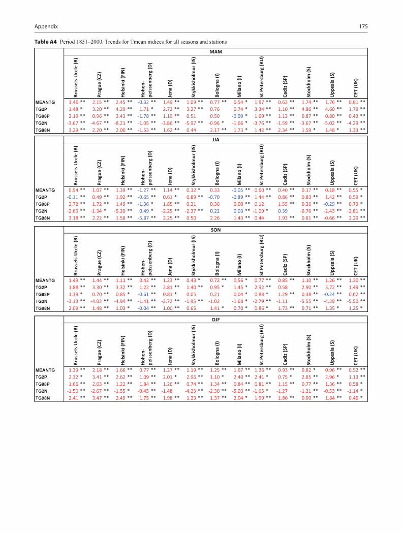
175
MEANTG 1.46 ** 2.15 ** 2.45 ** -0.32 ** 1.49 ** 1.09 ** 0.77 ** 0.54 * 1.97 ** 0.63 ** 1.74 ** 1.76 ** 0.81 **TG2P 1.48 * 3.20 ** 4.29 ** 1.71 * 2.72 ** 3.27 ** 0.76 0.74 * 3.34 ** 1.10 ** 4.86 ** 4.60 ** 1.79 **TG98P 2.19 ** 0.96 ** 3.43 ** -1.78 ** 1.19 ** 0.51 0.50 -0.09 * 1.69 ** 1.13 ** 0.87 ** 0.80 ** 0.43 **TG2N -3.67 ** -4.67 ** -8.21 ** -1.05 ** -3.86 ** -5.97 ** -0.96 * -1.66 * -3.76 ** -1.59 ** -3.67 ** -5.02 ** -4.29 **TG98N 3.29 ** 2.20 ** 2.00 ** -1.53 ** 1.62 ** 0.44 2.17 ** 1.73 * 1.42 ** 2.34 ** 1.59 * 1.48 * 1.33 **
MEANTG 0.94 ** 1.07 ** 1.39 ** -1.27 ** 1.14 ** 0.32 * 0.33 -0.05 ** 0.60 ** 0.40 ** 0.17 ** 0.18 ** 0.55 *TG2P -0.11 ** 0.49 ** 1.92 ** -0.65 ** 0.61 * 0.89 ** -0.70 -0.89 ** 1.44 ** 0.86 ** 0.83 ** 1.42 ** 0.59 *TG98P 2.72 ** 1.72 ** 1.49 ** -1.36 * 1.85 ** 0.21 0.36 0.00 ** 0.12 1.55 ** 0.26 ** -0.29 ** 0.79 *TG2N -2.66 ** -1.34 * -5.20 ** 0.49 * -2.25 ** -2.37 ** 0.22 0.03 ** -1.09 * 0.39 -0.76 ** -2.43 ** -2.81 **TG98N 3.18 ** 2.22 ** 1.58 ** -5.87 ** 2.25 ** 0.50 2.26 1.43 ** 0.44 1.93 ** 0.81 ** -0.66 ** 2.29 **
MEANTG 1.49 ** 1.44 ** 1.11 ** 0.42 ** 1.23 ** 0.43 * 0.72 ** 0.56 * 0.77 ** 0.85 ** 1.10 ** 1.26 ** 1.30 **TG2P 1.88 ** 3.30 ** 3.32 ** 1.22 ** 2.81 ** 1.40 ** 0.95 * 1.45 * 2.92 ** 0.58 2.90 ** 3.72 ** 1.49 **TG98P 1.39 * 0.70 ** 0.85 * -0.61 ** 0.81 * 0.05 0.21 0.04 * 0.88 * 1.29 ** 0.38 ** -0.24 ** 0.62 **TG2N -3.13 ** -4.03 ** -4.94 ** -1.41 ** -3.72 ** -1.95 ** -1.02 -1.68 * -2.79 ** -1.11 -5.55 ** -4.39 ** -5.50 **TG98N 2.09 ** 1.48 ** 1.03 * -0.04 ** 1.00 ** 0.65 1.41 * 0.70 * 0.86 * 1.73 ** 0.71 ** 1.35 * 1.25 *
MEANTG 1.39 ** 2.18 ** 1.66 ** 0.77 ** 1.27 ** 1.19 ** 1.25 ** 1.67 ** 1.36 ** 0.93 ** 0.82 * 0.96 ** 0.52 **TG2P 2.32 * 3.41 ** 2.62 ** 1.09 ** 2.01 * 2.96 ** 1.10 * 2.40 ** 2.41 * 0.75 * 2.85 ** 2.96 * 1.13 **TG98P 1.66 ** 2.03 ** 1.22 ** 1.84 ** 1.26 ** 0.74 ** 1.34 ** 0.84 ** 0.81 ** 1.15 ** 0.77 ** 1.36 ** 0.58 *TG2N -1.50 ** -2.67 ** -1.55 * -0.45 ** -1.48 -4.23 ** -2.30 ** -5.03 ** -1.65 * -1.27 -1.21 ** -0.53 ** -1.14 *TG98N 2.41 ** 3.47 ** 2.49 ** 1.75 ** 1.98 ** 1.23 ** 1.37 ** 2.04 * 1.99 ** 1.86 ** 0.90 ** 1.84 ** 0.46 *
MAM
Brus
sels
-Ucc
le (B
)
Prag
ue (C
Z)
Hel
sink
i (FI
N)
Hoh
en-
peis
senb
erg
(D)
Jena
(D)
Styk
kish
olm
ur (I
S)
CET
(UK)
Bolo
gna
(I)
Mila
no (I
)
St P
eter
sbur
g (R
U)
Cadi
z (S
P)
Stoc
khol
m (S
)
Upp
sala
(S)
Stoc
khol
m (S
)
JJA
Brus
sels
-Ucc
le (B
)
Prag
ue (C
Z)
Hel
sink
i (FI
N)
Hoh
en-
peis
senb
erg
(D)
Jena
(D)
CET
(UK)
Upp
sala
(S)
CET
(UK)
SON
Brus
sels
-Ucc
le (B
)
Prag
ue (C
Z)
Hel
sink
i (FI
N)
Hoh
en-
peis
senb
erg
(D)
Jena
(D)
Styk
kish
olm
ur (I
S)
Bolo
gna
(I)
Styk
kish
olm
ur (I
S)
Bolo
gna
(I)
Mila
no (I
)
St P
eter
sbur
g (R
U)
Cadi
z (S
P)
Mila
no (I
)
St P
eter
sbur
g (R
U)
Cadi
z (S
P)
Stoc
khol
m (S
)
Upp
sala
(S)
Cadi
z (S
P)
Stoc
khol
m (S
)
Upp
sala
(S)
CET
(UK)
DJF
Brus
sels
-Ucc
le (B
)
Prag
ue (C
Z)
Hel
sink
i (FI
N)
Hoh
en-
peis
senb
erg
(D)
Jena
(D)
Styk
kish
olm
ur (I
S)
Bolo
gna
(I)
Mila
no (I
)
St P
eter
sbur
g (R
U)
Table A4 Period 1851–2000. Trends for Tmean indices for all seasons and stations
Appendix
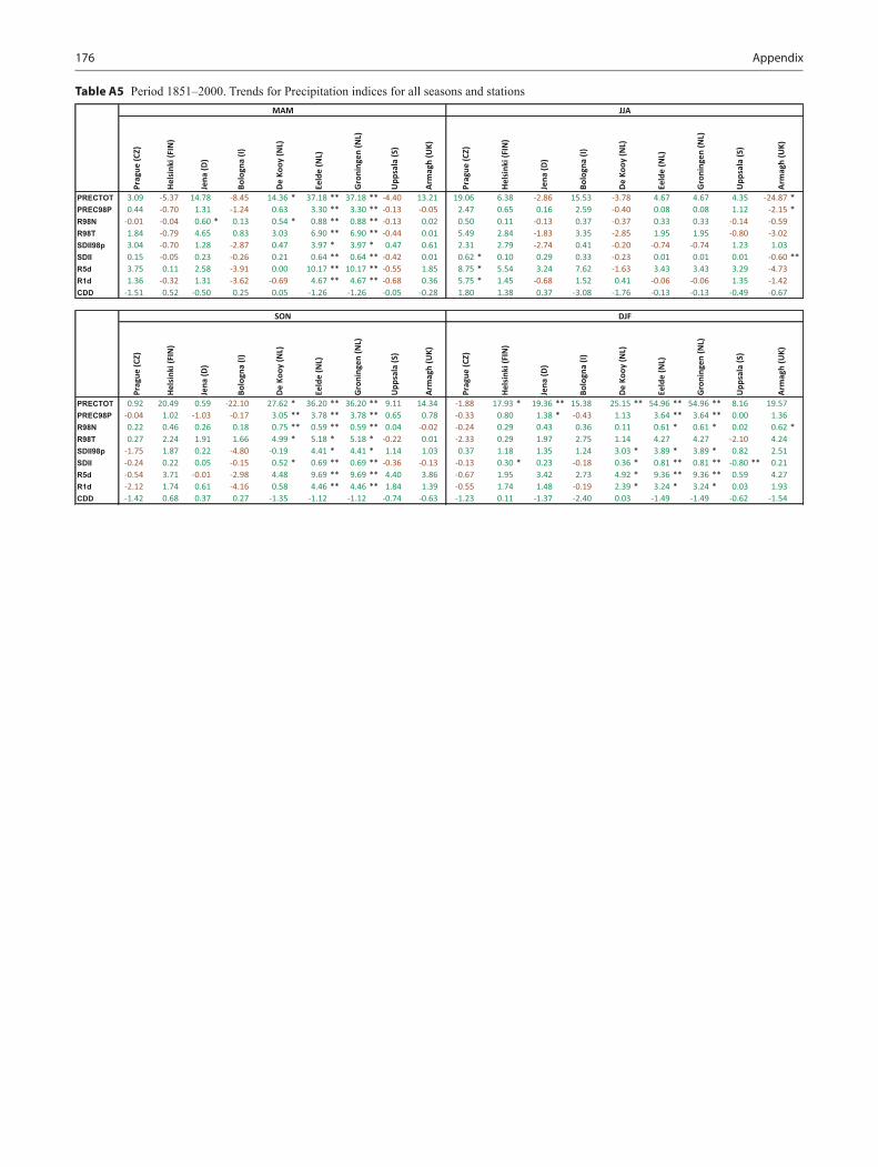
176
PRECTOT 3.09 -5.37 14.78 -8.45 14.36 * 37.18 ** 37.18 ** -4.40 13.21 19.06 6.38 -2.86 15.53 -3.78 4.67 4.67 4.35 -24.87 *PREC98P 0.44 -0.70 1.31 -1.24 0.63 3.30 ** 3.30 ** -0.13 -0.05 2.47 0.65 0.16 2.59 -0.40 0.08 0.08 1.12 -2.15 *R98N -0.01 -0.04 0.60 * 0.13 0.54 * 0.88 ** 0.88 ** -0.13 0.02 0.50 0.11 -0.13 0.37 -0.37 0.33 0.33 -0.14 -0.59R98T 1.84 -0.79 4.65 0.83 3.03 6.90 ** 6.90 ** -0.44 0.01 5.49 2.84 -1.83 3.35 -2.85 1.95 1.95 -0.80 -3.02SDII98p 3.04 -0.70 1.28 -2.87 0.47 3.97 * 3.97 * 0.47 0.61 2.31 2.79 -2.74 0.41 -0.20 -0.74 -0.74 1.23 1.03SDII 0.15 -0.05 0.23 -0.26 0.21 0.64 ** 0.64 ** -0.42 0.01 0.62 * 0.10 0.29 0.33 -0.23 0.01 0.01 0.01 -0.60 **R5d 3.75 0.11 2.58 -3.91 0.00 10.17 ** 10.17 ** -0.55 1.85 8.75 * 5.54 3.24 7.62 -1.63 3.43 3.43 3.29 -4.73R1d 1.36 -0.32 1.31 -3.62 -0.69 4.67 ** 4.67 ** -0.68 0.36 5.75 * 1.45 -0.68 1.52 0.41 -0.06 -0.06 1.35 -1.42CDD -1.51 0.52 -0.50 0.25 0.05 -1.26 -1.26 -0.05 -0.28 1.80 1.38 0.37 -3.08 -1.76 -0.13 -0.13 -0.49 -0.67
PRECTOT 0.92 20.49 0.59 -22.10 27.62 * 36.20 ** 36.20 ** 9.11 14.34 -1.88 17.93 * 19.36 ** 15.38 25.15 ** 54.96 ** 54.96 ** 8.16 19.57PREC98P -0.04 1.02 -1.03 -0.17 3.05 ** 3.78 ** 3.78 ** 0.65 0.78 -0.33 0.80 1.38 * -0.43 1.13 3.64 ** 3.64 ** 0.00 1.36R98N 0.22 0.46 0.26 0.18 0.75 ** 0.59 ** 0.59 ** 0.04 -0.02 -0.24 0.29 0.43 0.36 0.11 0.61 * 0.61 * 0.02 0.62 *R98T 0.27 2.24 1.91 1.66 4.99 * 5.18 * 5.18 * -0.22 0.01 -2.33 0.29 1.97 2.75 1.14 4.27 4.27 -2.10 4.24SDII98p -1.75 1.87 0.22 -4.80 -0.19 4.41 * 4.41 * 1.14 1.03 0.37 1.18 1.35 1.24 3.03 * 3.89 * 3.89 * 0.82 2.51SDII -0.24 0.22 0.05 -0.15 0.52 * 0.69 ** 0.69 ** -0.36 -0.13 -0.13 0.30 * 0.23 -0.18 0.36 * 0.81 ** 0.81 ** -0.80 ** 0.21R5d -0.54 3.71 -0.01 -2.98 4.48 9.69 ** 9.69 ** 4.40 3.86 -0.67 1.95 3.42 2.73 4.92 * 9.36 ** 9.36 ** 0.59 4.27R1d -2.12 1.74 0.61 -4.16 0.58 4.46 ** 4.46 ** 1.84 1.39 -0.55 1.74 1.48 -0.19 2.39 * 3.24 * 3.24 * 0.03 1.93CDD -1.42 0.68 0.37 0.27 -1.35 -1.12 -1.12 -0.74 -0.63 -1.23 0.11 -1.37 -2.40 0.03 -1.49 -1.49 -0.62 -1.54
MAM JJA
SON DJF
Prag
ue (C
Z)
Hel
sink
i (FI
N)
Jena
(D)
Bolo
gna
(I)
De
Kooy
(NL)
Eeld
e (N
L)
Upp
sala
(S)
Arm
agh
(UK)
Gro
ning
en (N
L)
Upp
sala
(S)
Arm
agh
(UK)
Prag
ue (C
Z)
Eeld
e (N
L)
Gro
ning
en (N
L)
Prag
ue (C
Z)
Hel
sink
i (FI
N)
Jena
(D)
Bolo
gna
(I)
De
Kooy
(NL)
Hel
sink
i (FI
N)
Jena
(D)
Eeld
e (N
L)
Bolo
gna
(I)
De
Kooy
(NL)
Arm
agh
(UK)
Gro
ning
en (N
L)
Upp
sala
(S)
Arm
agh
(UK)
Prag
ue (C
Z)
Hel
sink
i (FI
N)
Jena
(D)
Bolo
gna
(I)
De
Kooy
(NL)
Eeld
e (N
L)
Gro
ning
en (N
L)
Upp
sala
(S)
Table A5 Period 1851–2000. Trends for Precipitation indices for all seasons and stations
Appendix
177
References
Achberger, C., & Chen, D. (2006). Trend of extreme precipitation in Sweden and Norway during 1961–2004. Research report C72 (p. 58). Gothenburg: Department of Earth Sciences.
Arndt, D. S., Baringer, M. O., Johnson, M. R., Alexander, L. V., Dia-mond, H. J., Fogt, R. L., Levy, J. M., Richter-Menge, J., Thorne, P. W., Vincent, L. A., Watkins, A. B., & Willett, K. M. (2010). State of the climate in 2009. Bulletin of the American Meteorological Soci-ety, 91(7), S1–S218.
Auer, I., Böhm, R., Jurkovic, A., Lipa, W., Orlik, A., Potzmann, R., Schöner, W., Ungersböck, M., Matulla, C., Briffa, K., Jones, P., Efthymiadis, D., Brunetti, M., Nanni, T., Maugeri, M., Mercalli, L., Mestre, O., Moisselin, J. M., Begert, M., Müller-Westermeier, G., Kveton, V., Bochnicek, O., Stastny, P., Lapin, M., Szalai, S., Szentimrey, T., Cegnar, T., Dolinar, M., Gajic-Capka, M., Zani-novic, K., Majstorovic Z., & Nieplova E. (2007). HISTALP—His-torical instrumental climatological surface time series of the Greater Alpine Region. International Journal of Climatology, 27(1), 17–46.
Beniston, M. (2004). The 2003 heat wave in Europe. A shape of things to come? Geophysical Research Letters, 31, 2022–2026.
Beniston, M., & Stephenson, D. B. (2004). Extreme climatic events and their evolution under changing climatic conditions. Global and Planetary Change, 44, 1–9.
Beniston, M., Stephenson, D. B., Christensen, O. B., Ferro, C. A. T., Frei, C., Goyette, S., Halsnaes, K., Holt, T., Jylha, K., Koffi, B., Palutikof, J., Scholl, R., Semmler, T., & Woth, K. (2007). Future extreme events in European climate: An exploration of regional cli-mate model projections. Climatic Change, 81, 71–95.
Brown, B. G., & Katz, R. W. (1995). Regional analysis of temperature extremes: Spatial analog for climate change? Journal of Climate, 8, 108–119.
Brunet, M., & Jones, P. (2011). Data rescue initiatives: Bringing his-torical climate data into the 21st century. Climate Research, 47(1–2), 29–40.
Brunsden, D. (1999). Some geomorphological considerations for the future development of landslide models. Geomorphology, 30, 13–24.
Chen, D., Walther, A., Moberg, A., Jones, P. D., Jacobeit J., & Lister, D. (2006). Trend atlas of the EMULATE indices. Research Report C73 (p. 798). Gothenburg: Department of Earth Sciences.
Christidis, N., Stott, P. A., Brown, S., Hegerl, G. C., & Caesar, J. (2005). Detection of changes in temperature extremes during the second half of the 20th century. Geophysical Research Letters, 32(20), 1–4.
Donat, M. G., Alexander, L. V., Yang, H., Durre, I., Vose, R., Dunn, R. J. H., Willett, K. M., Aguilar, E., Brunet, M., Caesar, J., Hewit-son, B., Jack, C., Klein Tank, A. M. G., Kruger, A. C., Marengo, J., Peterson, T. C., Renom, M., Oria Rojas, C., Rusticucci, M., Salin-ger, J., Elrayah, A. S., Sekele, S. S., Srivastava, A. K., Trewin, B., Villarroel, C., Vincent, L. A., Zhai, P., Zhang, X., & Kitching S.
(2013). Updated analyses of temperature and precipitation extreme indices since the beginning of the twentieth century: The HadEX2 dataset. Journal of Geophysical Research D: Atmospheres, 118(5), 2098–2118.
Easterling, D. R., Meehl, G. A., Parmesan, C., Changnon, S. A., Karl, T. R., & Mearns, L. O. (2000). Climate extremes: Observations, modeling, and impacts. Science, 289, 2068–2074.
Field, C. B., Barros, V., Stocker, T. F., Qin, D., Dokken, D. J., Ebi, K. L., Mastrandrea, M. D., Mach, K. J., Plattner, G.-K., Allen, S. K., Tignor, M., & Midgley, P. M. (2012). Managing the risks of extreme events and disasters to advance climate change adaptation. A special report of working groups I and II of the intergovernmental panel on climate change. Cambridge: Cambridge University Press.
Fowler, H. J., & Kilsby, C. G. (2003). A regional frequency analysis of United Kingdom extreme rainfall from 1961–2000. International Journal of Climatology, 23, 1313–1334.
Frich, P., Alexander, L. V., Della-Marta, P., Gleason, B., Haylock, M., Klein-Tank, A., & Peterson, T. (2002). Observed coherent changes in climatic extremes during the second half of the 20th Century. Climate Research, 19, 193–212.
Groisman, P. Y., Karl, T. R., Easterling, D. R., Knight, R. W., Jame-son, P. F., Hennessy, K. J., Suppiah, R., Page, C., Wibig, J., Fortu-niak, K., Razuaev, V., Douglas, A., Førland, E., & Zhai, P. (1999). Changes in the probability of heavy precipitation: Important indica-tors of climatic change. Climatic Change, 42, 243–283.
Groisman, P. Y., Knight, R. W., Easterling, D. R., Karl, T. R., Hegerl, G. C., & Razuvaev, V. N. (2005). Trends in intense precipitation in the climate record. Journal of Climate, 18, 1326–1350.
Hansen, J., Sato, M., & Ruedy, R. (2012). Perception of climate change. Proceedings of the National Academy of Sciences of the United States of America, 109(37), E2415–E2423.
Haylock, M. R., & Goodess, C. M. (2004). Interannual variability of European extreme winter rainfall and links with mean large-scale circulation. International Journal of Climatology, 24, 759–776.
Houghton, J. T., Ding, Y., Griggs, D. J., Noguer, M., van der Linden, P. J., Dai, X., IPCC. (2002). Workshop report of the IPCC workshop on changes in extreme weather and climate events. 11–13 June, Beijing.
Hundecha, Y., & Bárdossy, A. (2005). Trends in daily precipitation and temperature extremes across western Germany in the second half of the 20th century. International Journal of Climatology, 25, 1189–1202.
IPCC. (2001). Climate change 2001: The scientific basis. Contribu-tion of working group I to the third assessment. Report of the inter-governmental panel on climate change (IPCC). UK: Cambridge University Press.
IPCC. (2007). Climate change 2007: The physical science basis. Con-tribution of working group I to the fourth assessment. Report of the intergovernmental panel on climate change. Cambridge: Cambridge University Press.
© Springer Science+Business Media Dordrecht 2015D. Chen et al., European Trend Atlas of Extreme Temperature and Precipitation Records, DOI 10.1007/978-94-017-9312-4
178 References
Jacobeit, J., Rathmann, J., Philipp, A., & Jones, P. D. (2009). Cen-tral European precipitation and temperature extremes in relation to large-scale atmospheric circulation types. Meteorologische Zeitschrift, 18(4), 397–410.
Jones, P. D., Horton, E. B., Folland, C. K., Hulme, M., Parker, D. E., & Basnett, T. A. (1999). The use of indices to identify changes in climatic extremes. Climatic Change, 42, 131–149.
Karl, T. R., & Easterling, D. R. (1999). Climate extremes: Selected review and future research directions. Climatic Change, 42, 309–325.
Katz, R. W., & Brown, B. G. (1992). Extreme events in a changing cli-mate: Variability is more important than averages. Climatic Change, 21, 289–302.
Klein-Tank, A. M. G., & Können, G. P. (2003). Trends in indices of daily temperature and precipitation extremes in Europe. Journal of Climate, 16, 3665–3680.
Klein-Tank, A. M. G., Wijngaard, J., & van Engelen, A. (2002a). Cli-mate of Europe: Assessment of observed daily temperature and pre-cipitation extremes. De Bilt: KNMI.
Klein-Tank, A. M. G., Wijngaard, J. B., Können, G. P., Böhm, R., Demarée, G., Gocheva, A., Mileta, M., Pashiardis, S., Hejkrlik, L., Kern-Hansen, C., Heino, R., Bessemoulin, P., Müller-Westermeier, G., Tzanakou, M., Szalai, S., Palsdottir, T., Fitzgerald, D., Rubin, S., Capaldo, M., Maugeri, M., Leitass, A., Bukantis, A., Aberfeld, R., van Engelen, A. F. V., Forland, E., Mietus, M., Coelho, F., Mares, C., Razuvaev, V., Nieplova, E., Cegnar, T., López, J. A., Dahlström, B., Moberg, A., Kirchhofer, W., Ceylan, A., Pachaliuk, O., Alexander, L. V., & Petrovic, P. (2002b). Daily dataset of 20th-century surface air temperature and precipitation series for the European climate assessment. International Journal of Climatology, 22, 1441–1453.
Mearns, L. O., Katz, R. W., & Schneider, S. H. (1984). Extreme high temperature events: Changes in their probabilities and changes in mean temperature. Journal of Climate and Applied Meteorology, 23, 1601–1613.
Moberg, A., & Bergström, H. (1997). Homogenization of Swed-ish temperature data. Part III: The long temperature records from Uppsala and Stockholm. International Journal of Climatology, 17(7), 667–699.
Moberg, A., & Jones, P. D. (2005). Trends in indices for extremes in daily temperature and precipitation in central and Western Europe 1901–1999. International Journal of Climatology, 25, 1149–1172.
Moberg, A., Jones, P. D., Lister, D., Walther, A., Brunet, M., Jacobeit, J., Alexander, L. V., Della-Marta, P. M., Luterbacher, J., Yiou, P., Chen, D. L., Tank, A. M. G. K., Saladie, O., Sigro, J., Aguilar, E., Alexandersson, H., Almarza, C., Auer, I., Barriendos, M., Begert, M., Bergstrom, H., Bohm, R., Butler, C. J., Caesar, J., Drebs, A., Founda, D., Gerstengarbe, F. W., Micela, G., Maugeri, M., Osterle, H., Pandzic, K., Petrakis, M., Srnec, L., Tolasz, R., Tuomenvirta, H., Werner, P. C., Linderholm, H., Philipp, A., Wanner, H., & Xoplaki, E. (2006). Indices for daily temperature and precipitation extremes in Europe analyzed for the period 1901–2000. Journal of Geophysical Research-Atmospheres, 111(D22106). doi:10.1029/2006JD007103.
Morak, S., Hegerl, G. C. & Kenyon, J. (2011). Detectable regional changes in the number of warm nights. Geophysical Research Let-ters, 38(17). doi:10.1029/2011GL048531.
Pellikka, P. & Järvenpää, E. (2003). Forest stand characteristics and snow and wind induced forest damage in boreal forests. Pro-ceedings of the international conference on wind effects on trees (pp. 269–276), 16–18 September. Karlsruhe: B. Ruck.
Peterson, T. C., Folland, C., Gruza, G., Hogg, W., Mokssit, A., & Plummer, N. (2001). Report on the activities of the working group on climate change detection and related rapporteurs 1998–2001.
Peterson, T. C., P., Stott, A., & Herring, S. (2012). Explaining extreme events of 2011 from a climate perspective. Bulletin of the American Meteorological Society, 93(7), 1041–1067.
Schmidli, J., & Frei, C. (2005). Trends in heavy precipitation and wet and dry spells in Switzerland during the 20th century. International Journal of Climatology, 25, 753–771.
Schuster, R. L. (1996). Socioeconomic significance of landslides. In A. K. Turner & R. L. Schuster (Eds.), Landslides: Investigation and mitigation (pp. 12–35). Washington, DC: National Academy Press.
Solantie, R. (1994). Effect of weather and climatological background on snow damage of forests in southern Finland in November 1991. Silva Fennica, 28(3), 203–211.
Trenberth, K. E. (1999). Conceptual framework for changes of extremes of the hydrological cycle with climate change. Climatic Change, 42(1), 327–339.
Vautard, R., & Yiou, P. (2009). Control of recent European surface climate change by atmospheric flow. Geophysical Research Letters, 36(22). L22702, doi:10.1029/2009GL040480.
Venema, V. K. C., Mestre, O., Aguilar, E., Auer, I., Guijarro, J. A., Domonkos, P., Vertacnik, G., Szentimrey, T., Stepanek, P., Zah-radnicek, P., Viarre, J., Müller-Westermeier, G., Lakatos, M., Wil-liams, C. N., Menne, M. J., Lindau, R., Rasol, D., Rustemeier, E., Kolokythas, K., Marinova, T., Andresen, L., Acquaotta, F., Frati-anni, S., Cheval, S., Klancar, M., Brunetti, M., Gruber, C., Prohom Duran, M., Likso, T., Esteban, P., & Brandsma, T. (2012). Bench-marking homogenization algorithms for monthly data. Climate of the Past, 8(1), 89–115.
Wigley, T. M. L. (1985). Impact of extreme events. Nature, 316, 106–107.
WISE. (1999). Workshop report of the workshop on economic and social impacts of climate extremes: Risks and benefits, 14–16 October.
Zhang, X., Wang, J., Zwiers, F. W., & Groisman, P. Y. (2010). The influence of large-scale climate variability on winter maximum daily precipitation over north America. Journal of Climate, 23(11), 2902–2915.
Zwiers, F. W., Zhang, X., & Feng, Y. (2011). Anthropogenic influence on long return period daily temperature extremes at regional scales. Journal of Climate, 24(3), 881–892.