European Journal of Combinatorics - CORE

European Journal of Combinatorics 30 (2009) 655–667

Contents lists available at ScienceDirect

European Journal of Combinatorics

journal homepage: www.elsevier.com/locate/ejc

New examples of Euclidean tight 4-designsEtsuko BannaiFaculty of Mathematics, Graduate School, Kyushu University, Hakozaki 6-10-1, Higashi-ku, Fukuoka 812-8581, Japan

a r t i c l e i n f o

Article history:Available online 2 September 2008

a b s t r a c t

In this paper we give some new examples of Euclidean tight 4-designs having good combinatorial structures including combina-torial tight 4-(23, 7, 1) design and tight 4-design in the Hammingscheme H(11, 3).

© 2008 Elsevier Ltd. All rights reserved.

1. Introduction

Delsarte defined the concept of t-designs and codes in association schemes and established theso-called Delsarte theory between them (see [8]). We note that classical combinatorial t-designs areconsidered as t-designs in Johnson association schemes. Then in 1977, Delsarte, Goethals and Seideldefined t-designs on the unit sphere in Rn and established the Delsarte theory on designs and codesfor spheres. Euclidean t-designs are defined by Neumaier and Seidel as a generalization of sphericalt-designs (see [15]). We note that spherical t-designs and Euclidean t-designs always exist if thecardinalities of the designs are large enough (see [20]). In this paper we study the Euclidean tight 4-designs X ⊂ Rn supported by 2 concentric spheres with positive radii and centered at the origin. Weshow that such Euclidean tight 4-designs have good combinatorial structures and construct new andinteresting examples having the structure of 4-(23, 7, 1) design and tight 4-design in the Hammingscheme H(11, 3). We also give partial classification, namely, classification for the cases when one ofthe layers X1 satisfies |X1| = n+ 1 or |X1| = n+ 2.In the following we give the definition of Euclidean t-designs and the definition of tight 2e-designs

on p concentric spheres. In Section 2, we state the main theorems of this paper. In Section 3, wegive some basic properties of Euclidean t-designs. In Section 4, we give the proof of the theorems.In Section 5, we give some remarks and a conjecture.The following are the notations and symbols we use in this paper. Let X be a finite set in Euclidean

spaceRn. Letw be a positive real valuedweight function defined on X .We consider theweighted finitesubsets. We assume n ≥ 2 throughout this paper and consider the weighted finite sets (X, w) in Rn.Let Sn−1 be the unit sphere centered at the origin. Let Sn−1(r) be the sphere of radius r centered at theorigin, where r is possibly 0. We can decompose X into a disjoint union of the subsets in the followingmanner, that is, r1, r2, . . . , rp are distinct non-negative real numbers and X = X1 ∪X2 ∪ · · · ∪Xp, Xi ⊂

E-mail address: [email protected].

0195-6698/$ – see front matter© 2008 Elsevier Ltd. All rights reserved.doi:10.1016/j.ejc.2008.07.012

brought to you by COREView metadata, citation and similar papers at core.ac.uk

provided by Elsevier - Publisher Connector

https://core.ac.uk/display/81958836?utm_source=pdf&utm_medium=banner&utm_campaign=pdf-decoration-v1

http://www.elsevier.com/locate/ejc

http://www.elsevier.com/locate/ejc

mailto:[email protected]

http://dx.doi.org/10.1016/j.ejc.2008.07.012

656 E. Bannai / European Journal of Combinatorics 30 (2009) 655–667

Sn−1(ri) for i = 1, 2, . . . , p. Let us denote Si = Sn−1(ri), 1 ≤ i ≤ p. Let S = ∪pi=1 Si. We say that X is

supported by p concentric spheres or supported by S. Let w(Xi) =∑

x∈Xi w(x) for i = 1, . . . , p. Foreach Xi and Xj we define A(Xi, Xj) = {x · y | x ∈ Xi, y ∈ Xj, x 6= y}, where x · y is the canonical innerproduct between x and y in Rn. We denote A(Xi) = A(Xi, Xi). If |A(Xi)| = s, then Xi is said to be ans-distance set.Let σ and σi, 1 ≤ i ≤ p, be the Haar measure on Sn−1 and Si, 1 ≤ i ≤ p, respectively.

Let |Sn−1| =∫Sn−1 dσ(x), |Si| =

∫Sidσi(x), 1 ≤ i ≤ p. We assume |Si| = rin−1|Sn−1|. P (Rn)

denotes the vector space of polynomials in n variables x1, . . . , xn over the fields R of real numbers.Let Homl(Rn) be the subspace of P (Rn) which consists of homogeneous polynomials of degree l. LetPl(Rn) = ⊕li=0 Homi(R

n). Let Harm(Rn) be the subspace ofP (Rn)which consists of all the harmonicpolynomials. LetHarml(Rn) = Harm(Rn)∩Homl(Rn). Formore information onharmonic polynomialssee [12].The following is the definition of the Euclidean t-designs proposed by Neumaier and Seidel.

Definition 1.1 (Euclidean t-Design (See [15])). Let t be a natural number. A weighted finite set (X, w)is a Euclidean t-design, if the following equation

p∑i=1

w(Xi)|Si|

∫x∈Sif (x)dσi(x) =

∑u∈X

w(u)f (u)

is satisfied for any polynomial f ∈ Pt(Rn).

Remark 1. In the above, if p = 1, S1 = Sn−1 and w is constant on X(= X1), then X is a spherical t-design. Originally spherical t-designs are defined for subsets on the unit sphere Sn−1. In what follows,a Euclidean t-design on a sphere of any positive radius is also called a spherical t-design.

For Euclidean 2e-designs, the following natural lower bound for the cardinality of X is well known(see [10,9,3]).

Theorem 1.2. Let (X, w) be a Euclidean 2e-design, then

|X | ≥ dim(Pe(S))

holds.

Definition 1.3 (Tight 2e-Design on p Concentric Spheres). Let (X, w) be a Euclidean 2e-designsupported by p concentric spheres. If

|X | = dim(Pe(S))

holds, then we call (X, w) a tight 2e-design on p concentric spheres or a tight 2e-design on S.

Definition 1.4 (Euclidean Tight 2e-Design). Let (X, w) be a Euclidean 2e-design on S. Moreover if

dim(Pe(S)) = dim(Pe(Rn))

holds, then we call (X, w) a Euclidean tight 2e-design.

Remark 2. In this paperwe give the definition of the tightness only for the casewhen t is even. Naturallower bound for the case t odd was proved by Möller [14]. We can give the tightness of the Euclidean(2e + 1)-designs in a similar way. A paper on this subject is now in preparation. As for the knownexamples of Euclidean tight designs, please refer to [1,4,5,7].

E. Bannai / European Journal of Combinatorics 30 (2009) 655–667 657

2. Main theorems

In this section we give themain results of this paper on tight 4-designs. We obtained the followingTheorems I, II and III.

Theorem I. Let (X, w) be a tight 4-design on 2 concentric spheres of positive radii. Assume |X1| = n+ 1.Then the following hold:

(1) n = 2, 4, 5, 6, and 22.(2) (X, w) is similar to one of the Euclidean designs whose parameters are given in the table below. As forthe precise construction please refer to Section 4, Case I of this paper.

(3) For n = 4, 5, 6, X2 has the structure of the Johnson scheme J(n + 1, 2), that is, the trivial tight 4-design in J(n + 1, 2). For n = 22, X2 has the structure of tight 4-(23, 7, 1) design in the Johnsonscheme J(23, 7).

n |X1| |X2| r1 r2 A(X1) A(X2) A(X1, X2) w1 w2

2 3 3 1 r 6= 1 − 12 −12 r2 1

2 r, −r 1 1r3

4 5 10 1 1√6

−14

136 , −

19

16 , −

14 1 27

5 6 15 1√85 −

15

25 , −

45

25 , −

45 1 1

2

6 7 21 1√15 −

16

92 , −6 1, − 52 1 1

81

22 23 253 1√12611 −

122

4522 , −

11744

2144 , −

1211 1 1

81

Theorem II. Let (X, w) be a tight 4-design on 2 concentric spheres of positive radii. Assume |X1| = n+2.Then n = 4, and (X, w) is similar to the Euclidean tight 4-design with the parameters given below.Moreover X2 has the structure of the Hamming scheme H(2, 3), that is, trivial tight 4-design of theHamming scheme. As for the precise construction please refer to Section 4, Case II.

n |X1| |X2| r1 r2 A(X1) A(X2) A(X1, X2) w1 w2

4 6 9 1√2 0, − 12

12 , −1

12 , −1 1 1

3

Theorem III. Let (X, w) be a tight 4-design on 2 concentric spheres of positive radii. Assume |X2| ≥|X1| ≥ n + 3 and 2 ≤ n ≤ 77. Then n = 22, |X1| = 33, and (X, w) is similar to the Euclidean tight 4-design with the parameters given below. Moreover X2 has the structure of tight 4-design in the Hammingscheme H(11, 3). As for the precise construction please refer to Section 4, Case III.

n |X1| |X2| r1 r2 A(X1) A(X2) A(X1, X2) w1 w2

22 33 243 1√11 0, − 12 2, − 52

12 , −1 1 1

81

3. Basic facts and the key points of the proofs of the main theorems

In this sectionwe give some basic facts on Euclidean t-designs and tight 2e-designs on p concentricspheres. Then we explain the key lemmas we use for the proof of our main theorems.

Theorem 3.1 (Neumaier–Seidel (See [15])). The following conditions are equivalent.


(1) (X, w) is a Euclidean t-design.(2) The following equation holds∑

x∈X

w(x)‖x‖2jϕl(x) = 0

for any harmonic polynomial ϕl ∈ Harml(Rn), integers l and j satisfying 1 ≤ l ≤ t and 0 ≤ j ≤ t−l2 .

Theorem 3.1 implies the following proposition (see [4]).

Proposition 3.2. Let (X, w) be a weighted finite set in Rn. Let λ and µ be positive real numbers. LetX ′ = {λx | x ∈ X}, and w′ be a weight function on X ′ defined by w′(x′) = µw( 1

λx′) for any x′ ∈ X ′. The

following conditions are equivalent.

(1) (X, w) is a Euclidean t-design.(2) (X ′, w′) is a Euclidean t-design.

Definition 3.3. We say that weighted finite sets (X, w) and (X ′, w′) given in Proposition 3.2 aresimilar to each other.

We have the following lemma (see Lemma 1.10 in [4] and Theorem 2.3 in [7]).

Lemma 3.4. Let (X, w) be a tight 2e-design on p concentric spheres. Then the following conditions hold.

1. The weight functionw is constant on each Xi, 1 ≤ i ≤ p.2. |A(Xi, Xj)| ≤ e for any i and j with 1 ≤ i, j,≤ p. In particular Xi is an at most e-distance set fori = 1, . . . , p.

3. If t − 2(p − εS − 1) ≥ 1, then Xi is a spherical t − 2(p − εS − 1)-design for any Xi 6= {0}, whereεS = 0 if 0 6∈ X, εS = 1 if 0 ∈ X.

The following theorem was proved in [9] which is very beautiful.

Theorem 3.5 (Delsarte–Goethals–Seidel). Let X be a spherical t-design and an s-distance set. If t ≥ 2s−2,then X has a structure of Q-polynomial scheme of class s.

Now we restrict our attention to tight 4-designs on 2 concentric spheres and show the key pointsof the proof of the main theorems. Lemma 3.4 and Theorem 3.5 imply the following proposition.

Proposition 3.6. Let (X, w) be a tight 4-design on 2 concentric spheres. Assume 0 6∈ X and 0 < |X1| ≤|X2|. Then the following hold.

(1) Xi is a spherical 2-design for i = 1, 2.(2) n+ 1 ≤ |X1| ≤ |X2| holds.(3) If |X1| = n + 1, then X1 is a regular simplex, which is a spherical tight 2-design, and X2 is a stronglyregular graph.

(4) If X1 > n+ 1, then both X1 and X2 are strongly regular graphs.

Proof. (1) is immediate. As for (2), since X1 and X2 are similar to spherical 2-designs, Theorem 1.2implies |Xi| ≥ dim(P1(Si)) = n + 1 for i = 1, 2. As for (3) and (4), if |X1| = n + 1, then X1 is aspherical tight 2-design and X1 is a 1-distance set (see [9]). Regular simplexes are the only 1-distancesets with n+ 1 points. If Xi > n+ 1, then Xi cannot be a 1-distance set (see [9]). Then Xi must be a 2-distance set and a spherical 2-design. Hence Theorem 3.5 implies that X1 and X2 must have structuresof strongly regular graphs. �

Let (X, w) be a tight 4-design on 2 concentric spheres with 0 6∈ X . Let X = X1 ∪ X2, |X1| ≤ |X2|.Since P2(S) = P2(R2) =

(n+22

), |X | =

(n+22

)and n + 1 ≤ |X1| ≤ |X2| ≤ n(n+1)

2 . Xi (1 ≤ i ≤ 2) is aregular simplex or a strongly regular graph. On the other hand, by Proposition 3.2 and Lemma 3.4 wemay assume r1 = 1, r2 = r 6= 1, w(x) = w1 = 1 for any x ∈ X1 and w(x) = w2 = w(a constant) forany x ∈ X2. We consider X = X1 ∪ X2 by dividing them into the following three cases.


Case I: |X1| = n+ 1 and |X2| = n(n+1)2 .

Case II: |X1| = n+ 2 and |X2| = (n+2)(n−1)2 .

Case III: n+ 3 ≤ |X1| ≤ |X2| ≤ 12 (n

2+ n− 4).

Then we can apply the following theorem on strongly regular graphs which was proved in [3] (seealso [13]).

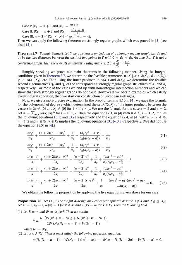
Theorem 3.7 (Bannai–Bannai). Let Y be a spherical embedding of a strongly regular graph. Let d1 andd2 be the two distances between the distinct two points in Y with 0 < d1 < d2. Assume that Y is not a

conference graph. Then there exists an integer k satisfying k ≥ 2 and d21d22=k−1k .

Roughly speaking we prove our main theorems in the following manner. Using the integralconditions given in Theorem 3.7, we determine the feasible parameters, n, |X1|, α ∈ A(X1), β ∈ A(X2),γ ∈ A(X1, X2), etc. Then using the inner products in A(X1) and A(X2) we determine the feasiblesecond eigenmatrices Q1 and Q2 of the corresponding strongly regular graph structures of X1 and X2respectively. For most of the cases we end up with non-integral intersection numbers and we canshow that such strongly regular graphs do not exist. However if we obtain examples which satisfyevery integral condition, then we start our construction of Euclidean 4-designs.Now, we give a more precise explanation. In the proof of Lemma 1.10 in [4], we gave the formula

for the polynomial of degree e which determined the set A(Xi, Xj) of the inner products between thevectors in Xi 6= {0} and Xj 6= {0} for 1 ≤ i, j ≤ p. We use the formula for the case e = 2 and p = 2.Let ai =

∑x∈X w(x)‖x‖

2i for i = 0, 1, 2. Then the equation (2.3) in [4] with u ∈ Xi, i = 1, 2, impliesthe following equations (3.1) and (3.2) respectively and the equation (2.4) in [4] with u 6= v ∈ Xi,i = 1, 2 and u ∈ X1, v ∈ X2 implies the following equations (3.3)–(3.5) respectively. (We did not usethe equation (3.5) in [4].)

nr12

a1+(n+ 2)(n− 1)r14

2a2+1a0+(a0r12 − a1)2

a0(a0a2 − a21)=1w1

(3.1)

nr22

a1+(n+ 2)(n− 1)r24

2a2+1a0+(a0r22 − a1)2

a0(a0a2 − a21)=1w2

(3.2)

n(u · v)a1

+(n+ 2)n(u · v)2

2a2−(n+ 2)r14

2a2+1a0+(a0r12 − a1)2

a0(a0a2 − a21)= 0 (3.3)

n(u · v)a1

+(n+ 2)n(u · v)2

2a2−(n+ 2)r24

2a2+1a0+(a0r22 − a1)2

a0(a0a2 − a21)= 0 (3.4)

n(u · v)a1

+(n+ 2)n(u · v)2

2a2−(n+ 2)(r1r2)2

2a2+1a0+(a0r12 − a1)(a0r22 − a1)

a0(a0a2 − a21)= 0. (3.5)

We obtain the following proposition by applying the five equations given above for our case.

Proposition 3.8. Let (X, w) be a tight 4-design on 2 concentric spheres. Assume 0 6∈ X and |X1| ≤ |X2|.Let r1 = 1, r2 = r,w(x) = 1 for x ∈ X1 andw(x) = w for x ∈ X2. Then the following hold.

(1) Let R = r2 and W = |X2|wR. Then we obtain

R =N1(W (n2 + n− 2N1)+ N1(n2 + 3n− 2N1)

)2W (N1(N1 − n− 1)+W (N1 − 1))

,

where N1 = |X1|.(2) Let α ∈ A(X1). Then α must satisfy the following quadratic equation.

n (N1(N1 − n− 1)+W (N1 − 1)) α2 + n(n− 1)N1α − N1(N1 − 2n)−W (N1 − n) = 0.


(3) Let β ∈ A(X2). Then β must satisfy the following quadratic equation.

4n ((N1 − n− 1)N1 + (N1 − 1)W )2W 2β2 + 4n(n− 1)N1 ((N1 − n− 1)N1+ (N1 − 1)W )W 2β − N21

((n2 + n− 2N1)W + N1(n2 + 3n− 2N1)

)×((n2 − n+ 2− 2N1)W + (n2 + n+ 2− 2N1)N1

)= 0.

(4) Let γ ∈ A(X1, X2). Then γ must satisfy the following quadratic equation.

2n (N1(N1 − n− 1)+W (N1 − 1))Wγ 2 + 2n(n− 1)N1Wγ−N1

(W (n2 + n− 2N1)+ N1(n2 + 3n− 2N1)

)= 0.

Proof. We have |X | = (n+2)(n+1)2 . Since N1 = |X1| ≤ |X2|, we obtain |X2| = |X | − N1 and

n+ 1 ≤ N1 ≤|X |2 . Let N2 = |X2|. Then we have ai =

∑u∈X w(u)‖u‖

2i= N1 + N2wRi = N1 +WRi−1

for i = 0, 1, 2. By substituting these values, (3.1) and (3.2) both imply the equation (1). Then (3.3) and(1), (3.4) and (1), (3.5) and (1) imply (2), (3) and (4) respectively. �

Let D be the discriminant of the quadratic equation (4) with respect to γ . Then D must be a non-negative real number and is given as follows:

D = nN1W(2(N1 − 1)(n2 + n− 2N1)W 2 −

(n3 + 8n2 + 7n+ 8N21 − 4(n

2− 3n− 2)N1

)× N1W + 2N21 (N1 − n− 1)(n

2+ 3n− 2N1)

). (3.6)

Then solution γ of (4) is given by γ = c1 ± c2 where c1 and c2 are given in the following way:

c1 = −N1(n− 1)

2 ((N1 − n− 1)N1 + (N1 − 1)W )< 0, (3.7)

c2 =

√D

2n ((N1 − n− 1)N1 + (N1 − 1)W )W≥ 0. (3.8)

Let X1 = {ui | 1 ≤ i ≤ N1} and X2 = {vi | 1 ≤ i ≤ N2}. Then, as we have seen in the argumentgiven above

ui · vj = c1 + εi,jc2 (3.9)

holds, where εi,j ∈ {1,−1}. We have the following lemma.

Lemma 3.9. Notations are as given above. Then, c2 is a positive rational number and the equation (4) hastwo distinct solutions. Moreover the following hold:

(1)∑N1i=1 εi,j = −N1

c1c2> 0 for any j = 1, . . . ,N2.

(2)∑N2j=1 εi,j = −N2

c1c2> 0 for any i = 1, . . . ,N1.

(3) Let m1 =∑N1l=1 εl,j and m2 =

∑N2l=1 εi,l. Then m1(> 0) and m2(> 0) do not depend on the choice of

j and i respectively.(4) For any u ∈ X1 and v ∈ X2, u · v must be a rational number.

Proof. Since X1 and X2 have the structure of Q-polynomial association schemes we must have∑N1i=1 ui =

∑N2j=1 vj = 0 (for more information please refer to [6]). Then (3.9) implies that N1c1 +∑N1

i=1 εi,jc2 = 0 for any fixed j. Since c1 < 0, c2 cannot be 0. Hence c2 must be a positive real number.Then (3.7)–(3.9) imply (1) and (2). Since by definition c1 is a rational number, c2 must be a rationalnumber. Then (3) and (4) follow immediately. �


4. Proof of the main theorems

Embeddings of Johnson schemesFirst we introduce the following expression of the Johnson scheme J(v, d) with v ≥ 2d. Let

F = {1,−1}. Instead of v point set of J(v, d) we take the direct product F v . As for the d point subsetof J(v, d), we take Jv,d = {f = (f1, . . . , fv) ∈ F v |

∑vl=1 fl = v − 2d}. Since |{i | fi = −1}| = d is

equivalent to∑vl=1 fl = v − 2d, | Jv,d| =

(v

d

)holds. Then for f , f ′ ∈ Jv,d and 0 ≤ i ≤ d, (f , f ′) is in the

ith relation of J(v, d) if and only if∑vl=1 fl f

′

l = v − 4i. Next, we define a map ρ : Jv,d −→ Rv−1 to be

ρ(f1, f2, . . . , fv−1, fv) = (f1, f2, . . . , fv) ∈ Rv. (4.1)

Since∑vl=1 fl = v − 2d holds for any f = (f1, f2, . . . , fv−1, fv) ∈ Jv,d, ρ is an injective map.

Case I (Proof of Theorem I). In this case we have N1 = n + 1 and N2 = n(n+1)2 . Then X1 is a regular

simplex. If n = 2, then N1 = N2 = 3 and X1 and X2 are both regular triangles in R2 and X is similar tothe example given in [4]. Now we assume n ≥ 3. Up to an orthogonal transformation of Rn we mayassume that X1 is the set of the following n+ 1 vectors. ui = (ui,1, . . . , ui,n), 1 ≤ i ≤ n+ 1, definedin the following way. The jth entry of ui with 1 ≤ i ≤ n is given by

ui,j ={a for j = ib for j 6= i, (4.2)

where a = − 1+(n−1)√n+1

n√n and b = −1+

√n+1

n√n . The jth entry of un+1 is given by un+1,j = 1

√n for

j = 1, . . . , n.

Proposition 4.1. Let |X1| = n + 1. Assume n ≥ 3. Let m1 be the positive integer defined in Lemma 3.9.Then the following holds.

(1) W = (n2−1)(n2−3m21−1)

2m21(n−2).

(2) n2 − 3m21 − 1 > 0.(3) X2 is a strongly regular graph.

Proof. Sincem1 = −N1 c1c2 , N1 = |X1| = n+ 1, (3.7) and (3.8) implym1 =n2−1√

3n2−3+2(n−2)W. Hence we

obtain

W =(n2 − 1)(n2 − 3m21 − 1)

2m21(n− 2). (4.3)

Since W = |X2|wR > 0, n2 − 3m21 − 1 > 0 holds. Since N1 = n + 1 and n ≥ 3, we haveN2 = n(n+1)

2 ≥ n+ 2. Therefore X2 must be a 2-distance set. Hence X2 is a strongly regular graph. �

Next we will show that the structure of X2 is uniquely determined by X1.

Lemma 4.2. Let π : X2 → Fn+1 be a map defined by π(vj) = (ε1,j, ε2,j, . . . , εn+1,j), where εi,j is givenin (3.9). Then the following hold.

(1) π(X2) ⊂ Jn+1, n+1−m12.

(2) The map π is injective.(3) For any vj, vj′ ∈ X2

vj · vj′ = c21

(−n+

n(n+ 1)m21

n+1∑j=1

εi,jεi,j′

)holds. Hence π is an isometry between X2 and π(X2) ⊂ Jn+1, n+1−m12

.


(4) π(X2) is a maximal 2-distance subset of Jn+1, n+1−m12. Hence it is a combinatorial tight 4-design in the

Johnson scheme J(n+ 1, n+1−m12 ).

Proof. (1) Since∑n+1l=1 εl,j = m1, π(vj) ∈ Jn+1, n+1−m12

.(2) Let M be the matrix of size n × n defined by M = aI + b(J − I), where a, b are the real numbersdefined in (4.2), I is the identitymatrix and J is thematrix whose entries are all 1. Then,M is invertibleand L = M−1 = 1+b

√n

a−b I +b√n

a−b (J − I), L2=

2nn+1 I +

nn+1 (J − I) hold. Since ui · vj = c1 + εi,jc2 for

1 ≤ i ≤ n + 1 and u1, . . . , un are the row vectors of M we have M tvj = c1 tu0+c2t(ε1,j, . . . , εn,j),

where u0 =√nun+1 = (1, 1, . . . , 1). Since M tu0 = −

1√ntu0, we have u0L = −

√nu0. Hence we

obtain

vj = −√nc1u0 + c2(ε1,j, . . . , εn,j)L = −

√nc1u0 + c2ρ(π(vj))L, (4.4)

where ρ is defined in (4.1). Since L is an invertible matrix and ρ is injective, π must be an injectivemap.(3) Next we compute the inner product of vj, vj′ ∈ X2.

vj · vj′ = (−√nc1u0 + c2ρ(π(vj))L) · (−

√nc1u0 + c2ρ(π(vj′))L)

= n2c21 −√nc1c2(u0 L) ·

(ρ(π(vj))+ ρ(π(vj′))

)+ c22

(ρ(π(vj))L2 · ρ(π(vj′))

)= n2c21 + nc1c2u0 ·

(ρ(π(vj))+ ρ(π(vj′))

)+ c22

(ρ(π(vj))L2 · ρ(π(vj′))

). (4.5)

In the computation given above, we note that L is a symmetric matrix. On the other hand,

ρ(π(vj))L2 = ρ(π(vj))(nn+ 1

J +nn+ 1

I)=

nn+ 1

n∑i=1

εi,ju0 +nn+ 1

ρ(π(vj)) (4.6)

holds for any j = 1, . . . ,N2. Since c2 = −(n+1)c1m1

, (4.5) and (4.6) imply (3).

(4) We have |π(X2)| = |X2| = (n+1)n2 =

(n+12

). It was proved by Ray-Chaudhuri and Wilson in [18],

that amaximal 2-distance set in J(n+1, d) has cardinality(n+12

). A 2-distance set in J(n+1, d) attains(

n+12

)if and only if it is a tight 4-design of J(n+ 1, d). �

Now we are ready to finish the proof of Theorem I. We have seen that X2 must be isomorphic toa combinatorial tight 4-design (see [18]). It is proved that only two non-trivial combinatorial tight 4-designs exist,which are the tight 4-designs in the Johnson schemes J(23, 7) and J(23, 16), equivalentlytight 4-(23, 7, 1) design and tight 4-(23, 16, 52) design respectively (see [18,11]). Hence the following(1), (2), or (3) holds.

(1) n+1−m12 = 2 and X2 is combinatorially isomorphic to Johnson scheme J(n+ 1, 2).(2) n+1−m12 = n− 1 and X2 is combinatorially isomorphic to Johnson scheme J(n+ 1, n− 1).(3) n = 22, 23−m12 = 7 or 16 and X2 is isomorphic to the non-trivial tight 4-design in J(23,

23−m12 ).

case (1): n+1−m12 = 2 impliesm1 = n− 3. Since n2 − 3m21 − 1 > 0, we must have n2− 9n+ 14 < 0.

Hence n = 4, 5, 6 andπ(X2) is the trivial tight 4-design of J(n+1, 2). Hence X2 has the structure of theJohnson scheme J(n+ 1, 2). Using Proposition 4.1 (1) and Proposition 3.8, we obtain the parametersgiven in the table of Theorem I.case (2): Sincem1 > 0, and n ≥ 3, this case does not occur.case (3): Since m1 > 0, we must have

23−m12 = 7 and m1 = 9. π(X2) is a tight 4-(23, 7, 1)-design

in J(23, 7). Proposition 4.1(1) and Proposition 3.8 give the parameters in the table of Theorem I forn = 22.The trivial tight 4-design in J(n + 1, 2) is uniquely determined and the tight 4-design in J(23, 7)

is determined uniquely up to permutations. Also Eq. (4.4) implies that X1 and the tight 4-design in


the Johnson scheme determine X2 uniquely. Hence the tight 4-design on 2 concentric spheres in Rn,(n = 4, 5, 6 and 22), is uniquely determined up to rotations and scaling. This completes the proof ofTheorem I. �

Embeddings of the Hamming schemesFor the proof of Theorems II and III, we use the 2-distance sets in the Hamming schemeH(d, 3). We

consider the following expression. Let H3 = {f1 = (−1, 1, 1), f2 = (1,−1, 1), f3 = (1, 1,−1)} ⊂ F 3and Hd,3 = direct product of d copies of H3 ⊂ F 3d. Then we have |Hd,3| = 3d. We express elementsf ∈ Hd,3 by f = (f (1)1 , f (1)2 , f (1)3 , . . . , f (l)1 , f

(l)2 , f

(l)3 , . . . , f

(d)1 , f (d)2 , f (d)3 ). We can consider the Hamming

scheme H(d, 3) on Hd,3. (f , f ′) ∈ Hd,3 × Hd,3 is in the ith relation of H(d, 3) if and only if∑3dj=1 fjf

′

j =

3d− 4i. Next, we define a map ρ : Hd,3 −→ R2d by

ρ(f (1)1 , f (1)2 , f (1)3 , . . . , f (l)1 , f(l)2 , f

(l)3 , . . . , f

(d)1 , f (d)2 , f (d)3 )

= (f (1)1 , f (1)2 , . . . , f (l)1 , f(l)2 , . . . , f

(d)1 , f (d)2 ) ∈ R2d. (4.7)

Since∑3i=1 f

(l)i = 1 for any l = 1, . . . , d, ρ is an injective map.

We also use the following 2-distance set in R2d. Let ∆ = {u1, u2, u3} be the regular triangle inR2 defined by u1 = (a, b), u2 = (b, a), u3 = 1

√2(1, 1), where a = −

√2+√6

4 and b = −√2−√6

4 . Let∆1, . . . ,∆d be regular triangles in R2d each of which is isometric to ∆ and mutually orthogonal toeach other. More precisely

∆l = {u(l)i = (02(l−1), ui, 02(d−l)) | 1 ≤ i ≤ 3} ⊂ R2 × · · · × R2 = R2d, (4.8)

where 0m is the zero in Rm for a natural number m. Then ∪dl=1∆l is a 2-distance set on S2d−1 with

A(∪dl=1∆l) = {0,−12 }.

Then we use the following matrixM2,d of size 2d× 2d whose lth row and l+ 1th row vectors areu(l)1 and u

(l)2 respectively. ThenM2,d is a symmetric and invertiblematrix. Let u0 = (1, 1, . . . , 1) ∈ R2d.

ThenM2,d tu0 = − 1√2

tu0 holds. Let L2,d = M2,d−1. Then we have

L22,d =

L 0 · · · 00 L 0 0

0 0. . . 0

0 0 0 L

, where L =

43

23

23

43

. (4.9)

Case II (Proof of Theorem II). In this case N1 = n+ 2. Then X1 is an (n+ 2)-point 2-distance set. SinceX1 is a spherical 2-design, X1 cannot be embedded in Rn−1. Seidel proved that such an (n + 2)-point2-distance set in Rn exists if and only if n is an even integer (see [19]). Moreover he proved that any(n+2)-point 2-distance set inRn is similar to the set {u(1)i | 1 ≤ i ≤

n2+1}∪{u

(2)i | 1 ≤ i ≤

n2+1} ⊂ Rn

satisfying ‖u(1)i ‖ = ‖u(2)j ‖ = 1, u

(1)i · u

(2)j = 0 for any 1 ≤ i, j ≤

n2 + 1 and both {u

(1)i | 1 ≤ i ≤

n2 + 1}

and {u(2)i | 1 ≤ i ≤n2+1} are isometric to the regular simplex inR

n2 . Henceu(1)i ·u

(1)j = u(2)i ·u

(2)j = −

2n

for any i 6= j, 1 ≤ i, j ≤ n2+1. If n = 2, thenN2 = |X |−N1 = 2 < N1. This contradicts our assumption.

Hence we must have n ≥ 4. Thus we have A(X1) = {0,− 2n }. Hence the quadratic equation of α given

in Proposition 3.8(2) must have the solution α = 0 and− 2n . This impliesW =n2−42 . Hence R =

nn−2 .

Let b1 and b2 be 2 distances of X2, then A(X2) = {R − 12b21, R −

12b22}. Then Proposition 3.8(3) implies(

b21+b22

b21−b22

)2=

(n+2)(n−1)n−2 . If X2 is not a conference graph, then Theorem 3.7 implies that

(b21+b

22

b21−b22

)2is the

square of an odd integer. However, if n > 6, then n+3 < (n+2)(n−1)n−2 < n+4 holds. This is impossible.

Also (n+2)(n−1)n−2 cannot be an odd integer for n = 3, 5, 6. Hence we obtain n = 4. If X2 is a conference


graph, then we must have N2 = 2n + 1. Since |X | = (n+2)(n+1)2 and N1 = n + 2, we must have

(n+2)(n+1)2 = 3n+ 3. This also implies n = 4.Now we let n = 4. Then N1 = 6 and N2 = 9. Then we may assume X1 = ∆1 ∪ ∆2, where ∆l

is the regular triangle in R4 defined in (4.8). Then α = 0,− 12 and W = 6, R = 2, w =13 . Hence

we obtain β = −1 or 12 , γ =12 ,−1 (c1 = −

14 , c2 =

34 ). Let X2 = {vj | 1 ≤ j ≤ 9}. Then (3.9)

implies u(l)i · vj = −14 +

34ε(l)i,j for 1 ≤ i ≤ 3, 1 ≤ j ≤ 9 and l = 1, 2 where ε

(l)i,j ∈ {1,−1}. Since ∆1

and ∆2 are regular triangles on the unit sphere S3, we have∑3i=1 u

(l)i = 0 for l = 1, 2. This implies∑3

i=1 ε(l)i,j = 1 for any fixed j. Then we can define as before π(vj) = (ε

(1)1,j , ε

(1)2,j , ε

(1)3,j , ε

(2)1,j , ε

(2)2,j , ε

(2)3,j ) ∈

H2,3. Let M2,2 be the 4 × 4 matrix defined above (note that d = 2 in this case). Then (3.9) and asimilar computation done in the proof of Theorem I imply vjM2,2 = − 14u0 +

34 (ε1,j, ε2,j, η1,j, η2,j),

where u0 = (1, 1, 1, 1). Since M2,2 is an injective matrix, ε(l)3,j = 1 − ε(l)1,j − ε

(l)2,j for l = 1, 2,

and |H3,2| = 9 = N2, the map π is a bijection between X2 and π(X2) = H2,3. Then we havevjM2,2 = − 14u0 +

34ρ(ε

(1)1,j , ε

(1)2,j , ε

(1)3,j , ε

(2)1,j , ε

(2)2,j , ε

(2)3,j ), where ρ is the injective map defined in (4.7).

Hence we have vj = 12u0 +

34 (ρ(ε

(1)1,j , ε

(1)2,j , ε

(1)3,j , ε

(2)1,j , ε

(2)2,j , ε

(2)3,j ))M2,2

−1. Thus the points in X2 areuniquely determined by H2,3. Then the similar argument given in the proof of Theorem I implies thatX2 with usual inner product and H2,3 with the Hamming distance are isometric to each other. HenceX2 has the structure of Hamming scheme H(2, 3). This completes the proof of Theorem II. �

Case III (Proof of Theorem III). In this section we assume |X1| ≥ n + 3 and we will give one moreexample of tight 4-design on 2 concentric spheres. In this case X1 and X2 are spherical 2-designs andalso 2-distance sets. Hence both of them are strongly regular graphs. If X2 is a conference graph, thenN2 = 2n+ 1. Since N1 ≤ N2, we must have n = 3, 4, 5. Case by case arguments show that this case isimpossible. Hence X2 is not a conference graph. Let b1, b2 be the distances between distinct points inX2. Assume 0 < b2 < b1. Then Theorem 3.7 implies that there exists an integer k satisfying

b2b1=k−1k .

Let A(X2) = {β1, β2}. Then {b21, b22} = {2R− 2β1, 2R− 2β2}. Hence we must have(

2R− β1 − β2β2 − β1

)2= (2k− 1)2. (4.10)

In the following we consider the case n = (2k− 1)2− 3. The reason why we assume this condition isbecause after an exhaustive search for the possible parameters n,m1,m2 etc. for n ≤ 100, there areno possible parameters except for the case n = (2k− 1)2− 3. It is also known that if a spherical tight4-design on Sn−1 exists, then nmust satisfy this condition (see [2,9]).First we prove the following proposition.

Proposition 4.3. Notation and definitions are given as above. Let A(X1) = {α1, α2}. Assume that (4.10)holds with n+ 3 = (2k− 1)2. Then we obtain(

2− α1 − α2α2 − α1

)2= (2k− 1)2 = n+ 3.

Proof. Solve for β1 and β2 using Proposition 3.8(3). Substitute β1, β2 and R in (4.10). We can expresseverything in terms ofW , n and N1, and we obtain a quadratic equation with respect toW . Solving forW then we have

W =N1

2(N1 − 1)(n2 + 2n− 3N1)×(6N21 − (3n

2+ 9n+ 6)N1

+ n3 + 5n2 + 6n± (n− 1)√n(n+ 3)(n2 + 3n+ 2− 2N1)N1

). (4.11)


Since n+3 ≤ N1 ≤ N2, we have N1 ≤ (n+2)(n+1)4 ≤

13 (n

2+2n). Therefore, by an elementary algebraic

computation, we can show thatW attains positive value only when

W =N1

2(N1 − 1)(n2 + 2n− 3N1)×(6N21 − (3n

2+ 9n+ 6)N1

+ n3 + 5n2 + 6n+ (n− 1)√n(n+ 3)(n2 + 3n+ 2− 2N1)N1

)(4.12)

and N1 < 16 (n+ 3)(n+ 2). Using (4.12) and Proposition 3.8(2), solve for α1 and α2 algebraically. Then

we can prove that(2−α1−α2α2−α1

)2= (2k− 1)2 = n+ 3 holds. �

If n + 3 = 9, i.e., k = 2 and n = 6, we can check easily there is no such Euclidean tight 4-design.In the following we show that in R22(n = 22, k = 3), Euclidean tight 4-design satisfying |X1| = 33

and(b21+b

22

b21−b22

)2= 52 is uniquely determined up to scaling. We actually construct the unique one using

the tight 4-design in the Hamming scheme H(11, 3). We note that it is known that a tight 4-design inH(d, q) exists only for d = 11 and q = 3 (see [16,17]).n = 22In this case |X | = 276. Since 25 ≤ N1 ≤ N2, we must have N1 ≤ 138. Since (4.12) implies

W = −

(N21 − 276N1 + 2200+ 35

√11N1(276− N1)

)N1

(N1 − 1)(N1 − 176), (4.13)

W > 0 holds if and only if 25 ≤ N1 ≤ 99. Since Lemma 3.9 shows that c2 is a positive rationalnumber,

√11N1(276− N1) must be an integer. This implies N1 = 33 and N2 = 243. Then we

have W = 33, and R = 11. Then Proposition 3.8(4) implies c1 = − 14 and c2 =34 . Hence we

have w = 181 . Then Proposition 3.8(2) and (3) imply {α1, α2} = {0,−

12 } and {β1, β2} = {−

52 , 2}

respectively. Then up to rotations in R22 we may assume X1 = ∪11l=1∆l, where ∆l is defined in (4.8).Let X2 = {vj | 1 ≤ j ≤ N2}. In the following we do the similar argument we did in the proof onTheorem II using H11,3. Eq. (3.9) implies u

(l)i · vj = c1 + c2ε

(l)i,j = −

14 +

34ε(l)i,j for each vj ∈ X2. Since∑3

i=1 u(l)i = 0 for l = 1, . . . 11, we obtain

∑3i=1 ε

(l)i,j = 1 for each l, j, 1 ≤ l ≤ 11, 1 ≤ j ≤ 243. For

vj ∈ X2, let π(vj) = (ε(1)1,j , ε

(1)2,j , ε

(1)3,j , . . . , ε

(l)1,j, ε

(l)2,j, ε

(l)3,j, . . . ε

(11)1,j , ε

(11)2,j , ε

(11)3,j ) ∈ H11,3. We will show that

π is injective andπ(X2) is a 2-distance subset inH11,3, that is, a 2-distance subset of Hamming schemeH(11, 3).LetM2,11 be the matrix defined as before. Let u0 = (1, 1, . . . , 1) ∈ R22. Then for vj ∈ X2 we obtain

M2,11 tvj = − 14tu0 + 3

4t(ε

(1)1,j , ε

(1)2,j , . . . , ε

(l)1,j, ε

(l)2,j, . . . , ε

(11)1,j , ε

(11)2,j ). Therefore we obtain

vj =√24

u0 +34(ρ(ε

(1)1,j , ε

(1)2,j , ε

(1)3,j , . . . , ε

(l)1,j, ε

(l)2,j, ε

(l)3,j, . . . ε

(11)1,j , ε

(11)2,j , ε

(11)3,j ))L2,11, (4.14)

where L2,11 = M2,11−1 and ρ is defined in (4.7). Then u0L2,11 = −√2u0 and (4.9) imply

vj · vj′ =

(√24

u0 +34ρ(π(vj))L2,11

)·

(√24

u0 +34ρ(π(vj′))L2,11

)

= −118+38

11∑l=1

3∑i=1

ε(l)i,j ε

(l)i,j′ . (4.15)

This implies that π is an isometry between X2 and H11,3. Since {β1, β2} = {− 52 , 2}, we have∑11l=1∑3i=1 ε

(l)i,j ε

(l)i,j′ = −3 or 9. Hence (π(xj), π(xj′)) is in relation 9 or 6 of the H(11, 3). Thus π(X2) is

a 2-distance subset ofH(11, 3). It is known that themaximal 2-distance set ofH(11, 3) has 243 pointsand is a tight 4-design of H(11, 3) (see [8]). Therefore π(X2) is a tight 4-design of H(11, 3). For a tight


4-design of H(11, 3), X2 is determined uniquely by (4.14). Tight 4-design of H(11, 3) is unique up topermutations. This completes the proof of Theorem III. �

5. Concluding remark

In Section 4, Case III, we assumed that n = (2k−1)2−3 and the 2-distances b1 and b2 (0 < b2 < b1)of X2 satisfy

b2b1=

k−1k . With this assumption we can find series of possible parameters for the

Euclidean tight 4-designs.All the examples of tight 4-design supported by 2 concentric spheres known at this point have the

structures of coherent configurations. In the following we propose a conjecture.

Conjecture. Let X be a Euclidean tight 4-design supported by 2 concentric spheres in Rn.(1) X has a structure of coherent configuration.(2) Let X1 and X2 be the two layers of X. Assume |X2| ≥ |X1| ≥ n+ 3. Then X1 and X2 are 2-distance setsand the following conditions hold:There exists an integer k ≥ 2 satisfying n = (2k − 1)2 − 3 and b2b1 =

k−1k , where b1 and b2 are the

two distances of X2 with 0 < b2 < b1.

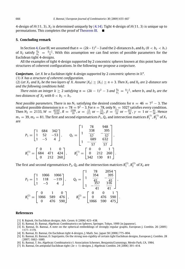
Next possible parameters. There is no N1 satisfying the desired conditions for n = 46 = 72 − 3. Thesmallest possible dimension is n = 78 = 92−3. For n = 78, onlyN1 = 1027 satisfies every condition.Then N2 = 2133, W = 42107

1539 , R =159919 , α =

13171 or −

53342 , β =

17719 or −

35738 , γ = 1 or −

4138 . Hence

m1 = 39,m2 = 81. The first and second eigenmatrices P1, Q1 and intersection matrices B(1)1 , B

(1)2 of X1

are

P1 =

[1 684 3421 52 −531 −5 4

], Q1 =

1 78 948

133857

−39557

1 −68957

63257

,

B(1)1 =

[ 0 1 0684 471 4240 212 260

], B(1)2 =

[ 0 0 10 212 260342 130 81

].

The first and second eigenmatrices P2, Q2 and the intersection matrices B(2)1 , B

(2)2 of X2 are

P2 =

[1 1066 10661 118 −1191 −5 4

], Q2 =

1 78 2054

135441

−39541

1 −35741

31641

,

B(2)1 =

[ 0 1 01066 589 4760 476 590

], B(2)2 =

[ 0 0 10 476 5901066 590 475

].

References

[1] B. Bajnok, On Euclidean designs, Adv. Geom. 6 (2006) 423–438.[2] Ei. Bannai, Et. Bannai, Algebraic Combinatorics on Spheres, Springer, Tokyo, 1999 (in Japanese).[3] Ei. Bannai, Et. Bannai, A note on the spherical embeddings of strongly regular graphs, European J. Combin. 26 (2005)1177–1179.

[4] Ei. Bannai, Et. Bannai, On Euclidean tight 4-designs, J. Math. Soc. Japan 58 (2006) 775–804.[5] Ei. Bannai, Et. Bannai, D. Suprijanto, On the strong non-rigidity of certain tight Euclidean designs, European J. Combin. 28(2007) 1662–1680.

[6] Ei. Bannai, T. Ito, Algebraic Combinatorics I: Association Schemes, Benjamin/Cummings, Menlo Park, CA, 1984.[7] Et. Bannai, On antipodal Euclidean tight (2e+ 1)-designs, J. Algebraic Combin. 24 (2006) 391–414.


[8] P. Delsarte, An algebraic approach to the association schemes of coding theory, Philips Res. Rep. Suppl. 10 (1973).[9] P. Delsarte, J.M. Goethals, J.J. Seidel, Spherical codes and designs, Geom. Dedicata 6 (1977) 363–388.[10] P. Delsarte, J.J. Seidel, Fisher type inequalities for Euclidean t-designs, Linear Algebra Appl. 114–115 (1989) 213–230.[11] H. Enomoto, N. Ito, R. Noda, Tight 4-designs, Osaka J. Math. 16 (1979) 39–43.[12] A. Erdelyi, et al., Higher Transcendental Functions, vol. II, McGraw-Hill, 1953, Bateman Manuscript Project.[13] D.G. Larman, C.A. Rogers, J.J. Seidel, On two-distance sets in Euclidean space, Bull London Math. Soc. 9 (1977) 261–267.[14] H.M. Möller, Lower bounds for the number of nodes in cubature formulae, in: Numerische Integration (Tagung, Math.

Forschungsinst., Oberwolfach, 1978), in: Internat. Ser. Numer. Math., vol. 45, Birkhäuser, Basel, Boston, MA, 1979,pp. 221–230.

[15] A. Neumaier, J.J. Seidel, Discrete measures for spherical designs, eutactic stars and lattices, Nederl. Akad. Wetensch. Proc.Ser. A 91=Indag. Math. 50 (1988) 321–334.

[16] R. Noda, On orthogonal arrays of strength 4 achieving Rao’s bound, J. London Math. Soc. (2) 19 (1979) 385–390.[17] R. Noda, On orthogonal arrays of strength 3 and 5 achieving Rao’s bound, Graphs Combin. 2 (1986) 277–282.[18] D.K. Ray-Chaudhuri, R.M. Wilson, On t-designs, Osaka J. Math. 12 (1975) 737–744.[19] J.J. Seidel, Quasiregular two-distance sets, Nederl. Akad. Wetensch. Proc. Ser. A 72 =Indag. Math. 31 (1969) 64–70.[20] P.D. Seymour, T. Zaslavsky, Averaging sets: A generalization of mean values and spherical designs, Adv. Math. 52 (1984)

213–240.

European Journal of Combinatorics - CORE

Documents

Transcript of European Journal of Combinatorics - CORE