1

Title 1

Estimating the cost of different strategies for measuring farmland biodiversity: evidence from a 2

Europe-wide field evaluation1 3

4

DOI 10.1016/j.ecolind.2014.04.050 5

6

Authors 7

Targetti S.1, Herzog F.2, Geijzendorffer I.R.3,4,Wolfrum S.5, Arndorfer M.6, Balàzs K.7, Choisis 8

J.P.8, Dennis P.9, Eiter S.10, Fjellstad W.10, Friedel J.K.6, Jeanneret, P.2, Jongman R.H.G.4, Kainz 9

M.5, Luescher G.2, Moreno G.11, Zanetti T.12, Sarthou J.P.13, 14, Stoyanova S.15, Wiley D.2, Paoletti 10

M.G.12, Viaggi D.1 11

12

Affiliations 13

1Department of Agricultural Sciences, University of Bologna, Italy 14

2 Agroscope, Institute for Sustainability Sciences ISS, Zurich, CH-8046 15

3Institut Méditerranéen de Biodiversité et d’Ecologie marine et continentale (IMBE), Aix-Marseille 16

Université, CNRS, IRD, Univ. Avignon, Technopôle Arbois-Méditerranée, Bât. Villemin – BP 80, 17

F-13545 Aix-en-Provence cedex 04, France 18

4Alterra, Wageningen UR, The Netherlands 19

5Technische Universität München, Germany 20

6Universität für Bodenkultur Wien, Austria 21

7Szent Istvan Egyetem, Hungary 22

8INRA, UMR 1201 DYNAFOR, F-31326 Castanet-Tolosan, France 23

9Institute of Biological, Environmental and Rural Sciences, Aberystwyth University, UK 24

10Norwegian Forest and Landscape Institute, Norway 25

11Forest Research Group, University of Extremadura, Spain 26

12Department of Biology, University of Padova, Padova, Italy 27

13INRA, UMR 1248 AGIR, F-31326 Castanet-Tolosan, France 28

14Université de Toulouse, INPT-ENSAT, UMR 1248 AGIR, F-31326 Castanet-Tolosan, France 29

15Institute of Plant Genetic Resources, Bulgaria 30

1 Abbreviations: H = habitat mapping; V = vegetation parameter; B= wild bees and bumblebees parameter; S = spiders

parameter; E = earthworms parameter; Q = farm management questionnaire parameter

2

31

Corresponding author 32

Stefano Targetti, Department of Agricultural Sciences, University of Bologna. V.le Fanin, 50, 33

40127 Bologna, Italy. 34

35

1 Introduction and objectives 36

Biodiversity provides important services that enhance the environmental resource base upon which 37

agriculture depends (Swift et al., 1996; Altieri 1999; Jackson et al., 2005; Paoletti et al., 2011;). 38

Biodiversity is declining globally (Butchart et al., 2010), including in agroecosystems (Tilman et 39

al., 2001; Kleijn et al., 2009). In response to this, several international programmes and measures 40

for halting biodiversity loss have been initiated in recent years (The Aichi Biodiversity Targets 41

2011-2020 - CBD, 2010; and European Commission, 2011). The European Commission has 42

indicated the need for a limited set of standard indicators (European Commission, 2005). However, 43

positive effects of policies and adopted measures on biodiversity both at farm and landscape scales 44

are controversial and more precise evaluations of their effects are still needed (Balmford et al., 45

2005; Batáry et al., 2011; Kleijn et al., 2011). 46

Several authors have highlighted the importance and the potential economic value of biodiversity 47

monitoring (e.g. Balmford and Gaston, 1999; James et al., 1999; Juutinen and Mönkkönen, 2004). 48

Evidence points to a positive correlation between monitoring efforts and the effectiveness of 49

policies (Naidoo, et al., 2006). Still, inadequate funding is a widespread constraint that undermines 50

the effectiveness of a number of existing monitoring programmes (McDonald-Madden, et al., 51

2011). Budget limitations and the optimization of resources need to be tackled during the 52

implementation of any monitoring programme. Thus, a cost analysis should be included alongside 53

consideration of the scientific credibility of the methods and relevance to stakeholders in any 54

process concerning indicator selection. Only after such an analysis the extent to which the 55

information value justifies the cost of the monitoring programme can be evaluated (Targetti et al., 56

2012a). 57

Recent literature focuses on cost-effectiveness procedures and analyses, and several studies are 58

directly concerned with the cost assessment of monitoring activities. Nevertheless, papers 59

addressing the topic are mainly based on: a) an indirect assessment of costs, (i.e. based on an ex-60

post analysis of project costs; e.g. Qi et al., 2008; Levrel et al., 2010; de Blust et al., 2012); b) a 61

proxy estimation, such as labour effort (e.g. Carlson and Schmiegelow, 2002); c) aggregated data 62

(i.e. not per single indicator or plot e.g. Juutinen and Mönkkönen, 2004); d) expert judgement (e.g. 63

Schmeller and Henle, 2008; Laycock et al., 2009); or e) localized studies (e.g. Schreuder et al., 64

3

1999; Bisevac and Majer, 2002; Franco et al., 2007; Cantarello and Newton, 2008; Gardner et al., 65

2008; Kessler et al., 2011; Sommerville et al., 2011). True empirical data from a large pool of farm 66

trials is currently lacking. In this paper, we address this issue by focusing on the costs of 67

biodiversity measurement at the farm scale since that is the scale at which the main decisions 68

regarding management practices and the adoption of policy measures are taken. 69

The objectives of this work are twofold: First, we present direct processing and analysis of 70

empirical data collected with regard to costs and effort spent on the measurement of agroecosystem 71

biodiversity, in twelve case study areas across Europe. Second, from our database we derive a cost 72

estimation for measuring biodiversity on a standardized farm. In doing so, we draw attention to the 73

cost differences between six biodiversity-related parameters and between different actors that may 74

be involved in the monitoring activities (professional agencies, farmers, volunteers). Our work takes 75

advantage of the large cost database built during the field activities of the EU-funded BioBio 76

Project (Herzog et al., 2013) and is based on a consistent methodology aimed at the analytical 77

assessment of costs. The database includes costs and efforts spent in the measurement of 78

biodiversity-related parameters on 192 farms representing more than 14,000 hectares of farmland in 79

11 European countries. 80

81

1.1 State of the art 82

Even though farmland monitoring can have a wide variety of targets (e.g. economic sustainability, 83

environmental performance, etc.), all current evaluation frameworks of policy impact are based on 84

indicators (Acosta-Alba and van der Werf, 2011). A specific theoretical framework for evaluating 85

the costs of measuring biodiversity indicators is not available in the literature. However, the main 86

cost components are provided by way of general economic cost theory and previous practical 87

attempts at assessing the costs of measuring biodiversity. 88

Economic theory tends to distinguish between the costs that are independent from the amount of a 89

monitoring/sampling effort (fixed costs) and the costs that are a function of the 90

monitoring/sampling effort (variable costs). Skalski and Robson (1992) adapted that classification 91

to costs of indicator measurement by distinguishing costs independent of the size of the survey 92

(fixed costs), costs of travelling to the research area (transportation costs) and costs related to the 93

number of study plots (variable costs). Indicators that include species also capture costs related to 94

trapping intensity, such as the purchase and maintenance of traps and the treatment and 95

identification of the specimens in each sample. 96

Practical insights regarding the data collection carried out in the framework of this study 97

highlighted further elements of complexity and the fact that the allocation of costs to a specific 98

4

indicator is usually based on a number of assumptions and simplifications. Firstly, measurement 99

costs may be shared in multiple different ways amongst indicators. For example, the measurement 100

of one parameter can provide data for the computation of different indicators; there can be costs for 101

labour or equipment that are shared between different indicators. These costs can be allocated to 102

individual indicators only through an “artificial” calculation process and usually under several 103

assumptions. An even more complex issue relates to the fact that some indicator output data can 104

serve as information inputs for calculating other indicators (e.g. habitat maps for floristic and fauna 105

indicators, see below), which adds the problem of assigning shares of costs of previous indicator 106

measurement to measurement occurring for the “second stage” indicator. Secondly, from a 107

budgetary and functional perspective, a monitoring programme includes three different phases: a) 108

development and setting-up (objective setting, planning the design of the survey, administrative 109

development, and pilot study); b) regular monitoring (scientific oversight, data collection, data 110

management, analysis and reporting, quality control of data, administration; Caughlan and Oakley, 111

2001); c) review and adaptation of the design to meet monitoring goals (Lindenmayer and Likens, 112

2009). Frequently, activities directly connected to parameter measurement (i.e. pilot study and data 113

collection) are the main budget items. Other activities, like the development and setting-up phase, 114

can be considered a fixed cost with regard to the regular monitoring phase as they do not vary with 115

the intensity of the final monitoring scheme or sampling protocol (e.g. the number of samples 116

collected; Skalski and Robson, 1992). Thus, a monitoring programme frequently involves a 117

consistent temporal delay between initial fixed monetary expenses and information delivery which 118

affects cost distribution per unit of data generated. 119

Moreover, costs may depend on the specific way in which resources are mobilised to carry out the 120

monitoring programme. For example, costs may be radically different if they come from the re-121

allocation of labour from already hired public administration staff or if specialised agencies/staff are 122

hired to complete the task. In order to combine feasibility and effectiveness, growing attention has 123

been drawn to the involvement of voluntary networks and farmers in the measurement of 124

biodiversity indicators (Danielsen et al., 2005; Schmeller et al. 2012; Von Haaren et al., 2012). In 125

fact, voluntary networks are currently involved in large species monitoring frameworks (Schmeller 126

et al., 2008) like in the Farmland Bird Index which is currently employed in policy contexts (e.g. 127

the Common Monitoring and Evaluation Framework of the CAP). For instance, Levrel et al., 128

(2010) estimated that the French administration saved between €678,523 and €4,415,251 in 2007-129

2008 thanks to volunteer-based monitoring of birds and butterflies. However, such monitoring data 130

require so-called ad-hoc indicator sets (i.e. indicators that fit farmers’ or volunteers’ knowledge) 131

and need a careful coordination to prevent statistical biases (Stevens et al., 2005). On the other 132

5

hand, the availability of consolidated data networks and the opportunity to promote societal 133

participation support the inclusion of “citizen science programmes” in monitoring schemes 134

(Devictor, et al., 2010; Conrad, et al., 2011; European Environment Agency, 2013a). 135

136

2 Material and methods 137

2.1 Sampling methodologies of biodiversity indicators 138

The BioBio Project included 12 case study regions across Europe covering the main European farm 139

types which were located in major bio-geographical regions (Herzog, et al., 2012). Between 8 and 140

19 farms were selected in a random procedure in each case study region (overall 192 farms). 141

Biodiversity indicators were selected on the basis of available literature, and feedback from 142

stakeholder panels. Habitat mapping (H) in BioBio consisted of registering the relative location, 143

size and type of all the different habitats which were directly or indirectly influenced by the 144

management of the farmer. Habitats have a direct relation with species and are characterised by 145

environmental, biological and management factors (Bunce et al., 2013). Mapping was done 146

according to a generic mapping approach developed for Europe (Bunce, et al., 2008 and 2011). The 147

habitat indicators recorded in BioBio therefore addressed the overall composition of the farm 148

related to specific habitat types that are relevant in the agricultural context (diversity of crops, share 149

of shrub and tree habitats), and captured the amount of semi-natural habitats. 150

Areal features (at least 5 m wide and covering 400 m2) and linear features (at least 0.5 m wide and 151

30 m long) on each farm were mapped and classified in different habitat types according to primary 152

life forms, environment and management (Bunce et al., 2008). A single example of each habitat 153

type per farm was randomly selected for species sampling (the ‘plot’). Plant species (V) were 154

recorded in 10 x 10 m2 squares for areal plots and 1 x 10 m2 rectangles for linear plots. Once the list 155

of plant species was completed, the percentage of ground cover occupied by each species was 156

estimated. Wild bees and bumblebees (B) were collected three times during good weather 157

conditions (i.e. during periods of sunshine when it was not too windy and the temperature was 158

higher than 15°C) along a predetermined 100 m transect through each plot. Spiders (S) were also 159

sampled three times on five circular areas of 35.7 cm diameter per plot using a modified leaf blower 160

with an attached net to allow a suction sample of 30-45 seconds duration to be taken. The suction 161

content was transferred to a labelled polyethylene bag and frozen for storage and later sorting and 162

identification of spider species. Earthworms (E) were sampled only once in three 30 x 30 cm metal 163

frames distributed across each plot. First, a solution of allyl isothiocyanate (0.1 g/l) was poured into 164

each frame to encourage earthworms to the surface. Subsequently, a 20-cm-deep earth-core was 165

sorted by hand. When required, plant, wild bee, spider and earthworm species collected in the plot 166

6

were transported to the laboratory and identified by experts, either within the research group or by a 167

subcontracted third party (see Dennis et al., 2012 for further details). 168

Farm management information was collected by means of interviews with farmers using a 169

standardised questionnaire (Q). This included questions regarding nutrient regimes, expenditure for 170

inputs (energy, fertilizer, pesticides), farm management, stocking density and crop and animal 171

genetic diversity. Interviews were arranged face-to-face and/or by telephone. 172

173

2.2 Cost of data collection 174

Data collection was organised in order to allow for an analytical assessment of recorded costs and 175

the subsequent simulation with standardised costs. During the field activities (2010) cost records 176

were gathered daily in the case study regions and then transferred and stored in a centralised 177

relational database. The database was organised in order to trace labour effort spent per farm, and 178

per biodiversity parameter measured. The records were related to labour time spent by the staff for 179

four types of activity: fieldwork, deskwork, laboratory and travel. Fieldwork activities included 180

field sampling and walking between the plots; deskwork included map digitalisation and data input; 181

laboratory work included sorting and preparation of species for taxonomic identification such as 182

insect pinning, etc.; and travel included transportation time to and from the sampled farm. In order 183

to account for surveyors sharing one car, the number of persons involved in each trip was also 184

recorded. Labour time spent by skilled and non-skilled workers was recorded separately. Costs for 185

taxonomic identification, consumables, equipment and other costs were also recorded. 186

The unitary cost of the utilisation of equipment was calculated as the cost of the equipment divided 187

by its lifetime. Vehicle costs were generally expressed per km (including fuel, road tax, car 188

insurance and vehicle depreciation) and multiplied by the actual distance travelled. Other costs 189

included accommodation and food for the fieldworkers etc. Free resources that were employed by 190

the research teams (e.g. labour time of volunteer and students, free accommodations or others) were 191

also recorded in order to include them in the cost standardisation process. 192

Costs related to reporting (e.g. analysis and calculation of indicators), programme start-up (e.g. time 193

spent for consumables or equipment purchase, the development of the programme, staff training, 194

etc.), data management, quality checks and other contingencies (such as crop damage due to 195

indicator measurements) are not included in the present analysis (see Targetti et al., 2011 for further 196

details). 197

7

198

2.3 Cost analysis and standardisation 199

In this work, we differentiate between the recorded costs incurred by the research units for the 200

biodiversity measurement (analytical assessment) and the standardised costs estimated for a regular 201

monitoring activity (cost standardisation). In the analytical assessment, labour for fieldwork and 202

travel was calculated for each day and traced back to the single farm and parameter measured. Costs 203

and effort related to deskwork, laboratory work, taxonomic identification and other resources were 204

aggregated per case study as they could not be attributed to a specific farm. 205

In order to establish a cost reference for biodiversity measurement at the farm scale and to simulate 206

a regular monitoring measurement, we applied a cost standardisation process based on the results of 207

the analytical assessment. This standardisation aimed to normalise fieldwork effort over the three 208

main factors that contributed to the variability of measurement costs and adjustments were based on 209

the data collection exercise (Skalski and Robson, 1992; Targetti et al., 2011): a) number of plots 210

and surveyed area on each farm; b) distance between farms and research centres (labour time spent 211

in travel); and c) unitary costs of resources in different countries. In this work, we referred the 212

standardised costs to a specific farm averaged over the 192 farms sampled in the BioBio Project: 73 213

ha farm area, 8 plots, 15 habitats patches2 and 1h travel distance (hereinafter, “standardised farm”). 214

Parcels of the standardised farm were assumed to be clustered in one single polygon. In some cases 215

(e.g. Norway) farm parcels were not clustered and fieldwork was organised in order to optimise the 216

number of trips and the time spent walking. These potential biases were considered during the cost 217

data collection identifying the farms served in each trip and the number of plots measured on each 218

farm. Moreover, in specific cases where the accessibility of plots was particularly difficult or the 219

walking area largely exceeded farm areas (e.g. Wales and Bulgaria), the time spent walking during 220

fieldwork was directly recorded. 221

We assessed the standardised field labour effort spent for each single farm using the following 222

equation (adapted from Skalski and Robson, 19923): 223

[eq. 1] 224

where Lf = fieldwork per farm (person days); i= biodiversity-related parameter; A = farm area (m2); 225

p= number of plots (p refers to number of habitats for habitat mapping); v = average walking speed 226

(fixed at 4500 m h-1); j = factor translating hours in person days (fixed at 8 hours per person day); l 227

= actual labour time per plot/habitat per survey round (person days); t = travel time from research 228

2 Species measurement was performed on one plot per habitat type. Therefore, the average number of habitats and

plots were different. 3 Assuming a random distribution of sampling plots, see Skalski and Robson, 1992.

8

centre to the farm (person days); d = days needed to complete the field survey round; k = number of 229

surveys required per farm (1 for H, V and E, 3 for B and S)4. Equation [1] was employed for the 230

estimation of labour time spent in transport from the research centre to the farm and walking to the 231

plots. This allowed for the assessment of the standardised field-labour required for the measurement 232

of one habitat in the habitat mapping and one plot in the species biodiversity parameters. 233

The costs of the sampling activity per farm were then assessed as: 234

F= (Lf + Ld) *C + T+ R [eq. 2] 235

where F= cost per farm (€ farm-1); Ld = deskwork (person days); C = person days cost (€); T = cost 236

of taxonomic identification of bees, spiders and earthworms; R = other resource costs (equipment, 237

consumables, vehicles, etc.). 238

Since the BioBio activities should be referred to as a “pilot study” with considerably higher labour 239

effort requirements than a regular monitoring phase (Caughlan and Oakley, 2001), the recorded 240

labour efforts were adapted in order to fit a more realistic estimation of costs for a regular data 241

collection activity. The envisaged reduction rates were specifically devised by the leaders of the 242

field activities and were based on the potential optimisation of the sampling design and synergies 243

between indicators groups (see Appendix A; Geijzendorffer et al., 2012 and Jongman et al., 2012 244

for further details). 245

246

2.4 Staff scenarios 247

Given the trends and existing monitoring efforts in Europe, we present results for three hypothetical 248

scenarios in which different actors may be involved in the monitoring activities: Strategy A is based 249

on the employment of professional agencies (e.g. by calls for tender). Strategy B directly involves 250

farmers in the field data collection, whilst deskwork and taxonomic identification is provided by 251

professional agencies as in strategy A. In strategy C, fauna data collection is performed by 252

volunteer networks while habitat mapping and vegetation sampling are performed by paid 253

professionals as in strategy A. 254

Strategy A is considered to be the general approach of public bodies that invite private agencies to 255

tender for the collection of information of interest. This approach is currently applied, for instance, 256

in LUCAS (Eurostat, 2013) where in situ monitoring is performed by private companies. In order to 257

consider the differences in labour costs across Europe, the costs of professional agencies in EU-27 258

countries were based on available information and assessed according to the correction factors 259

proposed in the Council Regulation –EC- No 1239/2010 (see Appendix B for data sources and 260

procedure of calculation). The same procedure was applied to the cost estimation of strategy B (see 261

4 For the farm questionnaire the function is simplified to L= l+2t

9

below). The rationale of strategies B and C lies in the growing interest in so-called “citizen science 262

programmes” that seek wider societal involvement in conservation (Devictor, et al., 2010; Conrad, 263

et al., 2011). In strategy B, information is provided directly by farmers under non-mandatory 264

contracts. This strategy involves “payment by results”, in which land managers are incentivised to 265

use their private knowledge to optimise actions for environmental conservation and claim support 266

for service provision from society (Oppermann, 2003; Gibbons et al., 2011). In this strategy, travel 267

costs are not included and an average person day cost of a farmer is hypothesised as a reasonable 268

incentive. Strategy C is related to the current data collection of several fauna monitoring schemes in 269

Europe (Schmeller et al., 2008) and the growing interest within European agencies, such as the 270

European Environment Agency, to incorporate “bottom-up” information in addition to scientifically 271

“top down” approaches or as a standalone source of knowledge (European Environment Agency, 272

2013a and 2013b). In this scenario, volunteers only receive reimbursement for consumables, vehicle 273

and equipment costs. 274

Standardised costs per farm for equipment, consumables, taxonomy and other costs were assessed 275

as an average of the costs incurred by the research units in the 11 European countries5 involved in 276

the BioBio Project. 277

278

3 Results 279

3.1 Analysis of research costs 280

The costs incurred by the research teams during the field trials were on average around € 4,000 per 281

farm (Table 1). Yet the large differences in unitary costs across the different countries (e.g. the cost 282

of researchers ranged between 6 € h-1 and 83 € h-1) led to substantial variability between the case 283

studies (range € 673 and € 8346 per farm; see Appendix C). As expected, labour (fieldwork, 284

deskwork and taxonomic identification) was the highest share of costs (about 90%). In particular, 285

fieldwork activities alone (i.e. labour time spent in travel, walking from one plot to the next and the 286

actual plot measurement) accounted for more than half of total costs. 287

Variability of data among the 192 sampled farms was less evident for the measures related to the 288

labour time spent by the research teams on the measurements (Figure 1). In particular, estimation of 289

actual fieldwork (i.e. fieldwork after travel and inter-plot walking) contributed to reduce 290

consistently the variability of effort requirements among the cases. The higher variability observed 291

for the lab and deskwork activities can be justified by the availability of aggregated results only (i.e. 292

at case study level, not per farm). In particular, spiders required considerable effort – but of large 293

5 The exchange rates from Norwegian Krone, British Pound, Swiss Franc and Hungarian Forint to Euro were: € = .92

NOK, € = . £, € = . CHF and € = ,818.25 HUF. All costs were related to 2010 (average published ECB

Exchange Rate values for year 2010).

10

variability - for laboratory work. This is related to the effort spent in sorting the captured specimens, 294

which was particularly time-consuming, and directly related to the characteristics of the sample 295

(e.g. number of species and individuals to be sorted, litter and other material present). Furthermore, 296

different strategies for the sorting of spider species were used in the different case study regions, 297

which is typical for the pilot phase of an investigation and contributed to higher variability. 298

Labour time spent in travel and time to access the plots was relevant for the “field-measured” 299

parameters (Table 2). It ranged between 4.23 and more than 7 hours per farm on average for H, and 300

the species indicator groups, whereas the farm questionnaire required the lowest travel time (Max 3 301

hours per farm6). Labour spent for travel is mainly related to the number of people involved and the 302

number of trips needed to collect the data for the biodiversity indicators. Even though the 303

measurement protocol was not strict concerning the number of persons to be included in the 304

fieldwork, the research units ended up converging with respect to an “optimal “organisation of 305

personnel: habitat mapping and vegetation were usually sampled during the same trip by a field 306

team composed of 2 persons (the number of persons ranged between 1 and 4). The staff involved in 307

the field activities for the other parameters ranged on average between 1 (wild bee and bumblebees, 308

farm questionnaire) and 3 (earthworms). The percentage of skilled workers used in the various case 309

studies was similar as well. Namely, the farm questionnaire, and the wild bee and bumblebee 310

parameters required about 80% of skilled workers, whereas involvement of persons without specific 311

skills was higher for the earthworm sampling. 312

313

3.2 Results of standardised costs 314

On average, the full set of parameters required a considerable amount of labour time for completing 315

the measurement of the standardised farm (14.3 person days - Table 3. See Appendix D for the 316

estimated person day requirements in farms characterised by different numbers of plots and 317

habitats). Nevertheless, consistent differences in labour time requirements were identified between 318

the biodiversity parameters. In general, fauna indicators were the most time consuming (almost 10 319

person days on average plus time needed for taxonomic identification). Of these, earthworms were 320

the most time consuming group of indicators (around 4.8 person days), whereas the farm 321

questionnaires required the lowest effort (about one person day per farm). Habitat mapping, 322

vegetation and bee recording required a similar labour effort (between 1.3 and 1.6 person days per 323

farm). The latter, however, required a higher number of journeys (because of the 3 repetitions) and 324

an extra-cost to be added for species identification subcontracts. Spiders were the most time-325

6 Farm questionnaires were performed by telephone in Norway and hence required no travel.

11

consuming indicator group for lab and deskwork activities only, whereas earthworms required the 326

highest labour time investment per farm for the fieldwork. 327

In Table 4, the estimated costs for the assessment of biodiversity of the standardised farm are 328

presented according to the three different strategies. On average, the assessment of biodiversity 329

would cost more than € 8,000 in strategy A (range € 4700 - € 9100 in EU 27 countries), with more 330

than 50% being spent on fieldwork activities. The possibility of employing farmers for the 331

fieldwork –strategy B- would allow for a 46% cost reduction in comparison to strategy A (range € 332

3200 - € 5800 in EU 27 countries). In this scenario, deskwork would absorb the greatest portion of 333

the available budget (around 78% of total costs). The volunteer-based approach – strategy C- would 334

clearly be the least expensive strategy allowing for a 77% cost reduction compared with strategy A 335

(range € 1600 - € 3100 in EU 27 countries). In this scenario, deskwork would be the most expensive 336

activity, absorbing more than 90% of the costs. Since sampling of fauna indicators is performed by 337

volunteers, the vegetation indicator group would be most costly budget item in strategy C. 338

339

4 Discussion 340

Our results revealed that labour is the critical resource for field-based indicator measurements. The 341

effort required to carry out the measurements on farms within each case study region varied greatly, 342

in particular for fieldwork activities. Similar variability was noted by other studies focusing on the 343

time requirements of measurement protocols (e.g. de Blust, et al., 2012). Labour effort variability 344

across different case studies was associated with the inherent organisational issues of the research 345

teams, ease of access to farms and plots, differences in farming types, farm size and habitat 346

diversity. The normalisation process allowed for a consistent reduction in the variability. This 347

enabled a more meaningful comparison of costs per farm referring to a standardised number of 348

plots/habitats, farm areas and travel distance. The high variability observed, however, underscores 349

the need to base cost estimations on a large number of observations in various conditions, and not 350

on generalised observations based on very few field teams or contexts. 351

The estimation of effort for biodiversity monitoring on a standardised farm allowed us to report the 352

costs of a monitoring set-up for a clearly defined object, defined by area, number of plots and 353

habitats. Nevertheless, a straightforward application of our results could lead to an 354

oversimplification of the problem. The literature on monitoring activities reports a wide range of 355

costs and effort for the measurement of different indicators. For instance, Levrel et al., (2010) 356

presented the effort spent in the measurement of 4 parameters (common bird census, bird ringing, 357

garden butterfly observation and common butterfly census) ranging from 7 h to 44 h per site (ratio 358

1:6). Our results were comparatively similar, ranging between 1 person day for questionnaires to 359

12

almost 5 person days for earthworm recording on the standardised farm (ratio 1:5). At the same 360

time, different objectives involve different protocol requirements for the measurement of the same 361

parameters along with notable labour time differences: for instance, Schmeller and Henle (2008) 362

reported an average 17.6 person days per site for high precision biodiversity surveys of plant 363

species, while Bisevac and Majer (2002) considered 0.67 person days per site to be sufficient for 364

surveying vegetation in restored areas. Even if sampling protocols and aims are similar, large 365

differences in effort can occur when sampling different environments. Time requirements for 366

habitat mapping in the European Biodiversity Observation Network Project (EBONE) were 367

considerably higher than in the farm scale BioBio Project (requirements for field mapping of 100 368

ha: between 4.1 and 5.2 person days in EBONE reported in de Blust et al., 2012 vs. 1.3 person 369

days7 in BioBio). Very likely, that difference was largely related to the more detailed list of habitat 370

categories required for the semi-natural environments targeted by EBONE in comparison to the 371

BioBio farmland areas. 372

The question arises whether the more costly indicators yield more (valuable) information than the 373

less costly ones. Amongst the six parameters, the more expensive ones include the direct 374

measurement of species and habitat diversity, whilst the questionnaire-based indicators only yielded 375

information on drivers (farm management practices), which are an indirect measure of biodiversity. 376

Whilst in the BioBio Project, correlations between farm management and biodiversity status 377

indicators were observed in individual case study regions, those correlations were not consistent 378

across study regions or farm types (Jeanneret et al. 2012). Therefore, the questionnaire- based 379

indicators did not generally allow for inferences for species or habitat diversity. 380

Information delivered by indicators could also be assessed with regard to its usefulness for different 381

end-users. For instance, a multicriteria evaluation was performed in order to assess the usefulness of 382

the BioBio indicator set. The survey was built upon three Stakeholder Advisory Board (SAB) 383

meetings over the course of the BioBio project and allowed for the comparison of the indicator 384

groups according to a list of ten criteria that was produced by the stakeholders. By means of a 385

multicriteria hierarchical procedure, the members of the SAB ranked the criteria and the parameters. 386

The results allowed for the evaluation of each measured parameter using a relative “usefulness” 387

scale which could be readily related to the cost of measurement. The pilot survey did not reveal any 388

linear relation between the costs of the measurement and the usefulness of the information (Targetti 389

et al., 2012b)8. Similar results concerning non-linearity between time requirements and information 390

of indicators are also reported e.g. in Gardner et al. (2008). If the costs and effectiveness of the 391

7 In order to compare with the EBONE Project, effort requirements for the mapping of 100 ha areas are estimated

before standardisation. 8 Further information are available upon request to the authors.

13

measurement are not related, a consistent cost/effort analysis should be included in order to 392

optimise monitoring programmes. 393

Flexibility afforded by the possibility of using low-skilled (and thus low cost) workers to complete 394

the field activities should also be considered. For instance, the average percentage of skilled persons 395

involved in spider sampling in the BioBio research activities could be considerably reduced. The 396

laborious laboratory work for sorting spiders from suction samples could also be assigned to non-397

skilled staff. This would lead to a significant simplification of logistics e.g. limited need for skilled 398

workers. Spider identification, on the other hand, requires specialised skills that could be scarce in 399

some countries. 400

Our reference of costs to the standardised farm allowed us to assess a reliable range of percentage 401

cost savings in the three scenarios based on a consistent methodology and a large data-set. For a 402

routine application in a monitoring scheme, the employment of professional agencies is the most 403

expensive option (even though some saving could be expected from the call for tender 404

mechanisms). Strategy A is most likely to assure the highest level of data quality because of the 405

technical and scientific expertise of the staff and because of the expertise that would be built over 406

the duration of the study. Nevertheless, the high cost of this approach could hinder the future 407

application of widespread biodiversity monitoring programmes at farm level, and the consideration 408

of less expensive options could be a conditio sine qua non that deserves specific consideration. 409

Considerable savings could be obtained if fieldwork measurements were carried out by farmers 410

themselves, for whom we considered an average person day cost as a reasonable incentive (Strategy 411

B). Travel time would be lower and farmers would also develop expertise and provide continuity. 412

Yet, the participation of farmers in the field activities introduces several shortcomings. Very likely, 413

habitat and vegetation surveys require botanical skills beyond the level of expertise that the average 414

farmer is willing to acquire. Farmers could take responsibility for the field sampling of spiders, bees 415

and earthworms after an appropriate training period but such sampling will overlap with periods of 416

high workloads for farmers (e.g. in spring). Moreover, to reduce biases, farmers would need to be 417

supervised by trained staff to make sure that sampling protocols are correctly and consistently 418

applied. Some of the labour cost savings would therefore be lost by increased training and 419

transaction costs (including data quality and control costs), which are not logistically easy to 420

provide for the large number of people involved. From a broader perspective, Strategy B could also 421

provide additional advantages, such as: endorsement of a bottom-up approach, information readily 422

available for farmers on their environmental performance, awareness raising and the incentive to 423

constitute environmentally-friendly brands and the possible implementation of a payment-for-424

results approach (Von Haaren, et al., 2012; Kelemen et al., 2013). Those advantages need to be 425

14

balanced against the potential of a less representative farm sample: i.e. the “monitoring effect” 426

which shows that the monitored farms increase their biodiversity performance more rapidly than the 427

farms which are not involved in the monitoring. 428

Strategy C (citizen science approach with volunteers) would allow for a substantial reduction of 429

costs but would require mechanisms to involve volunteer-networks and methods for maintaining 430

adequate quality of data (Schmeller et al., 2012; Holt et al., 2013). Similarly to Strategy B, the 431

involvement of volunteers would generate additional benefits such as societal inclusion and 432

commitment and mainstreaming of information on environmental performance of the farming 433

sector. Consistent money savings in Strategy C may also be realised because of the possibility of 434

recruiting the existing large pool of volunteer specialists who currently outnumber professionals for 435

some taxa (Schmeller et al., 2008; Levrel et al., 2010). As for Strategy B, this approach would need 436

to be framed by careful training and quality control activities. A major possible drawback consists 437

in potential restrictions for the sampling design (the selection of farms to be monitored). The 438

number of volunteers and interested laypersons is likely to be higher near urban areas, whereas in 439

more remote rural communities – which also need to be adequately sampled – it may be more 440

difficult to find sufficient volunteers. There will also be differences between countries due to 441

differences in size and distribution of volunteer networks (Van Swaay et al, 2008). A further 442

restriction is related to the actual biodiversity indicators. Volunteers tend to be attracted by 443

charismatic species (groups) such as birds and butterflies and by rare species often found in nature 444

reserves. It may be more difficult to motivate them to record earthworms and spiders on less 445

biodiverse farmland. 446

Even though the involvement of farmers and volunteers in monitoring activities could lead to 447

substantial savings, this opportunity requires a careful analysis of: a) the mechanisms needed to 448

incentivise the participation of farmers and volunteers; b) the methods needed to assure the required 449

level of data quality (Schmeller et al., 2012); c) the development of protocols that require lower 450

technical expertise if farmers are involved (e.g. Oppermann, 2003; Von Haaren, et al. 2012); and d) 451

the reliability of volunteer specialists for repeated periods of species identification. 452

453

5 Conclusions 454

Biodiversity monitoring is generally considered to be a relatively costly endeavour. Yet, systematic 455

information about the actual costs of different options and indicators for biodiversity monitoring are 456

not readily available. In addition, with regard to public decision making about biodiversity 457

monitoring, these costs would need to be balanced against the costs deriving from not being able to 458

measure to a higher detail the state and trends of biodiversity, thus to derive the costs incurred due 459

15

to biodiversity loss and the cost of not knowing the effects on biodiversity of different options 460

promoted by public policies. 461

In this paper, we focus on the former area of investigation (cost side). Our results confirm the 462

expectation that the costs for farmland biodiversity monitoring in Europe vary considerably 463

between countries and indicator types. The ratio of costs for measuring the BioBio indicator set was 464

1:12 between the lowest and the highest cost case studies. This evidence hampers the setting up a 465

common basket of biodiversity indicators because the cost-effectiveness of the programme will 466

inevitably diverge across EU countries. Nevertheless, the difficult implementation of a common 467

EU-wide monitoring program also depends from the different characteristics of farmland areas and 468

farming types, coupled to a difficulty in running a wide monitoring program9. 469

Our work was based on a consistent assessment methodology and involved a large and 470

comprehensive data set with selected habitat, management and species indicators. It could be a 471

plausible reference for the assessment of farm-scale monitoring of biodiversity. However, these 472

results can hardly be extrapolated to other types of indicators (e.g. other taxa, other indicators for 473

genetic diversity such as molecular-biological analysis, etc.), which would require specific cost 474

references or, at least, a careful consideration of the operational differences between the 475

measurement protocols. Similarly, specific features of the farms to be monitored should be 476

included. For instance, a farm consisting of a large number of scattered parcels would need more 477

journeys and walking time in comparison to clustered farms. 478

The paper also highlights the fact that the feasibility and coverage of a biodiversity monitoring 479

system is also dependent to the institutional arrangements that could be put in place. If a fixed 480

budget was available for farmland biodiversity monitoring (e.g. a percentage of the Common 481

Agricultural Policy –CAP- expenditure), our findings point to a potential 46% increase in the 482

coverage of a farm-scale biodiversity monitoring with Strategy B (farmer involvement) and a 77% 483

increase with Strategy C (volunteer involvement) in comparison with monitoring activities 484

subcontracted to private agencies only (Strategy A). Very likely, these opportunities come at a cost: 485

the quality of data and the statistical design should be carefully considered and adequate logistics 486

for the contribution of farmers and volunteers would be necessary. On the other hand, decisions 487

concerning the involvement of different actors are not only related to costs but also to “secondary” 488

additional returns. Namely, societal participation and information, increasing responsibility for 489

farmers’ environmental performance, education, etc. are aspects that might motivate farmers and 490

volunteers to be involved. In a policy context, these additional advantages could be of significant 491

value. Where labour costs are not a relevant limiting factor (e.g. in developing countries), the focus 492

9 But see http://www.bfn.de/0315_hnv+M52087573ab0.html for a succesful example of HNV monitoring

16

of the participative approach might be much more on education and information aspects than on 493

cost reduction. On the other hand, in policy contexts in which payments may be attached to 494

different levels of biodiversity provisions (such as in the context of the CAP or the implementation 495

of Payments for Ecosystem Services), such arrangement should also be balanced with the potential 496

emergence of distortions and acceptability issues. 497

As fieldwork was the most expensive activity, we focused on scenarios mainly based on different 498

strategies for field-data collection. This approach is also consistent with current approaches that 499

seek the involvement of local actors for field data collection. However, the possibility to involve 500

volunteers would allow also for cost reductions in species identification (laboratory work). This 501

opportunity was not included in strategy B. Nevertheless, Strategy B and C would involve extra-502

costs such as traning and data quality checks that are not included in this work. 503

A consistent assessment of the costs of biodiversity measurement is essential in order to minimize 504

the costs for a given level of information needed. This could be a first step towards the 505

improvement of knowledge-based decisions concerning biodiversity trends and cause-effect 506

mechanisms. The next major step that is envisaged in this paper, but still largely unexplored, is the 507

assessment of potential benefits of the additional information available through better monitoring. 508

In contexts heavily affected by public policies (i.e. the CAP in the EU), this primarily involves the 509

assessment of differential effects of better designed policies resulting from an improved knowledge 510

base for biodiversity. The potential for pursuing greater investment in biodiversity monitoring is 511

largely connected to the perception of these benefits, which makes this field a clear priority for 512

further investigation. 513

514

Acknowledgements 515

Part of the research was granted by the EU-FP7 Project BioBio, Indicators for biodiversity in 516

organic and low-input farming systems, contract No KBBE 227161. www.biobio-indicator.org. The 517

authors gratefully acknowledge the work of the field teams, the collaboration of the farmers that 518

allowed trampling of their plots and the valuable comments of two anonymous referees. This work 519

does not necessarily reflect the view of the European Union and in no way anticipates the 520

Commission’s future policy in this area. 521

522

References 523

Acosta-Alba, I., van der Werf, H.M.G., 2011. The Use of Reference Values in Indicator-Based 524

Methods for the Environmental Assessment of Agricultural Systems. Sustainability 3, 424–442. 525

Altieri M.A. 1999. The ecological role of biodiversity in agroecosystems. Agriculture, Ecosystems 526

& Environment 74, 19-31. 527

17

Balmford, A., Crane, P., Dobson, A., Green, R.E., Mace, G.M., 2005. The 2010 challenge: data 528

availability, information needs and extraterrestrial insights. Philosophical transactions of the Royal 529

Society of London. Series B, Biological Sciences 360, 221–8. 530

Balmford, A., Gaston, K.J., 1999. Why biodiversity surveys are good value. Nature, 398, 204-205. 531

Batáry, P., Báldi, A., Kleijn, D., Tscharntke, T. 2011. Landscape-moderated biodiversity effects of 532

agri-environmental management: a meta-analysis. Proceedings of the Royal Society B: Biological 533

Sciences, 22, 1894-1902. 534

Bisevac, L., Majer, J., 2002. Cost effectiveness and data-yield of biodiversity surveys. Journal of 535

the Royal Society of Western Australia, 85, 129-132. 536

de Blust, G., Laurijssens, G., van Calster, H., Verschelde, P., Bauwens, D., De Vos, B., Svensson, 537

J., 2012. Report 8.1: Optimization of biodiversity monitoring through close collaboration of users 538

and data providers. EBONE European Biodiversity Observation Network Project Project 539

Deliverable 8.1. Available at: http://www.wageningenur.nl/en/Expertise-Services/Research-540

Institutes/alterra/Projects/EBONE-2/Deliverables.htm Accessed on: July 2013. 541

Bunce, R.G.H., Metzger, M.J., Jongman, R.H.G., Brandt, J., Blust, G., de Elena-Rossello, R., 542

Groom, G.B., Halada, L., Hofer, G., Howard, D.C., Kovár, P., Mücher, C.A., Padoa-Schioppa, E., 543

Paelinx, D., Palo, A., Pérez-Soba, M., Ramos, I.L., Roche, P., Skånes,H., Wrbka, T., 2008. A 544

standardized procedure for surveillance and monitoring European habitats and provision of spatial 545

data. Landscape Ecology, 23, 11–25. 546

Bunce, R.G.H., Bogers, M.M. B., Roche, P., Walczak, M., Geijzendorffer, I.R., Jongman, R.H.G., 547

2011. Manual for Habitat and Vegetation Surveillance and Monitoring: Temperate, Mediterranean 548

and Desert Biomes. Alterra Report 2154, Wageningen UR. 549

Bunce, R.G.H, Bogers, M.M.B., Evans, D., Halada, L., Jongman, R.H.G., Mucher, C.A., Bauch, B., 550

de Blust, G., Parr, T.W., Olsvig-Whittaker, L., 2013. The significance of habitats as indicators of 551

biodiversity and their links to species. Ecological Indicators, 33, 19-25. 552

Butchart, S.H.M., Walpole, M., Collen, B., van Strien, A., Scharlemann, J.P.W., Almond, R.E.A, 553

Baillie, J.E.M., Bomhard, B., Brown, C., Bruno, J., Carpenter, K.E., Carr, G.M., Chanson, J., 554

Chenery, A.M., Csirke, J., Davidson, N.C., Dentener, F., Foster, M., Galli, A., Galloway, J.M., 555

Genovesi, P., Gregory, R.D., Hockings, M., Kapos, V., Lamarque, J.F., Leverington, F., Loh, J., 556

McGeoch, M.A., McRae, L., Minasyan, A., Hernández Morcillo, M., Oldfield, T.E.E., Pauly, D., 557

Quader, S., Revenga, C., Sauer, J.R., Skolnik, B., Spear, D., Stanwell-Smith, D., Stuart, S.N., 558

Symes, A., Tierney, T., Tyrrell, T.D., Vié, J.C., Watson R., 2010. Global biodiversity: indicators of 559

recent declines. Science, 328, 1164–1168. 560

Cantarello, E., Newton, A.C., 2008. Identifying cost-effective indicators to assess the conservation 561

status of forested habitats in Natura 2000 sites. Forest Ecology and Management 256, 815–826. 562

Carlson, M., Schmiegelow, F., 2002. Cost-effective sampling design applied to large scale 563

monitoring of boreal birds. Conservation Ecology. 6(2), 11. 564

18

Caughlan, L., Oakley, K.L., 2001. Cost considerations for long-term ecological monitoring. 565

Ecological Indicators 1, 123-134. 566

CBD, 2010. Strategic Plan, including Aichi Biodiversity Targets (2011–2020). Available at: 567

www.cbd.int/sp/sp2010p. Accessed on: January 2014. 568

Conrad, C.C., Hilchey, K.G., 2011. A review of citizen science and community-based 569

environmental monitoring: issues and opportunities. Environmental Monitoring and Assessment, 570

176 (1-4), 273–291. 571

Danielsen, F., Jensen, A.E., Alviola, P. A., Balete, D.S., Mendoza, M., Tagtag, A., Custodio, C., 572

Enghoff, M., 2005. Does Monitoring Matter? A Quantitative Assessment of Management Decisions 573

from Locally-based Monitoring of Protected Areas. Biodiversity and Conservation, 14, 2633–2652. 574

Dennis, P., Bogers, M.M.B., Bunce, R.G.H., Herzog, F. and Jeanneret, P., 2012. Biodiversity in 575

organic and low-input farming systems. Handbook for recording key indicators. Wageningen, 576

Alterra, Alterra-Report 2308. Available at: http://www.biobio-indicator.org/deliverables/D22.pdf. 577

Accessed on: March 2013. 578

Devictor, V., Whittaker, R.J., Beltrame, C., 2010. Beyond scarcity: citizen science programmes as 579

useful tools for conservation biogeography. Diversity and Distributions, 16(3), 354–362. 580

European Commission, 2005. Council regulation of 20 September 2005 on support for rural 581

development by the European Agricultural Fund for Rural Development (EAFRD). EC Nº 582

1698/2005. 583

European Commission, 2011. The Eu Biodiversity Strategy to 2020. Brussels. Available at: 584

http://ec.europa.eu/environment/nature/info/pubs/docs/brochures/2020%20Biod%20brochure%20fi585

nal%20lowres.pdf. Accessed on: January 2014. 586

European Environment Agency, 2013a. Biodiversity Monitoring in Europe. Copenhagen. Available 587

at: http://www.eea.europa.eu/publications/biodiversity-monitoring-in-europe. Accessed on: 588

September 2013. 589

European Environment Agency, 2013b. Science for Environment Policy In-depth Report: 590

Environmental Citizen Science. Copenhagen. Available at: 591

http://ec.europa.eu/environment/integration/research/newsalert/pdf/IR9.pdf. Accessed on: January 592

2014. 593

Eurostat, 2013. LUCAS the EU’s land use and land cover survey. European Union, 2013. Available 594

at: http://epp.eurostat.ec.europa.eu/cache/ITY_OFFPUB/KS-03-13-587/EN/KS-03-13-587-EN.PDF 595

Accessed on: January 2014. 596

Franco, A., Palmeirim, J., Sutherland, W., 2007. A method for comparing effectiveness of research 597

techniques in conservation and applied ecology. Biological Conservation, 134, 96–105. 598

Gardner, T. A, Barlow, J., Araujo, I.S., Avila-Pires, T.C., Bonaldo, A.B., Costa, J.E., Esposito, 599

M.C., Ferreira, L. V, Hawes, J., Hernandez, M.I.M., Hoogmoed, M.S., Leite, R.N., Lo-Man-Hung, 600

N.F., Malcolm, J.R., Martins, M.B., Mestre, L. a M., Miranda-Santos, R., Overal, W.L., Parry, L., 601

19

Peters, S.L., Ribeiro-Junior, M.A., Da Silva, M.N.F., Da Silva Motta, C., Peres, C., 2008. The cost-602

effectiveness of biodiversity surveys in tropical forests. Ecology Letters, 11, 139–150. 603

Geijzendorffer, I.R., Targetti, S., Jongman, R.H.G., Viaggi, D., 2012. Implementing a biodiversity 604

monitoring scheme for European farms. In: Herzog F., Balàzs K., Dennis P., Friedel J., 605

Geijzendorffer I., Jeanneret P., Kainz M., Pointereau P. (Eds.). Biodiversity indicators for European 606

farming systems. ART-Schriftenreihe, 17, 1-99. 607

Gibbons, J.M., Nicholson, E., Milner-Gulland, E.J., Jones, J.P.J., 2011. Should payments for 608

biodiversity conservation be based on action or results? Journal of Applied Ecology, 48, 1218-1226. 609

Herzog, F., Balàzs, K., Dennis, P., Friedel, J., Geijzendorffer, I., Jeanneret, P., Kainz, M., & 610

Pointereau, P. (eds.) (2012). Biodiversity indicators for European farming systems. A guidebook. 611

Zurich, ART-Schriftenreihe, 17. Available at: http://www.biobio-indicator.org/project.php 612

Accessed on January 2014. 613

Herzog, F., Jeanneret, P., Ammari, Y., Angelova, S., Arndorfer, M., Bailey, D., Balázs, K., Báldi, 614

A., Bogers, M.M.B., Bunce, R.G.H., Choisis, J.P., Cuming, D., Dennis, P., Dyman, T., Eiter, S., 615

Elek, Z., Falusi, E., Fjellstad, W., Frank, T., Friedel, J.K., Garchi, S., Geijzendorffer, I.R., Gomiero, 616

T., Jerkovich, G., Jongman, R.H.G., Kainz, M., Kakudidi, E., Kelemen, E., Kölliker, R., Kwikiriza, 617

N., Kovács-Hostyánszki, A., Last, L., Lüscher, G., Moreno, G., Nkwiine, C., Opio, J., Oschatz, M.-618

L., Paoletti, M.G., Penksza, K., Pointereau, P., Riedel, S., Sarthou, J.P., Schneider ,M.K., Siebrecht, 619

N., Sommaggio, D., Stoyanova, S., Szerencsits, E., Szalkovski, O., Targetti, S., Viaggi, D., Wilkes-620

Allemann, J., Wolfrum, S., Yashchenko, S., Zanetti, T., 2013. Measuring farmland biodiversity. 621

Solutions, 4(4), 52 – 58. 622

Holt, B.G., Rioja-Nieto, R., MacNeil, M.A., Lupton, J., Rahbeck, C., 2013. Comparing diversity 623

data collected using a protocol designed for volunteers with results from a professional alternative. 624

Methods in Ecology and Evolution, 4, 383-392. 625

Jackson, L., Bawa, K., Pascual, U., Perrings, C., 2005. Agrobiodiversity: A new science agenda for 626

biodiversity in support of sustainable agroecosystems. DIVERSITAS Report N°4. 627

James, A.N., Kevin, J., Balmford, A., 1999. Balancing the Earth’s accounts. Nature, 401, 323-324. 628

Jeanneret, P., Lüscher, G., Schneider, M., Arndorfer, M., Last, L., Wolfrum, S., Balàzs, K., Bailey, 629

D., Bogers, M.M.I., Dennis, P., Eiter, S., Fjellstad, W., Friedel, J.K., Geijzendorffer, I.R., Gomiero, 630

T., Herzog, F., Jongman, R.H.G, Kainz, M., Kovács, A., Kölliker, R., Moreno, G., Paoletti, M., 631

Sarthou, J.-P., Stoyanova, S., 2012. Report on scientific analysis containing an assessment of 632

performance of candidate farming and biodiversity indicators and an indication about the cost of 633

indicator measurements. BioBio Project deliverable 4.1. Available at: www.biobio-indicator.org 634

Accessed on: March 2013. 635

Jongman, R.H.G., Staritsky, I., Geijzendorffer, I.R., Herzog, F., Viaggi, D., Targetti, S., 2012. 636

Report on the suitability of continental scale indicators for reflecting biodiversity of organic/low 637

input farming systems, proposition of a monitoring system at the continental scale. BioBio Project 638

deliverable D4.2. Available at: www.biobio-indicator.org Accessed on: March 2013. 639

20

Juutinen, A., Mönkkönen, M., 2004. Testing alternative indicators for biodiversity conservation in 640

old-growth boreal forests: ecology and economics. Ecological Economics, 50, 35–48. 641

Kelemen E., Nguyen G., Gomiero, T., Kovács, E., Choisis, J.P., Choisis, N., Paoletti, M.G., 642

Podmaniczky, L., Ryschawy, J., Sarthou, J.P. Herzog, F., Dennis, P., Balázs, K., 2013. Farmers’ 643

perceptions of biodiversity: Lessons from a discourse-based deliberative valuation study. Land Use 644

Policy, 35, 318-328. 645

Kessler, M., Abrahamczyk, S., Bos, M., Buchori, D., Putra, D.D., Robbert Gradstein, S., Höhn, P., 646

Kluge, J., Orend, F., Pitopang, R., Saleh, S., Schulze, C.H., Sporn, S.G., Steffan-Dewenter, I., 647

Tjitrosoedirdjo, S.S., Tscharntke, T., 2011. Cost-effectiveness of plant and animal biodiversity 648

indicators in tropical forest and agroforest habitats. Journal of Applied Ecology, 48, 330–339. 649

Kleijn D, Kohler, F., Báldi, A., Batáry, P., Concepción, E.D., Clough, Y., Díaz, M., Gabriel, D., 650

Holzschuh, A., Knop, E., Kovács, A., Marshall, E.J.P., Tscharntke, T., Verhulst, J., 2009. On the 651

relationship between farmland biodiversity and land-use intensity in Europe. Proceedings of the 652

Royal Society B: Biological Sciences, 276, 903-909. 653

Kleijn, D., Rundlöf, M., Scheper, J., Smith, H.J., Tscharntke, T., 2011. Does conservation on 654

farmland contribute to halting the biodiversity decline? Trends in Ecology and Evolution, 26, 474-655

481. 656

Laycock, H., Moran, D., Smart, J., Raffaelli, D., White, P., 2009. Evaluating the cost-effectiveness 657

of conservation: The UK Biodiversity Action Plan. Biological Conservation, 142, 3120–3127. 658

Levrel, H., Fontaine, B., Henry, P.Y., Jiguet, F., Julliard, R., Kerbiriou, C., Couvet, D., 2010. 659

Balancing state and volunteer investment in biodiversity monitoring for the implementation of CBD 660

indicators: A French example. Ecological Economics, 69, 1580–1586. 661

Lindenmayer, D.B., Likens, G.E., 2009. Adaptive monitoring: a new paradigm for long-term 662

research and monitoring. Trends in Ecology & Evolution, 24(9), 482–486. 663

McDonald-Madden, E., Baxter, P.W.J., Fuller, R. a., Martin, T.G., Game, E.T., Montambault, J., 664

Possingham, H.P., 2011. Should we implement monitoring or research for conservation? Trends in 665

Ecology & Evolution 26, 108–109. 666

Naidoo, R., Balmford, A., Ferraro, P.J., Polasky, S., Ricketts, T.H., Rouget, M., 2006. Integrating 667

economic costs into conservation planning. Trends in Ecology & Evolution, 21, 681–687. 668

Oppermann, R., 2003. Nature balance scheme for farms—evaluation of the ecological situation. 669

Agriculture, Ecosystems and Environment 98, 463-475. 670

Paoletti, M.G., Gomiero, T., Pimentel, D., (Eds.). 2011. Towards a More Sustainable Agriculture. 671

Critical Reviews in Plant Sciences, 30(1-2), 1-237 672

Qi, A., Perry, J.N., Pidgeon, J.D., Haylock, L.A., Brooks, D.R., 2008. Cost-efficacy in measuring 673

farmland biodiversity – lessons from the Farm Scale Evaluations of genetically modified herbicide-674

tolerant crops. Annals of Applied Biology, 152, 93–101. 675

21

Schmeller, D.S., Henle, K., 2008. Cultivation of genetically modified organisms: resource needs for 676

monitoring adverse effects on biodiversity. Biodiversity Conservation, 17, 3551-3558. 677

Schmeller, D.S., Henle, K., Loyau, A., Besnard, A., Henry, P.Y., 2012. Bird-monitoring in Europe 678

– a first overview of practices, motivations and aims. Nature Conservation, 2, 41–57. 679

Schmeller, D.S., Henry, P.Y., Julliard, R., Gruber, B., Clobert, J., Dziock, F., Lengyel, S., Nowicki, 680

P., Déri, E., Budrys, E., Kull, T., Tali, K., Bauch, B., Settele, J., van Swaay, C., Kobler, A., Babij, 681

V., Papastergiadou, E., Henle, K., 2008. Advantages of volunteer-based biodiversity monitoring in 682

Europe. Conservation Biology, 23, 307–16. 683

Schreuder, H.T., Hansen, M., Kohl, M., 1999. Relative costs and benefits of a continuous and a 684

periodic forest inventory in Minnesota. Environmental Monitoring and Assessment, 59, 135-144. 685

Skalski, J.R., Robson, D.S., 1992. Techniques for wildlife investigations. Design and analysis of 686

capture data. Academic Press. San Diego, CA. 687

Sommerville, M.M., Milner-Gulland, E.J., Jones, J.P.G., 2011. The challenge of monitoring 688

biodiversity in payment for environmental service interventions. Biological Conservation, 144, 689

2832–2841. 690

Stevens, C.J., Thomas, M.B., Mitchley, J., Fraser, I.M., 2005. Workshop Report: Large Scale 691

Investigations in Ecology and Rural Land Use. Imperial College London, April 2005. 692

Swift, M.J., Vandermeer, J., Ramakrishnan, P.S., Anderson, J.M., Ong, C.K., Hawkins, B.A. 1996. 693

Biodiversity and Agroecosystem Function. In: Money, H.A., Cushman, J.H., Medina, E., Sala, 694

O.E., Schulze, E.D., (Eds.). Functional Roles of Biodiversity. A Global Perspective. John Wiley 695

and Sons Ltd, UK. 696

Targetti, S., Viaggi, D., Cuming, D., 2011. Analysis of Costs and Efforts of BioBio Indicators of 697

Biodiversity. BioBio Project deliverable D3.3. 698

Targetti, S., Viaggi, D., Cuming, D., Sarthou, J.P., Choisis, J.P., 2012a. Assessing the costs of 699

measuring biodiversity: Methodological and empirical issues. Food Economics, 1-8. 700

Targetti, S., Viaggi, D., Pointereau, P., Herzog, F., 2012b. Report on the SAB questionnaire. 701

Available at: www.biobio-indicator.org Accessed on: March 2013. 702

Tilman, D., Fargione, J., Wolff, B., D’Antonio, C., Dobson, A., Howarth, R., Schindler, D., 703

Schlesinger, W.H., Simberloff, D., Swackhamer, D., 2001. Forecasting agriculturally driven global 704

environmental change. Science, 292, 281-284. 705

Van Swaay, C.A.M., Nowicki, P., Settele, J., Van Strien, A.J., 2008. Butterfly monitoring in 706

Europe: methods, applications and perspectives. Biodiversity Conservation, 17, 3455-3469. 707

Von Haaren, C., Kempa, D., Vogel, K., Rüter, S., 2012. Assessing biodiversity on the farm scale as 708

basis for ecosystem service payments. Journal of Environmental Management, 113, 40–50.Acosta- 709

710

711

22

Tables 712

Table 1 Cost of resources spent per farm during the research activities in the 12 case studies and 713

cost share of the resources on total costs (standard error of the mean in brackets). 714

Average € farm-1 Share of total costs (%)

Fieldwork and travel 2017 (450) 52

Deskwork 754 (174) 19

Taxonomy 712 (140) 18

Transport (vehicle costs) 211 (52) 6

Consumables 69 (19) 2

Other costs* 85 (27) 2

Equipment 35 (9) 1

Total 3883

*Other costs include field accommodation, food allowances and incentives for farmers. 715

716

717

Table 2 Average labour time spent in travel and in walking to the plots, number of persons and 718

share of highly skilled persons involved in the research activities (standard error of the mean in 719

brackets; n = 192 for habitat mapping and vegetation, 189 for wild bees and bumblebees, 190 for 720

spiders, 182 for earthworms and 12 for questionnaires). 721

Habitat mapping

Vegetation

Wild bees and bumblebees

Spiders Earthworms

Questionnaire

Travel + transfers to plots [h farm-1

5.2 (0.30)

4.2 (0.35) 5.6 (0.31)

6.9 (0.48)

7.5 (0.50) 1.8 (0.44)

Persons involved in the field staff [Number]

1* (0.06)

1* (0.04)

1 (0.07) 2 (0.14) 3 (0.33) 1 (0.00)

Highly skilled persons in the field staff [%]

69 (2.66)

68 (2.41)

79 (2.54)

71 (2.58)

58 (3.00) 80 (9.79)

*very often, habitat mapping and vegetation surveys were performed together 722

723

724

Table 3 Standardised person days spent per farm in the measurement of biodiversity (data are 725

referred to the standardised farm: No of plots = 8, No of habitats = 15, area = 73 ha, travel distance 726

23

= 1 h). Time spent for taxonomic identification is included for vegetation, whereas it was 727

subcontracted for wild bees and bumblebees, spiders and earthworms and is not included in this 728

table (see Table 4). 729

H V B S E Q

Fieldwork 0.52 1.12 0.70 0.60 2.85 0.32

Lab and deskwork 0.86 0.51 0.56 1.58 0.94 0.37

Travel + transfers to plots 0.50 1.50 1.00 0.38

Total 14.3*

* Assuming travel synergies between habitat mapping and vegetation indicator groups and between 730

wild bees and bumblebees and spiders indicator groups 731

732

Table 4 Estimated costs of biodiversity measurement in EU-27 for the standardised farm in Euro. 733

Source: Levrel et al., (2010) and own data collection. Elaborations according to the Council 734

Regulation (EC) No 1239/2010 correction factors. Strategy A: all activities performed by 735

professionals; strategy B: fieldwork for vegetation and species indicators by paid farmers, deskwork 736

and laboratory by professionals; strategy C: species collection and identification by volunteers with 737

travels and consumables refunds, other desk and lab activities, habitat mapping and vegetation by 738

professionals. 739

H V B S E Q Total

Strategy A (professional agency-based) 894 1006 1438 1993 2332 513 8175

Strategy B (farmer-based fieldwork) 548 493 600 1196 1291 251 4380

Strategy C (volunteer-based species

sampling) 894 1006 66 88 107 513 2674

740

741

24

Figures 742

Figure 1 Average labour time spent for the measurement of the indicator groups during the research 743

activities. Bars over columns show the standard errors of the mean. Number of cases is 192 for 744

habitat mapping and vegetation, 189 for wild bees and bumblebees, 190 for spiders, 182 for 745

earthworms and 12 for farm questionnaires. Lab and deskwork data is aggregated at case study level 746

for all indicator groups (n=12). 747

*plot size: 100 m2 areal; 10 m2 linear 748

**actual fieldwork is fieldwork after time spent in travelling to the study area and estimated time 749

spent walking from plot to plot (see eq. 1) 750

751

752

753

25

Appendix 754

Appendix A. Reduction rates and explanations applied to labour efforts recorded for the activities of 755

the BioBio Project. 756

Parameter/activity Reduction rate (%)

Explanations

Habitat mapping 50 The regular monitoring phase will benefit from the availability of trained staff. The utilisation of field computer and the utilisation of open-source GIS software will contribute to cut costs. Synergies with the vegetation data collection are possible.

Vegetation 20 The reduction rate is mainly related to the possibility to employ ad-hoc species lists

Wild bees and bumblebees

- No cost reductions are envisaged.

Spiders 30 Very likely that the number of sub-samples can be reduced; possibilities to employ other machinery and methods (e.g. for spider sorting) is envisaged.

Earthworms - No cost reductions are envisaged. Questionnaire 30 Regular monitoring will benefit from a standardized

questionnaire in order to reduce the data input effort. A reduction in the number of questions is also envisaged.

Taxonomy 15 Taxonomy costs could be reduced by optimisation of staff resources (e.g. internal resources); availability of reference collections; electronic keys, bar-coding.

Consumables and equipment

20 Regular monitoring should benefit from economies of scale (e.g. bulk contracts)

757

Appendix B. Person day costs in the EU-27 Member States in Euro. Source: personal 758

communication from 4 private agencies in Italy and Germany, data presented in Levrel et al., 759

(2010), the current Italian national contract for managers in agriculture and own elaborations 760

according to the Council Regulation (EC) No 1239/2010 correction factors. 761

Private agency (skilled worker) Private agency (not- skilled worker) Farmer

Austria 567 344 180 Belgium 534 324 169 Bulgaria 335 203 106 Cyprus 447 271 142 Czech Republic 450 273 142 Denmark 716 435 227 Estonia 404 245 128 Finland 638 387 202 France 620 376 196 Germany 506 307 160 Greece 506 307 160 Hungary 423 257 134 Ireland 583 354 184 Italy 569 346 180 Latvia 397 241 126

26

Lithuania 387 235 123 Luxembourg 534 324 169 Malta 439 267 139 Netherlands 556 338 176 Poland 412 250 130 Portugal 454 276 144 Romania 366 222 116 Slovak Rep. 427 259 135 Slovenia 478 291 151 Spain 522 317 165 Sweden 633 385 201 UK 718 436 227 762

Appendix C Average costs of resources spent per farm in the 12 case studies during the field trials 763

in Euro 764

Fieldwork Deskwork Taxonomy Consumables Equipment Other costs Transport Total Austria 1949 1097 423 44 32 20 481 4045 France 5297 549 1479 155 40 233 595 8346 Germany 3221 1010 464 167 35 166 137 5198 Bulgaria 383 30 163 6 2 29 61 673 Hungary 745 88 416 38 8 3 75 1373 Norway 4197 361 1329 53 30 175 303 6448 Switzerland 2039 848 828 14 110 249 344 4432 Wales 1063 1072 536 72 25 0 107 2874 Spain (dehesas)

1544 986 975 186 25 78 146 3939

Spain (olive groves)

793 197 488 58 9 24 69 1637

Netherlands 2551 2220 1402 50 76 0 99 6397 Italy 428 598 44 32 26 46 113 1288 765

Appendix D Trend of person day requirements for the measurement of the six indicator groups: 766

Estimated person days to complete the measurement with different sampling intensity. The 767

standardised farm is the “average” farm from the study trials (15 habitats, 8 plots, 73 ha, 1 h travel 768

distance). Patches of the standardised farm are assumed to be clustered. 769

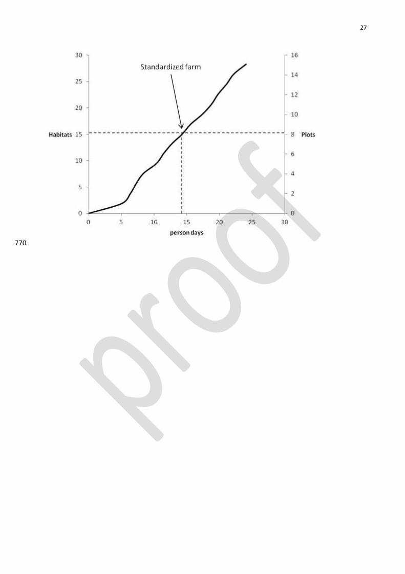
27

770