Landscape Ecology vol. 10 no. 6 pp 323-335 (1995) SPB Academic Publishing bv, Amsterdam

Error assessment in decision-tree models applied to vegetation analysis

Henry Lynn', Charles L. Mohler2, Stephen D. DeGloria3 and Charles E. McCulloch'

El45 Corson Hall; 3Department of Soil, Crop and Atmospheric Sciences, 158 Emerson Hall; 1 9 2 3 3 Cornell University, Ithaca, NY 14853, U.S.A.

Biometries Unit and Statistics Center, 338 Warren Hall; Section of Ecology and Systematics,

Keywords: scale, GIs, accuracy, robustness, prediction

Abstract

Methods were developed to evaluate the performance of a decision-tree model used to predict landscape-level patterns of potential forest vegetation in central New York State. The model integrated environmental data- bases and knowledge on distribution of vegetation. Soil and terrain decision-tree variables were derived by processing state-wide soil geographic databases and digital terrain data. Variables used as model inputs were soil parent material, soil drainage, soil acidity, slope position, slope gradient, and slope azimuth. Landscape- scale maps of potential vegetation were derived through sequential map overlay operations using a geographic information system (GIs). A verification sample of 276 field plots was analyzed to determine: (1) agreement between GIS-derived estimates of decision-tree variables and direct field measurements, (2) agreement be- tween vegetation distributions predicted using GIS-derived estimates and using field observations, (3) effect of misclassification costs on prediction agreement, (4) influence of particular environmental variables on model predictions, and ( 5 ) misclassification rates of the decision-tree model. Results indicate that the predic- tion model was most sensitive to drainage and slope gradient, and that the imprecision of the input data led to a high frequency of incorrect predictions of vegetation. However, in many cases of misclassification the predicted vegetation was similar to that of the field plots so that the cost of errors was less than expected from the misclassification rate alone. Moreover, since common vegetation types were more accurately predicted than rare types, the model appears to be reasonably good at predicting vegetation for a randomly selected plot in the landscape. The error assessment methodology developed for this study provides a useful approach for determining the accuracy and sensitivity of landscape-scale environmental models, and indi- cates the need to develop appropriate field sampling procedures for verifying the predictions of such models.

Introduction

Formulation of environmental policy, implementa- tion of environmental management strategies, and assessment of environmental degradation require that knowledge generated at local scale be extended to landscape scale. The spatial and temporal scales at which processes operate, observations and meas- urements are made, and environmental regulations

are promulgated seldom match. Methods are clear- ly needed for extrapolating results from studies of simplified microcosms at small spatial scales to complex landscapes.

Extrapolation of knowledge of the factors in- fluencing ecosystems requires the development of spatial databases comprised of the environmental variables determining these factors, as well as a predictive model for their effects. We will focus on

324

potential forest vegetation in central New York State, where the driving variables include both soil and terrain properties. These variables are available or derivable from existing databases (Reybold and TeSelle 1989; U.S. Geological Survey 1987).

Development of models which predict the distri- bution of vegetation using environmental databases requires understanding of the relationship of plant community composition to edaphic and terrain fac- tors. In central New York State, vegetation distri- bution patterns have been studied extensively using a combination of field measurements, land survey records and interpretation of topographic maps, soil surveys, and multi-temporal aerial photo- graphs (Marks and Gardescu 1992; Mohler and Marks, in prep.; Seischab 1985, 1990; Smith et al., in press). These field-based studies have permitted the development of a classification and key estab- lishing the relationship between the distribution of potential forest vegetation types and selected eda- phic and terrain factors (Mohler 1991; Mohler and Marks, in prep.). These relationships form the basis for subsequent development and application of spatially-explicit, descriptive simulation models which predict vegetation distribution at landscape scale in a fashion similar to Moore et al. (1991).

A number of authors have investigated the ac- curacy of spatial databases, proposing various stochastic models and assessing the propagation of error through processes of GIS (Goodchild and Gopal 1989; Goodchild et al. 1992; Heuvelink 1993). Our focus, however, is on the methodology of comparing the prediction accuracy of a decision tree model with reference data. This type of model makes predictions by a sequence of decisions based on a single variable at a time. Error in spatial data- bases is therefore considered as one of the several factors leading to poor prediction of the decision tree model. Specific objectives here include: (1) de- termination of agreement between field measure- ments and input variables derived from GIs, (2) as- sessment of prediction agreement between models using GIS data or field data as input, (3) examina- tion of the effect of misclassification costs on pre- diction agreement, (4) quantification of influence of individual environmental variables on the pre-

dictive power of the decision-tree model, and (5) es- timation of rates of misclassification of the predic- tive model. There has been extensive research on how errors in input affect predictions in ecological models (O’Neill 1973; Gardner et al. 1980; Rossi et al. 1993; Saltelli et al. 1993). However, the focus has primarily been on process models as opposed to decision tree models, and the input data are typi- cally continuous rather than categorical.

Methods and materials

Study area description

The study area is located in the Finger Lakes Region of central New York State, U.S.A. The area is defined by the boundaries of the Elmira 1 :250,000 scale topographic quadrangle, approximately 18,000 km2. The northern region of the study area is located on the Lake Ontario Plain in which land use is dominated by dairy farming. The elevation ranges from 100 to 400 meters, increasing from north to south. Average annual precipitation is 900 to 1150 mm, increasing from west to east. Local relief is nearly level to gently rolling terrain consist- ing of glacially-derived beach ridges, drumlins, and till plains. Soils are recently developed from mostly calcareous glacial tills, outwash, alluvial deposits, and lacustrine sediments. Natural vegetation con- sists of beech-maple and hemlock-northern hard- woods vegetation associations.

The southern region of the study area is located on the glaciated Allegheny Plateau in which land use is dominated by second- and third-growth deciduous and coniferous forest, conifer planta- tions, and some pasture and cropland associated with dairy farming. Elevation ranges from 200 to 1100 meters, with broad, steep-walled valleys and narrow ravines. Precipitation is similar to the northern portion, but the freeze-free period is shorter. Soils are derived from acidic glacial deposits, and support forest vegetation dominated by northern hardwoods, hemlock and upland oaks (Soil Conservation Service 1981).

325

Field observations and measurements

Field observations and measurements were made at selected plots within a 3400 km2 portion of the study area centered on Cayuga Lake. These pro- vided qualitative information for construction of our decision-tree model and served as a quantitative verification sample, though not all plots could be located accurately enough for use in verficiation. 180 relatively undisturbed stands representing the range of natural terrestrial and wetland vegetation in the region were sampled using the 0.1 ha method of Whittaker (1960). An additional 258 relevC samples were taken to balance sample density among environmental conditions. RelevCs consist- ed of estimates of percent cover of each woody spe- cies in an approximately 0.05 ha area with addi- tional notes on herbaceous species. Relevts were chosen by marking accessible locations represent- ing a range of topographic conditions on maps and then visiting sites until at least 5 relevt or 0.1 ha samples had been obtained from each combination of slope gradient (3 categories), aspect (3 cate- gories) and slope position (3 categories) in each of the northern and southern regions of the study area. Submerged aquatic vegetation, urban areas, plantations, orchards, cultivated fields and aban- doned farm land were excluded from the sample. In both the 0.1 ha plots and relevt samples, slope gra- dient, slope aspect, slope position, and elevation were recorded. Additional data on soil parent material, pH, and drainage were obtained from soil surveys of the region (Neeley 1965; Hutton 1971; Hutton 1972; Puglia 1979).

Samples were grouped into initial vegetation types by using two-way indicator species analysis (TWINSPAN) (Hill et al. 1975), and by consulting published descriptions of ravine and swamp forests of the region (Lewin 1974; Huenneke 1982). The in- itial classification was then refined by using an iter- ative process in which samples were moved between types until the best possible match between environ- mental conditions and composition of vegetation was approximated. This procedure resulted in 17 types (Mohler 1991), each of which is restricted to a well-defined range of environmental conditions.

To estimate error rates that would occur at ran-

domly selected plots in our study area we needed es- timates of the percent of the field study area in each vegetation type. These were made using the descrip- tive vegetation-environment model of Mohler and Marks (in prep.). For vegetation types which occur in only a few locations (e.g., bogs, cattail marsh), the approximate area of each type was directly measured on USGS topographic maps. The remain- ing area was divided into a northern region with cal- careous soils and a southern region with acidic soils, and within each region, into gorges, wetlands, steep south and west facing slopes, and other up- lands. Within a region, each of the topographic categories just listed corresponds to a relatively few vegetation types. Three topographic maps were chosen at random from each of the two regions and the area in each of the categories was estimated. The relative proportion of each vegetation type found in each topographic category in a region was approximated based on field experience (Mohler, pers. obs.) and the relative frequency of the types in the sample data. The area in each vegetation type was then computed by multiplying the area of each topographic category by the proportion of that category in each vegetation type, and then summing over topographic categories. Relative area in the various types ranged from 0.02% to 64%. The resulting area estimates were approximate, but were sufficient for assessing error rates.

Database design and development

Existing databases were compiled and integrated using established geographic information process- ing methods (Burrough 1986; ERDAS 1991) to pro- vide environmental data of the sort used in the vege- tation classification scheme. The spatial resolution of the database was defined using grid cells repre- senting a ground surface dimension of 100 m x 100 m and geo-referenced to the Universal Trans- verse Mercator projection and coordinate system (Snyder 1982). A state-level soil geographic data- base (STATSGO) provided groupings of soils into map units. For the study area, there were 46 soil map units each comprised of 20 or more compo- nents consisting of soil series phased by slope gra-

326

Soil Parent Material (SPM) DGTO = glacial till, deep DGTl = glacial till, fragipan MSGT = glacial till, mod. deep, shallow LCST = lacustrine OUTW = glacial outwash ALVM = alluvium ORGN = organics

Soil Drainage P = poor (P, VP) W = well (SP, MW, W, SE, E)

Soil Acidity A = acid (pH<6.1) B = non-acid (pH 6.1 +)

Slope Position L = lower M = middle U = upper

Slope Gradient N = nearly level (0-2%) G = gently sloping (3-1570) S = steeply sloping (> 15%)

Slope Aspect N = north (293-112”)

F = flat

Vegetation Type n

S = south (113-292’)

Fig. I . A schematic of the decision-tree model for a single soil parent material.

dient class. Map units had a minimum size delinea- tion of 625 hectares.

The STATSGO database was used to estimate soil parent material, drainage, acidity, and slope position for each grid cell. Interpretation of soil parent material for each map unit was derived from the STATSGO legend, and pedon descriptions for the components of each map unit. Seven parent material classes were defined: deep glacial till with- out restrictive layer (e.g. fragipan), deep glacial till with restrictive layer, moderately-deep to shallow glacial till, lacustrine sediments, glacial outwash deposits, alluvium, and organics.

For the remaining five environmental variables, break points were chosen in the continuous or cate- gorical gradients which field experience (Mohler, per. obs.) indicated would maximize differences in forest composition between contrasting categories. Database programming scripts were used to com- pute average soil pH and frequency distribution of

soil drainage for each map unit. Soil acidity for each map unit was computed as an area-weighted average by using the mid-point of pH range pub- lished for each map unit component. Based on the computed map unit average pH, each map unit was classified as ‘acid’ (pH < 6. l) , or ‘non-acid’ (pH > = 6.1). Soil drainage for each map unit was determined by computing the frequency distribu- tion of drainage classes based on the percent occur- rence of soil map unit components. If a majority of the drainage classes occurring in a map unit was es- timated to be very poorly or poorly drained soil, soil drainage for the map unit was classified as ‘poor’. If a majority of the drainage classes were somewhat poorly drained or better the map unit was classified as ‘well’. Slope position for each map unit was interpreted into three classes using the catena concept for characterizing and mapping soil landscapes in New York State (Cline and Marshall 1977): lower (toe- and foot-slopes), middle (back-

327

Table 1. Characteristics of environmental databases and field survey data used in decision tree variables.

7 classes

Variable Source

7 classes

Scale

Choropleth G I S

-

F I E L D

I

5 classes I 2 classes

Parent Material

Contours 0.1 ha

Position

percent 3 classes 17 10

classes classes

Soil Conservation

Services

Aspect Gradient

1 Aspect I G;l:ogd Vegetation Mohler & Gradient

Marks2

Mohler & Marks

Soil Survey'

0.1 ha I Position I I

degrees 3 classes percent 3 classes

1 :250,000

-- 1 :250,000

(1 ha pixel) 0.1 ha plot

1 : 15,840

0.1 ha plot

(625 ha)

20 m I degrees I 3 classes I

Choropleth 1 5 classes I 2 classes 1 5 classes 2 classes I 5 classes 3 classes

(0.405,ha)

1 Soil surveys from Neeley 1965; Hutton 1971, 1972; Puglia 1979. Mohler and Marks, in preparation.

slopes), and upper (shoulder- and summit-slopes). Nomenclature follows Wilding et al. (1983). Since slope position is generally correlated with soil drainage, soil components in each map unit were assigned a slope position class based on their drainage class. Soil components that were exces- sively well-drained or well-drained were assigned to the 'upper' slope position. Soil components that were moderately-well drained were assigned the 'middle' slope position, and those components that were somewhat-poorly, poorly, or very poorly drained were assigned to the 'lower' slope position. The map unit was assigned a slope position class based on the majority slope position class occurring in the map unit on an area percentage basis. Soil parent material class for each map unit component was determined by reviewing the official soil series description and assigning a parent material class to

the map unit based on the majority parent material occurring in the unit.

Slope gradient and slope azimuth were estimated from the Elmira 1:250,000 scale digital terrain data (U.S. Geological Survey 1987). Slope gradient classes were computed using finite differencing techniques (ERDAS, Inc. 1991) in one percent increments and then aggregated into three ranges: nearly level (0-4%), gently sloping (5- 15%), and steeply sloping (> 15%). Slope azimuth was com- puted in one-degree increments and then aggre- gated into three aspect classes: north (293-1 lZo), and south (1 13-292") as well as flat. The 22" clock- wise rotation was included in the definition of the aspect classes because vegetation on east facing slopes resembles that on north facing slopes more than does the vegetation on west slopes.

328

Table 2. Costs associated with the misclassification of vegetation groups. (0 equals no cost, and 10 equals maximum cost.)

VEGETATION GROUPS '

v 1 E 2 G 3

4 G 5 R 6 0 7 U 8 P 9 s 10

1 2 3 4 5 6 7 8 9 10 0 2 8 9 10 8 8 10 8 9

0 8 9 10 7 7 9 8 10 0 2 4 1 3 4 2 3

0 2 3 3 2 3 1 0 5 5 3 5 3

0 1 2 1 4 0 2 2 3

0 2 2 0 3

I)

Decision-tree model

A decision-tree model was developed to integrate the vegetation classification with the geographic database of the soil and terrain factors (Fig. 1). First, the digital soil map was overlain with the digi- tal map of terrain variables to derive a 414-class map of soil-terrain relationships. Next, each soil- terrain class was related to plant community types to form the decision-tree model.

Given the categorical and mapping detail at which soil and terrain data were available in the geographic database (Table l), not all 17 vegetation types could be discriminated. The original vegeta- tion classification scheme was aggregated into 10 generalized vegetation groups, each of which in- cluded several types which are commonly found adjacent to one another, intergrade, or occupy similar habitats. Because some of the more com- mon vegetation types occur in a broad range of con- ditions but with varying frequency, they were in- cluded in more than one of the vegetation groups predicted by the decision tree model.

Error assessment methodology

We assessed two possible sources of error: error in the input variables to our decision tree model and error in the actual prediction. For each of the six

decision tree variables, we examined the agreement between the GIS-derived estimates of these six vari- ables and direct field observations by cross-classi- fying the GIS data versus field data. The propor- tion of plots that fell along the main diagonal of such a cross-classification measures the overall agreement since it gives the number which were classified the same. Cohen's kappa (Cohen, 1960) measures agreement adjusted for chance on a scale where zero indicates no agreement and one indi- cates total agreement. Kappa equals zero when the estimates and field data are statistically indepen- dent (i.e., when the probability of agreement is equal to the product of the marginal probabilities). To estimate the agreement under independence, the observed marginal probabilities are typically used; in some sampling schemes these are not valid esti- mates of the true marginal probabilities and alter- nate measures of agreement should be used (Aickin 1990; Brennan and Prediger 1981). The preceding comparisons focus on a single variable at a time and ignore the associations that may exist between vari- ables. Therefore, as an multivariate extension of examining agreement, we calculated how often dis- agreements in one variable occur in conjunction with another variable. This shows which pairs of variables tend to be poorly approximated by the GIS data.

We also used the kappa coefficient to summarize agreement between vegetation distributions pre-

329

Table 3. Agreement between GIS data and field data for the six decision tree variables.

Input variable Proportion with Cohen’s Kappa same classification

Parent material .424 Drainage .786 Acidity .797 Slope position ,417 Slope gradient .515 Slope aspect .649

.303

.073

.592

.159

.267

.456

dicted using GIs-derived estimates and using field observations. For many uses it will be possible to specify or approximate the cost of misclassification by the model and, since certain misclassifications will have higher costs than others, it will lead to a more appropriate assessment of model perfor- mance. A matrix of misclassification costs was con- structed (Table 2) based on the degree of composi- tional similarity of the types composing pairs of vegetation groups. Pairs which differed primarily in the relative proportion of their component vege- tation types were given low misclassification costs (values of 1 to 3). In contrast, a pair received a max- imum value of 10 if their predominant vegetation types were characteristic of sites differing in both drainage and soil pH (e.g., poorly drained and cal- careous versus well drained and acid). Intermediate situations received intermediate misclassification costs, but a minimum cost of 8 was assigned to all pairs in which one was composed of types charac- teristic of uplands whereas the other was made up of wetland types. Average cost estimates must be referred to the above definitions for interpretation. Costs can be specified according to other criteria.

To estimate the expected cost of misclassification a table cross classifying vegetation groups predicted using field and GIS data was first prepared. The proportion of occurrence of each entry was then multiplied by its corresponding cost according to Table 2 and the product summed over all entries. This value was then compared with the expected cost of misclassification under statistical indepen- dence. This is equivalent to calculating a weighted kappa (see Fleiss 1981, p. 223), where weight =

1 - cost/lO.

Table 4 . Frequency of joint misclassification among the six deci- sion tree variables.

Parent material Drainage Acidity Position Gradient Aspect

Parent material 43 46 86 86 64 Drainage 15 25 10 10 Acidity 30 30 30 Position 75 55 Gradient 90

To investigate the effect of each decision tree variable on misclassification, the field data were replaced with GIS data one variable at a time, resulting in six transformed data sets. The model predictions obtained from these data sets were then compared with those obtained using only field data. This is similar to a sensitivity analysis, where one variable is varied while all other variables are kept constant. The six transformed data sets differ from the field data by only one variable. When the GIS estimate of the variable is the same as the field measurement, the same prediction necessarily results. However, when the GIS estimate of the variable is different from the field estimate, the transformed data and the field data can still have the same prediction since different combinations of input values may produce the same prediction. The more often this happens, the more robust is the model to misclassification in that variable. Like- wise, we define robustness as the proportion of plots with identical predictions among those with different variable input.

Finally, to assess the misclassification rate of the decision tree model, we compared the predicted vegetation groups with the actual field vegetation types. This was done with the field data as input and also with the GIS data as input. The former evaluates the pure prediction error of the decision tree model (assuming accuracy of the field data), whereas the latter includes the error involved in using the, sometimes inaccurate, GIS data as input. Overall misclassification rates were taken to be the total proportion of misclassified plots. Also, to es- timate the misclassification rate for a randomly selected plot in the study area, weighted misclassifi- cation rates were calculated by multiplying the proportion of misclassified plots in each field vege-

330

Table 5. Cross-classification of vegetation groups predicted using CIS input and using field input. Diagonal entries (in bold) sum to 98 (35.5%) and show the frequency that the two input sources shared the same predicted classification.

F1 F2

F F3 I F4 E %5 L F6 D F7

F8 F9 F10

GIs G1 G2 G3 G4 G5 (3j G7 G8 ~9 ~ 1 0 0 0 0 7 0 1 0 0 6 0 0 8 2 6 0 3 14 0 15 0 0 0 10 4 0 1 0 0 0 0 0 1 17 34 2 2 3 0 3 0 0 0 2 2 6 0 2 0 0 0 0 0 0 1 1 0 8 22 0 3 0 0 0 0 2 0 2 21 0 0 0 0 0 1 1 0 2 4 1 2 0 0 1 7 9 0 3 8 1 10 0 0 0 1 2 0 1 1 0 1 0

tation type by the estimated proportion of that vegetation type occurring in the study area, and then summing these products over all the vegetation types.

Results and discussion

Error analysis of input variables

There was moderate data agreement between GIS and field data for acidity but poor agreement for drainage (Table 3). Note that use of the proportion of plots with identical classification as the sole measure of agreement can give misleading conclu- sions as exemplified for the drainage variable. This indicates the importance of using several indices to measure agreement, and knowing when a particular index would yield valid inferences. Slope gradient and slope aspect had the highest frequency of joint misclassification (Table 4). This correlation is a reflection of the poor resolution of the digital eleva- tion map, from which the gradient and aspect were calculated. On the other hand, there does not seem to be a clear physical explanation for why high fre- quencies of misclassification in parent material and slope position occur together with slope gradient.

The imprecision of the soils and digital elevation databases used in the study contributed to a relative lack of agreement between field and GIS data

(Table 1). The imprecision resulted from both the coarse scale of the GIS data and inaccuracy in de- termining location of grid cells. The state-level soil survey data (Soil Conservation Service 1991) were derived by generalizing soil information contained in detailed soil surveys. This aggregation created map units with highly heterogeneous soil composi- tion, without adequate reference as to where the aggregated component-units were located spatially. Consequently, important soil conditions which occur in relatively small patches were not adequate- ly represented in the GIS data. Similarly, although slope gradient and aspect were computed for each 100 m x 100 m grid cell, the digital elevation model integrated over much larger areas when calculating the estimated values. In contrast, slope and azi- muth measurements taken in the field were only in- tended to characterize a small plot and therefore frequently differed from the average slope and aspect of the larger area. Finally, slope positions were approximated using the assumed slope posi- tion of the dominant soil series in its catena. This resulted in large landscape units being assigned a slope position which often was at variance with the slope position characterized at a given field plot. Thus, the accuracy assessment of environmental databases of such coarse categorical and carto- graphic resolution using highly detailed field plot data of limited spatial extent is problematic.

Although our use of spatial databases was rea-

331

Table 6. Robustness of input variables in the decision tree model.

Variable replaced No. w/same Robustness , prediction

Parent material 219 .642 (102/159) Drainage 218 .017 (1/59) Acidity 224 .071 (4/56) Slope position 216 .627 (101/161) Gradient 182 .299 (40/134) Aspect 186 .072 (7/97)

Predictions using field data for all six decision tree input varia- bles are compared with the predictions using GIS estimates for one of the input variables but field data for the other five varia- bles. The first column gives the number of plots with the same predictions when the GIS variables were used for each of the de- cision tree input variables. Robustness is the proportion of plots which have identical predictions among those with different variable values.

sonable given the constraints associated with their lack of detail, we consider these regional scale data- bases currently inadequate for prediction the distri- bution of potential vegetation types at landscape scale which meets the expectations of field ecol- ogists.

Error analysis of model predictions

Poor agreement between GIS and field data input variables does not necessarily cause incorrect pre- diction of the decision tree model since different combinations of values in the input variables may still give the same predicted vegetation. Summing the diagonal entries in Table 5 , we found 98 plots (35.5%) had identical predicted vegetation groups, and the kappa coefficient was 0.252. Hence, if the decision tree model gave perfect predictions, we would still expect a minimum misclassification rate of 65% when using GIS estimates because of errors in the input data. Based on the cost matrix, the ex- pected cost of misclassification was 2.55, compared with 3.49 if we assume an independence structure. Twenty percent of the plots had costs greater than five. As in a residual analysis, closer examination of individual entries with large number of misclassifi- cations in Table 5 may help identify weaknesses in

the decision tree model. The two entries with the highest misclassifications received costs not greater than two, which illustrates why adjusting for mis- classification costs in this case decreases the severity of misclassification.

Environmental variables differed in their effect on predictions of vegetation type by the decision tree model (Table 6). The model had low robustness with respect to acidity, aspect and drainage. Acidity and aspect had high agreement and thus may not be critical in causing misclassification. On the other hand, drainage had low agreement as indicated by its kappa statistic (Table 3), which makes it more critical to the decision tree. Similarly, slope gra- dient had fair agreement and robustness, which may cause a substantial amount of prediction error. Therefore, by combining results on agreement and robustness, we can assess the strength of input vari- ables on the decision tree model, which was not pos- sible by simply looking at data agreement between GIS and field data (Table 3) or just by comparing the predicted outcomes using the two types of input (Table 5 ) .

Cross classification of field vegetation types ver- sus predicted vegetation groups showed an overall misclassification rate of 0.233 (64/275) using field data (Table 7a). Thus, even with perfect input, the decision tree model had only 77% accuracy in pre- dicting vegetation at the field sample plots. This error resulted from several factors. First, it is pre- sumptuous to expect our six selected environmental variables to perfectly predict vegetation. Second, all of the field sample plots have experienced hu- man disturbance, which in some cases may have shifted the composition away from that expected from environmental influences alone. Third, since bogs, cliffs, and narrow ravines were of too limited spatial extent to be characterized by coarse scaled digital elevation and soils databases, the vegetation types corresponding to these landscape units were omitted from the decision tree, or had to be incor- porated as inclusions within a more broadly defined vegetation group. Moreover, since plots and sam- ples were selected in a way which favored rare and unusual types of vegetation, these environments were disproportionately represented in the field data relative to their area in the landscape. When

332

0 0 1 3 6 0 0 0 0 0 0 0 0 21 2 3 1 2 2 2 0 0 0 1 1 3 1 3 0 0 0 0 0 0 0 1 0 4 0 0 0 0 4 2 0 5 5 0 3 0 0 0 0 0 0 0 0 0 1 1 0 1 2 11 2 14 10 0 10 0 0 0 6 14 1 6 6 0 6 2 1 0 2 6 0 10 0 1 13 1 1 1 0 4 0 1 0 1 4 0 0 0 0 0 0 1 0 0 0 0 4 7 0 0 0 0 0 0 0 0 2 18 0 0 0 0 2 0 0 0 0 4 0 0 0 0 0 0 0 0 0 9 0 0 0 0 0 0 0 0 0 3 0 0 0 0 0 0 0 0 6 4 0 0 0 0 0 0 0 0

Table 7u. Cross-classification table of field vegetation types versus predicted map vegetation groups using field observations as input. ri =row total, ci = column total, mi = number of misclassified plots, and wi = percent of field vegetation type in study area. Tables entries in bold denote possible matches. Field vegetation type Q is a combination of four subtypes and only one of the four denotes a possible match.

10 4 33 4 9 6 5 5 19 6 2 1

50 3 41 1 34 11 12 12 1 1 11 0 22 2 4 0 9 0 3 0 10 8

A B

F C I D E E L F D G

H V I E J G K T L Y M P N E O

P Q

0 0 3 4 3 0 0 0 0 0 0 1 7 16 1 1 6 0 1 0 0 0 0 0 2 1 6 0 0 0 0 0 1 0 0 1 1 1 1 0 0 1 3 4 0 1 9 0 1 0 0 0 0 0 0 0 0 1 1 0 0 0 5 14 1 6 20 0 4 0 0 0 12 16 0 2 9 . o 2 0 0 0 5 9 0 6 7 0 7 0 0 0 3 4 1 0 2 0 2 0 0 0 0 0 0 1 0 0 0 0 0 0 0 5 0 1 1 0 4 0 0 4 0 3 0 0 12 0 3 0 0 2 0 0 0 0 1 0 1 0 0 2 1 1 0 3 0 0 2 0 0 0 0 1 0 0 0 0 2 0 0 0 0 1 0 0 1 0 8 0

Ci

10 33 9 5 19 2 50 41 34 12 1 11 22 4 9 3 10

14 47 15 62 12 44 25 11 39 6 275 64

Wi 0.20 3.00 0.20 0.02 2.00 0.05 63.9 27.0 0.50 0.25 0.06 0.40 1.70 0.30 0.10 0.05 0.02

Table 7b. Cross-classification table of field vegetation types versus predicted map vegetation groups using GIS estimates as input.

A B

F C I D E E L F D G

H V I E J G K T L Y M P N E O

P Q

mi wi 7 0.20 8 3.00 9 0.20 5 0.02 7 2.00 2 0.05 1 63.9 0 27.0

21 0.50 12 0.25 1 0.06 11 0.40 18 1.70 2 0.30 7 0.10 3 0.05 10 0.02

CI 0 10 40 78 8 23 75 2 39 0 275 124

333

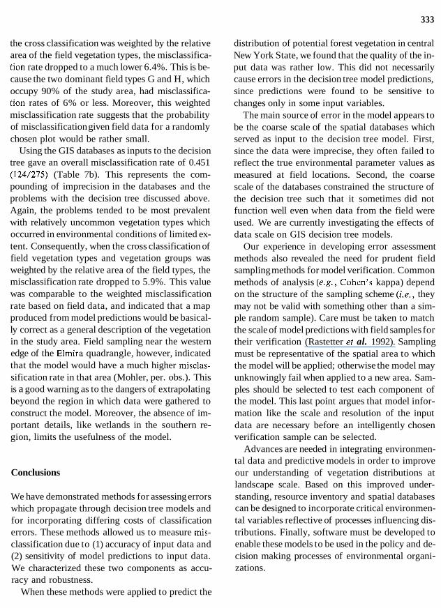
the cross classification was weighted by the relative area of the field vegetation types, the misclassifica- tion rate dropped to a much lower 6.4%. This is be- cause the two dominant field types G and H, which occupy 90% of the study area, had misclassifica- tion rates of 6% or less. Moreover, this weighted misclassification rate suggests that the probability of misclassification given field data for a randomly chosen plot would be rather small.

Using the GIS databases as inputs to the decision tree gave an overall misclassification rate of 0.451 (124/275) (Table 7b). This represents the com- pounding of imprecision in the databases and the problems with the decision tree discussed above. Again, the problems tended to be most prevalent with relatively uncommon vegetation types which occurred in environmental conditions of limited ex- tent. Consequently, when the cross classification of field vegetation types and vegetation groups was weighted by the relative area of the field types, the misclassification rate dropped to 5.9%. This value was comparable to the weighted misclassification rate based on field data, and indicated that a map produced from model predictions would be basical- ly correct as a general description of the vegetation in the study area. Field sampling near the western edge of the Elmira quadrangle, however, indicated that the model would have a much higher misclas- sification rate in that area (Mohler, per. obs.). This is a good warning as to the dangers of extrapolating beyond the region in which data were gathered to construct the model. Moreover, the absence of im- portant details, like wetlands in the southern re- gion, limits the usefulness of the model.

Conclusions

We have demonstrated methods for assessing errors which propagate through decision tree models and for incorporating differing costs of classification errors. These methods allowed us to measure mis- classification due to (1) accuracy of input data and (2) sensitivity of model predictions to input data. We characterized these two components as accu- racy and robustness.

When these methods were applied to predict the

distribution of potential forest vegetation in central New York State, we found that the quality of the in- put data was rather low. This did not necessarily cause errors in the decision tree model predictions, since predictions were found to be sensitive to changes only in some input variables.

The main source of error in the model appears to be the coarse scale of the spatial databases which served as input to the decision tree model. First, since the data were imprecise, they often failed to reflect the true environmental parameter values as measured at field locations. Second, the coarse scale of the databases constrained the structure of the decision tree such that it sometimes did not function well even when data from the field were used. We are currently investigating the effects of data scale on GIS decision tree models.

Our experience in developing error assessment methods also revealed the need for prudent field sampling methods for model verification. Common methods of analysis (e.g., Cohen’s kappa) depend on the structure of the sampling scheme (i.e., they may not be valid with something other than a sim- ple random sample). Care must be taken to match the scale of model predictions with field samples for their verification (Rastetter et al. 1992). Sampling must be representative of the spatial area to which the model will be applied; otherwise the model may unknowingly fail when applied to a new area. Sam- ples should be selected to test each component of the model. This last point argues that model infor- mation like the scale and resolution of the input data are necessary before an intelligently chosen verification sample can be selected.

Advances are needed in integrating environmen- tal data and predictive models in order to improve our understanding of vegetation distributions at landscape scale. Based on this improved under- standing, resource inventory and spatial databases can be designed to incorporate critical environmen- tal variables reflective of processes influencing dis- tributions. Finally, software must be developed to enable these models to be used in the policy and de- cision making processes of environmental organi- zations.

334

Acknowledgements

Thanks to David Weinstein (Boyce Thompson Institute) for numerous discussions and thorough review of a draft manuscript. The research reported here was supported by the USDA sponsored Agri- cultural Ecosystems Program at Cornell Univer- sity.

References

Aicken, M. 1990. Maximum likelihood estimation of agreement in the constant predictive probability model and its relation to Cohen’s kappa. Biometrics 46: 293-302.

Brennan, R.L. and Prediger, D.J. 1981. Coefficient kappa: some uses, misuses and alternatives. Ed. and Psych. Meas. 41:

Burrough, P.A. 1986. Principles of geographical information systems for land resources assessment. Clarendon Press, Ox- ford. 194p.

Cline, M.G. and Marshall, R.L. 1977. Soils of New York Land- scapes Information Bulletin #119. Cornell Cooperative Ex- tension. Cornell University. Ithaca, New York. 62p.

Cohen, J . 1960. A coefficient of agreement for nominal scales. Educational and Psychological Measurement 20: 37-46.

ERDAS, Inc. 1991. Field Guide, Version 7.5. ERDAS, Inc. Atlanta, Georgia.

Fleiss, J . 1981. Statistical Methods for Rates and Proportions. New York: John Wiley & Sons, Inc. 321p.

Gardner, R.H., Huff, D.D., O’Neill, R.V., Mankin, J.B., Carney, J . and Jones, J. 1980. Applications of error analysis to a marsh hydrology model. Water Resources Research

Goodchild, M. and Gopal, S. 1989. Accuracy of Spatial Data- bases. New York: Taylor & Francis. 290p.

Goodchild, M., Guoqing, S. and Shiren, Y. 1992. Development and test of an error model for categorical data. Int. J. Geo- graphical Information Systems 6(2): 87-104.

Heuvelink, G.B.M. 1993. Error propagation in quantitative spa- tial modelling: Applications in geographical information sys- tems. Netherlands Geographic Studies #163. Univ. Utrecht, the Netherlands, 295p.

Hill, M.O., Bunce, R.G.H. and Shaw, M.W. 1975. Indicator species analysis, a divisive polythetic method of classification, and its application to a survey of native pinewoods in Scot- land. J . Ecol. 63: 597-613.

Huenneke, L.E. 1982. Wetland forests of Tompkins County, New York. Bull. Torrey Bot. Club 109: 51-63.

Hutton, F.Z., Jr. 1971. Soil survey of Cayuga County, New York. USDA Soil Conservation Service. U.S. Govt. Printing Office. Washington, D.C. 205p.

Hutton, F.Z., Jr. 1972. Soil survey of Seneca County, New

687 -699.

16(4): 659-664.

York. USDA Soil Conservation Service, U.S. Govt. Printing Office. Washington, DC. 143p.

Lewin, D.C. 1974. The vegetation of the ravines of the southern Finger Lakes, New York, region. Am. Midl. Nat. 91:

Marks, P.L. and Gardescu, S. 1992. Vegetation of the central Finger Lakes Region of New York in 1790s. New York State Museum Bulletin #484 1-35. Albany, New York.

Mohler, C.L. 1991. Plant community types of the central Finger Lakes Region of New York: A synopsis and key. Proc. Rochester Acad. Sci. 17(2): 55-103.

Mohler, C.L. and Marks, P.L. Vegetation-environment rela- tions in the central Finger Lakes Region of New York. (In Preparation).

Moore, D.M., Lees, B.G. and Davey, S.M. 1991. A new method for predicting vegetation distributions using decision tree analysis in a geographic information system. Environmental Management 15: 59-71.

Neeley, J.A. 1965. Soil survey of Tompkins County, New York. USDA Soil Conservation Service. U.S. Govt. Printing Office, Washington, DC. 241p.

O’Neill, R.V. 1973. Error analysis of ecological models. In Radionuclides in Ecosystems. pp. 898-908. Edited by D.J. Nelson. CONF-710501. National Technical Information Ser- vice, Springfield, Virginia, U.S.A.

Puglia, S.P. 1979. Soil survey of Schuyler County, New York. USDA Soil Conservation Service. U.S. Printing Office. Washington, DC. 192p.

Rastetter , E.B., King, A.W., Cosby, B.J ., Hornberger, G.M., O’Neill, R.V. and Hobbie, J.E. 1992. Aggregating fine-scale ecological knowledge to model coarser-scale attributes of ecosystems. Ecological Applications 2(1): 55-70.

Reybold, W.U. and TeSelle, G.W. 1989. Soil geographic data- bases. J . Soil and Water Cons. 44: 28-29.

Rossi, R.E., Borth, P.W. and Tollefson, J.J. 1993. Stochastic simulation for characterizing ecological spatial patterns and appraising risk. Ecological Applications 3(4): 719-735.

Saltelli, A., Andres, T.H. and Homma, T. 1993. Sensitivity analysis of model output: an investigation of new techniques. Computational Statistics & Data Analysis 15: 21 1-238.

Seischab, F.K. 1985. An analysis of the forests of the Bristol Hills of New York. Am. Midl. Nat. 114: 77-83.

Seischab, F.K. 1990. Presettlement forests of the Phelps and Gorham Purchase in western New York. Bull. Torrey Bot.

Smith, B.E., Marks, P.L. and Gardescu, S. 1993. Two hundred years of forest cover changes in Tompkins County, New York. Bull. Torrey Botanical Club. 120: 229-247.

Snyder, J.P. 1982. Map projections used by the U.S. Geological Survey. Geol. Survey Bulletin #1532. U S . Government Print- ing Office, Washington, D.C.

Soil Conservation Service. 1991. State Soil Geographic Data Base (STATSGO). Misc. Publ. #1492. U.S. Dept. Agricul- ture. Washington, DC. 88p.

Soil Conservation Service. 1981. Land resource regions and

315-342.

Club 117: 27-38.

335

major land resource areas of the United States. USDA Soil Conservation Service Agric. Handbook #296. Washington, DC. 156p.

US. Geological Survey. 1987. Digital Elevation Models. Data Users’ Guide #5. U.S. Geological Survey. Reston, Virginia. 38p.

Whittaker, R.H. 1960. Vegetation of the Siskiyou Mountains, Oregon and California. Ecol. Monogr. 30: 279-338.

Wilding, L.P., Smeck, N.E. and Hall, G.F. (ed.) 1983. Pedo- genesis and soil taxonomy. I. Concepts and interactions. Else- vier, New York.