arX

iv:1

001.

4878

v2 [

hep-

ph]

4 A

pr 2

010

Preprint typeset in JHEP style - HYPER VERSION hep-ph/1001.4878

Energy-independent new physics in the flavour ratios

of high-energy astrophysical neutrinos

M. Bustamantea,b, A.M. Gagoa, C. Pena-Garayc

aSeccion Fısica, Departamento de Ciencias, Pontificia Universidad Catolica del Peru,

Apartado 1761, Lima, PerubTheoretical Physics Department, Fermi National Accelerator Laboratory, Batavia, IL

60510, USAcInstituto de Fısica Corpuscular (IFIC), Centro Mixto CSIC-UVEG Edificio

Investigacion Paterna, Apartado 22085, 46071 Valencia, Spain

E-mail: mbustamante@pucp.edu.pe,agago@pucp.edu.pe,carlos.penya@ific.uv.es

Abstract: We have studied the consequences of breaking the CPT symmetry in the

neutrino sector, using the expected high-energy neutrino flux from distant cosmological

sources such as active galaxies. For this purpose we have assumed three different hypotheses

for the neutrino production model, characterised by the flavour fluxes at production φ0e :

φ0µ : φ0

τ = 1 : 2 : 0, 0 : 1 : 0, and 1 : 0 : 0, and studied the theoretical and experimental

expectations for the muon-neutrino flux at Earth, φµ, and for the flavour ratios at Earth,

R = φµ/φe and S = φτ/φµ. CPT violation (CPTV) has been implemented by adding an

energy-independent term to the standard neutrino oscillation Hamiltonian. This introduces

three new mixing angles, two new eigenvalues and three new phases, all of which have

currently unknown values. We have varied the new mixing angles and eigenvalues within

certain bounds, together with the parameters associated to pure standard oscillations. Our

results indicate that, for the models 1 : 2 : 0 and 0 : 1 : 0, it might possible to find large

deviations for φµ, R, and S between the cases without and with CPTV, provided the

CPTV eigenvalues lie within 10−29 − 10−27 GeV, or above. Moreover, if CPTV exists,

there are certain values of R and S that can be accounted for by up to three production

models. If no CPTV were observed, we could set limits on the CPTV eigenvalues of the

same order. Detection prospects calculated using IceCube suggest that for the models

1 : 2 : 0 and 0 : 1 : 0, the modifications due to CPTV are larger and more clearly separable

from the standard-oscillations predictions. We conclude that IceCube is potentially able

to detect CPTV but that, depending on the values of the CPTV parameters, there could

be a mis-determination of the neutrino production model.

Keywords: astrophysical neutrinos, CPT violation.

Contents

1. Introduction 1

2. Theoretical framework 3

2.1 Standard mass-driven flavour oscillations 3

2.2 Adding an energy-independent Hamiltonian 5

2.3 Astrophysical neutrino flavour ratios 7

3. Effect of an energy-indepedent contribution on the astrophysical flavour

ratios 9

3.1 Detection of νµ 9

3.2 Detection of two flavours: νµ and νe 11

3.3 Detection of three flavours: νµ, νe and ντ 12

4. Detection prospects at IceCube considering CPTV 16

4.1 Experimental setup 16

4.2 Astrophysical neutrino flux models 19

4.3 Results 21

5. Summary and conclusions 22

1. Introduction

Experiments performed over the last thirty years have established that neutrinos can change

flavour: careful measurements of solar [1, 2, 3], atmospheric [4, 5], reactor [6] and accelerator

[7, 8] neutrinos have established that there is a nonzero probability that a neutrino created

with a certain flavour is detected with a different one after having propagated for some

distance, and that this probability is a periodic function of the propagated distance, L,

and the neutrino energy, E. The standard mechanism of neutrino flavour change requires

neutrinos to be massive and results in a probability of flavour change that is oscillatory,

with oscillation lengths that have a distinct 1/E dependence (see Section 2.1).

So far, the experiments that have studied neutrino flavour transitions [9] have been

designed to detect neutrinos with energies that range from a few MeV (solar neutrinos)

to the TeV scale (atmospheric neutrinos). Notably, data from the Super-Kamiokande

atmospheric neutrino experiment [10] was used to find an energy dependence of the oscil-

lation probability of En, with n = −0.9± 0.4 at 90% confidence level, thus confirming the

dominance of the mass-driven mechanism in this energy range, and relegating any other

– 1 –

potential mechanisms to subdominance. It is possible, however, that one or more of such

subdominant mechanisms become important at higher energies.

In the present paper, we have explored a possible scenario where there is an additional

oscillation mechanism present which results in an energy-independent contribution to neu-

trino oscillations. This mechanism, though subdominant in the MeV–TeV range, might

become dominant at higher energies, where the 1/E dependence of the standard oscillation

term might render it comparatively unimportant: the higher the energy, the stronger the

suppression of the standard oscillation term. The highest-energy flux of neutrinos available

is the expected ultra-high-energy (UHE, with energies at the PeV scale and higher) flux

from astrophysical sources –notably, active galaxies (see Section 4)– which are located at

distances in the order of tens or hundreds of Mpc.

We will deferr the detailed treatment of how the energy-independent contribution is

introduced to Section 2 and focus now on the possible mechanisms that might motivate

it. According to the CPT theorem, any Lorentz-invariant local quantum field theory must

be built out of a CPT-conserving Lagrangian. However, the Standard Model (SM) is

known to be valid at energies well below the Planck scale, mPl ≃ 1019 GeV and, at higher

energies, motivated by theories beyond the SM [11, 12], CPT and Lorentz invariance might

be broken. At accessible energies, the breaking of these symmetries can be described by

an effective field theory that contains the SM. We have explored the possibility that CPT

is not an exact symmetry, but rather that it is broken by the addition of a CPT-odd

term to an otherwise CPT-even Lagrangian. The observation of the non-conservation of

CPT would imply a fundamental revision of the usefulness of local quantum field theories as

accurate descriptions of fundamental interactions. A possible realisation of a CPT-violating

(CPTV) effective field theory is the Standard Model Extension [13, 14], which contains the

SM, conserves SU (3) × SU (2) × U (1), and also considers potential Lorentz- and CPT-

violating couplings in the gauge, lepton, quark and Yukawa sectors. It is worth noting that

an alternative mechanism that also results in an energy-independent contribution to the

oscillations is the nonuniversal coupling of the different neutrino flavours to an external

torsion field [15].

The rest of the paper is organised as follows. In Section 2, we explain how the contri-

butions from potential energy-independent new physics affect the flavour-transition proba-

bility and introduce the detected fluxes of the different flavours of astrophysical neutrinos,

and the ratios between them, as our observables. Section 3 discusses the deviations of

the flavour ratios from their standard values in three different cases: when only νµ can

be detected, when νµ and νe can be detected, and when the three flavours, νe, νµ, ντ ,

can be detected1. In Section 4, we predict the feasibility of detecting a possible energy-

independent contribution using the IceCube neutrino detector, and larger-volume versions

of it. We summarise our results and conclude in Section 5.

1Some preliminary results on the three-flavour detection case were presented by the authors elsewhere

[16].

– 2 –

2. Theoretical framework

2.1 Standard mass-driven flavour oscillations

The standard mechanism that explains neutrino flavour transitions makes use of two differ-

ent bases: the basis of neutrino mass eigenstates, which have well-defined masses, and the

basis of neutrino interaction states –the flavour basis– which are the ones that take part in

weak processes such as W decay. The two bases are connected through a unitary transfor-

mation, so that we can write each one of the flavour states |να〉 as a linear combination of

the mass eigenstates |νi〉, i.e.,

|να〉 =∑

i

[U0]∗αi |νi〉 , (2.1)

where the coefficients [U0]αi are components of the unitary mixing matrix that represents

the transformation. Assuming the existence of three active neutrino families (α = e, µ, τ),

as indicated by LEP [17], three mass eigenstates are required (i = 1, 2, 3 in the sum) and

so U0 is a 3 × 3 matrix. The mass eigenstates |νi〉 satisfy Schrodinger’s equation and so

propagate, sans a flavour-independent common phase e−iEL, as

|νi (L)〉 = e−iHL|νi〉 = e−im2

i2E

L|νi〉 , (2.2)

where we have assumed that mi ≪ E, so that p =√

E2 −m2i ≃ E − m2

i /(2E), and

that, because neutrinos are highly relativistic particles, t ≃ L (in natural units). Thus,

a neutrino created with a definite flavour α will, in general, become a superposition of

states of different flavour as it propagates, so that a detector placed in its way can, with a

certain probability, register it as having a different flavour from the one that it was created

with. This becomes evident by writing the Hamiltonian in the basis of flavour eigenstates,

a choice which will also allow us to introduce contributions from new physics later in a

more straightforward manner. In this basis, if a neutrino is produced with flavour α, then,

after having propagated for a distance L, its evolved state will be

|να (L)〉 = e−iHmL|να〉 , (2.3)

where the oscillation Hamiltonian Hm is the one corresponding to the standard, mass-

driven, mechanism, and is written in the flavour basis. Hm is related to the Hamiltonian

in the mass basis -the “mass matrix”- through a similarity transformation that makes use

of the unitary mixing matrix U0:

Hm = U0HU †0 = U0

diag(

0,∆m221,∆m2

31

)

2EU †0 . (2.4)

U0 is the Pontecorvo-Maki-Nakagawa-Sakata (PMNS) mixing matrix, which in the PDG

parametrisation [18] can be written in terms of three mixing angles, θ12, θ13 and θ23, and

one CP-violation phase, δCP, as

U0 (θij , δCP) =

c12c13 s12c13 s13e−iδCP

−s12c23 − c12s23s13eiδCP c12c23 − s12s23s13e

iδCP s23c13s12s23 − c12c23s13e

iδCP −c12s23 − s12c23s13eiδCP c23c13

,

– 3 –

with cij ≡ cos (θij), sij ≡ sin (θij). The standard flavour-oscillation probability Pαβ =

|〈νβ|να (L)〉|2 can hence be calculated, using Eq. (2.3) for the evolved neutrino state and

Eq. (2.4) for the standard Hamiltonian, to be

Pαβ = δαβ − 4∑

i>j

Re(

J ijαβ

)

sin2

(

∆m2ij

4EL

)

+ 2∑

i>j

Im(

J ijαβ

)

sin

(

∆m2ij

2EL

)

, (2.5)

where ∆m2ij ≡ m2

i −m2j , with mi the mass of the i-th eigenstate, and

J ijαβ ≡ [U0]

∗αi [U0]βi [U0]αj [U0]

∗βj . (2.6)

(For a detailed deduction, see, e.g., [19].) It is straightforward to conclude from Eq. (2.5)

that flavour transitions occur because neutrinos are massive, particularly, because different

mass eigenstates have different masses (clearly, if ∆m2ij = 0, no transitions occur), and

because flavour states are not mass eigenstates. Note the 1/E dependence on the energy

associated with this standard, mass-driven, oscillation mechanism. Note also that the full

form of the PMNS matrix includes two extra Majorana CP-violation phases, α1 and α2,

which are identically zero if neutrinos are Dirac, so that the complete matrix is given by

U0 × diag(

eiα1/2, eiα2/2, 1)

. (2.7)

However, these phases do not affect the oscillations, so we have not included them in the

definition of the standard mixing matrix U0.

Because, as was mentioned in Section 1, we will be considering UHE neutrinos of

extragalactic origin, the flavour-transition probability in Eq. (2.5) oscillates very rapidly,

and we use instead the average probability, which is obtained by averaging the oscillatory

terms in the expression, thus yielding

〈Pαβ〉 =∑

i

|[U0]αi|2|[U0]βi|

2 . (2.8)

When using the average probability, the information in the oscillation phase, including

any potential CPTV energy-independent contribution, is lost. The modifications to the

mixing angles due to CPTV, however, will still be present in the averaged version of the

probability.

Using the latest data from solar, atmospheric, reactor (KamLAND and CHOOZ) and

accelerator (K2K and MINOS) experiments, the authors of [20] performed a global three-

generations fit and found the best-fit values of the standard oscillation parameters and

their 3σ intervals to be

∆m221 = 7.65+0.69

−0.60 × 10−5 eV2 , |∆m231| = 2.40+0.35

−0.33 × 10−3 eV2 (2.9)

sin2 (θ12) = 0.304+0.066−0.054 , sin2 (θ13) = 0.01+0.046

−0.01 , sin2 (θ23) = 0.50+0.17−0.14 . (2.10)

The are no experimental values for δCP presently. We have assumed a normal mass hier-

archy, so that ∆m232 = ∆m2

31 −∆m221.

– 4 –

2.2 Adding an energy-independent Hamiltonian

The lepton sector of the Standard Model Extension contains the Lorentz-violating contri-

butions [13]

LLIV ⊃ − (aL)µαβ LαγµLβ +

1

2i (cL)µναβ Lαγ

µ←→D νLβ , (2.11)

where Lα is the usual SM lepton doublet and α, β are flavour indices. The first term is

CPT-odd, with the coefficients aL having dimensions of mass, while the second term is

CPT-even, with the cL dimensionless. Because we are interested in an energy-independent

CPTV contribution, we have kept only the first term in the Lagrangian. In the neutrino

sector, then, CPT violation can be introduced through an effective, model-independent,

vector coupling of the form [21]

LνCPTV = ναbαβµ γµνβ . (2.12)

The vector ναγµνβ is CPT-odd and bαβµ are real coefficients, so LνCPTV is CPT-odd, i.e.,

CPT (LνCPTV) = −LνCPTV. When the effective energy-independent Hamiltonian associated

to LνCPTV is added to the standard mass-driven neutrino oscillation Hamiltonian, it modifies

the energy eigenvalues and, as a result, the mixing matrix is modified as well.

Motivated by the vector coupling in Eq. (2.12), and in analogy to the standard oscil-

lation scenario, we can introduce an energy-independent contribution in the form of the

Hamiltonian (also in the flavour basis)

Hb = Ub diag (0, b21, b31)U†b , (2.13)

where bij ≡ bi − bj . Following [21], we write the mixing matrix in this case as

Ub = diag(

1, eiφ2 , eiφ3

)

U0 (θbij , δb) . (2.14)

The mixing angles associated with this Hamiltonian are θb12, θb13, θb23, and δb fills the role

of δCP in the standard Hamiltonian. The two extra phases, φ2 and φ3, appear because,

once the flavour states and the mass eigenstates have been related through Eq. (2.1), the

former are completely defined, and the two extra phases cannot be rotated away.

Hb is dependent on eight parameters –two eigenvalues (b21, b31), three mixing an-

gles (θb12, θb13, θb23) and three phases (δb, φ2, φ3)– whose values are currently unknown.

There are, however, experimental upper limits [21] on b21, obtained using solar and Super-

Kamiokande data, and on b32, obtained using atmospheric and K2K data:

b21 ≤ 1.6 × 10−21 GeV , b32 ≤ 5.0× 10−23 GeV . (2.15)

The full Hamiltonian, including standard oscillations and the energy-independent con-

tribution, is then

Hf = Hm +Hb . (2.16)

In Section 1, we saw that Hm has been experimentally demonstrated to be the dominant

contribution to the oscillations in the low to medium energy (MeV–TeV) regime: there

are no indications of new energy-independent physics at these energies and accordingly

– 5 –

the limits on bij shown in Eq. (2.15) were placed. Because of the 1/E dependence of

Hm, however, it remains possible that, at higher energies, where the contribution of Hm is

suppressed, the effect of a hypothetical energy-independent term Hb becomes comparable

to it or even dominant. Such energy requirement is expected to be fulfilled by the UHE

astrophysical neutrino flux (see Section 1).

We would like to write the flavour transition probability corresponding to this Hamil-

tonian in a form analogous to Eq. (2.8). In order to do this, we need to know what is the

mixing matrix Uf that connects the flavour basis and the basis in which Hf is diagonal. Us-

ing basic linear algebra, this is achieved simply by diagonalising Hf , finding its normalised

eigenvectors, and building Uf by arranging them in column form. The components of the

resulting matrix are in general complicated functions of the standard mixing parameters

(θij,

∆m2ij

, δCP) and of the parameters of Hb (θbij, bij, δb, φ2, φ3). By comparing

the mixing matrix obtained by diagonalisation of Hf with a general PMNS matrix, given

explicitly by Eq. (2.5) with mixing angles Θij and phase δf , we are then able to calculate

how the effective mixing angles Θij vary with the parameters of Hb and δCP. Succintly

put, we have

Uf = Uf

(

θij , θbij ,

∆m2ij

, bij , δCP, δb, φb2, φb3

)

= U0 (Θij , δf ) . (2.17)

Note that we have not used a perturbative expansion in the bij, as in [21], to calculate

Uf . This was done in order to allow for the possibility that the new physics effects become

dominant at high energies, a possibility that would be negated if we had assumed that

the effects are small from the start. As a result, the functional forms of the Θij and δf ,

while calculated in a straightforward manner, result in lengthy expressions and, due to

their unilluminating character, we have chosen not to present them here.

Thus defined, Uf is 14-parameter function. However, the standard mixing parameters

∆m221, ∆m2

31, θ12, θ13 and θ23 have been fixed by neutrino oscillation experiments (see

Eq. (2.9)). Additionally, in order to simplify the analysis, we have set the phases δb =

φ2 = φ3 = 0. The standard CP-violating phase δCP has been allowed to vary in the range

[0, 2π] in some of our plots, but otherwise we have set it to zero as well. As a further

simplification, we have made the eigenvalues of Hm proportional to those of Hb, at a fixed

energy of E⋆ = 1 PeV, that is,

bij = λ∆m2

ij

2E⋆, (2.18)

with λ the proportionality constant. The upper bounds on the bij, Eq. (2.15), are satisfied

for λ . 104. Standard, purely mass-driven oscillations are recovered when λ = 0. Thus

we are left with only four free parameters to vary: λ, θb12, θb13 and θb23 (and δCP, where

noted).

In analogy to Eq. (2.8), the average flavour transition probability associated to the

full Hamiltonian Hf is then

〈Pαβ〉 =∑

i

|[Uf ]αi|2|[Uf ]βi|

2 . (2.19)

– 6 –

We will use this expression for the flavour-transition probability hereafter. It is worth

noting that, if the CPTV contribution were introduced instead through a modified energy-

momentum relation, only the oscillation phase would be affected, and this information

would be lost when the average probability was used in place of the oscillatory one [22].

2.3 Astrophysical neutrino flavour ratios

We have seen that, in order for a potential energy-independent contribution to the flavour

transitions to be visible, we would need to use the expected UHE astrophysical neutrino

flux. As mentioned in Section 1, the sources of this flux, e.g., active galaxies, are located

at distances of tens to hundreds of Mpc, so that the average flavour transition probability,

Eq. (2.19), can be used.

If, at the sources, neutrinos of different flavours are produced in the ratios φ0e : φ

0µ : φ0

τ ,

then, because of flavour transitions during propagation, the ratios at detection will be

φα =∑

β=e,µ,τ

〈Pβα〉φ0β , (2.20)

for α = e, µ, τ . Note that the ratio in Eq. (2.20) is the proportion of να to the sum of

all flavours detected at Earth. We will later denote the actual neutrino fluxes, in units of

GeV−1 cm−2 s−1 sr−1, by Φα. Evidently, the initial flavour ratios depend on the astro-

physics at the source, which is currently not known with high certainty, while the detected

ratios depend also on the oscillation mechanism and could be affected by the presence

of an energy-independent contribution at high energies. Thus, the reconstruction of the

initial neutrino fluxes from the detected ones is a difficult task [25, 23, 24, 26, 27, 28, 29].

The effect of CPTV on the flavour ratios of high-energy astrophysical neutrinos has been

explored elsewhere literature: in [30], for instance, a two-neutrino approximation was em-

ployed and it was assumed that Hm and Hb are diagonalised by the same mixing matrix,

i.e., that θbij = θij , while, in [23], neutrinos and antineutrinos were treated differently due

to CPTV. Ref. [21] used a formalism similar to the one we have used, but applied it to

long-baseline terrestrial experiments and, due to the lower energies involved, introduced

the CPTV effects as perturbations. The main difference between the existing literature

on the effects of CPTV on the flavour fluxes of high-energy astrophysical neutrinos and

the present work is that we have not treated the CPTV contribution as a perturbation,

but, rather, we have allowed for the possibility that it becomes dominant at a high enough

energy scale.

The most commonly used assumption for the initial neutrino flux [26] considers that

the charged pions created in high-energy proton-proton and proton-photon collisions decay

into neutrinos and muons, which in turn decay into neutrinos:

π+ → µ+νµ → e+νeνµνµ , π− → µ−νµ → e−νeνµνµ . (2.21)

Such process yields approximately φ0e : φ0

µ : φ0τ = 1 : 2 : 0 (see [27] for a more detailed

treatment), where we have not discriminated between neutrinos and antineutrinos, as is the

case with current Cerenkov-based neutrino telescopes. In the standard oscillation scenario,

– 7 –

Production Initial flux Std. detected flux Rstd Sstd

mechanism φ0e : φ

0µ : φ0

τ φstde : φstd

µ : φstdτ

Pion decay 1 : 2 : 0 1 : 1 : 1 1 1

Muon cooling 0 : 1 : 0 0.22 : 0.39 : 0.39 1.77 1

Beta decay 1 : 0 : 0 0.57 : 0.215 : 0.215 0.38 1

Table 1: Standard values (without energy-independent new physics contributions) of the detected

flavour ratios φα (α = e, µ, τ) and of the ratios-of-ratios R, S, for the three scenarios of initial

flavour ratios considered in the text. The detected ratios were calculated using the average flavour-

transition probability in Eq. (2.8) with the central values of the mixing angles: sin2 (θ12) = 0.304,

sin2 (θ13) = 0.01, sin2 (θ23) = 0.50. We have defined Rstd = φstdµ /φstd

e and Sstd = φstdτ /φstd

µ .

i.e., in the absence of an energy-independent contribution, plugging this initial flux into

Eq. (2.20), and using the best-fit values of the mixing angles, Eq. (2.9), results in equal

detected fluxes of each flavour, i.e., φstde : φstd

µ : φstdτ ≈ 1 : 1 : 1.

In a related production process [27, 31, 32], the muons produced by pion decay lose

most of their energy before decaying, so that a pure-νµ flux is generated at the source, i.e.,

φ0e : φ0

µ : φ0τ = 0 : 1 : 0. In the standard oscillation scenario, these initial ratios result in

the detected ratios φstde : φstd

µ : φstdτ ≈ 0.22 : 0.39 : 0.39. Alternatively, a pure-νe initial

flux, corresponding to φ0e : φ0

µ : φ0τ = 1 : 0 : 0, produced through beta decay has been

considered, e.g., in [27]. In this scenario, high-energy nuclei emmitted by the source have

sufficient energy for photodisintegration to occur, but not enough to reach the threshold

for pion photoproduction. The neutrons created in the process generate νe through beta

decay. For these initial ratios, the resulting detected ratios, in the standard oscillation

scenario, are φstde : φstd

µ : φstdτ ≈ 0.57 : 0.215 : 0.215. The results are summarised in Table

1. In the following sections, we will consider the possibility of observing the hypothetical

energy-independent contribution of Hb assuming that the initial ratios correspond to one

of these three production scenarios.

Using the detected flavour ratios, we have defined the ratios of ratios

R =φµ

φe, S =

φτ

φµ. (2.22)

Their standard values, Rstd and Sstd, i.e., those calculated in the absence of Hb, are shown

in Table 1 for the three choices of initial flavour ratios. Note that Sstd = 1 for any choice

of initial ratios because the value of θ23 used was its best-fit value π/4, which yields equal

detected fluxes of νµ and ντ due to maximal mixing. Deviations from this value result in

S 6= 1 [33]. In the following sections, when we allow Hb to contribute, we will calculate the

extent to which the values of R and S deviate from their standard values.

Since we are considering neutrinos that travel distances of tens or hundreds of Mpc,

neutrino decay is a possibility. Flavour mixing and decays in astrophysical neutrinos have

been explored before, e.g., in [34, 35, 23] The current strongest direct limit on neutrino

lifetime, τ/m & 10−4 s eV−1, was obtained using solar neutrino data [36]. More stringent,

though indirect, limits can be obtained by considering neutrino radiative decays and using

cosmological data [37]: τ > few×1019 s or τ & 5×1020 s, depending on the mass hierarchy

– 8 –

and the absolute mass scale. Assuming that the heaviest mass eigenstates decay into the

lightest one plus an undetectable light or massless particle (e.g., a sterile neutrino), then,

following [24], the ratio of flavour α at Earth will be

φα =∑

β=e,µ,τ

∑

i

φ0β|[U0]βi|

2|[U0]αi|2e−L/τi L≫ τi−−−−→

∑

β=e,µ,τ

∑

i(stable)

φ0β|[U0]βi|

2|[U0]αi|2 ,

(2.23)

where τi is the lifetime of the i-th mass eigenstate in the laboratory frame. As explained

in [24], this expression corresponds to the case where the decay has been completed when

the neutrinos arrive at Earth. In a normal hierarchy, ν1 is the only stable state and so

φdec,normα = |[U0]α1|

2∑

β=e,µ,τ

φ0β|[U0]β1|

2 , (2.24)

while in an inverted hierarchy ν3 is the stable state and

φdec,invα = |[U0]α3|

2∑

β=e,µ,τ

φ0β |[U0]β3|

2 . (2.25)

Reference [24] provides expressions for the flavour ratios when the decay product accom-

panying the lightest eigenstate can also be detected, but since the focus of our analysis

is the modification of the oscillations through terms of the form Eq. (2.12), we have cho-

sen to include only the simplest case of neutrino decay, described by the two preceding

expressions.

The reader should bear in mind that there are other mechanisms involving new physics

that might also affect the astrophysical flavour fluxes at Earth, such, non-standard inter-

actions [38], coupling of neutrinos to dark energy [39], deviations from the unitarity of the

PMNS mixing matrix [40], to name just a few.

3. Effect of an energy-indepedent contribution on the astrophysical flavour

ratios

3.1 Detection of νµ

In Figure 1 we present a plot of the muon-neutrino flavour ratio, φµ, as a function of

λ. The coloured bands correspond to different neutrino production scenarios, namely:

φ0e : φ0

µ : φ0τ = 1 : 2 : 0 (blue), 0 : 1 : 0 (purple) and 1 : 0 : 0 (brown), which have

been generated by varying the three CPTV angles (θb12, θb13, θb23) within [0, π], and

the three standard mixing angles (θ12, θ13, θ23) within their 3σ bounds, with δCP = 0.

For comparison, we have included the hatched bands which represent the pure standard

oscillation case, that is, without CPTV. These have been generated by setting λ = 0 and

varying the three standard mixing angles within their 3σ bounds, again with δCP = 0. As

expected, the standard-oscillation bands are contained within the corresponding CPTV

region.

When CPTV is allowed, we observe large deviations of φµ with respect to the pure

standard-oscillation bands, especially for the scenarios φ0e : φ

0µ : φ0

τ = 1 : 2 : 0 and 0 : 1 : 0,

– 9 –

AΦΜstd,120E

AΦΜstd,010E

AΦΜstd,100E

Φe0 : ΦΜ

0 : ΦΤ0 = 1 : 2 : 0

Φe0 : ΦΜ

0 : ΦΤ0 = 0 : 1 : 0

Φe0 : ΦΜ

0 : ΦΤ0 = 1 : 0 : 0

0.01 0.1 1 10 1000.0

0.5

1.0

1.5

2.00.001 0.012 0.116 1.162 11.617

Λ

ΦΜ

b32 @´ 1026 GeVD

Figure 1: Allowed regions of values of the detected muon-neutrino flavour ratio, φµ, as a function

of λ for different neutrino production models. The three standard mixing angles (θ12, θ13, θ23) were

varied within 3σ bounds and the three CPTV angles (θb12, θb13, θb23) were varied within [0, π],

while δCP = 0. The hatched regions are the allowed regions of φµ when only standard oscillations

are allowed, and allowing the θij to vary within their 3σ bounds.

and less so for the scenario 1 : 0 : 0. Starting from λ ∼ 0.1 (b32 ≃ 1.2 × 10−28 GeV), the

CPTV bands start growing with λ, as was expected, since λ measures the strength of the

CPT violation. Thus, the influence of the CPTV contribution to the oscillations grows

and, as a consequence, the accessible region also grows. This is due to the wide range of

values that the CPTV mixing angles can take, in comparison with the standard ones. Past

λ = 1, the CPTV regions reach a plateau, owing to the fact that the CPTV term becomes

dominant over the standard-oscillation term in the Hamiltonian.

An interesting feature is the overlap between the standard-oscillation band for the sce-

nario 1 : 2 : 0 and the CPTV region for scenario 0 : 1 : 0. A similar overlap occurs between

the scenarios 0 : 1 : 0 (without CPTV) and 1 : 0 : 0 (with CPTV). As a consequence of

these overlaps, if CPTV exists for certain values of the parameters, a measurement of φµ

will be insufficient to distinguish what the neutrino production model is. For instance, if a

value of φµ ≃ 0.4 were measured, and λ & 0.2, we would not be able to assert whether the

initial fluxes were 0 : 1 : 0 or 1 : 0 : 0. Analogously, since the standard-oscillation bands are

contained within the CPTV regions, for these cases we will be unable to conclude, from

the measurement of φµ, whether or not CPTV effects are present.

Although we have not presented it here, we have tested that when varying δCP within

[0, 2π], the regions change only in a few percent. Therefore, the features observed in Fig. 1

are largely independent of the value of δCP.

– 10 –

AR120std E

AR010std E

AR100std E

0.01 0.1 1 10 1000

1

2

3

4

50.001 0.012 0.116 1.162 11.617

Λ

R

b32 @´ 1026 GeVD

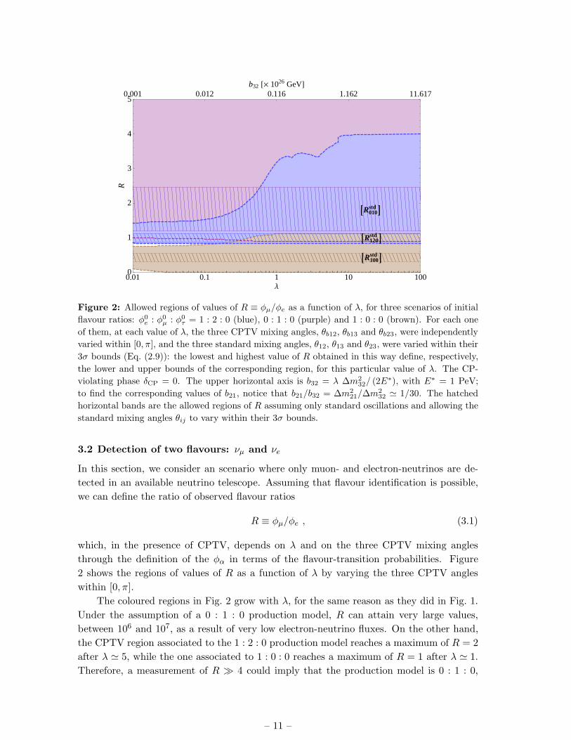
Figure 2: Allowed regions of values of R ≡ φµ/φe as a function of λ, for three scenarios of initial

flavour ratios: φ0e : φ0

µ : φ0τ = 1 : 2 : 0 (blue), 0 : 1 : 0 (purple) and 1 : 0 : 0 (brown). For each one

of them, at each value of λ, the three CPTV mixing angles, θb12, θb13 and θb23, were independently

varied within [0, π], and the three standard mixing angles, θ12, θ13 and θ23, were varied within their

3σ bounds (Eq. (2.9)): the lowest and highest value of R obtained in this way define, respectively,

the lower and upper bounds of the corresponding region, for this particular value of λ. The CP-

violating phase δCP = 0. The upper horizontal axis is b32 = λ ∆m232/ (2E

∗), with E∗ = 1 PeV;

to find the corresponding values of b21, notice that b21/b32 = ∆m221/∆m2

32 ≃ 1/30. The hatched

horizontal bands are the allowed regions of R assuming only standard oscillations and allowing the

standard mixing angles θij to vary within their 3σ bounds.

3.2 Detection of two flavours: νµ and νe

In this section, we consider an scenario where only muon- and electron-neutrinos are de-

tected in an available neutrino telescope. Assuming that flavour identification is possible,

we can define the ratio of observed flavour ratios

R ≡ φµ/φe , (3.1)

which, in the presence of CPTV, depends on λ and on the three CPTV mixing angles

through the definition of the φα in terms of the flavour-transition probabilities. Figure

2 shows the regions of values of R as a function of λ by varying the three CPTV angles

within [0, π].

The coloured regions in Fig. 2 grow with λ, for the same reason as they did in Fig. 1.

Under the assumption of a 0 : 1 : 0 production model, R can attain very large values,

between 106 and 107, as a result of very low electron-neutrino fluxes. On the other hand,

the CPTV region associated to the 1 : 2 : 0 production model reaches a maximum of R = 2

after λ ≃ 5, while the one associated to 1 : 0 : 0 reaches a maximum of R = 1 after λ ≃ 1.

Therefore, a measurement of R ≫ 4 could imply that the production model is 0 : 1 : 0,

– 11 –

Measured R Conclusion

R > 4 Initial ratios 0 : 1 : 0 and CPTV[

Rstd010

]

< R < 4 Initial ratios 0 : 1 : 0 or 1 : 2 : 0, and CPTV

R ∈[

Rstd010

]

(Initial ratios 0 : 1 : 0 and std. osc.) or (1 : 2 : 0 and CPTV)[

Rstd120

]

< R <[

Rstd010

]

Initial ratios 0 : 1 : 0 or 1 : 2 : 0, and CPTV

R ∈[

Rstd120

]

(Initial ratios 1 : 2 : 0 and std. osc.) or

(initial ratios 0 : 1 : 0 or 1 : 0 : 0, and CPTV)

0.84 < R <[

Rstd120

]

Initial ratios 1 : 2 : 0 or 1 : 0 : 0, and CPTV[

Rstd100

]

< R < 0.84 Initial ratios 1 : 0 : 0 and CPTV

R ∈[

Rstd100

]

Initial ratios 1 : 0 : 0 and std. osc.

R <[

Rstd100

]

Initial ratios 1 : 0 : 0 and CPTV

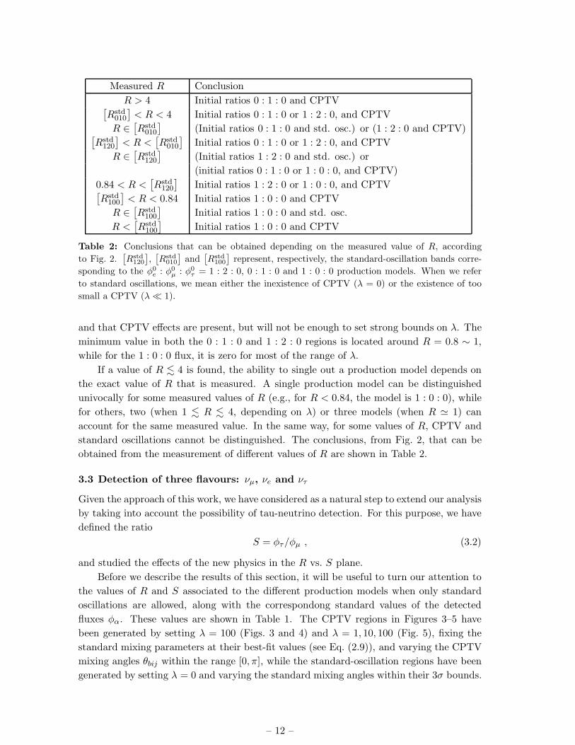
Table 2: Conclusions that can be obtained depending on the measured value of R, according

to Fig. 2.[

Rstd120

]

,[

Rstd010

]

and[

Rstd100

]

represent, respectively, the standard-oscillation bands corre-

sponding to the φ0e : φ0

µ : φ0τ = 1 : 2 : 0, 0 : 1 : 0 and 1 : 0 : 0 production models. When we refer

to standard oscillations, we mean either the inexistence of CPTV (λ = 0) or the existence of too

small a CPTV (λ≪ 1).

and that CPTV effects are present, but will not be enough to set strong bounds on λ. The

minimum value in both the 0 : 1 : 0 and 1 : 2 : 0 regions is located around R = 0.8 ∼ 1,

while for the 1 : 0 : 0 flux, it is zero for most of the range of λ.

If a value of R . 4 is found, the ability to single out a production model depends on

the exact value of R that is measured. A single production model can be distinguished

univocally for some measured values of R (e.g., for R < 0.84, the model is 1 : 0 : 0), while

for others, two (when 1 . R . 4, depending on λ) or three models (when R ≃ 1) can

account for the same measured value. In the same way, for some values of R, CPTV and

standard oscillations cannot be distinguished. The conclusions, from Fig. 2, that can be

obtained from the measurement of different values of R are shown in Table 2.

3.3 Detection of three flavours: νµ, νe and ντ

Given the approach of this work, we have considered as a natural step to extend our analysis

by taking into account the possibility of tau-neutrino detection. For this purpose, we have

defined the ratio

S = φτ/φµ , (3.2)

and studied the effects of the new physics in the R vs. S plane.

Before we describe the results of this section, it will be useful to turn our attention to

the values of R and S associated to the different production models when only standard

oscillations are allowed, along with the correspondong standard values of the detected

fluxes φα. These values are shown in Table 1. The CPTV regions in Figures 3–5 have

been generated by setting λ = 100 (Figs. 3 and 4) and λ = 1, 10, 100 (Fig. 5), fixing the

standard mixing parameters at their best-fit values (see Eq. (2.9)), and varying the CPTV

mixing angles θbij within the range [0, π], while the standard-oscillation regions have been

generated by setting λ = 0 and varying the standard mixing angles within their 3σ bounds.

– 12 –

÷

´ ´

´

1.0 1.5 2.0 2.5 3.0 3.5 4.00.0

0.2

0.4

0.6

0.8

1.0

R

SHaL

÷

´

´

´

0 5 10 150.0

0.2

0.4

0.6

0.8

1.0

1.2

R

S

HbL

÷

´

´

´

´

0.0 0.2 0.4 0.6 0.8 1.0 1.20.0

0.5

1.0

1.5

2.0

2.5

R

S

HcL

A

B C

DA

B

C

DA

B

C

D

E

Φe0 : ΦΜ

0 : ΦΤ0 = 1 : 2 : 0 Φe

0 : ΦΜ0 : ΦΤ

0 = 0 : 1 : 0 Φe0 : ΦΜ

0 : ΦΤ0 = 1 : 0 : 0

R = ΦΜ Φe S = ΦΤ ΦΜ

A : R = 1, S = 1B : R = 1, S = 0C : R = 2, S = 0D : R = 4, S = 1 4

A : R = 1.8, S = 1B : R = 1, S = 0C : R = 5, S = 0.2D : R = 10, S = 1

A : R = 0.38, S = 1B : R = 0, S = 0C : R = 0, S = 01.4D : R = 1, S = 0E : R = 1.1, S = 0 .6

CPTV dominant HΛ = 100L

standard osc. HΛ = 0L

CPTV dominant HΛ = 100L

standard osc. HΛ = 0L

CPTV dominant HΛ = 100L

standard osc. HΛ = 0L

Figure 3: Regions of R and S accessible with CPTV by assuming different neutrino production

scenarios. Different colours correspond to different initial ratios: φ0e : φ0

µ : φ0τ = 1 : 2 : 0 (blue), 0 : 1 :

0 (purple), 1 : 0 : 0 (brown). Darker regions are generated with standard (CPT-conserving) neutrino

flavour oscillations, by allowing the standard mixing angles to vary within their 3σ experimental

bounds. Lighter regions correspond to the case when we include a dominant CPTV contribution

with λ = 100, and allow the CPTV angles θbij to vary within [0, π]. All phases are set to zero.

With the exception of Figure 6, where δCP has been allowed to vary, we have set all phases

equal to zero.

In Fig. 3 we display in three R vs. S panels the allowed regions of values that correspond

to pure standard oscillations at 3σ, in dark tones, and the corresponding regions allowed by

the mixed solution composed of the standard oscillation plus CPTV effects, with λ = 100,

in lighter tones. At this value of λ, the CPTV contributions are the dominant ones in

the Hamiltonian, i.e., Hf ≃ Hb. Each plot corresponds to a different neutrino production

scenario: (a) to 1 : 2 : 0, (b) to 0 : 1 : 0, and (c) to 1 : 0 : 0.

From these plots we can extract two observations: one is the potentially dramatic

deviation of the allowed values of the pair (R,S) when CPTV is turned on, and the other

is the presence of points that are common to all scenarios. The latter implies that, if

there is CPTV, there could exist pairs (R,S), such as (1, 0), that can be generated by any

of the three production models, each with a different set of values for the CPTV mixing

angles. There are also (R,S) pairs which could be generated by one production model

with standard oscillations or with a different model with CPTV, e.g., those lying around

(1, 0.95). It is convenient to remark that this figure and Fig. 2 are consistent with each

other, which can be shown by projecting the CPTV regions of Fig. 3 onto the horizontal

axis and checking that the limits on R agree with those on Fig. 2. We have marked a few

notable points in each plot: for the three production models, the points labelled with A

correspond to the best-fit values of the standard-oscillation mixing parameters in Eq. (2.9).

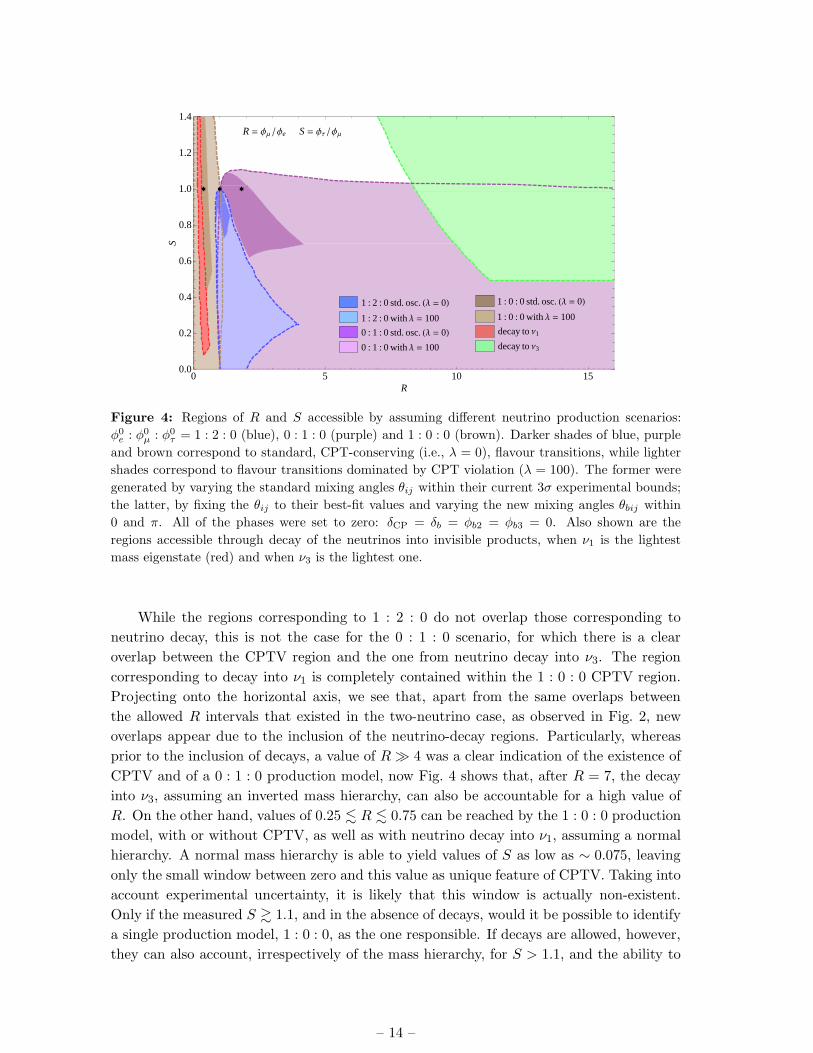
In Fig. 4, the allowed R − S regions corresponding to the three neutrino production

models are shown together: 1 : 2 : 0 in blue, 0 : 1 : 0 in purple, and 1 : 0 : 0 in brown,

where, as before, the darker tones correspond to pure standard oscillations, and the lighter

tones, to a dominant CPTV with λ = 100. Following the argument in Section 2.3, we have

also included the regions of (R,S) pairs allowed by neutrino decay into invisible products,

considering both the cases of a normal mass hierarchy (decay into the ν1 eigenstate), in

red, and of an inverted hierarchy (decay into ν3), in green. The decay regions were also

generated by varying the standard-oscillation mixing angles within their 3σ bounds.

– 13 –

÷ ÷÷

1 : 2 : 0 std. osc. HΛ = 0L

1 : 2 : 0 with Λ = 100

0 : 1 : 0 std. osc. HΛ = 0L0 : 1 : 0 with Λ = 100

1 : 0 : 0 std. osc. HΛ = 0L

1 : 0 : 0 with Λ = 100

decay to Ν1

decay to Ν3

R = ΦΜ Φe S = ΦΤ ΦΜ

0 5 10 150.0

0.2

0.4

0.6

0.8

1.0

1.2

1.4

R

S

Figure 4: Regions of R and S accessible by assuming different neutrino production scenarios:

φ0e : φ0

µ : φ0τ = 1 : 2 : 0 (blue), 0 : 1 : 0 (purple) and 1 : 0 : 0 (brown). Darker shades of blue, purple

and brown correspond to standard, CPT-conserving (i.e., λ = 0), flavour transitions, while lighter

shades correspond to flavour transitions dominated by CPT violation (λ = 100). The former were

generated by varying the standard mixing angles θij within their current 3σ experimental bounds;

the latter, by fixing the θij to their best-fit values and varying the new mixing angles θbij within

0 and π. All of the phases were set to zero: δCP = δb = φb2 = φb3 = 0. Also shown are the

regions accessible through decay of the neutrinos into invisible products, when ν1 is the lightest

mass eigenstate (red) and when ν3 is the lightest one.

While the regions corresponding to 1 : 2 : 0 do not overlap those corresponding to

neutrino decay, this is not the case for the 0 : 1 : 0 scenario, for which there is a clear

overlap between the CPTV region and the one from neutrino decay into ν3. The region

corresponding to decay into ν1 is completely contained within the 1 : 0 : 0 CPTV region.

Projecting onto the horizontal axis, we see that, apart from the same overlaps between

the allowed R intervals that existed in the two-neutrino case, as observed in Fig. 2, new

overlaps appear due to the inclusion of the neutrino-decay regions. Particularly, whereas

prior to the inclusion of decays, a value of R≫ 4 was a clear indication of the existence of

CPTV and of a 0 : 1 : 0 production model, now Fig. 4 shows that, after R = 7, the decay

into ν3, assuming an inverted mass hierarchy, can also be accountable for a high value of

R. On the other hand, values of 0.25 . R . 0.75 can be reached by the 1 : 0 : 0 production

model, with or without CPTV, as well as with neutrino decay into ν1, assuming a normal

hierarchy. A normal mass hierarchy is able to yield values of S as low as ∼ 0.075, leaving

only the small window between zero and this value as unique feature of CPTV. Taking into

account experimental uncertainty, it is likely that this window is actually non-existent.

Only if the measured S & 1.1, and in the absence of decays, would it be possible to identify

a single production model, 1 : 0 : 0, as the one responsible. If decays are allowed, however,

they can also account, irrespectively of the mass hierarchy, for S > 1.1, and the ability to

– 14 –

R = ΦΜ Φe S = ΦΤ ΦΜ

0 : 1 : 0Λ = 0

1 : 0 : 0, Λ = 0 Hstd. osc.L

1 : 2 : 0, Λ = 01

11, 10

10

10010

100 1000 5 10 15

0.0

0.2

0.4

0.6

0.8

1.0

1.2

1.4

R

S

Figure 5: Regions of values of R and S accessible when varying the parameter λ between 0 (no

CPT breaking) and 100 (dominant CPTV term), for different neutrino production models. In blue:

φ0e : φ0

µ : φ0τ = 1 : 2 : 0; in purple, 0 : 1 : 0; in brown, 1 : 0 : 0. The region corresponding to pure

standard oscillations (λ = 0) was generated by varying the standard mixing angles within their

3σ experimental bounds, Eq. (2.9). To generate the regions corresponding to λ = 1, 10, 100, the

standard mixing angles were fixed to their best-fit values, and the three CPTV mixing angles θbijwere varied independently within [0, π]. The CP-violating phase δCP = 0 for all of the regions.

single out a production model is lost. Thus, the signatures of CPTV become less unique

in the presence of decays. A more complete analysis of neutrino decays [23], exploring also

the possibility of incomplete decays and decay into visible products, further reduces our

ability to uniquely identify the presence of CPTV.

In the absence of neutrino decays, a measurement of R & 4.1 and S . 1.1 could

indicate the presence of dominant CPTV and a 0 : 1 : 0 production model. Also, for

R . 0.9, the production model is 1 : 0 : 0; if S . 0.45, there is dominant CPTV and, for

other values of S, the existence of CPTV will depend on the value of R measured. Close

to R = 1, and for S . 0.9, any of the three production models with dominant CPTV can

explain the measured (R,S) pair, while for 0.9 . S < 1, the pair could be generated either

by the 0 : 1 : 0 or 1 : 0 : 0 models with CPTV, or by the 1 : 2 : 0 model with standard

oscillations. For 1.1 . R < 4 and S . 0.6, there is a large region of overlap between the

1 : 2 : 0 and 0 : 1 : 0 models with dominant CPTV.

Fig. 5 shows the effect of the variation of the parameter λ between 0 (no CPTV, i.e.,

Hf = Hm) and 100 (dominant CPTV term, i.e., Hf ≃ Hb) on the allowed R − S regions,

for the different neutrino production scenarios. For the three of them, we can observe

significant deviations from the predictions of the standard-oscillation case, even for low

values of λ. In this sense, it is interesting to point out that in the case of an experimental

non-detection of CPTV in the neutrino flavour ratios, R and S can be used to set limits

on the related parameters. In fact, when λ = 1, and for a neutrino energy of 1 PeV, we

– 15 –

0.00 0.01 0.02 0.03 0.04 0.05

0.5

1.0

1.5

2.0

sin2 Θ13

RHaL

0.00 0.01 0.02 0.03 0.04 0.05

0.8

0.9

1.0

1.1

1.2

1.3

1.4

sin2 Θ13

S

HbL

1 : 2 : 0, 0 £ ∆CP £ 2 Π

0 : 1 : 0, 0 £ ∆CP £ 2 Π

1 : 0 : 0, 0 £ ∆CP £ 2 Π

Θ13 = 0 = ∆CP

Θ12 = 33.46 °, Θ23 = 45 °

std. osc. only HΛ = 0L∆CP = 0

∆CP = 0

Figure 6: Variation of R and S with θ13, when the CP-violation phase δCP is allowed to vary

between 0 and 2π. The upper limit for θ13 is given by the current bound sin2 (θ13) ≤ 0.056 (3σ)

and the mixing parameters θ12, θ23, ∆m221 and ∆m2

32 have been set to their current best-fit values;

standard flavour oscillations have been assumed throughout (i.e., λ = 0). Three different scenarios

of initial flavour ratios have been considered: φ0e : φ0

µ : φ0τ = 1 : 2 : 0 (in blue), 0 : 1 : 0 (in purple)

and 1 : 0 : 0 (in brown). To allow for comparison, the arrows point to the curves on which δCP = 0.

can attain limits for the CPTV eigenvalues bij in the order of 10−29 and 10−27 GeV, for

b21 and b23, respectively. It is also important to mention that these results can be easily

rescaled to any energy, just by doing bij×(PeV/E). This would mean a very significant

improvement over the current bounds of 10−23 − 10−21 GeV for b21 and b32, respectively

[21].

Finally, it is worth exploring the effect of the choice of value of δCP on R and S. From

Fig. 6, we see that the effect on R of a non-zero value of δCP in the standard-oscillation

regions is more prominent for a choice of initial ratios of 0 : 1 : 0, and less so for 1 : 2 : 0

and 1 : 0 : 0. For S, the effect of a non-zero phase is greater for 1 : 0 : 0, and less for 0 : 1 : 0

and 1 : 2 : 0. Note that using a non-zero value of δCP can lead to a variation in R of up to

42% (in the 0 : 1 : 0 case) and in S of up to 40% (in the 1 : 0 : 0 case) with respect to the

standard case of θ13 = δCP = 0, when the largest 3σ allowed value of sin2 (θ13) = 0.056 is

assumed.

4. Detection prospects at IceCube considering CPTV

4.1 Experimental setup

The IceCube neutrino telescope [41, 42], located at the South Pole, can detect both muons

and showers initiated by incoming high-energy astrophysical neutrinos. Muon-neutrinos are

detected through the high-energy muon produced in charged-current (CC) deep inelastic

neutrino-nucleon scattering: the Cerenkov light emitted by the fast-moving muon in ice

is detected by the photomultipliers buried in ice and used to reconstruct the muon track.

Electron-neutrinos can generate electromagnetic and hadronic showers in CC interactions.

Tau-neutrino CC events have a distinct topology: they either show two hadronic showers

joined by a tau track (a double bang) or a tau track ending with the decay of the tau in

– 16 –

a hadronic shower (lollipop). Additionally, every flavour of neutrino is able to generate

hadronic showers in neutral-current (NC) interactions. Flavour identification is expected

to be difficult at IceCube [24] and the number of lollipops expected is about one every two

years (for a neutrino flux of 10−7 GeV−1 s−1 cm−2 sr−1 [24]), so the useful observables turn

out to be the total number of NC plus CC showers, Nsh = NNCsh + NCC

sh and the number

of muon tracks, Nνµ . From this, we can construct the closest experimental analogue of

the variable R ≡ φµ/φe as Rexp ≡ Nνµ/Nsh. Due to the very low number of tau-neutrinos

expected at IceCube, there is no practical experimental analogue of S ≡ φτ/φµ.

Following our analysis of CPTV in the previous sections, where we set the scale of

CPTV at E∗ = 1 PeV, we have adopted the energy range Eminν = 106 ≤ Eν/GeV ≤ Emax

ν =

1012 for our predictions. Within this energy range, the Earth is opaque to neutrinos due

to the increased number of NC interactions which degrade their energy [45], so we have

calculated only the number of downgoing events. Bear in mind, however, that due to the

tighter background filtering that is required for the observation of downgoing neutrinos,

which we have not taken into account in the following calculations, our estimates may be

optimistic. Conveniently, for most of this range the atmospheric νµ background flux will

be well below the fluxes from the neutrino production models that we have probed (see

Figure 7). Using the expressions of [43], we can estimate the number of CC and NC events

at IceCube, for a given astrophysical all-flavour diffuse neutrino flux, denoted here by Φνall:

NCCνall

= TnTVeffΩ

∫ Emaxν

Eminsh

Φνall (Eν)1

2

[

σνNCC (Eν) + σνN

CC (Eν)]

dEν (4.1)

NNCνall

= TnTVeffΩ

∫ Emaxν

Eminsh

dEν

∫ Emaxν

Eν−Eminsh

dE′νΦ

νall (Eν)×

×1

2

[

dσνNNC

dE′ν

(

Eν , E′ν

)

+dσνN

NC

dE′ν

(

Eν , E′ν

)

]

, (4.2)

where E′ν is the energy of the secondary neutrino in the NC interaction, T is the exposure

time, nT = 5.1557×1023 cm−3 is the number density of targets (nucleons) in ice, Veff is the

effective detector volume (1 km3 for IceCube) and Ω = 5.736 sr is the detector’s opening

angle (up to 85). The total cross sections for neutrino and anti-neutrino deep inelastic

scattering, σνNCC, σ

νNCC , σ

νNNC and σνN

NC, have been extracted from [44]. The differential cross

sections used are written as a function of both the primary and the secondary neutrino

energies, which in NC interactions are related through E′ν = (1− 〈yNC〉)Eν , with 〈yNC〉

the NC inelasticity parameter, extracted from [45]. If the interval of interest (106 − 1012

GeV) is partitioned into small enough subintervals, then within each, the NC cross section

can be approximated by σNC = AEBν with A, B constants for each subinterval. We can

then write

σνNNC = AEB

ν = A[

(1− 〈yNC (Eν)〉)−1 E′

ν

]B, (4.3)

so thatdσNC

dE′ν

(

Eν , E′ν

)

= AB [1− 〈yNC (Eν)〉]−B (E′

ν

)B−1. (4.4)

– 17 –

Using this expression in Eq. (4.2) and performing the E′ν integral, we obtain the simplified

form

NNCνall≃ 1

2 TnTVeffΩ

∫ Emaxν

Eminsh

dEνΦνall (Eν)×

×

σνNNC (Emax

ν )− σνNNC

(

Eν − Eminsh

)

[

1−⟨

yνNNC (Eν)⟩]B

+σνNNC (Emax

ν )− σνNNC

(

Eν −Eminsh

)

[

1−⟨

yνNNC (Eν)⟩]B

,(4.5)

with B and B taking the appropriate values in each subinterval.

The number of CC showers generated by electron- and tau-neutrinos are, respectively,

NCCsh,e = φeN

CCνall

and NCCsh,τ = φτN

CCνall

, where

φα ≡φα

φe + φµ + φτ∈ [0, 1] (4.6)

are the normalised flavour ratios. The number of CC showers is given by

NCCsh = NCC

sh,e +NCCsh,τ =

(

φe + φτ

)

NCCνall

(4.7)

and the total number of CC plus NC showers is therefore

Nsh = NCCsh +NNC

sh =(

1− φµ

)

NCCνall

+NNCνall

, (4.8)

where we have used the fact that∑

β=e,µ,τ φβ = 1. In a similar way, the number of

downgoing muon-neutrinos is given by

Nνµ = φµNCCνall

. (4.9)

Using Eqs. (4.1), (4.5), (4.8) and (4.9), we find

Rexp =Nνµ

Nsh=

φµ(

1− φµ

)

+NNCνall

/NCCνall

, (4.10)

and we see that Rexp depends on only one of the normalised flavour ratios, φµ, and that it

is independent of the exposure time and the effective detector size. Increasing T and Veff,

however, results in a larger event yield and consequently in lower statistical uncertainty.

Considering NNCνall

and NCCνall

as independent variables with Poissonian errors, i.e.,√

NNCνall

and√

NCCνall

respectively, we find the error on Rexp to be

σRexp =Rexp

(

1− φµ

)

+NNCνall

/NCCνall

NNCνall

NCCνall

√

1

NNCνall

+1

NCCνall

. (4.11)

As expected, σRexp ∝ (TVeff)−1/2, so that, for a given neutrino flux, the statistical error on

Rexp decreases with the time of exposure and the size of the detector.

– 18 –

106

107

108

109

1010

1011

1012

Eν [GeV]

10-34

10-32

10-30

10-28

10-26

10-24

10-22

10-20

10-18

Φν al

l (E

ν) [G

eV-1

cm

-2 s

-1 s

r-1]

WBBB α = 2.7KT α = 2.6 no source evol.KT α = 2.3 strong source evol.atmospheric νµ

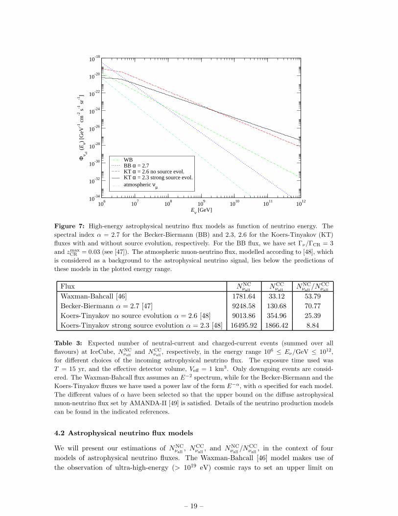
Figure 7: High-energy astrophysical neutrino flux models as function of neutrino energy. The

spectral index α = 2.7 for the Becker-Biermann (BB) and 2.3, 2.6 for the Koers-Tinyakov (KT)

fluxes with and without source evolution, respectively. For the BB flux, we have set Γν/ΓCR = 3

and zmaxCR = 0.03 (see [47]). The atmospheric muon-neutrino flux, modelled according to [48], which

is considered as a background to the astrophysical neutrino signal, lies below the predictions of

these models in the plotted energy range.

Flux NNCνall

NCCνall

NNCνall

/NCCνall

Waxman-Bahcall [46] 1781.64 33.12 53.79

Becker-Biermann α = 2.7 [47] 9248.58 130.68 70.77

Koers-Tinyakov no source evolution α = 2.6 [48] 9013.86 354.96 25.39

Koers-Tinyakov strong source evolution α = 2.3 [48] 16495.92 1866.42 8.84

Table 3: Expected number of neutral-current and charged-current events (summed over all

flavours) at IceCube, NNCνall

and NCCνall

, respectively, in the energy range 106 ≤ Eν/GeV ≤ 1012,

for different choices of the incoming astrophysical neutrino flux. The exposure time used was

T = 15 yr, and the effective detector volume, Veff = 1 km3. Only downgoing events are consid-

ered. The Waxman-Bahcall flux assumes an E−2 spectrum, while for the Becker-Biermann and the

Koers-Tinyakov fluxes we have used a power law of the form E−α, with α specified for each model.

The different values of α have been selected so that the upper bound on the diffuse astrophysical

muon-neutrino flux set by AMANDA-II [49] is satisfied. Details of the neutrino production models

can be found in the indicated references.

4.2 Astrophysical neutrino flux models

We will present our estimations of NNCνall

, NCCνall

, and NNCνall

/NCCνall

, in the context of four

models of astrophysical neutrino fluxes. The Waxman-Bahcall [46] model makes use of

the observation of ultra-high-energy (> 1019 eV) cosmic rays to set an upper limit on

– 19 –

the neutrino flux. The limit depends on the redshift evolution of the neutrino sources,

which could be active galactic nuclei (AGN) or gamma-ray bursts. We have adopted,

conservatively,

ΦWBνall

(Eν) = 10−8 (Eν/GeV)−2 GeV−1 cm−2 s−1 sr−1 . (4.12)

The second model, by Becker-Biermann [47], describes the production of neutrinos in the

relativistic jets of FR-I galaxies (low-luminosity radio galaxies with extended radio jets)

through the decay of pions produced in the interaction of shock-accelerated protons with

the surrounding photon field. The sources are assumed to evolve with redshift according

to certain luminosity functions. The flux is given by

ΦBBνall

(Eν) ≃ 5.4× 10−3 (Eν/GeV)−2.7 GeV−1 cm−2 s−1 sr−1 . (4.13)

The third and fourth models, by Koers-Tinyakov [48], predict an astrophysical neutrino

flux based on the assumption that the neutrinos originate predominantly at AGN and that

these behave like Centaurus A, the nearest active galaxy. The difference between these

last two models lies in the assumption about the redshift evolution of the source: in one

of them, sources are assumed not to evolve with redshift, while in the other one, they are

assumed to have a strong redshift evolution, following the star-formation rate of ∼ (1 + z)3.

These two fluxes are given, respectively, by

ΦKT, no evol.νall

(Eν) ≃ 3.5× 10−10 (Eν/GeV)−1.6 ×

×min (1, Eν/Eν,br) GeV−1 cm−2 s−1 sr−1 (4.14)

ΦKT, evol.νall

(Eν) ≃ 4.6× 10−12 (Eν/GeV)−1.3 ×

×min (1, Eν/Eν,br) GeV−1 cm−2 s−1 sr−1 , (4.15)

with Eν,br = 4×106 GeV the break energy. Both the Becker-Biermann and Koers-Tinyakov

models account for the change in cosmic-ray energy due to the adiabatic cosmological ex-

pansion, but only the latter take into account also energy losses due to pion photopro-

duction and electron-positron pair production in the interaction with the CMB photons.

Currently, the most stringent upper bound on the astrophysical muon-neutrino flux is the

one obtained by the AMANDA-II experiment [49], which restricts the integrated muon-

neutrino flux to be lower than 7.4 × 10−8 GeV cm−2 s−1 sr−1, within the interval 16

TeV – 2.5 PeV. We have checked that the four fluxes used in our analysis satisfy this

upper bound in the standard-oscillation case, i.e., when the detected flavour ratios are

φe : φµ : φτ = 1 : 1 : 1. The spectral indices of the power laws for the Koers-Tinyakov

fluxes, −1.6 and −1.3, have been chosen so that the integrated fluxes between 16 TeV and

2.5 PeV yield exactly the upper bound value set by AMANDA. A plot of the four different

fluxes is presented in Fig. 7.

We have evaluated Eqs. (4.1) and (4.5) numerically in the range 106 ≤ Eν/GeV ≤ 1012

for the four different fluxes, assuming T = 15 yr and Veff = 1 km3 (the IceCube effective

volume). The results are presented in Table 3. The Waxman-Bahcall model yields the

lowest number of CC and NC events, while the Koers-Tinyakov model with strong source

evolution yields the highest number, more than two orders of magnitude over Waxman-

Bahcall.

– 20 –

0.01 0.1 1 10 1000.00

0.02

0.04

0.06

0.08

0.10

0.12

0.001 0.012 0.116 1.162 11.617

Λ

Rex

p

b32 @´ 1026 GeVDHaL

0.01 0.1 1 10 1000.00

0.02

0.04

0.06

0.08

0.10

0.12

0.001 0.012 0.116 1.162 11.617

ΛR

exp

b32 @´ 1026 GeVDHbL

0.01 0.1 1 10 1000.00

0.02

0.04

0.06

0.08

0.10

0.12

0.001 0.012 0.116 1.162 11.617

Λ

Rex

p

b32 @´ 1026 GeVDHcL

0.01 0.1 1 10 1000.00

0.02

0.04

0.06

0.08

0.10

0.12

0.001 0.012 0.116 1.162 11.617

Λ

Rex

p

b32 @´ 1026 GeVDHdL

0.01 0.1 1 10 1000.00

0.02

0.04

0.06

0.08

0.10

0.12

0.001 0.012 0.116 1.162 11.617

Λ

Rex

p

b32 @´ 1026 GeVDHeL

0.01 0.1 1 10 1000.00

0.02

0.04

0.06

0.08

0.10

0.12

0.001 0.012 0.116 1.162 11.617

ΛR

exp

b32 @´ 1026 GeVDHfL

Φe0 : ΦΜ

0 : ΦΤ0 = 1 : 2 : 0 Φe

0 : ΦΜ0 : ΦΤ

0 = 0 : 1 : 0 Φe0 : ΦΜ

0 : ΦΤ0 = 1 : 0 : 0

Waxman - Bahcall

Koers - Tinyakovstrong source evol.

IceCube ´ 5 IceCube ´ 5 IceCube ´ 5

Φe0 : ΦΜ

0 : ΦΤ0 = 1 : 2 : 0 Φe

0 : ΦΜ0 : ΦΤ

0 = 0 : 1 : 0 Φe0 : ΦΜ

0 : ΦΤ0 = 1 : 0 : 0IceCube IceCube IceCube

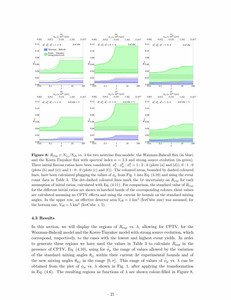
Figure 8: Rexp ≡ Nνµ/Nsh vs. λ for two neutrino flux models: the Waxman-Bahcall flux (in blue)

and the Koers-Tinyakov flux with spectral index α = 2.3 and strong source evolution (in green).

Three initial flavour ratios have been considered: φ0e : φ0

µ : φ0τ = 1 : 2 : 0 (plots (a) and (d)), 0 : 1 : 0

(plots (b) and (e)) and 1 : 0 : 0 (plots (c) and (f)). The coloured areas, bounded by dashed coloured

lines, have been calculated plugging the values of φµ from Fig. 1 into Eq. (4.10) and using the event

count data in Table 3. The dot-dashed coloured lines mark the 1σ uncertainty on Rexp for each

assumption of initial ratios, calculated with Eq. (4.11). For comparison, the standard value of Rexp

for the different initial ratios are shown in hatched bands of the corresponding colours; these values

are calculated assuming no CPTV effects and using the current 3σ bounds on the standard mixing

angles. In the upper row, an effective detector area Veff = 1 km3 (IceCube size) was assumed; for

the bottom one, Veff = 5 km3 (IceCube × 5).

4.3 Results

In this section, we will display the regions of Rexp vs. λ, allowing for CPTV, for the

Waxman-Bahcall model and the Koers-Tinyakov model with strong source evolution, which

correspond, respectively, to the cases with the lowest and highest event yields. In order

to generate these regions we have used the values in Table 3 to calculate Rexp in the

presence of CPTV, Eq. (4.10), using for φµ the range of values allowed by the variation

of the standard mixing angles θij within their current 3σ experimental bounds and of

the new mixing angles θbij in the range [0, π]. This range of values of φµ vs. λ can be

obtained from the plot of φµ vs. λ shown in Fig. 1, after applying the transformation

in Eq. (4.6). The resulting regions as functions of λ are shown colour-filled in Figure 8,

– 21 –

for the Waxman-Bahcall (blue) and Koers-Tinyakov (green) models. We have explored

two different detector effective volumes, 1 km3 (IceCube-sized) and 5 km3, and the three

different choices for the initial fluxes φ0e : φ0

µ : φ0τ = 1 : 2 : 0, 0 : 1 : 0 and 1 : 0 : 0, that

we introduced in the previous sections. Furthermore, this figure includes boundaries of 1σ

statistical uncertainty on Rexp that were obtained by adding (subtracting) 1σ to (from)

the upper (lower) boundaries of the coloured regions. The values of σ were calculated by

plugging into Eq. (4.11) the corresponding values of φµ that occur on the borderlines of

the coloured regions.

We note that the shapes of the coloured regions in Fig. 8 are similar to those in Fig. 1.

This can be understood if we note that Rexp, Eq. (4.10), is proportional to φµ. In Fig. 1

we saw that there exists overlap among the regions related to the different hypotheses of

the initial flux. In fact, in Fig. 8, there is overlap between the three production models,

with the region corresponding to φ0e : φ0

µ : φ0τ = 1 : 2 : 0 almost entirely enclosed within

the region for 0 : 1 : 0. This last fact can be explained on account of the reduction in

size of the region for 1 : 2 : 0, caused by the normalisation of φµ applied for this case, i.e.,

φµ = φµ/3. As we can anticipate, due to the higher event yield, the statistical uncertainty

on Rexp associated to the Koers-Tinyakov flux is lower than the one associated to the

Waxman-Bahcall flux, and is reduced when the larger detector volume is used. The size of

this uncertainty is also proportional to the value of φµ (see Eq. (4.11)). As a consequence,

the size of the 1σ regions is larger for an initial flux of 1 : 2 : 0, intermediate for 0 : 1 : 0,

and smallest for 1 : 0 : 0.

When a detector volume of 1 km3 is considered, there is a clear overlap among regions

corresponding to different assumptions of the neutrino flux model when the production

scenario is 1 : 0 : 0. This observation is reinforced when we consider also the regions

spanned by the statistical uncertainty. In comparison, for the 1 : 2 : 0 and 0 : 1 : 0

scenarios, the regions corresponding to the two flux models do not overlap. When the

5 km3 detector is assumed, the regions associated to 1 : 2 : 0 and 0 : 1 : 0 are further

separated at the 1σ level. However, there is still an overlap between the two flux models

in the 1 : 0 : 0 scenario. Here we do not show the results for the Becker-Biermann model

and the Koers-Tinyakov model with no source evolution, since their results are embodied

in what we have already presented. For instance, the mean value of Rexp and σRexp for

Becker-Biermann is similar to the one for Waxman-Bahcall. Similar estimates can be easily

obtained by plugging the values of Table 3 into Eqs. (4.10) and (4.11).

5. Summary and conclusions

Motivated by the CPT-violating (CPTV) neutrino coupling considered in the Standard

Model Extension, we have added a CPTV, energy-independent, contribution to the neu-

trino oscillation Hamiltonian and explored its effects on the flavour ratios of the high-energy

(1 PeV and higher) astrophysical neutrino flux predicted to come from active galactic nu-

clei. We have parametrised the strength of the CPTV contribution by the parameter λ,

defined as the quotient between the eigenvalues of the CPTV Hamiltonian, b21 and b32,

and those of the standard-oscillation one, ∆m221/ (2E

⋆) and ∆m232/ (2E

⋆), with E⋆ = 1

– 22 –

PeV, and allowed λ to vary between 10−2 and 100, corresponding to standard-oscillation

dominance and CPTV dominance, respectively. We have used three different neutrino pro-

duction scenarios for the flavour ratios at the astrophysical sources: production by pion

decay, which results in φ0e : φ0

µ : φ0τ = 1 : 2 : 0; muon cooling, which results in 0 : 1 : 0;

and neutron decay, resulting in 1 : 0 : 0, and explored the effect of a potential CPTV on

the neutrino flavour ratios at Earth, φα (α = e, µ, τ), and on the ratios between them.

With this objetive, we have studied the behaviour of φµ, R = φµ/φe, and S = φτ/φµ,

by letting the standard-oscillation mixing parameters vary within their current 3σ experi-

mental bounds, and varying the unknown CPTV parameters as broadly as possible, while

keeping b21 and b32 below their current upper limits (obtained from atmospheric and solar

experiment data).

From the observation of φµ, if CPTV is dominant, we found that there could be large

deviations with respect to the pure standard-oscillation case, depending on the values of

the CPTV parameters. These deviations start at λ = 0.1 (b32 ∼ 10−28 GeV, b21 ∼ 10−26

GeV) and reach a plateau at λ = 1. There are overlaps between the different neutrino

production models, in such a way that a measurement of certain values of φµ could be

satisfied by two different production models, either including CPTV or not.

When we consider the possibility of detecting φµ and φe, from which R ≡ φµ/φe can

be built, we find that the regions corresponding to 1 : 2 : 0 and 0 : 1 : 0 exhibit a similar

behaviour than when φµ alone is measured, though the former is now nearly contained by

the latter. This is not the case for 1 : 0 : 0, where the value of R could blow up owing to a

potentially very low value of φe, in comparison to φµ.

If tau-neutrinos can also be detected, then we can use the ratio S ≡ φτ/φµ. When we

combine R and S, i.e., when we assume the ability to measure φτ with enough statistics,

we improve the chances of discovering CPTV effects. In fact, large CPTV regions of (R,S)

values that are well distinguished from the standard-oscillation case are obtained for the

three neutrino production models that we have considered here. As a consequence of the

wideness of these regions, there are many overlapping areas where a given pair (R,S) can

be generated by any of the production models that we have explored, assuming a dominant

CPTV.

On the other hand, in the case of the non-observation of deviations in the flavour ratios,

it will be possible to impose very stringent limits on the parameters related to CPTV in

the neutrino sector, such as b21 . 10−29 GeV and b32 . 10−27 GeV, to be compared with

the current limits of 10−23 GeV and 10−21 GeV, respectively.

In order to compare CPTV with other competitive new physics scenarios, we have

included the possibility of neutrino decay to invisible products, both in the normal and

inverted mass hierarchies. As a result, there are additional overlaps between the CPTV

regions and the regions accessible by neutrino decays, for certain values of the CPTV

parameters.

With the purpose of presenting a more realistic perspective, we have performed an

analysis of the potential CPTV signals at a large ice Cerenkov detector such as IceCube.

On top of the three neutrino production models, 1 : 2 : 0, 0 : 1 : 0 and 1 : 0 : 0, we have used

two different models for the neutrino astrophysical flux, one by Waxman and Bahcall and

– 23 –

the other by Koers and Tinyakov, and compared their respective signals at the detector.

For this analysis, we have found that there are still overlaps among the three production

models, even more pronounced than the ones that were obtained in the theoretical plots.

In 15 years of exposure time, a 1 km3 detector (or, equivalently, tVeff = 15 yr km3) would

be able to distinguish between the two fluxes, in the 1 : 2 : 0 and 0 : 1 : 0 scenarios, while

a 5 km3 detector with the same exposure (or tVeff = 75 yr km3), would provide clearer

separation between the flux models at the 1σ level.

When λ ≥ 1, a separation of a few standard deviations between the CPT-conserving

and the CPTV scenarios is possible, depending on the values of the CPTV mixing param-

eters, both for the Waxman-Bahcall and the Koers-Tinyakov fluxes. This separation is

more clearly visible in the 1 : 2 : 0 and 0 : 1 : 0 cases. Our main result is that, while it is in

principle possible to detect the presence of CPTV with IceCube, it will not be possible, for

many values of (R,S), to find which one of the production models is the actual one. The

detection of CPTV can be aided by a more precise knowledge of the standard-oscillation

mixing parameters and by a considerably higher event yield, brought by a larger effective

volume or probably from a non-Cerenkov detector, but these two improvements do not

eliminate the overlaps that exist between (R,S) regions associated to different production

models. In the event of measuring values of R, S, or both, that fall inside an overlap region,

then, in the absence of knowledge of the values of the CPTV mixing parameters, one is able

to trade one production model, with a certain set of values of the CPTV parameters, by

one of the other overlapping models, with another set of values of the parameters. These

degeneracies could be lifted by an independent measurement of the CPTV parameters in

the neutrino sector, in a different kind of experiment.

Nevertheless, as a tool for detecting the presence of CPT breaking in the neutrino

sector, if not for measuring it in detail, IceCube might be a useful one. If CPT is broken,

and if the parameters introduced by the breaking have certain values, then IceCube could

be able to detect the deviation from the standard-oscillation scenario after 15 years of data

taking.

Acknowledgments

This work was supported by grants from the Direccion Academica de Investigacion of the

Pontificia Universidad Catolica del Peru (projects DAI-4075 and DAI-L009 [LUCET]) and

by a High Energy Latinamerican-European Network (HELEN) STT grant. MB acknowl-

edges the hospitality of IFIC during the development of this work.

References

[1] R. J. Davis, D. S. Harmer and K. C. Hoffman, Search for neutrinos from the sun, Phys. Rev.

Lett. 20 (1968) 1205.

[2] B. Aharmim et al. [SNO Collaboration], Electron energy spectra, fluxes, and day-night

asymmetries of B-8 solar neutrinos from the 391-day salt phase SNO data set, Phys. Rev. C

72 (2005) 055502 [nucl-ex/0502021].

– 24 –

[3] C. Arpesella et al. [Borexino Collaboration], Direct Measurement of the Be-7 Solar Neutrino

Flux with 192 Days of Borexino Data, Phys. Rev. Lett. 101 (2008) 091302

[astro-ph/0805.3843].

[4] Y. Ashie et al. [Super-Kamiokande Collaboration], Evidence for an oscillatory signature in

atmospheric neutrino oscillation, Phys. Rev. Lett. 93 (2004) 101801 [hep-ex/0404034].

[5] M. Ambrosio et al. [MACRO Collaboration], Measurements of atmospheric muon neutrino

oscillations, global analysis of the data collected with MACRO detector, Eur. Phys. J. C 36

(2004) 323.

[6] K. Eguchi et al. [KamLAND Collaboration], First results from KamLAND: Evidence for

reactor anti-neutrino disappearance, Phys. Rev. Lett. 90 (2003) 021802 [hep-ex/0212021].

[7] M. H. Ahn et al. [K2K Collaboration], Measurement of Neutrino Oscillation by the K2K

Experiment, Phys. Rev. D 74 (2006) 072003 [hep-ex/0606032].

[8] P. Adamson et al. [MINOS Collaboration], Measurement of Neutrino Oscillations with the

MINOS Detectors in the NuMI Beam, Phys. Rev. Lett. 101 (2008) 131802

[hep-ex/0806.2237].

[9] C. W. Walter, Experimental Neutrino Physics, [hep-ex/0810.3937].

[10] G. L. Fogli, E. Lisi, A. Marrone and G. Scioscia, Testing violations of special and general

relativity through the energy dependence of νµ ↔ ντ oscillations in the Super-Kamiokande

atmospheric neutrino experiment, Phys. Rev. D 60 (1999) 053006 [hep-ph/9904248].

[11] N. E. Mavromatos, Neutrinos and the phenomenology of CPT violation, [hep-ph/0402005].

[12] N. E. Mavromatos, CPT Violation and Decoherence in Quantum Gravity, J. Phys. Conf. Ser.

171 (2009) 012007 [hep-ph/0904.0606].

[13] D. Colladay and V. A. Kostelecky, Lorentz-violating extension of the standard model, Phys.

Rev. D 58 (1998) 116002 [hep-ph/9809521].

[14] V. A. Kostelecky and M. Mewes, Lorentz and CPT violation in the neutrino sector, Phys.

Rev. D 70 (2004) 031902 [hep-ph/0308300].

[15] V. De Sabbata and M. Gasperini, Neutrino Oscillations In The Presence Of Torsion, Nuovo

Cim. A 65 (1981) 479.

[16] M. Bustamante, A. M. Gago and C. Pena-Garay, Extreme scenarios of new physics in the

UHE astrophysical neutrino flavour ratios, J. Phys. Conf. Ser. 171 (2009) 012048

[hep-ph/0906.5329].

[17] D. Decamp et al. [ALEPH Collaboration], Determination of the Number of Light Neutrino

Species, Phys. Lett. B 231 (1989) 519.

[18] C. Amsler et al. [Particle Data Group], Review of particle physics, Phys. Lett. B 667 (2008)

1.

[19] B. Kayser, Neutrino Mass, Mixing, and Flavor Change, hep-ph/0804.1497.

[20] T. Schwetz, M. Tortola and J. W. F. Valle, Three-flavour neutrino oscillation update, New J.

Phys. 10 (2008) 113011 [hep-ph/0808.2016].

[21] A. Dighe and S. Ray, CPT violation in long baseline neutrino experiments: a three flavor

analysis, Phys. Rev. D 78 (2008) 036002 [hep-ph/0802.0121]].

– 25 –

[22] J. L. Bazo, M. Bustamante, A. M. Gago and O. G. Miranda, High energy astrophysical

neutrino flux and modified dispersion relations, Int. J. Mod. Phys. A 24 (2009) 5819

[hep-ph/0907.1979].

[23] G. Barenboim and C. Quigg, Neutrino observatories can characterize cosmic sources and

neutrino properties, Phys. Rev. D 67 (2003) 073024 [hep-ph/0301220].

[24] J. F. Beacom, N. F. Bell, D. Hooper, S. Pakvasa and T. J. Weiler, Measuring flavor ratios of

high-energy astrophysical neutrinos, Phys. Rev. D 68 (2003) 093005 [Erratum-ibid. 72 (2005)

019901] [hep-ph/0307025].

[25] A. Esmaili and Y. Farzan, An Analysis of Cosmic Neutrinos: Flavor Composition at Source

and Neutrino Mixing Parameters, Nucl. Phys. B 821 (2009) 197 [hep-ph/0905.0259].

[26] H. Athar, C. S. Kim and J. Lee, The intrinsic and oscillated astrophysical neutrino flavor

ratios, Mod. Phys. Lett. A 21 (2006) 1049 [hep-ph/0505017].

[27] P. Lipari, M. Lusignoli and D. Meloni, Flavor Composition and Energy Spectrum of

Astrophysical Neutrinos, Phys. Rev. D 75 (2007) 123005 [astro-ph/0704.0718].

[28] K. C. Lai, G. L. Lin and T. C. Liu, Determination of the Neutrino Flavor Ratio at the

Astrophysical Source, Phys. Rev. D 80 (2009) 103005 [hep-ph/0905.4003].

[29] Z. Z. Xing and S. Zhou, Towards determination of the initial flavor composition of

ultrahigh-energy neutrino fluxes with neutrino telescopes, Phys. Rev. D 74 (2006) 013010

[astro-ph/0603781].

[30] V. D. Barger, S. Pakvasa, T. J. Weiler and K. Whisnant, CPT odd resonances in neutrino

oscillations, Phys. Rev. Lett. 85 (2000) 5055 [hep-ph/0005197].

[31] J. P. Rachen and P. Meszaros, Photohadronic neutrinos from transients in astrophysical

sources, Phys. Rev. D 58 (1998) 123005 [astro-ph/9802280].

[32] T. Kashti and E. Waxman, Flavoring astrophysical neutrinos: Flavor ratios depend on

energy, Phys. Rev. Lett. 95 (2005) 181101 [astro-ph/0507599].

[33] Z. z. Xing, Neutrino telescopes as a probe of broken mu tau symmetry, Phys. Rev. D 74

(2006) 013009 [hep-ph/0605219].

[34] M. Maltoni and W. Winter, Testing neutrino oscillations plus decay with neutrino telescopes,

J. High Energy Phys. 0807 (2008) 064 [hep-ph/0803.2050].

[35] J. F. Beacom, N. F. Bell, D. Hooper, S. Pakvasa and T. J. Weiler, Decay of high-energy

astrophysical neutrinos, Phys. Rev. Lett. 90 (2003) 181301 [hep-ph/0211305].

[36] J. F. Beacom and N. F. Bell, Do solar neutrinos decay? Phys. Rev. D 65 (2002) 113009

[hep-ph/0204111].

[37] A. Mirizzi, D. Montanino and P. D. Serpico, Revisiting cosmological bounds on radiative

neutrino lifetime, Phys. Rev. D 76 (2007) 053007 [hep-ph/0705.4667].

[38] M. Blennow and D. Meloni, Non-standard interaction effects on astrophysical neutrino fluxes,

Phys. Rev. D 80 (2009) 065009 [hep-ph/0901.2110].

[39] S. Ando, M. Kamionkowski and I. Mocioiu, Neutrino Oscillations, Lorentz/CPT Violation,

and Dark Energy, Phys. Rev. D 80 (2009) 123522 [hep-ph/0910.4391].

[40] Z. z. Xing and S. Zhou, Cosmic Neutrino Flavor Democracy and Unitarity Violation at

Neutrino Telescopes, Phys. Lett. B 666 (2008) 166 [hep-ph/0804.3512].

– 26 –

[41] T. DeYoung, Neutrino Astronomy with IceCube, Mod. Phys. Lett. A 24 (2009) 1543

[astro-ph/0906.4530].

[42] F. Halzen, IceCube: The Rationale for Kilometer-Scale Neutrino Detectors,

[astro-ph/0910.0436].

[43] L. A. Anchordoqui, H. Goldberg, M. C. Gonzalez-Garcia, F. Halzen, D. Hooper, S. Sarkar

and T. J. Weiler, Probing Planck scale physics with IceCube, Phys. Rev. D 72 (2005) 065019

[hep-ph/0506168].

[44] R. Gandhi, C. Quigg, M. H. Reno and I. Sarcevic, Neutrino interactions at ultrahigh-energies,

Phys. Rev. D 58 (1998) 093009 [hep-ph/9807264].

[45] R. Gandhi, C. Quigg, M. H. Reno and I. Sarcevic, Ultrahigh-energy neutrino interactions,

Astropart. Phys. 5 (1996) 81 [hep-ph/9512364].

[46] E. Waxman, Astrophysical sources of high energy neutrinos, Nucl. Phys. 118 (Proc. Suppl.)

(2003) 353 [astro-ph/0211358].

[47] J. K. Becker and P. L. Biermann, Neutrinos from active black holes, sources of ultra high

energy cosmic rays, Astropart. Phys. 31 (2009) 138 [astro-ph/0805.1498].

[48] H. B. J. Koers and P. Tinyakov, Relation between the neutrino flux from Centaurus A and

the associated diffuse neutrino flux, Phys. Rev. D 78 (2008) 083009 [astro-ph/0802.2403].

[49] A. Achterberg et al. [IceCube Collaboration], Multi-year search for a diffuse flux of muon

neutrinos with AMANDA-II, Phys. Rev. D 76 (2007) 042008 [Erratum-ibid. 77 (2008)

089904] [astro-ph/0705.1315].

– 27 –