
EMPLOYMENT OF SINGLE MOTHERS: CHILD CARE COSTS ...
88
University of Kentucky University of Kentucky UKnowledge UKnowledge Theses and Dissertations--Economics Economics 2013 EMPLOYMENT OF SINGLE MOTHERS: CHILD CARE COSTS AND EMPLOYMENT OF SINGLE MOTHERS: CHILD CARE COSTS AND THE EFFECTIVENESS OF THE EITC THE EFFECTIVENESS OF THE EITC Salma Begum University of Kentucky, [email protected] Right click to open a feedback form in a new tab to let us know how this document benefits you. Right click to open a feedback form in a new tab to let us know how this document benefits you. Recommended Citation Recommended Citation Begum, Salma, "EMPLOYMENT OF SINGLE MOTHERS: CHILD CARE COSTS AND THE EFFECTIVENESS OF THE EITC" (2013). Theses and Dissertations--Economics. 10. https://uknowledge.uky.edu/economics_etds/10 This Doctoral Dissertation is brought to you for free and open access by the Economics at UKnowledge. It has been accepted for inclusion in Theses and Dissertations--Economics by an authorized administrator of UKnowledge. For more information, please contact [email protected].
-
Upload
khangminh22 -
Category
Documents
-
view
3 -
download
0
Transcript of EMPLOYMENT OF SINGLE MOTHERS: CHILD CARE COSTS ...

University of Kentucky University of Kentucky
UKnowledge UKnowledge
Theses and Dissertations--Economics Economics
2013
EMPLOYMENT OF SINGLE MOTHERS: CHILD CARE COSTS AND EMPLOYMENT OF SINGLE MOTHERS: CHILD CARE COSTS AND
THE EFFECTIVENESS OF THE EITC THE EFFECTIVENESS OF THE EITC
Salma Begum University of Kentucky, [email protected]
Right click to open a feedback form in a new tab to let us know how this document benefits you. Right click to open a feedback form in a new tab to let us know how this document benefits you.
Recommended Citation Recommended Citation Begum, Salma, "EMPLOYMENT OF SINGLE MOTHERS: CHILD CARE COSTS AND THE EFFECTIVENESS OF THE EITC" (2013). Theses and Dissertations--Economics. 10. https://uknowledge.uky.edu/economics_etds/10
This Doctoral Dissertation is brought to you for free and open access by the Economics at UKnowledge. It has been accepted for inclusion in Theses and Dissertations--Economics by an authorized administrator of UKnowledge. For more information, please contact [email protected].

STUDENT AGREEMENT: STUDENT AGREEMENT:
I represent that my thesis or dissertation and abstract are my original work. Proper attribution
has been given to all outside sources. I understand that I am solely responsible for obtaining
any needed copyright permissions. I have obtained and attached hereto needed written
permission statements(s) from the owner(s) of each third-party copyrighted matter to be
included in my work, allowing electronic distribution (if such use is not permitted by the fair use
doctrine).
I hereby grant to The University of Kentucky and its agents the non-exclusive license to archive
and make accessible my work in whole or in part in all forms of media, now or hereafter known.
I agree that the document mentioned above may be made available immediately for worldwide
access unless a preapproved embargo applies.
I retain all other ownership rights to the copyright of my work. I also retain the right to use in
future works (such as articles or books) all or part of my work. I understand that I am free to
register the copyright to my work.
REVIEW, APPROVAL AND ACCEPTANCE REVIEW, APPROVAL AND ACCEPTANCE
The document mentioned above has been reviewed and accepted by the student’s advisor, on
behalf of the advisory committee, and by the Director of Graduate Studies (DGS), on behalf of
the program; we verify that this is the final, approved version of the student’s dissertation
including all changes required by the advisory committee. The undersigned agree to abide by
the statements above.
Salma Begum, Student
Dr. Christopher Bollinger, Major Professor
Dr. Aaron Yelowitz, Director of Graduate Studies

EMPLOYMENT OF SINGLE MOTHERS: CHILD CARE COSTS AND
THE EFFECTIVENESS OF THE EITC
________________________________
DISSERTATION
________________________________
A dissertation submitted in partial fulfillment of the
Requirements for the degree of Doctor of Philosophy in the
College of Business and Economics
at the University of Kentucky
By
Salma Begum
Lexington, KY
Director: Dr. Christopher Bollinger, Gatton Endowed Professor of Economics
And
Director, Center for Business and Economics Research
Co-Director: Dr. Kenneth Troske, Sturgill Endowed Professor of Economics
And
Gatton College of Business and Economics Senior Associate Dean
Lexington, KY
2013
Copyright © Salma Begum 2013

ABSTRACT OF DISSERTATION
EMPLOYMENT OF SINGLE MOTHERS: CHILD CARE COSTS AND THE
EFFECTIVENESS OF THE EITC
This dissertation examines the effect of the Earned Income Tax Credit (EITC) on labor
force participation of single mothers by controlling for child care costs. Based on a
simple model of utility maximizing households that jointly determine hours worked and
hours of non-maternal child care demanded, I estimate the change in the labor force
participation rate of single mothers following the EITC expansions of the 1990s. In order
to investigate the usage of different modes of childcare services, a multinomial logit
model has been estimated. The data source for the study is topical module panels of the
Survey of Income and Program Participation (SIPP) for the years 1992, 1993, 1996 and
2001. These panels were selected to reflect the time horizon during which the policy
changes of the 1990s took place. The empirical estimation strategy is designed to deal
with the problems of both selection bias and simultaneity in choosing hours worked and
hours of non-maternal child care demanded. Due attention has been paid to the issue of
identification of the empirical equations to be estimated in this paper.
KEY WORDS: Labor Force Participation, Single Mothers,
EITC, Child Care Costs, SIPP
______________________________
Salma Begum
______________________________
March 14, 2013

EMPLOYMENT OF SINGLE MOTHERS: CHILD CARE COSTS AND THE
EFFECTIVENESS OF THE EITC
By
SALMA BEGUM
Dr. Christopher Bollinger
Director of Dissertation
Dr. Kenneth Troske
Co-Director of Dissertation
Dr. Aaron Yelowitz
Director of Graduate Studies
March 14, 2013

To my mother Rowshan Ara, my husband Mushfiqur Rahman, and my daughter Samihat
Rahman

[iii]
ACKNOWLEDGEMENTS
It would not have been possible for me to complete this dissertation without the guidance,
support and encouragement of many people. I express my deepest gratitude to Dr.
Christopher Bollinger who not only advised me, but was enormously patient, abundantly
helpful and offered invaluable assistance, support, understanding, and guidance
throughout the whole process. Sincere gratitude is also due to the members of the
supervisory committee, Dr. Kenneth Troske, Dr. Tom Ahn, Dr. Julie Zimmerman, and
Dr. Tim Woods. I greatly benefited from their knowledge and valuable comments.
Special thanks also to Dr. William Hoyt for his kind assistance in his capacity first as the
Director of Graduate Studies and later as the Chair of the department. I am indebted to
Dr. Christis Tombazos, my referee and undergraduate advisor at the Monash University,
Australia and Dr Habibullah Khan, my referee and graduate faculty at the National
University of Singapore. I am grateful to the department administrative staff Jeannie
Graves and Debbie Wheeler for helping run the department smoothly and for assisting
me in many different ways. I wish to thank all my graduate faculties and friends for
providing a stimulating and fun environment in which to learn and grow. Not forgetting
the siblings, in-laws and the entire extended family for providing me with a loving
environment. Lastly, and most importantly, I wish to thank my mother, Rowhsan Ara, my
husband Mushfiqur Rahman, and my lovely daughter Samihat Rahman for their
understanding, endless love, and emotional support throughout the process. To them I
dedicate this dissertation.

[iv]
TABLE OF CONTENTS
ACKNOWLEDGEMENTS ........................................................................................... iii
LIST OF TABLES ..........................................................................................................v
LIST OF FIGURES ....................................................................................................... vi
1 INTRODUCTION ....................................................................................................7
1.1 Overview of the EITC Program ....................................................................... 12
1.2 Review of Literature ........................................................................................ 21
1.2.1 Labor Force Participation of Single Mothers............................................. 22
1.2.2 Labor Supply of Married Couples ............................................................. 25
1.2.3 Hours of Work ......................................................................................... 26
1.2.4 Labor Supply and Child Care Costs .......................................................... 27
1.3 Theoretical Framework, Empirical Estimation, and Identification Issues ......... 29
1.3.1 Theoretical Framework............................................................................. 29
1.3.2 Empirical Estimation and Identification .................................................... 31
2 DATA DESCRIPTION .......................................................................................... 38
2.1 Demographic Summary Statistics of Single Mothers and Single Women ......... 40
2.2 Summary Statistics of Modes of Childcare Usage and Expenditures ................ 43
2.3 Summary Statistics of EITC-related Variables ................................................. 49
2.4 Summary Statistics across the Panels ............................................................... 50
3 SELECTION-CORRECTED WAGE AND CHILDCARE EXPENDITURE .......... 54
3.1 Results from Reduced-form Models of Labor- force Participation and Use of
Paid Childcare ............................................................................................................ 54
3.2 Selection-corrected Wage and Childcare Expenditure ...................................... 58
3.3 Results from Multinomial Logit Model of Modes of Childcare ........................ 60
4 FINAL-STAGE ESTIMATION OF LABOR-FORCE PARTICIPATION .............. 65
4.1 Results from the Final-stage Probit Model of Labor-force Participation ........... 65
4.2 Demand for Child care Post-Increase in Labor Force Participation .................. 69
4.3 Hours Worked and EITC Expansions .............................................................. 70
5 CONCLUSION ...................................................................................................... 73
6 BIBLIOGRAPHY .................................................................................................. 76
Vita ............................................................................................................................... 83

[v]
LIST OF TABLES
Table 1.1 Timeline of EITC .............................................................................................. 13
Table 1.2 EITC Parameters, 1975-1999 (in nominal dollars) .......................................... 17
Table 1.3 Variables included in various stages of the estimation .................................... 33
Table 2.1 SIPP Panels Covered ........................................................................................ 38
Table 2.2 Demographic Statistics of Single Mothers and Never Married Women (All Panels)
........................................................................................................................................... 41
Table 2.3 Childcare Arrangements of Single Mothers (All Panels) ................................. 46
Table 2.4 Tax Filing and EITC Claims (All Panels) ........................................................ 49
Table 2.5 Panel-wise Summary Statistics of Single Mothers and Single Women without
children ............................................................................................................................. 51
Table 3.1 Bi-variate Probit Estimation of Probability of Participation and Probability of
Using Paid Child care ....................................................................................................... 55
Table 3.2 Selection-corrected Wage Equation ................................................................. 59
Table 3.3 Selection-corrected Weekly Price of Childcare (constant 1982-84 dollars)..... 60
Table 3.4 Marginal Effects from Multinomal Logit Model for Formal Day Care .......... 63
Table 4.1 Final Estimates of Participation ....................................................................... 66
Table 4.2 Predicted Labor Force Participation of High School Grad Single Mothers ... 69
Table 4.3 Cost of care and Predicted Participation ......................................................... 70
Table 4.4 Effect of EITC Expansions on Hours Worked ................................................. 71

[vi]
LIST OF FIGURES
Figure 1.1 Labor Force Participation Rate For Single Mothers And Never Married Women
(Ages 18-60) ......................................................................................................................... 7
Figure 1.2 2010 Earned Income Tax Credit by Filing Status and Number of Children . 15
Figure 1.3 : Effect of the EITC on Household Budget Constraint................................... 19
Figure 4.1 Heckman and Bivariate Estimates of Labor Force Participation .................. 68

Page 7
1 INTRODUCTION
While the dramatic rise in the labor force participation of women in the latter half of the
twentieth century is considered as one of the striking labor market developments in the
post-World War II era, it is the labor force participation of single mothers that has
received considerable attention among policy researchers in recent years. It is well
documented that the growth in female labor force participation in the 1990s was largely
due to dramatic increases in the employment of single mothers (Blank, 2002; Eissa and
Liebman, 1996; Ellwood, 2000; Hotz and Scholz, 2001; Meyer and Rosenbaum, 2001;).
Between 1993 and 1999, the employment of single mothers with children increased by
more than 12 percentage points, even though never married women (without any
children) showed little or no change in their participation rates during the same period
(based on my estimates from the SIPP - Survey of Income and Program Participation –
panels) .
Figure 1.1 Labor Force Participation Rate For Single Mothers And Never Married
Women (Ages 18-60)
Source: Author’s own tabulations from Survey of Income and Program Participation (SIPP)
panels.
0
10
20
30
40
50
60
70
80P
a
r
t
i
c
i
p
a
t
i
o
n
R
a
t
e
(
%)
SIPP Panels and waves
Single Mothers
Never Married

Page 8
Figure 1.1 presents labor force participation rates among single mothers and never
married women from SIPP panels’ of 1992 to 2001, which refers to the time period 1993
to 2002. Never married women without any children have a high and almost unchanged
participation rate during this period. In sharp contrast, single mothers’ (with children
under 18) labor force participation rate dramatically increased between 1993 and 1999
(SIPP panels 1993 (wave 6) to 1996 (wave 10)).
A large number of studies have investigated this phenomenal growth in the employment
of single mothers. The 1990s was an eventful period of time when a number of policy
changes took place. It was the time when the welfare reform, tax reform, EITC
expansions, Child Care tax credit, etc. were introduced. This time period was also
characterized by unusually high and long period of economic growth. Possibly all these
factors influenced the observed changes in participation of single mothers. There is a
growing consensus from these studies that the policy changes of the 1990s, in particular
the 1996 policy reforms of the Personal Responsibility and Work Opportunity
Reconciliation Act (PROWRA) and expansions in the Earned Income Tax Credit (EITC)
have largely contributed to the dramatic rise in the employment of single mothers. The
results from these studies strongly suggest that the EITC expansions of the 1990s can
explain a significant part of the changes in the employment of single mothers (Eissa and
Liebman, 1996; Meyer and Rosenbaum, 2001; Ellwood, 2000; Hotz and Scholz, 2001).
It is also well-established that labor force participation of women is influenced by the
presence of child care costs. A number of studies done in the 1990s consistently estimate
a negative relationship between child care costs and mothers’ employment (Blau and
Robbins, 1991; Ribar, 1992; Connelly and Kimmel, 2003). As these single women move
into the workforce, they face additional costs in the form of child care expenditures.
Since these women are the sole or primary care-givers for their children, the cost of and
access to child care is a significant issue in their decision to join the labor force.
Concerns over childcare issues led to several federal programs in the 1990s. For example,
the federal government created the Child Care and Development Fund (CCDF) and
substantially increased expenditures on child care subsidies during the 1990s. Federal

Page 9
legislative changes allowed the States to use a certain portion of their Temporary
Assistance for Needy Families (TANF) budget for child care and also expanded the Child
Care Tax Credit for low-income families.
This study builds upon and connects these two growing strands of research by examining
labor supply effects of the EITC expansions of the 1990s in the presence of child care
costs. Even though a large volume of empirical work has been done to investigate and
estimate the impact of tax policy changes and child care subsidies on employment of
single mothers, none has looked at the joint effect of EITC expansions of the 1990s and
child care costs on labor force participation of single mothers. It is quite likely that the
EITC-induced labor force participation differs significantly due to child care expenditure.
Difference-in-Difference method is used to examine the changes in labor supply of single
mothers (the ‘treatment’ group) compared to never-married women without any children
(the ‘control’ group). By allowing variations in the cost of childcare to interact with the
treatment group and post-EITC expansion era, the impact of child care costs on the
efficacy of the EITC program can be identified. The dataset for the study is derived from
four panels of the Survey of Income and Program Participation (SIPP): 1992, 1993, 1996
and 2001 designed to capture the period of policy changes of the 1990s particularly the
EITC expansions.
I find that while higher child care cost has negative effect on labor force participation, the
effectiveness of the EITC expansions has been more pronounced for those single mothers
whose face relatively high child care costs. My findings suggest that while EITC
expansions increased participation of single mothers as a group, the increase was
particularly large for those single mothers who faced higher child care costs. My
estimates from the Bivariate Probit model suggest that the labor for participation of the
single mothers increased by 3.32% due to the post-EITC expansions of the 1990s, after
accounting for child care costs.

Page 10
To investigate how working mothers choose between various modes of child care, I
estimate a multinomial logit model using predicted child care expenses for the various
modes as well as a set of socio-economic characteristics. This analysis was performed
separately for young and older children. The marginal effects were estimated for formal
care. I find that women with some college or college degree are more likely to use formal
care compared with relative care. Non-naturalized mothers are less likely to rely on
formal day care than native citizens. While presence of young children reduces the
likelihood of using formal care, higher non-labor income increases the chances of relying
more on formal day care. However, the estimated effects of the (predicted) price
variables for the various modes of choice are found to be problematic. Though some of
these are estimated to be significant, many of them have incorrect signs. Nevertheless,
similar findings have been reported in other studies using SIPP, though in a smaller
sample (Connolly and Kimmel, 2003).
It is likely that the demand for child care would increase due to EITC expansions as more
single mothers seek to get employment. Assuming less than proportionate increase in the
supply of child care facilities, this is going to raise the price of child care for all users.
Therefore, it would be interesting to examine the effect of higher labor force participation
on child care expenses. My estimates suggest that cost of child care is weakly positively
related with labor force participation, meaning child care costs is likely to increase when
the rise in participation is taken into consideration.
As mentioned earlier, there are a number of studies that examined either the effectiveness
of EITC expansions or the impact of child care costs on labor supply. The main
contribution of my work is to allow predicted child care expenses to interact with the
EITC expansion era and my treatment group of single mothers and thus estimate child
care cost-adjusted effectiveness of EITC expansion. A recent study by Herbst (2010)
estimates the employment effects of single mothers by controlling for child care subsidies
and EITC. Findings from this study suggest that while child care subsidies generated the
largest labor supply response for the single mothers facing high child care costs, the
efficacy of the EITC benefits was the largest for single mothers with lower wages.

Page 11
There are a number of differences between the current study and this paper by Herbst.
First, unlike the current study, Herbst does not examine interactions between the EITC
era and child care costs. Secondly, his work also differs in terms of the data sources.
Herbst uses various panels of the SIPP to predict child care costs and applies the
parameter estimates from these child care cost equations to a sample of single mothers
drawn from the Current Population Survey (CPS). This process of temporal matching of
the SIPP and CPS surveys has drawbacks in terms of econometric considerations. Works
by Bollinger and Hirsch (2006) suggest that imputations often lead to biased estimates.
My study is similar to recent research on labor supply effects of child care costs by
Connelly and Kimmel (2003) and Ribar (1992). However, my study uses more recent
panels of the SIPP than these studies and also estimates the heterogeneous effects of the
EITC across the distribution of child care expenditures.
This paper also contributes to the recent literature on the EITC and local costs. Even
though there has been extensive work done to quantify the effects of the EITC on labor
supply, only few studies have attempted to adjust the impact of EITC by cost-of-living in
various local areas. The paper by Fitzpatrick and Thompson (2009) investigates how the
EITC expansions affect the labor supply response of single mothers due to differences in
the cost-of-living in various geographical areas. The authors include housing costs of
Metropolitan Statistical Areas (MSA) to analyze the differential effects of the EITC
program across geographical areas. Their findings show positive effects of EITC changes
on labor force participation of single mothers in the lowest cost areas, but no significant
impact in the highest cost areas. As a result, the authors are skeptic about the
effectiveness of EITC in addressing unemployment problems in large cities where the
cost-of-living is high. Since EITC is administered for the low-income working families,
other costs such as transportation and child care costs are likely to affect the effectiveness
of the EITC as well. My findings, however, suggest that single mothers living in cities
with very high child care costs were more responsive to the expansions of the EITC.

Page 12
The rest of the paper is organized as follows. An overview of the EITC program and a
review of the empirical research literature on the behavioral effects of EITC are discussed
in the following two sections. The closing section of the first chapter discusses the
theoretical framework, empirical estimation, and identification issues. The description of
data with summary statistics on demographics, child care expenses, and EITC credits are
provided in chapter two. The third chapter deals with the first-stage reduced-form
estimation of labor force participation and use of paid child care as well as selection-
corrected wage and child care expenditure. The multinomial logit estimation of the
various modes of child care is also discussed in this chapter. The final-stage estimates of
labor force participation is presented and discussed in chapter four. The final chapter is a
concluding section discussing some of the limitations of this study and future areas of
work.
1.1 Overview of the EITC Program
The Earned Income Tax Credit (EITC) is a federal benefit program which began in 1975
and has been expanded several times since then. Currently it is considered as one of the
largest anti-poverty programs of the federal government. It has been designed to offset
federal income taxes and Social Security payroll taxes, supplement earnings, and
encourage and reward work. The benefit structure of the EITC also reflects the reality
that larger families face higher living expenses than smaller families. The credit phases in
as a family’s income rises (at a rate higher for larger families), hits a maximum limit as a
family’s earnings approach the poverty line, and then phases out at a gradual rate as a
family’s earnings continues to rise.
According to the design of the EITC, working families with incomes below the federal
poverty line receive the largest benefits. Since the credit phases out gradually as income
rises, many families with incomes above the poverty line also benefit. Families with three
or more children receive larger credits than one- or two-child families, and married
couples get more than single parents. For many recipients, especially families just

Page 13
entering the workforce and those with very low earnings, the EITC more than offsets
taxes paid and thus act as a wage supplement. For example, a single mother with one
child working full-time at the minimum wage of $7.25 per hour earns $15,080 annually.
She does not owe any federal income tax, but qualifies for a 2010 EITC of $3,050. Her
tax liability is $1,154 (for payroll taxes), so the EITC refund completely offsets these
taxes and provides an additional $1,896 as a wage supplement.
Table 1.1 summarizes major developments in the history of the EITC. It was first
introduced in 1975 as a ‘work bonus’ for families with children on a temporary basis. It
was made permanent in 1978. There was little change in the credit till the Tax Reform
Act of 1986 (TRA86). As part of this tax reform package, the maximum credit of the
EITC was increased to match up to the level of credit in 1975 as the value of the credit
eroded due to lack of indexing. It was also indexed for inflation during this tax reform.
The largest expansions of the EITC took place during the 1990 and 1993 tax reform bills.
Table 1.1 Timeline of EITC
1975
Tax Reduction Act
Introduced EITC to the Internal Revenue Code, primarily to offset the
Social Security Taxes of low-income working tax-payers with children
1978
Revenue Act
Made EITC a permanent part of the Internal Revenue Code.
1984
The Deficit Reduction Act
Increased the maximum credit amount and renumbered it to its current
location in Internal Revenue Code.
1986
Tax Reform Act
Expanded the credit.
1987 Indexed for Inflation
1990
The Omnibus Budget
Reconciliation Act (OBRA)
Expanded the supplemental credit amount for families with two or
more children.
1993
The Omnibus Budget
Reconciliation Act (OBRA)
Expanded the credit further and added a small supplemental credit
amount for childless workers.
1997
The Taxpayer Relief Act
Added provisions to improve compliance issues.
2001
Economic Growth and Tax
Relief and Reconciliation Act
Made changes to add marriage penalty relief and to simplify.
2009
The American Recovery and
Reinvestment Act (ARRA)
Created a new category for families with 3 or more children and
expanded the maximum credit for this group and for married couples
filing jointly.
Source: Compiled from various sources (the Tax Policy Center, the Brookings Institution, and
Hotz and Scholz, 2001).

Page 14
The current EITC structure follows eight different schedules for workers based on their
marital status and number of children –single/married worker with no qualifying children,
those with one child, those with two children, and those with three or more children. Each
schedule has three ranges:
- Phase-in (or subsidy) Range
- Stationary Range
- Phase-out Range
The 2010 Federal EITC structure is presented in Figure 1.2 (Source:
http://www.taxpolicycenter.org/briefing-book/key-elements/family/eitc.cfm). The
upward-sloping segment of the schedule is the phase-in range where the EITC increases
with additional earnings. In the plateau or the stationary range, the EITC itself provides
no additional compensation as income rises. The phase-out range is the downward-
sloping segment of the schedule where the amount of credit falls with each additional
dollar earned. The phase-out rate is slower than the phase-in rate, which is reflected in the
flatter slope of the phase-out range.
Based on the 2010 schedule, a single parent with 3 or more qualifying children is entitled
to claim a maximum credit of $5,666. The credit is computed as 45% of the first $12,590
of earned income. This subsidy offsets federal income tax obligations (including taxes
that fund the Social Security and Medicaid programs) and surplus credits are refunded for
workers whose EITC subsidy is greater than their tax obligations. The credit amount
remains constant at this maximum level for income range $12,590-$16,450. Beyond this
income level of $16,450, it is the phase-out range where the maximum credit is reduced
at a rate of 21.06% of additional earned income. The subsidy is completely phased out at
$43,998 of income.
A single parent with 2 children is entitled to a phase-in credit rate of 40%, which is lower
than the rate for a single parent with 3 or more children, leading to a lower maximum
credit. However, the stationary plateau range is the same for these two groups of parents.

Page 15
Their phase-out rate is also same at 21.06%, but the subsidy is entirely phased out earlier
at an income level of $40,964.
Figure 1.2 2010 Earned Income Tax Credit by Filing Status and Number of
Children
Source: http://www.taxpolicycenter.org/briefing-book/key-elements/family/eitc.cfm
Similarly, a single parent with one child can receive a maximum credit of up to $3,050,
which is computed as 34% of the first $8,950 of earned income. The stationary range
extends from $8,950 to $16,420. The phase-out credit rate is 15.98% and is completely
phased out at an income level of $35,463.
A single worker with no qualifying child is also entitled to a small maximum credit of
$457, which is 7.65% of the first $5,970 of income. The stationary range is shorter than
those with children ($5,970-$7,160). The phase-out rate is also lower (7.16%). The
maximum credit is completely phased out at $13,440 of income.
Figure 2: 2010 Earned Income Tax Credit by Filing Status and Number of Children
0
1000
2000
3000
4000
5000
6000
0 10000 20000 30000 40000 50000
Earnings (dollars)
EITC Credits (Dollars)
EITC parameters taken from http://www.taxpolicycenter.org/taxfacts/displayafact.cfm?Docid=36
Married, 2 children
Single, 2 children
Married, 1 child
Single, 1 child
Single, childless
Married, childless
Single, 3 children
Married, 3 children

Page 16
For married couples filing jointly, the maximum credit is the same as the single parents
for a given number of children. However, the beginning and ending points of the phase-
out range are $5,010 higher than those of the single, head of household or qualifying
widow(er). This means the plateaus extend by $5,010 for married couples in each one of
the four schedules for no children, one child, two children, and three or more children.
In brief, the EITC structure provides lower phase-in and phase-out credit rates as well as
lower maximum credits for families with fewer numbers of children. However, the phase-
out range begins at the same income level for families with one/ two/three or more
children for a given marital status. The maximum credit is completely exhausted at earlier
income levels for families with fewer children. While married couples enjoy the same
maximum credit as the single families, their stationary range extends further than the
single parents.
The current schedule of the EITC went through a number of large expansions during
1984-1994. The expansions of the 1990 tax bill were phased in over three years. The
EITC parameters are shown in Table 1.2. For the first time, the taxpayers with two or
more children were entitled to a higher credit rate than those with one child in 1991,
though the increment was small until 1993. The requirements for qualifying children
were also changed in a way in 1991 that encouraged participation in the EITC. The
budget bill of 1993 raised the EITC benefits again and particularly for families with two
or more children.
A small amount of credit was made available in 1994 for families without any children.
Since 1994, the difference in credit for families with two or more children began to rise
sharply; it rose to $2,528 in 1994 from $1,511 in 1993 (in nominal dollars) and further
increased to $3,556 in 1996. The 1993 tax bills also significantly increased work
incentives for very low income women as both the credit rate and the maximum credit
experienced large increases. Another round of expansions took place in 2009 and a new
category for families with three or more children was introduced.

Page 17
A number of states have also enacted state-level EITC as a fraction of the federal EITC –
though small in size – through the State income tax codes. In 1994 seven states had their
own EITCs. In 2010, 23 states and the District of Columbia were administering their own
state-EITC programs. Since all of the state EITCs were set as a fraction of the Federal
EITC, these also increased when the Federal rates were expanded (not shown in Table
1.2).
Table 1.2 EITC Parameters, 1975-1999 (in nominal dollars)
Year Phase-in Rate
(%) Phase-in Range Maximum Credit
Phase-out Rate (%)
Phase-out Range
1975-78 10 $0-$4,000 $400 10 $4,000 - $8,000
1979-84 10 0-5,000 500 12.5 6,000 - 10,000
1985-86 11 0-5,000 550 12.22 6,500 - 11,000
1987 14 0-6,080 851 10 6,920 - 15,432
1988 14 0-6,240 874 10 9,840 - 18,576
1989 14 0-6,500 910 10 10,240 - 19,340
1990 14 0-6,810 953 10 10,730 - 20,264
1991a
16.71 0-7,140 1,192 11.93 11,250 - 21,250
17.3
2
1,235 12.36 11,250 - 21,250
1992a
17.61 0-7,520 1,324 12.57 11,840 - 22,370
18.4
2
1,384 13.14 11,840 - 22,370
1993a
18.51 0-7,750 1,434 13.21 12,200 - 23,050
19.5
2
1,511 13.93 12,200 - 23,050
1994 23.61 0-7,750 2,038 15.98 11,000 - 23,755
30
2 0-8,245 2,528 17.68 11,000 - 25,296
7.65
3 0-4,000 306 7.65 5,000 - 9,000
1995 341 0-6,160 2,094 15.98 11,290 - 24,396
36
2 0-8,640 3,110 20.22 11,290 - 26,673
7.65
3 0-4,100 314 7.65 5,130 - 9,230
1996 341 0-6,330 2,152 15.98 11,610 - 25,078
40
2 0-8,890 3,556 21.06 11,610 - 28,495
7.65
3 0-4,220 323 7.65 5,280 - 9,500
1997 341 0-6,500 2,210 15.98 11,930 - 25,750
402 0-9,140 3,656 21.06 11,930 - 29,290
7.653 0-4,340 332 7.65 5,430 - 9,770
1998 341 0-6,680 2,271 15.98 12,260 - 26,473
402 0-9,390 3,756 21.06 12,260 - 30,095
7.653 0-4,460 341 7.65 5,570 - 10,030
1999 341 0-6,800 2,312 15.98 12,460 - 26,928
402 0-9,540 3,816 21.06 12,460 - 30,580
7.653 0-4,530 347 7.65 5,670 - 10,200
Source: 1998 Green Book, Committee on Ways and Means, U.S. House of Representatives, U.S.
Government Printing Office,
page 867. 1998 and 1999 parameters come from Publication 596, Internal Revenue Service aBasic credit only. Does not include supplemental young child or health insurance credits.
1Taxpayers with one qualifying child.
2Taxpayers with more than one qualifying child.
3Childless taxpayers.

Page 18
As noted above, one of the policy goals of the EITC program is to encourage and reward
work. Since the credit acts as a wage supplement, there are important economic
implications, particularly for labor force participation. The theoretical effects of the EITC
on labor force participation can be traced out by looking at a model of labor supply based
on indifference curve analysis. A representative household is assumed to be maximizing
utility over a market good (C) and non-market time, leisure (L) subject to a budget
constraint. Household preference is represented by strictly concave utility function, U =
U(C, L). It is assumed that utility is increasing in C and L )0,0( LC UU . Since the
maximum available time is T, the time constraint must satisfy that hours spent for the
consumption (C) and leisure (L) must equal total time (T):
(1) T = C + L
The budget constraint of a representative individual maximizing utility from leisure and
consumption is illustrated in the Figure 1.3 below. The budget constraint for a typical
worker (assuming zero non-labor income) without the EITC benefit is shown by the line
OD. The introduction of the EITC alters the budget line from a linear OD to a non-linear
OABCD, where DC is the phase-in range, CB is the stationary range, and BA is the
phase-out range. Since the maximum credit is completely phased out beyond A, it
follows the original budget line after the phase-out range. It is assumed that initially the
individual is located at point D, supplying zero hours of labor; the reservation wage (the
slope of the indifference curve (not shown in the diagram) at point D) exceeds the wage
rate (the slope of the OD income budget line). Because of EITC, the new income budget
line rotates upwards from OD to OABCD as the wage rate is being supplemented with a
subsidy in the phase-in range. Given this new higher wage rate and new higher income
budget line, the individual can reach a higher indifference curve U1; the optimal position
is now where the indifference curve U1 is tangent with the new budget line OABCD. The
individual now participates in the labor force and supplies positive hours of work. As a
result, the labor force participation rate is predicted to increase for people who were not
in the labor force when the wage rate rises due to expansions in the EITC phase-in credit
rates.

Page 19
According to standard labor market theory in economics, EITC, therefore,
unambiguously makes joining the labor force (extensive margin) more attractive in the
phase-in range because it increases the market wage by the phase-in credit rate. However,
the effect of EITC on hours of work for those already in the labor force (intensive
margin) is ambiguous due to offsetting impacts of substitution and income effects in the
phase-in range and depends on their initial position (before the expansion) on the budget
line.
Figure 1.3 : Effect of the EITC on Household Budget Constraint
When the wage increases, the income effect makes workers feel wealthier and therefore
makes them want more of both leisure and consumption. The substitution effect,
however, makes leisure relatively expensive (since the worker would have to give up
higher wages to have free time or leisure); so workers will want more consumption and
less leisure. Because labor is inversely related to leisure, this means that an increase in
wages will cause labor to both increase (due to substitution effect) and decrease (due to
income effect). Therefore, when wages increase, the combined effect of the substitution
and income effect on the level of labor and leisure is uncertain for those already in the

Page 20
labor force and operating in the phase-in range. If we assume that the substitution effect
is stronger, then workers will choose to work more in the phase-in range. In contrast,
economic theory predicts that the effect of EITC would be to decrease labor supply
(intensive margin) for families in the stationary range due to negative income effect (and
no offsetting substitution effect). Economic theory also predicts that EITC would reduce
labor supply for earners in the phase-out range because of reinforcing negative
substitution effects and negative income effects. Therefore, EITC is clearly likely to
increase labor force participation (for those who are not working) because of positive
substitution effect, and decrease hours of work for those already in the labor force and
operating in the stationary range (due to negative income effects) or in the phase-out
range (because of reinforcing substitution and income effects). However, it has
ambiguous effects on hours of work for those who are working in the phase-in range due
to offsetting substitution and income effects.
Since the EITC phase-in schedule is steeper for families with more children (because of
higher credit rates), one expects the labor force participation effects to be stronger as
number of children increases. Similarly, a steeper phase-out schedule for families with
two or more children implies that the negative substitution and income effects in the
phase-out range would also be larger for these larger families than those with one or no
child. As discussed earlier, the stationary range is wider for families with one or more
children than those with no child. This would result in larger negative income effect for
hours of work for families with children in the stationary range. The same could be said
about married couples operating in the stationary range since their plateau also extends
wider than single families for a given number of children. There are also important
consequences for secondary earners of married couples. It can be argued that couples
filing tax returns as ‘married jointly’ may face reduced EITC credits and higher tax
liabilities than couples who file as ‘separated’ for the same amount of total income. This
is known as the ‘marriage penalty’ of EITC in the literature. The benefit structure of
EITC that rewards higher credit for families with children may also have impacts on
fertility decisions of households. I attempt to evaluate the effectiveness of the expansions
in the EITC benefits in encouraging work among single mothers.

Page 21
1.2 Review of Literature
The policy changes of the 1990s have been among the most widely and thoroughly
studied public policies in recent history as seen by the extensive volume of work done by
researchers from various disciplines. Hotz and Scholz (2001) provide a discussion of the
pros and cons of the different types of empirical approaches used to study the labor
market effects of the EITC changes. According to their discussion, three of the most
common approaches are:
“reduced form” effects, which examine the net effects of policy through observed
changes in the policy;
“quasi-structural” models, which simulates how the EITC affects the after-tax
wage and thus labor supply; and
“structural models” which posit and estimate specific models of preferences (e.g.
specific utility functions) and constraints (e.g. kinks and other features of the
budget line) facing consumers;
My estimation technique is of the first category where reduced form effects of labor for
participation is estimated after taking into consideration selection-corrected wage and
child care costs. It is important to note that there is effectively no cross-state variation in
the overall nature of the federal EITC program due to its uniform national eligibility and
benefit structure. The State-EITC programs provide some cross-state variation. As a
result, difference-in-difference methods have been generally used to evaluate the effects
of the EITC. The main sources of identification are variations in the program parameters
in two dimensions: time and family structure. These methods rely on explicit
comparisons between groups that are and are not affected by the changes in EITC
benefits. The commonly used “control” group is single women without children while the
“treatment” group is single women with children. This analysis is based on two
observations. Firstly, while the participation rates of single mothers have dramatically
increased between 1994 and 1999, there is no such trend in the participation rate of the
single women without children (refer to Figure 1). Secondly, as discussed above (refer to

Page 22
Table 2) the budget bill of 1993 raised the EITC benefits significantly for families with
two or more children during this period while only a small amount of credit was made
available in 1994 for families without any children. The timing of the rapid expansions in
the EITC, changes in welfare reforms, and the fact that these changes did not affect all
persons equally, creates a natural experiment-type situation. The difference-in-difference
methodology exploits this argument of natural experiment and attempts to investigate
whether a causal relationship exists between the policy changes of the 1990s, including
EITC expansions, and the changes in the participation rates.
There is a large volume of work done examining the effects of the EITC on a range of
behavioral issues: labor supply, income, poverty, human capital development,
consumption decisions, marriage and fertility, health outcomes, and child achievements.
Since the research objective in this study is to estimate effects of EITC on labor supply in
the presence of child care costs, the discussion focuses on literature of these strands.
1.2.1 Labor Force Participation of Single Mothers
There is considerable evidence from a number of important studies using a variety of
empirical methods that the EITC expansions increased the employment of single mothers.
In one of the earliest studies, Eissa and Liebman (1996) analyzed data from the March
Current Population Surveys (CPS) from 1985 to 1987 and 1989 to 1991, and found that
the EITC had important effects on the employment of single women. According to their
difference-in-difference estimates, the labor force participation of single mothers
increased by up to 2.8 percentage points between 1984-86 and 1988-1990. While there
were other policy and economic changes taking place during this period, Eissa and
Liebman (1996) argued that the changes in the EITC benefit was likely to be the main
reason for the estimated observed effect on labor supply of single mothers. Ellwood
(2000) also uses the difference-in-difference approach and finds evidence of expanded
work by single mothers, particularly for the least skilled group (constructed on the basis
of predicted wage quartiles), due to the EITC expansion. An important study by Meyer
and Rosenbaum (2001) estimated a large share of the EITC and other tax changes for the

Page 23
unprecedented increases in the employment of single mothers. Their results suggest
smaller shares for welfare reforms such as lower benefit, welfare waivers, training
programs and child care programs. According to their estimates based on the analysis of
the March CPS files and the merged Outgoing Rotation Group (ORG) data, EITC and
other tax changes accounted for over 60 percent of the 1984 to 1996 increase in weekly
and annual employment of single mothers relative to single women with without
children. Changes in welfare reforms were found to be less important, but still accounted
for a substantial part of the employment increases while contributions of other policy
changes such as Medicaid, training, and child care programs were found to be
considerably lower.
A number of other studies, using recent panel data from the Survey of Income and
Program Participation (SIPP), also found substantial effects of the EITC expansions on
labor force participation of women. Looney (2005) and Fitzgerald and Ribar (2004) are
two recent studies that use the SIPP panels and conclude that the EITC expansions lead to
less welfare use and increased work among single mothers. Grogger (2004) found that the
expansion of the EITC was important in encouraging entry into work. EITC was also
identified as a particularly important factor in explaining both the decrease in welfare use
and the increase in employment, as well as earnings among female-headed families by
Grogger (2003) where he relied on the March CPS data from 1979 to 2000. A general
finding from these studies has been that the EITC expansions and the welfare reforms
alone cannot explain all the changes in caseloads and employment in the 1990s. A recent
study by Fang and Keane (2004), based on March CPS data from 1980 to 2002,
attempted to completely account for the observed changes in caseloads and employment
over the 1990s by a large set of economic and policy variables. According to their
simulations, the EITC was the main policy variable contributing 33 percent of the
increase in participation of single mothers, while work requirement component of the
welfare reform accounted for an overwhelming 57 percent of the drop in welfare
participation rate of single mothers. However, their reliance on a complex set of
interaction terms and interpretations have been subject to criticisms (Blank, 2009).

Page 24
Hotz, Mullin, and Scholz (2005) created an exclusive dataset by matching administrative
data from public assistance records, unemployment insurance records, and federal tax
returns for a sample of California residents to examine the employment effects of the
EITC. They compare employment rates of families with two or more children relative to
one-child families for those who file tax returns (and claim the EITC credits) versus those
who don’t file tax returns (hence don’t claim the EITC credits). The reason for comparing
these two groups was due to the fact that the budget bill of 1993 raised the EITC benefits
significantly for families with two or more children. Comparing those who file (and
hence claim the credit) with those who do not, allows the authors to estimate the effect of
EITC expansions on the participation of families with two or more children relative to
one-child families. Their estimates suggest that the EITC expansions had substantial
positive effect on the employment of families with two or more children compared to
single-child families.
In contrast, several other studies estimate that the changes in the EITC had little effect on
labor supply of single mothers. Cancian and Levinson (2006) examine the effect of EITC
on labor supply by comparing families with three children to families with two children
in Wisconsin (which supplements the federal EITC for families with three children by
$1,107) versus states that do not supplement the federal EITC for three children. Their
cross-state comparison found no effect of the EITC on labor force participation of single
mothers with three children relative to single mothers with two children in Wisconsin.
While their findings seems to differ from previous estimates, the authors argue that there
might be less unmeasured differences between their comparison groups (single mothers
with three children versus single mothers with two children) as opposed to those of
previous studies - single mothers versus single women with no children – and hence their
estimates might be correctly measuring the impact of EITC on participation and hours of
work. They also state that Meyer and Rosenbaum (2001) found similar (small or no
effects) results when they compared mothers with different number of children. However,
the authors note that employment decisions of larger families might be more influenced
by non-pecuniary costs and benefits of employment leading to less sensitivity towards
EITC. Furthermore, since Wisconsin already had high employment rates prior to the

Page 25
EITC expansions, there was little room for increasing employment further by these
expansions.
In another study, Fitzpatrick and Thompson (2009) examined how the labor force
participation of single mothers is affected when the federal EITC interacts with the cost-
of-living. Their findings showed positive effects of EITC changes on labor force
participation of single mothers in the lowest housing cost areas, but no significant impact
in the highest housing cost areas. As a result, the authors raised questions about the
effectiveness of EITC in addressing unemployment problems in large cities where the
cost-of-living (in terms of housing cost) is high. Findings from my estimation indicate a
different phenomenon where single mothers facing higher child care costs experienced
significant increase in participation relative to those facing lower child care costs.
Most of these studies have also examined the magnitude and consequences of the implied
elasticity of employment due to effects of EITC with respect to a household’s net income
and/or net wage. Hotz and Scholz (2003) report that the range of the implied participation
elasticity for single mothers across studies of EITC using difference-in-difference method
is from 0.97 to 1.69, and 0.69 to 0.96 using structural models. In a review of recent
literature on labor supply elasticity, McClelland (2012) report that the EIC literature’s
estimate of participation elasticity is higher than those of other general studies. One
probable explanation for this finding is that low-income women with children have low
initial participation and hence when EITC credit limits expand, there is room for large
increases in their participation. However, this analysis does not consider the effects of
child care costs. Findings from my research suggest that there is variation in the
participation elasticity across the distribution of child care costs. My estimates show that
the increase in participation in the post-expansion period of EITC mostly came from
those women facing high child care costs and hence indicating relatively high elasticity
of participation for women facing high child care costs
1.2.2 Labor Supply of Married Couples
It has discussed earlier that there are important consequences of EITC for secondary
earners of married couples. It has been argued that EITC has a ‘marriage penalty’ since

Page 26
couples filing tax returns as ‘married jointly’ may face reduced EITC credits and higher
tax liabilities than couples who file as ‘separated’ for the same amount of total income.
This phenomenon is likely to have negative participation effects for secondary earners for
married couples.
Eissa and Hoynes (1998) find modest negative effects of the EITC on labor market
participation of married women. Eissa and Hoynes (2004) examine the labor force
participation response of married couples between 1984 and 1996 using quasi-
experimental and traditional reduced-form labor supply models. Their estimated results
suggest that the EITC expansions reduced total family labor supply of married couples.
Bar and Oksana (2009) examine a model of heterogeneous households and also find
similar negative effect of EITC participation, especially among married couples with
low-earning husbands. Results from Ellwood (2000) suggest reductions in work by
married mothers as well.
My study design involves estimating participation effects for single mothers, as opposed
to married women. The reasons are clear. Even though the participation of women was on
the rise during most of the 1990s, married women’s labor force participation declined
during this period as the findings of the above studies indicate. It is the single mothers
who experienced the most dramatic increase in participation in the 1990s (Mosissa and
Hipple, 2006). As a result, I decided to work with single mothers and investigate the
causes behind this phenomenon.
1.2.3 Hours of Work
As discussed earlier, a wider stationary range for married couples would, in theory, result
in larger negative income effect for hours of work for families with children in the
stationary range. A limited number of studies have looked at the effect of EITC on those
already working in the labor force, namely on hours of work. Most of the studies find no
or little negative effect. Eissa and Liebman (1996) found no change in the relative hours
worked by low-educated single mothers, conditional on working. Meyer and Rosenbaum
(1999) find mixed, but insignificant impacts on hours worked. Focusing on the phase-out
range of the EITC in the Current Population Survey Data cases, a recent study by Trampe

Page 27
(2007) show a small negative effect on hours worked for the population in the phase-out
range. However, some studies indicate that the aggregate effect of the EITC on hours
worked could be positive, once we account for the participation effects (Dickert, Houser
and Scholz, 1995; Keane and Moffitt, 1998; and Meyer and Rosenbaum, 2001). Thus I
focus on participation effects of the EITC and examine labor supply at the extensive
margin for single mothers.
1.2.4 Labor Supply and Child Care Costs
There are also a number of studies that provide estimates of the effect of the price of
child care on labor supply. Considering access to child care as one of the determinants of
female labor supply, this literature has focused on estimating the impact of child care
costs on the labor supply of women. However, none of these studies are in the context of
the EITC, particularly the interaction between EITC and child care costs and the resulting
impacts on labor supply.
This literature has been reviewed extensively in Anderson and Levine (2000), Blau
(2003b), Connelly (1991), and Ross (1998). Chaplin et al. (1999) provide a review of the
literature on the effect of the price of child care on various modes of child care choice.
These studies almost uniformly show negative price effects on employment (i.e. maternal
labor force participation increases when the price of child care falls), implying that child
care subsidies will indeed increase employment (see Connelly and Kimmel, 2003. Riber,
1992; Michalopoulos et.al, 1992; Blau and Robins (1991)). Anderson and Levine (2000)
discuss that the estimated employment elasticities with respect to a change in the cost of
child care across studies range from just over zero to almost one, with some clustering
around -0.3 to -0.4. They argue that the lack of low cost child care may be a crucial
determinant for the employment decisions of the less-skilled women. Using the SIPP
data, they examine child care decisions of women who differ by their level of skill, as
measured by their level of education, and the role of child care costs on their labor force
participation. They find elasticity of labor force participation with respect to child care
costs in the range of -0.05 and -0.35 for women with children under 13, with this
elasticity declining with the skill level. In other words, labor force participation of high

Page 28
educated mothers is less sensitive to increases in child care costs according to their
findings. Blau and Currie (2006) summarize results from twenty studies estimated the
effect of paid child care on employment of mothers. They show that while in all studies,
lowering the price of childcare increases mother’s labor force participation, estimates of
this elasticity vary significantly even within studies using the same source of data. In
their view, specification and estimation issues are the main reasons behind the wide range
of estimates for elasticity. Nevertheless, based on studies that modeled for unpaid child
care in accordance with the existence of an informal care option, the authors suspect that
the true elasticity may be small.
A second strain of the child care literature investigates the impact on the labor supply and
welfare dependence of single mothers (Garfinkel et al. 1990; Michalopoulos et al. 1992;
Connelly 1990; Berger and Black 1992; Kimmel 1995). The majority of these studies
indicate that lower child care costs not only significantly increase women’s labor supply,
but also reduce welfare caseloads.
In brief, investigation of the large research literature on labor supply provides evidence
that the EITC encourages labor force participation, particularly among single mothers.
There is also evidence that it has a modest negative effect on labor supply of married
couples or secondary earners. Most of the evidence on hours of work suggests that the
EITC has a small negative or no effect, but there are mixed results as well. The
participation effect of the EITC is also substantial in terms of explaining the observed
changes in labor force participation of single mothers, as suggested by the estimated
results of the studies. A number of studies estimate that the EITC was more important
than the welfare reform in explaining the increase in participation of single mothers
during the 1990s. The literature on child care costs finds negative impact on female labor
supply indicating lower child care costs increase women’s labor supply. This literature
also suggests that lower child care costs reduce welfare dependence. However, the best
available estimates suggest that the effects of the price of paid child care on labor force
participation, hours of work, and welfare use are small.

Page 29
Even though the effect of child care costs on labor supply, and the effect of EITC on
labor supply have been well researched as separate strands of research, the interaction
between the EITC and child care costs have not been investigated in the literature. An
attempt has been made in this study to estimate the labor force participation effects of the
EITC by explicitly incorporating child care costs in the decision to work.
1.3 Theoretical Framework, Empirical Estimation, and Identification Issues
A number of approaches have been applied in modeling the effect of child care costs as
fixed costs on labor supply. The following simple model adapted from Ribar (1992)
where the hours of non-market/market child care demanded and hours worked are results
of utility maximizing behaviors by representative households.
1.3.1 Theoretical Framework
The representative household is assumed to be maximizing utility over a market good and
leisure, a fixed portion of which is devoted to maternal care.
Suppose, a representative single mother with N children has preferences over leisure (L),
market goods (C) and average quality of child care (Q/N) where Q is a measure of quality
of child care and N is the number of children. Household preference is represented by
strictly concave utility function, U = U(C, Q/N, L). It is assumed that caring for children
yields utility and utility is increasing in C, L and Q/L ( )0,0,0 / NQLC UUU .
Mothers are assumed to spend working in the market by H hours. Since the maximum
available time is T, the time constraint is
(1) T = H + L
Since information on maternal child care is unavailable, it is assumed to be a proportion
of L. The children can also receive non-maternal care (paid or unpaid) outside the home.
Let F denote total hours of paid market child care demanded. Total hours of non-maternal

Page 30
unpaid care are denoted by I. The total quality of care provided to child j can be
expressed as:
( )
where αF, αI, αT are productivity coefficients of paid non-maternal care, unpaid non-
maternal care and maternal care, respectively. The linear specification assumes that
quality of a non-maternal care does not depend on utilization of that mode.
Given W as the mother’s hourly wage rate, the convex budget set, in terms of the market
goods, could be written as
(3a) C = WH + V – p = Y – pF- sI
where V is non-labor income, Y is total income, p represents the cost of hourly child care
(assumed to be given for the household) and s is the shadow price of unpaid non-maternal
care. Earnings of all other members of household are included in V and assumed to be
exogenous for the mother. This is the budget constraint faced by each household with
children in the absence of any EITC benefit.
We can incorporate the EITC credit in this model as a supplement to the wage income
since it is effectively like a wage subsidy. Since the amount of the EITC benefit varies
based on the three ranges, the budget set takes the following forms for a single parent
with two qualifying children (N = 2) based on the 2010 schedule:
(3b) Phase-in range: C = WH + V + o.4(WH) – pF- sI
(3c) Stationary range: C = WH + V + 5,036 – pF - sI
(3d) Phase-out range: C = WH + V + [5,036 – 0.2106(WH – 16,450)] – pF -sI
In general, the budget constraint could be written as
(4) C = WH + V + E – pF = Y + E – pF - sI

Page 31
where E is the amount of the EITC credit, which is a function of labor-income (WH),
number of children (N), and filing (or marital) status.
The objective of the household is to
(5) ),(/,/,
LCUMaxNINFH
=
),,(/,/,
HTN
HTN
IN
FsIpFEVWHU TIF
NINFHMax
subject to non-negativity constraints for the choice variables: H, F/N and I/N. First order
conditions of this maximization problem will yield demand functions for H
(employment) and F/N (non-maternal paid care). Setting H=0 and F/N=0 in the first
order conditions will lead to expressions for mother’s reservation wage as well as
reservation marginal price of child care. These are as follows:
(6) (
| ) (
| )
(7) (
| ⁄ )
The predictions of this model suggest that wages and labor force participation are
positively related, while an increase in the marginal price of child care leads to a decrease
in the demand for paid non-maternal care. Similarly, an increase in the shadow price of
unpaid non-maternal care is expected to reduce the demand for such services.
1.3.2 Empirical Estimation and Identification
The solution to the maximization problem would generate mothers’ labor force
participation (H) as a function of wages (W), the EITC benefit (E), number of children
(N), unearned income (V), and cost of paid non-maternal child care (P). It would also
yield a demand function for non-maternal child care as a function of these variables. The
reduced form solutions are:
(8) H = f (W, E, N, V, P, Z, );

Page 32
(9) F = g (E, N, V, P, Z, );
where Z is a vector of observed characteristics of the mother, and and are
unobserved determinants.
The specific employment and child care usage decisions are represented by
(10a) H* = f (W, E, N, V, P, Z, )
(10b) H = {1 (works), if H* >0
{0 (doesn’t work), otherwise.
Also,
(11a) F* = g (H, E, N, V, P, Z, )
(11b) F = { F* (uses non-parental care), if F
* >0
{0 (doesn’t use non-parental care), otherwise.
The joint distribution of the and are assumed to be given by
(12)
~ N ,0
The ultimate goal is to estimate probability of labor force participation as a function of
EITC credit expansions, wages, child care costs and demographic variables. To do that,
data on wages and child care costs for all women, regardless of their employment or child
care payment status, is required. However, both wages and child care costs are
endogenous since observed wages and child care costs do not fully capture all of the
relevant demand information and may be correlated with unobservable characteristics
included in the error terms ( ). Additionally, wages are not observed for mothers who
do not work, and cost of non-maternal child care is not observed for those mothers who
do not use these services. Child care costs are not observed for unemployed mothers in
earlier panels of SIPP, particularly for samples before 1996.

Page 33
The presence of the above two phenomenon mean that there is endogeneity problem and
sample selection bias. Therefore, I approach the analysis in several approaches. First,
using the exogenous determinants of participation and use of paid child care, a reduced
form specification for joint labor force participation and child care model is estimated.
Second, selection corrected wages and costs of child care equations are estimated.
Finally, using the selection corrected wage and cost estimates as instruments, a structural
equation for labor force participation is estimated to obtain the effects of these variables
(as well as EITC) on participation. Table 1.3 provides a summary of the three-step
estimation approach with exclusion variables.
Table 1.3 Variables included in various stages of the estimation
First Stage Bivariate Probit Model
Second Stage Selection-corrected
Model
Final Stage Probit
Employment Usage of Paid
Care Hourly wage
Weekly Cost of
Care Employment
Age Age Age Age -
Age squared Age squared Age-squared - -
Disabled - Disabled - Disabled
High School High School High school High school -
Some college Some college Some college Some college -
College College College College -
Post college Post college Post-college Post-college -
Naturalized Naturalized Naturalized Naturalized Naturalized
Not naturalized Not naturalized Not naturalized Not naturalized Not naturalized
Married (sps ab.) Married (sps ab.) Married (sps
ab.)
Married (sps
ab.) Married (sps ab.)
Widowed Widowed Widowed Widowed Widowed
Divorced Divorced Divorced Divorced Divorced
Separated Separated Separated Separated Separated
Never married Never married Never married Never married -

Page 34
Table 1.3 Variables included in various stages of the estimation (Continued)
First Stage Bivariate Probit Model
Second Stage Selection-corrected
Model
Final Stage Probit
Employment Usage of Paid
Care Hourly wage
Weekly Cost of
Care Employment
Black Black Black Black Black
Hispanic Hispanic Hispanic Hispanic Hispanic
Other race Other race Other race Other race Other race
Other adults Other adults - - -
- - Metro Metro -
No. of own kids No. of own kids - - No. of own kids
No. of infants No. of infants - No. of infants No. of infants
No of kids below
5
No of kids below
5 -
No. of kids
below 5 No of kids below 5
- No. of kids 6-12 - - -
- No. of kids 13-17 - No. of kids13-
17 -
No-labor income No-labor income - - No-labor income
Property income Property income - - Property income
State EITC -
Workers
compensation
Workers
compensation - - -
State
unemployment
rate
State
unemployment
rate
- - State unemployment rate
AFDC benefit
(2person)
AFDC benefit
(2person) - - AFDC benefit (2person)
AFDC benefit
(3person)
AFDC benefit
(3person) - - AFDC benefit (3person)
- - - - Predicted wage (hr)
- - - - Predicted cost (wk)
- - - - treatment
- - - - post96
- - - - treatment*post96
- - - - treatment*cost
- - - - cost*post96
- - - - treatment*cost*post96
In particular, the following equations are going to be estimated to investigate the effects
of the EITC expansions on labor supply in the presence of child care costs.
First stage Equations:
(13a) Reduced Form Participation: Pr[(H = 1)|M,V)

Page 35
where M includes observed variables such as age, age squared, education, race, etc. The
suggested identifiers for this equation of probability of employment are: non-labor
income, young children of various age groups, presence of other adults in the house and,
state variables regarding AFDC/TANF benefits, estimated workers’ compensation (a
state policy variable), unemployment rate and presence of state EITC. These variables do
not appear in the wage equation (14a).
(13b) Reduced Form Usage of Paid Child Care: Pr (F* >0)|D, Family characteristics)
where D is the vector of observed variables affecting the probability of using non-
maternal childcare such as age, years of education, non-labor income, race, number of
kids in various age groups, presence of other adults, health status of the mother, state
variables regarding AFDC benefits. The childcare expenses equation is identified by the
presence of other adults and teens in the house. These two variables do not appear in the
cost of childcare equation (14b).
These two equations in the first-stage are going to be jointly estimated using a bi-variate
probit model to jointly estimate the decision equations since it is likely that mothers make
the two decisions simultaneously. Based on the Mills Ratios constructed from this first
stage bi-variate probit estimate, correction terms are generated for the hourly wage and
weekly expenses of childcare so that a selection-corrected wage equation and a demand
equation for paid child care could be estimated in the second-stage.
Second Stage Equations:
(14a) Selection Corrected Wage: W = S
where S is the set of variables that affects wage and is a subset of M (from 13a) in order
to identify this equation. For example, it includes variables such as education, age, age
squared, marital status, citizenship status, race, health status, metro residence, and inverse
mills ratio (computed from the first stage bi-variate estimates). represents unobserved
determinants of wages.

Page 36
(14b) Selection Corrected Cost of Child Care: p = K
where K is a vector of variables affecting childcare expenses and similarly is a subset of
D (from 13b) in order to identify the equation for childcare expenses. In particular, we
exclude presence of other adults and teens in the house from this equation. The control
variables included in this equation are age, education, citizenship status, marital status,
race, number of infants, number of children in various age groups, metro residence, and
inverse mills ratio. is the set of unobserved factors that affects the cost of childcare.
Final Stage Equation:
(15)Structural Equation for Participation: Pr (H = 1)|
))ˆ*96*()96*(96ˆˆ( 543210 pPostTreatmentPostTreatmentPostTreatmentpWQ
In the final step, a Probit model is used to estimate the probability of employment
utilizing the predicted wage and predicted childcare expenses, among others, from the
second-stage results. I attempt to capture the EITC expansions included in the Omnibus
Budget Reconciliation Act of 1993 (OBRA93) through the dichotomous variable, Post96
where Post96 = 1 if the reference time period is after 1996 and 0 otherwise. Recall that
the expansions of the EITC were implemented in phases in 1994, 1995 and 1996. As a
result, the dichotomous variable, Post96 reflects the period before and after EITC
expansions.
Here, Q is a set of variables that affect the probability of labor force participation. It
excludes some variables that arguably affect either the probability of using non-parental
childcare, or wages, or the cost of childcare, but does not affect the probability of
employment. Following Connelly and Kimmel (2003), the following variables are
excluded from this final equation due to identification requirements: presence of other
adults, education, state regulations regarding employers estimated workers’
compensation. While many of these are also suggested in other studies, the exclusion of
age, age squared, and education from the final equation may be arguable.

Page 37
The treatment group is single mothers with at least one child under 18 and this group is
compared with the control group – never married women without children. There are two
groups of women who constitute the ‘usual’ control groups in existing literature: single
women with no children, single women who dropped out of high school and have no
children. These groups included women who are either widowed or separated or divorced
or never married. All these groups of women tend to show little change in their labor
force participation during the 1990s. However, assets and non-labor resources of
widowed/separated/divorced women may differ from those of never married women.
Furthermore, the widowed/separated/divorced women may represent different choices
regarding having children than the never married women. As a result, I have chosen the
never married women without any children as the ‘control’ group whose labor force
participation would be compared with that of the single mothers. However, some analysis
has been done using the other control groups for purposes of comparison.
Though my primary interest are the difference-in-difference estimators 4 and
5 , due to
the presence of several interaction terms we need to consider the partial derivative of the
dependent variable (labor force participation) with respect to the treatment group,
evaluated at the average predicted childcare expenses, to find out how single mothers
change their labor force participation relative to never married women without children
after the EITC expansions till 1996. Everything else being the same, we expect higher
costs of childcare to reduce the effectiveness of the EITC program on labor force
participation of single mothers, i.e. dampen the increase in labor force participation of
single mothers.

Page 38
2 DATA DESCRIPTION
The sample of women for my research comes from the Survey of Income and Program
Participation (SIPP). This dataset has been selected primarily because it collects detail
information on the variables of my interest, particularly on child care expenses, labor
force participation and taxes including EITC claims. Current Population Survey (CPS)
does not have information about child care modes and expenses. As a result, I have
selected SIPP panels of 1992, 1993, 1996 and 2001 to cover the policy period under
consideration when maximum credits of EITC were increased substantially in 1993 and
implemented in phases till 1996 (described above in Section 1.1, Table 1.2). In particular,
the following panels and waves of the Survey of Income and Program Participation
(SIPP) were drawn:
Table 2.1 SIPP Panels Covered
Panel Wave Reference Time Period Topical Module
1992 6 Sept 93 – Dec 93 Child care
1992 8 (Research) May 94 – Aug 94 Taxes
1993 3 Sept 93 – Dec 93 Child Care
1993 5 (Research) May 94 – Aug 94 Taxes
1993 6 Sept 94 – Dec 95 Child Care
1993 8 (Research) May 95 – Aug 95 Taxes
1996 4 March 97 – June 97 Taxes, Child Care
1996 10 March 99 – June 99 Taxes, Child Care
2001 4 Jan 02 – Apr 02 Taxes, Child Care
The programs for cleaning and pulling these panels have been downloaded from the
website of the Center for Economic and Policy Research (CEPR)
(http://www.ceprdata.org/sipp/sipp_data.php) while the raw data was downloaded from
the National Bureau of Economic Research (NBER) (http://www.nber.org/data/sipp.html)

Page 39
website. Using the programs from CEPR, I matched information from the ‘topical’
modules on childcare with the detail labor force, income and demographic information
from the ‘core’ modules. Since the CEPR programs do not cover the tax modules, the
‘topical’ modules relating to ‘taxes’ were match-merged with the rest of the data to
provide a complete set of information relating to demographics, childcare and EITC
variables. In addition, a set of state-level policy variables relating to economic and
program transfer information (from the website of UKCPR) was merged with these files
as a final step in data preparation.
The SIPP is a multistage-stratified sample covering the U.S. civilian non-institutionalized
population. Interviews are attempted for all household members 15 years of age and
older, with the option of proxy responses when household members are unavailable for
interviewing. The survey design consists of a continuous series of national panels, with
new panels (having a new set of sample households) being introduced periodically. The
sample size in a panel ranges from approximately 14,000 to 36,700 interviewed
households. The duration of each panel varies from thirty-two (32) months to forty-eight
(48) months. More information on SIPP is available at the website of the Census Bureau
(http://www.census.gov/sipp/overview.html).
The SIPP has two modules: Core and Topical. The “core modules” ask questions relating
to labor force, program participation, and income with an objective to measure economic
conditions of people. The "topical modules" are additional questions on a variety of
topics not covered in the core section and are assigned to particular interviewing waves of
the survey only. Topics covered by the topical modules include personal history, child
care, wealth, program eligibility, child support, utilization and cost of health care,
disability, school enrollment, taxes, and annual income.
The SIPP survey uses a 4-month recall period (called a ‘wave’), with approximately the
same number of random subsamples being interviewed in each month of the 4-month
period of each wave. Thus, each sample member is interviewed every 4 months for the
duration of a panel, with information about the previous 4-month period collected in each
interview. Due to this interview structure, data from only the fourth month of each

Page 40
relevant wave was analyzed. The topical modules of child care questions refer to
childcare arrangements of the “last month”. The User Guide of SIPP recommends using
the fourth reference month of current wave when the survey questions refer to
arrangements in the previous month (https://www.census.gov/sipp/usrguide/sipp2001.pdf
, page 273).
2.1 Demographic Summary Statistics of Single Mothers and Single Women
Since the research topic is to analyze labor force participation of single mothers as
compared to single women, the sample consists of only females, within the age group of
18-60 years. The choice of this age group is to consider the working age women. My
treatment group is single women (either married but spouse absent, single, divorced, or
never married) with at least one child below age 18. The control group consists of single
women (never married) who do not have any child (below age 18) of their own.
In order to get robust estimates of the predicted wage and price of childcare from a larger
sample, the first-stage bi-variate probit equations (joint reduced form labor force
participation and use of paid child care) as well as the second-stage selection-corrected
equations (on wage and cost of child care) have been run on a sample consisting of
married women, single mothers and never married women (with no children). As a result,
married women with spouses present were also included in the initial sample. The final-
stage analysis of labor force participation was conducted on only the treatment and
control group of women.
Table 2.2 presents the mean values of the variables included in the analysis for the three
categories of women between the ages 18 to 60 years as described above: single mothers,
single women, and all women (including married women with spouse present) for all the
panels. The summary statistics show that 57.67% of the sample is married women with
spouses present, while 18.34% are women without spouse or widowed or divorced or
separated and, 23.99% are never married women. Out of the total sample of 109,935
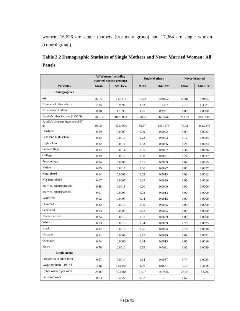
Page 41
women, 16,626 are single mothers (treatment group) and 17,364 are single women
(control group).
Table 2.2 Demographic Statistics of Single Mothers and Never Married Women: All
Panels
All Women (including
married, spouse present) Single Mothers Never Married
Variables Mean Std. Dev. Mean Std. Dev. Mean Std. Dev.
Demographics
age 37.76 11.5213 31.22 10.0462 28.84 9.9465
Number of other adults 2.15 0.9596 1.83 1.1387 2.15 1.3331
No of own children 0.90 1.1593 1.75 0.9921 0.00 0.0000
Family's other income (1997 $) 285.12 847.8093 270.52 560.5762 293.22 882.3908
Family's property income (1997
$) 98.33 425.4070 36.57 243.1879 79.31 381.3848
Disabled 0.09 0.0009 0.09 0.0022 0.09 0.0022
Less than high school 0.14 0.0010 0.23 0.0033 0.11 0.0024
High school 0.32 0.0014 0.33 0.0036 0.24 0.0033
Some college 0.32 0.0014 0.35 0.0037 0.36 0.0036
College 0.19 0.0012 0.08 0.0021 0.24 0.0032
Post-college 0.04 0.0006 0.01 0.0009 0.04 0.0015
Native 0.85 0.0011 0.86 0.0027 0.85 0.0027
Naturalized 0.04 0.0006 0.03 0.0013 0.02 0.0012
Not-naturalized 0.07 0.0007 0.07 0.0020 0.05 0.0016
Married, spouse present 0.58 0.0015 0.00 0.0000 0.00 0.0000
Married, spouse absent 0.01 0.0003 0.03 0.0013 0.00 0.0000
Widowed 0.02 0.0005 0.04 0.0015 0.00 0.0000
Divorced 0.12 0.0010 0.30 0.0036 0.00 0.0000
Separated 0.03 0.0005 0.12 0.0025 0.00 0.0000
Never married 0.24 0.0013 0.51 0.0039 1.00 0.0000
White 0.73 0.0013 0.54 0.0039 0.70 0.0035
Black 0.12 0.0010 0.26 0.0034 0.16 0.0028
Hispanic 0.11 0.0009 0.17 0.0029 0.09 0.0021
Otherace 0.04 0.0006 0.04 0.0015 0.05 0.0016
Metro 0.78 0.0012 0.79 0.0031 0.83 0.0029
Employment
Proportion in labor force 0.67 0.0014 0.64 0.0037 0.74 0.0033
Wage per hour (1997 $) 11.86 12.1056 9.56 8.9661 10.77 9.3616
Hours worked per week 24.00 19.1988 21.97 18.7666 26.43 18.5702
Full-time work 0.63 0.4827 0.57 -- 0.62 --

Page 42
Table 2.2 Demographic Statistics of Single Mothers and Never Married Women: All
Panels (Continued)
All Women (including
married, spouse present) Single Mothers Never Married
Variables Mean Std. Dev. Mean Std. Dev. Mean Std. Dev.
Child Care
Total cost per week((1997 $) 79.27 68.5918 67.20 57.2653
(Observations) 8832
Proportion paying for care 0.08 0.0008 0.12 0.0025
No. of Observations 109935
16626
17364
Values are in constant 1997 dollars.
It is seen that approximately 67% of the 109,935 women in the full sample have a job.
About 64% of the treatment group (single mothers) has a job, while 74% of the control
group (single women) are working. This is consistent with overall trends in participation
of single mothers and never married women. In general, participation rate of never
married women is found to be higher than that of single mothers. Average weekly
working hours for the full sample of women is 24 hours. However, the single mothers
work fewer hours than the single women (22 hours vs. 26 hours) and hence a smaller
proportion of the single mothers work full-time (40 or more hours per week).
Additionally, they (single mothers) earn a lower average hourly wage than the single
women ($9.56 vs. $10.77) in constant 1997 dollars.
Single mothers are 31 years of age on average, and most likely to have some college
education (35%) while a third of them are high school graduates. Single women are
younger in age (29 years) and also most like to hold some college education (36%).
However, they are approximately three times more likely than single mothers to have
completed college (24% vs 8%) and four times more likely to have post-college
education (4% vs. 1%).
A higher proportion of single women are likely to be White (70% vs. 54%). A higher
proportion of single mothers are, however, likely to be Black or of Hispanic origin.
Single mothers and single women predominantly live in a metro (79% and 83%,
respectively) and, are mostly native-born (86% and 85% respectively). A higher

Page 43
proportion of the single mothers (7% vs. 5%) are immigrants who have not become
citizens.
Both single mothers and single women have about two other adults present in their family
This may be due to the presence of other family members or sharing of a rental unit with
other adults. Single women have higher average monthly real non-labor income than
single mothers ($293.22 vs. $270.52). Additionally, they have higher stream of monthly
property income ($79.31 vs. $36.57). However, there is substantial variation in both of
these categories of income (non-labor and property income) as evidenced by the high
standard deviation. It is worth noting that SIPP divides household cash-income into four
categories: earned, property, transfers and other. Non-cash income includes food stamp,
WIC, and energy assistance.
2.2 Summary Statistics of Modes of Childcare Usage and Expenditures
Looking at the child-related variables, it is seen that single mothers have on average
about two children less than 18 years of age. Out of the single mothers, 12.14% are
making out-of-pocket payments for the usage of childcare services. This may reflect the
usage of informal and subsidized childcare services as well as assistance from other
sources.
Broadly, there are six different types of childcare arrangements that have been created by
out of the responses for the childcare questions in SIPP. These, as described in user notes
for the childcare module, are:
Family Care: This includes non-relative care outside the child’s home; for instance,
family daycare and informal care facilities in someone’s home.
Formal Day Care: This type refers to formal day care centers and is not situated in a
home. For example, it includes daycare, nursery school, and Head Start/ pre-school for
young children; for older children, it includes daycare, sports, lessons, clubs, and after-
school care.
Nanny/Sitter: This is for non-relative care inside a child’s home.

Page 44
Relative: This category refers to siblings over age 15 years, grandparents, or other
relatives taking care of a child either inside the home or outside the home.
Parent/Guardian: This is either parent/guardian respondent of a child or other
parent/guardian caring the child at home or at workplace of the parent/guardian.
Self Care: This means the child is taking care of himself/herself or is cared for by
siblings 15 years or younger.
My analysis of the SIPP data on childcare arrangement refers to only the primary mode
of arrangement (i.e. the childcare arrangement with the maximum number of hours for a
child) for the three youngest children, broken down into two age groups: children under
6 years of age and children 6 years or older. Even though recent panels (since 1996)
expand the childcare arrangement questions to more children/more types of
arrangements, I was unable to utilize this additional information due to lack of
consistency/availability in the earlier panels (1992, 1993). With respect to the payment
variables, the amounts show the total amount paid by a parent (in constant 1997 dollars),
on average, for a particular mode of child care arrangement, which is broken down along
the two age groups: all children under the age of six (for a parent), and all children six
years of age of older (for a parent).
Table 2.3 provides detail information regarding childcare usage and expenditures by
various modes for all the single mothers, further disaggregated by their employment
status. In general, it is seen that working single mothers are more likely to use child care
arrangements relative to non-working single mothers. It is observed that relative care is
the primary mode of arrangement for single mothers, both employed and unemployed
regardless of the age of children. Similar findings are reported by Connelly and Kimmel
(2002). They comment that this pattern of choice is consistent with the employment
pattern of single mothers, who typically work part-time (as seen by their average work
hours in Table 2). In addition, it provides greater flexibility to meet non-traditional work
hours. According to Washington State Department of Early Learning, family, friend and
neighbor providers – commonly known as FFN care – is the most common type of care

Page 45
around the nation for infants, toddlers and school-age children before and after school.
People choose FFN care for a variety of reasons such as existing bonds of love, shared
language, culture, religion and values, presence of a special- needs child, cost etc. Their
research also suggest that FFN providers do this work primarily because they enjoy being
with children and they like helping the parents. This explains why only 23.52% of single
mothers, who use relative care for a child under six years of age, make a payment for
such services. This proportion is slightly higher for the working single mothers (27.37%),
nevertheless still small compared to Family Care, Formal Care or Care by a Nanny/Baby
Sitter.
For children under six years of age, formal day care is the second major mode of
childcare arrangement for single mothers (whether working or not), followed by family
care. However, this is not the case for children six or older; for this group of children,
self-care is the second major mode for both working and non-working single mothers.

Page 46
Table 2.3 Childcare Arrangements of Single Mothers (All Panels)
Single Mothers (All) Single Mothers (working) Single Mothers (not working)
Child Under 6 Child 6 or older Child Under 6 Child 6 or older Child Under 6 Child 6 or older
Mean St Dev Mean St Dev Mean St Dev Mean St Dev Mean St Dev Mean St Dev
Usage of Modes (proportion):
Family Care 0.1236 0.0052 0.0684 0.0034 0.1592 0.0070 0.0828 0.0044 0.0501 0.0059 0.0279 0.0043
Formal Day Care 0.2688 0.0069 0.1394 0.0047 0.3138 0.0089 0.1560 0.0058 0.1759 0.0102 0.0930 0.0076
Nanny/Sitter 0.0319 0.0027 0.0348 0.0025 0.0370 0.0036 0.0400 0.0031 0.0213 0.0039 0.0203 0.0037
Relative care 0.3509 0.0075 0.3047 0.0063 0.3704 0.0093 0.3417 0.0076 0.3107 0.0124 0.2008 0.0105
Parent/Guardian 0.0716 0.0040 0.0762 0.0036 0.0844 0.0054 0.0947 0.0047 0.0450 0.0056 0.0243 0.0040
Self care 0.0065 0.0013 0.1694 0.0051 0.0061 0.0015 0.1885 0.0062 0.0072 0.0023 0.1160 0.0084
No of Observations 4081 5402 2698 3935 1383 1467
Pay for care of those who use (proportion):
Family Care 0.8301 0.0170 0.7321 0.0236 0.8666 0.0164 0.7600 0.0240 0.5905 0.0646 0.5000 0.0845
(No of Observations) 490 353 431 317 59 36
Formal Day Care 0.7199 0.0141 0.6626 0.0173 0.7901 0.0143 0.6902 0.0187 0.4614 0.0353 0.5328 0.0438
(No of Observations) 1016 746 815 615 201 131
Nanny/Sitter 0.5100 0.0437 0.4598 0.0378 0.5306 0.0480 0.4820 0.0404 0.4358 0.1057 0.3374 0.1057
(No of Observations) 132 175 109 154 23 21
Relative care 0.2352 0.0114 0.1325 0.0084 0.2737 0.0142 0.1449 0.0097 0.1405 0.0173 0.0732 0.0152
(No of Observations) 1395 1623 990 1330 405 293
Weekly expenditure of those who pay (1997 $)
Family Care 65.46 45.90 56.33 52.85 66.47 43.62 59.26 54.98 56.89 62.67 32.62 18.10
(No of Observations) 236 148 214 134 22 14
Formal Day Care 72.91 59.49 49.39 45.23 75.78 61.20 51.44 45.80 54.70 43.18 37.01 39.68
(No of Observations) 726 482 634 417 92 65
Nanny/Sitter 97.51 78.46 79.17 60.49 90.68 75.10 79.28 61.58 125.82 89.67 76.91 39.61
(No of Observations) 67 72 57 69 10 3
Relative care 53.39 50.38 48.30 37.74 57.20 56.69 49.40 38.14 37.22 27.26 38.41 33.08
(No of Observations) 314 201 264 181 50 20
Total Weekly Expediture (1997 $) 68.61 57.46 53.18 47.53 70.83 58.19 55.27 48.52 54.98 50.84 37.89 36.19
(No of Observations) 1333 895 1161 793 172 102
Note: all dollar figures have been adjusted for inflation and are in 1997 dollars.
Nanny/sitter care is the least used/preferred arrangement for single mothers whether
working or not. This pattern is also consistent with common findings as this mode is
relatively more expensive.

Page 47
Looking at the proportion of parents making payments (out of those who used a given
childcare mode), it is seen that working single mothers, overall, are more likely to make a
payment compared to the unemployed single mothers. As mentioned above, neither
group of mothers is very likely to pay for relative care. However, this may ignore
presence of other indirect forms of (cash or non-cash) payments for such informal care
services. For example, there might possibly be trading among parents and caregivers and
sometimes parents may pay for particular family needs of the caregivers (e.g., food or
clothing) rather than cash payments for their services. This would imply that our child
care expenditure is under-estimated and would be higher if we were able to measure and
include such indirect payments to the relative care providers.
Regarding care for a child under six, 87% of the working mothers are likely to pay for
family care, whereas only 59% of the unemployed mothers are likely to pay for family
care. Similarly, a high proportion of the working single mothers pay for formal day care
(79%) relative to unemployed single mothers (46%). As mentioned earlier, only 27% of
working single mothers pay for relative care, the mode least likely to make a payment
for. The unemployed single mothers are half as likely (14%) to pay for relative care.
We observe similar differences between the two (working vs. not-working) groups of
single mothers in terms of likelihood of paying for children six and over. 76% (out of
those who use the mode) of the working single mothers are likely to pay for family care
compared to only 50% of those single mothers who are not working. Regarding formal
care, the proportions are 69% vs. 53%, respectively. Again, we find that working single
mothers are twice as likely to pay for relative care (14.49% vs. 7.32%) then the
unemployed single mothers for children six and over.
In summary, working single mothers are more likely to pay for family care, followed by
formal care, nanny care, and finally relative care respectively for both younger and older
children. Similar pattern is observed for unemployed single mothers regarding children
less than six years of age. However, the order (in terms of likelihood of payment)
changes to formal care, family care, nanny care and lastly relative care for older children
for this group of mothers.

Page 48
When we compare the average weekly expenditures in real terms, we find that the
working single mothers’ payment is consistently higher than those who are not working,
for all modes of childcare arrangement. Nanny/sitter care is found to be the most
expensive one with average weekly expenses of $90.68 for a child under six, and $79.28
for a child six or over. It seems that single mothers without work incur higher costs on
average for nanny services for young children ($125.82 vs. $90.68).
However, we only have 10 unemployed single mothers with children under six years of
age and 3 unemployed single mothers with children six or older in this category
(nanny/sitter care), which is a sample size too small to draw any meaningful statistical
comparison. Apart from nanny/sitter care, formal day care for children under six is the
most expensive mode ($75.78) for working single mothers, while family care is the most
expensive for the older children for this group of mothers $59.26). We observe opposite
patterns for the unemployed single mothers, as they spend most for family care for the
younger children ($56.89) and formal care for the older children ($37.01). However, the
differences in the payments are small.
For a single mother, the average weekly expenditure is $68.61 for all children under six
and, $53.18 for all children six or older. The working single mothers make higher
payments on average per week than the non-working single mothers for children of both
age groups. In order to depict the relative magnitude, expenses for a child under six is
33.68% of a typical single mother’s weekly wage income (calculated based on real wage
[$9.56/hour] and hours worked per week [22 hours] from section 2.1). This is by no
means small considering that these women are likely to be the sole earners in their
family. However, the EITC expansion is likely to reduce the magnitude of this
proportion. As discussed earlier, the EITC is a supplement to wage income, especially in
the phase-in range. When we consider the after-EITC wage of the single mothers, the
relative magnitude of child care costs as a proportion of wag income is likely to go down.
This is likely to be the case as long as the cost or price of child care does not increase
faster than the increase in the phase-in credit rate of the EITC.

Page 49
2.3 Summary Statistics of EITC-related Variables
In the tax modules of the SIPP, respondents are asked questions regarding whether they
filed federal tax returns, whether they claimed EITC benefits and if so, the amount
claimed and other matters. Summaries of the tax-related variables from the sample of the
study are presented in Table 2.4.
Table 2.4 Tax Filing and EITC Claims (All Panels)
Variables All Women Single Mothers
Never Married Women
(no kids)
Mean Mean Mean
Tax filed (%) 48.16 53.28 58.96
(Observations) 109935 16626 17364
Of those who filed:
Has tax copy (%) 25.49 21.31 24.07
Filed as Single (%) 35.42 34.85 93.22
Filed as Married (joint) (%) 45.89 04.15 00.72
Filed as Married (Sep) (%) 03.41 02.73 00.04
Filed as Unmarried Head (%) 12.83 55.09 04.06
Filed for EITC (%) 12.16 36.18 04.24
(Observations) 53550 8945 10067
EITC amount claimed (1997 $) 1534.94 1613.56 1060.14
(standard deviation) 1084.99 1099.19 1084.15
Observations for EITC claim 3502 1721 224
It is observed that 48.16% of the full sample (consisting of married and single women),
53.28% of the single mothers and 58.96% of never-married no-children women said that
they filed the federal tax return. However, less than one-quarter of these women have tax
copies. The majority of the single mothers file taxes as unmarried head of household
followed by single filing status. 93.22% of the never-married women file taxes as single.
Out of those who filed a federal tax return, 36.18% of the single mothers claimed EITC
and the average claimed amount is $1,613.56 (in constant 1997 dollars). About 4.24% of
the never-married women claimed EITC when they filed federal tax returns, with an
average amount of $1,060.14 (in constant 1997 dollars).

Page 50
Often times these variables are considered of limited value because a large proportion of
the households tend not to respond these questions. Non-response is a major issue for
these questions (Karl Scholz, 1993). Sometimes many households are not even asked
these questions if the interviews take too long or if there is a danger of non-cooperation
on the part of the respondents. Scholz also points out that households relying on paid tax
preparers (a significant proportion of the EITC claimants) might not be aware of or
remember whether they received the EITC. As a result, he argues that the population of
households, who reported to have referred to the tax copy while answering the tax
module questions, would be a more reliable sample to estimate participation and amount
of EITC claimed.
2.4 Summary Statistics across the Panels
In order to capture snapshots of the key variables over time, I summarized some of the
variables across the four panels. The summary statistics are presented in Table 2.5.
It is evident that both of these groups of women experienced substantial fluctuations in
their ‘other’ income over the duration of the sample. Single mothers experiences
decreases in their property income during fall of 1993 and 1994. After remaining stable
during the summer 1997-summer 1999 periods, it rose slightly in 2001. The proportion of
single mothers with a job has been gradually on the rise over the sample period (except
for Panel 1993, wave 3). However, their hourly wage (in constant 1997 dollars) has
remained remarkably stagnant with very small increments, especially during fall 1993-
summer 1999. Their hours worked increased during fall 1993-1994, but continued to fall
since then. Though there is also fluctuations in childcare expenses (in constant 1997
dollars), it seems single mothers incurred lower amounts of these expenses in 2001 than
they did in fall of 1993. This may reflect lower demand for childcare as they work fewer
hours. These are expenses incurred by single mothers and do not reflect the market price
of providing for childcare services. The proportion of single mothers paying for care
dipped in the fall-1994, but has been hovering around 14% since then. It seems that the

Page 51
proportion of single mothers who filed federal tax return hovers around 54-57%, except
for the year 2001, when it is 46%.
Table 2.5 Panel-wise Summary Statistics of Single Mothers and Single Women
without children
Single Mothers
Variables 1992 1993 1993 1996 1996 2001
(wave 6 &
tm 8)
(wave 3 &
tm 5)
(wave 6 &
tm 8) (wave 4) (wave 10)
(wave
4)
Monthly non-labor income
(1997 $) 265.21 283.38 269.35 244.88 283.97 276.31
(standard deviation) 577.35 603.18 587.56 491.11 574.00 530.74
Monthly property income
(1997 $) 41.63 33.31 28.65 37.93 40.01 37.57
(standard deviation) 223.71 173.17 153.76 210.29 220.70 386.03
Proportion working (%) 59.36 57.17 58.45 67.56 70.82 67.96
Hourly wage (1997 $) 9.20 9.24 9.31 9.31 10.13 9.94
(standard deviation) 5.87 5.36 6.23 7.57 14.83 8.07
Weekly work hours 20.53 19.62 20.22 23.14 24.42 23.31
(standard deviation) 18.92 18.85 19.03 18.64 18.19 18.53
Proportion paying for
childcare (%) 10.62 10.44 09.92 14.06 13.56 13.68
Weekly expenditure on
childcare (1997 $) 71.37 69.48 71.18 63.25 64.68 66.70
(standard deviation) 50.16 46.89 68.19 50.67 59.67 63.67
Observations (Chilcare) 203 213 192 575 435 451
Proportion filed for tax (%) 55.05 52.27 53.56 56.27 57.00 45.88
Proportion claimed EITC
(%) 18.00 17.66 19.65 17.52 21.98 20.91
EITC amount claimed
(1997 $) 1094.24 1021.20 1834.70 1737.54 1761.99
2094.2
8
(standard deviation) 594.64 577.42 1066.14 1035.67 1025.15
1489.6
4
Observations (EITC) 202 212 231 323 400 353
Reference time period:
Childcare
Fall of
1993
Fall of
1993
Fall of
1994
Summer
of 1997
Summer
of 1999
Spring
2002
Tax year 1993 1993 1994 1996 1998 2001
No. of Observations 1942 2052 1941 4070 3315 3306

Page 52
Table 2.5 Panel-wise Summary Statistics of Single Mothers and Single Women
without children (Continued)
Never married women (without children)
Variables 1992 1993 1993 1996 1996 2001
(wave 6 &
tm 8)
(wave 3 &
tm 5)
(wave 6 &
tm 8)
(wave
4)
(wave
10)
(wave
4)
Monthly nonlabor income
(1997 $) 309.08 323.89 333.81 276.72 276.66 252.98
(standard deviation) 845.67 1058.83 1035.13 885.01 720.87 745.15
Monthly proporty income
(1997 $) 95.10 103.93 92.08 68.15 76.98 48.61
(standard deviation) 505.42 469.47 393.81 261.10 321.75 301.57
Proportion working (%) 72.45 74.25 74.16 75.67 74.23 73.48
Hourly wage (1997 $) 10.24 10.55 10.33 10.39 11.00 11.85
(standard deviation) 7.35 7.36 6.59 11.94 9.65 11.05
Weekly work hours 25.76 27.17 26.92 26.77 26.12 25.97
(standard deviation) 18.56 18.60 18.64 18.32 18.58 18.69
Proportion filed for tax (%) 62.48 66.55 63.70 63.03 58.56 43.15
Proportion claimed EITC
(%) 02.59 01.72 01.94 02.92 02.55 03.09
EITC amount claimed
(1997 $) 826.71 1030.10 793.17 758.26 1229.57
1518.4
5
(standard deviation) 553.32 651.93 936.35 738.00 1070.69
1613.3
0
Observations (EITC) 32 17 22 51 48 54
Tax year 1993 1993 1994 1996 1998 2001
No. of Observations 2209 2073 2029 4074 3434 3545
One possible reason for the lower percentage in 2001 may be due to the timing of the
survey. This wave was conducted in spring 2001 and hence may have been too early for a
lot of the respondents to file tax returns. The proportion of EITC claims have been
gradually on the rise, so has been the claimed amount which increased from $1094 in
fall-1993 to $2094 (1997 dollars). This is consistent with the expansions of the EITC
benefits since mid-1990s.
Never-married women with no children also experienced substantial drops in their ‘other’
income and property income during the sample period. Their wage rate remained

Page 53
stagnant during most part of the sample period, but it increased in 1999 and 2001. They
seem to working similar hours in 2001 as in 1993, though there were periodic rises in
hours worked between these years. Proportion of these women who are working is
slightly higher in 2001 than their 1993 shares.
Increasing proportion of these women are filing tax returns, though it dropped a little in
1999. As stated above, the figures for 2001 may have been affected by premature timing
of the survey for tax returns. Though the proportion of EITC claims shows a rising trend
over the panels, only a small proportion of these women claim EITC. There is significant
increases in the amount of EITC claimed, especially during 1999 and 2001. One might
argue that the control group of women is ‘contaminated’ in the sense that they are also
eligible for the EITC benefits since 1994. However, as seen from Table 2.5, the
proportion of never married women (with no children) claiming EITC is very small.
Furthermore, these are ‘claimed’, not ‘actual’ statistics and recall that there are serious
concerns regarding the credibility of these ‘claimed’ amounts (Karl Scholz, 1993).

Page 54
3 SELECTION-CORRECTED WAGE AND CHILDCARE
EXPENDITURE
I approached the empirical estimation process in several steps, as discussed in detail in
Section 1.3. The first step of the process is to estimate a bivariate model of probability of
participation and probability of using paid care. The inverse-mills-ratio constructed from
this first-stage model is then used to estimate selection-corrected wage and costs of care.
The need for estimating a joint reduced form participation and usage of paid care arises
because of the presence of endogeneity, simultaneity, and potential selection issues in
directly estimating wages and costs of care. The predicted wage and cost of care enter the
final-stage model of participation as regressors. Estimates of the first-stage bivariate
model and second-stage selection-corrected wage and costs of care and presented and
discussed below.
3.1 Results from Reduced-form Models of Labor- force Participation and Use of
Paid Childcare
I estimate the following reduced-form bivariate probit equation using the full sample of
married women (with spouses present) as well as all single women (with or without
children). The results are produced in Table 3.1. The dependent variables are probability
of employment and probability of using paid care services. The regressors include a set
of demographic characteristics of the women, a set of household composition variables,
and a set of structural variables. The demographic variables are age, non-labor income,
and a set of dichotomous variables for education levels, race, citizenship status and
disability. The household composition variables include presence of other adults, number
of own children, number of infants, number if children under 5, number of children
between 6-12, number of children between 13-17, marital status etc. Variables such as
state EITC (a dichotomous variable), state’s AFDC/TANF benefit levels for 2 and 3
persons’ family, the estimated employer costs of workers compensation insurance
payments by the state, state’s unemployment rate, etc. are the structural variables.

Page 55
Table 3.1 Bi-variate Probit Estimation of Probability of Participation and
Probability of Using Paid Child care
Employment Pay for Care
Coef. Robust Std. Error z Coef. Robust Std. Error z
Age 0.0803 0.0028 28.17 0.1322 0.0064 20.73
Age squared -0.0011 0.0000 -31.09 -0.0021 0.0001 -23.88
Disabled -1.0080 0.0146 -69.13 - - -
High School 0.3972 0.0134 29.63 0.2826 0.0267 10.59
Some college 0.5052 0.0137 36.88 0.4372 0.0265 16.48
College 0.6560 0.0159 41.37 0.5555 0.0281 19.77
Post college 0.7538 0.0255 29.57 0.7684 0.0367 20.92
Naturalized -0.0497 0.0235 -2.12 0.0437 0.0369 1.19
Not naturalized -0.3068 0.0191 -16.08 -0.0824 0.0308 -2.68
Married (sp ab.) 0.0131 0.0398 0.33 -0.2518 0.0648 -3.88
Widowed 0.0865 0.0267 3.24 -0.2152 0.0670 -3.21
Divorced 0.2891 0.0145 19.95 -0.0985 0.0230 -4.29
Separated 0.1820 0.0236 7.70 -0.1093 0.0356 -3.07
Never married 0.0818 0.0133 6.16 -0.5121 0.0222 -23.08
Black -0.0005 0.0134 -0.03 0.1122 0.0211 5.31
Hispanic -0.0021 0.0156 -0.13 0.1125 0.0241 4.66
Other race -0.1131 0.0220 -5.15 -0.0381 0.0357 -1.07
Other adults -0.0346 0.0048 -7.28 -0.1670 0.0113 -14.72
No. of own kids -0.1095 0.0045 -24.09 0.0419 0.0210 1.99
No. of infants -0.1103 0.0229 -4.83 -0.2807 0.0284 -9.89
No of kids below 5 -0.2520 0.0089 -28.39 0.5510 0.0216 25.48
No. of kids 6-12 - - - 0.1756 0.0220 8.00
No. of kids 13-17 - - - -0.1025 0.0244 -4.19
No-labor income -0.0002 0.0000 -11.81 0.0001 0.00001 -0.97
Property income -0.0002 0.0000 -13.30 0.00002 0.00003 0.96
Workers compensation 0.0000 0.0000 -7.57 0.00001 0.0000 -0.16
State unemploy. rate -0.0472 0.0032 -14.84 -0.0603 0.0046 -13.01
AFDC (2person) 0.0012 0.0003 4.06 -0.0006 0.0004 -1.45
AFDC (3person) -0.0006 0.0002 -2.53 0.0005 0.0004 1.55
State EITC -0.0085 0.0162 -0.52 - - -
Constant -0.7074 0.0598 -11.83 -3.2931 0.1220 -26.9900
Observations 109190
Rho 0.3828 0.0083
Wald test of rho=0: chi2(1) =1713.91 Prob > chi2 = 0.0000

Page 56
Results from the employment equation are consistent with prior expectations. First, we
find that age is positively related with labor force participation, but the relationship
becomes negative at some point indicating older people (beyond 36.5 years) are less
likely to be employed as they approach the retirement age. Disability also negatively
affects employment as expected. The effect of education on employment is positive.
Education signals ability of the individual and also increases the stock of human
resources of the individual, thus enhancing chances of employment. The findings suggest
that native citizens are more likely to be employed. This might be due to strict
immigration regulations, which is part of the reason why whites are more likely to be
employed. Single women (with or without children) are more likely to be working
relative to married women (with spouses present) as these women are most often the sole
earners in their families. Presence of other adults in the house might imply alternative
sources of income and hence negatively affects employment. Presence of children
(especially young children) also negatively affects labor force participation as they need
to be cared for. Due to negative income effect, non-labor income is inversely related with
participation, an expected prediction from the labor supply model. State policies relating
to workers’ compensation and AFDC benefit level for 3-person family also reduce
participation likelihood.
Findings from the use of non-parental childcare equation show that though age is
positively related with use of non-parental childcare, it becomes negative beyond 31.5
years of age. This is expected because as children get older, the need for child care
obviously falls. Higher educated women are more likely to demand child care services.
Native citizens are also more likely than non-naturalized citizens to seek paid non-
parental child care services. While married women (with spouses present) are more likely
to use paid non-parental child care services, white women are less likely to use do so.
Presence of other adult family members reduces the probability of using paid care.
Presence of young children increases the likelihood of using paid care. However,
presence of teenage children reduces the likelihood of using paid care. Non-labor and
property income do not affect likelihood of using paid care. Lastly, higher state

Page 57
unemployment rate and AFDC/TANF benefit reduce the likelihood of using paid
childcare.
The jointly estimated bivariate probit model accounts for the correlation between
employment participation and usage of paid childcare services. The justification for using
a bivariate model is that the two decisions of employment and usage of paid care are
interrelated. A standard bivariate model is where:
(16)
( )
The error terms consist of a common term and a second term that is unique to each model
and hence the two equations are related through correlated error terms. As expected, the
estimated correlation coefficient is positive and significant (rho=0.3828). This means that
unobserved factors that increase the probability of employment also increase the
probability of using paid non-parental care. We can test the hypothesis that the bivariate
probit model fits the data better than separate models, using a simple Wald test. The Wald
test statistic for the hypothesis that the two decisions are independent (i.e. uncorrelated
error terms or rho=0) is 1713.91 and is significant. This means that the probability of
employment will be dependent on the value/probability of using paid care.

Page 58
3.2 Selection-corrected Wage and Childcare Expenditure
Estimation of reduced form bivariate model was the first-stage of the three-step
estimation process. Presence of potential selection issues require us to estimate selection
–corrected wage and costs of paid care so that these could be used as regressors in the
final-stage estimation of participation. Therefore, inverse mills’ ratio was constructed
from the first-stage estimates to estimate selection-corrected equations of wage and cost
of child care. The resulting coefficients from these two estimated equations were used to
construct predicted unconditional hourly wage and predicted unconditional weekly price
or cost of childcare. Again, these results were generated utilizing the full sample of
married women (with spouses) as well as single women (with or without children) to
obtain robust estimates.
I omitted the following variables in the wage equation: non-labor income, number of
children, young children of various age groups, presence of other adults in the house and,
state variables regarding AFDC benefits, workers’ compensation, unemployment rate and
presence of state EITC. The variables that are included in the first-stage bivariate probit
model, but do not appear in the second-stage model of cost of childcare equation are: age
squared, number of own children, other adults in the family, presence of teenage children,
non-labor income, state variables regarding AFDC benefits, workers’ compensation and,
unemployment rate.
The results are produced in Table 3.2 and 3.3. The coefficients of the wage equation have
expected signs. It is found that age positively affects wage; however beyond a certain
level, wage falls with age. Higher educated women have higher wages. Additionally,
married women (with spouse present) have higher wage than single women (with or
without children). It might reflect the phenomenon that married women require a higher
wage than single women due to the presence of another earning member in the family.
Women living in the metro areas also have higher wage, which to a large extent is
reflecting the higher cost of living in the metro areas. The results also show that non-
white as well as disabled women have lower wage. Other studies (e.g. Connelly and
Kimmel, 2003) report similar findings.

Page 59
Table 3.2 Selection-corrected Wage Equation
Wage Coef. Std. Err. t P>t
Age 0.4113 0.0211 19.49 0.0000
Age-squared -0.0043 0.0003 -16.00 0.0000
High school 1.1302 0.1218 9.28 0.0000
Some college 2.3072 0.1279 18.04 0.0000
College 5.2430 0.1425 36.79 0.0000
Post-college 8.0119 0.1854 43.22 0.0000
Naturalized 0.7147 0.1635 4.37 0.0000
Not naturalized -1.1620 0.1536 -7.57 0.0000
Married (spouse absent) -0.5940 0.2909 -2.04 0.0410
Widowed -0.6514 0.1989 -3.27 0.0010
Divorced 0.0344 0.0945 0.36 0.7160
Separated -0.5324 0.1616 -3.29 0.0010
Never married -0.1471 0.0878 -1.67 0.0940
Black -0.3478 0.0906 -3.84 0.0000
Hispanic -0.6351 0.1118 -5.68 0.0000
Other race -0.0080 0.1565 -0.05 0.9590
Metro 1.2879 0.0702 18.34 0.0000
Disabled -1.8812 0.1926 -9.77 0.0000
Inverse Mills Ratio 1.3770 0.2243 6.14 0.0000
Constant -5.4981 0.4957 -11.09 0.0000
Adjusted R-Squared 0.1002
Observations 71524
Regarding weekly cost of childcare (shown in Table 3.3), I find that age has positive
impact on cost of childcare. Higher educated women pay a higher price for childcare.
Non-naturalized citizens pay a lower price than natives while naturalized citizens incur
higher costs. Married women pay a higher price than single women. White women tend
to pay more than others. Presence of young children raises the cost of childcare, while
presence of teenage children lowers the cost. Finally, women living in the metro areas
experience higher costs for childcare. It is important to note that I haven’t controlled for
quality of child care or income and hence some of these estimates may be affected by
these omissions.

Page 60
Table 3.3 Selection-corrected Weekly Price of Childcare (constant 1982-84 dollars)
Weekly Cost of Childcare Coef. Std. Err. t P>t
Age -0.0226 0.0166 -1.3600 0.1730
High school 1.5075 0.3477 4.3400 0.0000
Some college 3.2938 0.3645 9.0400 0.0000
College 8.0453 0.4297 18.7200 0.0000
Post-college 12.8104 0.6601 19.4100 0.0000
Naturalized 0.5708 0.5612 1.0200 0.3090
Not naturalized -1.6628 0.4326 -3.8400 0.0000
Married (spouse absent) -1.5875 1.0144 -1.5600 0.1180
Widowed 0.5196 0.9175 0.5700 0.5710
Divorced 0.2429 0.3501 0.6900 0.4880
Separated -0.3870 0.5411 -0.7200 0.4740
Never married -0.5016 0.4308 -1.1600 0.2440
Black -0.7267 0.3408 -2.1300 0.0330
Hispanic -0.1796 0.3618 -0.5000 0.6200
Other race -0.2962 0.5273 -0.5600 0.5740
Number of infants -5.1825 0.4188 -12.3700 0.0000
Number of kids below 5 6.3820 0.2246 28.4200 0.0000
No. of kids between 13-17 -2.0187 0.1667 -12.1100 0.0000
Metro 1.7540 0.2505 7.0000 0.0000
Inverse Mills Ratio -2.9218 0.3451 -8.4700 0.0000
Constant 7.3850 0.8927 8.2700 0.0000
Adjusted R-Squared 0.1011
Observations 52,308
The estimates of the standard errors from the bivariate model are incorrect. As a result, I
estimated Heckman selection-corrected equations for wage and costs of paid care, which
was utilized to predict wages and costs of care to be included in the final-stage model of
participation.
3.3 Results from Multinomial Logit Model of Modes of Childcare
The main focus of my study is to estimate effects of EITC expansions and child care
costs on participation. However, access to child care services is also key aspect in

Page 61
decision to work. As a result, I investigate the demand for child care services for working
mothers by applying a multinomial logit model and a sample selection model to augment
and enrich my analysis. My interest is in the analysis of factors, including the role of
child care expenditure, that influence the choice of child care services.
I consider five categories of choice for child care – family care, formal day care, nanny
care, relative care (including self-care), and parental care. The relative care has been
designated as the reference category since it is the most frequently used mode. This
requires estimating 4 (5-1) equations, one for each category relative to the reference
category to predict the probabilities of choosing the various modes of child care given the
independent variables.
Based on utility theory, we can argue that parents evaluate the different types of child
care services to choose the one that maximizes their utility, given the constraints of prices
and income. Suppose, a parent makes decision on which one of the modes of child care to
use from a set of M={0,1,….m}. Let denote the vector of prices for each of the
alternatives, to represent individual parental income, and to be a vector of socio-
economic characteristics that affect choice of modes of child care. Given this set up, each
individual parent i chooses child care service that maximizes the conditional indirect
utility function:
( ) ( )
where V(.) is the deterministic part of the utility function and is an independently and
identically distributed error term representing unobserved heterogeneity among
individuals and various modes of care. The probability that a parent i chooses out of
the set of alternatives can be written as:
( ) ( ) ( )
∑ ( )

Page 62
Substituting the expression for the indirect utility function into the above equation and by
normalization, we get:
( ) ( )
∑ ( )
where m=0 is the base/reference category.
The coefficients of a multinomial logit model are of limited value for analysis. As a
result, marginal effects need to be computed from the estimated coefficients. These
effects measure the impact of a unit change in the continuous explanatory variable (or
from 0 to 1 for dichotomous variables) on the probability of observing a specific mode of
care, evaluated at the mean of the explanatory variable.
I estimate separate multinomial logit models for modes of choice for young children
(below six) and older children (six and above) utilizing the sample of working mothers
(married or otherwise). The estimation process involves a number of steps. First, I use the
first-stage bivariate model (presented earlier) to construct inverse-mills-ratio, which is
later used in the second-stage to estimate selection-corrected price equations. Next, I
predict prices for each individual mode of care for those women who have children.
These predicted prices, together with socio-economic characteristics, are used in the
final-stage multinomial logit model. As stated, these steps have been applied first to
estimate choice of mode for young children, and later for older children. The marginal
effects from the multinomial logit model are presented in Table 3.4 for the formal day
care services.

Page 63
Table 3.4 Marginal Effects from Multinomal Logit Model for Formal Day Care
Children Under 6 Children 6 and over
Pr(formal care)= 0.3027 Pr(formal care)= 0.1740
variable dy/dx Std. Err. P>z dy/dx Std. Err. P>z
Age 0.0013 0.0036 0.7080 0.0046 0.0063 0.4590
High school 0.0190 0.0298 0.5240 -0.0076 0.1274 0.9520
Some college 0.0633 0.0300 0.0350 0.0148 0.1378 0.9140
College 0.0963 0.0423 0.0230 -0.0358 0.1799 0.8420
Post-college -0.0925 0.0781 0.2360 -0.0710 0.1011 0.4820
Naturalized -0.1574 0.0285 0.0000 -0.0349 0.0689 0.6120
Not naturalized -0.1585 0.0214 0.0000 -0.1274 0.0572 0.0260
Married (sps ab.) -0.0228 0.0555 0.6810 -0.0244 0.0554 0.6600
Widowed -0.1687 0.1355 0.2130 -0.0834 0.0654 0.2030
Divorced 0.0028 0.0440 0.9480 -0.0810 0.0719 0.2600
Separated 0.0022 0.0748 0.9770 -0.0518 0.0173 0.0030
Never married 0.0649 0.0415 0.1180 0.0165 0.0589 0.7790
Black 0.0583 0.0667 0.3830 -0.0295 0.0141 0.0370
Hispanic -0.1001 0.0280 0.0000 -0.0156 0.0809 0.8470
Other race 0.0073 0.0503 0.8840 -0.0598 0.0332 0.0720
fam_ads -0.0234 0.0214 0.2750 -0.0213 0.0079 0.0070
No. of infants -0.1169 0.0205 0.0000 -0.0073 0.0164 0.6560
No. of kids 0-5 0.0261 0.0183 0.1530 -0.0270 0.1345 0.8410
No. of kids 6-12 -0.0387 0.0069 0.0000 -0.0235 0.0056 0.0000
No. of kids 13-17 0.0522 0.0266 0.0500 -0.0557 0.0867 0.5200
Real other income 0.0001 0.0000 0.0030 0.0000 0.0000 0.0950
Real property income 0.0001 0.0000 0.1280 0.0000 0.0000 0.4820
Predicted price of family care -0.0266 0.0045 0.0000 -0.0005 0.0030 0.8620
Predicted price of formal care 0.0126 0.0058 0.0310 0.0044 0.0096 0.6500
Predicted price of nanny care -0.0005 0.0011 0.6400 0.0018 0.0040 0.6610
Predicted price of relative care 0.0164 0.0127 0.1960 -0.0033 0.0062 0.5960
Poverty rate 0.0055 0.0017 0.0010 -0.0007 0.0011 0.5530
These marginal effects presented in Table 12 measure the impact of a unit change in the
continuous explanatory variables (from 0 to 1 for dichotomous variables) on the
probability of choosing formal day care compared to relative care, evaluated at the mean
of the explanatory variables. We find that only a handful of the variables are statistically
significant. Regarding modes of choice for young children, women with some college or

Page 64
college degree are more likely to use formal care compared with relative care. Both
naturalized and non-naturalized mothers are less likely to rely on formal day care than
native citizens. Similarly, being of Hispanic race as well as having young children
reduces the likelihood of using formal care. Higher non-labor income increases the
chances of relying more on formal day care. However, the estimated effects of the
(predicted) price variables for the various modes of choice are problematic. Though some
of these are significant, but many of them have incorrect signs. I tried several alternative
methods to obtain better estimates. Unfortunately, those results were also similar. While
these results are problematic, nevertheless such findings are not uncommon in the
literature. Connelly and Kimmel (2003) report similar findings using SIPP 1992 and 1993
panels. One probable reason for such inaccurate estimates might be due to poor
price/costs of care information. A large number of mothers in the sample rely on relative
care, for which they seldom make payments. This leads to limited information as well as
variation in the price data. The problem of data quality is accentuated by lack of
information on non-cash forms of payment. Furthermore, there are important differences
in choice sets regarding availability of various modes of child care services. For example,
child care options are different in metro areas compared to non-metro areas (Walker et al.
2011). In the absence of information regarding what choices people face, estimates are
likely to be poor.

Page 65
4 FINAL-STAGE ESTIMATION OF LABOR-FORCE
PARTICIPATION
The primary objective of my dissertation is to estimate probability of labor force
participation as a function of EITC expansions, wages, child care costs and demographic
variables. As discussed earlier in detail, multiple equations are needed in several steps to
estimate this ultimate model. As part of the three-step approach, I estimated a bivariate
model of participation and usage of paid care services in the first stage. The second stage
involved estimating selection-corrected wage and costs of care equations based on the
inverse-mills-ratios from the first-stage bivariate model. Having corrected for the
endogeneity and selection issues, the final stage strategy is to estimate a probit model of
participation using the selection-corrected wage and costs of care as regressors together
with a set of socio-economic characteristics of the single mothers and single women (no
children).
4.1 Results from the Final-stage Probit Model of Labor-force Participation
The dependent variable in the final stage probit equation is labor force participation. The
treatment group of women is single mothers who were the primary target group of the
EITC expansions of the 1990s. The control group is the never married women with no
children. The before/after period of the EITC expansions is captured by a dummy
variable ‘post96’.
The following Table (Table 4.1) provides marginal effects from the final-stage probit
regression. Though my primary interest are the difference-in-difference estimators
‘treat*post96’ and ‘treat*cost*post96’, the presence of several interaction terms require
us to consider the partial derivative of the dependent variable (labor force participation)
with respect to the treatment group, evaluated at the average predicted childcare
expenses, to find out how single mothers change their labor force participation relative to
never married women (without children) after the EITC expansions of the 1990s that

Page 66
were implemented till 1996. The results show that labor force participation of the
treatment group was higher in post 1996 (coefficient on ‘treat*post96’ is positive), but it
is not statistically significant. This outcome is not surprising since there was a trend of
overall decline in women’s labor force participation since 2000 (Monthly Labor Review,
October 2006).
Table 4.1 Final Estimates of Participation
Probit regression, reporting marginal effects
Number of obs 33997
LR chi2(28) 5862.00
Prob > chi2 0.00
Pseudo R2 0.1403
Log likelihood -17953.723
hasjob1 dF/dx Std. Err. z P>z
disabled* -0.33294 0.0118 -28.6400 0.0000
naturalized -0.02484 0.0178 -1.4200 0.1560
not-naturalized* -0.02708 0.0121 -2.2900 0.0220
married/spouse absent -0.03272 0.0213 -1.5700 0.1160
widowed* -0.07067 0.0228 -3.2400 0.0010
divorced* 0.04218 0.0092 4.4400 0.0000
separated* 0.04373 0.0114 3.6900 0.0000
black* -0.08538 0.0091 -9.7200 0.0000
hispanic * -0.04055 0.0092 -4.5000 0.0000
otherace* -0.10828 0.0148 -7.7200 0.0000
metro -0.01729 0.0094 -1.8300 0.0670
rfoklt18 * -0.02546 0.0041 -6.2000 0.0000
No of Infants* -0.08935 0.0153 -5.8300 0.0000
No if kids (0-5) -0.02843 0.0225 -1.2600 0.2070
real other income* -0.00005 0.0000 -9.1100 0.0000
real property income* -0.00009 0.0000 -6.8000 0.0000
unemployment rate * -0.02025 0.0025 -8.2300 0.0000
AFDC benefit (2 person family) * 0.00048 0.0002 2.8000 0.0050
AFDC benefit (3 person family)* -0.00038 0.0001 -2.6500 0.0080
State EITC * -0.09197 0.0318 -2.8900 0.0040

Page 67
Table 4.1 Final Estimates of Participation (Continued)
hasjob1 dF/dx Std. Err. z P>z
realwage * 0.04813 0.0031 15.7300 0.0000
real total cost (wk)* -0.00260 0.0013 -2.0400 0.0410
treatment* -0.05170 0.0244 -2.1200 0.0340
post96 -0.03298 0.0236 -1.3900 0.1650
treat*post96 0.01366 0.0281 0.4800 0.6290
treat*cost 0.00001 0.0008 0.0100 0.9900
cost*post96 -0.00009 0.0008 -0.1100 0.9140
treat*cost*post96* 0.00236 0.0010 2.4700 0.0130
* statistically significant at 5% or less.
Higher cost for childcare reduces labor force participation on average since the
coefficient on ‘real total cost (wk)’ is negative and significant. In contrast, higher wage
increases participation on average (the coefficient on ‘real wage’ is both positive and
significant.
I evaluated the derivative of the dependent variable (labor force participation) with
respect to the ‘treatment’ variable at the mean of the predicted expenditure for child care.
This exercise indicates a 3.32% increase in the participation of single mothers in the post-
1996 era relative to never-married women without any children. This estimate is similar
to the roughly 3% participation increase estimated by Meyer and Rosenbaum (2001), or
4.7% increase found by Fitzpatrick and Thompson (2010) for the 1993 expansion. There
are a number of differences with respect to these studies. First, both of these studies used
CPS data to estimate the impact whereas I’ve used SIPP. Secondly, none of these studies
explicitly controlled for child care expenses. Moreover, their sample selection criterion,
the definition of treatment and control groups are different from this study. However, I
re-estimated the model using their definition of a control group
(widowed/separated/divorced/never married women without children) and found that
participation of single mothers increased by an estimated amount of 4.46% in the post-
1996 era relative to single women without any children. The size of the estimated effect
is larger when estimated using the ‘usual’ control group, but still within the range
commonly found in the literature.

Page 68
Taking derivative of the dependent variable (labor force participation) with respect to the
‘cost’ of child care variable yields a negative impact on participation for single mothers
in both pre and post 1996 period. This exercise reveals an estimated reduction in labor
force participation of single mothers by 0.259% in the pre-1996 period and 0.028% in the
post-1996 period relative to single women due to increase in the weekly cost of care. This
result implies that the cost of child care had smaller impact on participation in post-1996
than before 1996. Controls for immigration status, marital status, race and other
coefficients have the expected signs.
I evaluate the derivative of the dependent variable (labor force participation) with respect
to the ‘treatment’ variable at the respective quartiles of the predicted child care cost for
two alternative specifications. The first specification uses a reduced form bivariate probit
model in the first stage of estimation to create selection terms to be utilized for second
stage wage and cost of care equations. The predicted wage and cost of care from the
second stage is then used to estimate the final probit model of participation. The
alternative specification relies on Heckman selection corrected wage and cost of care
equations to estimate the final participation model.
The results of the derivative are presented below in Figure 4.1. As expected, it is seen
that the two methods of estimated results yield similar estimates for the effectiveness of
the EITC expansions of the 1990s.
Figure 4.1 Heckman and Bivariate Estimates of Labor Force Participation
1.24
2.78
5.02
1.28
2.77
5.48
0.00
1.00
2.00
3.00
4.00
5.00
6.00
7.00
8.00
9.00
q1 q2 q3
d LFP/d Treat
Quartiles of Predicted Child Care Costs
Heckman
Bivariate

Page 69
I predict participation from the final probit estimates and compared before and after
policy changes for high school educated women. The findings are summarized in the
following table (Table 4.2). It shows that though there were across the board increases in
labor force participation for single mothers of this educational group, it was those women
facing the highest childcare costs (fifth quintile) had the largest and the most dramatic
increase in labor market participation. Also, the increase in participation increases as we
gradually move to higher quintiles. This indicates higher responsiveness of women facing
high child care costs in the post-EITC expansion period.
Table 4.2 Predicted Labor Force Participation of High School Grad Single Mothers
Distribution of Predicted Cost of Care
Predicted Participation
Pre 1996 Post 1996 Change (Post-Pre)
Quintile 1 0.6124 0.6440 0.0316
Quintile 2 0.6398 0.7026 0.0628
Quintile 3 0.6611 0.7354 0.0743
Quintile 4 0.5709 0.6607 0.0898
Quintile 5 0.4704 0.6209 0.1505
4.2 Demand for Child care Post-Increase in Labor Force Participation
One can argue that there would be a feedback effect from the labor market to the cost of
child care. With limited expansions of supply of child care, the increase in labor force
participation is likely to increase the cost of child care. In order to capture the distribution
of cost at the MSA levels, I run a simple probit model of participation and predict
probability of working which is collapsed at the MSA level. Later, I regress the cost of
care on a set of demographic variables and the MSA-level predicted participation as
control variables. The estimates from this model are produced below in Table 4.3.

Page 70
Table 4.3 Cost of care and Predicted Participation
Real total weekly Cost Coeffcient Std. Err. T-stat
Age -0.0683 0.0157 -4.34
High school 2.2962 0.3348 6.86
Some college 4.4461 0.3380 13.15
College 9.5109 0.3926 24.23
Post-college 14.7509 0.6181 23.86
Naturalized 0.6586 0.5623 1.17
Not naturalized -1.8607 0.4333 -4.29
Married (sps ab.) -2.1167 1.0131 -2.09
Widowed -0.2857 0.9131 -0.31
Divorced 0.2986 0.3502 0.85
Separated -0.3744 0.5415 -0.69
Never married -2.5572 0.3562 -7.18
Black -0.1986 0.3354 -0.59
Hispanic 0.1976 0.3685 0.54
Other race -0.5240 0.5271 -0.99
No. of infants -6.0432 0.4066 -14.86
No. of kids 0-5 7.6653 0.1657 46.26
No. of kids 13-17 -2.4459 0.1590 -15.39
Metro 1.7185 0.2506 6.86
Predicted participation 6.0655 3.4404 1.76
Constant -1.5470 2.4212 -0.64
R-squared 0.1002
Number of observations 52,308
As expected, the estimated coefficient on predicted participation is positive. This means
that as employment increases, demand for child care increases and as a result, the cost of
care also increases. The estimated coefficient is weakly significant.
4.3 Hours Worked and EITC Expansions
I estimated a simple regression model of hours worked using the full sample conditional
on working. It is observed from Table 4.4 that married women with spouse absent,
widowed, divorced and separated women work longer hours than married women with

Page 71
spouse present. Only never married women tend to work fewer hours than married
women (spouse present). I also find Black, Hispanic and women from other race work
longer than White women. Number of children, presence of young children, non-labor
income, and availability of state EITC make women work fewer hours. It is also seen that
predicted child care costs has negative impact on hours worked and is significant.
Table 4.4 Effect of EITC Expansions on Hours Worked
Hours worked Coef. Std. Err. t P>t
disabled* -1.4724 0.2081 -7.0800 0.0000
naturalized -0.0104 0.2318 -0.0400 0.9640
not naturalized* 1.5808 0.2082 7.5900 0.0000
married, spouse absent* 1.2329 0.4161 2.9600 0.0030
widowed* 2.0232 0.3036 6.6600 0.0000
divorced* 2.5067 0.1214 20.6400 0.0000
separated* 1.8882 0.2246 8.4100 0.0000
never married* -1.2755 0.1123 -11.3600 0.0000
black* 1.0804 0.1456 7.4200 0.0000
hispanic* 1.9375 0.1590 12.1900 0.0000
otherace* 1.1283 0.2218 5.0900 0.0000
metro -0.1041 0.1367 -0.7600 0.4460
No of own kids* -1.5153 0.0561 -27.0300 0.0000
No of infants* -1.1267 0.2567 -4.3900 0.0000
No of kids below 5 years* 1.6850 0.3200 5.2700 0.0000
Other Income (real)* -0.0006 0.0001 -6.9900 0.0000
Property income (real)* -0.0022 0.0002 -13.0100 0.0000
unemployment rate -0.0542 0.0367 -1.4800 0.1400
AFDC benefit (2 person family) * 2.1000 0.0350
AFDC benefit (3 person family)* -0.0082 0.0022 -3.7700 0.0000
State EITC * -1.2342 0.4955 -2.4900 0.0130
realwage (predicted)* 1.1240 0.0407 27.6000 0.0000
total weekly cost of care (real)* -0.0990 0.0147 -6.7600 0.0000
post96* -0.6077 0.2371 -2.5600 0.0100
cost_post 0.0006 0.0062 0.1000 0.9220
constant* 34.6909 0.3389 102.3600 0.0000
No of Observations 73726
Adjusted R-square 0.0777
* statistically significant at 5% or less.

Page 72
Interestingly, the coefficient of the dichotomous variable post96 (capturing the EITC
expansions) is negative and statistically significant, implying overall reduction in hours
worked by those women who were already in the work force after the EITC expansions.
The literature on hours worked tend to find little or no change in hours worked after the
expansions of the EITC benefits. Meyer and Rosenbaum (2001) found mixed, but
insignificant impacts on hours worked. However, my findings are consistent with
economic predictions that EITC expansions can reduce labor supply, particularly for
those working in the stationary or phase-out range. It may be mentioned that nature of
employment (full-time vs. part-time) also has impact on hours worked, which hasn’t been
controlled for here.

Page 73
5 CONCLUSION
This dissertation has investigated the relationship between the EITC-induced labor force
participation of single mothers and the role of child care costs. A difference-in-difference
approach based on child care modules of SIPP panels has been presented. This exercise
differs from the existing research on the effects of EITC on labor supply as well as from
the effects of child care costs on labor supply by considering the interaction between the
effects of EITC and child care costs on employment.
The expansions of the EITC benefits significantly increased incentives for work,
particularly for low-income families with children. Existing research confirms that single
mothers significantly increased participation in the post-EITC expansion era. As the
single mothers seek employment, it has implications in terms of caring for their children.
The purpose of this dissertation was to estimate the effects of child care costs on labor
force participation of these women before and after the EITC expansions.
My findings suggest that participation of single mothers increased post-expansion of the
EITC benefits across the distribution of child care costs. However, the increase in
participation is not homogenous for all single mothers. I find that single mothers facing
low child care costs increased participation by an estimated 3.16% after the EITC
expansions, while those women facing high costs increased participation by remarkable
15.05%. This emerges as a new finding that has not been investigated earlier. As
expected because of the inverse relationship between participation and child care costs,
single mothers with high child care costs had low labor force participation before the
EITC expansions. When after-tax wage of single mothers increased after the expansions
particularly for those in the phase-in range, this resulted in increased participation.
However, this finding is likely to be applicable for metro areas since majority of the
sample live in metro areas. Studies find substantial differences between metro and non-
metro areas regarding responses to policy changes such as the EITC expansions
(CARSEY Fact Sheet, 2007). There are also important differences among the non-metro
tax files depending on state, race, education, family size etc. (Mammen et al. 2009).

Page 74
A multinomial logit model was estimated to investigate how working mothers make
choices regarding the mode of child care. Unfortunately, this exercise did not produce
reliable estimate of how choice of mode is affected by child care costs. However, this
result is not uncommon in the literature and raises concerns regarding the quality of the
data on cost of care.
The evidence from this dissertation suggests that the EITC expansions might have led to
large-scale increases in the labor force participation of single mothers living in high-cost
cities. While some previous investigations have suggested that the EITC expansion may
have been ineffective in increasing participation in large cities where cost-of-living (in
terms of housing cost) is high (Fitzpatrick and Thompson, 2009), the results from this
dissertation suggest a different phenomenon. The EITC expansion is found to be effective
for single mothers living in large cities such as Boston, Phoenix, San Francisco,
Washington, Seattle, San Diego etc. where child care costs are predicted to be the
highest.
A number of issues, however, need to be considered to rationalize these findings. First,
the 1990s was an eventful period of time when a host of changes took place. It was the
time when the welfare reform, tax reform, EITC expansions, Child Care subsidies etc.
were implemented. It was also characterized by unusually high and long period of
economic growth. It is reasonable to argue that all of these factors --- the welfare reform,
tax reform, EITC, Child care subsidies, macro-economy --- influenced the observed
changes in participation of single mothers. Disintegrating the effects of EITC and child
care costs on participation is, therefore, a complex and challenging task. I attempted,
albeit in a limited way, to account for some of these changes taking place during 1990s
by including variables such as states’ unemployment rate, AFDC/TANF benefit levels for
two and three-person families. Inclusion of a broader set of measures for these policy
changes would certainly strengthen the findings of this dissertation.
Notwithstanding these limitations, however it could be said that this finding is not
unusual in the existing literature where there is evidence of substantial positive effect of

Page 75
EITC on participation of single mothers based on a variety of techniques and data. The
findings from this dissertation have raised a number of questions regarding possible
interaction between EITC and child care costs and their impact on labor supply. It is the
first of this kind of study and further work needs to be done to consolidate the findings
from this research. Future work could assess the interaction between EITC and child care
costs by including a broader set of measures for the policy changes of the 1990s as well
as working with different datasets to investigate consistency of my findings. As an
extension of this analysis to a different context, it would be interesting to compare
experiences of other developed countries that implemented similar EITC-type tax
policies.

Page 76
6 BIBLIOGRAPHY
Ajilore, Olugbenga. 2008. “The Impact of the Earned Income Tax Credit on Poverty:
Analyzing the Dimensions by Race and Immigration.” Review of Black Political
Economy, 35 (4):117-27.
Albouy, David. 2009. “The Unequal Geographic Burden of Federal Taxation.” Journal of
Political Economy, 117(4):635-667.
Bar, Michael, and Oksana Leukhina. 2009. “ To Work or Not to Work: Did Tax Reforms
Affect Labor Force Participation of Married Couples?” B.E. Journal of Macroeconomics:
Contributions to Macroeconomics, 9 (1).
Barrow, Lisa and Leslie McGranahan. (2000). “The EITC and Durable Goods
Purchases.” National Tax Journal, 53 (4):1211-44.
Baughman, Reagan A. 2005. “Evaluating the Impact of the Earned Income Tax Credit on
Health Insurance Coverage.” National Tax Journal. 58 (4):665-84.
Blank, Rebecca. (2009). “What We Know and Need to Know about Welfare Reform.” in
Welfare Reform and Its Long-Term Consequences for America’s Poor. James P. Ziliak,
ed. New York: Cambridge University Press, 22-58.
Blank, Rebecca. 2002. “Evaluating Welfare Reform in the United States.” Journal of
Economic Literature, 40 (4):1105-1166.
Blau, D., and Currie, J. 2006. "Who's Minding the Kids?: Preschool, Day Care, and After
School Care," The Handbook of Education Economics, Finis Welch and Eric
Hanushek (eds). New York: North Holland, 2:1163-1278.
Blau, D., and Robins, P. 1991. “Child Care and the Labor Supply of Young Mothers
Over Time.” Demography, 28: 333-351.
Bollinger, Christopher, Luis Gonzales, and James P. Ziliak. 2009. “Welfare Reform and
the Level and Composition of Income.” in Welfare Reform and Its Long-Term
Consequences for America’s Poor. James P. Ziliak, ed. New York: Cambridge University
Press, 59-103.

Page 77
Bollinger, Christopher, and Barry Hirsch. 2006. “Match Bias From Earnings Imputation
in the Current Population Survey: The Case of Imperfect Matching.”
Journal of Labor Economics, 24 (3):
Cancian, Maria, and Arik Levinson. 2006. “Labor Supply Effects of the Earned Income
Tax Credit: Evidence from Wisconsin's Supplemental Benefit for Families with Three
Children.” National Tax Journal, 59 (4):781-800.
Card, David, and Dean Hyslop. 2005. “Estimating the Dynamic Treatment Effects of an
Earnings Subsidy for Welfare Leavers.” Econometrica, 73 (6):1723-1770.
CARSEY Fact Sheet. 2007. University of New Hampshire
Cherlin, Andrew J., and Paula Fomby. 2004. “Welfare, Work, and Changes in Mothers'
Living Arrangements in Low-Income Families.” Population Research and Policy
Review, 23 (5-6):543-65.
Center for Economic and Policy Research. 2012. SIPP Uniform Extracts, Version 2.1.7 .
Washington, DC.
Connelly, Rachel. Jean Kimmel. 2003. “The Effect of Child Care Costs on the
Employment and Welfare Recipiency of Single Mothers.” Southern Economic Journal,
69(3):498-519.
Cossa Ricardo, James J. Heckman and Lance Lochner. 1999. “Wage Subsidies and Skill
Formation: A Study of the Earned Income Tax Credit,” manuscript, University of
Chicago, May.
Council of Economic Advisers. 1998. “Good News for Low-Income Families:
Expansions in theEarned Income Tax Credit and the Minimum Wage.” Washington.
Currie, Janet M. 2006. The Invisible Safety Net: Protecting the Nation’s Poor Children
and Families. Princeton, New Jersey: Princeton University Press.
Dahl, Gordon, and Lance Lochner. 2008. “The Impact of Family Income on Child
Achievement: Evidence from the Earned Income Tax Credit.” National Bureau of
Economic Research Working Papers 14599. Cambridge, MA: NBER.
Dahl, Molly, Thomas DeLeire, and Jonathan Schwabish. 2009. “Stepping Stone or Dead
End? The Effect of the EITC on Earnings Growth.” National Tax Journal, 62 (2):329-46.

Page 78
Danziger, Sheldon, Colleen Heflin, Mary Corcoran, Elizabeth Oltmans, and Hui-Chen
Wang. 2002. “Does It Pay to Move from Welfare to Work?” Journal of Policy Analysis
and Management, 21 (4): 671-92.
Dickert-Conlin, Stacy, and Scott Houser. 2002. “EITC and Marriage.” National Tax
Journal, 55 (1):25-40.
Dickert-Conlin, Stacy, Scott Houser, and John Karl Scholz.1995. “The Earned Income
Tax Credit and Transfer Programs: A Study of Labor Market and Program Participation.”
In Tax Policy and the Economy. James M. Poterba, ed. National Bureau of Economic
Research & the MIT Press, 9, 1-50.
Eissa, Nada, and Jeffrey Liebman. 1996. “Labor Supply Response to the Earned Income
Tax Credit.” Quarterly Journal of Economics, 112 (2):605-37.
Eissa, Nada, and Hilary W. Hoynes. 2004. “Taxes and the Labor Market Participation of
Married Couples: The Earned Income Tax Credit.” Journal of Public Economics, 88 (9-
10):1931-58.
Ellwood, David T. 2000. “The Impact of the Earned Income Tax Credit and Social Policy
Reforms on Work, Marriage, and Living Arrangements.” National Tax Journal, 53
(4):1063-1105.
Fang, Hamming, and Michael P. Keane. 2004. “Assessing the Impact of Welfare Reform
on Single Mothers.” Brookings Paper on Economic Activity, 1-116.
Fitzgerald, John M., and David C. Ribar. 2004. “Transitions in Welfare Participation and
Female Headship.” Population Research and Policy Review, 23:641-670.
Fitzpatrick, Katie, and Jeff Thompson. 2009. “The Interaction of Metropolitan Cost-of-
living & the Federal Earned Income Tax Credit: One Size Fits All?” Political Economy
Research Institute, University of Massachusetts at Amherst Working Papers.
Gao, Qin, Neeraj Kausal, and Jane Waldfogel. 2009. “How Have Expansions in the
Earned Income Tax Credit Affected Family Expenditures?” in Welfare Reform and Its
Long-Term Consequences for America’s Poor. James P. Ziliak, ed. New York:
Cambridge University Press, 104-139.

Page 79
Goodman-Bacon, Andrew, and Leslie McGranahan. 2008. “How Do EITC Recipients
Spend Their Refunds?” Federal Reserve Bank of Chicago Economic Perspectives, 32
(2):17-32.
Green Book. 1998. Committee on Ways and Means, U.S. House of Representatives, U.S.
Government Printing Office, page 867.
Grogger, Jeffrey. 2003. “The Effects of Time Limits, the EITC, and Other Policy
Changes on Welfare Use, Work, and Income among Female-Headed Families.” Review
of Economics and Statistics, 85 (2):394-408.
Grogger, Jeffrey. 2004. “Welfare transitions in the 1990s: The Economy, Welfare Policy
and the EITC.” Journal of Policy Analysis and Management, 671-695.
Gunderson, Craig, and James P. Ziliak. 2004. “Poverty and Macroeconomic Performance
Across Space, Race, and Family Structure.” Demography, 41 (1): 61-86.
Herbst, Chris. 2010. “The Labor Supply Effects of Child Care Costs and Wages in the
Presence of Subsidies and the Earned Income Tax Credit.” Rev Econ Household. 8: 199-
230.
Hoffman, Saul, and Laurence Seidman. 2002. “Helping Working Families: The Earned
Income Tax Credit.” Kalamazoo, Michigan: Upjohn Institute for Employment Research.
Holt, Steve. 2006. “The Earned Income Tax Credit at Age 30: What We Know.”
Metropolitan Policy Program. The Brookings Institution Research Brief.
Holtzblatt, Janet, and Robert Rebelein. 2000. “Measuring the Effect of the EITC on
Marriage Penalties and Bonuses.” National Tax Journal, 53 (4):1107-33.
Hotz, V. Joseph, and John Karl Scholz. 2001. “The Earned Income Tax Credit.” National
Bureau of Economic Research Working Papers 8078. Cambridge, MA: NBER.
———. 2003. “The Earned Income Tax Credit.” In R. Moffitt,ed., Means-Tested
Transfer Programs in the United States. Chicago: The University of Chicago Press and
NBER.
———. 2005. “Can Administrative Data on Child Support Be Used to Improve the
EITC? Evidence from Wisconsin.” Working Paper. Institute for Research on Poverty,
University of Wisconsin, Madison

Page 80
(www.ssc.wisc.edu/~scholz/Research/EITC_Survey.pdf [December 2005]).
Hotz, V. Joseph, Charles H. Mullin, and John Karl Scholz. 2003. “Trends in EITC Take-
Up and Receipt for California’s Welfare Population, 1992–1999.” Working Paper.
Institute for Research on Poverty, University of Wisconsin, Madison
(www.econ.ucla.edu/hotz/working_papers/EITC3.pdf [December 2005]).
———. 2005. “The Earned Income Tax Credit and Labor Market Participation of
Families on Welfare.” In B. Meyer and G. Duncan, eds., The Incentives of Government
Programs and the Well-Being of Families. Chicago: Joint Center for Poverty Research.
http://www.taxpolicycenter.org/briefing-book/key-elements/family/eitc.cfm
http://www.census.gov/prod/2005pubs/p70-101.pdf
Keane, Michael, and Robert Moffitt. 1998. “A Structural Model of Multiple Welfare
Program Participation and Labor Supply.” International Economic Review, 39(3): 553-
589.
Leigh, Andrew. 2009. “Who Benefits from the Earned Income Tax Credit? Incidence
Among Recipients, Coworkers and Firms.” B.E. Journal of Economic Analysis and
Policy, Forthcoming.
Loeb, Susanna, and Mary Corcoran. 2001. “Welfare, Work Experience and Economic
Self-Sufficiency.” Journal of Policy Analysis and Management, 20 (1): 1-20.
Looney, Adam. 2005. “The Effects of Welfare Reform and Related Policies on Single
Mothers’ Welfare Use and Employment.” Federal Reserve Board of Governors, Finance
and Economics Discussion Series 2004-45, Washington, DC: Federal Reserve Board.
Mammen, Sheila, Frances C. Lawrence, Peter St. Marie, Ann A. Berry, and Suzanne
Enzian Knight. 2009.” Journal of Family and Economic Issues [revised and resubmitted]
McClelland, Robert., and Shannon Mok. 2012. “ A Review of Recent Research on Labor
Supply Elasticities.” Working Paper 2012-12. Congressional Budget Office Washington,
D.C.
Meyer, Bruce, and Daniel Rosenbaum. 2001. “Welfare, the Earned Income Tax Credit,
and the Labor Supply of Single Mothers.” Quarterly Journal of Economics, 116 (3):
1063-1114.

Page 81
Michalopoulos, Charles. Philip K. Robins. And Irwin Garfinkel. 1992. “A Structural
Model of Labor Supply and Child Care Demand.” The Journal of Human Resources,
27(1):166-203.
Moffitt, Robert A., and John K. Scholz. 2009. “Trends in the Level and Distribution of
Income Support.” National Bureau of Economic Research Working Papers 15488.
Cambridge, MA: NBER.
Monthly Labor Review. 2006. Bureau of Labor Statistics
National Center for Children in Poverty. 2001. “Untapped Potential: State Earned Income
Credits and Child Poverty Reduction.” Childhood poverty research brief 3. New York.
Neumark, David, and William Wascher. 2001. “Using the EITC to Help Poor Families:
New Evidence and a Comparison with the Minimum Wage.” National Tax Journal, 54
(2):281-317.
Publication 596. 1998. Internal Revenue Service, U.S. Government
Ribar, David. 1992. “Child Care and the Labor Supply of Married Women: Reduced
Form Evidence.” Journal of Human Resources, 27(1):134-165.
Rothstein, Jesse. 2008. “The Unintended Consequences of Encouraging Work: Tax
Incidence and the EITC.” Princeton University, Department of Economics, Center for
Economic Policy Studies Working Papers 1049.
Schmeiser, Maximilian D. 2009. “Expanding Wallets and Waistlines (2009): The Impact
of Family Income on the BMI of Women and Men Eligible for the Earned Income Tax
Credit.” Health Economics, 18 (11):1277-94.
Shephard, Andrew. 2009. “Equilibrium Search and Tax Credit Reform.” Job Market
Paper, University College London and Institute of Fiscal Studies.
Smeeding, Timothy, Katherine Ross Phillips, and Michael O’Connor. 2000. “The EITC:
Expectation, Knowledge, Use, and Economic and Social Mobility.” National Tax
Journal, 53 (2): 1187-209.
Trampe, Paul. 2007. “The EITC Disincentive: The Effects on Hours Worked from the
Phase-Out of the Earned Income Tax Credit.” Econ Journal Watch, 4 (3):308-20.

Page 82
Walker, S. and Manoogian, M. (2011). Child care. In Rural families and work: Contexts,
problems, and solutions., J. Bauer and E. Dolan, Eds. New York: Springer.
Ziliak, James P. 2005. Understanding Poverty Rates and Gaps: Concepts, Trends, and
Challenges, Foundations and Trends in Microeconomics 1(3): 127-199.
Ziliak, James P. 2008. “Filling the Poverty Gap, Then and Now.” Frontiers in Family
Economics 1: 39-114.

Page 83
Vita
Salma Begum
Birth place: Dhaka, Bangladesh
Education
Master of Social Sciences (Economics), National University of Singapore, Singapore,
2002
Bachelor of Economics (Hons), Monash University, Melbourne, Australia, 1997
Professional and Research Experience
Instructor, Economics and Business Statistics, University of Kentucky, Fall 2010 - Fall
2012
Instructor, Principles of Microeconomics, University of Kentucky, Fall 2008 - Spring
2010
Short-term Consultant, World Fish Center, Dhaka, Bangladesh, December 2006
Short-term Consultant, World Fish Center, Dhaka, Bangladesh, June - September 2005
Short-term Consultant, German Technical Assistance, Dhaka, Bangladesh, January -
April 2005
Short-term Consultant, International Labor Office, Dhaka, Bangladesh, April - June 2004
Short-term Consultant, Govt. of Bangladesh and UNICEF, Dhaka, Bangladesh, Jan-
March 2004
Consultant, Action Aid Bangladesh, Dhaka, Bangladesh, April 1998 - April 1999

Page 84
Academic Awards and Honors
Research Challenge Trust Fund II Gatton Doctoral Fellowship, Department of
Economics, University of Kentucky, 2009
Teaching Assistantship for Doctoral program, Department of Economics, University of
Kentucky, Fall 2007
Teaching Assistantship, Department of Economics, National University of Singapore,
2002
Tuition Fee Grant, Department of Economics, National University of Singapore, 2002
Golden Key National Honor Society, Monash Chapter, Australia, 1996
Undergraduate Scholarship, Australian International Development Assistance, 1993-1997
Higher Secondary Scholarship, Government of Bangladesh, 1992
Secondary School Scholarship, Government of Bangladesh, 1990
Publications
Begum, Salma, and Siddique Kaniz, Chapter on Industrial Sector in “Emerging Issues in
Bangladesh Economy: A Review of Bangladesh’s Development 2005-06”, Center for
Policy Dialogue and University Press Limited, Bangladesh, 2008
Ahmed, Muzaffar, and Begum Salma, Introductory Chapter in “Who gets what: A gender
analysis of public expenditure in Bangladesh”, Barbara Evers and Kaniz Siddique (eds.),
University Press Limited, Bangladesh, 2006