Empirical Investigation on the Relationship between Trade Openness and Gross

Domestic Product Growth Rate: The Case of South Africa (1980-2010)

Matsane S.H

Email: hemjum@gmail.com; shmatsane@hotmail.co.za

Tel: +27 79 045 0060

Abstract

The end of apartheid regime in the early 1990s radically expanded trade openness of South

Africa. This study conducted an investigation on trade openness and GDP growth in the South

African perspective. Trade openness has been measured in various ways in studies

investigating the matter. Ever since 1994, the South African economy has been through a

process of structural transformation. Hence, a significant increase in exports figures. However,

in comparison to international trends, the country’s exports are not growing fast enough. This

is due to the difficulty of measuring openness. A variety of studies have used different measures

to examine the effects of trade openness on GDP growth.

This study employed time series econometric techniques of cointegration and the Error

Correction Model to estimates a more precise relationship between GDP and its determinants

in South Africa.

The long run results conducted in this study shows that there is a positive relationship between

Exports and GDP Growth. Therefore, exports are found to be the main determinants of GDP

growth in the South African economy.

Keywords: Cointegration, Exports, Gross Capital Formation, GDP growth, Error Correction

Model, Imports and South Africa

1. Introduction

Trade openness has been measured in various ways in studies investigating the relationship

between trade openness and Gross domestic product (GDP) Growth Rate. Generally, trade is

expressed in terms of its share of GDP for a given country (Squalli & Wilson, 2006). The most

common and traditional measures are import and export ratios, and exports plus imports over

GDP. In 2000, trade openness in South Africa constituted about 16 percent of the GDP. The

total exports for 1994 were R92 million. This figure had increased to R396.5 million by 2006

(van der Walt, 2007). This shows a massive increase of more than 100 percent of the total

export for the past twelve years. The South Africa's economy is still largely reliant on the export

of primary and intermediate commodities to industrialised economies. In relation to the GDP,

exports increased from 18.7 percent of GDP in 1994 to 23 percent of GDP in 2006. This shows

a 4.3 percent in GDP for the past twelve years. It also provides evidence that South Africa's

trade and industrial policy is moving away from a highly protected inward looking economy

towards an internationally competitive economy. However, when compared to international

trends, the country’s exports are not growing fast enough. Srinivasan (2004) indicates that

China continues to outpace the world economy in trade openness. In 2002, China was the

world’s fifth largest exporter of merchandise with a share of 5 percent of the world exports. It

is clear that South Africa has much catching up to do to stimulate the growth rates of exports

in order to boost the GDP (Srinivasan, 2004).

2. Background

After the Apartheid regime, the South African economy has been through structural

transformation processes. Macroeconomic policies have been implemented which seek to

make the economy more outward orientated in order to promote domestic competitiveness,

growth and employment (Flatters & Stern, 2007). The country has embarked on a series of

trade negotiations such as Free Trade Agreement (FTA) (Andriamananjara & Hillberry, 2001).

Lewis (2001), and Andriamananjara and Hillberry (2001) indicated that FTA initiatives are

beneficial to South Africa and the region. In recent years, several emerging economies such as

India and Brazil in Latin America have experienced major macroeconomic and trade policy

reforms with emphasis on trade openness (Lewis, 2001).

Trade openness is often considered in the sense of an increase in the size of the country’s traded

sector in relation to total production. Hence, it is an acceptable proxy for trade liberalisation

(Yanikkaya, 2003). Actually, increasing trade openness often reflects the success of trade

liberalisation policies (Sarkar, 2007). Different studies have used different measures to

examine the effects of trade openness on economic growth. Emma and Samman (2005) argue

that reliance on the share of trade in GDP as an indicator of trade openness is highly misleading.

Despite the debate on what exactly are measures of trade openness, internationally the work of

Mbabazi, Milner and Morrissey (2004) indicates that trade openness is positively associated

with the growth of 44 developing countries over 1970-95. Moreover, Anderson (2007) states

that over the past 40 years since 1965, there is a one-on-one correlation between trade and GDP

growth in Asian countries. This in short, is export-led growth. International trade plays a

significant role in the Asians economies, while in South Africa, this is less so.

According to Rankin (2001), the trend GDP growth rate for South Africa’s real exports has

been increased by 5 percent in 1994. Although this is poor in comparison with countries such

as Malaysia and Indonesia. However, it is at least an improvement on the previous period. In

2001, the value of merchandise exports increased by 20.3 percent. The higher rand (ZAR) value

of merchandise exports in the first half of 2002 was related to the sharp depreciation of the

external value of the rand in the last quarter of 2001. Reports by the South African Reserve

Bank (SARB) (2008/09) indicates that the South Africa‘s exports increased by 8.1 percent in

2008 from 2007. Imports also increased by 7.1 percent in 2008 from US$ 81.9 billion in 2007

to US$ 87.7 billion in 2008. Total exports and imports of goods and services in 2007 amounted

to 31 percent and 35 percent of GDP, respectively.

South Africa’s real economic growth rate average was 3.1 percent during the period 1995 –

2004 (Du Plessis & Smit, 2007). This represented a substantial improvement in the economy.

Although it was a welcome improvement, South Africa’s growth performance remained

relatively low by world standards. According to SA Yearbook (2002/03), during 1997 and the

first half of 1998, the growth in total real GDP slowed down and subsequently turned negative

in the third quarter of 1998. It recovered again slightly in the fourth quarter of 1998 throughout

1999 and 2000. However, it is difficult to understand this performance with a change in the

long-run growth potential of the economy. In order to understand the nature of this

improvement in South Africa’s growth performance, the behaviour of trade openness may be

considered to determine whether it has an impact on the overall GDP growth.

The South African export sector has been characterised by low and fluctuating export growth

and exports earnings for the past years. Flatters and Stern (2007) indicate that a decade since

1994, South Africa’s average export growth fell marginally from 6.2 to 5.6 percent. On the

import side, Lewis (2001) states that during 1993 and 1997 Import penetration accounted

between -43 and -52 percent of the rise in GDP. He further indicates that relatively low import

penetration since 1993 suggests that trade openness has remained relatively resilient in the face

of domestic production. For this reason, this study intends to understand how South African

GDP growth has responded to trade openness.

3. Objectives

The main objective of this study was to investigate the causal relationship between trade

openness and GDP growth in the Republic of South Africa for the period 1980 to 2010. Specific

objectives were:

3.1. To evaluate the sensitivity of GDP growth to changes in trade openness.

3.2.To determine the degree of the relationship between GDP growth and trade openness.

3.3. To determine a long run relationship as well as a short run equilibrium model between

trade openness and GDP growth (a dynamic error correction model).

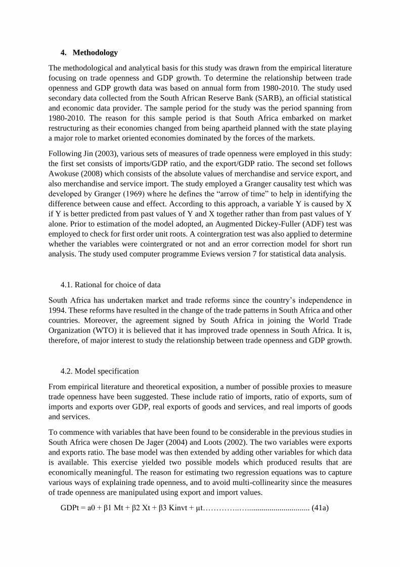
4. Methodology

The methodological and analytical basis for this study was drawn from the empirical literature

focusing on trade openness and GDP growth. To determine the relationship between trade

openness and GDP growth data was based on annual form from 1980-2010. The study used

secondary data collected from the South African Reserve Bank (SARB), an official statistical

and economic data provider. The sample period for the study was the period spanning from

1980-2010. The reason for this sample period is that South Africa embarked on market

restructuring as their economies changed from being apartheid planned with the state playing

a major role to market oriented economies dominated by the forces of the markets.

Following Jin (2003), various sets of measures of trade openness were employed in this study:

the first set consists of imports/GDP ratio, and the export/GDP ratio. The second set follows

Awokuse (2008) which consists of the absolute values of merchandise and service export, and

also merchandise and service import. The study employed a Granger causality test which was

developed by Granger (1969) where he defines the “arrow of time” to help in identifying the

difference between cause and effect. According to this approach, a variable Y is caused by X

if Y is better predicted from past values of Y and X together rather than from past values of Y

alone. Prior to estimation of the model adopted, an Augmented Dickey-Fuller (ADF) test was

employed to check for first order unit roots. A cointergration test was also applied to determine

whether the variables were cointergrated or not and an error correction model for short run

analysis. The study used computer programme Eviews version 7 for statistical data analysis.

4.1. Rational for choice of data

South Africa has undertaken market and trade reforms since the country’s independence in

1994. These reforms have resulted in the change of the trade patterns in South Africa and other

countries. Moreover, the agreement signed by South Africa in joining the World Trade

Organization (WTO) it is believed that it has improved trade openness in South Africa. It is,

therefore, of major interest to study the relationship between trade openness and GDP growth.

4.2. Model specification

From empirical literature and theoretical exposition, a number of possible proxies to measure

trade openness have been suggested. These include ratio of imports, ratio of exports, sum of

imports and exports over GDP, real exports of goods and services, and real imports of goods

and services.

To commence with variables that have been found to be considerable in the previous studies in

South Africa were chosen De Jager (2004) and Loots (2002). The two variables were exports

and exports ratio. The base model was then extended by adding other variables for which data

is available. This exercise yielded two possible models which produced results that are

economically meaningful. The reason for estimating two regression equations was to capture

various ways of explaining trade openness, and to avoid multi-collinearity since the measures

of trade openness are manipulated using export and import values.

GDPt = a0 + β1 Mt + β2 Xt + β3 Kinvt + µt…………..…............................... (41a)

GDPt = a0 + β1 Mrat + β2 Xrat + β3 Kinvt + µt………….............................. (4.1b)

where GDPt is Gross Domestic Product in levels, α and β are parameters to be estimated, Mt,

Xt, Kinvt, Mrat, Xrat and Kinvt which are defined as observable variables representing factors

affecting GDP in South Africa in year t, and µt is a random error term with a mean of zero,

representing measurement error and unmeasured and immeasurable factors.

4.2.1. Unit root test

Prior to estimation of the time series model, the first step was to check the stationarity of the

variables to be used as regressors in the model. The aim was to verify whether the series had a

stationary trend, and, if non-stationary, to establish orders of integration. To explain the

preceding statement, let Yt be a stochastic process of a time series variable as:

Yt = (t = 1, 2, 3…..)

for each Yt had its own mean, variance and covariance between different Yt then define such

time series as stationery if over time, its mean, variance and covariance remains constant that

is :

Mean: E (Yt) = constant

Variance: var (Yt) = constant

Covariance: cov (Yt, Yt + k) = constant

The problem with time series data is that independent variable can appear to be more significant

than they actually are if they have the same underlying trend as the dependent variable. This

causes the non-stationary variables to appear to be correlated even if they are not. Suppose

from both GDPt and OPENt are non-stationary to the same degree; that is, suppose that ∆GDPt

and ∆OPENt are both stationary. In such situation there is reasonable possibility that the non-

stationarity in the two variables will cancel each other out. Thus, the study needed to test for

stationarity conditions of variables in order to avoid spurious regression results.

The study first examined the stationarity in the time series by using graphical inspection on

series which were in their real values. Thereafter, all the variables were expressed in level form

to see whether after first differencing if the series exhibit non-stationarity. Scholars also argue

that although graphical evidence is useful as the first approximation to decide whether the

variables are non-stationary, most econometricians agree that this is clearly an unreliable

method to use to make inferences about unit roots. As a result, they advise the use of a formal

testing procedure in order to examine each of the variables under scrutiny (Medina-Smith,

2001).

To test the level of integration of the variables that were employed in the model, the study also

used the formal well known Augment Dickey-Fuller (ADF) test. The aim was to determine

whether the variables follow a non-stationary trend and were in fact of the order of 1 denoted

as I(1) or whether the series were stationary, i.e. of the order of 0 denoted as I(0). The

Augmented Dickey Fuller (ADF) tests were based on the estimation of the following

regression.

ΔXt = α0 + α1 + α2Xt-1 + Σ ΔXt-i + Фt …………………………..…… (4.2)

Where Δ is the first difference operator, t is a linear time trend and Фt is a normally distributed

error term. In (3), the null hypothesis that Ho: a2 = 0 against the alternative hypothesis H1: a2 ≠

0 is tested by comparing the calculated t- ratio of aX2 with Mackinnon critical values, which

are essentially adjusted t values. If the absolute value of the calculated t-ratio is greater than

the critical value, then the null hypothesis of a unit root (non-stationarity) is rejected, and the

time series Xt can be characterised as integrated of order zero, i.e. I(0), in levels.

However, first differencing was not an appropriate solution to the above problem and had a

major disadvantage: it prevented detection of the long-run relationship that may be present in

the data, i.e. the long-run information is lost, which was precisely the main question being

addressed (Gujarati, 1995).

The study also applied Phillips and Perron unit root test to verify ADF unit root results were

accurate. It was important to perform a second unit root test, which is the one developed by

Phillips and Perron (1988). This method utilises a nonparametric approach to control serial

correlation in the error term. Basically, the choices are the same as those explained in the ADF

test. Therefore, whichever assumption was used in the ADF test was also used for the P-P test.

The next section is the contegration test; here the study explains whether the series under

scrutiny were cointegrated.

4.2.2. Cointegration test

The study also followed the cointegration test as proposed by Engle and Granger (1987). The

question behind this test was to answer whether there was a long-run equilibrium relationship

between trade openness and GDP growth. A linear combination may exist between two or more

economic variables which converge to long-run equilibrium, even though the series tend to

move randomly over time. In other words, they are cointegrated when each individual variable

demonstrates stationarity only in first differences, but a linear combination of their levels may

result in stationarity.

Recent economic progress has made achievements in contegration methodology to examine

the long-run stable relationship between time series. Granger (1986); Engle and Granger (1987)

pioneered the area of cointegration tests. They proposed a two-step procedure to identify

cointegrating vectors. Firstly, this approach runs an ordinary least square (OLS) regression to

produce residuals. Secondly, it conducts a unit root test for the null hypothesis of no

cointegration relationship and against the alternative of a cointegration relationship between

them.

However, it is important to mention that Engle-Granger contegration procedure has a distinct

advantage and also that the test has several defects. This approach may suffer a bias since the

results are subject to arbitrary normalisation, and may also fail to distinguish the number of

cointegrating vectors. Moreover, literature holds that it is very important for empirical studies

to carry out several tests for cointegration instead of using one single procedure (Medina-

Smith, 2001). Alternatively, the study also applies the Johansen approach (1991). The

generalisation of the Johansen procedure is as follows:

∆yt = ΣΠi∆yt-1+ Πyt-n+εt…………………………………………..….… (4.3)

Where yt = (Kx1) vector of variables (β1yt-1, β1yt-2,…… βnyt-n), εt is independent and identically

distributed n-dimensional vector with mean zero and variance equal to matrix Σ ε,Π(αβ) is the

number of independent co-integration vectors, and Πyt-n is the error correction factor. The

Johansen procedure relies on the rank of Π and its characteristics roots. If rank (Π) =0, the

matrix is null (no cointegration) and equations in vector yt are a common VAR in first

differences. If Π has full rank (Π = k), the vector process is stationary and the equations in yt

are modeled in levels – I(0). If rank (Π)=1, there is evidence of a single cointegrating vectors

in Johansen’s cointegration procedure is applied to this study. These tests are:

Trace test

trace (r) = - T Σ In( 1- ) , and ……………………………………………….(4.4)

Maximum eigenvalue test

max (r,r + 1) = -T Σ In( 1- r+1) ,………………………………………………..(4.5)

Where r+1 ….,n are the (k-r) smallest estimated eigenvalues. In both tests, represents the

estimated values of the characteristics roots obtained from the estimated Π matrix, and T is the

number of observations. The trace test attempts to determine the number of cointegrating

vectors between the variables by testing the null hypothesis that r = 0 against the alternative

that r > 0 or r ≤ 1 (r equals the number of co-integrating vectors). The maximum eigenvalue

tests the null hypothesis that the number of co-integrating vectors is equal to r against the

alternative of r+1 co-integrating vectors. If the value of the likelihood ratio is greater than the

critical values, the null hypothesis of zero cointegrating vectors is rejected in favor of the

alternatives.

4.2.3. Error-correction Model (ECM)

An Error Correction Model (ECM) is an application of combining the long run, cointegrating

relationship between the levels variables and the short run relationship between the first

differences of the variables. It also has the advantage that other variables in the estimated

equation are stationary; hence there is no problem with spurious correlation. The error

correction model can be expressed as:

∆GDPt = a + ∑ α ∆GDPt-i + ∑ β ∆OPENt-j +Ω1ECTt-1+ µt…………………..... (4.6)

Where ∆ is the first difference operator, GDPt-I is lagged gross domestic product and OPENt-j

is lagged trade openness measures, respectively. The term ECTt-1 is all the residuals from the

spurious regressions estimated by OLS. This represents the short-term adjustment mechanism

from the equilibrium point, which is always significant regardless of the specifications

employed. The significance of the lagged residuals provides strong evidence of the adequacy

of an error correction framework.

4.2.4. Granger-Causality Tests

In examining the cause and effect on the variables, the study adopts the econometric

methodology followed by many time series studies such as Zestos and Tao (2002), and Beko

(2003). The study employs the granger causality test which has been developed by Granger

(1969) where he defines the “arrow of time” to help us identify between cause and effect.

According to this approach, a variable Y is caused by X if Y is better predicted from past values

of Y and X together rather than from past values of Y alone. For a simple bivariate model, the

pattern of causality can be identified by estimating regressions on Y and X using current and

past values of Y and X and by testing appropriate hypotheses. In using the following model,

causality between two variables will be tested.

GDPt = a + ∑ α GDPt-i + ∑ β OPENt-j + µt…………………………………………………………….. (4.7)

OPENt = a + ∑ α OPENt-i + ∑ β GDPt-j + έt ………..………………………...……………………… (4.8)

Where GDP is Gross domestic product and OPEN is all trade openness measures mentioned

above, µt and έt are serially uncorrelated white-noise residuals.

Ngozo (2006) explains that the test itself is just an F-test of the joint significance of the other

variable in a regression that includes lags of the dependent variable. The study tests whether

the null hypothesis trade openness does not causes GDP growth, where the alternative

hypothesis is that trade openness causes GDP growth. Given that the study has opted for α =

0.05 level of significance, the null hypothesis of no Granger causality must be rejected if the

p-value is smaller than the level of significance, that is, if (P > (F)) < 0.05. Otherwise, H0 cannot

be rejected.

5. Results and Discussions

5.1. Graphical inspection

The graphs below looked at the visual inspection of the graphs using raw data. After the visual

inspection of whether the graphs were stationary or non-stationary, correlation test was

employed to see if the prediction on visual inspection was true. The correlation table is found

in appendix A.

Figure 5.1: Graphical inspection

-20

-10

0

10

20

1980 1985 1990 1995 2000 2005 2010

X

-20

-10

0

10

20

30

1980 1985 1990 1995 2000 2005 2010

M

-4

-2

0

2

4

6

8

1980 1985 1990 1995 2000 2005 2010

GDP

12

16

20

24

28

1980 1985 1990 1995 2000 2005 2010

GCF

With the visual inspection on the above figure, X and GCF were seen non-stationary in level

form, meaning that their variances were not constant over time. GDP and M were non-

stationary in level form. Thus, correlation test for stationarity was employed. Appendix A

shows that GDP was the only variable that was non-stationary, and all other variables were

stationary. Meaning that the variance of GDP was not constant over time, it always changes.

5.2. Unit root results

Empirical literature suggests that the typical and well conventional method of detecting non-

stationary behaviour is to examine the tests for the existence of unit root (Sharma &

Panagiotidis, 2004). For this purpose, all the variables were examined through graphical check

of their time series plots. The variables were real gross domestic product (GDP), gross capital

formation (GCF), import ratio (M), and exports ratio (X).

Table 5.1: Unit root test

Variables Models ADF Lags PP Lags

GDP (Levels) Intercept -4.001705 0 -4.007703 1

trend and intercepts -5.018076 1 -4.544887 5

None -2.80377 0 -2.730896 2

M (Levels) intercept -4.950238 0 -4.938702 2

trend and intercepts -4.987907 0 -5.008933 4

None -4.494642 0 -4.480629 2

X (Levels) intercept -4.771585 0 -4.736737 3

trend and intercepts -4.687296 0 -4.646673 3

None -4.082808 0 -4.089778 2

GCF (Levels) intercept -3.097038 1 -1.832824 1

trend and intercepts -1.48184 2 -0.872475 5

None -1.209313 2 -1.150777 0

1st difference intercept -3.056603** 0 -3.159824** 2

trend and intercepts -4.310078** 1 -3.013424 10

None -2.998806** 0 -3.110413* 2 *; **; ***; level of the rejection at 1%, 5% and 10% respectively

The decision criterion when testing for stationary using ADF and P-P is to reject the null

hypothesis if the t-statistic is more negative than the critical values, or if the t-statistic is greater

than the critical values in absolute terms.

In the case of the above table, the variables: GDP, Exports, Imports were stationary at levels.

However the Gross capital formation appeared to have a unit root and had to be differenced

once to become stationary. With ADF the Gross capital formation was stationary after it had

been differences at 5 percent level of significance, and with P-P it was also stationary at 5

percent level of significance. This implies that Gross capital formation was integrated of order

one (I(1)), whereas other variables were integrated of order zero (I(0)).

5.3. Granger causality results

Since there was cointegration between trade openness and GDP growth, the next step was to

test for the direction of causality using a simple Granger causality test by estimating the

bivariate autoregressive processes for GDP and trade openness. The objective of this exercise

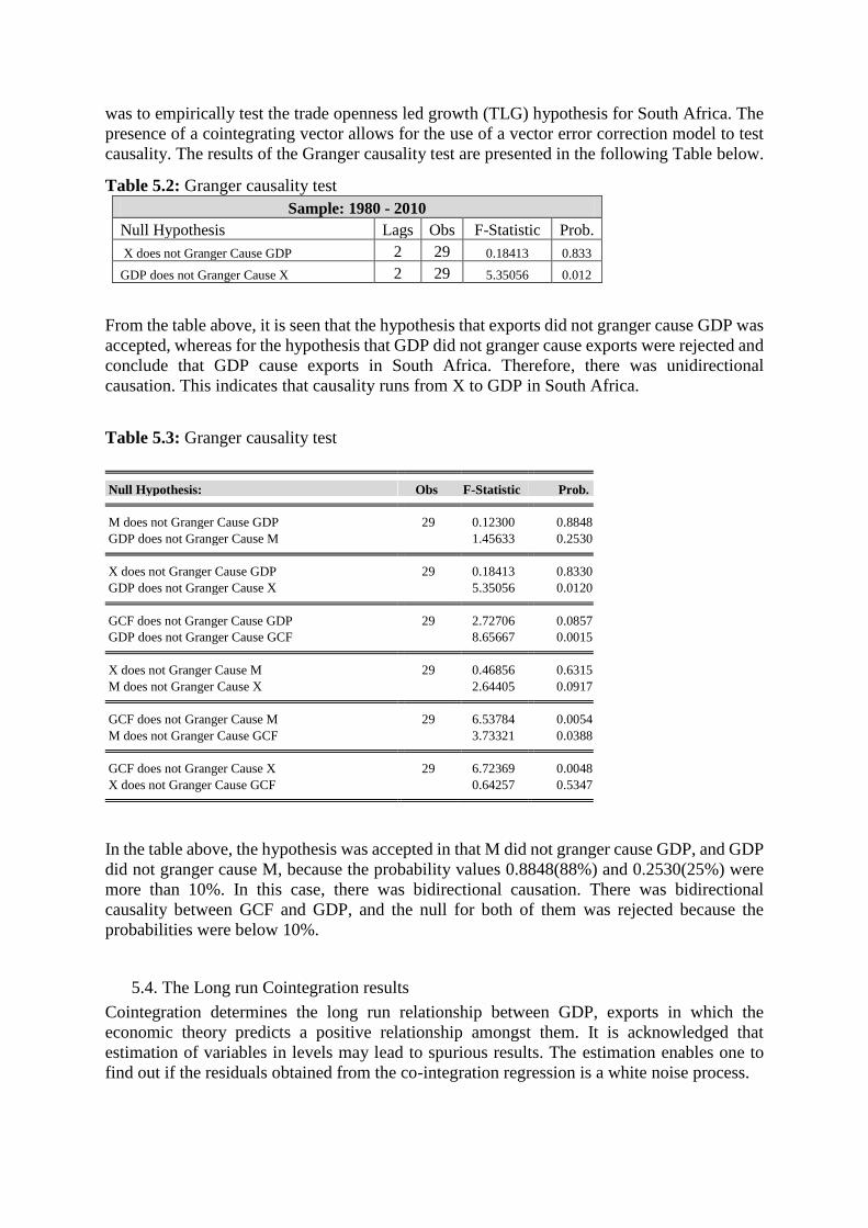
was to empirically test the trade openness led growth (TLG) hypothesis for South Africa. The

presence of a cointegrating vector allows for the use of a vector error correction model to test

causality. The results of the Granger causality test are presented in the following Table below.

Table 5.2: Granger causality test

Sample: 1980 - 2010

Null Hypothesis Lags Obs F-Statistic Prob.

X does not Granger Cause GDP 2 29 0.18413 0.833

GDP does not Granger Cause X 2 29 5.35056 0.012

From the table above, it is seen that the hypothesis that exports did not granger cause GDP was

accepted, whereas for the hypothesis that GDP did not granger cause exports were rejected and

conclude that GDP cause exports in South Africa. Therefore, there was unidirectional

causation. This indicates that causality runs from X to GDP in South Africa.

Table 5.3: Granger causality test

Null Hypothesis: Obs F-Statistic Prob.

M does not Granger Cause GDP 29 0.12300 0.8848

GDP does not Granger Cause M 1.45633 0.2530

X does not Granger Cause GDP 29 0.18413 0.8330

GDP does not Granger Cause X 5.35056 0.0120

GCF does not Granger Cause GDP 29 2.72706 0.0857

GDP does not Granger Cause GCF 8.65667 0.0015

X does not Granger Cause M 29 0.46856 0.6315

M does not Granger Cause X 2.64405 0.0917

GCF does not Granger Cause M 29 6.53784 0.0054

M does not Granger Cause GCF 3.73321 0.0388

GCF does not Granger Cause X 29 6.72369 0.0048

X does not Granger Cause GCF 0.64257 0.5347

In the table above, the hypothesis was accepted in that M did not granger cause GDP, and GDP

did not granger cause M, because the probability values 0.8848(88%) and 0.2530(25%) were

more than 10%. In this case, there was bidirectional causation. There was bidirectional

causality between GCF and GDP, and the null for both of them was rejected because the

probabilities were below 10%.

5.4. The Long run Cointegration results

Cointegration determines the long run relationship between GDP, exports in which the

economic theory predicts a positive relationship amongst them. It is acknowledged that

estimation of variables in levels may lead to spurious results. The estimation enables one to

find out if the residuals obtained from the co-integration regression is a white noise process.

It is extremely important to note that the customary diagnostic tests have not been reported.

Even though the coefficients reported in the spurious regression could be interpreted as

approximations of partial elasticities, they do not provide any kind of basis for sensible and

valid inferences at this stage. Furthermore, they cannot be used to draw any kind of inferences

without confirming in prior that the variables are in fact cointegrated.

Table 5.4: Cointegration

Cointegration

t-Statistic Prob.

Augmented Dickey-Fuller test statistic -4.137059 0.0002

Test critical values 1% level -2.644302

5% level -1.952473

10% level -1.610211

The results from the cointegration table shows that the ADF test on residuals with the model

of two variables, which were GDP and X(exports) were stationary and there was cointegration

between these two variables. The null hypothesis that residuals had a unit root was rejected and

the alternative that said the residuals did not have a unit root was accept.

5.5. Error correction model

Since the result shows that there was cointegration, then the next step was to test for the speed

of the adjustment that is displayed in the following table below.

Table 5.5: Error correction model Variable Coefficient Std. Error t-Statistic Prob.

RESID01(-1) -0.678881 0.168196 -4.036240 0.0004

D(X) 0.117481 0.050143 2.342923 0.0268

C -0.145550 0.394156 -0.369270 0.7148

R-squared 0.460607 Mean dependent var -0.123333

Adjusted R-squared 0.420652 S.D. dependent var 2.835816

S.E. of regression 2.158479 Akaike info criterion 4.471324

Sum squared residual 125.7938 Schwarz criterion 4.611444

Log likelihood -64.06986 Hannan-Quinn criter. 4.516149

F-statistic 11.52813 Durbin-Watson stat 2.077007

Probability (F-statistic) 0.000240

The result from the above table provides evidence for saying that there was cointegration

between GDP and X, because they had a positive relationship. The percentage change of D(x)

explains the variation of the dependent variable (GDP). This means that when D(X) increases

by 11%, GDP will increase by 1%. The R-squared which is the goodness of fit, in this case its

value was 0.460607, meaning that if there might be a shock in the process then GDP was going

to be able to recover with 46% per annum.

5.6. Engle and Granger cointegration test

Model specification for Engle and Granger is written on the equation below

GDPt = β0 + β1Xt + εt ……………………………………………………………………………… (4.7)

In the case of cointegration, two variables were tested, in the study it was for GDP as a

dependent variable and X as an independent variable from equation 4.7. The results on of PP

and ADF in table indicates that both of this variables were integrated of order zero I(0). The

null hypothesis was rejected if the probability value was less than 0.1 (10%). Similarly, the null

was rejected when the t-statistic value was more negative than the critical values. The results

obtained from the ADF test on residuals are shown on the table below.

Table 5.6: Engle and Granger cointegration ADF test results t-Statistic Prob.*

Augmented Dickey-Fuller test statistic -4.137059 0.0002

Test critical values: 1% level -2.644302

5% level -1.952473

10% level -1.610211

*MacKinnon (1996) one-sided p-values.

The above table shows that, after applying the ADF test the residuals were stationary at all

levels of significance. Therefore, the null hypothesis of non-stationary was rejected and the

alternative of stationary was accepted and these results were because the probability was far

below 10%.

5.7. Johansen cointergration

The Johansen procedure was employed to examine the question of cointegration and provided

not only an estimation methodology but also explicit procedures for testing for the number of

cointegrating vectors as well as for restrictions suggested by economic theory in a multivariate

settings. The following table presents the results of Johansen cointegration.

Table 5.7.1: Unrestricted Cointegration Rank Test (Trace)

Hypothesized Trace 0.05

No. of CE(s) Eigenvalue Statistic Critical Value Prob.**

None * 0.717869 72.02070 47.85613 0.0001

At most 1 * 0.567627 36.58998 29.79707 0.0071

At most 2 0.259391 13.11290 15.49471 0.1107

At most 3 * 0.154676 4.704990 3.841466 0.0301

Trace test indicates 2 cointegratingeqn(s) at the 0.05 level

* denotes rejection of the hypothesis at the 0.05 level

**MacKinnon-Haug-Michelis (1999) p-values

The above table states shows the rejection of the null hypothesis of cointegration and no

cointegrating vectors under both trace and eigenvalue form test. In the case of trace test, the

null hypothesis of no cointegrating vectors was rejected at 5 percent since the trace statistic of

72 was greater than the critical value of 47, this implies that cointegration exists at none.

Moving on to the test, the null of the at most 1 cointegration vectors, the trace statistic of 36

was greater than the critical value of 29, then this indicated the presence of cointegration. The

null of no cointegrating vectors was not rejected at most 2, the trace statistics of 13 was now

below the critical value of 15 at 5 percent indicating that the null should not be rejected. This

implies that the variables included in this study under trace statistics were cointegrated at none,

at most 1, and at most 3. Therefore, a unique long run relationship was expected to exist

between GDP and its variables.

Table 5.7.2: Unrestricted Cointegration Rank Test (Maximum Eigenvalue)

The Johansen test statistic for Maximum Eigenvalue in the table above shows that at none the

value of Max-Eigen Statistic 35 was greater than the critical value of 27. At most 1, and at most

3 there was cointegration since the Max-Eigen statistics were greater than the critical values at

5 percent, this means that the null hypothesis was reject. At most 2 Max-Eigen statistic was 8

which was well below the 5 percent critical value of 14, indicating that the null hypothesis of

no cointegartion vector was not rejected.

5.8. Diagnostic Test

The table below shows the results on residual diagnostic test which provides the tests for

heteroskedasticity, normality and serial correlation from the estimated equation and the

stability diagnostic by making use of the Ramsey reset test to check the model mis-

specification.

Table 5.8: Diagnostic summary and stability test

Table 4.8 diagnostic summary and stability test

Tests H0 Probability Diagnostic Test Conclusion

Breusch-Pagan

Godfrey

No

Heteroskedasticity

Prob.

F(3,27)

0.3562 Heteroskedasticity

There is no

heteroskedasticity

Jarque-Bera

Probability

Normal

Distribution 0.300391

Normality

Distribution

Normally

Distributed

BG Serial

Correlation LM

Test

No serial

correlation

Prob.

F(7,20)

0.1431 Serial Correlation

There is no serial

correlation

Ramsey reset

test

Normal

distribution ε ̴ N

(0,σ2I) 0.8688

Model Mis-

Specification

The model is

normally

distributed

Hypothesized Max-Eigen 0.05

No. of CE(s) Eigenvalue Statistic Critical Value Prob.**

None * 0.717869 35.43072 27.58434 0.0040

At most 1 * 0.567627 23.47708 21.13162 0.0230

At most 2 0.259391 8.407912 14.26460 0.3387

At most 3 * 0.154676 4.704990 3.841466 0.0301

Max-eigenvalue test indicates 2 cointegratingeqn(s) at the 0.05 level

* denotes rejection of the hypothesis at the 0.05 level

**MacKinnon-Haug-Michelis (1999) p-values

The result from the above table shows that the model of this study meets the requirements of

the assumption of the Classical Linear Regression Model (CLRM). This implies that the model

was homoscedastic and linear.

6. Conclusion and Recommendation

The results shows that in estimating equation (3.1a), the long-run equilibrium relationship

shows that variables such as exports, imports and gross fixed capital formation were positively

correlated with GDP growth. These results were expected from economic theory that an

increase in exports leads to an increase in GDP. The causal relationship between trade openness

and GDP growth was examined using Granger-causality tests. When testing Granger causality,

the study used exports as the main variable that affect GDP growth. It was found that GDP

granger cause exports.

The study has also utilised the concept of impulse response functions in order to investigate

how the system responds to a macroeconomic shock. This approach allows the simulation of

the effect of a given (predetermined) shock on the economic system. The response shocks show

no evidence of causality between trade openness and GDP growth. The only exception that can

be made is the shock made by GDP growth on imports but the shock does not last for a long

period. Finally, the results of the diagnostic tests employed in equation (4.1a) were satisfactory,

with no heteroskedasticity, and residuals were normally distributed with no problem of serial

correlation in residuals. This implies that the South African government should continue

improving the policy regarding trade openness and GDP growth.

The findings of the study show a smaller than expected effects of trade openness on the GDP

growth process in South Africa. This is mostly because the South African exports are more raw

resource based. Therefore, to promote openness, the South African government should

encourage exporters to improve their competitive advantage and change their trade pattern

from raw material based to more technological and human capital intensive goods.

7. References

Anderson J. (2007). Is China Export-Led? Global Economics Research. Asia Hong Kong,

UBS Investment Research,

Andriamananjara S. and Hillberry R. (2001). Regionalism, Trade and Growth: The Case of

the EU-South Africa Free Trade Arrangement. Office of Economics Working Paper. U.S.

International Trade Commission.

Awokuse T.O. (2008). Trade openness and economic growth: is growth export-led or import-

led?, Applied Economics, 40, pp161–173

Bekõ J. (2003). Causality Analysis of Exportsand Economic Growth, Aggregate and Sectoral

Results for Slovenia. Eastern European Economics, vol. 41, no. 6, pp. 70–92.

De Jager J.L.W (2004). Aspects of growth empirics in South Africa. Doctor commerce

(Economics). Faculty of economics and management science, University of Pretoria.

November 2003.

Du Plessis, S. and Smit, B. (2007). “South Africa’s growth revival after 1994”. Stellenbosch

Economic WP, 01/06.

Emma and Samman (2005). Openness and Growth: An empirical Investigation. Human

Development Report Office Occasional Paper, Human Development Report.

http://hdr.undp.org/en/reports/global/hdr2005/papers/HDR2005_Samman_Emma_22.pdf

Engle, R.F. and C.W.J. Granger (1987). “Cointegration and Error Correction:

Representation, Estimation and Testing” Econometrica, Vol. 55: 251-276.

Flatters F. and Stern M. (2007). Trade and Trade Policy in South Africa: Recent Trends and

Future Prospects, June, Development Network Africa.

Granger, C. W. J. (1969). Investigating causal relations by econometric models and cross-

spectral methods. Econometrica, 37, 424–438.

Granger, C.W.J. (1986). Developments in the Study of Cointegrated Economic Variables,

Oxford Bulletin of Economics and Statistics, 48,213-228.

Gujarati N. (1995). Basic Econometrics, Boston: McGraw Hill

Jin, J. C. (2003). Openness and growth in North Korea: Evidence from time-series data,

Review of International Economies, 11, 18–27.

Johansen, S. (1991). “Estimation and Hypothesis Testing of Cointegration Vectors in

Gaussian Vector Autoregressive Models”, Econometrica, 59: 1551–1580.

Lewis J.D. (2001). Reform and Opportunity: The Changing Role and Patterns of Trade in

South Africa and SADC, Africa Region Working Paper Series No.14

Loots E. (2002). Globalisation and Economic Growth in South Africa: Do We Benefit From

Trade and Financial Liberalisation? Trade and Industrial Policy Strategy (TIPS)

Mbabazi, Milner and Morrissey (2004). Trade Openness, Trade Costs and Growth: Why

Sub-Saharan Africa Performs Poorly. UK Department for International Development, CREDIT

Research Paper No. 06/08

Medina-Smith E.J (2001). Is The Export-Led Growth Hypothesis Valid For Developing

Countries? A Case Study of Costa Rica. Policy Issues in International Trade and Commodities

Study Series No. 7

Ngozo T. (2006). Openess and Economic Growth: The case of European Expansion. Munich

Personal RePEc Archive (MPRA) 15. December 2006. MPRA Paper No. 14538, posted 08.

April 2009

Phillips, P. C. and Perron, P. (1988). ‘Testing for a Unit Root in a Time Series Regression’,

Biometrica, Vol. 75, No. 2, pp. 335–346.

Rankin N. (2001). The Export Behaviour of South African Manufacturing Firms.10-12

September, 2001 Annual Forum at Misty Hills, Mulders drift. Centre for the Study of African

Economies, University of Oxford. Trade and Industrial Policy Strategies Forum (TIPS).

SARB (2008). Monetary Policy Review, Quarterly Bulletin No 249, South African Reserve

Bank. Available at:

http://www.reservebank.co.za/internet/Publication.nsf/LADV/E64F25FA7CF237F2422574B

900311E3A/$File/QBSep08.pdf

SARB (2009). Monetary Policy Review, Quarterly Bulletin, South African Reserve Bank.

Available at:

http://www.reservebank.co.za/internet/Publication.nsf/LADV/F58C9120364DBE604225762

600277D0E/$File/QBSept09.pdf

Sarkar P. (2007). Trade Openness and Growth: Is There Any Link? September, MPRA Paper

No. 4997, posted 07. November 2007. Accessed at: http://mpra.ub.uni-

muenchen.de/4997/1/MPRA_paper_4997.pdf

Sharma A. and Panagiotidis T. (2004). An Analysis of Exports and Growth in India:

Cointegration and Causality Evidence (1971 - 2001). Review of Development Economics, 9(2),

232–248

South African Yearbook (2002/03). Economy, Available at:

http://www.gcis.gov.za/resource_centre/sa_info/yearbook/2003/chapter6.pdf

Srinivasan T.N (2004). "China and India: Economic performance, Competition and

Cooperation." Policy Reform and Poverty. Beijing, China: World Trade Organisation (WTO),

pp 1-38.

van der Walt J. (2007). “Barriers to exports faced by the manufacturing SME’s in South

Africa”. A research project for the Gordon institute of business science, University of Pretoria

in partial fulfilment of the degree of masters of business administration. 14 November 2007.

Yanikkaya H. (2003). Trade openness and economic growth: a cross-country empirical

investigation. Journal of Development Economics 72. Pp 57– 89

Zestos G.K and Tao X. (2002). Trade and GDP Growth: Causal Relations in the United States

and Canada. Southern Economic Journal, Vol. 68, No. 4, pp. 859-874

Appendix A: Correlograms

GDP Growth Date: 10/22/12 Time: 22:26

Sample: 1980 2010

Included observations: 31

Autocorrelation Partial Correlation AC PAC Q-Stat Prob

. |******| . |******| 1 0.885 0.885 26.725 0.000

. |***** | ***| . | 2 0.686 -0.452 43.323 0.000

. |**** | . | . | 3 0.487 0.034 52.000 0.000

. |**. | . | . | 4 0.324 0.001 55.981 0.000

. |* . | . | . | 5 0.206 0.016 57.655 0.000

. |* . | . | . | 6 0.118 -0.057 58.226 0.000

. | . | . |* . | 7 0.069 0.092 58.428 0.000

. | . | . *| . | 8 0.024 -0.152 58.454 0.000

. | . | .**| . | 9 -0.059 -0.224 58.616 0.000

Gross Capital Formation

Date: 10/22/12 Time: 22:27

Sample: 1980 2010

Included observations: 31

Autocorrelation Partial Correlation AC PAC Q-Stat Prob

. |**. | . |**. | 1 0.323 0.323 3.5670 0.059

. | . | . *| . | 2 -0.052 -0.175 3.6629 0.160

. | . | . |* . | 3 -0.010 0.076 3.6669 0.300

. | . | . | . | 4 0.013 -0.021 3.6732 0.452

. *| . | . *| . | 5 -0.075 -0.082 3.8931 0.565

. | . | . |* . | 6 0.064 0.145 4.0619 0.668

. |* . | . | . | 7 0.154 0.069 5.0676 0.652

. |* . | . | . | 8 0.116 0.064 5.6614 0.685

. | . | . | . | 9 -0.006 -0.044 5.6629 0.773

Imports Date: 10/22/12 Time: 22:27

Sample: 1980 2010

Included observations: 31

Autocorrelation Partial Correlation AC PAC Q-Stat Prob

. |* . | . |* . | 1 0.093 0.093 0.2974 0.586

. *| . | . *| . | 2 -0.185 -0.196 1.5096 0.470

. *| . | . | . | 3 -0.082 -0.045 1.7555 0.625

. | . | . | . | 4 0.046 0.025 1.8370 0.766

.**| . | ***| . | 5 -0.342 -0.392 6.4292 0.267

. *| . | . *| . | 6 -0.174 -0.108 7.6732 0.263

. |* . | . | . | 7 0.098 -0.009 8.0866 0.325

. |* . | . | . | 8 0.160 0.025 9.2195 0.324

. | . | . | . | 9 -0.008 -0.003 9.2224 0.417

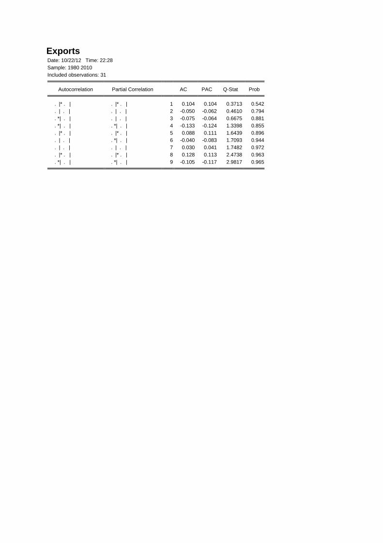
Exports Date: 10/22/12 Time: 22:28

Sample: 1980 2010

Included observations: 31

Autocorrelation Partial Correlation AC PAC Q-Stat Prob

. |* . | . |* . | 1 0.104 0.104 0.3713 0.542

. | . | . | . | 2 -0.050 -0.062 0.4610 0.794

. *| . | . | . | 3 -0.075 -0.064 0.6675 0.881

. *| . | . *| . | 4 -0.133 -0.124 1.3398 0.855

. |* . | . |* . | 5 0.088 0.111 1.6439 0.896

. | . | . *| . | 6 -0.040 -0.083 1.7093 0.944

. | . | . | . | 7 0.030 0.041 1.7482 0.972

. |* . | . |* . | 8 0.128 0.113 2.4738 0.963

. *| . | . *| . | 9 -0.105 -0.117 2.9817 0.965