EL2450 - Hybrid and Embedded Control Systems Exercises
130
EL2450 - Hybrid and Embedded Control Systems Exercises Alberto Speranzon, Oscar Flärdh, Magnus Lindhé, Carlo Fischione and Karl Henrik Johansson December 2008 Plant Hold Sample Computer int count; int u; int main(int y); count=count+1; u=1/2*sqrt(y)-r; int ref; string str; int main(int p); openport(p); ref=read(p); TASK 1 TASK 2 DA AD Automatic Control Lab, School of Electrical Engineering Royal Institute of Technology (KTH), Stockholm, Sweden
-
Upload
khangminh22 -
Category
Documents
-
view
3 -
download
0
Transcript of EL2450 - Hybrid and Embedded Control Systems Exercises

EL2450 - Hybrid and Embedded Control Systems
Exercises
Alberto Speranzon, Oscar Flärdh, Magnus Lindhé,Carlo Fischione and Karl Henrik Johansson
December 2008
Plant
Hold Sample
Computer
int count;int u;
int main(int y);
count=count+1;
u=1/2*sqrt(y)-r;
int ref;
string str;
int main(int p);
openport(p);
ref=read(p);
TASK 1 TASK 2
DA AD
Automatic Control Lab, School of Electrical EngineeringRoyal Institute of Technology (KTH), Stockholm, Sweden

2

Preface
The present compendium has been developed by Alberto Speranzon, Oscar Flärdh and Karl Henrik Johanssonin the beginning of 2005 for the course 2E1245 Hybrid and Embedded Control Systems, given at the RoyalInstitute of Technology, Stockholm. The material has been updated later in 2005 and in the beginning of 2006.Some of the exercises have been shamelessly borrowed (stolen) from other sources, and in that case a referenceto the original source has been provided.
Alberto Speranzon, Oscar Flärdh and Karl Henrik Johansson,January 2006.
The material was edited and some problems and solutions wereadded in 2008, by Magnus Lindhé and CarloFischione. The course code also changed to EL2450.
3

CONTENTS
Exercises 7
I Time-triggered control 71 Review exercises: aliasing,z-transform, matrix exponential . . . . . . . . . . . . . . . . . . . 82 Models of sampled systems . . . . . . . . . . . . . . . . . . . . . . . . . . . .. . . . . . . . 93 Analysis of sampled systems . . . . . . . . . . . . . . . . . . . . . . . . . .. . . . . . . . . 124 Computer realization of controllers . . . . . . . . . . . . . . . . . .. . . . . . . . . . . . . . 175 Implementation aspects . . . . . . . . . . . . . . . . . . . . . . . . . . . . .. . . . . . . . . 20
II Event-triggered control 236 Real-time operating systems . . . . . . . . . . . . . . . . . . . . . . . . .. . . . . . . . . . 247 Real-time scheduling . . . . . . . . . . . . . . . . . . . . . . . . . . . . . . .. . . . . . . . 268 Models of computation I: Discrete-event systems . . . . . . . .. . . . . . . . . . . . . . . . 299 Models of computation II: Transition systems . . . . . . . . . . .. . . . . . . . . . . . . . . 31
III Hybrid control 3410 Modeling of hybrid systems . . . . . . . . . . . . . . . . . . . . . . . . . .. . . . . . . . . 3511 Stability of hybrid systems . . . . . . . . . . . . . . . . . . . . . . . . .. . . . . . . . . . . 3812 Verification of hybrid systems . . . . . . . . . . . . . . . . . . . . . . .. . . . . . . . . . . 4213 Simulation and bisimulation . . . . . . . . . . . . . . . . . . . . . . . .. . . . . . . . . . . 44
Solutions 46
I Time-triggered control 46Review exercises . . . . . . . . . . . . . . . . . . . . . . . . . . . . . . . . . . . .. . . . . . . . 47Models of sampled systems . . . . . . . . . . . . . . . . . . . . . . . . . . . . .. . . . . . . . . . 54Analysis of sampled systems . . . . . . . . . . . . . . . . . . . . . . . . . . .. . . . . . . . . . . 64Computer realization of controllers . . . . . . . . . . . . . . . . . . .. . . . . . . . . . . . . . . . 75Implementation aspects . . . . . . . . . . . . . . . . . . . . . . . . . . . . . .. . . . . . . . . . . 83
II Event-triggered control 88Real-time operating systems . . . . . . . . . . . . . . . . . . . . . . . . . .. . . . . . . . . . . . 89
4

Real-time scheduling . . . . . . . . . . . . . . . . . . . . . . . . . . . . . . . .. . . . . . . . . . 93Models of computation I: Discrete-event systems . . . . . . . . .. . . . . . . . . . . . . . . . . . 101Models of computation II: Transition systems . . . . . . . . . . . .. . . . . . . . . . . . . . . . . 109
III Hybrid control 112Modeling of hybrid systems . . . . . . . . . . . . . . . . . . . . . . . . . . . .. . . . . . . . . . . 113Stability of hybrid systems . . . . . . . . . . . . . . . . . . . . . . . . . . .. . . . . . . . . . . . 116Verification of hybrid systems . . . . . . . . . . . . . . . . . . . . . . . . .. . . . . . . . . . . . 125Simulation and bisimulation . . . . . . . . . . . . . . . . . . . . . . . . . .. . . . . . . . . . . . 129
Bibliography 129
5

Exercises
6

Part I
Time-triggered control
7
1 Review exercises: aliasing,z-transform, matrix exponential
EXERCISE 1.1 (Ex. 7.3 in [13])
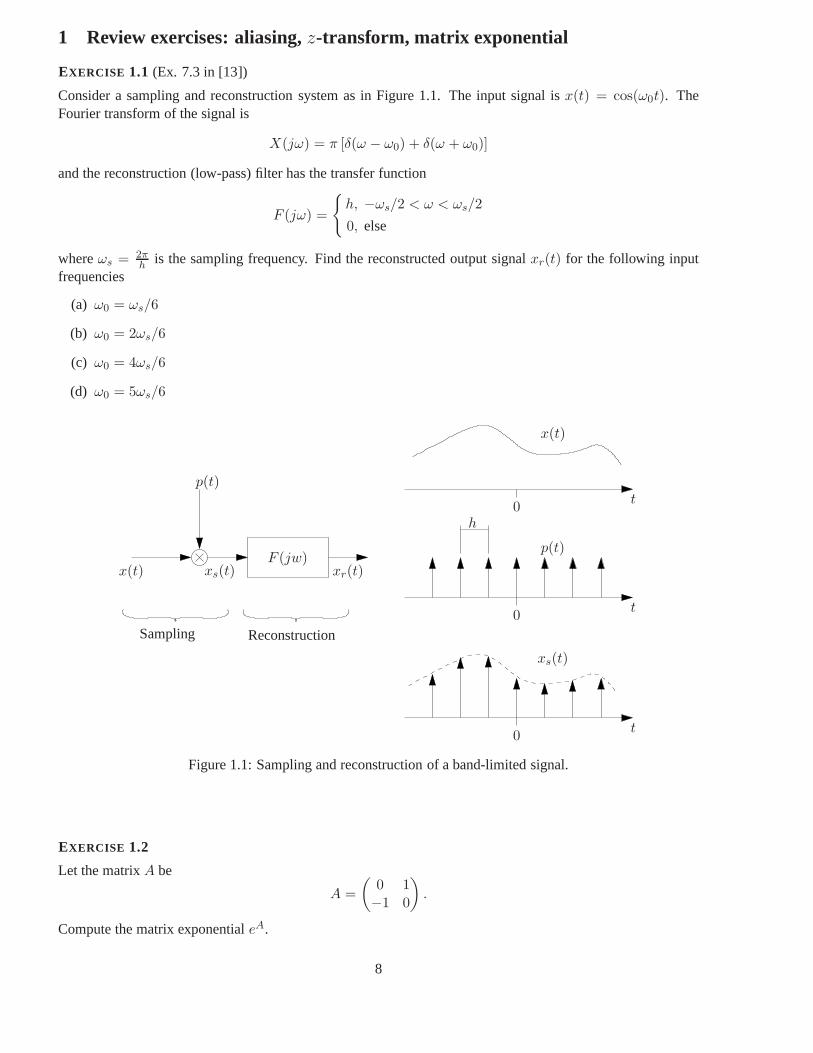
Consider a sampling and reconstruction system as in Figure 1.1. The input signal isx(t) = cos(ω0t). TheFourier transform of the signal is
X(jω) = π [δ(ω − ω0) + δ(ω + ω0)]
and the reconstruction (low-pass) filter has the transfer function
F (jω) =
h, −ωs/2 < ω < ωs/2
0, else
whereωs = 2πh is the sampling frequency. Find the reconstructed output signalxr(t) for the following input
frequencies
(a) ω0 = ωs/6
(b) ω0 = 2ωs/6
(c) ω0 = 4ωs/6
(d) ω0 = 5ωs/6
xs(t)F (jw)
xr(t)
p(t)
x(t)
x(t)
p(t)
xs(t)
t
t
t
h0
0
0
Sampling Reconstruction
Figure 1.1: Sampling and reconstruction of a band-limited signal.
EXERCISE 1.2
Let the matrixA be
A =
(0 1−1 0
)
.
Compute the matrix exponentialeA.
8

EXERCISE 1.3
Compute thez-transform ofx(kh) = e−kh/T T > 0.
EXERCISE 1.4
Compute thez-transform ofx(kh) = sin(wkh)
EXERCISE 1.5
Given the following system described by the following difference equation
y(k + 2)− 1.5y(k + 1) + 0.5y(k) = u(k + 1)
with initial conditiony(0) = 0.5 andy(1) = 1.25, determine the output when the inputu(k) is a unitary step.
2 Models of sampled systems
EXERCISE 2.1 (Ex. 2.1 in [2])
Consider the scalar system
dx
dt= −ax + bu
y = cx.
Let the input be constant over periods of lengthh. Sample the system and discuss how the poles of the discrete-time system vary with the sampling frequency.
EXERCISE 2.2
Consider the following continuous-time transfer function
G(s) =1
(s + 1)(s + 2).
The system is sampled with sampling periodh = 1.
(a) Derive a state-space representation of the sampled system.
(b) Find the pulse-transfer function corresponding to the system in (a).
9

EXERCISE 2.3 (Ex. 2.2 in [2])
Derive the discrete-time system corresponding to the following continuous-time systems when a zero order-hold circuit is used
(a)
x =
(0 1−1 0
)
x +
(01
)
u
y =(1 0
)x
(b)d2y
dt2+ 3
dy
dt+ 2y =
du
dt+ 3u
(c)d3y
dt3= u
EXERCISE 2.4 (Ex. 2.3 in [2])
The following difference equations are assumed to describecontinuous-time systems sampled using a zero-order-hold circuit and the sampling periodh. Determine, if possible, the corresponding continuous-time sys-tems.
(a)y(kh)− 0.5y(kh − h) = 6u(kh − h)
(b)
x(kh + h) =
(−0.5 1
0 −0.3
)
x(kh) +
(0.50.7
)
u(kh)
y(kh) =(1 1
)x(kh)
(c)y(kh) + 0.5y(kh − h) = 6u(kh − h)
EXERCISE 2.5 (Ex. 2.11 in [2])
The transfer function of a motor can be written as
G(s) =1
s(s + 1).
Determine:
(a) the sampled system
(b) the pulse-transfer function
(c) the pulse response
(d) a difference equation relating input and output
(e) the variation of the poles and zeros of the pulse-transfer function with the sampling period
10

EXERCISE 2.6 (Ex. 2.12 in [2])
A continuous-time system with transfer function
G(s) =1
se−sτ
is sampled with sampling periodh = 1, whereτ = 0.5.
(a) Determine a state-space representation of the sampled system. What is the order of the sampled-system?
(b) Determine the pulse-transfer function and the pulse response of the sampled system
(c) Determine the poles and zeros of the sampled system.
EXERCISE 2.7 (Ex. 2.13 in [2])
Solve Problem 2.6 with
G(s) =1
s + 1e−sτ
andh = 1 andτ = 1.5.
EXERCISE 2.8 (Ex. 2.15 in [2])
Determine the polynomialsA(q), B(q), A∗(q−1)) andB∗(q−1) so that the systems
A(q)y(k) = B(q)u(k)
andA∗(q−1)y(k) = B∗(q−1)u(k − d)
represent the systemy(k)− 0.5y(k − 1) = u(k − 9) + 0.2u(k − 10).
What isd? What is the order of the system?
EXERCISE 2.9 (Ex. 2.17 in [2])
Use the z-transform to determine the output sequence of the difference equation
y(k + 2)− 1.5y(k + 1) + 0.5y(k) = u(k + 1)
whenu(k) is a step atk = 0 and wheny(0) = 0.5 andy(−1) = 1.
11

EXERCISE 2.10
Consider the following continuous time controller
U(s) = −s0s + s1
s + r1Y (s) +
t0s + t1s + r1
R(s)
wheres0, s1, t0, t1 andr1 are parameters that are chosen to obtain the desired closed-loop performance. Dis-cretize the controller using exact sampling by means of sampled control theory. Assume that the samplinginterval ish, and write the sampled controller on the formu(kh) = −Hy(q)y(kh) + Hr(q)r(kh).
EXERCISE 2.11 (Ex. 2.21 in [2])
If β < α, thens + β
s + α
is called a lead filter (i.e. it gives a phase advance). Consider the discrete-time system
z + b
z + a
(a) Determine when it is a lead filter
(b) Simulate the step response for different pole and zero locations
3 Analysis of sampled systems
EXERCISE 3.1 (Ex. 3.2 in [2])
Consider the system in Figure 3.1 and let
H(z) =K
z(z − 0.2)(z − 0.4)K > 0
Determine the values ofK for which the closed-loop system is stable.
r ye
-H(z)
Figure 3.1: Closed-loop system for Problem 3.1.
12
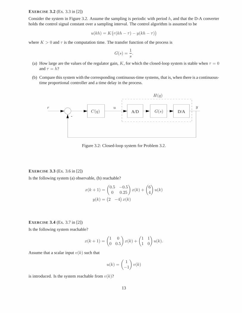
EXERCISE 3.2 (Ex. 3.3 in [2])
Consider the system in Figure 3.2. Assume the sampling is periodic with periodh, and that the D-A converterholds the control signal constant over a sampling interval.The control algorithm is assumed to be
u(kh) = K(r(kh− τ)− y(kh− τ)
)
whereK > 0 andτ is the computation time. The transfer function of the process is
G(s) =1
s.
(a) How large are the values of the regulator gain,K, for which the closed-loop system is stable whenτ = 0andτ = h?
(b) Compare this system with the corresponding continuous-time systems, that is, when there is a continuous-time proportional controller and a time delay in the process.
r u y
-C(q)
H(q)
A/D G(s) D/A
Figure 3.2: Closed-loop system for Problem 3.2.
EXERCISE 3.3 (Ex. 3.6 in [2])
Is the following system (a) observable, (b) reachable?
x(k + 1) =
(0.5 −0.50 0.25
)
x(k) +
(64
)
u(k)
y(k) =(2 −4
)x(k)
EXERCISE 3.4 (Ex. 3.7 in [2])
Is the following system reachable?
x(k + 1) =
(1 00 0.5
)
x(k) +
(1 11 0
)
u(k).
Assume that a scalar inputv(k) such that
u(k) =
(1−1
)
v(k)
is introduced. Is the system reachable fromv(k)?
13

EXERCISE 3.5 (Ex. 3.11 in [2])
Determine the stability and the stationary value of the output for the system described by Figure 3.2 with
H(q) =1
q(q − 0.5)
wherer is a step function andC(q) = K (proportional controller), K>0.
EXERCISE 3.6 (Ex. 3.12 in [2])
Consider the Problem 3.5. Determine the steady-state errorbetween the reference signalr and the outputy,whenr is a unit ramp, that isr(k) = k. AssumeC(q) to be a proportional controller.
EXERCISE 3.7 (Ex. 3.18 in [2])
Consider a continuous-time (CT) system
x(t) = Ax(t) + Bu(t)
y(t) = Cx(t).
The zero-order hold sampling of CT gives the discrete-time (DT) system
x(kh + h) = Φx(kh) + Γu(kh)
y(kh) = Cx(kh).
Consider the following statements:
(a) CT stable⇒ DT stable
(b) CT unstable⇒ DT unstable
(c) CT controllable⇒ DT controllable
(d) CT observable⇒ DT observable.
Which statements are true and which are false (explain why) in the following cases:
(i) For all sampling intervalsh > 0
(ii) For all h > 0 except for isolated values
(iii) Neither (i) nor (ii).
EXERCISE 3.8 (Ex. 3.20 in [2])
Given the system(q2 + 0.4q)y(k) = u(k),
(a) for which values ofK in the proportional controller
u(k) = K(r(k)− y(k)
)
is the closed-loop system stable?
(b) Determine the stationary errorr − y whenr is a step and K=0.5 in the controller (a).
14

EXERCISE 3.9 (Ex. 4.1 in [2])
A general second-order discrete-time system can be writtenas
x(k + 1) =
(a11 a12
a21 a22
)
x(k) +
(b1
b2
)
u(k)
y(k) =(c1 c2
)x(k).
Determine a state-feedback controller in the form
u(k) = −Lx(k)
such that the characteristic equation of the closed-loop system is
z2 + p1z + p2 = 0.
Use the previous result to compute the deadbeat controller for the double integrator.
EXERCISE 3.10 (Ex. 4.2 in [2])
Given the system
x(k + 1) =
(1 0.1
0.5 0.1
)
x(k) +
(10
)
u(k)
y(k) =(1 1
)x(k).
Determine a linear state-feedback controller
u(k) = −Lx(k)
such that the poles of the closed-loop system are placed in 0.1 and 0.25.
EXERCISE 3.11 (Ex. 4.5 in [2])
The system
x(k + 1) =
(0.78 00.22 1
)
x(k) +
(0.220.03
)
u(k)
y(k) =(0 1
)x(k).
represents the normalized motor for the sampling interval of h = 0.25. Determine observers for the state basedon the output by using each of the following:
(a) Direct calculation.
(b) An full-state observer.
(c) The reduced-order observer.
15
EXERCISE 3.12 (Ex. 4.8 in [2])
Given the discrete-time system
x(k + 1) =
(0.5 10.5 0.7
)
x(k) +
(0.20.1
)
u(k) +
(10
)
v(k)
y(k) =(1 0
)x(k).
wherev is a constant disturbance. Determine controller such that the influence ofv can be eliminated in steadystate in each of the following cases:
(a) The state andv can be measured.
(b) The state can be measured.
(c) Only the output can be measured.
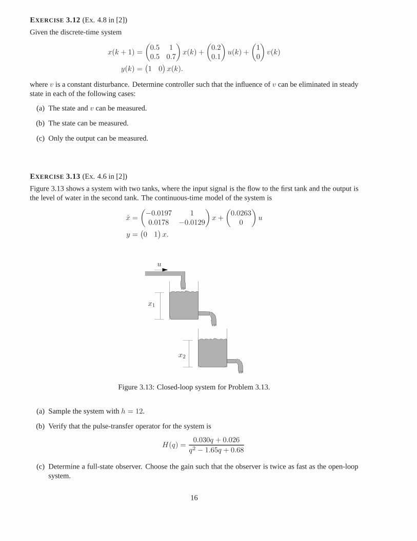
EXERCISE 3.13 (Ex. 4.6 in [2])
Figure 3.13 shows a system with two tanks, where the input signal is the flow to the first tank and the output isthe level of water in the second tank. The continuous-time model of the system is
x =
(−0.0197 10.0178 −0.0129
)
x +
(0.0263
0
)
u
y =(0 1
)x.
x1
x2
u
Figure 3.13: Closed-loop system for Problem 3.13.
(a) Sample the system withh = 12.
(b) Verify that the pulse-transfer operator for the system is
H(q) =0.030q + 0.026
q2 − 1.65q + 0.68
(c) Determine a full-state observer. Choose the gain such that the observer is twice as fast as the open-loopsystem.
16

EXERCISE 3.14
Consider the following scalar linear system
x(t) = −5x(t) + u(t)
y(t) = x(t).
(a) Sample the system with sampling periodh = 1,
(b) Show, using Lyapunov result, that the sampled system is stable when the inputu(kh) = 0 for k ≥ 0.
EXERCISE 3.15
Consider the following linear system
x(t) =
(−1 00 −2
)
x(t) +
(11
)
u(t)
y(t) = x(t).
(a) Sample the system with sampling periodh = 1
(b) Design a controller that place the poles in0.1 and0.2.
(c) Show, using Lyapunov result, that the closed loop sampled system is stable
4 Computer realization of controllers
EXERCISE 4.1
Consider the following pulse-transfer
H(z) =z − 1
(z − 0.5)(z − 2)
(a) Design a digital PI controller
Hc(z) =(K + Ki)z −K
z − 1
that places the poles of the closed-loop system in the origin.
(b) Find a state-space representation of the digital controller in (a).
EXERCISE 4.2 (Ex. 8.2 in [2])
Use different methods to make an approximation of the transfer function
G(s) =a
s + a
17

(a) Euler’s method
(b) Tustin’s approximation
(c) Tustin’s approximation with pre-warping usingω1 = a as warping frequency
EXERCISE 4.3 (Ex. 8.3 in [2])
The lead network with transfer function
Gℓ(s) = 4s + 1
s + 2
Give a phase advance of about20 atωc = 1.6rad/s. Approximate the network forh = 0.25 using
(a) Euler’s method
(b) Backward differences
(c) Tustin’s approximation
(d) Tustin’s approximation with pre-warping usingω1 = ωc as warping frequency
EXERCISE 4.4 (Ex. 8.7 in [2])
Consider the tank system in Problem 2.13. Assume the following specifications:
1. The steady-state error after a step in the reference valueis zero
2. The crossover frequency of the compensated system is 0.025 rad/s
3. The phase margin is about50.
(a) Design a PI-controller such that the specifications are fulfilled.
(b) Determine the poles and the zeros of the closed-loop system. What is the damping corresponding to thecomplex poles?
(c) Choose a suitable sampling interval and approximate thecontinuous-time controller using Tustin’s methodwith pre-warping. Use the crossover frequency as warping frequency.
EXERCISE 4.5 (Ex. 8.4 in [2])
The choice of sampling period depends on many factors. One way to determine the sampling frequency is to usecontinuous-time arguments. Approximate the sampled system as the hold circuit followed by the continuous-time system. Assuming that the phase margin can be decreasedby 5 to 15, verify that a rule of thumb inselecting the sampling frequency is
hωc ≈ 0.15 to 0.5
whereωc is the crossover frequency of the continuous-time system.
18
EXERCISE 4.6 (Ex. 8.12 in [2])
Consider the continuous-time double integrator describedby
x =
(0 10 0
)
x +
(01
)
u
y =(1 0
)x.
Assume that a time-continuous design has been made giving the controller
u(t) = 2r(t)−(12)x(t)
dx(t)
dt= Ax(t) + Bu(t) + K
(y(t)− Cx(t)
)
with KT = (1, 1).
(a) Assume that the controller should be implemented using acomputer. Modify the controller (not theobserver part) for the sampling intervalh = 0.2 using the approximation for state models.
(b) Approximate the observer using a backward-difference approximation
EXERCISE 4.7
Consider the following continuous time controller
U(s) = −s0s + s1
s + r1Y (s) +
t0s + t1s + r1
R(s)
wheres0, s1, t0, t1 andr1 are parameters that are chosen to obtain the desired closed-loop performance.
(a) Discretize the controller using forward difference approximation. Assume that the sampling interval ish, and write the sampled controller on the formu(kh) = −Hy(q)y(kh) + Hr(q)r(kh).
(b) Assume the following numerical values of the coefficients: r1 = 10, s0 = 1, s1 = 2, t0 = 0.5 andt1 = 10. Compare the discretizations obtained in part (a) for the sampling intervalsh = 0.01, h = 0.1andh = 1. Which of those sampling intervals should be used for the forward difference approximation?
EXERCISE 4.8
Consider the following continuous-time controller in state-space form
x = Ax + Be
u = Cx + De
(a) Derive the backward-difference approximation in state-space form of the controller, i.e. deriveΦc, Γc,H andJ for a system
w(k + 1) = Φcw(k) + Γce(k)
u(k) = Hw(k) + Je(k)
19

(b) Prove that the Tustin’s approximation of the controlleris given by
Φc =
(
I +Ach
2
)(
I − Ach
2
)−1
Γc =
(
I − Ach
2
)−1 Bch
2
H = Cc
(
I − Ach
2
)−1
J = Dc + Cc
(
I − Ach
2
)−1 Bch
2.
5 Implementation aspects
EXERCISE 5.1
Consider the discrete-time controller characterized by the pulse-transfer function
H(z) =1
(z − 1)(z − 1/2)(z2 + 1/2z + 1/4).
Implement the controller in parallel form.
EXERCISE 5.2
(a) Given the system in Figure 5.2, find the controllerCs(s) such that the closed loop transfer function fromr to y becomes
Hcℓ =C(s)P (s)
1 + C(s)P (s)e−sτ
(b) Let
P (s) =1
s + 1
Hcℓ(s) =8
s2 + 4s + 8e−sτ
find the expression for the Smith predictorCs(s).
__
r(t) y(t)Cs(s) e−sτ P (s)
Figure 5.2: System of Problem 5.2.
20
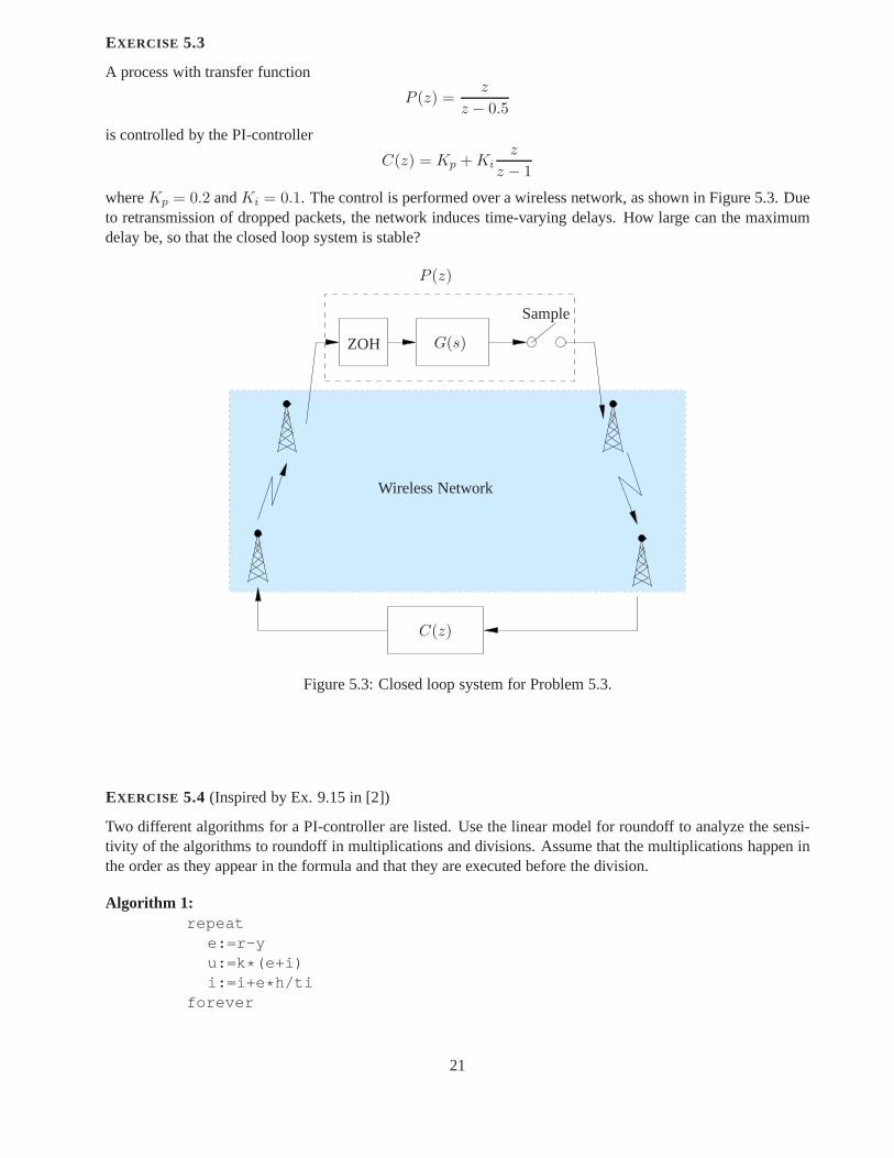
EXERCISE 5.3
A process with transfer function
P (z) =z
z − 0.5
is controlled by the PI-controller
C(z) = Kp + Kiz
z − 1
whereKp = 0.2 andKi = 0.1. The control is performed over a wireless network, as shown in Figure 5.3. Dueto retransmission of dropped packets, the network induces time-varying delays. How large can the maximumdelay be, so that the closed loop system is stable?
ZOH
Sample
G(s)
P (z)
C(z)
Wireless Network
Figure 5.3: Closed loop system for Problem 5.3.
EXERCISE 5.4 (Inspired by Ex. 9.15 in [2])
Two different algorithms for a PI-controller are listed. Use the linear model for roundoff to analyze the sensi-tivity of the algorithms to roundoff in multiplications anddivisions. Assume that the multiplications happen inthe order as they appear in the formula and that they are executed before the division.
Algorithm 1:repeat
e:=r-yu:=k*(e+i)i:=i+e*h/ti
forever
21

Algorithm 2:repeat
e:=r-yu:=i+k*ei:=k*i+k*h*e/ti
forever
EXERCISE 5.5
Consider a first-order system with the discrete transfer function
H(z) =1
1− az−1a =
1
8.
Assume the controller is implemented using fixed point arithmetic with 8 bits word length andh = 1 second.Determine the system’s unit step response for sufficient number of samples to reach steady-state. Assume thatthe data representation consists of
• 1 bit for sign
• 2 bits for the integer part
• 5 bits for the fraction part
and consider the cases of truncation and round-off.
22

Part II
Event-triggered control
23

6 Real-time operating systems
EXERCISE 6.1
In an embedded control system the control algorithm is implemented as a task in a CPU. The control taskJc
can compute the new control action only after the acquisition taskJa has acquired new sensor measurements.The two tasks are independent and they share the same CPU. Suppose the sampling period ish = 0.4 secondsand the tasks have the following specifications
Ci
Jc 0.1Ja 0.2
We assume that the periodTi and the deadlineDi are the same for the two tasks, and the release time is 0 forboth tasks.
(a) Is possible to schedule the two tasksJc andJa? Determine the schedule length and draw the schedule.
(b) Suppose that a third task is running in the CPU. The specifications for the task are
Ci Ti = Di ri
Jx 0.2 0.8 0.3
and we assume that the taskJx has higher priority than the tasksJc andJa. We also assume the CPU canhandle preemption. Are the three tasks schedulable? Draw the schedule and determine the worst-case responsetime for the control taskJc.
EXERCISE 6.2
A digital PID controller is used to control the plant, which sampled with periodh = 2 has the following transferfunction
P (z) =1
100
z − 0.1
z − 0.5.
The control law is
C(z) = 15
(
1 +z
z − 1
)
.
Assume that the control taskJc is implemented on a computer and hasCc = 1 as the worst case computationtime. Assume that a higher priority interrupt occurs at timet = 2 which has a worst case computation timeCI .Determine the largest value ofCI such that the closed loop system is stable.
EXERCISE 6.3
A robot has been designed with three different tasksJA, JB , JC , with increasing priority. The taskJA is a lowpriority thread which implements the DC-motor controller,the taskJB periodically send a "ping" through thewireless network card so that it is possible to know if the system is running. Finally the taskJC , with highestpriority, is responsible to check the status of the data bus between two I/O ports, as shown in Figure 6.3. Thecontrol task is at low priority since the robot is moving veryslowly in a cluttered environment. Since the databus is a shared resource there is a semaphore that regulates the access to the bus. The tasks have the followingcharacteristics
24

Ti Ci
JA 8 4JB 5 2JC 1 0.1
Assuming the kernel can handle preemption, analyze the following possible working condition:
• at timet = 0, the taskJA is running and acquires the bus in order to send a new control input to theDC-motors,
• at timet = 2 the taskJC needs to access the bus meanwhile the control taskJA is setting the new controlsignal,
• at the same tJB is ready to be executed to send the "ping" signal.
(a) Show graphically which tasks are running. What happens to the high priority taskJC? Compute theresponse time ofJC in this situation.
(b) Suggest a possible way to overcome the problem in (a).
I/O I/OData Bus
Dedicated Data BusNetwork Card
DC-Motors
Ping
CPU
Figure 6.3: Schedule for the control taskJc and the task handling the interrupt, of Problem 6.2.
EXERCISE 6.4 (Jackson’s algorithm, page 52 in [3])
We consider here the Jackson’s algorithm to schedule a setJ of n aperiodic tasks minimizing a quantity calledmaximum latenessand defined as
Lmax := maxi∈J
(fi − di
).
All the tasks consist of a single job, have synchronous arrival times but have different computation times anddeadlines. They are assumed to be independent. Each task canbe characterized by two parameters, deadlinedi
and computation timeCi
J = Ji|Ji = Ji(Ci, di), i = 1, . . . , n.The algorithm, also calledEarliest Due Date(EDD), can be expressed by the following rule
25

Theorem 1. Given a set ofn independent tasks, any algorithm that executes the tasks inorder of nondecreasingdeadlines is optimal with respect to minimizing the maximumlateness.
(a) Consider a set of 5 independent tasks simultaneously activated at timet = 0. The parameters are indi-cated in the following table
J1 J2 J3 J4 J5
Ci 1 1 1 3 2di 3 10 7 8 5
Determine what is the maximum lateness using the schedulingalgorithm EDD.
(b) Prove the optimality of the algorithm.
7 Real-time scheduling
EXERCISE 7.1 (Ex. 4.3 in [3])
Verify the schedulability and construct the schedule according to the rate monotonic algorithm for the followingset of periodic tasks
Ci Ti
J1 1 4J2 2 6J3 3 10
EXERCISE 7.2 (Ex. 4.4 in [3])
Verify the schedulability under EDF of the task set given in Exercise 7.1 and then construct the correspondingschedule.
EXERCISE 7.3
Consider the following set of tasks
Ci Ti Di
J1 1 3 3J2 2 4 4J3 1 7 7
Are the tasks schedulable with rate monotonic algorithm? Are the tasks schedulable with earliest deadline firstalgorithm?
26

EXERCISE 7.4
Consider the following set of tasks
Ci Ti Di
J1 1 4 4J2 2 5 5J3 3 10 10
Assume that taskJ1 is a control task. Every time that a measurement is acquired,taskJ1 is released. Whenexecuting, it computes an updated control signal and outputs it.
(a) Which scheduling of RM or EDF is preferable if we want to minimize the delay between the acquisitionand control output?
(b) Suppose thatJ2 is also a control task and that we want its maximum delay between acquisition andcontrol output to be two time steps. Suggest a schedule whichguarantees a delay of maximally two timesteps, and prove that all tasks will meet their deadlines.
EXERCISE 7.5
Consider the two tasksJ1 andJ2 with computation times, periods and deadlines as defined by the followingtable:
Ci Ti Di
J1 1 3 3J2 1 4 4
(a) Suppose the tasks are scheduled using the rate monotonicalgorithm. Will J1 andJ2 meet their deadlinesaccording to the schedulability condition on the utilization factor? What is the schedule length, i.e., theshortest time interval that is necessary to consider in order to describe the whole time evolution of thescheduler? Plot the time evolution of the scheduler when therelease time for both tasks is att = 0.
(b) If the two tasks implement a controller it is important toknow what is the worst-case delay between thetime the controller is ready to sample and the time a new inputu(kh) is ready to be released. Find theworst-case response time forJ1 andJ2. Compare with the result in (a).
EXERCISE 7.6
Consider the set of periodic tasks given in the table below:
Ci Ti Oi
J1 1 3 1J2 2 5 1J3 1 6 0
where for taski, Ci the worst-case execution time,Ti denotes the period, andOi the offset for the respectivetasks. Assume that the deadlines coincide with the period. The offset denotes the relative release time of thefirst task instance for each task. Assume that all tasks are released at time 0 with their respective offsetOi.
27

(a) Determine the schedule length.
Determine the worst-case response time for taskJ2 for each of the following three scheduling policies:
(b) Rate-monotonic scheduling
(c) Deadline-monotonic scheduling
(d) Earliest-deadline-first scheduling
EXERCISE 7.7
A control taskJc is scheduled in a computer together with two other tasksJ1 andJ2. Assume that the threetasks are scheduled using a rate monotonic algorithm. Assume that the release time for all tasks are at zero andthat the tasks have the following characteristics
Ci Ti Di
J1 1 4 4J2 1 6 6Jc 2 5 5
(a) Is the set of tasks schedulable with rate monotonic scheduling? Determine the worst-case response timefor the control taskJc.
(b) Suppose the control task implements a sampled version ofthe continuous-time controller with delay
x(t) = Ax(t) + By(t− τ)
u(t) = Cx(t)
where we letτ be the worst-case response timeRc of the taskJc. Suppose that the sampling period of thecontroller ish = 2 andRc = 3. Derive a state-space representation for the sampled controller. Suggestalso an implementation of the controller by specifying a fewlines of computer code.
(c) In order to improve performance the rate monotonic scheduling is substituted by a new scheduling al-gorithm that give highest priority to the control task and intermediate and lowest to the taskJ1 andJ2,respectively. Are the tasks schedulable in this case?
EXERCISE 7.8
Compute the maximum processor utilization that can be assigned to a polling server to guarantee the followingperiodic task will meet their deadlines
Ci Ti
J1 1 5J2 2 8
28

EXERCISE 7.9
Together with the periodic tasks
Ci Ti
J1 1 4J2 1 8
we want to schedule the following aperiodic tasks with a polling server havingTs = 5 andCs = 2. Theaperiodic tasks are
ai Ci
a1 2 3a2 7 2a3 9 1a3 29 4
EXERCISE 7.10
Consider the set of tasks in Problem 7.5, assuming that an aperiodic task could ask for CPU time. In orderto handle the aperiodic task we run a polling serverJs with computation timeCs = 3 and periodTs = 6.Assume that the aperiodic task has computation timeCa = 3 and asks for the CPU at timet = 3. Plot the timeevolution when a polling server is used together with the twotasksJ1 andJ2 scheduled as in Problem 7.5 part(a). Describe the scheduling activity illustrated in the plots.
8 Models of computation I: Discrete-event systems
EXERCISE 8.1
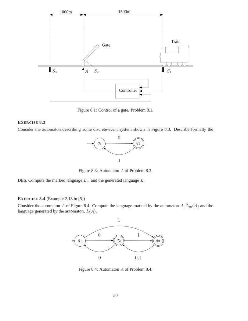
Consider the problem of controlling a gate which is lowered when a train is approaching and it is raised whenthe train has passed. We assume that the railway is unidirectional and that a train can be detected 1500m beforethe gate and 1000m after the gate. The sensors give binary outputs i.e., they give a ’0’ when the train is not overthe sensor and a ’1’ when the train is over the sensor. The gatehas a sensor which gives a binary informationand in particular gives ’0’ if the gate is (fully) closed and ’1’ if the gate is (fully) opened. Figure 8.1 showsa schema of the system. The gate needs to be lowered as soon as atrain is approaching, and raised when thetrain has passed. Model the system as a discrete-event system. Assume that trains, for safety reasons are distantfrom each other, so that no train approaches before the previous train has left.
EXERCISE 8.2
A vending machine dispenses soda for $0.45. It accepts only dimes ($0.10) and quarters ($0.25). It does notgive change in return if your money is not correct. The soda isdispensed only if the exact amount of moneyis inserted. Model the vending machine using a discrete-event system. Is it possible that the machine does notdispense soda? Prove it formally.
29
S1S2S3 A
Controller
GateTrain
1000m 1500m
Figure 8.1: Control of a gate. Problem 8.1.
EXERCISE 8.3
Consider the automaton describing some discrete-event system shown in Figure 8.3. Describe formally the
q1 q2
0
1
Figure 8.3: AutomatonA of Problem 8.3.
DES. Compute the marked languageLm and the generated languageL.
EXERCISE 8.4 (Example 2.13 in [5])
Consider the automatonA of Figure 8.4. Compute the language marked by the automatonA, Lm(A) and thelanguage generated by the automaton,L(A).
q1 q2 q3
1
0 1
0,10
Figure 8.4: AutomatonA of Problem 8.4.
30

EXERCISE 8.5 (Example 3.8 in [5])
Consider the automatonA of Figure 8.5. Determine the minimum state automaton.
a
e
b
f
c
g
0 1d
h0
11
1
0
1
0
1
0
1
00
1
0
Figure 8.5: AutomatonA of Problem 8.5.
EXERCISE 8.6 (Example 2.5 in [5])
Consider the automatonA = (q0, q1, 0, 1, δ, q0 , q1)
be a nondeterministic automaton where
δ(q0, 0) = q0, q1 δ(q0, 1) = q1 δ(q1, 0) = δ(q1, 1) = q0, q1.
Construct an deterministic automatonA′ which accept the sameLm.
9 Models of computation II: Transition systems
EXERCISE 9.1
Consider a Discrete Event System described by an automaton and model it formally as a transition system.
EXERCISE 9.2
Try to model by a transition system the basic functionalities of the keypad of a mobile phone, including thestatesmainmenu, contacts andlock.
EXERCISE 9.3 [4]
31

Queuing systems arises in many application domain such as computer networks, manufacturing, logistics andtransportation. A queuing systems is composed by three basic elements: 1) the entities, generally referred toascustomers, that do the waiting in their request for resources, 2) the resources for which the waiting is done,which are referred to asservers, and 3) the space where the waiting is done, which is defined asqueue. Typicalexamples of servers are communications channels, which have a finite capacity to transmit information. Insuch a case, the customers are the unit of information and thequeue is the amount of unit of information that iswaiting to be transmitted over the channel.
A basic queue system is reported in figure 9.3. The circle represent a server, the open box is a queuepreceding the server. The slots in the queue are waiting customers. The arrival rate of customers in the queueis denoted bya, whereas the departure rate of customers is denoted byb.
Model the queue system of figure 9.3 by a transition system. How many states has the system?
C ustom ers
A rriva ls
queue server
C ustom ers
D eparture
Figure 9.3: A basic queue system.
EXERCISE 9.4 [14]
Consider the transition systemT = S,Σ,→, SS, where the cardinality ofS is finite. The reachabilityalgorithm is
Initialization : Reach1 = ∅;Reach0 = SS;
i = 0;
Loop : While Reachi 6= Reachi−1 do
Reachi+1 = Reachi ∪ s′ ∈ S : ∃ : s ∈ Reachi, σ ∈ Σ, s→σ s′ ∈→;i = i + 1;
Prove formally that
• the reachability algorithm finishes in a finite number of steps;
• upon exiting the algorithm,Reachi = ReachT (SS).
EXERCISE 9.5 [14]
Give the Transition SystemT = S,Σ,→, SS reported in figure 9.5, describe the reach set whenSS = 3andSS = 2 by using the teachability algorithm.
32
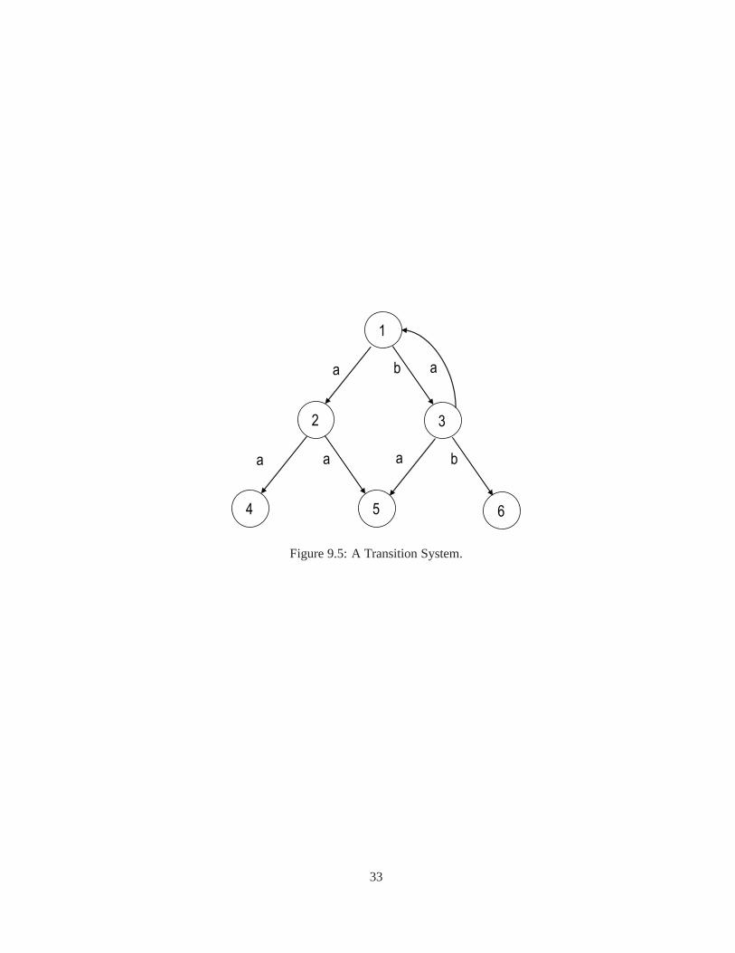
1
2 3
4 5 6
a b a
a a a b
Figure 9.5: A Transition System.
33

Part III
Hybrid control
34

10 Modeling of hybrid systems
EXERCISE 10.1
A water level in a tank is controlled through a relay controller, which senses continuously the water level andturns a pump on or off. When the pump is off the water level decreases by 2 cm/s and when it is on, the waterlevel increases by 1 cm/s. It takes 2 s for the control signal to reach the pump. It is required to keep the waterlevel between 5 and 12 cm.
(a) Assuming that the controller starts the pump when the level reaches some threshold and turns it of whenit reaches some other threshold, model the closed-loop system as a hybrid automaton.
(b) What thresholds should be used to fulfill the specifications?
EXERCISE 10.2
Consider the quantized control system in Figure 10.2. Such asystem can be modeled as a hybrid automatonwith continuous dynamics corresponding toP (s)C(s) and discrete states corresponding to the levels of thequantizer. Suppose that each level of the quantizer can be encoded by a binary word ofk bits. Then, howmany discrete statesN should the hybrid automaton have? Describe when discrete transitions in the hybridautomaton should take place.
u
u
v = Q(u)
v
C(s)
P (s)
Q D
D
2
Figure 10.2: Quantized system in Problem 10.2.
EXERCISE 10.3
A system to cool a nuclear reactor is composed by two independently moving rods. Initially the coolant temper-aturex is 510 degrees and both rods are outside the reactor core. Thetemperature inside the reactor increasesaccording to the following (linearized) system
x = 0.1x− 50.
When the temperature reaches 550 degrees the reactor mush becooled down using the rods. Three things canhappen
• the first rod is put into the reactor core
• the second rod is put into the reactor core
• none of the rods can be put into the reactor
35

For mechanical reasons a rod can be placed in the core if it hasnot been there for at least 20 seconds. If norod is available the reactor should be shut down. The two rodscan refrigerate the coolant according to the twofollowing ODEs
rod 1: x = 0.1x− 56
rod 2: x = 0.1x− 60
When the temperature is decreased to510 degrees the rods are removed from the reactor core. Model thesystem, including controller, as a hybrid system.
Reactor
Rod 1
Rod 2
Controller
Figure 10.3: Nuclear reactor core with the two control rods
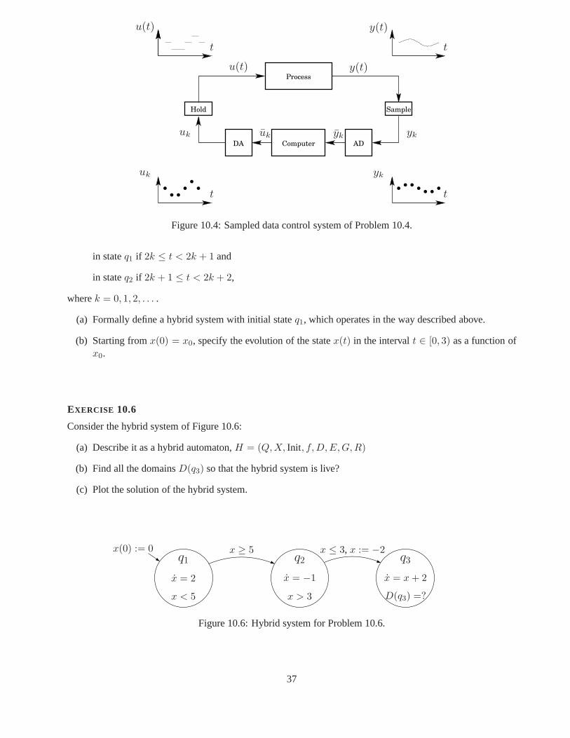
EXERCISE 10.4
Consider the classical sampled control system, shown in Figure 10.4. Model the system with a hybrid automa-ton. Suppose that the sampling period isk and that the hold circuit is a zero-order hold.
EXERCISE 10.5
Consider a hybrid system with two discrete statesq1 andq2. In stateq1 the dynamics are described by the linearsystem
x = A1x =
(−1 0p −1
)
and in stateq2 by
x = A2x =
(−1 p0 −1
)
.
Assume the system is
36
.
Hold
DA Computer AD
Sample
.. .. ..
Process
... ...
u(t)
u(t)
uk
uk uk
y(t)
y(t)
yk
ykyk
t
t
t
t
Figure 10.4: Sampled data control system of Problem 10.4.
in stateq1 if 2k ≤ t < 2k + 1 and
in stateq2 if 2k + 1 ≤ t < 2k + 2,
wherek = 0, 1, 2, . . . .
(a) Formally define a hybrid system with initial stateq1, which operates in the way described above.
(b) Starting fromx(0) = x0, specify the evolution of the statex(t) in the intervalt ∈ [0, 3) as a function ofx0.
EXERCISE 10.6
Consider the hybrid system of Figure 10.6:
(a) Describe it as a hybrid automaton,H = (Q,X, Init , f,D,E,G,R)
(b) Find all the domainsD(q3) so that the hybrid system is live?
(c) Plot the solution of the hybrid system.
x = 2
x(0) := 0q1
x < 5
x = −1
q2
x > 3
x = x + 2
q3
D(q3) =?
x ≥ 5 x ≤ 3, x := −2
Figure 10.6: Hybrid system for Problem 10.6.
37

11 Stability of hybrid systems
EXERCISE 11.1
Consider three balls with unit mass, velocitiesv1, v2, v3, and suppose that they are touching at timet = τ0, seeFigure 11.1. The initial velocity of Ball 1 isv1(τ0) = 1 and Balls 2 and 3 are at rest, i.e.,v2(τ0) = v3(τ0) = 0.
v1
Ball 1 Ball 2 Ball 3
Figure 11.1: Three balls system. The Ball 1 has velocityv1 at timet = 0.
Assume that the impact is a sequence of simple inelastic impacts occurring atτ ′0 = τ ′
1 = τ ′2 = . . . (using
notation from hybrid time trajectory). The first inelastic collision occurs atτ ′0 between balls 1 and 2, resulting
in v1(τ1) = v2(τ1) = 1/2 andv3(τ1) = 0. Sincev2(τ′1) > v3(τ
′1), Ball 2 hits Ball 3 instantaneously giving
v1(τ2) = 1/2, andv2(τ2) = v3(τ2) = 1/4. Now v1(τ′2) > v2(τ
′2), so Ball 1 hits Ball 2 again resulting in a new
inelastic collision. This leads to an infinite sequence of collisions.
(a) Model the inelastic collisions of the three-ball systemdescribed above as a hybrid automatonH =(Q,X, Init , f,D,E,G,R) with one discrete variableQ = q and three continuous variablesX =v1, v2, v3.
(b) Is the execution described above a Zeno execution? Motivate.
(c) What is the accumulation point of the infinite series of hits described above? Make a physical interpreta-tion.
EXERCISE 11.2
Consider the following system
x1
x2
x3
=
−1 0 20 −1 3−2 −3 −2
x1
x2
x3
Show, using a Lyapunov function, that the system is asymptotically stable.
EXERCISE 11.3
Consider the following theorem:
Theorem 2. A linear systemx = Ax
is asymptotically stable if and only if for any positive definite symmetric matrixQ the equation
AT P + PA = −Q
in the unknownP ∈ Rn×n has a solution which is positive definite and symmetric.
Show the necessary part of the previous theorem (i.e., theif part).
38

EXERCISE 11.4
Consider the following system
x1 = −x1 + g(x2)
x2 = −x2 + h(x1)
where the functionsg andh are such that
|g(z)| ≤ |z|/2 |h(z)| ≤ |z|/2
Show that the system is asymptotically stable.
EXERCISE 11.5
Consider the following discontinuous differential equations
x1 = −sgn(x1) + 2sgn(x2)
x2 = −2sgn(x1)− sgn(x2).
where
sgn(z) =
+1 if z ≥ 0
−1 if z < 0.
Assumex(0) 6= 0,
(a) define a hybrid automaton that models the discontinuous system
(b) does the hybrid automaton exhibit Zeno executions for every initial state?
EXERCISE 11.6
Consider the following switching system
x = aqx, aq < 0 ∀q
whereq ∈ 1, 2 and
Ω1 = x ∈ R|x ∈ [2k, 2k + 1), k = 0, 1, 2, . . . Ω2 = x ∈ R|x ∈ [2k + 1, 2k + 2), k = 0, 1, 2, . . .
Show that the system is asymptotically stable.
39

EXERCISE 11.7
Consider the following switching systemx = Aqx
whereq ∈ 1, 2 and
A1 =
(−1 00 −2
)
A2 =
(−3 00 −5
)
.
Let Ωq be such that
Ω1 = x ∈ R2|x1 ≥ 0Ω2 = x ∈ R2|x1 < 0
Show that the system is asymptotically stable.
EXERCISE 11.8
Consider the following switching systemx = Aqx
whereq ∈ 1, 2 and
A1 =
(−a1 b1
0 −c1
)
A2 =
(−a2 b2
0 −c2
)
.
Assume thatai, bi andci, i = 1, 2 are real numbers and thatai, ci > 0. Show that the switched system isasymptotically stable.
EXERCISE 11.9
Consider a system that follows the dynamicsx = A1x
for a timeǫ/2 and then switches to the system
x = A2x
for a timeǫ/2. It then switches back to the first system, and so on.
(a) Model the system as a switched system
(b) Model the system as a hybrid automaton
(c) Let t0 be a time instance at which the system begins a period in mode 1(the first system) with initialconditionx0. Determine the state att0 + ǫ/2 andt0 + ǫ.
(d) Let ǫ tend to zero (very fast switching). Determine the solution the hybrid system will tend to.
40

EXERCISE 11.10
Consider the following hybrid systemx = Aqx
where
A1 =
(−1 00 −2
)
A2 =
(−3 00 −5
)
.
Let Ωq be such that
Ω1 = x ∈ R2|x1 ≥ 0Ω2 = x ∈ R2|x1 < 0
show that the switched system is asymptotically stable using a common Lyapunov function.
EXERCISE 11.11(Example 2.1.5 page 18-19 in [12])
Consider the following switched system withq ∈ 1, 2
x = Aqx
where
A1 =
(−1 −11 −1
)
A2 =
(−1 −100.1 −1
)
.
(a) Show that is impossible to find a quadratic common Lyapunov function.
(b) Show that the origin is asymptotically stable for any switching sequence.
EXERCISE 11.12
Consider the following two-dimensional state-dependent switched system
x =
A1x if x1 ≤ 0
A2x if x1 > 0
where
A1 =
(−5 −4−1 −2
)
and A2 =
(−2 −420 −2
)
.
(a) Prove that there is not a common quadratic Lyapunov function suitable to prove stability of the system
(b) Prove that the switched system is asymptotically stableusing the multiple Lyapunov approach.
41

12 Verification of hybrid systems
EXERCISE 12.1
Consider the following linear system
x =
(−1 00 −5
)
x
Assume that the initial condition is defined in the followingset
x0 ∈ (x1, x2) ∈ R2|x1 = x2,−10 ≤ x1 ≤ 10We want to verify that no trajectories enter in aBadset defined as
Bad = (x1, x2) ∈ R| − 8 ≤ x1 ≤ 0 ∧ 2 ≤ x2 ≤ 6.
EXERCISE 12.2
Consider the following linear system
x =
(−5 −50 −1
)
x.
Assume that the initial condition lies in the following set
x0 ∈ (x1, x2) ∈ R2| − 2 ≤ x1 ≤ 0 ∧ 2 ≤ x2 ≤ 3.Describe the system as a transition system and verify that notrajectories enter aBadset defined as the trianglewith verticesv1 = (−3, 2), v2 = (−3,−3) andv3 = (−1, 0).
EXERCISE 12.3
Consider the following controlled switched system
(x1
x2
)
=
0 11
35
(x1
x2
)
+ B1u if ‖x‖ < 1
(x1
x2
)
=
0 11
3−1
3
(x1
x2
)
+
(01
)
u if 1 ≤ ‖x‖ ≤ 3
(x1
x2
)
= −
0 11
35
(x1 − 1
x2
)
+
(01
)
u
otherwise
Assume that the initial conditions arex0 ∈ x ∈ R2|‖x‖ > 3,(a) Determine a control strategy such that Reachq∪Ω1 6= ∅, i.e. Ω1 can be reached from any initial condition
whenB1 = 0.
Suppose in the followingB1 = (0, 1)T ,
(b) Is it possible to determine a linear control input such that (0, 0) is globally asymptotically stable?
(c) Construct a piecewise linear system such that(0, 0) is globally asymptotically stable.
(d) Suppose now, that we do not want that the solution of the linear system would enter theBad setΩ1.Determine a controller such that Reachq ∩Ω1 = ∅.
42

EXERCISE 12.4
A system to cool a nuclear reactor is composed by two independently moving rods. Initially the coolant temper-aturex is 510 degrees and both rods are outside the reactor core. Thetemperature inside the reactor increasesaccordingly to the following (linearized) system
x = 0.1x− 50.
When the temperature reaches 550 degrees the reactor mush becool down using the rods. Three things canhappen
• the first rod is put into the reactor core
• the second rod is put into the reactor core
• none of the rods can be put into the reactor
For mechanical reasons the rods can be placed in the core if ithas not been there for at least 20 seconds. Thetwo rods can refrigerate the coolant accordingly to the two following ODEs
rod 1: x = 0.1x− 56
rod 2: x = 0.1x− 60
When the temperature is decreased to510 degrees the rods are removed from the reactor core.
a Model the system as a hybrid system.
b If the temperature goes above 550 degrees, but there is no rod available to put down in the reactor, therewill be a meltdown. Determine if thisBadstate can be reached.
Reactor
Rod 1
Rod 2
Controller
Figure 12.4: Nuclear reactor core with the two control rods
43

a
a
a
a
b
b
c c
q0
q1 q2
q3 q4 q5 q6
Figure 13.1: The transition systemT .
13 Simulation and bisimulation
EXERCISE 13.1
Figure 13.1 shows a transition systemT = S,Σ,→, S0, SF , where
S = q0, . . . , q6Σ = a, b, c→ : According to the figure
S0 = q0SF = q3, q6.
Find the simplest quotient transition systemT that is bisimular toT .
EXERCISE 13.2
Here we should insert a problem that the students do themselves: Show a systemT and three candidatesTi.Determine which systems are bisimular toT .
44

Solutions
45

Part I
Time-triggered control
46

Solutions to review exercises
SOLUTION 1.1
Before solving the exercise we review some concepts on sampling and aliasing
Shannon sampling theorem
Let x(t) be band-limited signal that is,X(jω) = 0 for |ω| > ωm. Thenx(t) is uniquely determined by itssamplesx(kh), k = 0,±1,±2, . . . if
ωs > 2ωm
whereωs = 2π/h is the sampling frequency,h the sampling period. The frequencyws/2 is called the Nyquistfrequency.
Reconstruction
Let x(t) be the signal to be sampled. The sampled signalxs(t) is obtained multiplying the input signalx(t) bya period impulse train signalp(t), see Figure1.1. We have that
xs(t) = x(t)p(t)
p(t) =
∞∑
k=−∞δ(t − kh).
Thus the sampled signal is
xs(t) =
∞∑
k=−∞x(kh)δ(t − kh).
If we let the signalxs(t) pass through an ideal low-pass filter (see Figure 1.1.1) withimpulse response
f(t) = sinc(ws
2t)
and frequency response
F (jω) =
h, −ωs/2 < ω < ωs/2;o, otherwise.
as shown in Figure 1.1.1. The output signal is
xr(t) = xs(t) ∗ f(t) =
∫ ∞
−∞xs(t− τ)f(τ)dτ
=
∫ ∞
−∞
( ∞∑
k=−∞x(kh)δ(t − τ − kh)
)
f(τ)dτ
=∞∑
k=−∞x(kh)sinc
(ωs
2(t− kh)
)
=∞∑
k=−∞x(kh)sinc
(π
h(t− kh)
)
.
Notice that perfect reconstruction requires an infinite number of samples.Returning to the solution of the exercise we have that the Fourier transform of the sampled signal is given
by
Xs(ω) =1
h
∞∑
k=−∞X(ω + kωs)
(a) The reconstructed signal isxr(t) = cos(ω0t) sinceωs = 6ω0 > 2ω0.
47
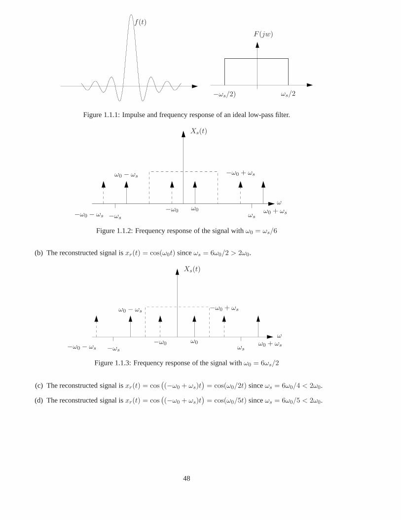
f(t)
F (jw)
−ωs/2) ωs/2
Figure 1.1.1: Impulse and frequency response of an ideal low-pass filter.
−ωs ωs
−ω0 ω0
−ω0 + ωs
ω0 + ωs−ω0 − ωs
ω0 − ωs
ω
Xs(t)
Figure 1.1.2: Frequency response of the signal withω0 = ωs/6
(b) The reconstructed signal isxr(t) = cos(ω0t) sinceωs = 6ω0/2 > 2ω0.
−ωs ωs−ω0 ω0
−ω0 + ωs
ω0 + ωs−ω0 − ωs
ω0 − ωs
ω
Xs(t)
Figure 1.1.3: Frequency response of the signal withω0 = 6ωs/2
(c) The reconstructed signal isxr(t) = cos((−ω0 + ωs)t
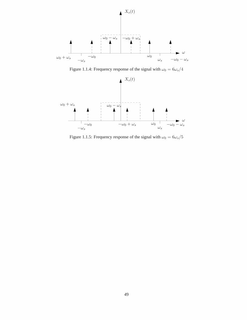
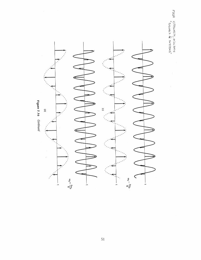
)= cos(ω0/2t) sinceωs = 6ω0/4 < 2ω0.
(d) The reconstructed signal isxr(t) = cos((−ω0 + ωs)t
)= cos(ω0/5t) sinceωs = 6ω0/5 < 2ω0.
48
−ωs ωs
−ω0 ω0
−ω0 + ωs
ω0 + ωs −ω0 − ωs
ω0 − ωs
ω
Xs(t)
Figure 1.1.4: Frequency response of the signal withω0 = 6ωs/4
−ωs ωs−ω0 ω0−ω0 + ωs
ω0 + ωs
−ω0 − ωs
ω0 − ωs
ω
Xs(t)
Figure 1.1.5: Frequency response of the signal withω0 = 6ωs/5
49

50
51

SOLUTION 1.2
We have thateAh = α0Ah + Iα1.
The eigenvalues ofAh are±ih thus we need to solve
eih = α0ih + α1
e−ih = −α0ih + α1.
This gives
α0 =eih − e−ih
2ih=
sinh
h
α1 =eih + e−ih
2= cos h.
Thus
eAh =sin h
h
(0 1−1 0
)
h + cos h
(1 00 1
)
We remind here some useful way of computing the matrix exponential of a matrixA ∈ Rn×n. Dependingon the form of the matrixA we can compute the exponential in different ways
• If A is diagonal then
A =
a11 0 . . . 00 a22 . . . 0...
.... . .
...0 0 . . . ann
⇒ eA =
ea11 0 . . . 00 ea22 . . . 0...
.... . .
...0 0 . . . eann
• A is nilpotent of orderm. ThenAm = 0 andAm+i = 0 for i = 1, 2, . . . . Then it is possible to use thefollowing series expansion to calculate the exponential
eA = I + A +A2
2!+ · · ·+ Am−1
(m− 1)!
• Using the inverse Laplace transform we have
eAt = L−1((sI −A)−1
)
• In general it is possible to compute the exponential of a matrix (or any continuous matrix functionf(A)))using the Cayley-Hamilton Theorem. For every functionf there is a polynomialp of degree less thannsuch that
f(A) = p(A) = α0An−1 + α1A
n−2 + · · ·+ αn−1I.
If the matrixA has distinct eigenvalues, then coefficientα0, . . . , αn−1 are computed solving the systemof n equations
f(λi) = p(λi) i = 1, . . . , n.
If the there is a multiple eigenvalue with multiplicititym, then the additional conditions
f (1)(λi) = p(i)(λi)
...
f (m−1)(λi) = p(m−1)(λi)
hold, wheref (i) is theith derivative with respect toλ.
52
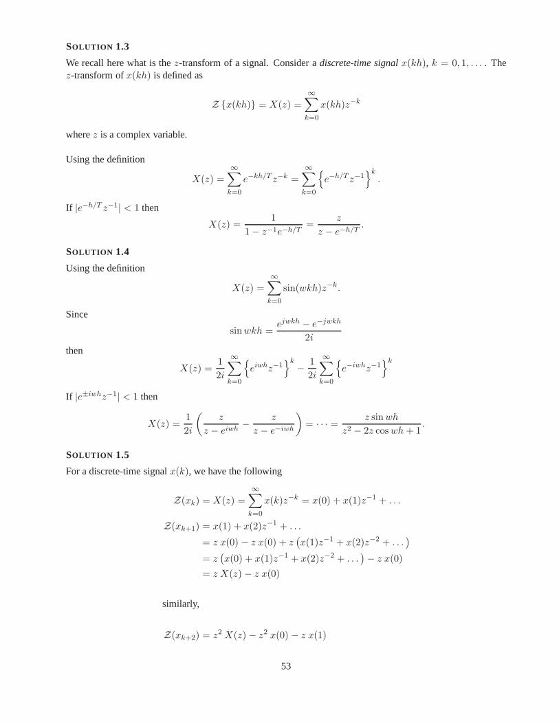
SOLUTION 1.3
We recall here what is thez-transform of a signal. Consider adiscrete-time signalx(kh), k = 0, 1, . . . . Thez-transform ofx(kh) is defined as
Z x(kh) = X(z) =
∞∑
k=0
x(kh)z−k
wherez is a complex variable.
Using the definition
X(z) =∞∑
k=0
e−kh/T z−k =∞∑
k=0
e−h/T z−1k
.
If |e−h/T z−1| < 1 then
X(z) =1
1− z−1e−h/T=
z
z − e−h/T.
SOLUTION 1.4
Using the definition
X(z) =
∞∑
k=0
sin(wkh)z−k .
Since
sin wkh =ejwkh − e−jwkh
2i
then
X(z) =1
2i
∞∑
k=0
eiwhz−1k− 1
2i
∞∑
k=0
e−iwhz−1k
If |e±iwhz−1| < 1 then
X(z) =1
2i
(z
z − eiwh− z
z − e−iwh
)
= · · · = z sin wh
z2 − 2z cos wh + 1.
SOLUTION 1.5
For a discrete-time signalx(k), we have the following
Z(xk) = X(z) =
∞∑
k=0
x(k)z−k = x(0) + x(1)z−1 + . . .
Z(xk+1) = x(1) + x(2)z−1 + . . .
= z x(0) − z x(0) + z(x(1)z−1 + x(2)z−2 + . . .
)
= z(x(0) + x(1)z−1 + x(2)z−2 + . . .
)− z x(0)
= z X(z) − z x(0)
similarly,
Z(xk+2) = z2 X(z) − z2 x(0) − z x(1)
53

The discrete step is the following function
u(k) =
0, if k < 0;1, if k ≥ 0.
ThusU(z) =
z
z − 1.
Using the previousz-transform we have
z2 Y (z)− z2 y(0)− z y(1)− 1.5z Y (z) + 1.5z y(0) + 0.5 Y (z) = z U(z)− z u(0).
CollectingY (z) and substituting the initial conditions we get
Y (z) =0.5z2 − 0.5z
z2 − 1.5z + 0.5+
z
z2 − 1.5z + 0.5U(z)
SinceU(z) = z/(z − 1) then
Y (z) =0.5z
z − 0.5+
z2
(z − 1)2(z − 0.5).
Inverse transform gives
y(k) = 0.5k+1 +
(0.5(k + 1)− 1
0.52+
0.5k+1
0.52
)
u(k − 1)
= 0.5k+1 +
(k − 1
0.5+ 0.5k−1
)
u(k − 1)
Solutions to models of sampled systems
SOLUTION 2.1
The sampled system is given by
x(kh + h) = Φx(kh) + Γu(kh)
y(kh) = Cx(kh)
where
Φ = e−ah
Γ =
∫ h
0e−asdsb =
b
a
(
1− e−ah)
.
Thus the sampled system is
x(kh + h) = e−ahx(kh) +b
a
(
1− e−ah)
u(kh)
y(kh) = cx(kh).
The poles of the sampled system are the eigenvalues ofΦ. Thus there is a real pole ate−ah. If h is smalle−ah ≈ 1. If a > 0 then the pole moves towards the origin ash increases, ifa < 0 it moves along the positivereal axis, as shown in Figure 2.1.1.
54

a > 0h incr.
a < 0h incr.
h = 0h =∞
Figure 2.1.1: Closed-loop system for Problem 2.1.
SOLUTION 2.2
(a) The transfer function can be written as
G(s) =1
(s + 1)(s + 2)=
α
s + 1+
β
s + 2=
1
s + 1− 1
s + 2.
A state-space representation (in diagonal form) is then
x =
(−1 00 −2
)
︸ ︷︷ ︸
A
x +
(11
)
︸︷︷︸
B
u
y =(1 −1
)
︸ ︷︷ ︸
C
x.
The state-space representation of the sampled system is
x(k + 1) = Φx(k) + Γu(k)
y(k) = Cx(k)
where
Φ = eAh =
(e−1 00 e−2
)
Γ =
∫ h
0eAs ds B =
∫ 1
0
(e−s
e−2sds
)
=
(1− e−1
1−e−2
2
)
sinceA is diagonal.
(b) The pulse-transfer function is given by
H(z) = C(zI − Φ)−1Γ =(1 −1
)( 1
z−e−1 0
0 1z−e−2
)(1− e−1
1−e−2
2
)
=z(3/2 + e−1 − 1/2e−2) + (3/2e−3 − e−2 − 1/2e−1)
(z − e−1)(z − e−2)
55

SOLUTION 2.3
(a) The sampled system is
x(kh + h) = Φx(kh) + Γu(kh)
y(kh) = Cx(kh)
where
Φ = eAh Γ =
∫ h
0eAhBds.
To computeeAh we use the fact that
eAh = L−1((sI −A)−1
)= L−1
(1
s2 + 1
(s 1−1 s
))
.
Since
L−1
(s
s2 + 1
)
= cos h
L−1
(1
s2 + 1
)
= sinh
then
eAh =
(cos h sin h− sin h cos h
)
.
Equivalently we can computeeAh using Cayley-Hamilton’s theorem. The matrixeAh can be written as
eAh = a0Ah + a1I
where the constantsa0 anda1 are computed solving the characteristic equation
eλk = a0λi + a1 k = 1, . . . , n
wheren is the dimension of the matrixA and λk are distinct eigenvalues of the matrixAh. In thisexample the eigenvalues ofAh are±hi. Thus we need to solve the following system of equations
eih = a0ih + a1
e−ih = −a0ih + a1
which gives
a0 =1
2hi
(
eih − e−ih)
=sin h
h
a1 =1
2
(
eih + e−ih)
= cos h.
Finally we have
eAh =sin h
h
(0 1−1 0
)
h + cos h
(1 00 1
)
=
(cos h sin h− sin h cos h
)
.
56

(b) Using Laplace transform we obtain
s2Y (s) + 3sY (s) + Y (s) = sU(s) + 3U(s).
Thus the system has the transfer function
G(s) =s + 3
s2 + 3s + 2=
2
s + 1− 1
s + 2.
One state-space realization of the system with transfer function G(s) is
x =
(−1 00 −2
)
︸ ︷︷ ︸
A
x +
(11
)
︸︷︷︸
B
u
y =(2 −1
)
︸ ︷︷ ︸
C
x.
Thus the sampled system is
x(kh + h) = Φx(kh) + Γu(kh)
y(kh) = Cx(kh)
with
Φ = eAh =
(e−h 00 e−2h
)
Γ =
∫ h
0eAsBds =
∫ h
0
(e−s
e−2s
)
ds =
(1− e−h
1−e−2h
2
)
(c) One state-space realization of the system is
x =
0 0 01 0 00 1 0
︸ ︷︷ ︸
A
x +
100
︸ ︷︷ ︸
B
u
y =(0 0 1
)
︸ ︷︷ ︸
C
x.
We need to computeΦ andΓ. In this case we can use the series expansion ofeAh
eAh = I + Ah +A2h2
2+ . . .
sinceA3 = 0, and thus all the successive powers ofA. Thus in this case
Φ = eAh =
1 0 0h 1 0
h2/2 h 1
Γ =
∫ h
0eAsBds =
∫ h
0
(1 s s2/2
)Tds =
(h h2/2 h3/6
)T
57

SOLUTION 2.4
We will use in this exercise the following relation
Φ = eAh ⇒ A =ln Φ
h
(a)y(kh) − 0.5y(kh − h) = 6u(kh− h)⇒ y(kh) − 0.5q−1y(kh) = 6q−1u(kh)
which can be transformed in state-space as
x(kh + h) = Φx(kh) + Γu(kh) = 0.5x(kh) + 6u(kh)
y(kh) = x(kh).
The continuous time system is then
x(t) = ax(t) + bu(t)
y(t) = x(t),
where, in this case sinceΦ andΓ are scalars, we have
a =ln Φ
h= − ln 2
h
b = Γ/
∫ h
0easds =
12 ln 2
h
(b)
x(kh + h) =
(−0.5 1
0 −0.3
)
︸ ︷︷ ︸
Φ
x(kh) +
(0.50.7
)
u(kh)
y(kh) =(1 1
)x(kh).
We compute the eigenvalues ofΦ
det(sI − Φ) =
(s + 0.5 −1
0 s + 0.3
)
= 0⇔ (s + 0.5)(s + 0.3) = 0
λ1 = −0.5, λ2 = −0.3.
Both eigenvalues ofΦ are on the negative real axis, thus no corresponding continuous system exists.
(c) We can proceed as in (a). In this caseΦ = −0.5 which means that the sampled system has a pole on thenegative real axis. Thus, as in (b), no corresponding continuous system exists.
SOLUTION 2.5
(Ex. 2.11 in [2])
(a) A state space representation of the transfer function is
x =
(0 00 −1
)
x +
(11
)
u
y =(1 −1
)x.
58

In this case
Φ = eAh =
(1 00 e−h
)
Γ =
∫ h
0eAsBds =
(h
1− e−h
)
(b) The pulse-transfer function is given by
H(z) = C(zI − Φ)−1Γ =(1 −1
)(
z − 1 00 z − e−h
)−1(h
1− e−h
)
=(h + e−h − 1)z + (1− e−h − he−h)
(z − 1)(z − e−h)
(c) The pulse response is
h(k) =
0, k = 0;CΦk−1Γ, k ≥ 1.
Since
Φk =(
eAh)k
= eAkh
then we have
h(k) = CΦk−1Γ =(1 −1
)(
1 0
0 e−(k−1)h
)(h
1− e−h
)
= h− e−(kh−h) + e−hk
(d) A difference equation relating input and output is obtained fromH(q).
y(kh) = H(q)u(kh) =(h + e−h − 1)q + (1− e−h − he−h)
(q − 1)(q − e−h)u(kh)
which gives
y(kh + 2h)− (1 + e−h)y(kh + h) + e−hy(kh) = (h + e−h − 1)u(kh + h) + (1− e−h − he−h)u(kh)
(e) The poles are inz = 1 andz = e−h. The second pole moves from 1 to 0 ash goes from 0 to∞. Thereis a zero in
z = −1− e−h − he−h
h + e−h − 1.
The zero moves from -1 to 0 ash increases, see Figure 2.5.1
SOLUTION 2.6
(a) We notice thatτ < h. The continuous-time system in state-space is
x = 0︸︷︷︸
A
·x + 1︸︷︷︸
B
·u(t− τ)
y = 1︸︷︷︸
C
·x
59

-0,2
-0,4
-0,6
-0,8
h
-1
20151050
Figure 2.5.1: The zero of Problem 2.5 as function ofh.
Sampling the continuous-time system with sampling periodh = 1 we get
x(k + 1) = Φx(k) + Γ0u(k) + Γ1u(k − 1)
y(k) = x(k),
where
Φ = eAh = e0 = 1
Γ0 =
∫ h−τ
0eAsdsB = 0.5
Γ1 = eA(h−τ)
∫ τ
0eAsdsB = 0.5.
The system in state space is(
x(k + 1)u(k)
)
=
(1 0.50 0
)(x(k)
u(k − 1)
)
+
(0.51
)
u(k)
y(k) =(1 0
)(
x(k)u(k − 1)
)
.
The system is of second order.
(b) The pulse-transfer function is
H(z) = C(zI − Φ)−1Γ = · · · = 0.5(z + 1)
z(z − 1).
To determine the pulse-response we inverse-transformH(z).
H(z) =0.5(z + 1)
z(z − 1)= 0.5
(
z−1 z
z − 1+ z−2 z
z − 1
)
.
60

The inverse transform ofz/(z − 1) is a step. Thus we have the sum of two steps delayed of 1 and 2time-steps, thus the pulse-response is
h(kh) =
0, k = 0;0.5, k = 1;1, k > 1.
(c) We can considerH(z) computed in (b). There are to poles, one inz = 0 and another inz = 1. There isa zero inz = −1.
SOLUTION 2.7
In this case the time delay is longer than the sampling period, τ > h. The sampled system withh = 1 is
x(k + 1) = Φx(k) + Γ0u(k − (d− 1)
)+ Γ1u(k − d)
y(k) = x(k),
where we computed as the integer such that
τ = (d− 1)h + τ ′, 0 < τ ′ ≤ h
and whereΓ0 andΓ1 are computed as in the solution of exercise 2.6, whereτ is replaced byτ ′. In this exampled = 2 andτ ′ = 0.5, and where
Φ = e−1
Γ0 = 1− e−0.5
Γ1 = e−0.5 − e−1.
A state representation is then
x(k + 1)u(k − 1)
u(k)
=
Φ Γ0 Γ1
0 0 10 0 0
x(k)u(k − 2)u(k − 1)
+
001
u(k)
y(k) =(1 0 0
)
x(k)u(k − 2)u(k − 1)
.
We still have a finite dimensional system (third order).
SOLUTION 2.8
The systemy(k)− 0.5y(k − 1) = u(k − 9) + 0.2u(k − 10)
can be shifted in time so that
y(k + 10) − 0.5y(k + 9) = u(k + 1) + 0.2u(k)
which can be written as(q10 − 0.5q9)y(k) = (q + 0.2)u(k).
Thus
A(q) = q10 − 0.5q9
B(q) = q + 0.2
61
and the system order is degA(q) = 10. We can rewrite the given system as
(1− 0.5q−1)y(k) = (1 + 0.2q−1)u(k − 9).
where
A∗(q−1) = 1− 0.5q−1
B∗(q−1) = 1 + 0.2q−1
with d = 9. Notice thatB(q)
A(q)=
q + 0.2
q10 − 0.5q9= q−9 1 + 0.2q−1
1− 0.5q−1=
B∗(q−1)
A∗(q−1)
SOLUTION 2.9
We can rewrite the systemy(k + 2)− 1.5y(k + 1) + 0.5y(k) = u(k + 1)
asq2y(k)− 1.5qy(k) + 0.5y(k) = qu(k).
We use the z-transform to find the output sequence when the input is a step, namely
u(k) =
0, k < 0;1, k ≥ 0.
wheny(0) = 0.5 andy(−1) = 1. We have
z2(Y (z)− y(0)− y(1)z−1)− 1.5z(Y (z)− y(0)
)+ 0.5Y (z) = z
(U − u(0)
).
We need to computey(1). From the given difference equation we have
y(1) = 1.5y(0) − 0.5y(−1) + u(0) = 1.25
Thus substituting in the z-transform and rearranging the terms, we get
(z2 − 1.5z + 0.5)Y (z)− 0.5z2 − 1.25z + 0.75z = zU(z) − z.
Thus we have
Y (z) =0.5z(z − 1)
(z − 1)(z − 0.5)+
z
(z − 1)(z − 0.5)U(z).
Now U(z) = z/(z − 1) this we obtain
Y (z) =0.5z
z − 0.5+
2
(z − 1)2+
1
z − 0.5.
Using the following inverse z-transforms
Z−1
(z
z − e1/T
)
= e−k/T , e−1/T = 0.5⇒ T = 1/ ln 2
Z−1
(
z−1 z
z − 0.5
)
= e−(k−1) ln 2
Z−1
(1
(z − 1)2
)
= Z−1
(
z−1 z
(z − 1)2
)
= k − 1
we gety(k) = 0.5e−k ln 2 + 2(k − 1) + e−(k−1) ln 2
62
SOLUTION 2.10
The controller can be written as
U(s) = −Uy(s) + Ur(s) = −Gy(s)Y (s) + Gr(s)R(s)
where the transfer functionsGy(s) andGr(s) are given
Gy(s) =s0s + s1
s + r1= s0 +
s1 − s0r1
s + r1
Gr(s) =t0s + t1s + r1
= t0 +t1 − t0r1
s + r1.
We need to transform this two transfer functions in state-space form. We have
xy(t) = −r1xy(t) + (s1 − s0r1)y(t)
uy(t) = xy(t) + s0y(t)
and
xr(t) = −r1xr(t) + (t1 − t0r1)r(t)
ur(t) = xr(t) + t0r(t).
The sampled systems corresponding to the previous continuous time systems, when the sampling interval inh,are
xy(kh + h) = Φxy(kh) + γyy(kh)
uy(kh) = xy(kh) + s0y(kh)
and
xr(kh + h) = Φxr(kh) + γrr(kh)
ur(kh) = xr(kh) + t0r(kh)
where
Φ = e−r1h
γy =
∫ h
0e−r1sds (s1 − s0r1) = −(e−r1h − 1)
s1 − s0r1
r1
γr =
∫ h
0e−r1sds (t1 − t0r1) = −(e−r1h − 1)
t1 − t0r1
r1.
From the state representation we can compute the pulse transfer function as
uy(kh) =
(γy
q − φy+ s0
)
y(kh)
ur(kh) =
(γr
q − φr+ t0
)
r(kh).
Thus the sampled controller in the form asked in the problem is
u(kh) = − s0q + γy − s0φy
q − φy︸ ︷︷ ︸
Hy(q)
y(kh) +t0q + γr − t0φr
q − φr︸ ︷︷ ︸
Hr(q)
r(kh).
63

SOLUTION 2.11
(Ex. 2.21 in [2]) Consider the discrete time filter
z + b
z + a
(a)
arg
(eiωh + b
eiωh + a
)
= arg
(cos ωh + b + i sin ωh
cos ωh + b + i sin ωh
)
= arctan
(sinωh
b + cos ωh
)
− arctan
(sin ωh
a + cos ωh
)
.
We have a phase lead if
arctan
(sin ωh
b + cos ωh
)
> arctan
(sin ωh
a + cos ωh
)
, 0 < ωh < π
sin ωh
b + cos ωh>
sin ωh
a + cos ωh.
Thus we have lead ifb < a.
Solutions to analysis of sampled systems
SOLUTION 3.1
The characteristic equation of the closed loop system is
z(z − 0.2)(z − 0.4) + K = 0 K > 0.
The stability can be determined using the root locus. The starting points arez = 0, z = 0.2 andz = 0.4. Theasymptotes have the directions±π/3 and−π. The crossing of the asymptotes is 0.2. To find the value ofKsuch that the root locus intersects the unit circle we letz = a + ib with a2 + b2 = 1. This gives
(a + ib)(a + ib− 0.2)(a + ib− 0.4) = −K.
Multiplying by a− ib and sincea2 + b2 = 1 we obtain
a2 − 0.6a − b2 + 0.08 + i(2ab− 0.6b) = −K(a− ib).
Equating real parts and imaginary parts we obtain
a2 − 0.6a− b2 + 0.08 = −Ka
b(2a− 0.6) = Kb.
If b 6= 0 then
a2 − 0.6a − (1− a2) + 0.087 = −a(2a + 0.6)
4a2 − 1.2a − 0.92 = 0.
Solving with respect toa we get
a = 0.15 ±√
0.0225 + 0.23 =
0.652−0.352
64

−1 −0.8 −0.6 −0.4 −0.2 0 0.2 0.4 0.6 0.8 1−1
−0.8
−0.6
−0.4
−0.2
0
0.2
0.4
0.6
0.8
1
0.8π/T
0.7π/T
0.6π/T0.5π/T
0.4π/T
0.3π/T
0.2π/T
0.1π/T
0.9
0.4π/T
0.3π/T
0.2π/T
0.1π/T
π/T
0.9π/T
0.9π/T
0.6π/T0.5π/T
0.8
0.6
0.8π/T
0.7π/T
0.1
0.7
π/T
0.5
0.2
0.3
0.4
System: H Gain: 0.705
Pole: 0.652 − 0.758i Damping: 0.00019
Overshoot (%): 99.9 Frequency (rad/sec): 0.86
Root Locus
Real Axis
Imag
inar
y A
xis
Figure 3.1.1: Root locus for the system in Problem 3.1
This givesK = 0.70 andK = −1.30. The root locus may also cross the unit circle ifb = 0 for a = ±1. Aroot atz = −1 is obtained when
−1(−1− 0.2)(−1 − 0.4) + K = 0
namely whenK = 1.68. There is a root atz = 1 whenK = −0.48. The closed loop system is stable for
K ≤ 0.70
SOLUTION 3.2
We sample the systemG(s). In order to do this we derive a state-space realization of the given system
x = u
y = x
which gives the following matrices of the sampled system
Φ = e−h 0 = 1
Γ =
∫ h
0ds = h.
The pulse transfer operator is
H(q) = C(qI − Φ)−1Γ =h
q − 1.
(a) Whenτ = 0 the regulator isu(kh) = Ke(kh)
and the characteristic equation of the closed loop system becomes
1 + C(z)H(z) = Kh + z − 1 = 0.
The system is stable if|1−Kh| < 1 ⇒ 0 < K < 2/h.
65

When there is a delay of one sample,τ = h then the characteristic equation becomes
z2 − z + Kh = 0.
The roots of the characteristic equation (the poles of the system) must be inside the unit circle for guar-anteeing stability and thus|z1| < 1 and |z2| < 1. Thus|z1||z2| = |z1z2| < 1. Sincez1z2 = Kh wehave
K < 1/h.
(b) Consider the continuous-time systemG(s) in series with a time delay ofτ seconds. The transfer functionis then
G(s) =K
se−sτ .
The phase of the system as function of the frequency is
argG(jω) = −π
2− ωτ
and the gain is
|G(jω)| = K
ω.
The system is stable if the gain is less than 1 at the cross overfrequency, which satisfies
−π
2− ωcτ = π ⇒ ωc =
π
2τ
The system is stable if
|G(jωc)| =K
ωc< 1
which yields
K <π
2τ=
∞ τ = 0π2h τ = π
The continuous-time system will be stable for all values ofK if τ = 0 and forK < π/2h whenτ = h.This value is about 50% larger than the value obtained for thesampled system in (a).
SOLUTION 3.3
(a) The observability matrix is
Wo =
(C
CΦ
)
=
(2 −41 −2
)
.
The system is not observable since rank(Wo) = 1, or detWo = 0.
(b) The controllability matrix is
Wc =(Γ ΦΓ
)=
(6 14 1
)
which has full rank. Thus the system is reachable.
66

SOLUTION 3.4
The controllability matrix is
Wc =(Γ ΦΓ
)=
(1 1 1 11 0 0.5 0
)
which has full rank (check the first two rows ofWc), thus the system is reachable. From the inputu we get thesystem
x(k + 1) =
(1 00 0.5
)
x(k) +
(01
)
v(k).
In this case
Wc =
(0 01 0.5
)
which has rank one, and thus the system is not reachable fromv.
SOLUTION 3.5
The closed loop system is
y(k) = Hcℓ(q)r(k) =C(q)H(q)
1 + C(q)H(q)r(k).
(a) WithC(q) = K, K > 0 we get
y(k) =K
q2 − 0.5q + Kr(k).
The characteristic polynomial of the closed loop system is
z2 − 0.5z + K = 0,
and stability is guaranteed if the roots of the characteristic polynomial are inside the unit circle. In general fora second order polynomial
z2 + a1z + a2 = 0
all the roots are inside the unit circle if1
a2 < 1
a2 > −1 + a1
a2 > −1− a1.
If we apply this result to the characteristic polynomial of the given systemHcℓ we get
K < 1
K > −1.5
K > −0.5
which together with the hypothesis thatK > 0 gives0 < K < 1. The steady state gain is given by
limz→1
Hcℓ(z) =K
K + 0.5.
1The conditions come from the Jury’s stability criterion applied to a second order polynomial. For details see pag. 81 in [2].
67

SOLUTION 3.6
Thez-transform of a ramp is given in Table 2, pag. 22 in [1] and we get
R(z) =z
(z − 1)2.
Using the pulse transfer function from Problem 3.5 and the final value theorem we obtain
limk→∞
e(k) = limk→∞
(r(k)− y(k)) = limz→1
z − 1
zHcℓ(z)R(z)︸ ︷︷ ︸
F (z)
if (1−z−1)F (z) does not have any root on or outside the unit circle. For theHcℓ(z) as in this case the conditionis not fulfilled. Let us consider the steady state of the first derivative of the error signale(k)
limk→∞
= limz→1
z − 1
z
z2 − 0.5z
z2 − 0.5z + K
z
(z − 1)2=
0.5
K + 0.5
which is positive, meaning that in steady state the reference and the output diverge.
SOLUTION 3.7
(a) (i) - Poles are mapped asz = esh. This mapping maps the left half plane on the unit circle
(b) (i) - The right half plane is mapped outside the unit circle
(c) (ii) - Consider the harmonic oscillator:
x =
(0 1−1 0
)
x +
(01
)
u
y =(1 0
)x
which is controllable since
Wc =
(0 11 0
)
has full rank. If we sampled with sampling periodh we get
x(kh + h) =
(cos ωh sin ωh− sin ωh cos ωh
)
x(kh) +
(1− cos ωh
sinωh
)
︸ ︷︷ ︸
Γ
u(kh)
y(kh) =(1 0
)x(kh)
If we chooseh = 2π/ω thenΓ is the 0 vector and clearly the system is not controllable.
(d) (ii) - as in (c) we can find example sampling periods that make the system not observable.
SOLUTION 3.8
The open loop system has pulse transfer operator
H0 =1
q2 + 0.4q
and the controller is proportional, thusC(q) = K.
68
(a) The closed loop system has pulse transfer operator
Hcℓ =KH0
1 + KH0=
K
q2 + 0.4q + K.
From the solution of Problem 3.5 we know that the poles are inside the unit circle if
K < 1
K > −1 + 0.4
K > −1− 0.4 ⇒ −0.6 < K < 1
(b) Lete(k) = r(k)− y(k) thenE(z) = (1−Hcℓ) R(z).
If K is chosen such that the closed loop system is stable, the final-value theorem can be used and
limk→∞
e(k) = limz→1
z − 1
z
1
1 + KH0R(z) =
z − 1
z
z2 + 0.4z
z2 + 0.4z + K
z
z − 1=
1.4
1.4 + K
If for example we chooseK = 0.5 thenlimk→∞ e(k) = 0.74.
SOLUTION 3.9
The closed loop system has the following characteristic equation
det(zI − (Φ− ΓL)) = z2−(a11+a22−b2ℓ2−b1ℓ1)z+a11a22−a12a21+(a12b2−a22b1)ℓ1+(a21b1−a11b2)ℓ2.
This must be equal to the given characteristic equations, thus(
b1 b2
a12b2 − a22b1 a21b1 − a11b2
)(ℓ1
ℓ2
)
=
(p1 + tr Φ
p2 − det Φ
)
where trΦ = a11 + a22 anddetΦ = a11a22 − a12a21. The solution is(
ℓ1
ℓ2
)
=1
∆
(a21b1 − a11b2 −b2
−a12b2 + a22b1 b1
)(p1 + tr Φ
p2 − detΦ
)
where∆ = a21b21 − a12b
22 + b1b2(a22 − a11). To check when∆ = 0 we consider the controllability matrix of
the system
Wc =(Γ ΦΓ
)=
(b1 a11b1 + a12b2
b2 a21b1 + a22b2
)
and we find that∆ = detWc. There exists a solution to the system of equation above if the system is control-lable, since then the rank of the controllability matrix is full anddetWc 6= 0.
For the double integratora11 = a12 = a22 = b2 = 1 anda21 = 0 andb1 = 0.5. In order to design an deadbeat controller we need to place the poles in zero, thusp1 = p2 = 0. This yields
(ℓ1
ℓ2
)
= −1
(−1 −1−0.5 −0.5
)(2−1
)
=
(1
1.5
)
.
SOLUTION 3.10
In this case the characteristic equation is
(z − 0.1)(z − 0.25) = z2 − 0.35z + 0.025.
Using the result from Problem 3.9 we find that∆ = 0.5 andL is obtained from
LT =
(ℓ1
ℓ2
)
=1
∆
(0.5 00.1 1
)(0.75−0.025
)
=
(0.750.1
)
.
69

SOLUTION 3.11
(a) The static observer gives
x(k) = Φn−1W−1o
y(k − n + 1)...
y(k)
+(Φn−2Γ Φn−3Γ . . . Γ
)− Φn−1W−1
o
0 0 . . . 0CΓ 0 . . . 0
CΦΓ CΓ . . . 0...
..... .
...CΦn−2Γ CΦn−3Γ . . . CΓ
︸ ︷︷ ︸
Wu︸ ︷︷ ︸
Ψ
u(k − n + 1)...
u(k − 1)
.
In this case we have
Wo =
(C
CΦ
)
=
(0 1
0.22 1
)
W−1o =
(−4.55 4.55
1 0
)
Wu =
(0
CΓ
)
=
(0
0.03
)
Ψ = Γ−ΦW−1o Wu
=
(0.220.03
)
−(
0.78 00.22 1
)(−4.55 4.55
1 0
)(0
0.03
)
=
(0.114
0
)
.
Thus we get
x(k) = ΦW−1o
(y(k − 1)
y(k)
)
+ Ψu(k − 1)
=
(−3.55 3.55
0 1
)(y(k − 1)
y(k)
)
+
(0.114
0
)
u(k − 1).
(b) The dynamic observer has the form
x(k + 1|k) = (Φ−KC)x(k|k − 1) + Γu(k) + Ky(k).
We chooseK such that the the eigenvalues ofΦ −KC are in the origin (very fast observer). Using theresults in Problem 3.9 where we useΦT andCT instead ofΦ andΓ, we obtain
K =
(2.771.78
)
.
(c) The reduced observer has the form
x(k|k) = (I −KC) [Φx(k − 1|k − 1) + Γu(k − 1)] + Ky(k).
In this case we want to findK such that
– CK = 1
– (I −KC)Φ has the eigenvalues in the origin.
70

The first condition imposesk2 = 1. Since
(I −KC)Φ =
(0.78 − 0.22k1 −k1
0 0
)
in order to have eigenvalues in the origin we need to choosek1 = 0.78/0.22 = 3.55. The reducedobserver is then
x(k|k) =
(0 −3.550 0
)
x(k − 1|k − 1) +
(0.114
0
)
u(k − 1) +
(3.551
)
y(k).
Sincex2(k|k) = y(k) the we get
x(k|k) =
(−3.55 3.55
0 1
)(y(k − 1)
y(k)
)
+
(0.114
0
)
u(k − 1)
which is the same as the static observer computed in (a).
SOLUTION 3.12
The constant disturbancev(k), which typically has high energy at low frequencies, can be described by thedynamical system
w(k + 1) = Aww(k)
v(k) = Cww(k),
where the matrixAw typically has eigenvalues at the origin or on the imaginary axis. We consider the aug-mented state vector
z =
(xw
)
.
The augmented system ca be described by(
xw
)
=
(A Cw
0 Aw
)(xw
)
+
(B0
)
u
y =(C 0
)(
xw
)
Sampling the system gives the following discrete-time system(
x(k + 1)w(k + 1)
)
=
(Φ Φxw
0 Φw
)(x(k)w(k)
)
+
(Γ0
)
u(k)
y(k) =(C 0
)(
x(k)w(k)
)
where
w(k + 1) = Φww(k)
v(k) = Cww(k),
andΦxw relatesx(k + 1) andw(k). In this exercise the disturbance can be modeled by the system
w(k + 1) = w(k)
v(k) = w(k),
and the process is described by
Φw = 1
Φxw =
(10
)
.
71

(a) If the statex and the disturbancev can be measured then we can use the controller
u(k) = −Lx(k)− Lww(k).
This gives the closed loop system
x(k + 1) = Φx(k) + Φxww(k) − ΓLx(k)− ΓLww(k)
y(k) = Cx(k)
In general it is not possible to eliminate completely the influence ofw(k). This is possible only ifΦxw − ΓLw = 0. We will therefore consider the situation at the output in steady state
y(∞) = C (I − (Φ− ΓL))−1 (Φxw − ΓLw)w(∞) = Hw(1)w(∞).
The influence ofw (or v) can be zero in steady state if
Hw(1) = 0.
Let φij the(i, j) element ofΦ− ΓL andγi theith element ofΓ. Then
C (I − (Φ − ΓL))−1 (Φxw − ΓLw) = −1− Lwγ1 − φ22 + φ22Lwγ1 − φ12Lwγ2
−1 + φ22 + φ11 − φ11φ22 + φ12φ21= 0
yields
Lw =−1 + φ22
−γ1 + φ22γ1 − φ12γ2.
If L is the feedback matrix that gives a dead beat controller, that is
L =(3.21 5.57
)
such that
Φ− ΓL =
(−0.142 −0.1140.179 0.142
)
then we haveLw = 5.356.
(b) In this case the state is measurable, but not the disturbance. The disturbance can be calculated from thestate equation
Φxww(k − 1) = x(k)−Φx(k − 1)− Γu(k − 1).
The first element of this vector gives
w(k − 1) = (1 0) (x(k)− Φx(k − 1)− Γu(k − 1)) .
Sincew(k) is constant andx(k) is measurable, it is possible to calculatew(k) = w(k − 1) . Thefollowing control law can then be used
u(k) = −Lx(k)− Lww(k)
whereL and Lw are the same as in (a). Compared with the controller in (a) there is a delay in thedetection of the disturbance.
72

(c) If only the output is measurable then the state and the disturbance can be estimated by using the followingobserver:
(x(k + 1)w(k + 1)
)
=
(Φ Φxw
0 1
)(x(k)w(k)
)
+
(Γ0
)
u(k) +
(KKw
)
ǫ(k)
ǫ(k) = y(k)− Cx(k).
The gainsK andKw can be determined so that the error goes to zero, provided that the augmentedsystem is observable. Letx(k) = x(k)− x(k) and similarlyw(k) = w(k)− w(k). Then
(x(k + 1)w(k + 1)
)
=
(Φ−KC Φxw
−KwC 1
)(x(k)w(k)
)
.
The characteristic equation of the system matrix for the error is
z3 + (k1 − 2.2)z2 + (1.05 − 1.7k1 + k2 + kw)z + 0.7k1 + 0.15 − 0.7kw − k2 = 0.
The eigenvalues can be placed at the origin if
K =
(2.2−0.64
)
Kw = 3.33.
The controller isu(k) = −Lx(k) − Lww(k)
whereL andLw are the same as (a).
SOLUTION 3.13
(a) The eigenvalues of the matrixA are
λ1 = −0.0197
λ2 = −0.0129.
The matrices of the sampled system are
Φ = eAh =
(0.790 00.176 0.857
)
Γ =
(0.2810.0296
)
(b) The pulse transfer operator is given by
H(q) = C(qI − Φ)−1Γ =(0 1
)(
q − 0.790 0−0176 q − 0.857
)−1(0.281 0.0297
)=
0.030q + 0.026
q2 − 1.65q + 0.68
(c) The poles of the continuous-time system are at -0.0197 and -0.0129. The observer should be twice as fast asthe fastest mode of the open-loop system, thus we choose the poles of the observer in
z = e−0.0192·2·12 = 0.62.
The desired characteristic equation ofΦ−KC is then
z2 − 1.24z + 0.38 = 0.
Using the results from Problem 3.9 we obtain
K =(0.139 0.407
).
73

SOLUTION 3.14
(a) The sampled system is
x(k + 1) = Φx(k) + Γu(k)
y(k) = x(k)
where
Φ = e−5
Γ =1− e−5
5.
(b) In order to to prove stability with Lyapunov argument we need to choose a Lyapunov functionV . LetV = |x|. The increment of the Lyapunov function is then
∆V = |x+| − |x| = |e−5x| − |x| = (e−5 − 1)|x| ≤ 0.
sinceu(k) = 0. Since∆V ≤ 0, then the system is stable. We actually know that the system isasymptotically stable, since the pole is inside the unit circle. We can conclude onasymptoticalstabilityusing the Lyapunov argument, noticing that∆V < 0 if x 6= 0. Thus the system is asymptotically stable.
SOLUTION 3.15
(a) The sampled system is
x(k + 1) = Φx(k) + Γu(k)
y(k) = x(k)
where
Φ =
(e−1 00 e−2
)
Γ =
1− e−1
1− e−2
2
.
(b) The characteristic polynomial is
(z − 0.1)(z − 0.2) = z2 − 0.3z + 0.02.
Using the result from Problem 3.9 we obtain
(ℓ1
ℓ2
)
=1
−0.0636
−e−11− e−2
2−1− e−2
2−e−2(1− e−1) 1− e−1
(−0.3 + e−1 + e−2
0.02 − e−1e−2
)
=
(0.30590.0227
)
(c) The closed loop system is
x(k + 1) =
(0.1745 −0.0143−0.1323 0.1255
)
︸ ︷︷ ︸
Φc
x(k).
74

We consider the following Lyapunov function
V (x) = xT x
then∆V (x) = xT ΦT
c Φcx− xT x = xT (ΦTc Φc − I)
︸ ︷︷ ︸
Ω, symmetric
x.
Since the eigenvalues of the symmetric matrixΩ are negative then∆V ≤ 0. Thus the closed loopsystem is stable. Notice that∆V < 0 if x 6= 0 thus the closed loop system is asymptotically stable (theeigenvalues are placed in 0.1 and 0.2).
Solutions to computer realization of controllers
SOLUTION 4.1
(a) The characteristic polynomial of the closed loop systemis equal to the numerator of1 + HHc, that is,
z2 + (K + Ki − 2.5)z −K + 1.
The poles of the closed-loop system are in the origin if
K + Ki − 2.5 = 0
−K + 1 = 0
which yieldsK = 1 andKi = 1.5.
(b) We can use the following partial fraction expansion forHc(z)
Hc(z) = M +N
z − 1.
With simple calculations we obtainM = 2.5 andN = 1.5. Thus the state-space representation of thecontroller is
x(k + 1) = x(k) + e(k)
u(k) = 1.5x(k) + 2.5e(k)
SOLUTION 4.2
(a) Using Euler’s method we get
H(z) =a
(z − 1)/h + a=
ah
z − 1 + ah.
This corresponds to the difference equation
y(kh + h) + (ah− 1)y(kh) = a h u(kh).
The difference equation is stable if
|ah− 1| < 1 ⇒ 0 < h < 2/a.
The approximation may be poor even if the difference equation is stable.
75

(b) Tustin’s approximation gives
H(z) =a
2
h
z − 1
z + 1+ a
=(z + 1ah/2)
(1 + ah/2)z + (ah/2 − 1)
=ah/2
1 + ah/2
z + 1
z +ah/2 − 1
ah/2 + 1
.
The pole of the discrete-time system will vary from 1 to - 1 when h varies from 0 to∞. The discrete-timeapproximation is always stable ifa > 0.
(c) Tustin’s approximation with prewarping gives
H(z) =a
αz − 1
z + 1+ a
=a/α
1 + a/α
z + 1
z +a/α − 1
a/α − 1
where
α =a
tan(ah/2).
SOLUTION 4.3
(a) Euler’s method gives
H(z) = 4(z − 1)/h + 1
(z − 1)/h + 2= 4
z − 1 + h
z − 1 + 2h= 4
z − 0.75
z − 0.5
(b) Backward differences give
H(z) = 4(z − 1)/(zh) + 1
(z − 1)/(zh) + 2= 4
z(1 + h)− 1
z(1 + 2h) + 1= 3.33
z − 0.80
z − 0.667
(c) Tustin’s approximation gives
H(z) = 4
2
h
z − 1
z + 1+ 1
2
h
z − 1
z + 1+ 2
= 4z(1 + h/2) − (1− h/2)
z(1 + h)− (1− h)= 3.6
z − 0.778
z − 0.6
(d) Tustin’s approximation with pre-warping
H(z) = 4α
z − 1
z + 1+ 1
αz − 1
z + 1+ 2
= 4z(1 + 1/α) − (1− 1α)
z(1 + 2/α) − (1− 2/α)= 3.596
z − 0.775
z − 0.596
All the four approximation has the form
H(z) = Kz + a
z + b.
76

The gain and phase atω = 1.6rad/s are obtained from
H(eiωh) = Keiωh + a
eiωh + b= K
(eiωh + a)(e−iωh + b)
(eiωh + b)(e−iωh + b)
= K1 + ab + (a + b) cos(ωh) + i(b− a) sin(ωh)
1 + b2 + 2b cos(ωh)
argH(eiωh) = arctan(b− a) sin ωh
1 + ab + (a + b) cos(ωh)
|H(eiωh)| = K
√
1 + a2 + 2a cos(ωh)
1 + b2 + 2b cos(ωh).
The four different approximations give atω = 1.6rad/s the following results
|H(.)| argH(.) Rel. err. |.| Rel. err. arg(.)
Continuous-time (no approx.) 2.946680646 0.3374560692Euler 2.966414263 0.4105225474 0.67% 21.65%Backward 2.922378065 0.2772636846 -0.82% -17.83%Tustin 2.959732059 0.3369122161 0.44% -0.16%Tustin with prewarping 2.946680646 0.3374560692 0.0% 0.0%
SOLUTION 4.4
The tank process in Problem 2.13 has the transfer function
G(s) =0.000468
(s + 0.0197)(s + 0.0129)
(a) At the desired cross-over frequency we have
|G(iωc)| = 0.525
argG(iωc) = −115.
We use a PI controller in the form
F (s) =K(T s + 1)
T s
and we have the following specifications atωc
– gain 1/0.525
– phase -15.
This givesK = 1.85 andT = 149.
(b) The characteristic equation of the closed loop system is
s2 + 0.0326s2 + 0.00112s + 5.91 10−6 = 0
which has rootss1,2 = −0.0135 ± i0.0281 ands3 = −0.006. The complex poles have a damping ofζ = 0.43. The zero of the closed loop system is−0.0062.
77

(c) Tustin’s approximation with given warping is
Hc(z) =
1.85
(
αz − 1
z + 1+ 0.0067
)
αz − 1
z + 1
=1.85(α + 0.0067)
α
(
1 +0.0134
(α + 0.0067)(z − 1)
)
.
The rule of thumb for the selection of the sampling period gives
h ≈ 6 − 20sec.
The choice ofh = 12 seems to be reasonable. This givesα = 0.165 and
Hc(z) = 1.925
(
1 +0.0778
z − 1
)
.
SOLUTION 4.5
The sample and zero-order hold circuit can be approximate bya delay ofh/2 seconds. Indeed the output of thezero-order hold is
uh(t) = u(kh), kh < t < kh + h
u(kh)
u(kh)
ZOHuh(t)uh(t)
t
t
Figure 4.5.1: The zero-order hold.
If u(kh) = δ(kh) thenuh(t) is the impulse response of the ZOH filter. In this case the output, let us call it,uδ
h(t) is a pulse of height1 and durationh i.e.,
uδh(t) = (1(t)− 1(t− h)) .
The Laplace transform of the impulse response is the transfer function of the ZOH filter, which is
ZOH(s) = Luδh(t) =
∫ ∞
0
1
h(1(t) − 1(t− h)) e−stdt = (1− e−sh)/s.
When we sample a signal we have a scaling factor of1/h, as
Xs(jω) =1
h
∞∑
k=−∞X(j(ω + kωs)).
78

Thus for smallh we have
SAMPLE(s) · ZOH(s) =1
h
(1− e−sh)
s=
1− 1 + sh− (sh)2/2 + . . .
sh= 1− sh
2+ · · · ≈ e−sh/2
which is approximately a delay ofh/2. If we assume a decrease of the phase margin of5 − 15, then
∆φZOH = ωch/2 =180ωch
2π=
ωch
0.035= 5 − 15,
which then givesωch = 0.17 − 0.52
orωch ≈ 0.15 − 0.5.
SOLUTION 4.6
Consider the general problem of controlling a continuous-time system
x(t) = Ax(t) + Bu(t)
y(t) = Cx(t)
with the continuous-time controller
u(t) = Mr(t)− Lx(t).
The closed-loop system is
x(t) = (A−BL)x(t) + BMr(t) = Acx(t) + BMr(t)
y(t) = Cx(t).
If r(t) is constant over one sampling period, then the previous equation can be sampled, giving
x(kh + h) = Φcx(kh) + ΓcMr(kh)
y(kh) = Cx(kh), (0.0)
where
Φc = eAch
Γc =
∫ h
0eAcsdsB.
Let us assume that the controlleru(kh) = Mr(kh)− Lx(kh)
is used to control the sampled system
x(kh + h) = Φx(kh) + Γu(kh)
y(kh) = Cx(kh),
where
Φ = eAh
Γ =
∫ h
0eAhdsB.
79

In this case the closed-loop system is
x(kh + h) = (Φ − ΓL)x(kh) + ΓMr(kh)
y(kh) = Cx(kh). (0.0)
It is in general not possible to chooseL such that
Φc = Φ− ΓL.
However, we can make a series expansion and equate terms. Assume
L = L0 + L1h/2
thenΦc ≈ I − (A−BL)h +
(A2 −BLA−ABL− (BL)2
)h2/2 + . . .
andΦ− ΓL ≈ I + (A−BL0)h +
(A2 −ABL0 − (BL1)
2)h2/2 + . . .
The systems (0.0) and (0.0) have the same poles up to and including orderh2 if
L = L (I + (A−BL)h/2) .
The modification onM is determined by assuming the steady-state values of (0.0) and (0.0) are the same. Letthe reference be constant and assume that the steady-state value of the state isx0. This gives the relations
(I − Φc)x0 = ΓcMr
and (
I − (Φ− ΓL))
x0 = ΓMr
The series expansion of the left-hand sides of these two relations are equal for power ofh up to and includingh2.Then, we need to determineM so that the expansions of the right-hands are the same forh andh2. Assuming
M = M0 + M1h/2
thenΓcM ≈ BMh + (A−BL)BMh2/2 + . . .
andΓM ≈ BM0h + (BM1 −ABM0)h
2/2 + . . . ,
which givesM = (I − LBh/2)M.
(a) We need to computeL andM , which are
L = L
(1 h/2−h/2 1− h
)
=(1 2
)(
1 h/2−h/2 1− h
)
=(0.8 1.7
)
M = 2− 2h = 1.6
(b) The backward difference approximation gives
1− q−1
hx(kh) = (A−KC)x(kh) + Bu(kh) + Ky(kh)
(I −Ah−KCh)x(kh) = q−1x(kh) + Bu(kh) + Ky(kh).
80

Let
Φ0 = (I −Ah−KCh)−1 =1
h2 + h + 1
(1 h−h 1 + h
)
.
This gives,
x(kh) = (Φ0x(kh− h) + Φ0Bu(kh) + Φ0Ky(kh)
=
(0.81 0.16−0.16 0.97
)
x(kh− h) +
(0.030.19
)
u(kh) +
(0.190.16
)
y(kh).
(c) Simulate the continuous-time controller and the discrete-time approximation. Letx(0) = (1, 1)T andx(t) = (0, 0)T .
SOLUTION 4.7
(a) To obtain the forward difference approximation we substitutes = q−1h in the continuous-time expression.
We obtain
u(kh) = −s0q − s0 + hs1
q + r1h− 1y(kh) +
t0q − t0 + ht1q + r1h− 1
r(kh)
(b) In order to compare the discretizations we examine the location of the controller pole. We use the graphavailable in order to compute the poles for the exact discretization. We have the following results:
Discretization h = 0.01 h = 0.1 h = 1
Exact 0.9048 0.3679 0.00004540Forward difference 0.9 0 -9
We notice that the forward difference approximation yieldsan unstable system forh = 1 (pole in -9).Forh = 0.1, the forward difference approximation gives a pole at the origin, which corresponds to a onestep delay. Thus this approximations of the continuous-time controller cannot be considered satisfactory.For h = 0.01 the pole of the forward difference approximation is very closed to the exact discretizationwhich means that this is a better choice.
We could also consider how the sampling interval relates to the dominating time constant of the system.We know that the relation between this two parameters is given by the following rule-of-thumb
Nr =Tr
h≈ 4− 10.
In this case only the controller dynamics are available, butusing the time constant of the controller thatis Tc = 1/r1 = 0.1 we see that only forh = 0.01 the rule-of-thumb is fulfilled.
SOLUTION 4.8
(a) The backward differences approximation substitutess with (z − 1)/zh. We can consider the Laplacetransform of the controller’s equation yields
sX(s) = AX(s) + BE(s)
U(s) = CX(s) + DE(s)
Substitutings with (z − 1)/zh we get the following equations
x(k + 1)− x(k) = hAx(k + 1) + hBe(k + 1)
u(k) = Cx(k) + De(k).
81

We consider first the state update equation. Dividing the signals at timek + 1 andk we get the following
x(k + 1)− hAx(k + 1)− hBe(k + 1) = x(k) =: w(k + 1).
Solving this equation forx in terms ofw ande we get
x(k + 1) = (I − hA)−1w(k + 1) + (I − hA)−1Bhe(k + 1)
thus, sincew(k + 1) = x(k) we get
w(k + 1) = (I − hA)−1w(k) + (I − hA)−1Bhe(k).
This gives that
Φc = (I − hA)−1
Γc = (I − hA)−1Bh.
From the output equation substitutingx(k) we get directly
u(k) = C(I − hA)−1 + D + C(I − hA)−1Bhe(k).
Thus
H = C(I − hA)−1
J = D + C(I − hA)−1Bh.
(b) To compute the Tustin’s approximation we proceed in the same way, and we substitutes with 2(z −1)/(h(z + 1)). The state equation then becomes
x(k + 1)− x(k) =Ach
2
(x(k + 1)− x(k)
)+
Bch
2(e(k + 1) + e(k)).
Again collecting thek + 1 terms on one side we get
x(k + 1)− Ah
2x(k)− Bh
2e(k + 1) = x(k) +
Ah
2x(k) +
Bh
2e(k)
=: w(k + 1).
Thus we can derivex(k + 1) from the previous equation as function ofw(k + 1) ande(k + 1)
x(k + 1) = (I − Ah
2)−1w(k + 1)− (I − Ah
2)−1 Bh
2e(k + 1).
The state equation becomes
w(k + 1) = (I +Ah
2)(I − Ah
2)−1
︸ ︷︷ ︸
Φc
w(k) +((I +
Ah
2)(I − Ah
2)−1 + I
)Bh
2︸ ︷︷ ︸
Γc
e(k).
The output equation becomes
u(k) = C(I − Ah
2)−1
︸ ︷︷ ︸
Hc
w(k) + D + C(I − Ah
2)−1 Bh
2
︸ ︷︷ ︸
Jc
e(k).
Notice that is possible to writeΓc in a more compact way as follows
((I +
Ah
2)(I − Ah
2)−1 + I
)Bh
2=((I +
Ah
2) + (I − Ah
2))(I − Ah
2)−1 Bh
2
= (I − Ah
2)−1 Bh
2.
82
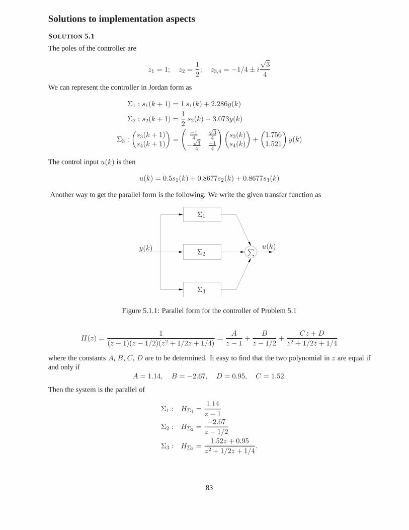
Solutions to implementation aspects
SOLUTION 5.1
The poles of the controller are
z1 = 1; z2 =1
2; z3,4 = −1/4± i
√3
4
We can represent the controller in Jordan form as
Σ1 : s1(k + 1) = 1 s1(k) + 2.286y(k)
Σ2 : s2(k + 1) =1
2s2(k) − 3.073y(k)
Σ3 :
(s3(k + 1)s4(k + 1)
)
=
(−14
√3
4
−√
34
−14
)(s3(k)s4(k)
)
+
(1.7561.521
)
y(k)
The control inputu(k) is then
u(k) = 0.5s1(k) + 0.8677s2(k) + 0.8677s3(k)
Another way to get the parallel form is the following. We write the given transfer function as
u(k)y(k)
Σ1
Σ2
Σ3
∑
Figure 5.1.1: Parallel form for the controller of Problem 5.1
H(z) =1
(z − 1)(z − 1/2)(z2 + 1/2z + 1/4)=
A
z − 1+
B
z − 1/2+
Cz + D
z2 + 1/2z + 1/4
where the constantsA, B, C, D are to be determined. It easy to find that the two polynomial inz are equal ifand only if
A = 1.14, B = −2.67, D = 0.95, C = 1.52.
Then the system is the parallel of
Σ1 : HΣ1=
1.14
z − 1
Σ2 : HΣ2=−2.67
z − 1/2
Σ3 : HΣ3=
1.52z + 0.95
z2 + 1/2z + 1/4.
83

y(kh)P (z)
C(z)
∆
Figure 5.3.1: Closed loop system for Problem 5.3.
SOLUTION 5.2
(a) The closed loop system fromr to y shown in Figure has the following transfer function
H(s) =Cs(s)P (s)e−sτ
1 + Cs(s)P (s)e−sτ.
In order to findCs(s) we need to solveH(s) = Hcℓ(s) which gives
Cs(s)P (s)e−sτ
1 + Cs(s)P (s)e−sτ=
C(s)P (s)
1 + C(s)P (s)e−sτ
Cs(s)(1 + C(s)P (s)
)= C(s)
(1 + Cs(s)P (s)e−sτ
)
Cs(s) =C(s)
1 + C(s)P (s)− C(s)P (s)e−sτ
(b) We first findC(s):
C(s)1
s + 1
1 + C(s)1
s + 1
e−sτ =8
s2 + 4s + 8⇒ C(s) =
8s + 8
s2 + 4s.
Using the result in (a) we get
Cs(s) =8(s + 1)
s2 + 4s + 8(1− e−sτ )
SOLUTION 5.3
The control problem over wireless network can be represented as shown Figure 5.3.1. The delay∆ is such that
∆(y(kh)) = y(kh− d(k)) d(k) ∈ 0, . . . , N
The closed loop system is stable if∣∣∣∣
P (eiω)C(eiω)
1 + P (eiω)C(eiω)
∣∣∣∣<
1
N |eiω − 1| ω ∈ [0, 2π]
whereN is the number of samples that the control signal is delayed. Notice that the previous result is valid ifthe closed loop transfer function is stable. In this case theclosed loop transfer function is stable with poles
z1 = 1, z2 = 0.861, z3 = 0.5, z4 = 0.447.
If we plot the bode diagram of the closed loop system without delay versus the function1/(N |eiω − 1|) fordifferent values ofN we obtain the results shown in Figure 5.3.2. It can be seen that the closed loop system isstable ifN ≤ 3. Thus the maximum delay is 3 samples. Notice that the result is only a sufficient condition.This means that it might be possible that the system is stablefor larger delays than 3 samples.
84
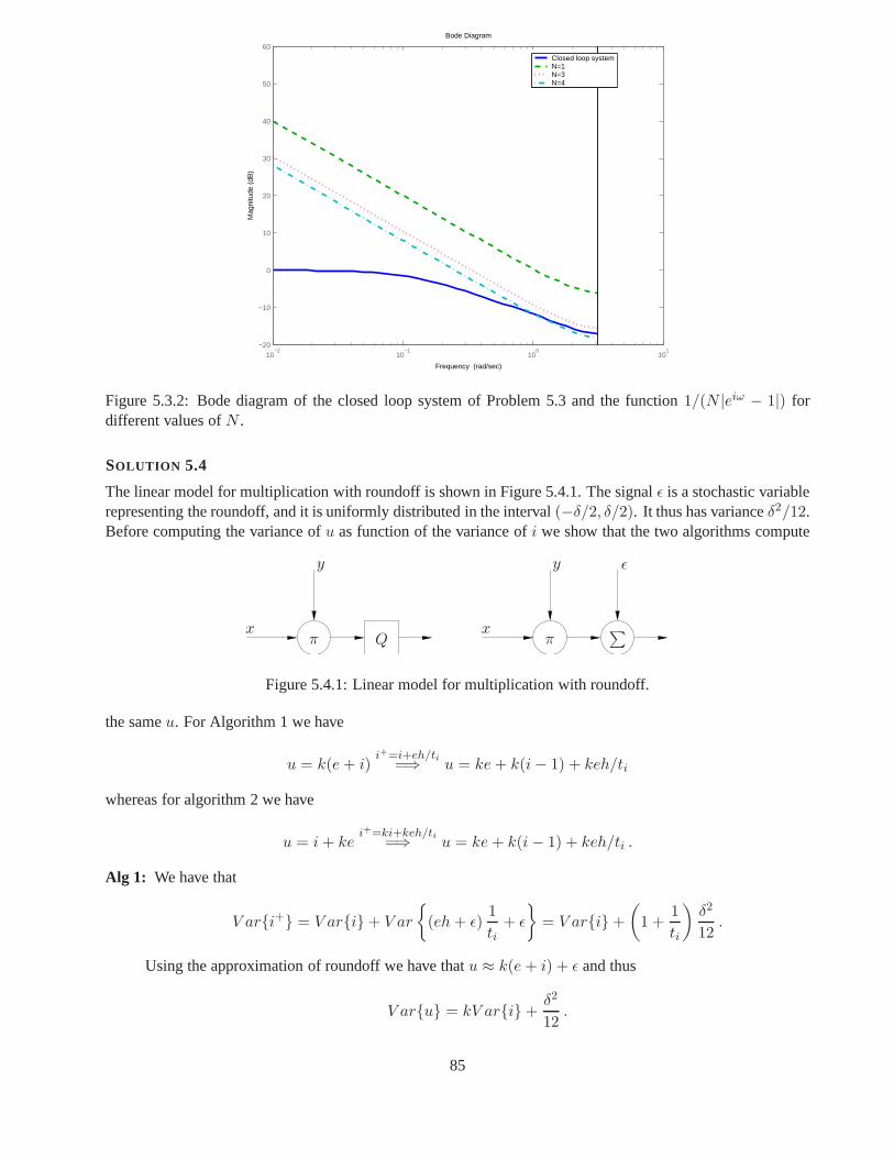
10−2
10−1
100
101
−20
−10
0
10
20
30
40
50
60
Mag
nitu
de (
dB)
Closed loop systemN=1N=3N=4
Bode Diagram
Frequency (rad/sec)
Figure 5.3.2: Bode diagram of the closed loop system of Problem 5.3 and the function1/(N |eiω − 1|) fordifferent values ofN .
SOLUTION 5.4
The linear model for multiplication with roundoff is shown in Figure 5.4.1. The signalǫ is a stochastic variablerepresenting the roundoff, and it is uniformly distributedin the interval(−δ/2, δ/2). It thus has varianceδ2/12.Before computing the variance ofu as function of the variance ofi we show that the two algorithms compute
xx
y y
Q
ǫ
ππ∑
Figure 5.4.1: Linear model for multiplication with roundoff.
the sameu. For Algorithm 1 we have
u = k(e + i)i+=i+eh/ti
=⇒ u = ke + k(i− 1) + keh/ti
whereas for algorithm 2 we have
u = i + kei+=ki+keh/ti
=⇒ u = ke + k(i− 1) + keh/ti .
Alg 1: We have that
V ari+ = V ari+ V ar
(eh + ǫ)1
ti+ ǫ
= V ari+
(
1 +1
ti
)δ2
12.
Using the approximation of roundoff we have thatu ≈ k(e + i) + ǫ and thus
V aru = kV ari+δ2
12.
85

Alg 2: We have that
V ari+ = kV ari+δ2
12+ V ar
((ke + ǫ)h + ǫ)1
ti+ ǫ
= kV ari+
(
2 +h
ti+
1
ti
)δ2
12.
Using the approximation of roundoff we have thatu ≈ i + ke + ǫ and thus
V aru = V ari+δ2
12.
If we considerV ari+ = αV ari+ f(δ2)
then aftern iteration we have that
V arin =
(n−1∑
i=0
αi
)
f(δ2) ,
where we have consideredV ari0 = 0. Thus we have that
Alg 1: In this case
V arin = n
(
1 +1
ti
)δ2
12
and thus
V arun =
(
kn +kn
ti+ 1
)δ2
12
Alg 2: In this case
V arin =
(n−1∑
i=0
ki
)(h
ti+
1
ti+ 2
)δ2
12
and thus
V arun =
(kn − 1
k − 1
)(h
ti+
1
ti+ 2
)δ2
12+
δ2
12
In order to compare the two algorithms, we assumeh = ti = 1. (This is just for comparison, since multiplica-tion with 1 normally does not add any roundoff error.) We thenhave for the two algorithms, that
V aru(1)n = (2kn + 1)δ2
12
V aru(2)n =
(
4kn − 1
k − 1+ 1
)δ2
12.
If we assumek < 1 andn large then
4kn − 1
k − 1+ 1 ≈ 4
1− k+ 1
and thus
2kn + 1 >4
1− k+ 1
which allows to conclude that the first algorithm is worst than the second. Ifk > 1 andn large then
4kn − 1
k − 1+ 1 ≈ kn
k − 1
and thus2kn(k − 1) + 1 < kn
which allows to conclude that in this case the second algorithm is worst than the first.
86
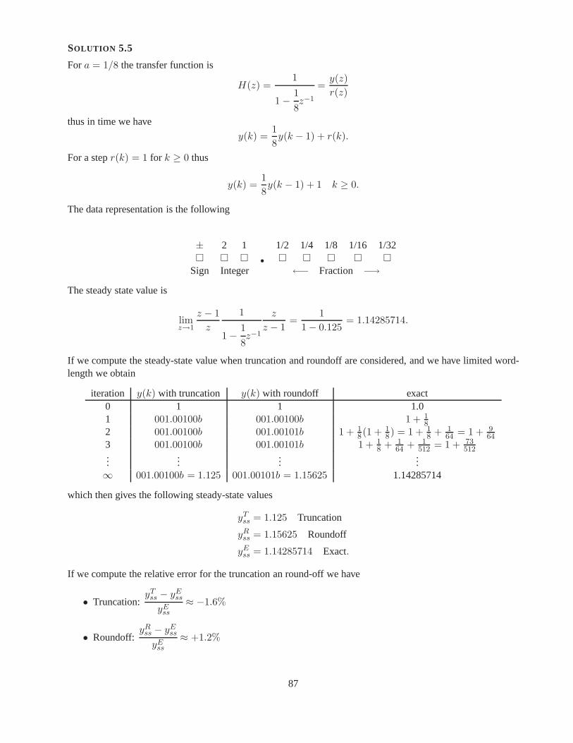
SOLUTION 5.5
Fora = 1/8 the transfer function is
H(z) =1
1− 1
8z−1
=y(z)
r(z)
thus in time we have
y(k) =1
8y(k − 1) + r(k).
For a stepr(k) = 1 for k ≥ 0 thus
y(k) =1
8y(k − 1) + 1 k ≥ 0.
The data representation is the following
± 2 1 1/2 1/4 1/8 1/16 1/32 •
Sign Integer ←− Fraction −→The steady state value is
limz→1
z − 1
z
1
1− 1
8z−1
z
z − 1=
1
1− 0.125= 1.14285714.
If we compute the steady-state value when truncation and roundoff are considered, and we have limited word-length we obtain
iteration y(k) with truncation y(k) with roundoff exact0 1 1 1.01 001.00100b 001.00100b 1 + 1
82 001.00100b 001.00101b 1 + 1
8 (1 + 18) = 1 + 1
8 + 164 = 1 + 9
643 001.00100b 001.00101b 1 + 1
8 + 164 + 1
512 = 1 + 73512
......
......
∞ 001.00100b = 1.125 001.00101b = 1.15625 1.14285714
which then gives the following steady-state values
yTss = 1.125 Truncation
yRss = 1.15625 Roundoff
yEss = 1.14285714 Exact.
If we compute the relative error for the truncation an round-off we have
• Truncation:yT
ss − yEss
yEss
≈ −1.6%
• Roundoff:yR
ss − yEss
yEss
≈ +1.2%
87

Part II
Event-triggered control
88

Solutions to real-time operating systems
SOLUTION 6.1
(a) The two tasks are not independent in this particular casehowever. We first compute the CPU utilization
U =
n∑
i=1
Ci
Ti=
Cc
Tc+
Ca
Ta
where the periodTc = Ta = h. The two tasks needs to be finished within the new sampling interval. Thus wehave
U =0.1
0.4+
0.2
0.4= 0.75
thus the CPU is utilized 75% of the time. We still do not know ifit is possible to schedule the tasks so thatthey meet their deadlines. In order to do this we calculate the schedule length and we draw the schedule. Theschedule length is
lcmTa, Tc = 0.4
0 0.1 0.2 0.3 0.4
Ja Jc
Figure 6.1.1: Schedule for the two tasksJa andJc of Problem 6.1.
(b) The utilization factor in this case is
U =0.1
0.4+
0.2
0.4+
0.2
0.8= 1
Thus the CPU will be fully occupied. In order to see if the tasks are schedulable we draw the schedule. In thiscase the schedule length is
lcmTa, Tc, Tx = 0.8.
Notice thatJx starts after 3 time steps since the release time isrx = 0.3. The worst case response time for thecontrol taskJc is 0.4 as is can be seen from Figure 6.1.2.
SOLUTION 6.2
In a closed loop with a delay we know that the stability is guaranteed if
∣∣∣∣
P (eiω)C(eiω)
1 + P (eiω)C(eiω)
∣∣∣∣<
1
N |eiω − 1| ω ∈ [0, π]
whereN = ⌈Rc/h⌉, with Rc the worst case response time of the control taskJc caused by the high prioritytask.
From the previous equation we have immediately that
N <|1 + P (eiω)C(eiω)||eiω − 1||P (eiω)C(eiω)|
89

0
0
0
0.1
0.1
0.1
0.2
0.2
0.2
0.3
0.3
0.3
0.4
0.4
0.4
0.5
0.5
0.5
0.6
0.6
0.6
0.7
0.7
0.7
0.8
0.8
0.8
Ja
Jc
Jx
Figure 6.1.2: Schedule for the two tasksJa, Jc andJx of Problem 6.1.
and this should hold for allω ∈ [0, π]. We have that the magnitude of the closed loop transfer function is
∣∣∣∣
P (eiω)C(eiω)
1 + P (eiω)C(eiω)
∣∣∣∣= 3
|10eiω − 1||130eiω − 103|
and thus we have that
N <1
3
|130eiω − 103||(eiω − 1)(10eiω − 1)|
for all ω ∈ [0, π]. This means that
N < minω∈[0,π]
1
3
|130eiω − 103||(eiω − 1)(10eiω − 1)|
Since the right hand side of the previous inequality can be regarded as the magnitude of a transfer function withone zero and two poles on the positive real axis, it is clear the minimum is atω = π.
Thus we have that
N <1
3
|130eiω − 103||(eiω − 1)(10eiω − 1)|
∣∣∣∣ω=π
≈ 3.53 .
SinceN is an integer then we have thatN = 3. Thus we have thatRc = 2N = 6.We know that the worst case computation time for the control task isCc = 1 with periodTc = h = 2. and
that the high priority task is not released until timet = 2. The worst case response time for the control task isgiven by
Rc = Cc + CI
which than givesCI = 5. The schedule in this case looks as in Figure 6.2.1. As we can notice the control taskmisses its deadlines att = 4 andt = 6. The control task is then delayed and the worst case responsetime isexactlyRc = 6, which represents the maximum delay of the control task.
SOLUTION 6.3
(a) The situation is depicted in Figure 6.3.1. Let us consider the single instances.
0) The taskJA is released and its starts its computations. The bus is locked.
1) The taskJC requires to be executed. Since it has high priority the CPU preempts the taskJA.
90

0
0
1
1
2
2
3
3
4
4
5
5
6
6
7
7
8
8
9
9
10
10
11
11
Jc
JI
Interrupt
Figure 6.2.1: Schedule for the control taskJc and the task handling the interrupt, of Problem 6.2.
JA
JB
JC
0 1
2
3
45
Figure 6.3.1: Priority inversion. Problem 6.3
2) SinceJC needs to access the bus, and this resource is occupied by the taskJA the taskJC is stopped.At the same time taskJB asks for CPU time, and sinceJC is stopped and it has higher priority ofJA, JB can be executed. The execution ofJB preventsJA to release the bus.
3) The taskJB with medium priority has finished to be executed and the CPU isgiven to the taskJA.
4) TaskJA finishes to write on the bus, and it releases it.
5) TaskJC finally can use the bus and it is scheduled by the CPU.
What we can see from this particular situation is that a high priority task asJC is blocked by a lowpriority task. We have a situation calledpriority inversion. The response time for the high priority taskJC in this case isRC = 4.1.
(b) A possible way to overcome the problem is to use thepriority inheritance protocol. In this case the taskJA inherits the priority of the task which has higher priority and needs to use the blocked resource. ThetaskJA, thus acquires high priority and is able to release the resource as soon as possible, so that the highpriority taskJC can be served as soon as possible. The priorities are set to the default one, once the busis released.
SOLUTION 6.4
(a) Using the EDD algorithm the tasks are scheduled considering the deadlines. Those that have earlydeadline are scheduled first. From the table given in the problem we see that the order of scheduling
91

isJ1 → J5 → J3 → J4 → J2.
The schedule is shown in Figure 6.4.1. The maximum lateness is equal to−1 due to taskJ4. The fact
d1 d5 d3 d4 d2
0 1 2 3 4 5 6 7 8 9 10
J1 J2J3 J4J5
Figure 6.4.1: Jackson’s scheduler
that the lateness is negative means that all the tasks meet their deadlines.
(b) Letσ be a schedule produced by any algorithmA. If A is different from EDD, then there exist two tasksJa andJb with da < db with Jb scheduled before the taskJa. Now, letσ′ be a schedule obtained fromσby exchangingJa with Jb in the scheduleσ, so thatJa is scheduled beforeJb in σ′. If we exchangeJa
with Jb in σ the maximum lateness cannot increase. In fact for the schedule σ we have that the maximumlateness is
Lmaxab= fa − da
as can be seen from Figure 6.4.2.
a0
σ
σ′
fb f ′a f ′
b = fa da db
Jb
Jb
Ja
Ja
Figure 6.4.2: Jackson’s scheduling - proof
In σ′ we have thatL′
maxab= max(L′
a, L′b).
We can have two possible cases
– L′a ≥ L′
b, thenL′maxab
= L′a = f ′
a − da, and sincef ′a < fa then we haveL′
maxab< Lmaxab
,
– L′a ≤ L′
b, thenL′maxab
= L′b = f ′
b−db = fa−db, and sinceda < db we have thatL′maxab
< Lmaxab.
Since in both casesL′maxab
< Lmaxab, then we can conclude that interchanging the tasksJa andJb in
σ we cannot increase the lateness of a set of tasks. By a finite number of such transpositions,σ can betransformed inσEDD. Since at each step the lateness cannot increase,σEDD is optimal.
92

Solutions to real-time scheduling
SOLUTION 7.1
Notice that the four assumptions under which the schedulability test can be use are satisfied. We can rememberhere the assumptions
A1 the instances of the taskJi are regularly activated at constant rate,
A2 all instances of the periodic taskJi have the same worst case execution timeCi,
A3 all instances of a periodic taskJi have the same relative deadline, which is equal to the period,
A4 all tasks are independent i.e., there are no precedence relations and no resource constraints.
The schedulability test gives
U =1
4+
2
6+
3
10= 0.8833 0.7798 = 3(21/3 − 1)
thus we cannot conclude if it is possible to schedule the three tasks. We need to use the necessary condition,which ensures that the tasks are schedulable if the worst-case response time is less than the deadline. Thepriority is assigned so thatJ1 has highest priority,J2 medium priority andJ3 lowest priority. The analysisyields
R1 = C1 = 1 ≤ D1 = 4
for taskJ2 we have
R02 = C2 = 2
R12 = C2 +
⌈R0
2
T1
⌉
C1 = 2 + 1 = 3
R22 = C2 +
⌈R1
2
T1
⌉
C1 = 2 + 1 = 3 ≤ D2 = 6
for taskJ3 we have
R03 = C3 = 3
R13 = C3 +
⌈R0
3
T1
⌉
C1 +
⌈R0
3
T2
⌉
C2 = 3 + 2 + 1 = 6
R23 = C3 +
⌈R1
3
T1
⌉
C1 +
⌈R1
3
T2
⌉
C2 = 3 + 2 + 2 = 7
R33 = C3 +
⌈R2
3
T1
⌉
C1 +
⌈R2
3
T2
⌉
C2 = 3 + 2 + 2 = 9
R43 = C3 +
⌈R3
3
T1
⌉
C1 +
⌈R3
3
T2
⌉
C2 = 3 + 3 + 4 = 10
R54 = C3 +
⌈R4
3
T1
⌉
C1 +
⌈R4
3
T2
⌉
C2 = 3 + 3 + 4 = 10 ≤ D3 = 10
Thus the three tasks are schedulable with rate monotonic. The schedule length is given by
lcm(T1, T2, T,3 ) = 60
The schedule is shown in figure 7.1.1.
93
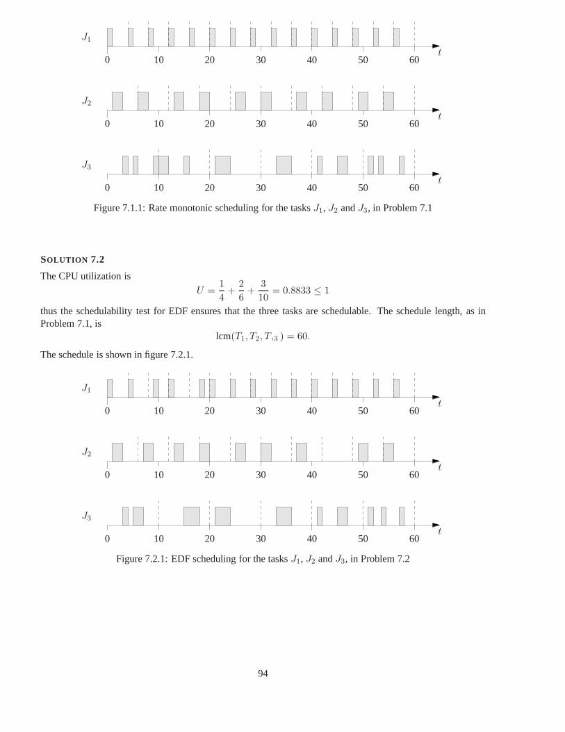
0
0
0
10
10
10
20
20
20
30
30
30
40
40
40
50
50
50
60
60
60
J1
J2
J3
t
t
t
Figure 7.1.1: Rate monotonic scheduling for the tasksJ1, J2 andJ3, in Problem 7.1
SOLUTION 7.2
The CPU utilization is
U =1
4+
2
6+
3
10= 0.8833 ≤ 1
thus the schedulability test for EDF ensures that the three tasks are schedulable. The schedule length, as inProblem 7.1, is
lcm(T1, T2, T,3 ) = 60.
The schedule is shown in figure 7.2.1.
0
0
0
10
10
10
20
20
20
30
30
30
40
40
40
50
50
50
60
60
60
J1
J2
J3
t
t
t
Figure 7.2.1: EDF scheduling for the tasksJ1, J2 andJ3, in Problem 7.2
94
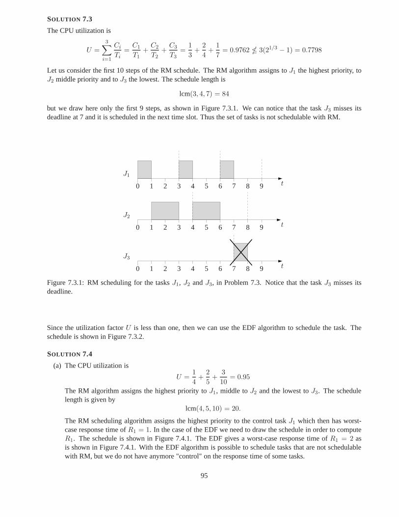
SOLUTION 7.3
The CPU utilization is
U =3∑
i=1
Ci
Ti=
C1
T1+
C2
T2+
C3
T3=
1
3+
2
4+
1
7= 0.9762 3(21/3 − 1) = 0.7798
Let us consider the first 10 steps of the RM schedule. The RM algorithm assigns toJ1 the highest priority, toJ2 middle priority and toJ3 the lowest. The schedule length is
lcm(3, 4, 7) = 84
but we draw here only the first 9 steps, as shown in Figure 7.3.1. We can notice that the taskJ3 misses itsdeadline at 7 and it is scheduled in the next time slot. Thus the set of tasks is not schedulable with RM.
0
0
0 1
1
1
2
2
2
3
3
3
4
4
4
5
5
5
6
6
6
7
7
7
8
8
8
9
9
9
J1
J2
J3
t
t
t
Figure 7.3.1: RM scheduling for the tasksJ1, J2 andJ3, in Problem 7.3. Notice that the taskJ3 misses itsdeadline.
Since the utilization factorU is less than one, then we can use the EDF algorithm to schedulethe task. Theschedule is shown in Figure 7.3.2.
SOLUTION 7.4
(a) The CPU utilization is
U =1
4+
2
5+
3
10= 0.95
The RM algorithm assigns the highest priority toJ1, middle toJ2 and the lowest toJ3. The schedulelength is given by
lcm(4, 5, 10) = 20.
The RM scheduling algorithm assigns the highest priority tothe control taskJ1 which then has worst-case response time ofR1 = 1. In the case of the EDF we need to draw the schedule in order to computeR1. The schedule is shown in Figure 7.4.1. The EDF gives a worst-case response time ofR1 = 2 asis shown in Figure 7.4.1. With the EDF algorithm is possible to schedule tasks that are not schedulablewith RM, but we do not have anymore "control" on the response time of some tasks.
95

0
0
0
10
10
10
20
20
20
30
30
30
40
40
40
50
50
50
60
60
60
70
70
70
80
80
80
84
84
84
J1
J2
J3
t
t
t
Figure 7.3.2: EDF scheduling for the tasksJ1, J2 andJ3, in Problem 7.3. Notice that all the tasks meet theirdeadlines.
0
0
0
1 2 3 4 5
5
6 7 8 9 10
10
10
11 12 13 14 15
15
16 17 18 19 20
20
20
J1
J2
J3
R1c
t
t
t
Figure 7.4.1: EDF scheduling for the tasksJ1, J2 andJ3 in Problem 7.4.
(b) In order to haveR2 = 1 we need to assign the highest priority to the task 2. We then give toJ1 middlepriority andJ3 the lowest. The tasks meet their deadline if the worst-case response time is less than thedeadline. In this case we have
R2 = C2 = 2 ≤ D1 = 5
for taskJ1 we have
R01 = C1 = 1
R11 = C1 +
⌈R0
1
T2
⌉
C2 = 1 + 2 = 3
R21 = C1 +
⌈R1
1
T2
⌉
C2 = 1 + 2 = 3 ≤ D1 = 4
96

for taskJ3 we have
R03 = C3 = 3
R13 = C3 +
⌈R0
3
T1
⌉
C1 +
⌈R0
3
T2
⌉
C2 = 3 + 1 + 2 = 6
R23 = C3 +
⌈R1
3
T1
⌉
C1 +
⌈R1
3
T2
⌉
C2 = 3 + 2 + 4 = 9
R33 = C3 +
⌈R2
3
T1
⌉
C1 +
⌈R2
3
T2
⌉
C2 = 3 + 3 + 4 = 10
R43 = C3 +
⌈R3
3
T1
⌉
C1 +
⌈R3
3
T2
⌉
C2 = 3 + 3 + 4 = 10 ≤ D3 = 10
Thus the three tasks are schedulable. The schedule is shown in Figure 7.4.2
0
0
0 1 2 3 4
5
5 6 7 8 9 10
10
10
11 12 13 14
15
15 16 17 18 19 20
20
20
J1
J2
J3
t
t
t
Figure 7.4.2: Fixed-priority scheduling for the tasksJ1, J2 andJ3, in Problem 7.4.J2 in this case has thehighest priority.
SOLUTION 7.5
(a) The tasks will meet their deadlines since the schedulability condition for RM scheduling is fulfilled:
U =
2∑
i=1
Ci
Ti=
C1
T1+
C2
T2=
7
12< 2(21/2 − 1
)≈ 0.8
The schedule length is equal to lcm(T1, T2) = 12. The time evolution is shown in Figure 7.5.1.
(b) The worst-case response time for the higher priority tasks is given by the worst-case computation time.ThusR1 = C1 = 1. For the second task we the worst-case response time is computed by
R2 = C2 +
⌈R2
T1
⌉
C1.
97

0
0 1 2 3 4
4
5 6 7 8
8
9 10 11 12
12
J1
J2
t
t
Figure 7.5.1: Rate monotonic scheduling for the tasksJ1 andJ2, in Problem 7.5
In order to solve the equation we need to use an iterative procedure. LetR02 = 0, then
R12 = C2 +
⌈R0
2
T1
⌉
C1 = C2 = 1
R22 = C2 +
⌈R1
2
T1
⌉
C1 = C2 + C1 = 2
R23 = C2 +
⌈R2
2
T1
⌉
= C2 + C1 = 2.
ThusR2 = 2. This agrees with the time evolution plotted in (a).
SOLUTION 7.6
Since the tasks have an offsetOi we cannot use the response time formula for rate-monotonic since itassumes that all tasks are released simultaneously at time 0. We need to solve the problem drawing theschedule.
(a) In order to draw the schedule for the three tasks we need tocompute the schedule length. The schedulelength is the least common multiple (l.c.m.) of the task periods plus the offset. The l.c.m. is 30, thus theschedule length is 30+1=31.
(b) Rate-monotonicThe rate-monotonic assigns the priority so thatJ1 has the highest priority,J2 medium priority andJ3 thelowest.
J1
J2
J3
t
t
t
0
1
1
4
6
6
7 10
11
12
13 16
16
18
19
21
22
24
25
26
28
30
31
31
31
Thus the worst-case response time for taskJ2 is R2 = 3.
(c) Deadline-monotonicThe deadlines agree by assumption with the periods, so deadline-monotonic scheduling is identical torate-monotonic scheduling. Thus the worst-case response time for taskJ2 is R2 = 3.
98
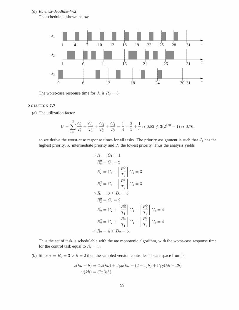
(d) Earliest-deadline-firstThe schedule is shown below.
J1
J2
J3
t
t
t
0
1
1 4
6
6
7 10
11
12
13
16
16
18
19
21
22
24
25
26
28
30 31
31
31
The worst-case response time forJ2 is R2 = 3.
SOLUTION 7.7
(a) The utilization factor
U =3∑
i=1
Ci
Ti=
C1
T1+
C2
T2+
C3
T3=
1
4+
2
5+
1
6≈ 0.82 3(21/3 − 1) ≈ 0.76.
so we derive the worst-case response times for all tasks. Thepriority assignment is such thatJ1 has thehighest priority,Jc intermediate priority andJ2 the lowest priority. Thus the analysis yields
⇒ R1 = C1 = 1
R0c = Cc = 2
R1c = Cc +
⌈R0
c
T1
⌉
C1 = 3
R2c = Cc +
⌈R1
c
T1
⌉
C1 = 3
⇒ Rc = 3 ≤ Dc = 5
R02 = C2 = 2
R12 = C2 +
⌈R0
2
T1
⌉
C1 +
⌈R0
2
Tc
⌉
Cc = 4
R22 = C2 +
⌈R1
2
T1
⌉
C1 +
⌈R1
2
Tc
⌉
Cc = 4
⇒ R2 = 4 ≤ D2 = 6.
Thus the set of task is schedulable with the ate monotonic algorithm, with the worst-case response timefor the control task equal toRc = 3.
(b) Sinceτ = Rc = 3 > h = 2 then the sampled version controller in state space from is
x(kh + h) = Φx(kh) + Γ0y(kh− (d− 1)h) + Γ1y(kh− dh)
u(kh) = Cx(kh)
99

whereτ = (d − 1)h + τ ′ with τ ′ ≤ h andd ∈ N. Thus if we choosed = 2 we getτ ′ = 1. The statespace description becomes
x(kh + h)y(kh− h)
y(kh)
=
Φ Γ1 Γ0
0 0 I0 0 0
x(kh)y(kh− 2h)y(kh− h)
+
00I
y(kh)
u(kh) =(C 0 0
)
x(kh)y(kh− 2h)y(kh− h)
A sketch of a computer program is given below. Notice that we assume that initial values ofx(0),y(−2h), y(−h) are known.
Computer Code
y=arrayy(-1),y(-2);nexttime = getCurrentTime();k = 0;while truedo
new_y=AD_conversion();x(k) = Φx(k − 1) + Γ1y(k − 3) + Γ0y(k − 2);u(k) = Cx(k);DA_conversion();y(k) =new_y;k = k + 1;nexttime = nexttime + h;sleepUntil(nexttime);
end while
(c) The set of tasks will be schedulable if the worst-case response time,Ri is less than theDi for i ∈ 1, 2, cIn this case the control task has the highest priority,J1 intermediate priority andJ2 the lowest priority.The analysis yields
⇒ Rc = Cc = 2
R01 = C1 = 1
R11 = C1 +
⌈R0
1
Tc
⌉
Cc = 3
R21 = C1 +
⌈R1
1
Tc
⌉
Cc = 3
⇒ R1 = 3 ≤ D1 = 4
R02 = C2 = 1
R12 = C2 +
⌈R0
2
Tc
⌉
Cc +
⌈R0
2
T1
⌉
C1 = 4
R22 = C2 +
⌈R1
2
Tc
⌉
Cc +
⌈R1
2
T1
⌉
C1 = 4
⇒ R2 = 4 ≤ D2 = 6.
Thus the tasks are schedulable even if the taskJc is a high priority task. In doing this the delayτ is thenequal toRc = 2.
100

SOLUTION 7.8
The schedulability of periodic tasks can be guaranteed by evaluating the interference by the polling server onperiodic execution. In the worst case, such an interferenceis the same as the one introduced by an equivalentperiodic task having a period equal toTs and computation time equal toCs. Independently of the number ofaperiodic tasks handled by the server, a maximum time equal to Cs is dedicated to aperiodic requests at eachserver period. The utilization factor of the polling serveris Us = Cs/Ts and hence the schedulability of aperiodic set withn tasks and utilizationUp can be guaranteed if
Up + Us ≤ (n + 1)(21/(n+1) − 1)
Thus we need to have
Us ≤ (n + 1)(21/(n+1) − 1)− Up = (n + 1)(21/(n+1) − 1)−n∑
i=1
Ci
Ti
which in this case is
Us ≤ 3(21/3 − 1)− 1
5− 2
8≈ 0.3298 ⇒ Umax
s = 0.3298
SOLUTION 7.9
The tasks and the polling server can be scheduled since we computed the maximum utilization as
U =
2∑
i=1
Ci
Ti+
Cs
Ts=
1
4+
2
8+
1
5= 0.77 ≤ 3(21/3 − 1) = 0.78
The schedule is shown is Figure 7.9.1
SOLUTION 7.10
The polling server has periodTs = 6 thus has lower priority with respect toJ1 andJ2. The time evolution isgiven in the following Figure 7.10.1.Note that the server is preempted both byJ1 andJ2, so the aperiodic task is finished to be served only after oneperiod of the server i.e.,Ts = 6. The server has lower priority, so it runs only afterJ1 andJ2 have terminated.At time t = 0 the server is ready to be executed, but since no aperiodic tasks are waiting the server is suspended.At t = 3 the aperiodic task is requiring the CPU but it will need to wait until the polling server is reactivatedi.e., until t = Ts = 6. At this time the server is ready to handle the request of the aperiodic task, but theJ1 andJ2 with higher priority preempt the server.
Solutions to models of computation I: Discrete-event systems
SOLUTION 8.1
Let us define the following event alphabet
E = s1, s1, s2, s2, s3, s3
where
si is triggered whenSi becomes 1
si is triggered whenSi becomes 0 i = 1, 2, 3.
101
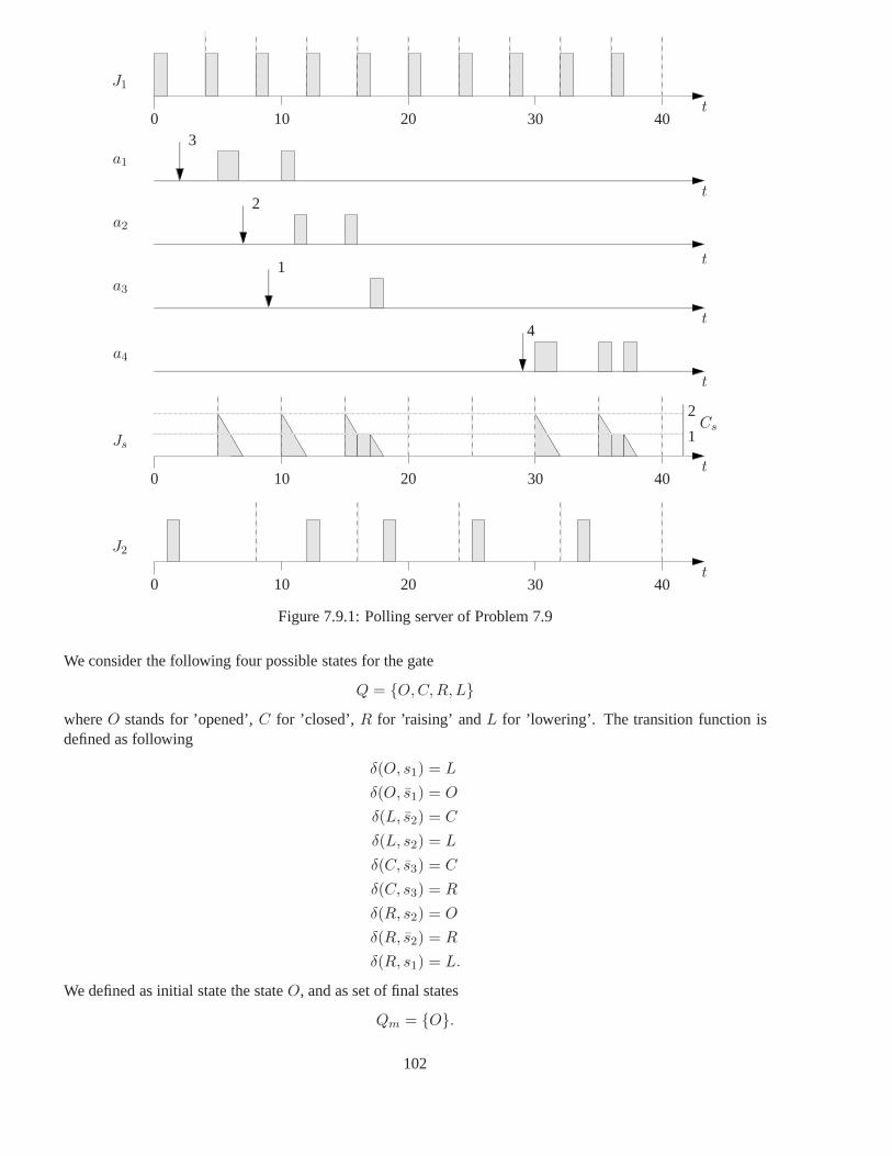
0
0
0
10
10
10
20
20
20
30
30
30
40
40
40
1
1
2
2
3
4
a1
a2
a3
a4
J1
Js
J2
t
t
t
t
t
t
t
Cs
Figure 7.9.1: Polling server of Problem 7.9
We consider the following four possible states for the gate
Q = O,C,R,LwhereO stands for ’opened’,C for ’closed’, R for ’raising’ andL for ’lowering’. The transition function isdefined as following
δ(O, s1) = L
δ(O, s1) = O
δ(L, s2) = C
δ(L, s2) = L
δ(C, s3) = C
δ(C, s3) = R
δ(R, s2) = O
δ(R, s2) = R
δ(R, s1) = L.
We defined as initial state the stateO, and as set of final states
Qm = O.
102
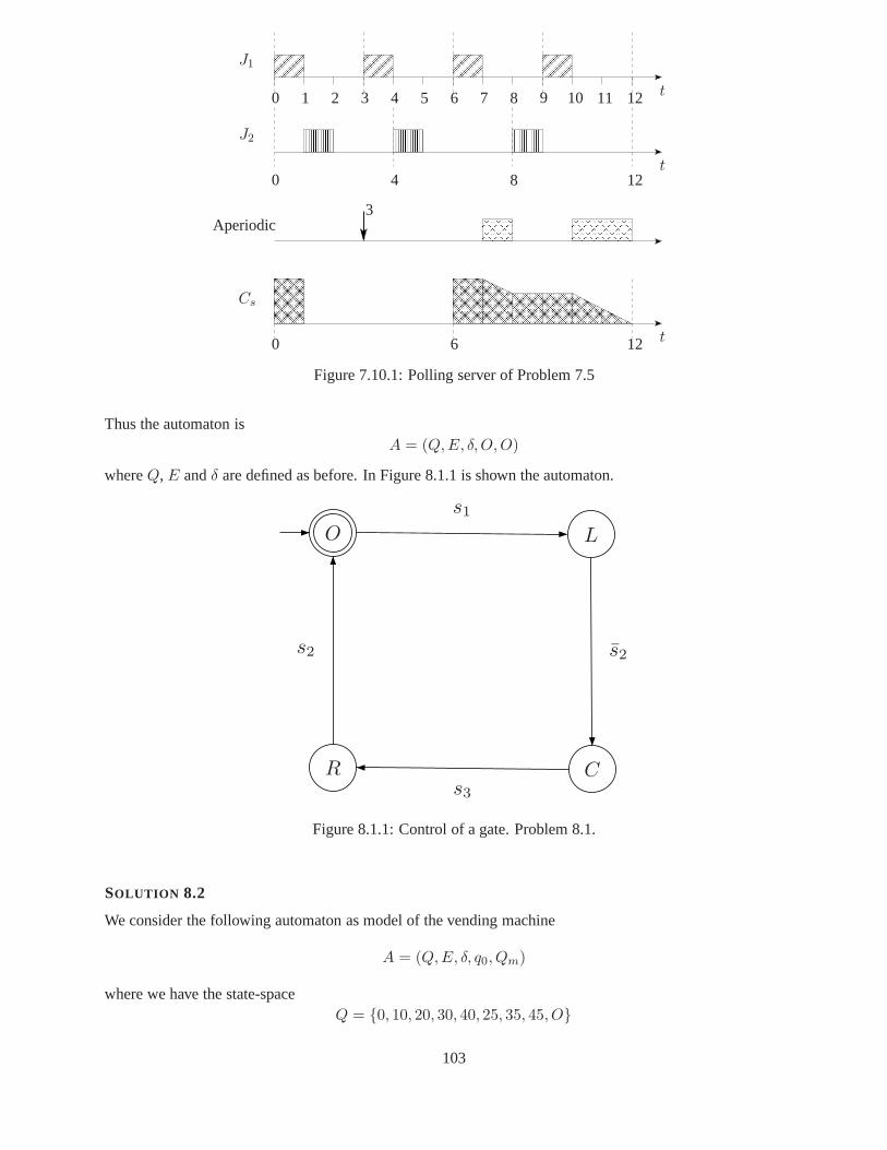
0
0
0
1 2 3
3
4
4 5 6
6
7
8
8 9 10 11
12
12
12
J1
J2
t
t
t
Aperiodic
Cs
Figure 7.10.1: Polling server of Problem 7.5
Thus the automaton isA = (Q,E, δ,O,O)
whereQ, E andδ are defined as before. In Figure 8.1.1 is shown the automaton.
O L
CR
s1
s2
s3
s2
Figure 8.1.1: Control of a gate. Problem 8.1.
SOLUTION 8.2
We consider the following automaton as model of the vending machine
A = (Q,E, δ, q0, Qm)
where we have the state-spaceQ = 0, 10, 20, 30, 40, 25, 35, 45, O
103

where the stateO denote ’overfull’. The event alphabet is
E = D, Q.
The initial state isq0 = 0 and the set of final states isQm = 45. The transition map is
δ(0, D) = 10
δ(0, Q) = 25
δ(10, D) = 20
δ(10, Q) = 35
δ(20, D) = 30
δ(20, Q) = 45
δ(25, D) = 35
δ(25, Q) = O
δ(30, D) = 40
δ(30, Q) = O
δ(35, D) = 45
δ(35, Q) = O
δ(40, Q) = 0
δ(40, D) = 0.
The automaton is shown in Figure 8.2.1. We can compute the marked language by inspection
10 20 30 40
25 35
0
45
O
D D D
D D
Q Q
Q Q, D
Q, D
Q
D
Figure 8.2.1: AutomatonA of Problem 8.2.
Lm(A) = DDQ, DQD, QDD.
We notice directly form Figure 8.2.1 that the machine will not dispense soda if the wrong amount of money isinserted. In that case we can reach the states30 or 40 or O from where is not possible to reach the state45 or ifwe reach the states25 or 35 and we overpay we will not get a soda. Notice that we can continue to insert coinsand the soda will never be dispensed i.e., we have a livelock.
In order to prove it formally we can notice that
DDD ∈ L(A)
104

but clearlyDDD /∈ Lm(A).
Thus the automaton blocks.
SOLUTION 8.3
In order to compute the marked language and generated language we consider the following notation. LetRkij
be the set of all stringsx such thatδ(qi, x) = qj , and ifδ(qi, y) = qℓ, for anyy that is prefix (initial segment)of x or ǫ, thenℓ ≤ k. That is,Rk
ij is the set of all strings that take the finite automaton from stateqi to stateqj
without going through any state numbered higher thank. Note that by “going through a state” we mean bothentering and leaving that state. Thusi or j may be greater thank. It is possible to defineRk
ij recursively
Rkij = Rk−1
ik
(Rk−1
kk
)Rk−1
kj ∪Rk−1ij
and
R0ij =
a|δ(qi, a) = qi if i = j
a|δ(qi, a) = qj if i 6= j
We then have thatLm(A) =
⋃
qj∈Qm
Rn0j
andL(A) =
⋃
qi∈Q
Rn0i.
A set of stringsRkij can be in general represented by theregular expressionsrk
ij , which allows a more compactnotation.
The automaton is formally defined by the following five-tuple
A = (Q,E, δ, q0, Qm)
where
Q = q1, q2E = 0, 1δ(q1, 0) = q2
δ(q1, 1) = q1
δ(q2, 0) = q2
δ(q2, 1) = q1
q0 = q1
Qm = q2
The first column of the table is computed by inspection can compute ther0ij,
k=0 k=1rk11 ǫ ǫ
rk12 0 0
rk21 1 1
rk22 ǫ 10
105

The second column is computed using the recursive formula introduced before. In particular we have
r111 = r0
11
(r011
)∗r011 + r0
11 = ǫ(ǫ)∗ǫ + ǫ = ǫ
r112 = r0
11
(r011
)∗r012 + r0
12 = ǫ(ǫ)∗0 + 0 = 0
r121 = r0
21
(r011
)∗r011 + r0
21 = 1(ǫ)∗ǫ + 1 = 1
r122 = r0
21
(r011
)∗r012 + r0
22 = 1(ǫ)∗0 + ǫ = 10
The marked language is then
Lm(A) = r212 = r1
12
(r122
)∗r122 + r1
12 = 0(10)∗10 + 0 = 0(10)∗
In this case the generated language is
L(A) = r211 + r2
12 = 0(10)∗1 + ǫ + 0(10)∗
The prefix closureLm(A) is
Lm(A) = s ∈ E∗|∃t ∈ E∗, st ∈ Lm(A).
We prove thatLm(A) = L(A).
ProveLm(A) ⊆ L(A): Let x ∈ Lm(A) then is trivial to see thatx ∈ L(A).
ProveLm(A) ⊇ L(A): Let nowx ∈ L(A). Thenx = ǫ, 0, 010, 01010, 0101010, . . . , 01, 0101, 010101, 01010101, . . . .The strings inLm(A) are0, 010, 01010, 0101010, . . . thus prefixes areǫ, 0, 01, 0101, 01010, 010101, . . . and as we can see thenx ∈ Lm(A).
We can conclude thatLm(A) = L(A), thus the DES is nonblocking.
SOLUTION 8.4
In this case the automaton isA = (Q,E, δ, q0, Qm)
where
Q = q1, q2, q3E = 0, 1δ(q1, 0) = q2
δ(q1, 1) = q3
δ(q2, 0) = q1
δ(q2, 1) = q3
δ(q3, 0) = q2
δ(q3, 1) = q2
q0 = q1
Qm = q2, q3
We apply the recursive formula introduced in the solution ofProblem 8.3 to compute the marked language andthe generated language.
106
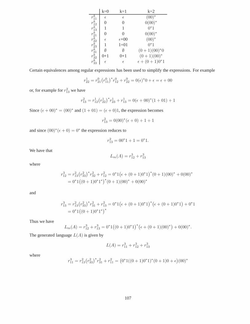
k=0 k=1 k=2rk11 ǫ ǫ (00)∗
rk12 0 0 0(00)∗
rk13 1 1 0∗1
rk21 0 0 0(00)∗
rk22 ǫ ǫ+00 (00)∗
rk23 1 1+01 0∗1
rk31 ∅ ∅ (0 + 1)(00)∗0
rk32 0+1 0+1 (0 + 1)(00)∗
rk33 ǫ ǫ ǫ + (0 + 1)0∗1
Certain equivalences among regular expressions has been used to simplify the expressions. For example
r122 = r0
21
(r011
)∗r012 + r0
22 = 0(ǫ)∗0 + ǫ = ǫ + 00
or, for example forr213 we have
r213 = r1
12
(r122
)∗r123 + r1
13 = 0(ǫ + 00)∗(1 + 01) + 1
Since(ǫ + 00)∗ = (00)∗ and(1 + 01) = (ǫ + 0)1, the expression becomes
r213 = 0(00)∗(ǫ + 0) + 1 + 1
and since(00)∗(ǫ + 0) = 0∗ the expression reduces to
r213 = 00∗1 + 1 = 0∗1.
We have thatLm(A) = r3
12 + r313
where
r312 = r2
13
(r233
)∗r232 + r2
12 = 0∗1(ǫ + (0 + 1)0∗1
)∗(0 + 1)(00)∗ + 0(00)∗
= 0∗1((0 + 1)0∗1∗
)∗(0 + 1)(00)∗ + 0(00)∗
and
r313 = r2
13
(r233
)∗r231 + r2
13 = 0∗1(ǫ + (0 + 1)0∗1
)∗(ǫ + (0 + 1)0∗1
)+ 0∗1
= 0∗1((0 + 1)0∗1∗
)∗
Thus we haveLm(A) = r3
12 + r313 = 0∗1
((0 + 1)0∗1
)∗(ǫ + (0 + 1)(00)∗
)+ 0(00)∗.
The generated languageL(A) is given by
L(A) = r311 + r3
12 + r313
wherer311 = r2
13
(r233
)∗r231 + r2
11 =(0∗1((0 + 1)0∗1)∗(0 + 1)0 + ǫ
)(00)∗
107

SOLUTION 8.5
Two statesp andq are said to beequivalent, p ≡ q if and only if for each input stringx, δ(p, x) is a markedstate if an only ifδ(q, x) is a marked place. Two statesp andq are said to be distinguishable if there exists anx such thatδ(p, x) is in Qm andδ(q, x) is not.
We build a table as follows
b Xc X Xd X X Xe X X Xf X X X Xg X X X X X Xh X X X X X X
a b c d e f g
where an ’X’ is placed in the table each time a pari of states cannot be equivalent. Initially an ’X’ is placedin each entry corresponding to one marked state and one non-marked state. It is in fact impossible that amarked state and a non-marked state are equivalent. In the example er place an ’X’ in the entries(a, c), (b, c),(c, d), (c, e), (c, f), (c, g) and (c, h). Next for each pair of statesp andq that are not already known to bedistinguishable, we consider the pairs of statesr = δ(p, a) ands = δ(q, a) for a input symbola. If statesradns have been shown to be distinguishable by some stringx thenp andq are distinguishable by the stringax.Thus if the entry(r, s) n the table has an ’X’, an ’X’ is also placed at the entry(p, q). If the entry(r, s) doesnot yet have an ’X’, then the pair(p, q) is placed on a list associated with the(r, s)-entry. At some future time,if (r, s) entry receives and ’X’, then each pair on the list associatedwith the(r, s)-entry also receives and ’X’.
In the example , we place and ’X’ in the entry(a, b), since the entry(δ(b, 1), δ(a, 1)) = (c, f) is alreadywith ’X’. Similarly, the (a, d)-entry receives an ’X’ since the entry(δ(a, 0), δ(b, 0)) = (b, c) has an ’X’.Consideration of the(a, e)-entry on input0 results in the pair(a, e) being placed on the list associated with(b, h). Observe that on input 1, botha ande go to the same statef and hence no string starting with 1 candistinguisha from e. Because of the 0-input, the pair(a, g) is placed on the list associated with(b, g). Whenthe(b, g)-entry is considered, it receives an ’X’ on account of a 1-input and(a, g) receives a ’X’. The string 01distinguishesa from g.
At the end of the algorithma ≡ e, b ≡ h andd ≡ f . The minimum automaton is shown in Figure 8.5.1.
SOLUTION 8.6
We can construct a deterministic automaton
A′ = (Q′, 0, 1, δ′ , [q0], Qm)
acceptingLm(A) as follows. The setQ consists of all subsets ofQ. These we denote with[q0], [q1], [q0, q1],and . Sinceδ(q0, 0) = q0, q1 then we have
δ′([q0], 0) = [q0, q1]
and similarlyδ′([q0], 1) = [q1] δ′([q1], 0) = δ′([q1], 1) = [q0, q1].
Naturally,δ′(, 0) = δ′(, 1) =. Finallyδ′([q0, q1], 0) = [q0, q1]
sinceδ(q0, q1, 0) = δ(q0, 0) ∪ δ(q1, 0) = q0, q1∪ = q0, q1,
108
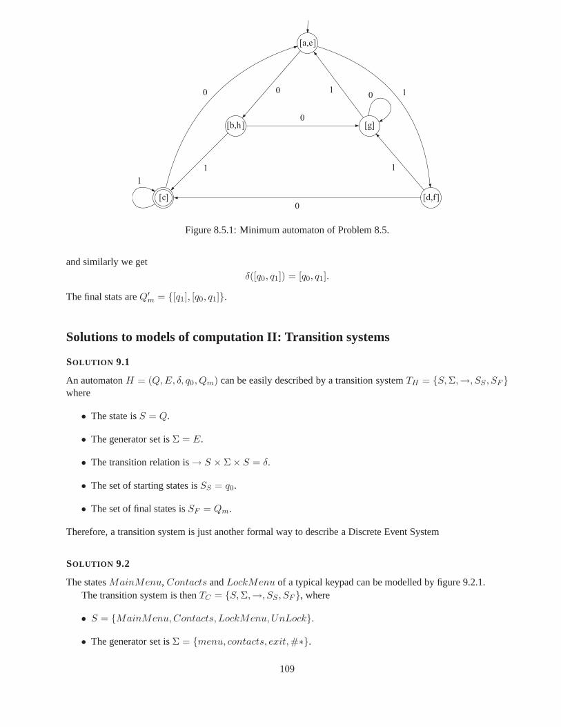
[a,e]
[b,h] [g]
[c] [d,f]
0
1
1
1
1
0
0
0 10
Figure 8.5.1: Minimum automaton of Problem 8.5.
and similarly we get
δ([q0, q1]) = [q0, q1].
The final stats areQ′m = [q1], [q0, q1].
Solutions to models of computation II: Transition systems
SOLUTION 9.1
An automatonH = (Q,E, δ, q0, Qm) can be easily described by a transition systemTH = S,Σ,→, SS , SFwhere
• The state isS = Q.
• The generator set isΣ = E.
• The transition relation is→ S × Σ× S = δ.
• The set of starting states isSS = q0.
• The set of final states isSF = Qm.
Therefore, a transition system is just another formal way todescribe a Discrete Event System
SOLUTION 9.2
The statesMainMenu, Contacts andLockMenu of a typical keypad can be modelled by figure 9.2.1.The transition system is thenTC = S,Σ,→, SS , SF , where
• S = MainMenu,Contacts, LockMenu,UnLock.
• The generator set isΣ = menu, contacts, exit,#∗.
109

M ain M enu
C ontactsC ontacts
U nLockU nLock
Lock M enuLock M enu
contacts
ex it
m enu
#*
key ≠ #*
#*
Figure 9.2.1: Possible states of a Keypad of a cellphone.
• The transition relation is→ S × Σ× S = δ, where
δ(MainMenu,#∗) = LockMenu ,
δ(MainMenu, contacts) = Contacts ,
...
• A starting state isSS = LockMenu.
• A final state isSF = LockMenu.
SOLUTION 9.3
The queuing system of figure 9.3 has a generator setΣ = a, d.A natural state variable is the number of customers in queue,thus the state-space is the set of non-negative
integersS = 0, 1, 2, . . ..The transition relation is
f(x, a) = x + 1 ∀x ≥ 0
f(x, d) = x− 1 ∀x > 0 .
The starting stateq0 is chosen to be the initial number of customers in the system.In figure 9.3.1, the transition system representing the basic queue system is reported. It is evident that the
cardinality of the state is infinite, but it is also countable.
0 1 2
a a a
b b b
Figure 9.3.1: A basic queue system.
SOLUTION 9.4
The proof is as follows:
110

1. In each iteration the number of elements inReachi increases by at least 1. Since it can have, at most,as many elements as S, there can only be as many iterations as the number of elements in S (minus thenumber of elements inSS).
2. Reachi is the set of states that can be reached in i steps, thus any state that can be reached in a finitenumber of steps must be in one of theReachi.
SOLUTION 9.5
Let SS = 3. By applying the reachability algorithm we have
SS = 3
Reach0 = 3Reach1 = 1, 3, 5, 6Reach2 = 1, 2, 3, 5, 6Reach3 = S
Reach4 = S
ReachT(3) = S
Let SS = 2. By applying the reachability algorithm we have
SS = 2
Reach0 = 2Reach1 = 2, 4, 5Reach2 = 2, 4, 5ReachT(2) = 2, 4, 5
111

Part III
Hybrid control
112

Solution to modeling of hybrid systems
SOLUTION 10.1
(a) Let the water level bex ≥ 0 m and use four discrete states. Let the thresholds bexon andxoff . Thesuggested model is illustrated in Figure 10.1.1.
q1
x = −0.02
τ = 1
q2
x = −0.02
τ = 1
q3
x = 0.01
τ = 1
q4
x = 0.01
τ = 1
“Pump off”
“Wait for on”
“Pump on”
“Wait for off”
x ≤ xon?
τ ≥ 2?x ≥ xoff ?
τ ≥ 2? τ := 0
τ := 0
Figure 10.1.1: Hybrid model of the tank and relay controllerin Problem 10.1.
(The variableτ is included as a “timer”, used to keep track of how long the system stays in the waitingstates.)
(b) The water level decreases2 · 0.02 m=0.04 m while waiting for the pump to turn on. Thus we need tochoosexon=0.09 to prevent underfilling. Similarly, choose
xoff = 0.12− 2 · 0.01 = 0.10.
SOLUTION 10.2
We see thatv can assume2k values, calledvi, i ∈ 0, . . . , 2k − 1. So we introduceN = 2k discrete statesqi.In stateqi, the system hasvi as constant control signal, illustrated in Figure 10.2.1.
vi P (s) Q(s) u
Figure 10.2.1: Dynamics of stateqi in Problem 10.2.
When do we switch states? We define the edges as
E = (qi, qi+1), (qi+1, qi)|i = 0, . . . , N − 2 ,
i.e., the system can only switch between adjacent states. The switchings are controlled by guards and domains.The guards define when switching isallowed, and when the system is outside the domain, itmustswitch:
G(qi, qi+1) = u ≥ vi + D/2G(qi+1, qi) = u ≤ vi+1 −D/2
D(qi) = vi −D/2 ≤ u ≤ vi + D/2
So the hybrid system can be illustrated as in Figure 10.2.2.
113

qN−1
q1
q0
...
u ≥ v0 + D/2u ≤ v1 −D/2
Figure 10.2.2: Control system with quantizer, modeled as a hybrid system. (Problem 10.2)
SOLUTION 10.3
A hybrid system system modeling the nuclear reactor is shownin Figure 10.3.1.
x = 0.1x− 56
c1 = c2 = 1
x = 0.1x − 60
c1 = c2 = 1
x = 0.1x − 50
c1 = c2 = 1
x = 510, c1 = c2 = 20
x ≥ 550 andc1 ≥ 20 x ≥ 550 andc2 ≥ 20
x ≤ 510 andc2 := 0x ≤ 510 andc1 := 0
Figure 10.3.1: The hybrid system for the nuclear reactor
SOLUTION 10.4
We model the system on linear state space form with a controller u = f(y) and neglect the time for computingthe control signal. (The computing time could otherwise be modeled as an extra waiting state between samplingy(t) and applying the newu(t).) The suggested hybrid model is illustrated in Figure 10.4.1.
“Execution”q1
x = Ax + Bu
τ = 1
“Computation”
u := f(Cx)
τ := 0
τ ≥ k?
Figure 10.4.1: The sampled control system in Problem 10.4.
The control law, as well as any quantization effects in the D/A or A/D converters are incorporated intof(y).
114

SOLUTION 10.5
(a) We need a timer variablet to control the switching, so the full state is(x, t)T . Now the hybrid automatoncan be described asH = (Q,X, Init , f,D,E,G,R), with
Q = q1, q2X = R2 × R+
Init = q1 × (0, 0)
f(qi, x, t) =[
Aix 1]T
D(qi) = (x, t)T |t < 1E = (q1, q2), (q2, q1)G(q1, q2) = G(q2, q1) = (x, t)T |t ≥ 1R(q1, q2, x, t) = R(q2, q1, x, t) =
[x 0
]T.
(b) The trajectory evolves as follows:
x(t) =
eA1tx0, t ∈ [0, 1)
eA2(t−1)x(1), t ∈ [1, 2)
eA1(t−2)x(2), t ∈ [2, 3)
In order to expressx(t) as a function ofx0 we need to derivex(1) andx(2) as functions ofx0. We have
x(1) = eA1(1−0)x0 = eA1x0
and
x(2) = eA2(2−1)x(1) = eA2x(1).
Combining the two previous equations we have
x(t) =
eA1tx0, t ∈ [0, 1)
eA2(t−1)eA1x0, t ∈ [1, 2)
eA1(t−2)eA2eA1x0, t ∈ [2, 3).
SOLUTION 10.6
115

(a) The hybrid automaton is defined asH = (Q,X, Init, f,D,E,G,R) with
Q = q1, q2, q3X = R
Init = q1 × 0
f(q1, x) = 2
f(q2, x) = −1
f(q3, x) = x + 2
D(q1) = x ∈ R|x < 5D(q2) = x ∈ R|x > 3D(q3) to be defined
E = (q1, q2), (q2, q3)G(q1, q2) = x ∈ R|x ≥ 5G(q2, q3) = x ∈ R|x ≤ 3R(q1, q2, x) = x
R(q2, q3, x) = −2
(b) In order for the hybrid automaton to be live we need to ensure that the domainD(q3) contains thetrajectory of the systemx = x + 2 with initial conditionx0 = −2. But
x0 = −2⇒ x = −2 + 2 = 0,
so the state will stay constant. Thus all domains that fulfillx = 2 ∈ D(q3) guarantee liveness of thesystem.
(c) The state-trajectory of the hybrid system is shown in Figure 10.6.1, whereτ0 = 0, τ1 = 2.5 andτ2 = 4.5.
-2
3
5
q
q1
q2
q3
x
τ0 τ ′0 τ ′
1τ1 τ2
Figure 10.6.1: Trajectory of the hybrid system in Problem 10.6
Solutions to stability of hybrid systems
SOLUTION 11.1
116
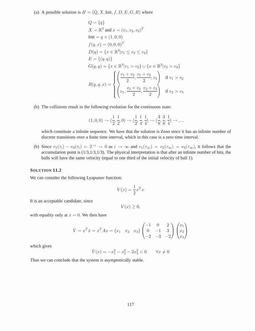
(a) A possible solution isH = (Q,X, Init, f,D,E,G,R) where
Q = qX = R3 andx = (v1, v2, v3)
T
Init = q × (1, 0, 0)
f(q, x) = (0, 0, 0)T
D(q) = x ∈ R3|v1 ≤ v2 ≤ v3E = (q, q)G(q, q) = x ∈ R3|v1 > v2 ∪ x ∈ R3|v2 > v3
R(q, q, x) =
(
v1 + v2
2,v1 + v2
2, v3
)
if v1 > v2
(
v1,v2 + v3
2,v2 + v3
2
)
if v2 > v3
(b) The collisions result in the following evolution for thecontinuous state:
(1, 0, 0) → (1
2,1
2, 0)→ (
1
2,1
4,1
4)→ (
3
8,3
8,1
4)→ . . .
which constitute a infinite sequence. We have that the solution is Zeno since it has an infinite number ofdiscrete transitions over a finite time interval, which in this case is a zero time interval.
(b) Sincev1(τi) − v3(τi) = 2−i → 0 as i → ∞ andv1(τ∞) = v2(τ∞) = v3(τ∞), it follows that theaccumulation point is (1/3,1/3,1/3). The physical interpretation is that after an infinite number of hits, theballs will have the same velocity (equal to one third of the initial velocity of ball 1).
SOLUTION 11.2
We can consider the following Lyapunov function:
V (x) =1
2xT x
It is an acceptable candidate, sinceV (x) ≥ 0,
with equality only atx = 0. We then have
V = xT x = xT Ax =(x1 x2 x3
)
−1 0 20 −1 3−2 −3 −2
x1
x2
x3
which givesV (x) = −x2
1 − x22 − 2x2
3 < 0 ∀x 6= 0
Thus we can conclude that the system is asymptotically stable.
117

SOLUTION 11.3
Let P be a positive definite symmetric matrix which satisfies
AT P + PA = −Q.
Then the functionV (x) = xT Px is a positive definite function. Let us computeV (x)
V (x) =d
dt(xT Px) = xT Px + xT Px = xT AT Px + xT PAx = xT (AT P + PA)x = −xT Qx.
ThusV (x) is negative definite. For Lyapunov’s stability criteria we can conclude that the system is asymptoti-cally stable.
SOLUTION 11.4
Let us consider the following Lyapunov function
V (x) =xT x
2=
x21 + x2
2
2
Let us compute the time derivative ofV (x). We have
V (x) = x1x1 + x2x2 = −x21 − x2
2 + x1g(x2) + x2h(x1)
≤ −x21 − x2
2 +1
2x1|x2|+
1
2x2|x1|
≤ −x21 − x2
2 + |x1x2|
≤ −1
2(x2
1 + x22)
where we used(|x1| − |x2|)2 ≥ 0, which gives|x1x2| ≤ 12(x2
1 + x22). Thus
V < 0 ∀x 6= 0
thus the system is asymptotically stable. Notice that we do not need to know the expressions forg(.) andh(.)to show asymptotic stability.
SOLUTION 11.5
(a) Depending on the sign ofx1 or x2 we have four systems. Ifx1 > 0 andx2 > 0 then we have
x1 = −1 + 2 = 1
x2 = −2− 1 = −3
If x1 < 0 andx2 > 0 then we have
x1 = 1 + 2 = 3
x2 = 2− 1 = 1
If x1 < 0 andx2 < 0 then we have
x1 = 1− 2 = −1
x2 = 2 + 1 = 3
118

x1
x2
Figure 11.5.1: A trajectory of the system in Problem 11.5. The dot represents the initial state.
If x1 > 0 andx2 < 0 then we have
x1 = −1− 2 = −3
x2 = −2 + 1 = −1
A trajectory is represented in Figure 11.5.1. We can then represent the discontinuous system as a hybridsystem with four states. Formally we haveH = (Q,X, Init, f,D,E,G,R) with
Q = q1, q2, q2, q4X = R2
Init = q0 × (x10, x20),
whereq0 depends on the statex0.
f(q1, x) = (1,−3)T
f(q2, x) = (3, 1)T
f(q3, x) = (−1, 3)T
f(q4, x) = (−3,−1)T
D(q1) = x ∈ R2|x1 ≥ 0, x2 ≥ 0D(q2) = x ∈ R2|x1 < 0, x2 ≥ 0D(q3) = x ∈ R2|x1 < 0, x2 < 0D(q4) = x ∈ R2|x1 ≥ 0, x2 < 0R(qi, qj , x) = x
We still need to define the set of edgesE and the guardsG. Since a trajectory of the given discontin-uous system is always such that from the 1st quadrant it movesto the 4th and then 3rd and 2nd (see
119

Figure 11.5.1), the set of edges is then
E = (q1, q4), (q4, q3), (q3, q2), (q2, q1).
The guards are
G(q1, q4) = x ∈ R2|x2 < 0G(q4, q3) = x ∈ R2|x1 < 0G(q3, q2) = x ∈ R2|x2 ≥ 0G(q2, q1) = x ∈ R2|x1 ≥ 0.
(b) We can notice that for any initial condition (x(0) 6= 0) a solution of the hybrid system will look like a’spiral’ which is moving towards the origin. As we approach the origin the number of switches increases,until we have an infinite number of switches in finite time. Thus we have Zeno behavior.
SOLUTION 11.6
Consider the Lyapunov function candidate
V (x) =1
2x2.
For bothq = 1 andq = 2 it holds that
V (x) = xx = aqx2 ≤ 0,
with equality only forx = 0. ThenV (x) is a common Lyapunov function for the switched system, and itisasymptotically stable.
SOLUTION 11.7
The matricesA1 andA2 commute,i.e.
A1A2 =
[3 00 10
]
= A2A1.
Further, they are both diagonal, which means that the eigenvalues are the diagonal elements. All eigenvaluesare negative, so each matrix is asymptotically stable.
If the system matrices commute and are asymptotically stable, then the switched system is also asymptoti-cally stable.
SOLUTION 11.8
1st method The second component of the statex satisfies
x2 = −cqx2
whereq = 1, 2. Thereforex2(t) decays to 0 asymptotically at the rate corresponding tominc1, c2.The first component ofx satisfies the equation
x1 = −aqx1 + bqx2.
This can be viewed as the asymptotically stable systemx1 = −aqx1 excited by a asymptotically decayinginput bqx2. Thusx1 also converges to zero asymptotically.
120
2nd method A second way to show that the switched system is asymptotically stable consists in constructinga common Lyapunov function for the family of linear systemAq. In this case it is possible to find aquadratic common Lyapunov function
V (x) = xT Px
with P = diag(d1, d2) with d1, d2 > 0, sinceP must be positive definite. We then have
−(AT
q P + PAq
)=
(2d1aq −d1bq
−d1bq 2d2cq
)
q = 1, 2
To ensure that this matrix is positive definite we can fixd1 > 0 and then choosed2 > 0 large enough sothat
4d2d1aqcq + d21b
2q > 0, q = 1, 2.
Thus this concludes the proof.
SOLUTION 11.9
(a) To model the system as a switching system, we introduce a timer variableτ :
x = Aqx
τ = 1,
whereq ∈ 1, 2 and
Ω1 = x, τ |kǫ ≤ τ < (k +1
2)ǫ, k = 0, 1, . . .
Ω2 = x, τ |(k +1
2)ǫ ≤ τ < (k + 1)ǫ, k = 0, 1, . . ..
(b) A corresponding hybrid automaton isH = (Q,X, Init , f,D,E,G,R), with
Q = q1, q2X = Rn × R+ ( state vector:(x, τ)T )
Init = q1 × (x0, t0)T
f(q1, x, τ) = (A1x, 1)T
f(q2, x, τ) = (A2x, 1)T
D(q) = x, τ |τ < ǫ/2 ∀q ∈ Q
E = (q1, q2), (q2, q1)G(e) = x, τ |τ ≥ ǫ/2 ∀e ∈ E
R(e, x, τ) = (x, 0)T ∀e ∈ E.
Note that here we letτ be reset at every switching instant, to simplify the system.
(c) If the system starts inq = q1, with x = x0 at t = t0, we get
x(t0 + ǫ/2) = eA1ǫ/2x0
andx(t0 + ǫ) = eA2ǫ/2eA1ǫ/2x0.
121
(d) We use the definition of the matrix exponential:
eAǫ = I + Aǫ + A2ǫ2 +O(ǫ3)
This allows us to write
eA2ǫ/2eA1ǫ/2 = (I + A2ǫ/2 + . . .) (I + A1ǫ/2 + . . .)
= I + (A1 + A2)/2ǫ + A2A1ǫ2/4 + . . . ≈ asǫ→ 0 ≈ e
A1+A22
ǫ
So for fast switching (smallǫ), the system behaves like the average of the two subsystems.
SOLUTION 11.10
We chooseQ = I and test if
P =
[p1 00 p2
]
solves the Lyapunov equation
PA1 + AT1 P = −I ⇔
[−2p1 0
0 −4p2
]
=
[−1 00 −1
]
.
Apparently it does, if we choosep1 = 1/2 andp2 = 1/4. SoV (x) = xT Px is a Lyapunov function forsystem 1. Does it also work for system 2?
V (x) = xT Px + xT Px = xT A2Px + xT PA2x
= xT
[−3 00 −5/2
]
x ≤ 0 ∀x,
with equality only forx = 0. SoV (x) is a common Lyapunov function for systems 1 and 2 and the switchedsystem is asymptotically stable.
SOLUTION 11.11
(a) Without loss of generality we can consider a positive definite matrixP in the form
P =
(1 ss r
)
.
Assume the matrixP satisfiesAT
q P + PAq < 0 ∀qthen forq = 1 we have
−AT1 P − PA1 =
(2− 2q 2q + 1− r
2q + 1− r 2q + 2r
)
and this matrix is positive definite only if
q < 1
8q2 + 1 + r2 − 6r < 0⇒ q2 +(r − 3)2
8< 1 (0.0)
Similarly for the other matrix we have
−AT2 P − PA2 =
(2− q
5 2q + 10− r10
2q + 10− r10 20q + 2r
)
122

which is a positive definite matrix if
q < 10
600r − 800q2 − 1000 − r2 ⇒ q2 +(r − 300)2
800< 100. (0.0)
The inequalities 0.0 and 0.0 represent the interiors of two ellipsoids As can be seen in Figure 11.11.1 thetwo ellipsoids do not intersect.
r
q
3 +√
8 ≈ 6
100(3 −√
8) ≈ 17
Figure 11.11.1: Ellipsoids representing the inequalities(0.0) and (0.0).
(b) We would like to show that the system is however asymptotically stable. In order to do that, since theswitching is arbitrary, we consider a ’worst-case-switching’, which we define as follows. The vectorsA1x andA2x are parallel on two lines which pass through the origin. If such lines define a switchingsurface, we then choose to follow the trajectory of the vector field which is pointing outward, so thatwe have a ’worst-case-switching’, in the sense that it should move away from the origin. The situationis shown in Figure 11.11.2. The switching surface can be found solving the equation which describescollinearity
(A1x)× (A2x) = 0
which gives the equation
(−x1 − x2)(0.1x1 − x2) + (x1 − x2)(x1 + 10x2) = 0.
The equations of the two lines are
x2 = 1.18x1
x2 = −0.08x1.
In order know which of the two vectors is pointing outward we can determine when(A1x)× (A2x) > 0which gives that between the line−0.08x1 and1.18x1 the vectorsA2x are pointing outward. We now
123

A1x
A1x
A1x
A1x
A2x
A2x
A2x
A2x
Figure 11.11.2: Worst case switching in Problem 11.11
need to show that the trajectory is converging toward the origin. Let us consider, for example, thefollowing initial condition
x0 = (100,−8)
which is a point on the switching surfacex2 = −0.08x1. The trajectory follows the vector fieldA1x andintersects the next switching surface at the point
(x1
1.18x1
)
= eA1 tx0
which in our case is the point with coordinates(25, 29.5). Then the trajectory is given by the vector fieldA2x and the intersection point with the switching surface is(−86.3, 6.8). The next point is(−21.7,−25).The next point is the intersection of the trajectory with theswitching surface that contained the initialconditionx0. We have the intersection at(25,−2). Thus after one rotation we have that the distanceof the trajectory to the origin is decreased from 100.1 to 25.1. Thus the system converges to the originconsidering the ’worst-case-switching’.
SOLUTION 11.12
(a) Use the same ideas as in Problem 11.11.
(b) Let us consider the following two positive definite symmetric matrices
P1 =
(1 00 3
)
and P2 =
(10 00 3
)
If we consider the following Lyapunov equations
ATq Pq + PqAq q = 1, 2
124
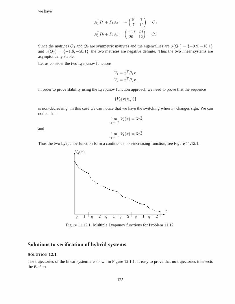
we have
AT1 P1 + P1A1 = −
(10 77 12
)
= Q1
AT2 P2 + P2A2 =
(−40 2020 12
)
= Q2
Since the matricesQ1 andQ2 are symmetric matrices and the eigenvalues areσ(Q1) = −3.9,−18.1andσ(Q2) = −1.6,−50.1, the two matrices are negative definite. Thus the two linear systems areasymptotically stable.
Let us consider the two Lyapunov functions
V1 = xT P1x
V2 = xT P2x.
In order to prove stability using the Lyapunov function approach we need to prove that the sequence
Vq(x(τiq))
is non-decreasing. In this case we can notice that we have theswitching whenx1 changes sign. We cannotice that
limx1→0+
V2(x) = 3x22
andlim
x1→0−V1(x) = 3x2
2
Thus the two Lyapunov function form a continuous non-increasing function, see Figure 11.12.1.
Vq(x)
q = 1 q = 1 q = 1q = 2 q = 2 q = 2
t
Figure 11.12.1: Multiple Lyapunov functions for Problem 11.12
Solutions to verification of hybrid systems
SOLUTION 12.1
The trajectories of the linear system are shown in Figure 12.1.1. It easy to prove that no trajectories intersectstheBadset.
125

−10 −8 −6 −4 −2 0 2 4 6 8 10−10
−8
−6
−4
−2
0
2
4
6
8
10
Figure 12.1.1: Trajectories of the linear system in Problem12.1.
1 3
Ω1
Ω2
Ω3
Figure 12.3.1: State-space partition for the system in Problem 12.3
126

Figure 12.3.2: Trajectories of the linear system in Problem12.3.
SOLUTION 12.3
The partition of the state-space is shown in Figure 12.3.1.
(a) Let us consider the system in the regionΩ3. It is easy to determine a linear state feedbackg3(x) = K3xwhich places the poles inp1 = p2 = −1, since the system is controllable. The feedback control gain isin this case
K3 =
(
−4
3−3
)
.
Notice that if we useg3 as controller for the system 2 we have a closed loop stable system with poles
p1 = −3 p2 = −1
3.
Notice moreover that the closed loop system for system 3 has the equilibrium point in(−1/3, 0) sincethe closed loop system is
x =
(0 −11 2
)(x1
x2
)
+
(0−1
3
)
This means that all trajectories starting inΩ3 will go towards(−1/3, 0), which is inΩ1. Hence they willenterΩ2, which also is stable with(0, 0) as equilibrium. Thus the trajectory will enterΩ1. An exampleof trajectories is shown in Figure 12.3.2.
(b) If B1 = (0, 1)T then as you can notice the dynamics in the setΩ3 = ‖x‖ > 3 is the negative of thedynamics inΩ1 (modulo a bias term that only makes the equilibrium different). Therefore is we usethe linear controllerg3 computed in (a), this will not make the system 1 stable. Thus,we need to use adifferent controller for the two regions.
(c) A simple choice to stabilize the system 1 is a feedback controller that place the poles inp1 = p2 = −1.Such controller controller for the system 1 is Let the controller
g1(x1, x2) =
(
−4
3−7
)(x1
x2
)
127

x = 0.1x− 56
c1 = c2 = 1
x = 0.1x − 60
c1 = c2 = 1
x = 0.1x − 50
c1 = c2 = 1
x = 510, c1 = c2 = 20
x ≥ 550 andc1 ≥ 20 x ≥ 550 andc2 ≥ 20
x ≥ 550 andc2 := 0x ≤ 510 andc1 := 0
Figure 12.4.1: The hybrid system for the nuclear reactor
Notice that that controllersg1 andg3 place the poles of the systems 1 and 3 inp1 = p2 = −1. Bothcontrollers stabilizes the system inΩ2, since the closed loop for the system 2, wheng3 is used, has polesin
p1 = −3 p2 = −1/3
and usingg1 the poles are
p1,2 =− 11 ± 4
√7
3.
thus a possible control strategy is
g(x) =
g1(x) if ‖x‖ ≤ α
g3(x) otherwise
with 1 ≤ α ≤ 3, which means that we can use eitherg1 or g3 in any subset of the regionΩ2.
(d) If the bad region corresponds toΩ1 then we need to avoid the trajectory to go enter inΩ1 at all. Onepossible solution is to design a control lawg1 such that the eigenvalues of the closed loop system forsystem 1 are placed inp1,2 = ±i. In this way we have that the trajectories are confined in a circle withradius 1.
SOLUTION 12.4
A hybrid system system modeling the nuclear reactor is shownin Figure 12.4.1.
128

aa
b
b
c
S0
R1
R2 SF
Figure 13.1.1: The resulting quotient transition systemT , which is bisimular toT .
Solutions to simulation and bisimulation
SOLUTION 13.1
We use the bisimulation algorithm, and start by defining the quotient transition system asT = S, Σ, →, S0, SF .Further, letPreσ(P ) denote all states from which we can get toP in one transitionσ.
We initialize the algorithm by lettingS1 = q1, . . . , q5 andS = S0, SF , S1. Now there areP1 = S1,P2 = SF andσ = b such that
P1
⋂
Preb(P2) = q1, q2 6= ∅.Thus we must partition the setP1:
R1 = P1
⋂
Preb(P2) = q1, q2R2 = P1\Preb(P2) = q4, q5S := S\P1
⋂
R1, R2 = S0, SF , R1, R2
Now there are no moreP1, P2 andσ that fulfill the criterion in the algorithm, so it terminates. The resultingquotient transition systemT is given in Fig. III.
129

BIBLIOGRAPHY
[1] Wittenmark, B. Åström, K.J. and Årzén K-H., “Computer Control: An Overview", IFAC ProfessionalBrief, 2003.
[2] Wittenmark, B. and Åström, K.J. , “Computer Controlled Systems”, Prentice Hall, 3rd Edition.
[3] Buttazzo, G.C., “Hard Real-Time Computing", Kluwer Academic Publisher, 4th edition, 2002. Systems"
[4] Cassandras, C.G. and Lafortune, S., “Introduction to Discrete Event Systems", Kluwer Academic Pub-lisher, 1999.
[5] Hopcroft, J.E. and Ullman, J.D. “Introduction to automata theory, languages, and computation”, Addison-Wesley, 1979.
[6] Murata, T., “Petri nets: Properties, analysis and applications", Proceedings of the IEEE, Volume: 77,Issue: 4, 1989
[7] David, R. and Alla, H., “Petri Nets and Grafcet”, Prentice Hall, 1992.
[8] Johansson, K.H. , “Hybrid Control System”, in Control Systems, Robotics, and Automation , from Ency-clopedia of Life Support Systems (EOLSS)
[9] Johansson, K.H. and Lygeros, J. and Sastry, S., “ Modeling of Hybrid Systems”, in Control Systems,Robotics and Automation, from Encyclopedia of Life SupportSystems (EOLSS)
[10] Branicky, M.S. “Stability of Hybrid Systems”, in Control Systems, Robotics and Automation, from En-cyclopedia of Life Support Systems (EOLSS)
[11] Schaft, A. van der and Schumacher, H., “An Introductionto Hybrid Dynamical Systems”, Lecture Notesin Control and Information Sciences, 251, Springer, 2000
[12] Liberzon, D., “Control Using Logic and Switching, PartI: Switching in Systems and Control”, Handoutnotes at Workshop CDC 2001.http://www.ece.ucsb.edu/~hespanha/cdc01/switchingcdc01.htm
[13] Oppenheim, A. V. and Willsky, A. S. and Nawab, S. H. “Signals & Systems”, Prentice Hall, 1997.
[14] Hespanha, João P. Lecture notes on Hybrid Control and Switched Systems, Reachability, University ofCalifornia at Santa Barbara, 2005.
130