
eJournal of Tax Research - UNSW Sydney
188
eJournal of Tax Research Volume 19, Number 1 June 2021 CONTENTS Editorial 1 The relevance of supply side taxation for attracting foreign direct investment to developing countries: evidence from Egypt Mahmoud M Abdellatif, Ashraf G Eid and Abdel-Salam G Abdel-Salam 17 GST treatment of electronic commerce: comparing the Singaporean and Australian approaches Evgeny Guglyuvatyy and Nikolai Milogolov 48 Taxpayer wealth and federal tax revenue under a tax policy that shields retained earnings used for growth from taxes Robert M Hull and John B Hull 97 Earmarked taxes: an Indian case study Ashrita Prasad Kotha and Pradnya Talekar 121 A review of objections to residential land values used to assess State land tax: a case study of inner Sydney, New South Wales Vince Mangioni and Heather MacDonald 146 Firms’ strategic responses to tax policies Sylvia Mwamba 168 Tax morale, perception of justice, trust in public authorities, tax knowledge, and tax compliance: a study of Indonesian SMEs Joshua Timothy and Yulianti Abbas © School of Accounting, Auditing & Taxation, UNSW Business School UNSW Sydney ISSN 1448-2398
-
Upload
khangminh22 -
Category
Documents
-
view
0 -
download
0
Transcript of eJournal of Tax Research - UNSW Sydney

eJournal of Tax Research
Volume 19, Number 1 June 2021
CONTENTS
Editorial
1 The relevance of supply side taxation for attracting foreign direct investment to developing countries: evidence from Egypt Mahmoud M Abdellatif, Ashraf G Eid and Abdel-Salam G Abdel-Salam
17 GST treatment of electronic commerce: comparing the Singaporean and Australian approaches Evgeny Guglyuvatyy and Nikolai Milogolov
48 Taxpayer wealth and federal tax revenue under a tax policy that shields retained earnings used for growth from taxes Robert M Hull and John B Hull
97 Earmarked taxes: an Indian case study Ashrita Prasad Kotha and Pradnya Talekar
121 A review of objections to residential land values used to assess State land tax: a case study of inner Sydney, New South Wales Vince Mangioni and Heather MacDonald
146 Firms’ strategic responses to tax policies Sylvia Mwamba
168 Tax morale, perception of justice, trust in public authorities, tax knowledge, and tax compliance: a study of Indonesian SMEs Joshua Timothy and Yulianti Abbas
© School of Accounting, Auditing & Taxation, UNSW Business School UNSW Sydney
ISSN 1448-2398
eJournal of Tax Research EDITORS
Professor John Taylor School of Accounting, Auditing & Taxation, UNSW Sydney
Professor Binh Tran-Nam School of Accounting, Auditing & Taxation, UNSW Sydney
ASSOCIATE EDITOR
Dr Alexandra Evans School of Accounting, Auditing & Taxation, UNSW Sydney
PRODUCTION EDITOR
Dr Peter Mellor School of Accounting, Auditing & Taxation, UNSW Sydney
EDITORIAL BOARD
Professor Robin Boadway Department of Economics, Queen’s University
Professor Cynthia Coleman University of Sydney Business School
Professor Graeme Cooper Faculty of Law, University of Sydney
Professor Robert Deutsch School of Accounting, Auditing & Taxation, UNSW Sydney
Professor Chris Evans School of Accounting, Auditing & Taxation, UNSW Sydney
Professor Judith Freedman Faculty of Law, University of Oxford
Professor Malcolm Gammie
Professor John Hasseldine
Chambers of Lord Grabiner QC, London
Paul College of Business and Economics, University of New Hampshire
Professor Jeyapalan Kasipillai School of Business, Monash University Malaysia Campus
Professor Rick Krever Law School, University of Western Australia
Professor Charles McLure Jr
Professor Dale Pinto
Hoover Institution, Stanford University
Curtin Business School, Curtin University
Professor John Prebble
Professor Adrian Sawyer
Faculty of Law, Victoria University of Wellington
College of Business and Law, University of Canterbury
Professor Joel Slemrod Stephen M. Ross School of Business, University of Michigan
Professor Jeffrey Waincymer Faculty of Law, Monash University
Professor Neil Warren School of Accounting, Auditing & Taxation, UNSW Sydney
Professor Robin Woellner School of Accounting, Auditing & Taxation, UNSW Sydney
eJournal of Tax Research PUBLISHER
The School of Accounting, Auditing & Taxation is part of the UNSW Business School at UNSW Sydney. The tax group in our school brings together a team of expert academic staff with backgrounds in law, tax and economics. At the School of Accounting, Auditing & Taxation, we’re working towards building excellence in the tax profession, looking at tax from both a theoretical and practical perspective. EDITORS’ NOTE
The eJournal of Tax Research is a refereed journal that publishes original, scholarly works on all aspects of taxation. It aims to promote timely dissemination of research and public discussion of tax-related issues, from both theoretical and practical perspectives. It provides a channel for academics, researchers, practitioners, administrators, judges and policy makers to enhance their understanding and knowledge of taxation. The journal emphasises the interdisciplinary nature of taxation. SUBMISSION OF ORIGINAL MATERIAL
Submission of original contributions on any topic of tax interest is welcomed, and should be sent as an email attachment (Microsoft Word format) to the Production Editor at <[email protected]>. Submission of a manuscript is taken to imply that it is an unpublished work and has not already been submitted for publication elsewhere. Potential authors are requested to follow the “Notes to Authors”, which is available from the journal's website. WEBPAGE
Current and past issues of the eJournal of Tax Research are available via the journal’s website: https://www.unsw.edu.au/business/our-research/research-environment/ejournal-tax-research.
eJournal of Tax Research (2021) vol. 19, no. 1, p. i
i
Editorial
Professor Richard M Bird
We note with profound sadness the unexpected passing of Richard Bird, Professor Emeritus of Economic Analysis and Policy at Rotman School of Management, University of Toronto.
Born a Canadian, Professor Bird was a giant in the field of public finance. In a career that spanned six decades, he worked in about 50 countries. Professor Bird was a prolific and influential tax economist with “a finely honed ability to combine general economic theory with institutional realities and politics, and a talent for innovative – and on occasion unconventional – approaches.” He was also a true mentor who displayed impressive "breadth of knowledge, range of interests, quality of analysis, clarity of prose, and the sheer volume of writing." Professor Bird was appointed a Fellow of the Royal Society of Canada in 1978. His many other honours included the National Tax Association’s 2006 Daniel M. Holland Award, and the Canadian Tax Foundation’s Lifetime Contribution Award 2017, Queen's Diamond Jubilee Award 2013 and Douglas Sherbaniuk Award 1997.
Professor Bird was a strong supporter of tax research at many universities around the world, including Australian universities. He was a visiting scholar and conference contributor at a number of Australian universities, and an author of numerous articles to Australian research journals and books. In particular, he held the position of Adjunct Professor at Atax, UNSW Sydney. He first visited Atax in 2007 to conduct a joint ARC Linkage International Project on personal income tax reform in Australia. As part of the visit, he presented an authoritative and inspirational seminar on tax policy and administration in developing countries at Atax, and delivered a keynote speech at an ARC-funded conference on tax reform in Australia.
Professor Bird’s passing is a great loss to the international community of tax scholars. On behalf of the eJournal of Tax Research and the Tax group at the School of Accounting, Auditing and Taxation at UNSW Sydney, we wish to extend our deepest sympathy to his widow, children and their spouses, and grandchildren.
John Taylor Binh Tran-Nam Alex Evans Peter Mellor
eJournal of Tax Research (2021) vol. 19, no. 1, pp. 1-16
1
The relevance of supply side taxation for attracting foreign direct investment to developing countries: evidence from Egypt
Mahmoud M Abdellatif, Ashraf G Eid and Abdel-Salam G Abdel-Salam
Abstract
Many developing countries commonly use tax incentives as a key instrument for attracting foreign direct investment (FDI). Empirical studies have identified a causal relationship between FDI and a number of determinants including tax incentives, because they lower multinational enterprises’ (MNEs) tax burden and consequently maximise their after-tax returns. Egypt is an example of a developing country that employed tax incentives through granting tax holidays to MNEs, in order to attract FDI, during the period 1974 to 2004. However, in 2005 the supply side tax policy was introduced through broadening the tax base and abolishing the bulk of tax incentives including tax exemptions. Nevertheless, in 2017 a new investment law was ratified which re-introduced tax incentives. This policy reversal raises a question about the relevance or otherwise of supply side tax policy in attracting FDI. To answer this question, we employ an econometric model to test the causal relationship between FDI and its determinants during the period 1975 to 2017. We assume that abolishing tax incentives would have a positive impact on inflow FDI. Using data from 1975 to 2017 for estimating the regression model, it is shown that there is a significant relationship between inflow FDI and implementation of supply side tax policy, while tax incentives have an insignificant effect on FDI. The result indicates that MNEs are looking for simplified tax provisions and lower tax rates, which are provided under supply side taxation. Further, the majority of MNEs are often taxed on their worldwide income in their residence countries, which indicates that they do not benefit from tax exemption. Accordingly, it is recommended that developing countries should consider broadening the income tax base and lowering income tax rates as an effective means of attracting FDI. Key words: foreign direct investment, tax incentives, supply side taxation, developing countries
Assistant Professor of Economics and Director of the Center for Entrepreneurship, College of Business and Economics, Qatar University, Doha, Qatar. Corresponding author, email: [email protected]. Associate Professor of Economics, Department of Finance and Economics, College of Business and Economics, Qatar University, email: [email protected]. Associate Professor of Statistics, Department of Student Data Management, VP for Student Affairs, Qatar University, Doha, Qatar, email: [email protected].
eJournal of Tax Research The relevance of supply side taxation for attracting foreign direct investment
2
1. INTRODUCTION
In developing countries, stimulating economic growth is a key objective for achieving many goals such as reducing poverty and unemployment rates and improving living standards. There are a number of tools to achieve this objective, and one of them is attracting foreign direct investment (FDI), which is considered an important source of international finance. The inflow of FDI plays an important role for creating new jobs through establishing new projects, developing human capabilities, improving living standards, increasing exports levels and attracting technology transfer to host countries (Organisation for Economic Co-operation and Development (OECD), 2002). These benefits motivate governments, particularly in developing countries, to design specific policies to attract FDI inflow, which includes, for example, improving business environments and providing tax incentives (Andersen, Kett & von Uexkull, 2018).
Using tax incentives to attract FDI is a common tool that many developing countries implement. Tax incentives help to minimise the cost of capital and consequently increase the after-tax profits of multinational enterprises (MNEs). There are many types of tax incentives, such as tax credits, tax holidays, tax breaks, specific tax deductions and allowances. Developing countries generally implement tax holidays or tax breaks (Abdellatif & Tran-Nam, 2016). Providing tax holidays with respect to FDI encourages many MNEs to relocate their businesses in order to access these tax benefits. Nevertheless, granting tax holidays to MNEs is costly compared with other types of tax incentives as it implies increasing the level of forgone tax revenues, which represents a form of tax expenditure (Burman, 2003). In addition, tax incentives in general, and tax holidays in particular, create economic distortion, which negatively affects investment decisions (Klemm, 2010). As a result, some countries have reconsidered the effectiveness of tax incentives, especially tax holidays, through rationalising or completely abolishing tax incentives and introducing new tax measures. In the recent study of developing countries compiled by the World Bank Group, 24% of developing countries were identified as having abolished or rationalised tax incentives during the period 2009 to 2015, which is considered an implicit implementation of a supply side taxation approach (Andersen et al., 2018).
The supply side tax policy focuses on making the tax system more efficient through cutting tax rates and broadening the tax base by eliminating tax deductions and exemptions. Many developed and developing countries employ supply side tax policy and this policy is often recommended by international financial institutions (Van Den Hauwe, 2000). In this context, a number of developing countries abolished selective tax incentives, including tax holidays, such as Indonesia in 1984 and Uganda in 1997 (Andersen et al., 2018).1 Furthermore, Egypt abolished tax incentives through carrying out a radical tax reform in 2005, based on supply side tax policy (OECD, 2007). Thus, investment tax incentives were abolished and tax rates cut. This tax policy contradicts historical practices where policy-makers employed tax incentives, mainly tax holidays, as the main incentive to encourage investment in general, and to attract the FDI in particular. The idea behind using supply side tax policy is to create a simple and a neutral tax system, which aims to result in establishing more businesses and
1 The World Bank has introduced a database for developing country tax incentives, which include various tax incentives granted by developing countries. According to this database, there are three categories of developing countries, which are; (1) low-income countries, (2) lower-middle-income countries and (3) upper-middle-income countries. Egypt is one of the lower-middle income countries (Andersen et al., 2018).

eJournal of Tax Research The relevance of supply side taxation for attracting foreign direct investment
3
encouraging businesses to comply with the tax law. Nevertheless, in 2017, the Egyptian government reintroduced tax incentives through the new Investment Law No. 72 of 2017, which provides specific tax incentives. Such changes in the tax policy raise the research question, ‘is the supply side tax policy relevant to attract FDI inflow to developing countries?’.
This study aims to address this question by: (i) discussing the conventional and supply side taxation policies to attract FDI; (ii) reviewing the determinants of FDI including the relationship between FDI and tax policy; (iii) explaining the tax policy practices in Egypt and its relationship with foreign direct investment; (iv) assessing the relevance for employing the supply side taxation to attract FDI in Egypt, and (v) suggesting specific policy recommendations. In doing so, a quantitative research method is used through developing a regression model and time series analysis. The scope of this article focuses on assessing the impact of policy based on tax incentives vs. supply side tax policy on FDI flow to developing countries through empirical study. It is not intended to examine the impact of specific types of tax incentives on FDI flow and it does not intend to examine the impact of tax policy/tax incentives on FDI flow in specific sectors or industries.
In that context, the rest of this article proceeds as follows: section 2 reviews previous research on tax incentives and FDI inflows in developing countries. Section 3 presents an overview of the history of tax incentives in Egypt. Section 4 develops the econometric model that helps to test the relationship between the tax policy and the FDI using a stepwise regression model (OLS) and time series tests and analyses the model results. Finally, section 5 presents concluding remarks and policy recommendations.
2. CONCEPTUAL FRAMEWORK AND LITERATURE REVIEW
2.1 Conventional tax policy vs. supply side tax policy
Attracting FDI is an important objective for developing countries. This is achieved through employing different means, including granting fiscal incentives, in order to encourage multinational enterprises (MNEs) to relocate their business activities to host countries. Fiscal incentives include direct and indirect subsidies granted by governments. The direct subsidy involves spending government revenues on specific programs, such as financial grants to private investment in specific economic sectors (e.g., subsidising energy prices, supporting research, and development (R&D) activities) to stimulate private investment in these sectors. On the other hand, the indirect subsidy is granted through the provision of tax incentives that result in forgoing an amount of tax revenue. Tax incentives can be defined as the preferential tax measures that deviate from tax norms. These special tax measures are designed to minimise the tax burden on specific business activities and MNEs in order to achieve specific economic objectives (Vermeend, van der Ploeg & Timmer, 2009). Because most governments face a revenue shortage, particularly in resource-poor countries, it is often difficult to use direct government expenditure as a tool to stimulate private investment. Consequently, most of these countries opt to grant tax incentives to private investment in general and to FDI in particular (United Nations Conference on Trade and Development (UNCTAD), 2000).
Tax incentives are broadly classified into two categories: (1) profit-based instruments, and (2) cost-based instruments. The first category includes tax holidays and preferential tax rates, which exempt generated profit from income tax and may allow carrying
eJournal of Tax Research The relevance of supply side taxation for attracting foreign direct investment
4
forward tax losses. The second category includes granting specific tax deductions or allowances and tax credits, which minimise taxable income and consequently the tax burden (Andersen et al., 2018). Most developing countries offer a number of forms of tax incentive, with tax holidays being the most widely used instrument, for which 77% are based on location (Andersen et al., p. 75). Nevertheless, tax holidays are costly when the forgone tax revenue that results is taken into account. Furthermore, tax incentives generally have three main shortcomings: (1) inefficient use because of being granted to all types of businesses; (2) lack of transparency measures for implementation that may encourage corruption, and (3) administrative burden related to approving eligible cases, which contributes to the complexity of tax system (Anderson et al., p. 87). Because of these shortcomings, some developing countries, such as Indonesia and Uganda, either abolished or restructured their tax incentives, in order to make the tax system more efficient. As mentioned above, the abolition of tax incentives or tax restructuring, is considered a kind of supply side economics.
The supply side economic approach focuses on the important role of both capital supply and labour supply to stimulate economic growth rates. Thus, eliminating tax incentives and reducing the marginal tax rates will result in increasing the capital and labour supply thereby increasing the return on capital and compensation on working. The increase of capital and labour supply will increase the output resulting in increasing economic growth rates (Canto, Joines & Laffer, 1981). This economic policy was implemented in the United States in the 1960s and 1980s. For instance, President Reagan’s tax reform in 1986 was based on the implementation of the supply side tax policy achieved through cutting tax rates, eliminating tax shelters and broadening the tax base. This tax reform resulted in minimising the tax burden on investment and simplifying tax legislation that reflect implementation of supply side tax policy (Auerbach & Slemrod, 1997). Thereafter, the International Monetary Fund (IMF) and the OECD sought the implementation of this kind of tax policy to attract FDI instead of employing tax incentives (OECD, 2010a, p. 7), which have a number of shortcomings as discussed previously.
Therefore, in this article we are concerned with understanding the relationship between FDI and taxation and seek to determine which tax policy is more effective in attracting FDI. In doing so, we review the determinants of FDI and develop an econometric model to test the relationship between FDI inflow and its determinants in the case of Egypt.
2.2 Tax incentives and the determinants of FDI
The review of scholarly work indicates there are two broad groups of studies that examine the relationship between FDI inflow and taxation. The first group focuses on the direct relationship between FDI and taxation, which concludes that a tax cut through using reduced tax rates has a positive impact on the FDI since it increases the after-tax profit or return on capital. Meanwhile, the second group is interested in identifying the determinants to FDI inflow in developed and developing countries (Andersen et al., 2018). Generally, these studies have determined that there are a number of economic factors influencing the FDI inflow in developed and developing countries. The determinants of FDI inflow to developed countries include market size, labour costs and corporate taxation, while the determinants to FDI inflow in developing countries include market size, labour cost, economic stability and exchange rate. However, that fact about developing countries conflicts with the practices of many developing countries which use tax incentives (e.g., tax holidays) as a main stimulus to attract FDI (Abdellatif & Tran-Nam, 2016). Therefore, some scholars have called for abolition of tax incentives,
eJournal of Tax Research The relevance of supply side taxation for attracting foreign direct investment
5
mainly tax holidays, in order to minimise the leakage of government revenues. At the same time they call for implementing the supply side taxation for a more transparent and simple tax system.
The OECD classifies the factors influencing FDI inflow into tax and non-tax factors. The tax factors include: (1) tax incentives; (2) lower tax rate, and (3) transparency and simplicity, while non-tax factors include: (1) market size; (2) political stability; (3) availability of labour force, and (4) modern infrastructure (OECD, 2008). However, the tax factors have gained greater importance, particularly tax incentives, compared to non-tax factors. This is because the ultimate objective of investors is to minimise the tax burden which results in increasing the after-tax profit. Further, tax incentives are appealing to investors who are influenced by political objectives, which often encourage many MNEs to relocate their business to developing countries. Thus, scholars do pay more attention to examining the relationship between tax incentives and FDI inflow (Economou et al., 2017).
The impact of tax incentives on investment has been assessed by many scholars such as Shah and Slemrod (1991), Devereux and Griffith (2003), Bénassy-Quéré, Fontagné and Lahrèche-Révil (2005), Beck and Chaves (2011), Becker, Fuest and Hemmelgarn (2006) and Economou et al. (2017). Shah and Slemrod (1991) conducted a study to assess the impact of income taxation on FDI in Mexico through carrying out an empirical study to test the responsiveness of the FDI inflow to income tax changes over the period 1965 to 1987.2 The result of the study indicates that FDI is responsive to income tax changes, which implies that a favourable tax treatment is necessary to encourage FDI. Becker, Fuest and Hemmelgarn (2006) carried out a similar study to assess the responsiveness of FDI to the German tax reform in 2000, which introduced a tax cut and broadened the tax base. By measuring the elasticity of FDI to the tax cut, they found that the tax cut had a positive impact on FDI flow. Baccini, Li and Mirkina (2014) obtained a similar result with regard to the relationship between FDI and taxation in autonomous independent states in Russia. They found that a tax cut has a positive impact on FDI inflow.
Furthermore, tax incentives may target various business activities, or may only be provided to the FDI that are located in specific region or location, which may affect investment decisions regarding where to locate business. In this context, Devereux and Griffith (2003) studied the impact of taxation on the company decision to choose the location of its business. Taking into account that each business is concerned with profit maximisation, the after-tax profit is therefore an essential element when choosing the business location. Devereux and Griffith (2003) measured the effective average tax rates (EATR) in a number of European countries and the US, which they compared to the nominal tax rates during the period 1979 to 1999. They found that the EATR, which reflects the actual tax burden, affects companies’ decision where to locate their businesses.
Other scholars have been interested in identifying all determinants, including taxation, affecting FDI inflow. These include Bevan and Estrin (2000), Alam and Shah (2013), and Arbatli (2011). Bevan and Estrin (2000) carried out a study to identify the determinants of FDI inflows to 11 countries in Central and Eastern Europe using panel datasets over 1994 to 1998. They found that, in the first level of analysis, the FDI is a
2 The FDI includes the capital flow from abroad and retained earnings of foreign companies.
eJournal of Tax Research The relevance of supply side taxation for attracting foreign direct investment
6
function of country risk, host country market size and labour cost; while in the second level, it is a function of private sector development, industrial development, government balance of payments and corruption. Alam and Shah (2013) conducted a similar study and found that FDI inflow to nine OECD member countries is a function of market size, labour costs and quality of infrastructure. Economou et al. (2017) found that the determinants of inflow FDI in 24 OECD countries during the period 1980 to 2012 were market size, capital formation and corporate taxation. However the determinants to FDI inflow in non-OECD member developing countries were market size, labour costs and institutional variables. This indicates that factors affecting the FDI inflow to developed countries are different from those factors affecting FDI inflow to developing countries (Economou et al., 2017, pp. 537-539). Jabri, Guesmi and Abid (2013) examined the determinants of FDI inflows to the MENA region using panel data analysis during the period 1970-2010.3 They found that macroeconomic factors have a significant impact on FDI inflows to MENA countries in the long run. Some of these factors have a positive impact, namely economic openness and GDP growth rates; while other factors such as economic instability and exchange rates have a negative impact.
Some scholars consider the political influence of MNEs on shaping the tax policy in developing countries. In this context, Calzolari (2004) examines the influence of MNEs on policy-makers in host countries. He finds that MNEs lobby to obtain more tax incentives through increasing the host countries shares in their businesses that enable them to receive more government subsidies, protect them from anti-dumping rules and lower their taxes. Kim and Milner (2019) show that MNEs can lobby and affect host countries’ policies including income tax regulations which can be manifested through obtaining tax incentives in order to minimise their tax burden. Another dimension of tax incentives is related to the enforcement of tax incentive provisions by tax administrators. It has been argued that corruption in the tax administration influences the implementation of tax incentives as the tax administration has a discretionary power in granting them. Also, tax incentives create opportunities for corruption during the assessment of tax or resolution of tax disputes (Ajaz & Ahmed, 2010). Nevertheless, this article focuses on the tax policy aspect related to introduction of tax incentives and does not deal with enforcement of tax incentive provisions, so that corruption in the tax administration is beyond the scope of this article.
There is not much research that examines whether conventional tax incentives or supply side tax policies are more suitable to attracting FDI in developing countries. Thus, this article aims to contribute to the literature through examining the relevance of supply side taxation as an alternative to the conventional tax incentives to attracting FDI to developing countries. This is carried out by exemplifying the case of Egypt. Egypt was selected as a case study because Egypt abolished tax incentives in 2005 and implemented a supply side tax policy. However, in 2017, Egypt reintroduced tax incentives again under the new Investment Law of 2017. The following section provides an overview of the development of the tax policy in Egypt and its relationship with FDI.
3. AN OVERVIEW OF TAXATION POLICY RELATED TO FDI IN EGYPT
The Egyptian investment policy employed tax incentives as one of the key instruments for attracting FDI to Egypt during the period 1974 to 2005. There were two main types
3 The MENA region refers to a group of Middle East and North African countries, which include, for example, Egypt, Algeria, Morocco, Jordan, etc.
eJournal of Tax Research The relevance of supply side taxation for attracting foreign direct investment
7
of tax incentives: (i) tax holidays granted for a period from five to 20 years to non-free zone investment, and (ii) absolute tax exemption for investment companies established in free zones. Those incentives were granted in accordance with specific eligibility criteria, which were stipulated either by investment or by tax legislation (Abdellatif & Tran-Nam, 2016).
The eligibility criteria were determined in accordance with: (i) investment location, or (ii) investment types. Holland and Vann (1998) examined the effectiveness of these tax incentives on private investment in Egypt and concluded that investment tax incentives led to increasing private investment in the new urban communities and also encouraged the flow of FDI to specific economic sectors. However, other studies have found that there are other important factors that affect the FDI inflow rather than tax incentives, which are often charged with creating economic distortions and losses of tax revenue (Zolt, 2013). This situation compelled the Egyptian government to consider other means to encourage private investment in addition to the inflow of FDI.
In 2005, a new tax policy was introduced which was based on eliminating tax incentives, broadening the tax base and cutting marginal tax rates (the highest income tax rate was reduced from 40% to 20%) through the ratification of Income Tax Law No. 91 of 2005 (OECD, 2010a, p. 19). Accordingly, tax incentives were repealed from the investment law No. 8 of 1997. In particular, this constituted those incentives that were used to stimulate domestic investment projects and the bulk of tax incentives that were included in the abolished Income Tax Law No. 157 of 1981. However, companies established in free zones are not subject to the income tax law. Instead, they are liable to pay only 1% of their annual value added as a service fee to the General Authority for Investment (GAFI) (Abdellatif & Tran-Nam, 2016). A number of developed countries, such as the US in the 1980s and Ireland in the 1990s, implemented this type of tax policy. Furthermore, a few developing countries implemented this tax policy, such as Taiwan in the late of 1980s and Uganda in 1997 (Andersen et al., 2018).
In 2017 a new investment law was ratified (Investment Law No. 72 of 2017), which provided specific types of incentives to particular industries. These specific types of incentives include allowing a deduction of 50% or 30% of invested capital from taxable income, depending on business location. This deduction is applicable within seven years from starting the business in accordance with article 11. This type of tax incentive targets specific industries focusing on technology transfer and increasing employment.
The reintroduction of tax incentives in 2017 under the new investment law may be interpreted as a result of MNEs lobbying to minimise their tax burden as previously discussed. Nevertheless, Imam and Jacobs (2007) found that there is a high level of corruption in tax collected from international trade (Customs tariffs) compared to other taxes in the Middle East countries including Egypt. A similar conclusion was obtained by Jewell et al. (2015) about the performance of tax administrations in MENA countries as they concluded that MENA countries focus on large corporations and foreign companies through establishing large taxpayers units (Jewell et al., 2015). In 2005, Egypt established the large taxpayer office, which focuses on large corporations and foreign companies (MNES) in order to ensure the payment of a fair tax burden. Also, in 2005, the Income Tax Law No. 91 of 2005 was introduced which abolished tax incentives as previously discussed that indicates negligible influence of MNEs in tax policy in Egypt. Another example of negligible influence of MNEs is reflected in introduction of a number of tax law amendments, which have increased the marginal tax rate from 20% to 22.5%, imposed dividends tax on domestic and foreign companies
eJournal of Tax Research The relevance of supply side taxation for attracting foreign direct investment
8
and introduced international anti-avoidance measures targeting MNEs. These measures indicate (Income Tax No. 91 of 2005, amendments) that MNE lobbying is unlikely to affect tax policy in Egypt. There is a process for ratification of any new tax legislation including introduction or abolition of tax incentives starting from initiating new tax measures until their ratification by the Parliament, which ensures independence of tax policy-makers from any MNE lobbying.
Accordingly, the use of tax incentives for the period 1974 to 2004, abolition of them during the period 2005 to 2016 and their reintroduction in 2017, raises the issue of whether tax incentive policy is an important factor in attracting FDI inflow to Egypt. Therefore, this study uses time series data and applies an econometric model to identify the causal relationship between FDI inflow and various types of tax incentives in Egypt. Based on the model estimation, the results are analysed and policy recommendations suggested. The following section explains the methodology of assessment and the sources of data.
4. METHODOLOGY AND DATA
4.1 Overall research methodology
Since this study reflects the need to examine causes that influence outcomes, its research framework (or knowledge claim) is the positivist approach. While it has sometimes been argued that it is not possible to be ‘positive’ about claims of knowledge when studying the behaviour and actions of humans (Creswell, 2003, p. 7), the present study is positivist in the sense that:
(i) we use the inflow FDI aggregate data to illustrate the trend of FDI and to test the regression model that provides evidence about the research finding and rational arguments shaping the knowledge, as the implication of this research is based on a scientific approach, and
(ii) we seek to establish relevant propositions that explain causal relationships in an objective manner. Consistent with its positivist research framework, this study adopts a primarily quantitative method of analysis (time series and stepwise regression). Therefore, we develop an econometric model to identify the causal relationship between FDI inflow and its determinants. In particular, we apply a stepwise regression model using secondary data. More details about the scientific background of causal relation, econometric model and descriptive stats are provided below.
4.2 Theoretical framework
Based on theoretical analysis and the OECD approach for identifying the determinants of FDI, the following tax and non-tax variables affect FDI flows:
1. Taxation. Investors are looking to maximise their profits manifested in the after-tax return on investment. It is assumed that there is a negative relationship between FDI and higher tax rates. Therefore, most developing countries provide tax incentives to attract FDI inflow. Other countries may implement supply side tax policy through cutting tax rates and broadening the tax base. This will result in a lower tax burden and a simpler tax system, which encourages FDI.
eJournal of Tax Research The relevance of supply side taxation for attracting foreign direct investment
9
2. Gross Domestic Product (GDP) growth rates. Higher GDP growth rates indicate the economy is booming and GDP per capita is increasing, which leads to an increase in household expenditure.
3. Foreign exchange (Forex). Relative stability of exchange rates of domestic currency against foreign currencies is an important factor for foreign investors. Accordingly, continuous fluctuations in exchange rates are expected to have a negative relationship with FDI flow.
4. Labour force participation rate. When a country has a high rate of labour force participation, the availability of workers (labour supply) to new projects increases, which leads to a positive relationship between the inflow of FDI and labour force participation rate.
5. Political stability (POL). Political stability plays an important role for FDI; scholarly works identify a positive relationship between FDI and political stability.
6. Trade openness (TROP). Trade openness is an indicator reflecting the level of integration with the world economy through dividing the aggregate value of exports and imports on GDP. Whenever the percentage is high (or greater than 100%), this reflects a high level of openness. It is expected that trade openness will have a positive impact on FDI inflow as it enables MNEs to import their needs (inputs) or export their products (outputs) to foreign markets.
Accordingly, the FDI regression model is as follows:
𝑌𝑖 = 𝛼 + 𝛽 𝑋𝑖𝑡 + 𝑣 ; t = 1, 2, …, p and i = 0, 1, 2, …, n (1)
Where 𝑌 is FDI inflow and 𝑋 are the FDI determinants (𝑋 , 𝑋 , 𝑋 , 𝑋 , … 𝑒𝑡𝑐) that will be tested in the study. The model explanatory variables are:
𝑋 : Tax policy 𝑋 : CPI 𝑋 : The GDP growth rates 𝑋 : Exchange Rate 𝑋 : Trade openness 𝑋 : Labour force participation rate 𝑋 : Political stability
Based on the theoretical analysis and the model specification, we assume that supply side tax policy is an important factor for encouraging investment in general, and attracting FDI in particular. Therefore, the research hypothesis is:
𝐻 : introducing supply side tax policy attracts FDI to Egypt.
We test this hypothesis through: (i) using time series analysis to identify the FDI trend and related fluctuation because of the changes in tax policy, and (ii) using the abovementioned regression model and utilising FDI data obtained from the World Bank database for the period 1975 to 2017.
eJournal of Tax Research The relevance of supply side taxation for attracting foreign direct investment
10
4.3 Time series analysis
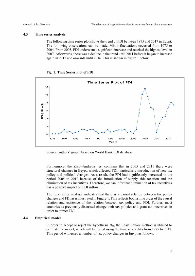
The following time series plot shows the trend of FDI between 1975 and 2017 in Egypt. The following observations can be made. Minor fluctuations occurred from 1975 to 2004. From 2005, FDI underwent a significant increase and reached the highest level in 2007. Afterwards, there was a decline in the trend until 2011 before it began to increase again in 2012 and onwards until 2016. This is shown in figure 1 below.
Fig. 1: Time Series Plot of FDI
Source: authors’ graph, based on World Bank FDI database.
Furthermore, the Zivot-Andrews test confirms that in 2005 and 2011 there were structural changes in Egypt, which affected FDI, particularly introduction of new tax policy and political changes. As a result, the FDI had significantly increased in the period 2005 to 2010 because of the introduction of supply side taxation and the elimination of tax incentives. Therefore, we can infer that elimination of tax incentives has a positive impact on FDI inflow.
The time series analysis indicates that there is a causal relation between tax policy changes and FDI as is illustrated in Figure 1. This reflects both a time order of the causal relation and existence of the relation between tax policy and FDI. Further, most countries as previously discussed change their tax policies and grant tax incentives in order to attract FDI.
4.4 Empirical model
In order to accept or reject the hypothesis 𝐻 , the Least Square method is utilised to estimate the model, which will be tested using the time series data from 1975 to 2017. This period witnessed a number of tax policy changes in Egypt as follows:
20152011200720031999199519911987198319791975
12
10
8
6
4
2
0
Years
FDI (
billi
on $
)
Time Series Plot of FDI

eJournal of Tax Research The relevance of supply side taxation for attracting foreign direct investment
11
- from 1975 to 2004, the implementation of a conventional tax policy, which focused on using tax incentives to stimulate FDI;
- from 2005 to 2016, the implementation of a supply side tax policy, which focused on eliminating tax incentives, broadening the tax base and lowering tax rates;
- from 2017 to date, the re-introduction of tax incentives.
Taking into account tax policy changes, we use a dummy variable for tax policy (the government opts to implement either a conventional tax policy or supply side tax policy) as follows:
- years in which the supply side tax policy is implemented will take the value of 1, while years in which the tax incentive policy is implemented will take the value of zero.
For the control variables, we use secondary data available in the World Bank database. Further, we use the World Bank Database of World Governance Indicators for the values of political stability data.
Descriptive statistics are used to describe the basic features regarding the data. Table 1 shows the mean, median and standard deviation of different variables.
Table 1: Summary of Descriptive Statistics
Variables FDI GDP Exchange Rate Trade
Labour Force
Political Stability
Mean 2.46 5.42 3.73 50.76 47.52 -0.68 Median 1.07 4.92 3.39 50.25 48.98 -0.55 Std. Deviation 3.14 2.53 3.34 11.17 5.49 0.42
4.4.1 Regression model
Normality test
Before running the regression analysis, we check the distribution of the FDI variable. According to Table 2 below, the distribution of FDI is not normal since the p-values of normality tests are less than 5%.
Table 2: Tests of Normality
Kolmogorov-Smirnov Shapiro-Wilk
Statistic DF Sig. Statistic DF Sig. FDI 0.371 43 0.000 0.713 43 0.000
To solve this issue, we will use a log transformation and the new variable (ln (FDI)) will be used in the regression.
eJournal of Tax Research The relevance of supply side taxation for attracting foreign direct investment
12
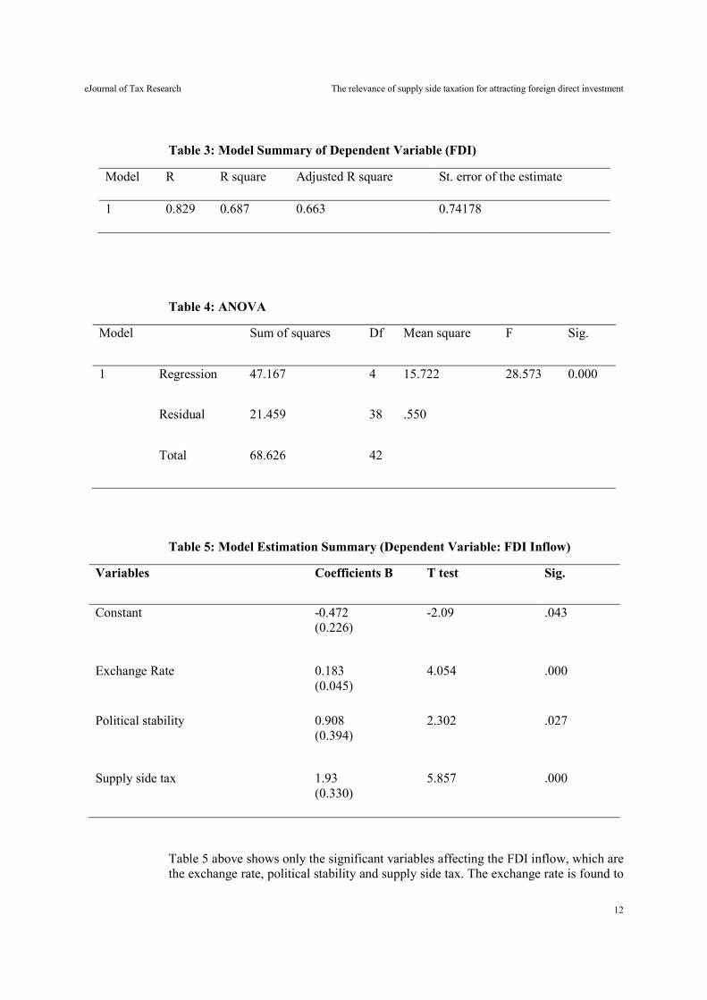
Table 3: Model Summary of Dependent Variable (FDI)
Model R R square Adjusted R square St. error of the estimate
1 0.829 0.687 0.663 0.74178
Table 4: ANOVA
Model Sum of squares Df Mean square F Sig.
1 Regression 47.167 4 15.722 28.573 0.000
Residual 21.459 38 .550
Total 68.626 42
Table 5: Model Estimation Summary (Dependent Variable: FDI Inflow)
Variables Coefficients B T test Sig.
Constant -0.472 (0.226)
-2.09 .043
Exchange Rate 0.183 (0.045)
4.054 .000
Political stability 0.908 (0.394)
2.302 .027
Supply side tax 1.93 (0.330)
5.857 .000
Table 5 above shows only the significant variables affecting the FDI inflow, which are the exchange rate, political stability and supply side tax. The exchange rate is found to
eJournal of Tax Research The relevance of supply side taxation for attracting foreign direct investment
13
positively and significantly affect FDI inflow with a point estimate of 0.183. The interpretation of this relationship is attributed to the significant depreciation of the Egyptian pound (EGP) value over the period 1991 to date. The EGP value has witnessed a significant depreciation since 1991 and culminated in 2016 when the exchange rate of the EGP against the US dollar depreciated around 100% (Elsherif, 2016). The depreciation of local currency encourages exports to foreign markets and consequently encourages investment in exporting industries and services (Hegazy, 2018). Therefore, this explains the positive relationship between the FDI inflow and exchange rate.
In addition, the model results indicate a positive and significant relationship between political stability and FDI inflow, with a point estimate of 0.908. This result aligns with previous studies such as Lucas (1990) and the OECD policy recommendations and practices that political stability is a critical factor for attracting FDI inflow.
Finally, the impact of the supply side tax policy on FDI inflow is found to be positive and significant with a point estimate of 1.93. The interpretation of this positive relationship is related to the nature of the supply side tax as it is based on a broader tax base and a lower tax rate, which create a simpler and neutral tax system. This tax system is based on supply side tax policy and is believed to be more competitive and attractive to many MNEs to invest in. Furthermore, MNEs often pay more attention to the simplicity of the tax system rather than tax incentives taking into account that most MNEs pay profit taxes in their home countries according to the worldwide income taxation approach (Kohlhase & Pierk, 2020). This means that their exempted income in the host country will be taxed in the home country. Therefore, providing tax incentives does not create a competitive tax system compared to the implementation of supply side taxation. Based on the above result, we accept the null hypothesis that a supply side tax policy has a positive impact on inflow FDI to Egypt.
The result of the time series analysis indicates that FDI inflow increased when the Egyptian government introduced the supply side taxation policy. Furthermore, testing of the econometric model indicates that abolishing tax incentives and cutting tax rates (implementation of supply side tax policy) has a positive impact on FDI inflow. Consequently, we can infer that a tax incentive policy is not considered a significant factor for attracting FDI compared to a supply side taxation policy.
Accordingly, we accept the study hypothesis that introducing supply side taxation had a positive impact on inflow FDI to Egypt. This result contrasts with practices of many developing countries that consider granting generous tax incentives to FDI to be an important factor for attracting FDI. The other structural change was in 2011 as FDI declined sharply because of an unstable political situation in Egypt and then resumed growth when political stability improved.
5. CONCLUDING REMARKS
This article aims to identify the relevance of supply side tax policy to attract FDI. In doing so, we reviewed the scholarly works related to the determinant factors for FDI inflow, which include tax and non-tax factors. Among the tax factors are tax incentives, which are commonly applied by the majority of developing countries, while the non-tax factors include important macroeconomic and political variables such as political stability and foreign exchange.
eJournal of Tax Research The relevance of supply side taxation for attracting foreign direct investment
14
The tax incentives take various forms such as tax holidays, tax exemption, tax credits and reduced tax rates. In addition to forgone tax revenue, tax incentives have a number of disadvantages that encourage some countries to abolish them and introduce a new tax policy known as supply side taxation, which is based on broadening the tax base through eliminating tax allowances, deductions, exemptions and lowering the tax rate, which creates a more competitive tax system. Both approaches in tax policy aim to minimise the tax burden and to increase FDI inflow. However, this situation raises a question about whether a tax incentive or supply side taxation policy is more effective for attracting FDI. In order to empirically identify which tax policy is more effective, we choose the case of Egypt, which has implemented both types of tax policies.
In this article, we used a regression model (OLS) and time series analysis to assess the impact of supply side taxation on inflow FDI in Egypt. In doing so, we reviewed the tax policy practices in Egypt, which have evolved since 1974 to date.
Egypt employed tax incentives as a key determinant for inflow FDI from 1974 to 2004. In 2005, a new tax policy was implemented through abolishing tax incentives and lowering tax rates (the supply side tax policy). The econometric model results, using the data from 1975 to 2017, show that the tax incentives policy is insignificant for attracting FDI while the supply side taxation positively and significantly affects FDI inflow in Egypt. This result draws attention for policy-makers in Egypt and other countries to designing broad-based tax legislation with a moderate tax rate. Such tax legislation will have a positive impact on the country’s competitiveness and FDI inflow. Therefore, the reintroduction of tax incentives under the new Egyptian tax legislation will add to complexity of tax system and is not expected to have a significant impact on FDI inflow.
6. REFERENCES
Abdellatif, M M 2009, ‘Looking for efficient tax incentives to stimulate research and development and economic growth’, New Zealand Journal of Taxation Law and Policy, vol. 15, no. 2, pp. 133-158.
Abdellatif, M & Tran-Nam, B 2016, ‘The tax policy debate regarding tax incentives in developing countries: The case of targeted tax incentives in Egypt’, Bulletin of International Taxation, vol. 70, no. 7, pp. 379-386.
Ajaz, T & Ahmad, E 2010, ‘The effect of corruption and governance on tax revenues’, The Pakistan Development Review, vol. 49, no. 4, pp. 405-417.
Auerbach, A J & Slemrod, J 1997, ‘The economic effects of the Tax Reform Act of 1986’, Journal of Economic Literature, vol. 35, no. 2, pp. 589-632.
Alam, A & Shah, S Z A 2013, ‘Determinants of foreign direct investment in OECD member countries’, Journal of Economic Studies, vol. 40, no. 4, pp. 515-527.
Andersen, M R, Kett, B R & von Uexkull, E 2018, ‘Corporate tax incentives and FDI in developing countries’, in World Bank, Global investment competitiveness report 2017/2018: Foreign investor perspectives and policy implications, World Bank, Washington, DC, pp. 73-99.
eJournal of Tax Research The relevance of supply side taxation for attracting foreign direct investment
15
Arbatli, E 2011, ‘Economic policies and FDI inflows to emerging market economies’, IMF Working Paper WP/11/192, Washington, DC, 1 August.
Baccini, L, Li, Q & Mirkina, I 2014, ‘Corporate tax cuts and foreign direct investment’, Journal of Policy Analysis and Management, vol. 33, no. 4, pp. 977-1006.
Beck, S & Chaves, A 2011, ‘The impacts of various taxes on foreign direct investment’, University of Delaware Department of Economics Working Paper 2018-11.
Becker, J, Fuest, C & Hemmelgarn, T 2006, ‘Corporate tax reform and foreign direct investment in Germany – evidence from firm-level data’, CESifo Working Paper Series No. 1722, May.
Bénassy-Quéré, A, Fontagné, L & Lahrèche-Révil, A 2005, ‘How does FDI react to corporate taxation?’, International Tax and Public Finance, vol. 12, no. 5, pp. 583-603.
Bevan, A A & Estrin, S 2000, ‘The determinants of foreign direct investment in transition economies’, William Davidson Institute Working Papers Series 342, University of Michigan, October.
Burman, L E 2003, ‘Is the tax expenditure concept still relevant?’, National Tax Journal, vol. 56, no. 3, pp. 613-627.
Calzolari, G 2004, ‘Incentive regulation of multinational enterprises’, International Economic Review, vol. 45, no. 1, pp. 257-282.
Canto, V A, Joines, D H & Laffer, A B 1981, ‘Tax rates, factor employment, and market production’, in Meyer, L H (ed), The supply-side effects of economic policy, Springer, Dordrecht, pp. 3-32.
Creswell, J W 2003, Research design: Qualitative, quantitative, and mixed methods approaches, 2nd edn, Sage Publications, Thousand Oaks, CA.
Devereux, M P & Griffith, R 2003, ‘Evaluating tax policy for location decisions’, International Tax and Public Finance, vol. 10, no. 2, pp. 107-126.
Economou, F, Hassapis, C, Philippas, N & Tsionas, M 2017, ‘Foreign direct investment determinants in OECD and developing countries’, Review of Development Economics, vol. 21, no. 3, pp. 527-542.
Elsherif, M 2016, ‘Exchange rate volatility and Central Bank actions in Egypt: Generalized autoregressive conditional heteroscedasticity analysis’, International Journal of Economics and Financial Issues, vol. 6, no. 3, pp. 1209-1216.
Feldstein, M 1986, ‘Supply side economics: Old truths and new claims’, The American Economic Review, vol. 76, no. 2, pp. 26-30.
Hegazy, Z S (2018, ‘Exchange rate volatility and Egyptian exports’, Australian Academy of Accounting and Finance Review, vol. 4, no. 3, pp. 100-110.
Holland, D & Vann, R 1998, ‘Income tax incentives for investment’, in Thuronyi, V (ed), Tax law design and drafting, vol. 2, International Monetary Fund, Washington, DC, pp. 986-1020.
Imam, P. A & Jacobs, D F 2007, ‘Effect of corruption on tax revenues in the Middle East’, IMF Working Paper WP/07/270, November. Available at: https://www.imf.org/external/pubs/ft/wp/2007/wp07270.pdf.
eJournal of Tax Research The relevance of supply side taxation for attracting foreign direct investment
16
International Monetary Fund (IMF) 2016, World economic outlook April 2016: Too slow for too long, International Monetary Fund, Washington, DC.
Jabri, A, Guesmi, K & Abid, I 2013, ‘Determinants of foreign direct investment in MENA region: Panel co-integration analysis’, The Journal of Applied Business Research, vol. 29, no. 4, pp. 1103-1110.
Jewell, A, Mansour, M, Mitra, P & Sdralevich, C 2015, ‘Fair taxation in the Middle East and North Africa’, IMF Staff Discussion Note SDN/15/16, September.
Kim, I S & Milner, H V 2019, ‘Multinational corporations and their influence through lobbying on foreign policy’, forthcoming in Multinational corporations in a changing global economy, Brookings Institution, Washington, DC. Available at:
https://scholar.princeton.edu/sites/default/files/hvmilner/files/revised_manuscript_submission_2_march.pdf.
Klemm, A 2010, ‘Causes, benefits, and risks of business tax incentives’, International Tax and Public Finance, vol. 17, no. 3, pp. 315-336.
Kohlhase, S & Pierk, J 2020, ‘The effect of a worldwide tax system on tax management of foreign subsidiaries’, Journal of International Business Studies, vol. 51, no. 8, pp. 1312-1330.
Lucas, R E, Jr. 1990, ‘Supply-side economics: An analytical review’, Oxford Economic Papers, vol. 42, no. 2, pp. 293-316.
Organisation for Economic Co-operation and Development (OECD) 2002, Foreign direct investment for development: Maximising benefits, minimising costs, OECD, Paris.
Organisation for Economic Co-operation and Development (OECD) 2007, OECD investment policy reviews: Egypt 2007, OECD, Paris.
Organisation for Economic Co-operation and Development (OECD) 2008, Making reforms succeed: Moving forward with the MENA investment policy agenda, OECD, Paris.
Organisation for Economic Co-operation and Development (OECD) 2010a, Business climate development strategy, phase 1 policy assessment: Egypt, dimension I-3, tax policy, MENA-OECD Initiative and European Commission, January, OECD, Paris. Available at: https://www.oecd.org/global-relations/46340489.pdf.
Organisation for Economic Co-operation and Development (OECD) 2010b, Choosing a broad base – low rate approach to taxation, OECD, Paris
Shah, A & Slemrod, J 1991, ‘Do taxes matter for foreign direct investment?’, The World Bank Economic Review, vol. 5, no. 3, pp. 473-491.
United Nations Conference on Trade and Development (UNCTAD) 2000, ‘Tax incentives and foreign direct investment: A global survey’, ASIT Advisory Studies No. 16, United Nations, New York and Geneva.
Vermeend, W, van der Ploeg, R & Timmer, J W 2009, Taxes and the economy: A survey on the impact of taxes on growth, employment, investment, consumption and the environment, Edward Elgar Publishing, Cheltenham, UK.
Zolt, E M 2013, ‘Tax incentives and tax base protection issues’, Papers on Selected Topics in Protecting the Tax Base of Developing Countries, Draft Paper No. 3, United Nations.
eJournal of Tax Research (2021) vol. 19, no. 1, pp. 17-47
17
GST treatment of electronic commerce: comparing the Singaporean and Australian approaches
Evgeny Guglyuvatyy and Nikolai Milogolov
Abstract
This article analyses the Australian and Singaporean indirect tax systems as they apply to electronic commerce (e-commerce), specifically focusing on mechanisms for taxation of cross-border transactions. Both countries have similar goods and services tax (GST) mechanisms (broad base, low rate and limited exemptions), and at the same time somewhat different economic determinants of tax policy (size of the economy, dependence on foreign trade, etc). Therefore, it is considered useful to assess how these countries adapt their indirect tax systems to digitalisation of the economy. Using the broader Australian and Singaporean e-commerce taxation systems as points of reference, the article identifies a set of criteria, or qualities (including, for example, neutrality and fairness), for an efficient system of e-commerce taxation, and evaluates the experience and measures in those two countries against these criteria. Key words: Indirect taxation, tax policy, electronic commerce, Singapore, Australia, VAT, GST
Senior Lecturer, School of Law and Justice, Southern Cross University, email: [email protected]. Senior Researcher, Tax Policy Center, Financial Research Institute (Moscow) and Senior Researcher, Laboratory of Tax Policy Research, Russian Presidential Academy of National Economy and Public Administration (RANEPA) (Moscow). This research has been funded by the Singapore Management University Tax Academy, Centre for Excellence in Taxation. The authors would like to thank two anonymous reviewers for their feedback that helped improve the manuscript.
eJournal of Tax Research GST treatment of electronic commerce
18
1. INTRODUCTION
Electronic commerce (e-commerce) is growing rapidly around the globe.1 International e-commerce transactions have become the norm rather than an exception, as cross-border flows have become faster and easier than ever before.2 However, taxation of these transactions raises various challenges for tax authorities in many countries. For example, a recent line of Organisation for Economic Co-operation and Development (OECD) recommendations3 underlines some of the tax-related challenges of the digital economy and e-commerce. These challenges include the following:
- creating the new nexus rules for highly digitalised business models;
- developing a profit allocation methodology that is consistent with the value creation process of new digitalised businesses;
- developing an effective and neutral mechanism for indirect tax collection from cross-border online sales of goods and services;
- ensuring international consistency in taxation of cross-border online transactions and prevention of double taxation and double non-taxation with respect to both indirect and direct taxes.4
Several international ‘best practice’ guidelines, such as the OECD’s International VAT/GST Guidelines (hereinafter ‘OECD Guidelines’), provide useful guidance on issues relating to the design of goods and services tax (GST).5 In particular, the OECD Guidelines pertain to the reform of GST in relation to e-commerce transactions. The OECD Guidelines represent an important step towards harmonisation of indirect international taxation. However, there are a number of differences in national approaches to indirect taxation of e-commerce some of which will be discussed in this article.
This article compares and contrasts the Australian and Singaporean e-commerce indirect tax systems, specifically focusing on mechanisms for taxation of cross-border transactions. The authors compare the Australian and Singaporean e-commerce indirect taxation systems using well-known criteria, or qualities (including efficiency, simplicity, neutrality and fairness) of the ‘best practice’ GST as benchmarks, and evaluate the experience and indirect tax reform approaches in those two countries against these criteria.
Sections 2 and 3 discuss in detail the approaches to indirect taxation of e-commerce in Australia and Singapore specifically focusing on cross-border supplies of goods and digital services. Section 4 identifies the criteria that should underpin an efficient system of e-commerce taxation, and analyses the two countries’ approaches to indirect taxation
1 Digital sectors of the economy are more dynamic on average: Organisation for Economic Co-operation and Development (OECD), Measuring the Digital Transformation: A Roadmap for the Future (OECD Publishing, 2019). 2 Ibid. 3 OECD, Tax Challenges Arising from Digitalisation – Interim Report 2018, OECD/G20 Base Erosion and Profit Shifting Project, Inclusive Framework on BEPS (OECD Publishing, 2018). 4 Ibid. 5 OECD, International VAT/GST Guidelines (OECD Publishing, 2017).
eJournal of Tax Research GST treatment of electronic commerce
19
of e-commerce. Conclusions are drawn in the final section of the article, together with recommendations to improve the existing systems.
2. SINGAPORE
Singapore has been positioning itself as a global hub of international trade since the 20th century,6 and has introduced various tax policies supporting trade and e-commerce.7
In 1993, Singapore introduced GST. Observers suggest that ‘some of the characteristics of the Singaporean GST system are due to the peculiarities of the country, such as the lack of natural resources, which pushed the country to develop a very trade-oriented economy, its strong connections with the United Kingdom, and its geographical location’.8 This quotation refers to the GST’s characteristic of international neutrality. It can be noted that GST design generally accommodates the destination principle well. This is due to the GST neutrality that is achieved by crediting input tax against output tax, thus applying the tax burden to the final consumer and remitting value added tax (VAT) to budgets at all levels of the supply chain. The OECD Guidelines endorse this fundamental advantage of GST.9
Recently, taxation of cross-border e-commerce trade in goods and digital services has appeared on the Singaporean political agenda, supported by tax officials.10 This political attention to the issue partly arose as a result of the relevant OECD recommendations and developments in neighbouring economies,11 primarily Australia and New Zealand. Internal reasons, such as the need to raise additional revenue, were also influential.12
Currently, the GST treatment of cross-border transactions of goods and services based on the destination principle is considered the primary tax policy option in Singapore,13 as discussed below and subsequent steps aimed at ensuring GST neutrality between digital and non-digital economy are being made by tax policy-makers.14 Tax conditions for e-commerce were more favourable before the reform because of the relatively high
6 Industrial Systems Research, Industry and Enterprise: An International Survey of Modernization and Development (Industrial Systems Research, 2013) 86. 7 Ramkishen S Rajan and Shandre M Thangavelu, Singapore: Trade, Investment and Economic Performance (World Scientific, 2009). 8 Francesco Cannas, ‘What Singapore Could Learn from the New Trends for VAT/GST Taxation of B2C Digital Supplies around the World’ (2016) 27(5) International VAT Monitor 320. 9 OECD, Measuring the Digital Transformation, above n 1; OECD, International VAT/GST Guidelines, above n 5. 10 See, eg, Suet Yen Loo, ‘Possible Tax on E-Commerce to Diversify Tax Base’, News IBFD (27 November 2017): ‘The Senior Minister of State (Finance and Law) was recently quoted as stating that e-commerce would be an area enabling Singapore to further diversify its tax base. Her comments followed those of the Prime Minister who had signalled that Singapore needs to prepare for tax increases to fund increasing government expenditure, particularly as the population ages’. 11 Clinton Alley and Joanne Emery, ‘Taxation of Cross-Border E-Commerce: Response of New Zealand and Other OECD Countries to BEPS Action 1’ (2017) 28(9) Journal of International Taxation 38; OECD, Addressing the Tax Challenges of the Digital Economy, Action 1 – 2015 Final Report, OECD/G20 Base Erosion and Profit Shifting Project (OECD Publishing, 2015). 12 Michelle Jamrisko, ‘Singapore to Ensure Rich Pay More in Tax Regime, Rajah Says’, Bloomberg (22 November 2017), https://www.bloomberg.com/news/articles/2017-11-21/singapore-will-ensure-rich-pay-more-in-tax-regime-minister-says (accessed 12 June 2021). 13 Goods and Services Tax (Amendment) Act 2018 (No 52 of 2018) (Singapore). 14 Inland Revenue Authority of Singapore, e-Tax Guide, GST: Taxing Imported Services by Way of Reverse Charge (22 August 2019); Inland Revenue Authority of Singapore, e-Tax Guide, GST: Taxing Imported Services by Way of an Overseas Vendor Registration Regime (26 August 2019).
eJournal of Tax Research GST treatment of electronic commerce
20
threshold (SGD 400) for offshore supply of goods (still applying as on June 2021)15 and because of the place of supply rules in the case of digital services which applied before the reform until recently (before 2020).16 This reform will be finalised by 2023. So, both B2B and B2C import cross-border supplies of low value goods and digital services are in the process of appearing into the scope of Singaporean GST.17
2.1 GST e-commerce tax reform in Singapore: background and key changes.
Singapore is a developed country in relation to the digital economy and e-commerce, and a leader in global digital transformation, as evidenced by the rankings.18
A survey by Ernst & Young indicates that Singapore has a highly device-centric and digitally savvy population that utilises devices and mobile phones on a daily basis. New digital technologies are also very popular in Singapore, including novel payment methods, music streaming and online purchases.19 It is important to note that Singapore’s population density is among that of the top three countries in the world.20 Thus, despite its relatively small territory Singapore has a rather large consumption tax base. The following factors should also be considered:
- the Singaporean e-commerce market is growing rapidly21 – it almost tripled from 2010 to 2014 and then grew by around 10 per cent per year, reaching USD 3,740 billion in 2018;
- the majority of e-commerce sales (about 60 per cent) are cross-border transactions;22
- most e-commerce players in Singapore are local;23
15 Loo, above n 10. 16 Cannas, above n 8, 321: ‘In order to determine whether a supply of services is made “in Singapore”, one has to look at section 13(4) of the Singapore GST Act, which provides that:
A supply of services shall be treated as made – (a) in Singapore if the supplier belongs in Singapore; and (b) in another country (and not in Singapore), if the supplier belongs in that other country’.
Furthermore, Goods and Services Tax Act 1993, s 15(3) provides: ‘The supplier of services shall be treated as belonging in a country if — (a) he has in that country a business establishment or some other fixed establishment and no such establishment elsewhere; (b) he has no such establishment in any country but his usual place of residence is in that country; or (c) he has such establishments both in that country and elsewhere and the establishment of his which is most directly concerned with the supply is in that country’. 17 Ernst & Young, Worldwide VAT, GST and Sales Tax Guide, Singapore (2017), http://www.ey.com/gl/en/services/tax/worldwide-vat--gst-and-sales-tax-guide---xmlqs?preview&XmlUrl=/ec1mages/taxguides/VAT-2017/VAT-SG.xml: ‘Supplies of goods or services in Singapore via the internet or any other electronic media does not alter the taxability of the transaction’. 18 See IMD, World Competitiveness Ranking (2019), https://www.imd.org/contentassets/6b85960f0d1b42a0a07ba59c49e828fb/one-year-change-vertical.pdf (accessed 11 June 2021). 19 Ernst & Young, Savvy Singapore: Decoding a Digital Nation (2017), http://www.ey.com/sg/en/services/advisory/ey-savvy-singapore-decoding-a-digital-nation. 20 World Bank, Population Density (people per sq. km of land area), https://data.worldbank.org/indicator/EN.POP.DNST?year_high_desc=true. 21 Statista, eCommerce, Singapore, Highlights, https://www.statista.com/outlook/243/124/ecommerce/singapore#. 22 US Department of Commerce, International Trade Administration, Export.Gov, Singapore Country Commercial Guide, https://www.export.gov/article?id=Singapore-eCommerce. 23 Ben Sim, ‘7 Out of 10 Top E-Commerce Players in Singapore Are Local, Study Finds’, E27 (5 September 2017), https://e27.co/7-10-top-e-commerce-players-singapore-local-study-finds-20170905/ (accessed 11 June 2021).
eJournal of Tax Research GST treatment of electronic commerce
21
- Singapore is a perfect location for starting an e-commerce business due to its favourable business climate (it ranked second in the World Bank ‘Doing Business’ ratings for 2017);24
- Singapore is a popular destination for businesses engaged in e-commerce because of its competitive tax system, highly developed legislation and generally favourable business conditions.25
E-commerce refers to business transactions (sales and purchases) that are concluded electronically. Any supply of goods or services in Singapore (except for export supplies) via the internet or any other electronic media is subject to GST, as is traditional commerce. This also applies when transactions are conducted ‘through a third party e-commerce service provider’.26 This means that traditional GST concepts also apply to cross-border e-commerce in Singapore, in particular the place of supply for services (section 13(4) of the Goods and Services Tax Act 1993 (Singapore)) and the rules on low value importation for goods.27 For GST purposes, the sale of goods (books, shoes, etc) via the internet is treated as a supply of goods, and the sale of digitalised goods (online music, games, smartphone apps) downloaded by the customer via the internet is treated as supply of services.28
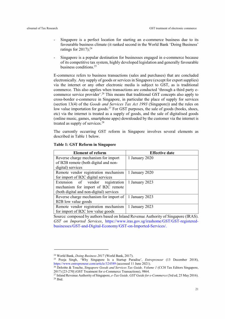
The currently occurring GST reform in Singapore involves several elements as described in Table 1 below.
Table 1: GST Reform in Singapore
Element of reform Effective date Reverse charge mechanism for import of B2B remote (both digital and non-digital) services
1 January 2020
Remote vendor registration mechanism for import of B2C digital services
1 January 2020
Extension of vendor registration mechanism for import of B2C remote (both digital and non-digital) services
1 January 2023
Reverse charge mechanism for import of B2B low value goods
1 January 2023
Remote vendor registration mechanism for import of B2C low value goods
1 January 2023
Source: composed by authors based on Inland Revenue Authority of Singapore (IRAS). GST on Imported Services, https://www.iras.gov.sg/irashome/GST/GST-registered-businesses/GST-and-Digital-Economy/GST-on-Imported-Services/.
24 World Bank, Doing Business 2017 (World Bank, 2017). 25 Pooja Singh, ‘Why Singapore Is a Startup Paradise’, Entrepreneur (13 December 2018), https://www.entrepreneur.com/article/324589 (accessed 11 June 2021). 26 Deloitte & Touche, Singapore Goods and Services Tax Guide, Volume 1 (CCH Tax Editors Singapore, 2017) [23-270] (GST Treatment for e-Commerce Transactions), 9864. 27 Inland Revenue Authority of Singapore, e-Tax Guide, GST Guide for e-Commerce (3rd ed, 25 May 2016). 28 Ibid.
eJournal of Tax Research GST treatment of electronic commerce
22
2.2 Cross-border supply of goods
All physical goods supplied over the internet attract GST if the supplier is GST registered and the supply is conducted in Singapore. Export exemption (by means of zero-rating) is available for the supply of goods conducted over the internet to offshore consumers.29 The supply of goods between an overseas supplier and a Singaporean purchaser will attract GST when the goods are imported, where the value of the goods being sold exceeds SGD 400.30 Importation of all goods below the threshold qualifies for so-called import relief. The value of imported goods for GST purposes is determined as the cost, insurance and freight (CIF) plus other chargeable costs and the duty payable (if applicable).31 To ensure a level playing field for local businesses to compete effectively, the GST will be extended to imported low-value goods.32 Reform has been proposed in this direction; the status quo will likely be changed from 1 January 2023.
As of June 2021 there are no separate rules for business-to-business (B2B) and business-to-consumer (B2C) importations of low-value goods. This implies that all imports exceeding the threshold (SGD 400) are subject to GST; thus, the importer pays 7 per cent of the customs value of importation to the Customs and Excise Department. The Customs and Excise Department collects GST from the supplier of the goods sold in Singapore. This could be the postal service or the courier company, which in turn collects the GST from the purchaser.33
From 1 January 2023 different rules will be applied for business-to-business (B2B) and business-to-consumer (B2C) importations of low-value goods. Imposition of GST on low-value goods will be effected as follows:34
1) Overseas Vendor Registration for B2C import of low-value goods; and
2) Reverse charge for Business-to-Business (‘B2B’) import of low-value goods.
Overseas suppliers of goods and services will be subject to the same GST treatment as local suppliers. As explained in IRAS Draft Guide (2021)35 the current non-taxation of low value goods results in a disparity in GST treatment between similar goods supplied by GST-registered local businesses and overseas ones. Therefore, the reform is aimed at ensuring the principle of destination and at taxation of all domestic consumption with GST. However, the existing import relief threshold of SGD 400 will remain which
29 Inland Revenue Authority of Singapore, GST Guide for e-Commerce, above n 27. 30 Ibid 6. 31 Inland Revenue Authority of Singapore, GST Guide for e-Commerce, above n 27. 32 Nikita Lingbawan, ‘Singapore Extends Incentives for Qualifying Expenses and Extends GST to Imported Low-Value Goods in 2021 Budget’, News IBFD (16 February 2021). 33 Inland Revenue Authority of Singapore, ‘Importing of Goods’, https://www.iras.gov.sg/irashome/GST/GST-registered-businesses/Working-out-your-taxes/Importing-of-Goods/. 34 Inland Revenue Authority of Singapore (IRAS), ‘GST on Imports of Low-Value Goods’, https://www.iras.gov.sg/irashome/GST/GST-registered-businesses/GST-and-Digital-Economy/GST-on-Imports-of-Low-Value-Goods/. 35 Inland Revenue Authority of Singapore, e-Tax Guide, GST: Taxing Imported Low-Value Goods by Way of the Overseas Vendor Registration Regime (Draft) (26 February 2021) 8, para 4.3, https://www.iras.gov.sg/irashome/uploadedFiles/IRASHome/e-Tax_Guides/DRAFT%20e-tax%20guide_Taxing%20imported%20low-value%20goods%20by%20way%20of%20the%20overseas%20vendor%20registration%20regime_v1.pdf.
eJournal of Tax Research GST treatment of electronic commerce
23
means that legally such supplies will not be regarded as import of goods but rather as another domestic supply.
2.3 Cross-border supplies of digital services
A sale of digital services (such as music or software) over the internet to an individual consumer or a business equates to a supply of services for GST purposes. There are no separate rules for domestic supplies of B2B and B2C digital services. All domestic supplies of digital services are taxable. Supplies of services are subject to GST if the place of supply is Singapore. Application of section 13(4) of the Goods and Services Tax Act 1993 determines whether the place of supply of services is Singapore. Specifically, a supply of services is treated as:
a) made in Singapore if the supplier is in Singapore; and
b) made in another country (and not in Singapore) if the supplier is in that other country.36
Export supplies of digital services are zero-rated under section 21(3) of the Goods and Services Tax Act 1993. Export of digital services means that services are performed for a consumer who is not in Singapore at the time the service is performed, and that the services are not supplied in direct connection to land or goods situated within Singapore.37 There is an extensive list of zero-rated international services, and this includes digital services.
The most problematic tax compliance challenge related to e-commerce export of digital services supplied by Singaporean businesses lies in determining whether the purchaser is in Singapore. This is a necessary step in determining the GST rate (0 per cent or 7 per cent) that should apply.38 The Internal Revenue Authority of Singapore (IRAS) GST Guide for e-Commerce (2016) provides the following criteria for that purpose:
- if the purchaser is a business, the supplier shall examine its address, domain name, internet protocol (IP) address, other information and customer declaration;
- if the purchaser is an individual, the supplier shall consider the usual place of residence.39
Generally, the supplier should make reasonable efforts to identify the residency of the customer. To resolve this issue, some global businesses require their customers to ‘declare’ their residence by selecting their country, and then direct them to country-specific web pages.40 However, if customers do not declare their residency, businesses must rely on their systems and the evidence they have.
The Goods and Services Tax Act 1993 also provides for a ‘reverse charge’ on the importation of ‘prescribed services’. This means that if the recipient is a taxable entity,
36 Section 13(4) of the Goods and Services Tax Act 1993 (Singapore). See also Cannas, above n 8. 37 Goods and Services Tax Act 1993, s 21(3)(j). 38 Seven per cent is the standard rate in Singapore. There is only one rate except for the zero rate in Singaporean GST (Goods and Services Tax Act 1993, s 16). 39 Inland Revenue Authority of Singapore, GST Guide for e-Commerce, above n 27, 4. 40 Kenny Foo, ‘Singapore: GST Planning for Electronic Commerce’ (2001) 7(5) Asia-Pacific Tax Bulletin 117.
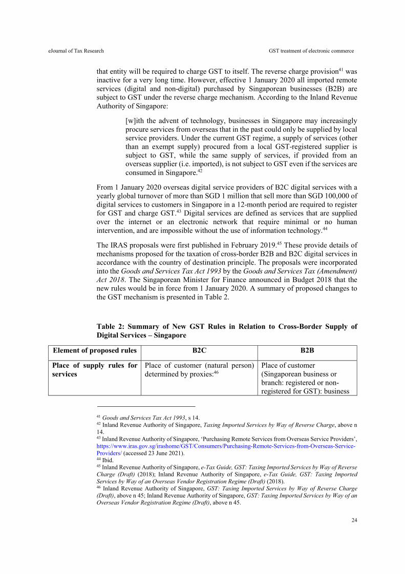
eJournal of Tax Research GST treatment of electronic commerce
24
that entity will be required to charge GST to itself. The reverse charge provision41 was inactive for a very long time. However, effective 1 January 2020 all imported remote services (digital and non-digital) purchased by Singaporean businesses (B2B) are subject to GST under the reverse charge mechanism. According to the Inland Revenue Authority of Singapore:
[w]ith the advent of technology, businesses in Singapore may increasingly procure services from overseas that in the past could only be supplied by local service providers. Under the current GST regime, a supply of services (other than an exempt supply) procured from a local GST-registered supplier is subject to GST, while the same supply of services, if provided from an overseas supplier (i.e. imported), is not subject to GST even if the services are consumed in Singapore.42
From 1 January 2020 overseas digital service providers of B2C digital services with a yearly global turnover of more than SGD 1 million that sell more than SGD 100,000 of digital services to customers in Singapore in a 12-month period are required to register for GST and charge GST.43 Digital services are defined as services that are supplied over the internet or an electronic network that require minimal or no human intervention, and are impossible without the use of information technology.44
The IRAS proposals were first published in February 2019.45 These provide details of mechanisms proposed for the taxation of cross-border B2B and B2C digital services in accordance with the country of destination principle. The proposals were incorporated into the Goods and Services Tax Act 1993 by the Goods and Services Tax (Amendment) Act 2018. The Singaporean Minister for Finance announced in Budget 2018 that the new rules would be in force from 1 January 2020. A summary of proposed changes to the GST mechanism is presented in Table 2.
Table 2: Summary of New GST Rules in Relation to Cross-Border Supply of Digital Services – Singapore
Element of proposed rules B2C B2B
Place of supply rules for services
Place of customer (natural person) determined by proxies:46
Place of customer (Singaporean business or branch: registered or non-registered for GST): business
41 Goods and Services Tax Act 1993, s 14. 42 Inland Revenue Authority of Singapore, Taxing Imported Services by Way of Reverse Charge, above n 14. 43 Inland Revenue Authority of Singapore, ‘Purchasing Remote Services from Overseas Service Providers’, https://www.iras.gov.sg/irashome/GST/Consumers/Purchasing-Remote-Services-from-Overseas-Service-Providers/ (accessed 23 June 2021). 44 Ibid. 45 Inland Revenue Authority of Singapore, e-Tax Guide, GST: Taxing Imported Services by Way of Reverse Charge (Draft) (2018); Inland Revenue Authority of Singapore, e-Tax Guide, GST: Taxing Imported Services by Way of an Overseas Vendor Registration Regime (Draft) (2018). 46 Inland Revenue Authority of Singapore, GST: Taxing Imported Services by Way of Reverse Charge (Draft), above n 45; Inland Revenue Authority of Singapore, GST: Taxing Imported Services by Way of an Overseas Vendor Registration Regime (Draft), above n 45.
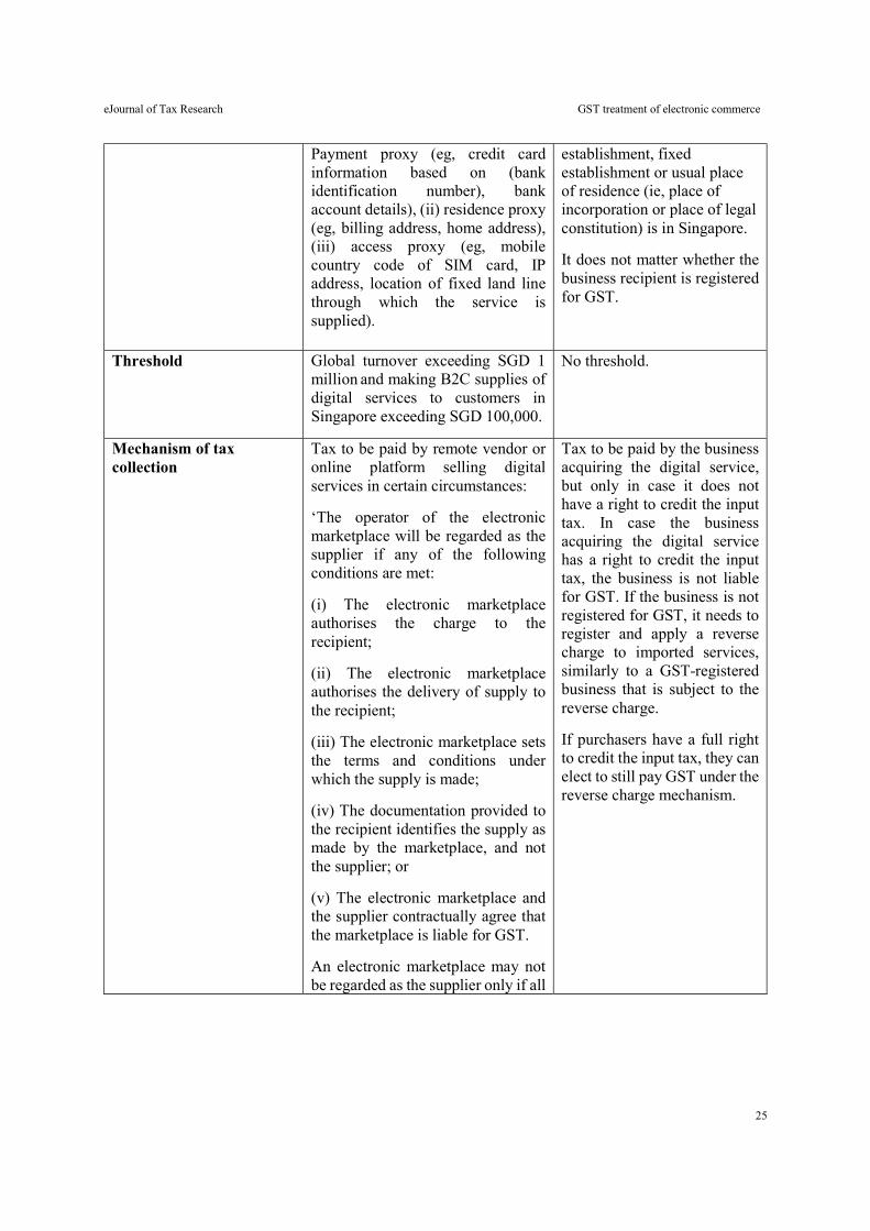
eJournal of Tax Research GST treatment of electronic commerce
25
Payment proxy (eg, credit card information based on (bank identification number), bank account details), (ii) residence proxy (eg, billing address, home address), (iii) access proxy (eg, mobile country code of SIM card, IP address, location of fixed land line through which the service is supplied).
establishment, fixed establishment or usual place of residence (ie, place of incorporation or place of legal constitution) is in Singapore.
It does not matter whether the business recipient is registered for GST.
Threshold Global turnover exceeding SGD 1 million and making B2C supplies of digital services to customers in Singapore exceeding SGD 100,000.
No threshold.
Mechanism of tax collection
Tax to be paid by remote vendor or online platform selling digital services in certain circumstances:
‘The operator of the electronic marketplace will be regarded as the supplier if any of the following conditions are met:
(i) The electronic marketplace authorises the charge to the recipient;
(ii) The electronic marketplace authorises the delivery of supply to the recipient;
(iii) The electronic marketplace sets the terms and conditions under which the supply is made;
(iv) The documentation provided to the recipient identifies the supply as made by the marketplace, and not the supplier; or
(v) The electronic marketplace and the supplier contractually agree that the marketplace is liable for GST.
An electronic marketplace may not be regarded as the supplier only if all
Tax to be paid by the business acquiring the digital service, but only in case it does not have a right to credit the input tax. In case the business acquiring the digital service has a right to credit the input tax, the business is not liable for GST. If the business is not registered for GST, it needs to register and apply a reverse charge to imported services, similarly to a GST-registered business that is subject to the reverse charge.
If purchasers have a full right to credit the input tax, they can elect to still pay GST under the reverse charge mechanism.

eJournal of Tax Research GST treatment of electronic commerce
26
of the abovementioned conditions are not satisfied.’47
Digital services covered Digital services are defined as services that are delivered over the internet or an electronic network, the nature of which renders their supply essentially automated, involving minimal human intervention and being impossible in the absence of information technology.
These services include supply of the following:
• downloadable digital content (eg, downloadable mobile applications, e-books and movies);
• subscription-based media (eg, news, magazines, streamed TV shows and music, and online gaming);
• software programs (eg, downloadable software, drivers, website filters and firewalls);
• electronic data management (eg, website hosting, online data warehousing, file sharing and cloud storage services); and
• support services, performed via electronic means, to arrange or facilitate a transaction, which may not be digital in nature (eg, commissions, listing fees and service charges).
Source: Composed by the authors based on Inland Revenue Authority of Singapore, e-Tax Guide, GST: Taxing Imported Services by Way of Reverse Charge (Draft) (2018) and GST: Taxing Imported Services by Way of an Overseas Vendor Registration Regime (Draft) (2018); Goods and Services Tax (Amendment) Act 2018.
Table 2 indicates that offshore suppliers of B2C digital services to customers in Singapore would be covered by the proposed GST rules. The reverse charge mechanism would cover B2B transactions between offshore suppliers of digital services and business recipients based in Singapore, which generally do not have full responsibility for the deduction of input GST. The GST-registered recipient is allowed to claim the corresponding GST as an input tax credit, subject to input tax refund rules. These proposals are generally in line with international practice, and recommendations outlined in the OECD Guidelines.48
2.4 Critics of GST Reform
Singaporean GST legislation is relatively modern and straightforward, which provides the jurisdiction with an important competitive advantage. For example, in comparison with EU VAT the advantages of the Singaporean GST are:
47 Inland Revenue Authority of Singapore, GST: Taxing Imported Services by Way of Reverse Charge (Draft), above n 45; Inland Revenue Authority of Singapore, GST: Taxing Imported Services by Way of an Overseas Vendor Registration Regime (Draft), above n 45. 48 OECD (2017), International VAT/GST Guidelines, above n 5.
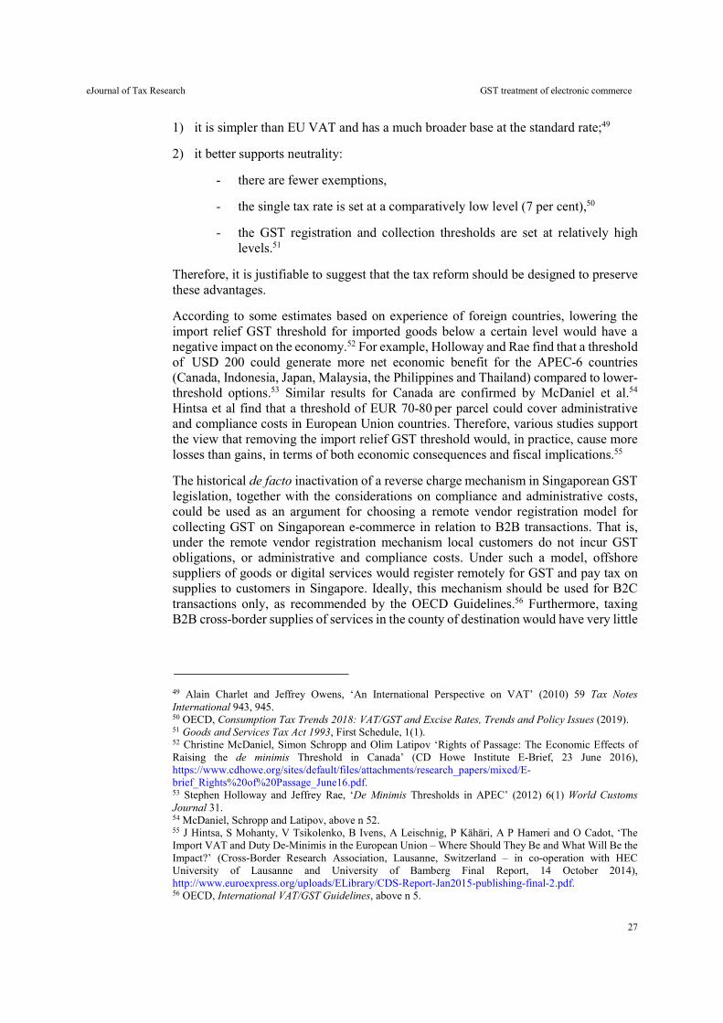
eJournal of Tax Research GST treatment of electronic commerce
27
1) it is simpler than EU VAT and has a much broader base at the standard rate;49
2) it better supports neutrality:
- there are fewer exemptions,
- the single tax rate is set at a comparatively low level (7 per cent),50
- the GST registration and collection thresholds are set at relatively high levels.51
Therefore, it is justifiable to suggest that the tax reform should be designed to preserve these advantages.
According to some estimates based on experience of foreign countries, lowering the import relief GST threshold for imported goods below a certain level would have a negative impact on the economy.52 For example, Holloway and Rae find that a threshold of USD 200 could generate more net economic benefit for the APEC-6 countries (Canada, Indonesia, Japan, Malaysia, the Philippines and Thailand) compared to lower-threshold options.53 Similar results for Canada are confirmed by McDaniel et al.54 Hintsa et al find that a threshold of EUR 70-80 per parcel could cover administrative and compliance costs in European Union countries. Therefore, various studies support the view that removing the import relief GST threshold would, in practice, cause more losses than gains, in terms of both economic consequences and fiscal implications.55
The historical de facto inactivation of a reverse charge mechanism in Singaporean GST legislation, together with the considerations on compliance and administrative costs, could be used as an argument for choosing a remote vendor registration model for collecting GST on Singaporean e-commerce in relation to B2B transactions. That is, under the remote vendor registration mechanism local customers do not incur GST obligations, or administrative and compliance costs. Under such a model, offshore suppliers of goods or digital services would register remotely for GST and pay tax on supplies to customers in Singapore. Ideally, this mechanism should be used for B2C transactions only, as recommended by the OECD Guidelines.56 Furthermore, taxing B2B cross-border supplies of services in the county of destination would have very little
49 Alain Charlet and Jeffrey Owens, ‘An International Perspective on VAT’ (2010) 59 Tax Notes International 943, 945. 50 OECD, Consumption Tax Trends 2018: VAT/GST and Excise Rates, Trends and Policy Issues (2019). 51 Goods and Services Tax Act 1993, First Schedule, 1(1). 52 Christine McDaniel, Simon Schropp and Olim Latipov ‘Rights of Passage: The Economic Effects of Raising the de minimis Threshold in Canada’ (CD Howe Institute E-Brief, 23 June 2016), https://www.cdhowe.org/sites/default/files/attachments/research_papers/mixed/E-brief_Rights%20of%20Passage_June16.pdf. 53 Stephen Holloway and Jeffrey Rae, ‘De Minimis Thresholds in APEC’ (2012) 6(1) World Customs Journal 31. 54 McDaniel, Schropp and Latipov, above n 52. 55 J Hintsa, S Mohanty, V Tsikolenko, B Ivens, A Leischnig, P Kähäri, A P Hameri and O Cadot, ‘The Import VAT and Duty De-Minimis in the European Union – Where Should They Be and What Will Be the Impact?’ (Cross-Border Research Association, Lausanne, Switzerland – in co-operation with HEC University of Lausanne and University of Bamberg Final Report, 14 October 2014), http://www.euroexpress.org/uploads/ELibrary/CDS-Report-Jan2015-publishing-final-2.pdf. 56 OECD, International VAT/GST Guidelines, above n 5.
eJournal of Tax Research GST treatment of electronic commerce
28
or no revenue effect, as business recipients would be able claim back the amount of GST included in the cost of supply.
3. AUSTRALIA
As discussed above, there has been a significant increase in the international trade of goods, services and intangibles. In particular, telecommunications and computer technologies have advanced enormously in recent years. Correspondingly, consumption by Australians of goods and services originating from offshore, both as a business input and for private consumption purposes, has increased significantly.57
Australia’s GST is a VAT that is applied at a rate of 10 per cent on most goods and services transactions connected with Australia. It is a consumption tax paid by final consumers when consumption takes place in Australia. The tax effectively excludes B2B transactions (via the mechanism of crediting the input tax against the output tax).58 Generally, GST applies to goods, services and intangibles acquired from outside Australia for consumption in Australia. Exports of goods, services and intangibles from Australia are treated as GST-free (zero-rated). This approach follows the destination principle as outlined above;59 that is, GST is applied to consumption that occurs in Australia, irrespective of the origin of the supply, and is not applied to consumption outside Australia.
Application of the destination principle to the taxation of supplies of services and intangibles is problematic, as in some cases it is difficult to identify whether the consumption is taking place in or outside Australia. Therefore, most jurisdictions implement proxies for determining the place of consumption, using the consumer’s location (or consumer residence or place of performance) instead. However, again, the significant growth in international electronic transactions has increasingly distorted identification of the place of consumption. As a result, some of the goods and services consumed in Australia are not taxed. For example, the purchase of digital content by an Australian consumer from an overseas supplier may not be taxed if the supplier is not registered for GST purposes.
Generally, if a person carries on a business or other form of enterprise in Australia, they must register for GST if their GST turnover60 over a 12-month period is AUD 75,000 or more (AUD 150,000 or more for non-profit organisations).61 A registration system is used for administration of the GST to ensure that GST is paid by liable businesses, and to provide relief (an entitlement to input tax credit)62 for GST imposed on acquisitions by businesses of goods and services. Once registered, businesses receive an Australian
57 National Australia Bank, Online Retail Sales Index, In-Depth Report June 2017 (2017), https://business.nab.com.au/wp-content/uploads/2017/08/NORSI-JUN-2017.pdf. 58 See, generally, A New Tax System (Good and Services Tax) Act 1999 (Cth) Div 11 (GST Act). 59 OECD, Committee on Fiscal Affairs Working Party No 9 on Consumption Taxes, International VAT/GST Guidelines: Guidelines on Neutrality (28 June 2011), https://www.oecd.org/tax/consumption/guidelinesneutrality2011.pdf. 60 ‘GST turnover’ refers to gross business income (not profit), and only supplies connected with Australia are included in the turnover. 61 GST Act, above n 58, Div 23. 62 However, an input tax credit is available for taxpayers ‘carrying on an enterprise’ and also satisfying some other conditions under s 11-15 of the GST Act.

eJournal of Tax Research GST treatment of electronic commerce
29
Business Number (ABN), which facilitates administration of the GST.63 If non‑resident businesses supply goods, services or other things (such as rights) for consumption in Australia, they may have an obligation to register for GST and pay GST on any taxable supplies they make.64 Non-resident businesses may register voluntarily for GST, and that allows them to recover GST incurred on their business acquisitions in Australia.65
Internet sales within the ‘indirect tax zone’ (ITZ)66 are taxed in the same way as the physical sale of goods and services; that is, registered businesses:
- are required to include GST in the price of sales to their customers and then remit the GST to the Australian Taxation Office (ATO);
- are able to claim credits for the GST included in the price of their business-related purchases, as a refund from the ATO or a credit against their GST.
In 2017, a new law covering B2C supplies of digital content purchased by Australian consumers was introduced.67 New GST rules for the import of low value goods purchased by Australian consumers were also implemented in June 2018. The key changes include elimination of the current threshold of AUD 1,000 for low value import of goods, and the introduction of a remote vendor model for payment of GST on such supplies.68
3.1 Cross-border supplies of goods
Previously, importation of goods from overseas suppliers to Australian purchasers attracted GST where the value of the goods being sold exceeded AUD 1,000. All transactions that take place online where the seller is an Australian business now attract GST.
The AUD 1,000 threshold originated from the customs entry thresholds and duty/tax-free thresholds for goods entering the country. James observes that such thresholds are generally established to balance revenue, administration and compliance costs.69 Nonetheless, the Australian threshold is also characterised as a mechanism for reducing the regulatory burden on international trade. According to the ATO, the low value threshold has served to ‘minimise delays in the delivery of mail and cargo, reducing the cost to business of importing low value consignments, determining a value below which it is uneconomical to collect the tax and duty, and to facilitate international trade by minimising intervention’.70
63 See Australian Taxation Office (ATO), ‘Registering for GST’ (last modified 20 April 2021), https://www.ato.gov.au/Business/GST/Registering-for-GST/ 64 GST Act, above n 58, Div 23. 65 Ibid. 66 Ibid, s 195-1. The indirect tax zone (ITZ) covers an area smaller than Australia and excludes certain offshore territories and sea locations. Section 9-25 of the GST Act distinguishes between the supply of goods, real property and ‘anything else’ with respect to the ITZ. 67 Treasury Laws Amendment (GST Low Value Goods) Act 2017. The Act specifically indicates ‘intangible supply’, which includes digital content. 68 Kathryn James, ‘Applying the GST to Imports of Low-Value Goods in Australia’ (2018) 47(2) Australian Tax Review 83. 69 Kathryn James, The Rise of the Value-Added Tax (Cambridge University Press, 2015) ch 2. 70 Ibid.
eJournal of Tax Research GST treatment of electronic commerce
30
Division 13 of the A New Tax System (Goods and Services Tax) Act 1999 (the GST Act) outlines the GST treatment of taxable importations.71 A taxable importation is described in section 13-5.72 Notably, section 13-5 provides that there is no requirement for the importer to be registered for GST and the importer does not need to be carrying on an enterprise.73 If the non-resident supplier is the importer, the supplier will be making a taxable supply and will therefore be liable for GST.74 However, a voluntary reverse charge mechanism was introduced into GST law. The mechanism allows a registered business (Australian or non‑resident), by arrangement with the non-resident supplier, to take on the GST obligations of the non-resident supplier.75
3.2 Recent reform
For more than a decade, the Australian retail industry had been calling for the Australian government to remove the preferential tax treatment granted to low value goods.76 For example, the National Retail Association argued that the low value threshold ‘poses the greatest threat to traditional retail jobs and domestic online retail growth’, and that Australian retail had lost a number of jobs because of that issue.77 It was claimed that such a move would provide a level playing field for Australian retailers. The call to tax low value goods led to the Australian government’s determination to broaden the tax base and improve revenue collection.
There have been various reports on the treatment of low value goods under the Australian GST system.78 Regarding the cost effectiveness of the GST application to low value goods, it is commonly concluded that low value goods should be treated in the same way as all goods sold domestically. According to a report by the Productivity Commission, eliminating the low value threshold would provide additional GST revenue of around AUD 480 million, but it would entail a collection cost of over AUD 2 billion, borne by businesses, consumers and the government.79 The Productivity Commission recommended removing the low value threshold only when it would be cost effective to do so. Similarly, the Low Value Parcel Processing Taskforce found in 2012 that if the low value threshold were removed, the GST collection costs would outweigh the revenue collected.80 The review also concluded that there would be a negative effect on the economy.
However, these studies anticipated that GST would be collected as an at-the-border charge using the then-current collection mechanism. Therefore, the Australian
71 GST Act, above n 58, Div 13. 72 Ibid, s 13-5. 73 Ibid. 74 Ibid, s 9-25(3)(a). 75 Ibid, s 84-10. 76 See, for example, Brett Winterford, ‘Retailers Call for GST Review as Online Sales Boom’, CRN (4 January 2011), https://www.crn.com.au/news/retailers-call-for-gst-review-as-online-sales-boom-243091 (accessed 11 June 2021). 77 News.com.au, ‘Retailers Call for GST on Online Sales’ (14 September 2012), http://www.news.com.au/finance/work/retailers-call-for-gst-on-online-sales/news-story/ 3a84e4dbab88452dcdcdd95db6fc6172 (accessed 11 June 2021). 78 Low Value Parcel Processing Taskforce, Final Report (July 2012); Productivity Commission, Collection Models for GST on Low Value Imported Goods, Discussion Paper (July 2017). 79 Productivity Commission. Economic Structure and Performance of the Australian Retail Industry, Inquiry Report (2011). 80 Low Value Parcel Processing Taskforce, above n 78, 7-10 and 10-11.
eJournal of Tax Research GST treatment of electronic commerce
31
government tried to find ways to reduce the costs of collection and the compliance burden. For example, one approach considered was to levy GST on international retailers via a point-of-sale charge rather than an at-the-border charge.81 In 2015, there was extensive discussion of GST-related issues between the Commonwealth Treasurer and the State and Territory (subnational) Treasuries, following which the Commonwealth Treasurer reported:
the [State and Territory] treasurers agreed to apply the GST to offshore sales into the Australian market. This is a significant initiative. From the 1 July 2017, the GST will be applied to all products and services sold by vendors overseas into Australia. This will deliver competitive neutrality for Australian businesses, it will ensure that there is fair and equal treatment of all goods and services, so that if goods and services in Australia were to have the GST applied by companies in Australia, then the same would apply overseas.82
The recent reform modifies the GST Act to cover sales of low value goods, digital products and other imported services to Australian consumers by non-resident entities.83 The new law covers the importation of low value goods, defined as goods with a customs value of AUD 1,000 or less.84 The AUD 1,000 threshold was established at the time when the consideration for the supply was first agreed.
These changes affect non-resident entities selling to Australian consumers. Moreover, freight forwarders and operators of electronic distribution platforms (EDPs) facilitating supplies to Australian consumers are also affected.85
Under the new law, a supply of goods is connected to the ITZ86 if:
- the supply involves the goods being brought to Australia with the assistance of the supplier or;
- the goods are low value; and
- the purchaser of the goods is a consumer.87
If the non-resident supplier meets the AUD 75,000 per year threshold, the supplier is required to register for GST and to remit GST to the Australian Taxation Office on its sales.88 Supplies that are connected with the ITZ need to be taken into account in determining whether the supplier’s turnover for GST purposes is AUD 75,000 or more annually.89
The new law also covers a supplier that assists in bringing goods into Australia. That includes the supplier delivering goods into Australia and the supplier procuring,
81 Productivity Commission, Collection Models for GST on Low Value Imported Goods, above n 78. 82 The date, 1 July 2017, was later changed to 1 July 2018. See Hon Joe Hockey (Treasurer), Transcript of Press Conference, Canberra (21 August 2015), https://ministers.treasury.gov.au/ministers/joe-hockey-2015/transcripts/press-conference-canberra-8. 83 Treasury Laws Amendment (GST Low Value Goods) Act 2017. 84 Tobacco and alcohol are subject to customs duty. GST Act, above n 58, s 84-79(3). 85 Ibid, s 84-81. 86 The ITZ refers to Australia, but does not include external territories and certain offshore areas. 87 Treasury Laws Amendment (GST Low Value Goods) Act 2017. 88 GST Act, above n 58, s 23-5. 89 Ibid.
eJournal of Tax Research GST treatment of electronic commerce
32
arranging or facilitating delivery of the goods into Australia (in other words, freight forwarding).90 Situations in which a supplier makes transport arrangements with third parties or provides assistance to the purchaser in relation to transport arrangements are similarly covered by the introduced law.91 If the goods are delivered to Australia by a freight forwarder as a result of an arrangement with the purchaser, the freight forwarder will be treated as making the supply. The freight forwarder and/or EDP is also required to register for GST purposes if its annual turnover is AUD 75,000 or more. A freight forwarder covered by this GST provision will need to collect information from the supplier about the transaction, such as the consideration for the supply, in order to be able to meet its GST liability.
According to the new law, an Australian consumer includes any entity that is generally an Australian resident. An entity is a consumer of a supply made to the entity if:
a) the entity is not registered; or
b) if the entity is registered, the entity does not acquire the thing supplied solely or partly for the purpose of an enterprise that the entity carries on in the ITZ.92
Notably, the connection is not the place of consumption but is reliant on the identity of the consumer as an Australian resident and the place to which the goods are sent. Identifying a consumer as an Australian resident for purposes of the Income Tax Assessment Act 1997 (Cth) might be a complex task. To address this issue, the new law provides that a supplier in some situations is treated as making a supply to an entity that is not an Australian consumer. In particular, GST liability will not apply where a supplier takes reasonable steps to obtain information about whether or not an entity is an Australian consumer,93 and if, after taking such steps, the supplier reasonably believes that the other entity is not an Australian consumer. 94
The new law does not specify which factors will allow a supplier to form a ‘reasonable belief’ about the identity of an Australian recipient. However, one important factor is whether the recipient is registered for GST.95 This should be confirmed by the ABN, or other identifying information relating to that entity disclosed to the supplier. Other important factors are prescribed by the Australian Commissioner of Taxation. Specifically, Goods and Services Tax Ruling GSTR 2017/1 provides other relevant details and examples of information needed to support a conclusion about the recipient’s residency status.96
Examples of information that the Commissioner will accept as supporting a conclusion about the recipient’s residency status include:
- the recipient’s billing address;
90 Ibid, s 38-355(3). 91 Ibid, s 84-81. 92 Ibid, s 84-75(2). 93 Ibid, s 84-83. 94 Ibid. 95 It should be noted that in many cases the recipient may not be registered for GST. 96 Australian Taxation Office, Goods and Services Tax Ruling GSTR 2017/1, ‘Goods and Services Tax: Making Cross-Border Supplies to Australian Consumers’.
eJournal of Tax Research GST treatment of electronic commerce
33
- the recipient’s mailing address;
- the recipient’s banking or credit card details, including the location of the bank or credit card issuer; and
- location-related data from third-party payment intermediaries and other information.97
However, the ATO notes that this is not a full list of evidence that would be relevant to establishing the residency status of a recipient.98
3.3 Mechanism of tax collection under the new rules
Under the introduced amendments, the current ‘border model’ arrangements for collecting GST on imports above AUD 1,000 will be retained. Currently, GST, customs duty and border clearance fees are required to be remitted to the Australian Border Force (ABF). However, imports of goods with a value of 1,000 AUD or less will be subject to a new and separate regime. The mechanism of administration and collection of GST under the new amendments could be described as an ‘expanded vendor’ model.99 The GST obligation is placed on the seller, the EDP or the freight forwarder, depending on the supply chain for the item in question. The GST is collected on transactions with consumers only (B2C). Australian entities registered for GST can provide their ABN to the supplier as evidence that they are registered. Under the new collection model, sellers, EDPs and redeliverers must provide the ABF with details of their ABN and the ABN of the recipient (where applicable); that is, freight companies and express carriers need to collect that information and provide it to the ABF.
According to the Australian government, the main advantages of this collection mechanism are improved tax neutrality, competitive neutrality for Australian retailers, additional government revenue and relatively low administration costs.100 In comparison to the border model, this mechanism entails lower administrative costs for government and avoids likely delays and disruptions to goods delivery for consumers.101
3.4 Cross-border supplies of digital services
As discussed above, the new amendments to the GST Act related to low value goods were delayed until July 2018. However, the delay did not affect the start of the previously introduced measure requiring non-resident suppliers to register and remit GST on services, digital products or rights supplied to Australian consumers. This measure has been in force since 1 July 2017. The introduced amendments affect section
97 Ibid, para 29. 98 The list is relevant in the context of GST Act, s 84-100. However, most of these examples are not relevant for income tax residency. 99 Productivity Commission, Collection Models for GST on Low Value Imported Goods, above n 78. 100 Hon Joe Hockey (Treasurer), ‘Statement: Council on Federal Financial Relations Tax Reform Workshop’, Media Release (21 August 2015), https://ministers.treasury.gov.au/ministers/joe-hockey-2015/media-releases/statement-council-federal-financial-relations-tax-reform; Hon Scott Morrison (Treasurer), ‘Delivering a Fairer Playing Field for Australian Businesses’, Media Release (21 June 2017), https://ministers.treasury.gov.au/ministers/scott-morrison-2015/media-releases/delivering-fairer-playing-field-australian-businesses. 101 Hon Joe Hockey (Treasurer), above n 100; Hon Scott Morrison (Treasurer), above n 100.

eJournal of Tax Research GST treatment of electronic commerce
34
9-25 of the GST Act in order to make a supply of services connected with the ITZ a taxable supply for GST purposes, unless the supply is GST-free or input taxed.102
According to the amended law, such sales are now generally subject to GST in the same way as are supplies made by Australian taxable persons to domestic consumers. The key changes are as follows:
- the GST is imposed on intangible supplies, such as supplies of digital content, games and software, and services performed offshore for customers in Australia;
- the supplier or the operator of an electronic distribution service (EDP) will be liable for the GST;
- the GST applies only to B2C transactions; B2B transactions are exempted.
The introduced requirement for supplies to ascertain whether recipients are ‘Australian consumers’103 allows the inclusion of the supply of anything that is not goods or real property (that is, services and intangibles such as digital products supplied from overseas to an Australian consumer).104 When such a supply is delivered to an Australian consumer from overseas and is made through an EDP, the operator of the platform is taxed, rather than the actual supplier. Considering the large number of suppliers of digital products supplying to Australian consumers, the proposed changes will also apply to EDPs. If an EDP is used to supply to Australian consumers, the operator of the platform, rather than the original supplier of the digital product, is deemed to be the supplier liable for the GST.105 This is a significant deviation from the previous rules contained in sections 9-5 and 9-10 of the GST Act, which made the actual supplier liable.106
The ‘Australian consumer’ test for low value goods is somewhat broader than the test that applies to the supply of inbound intangible consumer supplies. In addition to the above requirements, there is a further condition that the recipient of the supply be an Australian resident for income tax purposes. However, for low value goods there is a sufficient connection to Australia if the goods are imported to Australia (even by a non-resident).107
The concept of an EDP was introduced as part of amendments made to the GST treatment of supplies of intangibles by overseas suppliers. An EDP is categorised as a service (including a website, internet portal, gateway, store or marketplace that allows businesses to make supplies available to end users) where:
- the supplies are made to end users by means of the service;
102 GST Act, above n 58, s 9-5. 103 Ibid, s 9-25(7) provides a relevant definition: ‘Suppliers must take reasonable steps to ascertain whether recipients are Australian consumers’. 104 Ibid, s 9-25. 105 Ibid. 106 There are some exceptions to the general rule, such as the ‘reverse charge’ under Division 84. As part of these changes, the reverse charge rules in Division 84 of the GST Act were completely rewritten. The rules in Division 84 of the GST Act were expanded to impose a reverse charge on low value goods supplied to GST-registered businesses where a full input tax credit is not available. 107 GST Act, above n 58, s 9-26.
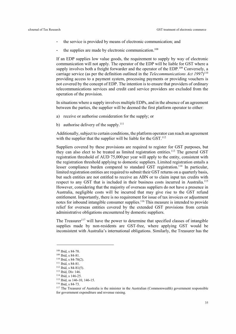
eJournal of Tax Research GST treatment of electronic commerce
35
- the service is provided by means of electronic communication; and
- the supplies are made by electronic communication.108
If an EDP supplies low value goods, the requirement to supply by way of electronic communication will not apply. The operator of the EDP will be liable for GST where a supply involves both a freight forwarder and the operator of the EDP.109 Conversely, a carriage service (as per the definition outlined in the Telecommunications Act 1997)110 providing access to a payment system, processing payments or providing vouchers is not covered by the concept of EDP. The intention is to ensure that providers of ordinary telecommunications services and credit card service providers are excluded from the operation of the provision.
In situations where a supply involves multiple EDPs, and in the absence of an agreement between the parties, the supplier will be deemed the first platform operator to either:
a) receive or authorise consideration for the supply; or
b) authorise delivery of the supply.111
Additionally, subject to certain conditions, the platform operator can reach an agreement with the supplier that the supplier will be liable for the GST.112
Suppliers covered by these provisions are required to register for GST purposes, but they can also elect to be treated as limited registration entities.113 The general GST registration threshold of AUD 75,000 per year will apply to the entity, consistent with the registration threshold applying to domestic suppliers. Limited registration entails a lesser compliance burden compared to standard GST registration.114 In particular, limited registration entities are required to submit their GST returns on a quarterly basis, but such entities are not entitled to receive an ABN or to claim input tax credits with respect to any GST that is included in their business costs incurred in Australia.115 However, considering that the majority of overseas suppliers do not have a presence in Australia, negligible costs will be incurred that may give rise to the GST refund entitlement. Importantly, there is no requirement for issue of tax invoices or adjustment notes for inbound intangible consumer supplies.116 This measure is intended to provide relief for overseas entities covered by the extended GST provisions from certain administrative obligations encountered by domestic suppliers.
The Treasurer117 will have the power to determine that specified classes of intangible supplies made by non-residents are GST-free, where applying GST would be inconsistent with Australia’s international obligations. Similarly, the Treasurer has the
108 Ibid, s 84-70. 109 Ibid, s 84-81. 110 Ibid, s 84-70(2). 111 Ibid, s 84-81. 112 Ibid, s 84-81(5). 113 Ibid, Div 146. 114 Ibid, s 146-25. 115 Ibid, ss 146-10, 146-15. 116 Ibid, s 84-73. 117 The Treasurer of Australia is the minister in the Australian (Commonwealth) government responsible for government expenditure and revenue raising.
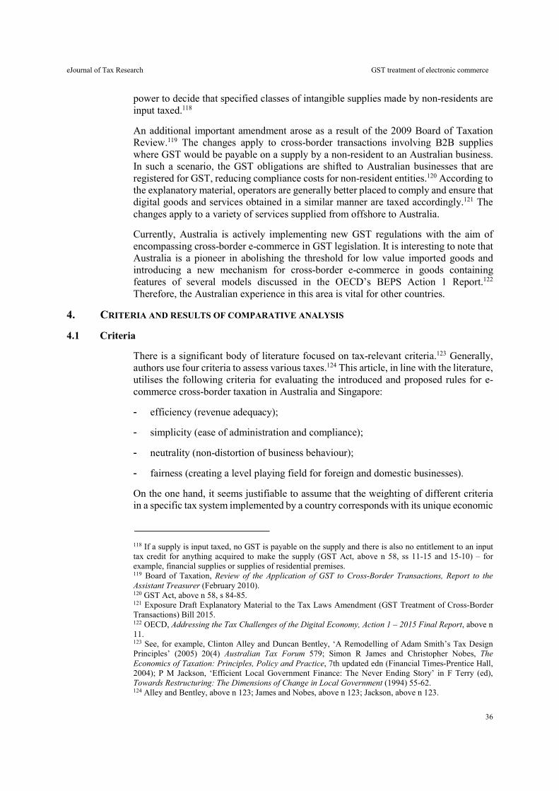
eJournal of Tax Research GST treatment of electronic commerce
36
power to decide that specified classes of intangible supplies made by non-residents are input taxed.118
An additional important amendment arose as a result of the 2009 Board of Taxation Review.119 The changes apply to cross-border transactions involving B2B supplies where GST would be payable on a supply by a non-resident to an Australian business. In such a scenario, the GST obligations are shifted to Australian businesses that are registered for GST, reducing compliance costs for non-resident entities.120 According to the explanatory material, operators are generally better placed to comply and ensure that digital goods and services obtained in a similar manner are taxed accordingly.121 The changes apply to a variety of services supplied from offshore to Australia.
Currently, Australia is actively implementing new GST regulations with the aim of encompassing cross-border e-commerce in GST legislation. It is interesting to note that Australia is a pioneer in abolishing the threshold for low value imported goods and introducing a new mechanism for cross-border e-commerce in goods containing features of several models discussed in the OECD’s BEPS Action 1 Report.122 Therefore, the Australian experience in this area is vital for other countries.
4. CRITERIA AND RESULTS OF COMPARATIVE ANALYSIS
4.1 Criteria
There is a significant body of literature focused on tax-relevant criteria.123 Generally, authors use four criteria to assess various taxes.124 This article, in line with the literature, utilises the following criteria for evaluating the introduced and proposed rules for e-commerce cross-border taxation in Australia and Singapore:
- efficiency (revenue adequacy);
- simplicity (ease of administration and compliance);
- neutrality (non-distortion of business behaviour);
- fairness (creating a level playing field for foreign and domestic businesses).
On the one hand, it seems justifiable to assume that the weighting of different criteria in a specific tax system implemented by a country corresponds with its unique economic
118 If a supply is input taxed, no GST is payable on the supply and there is also no entitlement to an input tax credit for anything acquired to make the supply (GST Act, above n 58, ss 11-15 and 15-10) – for example, financial supplies or supplies of residential premises. 119 Board of Taxation, Review of the Application of GST to Cross-Border Transactions, Report to the Assistant Treasurer (February 2010). 120 GST Act, above n 58, s 84-85. 121 Exposure Draft Explanatory Material to the Tax Laws Amendment (GST Treatment of Cross-Border Transactions) Bill 2015. 122 OECD, Addressing the Tax Challenges of the Digital Economy, Action 1 – 2015 Final Report, above n 11. 123 See, for example, Clinton Alley and Duncan Bentley, ‘A Remodelling of Adam Smith’s Tax Design Principles’ (2005) 20(4) Australian Tax Forum 579; Simon R James and Christopher Nobes, The Economics of Taxation: Principles, Policy and Practice, 7th updated edn (Financial Times-Prentice Hall, 2004); P M Jackson, ‘Efficient Local Government Finance: The Never Ending Story’ in F Terry (ed), Towards Restructuring: The Dimensions of Change in Local Government (1994) 55-62. 124 Alley and Bentley, above n 123; James and Nobes, above n 123; Jackson, above n 123.
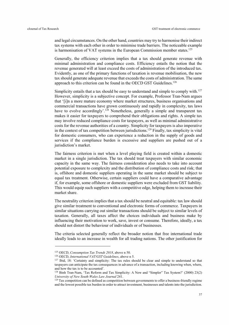
eJournal of Tax Research GST treatment of electronic commerce
37
and legal circumstances. On the other hand, countries may try to harmonise their indirect tax systems with each other in order to minimise trade barriers. The noticeable example is harmonisation of VAT systems in the European Commission member states.125
Generally, the efficiency criterion implies that a tax should generate revenue with minimal administration and compliance costs. Efficiency entails the notion that the revenue generated will at least exceed the costs of administration of the introduced tax. Evidently, as one of the primary functions of taxation is revenue mobilisation, the new tax should generate adequate revenue that exceeds the costs of administration. The same approach to this criterion can be found in the OECD GST Guidelines.126
Simplicity entails that a tax should be easy to understand and simple to comply with.127 However, simplicity is a subjective concept. For example, Professor Tran-Nam argues that ‘[i]n a more mature economy where market structures, business organisations and commercial transactions have grown continuously and rapidly in complexity, tax laws have to evolve accordingly’.128 Nonetheless, generally a simple and transparent tax makes it easier for taxpayers to comprehend their obligations and rights. A simple tax may involve reduced compliance costs for taxpayers, as well as minimal administrative costs for the revenue authorities of a country. Simplicity for taxpayers is also imperative in the context of tax competition between jurisdictions.129 Finally, tax simplicity is vital for domestic consumers, who can experience a reduction in the supply of goods and services if the compliance burden is excessive and suppliers are pushed out of a jurisdiction’s market.
The fairness criterion is met when a level playing field is created within a domestic market in a single jurisdiction. The tax should treat taxpayers with similar economic capacity in the same way. The fairness consideration also needs to take into account potential exposure to complexity and the distribution of compliance costs and risk; that is, offshore and domestic suppliers operating in the same market should be subject to equal tax treatment. Otherwise, certain suppliers could have a comparative advantage if, for example, some offshore or domestic suppliers were excluded from GST liability. This would equip such suppliers with a competitive edge, helping them to increase their market share.
The neutrality criterion implies that a tax should be neutral and equitable: tax law should give similar treatment to conventional and electronic forms of commerce. Taxpayers in similar situations carrying out similar transactions should be subject to similar levels of taxation. Generally, all taxes affect the choices individuals and business make by influencing their motivation to work, save, invest or consume. Therefore, ideally, a tax should not distort the behaviour of individuals or of businesses.
The criteria selected generally reflect the broader notion that free international trade ideally leads to an increase in wealth for all trading nations. The other justification for
125 OECD, Consumption Tax Trends 2018, above n 50. 126 OECD, International VAT/GST Guidelines, above n 5. 127 Ibid, 18: ‘Certainty and simplicity: The tax rules should be clear and simple to understand so that taxpayers can anticipate the tax consequences in advance of a transaction, including knowing when, where, and how the tax is to be accounted’. 128 Binh Tran-Nam, ‘Tax Reform and Tax Simplicity: A New and “Simpler” Tax System?’ (2000) 23(2) University of New South Wales Law Journal 241. 129 Tax competition can be defined as competition between governments to offer a business-friendly regime and the lowest possible tax burden in order to attract investment, businesses and talents into the jurisdiction.
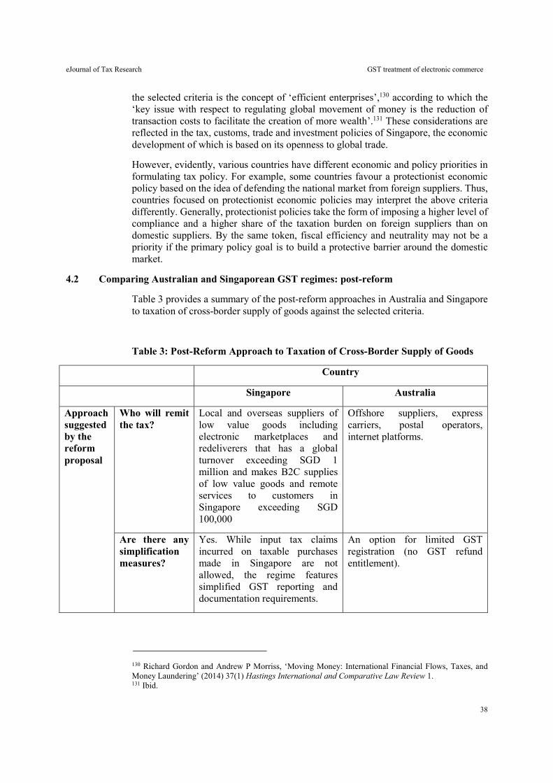
eJournal of Tax Research GST treatment of electronic commerce
38
the selected criteria is the concept of ‘efficient enterprises’,130 according to which the ‘key issue with respect to regulating global movement of money is the reduction of transaction costs to facilitate the creation of more wealth’.131 These considerations are reflected in the tax, customs, trade and investment policies of Singapore, the economic development of which is based on its openness to global trade.
However, evidently, various countries have different economic and policy priorities in formulating tax policy. For example, some countries favour a protectionist economic policy based on the idea of defending the national market from foreign suppliers. Thus, countries focused on protectionist economic policies may interpret the above criteria differently. Generally, protectionist policies take the form of imposing a higher level of compliance and a higher share of the taxation burden on foreign suppliers than on domestic suppliers. By the same token, fiscal efficiency and neutrality may not be a priority if the primary policy goal is to build a protective barrier around the domestic market.
4.2 Comparing Australian and Singaporean GST regimes: post-reform
Table 3 provides a summary of the post-reform approaches in Australia and Singapore to taxation of cross-border supply of goods against the selected criteria.
Table 3: Post-Reform Approach to Taxation of Cross-Border Supply of Goods
Country
Singapore Australia
Approach suggested by the reform proposal
Who will remit the tax?
Local and overseas suppliers of low value goods including electronic marketplaces and redeliverers that has a global turnover exceeding SGD 1 million and makes B2C supplies of low value goods and remote services to customers in Singapore exceeding SGD 100,000
Offshore suppliers, express carriers, postal operators, internet platforms.
Are there any simplification measures?
Yes. While input tax claims incurred on taxable purchases made in Singapore are not allowed, the regime features simplified GST reporting and documentation requirements.
An option for limited GST registration (no GST refund entitlement).
130 Richard Gordon and Andrew P Morriss, ‘Moving Money: International Financial Flows, Taxes, and Money Laundering’ (2014) 37(1) Hastings International and Comparative Law Review 1. 131 Ibid.

eJournal of Tax Research GST treatment of electronic commerce
39
What supplies are covered by the new rules?
B2C import supplies of tangible goods that have a value not exceeding the import relief threshold of SGD 400.
B2C import supplies of tangible goods with value of less than AUD 1,000.
Are there any differences between B2B and B2C?
B2B import supplies of low value goods are exempted beside where the purchaser is not taxable (at least partly). In the latter case reverse charge mechanism applies.
B2B import supplies of tangible goods are exempted.
Criteria Neutrality The new regime theoretically does not distort business decisions. Thus, neutrality may be achieved because the GST tax burden is equal for foreign and domestic supplies to local customers. However, neutrality is impacted if the supply is not zero-rated at the jurisdiction of origin. Some suppliers may avoid GST due to difficulties in administrative control of the regime.
Fairness In theory, the new regime is fair, since offshore and local suppliers are subject to equal GST liability. Thus, the reform eliminates the discrimination against local suppliers that existed before the reform. However, some non-compliant suppliers may evade GST liability by skipping the GST registration. The new mechanism relies on voluntary compliance as its main pre-condition. It is hard to perform GST control and audit in relation to cross-border e-commerce, in case of non-cooperative taxpayer’s behaviour.
Fiscal efficiency The new regime potentially generates a substantial amount of tax revenue. However, the costs of system administration and compliance might be also significant.
Simplicity The new regime adds complexity by requiring suppliers to collect various information from customers, to determine and calculate their tax liability and to identify the place of consumption. An additional issue is distribution of taxpayer/tax agent roles between suppliers, carriers and internet platforms involved in the supply.
Source: Authors
Table 3 indicates that the issues with neutrality, fairness and fiscal efficiency associated with the pre-reform Australian and Singaporean GST mechanisms can be addressed by the introduced reform. One of the major pillars of the reform is the extension of the destination principle, which ensures effective taxation in the state of consumption. This is in line with OECD guidance and the international consensus on this issue.
The neutrality criterion is addressed both under the Australian and Singaporean new rules, since equal GST liability applies to both foreign and domestic suppliers. However, thresholds apply differently for inbound supplies due to the EDP rules. Some authors suggest that ‘putting a GST on low value imports is unlikely to revive Australian retailing in the face of intense online shopping competition, given the significant price
eJournal of Tax Research GST treatment of electronic commerce
40
differentials for many popular consumer products’.132 Further, it is argued that Australia’s retail disadvantage can be attributed to its extremely regulated labour market and regulatory restrictions on retail and land use, rather than to the low value threshold.133
However, some commentators argue that the new measures will not achieve competitive neutrality. For example, representatives of EDPs, in their submission to the Senate Economics Legislation Committee inquiry into the enacting Bill, suggested that many sellers who use their services are microbusinesses whose turnover is below the AUD 75,000 threshold that would require them to register and apply GST to sales under AUD 1,000. Nevertheless, EDPs are treated as individual sellers under the new Australian regime. This means that a platform needs to register for the collection and remittance of GST and apply the GST charge to the products of each individual seller.134
Despite these arguments, the very fact of equal treatment of foreign and domestic suppliers under the new Australian rules addresses the neutrality principle significantly better compared to the previous regime. Some observers state that, since the purpose of the new regime is to create a level playing field, it would be reasonable to introduce such a regime even if there was a net revenue loss in the early years.135
There are some issues related to administration and compliance with the new rules. In particular, the new Australian regime introduces different tax remittance mechanisms for cross-border online supplies of low value goods in comparison with domestic supplies. This could create an ‘administrative barrier’ protecting the local market, which could be beneficial for domestic suppliers, owing to increased compliance requirements imposed on offshore suppliers. In this context, Berg and Davidson argue that the new measure is a tariff, since it levies GST on sellers who do not have the access to input tax credits that an Australian domestic seller would have.136 However, any seller can choose to register in the normal regime in order to claim credits.
Additionally, it is not clear on what basis express carriers are included in the GST net, given their limited role in the process of cross-border e-commerce. Generally, express carriers are not involved in funds transfer, which means that they cannot include GST in the cost of the goods; that is, the express carrier must request GST from another player involved in the transaction. According to the Explanatory Memorandum on the reforms, the rationale for making EDPs liable for tax collection is that they are normally larger and better resourced than most of the individual sellers making supplies via the platform.137 They also have more information about the consumers of supplies to enable them to decide whether the consumer is an Australian resident for tax purposes.138 The Treasury supposes that ‘compliance and administration would be simplified if liability
132 M Novak, No to the GST Tax Attack: Why the Exemption for Online Purchases Should Stay (Institute of Public Affairs, 2015). 133 Ibid. 134 Senate Economics Legislation Committee, Treasury Laws Amendment (GST Low Value Goods) Bill 2017 [Provisions]: Report (May 2017). 135 Ibid 136 Chris Berg and Sinclair Davidson, ‘Submission to the Productivity Commission Inquiry into Collection Models for GST on Low Value Imported Goods’, available at: https://www.pc.gov.au/__data/assets/pdf_file/0012/221430/sub033-collection-models.pdf. 137 Explanatory Memorandum to the Tax and Superannuation Laws Amendment (2016 Measures No 1) Bill 2016. 138 Ibid.
eJournal of Tax Research GST treatment of electronic commerce
41
for GST rested on the platform operator rather than the vendor’.139 A similar logic could be applied to the inclusion of express carriers in the GST net.
A significant issue is that the Australian regime imposes a number of requirements on offshore suppliers, including the requirements to assess whether they need to register for GST, to identify taxable sales, to collect GST on taxable sales, and to report on and remit GST to the ATO based on their sales to Australian consumers. Therefore, the Australian regime inflicts notable compliance costs on offshore suppliers. For example, in their submission to the Senate Economics Legislation Committee inquiry, the EDPs eBay, Alibaba and Etsy expressed concern that they would be liable for GST on goods that they have never owned, held, tracked or traded.140 EDPs in general suggest that the introduced system will be multifaceted and expensive to administer, and it is likely that the costs will be passed on to consumers. This would result in various impacts on consumers, including the apparent outcome that the tax and associated compliance costs would cause an upsurge in prices. However, the Australian Treasury notes that the chosen collection model is well balanced and that the inclusion of electronic platforms increased compliance with the new law.141 The Treasury also argues that this model is the most appropriate, given that the number of businesses involved is expected to grow rapidly.
Generally, Australia has the jurisdiction to impose GST on non-resident suppliers; however, Australia has no jurisdiction over enforcement.142 The Australian government has no power to issue a tax assessment for unpaid GST to an offshore supplier. Furthermore, some of Australia’s trade partners (for example, the United States) have multiple levels of government collecting different taxes, which may exacerbate the enforcement challenge for the ATO because the ATO would need to deal with various governments.
The other potential issue is double taxation of the same supply in cases where jurisdiction of consumption applies the country of destination principle to cross-border supplies but jurisdiction of supply applies the country of origin principle to the same supply.143 International tax treaties harmonising countries’ approaches to the GST treatment of cross-border transactions can provide relevant solutions for this issue, especially in countries with high volumes of cross-border e-commerce trade.
4.3 Comparing taxation of cross-border digital services in Singapore and Australia: post-reform
Table 4 presents a comparison of approaches in Australia and Singapore to taxation of cross-border digital services against the selected criteria.
139 Ibid 140 Senate Economics Legislation Committee, above n 134, 15. 141 Explanatory Memorandum to the Tax and Superannuation Laws Amendment (2016 Measures No 1) Bill 2016, above n 137. 142 Dale Boccabella and Kathrin Bain, ‘Removal of the GST Low Value Threshold: Analysis of Main Design Options and Enforcement Issues’ (2015) 2 Australia Tax Law Bulletin 172. 143 It should be noted that not many countries apply the origin principle.
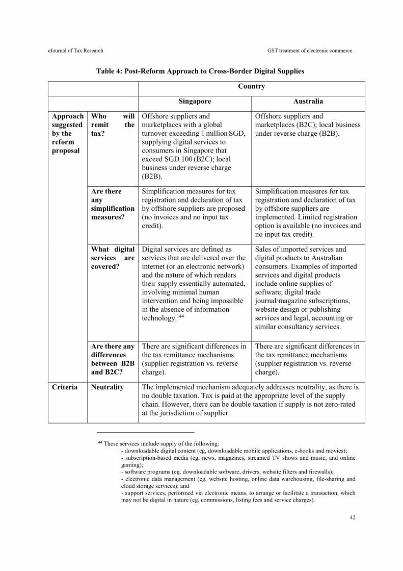
eJournal of Tax Research GST treatment of electronic commerce
42
Table 4: Post-Reform Approach to Cross-Border Digital Supplies
Country
Singapore Australia
Approach suggested by the reform proposal
Who will remit the tax?
Offshore suppliers and marketplaces with a global turnover exceeding 1 million SGD, supplying digital services to consumers in Singapore that exceed SGD 100 (B2C); local business under reverse charge (B2B).
Offshore suppliers and marketplaces (B2C); local business under reverse charge (B2B).
Are there any simplification measures?
Simplification measures for tax registration and declaration of tax by offshore suppliers are proposed (no invoices and no input tax credit).
Simplification measures for tax registration and declaration of tax by offshore suppliers are implemented. Limited registration option is available (no invoices and no input tax credit).
What digital services are covered?
Digital services are defined as services that are delivered over the internet (or an electronic network) and the nature of which renders their supply essentially automated, involving minimal human intervention and being impossible in the absence of information technology.144
Sales of imported services and digital products to Australian consumers. Examples of imported services and digital products include online supplies of software, digital trade journal/magazine subscriptions, website design or publishing services and legal, accounting or similar consultancy services.
Are there any differences between B2B and B2C?
There are significant differences in the tax remittance mechanisms (supplier registration vs. reverse charge).
There are significant differences in the tax remittance mechanisms (supplier registration vs. reverse charge).
Criteria Neutrality The implemented mechanism adequately addresses neutrality, as there is no double taxation. Tax is paid at the appropriate level of the supply chain. However, there can be double taxation if supply is not zero-rated at the jurisdiction of supplier.
144 These services include supply of the following:
- downloadable digital content (eg, downloadable mobile applications, e-books and movies); - subscription-based media (eg, news, magazines, streamed TV shows and music, and online gaming); - software programs (eg, downloadable software, drivers, website filters and firewalls); - electronic data management (eg, website hosting, online data warehousing, file-sharing and cloud storage services); and - support services, performed via electronic means, to arrange or facilitate a transaction, which may not be digital in nature (eg, commissions, listing fees and service charges).
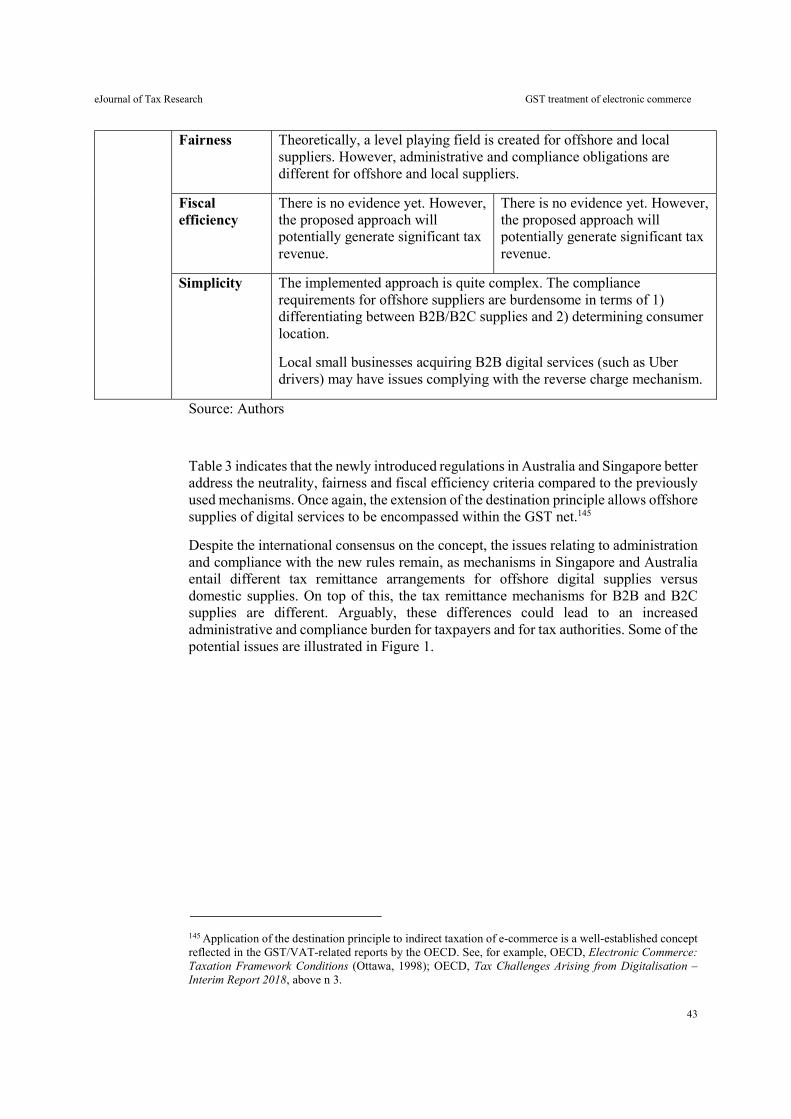
eJournal of Tax Research GST treatment of electronic commerce
43
Fairness Theoretically, a level playing field is created for offshore and local suppliers. However, administrative and compliance obligations are different for offshore and local suppliers.
Fiscal efficiency
There is no evidence yet. However, the proposed approach will potentially generate significant tax revenue.
There is no evidence yet. However, the proposed approach will potentially generate significant tax revenue.
Simplicity The implemented approach is quite complex. The compliance requirements for offshore suppliers are burdensome in terms of 1) differentiating between B2B/B2C supplies and 2) determining consumer location.
Local small businesses acquiring B2B digital services (such as Uber drivers) may have issues complying with the reverse charge mechanism.
Source: Authors
Table 3 indicates that the newly introduced regulations in Australia and Singapore better address the neutrality, fairness and fiscal efficiency criteria compared to the previously used mechanisms. Once again, the extension of the destination principle allows offshore supplies of digital services to be encompassed within the GST net.145
Despite the international consensus on the concept, the issues relating to administration and compliance with the new rules remain, as mechanisms in Singapore and Australia entail different tax remittance arrangements for offshore digital supplies versus domestic supplies. On top of this, the tax remittance mechanisms for B2B and B2C supplies are different. Arguably, these differences could lead to an increased administrative and compliance burden for taxpayers and for tax authorities. Some of the potential issues are illustrated in Figure 1.
145 Application of the destination principle to indirect taxation of e-commerce is a well-established concept reflected in the GST/VAT-related reports by the OECD. See, for example, OECD, Electronic Commerce: Taxation Framework Conditions (Ottawa, 1998); OECD, Tax Challenges Arising from Digitalisation – Interim Report 2018, above n 3.
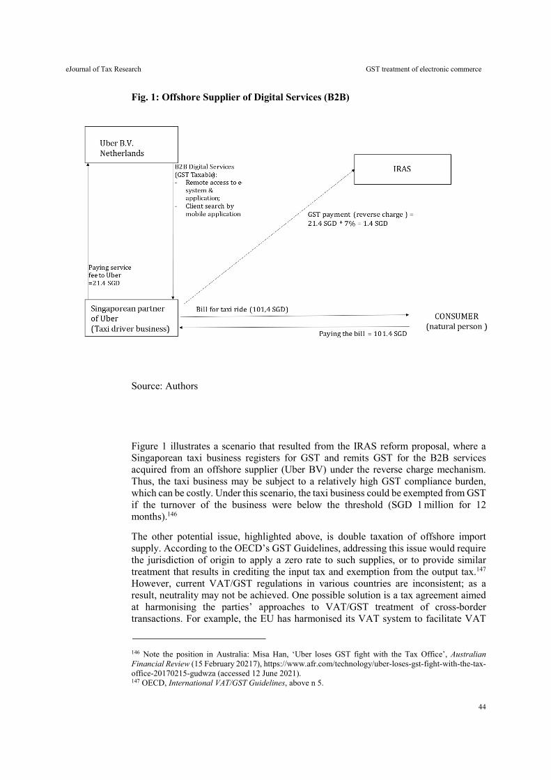
eJournal of Tax Research GST treatment of electronic commerce
44
Fig. 1: Offshore Supplier of Digital Services (B2B)
Source: Authors
Figure 1 illustrates a scenario that resulted from the IRAS reform proposal, where a Singaporean taxi business registers for GST and remits GST for the B2B services acquired from an offshore supplier (Uber BV) under the reverse charge mechanism. Thus, the taxi business may be subject to a relatively high GST compliance burden, which can be costly. Under this scenario, the taxi business could be exempted from GST if the turnover of the business were below the threshold (SGD 1 million for 12 months).146
The other potential issue, highlighted above, is double taxation of offshore import supply. According to the OECD’s GST Guidelines, addressing this issue would require the jurisdiction of origin to apply a zero rate to such supplies, or to provide similar treatment that results in crediting the input tax and exemption from the output tax.147 However, current VAT/GST regulations in various countries are inconsistent; as a result, neutrality may not be achieved. One possible solution is a tax agreement aimed at harmonising the parties’ approaches to VAT/GST treatment of cross-border transactions. For example, the EU has harmonised its VAT system to facilitate VAT
146 Note the position in Australia: Misa Han, ‘Uber loses GST fight with the Tax Office’, Australian Financial Review (15 February 20217), https://www.afr.com/technology/uber-loses-gst-fight-with-the-tax-office-20170215-gudwza (accessed 12 June 2021). 147 OECD, International VAT/GST Guidelines, above n 5.
eJournal of Tax Research GST treatment of electronic commerce
45
neutrality, at least within the borders of its member states, by means of common legislation.148
4.4 Results of comparative analysis
There are some important similarities between the two countries’ approaches to indirect tax treatment of imported digital services (for example, the offshore supplier model for B2C transactions and the reverse charge mechanism for B2B supplies warranting taxation in the country of consumption). This is justifiable, as this tax policy option is conventional and the OECD recommends it. Some other countries have adopted similar policies, including the EU member states. Such a policy is well grounded on neutrality, fairness, fiscal efficiency and administrative simplicity. Besides, the policy accommodates the reality of digital e-commerce business, which is characterised by the market dominance of large internet platforms and aggregators.
With regard to B2B supplies, the OECD Guidelines provide
that local VAT legislation may not require the reverse charge to be made if the establishment of use is entitled to full input tax credit in respect of this supply. In such cases, the tax administration is encouraged to publicise this. Jurisdictions that do require a reverse charge to be made are likewise recommended to make this clear.149
This simplification measure is quite effective, since it can minimise compliance costs for B2B supplies of digital services.
Based on the above analysis of Singaporean and Australian approaches to GST treatment of e-commerce, a significant difference can be identified. Australia is pioneering the new approach based on the offshore supplier model and increased compliance requirements for offshore suppliers, internet platforms and express carriers. On the other hand, Singapore is adhering to a traditional GST treatment of offshore suppliers with exemption for low value goods (as on June 2021). Even after the reform (effective from 1 January 2023) the existing import relief threshold of SGD 400 will remain which means that such supplies will not be treated in the same way as imports of other goods but rather as another kind domestic supply (in the same way as importation of digital services).
The Australian approach in implementing a zero threshold for low value imported goods can be justified on the following grounds:
1) the Australian domestic market is quite significant and very attractive for offshore suppliers, and there is therefore potential for substantial GST revenue;
2) the scale of distortion of competition and unfair tax treatment (without new rules) of domestic and foreign suppliers is relatively high in Australia in comparison with Singapore;
148 Council of the European Union, Council Directive 2006/112/EC of 28 November 2006 on the Common System of Value Added Tax. 149 OECD, International VAT/GST Guidelines, above n 5, 66.
eJournal of Tax Research GST treatment of electronic commerce
46
3) generally, Australia is more protectionist in its fiscal and trade policy compared to Singapore.
However, certain issues, such as high compliance costs of GST collection, may potentially create an administrative barrier for offshore suppliers in cross-border e-commerce transactions. This, in turn, may lead to low fiscal efficiency of the new rules and weaken the e-commerce sector of the economy overall.
5. CONCLUSIONS
Global digital developments have exacerbated a contradiction that existed long before digital business models emerged in their current form. This contradiction is between global business activities that have no national borders, and national sovereign taxation powers and tax administration capabilities. To address this contradiction, an increasing number of international cooperation projects are currently being undertaken. This ‘global tax governance’ (or ‘soft law’) line is highly relevant in the context of indirect taxation of the digital economy.
Based on the above analysis of the Australian and Singaporean experiences in addressing taxation of e-commerce, broader observations can be made about taxation of the digital economy. Cross-border e-commerce represents significant challenges for tax authorities in various countries. Tax policy-makers need to consider a number of common issues in adjusting national tax systems to these new developments; for example, potential shortfalls in tax revenue due to rapid increase in e-commerce, and ‘dead loss’ issues resulting from ineffective tax administration. However, as noted above, it is likely that various countries will address the related issues on the basis of their national priorities.
The Singaporean priority is to maintain the most business-friendly environment possible. This priority is reflected in a very cautious approach to e-commerce tax reform on the part of the Singaporean authorities, including an extended period of consultation with businesses and other stakeholders. The introduced reform focuses on cross-border e-commerce transactions (supply of digital services), while the other part (cross-border supply of goods) is not addressed fully as on June 2021. It appears that the Singaporean tax authorities are willing to study the experiences of other countries before implementing new GST rules for cross-border supply of goods.
The Australian priorities also include maintenance of a business-friendly environment; however, protection of the tax revenue base and creation of a level playing field for local business are additional important priorities. The Australian economy is arguably less oriented towards international trade compared to the Singaporean economy and, thus, it can be argued that tax revenues and a level playing field are salient factors for the Australian government.
The intention of the Australian government to tax e-commerce transactions has resulted in the introduction of the new GST regime in that country. Removing the threshold on low value supply in Australia eliminates preferential tax treatment of online sales and increases economic efficiency. The drawback of the introduced regulation is that higher-priced imports negatively impact Australian consumers. The compliance burden associated with GST may also create a barrier for offshore suppliers, pushing them out of the Australian market and, as a result, limiting competition and consumer choice. However, the imposition of GST on low value goods generally facilitates equal
eJournal of Tax Research GST treatment of electronic commerce
47
treatment of offshore and onshore retailers and helps to protect the GST base, given the rapid increase in the volume of such imports.
The Australian experience with new GST rules is very limited. Nonetheless, introducing new GST rules may not be enough per se to ensure an effective e-commerce taxation system. The system must be able to provide other sufficient qualities, or attributes, to ensure satisfactory outcomes for both taxpayers and tax authorities. To that end, the system must ensure a certain degree of transparency and simplicity, and must be able to provide consistent tax outcomes based on equal treatment of taxpayers. The Australian GST does not achieve all of these goals, but it performs sufficiently well on them not to cause undue ongoing concern.
The taxation of e-commerce in Singapore is in the process of reform, and the necessary qualities of a fully functioning GST system efficiently covering e-commerce are not yet fully in place. The delayed introduction of GST for low value imported goods in Singapore is justifiable; it is clear that Singapore may learn from some of the practices adopted in Australia in this sphere.
Overall, and despite the Singaporean reform being in its first phase, the GST approaches to e-commerce in both jurisdictions have many similarities and common issues related to neutrality, fairness, efficiency and simplicity. In both cases, however, it remains to be seen how effective the systems are in practice.
eJournal of Tax Research (2021) vol. 19, no. 1, pp. 48-96
48
Taxpayer wealth and federal tax revenue under a tax policy that shields retained earnings used for growth from taxes
Robert M Hull and John B Hull
Abstract
This article addresses shortcomings in US tax policy: the interest tax shield (ITS) that favours debt over equity; the unfavourable tax treatment of retained earnings (RE) that is used for growth; and the inequalities in the taxing of ownership forms. Taxpayer wealth is calculated under the assumption that growth increases 0.78% with the enactment of the Tax Cuts and Jobs Act of 2017 (TCJA), which is an increase projected by tax experts. We discover that taxpayer wealth under TCJA with an ITS increases 15.69% beyond it pre-TCJA value; total federal tax revenue (TFTR) decreases 4.20%; and C corporations are no longer taxed more heavily than pass-throughs. If we replace an ITS with a 50% retained earnings tax shield (½RTS) where half of every dollar used for RE is shielded from taxes, we show that taxpayer wealth increases 4.51% and TFTR rises 3.15%. If we replace a ½RTS with an RTS (where 100% of RE is shielded from taxes), we find that taxpayer wealth and TFTR together increase 5.53%. The switch to an RTS further serves to equalise the taxing of pass-throughs and C corporations. Finally, switching from an ITS to an RTS does not materially alter the optimal debt-to-firm value ratio. Key words: Taxpayer wealth, federal tax revenue, business growth, federal debt, tax shields, Capital Structure Model
Clarence W King Chair, Professor of Finance, School of Business, Washburn University, Topeka, Kansas, USA, [email protected]. Independent Researcher, Financial Advisor, OneDigital Services, Overland Park, Kansas USA, [email protected].
eJournal of Tax Research A tax policy that shields retained earnings used for growth from taxes
49
1. INTRODUCTION
During December 2017, the US Congress passed the Tax Cuts and Jobs Act (TCJA) that lowered tax rates enabling individuals and businesses to keep more of their earnings. With larger earnings, greater consumer spending and business production would follow thereby boosting growth in real gross domestic product (GDP). The Tax Policy Center (TPC) (2018) reports that the estimated boost in growth per year will be about 0.8% for both 2018-2020 (average of six sources) and for 2018-2027 (average of five sources).1 As reported by Page (2019), the Joint Committee on Taxation (JCT) expected (at the time of TCJA in December 2017) a USD 0.15 trillion decline per year in federal tax revenue for the next ten years. To put USD 0.15 trillion in perspective, it is 4.39% of the projected USD 3.42 trillion in US federal tax revenue for 2019. This estimate of 4.39% is consistent with the projection of 4.30% given by the Congressional Budget Office (CBO) (2019) as the average for 20202029.
Motivated by inefficiencies in US tax laws, we seek a solution to the growing US debt problem by exploring a tax law change where an interest tax shield (ITS) is replaced with a retained earnings tax shield (RTS) where retained earnings (RE) is a tax-deductible expense at the business level.2 In essence, RTS is a direct tax subsidisation of growth that is superior to any growth-related depreciation or amortisation that might exist over time. The tax law change that we propose is a direct response to inefficiencies especially those related to the tax deduction on interest (I) that favours debt over equity and the taxation of funds used for growth.
To test this tax law change where an RTS replaces an ITS, we use the Capital Structure Model (CSM) developed by Hull (2014a, 2018, 2019). Prior to full development of the CSM, Hull (2005) utilised a framework similar to the CSM to provide an application using market and company data for the Australian Gas Light Company (now AGL Energy). The CSM equations as presented by Hull (2019) allow for the use of ITS and/or RTS. By including CSM equations where RE can be eligible for a tax shield with I being taxed, we address the distortion presented by ITS that favours debt over equity and the taxation of funds that too often makes growth unaffordable. Of importance, these CSM equations are capable of identifying which tax shield or combination of tax shields yields greater maximum firm value that, ceteris paribus, leads to a greater federal tax revenue. As required by this study that includes all for-profit organisations (FPOs), CSM equations cover the two main FPO forms of ownership: C corporations and pass-
1 This article was updated May 2020 but the numbers cited are not changed. 2 An RTS includes all expenses that are used to create growth in goods and services. These expenses bring about new or improved capital as well as a more efficient labour force. Examples of expenses that might qualify include the general areas of expansion and research and development (R&D). First, in terms of expansion, qualifying expenses can include: (i) capital expenditures for new land, buildings and equipment that cause growth; (ii) acquisition of assets (facilities, businesses, products, or technologies) that supply synergy and lead to growth; and, (iii) raising capital for investment (particularly by banks/ real estate investment trusts (REITs)), new constructions (including expansion of subsidiaries); and (iv) increasing facilities to expand or develop land, properties, or resources that add new products and jobs. Second, in terms of R&D, qualifying expenses can include such items as product development, clinical tests, exploration, and accompanying R&D expenses such as sales, marketing, and commercialisation. In brief, any expense that is essential to growth would be a tax-deductible expense under an RTS. However, certain RTS expenses that cause double counting would be capped. For example, if a business already has a deduction from R&D expensing or depreciation of equipment, then there would be a limit on what could be deducted by an RTS tax policy. In fact, an RTS tax policy should be more comprehensive and supplant any prior growth-related tax deductions.

eJournal of Tax Research A tax policy that shields retained earnings used for growth from taxes
50
throughs (sole proprietors, partnerships, and S corporations). In this study, we apply the CSM pass-through equations to all personal taxpayers who, like pass-through owners, pay at the same personal tax rate level.
An ITS denotes that every dollar of I is a tax-deductible expense. Similarly, RTS signifies every dollar of RE is a tax-deductible expense. Besides utilising an ITS and RTS, this study also uses a partial RTS of one-half, which is called a ½RTS because one-half of every dollar of RE is a tax-deductible expense.3 We follow the CSM’s usage of RE, which is defined as those before-tax operational cash flows retained and used for growth purposes. Thus, any funds retained that are either idle or used for non-growth purposes (such as retiring debt) would not merit a tax deduction.
Our tests generate the following findings. First, when comparing pre-TCJA and TCJA results when an ITS is present, we find that taxpayer wealth (as captured by business wealth or firm value) increases 15.69% beyond its pre-TCJA value, total federal tax revenue (TFTR) falls 4.20%, and the weighted effective tax rate (WETR) drops 9.98%.4 These findings assume that growth increases 0.78% under TCJA, which is consistent with the TPC (2018) and empirical research (Romer & Romer, 2010; Barro & Redlick, 2011; Mertens & Ravn, 2013). Our 4.20% independent assessment is the same as the 4.20% given by CBO (2019) for 2019 and close to the 4.30% that they predict as the average for 2020–2029. These results suggest that we explore a tax policy reform because the greater growth from TCJA does not prevent a fall in TFTR, thereby worsening the federal debt.
Second, we find that replacing ITS with a ½RTS causes TFTR to climb 3.15% to a level near that found prior to TCJA. This increase in TFTR occurs while taxpayer wealth increases 4.51%, and WETR rises 0.62%. The latter represents an absolute change of only 0.10%. Taxpayers are the clear winner because, for every USD 1 of increase in TFTR, their wealth increases USD 52.18. The increase in TFTR along with sharing the enhanced taxpayer wealth offer hope that the US federal government can be set on a long-run trajectory of getting its debt to a reasonable percent of GDP with less fear of an out-of-control rise in debt. It is noteworthy that the loss in federal tax revenue from not taxing RE is offset by greater growth that leads to greater taxable income and substantial tax revenue from taxing I. Our results using a ½RTS tax policy show that removing tax barriers on RE enables real GDP and thus taxpayer wealth to grow in an unimpeded manner with less government interference caused by overtaxing growth.
Third, if we replace a ½RTS with an RTS thereby doubling the tax shield on RE, we find that taxpayer wealth increases 5.99%, TFTR declines 11.57%, and WETR rises 0.15% (absolute change of only 0.02%). Because taxpayer wealth and TFTR together increase 5.53% beyond that attained with a ½RTS, an RTS offers the greatest potential to
3 Alternative names for a ½RTS and an RTS would respectively be a 50%RTS and a 100%RTS. 4 For this article’s purposes, the term TFTR refers to total federal tax revenue from those three sources that are used to represent the total federal tax revenue from all sources. These three sources are corporate taxes as paid by C corporations and personal taxes as paid by pass-throughs and other personal taxpayers. As defined later, other personal taxpayers is a group of taxpayers who pay at the personal statutory tax rate as opposed to a pass-through group of pass-through owners who also pay at the same personal tax level. As will be seen in Figure 1, C corporations, pass-throughs, and other personal taxpayers make up 56% of federal tax revenue projected for 2019. These three sources of TFTR are directly associated with FPOs. Most of the remaining 44% also stems from FPOs because FPOs are largely responsible for social insurance taxes that make up 36% of the remaining 44%.
eJournal of Tax Research A tax policy that shields retained earnings used for growth from taxes
51
maximise taxpayer wealth and thus solve the problems involving excessive federal debt and social insurance insolvency. However, before these problems can be resolved, taxpayers would have to share their enhanced wealth achieved under an RTS tax policy. The increase in taxpayer wealth from an RTS has a monetary value that is 19.13 times greater than the drop in federal taxes paid, indicating there is plenty of wealth to increase TFTR if needed. The reason for the superiority of an RTS is that it provides a 100% tax subsidy on every dollar used for internal growth as captured by RE. Such a subsidy is a potent impetus to make growth affordable.5
Fourth, prior to TCJA, we discover that C corporations were at a tax disadvantage compared to pass-throughs where the WETR inequality gap was 4.138%. The gap not only dropped from 4.138% to 1.537% under TCJA with an ITS but the pass-through advantage was reversed as C corporations now have the advantage by paying 1.537% less in taxes. In absolute terms, the inequality gap dropped 2.601%. We find that replacing an ITS with a ½RTS further lowers the WETR inequality gap between pass-throughs and C corporations from 1.537% favouring C corporations to 0.848% favouring C corporations. This is a reduction of 0.689% in the tax gap. Finally, replacing a ½RTS with an RTS further lowers the WETR inequality gap between pass-throughs and C corporations from 0.848% favouring C corporations to 0.698% favouring C corporations. This is a further reduction of 0.150% in the WETR gap.
Fifth, a switch in the tax shield from I to RE does not notably alter the optimal debt-to-firm value ratio (ODV). The finding that leverage is not significantly influenced by tax policy is consistent with the claim that an ITS is an arbitrary tax deduction reflecting an inefficient tax policy that fails to properly subsidise growth. To illustrate the near irrelevance of ITS on debt choice, the ODV of 0.255 for an ITS under TCJA falls slightly to 0.246 with the switch to a ½RTS. It falls to 0.235 if we switch to an RTS. The relatively small changes in ODVs occur because the large jump in the credit spread, such as occurs when going from an investment grade rating to a speculative credit rating, is a major determinant of an ODV.6
To aid the reader in navigating the document with its many acronyms, we supply Exhibit 1 in the Appendices that contains the most common and key acronyms used in this article. Since acronyms (and the terms they identify) are described in detail in the article, Exhibit 1 focuses on providing a concise definition and/or meaning of the acronym associated with the term it represents. Common accounting acronyms are not included.7
The remainder of this article is set out as follows. Section 2 provides background information covering TCJA and tax inefficiencies, sources of US federal tax revenue, relation between tax rates and growth, and valuation models. Section 3 overviews the inputs we use when computing taxpayer wealth and federal tax revenue results. Section
5 While not discussed in this article, we find that pre-TCJA non-growth FPOs have, on average, greater firm value than growth C corporations for an ITS. Such is not the case for a ½RTS and even less so for an RTS where growth is taxed less. Similarly, such is also not the case for TCJA tests where lower tax rates also exist making growth more affordable. 6 Hull (2019) suggests ODVs will be above 0.3, while we find ODVs below 0.3 for most of our tests. However, Hull’s research began at a time when only 2018 credit spreads were available. For 2018, Moody’s Baa2 was the optimal credit rating as opposed to the higher Moody’s rating of A3 that we find for 2019. A lower optimal credit rating means a greater ODV. 7 Less common accounting acronyms are also not included because they are defined and used together in sections 4.1, 4.2 and 4.3.
eJournal of Tax Research A tax policy that shields retained earnings used for growth from taxes
52
4 reports results that support an RTS tax law. This law increases taxpayer wealth and federal tax revenue while also lowering the inequality gap when taxing different ownership forms. Section 5 covers key assumptions behind this article’s results, robustness tests, a blueprint for countries to overcome their debt problems, and future research possibilities. Section 6 provides summary statements and conclusions. Five appendices are included that contain the more quantitative and technical details needed to generate this article’s findings.
2. BACKGROUND
In this section, we discuss TCJA and tax inefficiencies; the sources of federal tax revenue; the literature on how changes in tax rates influence growth; and valuation models including the Capital Structure Model (CSM) that generates this article’s results.
2.1 TCJA and tax inefficiencies
TCJA includes two major tax changes. First, TCJA drops the maximum statutory personal tax rate from 39.6% to 37%. This article categorises all personal taxpayers who are subject to ordinary personal income tax brackets as PTPs. This category includes two groups consisting of the pass-through group and the other personal taxpayers group where the latter group includes those employed by for-profits, non-profits, and government.8 TCJA also alters personal income tax brackets in a way that lowers the effective personal tax rate paid by PTPs. Unless extended, the lower personal tax rates under TCJA will revert to their higher pre-TCJA values after 2025. Similarly, there is no guarantee that the TCJA business deduction of 20% for lower income pass-throughs will extend beyond 2025.
Second, TCJA lowers the maximum corporate tax rate paid by C corporations from 35% to a flat rate of 21%, which is a 40% decrease in the maximum. This decrease is considered permanent as there is no set date for this lower corporate tax rate to expire. Burke (2008) notes that C corporations accounted for 30% of federal tax revenue in 1953 but only 7% by 2003, which is the same percent estimated for the future (as seen later in the 2019 projections in Figure 1). The huge drop in the corporate tax rate raises a question of how C corporations will spend their tax savings. Matthews (2018) answers that historically firms repurchase shares when taxes fall as opposed to increasing wages for consumer spending. However, Knott (2019) notes that repurchasing shares is just another way of distributing cash to shareholders with repurchases occurring in greater numbers when companies already have healthy R&D investments. Thus, firms with unhealthy R&D investments would be more inclined to strengthen their R&D investments under TCJA where lower tax rates generate more cash flows for investments.
8 Since PTP includes two groups, this article’s use of PTP can refer to either the pass-through group or the other personal taxpayers group or both groups together. However, as seen later, we do not use the acronym PTP for pass-throughs when we are specifically discussing pass-throughs as a separate group. Examples include when testing the effects of TCJA on pass-throughs versus C corporations, referring to pass-through business taxes, or computing differences in tax rates between pass-throughs and C corporations. While the pass-through group is technically pass-through owners, for brevity, we just use the term pass-throughs.
eJournal of Tax Research A tax policy that shields retained earnings used for growth from taxes
53
2.1.1 Failure to abolish ITS
By lowering the maximum corporate tax rate by 40%, TCJA addresses the double tax on C corporations where their owners pay taxes on the same earnings at both the business and personal levels whereas pass-through owners only pay at the personal level (albeit the pass-through personal tax rate level is typically higher than that for a C corporation). Doran (2009) notes that the double taxation on C corporations is widely regarded as unfair and inefficient. Polito (2017) describes this double taxation as arbitrary and capricious. While TCJA addresses the baffling double taxation tax law for C corporations, it fails to address an equally perplexing tax law that allows an ITS to exist. This law is puzzling because there is no obvious reason that interest (I) should be a tax-deductible business expense for an FPO (be it a pass-through or C corporation). Despite any historical reasons that support its origins, there are longstanding and compelling reasons that the tax deduction on I serves no purpose and may even be detrimental.9 Besides being at the centre of the distortion that favours debt over equity (Burke, 2008; Norbäck, Persson & Tåg, 2018), we offer five other reasons to justify that TCJA should have abolished the law allowing an ITS.10
First, capital structure theorists (Jensen & Meckling, 1976; Jensen 1986) posit that a reasonable amount of debt embodies net positive agency effects regardless of its tax deductibility. Consequently, there is no imperative supporting a tax law that creates an artificial positive effect by legalising I as a tax-deductible expense for an FPO. Second, the cost of debt is already below the cost of equity so that a tax deduction on I (that further lowers the cost of debt) alters the natural differential between the costs of debt and equity when one security type receives a tax benefit that the other does not receive. Third, debt already has a niche as it appeals to conservative investors who want safer returns regardless of its deductibility. Fourth, ITS has a negative effect on taxpayer wealth to the extent it usurps the ability of governments to give tax breaks for growth. Fifth, for our tests, the optimal debt-to-firm value ratio (ODV) for an average FPO displays a relatively narrow range of ODV values regardless of what financial cost variable (interest or retained earnings) provides a tax shield. This is because the jump in the credit spread when going from an investment grade bond to a speculative grade credit rating can be a dominant determinant of ODV for a typical FPO.
Under TCJA, many businesses can only deduct I up to 30% of its earnings before interest, tax, depreciation and amortisation (EBITDA). EBIT will replace EBITDA in 2022, which can cause problems for businesses with large annual depreciation and/or amortisation deductions. However, for the tests we conduct, an average company would fall well below a 30% level at least when EBIT is used. Thus, for the most part, ITS is effectively preserved under TCJA. However, there can be exceptions. For example, we find that ITS is not totally preserved for the financial services industry.11
9 See Bank (2014) for a discussion of ITS including its origins. 10 See Hilling and Vilhelmsson (2015) for the problems in classifying financial instruments as debt and equity. 11 As a group and using EBIT, we find that the financial service industry exceeds the 30% level with a pre-TCJA of 67.47% and a TCJA of 78.58%. These results come from separately testing the financial services (FS) firm category. As discussed in Appendix 3, FS firms represent 7.2% of US GDP according to Federal Reserve Economic Data (FRED) (2019b). In contrast, the small and large categories (that account for 92.8% of businesses) average 14.88% and 19.11%, respectively, and are below the 30% level.
eJournal of Tax Research A tax policy that shields retained earnings used for growth from taxes
54
2.1.2 Failure to promote RTS
Besides failing to effectively address the shortcomings of an ITS, TCJA also falls short in terms of directly promoting either an RTS or a similar mode of subsidising growth. While TCJA boosts growth through a temporary provision for immediate (and full) expensing of qualified short-lived investment, TCJA ignores implementing an RTS. As a permanent initiative applicable to all FPOs, an RTS would be a more widespread provision that is superior to any depreciation, depletion, and amortisation of qualified assets used for growth.
Two underlying sources of growth that would be affected by an across the board RTS are R&D and innovation. Whereas R&D turns invested funds into knowledge, innovation is the process of commercialising this knowledge. By reducing taxes, TCJA lowers the after-tax cost related to R&D and innovation and thus makes growth more affordable. However, while freeing up more after-tax funds for growth, TCJA does not directly aid growth through a reduction in taxes on funds used for growth. For example, consider the following illustration. A company retains 5% of its before-tax cash flows. These retained funds are listed as retained earnings (RE) in its balance sheet and can be used for multiple purposes over time. Suppose all of these funds are invested for growth purposes such as the development of new products for which other costs are incurred related to sales and marketing as well as new capital assets like new heavy-duty transportation equipment to ship the newly developed goods. Under an RTS, these expenditures (that use funds from the RE account) get an immediate tax deduction, which is a tax subsidy equal to the company’s tax rate times the RE used.
Because a direct tax support for growth (such as an RTS) is not addressed by TCJA, TCJA appears to largely ignore the tax reform presented by researchers and tax experts (Noked, 2014; Nussim & Sorek, 2017; Pomerleau, 2017) whose writings are consistent with the notion that tax reform should be aimed more directly at the sources of growth. Noked examines optimal tax reform in regards to R&D and suggests a subsidy equal to the positive externality that R&D supplies. Nussim and Sorek discuss the value of government involvement in financing innovation and note that cash transfers and tax incentives can have the same effect if done correctly but also present an argument that non-tax cash transfers can be socially superior. Pomerleau contends that the high US tax code discourages investment and suggests immediate expensing as one permanent measure to decrease the cost of growth.
2.2 Sources of US federal tax revenue
Figure 1 shows the sources of US total federal tax revenue (TFTR) projected for 2019 at the time our research began. We form this Figure by borrowing from JCT (2018), Amadeo (2018), and Greenberg (2017). The use of multiple sources for forecasting TFTR serves a purpose. For example, PTPs (previously defined as all personal taxpayers who are subject to ordinary personal income tax brackets) are typically combined into one category but the use of multiple sources enables us to separate PTPs into the two groups of pass-throughs and other personal taxpayers both of which are seen in Figure 1. Separating out pass-throughs allows us to compare them to C corporations as well as combine them with C corporations to determine the impact of TCJA on FPOs together.
Figure 1 reveals that FPOs supply 23% of TFTR with 7% from C corporations and 16% for pass-throughs. Figure 1 also shows that other personal taxpayers provide 33% of federal tax revenue. The PTP group of other personal taxpayers works predominantly
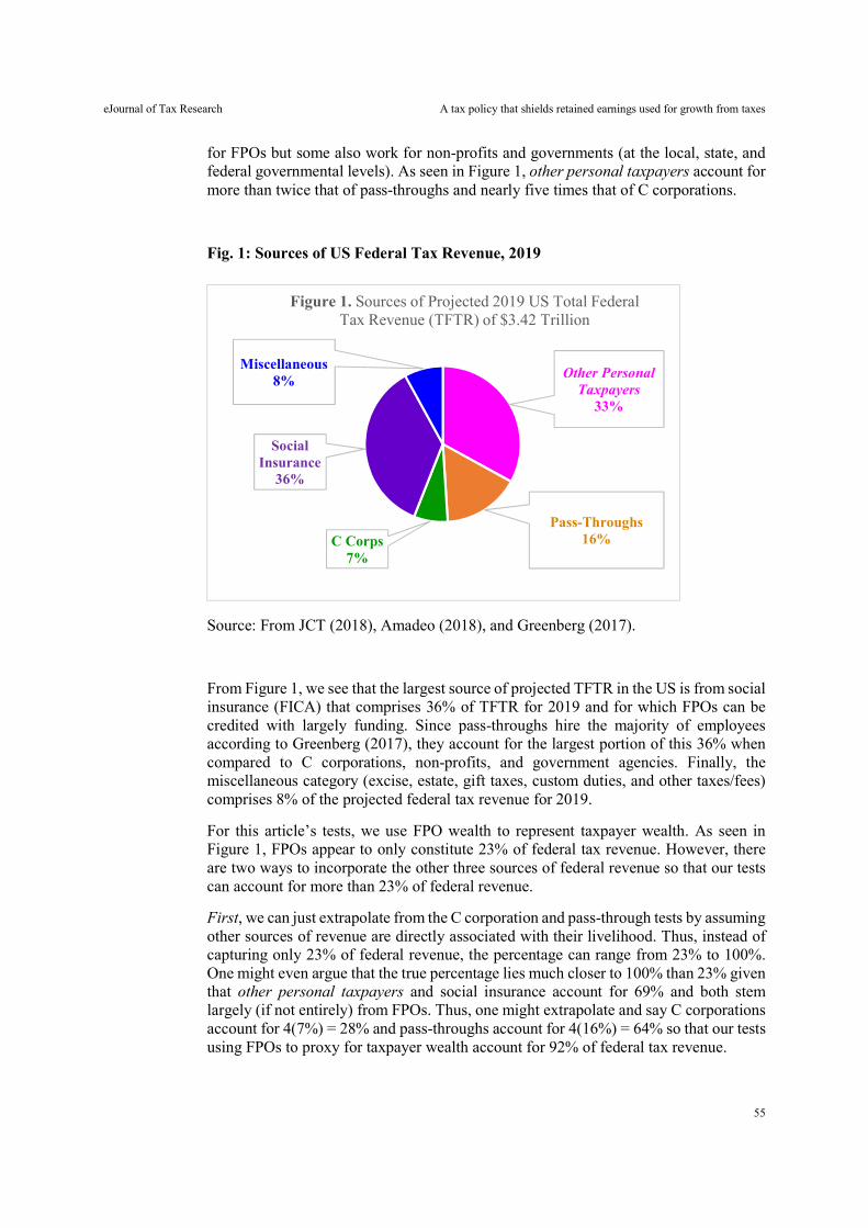
eJournal of Tax Research A tax policy that shields retained earnings used for growth from taxes
55
for FPOs but some also work for non-profits and governments (at the local, state, and federal governmental levels). As seen in Figure 1, other personal taxpayers account for more than twice that of pass-throughs and nearly five times that of C corporations.
Fig. 1: Sources of US Federal Tax Revenue, 2019
Source: From JCT (2018), Amadeo (2018), and Greenberg (2017).
From Figure 1, we see that the largest source of projected TFTR in the US is from social insurance (FICA) that comprises 36% of TFTR for 2019 and for which FPOs can be credited with largely funding. Since pass-throughs hire the majority of employees according to Greenberg (2017), they account for the largest portion of this 36% when compared to C corporations, non-profits, and government agencies. Finally, the miscellaneous category (excise, estate, gift taxes, custom duties, and other taxes/fees) comprises 8% of the projected federal tax revenue for 2019.
For this article’s tests, we use FPO wealth to represent taxpayer wealth. As seen in Figure 1, FPOs appear to only constitute 23% of federal tax revenue. However, there are two ways to incorporate the other three sources of federal revenue so that our tests can account for more than 23% of federal revenue.
First, we can just extrapolate from the C corporation and pass-through tests by assuming other sources of revenue are directly associated with their livelihood. Thus, instead of capturing only 23% of federal revenue, the percentage can range from 23% to 100%. One might even argue that the true percentage lies much closer to 100% than 23% given that other personal taxpayers and social insurance account for 69% and both stem largely (if not entirely) from FPOs. Thus, one might extrapolate and say C corporations account for 4(7%) = 28% and pass-throughs account for 4(16%) = 64% so that our tests using FPOs to proxy for taxpayer wealth account for 92% of federal tax revenue.
Other Personal Taxpayers
33%
Pass-Throughs16%C Corps
7%
Social Insurance
36%
Miscellaneous8%
Figure 1. Sources of Projected 2019 US Total Federal Tax Revenue (TFTR) of $3.42 Trillion

eJournal of Tax Research A tax policy that shields retained earnings used for growth from taxes
56
Second, we can assess if it is reasonable to add a source of revenue to either C corporations or pass-throughs or both. The most logical addition is to combine the other personal taxpayer source with the pass-through source. This addition is justified since both sources pay taxes at the personal tax level. Furthermore, as noted previously, pass-throughs are the largest employer of other personal taxpayers.
For this study, we choose the second alternative and so add other personal taxpayers to the pass-through source of revenue to form the group of personal taxpayers (PTP). The three categories of C corporations, pass-throughs, and other personal taxpayers are important for our tests because, as shown in Figure 1, they account for 56% of projected federal tax revenue in 2019. By using these three groups, our tests can also offer two comparisons based on two sets of weights found in Figure 1. First, the weights when combining C corporations and pass-throughs are 7/23 = 0.30435 for C corporations and 16/23 = 0.69565 for pass-throughs (roughly, 0.3 for C corporations versus 0.7 for pass-throughs). Second, the weights when combining C corporations and PTPs are 7/56 = 0.125 for C corporations and 49/56 = 0.875 for PTPs.
For our tests, the primary focus will be on the second set of weights as they have the greatest influence on federal tax revenue. If one assumes that both social insurance taxes and other minor miscellaneous sources of federal revenue are constant and/or extrapolated proportionally, then this second set of weights represents the total influence on taxpayer wealth and federal tax revenue.
2.3 Relation between tax rates and growth
McBride (2012) writes that 26 of 29 studies since 1983 find strong support for the notion that higher taxes have a negative effect on growth with the most harmful taxes being that paid at the business level. Romer and Romer (2010) find that a personal tax increase of 1% has a large negative effect on investment leading to a real GDP decrease of about 3% over the next three years. Barro and Redlick (2011) discover that a cut of 1% in the average marginal income tax rate raises per capita GDP in the US by 0.6% for the following year. Mertens and Ravn (2013) find that cuts in personal and corporate taxes increase investment.12 They add that cuts in personal taxes lead to a fall in federal tax revenue while similar size cuts in corporate taxes have less of an impact. The latter is consistent with Figure 1 where C corporation revenue is a much smaller part of federal tax revenue compared to PTPs.
The research just cited offers evidence that increased tax rates are a deterrent to investment thus hindering GDP growth and taxpayer wealth. This finding is embodied in the Capital Structure Model (CSM) where the growth rate is negatively affected by business level taxes on retained earnings (RE) with larger tax rates having greater negative effects on growth. The CSM points out that the cost of using RE for growth comes with a price, which is the business level tax on RE. For C corporations, the business level tax is a corporate tax rate. For pass-throughs, the business level tax is a personal tax rate. The CSM’s break-through concept of an equilibrating levered growth rate (gL) ties together the plowback-payout decision with the debt-equity choice. Thus, any influence of a business tax rate on RE and interest (I) is factored into CSM outcomes as both variables are in the gL equation (as seen in Appendix 1) where a smaller business
12 See Freebairn (2017) for an assessment of the comparative effects of a lower corporate tax rate on investment decisions of small and large businesses.
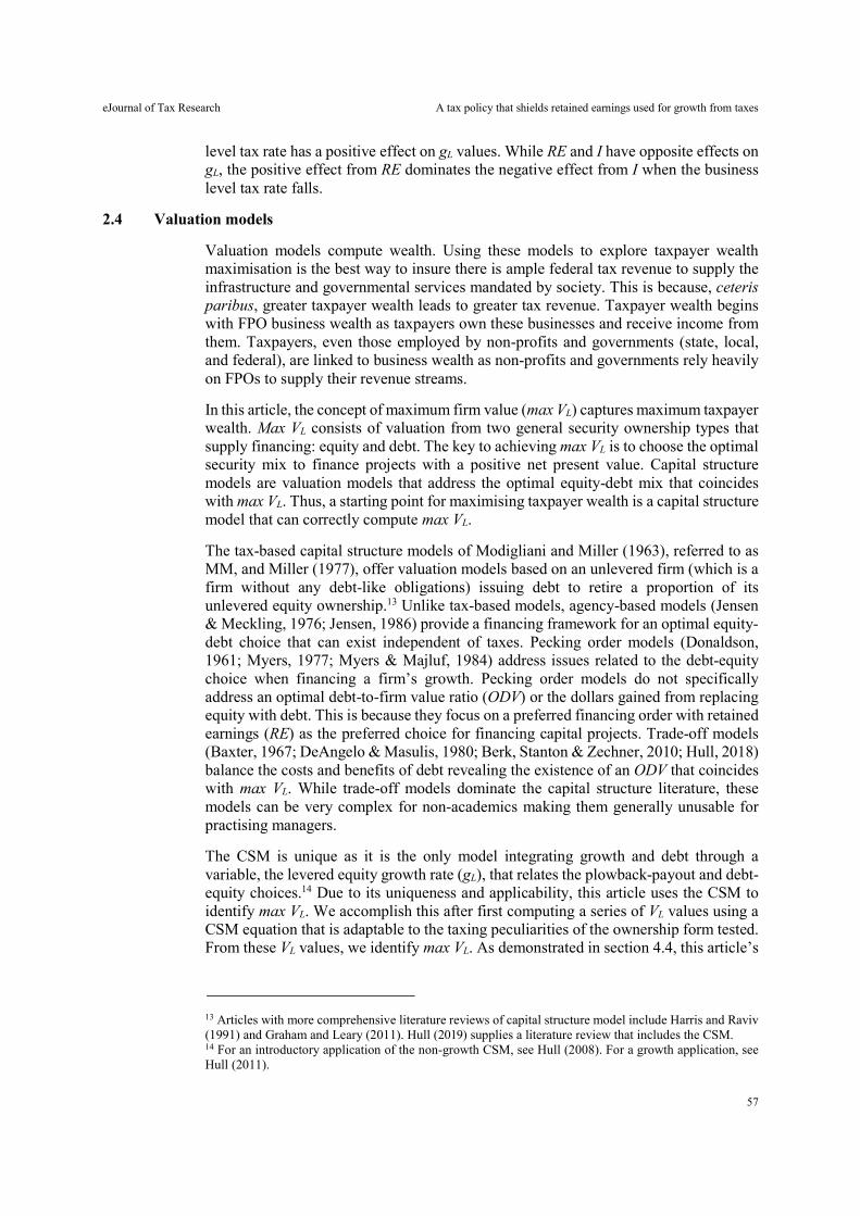
eJournal of Tax Research A tax policy that shields retained earnings used for growth from taxes
57
level tax rate has a positive effect on gL values. While RE and I have opposite effects on gL, the positive effect from RE dominates the negative effect from I when the business level tax rate falls.
2.4 Valuation models
Valuation models compute wealth. Using these models to explore taxpayer wealth maximisation is the best way to insure there is ample federal tax revenue to supply the infrastructure and governmental services mandated by society. This is because, ceteris paribus, greater taxpayer wealth leads to greater tax revenue. Taxpayer wealth begins with FPO business wealth as taxpayers own these businesses and receive income from them. Taxpayers, even those employed by non-profits and governments (state, local, and federal), are linked to business wealth as non-profits and governments rely heavily on FPOs to supply their revenue streams.
In this article, the concept of maximum firm value (max VL) captures maximum taxpayer wealth. Max VL consists of valuation from two general security ownership types that supply financing: equity and debt. The key to achieving max VL is to choose the optimal security mix to finance projects with a positive net present value. Capital structure models are valuation models that address the optimal equity-debt mix that coincides with max VL. Thus, a starting point for maximising taxpayer wealth is a capital structure model that can correctly compute max VL.
The tax-based capital structure models of Modigliani and Miller (1963), referred to as MM, and Miller (1977), offer valuation models based on an unlevered firm (which is a firm without any debt-like obligations) issuing debt to retire a proportion of its unlevered equity ownership.13 Unlike tax-based models, agency-based models (Jensen & Meckling, 1976; Jensen, 1986) provide a financing framework for an optimal equity-debt choice that can exist independent of taxes. Pecking order models (Donaldson, 1961; Myers, 1977; Myers & Majluf, 1984) address issues related to the debt-equity choice when financing a firm’s growth. Pecking order models do not specifically address an optimal debt-to-firm value ratio (ODV) or the dollars gained from replacing equity with debt. This is because they focus on a preferred financing order with retained earnings (RE) as the preferred choice for financing capital projects. Trade-off models (Baxter, 1967; DeAngelo & Masulis, 1980; Berk, Stanton & Zechner, 2010; Hull, 2018) balance the costs and benefits of debt revealing the existence of an ODV that coincides with max VL. While trade-off models dominate the capital structure literature, these models can be very complex for non-academics making them generally unusable for practising managers.
The CSM is unique as it is the only model integrating growth and debt through a variable, the levered equity growth rate (gL), that relates the plowback-payout and debt-equity choices.14 Due to its uniqueness and applicability, this article uses the CSM to identify max VL. We accomplish this after first computing a series of VL values using a CSM equation that is adaptable to the taxing peculiarities of the ownership form tested. From these VL values, we identify max VL. As demonstrated in section 4.4, this article’s
13 Articles with more comprehensive literature reviews of capital structure model include Harris and Raviv (1991) and Graham and Leary (2011). Hull (2019) supplies a literature review that includes the CSM. 14 For an introductory application of the non-growth CSM, see Hull (2008). For a growth application, see Hull (2011).
eJournal of Tax Research A tax policy that shields retained earnings used for growth from taxes
58
use of the CSM produces outcomes consistent with empirical research (Graham, 2000; Korteweg, 2010; Van Binsbergen, Graham & Yang, 2010).
3. INPUTS WHEN COMPUTING WEALTH AND TAX REVENUE RESULTS
This section often follows Hull (2019) and the process in that study to calculate outcomes for taxpayer wealth and federal tax revenue. We also supply our own details on how we determine values for CSM inputs, in particular, as relates to discount rates (costs of borrowing), debt ratios, tax rates, and growth rates. Given the disagreements over the extent of growth under TCJA, section 3.3 looks at historical growth in real US GDP when guiding the choice of growth rates for pre-TCJA and TCJA tests.
3.1 Perpetual cash flows and discount rates
To compute business wealth (and thus taxpayer wealth) in a perpetuity model like the CSM, two beginning variables are perpetual cash flows for equity and debt owners and corresponding equity and debt borrowing costs used as discount rates. We now describe these two variables.
First, we begin with a perpetual before-tax cash flow (CFBT) of USD 1,000,000 that creates annual taxable perpetuities paid to equity and debt owners. Given this article’s focus on federal taxes and a tax law that directly subsidises growth activities, we define CFBT as cash flows available to the FPO before federal taxes are paid and before any applicable tax shield lowers business level taxes. Thus, CFBT is an operational cash flow after all non-tax shield expenses. These expenses can include those related to non-federal taxes, replacement, depreciation, depletion, and amortisation. Thus, expenses can include items like state taxes and amortised R&D, albeit not all states have taxes and not all firms have amortised R&D. Restrictions may have to be put on items like R&D to prevent it from being used more than once as a tax deduction or exceeding specified limits related to its cost.15 Since we begin with an unlevered firm, interest (I) only lowers CFBT (for taxation purposes under an ITS tax law) after debt is issued. For an RTS, RE lowers the taxes on CFBT where RE refers to retained earnings, which is internal equity used for growth purposes.
Second, we need borrowing costs to discount perpetual equity and debt cash flows. To gather these borrowing costs, we use the five-step procedure found in Appendix 2. As seen in this appendix, we base borrowing costs on credit spreads matched to credit ratings and interest coverage ratios (ICRs).
Finally, there is the task of matching credit ratings and credit spreads (and thus costs of borrowing) to debt-to-firm value ratios (DV) and, in the process, determining how much unlevered equity (EU) must be retired by debt to maximise firm value at ODV.16 Damodaran (2019) makes this task possible by matching credit ratings and credit spreads with ICRs where each ICR can be used to compute a corresponding DV.17
15 While there is no exact comparison from an accounting standpoint, we equate CFBT with EBIT. Thus, in this article, we use EBIT and CFBT interchangeably. 16 Since unlevered firm value (VU) is unlevered equity value (EU) plus debt (D) and D is zero when the firm is unlevered, we have VU = EU + D = EU + 0 = EU. Thus, VU = EU. For the most part, this article uses EU instead of VU. 17 When we began our study, the most recent data available by Damodaran (2019) was for the year 2018. It should be pointed out that Damodaran not only updates his data each year but the details of the updated data can change such that his archived data can have differing degrees of details.
eJournal of Tax Research A tax policy that shields retained earnings used for growth from taxes
59
Damodaran supplies ICR for three categories: large, small, and financial service (FS). Damodaran reports ICRs in terms of ranges. For our tests, we use the average of each range for our tests except for endpoints where the range is extremely large so that we compute ICR as described by Hull and Van Dalsem (2021). They are the first researchers to use ICRs in conjunction with the CSM. We then weight these ICRs as described in Appendix 3 where we also provide an example of how we use an ICR (for a Moody’s credit rating of A3) to identify max VL and ODV.
3.2 Tax rates
For our tests, we allow the personal equity tax rate, the corporate tax rate, and personal debt tax rate to change in their predicted directions given by Hull (2014a) for each successive P choice where P refers to the proportion of unlevered equity retired with debt. Hull argues that the personal equity tax rate and corporate tax rate decrease and the personal debt tax rate increases with greater debt-for-equity transactions. While Hull’s arguments had C corporations in mind, they are also applicable to pass-throughs. For our tests, we use a 3% change in a tax rate for each of the 15 increasing P values.18 While disagreements about an effective tax rate exist and vary over time, our tax rates (described next) are consistent with the arguments and sources given by Hull (2019) as well as other sources (Frankel, 2017; Peter G Pederson Foundation, 2017; York, 2018).
For C corporations, the maximum corporate tax rate is 21% under TCJA and is also a flat rate. Prior to TCJA, the maximum was 35%. The personal equity tax rate for C corporations is based on tax laws governing dividends and capital gains tax laws.19 The typical personal maximum tax rate is 20% if we ignore the extra 3.8% for the wealthiest few who have net investment income above applicable threshold amounts. This holds for both capital gains and qualified dividends that result if equity shares are owned for more than 60 days during the 121-day period that begins 60 days before the ex-dividend date. TCJA did not change these rates. For PTPs, the personal equity tax rate has a maximum of 37% under TCJA and 39.6% prior to TCJA. For both C corporations and PTPs, the tax rate paid on interest has the same tax rates of 37% and 39.6%. However, if debt is held three years, taxes on capital gains follow the same laws governing that for equity. Additionally, capital gains on debt can be further reduced by indexation. The above maximums for C corporation equity owners and FPO debt owners are rarely achieved for a number of reasons, one of which is the ability to defer tax payments for long periods.
For unlevered C corporations, we set the unlevered corporate tax rate (TC1) at the maximum TCJA rate of 21% for TCJA tests and the maximum pre-TCJA rate of 35% for pre-TCJA tests where the subscript ‘1’ denotes that the tax rate is an unlevered rate. At ODV, these two unlevered rates become the effective levered corporate tax rate (TC2) of 18.03% for TCJA tests and 30.06% for pre-TCJA tests where the subscript ‘2’ denotes that the tax rate is a levered rate. We use 11% as the unlevered C corporation personal tax rate on equity (TE1). We set the personal debt tax rate (TD1) at 14% as the
18 The use of 3% best generates values for all of the effective levered tax rates identified in this subsection as occurring at ODV. Since the ODV for all of our tests occurs with a Moody’s A3 credit rating, the cumulative change from an unlevered tax rate to a levered tax rate never fluctuates more than 1/6 of its initial unlevered value. 19 See Steyn et al. (2019) and Vaillancourt and Kerkhoff (2019) for examples of recent reviews of the capital gains literature. See Hasseldine and Fatemi (2019) for a study on the distinction between ordinary income and capital gains.
eJournal of Tax Research A tax policy that shields retained earnings used for growth from taxes
60
starting point prior to debt being issued.20 At ODV, these two tax rates become effective levered C corporation tax rates of TE2 = 9.45% and TD2 = 16.23%.21 Since TCJA does not change the maximum tax laws governing these rates, they generally apply to both pre-TCJA and TCJA tests. An exception would a debt owner who would pay a slightly lower tax rate on interest income under TCJA. Finally, for PTP tests, we use TE1 = 37% for TCJA tests and TE1 = 39.6% for pre-TCJA tests. At ODV, these unlevered personal tax rates become effective levered personal tax rates of TE2 = 31.77% for TCJA tests and TE2 = 34.01% for pre-TCJA tests. Like our C corporation tests, TD1 = 14% for the PTP unlevered situation and TD2 = 16.23% at ODV.22
3.3 Growth rates
We use an annual growth rate of 3.12% for pre-TCJA tests and 3.90% for TCJA tests. The latter rate captures both the expected increase in growth of 0.78% under TCJA as given by the TPC (2018) and the rate found in the past 70 years of historical data for annual growth in real US GDP from US Bureau of Economic Analysis (2019). Because we find 3.12% for a 70-year period and 3.90% for shorter periods over the past 70 years (for example, 3.90% occurs for the 30 years from 1930 through 1959), we view the boost in growth of 0.78% as the difference in growth rates that are sustainable between longer periods and shorter periods. One can surmise that the difference of 3.90% – 3.12% = 0.78% represents enhanced growth for periods where the business environment is more conducive to growth due to more favourable tax legislation such as allowance for growth tax credits. Such a business environment can characterise what TCJA seeks to attain.
While C corporation tax rates are lowered by over five times more than pass-through tax rates under TCJA, Figure 1 shows that PTPs account for 49% of federal tax revenue (16% for pass-throughs and 33% for other personal taxpayers), which is seven times the federal tax revenue of 7% for C corporations. Thus, in terms of the impact on federal revenue, the five times greater drop in C corporation tax rates is more than offset by the fact PTPs provide seven times more of federal tax revenue. It follows that, all factors considered, changes in corporate and personal tax rates under TCJA have similar large impacts on growth in real GDP.
In the CSM, we capture growth by the levered equity growth rate gL. Given that retained earnings (RE) equals PBR(CFBT) where PBR is the before-tax plowback ratio as given by the growth CSM and gL is defined in terms of RE, we are able to change PBR until our chosen gL of 3.12% for pre-TCJA tests and 3.90% for TCJA tests are achieved for each target rating choice tested. Since our pre-TCJA versus TCJA results use a differential in growth of 0.78%, the growth rates of 3.12% and 3.90% are less important
20 Since we need a starting point, the use of an unlevered debt is hypothetically since, by definition, an unlevered debt rate does not exist as unlevered means there is no debt. For this reason, the CSM research will typically use TD for both TD1 and TD2 unless trying to distinguish between two debt choices as we do in this article. TD1 and TD2 are also used when modelling for wealth transfer such as found in Hull (2014b). 21 Compared to Hull (2020), our personal tax rates for equity and debt income for C corporations are low. On the other hand, it can be argued that our personal equity tax rates for PTPs are high. If so, our finding that an RTS lowers the inequality in taxing ownership form would be strengthened. 22 We do not use an estimate for TD2 that considers an imputed TD2 from municipal bonds and corporate bond yields because this estimated rate is a marginal rate instead of an effective rate and so would be expected to be higher. Earlier CSM research may not agree with this article’s tax rates due to changes over time in credit spreads that generate different ODVs or due to different research goals. For example, Hull and Price (2015) are as much concerned with differentials between TD2 and TE2 as exact rates.

eJournal of Tax Research A tax policy that shields retained earnings used for growth from taxes
61
as long as the differential is reasonably close to 0.78%. In other words, 3.00% and 3.70% with a 0.70% differential would generate similar results as these percentages are all close to the percentages we use.
We call the increase in maximum firm value (max VL) from enhancing growth by 0.78% as the firm size adjustment factor (FSAF). FSAFs are determined as shown in the four-step procedure in Appendix 4.
As displayed later in Table 2, FSAF values range from 1.054485 to 1.076333 for TCJA tests. Since pre-TCJA tests do not have the enhanced growth of 0.78%, FSAF is 1 for all pre-TCJA tests. The outcomes when using enhanced growth under TCJA are equivalent to multiplying the CFBT of USD 1,000,000 by the applicable FSAF. In turn, multiplying CFBT by FSAF while maintaining gL = 3.90%, causes values for taxpayer wealth and federal tax revenue outcomes to be multiplied by the same FSAF. Using enhanced growth to increase real GDP (as measured by the increase in max VL) is not only consistent with TPC (2018) but also consistent with empirical evidence cited in section 2.3 that finds GDP rises when tax rates fall.
4. TAXPAYER WEALTH AND FEDERAL TAX REVENUE RESULTS
This section presents results from applying the CSM equations overviewed in Appendix 1. We report results for taxpayer wealth and federal tax revenue outcomes in graphical and table formats. We find that a tax policy allowing for a retained earnings tax shield (RTS) is superior to the current tax policy that permits an interest tax shield (ITS). We also show that ownership forms are taxed more equitably under an RTS and that the choice of an ITS or RTS does not exercise an important influence on the optimal debt-to-firm value ratio (ODV).
4.1 Graphical results for C corporations and pass-throughs with an ITS
Using the CSM equations, we generate a series of firm values that corresponds to debt-to-firm value ratios (DVs). From this series, we identify max VL, which in turn reveals ODV. From the cash flows for equity and debt based on max VL, we compute values for ten tax-related variables. Outcomes for these ten variables are illustrated graphically in Figures 27 with the first four outcomes involving taxpayer wealth variables and the last six outcomes involving federal tax revenue variables. We normalise these variables by dividing by USD 1,000,000, which is amount of the before-tax cash flow, CFBT, prior to any firm size adjustment based on enhanced growth.
We now define the ten variables illustrated in Figures 2-7 (using accounting acronyms to represent them) where the accounting variable EBIT replaces CFBT.
(1) EBT (Earnings before tax): EBTITS = EBIT – I for an ITS where I = interest; EBTRTS = EBIT – RE for an RTS where RE is retained earnings used for growth purposes; EBT½RTS = EBIT – 0.5(RE) for a ½RTS.
(2) NI (Net income subject to equity personal tax): NIITS = (1TC2)EBTITS for an ITS where TC2 is the levered corporate tax rate at ODV; NIRTS = (1TC2)EBTRTS – I for an RTS; NI½RTS = (1TC2)EBT½RTS – I for a ½RTS; TC2 = 0 for PTPs. In essence, we define NI in terms of after-corporate tax cash flows.
eJournal of Tax Research A tax policy that shields retained earnings used for growth from taxes
62
(3) RE (Capital gains portion of NI subject to equity personal tax): RE = PBR(EBIT) where PBR is the before-tax plowback ratio as given by the growth CSM and RE captures the extent of the price appreciation or capital gains.23
(4) EP (Equity cash payout portion of NI subject to equity personal tax): EPITS = NIITS – RE for an ITS; EPRTS = NIRTS – RE for an RTS; EP½RTS = NI½RTS – RE for a ½RTS.
(5) CR-RE (Corporate tax revenue from RE and/or I): CR-REITS = TC2(RE) under ITS and CR-IRTS = TC2(I) under RTS; CR-RE/I½RTS = TC2(0.5)RE + TC2(I) under a ½RTS; TC2 = 0 for PTPs.
(6) CR-EP (Corporate tax revenue from equity cash payout subject to equity personal tax): CR-EPITS = TC2(EBTITS RE) under ITS; CR-EPRTS = TC2(EBTRTS I) under RTS; CR-EP½RTS = TC2(0.5)(EBTRE) + TC2(EBTI) under a ½RTS; TC2 = 0 for PTPs.
(7) PR-I (Personal tax revenue from interest): PR-I = TD2(I) for C corp for ITS, RTS, and ½RTS where TD2 is personal tax rate on debt at ODV; PR-I = TD2(I) + TE2(I) for PTPs for either an RTS or a ½RTS where TE2 is the levered personal tax rate paid by PTPs at ODV.
(8) PR-RE (Personal tax revenue from capital gains subject to equity personal tax); PR-RE = TE2(RE) where PTPs typically pay at higher ordinary personal tax rates compared to C corporations that pay at the capital gains tax rate.
(9) PR-EP (Personal tax revenue from equity cash payout subject to equity personal tax): PR-EP = TE2(NIRE) where NI takes on one of its three definitions in (2) depending on the tax law and PTPs typically pay at higher ordinary personal tax rates compared to C corporations that pay at the same low rate as the capital gains tax rate for qualified dividends.
(10) TFTR (Total Federal Tax Revenue): TFTR = (5) + (6) + (7) + (8) + (9) for C corps; TFTR = (7) + (8) + (9) for PTPs as they do not pay corporate taxes so that (5) and (6) are zero because TC2 = 0.
Figure 2 displays C corporation values for the ten tax-related variables when the C corporation is at its ODV. Values for these ten variables are all identified after first using (1), given in Appendix 1, to determines max VL as it also maximises taxpayer wealth and TFTR. The texture-fill columns contain C corporation values for the pre-TCJA tax code with maximum corporate tax rate = 35%, gL = 3.12%, and FSAF = 1. However, the pre-TCJA growth of 3.12% is not a factor as max VL occurs for a levered non-growth
23 Under CSM, the amount of RE (which is defined as retained earnings used for growth) is set aside for growth purposes before taxes are paid. This amount of RE is the best approximation we have for future taxable capital gains as they should, on average, be similar. Capital gain is the price appreciation from the time of buy to sell where price appreciation captures the expected perpetuity equity payout (EP). Thus, for a perpetuity model, like the CSM, all gains are technically EP. Regardless, capital gains and perpetuity EP (which are generally qualified dividends for C corporations) are taxed at the same rate for C corporations; similarly for PTPs, excepts PTPs have higher personal tax rates. In other words, it does not matter how much payout comes from RE or EP separately as both can be subject to the same tax rate and so the total taxes paid will be virtually the same. Thus, any errors in this study for individual RE and EP quantities that are taxed does not matter for our purposes given the same level of taxation.
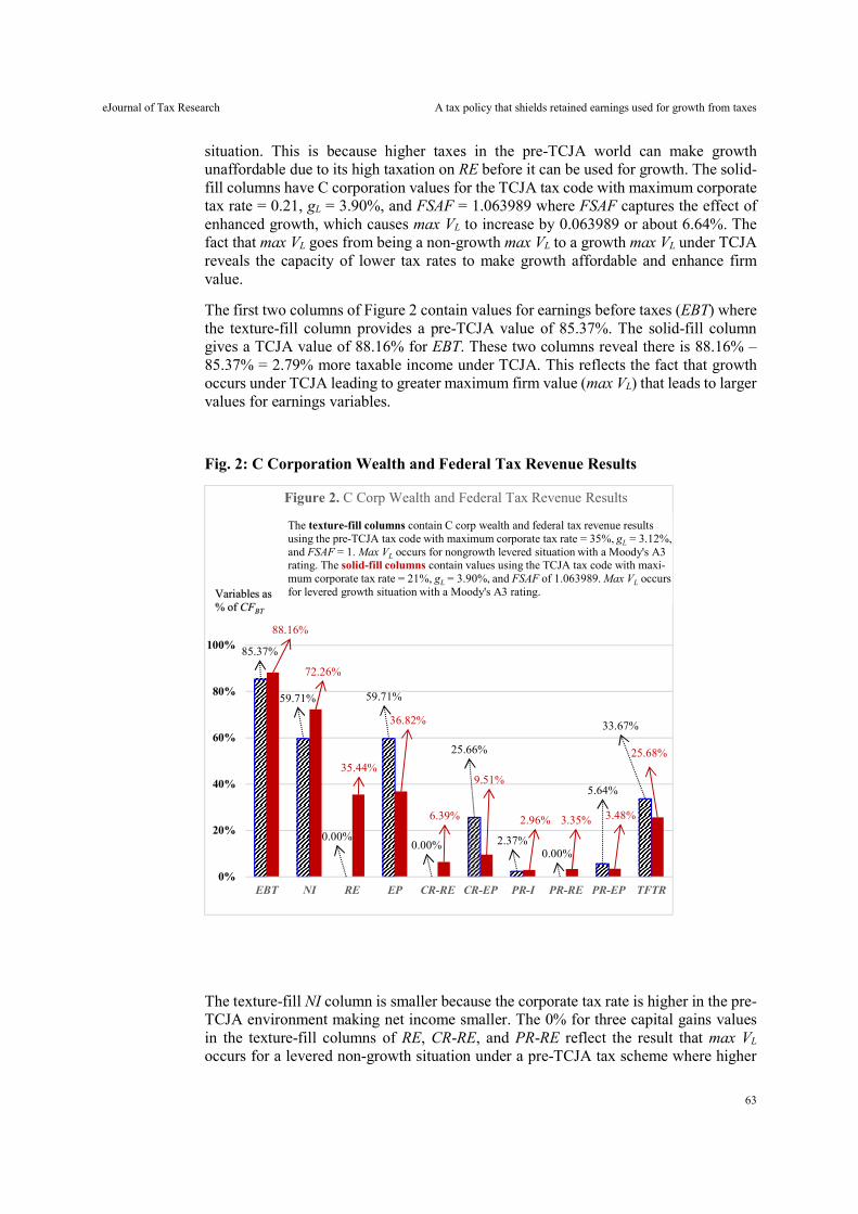
eJournal of Tax Research A tax policy that shields retained earnings used for growth from taxes
63
situation. This is because higher taxes in the pre-TCJA world can make growth unaffordable due to its high taxation on RE before it can be used for growth. The solid-fill columns have C corporation values for the TCJA tax code with maximum corporate tax rate = 0.21, gL = 3.90%, and FSAF = 1.063989 where FSAF captures the effect of enhanced growth, which causes max VL to increase by 0.063989 or about 6.64%. The fact that max VL goes from being a non-growth max VL to a growth max VL under TCJA reveals the capacity of lower tax rates to make growth affordable and enhance firm value.
The first two columns of Figure 2 contain values for earnings before taxes (EBT) where the texture-fill column provides a pre-TCJA value of 85.37%. The solid-fill column gives a TCJA value of 88.16% for EBT. These two columns reveal there is 88.16% – 85.37% = 2.79% more taxable income under TCJA. This reflects the fact that growth occurs under TCJA leading to greater maximum firm value (max VL) that leads to larger values for earnings variables.
Fig. 2: C Corporation Wealth and Federal Tax Revenue Results
The texture-fill NI column is smaller because the corporate tax rate is higher in the pre-TCJA environment making net income smaller. The 0% for three capital gains values in the texture-fill columns of RE, CR-RE, and PR-RE reflect the result that max VL occurs for a levered non-growth situation under a pre-TCJA tax scheme where higher
85.37%
59.71%
0.00%
59.71%
0.00%
25.66%
2.37%0.00%
5.64%
33.67%
88.16%
72.26%
35.44%
36.82%
6.39%
9.51%
2.96% 3.35% 3.48%
25.68%
0%
20%
40%
60%
80%
100%
EBT NI RE EP CR-RE CR-EP PR-I PR-RE PR-EP TFTR
Figure 2. C Corp Wealth and Federal Tax Revenue Results
The texture-fill columns contain C corp wealth and federal tax revenue resultsusing the pre-TCJA tax code with maximum corporate tax rate = 35%, gL = 3.12%,and FSAF = 1. Max VL occurs for nongrowth levered situation with a Moody's A3rating. The solid-fill columns contain values using the TCJA tax code with maxi-mum corporate tax rate = 21%, gL = 3.90%, and FSAF of 1.063989. Max VL occursfor levered growth situation with a Moody's A3 rating.Variables as
% of CFBT
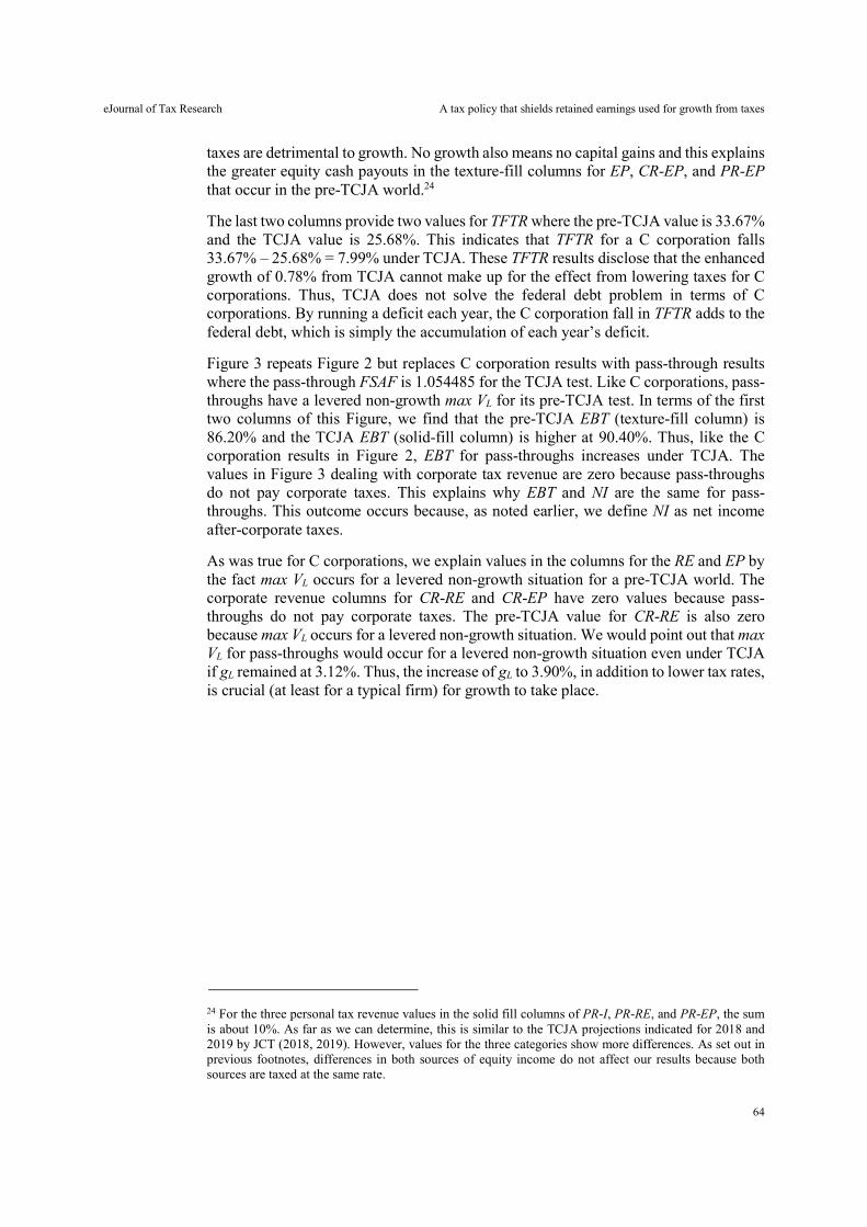
eJournal of Tax Research A tax policy that shields retained earnings used for growth from taxes
64
taxes are detrimental to growth. No growth also means no capital gains and this explains the greater equity cash payouts in the texture-fill columns for EP, CR-EP, and PR-EP that occur in the pre-TCJA world.24
The last two columns provide two values for TFTR where the pre-TCJA value is 33.67% and the TCJA value is 25.68%. This indicates that TFTR for a C corporation falls 33.67% – 25.68% = 7.99% under TCJA. These TFTR results disclose that the enhanced growth of 0.78% from TCJA cannot make up for the effect from lowering taxes for C corporations. Thus, TCJA does not solve the federal debt problem in terms of C corporations. By running a deficit each year, the C corporation fall in TFTR adds to the federal debt, which is simply the accumulation of each year’s deficit.
Figure 3 repeats Figure 2 but replaces C corporation results with pass-through results where the pass-through FSAF is 1.054485 for the TCJA test. Like C corporations, pass-throughs have a levered non-growth max VL for its pre-TCJA test. In terms of the first two columns of this Figure, we find that the pre-TCJA EBT (texture-fill column) is 86.20% and the TCJA EBT (solid-fill column) is higher at 90.40%. Thus, like the C corporation results in Figure 2, EBT for pass-throughs increases under TCJA. The values in Figure 3 dealing with corporate tax revenue are zero because pass-throughs do not pay corporate taxes. This explains why EBT and NI are the same for pass-throughs. This outcome occurs because, as noted earlier, we define NI as net income after-corporate taxes.
As was true for C corporations, we explain values in the columns for the RE and EP by the fact max VL occurs for a levered non-growth situation for a pre-TCJA world. The corporate revenue columns for CR-RE and CR-EP have zero values because pass-throughs do not pay corporate taxes. The pre-TCJA value for CR-RE is also zero because max VL occurs for a levered non-growth situation. We would point out that max VL for pass-throughs would occur for a levered non-growth situation even under TCJA if gL remained at 3.12%. Thus, the increase of gL to 3.90%, in addition to lower tax rates, is crucial (at least for a typical firm) for growth to take place.
24 For the three personal tax revenue values in the solid fill columns of PR-I, PR-RE, and PR-EP, the sum is about 10%. As far as we can determine, this is similar to the TCJA projections indicated for 2018 and 2019 by JCT (2018, 2019). However, values for the three categories show more differences. As set out in previous footnotes, differences in both sources of equity income do not affect our results because both sources are taxed at the same rate.
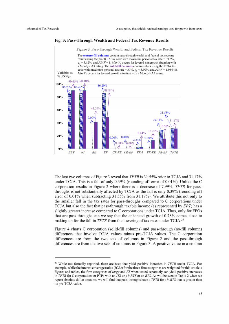
eJournal of Tax Research A tax policy that shields retained earnings used for growth from taxes
65
Fig. 3: Pass-Through Wealth and Federal Tax Revenue Results
The last two columns of Figure 3 reveal that TFTR is 31.55% prior to TCJA and 31.17% under TCJA. This is a fall of only 0.39% (rounding off error of 0.01%). Unlike the C corporation results in Figure 2 where there is a decrease of 7.99%, TFTR for pass-throughs is not substantially affected by TCJA as the fall is only 0.39% (rounding off error of 0.01% when subtracting 31.55% from 31.17%). We attribute this not only to the smaller fall in the tax rates for pass-throughs compared to C corporations under TCJA but also the fact that pass-through taxable income (as represented by EBT) has a slightly greater increase compared to C corporations under TCJA. Thus, only for FPOs that are pass-throughs can we say that the enhanced growth of 0.78% comes close to making up for the fall in TFTR from the lowering of tax rates under TCJA.25
Figure 4 charts C corporation (solid-fill columns) and pass-through (no-fill column) differences that involve TCJA values minus pre-TCJA values. The C corporation differences are from the two sets of columns in Figure 2 and the pass-through differences are from the two sets of columns in Figure 3. A positive value in a column
25 While not formally reported, there are tests that yield positive increases in TFTR under TCJA. For example, while the interest coverage ratios (ICRs) for the three firm categories are weighted for this article’s figures and tables, the firm categories of large and FS when tested separately can yield positive increases in TFTR for C corporations or PTPs with an ITS or a ½RTS or an RTS. As will be seen in Table 2 when we report absolute dollar amounts, we will find that pass-throughs have a TFTR for a ½RTS that is greater than its pre-TCJA value.
86.20% 86.20%
0.00%
86.20%
0.00% 0.00%2.24%
0.00%
29.31%
31.55%
90.40% 90.40%
41.56%
48.84%
0.00% 0.00%
2.44%13.20%
15.52%
31.17%
0%
20%
40%
60%
80%
100%
EBT NI RE EP CR-RE CR-EP PR-I PR-RE PR-EP TFTR
Figure 3. Pass-Through Wealth and Federal Tax Revenue Results
The texture-fill columns contain pass-through wealth and federal tax revenueresults using the pre-TCJA tax code with maximum personal tax rate = 39.6%,gL = 3.12%, and FSAF = 1. Max VL occurs for levered nongrowth situation witha Moody's A3 rating. The solid-fill columns contain values using the TCJA taxcode with maximum personal tax rate = 37%, gL = 3.90%, and FSAF = 1.054485.Max VL occurs for levered growth situation with a Moody's A3 rating.Variables as
% of CFBT
eJournal of Tax Research A tax policy that shields retained earnings used for growth from taxes
66
indicates an increase caused by TCJA while a negative value signifies a decrease attributable to TCJA.
Fig. 4: C Corporation and Pass-Through Differences in Wealth and TFTR
Figure 4 reveals the following C corporation results and pass-through results with the latter in parentheses. First, EBT rises 2.79% (4.20%). Second, NI increases 12.55% (4.20%). EBT and NI are the same at 4.20% for pass-throughs because they do not pay corporate taxes so that all of their EBT is subject to equity personal tax. Third, RE rises 35.44% (41.56%). The large rises reflect the fact that non-growth max VL values occur prior to TCJA for both C corporations and pass-throughs. Fourth, EP decreases 22.89% (37.35%). With capital gains now present due to growth under TCJA, the cash payout to equity owners falls. From the last two results, we see that TCJA causes pass-throughs to experience greater increases in capital gains and greater decreases in equity payouts when compared to C corporations.
Fifth, CR-RE rises 6.39% (0%) where 0% reflects the fact pass-throughs do not pay corporate taxes. The positive value of 6.39% reflects the growth that occurs under TCJA. Sixth, CR-EP falls 16.15% (0%) where, once again, the pass-through value is 0% since they do not pay corporate taxes. The fall in equity payout for C corporations reflects the fact that funds for growth now occur under TCJA. Seventh, PR-I rises slightly 0.59% (0.20%). Eighth, PR-RE increases 3.35% (13.20%). The personal tax revenue from capital gains is greater for pass-throughs that pay at a higher personal tax
2.79%
12.55%
35.44%
-22.89%
6.39%
-16.15%
0.59%3.35%
-2.16%
-7.99%
4.20%4.20%
41.56%
-37.35%
0.00% 0.00% 0.20%
13.20%
-13.79%
-0.39%
-60%
-40%
-20%
0%
20%
40%
60%
EBT NI RE EP CR-RE CR-EP PR-I PR-RE PR-EP TFTR
Figure 4. C Corp & Pass-through Differences in Wealth & TFTR
DifferencesUsing %of CFBT
C corp (solid-fill columns) and pass-through (no-fill columns) differencesinvolve TCJA values minus pre-TCJA values where TCJA values use gL = 3.90%and FSAFs of 1.063989 for C corps and 1.054485 for pass-throughs while pre-TCJA values use gL = 3.12% and FSAF of 1 for both C corps & pass-throughs.
The negative percentages for the TFTR columns indicate aC corp loss of 7.99% and a pass-through loss of 0.39%for every dollar of before-tax cash flow.
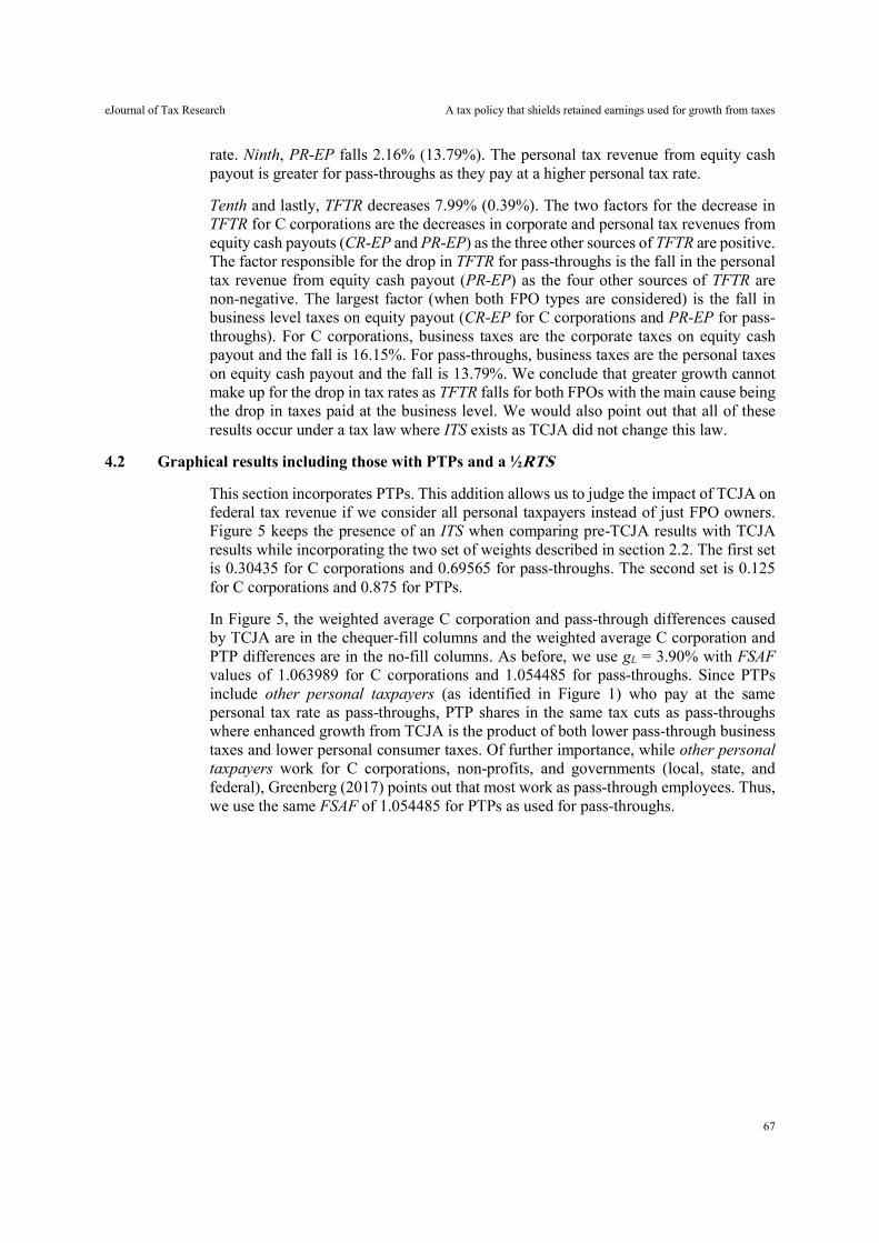
eJournal of Tax Research A tax policy that shields retained earnings used for growth from taxes
67
rate. Ninth, PR-EP falls 2.16% (13.79%). The personal tax revenue from equity cash payout is greater for pass-throughs as they pay at a higher personal tax rate.
Tenth and lastly, TFTR decreases 7.99% (0.39%). The two factors for the decrease in TFTR for C corporations are the decreases in corporate and personal tax revenues from equity cash payouts (CR-EP and PR-EP) as the three other sources of TFTR are positive. The factor responsible for the drop in TFTR for pass-throughs is the fall in the personal tax revenue from equity cash payout (PR-EP) as the four other sources of TFTR are non-negative. The largest factor (when both FPO types are considered) is the fall in business level taxes on equity payout (CR-EP for C corporations and PR-EP for pass-throughs). For C corporations, business taxes are the corporate taxes on equity cash payout and the fall is 16.15%. For pass-throughs, business taxes are the personal taxes on equity cash payout and the fall is 13.79%. We conclude that greater growth cannot make up for the drop in tax rates as TFTR falls for both FPOs with the main cause being the drop in taxes paid at the business level. We would also point out that all of these results occur under a tax law where ITS exists as TCJA did not change this law.
4.2 Graphical results including those with PTPs and a ½RTS
This section incorporates PTPs. This addition allows us to judge the impact of TCJA on federal tax revenue if we consider all personal taxpayers instead of just FPO owners. Figure 5 keeps the presence of an ITS when comparing pre-TCJA results with TCJA results while incorporating the two set of weights described in section 2.2. The first set is 0.30435 for C corporations and 0.69565 for pass-throughs. The second set is 0.125 for C corporations and 0.875 for PTPs.
In Figure 5, the weighted average C corporation and pass-through differences caused by TCJA are in the chequer-fill columns and the weighted average C corporation and PTP differences are in the no-fill columns. As before, we use gL = 3.90% with FSAF values of 1.063989 for C corporations and 1.054485 for pass-throughs. Since PTPs include other personal taxpayers (as identified in Figure 1) who pay at the same personal tax rate as pass-throughs, PTP shares in the same tax cuts as pass-throughs where enhanced growth from TCJA is the product of both lower pass-through business taxes and lower personal consumer taxes. Of further importance, while other personal taxpayers work for C corporations, non-profits, and governments (local, state, and federal), Greenberg (2017) points out that most work as pass-through employees. Thus, we use the same FSAF of 1.054485 for PTPs as used for pass-throughs.
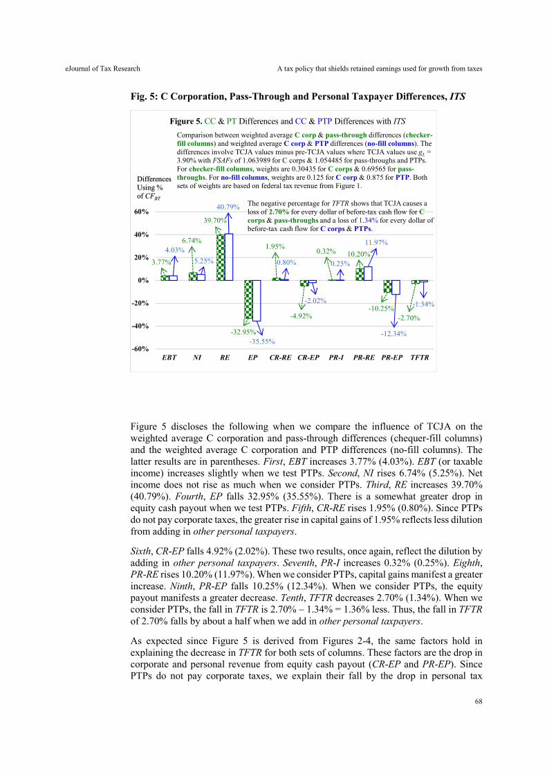
eJournal of Tax Research A tax policy that shields retained earnings used for growth from taxes
68
Fig. 5: C Corporation, Pass-Through and Personal Taxpayer Differences, ITS
Figure 5 discloses the following when we compare the influence of TCJA on the weighted average C corporation and pass-through differences (chequer-fill columns) and the weighted average C corporation and PTP differences (no-fill columns). The latter results are in parentheses. First, EBT increases 3.77% (4.03%). EBT (or taxable income) increases slightly when we test PTPs. Second, NI rises 6.74% (5.25%). Net income does not rise as much when we consider PTPs. Third, RE increases 39.70% (40.79%). Fourth, EP falls 32.95% (35.55%). There is a somewhat greater drop in equity cash payout when we test PTPs. Fifth, CR-RE rises 1.95% (0.80%). Since PTPs do not pay corporate taxes, the greater rise in capital gains of 1.95% reflects less dilution from adding in other personal taxpayers.
Sixth, CR-EP falls 4.92% (2.02%). These two results, once again, reflect the dilution by adding in other personal taxpayers. Seventh, PR-I increases 0.32% (0.25%). Eighth, PR-RE rises 10.20% (11.97%). When we consider PTPs, capital gains manifest a greater increase. Ninth, PR-EP falls 10.25% (12.34%). When we consider PTPs, the equity payout manifests a greater decrease. Tenth, TFTR decreases 2.70% (1.34%). When we consider PTPs, the fall in TFTR is 2.70% – 1.34% = 1.36% less. Thus, the fall in TFTR of 2.70% falls by about a half when we add in other personal taxpayers.
As expected since Figure 5 is derived from Figures 2-4, the same factors hold in explaining the decrease in TFTR for both sets of columns. These factors are the drop in corporate and personal revenue from equity cash payout (CR-EP and PR-EP). Since PTPs do not pay corporate taxes, we explain their fall by the drop in personal tax
3.77%
6.74%
39.70%
-32.95%
1.95%
-4.92%
0.32% 10.20%
-10.25%-2.70%
4.03%
5.25%
40.79%
-35.55%
0.80%
-2.02%
0.25%
11.97%
-12.34%
-1.34%
-60%
-40%
-20%
0%
20%
40%
60%
EBT NI RE EP CR-RE CR-EP PR-I PR-RE PR-EP TFTR
Figure 5. CC & PT Differences and CC & PTP Differences with ITS
The negative percentage for TFTR shows that TCJA causes aloss of 2.70% for every dollar of before-tax cash flow for Ccorps & pass-throughs and a loss of 1.34% for every dollar ofbefore-tax cash flow for C corps & PTPs.
Comparison between weighted average C corp & pass-through differences (checker-fill columns) and weighted average C corp & PTP differences (no-fill columns). Thedifferences involve TCJA values minus pre-TCJA values where TCJA values use gL =3.90% with FSAFs of 1.063989 for C corps & 1.054485 for pass-throughs and PTPs.For checker-fill columns, weights are 0.30435 for C corps & 0.69565 for pass-throughs. For no-fill columns, weights are 0.125 for C corp & 0.875 for PTP. Bothsets of weights are based on federal tax revenue from Figure 1.
DifferencesUsing %of CFBT

eJournal of Tax Research A tax policy that shields retained earnings used for growth from taxes
69
revenue from equity cash payout (PR-EP). The other two personal tax revenue factors (PR-I and PR-RE) are positive. Finally, because the fall of 2.70% for TFTR only includes C corporations and pass-throughs, the drop of 1.34% for TFTR that includes C corporations and PTPs is a better estimate on how TCJA influences TFTR as C corporations and PTPs include all taxpayers.26
Figure 6 repeats Figure 5 except we replace ITS with a ½RTS, which means that one-half of every dollar used for RE is not taxed at the business level while all of I is now taxed at the business level. This 50% tax deduction subsidises businesses for using RE where RE captures the use of internal equity funds utilised for growth-related activities. The chequer-fill columns in Figure 6 contain values that use the weights of 0.30435 for C corporations and 0.69565 for pass-throughs and the solid-fill columns use weights of 0.125 for C corporations and 0.875 for PTPs. The TCJA outcomes use gL = 3.90% and have FSAF values of 1.069279 for C corporations and 1.065982 for pass-throughs or PTPs. These FSAF values are greater than those in Figure 5 for an ITS. This indicates that a ½RTS tax law leads to a greater change in max VL when growth increases under TCJA.
For a ½RTS, the fifth set of columns in Figure 6 (that applies only to C corporations as PTPs do not pay corporate taxes) change from that used in Figures 2-5 so that the CR-RE column is now labelled CR-RE/I. 27 This is because all of I as well as one-half of RE are now taxed at the corporate level. For PTPs, the PR-I column is altered compared to Figures 2-5. This is because, under a ½RTS, the US federal government taxes I not only at the personal debt level but also at the personal business level since it is no longer a business tax deduction. Thus, like the cash equity payout, it is now taxed at the business and personal levels doing away with the tax distortion that favours interest over dividends under an ITS tax law. The column name of PR-I is kept since I is still the only source of federal tax revenue for FPOs.
26 Both normalised values of 2.70% and 1.34% are less than the estimated 4.20% given by the CBO (2019) for 2019. However, as will be seen later in Table 2 when we look at the exact dollar amounts of TFTR before and after TCJA, we find a 4.20% drop for 2019. Robustness tests, described in section 5.2, also produce similar results. Although not reported in that section, the average of all of our robustness tests is 4.43%. This agrees more with 4.39% given by JCT, as cited by TPC (2019), and the 4.30% average given by CBO (2019) for 2020–2029. 27 In section 4.1, we referred to CR-RE/I as CR-RE/I½RTS but since we are comparing TCJA results minus pre-TCJA results where the latter has no I, we use the more general label of CR-RE/I.
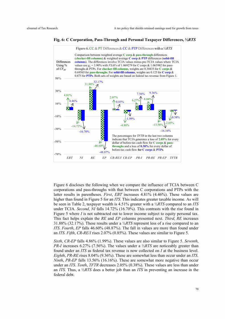
eJournal of Tax Research A tax policy that shields retained earnings used for growth from taxes
70
Fig. 6: C Corporation, Pass-Through and Personal Taxpayer Differences, ½RTS
Figure 6 discloses the following when we compare the influence of TCJA between C corporations and pass-throughs with that between C corporations and PTPs with the latter results in parentheses. First, EBT increases 4.81% (4.46%). These values are higher than found in Figure 5 for an ITS. This indicates greater taxable income. As will be seen in Table 2, taxpayer wealth is 4.51% greater with a ½RTS compared to an ITS under TCJA. Second, NI falls 14.72% (16.70%). This contrasts with the rise found in Figure 5 where I is not subtracted out to lower income subject to equity personal tax. This fact helps explain the RE and EP columns presented next. Third, RE increases 31.88% (32.17%). These results under a ½RTS represent less of a rise compared to an ITS. Fourth, EP falls 46.60% (48.87%). The fall in values are more than found under an ITS. Fifth, CR-RE/I rises 2.07% (0.85%). These values are similar to Figure 5.
Sixth, CR-EP falls 4.86% (1.99%). These values are also similar to Figure 5. Seventh, PR-I increases 6.27% (7.56%). The values under a ½RTS are noticeably greater than found under an ITS as federal tax revenue is now collected on I at the business level. Eighth, PR-RE rises 8.04% (9.36%). These are somewhat less than occur under an ITS. Ninth, PR-EP falls 13.56% (16.16%). These are somewhat more negative than occur under an ITS. Tenth, TFTR decreases 2.05% (0.38%). These values are less than under an ITS. Thus, a ½RTS does a better job than an ITS in preventing an increase in the federal debt.
4.81%
-14.72%
31.88%
-46.60%
2.07%
-4.86%
6.27% 8.04%
-13.58%-2.05%
4.46%
-16.70%
32.17%
-48.87%
0.85%
-1.99%
7.56% 9.36%
-16.16%
-0.38%
-70%
-50%
-30%
-10%
10%
30%
50%
EBT NI RE EP CR-RE/I CR-EP PR-I PR-RE PR-EP TFTR
Figure 6. CC & PT Differences & CC & PTP Differences with a ½RTS
The percentages for TFTR in the last two columnsindicate that TCJA generates a loss of 2.05% for everydollar of before-tax cash flow for C corps & pass-throughs and a loss of 0.38% for every dollar ofbefore-tax cash flow for C corps & PTPs.
Comparison between weighted average C corp & pass-through differences(checker-fill columns) & weighted average C corp & PTP differences (solid-fillcolumns). The differences involve TCJA values minus pre-TCJA values where TCJAvalues use gL = 3.90% with FSAFs of 1.069279 for C corps & 1.065982 for pass-throughs & PTPs. For checker-fill columns, weights are 0.30435 for C corps &0.69565 for pass-throughs. For solid-fill columns, weights are 0.125 for C corp &0.875 for PTPs. Both sets of weights are based on federal tax revenue from Figure 1.
DifferencesUsing %of CFBT
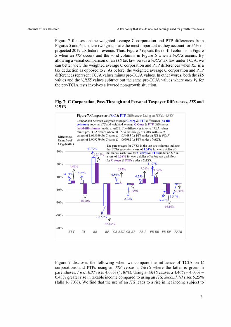
eJournal of Tax Research A tax policy that shields retained earnings used for growth from taxes
71
Figure 7 focuses on the weighted average C corporation and PTP differences from Figures 5 and 6, as these two groups are the most important as they account for 56% of projected 2019 tax federal revenue. Thus, Figure 7 repeats the no-fill columns in Figure 5 when an ITS occurs and the solid columns in Figure 6 when a ½RTS occurs. By allowing a visual comparison of an ITS tax law versus a ½RTS tax law under TCJA, we can better view the weighted average C corporation and PTP differences when RE is a tax deduction as opposed to I. As before, the weighted average C corporation and PTP differences represent TCJA values minus pre-TCJA values. In other words, both the ITS values and the ½RTS values subtract out the same pre-TCJA values where max VL for the pre-TCJA tests involves a levered non-growth situation.
Fig. 7: C Corporation, Pass-Through and Personal Taxpayer Differences, ITS and ½RTS
Figure 7 discloses the following when we compare the influence of TCJA on C corporations and PTPs using an ITS versus a ½RTS where the latter is given in parentheses. First, EBT rises 4.03% (4.46%). Using a ½RTS causes a 4.46% – 4.03% = 0.43% greater rise in taxable income compared to using an ITS. Second, NI rises 5.25% (falls 16.70%). We find that the use of an ITS leads to a rise in net income subject to
4.03% 5.25%
40.79%
-35.55%
0.80%
-2.02%
0.25%
11.97%
-12.34%-1.34%
4.46%
-16.70%
32.17%
-48.87%
0.85%
-1.99%
7.56% 9.36%
-16.16%
-0.38%
-70%
-50%
-30%
-10%
10%
30%
50%
EBT NI RE EP CR-RE/I CR-EP PR-I PR-RE PR-EP TFTR
Figure 7. Comparison of CC & PTP Differences Using an ITS & ½RTS
The percentages for TFTR in the last two columns indicatethat TCJA generates a loss of 1.34% for every dollar ofbefore-tax cash flow for C corps & PTPs under an ITS &a loss of 0.38% for every dollar of before-tax cash flowfor C corps & PTPs under a ½RTS.
Comparison between weighted average C corp & PTP differences (no-fillcolumns) under an ITS and weighted average C Corp & PTP differences(solid-fill columns) under a ½RTS. The differences involve TCJA valuesminus pre-TCJA values where TCJA values use gL = 3.90% with FSAFvalues of 1.063989 for C corps & 1.054485 for PTP under an ITS & FSAFvalues of 1.069279 for C corps & 1.065982 for PTP under a ½RTS.
DifferencesUsing % ofCFBT (EBIT)
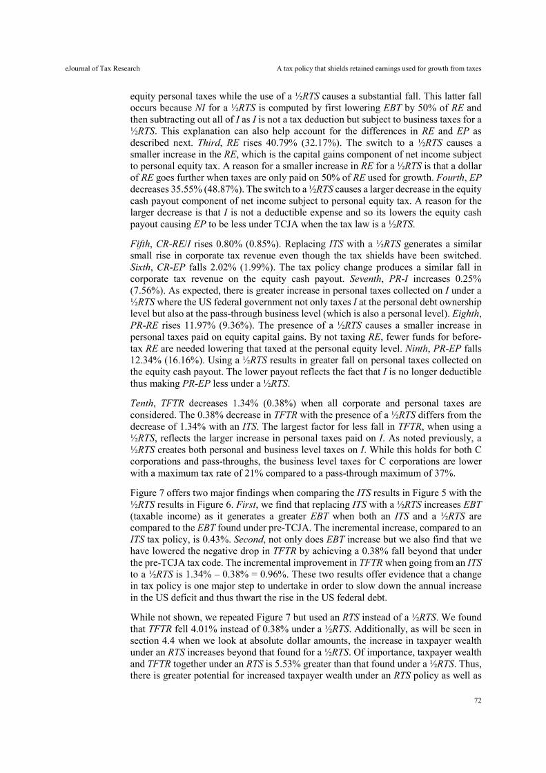
eJournal of Tax Research A tax policy that shields retained earnings used for growth from taxes
72
equity personal taxes while the use of a ½RTS causes a substantial fall. This latter fall occurs because NI for a ½RTS is computed by first lowering EBT by 50% of RE and then subtracting out all of I as I is not a tax deduction but subject to business taxes for a ½RTS. This explanation can also help account for the differences in RE and EP as described next. Third, RE rises 40.79% (32.17%). The switch to a ½RTS causes a smaller increase in the RE, which is the capital gains component of net income subject to personal equity tax. A reason for a smaller increase in RE for a ½RTS is that a dollar of RE goes further when taxes are only paid on 50% of RE used for growth. Fourth, EP decreases 35.55% (48.87%). The switch to a ½RTS causes a larger decrease in the equity cash payout component of net income subject to personal equity tax. A reason for the larger decrease is that I is not a deductible expense and so its lowers the equity cash payout causing EP to be less under TCJA when the tax law is a ½RTS.
Fifth, CR-RE/I rises 0.80% (0.85%). Replacing ITS with a ½RTS generates a similar small rise in corporate tax revenue even though the tax shields have been switched. Sixth, CR-EP falls 2.02% (1.99%). The tax policy change produces a similar fall in corporate tax revenue on the equity cash payout. Seventh, PR-I increases 0.25% (7.56%). As expected, there is greater increase in personal taxes collected on I under a ½RTS where the US federal government not only taxes I at the personal debt ownership level but also at the pass-through business level (which is also a personal level). Eighth, PR-RE rises 11.97% (9.36%). The presence of a ½RTS causes a smaller increase in personal taxes paid on equity capital gains. By not taxing RE, fewer funds for before-tax RE are needed lowering that taxed at the personal equity level. Ninth, PR-EP falls 12.34% (16.16%). Using a ½RTS results in greater fall on personal taxes collected on the equity cash payout. The lower payout reflects the fact that I is no longer deductible thus making PR-EP less under a ½RTS.
Tenth, TFTR decreases 1.34% (0.38%) when all corporate and personal taxes are considered. The 0.38% decrease in TFTR with the presence of a ½RTS differs from the decrease of 1.34% with an ITS. The largest factor for less fall in TFTR, when using a ½RTS, reflects the larger increase in personal taxes paid on I. As noted previously, a ½RTS creates both personal and business level taxes on I. While this holds for both C corporations and pass-throughs, the business level taxes for C corporations are lower with a maximum tax rate of 21% compared to a pass-through maximum of 37%.
Figure 7 offers two major findings when comparing the ITS results in Figure 5 with the ½RTS results in Figure 6. First, we find that replacing ITS with a ½RTS increases EBT (taxable income) as it generates a greater EBT when both an ITS and a ½RTS are compared to the EBT found under pre-TCJA. The incremental increase, compared to an ITS tax policy, is 0.43%. Second, not only does EBT increase but we also find that we have lowered the negative drop in TFTR by achieving a 0.38% fall beyond that under the pre-TCJA tax code. The incremental improvement in TFTR when going from an ITS to a ½RTS is 1.34% – 0.38% = 0.96%. These two results offer evidence that a change in tax policy is one major step to undertake in order to slow down the annual increase in the US deficit and thus thwart the rise in the US federal debt.
While not shown, we repeated Figure 7 but used an RTS instead of a ½RTS. We found that TFTR fell 4.01% instead of 0.38% under a ½RTS. Additionally, as will be seen in section 4.4 when we look at absolute dollar amounts, the increase in taxpayer wealth under an RTS increases beyond that found for a ½RTS. Of importance, taxpayer wealth and TFTR together under an RTS is 5.53% greater than that found under a ½RTS. Thus, there is greater potential for increased taxpayer wealth under an RTS policy as well as
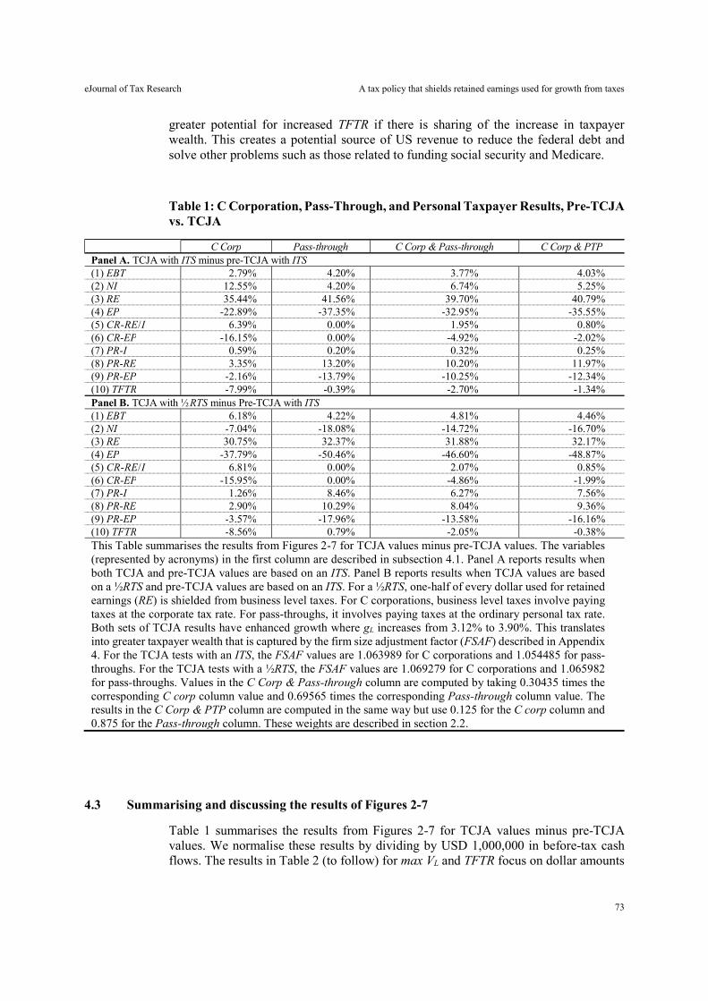
eJournal of Tax Research A tax policy that shields retained earnings used for growth from taxes
73
greater potential for increased TFTR if there is sharing of the increase in taxpayer wealth. This creates a potential source of US revenue to reduce the federal debt and solve other problems such as those related to funding social security and Medicare.
Table 1: C Corporation, Pass-Through, and Personal Taxpayer Results, Pre-TCJA vs. TCJA
C Corp Pass-through C Corp & Pass-through C Corp & PTP Panel A. TCJA with ITS minus pre-TCJA with ITS (1) EBT 2.79% 4.20% 3.77% 4.03% (2) NI 12.55% 4.20% 6.74% 5.25% (3) RE 35.44% 41.56% 39.70% 40.79% (4) EP -22.89% -37.35% -32.95% -35.55% (5) CR-RE/I 6.39% 0.00% 1.95% 0.80% (6) CR-EP -16.15% 0.00% -4.92% -2.02% (7) PR-I 0.59% 0.20% 0.32% 0.25% (8) PR-RE 3.35% 13.20% 10.20% 11.97% (9) PR-EP -2.16% -13.79% -10.25% -12.34% (10) TFTR -7.99% -0.39% -2.70% -1.34% Panel B. TCJA with ½RTS minus Pre-TCJA with ITS (1) EBT 6.18% 4.22% 4.81% 4.46% (2) NI -7.04% -18.08% -14.72% -16.70% (3) RE 30.75% 32.37% 31.88% 32.17% (4) EP -37.79% -50.46% -46.60% -48.87% (5) CR-RE/I 6.81% 0.00% 2.07% 0.85% (6) CR-EP -15.95% 0.00% -4.86% -1.99% (7) PR-I 1.26% 8.46% 6.27% 7.56% (8) PR-RE 2.90% 10.29% 8.04% 9.36% (9) PR-EP -3.57% -17.96% -13.58% -16.16% (10) TFTR -8.56% 0.79% -2.05% -0.38% This Table summarises the results from Figures 2-7 for TCJA values minus pre-TCJA values. The variables (represented by acronyms) in the first column are described in subsection 4.1. Panel A reports results when both TCJA and pre-TCJA values are based on an ITS. Panel B reports results when TCJA values are based on a ½RTS and pre-TCJA values are based on an ITS. For a ½RTS, one-half of every dollar used for retained earnings (RE) is shielded from business level taxes. For C corporations, business level taxes involve paying taxes at the corporate tax rate. For pass-throughs, it involves paying taxes at the ordinary personal tax rate. Both sets of TCJA results have enhanced growth where gL increases from 3.12% to 3.90%. This translates into greater taxpayer wealth that is captured by the firm size adjustment factor (FSAF) described in Appendix 4. For the TCJA tests with an ITS, the FSAF values are 1.063989 for C corporations and 1.054485 for pass-throughs. For the TCJA tests with a ½RTS, the FSAF values are 1.069279 for C corporations and 1.065982 for pass-throughs. Values in the C Corp & Pass-through column are computed by taking 0.30435 times the corresponding C corp column value and 0.69565 times the corresponding Pass-through column value. The results in the C Corp & PTP column are computed in the same way but use 0.125 for the C corp column and 0.875 for the Pass-through column. These weights are described in section 2.2.
4.3 Summarising and discussing the results of Figures 2-7
Table 1 summarises the results from Figures 2-7 for TCJA values minus pre-TCJA values. We normalise these results by dividing by USD 1,000,000 in before-tax cash flows. The results in Table 2 (to follow) for max VL and TFTR focus on dollar amounts
eJournal of Tax Research A tax policy that shields retained earnings used for growth from taxes
74
when gauging taxpayer and wealth and federal tax revenue and so bring more accuracy in terms of comparing the exact dollar amounts under different tax laws governing tax shields.
Panel A of Table 1 reports results when both TCJA and pre-TCJA values are based on an ITS. Panel B reports results when TCJA values are based on a ½RTS and pre-TCJA values are based on an ITS. Both sets of TCJA results have enhanced growth from lower tax rates. We compute values in the C Corp & Pass-through column by taking 0.30435 times the corresponding C corp column value and 0.69565 times the corresponding Pass-through column value. We calculate the results in the C Corp & PTP column in the same way but use 0.125 for the C Corp column values and 0.875 for the Pass-through column values. The C Corp & PTP column is the most important column because, as discussed in section 2.2, it considers federal taxes paid by C corporations, pass-throughs and other personal taxpayers, which together are 56% of federal tax revenue expected for 2019. Below, we focus on the results in this column.
For the ITS results in Panel A, the value for EBT in the first row of the C Corp & PTP column is 4.03%. This indicates that compared to its pre-TCJA value, EBT (or taxable income) increases 4.03%. This compares to 4.46% in the corresponding cell of Panel B. Thus, replacing ITS with a ½RTS increases taxable income by 0.43%. For the ITS results in Panel A, the value for TFTR in the last row of the C Corp & PTP column is 1.34%. This compares to 0.38% in the corresponding cell of Panel B for the ½RTS results. Thus, replacing ITS with a ½RTS increases TFTR by 0.96%.
Of importance, under TCJA with a ½RTS tax policy, EBT and TFTR are on trajectories increasing 0.43% and 0.96% compared to current tax legislation that allows an ITS. Thus, taxpayers and the IRS are both winners under a ½RTS policy. However, the TFTR of 0.38% under a ½RTS indicates that federal revenue is still declining. As will be seen in the next section, there is hope if the substantial increase in taxpayer wealth when switching the tax shield from I to RE can be used to increase TFTR.
The TFTR values in Table 1 are all negative except for a ½RTS in the last row in Panel B for the Pass-through column. For the C corp & PTP column of this panel, the value is negative at 0.38%. This indicates a federal deficit for the year, which adds to the federal debt. However, one must keep in mind the following when discussing a country’s debt problem and how to resolve it. First, debt must be compared with the country’s GDP to get a relative perspective on its ability to pay down debt. According to Federal Reserve Economic Data (FRED) (2019c), US debt as a percentage of GDP is 104%. The bad news is that this percentage has risen steadily since 1981 when it was 30%. Second, debt is more likely to be a problem if a foreign country (as compared to its own citizens) holds most of the debt. Amadeo (2019) notes that foreign holdings of US debt has ballooned in the past decade reaching 30% of the US public debt. Third, a low rate of borrowing diminishes any debt problem because there is less cost in maintaining it. While interest rates on debt have been low, Peter G Pederson Foundation (2018) expects the total US interest payments as a percent of GDP to double in the next decade from 1.6% to 3.2%. Fourth, the ability to cut tax expenditures can be a key to lowering of the annual deficit and thus reducing federal debt.28 The largest tax
28 Tax expenditures refer to revenue losses attributable to provisions of the federal tax laws which allow a special exclusion, exemption, or deduction from gross income or which provide a special credit, a preferential rate of tax, or a deferral of tax liability.
eJournal of Tax Research A tax policy that shields retained earnings used for growth from taxes
75
expenditure in the US is the exclusion of employer contributions for medical insurance premiums and medical care.
The findings illustrated in Figures 6-7 and capsulised in Panel B of Table 1 for a ½RTS are not offered as the optimal findings as more research is needed. For example, as will be seen later in Table 2, much more taxpayer wealth can be created if an RTS is pursued where all of RE is used as a tax shield instead of one-half. However, since an RTS lowers TFTR even more than a ½RTS, it would require businesses sharing some of their increased wealth by raising taxes.
4.4 Results for five key variables
Table 2 reports results for five key variables defined as follows: FSAF is the firm size adjustment factor (described in Appendix 4); max VL is maximum firm value that represents maximum taxpayer wealth; TFTR is the total federal tax revenue (described in detail in section 4.1); WETR is the weighted effective tax rate (described in Appendix 5); %∆EU is the percent change in unlevered firm value caused by leverage and equals maxGL/EU where max GL is given by (1) and EU is unlevered firm value; and, ODV is the optimal debt-to-firm value ratio that corresponds to max VL.
Results for the first row of each of the four panels are associated with a pre-TCJA and an ITS. The second row of each panel covers ITS under TCJA. The third row of each panel reports with a ½RTS under TCJA. The last row of each panel provides results for an RTS under TCJA. Unlike an ITS that is either 100% (first two rows of each panel) or 0% (last two rows of each panel), an RTS takes on three different values of 0% (first two rows of each panel), 50% (third row of each panel), and 100% (last row of each panel). Weighted average interest coverage ratios (ICRs), as described in Appendix 3, are used to generate the C corporation results in Panel A and the pass-through results in Panel B. The C corporation and pass-through results in Panel C are computed by taking 0.30435 times the corresponding C corporation value in Panel A and 0.69565 times the corresponding value in Panel B. The C corporation and PTP results in Panel D are computed in the same way but use 0.125 for the corresponding row in Panel A and 0.875 for the corresponding row in Panel B. The two sets of weights used in Panels C and D are described in section 2.2.
4.4.1 FSAF results
Disregarding FSAF values of 1 that occur for pre-TCJA tests where there is no increase in growth, the FSAF column of Table 2 shows that the range of FSAF values are from 1.054485 to 1.076333. Each panel reveals that greater FSAF values occur as the tax shield on RE increases. Because FSAF values reflect the percentage increase in max VL caused by an upsurge in growth from 3.12% to 3.90% under TCJA, the increasing FSAF values in each panel tell us that greater taxpayer wealth can be achieved as increasingly large amounts of RE are tax-deductible so that an RTS in the last row provides the greatest wealth.
To illustrate, the FSAF value of 1.057378 in the second row of Panel C tells us that max VL increases 5.7378% for an ITS tax policy. If we replace an ITS with a ½RTS, FSAF becomes 1.066985 as seen in the third row of Panel C revealing an increase of 6.6985% in max VL from enhanced growth. If we replace a ½RTS with an RTS, FSAF becomes 1.075814 as seen in the last row of Panel C revealing an increase of 7.5814% in max VL.
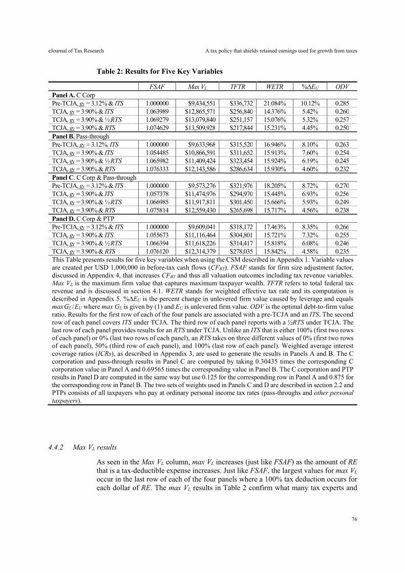
eJournal of Tax Research A tax policy that shields retained earnings used for growth from taxes
76
Table 2: Results for Five Key Variables
FSAF Max VL TFTR WETR %∆EU ODV Panel A. C Corp Pre-TCJA, gL = 3.12% & ITS 1.000000 $9,434,551 $336,732 21.084% 10.12% 0.285 TCJA, gL = 3.90% & ITS 1.063989 $12,865,571 $256,840 14.376% 5.42% 0.260 TCJA, gL = 3.90% & ½RTS 1.069279 $13,079,840 $251,157 15.076% 5.32% 0.257 TCJA, gL = 3.90% & RTS 1.074629 $13,509,928 $217,844 15.231% 4.45% 0.250 Panel B. Pass-through Pre-TCJA, gL = 3.12%, ITS 1.000000 $9,633,968 $315,520 16.946% 8.10% 0.263 TCJA, gL = 3.90% & ITS 1.054485 $10,866,591 $311,652 15.913% 7.60% 0.254 TCJA, gL = 3.90% & ½RTS 1.065982 $11,409,424 $323,454 15.924% 6.19% 0.245 TCJA, gL = 3.90% & RTS 1.076333 $12,143,586 $286,634 15.930% 4.60% 0.232 Panel C. C Corp & Pass-through Pre-TCJA, gL = 3.12% & ITS 1.000000 $9,573,276 $321,976 18.205% 8.72% 0.270 TCJA, gL = 3.90% & ITS 1.057378 $11,474,976 $294,970 15.445% 6.93% 0.256 TCJA, gL = 3.90% & ½RTS 1.066985 $11,917,811 $301,450 15.666% 5.93% 0.249 TCJA, gL = 3.90% & RTS 1.075814 $12,559,430 $265,698 15.717% 4.56% 0.238 Panel D. C Corp & PTP Pre-TCJA, gL = 3.12% & ITS 1.000000 $9,609,041 $318,172 17.463% 8.35% 0.266 TCJA, gL = 3.90% & ITS 1.055673 $11,116,464 $304,801 15.721% 7.32% 0.255 TCJA, gL = 3.90% & ½RTS 1.066394 $11,618,226 $314,417 15.818% 6.08% 0.246 TCJA, gL = 3.90% & RTS 1.076120 $12,314,379 $278,035 15.842% 4.58% 0.235 This Table presents results for five key variables when using the CSM described in Appendix 1. Variable values are created per USD 1,000,000 in before-tax cash flows (CFBT). FSAF stands for firm size adjustment factor, discussed in Appendix 4, that increases CFBT and thus all valuation outcomes including tax revenue variables. Max VL is the maximum firm value that captures maximum taxpayer wealth. TFTR refers to total federal tax revenue and is discussed in section 4.1. WETR stands for weighted effective tax rate and its computation is described in Appendix 5. %∆EU is the percent change in unlevered firm value caused by leverage and equals maxGL /EU where max GL is given by (1) and EU is unlevered firm value. ODV is the optimal debt-to-firm value ratio. Results for the first row of each of the four panels are associated with a pre-TCJA and an ITS. The second row of each panel covers ITS under TCJA. The third row of each panel reports with a ½RTS under TCJA. The last row of each panel provides results for an RTS under TCJA. Unlike an ITS that is either 100% (first two rows of each panel) or 0% (last two rows of each panel), an RTS takes on three different values of 0% (first two rows of each panel), 50% (third row of each panel), and 100% (last row of each panel). Weighted average interest coverage ratios (ICRs), as described in Appendix 3, are used to generate the results in Panels A and B. The C corporation and pass-through results in Panel C are computed by taking 0.30435 times the corresponding C corporation value in Panel A and 0.69565 times the corresponding value in Panel B. The C corporation and PTP results in Panel D are computed in the same way but use 0.125 for the corresponding row in Panel A and 0.875 for the corresponding row in Panel B. The two sets of weights used in Panels C and D are described in section 2.2 and PTPs consists of all taxpayers who pay at ordinary personal income tax rates (pass-throughs and other personal taxpayers).
4.4.2 Max VL results
As seen in the Max VL column, max VL increases (just like FSAF) as the amount of RE that is a tax-deductible expense increases. Just like FSAF, the largest values for max VL occur in the last row of each of the four panels where a 100% tax deduction occurs for each dollar of RE. The max VL results in Table 2 confirm what many tax experts and
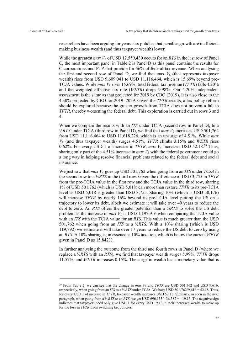
eJournal of Tax Research A tax policy that shields retained earnings used for growth from taxes
77
researchers have been arguing for years: tax policies that penalise growth are inefficient making business wealth (and thus taxpayer wealth) lower.
While the greatest max VL of USD 12,559,430 occurs for an RTS in the last row of Panel C, the most important panel in Table 2 is Panel D as this panel contains the results for C corporations and PTP that provide for 56% of federal tax revenue. When analysing the first and second row of Panel D, we find that max VL (that represents taxpayer wealth) rises from USD 9,609,041 to USD 11,116,464, which is 15.69% beyond pre-TCJA values. While max VL rises 15.69%, total federal tax revenue (TFTR) falls 4.20% and the weighted effective tax rate (WETR) drops 9.98%. Our 4.20% independent assessment is the same as that projected for 2019 by CBO (2019). It is also close to the 4.30% projected by CBO for 20192029. Given the TFTR results, a tax policy reform should be explored because the greater growth from TCJA does not prevent a fall in TFTR, thereby worsening the federal debt. This exploration is carried out in rows 3 and 4.
When we compare the results with an ITS under TCJA (second row in Panel D), to a ½RTS under TCJA (third row in Panel D), we find that max VL increases USD 501,762 from USD 11,116,464 to USD 11,618,226, which is an upsurge of 4.51%. While max VL (and thus taxpayer wealth) surges 4.51%, TFTR climbs 3.15% and WETR rises 0.62%. For every USD 1 of increase in TFTR, max VL increases USD 52.18.29 Thus, sharing only part of the 4.51% increase in max VL with the federal government could go a long way in helping resolve financial problems related to the federal debt and social insurance.
We just saw that max VL goes up USD 501,762 when going from an ITS under TCJA in the second row to a ½RTS in the third row. Given the difference of USD 3,755 in TFTR from the pre-TCJA value in the first row and the TCJA value in the third row, sharing 1% of USD 501,762 (which is USD 5,018) can more than restore TFTR to its pre-TCJA level as USD 5,018 is greater than USD 3,755. Sharing 10% (which is USD 50,176) will increase TFTR by nearly 16% beyond its pre-TCJA level putting the US on a trajectory to lower its debt, albeit we estimate it will take over 40 years to reduce the debt to zero. An RTS offers the greater potential than a ½RTS to solve the US debt problem as the increase in max VL is USD 1,197,916 when comparing the TCJA value with an ITS with the TCJA value for an RTS. This value is much greater than the USD 501,762 when going from an ITS to a ½RTS. With a 10% sharing (which is USD 119,792) we estimate it will take over 17 years to reduce the US debt to zero by using an RTS. A 10% sharing is, in essence, a 10% taxation, which is below the current WETR given in Panel D as 15.842%.
In further analysing the outcome from the third and fourth rows in Panel D (where we replace a ½RTS with an RTS), we find that taxpayer wealth surges 5.99%, TFTR drops 11.57%, and WETR increases 0.15%. The surge in wealth has a monetary value that is
29 From Table 2, we can see that the change in max VL and TFTR are USD 501,762 and USD 9,616, respectively, when going from an ITS to a ½RTS under TCJA. We have USD 501,762/9,616 = 52.18. Thus, for every USD 1 of increase in TFTR, taxpayer wealth increases USD 52.18. Similarly, as seen in the next paragraph, when going from a ½RTS to an RTS, we get USD 696,153/36,382 = 19.13. The negative sign indicates that taxpayers need only give USD 1 for every USD 19.13 in their increased wealth to make up for the loss in TFTR from switching tax policies.
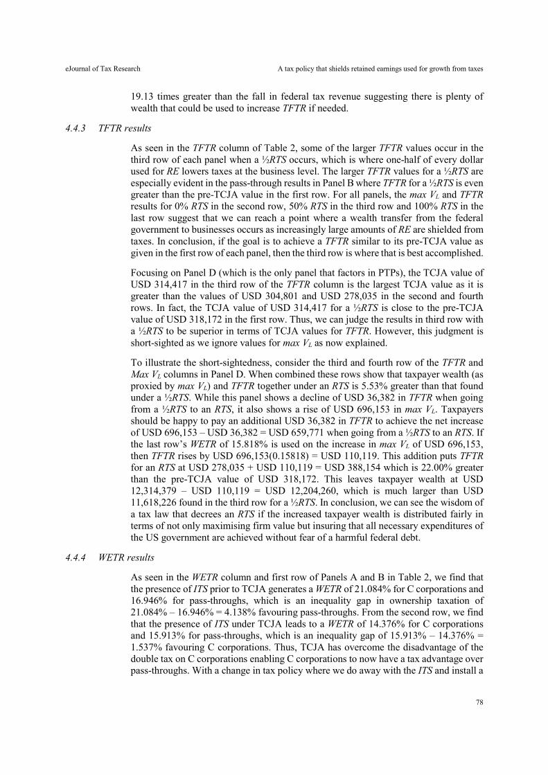
eJournal of Tax Research A tax policy that shields retained earnings used for growth from taxes
78
19.13 times greater than the fall in federal tax revenue suggesting there is plenty of wealth that could be used to increase TFTR if needed.
4.4.3 TFTR results
As seen in the TFTR column of Table 2, some of the larger TFTR values occur in the third row of each panel when a ½RTS occurs, which is where one-half of every dollar used for RE lowers taxes at the business level. The larger TFTR values for a ½RTS are especially evident in the pass-through results in Panel B where TFTR for a ½RTS is even greater than the pre-TCJA value in the first row. For all panels, the max VL and TFTR results for 0% RTS in the second row, 50% RTS in the third row and 100% RTS in the last row suggest that we can reach a point where a wealth transfer from the federal government to businesses occurs as increasingly large amounts of RE are shielded from taxes. In conclusion, if the goal is to achieve a TFTR similar to its pre-TCJA value as given in the first row of each panel, then the third row is where that is best accomplished.
Focusing on Panel D (which is the only panel that factors in PTPs), the TCJA value of USD 314,417 in the third row of the TFTR column is the largest TCJA value as it is greater than the values of USD 304,801 and USD 278,035 in the second and fourth rows. In fact, the TCJA value of USD 314,417 for a ½RTS is close to the pre-TCJA value of USD 318,172 in the first row. Thus, we can judge the results in third row with a ½RTS to be superior in terms of TCJA values for TFTR. However, this judgment is short-sighted as we ignore values for max VL as now explained.
To illustrate the short-sightedness, consider the third and fourth row of the TFTR and Max VL columns in Panel D. When combined these rows show that taxpayer wealth (as proxied by max VL) and TFTR together under an RTS is 5.53% greater than that found under a ½RTS. While this panel shows a decline of USD 36,382 in TFTR when going from a ½RTS to an RTS, it also shows a rise of USD 696,153 in max VL. Taxpayers should be happy to pay an additional USD 36,382 in TFTR to achieve the net increase of USD 696,153 – USD 36,382 = USD 659,771 when going from a ½RTS to an RTS. If the last row’s WETR of 15.818% is used on the increase in max VL of USD 696,153, then TFTR rises by USD 696,153(0.15818) = USD 110,119. This addition puts TFTR for an RTS at USD 278,035 + USD 110,119 = USD 388,154 which is 22.00% greater than the pre-TCJA value of USD 318,172. This leaves taxpayer wealth at USD 12,314,379 – USD 110,119 = USD 12,204,260, which is much larger than USD 11,618,226 found in the third row for a ½RTS. In conclusion, we can see the wisdom of a tax law that decrees an RTS if the increased taxpayer wealth is distributed fairly in terms of not only maximising firm value but insuring that all necessary expenditures of the US government are achieved without fear of a harmful federal debt.
4.4.4 WETR results
As seen in the WETR column and first row of Panels A and B in Table 2, we find that the presence of ITS prior to TCJA generates a WETR of 21.084% for C corporations and 16.946% for pass-throughs, which is an inequality gap in ownership taxation of 21.084% – 16.946% = 4.138% favouring pass-throughs. From the second row, we find that the presence of ITS under TCJA leads to a WETR of 14.376% for C corporations and 15.913% for pass-throughs, which is an inequality gap of 15.913% – 14.376% = 1.537% favouring C corporations. Thus, TCJA has overcome the disadvantage of the double tax on C corporations enabling C corporations to now have a tax advantage over pass-throughs. With a change in tax policy where we do away with the ITS and install a
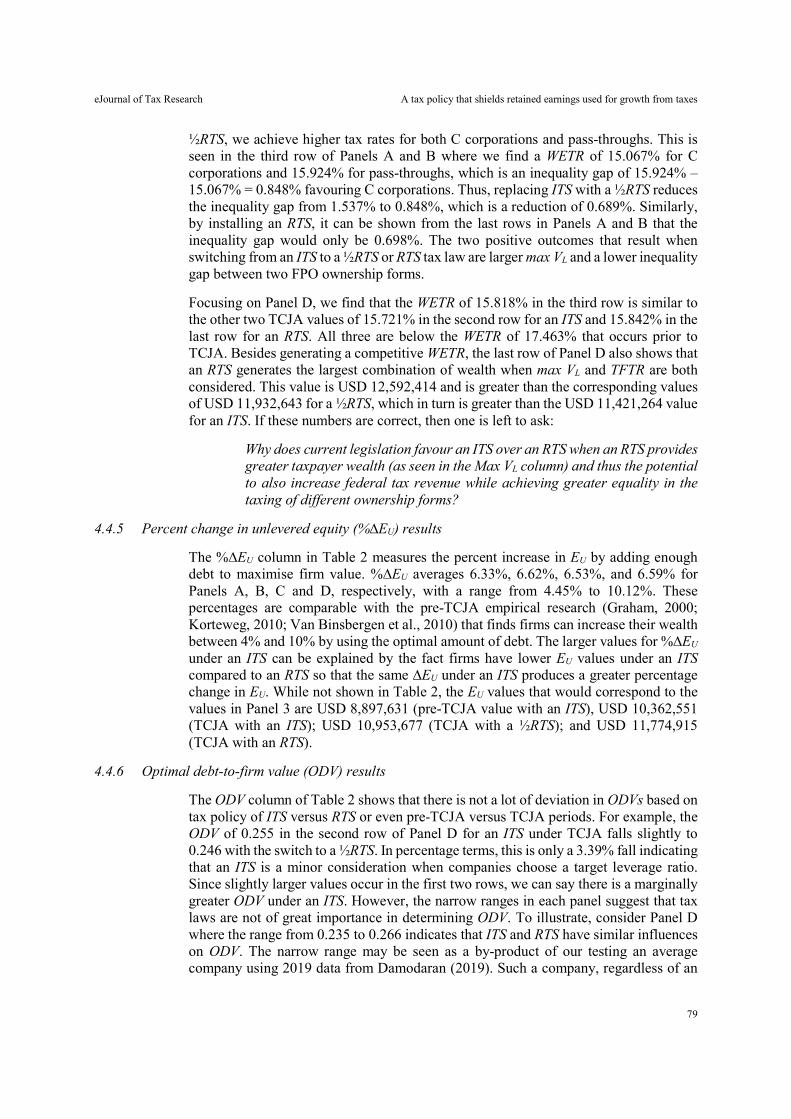
eJournal of Tax Research A tax policy that shields retained earnings used for growth from taxes
79
½RTS, we achieve higher tax rates for both C corporations and pass-throughs. This is seen in the third row of Panels A and B where we find a WETR of 15.067% for C corporations and 15.924% for pass-throughs, which is an inequality gap of 15.924% – 15.067% = 0.848% favouring C corporations. Thus, replacing ITS with a ½RTS reduces the inequality gap from 1.537% to 0.848%, which is a reduction of 0.689%. Similarly, by installing an RTS, it can be shown from the last rows in Panels A and B that the inequality gap would only be 0.698%. The two positive outcomes that result when switching from an ITS to a ½RTS or RTS tax law are larger max VL and a lower inequality gap between two FPO ownership forms.
Focusing on Panel D, we find that the WETR of 15.818% in the third row is similar to the other two TCJA values of 15.721% in the second row for an ITS and 15.842% in the last row for an RTS. All three are below the WETR of 17.463% that occurs prior to TCJA. Besides generating a competitive WETR, the last row of Panel D also shows that an RTS generates the largest combination of wealth when max VL and TFTR are both considered. This value is USD 12,592,414 and is greater than the corresponding values of USD 11,932,643 for a ½RTS, which in turn is greater than the USD 11,421,264 value for an ITS. If these numbers are correct, then one is left to ask:
Why does current legislation favour an ITS over an RTS when an RTS provides greater taxpayer wealth (as seen in the Max VL column) and thus the potential to also increase federal tax revenue while achieving greater equality in the taxing of different ownership forms?
4.4.5 Percent change in unlevered equity (%∆EU) results
The %∆EU column in Table 2 measures the percent increase in EU by adding enough debt to maximise firm value. %∆EU averages 6.33%, 6.62%, 6.53%, and 6.59% for Panels A, B, C and D, respectively, with a range from 4.45% to 10.12%. These percentages are comparable with the pre-TCJA empirical research (Graham, 2000; Korteweg, 2010; Van Binsbergen et al., 2010) that finds firms can increase their wealth between 4% and 10% by using the optimal amount of debt. The larger values for %∆EU under an ITS can be explained by the fact firms have lower EU values under an ITS compared to an RTS so that the same ∆EU under an ITS produces a greater percentage change in EU. While not shown in Table 2, the EU values that would correspond to the values in Panel 3 are USD 8,897,631 (pre-TCJA value with an ITS), USD 10,362,551 (TCJA with an ITS); USD 10,953,677 (TCJA with a ½RTS); and USD 11,774,915 (TCJA with an RTS).
4.4.6 Optimal debt-to-firm value (ODV) results
The ODV column of Table 2 shows that there is not a lot of deviation in ODVs based on tax policy of ITS versus RTS or even pre-TCJA versus TCJA periods. For example, the ODV of 0.255 in the second row of Panel D for an ITS under TCJA falls slightly to 0.246 with the switch to a ½RTS. In percentage terms, this is only a 3.39% fall indicating that an ITS is a minor consideration when companies choose a target leverage ratio. Since slightly larger values occur in the first two rows, we can say there is a marginally greater ODV under an ITS. However, the narrow ranges in each panel suggest that tax laws are not of great importance in determining ODV. To illustrate, consider Panel D where the range from 0.235 to 0.266 indicates that ITS and RTS have similar influences on ODV. The narrow range may be seen as a by-product of our testing an average company using 2019 data from Damodaran (2019). Such a company, regardless of an
eJournal of Tax Research A tax policy that shields retained earnings used for growth from taxes
80
ITS or RTS tax law, will shoot for an investment grade bond and try to avoid a speculative grade bond where ODV would be higher. For our tests, the optimal credit rating is Moody’s A3, which is also the most common rating for new issues during 2019.
In conclusion, the ODV column shows that doing away with an ITS does not materially alter ODV further supporting the claim that an ITS is an arbitrary tax deduction that has long outlived any useful purpose it may have originally had. The choice of either an ITS or RTS is important because more taxpayer wealth is associated with an RTS tax law than an ITS tax law.
5. ASSUMPTIONS, ROBUSTNESS TESTS, BLUEPRINT AND FUTURE RESEARCH
This section points out major assumptions, overviews robustness tests, offers a blueprint for countries with a debt problem, and suggests lines of study for future research.
5.1 Key assumptions
Like any research, this study makes assumptions including those for simplification purposes. Five assumptions worth calling attention to are as follows. First, we focus on federal tax revenue associated with taxes paid by C corporations and PTPs. Because these latter sources of federal revenue are only 56% of total federal tax revenue projected for 2019, we assume that 44% of federal tax revenue is constant and neutral when making conclusions about how our results affect the federal debt. However, as discussed in section 2.2, since most (if not all) of this 44% can be linked to FPOs, one can argue that all federal tax revenue changes have the same movements in value as that of FPOs. For example, if FPO business wealth increases, then those entities (like social insurance) that depend on this wealth also increase. Although social insurance is becoming an increasing burden, any increased business wealth from growth under TCJA and/or a change in tax policy (especially that under an RTS) may be considered a potential solution to this mounting burden.
Second, to incorporate personal taxpayers (called other personal taxpayers in Figure 1) who work for FPOs, non-profits, and governments, we group them with pass-throughs since they pay personal taxes like pass-throughs. This group is called personal taxpayers (PTPs). Including other personal taxpayers adds 33% in federal tax revenue to the 7% supplied by C corporations and the 16% supplied by pass-throughs. Besides paying at the same personal tax rates as pass-throughs, another justification for including other personal taxpayers with pass-throughs is that pass-throughs employ most of the taxpayers who are other personal taxpayers. However, potential problems can develop when treating other personal taxpayers like pass-throughs. For example, we assume that other personal taxpayers have their value increase in the same manner as pass-throughs through a firm size adjustment factor (FSAF). This implies that their increased capacity to purchase goods (from lower personal taxes) is a key to increasing growth under TCJA. This implication is reasonable since most other personal taxpayers are paid by pass-throughs and so their financial fortunes share that found for pass-throughs; similarly, if they work for C corporations where they share in the fortune of lower taxes.
Third, based on historical growth in real US GDP, we assume that TCJA increases growth from 3.12% to 3.90% and this increase of 0.78% occurs even if the tax policy changes from an ITS to an RTS. However, the latter assumption may hold better for an RTS since an RTS is pro-growth and so the odds of attaining 0.78% are more likely under an RTS. While there are mixed opinions on the success of increased growth at the
eJournal of Tax Research A tax policy that shields retained earnings used for growth from taxes
81
time of this writing, it is too early to know if an increase of 0.78% will be attained for the long haul. In conclusion, any assumption about a growth rate increase (such as 0.78%) is unknown.
Fourth, we had to make assumptions regarding the use of Damodaran’s firm categories when computing debt-to-firm value ratios (DV) to match credit spreads and credit rating. The chosen path described in Appendix 3 was the simplest choice in terms of presenting the results. As shown in the next section (where robustness tests are overviewed) this path proved adequate as other weighting systems (that involve three times the number of computations than presented in this article) confirm the results presented in Figures 1-7 and Tables 1-2.
Fifth, there can be questions about the use of FSAF that assumes there is an immediate jump in business wealth with this jump determined by the increase in value when going from 3.12% to 3.90%. Thus, our use of FSAF is akin to treating our perpetuities like an annuity due where the first cash flow occurs at time zero instead of what happens when taxes are collected periodically throughout the year. This serves to inflate business and taxpayer wealth. To the extent federal tax revenue depends on business wealth, one can conclude TFTR is also inflated. However, our treatment of TFTR can be viewed as an end of year value since our TFTR values achieved with 3.90% growth are simply the FSAF factor multiplied by TFTR values achieved with 3.12% growth. Thus, our tests can be said to deflate TFTR. While our use of FSAF may inflate business wealth, we can also argue that some might believe we have deflated it. For example, as reported by TPC (2018), consider the two highest forecasts that come from CBO (2019) and the Tax Foundation Taxes and Growth model. Together their predictions posit an average increase in growth of 1.4% under TCJA. This suggests a rate of around 4.50% instead of 3.90%. Finally, the 3.90% was actually the lower value from the two choices discussed earlier where the longer run choice would be 3.98%. While details are omitted, we ran a series of robustness tests with different assumptions and, on average, these tests indicate that this article’s results are an average representation of these tests. More robustness test results are discussed in the next section.
In conclusion, biases created by assumptions can cause taxpayer wealth and federal tax revenue outcomes to change. However, the direction of each of these biases is not fully known and they can even offset one another.
5.2 Robustness tests
Robustness tests are conducted to find out if our general findings and conclusions hold. We will now briefly overview these tests.
Instead of weighting interest coverage ratios (ICRs) for the three firm categories of Damodaran (2019) as described in Appendix 3, we conducted tests separately for each of these categories generating three separate results for the six variables in Table 2 (FSAF, max VL, TFTR, WETR, %∆EU, and ODV). Thus, we produced results for the large, small, and financial service (FS) firm categories. We then weight these three separate results using the same weights as described in Appendix 3 where the large, small, and FS results have the respective weights of 0.116, 0.812, and 0.072. When analysing the results for this robustness test and comparing them to Panel D of Table 2, we find similarities. For example, the average deviation for FSAF values between the two sets of results is 0.24% while those for max VL and TFTR are 1.07%, and 0.17%, respectively. As might be expected (given that all tax rates occur at a Moody’s credit
eJournal of Tax Research A tax policy that shields retained earnings used for growth from taxes
82
rating of A3), the average deviation for WETR is virtually zero when we compare the two sets of results. While the average deviations for %∆EU and ODV for the robustness test are greater at 22.71% and 12.74%, the same pattern of falling values for %∆EU and ODV as growth increases are observed. Of further importance for this robustness test, we detect the same pattern of increasing values for max VL, the favourable value for TFTR for a ½RTS and ODV values with a narrow range. In fact, the ½RTS value of USD 319,998 for TFTR is greater than the pre-TCJA value of USD 309,974 for this robustness test.
We also used other weights suggested by other sources. For example, we used the three weights suggested by Damodaran (2019) for his large, small, and FS firm categories, the weights suggested from Figure 1, equal weights, and combinations of weights based on multiple sources. In regards to Damodaran, his suggested weights for his categories are 0.7135 for large, 0.1202 for small, and 0.1663 for FS. While this weighting system assigns higher weights to the large and FS categories than given in Appendix 3, the results still generate the same pattern of increasing max VL values seen in Table 2 when increasingly large amounts of RE are exempt from taxation. This weighting system also finds that the greatest TFTR value occurs for a ½RTS. The deviations from the results in Panel D of Table 2 are larger (than those given in the prior paragraph) except for max VL where the deviation is smaller at 0.73% compared to 1.07%. Despite differences in weights used, we find the same general patterns and, most importantly, we find that a tax shield on RE is most conducive to maximising taxpayer wealth and thus offers the best chance to provide sufficient federal tax revenues.
To further illustrate, we also perform tests where the large and small categories were equally-weighted with and without the use of a weight of 0.072 for FS. Once again, we find the same pattern given in Table 2 including those for max VL and TFTR values. While the ODV values are closer to 0.30 than to the 0.25 reported in Table 2, the narrow range of ODVs still hold and so support our conclusion that tax laws do not exercise an important influence on a firm’s choice of leverage.
Finally, instead of allowing non-growth values to result when they are superior to growth values, we tested if using all growth values could change our findings. The results were similar for these robustness tests. In brief, the results for all of our robustness tests are consistent with our findings reported in Figures 2-7 and Tables 1 and 2. In particular, we confirm our findings about the overall advantages of a tax policy shift from an ITS to an RTS where taxpayer wealth can be increased, federal revenue problems can be resolved, and equality in taxing ownership forms can be achieved.
5.3 Blueprint for countries with debt problem
We now offer a blueprint for a tax policy reform that is designed to maximise taxpayer wealth, supply needed federal tax revenue, and achieve equality in the taxing of ownership forms.30 This blueprint is especially needed for countries with a rising federal debt and should contain the following items.
To begin with, a blueprint should include conducting the necessary tests to find an optimal mix of tax shields that maximise taxpayer wealth while achieving an acceptable
30 See Bird and Wilkie (2013) for a study on designing tax policy and Wilson-Rogers and Pinto (2009) for a framework for examining tax reform. See Clark (2007) for an investigation of a tax policy supportive of investment.
eJournal of Tax Research A tax policy that shields retained earnings used for growth from taxes
83
TFTR. While Table 2 only reports results when an ITS is 0% or 100% and an RTS is 0% or 50% or 100%, a more optimal and efficiency tax policy could be discovered if other tax shield percentages are tested. Part of any blueprint when seeking to identify the optimal tax shield percentages is to develop an algorithm to approximate optimal tax shield percentages. Without an algorithm, an unknown number of time-consuming tests might be necessary to achieve a satisfactory level of accuracy.
In regards to sharing taxpayer wealth or knowing how much of an ITS can be abandoned, an algorithm can pinpoint fair amounts of sharing as well as optimal values for a partial ITS and partial RTS within agreed parameters. These parameters would provide leeway in the use of tax shields because not all FPOs are like the average business used in our tests as these FPOs have differences in their effective tax rates, sustainable growth rates, and risks that affect the costs of borrowing and help determine a firm’s credit rating. In regards to the latter, we cannot assume that all FPOs will find that a Moody’s A3 credit rating is optimal as found in our tests where all FPOs face the same average risks. While tax laws need to be legislated that set limits governing ITS and RTS, laws also need to allow FPOs to choose their own allocations among tax shields within fixed limits. As illustrated next, limits would be based on a percentage of CFBT (or EBIT).
For our tests using the weights of 0.125 for C corporations and 0.875 for PTPs, we find that ITS is 4.35% of EBIT under TCJA with growth of 3.90%. If we switch to a ½RTS, the tax shield is 4.53% of EBIT. For an RTS, we jump to 8.08%. For purposes of illustration, let us say the government sets the maximum tax shield limit at 6% of EBIT so that an FPO could choose something like ⅔ of this limit for an RTS and the remaining ⅓ for an ITS. We also recommend that a separate maximum limit on ITS such as 3%, instead of a maximum of 6%, because an ITS creates a distortion between equity and debt ownership by favouring debt. Thus, if the maximum tax shield limit is 6% of EBIT, no more than one-half of this 6% can be used for an ITS. By allowing companies the ability to choose both tax shields, they would be less likely to seek a tax deduction when growth or debt is not otherwise desirable.
Besides identifying optimal tax shield percentages that maximise taxpayer wealth and meet TFTR goals, the WETR inequality gap needs to be reduced thereby removing the current disparity in the taxing of different ownership forms. While this study offers a tax policy that reduces the WETR inequality gap to less than 1% in the taxing of the two FPO ownership forms, the challenge of future research is to find a tax policy that achieves a 0% WETR inequality gap. To achieve a goal of zero, modifications of C corporation corporate tax rate and/or the pass-through personal tax rate might be necessary. Due to reasonable disagreements about effective tax rates in an environment where TCJA is still relatively new, it could be difficult to reach a general consensus in the near term as to the accuracy of tests that claim to have achieved a 0% WETR inequality gap. Besides equality in taxing all business forms and types, FPOs also need to be sufficiently taxed in order to provide the federal tax revenue needed for countries plagued with debt problems as well as supply the common and essential expenditures such as infrastructure, hospitals, schools and national defence.
5.4 Future research
Tasks for future research include instructional research, exploration of various effective tax rate scenarios, and the role of debt in growth. A first task for future research involves instructional research. This type of research can develop exercises to use in the
eJournal of Tax Research A tax policy that shields retained earnings used for growth from taxes
84
classroom as well as those to help policy-makers understand the relation between tax shields and growth in GDP. These exercises are important for educators who are commissioned to properly teach the relation between business growth and tax laws especially those governing interest (I) and retained earnings (RE). Instructional exercises are also valuable to practitioners and policy-makers who need examples of tax policy applications to guide them in their decision-making so that businesses prosper without undue tax impediments that make growth unaffordable.
For a second task, we take into consideration disagreements over effective tax rates.31 In this regard, future research can explore other effective tax rate scenarios including how tax rates change with leverage. These tests could cover a range of tax rates that include tax rate scenarios below and above the effective tax rates that we use in this article. Additionally, this study’s tests assume that tax rates change in the direction argued by Hull (2014a) for debt-for-equity transactions. Because this argument was formulated to apply to firms and not other personal taxpayers, future research can also consider repeating this article’s tests when tax rates are not allowed to change with leverage. In order words, the expected levered tax rate predicted by sources occurs for any leverage choice instead of the choice that achieves ODV. While we would not expect any major changes since an unlevered tax rate never fluctuated more than 1/6 from the unlevered tax rate, one never knows for sure until tests detailed tests are conducted.
For a third task, future research might consider exploring the role of debt in growth. This research could possibly shed light on a potential positive aspect of ITS that might justify debt as growth enhancing at least for some industries. If so, this research can help determine the limits placed on both an ITS and an RTS. For this study that uses the Capital Structure Model (CSM) equations, an unlevered firm sets its before-tax plowback ratio (PBR) before debt is undertaken and the firm’s RE is the sole source of growth. For the CSM (see Hull, 2018), PBR must be greater than the business tax rate on RE for growth to add value at the unlevered level. This implies that even debt may not make growth valuable if the business tax is too high. If a firm is unlevered, the CSM posits that debt has no part in affecting the growth rate. However, if debt is issued, the unlevered growth rate (gU) increases and becomes the levered growth rate (gL). Since the retained earnings is already fixed, the issuance of debt causes the remaining shareholders to take on more risk for each dollar used for RE. Thus, increased growth from debt comes with a price. Suppose debt and equity should be viewed as fractional suppliers of funds for growth. The role of debt in growth can be construed as being part of cash flows available to the firm for its chosen usages be it dividends, RE, or I. While an ITS could be viewed as subsidising growth, the other (and more common) viewpoint is that debt simply performs a leveraging activity so that equity value per share can increase but at a risk captured by lower credit ratings and higher costs of borrowing on equity and debt.
6. SUMMARY AND CONCLUSIONS
This article’s contributions to tax law research are aided by addressing three inefficiencies in historical and current tax laws and proposing changes based on these inefficiencies. The three inefficiencies are as follows. First, researchers question why
31 Part of the disagreement can relate to the complexity of tax laws, especially in the US as discussed by Burton and Karlinsky (2016).
eJournal of Tax Research A tax policy that shields retained earnings used for growth from taxes
85
an interest tax shield (ITS) should exist given it distorts security ownership favouring debt over equity. Second, just as perplexing as an ITS is the tax treatment of retained earnings (RE) that is contrary to the research that advocates direct tax incentives for funds used for growth. RE is by far the largest source of growth, yet interest (I) is shielded from taxes while RE does not receive proper tax relief. Third, we address the inequality in the taxing of different ownership forms stemming from the double taxation of C corporation earnings, which tax policy researchers have characterised as unfair, inefficient, arbitrary and capricious. While the US Congress passed the Tax Cuts and Jobs Act (TCJA) in December 2017 that alleviated the tax burden on C corporations caused by their double taxation, inequitable taxing between C corporations and pass-throughs still exists only now pass-throughs, on average, are at a disadvantage.
This article’s findings when addressing the three inefficiencies can be summarised as follows. Focusing on our tests that include all personal taxpayers (PTPs) so that conclusions can be based on 56% of federal tax revenue, we find that replacing an ITS with a ½RTS under TCJA expands taxpayer wealth by 4.51% beyond pre-TCJA wealth, where a ½RTS means that one-half of RE used for growth is a tax-deductible expense. This deductible expense amounts to a tax subsidy equal to the effective business level tax rate times the amount of RE used for growth. Of importance, this increase in wealth of 4.51% boosts TFTR so that it is 3.15% greater than that under TCJA with an ITS.
Next we find that replacing ITS with an RTS (instead of a ½RTS) increases the combined total of taxpayer wealth and TFTR. This makes both taxpayer wealth and federal revenues greater if the larger pie can be properly allocated. Additionally, we discover that the inequality gap in taxing ownership forms, as measured by the weighted effective tax rate (WETR), is reduced as increasingly large amounts of RE are shielded from taxation. Finally, we show that an RTS policy does not materially alter the optimal debt-to-firm value ratio (ODV) indicating that there is little, if any, impact on debt decision-making due to a tax deduction on interest. This is consistent with the notion that an ITS is not only an arbitrary tax deduction with little purpose but also has negative ramifications to the extent it deprives governments of funds that could support a tax law that directly subsidises growth.
Prior to TCJA, the US had one of the highest statutory tax rates and a spiralling debt. TCJA provides new wine in the form of lower tax rates that lead to greater growth. However, this new wine has been put in the old wineskin of an ITS tax law. Using the old wineskin assures that business wealth (and thus taxpayer wealth) will not increase in a manner that diminishes the rising federal debt. In fact, we document a 4.20% decrease in total federal tax revenue (TFTR) under TCJA and its current ITS policy, which agrees with that given by CBO (2019). Even here we have to assume no increase in spending including that for social insurance. The possibility of a spending reduction appears to be low given that federal expenditures have escalated during the first two years of TCJA (and before the current coronavirus crisis) causing the federal debt to rise about 10%. Furthermore, social insurance is also in trouble with outflows greater than inflows so that this adds to the federal debt. Thus, we conclude that a new wineskin is needed for the new wine of lower taxes and this new wineskin is provided by a retained earnings tax shield (RTS) policy that replaces the old wineskin of an ITS.
In conclusion, the switch from an ITS to an RTS is motivated by re-examining why we allow interest (I) to be tax-deductible and why we tax retained earnings (RE), which is the dominant source of growth used by companies. While TFTR can increase under an RTS policy, the key to creating a substantial increase in TFTR is to find a way to allow
eJournal of Tax Research A tax policy that shields retained earnings used for growth from taxes
86
the significant increase in taxpayer wealth to trickle down to the federal coffers. The conclusion about needing to switch tax shields is applicable to the many countries that share in US taxing characteristics and have been misguided by not replacing an ITS with an RTS.
7. REFERENCES
Amadeo, K 2018, ‘Current US federal government tax revenue’, The Balance. Available at: https://www.thebalance.com/current-u-s-federal-government-tax-revenue-3305762.
Amadeo, K 2019, ‘Who owns the US national debt?’, The Balance. Available at: https://www.thebalance.com/who-owns-the-u-s-national-debt-3306124.
Bank, S 2014, ‘Historical perspective on the corporate interest deduction’, Chapman Law Review, vol. 18, no. 1, pp. 29-48.
Barro, R & Redlick, C 2011, ‘Macroeconomic effects from government purchases and taxes’, The Quarterly Journal of Economics, vol. 126, no. 1, pp. 51-102.
Baxter, N 1967, ‘Leverage, risk of ruin and the cost of capital’, Journal of Finance, vol. 22, no. 3, pp. 395-403.
Berk, J, Stanton R & Zechner, J 2010, ‘Human capital, bankruptcy and capital structure’, Journal of Finance, vol. 65, no. 3, pp. 891-926.
Bird, R & Wilkie, J 2013, ‘Designing tax policy: Constraints and objectives in an open economy’, eJournal of Tax Research, vol. 11, no. 3, pp. 284-320.
Burke, K 2008, ‘Is the corporate tax system “broken”?’, Virginia Tax Review, vol. 28, no. 2, pp. 341-367.
Burton, H & Karlinsky, S 2016, ‘Tax professionals’ perception of large and mid-size business US tax law complexity’, eJournal of Tax Research, vol. 14, no. 1, pp. 61-95.
Clark, W 2007 ‘Tax policy for investment’, eJournal of Tax Research, vol. 5, no. 2, pp. 244-265.
Congressional Budget Office (CBO) 2019, ‘Updated budget projections: 2019 to 2029’, Congress of the United States, May. Available at: https://www.cbo.gov/system/files/2019-05/55151-budget_update_0.pdf.
Damodaran, A 2019, ‘Damodaran online: Home page for Aswath Damodaran’. Available at: http://people.stern.nyu.edu/adamodar/New_Home_Page/datacurrent.html. Archived data available at http://people.stern.nyu.edu/adamodar/New_Home_Page/dataarchived.html.
DeAngelo, H & Masulis, R 1980, ‘Optimal capital structure under corporate and personal taxes’, Journal of Financial Economics, vol. 8, no. 1, pp. 3-29.
Donaldson, G 1961, Corporate debt capacity: A study of corporate debt policy and the determination of corporate debt capacity, Harvard Business School, Boston.
eJournal of Tax Research A tax policy that shields retained earnings used for growth from taxes
87
Doran, M 2009, ‘Managers, shareholders, and the corporate double tax’, Virginia Law Review, vol. 95, no. 3, pp. 517-596.
Frankel, M 2017, ‘What’s the average American’s tax rate?’, USA Today, 10 March. Available at: https://www.usatoday.com/story/money/personalfinance/2017/03/10/whats-the-average-americans-tax-rate/98734396/.
Freebairn, J 2017, ‘Comparison of a lower corporate income tax rate for small and large businesses’, eJournal of Tax Research, vol. 15, no. 1, pp. 4-21.
Federal Reserve Economic Data (FRED) 2018, ‘Moody's seasoned Baa corporate bond yield’, Federal Reserve Bank of St. Louis. Available at: https://fred.stlouisfed.org/series/BAA.
Federal Reserve Economic Data (FRED) 2019a, ‘30-year treasury constant maturity rate’, Federal Reserve Bank of St. Louis. Available at: https://fred.stlouisfed.org/series/DGS30.
Federal Reserve Economic Data (FRED) 2019b, ‘Value added by private industries: Finance, insurance, real estate, rental, and leasing: Finance and insurance as a percentage of GDP’, Federal Reserve Bank of St. Louis. Available at: https://fred.stlouisfed.org/series/VAPGDPFI.
Federal Reserve Economic Data (FRED) 2019c, ‘Gross federal debt as percent of gross domestic product’, Federal Reserve Bank of St. Louis. Available at: https://fred.stlouisfed.org/series/GFDGDPA188S.
Graham, J 2000, ‘How big are the tax benefits of debt?’, Journal of Finance, vol. 55, no. 5, pp. 1901-1941.
Graham, J & Harvey, C 2001, ‘The theory and practice of corporate finance: Evidence from the field’, Journal of Financial Economics, vol. 60, nos. 2-3, pp. 187-243.
Graham, J & Leary, M 2011, ‘A review of empirical capital structure research and directions for the future’, vol. 3, December, pp. 309-345.
Greenberg, S 2017, ‘Pass-through businesses: Data and policy’, Tax Foundation Fiscal Fact, No. 536, 17 January. Available at: https://taxfoundation.org/pass-through-businesses-data-and-policy.
Harris, M & Raviv, A 1991, ‘The theory of capital structure’, Journal of Finance, vol. 46, no. 1, pp. 297-355.
Hasseldine, J & Fatemi, D 2019, ‘Tax practitioner judgements and client advocacy: The blurred boundary between capital gains vs. ordinary income’, eJournal of Tax Research, vol. 16, no. 2, pp. 303-316.
Hilling, A & Vilhelmsson, A 2015, ‘Equal taxation as a basis for classifying financial instruments as debt or equity – A Swedish case study’, eJournal of Tax Research, vol. 13, no. 3, pp. 677-715.
Hull, R 2005, ‘Firm value and the debt-equity choice’, Regional Business Review, vol. 24, May, pp. 50-75.
Hull, R 2008, ‘Capital structure decision-making: A pedagogical application’, Journal of Financial Education, vol. 34, Fall, pp. 88-111.
Hull, R 2011, ‘Debt-equity decision-making with and without growth’, Managerial Finance, vol. 37, no. 8, pp. 765-787.
eJournal of Tax Research A tax policy that shields retained earnings used for growth from taxes
88
Hull, R 2014a, ‘A capital structure model (CSM) with tax rate changes’, Investment Management and Financial Innovations, vol. 11, no. 3, pp. 8-21.
Hull, R 2014b, ‘Debt-equity decision-making with wealth transfers’, Managerial Finance, vol. 40, no. 12, pp. 1223-1250.
Hull, R 2018, ‘Capital structure model (CSM): Correction, constraints, and applications’, Investment Management and Financial Innovations, vol. 15, no. 1, pp. 245-262.
Hull, R 2019, ‘Business wealth and tax policy’, Theoretical Economics Letters, vol. 9, no. 4, pp. 1020-1039.
Hull, R 2020, ‘Credit ratings and firm value’, Investment Management and Financial Innovations, vol. 17, no. 2, pp. 157-168.
Hull, R & Price, D 2015, ‘Pass-through valuation’, The Journal of Entrepreneurial Finance, vol. 17, no. 1, pp. 82-116.
Hull, R & Van Dalsem, S 2021, ‘Nonprofits and pass-throughs: Performance comparison’, International Journal of Financial Studies, vol. 9, no. 1, pp. 1-40.
Jensen, M 1986, ‘Agency costs of free cash flow, corporate finance, and takeovers’, American Economic Review, vol. 76, no. 2, pp. 323-329.
Jensen, M & Meckling, W 1976, ‘Theory of the firm: Managerial behavior, agency costs and ownership structure’, Journal of Financial Economics, vol. 3, no. 4, pp. 305-360.
Joint Committee on Taxation (JCT) 2018, ‘Overview of the federal tax system as in effect for 2018’, (JCX-3-18), 7 February.
Available at: https://www.jct.gov/publications.html?func=startdown&id=5060.
Joint Committee on Taxation (JCT) 2019, ‘Overview of the federal tax system as in effect for 2019’, (JCX-3-19), 20 March. Available at:
https://www.jct.gov/publications.html?func=startdown&id=5172.
Kisgen, D 2006, ‘Credit ratings and capital structure’, Journal of Finance, vol. 61, no. 3, pp. 1035-1072.
Knott, A 2019, ‘Why the Tax Cuts and Jobs Act (TCJA) led to buybacks rather than investment’, Forbes, 21 February. Available at: https://www.forbes.com/sites/annemarieknott/2019/02/21/why-the-tax-cuts-and-jobs-act-tcja-led-to-buybacks-rather-than-investment/#34813f6d37fb.
Korteweg, A 2010, ‘The net benefits of leverage’, Journal of Finance, vol. 65, no. 6, pp. 2137-2170.
Matthews, D 2018, ‘The tax bill is a giant permission slip for shipping profits overseas’, Vox, 19 December. Available at: https://www.vox.com/2017/12/19/16791936/repatriation-holiday-republican-tax-bill-explained.
McBride, W 2012, ‘CRS, at odds with academic studies, continues to claim no harm in raising top earners tax rates’, Tax Foundation, 14 December. Available at: https://taxfoundation.org/crs-odds-academic-studies-continues-claim-no-harm-raising-top-earners-tax-rates.
Mertens, K & Ravn, M 2013, ‘The dynamic effects of personal and corporate income tax changes in the United States’, American Economic Review, vol. 103, no. 4, pp. 1212-1247.
Miller, M 1977, ‘Debt and taxes’, Journal of Finance, vol. 32, no. 2, pp. 261-275.

eJournal of Tax Research A tax policy that shields retained earnings used for growth from taxes
89
Modigliani, F & Miller, M 1963, ‘Corporate income taxes and the cost of capital: A correction’, American Economic Review, vol. 53, no. 3, pp. 433-443.
Myers, S 1977, ‘Determinants of corporate borrowing’, Journal of Financial Economics, vol. 5, no. 2, pp. 147-175.
Myers, S & Majluf, N 1984, ‘Corporate financing and investment decisions when firms have information that investors do not have’, Journal of Financial Economics, vol. 13, no. 2, pp. 187-221.
Noked, N 2014, ‘Integrated tax policy approach to designing research and development tax benefits’, Virginia Tax Review, vol. 34, no. 1, pp. 109-155.
Norbäck, P-J, Persson, L & Tåg, J 2018, ‘Does the debt tax shield distort ownership efficiency?’, International Review of Economics and Finance, vol. 54, March, pp. 299-310.
Nussim, J & Sorek, A 2017, ‘Theorizing tax incentives for innovation’, Virginia Tax Review, vol. 36, no. 1, pp. 25-82.
Page, B 2019, ‘Revisions to revenue projections suggest that the TCJA cost more than expected’, Tax Policy Center, 5 November. Available at: https://www.taxpolicycenter.org/taxvox/revisions-revenue-projections-suggest-tcja-cost-more-expected (accessed 8 June 2021).
Peter G Pederson Foundation 2017, ‘Budget basics: Who pays taxes?’. Available at: https://www.pgpf.org/budget-basics/who-pays-taxes.
Peter G Pederson Foundation 2018, ‘What is the national debt costing us?’, 29 November. Available at: https://www.pgpf.org/blog/2018/11/we-will-soon-be-spending-more-on-national-debt-interest-than-on-these-vital-programs.
Polito, A 2017, ‘Mandatory passthrough taxation for non-publicly traded businesses?’, Virginia Tax Review, vol. 36, no. 3, pp. 449-474.
Pomerleau, K 2017, ‘CBO report compares US corporate tax to G20’, Tax Foundation, 16 March. Available at: https://taxfoundation.org/cbo-report-compares-us-corporate-tax-g20/.
Romer, C & Romer, D 2010, ‘The macroeconomic effects of tax changes: Estimates based on a new measure of fiscal shocks’, American Economic Review, vol. 100, No. 3, pp. 763-801.
Steyn, T, Smulders, S, Stark, K & Penning, I 2019, ‘Capital gains tax research: An initial synthesis of the literature’, eJournal of Tax Research, vol. 16, no. 2, pp. 278-302.
Tax Policy Center (TPC) 2018, ‘What are the economic effects of the Tax Cuts and Jobs Act?’. Available at: https://www.taxpolicycenter.org/briefing-book/how-might-tax-cuts-and-jobs-act-affect-economic-output.
US Bureau of Economic Analysis 2019, ‘US real GDP growth rate by year’. Available at: https://www.bea.gov/data/gdp/gross-domestic-product.
Vaillancourt, F & Kerkhoff, A 2019, ‘Capital gains taxation in Canada, 1972-2017: Evolution in a federal setting’, eJournal of Tax Research, vol. 16, no. 2, pp. 340-361.
Van Binsbergen, J, Graham, J & Yang, J 2010, ‘Cost of debt’, Journal of Finance, vol. 65, no. 6, pp. 2089-2136.

eJournal of Tax Research A tax policy that shields retained earnings used for growth from taxes
90
Wilson-Rogers, N & Pinto, D 2009, ‘Tax reform: A matter of principle? An integrated framework for the review of Australian taxes’, eJournal of Tax Research, vol. 7, no. 1, pp. 72-105.
York, E 2018, ‘Summary of the latest federal income tax data, 2017 update’, Tax Foundation, 17 January. Available at https://taxfoundation.org/summary-federal-income-tax-data-2017/.
8. APPENDICES
Exhibit 1: Acronyms, Terms, Definitions and/or Meanings
Acronym: Term Definition and/or Meaning for this study’s purpose FPO: for-profit
organisation A business whose earnings are subject to taxes because they fall within either the C corporation or pass-through ownership form.
I: interest Payment to debt owners. ITS: I tax shield Tax-deductible expense on I that if given to an FPO serves to encourages debt financing over
equity financing. RE: retained
earnings Before-tax cash flows from operations used strictly for growth that leads to increased production of goods and/or services.
RTS: RE tax shield Tax-deductible expense on RE that if given to an FPO serves to encourage growth by using internal funds.
½RTS: ½RE tax shield
Tax-deductible expense on one-half of RE that if given to an FPO serves to encourage growth by using internal funds.
TFTR: total federal tax revenue
Represents the federal tax revenue with chosen sources used to represent the total.
WETR: weighted effective tax rate
Weighted average that includes up to five effective tax rates with weights supplied by up to five different taxable amounts.
EU : unlevered equity value
EU is the same as unlevered firm value (VU) because unlevered means no debt. Thus, value consists only of equity.
Max GL: maximum gain to leverage
The greatest gain to leverage among all feasible leverage choices where each leverage choice targets a different credit rating.
VL: firm value VL = EL + D where EL is levered equity value and D is debt value. For our application of the CSM, VL is also EU + GL.
DV: debt-to-firm value ratio
A leverage ratio computed as D /VL where D is debt value and VL is firm value.
Max VL: maximum firm value
Max VL = EU + max GL where max VL can also be identified by the greatest VL among all feasible VL outputs.
ODV: optimal debt-to-firm value ratio
The optimal DV associated with the greatest attainable firm value among feasible DV choices, which is max VL.
CFBT: cash flows before taxes
Cash flows available to the FPO before federal taxes are paid and before any applicable tax shield lowers business level taxes.
ICR: interest coverage ratio
Comes in three firm categories of small, large, and financial service and are used to compute leverage choices.
PTP: personal taxpayer
Refers to a taxpayer who pays at the personal statutory tax rate (includes pass-throughs and other personal taxpayers).
FSAF: firm size adjustment factor
Captures the increase in max VL (and thus taxpayer wealth) under TCJA from the projected increase in growth.
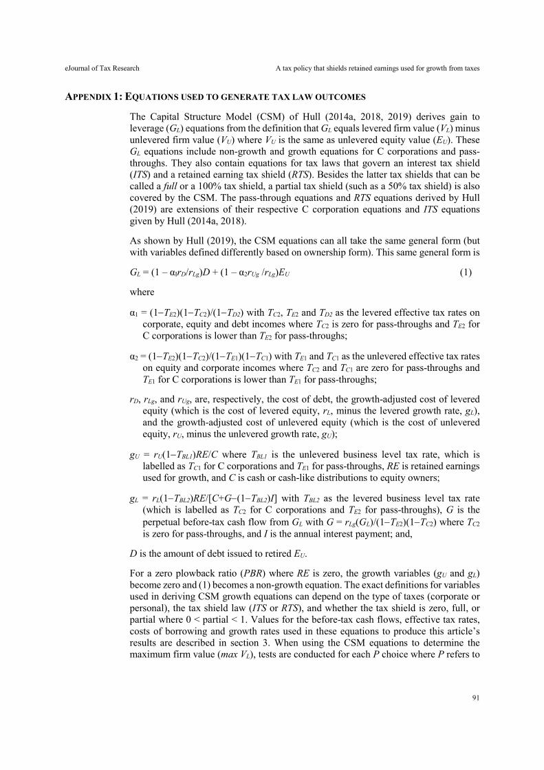
eJournal of Tax Research A tax policy that shields retained earnings used for growth from taxes
91
APPENDIX 1: EQUATIONS USED TO GENERATE TAX LAW OUTCOMES
The Capital Structure Model (CSM) of Hull (2014a, 2018, 2019) derives gain to leverage (GL) equations from the definition that GL equals levered firm value (VL) minus unlevered firm value (VU) where VU is the same as unlevered equity value (EU). These GL equations include non-growth and growth equations for C corporations and pass-throughs. They also contain equations for tax laws that govern an interest tax shield (ITS) and a retained earning tax shield (RTS). Besides the latter tax shields that can be called a full or a 100% tax shield, a partial tax shield (such as a 50% tax shield) is also covered by the CSM. The pass-through equations and RTS equations derived by Hull (2019) are extensions of their respective C corporation equations and ITS equations given by Hull (2014a, 2018).
As shown by Hull (2019), the CSM equations can all take the same general form (but with variables defined differently based on ownership form). This same general form is
GL = (1 ‒ αIrD/rLg)D + (1 ‒ α2rUg /rLg)EU (1)
where
α1 = (1TE2)(1TC2)/(1TD2) with TC2, TE2 and TD2 as the levered effective tax rates on corporate, equity and debt incomes where TC2 is zero for pass-throughs and TE2 for C corporations is lower than TE2 for pass-throughs;
α2 = (1TE2)(1TC2)/(1TE1)(1TC1) with TE1 and TC1 as the unlevered effective tax rates on equity and corporate incomes where TC2 and TC1 are zero for pass-throughs and TE1 for C corporations is lower than TE1 for pass-throughs;
rD, rLg, and rUg, are, respectively, the cost of debt, the growth-adjusted cost of levered equity (which is the cost of levered equity, rL, minus the levered growth rate, gL), and the growth-adjusted cost of unlevered equity (which is the cost of unlevered equity, rU, minus the unlevered growth rate, gU);
gU = rU(1TBL1)RE/C where TBL1 is the unlevered business level tax rate, which is labelled as TC1 for C corporations and TE1 for pass-throughs, RE is retained earnings used for growth, and C is cash or cash-like distributions to equity owners;
gL = rL(1TBL2)RE/[C+G(1TBL2)I] with TBL2 as the levered business level tax rate (which is labelled as TC2 for C corporations and TE2 for pass-throughs), G is the perpetual before-tax cash flow from GL with G = rLg(GL)/(1TE2)(1TC2) where TC2 is zero for pass-throughs, and I is the annual interest payment; and,
D is the amount of debt issued to retired EU.
For a zero plowback ratio (PBR) where RE is zero, the growth variables (gU and gL) become zero and (1) becomes a non-growth equation. The exact definitions for variables used in deriving CSM growth equations can depend on the type of taxes (corporate or personal), the tax shield law (ITS or RTS), and whether the tax shield is zero, full, or partial where 0 < partial < 1. Values for the before-tax cash flows, effective tax rates, costs of borrowing and growth rates used in these equations to produce this article’s results are described in section 3. When using the CSM equations to determine the maximum firm value (max VL), tests are conducted for each P choice where P refers to
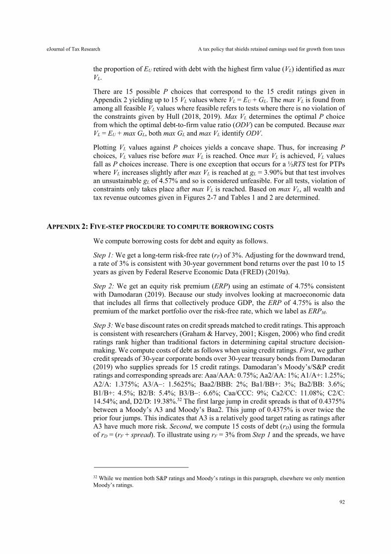
eJournal of Tax Research A tax policy that shields retained earnings used for growth from taxes
92
the proportion of EU retired with debt with the highest firm value (VL) identified as max VL.
There are 15 possible P choices that correspond to the 15 credit ratings given in Appendix 2 yielding up to 15 VL values where VL = EU + GL. The max VL is found from among all feasible VL values where feasible refers to tests where there is no violation of the constraints given by Hull (2018, 2019). Max VL determines the optimal P choice from which the optimal debt-to-firm value ratio (ODV) can be computed. Because max VL = EU + max GL, both max GL and max VL identify ODV.
Plotting VL values against P choices yields a concave shape. Thus, for increasing P choices, VL values rise before max VL is reached. Once max VL is achieved, VL values fall as P choices increase. There is one exception that occurs for a ½RTS test for PTPs where VL increases slightly after max VL is reached at gL = 3.90% but that test involves an unsustainable gL of 4.57% and so is considered unfeasible. For all tests, violation of constraints only takes place after max VL is reached. Based on max VL, all wealth and tax revenue outcomes given in Figures 2-7 and Tables 1 and 2 are determined.
APPENDIX 2: FIVE-STEP PROCEDURE TO COMPUTE BORROWING COSTS
We compute borrowing costs for debt and equity as follows.
Step 1: We get a long-term risk-free rate (rF) of 3%. Adjusting for the downward trend, a rate of 3% is consistent with 30-year government bond returns over the past 10 to 15 years as given by Federal Reserve Economic Data (FRED) (2019a).
Step 2: We get an equity risk premium (ERP) using an estimate of 4.75% consistent with Damodaran (2019). Because our study involves looking at macroeconomic data that includes all firms that collectively produce GDP, the ERP of 4.75% is also the premium of the market portfolio over the risk-free rate, which we label as ERPM.
Step 3: We base discount rates on credit spreads matched to credit ratings. This approach is consistent with researchers (Graham & Harvey, 2001; Kisgen, 2006) who find credit ratings rank higher than traditional factors in determining capital structure decision-making. We compute costs of debt as follows when using credit ratings. First, we gather credit spreads of 30-year corporate bonds over 30-year treasury bonds from Damodaran (2019) who supplies spreads for 15 credit ratings. Damodaran’s Moody’s/S&P credit ratings and corresponding spreads are: Aaa/AAA: 0.75%; Aa2/AA: 1%; A1/A+: 1.25%; A2/A: 1.375%; A3/A: 1.5625%; Baa2/BBB: 2%; Ba1/BB+: 3%; Ba2/BB: 3.6%; B1/B+: 4.5%; B2/B: 5.4%; B3/B: 6.6%; Caa/CCC: 9%; Ca2/CC: 11.08%; C2/C: 14.54%; and, D2/D: 19.38%.32 The first large jump in credit spreads is that of 0.4375% between a Moody’s A3 and Moody’s Baa2. This jump of 0.4375% is over twice the prior four jumps. This indicates that A3 is a relatively good target rating as ratings after A3 have much more risk. Second, we compute 15 costs of debt (rD) using the formula of rD = (rF + spread). To illustrate using rF = 3% from Step 1 and the spreads, we have
32 While we mention both S&P ratings and Moody’s ratings in this paragraph, elsewhere we only mention Moody’s ratings.
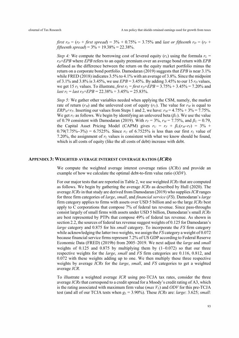
eJournal of Tax Research A tax policy that shields retained earnings used for growth from taxes
93
first rD = (rF + first spread) = 3% + 0.75% = 3.75% and last or fifteenth rD = (rF + fifteenth spread) = 3% + 19.38% = 22.38%.
Step 4: We compute the borrowing cost of levered equity (rL) using the formula rL = rD+EPB where EPB refers to an equity premium over an average bond return with EPB defined as the difference between the return on the equity market portfolio minus the return on a corporate bond portfolio. Damodaran (2019) suggests that EPB is near 3.1% while FRED (2018) indicates 3.5% to 4.1% with an average of 3.8%. Since the midpoint of 3.1% and 3.8% is 3.45%, we use EPB = 3.45%. By adding 3.45% to our 15 rD values, we get 15 rL values. To illustrate, first rL = first rD+EPB = 3.75% + 3.45% = 7.20% and last rL = last rD+EPB = 22.38% + 3.45% = 25.83%.
Step 5: We gather other variables needed when applying the CSM, namely, the market rate of return (rM) and the unlevered cost of equity (rU). The value for rM is equal to ERPM+rF. Inserting our values from Steps 1 and 2, we have: rM = 4.75% + 3% = 7.75%. We get rU as follows. We begin by identifying an unlevered beta (βU). We use the value of 0.79 consistent with Damodaran (2019). With rF = 3%, rM = 7.75%, and βU = 0.79, the Capital Asset Pricing Model (CAPM) gives rU = rF + βU(rMrF) = 3% + 0.79(7.75%3%) = 6.7525%. Since rU of 6.7525% is less than our first rL value of 7.20%, the assignment of rL values is consistent with what we know should be found, which is all costs of equity (like the all costs of debt) increase with debt.
APPENDIX 3: WEIGHTED AVERAGE INTEREST COVERAGE RATIOS (ICRS)
We compute the weighted average interest coverage ratios (ICRs) and provide an example of how we calculate the optimal debt-to-firm value ratio (ODV).
For our major tests that are reported in Table 2, we use weighted ICRs that are computed as follows. We begin by gathering the average ICRs as described by Hull (2020). The average ICRs in that study are derived from Damodaran (2019) who supplies ICR ranges for three firm categories of large, small, and financial service (FS). Damodaran’s large firm category applies to firms with assets over USD 5 billion and so the large ICRs best apply to C corporations that compose 7% of federal tax revenue. Since pass-throughs consist largely of small firms with assets under USD 5 billion, Damodaran’s small ICRs are best represented by PTPs that compose 49% of federal tax revenue. As shown in section 2.2, the sources of federal tax revenue suggest weights of 0.125 for Damodaran’s large category and 0.875 for his small category. To incorporate the FS firm category while acknowledging the latter two weights, we assign the FS category a weight of 0.072 because financial service firms represent 7.2% of US GDP according to Federal Reserve Economic Data (FRED) (2019b) from 2005–2019. We next adjust the large and small weights of 0.125 and 0.875 by multiplying them by (10.072) so that our three respective weights for the large, small and FS firm categories are 0.116, 0.812, and 0.072 with these weights adding up to one. We then multiply these three respective weights by average ICRs for the large, small, and FS categories to get a weighted average ICR.
To illustrate a weighted average ICR using pre-TCJA tax rates, consider the three average ICRs that correspond to a credit spread for a Moody’s credit rating of A3, which is the rating associated with maximum firm value (max VL) and ODV for this pre-TCJA test (and all of our TCJA tests when gL = 3.90%). These ICRs are: large: 3.625; small:

eJournal of Tax Research A tax policy that shields retained earnings used for growth from taxes
94
5.25; and, FS: 1.35. The weighted average ICR is 0.116(3.625) + 0.812(5.25) + 0.072(1.35) = 4.7807. Since there are 15 ICRs for each of the three categories, we compute 15 weighted average ICRs that correspond to Damodaran’s 15 credit spreads and credit ratings for the year 2018. Once we get these 15 weighted average ICRs, we can compute 15 annual interest (I) values, 15 debt (D) values, and 15 P choices where P refers to the proportion of unlevered equity (EU) retired with debt (D). Below we show computations for I, D and P using a Moody’s rating of A3 that is associated with weighted average ICR of 4.7807, max VL, and ODV.
Noting that our tests assume similar risk classes exist for all FPOs, we apply the same process to all FPOs. For Damodaran, ICR = (1TBL)EBIT/I where TBL is the average tax rate on business level income and EBIT is earning before interest and taxes.33 In terms of equation (1) given in Appendix 1, TBL is the same as the effective business tax rate described in section 3.2 (TC2 for a C corporation and TE2 for a pass-through) and EBIT is analogous to CFBT. To compute I per USD 1,000,000 in perpetual CFBT when applied to a C corporation, we rearrange the equation for ICR inserting TC2 for TBL and CFBT for EBIT to get I = (1TC2)CFBT/ICR. Using TD2 and rD values corresponding to I values, we calculate D using D = (1TD2)I/rD where TD2 is the effective tax rate on debt described in section 3.2 and rD is the cost of debt described in Appendix 2. Given D, we compute P choices where P = D/EU.
We now input values for variables in our three equations for I, D, and P. Using 4.7807 as the weighted average ICR for a Moody’s rating of A3 when we focus on pre-TCJA values for a C corporation, we first compute I using ICR = 4.7807, TC2 (pre-TCJA) = 0.30055691 and CFBT = USD 1,000,000. We have: I = (1TC2)CFBT/ICR = (10.30055691)1,000,000/4.7807 = USD 146,305.58. Given I, we next compute D using TD2 = 0.16229837 and rD = 0.045625. We have: D = (1TD2)I/rD = (10.16229837)146,305.58/0.045625 = USD 2,686,256. Given D, we now compute P given EU = USD 8,517,875. We have: P = D/EU = USD 2,686,256/8,517,875 = 0.3154.
To compute ODV, we first have to identify max VL. To achieve this, we begin by using (1) to compute the maximum gain to leverage (max GL). For a Moody’s rating of A3, max GL is USD 783,965 (e.g., it is the largest GL from all GL computations). We now use the equation of VL = EU + GL. We have VL = EU + GL = USD 8,517,875 + USD 783,965 = USD 9,301,841 (rounding off error of USD 1), which is max VL. Using our value for D and max VL, we have ODV = USD 2,686,256/9,301,841 = 0.289.
APPENDIX 4: FOUR-STEP PROCEDURE TO COMPUTE FSAFS
Firm size adjustment factors (FSAFs) capture the increase in maximum firm value (and thus taxpayer wealth and federal tax revenue) under TCJA when growth increases from 3.12% to 3.90%. We compute FSAFs as follows using TCJA tax rates.
Step 1: We set the CSM’s before-tax plowback ratio (PBR) to zero and use the CSM non-growth equation to determine max VL among all feasible levered P choices where P refers to the proportion of unlevered equity retired with debt. Each P choice is associated with one of the 15 credit ratings. From this test, we identify the greatest VL
33 A more common definition of ICR is EBIT / I.

eJournal of Tax Research A tax policy that shields retained earnings used for growth from taxes
95
value as max VL. For all of our non-growth tests, the max VL always occurs for the same P choice that corresponds to a Moody’s credit rating of A3 where the latter is the most common credit rating. For example, from 12 June 2018 through 29 April 2019, Morningstar (2019) reports that nearly 30% of all new debt obligations have a medium investment grade (IG) credit rating of A3 even though there are 20 other possible ratings to choose from. Furthermore, 61 of the 75 newly rated debt obligations have medium IG credit ratings.34 Thus, less than one-fifth of the ratings are either higher IG ratings or non-IG ratings.
Step 2: From our non-growth test, we identify A3 as the optimal credit rating to use for our growth tests. We run tests after setting PBR, as many times as needed through trial and error, until gL = 3.12% at a rating of A3. As it turns out, the VL value achieved with a rating of A3 is greater than VL values found for other ratings. In other words, other credit ratings with lower and higher growth rates do not generate larger VL values for these tests that set gL = 3.12% for a rating of A3. Since the VL achieved at a rating of A3 is the greatest VL value, it is a candidate for max VL.
Step 3: We check VL for non-growth and unlevered situations. If a VL value can be found that is greater than the growth max VL using gL = 3.12% identified in Step 2, then this VL value becomes max VL. We find that the growth max VL for 3.12% given in Step 2 generates the greatest VL except for a few incidences where the non-growth max VL has the greatest VL.35
Step 4: We set PBR (once again, through trial and error) so that gL = 3.90% for a rating of A3 and identify the VL associated with this rating as max VL.36 This max VL with gL = 3.90% is always greater than the max VL identified in Step 3. We then compute the increase in max VL caused by the increase in growth to 3.90%. This computation subtracts max VL (Step 3) from max VL (using gL = 3.90%) and divides this quantity by max VL (Step 3). This latter computation is added to one to get FSAF. The FSAF is important because it not only shows how firm value increases when growth increases from 3.12% to 3.90%, but it shows how federal tax revenue also is increased because federal tax revenue increases by the same FSAF. As seen in Table 2 where FSAFs are over 1.075, some tests can generate over a 7.50% increase in federal tax revenue if growth increases as predicted under TCJA.
APPENDIX 5: THREE-STEP PROCEDURE TO COMPUTE WETR
WETR is the weighted effective tax rate and is a weighted average that includes up to five effective tax rates with weights supplied by up to five different taxable amounts. Values for WETR are reported in Table 2. We calculate WETR as follows.
34 Damodaran (2019) only lists four of the six medium IG credit ratings. These four contain 46 of 61 medium IG ratings given by Morningstar (2019). 35 For TCJA tests where gL = 3.90%, max VL never occurs for a non-growth situation. 36 As noted Appendix 1, for one gL = 3.90% test, a greater VL value occurs past max VL but only with an unsustainable gL of 4.57%. Only if we use the most optimistic estimates of growth under TCJA can we attain long-run growth near 4.57%.
eJournal of Tax Research A tax policy that shields retained earnings used for growth from taxes
96
Step 1: We compute the five taxable amounts on which corporate and/or personal taxes are paid. They consist of the following amounts (with the type of taxes noted for each amount):
(1) RE (for ITS tax law) or I (for RTS tax law) or I + REpartial (for partial RTS tax law): corporate taxes paid at TC2 on that portion of EBT (taxable income) that is capital gains (RE) with an ITS or interest (I) with an RTS or both RE and I with a partial RTS;37
(2) EP = EBIT – RE (for ITS tax law) or EP = EBIT – I (for RTS tax law) or EP = EBIT – REpartial – I (for partial RTS tax law); corporate taxes paid at TC2 on that portion of EBT that is distributed as an equity cash payout;
(3) I: personal taxes paid on I at TD2 with an ITS by all FPOs and, for pass-through and PTP tests with an RTS, personal taxes are paid on I at TE2;
(4) RE: personal taxes paid at TE2 on capital gains where TE2 is greater for pass-throughs; and,
(5) EP = [(1TC2)(EBITI)] – RE for ITS tax law or EP = [(1TC2)(EBITRE) – I] – RE for RTS tax law or EP = [(1TC2)(EBITREpartial) – I] – RE for partial RTS tax law; personal taxes paid at TE2 on equity cash payout where TE2 is greater for pass-throughs and TC2 = 0 for pass-through and PTP tests.
The first two taxable amounts are applicable only for a C corporation and so are zero for pass-through and PTP tests. The last two amounts, when used with a C corporation, have lower personal tax rates as discussed in section 3.2. The same dollar of taxable income can be taxed more than once. For example, C corporations have double taxation where earnings are taxed at both corporate and personal level while pass-throughs can have RE or I taxed more than once depending on the tax shield and its nature (full or partial). Pass-throughs are taxed twice on RE under ITS and twice on I under RTS; pass-throughs are taxed twice on I and once plus partial on RE under partial RTS.
Step 2: Noting that the five taxable amounts on which corporate and/or personal taxes are paid represent the total taxable income, we divide each of these five taxable amounts by the total taxable income to get the five weights.
Step 3: We multiply these weights by their respective effective equity tax rates and add these sums to render a WETR value. As described in section 3.2, the levered effective tax rates (that occur at an interior ODV for all of our tests) are: TC2 (only applicable to C corporations), TE2, and TD2. TE2 varies based on the ownership form. In regards to the latter, while TE2 is based on tax laws governing dividends and capital gains for C corporations, such is not the case for PTPs who are typically taxed at the ordinary personal tax rates. FPOs are governed by the same tax law on I and so TD2 is the same for C corporations and PTPs.
37 We use the subscript ‘2’ instead of the unlevered subscript ‘1’ since all of the max VL values occur for a levered situation. These subscripts were presented in section 3.2.
eJournal of Tax Research (2021) vol. 19, no. 1, pp. 97-120
97
Earmarked taxes: an Indian case study
Ashrita Prasad Kotha and Pradnya Talekar
Abstract
Earmarked taxes called cesses are mandatory taxes specifically collected for earmarked public purposes. This article looks at the conceptual understanding of earmarking and then uses the Indian experience as a case study to examine how earmarking works in practice and the ensuing challenges. The article also explains the standards that a cess tax must fulfil under Indian law to be constitutionally valid while highlighting how the cess laws fare in this regard. Having demonstrated the gaps, the article presents the jurisprudence on cess taxes developed by the constitutional courts. The authors conclude by advocating the need for a rights-based analysis of earmarking. Key words: cesses, earmarked taxes, earmarking, hypothecation, India, taxpayer rights
Doctoral candidate (DIBT) and Teaching and Research Associate at the Institute for Austrian and International Tax Law, Vienna University for Economics and Business (WU), Assistant Professor, Jindal Global Law School (on leave). Corresponding author, email: [email protected]. The author is the petitioner in a public interest case (where the requirement of showing personal injury is dispensed in the wider public interests) filed before the Bombay High Court challenging the constitutional validity of various cess laws on grounds of competence and non-earmarking. The author was Assistant Professor at Jindal Global Law School, India when she commenced work on the paper. Practising advocate at the High Court of Bombay and the Supreme Court of India. Pradnya Talekar and Satish Talekar are the advocates appearing in the above public interest case. The authors would like to thank participants of the Australasian Tax Teachers Association Conference 2018 and the National Institute of Public Finance and Policy Refresher Course on Public Economics 2018, and M S Ananth, Professor Ilan Ben Shalom and Professor Pasquale Pistone for comments on the drafts. Special thanks are due to the members of the Fifteenth Finance Commission of India who provided inputs on the legal and policy arguments presented herein. The arguments have formed the basis of a policy report submitted by Ms Kotha in association with the Vidhi Centre for Legal Policy to the Fifteenth Finance Commission of India in a closed-door meeting. The authors would also like to extend their appreciation and gratitude to Sriya Sridhar and Rebekah Daniel for their prompt and diligent research assistance on the article. Ms Kotha would like to thank the Austrian Science Fund (FWF): Doc 92-G for providing funding in support of this research work.
eJournal of Tax Research Earmarked taxes: an Indian case study
98
1. INTRODUCTION
Taxes are compulsory contributions collected by governments to augment revenues. Proceeds from taxes are meant to be used for the common good of the public and thus, no individual taxpayer has the entitlement to ask for a specific reciprocal benefit out of that revenue.1 Governments can choose to apply tax proceeds for any public purpose(s) as deemed fit. Taxes are understood as an inherent attribute of sovereignty which grants governments larger latitude in matters of taxation.2
Tax systems of most countries comprise a varied mix of direct and indirect taxes. The Indian tax regime is no different.3 A closer perusal of the Indian scenario reveals that India also has hypothecated (earmarked) taxes called cesses under the broader umbrella of direct and indirect taxes.
Earmarking is the act of setting aside revenues for specific public purposes unlike general fund financing where budgetary proceeds may be used for any public purpose. Earmarking is prevalent in other countries too, such as the United States of America4 and Australia.5 In the Indian context, the term ‘cess’ is used to describe a levy for ‘specific purposes’ as described under Article 2706 of the Indian Constitution. It is thus, an instance of an earmarked tax constitutionally permitted to be levied in India.
It would be germane to begin the inquiry in this article as to the challenges involved in such imposts in India by setting out the difference between a cess tax (cess in the nature of a tax), tax simpliciter7 and fee. The answer lies in the key difference that proceeds from a cess tax are earmarked for ‘specific purposes’8 while proceeds from a tax simpliciter are not earmarked and can be used for any public purpose. The distinction between a cess tax and a fee simpliciter rests on a different criterion. A person
1 The Commissioner, Hindu Religious Endowments, Madras v Sri Lakshmindra Thirtha Swamiar of Sri Shirur Mutt reported in [1954] All India Reporter 282 (16 March 1954) [49]-[50] (Supreme Court of India) (citing Latham CJ of the High Court of Australia in Matthews v Chicory Marketing Board (1938) 60 CLR 263, 276). 2 Jindal Stainless Ltd v State of Haryana reported in [2017] 12 Supreme Court Cases 1 (11 November 2016) 128 [14] (Supreme Court of India); Commissioner of Income Tax, Udaipur, Rajasthan v McDowell and Co Ltd reported in [2009] 10 Supreme Court Cases 755 (Supreme Court of India). 3 See Ministry of Finance, Government of India, Tax Revenue (Receipts Budget 2016-2017, New Delhi), https://www.indiabudget.gov.in/budget2018-2019/ub2018-19/rec/allrec.pdf. 4 In the United States of America, state governments raise about 27 per cent of their revenues through various earmarked taxes: Jacob Funk Kirkegaard, ‘Earmarked Revenues: How the European Union Can Learn from US Budgeting Experience’ (Peterson Institute for International Economics Policy Brief 18-2, January 2018) 8, https://www.piie.com/system/files/documents/pb18-2.pdf. 5 In Australia the national (Commonwealth) government has introduced earmarked measures such as the Medicare levy, Gun buy back levy and Ansett ticket levy: Robert Carling, ‘Tax Earmarking: Is It Good Practice?’ (Centre for Independent Studies Policy Monograph 75, 2007), https://www.cis.org.au/app/uploads/2015/07/pm75.pdf. 6 Constitution of India 1950 (India) art 270(1) (Constitution of India):
All taxes and duties referred to in the Union List, except the duties and taxes referred to in articles 268, 269 and 269A, respectively, surcharge on taxes and duties referred to in Article 271 and any cess levied for specific purposes under any law made by Parliament shall be levied and collected by the Government of India and shall be distributed between the Union and the States in the manner provided in clause (2).
7 Income tax, corporate tax, excise duty, service tax are examples of taxes simpliciter. Such taxes are collected for raising revenue for general public purposes. Proceeds from such taxes form part of the Consolidated Fund of India and are distributed among the Union and State governments based on recommendations of the Finance Commission following the provisions of the Constitution. 8 Constitution of India, above n 6.

eJournal of Tax Research Earmarked taxes: an Indian case study
99
contributing to a cess tax is not entitled to a quid pro quo reciprocal benefit while an individual paying a fee is entitled to it. The common feature of a cess tax and a fee is that the collected sums are to be used for the pledged purpose or identified service, respectively.
A previous historical study of cess taxes levied by the federal government (the Union government) between 1950 and 2016 by one of the present authors revealed a surge in cess taxes over the past few decades and under-utilisation and diversion of cess proceeds for purposes other than the earmarked purpose, concluding that there has been a lack of accountability and transparency with respect to the appropriation and utilisation of amounts collected from Union cess taxes.9 The study presented two reasons for the popularity of cess taxes with successive Union governments. First, amounts raised by the Union government in the form of cess taxes are not shared with State governments. Cess taxes were thus an easy route for the Union government to raise revenues. However, poor administration of funds has resulted in short transfer and non-utilisation. Secondly, through the route of cess taxes, Union governments have been imposing cess taxes on purposes exclusively reserved for the State governments in the State List.10
The earlier study reveals the popularity of cess taxes despite the poor track record of utilisation by successive governments. This shows the gap in the constitutional mandate of earmarked taxes and the ground reality of implementation. A rights-based approach would allow us to recognise taxpayers as holders of rights, in terms of accountability and transparency in the imposition, administration and utilisation of cess taxes. This would, in turn, facilitate bridging the gap.
This article is meant to be a follow-on inquiry into the concept of earmarking by analysing the legal and constitutional implications of the way earmarking has been implemented in India. Hence, the article does not consider in any detail: (a) cess taxes imposed by the State governments; and (b) cess taxes in the nature of fees imposed by Union governments and State governments.
Section 2 elaborates on the conceptual understanding of earmarking, its merits and demerits and then uses the Indian experience as a case study to examine how the earmarking has worked in practice. Section 3 explains the standards that a cess tax has to fulfil to be constitutionally valid while highlighting how the cess laws fare in this regard. Having demonstrated the gaps, section 4 presents the jurisprudence on cess taxes developed by the constitutional courts. Section 5 concludes the discussion by advocating the need for a rights-based analysis of earmarking.
The article draws on observations by authors who have studied the phenomenon of earmarking abroad, but the legal analysis is restricted to the Indian context, more
9 The study quotes examples of short transfer/appropriation of proceeds of seven Union cess taxes (oil cess, research and development cess, automobile cess, sugar cess, clean energy (environment) cess, primary education cess and road cess/additional excise duty). Moreover, the study cites lack of transparency regarding the proceeds from the secondary and higher education cess and diversion of proceeds from the research and development cess: Ashrita Kotha, ‘Cesses in the Indian Tax Regime: A Historical Analysis’, in Peter Harris and Dominic de Cogan (eds), Studies in the History of Tax Law, Vol 8 (Hart Publishing, 2017) 483. 10 The Seventh Schedule of the Constitution distributes legislative entries including tax entries between the Union government and State governments. Matters in the exclusive domain of the Union government and State governments are enumerated in the Union List and State List respectively. Residuary matters including tax matters are within the power of the Union government.
eJournal of Tax Research Earmarked taxes: an Indian case study
100
particularly in light of the constitutional mandate of Article 270. The absence of studies on the legal implications of the Indian experience relating to cess taxes constitutes the literature gap that the article seeks to address.
2. EARMARKING OF TAXES
2.1 What is earmarking?
Earmarking has been defined to be the act of allocating specific tax revenues to fund a specific public service within fiscal systems collecting multiple taxes applied for varied purposes.11 The specific purpose is to be made public through the charging legislation, even before the taxes have been collected. This is the most important characteristic of an earmarked tax.12 Earmarking operates like a ‘spending promise’ from the government.13 Hypothecation is synonymous with earmarking.
A report by the Tax Foundation states that earmarking can happen in two ways: in one scenario where legislative control is retained through the intervention of enacting appropriation Acts and in another where earmarking happens directly without the need for any parliamentary approval by way of appropriation Acts.14
2.2 Kinds of earmarked taxes
Existing literature has classified earmarked taxes into four categories. The categorisation is based on two features: (a) the tax base, and (b) the earmarked purpose.
McCleary has classified earmarked taxes into four categories based on whether its tax base and earmarked purpose are narrow or broad.15 The first category constitutes taxes with a narrow base and narrow purpose. The contributors are also the beneficiaries of the earmarked tax which is described to be a case of ‘strong earmarking’ or a manifestation of the benefit theory. The other three categories are where: (a) a narrow base is applied towards a broad purpose; (b) a broad base is applied towards a narrow purpose, and (c) a broad base is applied towards a broad purpose. These categories reveal ‘weaker earmarking’ as the objective of setting aside fixed revenues is mixed with that of redistribution and social welfare. Also, the benefit principle is lacking in these three models.
In her writings on earmarking and the public choice theory referred to above, Camic has classified earmarked taxes using the matrix of the degree of concentration or diffusion of the cost and benefit of the tax. The cost looks at the tax base while the benefit looks at those who stand to gain from the collections of the tax. The four categories are as follows: (a) taxes with diffused costs and diffused benefits; (b) taxes with diffused costs and concentrated benefits; (c) taxes with concentrated costs and diffused benefits, and lastly, (d) taxes with concentrated costs and concentrated benefits.
11 James Buchanan, ‘The Economics of Earmarked Taxes’ (1963) 71(5) Journal of Political Economy 457, 457-458. 12 Susannah Camic, ‘Earmarking: The Potential Benefits’ (2006) 4(1) Pittsburgh Tax Review 55, 60. 13 Susannah Camic Tahk, ‘Public Choice Theory and Earmarked Taxes’ (2015) 68(4) Tax Law Review 755, 768. 14 Tax Foundation, Earmarked State Taxes (Tax Foundation, 1955) 4. 15 William McCleary, ‘The Earmarking of Government Revenue: A Review of Some World Bank Experience’ (1991) 6(1) The World Bank Research Observer 81, 82-84.
eJournal of Tax Research Earmarked taxes: an Indian case study
101
Both authors classify earmarked taxes along similar lines. The first factor of classification, that is, the tax base, is common to both. The second matrix is also related. McCleary’s use of purpose is akin to Camic’s use of beneficiaries as the breadth of the purpose dictates how diffused or concentrated the beneficiary group is.
We concur with these authors that a narrow base and narrow purpose, amongst other features, demonstrates strong earmarking. None of the Indian earmarked taxes bear a strict correlation between beneficiaries and contributors which is why this aspect is not relevant for classification of the taxes forming part of this case study. Nevertheless, there must be some nexus between the contributors and beneficiaries to legitimise the levy of any cess tax.
2.3 Earmarking classification: Indian case study
The classification by McCleary and Camic can be used in the Indian context as well. Unlike the American context studied by Camic, this study only looks at earmarked taxes imposed by the Union (national) government.
Cess taxes imposed in India have historically been imposed for three kinds of purposes: (a) industry/trade specific cesses garnering funds for growth of the chosen industry or trade; (b) labour welfare cesses, raising revenue for labour welfare within specific industries, and (c) cesses with broad based and general welfare purposes.16
In relation to the kinds of tax base and specific purposes currently used in India, the tax base adopted for a majority of earmarked taxes, that is in categories (a) and (b) above, has been excise duty, which is an indirect tax applied on the taxable event of manufacture of goods. Only from the early 2000s, when category (c) cesses were imposed, was the choice of tax base extended to other indirect taxes such as service tax, customs duty and direct taxes such as income tax and corporation tax.17
As most of the cess taxes have been applied on the indirect tax base of excise duty,18 the ultimate burden/cost could be shifted to the end consumer. At first therefore, it seems that all costs are diffused because of the large tax base. Based on the similarity between all cess taxes in terms of the possibility of shifting the ultimate burden, for the purposes of classification only the first point of tax is considered here.
In the case of industry/trade cess taxes, where the taxes have been applied as an add-on to excise duties, the taxable event is the manufacture of tea, rubber, etc. The beneficiaries are the concerned industry/trade at large. There is an identifiable and narrow contributor base and well-defined narrow purpose which limits the utilisation of proceeds to the development of the trade/industry. Also, there is some nexus between the contributors and beneficiaries as the former are manufacturers or consumers in the industry and the latter are also the manufacturers and the consumers, ultimately.
16 Kotha, ‘Cesses in the Indian Tax Regime’, above n 9, 499-501. 17 Ibid 492. 18 Historically, a majority of cess taxes were levied on the tax base of Union Excise Duty as can be seen from the Receipts Budget of the Union government. Heading 5.07 enumerates ten cess taxes administered by the Department of Revenue and six administered by other departments which form a majority of cess taxes levied by the Union government: Ministry of Finance, Government of India, Tax Revenue (Receipts Budget 2019-2020, New Delhi), https://www.indiabudget.gov.in/doc/rec/tr.pdf.

eJournal of Tax Research Earmarked taxes: an Indian case study
102
The labour welfare cess taxes have been levied on the owners of the mines and the proceeds are to be spent for the welfare of labourers within the specific mining industry. Here again, there is a narrow contributor base being the owners of particular mines (such as limestone, manganese, etc.) and the beneficiaries the labourers in the concerned industry. There is a link between the contributors and the beneficiaries as all belong to the concerned mining industry.
Hence, from the Indian experience, it would appear that the industry/trade cess taxes and labour welfare cess taxes are examples of strong earmarking using the classification of McCleary and Camic. However, as the legal and constitutional analysis in the later sections shows, these earmarked taxes also may not constitute examples of strong earmarking after all.
The third kinds of purposes adopted reveal weaker earmarking. Take for instance, the Swachh Bharat Cess19 (‘Clean India Cess’), krishi kalyan cess20 (‘Agricultural Welfare Cess’) and infrastructure cess21 which have been imposed on all taxable services for broad purposes such as promotion of hygiene and sanitation, agriculture and farmer welfare and infrastructure, respectively. The contributors are all consumers of taxable services and the beneficiaries are the public at large as the benefits of better sanitation, agriculture and infrastructure, accrue to the public at large. The correlation between the contributors and beneficiaries is extremely weak. The description of the purposes has also been done in a wide and open-ended manner which corroborates the understanding that the benefits are diffused. Another prominent example of a levy that comes under this category is the primary education22 and secondary and higher education cess23 as the levy has been collected across various tax bases (such as service tax, income tax, customs duty) and the purpose extends to facilitation of education to the public at large.
2.4 Merits and demerits of earmarking
Available literature points to certain merits and demerits of the practice of earmarking. Economists and lawyers have been divided in their opinion on the efficacy of earmarked taxes.
Earmarking has certain positive outcomes. First, the earmarking exercise identifies the maximum funds available for utilisation on the specific purposes which prevents any wastage or tapping into general budgetary funds.24
Secondly, the act of earmarking safeguards support for the chosen purposes in the face of any financial exigencies (internal or external), change in government, coalition politics, etc.25 Also, earmarking results in governments promising to fund such purposes
19 The Finance Act 2015 (India) Act No 20 of 2015, s 119 (Finance Act 2015). 20 The Finance Act 2016 (India) Act No 28 of 2016, s 161 (Finance Act 2016). 21 Ibid, s 162. 22 The Finance Act 2004 (India) Act No 23 of 2004, s 91-95. 23 The Finance Act 2007 (India) Act No 22 of 2007, s 2(12). 24 Bingyuang Hsiung, ‘A Note on Earmarked Taxation’ (2001) 29(3) Public Finance Review 223, 227. 25 Ranjit S Teja, ‘The Case for Earmarked Taxes’ (1988) 35(3) Staff Papers (International Monetary Fund) 523, 531; McCleary, above n 15, 85; Jeremy Jackson, ‘Tax Earmarking, Party Politics and Gubernatorial Veto: Theory and Evidence from US States’ (2013) 155 Public Choice 1, 2.

eJournal of Tax Research Earmarked taxes: an Indian case study
103
for years to come even in the absence of a strict legal obligation on account of symbolic and institutional reasons.26
Thirdly, in countries where tax compliance is poor on account of lack of credibility, earmarked taxes can help change this perception. If the government can demonstrate that the tax collected will be spent for pledged purposes, there are better chances that the community will pay the said taxes.27 It is relatively easier for the government to correlate collection and expenditure when there is a targeted contributor base and set of beneficiaries.28 This could possibly lead to increased revenues for the government.29
Fourthly, some believe that earmarking is justified because it applies the benefit principle.30 The benefit principle connotes that the very set of contributors is also the beneficiary group of the tax collections.
Fifthly, earmarked taxes provide better information on the amounts collected and spent which could help policy-makers design and monitor tax systems better and advocacy groups to hold the government responsible for the earmarking.31
On the flipside, earmarking also has some drawbacks.
First, it has been observed that the practice impedes legislative control as no appropriation bills are passed by the Parliament for usage of the earmarked funds.
Secondly, in practice, earmarking may involve setting aside an indefinite amount of money unlike budgetary allocation where specific sums of money are allocated based on estimated needs. The pledging of funds in advance precludes the opportunity of adjusting allocations depending on needs as and when they arise and actual revenue collections.32 Further, when there are pressing needs, due to the lack of availability of the earmarked funds, there is pressure on whatever sources remain.33
Thirdly, even for the earmarked purposes, considering the earmarked funds are pledged in advance, the sums have not been adjusted to current levels of inflation, which means that the government may still have to depend on additional budgetary allocations (apart from the earmarked funds).34
Fourthly, the act of locking-in funds for specific purposes leads to ‘misallocation of resources’; some purposes receive excessively disproportionate amounts while others do not get the necessary attention and support.35
26 Camic, ‘Earmarking: The Potential Benefits’, above n 12, 63-77. 27 Teja, above n 25, 531; McCleary, above n 15, 85. 28 Ashrita Prasad Kotha, ‘Indian Cess Taxes: A Call for Accountability’, Tax Justice Network (Blog Post, 11 December 2017), https://www.taxjustice.net/2017/12/11/indian-cess-taxes-call-accountability-guest-blog/. 29 Camic, ‘Earmarking: The Potential Benefits’, above n 12, 78. 30 Elizabeth Deran, ‘Earmarking and Expenditures: A Survey and a New Test’ (1965) 18(4) National Tax Journal 354, 357. 31 Camic, ‘Earmarking: The Potential Benefits’, above n 12, 59. 32 Hsiung, above n 24, 229. 33 Camic, ‘Earmarked State Taxes’, above n 14, 20. 34 McCleary, above n 15, 90. 35 Deran, above n 30, 357.
eJournal of Tax Research Earmarked taxes: an Indian case study
104
Fifthly, even though earmarking has been supported on the basis of benefit theory, practically, this is far from true.36
Sixthly, in practice, these provisions appear to remain on the statute books even after the purpose ceases to remain a pressing concern.37
2.5 Merits and demerits in practice: Indian case study
In India, the process of earmarking entails parliamentary intervention and thus, the demerit relating to lack of parliamentary oversight may not apply here. The law mandates that no tax can be imposed without legislative authority.38 Thus, the Parliament passes an independent Act imposing a cess for an earmarked purpose or by way of a provision in the relevant Finance Act. The proceeds are credited into the Union government’s exchequer termed as the Consolidated Fund of India.39 For withdrawal of funds from the Consolidated Fund of India, an appropriation Act needs to be passed in the Union Parliament.40 The appropriation Acts are money bills which must be introduced in the lower House of the Parliament. The upper House of the Parliament must return the bill within 14 days with recommendations that are not binding in nature.41
In practice, there is parliamentary approval for the imposition of every new cess. However, introduction of cesses in more recent years through a single section of the Finance Act42 creates doubt as to whether there is effective and meaningful deliberation on the cess tax proposals.
Earmarking of purposes has ensured that funds are available despite change in governments.43 However, as a corollary, sometimes levies have stayed on with apparently no requirement as the funds have not been transferred for the designated purpose.44 Additionally, benefit theory is not at play as contributors are not necessarily the beneficiaries, as highlighted through examples in the following section.
36 McCleary, above n 15, 101. 37 Deran, above n 30, 357. 38 Constitution of India, above n 6, art 265. 39 The Consolidated Fund of India is the fund where all tax monies are deposited and maintained. On the other hand, a Public Account is maintained for all public monies that the government holds as a beneficiary, on behalf of the public, as per Article 266(2). The Public Account is used for sums such as the Provident Fund, etc.: Constitution of India, above n 6, art 266(1). 40 Ibid, art 114. 41 Ibid, art 110. 42 For example, the Swachh Bharat/Hygiene Cess was levied through a single provision in the Finance Act: Finance Act 2015, above n 19, s 119. 43 A number of cesses imposed in the 1950s such as the rubber cess, coffee cess, tea cess, salt cess and cotton cess were in force for about 50 years until they were repealed more recently in 2016-2017. 44 See the Comptroller and Auditor General’s report auditing Union Government’s accounts for the 2016-2017 fiscal year which refers to short transfers in the case of the research and development cess, Swachh Bharat Cess/Hygiene Cess, sugar cess, tea cess, primary education cess, clean energy cess, road cess and Krishi Kalyan Cess/Farmer Welfare Cess: Comptroller and Auditor General, India, Report No 44 of 2017 – Financial Audit, Accounts of the Union Government, 2016-17, ch 2 (‘Comments on Finance Accounts’) 51, 51-56 [2.3.1]-[2.3.6], https://cag.gov.in/uploads/download_audit_report/2017/Chapter_2_Comments_on_Finance_Accounts_of_Report_No.44_of_2017_-_Financial_Audit_on_Accounts_of_the_Union_Government.pdf.
eJournal of Tax Research Earmarked taxes: an Indian case study
105
Earmarking has not avoided the need for additional budgetary allocation. For example, the primary education cess now modified as the health and education cess45 does not prevent the need for budgetary allocations for various health and education initiatives.46 When governments choose such broad and general welfare purposes this is bound to happen. This gives the impression that the earmarking exercise is merely symbolic and a proxy for pushing the agenda for certain chosen initiatives.
3. EARMARKED TAXES UNDER THE INDIAN CONSTITUTION
The power to tax is an inherent attribute of the sovereign. Undoubtedly, the sovereign has the prerogative to choose the class of persons to be taxed, the tax base and tax rate. In the case of a cess tax, the sovereign also has the privilege of identifying the earmarked purpose.
However, as a tax can only be brought in through the means of a statute,47 the law must be valid in the eyes of the law. Every tax law must: (a) be within the legislative competence of the relevant legislature;48 (b) not be violative of any fundamental rights contained in Part III of the Constitution,49 and (c) not be expressly prohibited under any other tax specific articles of the Constitution.50 The legal validity of the cess taxes will now be tested on these grounds.
As an initial point, it can be noted that many countries across the world have published taxpayers’/citizens’ charters that recognise the rights of taxpayers. Typically, taxpayers’ charters guarantee taxpayers’ rights such as the right to be informed of the tax liability, right to appeal, right to certainty, etc. The apex body of direct taxes in India (Central Board of Direct Taxes) has issued a taxpayers’ charter guaranteeing 14 rights. The rights enumerated include the right to a fair and just system, to hold authorities accountable, to provide complete and accurate information, etc.51 The citizens’ charter issued by the apex indirect tax department in India does not enumerate rights of taxpayers or cess taxpayers. Nevertheless, the department commits to work with ‘objectivity and transparency’.52 These undertakings by the executive are important to bear in mind while considering the irregularities and improprieties in administering cesses and furthering the rights-based approach.
3.1 Cess taxes must conform to Article 270
Article 270 provides that when the Union government imposes cesses for ‘specific purposes’, the revenues are to remain at their exclusive disposal and outside the divisible pool of tax revenues. The reference to cesses in Article 270 came in through the
45 The Finance Act 2018 (India) Act No 13 of 2018, s 2(13). 46 Ministry of Finance, Government of India, ‘Summary of Budget 2018-2019’ (Print Release, Press Information Bureau, 1 February 2018), https://pib.gov.in/Pressreleaseshare.aspx?PRID=1518569. 47 Constitution of India, above n 6, art 265. 48 Ibid, art 246, sch 7. 49 Ibid, art 13. 50 See, eg, ibid, arts 276(2), 285, 286, 304(a). 51 Income Tax Department, Government of India, Taxpayers’ Charter, https://www.incometaxindia.gov.in/Documents/taxpayer-charter.pdf. 52 Central Board of Indirect Taxes and Customs, Government of India, ‘Citizen Charter’ (1 December 2008), https://www.cbic.gov.in/htdocs-cbec/whoweare/ctzen-chtre#:~:text=This%20Charter%20is%20the%20declaration,trade%2C%20industry%20and%20other%20stakeholders.

eJournal of Tax Research Earmarked taxes: an Indian case study
106
Eightieth Constitution Amendment Act, 2000. Even prior to the amendment, the Supreme Court’s interpretation demonstrates that cess taxes are levied for a specific administrative expense.53 In the absence of a constitutional exception, successive Finance Commissions54 have treated cess taxes as a separate ‘bucket’ of revenues, not meant to be shared with State governments. For example, the Fourth Finance Commission opined that sharing proceeds with State governments would be undesirable as a purpose had already been earmarked.55 Even after the introduction of the Goods and Services Tax (GST),56 cesses are excluded from the divisible pool of tax revenues. Hence, there is consistency in the understanding of the concept and treatment of cess taxes.
The rationale for the differential treatment hinges on the ‘specific purposes’ championed by the cess taxes. Hence, it is important to analyse the phrase and whether the various cess taxes conform to the constitutional mandate.
3.1.1 Understanding ‘specific purposes’ by contrasting cess and surcharge
The term ‘specific purposes’ is not defined or explained in the Constitution. In order to understand the scope of the phrase, it is useful to look at the concept of surcharge which is another levy coming under the exception in Article 270.
A surcharge is an increase in duties or taxes ‘for the purposes of the Union Government’ as described in Article 27157 of the Constitution. The nature of a surcharge and its characteristic features have been explained in similar terms by the Supreme Court in Sarojini Tea Co (P) Ltd v Collector of Dibrugarh.58 An example of a surcharge is
53 Hon Justice Hidayatullah, as expressed in his dissenting opinions rendered in the matter of Shinde Bros v Deputy Commissioner Raichur and Others reported in [1967] 1 Supreme Court Reports 548 (26 September 1966) (Supreme Court of India) and Guruswamy and Co v State of Mysore reported in MANU/SC/0193/1966 (26 September 1966) (Supreme Court of India). The dissenting views were adopted by the majority in India Cement Ltd v State of Tamil Nadu reported in [1990] 1 Supreme Court Cases 12 (25 October 1989) 23 [19], [20] (Supreme Court of India). 54 The Finance Commissions are independent bodies envisaged under Article 280 of the Constitution of India to recommend the horizontal and vertical devolution of tax revenues for a period of five fiscal years. Currently the Fifteenth Finance Commission has been appointed under the chairmanship of Mr N K Singh. The Commission has made recommendations for five years starting 1 April 2020. The Commission has recommended reducing dependence on cesses as it impacts the divisible pool available to the State governments. The Commission has reiterated that the spirit of a cess is to be available for a specific purpose and provide requisite impetus to a particular sector/area. Most importantly, the Commission has highlighted that the Union government merely acts as a custodian of funds collected from cesses. See Finance Commission of India, Fifteenth Finance Commission: Report (Volume I: Main Report, New Delhi, 2020) ch III, 67, 95-96 and ch XI, 347. 55 Finance Commission of India, Fourth Finance Commission: Report (New Delhi, 1965) ch VI, 24 [48]. 56 GST was introduced on 1 July 2017 by way of an amendment to the Constitution as part of a significant indirect tax reform in India. The reform introduced a new tax base of goods and services that gives the Union and State governments concurrent power of taxation. Key objectives of the reform were to tackle the cascading effects in existing indirect taxes (excise duties, customs duties) and to replace various existing indirect taxes at the federal, state and municipal level. 57 Constitution of India, above n 6, art 271.
Notwithstanding anything in Articles 269 and 270, Parliament may at any time increase any of the duties or taxes referred to in those articles except the goods and services tax under article 246A, by a surcharge for purposes of the Union and the whole proceeds of any such surcharge shall form part of the Consolidated Fund of India.
58 Sarojini Tea Co (P) Ltd v Collector of Dibrugarh reported in [1992] 2 Supreme Court Cases 156 (24 January 1992) 164 [17] (Supreme Court of India).
eJournal of Tax Research Earmarked taxes: an Indian case study
107
individuals being required to pay an extra 15 per cent tax on their income tax liability if they earn more than INR 10,000,000 annually.59
A surcharge is essentially a tax-on-tax liability owed otherwise.60 Being a tax, the levy is not accompanied by an end purpose, pledged at the time of collection. Owing to the exception under Article 270, the proceeds can be used by the Union government for any purposes. Given that the nature of the levy is a tax, the purpose cannot be a private purpose but must be a public purpose.
The phrase ‘purposes of the Union Government’ used in the context of a surcharge in Article 271 must be contrasted with ‘specific purposes’ under Article 270 dealing with cess taxes. The former denotes the power of the Union government to appropriate the proceeds for any public purpose, as deemed fit, after the imposition of the levy. However, under the latter category the Union government’s power to utilise the proceeds is circumscribed by the scope of the earmarked purpose, defined and enumerated by the cess legislation. The cess proceeds thus, cannot be used for any and every public purpose, in disregard for the stipulated end purpose. If any other interpretation were to be attributed it would mar the constitutional intent in maintaining a distinction between a tax simpliciter, a cess tax and a surcharge.
3.1.2 ‘Specific purposes’: condition precedent for levy, maintenance and utilisation of a cess tax
Article 270 lays down the general rule that the taxes collected by the Union government must be shared with the State governments based on the recommendations of the Finance Commission. One of the exceptions to this rule involves cess taxes because the cesses are collected for ‘specific purposes’. The funds from the cesses are retained by the Union government for appropriation and disbursement and thus, the role of the Finance Commission is also not envisaged here.61 Hence, all steps in the ‘life cycle’ of a cess tax, from conception, levy, collection and maintenance to utilisation of proceeds must conform to fulfilling the threshold spelt out by ‘specific purposes’. If cess money is not spent for the earmarked purpose or is shared with State governments without going through the Finance Commission recommendations, it would amount to a violation of the Article 270 mandate.
We explain the ambit of ‘specific purposes’ through four limbs: (i) the levy should not be a revenue raising measure; (ii) there must be a clear and detailed set of specific purposes; (iii) a budget must be drawn, and (iv) the proceeds must be earmarked in financial accounts and utilised accordingly.
First, a cess tax should not be a general revenue raising measure but must be targeted towards a specified end purpose. This view can be supported through Justice Hidayatullah’s description of a cess tax as a levy for a ‘special administrative expense’. Hence, a cess tax should not be just for any earmarked purpose but also for some object
59 The Finance Act 2017 (India) Act No 3 of 2017, s 3(a). 60 For example, say an individual earns an annual income of INR 10 million that is subject to an income tax of 30 per cent and a surcharge of 10 per cent. The income tax payable would be INR 3 million and the surcharge would be 10 per cent of the tax liability which is INR 0.3 million. 61 While this article does not consider in detail the alternate scenario of the Union government replacing a cess tax with a tax simpliciter, a limited point on consequences is made here. If the measure was instead a tax simpliciter, the proceeds would form part of the Consolidated Fund of India and distributed (among the Union government and the State governments) based on the recommendations of the Finance Commission. The exception applicable to cess taxes under Article 270 of the Constitution would no longer be available.
eJournal of Tax Research Earmarked taxes: an Indian case study
108
which merits a special pledging of funds. Also, it is expected that resort to cess taxes is made cautiously and that there is some justification for the additional levy, over and above the existing tax. The reason for this is that the Union government has the power in any event to raise revenues without committing monies to any specific expense, through the route of tax simpliciter or even surcharge.
One levy which is a revenue raising measure under the garb of a cess is the GST Compensation Cess62 levied over and above the newly introduced GST. The contributors under the GST Compensation Cess are the consumers of stipulated goods and services.63 The beneficiary of the proceeds is not the contributor but any State government incurring losses on account of the implementation of the GST.64 Once the monies are given to the State governments, the administration is free to use it for any need including narrowing the fiscal deficit.
In McCleary’s language the levy can be classified as a ‘general tax’ for raising revenues.65 In the absence of earmarking, the levy is just a tax on tax. Moreover, even if one were to think of the GST Compensation Cess as a tax on tax,66 there are further problems.
A tax on tax or surcharge over and above the GST is prohibited under Article 271.67 Additionally, if the levy was indeed a tax, the proceeds should be distributed based on the recommendations of the Finance Commission. However, the mechanism adopted for distributing the proceeds of the GST Compensation Cess is unusual. During the term of the levy, the proceeds will be distributed among the State governments incurring losses based on a prescribed formula specified in the Goods and Services Tax (Compensation to States) Act, 2017. Upon the lapse of five years, 50 per cent of the remaining proceeds are to be transferred to the Union government. The remaining 50 per cent is to be divided among the State governments based on their revenue collections in the fifth year of the imposition of the levy.68 Cess taxes are kept outside the divisible pool under Article 270 and are thus at the exclusive disposal of the Union government. However, here it is peculiar that the proceeds are shared with State governments, contrary to the directive in Article 270. Bypassing the mandate of Article 270 and the recommendations of the Finance Commission through a statutory formula may open up this levy to further legal challenges.
Secondly, a cess tax must be accompanied by a detailed and clear set of ‘specific purposes’ to enable earmarking. Unfortunately, the recent trend has been to give a very
62 Goods and Services Tax (Compensation to States) Act 2017 (India) Act No 15 of 2017, s 8 (Goods and Services Tax Act). 63 Some items that are subject to the GST Compensation Cess are pan masala, tobacco and manufactured tobacco substitutes including tobacco products, aerated waters and motor cars: ibid s 8(2), sch. 64 Ibid. 65 McCleary, above n 15. 66 A two-judge bench of the Supreme Court upheld the constitutional validity of the GST Compensation Cess. The Court found the GST Compensation Cess to be a tax but never examined the issues of the statutory formula for distribution, violation of Article 271 if the levy was just a tax and whether the earmarked purpose was specific: Union of India and Anr v Mohit Minerals Pvt Ltd reported in [2019] 2 Supreme Court Cases 599 (3 October 2018) (Supreme Court of India). A review petition was filed by the respondent which was dismissed by the Supreme Court: Mohit Mineral Pvt. Ltd v Union of India & Anr, Review Petition (C) no 2718 of 2019 dated 21 January 2020. 67 Constitution of India, above n 6. 68 Goods and Services Tax Act, above n 62, s 10.
eJournal of Tax Research Earmarked taxes: an Indian case study
109
brief description of the earmarked purposes. For example, section 119 of Finance Act, 2015 which has imposed the Clean India Cess describes the purpose as being to ‘promote and finance Swachh Bharat initiatives and any related purpose thereto’. The term ‘any related purpose thereto’ is vague and uncertain. For example, huge sums have been booked for advertising expenses of the Swachh Bharat (‘Clean India’) campaign under which the Hygiene Cess was introduced. The expenses for print media, radio and television advertisements are being put under the information, education and communication aspects of the scheme.69 Whether or not expenditure of such a nature is justified as being for the earmarked purpose is questionable, particularly when there was no well-defined purpose in the charging legislation. Moreover, the accompanying guidelines70 and statements by ministers71 have led to mixed signalling of the scope of the earmarked purpose.
Thirdly, it would seem that the process of earmarking would entail drawing up a budget of required funds, based on which the rate and duration of the levy is fixed. While there may not be a mathematical equivalence between the funding required and the proceeds raised, it is expected that some calculation revealing the funding requirement is being carried out. Such forethought would also mean that the levy would not be imposed for an arbitrary or indefinite period. However, it is unfortunate that no such action plan or budget is shared when announcing earmarked taxes in India.
Ordinarily, Indian cess tax laws do not come with sunset clauses. The Goods and Services Tax (Compensation to States) Act, 2017 appears to collect the levy for the ‘transition period’,72 defined to be the first five years of implementation of the GST. However, the charging section states that the levy may be collected ‘for a period of five years or for such period as may be prescribed by the Council’.73 This cannot be considered a strict sunset clause but it at least necessitates an approval process from the GST Council74 and an accompanying legislative amendment if extension is contemplated.
69 Aroon Deep, ‘Swachh Bharat Spent Rs 530 Crore on Publicity in Three Years – But Little on Grassroots Awareness’, Scroll.in (22 November 2017), https://scroll.in/article/857030/centre-spent-rs-530-crores-in-3-years-on-swachh-bharat-publicity-but-has-little-to-show-for-it (accessed 7 June 2021). 70 The objectives are identified as accelerating sanitation coverage in rural areas, developing community managed sanitation systems and motivating communities to adopt sustainable sanitation practices: Ministry of Drinking Water and Sanitation, Guidelines for Swachh Bharat Mission (Gramin) (31 December 2018) 9, https://jalshakti-ddws.gov.in/sites/default/files/SBM(G)_Guidelines.pdf. 71 The Urban Development Minister, Hon Mr Naidu, states that the Government has a three-pronged strategy of educating the public, creating infrastructure and penalising errant members of the public as a last resort: Press Trust of India, ‘Can’t Penalise without Creating Awareness on Swachh Bharat: Government’, India.com (11 March 2016), https://www.india.com/news/india/cant-penalise-without-creating-awareness-on-swachh-bharat-government-1024335/ (accessed 7 June 2021). 72 Goods and Services Tax Act, above n 62, section 2(r) defines the transition period to be a period of five years from the transition date and section 2(q) defines transition date to mean, in respect of any State, the date on which the State Goods and Services Tax Act of the concerned State comes into force. 73 Goods and Services Tax Act, above n 62, s 8(1). 74 The GST Council is a constitutional body appointed under Article 279A of the Constitution of India for making recommendations on issues relating to GST. The Chairman of the GST Council is the Union Finance Minister and the other members are the Union State Minister of Finance and Ministers of Finance of all the State Governments. The GST Council makes recommendations to the Union government and State governments on important issues related to GST such as the goods and services that may be subjected to or exempted from GST, model GST Laws, GST rates including the floor rates with bands and special rates for raising additional resources during natural calamities and disasters.
eJournal of Tax Research Earmarked taxes: an Indian case study
110
Fourthly, proceeds from cess taxes are to be earmarked in the financial accounts as well as utilised for the earmarked purpose. The Constitution provides that all cess tax proceeds must be deposited into the Consolidated Fund of India.75 However, to uphold the true spirit of earmarking, monies from cess taxes must be segregated within the Consolidated Fund of India, by not only using separate accounting codes but also creating dedicated sub-funds. Once the dedicated sub-funds are set up, the money must be appropriated and actually utilised for the earmarked purpose.
In practice, separate sub-funds are not being created in the charging statutes that impose earmarked taxes. For example, the Hygiene Cess was imposed through a single provision which simply stipulated76 that funds were to be credited to the Consolidated Fund of India and appropriated therefrom.
If the cess tax is levied, maintained or utilised in a way that is contrary to the ‘specific purposes’ it would amount to a violation of the Constitution. Moreover, it could be argued that cess taxes not bearing the earmarking prerequisite become relegated to a tax simpliciter. As a consequence, the proceeds must be shared with State governments based on the Finance Commission’s recommendations as the monies are tax revenues which form part of the divisible pool.
3.1.3 Legislative dilution of utilisation of cess proceeds outside the ‘specific purpose’
In order to uphold the spirit of ‘specific purposes’ the laws charging cess taxes must mandate that the proceeds from the cess, minus amounts spent in collecting the cess, are to be utilised only for the earmarked purpose. For example, section 3 of the Sugar Development Fund Act, 1982 provides that all proceeds minus the monies spent towards collection ‘shall, after due appropriation made by Parliament by law, be credited to the Fund’.
The problem is that some statutes leave the utilisation for the ‘specific purposes’ to the discretion of the Union government.77 For example, section 4 of the Research and Development Cess Act, 1986 provides that, once the concerned cess is collected and deposited in the Consolidated Fund of India, ‘the Central Government may, if Parliament by appropriation made by law in this behalf so provides, pay to the Development Bank, from time to time, from out of such proceeds (after deducting the cost of collection), such sums of money as it may think fit for being utilised for the purposes of the Fund’.
It appears that upon the passing of an appropriation Act by the Parliament, the disbursal of funds to the concerned agency (the Development Bank, in the instant case) is subject to the additional action by the Union government. Moreover, the quantum of the funds to be released also seems to depend on the discretion of the Union government.
75 Constitution of India, above n 6, art 266(1). 76 Finance Act 2015, above n 19, s 119(4):
The proceeds of the Swachh Bharat Cess levied under sub-section (2) shall first be credited to the Consolidated Fund of India and the Central Government may, after due appropriation made by Parliament by law in this behalf, utilise such sums of money of the Swachh Bharat Cess for such purposes specified in sub-section (2), as it may consider necessary.
77 See Central Road Fund Act 2000 (India) Act No 54 of 2000, s 4; Rubber Act 1947 (India) Act No 24 of 1947, s 12(7); The Beedi Workers Welfare Fund Act 1976 (India) Act no. 62 of 1976, s 3(a).

eJournal of Tax Research Earmarked taxes: an Indian case study
111
Such wide discretion is nothing but a colourable exercise of power inasmuch as what cannot be done directly cannot be done indirectly. The Union government cannot use the proceeds from cess taxes for general purposes under Article 270. Thus, it cannot do so through legislation levying a cess tax for a specific purpose but permitting its use for general purposes.
3.2 Legislative competence of cess tax statutes
The power to enact laws is demarcated among the different spheres of Government through the Union List, State List and Concurrent List in the Seventh Schedule to the Constitution. The Parliament has the power to introduce laws on subjects mentioned in the Union List and Concurrent List.78 For a tax statute, the concerned Government must rely on a tax specific entry therein. However, this limitation does not apply to the Union government owing to the residuary powers vested in it.79
Cess taxes provide an interesting case study for legislative competence because there are two elements at play here – the tax base and the earmarked purpose. The question that needs consideration is, when the Union government is enacting a cess statute, is it enough that the tax base is covered in the Union List, but the purpose is in another List? It appears not.
The Supreme Court has differentiated between the power to impose a tax and the power to regulate. For example, the Supreme Court held that when a State government imposed a cess in reasonable limits the Union government’s power to regulate or control the same industry is not automatically interfered with.80 When the State government collected taxes the monies were not required to be shared with the Union government and thus the Finance Commission was not involved.
However, the situation is different in the case of cess taxes levied by the Union government. Owing to the constitutional protection, once a cess tax is imposed by the Union government the proceeds are to be retained and spent exclusively by it. As the proceeds are to be used by the Union government there is no need for horizontal or vertical distribution and thus cess taxes need not go through the recommendations of the Finance Commission. The Union government only has power to spend for purposes contained in the Union List. When the purpose is not in the Union List but is in the State List instead, the Union government can neither legislate in case of cess taxes, nor incur expenses on such purposes. Hence, if the purpose is mentioned elsewhere that would lead to an anomalous situation.
The next question is whether the residuary power of the Union government empowers it to impose not just taxes simpliciter but also cess taxes. The analysis would remain the same if the Union government invokes its residuary powers when the purpose is contained in the State List. Where the purpose is completely absent from the Seventh Schedule, it may be tenable for the Union Parliament to impose the cess legislation.
Several cess taxes are being levied by the Parliament on tax bases contained in the Union List but for specific purposes which relate to entries provided for in the State List. This
78 Constitution of India, above n 6, arts 245, 254. 79 Constitution of India, above n 6, sch 7, Union List, entry 97. 80 State of West Bengal v Kesoram Industries reported in [2005] All India Reporter 1646 (15 January 2004) (Supreme Court of India).
eJournal of Tax Research Earmarked taxes: an Indian case study
112
is an extremely dangerous scenario as it leads to a vulnerable situation and unprecedented financial dependency of the State governments on the Union government. An instance is the Hygiene Cess which was imposed for promoting and financing the Clean India initiatives which is the Union government’s campaign to achieve universal sanitation coverage.81 Sanitation is covered by Entry 682 of the State List. Likewise, agriculture is mentioned in Entry 1483 of the State List while the Farmer Welfare Cess has been imposed by the Union government.
A request filed by the authors under the Right to Information Act, 2005 revealed that proceeds from the Hygiene Cess are being shared by the Union government to different State governments and that the levels of spending vary vastly. Details of the spending as of 30 June 2017 as disclosed by the Ministry of Drinking Water and Sanitation, Union government of India, are set out in the Appendix.84 Given the constitutional scheme, Union tax proceeds were either to be shared with State governments if arising out of taxes simpliciter or kept aside if the levies were cess taxes. The Union government has labelled the measures as the latter to keep it outside the purview of the Finance Commission but has ultimately resorted to sharing the proceeds with different State governments on its own guidelines. This model of sharing bypasses the role of the Finance Commission which was crucial to the cooperative federalist model envisaged under the Constitution.
Cess laws such as those imposing Hygiene Cess and the Farmer Welfare Cess should be held invalid for lack of legislative competence.
4. JUDICIAL RESPONSE TO EARMARKED TAXES IN INDIA
In light of the above analysis as to the provisions of the Constitution in relation to cess taxes, it is important to examine what the response of the judiciary has been, in relation to the concept of a cess tax as well as legal issues pertaining thereto.
4.1 Features of a cess tax
The early court decisions on cess taxes state that the term may be still in vogue in Ireland85 and may have meant ‘a rate levied by a local authority and for local purposes’ in England. However, now the word cess has been replaced in those countries by rate
81 The Clean India campaign is run by the Ministry of Drinking Water and Sanitation. The objectives and vision of the Clean India campaign are available at: Department of Drinking Water and Sanitation, ‘Swachh Bharat Mission – About Us’ (5 May 2020), http://swachhbharatmission.gov.in/SBMCMS/about-us.htm (accessed 7 June 2021). 82 ‘Public health and sanitation; hospitals and dispensaries.’ 83 ‘Agriculture, including agricultural education and research, protection against pests and prevention of plant diseases.’ 84 A right to information application filed by the first author with the Ministry of Drinking Water and Sanitation reveals a discrepancy in utilisation (based on allocation) of cess proceeds. The response from the Ministry refers to Swachh Bharat Mission (Grameen) Guidelines which further detail that allocation is made on demands raised by the State government after final scrutiny by the Union Ministry. It is not clear what parameters dictate the final allocation approval by the Union government – need for funds, political interests, grant based on a ‘first come, first served’ basis, etc. While complete discretion on how to use the funds should ideally lie with the State governments because hygiene and sanitation comes under their purview, this allocation structure belies exclusive regulation or control by the State government machinery. 85 Shinde Bros v Deputy Commissioner Raichur and Others reported in [1967] 1 Supreme Court Reports 548 (26 September 1966) (Supreme Court of India); Guruswamy and Co v State of Mysore reported in MANU/SC/0193/1966 (26 September 1966) (Supreme Court of India).
eJournal of Tax Research Earmarked taxes: an Indian case study
113
and is described as a tax for a specific object86 or special administrative expense,87 as identified in the name. The examples quoted in the decisions are those of health cess, education cess, etc.
While these decisions refer to a cess as being a tax, it must not be forgotten that a cess may bear the characteristics of either a tax or a fee. Whether it would constitute a tax or a fee would depend ultimately on the facts at hand. For example, if a cess is in the nature of a tax, then the proceeds must form a part of the Consolidated Fund of India. On the other hand, if a cess shares the attributes of a fee, the funds are kept separately for rendering the service to the fee payer.88
The High Court studied the nature of the rubber cess introduced under section 12 of the Rubber Act, 1947 and stated it to be in the nature of a tax. The cess was described as a duty of excise, imposed on articles manufactured in India. The funds from the cess were to be used for research, training of students, providing technical advice to growers, etc. The ‘pith and substance and dominant purpose’ of the levy was to develop the rubber industry which connotes a public purpose rather than a specific facility to a person. The funds were to be first credited into the Consolidated Fund of India and then appropriated for the identified purpose into an earmarked fund. All these factors demonstrated that the levy bore the characteristics of a tax and not a fee.89
On the other hand, the Supreme Court considered the cess levied under the Orissa Mining Areas Development Fund Act, 1952 and held it to be a fee as the monies were not part of the Consolidated Fund of India. There was a correlation between the cess and the purpose for which it was levied. The cess was levied against the persons owning mines in the notified area and the funds were to be used to render specific services to the said class by developing the notified area.90
4.2 Specific purpose
The earmarked purpose of a cess tax must be for the benefit of the public.91 While there is no need to identify a quid pro quo to the contributor, the funds have to be used for the collective good of the society by spending for the promised earmarked purpose.
86 Daulat Ram v Municipal Committee reported in [1941] All India Reporter 40 (14 June 1040) 43 [9] (Lahore High Court). 87 This was the view of Justice Hidayatullah expressed in his dissenting opinions rendered in Shinde Bros v Deputy Commissioner Raichur and Others reported in [1967] 1 Supreme Court Reports 548 (26 September 1966) (Supreme Court of India) and Guruswamy and Co v State of Mysore reported in MANU/SC/0193/1966 (26 September 1966) (Supreme Court of India). As noted at n 53, above, in India Cement Ltd v State of Tamil Nadu reported in [1990] 1 Supreme Court Cases 12 (25 October 1989) 23 [19], [20] (Supreme Court of India) the dissenting views of Hidayatullah J. were adopted by the majority noting that there was no disagreement among the Judges on this aspect. 88 Hingir-Rampur Coal Co Ltd v State of Orissa reported in [1961] All India Reporter 459 (21 November 1960) 3 [9] (Supreme Court of India). In N Balaraju v The Hyderabad Municipal Corporation [1960] All India Reporter 234 (12 August 1959) (Andhra Pradesh High Court of India) the Court spoke of cess and tax interchangeably. However, that appears to be an error in light of the Supreme Court precedents quoted here. 89 Shri Krishna Rubber Works v Union of India reported in [1971] 73 Bombay Law Reporter 496 (30 November 1970) 504 [22]-[23] (Bombay High Court of India). 90 Hingir-Rampur Coal Co Ltd v State of Orissa reported in [1961] All India Reporter 459 (21 November 1960) 7 [18]. 91 Shri Krishna Rubber Works v Union of India reported in [1971] 73 Bombay Law Reporter 496 (30 November 1970).
eJournal of Tax Research Earmarked taxes: an Indian case study
114
The purpose for imposing a cess must not be vague or uncertain, as it could lead to a claim of excessive delegation of power. The purpose of the Iron Ore Mines Labour Welfare cess was to fund measures for, inter alia, improvement of standard of living including housing and nutrition, public health and sanitation, provision of water supplies, education, etc.92 The Supreme Court held that the purpose was specific in nature.93
The language in some cess tax statutes also refer to surcharge, despite the difference in the concept. For example, section 91 of the Finance Act, 2004 states that ‘there shall be levied …as surcharge for the purposes of the Union, a cess to be called the education cess, to fulfil the commitment of the Government to provide and finance universalized quality basic education’.
This language can cause problems, as can be seen from remarks which have been made by the Supreme Court. In SRD Nutrients Private Limited v Commissioner of Central Excise, Guwahati,94 the Supreme Court observed that primary education and higher education cess are surcharges. The Court was not called upon to decide the nature of the cess; the limited question was in respect of a manufacturer’s eligibility for refund of primary education cess and secondary and higher education cess paid during clearance of goods. The issue of refund could have been decided simply by interpreting the applicable sections of the Finance Act, 2004 which provide that the education cess is payable on aggregate duties of excise. If no duties of excise are payable, the cess amount would also be nil. As the remarks of the judges were not central to deciding the question at hand, it would be necessary to argue that the comments are obiter dicta.95 However, even obiter observations of the Supreme Court may be relied upon by the High Courts, further diverting from the clear language of the Constitution. There are also other statutes96 containing such language adding to the chaotic situation.
There is some hope as a clearer view was expressed by the Delhi High Court in Cellular Operators Association v Union of India & Anr97 which held that primary education cess and secondary and higher education cess were in the nature of taxes and not fees but could not be treated as excise duty or service tax. The Court held that the levies were ‘specific cesses for the objective and purpose specified’.
92 Iron Ore Mines Labour Welfare Cess Act 1961 (India) Act No 58 of 1961, s 3. 93 V Nagappa v Iron Ore Mines Cess Commissioner reported in [1973] 2 Supreme Court Cases 1 (10 April 1973) (Supreme Court of India). 94 SRD Nutrients (P) Ltd v CCE reported in [2018] 1 Supreme Court Cases 105 (Supreme Court of India). 95 Ashrita Prasad Kotha, ‘The Distinction between Cess and Surcharge is Significant for a Taxpayer’ (2018) 53(8) Economic and Political Weekly. 96 See section 136 of Finance Act 2007, above n 23, imposing secondary and higher education cess, which describes the levy as:
surcharge for purposes of the Union, a cess to be called the Secondary and Higher Education Cess, to fulfil the commitment of the Government to provide and finance secondary and higher education.
See also Finance Act 2016, above n 20, s 184(2), pertaining to Income Disclosure Scheme, which imposed a tax of 30 per cent and:
a surcharge, for the purposes of the Union, to be called the Krishi Kalyan Cess on tax calculated at the rate of twenty-five per cent of such tax so as to fulfil the commitment of the Government for the welfare of the farmers.
97 Cellular Operators Association of India and Others v Union of India (Unreported, Delhi High Court of India, Writ Petition (Civil) No 7837/2016, 15 February 2018).
eJournal of Tax Research Earmarked taxes: an Indian case study
115
4.3 Earmarking of proceeds
Once collected, the proceeds of a cess must be credited into the Consolidated Fund of India.98 However, within the Consolidated Fund of India the proceeds must be earmarked. If the proceeds are merged with the other monies in the Consolidated Fund of India the legislation would be rendered unconstitutional.99
The Supreme Court has observed that a cess tax contains an inherent check as it should be possible to correlate the collected amount with the amount required for the specific purpose.100 The Supreme Court has observed that earmarking must be accompanied by reports and accounts demonstrating transparency in maintenance of funds.101
Such reports and accounts must be available in the public domain to achieve the said purpose. This is the very essence of the earmarking exercise and when earmarking is done appropriately, the levies could prove to be good policy tools.
4.4 Non-appropriation/utilisation of proceeds
In Vijayalashmi Rice Mills v Commercial Tax Officers102 the Supreme Court described a cess as being a special kind of tax as proceeds have to be used for the specific purpose. By way of illustration, the Court explains that a health cess must be used for building hospitals, giving medicines to the poor, etc. Proceeds must thus be used for the earmarked purpose and not diverted for any other purpose.103
In another instance, the Supreme Court has had to consider a situation where over INR 270,000 million collected as Building and other Construction Workers Welfare cess has been lying unutilised. Essentially, less than 10 per cent of the collected funds had been spent, and the amount spent was also for purposes other than the identified purpose.104 The Court passed a series of orders taking strong objection to the state of affairs. The Court admonished the government, stating that ‘it would be perhaps more appropriate not to collect this money since it is not being utilised for the benefit of the persons for whom it is collected, but for other purposes’. The Supreme Court directed the Delhi Government, which had spent money on advertisements, to refund the same as it had nothing to do with worker welfare.105 As the money was not being transferred to the welfare board set up under the relevant legislation, the Court ordered transfer of funds within a prescribed time frame.106
98 Constitution of India, above n 6, art 266(1). 99 Sharma Transports v State of Karnataka reported in [2005] Indian Law Reporter Karnataka Series (18 November 2004) 80, 92 [19], 94 [24], 95 [25], 95 [28] (Karnataka High Court of India). 100 V Nagappa v Iron Ore Mines Cess Commissioner reported in [1973] 2 Supreme Court Cases 1 (10 April 1973) (Supreme Court of India) 7 [16]. 101 V Nagappa v Iron Ore Mines Cess Commissioner reported in [1973] 2 Supreme Court Cases 1 (10 April 1973) (Supreme Court of India) 7 [16]. 102 Vijayalashmi Rice Mill v Commercial Tax Officers, Palakol, reported in [2006] 6 Supreme Court Cases 763 (7 August 2006) 768 [13] (Supreme Court of India). 103 Vyapar Mandal v The Municipal Board reported in [1989] Allahabad Law Journal 1372, 133 [47], 134 [50] (Allahabad High Court of India). 104 National Campaign Commtt, C L, Labour v Union of India (Unreported, Supreme Court of India, Conmt. Pet. (C) No 52/2013 in Writ Petition (C) No 318/2006, 30 October 2017). 105 National Campaign Commtt, C L, Labour v Union of India (Unreported, Supreme Court of India, Conmt. Pet. (C) No 52/2013 in Writ Petition (C) No 318/2006, 21 August 2015). 106 National Campaign Commtt, C L, Labour v Union of India (Unreported, Supreme Court of India, Conmt. Pet. (C) No 52/2013 in Writ Petition (C) No 318/2006, 8 May 2017); National Campaign Commtt, C L,
eJournal of Tax Research Earmarked taxes: an Indian case study
116
The cess in question has been determined to bear the characteristics of a fee. The common feature between a cess bearing the characteristics of a fee and a cess tax is that the proceeds ought to be utilised for a specific purpose. Hence, a similar judicial response is warranted even for non-utilisation of cess tax funds.
On the other hand, the Karnataka High Court has observed that the proceeds of a cess in the nature of a tax may be used for any public purpose including the earmarked purpose as it is part of the Consolidated Fund of India.107 Such conclusion is contrary to the spirit of a cess tax treating it rather like a tax simpliciter.
The Kerala High Court has held that when considering the constitutional validity of a cess statute it would be ‘inappropriate and indeed illegitimate’ to enquire into whether the application of proceeds collected under the legislation conforms to the provisions of the Constitution.108 This reading is problematic as non-utilisation for the earmarked purpose should lead to violation of Article 270.
5. CONCLUDING THOUGHTS: NEED FOR A RIGHTS-BASED ANALYSIS
The foregoing discussion, which is one of the first accounts of its kind, highlights the legal discrepancies in the levy and administration of earmarked taxes in India. Earmarked taxes, levied and utilised in the true spirit, can bring in transparency and accountability and in turn, enhance tax compliance. However, the lack of strong earmarking in practice, use of open-ended and vague language with respect to defining purposes, governmental discretion in disbursing funds for earmarked purposes and entering the domain reserved for State governments are some of the prominent legal and constitutional issues the study reveals.
Given the gaps between the theoretical understanding and the actual reality of cesses, there is a need for a rights-based analysis of earmarked taxes. The rights-based perspective to different fields of study aims to look at the issue with rights at the core. Rights are entitlements (not) to perform certain actions, or (not) to be in certain states; or entitlements that others (not) perform certain actions or (not) be in certain states.109
Hohfeldian analysis includes the two primary incidents of right and privilege; right attaches an obligation on some party to do or not to do something, privilege on the other hand does not attach such an obligation.110 Rights are enforceable whereas privileges are not. Hohfeld explains the two concepts using the example of a car parking garage, where the reserved parking spot creates a right in favour of the person who has the reserved parking pass, whereas the general parking spot only creates a privilege in favour of all. Hohfeld distinguishes the two concepts based on the attachment to a ‘corollary duty’ in case of a right. In the case of the person holding a reserved car parking spot, everyone but that person has a duty not to park their car in that spot, thus
Labour v Union of India (Unreported, Supreme Court of India, Conmt. Pet. (C) No 52/2013 in Writ Petition (C) No 318/2006, 2 August 2017). 107 Commissioner of Central Excise, Customs and Service Tax v Shree Renuka Sugars Ltd reported in [2014] 302 Excise Law Times Karnataka 33 (6 August 2013) 40 [26] (Karnataka High Court of India). 108 Raja Oil Mills Chovva, Cannanore v Union of India reported in [1969] All India Reporter 176 (23 May 1968) 177 [6] (Kerala High Court of India). 109 Leif Wenar, ‘Rights’, The Stanford Encyclopedia of Philosophy (Fall 2015 edition), https://plato.stanford.edu/archives/fall2015/entries/rights/ (accessed 7 June 2021). 110 Wesley Newcomb Hohfeld, Fundamental Legal Conceptions As Applied in Judicial Reasoning (W Cook ed, Yale University Press, 1919).
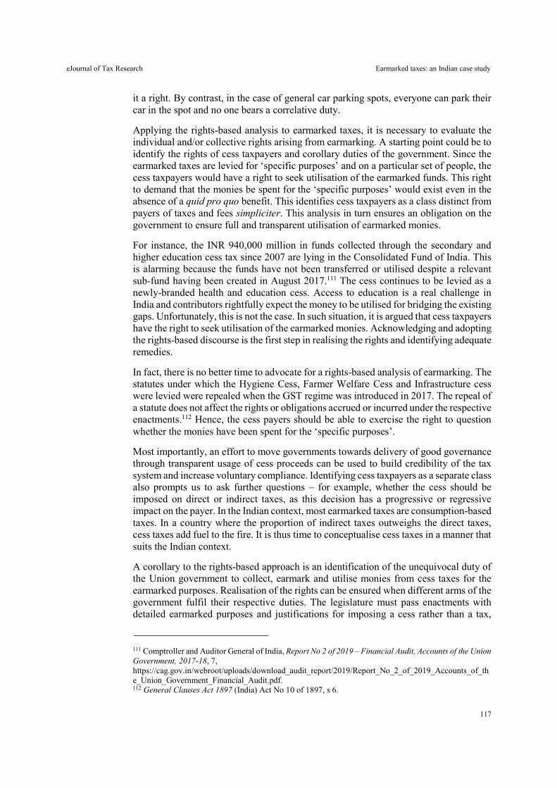
eJournal of Tax Research Earmarked taxes: an Indian case study
117
it a right. By contrast, in the case of general car parking spots, everyone can park their car in the spot and no one bears a correlative duty.
Applying the rights-based analysis to earmarked taxes, it is necessary to evaluate the individual and/or collective rights arising from earmarking. A starting point could be to identify the rights of cess taxpayers and corollary duties of the government. Since the earmarked taxes are levied for ‘specific purposes’ and on a particular set of people, the cess taxpayers would have a right to seek utilisation of the earmarked funds. This right to demand that the monies be spent for the ‘specific purposes’ would exist even in the absence of a quid pro quo benefit. This identifies cess taxpayers as a class distinct from payers of taxes and fees simpliciter. This analysis in turn ensures an obligation on the government to ensure full and transparent utilisation of earmarked monies.
For instance, the INR 940,000 million in funds collected through the secondary and higher education cess tax since 2007 are lying in the Consolidated Fund of India. This is alarming because the funds have not been transferred or utilised despite a relevant sub-fund having been created in August 2017.111 The cess continues to be levied as a newly-branded health and education cess. Access to education is a real challenge in India and contributors rightfully expect the money to be utilised for bridging the existing gaps. Unfortunately, this is not the case. In such situation, it is argued that cess taxpayers have the right to seek utilisation of the earmarked monies. Acknowledging and adopting the rights-based discourse is the first step in realising the rights and identifying adequate remedies.
In fact, there is no better time to advocate for a rights-based analysis of earmarking. The statutes under which the Hygiene Cess, Farmer Welfare Cess and Infrastructure cess were levied were repealed when the GST regime was introduced in 2017. The repeal of a statute does not affect the rights or obligations accrued or incurred under the respective enactments.112 Hence, the cess payers should be able to exercise the right to question whether the monies have been spent for the ‘specific purposes’.
Most importantly, an effort to move governments towards delivery of good governance through transparent usage of cess proceeds can be used to build credibility of the tax system and increase voluntary compliance. Identifying cess taxpayers as a separate class also prompts us to ask further questions – for example, whether the cess should be imposed on direct or indirect taxes, as this decision has a progressive or regressive impact on the payer. In the Indian context, most earmarked taxes are consumption-based taxes. In a country where the proportion of indirect taxes outweighs the direct taxes, cess taxes add fuel to the fire. It is thus time to conceptualise cess taxes in a manner that suits the Indian context.
A corollary to the rights-based approach is an identification of the unequivocal duty of the Union government to collect, earmark and utilise monies from cess taxes for the earmarked purposes. Realisation of the rights can be ensured when different arms of the government fulfil their respective duties. The legislature must pass enactments with detailed earmarked purposes and justifications for imposing a cess rather than a tax,
111 Comptroller and Auditor General of India, Report No 2 of 2019 – Financial Audit, Accounts of the Union Government, 2017-18, 7, https://cag.gov.in/webroot/uploads/download_audit_report/2019/Report_No_2_of_2019_Accounts_of_the_Union_Government_Financial_Audit.pdf. 112 General Clauses Act 1897 (India) Act No 10 of 1897, s 6.
eJournal of Tax Research Earmarked taxes: an Indian case study
118
estimated reverse calculations to substantiate the chosen tax rate, mechanisms for ensuring earmarking and utilisation, and a requirement for annual publication of collection and expenditure data and sunset clauses.
In order to ensure effective earmarking and utilisation, adequate administrative machinery and officers must be identified, separate sub-funds must be created within the Consolidated Fund of India and each of such sub-funds should have minor accounting codes so that the usage of funds can be traced. The executive must support strict compliance with the earmarked taxing statutes, make no expenses without the necessary appropriation Acts, and administer the disbursement and expenditure of proceeds in a transparent and timely manner with suitable accountability mechanisms in case it is not able to fulfil its duties. It would be a positive step if the tax departments specifically identified cess taxpayer rights in the taxpayers’/citizens’ charters.
The judiciary must also rise to the occasion and strike down an earmarked tax statute when there is lack of legislative competence and/or evidence of mismanagement of funds. The levying of cesses through a vague provision in the Finance Act with an open-ended purpose, and unclear justification, utilisation time frame, and administrative checks and balances should be called out. An analysis of the precedents by the various High Court and Supreme Court decisions shows that the rights-based jurisprudence is not always reflected in the outcomes. While on the one hand the Supreme Court has reprimanded a State government for diverting or not utilising cess funds in one instance, the Karnataka High Court has considered a cess tax as simply another tax, permitting the proceeds to be spent for any public purpose. These kinds of judicial precedents do a complete disservice to the earmarking of taxes. However, to be fair, a number of issues highlighted here have not yet been posed clearly before the courts. It can only be hoped that when the courts have occasion to decide the more nuanced issues, it will not be a lost opportunity.
APPENDIX
The authors had submitted a request under the Right to Information Act, 2005 in 2017 seeking disclosure of details pertaining to the collection and allocation of the proceeds from the Hygiene Cess. A response was received from the Ministry of Drinking Water and Sanitation, Union government of India in July 2017.
The disclosure stated that an amount of INR 24,000 million was allocated in the Financial Year 2015-16 (at the second supplementary stage) and INR 100,000 million in Financial Year 2016-17 under the Budget which was allocated to State governments as per the Swachh Bharat Mission (Gramin) Guidelines. As sanitation is within the purview of the State governments, the programme is implemented by State governments through the local self-governments. The details of expenditure of the Hygiene Cess as between the States for the year 2015-16, 2016-17 and 2017-18 are set out in the Table below.

eJournal of Tax Research Earmarked taxes: an Indian case study
119
Expenditure of Hygiene Cess, 2015-16, 2016-17 and 2017-18 (INR million)
Name of the States/UTs 2015 - 16 2016 - 17 2017 - 18 (as on 30.06.2017)
Andaman & Nicobar 24.00 30.00 50.00
Andhra Pradesh 657.94 3422.14 1652.00
Arunachal Pradesh 265.15 650.94 665.50
Assam 1726.04 7475.84 3006.55
Bihar 239.20 1318.64 0.00
Chhattisgarh 609.36 5844.65 3207.45
Goa 0.00 0.00 0.00
Gujarat 3436.99 7512.29 0.00
Haryana 23.86 687.91 0.00
Himachal Pradesh 0.00 1173.00 0.00
Jammu & Kashmir 0.00 595.13 739.11
Jharkhand 803.67 4554.64 1846.08
Karnataka 886.02 4195.61 1138.28
Kerala 0.00 1962.76 0.00
Madhya Pradesh 208.55 12107.67 3695.58
Maharashtra 2866.19 5289.42 4776.64
Manipur 0.00 544.86 0.00
Meghalaya 131.87 757.04 0.00
Mizoram 0.00 109.85 0.00
Nagaland 0.00 641.19 0.00
Odisha 2493.95 8636.45 2412.00
Puducherry 24 0.00 44.43
Punjab 147.97 1970.21 1326.06
Rajasthan 5093.55 7773.01 2916.57
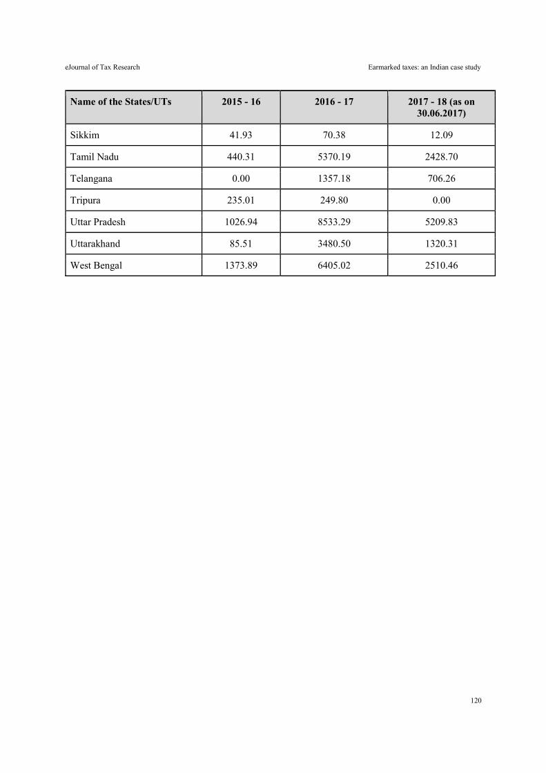
eJournal of Tax Research Earmarked taxes: an Indian case study
120
Name of the States/UTs 2015 - 16 2016 - 17 2017 - 18 (as on 30.06.2017)
Sikkim 41.93 70.38 12.09
Tamil Nadu 440.31 5370.19 2428.70
Telangana 0.00 1357.18 706.26
Tripura 235.01 249.80 0.00
Uttar Pradesh 1026.94 8533.29 5209.83
Uttarakhand 85.51 3480.50 1320.31
West Bengal 1373.89 6405.02 2510.46

eJournal of Tax Research (2021) vol. 19, no. 1, pp. 121-145
121
A review of objections to residential land values used to assess State land tax: a case study of inner Sydney, New South Wales
Vince Mangioni and Heather MacDonald
Abstract
New South Wales has experienced very intense affordability challenges during the 2012 to 2017 Australian housing price boom. While negative gearing has attracted the most attention in discussions of affordable housing in the media, other property tax elements also have market-distorting effects; here, we consider the effects of the land tax free threshold. We present the arguments for freezing the land tax free threshold, and examine the barriers to such a strategy, focusing on the likelihood of investor resistance to such a policy initiative by reference to objections to land values used to assess this tax.
Using ten local government areas (LGAs) in Sydney as case studies, objections to land values used to assess land tax across seven years are measured against the land tax free threshold. Census data is used to measure changes in residential property investment activity across LGAs and study periods. The article demonstrates that volatility, in particular increases in land values, is a primary factor impacting objections to land values in New South Wales. The study concludes that carefully designed changes to the land tax free threshold could smooth the transition and reduce objections to land values, while eliminating the distorting effects that the land tax free threshold has had on the competition between investors and homebuyers.
Key words: land tax free threshold, objections, land value, housing
Associate Professor, Property, University of Technology Sydney. Professor of Planning, University of Technology Sydney.

eJournal of Tax Research A review of objections to residential land values used to assess State land tax
122
1. INTRODUCTION
Property values and taxation have interacted to drive property investment behaviour over the last three decades in Australia. The literature on tax reform presents strong arguments that allowances and exemptions that once played a positive role now contribute to distorting housing investment decisions; these arguments support the position that property tax mechanisms are due for review. This article investigates how the exemptions offered by Australia’s State (subnational) governments affect the impost of land tax and in turn influence investment behaviour.
As of 2019 Australia’s housing assets were valued at approximately AUD 6.6 trillion, representing a decline of AUD 172 billion over the previous 18 months (Australian Bureau of Statistics (ABS), 2019). While such declines may be argued to have been caused to a large extent by Australia’s strong financial system, the factor that influenced the most recent decline in values related to the monetary reforms following the recommendations of the Royal Commission into Misconduct in the Banking, Superannuation and Financial Services Industry (Hon Kenneth Hayne, chair) of 2019. Changes to lending policy and tightening of monetary supply have impacted house prices (Stein, 2019) which demonstrates the commitment to reforms that have contributed to driving housing prices for the past decade, particularly in Sydney and New South Wales.
Further to monetary policy, taxation is a variable that influences house prices in high-priced markets. The objective of examining taxation and how it has interacted with property markets identifies the potential impact policy changes have had on residential house prices, and provides a basis to understand their likely impacts into the future. In undertaking this review, it is acknowledged that each tier of government in Australia impacts house prices and investment through fiscal imposts or exemptions and concessions to some degree. The ability to reform a tax concession in some circumstances may be mistakenly perceived to constitute a new tax, even when the reform responds to an outdated concession that no longer serves its initial purpose.
Taking a broader view, tax policy aimed at moderating housing prices and incentivising the provision of some types of housing is consistent with the principles expressed in the International Covenant on Economic, Social and Cultural Rights,1 a United Nations document ratified by Australia in 1975. Article 11(1) of the Covenant commits signatory states to ‘recognize the right of everyone to an adequate standard of living for himself and his family, including adequate food, clothing and housing, and to the continuous improvement of living conditions’. Hohmann (2020, pp. 293-294) argues that reframing the Australian discourse on housing affordability in terms of its basis in human rights principles is essential if we are to ‘shift the underlying terrain of debate’ and focus on housing as a social good rather than an investment good. A close examination of the structure and distributional impacts of tax policies can contribute to this new terrain of debate.
1 International Covenant on Economic, Social and Cultural Rights, opened for signature 16 December 1966, 993 UNTS 3 (entered into force 3 January 1976), https://treaties.un.org/pages/showDetails.aspx?objid=080000028002b6ed. See also Australian Human Rights Commission, ‘ICESCR: Human rights at your fingertips’, https://humanrights.gov.au/our-work/commission-general/international-covenant-economic-social-and-cultural-rights-human-rights (accessed 13 January 2021).
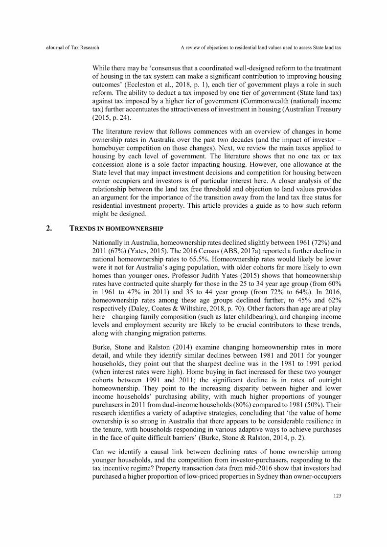
eJournal of Tax Research A review of objections to residential land values used to assess State land tax
123
While there may be ‘consensus that a coordinated well-designed reform to the treatment of housing in the tax system can make a significant contribution to improving housing outcomes’ (Eccleston et al., 2018, p. 1), each tier of government plays a role in such reform. The ability to deduct a tax imposed by one tier of government (State land tax) against tax imposed by a higher tier of government (Commonwealth (national) income tax) further accentuates the attractiveness of investment in housing (Australian Treasury (2015, p. 24).
The literature review that follows commences with an overview of changes in home ownership rates in Australia over the past two decades (and the impact of investor – homebuyer competition on those changes). Next, we review the main taxes applied to housing by each level of government. The literature shows that no one tax or tax concession alone is a sole factor impacting housing. However, one allowance at the State level that may impact investment decisions and competition for housing between owner occupiers and investors is of particular interest here. A closer analysis of the relationship between the land tax free threshold and objection to land values provides an argument for the importance of the transition away from the land tax free status for residential investment property. This article provides a guide as to how such reform might be designed.
2. TRENDS IN HOMEOWNERSHIP
Nationally in Australia, homeownership rates declined slightly between 1961 (72%) and 2011 (67%) (Yates, 2015). The 2016 Census (ABS, 2017a) reported a further decline in national homeownership rates to 65.5%. Homeownership rates would likely be lower were it not for Australia’s aging population, with older cohorts far more likely to own homes than younger ones. Professor Judith Yates (2015) shows that homeownership rates have contracted quite sharply for those in the 25 to 34 year age group (from 60% in 1961 to 47% in 2011) and 35 to 44 year group (from 72% to 64%). In 2016, homeownership rates among these age groups declined further, to 45% and 62% respectively (Daley, Coates & Wiltshire, 2018, p. 70). Other factors than age are at play here – changing family composition (such as later childbearing), and changing income levels and employment security are likely to be crucial contributors to these trends, along with changing migration patterns.
Burke, Stone and Ralston (2014) examine changing homeownership rates in more detail, and while they identify similar declines between 1981 and 2011 for younger households, they point out that the sharpest decline was in the 1981 to 1991 period (when interest rates were high). Home buying in fact increased for these two younger cohorts between 1991 and 2011; the significant decline is in rates of outright homeownership. They point to the increasing disparity between higher and lower income households’ purchasing ability, with much higher proportions of younger purchasers in 2011 from dual-income households (80%) compared to 1981 (50%). Their research identifies a variety of adaptive strategies, concluding that ‘the value of home ownership is so strong in Australia that there appears to be considerable resilience in the tenure, with households responding in various adaptive ways to achieve purchases in the face of quite difficult barriers’ (Burke, Stone & Ralston, 2014, p. 2).
Can we identify a causal link between declining rates of home ownership among younger households, and the competition from investor-purchasers, responding to the tax incentive regime? Property transaction data from mid-2016 show that investors had purchased a higher proportion of low-priced properties in Sydney than owner-occupiers
eJournal of Tax Research A review of objections to residential land values used to assess State land tax
124
over the prior 12 months (Fitzsimmons, 2016). State policy has adapted by reducing or eliminating stamp duty on lower priced homes for first home buyers (Gerathey, 2017), and recent changes to lending standards have disproportionately affected highly leveraged investor-purchasers (Letts, 2018). These trends suggest that tax policy is at most only a partial driver of shifts in the balance between investors and first-time buyers; lending standards, investor regulation regimes (abroad as well as within Australia) and other direct home buyer incentives are likely to play the dominant role. Nevertheless, as political debate continues at the national level around negative gearing and other investor incentives, States clearly have a role to play in managing the fallout of the intensely competitive investor-purchaser environment of the past half-decade. The following section explains the tax environment under the influence of which housing markets have evolved in Australia.
3. THE TAXATION OF PROPERTY AND CURRENT STATUS IN AUSTRALIA
3.1 Commonwealth
Negative gearing and the capital gains tax (CGT) discount in their application to residential property are two tax concessions that have increasingly featured in tax debates over the past 30 years in Australia. These concessions have progressively continued to distort property markets and embrace outdated objectives that no longer serve Australia’s modern housing needs (Wood, Ong & Stewart, 2010; Kelly, 2013).
3.1.1 Negative gearing
The Productivity Commission (2004) highlights Australia’s negative gearing provisions as being among the most generous of the Organisation for Economic Co-operation and Development (OECD) member countries. The Australian government removed negative gearing in 1985; this reform was repealed two years later following a campaign for reinstatement resulting from the negative impact on the Sydney housing rental market. In defining the growth of negative gearing in the Australian residential property market, Eccleston et al. (2018) refer to estimates from the Australian Taxation Office (ATO), in highlighting that 63% of all property investors were negatively geared in 2013-14, compared to just 50% in 1993-94. This incentive boosts investors cash flow enhancing their ability to compete against first home owners.
3.1.2 Capital gains tax
Eccleston et al. (2018, p. 23) have noted that ‘[t]he CGT discount for individuals and trusts represented AUD 6.84 billion in revenue forgone in 2016-17. Because most capital gains are accrued and realised by taxpayers with high taxable incomes, the benefits of the discount flow disproportionately to these households’. Among the provisions that have led to a distorted and inequitable distribution of housing assets and outcomes in the housing market, Kelly (2013) defines the CGT exemption applied to the main residence as encouraging over-investment in existing housing by owner occupiers.
In highlighting the impact of the capital gains tax exemption on the home, Yates (2010) refers to the report of the Senate Select Committee on Housing Affordability in Australia (2008, [4.38]), in stating that the capital gains tax subsidy ‘favours home owners, not home ownership’ (Yates 2010, p. 63). Overinvestment of owner-occupied housing further extends to include the store of wealth in housing that is fuelled by demand that outstrips supply, in which Yates (2009, p. 37) states:
eJournal of Tax Research A review of objections to residential land values used to assess State land tax
125
As demand side subsidies that create an economic incentive to increasing consumption of housing through home ownership, they add to price pressures in the housing market and thereby contribute to the affordability constraints faced by aspiring home owners.
3.2 State and local government
Eccleston et al. (2018, p. 41 (references omitted)) have noted that:
[i]n Australia, there are currently three forms of subnational tax on land and residential property: transfer duties, state land tax and local government rates. These taxes together raised over $40 billion in 2014-15, which was 10.1 per cent of all taxes collected in Australia. They are an important source of revenue for state and local governments, with transfer duty particularly lucrative ($18.5 billion in 2014-15, or almost half of all property tax).
Despite their revenue significance, however, there is agreement in the literature that state property taxes are poorly designed and require reform. … Transfer duties on property are inefficient, subject to housing market volatility, and responsible for under-utilisation of housing stock and constrained housing mobility.
Introducing a recurrent property tax on a broad base with few exemptions would provide a more stable, efficient source of revenue. Mangioni and Warren (2014) further state that that the efficiency factor often referred to is driven by the principle that property values are determined on highest and best use of land.
Transfer duties impose a ‘large, up-front cost’ on property, which impacts the optimal use of housing; Furthermore, ‘[b]ecause transfer duty revenue depends on the volume and value of transactions in the market, it is unpredictable and vulnerable to market disruptions’ (Eccleston et al., p. 41, citing Henry Review, 2009 and Productivity Commission, 2018). In contrast to other State imposed taxes, Figure 1 sets out the volatility in revenue from transfer tax compared with land tax and council rates. As Eccleston et al. conclude (2018, p. 41), ‘[s]hifting to a recurrent property tax would generate a significant efficiency dividend through greater stability in state revenue, improved transparency within the tax system while enhancing residential mobility and housing affordability (Daley & Coates, 2015; Henry Review, 2009; Mangioni, 2016)’.
While recurrent land and property taxation is stated to be economically efficient and least distortive of the property taxes, its perception by taxpayers is not readily accepted nor always understood and the base on which this tax is set is subject to challenge. It is this factor, challenges to land values that this article now turns to in examining objections against the contestable component of this tax, namely the land value on which this tax is assessed in New South Wales. While a number of studies have examined the benefits of transitioning from transaction taxes to a broad-based land tax, what has yet to be examined is how land tax may be expanded and the potential consequences of this reform in the form of objections to land values by residential property investors.
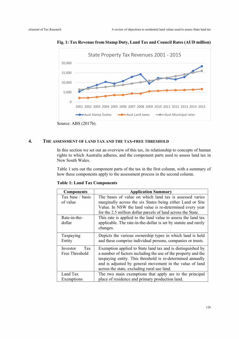
eJournal of Tax Research A review of objections to residential land values used to assess State land tax
126
Fig. 1: Tax Revenue from Stamp Duty, Land Tax and Council Rates (AUD million)
Source: ABS (2017b).
4. THE ASSESSMENT OF LAND TAX AND THE TAX-FREE THRESHOLD
In this section we set out an overview of this tax, its relationship to concepts of human rights to which Australia adheres, and the component parts used to assess land tax in New South Wales.
Table 1 sets out the component parts of the tax in the first column, with a summary of how these components apply to the assessment process in the second column.
Table 1: Land Tax Components
Components Application Summary Tax base / basis of value
The bases of value on which land tax is assessed varies marginally across the six States being either Land or Site Value. In NSW the land value is re-determined every year for the 2.5 million dollar parcels of land across the State.
Rate-in-the-dollar
This rate is applied to the land value to assess the land tax applicable. The rate-in-the-dollar is set by statute and rarely changes.
Taxpaying Entity
Depicts the various ownership types in which land is held and these comprise individual persons, companies or trusts.
Investor Tax Free Threshold
Exemption applied to State land tax and is distinguished by a number of factors including the use of the property and the taxpaying entity. This threshold is re-determined annually and is adjusted by general movement in the value of land across the state, excluding rural use land.
Land Tax Exemptions
The two main exemptions that apply are to the principal place of residence and primary production land.
0
5,000
10,000
15,000
20,000
2001 2002 2003 2004 2005 2006 2007 2008 2009 2010 2011 2012 2013 2014 2015
State Property Tax Revenues 2001 - 2015
Aust Stamp Duties Aust Land taxes Aust Municipal rates
eJournal of Tax Research A review of objections to residential land values used to assess State land tax
127
New South Wales initially introduced land tax in 1895, abolishing it in 1906 making way for the Commonwealth and local government to collect this tax. It reintroduced this tax in 1956 following the Commonwealth’s abolition of the tax in 1952. New South Wales was the first State to introduce a land tax free threshold which was set at AUD 55,000 in 1972. By 1987 the tax-free threshold was $94,000 with a tax rate-in-the-dollar of 2%. The initial rationale for introducing the land tax free threshold is stated by Mangioni (2016) as being to incentivise residential property investment with a view to encouraging more rental housing stock. By the late 1980s the government came under pressure to increase the land tax threshold which progressively increased to $125,000 in 1988, $135,000 in 1989 and $160,000 in 1990, where the threshold remained without adjustment for eight years.
Following revenue pressure, in 2004 the New South Wales Government concurrently announced the introduction of a tax on the sale of residential property and an amendment to the State land tax free threshold to commence in the 2005 tax year. The Vendor Duty was imposed on all residential property excluding the principal place of residence (subject to being owned for a minimum of two years) at a rate of 2.25% of the sale price (New South Wales Parliament, 2004). The implications for investors with investment properties which were below the land tax threshold before the changes in 2005, was an incurrence of up to $1,268 increase per year. The upside to the 2005 changes to land tax was the reduction in the rate-in-the-dollar from 1.7 cents to 1.4 cents. The breakeven point of no change in land tax payable was for investors with an aggregate land value of approximately $405,000 in the 2005 land tax year.
It is apt to highlight here that the land tax free threshold does not apply to each property held by the same owner. The threshold only applies once to the aggregate land value of all property (excluding exempt property) held by a property owner. Once the tax-free threshold has been reached, a tax incentive exists for investors that allows the deductibility of land tax as an expense against the income generated from the property, or where that expense exceeds the income from that property, against other assessable income as shown in Figure 2. In essence, State land tax is a mechanism used by State government, to redistribute the tax revenue collected by the Commonwealth as a deduction against the impost of a State-imposed tax. One could argue for its basis in principles of human rights (in particular the International Covenant on Economic, Social and Cultural Rights) defining the role of housing in guaranteeing a minimum quality of life.
This tax subsidy is achieved on the basis that the rent collected from property is defined as income and land tax is an expense. What has evolved as a challenge for the States is accepting that any taxpayer would prefer not to pay tax and hence the land tax free threshold ideologically contributes to serving that purpose.
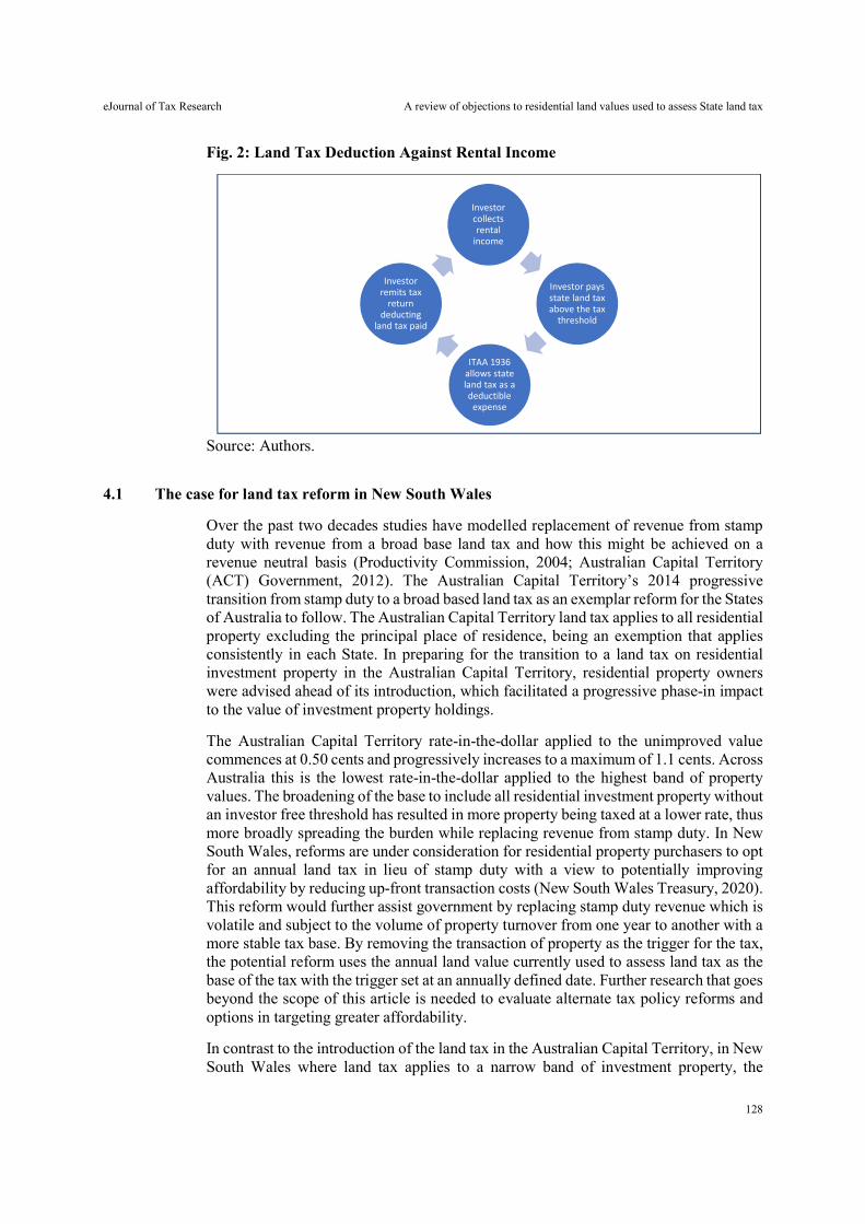
eJournal of Tax Research A review of objections to residential land values used to assess State land tax
128
Fig. 2: Land Tax Deduction Against Rental Income
Source: Authors.
4.1 The case for land tax reform in New South Wales
Over the past two decades studies have modelled replacement of revenue from stamp duty with revenue from a broad base land tax and how this might be achieved on a revenue neutral basis (Productivity Commission, 2004; Australian Capital Territory (ACT) Government, 2012). The Australian Capital Territory’s 2014 progressive transition from stamp duty to a broad based land tax as an exemplar reform for the States of Australia to follow. The Australian Capital Territory land tax applies to all residential property excluding the principal place of residence, being an exemption that applies consistently in each State. In preparing for the transition to a land tax on residential investment property in the Australian Capital Territory, residential property owners were advised ahead of its introduction, which facilitated a progressive phase-in impact to the value of investment property holdings.
The Australian Capital Territory rate-in-the-dollar applied to the unimproved value commences at 0.50 cents and progressively increases to a maximum of 1.1 cents. Across Australia this is the lowest rate-in-the-dollar applied to the highest band of property values. The broadening of the base to include all residential investment property without an investor free threshold has resulted in more property being taxed at a lower rate, thus more broadly spreading the burden while replacing revenue from stamp duty. In New South Wales, reforms are under consideration for residential property purchasers to opt for an annual land tax in lieu of stamp duty with a view to potentially improving affordability by reducing up-front transaction costs (New South Wales Treasury, 2020). This reform would further assist government by replacing stamp duty revenue which is volatile and subject to the volume of property turnover from one year to another with a more stable tax base. By removing the transaction of property as the trigger for the tax, the potential reform uses the annual land value currently used to assess land tax as the base of the tax with the trigger set at an annually defined date. Further research that goes beyond the scope of this article is needed to evaluate alternate tax policy reforms and options in targeting greater affordability.
In contrast to the introduction of the land tax in the Australian Capital Territory, in New South Wales where land tax applies to a narrow band of investment property, the
Investor collects rental
income
Investor pays state land tax above the tax
threshold
ITAA 1936 allows state land tax as a deductible
expense
Investor remits tax
return deducting
land tax paid
eJournal of Tax Research A review of objections to residential land values used to assess State land tax
129
proposed reform to broaden the land tax net would commence with the phase-out of the investor tax-free threshold. In contrast to the revenue replacement approach to reform, the research undertaken in this article aims to look at the potential resistance to phasing out the tax-free threshold in New South Wales. While it is beyond the scope and objective of this article to model the phase-out, the more important objective is to examine the resistance to the payment of land tax through objections to the land value component as set out in Table 1. The value is the variable component on which tax revenue increases each year and, more relevantly to this article, is the primary component of the tax that investors are able to object to in challenging this tax.
In May 2004 the New South Wales Government announced its intent to abolish the land tax free threshold in New South Wales from the 2005 land tax year, and reduce the top rate-in the-dollar from 1.7 to 1.4 cents-in-the-dollar (New South Wales Parliament, 2004). This reform resulted in the number of property owners subject to land tax increasing from 120,000 to 660,000 in New South Wales predominantly being residential property owners. This reform also resulted in objections to land values across New South Wales increasing to over 16,000; the reform was deemed to have been poorly executed and the threshold was reinstated for the 2006 land tax year. While the idea of removing the threshold was well-founded, as in any tax reform, the transition was manifestly inadequate with the threshold removed with six months notice provided and no economic scaffolding to manage the increase in objections that followed.
While small scale investors (who dominate the rental housing market in Australia) have enjoyed a range of tax incentives implicitly justified as a way to lower rents by increasing returns to landlords, it is unclear these de facto subsidies have had these effects in practice (Berry, 2000). The Reserve Bank estimates that the impact of removing negative gearing would be lower housing prices, and higher homeownership rates (reported in Ong, 2017), this in turn would constitute an overall net gain for Australians.
Offsetting arguments that investor tax incentives help lower the cost of rental housing are analyses demonstrating the longer term welfare consequences of falling rates of homeownership, particularly on retirement (Stebbing & Spies-Butcher, 2016). Intensifying inequality between owners and renters (particularly along generational lines) will also have longer term effects on social stability and the socio-economic integration that underpins both quality of life and economic growth (Daley et al., 2018).
5. RESEARCH METHOD
The two factors examined in this article are the changes in residential property investment holdings in the case study areas over the study period and whether the land tax free threshold is the primary factor impacting objections to land values used to determine land tax. In addressing these points, primary data has been provided by the New South Wales Valuer-General and Department of Land and Property Information, with secondary data sourced from the Australian Bureau of Statistics (ABS). In undertaking the review, the New South Wales Valuer-General provided objection data to land values from ten local government areas located within 15 kilometres of the centre of Sydney over seven land tax years (2011 to 2017).
As at the date of this analysis there were 41 local government areas within the Sydney metropolitan area, of which the sample of ten local government areas analysed represents approximately 25% of local government areas (LGAs). The rationale for
eJournal of Tax Research A review of objections to residential land values used to assess State land tax
130
selection of these local government areas is based their geographic proximity to the centre of Sydney; the highest values in Sydney are within these locations. A majority of the properties that attract State land tax are located within these local government areas. The New South Wales Valuer-General’s Office provided the land value objection data across these local government areas, which span a seven year period, used to determine the values being made available to land tax payers.
In analysing the number of objections to land values, two factors were considered. The first consideration was the location in which objections were grouped by local government area. The second consideration was the change in the number of objections between each of the base dates of valuation. In New South Wales, each parcel of land is valued annually as at 1 July each year; this is known as the base date and is used to assess land tax in New South Wales for the following land tax year. The analysis was undertaken using objection data on land values between base dates 1 July 2010 and 1 July 2016, which apply to the respective land tax years of 2011 to 2017 inclusive. The data was analysed to address the following four questions for the ten local government areas:
1. How did the proportionate share of rental property change between the 2011 and 2016 census dates?
2. What were the key trends in the volume of objections across inner Sydney between 2011 and 2017 land tax years, for houses and units?
3. How did the volume and proportion of objections below and above the land tax free threshold change across each local government area between 2011 and 2017, for houses and units?
4. How did trends in objections to land values relative to the land tax free threshold change in the 2016 land tax year?
6. FINDINGS
Table 2 (columns C and F) shows that between the 2011 and 2016 census dates there was an increase in the percentage of rental property in eight of the ten LGAs.2 Mosman LGA has no change between these census dates, while a decrease is noted in Woollahra. These two LGAs have the highest land values for both houses and units and have the lowest percentage of rented property as at the two census dates. It is further shown in Table 2 that there was an increase in residential unit dwellings during this period in nine of the ten LGAs with the exception of Leichhardt. Correspondingly, it is noted that there was a decrease in the number of houses in seven of the ten LGAs. Of the five LGAs with the largest increases in percentage of rental housing, three LGAs (Ashfield, Marrickville and Burwood) are located in the Inner West and two LGAs (Botany and Randwick) are located in Sydney East. In addressing the first question, we find an increase in the percentage of rented dwellings in the inner suburbs of Sydney and that as Sydney densifies, owner occupiers are indeed competing with investors for housing stock, particularly in the unit market.
To answer the second question, we commence by looking at the overall trends in objections to land values across inner Sydney in Table 3 and Figures 3 and 4 for houses
2 See Appendix for Tables 2 to 6 and Figures 3 to 7.
eJournal of Tax Research A review of objections to residential land values used to assess State land tax
131
and units between the 2010 and 2016 tax years. Next, we review the number of objections below and above the tax-free threshold in each LGA and draw conclusions about the relationship between median land values and the land tax threshold, for houses and units in each LGA over the study period. Table 3 and Figures 3 and 4 show 4,565 objections to land values for houses and 968 objections to land values for units. Across the study period different trends are evident. Over the 2009 to 2012 period, we find higher volatility in objections to land values for units compared to houses. The levels of volatility in objections to land values are similar for houses and units between 2013 and 2016. For both categories of dwellings, there is a sharp upward trend in objections in 2015-2016, which corresponds with the strong demand for housing and increase in values that peaked 12 months following that last period (the 2017 land tax year).
Addressing question 3, Table 4 and Figure 5 set out the percentage of objections to land values above and below the land tax free threshold for houses in each LGA. In nine of the ten LGAs, over 90% of objections are lodged against land values above the tax-free threshold on the basis that the land values are too high. The exception is Marrickville, where 20% of objections were lodged for houses valued below the threshold. We conclude that objections to land values used to assess land tax would primarily be lodged in cases of land values above the tax-free threshold as shown in objections to land values for houses. This supports the rationale that payment of land tax itself is one trigger for objections to land tax; however it does not provide the reasoning for why the objection is lodged, particularly where the land value is correct or is at the conservative end of the market value range. This factor is discussed next, in the analysis of objections to land values for units and again later in the analysis of the median land values against the land tax free threshold.
The review of objections to land values for units (in Table 5 and Figure 6) shows that in seven of the ten LGAs, more than 50% of objections to land values are below the tax-free threshold, which is in stark contrast to the percentage of objections to houses. It is important to reinforce the operation of the land tax free threshold again here in the assessment of land tax. The threshold only applies once to the aggregate land value of all property (excluding exempt property) held by a property owner, it does not apply to each property held in the same ownership. This provides insight into the likely rationale for objections to land values below the tax-free threshold: objections reflect the interests of owners holding multiple residential investment properties. The increase in objections is further emphasised by the increase noted in rented dwellings between the 2011 and 2016 census dates, which potentially renders more property liable to pay land tax once the land value trips the tax-free threshold.
In the objections to unit values, Randwick and Botany Bay stand out in Sydney East with 96% and 67% of objections to land values below the threshold. In the Inner West, Marrickville and Ashfield stand out with 59% and 100% respectively. In Sydney North, Mosman and North Sydney have objection rates of 55% and 62%. While these objection rates may appear high and in the case of units are likely to be impacted by multiple holdings pushing investors over the tax-free threshold, we now go back to Table 3 and Figures 3 and 4, to examine the spike in objections in the 2017 land tax year. Of all objections lodged across the six years examined, 37.7% were lodged against house land values and 41.5% were lodged against land values to units in the 2015 and 2016 tax years. The increase in objections to land values aligns with the increase in land values across these same two years. This provides evidence that tripping the tax-free threshold
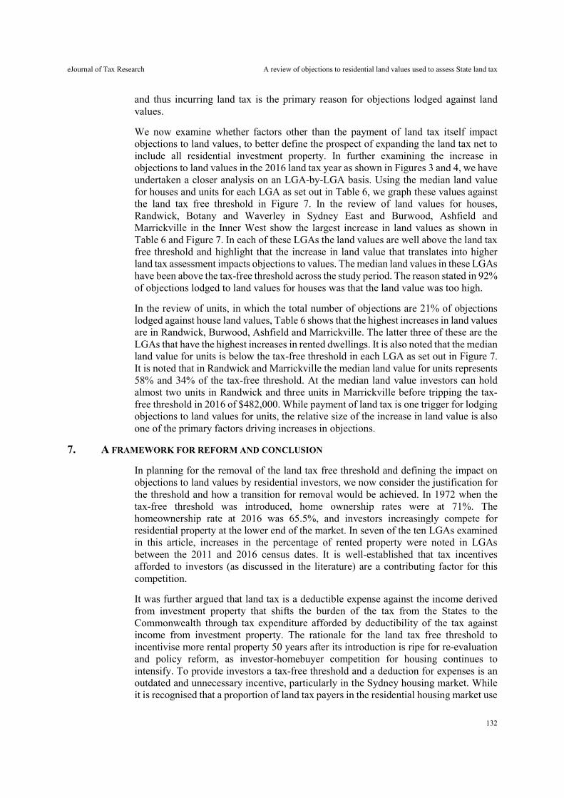
eJournal of Tax Research A review of objections to residential land values used to assess State land tax
132
and thus incurring land tax is the primary reason for objections lodged against land values.
We now examine whether factors other than the payment of land tax itself impact objections to land values, to better define the prospect of expanding the land tax net to include all residential investment property. In further examining the increase in objections to land values in the 2016 land tax year as shown in Figures 3 and 4, we have undertaken a closer analysis on an LGA-by-LGA basis. Using the median land value for houses and units for each LGA as set out in Table 6, we graph these values against the land tax free threshold in Figure 7. In the review of land values for houses, Randwick, Botany and Waverley in Sydney East and Burwood, Ashfield and Marrickville in the Inner West show the largest increase in land values as shown in Table 6 and Figure 7. In each of these LGAs the land values are well above the land tax free threshold and highlight that the increase in land value that translates into higher land tax assessment impacts objections to values. The median land values in these LGAs have been above the tax-free threshold across the study period. The reason stated in 92% of objections lodged to land values for houses was that the land value was too high.
In the review of units, in which the total number of objections are 21% of objections lodged against house land values, Table 6 shows that the highest increases in land values are in Randwick, Burwood, Ashfield and Marrickville. The latter three of these are the LGAs that have the highest increases in rented dwellings. It is also noted that the median land value for units is below the tax-free threshold in each LGA as set out in Figure 7. It is noted that in Randwick and Marrickville the median land value for units represents 58% and 34% of the tax-free threshold. At the median land value investors can hold almost two units in Randwick and three units in Marrickville before tripping the tax-free threshold in 2016 of $482,000. While payment of land tax is one trigger for lodging objections to land values for units, the relative size of the increase in land value is also one of the primary factors driving increases in objections.
7. A FRAMEWORK FOR REFORM AND CONCLUSION
In planning for the removal of the land tax free threshold and defining the impact on objections to land values by residential investors, we now consider the justification for the threshold and how a transition for removal would be achieved. In 1972 when the tax-free threshold was introduced, home ownership rates were at 71%. The homeownership rate at 2016 was 65.5%, and investors increasingly compete for residential property at the lower end of the market. In seven of the ten LGAs examined in this article, increases in the percentage of rented property were noted in LGAs between the 2011 and 2016 census dates. It is well-established that tax incentives afforded to investors (as discussed in the literature) are a contributing factor for this competition.
It was further argued that land tax is a deductible expense against the income derived from investment property that shifts the burden of the tax from the States to the Commonwealth through tax expenditure afforded by deductibility of the tax against income from investment property. The rationale for the land tax free threshold to incentivise more rental property 50 years after its introduction is ripe for re-evaluation and policy reform, as investor-homebuyer competition for housing continues to intensify. To provide investors a tax-free threshold and a deduction for expenses is an outdated and unnecessary incentive, particularly in the Sydney housing market. While it is recognised that a proportion of land tax payers in the residential housing market use

eJournal of Tax Research A review of objections to residential land values used to assess State land tax
133
secondary residences for recreational purposes, Mangioni (2016, p. 109) discusses that this factor should not impact the argument for reform to the land tax free threshold.
The analyses in this article demonstrate two important outcomes that prompt reform. The first is that in each of the LGAs examined, the tax-free threshold incentivises small residential unit property investors over investors with houses with the tax-free threshold sitting between units and houses in all LGAs. Secondly, while objections to units are lower in volume compared with houses, objections to land values of units below the tax-free threshold are tenfold compared with those for house land values. This in part is driven by the fact that the median land value for houses is well above the tax-free threshold, but also conversely shows the trend towards multiple unit holdings, particularly in some LGAs.
What the article finds is that the payment of land tax is not overwhelmingly the only factor that triggers objection to land values. The analyses clearly show that the size of the increase in land values that impacts the amount of land tax paid as set out in the 2016 land tax year is a significant contributor to increases in objections to land values on the basis that the value is too high. This raises the question of how the reforms that might be adopted could manage the spikes in objections during periods of rapid house price inflation. In summary, if there were an increase in the rate of objections proportionate with the increase in the number of investment properties caught in the land tax net, the issue is how this reform might be managed and what mechanisms are available for a smooth transition to the removal of the tax-free threshold.
In removing the tax-free threshold, a phase-in approach has been developed comprising four measures that support a smooth transition and address those factors that hampered the 2005 attempts at removing the tax-free threshold in New South Wales. The proposed measures are set out in the summary below and address the key elements of the threshold, land value, rate-in-the-dollar and payment mechanism. In contrast to removing the threshold in one tax year, a progressive phase in approach of freezing the tax-free threshold for a minimum of five years would apply. This would result in residential investment property, in particular residential unit investment, below the tax-free threshold moving progressively into paying the tax. To address the spike in land values that impacts objections as noted in the 2016 land tax year, extending the average land value from three to five years would also factor in cyclical corrections to values in the years of high property value growth. The rate-in-the-dollar should be maintained, or where additional revenue is raised as more property becomes liable for land tax, acknowledgement provided of a downward adjustment to the rate at three or five years of introduction of the reform, returning a portion of the gain in revenue raised back to property investors. The final reform is to more evenly stagger the payment options for the tax across the year as regular quarterly payments which better acclimatise taxpayers to the tax liability.
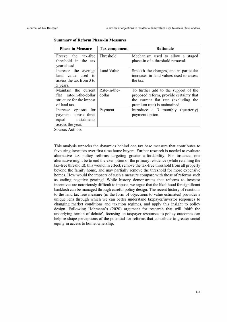
eJournal of Tax Research A review of objections to residential land values used to assess State land tax
134
Summary of Reform Phase-In Measures
Phase-in Measure Tax component Rationale
Freeze the tax-free threshold in the tax year ahead
Threshold Mechanism used to allow a staged phase-in of a threshold removal.
Increase the average land value used to assess the tax from 3 to 5 years.
Land Value Smooth the changes, and in particular increases in land values used to assess the tax.
Maintain the current flat rate-in-the-dollar structure for the impost of land tax.
Rate-in-the-dollar
To further add to the support of the proposed reform, provide certainty that the current flat rate (excluding the premium rate) is maintained.
Increase options for payment across three equal instalments across the year.
Payment Introduce a 3 monthly (quarterly) payment option.
Source: Authors.
This analysis unpacks the dynamics behind one tax base measure that contributes to favouring investors over first time home buyers. Further research is needed to evaluate alternative tax policy reforms targeting greater affordability. For instance, one alternative might be to end the exemption of the primary residence (while retaining the tax-free threshold); this would, in effect, remove the tax-free threshold from all property beyond the family home, and may partially remove the threshold for more expensive homes. How would the impacts of such a measure compare with those of reforms such as ending negative gearing? While history demonstrates that reforms to investor incentives are notoriously difficult to impose, we argue that the likelihood for significant backlash can be managed through careful policy design. The recent history of reactions to the land tax free measure (in the form of objections to value estimates) provides a unique lens through which we can better understand taxpayer/investor responses to changing market conditions and taxation regimes, and apply this insight to policy design. Following Hohmann’s (2020) argument for research that will ‘shift the underlying terrain of debate’, focusing on taxpayer responses to policy outcomes can help re-shape perceptions of the potential for reforms that contribute to greater social equity in access to homeownership.
eJournal of Tax Research A review of objections to residential land values used to assess State land tax
135
8. REFERENCES
Australian Capital Territory (ACT) Government 2012, ACT taxation review, Treasury Directorate ACT, May. Available at: http://www.treasury.act.gov.au/documents/ACT%20Taxation%20Review/ACT%20Taxation%20Review%20May%202012.pdf.
Australian Bureau of Statistics (ABS) 2017a, Census of population and housing, Australia, 2016, Cat 2008.0. Available at: https://www.abs.gov.au/websitedbs/censushome.nsf/home/2016.
Australian Bureau of Statistics (ABS) 2017b, Major components of total tax revenue 2015/16, Cat 5506.0. Available at:
https://www.abs.gov.au/ausstats/[email protected]/Previousproducts/5506.0Main%20Features22015-16?opendocument&tabname=Summary&prodno=5506.0&issue=2015-16&num=&view=
Australian Bureau of Statistics (ABS) 2019, Residential property price index: Eight capital cities, Cat 6416.0, March. Available at: https://www.abs.gov.au/Ausstats/[email protected]/exnote/6416.0 (accessed 9 October 2019).
Australian Parliament, Senate Select Committee on Housing Affordability in Australia 2008, A good house is hard to find: Housing affordability in Australia, report, 16 June. Available at: https://www.aph.gov.au/Parliamentary_Business/Committees/Senate/Former_Committees/hsaf/report/index.
Australian Treasury 2015, Re:think: Tax discussion paper, March. Available at: https://treasury.gov.au/sites/default/files/2019-03/c2015-rethink-dp-TWP_combined-online.pdf.
Australia’s Future Tax System Review Panel (Dr K Henry, chair) 2009, Australia’s future tax system: Report to the Treasurer, December (Henry Review).
Berry, M 2000, ‘Investment in rental housing in Australia: Small landlords and institutional investors’, Housing Studies, vol. 15, no. 5, pp. 661-681.
Burke, T, Stone, W & Ralston, L 2014, Generational change in home purchase opportunity in Australia, AHURI Final Report No 232, Australian Housing and Urban Research Institute, November. Available at: https://www.ahuri.edu.au/research/final-reports/232.
Daley, J & Coates, B 2015, ‘Property taxes’, Grattan Institute Working Paper No 2015-5, Grattan Institute, July. Available at: https://grattan.edu.au/wp-content/uploads/2015/07/826-Property-Taxes.pdf.
Daley, J, Coates, B & Wiltshire, T 2018, ‘Housing affordability: Re-imagining the Australian dream’, Grattan Institute Report 2018-04, March. Available at: https://grattan.edu.au/wp-content/uploads/2018/03/901-Housing-affordability.pdf.
Eccleston, R, Verdouw, J, Flanagan, K, Warren, N, Duncan, A, Ong, R, Whelan, S & Atalay, K 2018, Pathways to housing tax reform, Final inquiry report, Australian Housing and Urban Research Institute, July.
Fitzsimmons, C 2016, ‘How investors outgun first home buyers’, Sydney Morning Herald, 29 April. Available at: https://www.smh.com.au/money/tax/how-investors-outgun-firsthome-buyers-20160428-gogx87.html.

eJournal of Tax Research A review of objections to residential land values used to assess State land tax
136
Gerathey, S 2017, ‘First home buyers to have edge over investors under NSW housing affordability package’, ABC News, 2 June. Available at: http://www.abc.net.au/news/2017-06-01/nsw-first-home-buyers-to-have-edge-over-foreign-investors/8580042.
Hohmann, J 2020, ‘Toward a right to housing for Australia: Reframing affordability debates through article 11(1) of the International Covenant on Economic, Social and Cultural Rights’, Australian Journal of Human Rights, vol. 26, no. 2, pp. 292-307.
Kelly, J-F 2013, ‘Renovating housing policy’, Grattan Institute Report No 2013-12, October.
Letts, S 2018, ‘First home buyers shrug off the credit crunch as home loans are bigger than ever’, ABC News, 30 September. Available at: http://www.abc.net.au/news/2018-09-30/first-home-buyers-shrug-off-the-credit-crunch/10318704.
Mangioni, V 2016, Land tax in Australia: Fiscal reform of subnational government, Routledge, London and New York.
Mangioni, V & Warren, N 2014, ‘Re-defining the land tax base in highly urbanised locations’, Australian Tax Forum, vol. 29, no. 3, pp. 455-478.
New South Wales Treasury 2020, Buying in NSW, Building a future, consultation paper, November. Available at: https://www.treasury.nsw.gov.au/sites/default/files/2020-11/NSW%20Treasury%20property%20tax%20proposal%20Consultation%20Paper.pdf.
New South Wales Parliament, Legislative Council, General Purpose Standing Committee No 1 2004, Inquiry into the 2004 Mini Budget, Report No 25, 3 June. Available at: https://www.parliament.nsw.gov.au/lcdocs/inquiries/1643/Final%20Committee%20Report%2003%20June%202004%20-%20Inquiry%20into.pdf.
Ong, T 2017, ‘RBA’s Philip Lowe takes aim at negative gearing, questions global race to cut corporate taxes’, ABC News online, 24 February. Available at: https://www.abc.net.au/news/2017-02-24/philip-lowe-house-committee-economics/8299714.
Productivity Commission 2004, First home ownership, Inquiry Report No 28, 31 March. Available at: https://www.pc.gov.au/inquiries/completed/first-home-ownership/report/housing.pdf.
Productivity Commission 2018, Horizontal fiscal equalisation, Inquiry Report No 88, 15 May. Available at: https://www.pc.gov.au/inquiries/completed/horizontal-fiscal-equalisation/report/horizontal-fiscal-equalisation.pdf
Stebbing, A & Spies-Butcher, B 2016, ‘The decline of a homeowning society? Asset-based welfare, retirement and intergenerational equity in Australia’, Housing Studies, vol. 31, no. 2, pp. 190-207.
Stein, L 2019, ‘Buying a house? Here’s how the banking royal commission affects you’, ABC News, 11 February. Available at: https://www.abc.net.au/news/2019-02-10/heres-how-the-banking-royal-commission-affects-homebuyers/10788648.
Wood, G, Ong, R & Stewart, M 2010, ‘Housing taxes and the supply of private rental housing’, in Stewart, M (ed), Housing and tax policy, Australian Tax Research Foundation, Sydney, pp. 219-240.
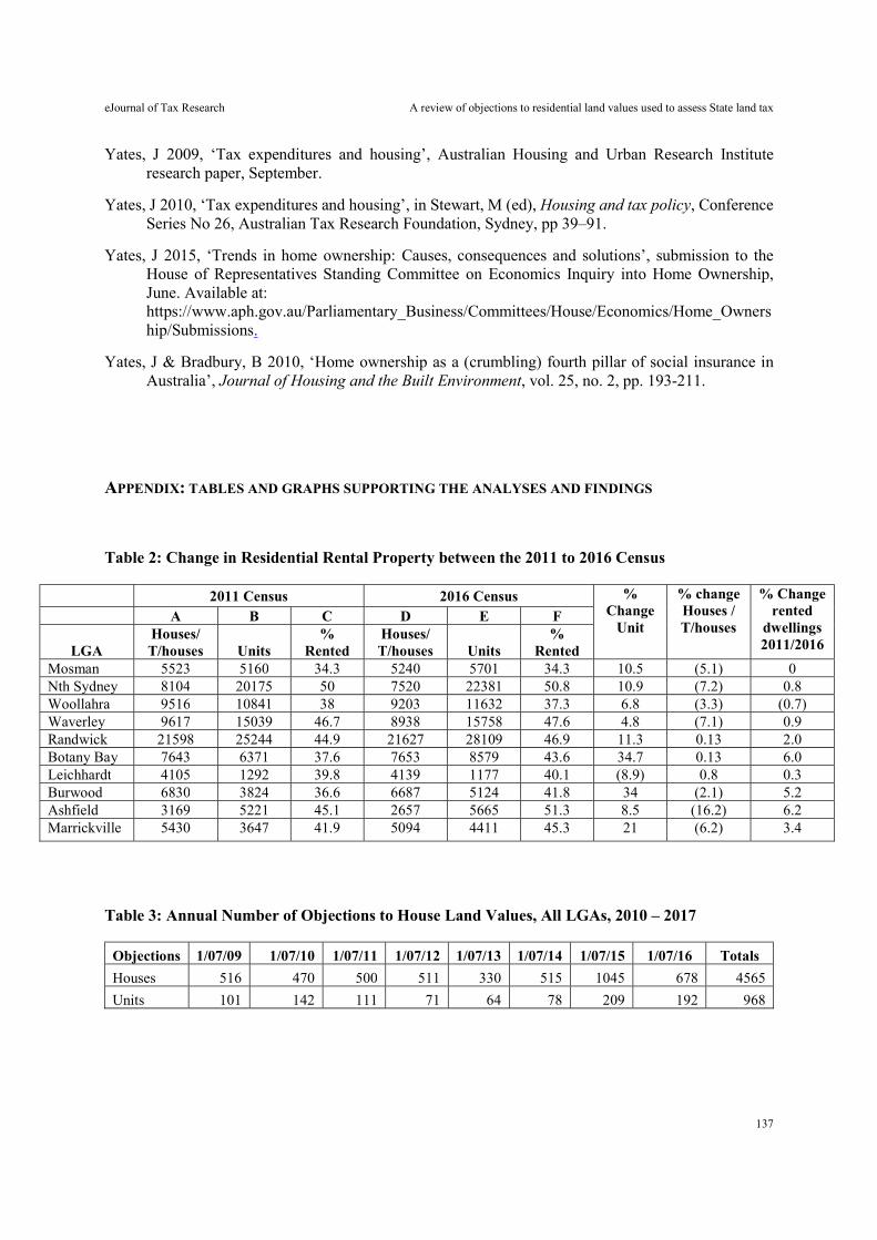
eJournal of Tax Research A review of objections to residential land values used to assess State land tax
137
Yates, J 2009, ‘Tax expenditures and housing’, Australian Housing and Urban Research Institute research paper, September.
Yates, J 2010, ‘Tax expenditures and housing’, in Stewart, M (ed), Housing and tax policy, Conference Series No 26, Australian Tax Research Foundation, Sydney, pp 39–91.
Yates, J 2015, ‘Trends in home ownership: Causes, consequences and solutions’, submission to the House of Representatives Standing Committee on Economics Inquiry into Home Ownership, June. Available at: https://www.aph.gov.au/Parliamentary_Business/Committees/House/Economics/Home_Ownership/Submissions.
Yates, J & Bradbury, B 2010, ‘Home ownership as a (crumbling) fourth pillar of social insurance in Australia’, Journal of Housing and the Built Environment, vol. 25, no. 2, pp. 193-211.
APPENDIX: TABLES AND GRAPHS SUPPORTING THE ANALYSES AND FINDINGS
Table 2: Change in Residential Rental Property between the 2011 to 2016 Census
2011 Census 2016 Census % Change
Unit
% change Houses / T/houses
% Change rented
dwellings 2011/2016
A B C D E F
LGA Houses/ T/houses
Units
% Rented
Houses/ T/houses
Units
% Rented
Mosman 5523 5160 34.3 5240 5701 34.3 10.5 (5.1) 0 Nth Sydney 8104 20175 50 7520 22381 50.8 10.9 (7.2) 0.8 Woollahra 9516 10841 38 9203 11632 37.3 6.8 (3.3) (0.7) Waverley 9617 15039 46.7 8938 15758 47.6 4.8 (7.1) 0.9 Randwick 21598 25244 44.9 21627 28109 46.9 11.3 0.13 2.0 Botany Bay 7643 6371 37.6 7653 8579 43.6 34.7 0.13 6.0 Leichhardt 4105 1292 39.8 4139 1177 40.1 (8.9) 0.8 0.3 Burwood 6830 3824 36.6 6687 5124 41.8 34 (2.1) 5.2 Ashfield 3169 5221 45.1 2657 5665 51.3 8.5 (16.2) 6.2 Marrickville 5430 3647 41.9 5094 4411 45.3 21 (6.2) 3.4
Table 3: Annual Number of Objections to House Land Values, All LGAs, 2010 – 2017
Objections 1/07/09 1/07/10 1/07/11 1/07/12 1/07/13 1/07/14 1/07/15 1/07/16 Totals
Houses 516 470 500 511 330 515 1045 678 4565
Units 101 142 111 71 64 78 209 192 968
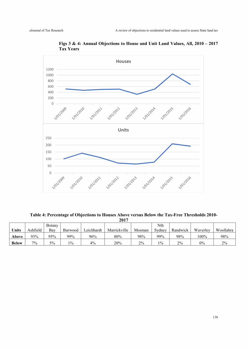
eJournal of Tax Research A review of objections to residential land values used to assess State land tax
138
Figs 3 & 4: Annual Objections to House and Unit Land Values, All, 2010 – 2017 Tax Years
Table 4: Percentage of Objections to Houses Above versus Below the Tax-Free Thresholds 2010-2017
Units Ashfield Botany
Bay Burwood Leichhardt Marrickville Mosman Nth
Sydney Randwick Waverley Woollahra
Above 93% 95% 99% 96% 80% 98% 99% 98% 100% 98%
Below 7% 5% 1% 4% 20% 2% 1% 2% 0% 2%
0200
400600800
10001200
Houses
0
50
100
150
200
250
Units
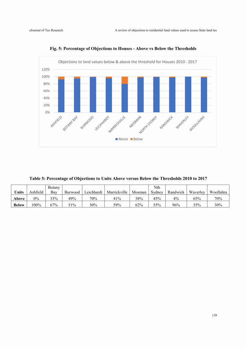
eJournal of Tax Research A review of objections to residential land values used to assess State land tax
139
Fig. 5: Percentage of Objections to Houses - Above vs Below the Thresholds
Table 5: Percentage of Objections to Units Above versus Below the Thresholds 2010 to 2017
Units Ashfield Botany
Bay Burwood Leichhardt Marrickville Mosman Nth
Sydney Randwick Waverley Woollahra
Above 0% 33% 49% 70% 41% 38% 45% 4% 65% 70%
Below 100% 67% 51% 30% 59% 62% 55% 96% 35% 30%
0%
20%
40%
60%
80%
100%
120%
Objections to land values below & above the threshold for Houses 2010 - 2017
Above Below
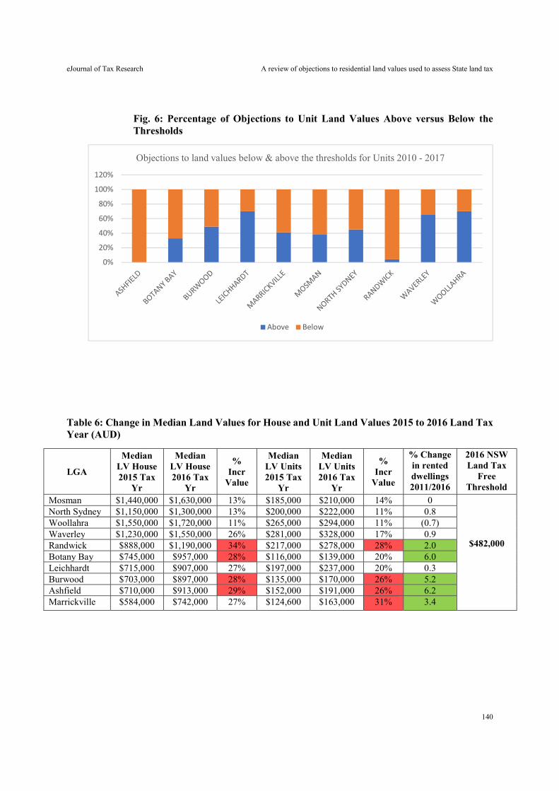
eJournal of Tax Research A review of objections to residential land values used to assess State land tax
140
Fig. 6: Percentage of Objections to Unit Land Values Above versus Below the Thresholds
Table 6: Change in Median Land Values for House and Unit Land Values 2015 to 2016 Land Tax Year (AUD)
LGA
Median LV House 2015 Tax
Yr
Median LV House 2016 Tax
Yr
% Incr
Value
Median LV Units 2015 Tax
Yr
Median LV Units 2016 Tax
Yr
% Incr
Value
% Change in rented dwellings 2011/2016
2016 NSW Land Tax
Free Threshold
Mosman $1,440,000 $1,630,000 13% $185,000 $210,000 14% 0
$482,000
North Sydney $1,150,000 $1,300,000 13% $200,000 $222,000 11% 0.8 Woollahra $1,550,000 $1,720,000 11% $265,000 $294,000 11% (0.7) Waverley $1,230,000 $1,550,000 26% $281,000 $328,000 17% 0.9 Randwick $888,000 $1,190,000 34% $217,000 $278,000 28% 2.0 Botany Bay $745,000 $957,000 28% $116,000 $139,000 20% 6.0 Leichhardt $715,000 $907,000 27% $197,000 $237,000 20% 0.3 Burwood $703,000 $897,000 28% $135,000 $170,000 26% 5.2 Ashfield $710,000 $913,000 29% $152,000 $191,000 26% 6.2 Marrickville $584,000 $742,000 27% $124,600 $163,000 31% 3.4
0%
20%
40%
60%
80%
100%
120%
Objections to land values below & above the thresholds for Units 2010 - 2017
Above Below
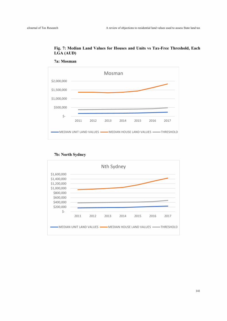
eJournal of Tax Research A review of objections to residential land values used to assess State land tax
141
Fig. 7: Median Land Values for Houses and Units vs Tax-Free Threshold, Each LGA (AUD)
7a: Mosman
7b: North Sydney
$-
$500,000
$1,000,000
$1,500,000
$2,000,000
2011 2012 2013 2014 2015 2016 2017
Mosman
MEDIAN UNIT LAND VALUES MEDIAN HOUSE LAND VALUES THRESHOLD
$- $200,000 $400,000 $600,000 $800,000
$1,000,000 $1,200,000 $1,400,000 $1,600,000
2011 2012 2013 2014 2015 2016 2017
Nth Sydney
MEDIAN UNIT LAND VALUES MEDIAN HOUSE LAND VALUES THRESHOLD
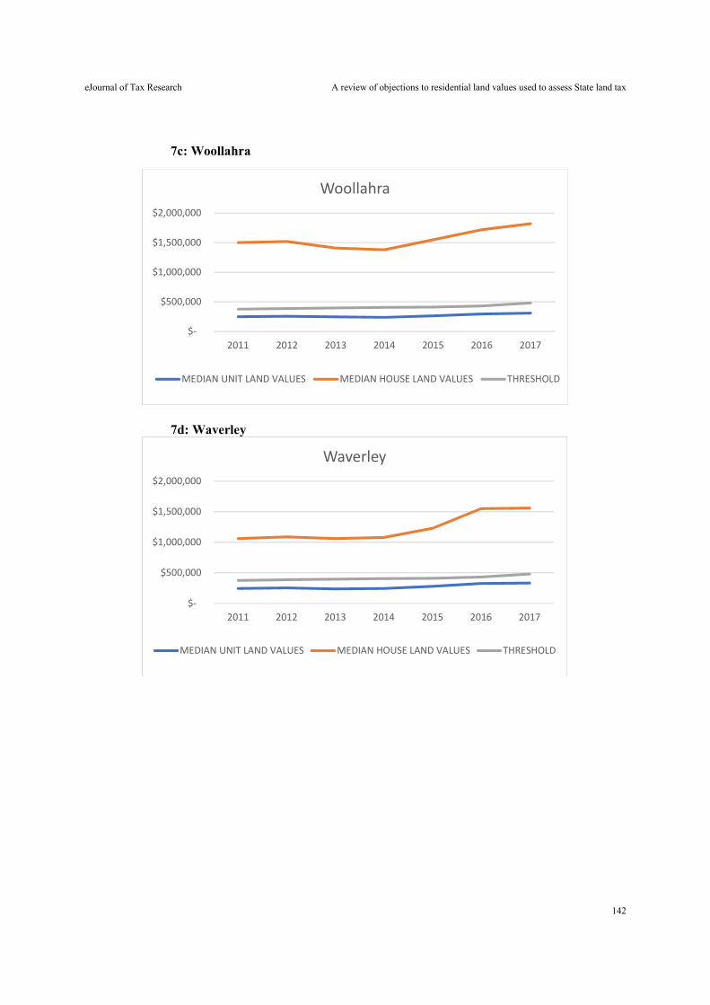
eJournal of Tax Research A review of objections to residential land values used to assess State land tax
142
7c: Woollahra
7d: Waverley
$-
$500,000
$1,000,000
$1,500,000
$2,000,000
2011 2012 2013 2014 2015 2016 2017
Woollahra
MEDIAN UNIT LAND VALUES MEDIAN HOUSE LAND VALUES THRESHOLD
$-
$500,000
$1,000,000
$1,500,000
$2,000,000
2011 2012 2013 2014 2015 2016 2017
Waverley
MEDIAN UNIT LAND VALUES MEDIAN HOUSE LAND VALUES THRESHOLD
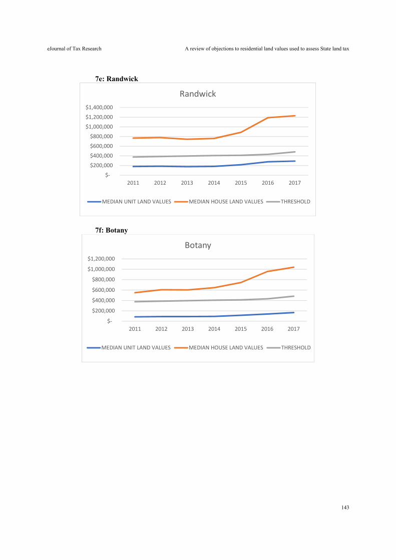
eJournal of Tax Research A review of objections to residential land values used to assess State land tax
143
7e: Randwick
7f: Botany
$-
$200,000
$400,000
$600,000
$800,000
$1,000,000
$1,200,000
$1,400,000
2011 2012 2013 2014 2015 2016 2017
Randwick
MEDIAN UNIT LAND VALUES MEDIAN HOUSE LAND VALUES THRESHOLD
$-
$200,000
$400,000
$600,000
$800,000
$1,000,000
$1,200,000
2011 2012 2013 2014 2015 2016 2017
Botany
MEDIAN UNIT LAND VALUES MEDIAN HOUSE LAND VALUES THRESHOLD
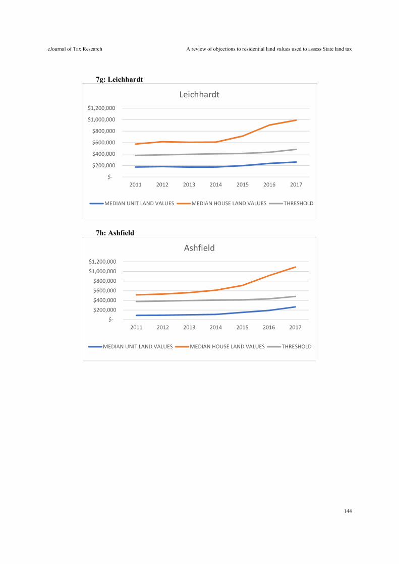
eJournal of Tax Research A review of objections to residential land values used to assess State land tax
144
7g: Leichhardt
7h: Ashfield
$-
$200,000
$400,000
$600,000
$800,000
$1,000,000
$1,200,000
2011 2012 2013 2014 2015 2016 2017
Leichhardt
MEDIAN UNIT LAND VALUES MEDIAN HOUSE LAND VALUES THRESHOLD
$-
$200,000
$400,000
$600,000
$800,000
$1,000,000
$1,200,000
2011 2012 2013 2014 2015 2016 2017
Ashfield
MEDIAN UNIT LAND VALUES MEDIAN HOUSE LAND VALUES THRESHOLD
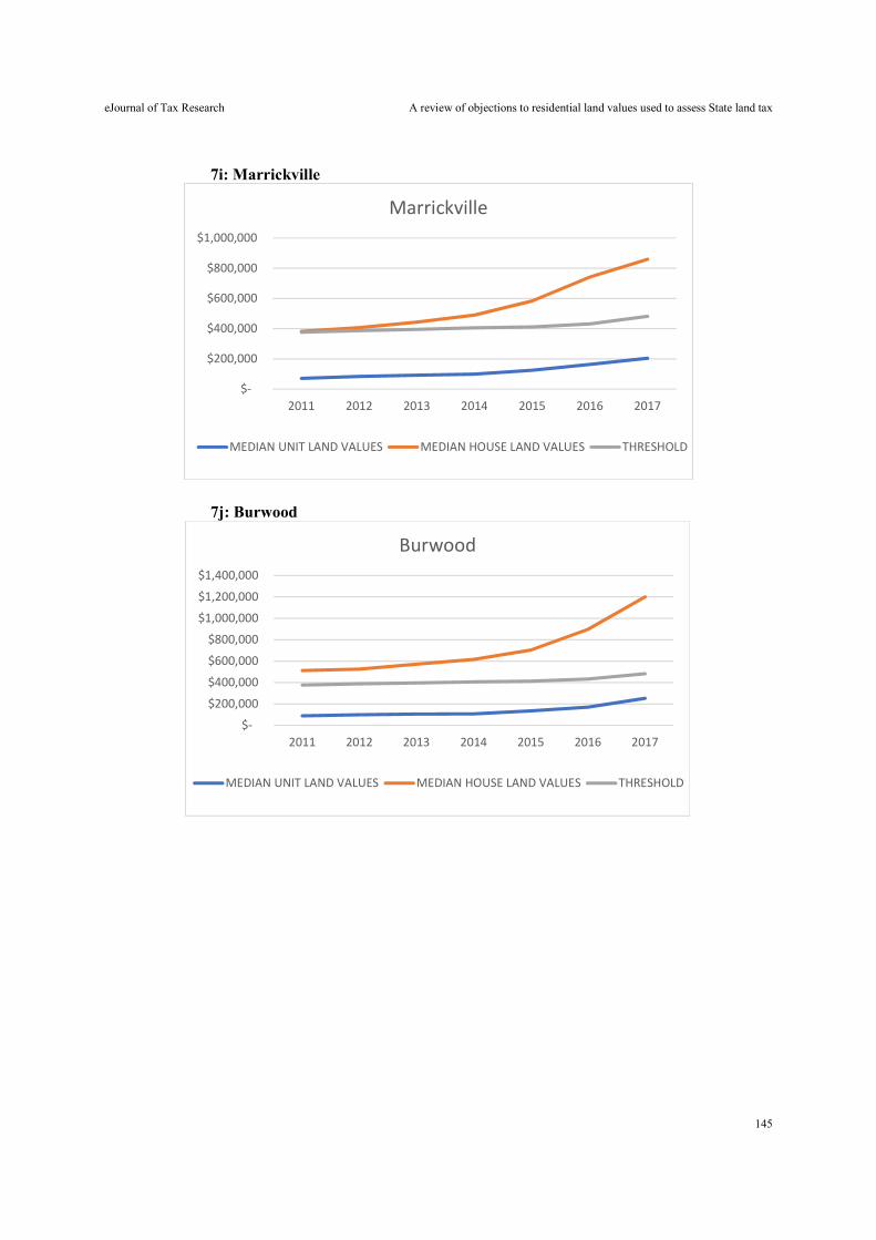
eJournal of Tax Research A review of objections to residential land values used to assess State land tax
145
7i: Marrickville
7j: Burwood
$-
$200,000
$400,000
$600,000
$800,000
$1,000,000
2011 2012 2013 2014 2015 2016 2017
Marrickville
MEDIAN UNIT LAND VALUES MEDIAN HOUSE LAND VALUES THRESHOLD
$-
$200,000
$400,000
$600,000
$800,000
$1,000,000
$1,200,000
$1,400,000
2011 2012 2013 2014 2015 2016 2017
Burwood
MEDIAN UNIT LAND VALUES MEDIAN HOUSE LAND VALUES THRESHOLD
eJournal of Tax Research (2021) vol. 19, no. 1, pp. 146-167
146
Firms’ strategic responses to tax policies
Sylvia Mwamba
Abstract
This article applies an explicit statistical test to a data set of US firms for the period 1988 to 2010 to test for the presence of bunching behaviour around kinks in the tax code implied by strategic cost-shifting. Using the McCrary’s (2008) density test, the study finds evidence of clustering behaviour at bracket thresholds associated with increases in marginal tax rates (convex kinks) and gaps or holes at bracket cut-points where the marginal tax rates drop. This evidence implies that kinked tax codes create incentives for taxpayers to engage in manipulation of taxable income.
Key words: bunching, manipulation, discontinuity, kinks, strategic responses, incentives
School of Business, Black Hills State University, email: [email protected]; [email protected].
eJournal of Tax Research Firms’ strategic responses to tax policies
147
1. INTRODUCTION
Tax policies have been known to create discontinuities in budget sets of economic agents. Such discontinuities usually manifest themselves as jumps in marginal tax rates (kinks) of tax schedules. There is evidence that taxpayers respond to the kinks in the graduated tax codes by bunching around the kink points or avoiding the region around the kink point. This manipulative behaviour usually aimed at influencing the tax liability has been termed strategic responses in the public finance literature (Saez, 2010; Chetty et al., 2011). This article seeks to establish whether firms in the United States have engaged in the manipulation of their incomes in response to the incentives generated by the graduated federal income tax schedule.
This article studies the tax schedules for the period 1988-2010. The study omits the period before 1988 because of the data limitations. Specifically, some of the key variables needed to compute taxable income are not available from 1982 to 1984. Two major reforms, namely the Tax Reform Act of 1986 (TRA 1986: 1988-1992) and the Omnibus Reconciliation Act (OBRA: 1993) were in effect during the study period. The reforms that were undertaken during the study period mainly involved changing the number of brackets and adjusting tax rates. The study follows prior literature (Altig & Carlstrom, 1992) and argues that tax policies that involve simplifying the tax codes generate substantial jumps in marginal tax rates, which may stimulate incentives for tax avoidance behaviour. Any evidence of clustering or bunching around tax bracket thresholds indicates strategic responses to tax codes.
Two types of kinks are considered in the literature. The first one is the convex (or upward) kink which refers to discrete jumps in marginal tax codes. This is the most common type of kink, and it has been a significant focus of research. The US federal corporate tax code features these convex kinks for greater portions of the tax schedule. The second type of kink is the non-convex (downward) kink, which occurs when there is a discrete drop in the marginal tax rate. Although this type of kink is not common, this article examines it briefly since the US federal corporate tax code includes this type of kink. For the US corporate tax code, the non-convex kink appears at the end of the tax schedule.
Understanding and quantifying how taxpayers respond to tax policy changes is vital for estimating the incidence and efficiency of tax policy. As Saez (2010) puts it, the magnitude of the bunching is proportional to the elasticity of taxable income which is of interest to economists. Additionally, the nature of strategic responses induced by a tax code is critical for estimating expected revenue, which is an essential aspect of public finance. Furthermore, by studying how firms respond to incentives generated by tax reforms, this study hopes to provide useful information about the effectiveness and efficiency of the tax reforms.
Although the proportion of corporate income tax in total revenue is not as significant as that of personal income tax, the strategic role that firms play in economic organisations necessitates investigation of the nature of their strategic responses to tax codes. Firms may respond to changes in tax policy through income shifting, exploring tax incentives, strategic reporting of input costs and output, and adjustment of wages or employment, among other responses. Such responses could result in misallocation of resources in the sense that factors of production get directed to less productive activities. Additionally, given the increased role of taxation in government stimulus plans, the importance of
eJournal of Tax Research Firms’ strategic responses to tax policies
148
understanding the responses of economic agents (firms, individuals) to tax policy changes cannot be overemphasised.
The strategic responses can be divided into real responses, in which the firms adjust their productivity (real activity) in response to taxation; and avoidance responses, in which firms engage in various income shifting and timing activities aimed at minimising their tax liability (Slemrod, 1995). Firms would opt to engage in this behaviour to minimise tax-related costs and uncertainties.
In order to investigate the strategic responses of firms, the article builds on the literature that uses bunching methods (Saez, 2010; Chetty et al., 2011) to study strategic responses of economic agents to changes in tax policy. A recent comprehensive review of this literature is provided by Kleven (2016), and it reveals mixed findings with regards to evidence of bunching. For instance, Saez (2010) finds no bunching for wage earners at the large kink points created by the US income tax schedule and Earned Income Tax Credit (EITC). Likewise, Bastani and Selin (2014) find that Swedish wage earners do not bunch at a larger kink. However, evidence of bunching has been established among wage earners in Denmark (Chetty et al., 2011) and Pakistan (Kleven & Waseem, 2013). Researchers have also reported lower taxable income elasticities for wage earners than for self-employed individuals (Saez, 2010; Chetty et al., 2011; Kleven & Waseem, 2013; Bastani & Selin, 2014).
Although most studies on the strategic responses to taxation have primarily focused on estimating the elasticity of taxable income for individual taxpayers (Feldstein, 1995; Saez, 2010; Chetty et al., 2011), there is also extant literature on firms’ strategic responses to tax policies. One such study is by Gruber and Rauh (2007) who use the Compustat data set covering 1960 to 2003 and an instrumental variable technique to estimate the elasticity of taxable income with respect to the effective marginal tax rate. Their study finds an elasticity of 0.2, which indicates that the corporate tax base is moderately responsive to tax rates. A more recent study by Coles et al. (2019) uses bunching and control group methods to investigate the responsiveness of US private firms to tax rates. Using an administrative data set of US private firms, their study estimates an elasticity of taxable income of 0.88, suggesting that US corporations are highly sensitive to tax rates.
This article mainly draws on the literature that applies regression discontinuity design (RDD) approaches to study the impact of taxation (Bruhn & Loeprick, 2014; Kneller & McGowan, 2013; Sánchez, 2014). Rather than applying RDD directly to study the impact of taxation, this study exploits McCrary’s (2008) density test – a validity test employed in RDD to provide evidence showing how the graduated tax code creates incentives for taxpayers to manipulate taxable income.
This article also makes a departure from the focus of prior literature by investigating the strategic responses to the kinks in the corporate income tax schedule and employing an alternative estimation technique with minimal data requirements. Specifically, unlike other studies that typically focus on one kink, this article expands the analysis to all kink points in the corporate tax schedule.
Due to the challenges of obtaining actual tax return data, the study uses Compustat to compute a measure of taxable income. The Compustat database includes financial statements for publicly traded C corporations. The article focuses on the period 1988-2010 since it has complete data for all the variables needed to construct a measure of
eJournal of Tax Research Firms’ strategic responses to tax policies
149
taxable income. Prior studies (Gruber & Rauh, 2007; Hanlon, 2003; Hanlon et al., 2005; Kinney & Swanson, 1993; Mills, Newberry & Novack, 2003) have acknowledged and highlighted the limitations of using Compustat data to estimate taxable income. The limitations mainly arise from the fact that financial statements and tax reporting differ along many dimensions. Additionally, because Compustat only includes publicly traded companies, the sample this article uses is not representative of the entire US corporate sector. Although there is some evidence that taxable income estimated from financial statements is a good proxy for a firm’s actual taxable income (Ayers, Jiang & Laplante, 2009; Plesko, 1999, 2007), the limitations of Compustat data should be kept in mind when interpreting the findings of this article.
The article then uses a combination of graphical techniques (histogram analysis) and explicit statistical procedures (RDD validity test) to test for the presence of bunching behaviour around kinks in the tax code implied by strategic cost-shifting behaviour. The advantage of using these estimation techniques is that they only require one variable (taxable income) to analyse the responses to changes in tax policy.
The results suggest that firms respond to the kinked tax code by avoiding the higher tax side of the bracket threshold. Specifically, this study establishes that firms respond to an increase in tax rate by bunching around the kink point. The results also reveal that a decline in tax rates is associated with gaps or holes around the kink point. These findings suggest that firms manipulate their taxable income in response to changes in tax policy.
The article proceeds as follows. Section 2 provides a brief overview of the US corporate income tax code. Section 3 discusses the estimation strategy, while section 4 describes the data and reports summary statistics. Section 5 presents the results, and section 6 concludes.
2. OVERVIEW OF THE US CORPORATE INCOME TAX CODE
Table 1 summarises the US corporate income tax schedules from 1988 to 2010. It should be noted that the federal income tax code underwent two major reforms during the period 1988 to 2010. The Tax Reform Act of 1986 (TRA 1986) was in effect from 1987 to 1992, while the Omnibus Reconciliation Act (OBRA) covered the period 1993 to 2010. It is also worth noting that the TRA 1986 remains the most comprehensive change to the US tax code. A common feature of these tax schedules is a progressive tax code for smaller firms while at the same time ensuring that larger firms pay more in taxes. This is partly achieved by ‘bubble’ tax rates of 39% and 38% that are designed to neutralise the advantages of lower tax bracket rates. Specifically, the formulation of the ‘bubble’ rates (39% and 38%) helps to ensure that higher-income corporations face higher effective tax rates and pay more taxes (Sherlock & Marples, 2014).
A look at Table 1 also reveals a variation in the number of tax brackets over the period with the OBRA having the highest number of tax brackets. Specifically, the number of tax brackets increased from five during TRA 1986 to eight for the OBRA. Table 1 also shows that the size of the jump or drop in tax rates ranged between 1 and 10 percentage points over the study period.
Additionally, the changes to the US federal income tax system also involved altering the top individual and corporate tax rates. The relationship between these rates is important for understanding income shifting behaviour. For example, when the top individual tax rate is set below the top corporate tax rate, firms could opt to report less
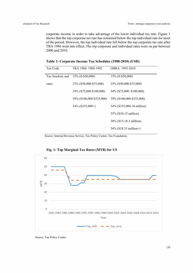
eJournal of Tax Research Firms’ strategic responses to tax policies
150
corporate income in order to take advantage of the lower individual tax rate. Figure 1 shows that the top corporate tax rate has remained below the top individual rate for most of the period. However, the top individual rate fell below the top corporate tax rate after TRA 1986 went into effect. The top corporate and individual rates were on par between 2000 and 2010.
Table 1: Corporate Income Tax Schedules (1988-2010) (USD)
Tax Code TRA 1986: 1988-1992 OBRA: 1993-2010
Tax brackets and
rates
15% (0-$50,000)
25% ($50,000-$75,000)
34% ($75,000 $100,000)
39% ($100,000-$335,000)
34% ($335,000+)
15% (0-$50,000)
25% ($50,000-$75,000)
34% ($75,000 -$100,000)
39% ($100,000-$335,000)
34% ($335,000-10 million)
35% ($10-15 million)
38% ($15-18.3 million)
34% ($18.33 million+)
Source: Internal Revenue Service; Tax Policy Center; Tax Foundation.
Fig. 1: Top Marginal Tax Rates (MTR) for US
Source: Tax Policy Center.
0
10
20
30
40
50
60
1982 1984 1986 1988 1990 1992 1994 1996 1998 2000 2002 2004 2006 2008 2010 2012 2014
MTR
Year
Top_indv Top_corp
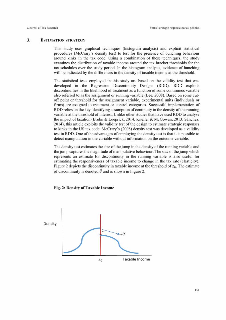
eJournal of Tax Research Firms’ strategic responses to tax policies
151
3. ESTIMATION STRATEGY
This study uses graphical techniques (histogram analysis) and explicit statistical procedures (McCrary’s density test) to test for the presence of bunching behaviour around kinks in the tax code. Using a combination of these techniques, the study examines the distribution of taxable income around the tax bracket thresholds for the tax schedules over the study period. In the histogram analysis, evidence of bunching will be indicated by the differences in the density of taxable income at the threshold.
The statistical tests employed in this study are based on the validity test that was developed in the Regression Discontinuity Designs (RDD). RDD exploits discontinuities in the likelihood of treatment as a function of some continuous variable also referred to as the assignment or running variable (Lee, 2008). Based on some cut-off point or threshold for the assignment variable, experimental units (individuals or firms) are assigned to treatment or control categories. Successful implementation of RDD relies on the key identifying assumption of continuity in the density of the running variable at the threshold of interest. Unlike other studies that have used RDD to analyse the impact of taxation (Bruhn & Loeprick, 2014; Kneller & McGowan, 2013; Sánchez, 2014), this article exploits the validity test of the design to estimate strategic responses to kinks in the US tax code. McCrary’s (2008) density test was developed as a validity test in RDD. One of the advantages of employing the density test is that it is possible to detect manipulation in the variable without information on the outcome variable.
The density test estimates the size of the jump in the density of the running variable and the jump captures the magnitude of manipulative behaviour. The size of the jump which represents an estimate for discontinuity in the running variable is also useful for estimating the responsiveness of taxable income to change in the tax rate (elasticity). Figure 2 depicts the discontinuity in taxable income at the threshold of 𝑧 . The estimate of discontinuity is denoted 𝜃 and is shown in Figure 2.
Fig. 2: Density of Taxable Income
=𝜃 Type equation here.
𝑧0 Taxable Income
Density
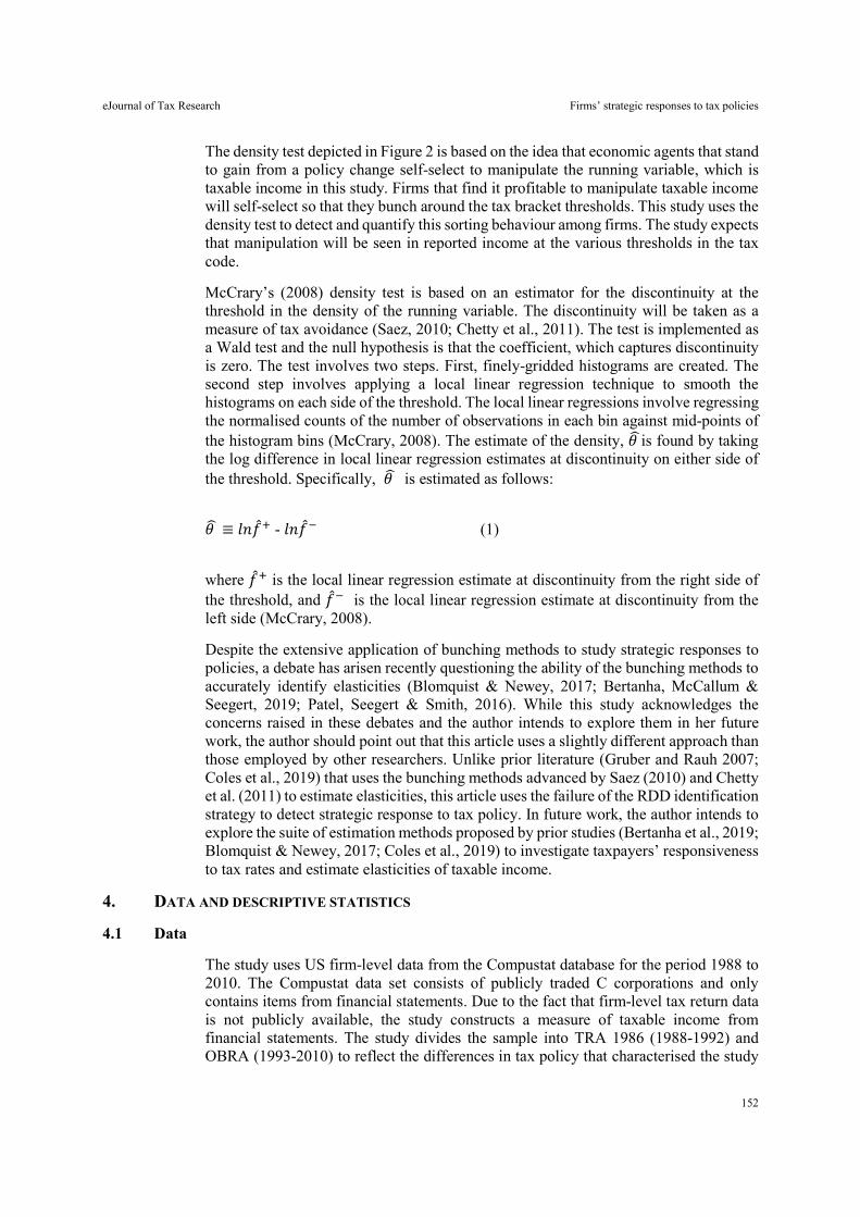
eJournal of Tax Research Firms’ strategic responses to tax policies
152
The density test depicted in Figure 2 is based on the idea that economic agents that stand to gain from a policy change self-select to manipulate the running variable, which is taxable income in this study. Firms that find it profitable to manipulate taxable income will self-select so that they bunch around the tax bracket thresholds. This study uses the density test to detect and quantify this sorting behaviour among firms. The study expects that manipulation will be seen in reported income at the various thresholds in the tax code.
McCrary’s (2008) density test is based on an estimator for the discontinuity at the threshold in the density of the running variable. The discontinuity will be taken as a measure of tax avoidance (Saez, 2010; Chetty et al., 2011). The test is implemented as a Wald test and the null hypothesis is that the coefficient, which captures discontinuity is zero. The test involves two steps. First, finely-gridded histograms are created. The second step involves applying a local linear regression technique to smooth the histograms on each side of the threshold. The local linear regressions involve regressing the normalised counts of the number of observations in each bin against mid-points of the histogram bins (McCrary, 2008). The estimate of the density, 𝜃 is found by taking the log difference in local linear regression estimates at discontinuity on either side of the threshold. Specifically, 𝜃 is estimated as follows:
𝜃 ≡ 𝑙𝑛𝑓 - 𝑙𝑛𝑓 (1)
where 𝑓 is the local linear regression estimate at discontinuity from the right side of the threshold, and 𝑓 is the local linear regression estimate at discontinuity from the left side (McCrary, 2008).
Despite the extensive application of bunching methods to study strategic responses to policies, a debate has arisen recently questioning the ability of the bunching methods to accurately identify elasticities (Blomquist & Newey, 2017; Bertanha, McCallum & Seegert, 2019; Patel, Seegert & Smith, 2016). While this study acknowledges the concerns raised in these debates and the author intends to explore them in her future work, the author should point out that this article uses a slightly different approach than those employed by other researchers. Unlike prior literature (Gruber and Rauh 2007; Coles et al., 2019) that uses the bunching methods advanced by Saez (2010) and Chetty et al. (2011) to estimate elasticities, this article uses the failure of the RDD identification strategy to detect strategic response to tax policy. In future work, the author intends to explore the suite of estimation methods proposed by prior studies (Bertanha et al., 2019; Blomquist & Newey, 2017; Coles et al., 2019) to investigate taxpayers’ responsiveness to tax rates and estimate elasticities of taxable income.
4. DATA AND DESCRIPTIVE STATISTICS
4.1 Data
The study uses US firm-level data from the Compustat database for the period 1988 to 2010. The Compustat data set consists of publicly traded C corporations and only contains items from financial statements. Due to the fact that firm-level tax return data is not publicly available, the study constructs a measure of taxable income from financial statements. The study divides the sample into TRA 1986 (1988-1992) and OBRA (1993-2010) to reflect the differences in tax policy that characterised the study

eJournal of Tax Research Firms’ strategic responses to tax policies
153
period. Additionally, the study excludes financial institutions (SIC codes 6000–6999), utilities (SIC codes 4900–4999), and firms that are not incorporated in the US because they are subjected to different tax rules and regulations (Ayers et al., 2009). Further, the study’s final sample only includes firms with complete data on all variables needed to construct the measure of taxable income.
Taxable income is the main variable of interest in this study and the study follows Hanlon, Laplante and Shevlin (2005) and constructs it as follows:
𝑇𝑎𝑥𝑎𝑏𝑙𝑒 𝐼𝑛𝑐𝑜𝑚𝑒 =
− Δ𝑁𝑂𝐿 (2)
where tax expense is a sum of foreign and federal income taxes; tax rate is as depicted in Table 2; and Δ𝑁𝑂𝐿 is the change in net operating loss (NOL) carryforwards.
These variables are readily available in Compustat for all the firms in the sample. To compute the taxable income, the study uses the information in Table 1 to reconstruct tax brackets for the tax expense variable. This is done to ensure that the measure of taxable income reflects the progressive nature of the tax code by allowing the estimate of tax liability to vary by tax rate. This approach is a slight departure from the accounting literature that uses the top tax rate in the denominator of equation 2. The accounting literature assumes that all firms are large, and are all subjected to the same top tax rate. This assumption justifies their reasoning to divide tax expense by the top rate when computing the taxable income variable. Table 2 presents the tax expense brackets and associated tax rates that this study uses to construct the measure of tax avoidance.
Table 2: Tax Expense Brackets and Tax Rates (TRA 1986)
Tax rate (%)
Taxable income (USD million)
bracket
Tax expense (USD million) bracket
0.15 (0 - 0.05) (0 - 0.008)
0.25 (0.05 - 0.075) (0.008 - 0.014)
0.34 (0.075 - 0.1) (0.014 - 0.022)
0.39 (0.1 - 0.335) (0.022 - 0.114)
0.34 (0.335 - 10) (0.114 - 3.29)
0.35 (10 - 15) (3.29 - 5.04)
0.38 (15 - 18.3) (5.04 - 6.30)
0.35 18.3+ 6.30+
eJournal of Tax Research Firms’ strategic responses to tax policies
154
Using the information in Table 2, the study is able to determine the appropriate tax rate for each of the tax expense brackets, and then use it to construct the measure of taxable income. In order to obtain a more accurate estimate of taxable income from the financial statements, the study follows the accounting literature and subtracts the change in net operating loss (NOL) carryforwards (Ayers et al., 2009).
There are several limitations associated with using the Compustat database to construct a measure of taxable income. First, Compustat contains financial statements data rather than actual tax return data. Because financial reporting differs from tax reporting, using financial statement data to estimate taxable income is challenging and may result in inaccurate taxable income estimates. For example, stock option deduction and tax cushion are treated differently for financial accounting purposes. Differences in consolidation rules for financial accounting and tax purposes also account for disparities between estimates of taxable income and tax liability from actual tax returns (Hanlon, 2003; Hanlon et al., 2005). Second, Compustat suffers from coding and reporting errors, especially for special items such as NOL carryforwards (Kinney & Swanson, 1993; Mills et al., 2003). Mills et al. (2003) also emphasise the need to be careful when using financial statement data to estimate taxable income for firms with foreign operations or acquisitions. Another issue with using the Compustat data set to obtain estimates of taxable income is that the data set is not representative of the entire US corporate sector. Despite these limitations, there is evidence that shows that taxable income estimated from financial statements is a reasonable estimate for actual taxable income as reflected on a tax return (Ayers et al., 2009; Plesko, 1999, 2007). Nevertheless, the data limitations and caveats highlighted above should be kept in mind when interpreting and generalising the findings of this article.
4.2 Descriptive statistics
Table 3 presents summary statistics for the variables of interest in this study. Since the analysis is done for two different tax policies or schedules, the study reports summary statistics separately for each tax schedule. Table 3a presents summary statistics for the TRA 1986 tax code (1988-1992), while Table 3b reports statistics for the 1993-2010 period. The sample in Table 3a is much smaller than the one in Table 3b because it only includes firms with taxable income between USD 0 and USD 0.5 million. The study restricts the sample this way because the highest tax bracket under TRA 1986 starts at USD 0.335 million, and the methods employed in this study only rely on observations in the neighbourhood of the bracket thresholds. Correspondingly, the study restricts the sample for Table 3b to include firms with taxable income between USD 0 and USD 25 million since the top tax bracket for the 1993-2010 tax code starts at USD 18.33 million.
The statistics in Table 3a show that the average firm in the sample has about USD 109 million in assets, USD 27,000 in tax expenses, a negative change in NOL carryforwards amounting to USD 39,000 and USD 119,000 in taxable income. When put in the context of the applicable tax schedule, the mean taxable income of USD 119,000 implies that an average firm falls in the fourth tax bracket (Table 1, column 2). This tax bracket also corresponds to the bubble tax rate. As explained earlier, the bubble tax rates are designed to ensure that higher-income corporations face a higher effective tax rate. Having the mean income that falls within this high-tax bracket is somewhat unexpected, given the study’s hypothesis that firms would opt to avoid the higher tax side of the bracket threshold. This result further suggests that an average firm faces a higher effective tax rate in the post-1986 reform period. Further, the presence of NOLs also indicates that firms have opportunities to influence their tax liabilities.
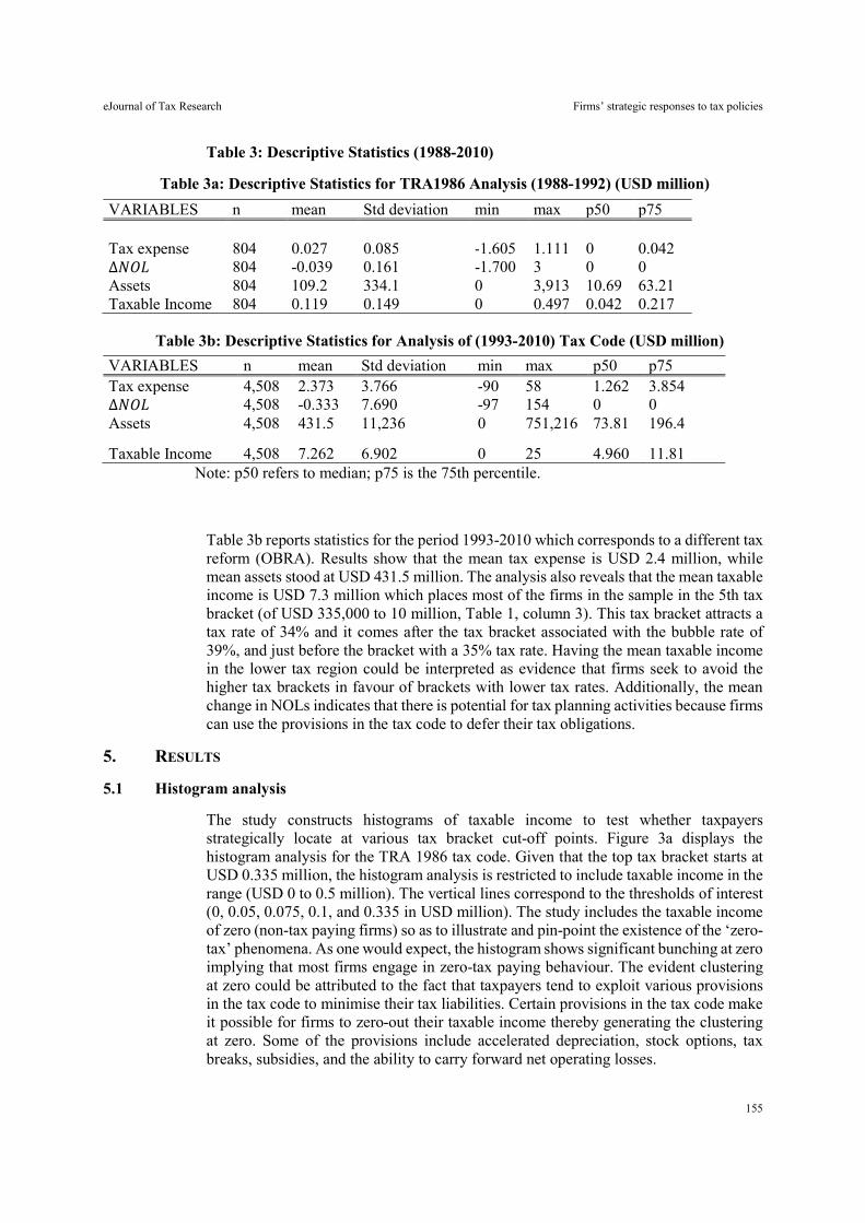
eJournal of Tax Research Firms’ strategic responses to tax policies
155
Table 3: Descriptive Statistics (1988-2010)
Table 3a: Descriptive Statistics for TRA1986 Analysis (1988-1992) (USD million)
Table 3b: Descriptive Statistics for Analysis of (1993-2010) Tax Code (USD million)
Note: p50 refers to median; p75 is the 75th percentile.
Table 3b reports statistics for the period 1993-2010 which corresponds to a different tax reform (OBRA). Results show that the mean tax expense is USD 2.4 million, while mean assets stood at USD 431.5 million. The analysis also reveals that the mean taxable income is USD 7.3 million which places most of the firms in the sample in the 5th tax bracket (of USD 335,000 to 10 million, Table 1, column 3). This tax bracket attracts a tax rate of 34% and it comes after the tax bracket associated with the bubble rate of 39%, and just before the bracket with a 35% tax rate. Having the mean taxable income in the lower tax region could be interpreted as evidence that firms seek to avoid the higher tax brackets in favour of brackets with lower tax rates. Additionally, the mean change in NOLs indicates that there is potential for tax planning activities because firms can use the provisions in the tax code to defer their tax obligations.
5. RESULTS
5.1 Histogram analysis
The study constructs histograms of taxable income to test whether taxpayers strategically locate at various tax bracket cut-off points. Figure 3a displays the histogram analysis for the TRA 1986 tax code. Given that the top tax bracket starts at USD 0.335 million, the histogram analysis is restricted to include taxable income in the range (USD 0 to 0.5 million). The vertical lines correspond to the thresholds of interest (0, 0.05, 0.075, 0.1, and 0.335 in USD million). The study includes the taxable income of zero (non-tax paying firms) so as to illustrate and pin-point the existence of the ‘zero-tax’ phenomena. As one would expect, the histogram shows significant bunching at zero implying that most firms engage in zero-tax paying behaviour. The evident clustering at zero could be attributed to the fact that taxpayers tend to exploit various provisions in the tax code to minimise their tax liabilities. Certain provisions in the tax code make it possible for firms to zero-out their taxable income thereby generating the clustering at zero. Some of the provisions include accelerated depreciation, stock options, tax breaks, subsidies, and the ability to carry forward net operating losses.
VARIABLES n mean Std deviation min max p50 p75 Tax expense 804 0.027 0.085 -1.605 1.111 0 0.042 ∆𝑁𝑂𝐿 804 -0.039 0.161 -1.700 3 0 0 Assets 804 109.2 334.1 0 3,913 10.69 63.21 Taxable Income 804 0.119 0.149 0 0.497 0.042 0.217
VARIABLES n mean Std deviation min max p50 p75 Tax expense 4,508 2.373 3.766 -90 58 1.262 3.854 ∆𝑁𝑂𝐿 4,508 -0.333 7.690 -97 154 0 0 Assets 4,508 431.5 11,236 0 751,216 73.81 196.4
Taxable Income 4,508 7.262 6.902 0 25 4.960 11.81
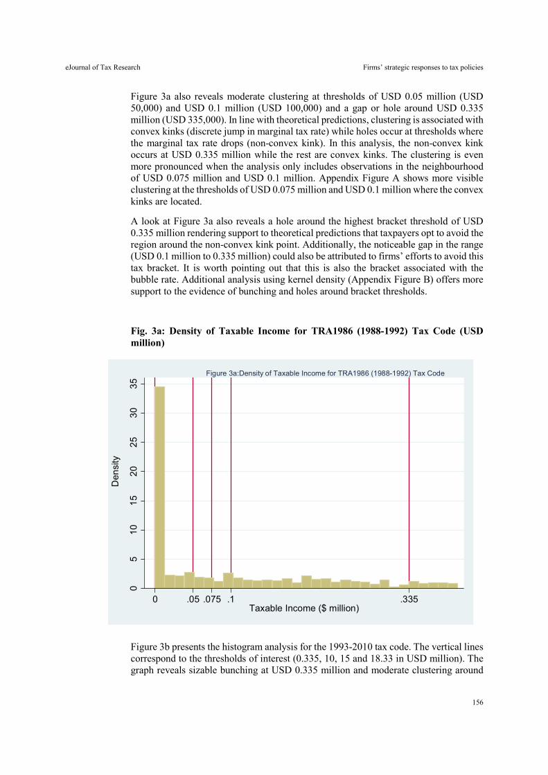
eJournal of Tax Research Firms’ strategic responses to tax policies
156
Figure 3a also reveals moderate clustering at thresholds of USD 0.05 million (USD 50,000) and USD 0.1 million (USD 100,000) and a gap or hole around USD 0.335 million (USD 335,000). In line with theoretical predictions, clustering is associated with convex kinks (discrete jump in marginal tax rate) while holes occur at thresholds where the marginal tax rate drops (non-convex kink). In this analysis, the non-convex kink occurs at USD 0.335 million while the rest are convex kinks. The clustering is even more pronounced when the analysis only includes observations in the neighbourhood of USD 0.075 million and USD 0.1 million. Appendix Figure A shows more visible clustering at the thresholds of USD 0.075 million and USD 0.1 million where the convex kinks are located.
A look at Figure 3a also reveals a hole around the highest bracket threshold of USD 0.335 million rendering support to theoretical predictions that taxpayers opt to avoid the region around the non-convex kink point. Additionally, the noticeable gap in the range (USD 0.1 million to 0.335 million) could also be attributed to firms’ efforts to avoid this tax bracket. It is worth pointing out that this is also the bracket associated with the bubble rate. Additional analysis using kernel density (Appendix Figure B) offers more support to the evidence of bunching and holes around bracket thresholds.
Fig. 3a: Density of Taxable Income for TRA1986 (1988-1992) Tax Code (USD million)
Figure 3b presents the histogram analysis for the 1993-2010 tax code. The vertical lines correspond to the thresholds of interest (0.335, 10, 15 and 18.33 in USD million). The graph reveals sizable bunching at USD 0.335 million and moderate clustering around
05
10
15
20
25
30
35
Den
sity
0 .05 .075 .1 .335Taxable Income ($ million)
Figure 3a:Density of Taxable Income for TRA1986 (1988-1992) Tax Code
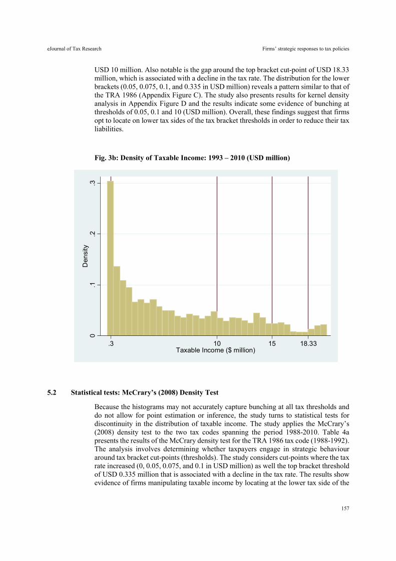
eJournal of Tax Research Firms’ strategic responses to tax policies
157
USD 10 million. Also notable is the gap around the top bracket cut-point of USD 18.33 million, which is associated with a decline in the tax rate. The distribution for the lower brackets (0.05, 0.075, 0.1, and 0.335 in USD million) reveals a pattern similar to that of the TRA 1986 (Appendix Figure C). The study also presents results for kernel density analysis in Appendix Figure D and the results indicate some evidence of bunching at thresholds of 0.05, 0.1 and 10 (USD million). Overall, these findings suggest that firms opt to locate on lower tax sides of the tax bracket thresholds in order to reduce their tax liabilities.
Fig. 3b: Density of Taxable Income: 1993 – 2010 (USD million)
5.2 Statistical tests: McCrary’s (2008) Density Test
Because the histograms may not accurately capture bunching at all tax thresholds and do not allow for point estimation or inference, the study turns to statistical tests for discontinuity in the distribution of taxable income. The study applies the McCrary’s (2008) density test to the two tax codes spanning the period 1988-2010. Table 4a presents the results of the McCrary density test for the TRA 1986 tax code (1988-1992). The analysis involves determining whether taxpayers engage in strategic behaviour around tax bracket cut-points (thresholds). The study considers cut-points where the tax rate increased (0, 0.05, 0.075, and 0.1 in USD million) as well the top bracket threshold of USD 0.335 million that is associated with a decline in the tax rate. The results show evidence of firms manipulating taxable income by locating at the lower tax side of the
0.1
.2.3
Den
sity
.3 10 15 18.33Taxable Income ($ million)
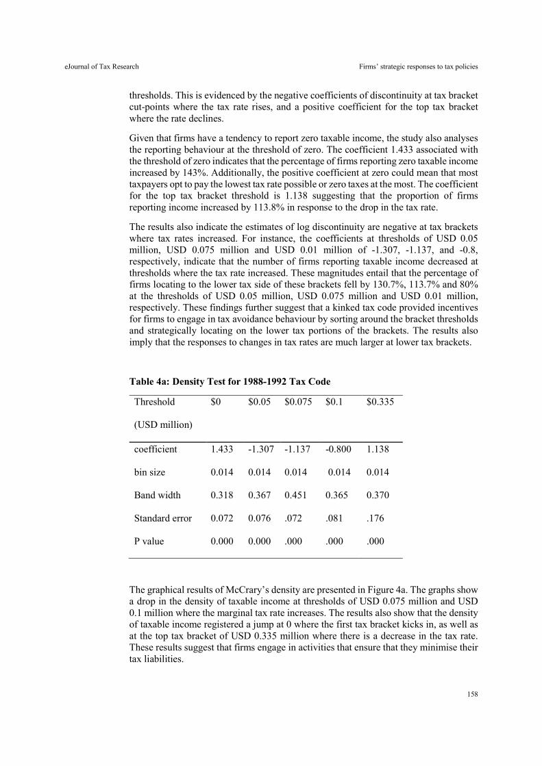
eJournal of Tax Research Firms’ strategic responses to tax policies
158
thresholds. This is evidenced by the negative coefficients of discontinuity at tax bracket cut-points where the tax rate rises, and a positive coefficient for the top tax bracket where the rate declines.
Given that firms have a tendency to report zero taxable income, the study also analyses the reporting behaviour at the threshold of zero. The coefficient 1.433 associated with the threshold of zero indicates that the percentage of firms reporting zero taxable income increased by 143%. Additionally, the positive coefficient at zero could mean that most taxpayers opt to pay the lowest tax rate possible or zero taxes at the most. The coefficient for the top tax bracket threshold is 1.138 suggesting that the proportion of firms reporting income increased by 113.8% in response to the drop in the tax rate.
The results also indicate the estimates of log discontinuity are negative at tax brackets where tax rates increased. For instance, the coefficients at thresholds of USD 0.05 million, USD 0.075 million and USD 0.01 million of -1.307, -1.137, and -0.8, respectively, indicate that the number of firms reporting taxable income decreased at thresholds where the tax rate increased. These magnitudes entail that the percentage of firms locating to the lower tax side of these brackets fell by 130.7%, 113.7% and 80% at the thresholds of USD 0.05 million, USD 0.075 million and USD 0.01 million, respectively. These findings further suggest that a kinked tax code provided incentives for firms to engage in tax avoidance behaviour by sorting around the bracket thresholds and strategically locating on the lower tax portions of the brackets. The results also imply that the responses to changes in tax rates are much larger at lower tax brackets.
Table 4a: Density Test for 1988-1992 Tax Code
Threshold
(USD million)
$0 $0.05 $0.075 $0.1 $0.335
coefficient 1.433 -1.307 -1.137 -0.800 1.138
bin size 0.014 0.014 0.014 0.014 0.014
Band width 0.318 0.367 0.451 0.365 0.370
Standard error 0.072 0.076 .072 .081 .176
P value 0.000 0.000 .000 .000 .000
The graphical results of McCrary’s density are presented in Figure 4a. The graphs show a drop in the density of taxable income at thresholds of USD 0.075 million and USD 0.1 million where the marginal tax rate increases. The results also show that the density of taxable income registered a jump at 0 where the first tax bracket kicks in, as well as at the top tax bracket of USD 0.335 million where there is a decrease in the tax rate. These results suggest that firms engage in activities that ensure that they minimise their tax liabilities.
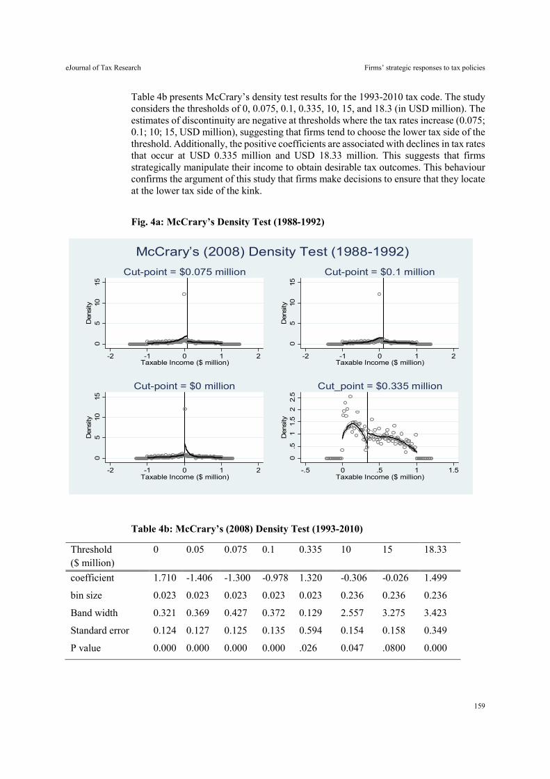
eJournal of Tax Research Firms’ strategic responses to tax policies
159
Table 4b presents McCrary’s density test results for the 1993-2010 tax code. The study considers the thresholds of 0, 0.075, 0.1, 0.335, 10, 15, and 18.3 (in USD million). The estimates of discontinuity are negative at thresholds where the tax rates increase (0.075; 0.1; 10; 15, USD million), suggesting that firms tend to choose the lower tax side of the threshold. Additionally, the positive coefficients are associated with declines in tax rates that occur at USD 0.335 million and USD 18.33 million. This suggests that firms strategically manipulate their income to obtain desirable tax outcomes. This behaviour confirms the argument of this study that firms make decisions to ensure that they locate at the lower tax side of the kink.
Fig. 4a: McCrary’s Density Test (1988-1992)
Table 4b: McCrary’s (2008) Density Test (1993-2010)
Threshold ($ million)
0 0.05 0.075 0.1 0.335 10 15 18.33
coefficient 1.710 -1.406 -1.300 -0.978 1.320 -0.306 -0.026 1.499
bin size 0.023 0.023 0.023 0.023 0.023 0.236 0.236 0.236
Band width 0.321 0.369 0.427 0.372 0.129 2.557 3.275 3.423
Standard error 0.124 0.127 0.125 0.135 0.594 0.154 0.158 0.349
P value 0.000 0.000 0.000 0.000 .026 0.047 .0800 0.000
05
1015
Den
sity
-2 -1 0 1 2Taxable Income ($ million)
Cut-point = $0.075 million
05
1015
Den
sity
-2 -1 0 1 2Taxable Income ($ million)
Cut-point = $0.1 million
05
1015
Dens
ity
-2 -1 0 1 2Taxable Income ($ million)
Cut-point = $0 million
0.5
11.
52
2.5
Dens
ity
-.5 0 .5 1 1.5Taxable Income ($ million)
Cut_point = $0.335 million
McCrary’s (2008) Density Test (1988-1992)
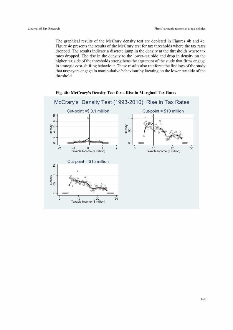
eJournal of Tax Research Firms’ strategic responses to tax policies
160
The graphical results of the McCrary density test are depicted in Figures 4b and 4c. Figure 4c presents the results of the McCrary test for tax thresholds where the tax rates dropped. The results indicate a discrete jump in the density at the thresholds where tax rates dropped. The rise in the density to the lower-tax side and drop in density on the higher tax side of the thresholds strengthens the argument of the study that firms engage in strategic cost-shifting behaviour. These results also reinforce the findings of the study that taxpayers engage in manipulative behaviour by locating on the lower tax side of the threshold.
Fig. 4b: McCrary's Density Test for a Rise in Marginal Tax Rates
02
46
810
Den
sity
-2 -1 0 1 2Taxable Income ($ million)
Cut-point =$ 0.1 million
0.0
5.1
Den
sity
0 10 20 30Taxable Income ($ million)
Cut-point = $10 million
0.0
5.1
.15
Den
sity
0 10 20 30Taxable Income ($ million)
Cut-point = $15 million
McCrary’s Density Test (1993-2010): Rise in Tax Rates
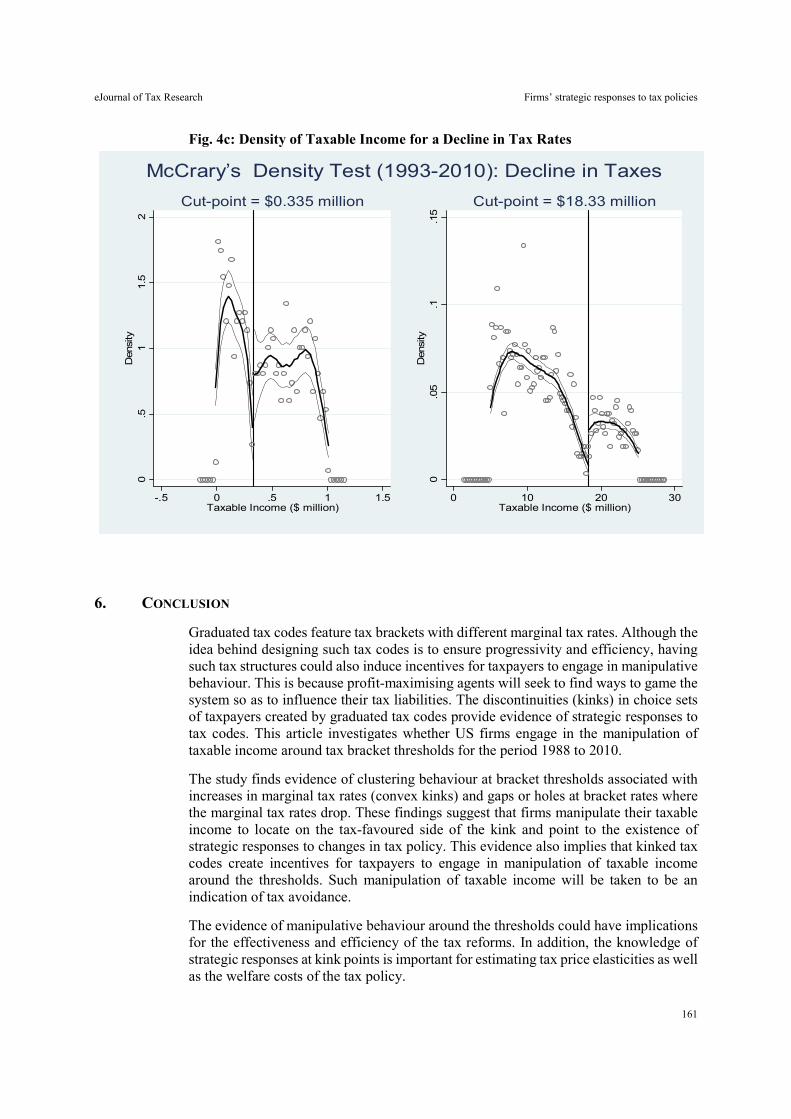
eJournal of Tax Research Firms’ strategic responses to tax policies
161
Fig. 4c: Density of Taxable Income for a Decline in Tax Rates
6. CONCLUSION
Graduated tax codes feature tax brackets with different marginal tax rates. Although the idea behind designing such tax codes is to ensure progressivity and efficiency, having such tax structures could also induce incentives for taxpayers to engage in manipulative behaviour. This is because profit-maximising agents will seek to find ways to game the system so as to influence their tax liabilities. The discontinuities (kinks) in choice sets of taxpayers created by graduated tax codes provide evidence of strategic responses to tax codes. This article investigates whether US firms engage in the manipulation of taxable income around tax bracket thresholds for the period 1988 to 2010.
The study finds evidence of clustering behaviour at bracket thresholds associated with increases in marginal tax rates (convex kinks) and gaps or holes at bracket rates where the marginal tax rates drop. These findings suggest that firms manipulate their taxable income to locate on the tax-favoured side of the kink and point to the existence of strategic responses to changes in tax policy. This evidence also implies that kinked tax codes create incentives for taxpayers to engage in manipulation of taxable income around the thresholds. Such manipulation of taxable income will be taken to be an indication of tax avoidance.
The evidence of manipulative behaviour around the thresholds could have implications for the effectiveness and efficiency of the tax reforms. In addition, the knowledge of strategic responses at kink points is important for estimating tax price elasticities as well as the welfare costs of the tax policy.
0.5
11.
52
Den
sity
-.5 0 .5 1 1.5Taxable Income ($ million)
Cut-point = $0.335 million
0.0
5.1
.15
Den
sity
0 10 20 30Taxable Income ($ million)
Cut-point = $18.33 million
McCrary’s Density Test (1993-2010): Decline in Taxes

eJournal of Tax Research Firms’ strategic responses to tax policies
162
This study makes a contribution to the literature by constructing a measure of taxable income from financial statements using a slightly different approach than that widely used in the accounting literature. Unlike the accounting literature that constructs taxable income by dividing tax expenses by the top tax rate, this study allows the tax expenses to have varying tax rates. The study does so by constructing tax brackets for tax expenses that it then uses in the formula for computing taxable income. This study also contributes to the literature by focusing on examining strategic responses to corporate tax schedules. To the author’s knowledge, strategic responses to personal income tax schedules have received more attention than responses to corporate income tax codes. Additionally, the study contributes to the literature by applying a density test to detect and quantify the strategic responses over a long study period that spans two different tax reforms.
One particular challenge of the many that continue to trouble researchers in the public finance and tax fields has to do with the lack of actual tax return data. As a result, most studies rely on estimates of taxable income and tax avoidance that unfortunately have issues. Some of the issues involve measurement errors that may have an adverse effect on inferences. Despite these data issues, this study helps to extend the literature by using an estimate of taxable income and methods that are more accurate at detecting and quantifying tax avoidance activities. For instance, while prior studies indicate that the 1986 reform was effective in reducing tax avoidance, this study shows evidence of manipulative behaviour. This is an important contribution to the tax avoidance literature and the findings of this article have potential implications for the design of more effective and efficient tax systems.
7. REFERENCES
Altig, D & Carlstrom C T 1992, ‘The efficiency and welfare effects of tax reform: Are fewer tax brackets better than more?’, Federal Reserve Bank of Cleveland working paper 9212, November.
Ayers, B C, Jiang, J & Laplante, S K 2009, ‘Taxable income as a performance measure: The effects of tax planning and earnings quality’, Contemporary Accounting Research, vol. 26, no. 1, pp. 15-54.
Bastani, S & Selin, H 2014, ‘Bunching and non-bunching at kink points of the Swedish tax schedule’, Journal of Public Economics, vol. 109, pp. 36-49.
Bertanha, M, McCallum, A H & Seegert, N 2019, ‘Better bunching, nicer notching’, draft working paper, 23 December.
Blomquist, S & Newey, W K 2017, ‘The bunching estimator cannot identify the taxable income elasticity’, National Bureau of Economic Research working paper 24136, December.
Bruhn, M & Loeprick, J 2014, ‘Small business tax policy, informality, and tax evasion – Evidence from Georgia’, World Bank Policy Research working paper 7010.
Chetty, R, Friedman, J N, Olsen, T & Pistaferri, L 2011, ‘Adjustment costs, firm responses, and micro vs. macro labor supply elasticities: Evidence from Danish tax records’, The Quarterly Journal of Economics, vol. 126, no. 2, pp. 749-804.
eJournal of Tax Research Firms’ strategic responses to tax policies
163
Coles, J L, Patel, E, Seegert, N & Smith, M 2019, ‘How do firms respond to corporate taxes?’, working paper, https://papers.ssrn.com/sol3/papers.cfm?abstract_id=3167369.
Feldstein, M 1995, ‘The effect of marginal tax rates on taxable income: A panel study of the 1986 Tax Reform Act’, Journal of Political Economy, vol. 103, no. 3, pp. 551-572.
Gruber, J & Rauh, J 2007, ‘How elastic is the corporate income tax base?’, in Auerbach, A J, Hines, J R, Jr. & Slemrod, J (eds), Taxing corporate income in the 21st century, Cambridge University Press, New York, pp. 140-163.
Hanlon, M 2003, ‘What can we infer about a firm’s taxable income from its financial statements?’, National Tax Journal, vol. 56, no. 4, pp. 831-863.
Hanlon, M, Laplante, S K and Shevlin, T J 2005, ‘Evidence for the possible information loss of conforming book income and taxable income’, The Journal of Law and Economics, vol. 48, no. 2, pp. 407-442.
Kinney, M R & Swanson, E P 1993, ‘The accuracy and adequacy of tax data in Compustat’, The Journal of the American Taxation Association, vol. 15, no. 1, pp. 121-135.
Kleven, H J 2016, ‘Bunching’, Annual Review of Economics, vol. 8, pp. 435-464.
Kleven, H J & Waseem, M 2013, ‘Using notches to uncover optimization frictions and structural elasticities: Theory and evidence from Pakistan’, The Quarterly Journal of Economics, vol. 128, no. 2, pp. 669-723.
Kneller, R & McGowan, D 2013, ‘Success taxes and entrepreneurship: A regression discontinuity approach’, University of Nottingham discussion paper in economics 13/03, October.
Lee, D S & Card, D 2008, ‘Regression discontinuity inference with specification error’, Journal of Econometrics, vol. 142, no. 2, pp. 655-674.
McCrary, J 2008, ‘Manipulation of the running variable in the regression discontinuity design: A density test’, Journal of Econometrics, vol. 142, no. 2, pp. 698-714.
Mills, L F, Newberry, K J & Novack, G F 2003, ‘How well do Compustat NOL data identify firms with US tax return loss carryovers?’, Journal of the American Taxation Association, vol. 25, no. 2, pp. 1-17.
Mills, L F, Newberry, K J & Trautman, W B 2002, ‘Trends in book-tax income and balance sheet differences’, working paper,
https://papers.ssrn.com/sol3/papers.cfm?abstract_id=313040.
Patel, E, Seegert, N & Smith, M G 2016, ‘At a loss: The real and reporting elasticity of corporate taxable income’, working paper,
https://papers.ssrn.com/sol3/papers.cfm?abstract_id=2608166.
Plesko, G A 1999, ‘Book-tax differences and the measurement of corporate income’, Proceedings of the Annual Conference on Taxation and Minutes of the Annual Meeting of the National Tax Association, vol. 92, pp. 171-176.
Plesko, G A 2007, ‘Estimates of the magnitude of financial and tax reporting conflicts’, National Bureau of Economic Research working paper 13295.
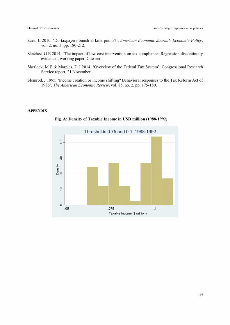
eJournal of Tax Research Firms’ strategic responses to tax policies
164
Saez, E 2010, ‘Do taxpayers bunch at kink points?’, American Economic Journal: Economic Policy, vol. 2, no. 3, pp. 180-212.
Sánchez, G E 2014, ‘The impact of low-cost intervention on tax compliance: Regression discontinuity evidence’, working paper, Citeseer.
Sherlock, M F & Marples, D J 2014, ‘Overview of the Federal Tax System’, Congressional Research Service report, 21 November.
Slemrod, J 1995, ‘Income creation or income shifting? Behavioral responses to the Tax Reform Act of 1986’, The American Economic Review, vol. 85, no. 2, pp. 175-180.
APPENDIX
Fig. A: Density of Taxable Income in USD million (1988-1992)
01
02
03
04
0D
ensi
ty
.05 .075 .1
Taxable Income ($ million)
Thresholds 0.75 and 0.1: 1988-1992
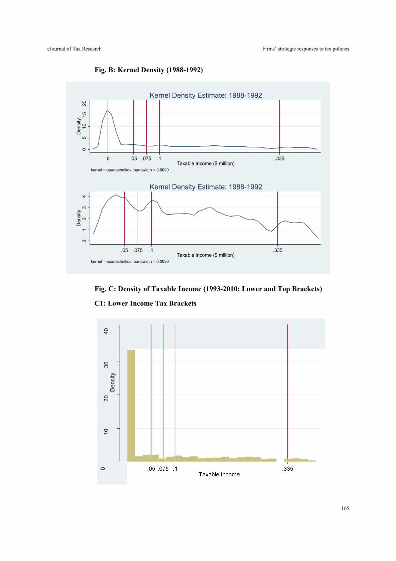
eJournal of Tax Research Firms’ strategic responses to tax policies
165
Fig. B: Kernel Density (1988-1992)
Fig. C: Density of Taxable Income (1993-2010; Lower and Top Brackets)
C1: Lower Income Tax Brackets
05
1015
20D
ensi
ty
0 .05 .075 .1 .335Taxable Income ($ million)
kernel = epanechnikov, bandwidth = 0.0090
Kernel Density Estimate: 1988-1992
01
23
4D
ensi
ty
.05 .075 .1 .335Taxable Income ($ million)
kernel = epanechnikov, bandwidth = 0.0090
Kernel Density Estimate: 1988-1992
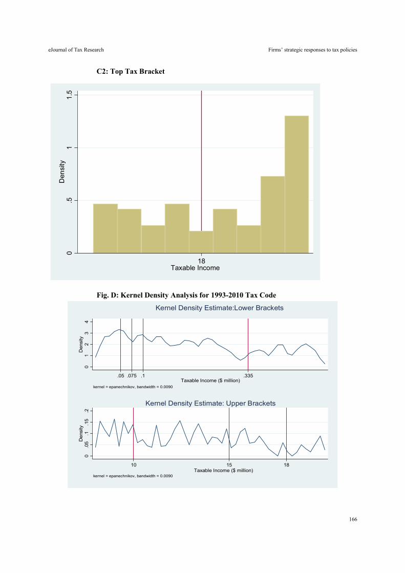
eJournal of Tax Research Firms’ strategic responses to tax policies
166
C2: Top Tax Bracket
Fig. D: Kernel Density Analysis for 1993-2010 Tax Code
0.5
11
.5D
ensi
ty
18Taxable Income
01
23
4D
ensi
ty
.05 .075 .1 .335Taxable Income ($ million)
kernel = epanechnikov, bandwidth = 0.0090
Kernel Density Estimate:Lower Brackets
0.0
5.1
.15
.2D
ens
ity
10 15 18Taxable Income ($ million)
kernel = epanechnikov, bandwidth = 0.0090
Kernel Density Estimate: Upper Brackets

eJournal of Tax Research Firms’ strategic responses to tax policies
167
Fig. E: Density for 1988 to 2010
0.0
5.1
.15
.2D
ensi
ty
0Taxable Income
kernel = epanechnikov, bandwidth = 0.0090
Density for 1988-19920
.05
.1.1
5.2
De
nsity
0 10 15 18Taxable Income
kernel = epanechnikov, bandwidth = 0.0090
Density for 1993-2010

eJournal of Tax Research (2021) vol. 19, no. 1, pp. 168-184
168
Tax morale, perception of justice, trust in public authorities, tax knowledge, and tax compliance: a study of Indonesian SMEs
Joshua Timothy and Yulianti Abbas
Abstract
This study aims to analyse whether and to what extent tax morality, trust in public authority, perception of justice, and tax knowledge are associated with tax compliance by small and medium enterprises (SMEs). Using a sample of 232 Indonesian SMEs in 2020, we found that SME taxpayers’ level of tax compliance is positively associated with their level of tax morality, perception of justice, and trust in public authorities. Our results also show that tax morality has the greatest magnitude in this association, which indicates its role as the main driver of tax compliance. We also found a significant positive association between tax knowledge and tax compliance, confirming the notion that taxpayers’ intrinsic motivation should be equipped with adequate tax knowledge. Our results suggest that in improving SMEs’ tax compliance, regulators need to consider strengthening the intrinsic motivation as well as enhancing the tax knowledge that promotes a greater understanding of tax obligations.
Key words: tax compliance, tax morale, tax knowledge, SMEs
Department of Accounting, Faculty of Economics and Business, University of Indonesia, UI Campus, Depok, 16424, Indonesia. Email: [email protected]. Department of Accounting, Faculty of Economics and Business, University of Indonesia, UI Campus, Depok, 16424, Indonesia. Corresponding author, email: [email protected]. The authors would like to thank Universitas Indonesia for funding this research through PUTI Grant with contract number NKB-4991/UN2.RST/HKP.05.00/2020.
eJournal of Tax Research Tax compliance: a study of Indonesian SMEs
169
1. INTRODUCTION
Small and medium enterprises (SMEs) hold an important role in the world economy. According to the OECD SME and Entrepreneurship Outlook 2019 (Organisation for Economic Co-operation and Development (OECD), 2019), SMEs contribute to 99% of all businesses, and between 50% to 60% of SMEs are involved in value-adding activities. One area of superiority of SMEs is their resilience towards global crises. Taxes from SMEs can serve as a reliable source of revenues for a country’s government to ensure public service provision during a crisis period. SMEs thus can be the backbone of a country’s economy to enable it to survive a crisis such as the current COVID-19 pandemic.
In Indonesia, which is a developing country, SMEs play a strategic role in advancing the economy. The SME sector takes a significant role in all business activities in Indonesia. In 2018, the contribution of the SME sector was equivalent to 60.34% of Indonesia’s gross domestic product (GDP). Moreover, through their business processes, SMEs are also capable of high labour force absorption. In 2017, the labour force absorption by SMEs in Indonesia reached 97.2%.
Despite the sizable contribution of SMEs in the Indonesian economy, the tax income collected from SMEs is much lower than the potential tax income which rough calculations would suggest is available from the SME sector. According to data from Indonesian Statistics Centre (BPS), SMEs contributed about USD 617 billion to the economy which leads to an estimated USD 3 billion in potential tax income. However, the Indonesian government only received 14% of this potential tax income. The Indonesian government’s difficulties in boosting domestic income from SME taxes is not a country-specific problem. Indeed, SME taxpayer delinquency has been recognised as an ongoing global issue (McKerchar & Evans, 2009).
This study aims to analyse factors associated with the tax compliance of Indonesian SMEs. We rely on prior studies suggesting that researchers should incorporate intrinsic motivation as a driver of voluntary tax compliance. Intrinsic motivation is viewed as a crucial factor in explaining tax compliance behaviour that economic deterrence models fail to explain (Alm & McClellan, 2012; Pope & McKerchar, 2011). Alm and Martinez-Vazquez (2007) suggest that to increase tax compliance, a government of a developing country needs to consider strengthening social norms to complement the improvement in tax administration.
Andreoni, Erard and Feinstein (1998) suggest that the concept of morals and social dynamics based on the psychological theories of guilt and shame are drivers of tax compliance. Moral and social dynamics consist of three aspects, which are the moral rules and sentiments, the issue of fairness, and the evaluation of government expenditures and corruption. Tax morality in individuals has long been considered an intrinsic motivation to pay taxes (Frey, 1994, 1997), while the perception of justice has become a core determinant in tax compliance models (Etzioni, 1986; Kirchler, 2007). Etzioni (1986) found that taxpayers committed tax evasion in periods they believed the tax levied was unfair although there was no change in the tax rate. He concluded that an unfair tax system is more likely to drive taxpayers towards tax evasion than a tax rate increase. The relationship between taxpayers and government is also a crucial aspect in understanding tax compliance behaviour (Smith, 1992; Torgler, 2012). If taxpayers trust their government, representatives, and justice system, taxpayers will be more willing to fulfil their tax duties (Alm, 1999; Alm & Martinez-Vazquez, 2007; Alm & Torgler,
eJournal of Tax Research Tax compliance: a study of Indonesian SMEs
170
2011). Torgler and Schneider (2007) stated that citizens are also more willing to fulfil their tax duties when they believe that public institutions adequately reflect their interests.
This study attempts to explain the tax compliance behaviour of SMEs using the concept of social morals and dynamics as suggested by Andreoni et al. (1998). In our study, we use questionnaires to assess the three dimensions of social morals and dynamics, which are tax morale, perception of fairness, and trust to authority. Additionally, we measure the association between tax compliance and tax knowledge. Prior studies suggest that the behaviour towards tax regulations is associated with a taxpayer’s lack of knowledge and abilities to obey (Fjeldstad & Heggstad, 2012; Braithwaite et al., 2010; OECD, 2019). Consistent with prior studies, we propose that SMEs’ tax knowledge will be an important factor in tax compliance.
Based on a survey of 232 Indonesian SMEs in 2020, we confirmed the importance of morals and social dynamics as suggested by Andreoni et al. (1998). Our analytical results show that SMEs’ level of tax compliance is positively associated with their level of tax morality, perception of justice, and trust in public authorities. Among all of these factors, tax morality has the largest magnitude in influencing the level of tax compliance. Additionally, we found that tax knowledge has a positive association with tax compliance. SMEs with a higher level of tax knowledge regarding their tax obligations and the tax administration have higher tax compliance compared to their peers.
Our research contributes to the literature looking at factors associated with SMEs’ tax compliance. Although there have been many studies measuring the intrinsic motivation of individual taxpayers to pay taxes, we cannot directly attribute the results to SMEs because prior studies suggest that SMEs are different from other taxpayers. Ahmed and Braithwaite (2005) found that SME taxpayers have different attitudes towards government functions. Their research showed that SME taxpayers favour minimum government interference and oppose tax expenditure for redistributive programs such as health, welfare, and education (Ahmed & Braithwaite, 2005). Similarly, Kamleitner, Korunka and Kirchler (2012) summarised the literature on SME taxation and suggested three aspects that distinguish SMEs from other businesses, namely a belief that they have greater opportunities to disobey the tax rules, a lack of taxation knowledge, and a perception that taxes are losses (Kamleitner et al., 2012). Prior studies looking at intrinsic motivation and SME tax compliance also found mixed results. Kogler, Muehlbacher and Kirchler (2015) find that both trust in the government and the perceived power of the government were important predictors of tax compliance. However, Morse, Karlinsky and Bankman (2009) found morality was not a predominant reason for compliance decisions for SMEs. Thus, although SMEs constitute a majority of firms in the economy, little is known regarding the intrinsic motivation associated with their tax compliance.
Additionally, most studies on SME tax compliance have used interviews and focus group discussions to gather information. We use a survey-based design that enables us to utilise a greater number of observations. We confirm that our sample indeed consists of SMEs by looking at the number of employees and annual turnover. In the analysis, we use a comprehensive model that considers norms, trust, fairness and knowledge in a single design. Our study focuses on Indonesia as SMEs have been considered as the driver of economic development in developing and emerging countries (Gherghina et al., 2020). The SME sector makes a significant contribution to national GDP and the tax
eJournal of Tax Research Tax compliance: a study of Indonesian SMEs
171
non-compliance of SMEs has become a critical problem for the Indonesian government. Our results provide a basis for understanding factors that need to be taken into consideration in improving SMEs’ tax compliance and designing the appropriate tax policy for SMEs in developing countries.
2. THEORETICAL REVIEW AND HYPOTHESIS DEVELOPMENT
There is no single theoretical definition of a small business (Curran & Blackburn, 2001; Josefy et al., 2015). D’Amboise and Muldowney (1988) described small businesses as businesses that are independently owned, managed by the individual, and not dominant in their field/industry. Small business is usually identified by the number of employees, net value of assets, or revenues. Regarding their tax obligations, small business owners are usually required to self-assess and self-report their income taxes.
As noted in section 1, SMEs’ tax compliance has been recognised as an ongoing global issue (McKerchar & Evans, 2009). Tax compliance refers to the fulfilment of all tax obligations as required by the law or the degree to which taxpayers comply with tax regulations in their country (Braithwaite, 2009; James & Alley, 2004). Tax compliance is also defined as the process in which taxpayers declare all income accurately and pay taxes correctly according to applicable tax laws and regulations (Palil & Mustapha, 2011).
Prior studies on tax compliance suggest that deterrence is the main factor that affects tax non-compliance. Hence, the notion of voluntary taxpaying and the intrinsic motivation to pay taxes has also gained a lot of support in recent years. Alm and Martinez-Vazquez (2007) suggest that in addition to a compliance strategy that is based on detection and punishment, the government should also strengthen the social norms of complying with tax regulations. Similarly, Alm and Torgler (2011) propose that tax administrations should not only emphasise enforcement but also consider tools that are consistent with service and trust paradigm. Jimenez and Iyer (2016) suggest that social norms influence compliance intentions indirectly through internalisation as personal norms. Andreoni et al. (1998) suggest that the concept of morals and social dynamics is significant in tax compliance. Based on the psychological theories of guilt and shame, Andreoni et al. (1998) propose three important factors that affect tax compliance, which are the moral rules and sentiments, the issue of fairness, and the evaluations of government expenditures and corruption (satisfaction with governments).
2.1 Tax morality
Tax morality is a moral obligation to pay taxes or a belief that one should contribute to society by paying taxes (Torgler & Schneider, 2007). Prior studies have concluded that tax morality holds a large role in explaining taxpayer decisions (Alm & McClellan, 2012; Luttmer & Singhal, 2014; Yücedoğru & Hasseldine, 2016) and high degree of tax compliance can be explained by tax morale (Torgler, 2001; Torgler & Schneider, 2007). Prior studies have also found that an increase in tax morality has a significant positive impact on taxpayers’ tax reporting and compliance (Alm, McClelland & Schulze, 1992; Alm & McClellan, 2012). A studies of UK businesses by Adams and Webley (2001) found that UK business owners have low tax morality and considered tax non-compliance as not a serious crime.
Prior studies suggest that tax morality is a necessary component in identifying a business’s perception of whether tax is an obstacle to doing business. Businesses with
eJournal of Tax Research Tax compliance: a study of Indonesian SMEs
172
a low tax morality have a higher probability of justifying tax evasion and considering taxes are a burden in doing business. Businesses with a low level of tax morality towards tax payments are thus more likely to consider taxes as an obstacle compared to a similar firm with a higher level of tax morality. The first hypothesis of this study is:
H1: Tax morality has a positive association with SMEs’ tax compliance.
2.2 Perception of government justice (fairness)
Perception of justice has become a core determinant in tax compliance models (Andreoni et al., 1998, Kirchler, 2007). Prior studies have found that a higher perception of justice has a negative association with tax evasion (Spicer & Lundstedt, 1976; Jackson & Milliron, 1986). The study of small businesses in the UK by Adams and Webley (2001) found that fairness is a major issue in small businesses’ value added tax (VAT) compliance. Similarly, Ahmed and Braithwaite (2005) found that small business owners in Australia believed they pay less than their fair share of tax. Based on these prior studies, we expect the perception of justice will be associated with tax compliance. The second hypothesis of this study is:
H2: Perception of government justice has a positive association with SMEs’ tax compliance.
2.3 Trust in public authority
Kirchler (2007) has stated that ‘trust is a critical factor in understanding the origins of civic engagement, cooperation with authorities and compliance’. If taxpayers trust their government, representatives, and justice system then taxpayers are more willing to fulfil their tax duties (Alm, 1999; Alm & Martinez-Vazquez, 2007; Alm & Torgler, 2011; Jimenez & Iyer, 2016). Citizens are also more willing to fulfil their tax duties when they believe public institutions adequately reflect their interests (Torgler & Schneider, 2007). The level of trust tends to increase a taxpayer’s positive attitude and commitment towards tax payment, which in turn results in a positive effect towards tax compliance (Smith, 1992). Kastlunger et al. (2013) found that trust is positively related to voluntary tax compliance. Muelbacher, Kirchler and Schwarzenberger (2011) also found that high levels of voluntary tax compliance are observed in conditions of high trust.
Prior studies suggest that as trust in government increases, the incentives to comply with tax obligations also increase. However, a study on small businesses in Australia by Ahmed and Braithwaite (2005) found that small businesses favour small government and minimum government interference. This study thus measures SMEs’ level of trust in government and its association with tax compliance. Therefore, the third hypothesis in this study is:
H3: Trust in public authority has a positive association with SMEs’ tax compliance.
2.4 Tax knowledge
Tax knowledge refers to a process where taxpayers gain understanding of taxation laws and other tax-related information (Hasseldine, Holland & van der Rijt, 2009). Delinquent behaviour towards tax regulations can be caused by the taxpayer’s lack of knowledge and abilities to obey (Fjeldstad & Heggstad, 2012; Braithwaite et al., 2010; OECD, 2019). Prior studies have shown varying results regarding the association
eJournal of Tax Research Tax compliance: a study of Indonesian SMEs
173
between tax knowledge and the level of tax compliance (Wadesango et al., 2018). Research by Adam and Webly (2012) concluded that tax knowledge is an important element in a system of voluntary tax compliance. The findings have also been supported by the research of Loo (2016) and Loo, McKerchar and Hansford (2014) which stated that taxation knowledge is the most influential factor in the process of determining taxpayer compliance behaviour in a self-assessment system.
Prior studies on small businesses have also suggested that SMEs have limited taxation knowledge. McKerchar (1995) found that small businesses in Australia did not realise the gap in their taxation knowledge, causing accidental delinquency. Based on prior studies, intrinsic motivation to pay taxes should be complemented by adequate taxation knowledge. Therefore, our fourth hypothesis is:
H4 : Taxpayer’s tax knowledge has a positive association with SMEs’ tax compliance.
2.5 Control variables
Similar to research regarding SMEs conducted by Huong and Cuong (2019), we control for firm size and firm age. Both variables represent the difference in firm efficiency and their access to funding (Farinha & Félix, 2015).
3. RESEARCH METHOD
3.1 Sample
We distributed questionnaires to Indonesian SME taxpayers. A total of 239 valid responses from Indonesian micro, small, and medium businesses were obtained. The questionnaire (see Appendix 1) includes a set of questions measuring tax morality, trust in public authority, taxpayer’s perception toward government justice, tax knowledge, and tax compliance. To test the validity of the responses, we checked the consistency of the respondent’s answers. We used reversed questions that served as an indicator of the respondent’s opinion consistency and dropped respondents whose answers were inconsistent. We also dropped respondents with an illogical answer.1
3.2 Statistical model
For data analysis, we used the Structural Equation Modelling Maximum Likelihood Estimator (SEM MLE) method. The Maximum Likelihood Estimator (MLE) method is chosen because our constructs are latent variables. We use several questions to measure one particular construct. The MLE estimator allows us to measure the latent variables by assigning weight to the questions based on respondents’ responses.
The following statistical model is used to test the association between tax morality, trust in public authority, a taxpayer’s perception towards government justice, tax knowledge, and SME taxpayers’ tax compliance level:
Compliancei = β1Moralityi + β2Justicei + β3Trusti + β4Knowledgei + β5Agei + β6Sizei + 𝜺i
1 One respondent claimed to have 500,000 employees, which is inconsistent with the SME characteristics.
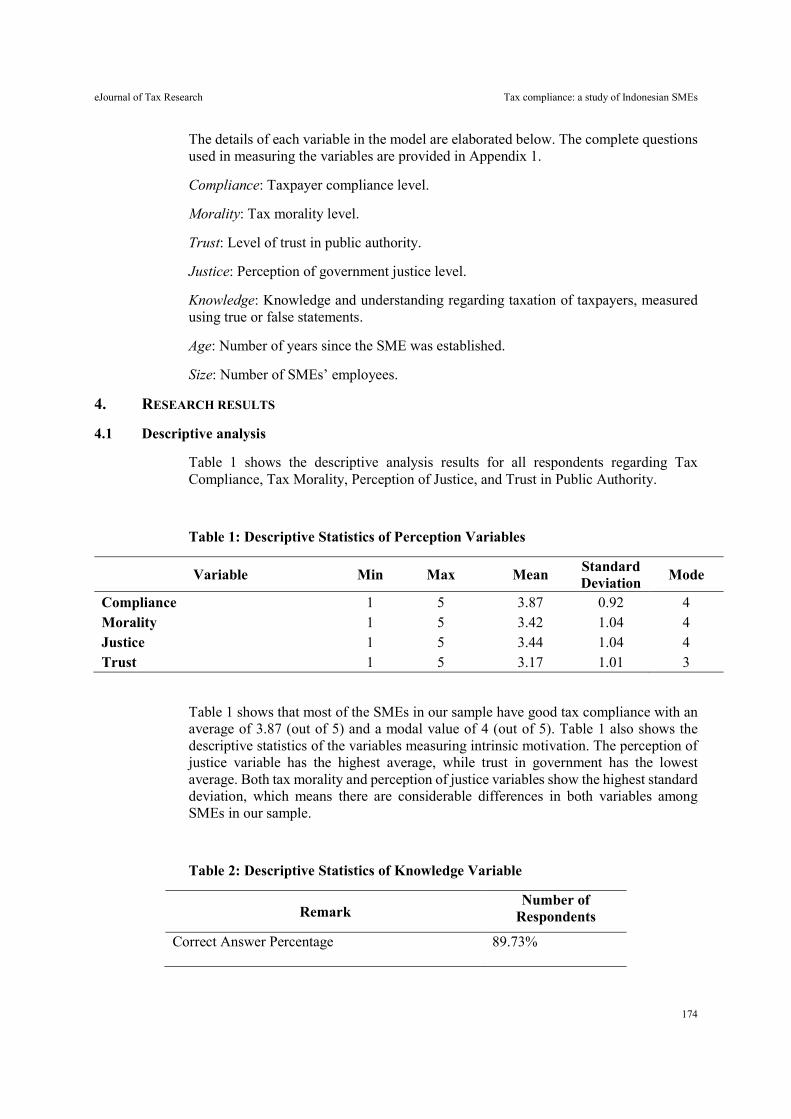
eJournal of Tax Research Tax compliance: a study of Indonesian SMEs
174
The details of each variable in the model are elaborated below. The complete questions used in measuring the variables are provided in Appendix 1.
Compliance: Taxpayer compliance level.
Morality: Tax morality level.
Trust: Level of trust in public authority.
Justice: Perception of government justice level.
Knowledge: Knowledge and understanding regarding taxation of taxpayers, measured using true or false statements.
Age: Number of years since the SME was established.
Size: Number of SMEs’ employees.
4. RESEARCH RESULTS
4.1 Descriptive analysis
Table 1 shows the descriptive analysis results for all respondents regarding Tax Compliance, Tax Morality, Perception of Justice, and Trust in Public Authority.
Table 1: Descriptive Statistics of Perception Variables
Variable Min Max Mean Standard Deviation
Mode
Compliance 1 5 3.87 0.92 4 Morality 1 5 3.42 1.04 4 Justice 1 5 3.44 1.04 4 Trust 1 5 3.17 1.01 3
Table 1 shows that most of the SMEs in our sample have good tax compliance with an average of 3.87 (out of 5) and a modal value of 4 (out of 5). Table 1 also shows the descriptive statistics of the variables measuring intrinsic motivation. The perception of justice variable has the highest average, while trust in government has the lowest average. Both tax morality and perception of justice variables show the highest standard deviation, which means there are considerable differences in both variables among SMEs in our sample.
Table 2: Descriptive Statistics of Knowledge Variable
Remark Number of
Respondents
Correct Answer Percentage 89.73%
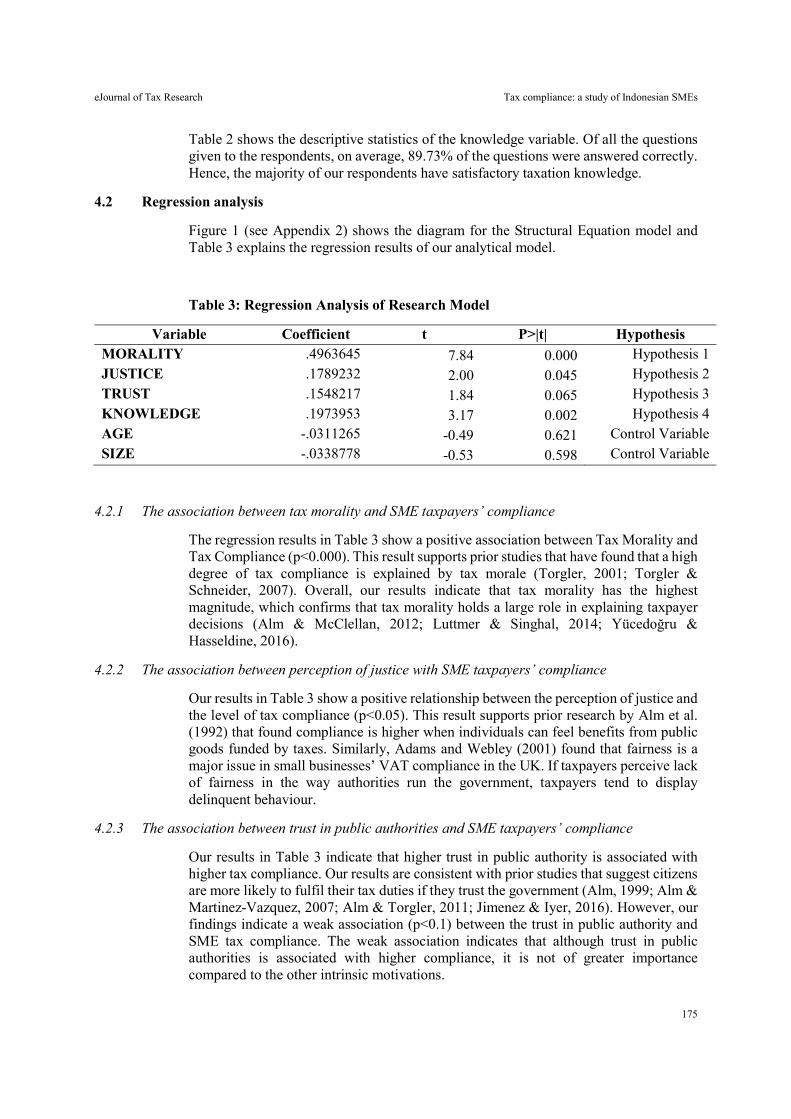
eJournal of Tax Research Tax compliance: a study of Indonesian SMEs
175
Table 2 shows the descriptive statistics of the knowledge variable. Of all the questions given to the respondents, on average, 89.73% of the questions were answered correctly. Hence, the majority of our respondents have satisfactory taxation knowledge.
4.2 Regression analysis
Figure 1 (see Appendix 2) shows the diagram for the Structural Equation model and Table 3 explains the regression results of our analytical model.
Table 3: Regression Analysis of Research Model
Variable Coefficient t P>|t| Hypothesis MORALITY .4963645 7.84 0.000 Hypothesis 1 JUSTICE .1789232 2.00 0.045 Hypothesis 2 TRUST .1548217 1.84 0.065 Hypothesis 3 KNOWLEDGE .1973953 3.17 0.002 Hypothesis 4 AGE -.0311265 -0.49 0.621 Control Variable SIZE -.0338778 -0.53 0.598 Control Variable
4.2.1 The association between tax morality and SME taxpayers’ compliance
The regression results in Table 3 show a positive association between Tax Morality and Tax Compliance (p<0.000). This result supports prior studies that have found that a high degree of tax compliance is explained by tax morale (Torgler, 2001; Torgler & Schneider, 2007). Overall, our results indicate that tax morality has the highest magnitude, which confirms that tax morality holds a large role in explaining taxpayer decisions (Alm & McClellan, 2012; Luttmer & Singhal, 2014; Yücedoğru & Hasseldine, 2016).
4.2.2 The association between perception of justice with SME taxpayers’ compliance
Our results in Table 3 show a positive relationship between the perception of justice and the level of tax compliance (p<0.05). This result supports prior research by Alm et al. (1992) that found compliance is higher when individuals can feel benefits from public goods funded by taxes. Similarly, Adams and Webley (2001) found that fairness is a major issue in small businesses’ VAT compliance in the UK. If taxpayers perceive lack of fairness in the way authorities run the government, taxpayers tend to display delinquent behaviour.
4.2.3 The association between trust in public authorities and SME taxpayers’ compliance
Our results in Table 3 indicate that higher trust in public authority is associated with higher tax compliance. Our results are consistent with prior studies that suggest citizens are more likely to fulfil their tax duties if they trust the government (Alm, 1999; Alm & Martinez-Vazquez, 2007; Alm & Torgler, 2011; Jimenez & Iyer, 2016). However, our findings indicate a weak association (p<0.1) between the trust in public authority and SME tax compliance. The weak association indicates that although trust in public authorities is associated with higher compliance, it is not of greater importance compared to the other intrinsic motivations.
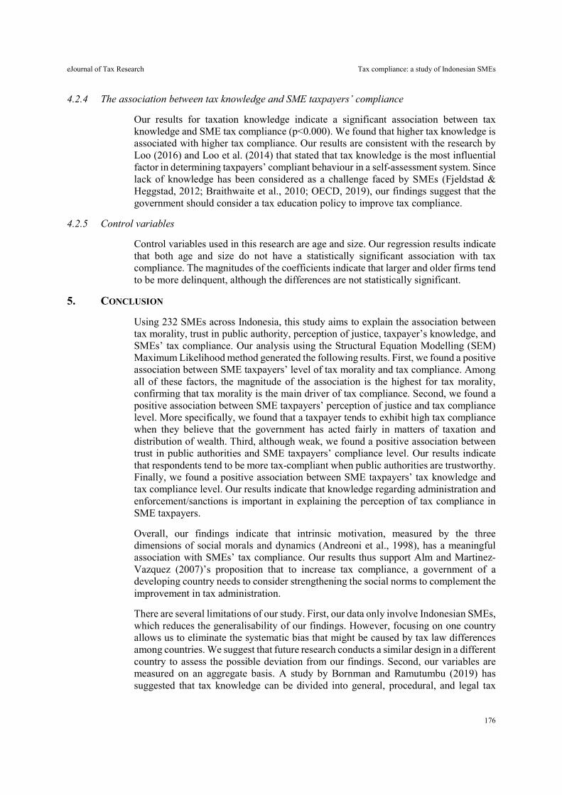
eJournal of Tax Research Tax compliance: a study of Indonesian SMEs
176
4.2.4 The association between tax knowledge and SME taxpayers’ compliance
Our results for taxation knowledge indicate a significant association between tax knowledge and SME tax compliance (p<0.000). We found that higher tax knowledge is associated with higher tax compliance. Our results are consistent with the research by Loo (2016) and Loo et al. (2014) that stated that tax knowledge is the most influential factor in determining taxpayers’ compliant behaviour in a self-assessment system. Since lack of knowledge has been considered as a challenge faced by SMEs (Fjeldstad & Heggstad, 2012; Braithwaite et al., 2010; OECD, 2019), our findings suggest that the government should consider a tax education policy to improve tax compliance.
4.2.5 Control variables
Control variables used in this research are age and size. Our regression results indicate that both age and size do not have a statistically significant association with tax compliance. The magnitudes of the coefficients indicate that larger and older firms tend to be more delinquent, although the differences are not statistically significant.
5. CONCLUSION
Using 232 SMEs across Indonesia, this study aims to explain the association between tax morality, trust in public authority, perception of justice, taxpayer’s knowledge, and SMEs’ tax compliance. Our analysis using the Structural Equation Modelling (SEM) Maximum Likelihood method generated the following results. First, we found a positive association between SME taxpayers’ level of tax morality and tax compliance. Among all of these factors, the magnitude of the association is the highest for tax morality, confirming that tax morality is the main driver of tax compliance. Second, we found a positive association between SME taxpayers’ perception of justice and tax compliance level. More specifically, we found that a taxpayer tends to exhibit high tax compliance when they believe that the government has acted fairly in matters of taxation and distribution of wealth. Third, although weak, we found a positive association between trust in public authorities and SME taxpayers’ compliance level. Our results indicate that respondents tend to be more tax-compliant when public authorities are trustworthy. Finally, we found a positive association between SME taxpayers’ tax knowledge and tax compliance level. Our results indicate that knowledge regarding administration and enforcement/sanctions is important in explaining the perception of tax compliance in SME taxpayers.
Overall, our findings indicate that intrinsic motivation, measured by the three dimensions of social morals and dynamics (Andreoni et al., 1998), has a meaningful association with SMEs’ tax compliance. Our results thus support Alm and Martinez-Vazquez (2007)’s proposition that to increase tax compliance, a government of a developing country needs to consider strengthening the social norms to complement the improvement in tax administration.
There are several limitations of our study. First, our data only involve Indonesian SMEs, which reduces the generalisability of our findings. However, focusing on one country allows us to eliminate the systematic bias that might be caused by tax law differences among countries. We suggest that future research conducts a similar design in a different country to assess the possible deviation from our findings. Second, our variables are measured on an aggregate basis. A study by Bornman and Ramutumbu (2019) has suggested that tax knowledge can be divided into general, procedural, and legal tax

eJournal of Tax Research Tax compliance: a study of Indonesian SMEs
177
knowledge, with general tax knowledge relating to fiscal awareness, procedural tax knowledge to understanding tax compliance procedures and legal tax knowledge to understanding tax regulations. Future studies might seek to disaggregate the knowledge variables and test which type of knowledge will be associated with tax compliance.
6. REFERENCES
Adam, C & Webley, P 2001, ‘Small business owners’ attitudes on VAT compliance in the UK’, Journal of Economic Psychology, vol. 22, no. 2, pp. 195-216.
Ahmed, E & Braithwaite, V 2005, ‘Understanding small business taxpayers: Issues of deterrence, tax morale, fairness and work practice’, International Small Business Journal, vol. 23, no. 5, pp. 539-568.
Alm, J 1999, ‘Tax compliance and administration’, in Hildreth, W & Richardson, J (eds.), Handbook on taxation, Marcel Dekker, New York, NY, pp. 741-768.
Alm, J & Torgler, B 2011, ‘Do ethics matter? Tax compliance and morality’, Journal of Business Ethics, vol. 101, no. 4, pp. 635-651.
Alm, J & Martinez-Vazquez, J 2007, ‘Tax morale and tax evasion in Latin America’, International Studies Program Working Paper 07-32, Andrew Young School of Policy Studies, Georgia State University, December. Available at: https://icepp.gsu.edu/files/2015/03/ispwp0732.pdf.
Alm, J & McClellan, C 2012, ‘Tax morale and tax compliance from the firm’s perspective’, Kyklos, vol. 65, no. 1, pp. 1-17.
Alm, J, McClelland, G H & Schulze, W D 1992, ‘Why do people pay taxes?’, Journal of Public Economics, vol. 48, no. 1, pp. 21-38.\
Andreoni, J, Erard, B & Feinstein, B 1998, ‘Tax compliance’, Journal of Economic Literature, vol. 36, no. 2, pp. 818-860.
Bornman, M & Ramutumbu, P 2019, ‘A conceptual framework of tax knowledge’, Meditari Accountancy Research, vol. 27, no. 6, pp. 823-839.
Bourletidis, K & Triantafyllopoulos, Y 2014, ‘SMEs survival in time of crisis: Strategies, tactics and commercial success stories’, Procedia - Social and Behavioral Sciences, vol. 148, pp. 639-644.
Braithwaite, V. (2009), Defiance in taxation and governance: Resisting and dismissing authority in a democracy, Edward Elgar, Cheltenham.
Braithwaite, V, Reinhart, M & Smart, M 2010, ‘Tax non-compliance among the under-30s: Knowledge, obligation or skepticism?’, in Alm, J, Martinez-Vazquez, J & Torgler, B (eds), Developing alternative frameworks for explaining tax compliance, Routledge, London, pp. 217-237.
Curran, J & Blackburn, R A 2001, ‘Older people and the enterprise society: Age and self-employment propensities’, Work, Employment and Society, vol. 15, no. 4, pp. 889-902.
eJournal of Tax Research Tax compliance: a study of Indonesian SMEs
178
D’Amboise, G & Muldowney, M 1988, ‘Management theory for small business: Attempts and requirements’, Academy of Management Review, vol. 13, no. 2, pp. 226-240.
Etzioni, A 1986, ‘Tax evasion and perceptions of tax fairness: A research note’, Journal of Applied Behavioral Science, vol. 22, no. 2, pp. 177-185.
Farinha, L & Félix, S 2015, ‘Credit rationing for Portuguese SMEs’, Finance Research Letters, vol. 14, pp. 167-177.
Fjeldstad, O-H & Heggstad, K 2012, Building taxpayer culture in Mozambique, Tanzania and Zambia: Achievements, challenges and policy recommendations, CMI Report R 2012:1, Chr Michelsen Institute, Bergen.
Frey, B S 1994, ‘Tertium datur: Pricing, regulating, and intrinsic motivation’, Kyklos, vol. 45, no. 2, pp. 161-184.
Frey, B S 1997, ‘A Constitution for Knaves Crowds Out Civic Virtues’, The Economic Journal, vol. 107, no. 443, pp. 1043-1053.
Gherghina, Ș C, Botezatu, M A, Hosszu, A & Simionescu, L N 2020, ‘Small and medium-sized enterprises (SMEs): The engine of economic growth through investments and innovation’. Sustainability, vol. 12, no. 1, 347.
Hasseldine, J, Holland, K & van der Rijt, P 2009, The management of tax knowledge, The Association of Chartered Certified Accountants Research Report 112, London.
Huong, V V & Cuong, L K 2019, ‘Does government support promote SME tax payments? New evidence from Vietnam’. Finance Research Letters, vol. 31, pp. 270-277.
Ibrahim, M, Musah, A & Abdul-Hanan, A 2015, ‘Beyond enforcement: What drives tax morale in Ghana?’, Humanomics, vol. 31, no. 4, pp. 399-414.
Jackson, B & Milliron, V 1986, ‘Tax compliance research: Findings, problems, and prospects’, Journal of Accounting Literature, 5, pp. 125-165.
James, S & Alley, C 2004, ‘Tax compliance, self-assessment and tax administration’, School of Economics and Business, University of Exeter.
Jimenez, P & Iyer, G S 2016, ‘Tax compliance in a social setting: The influence of social norms, trust in government, and perceived fairness on taxpayer compliance’, Advances in Accounting, vol. 34, pp. 17-26.
Josefy, M, Kuban, S, Ireland, R D & Hitt, M A 2015, ‘All things great and small: Organizational size, boundaries of the firm, and a changing environment’, The Academy of Management Annals, vol. 9, no. 1, pp. 715-802.
Kamleitner, B, Korunka, C & Kirchler, E 2012, ‘Tax compliance of small business owners: A review’, International Journal of Entrepreneurial Behavior and Research, vol. 18, no. 3, pp. 330-351.
Kastlunger, B, Lozza, E, Kirchler, E & Schabmann, A 2013, ‘Powerful authorities and trusting citizens: The Slippery Slope Framework and tax compliance in Italy’, Journal of Economic Psychology, vol. 34, pp. 36-45.
Kirchler, E 2007, The economic psychology of tax behaviour, Cambridge University Press, Cambridge.
eJournal of Tax Research Tax compliance: a study of Indonesian SMEs
179
Kogler, C, Muehlbacher, S & Kirchler, E 2015, ‘Testing the “slippery slope framework” among self-employed taxpayers’, Economics of Governance, vol. 16, no. 2, pp. 125-142.
Loo, E C 2016, The influence of the introduction on self-assessment on compliance behaviour of individual taxpayers in Malaysia, PhD thesis, University of Sydney.
Loo, E C, McKerchar, M & Hansford, A 2014, ‘Understanding the compliance behaviour of Malaysian individual taxpayers using a mixed method approach’, Journal of the Australasian Tax Teachers Association, vol. 4, no. 1, pp. 181-202.
Luttmer, E F P & Singhal, M 2014, ‘Tax morale’, Journal of Economic Perspectives, vol. 28 no. 4, pp. 149-168.
McKerchar, M 1995, ‘Understanding small business taxpayers: Their sources of information and level of knowledge of taxation’, Australian Tax Forum, vol. 12, no. 1, pp. 25-41.
McKerchar, M & Evans, C 2009, ‘Sustaining growth in developing economies through improved taxpayer compliance: Challenges for policy makers and revenue authorities’, eJournal of Tax Research, vol. 7, no. 2, pp. 171-201.
Morse, S C, Karlinsky, S & Bankman, J 2009, ‘Cash businesses and tax evasion’, Stanford Law and Policy Review, vol. 20, no. 1, pp. 37-68.
Muelbacher, S, Kirchler, E & Schwarzenberger, H 2011, ‘Voluntary versus enforced tax compliance: Empirical evidence from the “slippery slope” framework’, European Journal of Law and Economics, vol. 32, no. 1, pp. 89-97.
Wadesango, N, Mwandambira, N, Mhaka, C & Wadesango, O 2018, ‘Literature review on the impact of tax knowledge on tax compliance among small medium enterprises in a developing country’, International Journal of Entrepreneurship, vol. 22, no. 4, pp. 1-16.
Organisation for Economic Co-operation and Development (OECD) 2019, OECD SME and entrepreneurship outlook 2019, OECD Publishing, Paris.
Palil, M R & Mustapha, A F 2011, ‘Factors affecting tax compliance behaviour in self-assessment system’, African Journal of Business Management, vol. 5, no. 33, pp. 12864-12872.
Pope, J & McKerchar, M 2011, ‘Understanding tax morale and its effect on individual taxpayer compliance’, British Tax Review, vol. 2011, no. 5, pp. 587-600.
Smith, K W 1992, ‘Reciprocity and fairness: Positive incentives for tax compliance’, in Slemrod, J (ed.), Why people pay taxes: Tax compliance and enforcement, University of Michigan Press, Ann Arbor, MI, pp. 223-250.
Spicer, M & Lundstedt, S 1976, ‘Understanding tax evasion’, Public Finance, vol. 31, no. 2, pp. 295-305.
Torgler, B 2012, ‘Tax morale, Eastern Europe and European enlargement’, Communist and Post-Communist Studies, vol. 45, nos. 1-2, pp. 11-25.
Torgler, B & Schneider, F 2007, ‘What shapes attitudes toward paying taxes? Evidence from multicultural European countries’, Social Science Quarterly, vol. 88, no. 2, pp. 443-470.
Yücedoğru, R & Hasseldine, J 2016, ‘Understanding tax morale of SMEs: A qualitative study’, eJournal of Tax Research, vol. 14, no. 3, pp. 531-566.

eJournal of Tax Research Tax compliance: a study of Indonesian SMEs
180
7. APPENDICES
Appendix 1 Questionnaire 1 = strongly disagree; 2 = disagree; 3 = neutral; 4 = agree; 5 = strongly agree
Tax Compliance
No. Statement 1 (SD)
2 (D)
3 (N)
4 (A)
5 (SA)
1 A taxpayer must prepare the documents required to pay taxes
2 A taxpayer must find information regarding where and how to pay taxes
3 A taxpayer must find information regarding the due date of tax payment
4 A taxpayer must allocate funds to pay taxes 5 A taxpayer must pay taxes on income earned by
his/her business
6 A taxpayer is not required to pay income tax on time.
7 A taxpayer must pay the correct amount of income tax
8 A taxpayer must file and report income tax on his/her business (report tax returns – SPT)
9 A taxpayer is not required to report taxes (report tax returns) on time
10 A taxpayer must report taxes (report tax returns) with correct information
Tax Morality
No. Statement 1 (SD)
2 (D)
3 (N)
4 (A)
5 (SA)
1 It does not matter if a taxpayer exaggerates their business expenses to reduce payable personal taxes
2 It does not matter if a taxpayer exploits loopholes in taxation laws to minimize his/her taxes
3 It does not matter if a taxpayer only reports parts of his/her income to reduce payable taxes
4 In a difficult economic situation, it does not matter if taxpayers do not pay their taxes
5 Tax evasion is a serious crime

eJournal of Tax Research Tax compliance: a study of Indonesian SMEs
181
Perception of Justice
No. Statement 1 (SD)
2 (D)
3 (N)
4 (A)
5 (SA)
1 The current system of income tax is fair to all taxpayers
2 Income tax expense has been fairly distributed among all taxpayers
3 The facilities you receive from the government is proportionate to the taxes you have paid
4 It is fair for people with high income to pay proportionally more in taxes than those with lower income
5 Tax rates are fair if it is applied to every person regardless of their income
6 It is fair to apply a lower tax rate to SME taxpayers
7 The government giving different facilities to SMEs and non-SMEs is not fair
8 Lowering the tax rate for all types of businesses during a pandemic is fair
9 Bearing employees’ taxes during a pandemic regardless of income is fair
Trust in Public Authority
No. Statement 1 (SD)
2 (D)
3 (N)
4 (A)
5 (SA)
1 Currently the law is well enforced by the government
2 Politicians and representatives are executing their function and authority well
3 The government has allocated tax income well in the form of facilities for the people
4 The Directorate General of Taxation has been performing tax collection duties well
5 In general, the Directorate General of Taxation already possess good integrity
6 The Directorate General of Taxation has performed socializations or tax education well
7 The website for the Directorate General of Taxation provides adequate information
8 Account Representatives have performed and given their services well
9 The government has provided good facilities during the COVID-19 pandemic
10 Tax facilities given to MSMEs by the government during the COVID-19 pandemic has been well socialized.

eJournal of Tax Research Tax compliance: a study of Indonesian SMEs
182
11 Account representatives have provided adequate aid in helping MSMEs benefit from tax facilities during the COVID-19 pandemic
12 Government aid is crucial to economic recovery post-COVID-19
13 Public donation is crucial to economic recovery post-COVID-19
Tax Knowledge V = True; X = False
No. Statement V (True)
X (False)
1 Taxes are the largest source of national income in Indonesia 2 All taxpayers with income must register and obtain Tax ID
number
3 Taxpayers can register for Tax ID number 4 The Directorate General of Taxation can perform
inspections on taxpayers to test their tax compliance
5 Taxpayers can file for deferment or installments on their tax payments in certain conditions
6 Tax sanctions are applied to those who do not fulfil their tax obligations
7 Applicable tax sanctions include fines and imprisonment 8 Income tax rate for MSMEs is 0.5% 9 To obtain tax facilities, SMEs must first obtain a letter of
statement from the tax office
10 SME taxes can be paid off by personally depositing the taxes or by collection by other parties
11 SMEs must pay taxes on the 15th of every month 12 SME income tax is borne by the government during
COVID-19
13 During the COVID-19 pandemic, the government bears SME income taxes for 6 months
14 The government bears employee taxes for companies in certain sectors during COVID-19 pandemic
Please answer the following questions if your business is a Sole Proprietorship
No. Statement V (True)
X (False)
15 SMEs can use Final PPh rate of 0.5% for a maximum of 7 years
16 SMEs must record all their revenues for tax reporting purposes (Periodic Tax Return)

eJournal of Tax Research Tax compliance: a study of Indonesian SMEs
183
Please answer the following questions if your business is a Partnership/Cooperative No. Statement V
(True) X
(False) 15 SMEs can use Final PPh rate of 0.5% for a maximum of 4
years
16 SME taxpayers must record all their revenues for tax reporting purposes (Periodic Tax Returns)
Please answer the following questions if your business is a Corporation (limited liability company)
No. Statement V (True)
X (False)
15 SMEs can use Final PPh rate of 0.5% for a maximum of 3 years
16 SME taxpayers must record all their revenues for tax reporting purposes (Periodic Tax Returns)
17 SME taxpayers must fill data regarding assets, debt, and profit loss balance for tax reporting purposes (Annual Tax Returns)
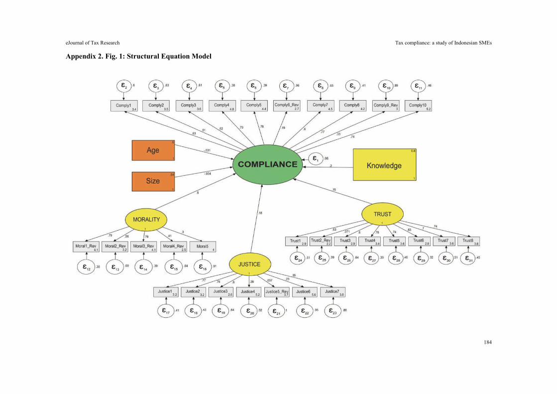
eJournal of Tax Research Tax compliance: a study of Indonesian SMEs
184
Appendix 2. Fig. 1: Structural Equation Model