Efficient Querying for Analytics on Internet of Things ...
255
UNIVERSITY OF SOUTHAMPTON Faculty of Physical Sciences and Engineering Electronics and Computer Science Web and Internet Science Efficient Querying for Analytics on Internet of Things Databases and Streams by Eugene Siow Thesis for the degree of Doctor of Philosophy February 2018
-
Upload
khangminh22 -
Category
Documents
-
view
0 -
download
0
Transcript of Efficient Querying for Analytics on Internet of Things ...

UNIVERSITY OF SOUTHAMPTON
Faculty of Physical Sciences and EngineeringElectronics and Computer Science
Web and Internet Science
Efficient Querying for Analytics onInternet of Things Databases and
Streams
by
Eugene Siow
Thesis for the degree of Doctor of Philosophy
February 2018


UNIVERSITY OF SOUTHAMPTON
ABSTRACT
FACULTY OF PHYSICAL SCIENCES AND ENGINEERINGElectronics and Computer Science
Web and Internet Science
Doctor of PhilosophyEfficient Querying for Analytics on Internet of Things Databases and
Streamsby Eugene Siow
This thesis is concerned with the development of efficient methods for managing contex-tualised time-series data and event streams produced by the Internet of Things (IoT) sothat both historical and real-time information can be utilised to generate value withinanalytical applications.
From a database systems perspective, two conflicting challenges motivate this research,interoperability and performance. IoT applications integrating streams of time-seriesdata from heterogeneous IoT agents require a level of semantic interoperability. Thissemantic interoperability can be achieved with a common flexible data model that repre-sents both metadata and data. However, applications might also have time constraintsor require processing to be performed on large volumes of historical and streamingtime-series data, possibly on resource-constrained platforms, without significant delay.Obtaining good performance is complicated by the complexity of the data model.
In the first part of the thesis, a graph data model is shown to support the representationof metadata and data that various research and standard bodies are working towards,while the ‘volume’ of IoT data is shown to exhibit flat, wide and numerical character-istics. A three step abstraction is defined to reconcile queries on the graph model withefficient underlying storage by query translation. This storage is iteratively improved toexploit the character of time-series IoT data, achieving orders of magnitude performanceimprovement over state-of-the-art commercial, open-source and research databases.
The second part of the thesis extends this abstraction to efficiently process real-time IoTstreams continuously and proposes an infrastructure for fog computing that shows howresource-constrained platforms close to source IoT agents can co-operatively orchestratestream processing. The main contributions of this thesis are therefore, i) a novel in-teroperable and performant abstraction for querying IoT graph representations, ii) highperformance historical, streaming and fog computing time-series database implementa-tions and iii) analytical applications and platforms built on this abstraction that act aspractical models for the socio-technical development of the IoT.


Contents
Nomenclature xi
List of Figures xv
List of Tables xix
Listings xxi
Declaration of Authorship xxiii
Acknowledgements xxiv
1 Introduction 11.1 Information in the IoT . . . . . . . . . . . . . . . . . . . . . . . . . . . . . 31.2 Database and Stream Processing in the IoT . . . . . . . . . . . . . . . . . 31.3 Applications and Analytics in the IoT . . . . . . . . . . . . . . . . . . . . 41.4 Research Questions . . . . . . . . . . . . . . . . . . . . . . . . . . . . . . . 51.5 Research Contributions . . . . . . . . . . . . . . . . . . . . . . . . . . . . 51.6 Thesis Outline . . . . . . . . . . . . . . . . . . . . . . . . . . . . . . . . . 61.7 Publications and Software . . . . . . . . . . . . . . . . . . . . . . . . . . . 7
2 Background 92.1 Definition and Categorisation the IoT . . . . . . . . . . . . . . . . . . . . 9
2.1.1 IoT Applications, Platforms and Building Blocks Categorisation . 112.1.2 IoT Applications: Application Areas, Domains and Themes . . . . 122.1.3 IoT Applications: A Survey of Techniques and Data Currency . . 152.1.4 IoT Platforms: Architectures, Layers, Middleware . . . . . . . . . 17
2.2 Databases and Stream Processing Systems . . . . . . . . . . . . . . . . . . 222.2.1 Time-series Databases . . . . . . . . . . . . . . . . . . . . . . . . . 22
2.2.1.1 Cassandra-based Storage . . . . . . . . . . . . . . . . . . 232.2.1.2 Native Time-series Storage . . . . . . . . . . . . . . . . . 242.2.1.3 HBase, MongoDB and Riak-based NoSQL Storage . . . . 252.2.1.4 Relational-database-based Storage . . . . . . . . . . . . . 26
2.2.2 Graph and RDF Databases . . . . . . . . . . . . . . . . . . . . . . 272.2.2.1 Introduction to RDF and Related Terminology . . . . . . 272.2.2.2 RDF, Linked Data and the IoT . . . . . . . . . . . . . . 282.2.2.3 RDF Stores . . . . . . . . . . . . . . . . . . . . . . . . . . 29
2.2.3 SPARQL-to-Relational Query Translation . . . . . . . . . . . . . . 31
v

vi CONTENTS
2.2.4 Federated SPARQL . . . . . . . . . . . . . . . . . . . . . . . . . . 322.2.5 Stream Processing Engines . . . . . . . . . . . . . . . . . . . . . . 32
2.3 Analytics for the IoT . . . . . . . . . . . . . . . . . . . . . . . . . . . . . . 332.3.1 Five Categories of Analytics Capabilities . . . . . . . . . . . . . . . 34
2.3.1.1 Descriptive Analytics . . . . . . . . . . . . . . . . . . . . 342.3.1.2 Diagnostic Analytics . . . . . . . . . . . . . . . . . . . . . 342.3.1.3 Discovery in Analytics . . . . . . . . . . . . . . . . . . . . 352.3.1.4 Predictive Analytics . . . . . . . . . . . . . . . . . . . . . 352.3.1.5 Prescriptive Analytics . . . . . . . . . . . . . . . . . . . . 35
2.3.2 Knowledge Hierarchy and IoT App Classification . . . . . . . . . . 352.4 Fog Computing . . . . . . . . . . . . . . . . . . . . . . . . . . . . . . . . . 36
2.4.1 Characteristics of Fog Computing Systems . . . . . . . . . . . . . . 382.4.2 Fog Computing Data and Control Planes . . . . . . . . . . . . . . 39
2.4.2.1 Example Fog Computing Applications and Infrastructure 392.5 Conclusions . . . . . . . . . . . . . . . . . . . . . . . . . . . . . . . . . . . 40
3 Analysis of the Characteristics of Internet of Things Data 413.1 Study of Public IoT Schemata . . . . . . . . . . . . . . . . . . . . . . . . . 41
3.1.1 Comparison of Flat and Complex Schemata . . . . . . . . . . . . . 423.1.2 Width of Schemata . . . . . . . . . . . . . . . . . . . . . . . . . . . 423.1.3 Data Types of Values within Schemata . . . . . . . . . . . . . . . . 433.1.4 Periodicity of Data Streams . . . . . . . . . . . . . . . . . . . . . . 443.1.5 Summary of Dweet.io IoT Data Characteristics . . . . . . . . . . . 46
3.2 Study of Cross-domain IoT Data and Schemata . . . . . . . . . . . . . . . 463.2.1 SparkFun: Public Streams from Arduino Devices . . . . . . . . . . 473.2.2 Array of Things: A “Fitness Tracker” for Smart Cities . . . . . . . 473.2.3 Linked Sensor Data: Inclement Weather Measurements . . . . . . 483.2.4 OpenEnergyMonitor: Home Energy Consumption . . . . . . . . . 493.2.5 ThingSpeak: A MatLab-based IoT Analytics Platform . . . . . . . 493.2.6 Open Humans: E-Health/Smart-Living with Wearable Data . . . . 503.2.7 A Summary of the Cross-IoT Study Data Characteristics . . . . . 51
3.3 Data Models for Interoperability in the IoT . . . . . . . . . . . . . . . . . 513.3.1 Study of the Structure of IoT Metamodels . . . . . . . . . . . . . . 51
3.3.1.1 Entity-Centric Models . . . . . . . . . . . . . . . . . . . . 523.3.1.2 Object-Centric Models . . . . . . . . . . . . . . . . . . . 533.3.1.3 Ontology-Centric Models . . . . . . . . . . . . . . . . . . 53
3.3.2 A Common Structure: The Graph Model . . . . . . . . . . . . . . 543.4 Characteristics of IoT RDF Graph Data . . . . . . . . . . . . . . . . . . . 55
3.4.1 Categories of IoT RDF Data from Ontology Sample . . . . . . . . 553.4.2 Metadata-to-Data Study on IoT RDF Data . . . . . . . . . . . . . 57
3.5 Conclusions . . . . . . . . . . . . . . . . . . . . . . . . . . . . . . . . . . . 59
4 Map-Match-Operate Abstract Graph Querying Framework 614.1 Introduction . . . . . . . . . . . . . . . . . . . . . . . . . . . . . . . . . . . 624.2 Definition of Map-Match-Operate: A Graph Query Execution Abstraction 62
4.2.1 Map: Binding M to T . . . . . . . . . . . . . . . . . . . . . . . . . 644.2.1.1 S2SML: A mRDF
map Data Model Mapping Language for RDF 65

CONTENTS vii
4.2.1.2 Mapping Closures: Logical Groupings of Mappings . . . . 674.2.1.3 Implicit Join Conditions by Template Matching . . . . . 684.2.1.4 Compatibility with R2RML and RML . . . . . . . . . . . 694.2.1.5 S2SML Example and a Comparison of Mappings . . . . . 71
4.2.2 Match: Retrieving Bmatch by Matching qgraph to Mmap . . . . . . . 734.2.3 Operate: Executing q’s Operators on T ∪M using Bmatch Results . 744.2.4 S2S Engine: A Map-Match-Operate Implementation . . . . . . . . 76
4.2.4.1 Building a Mapping Closure for Map . . . . . . . . . . . 774.2.4.2 Swappable Interface for Match: SWIBRE . . . . . . . . . 774.2.4.3 SPARQL-to-SQL Syntax Translation for Operate . . . . 78
4.3 Performance and Storage Experimentation . . . . . . . . . . . . . . . . . . 804.3.1 Distributed Meteorological System . . . . . . . . . . . . . . . . . . 804.3.2 Smart Home Analytics Dashboard . . . . . . . . . . . . . . . . . . 814.3.3 Experimental Setup, Stores and Metrics . . . . . . . . . . . . . . . 82
4.4 Results and Discussion . . . . . . . . . . . . . . . . . . . . . . . . . . . . . 834.4.1 Storage Performance Metric . . . . . . . . . . . . . . . . . . . . . . 834.4.2 Query Performance Metric . . . . . . . . . . . . . . . . . . . . . . 84
4.5 Conclusions . . . . . . . . . . . . . . . . . . . . . . . . . . . . . . . . . . . 88
5 TritanDB: A Rapid Time-series Analytics Database 915.1 Introduction . . . . . . . . . . . . . . . . . . . . . . . . . . . . . . . . . . . 915.2 Time-series Compression and Data Structures . . . . . . . . . . . . . . . . 92
5.2.1 Timestamp Compression . . . . . . . . . . . . . . . . . . . . . . . . 935.2.1.1 Delta-of-Delta Compression . . . . . . . . . . . . . . . . . 945.2.1.2 Delta-RLE-LEB128 Compression . . . . . . . . . . . . . . 955.2.1.3 Delta-RLE-Rice Compression . . . . . . . . . . . . . . . . 95
5.2.2 Value Compression . . . . . . . . . . . . . . . . . . . . . . . . . . . 965.2.2.1 FPC: Fast Floating Point Compression . . . . . . . . . . 965.2.2.2 Gorilla Value Compression . . . . . . . . . . . . . . . . . 965.2.2.3 Delta-of-Delta Value Compression . . . . . . . . . . . . . 97
5.2.3 IoT Datasets for Microbenchmarks . . . . . . . . . . . . . . . . . . 985.2.3.1 SRBench: Weather Sensor Data . . . . . . . . . . . . . . 985.2.3.2 Shelburne: Agricultural Sensor Data . . . . . . . . . . . . 995.2.3.3 GreenTaxi: Taxi Trip Data . . . . . . . . . . . . . . . . . 99
5.2.4 Compression Microbenchmark Results . . . . . . . . . . . . . . . . 995.2.4.1 Timestamp Compression Microbenchmark Results . . . . 1005.2.4.2 Value Compression Microbenchmark Results . . . . . . . 100
5.2.5 Data Structures and Indexing for Time-Partitioned Blocks . . . . . 1015.2.5.1 B+-Tree-based . . . . . . . . . . . . . . . . . . . . . . . . 1015.2.5.2 Hash-Tree-based . . . . . . . . . . . . . . . . . . . . . . . 1025.2.5.3 LSM-Tree-based . . . . . . . . . . . . . . . . . . . . . . . 1025.2.5.4 TrTables: A Novel Time-Partitioned Block Data Structure103
5.2.6 Data Structure Microbenchmark Results . . . . . . . . . . . . . . . 1055.2.6.1 Space Amplification and the Effect of Block Size, bsize . . 1055.2.6.2 Write Performance . . . . . . . . . . . . . . . . . . . . . . 1065.2.6.3 Read Amplification . . . . . . . . . . . . . . . . . . . . . 107
viii CONTENTS
5.2.6.4 Data Structure Performance Round-up: TrTables and64KB . . . . . . . . . . . . . . . . . . . . . . . . . . . . . 108
5.3 Design of TritanDB for IoT Time-series Data . . . . . . . . . . . . . . . . 1095.3.1 Input Stack: A Non-Blocking Req-Rep Broker and the Disruptor
Pattern . . . . . . . . . . . . . . . . . . . . . . . . . . . . . . . . . 1095.3.2 Storage Engine: TrTables and Mmap Models and Templates . . . . 1115.3.3 Query Engine: Swappable Interfaces . . . . . . . . . . . . . . . . . 1115.3.4 Design for Concurrency . . . . . . . . . . . . . . . . . . . . . . . . 113
5.4 Experiments, Results and Discussion . . . . . . . . . . . . . . . . . . . . . 1145.4.1 Experimental Setup and Design . . . . . . . . . . . . . . . . . . . . 115
5.4.1.1 Ingestion Experiment Design . . . . . . . . . . . . . . . . 1165.4.1.2 Query Experiment Design . . . . . . . . . . . . . . . . . . 116
5.4.2 Discussion of the Storage and Ingestion Results . . . . . . . . . . . 1175.4.3 Evaluation of Query Performance and Translation Overhead . . . . 119
5.4.3.1 Query Translation Overhead . . . . . . . . . . . . . . . . 1195.4.3.2 Cross-sectional, Deep-history and Aggregation Queries . 120
5.5 Conclusions . . . . . . . . . . . . . . . . . . . . . . . . . . . . . . . . . . . 124
6 Streaming Queries and A Fog Computing Infrastructure 1276.1 Stream Querying with Map-Match-Operate . . . . . . . . . . . . . . . . . 128
6.1.1 Extending S2S for Stream Processing . . . . . . . . . . . . . . . . 1286.1.2 RSP-QL Query Translation in S2S . . . . . . . . . . . . . . . . . . 1306.1.3 Evaluating the Stream Processing Performance of S2S . . . . . . . 131
6.2 Eywa: An Infrastructure for Fog Computing . . . . . . . . . . . . . . . . . 1346.2.1 Stream Query Delivery by Inverse-Publish-Subscribe . . . . . . . . 1356.2.2 Distributed Processing . . . . . . . . . . . . . . . . . . . . . . . . . 1366.2.3 Push Results Delivery and Sequence Diagram . . . . . . . . . . . . 1366.2.4 S2S RDF Stream Processing (RSP) in Eywa . . . . . . . . . . . . 1386.2.5 Eywa’s RSP-QL Query Translation of CityBench . . . . . . . . . . 1406.2.6 Eywa’s RSP Query Distribution . . . . . . . . . . . . . . . . . . . 1436.2.7 Eywa’s RSP Architecture . . . . . . . . . . . . . . . . . . . . . . . 144
6.3 Evaluation of Eywa with CityBench . . . . . . . . . . . . . . . . . . . . . 1456.3.1 Latency Evaluation Results . . . . . . . . . . . . . . . . . . . . . . 1456.3.2 Scalability Evaluation Results . . . . . . . . . . . . . . . . . . . . . 147
6.4 Fog Computing within the Internet of the Future . . . . . . . . . . . . . . 1516.5 Conclusions . . . . . . . . . . . . . . . . . . . . . . . . . . . . . . . . . . . 152
7 Applications of Efficient Graph Querying and Analytics 1557.1 PIOTRe: Personal Internet of Things Repository . . . . . . . . . . . . . . 156
7.1.1 Design and Architecture of PIOTRe . . . . . . . . . . . . . . . . . 1567.1.2 Example Applications using PIOTRe . . . . . . . . . . . . . . . . . 1587.1.3 PIOTRe as an Eywa Fog Computing Node . . . . . . . . . . . . . 1597.1.4 Publishing and Sharing Metadata with HyperCat . . . . . . . . . . 160
7.2 Time-series Analytics on TritanDB . . . . . . . . . . . . . . . . . . . . . . 1617.2.1 Resampling and Conversion of Non-Periodic Time-series . . . . . . 1617.2.2 Custom Models For Forecasting . . . . . . . . . . . . . . . . . . . . 164
7.3 Social Web of Things . . . . . . . . . . . . . . . . . . . . . . . . . . . . . . 164

CONTENTS ix
7.3.1 Social Capital Theory Inspired SWoT . . . . . . . . . . . . . . . . 1657.3.1.1 Decentralisation Pattern . . . . . . . . . . . . . . . . . . 1687.3.1.2 Collaboration Pattern . . . . . . . . . . . . . . . . . . . . 1697.3.1.3 Apps Pattern . . . . . . . . . . . . . . . . . . . . . . . . . 170
7.3.2 Human-to-Machine Transition . . . . . . . . . . . . . . . . . . . . 1707.3.2.1 Network Management . . . . . . . . . . . . . . . . . . . . 1717.3.2.2 Information Flow . . . . . . . . . . . . . . . . . . . . . . 1727.3.2.3 Patterns and Value . . . . . . . . . . . . . . . . . . . . . 173
7.3.3 Publish-Subscribe Infrastructure for the SWoT . . . . . . . . . . . 1737.3.3.1 Selective Publish-Subscribe Comparison . . . . . . . . . . 1757.3.3.2 Scaling Selective-Publish RelLogic . . . . . . . . . . . . . 1767.3.3.3 Lightweight and Scalable Pub-Sub for the Decentralised
SWoT . . . . . . . . . . . . . . . . . . . . . . . . . . . . . 1777.3.4 Hubber.space: An Experimental SWoT . . . . . . . . . . . . . . . 178
7.4 Conclusions . . . . . . . . . . . . . . . . . . . . . . . . . . . . . . . . . . . 180
8 Conclusions 1818.1 Summary . . . . . . . . . . . . . . . . . . . . . . . . . . . . . . . . . . . . 1818.2 Limitations and Future Work . . . . . . . . . . . . . . . . . . . . . . . . . 183
8.2.1 Multimodal Data . . . . . . . . . . . . . . . . . . . . . . . . . . . . 1838.2.2 Other Graph/Tree Models and RDF Property Paths . . . . . . . . 1838.2.3 Horizontal Scalability with Distributed Databases . . . . . . . . . 184
8.3 Opportunities and Future Work . . . . . . . . . . . . . . . . . . . . . . . . 1848.3.1 Eywa Fog Computing Operators . . . . . . . . . . . . . . . . . . . 1848.3.2 Social Web of Things Knowledge Graph . . . . . . . . . . . . . . . 185
8.4 Final Remarks and Conclusions . . . . . . . . . . . . . . . . . . . . . . . . 185
A Survey of IoT Applications 187A.1 Health: Ambient Assisted Living, Medical Diagnosis and Prognosis . . . . 187A.2 Industry: Product Management and Supply Chain Management . . . . . 188A.3 Environment: Disaster Warning, Wind Forecasting and Smart Energy
Systems . . . . . . . . . . . . . . . . . . . . . . . . . . . . . . . . . . . . . 189A.4 Living: Public Safety and Security, Lifestyle Monitoring, and Memory
Augmentation . . . . . . . . . . . . . . . . . . . . . . . . . . . . . . . . . . 190A.5 Smart City: Parking and Big Data Grid Optimisation . . . . . . . . . . . 191A.6 Smart Transportation: Traffic Control and Routing . . . . . . . . . . . . . 191A.7 Smart Buildings and Smart Homes . . . . . . . . . . . . . . . . . . . . . . 192
B The Smart Home Analytics Benchmark 193
C Operate Query Translation 197C.1 SPARQL Algebra to SQL . . . . . . . . . . . . . . . . . . . . . . . . . . . 197C.2 SPARQL Algebra to TritanDB Operators . . . . . . . . . . . . . . . . . . 201C.3 SPARQL Algebra to Streaming Operators . . . . . . . . . . . . . . . . . . 203
Bibliography 207


Nomenclature
Common AbbreviationsAoT Array of ThingsAPI Application Programming InterfaceARIMA Auto-RegressIve Moving AverageBGP Basic Graph PatternCEP Complex Event ProcessingCoAP Constrained Application ProtocolCOW Copy-On-WriteCPU Central Processing UnitCQELS Continuous Query Evaluation over Linked StreamsDBMS DataBase Management SystemEPL Event Processing LanguageES Elastic SearchFPC Floating Point CompressionH2M Human-to-MachineHTTP Hypertext Transfer ProtocolIoT Internet of ThingsIQR Inter-Quartile RangeIRI Internationalised Resource IdentifierJDBC Java Database ConnectivityJSON JavaScript Object NotationJVM Java Virtual MachineLSD Linked Sensor DataLSM-Tree Log-Structured Merge-TreeM2M Machine-to-MachineMAD Median Absolute DeviationMQTT Message Queuing Telemetry TransportOH Open HumansOLAP Online Analytical ProcessingOLTP Online Transaction ProcessingOS Operating System
xi

xii NOMENCLATURE
OWL Web Ontology LanguagePIOTRe Personal Internet Of Things RepositoryQRB Quantum Re-ordering BufferRAM Random Access MemoryRDF Resource Description FrameworkREST REpresentational State TransferRLE Run Length EncodingRPi Raspberry PiRSP RDF Stream ProcessingRSP-QL RSP Query LanguageSAO Stream Annotation OntologyS2S SPARQL-to-SQL or SPARQL-to-StreamS2SML S2S Mapping LanguageSAREF Smart Appliances REFerence OntologySIoT Social Internet of ThingsSMA Simple Moving AverageSPARQL SPARQL Protocol and RDF Query LanguageSPO Subject, Predicate, ObjectSQL Structured Query LanguageSSN Semantic Sensor NetworkSSTable Sorted String TableSSW Semantic Sensor WebSWIBRE SWappable Interface for BGP ResolutionSWIPE SWappable Iterator for oPErationsSWoT Social Web of ThingsTDB Tuple DataBaseTP Time-PartitionedTritanDB Time-series Rapid Internet of Things ANalytics DataBaseTrTable TritanDB Table Data StructureUUID Universally Unique IDentifierW3C World Wide Web ConsortiumWoT Web of ThingsXML eXtensible Markup Language
Common Symbols
. Append Operatorα Distribution Function, DecisionB Blank Nodeb Binding, Block, BrokerB Set of Bindings

NOMENCLATURE xiii
C Set of Columns, Connections, Consensusc Column, Connection, Evaluation∆ Difference Between Values, Time Boundsδ Difference Between Values, Discovery FunctionE Set of Edgesε Eywa NetworkF Faux NodeG BGP Operator, Graphg Gizmo2 SetupΓ Set of Streamsγ Group/Aggregation Operator, StreamI IRI Node./ Join Operatorn Left Join OperatorL Literal Node, Likingλ Conversion Function, Connectionµ Map-Match-Operate Function, TopicM Model Tier, Set of Mappings, Topicsm Mapping, Message, ModelN Nodeso Objectω, $ Work Function, Taskp Publish Function, Predicate, Pi SetupΠ Projection OperatorQ Quantum Re-ordering Buffer, Set of Queriesq Query, Quotient, Quantum, Sub-queryR Set of Relations, Result Setr Result, Remainder, Ratioρ Extend Operator, Run-length, Relation FunctionS Shelburne Datasets Source, Subscribe Function, Subject, Server Setupσ Selection/Filter OperatorT Database Tier, Sink, Taxi Datasett Time-seriesτ Set of Timestamps, Client, Time Horizon, Transmissionθ ThresholdUid UUID Placeholder in Faux Node∪ Union Operatorυ Set of VariablesV Set of VerticesW Window


List of Figures
1.1 Sensors, Actuators, Data and Metadata in a Smart Home Scenario . . . . 3
2.1 Visualisation of the IoT Definition . . . . . . . . . . . . . . . . . . . . . . 102.2 Application Areas from Surveys Categorised by Impact to Society, Econ-
omy and Environment . . . . . . . . . . . . . . . . . . . . . . . . . . . . . 122.3 Application Domains and Themes Based on Application Areas . . . . . . 142.4 IoT Architectures . . . . . . . . . . . . . . . . . . . . . . . . . . . . . . . . 172.5 IoT Architectural Layers Forming Platform Horizontals with Building
Blocks as Components . . . . . . . . . . . . . . . . . . . . . . . . . . . . . 192.6 Analytics and the Knowledge and Value Hierarchies . . . . . . . . . . . . 36
3.1 Width of Schema Histogram from Dweet.io Schemata . . . . . . . . . . . 433.2 Number of Attributes of Types of Values in Dweet.io Schemata . . . . . . 443.3 Non-Periodic Event-driven VS Periodic Regularly Sampled Smart Light
Bulb Time-series . . . . . . . . . . . . . . . . . . . . . . . . . . . . . . . . 453.4 Categories of Metamodel Structures Visualised . . . . . . . . . . . . . . . 523.5 An Example IoT Graph from Table 3.3 Showing Metadata Expansion . . 57
4.1 An Example IoT Graph from Table 3.3 Across Model and Database Tiers 634.2 Graph Representation of an Implicit Join within a Mapping Closure . . . 694.3 Graph Representation of an Example Instance of a Rainfall Observation . 724.4 Query Tree of Operators for Listing 4.6’s Bad Weather Query . . . . . . . 754.5 Query Tree of Operators for Listing 4.5’s Rainfall Query . . . . . . . . . . 784.6 Average Maximum Execution Time for Distributed SRBench Queries . . . 854.7 Average Execution Time for the Smart Home Analytical Queries . . . . . 87
5.1 Visualisation of the Timestamp Compression at Millisecond Precisionwith Various Delta-based Methods . . . . . . . . . . . . . . . . . . . . . . 94
5.2 ABLink Tree with Timestamps as Keys and Time-Partitioned (TP) BlocksStored Off Node . . . . . . . . . . . . . . . . . . . . . . . . . . . . . . . . 102
5.3 Operation of the Quantum Re-ordering Buffer, memtable and TrTableover Time . . . . . . . . . . . . . . . . . . . . . . . . . . . . . . . . . . . . 104
5.4 Database Size of Data Structures of Datasets at Varying bsize . . . . . . . 1065.5 Ingestion Times of Data Structures of Datasets at Varying bsize . . . . . . 1075.6 Full Scan Execution Time per bsize . . . . . . . . . . . . . . . . . . . . . . 1085.7 Range Query Execution Time per bsize . . . . . . . . . . . . . . . . . . . . 1085.8 Request-Reply Broker Design for Ingestion and Querying Utilising the
Disruptor Pattern . . . . . . . . . . . . . . . . . . . . . . . . . . . . . . . 110
xv

xvi LIST OF FIGURES
5.9 Modular Query Engine with Swappable Interfaces for Match, Operate andQuery Grammar . . . . . . . . . . . . . . . . . . . . . . . . . . . . . . . . 112
5.10 Extract, Transform and Load Stages of Ingestion Experiment over Time . 1165.11 Cross-sectional Range Query Average Execution Times for Databases,
Mean of s1 and s2 Setups . . . . . . . . . . . . . . . . . . . . . . . . . . . 1215.12 Deep-history Range Query Average Execution Time Mean of s1 and s2
on Each Database . . . . . . . . . . . . . . . . . . . . . . . . . . . . . . . 1225.13 Aggregation Range Query Average Execution Time Mean of s1 and s2 on
Each Database . . . . . . . . . . . . . . . . . . . . . . . . . . . . . . . . . 123
6.1 Continuous RSP-QL Queries on Streams with S2S and Esper . . . . . . . 1306.2 Query Tree of Operators for Listing 6.3’s Rainfall Query . . . . . . . . . . 1316.3 Percentage Latency at Various Rates for SRBench Query 1 (Focused be-
tween 99-100%) . . . . . . . . . . . . . . . . . . . . . . . . . . . . . . . . . 1336.4 Sequence Diagram of Stream Query Processing in Eywa . . . . . . . . . . 1376.5 Query Tree of CityBench Query 2 from Listing 6.6 . . . . . . . . . . . . . 1406.6 Query Tree of CityBench Query 5: Traffic Congestion Level at a Cultural
Event . . . . . . . . . . . . . . . . . . . . . . . . . . . . . . . . . . . . . . 1426.7 Projection Tree for Query 2 Streams . . . . . . . . . . . . . . . . . . . . . 1446.8 Architecture of Eywa’s RSP Fog Computing Framework . . . . . . . . . . 1446.9 Latency of CityBench Q1 across Time . . . . . . . . . . . . . . . . . . . . 1466.10 Average Latency of CityBench Queries on RSP Engines . . . . . . . . . . 1476.11 Algebra of Query 1 for Eywa-RSP . . . . . . . . . . . . . . . . . . . . . . 1476.12 Algebra of Query 1 for CQELS and C-SPARQL . . . . . . . . . . . . . . . 1486.13 Memory Consumed by CityBench Query 2 across Time on Client . . . . . 1486.14 Memory Consumed when Increasing Number of Concurrent Queries on
CityBench Query 5 from 1 to 20 . . . . . . . . . . . . . . . . . . . . . . . 1496.15 Memory Consumed by CityBench Query 10 with Varying Data Stream
Configurations of 2 and 5 . . . . . . . . . . . . . . . . . . . . . . . . . . . 1506.16 Fog vs Single-Node Eywa-RSP Networks: Memory Consumed while In-
creasing Streams on CityBench Query 10 from 5 to 8 . . . . . . . . . . . . 150
7.1 Architecture of PIOTRe . . . . . . . . . . . . . . . . . . . . . . . . . . . . 1577.2 What You See Is What You Get (WYSIWYG) S2SML Editor in PIOTRe 1577.3 Getting Started with PIOTRe and Adding IoT Data Sources . . . . . . . 1587.4 Applications using Streaming and Historical Data with PIOTRe . . . . . 1597.5 Visualisation of Simple Moving Average Calculation . . . . . . . . . . . . 1637.6 Layered Design of the SWoT . . . . . . . . . . . . . . . . . . . . . . . . . 1687.7 Human-driven to Machine-automated Technology Transition of SWoT
Functions . . . . . . . . . . . . . . . . . . . . . . . . . . . . . . . . . . . . 1717.8 Selective-Subscribe and Selective-Publish Pub-Sub Systems . . . . . . . . 1757.9 Comparison of Selective-Pub-Sub Systems by Average Latency of Message
Transmission . . . . . . . . . . . . . . . . . . . . . . . . . . . . . . . . . . 1767.10 Visualisation of the RelLogic Queue Implementations . . . . . . . . . . . . 1777.11 Comparison of Single-threaded, Multi-threaded Queues and Disruptor
Pattern RelLogic Servers . . . . . . . . . . . . . . . . . . . . . . . . . . . . 1787.12 Component Diagram of a Hubber Server and PIOTRe Nodes . . . . . . . 1797.13 Screenshot of the Hubber.space Landing Page . . . . . . . . . . . . . . . . 179
LIST OF FIGURES xvii
B.1 The Structure of a Weather Observation from the Environmental1 Sensor 194B.2 The Structure of an Energy Observation from the Refrigerator Meter . . . 194B.3 The Structure of Metadata from the Refrigerator Meter in the Kitchen . . 194B.4 The Structure of a Motion Observation from the Living Room Sensor . . 195


List of Tables
2.1 Chronological Summary of Previous IoT Surveys Categorised by Appli-cations, Platforms and Building Blocks Research . . . . . . . . . . . . . . 11
2.2 Summary of IoT Applications by Domains and Themes with the Tech-niques to Derive Insights and the Data Currency of Each Application . . 16
2.3 References for Application and Processing Layers Technologies . . . . . . 182.4 References for Network Layer Technologies . . . . . . . . . . . . . . . . . . 202.5 References for Perception Layer Technologies . . . . . . . . . . . . . . . . 212.6 Summary of Time-series Databases Storage Engines and Query Support . 232.7 Summary of Applications, Domains and their Analytical Capabilities by
Reference . . . . . . . . . . . . . . . . . . . . . . . . . . . . . . . . . . . . 37
3.1 Summary of the Cross-IoT Study on Characteristics of IoT Data . . . . . 473.2 Interoperability Models, their Metamodels and Structure across the IoT . 523.3 Data Categories of a Sample of RDF Triples from Rainfall Observations . 563.4 Metadata-to-Data Ratio across RDF Datasets . . . . . . . . . . . . . . . . 58
4.1 Definitions of Symbols in Map-Match-Operate . . . . . . . . . . . . . . . . 644.2 Examples of Elements in (s, p, o) Sets . . . . . . . . . . . . . . . . . . . . . 664.3 Other R2RML Predicates and the Corresponding S2SML Construct . . . 714.4 Operation Functions O and Corresponding SQL Clauses . . . . . . . . . . 804.5 Database Size of Each Dataset across Databases . . . . . . . . . . . . . . 844.6 SPARQL-to-SQL Translation Time and Query Structure . . . . . . . . . . 864.7 Average Query Execution Times (in s) of IoT Scenarios . . . . . . . . . . 88
5.1 Public IoT Datasets used for Microbenchmarks . . . . . . . . . . . . . . . 985.2 Compressed Size of Timestamps and Values in Datasets with Varying
Methods . . . . . . . . . . . . . . . . . . . . . . . . . . . . . . . . . . . . . 1005.3 Average Compression/Decompression Time of Datasets (100 Attempts) . 1015.4 Specifications of Each Experimental Setup . . . . . . . . . . . . . . . . . . 1155.5 Storage Space (in GB) Required for Each Dataset on Different Databases 1175.6 Average Rate of Ingestion for Each Dataset on Different Databases . . . . 1195.7 Average Query Translation Overhead (in ms) for Different Query Types
across Different Setups . . . . . . . . . . . . . . . . . . . . . . . . . . . . . 1205.8 Average Query Execution Time for Query Types on TritanDB on the Pi2
B+ and Gizmo2 . . . . . . . . . . . . . . . . . . . . . . . . . . . . . . . . 1225.9 Average Query Execution Time for Cross-sectional Queries on the Pi2 B+
and Gizmo2 . . . . . . . . . . . . . . . . . . . . . . . . . . . . . . . . . . . 1245.10 Average Query Execution Time for Deep-history Queries on the Pi2 B+
and Gizmo2 . . . . . . . . . . . . . . . . . . . . . . . . . . . . . . . . . . . 124
xix

xx LIST OF TABLES
5.11 Average Query Execution Time for Aggregation Queries on the Pi2 B+and Gizmo2 . . . . . . . . . . . . . . . . . . . . . . . . . . . . . . . . . . . 124
6.1 Average SRBench and Smart Home Analytics Benchmark Query RunTimes (in ms) . . . . . . . . . . . . . . . . . . . . . . . . . . . . . . . . . . 132
6.2 Average Latency (in ms) at Different Rates for Each SRBench Query . . . 1336.3 Glossary of Symbols used in the Eywa Definition . . . . . . . . . . . . . . 1386.4 CityBench: Observation from the AarhusWeatherData0 Stream . . . . . . 139
7.1 Summary of the Functions of the SWoT . . . . . . . . . . . . . . . . . . . 1697.2 Technologies used in Hubber.space . . . . . . . . . . . . . . . . . . . . . . 178
C.1 Summary of SPARQL Algebra to SQL with Listing References . . . . . . 198C.2 SPARQL Algebra to TritanDB Operator Translation . . . . . . . . . . . . 201C.3 Summary of SPARQL Algebra to EPL with Listing References . . . . . . 204

Listings
3.1 Flat Schema . . . . . . . . . . . . . . . . . . . . . . . . . . . . . . . . . . . 423.2 Complex Schema . . . . . . . . . . . . . . . . . . . . . . . . . . . . . . . . 424.1 Basic Pseudo-code to Convert from S2SML to R2RML . . . . . . . . . . . 694.2 Basic Pseudo-code to Convert from R2RML to S2SML . . . . . . . . . . . 704.3 S2SML Mapping of a Rainfall Observation using Faux Nodes . . . . . . . 724.4 R2RML Mapping of a Rainfall Observation . . . . . . . . . . . . . . . . . 724.5 SPARQL Query to Retrieve Rainfall Observations >10cm from a Station 744.6 SPARQL Query to Identify Stations Experiencing Bad Weather . . . . . . 754.7 SQL Query Translation of Listing 4.5 . . . . . . . . . . . . . . . . . . . . . 784.8 SQL Query Translation of Listing 4.6 . . . . . . . . . . . . . . . . . . . . . 794.9 SRBench Query 9: Getting the Daily Average Wind Force and Direction
Observed by a Sensor from a Particular Location . . . . . . . . . . . . . . 855.1 Insertion into the Quantum Re-ordering Buffer (QRB) . . . . . . . . . . . 1135.2 Flush memtable and Index to Disk . . . . . . . . . . . . . . . . . . . . . . 1135.3 Query a Range across Memory and Disk . . . . . . . . . . . . . . . . . . . 1145.4 Internal QRB Function to Get . . . . . . . . . . . . . . . . . . . . . . . . 1146.1 SPARQL ‘FROM’ Clause EBNF Definition for RSP-QL in S2S . . . . . . . 1296.2 SPARQL ‘GRAPH’ Clause EBNF Definition for RSP-QL in S2S . . . . . . 1296.3 RSP-QL Query Detecting Rainfall Observations >10cm within the Hour . 1306.4 EPL Query Translation of Listing 6.3’s Rainfall Query . . . . . . . . . . . 1316.5 CityBench AarhusWeatherData0 S2SML Mapping (Abbreviated) . . . . . 1396.6 CityBench Query 2: Finding the Traffic Congestion Level and Weather
Conditions of a Planned Journey (Abbreviated) . . . . . . . . . . . . . . . 1406.7 Basic Graph Pattern, Gweather, from CityBench Query 2 (Listing 6.6) . . 1416.8 CityBench Query 2 Translated to Event Processing Language (EPL) . . . 1416.9 CityBench Query 5: Traffic Congestion Level on the Road where a Given
Cultural Event is Happening . . . . . . . . . . . . . . . . . . . . . . . . . 1426.10 Graphcultural Portion of CityBench Query 5 Translated to SQL . . . . . . 1426.11 ‘FROM’ Clause of Translated EPL Query from CityBench Query 5 (Listing
6.9) after Graphsensor-Graphcultural Join . . . . . . . . . . . . . . . . . . . . 1436.12 Abbreviated ‘FROM’ Clause of Translated EPL Query from CityBench
Query 5 (Listing 6.9) after Join Operator on Window:traffic . . . . . . . . . 1436.13 Additional Metadata Triples for CQELS and C-SPARQL . . . . . . . . . 1466.14 Set Of Triples from a Row/Event of the Traffic Stream . . . . . . . . . . . 1487.1 JSON Result Streamed through WebSocket from RSP Engine in PIOTRe
for a Query Retrieving Average Power from a Smart Home Meter . . . . . 1587.2 A JSON HyperCat Catalogue Generated by PIOTRe . . . . . . . . . . . . 1607.3 Sensor Metadata of the Historical Store HyperCat Catalogue . . . . . . . 161
xxi

xxii LISTINGS
7.4 SPARQL Query on TritanDB to Resample the Unevenly-spaced to anEvenly-spaced Wind Speed Time-series . . . . . . . . . . . . . . . . . . . . 162
7.5 Algorithm to Calculate Simple Moving Average . . . . . . . . . . . . . . . 1637.6 Forecasting a Month with a 4-week-cycle Seasonal ARIMA Model on a
Year of Time-series . . . . . . . . . . . . . . . . . . . . . . . . . . . . . . . 164B.1 Query 1: Hourly Environmental Observation of Varying Type . . . . . . . 195B.2 Query 2: Daily Environmental Observations over a Month . . . . . . . . . 195B.3 Query 3: Hourly, Room-based (Platform) Energy Usage . . . . . . . . . . 195B.4 Query 4: Device Energy Usage in Rooms with No Activity by Hour . . . 196C.1 SQL Translation of the Join Operator, ./ . . . . . . . . . . . . . . . . . . 198C.2 SQL Translation of the Left Join Operator, n . . . . . . . . . . . . . . . . 198C.3 SQL Translation of the Filter Operator, σ . . . . . . . . . . . . . . . . . . 199C.4 SQL Translation of the Union Operator, ∪ . . . . . . . . . . . . . . . . . . 199C.5 SQL Translation of the Extend Operator, ρ . . . . . . . . . . . . . . . . . 199C.6 SQL Translation of the Minus Operator . . . . . . . . . . . . . . . . . . . 199C.7 SQL Translation of the Group/Aggregation Operator . . . . . . . . . . . . 200C.8 SQL Translation of the OrderBy Operator . . . . . . . . . . . . . . . . . . 200C.9 SQL Translation of the Project Operator, Π . . . . . . . . . . . . . . . . . 200C.10 SQL Translation of the Distinct and Reduced Operators, σD and σR . . . 200C.11 SQL Translation of the H2 Slice Operator, σS . . . . . . . . . . . . . . . . 201C.12 A Window Definition in EPL . . . . . . . . . . . . . . . . . . . . . . . . . 203C.13 EPL Translation of the Join Operator, ./ . . . . . . . . . . . . . . . . . . 203C.14 EPL Translation Difference of the Left Join Operator, n . . . . . . . . . . 204C.15 EPL Translation of the Filter Operator, σ . . . . . . . . . . . . . . . . . . 204C.16 Two Methods of EPL Translation for the Union Operator, ∪ . . . . . . . 205C.17 EPL Translation of the Extend Operator, ρ and Expression Aliases . . . . 205C.18 EPL Alternative Translation of the Minus Operator . . . . . . . . . . . . 205C.19 EPL Translation of the Group/Aggregation Operator . . . . . . . . . . . . 206C.20 EPL Translation of the OrderBy Operator . . . . . . . . . . . . . . . . . . 206C.21 EPL Translation of the Project Operator, Π . . . . . . . . . . . . . . . . . 206C.22 EPL Translation of the Distinct and Reduced Operators, σD and σR . . . 206C.23 EPL Translation of the Slice Operator, σS . . . . . . . . . . . . . . . . . . 206

Declaration of Authorship
I, Eugene Siow, declare that this thesis titled, ‘Efficient Querying for Analytics on In-ternet of Things Databases and Streams’ and the work presented in it are my own andhave been generated by me as a result of my own original research. I confirm that:
this work was done wholly or mainly while in candidature for a research degree atthis University;
where any part of this thesis has previously been submitted for a degree or anyother qualification at this University or any other institution, this has been clearlystated;
where I have consulted the published work of others, this is always clearly at-tributed;
where I have quoted from the work of others, the source is always given. With theexception of such quotations, this thesis is entirely my own work;
I have acknowledged all main sources of help;
where the thesis is based on work done by myself jointly with others, I have madeclear exactly what was done by others and what I have contributed myself;
parts of this work have been published as: Siow et al. (2016a), Siow et al. (2016b),Siow et al. (2016c) and Siow et al. (2017).
Signed:
Date:
xxiii

Acknowledgements
For their inspirational mentoring, help and support through the course of my PhD, Iwould like to thank my supervisors, Dr Thanassis Tiropanis and Professor Dame WendyHall. The advice, feedback and learning opportunities they have afforded me have beeninvaluable in leading towards the production of this thesis and I am extremely grateful.Additionally, I would like to thank Professor Kirk Martinez and Dr Nicholas Harris fortheir constructive feedback during my first year and upgrade vivas which has helped inthe writing of a more precise and refined thesis.
This thesis has been made possible by the support of my wife, family and friends whohave constantly encouraged and affirmed my efforts. I am also extremely thankful tothe University of Southampton and the EU VOICE project for funding my studentship.My employer DSO National Laboratories has also been exceptionally understanding ingranting me time off from work to explore my research directions within this doctorate.
Finally, I would like to reserve special thanks for my colleagues Dr Xin Wang, Dr AasthaMadaan and Dr Ramine Tinati for all the thought-provoking exchanges we have had inthe lab and on conference travel which has helped mould me into a better researcher.
“It is not knowledge, but the act of learning, not possession but the act ofgetting there, which grants the greatest enjoyment."
— Carl Friedrich Gauss
xxiv
Chapter 1
Introduction
“Who controls the past controls the future. Who controls the present controlsthe past.”
— George Orwell
A smart home. A robot vacuum cleaner whirrs to a stop as a car pulls up the driveway.Lights in the hallway brighten as a man enters the house. The temperature has beensubtly adjusted prior to his arrival. The man issues a voice command to a home assistantconsole to order a pizza for dinner. The assistant acknowledges the request and remindshim that the milk in the fridge is expiring soon. Behind the scenes, the robot vacuum,lights, motion sensors, heating, fridge and home assistant have all been exchangingsignals over a wireless network and cooperating to understand the man’s intentions andrespond to them.
A factory like many others. A product travels down a production line and interactswith equipment at various stages. Each piece of equipment has been adjusted basedon ambient conditions. A maintenance robot predictively replaces a piece of equipmentreaching the end of its life. The product reaches an automatic quality control machinethat ensures the product meets a set of criteria based on a specification. A self-directedvehicle picks up this batch of products at the end of the production line and deliversthem to the nearby warehouse.
A smart city. An autonomous car moves as part of a non-stop stream of vehicles on themain road of the city. There are no control signals as vehicles work together efficientlyto maintain the continuous flow of traffic. The car branches off into a parking lot andenters the empty designated parking space.
Each of these three situations have been inspired by the Internet of Things (IoT) ap-plications described by Manyika et al. (2015). Each situation, has in common, a large
1

2 Chapter 1 Introduction
ensemble of independent agents exchanging local information, both current and histori-cal, to seamlessly produce a global effect creating value for individuals and society. Thisinterconnected network of agents forms part of what has come under the umbrella of theIoT. Despite the wide range of applicable domains and interest from both academia andindustry, there has been little convergence when interoperability between these agentsand the integration of information produced is concerned.
Amidst the lack of consensus on standard formats and protocols however, informationcan be represented in a form whose meaning is independent of the agent generating itor the application using it, sometimes termed as semantic interoperability (Tolk et al.,2007). This in turn stands to facilitate the development of new types of applicationsand services within the IoT that have a more comprehensive understanding and are ableto derive quantitative insights from the physical world across application domains.
This thesis is concerned with how information produced by IoT agents, from a databasesystems perspective, can be i) represented, ii) stored and iii) utilised in applications.These concerns are systematically addressed. Firstly, an information representationfor semantic interoperability in the IoT, the graph model, is determined. A surveyof research and standard bodies’ proposals and literature for semantic interoperabilityshowed that each representation could be abstracted as a graph model that allows forboth contextual metadata and data to be represented. Next, an efficient means to storeand retrieve information with this representation, an abstraction of a query translationprocess, is iteratively improved for databases then streams. This abstraction allowsgraph metadata and time-series data to each be stored efficiently, exploiting their phys-ical characteristics and the nature of hardware, yet be seamlessly queried together as agraph. Finally, IoT applications and platforms that build on this efficient infrastructureare realised. In the process of developing these solutions, a deeper understanding of IoTsystems and their information characteristics is obtained through a series of scientificstudies.
The contribution of this thesis is grounded in the formal definition of solutions thatinform practical database implementations which are then experimented on using pub-lished public datasets and benchmarks to compare against state-of-the-art alternatives.
In order to contextualise this thesis the next three sections follow a flow of information inthe IoT from its production by agents (Section 1.1) to storage, retrieval and processingwithin databases (Section 1.2) and finally to its usage within applications (Section 1.3).This follows closely the phases of the IoT data lifecycle proposed by Abu-Elkheir et al.(2013), namely, collection, management and processing. The concerns of this thesisare then formulated as research questions in Section 1.4, followed by Section 1.5 whichhighlights specific intellectual contributions. Then, an outline of the remainder of thethesis is presented in Section 1.6 followed by a list of publications and software producedfor this thesis in Section 1.7.

Chapter 1 Introduction 3
1.1 Information in the IoT
Data is the product of observation. IoT agents possess sensors that observe ‘proper-ties of objects, events and their environment’ and produce symbols called data in theinformation hierarchy (Rowley, 2007).
Information is data with a context. The context of data is represented in metadata,data that describes this data. IoT sensor data is often only considered to be useful inthe presence of metadata like a description of the IoT agent, sensor location, sensor typeand unit of measurement. The readings produced, as Milenkovic (2015) argued, wouldotherwise be a meaningless set of values to another agent or application.
Data collected at points in time from a sensor of an IoT agent, form a sequence calleda time-series.
1.2 Database and Stream Processing in the IoT
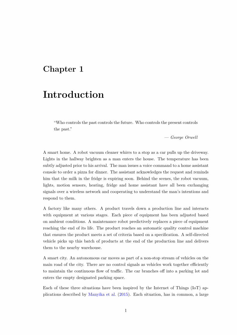
M ot ion Sensor
R obot Vacuum CleanerTemper at ur e Sensor
H eat er
18:00:0018:00:0118:00:02
NoNoYes
T imest amp M ot ion
D at a
M et adat a
Locat ion
H allway18:00:0018:00:0118:00:02
20.021.022.0
T imest amp Temp
D at a
M et adat a
Locat ion
18:00:00
T imest amp
D at a
Locat ion St at us
Off
H ome A ssist ant
State Off
H allway L ight
State On
Locat ion
from sensors
Locat ion
to actuators
Figure 1.1: Sensors, Actuators, Data and Metadata in a Smart Home Scenario
In the earlier smart home scenario, the motion sensor and temperature sensor in ahallway each produced a time-series stream of sensor data as shown in Figure 1.1. Ahome assistant application processed each stream and actuated the lights when motionwas detected two seconds after six in the evening and shut off the heater when anoptimal temperature of 22.0 degrees celsius was reached. All the sensors and actuators
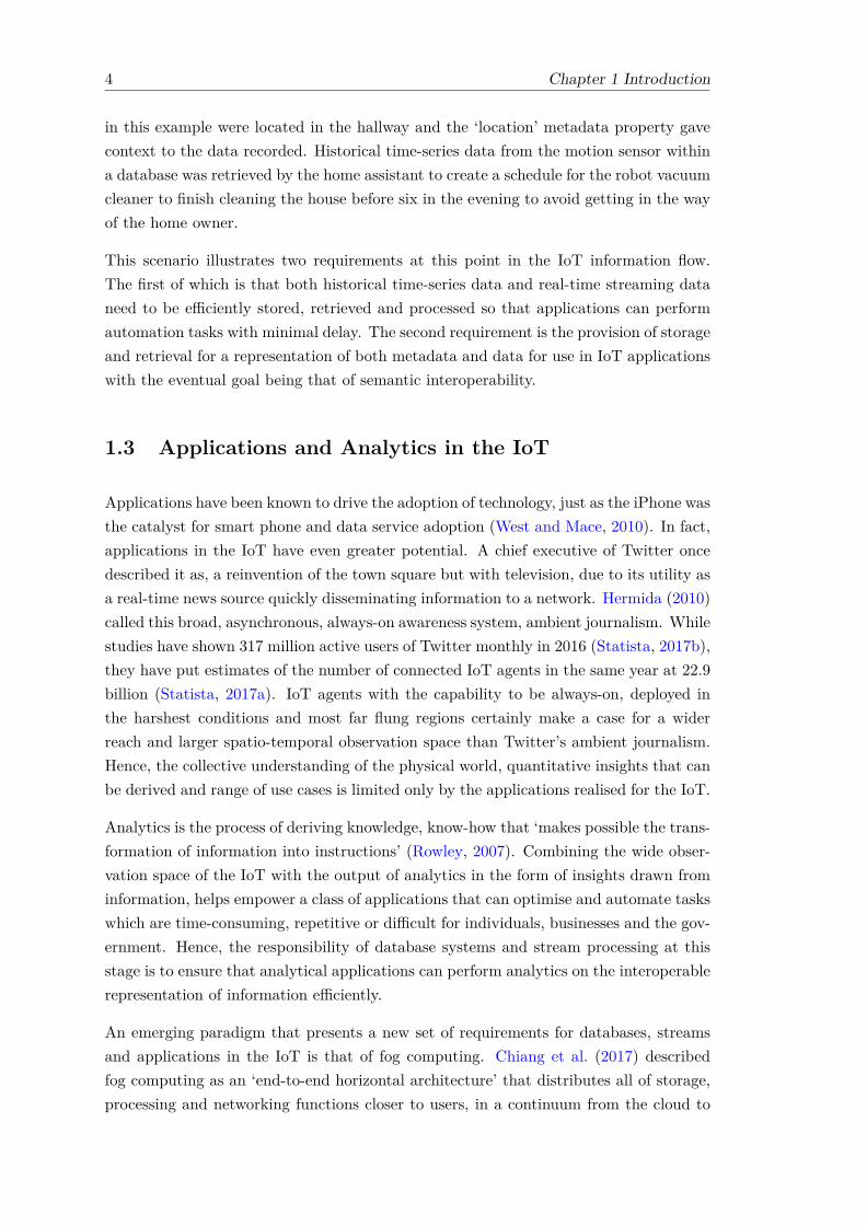
4 Chapter 1 Introduction
in this example were located in the hallway and the ‘location’ metadata property gavecontext to the data recorded. Historical time-series data from the motion sensor withina database was retrieved by the home assistant to create a schedule for the robot vacuumcleaner to finish cleaning the house before six in the evening to avoid getting in the wayof the home owner.
This scenario illustrates two requirements at this point in the IoT information flow.The first of which is that both historical time-series data and real-time streaming dataneed to be efficiently stored, retrieved and processed so that applications can performautomation tasks with minimal delay. The second requirement is the provision of storageand retrieval for a representation of both metadata and data for use in IoT applicationswith the eventual goal being that of semantic interoperability.
1.3 Applications and Analytics in the IoT
Applications have been known to drive the adoption of technology, just as the iPhone wasthe catalyst for smart phone and data service adoption (West and Mace, 2010). In fact,applications in the IoT have even greater potential. A chief executive of Twitter oncedescribed it as, a reinvention of the town square but with television, due to its utility asa real-time news source quickly disseminating information to a network. Hermida (2010)called this broad, asynchronous, always-on awareness system, ambient journalism. Whilestudies have shown 317 million active users of Twitter monthly in 2016 (Statista, 2017b),they have put estimates of the number of connected IoT agents in the same year at 22.9billion (Statista, 2017a). IoT agents with the capability to be always-on, deployed inthe harshest conditions and most far flung regions certainly make a case for a widerreach and larger spatio-temporal observation space than Twitter’s ambient journalism.Hence, the collective understanding of the physical world, quantitative insights that canbe derived and range of use cases is limited only by the applications realised for the IoT.
Analytics is the process of deriving knowledge, know-how that ‘makes possible the trans-formation of information into instructions’ (Rowley, 2007). Combining the wide obser-vation space of the IoT with the output of analytics in the form of insights drawn frominformation, helps empower a class of applications that can optimise and automate taskswhich are time-consuming, repetitive or difficult for individuals, businesses and the gov-ernment. Hence, the responsibility of database systems and stream processing at thisstage is to ensure that analytical applications can perform analytics on the interoperablerepresentation of information efficiently.
An emerging paradigm that presents a new set of requirements for databases, streamsand applications in the IoT is that of fog computing. Chiang et al. (2017) describedfog computing as an ‘end-to-end horizontal architecture’ that distributes all of storage,processing and networking functions closer to users, in a continuum from the cloud to

Chapter 1 Introduction 5
IoT agents called Things. Bonomi et al. (2012) argued that the wide-spread distributionof Things and run-time bounds or limited connectivity in certain use cases make such anarchitecture necessary. Database systems supporting applications across more diversehardware specifications is therefore also a point of consideration.
1.4 Research Questions
The flow of information from production to usage in the IoT, as described in the previoussections, forms the premise for an overall database systems research question:
“How can database systems support the efficient storage and retrieval of asemantically interoperable representation of data and metadata, both histor-ical and real-time, from the Internet of Things, for analytical applications?”
The literature surrounding database systems contains support for many different modelsof representation and optimisations for storing and retrieving such models. IoT researchis multi-faceted and spreads out in many directions, one of which is the collecting andprocessing of big data for the creation of knowledge which a semantically interoperablerepresentation is essential for (Stankovic, 2014). There has however only been sometentative effort to bring this research together which is elaborated on in Chapter 2 thatsets out the background literature in detail. To pursue the original research question,three additional sub-questions, developed in the following paragraph, are asked.
The first two sub-questions are “Are there unique characteristics in IoT time-seriesdata?” and “Can a representation of IoT metadata and time-series data that enablesinteroperability be found?”. These sub-questions motivate the study of IoT data, se-mantic interoperability in the IoT and other IoT literature. Having established thatthere exists a set of characteristics and a semantically interoperable representation forthe IoT, the next question is then “How can database and stream processing systemsutilise these characteristics to efficiently store and query this representation model foranalytics across diverse hardware?”. The answering of each sub-question proceeds theargument of the original research question, the output of which is shown in the nextsection listing the main research contributions.
1.5 Research Contributions
This thesis focuses on optimising database systems for the efficient and interoperablequerying of information from the IoT for analytical usage within applications. A sum-mary of the intellectual research contributions are as follows:

6 Chapter 1 Introduction
• A study of IoT survey literature that advises a categorisation of IoT research withfollow-up studies on advanced applications, architectures, technologies, databaseand stream processing systems and analytics (Chapter 2).
• A study of public IoT time-series data across application domains, showing the flat,wide and numerical nature of data streams that also display varying periodicity(Chapter 3).
• A study of metadata models for the IoT from different domains and perspectivesshowing there is a common underlying graph or tree representation (Chapter 3).
• A study of metadata and data ratios in graph model IoT data of the Resource De-scription Framework (RDF) format, highlighting the issue of metadata expansion(Chapter 3).
• An abstraction for query translation enabling graph queries to be executed acrossgraph model metadata and time-series data. An implementation using in-memoryRDF storage with a relational database demonstrates comparatively better aggre-gation support, fewer joins and greater storage and retrieval efficency than a rangeof RDF stores and translation engines (Chapter 4).
• A new compressed, time-reordering, performance-optimised data structure for stor-ing IoT time-series data, TrTables (Chapter 5).
• An evaluation of compression algorithms and data structures for time-series dataadvising the design of a time-series database, TritanDB (Chapter 5).
• An evaluation of multiple time-series, relational and NoSQL databases includingTritanDB for IoT time-series data across cloud and Thing hardware (Chapter 5).
• A method for translating and executing continuous queries on a stream of RDFgraph model data and an infrastructure for distributing this over a fog computingnetwork (Chapter 6).
• A set of applications and analytics applying the methods in this thesis, for per-formant and interoperable IoT storage and querying, to personal repositories, theSocial Web of Things and time-series analytics (Chapter 7).
1.6 Thesis Outline
This introduction chapter has provided the context from which this research originatedand its direction and contribution. This section explains the remainder of the thesiswhich is divided into seven components. The first component (Chapter 2) covers astudy of the background literature within the fields of IoT and database systems researchrelevant to this thesis.

Chapter 1 Introduction 7
The next four components address the research questions proposed in this thesis. Chap-ter 3 investigates the characteristics of IoT time-series and seeks a representation tomodel IoT metadata and IoT time-series data through a series of studies. Chapter 4moves on to propose and realise a solution to efficiently store and query both time-seriesdata and metadata within a flexible representation model, targeting greater semanticinteroperability. Chapter 5 then iterates on the storage and querying of time-series databy an understanding and sensitivity towards physical hardware characteristics and IoTdata characteristics. Next, Chapter 6 extends optimisations to stream processing, andstream processing within distributed fog computing systems. Each of these componentsfollow a common method whereby understanding is achieved through studies, whichthen advises the formalisation of solutions guided by the IoT use case. Design andimplementation follows which is benchmarked against the state-of-the-art within IoTscenarios and utilising public data for reproducibility.
Finally, Chapter 7 describes IoT applications and analytics that reflect and demonstratethe impact of the database systems research within this thesis on wider IoT themes.Chapter 8 concludes by analysing the limitations of this work and the potential forfurther study, before final remarks present a summary of this thesis.
1.7 Publications and Software
The work presented in this thesis has resulted in several publications, datasets, submis-sions under review and software projects presented as follows:
Published work
Eugene Siow, Thanassis Tiropanis, and Wendy Hall (2016a). Interoperable & Efficient:Linked Data for the Internet of Things. In Proceedings of the 3rd International Confer-ence on Internet Science, 2016.
Eugene Siow, Thanassis Tiropanis, and Wendy Hall (2016b). PIOTRe: Personal In-ternet of Things Repository. In Proceedings of the 15th International Semantic WebConference P&D, 2016.
Eugene Siow, Thanassis Tiropanis, and Wendy Hall (2016c). SPARQL-to-SQL on Inter-net of Things Databases and Streams. In Proceedings of the 15th International SemanticWeb Conference, 2016.
Eugene Siow, Thanassis Tiropanis, and Wendy Hall (2017). Ewya: An InteroperableFog Computing Infrastructure with RDF Stream Processing. In Proceedings of the 4thInternational Conference on Internet Science, 2017.
A note is made at the start of each chapter in this thesis of the sections which containthe above published work and the relevant citations.

8 Chapter 1 Introduction
Published Datasets
Eugene Siow (2017). Cross-IoT Study of the Characteristics of IoT Schemata and DataStreams. doi:10.5258/SOTON/D0202.
Eugene Siow (2016). Dweet.io IoT Device Schema. doi:10.5258/SOTON/D0076.
Submissions Under Review or Revision
Eugene Siow, Thanassis Tiropanis, Wendy Hall (2017). Analytics for the Internet ofThings: A Survey. ACM Computing Surveys, Submitted may 2016, Revised sep 2017.
Eugene Siow, Thanassis Tiropanis, Xin Wang, Wendy Hall (2017). TritanDB: Time-series Rapid Internet of Things Analytics. ACM Transactions on Database Systems,Submitted sep 2017.
Eugene Siow, Thanassis Tiropanis, Wendy Hall (2017). A Decentralised Social Web ofThings. IEEE Pervasive Computing, Submitted nov 2017.
Software Projects
• DistributedFog.com (Chapter 2): An educational resource describing the vari-ous technologies within the IoT landscape (http://distributedfog.com).
• S2S (Sections 4.2.4 and 6.1.1): An implementation of the Map-Match-Operateabstraction proposed in this thesis with support for graph query translation fromSPARQL queries to execution on relational databases or streams using the S2SMLdata model mapping language (https://github.com/eugenesiow/sparql2sql).
• TritanDB (Chapter 5): A time-series database for IoT analytics, implementing arich graph data model with underlying time-partitioned block compression usingTrTables and utilising Map-Match-Operate (http://tritandb.com).
• Eywa (Section 6.2): A fog computing infrastructure that provides control anddata planes for RDF stream processing to be performed on resource-constrainedclient, source and broker nodes (https://github.com/eugenesiow/eywa).
• PIOTRe (Section 7.1): A Personal IoT Repository based on S2S that consists ofa sink for IoT data streams and historical time-series that allows applications tobe built with it (https://github.com/eugenesiow/PIOTRe-web).
• Hubber.space (Section 7.3.4): An experimental sandbox application developedto realise the core social network functions of a decentralised Social Web of Thingswhich integrates a lightweight and scalable publish-subscribe broker to controlinformation flow among PIOTRe devices (http://hubber.space).

Chapter 2
Background
“If I have seen further than others, it is by standing upon the shoulders ofgiants.”
— Sir Isaac Newton
This chapter details an overview of the literature surrounding both Internet of Things(IoT) research and that of database systems which have increasingly been driven by theneed to store and process big data. Each research area has grown tangentially withoutmuch overlap and hence this chapter seeks to establish common ground, acknowledgethe tentative efforts taken to integrate research and surface the gaps that motivatedthe research within this thesis. The chapter starts by defining the IoT and introducinga means of categorising the broad, multi-directional research through an analysis ofvarious survey papers, building up to studies of IoT architectures, the layers withinthose architectures and the technology building blocks of interest within those layersin Section 2.1. The chapter then moves on to examine database and stream processingsystem literature in the IoT context in Section 2.2. The goal of efficient and interoperabledata management is to act as an enabler for advanced applications and services throughanalytics, which is the focus of Section 2.3. Finally, Section 2.4 summarises literatureinvolving the emerging IoT research area of fog computing.
2.1 Definition and Categorisation the IoT
The vision of the IoT was defined by the International Telecommunication Union (2012)as a ‘global infrastructure’ that interconnects Things with ‘interoperable informationand communication technologies’ to enable ‘advanced services’ that have ‘technologicaland societal’ impact. The report from the United Kingdom Government Office forScience agreed and added that the purpose of interconnecting these ‘everyday objects’is so that data can be shared (Walport, 2014). The same points were also observed in
9

10 Chapter 2 Background
the definition by Vermesan and Friess (2014) and can be summarised as follows. TheIoT is:
• an infrastructure that exists at a global scale,
• made up of IoT agents called Things,
• interconnected so that data can be shared and
• has the potential for technological and societal impact through advanced applica-tions and services.
Human-to-Machine (H2M) Machine-to-Machine (M2M)
St akeholder sE.g.Individuals,
Businesses,Government
T hings
Applications and Services
D at aproduceinteractwith
sharedwith
interactwith
produceactuate
Global Scale
InterconnectedNetwork
Figure 2.1: Visualisation of the IoT Definition
Figure 2.1 visualises the definition of the IoT and the interactions between its compo-nents. Various stakeholders in the IoT, for example individuals, businesses or the gov-ernment, interact with IoT agents called Things, or applications and services throughhuman-to-machine (H2M) interfaces. Both Things and applications produce data thatis shared through the interconnected network and this exchange is termed Machine-to-Machine (M2M) interaction. Applications and services, possibly across multiple applica-tion domains, act on data to actuate Things or produce more data which could containinsights that lead to various positive societal impacts, such as greater productivity withthe smart automation of time-consuming tasks. All of these interactions can occur on aglobal scale. The flow of information in the IoT, introduced in Chapter 1, describes theM2M flow of data produced by Things to applications and services.
This thesis is particularly concerned with the M2M interaction of IoT Things, data andapplications with the goal of improving how the data produced can be represented, storedand used by applications and services in both an interoperable and efficient manner. Assuch, this section moves forward to cover the broad spectrum of IoT research through asensible means of categorising the literature that will be introduced in Section 2.1.1.

Chapter 2 Background 11
2.1.1 IoT Applications, Platforms and Building Blocks Categorisation
Given the broadness of the IoT landscape, a sensible way of categorising literature isthe one used by IoT venture capitalist, Turck (2016), who categorised IoT stakeholders(businesses and organisations) into those involved with verticals, IoT applications, thoseinvolved with horizontals, IoT platforms, and those involved with the building blocksthat make up these. Research literature can be categorised similarly as verticals, hor-izontals and building blocks but with a focus on the underlying technologies, originalresearch and state-of-the-art applications instead of stakeholders.
Year Survey Reference A P B Description2010 Atzori et al. (2010) 3 3 3 IoT Survey2011 Bandyopadhyay et al. (2011) 3 3 Middleware for IoT2012 Miorandi et al. (2012) 3 3 3 IoT Vision, Apps, Challenges
Barnaghi et al. (2012) 3 3 Semantic Interoperability2013 Vermesan and Friess (2013) 3 3 3 IoT Ecosystem2014 Perera et al. (2014) 3 3 Context Aware Computing
Zanella et al. (2014) 3 3 3 IoT for Smart CitiesXu et al. (2014) 3 3 3 IoT in IndustriesStankovic (2014) 3 IoT Challenges
2015 Al-Fuqaha et al. (2015) 3 3 3 Protocols, Challenges, AppsGranjal et al. (2015) 3 3 Security Protocols, Challenges
2016 Ray (2016) 3 3 3 IoT ArchitecturesRazzaque et al. (2016) 3 Middleware for IoT
2017 Lin et al. (2017) 3 3 3 Fog ComputingFarahzadia et al. (2017) 3 Middleware for Cloud IoTSethi and Sarangi (2017) 3 3 3 IoT Architectures, Apps
Legend: A = Applications, P = Platforms, B = Building Blocks
Table 2.1: Chronological Summary of Previous IoT Surveys Categorised by Applica-tions, Platforms and Building Blocks Research
Table 2.1 presents a sequence of IoT surveys in chronological order and categorisedaccording to whether they studied IoT applications, platforms or building blocks or acombination of the three. The progression of surveys showed an increasing amount ofinterest in a variety of topics related to the IoT since its inception when the term wascoined by Ashton (2009).
The surveys also covered a range of research topics from defining the general vision,challenges and ecosystem of the IoT (Atzori et al., 2010; Miorandi et al., 2012; Ver-mesan and Friess, 2013; Stankovic, 2014; Al-Fuqaha et al., 2015; Ray, 2016; Sethi andSarangi, 2017) to tackling specific domains like Smart Cities (Zanella et al., 2014) orindustries (Xu et al., 2014) to surveying specific technologies and platforms like mid-dleware (Bandyopadhyay et al., 2011; Razzaque et al., 2016; Farahzadia et al., 2017),semantic interoperability technology (Barnaghi et al., 2012), context aware computing(Perera et al., 2014) or fog computing (Lin et al., 2017), to addressing specific issues like

12 Chapter 2 Background
security (Granjal et al., 2015). They also showed a sustained amount of interest andactivity in each segment of the categorisation.
2.1.2 IoT Applications: Application Areas, Domains and Themes
A range of application areas were first elicited from all the surveys describing IoT appli-cations. To better understand the ‘technological and societal impact’ of each applicationarea, they were categorised according to their impact towards the three drivers of sustain-able development, namely, society, economy and environment. The goal of sustainabledevelopment, which is used for analysing medium to long term development issues ata large scale, is usually defined within literature as the intersection of the society, theeconomy and the environment (Giddings et al., 2002).
Smart Energy/ Grid
Societ y
Economy Envir onment
Social Networks and IoT
Smart Cities
Smart Transportation
Smart Home/Home Automat ion
Smart Buildings
Smart Factory/Smart Manufacturing
Part icipatory Sensing
Healthcare
Food and Water Tracking and Security
Food Supply Chain
Mining Product ion
Agriculture
Supply Chain Logist ics
Fitness
Social Life and Entertainment
Environmental Monitoring
Firefight ing
Figure 2.2: Application Areas from Surveys Categorised by Impact to Society, Econ-omy and Environment
Figure 2.2 shows the categorisation of the various application areas elicited from thesurveys. The categorisation was based on the most direct impact of the output eachapplication area had, for example, the improvement that IoT healthcare brought inthe ambient-assisted-living use case (Dohr et al., 2010) benefited a group of peoplewithin the society directly, while any economic impact was indirect. Hence, healthcare

Chapter 2 Background 13
is categorised under society only. Most application areas can be seen to impact thesociety and economy, as explained by Giddings et al. (2002), because of the politicaland material reality within countries, constructed by businesses and governments, thatprioritises these two areas over the environment.
All of the surveys, except the one by Xu et al. (2014) on industries, have listed smartcities as an IoT application area. Smart cities whose vision, as presented by Zanellaet al. (2014), is to use advanced technologies to ‘support added-value services for the ad-ministration of the city and for the citizens’, have an impact on the environment, societyand economy. In the 101 scenarios within a smart city listed by Presser et al. (2016),there are scenarios with environmental impact like air pollution monitoring and countermeasures, those with societal impact like public parking space availability prediction,and those with economic impact like efficient lighting to reduce energy costs.
Smart transportation systems also span smart cities and other application areas likesupply chain logistics (Atzori et al., 2010; Xu et al., 2014), can intelligently manage traf-fic, parking and minimise accidents (Sethi and Sarangi, 2017), or even provide assisteddriving or vehicle control and management (Vermesan and Friess, 2013) and impact theeconomy, society and environment.
Some of the scenarios for the smart city (Presser et al., 2016) also overlap other appli-cation areas mentioned like environmental monitoring covered by Miorandi et al.(2012) which also extends monitoring to wide areas outside cities for anomalies andearly-warning for disasters. The smart grid, smart energy (Vermesan and Friess, 2013;Lin et al., 2017) and energy conservation systems (Sethi and Sarangi, 2017) are flexibleelectrical serving and storage infrastructure utilising renewable sources of energy. Thesmart grid is able to react to power fluctuations through reconfiguration and optimisa-tion, providing a positive economic and environmental impact.
The application areas of the IoT with an economic impact within industries are alsovery wide and include monitoring and controlling the food supply chain and safermining production, all of which were described in the survey by Xu et al. (2014).Smart inventory and product management as described by Miorandi et al. (2012) helpsimprove the supply chain logistics throughput. Smart factories that allow efficientproduction and optimisation of the manufacturing process are another industrial use case(Vermesan and Friess, 2013). The automatic control of environmental parameters suchas temperature and humidity for agriculture is yet another industrial IoT applicationarea described by Sethi and Sarangi (2017). Firefighting which minimises propertydamage has both economic and social impact (Xu et al., 2014).
Smart buildings as described by Miorandi et al. (2012) help to reduce the consumptionof resources, benefiting the environment, and improve the ‘satisfaction level of humanspopulating it’, benefiting the society. Smart homes are a particularly popular IoTapplication area, sometimes considered a specific type of smart building, and have been

14 Chapter 2 Background
described in quite a few surveys (Atzori et al., 2010; Miorandi et al., 2012; Vermesanand Friess, 2013; Sethi and Sarangi, 2017). This popularity was attributed by Sethi andSarangi (2017) to two reasons, the increasing ubiquity of sensors, actuators and wirelessnetworks within home settings, and the increased trust in technology to improve ‘qualityof life and security’ within homes. Other application areas with societal impact includeparticipatory sensing, social networks and IoT, that involve community informa-tion and knowledge, and food and water tracking and security, each described byVermesan and Friess (2013), social life and entertainment as well as fitness de-scribed by Sethi and Sarangi (2017) with facilities like the smart gym for fitness andsmart museum for education and entertainment described by Atzori et al. (2010).
Hence this categorisation of application areas helps introduce the full range of use casespresented in all the surveys studied while establishing an understanding of the directimpact of an application area on the development of the society, economy and environ-ment. It is then possible to further distil and group the application areas to derive aset of general domains, namely, health, industry, environment and living, and anotherset of broad application themes that cut across domains, namely, smart cities, smarttransportation and smart buildings. The grouping is shown in Figure 2.3.
Domains
Health
HealthcareFitness
Food/Water Safety
Industry
AgricultureMining
Supply ChainSmart Factory
Environment
MonitoringSmart Grid
Living
Social NetworksEntertainment
Participatory Sensing
Themes
Smart Cities Smart TransportationSmart Buildings
Smart Homes
Figure 2.3: Application Domains and Themes Based on Application Areas
This structure of application domains and themes is then helpful for conducting a sys-tematic review to address one of the gaps in the literature present in the reviewedsurveys, that is, by producing a summary of IoT research involving actual advanced ap-plications and services, how these applications derive insights and knowledge from dataand the kind of data used, streaming or historical. This is covered in the next section.

Chapter 2 Background 15
2.1.3 IoT Applications: A Survey of Techniques and Data Currency
To further the understanding of IoT verticals within applications for this thesis, a surveyof the research literature detailing actual advanced applications and services developedfor each application domain and theme was conducted. This helps to fill a gap inthe literature as the purpose of each of the surveys from Table 2.1 was to introduceapplication use cases rather than review applications and in particular, the techniquesand approaches the applications took to produce smart or intelligent outputs or performautomation. Another goal is also to identify in literature whether IoT applications actedon historical data in databases or processed real-time streaming data.
The methodology for this survey follows that of an evidence-based systematic review(Khan et al., 2003). A total of 460 articles were retrieved from 2011 to 2015, and an-other 311 articles from 2016 and 2017 were added as the survey was revised and updated.The articles were identified from the Web of Science platform1, that indexed an exten-sive list of multi-disciplinary journals and conferences across research databases, with asearch criteria that included the keywords ‘big data’ or ‘analytics’ and filtered by‘internet of things’. The articles were screened manually with an inclusion criteriathat mandated they 1) were original research, 2) described actual designs, implementa-tions and results, 3) had value-added output and 4) served IoT use-cases, bringing thetotal to a set of 32 articles. These articles were further classified into the four applicationdomains and three application themes derived in the previous section with each domainand theme well-represented as shown in Table 2.2. In addition, the table also states therespective techniques used to derive insights and the currency of the data used, whetherit was historical data from a database or real-time streaming data.
Appendix A provides more detailed descriptions of the individual papers for each appli-cation domain and theme. A point to note from an analysis of the survey of applicationpapers was that both historical data and real-time streaming data was used in IoT ap-plications across domains which justifies the need to support both databases and streamprocessing in this thesis’ work, as highlighted in Chapter 1. Another point to note wasthat although the papers covered a broad range of techniques, there was little mentionor usage of any common IoT platforms, and each application used their own stack oftechnologies while data produced was placed in a vertical silo, hence, there was littlecross-domain integration of data within the applications, even within application themeslike smart cities and smart transportation, at the point of this survey.
The next section continues the study of the IoT by looking at the next category, plat-forms, backed by the research summarised in the set of IoT surveys from Table 2.1.
1https://webofknowledge.com/

16 Chapter 2 Background
Reference Application Technique CCHealth
Mukherjee et al. (2012) Ambient-Assisted-Living Rules, Ontologies RHenson et al. (2012) Medical Diagnosis Abductive Logic HRodríguez-González et al. (2012) Medical Diagnosis Descriptive Logic HHunink et al. (2014) Prognosis Data mining HLi et al. (2013) Healthcare Costing Random Forests H
IndustryVargheese and Dahir (2014) On Shelf Availability Video Analytics RNechifor et al. (2014) SCM Environment Control CEP RVerdouw et al. (2013) Agriculture SCM CEP RRobak et al. (2013) SCM Ontologies REngel and Etzion (2011) SCM Critical Shipments MDP R
EnvironmentYue et al. (2014) Haze Early Warning Data mining RSchnizler et al. (2014) Disaster Warning Anomaly Detection RMukherjee et al. (2013) Wind Forecasting ANN HAlonso et al. (2013) Recommend Energy Usage ML + Rules HAhmed (2014) Energy Policy Planning Classifier + Models HGhosh et al. (2013) Smart Energy System Data mining H
LivingGimenez et al. (2012) Security Monitoring Video Analytics RMukherjee and Chatterjee (2014) Wearable Lifestyle Monitor Anomaly Detection RMcCue (2006) Police Deployment Data mining HMcCue (2005) Suspicious Activity Detection Visualisation HRazip et al. (2014) Situational Awareness Visualisation HRamakrishnan et al. (2014) Civil Unrest Prediction Multimodal HGuo et al. (2011) Memory Augmentation Data mining H
Smart CitiesZheng et al. (2014) Smart Parking Data mining RHe et al. (2014) Smart Parking Data mining RStrohbach et al. (2015) Smart City Grid CEP + Models R
Smart TransportationMak and Fan (2006) Traffic Control Video Analytics RLiebig et al. (2014) Travel Routing CRF, A*Search RWang and Cao (2014) Travel Routing Bn & MDP R
Smart BuildingsPloennigs et al. (2014) Smart Building Heating Anomaly Detection RMakonin et al. (2013) Smart Home Energy Rules RWeiss et al. (2012) Smart Meter Patterns Signature Detection H
Legend: ANN=Artificial Neural Network, Bn=Bayesian Network, CC = Data Currency, CEP=ComplexEvent Processing, CRF=Conditional Random Fields, H=Historical, MDP=Markov Decision Process,
ML=Machine Learning, R=Real-time, SCM=Supply Chain Management
Table 2.2: Summary of IoT Applications by Domains and Themes with the Techniquesto Derive Insights and the Data Currency of Each Application

Chapter 2 Background 17
2.1.4 IoT Platforms: Architectures, Layers, Middleware
The literature on the IoT has proposed a number of general reference architectures whichare summarised in Figure 2.4. The three-layer architecture initially proposed by Yun andYuxin (2010) drew from service-oriented paradigms in industrial informatics literatureand defined an application, network and perception layer. The perception layer for theIoT consists of Things, while the network layer connects applications and services in theapplication layer to these Things. A similar proposal by Ning and Wang (2011) wasinspired by the human nervous system and models the three layers as the brain, spinalcord and nerves. Wu et al. (2010) expanded the application layer to business, applicationand processing layers to form a five-layer architecture. The business layer containssystems that manage applications, business models and privacy within organisations.The processing layer, also called the middleware layer by Mashal et al. (2015), wasintroduced to store and process data, delivered by the transport layer and created byThings from the perception layer, for applications. The transport layer, which handlesflow control and consistency, and the network layer, which provides addressing androuting, are often combined in IoT literature and referred to by either name.
Applicat ion Layer
Network Layer
Percept ion Layer
Business Layer
Applicat ion Layer
Processing Layer
Transport Layer
Percept ion Layer
Applicat ion Layer
Middleware Layer
Coordinat ion Layer
Backbone Network Layer
EdgeApplicat ion
System
Access Layer
Edge Technology
Applicat ions
Service Composit ion
Service Management
Object Abst ract ion
Objects
Transport Layer
Monitoring Layer
Physical Layer
Preprocessing Layer
Storage Layer
Security Layer
Other Layers
T hr eeLayer
F ive Layer
Ser v ice Or ient ed
Edge Technology
Fog Comput ing
Brain(Data Centre)
Spinal Cord(Network ControlNodes)
Nerves(Sensors)
H umanI nspir ed
Applicat ions ThingsIntermediate (Network/ Transport / Processing)
Figure 2.4: IoT Architectures
The service-oriented architecture proposed by Atzori et al. (2010) provides well-definedcomponents to describe services for a middleware software layer between the applicationand perception layer of the IoT, which can also be seen as a sub-layer architecture forthe intermediate processing layer.
Tan and Wang (2010) proposed an ‘edge technology’ architectural design that extendsthe processing, transport and perception layers to cater for applications that run on

18 Chapter 2 Background
IoT Related Technology Reference/LinkApplication Layer: App Protocols
Advanced Message Queuing Protocol (AMQP) http://www.amqp.orgConstrained Application Protocol (CoAP) http://coap.technologyData Distribution Service (DDS) http://portals.omg.org/ddsHypertext Transfer Protocol (HTTP) http://http2.github.ioMQ Telemetry Transport (MQTT) http://mqtt.orgWebSockets Fette and Melnikov (2011)XMPPa http://xmpp.org
Application Layer: OthersAnalytics Section 2.3Cloud of Things Aazam et al. (2014)Social IoT Atzori et al. (2012)Social Web of Things Section 7.3Web of Things https://www.w3.org/WoT
Processing LayerBig Data Processing Chen et al. (2014)Databases and Stream Processing Section 2.2Middleware Razzaque et al. (2016)
aExtensible Messaging and Presence Protocol (XMPP)
Table 2.3: References for Application and Processing Layers Technologies
Things themselves or on gateways deployed within localised ‘edge networks’. This par-ticular architecture has started to gain popularity recently with the emergence of a newparadigm, fog computing, that provides compute services for ‘customers or applicationsin the space between networking central servers and end-users’ (Lin et al., 2017).
Aazam and Huh (2014) proposed an architecture for a fog computing node like a smartgateway, that adds four layers, security, temporary storage, preprocessing and moni-toring, between the physical Thing layer and the transport layer. According to thisarchitecture, the security layer provides protection for private and sensitive data, thestorage layer stores data on fog resources, the preprocessing layer manages, aggregatesand filters data, and the monitoring layer monitors the activities of the underlying nodes.
Each of the surveys with literature on platforms and building blocks was reviewed, withthe set of proposed architectures from Figure 2.4 in mind, to determine componentswithin each of the layers. A summary of the findings is presented in Figure 2.5 thatshows architectural layers made up of components from the literature. Platforms arehorizontals of one or more architectural layers made up of building block components(each a box in the figure) that contain lists of technologies, standards or requirements.The areas of particular research within this thesis, which is concerned with efficient andinteroperable data representations within database and stream processing systems foranalytical applications, are also highlighted (shaded) in Figure 2.5. The business and

Chapter 2 Background 19
Per
cept
ion
Lay
erN
etw
ork
Lay
erP
roce
ssin
g L
ayer
App
licat
ion
Lay
er
Gateway Networks
EthernetGSMGPRSLTE
LoRaISMWiFi
WiMax
Network Protocols
IPv4 IPv6
Operat ing Systems
AndroidBrillo
Cont ikiLiteOSRiot OSTinyOS
Sensor Networks
6LowPAN802.15.4
ANTBT(LE)DASH7
FireWireHAN
P1906.1IR
IrDAInsteonNFCSANUWBRPL
W-USBZ-WaveZigBee
Tags
BarcodeiBeaconQR code
RFID(UHF/ HF/ LF)UriBeacon
Hardware
App ProtocolsAMQPCoAPDDS
HTTP(/ 2)MQTT
WebSocketsXMPP
ArduinoGalileoGizmo2
RPiGadgeteer
BeagleBoneCubieboard
SmartThingsEssent ialHomeSmartphonesTinkerBoard
PhidgetsNUC
Microbit
Security
1888.3IPSec
Discovery
DNS-SDµPnP
MC-CoAPmDNSSSDP
Middleware
Resource DiscoveryResource ManagementD at a M anagementEvent M anagement
Code Management
Architectural Requirements
I nt er oper ableContext -AwareAutonomous
Adapt iveService-orientedProgrammable
LightweightDist ributed
Functional RequirementsDatabasesRelat ional
GraphSemant ic/ RDF
NoSQLTime-series
Stream/ Complex Event Processing
Analyt ics
Big Data Processing
Fog/ Edge Gateways
SecurityStorage
ProcessingMonitoring
Sensors and Actuators
Classes
Descript iveDiagnost icDiscoveryPredict ive
Prescript ive
Types/ Research Areas
VisualContent
TextVideoTrend
Data MiningOLAP
BusinessAnomalyPat tern
Social IoT
Thing Directories
CoRE DirectorydigrectoryHyperCat
SIR
Web of Things
Cloud of Things
Social Web of Things
Power
Energy Harvest ingMot ion ChargingWireless Power
TCP UDP
Figure 2.5: IoT Architectural Layers Forming Platform Horizontals with BuildingBlocks as Components
application layers are combined to form a single layer in this summary, while the networklayer contains data-link, network and transport layer functions. Table 2.3 providesreferences or links to the literature for the application and processing layers while Table2.4 provides references for the network layer and Table 2.5 for the perception layer.
Middleware for the IoT provides a software layer between the application and the net-work communications layer. The processing layer, sometimes called the middlewarelayer, contains IoT middleware which has received much attention within literature(Bandyopadhyay et al., 2011; Farahzadia et al., 2017). In the survey paper on IoT

20 Chapter 2 Background
IoT Related Technology Reference/LinkNetwork Layer: Gateway Networks
Ethernet IEEE 802.3GSM and GPRSa Hillebrand (2013)Long-Term Evolution (LTE) http://www.3gpp.org/article/lteLong Range (LoRa) Wide Area Network http://www.lora-alliance.orgWaveLAN-II using ISMb Kamerman and Monteban (1997)WiFi IEEE 802.11WiMaxc IEEE 802.16
Network Layer: Sensor Networks6LowPAN, IEEE 802.15.4 RFC 4944, IEEE 802.15.4ANT/ANT+ http://www.thisisant.comBluetooth (BT) Low Energy (LE) http://www.bluetooth.comDASH7 http://www.dash7-alliance.orgIEEE 1394 FireWire http://1394ta.orgHome Area Network (HAN) Huq and Islam (2010)IEEE P1906.1 Nanoscale Communication IEEE 1906.1-2015Infrared Protocols (IrDA) http://www.irda.orgInsteon Home Automation Protocol http://www.insteon.comNear Field Communication (NFC) ISO/IEC 18000-3Storage Area Network (SAN) O’Connor (2003)Ultra-wideband (UWB), Impulse Radio (IR) Akyildiz et al. (2002)Wireless USB (W-USB) http://usb.org/developers/wusbZ-Wave http://www.z-wave.comZigBee http://www.zigbee.org
Network Layer: SecurityIEEE 1888.3 Network Security IEEE 1888.3-2013IPSec RFC 4301, RFC 4309
Network Layer: DiscoveryDNS Service Discovery (DNS-SD) http://www.dns-sd.orgMicro Plug and Play (µPnP) Yang et al. (2015)Multicast CoAP (MC-CoAP) RFC 7252Multicast DNS (mDNS) RFC 6762Simple Service Discovery Protocol (SSDP) IETF Draft Revision 3
Network Layer: Thing DirectoriesCoRE Directory IETF Draft Revision 11digrectory Jara et al. (2013)HyperCat http://www.hypercat.ioSensor Instance Repository (SIR) Jirka and Nüst (2010)
Network Layer: OthersFog/Edge Gateways Aazam and Huh (2014)Internet Protocol, Version 6 (IPv6) RFC 2460
aGlobal System for Mobile Communications (GSM), General Packet Radio Service (GPRS)bIndustrial, Scientific and Medical (ISM) Radio BandscWorldwide Interoperability for Microwave Access (WiMax)
Table 2.4: References for Network Layer Technologies

Chapter 2 Background 21
IoT Related Technology Reference/LinkSensors and Actuators http://distributedfog.com
Perception Layer: Operating SystemsAndroid and Brillo http://developer.android.com/thingsContiki http://www.contiki-os.orgLiteOS Cao et al. (2008)Riot OS https://riot-os.orgTinyOS Levis et al. (2005)
Perception Layer: TagsiBeacon http://developer.apple.com/ibeaconQuick Response (QR) Code ISO/IEC 18004:2015Radio-frequency identification (RFID) http://www.ieee-rfid.orgUriBeacon http://github.com/google/eddystone
Perception Layer: HardwareArduino http://www.arduino.ccBeagleBone Boards http://beagleboard.org/boneCubieboard http://cubieboard.orgEssentialHome http://www.essential.com/homeGalileo http://software.intel.com/iot/Gizmo2 x86 http://www.gizmosphere.orgMicrobit http://microbit.org.NET Gadgeteer Villar et al. (2012)Next Unit of Computing (NUC) http://www.intel.com/nucPhidgets http://www.phidgets.comRaspberry Pi (RPi) https://www.raspberrypi.orgSmartThings http://www.smartthings.comTinkerBoard https://tinkerboarding.co.uk
Perception Layer: PowerEnergy Harvesting Wolf (2017)Motion Charging: Ampy http://www.getampy.comWireless Power: ubeam https://ubeam.com
Table 2.5: References for Perception Layer Technologies
middleware, Razzaque et al. (2016) defined a set of functional and architectural require-ments for middleware. A key architectural requirement is that middleware should beinteroperable, working with heterogeneous Things and technologies without any ‘addi-tional effort from the application or service developer’. Two functional requirements thatmiddleware should service are data management and event management, in other words,the management of historical databases and real-time event streams of IoT data. Theserequirements are highlighted among others in Figure 2.5. Hence, there is motivationto study databases and stream processing systems as building blocks for the processinglayer platforms to be utilised by analytics within the application layer. Backgroundliterature on databases and stream processing systems are covered in detail in Section

22 Chapter 2 Background
2.2 while that on analytics for the IoT is covered in Section 2.3.
2.2 Databases and Stream Processing Systems
Two functional requirements of IoT software within the processing layer according toRazzaque et al. (2016) are to provide services that manage data and manage events.As Wu et al. (2011) pointed out, the sheer multitude of diverse Things periodicallysending observations about phenomena, or reporting events or anomalies when detected,produce what Abu-Elkheir et al. (2013) described as a massive volume of ‘heterogeneous,streaming and geographically-dispersed real-time data’, which present a different set ofrequirements and challenges than traditional database management scenarios.
Efficient data and event management for databases and stream processing systems areone requirement. The motivation behind this requirement is the volume of ‘streamingand continuous’ observation data together with an ‘urgency of the response’ within cer-tain applications, like traffic control or early warning systems (Abu-Elkheir et al., 2013).Observation and event data is also of the time-series form, with certain applications de-manding fast response times from database systems on queries ‘across time scales fromyears to milliseconds’, requiring what Andersen and Culler (2016) termed as a ‘newclass’ of systems, to meet the ‘unique storage’ demands of the high volume of time-seriesdata.
Interoperability is another key requirement within IoT data management systems, bothstreaming and historical. Abu-Elkheir et al. (2013), Milenkovic (2015) and Manyikaet al. (2015) all have pointed out the importance of integrating metadata, that includesThing ‘identification, location, processes and services provided’, with the data produced,for interoperability. Hence, flexible data representations that enable the modelling andstorage of metadata and data, which provide a means of semantic interoperability, arealso desirable.
With these two requirements in mind, this thesis studies the literature behind spe-cialised time-series databases for storing time-series data in Section 2.2.1, flexible graph-based databases like Resource Description Framework (RDF) stores in Section 2.2.2,and stream processing engines in Section 2.2.5.
2.2.1 Time-series Databases
In recent years, large amounts of telemetry data from monitoring various metrics ofoperational web systems, have provided a strong use case for research involving time-series databases. This research has been driven most recently by the industry, especiallytechnology companies that utilise and manage large web-scale systems. Sensor networks

Chapter 2 Background 23
Time-series Database Storage Engine Read Query Supporta
Π σ ./ γHeroic
Cassandra
HQL X X × XKairosDB JSON × t × XHawkular REST × t × XBlueflood × t × ×
InfluxDB
Native
LSM-based InfluxQL X X t XVulcan/Prometheus Chunks-on-FS PromQL X X × X
Gorilla/Beringei In-memoryREST
× t × ×BTrDb COW-tree × t × X
Akumuli Numeric-B+-tree × t × X
OpenTSDB HBase REST × X × X
Cube MongoDB REST × t × X
DalmatinerDB Riak DQL X X × XRiak-TS SQL-like X X × X
Tgres Postgres SQL X X X XTimescale X X X X
aΠ = Projection, σ = Selection, where t is selection by time only, ./ = Join, where t is joins by timeonly, γ = Aggregation functions
Table 2.6: Summary of Time-series Databases Storage Engines and Query Support
and financial systems are also sources of time-series data, while the IoT presents a rapidlygrowing source and sink of such data. Time-series databases from research publications,the industry and open source projects were reviewed and are summarised in Table 2.6describing the storage engine utilised, the means that applications can query or readdata from that particular database and the types of queries supported. The types ofqueries analysed were guided by basic relational algebra with projections (Π), selections(σ), joins (./) and aggregate functions (γ) essential for time-series data listed. Projectionrefers to selecting a subset of columns or attributes of a time-series, selection refers tofiltering specified columns or attributes of a time-series by a set of conditions, joins referto joining two or more time-series based on a set of conditions and aggregate functions area set of common functions like mean, summation or finding the maximum of a groupingof values within specified columns. The following sections, Sections 2.2.1.1 to 2.2.1.4,introduce the time-series databases categorised by their underlying storage engines inmore detail.
2.2.1.1 Cassandra-based Storage
Cassandra is a distributed NoSQL database initially developed by Lakshman and Malik(2010) and has a hybrid key-value and columnar (or tabular) data model supporting aSQL-like query language without support for table joins. The storage engine architecture

24 Chapter 2 Background
consists of an append-only commit log which then writes to an in-memory memtablefor buffering writes which are eventually flushed onto disk as immutable Sorted StringTables (SSTables). This design improves write-performance. Cassandra periodicallymerges SSTables together into larger SSTables using a process called compaction whichimproves read-performance. The storage engine is a particular implementation of aLog-Structured Merge-tree (LSM-tree) described by O’Neil et al. (1996).
Spotify (2017), a digital music streaming service, developed the time-series database,Heroic, that builds a monitoring system on top of Cassandra for time-series data storageand also uses the distributed full-text indexing search engine Elasticsearch by Elas-tic (2017) for metadata storage and indexing. Time-series databases Hawkular (Red-hat, 2017), KairosDB (2015) and Blueflood from cloud computing provider, Rackspace(2013), were all built on top of Cassandra.
KairosDB provides a JSON-based querying interface, while Heroic has a functionalquerying language HQL. Hawkular and Blueflood have Representational State Transfer(REST) interfaces that allow query parameters to be passed through Hypertext TransferProtocol (HTTP) requests for the results to be returned in the subsequent replies.
2.2.1.2 Native Time-series Storage
Gorilla (Pelkonen et al., 2015) is a fast, in-memory time-series database that was de-veloped by researchers at Facebook for their particular monitoring use case to act asan Operational Data Store (ODS) for time-series data. Gorilla uses a novel time-seriescompression method adapted specifically to the timestamps and values of time-seriesdata within their ODS. Gorilla was open-sourced in part as the time-series databaseBeringei2.
InfluxDB by Influx Data (2017) is another native time-series database that allows meta-data to be stored as a set of tags for each event. It utilises an LSM-tree (O’Neil et al.,1996) inspired design for its storage engine, similar to Cassandra, but applies Gorilla’scompression method for time-series storage and stores metadata tags in-memory.
Andersen and Culler (2016) introduced a time-partitioned, version-annotated, Copy-On-Write (COW) tree data structure for their time-series database, BTrDb, specifically tosupport high throughput time-series data from metering devices, called microsynchopha-sors, deployed within an electrical grid. Akumuli by Lazin (2017) is a similar time-seriesdatabase built for high throughput writes using a Numeric-B+-tree (a log-structured,append-only B+-tree) as its storage data structure. Timestamps within both databasesuse delta-of-delta compression similar to Gorilla’s compression algorithm. Akumuli usesFPC (Burtscher and Ratanaworabhan, 2009), a compression for floating-point valueswhile BTrDb uses delta-of-delta compression on the mantissa and exponent from each
2https://github.com/facebookincubator/beringei

Chapter 2 Background 25
floating point number within the sequence. Both databases also utilise the tree struc-tures to store aggregate data to speed up specific aggregate queries (like averages).
Vulcan3 from cloud-hosting provider, DigitalOcean, added horizontal scalability to thePrometheus (2016) time-series database, originally built by online audio distributionplatform, SoundCloud. Prometheus has a native storage layer, which organises time-series data in compressed chunks of a constant size on the filesystem (FS) on disk.Indexes of the time-series metadata and aggregations are stored in the LSM-tree struc-tured key-value store, LevelDB4.
Prometheus supports a limited, quite terse, functional query language, PromQL, whileGorilla, BTrDb and Akumuli all use REST interfaces and HTTP request-reply querying.InfluxDB features an SQL-like query language, InfluxQL, that supports a limited formof internal joins, only by time or an approximation of time, of two or more time-series.
All the time-series databases that implemented native storage also implemented a meansof compression for the individual points within the time-series. Each of the time-seriescompression algorithms and specialised native storage data structures are explained andanalysed in greater detail in Section 5.2.
2.2.1.3 HBase, MongoDB and Riak-based NoSQL Storage
OpenTSDB was originally developed by web content recommendation and discoveryengine StumbleUpon (2017) on top of a distributed NoSQL column-oriented key-valuestore, HBase, described by Wlodarczyk (2012). DalmatinerDB by Project FiFo (2014)and Riak-TS by Basho (2017) were both developed on top of Riak, originally a dis-tributed NoSQL key-value database, while Cube by Square (2012) was developed onMongoDB (Banker, 2011), a NoSQL document-oriented database that stores collectionsof structured JSON-like (JavaScript Object Notation) documents.
HBase, like Cassandra, has its roots in the Chang et al. (2008) paper on Google’s ‘sparse,distributed, persistent multidimensional map’ design called BigTable. The conceptualdata model, like Cassandra’s, is tabular, however, the physical view is that of key-valuepairs grouped by ‘column families’ where the key is the row identifier and value is theindividual field or attribute. Zhang (2009) provided a description of the underlying HFileformat, similar to the SSTable proposed in BigTable and used in Cassandra, explainingthe actual key-value storage format in more detail. Internally, OpenTSDB stores alldata points in a single table within HBase. All individual values are stored within acolumn family, and row keys are byte arrays that store the identifier of the time-series,timestamps and metadata tags in such a way as to group data together within time
3https://github.com/digitalocean/vulcan4https://github.com/google/leveldb

26 Chapter 2 Background
buckets, by utilising HBase’s sorted key-value organisation, for more efficient queryingas detailed in their design documentation5.
Both Riak-TS and DalmatinerDB, built on the distributed infrastructure of Riak, offerspecialised time-series storage. Riak-TS as described by Sicular (2016), introduces theneed for structuring data according to quanta, single ranges of time, so that logicalkeys can be stored together internally, thereby achieving ‘data co-location’ and makingqueries more efficient. DalmatinerDB was developed on top of Riak and utilises specificfeatures of ZFS, originally called the Zettabyte File System (Bonwick et al., 2003), likedisk caching mechanisms ARC and ZIL, and native data compression.
DalmatinerDB and Riak-TS implement SQL-like syntaxes, DQL and a subset of SQLrespectively, without support for join operations. OpenTSDB and Cube have RESTinterfaces allowing query parameters to be passed via HTTP requests and returningresults via HTTP replies.
2.2.1.4 Relational-database-based Storage
Tgres by Trubetskoy (2017b) and Timescale (2017) are time-series databases devel-oped on top of or as an extension to PostgreSQL6, an advanced open-source relationaldatabase system. Both Tgres and Timescale have full SQL query support as a result.
Tgres builds a database system on top of PostgreSQL and at the time of writing, featureda write-optimised storage design for time-series data at regularly-spaced intervals. Thisdesign avoided the inefficiency of appending each time-series point to a table, which inrelational databases involves a look up of the new identifier, locking of the table or partof the table and blocking until data has been synchronised to disk in most cases. This isavoided by implementing a round-robin database design, introduced by Oetiker (1998),with PostgreSQL arrays, where a whole series or even multiple series for a period oftime, would be stored in a single row (Trubetskoy, 2017a). An SQL view is created toincrease the efficiency of queries explained by Trubetskoy (2016). The drawback of thisapproach though is that points have to be evenly-spaced and if multiple series are storedin a row, there is no way to read a single series in isolation. Even though individualarray elements can be selected in a view, ‘under the hood Postgres reads the whole row’.
Timescale implements an extension within the reliable and mature Postgres ecosystem,that optimises the storage of time-series data chunks, partitioning across machines andquery planning to access this data. To support the high data write rates of time-seriesstreams, Timescale uses batched commits and in-memory indexes during ingestion.
5http://opentsdb.net/docs/build/html/user_guide/backends/hbase.html6https://www.postgresql.org/

Chapter 2 Background 27
2.2.2 Graph and RDF Databases
A graph database stores a finite edge-labelled graph (Angles and Gutierrez, 2008; Cruzet al., 1987). This graph, G, where G = (V,E), has a set of vertices V and edges E, inwhich E ⊆ V × Σ × V , using the notation from Reutter (2013). Σ is a finite alphabetand V , a countably infinite set of vertices.
Extending on this definition, Libkin et al. (2016) introduced graph databases storingdata graphs, which extend the graph to be G = (V,E, ρ), where ρ is a function thatassigns data to each vertex in V, such that V → D. This data graph model is usefulfor representing IoT data and metadata within a flexible, extensible model. This modelalso has the potential for semantic interoperability and data integration as edges can bemade between metadata, for example, definitions of locations, Things descriptions andprovenance information.
Some common data graph types that have emerged from the survey literature on graphdatabases (Buerli, 2012; Kumar Kaliyar, 2015) are the property graph and the ResourceDescription Framework (RDF) graph. Vrgoc (2014) pointed out that RDF graphs havethe added advantage of edge labels being objects themselves, which ‘becomes increasinglyimportant in areas such as data integration, provenance tracking, or querying and main-taining clustered data’. There has also been a large body of work on RDF graphs even inthe context of the IoT that can be drawn from, hence, the focus of this background chap-ter is on RDF graph databases. Section 2.2.2.1 introduces RDF and related terminologywhile Section 2.2.2.2 introduces its relation to the IoT, and Section 2.2.2.3 surveys RDFstores. This is then followed by Section 2.2.3 that details SPARQL-to-relational querytranslation research and Section 2.2.4 that introduces federated SPARQL research.
2.2.2.1 Introduction to RDF and Related Terminology
The Resource Description Framework (RDF)7 is a Linked Data format for representingdata as a directed, labelled graph on the web. It defines an abstract syntax which isthen implemented or serialised as various languages like RDF/Turtle8 or RDF/XML.RDF documents consist of two key data structures: i) RDF graphs, which are sets ofsubject-predicate-object triples, where the elements may be Internationalised ResourceIdentifiers (IRIs), blank nodes, or data-typed literals and ii) RDF datasets, which areused to organise collections of RDF graphs, and comprise a default graph and zero ormore named graphs.
Formally, adopting the notation introduced by Chebotko et al. (2009), an RDF graphis a type of graph data model that consists of a set of triple patterns, tp = (s, p, o),
7https://www.w3.org/TR/rdf11-concepts8https://www.w3.org/TR/turtle/

28 Chapter 2 Background
whereby each triple pattern has a subject, s, predicate, p, and an object, o. A triplepattern describes a relationship where a vertex, s, is connected to a vertex, o, via anedge, p and (s, p, o) ∈ (IB)× I × (IBL) where I, B and L are pairwise disjoint infinitesets of IRIs, blank nodes and literal values respectively.
SPARQL9 is a query language for RDF that supports queries defining triple patterns,conjunctions, disjunctions and optional patterns for retrieval from a graph. It supportsmany features of modern query languages like aggregations, filters, limits and federation.The ability to perform such operations is essential in queries for analytical applications.
RDF stores are purpose-built databases for the storage and retrieval of triples or quads,triples with a context, through semantic queries, like those written in SPARQL. Quadsare triples with an additional graph label or context as a fourth element. This graphlabel refers to an IRI for a named RDF graph or if not specified, the default graph.
Linked Data10 is defined as a set of best practices for publishing data on the web so thatdistributed, structured data can be interconnected and made more useful by semanticqueries (Bizer et al., 2009). RDF has been described11 as one of the key ingredientsof Linked Data that provides the means for building a graph data model to representconcepts and their relationships with other concepts.
2.2.2.2 RDF, Linked Data and the IoT
Linked Data has demonstrated its feasibility as a means of connecting and integratingweb data using current infrastructure (Heath and Bizer, 2011). This has been extendedto represent sensor data in RDF with the Semantic Sensor Network (SSN) ontology(Compton et al., 2012), Semantic Sensor Web (SSW) (Sheth et al., 2008) and LinkedSensor Data (LSD) (Patni et al., 2010). Sensors and devices can be described and linkedto sensor observations and measured values as Linked Data through these ontologies.
Furthermore, Linked Data has proved successful in various IoT deployments. The Smart-Santander project (Sanchez et al., 2011) is a city-scale experimental research facility andtest bed which allows IoT technologies to be deployed and validated. In the context ofthis project, Turchi et al. (2014) leveraged Linked Data and Representational StateTransfer (REST) paradigms to model and create a Web of Things with InterDataNet(Pettenati et al., 2011) middleware, which wrapped sensor data and exposed it as struc-tured documents.
Barnaghi and Presser (2010) also took a similar approach in using Linked Data forintegration. In their Web of Things work, Linked Data was used as a standards-basedmeans of connecting devices and abstracting the underlying heterogenous sensor data.
9https://www.w3.org/TR/sparql11-query10http://www.w3.org/DesignIssues/LinkedData.html11http://linkeddata.org/faq

Chapter 2 Background 29
Part of the data transformation process was pushed to either the sensor itself or agateway connected to the sensor so that at query level, data formats were homogeneous.Pfisterer et al. (2011) added to this technique by providing a machine-learning-enhanced,semi-automated approach to annotating sensors with RDF and a prediction model tooptimise returning the top-N queries of the current state of all sensors. Kolozali et al.(2014) also proposed an RDF annotation framework for stream data from sensors andGanz et al. (2013) applied analysis and reasoning on IoT data to integrate and compressheterogenous streams through abstraction.
Barnaghi et al. (2012) summarised that semantics can serve to facilitate interoperability,data abstraction, access and integration with other cyber, social or physical world datain the IoT. In particular, Linked Data helps with interoperability in the IoT through:
1. The use and referencing of common identifiers, Internationalised Resource Identi-fiers (IRIs), and ontologies, like the SSN and SSW, to help establish common datastructures and types for data integration.
2. The provision of rich machine-interpretable descriptions, content metadata, withinLinked Data to describe what data represents, where it originates from, how it canbe related to its surroundings, who provides it, and what its attributes are.
3. A common, flexible graph data model with RDF to flexibly represent metadataand data which can be extended for provenance tracking and other structuralmetadata.
However, Buil-Aranda et al. (2013) have examined RDF store endpoints on the weband shown that performance for generic queries can vary by up to 3 to 4 orders ofmagnitude and stores generally limit or have worsened reliability when issued with aseries of non-trivial queries, putting the performance of RDF stores in doubt.
Database researchers like Abadi et al. (2009) have also remarked that although the RDFdata representation is flexible, it also ‘has the potential for serious performance issues’because ‘almost all interesting queries’ involve many self-joins over the set of triple orquad tuples stored by the RDF store. The next section covers the literature on RDFstores and how they try to mitigate performance challenges.
2.2.2.3 RDF Stores
One of the ways that RDF stores overcome query performance issues is by the use of in-dexes. Indexes, like the 6 SPO (Subject-Predicate-Object) permutations that Neumannand Weikum (2010) proposed in RDF-3X and Weiss et al. (2008) described in Hexastore,are often used in RDF stores which use relational tables or triple tuple-like structuresfor reducing scans. Ideally, small indexes should also be stored in-memory.

30 Chapter 2 Background
Virtuoso is one such RDF store based on an Object-Relational database optimised forRDF storage by using indexes (Erling, 2001). Virtuoso creates 5 quad indexes, with thecombinations PSOG, POGS, SP, OP and GS, where G is the graph label in a quad. Theorder of the letters denotes how each index has been organised, for example, the SPOindex contains all of the triples sorted first by subject, then by predicate, then by object.The open-source Jena Tuple Database (TDB)12 is a native RDF store, that implementsits own underlying storage engine, which uses a single table to store triples/quads. TDBcreates 3 triple indexes (OSP, POS, SPO) and 6 quad indexes. The means of organisingand storing triples within a table was established by Harris and Shadbolt (2005), whoengineered a hashing function for IRIs and literals to become Resource IDentifiers (RIDs)in 3Store, so that triples could be stored in a table with fixed length columns, separatedfrom a symbols table that served as a ‘reverse lookup from the hash to the hashed value’.RDFox (Nenov et al., 2015) is a recent in-memory RDF store that uses a more compactincremental index for RIDs to form a dictionary. This is then used in tandem with a sixcolumn triple list that stores subject, object, predicate RIDs and pointers to linked listindexes ‘grouped by subject, predicate, and object, respectively’.
Commercial stores like GraphDB13, formerly OWLIM, have also shown to perform wellon some benchmarks (Bishop et al., 2011) using 6 indexes (PSO, POS, entities, classes,predicates, literals). Indexing, however, increases the storage size and more memory isrequired to load indexes. If indexes are larger than memory, either paging or out-of-memory errors might occur. Stardog14 and AllegroGraph15 are other commercial RDFstores that integrate other features like full-text search indexing and geospatial queriesalthough their internal design and architecture are proprietary. Both the commercialNoSQL document store, MarkLogic16, and Oracle’s 11g17 relational database, implementa layer for storing RDF on top of their underlying storage engines.
Another means of scaling of RDF stores that has been deliberated in research is thepartitioning of RDF data on distributed clusters. Ladwig and Harth (2011) developedCumulusRDF to store RDF data on the cloud across a distributed Cassandra storagebackend. Similarly, clustered and distributed stores were also researched in work byHarris et al. (2009) with 4Store, Thompson (2013) with Blazegraph, formerly known asBigdata, and Owens et al. (2008) with a clustered version of TDB.
One other bottleneck for RDF stores is scan-intensive tasks which are common in certainanalytical queries like data mining for correlations and calculating statistics of a dataset.Hagedorn and Sattler (2013) proposed a solution of an in-memory, scan-optimised, cache-aware engine that exploits parallel processing through the awareness of partitions in
12http://jena.apache.org13http://ontotext.com/products/graphdb14http://www.stardog.com/15https://franz.com/agraph/allegrograph/16http://www.marklogic.com/17http://www.oracle.com/technetwork/database/

Chapter 2 Background 31
scans and employs work-stealing or work-sharing depending on the query, joining orfiltering for better utilisation of multi-core systems.
Concerned with the heavy load and reduced availability of SPARQL endpoints, Verborghet al. (2014) proposed an alternative query method using Linked Data Fragments (LDF),to increase the availability of endpoints. Part of the workload of SPARQL queries isshifted to the client side. The server side preserves resources to handle more clients byserving Triple Pattern Fragments, while leaving joins and aggregations to the client.
2.2.3 SPARQL-to-Relational Query Translation
SPARQL queries can be performed on data stored in relational databases and queriedwith SQL without transformation to RDF with the help of mappings and SPARQL-to-SQL query translation. The RDB to RDF Mapping Language (R2RML)18 is a W3Crecommendation based on the concept of mapping logical tables in relational databasesto RDF with Triples Maps. Triple Maps specify how a set of triples, with their subject,predicate and object are each mapped to columns in a table. The RDFMapping language(RML) by Dimou et al. (2014) extended R2RML beyond relational data sources. Theseinput sources could be tabular data within CSV files, hierarchical data within XML,HTML documents or web Application Programming Interfaces (APIs).
Efficient SPARQL-to-SQL translation that supports R2RML has been investigated byPriyatna et al. (2014) and Rodriguez-Muro and Rezk (2015) with state-of-the-art trans-lation engines Ontop and Morph respectively. Both engines optimise query transla-tion to remove redundant self-joins, improving on work in D2RQ (Bizer and Cyganiak,2007), work by Elliott et al. (2009) who proposed an augmentation-based approachthat highlighted required variables to minimise self-joins and by Chebotko et al. (2009)who proposed a set of six semantics preserving simplifications to a formal method ofSPARQL-to-SQL translation for relational databases storing triples.
Ontop, which translates mappings and queries to a set of Datalog rules, applies querycontainment and semantic query optimisation to create efficient SQL queries. The op-timiser can chase equality generating dependencies for semantic query optimisation, forexample, in the case of a self-join on the same column, if the column is a primarykey, chasing dependencies generates duplicated atoms which can be safely eliminated,removing the redundant self-join.
Both Morph, which extended the approach of Chebotko et al. (2009) for R2RML-mappedrelational databases, and Ontop, have been shown to perform better on various bench-marks like the Berlin SPARQL Benchmark (Bizer and Schultz, 2001) and FishMark (Bailet al., 2012), as well as various project deployments, when compared to traditional RDF
18http://www.w3.org/TR/r2rml/

32 Chapter 2 Background
stores. Efficient SPARQL-to-relational translation for the IoT is studied in Chapter 4with comparisons to Morph and Ontop.
2.2.4 Federated SPARQL
Federated SPARQL queries are queries executed on different, distributed SPARQL end-points, aggregating the results. They can be seen as a means of gathering Linked Datafrom a set of disparate sources, hence, the performance of federated queries is almostentirely dependant on the underlying endpoint performance. However, there is an areaof work in improving the performance of federated engines which is surveyed as fol-lows. DARQ (Quilitz and Leser, 2008), ADERIS (Lynden et al., 2011), FedX (Schwarteet al., 2011), SPLENDID (Gorlitz and Staab, 2011) and LHD (Wang et al., 2013) areall engines that optimise federated query performance. While FedX uses a heuristic tooptimise the join order, all the other engines use statistical means of optimising thefederated join order of queries. These systems have been evaluated and reviewed bySchmidt et al. (2011), Hartig (2013) and Saleem et al. (2014), with benchmarks tunedfor federated queries. In the evaluation by Saleem et al. (2014), a cached version of FedXperformed the best over the range of queries. However, it is inconclusive whether theuse of iterative dynamic programming or greedy algorithms perform better in generalscenarios and also depend on the availability of source metadata (data access statistics).
More specific performance bottlenecks like data distribution (Rakhmawati and Hausen-blas, 2012) and other challenges (Rakhmawati et al., 2013) for federated engines havebeen identified. Further work by Konrath et al. (2012) in designing a Linked Data spi-der, that crawls and streams data back to index and identify sources of specific datatypes, data types (clusters) or equivalence classes, could be useful in providing sourceinformation, metadata and indexes for federated systems.
2.2.5 Stream Processing Engines
Stankovic (2014) explained that the IoT will increasingly be composed of ‘a very largenumber of real-time sensor data streams’ and that a ‘given stream of data will be used inmany different ways’. The large volume of data within streams and the need to processthese streams quickly and in complex ways, interacting with historical data and otherinformation sources, has led to the development of stream processing systems. Streamprocessing systems are sometimes called event processing systems or Complex EventProcessing (CEP) systems.
As in previous sections, the focus for this thesis is on interoperable models for metadataand data storage, hence, stream processing engines that support the flexible RDF graphmodel are considered. RDF Stream Processing (RSP) is the area of work which enables

Chapter 2 Background 33
Linked Data as RDF to be produced, transmitted and continuously queried as streams19.RSP takes advantage of the semantic interoperability of RDF graphs, while preservingthe power of continuously running queries on high volume streams of time-series IoTdata.
Zhang et al. (2012) evaluated the functionality of three streaming engines that respec-tively represent pull-based querying on streams, C-SPARQL (Barbieri et al., 2010),query translation to process streaming data, Morph-streams (Calbimonte et al., 2010),and a native stream processing engine, CQELS (Le-Phuoc et al., 2011). The evaluation,though, focused on the functionality rather than the performance of RSP engines.
The C-SPARQL engine supports continuous pull-based SPARQL queries over RDF datastreams by using Esper20, an open-source complex event processing engine, to formwindows in which SPARQL queries can be executed on an in-memory RDF model.
Morph-streams, previously SPARQLstream, supports query translation and rewritingfrom SPARQL to event processing languages with R2RML mappings and execution onthe corresponding event processing engine e.g. Esper.
CQELS is a native RDF stream engine, supporting push and pull queries, that takes a‘white-box’ approach for full control over query optimisation and execution. The authorsargue that the need for query translation and data transformation in other engines, aswell as the lack of full control over the query execution, pose major drawbacks in termsof efficiency. Therefore, CQELS natively implements the required query operators andoptimises query execution by continuously re-ordering operators according to heuristicsand caching intermediate results. Efficient RSP for the IoT is studied in Chapter 6 withcomparisons to CQELS and C-SPARQL.
2.3 Analytics for the IoT
Analytics is the science or method of using analysis to examine something complex(Oxford English Dictionary, 2017a). When applied to data, analytics is the process ofderiving (the analysis step) knowledge and insights from data (something complex). Theevolution to the concept of analytics today can be traced back to 1962.
Tukey (1962) first defined data analysis as procedures for analysing data, techniquesfor interpreting the results, data gathering that makes analysis easier, more precise andaccurate and finally, all the related machinery and statistical methods used. In 1996,Fayyad et al. (1996) published an article explaining Knowledge Discovery in Databases(KDD) as the overall process of ‘discovering useful knowledge from data’. Data mining
19https://www.w3.org/community/rsp/20http://www.espertech.com/products/esper.php
34 Chapter 2 Background
serves as a step in this process - the application of ‘specific algorithms for extractingpatterns from data’.
In 2006, Davenport (2006) introduced analytics as quantitative, statistical or predictivemodels to analyse business problems like financial performance or supply chains andstressed its emergence as a fact-based decision-making tool in businesses. In 2009, Varian(2009) highlighted the ability to take data and ‘understand it, process it, extract valuefrom it, visualise it and communicate it’, as a hugely important skill in the comingdecade. In 2013, Davenport (2013) introduced the concepts of Analytics 1.0, traditionalanalytics, Analytics 2.0, the development of big data technology, and Analytics 3.0,where this big data technology is integrated agilely with analytics, yielding rapid insightsand business impact.
2.3.1 Five Categories of Analytics Capabilities
To start to understand analytics, a classification of analytics according to its capabilitieswas derived from literature. Bertolucci (2013) proposed descriptive, predictive and pre-scriptive categories while Gartner (Chandler et al., 2011; Kart, 2012) proposed the extracategory of diagnostic analytics. Finally, Corcoran (2012) introduced the additional cat-egory of discovery. This thesis adopts the latter, the most comprehensive categorisationof analytic capabilities: descriptive, diagnostic, discovery, predictive and prescriptiveanalytics. These capabilities are discussed in the next few sub-sections.
2.3.1.1 Descriptive Analytics
Descriptive Analytics helps to answer the question: “What happened?”. It can take theform of describing, summarising or presenting raw IoT data that has been gathered.Data is decoded, interpreted, fused and then presented so that it can be understood andmight take the form of a chart, a report, statistics or some aggregation of information.
2.3.1.2 Diagnostic Analytics
Diagnostic Analytics is the process of understanding why something has happened. Thisgoes one step deeper than descriptive analytics in that the root cause and explanationsfor the IoT data are diagnosed. Both descriptive and diagnostic analytics give hindsighton what and why things have happened.

Chapter 2 Background 35
2.3.1.3 Discovery in Analytics
Through the application of inference, reasoning or detecting non-trivial informationfrom raw IoT data, the capability of Discovery in Analytics is obtained. Given the acuteproblem of volume that big data presents, Discovery in Analytics is also very valuablein narrowing down the search space of analytics applications. Discovery in Analytics ondata tries to answer the question of what happened that was not previously known andthe outcome is insight into what happened. What differentiates this from the previoustypes of analytics is using the data to detect something new, novel or different, forexample, trends, exceptions or clusters, rather than simply describing or explaining it.
2.3.1.4 Predictive Analytics
For the final two categories of analytics, the focus is shifted from hindsight and insight toforesight. Predictive Analytics tries to answer the question: “What is likely to happen?”.It uses past data and knowledge to predict future outcomes (Hair Jr, 2007) and providesmethods to assess the quality of these predictions (Shmueli and Koppiu, 2010).
2.3.1.5 Prescriptive Analytics
Prescriptive Analytics looks at the question of what to do about what has happened oris likely to happen. It enables decision-makers to not only look into the future aboutpotential opportunities (and issues), but also presents the best course of action to act onforesight in a timely manner (Basu, 2013) with the consideration of uncertainty. Thisform of analytical capability is closely coupled with optimisation, answering ‘what if’questions so as to evaluate and present the best solution.
2.3.2 Knowledge Hierarchy and IoT App Classification
Figure 2.6 shows how each of the five analytical capabilities proposed in the previoussection fits in with the Knowledge Hierarchy (Rowley, 2007; Bernstein, 2011), which isa framework used in the Knowledge Management domain. The value of each capability,is also highlighted in the figure. The knowledge hierarchy starts with data at the base,examples of which are facts, figures and observations (e.g. the raw data produced byThings). Information is interpreted data with context, for example, temperature fora particular location represented by descriptive analytics: an average over a month ora categorical description of the day being sunny and warm. Knowledge is informationwithin a context with added understanding and meaning, for example, possible reasonsfor the high average temperature this month. Finally, wisdom is knowledge with insight,for example, discovering a particular trend in temperature and projecting it across future

36 Chapter 2 Background
Prescript ion
Predict ion
Discovery
Diagnosis
Descript ion
K nowledge H ier achy
Wisdom
Knowledge
Informat ion
Data
Value
Foresight
Insight
Hindsight
Figure 2.6: Analytics and the Knowledge and Value Hierarchies
months while providing cost saving energy management solutions for heating a smarthome based on these predictions.
Each component of the knowledge hierarchy builds on the previous tier and the sameapplies to analytical capabilities. To add a practical view from business managementliterature to our discussion, a review of organisations adopting analytics (Lavalle et al.,2010) categorised them as Aspirational, Experienced and Transformed. Aspirationalorganisations were seen to use analytics in hindsight as a justification for actions, utilisingthe data, information and knowledge tiers in the process. Experienced organisationsutilised insights to guide decisions and transformed organisations were characterised bytheir ability to use analytics to prescribe their actions, effectively applying foresight intheir decision making process.
The IoT applications surveyed in Table 2.2 can then be classified according to each of thefive analytical capabilities they possess. Table 2.7 shows each application, their domainand the capabilities they achieve. It can be seen that there is a good representation ofcapabilities across IoT applications and that support for processing each type of analyticsis required. Discovery and predictive analytics were the most common in applications,while prescriptive analytics was the hardest to achieve in most applications.
2.4 Fog Computing
Chiang et al. (2017) defined fog computing as an ‘end-to-end horizontal architecture’ forthe IoT that distributes the communication, compute, storage and control planes nearerto users ‘along the cloud-to-thing continuum’. This is a wider definition than the oneby Bonomi et al. (2012) who initially introduced fog computing as extending the cloud

Chapter 2 Background 37
Reference Describe Diagnose Discover Predict PrescribeHealth
Mukherjee et al. (2012) 3 3
Henson et al. (2012) 3
Rodríguez-González et al. (2012) 3
Hunink et al. (2014) 3
Li et al. (2013) 3
IndustryVargheese and Dahir (2014) 3
Nechifor et al. (2014) 3
Verdouw et al. (2013) 3
Robak et al. (2013) 3
Engel and Etzion (2011) 3
EnvironmentYue et al. (2014) 3
Schnizler et al. (2014) 3
Mukherjee et al. (2013) 3
Alonso et al. (2013) 3
Ahmed (2014) 3
Ghosh et al. (2013) 3
LivingGimenez et al. (2012) 3
Mukherjee and Chatterjee (2014) 3
McCue (2006) 3
McCue (2005) 3
Razip et al. (2014) 3
Ramakrishnan et al. (2014) 3
Guo et al. (2011) 3
Smart CitiesZheng et al. (2014) 3
He et al. (2014) 3
Strohbach et al. (2015) 3 3
Smart TransportationMak and Fan (2006) 3
Liebig et al. (2014) 3
Wang and Cao (2014) 3
Smart BuildingsPloennigs et al. (2014) 3
Makonin et al. (2013) 3 3 3
Weiss et al. (2012) 3 3
Table 2.7: Summary of Applications, Domains and their Analytical Capabilities byReference

38 Chapter 2 Background
computing paradigm ‘to the edge of the network’. Some authors like Lin et al. (2017)have also used the terms fog and edge computing interchangeably.
Edge computing is commonly defined in IoT literature as performing compute and stor-age on edge devices like smart devices, routers, base stations or home gateways. Forexample, a smart security camera system might be capable of ‘Edge Analytics’ by per-forming face recognition and signature generation on video content before sending justthe signature to the cloud for database matching (Intel, 2016).
Across the literature though, common characteristics of fog computing systems can bedetermined and a set of common planes for fog computing networks, largely borrowedfrom routing literature (Yang et al., 2004), can be determined. These are presented inthe next two sections (Sections 2.4.1 and 2.4.2) with example applications in Section2.4.2.1.
2.4.1 Characteristics of Fog Computing Systems
Fog computing systems have the advantage of lower latency, greater efficiency and cansupport performance-critical, ‘time-sensitive control functions’ as they are in closer prox-imity and can be more closely integrated with local IoT systems (Chiang et al., 2017).Bonomi et al. (2014) also noted that this is an advantage fog computing systems haveover the cloud for applications which require ‘very low and predictable latency’.
There are also security advantages in fog computing systems as the distance that datais sent is minimised, reducing the vulnerability to eavesdropping. Proximity-based au-thentication also becomes a possibility. However, unique security challenges also existlike node capture attacks and sleep deprivation attacks of low-powered devices (Linet al., 2017). Byers and Swanson (2017) argued that end-to-end security is critical tothe success of all fog computing deployment scenarios.
Another characteristic is the large number of nodes. This could be a result of wide geo-graphical distribution and large-scale sensor networks like Smart Grids (Bonomi et al.,2012). Chiang et al. (2017) suggested that this brings about a certain agility, allowingrapid innovation and scaling on affordable nodes. However, this also means that fognodes will likely be heterogeneous (Vaquero and Rodero-Merino, 2014) making semanticinteroperability an important concern.
Finally, localised data analytics coupled with control (Byers and Swanson, 2017) shouldalso work with support for online analytics and interplay with the cloud (Bonomi et al.,2012) achieving the vision of a continuum.

Chapter 2 Background 39
2.4.2 Fog Computing Data and Control Planes
In Section 2.1.4, it was highlighted that Aazam and Huh (2014) proposed an architecturefor a fog computing node that contained security, storage, processing (compute) andmonitoring layers. Fog computing literature borrows from routing literature (Yang et al.,2004) in defining common data and control planes. From this definition, the data planecan be seen to encompass storage and processing of data while the control plane can beseen to handle security and monitoring tasks.
Another alternative way of envisioning fog computing is by dividing it into architecturesfor compute, control and communication (Chiang et al., 2017).
2.4.2.1 Example Fog Computing Applications and Infrastructure
An example fog computing application given by Bonomi et al. (2014) is a Smart TrafficLight system that has local subsystem latency requirements in the order of less than10ms, while requiring deep analytics over long-periods in the cloud.
Lin et al. (2017) described smart grid, smart transportation and smart city examplesof integrating fog computing. Each example highlights how fog computing nodes cancollect data in a distributed manner and advise distributed energy generators, smartvehicles and smart city sub-applications respectively.
Dastjerdi and Buyya (2016) also described healthcare IoT applications utilising fog com-puting, giving the example of fall-detection, prediction and prevention. Experimentsimplementing the proposed fog computing solution had lower latency and consumed lessenergy than ‘cloud-only approaches’.
Fog computing technologies like ANGELS (Mukherjee et al., 2014) and the schedulerdesigned by Dey et al. (2013), proposed utilising the idle computing resources of smart-phones serving as fog computing nodes ‘on the edge’ through a scheduler in cloud. Thenodes themselves keep track of their resource usage states, which are formed based onuser behavioural patterns, and advertise free slot availability. The cloud servers re-ceive analytics jobs and advertisements from nodes and then schedule subtasks to them.Cloudlets allow a mobile user to instantiate virtualised compute tasks on physicallyproximate cloudlet hardware (Satyanarayanan et al., 2009) while IOx by Cisco (2015)is another platform that consists of a fog director, application host and managementcomponents, allowing tasks to be virtualised and executed on fog computing nodes.
Machine learning on resource-constrained fog computing nodes has also been demon-strated in the context of a variety of supervised learning and classification tasks (Guptaet al., 2017) and on prediction using a tree model (Kumar et al., 2017).

40 Chapter 2 Background
2.5 Conclusions
This chapter presented the background literature from IoT and database systems re-search. A study of IoT surveys helped advise a categorisation of the IoT according toapplications and platforms with building blocks. Application domains and themes weredetermined and a survey of IoT applications was done. IoT architectures and platformswere also explored with a layered architecture used to group building blocks of IoT tech-nology. This understanding of the IoT literature, helped to focus the next few sectionsstudying database systems literature on time-series databases and graph databases, es-pecially RDF stores and graph stream processing. This was followed by a study of thehistory of analytics and analytical capabilities from the literature. IoT applications sur-veyed were also classified according to how they realised analytical capabilities. Finally,common characteristics that defined fog computing across the literature were identifiedwhile example applications and infrastructure were reviewed briefly.
Hence, equipped with a better understanding of the IoT, database systems and spe-cific focus areas of fog computing, time-series databases, RDF databases and streamprocessing, the next chapter looks at the structure and nature of public IoT data totry and determine if an interoperable data representation can be found and how thisrepresentation can be optimised for performance.

Chapter 3
Analysis of the Characteristics ofInternet of Things Data
“Life can only be understood backwards; but it must be lived forwards.”
— Soren Kierkegaard
This chapter describes several studies performed on publicly available sources of datato analyse the characteristics of Internet of Things (IoT) data. The first study, in Sec-tion 3.1, establishes an understanding of the structure and four characteristics that canbe elicited from IoT data - flatness, wideness, numerical value types and a mixture ofperiodicity. A cross-IoT study in Section 3.2 then investigates a more diverse sample ofsources across IoT application domains for evidence of the characteristics. The chap-ter moves on to study proposals for metadata representation that enhances semanticinteroperability in the IoT in Section 3.3. Finally, Section 3.4 details a study of thecharacteristics, from a database systems perspective, of a particular rich graph model,the Resource Description Format (RDF), which was found to be more flexible than tree-based models and hence appropriate for modelling metadata and data in the IoT andSection 3.5 concludes with a summary of findings.
3.1 Study of Public IoT Schemata
To investigate the characteristics of data from Internet of Things (IoT) sensors, thepublic schemata of 11,560 unique Things from data streams on Dweet.io1 for a monthin 2016 were analysed. These were drawn from a larger collected set of 22,662 schemataof which 1,541 empty and 9,561 non-IoT schemata were filtered away. The non-IoTschemata were largely from the use of Dweet.io for rooms in a relay chat stream.
1http://dweet.io/see
41

42 Chapter 3 Analysis of the Characteristics of Internet of Things Data
Dweet.io is a cloud-based platform that supports the publishing of sensor data fromThings in JavaScript Object Notation (JSON). JSON is a data-interchange format thatuses human-readable text to transmit data objects consisting of attribute-value pairs, ar-ray data types and nested data objects. From the public JSON harvested from Dweet.ioThings, schemata were derived, classified and analysed for the following characteris-tics: 1) flat or complex, 2) width and 3) types of values. These characteristics, froma database systems perspective, help to determine how IoT time-series data should berepresented for better read, write and storage performance. For example, they representdesign decisions for databases on the conceptual organisation (e.g. table or documenttree organisation), physical organisation (e.g. rows or columns) and compression sup-port (e.g. variable-length string compression or fixed-length floating point compression)respectively. Additionally, streams of JSON data objects from each Thing were analysedand the periodicity of data was determined. Each of these characteristics is explainedand the results are presented in the following sub-sections.
3.1.1 Comparison of Flat and Complex Schemata
timestamp : 1501513833 ,temperature : 3 2 . 0 ,humidity : 1 0 . 5 ,l ight : 120 .0 ,pressure : 2 8 . 0 ,wind_speed : 1 0 . 5 ,wind_direction : 0
Listing 3.1: Flat Schema
timestamp : 1501513833 ,temperature :
max: 2 2 . 0 ,current : 1 7 . 0 ,error :
percent : 5 . 0
Listing 3.2: Complex Schema
A flat schema in JSON, as shown in Listing 3.1, is a schema with only a single levelof attribute-value pairs, while a complex schema in JSON, as shown in Listing 3.2, hasmultiple nested levels of data within a tree-like, hierarchical structure.
It was observed that of the schemata sampled, 99.2% (11,468) were flat while only 0.8%(92) were complex.
3.1.2 Width of Schemata
The width of a schema refers to the number of attributes it contains besides the times-tamp attribute. In Listing 3.1, the flat JSON schema has a width of 6 because it has a setcontaining 6 attributes besides the timestamp: (temperature, humidity, light, pressure,wind_speed, wind_direction). A schema is considered wide if the width is 2 or more.

Chapter 3 Analysis of the Characteristics of Internet of Things Data 43
0 1,000 2,000
12345678
9+
2,2891,458
1,925533
1,910185
2,027455
684
Number of Schemata
Width
Figure 3.1: Width of Schema Histogram from Dweet.io Schemata
This definition borrows from the tall versus wide schema design philosophy in big datakey-value stores for time-series such as in BigTable and HBase2.
In the schemata sampled, it was found that 80.0% of Things had a schema that was widewhile the majority, 57.3%, had 5 or more attributes related to each timestamp. How-ever, only about 6% had more than 8 attributes. Results are presented in Figure 3.1.The most common set of attributes was from inertial sensors (gyroscope and accelerom-eter), (tilt_x, tilt_y, tilt_z), at 31.3% and networking metrics, (memfree, avgrtt, cpu,hsdisabled, users, ploss, uptime), at 9.8%. 1.1% (122) of the schemata were environmentsensors with (temperature, humidity) attributes.
3.1.3 Data Types of Values within Schemata
The value from an attribute-value pair within a schema can assume varying data types.To determine the distribution of data types of values across all attribute-value pairs, thesampled data was first classified based on basic JSON data types, implicit within flatschema data objects: Number, String and Boolean. The String attribute-value pairs werethen further analysed to properly categorise numerical strings, boolean strings, identifierswith a Universally Unique Identifier (UUID) format, categorical strings and test datawithin their respective categories. A semi-automated process that used human-curatedregular expression filters on attribute-values and a dictionary of common attribute-keyswas applied to the dataset for this further categorisation. The results were manuallyverified for accuracy. A similar process was done on numbers to categorise categoricalnumbers (numerical fields that exhibited qualitative properties so that they took onone of a fixed number of possible values) and identifiers as the appropriate data type.The source code of the classifier and the dictionaries created are available from a publicrepository3.
2http://hbase.apache.org/book.html#casestudies.schema3https://github.com/eugenesiow/iotdevices

44 Chapter 3 Analysis of the Characteristics of Internet of Things Data
0 1 2 3 4 5·104
StringBoolean
NumericalCategoricalIdentifiersTest Data
2,5411,338
46,7101,6371,168
173
Total Number of Attributes
DataTy
pe
Figure 3.2: Number of Attributes of Types of Values in Dweet.io Schemata
It was observed that a majority of attributes besides the timestamp were numerical(87.2%) as shown in Figure 3.2. Numerical attributes include integers, floating pointnumbers and time values. Identifiers (2.2%), categorical attributes (3.1%) that takeon only a limited number of possible values, e.g. a country field, and Boolean fields(2.5%) occupied a small percentage each. Some test data (0.3%) like ‘hello world’ and‘foo bar’ were also discovered within string attributes and separately categorised by theclassification process. String attributes occupied 4.7%. Of the 2,541 string attributekeys, 13.7% were ‘name’, 8.1% were ‘message’ and 3.2% were ‘raw’ attribute keys.
3.1.4 Periodicity of Data Streams
One of the fundamental characteristics of data streams that form a time-series is howfrequently and evenly the observations are spaced in time. The definition of periodicityadopted in this thesis is from the Oxford English Dictionary (2017b) and refers to ‘thequality of regular recurrence’, in particular, the tendency for data observations in astream to ‘recur at regular intervals’. This should not be confused with the definitionof periodicity as seasonality in some data mining literature. A period is the intervalbetween subsequent observations in a time-series and a periodic stream is defined asone with exactly regular timestamp intervals or in other words, a constant period, whilea non-periodic stream has unevenly-spaced intervals or a varying period. A periodicstream has maximum periodicity while a non-periodic stream could have high or lowperiodicity.
One of the differences between the Internet of Things and traditional wireless sensor net-works is the potentially advantageous deployment of event-driven sensors within Thingsinstead of sensors that record measurements at regular time intervals, determined by aconstant sampling rate. For example, a smart light bulb that measures when a light ison can either send the signal only when the light changes state, i.e. is switched on or off,or send its state regularly every second. The former type of event-driven sensor givesrise to a non-periodic time series as shown in Figure 3.3.

Chapter 3 Analysis of the Characteristics of Internet of Things Data 45
0 2 4 6 8 10 12Regularly Sampled
Event-driven
Time of Day (hours)
App
roach
OffOn
Figure 3.3: Non-Periodic Event-driven VS Periodic Regularly Sampled Smart LightBulb Time-series
Wolf (2017) provided evidence that self-powered, energy-scavenging Things can onlyrun and communicate at ‘very low’ sample rates to ‘live within the power generationcapabilities of even fairly robust energy-scavenging mechanisms’. By taking an event-driven approach where data is only transmitted when an important feature is found ora state changed, Things can take advantage of the power consumption characteristics ofa lower cost of local computation as opposed to the higher cost of communication.
Hence, event-driven sensing has the advantages of 1) more efficient energy usage pre-serving the battery as long as events occur less often than regular updates, 2) bettertime resolution as timestamps of precisely when the state changed or event occurred areknown without needing to implement buffering logic on the sensor itself between regularsignals and 3) less redundancy in sensor data storage. Both data redundancy and higherprecision timestamps are particularly pertinent to this thesis, which is concerned withhandling redundant values and high precision timestamps, so as to best store and re-trieve IoT time-series. There is a potential disadvantage of event-driven sensing though,in that missing a signal can cause errors, although this can be addressed by an infrequent‘heartbeat’ signal to avoid large measurement errors.
To measure the periodicity of each unique Thing sampled, the timestamps of the last 5observations, ‘dweets’, from each Thing were retrieved over a 24 hour period (this wasthe limit of the Dweet.io Application Programming Interface (API)). It was observedfrom the available streams of Things that 62.1% were non-periodic while 37.9% wereperiodic.
However, to take into account slight fluctuations in the period that could be a result oftransmission delays caused by the communication medium, processing delays or highlyprecise timestamps, an alternative statistical measure besides the percentages of peri-odic and non-periodic schemata, the Median Absolute Deviation (MAD) of periods wasemployed. The MAD of periods, the median of the absolute deviations from the medianof periods, is more robust to fluctuations and outliers than the mean or standard devi-ation. Given the set of periods (the difference between subsequent timestamps) is X,then equation 3.1 defines the MAD of the set X.
MAD(X) = median(|X −median(X)|) (3.1)

46 Chapter 3 Analysis of the Characteristics of Internet of Things Data
A smaller MAD reflects a greater periodicity and in particular, the percentage of datastreams with an MAD of zero reflects a measure of the percentage of approximatelyperiodic IoT time-series in that study. 51.58% of the streams sampled, roughly half thestreams, had an MAD of zero and were approximately periodic.
3.1.5 Summary of Dweet.io IoT Data Characteristics
From the sample of 11,560 public IoT schemata from Dweet.io, the following character-istics of IoT data were observed. IoT data tends to be flat and wide. The width of datathough, is seldom very wide and is mostly less than 8. The data type of values is largelynumerical and roughly half the data streams exhibited non-periodic characteristics whilethe other half exhibited approximately periodic character. All schemata and collectedstreams have been published as research data within an open repository4.
To verify the results of this study and to investigate a range of real-world data acrossthe IoT, so that any possible effects of hobbyist data within the Dweet.io dataset arereduced, a cross-IoT study was performed and is elaborated on in the following section.
3.2 Study of Cross-domain IoT Data and Schemata
The purpose of performing a series of cross-IoT studies was to confirm the characteristicsof IoT data across application domains by investigating a broad range of IoT platforms,many of which contain data from numerous real-world application deployments. Thestudy was not intended to be exhaustive by any means but to be representative of IoTdata across the range of application themes and domains from Section 2.1.2 with smartcities, smart buildings, environmental and disaster monitoring, smart living, health andgeneral public data streams. Industrial and transportation IoT streams are also studiedin Section 5.2.3. All the streams studied could be identified as time-series.
The results of the studies are summarised in Table 3.1 and described in detail in thefollowing sub-sections. Each row of the table presents the details of a study in this order:the name, the reference to the relevant sub-section and the total number of schemata.This is followed by the percentage of flat schemata, the percentage of wide schemata,the percentage of numerical attributes, the percentage of periodic data streams and thepercentage of approximately periodic streams with a Median Absolute Deviation (MAD)of periods of zero as explained previously in Section 3.1.4. This cross-IoT dataset waspublished as research data supporting this thesis through an open repository5.
4http://dx.doi.org/10.5258/SOTON/D00765http://doi.org/10.5258/SOTON/D0202

Chapter 3 Analysis of the Characteristics of Internet of Things Data 47
Study Details Characteristics (%)Section #a Flat Wide Num Periodic 0MAD
b
SparkFun 3.2.1 614 100.0 76.3 93.5 0.0 27.6Array of Things 3.2.2 18 100.0 50.0 100.0 0.0 100.0LSD Blizzard 3.2.3 4702 100.0 98.8 97.0 0.004 91.8OpenEnergy Monitor 3.2.4 9033 100.0 52.5 100.0 - -ThingSpeak 3.2.5 9007 100.0 84.1 83.2 0.004 46.9OH: Fitbit 3.2.6 19 94.7 10.5 92.0 100.0 100.0OH: RunKeeper 3.2.6 1 100.0 100.0 75.0 0.0 0.0cOH: Moves 3.2.6 1 0.0 - - - -OH: HealthKit 3.2.6 15 86.7 92.3 52.0 0.0 15.1
aNumber of unique schematabPercentage with Median Absolute Deviation (MAD) of zero (approximately periodic time-series)cAlthough there was a single schema for RunKeeper, this percentage was derived by looking across
the data streams of the 56 members who shared data publicly.
Table 3.1: Summary of the Cross-IoT Study on Characteristics of IoT Data
3.2.1 SparkFun: Public Streams from Arduino Devices
SparkFun is a manufacturer and retailer of micro-controller boards especially Arduinodevices which are popular for prototyping and developing IoT projects and Things.SparkFun provides a SparkFun Data Service6 that supports the publishing of observa-tions from Things to public data streams in the cloud.
A sample of 614 unique Things schemata was obtained in January 2016 (over the sameperiod as the Dweet.io dataset) from SparkFun. Only flat schemata were supported whilemost schemata sampled were wide (76.3%) and 93.5% of the attributes were numericalwhile only 4.5% were string attributes.
SparkFun allowed the storage and retrieval of much longer time-series sequences thanDweet.io. A history of up to 50MB was allowed, though inserts were limited in quantityto a 100 pushes within a 15 minute window, which together with the greater length ofcollected streams, hence a greater window for delays, were possible causes for none ofthe streams being periodic. However, 27.6% were approximately periodic with a MedianAbsolute Deviation of zero.
3.2.2 Array of Things: A “Fitness Tracker” for Smart Cities
The Array of Things (AoT)7 is an urban sensing project in which a network of nodes,each containing a modular array of sensors, were deployed around Chicago City in theUnited States, as part of a smart city development. The nodes measure various factors
6https://data.sparkfun.com/streams7https://arrayofthings.github.io/

48 Chapter 3 Analysis of the Characteristics of Internet of Things Data
including the climate, traffic, air quality and noise that impact the efficiency of and howliveable the city is.
A sample of 18 unique sensor schemata from nodes that made up an AoT sensor networkwere obtained in July 2017. All the schemata sampled were flat while half the schematasampled were wide. All the attributes from the sampled sensor schemata were numerical.Although 0% of the data streams were periodic, this was a result of slight fluctuationsin the period of observations and 100% of the streams were approximately periodic witha Median Absolute Deviation (MAD) of zero.
Each AoT node contained an array of sensor modules8 and each produced a uniqueflat schema and data stream with a fixed sampling interval. Delays in transmissioncaused slight fluctuations in the recorded intervals. Some sensors like the HoneywellHIH4030 humidity sensor measured a single quantity, the relative humidity. Othersensors measured more attributes, like the Honeywell HMC5883L magnetic field sensorto detect heavy vehicle flow that measured three attributes corresponding to the threedimensional axes. Finally, the ChemSense sensor module aggregated five individual airquality sensors data into a single stream forming a schema with a width of 7 (additionalattributes containing oxidising and reducing gas concentrations were calculated). Halfthe sensors produced more than a single attribute and hence only half the schematawere wide. If properties like temperature and light intensity were aggregated among thesensors though, all the schemata would be wide.
3.2.3 Linked Sensor Data: Inclement Weather Measurements
Patni et al. (2010) published the Linked Sensor Data (LSD) dataset that describessensor data from weather stations across the United States with recorded observationsfrom periods of bad weather. This study analysed schemata from 4702 weather stationsduring the Nevada Blizzard that were collected from the 1st to the 6th of April 2003.Data streams harvested included more than 647,000 rows of observations with over 4.3million attribute-value pairs from the stations.
Each of the weather stations recorded a specific set of measurements and produced aunique schema. All of the schemata were flat and most of the schemata, 98.8%, were widewith two or more attributes measured. The stations had measurements that producedeither numerical or boolean types of values of which 97.0% of the attributes measuredhad numerical data types. Although only 0.004% of the stations produced periodicstreams, a majority of 91.8% of the stations had fixed sampling rates and recordedapproximately periodic observations with Median Absolute Deviation of zero.
8https://arrayofthings.github.io/node.html

Chapter 3 Analysis of the Characteristics of Internet of Things Data 49
3.2.4 OpenEnergyMonitor: Home Energy Consumption
The OpenEnergyMonitor system consists of open-hardware electricity, temperature andhumidity monitoring units for analysing home energy consumption and environmentaldata and can be deployed as part of smart homes or smart energy grid systems. Emon-Cms.org9 is the companion cloud-based data portal for the OpenEnergyMonitor projectthat supports applications, dashboards and analytics on the data streams. A sample of9,033 schemata were retrieved from 2,529 users who published public data feeds of theirmonitoring systems in July 2017.
The schemata were reconstructed from feeds according to the following methodology.Each of the users sampled had published a list of public feeds, whereby each feed had atag, a timestamp and a value. Feeds from the same user under the same tag and withthe same timestamp were merged as individual attributes of a single schema.
All schemata were flat and a slight majority of 52.5% were wide. If each user’s feedswere merged to form a single schemata per user though, 85.2% of the schemata would bewide. All attributes were numerical. It was also not possible to determine the periodicityof streams as EmonCms restricted the format of data retrieved to have a fixed, user-specified period as this was the main use case for energy monitoring dashboards.
3.2.5 ThingSpeak: A MatLab-based IoT Analytics Platform
ThingSpeak is a cloud-based IoT platform service developed by the company behindMatLab, a technical software used in scientific and engineering communities. ThingS-peak allows the aggregation, visualisation and analysis of IoT data streams throughintegration with MatLab and other applications. A sample of 9,007 unique schematawere collected from public channels on ThingSpeak10 in July 2017. Each channel onThingSpeak also provides more metadata than on Dweet.io like the latitude and longi-tude, a Uniform Resource Locator (URL) and a description.
There was only support for flat schemata on ThingSpeak while a majority of 84.1%of schemata were wide. Most of the attributes (83.2%) were numerical. Although thepercentage of periodic streams was low at only 0.004%, a larger percentage of about half(46.9%) of the streams recorded approximately periodic observations with a MedianAbsolute Deviation of periods equal to zero.
9https://emoncms.org/10https://thingspeak.com/channels/public

50 Chapter 3 Analysis of the Characteristics of Internet of Things Data
3.2.6 Open Humans: E-Health/Smart-Living with Wearable Data
Open Humans11 is a research and citizen science initiative in which members gather andshare data about themselves. Public smart living datasets from four wearable and smart-phone applications, namely the Fitbit wearable12, Apple’s Health Kit13, RunKeeper14
and Moves15 were collected, totalling 278 entries.
With the Fitbit data, 19 schemata were derived from each member’s data. These in-cluded activities, sleep, heart rate and additional body weight measures from user inputand the Aria Smart Bathroom Scale16. 94.7% of the schemata were flat with only theheart rate measures having a complex schema. The schemata for activity tracking andsleep were designed such that each attribute was represented in a separate schema, hence,only 10.5% of schemata were wide. If all the activities and sleep schemata were merged,all schemata would be wide and there would be a total of five schemata. Attributeswere mainly numerical (92.0%) while the data retrieved was already aggregated by theapplication and hence periodic, with a period of one day.
Each fitness activity tracked by RunKeeper contained a path made up of a time-serieswith flat, wide schema that contained three numerical attributes of four attributes be-sides the timestamp, namely the latitude, longitude, altitude and a type string-attribute.The time-series of the activities, made up primarily of Global Positioning System (GPS)points, produced by 56 members who shared public data, were all non-periodic and nonewere approximately periodic with a Median Absolute Deviation of zero.
The Moves App produced a single complex schema recording data within a hierarchyof a storyline, segments, activities and individual tracking points. Certain activitiesproduced a time-series of individual geo-spatial tracking points that was flat, wide,entirely numerical and non-periodic, quite similar to a RunKeeper activity.
15 unique schemata were determined from HealthKit data which were from four groupsof base schema: Category, Correlation, Quantity and Workout. Correlation and Work-out types of schemata were complex while Category and Quantity types were flat. Asmost schemata from Open Humans public data were the Quantity type of schema (e.g.heart rate, step count or blood glucose), 86.7% of HealthKit schemata were flat. 92.3%of the flat schemata were wide, while about half the attributes (52.0%) were numeri-cal as schemata contained value and unit attributes, with unit attributes being string-attributes. None of the data streams were exactly periodic while 15.1% were approxi-mately periodic (e.g. heart rate monitoring).
11https://www.openhumans.org/12https://www.fitbit.com/13https://developer.apple.com/healthkit/14https://runkeeper.com/15https://moves-app.com/16https://www.fitbit.com/aria

Chapter 3 Analysis of the Characteristics of Internet of Things Data 51
3.2.7 A Summary of the Cross-IoT Study Data Characteristics
The cross-IoT study of a more diverse sample of IoT data confirmed that IoT data exhib-ited certain characteristics initially informed by the Dweet.io study. There was strongcross-source support that IoT data tended to be flat rather than complex. IoT schemataalso tended to be wide, even more so if there was aggregation or grouping of multiplesensors. Numerical data types were also the most common. Finally, IoT database man-agement systems have to account for both evenly-spaced, approximately-periodic andunevenly-spaced, non-periodic data as both were present in the study results.
3.3 Data Models for Interoperability in the IoT
In McKinsey’s report on unlocking the potential of the IoT, Manyika et al. (2015) anal-ysed over 150 use cases across domains and concluded with estimates that interoperabil-ity will unlock an additional 40 to 60 percent of the total projected IoT market value.Milenkovic (2015) argued that metadata, which provides context to the data reportedby sensors, is essential for achieving this interoperability in the IoT. Efforts like that ledby the W3C’s Web of Things Working Group also proposed to utilise ‘metadata thatenables easy integration across IoT platforms’ as a means for countering fragmentationand promoting interoperability in the IoT17.
This section seeks to study how metadata is represented in a range of data modelsproposed across application domains and organisations for the IoT. In particular, thissection seeks to understand if there is a common structure underlying the metamodelsproduced to represent metadata and data by the IoT community. A metamodel can bedefined as the model of the data model, an abstraction highlighting properties of thedata model itself.
3.3.1 Study of the Structure of IoT Metamodels
Looking across the spectrum of IoT standardisation efforts, three categories of thinkingabout models for data and metadata were determined based on the three perspectives ofthe IoT introduced in the pioneering and most widely referenced IoT survey by Atzoriet al. (2010) and adapted to use the terminology of the IoT semantic interoperabilitycommunity. The first was an entity-centric mentality, which corresponds to the internet-oriented perspective, where the relations between various entities, both physical andvirtual, were modelled in a bottom-up approach with reference to their applicationdomain. Examples are presented in Section 3.3.1.1. Section 3.3.1.2 presents examplesfrom object-centric models, which corresponds to the Things-oriented perspective, where
17http://w3c.github.io/wot/charters/wot-white-paper-2016.html

52 Chapter 3 Analysis of the Characteristics of Internet of Things Data
Ent ityRelat ion
Object
Modules/ Act ions/ Events
Composite Object
Ent i t y-cent r ic/I nt er net -or ient ed
Object -cent r ic/T hing-or ient ed
Ont ology-cent r ic/Semant ic-or ient ed
Individual
Concept
Class
Sub-class
Relat ion
Figure 3.4: Categories of Metamodel Structures Visualised
Model Name Domain Specified Section Structure MetamodelHaystack Energy & Buildings 3.3.1.1 Graph TagsOGC SensorThings Geospatial Data 3.3.1.1 Graph EntitiesIPSO Objects Smart Objects 3.3.1.2 Tree ObjectsoneM2M SDT Home Appliances 3.3.1.2 Tree DevicesThing Description Web of Things 3.3.1.2 Graph RDFETSI SAREF Smart Appliances 3.3.1.3 Graph RDFW3C SSN Sensors & Actuators 3.3.1.3 Graph RDFIoT-O 6 Core Domains 3.3.1.3 Graph RDFLOV4IoT Cross Domain 3.3.1.3 Graph RDF
Table 3.2: Interoperability Models, their Metamodels and Structure across the IoT
the object, perhaps a device or sensor, is the centre of a model which expands andforms composites with other objects. Finally, the ontology-centric approach in Section3.3.1.3, which corresponds to the semantic-oriented perspective, draws from a top-downmodelling of an information model to represent IoT-related concepts and their relations.Table 3.2 shows a summary of the example models, their metamodels and structure.
Figure 3.4 shows a visualisation of the three models. The entity-centric model is madeup of a network of entities and relations while the object-centric model is focused onobjects and their related actions and events. The ontology-centric model shows how aclass structure of concepts helps to define an information model for IoT ‘individuals’, aterm used to represent instances of classes in ontology design18, and their relations.
3.3.1.1 Entity-Centric Models
Project Haystack19 from the building management systems application domain uses amodel of entities, abstractions for physical objects in the real world, and tags, key-value
18https://www.w3.org/TR/owl-ref/#Individual19http://project-haystack.org/
Chapter 3 Analysis of the Characteristics of Internet of Things Data 53
pairs applied to an entity, to build a metadata model. Entities have multiple relation-ships defined using reference tags forming a graph structure. The basic entities definedin the model are from the building management domain and include site, equipment andpoint. Point is the actual sensor or actuator associated with the equipment.
The Open Geospatial Consortium’s (OGC) SensorThings standard20 defines entitieslike a Thing, Sensor or Location, each containing properties and connected together byrelations taking the form of a navigation link. By traversing links and retrieving entitiesfrom Representational State Transfer (REST) endpoints, a graph of metadata and datacan be formed.
3.3.1.2 Object-Centric Models
Internet Protocol for Smart Objects (IPSO Objects) aims to create common objectmodel for IoT devices and applications21 by building on the Open Mobile Alliance’sLightweight Specification (OMA LWM2M)22 to create a repository of generic smartobject definitions for interoperability. Examples from the starter pack of IPSO objectdefinitions include a humidity sensor, a light control and an accelerometer among others,each including provision for optional metadata like units. Composite objects, consistingof uni-directional object links from one object to another, form a tree structure withinthe model.
The Smart Device Template (SDT) schema adopted in a technical specification for homeappliances by the OneM2M (2016) standards body allows templates for devices to bedefined for different domains. A device is then associated with modules that are associ-ated with properties, events, actions and data points. A tree hierarchy from the domainand device nodes are thus formed.
The Web of Things (WoT) Thing Description defines a model for representing the meta-data and a functional description of the interface of a Thing23. The common vocabularycontains classes like ‘Thing’, ‘Action’ and ‘Event’ and relies on an underlying ResourceDescription Framework (RDF) graph model to represent these.
3.3.1.3 Ontology-Centric Models
The Smart Appliances Reference Ontology (SAREF) is an ontology for IoT smart appli-ances published as a standard by the SmartM2M (2017) group of the European Telecom-munications Standards Institute and extended for the energy, building and environmentdomains. The ontology models concepts of devices, services, tasks and properties. These
20https://github.com/opengeospatial/sensorthings21https://github.com/IPSO-Alliance/pub22http://www.openmobilealliance.org/wp/OMNA/LwM2M/LwM2MRegistry.html23https://www.w3.org/TR/wot-thing-description/

54 Chapter 3 Analysis of the Characteristics of Internet of Things Data
concepts are related to each other by predicates within a Resource Description Frame-work (RDF) graph. The Semantic Sensor Network (SSN) Ontology is a similar ontologywith an underlying RDF model for describing sensors, observations, actuators and sam-pling24 by the W3C.
The IoT-O ontology introduced in the paper by Seydoux et al. (2016) drew from andreferenced many existing IoT ontologies including the SSN and SAREF ontologies tobuild a modular ontology where each module covers a specific core-domain. Thesedomains included sensing, actuation, lifecycles, services and energy. The design of theontology followed a known methodology (Suárez-Figueroa, 2010), where a requirementsgathering phase drew conceptual (the concepts) and functional (the structure and design)requirements from 8 different IoT ontologies which also included the SPITFIRE ontologyby Pfisterer et al. (2011), the oneM2M base ontology25 and the IoT-Lite ontology byBermudez-Edo et al. (2016). The underlying model is also an RDF graph.
The Linked Open Vocabularies for Internet of Things (LOV4IoT) dataset published byGyrard et al. (2016) which comes with a catalogue of 354 ontologies relevant to theIoT26 helps power a framework that aids the design of cross-domain IoT applicationsby reusing domain knowledge included in ontologies. The base ontology that connectsother ontologies extends concepts from the SSN ontology. The catalogue and outputfrom the framework are RDF graphs.
There is emerging work by Koster (2017) as part of a schema.org working group toprovide IoT definitions and a vocabulary that will help reconcile ontology-centric infor-mation models and object-centric models like the Thing Description through semanticannotation. The vocabulary used in the parent schema.org project is largely derivedfrom RDF Schema and the RDF graph as a knowledge representation data model.
3.3.2 A Common Structure: The Graph Model
The structure of IoT models observed from the examples in Table 3.2 were either agraph or a tree. A tree is a restricted, hierarchical form of a directed graph withoutcycles where a child node can have only one parent. Formats like YANG (Schonwalderet al., 2010), Document Type Definition (DTD)27, JSON Schema28 and JSON ContentRules (Newton and Cordell, 2017) allow tree model schema to be defined and validatedas building blocks for metadata interoperability within models such as those in Section3.3.1. JSON, the Concise Binary Object Representation (Bormann and Hoffman, 2013)and the eXtensible Markup Language (XML) are some examples of how tree models canbe serialised for exchange in the IoT.
24https://www.w3.org/TR/vocab-ssn/25http://www.onem2m.org/ontology/Base_Ontology/26http://www.sensormeasurement.appspot.com/?p=ontologies27https://www.w3.org/TR/xml/28http://json-schema.org/

Chapter 3 Analysis of the Characteristics of Internet of Things Data 55
The graph model can be realised either as a property graph, where nodes can also storeproperties (key-value pairs), or as a general graph like a Resource Description Framework(RDF) graph where all properties are first-class nodes as well. RDF Schema providesa data-modelling vocabulary and simple semantics for the RDF graph29 while the WebOntology Language (OWL) allows more complex modelling and non-trivial automatedreasoning30. The ontologies in Section 3.3.1.3 were built on RDF schema, providing abasis for metadata interoperability in RDF graphs. RDF can also be serialised as asimilar variety of formats like JSON-LD31, XML and RDF Binary using Thrift32.
Hence, both tree and graph models offer support for rich data and metadata modellingin the IoT with support for a range of schema definition, validation and serialisationformats. As an abstraction of a common structure underlying many standardisationsacross the IoT for the representation of metadata, the graph model, which can alsorepresent tree structures, is less restrictive. Entities, objects and concepts can be repre-sented as vertices in the graph while relations between them can be represented as edgesof the graph. Hence, each of the three entity-centric, object-centric and ontology-centricmodels can be represented within a graph structure. The next section analyses, from adatabase systems perspective, the characteristics of RDF graph data and model designin the IoT to establish an understanding of graphs for IoT information representation.
3.4 Characteristics of IoT RDF Graph Data
As established in Section 3.3.2, the graph model is a good abstraction of a commonstructure for rich metadata and data representation in the IoT. It was also observedfrom the examples in Sections 3.3.1.2 and 3.3.1.3 that both object-centric and ontology-centric IoT models have used Resource Description Framework (RDF) graphs as theunderlying data model, indicating an availability of IoT-related RDF work.
However, the graph model adds a layer of complexity on top of IoT data which wasobserved from the studies in Section 3.1 to be largely flat. From a database systemsperspective, the graph which can integrate both IoT metadata and data within the samestructure presents with it certain inefficiencies, the chief of them being the dispropor-tionate expansion of metadata, explained through the study that follows.
3.4.1 Categories of IoT RDF Data from Ontology Sample
Analysing the schemata that a sample of IoT ontologies proposed led to the observationthat the RDF graphs produced contained 3 main categories of data:
29https://www.w3.org/TR/rdf-schema/30https://www.w3.org/OWL/31https://json-ld.org/32https://afs.github.io/rdf-thrift/

56 Chapter 3 Analysis of the Characteristics of Internet of Things Data
Data Category Sample RDF Triples
Domain/Device metadata sensor1 ssw:processLocation point1point1 wgs:lat "40.82944"
Observation metadata
obs1 a weather:RainfallObservationobs1 ssw:result data1obs1 ssw:samplingTime time1data1 ssw:uom weather:centimeters
Observation data data1 ssw:floatValue "0.1"time1 time:inXSDDateTime "2017-06-01T15:46:08"
Table 3.3: Data Categories of a Sample of RDF Triples from Rainfall Observations
• domain and device metadata like the location and specifications of sensors,
• observation metadata like the units of measure and types of observation and
• observation data like timestamps and actual readings.
The Semantic Sensor Web (SSW) project (Sheth et al., 2008), for example, uses an ontol-ogy built on the Open Geospatial Consortium’s (OGC) observations and measurementsmodel that consists of RDF data of these three categories. Table 3.3 shows a sampleof RDF triples from a rainfall observation in the Linked Sensor Data (LSD) datasetrecording weather station readings (Patni et al., 2010), adopting the SSW ontology.
Other IoT ontologies from standards bodies, like SAREF and SSN described in Section3.3.1.3, have a similar structure. SAREF has the concept of devices related to mea-surements which are directly related to actual data values, while the SSN has systemsrelated to observations and results related to actual data values. Streaming ontologieslike the Stream Annotation Ontology (SAO), described by Kolozali et al. (2014), alsohave a similar structure of a sensor related to a piece of stream data, either a point ora segment, which then relate to actual data values.
Systems can then build on these ontologies to include domain-specific metadata andknowledge. Gray et al. (2011), for example, described the SemSorGrid4Env systemused within a flood emergency planning scenario that references a network of ontologiesincluding the SSN to describe its sensor network and upper ontologies, like the Seman-tic Web for Earth and Environmental Terminology (SWEET) ontologies, to representdomain-specific infrastructural services and datasets.
The graph structure from the design of ontologies presented above is advantageous from adatabase systems perspective in that rich device and domain metadata that encouragesinteroperability can be stored just once within the graph and linked to. Observationmetadata, however, grows with the volume of observation data within the graph. If

Chapter 3 Analysis of the Characteristics of Internet of Things Data 57
the proportion of observation metadata to observation data is large, then there is anundesirable expansion of metadata as the volume of IoT data increases.
3.4.2 Metadata-to-Data Study on IoT RDF Data
In RDF graphs, observation metadata serves the purpose of connecting observationdata and hence, has to be repeated with each attribute from each row of observationdata. Figure 3.5 expands on the example from Table 3.3 to show how another rowof observation data will produce another observation, ‘obs2’, with additional observa-tion metadata (‘obs2’,‘data2’,‘time2’) to connect the graph. Therefore, observationmetadata grows with the volume of observation data within the graph.
Leg
end
sensor1
point1
obs1 data1
ssw:processLocat ion
"40.82944"wgs:lat
ssw:observedBy
weather:RainfallObservat ion
a
ssw:result
t ime1ssw:samplingTime
weather:cent imeters
ssw:uom
"0.1"
ssw:floatValue
2017-06-01T15:46:08
t ime:inXSDDateTime
obs2data2
t ime2
2017-06-01T15:51:02
"0.1"
a
ssw:observedByssw:uom
ssw:floatValue
ssw:result
ssw:samplingTime
t ime:inXSDDateTime
Observat ion Metadata Connect ing Nodes
Observat ion Data
Figure 3.5: An Example IoT Graph from Table 3.3 Showing Metadata Expansion
This section investigates IoT RDF data from different domains and utilising differentontologies to determine the ratio of metadata-to-data. Table 3.4 summarises the resultsfrom each dataset showing the domain, ontology, total number of triples and ratio ofmetadata-to-data triples as categorised in Section 3.4.1.
The Linked Sensor Data (LSD) dataset consisted of a period where there was a blizzard inNevada, United States, where 108,830,518 triples were recorded from weather stationsaround the country and another period during Hurricane Ike produced a dataset of534,469,024 triples. Only 12.5% of each dataset using the same base SSW ontologywere observation data, while 0.17% were device metadata and the remaining majorityof 87.3% each were observation metadata.

58 Chapter 3 Analysis of the Characteristics of Internet of Things Data
Dataset Domain Ontologya Triples (106) Ratiob
LSD Blizzard Environment SSW 108.8 7:1LSD Hurricane Ike Environment SSW 534.5 7:1Smart Home Analytics Smart Home SSN 11.2 4.5:1CityPulse Parking Smart City SAO 0.7 5.9:1CityPulse Weather Smart City SAO 0.2 2:1CityPulse Traffic Smart City SAO + CT 488.8 3.5:1CityPulse Pollution Smart City SAO 552.2 6:1CityPulse Events Smart City SAO + CT 0.02 1.8:1
aSSW = Semantic Sensor Web, SAO = Stream Annotation Ontology, CT = City TrafficbRatio of Metadata-to-Data, where metadata includes domain/device and observation metadata
Table 3.4: Metadata-to-Data Ratio across RDF Datasets
The Smart Home Analytics Benchmark dataset, described in Appendix B, was basedon a different ontology, the SSN ontology, but exhibited a similarly large percentage,81.7%, of observation metadata. There were 11,157,281 triples in total.
The CityPulse Project produced a set of semantically-annotated RDF graphs from smartcity streams of data described in the publication by Bischof et al. (2014). The StreamAnnotation Ontology (SAO) (Kolozali et al., 2014) and the City Traffic (CT) ontology33
were used to describe parking, traffic, weather, pollution and event data from Aarhusin Denmark. A parking stream from May to November 2014 had 759,891 triples ofwhich 14.5% were observation data while 85.5% were metadata. A weather stream fromAarhus in February to June and August to September 2014 had 220,066 triples, 33.5%of which were observation data and 66.5% metadata. The traffic streams from Februaryto June 2014 contained 488,778,997 triples of which 22.2% were observation data andthe rest metadata. The pollution streams contained 552,169,405 triples over the periodof August to October 2014 whereby 14.3% were observation data triples while 85.7%were metadata. Finally, there were events streams from Surrey, United Kingdom andfrom Aarhus indicating events in their respective cities counting 23,359 triples in total.35.6% of the triples were event data including the geospatial position, description and alink to the event’s webpage, while 64.4% were metadata triples.
An observation made across all the datasets was that observation metadata, which con-nected domain metadata and device metadata with time and measurement data, con-sisted of identifiers. In the example in Figure 3.3, these identifiers are simplified as obs1,data1 and time1. However, in practice as observed from this set of datasets, publish-ers of RDF IoT data often realise these identifiers by generating 128-bit UniversallyUnique Identifiers (UUIDs) and appending these at the end of Uniform Resource Iden-tifiers (URIs) namespaces. This observation is in agreement with the results in Section3.1.3 which show that the majority of IoT data attributes sampled, some 97.8%, did not
33http://iot.ee.surrey.ac.uk:8080/info.html

Chapter 3 Analysis of the Characteristics of Internet of Things Data 59
contain identifiers. These additional structures within the RDF graph contributed tometadata expansion.
Hence, as seen from the metadata-to-data ratios across RDF datasets, representing IoTdata within RDF graphs causes metadata expansion based on the ontology guiding thedesign of its schema. As the volume of data increases, the ratio remains constant as canbe seen from weather observations in the LSD datasets, however, the size of metadatais still many times larger, presenting problems with storing and processing the data.
3.5 Conclusions
From several studies on public, in-use sources of Internet of Things (IoT) data and ananalysis of schemata, the current prevalent characteristics of data that emerged were thatthey are flat, wide and numerical. Periodicity was also shown to vary in streams of time-series data. However, a study of data models in the IoT, driven by the goal of greaterinteroperability, showed that a common structure underlying many standards was agraph model that could represent rich metadata and data. The Resource DescriptionFramework (RDF) graph is an example of such a implementation. If a graph model wereto be used in the IoT for greater interoperability though, an efficient means of storingand querying data needs to be developed, taking advantage of the characteristics of IoTdata and mitigating the issue of metadata expansion. The work in the following chaptersseek to address this.


Chapter 4
Map-Match-Operate AbstractGraph Querying Framework
“Everything is expressed through relationship. Colour can exist only throughother colours, dimension through other dimensions, position through otherpositions that oppose them. That is why I regard relationship as the principalthing.”
— Piet Mondrian
The premise of this chapter’s work is to examine the appropriateness of the graph modelfor Internet of Things (IoT) metadata and data in terms of performance. A solution toaddress the mismatch between the characteristics of IoT datasets and the characteristicsof graph models that store rich metadata for interoperability in the IoT, both establishedin Chapter 3, is proposed. Section 4.1 identifies and introduces the mismatch andproposes a solution to translate graph queries for the efficient execution on time-seriesIoT data. Section 4.2 then formally defines the Map-Match-Operate solution proposedand discusses its application on an example Resource Description Framework (RDF)graph model, accepting SPARQL graph queries while utilising a relational database forstoring time-series IoT data. Section 4.3 describes experiments to benchmark the storagesize and performance of this query translation method against RDF databases and state-of-the-art RDF translation methods. Section 4.4 discusses the results of benchmarkswhile Section 4.5 concludes with a summary of findings in this chapter.
Section 4.2.1.1 on formalising a data model mapping language was published in the Siowet al. (2016a) paper. Sections 4.3 and 4.4 on comparing storage and query performancewere published in the Siow et al. (2016c) paper.
61

62 Chapter 4 Map-Match-Operate Abstract Graph Querying Framework
4.1 Introduction
The graph is a flexible means of expressing concepts and relationships that allows meta-data and data to be modelled, stored and queried together in the IoT. Intuitively, thisseems to be a boon for interoperability between devices and applications from differentvendors across different domains, while studies in the previous chapter showed that datamodels by standards bodies seemed to concur and tended to converge on an underlyinggraph model. However, actual implementations of the graph model as Resource De-scription Framework (RDF) graphs suffered from metadata expansion that resulted inobservation metadata occupying a majority of the graph, from about 2 to 7 times morethan actual data, as shown in Section 3.4.2.
On the other hand, current public IoT data from streams were established to be largelymade up of observations within a time-series, whereby each observation point of dataexhibited flat, wide and numerical characteristics. Conceptually, a compact way ofstructuring such flat and wide data in two dimensions would be with one dimensionrepresenting a row or array of timestamp and connected measurements while the otherdimension representing these rows of measurements made over time.
Therefore, there is a mismatch between the graph structure for interoperability, thatallows the integration of rich metadata with data, and the conceptual compact struc-ture suitable for IoT time-series data. Furthermore, the RDF graph model presentsinefficiencies due to metadata expansion caused by generating identifiers as observationmetadata to connect the graph. This larger data size can adversely impact the storageand query performance, especially on resource-constrained IoT hardware.
This thesis proposes a solution for this mismatch that structures metadata and data intotwo tiers, a model tier and a database tier, with a binary relation over these two tiersto connect them. An issued graph query can then be translated by Map-Match-Operate,described in the next section, to retrieve results from both tiers. Example applicationto the RDF graph model helps to explain the abstract Map-Match-Operate solution.
4.2 Definition of Map-Match-Operate: A Graph QueryExecution Abstraction
A graph query is a means of retrieving content from a graph data structure. In particular,this thesis refers to the specific functionality of subgraph matching to retrieve contentfrom a graph, among those defined by Wood (2012) in a survey of graph query languages.
Map-Match-Operate is an abstraction for graph query execution on data structures usedto represent IoT metadata and data. This abstraction allows a graph query, by means

Chapter 4 Map-Match-Operate Abstract Graph Querying Framework 63
of translating the query, to be executed over two-tiers: a rich graph model and a two-dimensional database of IoT data. One dimension within the database consists of rowsof measurements made at points in time and another dimension corresponds to the at-tributes of each row of measurements. Hence, the database tier could also be understoodas a set of IoT time-series with flat and wide characteristics.
Figure 4.1 shows how the RDF graph of IoT device metadata, observation metadataand observation data from the example in Table 3.3 and Figure 3.5 can be representedacross model and database tiers. Time-series observation data is represented in thedatabase tier in rows, where each row consists of rainfall and wind speed measurementsat a particular instant in time. The model tier consists of the graph structure, deviceand observation metadata and bindings from particular nodes in the graph, for example‘"series1.rainfall"’, to corresponding columns in the database tier, for example‘rainfall’.
Mod
el T
ier
sensor1
point1
obs data
ssw:processLocat ion
"40.82944"wgs:lat
ssw:observedBy
weather:RainfallObservat ion
a
ssw:result
t imessw:samplingTime
weather:cent imeters
ssw:uom
"series1.rainfall"
ssw:floatValue
"series1.t ime"
t ime:inXSDDateTime
Dat
abas
e T
ier
t ime rainfall windSpeed
2017-06-01T15:46:08 0.1 10.2
2017-06-01T15:51:02 0.1
0.1 7.1
7.8
2017-06-01T15:56:23
Observat ion Metadata Nodes
Elements of a Binding between the Model and Database t iers
series1
row1
row2
row3
Figure 4.1: An Example IoT Graph from Table 3.3 Across Model and Database Tiers
Observation metadata nodes in the model tier, for example ‘obs’, are stored only oncefor each type of observation within the model tier rather than once for every row, whichsolves the problem of metadata expansion required for connecting the graph in RDF.
Definition 4.1 formally describes Map-Match-Operate while each individual step, map,match and operate, are defined in the Sections 4.2.1, 4.2.2 and 4.2.3 respectively, withthe nomenclature of symbols used presented in Table 4.1 for reference. Each step alsoincludes an example application to the RDF graph and the associated SPARQL querylanguage for querying RDF graphs. In these examples, the model tier consists of an RDFgraph while the database tier consists of a relational database. The justification for using

64 Chapter 4 Map-Match-Operate Abstract Graph Querying Framework
a relational database is that the tabular data representation in relational databases, con-sisting of rows and columns, fits the requirement of a compact two-dimensional storagemodel for flat and wide IoT time-series data. Furthermore, existing literature describ-ing various SPARQL-to-relational query translation methods also provides a platformfor comparing the query performance of Map-Match-Operate against the state-of-the-art. Section 4.2.4 describes the details of the S2S engine that implements Map-Match-Operate for SPARQL-to-relational translation and execution.
Definition 4.1 (Map-Match-Operate, µ). Given a database tier, T , which stores a setof time-series, t ∈ T , a graph data model for each time-series, m ∈ M where M is themodel tier, and a query, q, whose intention is to extract data from T and M , the Map-Match-Operate function, µ(q,M, T ), returns an appropriate result set, R, as an answerto the query, q.
Symbol(s) Description Definition(s)µ Map-Match-Operate Function 4.1
M , m Model Tier, Individual Graph Model 4.1,4.2T , t Database Tier, Individual Time-series 4.1,4.2C, c All Columns, Individual Column 4.2V , E Vertices of a Model, Edges of a Model 4.2
τ Set of Timestamps in Time-series 4.2B Set of Bindings 4.2
b, bRDF Binding, Binding for RDF Model 4.2,4.4,4.5,4.6µmap, µmatch, µoperate Map, Match, Operate Functions 4.2,4.9,4.10
mmap Model Mapping 4.2ms2smap S2SML Mapping for RDF Graph 4.3
Imap, Lmap IRI Map, Literal Map 4.4,4.5IC , Ic Binding Strings in IRI, Binding String 4.4,4.5
Ip IRI String Parts 4.4,4.6,4.8F Faux Node 4.6Uid Unique Identifier Placeholder 4.6
MCmap Mapping Closure 4.7,4.10
q, qgraph Graph Query, Graph Subset of Query 4.9,4.10Bmatch, bmatch Set, Elements of Subgraph Matches 4.9,4.10
Vm, Em Vertices, Edges within a MCmap 4.9
υg Set of Variables in qgraph 4.9qop Sequence of Query Operations 4.10
O, OG Operation Function, Graph Operator 4.10Π, σ,∪ Operators (Özsu and Valduriez, 2011) -
Table 4.1: Definitions of Symbols in Map-Match-Operate
4.2.1 Map: Binding M to T
A rich graph data model, m = (V,E), consists of a set of vertices, V, and edges, E. Atime-series t, consists of a set of timestamps, τ and a set of all columns C where each

Chapter 4 Map-Match-Operate Abstract Graph Querying Framework 65
individual column c ∈ C. Definition 4.2 describes the map step on m and t, which areelements of M and T respectively.
Definition 4.2 (Map, µmap). The map function, µmap(M ×T )→ B, produces a binaryrelation, B, between the set of vertices, V , and the set of timestamps and columns(τ × C). Each element, b ∈ B, is called a binding and b = (x, y), where x ∈ V andy ∈ (τ × C).
A data model mapping, mmap, is a means of representing the set of bindings, B, withineach data model, m, in the model tier, M .
An RDF graph, mRDF is a specific type of graph data model (an instantiation of theabstract m) that consists of a set of triple patterns, tp = (s, p, o), whereby each triplepattern has a subject, s, predicate, p, and an object, o. A triple pattern describes arelationship where a vertex, s, is connected to a vertex, o, via an edge, p. Adopting thenotation introduced by Chebotko et al. (2009), (s, p, o) ∈ (IB)× I × (IBL) where I, Band L are pairwise disjoint infinite sets of Internationalised Resource Identifiers (IRIs),blank nodes and literal values respectively. A binding bRDF = (xRDF, y) is an element ofBRDF where xRDF = (I×L). The data model mapping for RDF, mRDF
map (an instantiationof the abstract mmap), can itself be expressed as an RDF graph with the S2SML datamodel mapping language formalised in the next section, Section 4.2.1.1. Two features ofS2SML mappings, logical groupings called mapping closures for bottom-up IoT systemsand implicit join condition detection within mapping closures are covered in Sections4.2.1.2 and 4.2.1.3. Finally, S2SML’s compatibility with other mapping languages anda comparison of the different syntaxes are discussed in Sections 4.2.1.4 and 4.2.1.5.
4.2.1.1 S2SML: A mRDFmap Data Model Mapping Language for RDF
S2SML (Semantic-to-Structured Mapping Language) is a mapping language, developedas part of this thesis, that allows a data model mapping, mRDF
map , to be defined as anRDF graph. An S2SML mapping represents the structure and content from the modeltier in conjunction with bindings to the database tier. The language was designed to becompatible, through automated translation described in Section 4.2.1.4, with the W3C-recommended Relational Database to RDF Mapping Language (R2RML)1 and the RDFMapping language (RML) by Dimou et al. (2014), that extends R2RML beyond rela-tional data sources. S2SML, however, provides additional IoT-schema-specific featuresfor preventing metadata expansion and improving query performance like faux nodes,which contain identifiers only created on projection, and a less verbose syntax.
Hence, this section proceeds to define S2SML. Expanding on the notation that definesI, B, L as sets of Internationalised Resource Identifiers (IRIs), blank nodes and literals,
1https://www.w3.org/TR/r2rml/

66 Chapter 4 Map-Match-Operate Abstract Graph Querying Framework
Symbol Name ExampleI IRI <http://knoesis.wright.edu/ssw/ont/weather.owl#degrees>Imap IRI Map <http://knoesis.wright.edu/ssw/sensors.sensorName>B Blank Node _:bNodeIdL Literal "-111.88222"ˆˆ<xsd:float>Lmap Literal Map "readings.temperature"ˆˆ<s2s:literalMap>F Faux Node <http://knoesis.wright.edu/ssw/obs/readings._uuid>
Table 4.2: Examples of Elements in (s, p, o) Sets
Imap (Definition 4.4), Lmap (Definition 4.5) and F (Definition 4.6) are pairwise disjointinfinite sets of IRI Maps, Literal Maps and Faux Nodes (nodes specifically designedto represent identifiers that connect observation metadata in IoT RDF graphs, thatonly materialise as IRIs on projection in queries, and mitigate the metadata expansionproblem) respectively. Examples of the types of elements within these sets from LinkedSensor Data (LSD) modelled with the Semantic Sensor Web (SSW) ontology can befound in Table 4.2. Combinations of these terms, for example ImapIBF , denote theunion of their component sets, for example Imap ∪ I ∪B ∪F . Definition 4.3 describes anS2SML mapping, ms2s
map, formally. An example of S2SML and a comparison to R2RMLis given in Section 4.2.1.5.
Definition 4.3 (S2SML Mapping, ms2smap). Given a set of all possible S2SML map-
pings, M s2smap, an S2SML mapping, ms2s
map ∈ M s2smap, is a set of triple tuples, (s, p, o) ∈
(ImapIBF ) × I × (ImapIBLmapLF ) where s, p and o are the subject, predicate andobject respectively.
Using the examples from Table 4.2 as reference, Imap elements, as defined in Definition4.4, form templates for an IRI that consist of the concatenation of an ordered list ofstrings with two types of elements. These elements are either parts of the IRI string,like ‘http://knoesis.wright.edu/ssw/’, or binding strings to data in the databasetier, for example, ‘timeSeries.colName’, which refers to a particular column withina relational database table storing a time-series in the database tier. Lmap elements, de-fined in Definition 4.5, are RDF literals with a specific datatype of ‘<s2s:literalMap>’
whose value contains a binding to the database tier, in this example, to the column ofthe table representing a time-series in the format ‘timeSeries.colName’.
Definition 4.4 (IRI Map, Imap). An Imap is a string that forms a template for an IRIwhich consists of the concatenation of all n elements in an ordered list, (ak)nk=1, wheren > 1. Each element, ak in the list is either part of an IRI string, Ip, or a bindingstring, Ic, that references an individual column in the database tier, c. A bindingbRDF = (Imap, c) is formed for each Ic.
Definition 4.5 (Literal Map, Lmap). An Lmap is defined as an RDF literal that consistsof a binding string, Ic, as its value and a datatype IRI of <s2s:literalMap> identifying

Chapter 4 Map-Match-Operate Abstract Graph Querying Framework 67
it as an S2SML literal map. A binding bRDF = (Lmap, c) is formed from the Ic valuewhere c is an individual column in the database tier.
The example of a faux node, F , in Table 4.2 also shows how a placeholder is defined in theformat of ‘tableName._uuid’ with the keyword ‘_uuid’ identifying this as a Fauxnode and this part of the IRI string as a placeholder for a set of generated UniversallyUnique Identifiers (UUIDs) within the referenced time-series table in the database tier,‘readings’ in this example. Definition 4.6 formally expresses a faux node.
Definition 4.6 (Faux Node, F ). A faux node, F , is defined as a string that forms atemplate for an IRI that consists of the concatenation of all n elements in an orderedlist, (ak)nk=1, where n > 1. Each element, ak in the list is either part of an IRI string, Ip,or a placeholder string for a generated identifier, Uid, referencing a time-series t in thedatabase tier. If F is projected in a query on a ms2s
map, a new column cuuid is generated inthe time-series t referenced by Uid and a binding bRDF = (F, cuuid) is formed in ms2s
map.
From the example in Figure 4.1, observation metadata nodes like ‘obs’ can be modelledas faux nodes. The advantage of doing so are that they are only created (materialised)as a column within the database tier at query time, when projected within a query.In certain IoT benchmarks like SRBench by Zhang et al. (2012), none of the queriesproject the observation metadata nodes, hence, the storage space and query executiontime can be efficiently reduced with the use of faux nodes. Furthermore, unlike blanknodes, faux nodes, once projected within a query, produce IRIs which are stable and canbe exchanged across linked data endpoints. However, in a benchmark like CityBench byAli et al. (2015), most of the queries project observation metadata nodes and there isno additional benefit in using faux nodes for these queries.
Therefore, each of Imap, Lmap and F in S2SML forms a binding, bRDF = (xRDF, y), fromthe model tier to the database tier for ms2s
map which specifies a mRDFmap instantiation of the
abstract mmap. For Imap and F , xRDF is an IRI formed from a string template, whilein Lmap, xRDF is a literal. y for all three are references to a column, c, in the databasetier (a new identifier column in the case of F ).
4.2.1.2 Mapping Closures: Logical Groupings of Mappings
A mapping closure is a logical group of mappings which can be understood as a singlegraph consisting of one or more individual mappings. In RDF, each mapping closure isa named graph formed from S2SML mappings. This concept is useful for capturing theuse case where several devices work within an IoT system and each publishes individualmappings in a bottom-up fashion. Mappings overlap on common nodes, IRIs in RDF,representing common infrastructure and forming a graph of the entire system within themapping closure. Definition 4.7 explains a mapping closure.

68 Chapter 4 Map-Match-Operate Abstract Graph Querying Framework
Definition 4.7 (Mapping Closure, MCmap). A mapping closure, MC
map, is composedof individual mappings, mmap, from a particular IoT system that produces a set ofmappings M system
map = mmap|mmap ∈ Mmap, where Mmap is a set of all possible map-pings. The mapping closure is formed from the union of all elements in M system
map , soMCmap = ⋃
m∈Msystemmap
m.
For example, Figure 4.2 shows a graph representation of a mapping of sensors and arainfall observation mapping. There can also be observation mappings for wind speedand temperature besides this one for rainfall, all connected to a single sensors mapping.Together, this set of mappings forms the mapping closure of a weather station.
4.2.1.3 Implicit Join Conditions by Template Matching
Multiple mappings within a mapping closure might contain a set of bindings to multipletime-series in the database tier. A graph query that retrieves a graph from acrossmultiples mappings might require that columns from multiple time-series be joined toform a result set. In other mapping languages like R2RML and RML, one or more joinconditions (‘rr:joinCondition’2) may be specified between triple maps of differentlogical tables. In RML, this join condition is between logical sources instead of tables3.
In S2SML, however, these join conditions are automatically discovered as they are im-plicit within mapping closures involving mappings with similar IRI maps, Imap, whichrefer to two or more time-series references in the database tier. This is made possibleby a process called IRI template matching, formalised in Definition 4.8 as follows.
Definition 4.8 (IRI Template Matching). Given that IP is the concatenated sequenceof strings from the ordered list of only the Ip elements in Imap from Definition 4.4. TwoImap elements, Imap1 and Imap2 , with the concatenated sequence of strings IP1 and IP2
respectively, fulfil an IRI template matching if IP1 = IP1.
Hence, matching Imap elements from different mappings that are bound to differenttime-series, result in inferred join conditions. This occurs automatically when mappingsare added to a mapping closure forming a graph. Figure 4.2 shows a mapping closurewith a sensors mapping and a rainfall observation mapping. An element of Imap in eachof the mappings, ‘sen:system_sensors.name’ in the sensors mapping, Imap1 , and‘sen:system_readings.sensor’ in the observation mapping, Imap2 , fulfil a templatematching as both their IP are ‘sen:system_’. A join condition is inferred between thecolumns ‘sensors.name’ and ‘readings.sensor’ as a result. When a graph query retrievesthis part of the model, with the node in question, a join operation can then be performedon the underlying time-series in the database tier.
2https://www.w3.org/TR/r2rml/#foreign-key3http://rml.io/spec.html#logical-join

Chapter 4 Map-Match-Operate Abstract Graph Querying Framework 69
Rainfall Observat ion Mapping
Sensors Mapping
sen:system_ sensors.name
sen:system_ readings.sensor
weather:RainfallObservat ion
ssw:Procedure
wgs:Point "sensors.lon"
"sensors.alt "
"sensors.lat "wgs:lat
wgs:alt
wgs:long
ssw:processLocat ionssw:LocatedNearRel
ssw:hasLocatedNearRel
geonames: sensors.near
ssw:hasLocat ion
Literal Map, Lmap
IRI Map, Imap
Class of a Faux Node, F
obs:MeasureData ssw:result
"stat ion.precipitat ion"
obs:floatValue
Figure 4.2: Graph Representation of an Implicit Join within a Mapping Closure
4.2.1.4 Compatibility with R2RML and RML
S2SML was designed to be compatible with R2RML and RML through a machine trans-lation service. Triple maps in R2RML and RML are translated to triples in S2SML basedon the elements in Table 4.2. For example, an ‘rr:SubjectMap’ with an ‘rr:template’
is automatically translated as an element of Imap. Each subject map in R2RML togetherwith the predicate map and object map within a triple map are translated to a triple inS2SML and vice versa.
Listing 4.1 shows the pseudo-code of an algorithm to perform a basic conversion ofS2SML to R2RML. The S2SML data model mapping is already in a global in-memory ob-ject (‘s2sml’) while the R2RML produced is written to a file (specified by ‘filename’).Listing 4.2 shows the pseudo-code of an algorithm to perform the opposite conversionfrom R2RML (‘r2rml’ object) to an S2SML file (specified by ‘filename’). Implemen-tations in Java to convert from S2SML to R2RML and vice versa are available online4,5.
1 fun GenerateR2RML ( filename ) // Converts S2SML to an R2RML file2 for ((s,p,o) in s2sml. triples ) // Loops through S2SML triples3 tpMap = GetTripleMapReference (s) // References the relevant triple map4 PutPredicateObjectMap (tpMap ,p,o) // Adds p and o maps to the triple map5 r2rml. writeTo ( filename )6 7 fun GetTripleMapReference (node) : TpMapRef 8 var ref = tpMapSet .get(node)9 if(ref == null)
10 val tpMapId = r2rml. generateTpMapId ()11 val subjectMapId = r2rml. generateSubjectMapId ()12 r2rml. addTurtle ("13 $tpMapId a rr: TriplesMap ;
4https://github.com/eugenesiow/lsd-ETL/blob/master/src/main/java/S2SMLtoR2RML.java5https://github.com/eugenesiow/lsd-ETL/blob/master/src/main/java/R2RMLtoS2SML.java

70 Chapter 4 Map-Match-Operate Abstract Graph Querying Framework
14 rr: subjectMap $subjectMapId .15 $subjectMapId a rr: Subject ;16 $ ProcessNode (node ).") // Adds R2RML triple map with subject17 ref = TpMapRef (id=tpMapId , subject = subjectMapId )18 tpMapSet .put(ref) 19 return ref 20 fun PutPredicateObjectMap (tpMap ,p,o) // Adds a PO Map to the triple map21 if(p.val == "a") 22 r2rml. addTurtle ("23 $tpMap. subjectMapId rr:class <$o.val >.")24 return 25 r2rml. addTurtle ("26 $tpMap.id rr: predicateObjectMap [27 rr: predicateMap [ $ ProcessNode (p) ];28 rr: objectMap [ $ ProcessNode (o) ]; ].")29 if(o.type == " literalMap " || o.type == " IRIMap ") // Adds the logical table30 r2rml. addTurtle ("31 $tpMap.id rr: logicalTable [ rr: tableName \"$node. tableVal \" ]") 32 fun ProcessNode (node) : String 33 if(node.type == "IRI") 34 return "rr: constant <$node.val>"35 else if(node.type == " literal ") 36 return "rr: constant \"$node.val \""37 else if(node.type == " literalMap ") 38 return "rr: termType rr: Literal ; rr: column \"$node. colVal \";"39 else if(node.type == " IRIMap ") 40 return "rr: termType rr:IRI;41 rr: template \"$node. IRIValPre $node. colVal $node. IRIValPost \";"42 else if(node.type == "blank") 43 return "rr: parentTriplesMap <$ GetTripleMapReference (node ).id>"44 else if(node.type == "faux") 45 return "rr: termType rr:IRI;46 rr: template \"$node. IRIValPre $node. uuidCol $node. IRIValPost \";"47
Listing 4.1: Basic Pseudo-code to Convert from S2SML to R2RML
1 fun GenerateS2SML ( filename ) // Converts R2RML to an S2SML file2 results = r2rml.query(" PREFIX rr: <http :// www.w3.org/ns/r2rml#>3 SELECT * ?tpMap a rr: TriplesMap ;4 rr: subjectMap ?sMap. ")5 for (( tpMap ,sMap) in results ) // Loops through R2RML triple maps6 tableName = GetTable () // Gets the logical table7 subject = ProcessMap (tableName ,sMap)8 tpMapRef .put(tpMap , subject )9 classStmt = r2rml. getStatement (sMap ,"rr:class",null) // Get class
10 if( classStmt ) s2sml.add(subject ,"a",classStmt . object ) // Set class11 poResults = r2rml.query(" PREFIX rr: <http :// www.w3.org/ns/r2rml#>12 SELECT * <$tpMap > rr: predicateObjectMap ?po.;13 ?po rr: predicateMap ?pMap;14 rr: objectMap ?oMap. ")15 for (( tpMap ,sMap) in poResults ) // Convert PO Maps16 predicate = ProcessMap (tableName ,pMap)17 object = ProcessMap (tableName ,oMap)18 s2sml.add(subject ,predicate , object ) 19 s2sml. writeTo ( filename ) 20 fun ProcessMap (table ,node) : Node // Process triples in map21 if(r2rml. contains (node ,"rr: termType ","rr: Literal ")) 22 colStmt = r2rml. getStatement (node ,"rr: column ",null)

Chapter 4 Map-Match-Operate Abstract Graph Querying Framework 71
R2RML predicate S2SML examplerr:language "literal"@enrr:datatype "literal"ˆˆ<xsd:float>rr:inverseExpression "COL1 = SUBSTRING(COL2, 3)"ˆˆ<s2s:inverse>rr:class a <ont:class>.rr:sqlQuery <context1> <sen:sys_table.col> ?p ?o.
<context1> s2s:sqlQuery "query".
Table 4.3: Other R2RML Predicates and the Corresponding S2SML Construct
23 res = Literal (" $tableName .$ colStmt . object ")24 else if(r2rml. contains (node ,"rr: termType ","rr:IRI")) 25 tStmt = r2rml. getStatement (node ,"rr: template ",null)26 res = Resource (tStmt. object . replace (""," $tableName "))27 else if(r2rml. contains (node ,"rr: constant ")) 28 res = r2rml. getStatement (node ,"rr: constant ",null ). object29 else if(r2rml. contains (node ,"rr: parentTriplesMap ")) 30 ptStmt = r2rml. getStatement (node ,"rr: parentTriplesMap ",null)31 res = tpMapRef .get( ptStmt . object ) // triple map to subject32 return res
Listing 4.2: Basic Pseudo-code to Convert from R2RML to S2SML
Table 4.3 defines additional advanced R2RML predicates and the corresponding S2SMLconstruct. ‘rr:inverseExpression’, for example, is encoded within a literal, Liv,with a datatype of ‘<s2s:inverse>’ and the ‘rr:column’ denoted with double braces‘COL2’. ‘rr:sqlQuery’ is encoded by generating a context (named graph) togroup triples produced from that Triple Map and the query is stored in a literal objectwith the generated context as the subject and ‘<s2s:sqlQuery>’ as predicate. Fauxnodes in S2SML have no related concept in R2RML and by default are translated asIRI templates related to a column named ‘_uuid’. This Universally Unique Identifier(UUID) column needs to be manually generated or can be implemented in the applicationlayer for engines accepting R2RML. The S2SML specification is published online6.
4.2.1.5 S2SML Example and a Comparison of Mappings
Listings 4.3 and 4.4 show examples of a rainfall observation from a station in theLinked Sensor Data (LSD) dataset modelled as mappings in S2SML and R2RML re-spectively. Both RDF graphs are written in the compact text form of the Terse RDFTriple Language 1.1 (RDF Turtle7). An example instance of a rainfall observationwhich both mappings model is shown as a graph in Figure 4.3. An RML mapping hasthe same syntax as R2RML except the ‘rr:LogicalTable’ predicate is replaced by an‘rml:logicalSource’ predicate to support data sources other than relational tables.
6https://github.com/eugenesiow/sparql2sql/wiki/S2SML7https://www.w3.org/TR/turtle/

72 Chapter 4 Map-Match-Operate Abstract Graph Querying Framework
1 @prefix : <http :// example .com/ns#>.2 @prefix s2s: <http :// iot.soton.ac.uk/s2s/s2sml#>.3 @prefix weather : <http :// knoesis . wright .edu/ssw/ont/ weather .owl#>.4 @prefix ssw: <http :// knoesis . wright .edu/ssw/ont/sensor - observation .owl#>.5 :obs station ._uuid a weather : RainfallObservation ;6 ssw: result :res station ._uuid.7 :res station ._uuid a ssw: MeasureData ;8 ssw: floatValue " station . Rainfall "^^< s2s:LiteralMap >.
Listing 4.3: S2SML Mapping of a Rainfall Observation using Faux Nodes
1 @prefix : <http :// example .com/ns#>.2 @prefix rr: <http :// www.w3.org/ns/r2rml#>.3 @prefix weather : <http :// knoesis . wright .edu/ssw/ont/ weather .owl#>.4 @prefix ssw: <http :// knoesis . wright .edu/ssw/ont/sensor - observation .owl#>.5 :t1 a rr: TriplesMap ;6 rr: logicalTable [ rr: tableName " station " ];7 rr: subjectMap [8 rr: template "http :// example .com/ns#obstime ";9 rr:class weather : RainfallObservation ];
10 rr: predicateObjectMap [11 rr: predicate ssw: result ;12 rr: objectMap [ rr: parentTriplesMap :t2 ]].13 :t2 a rr: TriplesMap ;14 rr: logicalTable [ rr: tableName " station " ];15 rr: subjectMap [16 rr: template "http :// example .com/ns#restime ";17 rr:class ssw: MeasureData ];18 rr: predicateObjectMap [19 rr: predicate ssw: floatValue ;20 rr: objectMap [21 rr: column " Rainfall " ]].
Listing 4.4: R2RML Mapping of a Rainfall Observation
weather:RainfallObservat ion:obs1 a
:res1
ssw:result
ssw:MeasureDataa"1.5" ssw:floatValue
Figure 4.3: Graph Representation of an Example Instance of a Rainfall Observation
The examples show that both mapping languages can be used as a mRDFmap data mod-
elling language for the map step in Map-Match-Operate to represent LSD observations.However, the examples also highlight certain differences between S2SML and R2RML.R2RML is more verbose as it uses an RDF graph to model how each triple in the result-ing graph model is mapped. S2SML syntax is more succinct as it uses the RDF graphto represent the resulting graph model itself. S2SML also uses faux nodes to modelobservation metadata like ‘:obsstation._uuid’ while R2RML, in this instance, caneither generate a unique identifier column or use an existing column like ‘time’ within

Chapter 4 Map-Match-Operate Abstract Graph Querying Framework 73
its IRI template. This column effectively acts as a primary key and should be unique,hence, if there are duplicate timestamps, the ‘time’ column cannot be used.
The binding from the model to the database tier is made for the value of rainfall measuredin each rainfall observation in S2SML by the ‘station.Rainfall’ literal map. InR2RML, the binding to a relational table is made from the second triple map ‘:t2’
through a chain of predicates from ‘rr:logicalTable’ to ‘rr:tableName’ to the literalvalue and table name: ‘station’ . The binding to the column in that table is made fromthe predicate object map with the ‘rr:column’ predicate to the literal ‘Rainfall’. Thebinding from RML is similar to R2RML with the exception that ‘rr:logicalTable’ isreplaced by ‘rml:logicalSource’ and ‘rr:tableName’ by ‘rml:source’.
4.2.2 Match: Retrieving Bmatch by Matching qgraph to Mmap
The goal of the match operation is to perform a subgraph matching of the structure andcontent within a graph query, q and the model represented by a data model mapping,Mmap. The result is a set of matched bindings and nodes, Bmatch, from the modelsubgraph to variables within the query graph.
The Mmap used by the match operation is a union of data model mappings known as amapping closure, MC
map, from Definition 4.7. Each mmap in the mapping closure relatesto a subset of time-series in T , the database tier.
The formalisation of the match operation is expressed in Definition 4.9. qgraph is givenas a subset of query, q, that consists of a graph with a set of vertices, Vg, and edges, Eg.υg is given as the subset of variable vertices and edges from Vg and Eg.
Definition 4.9 (Match, µmatch). The match function, µmatch(qgraph,MCmap), performs
subgraph matching of qgraph to MCmap. Given qgraph = (Vg, Eg) and MC
map = (Vm, Em)where Vg and Vm are finite sets of vertices and Eg and Em are finite sets of edges,a subgraph match exists if there is a one-to-one mapping f : Vg → Vm such that(u, v) ∈ Eg ⇐⇒ (f(u), f(v)) ∈ Em. If f exists, there also exists a relation, Bmatch,between the set of variables from qgraph, υg, and Vm∪Em. Each element, bmatch ∈ Bmatch,is an ordered pair of variable to either vertex or edge, including bindings from MC
map.
A graph query on an RDF graph can be expressed in the SPARQL Query Languagefor RDF. Listing 4.5 shows a SPARQL query, an example of q, that retrieves rainfallobservations with recorded measurements of over 10cm at a weather station. The struc-ture of the RDF graph for an instance of such an observation can be seen in Figure 4.3.The graph to be matched in the query, qgraph, is expressed textually as a Basic GraphPattern (BGP) from lines 5 to 7 in the listing. A BGP consists of a set of triple patterns,tp. Any of the subject, stp, predicate, ptp or object, otp in tp can be a query variable

74 Chapter 4 Map-Match-Operate Abstract Graph Querying Framework
from the set υg within a BGP. In this example, υg consists of two variables: ‘?obs’ and‘?value’.
1 PREFIX weather : <http :// knoesis . wright .edu/ssw/ont/ weather .owl#>.2 PREFIX ssw: <http :// knoesis . wright .edu/ssw/ont/sensor - observation .owl#>3 PREFIX xsd: <http :// www.w3.org /2001/ XMLSchema #>4 SELECT ?value WHERE 5 ?obs a weather : RainfallObservation ;6 ssw: result [7 ssw: floatValue ?value ].8 FILTER ( ?value > "10"^^ xsd:float)9
Listing 4.5: SPARQL Query to Retrieve Rainfall Observations >10cm from a Station
Hence, the match function, µmatch, returns a set of matches, Bmatch, between the querygraph and model mapping subgraph. In this example, the data model mapping is froma mapping closure that includes the mapping shown in Listing 4.3. As such, there arebmatch elements of Bmatch that match ‘?obs’ to ‘:obsstation._uuid’, a vertex of Vmin the model mapping which is a faux node, and variable ‘?value’ to the binding withthe database tier column referred to as ‘station.Rainfall’.
4.2.3 Operate: Executing q’s Operators on T ∪M using Bmatch Results
The final step in Map-Match-Operate is the operate step in Definition 4.10 that usesresults from the match step, Bmatch, to execute a sequence of operations, qop, from thequery q, on the database and model tiers, T ∪M , to return a result set, R.
Definition 4.10 (Operate, µoperate). The operate function, µoperate(q,MCmap, T ∪M),
produces a result set R from a sequence of operations, qop, from the query q. Eachindividual operation in the sequence qop is in the form of a function, O(j) = k, whichtakes in an input set j and returns an output set k. A specific graph operation function,OG, takes in an input set, jG, of qgraph, MC
map and T ∪M , performs the match functionµmatch that returns Bmatch and generates an output set, kG, with each variable in Bmatch
related to results retrieved from the database and model tiers, T ∪M .
To walkthrough the operate step, µoperate, a graph query expressed in SPARQL is shownin Listing 4.6. The graph query specifies a union of three graphs, a graph for snowobservations, one for rainfall observations and one for wind speed observations. Theintention of the query is to retrieve all weather stations IRIs which are experiencing badweather with either snow, heavy rainfall or high wind speed. The query is based onquery 6 from the SRBench benchmark by Zhang et al. (2012), which uses the LinkedSensor Data (LSD) dataset.

Chapter 4 Map-Match-Operate Abstract Graph Querying Framework 75
1 PREFIX weather : <http :// knoesis . wright .edu/ssw/ont/ weather .owl#>.2 PREFIX ssw: <http :// knoesis . wright .edu/ssw/ont/sensor - observation .owl#>3 PREFIX time: <http :// www.w3.org /2006/ time#>4 PREFIX xsd: <http :// www.w3.org /2001/ XMLSchema #>5 SELECT ? station WHERE 6 7 ? observation ssw: procedure ? station ;8 a weather : SnowObservation ;9 ssw: result [ ssw: boolValue ?value ] ;
10 ssw: samplingTime [ time: inXSDDateTime ?time ] .11 FILTER ( ?value == "true" )12 FILTER ( ?time >="2003 -04 -03 T16 :00:00"^^ xsd: dateTime &&13 ?time <"2003 -04 -03 T17 :00:00"^^ xsd: dateTime )14 UNION 15 ? observation ssw: procedure ? station ;16 a weather : RainfallObservation ;17 ssw: result [ ssw: floatValue ?value ] ;18 ssw: samplingTime [ time: inXSDDateTime ?time ] .19 FILTER ( ?value > "30"^^ xsd:float ) # centimeters20 FILTER ( ?time >="2003 -04 -03 T16 :00:00"^^ xsd: dateTime &&21 ?time <"2003 -04 -03 T17 :00:00"^^ xsd: dateTime )22 UNION 23 ? observation ssw: procedure ? station ;24 a weather : WindSpeedObservation ;25 ssw: result [ ssw: floatValue ?value ] ;26 ssw: samplingTime [ time: inXSDDateTime ?time ] .27 FILTER ( ?value > "100"^^ xsd:float ) # knots28 FILTER (?time >="2003 -04 -03 T16 :00:00"^^ xsd: dateTime &&29 ?time <"2003 -04 -03 T17 :00:00"^^ xsd: dateTime )30 31
Listing 4.6: SPARQL Query to Identify Stations Experiencing Bad Weather
The query can be decomposed to form a tree of operators as shown in Figure 4.4 rep-resenting qop. Each node in the tree is an operation function, O, and the sequence ofoperations in qop is obtained by traversing the tree from its leaf nodes to its root node.A relational algebra vocabulary and notation as described by Özsu and Valduriez (2011)is utilised to denote each operation function. The O symbol is omitted for brevity, forexample, the Π function refers to OΠ and the G function refers to OG.
Project, Πstation
Union, ∪
Filter, σtrue,time
Gsnow
Union, ∪
Filter, σ>30,time
Grain
Filter, σ>100,time
GwindSpeed
Figure 4.4: Query Tree of Operators for Listing 4.6’s Bad Weather Query

76 Chapter 4 Map-Match-Operate Abstract Graph Querying Framework
The leaf nodes of the tree are made up of graph operator functions, OG or simply G, asintroduced in Definition 4.10. For example, theGrain operator has a qgraph correspondingto lines 15 to 18 in Listing 4.6, which produces a Bmatch by the µmatch function withvariables ‘?observation’, ‘?station’, ‘?value’ and ‘?time’. The output set fromthe function Grain includes each of these variables and the results retrieved from T ∪M .A filter, Oσ, then constrains the input results, under the conditions that ‘?value’ ismore than 30 and that ‘?time’ is within a specified bounds, to an output set enteringthe O∪ operator. A union is performed at this level by the O∪ between this input andanother from the wind speed observation. Subsequently, another union is performedwith the output from the branch of the tree with the snow observation. Finally, aprojection operation function, OΠ, outputs a result set, R, containing the values ofvariable ‘?station’ from the output of the union operator. By traversing the tree fromleaves to root, a sequence of operations is obtained that can be expressed as equations4.1 and 4.2 where x and y are the start and end times specified in the filter operations.
∪1 = ∪(σwindSpeed>100∧x<time<y(GwindSpeed), σrain>30∧x<time<y(Grain)) (4.1)
R = Πstation(∪(∪1, σsnow=true∧x<time<y(Gsnow))) (4.2)
These equations can also be seen as a high-level query execution plan, sq. By executingeach operation in sq, a final result set, R, can be obtained from this final step of Map-Match-Operate, the µoperate function.
The next section describes an implementation of Map-Match-Operate that translatesSPARQL graph queries with S2SML mapping closures to Structured Query Language(SQL) queries for execution on a database tier with a relational database storing IoTtime-series data.
4.2.4 S2S Engine: A Map-Match-Operate Implementation
S2S is an engine that allows graph queries expressed in SPARQL to be executed on amodel and database tier consisting of an RDF graph and relational database respectively.The implementation in S2S follows the Map, Match and Operate steps for RDF graphsfrom Sections 4.2.1, 4.2.2 and 4.2.3 respectively.
The map step supports S2SML, defined in Section 4.2.1.1, as a data model mappinglanguage for building mapping closures with the RDF graph model. Details on how amapping closure is built in S2S is covered in Section 4.2.4.1. The match step employs aflexible swappable interface for subgraph matching covered in Section 4.2.4.2. Finally,the operate step translates the SPARQL query to a Structured Query Language (SQL)

Chapter 4 Map-Match-Operate Abstract Graph Querying Framework 77
query and executes it on the relational database of which more details can be found inSection 4.2.4.3. S2S source code and documentation is published in an open respository8.
4.2.4.1 Building a Mapping Closure for Map
In Map-Match-Operate, various data model mappings, mmap, can be built up in abottom-up fashion to form a mapping closure, MC
map. Following from Definition 4.7of a mapping closure, the S2S engine performs a union of data model mappings withina closure, ⋃
m∈MCmap
m. In S2S, the mapping closure is implemented as an in-memoryRDF graph and as data model mappings are added, template matching as formalisedpreviously in Definition 4.8 is performed. Each Imap element within the graph of eachmapping m is reduced to Ip, the union of IRI string parts. The union of the set of bind-ing strings from each Imap, IC , as formalised in Definition 4.4, is extracted and stored ina key-value map ,mjoin, with Ip as the key and the set of IC bindings to columns frommatching templates, within an array as the value.
For example, from the data model mappings in Figure 4.2, the reduced union of stringparts, Ip ‘<sen:system_>’, will replace both the Imap elements from different map-pings, ‘<sen:system_sensors.name>’ and ‘<sen:system_readings.sensor>’,when the rainfall observation mapping and sensors mapping are added to the in-memorymapping closure graph. Hence, the graph formed from the two mappings is linked atthe ‘<sen:system_>’ vertex as it should be. mjoin will store the extracted key-valuepair of (<sen:system_>, [sensors.name, readings.sensor]). Hence, this implicitjoin condition between the columns ‘sensors.name’ and ‘readings.sensor’ is knownto S2S whenever the ‘<sen:system_>’ vertex is present in a match result set, Bmatch,from the match step.
4.2.4.2 Swappable Interface for Match: SWIBRE
Basic graph patterns (BGPs) are sets of triple patterns within a SPARQL query. Thematch step of Map-Match-Operate as elaborated previously in Definition 4.9 performsa subgraph matching of the BGPs in a query with any relevant subgraphs from themapping closure, MC
map. S2S specifies the Swappable Interface for BGP ResolutionEngines (SWIBRE) to perform the matching function, µmatch. SWIBRE is an interfacethat takes an input of a BGP, qgraph and performs a subgraph matching with the in-memory mapping closure as a RDF graph,MC
map, which is built according to the previoussection, Section 4.2.4.1.
8https://github.com/eugenesiow/sparql2sql

78 Chapter 4 Map-Match-Operate Abstract Graph Querying Framework
S2S includes two implementations of the SWIBRE interface specification9 using opensource projects Apache Jena10 and Eclipse RDF4J11 respectively. Each implementationis able to load a mapping closure and execute subgraph matching to return an iteratoron a result set of matches, Bmatch. A simple means of implementing a SWIBRE interfacefor any RDF store that supports SPARQL queries is to simply convert each BGP qgraph
to a SPARQL query, ‘select * where BGP ’, and execute this on the RDF graphof the mapping closure. The result set obtained corresponds to Bmatch.
4.2.4.3 SPARQL-to-SQL Syntax Translation for Operate
S2S parses a SPARQL query to form a query tree of operators like the example in Figure4.4. By walking the query tree from leaf nodes to the root following the procedurepreviously defined in the operate function, µoperate of Definition 4.10, a sequence ofoperation functions is obtained. This sequence can be translated to an SQL query.
A SPARQL query to retrieve rainfall observations from a station in Listing 4.5, producesa query tree like in Figure 4.5 and a SQL translation as shown in Listing 4.7. In the Grainfunction, variable ‘?value’ has a binding, bmatch, to the database tier column referredto as ‘station.Rainfall’ within the match results set, Bmatch. The table ‘station’
is added to the ‘FROM’ SQL clause. The filter operation function, σ, adds a restrictionto the SQL ‘WHERE’ clause ‘Rainfall > 10’ for a column using the results in Bmatch.Finally, the project operation function, Π, adds the corresponding ‘rainfall’ columnfor the variable ‘?value’ from Bmatch to the SQL ‘SELECT’ clause.
Project, Πvalue
Filter, σ>10
Grain
Figure 4.5: Query Tree of Operators for Listing 4.5’s Rainfall Query
1 SELECT rainfall FROM station WHERE rainfall > 10
Listing 4.7: SQL Query Translation of Listing 4.5
If faux nodes, F , are encountered in the projection operation function, Π, an SQLupdate statement of the format ‘UPDATE table SET col=RANDOM_UUID()’ is run togenerate a column of identifiers within the database tier table. The relevant Imap elementwithin the mapping closure is updated from ‘table._uuid’ to ‘table.col’ sothat subsequent queries that refer to the faux node automatically retrieve the identifiercolumn. Therefore, if ‘?obs’ was projected in the SPARQL query from Listing 4.5 of
9https://github.com/eugenesiow/sparql2sql/wiki/SWIBRE10https://jena.apache.org/11http://rdf4j.org/

Chapter 4 Map-Match-Operate Abstract Graph Querying Framework 79
rainfall observations, the faux node of ‘:obsstation._uuid’ would create a identifiercolumn in the station table and the result set would contain the generated identifiers.
1 SELECT station FROM (2 SELECT ‘http :// knoesis . wright .edu/ssw/ system_AROC2 ’ AS station3 FROM station WHERE station .Rainfall >304 AND station .time >= ’2003 -04 -03 T16 :00:00 ’5 AND station .time < ’2003 -04 -03 T17 :00:00 ’6 UNION7 SELECT ‘http :// knoesis . wright .edu/ssw/ system_AROC2 ’ AS station8 FROM station WHERE station .WindSpeed >1009 AND station .time >= ’2003 -04 -03 T16 :00:00 ’
10 AND station .time < ’2003 -04 -03 T17 :00:00 ’11 UNION12 SELECT ‘http :// knoesis . wright .edu/ssw/ system_AROC2 ’ AS station13 FROM station WHERE station . Snowfall =true14 AND station .time >= ’2003 -04 -03 T16 :00:00 ’15 AND station .time < ’2003 -04 -03 T17 :00:00 ’16 )
Listing 4.8: SQL Query Translation of Listing 4.6
The SPARQL query from Listing 4.6 identifying weather stations experiencing badweather, when executed on a particular station and mapping closure generated fromthe LSD dataset, station AROC2 in Salt Lake City, produces the query operator treein Figure 4.4, that translates to the SQL query in Listing 4.8. There is a union of thethree sub-queries for rainfall, snow and wind speed observations and a projection of the‘station’ variable from that union.
Table 4.4 shows a list of common operation functions, O, and their relation to corre-sponding SQL clauses with descriptions. The SQL syntax used is based on the BackusNormal Form (BNF) notation description of the SQL-2003 standard by Savage (2017a)and specifically realised as SQL grammar for the open source H2 database12. Each Oin the table also includes a reference to the particular listing in the appendix describingthe translation in BNF notation. A special case occurs if there are multiple orphanedtables in the ‘FROM’ SQL clause in a translated query, without any join conditions fromthe operation functions or from the mjoin key-value map introduced in Section 4.2.4.1,whereby a cartesian product (cross join) of orphaned tables has to be taken.
Examples of queries in SPARQL and the corresponding S2S SQL translation from SR-Bench (Zhang et al., 2012) and the Smart Home Analytics Benchmark in Appendix Bare published as documentation online13,14. The full set of operator translations fromSPARQL algebra is also presented in Appendix C for completeness.
12http://www.h2database.com/html/grammar.html13https://github.com/eugenesiow/sparql2sql/wiki/SRBench14https://github.com/eugenesiow/ldanalytics-pismarthome/wiki

80 Chapter 4 Map-Match-Operate Abstract Graph Querying Framework
O SQL Clause Description BNFa
Project Π Select, From Subset of relation using Bmatch C.9Extend ρ Select Alias of variable in Bmatch C.5Filter σ Where, Having, From Restriction translated using Bmatch C.3Union ∪ Union Union between query terms C.4Group γ Group By, From Aggregation translated using Bmatch C.7Slice σS Limit Add a ‘Limit’ clause C.11Distinct σD Select Add a ‘Distinct’ to ‘Select’ clause C.10Left Join n Left Join..On, Select If I add to Bmatch, else ‘Left Join’ C.2
aReference to the appendix listing with the translation in BNF using the SQL-2003 standard.
Table 4.4: Operation Functions O and Corresponding SQL Clauses
4.3 Performance and Storage Experimentation
The motivation behind Map-Match-Operate and the S2S engine implementation is todesign a solution to address the mismatch between the graph structure for the integra-tion of rich metadata and a compact structure suitable for IoT time-series data, whichexacerbated by inefficiencies due to metadata expansion in the RDF model, is thoughtto detrimentally impact storage and query performance.
As such, this section seeks to introduce the experiments which were used to evaluate thestorage and query performance of S2S against a range of 1) graph model RDF storesand 2) state-of-the-art SPARQL-to-relational engines. Two unique IoT scenarios, fromdifferent domains producing IoT time-series data, with published datasets are consideredin Sections 4.3.1 and 4.3.2. The experimental setup, the stores benchmarked and themetrics compared in these scenarios are described in Section 4.3.3.
4.3.1 Distributed Meteorological System
The first scenario was based on the Linked Sensor Data (LSD) dataset from the Patniet al. (2010) paper, which recorded sensor metadata and observation data from about20,000 weather stations across the United States. Two known periods of different typesof inclement weather were highlighted for performance benchmarks with queries fromthe SRBench analytics benchmark paper by Zhang et al. (2012). The first period wasof the Nevada Blizzard which took place from the 1st to the 6th of April 2003 and thedataset contained 108,830,518 RDF triples from 10,237,791 observations which were usedfor storage and query experiments. Another period from the 1st to the 13th of Septem-ber 2008 recorded weather during Hurricane Ike. It was the largest LSD dataset with534,469,024 triples and 49,487,873 observations and was utilised for storage experiments.

Chapter 4 Map-Match-Operate Abstract Graph Querying Framework 81
Queries 1 to 10 from SRBench15 were utilised in this scenario as they were relevant to thescope of the experiment on IoT data from the environmental and disaster managementdomain. Queries 11 to 17 involved testing federation query performance across multipleSPARQL endpoints of Linked Data datasets on the web like DBpedia or Geonameswhich was not the aim of the experiment. Although the SRBench queries were writtenin various streaming SPARQL query languages, modifying them to become SPARQLqueries was a trivial process of adding a time constraint. The full set of queries ispublished online16.
Each weather station in this scenario stored metadata of its location and its sensors andalso recorded observation data from its sensors on a local IoT device. The network ofIoT device at stations geographically distributed across the country formed a distributedmeteorological system. This scenario models a simple geo-distributed fog computingscenario described by Bonomi et al. (2014) where a large number of sensors that are‘naturally distributed’ and have to be ‘managed as a coherent whole’ maintain a dataplane (Yin et al., 2014) where historical data and operational metadata are stored andprocessed on fog device nodes, while deep analytics over a large territory occurs acrossthe cloud-to-thing continuum.
Hence, at the system level, an application in the cloud executed SRBench queries todetect inclement weather nationally. Each analytical query was broadcasted to all sta-tions in the network. The execution time for each query in the distributed system wasmeasured as the time taken for the slowest station to return results.
4.3.2 Smart Home Analytics Dashboard
The second scenario involved an application dashboard that performed analytics on andvisualised smart home data. A variety of data observations from environmental sensors,motion sensors in each room and energy meters from smart home sensors were collectedby Barker et al. (2012) over 4 months from April to July in 2012. These observationsincluded 26,192 environment sensor readings with 13 attributes, 748,881 energy meterreadings from 53 meters and 232,073 motion sensor readings from six rooms in a smarthome. A dashboard and benchmark were developed based on this dataset.
Appendix B describes the dataset, integration as a graph of metadata and data, ap-plication dashboard and individual queries that power it in more detail. The set offour queries used in the dashboard also formed an analytics performance benchmarkfor this scenario. The first three queries were descriptive analytics queries that allowedthe examination of data like the temperature and energy usage over time through vi-sualisation on the dashboard. The fourth query allowed anomalies in energy usage to
15http://www.w3.org/wiki/SRBench16https://github.com/eugenesiow/sparql2sql/wiki

82 Chapter 4 Map-Match-Operate Abstract Graph Querying Framework
be detected and diagnosed by identifying unused rooms with appliances running andconsuming energy.
The metadata and observation data for this scenario were stored on a local smart homehub, an IoT device that stored data collected from various smart home sensors andwas able to deploy various applications like the the smart home analytics dashboardthat monitored the conditions in the smart home or a Heating, Ventilation, and AirConditioning (HVAC) control application that controlled the temperature in the smarthome through various actuators like heaters connected to the hub.
4.3.3 Experimental Setup, Stores and Metrics
In both of the IoT scenarios described in the previous two sections, IoT devices wereused to store and process metadata and data. Both scenarios utilised datasets that useda rich RDF graph model to represent sensor metadata for interoperability and allowedthe Map-Match-Operate S2S engine to be compared against other graph RDF storesand SPARQL-to-relational translation engines. Both scenarios also included a set ofSPARQL graph queries relevant for the IoT data involved within specified applicationuse cases of a national inclement weather detection system and a smart home dashboardfor monitoring environment conditions and energy usage.
The experimental setup for both scenarios used the compact, affordable and widely-available Raspberry Pi 2 Model B+ (RPi) as IoT devices. For the distributed meteoro-logical system, each IoT device acted as a fog device node deployed in a weather station.The IoT device in the smart home scenario acted as the smart home hub. Each RPihad the following specifications of 1GB of Random-Access Memory (RAM), a 900MHzquad-core ARM Cortex-A7 processor and a Class 10 SD Card for storage. The cloud-tier where the meteorological application executed queries from had a 3.2GHz quad-coreprocessor, 8GB of memory and a hybrid drive. Ethernet connections were used in eachnetwork to minimise network latency as a factor within these experiments. The RPiIoT devices ran Raspbian 4.1 based on Debian 7.0 (Wheezy). If a Java Virtual Machine(JVM) was used, the recommended best practice of initially allocating half the system’stotal physical memory of 512MB was taken (Neat, 2004).
Two RDF stores were included in the benchmark scenarios, the open-source Apache JenaTuple Database (TDB) and the commercial GraphDB (formerly OWLIM). The otherpopular commercial RDF store, Virtuoso, was not tested as Virtuoso 7 could not run onthe 32-Bit RPi and previous versions did not support SPARQL 1.1 time functions like‘hours’ which were required for most time-series aggregation queries. Version 3.0.1 ofTDB and 6.6.3 of GraphDB Standard were tested.
Two state-of-the-art SPARQL-to-relational engines, Ontop by Rodriguez-Muro and Rezk(2015) and Morph by Priyatna et al. (2014), were also tested. A common underlying

Chapter 4 Map-Match-Operate Abstract Graph Querying Framework 83
relational database for these engines and for S2S, the H2 relational database17, was used.Version 1.6.1 of Ontop, 3.5.16 or Morph and 1.4.187 of H2 were used. Additionally, aquantitative evaluation of the SQL queries produced and the translation time measuredwas carried out as part of the experiment.
The storage and query performance metrics of storage size of the database for eachscenario and the query latency of each query were measured. The query latency wasmeasured by calculating the average query execution time over three runs.
Due to resource constraints for the distributed meteorological scenario, the difference inbroadcast and individual connection times for each station was assumed to be minimal,hence, distributed tests for the 4700 plus stations were run in series on a test harnessconsisting of three RPi devices. The individual times for each station were recorded andaveraged over three runs and the maximum among stations for each query was noted.
4.4 Results and Discussion
This section presents the results of the benchmarks from the two IoT scenarios proposed,a distributed meteorological system and a smart home analytics dashboard. Section 4.4.1analyses the results from the storage performance metric of database size while Section4.4.2 discusses the query performance metric of query latency.
4.4.1 Storage Performance Metric
Table 4.5 shows the database size of different datasets from the two IoT scenariosproposed on each database benchmarked. Nevada Blizzard and Hurricane Ike aredatasets from two periods of observations in the distributed meteorological system whilethe Smart Home dataset is from the smart home analytics dashboard scenario. Thedatabases compared include the H2 relational database that is used for query translationengines S2S, Ontop and Morph, the open-source TDB RDF store and the commercialGraphDB RDF store. The label S2S is used for the H2 database size in the table tomore easily differentiate between the Map-Match-Operate and traditional RDF storageapproaches. The number of stores for each dataset is also listed in the table and corre-sponds to the number of individual weather stations for the distributed meteorologicalsystem scenario.
As IoT sensor data benefited from the succinct storage format offered by relationaldatabases for each time-series, S2S using H2 outperformed the RDF stores from aboutone to three orders of magnitude. The larger database size and worsened storage effi-ciency in both RDF stores, TDB and GraphDB, was due to metadata expansion and
17http://www.h2database.com/

84 Chapter 4 Map-Match-Operate Abstract Graph Querying Framework
Dataset #Store(s) Size (102 MB) RatioS2S TDB GraphDB
Nevada Blizzard 4701 0.90 61.62 1216.94 1 : 68 : 1352Hurricane Ike 12381 7.61 852.74 3450.04 1 : 112 : 453Smart Home 1 1.35 21.03 12.21 1 : 15 : 9
Table 4.5: Database Size of Each Dataset across Databases
the need for more indices to improve query performance as described by Weiss et al.(2008). TDB creates 3 types of triple indices, OSP , POS and SPO. S stands for thesubject IRI, P for the predicate IRI and O for the object IRI or literal within a triple.The order of the letters denotes how each index has been organised, for example, theSPO index contains all of the triples sorted first by subject, then by predicate, thenby object. GraphDB created 6 indices PSO, POS and indices listing entities, classes,predicates and literals which explains the larger database size. TDB, however, sufferedfrom greater overheads on each store and a larger number of stores resulted in worsenedstorage efficiency and a larger size ratio to S2S.
4.4.2 Query Performance Metric
Figure 4.6 shows the query latency of SRBench queries, measured by the average max-imum execution time across all the distributed stations, on each of the databases orengines with the LSD Nevada Blizzard dataset. Both versions of Ontop and Morphengines, at the time of experimentation, did not support the aggregation operators re-quired for queries 3 to 9 sans query 6. Additionally, Morph was unable to translatequeries 6 and 10 while Ontop’s translation of query 10 did not return a result on certainstations (e.g. station BLSC2).
The S2S engine performed better than other databases and engines consistently on allSRBench queries and also had a stable average execution time within the relatively smallrange of 0.32 to 0.54 seconds. The more compact storage of flat and wide IoT time-series data within relational tables allowed for faster retrieval than with RDF stores.As explained by Abadi et al. (2009), the RDF graph model and data representation astriples, though flexible, has ‘the potential for serious performance issues’ as a result ofrequiring self-joins to connect each set of triples.
Of the RDF stores, GraphDB generally performed better than TDB, especially on query9. Query 9 shown in Listing 4.9, which gets the daily average wind force and directionobserved by the sensor at a given location during a range of time, results in TDB doing atime consuming join operation between two subgraphs, ‘WindSpeedObservation’ and

Chapter 4 Map-Match-Operate Abstract Graph Querying Framework 85
1 2 3 4 5 6 7 8 9 100
2
4
6
8
10 47 13281747 2097
SRBench Query
Averag
eEx
ecutionTim
e(s)
S2S TDB GraphDB Ontop Morph
Figure 4.6: Average Maximum Execution Time for Distributed SRBench Queries
‘WindDirectionObservation’, within the memory-constrained environment of a dis-tributed fog node. An investigation where the subgraphs in query 9 were retrieved indi-vidually in TDB by separate queries showed that each query cost a 100 times less in termsof execution time, confirming that large in-memory joins were an issue. Query 4 in SR-Bench was similar but with ‘TemperatureObservation’ and ‘WindSpeedObservation’
instead, and where the slowest station had considerably smaller subgraphs.
1 SELECT ( IF(AVG (? windSpeed ) < 1, 0,2 IF(AVG (? windSpeed ) < 4, 1,3 IF(AVG (? windSpeed ) < 8, 2,4 // ... more wind force cases omitted for brevity5 IF(AVG (? windSpeed ) < 73, 11, 12) ))) AS ? windForce )6 ( AVG (? windDirection ) AS ? avgWindDirection )7 WHERE 8 ? sensor ssw: generatedObservation ?o1 ;9 ssw: generatedObservation ?o2 .
10 ? sensor ssw: processLocation ? sensorLocation .11 ? sensorLocation wgs84_pos :lat " latitude "^^ xsd:float ;12 wgs84_pos :long " longitude "^^ xsd:float .13 ?o1 a weather : WindDirectionObservation ;14 ssw: observedProperty weather : _WindDirection ;15 ssw: result [ssw: floatValue ? windDirection ] ;16 ssw: samplingTime ? instant .17 ?o2 a weather : WindSpeedObservation ;18 ssw: observedProperty weather : _WindSpeed ;19 ssw: result [ssw: floatValue ? windSpeed ] ;20 ssw: samplingTime ? instant .

86 Chapter 4 Map-Match-Operate Abstract Graph Querying Framework
21 ? instant time: inXSDDateTime ?time .22 FILTER (?time >"2003 -04 -01 T00 :00:00"^^ xsd: dateTime &&23 ?time <"2003 -04 -02 T00 :00:00"^^ xsd: dateTime )24 GROUP BY ? sensor
Listing 4.9: SRBench Query 9: Getting the Daily Average Wind Force and DirectionObserved by a Sensor from a Particular Location
Of the SPARQL-to-relational engines compared against, Ontop performed better thanthe RDF stores on queries 2 and 6, although it performed worse on query 1. Morphperformed worse on both queries 1 and 2. The queries that were translated by S2S, Ontopand Morph were different although similar mappings (S2SML for S2S and translated toan R2RML equivalent for Ontop and Morph) were used, hence, resulting in differencesin query latency. An additional comparison between SPARQL-to-relational engines,including S2S, in terms of the structure of queries generated and translation time wasdone. Table 4.6 shows the average translation time, ttrans, of the 3 engines. The S2SSWIBRE interface used for the match step in Map-Match-Operate, as described inSection 4.2.4.2, was the Jena implementation.
Qa ttrans (ms) Joins Join Type & StructureS2S Ontop Morph S2S Ontop Morph Ontop (qview) Morph
1 16 702 146 0 6 4 implicit 4 inner2 17 703 144 0 6 4 5 nested, 1 left outer 4 inner6 19 703 - 0 5 - 5 implicit -10 32 846 - 0 6 - UNION(2x3 implicit) -
aThe number of a particular SRBench query (Zhang et al., 2012).
Table 4.6: SPARQL-to-SQL Translation Time and Query Structure
In R2RML, used in Ontop and Morph, as shown by the example in Listing 4.4, the timecolumn of the relational table that stored time-series data was used in IRI templates togenerate identifiers for intermediate observation metadata nodes. The time column neednot be unique and in the LSD dataset there were occurrences of repeated timestamps,hence, the column was not suited to be and was not listed as a primary key. Therefore,Ontop’s semantic query optimisation process to chase equality generating dependenciesas elaborated on by Rodriguez-Muro and Rezk (2015) could not be used to reduce joins.Hence, of the queries that could be run by Ontop and Morph as shown in Table 4.6,all had redundant inner joins on the time column as compared to S2S, that used Fauxnodes when modelling IoT time-series data, which produced more efficient SQL queries.
S2S had the fastest query translation time, ttrans, averaged over 100 tries for each ofthe queries. Both Ontop and Morph though, supported additional inferencing or rea-soning features motivated by semantic web use cases. Ontop, which performed an extraround trip to obtain database metadata from the relational database, had the longesttranslation times.

Chapter 4 Map-Match-Operate Abstract Graph Querying Framework 87
1 2 3 4
0
100
200
300
400 527.18
Smart Home Analytics Benchmark Query
Averag
eEx
ecutionTim
e(s)
S2S TDB GraphDB
Figure 4.7: Average Execution Time for the Smart Home Analytical Queries
Although queries 1 and 2 were similar in purpose, in that both retrieved the rainfallobserved from a station in an hour, query 2 had an additional ‘OPTIONAL’ SPARQLclause on the unit of measure term, hence, Ontop generated different structures for eachquery, explaining the discrepancy in time taken in Figure 4.6. The types of join syntaxproduced are listed in the table. For query 1, Ontop produced a query with 6 joinsusing the implicit join notation that listed 7 tables in the ‘FROM’ clause of the ‘SELECT’
statement and 6 filter-predicates in the ‘WHERE’ clause connecting the time columns.This was opposed to the inner join notation produced by Morph for the same query.The SQL translations of each query from all the engines are available in the SRBenchsection of the S2S documentation18.
In the smart home scenario, S2S query performance on aggregation queries as shown inFigure 4.7 was once again ahead of the RDF stores, from 3 to 70 times faster. The onlyexception was for query 4 in which S2S and GraphDB had similar query latency. All thequeries in the scenario required SPARQL 1.1 space-time aggregations which excluded theother SPARQL-to-relational engines from the benchmark. Of the RDF stores, GraphDBhad all-round better performance than TDB for this set of queries.
S2S, TDB and GraphDB all performed faster on queries 1 and 2, which aggregatedtemperature time-series data over a day in query 1 and a month in query 2, than onqueries 3 and 4. The set of about 30 thousand temperature sensor readings was sig-nificantly smaller than the set of about 750 thousand energy meter readings accessedin query 3, which aggregated the hourly room-based energy usage. As disk access forall the databases was expensive, especially on the slow SD card medium used on the
18https://github.com/eugenesiow/sparql2sql/wiki/SRBench
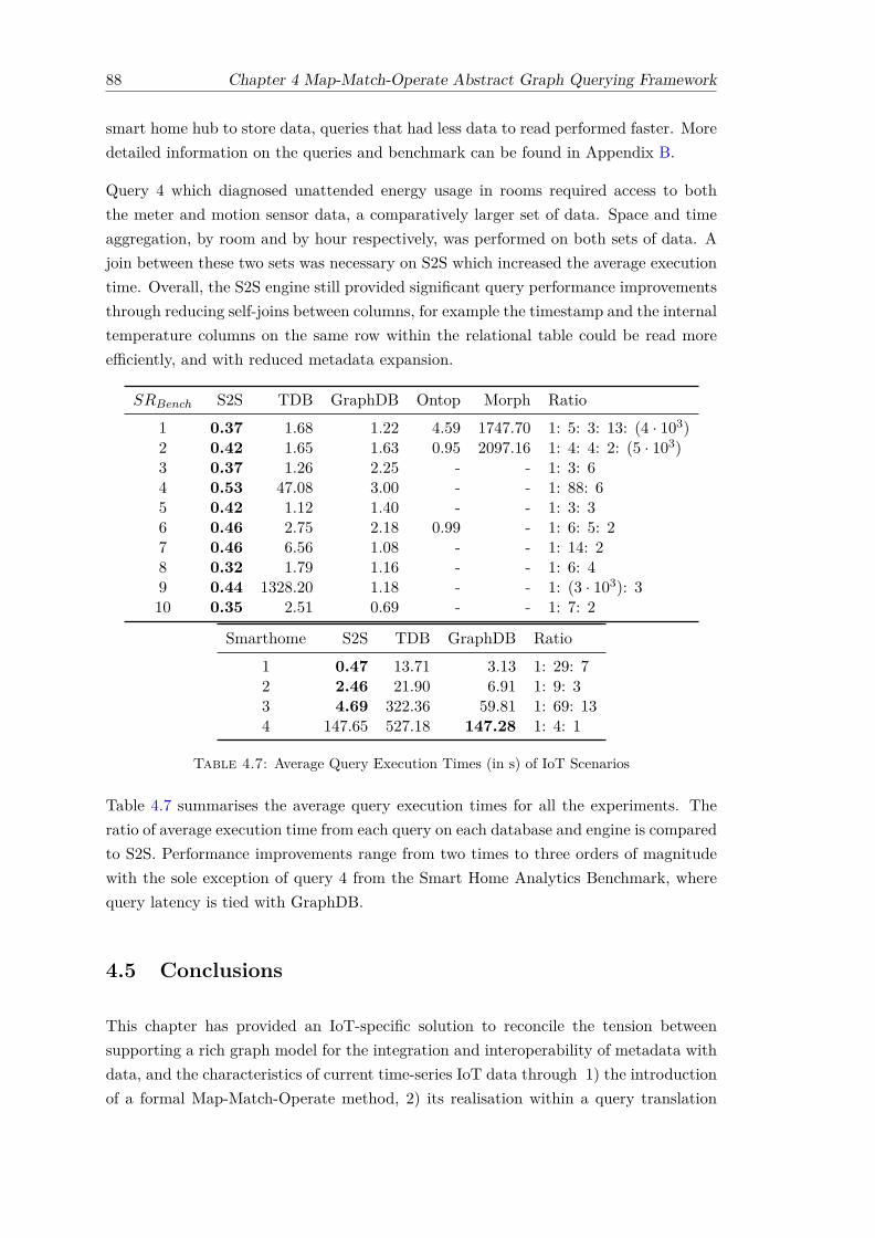
88 Chapter 4 Map-Match-Operate Abstract Graph Querying Framework
smart home hub to store data, queries that had less data to read performed faster. Moredetailed information on the queries and benchmark can be found in Appendix B.
Query 4 which diagnosed unattended energy usage in rooms required access to boththe meter and motion sensor data, a comparatively larger set of data. Space and timeaggregation, by room and by hour respectively, was performed on both sets of data. Ajoin between these two sets was necessary on S2S which increased the average executiontime. Overall, the S2S engine still provided significant query performance improvementsthrough reducing self-joins between columns, for example the timestamp and the internaltemperature columns on the same row within the relational table could be read moreefficiently, and with reduced metadata expansion.
SRBench S2S TDB GraphDB Ontop Morph Ratio1 0.37 1.68 1.22 4.59 1747.70 1: 5: 3: 13: (4 · 103)2 0.42 1.65 1.63 0.95 2097.16 1: 4: 4: 2: (5 · 103)3 0.37 1.26 2.25 - - 1: 3: 64 0.53 47.08 3.00 - - 1: 88: 65 0.42 1.12 1.40 - - 1: 3: 36 0.46 2.75 2.18 0.99 - 1: 6: 5: 27 0.46 6.56 1.08 - - 1: 14: 28 0.32 1.79 1.16 - - 1: 6: 49 0.44 1328.20 1.18 - - 1: (3 · 103): 310 0.35 2.51 0.69 - - 1: 7: 2
Smarthome S2S TDB GraphDB Ratio1 0.47 13.71 3.13 1: 29: 72 2.46 21.90 6.91 1: 9: 33 4.69 322.36 59.81 1: 69: 134 147.65 527.18 147.28 1: 4: 1
Table 4.7: Average Query Execution Times (in s) of IoT Scenarios
Table 4.7 summarises the average query execution times for all the experiments. Theratio of average execution time from each query on each database and engine is comparedto S2S. Performance improvements range from two times to three orders of magnitudewith the sole exception of query 4 from the Smart Home Analytics Benchmark, wherequery latency is tied with GraphDB.
4.5 Conclusions
This chapter has provided an IoT-specific solution to reconcile the tension betweensupporting a rich graph model for the integration and interoperability of metadata withdata, and the characteristics of current time-series IoT data through 1) the introductionof a formal Map-Match-Operate method, 2) its realisation within a query translation

Chapter 4 Map-Match-Operate Abstract Graph Querying Framework 89
engine for the RDF graph model and 3) experimentation that substantiated its storageand query performance improvements over other databases and SPARQL-to-relationalengines. It was also noted that the state-of-the-art SPARQL-to-relational engines, likeOntop and Morph, that have reported significant performance improvements over RDFstores on various benchmarks and deployments, were not yet equipped to support oroptimised for queries and models from the IoT domain. As such, the contribution ofMap-Match-Operate, S2S, and S2SML as a data modelling language, fills a gap in theliterature for IoT time-series data, IoT scenarios and analytical queries.


Chapter 5
TritanDB: A Rapid Time-seriesAnalytics Database
“I see a picture right now that’s not parallel, so I’m going to go straightenit. Things must be in order.”
— Katherine Johnson
While the previous chapter established the efficiency of the Map-Match-Operate methodfor the execution of graph queries over a graph model tier and a relational database tier,this chapter seeks to investigate even more efficient and specialised representations oftime-series data within the database tier to further enhance storage and query perfor-mance. Section 5.1 introduces the gap between the conceptual and physical representa-tions of time-series data in the database tier and the potential opportunity for greateroptimisation. This potential drives an investigation of state-of-the-art data structuresand compression for time-series data in Section 5.2 that then advises the design of atime-series database for Internet of Things (IoT) data, TritanDB, described in Section5.3 which replaces the relational database in the database tier. The implementationwithin a Map-Match-Operate engine is then compared against several state-of-the-arttime-series databases and the results are presented and discussed in Section 5.4. Finally,Section 5.5 draws conclusions from the findings in the chapter.
5.1 Introduction
Conceptually, time-series Internet of Things (IoT) data that show flat and wide charac-teristics can be stored compactly as a two-dimensional relational table. One dimensionof the table, rows, correspond to points in time while another dimension, columns, cor-responds to various measurements made at those points in time. There is, however, a
91

92 Chapter 5 TritanDB: A Rapid Time-series Analytics Database
distinction between the conceptual and physical properties of these database tables. Ata physical level, database tables on common storage media like magnetic disks, solidstate drives or Random Access Memory (RAM) need to be mapped to one-dimensionalstructures to be stored and retrieved. Internally, these storage media provide just aone-dimensional interface, for example, reading and writing from a given linear offset.
Therefore, this chapter’s work is motivated by the opportunity to combine the flatand wide characteristics of IoT data, with a deeper understanding of how time-seriesdata can best be organised with respect to the underlying physical properties of thestorage medium for storage and retrieval. Furthermore, the largely numerical typeof data and the presence of both approximately periodic and non-periodic data alsosuggest that a study of state-of-the-art compression algorithms and data structures willbe beneficial for designing a means for storing time-series data efficiently. Fortuitously,the big data era has driven advances in data management and processing technologywith new databases emerging for specialised use cases. The large volumes of telemetrydata from performance monitoring scenarios within web-scale systems have pushed theresearch and development of time-series databases to the forefront, providing an arrayof technologies and designs to study, build upon and compare against. A survey of thesetime-series databases was presented in Section 2.2.1.
A three-time Formula One champion, Sir Jackie Stewart, was reputed to have coinedthe term ‘mechanical sympathy’, also quoted by Robinson et al. (2015) in their unre-lated discussion on idiomatic query design for graph databases. It reflects how a racecar driver, by understanding the mechanics and engineering behind the vehicle, is ableto work harmoniously together with it to achieve the best performance. This idea of‘mechanical sympathy’ forms a driving factor behind this chapter’s work that seeks tofurther optimise the performance of Match-Map-Operate from Chapter 4, which alreadyrepresents significant gains in flexibility and storage and query performance. A series ofmicrobenchmarks helps form a scientific understanding on compression techniques anddata structures to achieve greater ‘mechanical sympathy’.
5.2 Time-series Compression and Data Structures
In Section 3.1, it was established that a current sample of Internet of Things (IoT)data exhibited numerous characteristics. The time-series data studied tended to beflat, wide and numerical. Furthermore, there was a mixture of periodic, approximatelyperiodic and non-periodic time-series data. Flat, wide and numerical IoT time-seriesdata presents a unique use case for compression algorithms across the dimension ofcolumns, on its timestamp column as well as each column representing an attribute,likely of numerical type data.

Chapter 5 TritanDB: A Rapid Time-series Analytics Database 93
Compression is used in relational databases and is especially important in advancedcolumn-stores as a performance optimisation rather than just for reducing storage size.When data is compressed, less time is spent on input-output operations with the physicalstorage medium interface when data is read from disk into memory (or from memoryto CPU). Another motivation of compression is related to CPU speed increasing fasteras compared to memory bandwidth, hence, the comparative cost of accessing data asopposed to compressing and decompressing it in terms of CPU cycles has become greateras explained by Abadi et al. (2012). Section 5.2.1 explains timestamp compression,compressing the sequence of timestamps in a time-series, while Section 5.2.2 explainscompressing values within columns of each attribute over the range of timestamps.
To evaluate the performance and compression ratios produced by each of these algo-rithms for timestamp and value compression, Section 5.2.3 describes a set of IoT time-series datasets from different application domains for use in microbenchmarks and Sec-tion 5.2.4 presents and discusses the results of microbenchmarks of the compressionalgorithms on each dataset.
The large volumes of time-series data from the IoT that have been efficiently compressedneed to be persisted to disk in a way that they can be efficiently retrieved during queries.This motivates the study of a range of data structures commonly associated with state-of-the-art time-series databases. Hence, Section 5.2.5 describes a number of implemen-tations of data structures for storing time-partitioned, compressed blocks of time-seriesIoT data. A proposal for a novel data structure called TrTables is made in Section5.2.5.4 and the performance of each implementation is then evaluated in terms of read,write and space amplification metrics by microbenchmarks in Section 5.2.6.
5.2.1 Timestamp Compression
Timestamps in a series can be compressed to great effect based on the knowledge thatin practice, the delta of a timestamp, the difference between this timestamp and theprevious, is a fraction of the length of the timestamp itself and can be combined withvariable-length encoding to reduce storage size. If the series is somewhat evenly-spaced,Run Length Encoding (RLE) can be applied to further compress the timestamp deltas.As shown in Sections 3.1 and 3.2, a significant proportion of IoT time-series exhibitedperiodic or approximately periodic, evenly-spaced data streams.
For high precision timestamps (e.g. in nanoseconds), where deltas themselves are largehowever, delta-of-delta compression that stores the difference between deltas can of-ten be more effective. Figure 5.1 depicts various methods of compressing a series oftimestamps with millisecond precision. The following sections go into each of the three

94 Chapter 5 TritanDB: A Rapid Time-series Analytics Database
Header1496331968000
?3602
? : ? ?'10' : -2
?'0'
Header1496331968000
?'10011100 00010010'
?'00000001'
64 24 2 + 7 1
64 8 16
?2
8
?3600
16
Header1496331968000
?'111010 00010010'
?'001'
64 3 14 14
?'100'
3
?'001110 00010000'
Bit Length
D elt a-of-D elt a
D elt a-R LE-LEB 128
D elt a-R LE-R icekrle= 2, kval= 10
1 June 2017 15:46:08.000
1 June 201715:46:11.602
1 June 201715:46:15.202
1 June 201715:46:18.802T imest amps
Figure 5.1: Visualisation of the Timestamp Compression at Millisecond Precisionwith Various Delta-based Methods
methods, Delta-of-Delta compression in Section 5.2.1.1, Delta-RLE-LEB128 compres-sion in Section 5.2.1.2 and backwards adaptive Delta-RLE-Rice compression in Section5.2.1.3.
5.2.1.1 Delta-of-Delta Compression
Delta-of-Delta compression builds on the technique for compressing timestamps intro-duced by Pelkonen et al. (2015) to support effective compression on varying timestampprecision. The header stores a full starting timestamp for the block in 64 bits and thenext length of bits depends on the timespan of a block and the precision of the times-tamps. In the example in Figure 5.1, a 24 bit length is used to store the timestampdelta of ‘3602’. The 24 bit length is derived for a 4 hour block at millisecond precisionwith the first delta assumed to be positive. For the same 4 hour block, if the precisionof timestamps during ingestion is determined to be in seconds a 14 bits length is cal-culated and used, while this length is 24 bits for millisecond precision and 44 bits fornanoseconds precision.
ε is a 1 to 4 bit variable-length binary value that indicates the next number of bits toread for the first delta-of-delta value. ‘0’ means the delta-of-delta (∆∆) is 0, while ‘10’means read the next 7 bits as the value is between ‘-63’ and ‘64’ (range of 27), ‘110’ thenext 24 bits, ‘1110’ the next 32 bits. Finally, an ε of ‘1111’ means reading a 64 bit ∆∆.The example follows with ∆∆s of ‘-2’ and ‘0’ stored in just 10 bits which reflect thedelta of the next two timestamps is ‘3600’. These lengths are adapted from the empiricalmeasurement of the distribution of ∆∆ values from the Pelkonen et al. (2015) paper.

Chapter 5 TritanDB: A Rapid Time-series Analytics Database 95
5.2.1.2 Delta-RLE-LEB128 Compression
The LEB128 encoding format is a variable-length encoding recommended in the DWARFdebugging format specification by the DWARF Debugging Information Format Com-mittee (2017) and commonly used in Android’s Dalvik executable format. Numericalvalues like timestamps can be compressed efficiently along byte boundaries (minimumof 1 byte). In the example in Figure 5.1, the header stores a full starting timestamp forthe block in 64 bits followed by a run-length value, ρ, of 1 and the actual delta, ∆, of3602, both compressed with LEB128 to 8 and 16 bits respectively. The first bit in each8 bits is a control bit that signifies to read another byte for the sequence if ‘1’ or thelast byte in the sequence if ‘0’. The remaining 7 bits are appended with any others inthe sequence to form the numerical value. Binary ‘00001110 00010010’ is formed fromappending the last 7 bits from each byte of ∆ which translates to the value of ‘3602’ inbase 10. This is followed by a run-length, ρ, of two ∆s of ‘3600’ each in the example.
5.2.1.3 Delta-RLE-Rice Compression
This proposal for Delta-RLE-Rice compression is inspired by the backward adaptationstrategy from Malvar (2006) for the run-length encoding method initially proposed byRice and Plaunt (1971). The backward adaptation strategy succeeds by tuning a k
parameter which allows the adaptive compression of timestamps and run-lengths ofvarying precision and periodicity respectively. Rice coding divides a value, u, into twoparts based on k, giving a quotient q =
⌊u/2k
⌋and the remainder, r = u%2k. The
quotient, q is stored in unary coding, for example, the ∆ value ‘3602’ with a k of 10 hasa quotient of 3 and is stored as ‘1110’. The remainder, r, is binary coded in k bits. Initialk values of 2 and 10 are used in this example in Figure 5.1 and are adaptively tunedbased on the previous value in the sequence so this can be reproduced during decoding.Three rules govern the tuning based on the value of q, allowing quick convergence ongood k values.
if q =
0, k → k − 1
1, no change in k
> 1, k → k + q
This adaptive coding adjusts k based on the actual data to be encoded so no otherinformation needs to be retrieved on the side for decoding. It also has a fast learningrate that chooses good, though not necessarily optimal, k values and does not have thedelay of forward adaptation methods. k is adapted from 2 and 10 to 1 and 13 respectivelyin the Figure 5.1 example.

96 Chapter 5 TritanDB: A Rapid Time-series Analytics Database
5.2.2 Value Compression
This section explores two opportunities when considering value compression for time-series IoT data. The first being that most of the time-series values were determinedto be of numerical data type, hence, this section focuses on floating point compressionalgorithms that also support long integers. Secondly, as noted by Abadi et al. (2012) intheir work on column-stores, compressing data with a low information entropy and highdata value locality has better performance and intuitively, values from the same columntend to have more value locality and less entropy. Therefore, each attribute value froma time-series can be compressed more effectively with the next value in the sequence andthis section of value compression studies compressing along the column dimension.
Three state-of-the-art floating point compression algorithms are considered, the fastFloating Point Compression (FPC) algorithm by Burtscher and Ratanaworabhan (2009)is described in Section 5.2.2.1, the simpler block-aligned method used in Facebook’s Go-rilla by Pelkonen et al. (2015) is studied in Section 5.2.2.2 and the delta-of-delta methodused in the time-series database BTrDb by Andersen and Culler (2016) is considered inSection 5.2.2.3.
5.2.2.1 FPC: Fast Floating Point Compression
The FPC algorithm introduced by Burtscher and Ratanaworabhan (2009) uses the moreaccurate of two value predictors to predict the next value in a double-precision numericalsequence of floating point numbers. These include the Finite Context Method (FCM)value predictor described by Sazeides and Smith (1997) and the Differential Finite Con-text Method (DFCM) value predictor introduced by Goeman et al. (2001). Accuracy isdetermined by the number of significant bits shared between the actual value and eachpredicted value. After an XOR operation between the chosen predicted value and ac-tual value, the leading zeroes are collapsed into a 3 bit value and appended with a singlebit indicating which predictor was used and the remaining non-zero bytes. As XOR isreversible and the predictors are effectively hash tables, fast and lossless decompressioncan thus be performed.
5.2.2.2 Gorilla Value Compression
Gorilla, unlike FPC does not use predictors and instead compares the current value toonly the previous value for speed, as detailed in the paper by Pelkonen et al. (2015).After an XOR operation between the values, the result, r, is stored according to theoutput from a function gor() described as follows, where ‘.’ is an operator that appendsbits together, p is the previous XOR value, lead() and trail() return the number of leading

Chapter 5 TritanDB: A Rapid Time-series Analytics Database 97
and trailing zeroes respectively, len() returns the length in bits and n is the number ofmeaningful bits remaining within the value.
gor(r) =
′0′, if r = 0′10′.n, if lead(r) >= lead(p) and trail(r) = trail(p)′11′.l.m.n, else, where l = lead(r) and m = len(n)
The algorithm was designed for the fast encoding and decoding of blocks of time-seriesdata as there is no condition within the gor(r) function to reduce the number of sig-nificant bits stored in the sequence but only to increase them. However, each blockresets the counter on significant bits and ‘localises’ the compression. This phenomenonis explained in greater detail in Section 5.2.6.1 on space amplification.
5.2.2.3 Delta-of-Delta Value Compression
Andersen and Culler (2016) suggested the use of a delta-of-delta method for compressingthe mantissa and exponent components of floating point numbers within a series sepa-rately. The method was not described in detail in the paper but this thesis interpretsit as such: an IEEE-754 double precision floating point number defined by the IEEEStandards Association (2008) can be split into sign, exponent and mantissa components.The 1 bit sign is written, followed by at most 11 bits delta-of-delta of the exponent, δexp,encoded by a function Eexp(), described as follows, and at most 53 bits delta-of-delta ofthe mantissa, δm, encoded by Emantissa(), also described as follows.
Eexp(δexp) =
′0′, if δexp = 0′1′.e, else, where e = δexp + (211 − 1)
Emantissa(δm) =
′0′, if δm = 0′10′.m, if − 26 + 1 <= δm <= 26, m = δm + (26 − 1)′110′.m, if − 231 + 1 <= δm <= 231, m = δm + (231 − 1)′1110′.m, if − 247 + 1 <= δm <= 247, m = δm + (247 − 1)′1111′.m, else, where m = δm + (253 − 1)
The operator ‘.’ appends binary coded values in the above functions. e and m areexpressed in binary coding (of base 2). A maximum of 12 and 53 bits are needed for theexponent and mantissa deltas respectively as they could be negative.

98 Chapter 5 TritanDB: A Rapid Time-series Analytics Database
Dataset Metadata Timestamps Field TypesDomain Rows Fields P δMAD δIQR Bool FP Int
SRBench Weather 647k 4.3m s 0a 0 0b 6 0Shelburne Agriculture 12.4m 74.7m ms/ns 0/0 0.29/293k 0 6 0GreenTaxi Taxi 4.4m 88.9m s 1.48 2 1 12 7
aAs there were 4702 stations, a median of the MAD and IQR of all stations was taken, the meansare 538 and 2.23 × 10⁶
bA mean across the 4702 stations was taken for each field type in SRBenchLegend: FP = Floating Point Number, Bool = Boolean, Int = Integer, P = Precision, s,ms,ns =seconds,milliseconds,nanoseconds, k = ×103 and m = ×106.
Table 5.1: Public IoT Datasets used for Microbenchmarks
5.2.3 IoT Datasets for Microbenchmarks
To evaluate the performance of various algorithms and system designs with microbench-marks, a set of publicly available IoT time-series datasets were collated. The use ofpublic, published data, as opposed to proprietary data, enables reproducible evaluationsand a base for new systems and techniques to make fair comparisons.
Table 5.1 summarises the set of datasets collated, describing the precision of times-tamps, Median Absolute Deviation (MAD) of deltas, δMAD, Inter-quartile Range (IQR)of deltas, δIQR, and the types of fields for each dataset. Each dataset, SRBench, Shel-burne and GreenTaxi (when necessary, shortened to Taxi for brevity) are described inmore detail in Sections 5.2.3.1, 5.2.3.2 and 5.2.3.3 respectively.
The MAD was defined previously in Section 3.1.4 while the IQR is defined as the differ-ence between the upper quartile, the 75th percentile, and the lower quartile, the 25thpercentile and is a measure of the statistical dispersion of data points.
5.2.3.1 SRBench: Weather Sensor Data
SRBench by Zhang et al. (2012) is a benchmark based on the Linked Sensor Data (LSD)dataset by Patni et al. (2010) that described sensor data from weather stations acrossthe United States with recorded observations from periods of bad weather. In particular,the Nevada Blizzard period of data from 1st to 6th April 2003 which included more than647 thousand rows with over 4.3 million fields of data from 4702 of the stations was used.Stations have timestamp precision in seconds with the median δMAD and δIQR acrossstations both zero, showing regular, periodic intervals of measurement. The main datatype is small floating point numbers, mostly up to a decimal place in accuracy.

Chapter 5 TritanDB: A Rapid Time-series Analytics Database 99
5.2.3.2 Shelburne: Agricultural Sensor Data
Shelburne is an agriculture dataset aggregating data from a network of wireless sensorsobtained from a vineyard planting site in Charlotte, Vermont, United States. Eachreading includes a timestamp and fields like solar radiation, soil moisture and leaf wetnessamong others. The dataset is available on SensorCloud1 and was collected from April2010 to July 2014 with 12.4 million rows and 74.7 million fields. Timestamps wererecorded up to nanosecond precision. The δMAD is zero as the aggregator records atregular intervals (median of 10s), however, due to the high precision timestamps andoutliers, there is a δIQR of 2.93× 10⁵ (in the microsecond range). All the fields recordedare floating point numbers recorded with a high decimal count and accuracy.
5.2.3.3 GreenTaxi: Taxi Trip Data
This dataset includes trip records from green taxis in New York City from January toDecember 2016. The data was provided by the Taxi and Limousine Commission2 andconsists of 4.4 million rows with 88.9 million fields of data. Timestamp precision is inseconds and is unevenly-spaced as expected from a series of taxi pick-up times withina big city with a δMAD of 1.48. However, as the time-series also has overlapping valuesand is very dense, the δMAD and δIQR are all within 2 seconds. There is one booleanfield type for the store and forward flag which indicates whether the trip record washeld in vehicle memory before sending to the vendor because the vehicle did not have aconnection to the server at that time. There are 12 floating point field types includinglatitude and longitude values with high decimal counts and fares with a low decimalcount. There are also integer field types including vendor ID, rate code ID and drop offtimestamps.
5.2.4 Compression Microbenchmark Results
A series of microbenchmarks were performed to evaluate the performance of the com-pression algorithms for timestamps and values on each IoT time-series dataset. Fortimestamp compression, the storage size of the dataset after compression with the spe-cific algorithm is presented in Section 5.2.4.1. For value compression, both the storagesize and the average compression and decompression times were recorded as in Section5.2.4.2. The experimental setup for the microbenchmarks had a 4× 3.2GHz CPU, 8 GBmemory and average disk data rate of 146.2 MB/s. The source code for running themicrobenchmarks is available on Github3.
1https://sensorcloud.microstrain.com/SensorCloud/data/FFFF0015C9281040/2http://www.nyc.gov/html/tlc/html/about/trip_record_data.shtml3https://github.com/eugenesiow/tritandb-kt

100 Chapter 5 TritanDB: A Rapid Time-series Analytics Database
Dataset Timestamps (MB)a Values (MB)b
δ∆ δleb δrice δ∅ Cgor Cfpc C∆ C∅SRBench 0.6 0.5 0.4 5.2 8.2 23.8 21.9 33.9Shelburne (ms) 8.0 18.3 13.6 99.5 440.8 419.3 426.6 597.4Shelburne (ns) 35.9 56.2 44.1 99.5GreenTaxi 4.0 6.9 1.5 35.5 342.1 317.1 318.8 710.9
aδ∆ = Delta-of-Delta, δleb = Delta-RLE-LEB128, δrice = Delta-RLE-Rice, δ∅ = Delta-UncompressedbCgor = Gorilla, Cfpc = FPC, C∆ = Delta-of-Delta , C∅ = Uncompressed
Table 5.2: Compressed Size of Timestamps and Values in Datasets with VaryingMethods
5.2.4.1 Timestamp Compression Microbenchmark Results
Table 5.2 shows the results of running each of the timestamp compression methodsincluding a control uncompressed set for each dataset. Delta-RLE-Rice, δrice, was ob-served to perform best for low precision timestamps (to the second) while delta-of-deltacompression, δ∆, performed well on high precision, milli and nanosecond timestamps.The adaptive δrice performed exceptionally well on the GreenTaxi dataset which hadprecision to seconds and small intervals between records and therefore small deltas. δ∆
performed well on Shelburne due to an approximately periodic time-series but with largedeltas due to high precision.
5.2.4.2 Value Compression Microbenchmark Results
Table 5.2 shows the results comparing Gorilla, FPC and delta-of-delta value compres-sion against each of the datasets. Each compression method has advantages, however,in terms of compression and decompression times, Gorilla compression consistently per-formed best, as shown in Table 5.3, where each dataset was compressed to a file 100times and the time taken was averaged. Each dataset was then decompressed and thetime taken was averaged over a 100 tries. A read and write buffer of 212 bytes was usedfor all experiments. FPC had the best compression ratio on values with high decimalcount in Shelburne and was slightly better on a range of field types in GreenTaxi thandelta-of-delta compression, however, even though the hash table prediction had similarspeed to the delta-of-delta technique, it was still up to 25% slower on encoding thanGorilla. Gorilla though, expectedly trailed FPC and delta-of-delta in terms of size forthe Shelburne and Taxi datasets which had more rows of data. This was to be expectedas Gorilla is a block-based compression algorithm optimised for smaller time-partitionedblocks of data which is explained in more detail in Section 5.2.6.1 on Space Amplification.
As can be observed from Table 5.2, even the worse compression method for timestamps,δmax, occupies but a fraction of the total space using the best value compression method,Cmin, as shown by the percentage of total size calculation, δmax÷ (δmax +Cmin)× 100%,

Chapter 5 TritanDB: A Rapid Time-series Analytics Database 101
Dataset Compression (s)a Decompression (s)Cgor Cfpc C∆ Top Cgor Cfpc C∆ Top
SRBench 2.10 3.25 3.10 Cgor 0.97 1.61 1.36 CgorShelburne 30.68 42.02 40.91 Cgor 3.80 4.57 5.42 CgorGreenTaxi 28.85 32.11 32.94 Cgor 2.94 4.32 5.77 Cgor
aCgor = Gorilla, Cfpc = FPC, C∆ = Delta-of-Delta
Table 5.3: Average Compression/Decompression Time of Datasets (100 Attempts)
which results in percentages of 6.8%, 11.8% and 2.1% for SRBench, Shelburne and GreenTaxi respectively. Hence, an effective and fast compression method supporting hard-to-compress numerical values of both floating point numbers and long integers can greatlyimprove compression ratios and also read and write performance.
5.2.5 Data Structures and Indexing for Time-Partitioned Blocks
In time-series databases, as seen in microbenchmark results in the previous section,Section 5.2.4, data can be effectively compressed in time order. A common way ofpersisting this to disk is to partition each time-series by time to form time-partitionedblocks that can be aligned on page-sized boundaries or within memory-mapped files.This section studies generalised implementations of data structures used in state-of-the-art time-series databases to store and retrieve time-partitioned blocks: concurrentB+-trees, Log-Structured Merge (LSM) trees and segmented Hash-trees and each isexplained in Sections 5.2.5.1, 5.2.5.2 and 5.2.5.3 respectively. Finally, a novel datastructure, the TritanDB Table (TrTable) inspired by the Sorted String Table (SSTable)is proposed for IoT time-series block storage in Section 5.2.5.4.
5.2.5.1 B+-Tree-based
A concurrent B+-Tree can be used to store time-partitioned blocks with the keys be-ing block timestamps and the values being the compressed binary blocks. Time-seriesdatabases, like Akumuli from Lazin (2017) which implements an LSM-tree with B+-treesinstead of SSTables, and BTrDb from Andersen and Culler (2016) which implements anappend-only, Copy-On-Write (COW) B+-tree, use variations of this data structure. Thisthesis implements the general Sagiv (1986) BLink balanced search tree utilising the ver-ified algorithm in the work by da Rocha Pinto et al. (2011) for the microbenchmarks.The leaves of the tree are nodes that contain a fixed size list of key and value-pointerpairs stored in order. The value-pointer points to the actual block location so as tominimise the size of nodes that have to be read during traversal. The final pointer ineach node’s list, called a link pointer, points to the next node at that level which al-lows for fast sequential traversal between nodes. A prime block includes pointers to the

102 Chapter 5 TritanDB: A Rapid Time-series Analytics Database
Prime Block-? ?
1496331968-?
-?
...2870 ...3700 ...4920
1496333700 ...5840
1496335840
...7890
...5840 ...6910 ...7890 ...8880
?
?
TP-Block TP-Block TP-Block TP-Block. . .
Figure 5.2: ABLink Tree with Timestamps as Keys and Time-Partitioned (TP) BlocksStored Off Node
first node in each level. Figure 5.2 shows this BLink tree with timestamps as keys andtime-partitioned (TP) blocks stored off node with a pointer to an offset.
5.2.5.2 Hash-Tree-based
Given that hashing is commonly used in building distributed storage systems and varioustime-series databases, like Riak-TS by Basho (2017) which uses a hash ring, a generalisedconcurrent hash map data structure is investigated within these microbenchmarks. Acentral difficulty of hash table implementations is defining an initial size of the roottable especially for streaming time-series of indefinite sizes. Instead of using a fixed-sizedhash table that suffers from fragmentation and requires the rehashing of data when itgrows, an auto-expanding Hash-tree of hash indexes is used in the implementation formicrobenchmarks instead. Leaves of the tree contain expanding nodes with keys andvalue pointers. Concurrency is supported by implementing a variable segmented Read-Write-Lock approach, the variable of which corresponds to the concurrency factor, thatis similar to the one implemented in JDK7’s ConcurrentHashMap data structure asdescribed by Burnison (2013), and 32-bit hashes are used for block timestamp keys.
5.2.5.3 LSM-Tree-based
The Log-Structured Merge (LSM) tree described by O’Neil et al. (1996) is a writeoptimised data structure used in time-series databases like InfluxDb by Influx Data(2017), which uses a variation called a Time-Structured Merge (TSM) tree, OpenTSDBon HBase by StumbleUpon (2017), and various Cassandra-based databases that usean LSM-tree implementation described by Lakshman and Malik (2010). High writethroughput is achieved by performing sequential writes instead of dispersed, update-in-place operations that most tree-based structures require. This particular implementationof the LSM-tree is based on the bLSM design by Sears and Ramakrishnan (2012) and has

Chapter 5 TritanDB: A Rapid Time-series Analytics Database 103
an in-memory buffer, a memtable, that holds block timestamp keys and time-partitionedblocks as values within a red-black tree to preserve key ordering. When the memtableis full, the sorted data is flushed to a new file on disk requiring only a sequential write.Any new blocks or edits simply create successive files which are traversed in order duringreads. The system periodically performs a compaction to merge files together, removingduplicates.
5.2.5.4 TrTables: A Novel Time-Partitioned Block Data Structure
TritanDB Tables (TrTables) are a novel IoT time-series optimised storage data structureproposed in this thesis which takes inspiration from the Sorted String Table (SSTable)that consists of a persistent, ordered, immutable map from keys to values and thememtable, a sorted in-memory buffer used to order random writes of recent commits.Both are used in tandem in big data systems based on BigTable, initially described byChang et al. (2008).
The main difference between TrTables and the SSTable and memtable combinationproposed in BigTable is that no additional background compaction process, which canprove expensive, is required. This is due to the natural temporal ordering (one-wayordering of time) of time-series data and to the introduction of a novel Quantum Re-ordering Buffer (QRB) structure within TrTables. The QRB is an in-memory datastructure that supports the re-shuffling of out-of-order timestamps (and correspondingobservation data) within a time window. This provides for the scenario that due to best-effort network delivery, IoT time-series sensor data arrives out-of-order on occasion.
To explain the TrTables data structure, three main components, the QRB, the in-memory memtable and the on-disk TrTable file are discussed as follows. Definition 5.1introduces the term quantum, q, and the QRB, Q. This is followed by an explanationof the memtable and the TrTable as shown in Figure 5.3.
Definition 5.1 (Quantum Re-ordering Buffer, Q, and Quantum, q). A quantum re-ordering buffer, Q, is a list-like window that contains a number of timestamp-row pairsas elements. A quantum, q, is the amount of elements within Q to cause an expirationoperation where an insertion sort is performed on the timestamps of q elements andthe first a × q elements are flushed to the memtable, where 0 < a ≤ 1. The remaining(1− a)× q elements now form the start of the window.
An insertion sort which has a complexity of O(nk) is used to re-order the QRB. k, thefurthest distance of an element from its final sorted position, is small if the window isalready partially sorted, which is the case unless there are significant network delays.Any timestamp now entering the re-ordering buffer less than the minimum allowedtimestamp, tminA (the first timestamp in the buffer) is rejected, marked as ‘late’ and

104 Chapter 5 TritanDB: A Rapid Time-series Analytics Database
...58401496331968 Row ...2870 ...3700 ...4920 ...6910
q = 6
a × q = 4
1496331968 Row ...2870 ...3700 ...4920
insert ion sort
...78901496335840 ...6910
(1-a) × q = 2
Tim
e flush
Block T imestamp1496331968
?902
? : ? ?'110' : -72 ...Row
Index 1496331968 n 4Avg Max Min
OffsetT imestamp Count
... 902 '110' : -72 ...Row
n bytes
flush
1496331968 n 4Avg Max Min...
TrTable
Index Block DataIngress
Quantum Re-ordering Buffer memtable and TrTablememtable
Figure 5.3: Operation of the Quantum Re-ordering Buffer, memtable and TrTableover Time
returned with a warning. Figure 5.3 shows the operation of Q over time (along they-axis). When Q has 6 elements and q = 6, an expiration operation occurs where aninsertion sort is performed and the first 4 sorted elements are flushed to the memtable. Anew element that enters has timestamp, t = 1496337890, which is greater than tminA =1496335840 and hence is appended at the end of Q.
The memtable, also shown in Figure 5.3, consists of an index entry, i, that stores valuesof the block timestamp, current TrTable offset and average, maximum, minimum andcounts of the row data which are updated when elements from Q are inserted. It alsostores a block entry, b, which contains the current compressed time-partitioned blockdata. The memtable gets flushed to a TrTable file once it reaches the time-partitionedblock size, bsize. Each time-series has a memtable and corresponding TrTable file on-disk.
Like the SSTable and memtable combination, operations on TrTables take the form of ef-ficient sequential reads and writes due to it maintaining a sorted order both in-memorywith a memtable and on disk with a TrTable file. However, unlike the SSTable andmemtable, each key in a TrTable file is a block timestamp while each value is a time-partitioned block, compressed with both state-of-the-art timestamp and value compres-sion. The efficiency of an interface of only sequential reads and writes is magnified bythe use of compressed, compact blocks, ordered blocks which require comparatively lessdisk input-output operations. The block index table which is produced during ingestionand requires no further maintenance as it is immutable once written to disk as a parallelto a TrTable file, boosts the performance of range and aggregation queries.
TrTables also inherit other beneficial characteristics from SSTables, which are fitting forstoring time-series IoT data, like simple locking semantics for only the memtable withno contention on immutable TrTable files. However, TrTables do not support expensiveupdates and deletions outside of the time window of the quantum re-ordering buffer asthis thesis argues that there is no established use case for individual points within anIoT time-series in the (distant) past to be modified. In the situation that such a usecase arises, this can be more efficiently managed by an offline batch process instead.

Chapter 5 TritanDB: A Rapid Time-series Analytics Database 105
5.2.6 Data Structure Microbenchmark Results
Microbenchmarks aimed to measure 3 metrics that characterised the performance of eachdata structure: write performance, read amplification and space amplification. Writeperformance was measured by the average time taken to ingest each of the datasets overa 100 tries. Borrowing from the definition of Kuszmaul (2014), ‘the number of input-output operations required to satisfy a particular query’ is the read amplification thatwas measured here by taking the average execution time of a 100 tries of scanning thewhole database (scan) and the average execution time of range queries over a 100 pairsof deterministic pseudo-random values with a fixed seed from the entire time range ofeach dataset (range). Space amplification is the ‘space required by a data structure thatcan be inflated by fragmentation or temporary copies of the data’ and was measuredhere by the resulting size of the database after compaction operations. Each time-partitioned block was compressed using δ∆ and Cgor compression for timestamps andvalues respectively. Results for each of the metrics follow in Sections 5.2.6.1, 5.2.6.2and 5.2.6.3. A similar experimental setup as with the compression microbenchmarks(Section 5.2.4) was used.
5.2.6.1 Space Amplification and the Effect of Block Size, bsize
The block size, bsize, refers to the maximum size that each time-partitioned block oc-cupies within a data structure. Base 2 multiples of 212, the typical block size on filesystems, were used such that bsize = 212 × 2x and in these experiments x = 2..8was used. Figure 5.4 shows the database size in bytes, which suggests the space am-plification, for the Shelburne and Taxi datasets of each data structure at varying bsize.Both TrTables-LSM-tree and B+-tree-Hash-tree pairs have database sizes that were al-most identical with the maximum difference only about 0.2%, hence, they were groupedtogether for better visibility in the figure.
A trend where the database size decreased as bsize decreased was observed. This isa characteristic of the Cgor algorithm used for value compression described in Section5.2.2.2 as more ‘localised’ compression occurs. Each new time-partitioned block wouldtrigger the else clause in the gor(r) function to encode the longer ′11′.l.m.n, however,the subsequent lead(p) and trail(p) were also likely to be smaller and more ‘localised’and hence, fewer significant bits needed to be used for values in the block.
TrTables and LSM-tree data structures have smaller database sizes than the B+-tree andHash-tree data structures for both datasets. As sorted keys and time-partitioned blocksin append-only, immutable structures like TrTables and the LSM-tree after compactionare stored in contiguous blocks on disk, they are expectedly more efficiently packed andstored size-wise. Results from SRBench are omitted as the largest time-partitioned block

106 Chapter 5 TritanDB: A Rapid Time-series Analytics Database
2 4 6 8
3
3.5
4
·108
x Parameter of Block Size, bsize (212 × 2x bytes)
Datab
aseSize
(bytes)
STr/SlsmTTr/TlsmSB+/SHTB+/TH
Figure 5.4: Database Size of Data Structures of Datasets at Varying bsizeDatasets: Shelburne = S, Taxi = T , Data Structures: TrTables = Tr, LSM-tree = lsm, B+-tree = B+, Hash-tree = H
across all the stations was smaller than the smallest bsize where x = 2, hence, there wasno variation across different x values and bsize.
Key clashing was avoided in tree-based stores for the Taxi dataset, where multiple triprecords had the same starting timestamp, by using time-partitioned blocks where bsize >ssize, where ssize was the longest compressed sequence with the same timestamp.
5.2.6.2 Write Performance
Figure 5.5 shows the ingestion time in seconds for the Shelburne and Taxi datasetsof each data structure when varying bsize. Both TrTables and LSM-tree performedconsistently across bsize due to append-only sequential writes which corresponded totheir log-structured nature. TrTables were about 8 and 16 seconds faster on averagethan LSM-tree for the Taxi and Shelburne datasets respectively due to no overhead ofa compaction process. Both the Hash-tree and B+-tree performed much slower (up to10 times slower on Taxi between the B+-tree and TrTables when x = 2) on smallerbsize as each of these data structures were comparatively not write-optimised and thetrees became expensive to maintain as the amount of keys grew. When x = 8, theingestion time for LSM-tree and Hash-tree converged, while the B+-tree was still slowerand TrTables were still about 10s faster for both datasets. At that point, the bottleneckwas no longer due to write amplification but rather subject to disk input-output speeds.
For the concurrent B+-tree and and Hash-tree, both parallel and sequential writers weretested and the faster parallel times were recorded in the microbenchmark results. In theparallel implementation, the write and commit operations for each time-partitioned block

Chapter 5 TritanDB: A Rapid Time-series Analytics Database 107
2 3 4 5 6 7 8
100
200
300
400
500
x Parameter of Block Size, bsize (212 × 2x bytes)
IngestionTim
e(s)
STrTTrSHTHSB+TB+SlsmTlsm
Figure 5.5: Ingestion Times of Data Structures of Datasets at Varying bsizeDatasets: Shelburne = S, Taxi = T , Data Structures: TrTables = Tr, LSM-tree = lsm, B+-tree = B+, Hash-tree = H
(a key-value pair) were handed to worker threads from a common pool using Kotlin’slightweight asynchronous coroutines4.
5.2.6.3 Read Amplification
Figure 5.6 shows the execution time for a full scan on each data structure while varyingbsize and Figure 5.7 shows the execution time for range queries. All scans and querieswere averaged across 100 tries and for the range queries, the same pseudo-random rangeswith a fixed seed were used. The write-optimised LSM-tree performed the worst for fullscans. The B+-tree and Hash-tree performed quite similarly while TrTables recordedthe fastest execution times. A full scan on a TrTable file was efficient, consisting of astraightforward sequential read of the TrTable file with no intermediate seeks necessary,hence, almost no read amplification.
From the results of the range queries in Figure 5.7, it can be seen that the LSM-treehad the highest read amplification for both datasets as it had to perform a scan ofkeys across levels while trying to access a sub-range of keys. The Hash-tree had thesecond highest read amplification, which was expected as it had to perform randominput-output operations to retrieve time-partitioned blocks based on the distributionby the hash function. There is the possibility of using an order-preserving minimalperfect hashing function as proposed by Czech et al. (1992) at the expense of hashingperformance and space, however, this was out of the scope of the microbenchmarks.
4https://github.com/Kotlin/kotlinx.coroutines

108 Chapter 5 TritanDB: A Rapid Time-series Analytics Database
2 4 6 83.6
3.8
4
4.2
Block Size, bsize, x (212 × 2x bytes)
ExecutionTim
e(s)
Tr B+ H lsm
(a) Shelburne Dataset
2 4 6 83
3.2
3.4
3.6
3.8
Block Size, bsize, x (212 × 2x bytes)
ExecutionTim
e(s)
Tr B+ H lsm
(b) Taxi Dataset
Figure 5.6: Full Scan Execution Time per bsizeData Structures: TrTables = Tr, LSM-tree = lsm, B+-tree = B+, Hash-tree = H
2 4 6 81
1.1
1.2
1.3
Block Size, bsize (212 × 2x bytes)
ExecutionTim
e(s)
Tr B+ H lsm
(a) Shelburne Dataset
2 4 6 80.8
0.9
1
1.1
1.2
Block Size, bsize (212 × 2x bytes)Ex
ecutionTim
e(s)
Tr B+ H lsm
(b) Taxi Dataset
Figure 5.7: Range Query Execution Time per bsizeData Structures: TrTables = Tr, LSM-tree = lsm, B+-tree = B+, Hash-tree = H
TrTables also had better performance on both datasets than the read-optimised B+-tree due to its block index that guaranteed a maximum of just one seek operation onthe related TrTable file.
From the microbenchmarks on these IoT datasets, 212×24 bytes was observed to be themost suitable bsize for reads and TrTables were noted to have the best performance forboth full scans and range queries at this particular bsize.
5.2.6.4 Data Structure Performance Round-up: TrTables and 64KB
TrTables had the best write performance and storage size due to its immutable, com-pressed, write-optimised structure that benefited from fast, batched sequential writes.

Chapter 5 TritanDB: A Rapid Time-series Analytics Database 109
The in-memory quantum re-ordering buffer and memtable support ingestion of out-of-order, unevenly-spaced data within a window, which was a requirement for IoTtime-series data explored previously in Section 3.1. Furthermore, the memtable allowedbatched writes and helped amortise the compression time. A bsize of 64 KB when x = 4for a size of 212×2x bytes with TrTables also provided the best read performance acrossboth full scans and range queries on the various datasets.
B+-tree and Hash-tree were observed to have higher write amplification, especially fora smaller bsize and LSM-tree had higher read amplification.
5.3 Design of TritanDB for IoT Time-series Data
The Time-series Rapid Internet of Things Analytics Database (TritanDB) is a realisationof the Map-Match-Operate abstraction, described previously in Section 4.2, that includesa database tier optimised for time-series data from the Internet of Things. This databasetier design follows on from findings made in the previous section, Section 5.2, whichevaluated compression and data structures for IoT time-series data. The design ofTritanDB is presented in four sections with Section 5.3.1 introducing the input stack,Section 5.3.2 describing the storage engine utilising compression and the TrTables datastructure, Section 5.3.3 elaborating on the query engine design that realises Map-Match-Operate and finally, Section 5.3.4 explaining how concurrency is supported.
5.3.1 Input Stack: A Non-Blocking Req-Rep Broker and the DisruptorPattern
The Constrained Application Protocol (CoAP)5, MQTT6 and HTTP are just some ofmany protocols used to communicate between devices in the IoT. Instead of makingchoices between these protocols, TritanDB implements a general non-blocking Request-Reply (Req-Rep) broker that exposes a ZeroMQ7 Application Programming Interface(API) as sockets to utilise the many client libraries provided so that each of the protocolscan be implemented on top of it. The broker is divided into a Router frontend componentthat clients bind to and send requests and a Dealer backend component that binds to aworker to forward requests. Replies are sent through the dealer to the router and thento clients. Figure 5.8 shows the broker design. All messages are serialised as protocolbuffer messages, a small, fast, and simple means of binary transport for structured datawith minimal overhead.
5http://coap.technology/6http://mqtt.org/7http://zeromq.org/

110 Chapter 5 TritanDB: A Rapid Time-series Analytics Database
Figure 5.8: Request-Reply Broker Design for Ingestion and Querying Utilising theDisruptor Pattern
The worker that the dealer binds to is a high performance queue drawing inspiration fromwork on the Disruptor pattern8 used in high frequency trading that reduces both cachemisses at the CPU-level and locks requiring kernel arbitration by utilising just a singlethread. Data is referenced, as opposed to memory being copied, within a ring bufferstructure. Furthermore, multiple processes can read data from the ring buffer withoutovertaking the head, ensuring consistency in the queue. Figure 5.8 shows the ring bufferwith the producer, the dealer component of the broker, writing an entry at slot 25, whichit has claimed by reading from a write counter. Write contention is avoided as data isowned by only one thread for write access. Once done, the producer updates a readcounter with slot 25, representing the cursor for the latest entry available to consumers.The pre-allocated ring buffer with pointers to objects has a high chance of being laid outcontiguously in main memory, thus supporting cache striding. Cache striding refers tothe cache recognising regular stride-based memory access patterns, usually under 2 KBin stride length, and pre-emptively loading these in the cache. Furthermore, garbagecollection (in Java) is also avoided with pre-allocation. Consumers wait on the memorybarrier and check they never overtake the head with the read counter.
A journaler at slot 19 records data on the ring buffer for crash recovery. If two journalersare deployed, one could record even slots while the other odd slots for better concurrentperformance. The Quantum Re-ordering Buffer (QRB) reads a row of time-series datato be ingested from slot 6. The memory needs to be copied and deserialised in thisstep. A Query Processor reads a query request at slot 5, processes it and a reply is sentthrough the router to the client that contains the result of the query.
The disruptor pattern describes an event-based asynchronous system. Hence, requestsare converted to events when the worker bound to a dealer places them on the ring buffer.Replies are independent of the requests although they do contain the address of the clientto respond to. Therefore, in an HTTP implementation on top of the broker, replies can
8https://lmax-exchange.github.io/disruptor/

Chapter 5 TritanDB: A Rapid Time-series Analytics Database 111
be sent chunked via a connection utilising Comet style programming (long polling). Inan MQTT implementation, results are pushed to the client through a publish-subscribesystem. Other alternatives are duplex communication via protocols like Websockets.
5.3.2 Storage Engine: TrTables and Mmap Models and Templates
TritanDB Tables (TrTables) form the basis of the storage engine and are a persistent,compressed, ordered, immutable and optimised time-partitioned block data structure.TrTables consist of four major components: a quantum re-ordering buffer to supportingestion of out-of-order timestamps within a time quantum, the memtable, a sortedin-memory time-partitioned block, and persistent, sorted TrTable files on-disk for eachtime-series, consisting of time-partitioned blocks and a block and aggregate index. Section5.2.5.4 covers the design of TrTables in more detail.
Each time-partitioned block is compressed using the adaptive Delta-RLE-Rice encod-ing for lower precision timestamps and delta-of-delta compression for higher precisiontimestamps (milliseconds onwards) as explained in Section 5.2.1. Value Compressionuses the Gorilla algorithm explained in Section 5.2.2. Time-partitioned blocks of 64 KBare used, as proposed in Section 5.2.6.4 on evaluating the microbenchmark results.
Additionally, as part of a Map-Match-Operate engine, TritanDB requires data modelmappings to execute graph queries on the database tier. To ease the process of designingrich graph models for IoT time-series data, the storage engine includes a templatingfeature to automatically generate mmap model mappings for new time-series. When atime-series is created and a row of data is added to TritanDB, a customisable templatebased on the Semantic Sensor Network Ontology by Compton et al. (2012) models eachcolumn as an observation and automatically generates ammap model map. Themmap cansubsequently be modified on-the-fly, imported from RDF serialisation formats (XML,JSON, Turtle, etc.) or exported. Internally, TritanDB stores the union of all mmap, amapping closure, MmapC , within an in-memory model. Changes are persisted to diskusing an efficient binary format, RDF Thrift9. The use of customisable templates helpsto realise a reduced configuration philosophy on setup and on the ingestion of time-series data, but still allows the flexibility of evolving the rich graph model and addingadditional metadata and data.
5.3.3 Query Engine: Swappable Interfaces
Figure 5.9 shows the modular query engine design in TritanDB that can be extended tosupport other rich graph models and query languages besides RDF and SPARQL. Thequery engine builds on the S2S engine work from Section 4.2.4. The impact on runtime
9https://afs.github.io/rdf-thrift/

112 Chapter 5 TritanDB: A Rapid Time-series Analytics Database
ParserQuery,q
Parse Tree
Query Grammar
Result ,r In-memory Model, Mmap
Persistent Store
Importer Exporter
Match Engine, ?matchSW
appable Interface for BG
P
Resolution E
ngines (SWIB
RE
)
Wal
k MatchOp
Operate
SWap
pabl
e It
erat
or f
or
oPE
rati
ons
(SW
IPE
) Ring Buffer Slot
Figure 5.9: Modular Query Engine with Swappable Interfaces for Match, Operate andQuery Grammar
performance due to providing for modularity is minimised as each module is connectedby pre-compiled interfaces and utilises reflection in Kotlin and the performance is em-pirically justified by the experiments in Section 5.4.
There are three main modular components in the query engine, the parser, the matcherand the operator. The compiled query grammar enables a parser to produce a parsetree from an input query, q. The query request is accessed from the input ring bufferdescribed in Section 5.3.1. The parse tree is walked by the operator component thatsends the G leaves of a parse tree to the matcher. The matcher performs µmatch basedon the relevant mmap model from the in-memory mapping closure MC
map produced inSection 5.3.2. The Bmatch is returned to the operator which continues walking the parsetree and executing operations till a result, r is returned at the root. This result is sentback to the requesting client through the Request-Reply broker.
The default implementation of modules for TritanDB follows that of the S2S implemen-tation of Map-Match-Operate, covered in Section 4.2.4, with graph queries expressed inSPARQL query grammar, the RDF graph model for the model tier and S2SML datamodelling language for mappings. The match engine performing µmatch, by default,implements a minimal version of the Jena interface used in S2S that connects to theoperate step via the SWappable Interface for BGP Resolution (SWIBRE) described inSection 4.2.4.2. The operate step that plugs in to the SWappable Iterator for oPerations(SWIPE)10, iterates through the sequence of operations from the SPARQL query togenerate a query execution plan for TritanDB. This is similar to the process from theS2S engine described previously except that instead of translating the query to SQL,the query execution plan, like that of the equation 4.2 in Section 4.2.3, is executed onthe underlying storage engine from Section 5.3.2. The full set of operators implementedand the mapping to translate from SPARQL algebra is presented in Appendix C.
10https://eugenesiow.gitbooks.io/tritandb/

Chapter 5 TritanDB: A Rapid Time-series Analytics Database 113
5.3.4 Design for Concurrency
Immutable TrTable files simplify the locking semantics to only the quantum re-orderingbuffer (QRB) and memtable in TritanDB. Furthermore, reads on time-series data canalways be associated with a range of time (if a range is unspecified, then the whole rangeof time) which simplifies the look up via a block index across the QRB, memtable andTrTable files. The QRB has the additional characteristic of minimising any blocking onthe memtable writes as it flushes and writes to disk a TrTable as long as tq, the timetaken for the QRB to reach the next quantum expiration and flush to memtable, is morethan twrite, the time taken to write the current memtable to disk.
The following listings describe some functions within TritanDB that elaborate on main-taining concurrency during ingestion and queries. The QRB is backed by a concurrentArrayBlockingQueue in this implementation and inserting is shown in Listing 5.1 wherethe flush to memtable has to be synchronised. The insertion sort needs to synchroniseon the QRB as the remainder (1 − a) × q values are put back in. The ‘QRB.min’ isnow the maximum of the flushed times. Listing 5.2 shows the synchronised code on thememtable and index to flush to disk and add to the BlockIndex. A synchronisation lockis necessary as time-series data need not be idempotent (i.e. same data in the memtableand TrTable at the same time is incorrect on reads). The memtable stores compresseddata to amortise write cost, hence flushing to disk, twrite, is kept minimal and the timeblocking is reduced as well. Listing 5.3 shows that a range query checks the index toobtain the blocks it needs to read, which can be from the QRB, memtable or TrTable,before it actually retrieves each of these blocks for the relevant time ranges. Listing 5.4shows the internal get function in the QRB for iterating across rows to retrieve a range.
1 fun insert (row) 2 if(QRB. length >= q) 3 synchronized (QRB) 4 arr = insertionSort (QRB.drain ())5 QRB.put( remainder = arr.split(a*q,arr. length ))6 synchronized ( memtable ) 7 memtable . addAll ( flushed = arr.split (0,a*q -1))8 memidx . update ()9
10 row.time > QRB.min ? QRB.put(row , row.time)
Listing 5.1: Insertion into the Quantum Re-ordering Buffer (QRB)
1 fun flushMemTable () 2 synchronized ( memtable ) 3 TrTableWriter . flushToDisk (memtable , memidx )4 BlockIndex .add( memidx )5 memidx .clear ()6 memtable .clear ()7
Listing 5.2: Flush memtable and Index to Disk

114 Chapter 5 TritanDB: A Rapid Time-series Analytics Database
1 fun query(start ,end ): Result 2 blocks = BlockIndex .get(start ,end)3 for (( btype ,s,e,o) in blocks ) // relevant blocks4 when(btype) 5 ‘QRB ’ -> r += QRB.get(s,e)6 ‘memtable ’-> r += memtable .get(s,e)7 ‘trtable ’ -> r += trReader .get(s,e,o) // offset8 9 return r
Listing 5.3: Query a Range across Memory and Disk
Finally, handling faux nodes (Definition 4.6) in TritanDB requires a specific design forconcurrency. The criteria for faux node materialisation in TritanDB is that the identifierproduced within the IRI pattern should be stable and unique. This is achieved for thememtable and TrTables, which are immutable once written, by assigning a fixed univer-sally unique identifier (UUID) to each block and concatenating the sequence number ofeach point in the time-series to this identifier. However, if the range of time specifiedin a query that has faux nodes (within Bmatch) is unbounded or has a maximum times-tamp larger than the minimum QRB timestamp (‘QRB.min’), the QRB is immediatelyflushed to the memtable.
1 fun QRB.get(start ,end ): Result 2 for(row in this. iterator ()) 3 if(row.time in start ... end) r.add(row)4 else if(row.time > end) break 5 return r
Listing 5.4: Internal QRB Function to Get
5.4 Experiments, Results and Discussion
This section covers an experimental evaluation of TritanDB with other time-series, re-lational and NoSQL databases, commonly used to store time-series data. Results arepresented and discussed across a range of experimental setups, datasets and metrics foreach database. Section 5.4.1 introduces the experimental setup which provides hardwarespecifications covering a cloud-to-thing continuum and the design of each individual ex-periment to measure various performance metrics. Section 5.4.2 evaluates the storageand ingestion performance results while Section 5.4.3 evaluates the translation overheadof Map-Match-Operate in TritanDB and the query performance results.

Chapter 5 TritanDB: A Rapid Time-series Analytics Database 115
Specification Server1 Server2 Gizmo2 Pi2 B+CPU 2× 2.6 GHz 4× 2.6 GHz 2× 1 GHz 4× 0.9 GHzMemory 32 GB 4 GB 1 GB 1 GBDisk Data Rate 380.7 MB/s 372.9 MB/s 154 MB/s 15.6 MB/sOS Ubuntu 14.04 64-bit Raspbian Jessie 32-bit
Table 5.4: Specifications of Each Experimental Setup
5.4.1 Experimental Setup and Design
Due to the emergence of large volumes of streaming IoT data and a trend towards fogcomputing networks that Chiang et al. (2017) described as an ‘end-to-end horizontal ar-chitecture that distributes computing, storage, control, and networking functions closerto users along the cloud-to-thing continuum’, there is a case for experimenting on bothcloud and Thing setups with diverse hardware specifications.
Table 5.4 summarises the CPU, memory, disk data rate and Operating System (OS)specifications of each experimental setup. The disk data rate was measured by copyinga file with random chunks and syncing the filesystem to remove the effect of caching.Server1 is a high memory setup with high disk data rate but lower compute (less cores).Server2 on the other hand is a lower memory setup with more CPU cores and a sim-ilarly high disk data rate. Both of these setups represent cloud-tier specifications in afog computing network. The Pi2 B+ and Gizmo2 setups represent the Things-tier ascompact, lightweight computers with low memory and CPU clock speeds, ARM and x86processors respectively and a Class 10 SD card and a mSATA SSD drive respectivelywith relatively lower disk data rates. The Things in these setups perform the role of low-powered, portable base stations or embedded sensor platforms within a fog computingnetwork and are sometimes referred to as fog computing nodes.
The databases tested were drawn from the survey of time-series databases in Section2.2.1 and included state-of-the-art time-series databases InfluxDB (Influx Data, 2017)and Akumuli (Lazin, 2017) with innovative LSM-tree and B+-tree inspired storage en-gine designs respectively. Two popular NoSQL, schema-less databases that underlymany emerging time-series databases: MongoDb11 and Cassandra (Lakshman and Ma-lik, 2010) were also compared against. OpenTSDB (StumbleUpon, 2017), an establishedopen-source time-series database that works on HBase, a distributed key-value store,was also tested. Other databases tested against include the fully-featured relationaldatabase, H2 SQL12 and the search-index-based ElasticSearch (Elastic, 2017) which wasshown to perform well for time-series monitoring by Mathe et al. (2015).
11https://www.mongodb.com/12http://www.h2database.com/

116 Chapter 5 TritanDB: A Rapid Time-series Analytics Database
Ext r act &Tr ansfor m
Reader
RawDataset
Transformer
Row Data
Compressor
Format tedRow Data
CompressedRow Data
Load Decompressor
CompressedRow Data Bulk Loader
(x Workers)
Format tedRow Data
InputData
timeDatabase
File
File
t
Figure 5.10: Extract, Transform and Load Stages of Ingestion Experiment over Time
Experiments on each setup were performed and the design of each experiment is de-scribed in Sections 5.4.1.1 and 5.4.1.2 to test the ingestion performance and query per-formance respectively for IoT data.
5.4.1.1 Ingestion Experiment Design
Figure 5.10 summarises the ingestion experiment process in well-defined Extract, Trans-form and Load stages. A reader sent the raw dataset as rows to a transformer in theExtract stage. In the Transform stage, the transformer formatted the data accordingto the intended database’s bulk write protocol format and compressed the output usingGzip to a file. In the Load stage, the file was decompressed and the formatted data wassent to the database by a bulk loader which employed x workers, where x correspondedto the number of cores on the experimental setup. The average ingestion time, t, wasmeasured by averaging across 5 runs for each setup, dataset and database. The averagerate of ingestion for each setup, s1, s2, p and g was calculated by dividing the number ofrows of each dataset by the average ingestion time. The storage space required for thedatabase was measured 5 minutes after ingestion to allow for any additional backgroundprocesses to conclude, as a diverse set of databases were tested. Each database wasdeployed in a Docker container for uniformity.
The schema design for MongoDB, Cassandra and OpenTSDB were optimised for readperformance in ad-hoc querying scenarios and followed the recommendations of Persenand Winslow (2016b) in their series of technical papers on mapping the time-series usecase to each of these databases. This approach modelled each row by their individualfields in documents, columns (Persen and Winslow, 2016a) or key-value pairs (Persenand Winslow, 2016c) respectively with the tradeoff of storage space and ingestion per-formance for better query performance on a subset of queries deemed important.
5.4.1.2 Query Experiment Design
The aim of the query experimentation was to determine the overhead of query translationand the performance of TritanDB against other state-of-the-art stores for IoT data andqueries, particularly analytical queries useful for advanced applications. Since, there was

Chapter 5 TritanDB: A Rapid Time-series Analytics Database 117
Database Shelburne Taxi SRBenchTritanDB 0.350 0.294 0.009InfluxDb 0.595 0.226a 0.015Akumuli 0.666 0.637 0.005MongoDb 5.162 6.828 0.581OpenTSDB 0.742 1.958 0.248H2 SQL 1.109/2.839b 0.579/1.387 0.033Cassandra 1.088 0.838 0.064ElasticSearch (ES) 2.225 1.134 - c
aInfluxDb points with the same timestamp were silently overwritten (due to its log-structured-merge-tree-based design), hence, database size was smaller as there were only 3.2 × 10⁶ unique timestamps of4.4 × 106 rows.
b(size without indexes, size with an index on the timestamp column)cAs each station was an index, ES on even the high RAM Server1 setup failed when trying to create
4702 stations.
Table 5.5: Storage Space (in GB) Required for Each Dataset on Different Databases
little precedence in terms of time-series benchmarks for the IoT, the types of queries wereadvised by literature for measuring the characteristics of financial time-series databases,an established use case, from the set of queries proposed by Jacob et al. (1999). Each ofthe following query types was executed and averaged 100 times using the pseudo-randomtime ranges generated from a fixed seed:
1. Cross-sectional range queries that access all columns of a dataset.
2. Deep-history range queries that access a random single column of a dataset.
3. Aggregating a subset of columns of a dataset by arithmetic mean (average).
The execution time of each query was measured as the time from sending the queryrequest to when the query results had been completely written to a file on disk. Theabove queries were measured on the Shelburne and GreenTaxi datasets as the timeperiods of SRBench from each weather station were too short for effective comparison.
All source code and information on database-specific formats for ingestion and queryexperiments are available from an open Github repository13.
5.4.2 Discussion of the Storage and Ingestion Results
Table 5.5 shows the storage space, in gigabytes (GB), required for each dataset with eachdatabase. TritanDB, that makes use of time-series compression, time-partitioning blocksand TrTables that have minimal space amplification, had the best storage performancefor the Shelburne and GreenTaxi datasets and was second to Akumuli, which had a
13https://github.com/eugenesiow/influxdb-comparisons

118 Chapter 5 TritanDB: A Rapid Time-series Analytics Database
smaller 4 KB block size, for the SRBench dataset which consisted of many stationseach storing a shorter range of time. TritanDB was however still about 4 times morestorage efficient than the H2 relational database and 65 times smaller than the read-optimised MongoDb schema design. InfluxDb and Akumuli, that also utilise time-seriescompression, produced significantly smaller database sizes than the other relational andNoSQL stores.
MongoDb needed the most storage space amongst the databases for the read-optimisedschema design chosen, while search index based ElasticSearch (ES) also required morestorage. ES also struggled with ingesting the SRBench dataset, when creating manytime-series as separate indexes, and failed even on the high RAM Server1 configuration.In this design, each of the 4702 stations were an index on their own to be consistentwith the other NoSQL database schema designs.
As InfluxDb silently overwrote rows with the same timestamp, it produced a smallerdatabase size for the GreenTaxi dataset of trips. Trips for different taxis that started atthe same timestamp were overwritten. Only 3.2× 10⁶ of 4.4× 10⁶ trips were eventuallystored. It was possible to use unique tags to differentiate each taxi in InfluxDb but thiswas also limited by the fixed maximum tag cardinality of 100,000, hence, not feasible.
TritanDB had from 1.7 times to an order of magnitude better storage efficiency than allother databases for the larger Shelburne and Taxi datasets. It had a similar 1.7 to anorder of magnitude advantage over all other databases except Akumuli for SRBench.
Table 5.6 shows the average rate of ingestion, in rows per second, for each datasetwith each database, across setups. From the Server1 and Server2 results, it can be ob-served that TritanDB, InfluxDb, MongoDb, H2 SQL and Cassandra all performed betterwith more processor cores rather than more memory, while Akumuli and OpenTSDBperformed slightly better on the high memory Server2 setup which also had a slightlybetter disk data rate. For both setups and all datasets, TritanDB had the highest rateof ingestion from 1.5 times to 3 orders of magnitude higher on Server1 and from 2 timesto 3 orders of magnitude higher on Server2 due to the ring buffer and sequential writeout to TrTable files.
The Class 10 SD card, a Sandisk Extreme with best-of-class advertised write speeds, ofthe Pi2 B+ setup was an order of magnitude slower than the mSATA SSD of the Gizmo2setup. Certain databases like Akumuli did not support the 32-bit ARM Pi2 B+ setup atthe time of writing, therefore, some experiments listed in Table 5.6 could not be carriedout. On the Gizmo2, TritanDB ingestion rates were about 8 to 12 times slower than onServer2 due to a CPU with less cores, however, it still performed the best among thedatabases and was at least 1.3 times faster than its nearest competitor, H2 SQL.

Chapter 5 TritanDB: A Rapid Time-series Analytics Database 119
Database Server1 (103 rows/s) Server2 (103 rows/s)s1shelburne s1
taxi s1srbench s2
shelburne s2taxi s2
srbenchTritanDB 173.59 68.28 94.01 252.82 110.07 180.19InfluxDb 1.08 1.05 1.88 1.39 1.34 1.09Akumuli 49.63 18.96 61.78 46.44 17.71 59.23MongoDb 1.35 0.39 1.23 1.96 0.58 1.81OpenTSDB 0.26 0.08 0.24 0.25 0.07 0.22H2 SQL 80.22 45.23 51.89 84.42 52.67 77.12Cassandra 0.90 0.25 0.78 1.47 0.45 1.66ES 0.10 0.09 - 0.11 0.04 -
Pi2 B+ (102 rows/s)a Gizmo2 (103 rows/s)pshelburne ptaxi psrbench gshelburne gtaxi gsrbench
TritanDB 73.68 26.58 48.42 32.62 12.77 14.05InfluxDb 1.33 1.28 1.43 0.26 0.25 0.28Akumuli -b - - 9.79 3.84 10.48MongoDb -c - 1.78 0.22 0.06 0.21OpenTSDB 0.10 0.03 0.08 0.05 0.02 0.05H2 SQL 32.11 18.80 34.26 15.13 8.30 10.42Cassandra 0.67 0.27 0.85 0.16 0.05 0.15ES -d - - 0.03 0.01 -
aNote the difference in order of magnitude of 102 rather than 103
bAt the time of writing, Akumuli does not support ARM systems.cIngestion on MongoDb on the 32-bit Pi2 for larger datasets fails due to memory limitations.dIngestion on ElasticSearch fails due to memory limitations (Java heap space).
Table 5.6: Average Rate of Ingestion for Each Dataset on Different Databases
5.4.3 Evaluation of Query Performance and Translation Overhead
TritanDB supports a rich graph model for integrating IoT metadata and data over modeland database tiers. This is possible through the use of the Map-Match-Operate methodwhich involves a query translation process. Hence, the query translation overhead isa part of benchmarking query performance against other state-of-the-art time-seriesdatabases, relational databases and NoSQL databases used to store time-series data.Section 5.4.3.1 measures the query translation overhead independently, while Section5.4.3.2 presents the evaluation of query latency for different query types on each databasefor the Shelburne and GreenTaxi (Taxi) datasets. TritanDB results included the timetaken for the query translation process (although not from a cold start of the JVM).
5.4.3.1 Query Translation Overhead
The translation overhead was measured as the time taken to parse the input query,perform the match and operate steps and produce a query plan for execution. The JVM

120 Chapter 5 TritanDB: A Rapid Time-series Analytics Database
Setup Cross-sectional Deep-history AggregationServer1 53.99 52.16 53.72Server2 58.54 53.31 53.99Pi2 B+ 581.99 531.95 537.80Gizmo2 449.33 380.18 410.58
Table 5.7: Average Query Translation Overhead (in ms) for Different Query Typesacross Different Setups
was shutdown after each run and a Gradle14 compile and execute task started the nextrun (performing a cold start) to minimise the impact of the previous run’s caching onthe run time. Time for loading the models in the map step was not included as thisoccurs on startup of TritanDB rather than at query time. Table 5.7 shows the querytranslation overhead, averaged across a 100 different queries of each type (e.g. cross-sectional, deep-history) and then averaged among datasets, across different setups.
The mean query overhead for all three types of queries were similar, with deep-historyqueries the simplest in terms of query tree complexity followed by aggregation and thencross-sectional queries, which involved unions between graphs. The results reflected thisorder. Queries on the Pi2 B+ and Gizmo2 were an order of magnitude slower thanthose running on the server setups, however, still executed in sub-second times andin practice are much improved with the caching of query trees. When executed in asequence without restarting the JVM, subsequent query overhead was under 10ms onthe Pi2 B+ and Gizmo2 and under 2ms on the server setups. The Gizmo2 was fasterthan the Pi2 B+ in processing queries and Server2 was slightly faster than Server1.
5.4.3.2 Cross-sectional, Deep-history and Aggregation Queries
Figure 5.11 shows the results of a cross-sectional range query on the server setups Server1(s1) and Server2 (s2). As cross-sectional queries are wide and involve retrieving manyfields/columns from each row of data, the columnar schema design in MongoDb, whereeach document contained a field of a row, had the slowest average execution time. Fur-thermore, the wider Taxi dataset of 20 columns had longer execution times than the nar-rower Shelburne dataset of 6 columns. This disparity between the results of each datasetwas also observed for Cassandra, where a similar schema design was used. Row-based H2SQL and ElasticSearch, where each row was a document, showed the inverse phenomenabetween datasets. Purpose-built time-series databases TritanDB, OpenTSDB and Aku-muli performed the best for this type of query. TritanDB had the fastest average queryexecution time of about 2.4 times better than the next best, OpenTSDB running onHBase, which did not support the Taxi dataset due to multiple duplicate timestamps in
14https://gradle.org/

Chapter 5 TritanDB: A Rapid Time-series Analytics Database 121
Trita
nDB
Influ
xDb
Aku
muli
Mon
goDb
Ope
nTSD
Ba
H2SQ
L
Cassand
ra ES
100
101
102
103
Averag
eEx
ecutionTim
e(log 1
0)(s)b
ShelburneTaxi
aOpenTSDB queries cannot be executed on the Taxi dataset because multiple duplicate timestampsare not supported
bThe execution times are the mean of s1 and s2 while the confidence interval to the left of each barindicates the range of execution time.
Figure 5.11: Cross-sectional Range Query Average Execution Times for Databases,Mean of s1 and s2 Setups
the dataset, and 4.7 times faster than the third best, Akumuli, for cross-sectional rangequeries on server setups.
Figure 5.12 shows the average execution time for each database taking the mean timefrom s1 and s2 setups for deep-history range queries. It was observed that all databasesand not only those that utilised columnar storage design performed better on the Taxidataset than on Shelburne when retrieving deep-history queries on a single column dueto there being less rows of data in the Taxi dataset. TritanDB once again had the fastestquery execution times for deep-history queries and was 1.1 times faster than OpenTSDBand 3 times faster than the third best Cassandra. Both OpenTSDB and Cassandra hadcolumnar schema design optimised for retrieving deep history queries which explainedthe narrower performance gap than for cross-sectional queries. ElasticSearch, whichstored rows as documents and required a filter to retrieve a particular field from eachdocument to form the single deep-history column, performed poorly.
Table 5.8 shows the average execution time for various queries on TritanDB on bothThings setups. The Gizmo2 was faster than the Pi2 B+ but was from 3 to 13 timesslower than the mean of the server setups execution times across various queries. ThePi2 B+ setup was 6 to 36 times slower than the servers. It was observed that therewas an inversion of results between the narrow Shelburne and wide Taxi datasets, whereShelburne execution times were lower than those of the Taxi dataset, on the Gizmo2

122 Chapter 5 TritanDB: A Rapid Time-series Analytics Database
Trita
nDB
Influ
xDb
Aku
muli
Mon
goDb
Ope
nTSD
Ba
H2SQ
L
Cassand
ra ES
100
101
102
Averag
eEx
ecutionTim
e(log 1
0)(s)
ShelburneTaxi
aOpenTSDB queries cannot be executed on the Taxi dataset because multiple duplicate timestampsare not supported
Figure 5.12: Deep-history Range Query Average Execution Time Mean of s1 and s2
on Each Database
TritanDB Pi2 B+ (s) Gizmo2 (s) Ratio (s:p:g)pshelburne ptaxi gshelburne gtaxi rshelburne rtaxi
Cross-Sectional 388.18 375.97 54.44 62.19 1:35:5 1:36:6Deep-History 111.10 47.95 19.03 21.37 1:22:4 1:30:13Aggregation 0.13 0.16 0.07 0.06 1:6:3 1:15:6
Table 5.8: Average Query Execution Time for Query Types on TritanDB on the Pi2B+ and Gizmo2
for both the cross-sectional and deep-history queries where the bottleneck was the CPUfor reading and decompressing time-partitioned blocks. However, the bottleneck shiftedto the slow write speed of the Pi2 B+ to the SD card and so the larger number ofrows in the Shelburne dataset took precedence in performance metrics and Shelburnedataset execution times were slower than on the Taxi dataset for cross-sectional anddeep-history queries on the Pi2 B+. Aggregation queries on the Thing setups were allin the sub-second range for TritanDB, in the tens of milliseconds range on the Gizmo2and about a hundred milliseconds on the Pi2 B+.
Figure 5.13 shows the average execution time for each database taking the mean timefrom s1 and s2 setups for aggregation range queries. An average aggregator was used inthe queries on a subset of columns and a 101log10 scale was used to fit the range of execu-tion times in the graph. TritanDB and Akumuli had the fastest execution times, withinabout 10 to 100 milliseconds, as they both store aggregates for blocks (e.g. sum, max,

Chapter 5 TritanDB: A Rapid Time-series Analytics Database 123
Trita
nDBa
Influ
xDb
Aku
muli
Mon
goDb
Ope
nTSD
Bb
H2SQ
L
Cassand
ra ES
100
101
102
103
Averag
eEx
ecutionTim
e(1
01 log
10)(m
s)Shelburne
Taxi
aAs the 100 queries are executed in sequence, the query translation overhead decreases to 0 to 2msafter the initial query
bOpenTSDB queries cannot be executed on the Taxi dataset because multiple duplicate timestampsare not supported
Figure 5.13: Aggregation Range Query Average Execution Time Mean of s1 and s2
on Each Database
min, count) within the in-memory block index and within the B+-tree structure respec-tively. TritanDB performs a fast lookup of the in-memory index and scanned the firstand last blocks if required to obtain the aggregation on the remainder subset of pointswithin those blocks and was 3.3 and 1.2 times faster than Akumuli for the Shelburneand Taxi datasets respectively. Native time-series databases like InfluxDB, TritanDBand Akumuli performed the best for aggregation queries as this is a key optimisation fortime-series rollup and resampling operations. ElasticSearch also performed well for ag-gregation queries with indexing tuned specifically for time-series metrics, agreeing withindependent benchmark results by Mathe et al. (2015).
Table 5.9 shows the average cross-sectional query execution time on the Pi2 B+ andthe Gizmo2, while Table 5.10 shows the results for deep-history queries, and Table 5.11shows the results for aggregation. These results are presented as such for completeness.TritanDB as shown in Table 5.8 was faster than all other databases on each type ofquery on the Thing setups of the Pi2 B+ and Gizmo2 as well.

124 Chapter 5 TritanDB: A Rapid Time-series Analytics Database
Database Pi2 B+ (102 s) Gizmo2 (102 s)pshelburne ptaxi gshelburne gtaxi
InfluxDb - a - - -Akumuli - - 2.46 2.04MongoDb - - 28.35 41.22OpenTSDB - b - - -H2 SQL 21.65 11.49 10.45 3.75Cassandra 26.44 25.28 6.82 6.15ElasticSearch - - 8.74 5.54
aInfluxDB encounters out of memory errors for cross-sectional and deep-history queries on bothsetups.
bOpenTSDB on both setups runs out of memory incurring Java Heap Space errors on all 3 types ofqueries.
Table 5.9: Average Query Execution Time for Cross-sectional Queries on the Pi2 B+and Gizmo2
Database Pi2 B+ (102 s) Gizmo2 (102 s)pshelburne ptaxi gshelburne gtaxi
InfluxDb - - - -Akumuli - - 1.14 0.40MongoDb - - 4.44 1.88OpenTSDB - - - -H2 SQL 13.52 5.03 3.04 1.25Cassandra 4.77 1.30 1.10 0.32ElasticSearch - - 8.64 3.53
Table 5.10: Average Query Execution Time for Deep-history Queries on the Pi2 B+and Gizmo2
Database Pi2 B+ (s) Gizmo2 (s)pshelburne ptaxi gshelburne gtaxi
InfluxDb 7.10 1.76 2.75 0.62Akumuli - - 0.37 0.33MongoDb - - 96.45 57.90OpenTSDB - - - -H2 SQL 400.40 192.54 126.49 54.04Cassandra 102.67 56.75 35.32 19.89ElasticSearch - - 0.45 0.24
Table 5.11: Average Query Execution Time for Aggregation Queries on the Pi2 B+and Gizmo2
5.5 Conclusions
The results in this chapter showed that TritanDB, as a Map-Match-Operate engine forthe execution of graph queries on IoT data, provides better storage and query perfor-mance than a diverse set of state-of-the-art time-series, relational and NoSQL databases.

Chapter 5 TritanDB: A Rapid Time-series Analytics Database 125
The novel design and implementation of TritanDB was made possible by an understand-ing of compression algorithms and data structures optimised for time-series IoT data thatshowed ‘mechanical sympathy’ to the physical representation of time-series data on stor-age media. Furthermore, the comparison of TritanDB with other databases showed thatthis storage and query performance improvement also applied across different hardwaredevices along a cloud-to-thing continuum.
As TritanDB showed in this chapter, IoT data can be stored and queried efficiently whileat the same time maintaining a graph data model for the semantic interoperabilityof metadata. The next chapter (Chapter 6) introduces another dimension of streamprocessing on real-time flows of IoT time-series data with continuous streaming queries.Chapter 7 then describes how TritanDB can be used in personal data stores for IoTdata (Section 7.1) and some optimisations of TritanDB for application workloads andquerying involving time-series analytics (Section 7.2).


Chapter 6
Streaming Queries and A FogComputing Infrastructure
“No bit is faster than one that is not sent; send fewer bits.”
— Ilya Grigorik
Stankovic (2014) predicted that the IoT will have ‘a very large number of real-time sen-sor data streams’ and those streams of data ‘will be used in many different ways’. WhileMap-Match-Operate with TritanDB represents progress in terms of the efficient query-ing of historical graph-model time-series IoT data stored on disk, this chapter seeks tocontinue the train of research by investigating efficient stream processing and interop-erable graph-model querying on high velocity real-time streams of IoT data. In Section6.1, the Map-Match-Operate abstraction is applied to continuous queries on streams oftime-series data and the performance and scalability of the resulting engine implemen-tation is evaluated. Section 6.2 then extends this streaming Map-Match-Operate engineto build a fog computing infrastructure for distributed stream processing on resource-constrained fog nodes. The performance within a smart city scenario, which involvesmany distributed devices, different stakeholders, diverse datasets and streams, and ap-plications benefitting the society, environment and economy, is evaluated in Section 6.3.Section 6.4 then presents the implications of this fog computing research to the visionof the internet of the future and Section 6.5 concludes the chapter.
The work involving the efficient query translation from streaming SPARQL to the EventProcessing Language (EPL) in this chapter was published in the Siow et al. (2016c) paperwhile the work on the fog computing infrastructure, Eywa, was published in the Siowet al. (2017) paper.
127

128 Chapter 6 Streaming Queries and A Fog Computing Infrastructure
6.1 Stream Querying with Map-Match-Operate
In the previous chapters, Map-Match-Operate was applied to a graph data model and anunderlying relational model, which was further improved with native time-series storagein TritanDB. Abadi et al. (2003) called this type of Database Management System(DBMS) a Human-Active DBMS-Passive (HADP) model, where the DBMS is a passiverepository of historical data and humans initiate queries to retrieve results from thedatabase. They went on to introduce a model for monitoring sensor streams where therole of the database is to actively process data and alert humans when abnormal activityis detected and called it a DBMS-Active Human-Passive (DAHP) model.
Arasu et al. (2006) formalised a language, the Continuous Query Language (CQL), towork on such a DAHP model, that allows queries to be issued once and continuouslyevaluated over real-time streams and relations. Stonebraker et al. (2005) qualified thatintegrating both stored relations and streaming data is an essential requirement of streamprocessing. RDF stream processing (RSP)1 is the area of work that draws from the workon CQL and enables RDF graph data to be produced, transmitted and continuouslyqueried as streams and relations (static RDF graphs).
Map-Match-Operate for stream processing, similar to Map-Match-Operate on a rela-tional (HADP) database or with TritanDB, allows a graph query, for example an RSPquery, to be executed on both a graph data model mapping and time-series data. In-stead of storage in a relational database though, the time-series data is represented asan underlying stream of real-time data, where each point in each time-series is an event.Section 6.1.1 describes how the S2S Map-Match-Operate engine from Section 4.2.4 isextended for RSP, by translating continuous graph queries (Section 6.1.2), and is evalu-ated against a state-of-the-art RSP engine, CQELS, in Section 6.1.3, showing orders ofmagnitude performance gain.
6.1.1 Extending S2S for Stream Processing
S2S, which was introduced in Section 4.2.4, is an engine for Map-Match-Operate thattranslates SPARQL queries to SQL queries for execution on relational databases. Forprocessing streams, the relational database is replaced by a Complex Event Processing(CEP) engine which ingests a stream of events. Continuous queries can be registered onthe CEP engine that pushes results when they are detected. SPARQL is replaced by acontinuous query language drafted by the W3C RSP community group2, RSP-QL.
There is no standard for RSP languages and different engines like CQELS (Le-Phuocet al., 2011), C-SPARQL (Barbieri et al., 2010) and SPARQLstream (Calbimonte et al.,
1https://www.w3.org/community/rsp/2http://streamreasoning.github.io/RSP-QL/RSP_Requirements_Design_Document/

Chapter 6 Streaming Queries and A Fog Computing Infrastructure 129
2010) each implemented different SPARQL-like syntaxes. Dell’Aglio et al. (2014) how-ever, presented a formal unified model for RSP languages that captured a cover set ofthe operational semantics of each engine’s extension to SPARQL for streaming. S2S forstream queries implements a syntax of RSP-QL that is derived from the W3C RSP de-sign document based on this unified model. At the time of writing, this implementationwithin S2S is the only available RSP engine supporting RSP-QL.
To support continuous stream queries, the SPARQL 1.1 syntax is extended from twoclauses, ‘FROM’ and ‘GRAPH’, in S2S’s implementation of RSP-QL. Listing 6.1 showsthe RSP-QL ‘FROM’ clause specified in Extended Backus Naur Form (EBNF) notationwhile Listing 6.2 shows the ‘GRAPH’ clause in EBNF.
From = ‘FROM NAMED [ WINDOW ]’ <ID > [‘ON ’ <SourceIRI > ‘[RANGE ’ WindowSpec ‘] ’];WindowSpec = ‘BGP ’ Count | Time TimeUnit [‘[SLIDE ’ Time TimeUnit ‘] ’];TimeUnit = ‘ms ’ | ‘s’ | ‘m’ | ‘h’ | ‘d’;
Listing 6.1: SPARQL ‘FROM’ Clause EBNF Definition for RSP-QL in S2S
Graph = ‘GRAPH ’ <ID > TriplePattern | ‘WINDOW ’ <ID > TriplePattern ;
Listing 6.2: SPARQL ‘GRAPH’ Clause EBNF Definition for RSP-QL in S2S
The ‘FROM’ clause is extended in RSP-QL to support defining both relations, callednamed graphs, and streams, called named windows, with the omission or addition ofthe ‘WINDOW’ keyword. If a stream is defined, the ‘SourceIRI’ of the stream has to bespecified. A certain range for this window of the stream should also be provided.
Three options are supported for this range called ‘WindowSpec’, a count-based BasicGraph Pattern (BGP) window, a time-based tumbling window and a time-based slidingwindow. These types of windows were described in detail by Chakravarthy and Jiang(2009), with the count-based window specifying the count of events fulfilling this par-ticular BGP to keep in the window, and the time-based tumbling window specifyingthe size in terms of a time duration to be kept in the window. The time-based slidingwindow adds a ‘SLIDE’ parameter that indicates how often the window specified willbe computed (the tumbling window has a slide size equal to the window length).
S2SML, described in Section 4.2.1.1, is supported in S2S for creating data model map-pings so that the map step in Map-Match-Operate can be performed. Each mappingclosure (Section 4.2.1.2) is associated with a particular IRI. Within each mapping closure,there can be multiple streams (identified by a stream identifier) or relations (specifiedby their table name). The match step then resolves BGPs within streaming queriesregistered with S2S, matching them with the related mapping closure.
The operate step in S2S then translates the streaming query in RSP-QL to an EventProcessing Language (EPL) query which is registered with the underlying Esper eventprocessing engine3 that also connects via Java Database Connectivity (JDBC) to any
3http://www.espertech.com/products/esper.php

130 Chapter 6 Streaming Queries and A Fog Computing Infrastructure
Esper CEP Engine S2S Translator
S2SML Mapping Store
Read Mappings
RegisterEPL Query
Relat ional Database
Results
Query
JDBC
Relat ional Data
RSP-QLQuery
Event St ream
PushResults
Figure 6.1: Continuous RSP-QL Queries on Streams with S2S and Esper
relational database sources. Esper is a mature, open-source Complex Event Processing(CEP) engine that has shown high throughput and low latency in benchmarks4, inenterprise systems (San Miguel et al., 2015) and in comparison with state-of-the-art bigdata streaming systems like Spark Streaming when compared on a single node (Zaharia,2016). Figure 6.1 shows the entire process from the registering of an RSP-QL query, itstranslation to an EPL query on Esper by S2S, that also takes in an event stream and isconnected to any relational database required. Results for the query are pushed to therequesting client when they are calculated by the Esper engine.
6.1.2 RSP-QL Query Translation in S2S
The SPARQL query in Listing 4.5 can be written as an RSP-QL continuous query on astream as follows in Listing 6.3. This query pushes results of rainfall observations witha depth of more than 10cm in the last hour.
1 PREFIX weather : <http :// knoesis . wright .edu/ssw/ont/ weather .owl#>.2 PREFIX ssw: <http :// knoesis . wright .edu/ssw/ont/sensor - observation .owl#>3 PREFIX xsd: <http :// www.w3.org /2001/ XMLSchema #>4 SELECT ?value FROM NAMED WINDOW :obs ON <ssw: observations > [RANGE 1h]5 WHERE 6 WINDOW :obs 7 ?obs a weather : RainfallObservation ;8 ssw: result [ ssw: floatValue ?value ].9 FILTER ( ?value > "10"^^ xsd:float)
10 11
Listing 6.3: RSP-QL Query Detecting Rainfall Observations >10cm within the Hour
The S2S Translator component in Figure 6.1 produces a query tree, in Figure 6.2, fromthe RSP-QL in Listing 6.3, that consists of a sequence of BGP match, filter, windowand project operators. There is an additional ‘WINDOW’ operator as compared to thequery tree produced from the similar SPARQL query on historical data in Figure 4.5.
4http://www.espertech.com/esper/performance.php
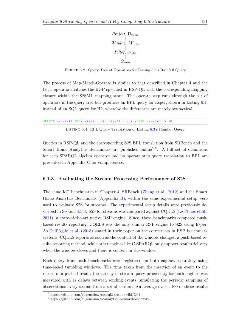
Chapter 6 Streaming Queries and A Fog Computing Infrastructure 131
Project, Πvalue
Window, W :obs
Filter, σ>10
Grain
Figure 6.2: Query Tree of Operators for Listing 6.3’s Rainfall Query
The process of Map-Match-Operate is similar to that described in Chapter 4 and theGrain operator matches the BGP specified in RSP-QL with the corresponding mappingclosure within the S2SML mapping store. The operate step runs through the set ofoperators in the query tree but produces an EPL query for Esper, shown in Listing 6.4,instead of an SQL query for H2, whereby the differences are merely syntactical.
1 SELECT rainfall FROM station .win:time (1 hour) WHERE rainfall > 10
Listing 6.4: EPL Query Translation of Listing 6.3’s Rainfall Query
Queries in RSP-QL and the corresponding S2S EPL translation from SRBench and theSmart Home Analytics Benchmark are published online5,6. A full set of definitionsfor each SPARQL algebra operator and its operate step query translation to EPL arepresented in Appendix C for completeness.
6.1.3 Evaluating the Stream Processing Performance of S2S
The same IoT benchmarks in Chapter 4, SRBench (Zhang et al., 2012) and the SmartHome Analytics Benchmark (Appendix B), within the same experimental setup wereused to evaluate S2S for streams. The experimental setup details were previously de-scribed in Section 4.3.3. S2S for streams was compared against CQELS (Le-Phuoc et al.,2011), a state-of-the-art native RSP engine. Since, these benchmarks compared push-based results reporting, CQELS was the only similar RSP engine to S2S using Esper.As Dell’Aglio et al. (2013) stated in their paper on the correctness in RSP benchmarksystems, CQELS reports as soon as the content of the window changes, a push-based re-sults reporting method, while other engines like C-SPARQL only support results deliverywhen the window closes and there is content in the window.
Each query from both benchmarks were registered on both engines separately usingtime-based tumbling windows. The time taken from the insertion of an event to thereturn of a pushed result, the latency of stream query processing, for both engines wasmeasured with 1s delays between sending events, simulating the periodic sampling ofobservations every second from a set of sensors. An average over a 100 of these results
5https://github.com/eugenesiow/sparql2stream/wiki/Q016https://github.com/eugenesiow/ldanalytics-pismarthome/wiki

132 Chapter 6 Streaming Queries and A Fog Computing Infrastructure
was taken. For S2S, the one-off translation time at the start (ranging from 16ms to32ms) was included in the sum during the average calculation.
Table 6.1 shows the results, for both benchmarks, of the average time taken to evaluatea query from the insertion of an event to the return of a push-based result from S2S,tS2S , and CQELS, tCQELS , with 1s delays in between. Query 67 of SRBench, a query todetect weather stations with low visibility by getting the union of visibility, rainfall andsnowfall observations, was omitted due to CQELS not supporting the ‘UNION’ operator.For all other queries, the S2S engine showed over two orders of magnitude performanceimprovement over CQELS. Queries 4, 5 and 9 that involved joining subgraphs of obser-vations (e.g. WindSpeed and WindDirection in Query 9) and aggregations showed largerperformance gains. This was similar to the results on historical data in S2S previouslyreported in Section 4.4.2. It was noted, that although CQELS returned valid resultsfor these queries, they contained an increasing number of duplicates, perhaps due to anissue with the adaptive caching of results within the window, which caused a significantslowdown over a 100 pushes, which is an undesirable behaviour over time. The sourcecode for the experiments are published on Github8,9.
A point of note is that the Java function ‘System.nanoTime()’ used to measure latencyin the benchmarks, relied on a system counter within the CPU which is usually accurateto about 1 microsecond but in the worst case could have only millisecond accuracy.Hence, it was necessary to average the results over at least a 100 measurements.
SRBench tS2S tCQELS Ratio1 0.47 138 1 : 2942 0.46 119 1 : 2613 0.66 202 1 : 3064 0.67 (1.86 · 105) 1 : (2.77 · 105)5 0.63 (1.48 · 106) 1 : (3.24 · 106)6 - - -7 0.66 2885 1 : 52458 0.67 282 1 : 4269 0.67 (1.88 · 105) 1 : (2.8 · 105)10 0.73 72 1 : 98
Smarthome tS2S tCQELS Ratio1 0.64 125 1 : 1962 0.77 129 1 : 1673 0.81 - -4 3.78 - -
Table 6.1: Average SRBench and Smart Home Analytics Benchmark Query RunTimes (in ms)
To verify that S2S was able to answer SRBench queries close to the rate they were sent,even at high velocity, the delay between insertions was reduced first from 1s to 1msand then to 0.1ms to produce rates of 1 row/ms and 10 rows/ms respectively. Table6.2 shows a summary of the average latency, the time from insertion to when queryresults were returned, of each query for both rates (in ms). It can be observed that the
7https://github.com/eugenesiow/sparql2stream/wiki/Q068https://github.com/eugenesiow/cqels9https://github.com/eugenesiow/sparql2stream

Chapter 6 Streaming Queries and A Fog Computing Infrastructure 133
Rate Latency (in ms) of SRBench Query Number(rows/ms) 1 2 3 4 5 7 8 9 10
1 1.300 1.374 1.279 1.303 1.2561 1.268 1.267 1.295 1.25510 0.155 0.159 0.143 0.161 0.1291 0.137 0.141 0.155 0.129
Table 6.2: Average Latency (in ms) at Different Rates for Each SRBench Query
99% 100%
1
2
5
10
100
1000
Percentage events at latency band
Rat
e (r
ows/
ms)
0-1
1-5
5-10
10-100
Latency (ms)
Figure 6.3: Percentage Latency at Various Rates for SRBench Query 1 (Focusedbetween 99-100%)
average latency was slightly higher than the inverse of the rate. The underlying streamengine, Esper, maintains context partition states consisting of aggregation values, partialpattern matches and data windows. At high rates, the engine introduces blocking tolock and protect context partition states which results in a slightly higher latency.
To ensure that the impact of this overhead was minimal even at high velocities, a com-parison method used by Calbimonte et al. (2012) to compare RSP engines was employedto group messages by latency ranges. Figure 6.3 shows that the effect of Esper’s block-ing on S2S latency was very minimal as the percentage of high latency query processingtime, of more than 1ms, was less than 0.3% (note that the x-axis is from 99% to 100%)even at the highest velocity with a rate of 1000 rows/ms. The longest latency timeswere also within 100ms and these were only observed at the high rates of 100 and 1000rows/ms, coinciding with Garbage Collection (GC) pauses of the Java Virtual Machineas a result of a larger number of ‘live’ objects10 in memory and greater memory frag-mentation. SRBench query 111 which involved getting the rainfall observed within anhourly window was used for the latency banding measurement.
Another test was performed to determine the maximum size of data that S2S couldprocess in-memory on the experimental setup of a lightweight IoT device, a RaspberryPi 2 B+ (RPi) with 1GB of memory. A query with a long TUMBLING window, SRBenchquery 812, which measures the daily maximum and minimum air temperature observedby the sensor at a given location, was used. The engine ran out of memory after inserting
10https://www.dynatrace.com/resources/ebooks/javabook/impact-of-garbage-collection-on-performance/
11https://github.com/eugenesiow/sparql2stream/wiki/Q0112https://github.com/eugenesiow/sparql2stream/wiki/Q08

134 Chapter 6 Streaming Queries and A Fog Computing Infrastructure
33.5 million rows, within the window of one day. Each row produced an equivalent of75 triples at the weather station measured, where each individual observation, thatcorresponded to a column within the row, produced about 10 triples. By projection, anRDF dataset size of 2.5 billion triples could theoretically fit in the RPi’s memory for asingle continuous query.
Queries 1 and 2 of the Smart Home Analytics Benchmark, presented in Appendix B, alsocorroborated the two orders of magnitude performance advantage of S2S over CQELS asshown in Table 6.1. Query 1 measured an average of the internal or external temperaturewithin the smart home over the last hour while query 2 measured the maximum andminimum temperatures over a day. Queries 3 and 4 could not be run on CQELS due tothe ‘FILTER’ operator throwing an error. Query 4 which detected unattended electricalusage based on metering and motion data involved joining both streams and performingan aggregation for average power. This query saw the average latency of S2S increase,though still stay under 4ms. The latency for this query was measured from the insertiontime of the last event involved that produced a result and hence initiated a push, tothat of receiving the push result.
Hence, results from the two benchmarks both show that S2S performs better thanCQELS for processing IoT time-series data streams with continuous queries. Rowsof data ingested by S2S are a more compact representation than sets of triples form-ing graphs that CQELS processes, which benefits not only push-based results reportinglatency but also the maximum size of data that can be streamed in a window. Map-Match-Operate allows S2S to serve as an RSP engine by maintaining the balance ofinteroperability, with a flexible graph model representation, and efficiency, with querytranslation.
6.2 Eywa: An Infrastructure for Fog Computing
In the science-fiction motion picture Avatar13, Eywa was the name of the biologicalinternet on the planet Pandora, made up of trees which were distributed over the surfaceof the planet. The trees stored memories and processed information. The flora and faunaof the planet then formed an ubiquitous sensor network feeding Eywa.
The Internet of Things (IoT) is growing to become a similar ubiquitous network of sen-sors and actuators for the planet. Fog computing is an emerging technology which seeksto bridge a gap for the IoT, like the fictional Eywa on Pandora, between the ground,where sensors and actuators are deployed (collect and act on data), and the cloud, wherelarger amounts of resources for processing and storing data can be provisioned dynami-cally. Application themes like the smart city from Section 2.1.2 experience the challenges
13http://www.avatarmovie.com/

Chapter 6 Streaming Queries and A Fog Computing Infrastructure 135
of wide IoT data stream distribution and real-time application query workloads whichfit with the concept of Eywa.
The purpose and contribution of this section is to introduce and formally define Eywa,an infrastructural fog computing framework,
• where stream processing can be performed on resource-constrained lightweight fogcomputing nodes,
• where the processing workload can be distributed among nodes utilising a novelinverse-pub-sub control plane and
• each node can maintain independence and control over access, resources, securityand privacy.
An Eywa network, that forms the basis for the Eywa fog computing infrastructure, isexplained as follows. An Eywa network, ε, consists of a set of nodes, N and connections,C, such that ε = (N,C). Each node, n ∈ N , can be a source, s, client, τ , or broker, b,node. Each connection, c ∈ C exists uniquely between two nodes such that C ⊆ N ×N .
A source node, s ∈ S, is a node that produces a set of time-series streams, Γ. A clientnode, τ ∈ T , is a node with a set of queries Q expecting a set of corresponding results,R. A broker node, b ∈ B, establishes a connection, c, for new source and client nodes toenter the network.
As source and client nodes form up in an Eywa network, broker nodes 1) provide apoint of entry for new nodes into the network, 2) do not store or process but forwarddata, 3) consume minimal resources and 4) employ redundancy through multiple sepa-rate instances within the network so as not to become single points of failure. Hence,facilitating both the formation and data flow in Eywa.
The utility of this Eywa network for processing streams is to facilitate 1) stream querydelivery to relevant nodes, 2) distributed processing and 3) results delivery to the request-ing nodes. To this end, Section 6.2.1 explains query delivery, Section 6.2.2 describesdistributed processing and Section 6.2.3 defines results delivery.
6.2.1 Stream Query Delivery by Inverse-Publish-Subscribe
Once an Eywa network has been formed, stream processing can take place as clients, τ ,issue stream queries, Q. Traditionally, source nodes, s, publish data while client nodessubscribe to data. In wireless sensor networks literature, these are sometimes referredto as the source and sink respectively (Ciciriello et al., 2007), where both many-to-one(Mainwaring et al., 2002; Intanagonwiwat et al., 2003) and many-to-many (Kim et al.,2003; Akyildiz and Kasimoglu, 2004) paradigms have been studied in the data plane, a

136 Chapter 6 Streaming Queries and A Fog Computing Infrastructure
fog computing term borrowed from routing literature (Yang et al., 2004). However, inEywa, it is desirable for clients to collaborate with the sources in a many-to-many fashionto share the workload, hence, an inverse-publish-subscribe mechanism for streamingquery delivery in the control plane is proposed.
Each source node subscribes to a topic for each of its streams. Client nodes then publishqueries to the relevant topics. Internationalised Resource Identifiers (IRIs), that workwell for the web, are used to provide a means of uniquely identifying and exchangingtopics. Definition 6.1 formally describes this mechanism.
Definition 6.1 (Inverse-publish-subscribe). Given the set of topics, M , a source node,s, subscribes to a topic, µ ∈ M for each stream within Γ to form ⋃
µ∈MΓsub(µ), where
MΓ is the set of all topics of s and sub(µ) is a function that produces a subscription toµ. For each query, q ∈ Q, from a client node, τ , a distribution function, α, builds a setof query-topic pairs α(q) = (Qµ,Mq) where Qµ is the set of all sub-queries in q, eachreferencing a particular topic µ and Mq is the set of all topics referenced in q. Eachsub-query, qµ ∈ Qµ, is published to its particular topic, µq ∈Mq, by the publish functionof query x to topic y, pub(x, y), so all publications from q form ⋃
pub(qµ, µq).
6.2.2 Distributed Processing
Source nodes receive the queries, perform part of the processing and deliver the resultsto clients that process the results. This forms the axis of client-source collaboration anddistributing processing workload as defined in Definition 6.2. Source nodes control theirown resources and response to queries. Quality of service is not in the scope of this workand by default is considered best effort within Eywa, however, service-level agreements,trustless networks or consensus protocols can be deployed on top of Eywa which arediscussed in the Social Web of Things application in Section 7.3.
Definition 6.2 (Distributed Source Node Processing). A source node, s, receives aquery, q, for a topic, µ, and converts it into a work function, ω, with a conversionfunction, λ(q) → ω. The work function, ω, is applied to the corresponding stream fortopic µ, γµ, where γµ ∈ Γ, so that ω(γµ) = γr and the resulting stream, γr, is pushed tothe requesting client, τ .
6.2.3 Push Results Delivery and Sequence Diagram
Client nodes receive result streams via a direct push from source nodes. Operationsinvolving multiple streams, like aggregations, are performed on the clients and resultsof the queries are published to topics for applications. Definition 6.3 details the processof results delivery and query output. Unlike in a Wireless Sensor Network (WSN), pro-longed operation and the network’s survival due to power-constrained nodes take lower

Chapter 6 Streaming Queries and A Fog Computing Infrastructure 137
precedence than performance and utility; hence, the underlying routing and transportnetworks are not of concern and decoupled.
Client , ? Broker, b Source1, s1 Source2, s2
sub(?1)
sub(?2)
pub(q11,?1),pub(q12,?2)
q11
q12
? (q11)? (q12)
?r1
?r2? (?r1 U ?r2)
InversePublish
Subscribe
Push
Figure 6.4: Sequence Diagram of Stream Query Processing in Eywa
Definition 6.3 (Push Results Delivery). A client node, τ , receives a set of resultstreams, Γr, by push delivery. For each query, q ∈ Q, in the set of queries for that client,a work function, ωτ , is produced by λτ (q)→ ωτ and executed on ⋃
γr, where γr are allthe result streams corresponding to the query, q. The result, γq, from ωτ (⋃ γr) = γq ispublished to a client results topic, µτ .
Figure 6.4 shows the full sequence diagram of the query processing process beginningfrom the source nodes subscribing to topic URIs, receiving queries when published byclient nodes, distributed processing and result delivery.
Source1, s1, produces a stream named, µ1, and subscribes to the corresponding topic, µ1,through broker, b. Source2, s2, does the same for its µ2 stream. A query, q1, is registeredwith client, τ , which executes the distribution function, α(), which forms pairs of the twosub-queries of q1 and their relevant topics. Each sub-query, q11 and q12, are publishedto topics µ1 and µ2 respectively. s1 and s2 receive the sub-queries and register themwith a conversion function, λ(). The work function, ω(), continuously processes thestreams produced and registered queries and pushes the results, when available, to τ ,which combines the result streams through ω(). Table 6.3 shows a glossary of symbolsused and their corresponding definitions for reference.

138 Chapter 6 Streaming Queries and A Fog Computing Infrastructure
Description Definition(s)τ Client node 6.1µ Topic (Uniformed Resource Identifier) 6.1γ,Γ Stream, Set of streams 6.1, 6.2, 6.3α() Distribution function, build query-topic pairs 6.2λ() Conversion function, converts query to work function 6.2, 6.3ω() Work function, applied to streams 6.2, 6.3
Table 6.3: Glossary of Symbols used in the Eywa Definition
6.2.4 S2S RDF Stream Processing (RSP) in Eywa
The work function, ω(), that is applied to streams in Eywa on source nodes duringthe distributed processing phase, can be implemented with an RDF Stream Processing(RSP) engine. Following the Map-Match-Operate philosophy in Chapter 4 and imple-mentation with S2S for streams in Section 6.1.1, Eywa utilises S2S as an RSP engineand together they are optimised to:
1. Ingest observation time-series data that exhibits flat and wide characteristics assuccinctly as possible.
2. Abstract the small set of device metadata with a flexible graph model to storein-memory as S2SML data model mappings for more semantic interoperability.
3. Distribute parts of the query to be applied on streams on an Eywa source node toshare the workload and possibly reduce the bandwidth required by transmittingfiltered results rather than raw data (predicate pushdown).
When an RSP-QL query is registered with a client, sub-queries are distributed to therelevant source streams as described previously (Section 6.2.1), translated with Map-Match-Operate and registered as a continuous query on each source node involved.Predicate pushdown is a term used in database literature (Reinwald et al., 1999) andpresents certain advantages especially in distributed systems like Eywa. The concept isas such, when a query is issued from a client node in one place to run against a lot ofdata produced by a set of source nodes in another place, a lot of network traffic couldbe spawned in transmitting raw data, which could be slow and costly. When certainparts of the query can be ‘pushed down’ to where the data is actually stored, filteringout most of the data, then network traffic can be greatly reduced.
Examples from CityBench (Ali et al., 2015), a published benchmark of smart city IoTdata, are used to elaborate on the translation process. CityBench consists of smart citystreams and metadata gathered from IoT sensors deployed within the city of Aarhus inDenmark from February 2014 to November 2015.

Chapter 6 Streaming Queries and A Fog Computing Infrastructure 139
Timestamp Humidity Temperature Wind Speed2014-08-01T00:00:00 56.0 18.0 7.4
Table 6.4: CityBench: Observation from the AarhusWeatherData0 Stream
Table 6.4 shows a weather observation from a CityBench stream. This is a stream ofactual flat and wide time-series observation data and consists of humidity, temperatureand wind speed readings measured at a particular timestamp. A source node with thisstream subscribes to the relevant IRI of the form, ‘http://...#AarhusWeatherData0’.
Listing 6.5 is the corresponding S2SML data model mapping that stores the sensor andobservation metadata of the weather data stream. It also contains bindings to fieldswithin the underlying stream, like ‘AarhusWeatherData0.tempm’.
1 @prefix ssn : <http :// purl.oclc.org/NET/ssnx/ssn#>2 @prefix sao : <http :// purl.oclc.org/NET/sao/>3 @prefix ct : <http :// www.insight - centre .org/ citytraffic #>4 @prefix ns : <http :// www.insight - centre .org/ dataset / SampleEventService #>5 @prefix s2s : <http :// iot.soton.ac.uk/s2s/s2sml#>6 ns: obsTemp AarhusWeatherData0 ._uuid a ssn: Observation ;7 ssn: observedProperty ns:Property -1;8 sao: hasValue " AarhusWeatherData0 .tempm"^^ s2s: literalMap ;9 ssn: observedBy ns: AarhusWeatherData0 .
10 ns:Property -1 a ct: Temperature .11 ns: obsHum AarhusWeatherData0 ._uuid a ssn: Observation ;12 ssn: observedProperty ns:Property -2;13 sao: hasValue " AarhusWeatherData0 .hum"^^ s2s: literalMap ;14 ssn: observedBy ns: AarhusWeatherData0 .15 ns:Property -2 a ct: Humidity .16 ns:obsWS AarhusWeatherData0 ._uuid a ssn: Observation ;17 ssn: observedProperty ns:Property -3;18 sao: hasValue " AarhusWeatherData0 .wspdm"^^ s2s: literalMap ;19 ssn: observedBy ns: AarhusWeatherData0 .20 ns:Property -3 a ct: WindSpeed .
Listing 6.5: CityBench AarhusWeatherData0 S2SML Mapping (Abbreviated)
This mapping references various ontologies like the Semantic Sensor Network (SSN)Ontology14 and City Traffic Ontology, providing a common way of describing sensordata, increasing interoperability. A formal definition of the S2SML mapping languageis covered in Section 4.2.1.1. Similarly, a mapping is available for the stream of trafficdata, with ‘avgSpeed’ and ‘congestionLevel’ fields, at locations in the city and alsoother smart city streams like pollution data available from the RSP-QL fork15 of S2S.
Listing 6.6 shows Query 2 of CityBench expressed in RSP-QL syntax that checks thetraffic congestion level and weather conditions on each road of a planned journey. Whenregistered, it processes both traffic and weather streams for observations of traffic con-gestion level and weather (e.g. temperature), from a particular stretch of road, for the
14http://www.w3.org/TR/vocab-ssn/15https://github.com/eugenesiow/sparql2stream/tree/RSP-QL

140 Chapter 6 Streaming Queries and A Fog Computing Infrastructure
Project
Join
Window:weather
Gweather
Window:traffic
Gtraffic
Figure 6.5: Query Tree of CityBench Query 2 from Listing 6.6
last 3 seconds. The query is abbreviated for better readability and the weather windowactually queries ‘v1’ to ‘v3’ for temperature, humidity and wind speed respectively.The graph query provides for interoperability by including metadata in a flexible waywhile the values ‘v1’ to ‘v4’ are efficiently retrieved from fields within the flat streams.‘v1’ to ‘v3’ can be retrieved all at once from the same weather stream event.
1 SELECT ?v1 ?v2 ?v3 ?v42 FROM NAMED WINDOW : traffic ON <http ://...# AarhusTrafficData158505 > [RANGE 3s]3 FROM NAMED WINDOW : weather ON <http ://...# AarhusWeatherData0 > [RANGE 3s]4 WHERE 5 WINDOW : weather 6 ?obId1 a ssn: Observation ;7 ssn: observedProperty ?p1;8 sao: hasValue ?v1;9 ssn: observedBy ns: AarhusWeatherData0 .
10 ?p1 a ct: Temperature .11 # obsId2 for Humidity and obsId3 for WindSpeed abbreviated ... 12 WINDOW : traffic 13 ?obId4 a ssn: Observation ;14 ssn: observedProperty ?p4;15 sao: hasValue ?v4;16 ssn: observedBy ns: AarhusTrafficData158505 .17 ?p4 a ct: CongestionLevel . 18
Listing 6.6: CityBench Query 2: Finding the Traffic Congestion Level and WeatherConditions of a Planned Journey (Abbreviated)
A walkthrough of the query translation process for this query is in Section 6.2.5, while thedistribution by Eywa’s inverse-pub-sub, processing and return to the client for furtherprocessing is described in Section 6.2.6. The entire architecture of Eywa’s RSP engineis then summarised in Section 6.2.7.
6.2.5 Eywa’s RSP-QL Query Translation of CityBench
Eywa uses the S2S engine for stream query translation that was introduced in Sec-tion 6.1.2. Firstly, the RSP-QL query was parsed into algebra as shown in Figure 6.5.
The algebra query tree was traversed from leaf to root. The Basic Graph Pattern (BGP),Gweather, which compromises the portion of the query shown in Listing 6.7 was matched

Chapter 6 Streaming Queries and A Fog Computing Infrastructure 141
against the AarhusWeatherData0 S2SML mapping from Listing 6.5 in the match stepof Map-Match-Operate that Eywa-RSP’s S2S engine follows.
1 ?obId1 a ssn: Observation ;2 ssn: observedProperty ?p1;3 sao: hasValue ?v1;4 ssn: observedBy ns: AarhusWeatherData0 .5 ?p1 a ct: Temperature . #(... humidity and wind speed parts)
Listing 6.7: Basic Graph Pattern, Gweather, from CityBench Query 2 (Listing 6.6)
The result of the match step was Bweathermatch that contained bindings like that from variable
‘v1’ from Gweather to the field ‘tempm’ in the stream ‘AarhusWeatherData0’. Similarly,from Gtraffic, Btraffic
match contained the binding of variable ‘v4’ to ‘congestionLevel’ inthe stream ‘AarhusTrafficData158505’. The results were passed to the join operator.
Since no variables overlapped from the weather and traffic windows, the result sets werepassed upwards, unchanged, to the project operator. At the project node, variables‘v1’ to ‘v4’ were projected. Any variable renaming or aliases (none in this example)would be taken care of in the projection operator as well. The simplified stream queryproduced, expressed in Event Processing Language (EPL), is shown in Listing 6.8.
1 SELECT AarhusWeatherData0 .tempm AS v1 ,2 AarhusWeatherData0 .hum AS v2 ,3 AarhusWeatherData0 .wspdm AS v3 ,4 AarhusTrafficData158505 . congestionLevel AS v45 FROM AarhusWeatherData0 .win:time (3 sec) ,6 AarhusTrafficData158505 .win:time (3 sec)
Listing 6.8: CityBench Query 2 Translated to Event Processing Language (EPL)
CityBench Query 5 in Listing 6.9 which discovers the traffic congestion level on theroad where a given cultural event is happening has algebra as shown in Figure 6.6.Window:traffic produced a similar result set as in Query 2. However, Graphsensor andGraphcultural reference relations, historical data sources, instead of streams, hence, SQLinstead of EPL queries were produced for each by the S2S translation engine. Thetranslated SQL query syntax from Graphcultural is shown in Listing 6.10.

142 Chapter 6 Streaming Queries and A Fog Computing Infrastructure
Project
Filterδlat2+δlon2<0.1
Join
Window:traffic
Gtraffic
Join
Graphsensor
Gsensor
Graphcultural
Gcultural
Figure 6.6: Query Tree of CityBench Query 5: Traffic Congestion Level at a CulturalEvent
1 SELECT ?title ?lat1 ?lon1 ?lat2 ?lon2 ?v22 FROM NAMED WINDOW : traffic ON <http ://...# AarhusTrafficData158505 > [RANGE 3s]3 FROM NAMED <http ://...# AarhusCulturalEvents >4 FROM NAMED <http ://...# SensorRepository >5 WHERE 6 GRAPH ns: SensorRepository 7 ?p2 a ct: CongestionLevel ;8 ssn: isPropertyOf ?foi2.9 ?foi2 ct: hasStartLatitude ?lat2;
10 ct: hasStartLongitude ?lon2.11 12 GRAPH ns: AarhusCulturalEvents 13 ?evtId a ssn: Observation ;14 sao:value ?title;15 ssn: featureOfInterest ?foi.16 ?foi ct: hasFirstNode ?node.17 ?node ct: hasLatitude ?lat1;18 ct: hasLongitude ?lon1.19 20 WINDOW : traffic 21 ?obId2 a ssn: Observation ;22 ssn: observedProperty ?p2;23 sao: hasValue ?v2;24 ssn: observedBy ns: AarhusTrafficData158505 .25 26 FILTER (((? lat2 -? lat1)*(? lat2 -? lat1)+(? lon2 -? lon1)*(? lon2 -? lon1)) <0.1)27
Listing 6.9: CityBench Query 5: Traffic Congestion Level on the Road where a GivenCultural Event is Happening
1 SELECT title , lat , lon FROM AarhusCulturalEvents
Listing 6.10: Graphcultural Portion of CityBench Query 5 Translated to SQL
At the first join operator from the bottom of the tree, the SQL queries were integratedinto the ‘FROM’ clause of the EPL statement produced in the S2S translation as shownin Listing 6.11.

Chapter 6 Streaming Queries and A Fog Computing Infrastructure 143
1 FROM sql: AarhusCulturalEvents [ ‘SELECT title , lat , lon2 FROM AarhusCulturalEvents ’ ] AS AarhusCulturalEsvents ,3 sql: SensorRepository [ ‘SELECT lat , lon FROM SensorRepository ’ ] AS
SensorRepository
Listing 6.11: ‘FROM’ Clause of Translated EPL Query from CityBench Query 5(Listing 6.9) after Graphsensor-Graphcultural Join
At the next join operator, as there was a variable ‘p2’ present in both inbound nodes,a join was performed between the metadata in the model from Window:traffic and theprevious join. The modified translation to SQL within the ‘FROM’ clause is shown inListing 6.12.
1 ... [ ‘SELECT lat , lon FROM SensorRepository2 WHERE propId =\‘ Property -b9f9 ...\ ’’ ] AS SensorRepository ,
AarhusTrafficData158505 .win:time (3 sec)
Listing 6.12: Abbreviated ‘FROM’ Clause of Translated EPL Query from CityBenchQuery 5 (Listing 6.9) after Join Operator on Window:traffic
Finally, a filter on the addition of the square delta of latitude and longitude constrainsthe traffic sensor and cultural event locations to within 0.1 units of area16. All City-Bench queries and corresponding S2S translations have been published on the benchmarkwiki17.
6.2.6 Eywa’s RSP Query Distribution
Query distribution is the process whereby part of a query workload, ωτ , is distributedfrom the client (where the query is registered and the results are expected), to the sourcenode (where the data is produced or stored). The workload is distributed within theEywa network and a simple form of predicate pushdown is achieved.
For example, for Query 2 in CityBench (Listing 6.6), at the project operator at theroot of the algebra tree, the S2S engine in Eywa tracks that hum, tempm and wspdmare the fields required from Window:weather while only congestionLevel is required fromWindow:traffic. Hence, the projection of these fields is the work function, ωτ , pushedto each source node producing the traffic and weather streams. These relationships aretracked as a projection tree for the streams as shown in Figure 6.7 for Query 2.
Following RSP Query Translation (Section 6.2.5), the resulting simplified, translatedEPL query is registered on the client. The projection tree is distributed through Eywa’sinverse-pub-sub mechanism to the subscribing source nodes of the IRIs ofWindow:weather
and Window:traffic. Hence, each source node pushes only an effective subset of eachstream, γq, with only the projected fields to the client which combines and does any
16https://github.com/eugenesiow/Benchmark/wiki/Q0517https://github.com/eugenesiow/Benchmark/wiki/

144 Chapter 6 Streaming Queries and A Fog Computing Infrastructure
Weathertempm,hum,wspdm,TrafficcongestionLevel
tempm,hum,wspdm
v1,v2,v3
congestionLevel
v4
Figure 6.7: Projection Tree for Query 2 Streams
Stat ic Source (SQL)
Stream Dist ributor
Sens
or D
ata
Source Node, s Broker Node, b
Publish-Subcribe IRIS
Subs
crib
eQuery Translat ion
RDF Mappings
Client Node, ?
RSP
-QL
Q
ueri
es
EPL Engine
Push
Pub
lish
Figure 6.8: Architecture of Eywa’s RSP Fog Computing Framework
further processing on the received streams. For relations, static sources of historical data,the work function, ωτ , also comprises SQL queries which are automatically distributedto the source nodes by the underlying Esper engine in S2S through Java DatabaseConnectivity (JDBC) connections. In Query 5 of CityBench as shown in Listing 6.11,an SQL query is executed on the static SensorRepository source node.
6.2.7 Eywa’s RSP Architecture
Figure 6.8 shows the architecture of Eywa’s RSP implementation in this thesis consist-ing of client, source and broker nodes. The brokers use lightweight ZeroMQ socketswhich use a binary transmission protocol that has minimal overhead to support publish-subscribe IRI topics. Client nodes receive queries in RSP-QL and projected streamsvia push from source nodes. They process complex events in queries using an EPL en-gine, Esper, that registers translated queries with data model mappings. Source nodesproduce streams of time-series IoT data or store static data, e.g. sensor location data,cultural event data. A stream distributor component pushes projected streams, γq, toclient nodes as required. Static queries utilise JDBC connections from client to sourcenodes.
The current design of Eywa makes several assumptions. Firstly, the source, broker andclient nodes are assumed to be co-operative. At least one broker node is active withinEywa and known by the source and client nodes. Delivery via push from the source toclient nodes is considered best effort.

Chapter 6 Streaming Queries and A Fog Computing Infrastructure 145
6.3 Evaluation of Eywa with CityBench
The performance and scalability of the Eywa fog computing infrastructure was evaluatedon smart city vehicle traffic, parking, cultural events, weather and pollution IoT datastreams with CityBench (Ali et al., 2015). As explained earlier in Section 6.2, the smartcity scenario, which envisions affordable fog devices owned by people and organisationsthat are distributed throughout the city, its buildings and infrastructure, is a particularpertinent use case for Eywa. The benchmark featured continuous stream queries thatpowered smart city applications, for example, a parking space finder and an adminconsole. Eywa and the underlying S2S RSP engine were compared against CQELS(Le-Phuoc et al., 2011) and C-SPARQL (Barbieri et al., 2010) RSP engines.
The streaming and static source nodes, client nodes and broker nodes within the ex-perimental setup were hosted on resource-constrained lightweight computers, RaspberryPi (RPi) 2 Model B+s, which were widely available and had good community support.Each RPi had 1GB RAM, a 900MHz quad-core ARM Cortex-A7 CPU and used Class10 SD Cards. Ethernet connections were used between the nodes for reliable transportduring the experiment and each node’s clock was synchronised using the Network TimeProtocol (NTP).
For each query, experiments were performed for a varying amount of concurrent queriesand data streams. Both the latency and memory consumption were measured for eachengine. Tests were run for 15 minutes each, based on the methodology from the bench-mark paper (Ali et al., 2015), and averaged over 3 runs. The goal was to measure theperformance, in terms of the latency of queries, and scalability, which was shown bythe memory consumption while varying the number of data streams and concurrentqueries. Additionally, to measure the benefits in scalability of Eywa’s fog computinginfrastructure, Eywa-RSP with S2S was tested and compared with client, source andbroker on a single node against when they were distributed across multiple nodes withworkload distribution. A client and broker were deployed on one node, while two sourceand broker nodes producing different streams were deployed within the network.
6.3.1 Latency Evaluation Results
The latency of a query refers to the average time between when a stream observationarrived and when the results from the query output were generated.
Figure 6.9 shows the latency over time of each of the engines for Query 118 in City-Bench which measured the traffic congestion level on two roads. Eywa-RSP had thelowest latency and best query performance. The average latency over time for queries inCityBench, measurements were made at one minute intervals over the total time of 15
18https://github.com/eugenesiow/Benchmark/wiki/Q01

146 Chapter 6 Streaming Queries and A Fog Computing Infrastructure
5 10 150
5
10
15
Experiment Time (min)
Latenc
y(s)
CQELSEywa-RSPC-SPARQL
Figure 6.9: Latency of CityBench Q1 across Time
minutes, are summarised in Figure 6.10. Eywa-RSP was the fastest on each of the queriesfollowed by CQELS and then C-SPARQL. By representing metadata triples within datamodel mappings which are processed in the query translation process as opposed to inthe stream itself, Eywa-RSP was able to more efficiently process more concise streams ofIoT time-series data than CQELS and C-SPARQL, resulting in better average latencyfor almost every query. The only exception was for Query 11, which notified when anyweather observation was detected, where CQELS was marginally faster. As CQELS pro-cessed triples, the CQELS query was actually simpler and was optimised with adaptivecaching as it specified a single BGP for a general weather observation, which had oneless triple than one which specified the type of observation. In Eywa-RSP, a union ofall the ‘wspdm’, ‘tempm’ and ‘hum’ had to be performed on the stream.
Figure 6.11 shows the algebra of the translated Query 1 from CityBench, registered onthe client node. q is the operator for retrieving the projected columns (e.g. congestion-Level) from each event in the stream window from a source node.
The algebra for CQELS and C-SPARQL on the other hand, as shown in Figure 6.12,require the retrieval of, τBGP , for each event in the stream. The extra triples for each ob-servation in the stream are shown in Listing 6.13, representing the observation metadata(lines 1 to 3) and relation to sensor metadata (line 4). It is more expensive in termsof overall latency when retrieving the extra triples and processing the query withoutworkload distribution at the source.
1 ?obId1 a ?ob.2 ?obId1 ssn: observedProperty ?p1.3 ?obId1 sao: hasValue ?v1.4 ?obId1 ssn: observedBy <http ://...# AarhusTrafficData182955 >.
Listing 6.13: Additional Metadata Triples for CQELS and C-SPARQL

Chapter 6 Streaming Queries and A Fog Computing Infrastructure 147
1 2 3 5 6 7 8 9 10 11
0
2
4
6
8
10
12
14
CityBench Query
Averag
eLa
tenc
y(s)
CQELS Eywa-RSP C-SPARQL
Queries for each engine that could not be run were Eywa:4, CQELS:4,10,12, C-SPARQL:4,6,11,12
Figure 6.10: Average Latency of CityBench Queries on RSP Engines
Project
Join
Window:traffic1
qcongestionLevel
Window:traffic2
qcongestionLevel
Figure 6.11: Algebra of Query 1 for Eywa-RSP
6.3.2 Scalability Evaluation Results
Scalability evaluation looked at the amount of memory resources used by each RSPengine and the results when increasing the number of concurrent queries and increasingthe number of data streams. The lower the memory resources used, the more scalablethe system was, especially on resource-constrained fog nodes.
Figure 6.13 shows the memory consumption of each engine across time. Eywa-RSPstreamed a more concise format of time-series data points as events and only the nec-essary projected fields from the source node, hence, as compared to the more verboseset of triples shown in Listing 6.14 for other engines, Eywa-RSP used significantly less

148 Chapter 6 Streaming Queries and A Fog Computing Infrastructure
Project
Join
Window:traffic1
τBGP
Window:traffic2
τBGP
Figure 6.12: Algebra of Query 1 for CQELS and C-SPARQL
5 10 150
100
200
Experiment Time (min)
Mem
oryCon
sumed
(MB)
CQELSEywa-RSPC-SPARQL
Figure 6.13: Memory Consumed by CityBench Query 2 across Time on Client
memory, about 20 times less than CQELS and two orders of magnitude less than C-SPARQL. As expected, the more complex Query 519, a filter operation on two graphsand a stream, took the most memory and Query 1120, checking for observations fromweather sensors only on a single stream, took the least on all engines with Eywa-RSP anorder of magnitude less than CQELS and two orders of magnitude less than C-SPARQL.
1 : Property1 a ct: CongestionLevel .2 : Observation1 a ssn: Observation ;3 ssn: observedProperty : Property1 ;4 sao: hasValue " congestionLevel ";5 ssn: observedBy ns: AarhusTrafficData158505 ;6 time: inXsdDateTime " timestamp ".7 : Observation2 a ssn: Observation ;8 ssn: observedProperty : Property2 ;9 sao: hasValue " avgSpeed ";
10 ssn: observedBy ns: AarhusTrafficData158505 ;11 time: inXsdDateTime " timestamp ".
Listing 6.14: Set Of Triples from a Row/Event of the Traffic Stream
When increasing the number of concurrent queries on each engine, Eywa-RSP once againachieved the lowest memory consumption. The memory consumed on Eywa-RSP wasalso the only one consistent and did not increase over time like C-SPARQL and CQELS.
19https://github.com/eugenesiow/Benchmark/wiki/Q0520https://github.com/eugenesiow/Benchmark/wiki/Q11
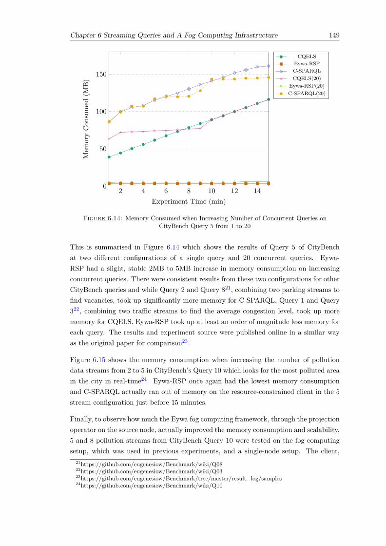
Chapter 6 Streaming Queries and A Fog Computing Infrastructure 149
2 4 6 8 10 12 140
50
100
150
Experiment Time (min)
Mem
oryCon
sumed
(MB)
CQELSEywa-RSPC-SPARQLCQELS(20)
Eywa-RSP(20)C-SPARQL(20)
Figure 6.14: Memory Consumed when Increasing Number of Concurrent Queries onCityBench Query 5 from 1 to 20
This is summarised in Figure 6.14 which shows the results of Query 5 of CityBenchat two different configurations of a single query and 20 concurrent queries. Eywa-RSP had a slight, stable 2MB to 5MB increase in memory consumption on increasingconcurrent queries. There were consistent results from these two configurations for otherCityBench queries and while Query 2 and Query 821, combining two parking streams tofind vacancies, took up significantly more memory for C-SPARQL, Query 1 and Query322, combining two traffic streams to find the average congestion level, took up morememory for CQELS. Eywa-RSP took up at least an order of magnitude less memory foreach query. The results and experiment source were published online in a similar wayas the original paper for comparison23.
Figure 6.15 shows the memory consumption when increasing the number of pollutiondata streams from 2 to 5 in CityBench’s Query 10 which looks for the most polluted areain the city in real-time24. Eywa-RSP once again had the lowest memory consumptionand C-SPARQL actually ran out of memory on the resource-constrained client in the 5stream configuration just before 15 minutes.
Finally, to observe how much the Eywa fog computing framework, through the projectionoperator on the source node, actually improved the memory consumption and scalability,5 and 8 pollution streams from CityBench Query 10 were tested on the fog computingsetup, which was used in previous experiments, and a single-node setup. The client,
21https://github.com/eugenesiow/Benchmark/wiki/Q0822https://github.com/eugenesiow/Benchmark/wiki/Q0323https://github.com/eugenesiow/Benchmark/tree/master/result_log/samples24https://github.com/eugenesiow/Benchmark/wiki/Q10

150 Chapter 6 Streaming Queries and A Fog Computing Infrastructure
2 4 6 8 10 12 140
50
100
150
200
250
Experiment Time (min)
Mem
oryCon
sumed
(MB)
CQELS(2)Eywa-RSP(2)C-SPARQL(2)CQELS(5)
Eywa-RSP(5)C-SPARQL(5)
Figure 6.15: Memory Consumed by CityBench Query 10 with Varying Data StreamConfigurations of 2 and 5
The graph lines formed from the results of Eywa-RSP(2) and Eywa-RSP(5) are very close, as are those from CQELS(2) and
CQELS(5).
2 4 6 8 10 12 140
10
20
30
40
50
60
Experiment Time (min)
Mem
oryCon
sumed
(MB)
Fog(5)Fog(8)
Single(5)Single(8)
Figure 6.16: Fog vs Single-Node Eywa-RSP Networks: Memory Consumed whileIncreasing Streams on CityBench Query 10 from 5 to 8

Chapter 6 Streaming Queries and A Fog Computing Infrastructure 151
broker and source nodes were all run on the same node in the single-node setup. Figure6.16 shows the amount of memory consumed by the distributed fog execution of thequery (on the client) and the single-node execution of the query.
As the projection operator was distributed to the source nodes and only the applicablepart of the stream was sent to the client, there was a significant difference in memoryconsumed when the number of incoming data streams was increased. At 2 and 5 streamsfor Query 10, the memory consumed was similar for distributed fog and single-nodesetups, hence the results of 2 streams was omitted from the graph. When there were8 streams on Query 10 however, the fog computing approach consumed less memory.This was due to the flow of data being significantly large enough that the projectionoperation passed down to the source node of each stream also had a significant effect onthe overall memory consumed. Hence, as the amount of streams increase, Eywa’s FogInfrastructure provides greater scalability.
6.4 Fog Computing within the Internet of the Future
The Internet has been a great motor of socio-economic activity in the past decade andthe Internet of the Future has the potential to do even more. Like the fictional Eywa inAvatar, Eywa as a fog computing infrastructure has the potential to make the IoT andthe planet more intelligent, more connected and at the same time more engaged andsocial, while valuing privacy and security.
Learning from the web, that grew as a free, open and standards-based information spaceon top of the internet (Berners-Lee and Fischetti, 2000), the IoT needs to endeavourto support interoperability. Modelling and publishing metadata as RDF not only en-courages interoperation through the use of common identifiers in IRIs and referencingcommon ontologies, it also represents concepts as machine-readable graphs (Bizer et al.,2009) which goes towards solving challenges like discovery and data integration in theIoT. Fog computing that serves as a layer between sensors and actuators, and the cloud,and possesses comparatively more compute and storage than sensors, serves as the entrylevel compute and storage platform for interoperability and integration.
The current business model for many web services is that free content is exchanged forour personal data. However, ‘as our data is held in proprietary silos, out of sight to us, welose out on the benefits we could realise if we had direct control over this data and chosewhen and with whom to share it25’, argued inventor of the web Sir Tim Berners-Lee.Fog computing on lightweight, distributed computers means that data that is collectedfrom sensors and devices are stored and processed locally. As access control technologyevolves, specific privacy policies with additional trust and fault tolerance mechanismscan be created (Roman et al., 2013) to control what goes to the cloud.
25http://theguardian.com/technology/2017/mar/11/tim-berners-lee-web-inventor-save-internet

152 Chapter 6 Streaming Queries and A Fog Computing Infrastructure
Furthermore, as data is stored and processed by some applications locally, the need toshuttle data to and from the cloud is minimised, providing better guarantees of qualityof service for mission-critical IoT apps and there is less dependency on supporting highbandwidth global connections. In disaster management IoT scenarios, where last-mileconnectivity is lost, having data locality and offline access is especially valuable. Thereare also performance benefits over storing encrypted data in traditional clouds as ameans to maintain privacy because it is easier to perform processing over data. Forexample, there is no need for crypto-processors or to apply special encryption functionson data. When access controls permit, data can still be sent to the cloud for big dataanalytics.
Finally, as the internet and IoT advance, studying the socio-technical aspects of the in-tersection between intelligent, co-operative, autonomous machines in the IoT and humanusers is gaining importance. Fog computing, as a distributed, interoperable applicationlayer between the network, autonomous IoT end-devices, applications and human end-users, can serve 1) to build and manage this socio-technical network, 2) to facilitateinformation flow or sharing, 3) to host applications and 4) as an observation platformfor the study of these emerging networks. This application of a decentralised Social Webof Things is covered in greater detail in the next chapter (Chapter 7).
6.5 Conclusions
This chapter highlighted the extension of Map-Match-Operate to efficiently process real-time streams in the IoT and proposed an infrastructure, Eywa, for fog computing thatshows how resource-constrained platforms close to the source IoT agents can be utilisedfor stream processing.
The implementation of S2S, a Map-Match-Operate engine that translates streamingSPARQL graph queries expressed as RSP-QL to the Event Processing Language (EPL),showed greater efficiency than state-of-the-art RSP engine CQELS for the same pub-lished benchmarks, within the same experimental setup as that described in Chapter4.
Eywa, which utilises an inverse-publish-subscribe system to distribute streaming queriesacross fog nodes running S2S engines, showed improvements in stream processing withina smart city scenario for both scalability and latency metrics as compared to CQELSand C-SPARQL. The current design limitations of Eywa though, are that it makesthe assumptions of a co-operative network, with a set of well-known broker nodes andbest-effort delivery from source to client nodes. Hence, applications that require strictguarantees on the correctness of results cannot be served by Eywa at present. Mitigatingthe reliability of Eywa would require implementing a Byzantine Fault Tolerant (Lamportet al., 1982) consensus within the distributed system which is not the focus of this thesis.

Chapter 6 Streaming Queries and A Fog Computing Infrastructure 153
The next chapter introduces analytical applications and platforms that put into per-spective how the efficient data and event management that Map-Match-Operate bringsfor historical and streaming data, can motivate the socio-technical development of theIoT especially when considering the emerging distributed fog computing paradigm.


Chapter 7
Applications of Efficient GraphQuerying and Analytics
“People think that computer science is the art of geniuses but the actualreality is the opposite, just many people doing things that build on eachother, like a wall of mini stones.”
— Donald Knuth
This chapter introduces analytical applications and platform infrastructure that build onthe interoperable and efficient data management with Map-Match-Operate for historicaland streaming data in the Internet of Things (IoT). Previous chapters in this thesisintroduced and have already evaluated Map-Match-Operate as a means of performantand interoperable IoT time-series storage, hence, the main aim of the applications andplatforms described in this chapter are not to validate Map-Match-Operate but ratherto show how this research can lead to applications in different directions. Section 7.1describes how Map-Match-Operate can power personal IoT repositories and analyticaldashboards running on them while Section 7.2 describes how TritanDB can be used fortime-series analytics. Section 7.3 introduces how a Social Web of Things, based on socialcapital theory, can be built on current infrastructure and be evolved over time, producinggreater value for personal repositories. A mechanism for distributing IoT informationwithin resource-constrained decentralised social networks under ten thousand nodes isalso devised by comparing the scalability of existing technologies.
The work involving personal IoT repositories in this chapter was published in the Siowet al. (2016b) paper and demonstrated at the International Semantic Web Conference.
155

156 Chapter 7 Applications of Efficient Graph Querying and Analytics
7.1 PIOTRe: Personal Internet of Things Repository
Resource-constrained IoT devices like Raspberry Pis, with specific performance optimi-sation, can serve as interoperable personal repositories that store and process time-seriesIoT data for analytical applications. This thesis implements PIOTRe, a personal data-store that utilises S2S query translation technology on Pis to process, store and publishhistorical and streaming IoT time-series data. PIOTRe was demonstrated in a smarthome scenario with a real-time dashboard and historical visualisation application thatutilised RDF stream processing (RSP), a set of descriptive analytics visualisations onhistorical data, a framework for registering stream queries within a local fog computingnetwork and a means of sharing metadata globally with Thing directories and catalogueslike HyperCat. In particular, the following contributions are presented in this section:
• A real-time smart home dashboard that utilises S2S’s RDF stream processing(RSP) engine to push results to descriptive analytics widgets via websockets.
• A smart home descriptive analytics application that uses a set of SPARQL querieswith space-time aggregations, translated by S2S, to visualise historical data overtime, stored by TritanDB.
• A means of publishing and sharing metadata and mappings with a standardisedformat called HyperCat.
Section 7.1.1 covers the design and architecture of PIOTRe while Section 7.1.2 intro-duces a real-time dashboard and a historical visualisation application, both runningon PIOTRe. Section 7.1.3 and Section 7.1.4 show how PIOTRe interacts with a fogcomputing network using Eywa and the wider IoT using HyperCat respectively.
7.1.1 Design and Architecture of PIOTRe
PIOTRe was designed, tested and demonstrated to run on a compact and mobilelightweight computer, like a Raspberry Pi, or an x86 alternative, like the Gizmo21.PIOTRe can also start as a source, client or broker node, or a combination of all three,within an Eywa fog computing network as described in Section 6.2. Internally, PIOTReconsists of a number of components as shown in Figure 7.1 that are described as follows.
Sensors, human input and other event streams take the form of time-series input datastreams to the PIOTRe system. Data streams are ingested as an event stream with Esperwhich underlies the RDF stream processing (RSP) engine and are also simultaneouslystored in a historical TritanDB store (Chapter 5). Each stream forms a time-series
1http://www.gizmosphere.org/products/gizmo-2/

Chapter 7 Applications of Efficient Graph Querying and Analytics 157
App
sM
etad
ata
Pub
lishi
ng
S2SML Mappings
TritanDB Esper
S2S
Eywa
SPARQLEndpoint
Source Client
Broker
T hings
Stream Data
PIO
TR
e
Sensors
Human Input
Events
Figure 7.1: Architecture of PIOTRe
within TritanDB. The RSP engine is driven by an S2S engine that works on translatingRSP-QL queries to Event Processing Language (EPL) queries for Esper2, the methodof which was described in Section 6.1.
Mappings are shared across the S2S engine for streams and TritanDB and are representedin S2SML, as introduced in Section 4.2.1.1, which is an RDF representation of how ametadata graph maps to fields within a TritanDB time-series or an event within a stream.PIOTRe provides both a visual What You See Is What You Get (WYSIWYG) interface,as shown in Figure 7.2, and a script editor to author S2SML data model mappings.
Figure 7.2: What You See Is What You Get (WYSIWYG) S2SML Editor in PIOTRe
Applications in PIOTRe have the flexibility of being written in any language and frame-work and communicate with the TritanDB through the interface of a SPARQL Endpointfor historical data and with S2S for streams by registering an RSP-QL continuous query
2http://www.espertech.com/

158 Chapter 7 Applications of Efficient Graph Querying and Analytics
with an Eywa client. The metadata publishing component publishes the metadata frommappings, like the sensor descriptions, locations, data fields and formats to supportglobal discovery and interoperability with the wider IoT. Screenshots of the PIOTReinterface, which walks users through adding data and weaving mappings, are shown inFigure 7.3 and the source code is published online on GitHub3.
Figure 7.3: Getting Started with PIOTRe and Adding IoT Data Sources
7.1.2 Example Applications using PIOTRe
IoT Freeboard4 is a real-time dashboard that consists of a simulator that replays astream of smart home data at a variable rate to PIOTRe and a high customisable webapplication dashboard that receives the output from the set of registered push-basedstreaming RSP-QL queries as a websocket events stream. Each result in the streamconsists of the query name it was generated by and fields of the result set. An examplein Listing 7.1 shows a result of an RSP-QL query that calculates the average power froma particular smart meter every time there is a change in consumption. This result is thenvisualised as a spark line on the application dashboard that shows the trend of powerconsumption of this meter. A host of other widgets can be added to the dashboard tovisualise events. A demonstration of the dashboard’s capabilities was presented at theInternational Semantic Web Conference and is available online5.
1 2 " queryName ":" averagePower ",3 " averagePower ":"10.5" ,4 "uom ":"W"5
Listing 7.1: JSON Result Streamed through WebSocket from RSP Engine in PIOTRefor a Query Retrieving Average Power from a Smart Home Meter
The Pi Smart Home Dashboard6 is an application that uses SPARQL queries on his-torical smart home data to provide visualisations across time and space. The queries
3https://github.com/eugenesiow/piotre-web4https://github.com/eugenesiow/iotwo5https://youtu.be/oH0iSWTmKUg6https://github.com/eugenesiow/ldanalytics-PiSmartHome

Chapter 7 Applications of Efficient Graph Querying and Analytics 159
Figure 7.4: Applications using Streaming and Historical Data with PIOTRe
are presented within the Smart Home Analytics Benchmark described in Appendix B.The application allows the user to tweak the time range and sensor types through a userinterface that changes parameters to SPARQL queries which generates different result-ing graph visualisations. A demonstration video is available online and a live demo waspresented at the International Semantic Web Conference7. Figure 7.4 shows screenshotsof IoT freeboard on the left and the Pi Smart Home on the right.
7.1.3 PIOTRe as an Eywa Fog Computing Node
PIOTRe stores, processes and runs applications on data. As such, PIOTRe can serve asa source, client and broker or a combination of all three within an Eywa fog computingnetwork to perform RDF stream processing (RSP) on streams. In some IoT scenarioslike disaster management or environmental monitoring in remote locations, Eywa canbe used as a local, offline network for processing data. The Eywa client-broker-serverarchitecture was described previously in Section 6.2 and enables stream queries to beregistered within the control plane of a fog computing network using inverse-publish-subscribe and allows results to be delivered by a push-pull mechanism within the dataplane of the network. The mechanism is known as inverse-publish-subscribe as sourcenodes subscribe to IRIs instead of publishing to topics and clients nodes publish queriesdirected at particular IRIs and this communication is facilitated by brokers with knownaddresses. An Eywa client uses the S2S engine to translate and execute RSP-QL queriesacross the distributed network. The entire sequence of events from registering a queryto receiving results was described previously with a sequence diagram in Section 6.2.3.
7https://youtu.be/g8FLr974v9o

160 Chapter 7 Applications of Efficient Graph Querying and Analytics
7.1.4 Publishing and Sharing Metadata with HyperCat
HyperCat8 is a catalogue for exposing and describing collections of IRIs that refer toIoT assets over the web. PIOTRe automatically publishes metadata describing streamsand historical data sources of Things within its repository as a HyperCat cataloguewhen the system is online. PIOTRe acts as a HyperCat server and serves the maincatalogue through the ‘/cat’ endpoint as a JSON document following the HyperCat3.00 specification described by Jaffey et al. (2016). Listing 7.2 shows an automaticallygenerated catalogue from PIOTRe which consists of a historical store and a stream, eachproviding a unique IRI with the ‘href’ key (lines 10 and 20) which can be accessedto discover individual metadata catalogues describing the related Things. For example,the historical store consists of data from temperature, wind speed and humidity sensors.
1 2 "catalogue - metadata ": [3 "rel": "urn:X- hypercat :rels: isContentType ",4 "val": " application /vnd. hypercat . catalogue +json"5 ,6 "rel": "urn:X- hypercat :rels: hasDescription :en",7 "val": "My PIOTRe Catalogue "8 ],9 "items": [
10 "href": "/ data/e587f08b -dd2a -43bc -87e9 - e5560cd9b9c5 ",11 " metadata ": [12 13 "rel": "urn:X- hypercat :rels: hasDescription :en",14 "val": " Example TritanDB database with weather data and mappings ."15 ,16 17 "rel": "http :// purl.org/net/iot#type",18 "val": "store"19 ] ,20 "href": "/ data/f3bc4714 -8658 -426f-bc71 -0 b1fe7e41900 ",21 " metadata ": [22 23 "rel": "urn:X- hypercat :rels: hasDescription :en",24 "val": "An example stream and mappings from a smart home ."25 ,26 27 "rel": "http :// purl.org/net/iot#type",28 "val": " stream "29 ] ]30
Listing 7.2: A JSON HyperCat Catalogue Generated by PIOTRe
Listing 7.3 shows an abbreviated HyperCat catalogue, generated for the example his-torical TritanDB store in Listing 7.2, showing the metadata of the wind direction sen-sor automatically generated from the S2SML mappings. This is possible as HyperCat
8http://www.hypercat.io/

Chapter 7 Applications of Efficient Graph Querying and Analytics 161
supports the listing of any number of IRIs and any number of RDF-like triple state-ments related to them. Hence, the unit of measure, ‘uom’ and the observed property,‘WindDirection’ are detected from the mapping because they are linked as triples tothe binding of the underlying TritanDB time-series field, ‘WindDirection’.
1 2 "item - metadata ": [3 "rel": "urn:X- hypercat :rels: isContentType ",4 "val": " application /vnd. hypercat . catalogue +json"5 ,6 "rel": "urn:X- hypercat :rels: hasDescription :en",7 "val": " Example TritanDB database with weather data and mappings ."8 ],9 "items": [
10 "href": "/ data/e587f08b -dd2a -43bc -87e9 - e5560cd9b9c5 / WindDirection ",11 " metadata ": [12 13 "rel": "urn:X- hypercat :rels: hasDescription :en",14 "val": " WindDirection "15 ,16 17 "rel": "ssw:uom",18 "val": " weather : degrees "19 ,20 21 "rel": "ssw: observedProperty ",22 "val": " weather : WindDirection "23 ] ]24
Listing 7.3: Sensor Metadata of the Historical Store HyperCat Catalogue
7.2 Time-series Analytics on TritanDB
Chapter 5 showed that TritanDB, as a Map-Match-Operate engine for interoperablegraph-based metadata and time-series IoT data, provided better storage and query per-formance than a range of time-series, relational and NoSQL databases. This sectionpresents the features of TritanDB that enable applications to utilise queries written inSPARQL, with appropriate extension functions, for time-series analysis.
7.2.1 Resampling and Conversion of Non-Periodic Time-series
In Chapter 3, it was discovered that IoT data collected from across a range of domainsin the IoT consisted of both evenly-spaced, periodic or approximately periodic, andnon-evenly spaced, non-periodic time-series. While there exists an extensive body of lit-erature on the analysis of evenly-spaced time-series data (Lütkepohl, 2010), few methodsexist specifically for unevenly-spaced time series data. As Eckner (2014) explained, this

162 Chapter 7 Applications of Efficient Graph Querying and Analytics
was because the basic theory for time-series analysis was developed ‘when limitations incomputing resources favoured the analysis of equally spaced data’, where efficient linearalgebra routines could be used to provide explicit solutions. TritanDB that works acrossboth resource-constrained fog computing platforms and the cloud, provides two efficientmethods for dealing with unevenly-spaced data.
One method of transforming unevenly-spaced to evenly-spaced time-series in TritanDBis resampling. This is achieved by splitting the time series into time buckets and applyingan aggregation function, such as an average function, to perform linear interpolation onthe values in that series. Listing 7.4 shows a SPARQL 1.1 query compliant with theW3C specification that converts an unevenly-spaced time-series to an hourly aggregatedtime-series of average wind speed values per hour.
1 SELECT (AVG (? wsVal) AS ?val) ?hours WHERE 2 ? sensor isA windSensor ;3 has ?obs.4 ?obs hasValue ?wsVal;5 hasTime ?time.6 FILTER (?time >"2003 -04 -01 T01 :00:00" && ?time <"2003 -04 -01 T11 :00:00"^^ xsd: dateTime
)7 GROUP BY (hours (? time) as ?hours)
Listing 7.4: SPARQL Query on TritanDB to Resample the Unevenly-spaced to anEvenly-spaced Wind Speed Time-series
However, as Eckner (2014) summarised from a series of examples, performing the con-version from unevenly-spaced to evenly-spaced time-series results in data loss with densepoints and dilution with sparse points, the loss of time information like the frequency ofobservations, and causality being affected. The linear interpolation used in resamplingalso ‘ignores the stochasticity around the conditional mean’ which leads to a difficult-to-quantify but significant bias when various methods of analysing evenly-spaced time-series are applied, as shown in experiments comparing correlation analysis techniquesby Rehfeld et al. (2011).
Hence, a more graceful approach to working with unevenly-spaced time-series is to useSimple Moving Averages (SMA). Each successive average is calculated from a movingwindow of a certain time horizon, τ , over the time-series. An efficient algorithm to doso is from an SMA function defined in Definition 7.1 as proposed by Eckner (2017).
Definition 7.1 (Simple Moving Average, SMA(X, τ)t). Given an unevenly-spaced time-series, X, the simple moving average, for a time horizon of τ where τ > 0 and t ∈ T (X),is SMA(X, τ)t = 1
τ
∫ τ0 X[t− s]ds. T (X) is the vector of the observation times within the
time-series X, X[t] is the sampled value of time series X at time t and s is the spacingof observation times (between this and the last).
Figure 7.5 shows a visualisation of how SMA is calculated. Each observation is markedby a cross in the figure and this particular time horizon is from t − τ to t. The area

Chapter 7 Applications of Efficient Graph Querying and Analytics 163
under the graph averaged over τ gives the SMA value for this window. In this case, s isthe time interval between the rightmost observation at t and the previous observation.
tt -? t -st ime
valu
e
X[t ]
X[t -s]
X[t -?] X[t -s]× s
Figure 7.5: Visualisation of Simple Moving Average Calculation
The ‘hours()’ function in Listing 7.4’s query can be changed to a ‘sma(?time,tau)’
function from an extension to SPARQL implemented in TritanDB. This produces anSMA time-series using the efficient algorithm implementing the SMA function by Eckner(2017) and shown in pseudo-code form in Listing 7.5.
1 left = 1; area = left_area = X[1] * tau; SMA [1] = X[1];2 for (right in 2:N(X)) 3 // Expand interval on right end4 area = area + X[right -1] * (T[right] - T[right -1]);5 // Remove truncated area on left end6 area = area - left_area ;7 // Shrink interval on left end8 t_left_new = T[right] - tau;9 while (T[left] <= t_left_new )
10 area = area - X[left] * (T[left +1] - T[left ]);11 left = left + 1;12 13 // Add truncated area on left end14 left_area = X[max (1, left -1)] * (T[left] - t_left_new )15 area = area + left_area ;16 // Save SMA value for current time window17 SMA[right] = area / tau;18
Listing 7.5: Algorithm to Calculate Simple Moving Average
This algorithm incrementally calculates the SMA for a N(X)-sized moving window, whereN(X) is the number of observations in time-series X, reusing the previous calculations.There are four main areas (under the graph) involved for each SMA value calculated,the right area, the central area, the new left area and the left area. The central area

164 Chapter 7 Applications of Efficient Graph Querying and Analytics
is unchanged in each calculation. The algorithm first expands and adds the new rightarea from T[right] - T[right-1], where ‘right’ is the new rightmost observation. Theleftmost area from the previous iteration is removed and any additional area to the leftless than T [right] − τ , the time horizon, is also removed. The removed area is the leftarea. A new left area from T [right]− τ till the next observation is then calculated andadded to the total area. This new total area is then divided by the time horizon value,τ , to obtain the SMA for this particular window.
7.2.2 Custom Models For Forecasting
TritanDB includes an extendable model operator that is added to queries as a functionextension in SPARQL. An example is shown in Listing 7.6 which shows how a forecastingof the next months points of evenly-spaced time-series can be made using a movingaverage function, a seasonal ARIMA model function with a 4-week seasonal cycle and ayears worth of time-series data in a SPARQL query.
1 SELECT ( FORECAST (?tVal ,30) AS ?val) WHERE 2 ? sensor isA tempSensor ;3 has ?obs.4 ?obs hasValue ?tVal;5 hasTime ?time.6 FILTER (?time >"2011 -04 -01 T00 :00:00" && ?time <"2012 -04 -01 T00 :00:00"^^ xsd: dateTime
)7 GROUP BY ARIMA_S (sma (?time ,1d) ,4w)
Listing 7.6: Forecasting a Month with a 4-week-cycle Seasonal ARIMA Model on aYear of Time-series
The result set of the query includes a forecast of 30 points representing values of thetemperature sensor in the next month. ARIMA and random walk models are alsoincluded from an open source time-series analysis library9.
7.3 Social Web of Things
One of the major advantages of the IoT is that the collective knowledge and increasedspatio-temporal observation space enables a level of decision-making that is greater thanthe sum of its parts. How this flow of information is construed and managed, however, isa challenging problem, especially as the volume of information increases past the humancapacity for comprehension.
Atzori et al. (2011) first conceptualised a Social Internet of Things (SIoT) as a ‘socialnetwork of intelligent objects’ and further developed a conceptual three-tiered architec-ture consisting of application, network and sensing layers centred around SIoT servers,
9https://github.com/jrachiele/java-timeseries

Chapter 7 Applications of Efficient Graph Querying and Analytics 165
gateways and smart objects (Atzori et al., 2012). Establishing and maintaining socialrelationships for the exchange of information within the SIoT are recognised as essentialwithin their SIoT concept. One possible socio-technical approach to realise the SIoT isto combine an understanding of Social Capital, a resource made available by developingnorms of trust and reciprocity through interactions with relations within social networks,with an understanding of technologies that can facilitate a technological transition fromhuman-centric networks to machine-automated ones. The foundations for efficient andinteroperable data management developed within this thesis form a basis for this ap-plication that proposes a decentralised social network application ecosystem called theSocial Web of Things (SWoT) on top of Map-Match-Operate with publish-subscribetechnologies for information exchange. Section 7.3.1 formalises the SWoT, drawing in-spiration from the dimensions of Social Capital Theory. Section 7.3.2 then describeshow a transition can be made from a human-driven SWoT to a machine-automated one,that can handle the increasing volume of data, for the core SWoT functions. Next,Section 7.3.3 describes how experiments advise a scalable publish-subscribe infrastruc-ture for decentralised SWoT fog computing nodes. Finally, Section 7.3.4 describes anexperimental SWoT implementation.
7.3.1 Social Capital Theory Inspired SWoT
The Social Web of Things (SWoT) is an application that manages the informationflow within the IoT. The SWoT draws from the theory of Social Capital, that identifiesresources for the conduct of activities, for example, information access and collaboration,gained from the interaction with relations within a social network, to shape its design.
The sociological origin of the term social network, as explained by Scott (2012), was asa metaphor to relate the social world, the ‘intertwined mesh of connections’ in whichactors were bound, to familiar everyday concepts drawn from textile production. Withinthis mesh of connections, the interaction between actors creates norms of trust and reci-procity, which generates an abstract resource known as Social Capital. Social Capitalthen gives access to information, opportunities and collaborative work (Nahapiet andGhoshal, 1998). Easley and Kleinberg (2010) summed up the notion of Social Capitalnicely as providing a framework for considering ‘social structures as facilitators of effec-tive action’ by actors. The purpose of the SWoT is not to develop a metric for abstractSocial Capital measurement but to take inspiration from its theoretical aspects, specifi-cally its three dimensions, structural, cognitive and relational, to design and equip thesocial structure, the network connecting Things, for the effective action of disseminatinginformation for the running of applications and collaborating on work.
Nahapiet and Ghoshal (1998) identified the dimensions of Social Capital motivating‘knowledge transfer’ as

166 Chapter 7 Applications of Efficient Graph Querying and Analytics
• structural, how the network is connected and configured,
• cognitive, through the sharing of language and narratives and
• relational, referring to the trust, norms and obligations in the network.
Firstly, Definition 7.2 defines the underlying network called the SWoT core networkwhich consists of a graph of Things and edges. Next, Definition 7.3 introduces thefunctions that facilitate the establishment and growth of G and the structural dimensionof Social Capital in the SWoT, and Definition 7.4 describes, using terminology frominformation theory by Sanders et al. (2003), the network information flow.
Definition 7.2 (SWoT Core Network). A SWoT network consists of a finite, directedgraph, G, where G = (V,E). V are the vertices of G and E are the ordered edges of Gwhere E ⊆ V × V .
Each vertex v, where v ∈ V , is a Thing and each edge e, where e ∈ E, refers to a setof relations between Things. A Thing can refer to a 1) physical thing like a sensor,actuator or device, or 2) a virtual thing like an intelligent agent, app or human avatar.A relation set, R, is obtained by a function, ρ, where ρ(e) = R. r, where r ∈ R, isa relation between Things, for example, follows or trusts, or any of the relationshipsdefined by Atzori et al. (2012) like a parental object or a co-location object relationship.
Definition 7.3 (SWoT Structural Dimension Functions). A discovery function, δ(G),where δ(G) ⊆ V , enables the discovery of a limited (public) subset of vertices withinthe SWoT. A connection function, λ(G, u, v, r,±), adds or removes a relation, r, to thegraph G for the edge u, v, where u ∈ V and u 6= v.
Definition 7.4 (SWoT Information Flow Function). Considering the SWoT graph G =(V,E), a source vertex s ∈ V and a set of sink vertices T ⊆ V , the task of publishing andtransmitting information from source to sink set is performed by the function τ(s, T,m),where m is the message to be transmitted.
The quality or weight of relations of the structural dimension of Social Capital motivatedinformation flow is reflected by the relational dimension where repeated interactionsamong vertices over time accumulates trust and mutual obligations, forming ‘socialsolidarity’ (Sandefur and Laumann, 1998). Therefore, transmission from a source toa sink vertex is governed by a flow control function specified in Definition 7.5 whichcan aid the relevance, timeliness and trustworthiness (Nahapiet and Ghoshal, 1998) ofmessages in Definition 7.4. The evaluation function, c, and threshold, θ are measuresof trustworthiness that work on particular trust models. Nitti et al. (2014) suggestedsubjective and objective trust models for the SIoT where the subjective model reflectstrustworthiness calculated through peer-to-peer relationships while the objective modelreflects trustworthiness decided by the entire network. Both methods align with theunderstanding of Social Capital Theory utilised by the SWoT and can be applied.

Chapter 7 Applications of Efficient Graph Querying and Analytics 167
Definition 7.5 (SWoT Flow Control Function). α(s, t) = 0, 1, where t ∈ T , governsthe boolean decision to transmit a message from source s to sink t vertex and α includesan evaluation function c(s, t) = [0, 1] determining if the value of relational dimension ofSocial Capital is within a threshold, θ, of range [0,1] as expressed by:
α(s, t) =
0, if c(s, t) ≤ θ
1, otherwise
The cognitive dimension involves speaking common languages and sharing narrativesand translates to the issues of interoperability and understanding the features and char-acteristics of other Things within the IoT. As identified previously in this thesis, theheterogeneity of Things is a critical challenge for the IoT. The idea of cognitive SocialCapital however, provides added incentive for researchers, governments and the industryto build semantically interoperable Things which publish rich metadata of themselves.Learning from the experience of the Web, Raggett (2016) explains that web developersinitially did not benefit enough from semantic annotations and microformats to justifythe effort invested in learning and adding them. However, the promise of instantlygetting a better presentation and ranking on search engines drove adoption of commonschema.org microformat10, thus gaining a form of cognitive social capital. This cognitivedimension is implicit within the flow of information as per Definition 7.4.
It follows that there are varying types of information flows within the SWoT. A one-to-one form of propagating messages, m, is called direct messaging, described in Definition7.6 where the cardinality of the sink set, T , is one such that, |T | = 1. A one-to-manyform is called sharing, introduced in Definition 7.7, where |T | ≥ 1.
Definition 7.6 (SWoT Direct Messaging Function). Messaging, τM (m, s, vr), is a func-tion that sends a direct message, m, from a sender vertex, s to a receiver vertex, vr.This is a special case of the information flow function, τ(s, T,m), where the receiververtex is the only sink vertex, such that vr ∈ T and |T | = 1.
Definition 7.7 (SWoT Sharing Function). Sharing a message is the task of transmittingor retransmitting from the source or receiver vertex, u, to a sink set of vertices, T , bythe function τs(u, T,m), where m is the message received and |T | ≥ 1.
Sharing messages also entails the retransmission of received messages to a set of one ormore sink vertices. This allows the propagation of messages through the social networkcalled diffusion in online social network literature. Studies have shown that the contentvalue of the message, rather than in-degree of source (decided by the structural andrelational dimensions of the network), contributed to its fast diffusion through sharing(Cha et al., 2010; Kwak et al., 2010). Hence, a means of feedback to evaluate the contentvalue of messages called liking in the SWoT is provided in Definition 7.8.
10https://schema.org/docs/gs.html

168 Chapter 7 Applications of Efficient Graph Querying and Analytics
SWoTCore
IoT
Patterns
Apps
Decentralisation
Collaborative Work
Discovery+LinkingPublishingSharing+Liking
Social Graph Physical + Virtual
Things Vertices
Common Interface
Networking
Sensory
Structural
Relational
Pods
Foreign Relations
App StoreApps
Task
Result + Proof
TETIARYAPPLICATIONS
PRIMARYAPPLICATION
INFRASTRUCTURE
Cognitive
Figure 7.6: Layered Design of the SWoT
Definition 7.8 (SWoT Like Scoring Function). Liking is the feedback mechanism ofa vertex assigning a like rating, l = [−1, 1], to a message m. A like-score function,L(m) = x | − 1 ≤ x ≤ 1, returns the set of likes for a particular message m.
Table 7.1 summarises the SWoT functions presented and related definitions of the socialcapital inspired design. These can be clearly recognised within steps of building andmaintaining the SWoT network, propagating information flow and providing a commoninterface with feedback mechanisms for information content. Figure 7.6 places the abovesocial capital inspired design of the SWoT core under the segments of the social graphand common interface within a layered SWoT design. This SWoT core is a primaryapplication deployed in the IoT and running on the lower perception and network layersof the IoT infrastructure introduced in the background section, Section 2.1.4. Patternspresent general reusable solutions within the tertiary application layer, sometimes calleda business layer, working on the core to introduce decentralisation in Section 7.3.1.1,collaborative work in Section 7.3.1.2 and apps in Section 7.3.1.3 for the SWoT.
7.3.1.1 Decentralisation Pattern
Yeung et al. (2009) and Datta et al. (2010) argued that the future of online socialnetworks is decentralised with users having greater control over privacy, ownership anddissemination of their personal data. Mastodon11 in particular, which styles itself as a
11https://mastodon.social/about

Chapter 7 Applications of Efficient Graph Querying and Analytics 169
Functions Symbol(s) and Names Definition(s)Building and Maintaining a Network (Structural)
Core Network G, R, Relation Function (ρ) 7.2Structural Dimension Discovery (δ), Connection (λ) 7.3
Information Flow (Structural + Relational)Information Flow Transmission (τ), Source (s), Sink (T) 7.4Flow Control Decision (α), Evaluation (c), Threshold (θ) 7.5Direct Messaging Messaging (τM ) 7.6Sharing/Re-sharing Sharing (τs) 7.7
Feedback and Interoperability (Cognitive)Liking Feedback Liking (L) 7.8Common Interface Interoperable Message (m) and Metadata 7.3,7.4
Table 7.1: Summary of the Functions of the SWoT
federated Twitter-like social network based on open source technology, has gained muchpopularity in recent times.
When translated to an IoT disaster management scenario, ad-hoc decentralised networksof Things and people might need to be formed to exchange information, an example ofwhich was when last-mile connectivity in Nepal was disrupted after the earthquake(Madory, 2015). Fog computing, that was introduced in the study of background litera-ture in Chapter 2, presents a greater availability of computing resources near to Thingsthat can be utilised for decentralised SWoT needs. Research literature, like Diaspora(Bielenberg et al., 2012), PIOTRe (Siow et al., 2016b) and Solid (Mansour et al., 2016),also have demonstrated how decentralised pods, servers and repositories can manageand store data independently of the social network creating and consuming it.
A pattern for decentralisation can be built on the SWoT core where localised networkscan be deployed on decentralised pods. Definition 7.9 describes a pod in reference to thecore SWoT terminology presented previously and summarised in Table 7.1. Foreign re-lations can exist between vertices in different pods connecting a network of decentralisedpods.
Definition 7.9. Gp = (Vp, Ep), where Gp ⊆ G, is the graph stored in a pod, a decen-tralised unit server. Let P be the set of all pods, then G = ⋃
Gp∈P Gp. Finally, givena vertex v ∈ Gp1 and a vertex q ∈ Gp2 in another pod, (v, q) or simply vq is a foreignedge and ρ(vq) = r (Definition 7.2) where r is a foreign relation across pods.
7.3.1.2 Collaboration Pattern
This definition of a collaborative work pattern draws from the decomposition of decen-tralised blockchains, distributed lists of records linked and secured using cryptography,

170 Chapter 7 Applications of Efficient Graph Querying and Analytics
into abstraction layers by Croman et al. (2016). The network plane and storage planeof any collaborative work in the SWoT is the underlying IoT infrastructure. The SWoTapplication with its social graph, G, facilitate vertices performing collaborative work,while the consensus plane is defined as follows in Definition 7.10.
Definition 7.10. Let $ be a task that requires work, p be the proprietor who createsthe task, w be the worker accepting the task and ∆ the time bounds for the task. r
is the result of the task and the consensus function C($, r,∆) returns a boolean valuesignifying if the task has been completed by w within the time bounds ∆.
This pattern where p, w ∈ V , allows a basis for vertices to share work through unitscalled tasks $. Consensus provides a means of assuring that work has been done, ageneral form of the proof-of-work concept (Wood, 2014).
7.3.1.3 Apps Pattern
An app, a, builds on the features of the SWoT core and patterns like collaborative work(lower layers of Figure 7.6) to provide utility to Things or users, make decisions anddrive actuators in response. An app can possess its own storage, processing and outputexternal to a pod (Definition 7.9), however, is itself a vertex, v ∈ V , as a virtual Thingwithin a pod (Definition 7.2).
An app store, A, is a set of apps, a ∈ A, made available to the vertices of a pod. Theunion of app stores form the app ecosystem.
7.3.2 Human-to-Machine Transition
The previous section on a social capital inspired design helped to establish core functionsof the SWoT application with patterns for collaboration and decentralisation, all withinthe specific context of the IoT. This section presents how, with an understanding ofcurrent and proposed future technologies, a transition can be made from an initiallyhuman-driven and curated SWoT to a machine-automated one for each function. Giventhe increasing volume of information the IoT promises, this transition is necessary in thelong run as information and the complexity of interactions and relationships increasespast the human capacity for comprehension. A social network of human-curated andconfigured Things might seem contrary to the vision of the IoT but provides a realisticstarting point to develop and evolve the applications, information flow and collaborativetechnologies towards machine-automation.
Figure 7.7 summarises the contribution of this section, in which the vertical axis showsfunctions of the SWoT, for example, managing the SWoT network or information flow,running apps and collaborating on work while the horizontal axis presents the spectrum

Chapter 7 Applications of Efficient Graph Querying and Analytics 171
H U M A N -T O-M A CH I N E T ECH SPECT RU MHuman-Driven Machine-Automated
SW
OT
FU
NC
TIO
NS
N etwork M anagement
Social Graph
Profile
I nformation Flow
Messaging
Sharing
Feed Management
Patterns and Value
Collaborat ion
Apps
Analyt ics
- Web2.0/ Mobile - Rule-based - Algorithimic/ Learned - Strong-AI- Manual - Policy - Edge Predict ion - Game Theory - Trust less Networks
- Manual - Semant ically-enriched - Self-awareness
- Messaging Clients - Chatbots - Neural Representat ions
- Per Message - Aspects/ Policy - P2P Trustworthiness - Social Capital
- Manual - Content / Collaborat ive Filtering - Machine Reasoning
- Collaborat ive Edit ing - Crowd-sourcing - Trust less/ Proof
- Manual - Big Data Model-Driven - Big Data AI-driven
- Descript ive - Diagnost ic - Discovery - Predict ive - Prescript ive
Management Interface
Figure 7.7: Human-driven to Machine-automated Technology Transition of SWoTFunctions
of transition from human-driven to machine-automated technologies. Sections 7.3.2.1 to7.3.2.3 introduce the technology transition for each group of functions in more detail.This survey of technologies can serve as a research roadmap for various components ofthe SWoT.
7.3.2.1 Network Management
The interface to manage and interact with the SWoT starts its transition from oneheavily dependent on human-computer user interfaces with Web 2.0 and mobile front-ends where users control the management of networks of Things and each interactionbetween Things, for example the vision presented in Ericsson’s UX Lab Demo12. Thisproceeds to semi-automated rule-based approaches (e.g. if-then-else rules13) and thento automated agent-based approaches including algorithmic (e.g. sub-gradient methodsfor multi-agent optimisation (Nedić and Ozdaglar, 2009)) and learning (e.g. adaptiveagent (Sayed, 2014)) technologies. Finally, a transition to a strong Artificial Intelligence(AI) approach (Copeland, 2015) to manage all social network interaction.
The Social Graph, G, from Definition 7.2, transitions from relations being formed bymanual human-curation (e.g. searching, requesting and accepting friend/follower re-quests), to those formed by human-defined policy-based approaches (Bonatti et al.,2005), to automated approaches of edge prediction using various machine learning tech-niques to predict positive and negative links (Leskovec et al., 2010a; Backstrom andLeskovec, 2010). Game theory utilised to model Things as selfish agents can also beused to build or maintain the social graph as a large network at nash equilibrium, a
12http://www.ericsson.com/uxblog/2012/04/a-social-web-of-things/13https://ifttt.com/

172 Chapter 7 Applications of Efficient Graph Querying and Analytics
state from which no agent has an incentive to deviate (Anshelevich et al., 2003). Fi-nally, trustless networks can be a distributed, peer-to-peer means of forming the socialgraph where nodes trust only contracts, proof-of-work and payments in their interactions(Christidis and Devetsikiotis, 2016).
A Thing’s description within its profile transitions from being user-curated to automat-ically semantically-enriched (e.g. adding a semantic annotation of the location of a newsensor by correlating to an existing sensor with similar output (Pfisterer et al., 2011)).Self-awareness is furthest along the spectrum as it represents the ability of Things toform representations about themselves (Copeland, 2015), learn and modify their profileaccordingly and project this understanding to interpret other Thing’s profiles.
7.3.2.2 Information Flow
Messaging and communication between Things can initially be driven by administratorsof Things through user interfaces like messaging clients before transitioning to Chatbotswhich utilise a natural language representation and computer vision as a generic interfacewith increased interoperability. When coupled with a knowledge base, domain-specificChatbots have been shown, through reinforcement learning, to improve performancewithin noisy conditions (Dhingra et al., 2017). Finally, results in the domain of end-to-end Neural Machine Translation (Johnson et al., 2016) have hinted that it is possible formachines to internally develop and learn a universal interlingua representation. A tran-sition to such neural representations promises fully machine automated communicationbetween Things.
The propagation of information to other vertices is through a mechanism called Sharingwhich transitions from each message, m, being individually shared through a humandecision, to a semi-automated approach that utilises a human-configured policy to shareinformation to groups of Things (e.g. Aspects14 within Diaspora). Finally, in a machine-automated environment, it is possible to utilise peer-to-peer trust models (Nitti et al.,2014) or cost-based models to decide how to maximise social capital for each interaction.
The feed is a stream of all information received from the network. Feed managementtransitions from an unfiltered feed and manual curation of all Thing events through auser interface, to a filtered feed that utilises techniques like content-based recommenders(Lops et al., 2010), that exploit feedback mechanisms like likes to determine value, orcollaborative filtering, that exploits a shared understanding of value for recommenda-tions (e.g. it has been shown that familiarity rather than similarity provides superiorrecommendations (Guy et al., 2009)). Finally, as machine reasoning develops, Thingsand apps would be able to identify what events to store and process (Bottou, 2014).
14https://diasporafoundation.org/about#aspects

Chapter 7 Applications of Efficient Graph Querying and Analytics 173
7.3.2.3 Patterns and Value
Collaboration transitions from user interface based, human-driven collaborative editingof Things like bringing together web mashups and dashboards of Things data (Guinardand Trifa, 2009) or creating a consistent environment for co-creating apps (Oster et al.,2006), to crowd sourcing systems that harness the collective intelligence of crowds (Mal-one et al., 2009) with increasing reliability and resilience to unreliable individual sources(Qi et al., 2013), through forming a probabilistic model of group-level reliability, likewithin the SWoT social graph, for true value inference. Further down the spectrum,trustless networks that harness concepts like proof-of-work can form a basis for machine-automated collaborative applications running on a decentralised, singleton compute re-source, like that envisioned in Ethereum by Wood (2014). However, there is also a needto improve the performance and scalability of trustless networks.
Applications (apps) transition from user input-output driven apps which utilise inputfrom Things, a feedback loop to the user and output to the actuators, to model-driven bigdata apps (e.g. early warning, real-time monitoring and real-time feedback apps (Chenet al., 2014)) which provide higher value output that can be combined with analytics toautomate actuation. Finally, big data-driven artificial intelligence apps can analyse thecontent of messages, m, and structure of the graph, G, to automatically drive systemslike Intelligent Transport Systems and Smart Cities (Al-Fuqaha et al., 2015). Section 2.3explains the transition of analytics used in apps from lower-value descriptive, diagnosticand discovery analytics to higher-value predictive and prescriptive analytics.
7.3.3 Publish-Subscribe Infrastructure for the SWoT
The SWoT application gives rise to a set of requirements for implementing its corefunctions. From the building of the social graph, management of the network and in-formation flow, to the functioning of apps, a mechanism for transmitting informationbetween nodes and for storing and processing information is required. This thesis previ-ously discussed Map-Match-Operate that improves the efficiency and interoperability ofinformation storage and processing for IoT sources. However, a mechanism for transmit-ting information within the SWoT is still required. Hence, different publish-subscribemechanisms and protocols for the dissemination of information within a network areconsidered to overlay the Map-Match-Operate data storage and processing technologywithin the SWoT infrastructure.
Definition 7.4 describes the publishing of a message, m, from a source (publisher) toa set of sink vertices (subscribers). The performance of a publish-subscribe systemthat allows the transmission of information from the source to sinks can be measuredby the average latency from publishing to receiving messages. Two state-of-the-art
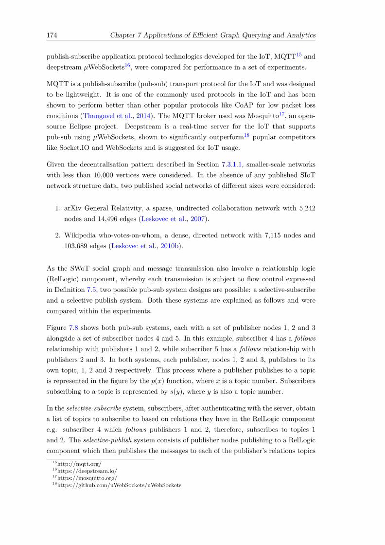
174 Chapter 7 Applications of Efficient Graph Querying and Analytics
publish-subscribe application protocol technologies developed for the IoT, MQTT15 anddeepstream µWebSockets16, were compared for performance in a set of experiments.
MQTT is a publish-subscribe (pub-sub) transport protocol for the IoT and was designedto be lightweight. It is one of the commonly used protocols in the IoT and has beenshown to perform better than other popular protocols like CoAP for low packet lossconditions (Thangavel et al., 2014). The MQTT broker used was Mosquitto17, an open-source Eclipse project. Deepstream is a real-time server for the IoT that supportspub-sub using µWebSockets, shown to significantly outperform18 popular competitorslike Socket.IO and WebSockets and is suggested for IoT usage.
Given the decentralisation pattern described in Section 7.3.1.1, smaller-scale networkswith less than 10,000 vertices were considered. In the absence of any published SIoTnetwork structure data, two published social networks of different sizes were considered:
1. arXiv General Relativity, a sparse, undirected collaboration network with 5,242nodes and 14,496 edges (Leskovec et al., 2007).
2. Wikipedia who-votes-on-whom, a dense, directed network with 7,115 nodes and103,689 edges (Leskovec et al., 2010b).
As the SWoT social graph and message transmission also involve a relationship logic(RelLogic) component, whereby each transmission is subject to flow control expressedin Definition 7.5, two possible pub-sub system designs are possible: a selective-subscribeand a selective-publish system. Both these systems are explained as follows and werecompared within the experiments.
Figure 7.8 shows both pub-sub systems, each with a set of publisher nodes 1, 2 and 3alongside a set of subscriber nodes 4 and 5. In this example, subscriber 4 has a followsrelationship with publishers 1 and 2, while subscriber 5 has a follows relationship withpublishers 2 and 3. In both systems, each publisher, nodes 1, 2 and 3, publishes to itsown topic, 1, 2 and 3 respectively. This process where a publisher publishes to a topicis represented in the figure by the p(x) function, where x is a topic number. Subscriberssubscribing to a topic is represented by s(y), where y is also a topic number.
In the selective-subscribe system, subscribers, after authenticating with the server, obtaina list of topics to subscribe to based on relations they have in the RelLogic componente.g. subscriber 4 which follows publishers 1 and 2, therefore, subscribes to topics 1and 2. The selective-publish system consists of publisher nodes publishing to a RelLogiccomponent which then publishes the messages to each of the publisher’s relations topics
15http://mqtt.org/16https://deepstream.io/17https://mosquitto.org/18https://github.com/uWebSockets/uWebSockets

Chapter 7 Applications of Efficient Graph Querying and Analytics 175
Figure 7.8: Selective-Subscribe and Selective-Publish Pub-Sub Systems
e.g. publisher 1 publishes a message to subscriber 4’s topic (as subscriber 4 is a follower),while publisher 2 publishes to subscriber 4 and 5’s topics (its followers). Each subscribersubscribes to its own corresponding topic e.g. subscriber 4 to topic 4. The end result forboth systems, in terms of message delivery, is the same. Subscriber 4 receives messagesfrom publishers 1 and 2, while subscriber 5 receives messages from publishers 2 and 3.
The experimental setup included a decentralised server and broker for the SWoT thatcontained the authentication and RelLogic components. This was hosted on a compactIntel Next Unit of Computing (NUC) platform with dimensions of 4 by 4 by 1.5 inchesand contained an i5 processor and 8GB RAM. Publisher and subscriber nodes were runon Raspberry Pi 2 Model B+s (RPi) with 1GB RAM, a 900MHz quad-core ARM Cortex-A7 CPU and Class 10 SD Cards. Ethernet connections were used between the RPi nodesand the server. Due to resource constraints, multiple publishers and subscribers had tobe run on the RPi devices as separate threads. Section 7.3.3.1 presents and discussesthe results of the experiments, while the design of the RelLogic component is improvedin Section 7.3.3.2 by using ideas from TritanDB’s ingestion pipeline.
7.3.3.1 Selective Publish-Subscribe Comparison
Figure 7.9 shows the results of the experiments where the vertical axis displays a log-arithmic scale of the average latency of receiving fixed size messages with a 32 bytepayload across all client nodes while the horizontal axis shows different periods of send-ing messages e.g. each node sends a message every 5 seconds.

176 Chapter 7 Applications of Efficient Graph Querying and Analytics
1 2 5 10100
101
102
Period of Sending Messages (s)
Averag
eLa
tenc
y(log 1
0ms)
DS-sub-wikiDS-pub-wikiDS-sub-aX
MQTT-sub-wikiMQTT-pub-wiki
DS-pub-aXMQTT-sub-aXMQTT-pub-aX
Protocol: DS = Deepstream µWebSockets, System: sub = Selective-Subscribe, pub = Selective-Publish,Network: wiki = Wikipedia (dense), aX = arXiv (sparse)
Figure 7.9: Comparison of Selective-Pub-Sub Systems by Average Latency of MessageTransmission
The results can be summarised as such:
• selective-publish performs better than selective-subscribe (has lower average la-tency from 1.2x to 4.2x) as the connection overhead of many subscribers on aclient causes delay and higher latency,
• MQTT performs better (from 2x to 49x) than deepstream µWebSockets with boththe sparse arXiv graphs and dense wiki graphs and
• as the period of sending messages increases, as expected, average latency decreases,however, both deepstream and MQTT have sub 50ms average latencies at rates ofup to 7,115 messages per second (about 427,000 messages in a minute).
7.3.3.2 Scaling Selective-Publish RelLogic
Although the comparison in the previous section showed that selective-publish systemsperformed better, they also required that the RelLogic component in Figure 7.8 was ableto handle the volume of messages published.
Hence, a high performance queue to process messages being published to RelLogic,lookup the relevant topics to forward to and connect and forward the MQTT messagesis required. Hence, three designs are compared. A RelLogic component that implementsthe disruptor pattern used in high-frequency trading and utilised in TritanDB’s ingestionpipeline (Section 5.3.1) is compared to a single threaded and a multi threaded queue.

Chapter 7 Applications of Efficient Graph Querying and Analytics 177
Experiments are performed at increasing velocities of messages per second, from 1,000to 10,000. Messages are addressed from a random node to the corresponding set ofsubscribers from both the arXiv and wikipedia networks. Each experiment is repeatedand averaged over 10 runs on the same server as with the previous benchmark. AJava LinkedBlockingQueue is used for the single-threaded implementation and a JavaConcurrentLinkedQueue and AtomicIntegers (for averaging latency) are used for themulti-threaded queue. Figure 7.10 visualises the 3 types of RelLogic queues tested.
Figure 7.10: Visualisation of the RelLogic Queue Implementations
Figure 7.11 shows the results of the wikipedia network (*.wiki) and arXiv (*.aX) networkbenchmarks of the disruptor (d.*), single threaded (1.*) and multi-threaded (10.*)queues. The performance of the disruptor selective-publish servers are from 12 to 800times faster (have a lower average latency) than the single-threaded queue servers andfrom 5.5 to 400 times better than the multi-threaded servers. Furthermore, as messagefrequency increased, average latency remained stable, displaying scalability to increasingmessage velocity.
7.3.3.3 Lightweight and Scalable Pub-Sub for the Decentralised SWoT
The experimental setup emphasised the use of compact platforms for decentralised de-ployments of the SWoT which display the lightweight nature of the selective-publishMQTT system, including the RelLogic Disruptor pattern. Even on the more densewikipedia network with more than 7,000 nodes and 100,000 edges, sub 10ms averagelatencies could be achieved. These results also show that smaller distributed networkscan be supported on fog computing resources like gateway routers and hubs.
Increasing the velocity of messages on both sparse and dense networks up to 10,000messages per second could also be handled without increasing the average latency withthe selective-publish RelLogic component using the Disruptor pattern. Increasing thenumber of edges about 7 times from sparse to dense networks, results in only a 2.5 timesincrease in average latency for RelLogic and a maximum of 3.8 times with the selective-publish system. Furthermore, performance can be further enhanced by deploying a

178 Chapter 7 Applications of Efficient Graph Querying and Analytics
0.1 0.2 0.3 0.4 0.5 0.6 0.7 0.8 0.9 1·104
101
102
103
104
Message Frequency (s−1)
Averag
eLa
tenc
y(log 1
0ms)
1.wiki10.wiki1.aX10.aXd.wikid.aX
Queue: 1 = Single-threaded, 10 = Multi-threaded, d = Disruptor, Network: wiki = Wikipedia, aX = arXiv
Figure 7.11: Comparison of Single-threaded, Multi-threaded Queues and DisruptorPattern RelLogic Servers
Hubber Component TechnologyBroker Selective-Publish MQTTRelLogic Disruptor PatternPIOTRe Map-Match-Operate TritanDBAuth OAuth 2.0GraphDB Neo4j, W3C Things DescriptionForeign Relations Internationalised Resource Identifiers (IRIs)
Table 7.2: Technologies used in Hubber.space
load balancer and bridge or replicating across multiple MQTT brokers to build a high-availability cluster. The experiment source code is available in an online repository19.
7.3.4 Hubber.space: An Experimental SWoT
Hubber.space20 is an experimental sandbox application developed to realise the corefunctions of the SWoT, integrating the selective-publish MQTT broker and RelLogiccomponents in a server, with a data management layer using Map-Match-Operate tostore data on nodes. Figure 7.12 shows a component diagram of a decentralised Hubberserver, while Table 7.2 shows the technologies employed in each component.
Each decentralised Hubber server contains a selective-publish MQTT broker and a Rel-Logic component implemented using the disruptor pattern to handle messages, m. TheSWoT social network is managed as a graph stored within a graph database like Neo4j(Robinson et al., 2015) and each vertex is described by a W3C Things Description21
19https://github.com/eugenesiow/hubber-bench-js20http://hubber.space21https://w3c.github.io/wot/current-practices/wot-practices.html#thing-description

Chapter 7 Applications of Efficient Graph Querying and Analytics 179
H ubber Ser ver
RelLogic Disruptor
Broker
Authent icat ion
PIOTRe Publisher
PIOTRe Publisher
PIOTRe Subscriber
Pub m
Sub m
Informat ion Flow
Server Apps
Store API
Network Management
Graph DatabaseOther
Hubber Server
ForeignRelat ion
Figure 7.12: Component Diagram of a Hubber Server and PIOTRe Nodes
Figure 7.13: Screenshot of the Hubber.space Landing Page
for interoperability. Foreign relations can be retrieved from other Hubber servers byaccessing their IRIs. The information flow components sit behind an OAuth 2.0 au-thorisation barrier22. Apps can be downloaded by nodes from the server App Store.Apps on nodes can also interact with app code running on the server through an API.Nodes can run PIOTRe (Section 7.1) which allows the subscribed messages that includesensor observations and events from the social network to be stored as time-series witha Map-Match-Operate TritanDB engine.
Figure 7.13 shows a screenshot of a decentralised Hubber.space app. The purpose ofthis deployment was as a seed for users, vendors, developers and machines to co-createthe SWoT and start utilising PIOTRe on personal repositories for their IoT data.
22https://oauth.net/2/

180 Chapter 7 Applications of Efficient Graph Querying and Analytics
7.4 Conclusions
This chapter introduced PIOTRe, an application for managing personal IoT repositorydata and applications, and the SWoT which builds a social network on PIOTRe reposi-tories and other Things through a social capital inspired design. Features like resamplingand moving averages that allow TritanDB to perform time-series analytics like predictiveforecasting were also introduced. Map-Match-Operate for historical and streaming datamanagement and processing promises greater interoperability and efficiency for the IoT.These applications and platforms go towards promoting adoption and providing a basisto build useful applications which add value to the current and future IoT. Each of theseapplications was designed and tested on resource-constrained fog computing hardwarebut also scaled to work in cloud environments, by virtue of TritanDB and S2S, providingbetter performance and enabling them to handle larger volumes of data.

Chapter 8
Conclusions
“We can only see a short distance ahead, but we can see plenty there thatneeds to be done.”
— Alan Turing
This chapter presents a summary and a recap of the contributions of this thesis in Section8.1. Limitations and opportunities for future work are also discussed in Sections 8.2 and8.3 before final conclusions are made in Section 8.4.
8.1 Summary
This thesis started by asking the question of how database systems can support theefficient and semantically interoperable storage and retrieval of Internet of Things (IoT)data and metadata, both historical and real-time, for use in analytical applications.The direction taken was to bring together the unique characteristics and requirementsof IoT time-series data, established through a series of studies, with an understandingof database and stream processing system design and innovations. The methodologyemployed throughout was to investigate the state-of-the-art and improve it for the IoTthrough formal theoretical definition, then practical implementation and finally experi-mental comparison using well-defined benchmarks, datasets and scenarios.
Chapter 2, a study of background literature of the IoT and database systems, establishedthe need for niche database and stream processing systems within the processing layerof the IoT to support applications and analytics across diverse hardware. The chaptercontributed an overall understanding of the IoT landscape divided by applications, plat-forms and building blocks, from an analysis of survey literature, before focusing on moredetailed studies of specific building blocks and technologies like time-series databases,
181

182 Chapter 8 Conclusions
Resource Description Framework (RDF) graph databases, stream processing, fog com-puting and analytics within IoT applications.
An analysis of public IoT time-series data across application domains in Chapter 3showed that a large proportion of schemata exhibited the unique characteristics of beingflat, wide and numerical. It was also established that both periodic or approximatelyperiodic and non-periodic time-series data were present in streams. These characteristicsaffect the efficient storage and retrieval of data. In addition, the chapter also contributeda study of metadata models for the IoT showing a diversity taken in approaches to modelheterogeneous data from different domains. Standards bodies and research initiativesthough, converged on approaches that could be generalised to a graph or tree represen-tation for metadata. However, a follow-up study of metadata and data ratios in graphmodel IoT data of the Resource Description Framework (RDF) format highlighted theissue of metadata expansion, resulting in inflated data sizes. Efficiency and compactnesswas traded-off for interoperability and flexibility.
Building on the understanding of the characteristics of IoT time-series data and moti-vated by the inefficiency of graph model RDF for IoT data, a method for query trans-lation called Map-Match-Operate that abstracted graph queries to be executed acrossgraph model metadata from the data representation of time-series data was devisedin Chapter 4. The implementation of this method across RDF graph metadata andtime-series data in relational databases showed from two to three orders of magnitudeperformance improvements, comparatively better aggregation support and fewer joinswhen compared against a range of databases and translation engines.
The physical interface for storing and retrieving time-series data from hardware is one-dimensional while relational databases present a conceptual two-dimensional interface.Hence, this discrepancy between physical and conceptual representations was identifiedas an area of further performance optimisation. A new compressed, time-reordering,performance-optimised data structure for the storage of IoT time-series data, TrTa-bles, was proposed in Chapter 5 as a result of an evaluation of time-series databasecompression algorithms and storage structures. A Map-Match-Operate database sys-tem, TritanDB, was implemented to use TrTables and performed better in storage andprocessing experiments compared against a range of time-series, relational and NoSQLdatabases on both cloud and Thing hardware.
Chapter 6 investigated stream processing systems and implemented Map-Match-Operateto efficiently translate graph queries for continuous execution on real-time streams ofIoT data. Map-Match-Operate for streams was then integrated with a fog computinginfrastructure for distributed stream processing, Eywa. Eywa introduced a novel inversepublish-subscribe approach to distribute queries within the control plane and employedpredicate pushdown in the data plane, of the projection operator, to distribute theworkload among co-operative fog computing nodes.

Chapter 8 Conclusions 183
Finally, Chapter 7 described applications built on Map-Match-Operate’s performantand interoperable IoT storage and querying. This included a demonstration of bothstreaming and historical smart home application dashboards running on PIOTRe, apersonal repository for IoT data, deployed on a compact Raspberry Pi device. A socialcapital theory inspired Social Web of Things application, that provided social networkfunctions to manage the information flow between PIOTRe instances and other Things,was also introduced. Features like resampling and moving averages that allow TritanDBto perform time-series analytics like predictive forecasting were also discussed.
Thus, the contributions presented in this thesis, from identifying that IoT data has a setof unique characteristics, to using these characteristics to improve the performance ofgraph queries on databases and streams, represent an advance in the state-of-the-art forthe efficient storage and retrieval of a semantically interoperable representation of IoTdata and metadata for analytical applications. Despite these advances, however, certainlimitations exist, while more opportunities have also emerged. The next two sectionssuggest a number of promising directions for future research.
8.2 Limitations and Future Work
This thesis focused on an understanding of current time-series IoT data characteristics,a particular graph model for databases and stream processing systems, RDF, wheremost processing is done on a single node whether in cloud or cooperative fog computingscenarios on distributed, resource-constrained fog nodes. This section recognises somelimitations in the solutions proposed and suggests extensions and future work.
8.2.1 Multimodal Data
Although a large proportion of current IoT data from sensors conformed to flat, wideand numerical characteristics of time-series, there is a case for providing for a variety offorms of multimodal data in future. Increasingly, images, sounds and unstructured textdata might become inputs to the IoT and the storage, integration and processing of suchdata will gain more importance. More complex hierarchical schemata might also becomemore common. Research in compression and storage structures can be combined withtechniques for extracting feature sets and the machine-understanding of such data.
8.2.2 Other Graph/Tree Models and RDF Property Paths
RDF is considered as the example of a graph data model in this thesis due to thepresence of a large body of research work, data availability and its application withinthe IoT. JSON, however, is increasingly becoming the data-interchange format of choice

184 Chapter 8 Conclusions
within the IoT and semantic interoperability discussions within groups like the InternetEngineering Task Force (IETF) are centred around data models that utilise annotationslike JSON Schema1. Hence, a future direction for work is to extend (or limit, since thetree is a limited form of a graph) Map-Match-Operate to work on JSON-based models.
Another limitation of Map-Match-Operate in this thesis is that path queries2, queriesthat specify a chain of predicates and predicate cardinality (arbitrary number of hops),across tiers are not supported at the moment. There is an established theoretical basis forsuch queries both in SPARQL (Kostylev et al., 2015) and in other graph databases (Reut-ter, 2013), however, the feasibility of query translation across the model and databasetiers is an area of future research.
8.2.3 Horizontal Scalability with Distributed Databases
Horizontal scalability allows a database system to increase capacity by connecting to-gether multiple instances across hardware entities so that the system works as a singlelogical unit. Many of the NoSQL databases compared against TritanDB like Cassandraand OpenTSDB support horizontal scalability to handle larger volumes of data. Hence,an area for future research includes investigating the feasibility of partitioning time-series data across instances to extend TritanDB for horizontal scalability in the cloud oracross fog computing networks with both cooperative and uncooperative nodes.
8.3 Opportunities and Future Work
This section recognises some opportunities for future work that open up due to thecontributions of this thesis.
8.3.1 Eywa Fog Computing Operators
Eywa formally defined an infrastructure for stream query delivery to source nodes, dis-tributed processing and results delivery to the client nodes in Section 6.2. Since Eywaprovides a means of distributing queries and performing workload coordination in thecontrol plane of a fog network, it opens up the opportunity for research on how variousworkload operators, besides projections, can be processed in the data plane between thesource and client nodes. Query optimisation in the absence of accurate statistics at theclient nodes (an issue also experienced in Federated SPARQL, described in Section 2.2.4)and the appropriate division of resources at source nodes are challenges to consider inthis future work on operator distribution.
1http://json-schema.org/2https://www.w3.org/TR/sparql11-query/#propertypath-syntaxforms

Chapter 8 Conclusions 185
8.3.2 Social Web of Things Knowledge Graph
A knowledge graph that contains entities and relations within the Social Web of Things(SWoT) introduced in Section 7.3 can be formed by integrating mappings of Thingmetadata provided as S2SML (Section 4.2.1.1) for Map-Match-Operate. This opens upan area of future work for research on and applications utilising the integrated SWoTknowledge graph.
8.4 Final Remarks and Conclusions
The IoT has huge potential to provide advanced services and applications across manydomains and the momentum that it has generated, together with its broad visions,make it an ideal ground for pushing technological innovation and generating value forthe society, economy and environment. Data management and processing that supportsdescriptive, diagnostic, discovery, predictive and prescriptive analytical capabilities willcontribute to the growth of the IoT as various stakeholders seek solutions to the problemsposed by growing volumes and velocities of information.
This thesis considered the requirements of performance and interoperability when han-dling the increasing amount of streaming data from the IoT, with an understandingof the unique characteristics of IoT time-series data, while building on advances inRDF graph databases, query translation and time-series databases for telemetry data.The methods and novel designs proposed, Map-Match-Operate, TritanDB and Eywa, allshowed improvements in storage and query performance, and scalability when comparedwith state-of-the-art database and stream processing systems. The results also showedthat there is no need to compromise interoperability or performance when using thesetechnologies for the specific use case of IoT time-series data. There was also a focus onbenchmarking performance on resource-constrained hardware serving as fog computingnodes in IoT scenarios - base stations, hubs, gateways and routers. In particular, streamprocessing was shown to be a performant option for analytical querying on resource-constrained nodes, and the performance was further improved by workload distributionwithin a cooperative fog computing network.
Apart from these, the thesis also looked beyond the immediate performance and interop-erability of the solutions proposed, showing how the solutions could lead to applicationsand platforms in different directions: personal dashboards and repositories, time-seriesanalytics and a Social Web of Things.
Each of the smart home, smart factory and smart city scenarios, presented in the intro-duction to this thesis, seeks to benefit people by enhancing their daily experiences andoptimising the machines and systems that deliver services to them. The work in thisthesis is ultimately an endeavour in that direction.


Appendix A
Survey of IoT Applications
Table 2.2 in Chapter 2 summarises 32 IoT application papers by application domainor theme and states the respective techniques used to derive insights and the currencyof their data, whether real-time streaming data was used or historical data stored ina database was utilised. More detailed descriptions of the papers are provided in thisappendix as follows.
A.1 Health: Ambient Assisted Living, Medical Diagnosisand Prognosis
Mukherjee et al. (2012) surveyed the use of data analytics in healthcare informationsystems. One area in healthcare where analytics had been applied to was AmbientAssisted Living (Dohr et al., 2010). The solution proposed in the application appliedrules to IoT data collected from smart objects in the homes of elderly or chronic diseasepatients while also considering contextual information and applying inferencing usingontologies to give health advisories to users, update care-givers or contact the hospitalin emergencies. In their work, Henson et al. (2012) used abductive logic, ‘inference tothe best explanation’, to provide an intelligent diagnosis for a given set of symptoms.Rodríguez-González et al. (2012), for a similar use case, used descriptive logic combinedwith knowledge from an ontology to provide their medical diagnosis with inputs frommultiple IoT agents. Hunink et al. (2014) went a step further in providing prognosis,the science of predicting the future medical condition of a patient, to help doctors andmedical staff make more informed decisions by analysing certain key health indicatorsof patients, comparing these with records from similar patients and combining this withdomain knowledge and medical research to make conjectures about potential medicalconditions.
187

188 Appendix A Survey of IoT Applications
IoT agents like wearables collect a large volume of high dimensional health data. Li et al.(2013) applied the Random Forests algorithm, a data mining technique for predictingclasses or dependent variables from high dimensional data (125 risk factors for healthexpenditure), to health data to provide the input for a healthcare costing model.
A.2 Industry: Product Management and Supply ChainManagement
Vargheese and Dahir (2014) proposed a system that improved shoppers’ experience byenhancing the ‘On the Shelf Availability (OSA)’ of products. Furthermore, the systemalso looked at forecasting demand and providing insights on buyers’ behaviour. IoTsensors captured imagery of inventory and these video streams were analysed and cross-verified with other light, infra-red and RFID sensors. This real time data was combinedwith models from learning systems, data from enterprise Point of Sale (POS) systemsand inventory systems to recommend action plans to maintain the OSA of products.The staff of the store were informed and action was taken to restock products. Weatherdata, local events and promotion details were also analysed with the current OSA andprovided demand forecasting and modelled buyers behaviour which was fed back intothe system.
Nechifor et al. (2014) described the use of real-time data analytics in their cold chainmonitoring process. Trucks which were used for transporting perishable goods and drugsrequired particular thermal and humidity conditions. Sensors measured the positionand conditions in the truck and of each package while actuators - air conditioning andventilation were controlled automatically to maintain these conditions. On a larger scale,predictions were made on delays in routes and when necessary to satisfy the productcondition needs, longer but faster routes with less congestion were selected.
Similarly, Verdouw et al. (2013) examined supply chains - the integrated, physical flowfrom raw material to end products with a shared objective, and formulated a frame-work based on their virtualisation in the IoT. These virtual supply chain for the Dutchfloricultural sector supported intelligent analysis and reporting. Early warning signalscould be sent in case of disruptions or unexpected deviations in the supply chain. Inthis example and the previous example, Complex Event Processing systems were usedto process, analyse and act on the real-time data stream.
Robak et al. (2013) also looked at supply chain management from the perspective of aFourth-party logistics provider (4PL) that acts as an integrator of resources and tech-nologies to build supply chains. The tracking data gathered by the the 4PL was usedto describe what was happening along the transport routes and when combined withinformation from social media and weather reports, helped users to forecast order andtransport volumes, diagnose delays and optimise transport plans.

Appendix A Survey of IoT Applications 189
Engel and Etzion (2011) applied a Markov decision process (MDP) (Bellman, 1957) toan event processing network for supply chain planning and optimisation, to deliver acritical shipment in time, avoiding penalties and handling delays.
A.3 Environment: Disaster Warning, Wind Forecastingand Smart Energy Systems
This combination of sensor and social media data was applied to a haze detection scenarioby Yue et al. (2014) in their work that used data mining techniques to detect spikes insocial media volume on the haze and processes and combined it with IoT sensor data toprovide geospatial haze observations.
Schnizler et al. (2014) described a disaster detection system that worked on heteroge-nous streams of IoT sensor data. Their method involved Intelligent Sensor Agents(ISAs) that detected anomalies, low level events with location and time information,for example, an abnormal change in mobile phone connections at a ISA in a telecomcell or base station, a sudden decrease in traffic, increase in twitter messages, changein water level or change in the volume of moving objects at a certain location. Theseanomaly events then entered Round Table (RT) components that fused heterogenoussources together by mapping them to a common incident ontology through feedbackloops that involve dcrowdsourcing, human-in-the-loop or adjusting parameters of otherISAs to find matches. The now homogenous incident stream was then be processed bya Complex Event Processing (CEP) engine to complete the situation reconstruction bydoing aggregation and clustering with higher-level semantic data, simulation and predic-tion of outcomes and damage. The resultant incident stream was then used to provideearly warning and detection of disaster situations as well as providing better situationalawareness for emergency response and relief teams.
Another environmental application was wind forecasting (Mukherjee et al., 2013). Datawas collected from wind speed sensors in wind turbines and an Artificial Neural Network(ANN) was used on this historical data over time to perform wind speed forecasting.
Ghosh et al. (2013) implemented a localised smart energy system that used smart plugsand data analysis to actively monitor energy policy and by performing pattern recogni-tion analysis on accumulated data, additional opportunities to save energy were spotted.This resulted in saving on electricity bills especially by reducing the amount of powerwasted in non-office hours from appliances.
Similar work by Alonso et al. (2013) worked on using machine learning and an rule-basedexpert system to provide personalised recommendations, based on energy usage datacollected in Smart Homes, that helped a user to more efficiently utilise energy. Theywent one step further in also providing recommendations through predicting cheaper

190 Appendix A Survey of IoT Applications
options by detecting similar patterns in big data collected from a large set of homes.Ahmed (2014) also applied similar analysis on combined consumption data for use inorganisations to help in energy policy planning. The model developed helped to classifythe energy efficiency of buildings and the seasonal shifts in this classification. By alsousing more detailed appliance specific data, the model was able to forecast future energyusage.
A.4 Living: Public Safety and Security, Lifestyle Monitor-ing, and Memory Augmentation
On the issue of public safety and security, McCue (2006), gave examples of how datamining of crime incident data, including spatial-temporal information collected fromsensors helped the police to device a targeted deployment strategy which increased therecovery of illegal weapons and decreased incidents of random gunfire while reducingthe total number of officers that needed to be deployed. Using visualisation, possiblyhostile surveillance activity was detected around a facility and it was noticed that therewas a spatial-temporal specificity to it, surveillance was done on a specific day of theweek and around a particular part of the building (McCue, 2005).
Visualisation that taps the human cognitive ability to recognise patterns was also em-ployed by Razip et al. (2014) in helping law enforcement officers to have increased sit-uational awareness. Officers were equipped with mobile devices that tapped into crimedata and spatial and temporal sensor data to show interactive alerts of hotspots, riskprofiles and on demand chemical plume models.
Additionally, there were also public safety and military applications that apply videoanalytics in detecting movement, intruders or targets. The public safety use case waselaborated on by Gimenez et al. (2012) where they discuss how given the big dataproblem of having huge amounts of video footage, smart video analytics systems canproactively monitor, automatically recognise and bring to notice situations, flag outsuspicious people, trigger alarms and lock down facilities through the recognition ofpatterns and directional motion, recognising faces and spotting potential problems bytracking, with multiple cameras, how people move in crowded scenes.
Guo et al. (2011) looked at discovering various insights from mining the digital tracesleft by IoT data from cameras to wearables, to mobile phones and smart appliances. Theresulting life logging application helped to augment human memory with recorded data,real world search for objects and interactions with people. The system was also used toimprove urban mobility systems by studying large-scale human mobility patterns.

Appendix A Survey of IoT Applications 191
Mukherjee and Chatterjee (2014) presented an application of a fast algorithm for de-tecting anomalies and for classifying high dimensional data to recognise human activityin real-time and classify activities from sensor data to provide a lifestyle monitor.
The application of analytics to predict civil unrest was shown to be effective in thework by Ramakrishnan et al. (2014) where multiple models (5 different models thatinclude looking at volume, detecting planned protests, using dynamic query expansionto flexibly detect causes and motivations, checking to see if activity cascades through thespread of targeted campaigns to recruit protestors and a baseline model that looks atthe likelihood of events occurring based on recent events) were used on a wide range ofheterogenous data sources including sensor data to provide robust predictions of futureevents through corroboration between models. This can also be applied to IoT dataincluding mobile device information, smart appliance and voice controlled device searchdata, video data and spatial data of crowds, vehicles and security forces to detect civilunrest.
A.5 Smart City: Parking and Big Data Grid Optimisation
Zheng et al. (2014) applied temporal clustering and anomaly detection to IoT parkingdata in San Francisco to discover extreme car parking behaviour and characterise normalbehaviour that helped parking managers to device suitable parking strategies. This typeof analysis that helps discover information can be fed back into smart parking systemsto optimise the use of limited space in cities. Data mining techniques including a naiveBayes model and a logistic regression model were also applied by He et al. (2014) onsensor data to find suitable car parking spaces in real-time within a smart city scenario.
Strohbach et al. (2015) described a real-time grid monitoring system within a pilot smartcity that utilised stream processing with Complex Event Processing (CEP) technologyto provide power quality and consumption analysis from a stream of about 360,000 newmeasurements every second. A forecasting model that balanced the grid not only byadapting the production of energy but also by adapting the consumption through thedistributed use of smart meters within smart homes was proposed.
A.6 Smart Transportation: Traffic Control and Routing
Liu et al. (2013) looked at the latest technologies and applications of video analytics andintelligent video systems. The traffic control system described by Mak and Fan (2006)successfully applied video analytics to detecting traffic volume for planning, highlightingincidents and punishing offenders of traffic rules for enhanced safety. Another set of

192 Appendix A Survey of IoT Applications
applications was for intelligent vehicles to do in-lane, pedestrian and traffic sign detectionthat assists the driver.
Work on Intelligent Transport Systems in Dublin city by Liebig et al. (2014) also in-cluded prescribing good routes in travel planning using analytical techniques, like aspatiotemporal random field based on conditional random fields research (Pereira et al.,2001), for traffic flow prediction and a gaussian process model to fill in missing valuesin traffic data, to predict the future traffic flow based on historical sensor data and toestimate traffic flow in areas with limited sensor coverage. These were then used toprovide the cost function for the A* search algorithm (Hart et al., 1968) that uses thecombination of a search heuristic and cost function to prescribe optimal routes providedthe heuristic is admissible and the predicted costs are accurate.
Wang and Cao (2014) also did work on traffic congestion prediction and prescription tooptimise traffic flow through a decision-making component. They used a multilayeredadaptive dynamic bayesian network (Zhu et al., 2013) to model and predict traffic eventsand a Markov decision process (MDP) (Bellman, 1957) method to make optimal deci-sions within the bounds of some uncertainty and some time frame. This was simulatedon traffic in Beijing city to show that in a cooperative traffic scenario, which is possiblein the context of smart transportation systems, it would reduce congestion.
A.7 Smart Buildings and Smart Homes
Ploennigs et al. (2014) showed how analytics when applied to energy monitoring couldhelp adapt heating for smart buildings. The system was able to diagnose anomalies in thebuilding temperature, for example, break downs of the cooling system, high occupancyof rooms, or open windows causing air exchange with the external surroundings. Usinga semantics-based approach, the system could also automatically derive diagnosis rulesfrom sensor network definitions, metadata and behaviour of specific buildings, makingit sensitive to new anomalies.
Makonin et al. (2013) described how a rule-based system used in a smart home couldhelp to conserve energy and improve the quality of living through adaptive lighting andadaptive heating. Weiss et al. (2012) similarly leveraged smart meter data in smarthomes to raise energy awareness and provide feedback on energy consumption withoutthe need for specialised hardware. This was achieved in their application by developinga signature detection algorithm to identify home appliances by analysing smart meterpatterns.

Appendix B
The Smart Home AnalyticsBenchmark
The aim of the Smart Home Analytics Benchmark was to provide a dataset from thesmart home application domain containing an integrated graph of rich metadata anddata. The graph is realised as a Resource Description Framework (RDF) graph and theschema designed to integrate the data was based on a reference Internet of Things (IoT)ontology, the Semantic Sensor Network (SSN) ontology1. A related set of analyticalqueries on the graph model that power an application dashboard for visualising smarthome data was also devised and form a performance benchmark for graph queries.
The data from smart home sensors was collected by Barker et al. (2012) over 4 monthsfrom April to July in 2012. There were a variety of data observations from environmentalsensors, motion sensors in each room and energy meters within a smart home. There were26,192 environment sensor readings with 13 attributes, 748,881 energy meter readingsfrom 53 meters and 232,073 motion sensor readings from 6 rooms.
Sensor metadata, observation metadata and observation data from sensor and meterreadings were integrated as an RDF graph utilising a schema that references the SSNontology. This publicly available schema2 represents a weather observation from anenvironmental sensor as shown in Figure B.1. Energy meters produce observationsrepresented by the graph structure in Figure B.2, which were observed by a metermeasuring energy usage of a refrigerator in the kitchen described in Figure B.3. Finally,Figure B.4 shows the graph structure of an observation from the motion sensor in theliving room.
A set of analytical queries was designed for an application dashboard to allow the mon-itoring of the smart home environment, visualise trends and detect possible anomalies
1http://purl.oclc.org/NET/ssnx/ssn2http://purl.org/net/iot
193

194 Appendix B The Smart Home Analytics Benchmark
sh:WeatherObs1 sh:T ime1
sh:Environmental1
sh:WeatherOut1
sh:InternalTemp1
hasValue
observat ionResult
isProducedByobservedBy
observat ionSamplingTime
"2012-01-10 12:00:00"
inXSDDateTime
sh:ExternalTemp1
"30.5"
hasQuant ityValue
"20.2"
hasQuant ityValue
Figure B.1: The Structure of a Weather Observation from the Environmental1 Sensor
sh:EnergyObservat ion2 sh:T ime2
sh:MeterKitchen2
sh:EnergySensorOut2
sh:EnergyValue2
hasValue
observat ionResult
isProducedByobservedBy
observat ionSamplingTime
"2012-01-10 13:00:00"
inXSDDateTime
"1.5"hasQuant ityValue
Figure B.2: The Structure of an Energy Observation from the Refrigerator Meter
sh:MeterKitchen2 ssn:SensingDevice
sh:KitchenSensors
"K itchen Refrigerator" label
onPlat form
a
ssn:Plat forma
Figure B.3: The Structure of Metadata from the Refrigerator Meter in the Kitchen
over time. Each query requires space-time aggregations on the time-series of observa-tions. The set of queries forms a non-synthetic benchmark using real-world data underan analytical application workload. The set of four graph queries are as follows:
1. the hourly aggregation of internal or external temperature,
2. the daily aggregation of temperature,
3. the hourly, room-based aggregation of energy usage and
4. the diagnosis of unattended energy usage comparing motion detectors and energymeters to determine energy usage in rooms with no activity, aggregating by hourand room.

Appendix B The Smart Home Analytics Benchmark 195
sh:Mot ionObservat ion3 sh:T ime3
sh:Mot ionLiving3
sh:Mot ionSensorOut3
sh:Mot ionValue3
hasValue
observat ionResult
isProducedByobservedBy
observat ionSamplingTime
"2012-01-10 14:00:00"
inXSDDateTime
"t rue"hasQuant ityValue
Figure B.4: The Structure of a Motion Observation from the Living Room Sensor
The actual query syntax for each query expressed in SPARQL 1.1, a query language forRDF graphs, is as follows in Listings B.1, B.2, B.3 and B.4.
1 PREFIX ssn: <http :// purl.oclc.org/NET/ssnx/ssn#>2 PREFIX xsd: <http :// www.w3.org /2001/ XMLSchema #>3 PREFIX time: <http :// www.w3.org /2006/ time#>4 PREFIX sh: <http :// iot.soton.ac.uk/ smarthome / sensor #>5 PREFIX iot: <http :// purl.oclc.org/NET/iot#>6
7 SELECT (avg (? val) as ?sval) ?hours WHERE 8 ? instant time: inXSDDateTime ?date.9 ?obs ssn: observationSamplingTime ? instant ;
10 ssn: observedBy sh: environmental1 ;11 ssn: observationResult ?snout.12 ?snout ssn: hasValue ? obsval .13 ? obsval a iot : type;14 iot: hasQuantityValue ?val.15 FILTER (? date > " start "^^ xsd: dateTime && ?date <= " end "^^ xsd: dateTime )16 GROUP BY (hours(xsd: dateTime (? date)) as ?hours)
Listing B.1: Query 1: Hourly Environmental Observation of Varying Type
1 ...2 SELECT (max (? val) as ?max) (min (? val) as ?min) ?day WHERE 3 ? instant time: inXSDDateTime ?date.4 ?obs <<ssn: observationSamplingTime ? instant ;5 ssn: observedBy sh: environmental1 ;6 ssn: observationResult ?snout.7 ?snout ssn: hasValue ? obsval .8 ? obsval a iot : type;9 iot: hasQuantityValue ?val.
10 FILTER (? date > "2012 - month -01 T00 :00:00"^^ xsd: dateTime &&11 ?date < "2012 - month -30 T00 :00:00"^^ xsd: dateTime )12 GROUP BY (day(xsd: dateTime (? date)) as ?day)
Listing B.2: Query 2: Daily Environmental Observations over a Month
1 ...2 SELECT ? platform ? dateOnly (sum (? power) as ? totalpower ) WHERE 3 SELECT ? platform ?hours ? dateOnly (avg (? meterval ) as ?power) WHERE 4 ?meter ssn: onPlatform ? platform .5 ? meterobs ssn: observedBy ?meter.6 ? meterobs ssn: observationSamplingTime ? meterinstant ;7 ssn: observationResult ? metersnout .

196 Appendix B The Smart Home Analytics Benchmark
8 ? meterinstant time: inXSDDateTime ? meterdate .9 ? metersnout ssn: hasValue ? meterobsval .
10 ? meterobsval a iot: EnergyValue .11 ? meterobsval iot: hasQuantityValue ? meterval .12 FILTER (? meterval > 0)13 FILTER (? meterdate > " startDate "^^ xsd: dateTime14 && ? meterdate < " endDate "^^ xsd: dateTime )15 GROUP BY ? platform ?meter (hours (? meterdate ) as ?hours)16 (xsd:date (? meterdate ) as ? dateOnly )17 GROUP BY ? platform ? dateOnly
Listing B.3: Query 3: Hourly, Room-based (Platform) Energy Usage
1 ...2 SELECT ? motiondate ? motionhours ? motionplatform ?power ?meter ?name WHERE 3 SELECT (? platform as ? meterplatform ) (? hours as ? meterhours )4 (? dateOnly as ? meterdate ) (avg (? meterval ) as ?power) ?meter5 ( sample (? label) as ?name) WHERE 6 ?meter rdfs:label ?label.7 ?meter ssn: onPlatform ? platform .8 ? meterobs ssn: observedBy ?meter.9 ? meterobs ssn: observationSamplingTime ? meterinstant ;
10 ssn: observationResult ? metersnout .11 ? meterinstant time: inXSDDateTime ?date.12 ? metersnout ssn: hasValue ? meterobsval .13 ? meterobsval a iot: EnergyValue .14 ? meterobsval iot: hasQuantityValue ? meterval .15 FILTER (? meterval > 0)16 FILTER (? date > " startDate "^^ xsd: dateTime &&17 ?date < " endDate "^^ xsd: dateTime )18 GROUP BY ? platform (hours (? date) as ?hours)19 (xsd:date (? date) as ? dateOnly ) ?meter 20 SELECT (? platform as ? motionplatform ) (? hours as ? motionhours )21 (? dateOnly as ? motiondate ) WHERE 22 ? obsval a iot: MotionValue ;23 iot: hasQuantityValue false.24 ?snout ssn: hasValue ? obsval .25 ?obs ssn: observationSamplingTime ? instant ;26 ssn: observationResult ?snout.27 ? instant time: inXSDDateTime ?date.28 ?obs ssn: observedBy ? sensor .29 ? sensor ssn: onPlatform ? platform .30 FILTER (? date > " startDate "^^ xsd: dateTime &&31 ?date < " endDate "^^ xsd: dateTime )32 GROUP BY ? platform (hours (? date) as ?hours)33 (xsd:date (? date) as ? dateOnly ) 34 FILTER (? motionplatform = ? meterplatform && ? motionhours = ? meterhours35 && ? motiondate = ? meterdate )36
Listing B.4: Query 4: Device Energy Usage in Rooms with No Activity by Hour
The source code of queries, application dashboard and data integration components areavailable on an open repository3.
3https://github.com/eugenesiow/ldanalytics-PiSmartHome

Appendix C
Operate Query Translation
In this appendix, the detailed mapping of query translation vocabulary in the Oper-ate step from the Map-Match-Operate abstraction is presented for completeness. Theappendix is divided into three sections, Section C.1 elaborates on the translation ofSPARQL Algebra from an input graph query to SQL, Section C.2 elaborates on transla-tion to TritanDB operators and Section C.3 on translation to EPL for stream processing.
The set of possible SPARQL algebra operators, obtained from the parsing of an inputSPARQL graph query, forms the input that is common across each section. Propertypath operations, which are not supported, are excluded from this set of algebra. Thelist of SPARQL algebra operators is obtained from the ‘Translation to SPARQL algebra’section in the SPARQL 1.1 specification1.
C.1 SPARQL Algebra to SQL
The translation from SPARQL algebra operators to SQL in this section uses the BackusNormal Form (BNF) notation description of the SQL-2003 standard by Savage (2017a)and when there are ambiguities, adopts the specific open source H2 database SQL gram-mar2. Table C.1 shows the input parameters, binding output from the Bmap and corre-sponding SQL listing reference for each SPARQL algebra operator expanding on Table4.4. The translation of each SPARQL algebra operator is elaborated on using the BNFnotation presented in Listings C.1 to C.11. Each listing highlights the input parametersand binding output from Bmap in the context of the translated SQL clauses and syntax.For example, in Listing C.8 for the ‘OrderBy’ solution modifier, the SQL ‘order by
clause’ is represented in BNF notation (SQL-2003 BNF Section 14.1). The input to‘OrderBy’ is a variable, ‘var’, that specifies the result column to order by and whetherto sort in ascending or descending order, specified by ‘order’. The binding output from
1https://www.w3.org/TR/sparql11-query/#sparqlQuery2http://www.h2database.com/html/grammar.html
197

198 Appendix C Operate Query Translation
SPARQL Algebra Input Binding Output ListingGraph Pattern
BGP, G [triple pattern] [binding.col], [binding.table] -Join, ./ [join_condition] [binding.col], [binding.table] C.1LeftJoin, n [join_condition] [binding.col], [binding.table] C.2Filter, σ [var, predicate] [binding.col], [binding.table] C.3Union, ∪ query_term - C.4Graph graph map -Extend, ρ [var, expr], [alias] [binding.col], [binding.table] C.5Minus query_term - C.6Group/Aggr, γ [var], [func] [binding.col], [binding.table] C.7
Solution ModifiersOrderBy var, order binding.col, binding.table C.8Project, Π [var] [binding.col], [binding.table] C.9Distinct, σD - - C.10Reduced σR - - C.10Slice, σS offset, fetch - C.11
Table C.1: Summary of SPARQL Algebra to SQL with Listing References
the match step gives the ‘binding.col’ value from Bmap, which corresponds to ‘var’
and this is used in ‘sort spec’ as shown in the listing.
<joined table > ::= <cross join > | <qualified join > | <natural join > | <union join ><qualified join > ::= <binding .table > [ <join type > ]
JOIN <binding .table > <join spec ><join spec > ::= <join condition > | <named columns join ><join condition > ::= ON <search condition ><named columns join > ::= USING <left paren > <join column list > <right paren ><join type > ::= INNER | <outer join type > [ OUTER ]<outer join type > ::= LEFT | RIGHT | FULL<join column list > ::= <column name list ><column name list > ::= <binding .col > [ <comma > <binding .col > ... ]
Listing C.1: SQL Translation of the Join Operator, ./
Listing C.2 details the differences in SQL translation of the ‘LeftJoin’ operator fromthe ‘Join’ operator in Listing C.1. The ‘LeftJoin’ operator in SPARQL is used whenan optional graph pattern3 is specified.
<join type > ::= <outer join type > [ OUTER ]<outer join type > ::= LEFT
Listing C.2: SQL Translation of the Left Join Operator, n
Listing C.3 defines the SQL translation in BNF for the ‘Filter’ operator. Both the‘WHERE’ and ‘HAVING’ clauses specified in SPARQL result in the ‘Filter’ SPARQLalgebra operator. These translate directly to SQL-2003 clauses of the same names.
3https://www.w3.org/TR/sparql11-query/#optionals

Appendix C Operate Query Translation 199
While ‘HAVING’ specifies a ‘search condition’ for a group or an aggregate function,as it can be written after the SPARQL or SQL ‘SELECT’ clause, the ‘WHERE’ clause islimited to within the ‘SELECT’ statement.
<table expression > ::= <from clause > [ <where clause > ][ <group by clause > ] [ <having clause > ] [ <window clause > ]
<where clause > ::= WHERE <search condition ><having clause > ::= HAVING <search condition ><search condition > ::= <boolean value expression ><boolean value expression > ::= <boolean term >
| <boolean value expression > OR <boolean term ><boolean term > ::= <boolean factor > | <boolean term > AND <boolean factor ><boolean factor > ::= [ NOT ] <boolean test ><boolean test > ::= <boolean primary > [ IS [ NOT ] <truth value > ]<truth value > ::= TRUE | FALSE | UNKNOWN<boolean primary > ::= <predicate > | <boolean predicand ><predicate > ::= <comparison predicate >
| <in predicate > | <like predicate > | ...<boolean predicand > ::= <binding .col > | ...<from clause > ::= FROM <table reference list ><table reference list > ::= <binding .table > [ <comma > <binding .table > ... ]
Listing C.3: SQL Translation of the Filter Operator, σ
<query expr body > ::= <non -join query expr > | <joined table ><non -join query expr > ::=
<non -join query term >| <query expr body > UNION [ ALL | DISTINCT ] <query term >| <query expr body > EXCEPT [ ALL | DISTINCT ] <query term >
Listing C.4: SQL Translation of the Union Operator, ∪
<query spec > ::= SELECT [ <set quantifier > ] <select list > <table expr ><select list > ::= <select sublist > [ <comma > <select sublist > ... ]<select sublist > ::= <derived column > | <qualified asterisk ><derived column > ::= <binding .col > [ <as clause > ]<binding .col > ::= <expr ><as clause > ::= [ AS ] <alias >
Listing C.5: SQL Translation of the Extend Operator, ρ
Listing C.6, which details the SQL translation of the ‘minus’ operator, uses the SQL-2003 specification ‘EXCEPT’ clause supported in almost every SQL dialect. In the H2,Oracle and SQL Server grammar, both ‘minus’ and ‘EXCEPT’ can be used interchange-ably. MySQL uses ‘NOT IN’, while PostgreSQL only supports ‘EXCEPT’.
<non -join query expr > ::= ...| <query expr body > EXCEPT [ ALL | DISTINCT ] <query term >
Listing C.6: SQL Translation of the Minus Operator
Listing C.7 explains the SQL translation of the ‘group by’ operator and aggregationfunctions. The aggregate functions4 defined in SPARQL 1.1 are COUNT, SUM, MIN,
4https://www.w3.org/TR/sparql11-query/#aggregates

200 Appendix C Operate Query Translation
MAX, AVG, GROUP_CONCAT, and SAMPLE. The SQL-2003 specification equivalents areCOUNT, SUM, MIN, MAX, AVG, COLLECT and ANY respectively. ‘COLLECT’ which cre-ates a multi-set from the value of the argument in each row of a group is an imperfecttranslation for the ‘GROUP_CONCAT’ function, which is supported in the H2 and MySQLgrammars, as it returns a multi-set rather than a string and needs to be subsequentlypassed through the ‘CAST’ function. Oracle uses the ‘LISTAGG’ function instead whileSQL Server from 20175, supports ‘STRING_AGG’. In PostgreSQL, the ‘ARRAY_AGG’ func-tion which is then ‘CAST’ to a string, is an alternative.
// group by clause<group by clause > ::= GROUP BY [ <set quantifier > ] <grouping el list ><grouping el list > ::= <grouping el > [ <comma > <grouping element > ... ]<grouping el > ::= <ordinary grouping set > | ...<ordinary grouping set > ::= <grouping col ref >
| <left paren > <grouping col ref list > <right paren ><grouping col ref list > ::= <grouping col ref > [ <comma > <grouping col ref > ...]<grouping col ref > ::= <binding .col > [ <collate clause > ]// aggregation function<aggregate function > ::=
COUNT <left paren > <asterisk > <right paren > [ <filter clause > ]| <general set function > [ <filter clause > ] | ...
<general set function > ::= <func ><left paren > [ <set quantifier > ] <binding .col > <right paren >
<func > ::= <computational operation ><computational operation > ::= AVG | MAX | MIN | SUM
| EVERY | ANY | SOME| COUNT | COLLECT ...
Listing C.7: SQL Translation of the Group/Aggregation Operator
<order by clause > ::= ORDER BY <sort spec list ><sort spec list > ::= <sort spec > [ <comma > <sort spec > ... ]<sort spec > ::= <binding .col > [ <order > ] [ <null ordering > ]<order > ::= ASC | DESC
Listing C.8: SQL Translation of the OrderBy Operator
<query spec > ::= SELECT [ <set quantifier > ] <select list > <table expr ><select list > ::= <select sublist > [ <comma > <select sublist > ... ]<select sublist > ::= <derived column > | <qualified asterisk ><derived column > ::= <binding .col > [ <as clause > ]<table expr > ::= <from clause > ...<from clause > ::= FROM <table reference list ><table reference list > ::= <binding .table > [ <comma > <binding .table > ... ]
Listing C.9: SQL Translation of the Project Operator, Π
<query spec > ::= SELECT [ <set quantifier > ] <select list > <table expr ><set quantifier > ::= DISTINCT | ALL
Listing C.10: SQL Translation of the Distinct and Reduced Operators, σD and σR
Listing C.11 which details the SQL translation of the ‘slice’ operator uses the H2Database Grammar as the SQL-2003 specification does not specify a clear ‘limit’
5https://docs.microsoft.com/en-us/sql/t-sql/functions/string-agg-transact-sql
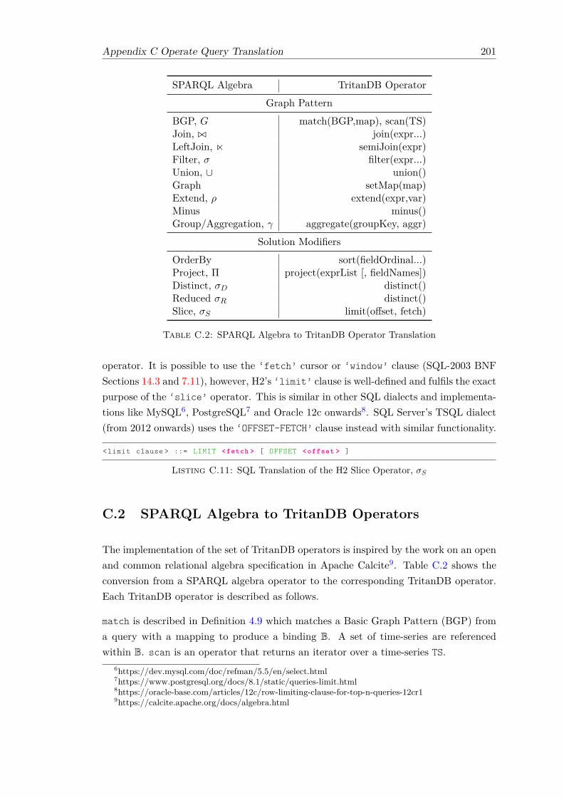
Appendix C Operate Query Translation 201
SPARQL Algebra TritanDB OperatorGraph Pattern
BGP, G match(BGP,map), scan(TS)Join, ./ join(expr...)LeftJoin, n semiJoin(expr)Filter, σ filter(expr...)Union, ∪ union()Graph setMap(map)Extend, ρ extend(expr,var)Minus minus()Group/Aggregation, γ aggregate(groupKey, aggr)
Solution ModifiersOrderBy sort(fieldOrdinal...)Project, Π project(exprList [, fieldNames])Distinct, σD distinct()Reduced σR distinct()Slice, σS limit(offset, fetch)
Table C.2: SPARQL Algebra to TritanDB Operator Translation
operator. It is possible to use the ‘fetch’ cursor or ‘window’ clause (SQL-2003 BNFSections 14.3 and 7.11), however, H2’s ‘limit’ clause is well-defined and fulfils the exactpurpose of the ‘slice’ operator. This is similar in other SQL dialects and implementa-tions like MySQL6, PostgreSQL7 and Oracle 12c onwards8. SQL Server’s TSQL dialect(from 2012 onwards) uses the ‘OFFSET-FETCH’ clause instead with similar functionality.
<limit clause > ::= LIMIT <fetch > [ OFFSET <offset > ]
Listing C.11: SQL Translation of the H2 Slice Operator, σS
C.2 SPARQL Algebra to TritanDB Operators
The implementation of the set of TritanDB operators is inspired by the work on an openand common relational algebra specification in Apache Calcite9. Table C.2 shows theconversion from a SPARQL algebra operator to the corresponding TritanDB operator.Each TritanDB operator is described as follows.
match is described in Definition 4.9 which matches a Basic Graph Pattern (BGP) froma query with a mapping to produce a binding B. A set of time-series are referencedwithin B. scan is an operator that returns an iterator over a time-series TS.
6https://dev.mysql.com/doc/refman/5.5/en/select.html7https://www.postgresql.org/docs/8.1/static/queries-limit.html8https://oracle-base.com/articles/12c/row-limiting-clause-for-top-n-queries-12cr19https://calcite.apache.org/docs/algebra.html

202 Appendix C Operate Query Translation
join, combines two time-series according to conditions specified as expr while semiJoin
joins two time-series according to some condition, but outputs only columns from theleft input.
filter modifies the input to return an iterator over points for which the conditionsspecified in expr evaluates to true. A common filter condition would a specification ofa range of time for a time-series.
union returns the union of the input time-series and bindings B. If the same time-series is referenced within inputs, only the bindings need to be merged. If two differenttime-series are merged, the iterator is formed in linear time by a comparison-basedsorting algorithm, for example, the merge step within a merge sort, as the time-seriesare retrieved in sorted time order.
setMap is used to apply the specified mapping to its algebra tree leaf nodes for match.
extend allows the evaluation of an expression expr to be bound to a new variable var.This evaluation is performed only if var is projected. There are three means in SPARQLto produce the algebra: using bind, expressions in the select clause or expressions inthe group by clause.
minus returns the iterator of first input excluding points from the second input.
aggregate produces an iteration over a set of aggregated results from an input. Tocalculate aggregate values for an input, the input is first divided into one or moregroups by the groupKey field and the aggregate value is calculated for the particularaggr function for each group. The aggr functions supported are count, sum, avg, min,max, sample and groupconcat.
sort imposes a particular sort order on its input based on a sequence consisting offieldOrdinals, each defining the time-series field index (zero-based) and specifying apositive ordinal for ascending and negative for descending order.
project computes the set of chosen variables to ‘select’ from its input, as specified byexprList, and returns an iterator to the result containing only the selected variables.The default name of variables provided can be renamed by specifying the new namewithin the fieldNames argument.
distinct eliminates all duplicate records while reduced, in the TritanDB implemen-tation, performs the same function. The SPARQL specification defines the differencebeing that distinct ensures duplicate elimination while reduced simply permits du-plicate elimination. Given that time-series are retrieved in sorted order of time, thedistinct function works the same for reduced as well and eliminates immediately re-peated duplicate result rows.

Appendix C Operate Query Translation 203
limit computes a window over the input returning an iterator over results that are ofa maximum size (in rows) of fetch and are a distance of offset from the start of theresult set.
C.3 SPARQL Algebra to Streaming Operators
The translation from SPARQL algebra operators to streaming operators is describedwith the Event Processing Language (EPL) using the Backus Normal Form (BNF)notation. The EPL grammar is based on an extension to the SQL-92 standard describedby Savage (2017b) and defined within the Esper engine documentation10.
Translation is similar to SQL translation (Section C.1) with the main difference beingthat the concept of tables is replaced by that of windows which could either be a stream ora static SQL data source connected by JDBC (non-relational data sources are supportedin Esper but not in S2S at the moment). Listing C.12 explains the syntax of a windowdefinition in BNF. A ‘binding.window’ is the specific ‘window def’ produced fromthe match operation containing either a ‘binding.stream’ or ‘binding.table’.
<from clause > ::= FROM <window def > [ <comma > <window def > ... ]<window def > ::= <window > [ <hash > <view spec > ... ] [ AS <window alias > ]<window > ::= <stream def > [ unidirectional ] [ <retain > ] | <sql def ><retain > ::= retain -union | retain - intersection<stream def > ::= <binding .stream > <colon > <view > <left paren > <size > <right paren ><view > ::= length | length_batch | time | time_batch | time_length_batch | ...<sql def > ::= sql <colon > <database_name > <parameterized_sql_query >
Listing C.12: A Window Definition in EPL
Table C.3 shows the input parameters, binding output from the Bmap and correspond-ing EPL listing reference for each SPARQL algebra operator. The translation of eachSPARQL algebra operator is elaborated on using the BNF notation presented in ListingsC.13 to C.23.
<qualified join > ::= <binding .window > [ <join type > ]JOIN <binding .window > <join spec >
<join spec > ::= <join condition > | <named columns join ><join condition > ::= ON <search condition ><named columns join > ::= USING <left paren > <join column list > <right paren ><join type > ::= INNER | <outer join type > [ OUTER ]<outer join type > ::= LEFT | RIGHT | FULL<join column list > ::= <column name list ><column name list > ::= <binding .col > [ <comma > <binding .col > ... ]
Listing C.13: EPL Translation of the Join Operator, ./
Listing C.14 details the differences in EPL translation of the ‘LeftJoin’ operator fromthe ‘Join’ operator in Listing C.13.
10http://www.espertech.com/esper/release-7.0.0-beta2/esper-reference/html/epl_clauses.html

204 Appendix C Operate Query Translation
SPARQL Algebra Input Binding Output ListingGraph Pattern
BGP, G [triple pattern] [binding.col], [binding.window] -Join, ./ [join_condition] [binding.col], [binding.window] C.13LeftJoin, n [join_condition] [binding.col], [binding.window] C.14Filter, σ [var, predicate] [binding.col], [binding.window] C.15Union, ∪ - [binding.window] C.16Graph graph map -Extend, ρ [var, expr], [alias] [binding.col], [binding.window] C.17Minus - [binding.window] C.18Group/Aggr, γ [var], [func] [binding.col], [binding.window] C.19
Solution ModifiersOrderBy var, order binding.col, binding.window C.20Project, Π [var] [binding.col], [binding.window] C.21Distinct, σD - - C.22Reduced σR - - C.22Slice, σS offset, fetch - C.23
Table C.3: Summary of SPARQL Algebra to EPL with Listing References
<join type > ::= <outer join type > [ OUTER ]<outer join type > ::= LEFT
Listing C.14: EPL Translation Difference of the Left Join Operator, n
<where clause > ::= WHERE <search condition ><having clause > ::= HAVING <search condition ><search condition > ::= <boolean value expression ><boolean value expression > ::= <boolean term >
| <boolean value expression > OR <boolean term ><boolean term > ::= <boolean factor > | <boolean term > AND <boolean factor ><boolean factor > ::= [ NOT ] <boolean test ><boolean test > ::= <boolean primary > [ IS [ NOT ] <truth value > ]<truth value > ::= TRUE | FALSE | UNKNOWN<boolean primary > ::= <predicate > | <boolean predicand ><predicate > ::= <comparison predicate > | <like predicate > | ...<boolean predicand > ::= <binding .col > | ...<from clause > ::= <binding .window > [ <comma > <binding .window > ... ]
Listing C.15: EPL Translation of the Filter Operator, σ
EPL does not support a ‘Union’ operator between query terms as in SQL (Listing C.4).However, Listing C.16 shows two possible methods in EPL using a full-outer-join or a‘retain-union’ within the ‘FROM’ clause.

Appendix C Operate Query Translation 205
// full -outer -join method<qualified join > ::= <binding .window > [ <join type > ]
JOIN <binding .window > <join spec ><join type > ::= <outer join type > [ OUTER ]<outer join type > ::= FULL// retain -union method<from clause > ::= FROM <binding .window > [ <comma > <binding .window > ... ]<binding .window > ::= <window > [ <hash > <view spec > ... ] [ AS <window alias > ]<window > ::= <stream def > [ unidirectional ] [ <retain > ]<retain > ::= retain -union<stream def > ::= <binding .stream > ...
Listing C.16: Two Methods of EPL Translation for the Union Operator, ∪
EPL supports an expression alias11 feature that can be used to reduce translated EPLquery length by assigning expression aliases. This is shown in the BNF notation inaddition to the translation of ‘Extend’ within ‘SELECT’ in Listing C.17.
<query spec > ::= SELECT [ <set quantifier > ] <select list > <window expr ><select list > ::= <select sublist > [ <comma > <select sublist > ... ]<select sublist > ::= <derived column > | <qualified asterisk ><derived column > ::= <binding .col > [ <as clause > ]<binding .col > ::= <expr ><as clause > ::= [ AS ] <alias >// expression alias<expr alias > ::= EXPRESSION <expr name > ALIAS FOR <expr >
Listing C.17: EPL Translation of the Extend Operator, ρ and Expression Aliases
EPL does not support the ‘MINUS’ or ‘EXCEPT’ operators. A possible alternative is aleft-outer-join with a null check on each join column.
<qualified join > ::= <binding .window > [ <join type > ]JOIN <binding .window > <join spec >
<join type > ::= <outer join type > [ OUTER ]<outer join type > ::= LEFT<where clause > ::= WHERE <binding .col > IS NULL
[ <comma > <binding .col > IS NULL ... ]
Listing C.18: EPL Alternative Translation of the Minus Operator
Listing C.19 explains the EPL translation of the ‘group by’ operator and aggregationfunctions. EPL supports the aggregation functions12 defined in SPARQL 1.1, COUNT,
SUM, MIN, MAX and AVG. ‘GROUP_CONCAT’ is not supported while ‘SAMPLE’ can beemulated with ‘FIRST’.
11http://www.espertech.com/esper/release-7.0.0-beta2/esper-reference/html/epl_clauses.html#epl-syntax-expression-alias
12http://www.espertech.com/esper/release-7.0.0-beta2/esper-reference/html/functionreference.html#epl-function-aggregation-std

206 Appendix C Operate Query Translation
// group by clause<group by clause > ::= GROUP BY [ <set quantifier > ] <grouping el list ><grouping el list > ::= <grouping el > [ <comma > <grouping element > ... ]<grouping el > ::= <ordinary grouping set > | ...<ordinary grouping set > ::= <grouping col ref >
| <left paren > <grouping col ref list > <right paren ><grouping col ref list > ::= <grouping col ref > [ <comma > <grouping col ref > ...]<grouping col ref > ::= <binding .col > [ <collate clause > ]// aggregation functions<aggregate function > ::=
COUNT <left paren > <asterisk > <right paren > [ <filter clause > ]| <general set function > [ <filter clause > ] | ...
<general set function > ::= <func ><left paren > [ <set quantifier > ] <binding .col > <right paren >
<func > ::= <computational operation ><computational operation > ::= AVG | MAX | MIN | SUM | COUNT | FIRST ...
Listing C.19: EPL Translation of the Group/Aggregation Operator
<order by clause > ::= ORDER BY <sort spec list ><sort spec list > ::= <sort spec > [ <comma > <sort spec > ... ]<sort spec > ::= <binding .col > [ <order > ] [ <null ordering > ]<order > ::= ASC | DESC
Listing C.20: EPL Translation of the OrderBy Operator
<query spec > ::= SELECT [ <set quantifier > ] <select list > <window expr ><select list > ::= <select sublist > [ <comma > <select sublist > ... ]<select sublist > ::= <derived column > | <qualified asterisk ><derived column > ::= <binding .col > [ <as clause > ]<window expr > ::= <from clause > ...<from clause > ::= FROM <binding .window > [ <comma > <binding .table > ... ]
Listing C.21: EPL Translation of the Project Operator, Π
<query spec > ::= SELECT [ <set quantifier > ] <select list > <table expr ><set quantifier > ::= DISTINCT
Listing C.22: EPL Translation of the Distinct and Reduced Operators, σD and σR
<limit clause > ::= <limit form 1> | <limit form 2><limit form 1> ::= LIMIT <fetch > [ OFFSET <offset > ]<limit form 2> ::= LIMIT <offset > [ <comma > <fetch > ]
Listing C.23: EPL Translation of the Slice Operator, σS
SQL and EPL translation from SPARQL using Map-Match-Operate following these rulesis implemented within the S2S engine while TritanDB implements the translation fromSPARQL to internal operators.
Bibliography
Mohammad Aazam and Eui Nam Huh. Fog Computing and Smart Gateway BasedCommunication for Cloud of Things. In Proceedings of the International Conferenceon Future Internet of Things and Cloud, 2014.
Mohammad Aazam, Imran Khan, Aymen Abdullah Alsaffar, and Eui Nam Huh. Cloud ofThings: Integrating Internet of Things and Cloud Computing and the Issues Involved.In Proceedings of 11th International Bhurban Conference on Applied Sciences andTechnology, 2014.
Daniel Abadi, Peter Boncz, Stavros Harizopoulos, Stratos Idreos, and Samuel Mad-den. The Design and Implementation of Modern Column-Oriented Database Systems.Foundations and Trends in Databases, 5(3):197–280, 2012. ISSN 1931-7883.
Daniel Abadi, Don Carney, Ugur Cetintemel, Mitch Cherniack, Christian Convey, Sang-don Lee, Michael Stonebraker, Nesime Tatbul, and Stan Zdonik. Aurora: A NewModel And Architecture For Data Stream Management. The VLDB Journal, 12(2):120–139, 2003. ISSN 1066-8888.
Daniel Abadi, Adam Marcus, Samuel Madden, and Kate Hollenbach. SW-Store: A Ver-tically Partitioned DBMS for Semantic Web Data Management. The VLDB Journal,18(2):385–406, apr 2009. ISSN 1066-8888.
Mervat Abu-Elkheir, Mohammad Hayajneh, and Najah Abu Ali. Data Management forthe Internet of Things: Design Primitives and Solution. Sensors, 13(11):15582–15612,2013. ISSN 14248220.
Hussnain Ahmed. Applying Big Data Analytics for Energy Efficiency. Masters thesis,Aalto University, 2014.
Ian Akyildiz, Weilian Su, Yogesh Sankarasubramaniam, and Erdal Cayirci. Wireless Sen-sor Networks: A Survey. Computer Networks, 38(4):393–422, 2002. ISSN 13891286.
Ian F Akyildiz and Ismail H Kasimoglu. Wireless Sensor And Actor Networks: ResearchChallenges. Ad Hoc Networks, 2(4):351–367, 2004. ISSN 15708705.
207

208 BIBLIOGRAPHY
Ala Al-Fuqaha, Mohsen Guizani, Mehdi Mohammadi, Mohammed Aledhari, and MoussaAyyash. Internet of Things: A Survey on Enabling Technologies, Protocols and Appli-cations. IEEE Communications Surveys and Tutorials, 17(4):2347–2376, 2015. ISSN1553-877X.
Muhammad Ali, Feng Gao, and Alessandra Mileo. CityBench: A Configurable Bench-mark to Evaluate RSP Engines Using Smart City Datasets. In Proceedings of the 14thInternational Semantic Web Conference, 2015.
Ignacio González Alonso, María Rodríguez Fernández, Juan Jacobo Peralta, andAdolfo Cortés García. A Holistic Approach to Energy Efficiency Systems throughConsumption Management and Big Data Analytics. International Journal on Ad-vances in Software, 6(3):261–271, 2013.
Michael P Andersen and David E Culler. BTrDB : Optimizing Storage System Designfor Timeseries Processing. In Proceedings of the 14th USENIX Conference on Fileand Storage Technologies, 2016.
Renzo Angles and Claudio Gutierrez. Survey of Graph Database Models. ACM Com-puting Surveys, 40(1):1–39, feb 2008. ISSN 03600300.
Elliot Anshelevich, Anirban Dasgupta, Eva Tardos, and Tom Wexler. Near-optimalNetwork Design With Selfish Agents. In Proceedings of the 35th ACM Symposium onTheory of Computing, 2003.
Arvind Arasu, Shivnath Babu, and Jennifer Widom. The CQL Continuous Query Lan-guage: Semantic Foundations And Query Execution. The VLDB Journal, 15(2):121–142, 2006. ISSN 10668888.
Kevin Ashton. That ‘Internet of Things’ Thing. RFiD Journal, 2009.
Luigi Atzori, Antonio Iera, and Giacomo Morabito. The Internet of Things: A Survey.Computer Networks, 54(15):2787–2805, oct 2010. ISSN 13891286.
Luigi Atzori, Antonio Iera, and Giacomo Morabito. SIoT: Giving A Social StructureTo The Internet Of Things. IEEE Communications Letters, 15(11):1193–1195, 2011.ISSN 10897798.
Luigi Atzori, Antonio Iera, Giacomo Morabito, and Michele Nitti. The Social Internetof Things (SIoT) - When Social Networks meet the Internet of Things: Concept,Architecture and Network Characterization. Computer Networks, 56(16):3594–3608,2012. ISSN 13891286.
Lars Backstrom and Jure Leskovec. Supervised Random Walks: Predicting and Rec-ommending Links in Social Networks. In Proceedings of the 4th ACM InternationalConference on Web Search and Data Mining, 2010.

BIBLIOGRAPHY 209
Samantha Bail, Sandra Alkiviadous, Bijan Parsia, David Workman, Mark Van Harme-len, Rafael S. Goncalves, and Cristina Garilao. FishMark: A Linked Data ApplicationBenchmark. In Proceedings of the 8th International Workshop on Scalable SemanticWeb Knowledge Base Systems, 2012.
Soma Bandyopadhyay, Munmun Sengupta, Souvik Maiti, and Subhajit Dutta. A Surveyof Middleware for Internet of Things. Communications in Computer and InformationScience, 162:288–296, 2011. ISSN 18650929.
Kyle Banker. MongoDB in Action. Manning Publications, 2011.
Davide F Barbieri, Daniele Braga, Stefano Ceri, Emanuele Della Valle, and MichaelGrossniklaus. Querying RDF streams with C-SPARQL. ACM SIGMOD Record, 39(1):20, 2010. ISSN 01635808.
Sean Barker, Aditya Mishra, David Irwin, and Emmanuel Cecchet. Smart*: An OpenData Set and Tools for Enabling Research in Sustainable Homes. In Proceedings ofthe Workshop on Data Mining Applications in Sustainability, 2012.
Payam Barnaghi and Mirko Presser. Publishing Linked Sensor Data. In Proceedings ofthe 3rd International Workshop on Semantic Sensor Networks, 2010.
Payam Barnaghi, Wei Wang, Cory Henson, and Kerry Taylor. Semantics for the Internetof Things: Early Progress and Back to the Future. International Journal on SemanticWeb and Information Systems, 8(1):1–21, 2012.
Basho. RiakTS: NoSQL Time-series Database, Retrieved June 2017, fromhttp://basho.com/products/riak-ts/, jun 2017.
Atanu Basu. Five Pillars of Prescriptive Analytics Success. Analytics Magazine, pages8–12, 2013.
Richard Bellman. A Markovian Decision Process. Journal Of Mathematics And Me-chanics, 6:679–684, 1957. ISSN 01650114.
Maria Bermudez-Edo, Tarek Elsaleh, Payam Barnaghi, and Kerry Taylor. IoT-Lite: ALightweight Semantic Model for the Internet of Things. In Proceedings of the IEEEConference on Ubiquitous Intelligence & Computing, 2016.
Tim Berners-Lee and Mark Fischetti. Weaving the Web: The Original Design andUltimate Destiny of the World Wide Web by its Inventor. Harper, 2000. ISBN0062515861.
Jay H Bernstein. The Data-Information-Knowledge-Wisdom Hierarchy and its Antithe-sis. NASKO 2.1, pages 68–75, 2011. ISSN 1931-3896.
Jeff Bertolucci. Big Data Analytics: Descriptive Vs. Predictive Vs. Prescriptive, Re-trieved June 2017, from http://goo.gl/dyNDFV, dec 2013.

210 BIBLIOGRAPHY
Ames Bielenberg, Lara Helm, Anthony Gentilucci, Dan Stefanescu, and HonggangZhang. The Growth Of Diaspora - A Decentralized Online Social Network In TheWild. In Proceedings of the IEEE INFOCOM Computer Communications Workshop,2012.
Stefan Bischof, Athanasios Karapantelakis, Amit Sheth, Alessandra Mileo, and PayamBarnaghi. Semantic Modelling of Smart City Data. In Proceedings of the W3C Work-shop on the Web of Things, 2014.
Barry Bishop, Atanas Kiryakov, and Damyan Ognyanoff. OWLIM: A Family of ScalableSemantic Repositories. Semantic Web Journal, 2(1):33–42, 2011. ISSN 15700844.
Chris Bizer, Tom Heath, and Tim Berners-Lee. Linked Data - The Story So Far. Inter-national Journal on Semantic Web and Information Systems, 5:1–22, 2009.
Christian Bizer and Richard Cyganiak. D2RQ - Lessons Learned. In Proceedings of theW3C Workshop on RDF Access to Relational Databases, 2007.
Christian Bizer and Andreas Schultz. The Berlin SPARQL Benchmark. InternationalJournal on Semantic Web and Information Systems, 5(2):1–24, 2001. ISSN 1552-6283.
Piero Bonatti, Claudiu Duma, Daniel Olmedilla, and Nahid Shahmehri. An Integra-tion Of Reputation-based And Policy-based Trust Management. In Proceedings ofSemantic Web Policy Workshop, 2005.
Flavio Bonomi, Rodolfo Milito, Preethi Natarajan, and Jiang Zhu. Fog Computing: APlatform for Internet of Things and Analytics. Big Data Platforms for the Internet ofThings: A Roadmap for Smart Environments, pages 169–186, 2014. ISSN 1860949X.
Flavio Bonomi, Rodolfo Milito, Jiang Zhu, and Sateesh Addepalli. Fog Computing andIts Role in the Internet of Things. In Proceedings of the 1st Workshop on Mobile CloudComputing, 2012.
Jeff Bonwick, Matt Ahrens, Val Henson, Mark Maybee, and Mark Shellenbaum. TheZettabyte File System. In Proceedings of the USENIX Conference on File and StorageTechnologies, 2003.
Carsten Bormann and Paul Hoffman. Concise Binary Object Representation (CBOR).Technical report, Internet Engineering Task Force, oct 2013.
Léon Bottou. From Machine Learning to Machine Reasoning: An Essay. MachineLearning, 94(2):133–149, 2014. ISSN 08856125.
Mike Buerli. The Current State of Graph Databases. Technical report, CaliforniaPolytechnic State University, dec 2012.

BIBLIOGRAPHY 211
Carlos Buil-Aranda, Aidan Hogan, Jürgen Umbrich, and Pierre-Yves Vandenbussche.SPARQL Web-Querying Infrastructure: Ready for Action? In Proceedings of the 12thInternational Semantic Web Conference, 2013.
Richard Burnison. The Concurrency Of ConcurrentHashMap, Retrieved June 2017, fromhttps://www.burnison.ca/articles/the-concurrency-of-concurrenthashmap, mar 2013.
Martin Burtscher and Paruj Ratanaworabhan. FPC: A High-Speed Compressor forDouble-Precision Floating-Point Data. IEEE Transactions on Computers, 58(1):18–31, jan 2009. ISSN 0018-9340.
Charles Byers and Robert Swanson. The OpenFog Consortium Reference Architecture.Technical report, The OpenFog Consortium, 2017.
Jean-Paul Calbimonte, Óscar Corcho, and Alasdair JG Gray. Enabling Ontology-basedData Access to Streaming Data Sources. In Proceedings of the 9th InternationalSemantic Web Conference, 2010.
Jean-Paul Calbimonte, Hoyoung Jeung, Oscar Corcho, and Karl Aberer. Enabling QueryTechnologies for the Semantic Sensor Web. International Journal on Semantic Weband Information Systems, 8(1):43–63, 2012. ISSN 1552-6283.
Qing Cao, Tarek Abdelzaher, John Stankovic, and Tian He. The LiteOS operatingsystem: Towards Unix-like abstractions for wireless sensor networks. In Proceedingsof the International Conference on Information Processing in Sensor Networks, 2008.
Meeyoung Cha, Hamed Haddai, Fabricio Benevenuto, and Krishna P Gummadi. Mea-suring User Influence in Twitter : The Million Follower Fallacy. In Proceedings of the4th International Conference on Web and Social Media, 2010.
Sharma Chakravarthy and Qingchun Jiang. Stream Data Processing: A Quality ofService Perspective Modeling, Scheduling, Load Shedding, and Complex Event Pro-cessing. Springer Publishing, 2009. ISBN 9780387710020.
Neil Chandler, Bill Hostmann, Nigel Rayner, and Gareth Herschel. Gartner’s BusinessAnalytics Framework. Technical report, Gartner Inc., 2011.
Fay Chang, Jeffrey Dean, Sanjay Ghemawat, Wilson C Hsieh, Deborah A Wallach,Mike Burrows, Tushar Chandra, Andrew Fikes, and Robert E Gruber. Bigtable: ADistributed Storage System for Structured Data. ACM Transactions on ComputerSystems, 26(2):1–26, 2008.
Artem Chebotko, Shiyong Lu, and Farshad Fotouhi. Semantics Preserving SPARQL-to-SQL Translation. Data and Knowledge Engineering, 68(10):973–1000, 2009. ISSN0169023X.
Min Chen, Shiwen Mao, and Yunhao Liu. Big Data: A Survey. Mobile Networks andApplications, 19:171–209, 2014. ISSN 1383469X.

212 BIBLIOGRAPHY
Mung Chiang, Sangtae Ha, Chih-Lin I, Fulvio Risso, and Tao Zhang. Clarifying FogComputing and Networking: 10 Questions and Answers. IEEE Communications Mag-azine, 55(4):18–20, apr 2017. ISSN 0163-6804.
Konstantinos Christidis and Michael Devetsikiotis. Blockchains and Smart Contractsfor the Internet of Things. IEEE Access, 4:2292–2303, 2016. ISSN 21693536.
Pietro Ciciriello, Luca Mottola, and Gian Pietro Picco. Efficient Routing From MultipleSources To Multiple Sinks In Wireless Sensor Networks. Wireless Sensor Networks,2:34–50, 2007. ISSN 03029743.
Cisco. IOX, Retrieved June 2017, from https://developer.cisco.com/site/iox/, 2015.
Michael Compton, Payam Barnaghi, Luis Bermudez, Raúl García-Castro, Oscar Corcho,Simon Cox, John Graybeal, Manfred Hauswirth, Cory Henson, Arthur Herzog, Vin-cent Huang, Krzysztof Janowicz, W. David Kelsey, Danh Le Phuoc, Laurent Lefort,Myriam Leggieri, Holger Neuhaus, Andriy Nikolov, Kevin Page, Alexandre Passant,Amit Sheth, and Kerry Taylor. The SSN Ontology of the W3C Semantic Sensor Net-work Incubator Group. Web Semantics: Science, Services and Agents on the WorldWide Web, 17:25–32, dec 2012. ISSN 15708268.
Jack Copeland. Artificial Intelligence: A Philosophical Introduction. John Wiley &Sons, 2015.
Michael Corcoran. The Five Types Of Analytics. Technical report, Information Builders,2012.
Kyle Croman, Christian Decker, Ittay Eyal, Adem Efe Gencer, Ari Juels, Ahmed Kosba,Andrew Miller, Prateek Saxena, Elaine Shi, Emin Gün Sirer, Dawn Song, and RogerWattenhofer. On Scaling Decentralized Blockchains. In Proceedings of the 20th Inter-national Conference on Financial Cryptography and Data Security, 2016.
Isabel F Cruz, Alberto O Mendelzon, and Peter T Wood. A Graphical Query LanguageSupporting Recursion. ACM SIGMOD Record, 16:323–330, 1987. ISSN 01635808.
Zbigniew Czech, George Havas, and Bohdan Majewski. An Optimal Algorithm forGenerating Minimal Perfect Hash Functions. Information Processing Letters, 43(5):257–264, 1992. ISSN 00200190.
Pedro da Rocha Pinto, Thomas Dinsdale-Young, Mike Dodds, Philippa Gardner, andMark Wheelhouse. A Simple Abstraction for Complex Concurrent Indexes. ACMSIGPLAN Notices, 46(10):845, 2011. ISSN 03621340.
Amir V Dastjerdi and Rajkumar Buyya. Fog Computing: Helping the Internet of ThingsRealize Its Potential. Computer, 49(8):112–116, 2016. ISSN 00189162.

BIBLIOGRAPHY 213
Anwitaman Datta, Sonja Buchegger, Le-Hung Vu, Thorsten Strufe, and KrzysztofRzadca. Decentralized Online Social Networks. In Handbook of Social Network Tech-nologies and Applications, pages 349–378. Springer, 2010. ISBN 978-1-4419-7142-5.
Thomas Davenport. Competing on Analytics. Harvard Business Review, 84(1):98–107,2006. ISSN 0017-8012.
Thomas Davenport. Analytics 3.0, Retrieved June 2017, fromhttps://hbr.org/2013/12/analytics-30, dec 2013.
Daniele Dell’Aglio, Jean Paul Calbimonte, Marco Balduini, Oscar Corcho, and EmanueleDella Valle. On Correctness In RDF Stream Processor Benchmarking. In Proceedingsof the 12th International Semantic Web Conference, 2013.
Daniele Dell’Aglio, Emanuele Della Valle, Jean-Paul Calbimonte, and Oscar Corcho.RSP-QL Semantics: A Unifying Query Model To Explain Heterogeneity Of RdfStream Processing Systems. International Journal on Semantic Web and Informa-tion Systems, 10(4):17–44, 2014. ISSN 1552-6283.
Swarnava Dey, Arijit Mukherjee, Himadri Sekhar Paul, and Arpan Pal. Challenges OfUsing Edge Devices In IoT Computation Grids. In Proceedings of the InternationalConference on Parallel and Distributed Systems, 2013.
Bhuwan Dhingra, Lihong Li, Xiujun Li, Jianfeng Gao, Yun-Nung Chen, Faisal Ahmed,and Li Deng. End-to-End Reinforcement Learning of Dialogue Agents for InformationAccess. In Proceedings of the Annual Meeting of the Association for ComputationalLinguistics, 2017.
Anastasia Dimou, Miel Vander Sande, Pieter Colpaert, Ruben Verborgh, Erik Mannens,and Rik Van De Walle. RML: A Generic Language for Integrated RDF Mappings ofHeterogeneous Data. In Proceedings of the 7th Workshop on Linked Data on the Web,2014.
Angelika Dohr, R Modre-Opsrian, Mario Drobics, Dieter Hayn, and Günter Schreier.The Internet of Things for Ambient Assisted Living. In Proceedings of the 7th Inter-national Conference on Information Technology, pages 804–809, 2010.
DWARF Debugging Information Format Committee. DWARF Debugging InformationFormat, Version 5. Technical report, Free Standards Group, feb 2017.
David Easley and Jon Kleinberg. Networks, Crowds, and Markets: Reasoning about aHighly Connected World. Cambridge University Press, 2010. ISBN 9780521195331.
Andreas Eckner. A Framework For The Analysis Of Unevenly Spaced Time Series Data,Retrieved June 2017. Working paper, 2014.
Andreas Eckner. Algorithms for Unevenly Spaced Time Series : Moving Averages andOther Rolling Operators, Retrieved June 2017. Working paper, 2017.

214 BIBLIOGRAPHY
Elastic. Elasticsearch: RESTful, Distributed Search & Analytics, Retrieved June 2017,from https://www.elastic.co/products/elasticsearch, jun 2017.
Brendan Elliott, En Cheng, Chimezie Thomas-Ogbuji, and Z. Meral Ozsoyoglu. A Com-plete Translation from SPARQL Into Efficient SQL. In Proceedings of the InternationalDatabase Engineering & Applications Symposium, 2009.
Yagil Engel and Opher Etzion. Towards Proactive Event-driven Computing. In Pro-ceedings of the 5th ACM International Conference on Distributed Event-based Systems,2011.
Orri Erling. Implementing a SPARQL Compliant RDF Triple Store Using a SQL-ORDBMS. Technical report, OpenLink Software, 2001.
Amirhossein Farahzadia, Pooyan Shams, Javad Rezazadeh, and Reza Farahbakhsh. Mid-dleware Technologies for Cloud of Things - A Survey. Digital Communications andNetworks, 3(4):1–13, 2017. ISSN 23528648.
Usama Fayyad, Gregory Piatetsky-Shapiro, and Padhraic Smyth. From Data Mining toKnowledge Discovery in Databases. AI Magazine, 17(3):37–53, 1996. ISSN 0738-4602.
Ian Fette and Alexey Melnikov. The WebSockets Protocol. Technical report, InternetEngineering Task Force, dec 2011.
Frieder Ganz, Payam Barnaghi, and Francois Carrez. Information Abstraction for Het-erogeneous Real World Internet Data. IEEE Sensors Journal, 13:3793–3805, 2013.ISSN 1530437X.
Animikh Ghosh, Ketan a. Patil, and Sunil Kumar Vuppala. PLEMS: Plug Load EnergyManagement Solution for Enterprises. In Proceedings of the 27th IEEE InternationalConference on Advanced Information Networking and Applications, 2013.
Bob Giddings, Bill Hopwood, and Geoff O’Brien. Environment, Economy and Society:Fitting Them Together Into Sustainable Development. Sustainable Development, 10:187–196, 2002. ISSN 09680802.
Roberto Gimenez, Diego Fuentes, Emilio Martin, Diego Gimenez, Judith Pertejo, SofiaTsekeridou, Roberto Gavazzi, Mario Carabaño, and Sofia Virgos. The Safety Trans-formation in the Future Internet Domain. The Future Internet, pages 190–200, 2012.ISSN 03029743.
Bart Goeman, Hans Vandierendonck, and Koen de Bosschere. Differential FCM: Increas-ing Value Prediction Accuracy By Improving Table Usage Efficiency. In Proceedings ofthe 7th International Symposium on High-Performance Computer Architecture, 2001.
Olaf Gorlitz and Steffen Staab. SPLENDID : SPARQL Endpoint Federation ExploitingVOID Descriptions. In Proceedings of the 2nd International Workshop on ConsumingLinked Data, 2011.

BIBLIOGRAPHY 215
Jorge Granjal, Edmundo Monteiro, and Jorge Sa Silva. Security for the Internet ofThings: A Survey Of Existing Protocols and Open Research Issues. IEEE Commu-nications Surveys and Tutorials, 17(3):1294–1312, 2015. ISSN 1553877X.
Alasdair J G Gray, Raúl García-Castro, Kostis Kyzirakos, Manos Karpathiotakis, Jean-Paul Calbimonte, Kevin Page, Jason Sadler, Alex Frazer, Ixent Galpin, Alvaro A AFernandes, Norman W. Paton, Oscar Corcho, Manolis Koubarakis, David De Roure,Kirk Martinez, and Asunción Gómez-Pérez. A Semantically Enabled Service Architec-ture for Mashups over Streaming and Stored Data. In Proceedings of the 8th ExtendedSemantic Web Conference, 2011.
Dominique Guinard and Vlad Trifa. Towards the Web of Things : Web Mashups forEmbedded Devices. In Proceedings of the Workshop on Mashups, Enterprise Mashupsand Lightweight Composition on the Web, 2009.
Bin Guo, Daqing Zhang, and ZhuWang. LivingWith Internet of Things: The Emergenceof Embedded Intelligence. In Proceedings of the 2011 IEEE International Conferenceson Internet of Things and Cyber, Physical and Social Computing, 2011.
Chirag Gupta, Arun S Suggala, Ankit Goyal, Harsha V Simhadri, Bhargavi Paranjape,Ashish Kumar, Saurabh Goyal, Raghavendra Udupa, Manik Varma, and Prateek Jain.ProtoNN: Compressed and Accurate kNN for Resource-scarce Devices. In Proceedingsof the 34th International Conference on Machine Learning, 2017.
Ido Guy, Naama Zwerdling, David Carmel, Inbal Ronen, Erel Uziel, Sivan Yogev, andShila Ofek-Koifman. Personalized Recommendation of Social Software Items Basedon Social Relations. In Proceedings of the 3rd ACM Conference on RecommenderSystems, 2009.
Amelie Gyrard, Christian Bonnet, Karima Boudaoud, and Martin Serrano. LOV4IoT:A Second Life For Ontology-based Domain Knowledge To Build Semantic Web OfThings Applications. In Proceedings of the 4th IEEE International Conference onFuture Internet of Things and Cloud, 2016.
Stefan Hagedorn and Kai-Uwe Sattler. Efficient Parallel Processing of Analytical Querieson Linked Data. In Proceedings of the OTM Confederated International Conferences"On the Move to Meaningful Internet Systems", 2013.
Joe F Hair Jr. Knowledge Creation in Marketing: The Role of Predictive Analytics.European Business Review, 19:303–315, 2007. ISSN 0955-534X.
Stephen Harris and Nigel Shadbolt. SPARQL Query Processing with ConventionalRelational Database Systems. In Proceedings of the International Conference on WebInformation Systems Engineering, 2005.

216 BIBLIOGRAPHY
Steve Harris, Nick Lamb, and Nigel Shadbolt. 4store: The Design and Implementation ofa Clustered RDF Store. In Proceedings of the 5th International Workshop on ScalableSemantic Web Knowledge Base Systems, 2009.
Peter E Hart, Nils J Nilsson, and Betram Raphael. A Formal Basis for the HeuristicDetermination of Minimum Cost Paths. IEEE Transactions on Systems Science andCybernetics, 4(2):100–107, 1968.
Olaf Hartig. An Overview on Execution Strategies for Linked Data Queries. Datenbank-Spektrum, 13(2):89–99, 2013. ISSN 1618-2162.
Wu He, Gongjun Yan, and Li Da Xu. Developing Vehicular Data Cloud Services in theIoT Environment. IEEE Transactions on Industrial Informatics, 10(2):1587–1595,2014. ISSN 15513203.
Tom Heath and Christian Bizer. Linked Data Evolving the Web into a Global DataSpace. In Synthesis Lectures on the Semantic Web: Theory and Technology. Morgan& Claypool, 2011. ISBN 9781608454303.
Cory Henson, Amit Sheth, and Krishnaprasad Thirunarayan. Semantic Perception:Converting Sensory Observations to Abstractions. IEEE Internet Computing, 16(2):26–34, mar 2012. ISSN 1089-7801.
Alfred Hermida. Twittering the News: The Emergence of Ambient Journalism. Jour-nalism Practice, 4(3):297–308, 2010. ISSN 1751-2786.
Friedhelm Hillebrand. The Creation of Standards for Global Mobile Communication:GSM and UMTS Standardization from 1982 to 2000. IEEE Wireless Communications,20(5):24–33, 2013. ISSN 15361284.
Myriam Hunink, Milton Weinstein, Eve Wittenberg, Michael Drummond, JosephPliskin, John Wong, and Paul Glasziou. Decision Making in Health and Medicine:Integrating Evidence and Values. Cambridge University Press, jun 2014. ISBN9781107690479.
Md Zahurul Huq and Sayed Islam. Home Area Network Technology Assessment forDemand Response in Smart Grid Environment. In Proceedings of the 20th AustralasianUniversities Power Engineering Conference, 2010.
IEEE Standards Association. IEEE Standard for Floating-Point Arithmetic 754-2008.Technical report, IEEE Standards Association, aug 2008.
Influx Data. InfluxDB Documentation, Retrieved June 2017, fromhttps://docs.influxdata.com/influxdb/v1.2/, jun 2017.
Chalermek Intanagonwiwat, Ramesh Govindan, Deborah Estrin, John Heidemann, andFabio Silva. Directed Diffusion For Wireless Sensor Networking. IEEE/ACM Trans-actions on Networking, 11(1):2–16, feb 2003. ISSN 1063-6692.

BIBLIOGRAPHY 217
Intel. Video Analytics at the Edge, Retrieved June 2017, fromhttps://www.intel.com/content/www/us/en/embedded/digital-security-surveillance/video-analytics-at-the-edge-solution-brief.html, 2016.
International Telecommunication Union. Overview of the Internet of Things. Technicalreport, International Telecommunication Union, jun 2012.
Kaippallimalil J Jacob, Morgan Stanley, Dean Witter, New York, and Dennis Shasha.FinTime - A Financial Time Series Benchmark. ACM SIGMOD Record, 28(4):42–48,dec 1999. ISSN 01635808.
Toby Jaffey, John Davies, and Pilgrim Beart. Hypercat 3.00 Specification. Technicalreport, Hypercat Limited, feb 2016.
Antonio Jara, Pablo Lopez, David Fernandez, Jose Castillo, Miguel Zamora, and AntonioSkarmeta. Mobile digcovery: A Global Service Discovery for the Internet of Things. InProceedings of the 27th International Conference on Advanced Information Networkingand Applications Workshops, 2013.
Simon Jirka and Daniel Nüst. OGC Sensor Instance Registry Discussion Paper. Tech-nical report, Open Geospatial Consortium, oct 2010.
Melvin Johnson, Mike Schuster, Quoc V Le, Maxim Krikun, Yonghui Wu, Zhifeng Chen,Nikhil Thorat, Fernanda Viégas, Martin Wattenberg, Greg Corrado, Macduff Hughes,and Jeffrey Dean. Google’s Multilingual Neural Machine Translation System: En-abling Zero-Shot Translation, Retrieved June 2017. Working paper, 2016.
KairosDB. KairosDB: Fast Time Series Database on Cassandra, Retrieved June 2017,from https://kairosdb.github.io/, jun 2015.
Ad Kamerman and Leo Monteban. WaveLAN-II: A High-performance Wireless LAN forthe Unlicensed Band. Bell Labs Technical Journal, 2(3):118, 1997. ISSN 10897089.
Lisa Kart. Advancing Analytics. Technical report, Gartner Inc., 2012.
Khalid S Khan, Regina Kunz, Jos Kleijnen, and Gerd Antes. Five Steps to Conductinga Systematic Review. Journal of the Royal Society of Medicine, 96(3):118–121, 2003.
Sooyeon Kim, Sang H Son, John Stankovic, Shuoqi Li, and Yanghee Choi. SAFE: AData Dissemination Protocol for Periodic Updates in Sensor Networks. In Proceedingsof the 23rd International Conference on Distributed Computing Systems Workshops,2003.
Sefki Kolozali, Maria Bermudez-Edo, Daniel Puschmann, Frieder Ganz, and PayamBarnaghi. A Knowledge-Based Approach for Real-Time IoT Data Stream Annotationand Processing. In Proceedings of the 2014 IEEE International Conference on Internetof Things, 2014.

218 BIBLIOGRAPHY
Mathias Konrath, Thomas Gottron, Steffen Staab, and Ansgar Scherp. SchemEX -Efficient Construction of a Data Catalogue By Stream-based Indexing of Linked Data.Web Semantics: Science, Services and Agents on the World Wide Web, 16:52–58, nov2012. ISSN 1570-8268.
Michael Koster. iot.schema.org. In Proceedings of the Workshop on IoT Semantic/Hy-permedia Interoperability, 2017.
Egor V Kostylev, Juan L Reutter, and Miguel Romero. SPARQL with Property Paths.In Proceedings of the 14th International Semantic Web Conference, 2015.
Ashish Kumar, Saurabh Goyal, and Manik Varma. Resource-efficient Machine Learningin 2 KB RAM for the Internet of Things. In Proceedings of the 34th InternationalConference on Machine Learning, 2017.
Rohit Kumar Kaliyar. Graph Databases: A Survey. In Proceedings of the InternationalConference on Computing, Communication and Automation, 2015.
Bradley C Kuszmaul. A Comparison of Fractal Trees to Log-Structured Merge (LSM)Trees. DZone Refcardz, pages 1–15, 2014.
Haewoon Kwak, Changhyun Lee, Hosung Park, and Sue Moon. What is Twitter, a SocialNetwork or a News Media? In Proceedings of the 19th International Conference onWorld Wide Web, 2010.
Gunter Ladwig and Andreas Harth. CumulusRDF: Linked Data Management on NestedKey-Value Stores. In Proceedings of the 7th International Workshop on Scalable Se-mantic Web Knowledge Base Systems, 2011.
Avinash Lakshman and Prashant Malik. Cassandra: A Decentralized Structured StorageSystem. ACM SIGOPS Operating Systems Review, 44(2):35–40, 2010. ISSN 01635980.
Leslie Lamport, Robert Shostak, and Marshall Pease. The Byzantine Generals Prob-lem. ACM Transactions on Programming Languages and Systems, 4(3):382–401, 1982.ISSN 01640925.
Steve Lavalle, Michael S Hopkins, Eric Lesser, Rebecca Shockley, and Nina Kruschwitz.Analytics : The New Path to Value. MIT Sloan Management Review, pages 1–24,2010. ISSN 15329194.
Eugene Lazin. Akumuli Time-series Database, Retrieved June 2017, fromhttp://akumuli.org/, jun 2017.
Danh Le-Phuoc, Minh Dao-Tran, Josiane Xavier Parreira, and Manfred Hauswirth. ANative and Adaptive Approach for Unified Processing of Linked Streams and LinkedData. In Proceedings of the 10th International Semantic Web Conference, 2011.

BIBLIOGRAPHY 219
Jure Leskovec, Daniel Huttenlocher, and Jon Kleinberg. Predicting Positive And Nega-tive Links In Online Social Networks. In Proceedings of the 19th International WorldWide Web Conference, 2010a.
Jure Leskovec, Daniel Huttenlocher, and Jon Kleinberg. Signed Networks in SocialMedia. In Proceedings of the SIGCHI Conference on Human Factors in ComputingSystems, 2010b.
Jure Leskovec, Jon Kleinberg, and Christos Faloutsos. Graph Evolution: Densificationand Shrinking Diameters. ACM Transactions on Knowledge Discovery from Data, 1(2):1–39, 2007. ISSN 15564681.
Philip Levis, Samuel Madden, Joseph Polastre, Robert Szewczyk, Kamin Whitehouse,Alec Woo, David Gay, Jason Hill, Matt Welsh, Eric Brewer, and David Culler.TinyOS: An Operating System for Wireless Sensor Networks. Ambient Intelligence,8491:115–148, 2005. ISSN 03796566.
Lin Li, Saeed Bagheri, Helena Goote, Asif Hasan, and Gregg Hazard. Risk Adjustmentof Patient Expenditures: A Big Data Analytics Approach. In Proceedings of the 2013IEEE International Conference on Big Data, 2013.
Leonid Libkin, Wim Martens, and Domagoj Vrgoc. Querying Graphs with Data. Journalof the ACM, 63(2):1–53, 2016. ISSN 1557735X.
Thomas Liebig, Nico Piatkowski, Christian Bockermann, and Katharina Morik. Predic-tive Trip Planning-Smart Routing in Smart Cities. In Proceedings of the Workshopsof the EDBT/ICDT 2014 Joint Conference, 2014.
Jie Lin, Wei Yu, Nan Zhang, Xinyu Yang, Hanlin Zhang, and Wei Zhao. A Survey onInternet of Things: Architecture, Enabling Technologies, Security and Privacy, andApplications. IEEE Internet of Things Journal, 2017. ISSN 2327-4662.
Honghai Liu, Shengyong Chen, and Naoyuki Kubota. Intelligent Video Systems andAnalytics: A Survey. IEEE Transactions on Industrial Informatics, 9(3):1222–1233,2013. ISSN 15513203.
Pasquale Lops, Marco de Gemmis, and Giovanni Semeraro. Content-based Recom-mender Systems: State of the Art and Trends. Springer, 2010.
Helmut Lütkepohl. New Introduction to Multiple Time Series Analysis. Springer, 2010.
Steven Lynden, Isao Kojima, Akiyoshi Matono, and Yusuke Tanimura. ADERIS: AnAdaptive Query Processor for Joining Federated SPARQL Endpoints, 2011.
Doug Madory. Earthquake Rocks Internet In Nepal, Retrieved June 2017, fromhttp://dyn.com/blog/earthquake-rocks-internet-in-nepal/, 2015.

220 BIBLIOGRAPHY
Alan Mainwaring, David Culler, Joseph Polastre, Robert Szewczyk, and John Anderson.Wireless Sensor Networks For Habitat Monitoring. In Proceedings of the 1st ACMInternational Workshop On Wireless Sensor Networks And Applications, 2002.
Chin Mak and Henry Fan. Heavy Flow-Based Incident Detection Algorithm Using Infor-mation From Two Adjacent Detector Stations. Journal of Intelligent TransportationSystems, 10(1):23–31, 2006. ISSN 1547-2450.
Stephen Makonin, Lyn Bartram, and Fred Popowich. A Smarter Smart Home: CaseStudies of Ambient Intelligence. IEEE Pervasive Computing, 12(1):58–66, 2013. ISSN1536-1268.
Thomas W Malone, Robert Laubacher, and Chrysanthos Dellarocas. Harnessing Crowds: Mapping The Genome Of Collective Intelligence. MIT Sloan Research Paper, 1:1–20,2009. ISSN 15565068.
Henrique S Malvar. Adaptive Run-Length / Golomb-Rice Encoding of Quantized Gen-eralized Gaussian Sources with Unknown Statistics. In Proceedings of the Data Com-pression Conference, 2006.
Essam Mansour, Andrei Vlad Sambra, Sandro Hawke, Maged Zereba, Sarven Capadisli,Abdurrahman Ghanem, Ashraf Aboulnaga, and Tim Berners-Lee. A Demonstrationof the Solid Platform for Social Web Applications. In Proceedings of the 25th Inter-national Conference on World Wide Web Companion, 2016.
James Manyika, Michael Chui, Peter Bisson, Jonathan Woetzel, Richard Dobbs, JacquesBughin, and Dan Aharon. The Internet of Things: Mapping the Value Beyond theHype. Technical report, McKinsey Global Institute, jun 2015.
Ibrahim Mashal, Osama Alsaryrah, Tein Yaw Chung, Cheng Zen Yang, Wen HsingKuo, and Dharma P. Agrawal. Choices for Interaction With Things on Internet andUnderlying Issues. Ad Hoc Networks, 28:68–90, 2015. ISSN 15708705.
Zoltan Mathe, Adrian Casajus Ramo, Federico Stagni, and Luca Tomassetti. Evaluationof NoSQL Databases for DIRAC Monitoring and Beyond. In Proceedings of the 21stInternational Conference on Computing in High Energy and Nuclear Physics, 2015.
Colleen McCue. Data Mining and Predictive Analytics: Battlespace Awareness for theWar on Terrorism. Defense Intelligence Journal, 2:47–63, 2005.
Colleen McCue. Data Mining and Predictive Analytics in Public Safety and Security.IT Professional, 8(August), 2006. ISSN 1520-9202.
Milan Milenkovic. A Case for Interoperable IoT Sensor Data and Meta-data Formats.Ubiquity, 2015(November):1–7, 2015. ISSN 15302180.

BIBLIOGRAPHY 221
Daniele Miorandi, Sabrina Sicari, Francesco De Pellegrini, and Imrich Chlamtac. Inter-net of Things: Vision, Applications and Research Challenges. Ad Hoc Networks, 10(7):1497–1516, 2012. ISSN 15708705.
Arijit Mukherjee, Swarnava Dey, Himadri Sekhar Paul, and Batsayan Das. UtilisingCondor for Data Parallel Analytics in an IoT Context - An Experience Report. InProceedings of the 9th IEEE International Conference on Wireless and Mobile Com-puting, Networking and Communications, 2013.
Arijit Mukherjee, Arpan Pal, and Prateep Misra. Data Analytics in Ubiquitous Sensor-based Health Information Systems. In Proceedings of the 6th International Conferenceon Next Generation Mobile Applications, Services, and Technologies, 2012.
Arijit Mukherjee, Himadri Sekhar Paul, Swarnava Dey, and Ansuman Banerjee. AN-GELS for Distributed Analytics In IoT. In Proceedings of IEEE World Forum onInternet of Things, 2014.
Ujjal Kumar Mukherjee and Snigdhansu Chatterjee. Fast Algorithm for ComputingWeighted Projection Quantiles and Data Depth for High-Dimensional Large DataClouds. In Proceedings of the 2014 IEEE International Conference on Big Data,2014.
Janine Nahapiet and Sumantra Ghoshal. Social Capital, Intellectual Capital, And TheOrganizational Advantage. The Academy of Management Review, 23(2):242–266,1998. ISSN 03637425.
Adam Neat. Maximizing Performance and Scalability with IBM WebSphere. Apress,2004. ISBN 978-1-59059-130-7.
Septimiu Nechifor, Anca Petrescu, Dan Puiu, and Bogdan Tarnauca. Predictive Analyt-ics based on CEP for Logistic of Sensitive Goods. In Proceedings of the InternationalConference on Optimization of Electrical and Electronic Equipment, 2014.
Angelia Nedić and Asuman Ozdaglar. Distributed Subgradient Methods For Multi-agent Optimization. IEEE Transactions On Automatic Control, 54(1):4711–4716,2009. ISSN 01912216.
Yavor Nenov, Robert Piro, Boris Motik, Ian Horrocks, Zhe Wu, and Jay Banerjee. RD-Fox: A Highly-Scalable RDF Store. In Proceedings of the 14th International SemanticWeb Conference, 2015.
Thomas Neumann and Gerhard Weikum. x-RDF-3X: Fast Querying, High UpdateRates, and Consistency for RDF Databases. Proceedings of the VLDB Endowment, 3(1-2):256–263, 2010. ISSN 21508097.
Andrew Newton and Pete Cordell. A Language for Rules Describing JSON Content.Technical report, Internet Engineering Task Force, mar 2017.

222 BIBLIOGRAPHY
Huansheng Ning and Ziou Wang. Future Internet of Things Architecture: Like MankindNeural System or Social Organization Framework? IEEE Communications Letters,15(4):461–463, 2011. ISSN 1089-7798.
Michele Nitti, Roberto Girau, and Luigi Atzori. Trustworthiness Management In TheSocial Internet Of Things. IEEE Transactions on Knowledge and Data Engineering,26(5):1253–1266, 2014. ISSN 10414347.
Michael O’Connor. Method of Enabling Heterogeneous Platforms to Utilize a UniversalFile System in a Storage Area Network, US Patent 6,564,228, 2003.
Tobias Oetiker. Rrdtool: Round Robin Database Tool, Retreived June 2017, fromhttps://oss.oetiker.ch/rrdtool/, 1998.
Patrick O’Neil, Edward Cheng, Dieter Gawlick, and Elizabeth O’Neil. The Log-Structured Merge-Tree (LSM-Tree). Acta Informatica, 33(4):351–385, 1996. ISSN0001-5903.
OneM2M. Home Appliances Information Model and Mapping. Technical report, Euro-pean Telecommunications Standards Institute, sep 2016.
Gerald Oster, Pascal Molli, Pascal Urso, and Abdessamad Imine. Tombstone Trans-formation Functions for Ensuring Consistency in Collaborative Editing Systems. InProceedings of the International Conference on Collaborative Computing, 2006.
Alisdair Owens, Andy Seaborne, Nick Gibbins, and Mc Schraefel. Clustered TDB: AClustered Triple Store for Jena. Technical report, University of Southampton, 2008.
Oxford English Dictionary. “analytics, n.”., aug 2017a.
Oxford English Dictionary. “periodicity, n."., aug 2017b.
M Tamer Özsu and Patrick Valduriez. Principles of Distributed Database Systems.Springer Science & Business Media, 2011. ISBN 1441988343.
Harshal Patni, Cory Henson, and Amit Sheth. Linked Sensor Data. In Proceedings ofthe International Symposium on Collaborative Technologies and Systems, 2010.
Tuomas Pelkonen, Scott Franklin, Justin Teller, Paul Cavallaro, Qi Huang, Justin Meza,and Kaushik Veeraraghavan. Gorilla: A Fast, Scalable, In-Memory Time SeriesDatabase. In Proceedings of the 41st International Conference on Very Large DataBases, 2015.
Fernando Pereira, John Lafferty, and Andrew Mccallum. Conditional Random Fields:Probabilistic Models for Segmenting and Labeling Sequence Data. In Proceedings of18th International Conference on Machine Learning, 2001.

BIBLIOGRAPHY 223
Charith Perera, Arkady Zaslavsky, Peter Christen, and Dimitrios Georgakopoulos. Con-text Aware Computing for the Internet of Things: A Survey. IEEE CommunicationsSurveys and Tutorials, 16(1):414–454, 2014. ISSN 1553877X.
Todd Persen and Robert Winslow. Benchmarking InfluxDB vs. Cassandra for Time-series Data, Metrics & Management. Technical report, InfluxData, nov 2016a.
Todd Persen and Robert Winslow. Benchmarking InfluxDB vs. MongoDB for Time-series Data, Metrics & Management. Technical report, InfluxData, nov 2016b.
Todd Persen and Robert Winslow. Benchmarking InfluxDB Vs. OpenTSDB Time-seriesData, Metrics & Management. Technical report, InfluxData, nov 2016c.
Maria Chiara Pettenati, Lucia Ciofi, Franco Pirri, and Dino Giuli. Towards a RESTfulArchitecture for Managing a Global Distributed Interlinked Data-Content-InformationSpace. In Proceedings of the Future Internet Assembly, 2011.
Dennis Pfisterer, Kay Romer, Daniel Bimschas, Oliver Kleine, Richard Mietz, CuongTruong, Henning Hasemann, Alexander Kröller, Max Pagel, Manfred Hauswirth, Mar-cel Karnstedt, Myriam Leggieri, Alexandre Passant, and Ray Richardson. SPITFIRE:Toward a Semantic Web of Things. IEEE Communications Magazine, 49(11):40–48,2011. ISSN 0163-6804.
Joern Ploennigs, Anika Schumann, and Freddy Lécué. Adapting Semantic Sensor Net-works for Smart Building Diagnosis. In Proceedings of the 13th International SemanticWeb Conference, 2014.
Mirko Presser, Lasse Vestergaard, and Sorin Ganea. CityPulse 101 Smart City Scenarios,Retrieved June 2017, from http://www.ict-citypulse.eu/scenarios/, 2016.
Freddy Priyatna, Oscar Corcho, and Juan Sequeda. Formalisation and Experiences ofR2RML-based SPARQL to SQL Query Translation using Morph. In Proceedings ofthe 23rd International Conference on World Wide Web, pages 479–489, 2014.
Project FiFo. DalmatinerDb: A Fast, Distributed Metric Store, Retrieved June 2017,from https://dalmatiner.io/, jun 2014.
Prometheus. Prometheus Monitoring System and Time-series Database, Retrieved June2017, from https://prometheus.io/, jun 2016.
Guo-Jun Qi, Charu C Aggarwal, Jiawei Han, and Thomas Huang. Mining CollectiveIntelligence in Diverse Groups. In Proceedings of the 22nd International World WideWeb Conference, 2013.
Bastian Quilitz and Ulf Leser. Querying Distributed RDF Data Sources With SPARQL.In Proceedings of the 5th European Semantic Web Conference, 2008.

224 BIBLIOGRAPHY
Rackspace. Blueflood DB for Metrics, Retrieved June 2017, from http://blueflood.io/,jun 2013.
Dave Raggett. Countering Fragmentation With The Web of Things, Retrieved June2017, from https://www.w3.org/Talks/2016/04-27-countering-fragmentation.pdf, apr2016.
Nur Aini Rakhmawati and Michael Hausenblas. On the Impact of Data Distribution inFederated SPARQL Queries. In Proceedings of 6th IEEE International Conference onSemantic Computing, 2012.
Nur Aini Rakhmawati, Jürgen Umbrich, Marcel Karnstedt, Ali Hasnain, and MichaelHausenblas. Querying Over Federated SPARQL Endpoints - A State of the ArtSurvey. Technical report, Digital Enterprise Research Institute, 2013.
Naren Ramakrishnan, Patrick Butler, and Sathappan Muthiah. ’Beating the news’ withEMBERS: Forecasting Civil Unrest using Open Source Indicators. In Proceedings ofthe 20th International Conference on Knowledge Discovery and Data Mining, 2014.
Partha Pratim Ray. A Survey on Internet of Things Architectures. Journal of KingSaud University - Computer and Information Sciences, 2016. ISSN 22131248.
Ahmad Razip, Abish Malik, Shehzad Afzal, Matthew Potrawski, Ross Maciejewski,Yun Jang, Niklas Elmqvist, and David Ebert. A Mobile Visual Analytics Approachfor Law Enforcement Situation Awareness. In Proceedings of the 2014 IEEE PacificVisualization Symposium, 2014.
Mohammad Abdur Razzaque, Marija Milojevic-Jevric, Andrei Palade, and Siobhán Cla.Middleware for Internet of Things: A Survey. IEEE Internet of Things Journal, 3(1):70–95, 2016. ISSN 23274662.
Redhat. Hawkular Open Source Monitoring Components, Retrieved June 2017, fromhttp://www.hawkular.org/, jun 2017.
Kira Rehfeld, Norbert Marwan, Jobst Heitzig, and Jürgen Kurths. Comparison Of Cor-relation Analysis Techniques for Irregularly Sampled Time Series. Nonlinear Processesin Geophysics, 18(3):389–404, 2011. ISSN 10235809.
Berthold Reinwald, Hamid Pirahesh, Ganapathy Krishnamoorthy, George Lapis, BrianTran, and Swati Vora. Heterogeneous Query Processing Through Sql Table Functions.In Proceedings of the 15th International Conference on Data Engineering, 1999.
Juan L Reutter. Graph Patterns: Structure , Query Answering and Applications inSchema Mappings and Formal Language Theory. PhD thesis, University of Edinburgh,2013.

BIBLIOGRAPHY 225
Robert Rice and James Plaunt. Adaptive Variable-Length Coding for Efficient Com-pression of Spacecraft Television Data. IEEE Transactions on Communications, 19(6):889–897, dec 1971. ISSN 0096-2244.
Silva Robak, Bogdan Franczyk, and Marcin Robak. Applying Big Data and Linked DataConcepts in Supply Chains Management. In Proceedings of the Federated Conferenceon Computer Science and Information Systems, 2013.
Ian Robinson, Jim Webber, and Emil Eifrem. Graph Databases: New Opportunities forConnected Data. O’Reilly, 2015. ISBN 1449356265.
Alejandro Rodríguez-González, Javier Torres-Niño, Gandhi Hernández-Chan, EnriqueJiménez-Domingo, and Jose Maria Alvarez-Rodríguez. Using Agents to Parallelizea Medical Reasoning System Based on Ontologies and Description Logics as an Ap-plication Case. Expert Systems with Applications, 39(18):13085–13092, 2012. ISSN09574174.
Mariano Rodriguez-Muro and Martin Rezk. Efficient SPARQL-to-SQL with R2RMLmappings. Web Semantics: Science, Services and Agents on the World Wide Web, 33:141–169, 2015. ISSN 1570-8268.
Rodrigo Roman, Jianying Zhou, and Javier Lopez. On the Features and Challenges ofSecurity and Privacy in Distributed Internet of Things. Computer Networks, 57(10):2266–2279, 2013. ISSN 13891286.
Jennifer Rowley. The Wisdom Hierarchy: Representations of the DIKW Hierarchy.Journal of Information Science, 33(2):163–180, 2007. ISSN 0165-5515.
Yehoshua Sagiv. Concurrent Operations On B-trees With Overtaking. Journal of Com-puter and System Sciences, 33(2):275–296, 1986.
Muhammad Saleem, Yasar Khan, Ali Hasnain, Ivan Ermilov, and Axel-Cyrille NgongaNgomo. A Fine-Grained Evaluation of SPARQL Endpoint Federation Systems. Se-mantic Web Journal, 1:1–5, 2014.
Beatriz San Miguel, Jose M del Alamo, and Juan C Yelmo. Integrating Business Informa-tion Streams in a Core Banking Architecture: A Practical Experience. In Proceedingsof the 16th International Conference on Enterprise Information Systems, 2015.
Luis Sanchez, Jose Antonio Galache, Veronica Gutierrez, Jose Manuel Hernandez, Je-sus Bernat, Alex Gluhak, and Tomas Garcia. SmartSantander: The Meeting PointBetween Future Internet Research and Experimentation and the Smart Cities. InProceedings of the Future Network & Mobile Summit, 2011.
Rebecca Sandefur and Edward Laumann. A Paradigm for Social Capital. Rationalityand Society, 10(4):481–501, 1998.

226 BIBLIOGRAPHY
Peter Sanders, Sebastian Egner, and Ludo Tolhuizen. Polynomial Time Algorithms ForNetwork Information Flow. In Proceedings of the 15th ACM Symposium on ParallelAlgorithms and Architectures, 2003.
Mehadev Satyanarayanan, Paramvir Bahl, Ramon Caceres, and Nigel Davies. The Casefor VM-Base Cloudlets in Mobile Computing. Pervasive Computing, 8:14–23, 2009.ISSN 1536-1268.
Ron Savage. BNF Grammar for ISO/IEC 9075-2:2003 - Database Language SQL (SQL-2003) SQL/Foundation. Technical report, jan 2017a.
Ron Savage. BNF Grammar for ISO/IEC 9075:1992 - Database Language SQL (SQL-92). Technical report, jan 2017b.
Ali H Sayed. Adaptation, Learning, And Optimization Over Networks. Foundations andTrends in Machine Learning, 7(4-5):311–801, 2014.
Yiannakis Sazeides and James E Smith. The Predictability of Data Values. In Proceed-ings of 30th Annual International Symposium on Microarchitecture. IEEE ComputerSociety, 1997.
Michael Schmidt, Olaf Görlitz, Peter Haase, Günter Ladwig, Andreas Schwarte, andThanh Tran. FedBench: A Benchmark Suite for Federated Semantic Data QueryProcessing. In Proceedings of the 10th International Semantic Web Conference, 2011.
Francois Schnizler, Thomas Liebig, Shie Mannor, Gustavo Souto, Sebastian Bothe, andHendrik Stange. Heterogeneous Stream Processing for Disaster Detection and Alarm-ing. In Proceedings of the 2014 IEEE International Conference on Big Data, 2014.
Jurgen Schonwalder, Martin Bjorklund, and Phil Shafer. Network Configuration Man-agement Using NETCONF and YANG. IEEE Communications Magazine, 48(9):166–173, 2010. ISSN 0163-6804.
Andreas Schwarte, Peter Haase, Katja Hose, Ralf Schenkel, and Michael Schmidt. FedX:Optimization Techniques For Federated Query Processing On Linked Data. In Pro-ceedings of the 10th International Semantic Web Conference, 2011.
John Scott. The History of Social Network Analysis. In Social Network Analysis. Sage,2012. ISBN 9781473952126.
Russell Sears and Raghu Ramakrishnan. bLSM: A General Purpose Log StructuredMerge Tree. In Proceedings of the 2012 ACM SIGMOD International Conference onManagement of Data, 2012.
Pallavi Sethi and Smruti R Sarangi. Internet of Things: Architectures, Protocols, andApplications. Journal of Electrical and Computer Engineering, 2017, 2017. ISSN20900155.

BIBLIOGRAPHY 227
Nicolas Seydoux, Khalil Drira, Nathalie Hernandez, and Thierry Monteil. IoT-O, ACore-Domain IoT Ontology to Represent Connected Devices Networks. In Proceed-ings of the 20th International Conference on Knowledge Engineering and KnowledgeManagement, 2016.
Amit Sheth, Cory Henson, and Satya S Sahoo. Semantic Sensor Web. IEEE InternetComputing, 12(4):78–83, 2008. ISSN 1089-7801.
Galit Shmueli and Otto Koppiu. Predictive Analytics in Information Systems Research.Robert Smith Research, pages 06–138, 2010. ISSN 00390895.
Alexander Sicular. Time Series, The New Shiny?, Retreived June 2017, fromhttp://basho.com/posts/technical/time-series-the-new-shiny/, may 2016.
Eugene Siow, Thanassis Tiropanis, and Wendy Hall. Interoperable & Efficient : LinkedData for the Internet of Things. In Proceedings of the 3rd International Conferenceon Internet Science, 2016a.
Eugene Siow, Thanassis Tiropanis, and Wendy Hall. PIOTRe: Personal Internet ofThings Repository. In Proceedings of the 15th International Semantic Web ConferenceP&D, 2016b.
Eugene Siow, Thanassis Tiropanis, and Wendy Hall. SPARQL-to-SQL on Internet ofThings Databases and Streams. In Proceedings of the 15th International SemanticWeb Conference, 2016c.
Eugene Siow, Thanassis Tiropanis, and Wendy Hall. Ewya: An Interoperable FogComputing Infrastructure with RDF Stream Processing. In Proceedings of the 4thInternational Conference on Internet Science, 2017.
SmartM2M. Smart Appliances; SAREF Extension Investigation. Technical report,European Telecommunications Standards Institute, feb 2017.
Spotify. Heroic Time-series Database, Retrieved June 2017, fromhttps://spotify.github.io/heroic/, jun 2017.
Square. Cube Time-series Data Collection and Analysis, Retrieved June 2017, fromhttp://square.github.io/cube/, jun 2012.
John A Stankovic. Research Directions for the Internet of Things. IEEE Internet ofThings Journal, 1(1):3–9, 2014. ISSN 2327-4662.
Statista. Internet of Things (IoT): Number of Connected Devices Worldwide. Technicalreport, Statista Inc., jan 2017a.
Statista. Number of Monthly Active Twitter Users Worldwide. Technical report, StatistaInc., jan 2017b.

228 BIBLIOGRAPHY
Michael Stonebraker, Ugur Cetintemel, and Stan Zdonik. The 8 Requirements of Real-time Stream Processing. ACM SIGMOD Record, 34(4):42–47, 2005. ISSN 01635808.
Martin Strohbach, Holger Ziekow, Vangelis Gazis, and Navot Akiva. Towards a BigData Analytics Framework for IoT and Smart City Applications. Modeling and Op-timization in Science and Technologies, 4(July):257–282, 2015.
StumbleUpon. OpenTSDB - A Scalable, Distributed Monitoring System, Retrieved June2017, from http://opentsdb.net/, jun 2017.
Mari Carmen Suárez-Figueroa. NeOn Methodology for Building Ontology Networks:Specification, Scheduling and Reuse. PhD thesis, Universidad Politécnica De Madrid,jun 2010.
Lu Tan and Neng Wang. Future Internet: The Internet of Things. In Proceedings of the3rd International Conference on Advanced Computer Theory and Engineering, 2010.
Dinesh Thangavel, Xiaoping Ma, Alvin Valera, Hwee-Xian Tan, and Colin Keng-YanTan. Performance Evaluation Of MQTT And CoAP Via A Common Middleware. InProceedings of the 9th IEEE International Conference on Intelligent Sensors, SensorNetworks and Information Processing, 2014.
Bryan Thompson. Bigdata Database Architecture. Technical report, Systap, 2013.
Timescale. Timescale: SQL Made Scalable for Time-series Data, Retrieved June 2017,from http://www.timescale.com/, jun 2017.
Andreas Tolk, Saikou Diallo, and Charles Turnitsa. Applying the Levels of ConceptualInteroperability Model in Support of Integratability, Interoperability and Compos-ability for System-of-Systems Engineering. Journal of Systemics, Cybernetics andInformatics, 5(5):65–74, 2007. ISSN 1690-4524.
Grisha Trubetskoy. Storing Time Series in PostgreSQL, Retreived June 2017, fromhttps://grisha.org/blog/2016/12/16/storing-time-series-in-postgresql-part-ii/, dec2016.
Grisha Trubetskoy. Storing Time Series in PostgreSQL - Optimize for Write, RetreivedJune 2017, from https://grisha.org/blog/2017/01/21/storing-time-seris-in-postgresql-optimize-for-write/, jan 2017a.
Grisha Trubetskoy. Tgres, Retrieved June 2017, from https://github.com/tgres/tgres,jun 2017b.
John W Tukey. The Future of Data Analysis. Annals of Mathematical Statistics, 33(1):1–67, 1962. ISSN 0003-4851.

BIBLIOGRAPHY 229
Stefano Turchi, Federica Paganelli, Lorenzo Bianchi, and Dino Giuli. A LightweightLinked Data Implementation for Modeling the Web of Things. In Proceedings of theIEEE International Conference on Pervasive Computing and Communication Work-shops, 2014.
Matt Turck. Internet of Things: Are We There Yet? (The 2016 IoT Landscape),Retrieved June 2017, from http://mattturck.com/2016-iot-landscape/, 2016.
Luis M Vaquero and Luis Rodero-Merino. Finding Your Way In The Fog: Towards aComprehensive Definition of Fog Computing. ACM SIGCOMM Computer Commu-nication Review, 44(5):27–32, 2014. ISSN 01464833.
Rajesh Vargheese and Hazim Dahir. An IoT / IoE Enabled Architecture Framework forPrecision On Shelf Availability. In Proceedings of the IEEE International Conferenceon Big Data, 2014.
Hal Varian. How the Web Challenges Managers, Retrieved June 2017, fromhttp://www.mckinsey.com/industries/high-tech/our-insights/hal-varian-on-how-the-web-challenges-managers, jan 2009.
Ruben Verborgh, Olaf Hartig, Ben De Meester, Gerald Haesendonck, Laurens De Vocht,Miel Vander Sande, Richard Cyganiak, Pieter Colpaert, Erik Mannens, and RikVan De Walle. Querying Datasets on the Web with High Availability. In Proceedingsof the 13th International Semantic Web Conference, 2014.
Cor Verdouw, Adrie Beulens, and Jack van der Vorst. Virtualisation Of FloriculturalSupply Chains: A Review From An IoT Perspective. Computers and Electronics inAgriculture, 99:160–175, 2013. ISSN 01681699.
Ovidiu Vermesan and Peter Friess. Internet of Things: Converging Technologies forSmart Environments and Integrated Ecosystems. River Publishers, 2013. ISBN9788792982735.
Ovidiu Vermesan and Peter Friess. Internet of Things – From Research and Innovationto Market Deployment. River Publishers, 2014. ISBN 9788793102941.
Nicolas Villar, James Scott, Steve Hodges, Kerry Hammil, and Colin Miller. .NETgadgeteer: A Platform for Custom Devices. In Proceedings of the 10th InternationalConference on Pervasive Computing, 2012.
Domagoj Vrgoc. Querying Graphs With Data. PhD thesis, University of Edinburgh,2014.
Mark Walport. The Internet of Things: Making the Most of the Second Digital Revo-lution. Technical report, The United Kingdom Government Office for Science, 2014.

230 BIBLIOGRAPHY
Xin Wang, Thanassis Tiropanis, and Hugh C Davis. LHD: Optimising Linked DataQuery Processing Using Parallelisation. In Proceedings of the Workshop on LinkedData on the Web, 2013.
Yongheng Wang and Kening Cao. A Proactive Complex Event Processing Methodfor Intelligent Transportation Systems. International Journal of Distributed SensorNetworks, 10(3):109–113, 2014. ISSN 23013788.
Cathrin Weiss, Panagiotis Karras, and Abraham Bernstein. Hexastore: Sextuple Index-ing for Semantic Web Data Management. Proceedings of the VLDB Endowment, 1(1):1008–1019, aug 2008.
Markus Weiss, Adrian Helfenstein, Friedemann Mattern, and Thorsten Staake. Lever-aging Smart Meter Data to Recognize Home Appliances. In Proceedings of the 2012IEEE International Conference on Pervasive Computing and Communications. IEEE,mar 2012.
Joel West and Michael Mace. Browsing as the Killer App: Explaining the Rapid Successof Apple’s iPhone. Telecommunications Policy, 34(5-6):270–286, 2010. ISSN 03085961.
Tomasz W Wlodarczyk. Overview of Time Series Storage and Processing in a CloudEnvironment. In Proceedings of the 4th IEEE International Conference on CloudComputing Technology and Science, 2012.
Marilyn Wolf. The Physics of Event-Driven IoT Systems. IEEE Design and Test, 34(2):87–90, 2017. ISSN 21682356.
Gavin Wood. Ethereum: A Secure Decentralised Generalised Transaction Ledger. Tech-nical report, Ethereum Project, 2014.
Peter T Wood. Query Languages for Graph Databases. ACM SIGMOD Record, 41(1):50, 2012. ISSN 01635808.
Geng Wu, Shilpa Talwar, Kerstin Johnsson, Nageen Himayat, and Kevin Johnson. M2M:From Mobile to Embedded Internet. IEEE Communications Magazine, 49(4):36–43,apr 2011. ISSN 0163-6804.
Miao Wu, Ting Jie Lu, Fei Yang Ling, Jing Sun, and Hui Ying Du. Research on theArchitecture of Internet of Things. In Proceedings of the 3rd International Conferenceon Advanced Computer Theory and Engineering, 2010.
Lida Xu, Wu He, and Shancang Li. Internet of Things in Industries: A Survey. IEEETransactions on Industrial Informatics, PP(4):1–11, 2014. ISSN 1551-3203.
Fan Yang, Nelson Matthys, Rafael Bachiller, Sam Michiels, Wouter Joosen, and DannyHughes. uPnP: Plug and Play Peripherals for the Internet of Things. In Proceedingsof the 10th European Conference on Computer Systems, 2015.

BIBLIOGRAPHY 231
Lily Yang, Ram Dantu, Terry Anderson, and Ram Gopal. Forwarding and ControlElement Separation (ForCES) Framework. Technical report, Internet EngineeringTask Force, apr 2004.
Ching-man Au Yeung, Ilaria Liccardi, Kanghao Lu, Oshani Seneviratne, and TimBerners-Lee. Decentralization : The Future of Online Social Networking. In Pro-ceedings of the W3C Workshop on the Future of Social Networking, 2009.
Hao Yin, Yong Jiang, Chuang Lin, Yan Luo, and Yunjie Liu. Big data: Transformingthe Design Philosophy of Future Internet. IEEE Network, 28(4):14–19, jul 2014. ISSN08908044.
Peng Yue, Chenxiao Zhang, Mingda Zhang, and Liangcun Jiang. Sensor Web EventDetection and Geoprocessing over Big Data. In Proceedings of the IEEE InternationalConference on Geoscience and Remote Sensing Symposium, 2014.
Miao Yun and Bu Yuxin. Research on the Architecture and Key Technology of Internetof Things (loT) Applied on Smart Grid. In Proceedings of the International Conferenceon Advances in Energy Engineering, 2010.
Matei Zaharia. An Architecture for Fast and General Data Processing on Large Clusters.ACM Books, 2016. ISBN 978-1-97000-157-0.
Andrea Zanella, Nicola Bui, Angelo P Castellani, Lorenzo Vangelista, and Michele Zorzi.Internet of Things for Smart Cities. IEEE Internet of Things Journal, 1(1):22–32,2014. ISSN 2327-4662.
Schubert Zhang. HFile: A Block-Indexed File Format to Store Sorted Key-ValuePairs, Retreived June 2017, from http://cloudepr.blogspot.com/2009/09/hfile-block-indexed-file-format-to.html, sep 2009.
Ying Zhang, Pham Minh Duc, Oscar Corcho, and Jean Paul Calbimonte. SRBench:A streaming RDF/SPARQL benchmark. In Proceedings of the 11th InternationalSemantic Web Conference, 2012.
Yanxu Zheng, Sutharshan Rajasegarar, Christopher Leckie, and MarimuthuPalaniswami. Smart Car Parking: Temporal Clustering and Anomaly Detection inUrban Car Parking. In Proceedings of the 9th IEEE International Conference onIntelligent Sensors, Sensor Networks and Information Processing, 2014.
Xinghui Zhu, Fang Kui, and Yongheng Wang. Predictive Analytics By Using BayesianModel Averaging for Large-scale Internet of Things. International Journal of Dis-tributed Sensor Networks, 2013. ISSN 15501329.