Efficient grey-level image segmentation using an optimised MUSIG (OptiMUSIG) activation function
40
PLEASE SCROLL DOWN FOR ARTICLE This article was downloaded by: [De, Sourav] On: 23 February 2010 Access details: Access Details: [subscription number 919433282] Publisher Taylor & Francis Informa Ltd Registered in England and Wales Registered Number: 1072954 Registered office: Mortimer House, 37- 41 Mortimer Street, London W1T 3JH, UK International Journal of Parallel, Emergent and Distributed Systems Publication details, including instructions for authors and subscription information: http://www.informaworld.com/smpp/title~content=t713729127 Efficient grey-level image segmentation using an optimised MUSIG (OptiMUSIG) activation function Sourav De a ; Siddhartha Bhattacharyya a ; Paramartha Dutta b a Department of Computer Science and Information Technology, University Institute of Technology, The University of Burdwan, Burdwan, WB, India b Department of Computer and System Sciences, Santiniketan, WB, India First published on: 22 February 2010 To cite this Article De, Sourav, Bhattacharyya, Siddhartha and Dutta, Paramartha(2010) 'Efficient grey-level image segmentation using an optimised MUSIG (OptiMUSIG) activation function', International Journal of Parallel, Emergent and Distributed Systems,, First published on: 22 February 2010 (iFirst) To link to this Article: DOI: 10.1080/17445760903546618 URL: http://dx.doi.org/10.1080/17445760903546618 Full terms and conditions of use: http://www.informaworld.com/terms-and-conditions-of-access.pdf This article may be used for research, teaching and private study purposes. Any substantial or systematic reproduction, re-distribution, re-selling, loan or sub-licensing, systematic supply or distribution in any form to anyone is expressly forbidden. The publisher does not give any warranty express or implied or make any representation that the contents will be complete or accurate or up to date. The accuracy of any instructions, formulae and drug doses should be independently verified with primary sources. The publisher shall not be liable for any loss, actions, claims, proceedings, demand or costs or damages whatsoever or howsoever caused arising directly or indirectly in connection with or arising out of the use of this material.
-
Upload
visvabharti -
Category
Documents
-
view
5 -
download
0
Transcript of Efficient grey-level image segmentation using an optimised MUSIG (OptiMUSIG) activation function
PLEASE SCROLL DOWN FOR ARTICLE
This article was downloaded by: [De, Sourav]On: 23 February 2010Access details: Access Details: [subscription number 919433282]Publisher Taylor & FrancisInforma Ltd Registered in England and Wales Registered Number: 1072954 Registered office: Mortimer House, 37-41 Mortimer Street, London W1T 3JH, UK
International Journal of Parallel, Emergent and Distributed SystemsPublication details, including instructions for authors and subscription information:http://www.informaworld.com/smpp/title~content=t713729127
Efficient grey-level image segmentation using an optimised MUSIG(OptiMUSIG) activation functionSourav De a; Siddhartha Bhattacharyya a; Paramartha Dutta b
a Department of Computer Science and Information Technology, University Institute of Technology,The University of Burdwan, Burdwan, WB, India b Department of Computer and System Sciences,Santiniketan, WB, India
First published on: 22 February 2010
To cite this Article De, Sourav, Bhattacharyya, Siddhartha and Dutta, Paramartha(2010) 'Efficient grey-level imagesegmentation using an optimised MUSIG (OptiMUSIG) activation function', International Journal of Parallel, Emergentand Distributed Systems,, First published on: 22 February 2010 (iFirst)To link to this Article: DOI: 10.1080/17445760903546618URL: http://dx.doi.org/10.1080/17445760903546618
Full terms and conditions of use: http://www.informaworld.com/terms-and-conditions-of-access.pdf
This article may be used for research, teaching and private study purposes. Any substantial orsystematic reproduction, re-distribution, re-selling, loan or sub-licensing, systematic supply ordistribution in any form to anyone is expressly forbidden.
The publisher does not give any warranty express or implied or make any representation that the contentswill be complete or accurate or up to date. The accuracy of any instructions, formulae and drug dosesshould be independently verified with primary sources. The publisher shall not be liable for any loss,actions, claims, proceedings, demand or costs or damages whatsoever or howsoever caused arising directlyor indirectly in connection with or arising out of the use of this material.
Efficient grey-level image segmentation using an optimised MUSIG(OptiMUSIG) activation function
Sourav Dea*, Siddhartha Bhattacharyyaa and Paramartha Duttab
aDepartment of Computer Science and Information Technology, University Institute of Technology,The University of Burdwan, Burdwan, WB 713104, India; bDepartment of Computer and System
Sciences, Visva-Bharati, Santiniketan, WB 731235, India
(Received 28 March 2009; final version received 6 December 2009)
The conventional multilevel sigmoidal (MUSIG) activation function is efficient insegmenting multilevel images. The function uses equal and fixed class responses,thereby ignoring the heterogeneity of image information content. In this article, a novelapproach for generating optimised class responses of the MUSIG activation function isproposed so that image content heterogeneity can be incorporated in the segmentationprocedure. Four different types of objective function are used to measure the quality ofthe segmented images in the proposed genetic algorithm-based optimisation method.Results of segmentation of one synthetic and two real-life images by the proposedoptimised MUSIG (OptiMUSIG) activation function with optimised class responsesshow better performances over the conventional MUSIG counterpart with equal andfixed responses. Comparative studies with the standard fuzzy c-means (FCM) algorithm,efficient in clustering of multidimensional data, also reveal better performances of theproposed function.
Keywords: multilevel image segmentation; MUSIG activation function; multilayerself-organising neural network; optimisation procedures; fuzzy c-means; segmentationefficiency
1. Introduction
Image segmentation is a fundamental process for analysis and understanding of
information in various image, video and computer vision applications. Segmentation
subdivides an image into its constituent regions or objects based on shape, colour, position,
texture and homogeneity of image regions. The non-overlapping regions in a segmented
image are homogeneous and the union of any two adjacent regions in the segmented image
is heterogeneous. Segmentation can be carried out by different techniques that are based
mostly on the discontinuity and similarity of the intensity levels of an image. Image
segmentation finds wide applications in the fields of feature extraction, object recognition,
satellite image processing and astronomical applications [1–3].
Images consisting of texture and non-texture regions, can be segmented based on local
spectral histograms and graph partitioning methods [4–6]. Yang et al. [5] proposed an
image segmentation method referred to as the first watershed then normalised cut method,
based on watershed and graph theory. Malik et al. [7] presented another graph-theoretic
framework-based algorithm to partition a grey scale image into brightness and
ISSN 1744-5760 print/ISSN 1744-5779 online
q 2010 Taylor & Francis
DOI: 10.1080/17445760903546618
http://www.informaworld.com
*Corresponding author. Email: [email protected]
International Journal of Parallel, Emergent and Distributed Systems
iFirst article, 2010, 1–39
Downloaded By: [De, Sourav] At: 01:23 23 February 2010
texture-based regions. A gating operator, based on the likelihood of the neighbourhood of
a pixel, has been introduced in this article.
Since real-life images exhibit a valid amount of uncertainty, fuzzy set theory has often
been resorted for the segmentation process. The fuzzy c-means (FCM) clustering
algorithm [8] is the most popular method based on membership values of different classes.
This technique is efficient in clustering multidimensional feature spaces. Each data point
belongs to a cluster to a degree specified by a membership grade. The FCM algorithm
partitions a collection of n pixels Xi; i ¼ 1; . . . ; n into c-fuzzy groups, and finds a cluster
centre in each group such that a cost function of dissimilarity measure is minimised.
However, the FCM algorithm does not fully utilise the spatial information and it only
works well on noise-free images. Ahmed et al. [9] proposed a modified version of the
objective function for the standard FCM algorithm to allow the labels in the immediate
neighbourhood of a pixel to influence its labelling. The modified FCM algorithm improved
the results of conventional FCM method on noisy images. A geometrically guided FCM
algorithm is introduced in [10], based on a semi-supervised FCM technique for
multivariate image segmentation. In this method, the local neighbourhood of each pixel is
applied to determine a geometrical condition information of each pixel before clustering.
Segmentation and clustering of image data followed by the extraction of specified
regions can also be accomplished by neural networks as well, due to the inherent
advantages of adaptation and graceful degradation offered by them [11–20]. Kohonen’s
self-organising feature map (SOFM) [13] is a competitive neural network used for data
clustering. Jiang et al. [14] presented an image segmentation method using the SOFM. The
pixels of an image are clustered with several SOFM neural networks and the final
segmentation is obtained by grouping the clusters thus obtained. SOFM has also been used
to segment medical images through identification of regions of interest [16,17]. A pixel-
based two-stage approach for segmentation of multispectral MRI images by SOFM is
presented by Reddick et al. [17]. A multilayer self-organising neural network (MLSONN)
[18] is capable of extracting objects from a noisy binary image by applying some fuzzy
measures of the outputs in the output layer of the network architecture. The network uses
the standard backpropagation algorithm to adjust the network weights with a view to
arriving at a convergent stable solution. However, multilevel objects cannot be extracted
with this network architecture since it is characterised by the generalised bilevel/bipolar
sigmoidal activation function. A layered version of the same has been proposed in [19] to
deal with multilevel objects at the expense of greater network complexity.
Bhattacharyya et al. [20] addressed this problem by introducing a functional
modification of the MLSONN architecture. They introduced a multilevel sigmoidal
(MUSIG) activation function for mapping multilevel input information into multiple
scales of grey. The MUSIG activation function is a multilevel version of the standard
sigmoidal function which induces multiscaling capability in a single MLSONN
architecture. The number of grey scale objects and the representative grey scale intensity
levels determine the different transition levels of theMUSIG activation function. The input
image can thus be segmented into different levels of grey using the MLSONN architecture
guided by the MUSIG activation function. However, the approach assumes that the
information contained in the images are homogeneous in nature, which on the contrary,
generally exhibit a varied amount of heterogeneity.
Genetic algorithms (GAs) [21–23] have also been used for the purpose of image
segmentation. Since, GAs have the capability to generate class boundaries in an
N-dimensional data space, a set of non-redundant hyperplanes has been generated in the
feature space to produce minimummisclassification of images in [24]. In [25], a three-level
S. De et al.2
Downloaded By: [De, Sourav] At: 01:23 23 February 2010
thresholding method for image segmentation is presented, based on the optimal
combination of probability partition, fuzzy partition and entropy theory. Pignalberi et al.
[26] presented a tuning range image segmentation technique using GA. Other notable
applications of GA-based image segmentation approaches can be found in the literature
[27–29].
In this article, the optimised class boundaries needed to segment grey-level images into
different classes are generated by GA. The resultant optimised class boundaries are used to
design an optimised MUSIG (OptiMUSIG) activation function for effecting multilevel
image segmentation using a single MLSONN architecture. An application of the proposed
approach is demonstrated using a synthetic and two real-life multilevel images, viz. the
Lena and Baboon images. Four measures, viz. the standard measure of correlation
coefficient ðrÞ [20], F due to Liu and Yang [30] and F 0 and Q due to Borsotti et al. [31] are
used to evaluate the segmentation efficiency of the proposed approach. Results of
segmentation using the proposed OptiMUSIG activation function show better
performance over the conventional MUSIG activation function employing heuristic
class responses. The OptiMUSIG function is also found to outperform the standard FCM
algorithm in this regard.
The article is organised as follows. Section 2 describes the mathematical prerequisites.
A brief description of the MLSONN architecture and its operation are given in Section 3.
Section 4 discusses the proposed OptiMUSIG activation function. The algorithm for
designing of the OptiMUSIG activation function is also presented in this section. An
overview of four standard quantitative measures of the efficiency of segmentation is
provided in Section 5. In Section 6, a description of the proposed methodology for grey-
level image segmentation is presented. A comparative study of the results of segmentation
of the test images by the proposed approach vis-a-vis by the conventional MUSIG
activation function and the standard FCM algorithm is illustrated in Section 7. Section 8
concludes the paper with future directions of research.
2. Mathematical prerequisites
An overview of fuzzy set theory, FCM algorithm and GA is discussed in this section.
2.1 Fuzzy set theory
A fuzzy set [32,33] is a collection of elements, A ¼ {x1; x2; x3; . . . ; xn} characterised by a
membership function, mAðxÞ. An element, x, has a stronger containment in a fuzzy set if its
membership value is close to unity and a weaker containment therein if its membership
value is close to zero. A fuzzy set A, comprising elements xi, i ¼ 1; 2; 3; . . . ; n with
membership mAðxiÞ, is mathematically expressed as [32,33]
A ¼Xi
mAðxiÞ
xi; i ¼ 1; 2; 3; . . . ; n; ð1Þ
where Si represents a collection of elements.
The set of all those elements whose membership values are greater than 0 is referred as
the support SA [ ½0; 1� of a fuzzy set A. SA can be denoted as [32,33]
SA ¼Xni
mAðxiÞ
xi: xi [ X and mAðxiÞ . 0
( ): ð2Þ
International Journal of Parallel, Emergent and Distributed Systems 3
Downloaded By: [De, Sourav] At: 01:23 23 February 2010

The maximum membership value of all the elements in a fuzzy set A is referred as the
height ðhgtAÞ of the fuzzy set. A fuzzy set is a normal or subnormal fuzzy set depending on
whether hgtA is equal to 1 or is less than 1.
The normalised version of the subnormal fuzzy subset ðAsÞ can be expressed by [20]
NormAsðxÞ ¼AsðxÞ
hgtAs
: ð3Þ
The normalisation operator for a subnormal fuzzy subset As with support, SAs[ ½L;U� is
expressed as [20]
NormAsðxÞ ¼AsðxÞ2 L
U 2 L: ð4Þ
The corresponding denormalisation can be attained by [20]
DenormAsðxÞ ¼ Lþ ðU 2 LÞ £ NormAsðxÞ: ð5Þ
The normalised linear index of fuzziness [18] of a fuzzy set A having n supporting points is
a measure of the fuzziness of A. It is given by the distance between the fuzzy set A and its
nearest ordinary set A. It is given by [18]
nlðAÞ ¼2
n
Xni¼1
jmAðxiÞ2 mAðxiÞj; ð6Þ
i.e.
nlðAÞ ¼2
n
Xni¼1
½min{mAðxiÞ; ð12 mAðxiÞÞ}�: ð7Þ
The subnormal linear index of fuzziness ðnlsÞ [20] for a subnormal fuzzy subset As with
support SAs[ ½L;U� is given by
nls ¼2
n
Xni¼1
½min{ðmAðxiÞ2 LÞ; ðU 2 mAðxiÞÞ}�: ð8Þ
2.2 Fuzzy c-means
The FCM data clustering algorithm, introduced by Bezdek [8], assigns each data point to a
cluster to a degree specified by its membership value. Each data point in the universe of
data points is classified in a fuzzy c-partition and assigned a membership value. Hence,
each data point possesses a partial membership value in each and every cluster.
Let X ¼ {x1; x2; . . . ; xN}, where xi [ Rn represents a given set of feature data. FCM
attempts to minimise the cost function
JðU;MÞ ¼Xci¼1
XNj¼1
ðuijÞmDij; ð9Þ
where M ¼ {m1; . . . ;mc} is the cluster prototype (mean or centre) matrix. U ¼ ðuijÞc£N is
the fuzzy partition matrix and uij [ ½0; 1� is the membership coefficient of the jth data
point in the ith cluster. The values of matrix U should satisfy the following conditions
uij ¼ ½0; 1�; ; i ¼ 1; . . . ;N; ; j ¼ 1; . . . ; c; ð10Þ
S. De et al.4
Downloaded By: [De, Sourav] At: 01:23 23 February 2010
Xcj¼1
uij ¼ 1; ; i ¼ 1; . . . ;N: ð11Þ
The exponent m [ ½1;1Þ is the fuzzification parameter and is usually set to 2. The most
commonly used distance norm between a data point xj and mi is the Euclidean distance
denoted as Dij ¼ Dðxj;miÞ.
Minimisation of the cost function JðU;MÞ is a non-linear optimisation problem, which
can be performed with the following iterative algorithm:
(1) Fix values for c, m and a small positive number e and initialise the fuzzy partition
matrix (U) randomly. Set step variable t ¼ 0.
(2) Calculate (at t ¼ 0) or update (at t . 0) the membership matrix U by
uðtþ1Þij ¼
1Pcl¼1ðDlj=DijÞ
1=ð12mÞ; ð12Þ
for i ¼ 1; . . . ; c and j ¼ 1; . . . ;N.(3) Update the prototype matrix M by
mðtþ1Þi ¼
PNj¼1ðu
ðtþ1Þij ÞmxjPN
j¼1ðuðtþ1Þij Þm
; ð13Þ
for i ¼ 1; . . . ; c:(4) Repeat steps 2–3 until kMðtþ1Þ 2MðtÞk , e :
The conventional FCM algorithm suffers from the presence of noise in images. This
algorithm has no capability to incorporate any information about spatial context.
Moreover, the fuzzy partitioning approach, applied in FCM, is not an optimised method.
2.3 Genetic algorithm (GA)
GAs [21] are efficient search techniques for complex non-linear models, where
localisation of the global optimum is a difficult task. GAs use the principles of selection
and evolution to produce several solutions to a given search problem. GAs have the ability
to encode each complex information of a search space into a binary bit string called a
chromosome, which is usually of a fixed length. Each chromosome is associated with a
fitness value. An objective/fitness function associated with each string provides a mapping
from the chromosomal space to the solution space. GAs are suitable for solving
maximisation problems.
GA starts with a set of possible solutions or chromosomes as a population or gene
pool, which is created randomly. A new population is evolved by taking the solutions
from the previous populations. This is motivated by the fact that newer populations will
be better than the older ones. The chromosomes are iteratively updated by genetic
operators such as crossover and mutation in each generation. Members with higher
fitness values are more likely to survive and participate in the crossover operation. After
a number of generations, the population contains members with better fitness values.
The main advantage of GA is that it can manipulate a number of strings at the same time,
where each chromosome presents a different solution to a given problem. GAs find
applications in the field of image processing, data clustering [22], path finding [34],
project management, portfolio management [35], etc. GAs are defined by the following
five distinct components:
International Journal of Parallel, Emergent and Distributed Systems 5
Downloaded By: [De, Sourav] At: 01:23 23 February 2010
(1) Chromosome encoding. Different types of encoding representation are applied on a
chromosome to replicate information about the solution it represents. These include
binary encoding, value encoding, permutation encoding and tree encoding.
(2) Fitness evaluation. The fitness function determines the quality/suitability of a
chromosome as a solution to a particular problem. In other words, the fitness
function is characterised over a genetic representation that measures the quality of
the represented solution. The fitness value f i of the ith member is usually the
objective function evaluated for this member.
(3) Selection. A new population is generated from the initial population through the
evaluation of the fitness values of each chromosome. A selection probability
proportional to the fitness value is used to select the parent members for mating.
The selection of a chromosome with higher fitness value has a higher probability to
contribute one ormore offsprings in the next generation. There are various selection
methods, viz. roulette wheel selection, Boltzmann selection and rank selection.
(4) Crossover. The crossover operator retains the quality features from the previous
generations. Parents with equal probability of crossover rate are selected for
breeding. Various types of crossover operators are found in the literature [21].
The basic single-point crossover uses a randomly selected crossover point. The two
strings are divided into heads and tails at the crossover point. The tail pieces are
swapped and rejoined with the head pieces to produce a new string.
(5) Mutation. In mutation, a position is selected randomly in a chromosome and the
value in that position is flipped. It provides insurance against the development of a
uniform population incapable of further evolution.
The main drawback of GAs is that the chromosomes originating from a few
comparatively highly fit solutions may rapidly dominate the population, causing it to
converge on a local optimum. The ability of GAs to continue to search for better solutions
is effectively eliminated once the population has converged. Image segmentation by GAs
are proposed in the literature [22,23]. GAs are also used to optimise neural network
parameters. Neural networks possess the capabilities of generalisation and approximation
and the MLSONN architecture [18] is no exception in this regard. The MLSONN
architecture, when fed with the optimised class levels, is able to arrive at an optimal
segmentation solution.
2.3.1 Complexity analysis of GA
Considering an elitist selection strategy, let p be the probability that the elitist buffer
is refreshed and q is the probability that the buffer remains unchanged, i.e. q ¼ 12 p.
The maximum number of generations below which the buffer refreshment would lead the
evolution process to start afresh is denoted as M. In other words, M consecutive
generations with no buffer refreshment means termination of the evolution process and
reporting the buffer content as the possible solution. The number of generations before
buffer refreshment in the ith evolution is denoted as Xi, where i $ 1. Clearly,
1 # Xi # M; ; i $ 1.
Now, Xi follows truncated geometric distribution. Moreover, Xi; i $ 1 is independent
and identically distributed random variables.
Now,
pk ¼ P½Xi ¼ k� ¼ Cqk21p; 1 # k # M; ð14Þ
S. De et al.6
Downloaded By: [De, Sourav] At: 01:23 23 February 2010
such that,PM
k¼1pk ¼ 1. Here, C is a constant. This implies that
XMk¼1
Cqk21p ¼ 1 , CpXMk¼1
qk21 ¼ 1
, Cpð12 qMÞ
ð12 qÞ¼ 1 , Cð12 qMÞ ¼ 1 , C ¼
1
12 qM:
ð15Þ
Therefore,
pk ¼ P½Xi ¼ k� ¼1
12 qMpqk21; 1 # k # M; i $ 1: ð16Þ
Now, we refer to ‘Success’ as the event that the evolutionary process terminates in an
evolution after completingM generations within that evolution. Naturally, ‘Failure’ means
that the evolutionary process does not terminate in an evolution before completion of M
generations within that evolution.
Naturally,
PðFailureÞ ¼XðM21Þ
r¼1
pr ¼ P½X , M� ¼XðM21Þ
r¼1
1
ð12 qMÞpqr21 ¼ p
ð12 q ðM21ÞÞ
ð12 qÞð12 qMÞ
¼12 q ðM21Þ
12 qM
� �ð17Þ
) PðSuccessÞ ¼ 1212 q ðM21Þ
12 qM
� �: ð18Þ
If it is assumed that N evolutions are required for termination of the evolution process, then
this means that there are ðN 2 1Þ failures and subsequent success at the Nth evolution and
N $ 1. Let Z be a random variable following a geometric distribution which represents the
number of evolutions required for termination.
Hence, the probability of termination of the evolution process after N evolutions is
given by
PðZ ¼ NÞ ¼12 q ðM21Þ
12 qM
� �ðN21Þ
¼ 1212 q ðM21Þ
12 qM
� �� �; N $ 1: ð19Þ
Since Z follows geometric distribution, the expected convergence is given by
EðZÞ ¼12 ðð12 q ðM21ÞÞ=ð12 qMÞÞ
ðð12 q ðM21ÞÞ=ð12 qMÞÞ¼
ðð12 qMÞ2 ð12 q ðM21ÞÞÞ=ð12 qMÞ
ðð12 q ðM21ÞÞ=ð12 qMÞÞ
¼q ðM21Þð12 qÞ
ð12 q ðM21ÞÞ¼
pð12 pÞðM21Þ
12 ð12 pÞðM21Þ: ð20Þ
3. MLSONN architecture
A single MLSONN architecture [18] is efficient in extracting binary objects from a noisy
image. This feed forward neural network architecture operates in a self-supervised
International Journal of Parallel, Emergent and Distributed Systems 7
Downloaded By: [De, Sourav] At: 01:23 23 February 2010
manner. It comprises an input layer, any number of hidden layers and an output layer of
neurons. The neurons of each layer are connected with the neighbours of the
corresponding neuron in the previous layer following a neighbourhood-based topology.
Each output layer neuron is connected with the corresponding input layer neurons on a
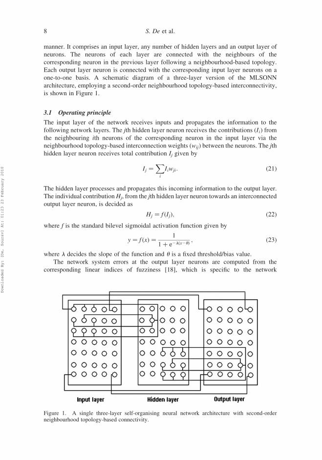
one-to-one basis. A schematic diagram of a three-layer version of the MLSONN
architecture, employing a second-order neighbourhood topology-based interconnectivity,
is shown in Figure 1.
3.1 Operating principle
The input layer of the network receives inputs and propagates the information to the
following network layers. The jth hidden layer neuron receives the contributions ðIiÞ from
the neighbouring ith neurons of the corresponding neuron in the input layer via the
neighbourhood topology-based interconnection weights ðwijÞ between the neurons. The jth
hidden layer neuron receives total contribution Ij given by
Ij ¼Xi
Iiwji: ð21Þ
The hidden layer processes and propagates this incoming information to the output layer.
The individual contributionHj, from the jth hidden layer neuron towards an interconnected
output layer neuron, is decided as
Hj ¼ f ðIjÞ; ð22Þ
where f is the standard bilevel sigmoidal activation function given by
y ¼ f ðxÞ ¼1
1þ e2lðx2uÞ; ð23Þ
where l decides the slope of the function and u is a fixed threshold/bias value.
The network system errors at the output layer neurons are computed from the
corresponding linear indices of fuzziness [18], which is specific to the network
Figure 1. A single three-layer self-organising neural network architecture with second-orderneighbourhood topology-based connectivity.
S. De et al.8
Downloaded By: [De, Sourav] At: 01:23 23 February 2010
architecture. The interconnection weights are adjusted using the standard backpropagation
algorithm. The next stage of processing is carried out by network architecture on the
outputs fed back into the input layer from the output layer after the weights are adjusted.
This processing is repeated until the interconnection weights stabilise or the system errors
are reduced below some tolerable limits.
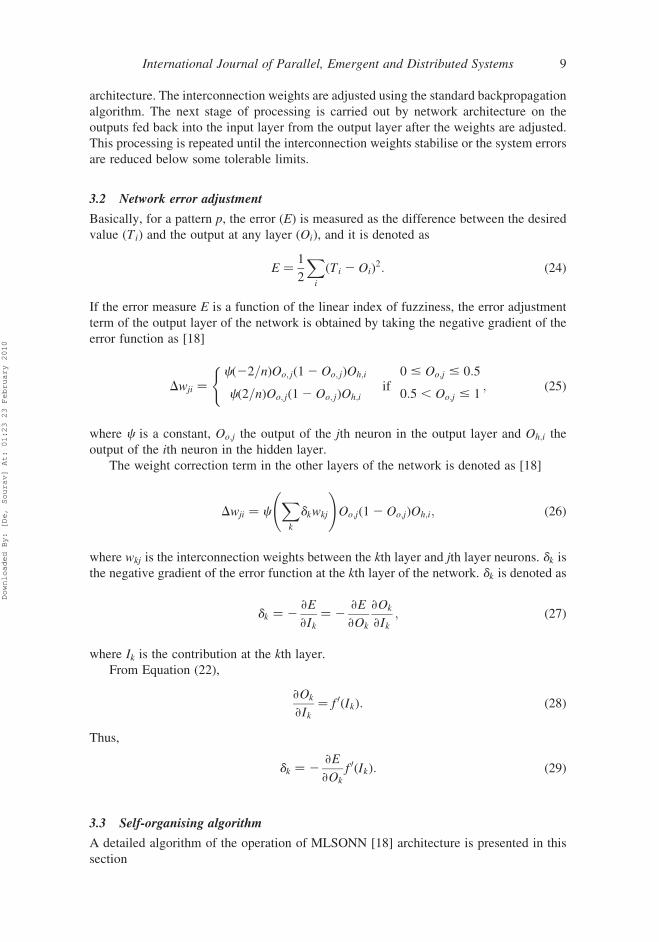
3.2 Network error adjustment
Basically, for a pattern p, the error (E) is measured as the difference between the desired
value ðTiÞ and the output at any layer ðOiÞ, and it is denoted as
E ¼1
2
Xi
ðTi 2 OiÞ2: ð24Þ
If the error measure E is a function of the linear index of fuzziness, the error adjustment
term of the output layer of the network is obtained by taking the negative gradient of the
error function as [18]
Dwji ¼cð22=nÞOo; jð12 Oo; jÞOh;i
cð2=nÞOo; jð12 Oo; jÞOh;iif
0 # Oo;j # 0:5
0:5 , Oo;j # 1
(; ð25Þ
where c is a constant, Oo;j the output of the jth neuron in the output layer and Oh;i the
output of the ith neuron in the hidden layer.
The weight correction term in the other layers of the network is denoted as [18]
Dwji ¼ cXk
dkwkj
!Oo;jð12 Oo;jÞOh;i; ð26Þ
where wkj is the interconnection weights between the kth layer and jth layer neurons. dk is
the negative gradient of the error function at the kth layer of the network. dk is denoted as
dk ¼ 2›E
›Ik¼ 2
›E
›Ok
›Ok
›Ik; ð27Þ
where Ik is the contribution at the kth layer.
From Equation (22),
›Ok
›Ik¼ f 0ðIkÞ: ð28Þ
Thus,
dk ¼ 2›E
›Ok
f 0ðIkÞ: ð29Þ
3.3 Self-organising algorithm
A detailed algorithm of the operation of MLSONN [18] architecture is presented in this
section
International Journal of Parallel, Emergent and Distributed Systems 9
Downloaded By: [De, Sourav] At: 01:23 23 February 2010

1 Begin
2 Read pix[l] [m] [n]
3 t:=0, wt[t] [l] [l+1] :=1, l= [1,2,3]
4 Do
5 Do
6 pix[l+1] [m] [n]= fsig [SUM[pix[l] [m] [n] x wt[t] [l] [l+1]]]
7 Loop for all layers
8 Do
9 Determine Deltawt[t] [l] [l+1] using backpropagation algorithm
10 Loop for all layers
11 pix[1] [m] [n]=pix[3] [m] [n]
12 Loop Until((wt[t] [l] [l-1]-wt[t-1] [l] [l-1])<eps)
13 End
Remark. pix[l] [m] [n] is the fuzzified image pixel information at row m and column n
at the network layers, i.e. the fuzzy membership values of the pixel intensities in the
image scene. pix[1][m] [n] is the fuzzy membership information of the input
image scene and is fed as inputs to the input layer of the network. pix[2][m] [n] and
pix[3][m] [n] are the corresponding information at the hidden and output layers. fsig is
the standard sigmoidal activation function and wt[t][l][l þ 1] is the inter-layer
interconnection weights between the network layers at a particular epoch t. Deltawt [t]
[l] [l þ 1] is the weight correction term at a particular epoch.eps is the tolerable error.
Algorithm Description
The above algorithm demonstrates self-organisation of the MLSONN [18] architecture
of the fuzzified image pixel intensity levels, pix[l][m][n], by means of a neighbourhood
topology-based interconnection weights wt[t][l][l þ 1] between its layers. Each individual
layer processes the input information by applying a sigmoidal activation function (fsig).
This process is repeated for all the layers. The interconnection weights are adjusted by
computing the network errors. The output layer outputs are fed back to the input layer.
This processing is carried out until the network converges.
It may be noted that the MLSONN architecture uses a sigmoidal activation function
characterised by a bilevel response. Moreover, the architecture assumes homogeneity of
the input image information. However, in real-world situations, images exhibit a fair
amount of heterogeneity in its information content which encompasses over the entire
image pixel neighbourhoods. In the next section, we present two improved versions of the
sigmoidal activation function to address these limitations.
4. OptiMUSIG activation function
It is evident that the standard bilevel sigmoidal activation function given in Equation
(23) produces bipolar responses [0(darkest)/1(brightest)] to incident input information.
Hence, this activation function is unable to classify an image into multiple levels of grey.
The bipolar form of the sigmoidal activation function has been extended into a
MUSIG activation function [20] to generate multilevel outputs corresponding to input
multilevel information. The multilevel form of the standard sigmoidal activation
S. De et al.10
Downloaded By: [De, Sourav] At: 01:23 23 February 2010
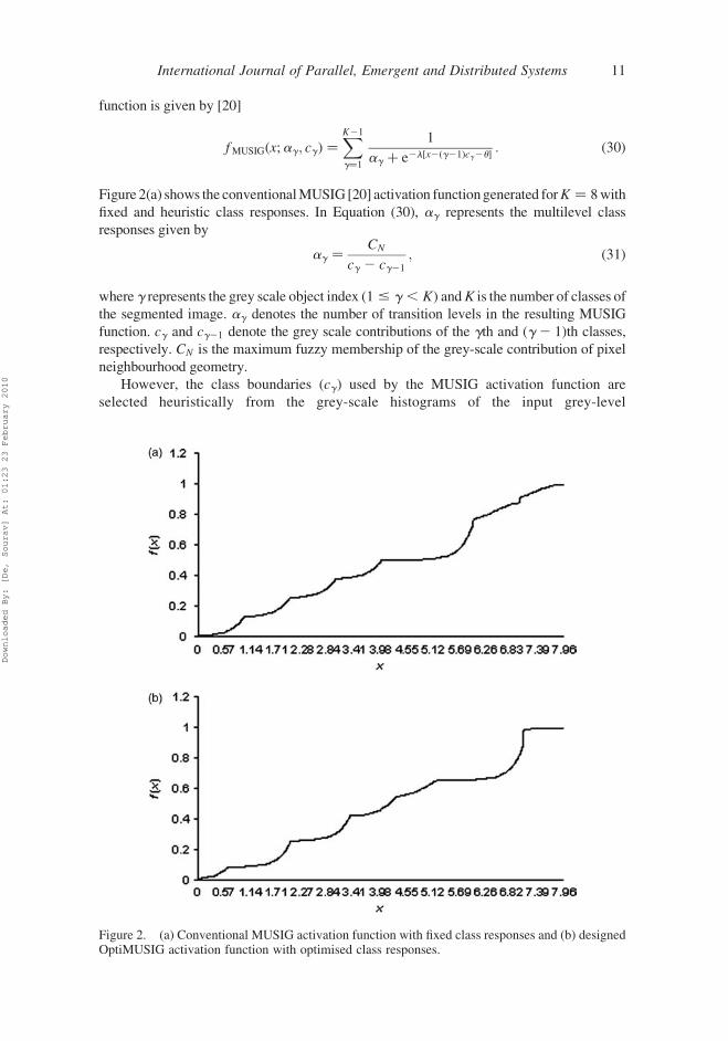
function is given by [20]
fMUSIGðx;ag; cgÞ ¼XK21
g¼1
1
ag þ e2l½x2ðg21Þcg2u�: ð30Þ
Figure 2(a) shows the conventionalMUSIG [20] activation functiongenerated forK ¼ 8with
fixed and heuristic class responses. In Equation (30), ag represents the multilevel class
responses given by
ag ¼CN
cg 2 cg21
; ð31Þ
where g represents the grey scale object index ð1 # g , KÞ andK is the number of classes of
the segmented image. ag denotes the number of transition levels in the resulting MUSIG
function. cg and cg21 denote the grey scale contributions of the gth and ðg2 1Þth classes,
respectively. CN is the maximum fuzzy membership of the grey-scale contribution of pixel
neighbourhood geometry.
However, the class boundaries ðcgÞ used by the MUSIG activation function are
selected heuristically from the grey-scale histograms of the input grey-level
Figure 2. (a) Conventional MUSIG activation function with fixed class responses and (b) designedOptiMUSIG activation function with optimised class responses.
International Journal of Parallel, Emergent and Distributed Systems 11
Downloaded By: [De, Sourav] At: 01:23 23 February 2010

images, assuming homogeneity of the underlying image information. Since real-life
images are heterogeneous in nature, the class boundaries would differ from one
image to another. So, optimised class boundaries derived from the image context would
faithfully incorporate the intensity distribution of the images in the characteristic
neuronal activations.
An optimised form of the MUSIG activation function, using optimised class
boundaries, can be represented as
fOptiMUSIG ¼XK21
g¼1
1
agopt þ e2l½x2ðg21Þcgopt2u�; ð32Þ
where cgopt are the optimised grey-scale contributions corresponding to optimised class
boundaries. agopt are the respective optimised multilevel class responses. These parameters
can be derived by suitable optimisation of the segmentation of input images.
The algorithm for designing the OptiMUSIG activation function through the evolution
of optimised class responses is illustrated below.
Algorithm for designing OptiMUSIG activation function
1 Begin
Generation of Optimised class boundaries
2 count: =0
3 Initialise Pop [count], K
4 Compute Fun(Pop [count])
5 Do
6 count:= count+1
7 Select Pop [count]
8 Crossover Pop [count]
9 Mutate Pop [count]
10 Loop Until (Fun(Pop [count])-Fun(Pop [count-1])<=eps)
11 clbound [K]:=Pop [count]
OptiMUSIG function generation phase
12 Generate OptiMUSIG with clbound [K]
13 End
Remark. Pop[count] is the initial population of class boundaries clbound[K] in the
range [0,255]. K is the number of target classes. Fun represents either of the
fitness functions r, F, F0 and Q. Selection of chromosomes based on better
fitness value. GA crossover operation. GA mutation operation. eps is the tolerable
error.
S. De et al.12
Downloaded By: [De, Sourav] At: 01:23 23 February 2010
5. Evaluation of segmentation efficiency
Several unsupervised subjective measures have been proposed [37] to determine the
segmentation efficiency of the existing segmentation algorithms. The following
subsections discuss some of these measures.
5.1 Correlation coefficient (r)
The standard measure of correlation coefficient (r) [20] can be used to assess the quality of
segmentation achieved. It is given by
r ¼ð1=n2Þ
Pni¼1
Pnj¼1ðIij 2
�IÞðSij 2 �SÞffiffiffiffiffiffiffiffiffiffiffiffiffiffiffiffiffiffiffiffiffiffiffiffiffiffiffiffiffiffiffiffiffiffiffiffiffiffiffiffiffiffiffiffiffiffiffiffiffiffiffið1=n2Þ
Pni¼1
Pnj¼1ðIij 2
�IÞ2q ffiffiffiffiffiffiffiffiffiffiffiffiffiffiffiffiffiffiffiffiffiffiffiffiffiffiffiffiffiffiffiffiffiffiffiffiffiffiffiffiffiffiffiffiffiffiffiffiffiffiffiffiffi
ð1=n2ÞPn
i¼1
Pnj¼1ðSij 2
�SÞ2q ; ð33Þ
where Iij; 1 # i; j # n and Sij; 1 # i; j # n are the original and the segmented images
respectively, each of dimensions n £ n. �I and �S are their respective mean intensity values.
A higher value of r implies better quality of segmentation.
However, correlation coefficient has many limitations. The foremost disadvantage is
that it is computationally intensive. This often confines its usefulness for image
registration, i.e. orienting and positioning two images so that they overlap. Moreover, the
correlation coefficient is very much sensible to image skewing, fading, etc. that inevitably
occur in imaging systems.
5.2 Empirical goodness measures
In this subsection, an overview of three different empirical goodness measures is
discussed.
Let SI be the area of image (I) to be segmented into N number of regions. If Rk denotes
the number of pixels in region k, then the area of region k is Sk ¼ jRkj. For the grey-level
intensity feature t, let CtðpÞ denote the value of t for pixel p. The average value of t in
region k is then represented as
CtðRkÞ ¼
Pp[Rk
CtðpÞ
Sk: ð34Þ
The squared colour error of region k is then represented as
e2k ¼X
t1ðr;g;bÞ
Xp[Rk
ðCtðpÞ2 CtðRkÞÞ2: ð35Þ
Based on these notations, three empirical measures (F, F0 and Q) are described below.
5.2.1 Segmentation efficiency measure (F)
Liu and Yang proposed a quantitative evaluation function (EF) F for image segmentation
[30]. It is given as
FðIÞ ¼ffiffiffiffiN
p XNk¼1
e2kffiffiffiffiffiSk
p : ð36Þ
International Journal of Parallel, Emergent and Distributed Systems 13
Downloaded By: [De, Sourav] At: 01:23 23 February 2010
5.2.2 Segmentation efficiency measure (F0)
Borsotti et al. [31] proposed another EF, F0, to improve the performance of Liu and Yang’s
method [30]. The EF, F0, is represented as
F0ðIÞ ¼1
SI
ffiffiffiffiffiffiffiffiffiffiffiffiffiffiffiffiffiffiffiffiffiffiffiffiffiffiffiffiffiffiffiffiffiffiffiffiffiffiffiffiXMaxArea
m¼1
½NðmÞ�1þð1=mÞ
vuut Xk¼1
Ne2kffiffiffiffiffiSk
p ; ð37Þ
where NðmÞ is represented as the number of regions in the segmented image of an area ofm
and MaxArea is used as the area of the largest region in the segmented image.
5.2.3 Segmentation efficiency measure (Q)
Borsotti et al. [31] suggested another EF, Q, to improve upon the performance of F and F0.
The EF, Q, is denoted as
QðIÞ ¼1
1000:SI
ffiffiffiffiN
p XNk¼1
e2k1þ log Sk
þNðSkÞ
Sk
� �2" #
: ð38Þ
It may be noted that lower values of F, F0 and Q imply better segmentation in contrast
to the correlation coefficient (r) where higher values dictate terms.
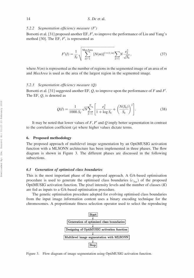
6. Proposed methodology
The proposed approach of multilevel image segmentation by an OptiMUSIG activation
function with a MLSONN architecture has been implemented in three phases. The flow
diagram is shown in Figure 3. The different phases are discussed in the following
subsections.
6.1 Generation of optimised class boundaries
This is the most important phase of the proposed approach. A GA-based optimisation
procedure is used to generate the optimised class boundaries ðcgoptÞ of the proposed
OptiMUSIG activation function. The pixel intensity levels and the number of classes (K)
are fed as inputs to a GA-based optimisation procedure.
The genetic optimisation procedure adopted for evolving optimised class boundaries
from the input image information content uses a binary encoding technique for the
chromosomes. A proportionate fitness selection operator used to select the reproducing
Figure 3. Flow diagram of image segmentation using OptiMUSIG activation function.
S. De et al.14
Downloaded By: [De, Sourav] At: 01:23 23 February 2010

chromosomes is supported by a single point crossover operation. A population size of 50
has been used in this treatment.
The segmentation efficiency measures (r, F, F0, Q) given in Equations (33,36–38),
respectively, are used as fitness functions for this phase. The selection probability of the ith
chromosome is determined as
pi ¼f iXn
j¼1
f j
; ð39Þ
where f i is the fitness value of the ith chromosome and n is the population size. The
cumulative fitness Pi of each chromosome is evaluated by adding individual fitnesses in
ascending order. Subsequently, the crossover and mutation operators are applied to evolve
a new population.
6.2 Designing of OptiMUSIG activation function
In this phase, the optimised cgopt parameters obtained from the previous phase are used to
determine the corresponding agopt parameters using Equation (31). These agopt
parameters are further employed to obtain the different transition levels of the
OptiMUSIG activation function. Figure 2(b) shows a designed OptiMUSIG activation
function for K ¼ 8.
6.3 Multilevel image segmentation by OptiMUSIG
This is the final phase of the proposed approach. A single MLSONN architecture guided
by the designed OptiMUSIG activation function is used to segment real-life multilevel
images in this phase. The neurons of the different layers of the MLSONN architecture
generate different grey-level responses to the input image information. The processed
input information propagates to the succeeding network layers. Since the network has no
a priori knowledge about the output, the system errors are determined by the subnormal
linear index of fuzziness ðnls Þ, using Equation (8) at the output layer of the MLSONN
architecture. These errors are used to adjust the interconnection weights between the
different layers using the standard backpropagation algorithm. The outputs at the
output layer of the network are then fed back to the input layer for further processing
to minimise the system errors. When the self-supervision of the network attains
stabilisation, the original input image gets segmented into different multilevel
regions depending upon the optimised transition levels of the OptiMUSIG activation
function.
7. Results
The proposed approach has been applied for the segmentation of a synthetic multilevel
image (Figure 4 of dimensions 128 £ 128) and two multilevel real-life images, viz. Lena
and Baboon (Figures 5 and 6 of dimensions 128 £ 128). Experiments have been conducted
with K ¼ {6; 8} classes [segmented outputs are reported for K ¼ 8]. The OptiMUSIG
activation function has been designed with a fixed slope (l) and a fixed threshold (u)
[results are reported for l ¼ 4 and u ¼ 2]. Higher l values lead to a faster convergence at
the cost of lower segmentation quality and vice versa. Higher u values lead to
overthresholding, whereas lower values lead to underthresholding.
International Journal of Parallel, Emergent and Distributed Systems 15
Downloaded By: [De, Sourav] At: 01:23 23 February 2010

Sections 7.1.1 and 7.2.1, respectively, discuss the segmentation efficiency of the
proposed OptiMUSIG activation function and the corresponding segmented outputs.
The proposed approach has been compared with the segmentation achieved by means
of the conventional MUSIG activation function with heuristic class levels and same
number of classes. Furthermore, comparative studies with the standard FCM algorithm
have also been carried out for the same number of classes.
Figure 4. Original synthetic image.
Figure 5. Original Lena image.
S. De et al.16
Downloaded By: [De, Sourav] At: 01:23 23 February 2010

Sections 7.1.2 and 7.2.2, respectively, elaborate the performance of the conventional
MUSIG activation function as regard to its efficacy in the segmentation of multilevel test
images. The corresponding performance metrics and the segmented output images
obtained by the standard FCM algorithm are illustrated in Sections 7.1.3 and 7.2.3,
respectively.
7.1 Quantitative performance analysis of segmentation
This section illustrates the quantitative measures of evaluation of the segmentation
efficiency of the proposed OptiMUSIG, MUSIG and the FCM algorithm for K ¼ {6; 8}using the four measures of the segmentation efficiency, viz. correlation coefficient (r) and
EFs (F, F0 and Q). Section 7.1.1 discusses the results obtained with the OptiMUSIG
activation function. The corresponding results obtained with the conventional fixed class
response-based MUSIG activation function and with the standard FCM algorithm are
provided in Sections 7.1.2 and 7.1.3, respectively.
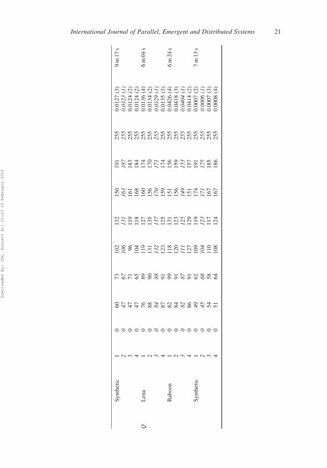
7.1.1 OptiMUSIG-guided segmentation evaluation
The optimised sets of class boundaries ðcgoptÞ obtained using GAwith four EFs (r, F, F0 and
Q) and different classes are shown in Tables 1–6. The EFs, shown in the first columns of
the tables, are applied as the fitness functions to generate GA-based optimised class
boundaries. The penultimate columns of the tables show the quality measures h [graded on
a scale of 1 (best) to 4 (worst)] obtained by segmentation of the test images based on the
corresponding set of optimised class boundaries. The best values obtained are indicated in
the tables in italic face for easy reckoning. The average computation times (AvgTime) are
also shown in the table alongside.
Figure 6. Original Baboon image.
International Journal of Parallel, Emergent and Distributed Systems 17
Downloaded By: [De, Sourav] At: 01:23 23 February 2010
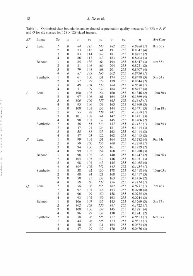
Table 1. Optimised class boundaries and evaluated segmentation quality measures for EFs r, F, F0
and Q for six classes for 128 £ 128-sized images.
EF Image Set c1 c2 c3 c4 c5 c6 h AvgTime
r Lena 1 0 84 115 143 182 255 0.8488 (1) 8m56 s2 0 73 115 141 191 255 0.8347 (4)3 0 83 114 142 181 255 0.8457 (2)4 0 86 117 143 183 255 0.8404 (3)
Baboon 1 0 85 136 164 194 255 0.8647 (3) 4m 55 s2 0 81 146 169 204 255 0.8721 (2)3 0 79 148 168 201 255 0.8607 (4)4 0 81 143 165 202 255 0.8750 (1)
Synthetic 1 0 61 100 131 174 255 0.8478 (3) 5m 24 s2 0 57 99 129 179 255 0.8544 (2)3 0 49 104 132 184 255 0.8630 (1)4 0 51 99 132 184 255 0.8457 (4)
F Lena 1 0 100 105 154 160 255 0.1346 (2) 10m50 s2 0 97 106 161 164 255 0.1369 (4)3 0 100 106 157 165 255 0.1345 (1)4 0 95 106 153 163 255 0.1360 (3)
Baboon 1 0 100 101 133 144 255 0.1471 (3) 11m18 s2 0 95 98 139 141 255 0.1459 (1)3 0 101 108 141 142 255 0.1471 (3)4 0 98 101 137 145 255 0.1466 (2)
Synthetic 1 0 56 85 133 137 255 0.1411 (1) 10m55 s2 0 47 91 124 181 255 0.1414 (3)3 0 55 88 133 163 255 0.1414 (3)4 0 47 93 122 168 255 0.1413 (2)
F0 Lena 1 0 99 101 151 164 255 0.1282 (4) 9m 34s2 0 99 100 155 168 255 0.1278 (1)3 0 94 106 156 161 255 0.1279 (2)4 0 99 105 154 168 255 0.1280 (3)
Baboon 1 0 98 102 136 140 255 0.1447 (2) 10m36 s2 0 104 105 142 146 255 0.1451 (3)3 0 98 101 143 145 255 0.1465 (4)4 0 104 105 142 145 255 0.1434 (1)
Synthetic 1 0 58 92 130 178 255 0.1418 (4) 10m05 s2 0 48 94 121 168 255 0.1417 (3)3 0 50 85 132 163 255 0.1416 (2)4 0 59 80 137 156 255 0.1414 (1)
Q Lena 1 0 96 98 155 162 255 0.0731 (1) 7m46 s2 0 97 101 146 153 255 0.0750 (4)3 0 96 99 150 158 255 0.0735 (2)4 0 93 102 159 163 255 0.0744 (3)
Baboon 1 0 106 107 137 145 255 0.1769 (3) 5m 37 s2 0 102 103 135 141 255 0.1722 (1)3 0 100 106 139 145 255 0.1781 (4)4 0 96 99 137 138 255 0.1741 (2)
Synthetic 1 0 50 96 125 177 255 0.0673 (1) 6m37 s2 0 48 96 126 173 255 0.0673 (1)3 0 50 90 131 164 255 0.0674 (2)4 0 47 99 137 170 255 0.0676 (3)
S. De et al.18
Downloaded By: [De, Sourav] At: 01:23 23 February 2010

Table 2. Optimised class boundaries and evaluated segmentation quality measures for EFs r, F, F0
and Q for six classes for 256 £ 256-sized images.
EF Image Set c1 c2 c3 c4 c5 c6 h AvgTime
r Lena 1 0 60 102 141 197 255 0.9570 (1) 10m37 s2 0 69 115 151 190 255 0.9516 (2)3 0 67 112 151 190 255 0.9469 (3)4 0 60 102 142 192 255 0.9301 (4)
Baboon 1 0 68 112 152 190 255 0.9320 (1) 7m55 s2 0 67 107 147 185 255 0.9269 (2)3 0 69 115 151 190 255 0.9088 (3)4 0 67 112 151 190 255 0.9001 (4)
F Lena 1 0 77 91 159 166 255 0.2000 (2) 11m44 s2 0 84 87 161 165 255 0.1995 (1)3 0 81 87 165 168 255 0.2002 (3)4 0 71 99 159 164 255 0.2013 (4)
Baboon 1 0 98 99 149 150 255 0.3003 (2) 18m49 s2 0 94 95 145 146 255 0.3000 (1)3 0 96 97 147 148 255 0.3004 (3)4 0 97 99 149 150 255 0.3027 (4)
F0 Lena 1 0 82 96 163 164 255 0.1807 (3) 11m44 s2 0 77 90 163 169 255 0.1797 (1)3 0 72 94 162 164 255 0.1806 (2)4 0 77 96 154 163 255 0.1808 (4)
Baboon 1 0 92 93 143 144 255 0.2591 (1) 10m28 s2 0 89 96 147 152 255 0.2637 (3)3 0 95 98 149 153 255 0.2638 (4)4 0 101 104 151 152 255 0.2635 (2)
Q Lena 1 0 79 91 158 160 255 0.4277 (1) 11m27 s2 0 81 89 154 157 255 0.4288 (3)3 0 82 89 160 161 255 0.4280 (2)4 0 80 89 159 162 255 0.4291 (4)
Baboon 1 0 95 100 146 148 255 0.0769 (1) 9m13 s2 0 95 99 151 152 255 0.0781 (4)3 0 102 103 150 154 255 0.0779 (2)4 0 102 103 143 145 255 0.0780 (3)
Table 3. Optimised class boundaries and evaluated segmentation quality measures for EFs r, F, F0
and Q for six classes for 512 £ 512-sized images.
EF Image Set c1 c2 c3 c4 c5 c6 h AvgTime
r Lena 1 0 49 107 148 190 255 0.9402 34m59 sBaboon 1 0 70 115 150 180 255 0.8922 45m01 s
F Lena 1 0 107 114 160 164 255 0.2892 29m36 sBaboon 1 0 92 93 144 145 255 0.2671 30m15 s
F0 Lena 1 0 86 87 143 145 255 0.3074 28m31 sBaboon 1 0 90 91 141 143 255 0.3272 49m35 s
Q Lena 1 0 107 114 160 162 255 0.1864 35m02 sBaboon 1 0 86 91 143 145 255 0.2840 29m26 s
International Journal of Parallel, Emergent and Distributed Systems 19
Downloaded By: [De, Sourav] At: 01:23 23 February 2010
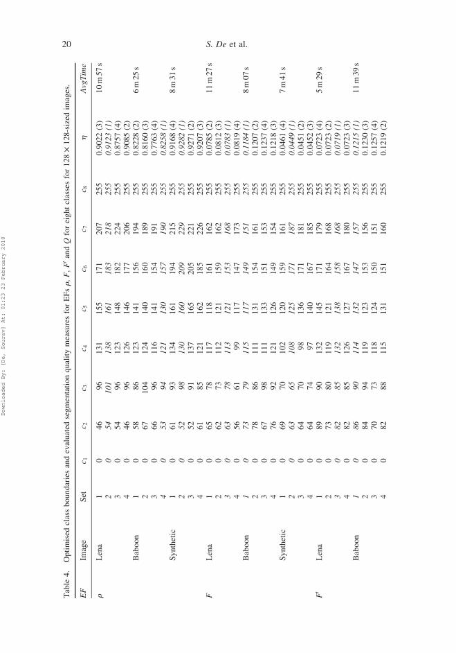
Table
4.
Optimised
classboundariesandevaluated
segmentationqualitymeasuresforEFsr,F,F0andQ
foreightclassesfor128£128-sized
images.
EF
Image
Set
c 1c 2
c 3c 4
c 5c 6
c 7c 8
hAvgTime
rLena
10
46
96
131
155
171
207
255
0.9022(3)
10m57s
20
54
101
138
161
183
218
255
0.9123(1)
30
54
96
123
148
182
224
255
0.8757(4)
40
46
96
126
146
177
206
255
0.9085(2)
Baboon
10
58
86
123
141
156
194
255
0.8228(2)
6m25s
20
67
104
124
140
160
189
255
0.8160(3)
30
66
96
116
141
154
191
255
0.7763(4)
40
53
94
121
130
157
190
255
0.8258(1)
Synthetic
10
61
93
134
161
194
215
255
0.9168(4)
8m31s
20
52
98
130
160
209
229
255
0.9282(1)
30
52
91
137
165
205
221
255
0.9271(2)
40
61
85
121
162
185
226
255
0.9207(3)
FLena
10
65
78
117
118
161
162
255
0.0785(2)
11m27s
20
62
73
112
121
159
162
255
0.0812(3)
30
63
78
113
121
153
168
255
0.0783(1)
40
56
61
99
117
147
173
255
0.0819(4)
Baboon
10
73
79
115
117
149
151
255
0.1184(1)
8m07s
20
78
86
111
131
154
161
255
0.1207(2)
30
67
98
111
133
151
153
255
0.1237(4)
40
76
92
121
126
149
154
255
0.1218(3)
Synthetic
10
69
70
102
120
159
161
255
0.0461(4)
7m41s
20
63
65
108
125
171
187
255
0.0449(1)
30
64
70
98
136
171
181
255
0.0451(2)
40
64
74
97
140
167
185
255
0.0452(3)
F0
Lena
10
89
90
132
145
171
179
255
0.0723(4)
5m29s
20
73
80
119
121
164
168
255
0.0723(2)
30
82
85
132
138
158
168
255
0.0719(1)
40
82
85
126
127
167
180
255
0.0723(3)
Baboon
10
86
90
114
132
147
157
255
0.1215(1)
11m39s
20
84
94
119
123
153
156
255
0.1230(3)
30
70
73
118
124
150
151
255
0.1257(4)
40
82
88
115
131
151
160
255
0.1219(2)
S. De et al.20
Downloaded By: [De, Sourav] At: 01:23 23 February 2010
Synthetic
10
60
73
102
132
150
191
255
0.0127(3)
9m17s
20
47
67
106
131
163
187
255
0.0123(1)
30
47
71
96
119
161
183
255
0.0124(2)
40
47
65
104
118
168
184
255
0.0124(2)
QLena
10
76
89
119
127
160
174
255
0.0136(4)
6m04s
20
88
90
131
135
156
170
255
0.0134(2)
30
84
88
132
137
170
171
255
0.0129(1)
40
87
91
123
125
159
174
255
0.0135(3)
Baboon
10
82
99
118
131
151
156
255
0.0426(4)
6m24s
20
84
91
120
123
156
159
255
0.0418(3)
30
82
87
111
125
149
153
255
0.0404(1)
40
86
91
127
129
151
157
255
0.0414(2)
Synthetic
10
49
62
109
119
174
191
255
0.0007(2)
7m13s
20
45
68
104
123
171
175
255
0.0006(1)
30
54
58
110
117
167
185
255
0.0007(3)
40
51
64
108
124
167
186
255
0.0008(4)
International Journal of Parallel, Emergent and Distributed Systems 21
Downloaded By: [De, Sourav] At: 01:23 23 February 2010
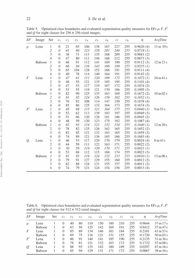
Table 5. Optimised class boundaries and evaluated segmentation quality measures for EFs r, F, F0
and Q for eight classes for 256 £ 256-sized images.
EF Image Set c1 c2 c3 c4 c5 c6 c7 c8 h AvgTime
r Lena 1 0 21 65 106 138 167 227 255 0.9620 (4) 11m 39 s2 0 41 80 123 158 201 240 255 0.9718 (1)3 0 38 71 113 135 168 209 255 0.9681 (2)4 0 47 80 111 146 168 212 255 0.9673 (3)
Baboon 1 0 68 91 112 141 169 190 255 0.9112 (3) 12m21 s2 0 66 84 116 143 166 189 255 0.9235 (1)3 0 65 104 128 152 168 191 255 0.9111 (4)4 0 40 78 114 140 164 191 255 0.9143 (2)
F Lena 1 0 47 61 111 120 169 172 255 0.1072 (1) 24m41 s2 0 48 55 121 135 185 195 255 0.1101 (4)3 0 47 53 117 119 167 172 255 0.1074 (2)4 0 53 55 119 121 170 186 255 0.1095 (3)
Baboon 1 0 82 90 125 133 163 169 255 0.1672 (2) 10m02 s2 0 81 82 124 126 159 162 255 0.1652 (1)3 0 76 82 108 114 147 150 255 0.1678 (4)4 0 85 86 125 132 164 173 255 0.1674 (3)
F0 Lena 1 0 48 69 115 121 164 175 255 0.0940 (1) 9m53 s2 0 52 62 113 139 183 197 255 0.0949 (3)3 0 51 66 120 128 181 186 255 0.0945 (2)4 0 48 59 120 123 175 182 255 0.1087 (4)
Baboon 1 0 82 83 114 121 152 154 255 0.1640 (1) 12m20 s2 0 78 82 125 126 162 165 255 0.1652 (2)3 0 82 85 121 132 163 165 255 0.1659 (3)4 0 74 89 121 136 165 166 255 0.1683 (4)
Q Lena 1 0 46 53 117 120 170 179 255 0.0024 (4) 8m 43 s2 0 44 59 111 122 163 171 255 0.0022 (2)3 0 50 59 119 120 170 171 255 0.0021 (1)4 0 53 68 112 115 168 174 255 0.0023 (3)
Baboon 1 0 81 85 119 124 152 153 255 0.0010 (1) 13m06 s2 0 79 91 127 129 155 160 255 0.0012 (3)3 0 82 88 124 131 155 157 255 0.0011 (2)4 0 74 79 121 124 154 156 255 0.0013 (4)
Table 6. Optimised class boundaries and evaluated segmentation quality measures for EFs r, F, F0
and Q for eight classes for 512 £ 512-sized images.
EF Image Set c1 c2 c3 c4 c5 c6 c7 c8 h AvgTime
r Lena 1 0 40 80 110 150 180 210 255 0.9644 37m17 sBaboon 1 0 63 94 125 142 169 191 255 0.9412 37m47 s
F Lena 1 0 85 89 134 146 181 184 255 0.2101 41m53 sBaboon 1 0 69 75 116 121 151 155 255 0.1720 50m03 s
F0 Lena 1 0 86 91 140 141 185 190 255 0.2135 31m36 sBaboon 1 0 78 81 121 132 163 172 255 0.1732 57m08 s
Q Lena 1 0 88 93 135 142 180 189 255 0.0297 47m16 sBaboon 1 0 85 94 129 131 171 172 255 0.0067 38m16 s
S. De et al.22
Downloaded By: [De, Sourav] At: 01:23 23 February 2010

7.1.2 MUSIG-guided segmentation evaluation
Tables 7–12 show the heuristically selected class boundaries for the conventional MUSIG
activation function used in the segmentation of the test images alongwith the corresponding
quality measure values evaluated after the segmentation process. Similar to the optimised
results, the best values obtained are also indicated in these tables in italic face.
7.1.3 FCM-guided segmentation evaluation
The standard FCM algorithm has been applied for the segmentation of the test multilevel
images. As already stated, the FCM algorithm resorts to an initial random selection of the
cluster centroids out of the image data. The algorithm converges to a known number of
cluster centroids. Tables 13–18 list the segmentation metrics r, F, F0 andQ obtained in the
segmentation of the test images of different dimensions and number of classes. The italic
faced values in Tables 13–18 signify the best metrics obtained with the FCM algorithm.
7.2 Multilevel image segmentation outputs
In this section, the segmented multilevel output images obtained for the different classes,
with the proposed optimised approach vis-a-vis those obtained with the heuristically
chosen class boundaries and the standard FCM algorithm, are presented for the four
quantitative measures used.
7.2.1 OptiMUSIG-guided segmented outputs
The segmented multilevel test images obtained with the MLSONN architecture using the
OptiMUSIG activation function for the K ¼ 8 class and different dimensions (128 £ 128
and 256 £ 256) corresponding to the best segmentation quality measures (r, F, F0, Q)
achieved are shown in Figures 7–11.
The best outputs of the test images (512 £ 512) obtained with the OptiMUSIG
activation function with the EF Q are shown in Figures 12 and 13.
7.2.2 MUSIG-guided segmented outputs
The segmented multilevel test images obtained with the MLSONN architecture
characterised by the conventional MUSIG activation employing fixed class responses
for K ¼ 8 classes and different dimensions (128 £ 128 and 256 £ 256) yielding the best
segmentation quality measures (r, F, F0, Q) achieved are shown in Figures 14–18.
The best outputs of the test images (512 £ 512) obtained with the MUSIG activation
function with the EF Q are shown in Figures 19 and 20.
7.2.3 FCM-guided segmented outputs
The segmented multilevel test images obtained with the standard FCM algorithm for
K ¼ 8 classes and different dimensions (128 £ 128 and 256 £ 256) yielding the best
segmentation quality measures (r, F, F0,Q) achieved are shown in Figures 21–25. The best
outputs of the test images (512 £ 512) obtained with the FCM activation function with the
EF Q are shown in Figures 26 and 27. From the results obtained, it is evident that the
OptiMUSIG activation function outperforms its conventional MUSIG counterpart as well
as the standard FCM algorithm as regard to the segmentation quality of the images for the
different classes and dimensions of the test images.
International Journal of Parallel, Emergent and Distributed Systems 23
Downloaded By: [De, Sourav] At: 01:23 23 February 2010
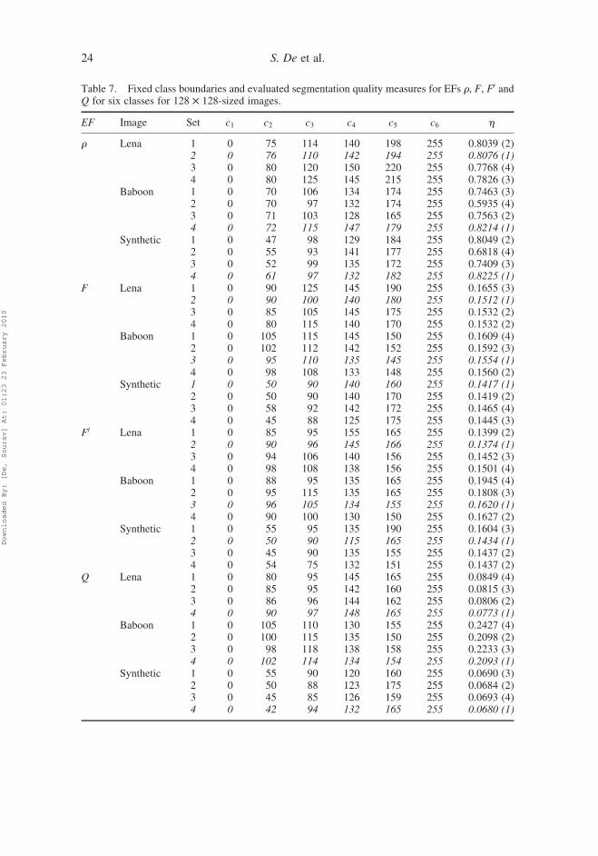
Table 7. Fixed class boundaries and evaluated segmentation quality measures for EFs r, F, F0 andQ for six classes for 128 £ 128-sized images.
EF Image Set c1 c2 c3 c4 c5 c6 h
r Lena 1 0 75 114 140 198 255 0.8039 (2)2 0 76 110 142 194 255 0.8076 (1)3 0 80 120 150 220 255 0.7768 (4)4 0 80 125 145 215 255 0.7826 (3)
Baboon 1 0 70 106 134 174 255 0.7463 (3)2 0 70 97 132 174 255 0.5935 (4)3 0 71 103 128 165 255 0.7563 (2)4 0 72 115 147 179 255 0.8214 (1)
Synthetic 1 0 47 98 129 184 255 0.8049 (2)2 0 55 93 141 177 255 0.6818 (4)3 0 52 99 135 172 255 0.7409 (3)4 0 61 97 132 182 255 0.8225 (1)
F Lena 1 0 90 125 145 190 255 0.1655 (3)2 0 90 100 140 180 255 0.1512 (1)3 0 85 105 145 175 255 0.1532 (2)4 0 80 115 140 170 255 0.1532 (2)
Baboon 1 0 105 115 145 150 255 0.1609 (4)2 0 102 112 142 152 255 0.1592 (3)3 0 95 110 135 145 255 0.1554 (1)4 0 98 108 133 148 255 0.1560 (2)
Synthetic 1 0 50 90 140 160 255 0.1417 (1)2 0 50 90 140 170 255 0.1419 (2)3 0 58 92 142 172 255 0.1465 (4)4 0 45 88 125 175 255 0.1445 (3)
F0 Lena 1 0 85 95 155 165 255 0.1399 (2)2 0 90 96 145 166 255 0.1374 (1)3 0 94 106 140 156 255 0.1452 (3)4 0 98 108 138 156 255 0.1501 (4)
Baboon 1 0 88 95 135 165 255 0.1945 (4)2 0 95 115 135 165 255 0.1808 (3)3 0 96 105 134 155 255 0.1620 (1)4 0 90 100 130 150 255 0.1627 (2)
Synthetic 1 0 55 95 135 190 255 0.1604 (3)2 0 50 90 115 165 255 0.1434 (1)3 0 45 90 135 155 255 0.1437 (2)4 0 54 75 132 151 255 0.1437 (2)
Q Lena 1 0 80 95 145 165 255 0.0849 (4)2 0 85 95 142 160 255 0.0815 (3)3 0 86 96 144 162 255 0.0806 (2)4 0 90 97 148 165 255 0.0773 (1)
Baboon 1 0 105 110 130 155 255 0.2427 (4)2 0 100 115 135 150 255 0.2098 (2)3 0 98 118 138 158 255 0.2233 (3)4 0 102 114 134 154 255 0.2093 (1)
Synthetic 1 0 55 90 120 160 255 0.0690 (3)2 0 50 88 123 175 255 0.0684 (2)3 0 45 85 126 159 255 0.0693 (4)4 0 42 94 132 165 255 0.0680 (1)
S. De et al.24
Downloaded By: [De, Sourav] At: 01:23 23 February 2010
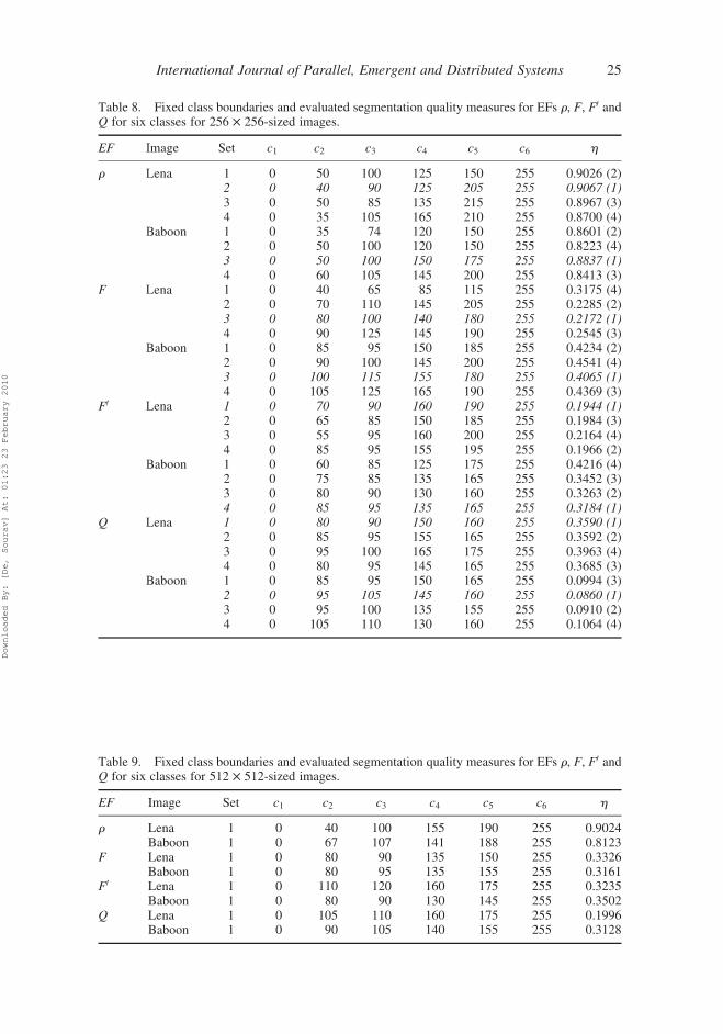
Table 8. Fixed class boundaries and evaluated segmentation quality measures for EFs r, F, F0 andQ for six classes for 256 £ 256-sized images.
EF Image Set c1 c2 c3 c4 c5 c6 h
r Lena 1 0 50 100 125 150 255 0.9026 (2)2 0 40 90 125 205 255 0.9067 (1)3 0 50 85 135 215 255 0.8967 (3)4 0 35 105 165 210 255 0.8700 (4)
Baboon 1 0 35 74 120 150 255 0.8601 (2)2 0 50 100 120 150 255 0.8223 (4)3 0 50 100 150 175 255 0.8837 (1)4 0 60 105 145 200 255 0.8413 (3)
F Lena 1 0 40 65 85 115 255 0.3175 (4)2 0 70 110 145 205 255 0.2285 (2)3 0 80 100 140 180 255 0.2172 (1)4 0 90 125 145 190 255 0.2545 (3)
Baboon 1 0 85 95 150 185 255 0.4234 (2)2 0 90 100 145 200 255 0.4541 (4)3 0 100 115 155 180 255 0.4065 (1)4 0 105 125 165 190 255 0.4369 (3)
F0 Lena 1 0 70 90 160 190 255 0.1944 (1)2 0 65 85 150 185 255 0.1984 (3)3 0 55 95 160 200 255 0.2164 (4)4 0 85 95 155 195 255 0.1966 (2)
Baboon 1 0 60 85 125 175 255 0.4216 (4)2 0 75 85 135 165 255 0.3452 (3)3 0 80 90 130 160 255 0.3263 (2)4 0 85 95 135 165 255 0.3184 (1)
Q Lena 1 0 80 90 150 160 255 0.3590 (1)2 0 85 95 155 165 255 0.3592 (2)3 0 95 100 165 175 255 0.3963 (4)4 0 80 95 145 165 255 0.3685 (3)
Baboon 1 0 85 95 150 165 255 0.0994 (3)2 0 95 105 145 160 255 0.0860 (1)3 0 95 100 135 155 255 0.0910 (2)4 0 105 110 130 160 255 0.1064 (4)
Table 9. Fixed class boundaries and evaluated segmentation quality measures for EFs r, F, F0 andQ for six classes for 512 £ 512-sized images.
EF Image Set c1 c2 c3 c4 c5 c6 h
r Lena 1 0 40 100 155 190 255 0.9024Baboon 1 0 67 107 141 188 255 0.8123
F Lena 1 0 80 90 135 150 255 0.3326Baboon 1 0 80 95 135 155 255 0.3161
F0 Lena 1 0 110 120 160 175 255 0.3235Baboon 1 0 80 90 130 145 255 0.3502
Q Lena 1 0 105 110 160 175 255 0.1996Baboon 1 0 90 105 140 155 255 0.3128
International Journal of Parallel, Emergent and Distributed Systems 25
Downloaded By: [De, Sourav] At: 01:23 23 February 2010
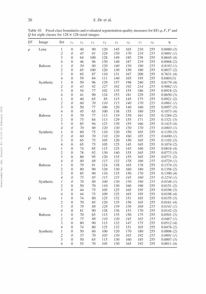
Table 10. Fixed class boundaries and evaluated segmentation quality measures for EFs r, F, F0 andQ for eight classes for 128 £ 128-sized images.
EF Image Set c1 c2 c3 c4 c5 c6 c7 c8 h
r Lena 1 0 40 90 120 145 165 210 255 0.8880 (3)2 0 45 91 128 150 170 218 255 0.9001 (1)3 0 64 100 128 149 185 238 255 0.8645 (4)4 0 46 96 130 140 187 219 255 0.8968 (2)
Baboon 1 0 50 80 120 140 150 190 255 0.8183 (1)2 0 65 100 120 130 150 180 255 0.8037 (2)3 0 65 87 110 131 167 200 255 0.7631 (4)4 0 59 84 111 140 165 195 255 0.6801(3)
Synthetic 1 0 50 96 129 157 198 240 255 0.8179 (4)2 0 43 92 127 162 192 214 255 0.9062 (1)3 0 54 77 102 135 155 186 255 0.8918 (2)4 0 41 90 124 153 181 229 255 0.8650 (3)
F Lena 1 0 40 65 85 115 145 175 255 0.0921 (2)2 0 60 70 110 115 140 170 255 0.0861 (1)3 0 50 77 100 120 140 160 255 0.0957 (3)4 0 45 65 100 138 155 180 255 0.1073 (4)
Baboon 1 0 70 77 113 119 159 161 255 0.1284 (2)2 0 75 84 113 129 155 171 255 0.1321 (3)3 0 65 94 123 139 155 166 255 0.1415 (4)4 0 70 90 120 130 150 170 255 0.0803 (1)
Synthetic 1 0 60 75 110 120 150 165 255 0.1150 (3)2 0 60 70 110 120 160 185 255 0.0490 (1)3 0 65 75 105 120 150 165 255 0.1102 (3)4 0 65 75 105 125 145 165 255 0.1074 (2)
F0 Lena 1 0 74 85 115 125 145 160 255 0.0818 (4)2 0 78 92 130 140 155 165 255 0.0773 (3)3 0 80 95 120 135 155 165 255 0.0771 (2)4 0 80 88 115 132 158 166 255 0.0729 (1)
Baboon 1 0 79 91 124 138 165 178 255 0.1374 (3)2 0 80 90 120 130 160 180 255 0.1356 (2)3 0 85 90 110 135 150 170 255 0.1390 (4)4 0 75 85 115 125 145 160 255 0.1254 (1)
Synthetic 1 0 70 80 100 130 150 180 255 0.0146 (1)2 0 50 70 110 130 160 190 255 0.0151 (2)3 0 44 75 105 125 165 195 255 0.0196 (3)4 0 44 75 109 125 165 195 255 0.0198 (4)
Q Lena 1 0 74 80 125 132 151 165 255 0.0155 (3)2 0 70 85 120 135 150 165 255 0.0161 (4)3 0 78 88 128 139 156 168 255 0.0141 (1)4 0 81 90 128 136 153 170 255 0.0142 (2)
Baboon 1 0 70 85 115 135 150 175 255 0.0501 (3)2 0 75 88 110 130 145 165 255 0.0467 (1)3 0 80 90 115 132 147 175 255 0.0512 (4)4 0 74 80 125 132 151 165 255 0.0476 (2)
Synthetic 1 0 50 60 100 120 170 180 255 0.0006 (2)2 0 55 70 105 130 165 192 255 0.0001 (1)3 0 50 65 115 130 160 185 255 0.0007 (3)4 0 55 70 105 130 165 192 255 0.0011 (4)
S. De et al.26
Downloaded By: [De, Sourav] At: 01:23 23 February 2010

Table 11. Fixed class boundaries and evaluated segmentation quality measures for EFs r, F, F0 andQ for eight classes for 256 £ 256-sized images.
EF Image Set c1 c2 c3 c4 c5 c6 c7 c8 h
r Lena 1 0 32 64 96 128 192 224 255 0.8927 (2)2 0 38 82 115 145 175 213 255 0.8952 (1)3 0 34 72 105 128 155 193 255 0.8903 (3)4 0 53 78 111 148 187 224 255 0.8675 (4)
Baboon 1 0 30 60 90 120 160 200 255 0.8640 (3)2 0 25 95 110 140 170 210 255 0.8792 (2)3 0 30 90 115 145 175 215 255 0.8826 (1)4 0 25 95 120 140 175 215 255 0.8033 (4)
F Lena 1 0 30 60 90 120 150 180 255 0.1218 (2)2 0 40 67 110 125 140 190 255 0.1274 (4)3 0 35 55 100 138 155 180 255 0.1206 (1)4 0 45 58 110 128 145 200 255 0.1264 (3)
Baboon 1 0 70 90 120 140 160 180 255 0.1794 (1)2 0 65 85 115 135 155 185 255 0.1876 (4)3 0 68 88 118 138 158 188 255 0.1859 (3)4 0 73 85 113 125 143 160 255 0.1806 (2)
F0 Lena 1 0 40 70 110 120 160 200 255 0.1044 (3)2 0 35 65 105 115 165 205 255 0.1078 (4)3 0 45 75 105 125 155 195 255 0.1027 (2)4 0 43 73 113 133 153 193 255 0.1016 (1)
Baboon 1 0 80 90 125 135 170 190 255 0.1926 (4)2 0 80 95 120 136 160 190 255 0.1866 (3)3 0 85 93 122 133 165 188 255 0.1831 (2)4 0 79 91 124 138 165 178 255 0.1747 (1)
Q Lena 1 0 38 63 105 125 155 205 255 0.0068 (4)2 0 40 65 85 115 145 175 255 0.0067 (3)3 0 55 75 120 130 165 190 255 0.0064 (1)4 0 40 60 100 130 165 190 255 0.0065 (2)
Baboon 1 0 80 90 120 130 145 175 255 0.0014 (4)2 0 82 92 122 132 150 165 255 0.0011 (1)3 0 75 90 125 140 155 180 255 0.0012 (2)4 0 70 85 115 135 150 175 255 0.0013 (3)
Table 12. Fixed class boundaries and evaluated segmentation quality measures for EFs r, F, F0 andQ for eight classes for 512 £ 512-sized images.
EF Image Set c1 c2 c3 c4 c5 c6 c7 c8 h
r Lena 1 0 40 80 110 130 190 224 255 0.9363Baboon 1 0 38 81 118 140 165 195 255 0.9057
F Lena 1 0 75 95 120 140 170 180 255 0.2389Baboon 1 0 75 80 120 140 150 185 255 0.1882
F0 Lena 1 0 80 90 130 160 180 200 255 0.2446Baboon 1 0 70 85 120 140 155 180 255 0.1829
Q Lena 1 0 80 95 120 135 160 180 255 0.0333Baboon 1 0 90 100 135 145 175 195 255 0.0075
International Journal of Parallel, Emergent and Distributed Systems 27
Downloaded By: [De, Sourav] At: 01:23 23 February 2010
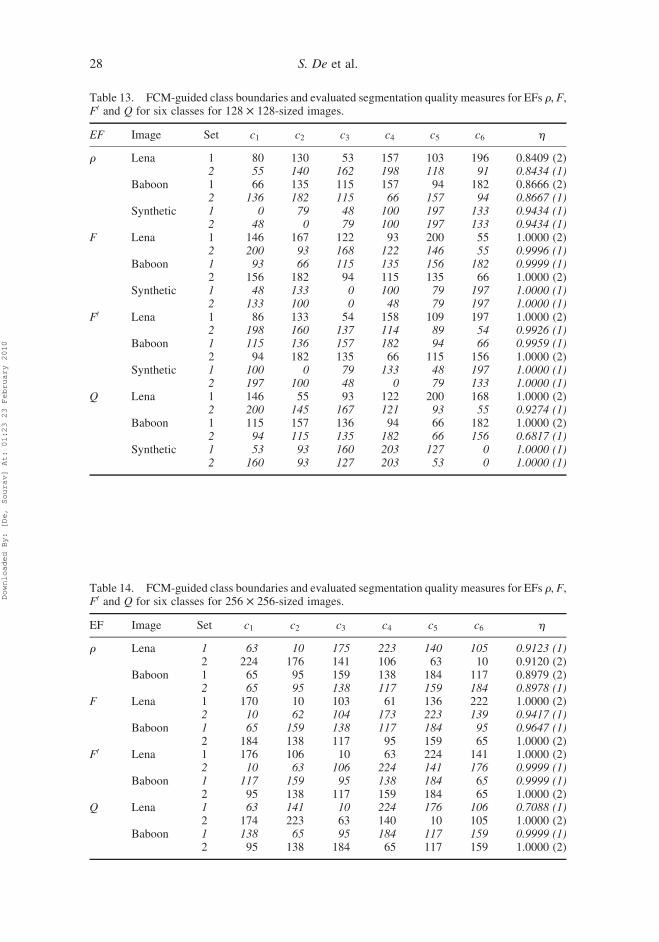
Table 13. FCM-guided class boundaries and evaluated segmentation quality measures for EFs r, F,F0 and Q for six classes for 128 £ 128-sized images.
EF Image Set c1 c2 c3 c4 c5 c6 h
r Lena 1 80 130 53 157 103 196 0.8409 (2)2 55 140 162 198 118 91 0.8434 (1)
Baboon 1 66 135 115 157 94 182 0.8666 (2)2 136 182 115 66 157 94 0.8667 (1)
Synthetic 1 0 79 48 100 197 133 0.9434 (1)2 48 0 79 100 197 133 0.9434 (1)
F Lena 1 146 167 122 93 200 55 1.0000 (2)2 200 93 168 122 146 55 0.9996 (1)
Baboon 1 93 66 115 135 156 182 0.9999 (1)2 156 182 94 115 135 66 1.0000 (2)
Synthetic 1 48 133 0 100 79 197 1.0000 (1)2 133 100 0 48 79 197 1.0000 (1)
F0 Lena 1 86 133 54 158 109 197 1.0000 (2)2 198 160 137 114 89 54 0.9926 (1)
Baboon 1 115 136 157 182 94 66 0.9959 (1)2 94 182 135 66 115 156 1.0000 (2)
Synthetic 1 100 0 79 133 48 197 1.0000 (1)2 197 100 48 0 79 133 1.0000 (1)
Q Lena 1 146 55 93 122 200 168 1.0000 (2)2 200 145 167 121 93 55 0.9274 (1)
Baboon 1 115 157 136 94 66 182 1.0000 (2)2 94 115 135 182 66 156 0.6817 (1)
Synthetic 1 53 93 160 203 127 0 1.0000 (1)2 160 93 127 203 53 0 1.0000 (1)
Table 14. FCM-guided class boundaries and evaluated segmentation quality measures for EFs r, F,F0 and Q for six classes for 256 £ 256-sized images.
EF Image Set c1 c2 c3 c4 c5 c6 h
r Lena 1 63 10 175 223 140 105 0.9123 (1)2 224 176 141 106 63 10 0.9120 (2)
Baboon 1 65 95 159 138 184 117 0.8979 (2)2 65 95 138 117 159 184 0.8978 (1)
F Lena 1 170 10 103 61 136 222 1.0000 (2)2 10 62 104 173 223 139 0.9417 (1)
Baboon 1 65 159 138 117 184 95 0.9647 (1)2 184 138 117 95 159 65 1.0000 (2)
F0 Lena 1 176 106 10 63 224 141 1.0000 (2)2 10 63 106 224 141 176 0.9999 (1)
Baboon 1 117 159 95 138 184 65 0.9999 (1)2 95 138 117 159 184 65 1.0000 (2)
Q Lena 1 63 141 10 224 176 106 0.7088 (1)2 174 223 63 140 10 105 1.0000 (2)
Baboon 1 138 65 95 184 117 159 0.9999 (1)2 95 138 184 65 117 159 1.0000 (2)
S. De et al.28
Downloaded By: [De, Sourav] At: 01:23 23 February 2010
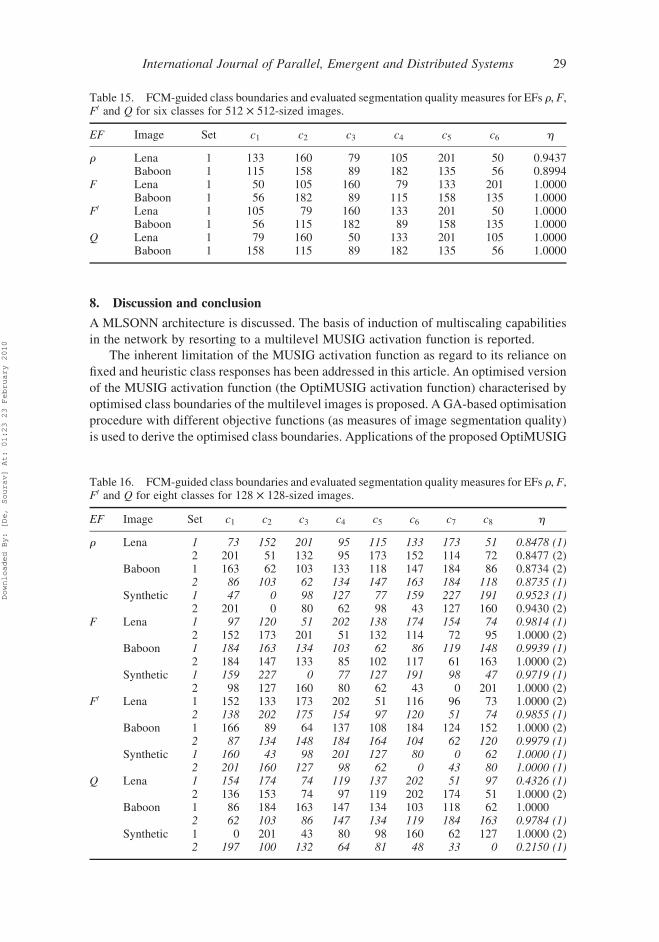
8. Discussion and conclusion
A MLSONN architecture is discussed. The basis of induction of multiscaling capabilities
in the network by resorting to a multilevel MUSIG activation function is reported.
The inherent limitation of the MUSIG activation function as regard to its reliance on
fixed and heuristic class responses has been addressed in this article. An optimised version
of the MUSIG activation function (the OptiMUSIG activation function) characterised by
optimised class boundaries of the multilevel images is proposed. A GA-based optimisation
procedure with different objective functions (as measures of image segmentation quality)
is used to derive the optimised class boundaries. Applications of the proposed OptiMUSIG
Table 15. FCM-guided class boundaries and evaluated segmentation quality measures for EFs r, F,F0 and Q for six classes for 512 £ 512-sized images.
EF Image Set c1 c2 c3 c4 c5 c6 h
r Lena 1 133 160 79 105 201 50 0.9437Baboon 1 115 158 89 182 135 56 0.8994
F Lena 1 50 105 160 79 133 201 1.0000Baboon 1 56 182 89 115 158 135 1.0000
F0 Lena 1 105 79 160 133 201 50 1.0000Baboon 1 56 115 182 89 158 135 1.0000
Q Lena 1 79 160 50 133 201 105 1.0000Baboon 1 158 115 89 182 135 56 1.0000
Table 16. FCM-guided class boundaries and evaluated segmentation quality measures for EFs r, F,F0 and Q for eight classes for 128 £ 128-sized images.
EF Image Set c1 c2 c3 c4 c5 c6 c7 c8 h
r Lena 1 73 152 201 95 115 133 173 51 0.8478 (1)2 201 51 132 95 173 152 114 72 0.8477 (2)
Baboon 1 163 62 103 133 118 147 184 86 0.8734 (2)2 86 103 62 134 147 163 184 118 0.8735 (1)
Synthetic 1 47 0 98 127 77 159 227 191 0.9523 (1)2 201 0 80 62 98 43 127 160 0.9430 (2)
F Lena 1 97 120 51 202 138 174 154 74 0.9814 (1)2 152 173 201 51 132 114 72 95 1.0000 (2)
Baboon 1 184 163 134 103 62 86 119 148 0.9939 (1)2 184 147 133 85 102 117 61 163 1.0000 (2)
Synthetic 1 159 227 0 77 127 191 98 47 0.9719 (1)2 98 127 160 80 62 43 0 201 1.0000 (2)
F0 Lena 1 152 133 173 202 51 116 96 73 1.0000 (2)2 138 202 175 154 97 120 51 74 0.9855 (1)
Baboon 1 166 89 64 137 108 184 124 152 1.0000 (2)2 87 134 148 184 164 104 62 120 0.9979 (1)
Synthetic 1 160 43 98 201 127 80 0 62 1.0000 (1)2 201 160 127 98 62 0 43 80 1.0000 (1)
Q Lena 1 154 174 74 119 137 202 51 97 0.4326 (1)2 136 153 74 97 119 202 174 51 1.0000 (2)
Baboon 1 86 184 163 147 134 103 118 62 1.00002 62 103 86 147 134 119 184 163 0.9784 (1)
Synthetic 1 0 201 43 80 98 160 62 127 1.0000 (2)2 197 100 132 64 81 48 33 0 0.2150 (1)
International Journal of Parallel, Emergent and Distributed Systems 29
Downloaded By: [De, Sourav] At: 01:23 23 February 2010

Table 17. FCM-guided class boundaries and evaluated segmentation quality measures for EFs r, F,F0 and Q for eight classes for 256 £ 256-sized images.
EF Image Set c1 c2 c3 c4 c5 c6 c7 c8 h
r Lena 1 70 130 153 184 104 39 6 226 0.9183 (1)2 130 184 70 39 6 104 226 153 0.9182 (2)
Baboon 1 168 86 137 61 186 121 151 105 0.9056 (1)2 103 60 120 167 84 186 150 118 0.9051 (2)
F Lena 1 103 6 38 70 153 226 184 129 0.9997 (1)2 226 153 39 185 104 70 130 6 1.0000 (2)
Baboon 1 61 86 186 105 137 152 122 168 0.9984 (1)2 167 61 104 121 186 136 151 85 1.0000 (2)
F0 Lena 1 127 151 226 183 6 38 69 101 1.0000 (2)2 39 153 226 70 104 6 130 185 0.9964 (1)
Baboon 1 85 121 186 104 167 136 61 151 0.9978 (1)2 151 105 186 168 86 61 137 121 1.0000 (2)
Q Lena 1 152 127 69 6 38 183 102 226 1.0000 (2)2 130 184 39 153 70 104 226 6 0.8223 (1)
Baboon 1 104 151 86 168 137 121 61 186 0.8429 (1)2 186 60 120 84 103 136 150 167 1.0000 (2)
Table 18. FCM-guided class boundaries and evaluated segmentation quality measures for EFs r, F,F0 and Q for eight classes for 512 £ 512-sized images.
EF Image Set c1 c2 c3 c4 c5 c6 c7 c8 h
r Lena 1 99 123 157 49 206 178 75 140 0.9514Baboon 1 132 97 116 167 50 185 149 76 0.9076
F Lena 1 99 206 75 140 178 49 157 123 1.0000Baboon 1 132 185 76 149 97 50 116 167 1.0000
F0 Lena 1 49 157 178 99 140 123 74 206 1.0000Baboon 1 185 76 131 167 97 116 149 50 1.0000
Q Lena 1 156 99 74 177 49 140 206 122 1.0000Baboon 1 185 97 76 167 116 131 149 50 1.0000
Figure 7. Eight-class segmented 128 £ 128 synthetic image corresponding to the best EF valueobtained with OptiMUSIG activation function: (a) r, (b) F, (c) F0 and (d) Q.
Figure 8. Eight-class segmented 128 £ 128 Lena image corresponding to the best EF valueobtained with OptiMUSIG activation function: (a) r, (b) F (c) F0 and (d) Q.
S. De et al.30
Downloaded By: [De, Sourav] At: 01:23 23 February 2010

activation function for the segmentation of real-life multilevel images show superior
performance as compared to the MUSIG activation function with heuristic class
boundaries. Furthermore, comparative analysis of the results obtained with the standard
FCM algorithm also signifies the merit of the proposed approach.
Methods, however, remain to be investigated to apply the proposed OptiMUSIG
activation function for the segmentation of colour images as well. The authors are
currently engaged in this direction.
Figure 10. Eight-class segmented 256 £ 256 Lena image corresponding to the best EF valueobtained with OptiMUSIG activation function: (a) r, (b) F (c) F0 and (d) Q.
Figure 9. Eight-class segmented 128 £ 128 Baboon image corresponding to the best EF valueobtained with OptiMUSIG activation function: (a) r, (b) F (c) F0 and (d) Q.
International Journal of Parallel, Emergent and Distributed Systems 31
Downloaded By: [De, Sourav] At: 01:23 23 February 2010
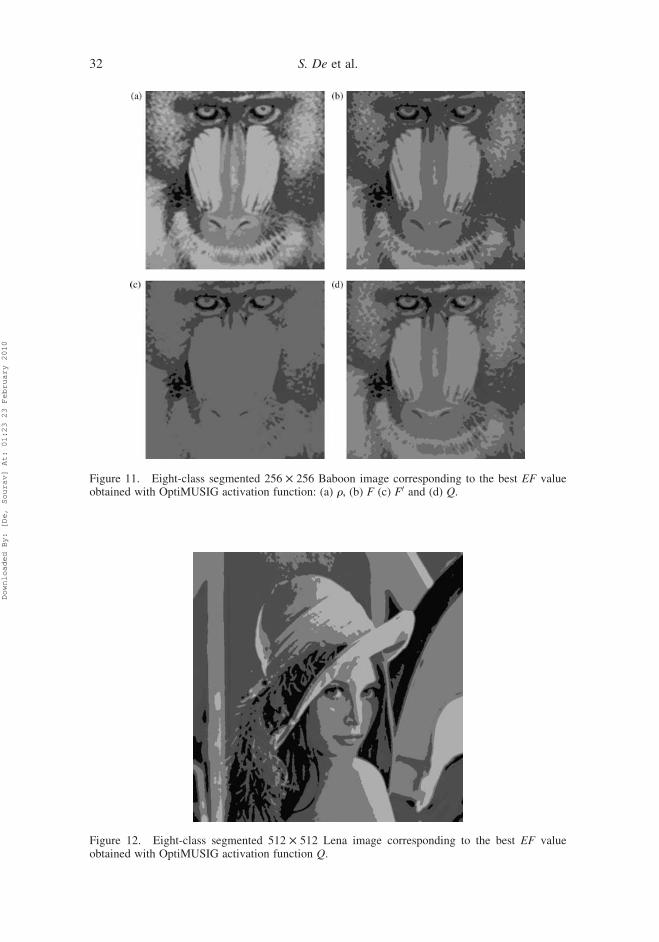
Figure 11. Eight-class segmented 256 £ 256 Baboon image corresponding to the best EF valueobtained with OptiMUSIG activation function: (a) r, (b) F (c) F0 and (d) Q.
Figure 12. Eight-class segmented 512 £ 512 Lena image corresponding to the best EF valueobtained with OptiMUSIG activation function Q.
S. De et al.32
Downloaded By: [De, Sourav] At: 01:23 23 February 2010

Figure 13. Eight-class segmented 512 £ 512 Baboon image corresponding to the best EF valueobtained with OptiMUSIG activation function Q.
Figure 14. Eight-class segmented 128 £ 128 synthetic image corresponding to the best EF valueobtained with MUSIG activation function: (a) r, (b) F (c) F0 and (d) Q.
Figure 15. Eight-class segmented 128 £ 128 Lena image corresponding to the best EF valueobtained with MUSIG activation function: (a) r, (b) F (c) F0 and (d) Q.
Figure 16. Eight-class segmented 128 £ 128 Baboon image corresponding to the best EF valueobtained with MUSIG activation function: (a) r, (b) F (c) F0 and (d) Q.
International Journal of Parallel, Emergent and Distributed Systems 33
Downloaded By: [De, Sourav] At: 01:23 23 February 2010
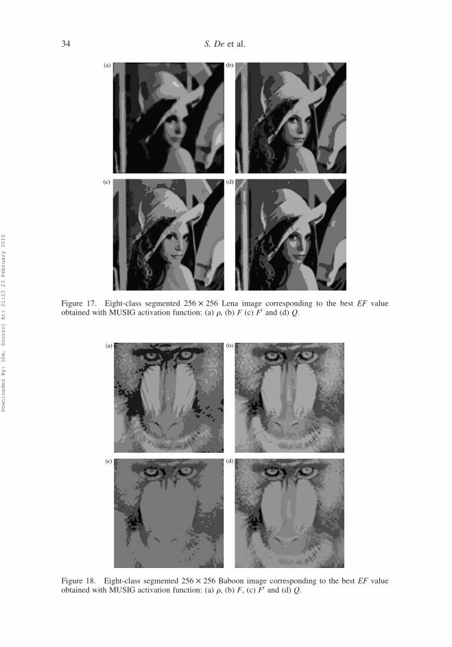
Figure 17. Eight-class segmented 256 £ 256 Lena image corresponding to the best EF valueobtained with MUSIG activation function: (a) r, (b) F (c) F0 and (d) Q.
Figure 18. Eight-class segmented 256 £ 256 Baboon image corresponding to the best EF valueobtained with MUSIG activation function: (a) r, (b) F, (c) F0 and (d) Q.
S. De et al.34
Downloaded By: [De, Sourav] At: 01:23 23 February 2010

Figure 19. Eight-class segmented 512 £ 512 Lena image corresponding to the best EF valueobtained with MUSIG activation function Q.
Figure 20. Eight-class segmented 512 £ 512 Baboon image corresponding to the best EF valueobtained with MUSIG activation function Q.
Figure 21. Eight-class segmented 128 £ 128 synthetic image corresponding to the best EF valueobtained with FCM standard algorithm: (a) r, (b) F, (c) F0 and (d) Q.
International Journal of Parallel, Emergent and Distributed Systems 35
Downloaded By: [De, Sourav] At: 01:23 23 February 2010
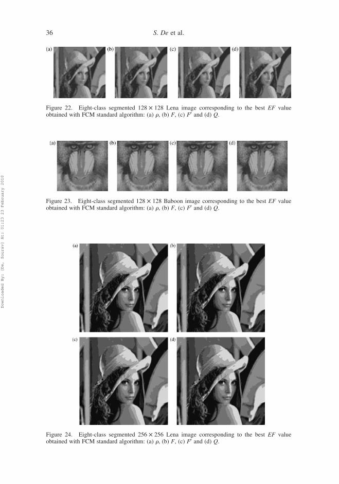
Figure 23. Eight-class segmented 128 £ 128 Baboon image corresponding to the best EF valueobtained with FCM standard algorithm: (a) r, (b) F, (c) F0 and (d) Q.
Figure 22. Eight-class segmented 128 £ 128 Lena image corresponding to the best EF valueobtained with FCM standard algorithm: (a) r, (b) F, (c) F0 and (d) Q.
Figure 24. Eight-class segmented 256 £ 256 Lena image corresponding to the best EF valueobtained with FCM standard algorithm: (a) r, (b) F, (c) F0 and (d) Q.
S. De et al.36
Downloaded By: [De, Sourav] At: 01:23 23 February 2010
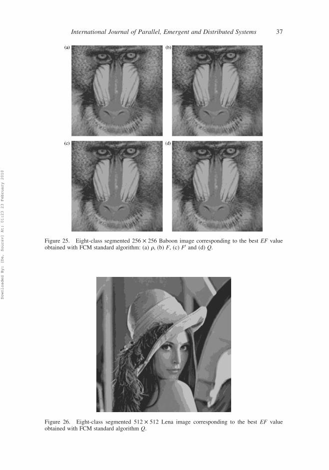
Figure 25. Eight-class segmented 256 £ 256 Baboon image corresponding to the best EF valueobtained with FCM standard algorithm: (a) r, (b) F, (c) F0 and (d) Q.
Figure 26. Eight-class segmented 512 £ 512 Lena image corresponding to the best EF valueobtained with FCM standard algorithm Q.
International Journal of Parallel, Emergent and Distributed Systems 37
Downloaded By: [De, Sourav] At: 01:23 23 February 2010

References
[1] R.C. Gonzalez and R.E. Woods, Digital Image Processing, Prentice-Hall, Upper Saddle River,NJ, 2002.
[2] A. Jain, M. Murthy, and P. Flynn,Data clustering: A review, ACMComput. Surveys 31 (1999),pp. 265–322.
[3] P.F. Felzenszwalb and D.P. Huttenlocher, Efficient graph-based image segmentation,Int. J. Comput. Vision 59(2) (2004), pp. 167–181.
[4] X. Liu and D. Wang, Image and texture segmentation using local spectral histograms,IEEE Trans. Image Process. 15(10) (2006), pp. 3066–3077.
[5] W. Yang, L. Guo, T. Zhao, and G. Xiao, Improving watersheds image segmentation methodwith graph theory, 2nd IEEE Conference on Industrial Electronics and Applications (2007),pp. 2550–2553.
[6] J. Shi and J. Malik, Normalized cuts and image segmentation, IEEE Trans. Pattern Anal. Mach.Intell. 22(8) (2000), pp. 888–905.
[7] J. Malik, S. Belongie, T. Leung, and J. Shi, Contour and texture analysis for imagesegmentation, Int. J. Comput. Vision 43(1) (2001), pp. 7–27.
[8] J.C. Bezdek, Pattern Recognition with Fuzzy Objective Function Algorithms, Plenum Press,New York, NY, 1981.
[9] M.N. Ahmed, S.M. Yamany, N. Mohamed, A.A. Farag, and T. Moriarty, A modified fuzzyc-means algorithm for bias field estimation and segmentation of MRI data, IEEE Trans. Med.Imaging 21 (2002), pp. 193–199.
[10] J.C. Noordam, W.H.A.M. van den Broek, and L.M.C. Buydens, Geometrically guided fuzzy C-means clustering for multivariate image segmentation, Proc. Int. Conf. Pattern Recogn. 1(2000), pp. 462–465.
[11] M. Egmont-Petersen and D. de Ridder, Image processing using neural networks – a review,Pattern Recogn. 35(10) (2002), pp. 2279–2301.
[12] S.H. Choi and P. Rockett, The training of neural classifiers with condensed datasets,IEEE Trans. Syst. Man Cybern. Part B 32(2) (2002), pp. 202–206.
[13] T. Kohonen, Self-Organization and Associative Memory, Springer-Verlag, Berlin, Germany,1989.
Figure 27. Eight-class segmented 512 £ 512 Baboon image corresponding to the best EF valueobtained with FCM standard algorithm Q.
S. De et al.38
Downloaded By: [De, Sourav] At: 01:23 23 February 2010
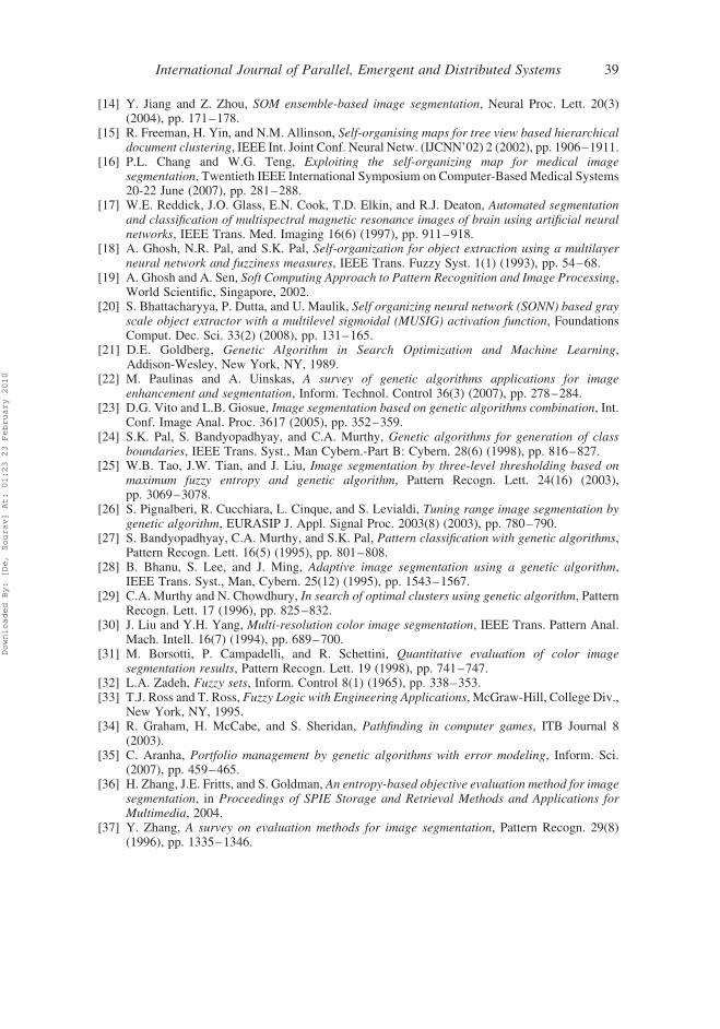
[14] Y. Jiang and Z. Zhou, SOM ensemble-based image segmentation, Neural Proc. Lett. 20(3)(2004), pp. 171–178.
[15] R. Freeman, H. Yin, and N.M. Allinson, Self-organising maps for tree view based hierarchicaldocument clustering, IEEE Int. Joint Conf. Neural Netw. (IJCNN’02) 2 (2002), pp. 1906–1911.
[16] P.L. Chang and W.G. Teng, Exploiting the self-organizing map for medical imagesegmentation, Twentieth IEEE International Symposium on Computer-Based Medical Systems20-22 June (2007), pp. 281–288.
[17] W.E. Reddick, J.O. Glass, E.N. Cook, T.D. Elkin, and R.J. Deaton, Automated segmentationand classification of multispectral magnetic resonance images of brain using artificial neuralnetworks, IEEE Trans. Med. Imaging 16(6) (1997), pp. 911–918.
[18] A. Ghosh, N.R. Pal, and S.K. Pal, Self-organization for object extraction using a multilayerneural network and fuzziness measures, IEEE Trans. Fuzzy Syst. 1(1) (1993), pp. 54–68.
[19] A. Ghosh and A. Sen, Soft Computing Approach to Pattern Recognition and Image Processing,World Scientific, Singapore, 2002.
[20] S. Bhattacharyya, P. Dutta, and U. Maulik, Self organizing neural network (SONN) based grayscale object extractor with a multilevel sigmoidal (MUSIG) activation function, FoundationsComput. Dec. Sci. 33(2) (2008), pp. 131–165.
[21] D.E. Goldberg, Genetic Algorithm in Search Optimization and Machine Learning,Addison-Wesley, New York, NY, 1989.
[22] M. Paulinas and A. Uinskas, A survey of genetic algorithms applications for imageenhancement and segmentation, Inform. Technol. Control 36(3) (2007), pp. 278–284.
[23] D.G. Vito and L.B. Giosue, Image segmentation based on genetic algorithms combination, Int.Conf. Image Anal. Proc. 3617 (2005), pp. 352–359.
[24] S.K. Pal, S. Bandyopadhyay, and C.A. Murthy, Genetic algorithms for generation of classboundaries, IEEE Trans. Syst., Man Cybern.-Part B: Cybern. 28(6) (1998), pp. 816–827.
[25] W.B. Tao, J.W. Tian, and J. Liu, Image segmentation by three-level thresholding based onmaximum fuzzy entropy and genetic algorithm, Pattern Recogn. Lett. 24(16) (2003),pp. 3069–3078.
[26] S. Pignalberi, R. Cucchiara, L. Cinque, and S. Levialdi, Tuning range image segmentation bygenetic algorithm, EURASIP J. Appl. Signal Proc. 2003(8) (2003), pp. 780–790.
[27] S. Bandyopadhyay, C.A. Murthy, and S.K. Pal, Pattern classification with genetic algorithms,Pattern Recogn. Lett. 16(5) (1995), pp. 801–808.
[28] B. Bhanu, S. Lee, and J. Ming, Adaptive image segmentation using a genetic algorithm,IEEE Trans. Syst., Man, Cybern. 25(12) (1995), pp. 1543–1567.
[29] C.A. Murthy and N. Chowdhury, In search of optimal clusters using genetic algorithm, PatternRecogn. Lett. 17 (1996), pp. 825–832.
[30] J. Liu and Y.H. Yang, Multi-resolution color image segmentation, IEEE Trans. Pattern Anal.Mach. Intell. 16(7) (1994), pp. 689–700.
[31] M. Borsotti, P. Campadelli, and R. Schettini, Quantitative evaluation of color imagesegmentation results, Pattern Recogn. Lett. 19 (1998), pp. 741–747.
[32] L.A. Zadeh, Fuzzy sets, Inform. Control 8(1) (1965), pp. 338–353.[33] T.J. Ross and T. Ross, Fuzzy Logic with Engineering Applications, McGraw-Hill, College Div.,
New York, NY, 1995.[34] R. Graham, H. McCabe, and S. Sheridan, Pathfinding in computer games, ITB Journal 8
(2003).[35] C. Aranha, Portfolio management by genetic algorithms with error modeling, Inform. Sci.
(2007), pp. 459–465.[36] H. Zhang, J.E. Fritts, and S. Goldman, An entropy-based objective evaluation method for image
segmentation, in Proceedings of SPIE Storage and Retrieval Methods and Applications forMultimedia, 2004.
[37] Y. Zhang, A survey on evaluation methods for image segmentation, Pattern Recogn. 29(8)(1996), pp. 1335–1346.
International Journal of Parallel, Emergent and Distributed Systems 39
Downloaded By: [De, Sourav] At: 01:23 23 February 2010