Efficient and Robust Acoustic Feedback Cancellation Algorithm FOR In-car communication system A...

Efficient and Robust Acoustic Feedback Cancellation Algorithm FOR In-car communication system

KUMAR PRADHAN ARUN

SCHOOL OF ELECTRICAL AND ELECTRONIC ENGINEERING

A DISSERTATION SUBMITTED IN PARTIAL FULFILMENT OF THE REQUIREMENTS

FOR THE DEGREE OFMASTER OF SCIENCE IN SIGNAL PROCESSING IN 2011

1/1/2011

1

Acknowledgments Upon the completion of the dissertation, I would like to express my gratitude towards those who have

been supporting me in every stage along the way of research. It is their guidance and patience that have

bolstered me up to finally achieve the goal.

I would like to express my deepest appreciation and thanks to my supervisor Prof. Khong Wai Hoong,

Andy, who has given me valuable advices and guidance throughout the project. It is him that has led me

to the world of adaptive filtering of digital signal processing, and has motivated me by his enthusiasm and

also strict attitude towards research works. Every talk between us benefits me a lot, from the attitude

towards negative results to the ways of thinking of new ideas. He never tells me a full story but provides

me enough prerequisites and clues and encourages me to discover the consequences and results myself,

which has effectively reinforced the knowledge that I gained through exploring, and also has improved

my research and troubleshooting skills. I appreciate the opportunity of being supervised by Andy for the

academic year.

PhD student, Mr. Vinod Veera Reddy have helped me a lot. He never hesitates to share his experience

and knowledge to solve my problems and give me inspirations.

I am indebted to my wife, Ruchira. It is her constant encouragement and support inspired me to

successfully complete this thesis at satisfactory level.

Pradhan Kumar Arun

2

Summary

In this thesis, I attempted to develop high performing but computationally efficient and robust

adaptive signal processing algorithm in order to cancel artifacts created by acoustic feedback path in

intercom system of car cabin while trying improving the speech quality and intelligibility between

passengers.

This thesis is organized as follows.

Chapter 1: Introduced the problem of AFC and motivation for the viable and efficient solution.

Chapter2: Discussion about functional requirements of car cabin intercom system and its basic signal

processing units in order to improve the speech quality and intelligibility which is just basic requirement.

Chapter 3: Discussion about the problem created by acoustic feedback whenever a microphone captures a

desired sound signal which is then processed (e.g., amplified) and played back by a loudspeaker in the

same environment, as it is the case in a car cabin system (CCS).

Chapter 4: Reviews of several existing traditional AFC algorithm.

Chapter 5: Detailed analysis of three algorithms as potential solution of the AFC problem. In depth

analyses, their computational complexities and performance assessment are done using simulation results

of experimentation. In addition to this, improvement techniques of robustness of the AFC system are also

discussed here.

Chapter 6: Conclusion about the performance of the AFC algorithms developed here and their limitation

along with further research challenges also was discussed here.

3

Content

1 Contents Acknowledgments ......................................................................................................................................... 1

Summary ....................................................................................................................................................... 2

Content ......................................................................................................................................................... 3

List of symbols and notations ....................................................................................................................... 6

Abbreviations ................................................................................................................................................ 8

List of Figures .............................................................................................................................................. 12

List of Tables .............................................................................................................................................. 14

Chapter 1 Introduction ............................................................................................................................... 15

1.1 Motivation ................................................................................................................................... 15

Chapter 1 .................................................................................................................................................... 15

1.2 Objectives.................................................................................................................................... 15

1.3 Major contribution of the thesis ................................................................................................. 16

Chapter 2 In-car communication system .................................................................................................... 17

2.1 Introduction ................................................................................................................................ 17

2.2 Requirements of functionalities.................................................................................................. 19

Chapter 2 .................................................................................................................................................... 20

2.3 System requirements .................................................................................................................. 20

2.4 Signal processing for the intercom system ................................................................................. 21

Chapter 3 Acoustic Feedback ...................................................................................................................... 23

3.1 What is acoustic feedback?......................................................................................................... 23

3.2 What problem acoustic feedback creates .................................................................................. 23

3.3 What is aim of acoustic feedback cancellation ........................................................................... 25

3.4 Review of different solutions ...................................................................................................... 26

3.4.1 Phase Modulation methods ................................................................................................ 26

3.4.2 Gain Reduction method ...................................................................................................... 27

4

3.4.3 Spatial filtering method ...................................................................................................... 28

3.4.4 Room modeling method ..................................................................................................... 29

Chapter 4 Acoustic Feedback Cancellation ................................................................................................. 31

Chapter 3 .................................................................................................................................................... 31

4.1 Adaptive feedback cancellation (AFC): Concept ......................................................................... 31

4.2 Least Squares Estimate: bias and variance Issues ...................................................................... 32

4.3 Review of different AFC realizations ........................................................................................... 34

4.3.1 Adaptive filtering ................................................................................................................. 34

4.3.2 Decorrelation ...................................................................................................................... 35

4.3.3 Post filter ............................................................................................................................. 40

Chapter 5 Prediction Error Method (PEM) ................................................................................................. 41

Chapter 4 .................................................................................................................................................... 41

5.1 Introduction ................................................................................................................................ 41

5.2 Standard CAF AFC realization using PB-FDAF ............................................................................. 42

5.2.1 CAF algorithm and bias ....................................................................................................... 43

5.2.2 Partitioned-block frequency-domain (PBFD) LMS implementation ................................... 45

5.3 PEM based AFC using PB-FDAF for speech application .............................................................. 50

5.3.1 Closed-loop identification of the feedback path with the direct method .......................... 50

5.3.2 Adaptive desired signal model ............................................................................................ 51

5.4 Robustness and performance improvement .............................................................................. 59

5.4.1 Constraint on step size ........................................................................................................ 60

5.4.2 Onset Detection .................................................................................................................. 60

5.4.3 Prior Knowledge of the Feedback Path ............................................................................... 61

5.4.4 Foreground/Background Filter ............................................................................................ 63

5.4.5 Nonlinearities ...................................................................................................................... 65

5.5 Performance evaluation procedures .......................................................................................... 66

5.5.1 Performance of acoustic feedback ..................................................................................... 66

5.5.2 Performance of adaptive filter ............................................................................................ 68

5.6 Computational complexity .......................................................................................................... 68

5.7 Experimentation Setup ............................................................................................................... 71

5.7.1 In-Car speech Communication system Analysis .................................................................. 71

5.7.2 Analysis of the Forward Path Gain and Delay ..................................................................... 73

5

5.7.3 Create Howling as an effect of Acoustic feedback .............................................................. 75

5.8 Simulation Results ....................................................................................................................... 77

5.8.1 PB-FDAF based AFC without decorrelation......................................................................... 78

5.8.2 PB-FDAF based PEM AFC with decorrelation: pre-filtering only by STP ............................. 88

5.8.3 PB-FDAF based PEM AFC with decorrelation : pre-filtering by STP and LTP ...................... 97

5.8.4 Comparisons ..................................................................................................................... 110

Chapter 6 ................................................................................................................................................... 115

6.1 Conclusion ................................................................................................................................. 115

6.2 Limitation .................................................................................................................................. 116

6.3 Recommendations for further research ................................................................................... 116

7 Bibliography: ..................................................................................................................................... 118

8 Appendices ........................................................................................................................................ 129

6

List of symbols and notations

(q,t) near-end/source signal model prediction error filter estimate (time-varying)

A(q, t) near-end/source signal model prediction error filter (time varying)

v(t) near-end/source signal vector (time-varying data window)

u(t) far-end/loudspeaker signal vector (time-varying data window)

x(t) echo/feedback signal

y(t) microphone signal

U(ω, t) Far-end/loudspeaker signal frequency spectrum (time varying data window).

V (ω, t) Near-end/source signal frequency spectrum (time-varying data window)

Y (ω, t) microphone signal frequency spectrum (time-varying data window)

F(q) echo/feedback path model (time-invariant)

F(q, t) echo/feedback path model (time-varying)

(q) echo/feedback path estimate (time-invariant)

(q,t) echo/feedback path estimate (time-varying)

(q,t ) AFC cancellation filter (time-varying)

…… echo/feedback path impulse response coefficients (time invariant)

…… (t) echo/feedback path impulse response coefficients (time varying)

f echo/feedback path impulse response vector (time invariant)

f (t) echo/feedback path impulse response vector (time varying)

(ω)

echo/feedback path estimate frequency response (time invariant)

(ω,t) ( ,t) (q, t) echo/feedback path estimate frequency response (time varying)

delay-compensated echo/feedback path model (time varying)

(q,t)

delay-compensated echo/feedback path estimate (time varying)

G{·} electro-acoustic forward path operator (time-invariant)

G(q)

electro-acoustic forward path model (time-invariant) far-end echo path model

(time-invariant)

G(q, t)

electro-acoustic forward path model (time-varying) far-end echo path model

(time-varying)

7

… electro-acoustic forward path impulse response coefficients (time-varying)

(ω,t) near-end/source signal model estimate (time-varying)

H(q, t) near-end/source signal model (time-varying)

J(q, t) electro-acoustic forward path model before amplification (time-varying)

J( , t) electro-acoustic forward path frequency response before amplification (time-

varying)

K(t) electro-acoustic forward path gain (time-varying)

K integer pitch lag

integer pitch lag (piecewise time-invariant, frame index j)

Ƥ set of frequencies at which Nyquist phase condition holds

perceptual frequency weighting function

K(t) electro-acoustic forward path gain

∆K electro-acoustic forward path gain increase (dB)

minimum integer pitch lag (pitch prediction)

maximum integer pitch lag (pitch prediction)

echo/feedback path impulse response length

M frame length

AFC filterbank implementation number of subbands

near-end/source signal model order

near-end/source signal tonal components model order

echo/feedback path model order

echo/feedback path estimate order

T 60, T60 T 60 reverberation time (s)

exponential forgetting factor for prediction error variance Estimation

ε prediction error vector (time-invariant data window)

μ NLMS step size parameter

NLMS background filter ste

electro-acoustic forward path delay

adaptive filter delay

sampling frequency (Hz)

number of howling occurrences

8

Abbreviations ADC: analog-to-digital

AEC: acoustic echo cancellation

AEQ: automatic equalization

AFC: adaptive feedback cancellation, acoustic feedback cancellation.

AGC: automatic gain control

AIF: adaptive inverse filtering

ANF: adaptive notch filter

ANSI: American National Standards Institute

APA: affine projection algorithm

AFBFL: Filter length of true acoustic feedback path

CD compact disc

cf. confer, compare with

cm centimeters

CCS: car cabin system

CAF: continuous adaptive filter

DAC: digital-to-analog

DFT: discrete Fourier transform

9

e.g. exempli gratia, for example

Eq. equation

FDAF: frequency domain adaptive filter

FFT: fast Fourier transform

FIR: finite impulse response

FNR: feedback-to-near-end ratio

FS: frequency shifting

Hz hertz

HOP: howling occurrence probability

i.e. that is

IIR: infinite impulse response

IIR-ANF: infinite impulse response adaptive notch filter

KHz: kilohertz

LEC: line echo cancellation

LMS: least mean squares

LS: least squares

LTP: long-term predictor

LFHP: LTP computation frame hop size.

LTV: linear time-varying

PEM: prediction error method.

ms milliseconds

10

MSE: mean square error

MSG: maximum stable gain

∆MSG: maximum stable gain increase/delta MSG

N/A not applicable

NHS: notch-filter-based howling suppression

NLMS: normalized least mean squares

no. number

PA: public address

PBFDAF: partitioned block frequency domain adaptive filtering

PC personal computer

PAPR: peak-to-average power ratio

PEM: prediction error method

PEM-AFROW prediction-error-method-based adaptive filtering with row operations

PHPR: peak-to-harmonic power ratio

PLP: pitch prediction

PM: phase modulation

PSD: power spectral density

rad radians

RIR: room impulse response

RLS: recursive least squares

RMS: root mean square

11

s seconds

SD: frequency-weighted log-spectral signal distortion

SNR: signal-to-noise ratio

SPL: sound pressure level

s.t. subject to

STP: short-term predictor

SFHP: STP computation frame hop size.

TRI: time to recover from instability

TVAR time-varying autoregressive

vs. versus

WLP: (frequency-) warped linear prediction

w.r.t. with respect to

12

List of Figures Figure 2-1 Communication between passengers in a car (*acoustic loss, referred to ................................. 17

Figure 2-2 Structure of a basic car interior communication system. Soucre[1] .......................................... 18

Figure 2-3 average directionality of the human mouth. Soucre[1] .............................................................. 19

Figure 2-4.Structure of a car interior communication system aimed to support front-to-rear

conversations. Source [1] ......................................................................................................................... 21

Figure 3-1: Acoustic feedback. .................................................................................................................... 23

Figure 3-2 Acoustic Feedback problem. ...................................................................................................... 24

Figure 3-3: Phase modulation method. ...................................................................................................... 27

Figure 3-4 Gain reduction method. ............................................................................................................. 28

Figure 3-5spatial filtering method .............................................................................................................. 29

Figure 3-6 Room modeling method (AFC) .................................................................................................. 30

Figure 4-1.Adaptive feedback cancellation (AFC) by predicting the feedback signal component x(t) in the

microphone signal, and hence subtracting the prediction ], from the microphone signal y(t). The

prediction is obtained by filtering the loudspeaker signal with a model of the acoustic feedback

path, which is calculated using an adaptive filter. ...................................................................................... 32

Figure 4-2decorrelation in closed signal loop. Here DEC is decorrelation device ...................................... 35

Figure 4-3 AFC with decorrelation by noise injection. ................................................................................ 36

Figure 4-4 AFC with decorrelation by a time varying/ nonlinear/delay operation in the forward path. ... 36

Figure 4-5 decorrelation in adaptive filtering circuit. Here DEC is decorrelation device. .......................... 37

Figure 4-6 AFC with decorrelating pre-filters in the adaptive filtering circuit. ........................................... 38

Figure 4-7 : AFC with post filtering: the post filter H(q, t) can either be a spectral subtraction filter for

residual feedback suppression, or a bank of notch filters to avoid closed-loop instability. ...................... 41

Figure 5-1 Adaptive feedback canceller. ..................................................................................................... 43

Figure 5-2. Block diagram of the PBFD implementation of CAF. ................................................................ 49

Figure 5-3 Adaptive Feedback cancellation with the prediction-error method. ........................................ 51

Figure 5-4 Forward path transfer function G(q) of Fig 5.3 is expanded into delay ( d) and Gain (K). ........ 59

Figure 5-5: Timeline of the far-end near-end ratio, starting from a near-end speech onset. .................... 60

Figure 5-6: A limiter or clipper should be added to avoid clipping in the loudspeaker/amplifier.............. 65

Figure 5-7: Schematic Diagram of an In-Car Communication System without AFC. .................................. 71

Figure 5-8: Frequency Response of Acoustic Path from Loudspeaker to Microphone. ............................. 74

Figure 5-9: Speech signal s(n) and a Direct Simulation of Corrupted Speech d(n) [ A= 30,M=100 (a):

Speech Signal, (b): Corrupted Speech]. ....................................................................................................... 75

13

Figure 5-10: Real-time Simulation of In-Car Feedbacks. ............................................................................. 76

Figure 5-11 : Misalignment of PB-FDAF at different frame size but for same step size =0.005. ................ 79

Figure 5-12 : Misalignment of PB-FDAF at different step size but for same frame size =256 .................... 80

Figure 5-13: Delta MSG comparisons of PB-FDAF at different frame size for same step size =256. .......... 81

Figure 5-14 : Delta MSG comparisons of PB-FDAF at different step size for same frame size =256 .......... 82

Figure 5-15: MSG comparisons of PB-FDAF at different frame size for same step size 0.005. .................. 83

Figure 5-16 : MSG comparisons of PB-FDAF at different step size for same frame size =256. .................. 84

Figure 5-17 : Log Spectral Signal distortion comparisons of PB-FDAF with different block size. ............... 85

Figure 5-18 : Mean log Spectral Signal distortion comparisons of PB-FDAF with different block size. ...... 86

Figure 5-19 : Feedback compensated Microphone Speech of PB-FDAF ..................................................... 87

Figure 5-20 : Misalignment comparison of STP at different SFHP order while frame size = 256, STP order

= 20, and step size =0.005. .......................................................................................................................... 88

Figure 5-21 : Misalignment comparison of STP at different STP order while frame size = 256, SFHP = 2,

and step size =0.005. ................................................................................................................................... 89

Figure 5-22 : MSG comparison of STP at different SFHP while frame size = 256, STP order = 2, and step

size =0.005. ................................................................................................................................................. 90

Figure 5-23 : Delta MSG comparison of STP at different STP order while frame size = 256, SFHP = 2, and

step size =0.005. .......................................................................................................................................... 91

Figure 5-24 : MSG comparison of STP at different SFHP while frame size = 256, STP order = 20, and step

size =0.005. ................................................................................................................................................. 92

Figure 5-25 : MSG comparison of STP at different STP order while frame size = 256, SFHP = 2, and step

size =0.005. ................................................................................................................................................. 93

Figure 5-26: Log Spectral Signal distortions of STP at configurations: frame size = 256, SFHP = 2, STP

order =20 and step size =0.005 ................................................................................................................... 94

Figure 5-27: Mean Log Spectral Signal distortions of STP at configurations: frame size = 256, SFHP = 2,

STP order =20 and step size =0.005 ............................................................................................................ 95

Figure 5-28: Feedback Compensated Microphone Speech of STP at configurations: frame size = 256,

SFHP = 2, STP order =20 and step size =0.005 ............................................................................................ 96

Figure 5-29: Misalignment comparison of LTP for different configurations ............................................. 97

Figure 5-30: Delta MSG comparison of LTP for different configurations .................................................. 98

Figure 5-31: MSG comparison of LTP for different configurations. ............................................................ 99

Figure 5-32: Log Spectral Signal Distortion of LTP for different configurations ....................................... 100

Figure 5-33: Frequency Response of true feedback path generated from RIR. ....................................... 101

Figure 5-34: Steady State Frequency Response: PB-FDAF ........................................................................ 102

Figure 5-35: Steady State Frequency Response: PB-FDAF + STP .............................................................. 103

Figure 5-36: Steady State Frequency Response: PB-FDAF + STP + LTP ..................................................... 104

Figure 5-37: Impulse Response of true feedback path generated from RIR............................................ 105

Figure 5-38: Steady State Impulse Response: PB-FDAF ........................................................................... 106

Figure 5-39 : Steady State Impulse Response: PB-FDAF + STP................................................................. 107

Figure 5-40: Steady State Impulse Response: PB-FDAF + STP + LTP ......................................................... 108

Figure 5-41: Feedback Compensated Microphone Speech: PB-FDAF + STP+ LTP. .................................. 109

Figure 5-42: Misalignment Comparison of all these three algorithms ..................................................... 110

14

Figure 5-43: Misalignment Comparison of all these three algorithms. .................................................... 111

Figure 5-44 : Delta Misalignment Comparison of all these three algorithms. .......................................... 112

Figure 5-45: Misalignment Comparison of all these three algorithms. .................................................... 113

Figure 5-46 : Log Spectral Signal Distortion Comparisons of all these three algorithms. ........................ 114

List of Tables Table 4-1: Comparison of adaptive feedback cancellation (AFC) methods. .............................................. 39

Table 5-1: Only PB-FDAF based AFC without decorrelation .................................................................... 48

Table 5-2: PB-FDAF based PEM AFC with STP pre-filter ...................................................................... 55

Table 5-3: PB-FDAF based PEM AFC with cascaded STP and LTP pre-filters ........................................ 58

Table 5-4: Computational complexity. ........................................................................................................ 68

Table 5-5.Acoustic feedback system for these different values of system parameters (N, M, A, AFBFL).

.................................................................................................................................................................... 78

Table 5-6: Performance comparisons among three algorithms ............................................................... 114

15

Chapter 1 Introduction

1.1 Motivation In current situation, communication between passengers of mid and high class automobiles, is difficult,

because of 1) the acoustic loss (especially front to back), 2) Front passengers have to speak louder than

normal – longer conversations will be tiring 3) Driver turns around – road safety is reduced 4) Due to a

large amount of background noise while a car driving at high or even moderate speed is often difficult.

Whenever a microphone captures a desired sound signal which is then processed (e.g., amplified) and

played back by a loudspeaker in the same environment, as it is the case in a car cabin system (CCS), the

loudspeaker signal is unavoidably fed back into the microphone. In this way, a closed signal loop is

created which affects the system performance, deteriorating the sound quality and limiting the achievable

amplification. Among the different artifacts that are produced by this acoustic coupling between

loudspeaker and microphone, the howling effect is without any doubt the most characteristic one.

In order to improve the speech quality and intelligibility by means of an intercom system while leveraging

already equipped with the necessary audio and signal processing components, I attempted to develop a

class of high performing but computationally efficient and robust adaptive signal processing algorithm.

1.2 Objectives This work aims to develop efficient and robust adaptive algorithms for the in-car acoustic feedback

cancellation (AFC) system to enhance the communication between the driver and passengers in car by

effectively cancelling the feedback interference.

A fundamental problem encountered in AFC is the signal correlation between the far-end and near-end

signal, which leads to biased and high-variance acoustic feedback path estimates when standard least-

squares (LS)-based adaptive filtering algorithms are used. For this reason, the AFC approach usually

entails a decorrelation method to reduce the far-end to near-end signal correlation.

The main goal has been to develop solutions that provide a high performance and sound quality, and

behave in a robust way in realistic conditions. This can be achieved by departing from the traditional

adhoc methods, and instead deriving theoretically well-founded solutions, based on results from

parameter estimation and system identification. In the development of these solutions, the computational

16

efficiency has permanently been taken into account as a design constraint, in that the complexity increase

compared to the state-of-the-art solutions should not exceed 50 % of the original complexity.

1.3 Major contribution of the thesis In general feedback cancellation setups, standard adaptive filtering techniques fail to provide a reliable

feedback path estimate if the desired signal is spectrally colored because of the presence of a closed signal

loop.

In this work, prediction error method (PEM) based scheme was adopted which identifies both the acoustic

feedback path and the nonstationary speech source model. A cascade of a short– and a long term predictor

removes the coloring and periodicity in voiced speech segments, which account for the unwanted

correlation between the loudspeaker signal and the speech source signal. The predictors calculate row

operations which are applied to pre–whiten a least squares system, which is then solved recursively by

means of e.g. NLMS algorithms. To avoid biased and slowly converging feedback path estimation, the

AFC approach is usually realized by combining an adaptive filter with this decorrelation method of

cascaded model of predictors. But finally realization of NLMS was done frequency domain which not

only improves convergence speed but computationally efficient. In this work, NLMS is realized in

frequency domain namely called PB-FDAF where error energy and signal energy both were considered

for step size computation for faster convergence of adaptive filter which does unbiased estimation of the

acoustic feedback path.

Frequency domain NLMS algorithm with combination of PEM based decorrelation scheme, three

algorithms were simulated.

At first only PB-FDAP without decorrelation scheme was implemented. Then PB-FDAF with STP

prediction was used as decorrelation scheme and finally PB-FDAF was combined with cascaded STP

and LTP prediction of near end signal as decorrelation or pre-whiten strategy to effectively remove

correlation between speaker and loud speaker signal thus near accurate estimation feedback path to

cancel artifacts of acoustic feedback in the intercom system.

It has been shown that though PB-FDAF combined with STP performs much better than only PB-FDAF

but this does not perform well in case of long non stationary acoustic feedback path. In this case, PB-

FDAF with combination of cascaded prediction (STP and LTP) based decorrelation scheme is always a

better choice.

The evaluation is based on computer simulation results using realistic room acoustic models and using

real speech signals.

Finally performance of these three algorithm has been assessed and shown that PB-FDAF with cascaded

model of near end signal predictors (STP and LTP ) as decorrelation scheme not only effectively

removes acoustic feedback artifacts but this algorithm computationally efficient and robust to changes of

acoustic feedback path .

In addition to this, several techniques (e.g. shadow filter approach) have been devised so that the tracking

performance of the PEM-based feedback canceller with adaptive signal model can be improved for

robustness to the changes of acoustic feedback path.

17

Chapter 2 In-car communication system

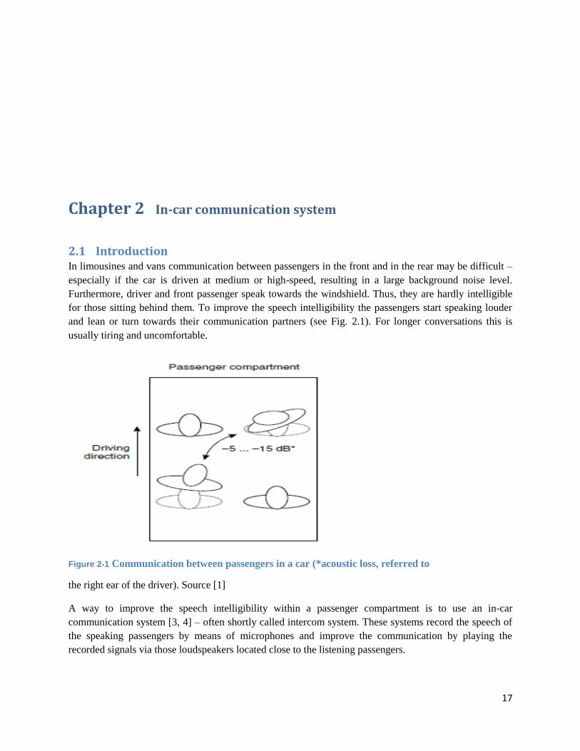
2.1 Introduction In limousines and vans communication between passengers in the front and in the rear may be difficult –

especially if the car is driven at medium or high-speed, resulting in a large background noise level.

Furthermore, driver and front passenger speak towards the windshield. Thus, they are hardly intelligible

for those sitting behind them. To improve the speech intelligibility the passengers start speaking louder

and lean or turn towards their communication partners (see Fig. 2.1). For longer conversations this is

usually tiring and uncomfortable.

Figure 2-1 Communication between passengers in a car (*acoustic loss, referred to

the right ear of the driver). Source [1]

A way to improve the speech intelligibility within a passenger compartment is to use an in-car

communication system [3, 4] – often shortly called intercom system. These systems record the speech of

the speaking passengers by means of microphones and improve the communication by playing the

recorded signals via those loudspeakers located close to the listening passengers.

18

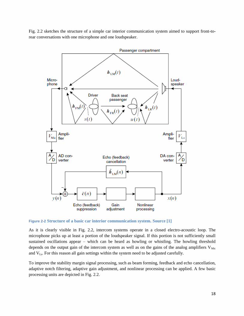
Fig. 2.2 sketches the structure of a simple car interior communication system aimed to support front-to-

rear conversations with one microphone and one loudspeaker.

Figure 2-2 Structure of a basic car interior communication system. Source [1]

As it is clearly visible in Fig. 2.2, intercom systems operate in a closed electro-acoustic loop. The

microphone picks up at least a portion of the loudspeaker signal. If this portion is not sufficiently small

sustained oscillations appear – which can be heard as howling or whistling. The howling threshold

depends on the output gain of the intercom system as well as on the gains of the analog amplifiers VMic

and VLs. For this reason all gain settings within the system need to be adjusted carefully.

To improve the stability margin signal processing, such as beam forming, feedback and echo cancellation,

adaptive notch filtering, adaptive gain adjustment, and nonlinear processing can be applied. A few basic

processing units are depicted in Fig. 2.2.

19

2.2 Requirements of functionalities The urge for in –car communications systems are to meet these following basic functional requirements

1) To preserve the loss of acoustic gain.

As shown above in fig 2.1 There is acoustic loss due to this fact that:

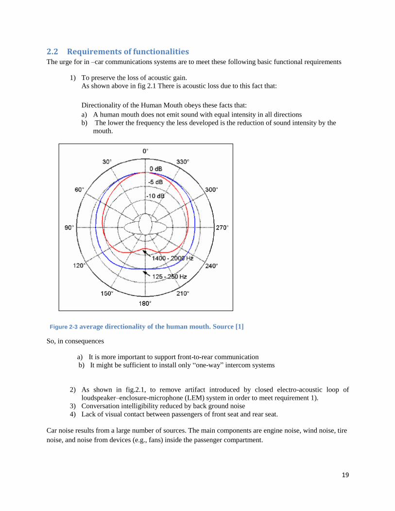
Directionality of the Human Mouth obeys these facts that:

a) A human mouth does not emit sound with equal intensity in all directions

b) The lower the frequency the less developed is the reduction of sound intensity by the

mouth.

Figure 2-3 average directionality of the human mouth. Source [1]

So, in consequences

a) It is more important to support front-to-rear communication

b) It might be sufficient to install only “one-way” intercom systems

2) As shown in fig.2.1, to remove artifact introduced by closed electro-acoustic loop of

loudspeaker–enclosure-microphone (LEM) system in order to meet requirement 1).

3) Conversation intelligibility reduced by back ground noise

4) Lack of visual contact between passengers of front seat and rear seat.

Car noise results from a large number of sources. The main components are engine noise, wind noise, tire

noise, and noise from devices (e.g., fans) inside the passenger compartment.

20

2.3 System requirements Ideal requirements of the in car communication system

1) The speech signal of the driver and the front passenger should be reproduced with high quality and

with a minimum system delay (<10 ms) by the rear loudspeakers (rear

-> front vice versa).

2) The passengers should not be aware of the system.

3) Speaker localization should be preserved by the system.

4) System stability has to be guaranteed.

5) The in-car communication system has to be realized on existing hardware (e.g. hands-free-system/

speech-dialog-system).

6)

But problems in real system are as following

1) At medium to large output gain the acoustic situations starts becoming „diffuse“, i.e. spatial

localization is not possible any more.

2) At large output gain visual and acoustic sensation do not fit any more (driver is visually located in

front of the rear passengers but acoustically behind the rear passengers) – very irritating for a few

people.

3) At very large output gains the system will become instable (without signal processing).

4) In case of too large system delay the signals sound reverberant (“bathroom atmosphere”) and the

speaking passengers will be aware of their own echo.

Hence design Problems and Challenges are here as following

1) Stability: Stability has to be guaranteed in all situations.

2) Correlation of excitation and distortion.

3) Acoustic Echoes/Acoustic feedback should be reduced by an appropriate signal processing

algorithm.

4) The output gain has to be adjusted continuously to the current driving and background noise

conditions.

5) The overall system delay should not exceed 10 ms.

21

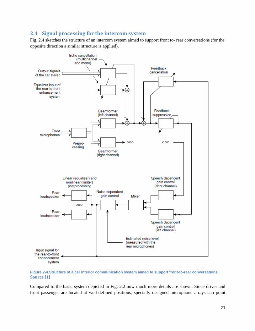
2.4 Signal processing for the intercom system Fig. 2.4 sketches the structure of an intercom system aimed to support front to- rear conversations (for the

opposite direction a similar structure is applied).

Figure 2-4.Structure of a car interior communication system aimed to support front-to-rear conversations.

Source [1]

Compared to the basic system depicted in Fig. 2.2 now much more details are shown. Since driver and

front passenger are located at well-defined positions, specially designed microphone arrays can point

22

towards each of them, which allows to use fixed beamformers. This allows to start with the echo and

feedback cancellation after the beamformer (and to reduce the computational complexity because only

one echo cancellation filter per reference channel is required). Feedback suppression by means of an

adaptive notch filter can improve the system stability by rising the howling margin. A mixer combines the

signals of driver and second front passenger according to the detected speech activity. A device with

nonlinear characteristic attenuates large signal amplitudes before the signals are played back via the

loudspeakers. The output gain of a car intercom system needs to be adjusted continuously according to

the current driving situation. While only a moderate gain is required whenever the car is in low noise

conditions, a large gain is required and more artifacts will be tolerated at high speed. Finally, loudspeaker

equalization (either adaptive or fixed) can be applied.

Processing structure

Besides selecting adaptive algorithms [2] like NLMS, affine projection, RLS, etc., the system designer

also has the freedom to choose between different processing structures. The most popular ones are

broadband processing, block processing1, and subband processing. The special challenge in in-car

communication systems consists in designing a system with an overall delay of not more than 10 ms.

Signals from the loudspeakers delayed for more than that will be perceived as echoes and reduce the

subjective quality of the system.

For this reason, only broadband processing or block processing with very small block sizes can be applied

if a high system quality should be achieved.

In subsequent chapters of this thesis, only signal processing algorithm of feedback cancellation will be

considered.

1 By block processing we mean performing the convolution and/or the adaptation in the frequency domain and using

overlap-add or overlap-save techniques.

23

Chapter 3 Acoustic Feedback

3.1 What is acoustic feedback? As mentioned in previous chapter, as one of the critical requirement of in-car communication system to

improve the intelligibility and comfort ability between front seat and rear seat passenger, whenever a

microphone captures a desired sound signal which is then processed (e.g., amplified) and played back by

a loudspeaker in the same environment and enclose, as it is the case of in-car communication system, the

loudspeaker signal is unavoidably fed back into the microphone.

Figure 3-1: Acoustic feedback.

In this way, a closed signal loop is created which affects the system performance, deteriorating the sound

quality and limiting the achievable amplification. Among the different artifacts that are produced by this

acoustic coupling between loudspeaker and microphone, the howling effect is without any doubt the most

characteristic one.

The term acoustic feedback has been used to refer to the undesired acoustic coupling between

a loudspeaker and a microphone as well as to the howling effect that results from the coupling.

Both the acoustic coupling and the howling effect are sometimes also referred to as the Larsen effect, after

the Danish physicist Søren Larsen, who is said to have been one of the first researchers to investigate the

acoustic feedback problem [5].

3.2 What problem acoustic feedback creates While many sound reinforcement systems comprise multiple loudspeakers and microphones, most

acoustic feedback control methods have been proposed in a single-channel context (i.e., for one

loudspeaker and one microphone), without a framework for an extension to multi-channel systems being

explicitly provided. For this reason, we will analyze the acoustic feedback problem and explain the

acoustic feedback control methods in a single-channel context. We will however comment on the

implications of extending a particular method to a multi-channel system whenever appropriate

Feed-back path

Source signal

24

Figure 3-2 Acoustic Feedback problem.

The problem of acoustic feedback is illustrated in Fig. 3.2 with a single microphone. For the notation, we

refer to the end of this section.

The so-called forward path

where denotes the filter length

of represents the regular signal processing path or forward path of the intercom system (i.e., a

frequency-specific gain, compression and/or noise reduction). We assume that has a delay of at

least one sample, i.e., . The feedback path between the loudspeaker and the microphone is denoted

by F(q,n). The loudspeaker and microphone signals are ul[n] and y[n], respectively. The desired signal is

denoted by x[n] and the feedback signal is denoted by v(n) =F(q,n)ul[n]. Because of acoustic feedback,

the amplified sound ul[n] sent through the loudspeaker is fed back into the microphone, resulting in a

closed-loop system.

This way, in a single-channel sound reinforcement system (referring fig 3.1), the closed-loop frequency

response from the source signal to the loudspeaker signal can be expressed as follows:

3.1

Here ] ,represents the radial frequency variable, U(ω, t) and V (ω, t) denote the short-term

frequency spectra of the loudspeaker and source signal, and G(ω, t) and F(ω, t) are the short-term

frequency responses of the forward and feedback path, which can be calculated using the short-time

discrete Fourier transform (DFT). The frequency function G(ω, t)F(ω, t) appearing in the denominator of

(3.1) is often referred to as the “loop response” of the system, and plays a crucial role in acoustic

feedback control (the corresponding magnitude response |G(ω, t)F(ω, t)| is then referred to as the “loop

gain” and the phase response ∠G(ω, t)F(ω, t) as the “loop phase”). It is well known that a closed-loop

system can exhibit instability, which may lead to oscillations that, in an acoustic system, are perceived as

howling. Stability analysis of linear closed-loop systems is by now a well-understood topic in control

systems theory, which originated from early studies on feedback amplifiers. The current approach to

closed-loop system stability analysis is based on a classical paper by Nyquist [6].

25

The Nyquist stability criterion can be formulated as follows: if there exists a radial frequency

ω = 2π (f/fs) for which

loop gain = 3.2

loop phase = ∠ = n2 n Z 3.3

Then the closed-loop system is unstable. If the unstable system is moreover excited at the critical

frequency f, i.e., if the source signal contains a non-zero frequency component at f, then an oscillation at

this frequency will occur. The criterion in (3.2)-(3.3) is essential in the remainder of this thesis, since any

acoustic feedback control method effectively attempts at preventing either one or both of these conditions

from being met.

So, finally as consequence, we will see these two problems. First of all, there is an upper limit to the

amount of amplification that can be applied if the system is required to remain stable, which is referred to

as the maximum stable gain (MSG). Second, the sound quality is affected by occasional howling when

the MSG is exceeded, or, even when the system is operating below the MSG, by ringing and excessive

reverberation.

3.3 What is aim of acoustic feedback cancellation

With the aim of quantifying the achievable amplification in a sound reinforcement system with and

without acoustic feedback control, it is customary to define a broadband gain factor K(t) as the average

magnitude of the forward path frequency response G(ω, t) and extract it from the forward path transfer

function G(q, t), i.e.,

G (q,t) = K(t)J(q, t) 3.4

With

3.5

Assuming now that J(q, t) is given, and that K(t) can be varied, the maximum stable gain (MSG) can be

defined as follows:

MSG (t) [dB] 20*log10 K(t) such that max ω P |G(ω, t)F(ω, t)| = 1. 3.6

-20* [max ω P |J (ω, t) F(ω, t)|]. 3.7

where P denotes the set of frequencies at which the phase condition (3.3) is fulfilled, i.e.

P = { ω|∠G(ω, t) F (ω, t) = n2π }. 3.8

26

From a statistical analysis of room acoustics, Schroeder concluded that in a sound reinforcement system

without feedback control and having a reverberation time of T60 s and a bandwidth of B Hz, the average

MSG can be calculated as [7]

MSG (t) [dB] = -10 - 3.8 3.9

The gain margin is defined as the difference between the MSG and the actual gain of the system. From a

sound quality point of view, a gain margin of 2 to 3 dB is recommended to avoid audible ringing effects

[7], [8].

3.4 Review of different solutions As already mentioned, we will only deal with automatic methods for acoustic feedback control. A review

of manual feedback control methods is given in [9]. These methods are based on a proper microphone and

loudspeaker selection and positioning, suppression of discrete room modes using notch filters, and

equalization of the entire room response using 1/3 octave graphic equalizer filters, and may result in an

MSG increase of 5 to 8 dB [9].

Automatic feedback control methods may be categorized into four classes: phase modulation methods,

gain reduction methods, spatial filtering methods, and room modeling methods.

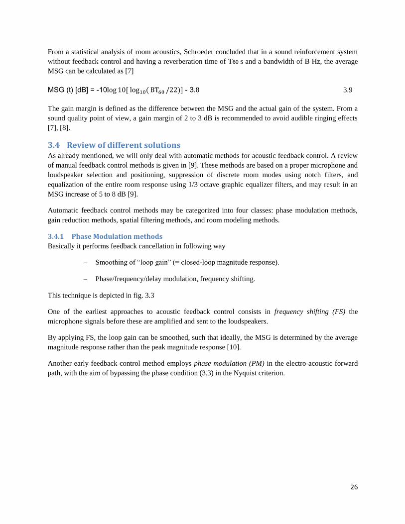
3.4.1 Phase Modulation methods

Basically it performs feedback cancellation in following way

– Smoothing of “loop gain” (= closed-loop magnitude response).

– Phase/frequency/delay modulation, frequency shifting.

This technique is depicted in fig. 3.3

One of the earliest approaches to acoustic feedback control consists in frequency shifting (FS) the

microphone signals before these are amplified and sent to the loudspeakers.

By applying FS, the loop gain can be smoothed, such that ideally, the MSG is determined by the average

magnitude response rather than the peak magnitude response [10].

Another early feedback control method employs phase modulation (PM) in the electro-acoustic forward

path, with the aim of bypassing the phase condition (3.3) in the Nyquist criterion.

27

Figure 3-3: Phase modulation method.

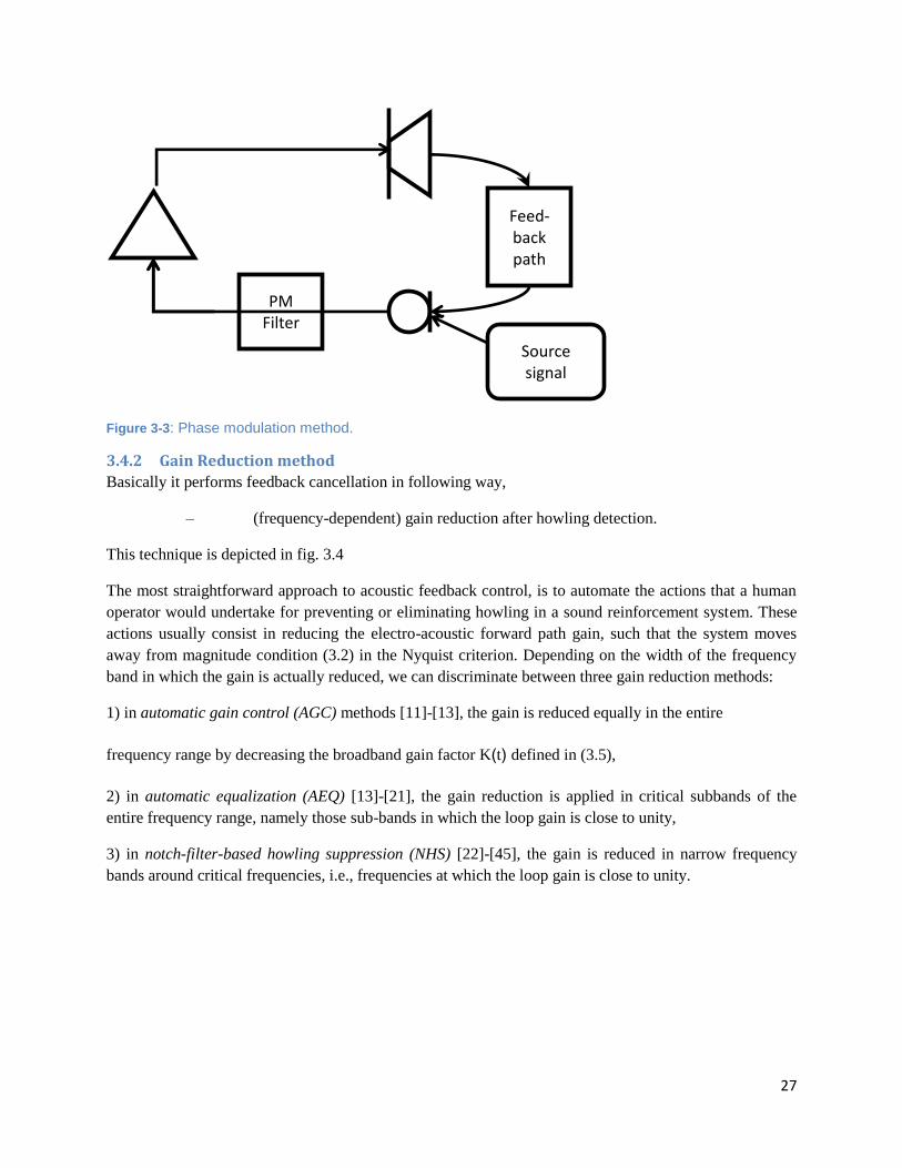
3.4.2 Gain Reduction method

Basically it performs feedback cancellation in following way,

– (frequency-dependent) gain reduction after howling detection.


The most straightforward approach to acoustic feedback control, is to automate the actions that a human

operator would undertake for preventing or eliminating howling in a sound reinforcement system. These

actions usually consist in reducing the electro-acoustic forward path gain, such that the system moves

away from magnitude condition (3.2) in the Nyquist criterion. Depending on the width of the frequency

band in which the gain is actually reduced, we can discriminate between three gain reduction methods:

1) in automatic gain control (AGC) methods [11]-[13], the gain is reduced equally in the entire

frequency range by decreasing the broadband gain factor K(t) defined in (3.5),

2) in automatic equalization (AEQ) [13]-[21], the gain reduction is applied in critical subbands of the

entire frequency range, namely those sub-bands in which the loop gain is close to unity,

3) in notch-filter-based howling suppression (NHS) [22]-[45], the gain is reduced in narrow frequency

bands around critical frequencies, i.e., frequencies at which the loop gain is close to unity.

PM

Filter

Feed-back path

Source signal

28

Figure 3-4 Gain reduction method.

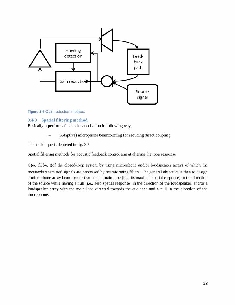
3.4.3 Spatial filtering method


– (Adaptive) microphone beamforming for reducing direct coupling.


Spatial filtering methods for acoustic feedback control aim at altering the loop response

G(ω, t)F(ω, t)of the closed-loop system by using microphone and/or loudspeaker arrays of which the

received/transmitted signals are processed by beamforming filters. The general objective is then to design

a microphone array beamformer that has its main lobe (i.e., its maximal spatial response) in the direction

of the source while having a null (i.e., zero spatial response) in the direction of the loudspeaker, and/or a

loudspeaker array with the main lobe directed towards the audience and a null in the direction of the

microphone.

Gain reduction

Feed-back path

Source signal

Howling detection

29

Figure 3-5 spatial filtering method

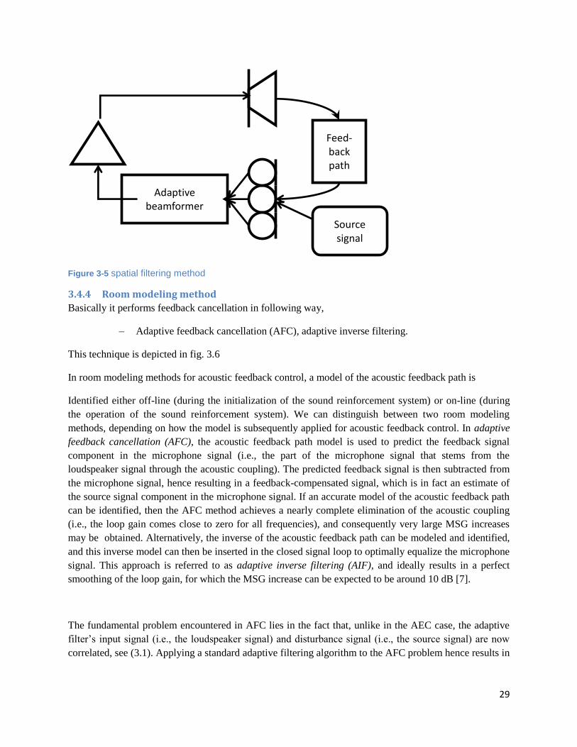
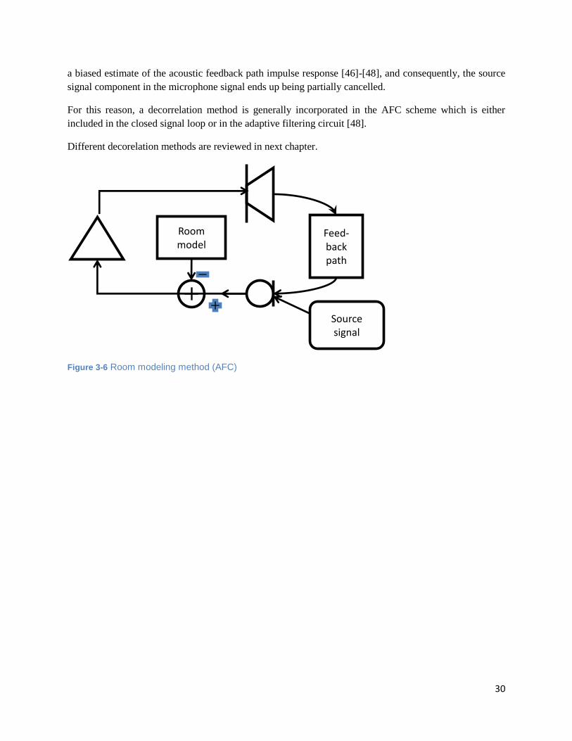
3.4.4 Room modeling method


– Adaptive feedback cancellation (AFC), adaptive inverse filtering.


In room modeling methods for acoustic feedback control, a model of the acoustic feedback path is

Identified either off-line (during the initialization of the sound reinforcement system) or on-line (during

the operation of the sound reinforcement system). We can distinguish between two room modeling

methods, depending on how the model is subsequently applied for acoustic feedback control. In adaptive

feedback cancellation (AFC), the acoustic feedback path model is used to predict the feedback signal

component in the microphone signal (i.e., the part of the microphone signal that stems from the

loudspeaker signal through the acoustic coupling). The predicted feedback signal is then subtracted from

the microphone signal, hence resulting in a feedback-compensated signal, which is in fact an estimate of

the source signal component in the microphone signal. If an accurate model of the acoustic feedback path

can be identified, then the AFC method achieves a nearly complete elimination of the acoustic coupling

(i.e., the loop gain comes close to zero for all frequencies), and consequently very large MSG increases

may be obtained. Alternatively, the inverse of the acoustic feedback path can be modeled and identified,

and this inverse model can then be inserted in the closed signal loop to optimally equalize the microphone

signal. This approach is referred to as adaptive inverse filtering (AIF), and ideally results in a perfect

smoothing of the loop gain, for which the MSG increase can be expected to be around 10 dB [7].

The fundamental problem encountered in AFC lies in the fact that, unlike in the AEC case, the adaptive

filter’s input signal (i.e., the loudspeaker signal) and disturbance signal (i.e., the source signal) are now

correlated, see (3.1). Applying a standard adaptive filtering algorithm to the AFC problem hence results in

Adaptive beamformer

Feed-back path

Source signal

30

a biased estimate of the acoustic feedback path impulse response [46]-[48], and consequently, the source

signal component in the microphone signal ends up being partially cancelled.

For this reason, a decorrelation method is generally incorporated in the AFC scheme which is either

included in the closed signal loop or in the adaptive filtering circuit [48].

Different decorelation methods are reviewed in next chapter.

Figure 3-6 Room modeling method (AFC)

Feed-back path

Source signal

Room model

31

Chapter 4 Acoustic Feedback Cancellation

4.1 Adaptive feedback cancellation (AFC): Concept

In a sound reinforcement system, the microphone signal y(t) consists of a source signal component v(t)

and a feedback signal component x(t), the latter denoting the entire signal that is fed back from the

loudspeaker to the microphone. The AFC approach to acoustic feedback control is aimed at predicting the

feedback signal component and then subtracting this prediction from the microphone signal. The

predicted feedback signal, denoted as ], is obtained by filtering the loudspeaker signal u(t) with a

model of the acoustic feedback path, see Fig. 4.1. This model is calculated using an adaptive filter

that is designed to identify the feedback path impulse response f (t) and track its changes. The feedback

path and adaptive filter impulse responses are defined at time t as

f(t) = 4.1

(t) = 4.2

respectively.

The closed-loop frequency response of the system shown in Fig. 4.1, employing an AFC method, is given

by

4.3

and, as a consequence, the Nyquist stability criterion can be rewritten as follows,

4.4

∠ = n2 n Z 4.5

And this leads to the following expression for the MSG

MSG (t) [dB] = -20 4.6

32

From (4.6), it immediately follows that the better the fit between the estimated and actual feedback path

frequency response, particularly at critical frequencies of the closed-loop system, the larger the achievable

MSG increase. Theoretically, if ≡F(q, t), the system would no longer exhibit a closed signal loop

and hence the MSG would be infinitely large.

Figure 4-1.Adaptive feedback cancellation (AFC) by predicting the feedback signal component x(t) in the

microphone signal, and hence subtracting the prediction ], from the microphone signal y(t). The

prediction is obtained by filtering the loudspeaker signal with a model of the acoustic feedback path,

which is calculated using an adaptive filter.

4.2 Least Squares Estimate: bias and variance Issues In the identification of the acoustic feedback path model a fundamental problem appears which is

due to the closed-loop nature of the system. The least-squares (LS) estimate , of the acoustic

feedback path impulse response f (t) can straightforwardly be calculated as

(t) = 4.7

where the data vectors and matrices are defined as follows

y = 4.8

U = 4.9

u(t) = 4.10

The LS estimate may be characterized by its bias and variance [50]. The bias corresponds to the

difference between the expected value of the LS estimate and the true feedback path impulse response,

i.e.

bias =

-f(t) 4.11

Where E {·} denotes the expectation operator. Under a sufficient order assumption (i.e., ), the

expected value of the LS estimate can be shown to correspond to [48]

33

= f(t) + 4.12

The rightmost term in (4.12) can be understood to be generally non-zero due to the closed-loop nature of

the system, which induces a correlation between the source signal and the loudspeaker signal, and hence

= ≠ 0 4.13

The resulting effect in AFC is that the adaptive filter does not only predict and cancel the feedback

component in the microphone signal, but also (part of) the source signal component. As a consequence,

the feedback-compensated signal d[t is a distorted estimate of the source signal v(t). On the other

hand, the variance of the LS estimate can be obtained by considering its covariance matrix, which is

calculated as [131].

cov 4.14

= 4.15

where the source signal covariance matrix is defined as

E{ } 4.16

with

v= 4.17

See note for covariance2 The interpretation of (4.15) can be related to the double-talk problem occurring

in AEC [52]. In AEC, when the loudspeaker signal is active while the source signal is not, the covariance

matrix of the acoustic echo path LS estimate is relatively small, since Rv≈0. However, when both signals

are active at the same time (i.e., in a double-talk situation), the covariance matrix may become large,

which may be observed in the adaptive filter performance as a decrease in convergence speed, or even a

divergence. This problem becomes more severe as the source signal has a larger degree of coloration,

since then the source signal covariance matrix Rv exhibits a denser structure [52]. In AFC, the closed

signal loop result in a continuous double-talk situation, and then this is made even worse by the

correlation between the source and loudspeaker signal.

2Note that the covariance matrix of the estimate is in fact defined as cov

, which corresponds to cov if f(t) ,i.e , if the

estimate is unbiased. , However, in the analysis of closed-loop identification methods it has been found more meaningful to work

directly with the covariance expression cov even if ≠ f(t) see,

e.g., [51].

34

To prevent the adaptive filter from converging to a biased solution, and to increase its convergence speed

despite the inevitable continuous double-talk situation, a decorrelation procedure is typically included in

the AFC approach, with the aim of reducing the correlation between the source and loudspeaker signal.

We can distinguish between two types of decorrelation [48], namely decorrelation in the closed signal

loop and decorrelation in the adaptive filtering circuit. The former approach has the disadvantage of

distorting the loudspeaker signal, while the latter approach requires somewhat more computations.

4.3 Review of different AFC realizations AFC can be realized in these three steps 1) adaptive filtering, 2) decorrelation and 3) post filtering as

explained below in these following sections.

4.3.1 Adaptive filtering

The adaptive calculation of the LS estimate (4.7) of the acoustic feedback path impulse response, and the

subsequent calculation of the feedback-compensated signal can be performed using adaptive filtering

technique like recursive least squares (RLS), affine projection algorithm (APA) and normalized least

mean squares (NLMS). Among these, NLMS is simpler to implement to achieve reasonably good

performance with lower complexity.

ε[t, ] = y(t)- (t) 4.18

= + µ

4.19

d[t, ] = y(t)- (t) 4.20

The required number of multiplications per time update is O( ), more specifically 4 + 6 (if the

calculation of the feedback-compensated signal in (4.20) is also taken into account). The choice of the

NLMS step size μ is crucial to obtain a good compromise between a stable and fast convergence.

Finally, the choice of the adaptive filter order , is obviously extremely important, regardless of which

adaptive filtering algorithm is used. It is clear that the choice of , has a profound influence on the

computational requirements of the AFC approach. One could argue that it may be sufficient to choose

such that the largest components in the acoustic feedback path impulse response (originating from the

early reflections) can be modeled.

Unfortunately, such an approach would be inefficient for two reasons: firstly, large impulse response

components do not necessarily correspond to large frequency response components and hence stability

may not be improved by only cancelling the early reflections. Secondly, if the impulse response is under

modeled (i.e., < ) then an additional bias component will appear in the LS estimate (in addition to the

bias due to the source and loudspeaker signal correlation) and moreover its variance will increase [55].

The best compromise between computational complexity and feedback control performance probably

consists in choosing just large enough to obtain a satisfying MSG increase, and applying a technique

for reducing the bias and variance due to under modeling [55]-[57]. We should point out that the

technique proposed by Rombouts et al. [55] for consistently identifying under modeled room impulse

responses is particularly interesting in the context of AFC, since it additionally provides a decorrelation in

the adaptive filtering circuit.

35

In this work, it has been emphasized that the above adaptive algorithms are often not implemented as

such, since both the robustness and the efficiency of these algorithms can be further improved [121]. A

robust adaptive filter implementation for AFC may include the following features: an adaptation control

that freezes the adaptive filter coefficients during source signal onsets [121], a foreground/background

adaptive filter implementation to combine good tracking properties with a small steady-state error [121],

and a regularization method that compensates for the coloration of the loudspeaker signal

[121],[122].Moreover, the AFC efficiency in terms of computational load and convergence speed can be

improved by considering a subband or frequency domain adaptive filter implementation rather than the

time domain implementations shown here [121].

4.3.2 Decorrelation

As it is seen that correlation of source and loudspeaker signal leads to biased and high-variance room

model it can be removed it two ways.

– decorrelation in the closed signal loop.

– decorrelation in the adaptive filtering circuit.

4.3.2.1 Decorrelation in the closed signal loop

Decorrelation of the far-end and near-end signal can be achieved by inserting a decorrelating signal

operation in the closed signal loop. Four such decorrelation methods have been proposed: noise injection,

time-varying processing, nonlinear processing, and forward path delay.

Figure 4-2 decorrelation in closed signal loop. Here DEC is decorrelation device

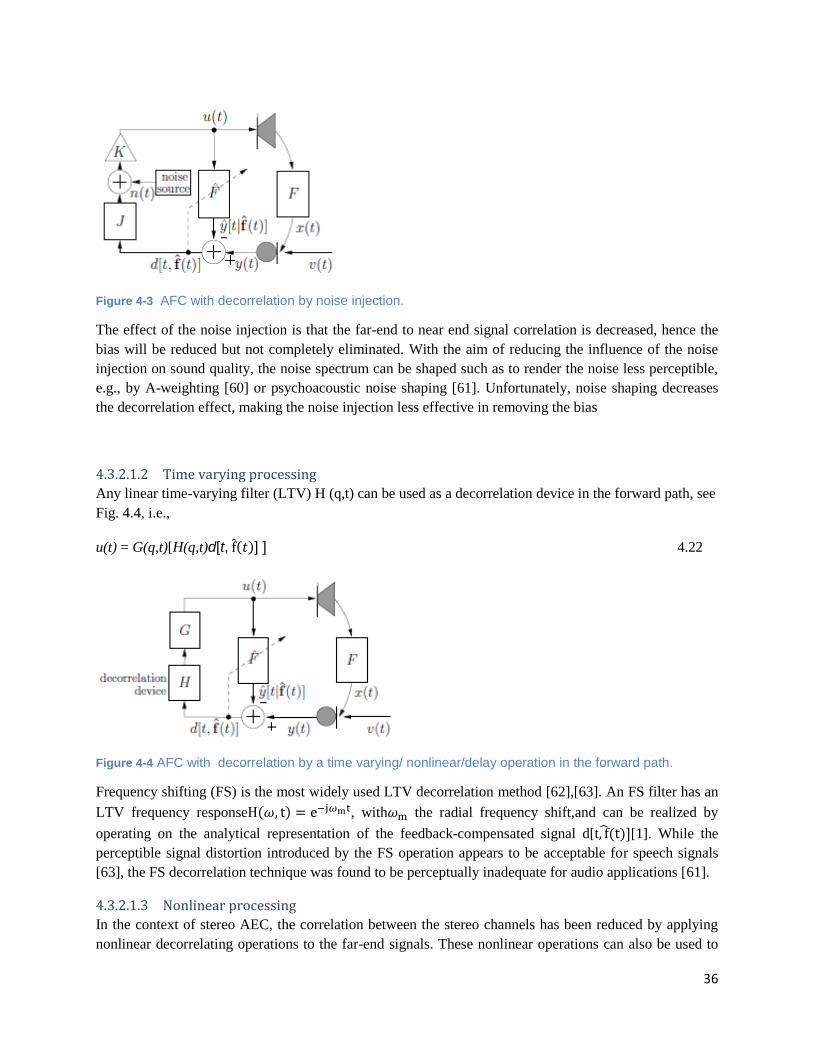
4.3.2.1.1 Noise Injection

A white noise signal n(t) is added to the feedback compensated signal after the forward path processing

(but before the forward path amplification), see Fig. 4.3, i.e.,

u(t) = K(t)[J(q,t)d[t, ] +n(t)] 4.21

Feed-back path

Source signal

Room model

DEC

36

Figure 4-3 AFC with decorrelation by noise injection.

The effect of the noise injection is that the far-end to near end signal correlation is decreased, hence the

bias will be reduced but not completely eliminated. With the aim of reducing the influence of the noise

injection on sound quality, the noise spectrum can be shaped such as to render the noise less perceptible,

e.g., by A-weighting [60] or psychoacoustic noise shaping [61]. Unfortunately, noise shaping decreases

the decorrelation effect, making the noise injection less effective in removing the bias

4.3.2.1.2 Time varying processing

Any linear time-varying filter (LTV) H (q,t) can be used as a decorrelation device in the forward path, see

Fig. 4.4, i.e.,

u(t) = G(q,t)[H(q,t)d[t, ] ] 4.22

Figure 4-4 AFC with decorrelation by a time varying/ nonlinear/delay operation in the forward path.

Frequency shifting (FS) is the most widely used LTV decorrelation method [62],[63]. An FS filter has an

LTV frequency response , with the radial frequency shift,and can be realized by

operating on the analytical representation of the feedback-compensated signal d[t [1]. While the

perceptible signal distortion introduced by the FS operation appears to be acceptable for speech signals

[63], the FS decorrelation technique was found to be perceptually inadequate for audio applications [61].

4.3.2.1.3 Nonlinear processing

In the context of stereo AEC, the correlation between the stereo channels has been reduced by applying

nonlinear decorrelating operations to the far-end signals. These nonlinear operations can also be used to

37

reduce the far-end to near-end signal correlation in AFC. In particular, half-wave rectification has been

applied to AFC decorrelation [1], i.e.,

4.23

4.3.2.1.4 Forward path delay

In hearing aid AFC applications [59], inserting a processing delay of samples in the electro-acoustic

forward path has been proposed to decorrelate the far-end and near-end signal,

u(t) = G(q,t)[d[t- , (t- )] 4.24

This approach is particularly useful for near-end signals that have an autocorrelation function that decays

rapidly, e.g., voiceless speech signals, provided that the delay value is chosen accordingly.

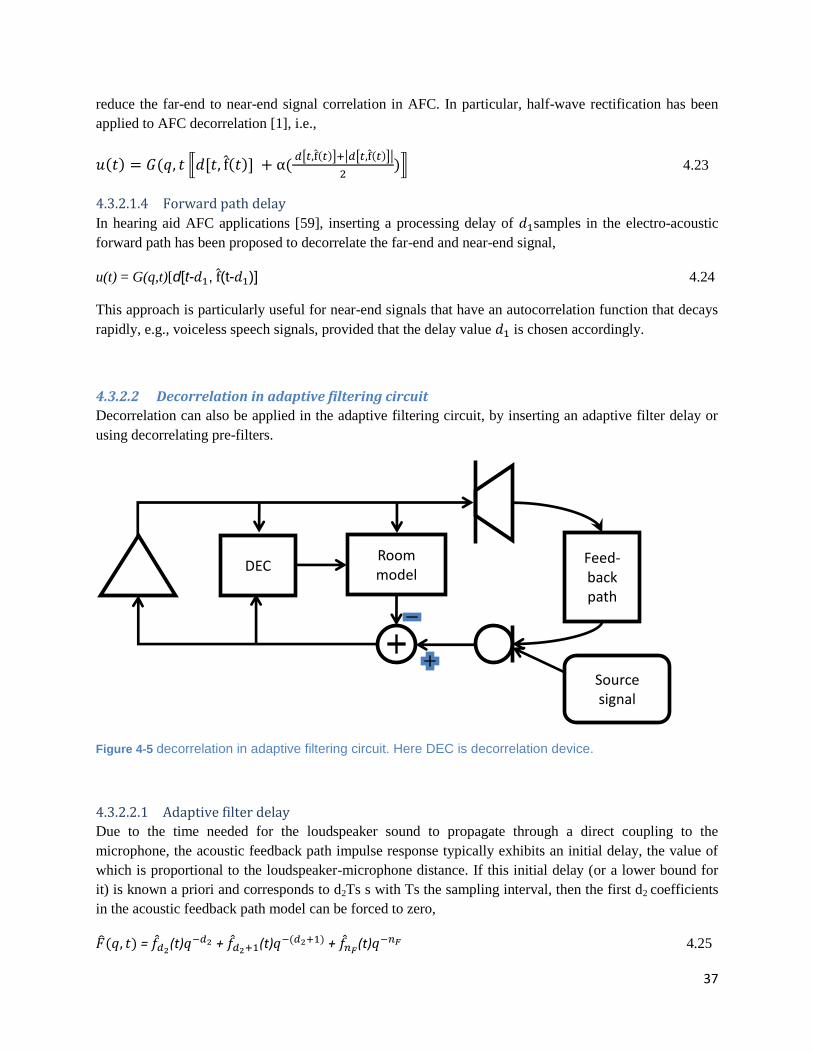
4.3.2.2 Decorrelation in adaptive filtering circuit

Decorrelation can also be applied in the adaptive filtering circuit, by inserting an adaptive filter delay or

using decorrelating pre-filters.

Figure 4-5 decorrelation in adaptive filtering circuit. Here DEC is decorrelation device.

4.3.2.2.1 Adaptive filter delay

Due to the time needed for the loudspeaker sound to propagate through a direct coupling to the

microphone, the acoustic feedback path impulse response typically exhibits an initial delay, the value of

which is proportional to the loudspeaker-microphone distance. If this initial delay (or a lower bound for

it) is known a priori and corresponds to d2Ts s with Ts the sampling interval, then the first d2 coefficients

in the acoustic feedback path model can be forced to zero,

= (t) + (t) + (t) 4.25

Feed-back path

Source signal

Room model

DEC

38

If the far-end and near-end signal cross-correlation function is small for time lags larger than d2 samples,

then the remaining bias can be considered negligible.

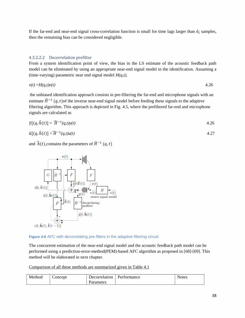
4.3.2.2.2 Decorrelation prefilter

From a system identification point of view, the bias in the LS estimate of the acoustic feedback path

model can be eliminated by using an appropriate near-end signal model in the identification. Assuming a

(time-varying) parametric near end signal model H(q,t),

v(t) =H(q,t)e(t) 4.26

the unbiased identification approach consists in pre-filtering the far-end and microphone signals with an

estimate of the inverse near-end signal model before feeding these signals to the adaptive

filtering algorithm. This approach is depicted in Fig. 4.5, where the prefiltered far-end and microphone

signals are calculated as

= (q,t)y(t) 4.26

= (q,t)u(t) 4.27

and ,contains the parameters of

Figure 4-6 AFC with decorrelating pre-filters in the adaptive filtering circuit.

The concurrent estimation of the near-end signal model and the acoustic feedback path model can be

performed using a prediction-error-method(PEM)-based AFC algorithm as proposed in [68]-[69]. This

method will be elaborated in next chapter.

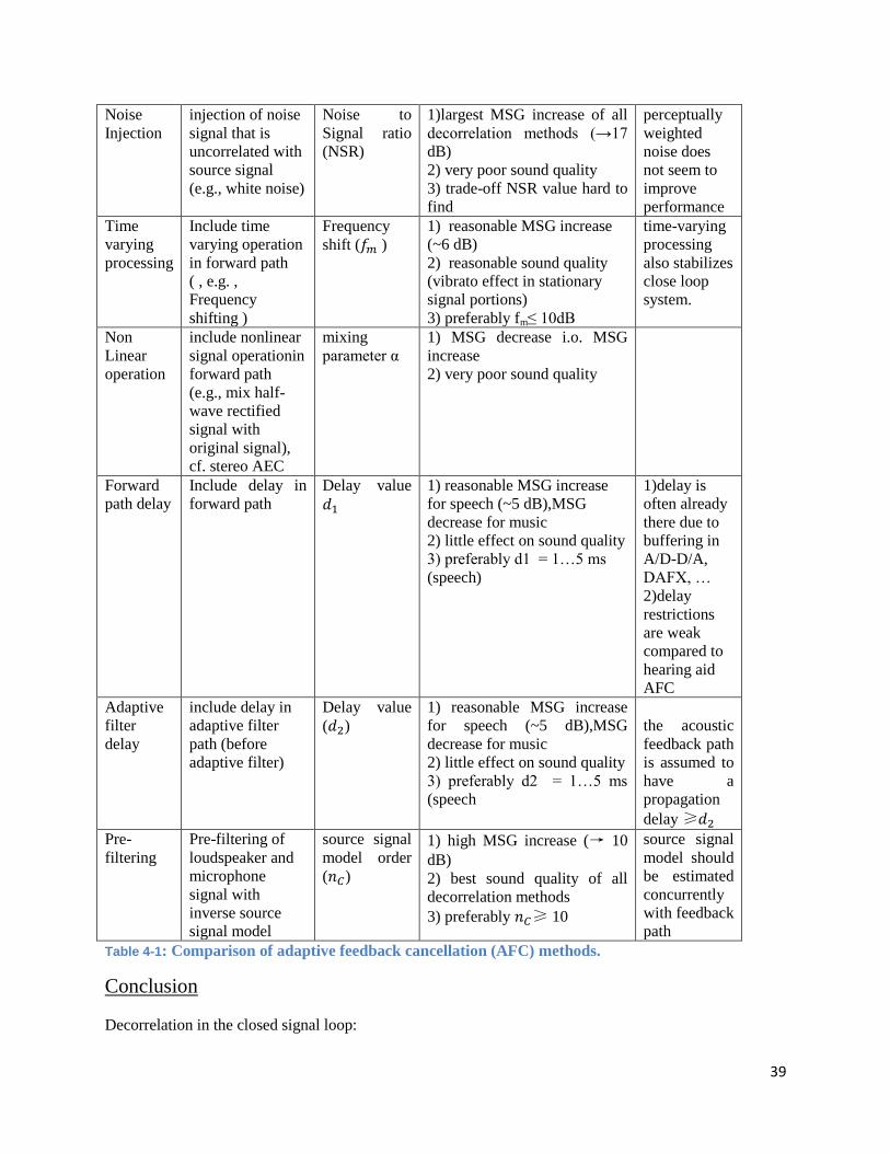
Comparison of all these methods are summarized given in Table 4.1

Method Concept Decorrelation

Parametrs

Performance Notes

39

Noise

Injection

injection of noise

signal that is

uncorrelated with

source signal

(e.g., white noise)

Noise to

Signal ratio

(NSR)

1)largest MSG increase of all

decorrelation methods (→17

dB)

2) very poor sound quality

3) trade-off NSR value hard to

find

perceptually

weighted

noise does

not seem to

improve

performance

Time

varying

processing

Include time

varying operation

in forward path

( , e.g. ,

Frequency

shifting )

Frequency

shift ( )

1) reasonable MSG increase

(~6 dB)

2) reasonable sound quality

(vibrato effect in stationary

signal portions)

3) preferably fm≤ 10dB

time-varying

processing

also stabilizes

close loop

system.

Non

Linear

operation

include nonlinear

signal operationin

forward path

(e.g., mix half-

wave rectified

signal with

original signal),

cf. stereo AEC

mixing

parameter α

1) MSG decrease i.o. MSG

increase

2) very poor sound quality

Forward

path delay

Include delay in

forward path

Delay value


for speech (~5 dB),MSG

decrease for music

2) little effect on sound quality

3) preferably d1 = 1…5 ms

(speech)

1)delay is

often already

there due to

buffering in

A/D-D/A,

DAFX, …

2)delay

restrictions

are weak

compared to

hearing aid

AFC

Adaptive

filter

delay

include delay in

adaptive filter

path (before

adaptive filter)

Delay value

( )


for speech (~5 dB),MSG

decrease for music

2) little effect on sound quality

3) preferably d2 = 1…5 ms

(speech

the acoustic

feedback path

is assumed to

have a

propagation

delay ≥

Pre-

filtering

Pre-filtering of

loudspeaker and

microphone

signal with

inverse source

signal model

source signal

model order

( )

1) high MSG increase (→ 10

dB)

2) best sound quality of all

decorrelation methods

3) preferably ≥ 10

source signal

model should

be estimated

concurrently

with feedback

path

Table 4-1: Comparison of adaptive feedback cancellation (AFC) methods.

Conclusion

Decorrelation in the closed signal loop:

40

• Decorrelation by noise injection delivers very high MSG (> 15 dB), but is inappropriate in terms

of sound quality.

• Decorrelation by time-varying processing is a “fair compromise” approach that combines

reasonable MSG and sound quality.

• Decorrelation by nonlinear processing is clearly unsuited for AFC applications (in contrast to

stereo AEC).

• Decorrelation by forward path delay is suited only for speech signals, resulting in limited MSG

but good sound quality.

Decorrelation in the adaptive filtering circuit:

• Decorrelation by adaptive filter delay does not outperform forward path delay yet relies on

propagation delay assumption.

• Decorrelation by pre-filtering is superior in terms of sound quality and moreover delivers high

MSG values (up to 10 dB).

4.3.3 Post filter

Mainly owing to under modeling and steady-state as well as tracking errors, a mis-adjustment between the

AFC adaptive filter coefficients and the acoustic feedback path impulse response will unavoidably exist.

As a result, the feedback signal x(t) will typically not be completely cancelled from the microphone

signal, and so the feedback-compensated signal contains a residual feedback signal component r[t, ],

d[t, ] = v(t) +

. 4.28

Several attempts have been made to apply the AEC postfiltering approach to the AFC scenario [71],[72],

resulting in the AFC scheme shown in Fig. 4.5. We should emphasize that, again, the correlation between

the loudspeaker and source signal makes the residual feedback suppression problem much harder in the

AFC case as compared to the AEC case. Since the postfiltering approach is based on spectral subtraction,

the postfilter is usually designed directly in the frequency domain.

41

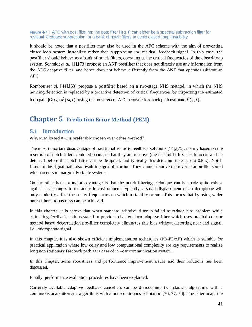
Figure 4-7 : AFC with post filtering: the post filter H(q, t) can either be a spectral subtraction filter for residual feedback suppression, or a bank of notch filters to avoid closed-loop instability.

It should be noted that a postfilter may also be used in the AFC scheme with the aim of preventing

closed-loop system instability rather than suppressing the residual feedback signal. In this case, the

postfilter should behave as a bank of notch filters, operating at the critical frequencies of the closed-loop

system. Schmidt et al. [1],[73] propose an ANF postfilter that does not directly use any information from

the AFC adaptive filter, and hence does not behave differently from the ANF that operates without an

AFC.

Romboutset al. [44],[53] propose a postfilter based on a two-stage NHS method, in which the NHS

howling detection is replaced by a proactive detection of critical frequencies by inspecting the estimated

loop gain |G(ω, t) | using the most recent AFC acoustic feedback path estimate .

Chapter 5 Prediction Error Method (PEM)

5.1 Introduction Why PEM based AFC is preferably chosen over other method?

The most important disadvantage of traditional acoustic feedback solutions [74],[75], mainly based on the

insertion of notch filters centered on , is that they are reactive (the instability first has to occur and be

detected before the notch filter can be designed, and typically this detection takes up to 0.5 s). Notch

filters in the signal path also result in signal distortion. They cannot remove the reverberation-like sound

which occurs in marginally stable systems.

On the other hand, a major advantage is that the notch filtering technique can be made quite robust

against fast changes in the acoustic environment: typically, a small displacement of a microphone will

only modestly affect the center frequencies on which instability occurs. This means that by using wider

notch filters, robustness can be achieved.

In this chapter, it is shown that when standard adaptive filter is failed to reduce bias problem while

estimating feedback path as stated in previous chapter, then adaptive filter which uses prediction error

method based decorrelation pre-filter completely eliminates this bias without distorting near end signal,

i.e., microphone signal.

In this chapter, it is also shown efficient implementation techniques (PB-FDAF) which is suitable for

practical application where low delay and low computational complexity are key requirements to realize

long non stationary feedback path as is case of in –car communication system.

In this chapter, some robustness and performance improvement issues and their solutions has been

discussed.

Finally, performance evaluation procedures have been explained.

Currently available adaptive feedback cancellers can be divided into two classes: algorithms with a

continuous adaptation and algorithms with a non-continuous adaptation [76, 77, 78]. The latter adapt the

42

coefficients of the feedback canceller only when instability is detected or when the input signal level is

low [78]–[80]. Due to this reactive, rather than proactive, adaptation, such systems may be objectionable.

A continuous adaptation feedback (CAF) canceller continuously adapts the coefficients of the feedback

path estimate in such a way that the energy of the feedback-compensated signal is minimized. This is

depicted in Fig. 4.7.

5.2 Standard CAF AFC realization using PB-FDAF The greatest challenge in AFC, however, consists in reducing the computational complexity. Since

typically an already cheap NLMS-type algorithm is used, a significant complexity reduction in the AFC

adaptive filtering algorithm cannot be expected. The fundamental problem lies in the fact that in AFC, the

acoustic feedback path is traditionally modeled using its impulse response, which typically has a large

number of coefficients. This is especially so when a high sampling frequency is applied (e.g., in audio

applications). The impulse response is then more densely sampled and in addition more adaptive filter

updates have to be performed per second. However, from a stability point of view, it may suffice to only

model the peaks in the acoustic feedback path magnitude response instead of the complete impulse

response. This may be achieved with frequency domain adaptive filtering (FDAF). However, since the

frequency domain models currently used in FDAF have a fixed and uniform frequency resolution, the

required FDAF modeled with sufficient accuracy, see, e.g., the FDAF experimental results in [53].

Thus even if the adaptive filter is realized in frequency domain when filter order is still very high , there

will be unacceptable day due to large input block size to be processed in FDAF.

So, alternative solution to this problem is the second frequency domain implementation which reduces

this latency since it is based on the partitioned block frequency domain adaptive filtering (PBFDAF)

algorithm.

This PBFDAF, which combines the beneficial properties of frequency domain algorithms, that is a

frequency-dependent step size control and faster convergence thanks to the decorrelation properties of the

FFT, and a reduced complexity, with a small processing delay as required for real-time applications.

The superscripts T and H denote matrix/vector transpose and complex conjugate transpose, respectively.

The expectation operator is denoted by ε{.} The matrix F is the M x M DFT matrix. The matrix is the L

x L identity matrix. The matrix is an L x L dimensional matrix of zeros.

The discrete-time index is denoted by n. The symbol denotes the discrete-time delay operator, i.e.,

u[n]=u[n-1]

A discrete-time filter with coefficient vector f[n]

f[n] = [n] [n] …. [n]]T

,

and filter length is represented as a polynomial transfer function F(q,n) in q, i.e.,

F(q,n)= [n]q,

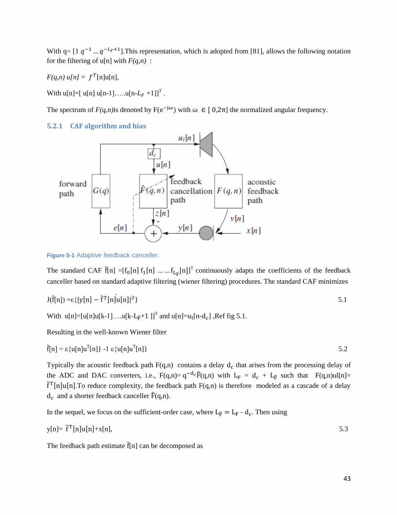
43

With q= [1 ].This representation, which is adopted from [81], allows the following notation

for the filtering of u[n] with F(q,n) :

F(q,n) u[n] = [n]u[n],

With u[n]=[ u[n] u[n-1]…..u[n- +1]]T .

The spectrum of F(q,n)is denoted by F( with ] the normalized angular frequency.

5.2.1 CAF algorithm and bias

Figure 5-1 Adaptive feedback canceller.

The standard CAF [n] =[ ]T

continuously adapts the coefficients of the feedback

canceller based on standard adaptive filtering (wiener filtering) procedures. The standard CAF minimizes

J( [n]) =ε{ } 5.1

With u[n]=[u[n]u[k-1]….u[k- +1 ]]T and u[n]= [n- ] ,Ref fig 5.1.

Resulting in the well-known Wiener filter

[n] = ε{u[n]uT[n]} -1 ε{u[n]u

T[n]} 5.2

Typically the acoustic feedback path F(q,n) contains a delay that arises from the processing delay of

the ADC and DAC converters, i.e., F(q,n)= (q,n) with = + such that F(q,n)ul[n]=

.To reduce complexity, the feedback path F(q,n) is therefore modeled as a cascade of a delay

and a shorter feedback canceller (q,n).

In the sequel, we focus on the sufficient-order case, where - . Then using

y[n]= +x[n], 5.3

The feedback path estimate [n] can be decomposed as

44

[n] =ε{u[n]uT[n]} -1 (ε {u[n] u

T[n] [n] } + ε {u[n] x[n]})

= [n]+ ε{u[n]uT [n]}

-1 ε{u[n] x[n]} 5.4

If ε{u[n]uT[n]} = 0 , then the feedback path estimate is unbiased.

However, because of the presence of the closed signal loop G(q), the input signal u[n] to the adaptive

filter [n] relates to x[n] as

u[n]

5.5

where C(q,n) is the transfer function from x[n] to the loudspeaker signal u[n]. Assume that G(q) contains

a delay dG with dG 1 and assume that G(n), F(q,n) and (q,n) arecausal. Then, the closed-loop

system C(q,n) can be specified as

+ ….+ 5.6

And hence

u[n] = )x[n- ] 5.7

as a result , ε{u[n]x[n]} = 0 if and only if

ε{x[n- ]x[n } = 0 5.8

for - -2

Most practical sound signals x[n] are spectrally colored, meaning that the signal values x[n] are correlated

in time (e.g., speech, music, etc.). Many of these audio signals may be well approximated as low-order,

autoregressive (AR) random processes,

x[n] = H(q)w(n) =

w[n] 5.9

with w[n] white noise signal. Hence, the signal model H(q) is often IIR, so that the length LH of

H(q)exceeds andhence,ε{u[n]x[n]} 0 .The CAF will then cancel the desired signal x[n] instead

of the feedback signal v[n] = [n]u[n](see Eq. (5.4)), leading to signal distortion. From Eq. (5.4), we

observe that the bias in the feedback path estimate decreases with an increasing power ratio of the

feedback signal v[n] (i.e., the signal to identify) to the desired signal x[n] (which acts as a

disturbance).Since v[n] =F(q)C(q,n)x[n] with C(n,q) defined in Eq. (5.5), the larger the loop gain

|G(q)F(q,n)|,the smaller the bias will be. This indicates that the bias will be smallest for large gains

G(q)and for frequencies that are closest to instability.

In following Sections, solutions for reducing the bias of the CAF will be described.

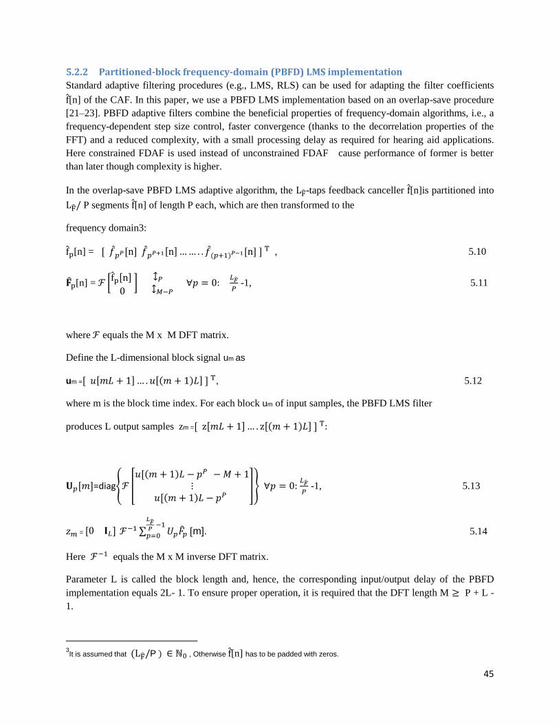
45

5.2.2 Partitioned-block frequency-domain (PBFD) LMS implementation

Standard adaptive filtering procedures (e.g., LMS, RLS) can be used for adapting the filter coefficients

[n] of the CAF. In this paper, we use a PBFD LMS implementation based on an overlap-save procedure

[21–23]. PBFD adaptive filters combine the beneficial properties of frequency-domain algorithms, i.e., a

frequency-dependent step size control, faster convergence (thanks to the decorrelation properties of the

FFT) and a reduced complexity, with a small processing delay as required for hearing aid applications.

Here constrained FDAF is used instead of unconstrained FDAF cause performance of former is better

than later though complexity is higher.

In the overlap-save PBFD LMS adaptive algorithm, the -taps feedback canceller [n]is partitioned into

P segments [n] of length P each, which are then transformed to the

frequency domain3:

[n] =

, 5.10

[n] =

-1, 5.11

where equals the M x M DFT matrix.

Define the L-dimensional block signal um as

um = , 5.12

where m is the block time index. For each block um of input samples, the PBFD LMS filter

produces L output samples zm =

=diag

-1, 5.13

=

m]. 5.14

Here equals the M x M inverse DFT matrix.

Parameter L is called the block length and, hence, the corresponding input/output delay of the PBFD

implementation equals 2L- 1. To ensure proper operation, it is required that the DFT length M P + L -

1.

3It is assumed that P , Otherwise [n] has to be padded with zeros.

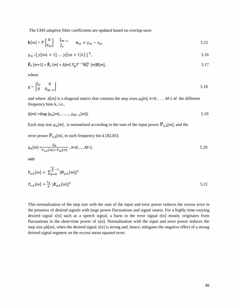
46

The LMS adaptive filter coefficients are updated based on overlap-save:

E[m] =

5.15

= , 5.16

[m+1] = [m] + Δ[m]

[m]E[m], 5.17

where

g =

5.18

and where [m] is a diagonal matrix that contains the step sizes µk[m], k=0; . . . ;M-1 of the different

frequency bins k, i.e.,

Δ[m] =diag { [m],………, [m]}. 5.19

Each step size [m] , is normalized according to the sum of the input power Pu,k[m], and the

error power Pe,k[m], in each frequency bin k [82,85]:

[m] =

, k=0,…..,M-1, 5.20

with

5.21

This normalization of the step size with the sum of the input and error power reduces the excess error in

the presence of desired signals with large power fluctuations and signal onsets. For a highly time-varying

desired signal x[n] such as a speech signal, a burst in the error signal e[n] mostly originates from

fluctuations in the short-time power of x[n]. Normalization with the input and error power reduces the

step size µk[m], when the desired signal x[n] is strong and, hence, mitigates the negative effect of a strong

desired signal segment on the excess mean squared error.

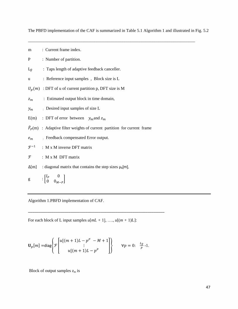
47

The PBFD implementation of the CAF is summarized in Table 5.1 Algorithm 1 and illustrated in Fig. 5.2

______________________________________________________________________________

m : Current frame index.

P : Number of partition.

: Taps length of adaptive feedback canceller.

u : Reference input samples , Block size is L

) : DFT of u of current partition p, DFT size is M

: Estimated output block in time domain,

: Desired input samples of size L

E(m) : DFT of error between and

(m) : Adaptive filter weights of current partition for current frame

: Feedback compensated Error output.

: M x M inverse DFT matrix

: M x M DFT matrix

[m] : diagonal matrix that contains the step sizes µk[m],

g :

Algorithm 1.PBFD implementation of CAF.

________________________________________________________________

For each block of L input samples u[mL + 1], …., u[(m + 1)L]:

diag

-1.

Block of output samples zm is

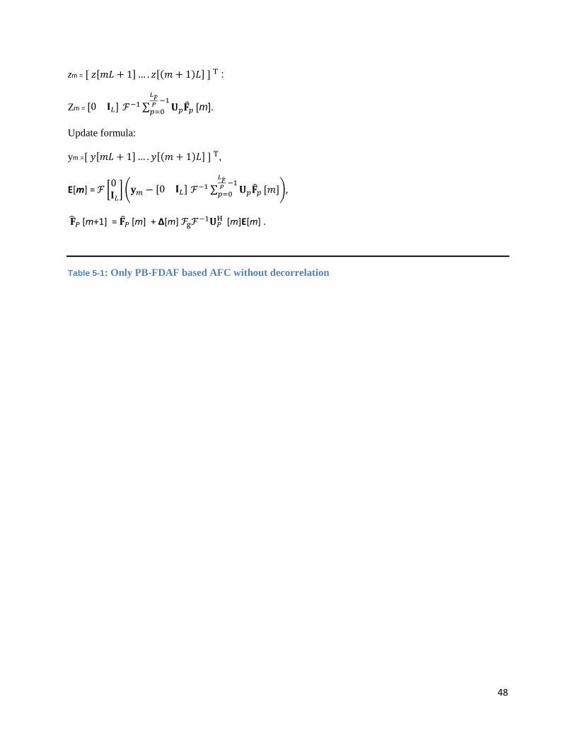
48

zm = :

Zm =

m].

Update formula:

ym = ,

E[m] =

,

[m+1] = [m] + Δ[m]

[m]E[m] .

Table 5-1: Only PB-FDAF based AFC without decorrelation

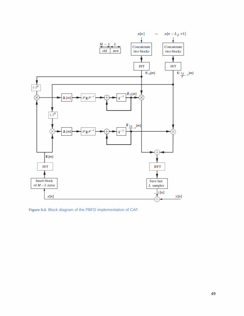
49

Figure 5-2. Block diagram of the PBFD implementation of CAF.

50

5.3 PEM based AFC using PB-FDAF for speech application The desired signal model is then used to pre-whiten the desired signal component in the microphone and

the loudspeaker signals. This approach has been adopted from direct closed-loop system identification

with the PEM [86, 87].

5.3.1 Closed-loop identification of the feedback path with the direct method

For the time being, we assume that the desired signal x[n] can be modeled as

x[n] = H(q,n)w[n] 5.22

with w[n] a zero mean, white noise sequence and H(q,n) monic and inversely stable. In the direct method

of closed-loop identification, the open-loop system { F(q,n),H(q,n)}

y[n] =F(q,n) [n] + H(q,n)w[n],

= (q,n)u[n] + H(q,n)w[n], 5.23

is identified from the loudspeaker signal ul[n] and the microphone signal y[n] by an open-loop

identification method, thereby ignoring the presence of the closed signal loop G(q).Only some specific

open-loop identification methods can be applied to closed-loop systems, such as the PEM [37,38]. The

PEM produces an estimate (q,n) and (q,n);of thefeedback path (q,n) and the desired signal model

H(q,n) respectively, by minimizing the energy of the so-called prediction error [n] ,i.e.,

[n] = (q,n)u[n]), 5.24

J( [n]) = ε{ }

= ε{ }, 5.25

where

= , 5.26

= , . 5.27

Minimization of Eq. (5.25) results in

ε , 5.28

where can be decomposed as (cf. Eq. (5.23)):

(q,n) . 5.29

If (q,n) equals the true desired signal model H(q,n)

(q,n) . 5.30

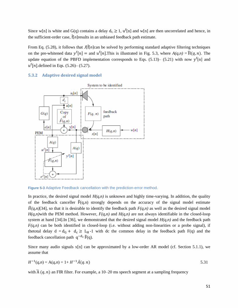
51

Since w[n] is white and G(q) contains a delay dG 1, [n] and w[n] are then uncorrelated and hence, in

the sufficient-order case, [n]results in an unbiased feedback path estimate.

From Eq. (5.28), it follows that J[ [n]can be solved by performing standard adaptive filtering techniques

on the pre-whitened data and This is illustrated in Fig. 5.3, where A(q,n) = . The

update equation of the PBFD implementation corresponds to Eqs. (5.13)– (5.21) with now [n] and

.defined in Eqs. (5.26)– (5.27).

5.3.2 Adaptive desired signal model

Figure 5-3 Adaptive Feedback cancellation with the prediction-error method.

In practice, the desired signal model H(q,n) is unknown and highly time-varying. In addition, the quality

of the feedback canceller (q,n) strongly depends on the accuracy of the signal model estimate

(q,n)[34], so that it is desirable to identify the feedback path F(q,n) as well as the desired signal model

H(q,n)with the PEM method. However, F(q,n) and H(q,n) are not always identifiable in the closed-loop

system at hand [34].In [36], we demonstrated that the desired signal model H(q,n) and the feedback path

F(q,n) can be both identified in closed-loop (i.e. without adding non-linearities or a probe signal), if

thetotal delay d = -1 with dc the common delay in the feedback path F(q) and the

feedback cancellation path (q).

Since many audio signals x[n] can be approximated by a low-order AR model (cf. Section 5.1.1), we

assume that

(q,n) = A(q,n) = 1+ 5.31

with an FIR filter. For example, a 10–20 ms speech segment at a sampling frequency

52

fs = 16 kHz can be modeled by a 10–20th order AR model with w[n] a white noise excitation (in case of

unvoiced sounds) or a pulse train excitation (in case of voiced sounds) [88]. The AR model A(q,n) is

computed through linear prediction of the feedback- compensated signal,

e[n]= y[n] - [n] u[n]. 5.32

Note that e[n]= x[n] , if [n] = [n] .

In this paper, the AR model is estimated on subsequent frames of N = 160 samples (i.e., 10 ms) through

the Levinson–Durbin algorithm [88]. The feedback canceller (q, n) is then updated with the PBFD LMS

algorithm using the updated AR model

-1(q,n) = A(q,n) in eqns. (5.26)– (5.27).

So far, we have assumed that the excitation of the desired signal model H(n,q) is a white noise sequence

w[n]. This assumption does not apply for voiced speech, where the excitation w[n] approximates a pulse

train that is periodical with the pitch period P (expressed as number of samples). Due to this periodicity,

the pre-filtered loudspeaker signal [n] is still correlated with the excitation signal w[n] at the pitch

frequency and its harmonics. From eqs. (5.28)–(5.30), it follows that the feedback canceller [n] will then

still be biased if

ε{ } ≠ 0. 5.33

Using [n] = (q,n) C(q)x[n] with (q,n) = (q,n) it can be shown that (5.33)

corresponds to

ε{ } ≠ 0. 5.34

For - -2.Hence, if

-2. 5.35

With i , the feedback path estimate will be biased at the frequencies i /P with i/P < ½, where fs

equals the sampling frequency. For speech, the pitch frequency fs/P lies between 50 and 400 Hz and

hence, for fs = 16 kHz, typically P lies between 40 and 320 samples. To remove the residual correlation

caused by the pulse train excitation, a short-term AR model AST(q,n )can be cascaded with a long-term

predictor ALT(q,n ) = (1-b ) , where is an estimate of pitch period P[ 40].See appendix

for open loop pitch (P) and gain (b) computation algorithm details.

A(q,n) = AST ((1-b )). 5.36

To guarantee identifiability, the delay = [n] + , and, hence, [n] should be

constraint as

[n] LAST , 320) 5.37

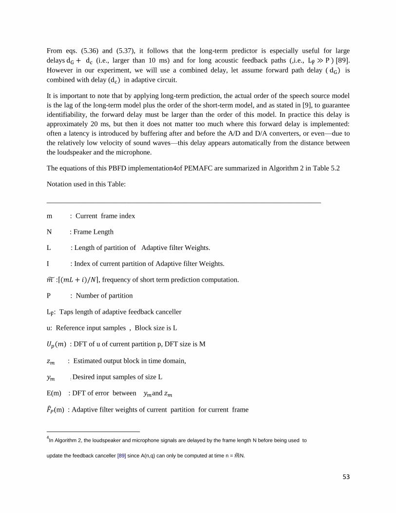
53

From eqs. (5.36) and (5.37), it follows that the long-term predictor is especially useful for large

delays (i.e., larger than 10 ms) and for long acoustic feedback paths (,i.e.,

However in our experiment, we will use a combined delay, let assume forward path delay ( is

combined with delay ( in adaptive circuit.

It is important to note that by applying long-term prediction, the actual order of the speech source model

is the lag of the long-term model plus the order of the short-term model, and as stated in [9], to guarantee

identifiability, the forward delay must be larger than the order of this model. In practice this delay is

approximately 20 ms, but then it does not matter too much where this forward delay is implemented:

often a latency is introduced by buffering after and before the A/D and D/A converters, or even—due to

the relatively low velocity of sound waves—this delay appears automatically from the distance between

the loudspeaker and the microphone.

The equations of this PBFD implementation4of PEMAFC are summarized in Algorithm 2 in Table 5.2

Notation used in this Table:

_____________________________________________________________________________

m : Current frame index

N : Frame Length

L : Length of partition of Adaptive filter Weights.

I : Index of current partition of Adaptive filter Weights.

: , frequency of short term prediction computation.

P : Number of partition

: Taps length of adaptive feedback canceller

u: Reference input samples , Block size is L






4In Algorithm 2, the loudspeaker and microphone signals are delayed by the frame length N before being used to

update the feedback canceller [89] since A(n,q) can only be computed at time n = N.

54



: M x M DFT matrix

[m] : pre-filtered speaker signal block of current partition . This is also input to adaptive filter.

[m] : pre-filtered microphone signal block of current partition

[m] : DFT of

[m].

A(q,m) : coefficient of short term predictor.

: STP estimated signal

: Lag of LTP at current frame.

: Gain at lag .


g:

Algorithm 2.PBFD implementation of CAF.

________________________________________________________________

For each block of L input samples u[mL +1],……, u[(m +1)L]:

=diag

-1,


zm = :

Zm =

m].

Pre-filtering of loudspeaker and microphone signals with inverse of STP

55

A(q, -1) , = :

[ ] = A(q, -1)u[ ],

[ ] = A(q, -1)y[ ], i=1,……,L,

=diag

-1,

Update AR model with A(q, -1)

If mL + i = where

A(q, )= )

With e[ = y[ .

End

Update formula:

= =

[m]=

,

[m+1] = [m] + Δ[m]

[m] [m].

Table 5-2: PB-FDAF based PEM AFC with STP pre-filter

If near end signal mode for speech LTP is cascaded with STP for the purpose of pre-filtering of the input

of adaptive filter for better decorrelation, the bias in estimation of feedback path is reduced more. Hence,

performance is better than when same is achieved using only STP. This algorithm is explained here in

Table 5.4.

The equations of this PBFD implementation of PEMAFC are summarized in Algorithm 3 in Table 5.3

Notation used in this Table:

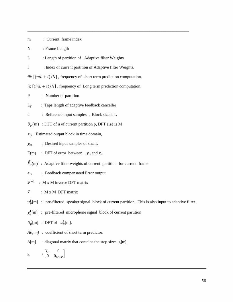
56

_____________________________________________________________________________

m : Current frame index

N : Frame Length

L : Length of partition of Adaptive filter Weights.

I : Index of current partition of Adaptive filter Weights.

: , frequency of short term prediction computation.

: , frequency of Long term prediction computation.

P : Number of partition

: Taps length of adaptive feedback canceller

u : Reference input samples , Block size is L








: M x M DFT matrix

[m] : pre-filtered speaker signal block of current partition . This is also input to adaptive filter.

[m] : pre-filtered microphone signal block of current partition

[m] : DFT of

[m].

A(q,m) : coefficient of short term predictor.


g :

57

Algorithm 3. PBFD implementation of CAF.

________________________________________________________________

For each block of L input samples u[mL +1],……, u[(m +1)L]:

=diag

-1,


zm = :

zm =

m].

Pre-filtering of loudspeaker and microphone signals with inverse of

A(q, -1) , = :

[ ] = A(q, -1)u[ ],

[ ] = A(q, -1)y[ ], i =1,……,L,

Pre-filtering of loudspeaker and microphone signals with inverse of LTP

[mL + i] = [mL + i] - [mL + i- N- ]

[mL + i] = [mL + i] - [mL + i- N- ] i = 1…L,

Here and K are LTP pitch gain and lag respectively of previous frame.

=diag

-1,

Update AR model with A(q, -1)

If mL + i = where

A(q, )= )

With e[ = y[ .

End

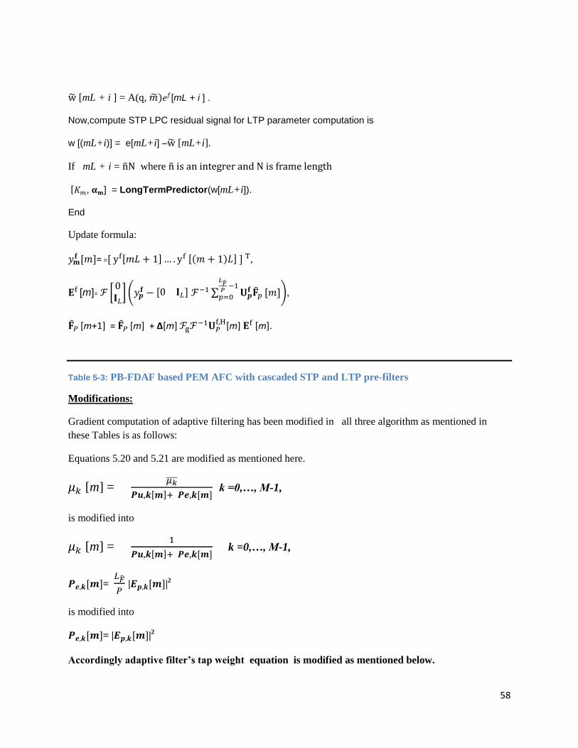
58

[mL + i ] = A(q, [mL + i ] .

Now,compute STP LPC residual signal for LTP parameter computation is

w [(mL+i)] = e[mL+i] – [mL+i].

If mL + i = where

[ , ] = LongTermPredictor(w[mL+i]).

End

Update formula:

= =

[m]=

,

[m+1] = [m] + Δ[m]

[m] [m].

Table 5-3: PB-FDAF based PEM AFC with cascaded STP and LTP pre-filters

Modifications:

Gradient computation of adaptive filtering has been modified in all three algorithm as mentioned in

these Tables is as follows:

Equations 5.20 and 5.21 are modified as mentioned here.

[m] =

k =0,…, M-1,

is modified into

[m] =

k =0,…, M-1,

=

| |

2

is modified into

= | |2

Accordingly adaptive filter’s tap weight equation is modified as mentioned below.

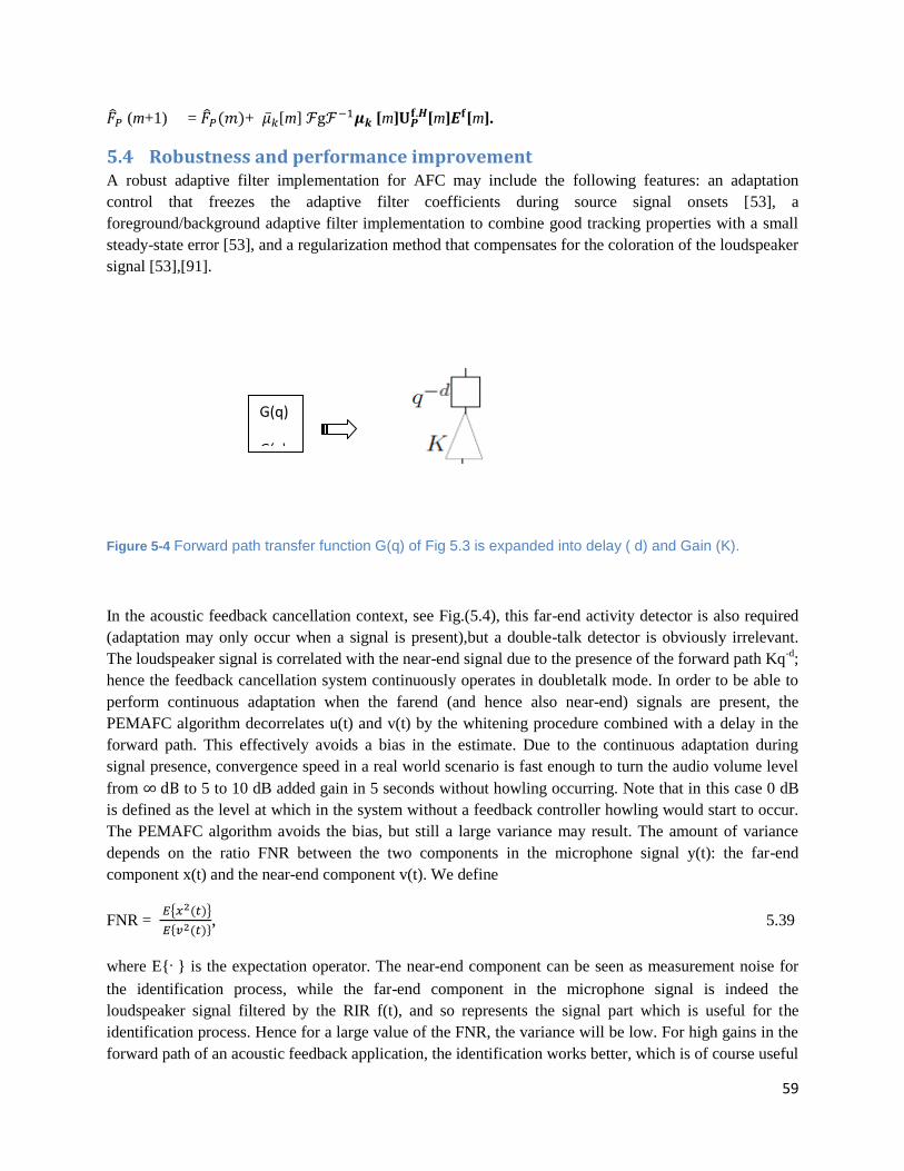
59

(m+1) = + [m] [m] [m] [m].

5.4 Robustness and performance improvement A robust adaptive filter implementation for AFC may include the following features: an adaptation

control that freezes the adaptive filter coefficients during source signal onsets [53], a

foreground/background adaptive filter implementation to combine good tracking properties with a small

steady-state error [53], and a regularization method that compensates for the coloration of the loudspeaker

signal [53],[91].

Figure 5-4 Forward path transfer function G(q) of Fig 5.3 is expanded into delay ( d) and Gain (K).

In the acoustic feedback cancellation context, see Fig.(5.4), this far-end activity detector is also required

(adaptation may only occur when a signal is present),but a double-talk detector is obviously irrelevant.

The loudspeaker signal is correlated with the near-end signal due to the presence of the forward path Kq-d

;

hence the feedback cancellation system continuously operates in doubletalk mode. In order to be able to

perform continuous adaptation when the farend (and hence also near-end) signals are present, the

PEMAFC algorithm decorrelates u(t) and v(t) by the whitening procedure combined with a delay in the

forward path. This effectively avoids a bias in the estimate. Due to the continuous adaptation during

signal presence, convergence speed in a real world scenario is fast enough to turn the audio volume level

from to 5 to 10 dB added gain in 5 seconds without howling occurring. Note that in this case 0 dB

is defined as the level at which in the system without a feedback controller howling would start to occur.

The PEMAFC algorithm avoids the bias, but still a large variance may result. The amount of variance

depends on the ratio FNR between the two components in the microphone signal y(t): the far-end

component x(t) and the near-end component v(t). We define

FNR =

, 5.39

where E{·} is the expectation operator. The near-end component can be seen as measurement noise for

the identification process, while the far-end component in the microphone signal is indeed the

loudspeaker signal filtered by the RIR f(t), and so represents the signal part which is useful for the

identification process. Hence for a large value of the FNR, the variance will be low. For high gains in the

forward path of an acoustic feedback application, the identification works better, which is of course useful

G(q)

G(q)

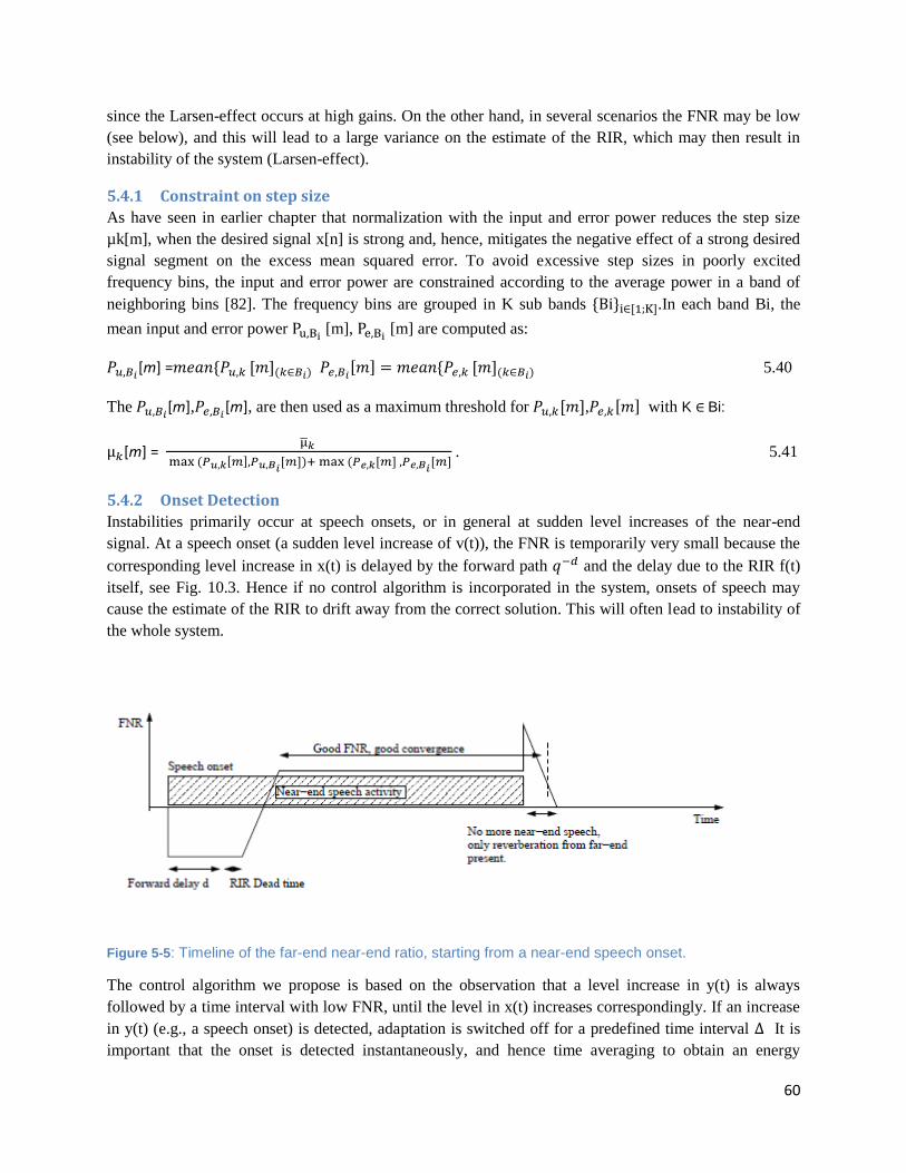
60

since the Larsen-effect occurs at high gains. On the other hand, in several scenarios the FNR may be low

(see below), and this will lead to a large variance on the estimate of the RIR, which may then result in

instability of the system (Larsen-effect).

5.4.1 Constraint on step size

As have seen in earlier chapter that normalization with the input and error power reduces the step size

µk[m], when the desired signal x[n] is strong and, hence, mitigates the negative effect of a strong desired

signal segment on the excess mean squared error. To avoid excessive step sizes in poorly excited

frequency bins, the input and error power are constrained according to the average power in a band of

neighboring bins [82]. The frequency bins are grouped in K sub bands .In each band Bi, the

mean input and error power [m], [m] are computed as:

[m] = 5.40

The [m], [m], are then used as a maximum threshold for , with K Bi:

[m] =

. 5.41

5.4.2 Onset Detection

Instabilities primarily occur at speech onsets, or in general at sudden level increases of the near-end

signal. At a speech onset (a sudden level increase of v(t)), the FNR is temporarily very small because the

corresponding level increase in x(t) is delayed by the forward path and the delay due to the RIR f(t)

itself, see Fig. 10.3. Hence if no control algorithm is incorporated in the system, onsets of speech may

cause the estimate of the RIR to drift away from the correct solution. This will often lead to instability of

the whole system.

Figure 5-5: Timeline of the far-end near-end ratio, starting from a near-end speech onset.

The control algorithm we propose is based on the observation that a level increase in y(t) is always

followed by a time interval with low FNR, until the level in x(t) increases correspondingly. If an increase

in y(t) (e.g., a speech onset) is detected, adaptation is switched off for a predefined time interval It is

important that the onset is detected instantaneously, and hence time averaging to obtain an energy

61

estimate of y(t) is impossible, because the lag introduced by the averaging would already allow the

adaptive filter coefficients to drift substantially.

In order to achieve instantaneous detection, a Gaussian distribution of the (whitened) near-end signal (t)

is assumed, and the short-term variance (t) of this distribution is estimated over an exponential

window

(t-1) + (t) , 5.42

With 0 <1 forgetting factor. A speech onset is detected at time t0 when an (instantaneous) value of

(t) occurs which is larger than with c a constant.

If an onset is detected, adaptation is disabled from time t0 to time t0 + . A conservative setting

for would be the sum of the forward delay and the number of taps in the RIR. Sometimes most energy of

the RIR is concentrated in the beginning of the RIR, and can be taken smaller: it is important that after

the delay , the FNR assumes a sufficiently large value.

5.4.3 Prior Knowledge of the Feedback Path

The near-end speech source signal takes on the role of “measurement noise” for the identification process

of the RIR by an adaptive filter. The PEMAFC algorithm contains an adaptive filter, which identifies the

RIR, and a pre-whitening stage, which whitens the measurement noise. The whitened measurement noise

will result in a variance on the estimate of the room impulse response.

In order to provide robustness, the cost function can be modified to incorporate prior knowledge. This

will lead to regularized versions [93],[94] of the adaptive filtering algorithm, in which the variance on the

estimate of the RIR is reduced at the expense of a (hopefully) minor bias. We now introduce other

regularized versions of the NLMS algorithm starting from a Mean Square Error (MSE) cost function:

V[ ] =E{ 5.43

= E{ }, 5.45

with (t)= (t) the whitened microphone signal where

62

y(t)=

5.46

and

(t)=

5.47

With nF + 1 the adaptive filter length and = the whitened loudspeaker signal where

=

5.48

From this minimization problem, the well-known LMS or stochastic gradient algorithm is derived:

-

5.49

= - E{ } 5.50

(t) , 5.51

Where is the step size parameter. With a normalized step size,

5.52

the update formula for Normalized LMS (NLMS) is obtained as

(t) . 5.53

If a good estimate for (t) has been obtained off-line (e.g., by a measurement of the impulse response at

system setup, or by an off-line procedure based on, e.g., RLS, which does not exhibit excess mismatch as

NLMS does, but which is computationally more expensive), then an alternative cost function can be

defined:

V[ ] =E{ . 5.54

Here is a parameter which can be used to weight the importance of both terms. Along the lines of the

derivation of the LMS and NLMS algorithms, regularized LMS and NLMS algorithms can be obtained.

The regularized LMS update is

63

+ ( – 5.55

= (1-β ) + – 5.56

from which the regularized NLMS update follows by choosing to minimize the a posteriori error, and

then introducing an additional step size parameter,

5.57

= – 5.58

Experiments show that using the update formula (5.57) instead of (5.53) in the RIR identification part of

the PEM-AFC algorithm is especially useful at system startup. So at startup, a relatively large can be

used, which can then be decreased gradually. A similar approach was used in [95].

5.4.4 Foreground/Background Filter

In order to minimize the variance on the estimate and (for NLMS algorithms) the excess mismatch due to

the presence of the (whitened) speech source signal (measurement noise), a small step size should be

chosen. While this provides robustness against measurement noise, it results in slow convergence. Under

variations in the RIR however, fast tracking is required, in order to avoid instability.

Thus adaptive feedback canceller requires a slow convergence speed, and, hence, small step sizes = 0; .

. ., M-1, in order to obtain an accurate feedback path estimate at angular frequencies o with a small loop

gain |G(ω, t)F(ω, t)|.At those frequencies, the feedback signal to desired signal power ratio is small,

resulting in a large mis-adjustment of the feedback canceller. On the other hand, a fast adaptation is

required to track changes in the feedback path. To improve the tracking performance of the PEMAFC, a

second faster adaptive filter 0; . . . ; P (the so-called shadow filter) is put in parallel to the

adaptive feedback canceller [19]:

[m+1] =

[m] + [m]

[m] [m], 5.59

[m]= .

, 5.60

[m] =diag

, 5.61

Where and

64

5.62

When a change in feedback path occurs, the shadow filter converges faster than thefeedback

canceller and hence, produces a better feedback path estimate. After convergence, the slower

adapting feedback canceller yields a smaller mis-adjustment and, hence, better steady-state

performance than the shadow filter. To combine the advantages of the fast and slowly adapting filter, the

average error power and of the shadow filter and the feedback canceller in each frequency bin k

are compared:

m] = m] + (1- , 5.63

[m] =

[m] + (1-

[m], 5.64

where is an exponential weighting factor. If the shadow filter results in a smaller average error in a

frequency bin, the filter coefficients of the shadow filter in this bin are copied to the feedback canceller.

If, on the other hand, the shadow filter results in a larger average error in a frequency bin, the shadow

filter coefficients in this bin are replaced by the coefficients of the slower adapting filter:

[m+1] = if

[m] < m], 5.65

[m+1] if m] <

[m], 5.66

Where 1, 1 (for e.g. 5

The shadow filter approach assumes that the faster adapting filter only results in a smaller error when a

change in the feedback path occurs [96]. Note that this assumption does not hold for the standard CAF

algorithm, where the shadow filter will cancel desired signals with a temporarily strong autocorrelation.

In the PEMAFC, cancellation of the desired signal is impeded through pre-whitening with an estimate of

the instantaneous desired signal model H(q,n). To improve the robustness of the shadow filter approach in

scenarios where the adaptive estimate A(q,n) only achieves partial decorrelation of u[n] and x[n], the

feedback canceller is only replaced by the shadow filter if the shadow filter produces a smaller average

error in at least C > 1 of the M/2 + 1 frequency bins.

In our experiment , the step sizes of the fast adapting shadow filter are set 15 times larger than

the step sizes of the slowly adapting feedback canceller, i.e., = 15 .The parameter C is set to

where denotes the smallest integer larger than or equal to x.

5To avoid a continuous and a possibly erroneous switching between the slow and fast adapting filter, and should not be set

too close to one. The slower adapting filter has a lower variance and is less sensitive to a possible residual correlation between

and . Therefore, the example value for is larger than the value for .

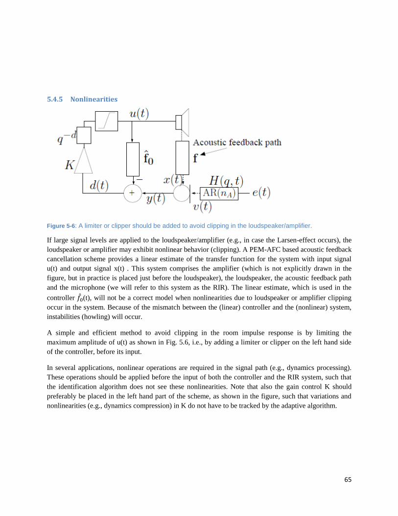
65

5.4.5 Nonlinearities

Figure 5-6: A limiter or clipper should be added to avoid clipping in the loudspeaker/amplifier.

If large signal levels are applied to the loudspeaker/amplifier (e.g., in case the Larsen-effect occurs), the

loudspeaker or amplifier may exhibit nonlinear behavior (clipping). A PEM-AFC based acoustic feedback

cancellation scheme provides a linear estimate of the transfer function for the system with input signal

u(t) and output signal x(t) . This system comprises the amplifier (which is not explicitly drawn in the

figure, but in practice is placed just before the loudspeaker), the loudspeaker, the acoustic feedback path

and the microphone (we will refer to this system as the RIR). The linear estimate, which is used in the

controller (t), will not be a correct model when nonlinearities due to loudspeaker or amplifier clipping

occur in the system. Because of the mismatch between the (linear) controller and the (nonlinear) system,

instabilities (howling) will occur.

A simple and efficient method to avoid clipping in the room impulse response is by limiting the

maximum amplitude of u(t) as shown in Fig. 5.6, i.e., by adding a limiter or clipper on the left hand side

of the controller, before its input.

In several applications, nonlinear operations are required in the signal path (e.g., dynamics processing).

These operations should be applied before the input of both the controller and the RIR system, such that

the identification algorithm does not see these nonlinearities. Note that also the gain control K should

preferably be placed in the left hand part of the scheme, as shown in the figure, such that variations and

nonlinearities (e.g., dynamics compression) in K do not have to be tracked by the adaptive algorithm.

66

5.5 Performance evaluation procedures

5.5.1 Performance of acoustic feedback

Our goal is to evaluate the acoustic feedback control methods based on three general objectives: the

achievable amplification, the sound quality, and the reliability. These objectives can be quantified by a

number of performance measures, which are calculated during the third and fourth simulation phases,

since these phases correspond to the preferential mode of operation for the sound reinforcement system.

The achievable amplification is measured by the MSG and the MSG increase, which by using (3.7) are

and (4.6) as follows,

MSG (t) [dB] = -20 5.67

MSG(t)[dB] = -20

5.68

Here we will use the instantaneous value of the MSG (t), as well as the mean and maximum value of the

MSG(t), as a performance measure in the evaluation.

Where J(q, t) = G(q,t) K(t) denotes the forward path transfer function without the amplification gain K(t),

and P denotes the set of frequencies at with the feedback signal x(t) is in phase with the near end signal

v(t).

An objective measure for quantifying the sound quality resulting from acoustic feedback control was

proposed in the context of hearing aid AFC in [97]. This measure, known as the frequency-weighted log-

spectral signal distortion (SD), is defined as6

SD(t)=

5.69

where Sd(f, t) and Sv(f, t) denote the short-term PSD of the feedback-compensated signal and source

signal, respectively, and (f)is a weighting function that gives equal weight to each auditory critical

band in the Nyquist interval, following Table II of the ANSI S3.5-1997 standard [137].

More simply, we can use LSD (log-spectral signal distortion) for this purpose.

6Note that in a real-time experiment, the source signal is not available, hence its PSD Sv(ω, t) cannot be calculated. The SD

measure can then be calculated by comparing the loudspeaker signal PSD with the PSD of a reference signal that is obtained in a

secondary experiment, in the absence of acoustic feedback [97].

67

LSD(i) =

5.70

where K is the number of frequency bin for each frame, i the frame index and Se(i, k) and Ss(i, k) are the

short-term PSD of the feedback compensated signal and source signal respectively. Only frames of

speech activity are selected in the LSD computation.

Finally, the reliability is quantified using two performance measures: the howling occurrence probability

(HOP) and the time to recover from instability (TRI). These measures rely on an estimate of the time

intervals during which howling occurs in the simulation. Howling occurrences are manually identified

using the following procedure:

1) a rough estimate of the howling time intervals is obtained by listening to the feedback-

compensated signal.

2) a spectrogram of the feedback-compensated signal is plotted for each of the time intervals identified

in the first step, and the frequency bin(s) in which howling occurs are visually identified from the

spectrogram.

3) a time-varying PAPR feature is calculated for each of the time intervals identified in the first step,

where the peak PSD is estimated by averaging the power in the howling frequency bins identified in the

second step.

4) the time interval during which howling occurs is then defined by the time points on either side of

the PAPR maximum value, at which the PAPR has decreased to a value that is 3 dB below the maximum

value.

From the time points identified in the last step of the above procedure, we can estimate the time duration

ti (s) of each howling occurrence, i = 1, . . . ,NHO, with NHO the number of howling occurrences

estimated in the first step of the above procedure. The HOP and TRI measures are then defined as

follows,

HOP(%) =

5.71

TRI (s) =

5.72

where T (s) denotes the length of the simulation.

Here The Peak-to-Average Power Ratio (PAPR) [97]-[108] is a spectral feature that determines the ratio

of the candidate howling component power |Y ( ,t)|2 and the average microphone signal power (t),

i.e.,

PAPR( ,t ) [dB] =10

5.73

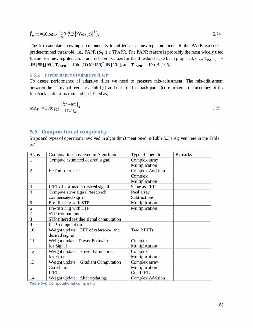
68

(t) =10

. 5.74

The ith candidate howling component is identified as a howling component if the PAPR exceeds a

predetermined threshold, i.e., PAPR ( ,t) ≥ TPAPR. The PAPR feature is probably the most widely used

feature for howling detection, and different values for the threshold have been proposed, e.g., = 6

dB [98],[99], = 10log10(M/150)2 dB [104], and = 10 dB [105].

5.5.2 Performance of adaptive filter

To assess performance of adaptive filter we need to measure mis-adjustment. The mis-adjustment

between the estimated feedback path and the true feedback path f(t) represents the accuracy of the

feedback path estimation and is defined as,

M = 20

. 5.75

5.6 Computational complexity Steps and types of operations involved in algorithm3 mentioned in Table 5.3 are given here in the Table

5.4

Steps Computations involved in Algorithm Type of operation Remarks

1 Compute estimated desired signal Complex array

Multiplication

2 FFT of reference. Complex Addition

Complex

Multiplication

3 IFFT of estimated desired signal Same as FFT

4 Compute error signal /feedback

compensated signal

Real array

Subtractions

5 Pre-filtering with STP Multiplication

6 Pre-filtering with LTP Multiplication

7 STP computation

8 STP filtered residue signal computation

9 LTP computation

10 Weight update : FFT of reference and

desired signal

Two 2 FFTs.

11 Weight update: Power Estimation

for Signal

Complex

Multiplication

12 Weight update: Power Estimation

for Error

Complex

Multiplication

13 Weight update : Gradient Computation

Correlation

IFFT

Complex array

Multiplication

One IFFT.

14 Weight update: filter updating. Complex Addition

Table 5-4: Computational complexity.

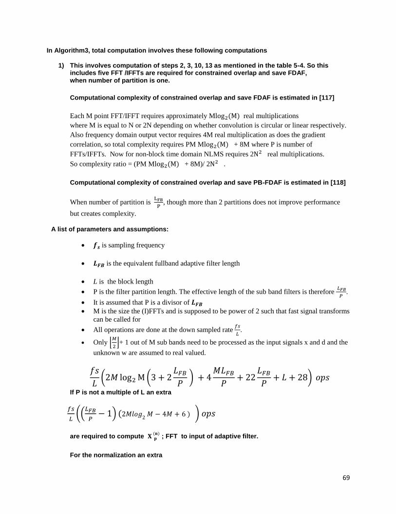
69

In Algorithm3, total computation involves these following computations

1) This involves computation of steps 2, 3, 10, 13 as mentioned in the table 5-4. So this includes five FFT /IFFTs are required for constrained overlap and save FDAF, when number of partition is one.

Computational complexity of constrained overlap and save FDAF is estimated in [117]

Each M point FFT/IFFT requires approximately M real multiplications

where M is equal to N or 2N depending on whether convolution is circular or linear respectively.

Also frequency domain output vector requires 4M real multiplication as does the gradient

correlation, so total complexity requires PM M + 8M where P is number of

FFTs/IFFTs. Now for non-block time domain NLMS requires 2 real multiplications.

So complexity ratio = (PM M + 8M)/ 2 .

Computational complexity of constrained overlap and save PB-FDAF is estimated in [118]

When number of partition is

, though more than 2 partitions does not improve performance

but creates complexity.

A list of parameters and assumptions:

is sampling frequency

is the equivalent fullband adaptive filter length

L is the block length

P is the filter partition length. The effective length of the sub band filters is therefore

.

It is assumed that P is a divisor of

M is the size the (I)FFTs and is supposed to be power of 2 such that fast signal transforms

can be called for

All operations are done at the down sampled rate

.

Only

+ 1 out of M sub bands need to be processed as the input signals x and d and the

unknown w are assumed to real valued.

If P is not a multiple of L an extra

are required to compute

; FFT to input of adaptive filter.

For the normalization an extra

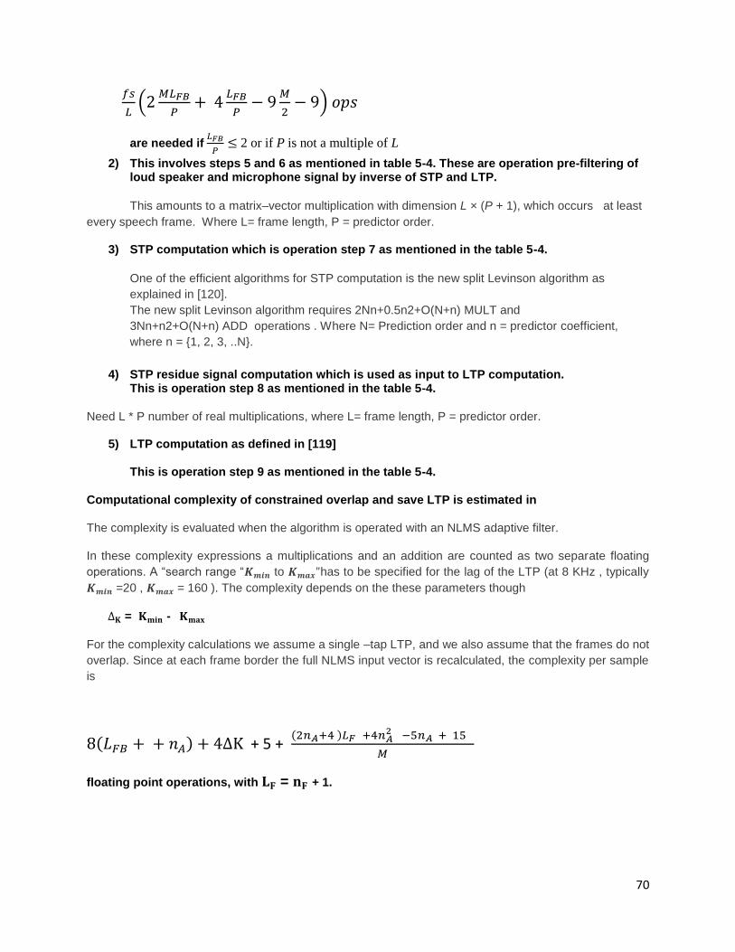
70

are needed if

2 or if P is not a multiple of L

2) This involves steps 5 and 6 as mentioned in table 5-4. These are operation pre-filtering of loud speaker and microphone signal by inverse of STP and LTP.

This amounts to a matrix–vector multiplication with dimension L × (P + 1), which occurs at least

every speech frame. Where L= frame length, P = predictor order.

3) STP computation which is operation step 7 as mentioned in the table 5-4.

One of the efficient algorithms for STP computation is the new split Levinson algorithm as

explained in [120].

The new split Levinson algorithm requires 2Nn+0.5n2+O(N+n) MULT and

3Nn+n2+O(N+n) ADD operations . Where N= Prediction order and n = predictor coefficient,

where n = {1, 2, 3, ..N}.

4) STP residue signal computation which is used as input to LTP computation. This is operation step 8 as mentioned in the table 5-4.

Need L * P number of real multiplications, where L= frame length, P = predictor order.

5) LTP computation as defined in [119] This is operation step 9 as mentioned in the table 5-4.

Computational complexity of constrained overlap and save LTP is estimated in

The complexity is evaluated when the algorithm is operated with an NLMS adaptive filter.

In these complexity expressions a multiplications and an addition are counted as two separate floating

operations. A “search range “ to has to be specified for the lag of the LTP (at 8 KHz , typically

=20 , = 160 ). The complexity depends on the these parameters though

= -

For the complexity calculations we assume a single –tap LTP, and we also assume that the frames do not

overlap. Since at each frame border the full NLMS input vector is recalculated, the complexity per sample

is

+ 5 +

floating point operations, with = + 1.

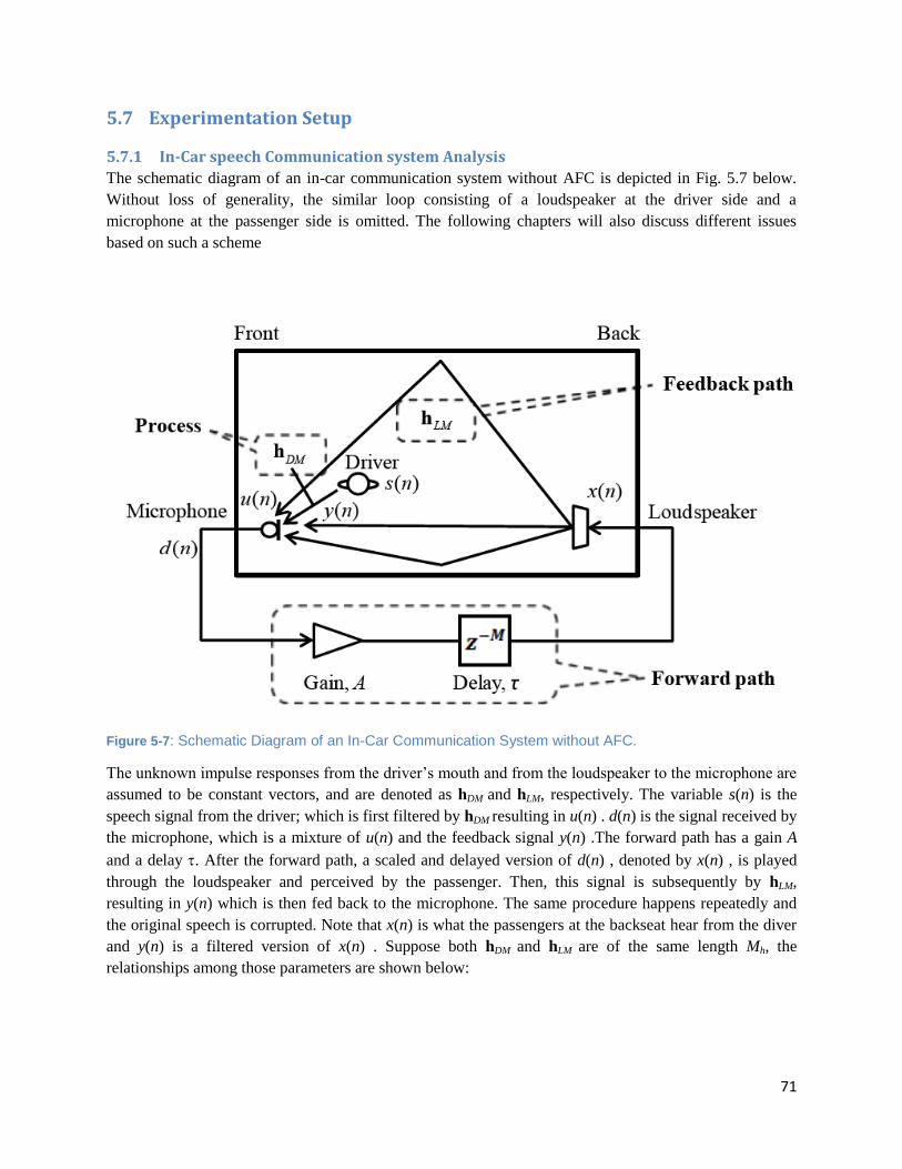
71

5.7 Experimentation Setup

5.7.1 In-Car speech Communication system Analysis

The schematic diagram of an in-car communication system without AFC is depicted in Fig. 5.7 below.

Without loss of generality, the similar loop consisting of a loudspeaker at the driver side and a

microphone at the passenger side is omitted. The following chapters will also discuss different issues

based on such a scheme

Figure 5-7: Schematic Diagram of an In-Car Communication System without AFC.

The unknown impulse responses from the driver’s mouth and from the loudspeaker to the microphone are

assumed to be constant vectors, and are denoted as hDM and hLM, respectively. The variable s(n) is the

speech signal from the driver; which is first filtered by hDM resulting in u(n) . d(n) is the signal received by

the microphone, which is a mixture of u(n) and the feedback signal y(n) .The forward path has a gain A

and a delay . After the forward path, a scaled and delayed version of d(n) , denoted by x(n) , is played

through the loudspeaker and perceived by the passenger. Then, this signal is subsequently by hLM,

resulting in y(n) which is then fed back to the microphone. The same procedure happens repeatedly and

the original speech is corrupted. Note that x(n) is what the passengers at the backseat hear from the diver

and y(n) is a filtered version of x(n) . Suppose both hDM and hLM are of the same length Mh, the

relationships among those parameters are shown below:

72

u(n )= , 5.76

d(n) = u(n) + y(n) , 5.77

x(n) =Ad(n-M), 5.78

y(n )= , 5.79

The four equations are valid for the in-car communication case without AFC system, representing the rule

of the changing of the voice signal inside the car compartment mathematically. Note that

s(n) = ,

x(n) = .

The forward path output x(n) represents the corrupted speech signal which is mixed with feedbacks. As

x(n) is a scaled and delayed version of d(n) according to (5.78), the simulation of x(n) is done by

simulating d(n) instead for the convenience.

Assumptions

For simplicity and emphasis on key points of the thesis, some ideal environment factors are assumed and

some algorithms of measurements of parameters are omitted. The detailed assumptions and settings are

given as shown below

1) The direct coupling of the driver speech signal to his own ear is not taken into consideration in

this research. And the acoustic path from the driver’s mouth directly to the back passenger’s ear

inside the car compartment is ignored. These two acoustic channels do not affect much on the in-

car compartment speech quality, and intuitively, distortion will not be caused by the effect of

these two paths.

2) All the implementations of simulation are conducted in a quiet environment, i.e., without

background noise and other interferences. Most AFC researches are conducted and analyzed

under this assumption such that the analysis is closer to the natural feature of the system.

3) The car compartment space is approximated as a rectangular block with dimension m.

Loudspeaker position: (4 m x 2 m x 1.4 m); Microphone position: (3 m x 0.5 m x 1 m);

Driver position (1 m x 0.5 m x 1 m).All the positions are fixed.

4) Impulse responses hDM and hLM are finite impulse response (FIR) filters, with equal filter

lengths Mh= 512. This assumption is made based on the result of [112]. As the sampling

frequency of the AD convertor is fs=16 kHz for the speech, the in-car reverberation time, which is

the time interval for a signal to be attenuated by -60 dB, follows that RT60 x fs, where RT60

denotes the reverberation time. Sang-Kwon Lee in [13] has shown that the reverberation time in

73

car is approximately 0.05 second, thus is Mh, chosen to be 1536 for the convenience of hardware

implementation.

5) The measurements of hDM and hLM are simulated using the source image model. This

implementation is based on the implementation in [113], and the version has been modified

according to [114]. The simulation of measurements of impulse response of acoustic enclosure

environments is another research area which is not in the content of this thesis.

5.7.2 Analysis of the Forward Path Gain and Delay

Due to the nature of closed-loop systems, there are feedbacks to the input of forward path. Particularly in

an in-car acoustic loop, the forward loop gain usually causes the system unstable such that the feedbacks

accumulate to infinity and “howling” or oscillation occurs. This causes annoyance to the people inside the

car compartment.

In the system depicted in Fig. 5.7, the input s(n) of the system is and the output of the system is x(n) ,

because the former is the excitation of the system and also the speech signal from the driver whereas the

latter is what the backseat passengers perceive. Substitute (5.77) and (5.79) into (5.78)

x(n+M )= + . 5.80

A recursive equation is obtained. Suppose the length of signal is L. When the iteration index n becomes

larger than L+M, x(n)T

hDM the portion becomes 0 because for s(n) = 0 for n > L+M. Under this condition,

x(n+M )= . 5.81

From the observation of (5.81), we can see that A and hLM contribute to the system gain and determine

whether the system is stable. To further illustrate the point, let HLMdenote the Fourier transform of

sequence hLM, which is the frequency response from the loudspeaker to the microphone. Fig. 5.8 shows

the plot of HLM:

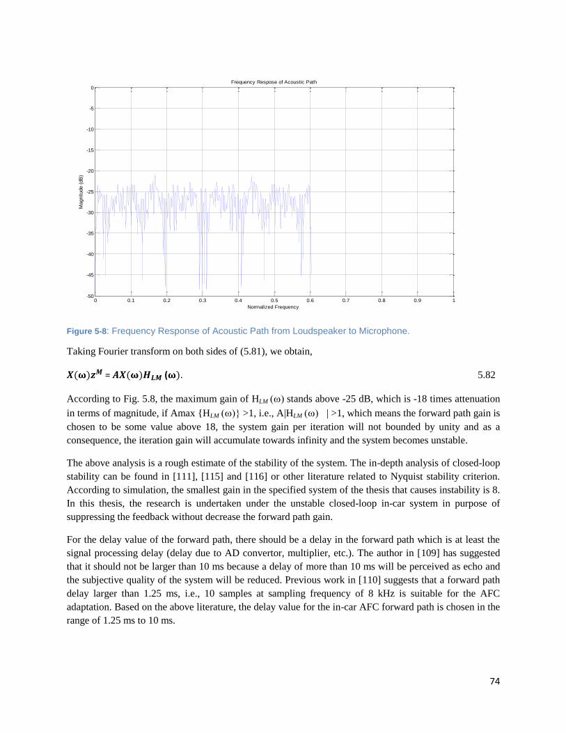
74

Figure 5-8: Frequency Response of Acoustic Path from Loudspeaker to Microphone.

Taking Fourier transform on both sides of (5.81), we obtain,

= ( . 5.82

According to Fig. 5.8, the maximum gain of HLMstands above -25 dB, which is -18 times attenuation

in terms of magnitude, if Amax {HLM>1, i.e., A|HLM | >1, which means the forward path gain is

chosen to be some value above 18, the system gain per iteration will not bounded by unity and as a

consequence, the iteration gain will accumulate towards infinity and the system becomes unstable.

The above analysis is a rough estimate of the stability of the system. The in-depth analysis of closed-loop

stability can be found in [111], [115] and [116] or other literature related to Nyquist stability criterion.

According to simulation, the smallest gain in the specified system of the thesis that causes instability is 8.

In this thesis, the research is undertaken under the unstable closed-loop in-car system in purpose of

suppressing the feedback without decrease the forward path gain.

For the delay value of the forward path, there should be a delay in the forward path which is at least the

signal processing delay (delay due to AD convertor, multiplier, etc.). The author in [109] has suggested

that it should not be larger than 10 ms because a delay of more than 10 ms will be perceived as echo and

the subjective quality of the system will be reduced. Previous work in [110] suggests that a forward path

delay larger than 1.25 ms, i.e., 10 samples at sampling frequency of 8 kHz is suitable for the AFC

adaptation. Based on the above literature, the delay value for the in-car AFC forward path is chosen in the

range of 1.25 ms to 10 ms.

0 0.1 0.2 0.3 0.4 0.5 0.6 0.7 0.8 0.9 1-50

-45

-40

-35

-30

-25

-20

-15

-10

-5

0Frequency Respose of Acoustic Path

Normalized Frequency

Magnitude (

dB

)

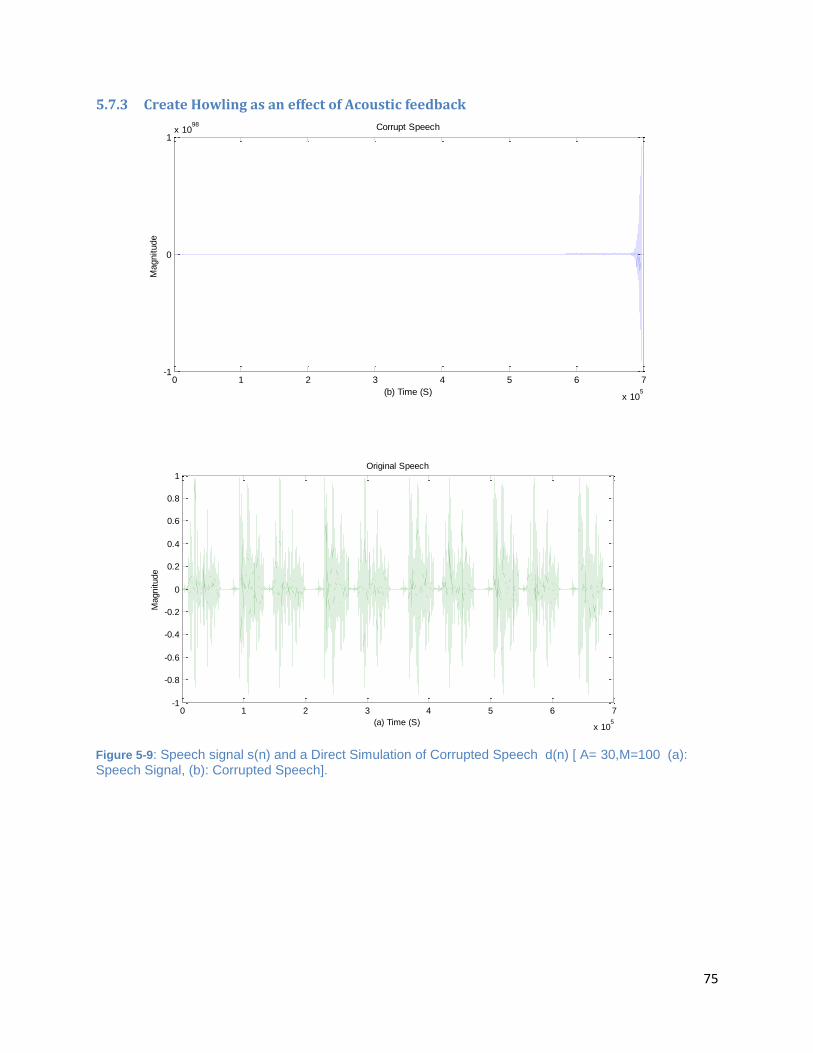
75

5.7.3 Create Howling as an effect of Acoustic feedback

Figure 5-9: Speech signal s(n) and a Direct Simulation of Corrupted Speech d(n) [ A= 30,M=100 (a): Speech Signal, (b): Corrupted Speech].

0 1 2 3 4 5 6 7

x 105

-1

0

1x 10

98 Corrupt Speech

(b) Time (S)

Magnitude

0 1 2 3 4 5 6 7

x 105

-1

-0.8

-0.6

-0.4

-0.2

0

0.2

0.4

0.6

0.8

1Original Speech

(a) Time (S)

Magnitude

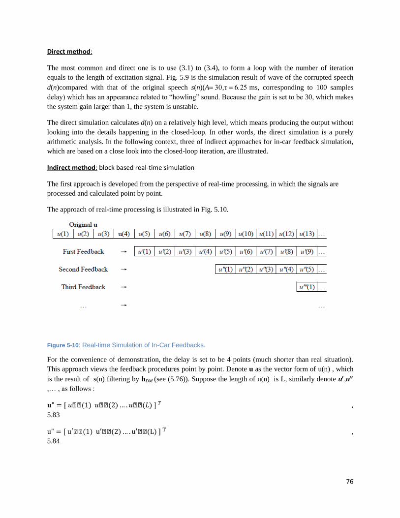
76

Direct method:

The most common and direct one is to use (3.1) to (3.4), to form a loop with the number of iteration

equals to the length of excitation signal. Fig. 5.9 is the simulation result of wave of the corrupted speech

d(n)compared with that of the original speech s(n)(A,ms, corresponding to 100 samples

delay) which has an appearance related to “howling” sound. Because the gain is set to be 30, which makes

the system gain larger than 1, the system is unstable.

The direct simulation calculates d(n) on a relatively high level, which means producing the output without

looking into the details happening in the closed-loop. In other words, the direct simulation is a purely

arithmetic analysis. In the following context, three of indirect approaches for in-car feedback simulation,

which are based on a close look into the closed-loop iteration, are illustrated.

Indirect method: block based real-time simulation

The first approach is developed from the perspective of real-time processing, in which the signals are

processed and calculated point by point.

The approach of real-time processing is illustrated in Fig. 5.10.

Figure 5-10: Real-time Simulation of In-Car Feedbacks.

For the convenience of demonstration, the delay is set to be 4 points (much shorter than real situation).

This approach views the feedback procedures point by point. Denote u as the vector form of u(n) , which

is the result of s(n) filtering by hDM (see (5.76)). Suppose the length of u(n) is L, similarly denote u,u

,… , as follows :

,

5.83

,

5.84

77

,

5.85

and so on. The sum of all the vectors constructs the vector form of d(n),denoted as, d

d = , 5.86

d = u + u + u5.87

Note that d(n) has a length of infinity because there are infinity versions of feedbacks, and each has a

delay of 4 samples. To illustrate (5.87) and Fig.5.9, we take a temporal view of the feedback system. In

the first four iterations, there is no signal fed back to the input because of the delay. At the fifth iteration,

the first sample in the loop, which is the first sample of u(n) , has rightly been transmitted back to the

input and is mixed up with it. Thus at the fifth iteration, the fifth original point u(5) along with a gained

and filtered version of the first original point which is denoted as u(1) , join together as the new input.

Similar procedures happen from the fifth iteration to the eighth iteration. At the ninth iteration, u(1),the

point processed from the first original point u(1) , travels back again and is mixed with the ninth point of

original signal u(9). At the same time, the fifth point of the original signal u(5) is rightly transmitted back

to the input, i.e., u(5) becomes u(5) , and is mixed with u(9) and u(1) .Thus at the ninth iteration, the

original signal is affected by two feedbacks. Similarly, the feedbacks accumulate till the infinity. And the

original speech is corrupted.

In general, by taking a vertical view of Fig. 5.9, the sum of each column gives the value of the corrupted

signal at the iteration corresponding to the column number. By taking a transversal view, each row below

the original u gives a version of feedback signal which is one feedback component of the corrupted

original speech. By synthesizing all the analysis, the corrupted signal results in the expression of (5.89).

And the filtering process in this approach is calculated using vector multiplication.

5.8 Simulation Results Acoustic feedback system has been simulated for different values of these system parameters as listed in

the table 5.4

1) Forward path delay (M), 2) Feedback Gain (A), 3) Frame size (N), 4) Filter length of true

Acoustic Feedback Path (AFBFL) generated from RIR model. This is filter length of acoustic

path f as mentioned in fig 5.6.

Test system N M A AFBFL

Fbsys1 320 128 35 1280

Fbsys2 256 100 30 1536

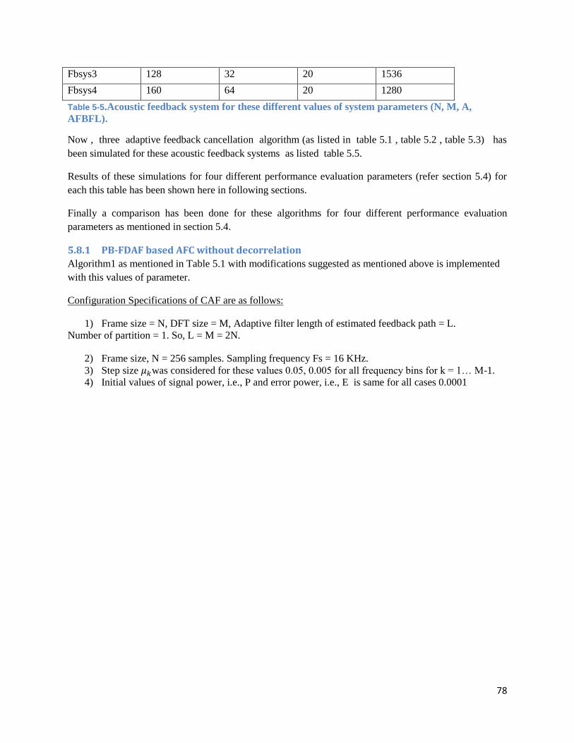
78

Fbsys3 128 32 20 1536

Fbsys4 160 64 20 1280

Table 5-5.Acoustic feedback system for these different values of system parameters (N, M, A,

AFBFL).

Now , three adaptive feedback cancellation algorithm (as listed in table 5.1 , table 5.2 , table 5.3) has

been simulated for these acoustic feedback systems as listed table 5.5.

Results of these simulations for four different performance evaluation parameters (refer section 5.4) for

each this table has been shown here in following sections.

Finally a comparison has been done for these algorithms for four different performance evaluation

parameters as mentioned in section 5.4.

5.8.1 PB-FDAF based AFC without decorrelation

Algorithm1 as mentioned in Table 5.1 with modifications suggested as mentioned above is implemented

with this values of parameter.

Configuration Specifications of CAF are as follows:

1) Frame size = N, DFT size = M, Adaptive filter length of estimated feedback path = L.

Number of partition = 1. So, L = M = 2N.

2) Frame size, N = 256 samples. Sampling frequency Fs = 16 KHz.

3) Step size was considered for these values 0.05, 0.005 for all frequency bins for k = 1… M-1.

4) Initial values of signal power, i.e., P and error power, i.e., E is same for all cases 0.0001

79

1) Misalignment :

Figure 5-11 : Misalignment of PB-FDAF at different frame size but for same step size =0.005.

0 200 400 600 800 1000 1200 1400 1600 1800 2000-8

-7

-6

-5

-4

-3

-2

-1

0

Frame No

Magnitude (

dB

)

Misalignment compare at diffterent block size with same step size (0.005)

N= 320

N= 256

N= 128

N= 160

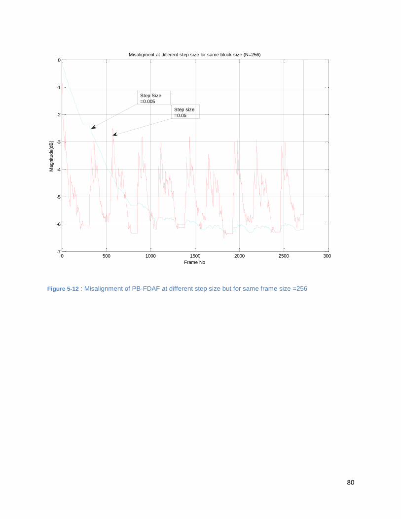
80

Figure 5-12 : Misalignment of PB-FDAF at different step size but for same frame size =256

0 500 1000 1500 2000 2500 3000-7

-6

-5

-4

-3

-2

-1

0Misaligment at different step size for same block size (N=256)

Frame No

Magnitude(d

B)

Step size

=0.05

Step Size

=0.005

81

2) Delta MSG :

Figure 5-13: Delta MSG comparisons of PB-FDAF at different frame size for same step size =256.

0 200 400 600 800 1000 1200 1400 1600 1800 20000

2

4

6

8

10

12

14Delta MSG comaparison at different block with same step size ( 0.005)

Frame No.

Magnitude (

dB

)

N =128

N=160

N = 320

N= 256

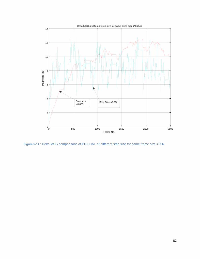
82

Figure 5-14 : Delta MSG comparisons of PB-FDAF at different step size for same frame size =256

0 500 1000 1500 2000 25000

2

4

6

8

10

12

14Delta MSG at different step size for same blcok size (N=256)

Frame No.

Magnitude (

dB

)

Step size

=0.005Step Size =0.05

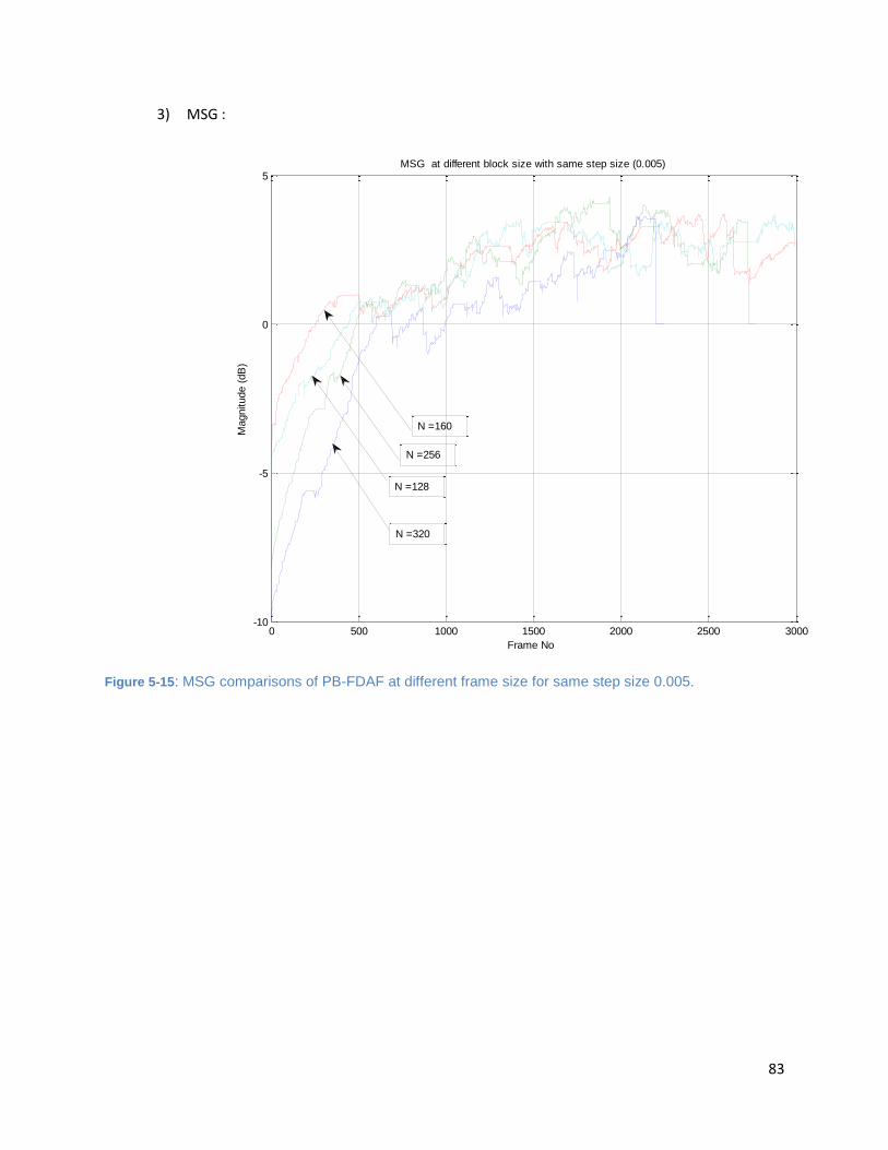
83

3) MSG :

Figure 5-15: MSG comparisons of PB-FDAF at different frame size for same step size 0.005.

0 500 1000 1500 2000 2500 3000-10

-5

0

5MSG at different block size with same step size (0.005)

Frame No

Magnitude (

dB

)

N =128

N =160

N =256

N =320

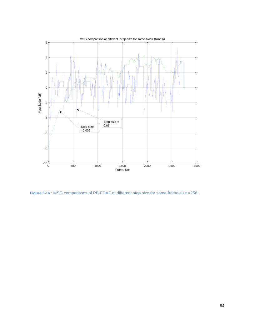
84

Figure 5-16 : MSG comparisons of PB-FDAF at different step size for same frame size =256.

0 500 1000 1500 2000 2500 3000-10

-8

-6

-4

-2

0

2

4

6MSG comparison at different step size for same block (N=256)

Frame No

Magnitude (

dB

)

Step size =

0.05Step size

=0.005

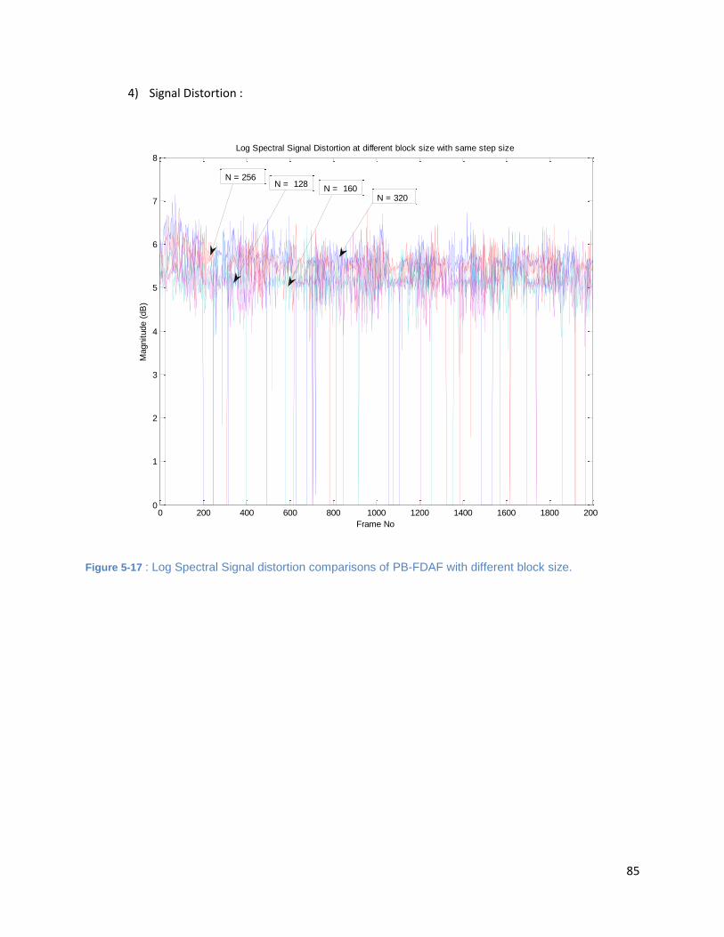
85

4) Signal Distortion :

Figure 5-17 : Log Spectral Signal distortion comparisons of PB-FDAF with different block size.

0 200 400 600 800 1000 1200 1400 1600 1800 20000

1

2

3

4

5

6

7

8Log Spectral Signal Distortion at different block size with same step size

Frame No

Magnitude (

dB

)

N = 256 N = 128

N = 160N = 320

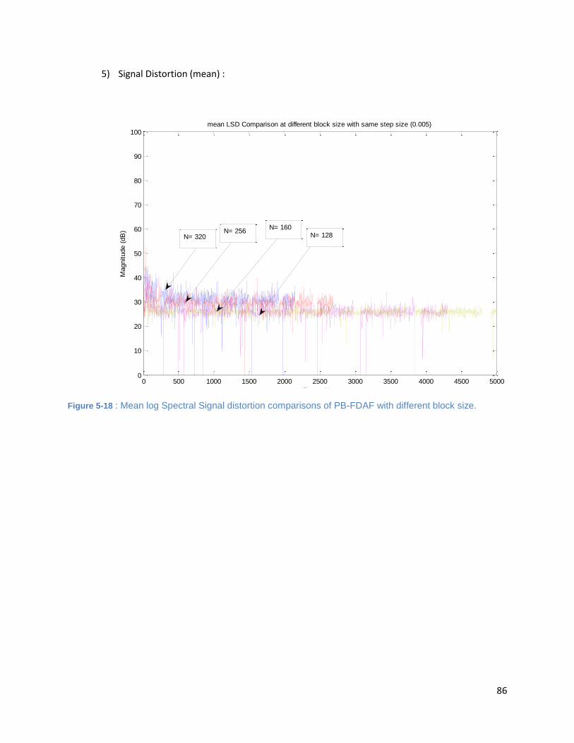
86

5) Signal Distortion (mean) :

Figure 5-18 : Mean log Spectral Signal distortion comparisons of PB-FDAF with different block size.

0 500 1000 1500 2000 2500 3000 3500 4000 4500 50000

10

20

30

40

50

60

70

80

90

100mean LSD Comparison at different block size with same step size (0.005)

Frame No.

Magnitude (

dB

)

N= 320N= 256

N= 160N= 128

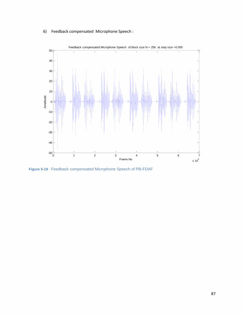
87

6) Feedback compensated Microphone Speech :

Figure 5-19 : Feedback compensated Microphone Speech of PB-FDAF

0 1 2 3 4 5 6 7

x 105

-50

-40

-30

-20

-10

0

10

20

30

40

50Feedback compensated Microphone Speech of block size N = 256 at step size =0.005

Frame No

Am

plit

ude

88

5.8.2 PB-FDAF based PEM AFC with decorrelation: pre-filtering only by STP



Configuration specifications of STP computation pre-filtering are as follow:

1) Values for adaptive filter were same as previous.

2) STP order was considered these values: 15, 20, and 25.

3) = SFHP (STP computation frame hop size.) was considered for these values: 1,2,3,4.

1) Misalignment:

Figure 5-20 : Misalignment comparison of STP at different SFHP order while frame size = 256, STP order = 20, and step size =0.005.

0 500 1000 1500 2000 2500 3000-8

-7

-6

-5

-4

-3

-2

-1

0Misalignment comarison at different STP frame interval ( SFHP) at step size 0.005 , frame size N=256 and STP order 20

Frame No.

Magnitude (

dB

)

SFHP = 2

SFHP = 3

SFHP = 1

SFHP = 4

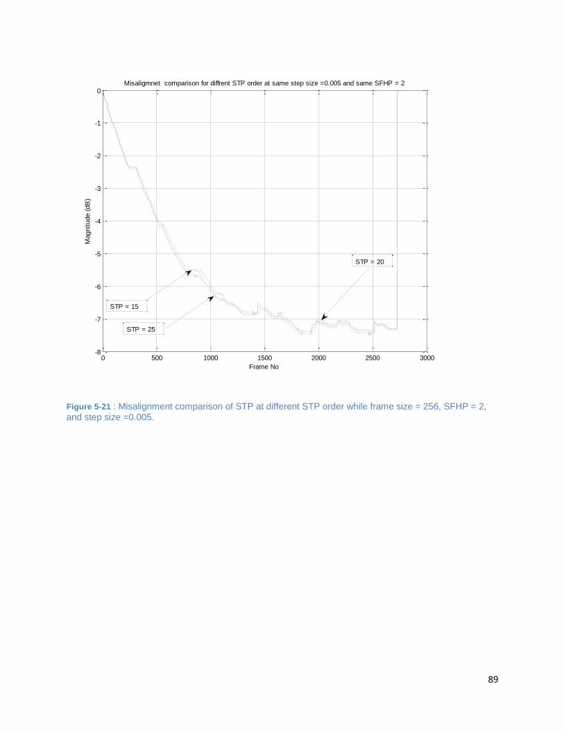
89

Figure 5-21 : Misalignment comparison of STP at different STP order while frame size = 256, SFHP = 2, and step size =0.005.

0 500 1000 1500 2000 2500 3000-8

-7

-6

-5

-4

-3

-2

-1

0Misaligmnet comparison for diffrent STP order at same step size =0.005 and same SFHP = 2

Frame No

Magnitude (

dB

)

STP = 25

STP = 15

STP = 20

90

2) Delta MSG :

Figure 5-22 : MSG comparison of STP at different SFHP while frame size = 256, STP order = 2, and step size =0.005.

0 500 1000 1500 2000 25000

2

4

6

8

10

12

14

16Delta MSG Comparison at different SFHP , same step size =0.005 , STP order = 20 , frame size =256

Frame No

Magnitude (

dB

)

SFHP = 2

SFHP = 3

SFHP = 4

SFHP = 1

91

Figure 5-23 : Delta MSG comparison of STP at different STP order while frame size = 256, SFHP = 2, and step size =0.005.

0 500 1000 1500 2000 2500 30000

2

4

6

8

10

12

14

16Delta MSG for diffrent STP order at same step size =0.005 , same SFHP =2 , Frame size =256

Frame No.

Magnitude (

dB

)

STP = 15

STP = 20

STP = 25

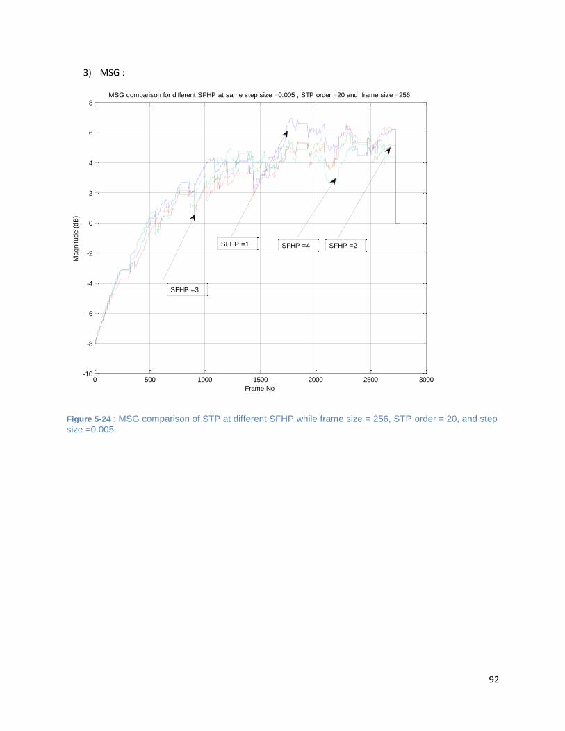
92

3) MSG :

Figure 5-24 : MSG comparison of STP at different SFHP while frame size = 256, STP order = 20, and step size =0.005.

0 500 1000 1500 2000 2500 3000-10

-8

-6

-4

-2

0

2

4

6

8MSG comparison for different SFHP at same step size =0.005 , STP order =20 and frame size =256

Frame No

Magnitude (

dB

)

SFHP =3

SFHP =1 SFHP =4 SFHP =2

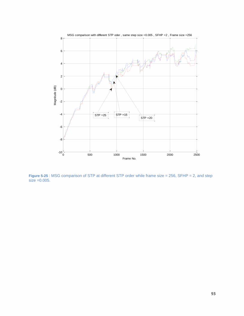
93

Figure 5-25 : MSG comparison of STP at different STP order while frame size = 256, SFHP = 2, and step size =0.005.

0 500 1000 1500 2000 2500-10

-8

-6

-4

-2

0

2

4

6

8MSG comparison with different STP oder , same step size =0.005 , SFHP =2 , Frame size =256

Frame No.

Magnitude (

dB

)

STP =25 STP =15STP =20

94

4) Signal Distortion :

Figure 5-26: Log Spectral Signal distortions of STP at configurations: frame size = 256, SFHP = 2, STP order =20 and step size =0.005

0 500 1000 1500 2000 2500 30000

1

2

3

4

5

6

7

8Log Spectral Signal distortion at Frame size =256 , SFHP =2 , STP order =20 , step size =0.005

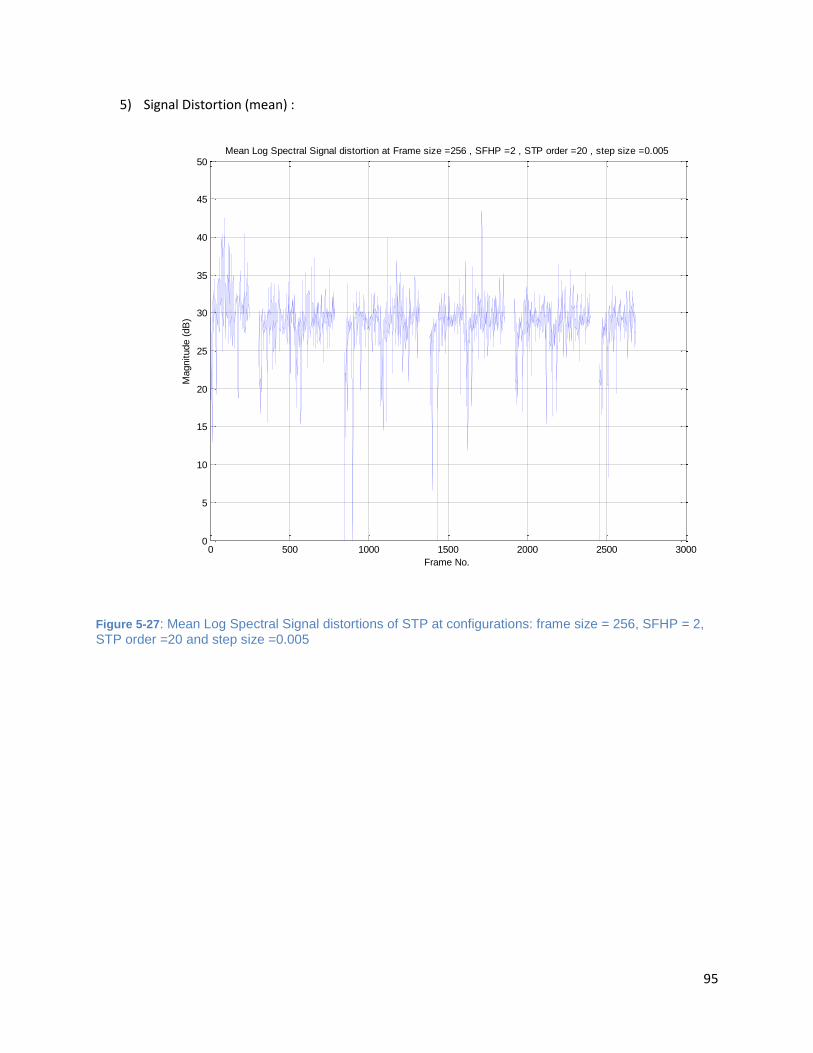
95

5) Signal Distortion (mean) :

Figure 5-27: Mean Log Spectral Signal distortions of STP at configurations: frame size = 256, SFHP = 2, STP order =20 and step size =0.005

0 500 1000 1500 2000 2500 30000

5

10

15

20

25

30

35

40

45

50Mean Log Spectral Signal distortion at Frame size =256 , SFHP =2 , STP order =20 , step size =0.005

Frame No.

Magnitude (

dB

)

96

6) Feedback Compensated Microphone Speech :

Figure 5-28: Feedback Compensated Microphone Speech of STP at configurations: frame size = 256, SFHP = 2, STP order =20 and step size =0.005

0 1 2 3 4 5 6 7

x 105

-50

-40

-30

-20

-10

0

10

20

30

40

50Feedback Compensated Microphone Speech at frame size =256 , step size =0.005 , STP order =20, SFHP =2.

Frame No

Am

plit

ude

97

5.8.3 PB-FDAF based PEM AFC with decorrelation : pre-filtering by STP and LTP



Configuration specifications of LTP computation pre-filtering are as follow:

1) Values for adaptive filter and STP were same as previous.

2) LTP was single pole pitch and its corresponding gain.

3) = LFHP (LTP computation frame hop size ) was considered for these values: 2, 3, 4.

4) LTP Pitch window buffer size was as follows: 2N, 3N with 50 % and 100 % window overlap.

5) LTP search range was as follows Pin: 18,Pmax =256 (same as fame size , N) and

Pin: 18, Pmax = 128 (half of frame size, N/2).

6) Threshold for deciding multiple pitch in same window buffer was as follows: PMultThr= 0.75

1) Misalignment :

Figure 5-29: Misalignment comparison of LTP for different configurations

0 500 1000 1500 2000 2500 3000-8

-7

-6

-5

-4

-3

-2

-1

0MisAlignment Comparison with different STP and LTP configurations

Frame No.

Magnitude (

dB

)

SFHP = 2

LFHP = 4

LTP buffer size = 3N

LTP Search Range =

18 -128

LTP overlap Wind = 50 %

SFHP = 1

LFHP = 2


LTP Search Range =

18- 256

LTP overlap Wind = 100%

98

2) Delta MSG :

Figure 5-30: Delta MSG comparison of LTP for different configurations

0 500 1000 1500 2000 2500 30000

2

4

6

8

10

12

14

16Delta MSG comparison with LTP and STP configurations

Frame No.

Magnitude (

dB

)

SFHP = 1

LFHP = 4


LTP Search Range =

18- 128


SFHP = 2

LFHP = 3


LTP Search Range =

18- 256


99

3) MSG :

Figure 5-31: MSG comparison of LTP for different configurations.

0 500 1000 1500 2000 2500-10

-8

-6

-4

-2

0

2

4

6

8MSG comparisons with diffrent LTP and STP configurations

Frame No.

Magnitude (

dB

)

SFHP = 2

LFHP = 3


LTP Search Range =

18- 256


SFHP = 1

LFHP = 4


LTP Search Range =

18- 128


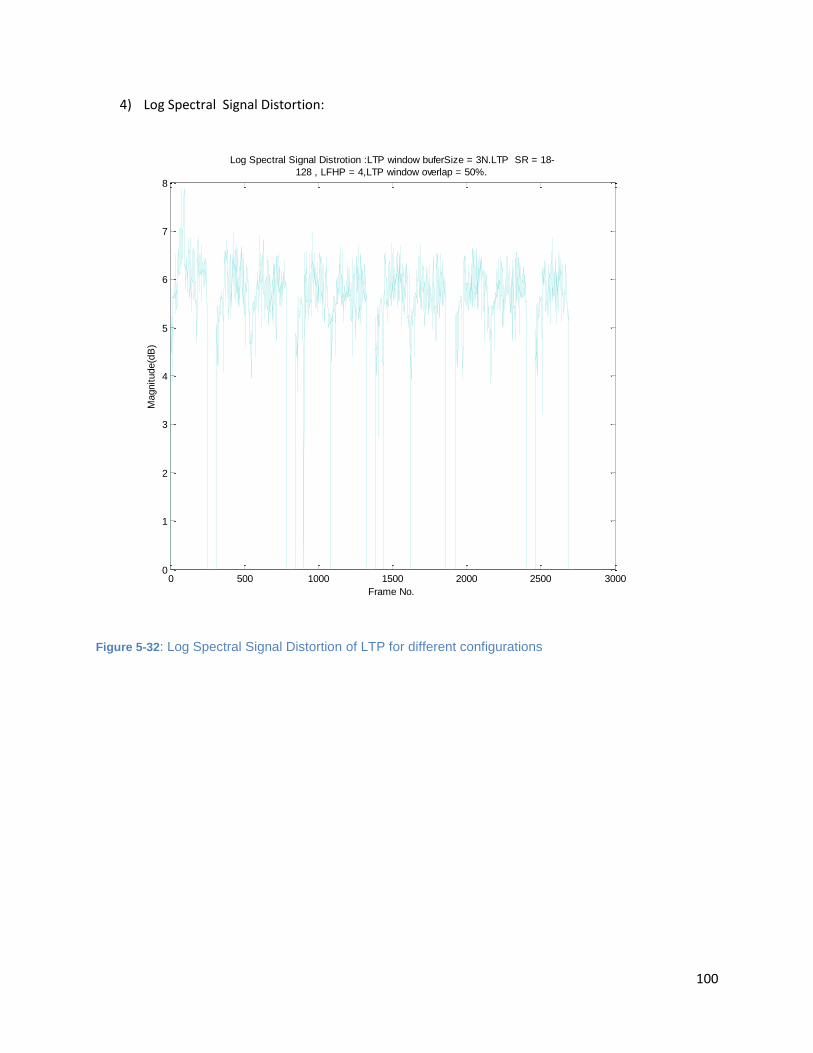
100

4) Log Spectral Signal Distortion:

Figure 5-32: Log Spectral Signal Distortion of LTP for different configurations

0 500 1000 1500 2000 2500 30000

1

2

3

4

5

6

7

8

Log Spectral Signal Distrotion :LTP window buferSize = 3N.LTP SR = 18-

128, LFHP = 4,LTP window overlap = 50%.

Frame No.

Magnitude(d

B)

101

5) Steady State Frequency Response :

Figure 5-33: Frequency Response of true feedback path generated from RIR.

0 100 200 300 400 500 6000

0.01

0.02

0.03

0.04

0.05

0.06

0.07

0.08

0.09

Frequency grid

Magnitude

Frequency Response : Ture feedback path generated from RIR model

102

Figure 5-34: Steady State Frequency Response: PB-FDAF

0 100 200 300 400 500 6000

0.01

0.02

0.03

0.04

0.05

0.06

0.07

0.08

Frequency grid

Magnitude

Steady State Frequency Response: PB-FDAF

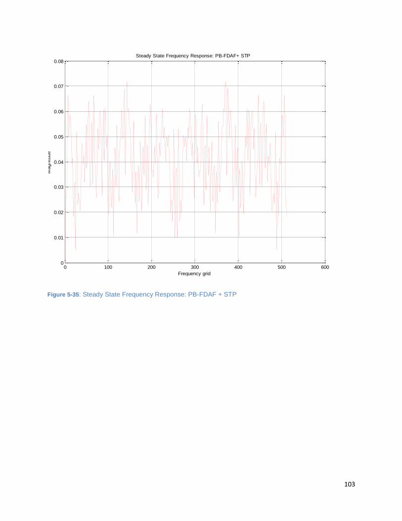
103

Figure 5-35: Steady State Frequency Response: PB-FDAF + STP

0 100 200 300 400 500 6000

0.01

0.02

0.03

0.04

0.05

0.06

0.07

0.08

Frequency grid

Magnitude

Steady State Frequency Response: PB-FDAF+ STP

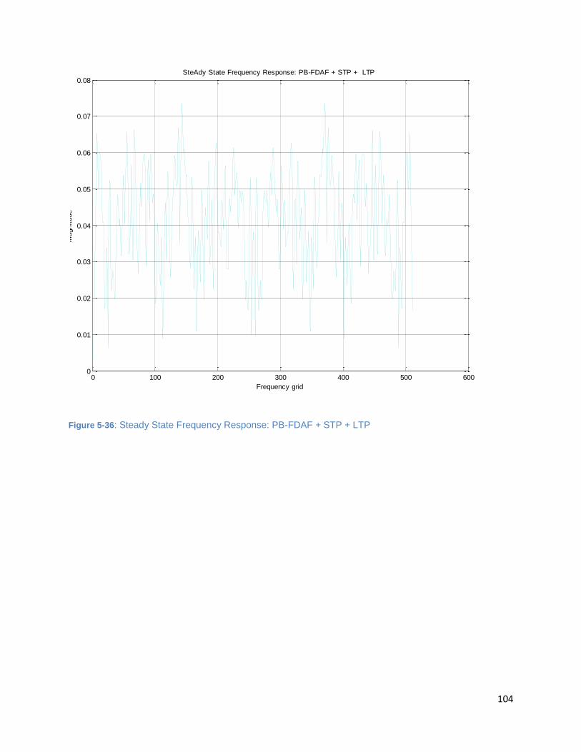
104

Figure 5-36: Steady State Frequency Response: PB-FDAF + STP + LTP

0 100 200 300 400 500 6000

0.01

0.02

0.03

0.04

0.05

0.06

0.07

0.08

Frequency grid

Magnitude

SteAdy State Frequency Response: PB-FDAF + STP + LTP

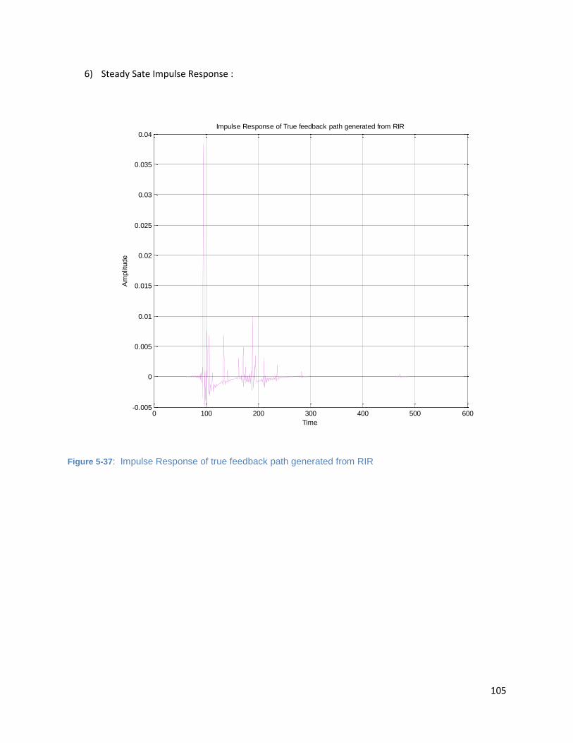
105

6) Steady Sate Impulse Response :

Figure 5-37: Impulse Response of true feedback path generated from RIR

0 100 200 300 400 500 600-0.005

0

0.005

0.01

0.015

0.02

0.025

0.03

0.035

0.04Impulse Response of True feedback path generated from RIR

Time

Am

plit

ude

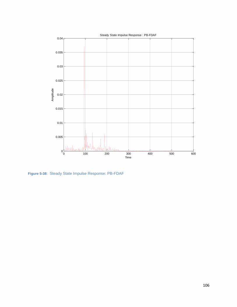
106

Figure 5-38: Steady State Impulse Response: PB-FDAF

0 100 200 300 400 500 6000

0.005

0.01

0.015

0.02

0.025

0.03

0.035

0.04Steady State Impulse Response : PB-FDAF

Time

Am

plit

ude

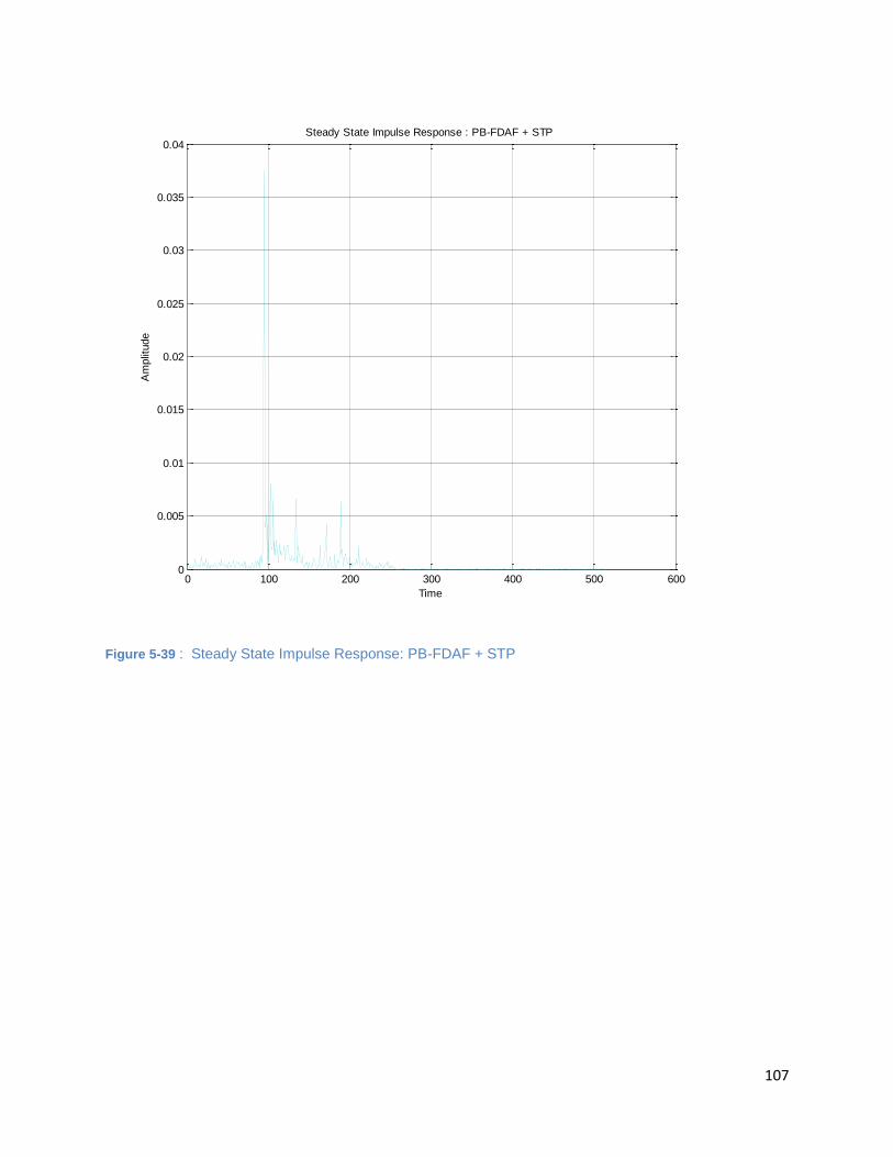
107

Figure 5-39 : Steady State Impulse Response: PB-FDAF + STP

0 100 200 300 400 500 6000

0.005

0.01

0.015

0.02

0.025

0.03

0.035

0.04Steady State Impulse Response : PB-FDAF + STP

Time

Am

plit

ude

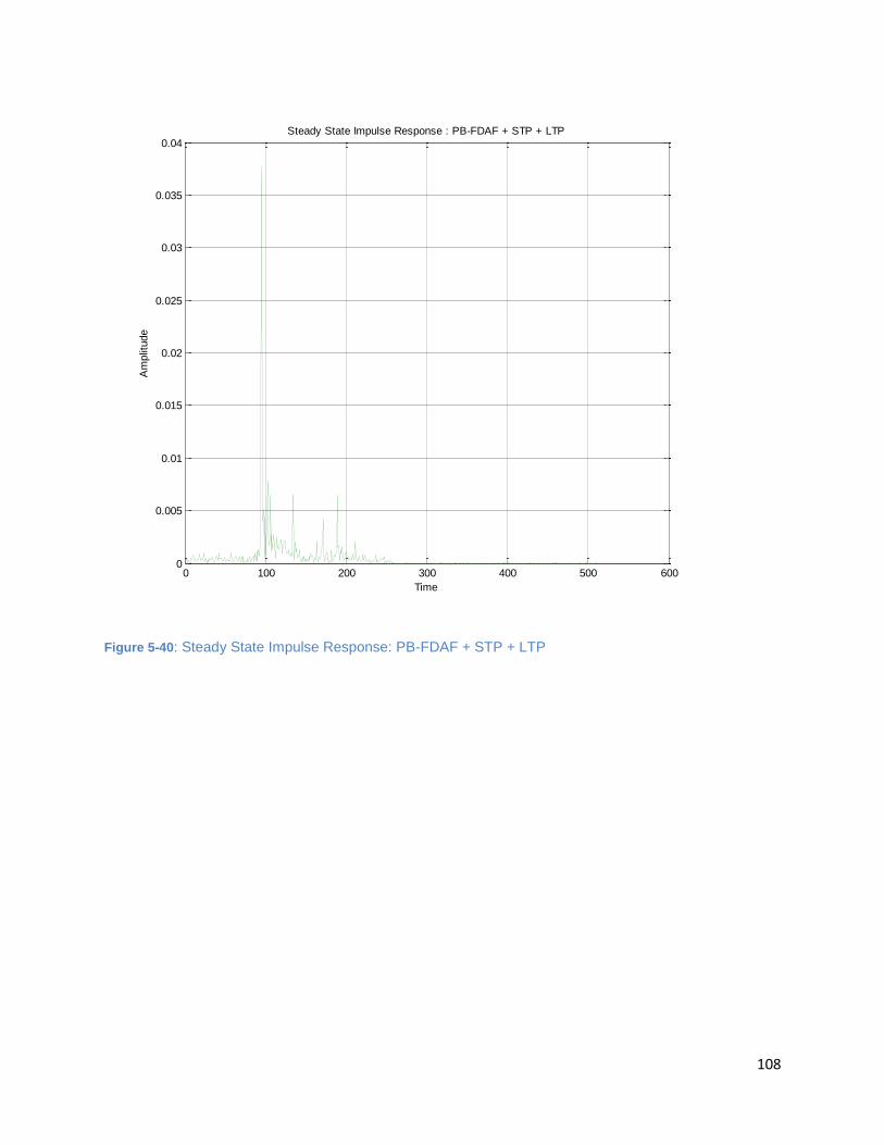
108

Figure 5-40: Steady State Impulse Response: PB-FDAF + STP + LTP

0 100 200 300 400 500 6000

0.005

0.01

0.015

0.02

0.025

0.03

0.035

0.04Steady State Impulse Response : PB-FDAF + STP + LTP

Time

Am

plit

ude

109

7) Feedback compensated Microphone Speech:

Figure 5-41: Feedback Compensated Microphone Speech: PB-FDAF + STP+ LTP.

0 1 2 3 4 5 6 7

x 105

-80

-60

-40

-20

0

20

40

60

80Feedback Compensated MicSpeech

Frame No.

Am

plit

ude

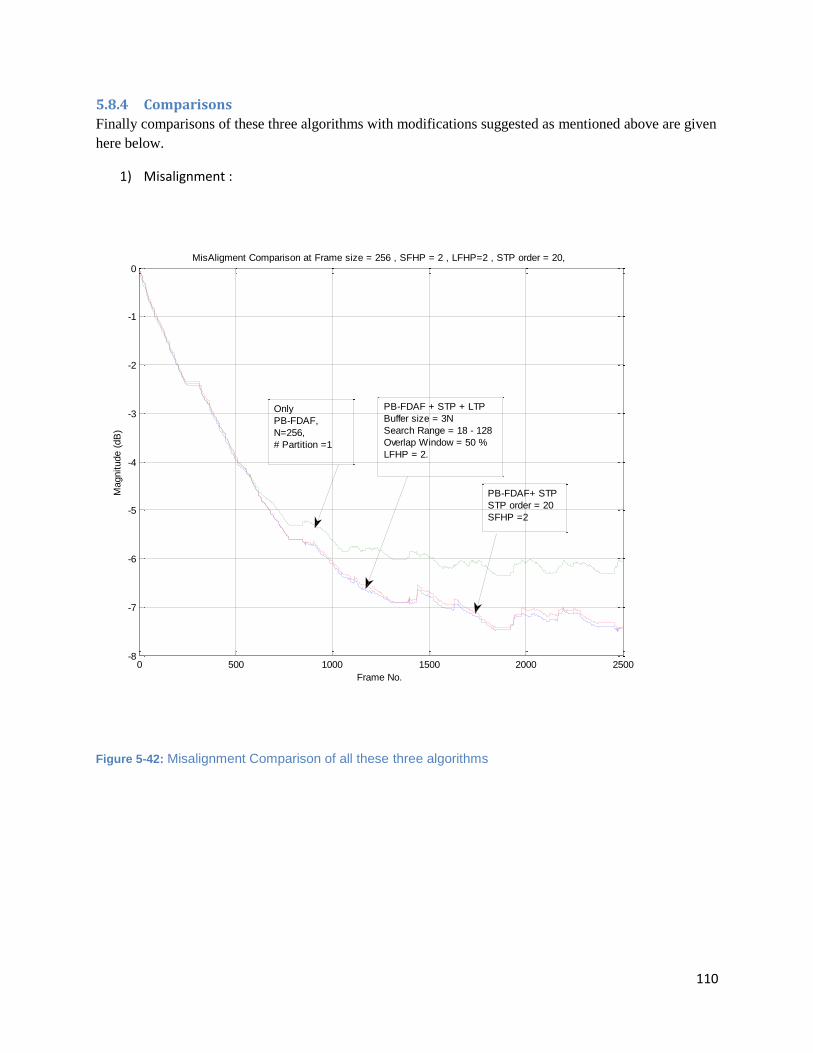
110

5.8.4 Comparisons

Finally comparisons of these three algorithms with modifications suggested as mentioned above are given

here below.

1) Misalignment :

Figure 5-42: Misalignment Comparison of all these three algorithms

0 500 1000 1500 2000 2500-8

-7

-6

-5

-4

-3

-2

-1

0MisAligment Comparison at Frame size = 256 , SFHP = 2 , LFHP=2 , STP order = 20,

Frame No.

Magnitude (

dB

)

PB-FDAF + STP + LTP

Buffer size = 3N

Search Range = 18 - 128

Overlap Window = 50 %

LFHP = 2.

Only

PB-FDAF,

N=256,

# Partition =1

PB-FDAF+ STP

STP order = 20

SFHP =2

111

Figure 5-43: Misalignment Comparison of all these three algorithms.

0 500 1000 1500 2000 2500-8

-7

-6

-5

-4

-3

-2

-1

0MisAligment Comparison at Frame size = 256 , SFHP = 2 , LFHP=4 , STP order = 20,

Frame No.

Magnitude (

dB

)

Only

PB-FDAF,

N=256,

# Partition =1

PB-FDAF+ STP

STP order = 20

SFHP =2

PB-FDAF + STP + LTP

Buffer size = 3N

Search Range = 18 - 128

Overlap Window = 50 %

LFHP = 4.

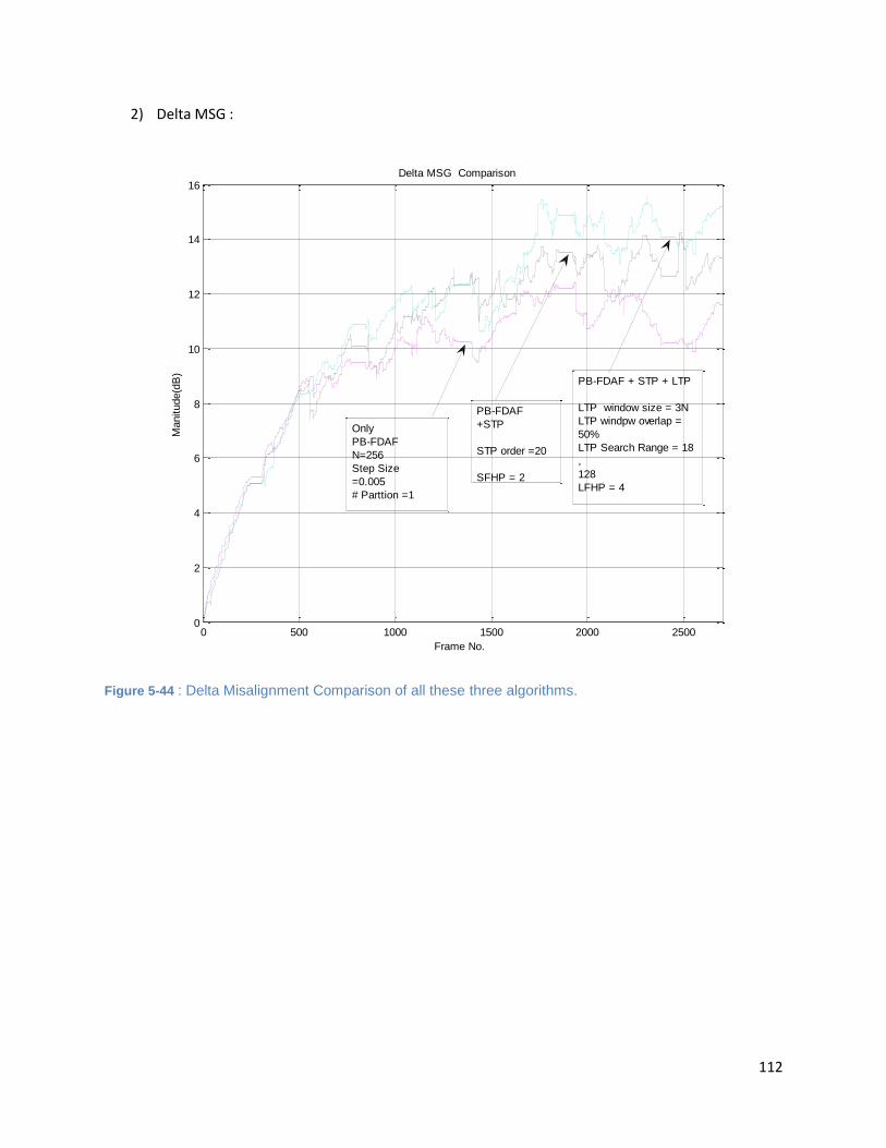
112

2) Delta MSG :

Figure 5-44 : Delta Misalignment Comparison of all these three algorithms.

0 500 1000 1500 2000 25000

2

4

6

8

10

12

14

16Delta MSG Comparison

Frame No.

Manitude(d

B)

Only

PB-FDAF

N=256

Step Size

=0.005

# Parttion =1

PB-FDAF

+STP

STP order =20

SFHP = 2

PB-FDAF + STP + LTP

LTP window size = 3N

LTP windpw overlap =

50%

LTP Search Range = 18

,

128

LFHP = 4

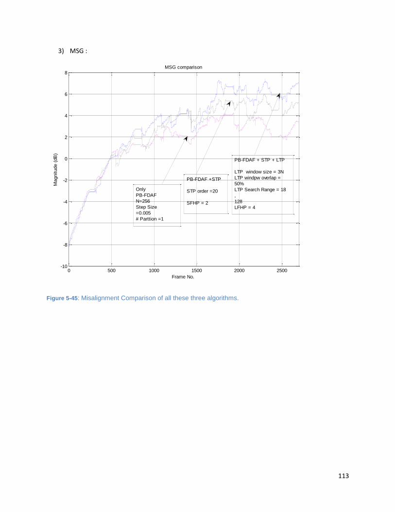
113

3) MSG :

Figure 5-45: Misalignment Comparison of all these three algorithms.

0 500 1000 1500 2000 2500-10

-8

-6

-4

-2

0

2

4

6

8MSG comparison

Frame No.

Magnitude (

dB

)

PB-FDAF + STP + LTP

LTP window size = 3N

LTP windpw overlap =

50%

LTP Search Range = 18

,

128

LFHP = 4

PB-FDAF +STP

STP order =20

SFHP = 2

Only

PB-FDAF

N=256

Step Size

=0.005

# Parttion =1

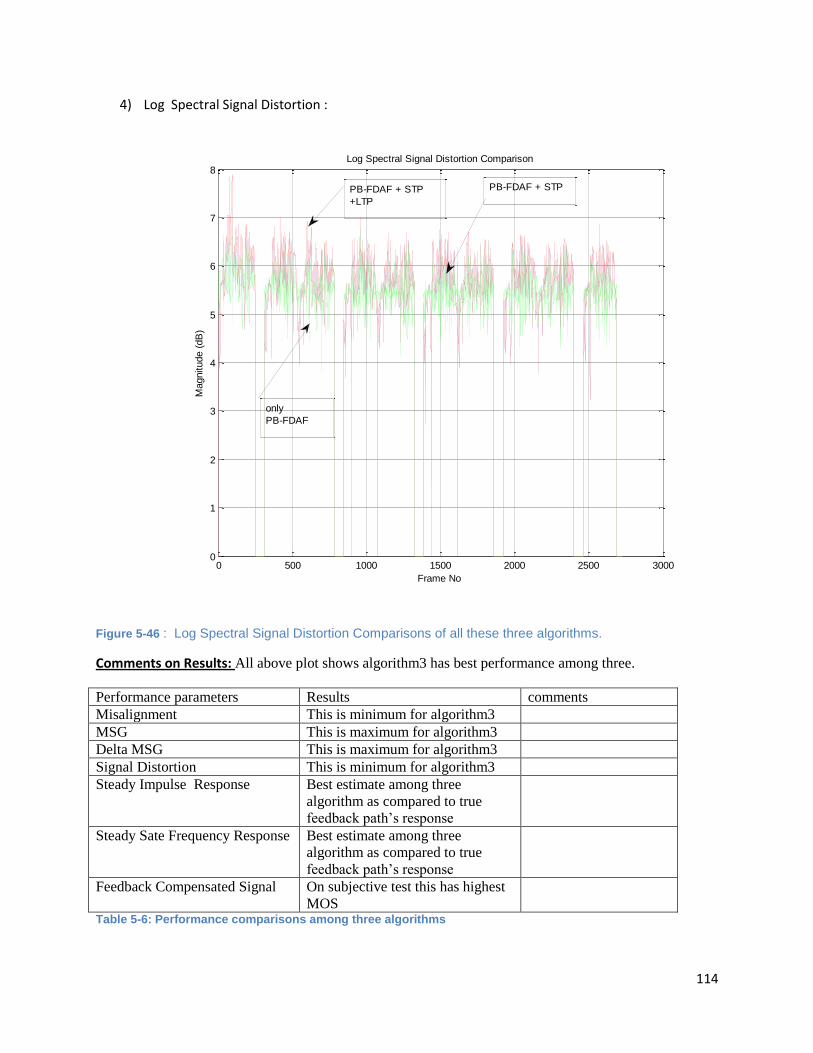
114

4) Log Spectral Signal Distortion :

Figure 5-46 : Log Spectral Signal Distortion Comparisons of all these three algorithms.

Comments on Results: All above plot shows algorithm3 has best performance among three.

Performance parameters Results comments

Misalignment This is minimum for algorithm3

MSG This is maximum for algorithm3

Delta MSG This is maximum for algorithm3

Signal Distortion This is minimum for algorithm3

Steady Impulse Response Best estimate among three

algorithm as compared to true

feedback path’s response

Steady Sate Frequency Response Best estimate among three

algorithm as compared to true

feedback path’s response

Feedback Compensated Signal On subjective test this has highest

MOS

Table 5-6: Performance comparisons among three algorithms

0 500 1000 1500 2000 2500 30000

1

2

3

4

5

6

7

8Log Spectral Signal Distortion Comparison

Frame No

Magnitude (

dB

)

only

PB-FDAF

PB-FDAF + STP

+LTP

PB-FDAF + STP

115

Chapter 6

6.1 Conclusion In general feedback cancellation setups, standard adaptive filtering techniques fail to provide a reliable

feedback path estimate if the desired signal is spectrally colored because of the presence of a closed signal

loop.

But while several proactive acoustic feedback (Larsen-effect) cancellation schemes have been presented

for speech applications with short acoustic feedback paths as encountered in application like hearing aids,

these schemes fail with the long impulse responses inherent to for instance and car cabin intercom system

and public address systems. Here a new prediction-error-method (PEM)-based scheme which identifies

both the acoustic feedback path and the non-stationary speech source model. A cascade of a short- and a

long-term predictor removes the coloring and periodicity in voiced speech segments, which account for

the unwanted correlation between the loudspeaker signal and the speech source signal. The predictors are

used to pre-whiten the speech source signal, resulting in a least squares system which is solved

recursively by means of NLMS or RLS algorithms. Simulations show that this approach is indeed

superior to earlier approaches whenever long acoustic channels are dealt with.

These new algorithm is introduced which is modification of algorithm PEM-AFC, which allows for

acoustic feedback cancellation in setups with long acoustic paths. It uses a speech source model with

short- and long-term prediction. Not only the howling phenomenon is suppressed but also the

reverberation-like sounds, which indeed become audible in the region of marginal stability. The main

difference with existing schemes is twofold. First, our algorithm incorporates a long-term prediction filter

which removes periodicity in the short-term speech signal residual, and second, we do not assume

stationarity of the speech signal over the length of the data window on which the acoustic path is

identified.

The modified version of algorithm PEM-AFC hence performs very well for long acoustic paths,

contrarily to existing algorithms which were developed for short path applications. For short acoustic

paths the performance of PEM-AFC is equal to that of the existing methods. Also, thanks to the low

computational complexity and delay because of partition block frequency domain adaptive filtering (PB-

FDAF) implementation, the algorithm can easily be implemented in real time. PB-FDAF is always

preferred over sub–band implementation because of low latency which is primary requirement in real

time application

In this thesis, results of a comparative evaluation of existing decorrelation methods are reported, in terms

of two measures that actually determine the acoustic feedback control performance, namely the maximum

stable gain (MSG) increase and the sound quality. It appears that the choice of the decorrelation method

and its parameters has a profound influence on these performance measures. Moreover, when

decorrelation is applied in the closed signal loop, a trade-off between the resulting MSG increase and

sound quality is unavoidable.

It is also shown that the AFC method should preferably be combined with a decorrelation approach that

operates in the adaptive filtering circuit, e.g., using decorrelating pre-filters (AFC-PF), since this approach

appears to be beneficial w.r.t. the achievable amplification and sound quality. We have found the AFC-PF

116

approach to be capable of providing an average MSG increase of approximately 9 dB, and a maximum

MSG increase around 12 dB.

6.2 Limitation PB-FDAF has poor frequency selectivity so that tracking behavior may not be robust enough. In current

experimentation, speed of convergence and robustness improvement methods not implemented though

several methods have been discussed here.

Computational complexity increases as number partitions in the input delay line if adaptive filter

increases. When number partitions increases, the system tends to be also unstable.

Order STP and wider pitch search of LTP for accurate estimation of pitch lag increases computational

complexity. Interval of STP and LTP calculation should be decided experimentally and should be tuned

according to real time scenario.

Amount of delay in forward path and adaptive filter path should be tuned /calculated according to real

time scenario and experimentation. Also Initial set sizes for frequency bins should be decided

experimentally.

The fundamental problem lies in the fact that in AFC, the acoustic feedback path is traditionally modeled

using its impulse response, which typically has a large number of coefficients. This is especially so when

a high sampling frequency is applied (e.g., in audio applications). The impulse response is then more

densely sampled and in addition more adaptive filter updates have to be performed per second.

Although frequency domain implementation reduced computational complexity significantly , since the

frequency domain models currently used in FDAF have a fixed and uniform frequency resolution, the

required FDAF filter order should still be high to guarantee that the magnitude peaks are modeled with

sufficient accuracy, see, e.g., the FDAF experimental results in [53].

This AFC method is devised only for speech but not for audio which is also need to be accommodated

in-car communication system for better communication.

6.3 Recommendations for further research As pointed in limitation ,in terms of robustness, this AFC approach would be benefited much from recent

improvements such as post-filtering [122]-[124], notch filtering [1],[53],[121], adaptation control [53],

and regularization [53],[54],[129].

In [59] it is shown that, concerning robustness, how onset detection avoids instability at onsets of the

near-end signal. It is also shown that an NLMS-type algorithm is derived that allows for prior knowledge

of the RIR to be incorporated in the adaptation rule, which is particularly useful at system startup. Then a

twin-filter structure (adopted from acoustic echo cancellation) was shown to be also effective in acoustic

feedback cancellation. On the one hand room impulse response changes can be tracked quickly while on

the other hand a small variance on the estimate of the RIR can be maintained during steady-state

operation. A high-pass filter is included to avoid high variance on the low-frequency part of the RIR

estimate. Finally the combination of notch filtering and PEM was shown to provide a more robust

solution to echo path changes if some distortion is allowable

117

The AFC method in frequency domain implementation appears to produce promising results, the main

challenges for future research in acoustic feedback control lie in further increasing the AFC reliability and

reducing its computational complexity.

Another possibility for reducing the acoustic feedback path model complexity consists in using a time

domain model different from the FIR model. Since the peaks in the acoustic feedback path magnitude

response can be modeled as narrowband resonances, an IIR (or pole-zero) model seems to be an

appropriate choice. The use of such models in room acoustics has both been recommended

[125],[130],[131] and discouraged [132],[133], however, no results on the use of IIR models in AFC are

available. The appeal of using such models in room acoustic applications is related to the conjecture that

the IIR model denominator coefficients can in fact be assumed time-invariant in a certain acoustic

environment, regardless of the loudspeaker and microphone positions [125]. A related model, which also

exploits the assumption of time-invariant room acoustic resonance frequencies, is based on the use of

orthogonal basis functions such as the discrete-time Laguerre or Kautz functions, which have been

evaluated in an AEC context in [135],[136].

Another great challenge in acoustic feedback control and in AFC in particular, is to generalize the

methods proposed in a single-channel context to multi-channel systems. Since the number of acoustic

feedback paths in a multi-channel system equals the number of loudspeakers times the number of

microphones, the AFC computational complexity can be expected to increase very quickly in a

multichannel context. Again, the use of IIR models or models based on orthogonal basis functions may

bring some relief, since, following the arguments in [125],[135], these models could then share a common

denominator. Another problem arising in multi-channel AFC is related to the identifiability of the

acoustic feedback path models in case the loudspeaker signals are correlated. A similar problem occurs in

multichannel AEC, and has received quite some attention in the literature, see, e.g., [126], [136].

In terms of reliability, recent research has pointed out that so-called hybrid AFC methods, in which AFC

is combined with other methods for acoustic feedback control, are far more robust compared to the

traditional AFC approach. However, we believe that in the existing hybrid AFC methods, the cooperation

between the different methods is still suboptimal. For example, in the combined AFC and postfiltering

methods proposed in [122]-[124], the postfilter design is solely based on the feedback-compensated signal

spectrum, while it is known from AEC that the joint design of a cancellation filter and a postfilter

generally results in a better performance [127],[128]. A related issue is the combination of AFC with a

gain reduction method: in [1],[121], the AFC and ANF filters are adapted independently, while in the

combined AFC and AEQ approach proposed in [124] and in the combined AFC and NHS approach

proposed in [53], the AEQ/NHS design is based on the most recent AFC estimate. Similarly to the joint

AFC and postfilter design, it can be expected that a joint estimation of the AFC and gain reduction filter

coefficients is to be preferred over a decoupled estimation.

A general framework of AFC algorithm sets can be next level of future research to accommodate both

speech and audio in intercom system.

Finally, a similar remark can be made on the joint design of an AFC and a spatial filtering method, which

would probably outperform the state-of-the-art approach of AFC combined with a fixed beamformer [1]

or an adaptive beamformer steered by the feedback-compensated signal [124].

118

7 Bibliography: Chapter 2

[1] G. Schmidt and T. Haulick, “Signal processing for in-car communication systems,” Signal

Processing, vol. 86, no. 6, pp. 1307–1326, June 2006, special Issue on Applied Speech and Audio

Processing.

[2] G. Glentis, K. Berberidis, S. Theodoridis: Efficient least squares adaptive algorithms for FIR

transversal filtering: a unified view, IEEE Signal Process. Mag.,16(4), 13–41, 1999.

[3] E. Lleida, E. Masgrau, A. Ortega: Acoustic echo and noise reduction for car cabin communication,

Proc. EUROSPEECH ’01, 3, 1585–1588, Aalborg, Denmark, 2001.

[4] A. Ortega, E. Lleida, E. Masgrau, F. Gallego: Cabin car communication system to improve

communication inside a car, Proc. ICASSP ’02, 4, 3836–3839, Orlando, FL, USA, 2002.

Chapter 3

[5] D. A. Bohn, “Pro audio reference,” cRane Corp. [Online]. Available: http://www.rane.com/digi-

dic.html

[6] H. Nyquist, “Regeneration theory,” Bell Syst. Tech. J., vol. 11, pp. 126–147, 1932.

[7] M. R. Schroeder, “Improvement of acoustic-feedback stability by frequency shifting,” J. Acoust.

Soc. Amer., vol. 36, no. 9, pp. 1718–1724, Sept. 1964.

[8] R. W. Guelke and A. D. Broadhurst, “Reverberation time control by direct feedback,” Acustica,

vol. 24, pp. 33–41, 1971.

[9] P. Mapp and C. Ellis, “Improvements in acoustic feedback margin in sound reinforcement

systems,” in Preprints AES 105th Convention, San Francisco, CA, USA, Sept. 1998, AES Preprint 4850.

[10] M. R. Schroeder, “Improvement of feedback stability of public address systems by frequency

shifting,” J. Audio Eng. Soc., vol. 10, no. 2, pp. 108–109, Apr. 1962.

[11] E. T. Patronis, Jr., “Acoustic feedback detector and automatic gain control,” U.S. Patent

4,079,199, Mar., 1978.

[12] ——, “Electronic detection of acoustic feedback and automatic sound system gain control,” J.

Audio Eng. Soc., vol. 26, no. 5, pp. 323–326, May 1978.

[13] S. Ando, “Howling detection and prevention circuit and a loudspeaker system employing the

same,” U.S. Patent 6,252,969, June, 2001.

http://www.rane.com/digi-dic.html

http://www.rane.com/digi-dic.html

119

[14] Y. Nagata, S. Suzuki, M. Yamada, M. Yoshida, M. Kitano, K. Kuroiwa, and S. Kimura, “Howling

remover having cascade connected equalizers suppressing multiple noise peaks,” U.S. Patent

5,710,823, Jan., 1998.

[15] ——, “Howling remover composed of adjustable equalizers for attenuating complicated noise

peaks,” U.S. Patent5,729,614, Mar., 1998.

[16] M. Hanajima, M. Yoneda, and T. Okuma, “Howling eliminator,” WIPO Patent Application

WO/1999/021 396, Apr., 1999.

[17] ——, “Howling eliminating apparatus,” U.S. Patent 6,125,187, Sept., 2000.

[18] Y. Terada and A. Murase, “Howling control device and howling control method,” U.S. Patent

7,190,800, Mar., 2007.

[19] N. Osmanovic and V. Clarke, “Acoustic feedback cancellation system,” U.S. Patent Application

2007/0 019 824 A1, Jan., 2007.

[20] ——, “Acoustic feedback cancellation system,” WIPO Patent Application WO/2007/013 981,

Feb., 2007.

[21] N. Osmanovic, V. E. Clarke, and E. Velandia, “An in-flight low latency acoustic feedback

cancellation algorithm,” in Preprints AES 123rd Convention, New York, NY, USA, Oct. 2007, AES

Preprint 7266.

[22] J. B. Foley, “Adaptive periodic noise cancellation for the control of acoustic howling,” in Proc.

IEE Colloq. Adaptive Filters, London, UK, Mar. 1989, pp. 7/1–7/4.

[23] D. M. Oster, M. P. Lewis, and T. J. Tucker, “Method and apparatus for adaptive audio resonant

frequency filtering,” WIPO Patent Application WO/1991/020 134, Dec., 1991.

[24] S. M. Kuo and J. Chen, “New adaptive IIR notch filter and its application to howling control in

speakerphone system,” IEE Electronics Lett., vol. 28, no. 8, pp. 764–766, Apr. 1992.

[25] M. P. Lewis, T. J. Tucker, and D. M. Oster, “Method and apparatus for adaptive audio resonant

frequency filtering,” U.S. Patent 5,245,665, Sept., 1993.

[26] M. H. Er, T. H. Ooi, L. S. Li, and C. J. Liew, “A DSP-based acoustic feedback canceller for public

address systems,” in Proc. Int. Conf. Signal Process. (ICSP ’93), Beijing, China, Oct. 1993, pp. 1251–

1254.

[27] ——, “A DSP-based acoustic feedback canceller for public address systems,” Microprocessors

and Microsystems, vol. 18, no. 1, pp. 39–47, Jan./Feb. 1994.

120

[28] A. Kawamura, M. Matsumoto, M. Serikawa, and H. Numazu, “Sound amplifying apparatus with

automatic howlsuppressing function,” U.S. Patent 5,442,712, Aug., 1995.

[29] M. Tahernezhadi and L. Liu, “An adaptive notch filter for howling cancellation,” Acoust.Lett.,

vol. 18, no. 8, pp. 142–145, 1995.

[30] W. Staudacher, “Acoustic feedback cancellation for equalized amplifying systems,” U.S. Patent

5,533,120, July, 1996.

[31] J. Timoney and F. B. Foley, “Robust performance of the adaptive periodic noise canceller in a

closed-loop system,” in Proc. 9th European Signal Process. Conf. (EUSIPCO ’98), Rhodes, Greece,

Sept. 1998, pp. 1177–1180.

[32] J. E. Lane, D. Hoory, and J. Choe, “Method and apparatus for suppressing acoustic feedback in

an audio system,” U.S. Patent 5,717,772, Feb., 1998.

[33] R. Porayath and D. J. Mapes-Riordan, “Acoustic feedback elimination using adaptive notch filter

algorithm,” U.S. Patent 5,999,631, Dec., 1999.

[33] A. Kawamura, M. Matsumoto, M. Serikawa, and H. Numazu, “Sound amplifying apparatus with

automatic howlsuppressing function,” European Patent EP0 599 450, Nov., 2001.

[34] P. R. Williams, “Method and system for elimination of acoustic feedback,” WIPO Patent

Application WO/2002/021 817, Mar., 2002.

[35] W. Loetwassana, R. Punchalard, and W. Silaphan, “Adaptive howling canceller using adaptive

IIR notch filter: simulation and implementation,” in Proc. 2003 IEEE Int. Conf. Neural Networks and

Signal Process. (ICNNSP ’03), Nanjing, China, Dec. 2003, pp. 848–851.

[36] J. Timoney, F. B. Foley, and A. T. Schwarzbacher, “An explicit criterion for adaptive periodic

noise canceller robustness applied to feedback cancellation,” in 4th Electron. Circuits Syst. Conf.

(ECS ’03), Bratislava, Slovakia, Sept. 2003, pp. 23–26. [46] J. Wei, L. Du, Z. Chen, and F. Yin, “A new

algorithm for howling detection,” in Proc. 2003 IEEE Int. Symp. Circuits Syst. (ISCAS ’03), vol. 4,

Bangkok, Thailand, May 2003, pp. 409–411.

[37] A. F. Rocha and A. J. S. Ferreira, “An accurate method of detection and cancellation of multiple

acoustic feedbacks,” in Preprints AES 118th Convention, Barcelona, Spain, May 2005, AES Preprint

6335.

[38] M. B¨orsch, “Method for constraining electroacoustic feedback,” European Patent Application

EP1 684 543 A1, July, 2006.

[39] ——, “Method for suppressing electro-acoustic feedback,” U.S. Patent Application 2006/0 159

282 A1, July, 2006.

121

[40] G. Rombouts, T. van Waterschoot, and M. Moonen, “Proactive notch filtering for acoustic

feedback cancellation,” in Proc. 2nd Annual IEEE Benelux/DSP Valley Signal Process. Symp. (SPS-

DARTS’06), Antwerp, Belgium, Mar. 2006, pp.169–172.

[Online].Available:ftp.esat.kuleuven.be/pub/sista/vanwaterschoot/abstracts/06-81.html

[41] R. Abe, “Howling suppression device and howling suppression method,” U.S. Patent 7,295,670,

Nov., 2007.

[42] W. Loetwassana, R. Punchalard, A. Lorsawatsiri, J. Koseeyaporn, and P. Wardkein, “Adaptive

howling suppressor in an audio amplifier system,” in Proc. 2007 Asia-Pacific Conf. Commun. (APCC

’07), Bangkok, Thailand, Oct. 2007, pp. 445–448.

[43] D. Somasundaram, “Feedback cancellation in a sound system,” European Patent Application

EP1 903 833 A1, Mar., 2008.

[44] T. Kawamura and T. Kanamori, “Howling detection device and method,” U.S. Patent Application

2008/0 021 703 A1, Jan., 2008.

[45] P. Gil-Cacho, T. van Waterschoot, M. Moonen, and S. H. Jensen, “Regularized adaptive notch

filters for acoustic howling suppression,” submitted for publication in Proc. 17th European Signal

Process. Conf. (EUSIPCO ’09), ESAT-SISTA Technical Report, KatholiekeUniversiteit Leuven, Belgium,

Feb. 2009. [Online]. Available: ftp.esat.kuleuven.be/pub/sista/vanwaterschoot/abstracts/09-

RANF.html

[46] M. G. Siqueira and A. Alwan, “Steady-state analysis of continuous adaptation in acoustic

feedback reduction systems for hearing-aids,” IEEE Trans. Speech Audio Process., vol. 8, no. 4, pp.

443–453, July 2000.

[47] J. Hellgren and U. Forssell, “Bias of feedback cancellation algorithms in hearing aids based on

direct closed loopidentification,” IEEE Trans. Speech Audio Process., vol. 9, no. 7, pp. 906–913, Nov.

2001.

[48] T. van Waterschoot, G. Rombouts, and M. Moonen, “On the performance of decorrelation by

prefiltering foradaptive feedback cancellation in public address systems,” in Proc. 4th IEEE Benelux

Signal Process.Symp. (SPS

’04), Hilvarenbeek, The Netherlands, Apr. 2004, pp. 167–170. [Online]. Available:

ftp.esat.kuleuven.be/pub/sista/vanwaterschoot/abstracts/04-24.html

Chapter 4

ftp://ftp.esat.kuleuven.be/pub/sista/vanwaterschoot/abstracts/06-81.html

ftp://ftp.esat.kuleuven.be/pub/sista/vanwaterschoot/abstracts/09-RANF.html

ftp://ftp.esat.kuleuven.be/pub/sista/vanwaterschoot/abstracts/09-RANF.html


122


prefiltering foradaptive feedback cancellation in public address systems,” in Proc. 4th IEEE Benelux

Signal Process.Symp. (SPS’04), Hilvarenbeek, TheNetherlands, Apr.2004, pp.167–170. [Online].

Available:ftp.esat.kuleuven.be/pub/sista/vanwaterschoot/abstracts/04-24.html

[50] S. M. Kay, Fundamentals of statistical signal processing: estimation theory. Upper Saddle River,

New Jersey: Prentice-Hall, 1993.

[51] U. Forssell and L. Ljung, “Closed-loop identification revisited,” Automatica, vol. 35, no. 7, pp.

1215–1241, July 1999.

[52] T. van Waterschoot, G. Rombouts, P. Verhoeve, and M. Moonen, “Double-talk-robust

prediction error identification

[53] G. Rombouts, T. van Waterschoot, and M. Moonen, “Robust and efficient implementation of

the PEM-AFROW algorithm for acoustic feedback cancellation,” J. Audio Eng. Soc., vol. 55, no. 11,

pp. 955–966, Nov. 2007.

[54] ——, “Optimally regularized adaptive filtering algorithms for room acoustic signal

enhancement,” Signal Processing, vol. 88, no. 3, pp. 594–611, Mar. 2008.

[55] G. Rombouts, T. van Waterschoot, K. Struyve, P. Verhoeve, and M. Moonen, “Identification of

undermodelled room impulse responses,” in Proc. 2005 Int. Workshop Acoustic Echo Noise Control

(IWAENC ’05), Eindhoven, The Netherlands, Sept. 2005, pp. 153–156.

[56] R. D. Poltmann, “Stochastic gradient algorithm for system identification using adaptive FIR-

filters with too low number of coefficients,” IEEE Trans. Circuits Syst., vol. 35, no. 2, pp. 247–250,

Feb. 1988.

[57] C. Paleologu, S. Ciochina, and J. Benesty, “Variable step-size NLMS algorithm for under-

modeling acoustic echo cancellation,” IEEE Signal Process.Lett., vol. 15, pp. 5–8, 2008.

[58] T. van Waterschoot and M. Moonen, “50 years of acoustic feedback control: state of the art

and futurechallenges,” Proc. IEEE, submitted for publication, Feb. 2009, ESAT-SISTA Technical

Report TR 08-13,KatholiekeUniversiteit Leuven, Belgium.

[59] A. Spriet, G. Rombouts, M. Moonen, and J. Wouters, “Adaptive feedback cancellation in

hearing aids,” J.Franklin Inst., vol. 343, no. 6, pp. 545–573, Sept. 2005.

[60] A. Goertz, “An adaptive subtraction filter for feedback cancellation in public address sound

systems,” in Proc. 15th Int. Congr. Acoust. (ICA ’95), Trondheim, Norway, June 1995, pp. 69–72.

[61] C. P. Janse and C. C. Tchang, “Acoustic feedback suppression,” WIPO Patent

ApplicationWO/2005/079 109, Aug., 2005.

123

[62] C. P. Janse and P. A. A. Timmermans, “Signal amplifier system with improved echo

cancellation,” U.S. Patent 5,748,751,May, 1998.

[63] S. Kamerling, K. Janse, and F. van derMeulen, “A new way of acoustic feedback suppression,” in

Preprints AES 104th Convention, Amsterdam, The Netherlands, May 1998, AES Preprint 4735.

[64] F. Gallego, E. Lleida, E. Masgrau, and A. Ortega, “Method and system for suppressing echoes

andnoises in environments under variable acoustic and highly feedback conditions,”WIPO Patent

ApplicationWO/2002/101 728, Dec., 2002.

[65] A. Ortega, E. Lleida, and E. Masgrau, “Speech reinforcement system for car cabin

communications,” IEEE Trans. Speech Audio Process., vol. 13, no. 5, pp. 917– 929, Sept. 2005.


prefiltering for adaptive feedback cancellation in public address systems,” in Proc. 4th IEEE Benelux

Signal Process.Symp. (SPS ’04), Hilvarenbeek, The Netherlands, Apr. 2004, pp. 167–170.

[67] A. Ortega, E. Lleida, E. Masgrau, L. Buera, and A. Miguel, “Acoustic feedback cancellation in

speechreinforcement systems for vehicles,” in Proc. Interspeech 2005, Lisbon, Portugal, Sept. 2005,

pp. 2061–2064.

[68] G. Rombouts, T. van Waterschoot, K. Struyve, and M. Moonen, “Acoustic feedback suppression

for long acoustic paths using a nonstationary source model,” IEEE Trans. Signal Process., vol. 54, no.

9, pp. 3426– 3434, Sept. 2006.

[69] T. van Waterschoot and M. Moonen, “Adaptive feedback cancellation for audio

applications,”Signal Processing, 2009, article in press, doi:10.1016/j.sigpro.2009.04.036.

[70] G. Rombouts, T. van Waterschoot, and M. Moonen, “Proactive notch filtering for acoustic

feedback cancellation,” in Proc. 2nd Annual IEEE Benelux/DSP Valley Signal Process. Symp. (SPS-

DARTS ’06), Antwerp, Belgium, Mar. 2006, pp. 169–172. [Online]. Available:

ftp.esat.kuleuven.be/pub/sista/vanwaterschoot/abstracts/06-81.html

[71] C. P. Janse and H. J. W. Belt, “Sound reinforcement system having an echo suppressor and

loudspeaker beamformer,” WIPO Patent Application WO/2003/010 996, Feb., 2003.

[72] G. Rombouts, T. van Waterschoot, and M. Moonen, “Robust and efficient implementation of

the PEM-AFROW algorithm for acoustic feedback cancellation,” J. Audio Eng. Soc., vol. 55, no. 11,

pp. 955–966, Nov. 2007.

[73] T. Haulick, G. U. Schmidt, and H. Lenhardt, “Feedback reduction in communication systems,”

European Patent EP1 679 874, May, 2008.

Chapter 5


124

[74] R. Porayath and D. J. Mapes-Riordan, “Acoustic feedback elimination using adaptive notch filter

algorithm,” U.S. Patent 5,999,631, Dec., 1999.

[75] M. P. Lewis, T. J. Tucker, and D. M. Oster, “Method and apparatus for adaptive audio resonant

frequency filtering,” U.S. Patent 5,245,665, Sep., 1993.

[76] J.A. Maxwell, P.M. Zurek, Reducing acoustic feedback in hearing aids, IEEE Trans. Speech Audio

Process. 3 (4) (1995) 304–313.

[77] J.E. Greenberg, P.M. Zurek, M. Brantley, Evaluation of feedback-reduction algorithms for

hearing aids, J. Acoust. Soc. Am. 108 (5) (2000) 2366–2376.

[78] J.M. Kates, Feedback cancellation in hearing aids: results from a computer simulation, Signal

Process. 39 (3) (1991) 553–562.

[79] Y. Park, D. Kim, I. Kim, An efficient feedback cancellation for multiband compression hearing

aids, in: Proceedings of the 20th Annual International Conference on Engineering in Medicine and

Biology Society, vol. 5, 1998, pp. 2706–2709.

[80] S. Thipphayathetthana, C. Chinrungrueng, Variable step-size of the least-mean-square

algorithm for reducing acoustic feedback in hearing aids, in: IEEE Asia-Pacific Conference on Circuits

and Systems, 2000, pp. 407–410.

[81] L. Ljung, T. So¨ derstro¨ m, Theory and Practice of Recursive Identification, MIT Press,

Cambridge, MA, 1983.

[82] T. Fillon, J. Prado, Acoustic feedback cancellation for hearing-aids, using multi-delay filter, in:

Fifth Nordic Signal Processing Symposium (NORSIG), on board Hurtigruten, Norway, 2002.

[83] A. Kaelin, A. Lindgren, S. Wyrsch, A digital frequency-domain implementation of a very high

gain hearing aid with compensation for recruitment of loudness and acoustic echo cancellation,

Signal Process. 64 (1) (1998) 71–85.

[84] J.-S. Soo, K. Pang, Multidelay block frequency domain adaptive filter, IEEE Trans. Acoust.

Speech Signal Process. 38 (4) (1990) 788–798.

[85] J.E. Greenberg, Modified LMS algorithms for speech processing with an adaptive noise

canceller, IEEE Trans. Speech Audio Process. 6 (4) (1998) 338–350.

[86] U. Forssell, Closed-loop identification—methods, theory and applications, Ph.D. Thesis, Linko¨

ping Universitet, Linko¨ ping, Sweden, 1999.

[87] U. Forssell, L. Ljung, Closed-loop identification revisited, Automatica 35 (1999) 1215–1241.

125

[88] J.R. Deller, J.G. Proakis, J.H.L. Hansen, Discrete-Time Processing of Speech Signals, Macmillan

PublishingCompany, Englewood Cliffs, NJ, 1993.

[89] G. Rombouts, T. van Waterschoot, K. Struyve, M. Moonen, Acoustic feedback suppression for

long acoustic paths using a nonstationary source model, IEEE Trans. Signal Process 54 (9) (2006)

3426–3434.

[90] A. Spriet, I. Proudler, M. Moonen, and J. Wouters, “Adaptive feedback cancellation in hearing

aids with linear prediction of the desired signal,” IEEE Trans. Signal Process., vol. 53, no. 10, pp.

3749–3763, Oct. 2005.

[91] ——, “Optimally regularized adaptive filtering algorithms for room acoustic signal

enhancement,” Signal Processing, vol. 88, no. 3, pp. 594– 611, Mar. 2008.

[92] T. Fillon, J. Prado, Acoustic feedback cancellation for hearing-aids, using multi-delay filter, in:

Fifth NordicSignal Processing Symposium (NORSIG), on board Hurtigruten, Norway, 2002.

[93] T. van Waterschoot, G. Rombouts, and M. Moonen, “Optimally regularized adaptive filtering

algorithms for room acoustic signal enhancement,” Signal Processing, vol. 88, no. 3, pp. 594–611,

Mar. 2008.

[94] ——, “MSE optimal regularization of APA and NLMS algorithms in room acoustic applications,”

in Proc. 2006 Int. Workshop Acoustic Echo Noise Control (IWAENC ’06), Paris, France, Sep. 2006.

[95] J. M. Kates, “Constrained adaptation for feedback cancellation in hearing aids,” J. Acoust. Soc.

Amer., vol. 106, no. 2, pp. 1010–1019, Aug. 1999.

[96] H. Puder, B. Beimel, Controlling the adaptation of feedback cancellation filters—problem

analysis and solution approaches, in: Proceedings of the European Signal Processing Conference

(EUSIPCO), Vienna, Austria, 2004, pp. 25–28.

[97] A. Spriet, K. Eneman, M. Moonen, and J. Wouters, “Objective measures for real-time evaluation

of adaptive feedback cancellation algorithms in hearing aids,” in Proc. 16th European Signal

Process. Conf. (EUSIPCO ’08), Lausanne, Switzerland, Aug. 2008.

[98] M. Hanajima, M. Yoneda, and T. Okuma, “Howling eliminator,” WIPO Patent Application

WO/1999/021 396, Apr., 1999.

[99] ——, “Howling eliminating apparatus,” U.S. Patent 6,125,187, Sept., 2000.

[100] M. H. Er, T. H. Ooi, L. S. Li, and C. J. Liew, “A DSP-based acoustic feedback canceller for public

address systems,” in Proc. Int. Conf. Signal Process. (ICSP ’93), Beijing, China, Oct. 1993, pp. 1251–

1254.

126

[101] ——, “A DSP-based acoustic feedback canceller for public address systems,” Microprocessors

and Microsystems, vol. 18, no. 1, pp. 39–47, Jan./Feb. 1994.

[102] A. Kawamura, M. Matsumoto, M. Serikawa, and H. Numazu, “Sound amplifying apparatus

with automatic howlsuppressing function,” U.S. Patent 5,442,712, Aug., 1995.

[103] A. Kawamura, M. Matsumoto, M. Serikawa, and H. Numazu, “Sound amplifying apparatus

with automatic howlsuppressing function,” European Patent EP0 599 450, Nov., 2001.

[104] P. R. Williams, “Method and system for elimination of acoustic feedback,” WIPO Patent

Application WO/2002/021 817, Mar., 2002.

[105] A. F. Rocha and A. J. S. Ferreira, “An accurate method of detection and cancellation of

multiple acoustic feedbacks,” in Preprints AES 118th Convention, Barcelona, Spain, May 2005, AES

Preprint 6335.

[106] M. B¨orsch, “Method for constraining electroacoustic feedback,” European Patent Application

EP1 684 543 A1, July, 2006.

[107] ——, “Method for suppressing electro-acoustic feedback,” U.S. Patent Application 2006/0 159

282 A1, July, 2006.

[108] D. Somasundaram, “Feedback cancellation in a sound system,” European Patent Application

EP1 903 833 A1, Mar., 2008.

[109] G. Schmidt, “Applications of Acoustic Echo Control – An Overview,” in Proc. Eur. Signal

Process, Conf. (EUSIPCO), 2004.

[110] M. G. Siqueira and A. Alwan, “Steady-state Analysis of Continuous Adaptation in Acoustic

Feedback Reduction Systems for Hearing-aids,” IEEE Trans. Speech Audio Process., vol. 8, no. 4, pp.

443–453, Jul. 2000.

[111] Toon van Waterschoot and Marc Moonen, “Adaptive Feedback Cancellation for Audio Applications,” Signal Processing, Vol. 89, Issue 11, pp. 2185-2201, 2009

[112] Sang-Kwon Lee, “Measurement of Reverberation Times Using a Wavelet Filter Bank and

Application to a Passenger Car,” J. Audio Eng. Soc., Vol. 52, No. 5, May 2004.

[113] J.B. Allen and D.A. Berkley, “Image Method for Efficiently Simulating Small Room Acoustics,” J. Acoust. Soc. Am., vol. 65, no.4, pp. 943-950, April 1979.

[114] P.M. Ptereson, “Simulating the Response of Multiple Microphones to a Single Acoustic Source in a Reverberant Room,” J. Acoust. Soc. Am., vol. 80, no. 5, November 1986. [115] H. Nyquist, “Regeneration Theory,” Bell Syst. Tech. J. 11, pp. 126-147, 1932.

127

[116] J. Hellgren and U. Forssell, “Bias of Feedback Cancellation Algorithm in Hearing Aids Based on

Direct Closed Loop Identification”, IEEE Trans. Speech and Audio Processing, Vol. 9, No. 7,

November, 2001.

[117] John J. Shynk “Frequency-Domain and Multirate Adaptive Filtering” Signal Processing

Magazine, IEEE , Volume: 9 , Issue: 1 ,Jan. 1992

[118] PHD thesis :KoenEneman, Subband and Frequency-Domain Adaptive Filtering Techniques for

Speech Enhancement in Hands-free Communication . PhD thesis, KatholiekeUniversiteit Leuven,

March 2002 (Nederlands).

[119] G. Rombouts, T. van Waterschoot, K. Struyve, and M. Moonen, “Acoustic feedback

suppression for long acoustic paths using a nonstationary source model,” in Proc. 13th European

Signal Process. Conf. (EUSIPCO ’05), Antalya, Turkey, Sept. 2005.

[ 120 ] P.Delsarte and Y.Genin: The split Levinson algorithm", iEEE Trans. Qli ASS P. vol. ASSP-34, pp.

470.478, June 1986.

Chapter 6

[121] T. Haulick, G. U. Schmidt, and H. Lenhardt, “Feedback reduction in communication systems,”

European PatentEP1 679 874, May, 2008.

[122] F. Gallego, E. Lleida, E. Masgrau, and A. Ortega, “Method and system for suppressing echoes

and noises in environments under variable acoustic and highly feedback conditions,” WIPO Patent

Application WO/2002/101 728, Dec., 2002.

[123] A. Ortega, E. Lleida, and E. Masgrau, “Speech reinforcement system for car cabin

communications,” IEEE Trans. Speech Audio Process., vol. 13, no. 5, pp. 917–929, Sept. 2005.

[124] C. P. Janse and H. J. W. Belt, “Sound reinforcement system having an echo suppressor and

loudspeaker beamformer,” WIPO Patent Application WO/2003/010 996, Feb., 2003.

[125] Y. Haneda, S. Makino, and Y. Kaneda, “Common acoustical pole and zero modeling of room

transfer functions,” IEEE Trans. Speech Audio Process., vol. 2, no. 2, pp. 320–328, 1994.

[126] M. M. Sondhi, D. R. Morgan, and J. L. Hall, “Stereophonic acoustic echo cancellation – an

overview of the fundamental problem,” IEEE Signal Process. Lett., vol. 2, no. 8, pp. 148–151, Aug.

1995.

[127] E. Haensler and G. U. Schmidt, “Hands-free telephones – joint control of echo cancellation and

postfiltering,” Signal Processing, vol. 80, no. 11, pp. 2295–2305, Nov. 2000.

http://gilbert.med.kuleuven.be/~koen/abstracts/phd.html

http://gilbert.med.kuleuven.be/~koen/abstracts/phd.html

http://gilbert.med.kuleuven.be/~koen/abstracts/phd_nl.html

128

[128] G. Enzner and P. Vary, “Frequency-domain adaptive Kalman filter for acoustic echo control in

hands-free telephones,” Signal Processing, vol. 86, no. 6, pp. 1140–1156, June 2006, special Issue on

Applied Speech and Audio Processing.

[129] T. van Waterschoot, G. Rombouts, and M. Moonen, “MSE optimal regularization of APA and

NLMS algorithms in room acoustic applications,” in Proc. 2006 Int. Workshop Acoustic Echo Noise

Control (IWAENC ’06), Paris, France, Sept. 2006.

[130] J. Pongsiri, P. Amin, and C. Thompson, “Modeling the acoustic transfer function of a room,” in

Proc. 12th Int. Conf. Mathematical Comput.Modelling Scientific Comput. (ICMCMSC ’99), Chicago,

Illinois, USA, Aug. 1999.

[131] T. Gustafsson, J. Vance, H. R. Pota, B. D. Rao, and M. M. Trivedi, “Estimation of acoustical

room transfer functions,” in Proc. 39th IEEE Conf. Decision Control (CDC ’00), Sydney, Australia, Dec.

2000, pp. 5184–5189.

[132] S. Gudvangen and S. J. Flockton, “Comparison of pole-zero and all-zero modelling of acoustic

transfer functions,” IEE Electronics Lett., vol. 28, no. 21, pp. 1976–1978, 1992.

[133] A. P. Liavas and P. A. Regalia, “Acoustic echo cancellation: Do IIR models offer better modeling

capabilities than their FIR counterparts,” IEEE Trans. Signal Process., vol. 46, no. 9, pp. 2499–2504,

Sept. 1998.

[134] G. W. Davidson and D. D. Falconer, “Reduced complexity echo cancellation using orthonormal

functions,” IEEE Trans. Circuits Syst., vol. 38, no. 1, pp. 20–28, Jan. 1991.

[135] L. S. H. Ngia, “Recursive identification of acoustic echo systems using orthonormal basis

functions,” IEEE Trans. Speech Audio Process., vol. 11, no. 3, pp. 278–293, May 2003.

[136] J. Benesty, D. R. Morgan, and M. M. Sondhi, “A better understanding and an improved

solution to the specific problems of stereophonic acoustic echo cancellation,” IEEE Trans. Speech

Audio Process., vol. 6, no. 2, pp. 156–165, Mar. 1998.

[137] ANSI S3.5-1997, “American national standard methods for calculation of the speech

intelligibility index,” American National Standards Institute: New York, 1997.

129

8 Appendices

Open-Loop Pitch Estimation:

The open loop pitch estimate finds the pitch lag and pitch gain values that minimize the mean-square

prediction error. The open-loop pitch is determined from the output of the perceptually weighting

filter . The prediction error is

[n] -g [n-L]

The squared prediction error for a frame can be written as

=R[0,0]-2gR[0,L] + R[L,L],

where the correlation terms are defined as

R[i,j] = .

The open-loop pitch is determined for two sub frames at a time. This means that the summation is over

120 samples for example. The optimum value of gain for a given lag is

=

With this value of gain the squared error for a frame is

=

The best lag value is chosen by maximizing the reduction in error as given by the second term in the

equation above, L

=

.

The denominator can be computed recursively,

R[l+1,l+1]=R[l,l] + [-i-1]- [N-1-i].

The search is done from small lags to large lags. Only lags with positive values of R[0,L] are pitch

candidates. Given a current lag candidate, a close-by lag giving a reduced squared error becomes the

next lag candidate, i.e., the new lag is chosen if

, L <

130

However, if the search encounters a reduced squared error for a lag that is not close to the current

candidate, that new reduction in error must be substantially greater than that for the cur-rent

candidate,

, L ,

Where A is 4/3.This additional check is done to try to avoid choosing pitch multiples.

Efficient and Robust Acoustic Feedback Cancellation Algorithm FOR In-car communication system A...

Documents

Transcript of Efficient and Robust Acoustic Feedback Cancellation Algorithm FOR In-car communication system A...