Efficacité des aires protégées: la pierre angulaire de la ...
231
HAL Id: tel-03145337 https://tel.archives-ouvertes.fr/tel-03145337 Submitted on 18 Feb 2021 HAL is a multi-disciplinary open access archive for the deposit and dissemination of sci- entific research documents, whether they are pub- lished or not. The documents may come from teaching and research institutions in France or abroad, or from public or private research centers. L’archive ouverte pluridisciplinaire HAL, est destinée au dépôt et à la diffusion de documents scientifiques de niveau recherche, publiés ou non, émanant des établissements d’enseignement et de recherche français ou étrangers, des laboratoires publics ou privés. Effcacité des aires protégées : la pierre angulaire de la conservation de la biodiversité permet-elle réellement de protéger la nature ? Victor Cazalis To cite this version: Victor Cazalis. Effcacité des aires protégées : la pierre angulaire de la conservation de la biodiver- sité permet-elle réellement de protéger la nature ?. Sciences agricoles. Université Montpellier, 2020. Français. NNT : 2020MONTG019. tel-03145337
-
Upload
khangminh22 -
Category
Documents
-
view
1 -
download
0
Transcript of Efficacité des aires protégées: la pierre angulaire de la ...
HAL Id: tel-03145337https://tel.archives-ouvertes.fr/tel-03145337
Submitted on 18 Feb 2021
HAL is a multi-disciplinary open accessarchive for the deposit and dissemination of sci-entific research documents, whether they are pub-lished or not. The documents may come fromteaching and research institutions in France orabroad, or from public or private research centers.
L’archive ouverte pluridisciplinaire HAL, estdestinée au dépôt et à la diffusion de documentsscientifiques de niveau recherche, publiés ou non,émanant des établissements d’enseignement et derecherche français ou étrangers, des laboratoirespublics ou privés.
Efficacité des aires protégées : la pierre angulaire de laconservation de la biodiversité permet-elle réellement de
protéger la nature ?Victor Cazalis
To cite this version:Victor Cazalis. Efficacité des aires protégées : la pierre angulaire de la conservation de la biodiver-sité permet-elle réellement de protéger la nature ?. Sciences agricoles. Université Montpellier, 2020.Français. �NNT : 2020MONTG019�. �tel-03145337�
THÈSE POUR OBTENIR LE GRADE DE DOCTEUR
DE L’UNIVERSITÉ DE MONTPELLIER
En Ecologie et Biodiversité
Ecole doctorale GAIA
Unité de recherche : Centre d’Ecologie Fonctionnelle et Evolutive (CEFE, UMR 5175)
Présentée par Victor CAZALIS Le 9 Novembre 2020
Sous la direction de Ana S.L. RODRIGUES
Devant le jury composé de
Sandrine PAVOINE, Maîtresse de Conférences, Muséum National d’Histoire Naturelle (CESCO) – Paris
Wilfried THUILLER, Directeur de Recherche CNRS, Université Grenoble Alpes (LECA) – Grenoble
Christine MEYNARD, Chargée de Recherche INRAE, Université de Montpellier (CBGP) – Montferrier- sur-Lez
Laurent GODET, Directeur de Recherche CNRS, Université de Nantes (LETG) – Nantes
Ana S.L. RODRIGUES, Directrice de Recherche CNRS, Université de Montpellier (CEFE) – Montpellier
Rapportrice
Rapporteur
Examinatrice
Examinateur (Président de jury)
Directrice de thèse
Eff icacité des aires protégées : La pierre angulaire de la conservat ion de la biodiversité
permet-el le réel lement de protéger la nature ?

"Pour reconnaître et respecter la part sauvage du monde, y compris
dans ses manifestations les plus quotidiennes, il faut l’envisager
d’emblée dans sa plus grande altérité. Il faut imaginer les échos du
cerf qui brame dans le soir tombant sur les bois de la forêt de
Białowieza, les nuées de grues cendrées remontant vers le nord, le
vol d’un aigle royal au-dessus du massif des Ecrins. Il faut avoir vu
cela, ne serait-ce qu’en pensée, ne serait-ce qu’en rêve, pour ne pas
se laisser convaincre par ceux qui assurent que la nature est morte
et que le mieux qu’il nous reste à faire, pour nous et pour la planète,
serait de jardiner intelligemment un monde devenu
totalement nôtre."
Virginie Maris, La part sauvage du Monde, Editions du Seuil

Remerciements
Quelles chances d’avoir vécu ces trois ans de thèse ! Je mets volontairement au pluriel parce
qu’il a fallu plusieurs chances alignées pour me permettre cette belle expérience : la chance d’être
là, la chance d’avoir cheminé jusqu’à la thèse, la chance d’avoir un travail quotidien passionnant
avec un encadrement exceptionnel et la chance d’être bien entouré.
Avant de remercier les personnes qui m’ont aidé ou soutenu pendant ma thèse, j’aimerais
remercier celles qui, petit à petit, m’ont mis sur la voie de la recherche et de la conservation de
la biodiversité. En premier lieu, cela concerne les personnes qui m’ont initié à la nature et aux
problématiques écologiques depuis les Cévennes. Bien sûr, il y a mes parents qui m’ont fait grandir
dans cet endroit merveilleux, m’ont fait rencontrer la montagne et la mer, ont aiguisé ma curiosité
et m’ont toujours soutenu dans mes projets, avec une confiance certaine et inconditionnelle. Il y
a également tou·te·s les voisin·e·s et ami·e·s qui ont toujours pris le temps de discuter avec moi et
ont fait germer dans ma tête les préoccupations écologistes. Je pense en particulier à mon voisin
Andréas Johnes, philosophe à ses heures perdues, qui m’a bien fait grandir. Une fois que cette
graine écologiste avait germé et qu’un arbre avait commencé à pousser dans ma tête, ce sont des
oiseaux qui sont venus s’y percher. Grâce à mes belles rencontres au COGard, j’ai pu apprendre
à les observer et les comprendre. Je tiens particulièrement à remercier Elisabeth et Roger Védère
pour m’avoir initié avec tant de bienveillance, et les ami·e·s du groupe Atlas avec qui j’ai vécu cette
folle aventure de rédaction qui m’a tant appris.
Ma curiosité a particulièrement été fertilisée par les dizaines d’enseignant·e·s que j’ai
croisé·e·s au cours de ma scolarité, de la maternelle au Master, et que je souhaite remercier
ici chaleureusement. Bien que toutes et tous mériteraient des remerciements individuels pour
leurs efforts (oui, même Madame Papon qui m’a fait faire du lancer de poids au collège), c’est
Dominique Chirpaz que je souhaite remercier en particulier pour cette année de Terminale S
extrêmement stimulante et pour tous les projets qui ont suivi. C’est notamment grâce à elle que
j’ai pu découvrir le monde de la recherche par le biais d’un petit stage avec Vincent Devictor, qui
a eu la gentillesse de prendre une semaine de son temps pour me raconter en quoi consistait son
travail et me donner le goût de la recherche et de la liberté et créativité qu’elle implique, un goût
qui ne m’a pas quitté depuis. Enfin, je souhaite remercier mes différents encadrant·e·s de stage,
grâce à qui ce goût de la recherche a grandi, d’abord en Suède avec Susanne Åkesson et Mihaela
Ilieva, ensuite à Montpellier avec Pierrick Devoucoux et Aurélien Besnard, puis en Ariège avec
Kirsten Henderson et Michel Loreau.
Le plus volumineux et important de mes remerciements va à la personne qui m’a offert
l’opportunité de passer trois années passionnantes, durant lesquelles je me suis levé chaque matin
avec enthousiasme : Ana. Je me sens extrêmement chanceux d’avoir pu travailler avec toi et je
pense honnêtement que je n’aurais pu rêver d’une meilleure direction de thèse. J’ai énormément
appris durant ces trois années grâce à toi et c’est uniquement parce que tu m’as accordé beaucoup
de temps que j’ai pu profiter autant de ton savoir et savoir-faire. Merci pour l’équilibre parfait
entre la présence constante que tu m’as assurée et l’immense liberté que tu m’as laissée. Merci
d’avoir pris le temps de discuter longuement à chaque fois que j’en avais besoin, que ce soit en
lien avec la thèse ou des questions plus larges sur le monde de la recherche, la communication ou
de la conservation. Merci surtout pour l’humanité dont tu fais preuve au quotidien, qui participe
beaucoup au sentiment de bienveillance qui règne au troisième étage, qui fait chaud au cœur et
qui témoigne de ta grande générosité. J’ai, pour tout ça, une immense gratitude envers toi, qui ne
me quittera pas de sitôt.
Mon travail a été largement enrichi par des collaborations avec d’autres chercheur·se·s qui
m’ont beaucoup aidé et appris. J’aimerais particulièrement remercier Karine Princé et Jean-
Baptiste Mihoub pour les nombreuses discussions scientifiques, Stuart Butchart pour avoir
partagé ses connaissances de terrain sur les forêts tropicales, Sean Maxwell et James Watson pour
l’invitation à collaborer sur un projet captivant, et Anne-Caroline Prévot pour m’avoir suivi et
accompagné avec tant de bienveillance sur le projet en Psychologie de la Conservation. Merci
également aux trois brillant·e·s stagiaires que j’ai eu la chance d’encadrer : Théo Daön, Aminetou
Ciré et Loïse Huot. Travailler avec vous a été une riche expérience humaine et scientifique.
Au quotidien, je dois principalement mon bien-être dans les locaux du CEFE aux habitants
du troisième étage grâce à qui je me suis rapidement senti chez moi et avec qui j’ai partagé
de très bons repas et goûters ! Merci en particulier à Anne Charpentier pour sa bonne humeur
constante et pour ses récits exaltés sur le Brexit ou les oiseaux de son jardin. Je réserve d’ores et
déjà ma place au premier rang si tu montes un jour un One-woman Show. Merci également à
Ana pour l’ambiance collective et distrayante qu’elle insuffle à cet étage. Merci à mes différent·e·s
co-bureaux pour tous les moments partagés et votre bonne humeur quotidienne (Agathe, Anne-
Sophie, Camille A., Camille V., Charlotte, Elodie, Estelle, Morgane, Nadège, Pauline et Rémi). Merci
également aux autres membres de l’équipe pour leur gentillesse et les moments de partage autour
d’un pique-nique, d’une glace ou sur un canoé (et parfois dessous) : Aurélie, Benjamin, Jean-
Louis, João, Joe, Manon, Marie-Morgane, Nicolas, Olivier, Simon B., Simon C., Yves, et toutes celles
et ceux qui sont passé·e·s par l’équipe. Merci également aux membres de l’équipe NCS pour la
totalité des repas à la cantine et merci de nous avoir acceptés, mon inculture et moi, lors de
vos discussions philosophiques qui m’ont beaucoup appris. Merci en particulier à Antoine, Clara,
Clémence, Edouard, Kathrin, Marine et Virginie M. pour leur présence amicale et enjouée. Enfin,
merci à Paul Isenmann pour sa présence chaleureuse et à Jean-Yves Barnagaud pour les longues
discussions et les sorties ornithos.
J’aimerais maintenant remercier celles et ceux dont le travail permet de créer un environne-
ment professionnel dans lequel nous nous sentons bien. Merci donc au personnel d’entretien
et de ménage qui nous permet d’arriver chaque matin dans des locaux propres et fonctionnels,
au personnel administratif qui nous assiste sur de nombreuses tâches, au service informatique
pour leur soutien technique et au personnel de la cantine qui nous propose chaque jour une offre
variée de grande qualité. Merci enfin à celles et ceux qui s’investissent dans le collectif du labo, en
particulier à Marie-Laure Navas pour toute l’énergie qu’elle met dans la direction du CEFE.
Pour terminer les remerciements professionnels, je souhaite remercier chaleureusement les
membres de mon comité de suivi individuel, dont le regard extérieur a été précieux : Aurélie
Célérier, Vincent Devictor et Clélia Sirami. Un grand merci également aux membres du jury pour
avoir accepté d’évaluer mon travail. Enfin merci à celles et ceux qui m’ont aidé à finaliser ma thèse
par de la relecture ou de l’aide à la mise en page : Alexis, Anne-Sophie, Gilles, Jean-Yves, João,
Karine, Laure, Marie-Morgane, Noëlle, papa, et mon expert LaTeX : Rémi.
J’ai également eu la chance, durant ces trois ans, de trouver source de réconfort, d’énergie et de
divertissement auprès de mon entourage. J’aimerais ainsi sincèrement remercier les membres de
ma famille pour leur présence permanente au cours de ces trois années, et plus généralement dans
ma vie. Merci donc à ma mère, à mon père, à ma sœur et à mon frère, mais également au reste de
la famille. L’arrivée sur Terre de ma nièce, deux mois après le début de ma thèse, fut une nouvelle
source de joie et c’est un régal de la voir grandir et s’épanouir. Enfin, je tiens à remercier ma tante
Catherine pour m’avoir permis deux évasions merveilleuses dans le Queyras, lieu ressourçant au
possible !
J’ai également eu la chance d’être extrêmement bien entouré amicalement et notamment
grâce à de très belles rencontres via le CEFE, que j’espère garder longtemps. En premier lieu,
j’aimerais adresser un merci gros comme le Vignemale à Rémi et Alexis chez qui j’ai passé tant
d’après-midis et de soirées à vider leurs placards, à jouer à Scythe ou à vanter nos exploits de
tennis. Merci de m’avoir invité trois fois à Cauterets pour profiter de l’air de la montagne et de la
fondue! C’était une sacrée chance de vous avoir à mes côtés, ma vie montpelliéraine aurait été
bien différente sans vous. Merci Laure pour ton dynamisme et ton humanité, pour la découverte
de la force basque et du bushti-bushti et cette semaine de rêve dans le pays où je me fais appeler
Bittor ! J’espère avoir le privilège de t’avoir dans mon entourage encore longtemps. Merci à Thomas
pour les bobuns et les chouettes moments partagés avec la bande! Merci à Anne-Sophie pour
son amitié, ses histoires à transporter des valises dans une brouette, nos visio de trois heures et
ce superbe voyage au Portugal ! Merci à toi ainsi qu’à Sylvain et Octavio pour l’organisation des
banquets fastueux qui m’ont permis d’avoir une impression de vie mondaine ! C’est grâce à cette
vie mondaine que j’ai pu rencontrer Iris et Matthias avec qui j’ai partagé de très bons moments,
notamment en fin de thèse en mangeant une glace ou un bimbimbap! Enfin, merci à Antoine pour
ton humour, les sorties champignons et le partage de glaces, une belle passion commune.
Ma vie à Montpellier a été grandement enrichie par les personnes avec qui j’ai vécu et partagé
tant de burratas, de discussions, de moments de joie, dans cette chouette maison des Arceaux.
Avec David, j’ai été ravi de découvrir la saucisse à l’huile aveyronnaise pour un apéro toujours
plus gras ! Avec Ondine, je me souviens d’avoir gardé trois « crapauds » pendant que David courait
dans la boue, merci de t’être tordu la cheville, je n’y serais pas arrivé seul ! Je me souviendrai des
séances de vaisselle ou de ménage avec Raphaël en chantant « Strike the viol » de Henry Purcell.
Avec Claire, je garde en mémoire les belles dégustations de vin, mais aussi le fait non anodin
d’avoir partagé la grossesse du petit Léo, qui est depuis devenu mon filleul adoré ! Avec Thomas,
je me souviens des projets bricolages un peu délirants, comme le fait d’aller chercher une cuve de
1000L à pied à l’autre bout de Montpellier, « au moins on s’en souviendra » argumenta-t-il. Merci à
Pauline, de m’avoir fait voir le monde de façon complètement Bojangles, nourri par les comédies
musicales et les soirées à danser le lindy hop ou les claquettes. Un merci très particulier aux quatre
colocataires avec qui j’ai terminé cette thèse et avec qui j’ai passé le confinement, notamment
pour m’avoir nourri d’autant de bonnes choses, tel un poussin de coucou ! Merci à Bastien pour. . .
pour la bouffe évidemment, du marron suisse au cidre maison et aux beignets de courgette,
toujours un plaisir à partager avec toi ! Merci à Adrien pour ta gentillesse et bienveillance et pour
le partage de la passion du jeu, en particulier pour nos sessions de détectives d’Antarès, confinés
dans le salon. Merci à Justine pour avoir suivi ou proposé les projets chronophages du dimanche,
de la construction d’une table d’extérieur ou d’un meuble à légumes, au tamisage méticuleux
d’une farine mitée, à la confection de kilos de lasagnes, ou à la fabrication d’un twister maison,
toujours dans la bonne humeur ! Enfin merci à Marion pour sa pugnacité au palet breton, pour
son empathie, et pour avoir rythmé chaque matin du confinement d’un grave et éraillé « Coucou »
en grenouillère. Je n’ai malheureusement pas vécu avec eux mais merci à Alex et Marie, une de
mes rencontres les plus décoiffantes de ces trois ans, merci pour la musique, pour les échanges
pendant le confinement et pour la leçon constante de joie de vivre.
Au-delà des murs du CEFE et de ma maison, j’aimerais remercier mes ami·e·s de longue date.
Eve pour son soutien permanent, les longues discussions autour d’un thé et d’un chat ne sachant
pas ronronner sans baver. Merci également pour ce chouette voyage à Paris, où nous avons fait une
boulimie de culture juste avant que notre grand âge implique que nous ayons à payer les musées.
Merci à mon acolyte musicien Maël, pour son imagination débordante et toutes les aventures que
l’on a vécu : de voyage en vélo en émission de fausse-radio ou en concert privé autour d’une galette
ou d’une vieille tante. Vivement les prochaines ! Merci à Dimitri et Gretel pour les discussions, pour
vos visites et pour ce nouvel an dans le Douro! Merci également à Sarah pour tout l’impact positif
que tu as eu sur moi ces douze dernières années (aïe, ça fait mal !) et pour les chouettes moments
passés ensemble durant ma thèse. Merci à Camille qui, pendant que j’ai écrit 200 pages de blabla
(dont beaucoup sont remplies par des images) a eu le temps de faire deux merveilleux enfants
avec qui j’aimerais passer plus de temps ! Enfin, merci à la bande de Moulis, en particulier Alex,
Manon et Baptiste pour le temps passé ensemble, notamment cette semaine cantalaise dans le
fief de la boule carrée, et de m’aider à maintenir ce doux rêve d’une vie de chercheur qui ne soit
pas nécessairement synonyme d’une vie urbaine.
Pour terminer ces remerciements, j’ai une pensée émue pour celles et ceux qui étaient à mes
côtés au début de ma thèse mais qui n’ont pas pu en voir l’achèvement. Je pense en particulier
à ma joyeuse mamie, joliment qualifiée de « fantaisie incarnée », mon admirable grand-père à la
voix tonitruante, mon érudite et adorable tante Jacqueline, Hélène qui était une source de bonne
humeur impressionnante et, enfin, mon ami Roberto avec qui j’avais encore tant de choses à
partager.

Abstract
Humanity’s main hope to halt the ongoing dramatic biodiversity declines is to buffer and
restrict human activities from some sites, called protected areas. Despite the central role that
protected areas have in biodiversity conservation strategies, there have been surprisingly few
studies evaluating their practical effects in terms of avoiding biodiversity loss. Measuring the
difference protected areas make is challenging, as it requires substantial datasets that enable
comparing biodiversity from protected versus unprotected counterfactual sites (differing only in
their protection status). In this thesis, I take advantage of extensive publicly available datasets,
mainly from citizen science programs, to measure the effectiveness of protected areas. In the first
chapter, I use bird data from the North American Breeding Bird Survey and show that protected
areas do not increase overall species richness or abundance but that they favour specialist species.
In the second chapter, I focus on tropical forests from eight biodiversity hotpots and use eBird data
(a global network of bird observations) to show that protected areas mitigate declines from forest-
dependent, endemic, and threatened species. I additionally show that this positive effect on birds
is due to the mitigating effect that protected areas have on both forest loss and forest degradation.
In the third chapter, I model the sensitivity to human pressure of all bird species breeding in the
Americas and explore the ability of the protected area network to conserve the most sensitive
species. I show that protected area intactness is not higher where species need it the most, leaving
many high-sensitivity species with null coverage of their distribution by intact protected habitats.
Finally, in the fourth chapter, I question the effects that protected areas can have on human
behaviours, showing that inhabitants from municipalities that are located close to natural parks
in France are more likely to adopt pro-environmental behaviours. Globally, this thesis emphasises
that protected areas can be an effective tool to conserve biodiversity and highlights the need to,
and the complexity of, measuring their effectiveness.
Résumé
Les espoirs de stopper la crise actuelle de biodiversité reposent principalement sur les aires
protégées, qui visent à écarter ou restreindre les activités humaines de ces sites. Malgré le rôle
central que jouent les aires protégées dans les stratégies de conservation de la biodiversité, les
études mesurant leur efficacité réelle à limiter la perte de biodiversité restent rares. Mesurer cette
différence n’est pas si évident qu’il y paraît puisque cela nécessite de comparer la biodiversité
de sites protégés et de sites témoins non-protégés (qui ne diffèrent que par leur statut de
protection) et requiert donc l’utilisation de gros jeux de données, qui sont rares. Dans cette
thèse, j’utilise plusieurs jeux de données publics, principalement issus de programmes de sciences
participatives, pour mesurer l’efficacité des aires protégées. Dans le premier chapitre, j’utilise
des données d’abondance d’oiseaux issues de la « North American Breeding Bird Survey » et je
montre que les aires protégées n’ont pas d’effet sur la richesse spécifique ou l’abondance totale
mais qu’elles favorisent les espèces spécialistes. Dans le second chapitre, je me concentre sur
les forêts tropicales de huit points chauds de biodiversité et j’utilise les données eBird pour
montrer que les aires protégées ralentissent les déclins d’espèces d’oiseaux dépendantes des
forêts, endémiques et menacées. De plus, je montre que cet effet sur les oiseaux est induit par le
double effet qu’ont les aires protégées sur la réduction de la déforestation et de la dégradation
de la forêt. Dans le troisième chapitre, je modélise la sensibilité à la pression humaine de
chaque espèce d’oiseaux se reproduisant en Amérique et j’explore la capacité du réseau d’aires
protégées à conserver les espèces les plus sensibles. Je montre que les zones où les espèces
sont très sensibles (principalement dans les tropiques) sont souvent trop peu couvertes par des
aires protégées intactes, laissant de nombreuses espèces sensibles sans aucun habitat protégé
intact sur l’ensemble de leur aire de répartition. Enfin, dans le quatrième chapitre, j’interroge
l’effet que peuvent avoir les aires protégées sur les comportements humains, en montrant que
les habitants de municipalités françaises qui sont proches de parcs naturels adoptent plus de
comportements pro-environnementaux. Dans leur ensemble, ces travaux de thèse soutiennent
que les aires protégées peuvent constituer un outil efficace pour conserver la biodiversité et
soulignent l’importance et la complexité de mesurer leur efficacité.

Table des matières
Table des figures iii
Liste des tableaux vi
Introduction générale 1
Chapitre 1 : Utilisation d’un jeu de données de suivi de biodiversité à largeéchelle pour tester l’efficacité des aires protégées dans la protection des oiseauxd’Amérique du Nord 31
Chapitre 2 : Efficacité des aires protégées dans la conservation des assemblagesd’oiseaux des forêts tropicales 61
Chapitre 3 : Les aires protégées sont trop rares et dégradées pour protéger lesespèces les plus sensibles 117
Chapitre 4 : Les aires protégées sont-elles efficaces dans la conservation de laconnexion des humains avec la nature et la promotion de comportements pro-environnementaux ? 149
Chapitre 5 : Autres contributions scientifiques 171
Discussion générale 181
Références 193
i

ii
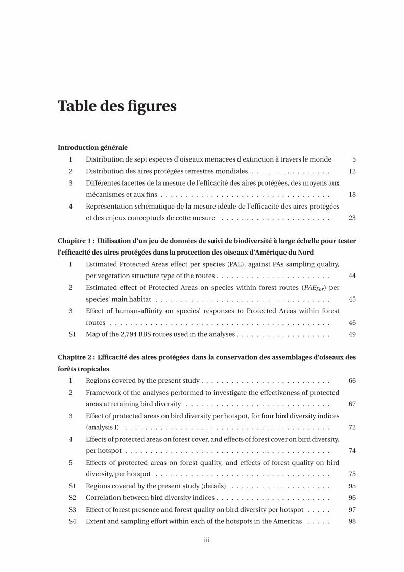
Table des figures
Introduction générale
1 Distribution de sept espèces d’oiseaux menacées d’extinction à travers le monde 5
2 Distribution des aires protégées terrestres mondiales . . . . . . . . . . . . . . . . 12
3 Différentes facettes de la mesure de l’efficacité des aires protégées, des moyens aux
mécanismes et aux fins . . . . . . . . . . . . . . . . . . . . . . . . . . . . . . . . . . 18
4 Représentation schématique de la mesure idéale de l’efficacité des aires protégées
et des enjeux conceptuels de cette mesure . . . . . . . . . . . . . . . . . . . . . . 23
Chapitre 1 : Utilisation d’un jeu de données de suivi de biodiversité à large échelle pour tester
l’efficacité des aires protégées dans la protection des oiseaux d’Amérique du Nord
1 Estimated Protected Areas effect per species (PAE), against PAs sampling quality,
per vegetation structure type of the routes . . . . . . . . . . . . . . . . . . . . . . . 44
2 Estimated effect of Protected Areas on species within forest routes (PAEFor) per
species’ main habitat . . . . . . . . . . . . . . . . . . . . . . . . . . . . . . . . . . . 45
3 Effect of human-affinity on species’ responses to Protected Areas within forest
routes . . . . . . . . . . . . . . . . . . . . . . . . . . . . . . . . . . . . . . . . . . . . 46
S1 Map of the 2,794 BBS routes used in the analyses . . . . . . . . . . . . . . . . . . . 49
Chapitre 2 : Efficacité des aires protégées dans la conservation des assemblages d’oiseaux des
forêts tropicales
1 Regions covered by the present study . . . . . . . . . . . . . . . . . . . . . . . . . . 66
2 Framework of the analyses performed to investigate the effectiveness of protected
areas at retaining bird diversity . . . . . . . . . . . . . . . . . . . . . . . . . . . . . 67
3 Effect of protected areas on bird diversity per hotspot, for four bird diversity indices
(analysis I) . . . . . . . . . . . . . . . . . . . . . . . . . . . . . . . . . . . . . . . . . 72
4 Effects of protected areas on forest cover, and effects of forest cover on bird diversity,
per hotspot . . . . . . . . . . . . . . . . . . . . . . . . . . . . . . . . . . . . . . . . . 74
5 Effects of protected areas on forest quality, and effects of forest quality on bird
diversity, per hotspot . . . . . . . . . . . . . . . . . . . . . . . . . . . . . . . . . . . 75
S1 Regions covered by the present study (details) . . . . . . . . . . . . . . . . . . . . 95
S2 Correlation between bird diversity indices . . . . . . . . . . . . . . . . . . . . . . . 96
S3 Effect of forest presence and forest quality on bird diversity per hotspot . . . . . 97
S4 Extent and sampling effort within each of the hotspots in the Americas . . . . . 98
iii
TABLE DES FIGURES
S5 Extent and sampling effort within each of the hotspots in the Africa and Asia . . 99
S6 Comparison between a binary and a continuous classification of protection . . 100
S7 Distribution of three variables used to control for location bias for protected and
unprotected sites . . . . . . . . . . . . . . . . . . . . . . . . . . . . . . . . . . . . . 101
S8 Effects of each of the variables used to control for location bias on bird diversity
(Analysis I) . . . . . . . . . . . . . . . . . . . . . . . . . . . . . . . . . . . . . . . . . 102
S9 Effects of each of the variables used to control for location bias on habitat (Analysis
II) . . . . . . . . . . . . . . . . . . . . . . . . . . . . . . . . . . . . . . . . . . . . . . . 103
S10-17 Effects of each of the covariates used as controls in analysis III on each of the
four bird diversity indices per hotspot . . . . . . . . . . . . . . . . . . . . . . . . . 104
S18 Effect of protected areas’ age on residuals of models in analysis I . . . . . . . . . 112
Chapitre 3 : Les aires protégées sont trop rares et dégradées pour protéger les espèces les plus
sensibles
1 Frequency distribution of sensitivity values across all 4,424 bird species that breed
in the Americas . . . . . . . . . . . . . . . . . . . . . . . . . . . . . . . . . . . . . . 129
2 Spatial patterns in the proportion of high-sensitivity bird species, of protection
intensity and the relationship between the two . . . . . . . . . . . . . . . . . . . . 131
3 Biome distribution of the match between protection intensity and proportion of
high-sensitivity bird species per ecoregion . . . . . . . . . . . . . . . . . . . . . . 132
4 Spatial and characteristics distribution of the 208 high-sensitivity species with
minor coverage by intact protected areas . . . . . . . . . . . . . . . . . . . . . . . 133
5 Trends in protected area intactness . . . . . . . . . . . . . . . . . . . . . . . . . . . 135
S1 Temporal distribution of eBird breeding codes per latitude . . . . . . . . . . . . . 140
S2 Species traits effects on sensitivity to human footprint for 7 variables . . . . . . . 142
S3 Inferred sensitivity and corrected inferred sensitivity of the 2,550 species for which
sensitivity was directly measured . . . . . . . . . . . . . . . . . . . . . . . . . . . . 142
S4 Distribution of human footprint raster cells compared with distribution of human
footprint of checklists buffers . . . . . . . . . . . . . . . . . . . . . . . . . . . . . . 143
S5 Distribution of protected area extent and protected area intactness per ecoregion
and their correlation with the proportion of high-sensitivity species . . . . . . . 144
S6 Spatial distribution of three ecoregion-level metric of sensitivity . . . . . . . . . 145
S7 Distribution of threatened species per ecoregion and correlation with the distribu-
tion of high-sensitivity species . . . . . . . . . . . . . . . . . . . . . . . . . . . . . . 146
Chapitre 4 : Les aires protégées sont-elles efficaces dans la conservation de la connexion des
humains avec la nature et la promotion de comportements pro-environnementaux ?
1 Map of the studied area . . . . . . . . . . . . . . . . . . . . . . . . . . . . . . . . . . 158
2 Effect of distance to PAs on Pro-Environmental Behaviours . . . . . . . . . . . . 160
iv
TABLE DES FIGURES
3 Covariates effects on Pro-Environmental Behaviours in models including exposure
to nature . . . . . . . . . . . . . . . . . . . . . . . . . . . . . . . . . . . . . . . . . . 161
4 PEBs’ levels differences between municipalities located inside a PA and municipal-
ities located outside but close to a PA . . . . . . . . . . . . . . . . . . . . . . . . . . 162
S1 Covariates effects on PEBs in models not including exposure to nature . . . . . . 166
S2 All variables effects on Pro-Environmental Behaviours in models including expo-
sure to nature . . . . . . . . . . . . . . . . . . . . . . . . . . . . . . . . . . . . . . . . 166
S3 All variables effects on Pro-Environmental Behaviours in models not including
exposure to nature . . . . . . . . . . . . . . . . . . . . . . . . . . . . . . . . . . . . . 167
Chapitre 5 : Autres contributions scientifiques
1 Effet de la couverture des sites par des aires protégées sur la diversité en
Rhopalocères pour trois habitats . . . . . . . . . . . . . . . . . . . . . . . . . . . . 172
2 Coefficients de régression de modèles estimant l’effet des variables de naturalité sur
les CPE dans les communes de France de plus de 500 habitants . . . . . . . . . . 173
3 Différences de diversité en oiseaux entre des checklists réalisées dans 12 aires pro-
tégées urbaines et des aires protégées similaires servant de contrôle en Amérique
latine . . . . . . . . . . . . . . . . . . . . . . . . . . . . . . . . . . . . . . . . . . . . 175
4 Tendances de populations des espèces d’oiseaux d’eau dans les sites Ramsar et hors
des sites Ramsar . . . . . . . . . . . . . . . . . . . . . . . . . . . . . . . . . . . . . . 176
5 Progrès des aires protégées réalisés entre 2010 et 2020 en terme de couverture des
pays et en terme de représentation des espèces et écosystèmes . . . . . . . . . . 177
v
Liste des tableaux
Introduction générale
1 Catégories de gestion des aires protégées présentes dans la WDPA sous le nom de
«IUCN category» . . . . . . . . . . . . . . . . . . . . . . . . . . . . . . . . . . . . . . 13
Chapitre 1 : Utilisation d’un jeu de données de suivi de biodiversité à large échelle pour tester
l’efficacité des aires protégées dans la protection des oiseaux d’Amérique du Nord
1 Model summaries regarding the estimated effect of Protected Areas on species
within forest routes (PAEFor) . . . . . . . . . . . . . . . . . . . . . . . . . . . . . . . 43
S1 Model summaries regarding the estimated effect of Protected Areas on species
within shrub routes (PAEShrub) . . . . . . . . . . . . . . . . . . . . . . . . . . . . . . 50
S2 Model summaries regarding the estimated effect of Protected Areas on species
within herbaceous routes (PAEHerb) . . . . . . . . . . . . . . . . . . . . . . . . . . . 51
S3 List of 136 species used in the species level analysis . . . . . . . . . . . . . . . . . 51
S4 Model summaries regarding the estimated effect of Protected Areas on species
within forest routes (PAEFor) with non-native species . . . . . . . . . . . . . . . . 55
S5 Model summaries regarding the estimated effect of strict Protected Areas (IUCN
categories Ia to IV only) on species within forest routes (PAEFor) with non-native
species . . . . . . . . . . . . . . . . . . . . . . . . . . . . . . . . . . . . . . . . . . . . 56
Chapitre 2 : Efficacité des aires protégées dans la conservation des assemblages d’oiseaux des
forêts tropicales
S1 Effect of protected areas on each of the response variables considered in analyses I,
II and IIIa, measured as percentage of difference . . . . . . . . . . . . . . . . . . . 92
S2 Summary statistics per hotspot . . . . . . . . . . . . . . . . . . . . . . . . . . . . . 93
S3 Statistical power of each test made in analyses I . . . . . . . . . . . . . . . . . . . 94
Chapitre 3 : Les aires protégées sont trop rares et dégradées pour protéger les espèces les plus
sensibles
S1 Breeding season per latitude class used to restrict the dataset to the breeding
season . . . . . . . . . . . . . . . . . . . . . . . . . . . . . . . . . . . . . . . . . . . . 139
Chapitre 4 : Les aires protégées sont-elles efficaces dans la conservation de la connexion des
humains avec la nature et la promotion de comportements pro-environnementaux ?
vi

LISTE DES TABLEAUX
1 Estimated effects of the distance to PAs for the five studied PEBs measured in
French metropolitan municipalities with at least 500 inhabitants . . . . . . . . . 160
S1 Estimated effects of the distance to regional parks only for the five studied PEBs
measured in French metropolitan municipalities with at least 500 inhabitants . 168
S2 Comparison of percentage of deviance explained by models using as response
variables distance to regional parks only vs all parks for all models . . . . . . . . 169
vii


Introduction générale
INTRODUCTION GÉNÉRALE
Dans les hauteurs de la Sierra Madre del Sur, au Mexique, alors que les amphibiens, oiseaux et
primates forment un brouhaha aussi dense que la brume matinale qui vient de s’élever au-dessus
de la canopée, une fleur de coulequin perchée à quinze mètres du sol s’épanouit. Fortement
intéressée, une coquette de Guerrero, Lophornis brachylophus, s’en approche et, après quelques
papillonnages, se stabilise face à la fleur, y plonge son bec et en aspire le nectar sucré du bout
de sa langue. A quelques 8 000 kilomètres de là, dans une localité groenlandaise qui n’a pas de
nom tant elle est inhospitalière aux humains, une femelle harfang des neiges, Bubo scandiacus,
vient de perforer la neige printanière de ses serres pour y saisir un lemming sortant tout juste
d’hibernation. Le même succès sourit à une pie-grièche méridionale, Lanius meridionalis, dans
la plaine de Pompignan en France, dont la chasse est si efficace qu’elle peut se permettre de
mettre des réserves de côté. Pour cela, elle empale quelques criquets sur les épines de la branche
inférieure d’une aubépine, et reviendra les chercher plus tard, quand l’appétit se fera sentir.
Moins chanceux, le groupe de vautours oricous, Torgos tracheliotos, arpente la savane tanzanienne
depuis des heures à la recherche d’un cadavre d’éléphant ou d’antilope et doit se rendre à
l’évidence : les milliers d’ongulés croisés aujourd’hui sont en forme olympique et, faute de savoir
les abattre, il faudra encore une fois se résoudre à dormir le ventre vide ce soir. Décalage horaire
oblige, tandis que ce groupe de vautours profite des derniers rayons de soleil sur les flamboyants,
une sterne néréis, Sternula nereis, est déjà bien plongée dans le sommeil sur une plage au nord
de Nouméa en Nouvelle-Calédonie. Mais elle ne manquera pas, dès son réveil, de prendre le large
et de pratiquer un vol stationnaire jusqu’à repérer un poisson frétillant à la surface de l’eau et
de piquer sur lui. Un peu plus au nord, à Bhavnagar en Inde, une outarde à tête noire, Ardeotis
nigriceps, gonfle son cou pour émettre des sons caverneux puissants, dans une parade visant à
séduire une femelle tapie dans l’herbe, mais ses efforts semblent insuffisants pour la convaincre.
Un peu plus tard, une lumière crépusculaire tombe sur le bras du Rio Xingu, en Amazonie, et signe
la fin des recherches alimentaires pour le couple de aras hyacinthes, Anodorhynchus hyacinthinus,
qui après s’être perché dans la canopée, se délecte du bout des papilles d’un léger goût persistant
de noix de coco.
1. Une biodiversité en déclin
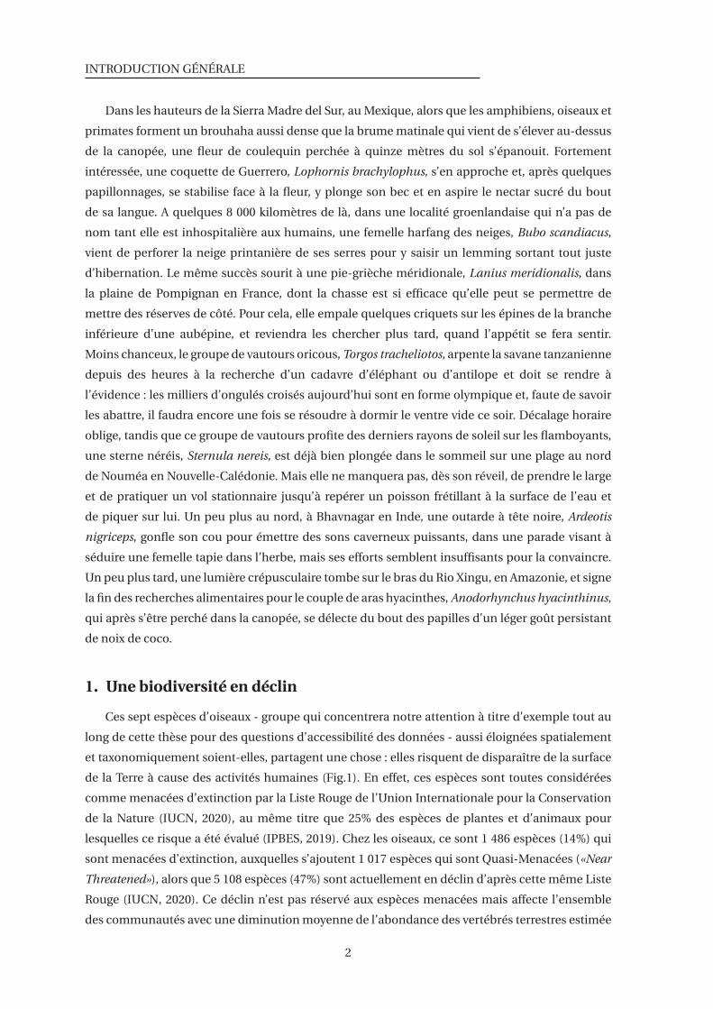
Ces sept espèces d’oiseaux - groupe qui concentrera notre attention à titre d’exemple tout au
long de cette thèse pour des questions d’accessibilité des données - aussi éloignées spatialement
et taxonomiquement soient-elles, partagent une chose : elles risquent de disparaître de la surface
de la Terre à cause des activités humaines (Fig.1). En effet, ces espèces sont toutes considérées
comme menacées d’extinction par la Liste Rouge de l’Union Internationale pour la Conservation
de la Nature (IUCN, 2020), au même titre que 25% des espèces de plantes et d’animaux pour
lesquelles ce risque a été évalué (IPBES, 2019). Chez les oiseaux, ce sont 1 486 espèces (14%) qui
sont menacées d’extinction, auxquelles s’ajoutent 1 017 espèces qui sont Quasi-Menacées («Near
Threatened»), alors que 5 108 espèces (47%) sont actuellement en déclin d’après cette même Liste
Rouge (IUCN, 2020). Ce déclin n’est pas réservé aux espèces menacées mais affecte l’ensemble
des communautés avec une diminution moyenne de l’abondance des vertébrés terrestres estimée
2

1. UNE BIODIVERSITÉ EN DÉCLIN
à 60% entre 1970 et 2014 par le « Living Planet Index » (WWF, 2018). Ce déclin constaté sur
l’ensemble des continents est particulièrement marqué dans les Néotropiques et dans la partie
Océano-Pacifique (WWF, 2018).
1.1 Des menaces pesant sur les espèces
La cause majeure du déclin d’abondance des espèces et de l’augmentation de leur risque
d’extinction est la destruction des habitats naturels (IPBES, 2019) qui est répertoriée comme une
menace pesant sur 1 243 (84%) espèces menacées d’oiseaux dans le monde, dont cinq des sept
espèces citées précédemment (Fig.1, (IUCN, 2020)). Des estimations suggèrent par exemple que
la surface continentale couverte par des espaces urbains et agricoles est passée de 5% en 1700
à 39% en 2000 (Ellis et al., 2010). Par conséquent, 75% de la surface continentale présentait en
2009 une empreinte écologique non nulle (i.e., avec des impacts d’activités humaines visibles
depuis l’espace, d’après la mesure de la «Human Footprint»), avec des niveaux importants visibles
sur tous les continents, particulièrement dans l’hémisphère Nord (Venter et al., 2016b). Les
zones importantes pour la biodiversité sont particulièrement touchées puisque seuls 3% des
points chauds de biodiversité («Biodiversity Hotspots») et 2% des zones à forte concentration
d’espèces menacées de vertébrés sont dépourvues d’empreinte écologique mesurable (contre
25% globalement). Cette empreinte écologique a augmenté globalement de 9% entre 1993 et
2009, avec cependant des nuances : une augmentation particulièrement forte sous les tropiques,
mais une diminution dans plusieurs pays à haut PIB (Venter et al., 2016b).
Les habitats forestiers sont emblématiques de cette menace qui transforme les paysages
et la biodiversité. La déforestation dure depuis des siècles avec une accélération mondiale au
XXème siècle (Mouillot and Field, 2005) et continue principalement dans les forêts tropicales, avec
une perte de 129 millions d’hectares de forêt tropicale (3%) entre 1990 et 2015 (Hansen et al., 2013;
Keenan et al., 2015). Cette déforestation intense affecte fortement la biodiversité, ce qui a poussé la
coquette de Guerrero au bord de l’extinction (IUCN, 2018b) et participe également au déclin actuel
du ara hyacinthe (IUCN, 2016a) (Fig.1). Plus généralement, la destruction des forêts tropicales est
la première menace pour la biodiversité associée à ces milieux (Barlow et al., 2018), pouvant aller
jusqu’à l’extinction locale de la quasi-totalité des espèces forestières (Barlow et al., 2016; Gibson
et al., 2013). A la destruction des habitats forestiers s’ajoute la dégradation des forêts restantes par
des activités telles que la coupe sélective des arbres, la construction de chemins ou l’affinage de
la canopée. Cette dégradation impacte fortement la biodiversité, avec un effet d’une magnitude
parfois proche de la déforestation (Barlow et al., 2016), rendant les forêts primaires irremplaçables
(Gibson et al., 2011).
Les forêts, bien qu’emblématiques, ne sont qu’un exemple de l’impact que la perte d’habitat
peut avoir sur la biodiversité (IPBES, 2019; WWF, 2018). L’outarde à tête noire, dont les populations
avaient déjà été largement amoindries par d’autres causes dont nous parlerons plus loin, subit
actuellement un déclin attribué à la conversion des prairies naturelles qui l’hébergent en zones
agricoles (Fig.1, (IUCN, 2018a)). La pie-grièche méridionale qui niche dans les garrigues du Sud-
Ouest de l’Europe, voit également son territoire de reproduction se réduire à cause de la coupe
3
INTRODUCTION GÉNÉRALE
des haies et d’arbres induite par l’intensification de l’agriculture (Fig.1, (IUCN, 2017b)), et est
paradoxalement également menacée dans certains secteurs par la déprise agricole qui referme
les habitats de garrigues. Enfin, la sterne néréis voit les plages sur lesquelles elle pond grignotées
petit à petit par l’urbanisation et l’érosion littorale de certaines côtes australiennes et de Nouvelle-
Calédonie (Fig.1, (IUCN, 2018c)).
La perte d’habitat, bien que jouant un rôle majeur, est loin d’être l’unique menace pesant
sur la biodiversité. Une autre menace évidente, puisque son effet est direct, est le prélèvement
d’individus impactant 590 espèces d’oiseaux menacées (40%, (IUCN, 2020)). En première ligne, la
chasse impacte significativement certaines espèces de manière ciblée (IPBES, 2019; WWF, 2018).
Cette activité a amené certaines espèces à l’extinction comme cela a été mis en évidence pour le
pigeon voyageur, Ectopistes migratorius. Cette espèce nord-américaine dont l’abondance pouvait
noircir le ciel durant la migration jusqu’au XIXème siècle, a été décimée jusqu’au dernier individu
sauvage probablement abattu en 1901 (Schorger, 1955). Plus d’actualité est le cas de l’outarde à
tête noire, dont le déclin est principalement attribué à une chasse massive, mettant cette espèce
en danger critique d’extinction. Malgré une population globale aujourd’hui estimée entre 50 et
250 individus matures, la pression de chasse illégale continue (Fig.1, (IUCN, 2018a)). Une méta-
analyse d’études réalisées dans les forêts tropicales suggère que les activités de chasse diminuent
l’abondance en oiseaux de 58% en moyenne, avec des effets perceptibles à plusieurs dizaines de
kilomètres des routes et autres points d’accès des chasseur·se·s (Benítez-López et al., 2017). Quand
ces prélèvements ne se font pas avec des fusils, ils peuvent se faire avec des pièges afin de capturer
des individus vivants qui seront ensuite vendus pour devenir des oiseaux de captivité. Le ara
hyacinthe est aujourd’hui classé comme vulnérable d’extinction à cause de captures importantes
durant la seconde moitié du XXème siècle (par exemple, >10 000 individus prélevés dans les
années 1980), captures qui continuent occasionnellement (Fig.1, (IUCN, 2016a)). Globalement,
c’est un tiers des espèces de l’avifaune mondiale qui a fait l’objet d’échange d’individus captifs
vivants (BirdLife International, 2008), avec un taux de capture particulièrement élevé pour les
Psittaciformes (par exemple, perroquets, cacatoès, loris), les Passeriformes (passereaux) et les
Falconiformes (par exemple, faucons, fauconnets, caracaras), et affectant tous les continents
(Bush et al., 2014).
Une autre menace pesant sur les espèces est la pollution, qui peut avoir un impact direct (par
exemple mortalité des individus ou baisse de fertilité) ou indirect (par exemple en entraînant
la raréfaction des proies). Son impact direct a été relevé dans de nombreux cas, notamment
concernant les rapaces capturant des proies ayant ingéré des poisons. Chez les oiseaux, l’empoi-
sonnement impacte particulièrement les rapaces, en haut de la chaîne alimentaire, représentant
pour eux la sixième menace et la seconde pour les vautours de l’ancien monde (McClure et al.,
2018). C’est par exemple le cas du vautour oricou dont les déclins sont largement associés à
l’utilisation de Strycnine pour contrôler les populations de corvidés ravageurs de culture et de
rongeurs dont le vautour se nourrit en partie (Fig.1, (IUCN, 2016c)). D’autres produits impactent
les populations d’insectes et donc indirectement toute la chaîne trophique au-dessus d’elles.
En effet, les intrants de l’agriculture intensive induisent des déclins de populations importants
4
1.UN
EB
IOD
IVE
RSIT
ÉE
ND
ÉC
LIN
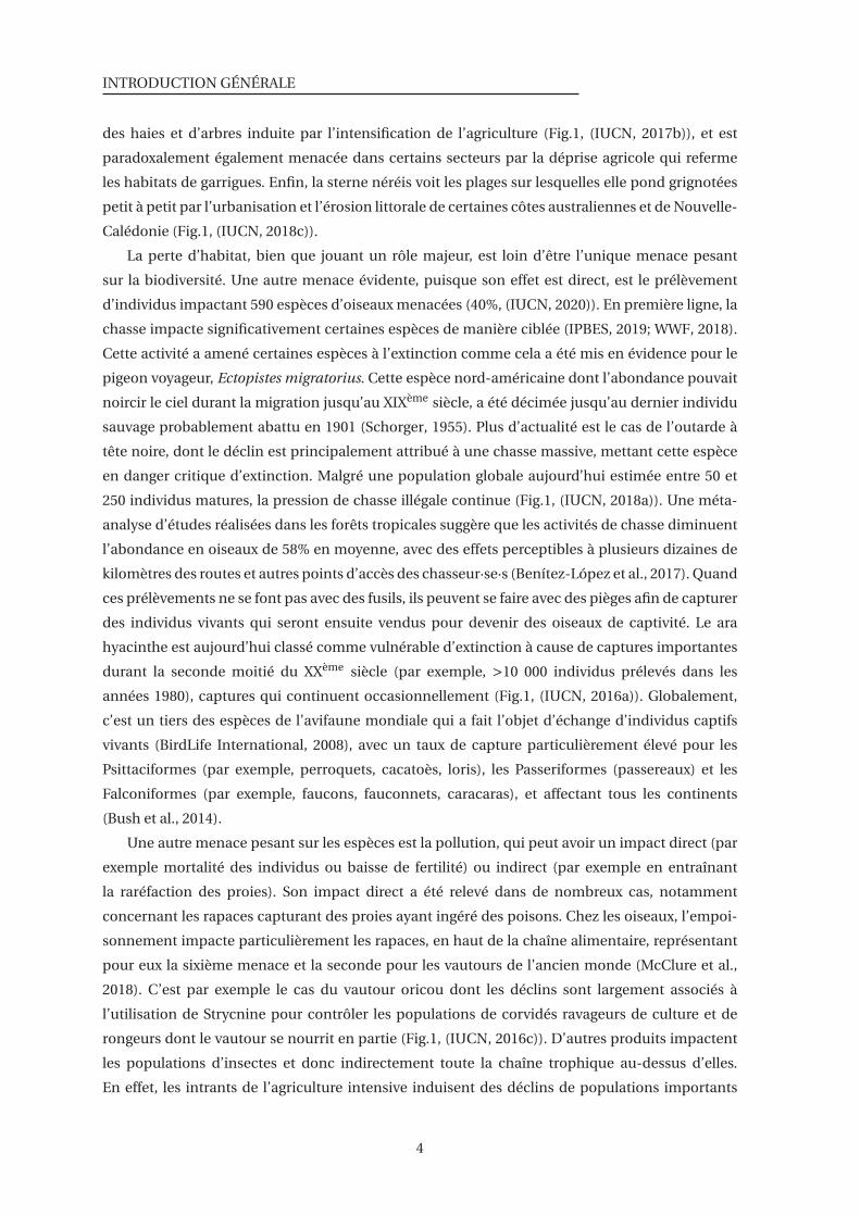
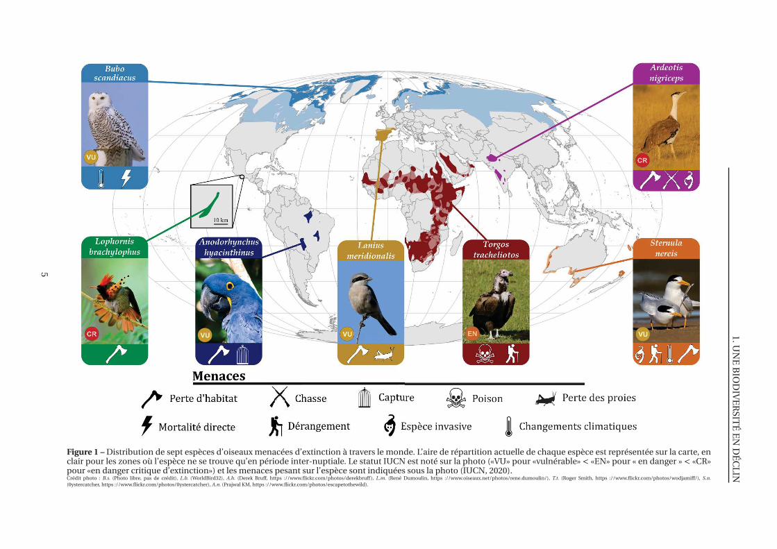
Figure 1 – Distribution de sept espèces d’oiseaux menacées d’extinction à travers le monde. L’aire de répartition actuelle de chaque espèce est représentée sur la carte, enclair pour les zones où l’espèce ne se trouve qu’en période inter-nuptiale. Le statut IUCN est noté sur la photo («VU» pour «vulnérable» < «EN» pour « en danger » < «CR»pour «en danger critique d’extinction») et les menaces pesant sur l’espèce sont indiquées sous la photo (IUCN, 2020).Crédit photo : B.s. (Photo libre, pas de crédit), L.b. (WorldBird32), A.h. (Derek Bruff, https ://www.flickr.com/photos/derekbruff), L.m. (René Dumoulin, https ://www.oiseaux.net/photos/rene.dumoulin/), T.t. (Roger Smith, https ://www.flickr.com/photos/wodjamiff/), S.n.(0ystercatcher, https ://www.flickr.com/photos/0ystercatcher), A.n. (Prajwal KM, https ://www.flickr.com/photos/escapetothewild).
5
INTRODUCTION GÉNÉRALE
d’insectes (Forister et al., 2019), ce qui entraîne des déclins d’espèces d’oiseaux insectivores
(Goulson, 2014). La pie-grièche méridionale, par exemple, semble menacée en grande partie par
la raréfaction des populations d’insectes due à l’intensification de l’agriculture (Fig.1, (IUCN,
2017b)).
Une menace plus récente est liée aux changements climatiques qui peuvent avoir un effet
néfaste – en particulier par des hausses de température, baisses de précipitations et fonte des
glaces – sur la survie et la fécondité des populations d’oiseaux (Jenouvrier, 2013), notamment
chez les espèces les moins thermophiles (Jiguet et al., 2010). C’est par exemple le cas du harfang
des neiges, dont la proie de choix, le lemming, est de moins en moins abondante au moment de
la période de reproduction des chouettes (Fig.1, (Gilg et al., 2009; IUCN, 2017a)). Ces pressions
exercées par les changements climatiques mènent certaines espèces à décaler progressivement,
quand cela leur est possible, leur aire de répartition en latitude (en direction des pôles) ou en
altitude (vers des altitudes plus élevées) pour retrouver des conditions thermiques similaires
(Hobbs et al., 2018). Une étude menée sur les oiseaux communs européens suggère par exemple
que les espèces se sont décalées vers le Nord de 37 km en moyenne entre 1990 et 2008, ce qui
pourrait en partie être dû aux changements climatiques (Devictor et al., 2012). Ces menaces pèsent
particulièrement sur les espèces dont l’aire de répartition est restreinte ou en altitude (Sekercioglu
et al., 2012). D’autres effets des changements climatiques risquent d’avoir des conséquences
importantes pour quelques espèces, comme par exemple la montée du niveau des mers qui
menace d’inonder les colonies de la sterne néréis (Fig.1, (IUCN, 2018c)).
D’autres activités anthropiques peuvent également menacer les espèces (IPBES, 2019; WWF,
2018). La mortalité directe, provoquée par des collisions avec des véhicules, des lignes électriques
ou des avions peut impacter fortement certaines populations, comme cela semble le cas avec le
harfang des neiges (Fig.1, (IUCN, 2017a)). Les dérangements humains, principalement durant la
reproduction, peuvent également affecter les populations. Ainsi, les adeptes de kite-surf ou de
balades canines sur les plages d’Océanie augmentent les difficultés de la sterne néréis à mener
à terme ses nidifications (Fig.1, (IUCN, 2018c)). En parallèle, cette même sterne est menacée
par des espèces invasives de prédateurs (chats, chiens, renards) qui diminuent encore le succès
reproducteur de cette espèce nidifuge. Les espèces invasives peuvent également impacter les
populations natives en entrant en compétition avec elles, ou en modifiant l’habitat. C’est par
exemple le cas de l’arbre Prosopis juliflora, une espèce invasive des prairies indiennes qui a un
fort impact sur les populations d’outarde à tête noire (Fig.1, (IUCN, 2018a)).
L’ensemble de ces activités induit une diminution des abondances (par exemple, un site qui
comptait autrefois 500 individus d’outarde à tête noire voit sa population passer à 50 individus
suite à une perturbation), ce qui peut à terme induire la disparition de cette espèce au niveau
local (la perturbation devient si forte que la population d’outardes à tête noire ne peut plus se
reproduire sur ce site et disparaît). C’est ce que l’on appelle l’extinction locale : la disparition sur
un site donné d’une espèce qui était présente auparavant. C’est en accumulant les extinctions
locales qu’une espèce peut voir son aire de répartition se restreindre (ainsi l’outarde à tête noire a
6
1. UNE BIODIVERSITÉ EN DÉCLIN
été évincée de 90% de son aire de répartition; Fig.1, (IUCN, 2018a)), et à terme mener à l’extinction
globale de l’espèce.
Ces impacts des activités humaines au niveau spécifique, qu’ils causent des baisses d’abon-
dance ou des extinctions locales, vont se traduire par des modifications du cortège d’individus et
d’espèces présents sur un site donné. Au cours de cette thèse, nous désignerons cet ensemble
d’individus d’espèces d’oiseaux présents sur un site donné en utilisant le terme «assemblage»
plutôt que «communauté». Le terme de communauté, s’il est employé, sous-tendra un intérêt
pour les interactions entre les individus, là où l’assemblage désignera l’ensemble des individus,
qu’ils soient en interactions directes ou pas.
1.2 Impact des activités anthropiques sur les assemblages
Une première conséquence attendue des impacts des activités humaines sur les assemblages
est une baisse de l’abondance totale des individus présents sur un site suite aux effets néfastes de
ces activités sur les espèces. Une étude récente, combinant les résultats de suivis à long terme des
oiseaux d’Amérique du Nord à des suivis par radar des oiseaux en migration, suggère par exemple
une chute nette de 29% de l’abondance totale d’oiseaux depuis 1970 (Rosenberg et al., 2019).
Dans le cas où ces baisses d’abondance sont si drastiques que certaines espèces subissent une
extinction locale, une autre conséquence sera attendue au niveau de l’assemblage : une baisse de
richesse spécifique, c’est-à-dire du nombre d’espèces présentes sur le site. Newbold et al. (2015),
dans une analyse globale et multi-taxon, ont mesuré une perte de richesse spécifique sur des
sites ayant subi des pressions anthropiques, de 14% en moyenne, pouvant atteindre localement
77% quand les pressions sont particulièrement intenses. Similairement, Murphy and Romanuk
(2014), en combinant les résultats de 245 études, ont mesuré une baisse de richesse spécifique
de 18% dans les sites ayant subi des perturbations anthropiques, notamment des changements
d’utilisation du sol.
Cet indice de richesse spécifique est très couramment utilisé mais n’est pourtant pas le plus
pertinent pour mesurer les transformations des assemblages, puisque ces transformations ne se
traduisent pas nécessairement par une baisse d’abondance totale ou de richesse spécifique des
assemblages (Chase et al., 2019). En effet, la réponse des espèces aux pressions anthropiques est
loin d’être homogène, menant certaines espèces à voir leurs tailles de populations augmenter du
fait des pressions anthropiques (Rosenberg et al., 2019). La déforestation au Mexique, par exemple,
menace la coquette de Guerrero (Fig.1), mais permet à des espèces de milieux ouverts telles que
le tyran mélancolique, Tyrannus melancholicus, de coloniser les sites nouvellement déforestés
et de voir ainsi leurs populations augmenter (Rutt et al., 2019; Mobley, 2020). Les changements
climatiques que subissent les toundras groenlandaises font chuter la population de harfang des
neiges (Fig.1), mais semblent partiellement expliquer l’expansion vers le Nord du bruant lapon,
Calcarius lapponicus (Virkkala et al., 2014). Ainsi, dans bon nombre de cas, les extinctions locales
sont suivies par des colonisations locales. Dans ces cas-là, documentés par de nombreuses études,
la transformation des assemblages ne se traduit pas nécessairement par une variation de la
richesse spécifique. Une étude portant sur des phytoplanctons et des assemblages de plantes
7
INTRODUCTION GÉNÉRALE
prairiales a notamment mis en évidence une transformation quasi-complète de la composition
des assemblages sans qu’aucun effet sur la richesse spécifique ne soit mesuré (Hillebrand et al.,
2018). A plus large échelle, une méta-analyse incluant plus de 100 suivis temporels standardisés de
la biodiversité, n’a détecté aucune variation de richesse spécifique malgré de fortes modifications
de la composition des assemblages (Dornelas et al., 2014).
Dans certains cas, non seulement la richesse spécifique ne diminue pas en réponse à des
pressions humaines, mais elle augmente. Reprenons le cas du site subissant une déforestation
au Mexique, entraînant simultanément l’extinction locale de la coquette de Guerrero et la
colonisation du tyran mélancolique. Imaginons que la perte de forêt sur le site n’ait pas été totale
et que seule la moitié de la forêt ait été coupée. Le morceau restant de forêt suffira peut-être
à maintenir, au moins temporairement, quelques couples de coquettes, alors que les premiers
couples de tyrans pourront s’installer grâce à l’ouverture partielle du paysage. Dans ce cas-là,
la perturbation induit une augmentation de la richesse spécifique car cette perturbation est
intermédiaire : l’absence de perturbation n’aurait pas permis au tyran de s’installer et une
perturbation trop importante aurait conduit la coquette de Guerrero à l’extinction locale. Cette
théorie, très utilisée mais finalement peu étayée par des résultats empiriques (Fox, 2013), a été
formalisée sous le nom d’hypothèse de perturbation intermédiaire, ou «Intermediate Disturbance
Hypothesis» (Roxburgh et al., 2004). D’autres perturbations peuvent induire des augmentations
de richesse spécifique, notamment l’introduction d’espèces exogènes (Ellis et al., 2012).
Cette apparente contradiction entre le fort impact des activités humaines sur les espèces
dont nous avons discuté précédemment, et l’effet faible voire nul de ces activités sur la richesse
spécifique, s’explique par le fait que les impacts sur les espèces ne se font pas au hasard et
ont tendance à homogénéiser les assemblages. En effet, les pressions anthropiques profitent en
général à quelques espèces aux caractéristiques particulièrement adaptées aux activités humaines
et pouvant ainsi mener à un accroissement de la similarité entre les assemblages de différents
sites (c’est-à-dire une baisse de la dissimilarité des assemblages, que l’on appelle la diversité
β) dans un processus appelé homogénéisation biotique (McKinney and Lockwood, 1999; Clavel
et al., 2011; Finderup Nielsen et al., 2019). Cela serait par exemple le cas si le remplacement de
la coquette de Guerrero par le tyran mélancolique mentionné précédemment s’accompagnait,
sur des sites voisins, du remplacement d’autres espèces spécialistes des habitats forestiers par
le même tyran mélancolique. La richesse spécifique des sites (diversité α) n’aurait alors pas
varié puisque chaque site aurait subi une extinction locale et une colonisation. En revanche,
la diversité β aurait diminué puisque ces transformations auraient rendu les assemblages plus
similaires et la diversité γ, c’est-à-dire le nombre total d’espèces de la région, aurait également
diminué. Ce concept d’homogénéisation biotique décrit que les perturbations profitent en général
à quelques espèces, telles le tyran mélancolique qui est en expansion globalement (Mobley, 2020),
mais affectent négativement une majorité d’espèces et que cette relation dépend fortement des
caractéristiques des espèces.
En premier lieu, l’impact des perturbations humaines sur les espèces dépend fortement de
8
1. UNE BIODIVERSITÉ EN DÉCLIN
la niche écologique des espèces (i.e., l’ensemble des conditions nécessaires à la viabilité de
ses populations). Dans l’exemple ci-dessus, toutes les espèces ayant disparu partageaient une
préférence d’habitat pour les forêts tandis qu’une unique espèce préférant les milieux ouverts
est apparue. Les traits fonctionnels représentés au sein de l’assemblage (par exemple, préférence
d’habitat, régime alimentaire, taille, trait comportemental. . . ) ont donc changé. De nombreuses
études montrent que ces transformations de composition des assemblages en réponse à des
pressions anthropiques vont souvent dans le sens d’une perte de diversité fonctionnelle, c’est-
à-dire d’une diminution de la diversité de traits représentés dans les assemblages (Barnagaud
et al., 2017b, 2019). De plus, les espèces les plus affectées sont souvent celles présentant une
forte spécialisation envers leur habitat comme le résument Clavel et al. (2011) dans une revue
de littérature combinant résultats empiriques et théoriques. Cette revue met en évidence un
impact plus important des activités anthropiques sur les espèces spécialistes (i.e., avec une
niche écologique étroite) que sur les espèces généralistes (i.e., avec une niche écologique large),
qui bénéficient souvent de ces activités. Cela suggère à terme une ressemblance accrue entre
les assemblages avec une perte des espèces les plus originales au profit d’espèces généralistes.
Rutt et al. (2019) observent également ces changements d’assemblages d’oiseaux au Brésil à la
suite d’une déforestation expérimentale. En effet, les espèces qui colonisent ces sites suite à la
déforestation sont des espèces généralistes qui viennent remplacer des espèces spécialistes des
habitats de forêts.
D’après cette même étude, les espèces endémiques et donc à petite aire de répartition sont
plus touchées par ces perturbations humaines puisque les espèces colonisant les sites ayant subi
la déforestation étaient principalement des espèces à large aire de répartition (Rutt et al., 2019).
D’autres études mettent en évidence des transformations des assemblages au profit des espèces
à large aire de distribution (Newbold et al., 2018; Finderup Nielsen et al., 2019), suggérant là aussi
une homogénéisation des assemblages.
Les activités humaines ont également tendance à affecter de manière différenciée les différents
groupes taxonomiques. Imaginons par exemple qu’une extinction locale d’outarde à tête noire soit
accompagnée d’une extinction locale de toutes les espèces de la famille des Otididae (outardes). La
perte ne sera alors plus uniquement taxonomique (i.e., perte d’un certain nombre d’espèces), mais
tout un pan de la phylogénie des oiseaux disparaîtra du site, menant donc à une perte importante
de la diversité des espèces pouvant être observées sur un site. Dans ce cas-là, la diversité phy-
logénétique, c’est-à-dire la diversité de lignées évolutives représentées par les espèces présentes
sur le site, diminue. Cela a été observé par exemple sur les assemblages d’oiseaux au Costa Rica,
où l’agriculture intensive mène à l’extinction locale de lignées entières des assemblages (par
exemple, trogons, manakins, toucans) menant à une perte de diversité phylogénétique (Frishkoff
et al., 2014). La même étude rapporte une baisse de diversité phylogénétique significative, bien
que moins importante, dans les milieux agricoles plus extensifs mais qui n’est pas associée à
une baisse de la richesse spécifique. Cela suggère donc le remplacement d’espèces éloignées
phylogénétiquement par des espèces moins distinctes évolutivement. Ces extinctions locales de
lignées touchent principalement les taxons dont la niche écologique a peu évolué (notamment
9
INTRODUCTION GÉNÉRALE
en termes de préférences d’habitats), c’est-à-dire que les espèces à fort conservatisme de niche
sont moins capables de s’adapter aux perturbations humaines (Lavergne et al., 2013). A l’inverse,
certains taxons s’accommodent bien de la présence humaine grâce à la largeur de leur niche
écologique (par exemple les étourneaux ou certains laridés), voire ont évolué vers une relation
commensale avec les populations humaines (par exemple les hirondelles et martinets en Europe).
Cette perte des espèces les plus caractéristiques des assemblages (endémiques, spécialistes,
originales taxonomiquement ou simplement rares) accroit fortement la ressemblance de
composition entre les sites et participe donc à l’homogénéisation biotique (Clavel et al., 2011).
Ce phénomène est particulièrement marqué dans les milieux urbains qui constituent des
milieux d’extrême pression anthropique, fortement homogènes à travers le globe et subissant
de forts taux d’invasions biologiques (McKinney, 2006). De ce fait, bon nombre de villes ont vu
leurs espèces locales disparaître et être remplacées par une poignée d’espèces anthropophiles
(i.e., espèces actuellement adaptées aux activités humaines). Ainsi, le pigeon biset, Columba
livia, la perruche à collier, Psittacula krameri, et le moineau domestique, Passer domesticus,
sont aujourd’hui présents sur tous les continents (sauf Antarctique) suite à des introductions
d’origine anthropique. Ce constat de substitution des espèces anthropophobes (i.e., sensibles aux
pressions humaines), par des espèces anthropophiles se vérifie bien au-delà de la ceinture des
villes, atteignant d’autres milieux perturbés par les activités humaines (McKinney, 2006; Guetté
et al., 2017).
Tous ces éléments soulignent que la diversité des espèces est bien trop multivariée pour
être résumée en une seule variable puisque la tendance émergente dépend de la facette de
la biodiversité et de l’échelle considérées. McGill et al. (2015) proposent une catégorisation en
quinze formes de tendances de la biodiversité. La richesse spécifique par exemple, est en claire
diminution à l’échelle globale (diversité γ globale), puisque le taux global d’extinction est plus
élevé que le taux de spéciation, alors qu’à l’échelle locale la richesse spécifique (diversité α) ne
montre pas de tendance cohérente. Cependant, les auteur·rice·s suggèrent que les assemblages
subissent des changements de composition de plus en plus importants, ce qui se traduit par
une augmentation de la diversité β temporelle, c’est-à-dire la dissimilarité de composition d’un
même site acquise entre deux dates. Ces transformations affectant les assemblages de façon
similaire mènent à une baisse de la différence entre assemblages, ou homogénéisation biotique,
à l’échelle locale mais également à l’échelle biogéographique. Les auteur·rice·s suggèrent donc
de s’intéresser à différents traits des espèces composant les assemblages afin de caractériser les
transformations que ces derniers subissent : la diversité fonctionnelle des espèces, leur diversité
phylogénétique, leur degré de rareté, leur degré de spécialisation, et leur degré d’anthropophilie
(McGill et al., 2015), des variables qui ne sont pas nécessairement corrélées (Devictor et al., 2010).
1.3 La Biologie de la Conservation à la recherche de solutions
Ce constat de la perte de biodiversité et de ses causes est largement dressé par la Biologie de
la Conservation (IPBES, 2019). Cette discipline scientifique, trouvant ses origines au XXème siècle,
se place comme une discipline de crise, visant à répondre de manière imminente à un problème :
10
2. LE RÔLE CLÉ DES AIRES PROTÉGÉES EN CONSERVATION
la perte de biodiversité (Soulé, 1985). Son coeur peut être résumé en un triptyque consistant à
évaluer l’évolution des populations (par exemple, les populations d’outarde à tête noire déclinent),
identifier les causes de ces tendances (par exemple, ce déclin est dû à une forte activité de chasse),
et proposer et accompagner d’éventuelles solutions (par exemple, interdire et/ou contrôler la
chasse) (Godet and Devictor, 2018).
Les solutions étudiées par la discipline forment un large spectre allant d’actions globales (par
exemple, interdire la vente d’individus sauvages de certaines espèces) à locales (par exemple,
restauration d’un habitat), allant de mesures d’atténuation des menaces (par exemple, empêcher
la chasse localement) à la compensation de l’effet de ces menaces quand elles n’ont pu être évitées
(par exemple, lâchers d’individus élevés pour renforcer les populations naturelles) et allant de
mesures visant à protéger toute la communauté (par exemple, contrôle d’une espèce invasive
modifiant l’habitat) à des mesures spécifiques à une espèce (par exemple, création de sites de
reproduction artificiels) (Godet and Devictor, 2018).
Au cœur des solutions se trouve l’idée de restreindre et contrôler, dans un endroit délimité,
les activités humaines dans le but de limiter leur impact sur les espèces : c’est ce que l’on appelle
les aires protégées. Les aires protégées accueillant des populations de ara hyacinthe peuvent par
exemple limiter la déforestation, alors que celles accueillant l’outarde à tête noire peuvent être
patrouillées pour limiter la chasse illégale, et celles accueillant des pies-grièches méridionales
peuvent travailler avec les agriculteur·rice·s pour limiter l’utilisation de pesticides (Fig.1). Au-
delà de leur potentiel effet sur les activités humaines, les aires protégées peuvent également
servir de cadre pour mettre en place d’autres mesures de conservation plus spécifiques, telles que
l’installation de supports artificiels pour la nidification de la sterne néréis ou la mise en place de
placettes d’alimentation contrôlées pour les vautours oricous.
2. Le rôle clé des aires protégées en conservation
2.1 Définition des aires protégées
Une aire protégée est définie comme «un espace géographique clairement défini, reconnu,
consacré et géré, par tout moyen efficace, juridique ou autre, afin d’assurer à long terme la
conservation de la nature et des services écosystémiques et des valeurs culturelles qui lui sont
associés» (UNEP-WCMC, IUCN and NGS, 2020).
Bien que le concept de restrictions des usages d’espaces naturels existe depuis des millénaires
(par exemple, lieux sacrés, réserves de chasse), les aires protégées telles que nous les définissons
aujourd’hui trouvent leurs origines au XIXème siècle (Watson et al., 2014). Les premiers à formuler
le besoin d’aires protégées sont des artistes : le poète anglais William Wordsworth imagine en
1810 que le Lake District devienne «a sort of national property» et le peintre George Catlin en
1832 imagine protéger les espaces naturels et les populations indiennes menacés par les colons
par le biais d’un «nation’s park, containing man and beast, in all the wild and freshness of their
nature’s beauty» (Phillips, 2004). C’est ensuite en 1864 que la première aire protégée est créée par
la signature du «Yosemite Grant Act», aux Etats-Unis et qui sera suivie quelques années plus tard
11

INTRODUCTION GÉNÉRALE
Par continent
Global
1864 1900 1950 2000 2020
0.0e
+005.
0e+0
61.0e
+071.
5e+0
7
0e+0
01e
+06
2e+0
63e
+06
Surf
ace
pro
tégée
(km
2)
0
2000
0
4000
0
6000
0
Ia Ib II III IV V VI Inconnu
co
un
t
0
5000
1000
0
1500
0
1e-03 1e-01 1e+01 1e+03 1e+05
co
un
t
Par continent
Global
1864 1900 1950 2000 2020
0.0e
+005.
0e+0
61.0e
+071.
5e+0
7
0e+0
01e
+06
2e+0
63e
+06
0
2000
0
4000
0
6000
0
Ia Ib II III IV V VI Inconnu
0
5000
1000
0
1500
0
1e-03 1e-01 1e+01 1e+03 1e+05
A
B C D
0 10 20 30 >40
Protection (%)
Année Catégorie de gestion Surface (km2)
Effectif
Effectif
Surf
ace
pro
tégée
(km
2)
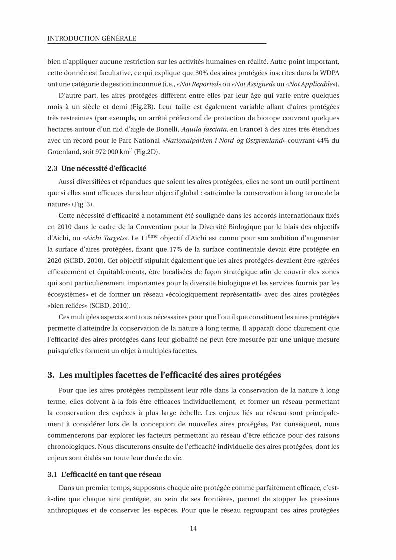
Figure 2 – Distribution des aires protégées terrestres mondiales. A : Proportion de territoire continentalcouvert par des aires protégées par pays. B : Surface couverte par des aires protégées à l’échelle globaleet par continent (voir couleurs sur mini carte). C : Distribution des catégories de gestion de l’UICN parcontinent (Table 1). D : Distribution de la taille des aires protégées par continent. Les données du graphiqueA proviennent des calculs effectués par les gestionnaires de la World Database on Protected Areas (WDPA)et disponibles sur protectedplanet.net. Les graphiques B-D proviennent de calculs personnels effectués àpartir des données brutes de la WDPA, version de Janvier 2020 (UNEP-WCMC & IUCN, 2020).
par la création du premier Parc National au Yellowstone (Phillips, 2004).
Les aires protégées se sont ensuite multipliées sur l’ensemble du globe pour atteindre
aujourd’hui un nombre de 245 133 aires protégées enregistrées dans le monde (Fig.2A-B, (UNEP-
WCMC, IUCN and NGS, 2020)). Elles couvrent aujourd’hui 15,2% des surfaces continentales et
7,4% des surfaces marines et sont présentes dans tous les pays (Fig.2, (UNEP-WCMC, IUCN
and NGS, 2020)). Elles sont considérées comme le principal outil pour conserver la biodiversité
(Watson et al., 2014; Maxwell et al., 2020).
Leur existence est consignée dans une base de données, la «World Database on Protected
Areas» (WDPA) qui rassemble la majorité des aires protégées connues à ce jour (UNEP-WCMC,
IUCN and NGS, 2020; Bingham et al., 2019). La plupart des aires protégées incluses dans cette
base de données sont spatialisées (i.e., accompagnées d’un polygone cartographiant précisément
les limites de chaque aire protégée) et sont suivies de quelques informations caractéristiques de
ces aires protégées, telles que leur année de création, leur mode de désignation, leur taille, etc.
Les aires marines protégées et les aires terrestres diffèrent de manière importante dans leurs
12
2. LE RÔLE CLÉ DES AIRES PROTÉGÉES EN CONSERVATION
enjeux et leurs pratiques et sont ainsi considérées de manière distincte. Au cours de cette thèse,
nous nous concentrerons sur les aires protégées terrestres uniquement, mettant de côté les aires
marines protégées.
2.2 Une diversité d’aires protégées
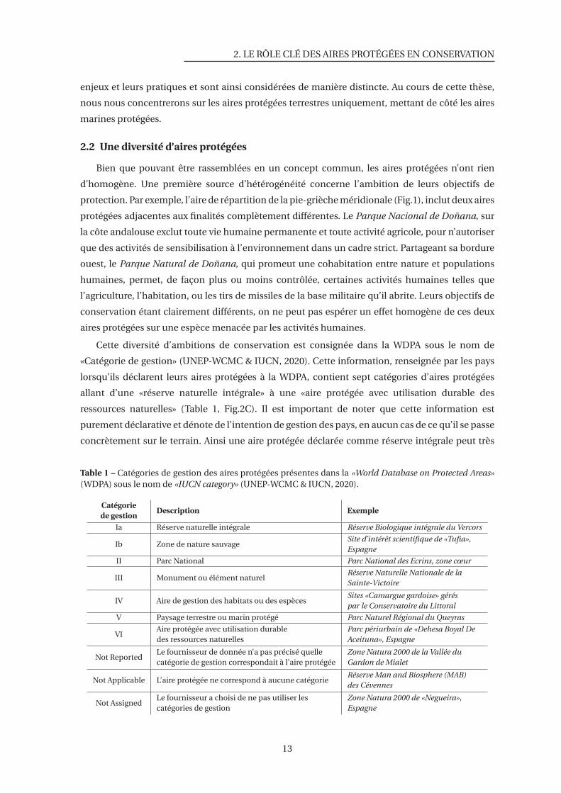
Bien que pouvant être rassemblées en un concept commun, les aires protégées n’ont rien
d’homogène. Une première source d’hétérogénéité concerne l’ambition de leurs objectifs de
protection. Par exemple, l’aire de répartition de la pie-grièche méridionale (Fig.1), inclut deux aires
protégées adjacentes aux finalités complètement différentes. Le Parque Nacional de Doñana, sur
la côte andalouse exclut toute vie humaine permanente et toute activité agricole, pour n’autoriser
que des activités de sensibilisation à l’environnement dans un cadre strict. Partageant sa bordure
ouest, le Parque Natural de Doñana, qui promeut une cohabitation entre nature et populations
humaines, permet, de façon plus ou moins contrôlée, certaines activités humaines telles que
l’agriculture, l’habitation, ou les tirs de missiles de la base militaire qu’il abrite. Leurs objectifs de
conservation étant clairement différents, on ne peut pas espérer un effet homogène de ces deux
aires protégées sur une espèce menacée par les activités humaines.
Cette diversité d’ambitions de conservation est consignée dans la WDPA sous le nom de
«Catégorie de gestion» (UNEP-WCMC & IUCN, 2020). Cette information, renseignée par les pays
lorsqu’ils déclarent leurs aires protégées à la WDPA, contient sept catégories d’aires protégées
allant d’une «réserve naturelle intégrale» à une «aire protégée avec utilisation durable des
ressources naturelles» (Table 1, Fig.2C). Il est important de noter que cette information est
purement déclarative et dénote de l’intention de gestion des pays, en aucun cas de ce qu’il se passe
concrètement sur le terrain. Ainsi une aire protégée déclarée comme réserve intégrale peut très
Table 1 – Catégories de gestion des aires protégées présentes dans la «World Database on Protected Areas»(WDPA) sous le nom de «IUCN category» (UNEP-WCMC & IUCN, 2020).
Catégoriede gestion
Description Exemple
Ia Réserve naturelle intégrale Réserve Biologique intégrale du Vercors
Ib Zone de nature sauvageSite d’intérêt scientifique de «Tufia»,Espagne
II Parc National Parc National des Ecrins, zone cœur
III Monument ou élément naturelRéserve Naturelle Nationale de laSainte-Victoire
IV Aire de gestion des habitats ou des espècesSites «Camargue gardoise» géréspar le Conservatoire du Littoral
V Paysage terrestre ou marin protégé Parc Naturel Régional du Queyras
VIAire protégée avec utilisation durabledes ressources naturelles
Parc périurbain de «Dehesa Boyal DeAceituna», Espagne
Not ReportedLe fournisseur de donnée n’a pas précisé quellecatégorie de gestion correspondait à l’aire protégée
Zone Natura 2000 de la Vallée duGardon de Mialet
Not Applicable L’aire protégée ne correspond à aucune catégorieRéserve Man and Biosphere (MAB)des Cévennes
Not AssignedLe fournisseur a choisi de ne pas utiliser lescatégories de gestion
Zone Natura 2000 de «Negueira»,Espagne
13
INTRODUCTION GÉNÉRALE
bien n’appliquer aucune restriction sur les activités humaines en réalité. Autre point important,
cette donnée est facultative, ce qui explique que 30% des aires protégées inscrites dans la WDPA
ont une catégorie de gestion inconnue (i.e., «Not Reported» ou «Not Assigned» ou «Not Applicable»).
D’autre part, les aires protégées diffèrent entre elles par leur âge qui varie entre quelques
mois à un siècle et demi (Fig.2B). Leur taille est également variable allant d’aires protégées
très restreintes (par exemple, un arrêté préfectoral de protection de biotope couvrant quelques
hectares autour d’un nid d’aigle de Bonelli, Aquila fasciata, en France) à des aires très étendues
avec un record pour le Parc National «Nationalparken i Nord-og Østgrønland» couvrant 44% du
Groenland, soit 972 000 km2 (Fig.2D).
2.3 Une nécessité d’efficacité
Aussi diversifiées et répandues que soient les aires protégées, elles ne sont un outil pertinent
que si elles sont efficaces dans leur objectif global : «atteindre la conservation à long terme de la
nature» (Fig. 3).
Cette nécessité d’efficacité a notamment été soulignée dans les accords internationaux fixés
en 2010 dans le cadre de la Convention pour la Diversité Biologique par le biais des objectifs
d’Aichi, ou «Aichi Targets». Le 11ème objectif d’Aichi est connu pour son ambition d’augmenter
la surface d’aires protégées, fixant que 17% de la surface continentale devait être protégée en
2020 (SCBD, 2010). Cet objectif stipulait également que les aires protégées devaient être «gérées
efficacement et équitablement», être localisées de façon stratégique afin de couvrir «les zones
qui sont particulièrement importantes pour la diversité biologique et les services fournis par les
écosystèmes» et de former un réseau «écologiquement représentatif» avec des aires protégées
«bien reliées» (SCBD, 2010).
Ces multiples aspects sont tous nécessaires pour que l’outil que constituent les aires protégées
permette d’atteindre la conservation de la nature à long terme. Il apparaît donc clairement que
l’efficacité des aires protégées dans leur globalité ne peut être mesurée par une unique mesure
puisqu’elles forment un objet à multiples facettes.
3. Les multiples facettes de l’efficacité des aires protégées
Pour que les aires protégées remplissent leur rôle dans la conservation de la nature à long
terme, elles doivent à la fois être efficaces individuellement, et former un réseau permettant
la conservation des espèces à plus large échelle. Les enjeux liés au réseau sont principale-
ment à considérer lors de la conception de nouvelles aires protégées. Par conséquent, nous
commencerons par explorer les facteurs permettant au réseau d’être efficace pour des raisons
chronologiques. Nous discuterons ensuite de l’efficacité individuelle des aires protégées, dont les
enjeux sont étalés sur toute leur durée de vie.
3.1 L’efficacité en tant que réseau
Dans un premier temps, supposons chaque aire protégée comme parfaitement efficace, c’est-
à-dire que chaque aire protégée, au sein de ses frontières, permet de stopper les pressions
anthropiques et de conserver les espèces. Pour que le réseau regroupant ces aires protégées
14
3. LES MULTIPLES FACETTES DE L’EFFICACITÉ DES AIRES PROTÉGÉES
permette la conservation des espèces à un niveau global, il faudra qu’il soit suffisamment étendu,
qu’il comprenne les sites les plus importants pour la biodiversité, qu’il soit représentatif des
espèces et écosystèmes et que les aires protégées soient bien connectées (Fig.3, Rodrigues and
Cazalis (2020)).
3.1.1 Un réseau suffisamment étendu
Aussi efficaces que soient les aires protégées, elles ne pourront conserver la biodiversité dans
son ensemble que si elles couvrent une surface suffisante. La proportion de surface qu’elles
couvrent, aujourd’hui 15,2% pour la surface continentale (UNEP-WCMC, IUCN and NGS, 2020),
est donc une facette clé de leur efficacité en tant que réseau. Les appels à continuer l’expansion
des aires protégées sont courants et sont transcrits dans les engagements internationaux (SCBD,
2010, 2020). En effet, les études sur la représentativité de la biodiversité dans les aires protégées
(discutées en partie 3.1.3) montrent clairement que la proportion de surface terrestre actuellement
protégée est insuffisante pour permettre une conservation efficace de la biodiversité, mais il reste
difficile de fixer objectivement la surface qui devrait l’être (Noss et al., 2012).
Cependant, augmenter la couverture des aires protégées est loin d’être suffisant pour
conserver la biodiversité. Les objectifs d’augmentation de la surface d’aires protégées, tel que
l’objectif d’Aichi 11, sont même accusés d’avoir des effets pervers. En effet, ils pourraient dévier les
efforts de conservation vers l’augmentation de la surface protégée au détriment d’autres aspects
nécessaires à l’efficacité du réseau d’aires protégées (Barnes et al., 2018; Visconti et al., 2019).
3.1.2 Un réseau comprenant les sites les plus importants pour la biodiversité
Indépendamment de sa surface, le réseau d’aires protégées doit couvrir des zones particuliè-
rement importantes pour maximiser son effet sur la biodiversité. Bien qu’il semble relativement
évident que des zones naturellement pauvres ou des zones desquelles la biodiversité a déjà
été complètement anéantie ne sont pas des zones d’importance prioritaire pour la protection,
il est difficile de définir les zones qui le sont. En particulier, cela nécessite de composer avec
deux approches de la conservation, radicalement contraires et pourtant toutes les deux cruciales
(Brooks et al., 2006; Sacre et al., 2019). D’une part, l’approche réactive considère de première
importance la protection de régions qui font face à des pressions humaines en cours (par exemple
la Forêt Atlantique du Brésil qui a perdu plus de 90% de sa surface (Myers et al., 2000)). D’autre
part, l’approche proactive priorise la protection de régions dénuées de pressions humaines dans
l’optique de garder les régions terrestres les plus sauvages (par exemple le cœur de la forêt
amazonienne).
Du côté de l’approche réactive se trouve la cartographie des sites contenant les dernières
populations d’espèces au bord de l’extinction, les «Alliance for Zero Extinction sites», comprenant
par exemple un site englobant l’aire de répartition actuelle de la coquette de Guerrero. En 2013,
58,7% de ces sites d’extrême importance pour éviter les extinctions d’espèces n’étaient toujours
pas protégés (Butchart et al., 2015), mettant en exergue le manque de protection de certaines
zones clés pour conserver les espèces les plus proches de l’extinction. Du côté de l’approche
proactive se trouvent les «Wilderness areas», qui concentrent les espaces les plus dénués de
pression humaine et méritent à ce titre des efforts de conservation importants (Allan et al., 2017;
15
INTRODUCTION GÉNÉRALE
Maris, 2018). Ces zones sont actuellement protégées à hauteur de 22,1% (Maxwell et al., 2020).
L’UICN a développé un standard pour l’identification de zones d’importance globale pour
la conservation de la biodiversité - les «Key Biodiversity Areas» (KBAs) - qui englobent ces deux
approches de conservation. Une zone peut être qualifiée de KBA si elle remplit au moins un des
onze critères basés sur la présence d’espèces endémiques ou menacées, l’intégrité écologique
du site, la présence de processus biologiques exceptionnels ou l’irremplaçabilité du site (IUCN,
2016b). Actuellement 9% de la surface continentale terrestre a été qualifiée de KBA, dont plus de la
moitié n’est pas couverte par une aire protégée (Maxwell et al., 2020), montrant là encore les efforts
nécessaires pour atteindre la protection des zones les plus importantes pour la biodiversité.
3.1.3 Un réseau représentatif de la biodiversité
Si les aires protégées doivent conserver les écosystèmes et les espèces terrestres de manière
globale, il faut au minimum, que chaque écosystème et chaque espèce soit présente dans les
aires protégées, c’est-à-dire que le réseau d’aires protégées soit représentatif de la diversité
d’écosystèmes et d’espèces. Par exemple, aucune aire protégée ne croise l’aire de répartition de
la coquette de Guerrero (Fig.1), on ne peut donc en aucun cas espérer que les aires protégées
seront capables de protéger cette espèce. Comme elle, 266 espèces d’oiseaux (dont 150 menacées)
ont une aire de répartition qui n’était couverte par aucune aire protégée en 2013 ; certaines
ayant une aire de répartition relativement large, jusqu’à 39 000 km2 pour le faucon taita, Falco
fasciinucha (Butchart et al., 2015). A cela s’ajoutent les 44,3% d’espèces d’oiseaux (78,9% des
espèces menacées) qui n’étaient pas suffisamment couvertes par les aires protégées. Depuis 2010
la représentativité des espèces a augmenté mais à un taux relativement faible, passant de 41%
d’espèces d’oiseaux bien représentées à 45% (Maxwell et al., 2020). Cette couverture incomplète
de la diversité spécifique se traduit au niveau des assemblages par une couverture limitée de la
diversité fonctionnelle et phylogénétique par les aires protégées (Brum et al., 2017).
Au niveau des écosystèmes, seules 41% des écorégions terrestres étaient couvertes par plus de
17% d’aires protégées en 2013 (Butchart et al., 2015) alors que certains biomes étaient particulière-
ment peu protégés. Ainsi les prairies, savanes et garrigues tempérées n’étaient couvertes qu’à 4%,
tandis que les forêts boréales, les forêts sèches tropicales et les déserts atteignaient péniblement
les 10% (Butchart et al., 2015). Entre 2010 et 2020, certains de ces biomes ont vu leur couverture
d’aires protégées fortement augmenter (par exemple, + 34,5% pour les déserts) alors que d’autres
ont stagné (par exemple, + 0,7% pour les forêts sèches tropicales), soulignant l’hétérogénéité dans
la conservation de la biodiversité entre types d’écosystèmes (Maxwell et al., 2020).
La représentativité des espèces et écosystèmes dans le réseau d’aires protégées est bien
évidemment fonction de la quantité totale d’aires protégées mais pas uniquement : le choix
de la localisation des aires protégées joue un rôle crucial. Pourtant, ces choix ont été faits de
manière peu stratégique, menant le réseau actuel à une représentativité bien moindre que ce qui
aurait pu être atteint. Par exemple, Venter et al. (2018) ont mis en évidence que la localisation
des aires protégées était négativement corrélée avec le potentiel agricole, alors qu’il n’était pas
corrélé avec la richesse en vertébrés menacés, cela étant aussi vrai pour les anciennes aires
protégées que les plus récentes. D’après cette étude, les aires protégées créées entre 2004 et 2014
16
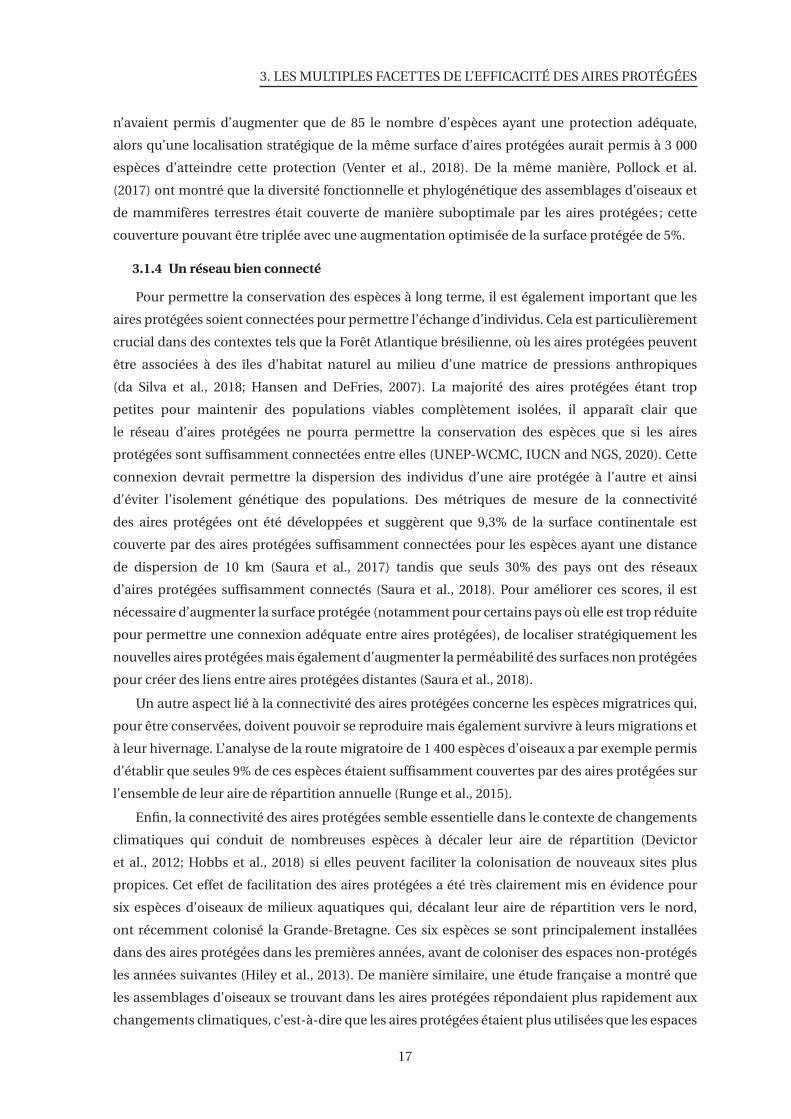
3. LES MULTIPLES FACETTES DE L’EFFICACITÉ DES AIRES PROTÉGÉES
n’avaient permis d’augmenter que de 85 le nombre d’espèces ayant une protection adéquate,
alors qu’une localisation stratégique de la même surface d’aires protégées aurait permis à 3 000
espèces d’atteindre cette protection (Venter et al., 2018). De la même manière, Pollock et al.
(2017) ont montré que la diversité fonctionnelle et phylogénétique des assemblages d’oiseaux et
de mammifères terrestres était couverte de manière suboptimale par les aires protégées ; cette
couverture pouvant être triplée avec une augmentation optimisée de la surface protégée de 5%.
3.1.4 Un réseau bien connecté
Pour permettre la conservation des espèces à long terme, il est également important que les
aires protégées soient connectées pour permettre l’échange d’individus. Cela est particulièrement
crucial dans des contextes tels que la Forêt Atlantique brésilienne, où les aires protégées peuvent
être associées à des îles d’habitat naturel au milieu d’une matrice de pressions anthropiques
(da Silva et al., 2018; Hansen and DeFries, 2007). La majorité des aires protégées étant trop
petites pour maintenir des populations viables complètement isolées, il apparaît clair que
le réseau d’aires protégées ne pourra permettre la conservation des espèces que si les aires
protégées sont suffisamment connectées entre elles (UNEP-WCMC, IUCN and NGS, 2020). Cette
connexion devrait permettre la dispersion des individus d’une aire protégée à l’autre et ainsi
d’éviter l’isolement génétique des populations. Des métriques de mesure de la connectivité
des aires protégées ont été développées et suggèrent que 9,3% de la surface continentale est
couverte par des aires protégées suffisamment connectées pour les espèces ayant une distance
de dispersion de 10 km (Saura et al., 2017) tandis que seuls 30% des pays ont des réseaux
d’aires protégées suffisamment connectés (Saura et al., 2018). Pour améliorer ces scores, il est
nécessaire d’augmenter la surface protégée (notamment pour certains pays où elle est trop réduite
pour permettre une connexion adéquate entre aires protégées), de localiser stratégiquement les
nouvelles aires protégées mais également d’augmenter la perméabilité des surfaces non protégées
pour créer des liens entre aires protégées distantes (Saura et al., 2018).
Un autre aspect lié à la connectivité des aires protégées concerne les espèces migratrices qui,
pour être conservées, doivent pouvoir se reproduire mais également survivre à leurs migrations et
à leur hivernage. L’analyse de la route migratoire de 1 400 espèces d’oiseaux a par exemple permis
d’établir que seules 9% de ces espèces étaient suffisamment couvertes par des aires protégées sur
l’ensemble de leur aire de répartition annuelle (Runge et al., 2015).
Enfin, la connectivité des aires protégées semble essentielle dans le contexte de changements
climatiques qui conduit de nombreuses espèces à décaler leur aire de répartition (Devictor
et al., 2012; Hobbs et al., 2018) si elles peuvent faciliter la colonisation de nouveaux sites plus
propices. Cet effet de facilitation des aires protégées a été très clairement mis en évidence pour
six espèces d’oiseaux de milieux aquatiques qui, décalant leur aire de répartition vers le nord,
ont récemment colonisé la Grande-Bretagne. Ces six espèces se sont principalement installées
dans des aires protégées dans les premières années, avant de coloniser des espaces non-protégés
les années suivantes (Hiley et al., 2013). De manière similaire, une étude française a montré que
les assemblages d’oiseaux se trouvant dans les aires protégées répondaient plus rapidement aux
changements climatiques, c’est-à-dire que les aires protégées étaient plus utilisées que les espaces
17
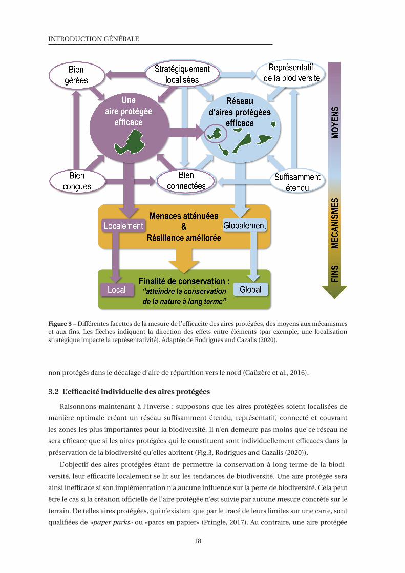
INTRODUCTION GÉNÉRALE
Figure 3 – Différentes facettes de la mesure de l’efficacité des aires protégées, des moyens aux mécanismeset aux fins. Les flèches indiquent la direction des effets entre éléments (par exemple, une localisationstratégique impacte la représentativité). Adaptée de Rodrigues and Cazalis (2020).
non protégés dans le décalage d’aire de répartition vers le nord (Gaüzère et al., 2016).
3.2 L’efficacité individuelle des aires protégées
Raisonnons maintenant à l’inverse : supposons que les aires protégées soient localisées de
manière optimale créant un réseau suffisamment étendu, représentatif, connecté et couvrant
les zones les plus importantes pour la biodiversité. Il n’en demeure pas moins que ce réseau ne
sera efficace que si les aires protégées qui le constituent sont individuellement efficaces dans la
préservation de la biodiversité qu’elles abritent (Fig.3, Rodrigues and Cazalis (2020)).
L’objectif des aires protégées étant de permettre la conservation à long-terme de la biodi-
versité, leur efficacité localement se lit sur les tendances de biodiversité. Une aire protégée sera
ainsi inefficace si son implémentation n’a aucune influence sur la perte de biodiversité. Cela peut
être le cas si la création officielle de l’aire protégée n’est suivie par aucune mesure concrète sur le
terrain. De telles aires protégées, qui n’existent que par le tracé de leurs limites sur une carte, sont
qualifiées de «paper parks» ou «parcs en papier» (Pringle, 2017). Au contraire, une aire protégée
18
3. LES MULTIPLES FACETTES DE L’EFFICACITÉ DES AIRES PROTÉGÉES
parfaitement efficace se traduit par l’empêchement du déclin de la biodiversité qui aurait eu lieu
sans cette protection, voire dans certains cas par le rétablissement des populations. Cette efficacité
maximale serait le produit d’une chaîne partant d’une gestion efficace dans les bordures de l’aire
protégée (par exemple, interdiction de la chasse, contrôle des changements d’utilisation des sols,
contrôle des activités de dérangement. . . ) qui permettrait de supprimer les pressions humaines et
ainsi de stopper le déclin de biodiversité (Fig.3).
Ainsi, l’efficacité réelle des aires protégées ne peut se mesurer que sur la biodiversité elle-
même, puisque la gestion des aires protégées et la réduction des pressions anthropiques ne
seront jugées efficaces que si elles empêchent à terme le déclin de la biodiversité. Cependant,
la mesure de ces aspects intermédiaires s’avère utile, soit pour être utilisées comme proxy (quand
la mesure de l’effet des aires protégées sur la biodiversité est impossible) soit pour comprendre
les mécanismes menant à une conservation efficace de la biodiversité. De ce fait, la littérature
sur l’efficacité individuelle des aires protégées contient des études mesurant (1) les moyens dont
jouissent les aires protégées pour mettre en place des mesures de gestion, (2) l’effet des aires
protégées sur les pressions humaines, et (3) leur effet sur la biodiversité.
3.2.1 Les moyens des aires protégées
Contrer les pressions anthropiques dans une aire protégée nécessite des moyens : des gardes
et véhicules pour empêcher le braconnage d’outarde à tête noire en Inde, du personnel pour
contrôler la déforestation qui atteint le ara hyacinthe au Brésil (Fig.1). Des données sur les
moyens des aires protégées sont collectées et rassemblées dans la «Protected Area Management
Effectiveness database» (PAME). Cette base de données contient 27 665 évaluations réalisées dans
21 402 aires protégées à travers le monde (UNEP-WCMC & IUCN, 2020).
Ces données ont montré à de nombreuses reprises que la majorité des aires protégées sont
dotées de moyens humains et financiers insuffisants pour atteindre leurs objectifs. Une étude
récente a par exemple trouvé que 78% des 2 167 aires protégées de leur échantillon avaient des
ressources insuffisantes, particulièrement dans les Néotropiques (Coad et al., 2019). La suffisance
de ces moyens dépend fortement de la façon dont l’aire protégée a été conçue spatialement (Fig.3)
puisque sa forme et sa taille vont par exemple influencer la possibilité pour les agents des aires
protégées de contrôler les activités humaines (par exemple, patrouilles anti-braconnage). Elle
dépend également du contexte dans lequel l’aire protégée est créée. Si une aire protégée venait
à être créée dans les quelques dizaines de kilomètres carrés restants à la coquette de Guerrero
(Fig.1), ses besoins de moyens et de soutien seraient très importants puisque cette espèce vit dans
une zone de culture de drogue, aux mains des cartels (IUCN, 2018b).
Bien que les moyens humains et financiers soient nécessaires pour rendre une aire protégée
efficace, ils ne sont pas suffisants et ne nous informent donc pas sur l’effet réel des aires protégées
sur le terrain. Pour cela il faut donc observer comment évoluent les pressions humaines et la
biodiversité dans les aires protégées.
3.2.2 La réduction des pressions anthropiques
Les images satellite sont largement utilisées dans les études s’intéressant à l’efficacité des aires
protégées dans l’atténuation des pressions humaines en permettant notamment de cartographier
19
INTRODUCTION GÉNÉRALE
l’évolution de l’utilisation des sols. Une étude globale a montré que 75% des pays voyaient leur
taux de conversion d’habitats naturels réduit dans les aires protégées entre 2000 et 2005, par
rapport à des sites non-protégés similaires (Joppa and Pfaff, 2010). Cet effet est particulièrement
clair sur les forêts, puisque de nombreuses études montrent que les aires protégées réduisent,
mais n’empêchent pas complètement, la déforestation (Nelson and Chomitz, 2009; Andam et al.,
2008; Eklund et al., 2016; Spracklen et al., 2015). Une attention plus particulière peut être portée
sur l’extension des infrastructures urbaines par le biais des tendances de l’éclairage nocturne.
Là-encore, les aires protégées semblent atténuer l’augmentation de la pression humaine, qui a
tendance à augmenter fortement dans la périphérie (25-75 km) des aires protégées (Guetté et al.,
2018).
L’indice d’empreinte écologique, regroupant des données satellite d’utilisation des sols, de
densité humaine, de l’éclairage nocturne et des infrastructures de transport (Venter et al.,
2016b), peut également être utilisé pour suivre l’évolution des pressions humaines dans les aires
protégées. Jones et al. (2018) ont ainsi montré que l’empreinte écologique était plus faible dans
les aires protégées (car elles sont souvent créées dans des sites relativement naturels) tandis
que 32,8% de la surface protégée terrestre était sous une empreinte écologique intense. Une
autre étude a comparé, dans des aires sauvages, les «Wilderness areas», l’augmentation de cet
indice dans les aires protégées par rapport à des sites non protégés similaires et a montré que
l’empreinte écologique augmentait moins rapidement dans les aires protégées qu’à l’extérieur
(respectivement + 0,20 et + 0,32) entre 1993 et 2009 (Anderson and Mammides, 2019). Au contraire,
(Geldmann et al., 2019) n’ont mesuré un effet significatif des aires protégées sur l’évolution de
la pression humaine que dans les forêts. Cela suggère une efficacité faible ou nulle des aires
protégées non forestières dans l’atténuation des pressions anthropiques. De nouvelles études
seraient nécessaires pour trancher ce point.
D’autres pressions ne peuvent pas être mesurées par satellite et requièrent une présence sur
le terrain pour récolter les données. De ce fait, l’effet des aires protégées sur ces pressions est
moins connu et son étude est plus locale. (Bruner et al., 2001) par exemple ont montré que les
93 aires protégées tropicales étudiées dans leur analyse réduisaient la probabilité de dégradation
de la forêt par coupe partielle et réduisait également les activités illégales de chasse. Ce même
constat a été fait au Rwanda où une fréquentation régulière de rangers a conduit à un arrêt de
la fréquentation de certains sites par les braconniers (Moore et al., 2017). Les aires protégées
peuvent également s’avérer efficaces pour diminuer les menaces liées aux espèces invasives en
étant imperméables à leur colonisation (Giakoumi and Pey, 2017; Hiley et al., 2016), mais les
études sur ce sujet restent très rares.
3.2.3 L’empêchement du déclin de la biodiversité
L’efficacité des aires protégées telle que définie dans cette thèse – permettre d’atteindre la
conservation de la nature à long-terme (Fig.3) – doit se traduire par un arrêt du déclin de la
biodiversité dans les aires protégées (i.e., tendances de population stables), voire le rétablissement
des populations (i.e., tendances de population positives). Sur cette base, il apparaît clair que les
aires protégées ne sont actuellement pas parfaitement efficaces puisque de nombreux déclins
20
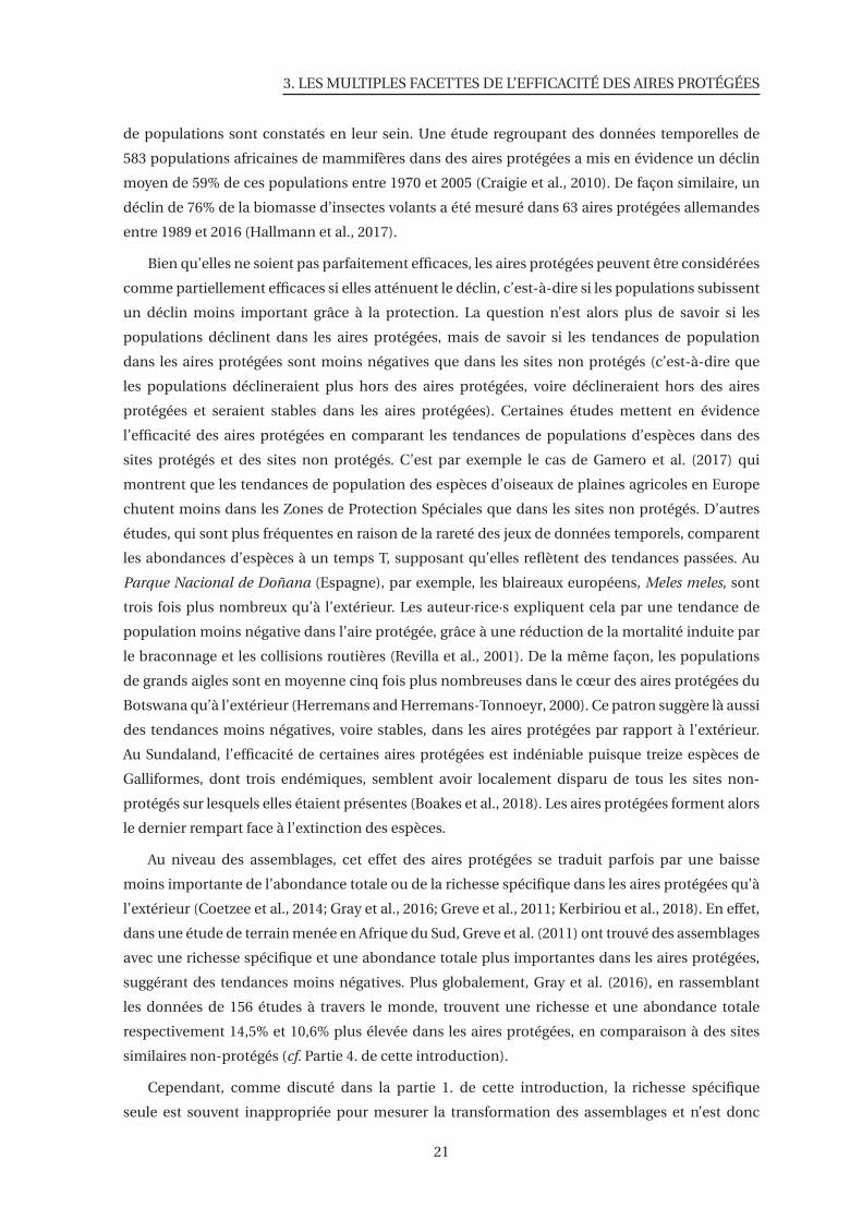
3. LES MULTIPLES FACETTES DE L’EFFICACITÉ DES AIRES PROTÉGÉES
de populations sont constatés en leur sein. Une étude regroupant des données temporelles de
583 populations africaines de mammifères dans des aires protégées a mis en évidence un déclin
moyen de 59% de ces populations entre 1970 et 2005 (Craigie et al., 2010). De façon similaire, un
déclin de 76% de la biomasse d’insectes volants a été mesuré dans 63 aires protégées allemandes
entre 1989 et 2016 (Hallmann et al., 2017).
Bien qu’elles ne soient pas parfaitement efficaces, les aires protégées peuvent être considérées
comme partiellement efficaces si elles atténuent le déclin, c’est-à-dire si les populations subissent
un déclin moins important grâce à la protection. La question n’est alors plus de savoir si les
populations déclinent dans les aires protégées, mais de savoir si les tendances de population
dans les aires protégées sont moins négatives que dans les sites non protégés (c’est-à-dire que
les populations déclineraient plus hors des aires protégées, voire déclineraient hors des aires
protégées et seraient stables dans les aires protégées). Certaines études mettent en évidence
l’efficacité des aires protégées en comparant les tendances de populations d’espèces dans des
sites protégés et des sites non protégés. C’est par exemple le cas de Gamero et al. (2017) qui
montrent que les tendances de population des espèces d’oiseaux de plaines agricoles en Europe
chutent moins dans les Zones de Protection Spéciales que dans les sites non protégés. D’autres
études, qui sont plus fréquentes en raison de la rareté des jeux de données temporels, comparent
les abondances d’espèces à un temps T, supposant qu’elles reflètent des tendances passées. Au
Parque Nacional de Doñana (Espagne), par exemple, les blaireaux européens, Meles meles, sont
trois fois plus nombreux qu’à l’extérieur. Les auteur·rice·s expliquent cela par une tendance de
population moins négative dans l’aire protégée, grâce à une réduction de la mortalité induite par
le braconnage et les collisions routières (Revilla et al., 2001). De la même façon, les populations
de grands aigles sont en moyenne cinq fois plus nombreuses dans le cœur des aires protégées du
Botswana qu’à l’extérieur (Herremans and Herremans-Tonnoeyr, 2000). Ce patron suggère là aussi
des tendances moins négatives, voire stables, dans les aires protégées par rapport à l’extérieur.
Au Sundaland, l’efficacité de certaines aires protégées est indéniable puisque treize espèces de
Galliformes, dont trois endémiques, semblent avoir localement disparu de tous les sites non-
protégés sur lesquels elles étaient présentes (Boakes et al., 2018). Les aires protégées forment alors
le dernier rempart face à l’extinction des espèces.
Au niveau des assemblages, cet effet des aires protégées se traduit parfois par une baisse
moins importante de l’abondance totale ou de la richesse spécifique dans les aires protégées qu’à
l’extérieur (Coetzee et al., 2014; Gray et al., 2016; Greve et al., 2011; Kerbiriou et al., 2018). En effet,
dans une étude de terrain menée en Afrique du Sud, Greve et al. (2011) ont trouvé des assemblages
avec une richesse spécifique et une abondance totale plus importantes dans les aires protégées,
suggérant des tendances moins négatives. Plus globalement, Gray et al. (2016), en rassemblant
les données de 156 études à travers le monde, trouvent une richesse et une abondance totale
respectivement 14,5% et 10,6% plus élevée dans les aires protégées, en comparaison à des sites
similaires non-protégés (cf. Partie 4. de cette introduction).
Cependant, comme discuté dans la partie 1. de cette introduction, la richesse spécifique
seule est souvent inappropriée pour mesurer la transformation des assemblages et n’est donc
21
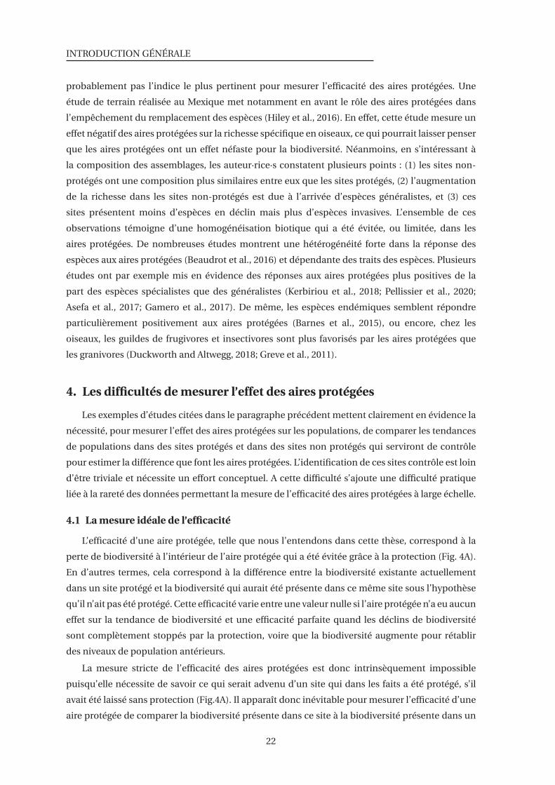
INTRODUCTION GÉNÉRALE
probablement pas l’indice le plus pertinent pour mesurer l’efficacité des aires protégées. Une
étude de terrain réalisée au Mexique met notamment en avant le rôle des aires protégées dans
l’empêchement du remplacement des espèces (Hiley et al., 2016). En effet, cette étude mesure un
effet négatif des aires protégées sur la richesse spécifique en oiseaux, ce qui pourrait laisser penser
que les aires protégées ont un effet néfaste pour la biodiversité. Néanmoins, en s’intéressant à
la composition des assemblages, les auteur·rice·s constatent plusieurs points : (1) les sites non-
protégés ont une composition plus similaires entre eux que les sites protégés, (2) l’augmentation
de la richesse dans les sites non-protégés est due à l’arrivée d’espèces généralistes, et (3) ces
sites présentent moins d’espèces en déclin mais plus d’espèces invasives. L’ensemble de ces
observations témoigne d’une homogénéisation biotique qui a été évitée, ou limitée, dans les
aires protégées. De nombreuses études montrent une hétérogénéité forte dans la réponse des
espèces aux aires protégées (Beaudrot et al., 2016) et dépendante des traits des espèces. Plusieurs
études ont par exemple mis en évidence des réponses aux aires protégées plus positives de la
part des espèces spécialistes que des généralistes (Kerbiriou et al., 2018; Pellissier et al., 2020;
Asefa et al., 2017; Gamero et al., 2017). De même, les espèces endémiques semblent répondre
particulièrement positivement aux aires protégées (Barnes et al., 2015), ou encore, chez les
oiseaux, les guildes de frugivores et insectivores sont plus favorisés par les aires protégées que
les granivores (Duckworth and Altwegg, 2018; Greve et al., 2011).
4. Les difficultés de mesurer l’effet des aires protégées
Les exemples d’études citées dans le paragraphe précédent mettent clairement en évidence la
nécessité, pour mesurer l’effet des aires protégées sur les populations, de comparer les tendances
de populations dans des sites protégés et dans des sites non protégés qui serviront de contrôle
pour estimer la différence que font les aires protégées. L’identification de ces sites contrôle est loin
d’être triviale et nécessite un effort conceptuel. A cette difficulté s’ajoute une difficulté pratique
liée à la rareté des données permettant la mesure de l’efficacité des aires protégées à large échelle.
4.1 La mesure idéale de l’efficacité
L’efficacité d’une aire protégée, telle que nous l’entendons dans cette thèse, correspond à la
perte de biodiversité à l’intérieur de l’aire protégée qui a été évitée grâce à la protection (Fig. 4A).
En d’autres termes, cela correspond à la différence entre la biodiversité existante actuellement
dans un site protégé et la biodiversité qui aurait été présente dans ce même site sous l’hypothèse
qu’il n’ait pas été protégé. Cette efficacité varie entre une valeur nulle si l’aire protégée n’a eu aucun
effet sur la tendance de biodiversité et une efficacité parfaite quand les déclins de biodiversité
sont complètement stoppés par la protection, voire que la biodiversité augmente pour rétablir
des niveaux de population antérieurs.
La mesure stricte de l’efficacité des aires protégées est donc intrinsèquement impossible
puisqu’elle nécessite de savoir ce qui serait advenu d’un site qui dans les faits a été protégé, s’il
avait été laissé sans protection (Fig.4A). Il apparaît donc inévitable pour mesurer l’efficacité d’une
aire protégée de comparer la biodiversité présente dans ce site à la biodiversité présente dans un
22
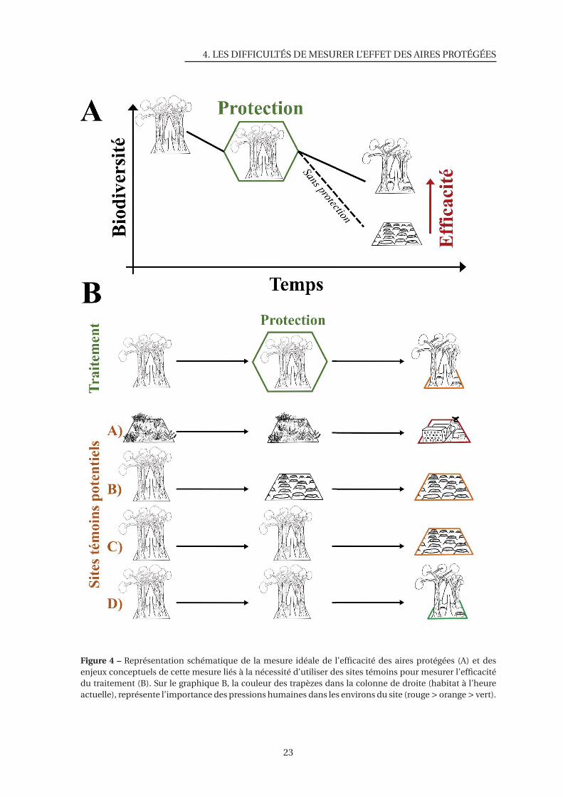
4. LES DIFFICULTÉS DE MESURER L’EFFET DES AIRES PROTÉGÉES
Figure 4 – Représentation schématique de la mesure idéale de l’efficacité des aires protégées (A) et desenjeux conceptuels de cette mesure liés à la nécessité d’utiliser des sites témoins pour mesurer l’efficacitédu traitement (B). Sur le graphique B, la couleur des trapèzes dans la colonne de droite (habitat à l’heureactuelle), représente l’importance des pressions humaines dans les environs du site (rouge > orange > vert).
23
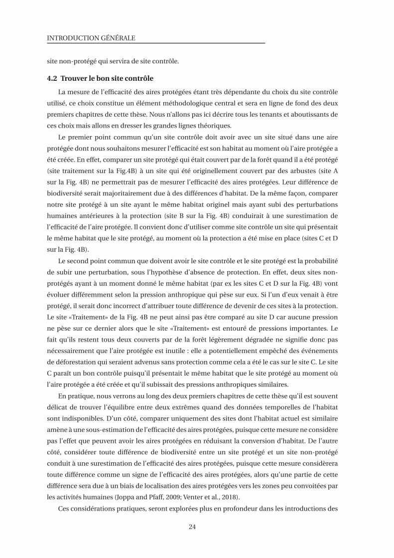
INTRODUCTION GÉNÉRALE
site non-protégé qui servira de site contrôle.
4.2 Trouver le bon site contrôle
La mesure de l’efficacité des aires protégées étant très dépendante du choix du site contrôle
utilisé, ce choix constitue un élément méthodologique central et sera en ligne de fond des deux
premiers chapitres de cette thèse. Nous n’allons pas ici décrire tous les tenants et aboutissants de
ces choix mais allons en dresser les grandes lignes théoriques.
Le premier point commun qu’un site contrôle doit avoir avec un site situé dans une aire
protégée dont nous souhaitons mesurer l’efficacité est son habitat au moment où l’aire protégée a
été créée. En effet, comparer un site protégé qui était couvert par de la forêt quand il a été protégé
(site traitement sur la Fig.4B) à un site qui été originellement couvert par des arbustes (site A
sur la Fig. 4B) ne permettrait pas de mesurer l’efficacité des aires protégées. Leur différence de
biodiversité serait majoritairement due à des différences d’habitat. De la même façon, comparer
notre site protégé à un site ayant le même habitat originel mais ayant subi des perturbations
humaines antérieures à la protection (site B sur la Fig. 4B) conduirait à une surestimation de
l’efficacité de l’aire protégée. Il convient donc d’utiliser comme site contrôle un site qui présentait
le même habitat que le site protégé, au moment où la protection a été mise en place (sites C et D
sur la Fig. 4B).
Le second point commun que doivent avoir le site contrôle et le site protégé est la probabilité
de subir une perturbation, sous l’hypothèse d’absence de protection. En effet, deux sites non-
protégés ayant à un moment donné le même habitat (par ex les sites C et D sur la Fig. 4B) vont
évoluer différemment selon la pression anthropique qui pèse sur eux. Si l’un d’eux venait à être
protégé, il serait donc incorrect d’attribuer toute différence de devenir de ces sites à la protection.
Le site «Traitement» de la Fig. 4B ne peut ainsi pas être comparé au site D car aucune pression
ne pèse sur ce dernier alors que le site «Traitement» est entouré de pressions importantes. Le
fait qu’ils restent tous deux couverts par de la forêt légèrement dégradée ne signifie donc pas
nécessairement que l’aire protégée est inutile : elle a potentiellement empêché des événements
de déforestation qui seraient advenus sans protection comme cela a été le cas sur le site C. Le site
C paraît un bon contrôle puisqu’il présentait le même habitat que le site protégé au moment où
l’aire protégée a été créée et qu’il subissait des pressions anthropiques similaires.
En pratique, nous verrons au long des deux premiers chapitres de cette thèse qu’il est souvent
délicat de trouver l’équilibre entre deux extrêmes quand des données temporelles de l’habitat
sont indisponibles. D’un côté, comparer uniquement des sites dont l’habitat actuel est similaire
amène à une sous-estimation de l’efficacité des aires protégées, puisque cette mesure ne considère
pas l’effet que peuvent avoir les aires protégées en réduisant la conversion d’habitat. De l’autre
côté, considérer toute différence de biodiversité entre un site protégé et un site non-protégé
conduit à une surestimation de l’efficacité des aires protégées, puisque cette mesure considèrera
toute différence comme un signe de l’efficacité des aires protégées, alors qu’une partie de cette
différence sera due à un biais de localisation des aires protégées vers les zones peu convoitées par
les activités humaines (Joppa and Pfaff, 2009; Venter et al., 2018).
Ces considérations pratiques, seront explorées plus en profondeur dans les introductions des
24

4. LES DIFFICULTÉS DE MESURER L’EFFET DES AIRES PROTÉGÉES
deux premiers chapitres de cette thèse, qui s’intéressent à l’efficacité des aires protégées dans la
conservation des oiseaux dans deux zones différentes : l’Amérique du Nord (uniquement Etats-
Unis et Canada) dans le premier chapitre, et dans les forêts tropicales de huit points chauds
de biodiversité dans le second chapitre. Par souci didactique, le choix des contrôles a été ici
présenté dans une approche quasi-expérimentale (comment trouver le bon site contrôle pour un
site protégé), alors qu’ils se traduiront au cœur des chapitres par des approches statistiques. Pour
cela nous appliquerons, dans nos modèles, des contrôles pour des variables associées au biais de
localisation des aires protégées, méthodes qui seront détaillées dans les chapitres.
4.3 Trouver les bonnes données
La mesure de l’effet des aires protégées sur les populations est également contrainte par
l’existence des données de biodiversité qui permettront de comparer les assemblages entre sites
protégés et non-protégés.
Une dichotomie majeure dans les données de biodiversité est la différence entre les données
de «présence-seule» et les données de «présence-absence». Les données de «présence-seule» sont
par exemple des données récoltées par une ornithologue qui se baladerait autour de Portel, au
Nord-Est du Brésil, et rapporterait trois observations de ara hyacinthe dans des sites différents.
Cela nous informerait sur les lieux de présence de cette espèce mais ne nous indiquerait ni
que les aras n’étaient pas présents dans d’autres sites visités, ni que d’autres espèces comme le
manakin auréole, Pipra aureola, n’étaient pas présentes sur ces sites. Ces données sont difficiles
à utiliser pour comparer des assemblages et donc pour mesurer l’efficacité des aires protégées.
On leur préfère les données de «présence-absence» qui sont en général constituées de listes
complètes d’espèces détectées. Si l’ornithologue brésilienne mentionnée précédemment déclare
avoir rapporté dans la base de données toutes les espèces qu’elle a observées et identifiées, cela
nous indique non seulement que le ara hyacinthe a été observé mais également que le manakin
auréole n’a pas été observé. Cela veut dire qu’il était absent du site, ou bien qu’il était présent
mais n’a pas été détecté. Ces données, en considérant prudemment les biais liés à des différences
de détection, permettent de comparer les assemblages et donc de mesurer l’efficacité des aires
protégées. Elles peuvent également inclure des données d’abondance des espèces (par exemple :
huit aras hyacinthes ont été observés sur un site mais zéro manakin auréole). Elles seront au centre
de cette thèse.
Les données de «présence-absence» peuvent être récoltées par différents moyens. Certaines
études utilisent des données récoltées spécifiquement pour répondre à cette question (Hiley et al.,
2016; da Silva et al., 2018) ou issues d’autres travaux de recherche (Gray et al., 2016). Cependant,
la majorité des études se basent sur des données issues de jeux de données récoltés par des
naturalistes bénévoles tels que des atlas (Barnes et al., 2015; Duckworth and Altwegg, 2018) ou
des jeux de données récoltés par protocoles standardisés (Gaget et al., 2020; Pellissier et al., 2020;
Devictor et al., 2007), souvent liés à des projets de sciences participatives.
Ces protocoles standardisés sont par exemple les suivis d’oiseaux nicheurs menés par des
ornithologues bénévoles. Ces ornithologues se voient attribuer un site sur lequel il faudra
échantillonner chaque année, à une date donnée, pendant une durée fixe, les oiseaux qui
25

INTRODUCTION GÉNÉRALE
s’y trouvent. En Amérique du Nord par exemple, les ornithologues participant à la «Breeding
Bird Survey» arpentent des routes de 40 km en s’arrêtant à chaque kilomètre pour noter les
oiseaux vus ou entendus pendant 3 minutes. En France, les ornithologues participant au «Suivi
Temporel des Oiseaux Communs» réalisent 10 points d’écoute dans un carré de 2 km de
côté et notent les espèces vues ou entendues durant une période de 5 minutes. Ces données
incluent automatiquement des données sur l’absence (ou non-détection) des espèces puisque les
observateur·rice·s se doivent de rapporter toutes les espèces observées. Elles sont très utilisées
pour la mesure de l’efficacité des aires protégées car elles sont aisément comparables grâce
à l’application d’un protocole commun mais également parce qu’elles incluent en général des
données d’abondance et que les sites suivis sont nombreux et répartis sur de grands territoires. Le
chapitre 1 de cette thèse est basé sur le jeu de données standardisé de la «Breeding Bird Survey».
Malheureusement de tels jeux de données n’existent pas dans tous les pays et sont princi-
palement concentrés en Amérique du Nord, en Europe et en Océanie, étant presque absents
des milieux tropicaux (Chandler et al., 2017). De ce fait, l’efficacité des aires protégées dans la
conservation des espèces tropicales est peu étudiée. Une base de données plus récente permet de
combler partiellement ce manque : la base de données eBird. Cette base de données accueille
une quantité massive de données récoltées tout au long de l’année, sur l’ensemble du globe
et par une multitude d’observateur·rice·s. La grande liberté laissée aux observateur·rice·s crée
une forte hétérogénéité dans les données. En effet, une certaine observatrice notera peut-être
toutes les espèces observées durant une journée entière dédiée à l’ornithologie, alors qu’un autre
rapportera uniquement les trois espèces les plus intéressantes observées pendant qu’il buvait
un thé depuis son balcon en période de confinement. Cette hétérogénéité rend la comparaison
des données plus délicate, mais possible grâce à un certain nombre d’informations précisées par
les observateur·rice·s quant à leur effort d’échantillonnage. Cette base de données a été utilisée
dans deux chapitres de cette thèse, l’un à travers huit points chauds de biodiversité tropicaux (en
Amérique du Sud et Centrale, en Afrique et en Asie) et l’autre à travers l’Amérique toute entière.
4.4 Dépasser la binarité de la protection pour un gradient de qualité
Jusqu’ici nous avons considéré l’efficacité des aires protégées comme une valeur commune
à toutes les aires protégées visant à mettre en exergue l’effet du réseau d’aires protégées sur
la biodiversité (Fig. 3). Pour autant, les aires protégées sont loin d’être homogènes (cf. Fig.2 et
partie 2.2 de cette introduction) et il convient donc d’appréhender leur diversité qui se traduit
probablement par une variation de leur efficacité. Par exemple, bien que les résultats soient
souvent non-significatifs, de nombreuses études comparent l’efficacité des aires protégées selon
leur catégorie de gestion (Fig.2) (Anderson and Mammides, 2019; Coetzee et al., 2014; Gray et al.,
2016). De manière similaire, deux études sur des populations animales suggèrent que les aires
protégées qui sont petites et récentes sont plus efficaces, car elles sont en général localisées de
façon plus stratégique (Geldmann et al., 2018; Gray et al., 2016).
Des différences d’efficacité entre types d’aires protégées sont explorées, de manière succincte,
dans le chapitre 1 de cette thèse et sont au cœur du chapitre 3. Ce chapitre a pour but de mesurer
l’adéquation entre le besoin de protection des espèces (en considérant les espèces sur un gradient
26
4. LES DIFFICULTÉS DE MESURER L’EFFET DES AIRES PROTÉGÉES
de sensibilité aux pressions anthropiques) et la protection qui leur est offerte (en considérant les
aires protégées sur un gradient d’anthropisation) par le biais de l’indice d’empreinte écologique ou
«Human Footprint» (Venter et al., 2016b). Nous nous demanderons donc si les espèces d’oiseaux
les plus sensibles aux activités humaines ont accès à des aires protégées suffisamment intactes
pour être protégées efficacement.
4.5 L’effet des aires protégées sur les comportements humains
Pour finir, nous dépasserons les considérations purement écologiques visant à mesurer
l’effet des aires protégées sur les populations d’oiseaux pour nous intéresser au rôle qu’elles
peuvent jouer dans la sensibilisation aux problématiques environnementales sur les populations
humaines. En effet, il est bien connu par la Psychologie de la Conservation que la présence d’un
environnement naturel, ainsi que l’exposition à des activités récréatives de nature ou à des actions
de sensibilisation renforce la conscience écologique des individus, ce qui peut conduire à une
augmentation des comportements pro-environnementaux (Clayton and Myers, 2015c; Gifford
and Nilsson, 2014; Spence et al., 2012). Nous pouvons donc imaginer que la présence d’une aire
protégée autour de notre lieu de vie influence positivement nos comportements et ainsi que
les aires protégées jouent un rôle dans la conservation de la connexion entre les humains et
la nature, et dans l’adoption de modes de vie plus respectueux de l’environnement. L’efficacité
des aires protégées pourrait alors également se mesurer en s’intéressant aux comportements
humains. Cette question de l’effet des aires protégées sur les comportements humains, jusqu’alors
absente de la littérature scientifique sera traitée dans le Chapitre 4 de cette thèse, dans lequel nous
comparerons trois types de comportements pro-environnementaux (vote écologiste, adhésion à
des ONG de protection de la nature, et participation à des programmes de sciences participatives)
dans les communes de France Métropolitaine en fonction de leur distance à un Parc National ou
à un Parc Naturel Régional.
27


30
Chapitre 1
Utilisation d’un jeu de données de suivi de
biodiversité à large échelle pour tester l’efficacité
des aires protégées dans la protection des oiseaux
d’Amérique du Nord
31
Comme annoncé dans l’Introduction générale, les deux premiers chapitres de cette thèse
vont partager l’objectif de mesurer l’effet des aires protégées sur les populations d’oiseaux. En
revanche, la zone géographique d’intérêt et l’approche utilisée pour mesurer l’efficacité des aires
protégées diffèreront en fonction des contraintes imposées par les données. Pour le premier
chapitre, nous allons utiliser un jeu de données standardisé bien connu des écologues : la
« Breeding Bird Survey » déployée en Amérique du Nord qui n’apparaît curieusement pas dans la
littérature sur l’efficacité des aires protégées alors qu’elle est tant utilisée en écologie quantitative.
Le protocole standardisé appliqué par les ornithologues participant à ce programme permet une
comparaison facile des assemblages d’oiseaux présents dans les sites protégés et non-protégés.
Au-delà des résultats propres à l’Amérique du Nord, ce premier chapitre permettra de développer
les bases conceptuelles évoquées en partie 4. de l’Introduction générale et de réfléchir à travers
une approche statistique au concept de contrôle dans le but d’isoler autant que possible l’efficacité
des aires protégées.
32
THIS MANUSCRIPT HAS BEEN PEER-REVIEWED AND PUBLISHED
Using a large-scale biodiversity monitoring dataset
to test the effectiveness of protected areas at con-
serving North-American breeding birds
Victor Cazalis1, ∗, Soumaya Belghali1, and Ana S.L. Rodrigues1
Authors affiliation:1 CEFE, Univ Montpellier, CNRS, EPHE, IRD, Univ. Paul Valéry Montpellier 3, Montpellier, France
∗ Corresponding author: [email protected]
Cite as: Cazalis, V., Belghali, S., Rodrigues A.S.L. Using a large-scale biodiversity monitoring
dataset to test the effectiveness of protected areas at conserving North-American breeding
birds. bioRxiv 433037, ver. 4 peer-reviewed and recommended by PCI Ecology (2019). DOI:
10.1101/433037
33
CHAP.1: PA EFFECTS IN NORTH AMERICA (BBS)
Abstract
Protected areas currently cover about 15% of the global land area, and constitute one of the
main tools in biodiversity conservation. Quantifying their effectiveness at protecting species
from local decline or extinction involves comparing protected with counterfactual unprotected
sites representing “what would have happened to protected sites had they not been protected”.
Most studies are based on pairwise comparisons, using neighbour sites to protected areas as
counterfactuals, but this choice is often subjective and may be prone to biases. An alternative
is to use large-scale biodiversity monitoring datasets, whereby the effect of protected areas is
analysed statistically by controlling for landscape differences between protected and unprotected
sites, allowing a more targeted and clearly defined measure of the protected areas effect. Here
we use the North American Breeding Bird Survey dataset as a case study to investigate the
effectiveness of protected areas at conserving bird assemblages. We analysed the effect of
protected areas on species richness, on assemblage-level abundance, and on the abundance of
individual species by modelling how these metrics relate to the proportion of each site that is
protected, while controlling for local habitat, altitude, productivity and for spatial autocorrelation.
At the assemblage level, we found almost no relationship between protection and species richness
or overall abundance. At the species level, we found that forest species are present in significantly
higher abundances within protected forest sites, compared with unprotected forests, with the
opposite effect for species that favour open habitats. Hence, even though protected forest
assemblages are not richer than those of unprotected forests, they are more typical of this habitat.
We also found some evidence that species that avoid human activities tend to be favoured by
protection, but found no such effect for regionally declining species. Our results highlight the
complexity of assessing protected areas effectiveness, and the necessity of clearly defining the
metrics of effectiveness and the controls used in such assessments.
Key words: biodiversity conservation; biodiversity monitoring; protected areas effectiveness;
birds; North-American Breeding Bird Survey; conservation effectiveness
34
1. INTRODUCTION
1. Introduction
The increasing human footprint on natural ecosystems is leading to major declines in species’
populations (McRae et al., 2016) and has already resulted in thousands of extinctions (BirdLife
International, 2017), to such an extent that Ceballos et al. (2017) characterised current times
as a period of “biodiversity annihilation”. Habitat loss and degradation are the most important
pressures on biodiversity (Vié et al., 2009; Balmford and Bond, 2005), as a result of anthropogenic
activities such as agriculture, urbanisation, industry, transport and recreation (Foley et al., 2005).
The most evident response to these threats is to establish areas with restricted, or even no human
activities, i.e., to create protected areas (PAs). Modern PAs have their origins in the 19th century
and currently represent the most important conservation tool, with about 15% of the global land
area already protected to some extent, and coverage planned to reach 17% by 2020 (UNEP-WCMC
IUCN, 2016).
Understanding the extent to which PAs are effective as biodiversity conservation tools is thus
fundamental for guiding future conservation efforts. Accordingly, there is a substantial literature
on PA effectiveness: as of the 1st October 2018, 260 publications in the Web of Science included
in their title “protected AND area∗ AND effective∗”. However, within this literature there are
disparate approaches to the concept of “effectiveness”.
A first set of studies questions whether PAs are effective at representing species or ecosystems,
using gap analyses for measuring the overlap between PAs and the distributions of species or of
ecosystem types (Rodrigues et al., 2004b; Brooks et al., 2004). These studies do not directly quantify
the effectiveness of PAs at conserving biodiversity, but the extent to which species or ecosystems
are buffered from human impacts under the assumption that PAs are highly effective in doing so.
A second set of studies focuses on the means employed locally by PA managers in order to protect
biodiversity, for example in terms of staff or money (Leverington et al., 2010). These analyses
do not directly measure PA effectiveness in reducing human impacts, but rather the resources
allocated to this purpose. A third type of studies quantifies the effectiveness of PAs at preventing
the conversion of natural ecosystems, typically by comparing land use change (e.g., deforestation
rates) in protected versus unprotected areas (Nelson and Chomitz, 2009; Andam et al., 2008).
These studies quantify PA effects at the habitat or ecosystem level, rather than at the species level.
Finally, a set of analyses focuses on measuring the effect of PAs on species themselves, either on
the diversity of assemblages or on the abundance of individual species, typically by contrasting
protected versus unprotected sites. This fourth approach to PA effectiveness is the focus of the
present study.
The effectiveness of PAs at conserving species can be assessed by comparing population trends
inside and outside PAs (Gamero et al., 2017; Devictor et al., 2007; Pellissier et al., 2013). Indeed, if
PAs are effective, populations inside these areas are expected to be better buffered from threats
and thus to decline less, or even to increase more, than those outside. Trends however can be
misleading, because they are calculated in relation to a reference date (that seldom precedes
all anthropogenic impacts) and because they are measured as percentages (which emphasise
changes in small numbers). In this study, we focus instead on measures of PA effectiveness
35
CHAP.1: PA EFFECTS IN NORTH AMERICA (BBS)
that assess current state, namely by contrasting population abundances and species diversity
inside versus outside PAs (Coetzee et al., 2014; Kerbiriou et al., 2018; Devictor et al., 2007). These
measures combine two types of effects: the effectiveness at selecting as PAs sites of higher-than-
average conservation interest (i.e. differences that existed at the time of PA designation); and
effectiveness at maintaining species richness and abundance within existing PAs (i.e. differences
established subsequently to PA designation).
Three recent meta-analyses investigated the effects of PAs on the state of species abundance
and/or diversity by synthesising studies that made pairwise comparisons between protected and
unprotected sites (Geldmann et al., 2013; Coetzee et al., 2014; Gray et al., 2016). The underlying
studies used in these meta-analyses did not necessarily aim to measure PA effectiveness; more
often they investigated the effects of anthropogenic pressure, using PAs as benchmarks (e.g.
Sinclair et al. (2002); Bihn et al. (2008); Wunderle et al. (2006), all integrated in Coetzee meta-
analysis). In the meta-analyses, unprotected sites were treated as counterfactuals to the protected
sites (i.e., by assuming that the latter would be in a similar condition to the former if it had not been
protected), measuring the effect of protection as the observed difference between the two. These
pairwise comparisons often contrast neighbouring sites, which presents the advantage of ensuring
that both have broadly similar environmental characteristics (e.g. same climate). However, they
do not necessarily take into account the fact that PAs tend to be biased in their location towards
higher altitudes and lower productivity areas (Joppa and Pfaff, 2009). To reduce these biases, Gray
et al. (2016) controlled for the differences in altitude, slope and agricultural suitability. Controlling
for these factors means that their results are less influenced by PAs’ location biases and, therefore,
that they reflect more strongly the effects of protection itself. Another potential confounding effect
in pairwise comparisons of neighbouring sites arises from the leakage effect, whereby the human
activities that would have taken place inside a PA are displaced to areas around it, artificially
inflating the perceived effectiveness of PAs (Ewers and Rodrigues, 2008). This effect is difficult
to control for, but should be reduced if the counterfactual sites are not immediately adjacent to
the PAs.
An important decision when choosing a suitable spatial counterfactual to a PA, one that
strongly affects the definition and thus the measure of PA effectiveness, is whether to control for
habitat type or not. On the one hand, not controlling for habitat can lead to comparing sites that
are not expected to have similar biodiversity regardless of their protection status (e.g. protected
grasslands vs unprotected forests). On the other hand, controlling for habitat type can result in
an overlooking of the effects that PAs have on biodiversity by preventing habitat changes (e.g.
deforestation or urbanisation). For instance, given a hypothetical PA covering a natural grassland,
possible counterfactuals include an unprotected site of similar habitat (i.e., natural grassland), an
unprotected site with a different type of natural habitat (e.g., forest, wetland), or an unprotected
site with human-modified habitat (e.g., extensive pasture, herbaceous cropland, urban area). The
choice of counterfactual is certain to have a major impact on the differences observed, and thus
on the measure of PA effectiveness, but it is not necessarily obvious which option is the best
counterfactual. In theory, it is the site that best represents “what would have happened to the PA
36

1. INTRODUCTION
in the absence of protection”; in practice, this is not necessarily easily determined. All three meta-
analyses (Geldmann et al., 2013; Coetzee et al., 2014; Gray et al., 2016) include comparisons where
habitat has not been controlled for, meaning that the counterfactual’s habitat may be different or
similar to the protected site’s habitat. Additionally, a subset of Gray et al. (2016)’s analyses focuses
on comparisons between protected and unprotected sites with matched habitats. In the latter, the
measure of PA effectiveness concerns protection from habitat degradation rather than protection
from habitat conversion.
Another key consideration in analysing PA effectiveness is the biodiversity metrics applied
to comparing protected and unprotected sites. The three meta-analyses employed a diversity
of metrics, some at the level of species’ assemblages, some focused on individual species. Gray
et al. (2016) used only assemblage-level metrics and found higher species richness and overall
abundance inside PAs than outside, but no difference in rarefaction-based richness (i.e. number
of species for a given number of individuals) nor in the proportion of endemic species. When
matching sites with similar habitats, species richness was only higher in young and small PAs than
in unprotected sites (no difference between other protected and unprotected sites), suggesting
that the effect of PAs in preventing habitat degradation was light. Conversely, Geldmann et al.
(2013) considered only species-level metrics (presence, abundance, nest survival) and found
contrasted but mainly positive effects of PAs. Finally, Coetzee et al. (2014) considered both levels;
at the assemblage level, they found higher species richness and overall abundance in protected
than in unprotected sites; at the species level, they found that individual species abundances were
typically higher inside PAs.
An alternative to measuring PA effectiveness through pairwise comparisons is to use statistical
models in which covariates control for differences between protected and unprotected sites. This
approach requires access to a large dataset on the spatial distribution of biodiversity, but reduces
the subjectivity in the choice of counterfactuals, by making explicit which variables are controlled
for, and the measure of effectiveness being investigated. For example, Devictor et al. (2007) applied
this approach to survey data on common birds across France to find a positive effect of PAs on
bird abundances for half of the species investigated, especially declining species. Duckworth
and Altwegg (2018), working on bird abundance data collected across South Africa, found that
PA coverage was positively correlated with occupancy of frugivorous, insectivorous, vegivores and
predator species, and negatively correlated with occupancy of granivorous species.
In the present study, we quantify the effectiveness of Protected Areas at protecting birds by
taking advantage of a large dataset of bird counts across a near-continental area – the North
American Breeding Bird Survey (Pardieck et al., 2017). Controlling statistically for altitude and
productivity in order to reduce the effect of PA location biases, we estimated PA effectiveness
on two levels of biodiversity: on species’ assemblages, through indices of richness and summed
abundance; and on individual common species, by estimating the effect of PAs on species’
abundance. At the assemblage level, we expected to find higher species diversity and abundance
inside PAs. Indeed, as human activities are causing species population declines and local
extinctions (Ceballos et al., 2017), and as PAs are expected to buffer against these activities, this
37
CHAP.1: PA EFFECTS IN NORTH AMERICA (BBS)
should predictably lead to overall higher species richness and higher total abundance inside PAs,
as found by Coetzee et al. (2014) and Gray et al. (2016). At the individual species level, we expected
higher abundances within PAs. However, given differences in species’ habitat requirements, this
result cannot be expected to hold universally (i.e., species are not all expected to be more abundant
in all PAs). For example, we expected protected forests to have a positive effect on forest species,
but not on grassland species. Hence, we controlled in our analyses for broad vegetation structure
(forest, shrub, herbaceous), by investigating separately the effects of PAs dominated by a particular
vegetation structure on species with different habitat requirements. Additionally, we expected
species with overall declining populations (thus more affected by anthropogenic activities), and
species that avoid human presence (more sensitive to human disturbance) to present higher
abundances inside PAs.
2. Methods
In this study, we use the term “PA effectiveness” to refer to the difference in species diversity or
abundance between protected and unprotected sites. This difference combines the effects of
PA site selection (i.e., differences existing prior to the implementation of PA, for example if they
are implemented in sites with higher-than-average richness or abundances) and the effects of
protection itself (i.e., difference that arise after PA designation, if PAs effectively reduce population
depletions and species local extinctions).
2.1 Bird data
We used data from the North-American Breeding Bird Survey (BBS), a long-term volunteer-based
monitoring scheme in Canada, the USA, and Mexico (Pardieck et al., 2017), version 2016.0. Our
study region encompasses solely Canada and the USA, as few Mexican routes are monitored. This
program is based on the annual monitoring of thousands of routes, each approximately 40 km
long, during the bird breeding season. Each route is split into 50 stops; at each stop, the observer
counts every bird heard or seen during three minutes, before moving to the next stop.
Given the length of BBS routes, they often intersect multiple land use types (e.g. forested,
urban, agriculture; each with different bird assemblages), and they are rarely wholly contained
within protected sites (most of the routes that cross PAs do so only in small fractions of their
length). As a result, whole BBS routes are not particularly suited sampling units for investigating
how PAs affect bird species. We chose instead to focus on small sections of routes – sequences
of five stops, covering about 4 km – in order to obtain field-sampling units that are more
homogeneous in terms of land use types and whose bird assemblages can be more directly linked
to local landscape characteristics, especially protection. For each route, we only used the first
sequence of five stops, because the only precisely georeferenced point we had access to was the
first stop of each route. Indeed, even if in principle additional stops are spaced about 0.8 km from
each other, in practice this distance can vary, making the location of additional stops in each route
progressively more imprecise. Henceforth, and for simplicity, we use the term “routes” to refer to
these initial sections of five stops rather than to entire BBS routes.
38
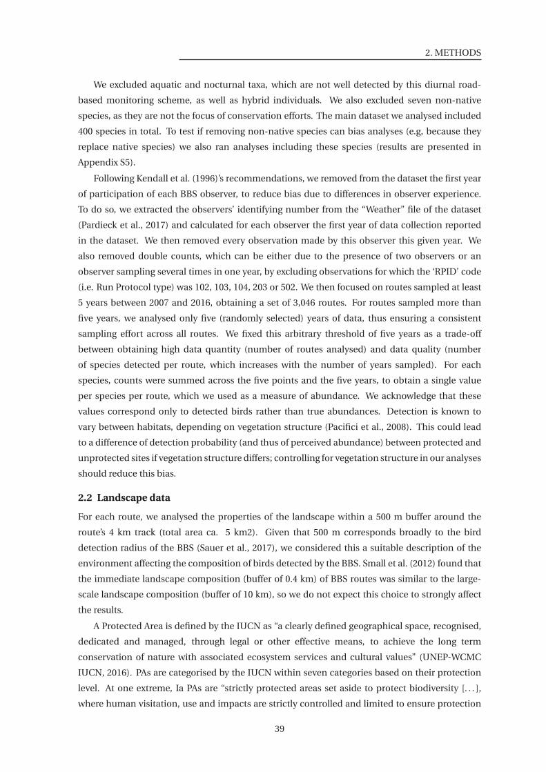
2. METHODS
We excluded aquatic and nocturnal taxa, which are not well detected by this diurnal road-
based monitoring scheme, as well as hybrid individuals. We also excluded seven non-native
species, as they are not the focus of conservation efforts. The main dataset we analysed included
400 species in total. To test if removing non-native species can bias analyses (e.g, because they
replace native species) we also ran analyses including these species (results are presented in
Appendix S5).
Following Kendall et al. (1996)’s recommendations, we removed from the dataset the first year
of participation of each BBS observer, to reduce bias due to differences in observer experience.
To do so, we extracted the observers’ identifying number from the “Weather” file of the dataset
(Pardieck et al., 2017) and calculated for each observer the first year of data collection reported
in the dataset. We then removed every observation made by this observer this given year. We
also removed double counts, which can be either due to the presence of two observers or an
observer sampling several times in one year, by excluding observations for which the ‘RPID’ code
(i.e. Run Protocol type) was 102, 103, 104, 203 or 502. We then focused on routes sampled at least
5 years between 2007 and 2016, obtaining a set of 3,046 routes. For routes sampled more than
five years, we analysed only five (randomly selected) years of data, thus ensuring a consistent
sampling effort across all routes. We fixed this arbitrary threshold of five years as a trade-off
between obtaining high data quantity (number of routes analysed) and data quality (number
of species detected per route, which increases with the number of years sampled). For each
species, counts were summed across the five points and the five years, to obtain a single value
per species per route, which we used as a measure of abundance. We acknowledge that these
values correspond only to detected birds rather than true abundances. Detection is known to
vary between habitats, depending on vegetation structure (Pacifici et al., 2008). This could lead
to a difference of detection probability (and thus of perceived abundance) between protected and
unprotected sites if vegetation structure differs; controlling for vegetation structure in our analyses
should reduce this bias.
2.2 Landscape data
For each route, we analysed the properties of the landscape within a 500 m buffer around the
route’s 4 km track (total area ca. 5 km2). Given that 500 m corresponds broadly to the bird
detection radius of the BBS (Sauer et al., 2017), we considered this a suitable description of the
environment affecting the composition of birds detected by the BBS. Small et al. (2012) found that
the immediate landscape composition (buffer of 0.4 km) of BBS routes was similar to the large-
scale landscape composition (buffer of 10 km), so we do not expect this choice to strongly affect
the results.
A Protected Area is defined by the IUCN as “a clearly defined geographical space, recognised,
dedicated and managed, through legal or other effective means, to achieve the long term
conservation of nature with associated ecosystem services and cultural values” (UNEP-WCMC
IUCN, 2016). PAs are categorised by the IUCN within seven categories based on their protection
level. At one extreme, Ia PAs are “strictly protected areas set aside to protect biodiversity [. . . ],
where human visitation, use and impacts are strictly controlled and limited to ensure protection
39
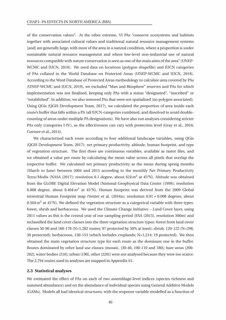
CHAP.1: PA EFFECTS IN NORTH AMERICA (BBS)
of the conservation values”. At the other extreme, VI PAs “conserve ecosystems and habitats
together with associated cultural values and traditional natural resource management systems
[and] are generally large, with most of the area in a natural condition, where a proportion is under
sustainable natural resource management and where low-level non-industrial use of natural
resources compatible with nature conservation is seen as one of the main aims of the area” (UNEP-
WCMC and IUCN, 2018). We used data on locations (polygon shapefile) and IUCN categories
of PAs collated in the World Database on Protected Areas (UNEP-WCMC and IUCN, 2018).
According to the Word Database of Protected Areas methodology to calculate area covered by PAs
(UNEP-WCMC and IUCN, 2019), we excluded “Man and Biosphere” reserves and PAs for which
implementation was not finalised, keeping only PAs with a status “designated”, “inscribed” or
“established”. In addition, we also removed PAs that were not spatialized (no polygon associated).
Using QGis (QGIS Development Team, 2017), we calculated the proportion of area inside each
route’s buffer that falls within a PA (all IUCN-categories combined, and dissolved to avoid double-
counting of areas under multiple PA designations). We have also run analyses considering stricter
PAs only (categories I-IV), as the effectiveness can vary with protection level (Gray et al., 2016;
Coetzee et al., 2014).
We characterised each route according to four additional landscape variables, using QGis
(QGIS Development Team, 2017): net primary productivity, altitude, human footprint, and type
of vegetation structure. The first three are continuous variables, available as raster files, and
we obtained a value per route by calculating the mean value across all pixels that overlap the
respective buffer. We calculated net primary productivity as the mean during spring months
(March to June) between 2004 and 2015 according to the monthly Net Primary Productivity
Terra/Modis (NASA (2017); resolution 0.1 degree, about 62km2 at 45°N). Altitude was obtained
from the GLOBE Digital Elevation Model (National Geophysical Data Center (1999); resolution
0.008 degree, about 0.40km2 at 45°N). Human footprint was derived from the 2009 Global
terrestrial Human Footprint map (Venter et al. (2016a); resolution 0.01 × 0.008 degrees, about
0.50km2 at 45°N). We defined the vegetation structure as a categorical variable with three types:
forest, shrub and herbaceous. We used the Climate Change Initiative – Land Cover layer, using
2011 values as this is the central year of our sampling period (ESA (2015), resolution 300m) and
reclassified the land cover classes into the three vegetation structure types: forest from land cover
classes 50-90 and 160-170 (N=1,282 routes; 97 protected by 50% at least); shrub, 120-122 (N=298,
30 protected); herbaceous, 130-153 (which includes croplands; N=1,214; 19 protected). We then
obtained the main vegetation structure type for each route as the dominant one in the buffer.
Routes dominated by other land use classes (mosaic, [30-40, 100-110 and 180]; bare areas [200-
202]; water bodies [210]; urban [190], other [220]) were not analysed because they were too scarce.
The 2,794 routes used in analyses are mapped in Appendix S1.
2.3 Statistical analyses
We estimated the effect of PAs on each of two assemblage-level indices (species richness and
summed abundance) and on the abundance of individual species using General Additive Models
(GAMs). Models all had identical structures, with the response variable modelled as a function of
40
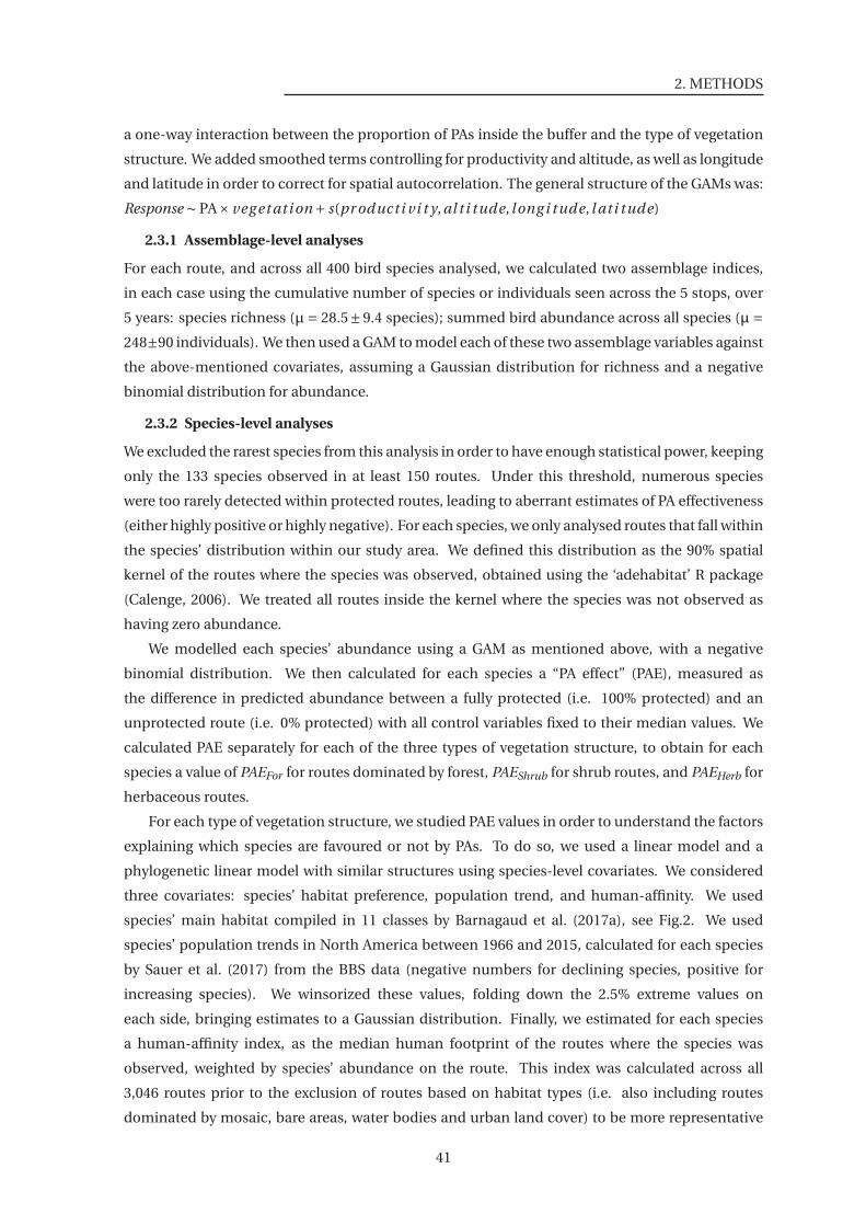
2. METHODS
a one-way interaction between the proportion of PAs inside the buffer and the type of vegetation
structure. We added smoothed terms controlling for productivity and altitude, as well as longitude
and latitude in order to correct for spatial autocorrelation. The general structure of the GAMs was:
Response ∼ PA× veg et ati on + s(pr oducti vi t y, al t i tude, long i tude, l at i tude)
2.3.1 Assemblage-level analyses
For each route, and across all 400 bird species analysed, we calculated two assemblage indices,
in each case using the cumulative number of species or individuals seen across the 5 stops, over
5 years: species richness (µ= 28.5±9.4 species); summed bird abundance across all species (µ=
248±90 individuals). We then used a GAM to model each of these two assemblage variables against
the above-mentioned covariates, assuming a Gaussian distribution for richness and a negative
binomial distribution for abundance.
2.3.2 Species-level analyses
We excluded the rarest species from this analysis in order to have enough statistical power, keeping
only the 133 species observed in at least 150 routes. Under this threshold, numerous species
were too rarely detected within protected routes, leading to aberrant estimates of PA effectiveness
(either highly positive or highly negative). For each species, we only analysed routes that fall within
the species’ distribution within our study area. We defined this distribution as the 90% spatial
kernel of the routes where the species was observed, obtained using the ‘adehabitat’ R package
(Calenge, 2006). We treated all routes inside the kernel where the species was not observed as
having zero abundance.
We modelled each species’ abundance using a GAM as mentioned above, with a negative
binomial distribution. We then calculated for each species a “PA effect” (PAE), measured as
the difference in predicted abundance between a fully protected (i.e. 100% protected) and an
unprotected route (i.e. 0% protected) with all control variables fixed to their median values. We
calculated PAE separately for each of the three types of vegetation structure, to obtain for each
species a value of PAEFor for routes dominated by forest, PAEShrub for shrub routes, and PAEHerb for
herbaceous routes.
For each type of vegetation structure, we studied PAE values in order to understand the factors
explaining which species are favoured or not by PAs. To do so, we used a linear model and a
phylogenetic linear model with similar structures using species-level covariates. We considered
three covariates: species’ habitat preference, population trend, and human-affinity. We used
species’ main habitat compiled in 11 classes by Barnagaud et al. (2017a), see Fig.2. We used
species’ population trends in North America between 1966 and 2015, calculated for each species
by Sauer et al. (2017) from the BBS data (negative numbers for declining species, positive for
increasing species). We winsorized these values, folding down the 2.5% extreme values on
each side, bringing estimates to a Gaussian distribution. Finally, we estimated for each species
a human-affinity index, as the median human footprint of the routes where the species was
observed, weighted by species’ abundance on the route. This index was calculated across all
3,046 routes prior to the exclusion of routes based on habitat types (i.e. also including routes
dominated by mosaic, bare areas, water bodies and urban land cover) to be more representative
41
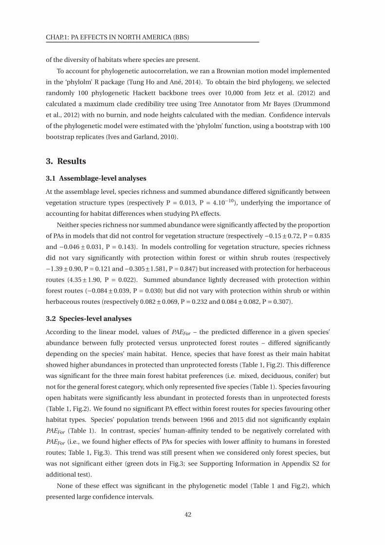
CHAP.1: PA EFFECTS IN NORTH AMERICA (BBS)
of the diversity of habitats where species are present.
To account for phylogenetic autocorrelation, we ran a Brownian motion model implemented
in the ‘phylolm’ R package (Tung Ho and Ané, 2014). To obtain the bird phylogeny, we selected
randomly 100 phylogenetic Hackett backbone trees over 10,000 from Jetz et al. (2012) and
calculated a maximum clade credibility tree using Tree Annotator from Mr Bayes (Drummond
et al., 2012) with no burnin, and node heights calculated with the median. Confidence intervals
of the phylogenetic model were estimated with the ‘phylolm’ function, using a bootstrap with 100
bootstrap replicates (Ives and Garland, 2010).
3. Results
3.1 Assemblage-level analyses
At the assemblage level, species richness and summed abundance differed significantly between
vegetation structure types (respectively P = 0.013, P = 4.10−10), underlying the importance of
accounting for habitat differences when studying PA effects.
Neither species richness nor summed abundance were significantly affected by the proportion
of PAs in models that did not control for vegetation structure (respectively −0.15±0.72, P = 0.835
and −0.046± 0.031, P = 0.143). In models controlling for vegetation structure, species richness
did not vary significantly with protection within forest or within shrub routes (respectively
−1.39±0.90, P = 0.121 and −0.305±1.581, P = 0.847) but increased with protection for herbaceous
routes (4.35±1.90, P = 0.022). Summed abundance lightly decreased with protection within
forest routes (−0.084±0.039, P = 0.030) but did not vary with protection within shrub or within
herbaceous routes (respectively 0.082±0.069, P = 0.232 and 0.084±0.082, P = 0.307).
3.2 Species-level analyses
According to the linear model, values of PAEFor – the predicted difference in a given species’
abundance between fully protected versus unprotected forest routes – differed significantly
depending on the species’ main habitat. Hence, species that have forest as their main habitat
showed higher abundances in protected than unprotected forests (Table 1, Fig.2). This difference
was significant for the three main forest habitat preferences (i.e. mixed, deciduous, conifer) but
not for the general forest category, which only represented five species (Table 1). Species favouring
open habitats were significantly less abundant in protected forests than in unprotected forests
(Table 1, Fig.2). We found no significant PA effect within forest routes for species favouring other
habitat types. Species’ population trends between 1966 and 2015 did not significantly explain
PAEFor (Table 1). In contrast, species’ human-affinity tended to be negatively correlated with
PAEFor (i.e., we found higher effects of PAs for species with lower affinity to humans in forested
routes; Table 1, Fig.3). This trend was still present when we considered only forest species, but
was not significant either (green dots in Fig.3; see Supporting Information in Appendix S2 for
additional test).
None of these effect was significant in the phylogenetic model (Table 1 and Fig.2), which
presented large confidence intervals.
42
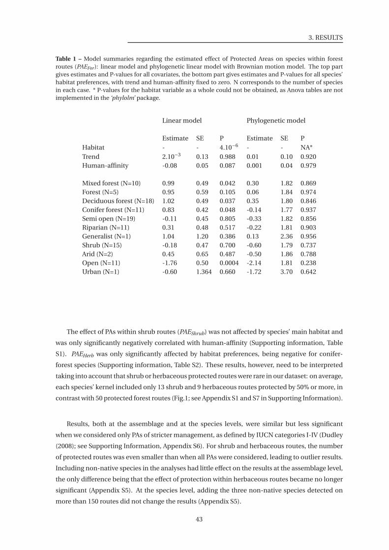
3. RESULTS
Table 1 – Model summaries regarding the estimated effect of Protected Areas on species within forestroutes (PAEFor): linear model and phylogenetic linear model with Brownian motion model. The top partgives estimates and P-values for all covariates, the bottom part gives estimates and P-values for all species’habitat preferences, with trend and human-affinity fixed to zero. N corresponds to the number of speciesin each case. * P-values for the habitat variable as a whole could not be obtained, as Anova tables are notimplemented in the ‘phylolm’ package.
Linear model Phylogenetic model
Estimate SE P Estimate SE PHabitat - - 4.10−6 - - NA*Trend 2.10−3 0.13 0.988 0.01 0.10 0.920Human-affinity -0.08 0.05 0.087 0.001 0.04 0.979
Mixed forest (N=10) 0.99 0.49 0.042 0.30 1.82 0.869Forest (N=5) 0.95 0.59 0.105 0.06 1.84 0.974Deciduous forest (N=18) 1.02 0.49 0.037 0.35 1.80 0.846Conifer forest (N=11) 0.83 0.42 0.048 -0.14 1.77 0.937Semi open (N=19) -0.11 0.45 0.805 -0.33 1.82 0.856Riparian (N=11) 0.31 0.48 0.517 -0.22 1.81 0.903Generalist (N=1) 1.04 1.20 0.386 0.13 2.36 0.956Shrub (N=15) -0.18 0.47 0.700 -0.60 1.79 0.737Arid (N=2) 0.45 0.65 0.487 -0.50 1.86 0.788Open (N=11) -1.76 0.50 0.0004 -2.14 1.81 0.238Urban (N=1) -0.60 1.364 0.660 -1.72 3.70 0.642
The effect of PAs within shrub routes (PAEShrub) was not affected by species’ main habitat and
was only significantly negatively correlated with human-affinity (Supporting information, Table
S1). PAEHerb was only significantly affected by habitat preferences, being negative for conifer-
forest species (Supporting information, Table S2). These results, however, need to be interpreted
taking into account that shrub or herbaceous protected routes were rare in our dataset: on average,
each species’ kernel included only 13 shrub and 9 herbaceous routes protected by 50% or more, in
contrast with 50 protected forest routes (Fig.1; see Appendix S1 and S7 in Supporting Information).
Results, both at the assemblage and at the species levels, were similar but less significant
when we considered only PAs of stricter management, as defined by IUCN categories I-IV (Dudley
(2008); see Supporting Information, Appendix S6). For shrub and herbaceous routes, the number
of protected routes was even smaller than when all PAs were considered, leading to outlier results.
Including non-native species in the analyses had little effect on the results at the assemblage level,
the only difference being that the effect of protection within herbaceous routes became no longer
significant (Appendix S5). At the species level, adding the three non-native species detected on
more than 150 routes did not change the results (Appendix S5).
43
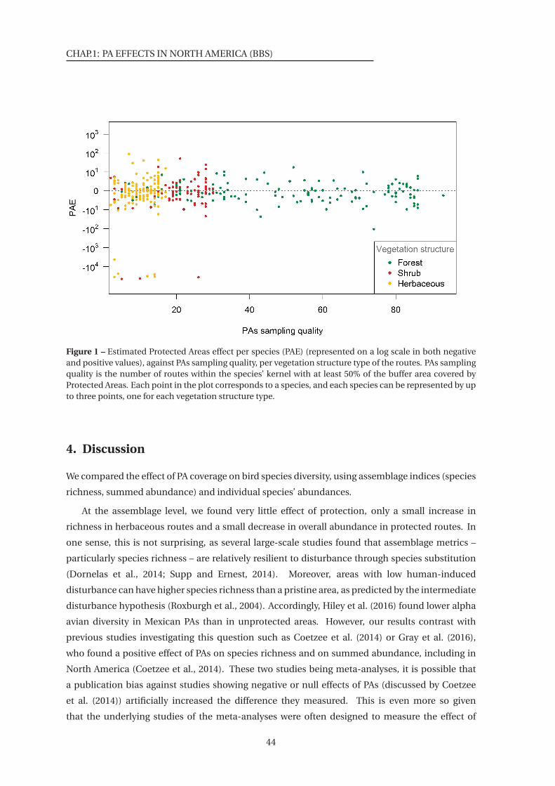
CHAP.1: PA EFFECTS IN NORTH AMERICA (BBS)
Figure 1 – Estimated Protected Areas effect per species (PAE) (represented on a log scale in both negativeand positive values), against PAs sampling quality, per vegetation structure type of the routes. PAs samplingquality is the number of routes within the species’ kernel with at least 50% of the buffer area covered byProtected Areas. Each point in the plot corresponds to a species, and each species can be represented by upto three points, one for each vegetation structure type.
4. Discussion
We compared the effect of PA coverage on bird species diversity, using assemblage indices (species
richness, summed abundance) and individual species’ abundances.
At the assemblage level, we found very little effect of protection, only a small increase in
richness in herbaceous routes and a small decrease in overall abundance in protected routes. In
one sense, this is not surprising, as several large-scale studies found that assemblage metrics –
particularly species richness – are relatively resilient to disturbance through species substitution
(Dornelas et al., 2014; Supp and Ernest, 2014). Moreover, areas with low human-induced
disturbance can have higher species richness than a pristine area, as predicted by the intermediate
disturbance hypothesis (Roxburgh et al., 2004). Accordingly, Hiley et al. (2016) found lower alpha
avian diversity in Mexican PAs than in unprotected areas. However, our results contrast with
previous studies investigating this question such as Coetzee et al. (2014) or Gray et al. (2016),
who found a positive effect of PAs on species richness and on summed abundance, including in
North America (Coetzee et al., 2014). These two studies being meta-analyses, it is possible that
a publication bias against studies showing negative or null effects of PAs (discussed by Coetzee
et al. (2014)) artificially increased the difference they measured. This is even more so given
that the underlying studies of the meta-analyses were often designed to measure the effect of
44
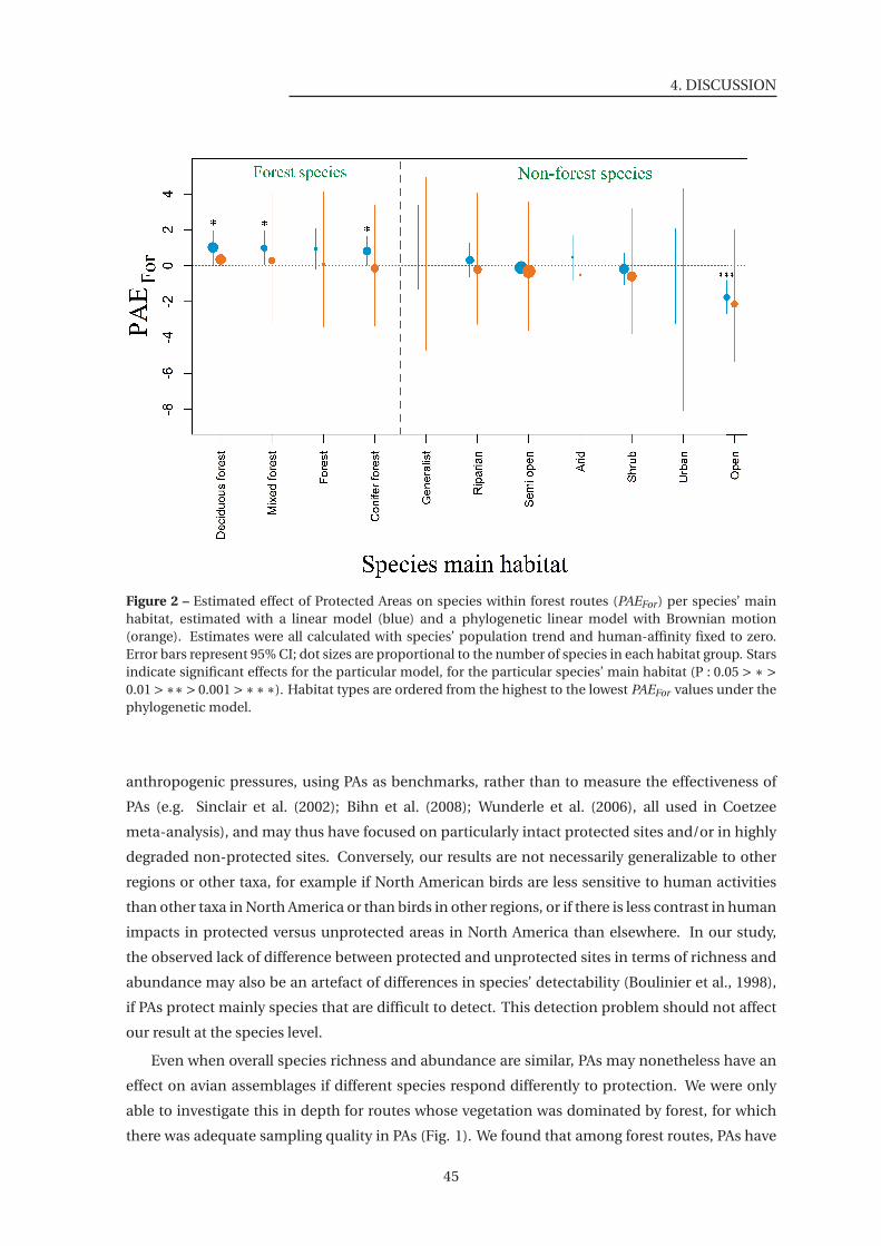
4. DISCUSSION
Figure 2 – Estimated effect of Protected Areas on species within forest routes (PAEFor) per species’ mainhabitat, estimated with a linear model (blue) and a phylogenetic linear model with Brownian motion(orange). Estimates were all calculated with species’ population trend and human-affinity fixed to zero.Error bars represent 95% CI; dot sizes are proportional to the number of species in each habitat group. Starsindicate significant effects for the particular model, for the particular species’ main habitat (P : 0.05 > ∗ >
0.01 >∗∗> 0.001 >∗∗∗). Habitat types are ordered from the highest to the lowest PAEFor values under thephylogenetic model.
anthropogenic pressures, using PAs as benchmarks, rather than to measure the effectiveness of
PAs (e.g. Sinclair et al. (2002); Bihn et al. (2008); Wunderle et al. (2006), all used in Coetzee
meta-analysis), and may thus have focused on particularly intact protected sites and/or in highly
degraded non-protected sites. Conversely, our results are not necessarily generalizable to other
regions or other taxa, for example if North American birds are less sensitive to human activities
than other taxa in North America or than birds in other regions, or if there is less contrast in human
impacts in protected versus unprotected areas in North America than elsewhere. In our study,
the observed lack of difference between protected and unprotected sites in terms of richness and
abundance may also be an artefact of differences in species’ detectability (Boulinier et al., 1998),
if PAs protect mainly species that are difficult to detect. This detection problem should not affect
our result at the species level.
Even when overall species richness and abundance are similar, PAs may nonetheless have an
effect on avian assemblages if different species respond differently to protection. We were only
able to investigate this in depth for routes whose vegetation was dominated by forest, for which
there was adequate sampling quality in PAs (Fig. 1). We found that among forest routes, PAs have
45
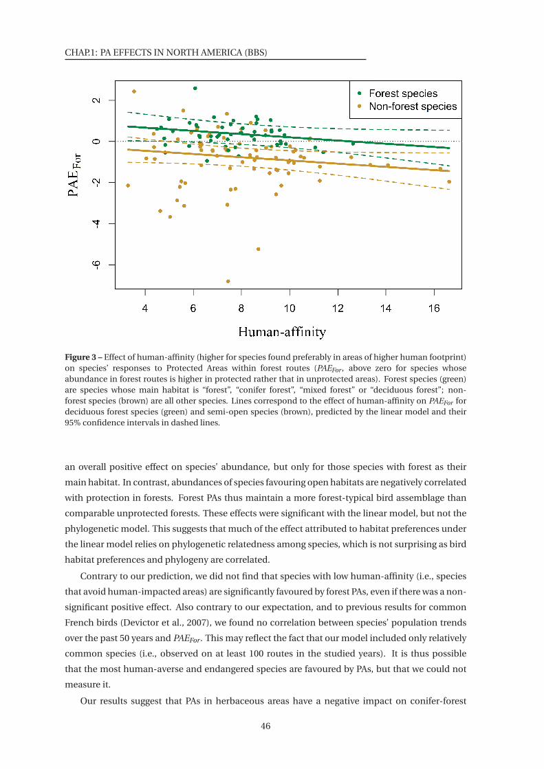
CHAP.1: PA EFFECTS IN NORTH AMERICA (BBS)
Figure 3 – Effect of human-affinity (higher for species found preferably in areas of higher human footprint)on species’ responses to Protected Areas within forest routes (PAEFor , above zero for species whoseabundance in forest routes is higher in protected rather that in unprotected areas). Forest species (green)are species whose main habitat is “forest”, “conifer forest”, “mixed forest” or “deciduous forest”; non-forest species (brown) are all other species. Lines correspond to the effect of human-affinity on PAEFor fordeciduous forest species (green) and semi-open species (brown), predicted by the linear model and their95% confidence intervals in dashed lines.
an overall positive effect on species’ abundance, but only for those species with forest as their
main habitat. In contrast, abundances of species favouring open habitats are negatively correlated
with protection in forests. Forest PAs thus maintain a more forest-typical bird assemblage than
comparable unprotected forests. These effects were significant with the linear model, but not the
phylogenetic model. This suggests that much of the effect attributed to habitat preferences under
the linear model relies on phylogenetic relatedness among species, which is not surprising as bird
habitat preferences and phylogeny are correlated.
Contrary to our prediction, we did not find that species with low human-affinity (i.e., species
that avoid human-impacted areas) are significantly favoured by forest PAs, even if there was a non-
significant positive effect. Also contrary to our expectation, and to previous results for common
French birds (Devictor et al., 2007), we found no correlation between species’ population trends
over the past 50 years and PAEFor . This may reflect the fact that our model included only relatively
common species (i.e., observed on at least 100 routes in the studied years). It is thus possible
that the most human-averse and endangered species are favoured by PAs, but that we could not
measure it.
Our results suggest that PAs in herbaceous areas have a negative impact on conifer-forest
46
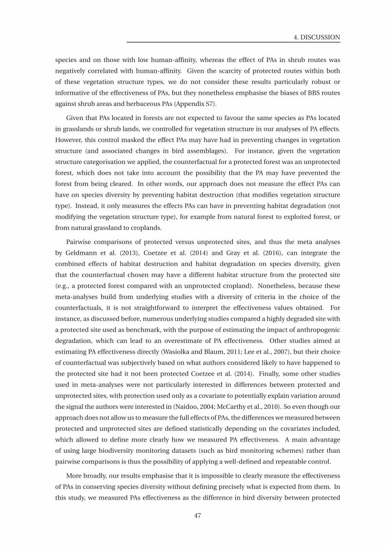
4. DISCUSSION
species and on those with low human-affinity, whereas the effect of PAs in shrub routes was
negatively correlated with human-affinity. Given the scarcity of protected routes within both
of these vegetation structure types, we do not consider these results particularly robust or
informative of the effectiveness of PAs, but they nonetheless emphasise the biases of BBS routes
against shrub areas and herbaceous PAs (Appendix S7).
Given that PAs located in forests are not expected to favour the same species as PAs located
in grasslands or shrub lands, we controlled for vegetation structure in our analyses of PA effects.
However, this control masked the effect PAs may have had in preventing changes in vegetation
structure (and associated changes in bird assemblages). For instance, given the vegetation
structure categorisation we applied, the counterfactual for a protected forest was an unprotected
forest, which does not take into account the possibility that the PA may have prevented the
forest from being cleared. In other words, our approach does not measure the effect PAs can
have on species diversity by preventing habitat destruction (that modifies vegetation structure
type). Instead, it only measures the effects PAs can have in preventing habitat degradation (not
modifying the vegetation structure type), for example from natural forest to exploited forest, or
from natural grassland to croplands.
Pairwise comparisons of protected versus unprotected sites, and thus the meta analyses
by Geldmann et al. (2013), Coetzee et al. (2014) and Gray et al. (2016), can integrate the
combined effects of habitat destruction and habitat degradation on species diversity, given
that the counterfactual chosen may have a different habitat structure from the protected site
(e.g., a protected forest compared with an unprotected cropland). Nonetheless, because these
meta-analyses build from underlying studies with a diversity of criteria in the choice of the
counterfactuals, it is not straightforward to interpret the effectiveness values obtained. For
instance, as discussed before, numerous underlying studies compared a highly degraded site with
a protected site used as benchmark, with the purpose of estimating the impact of anthropogenic
degradation, which can lead to an overestimate of PA effectiveness. Other studies aimed at
estimating PA effectiveness directly (Wasiolka and Blaum, 2011; Lee et al., 2007), but their choice
of counterfactual was subjectively based on what authors considered likely to have happened to
the protected site had it not been protected Coetzee et al. (2014). Finally, some other studies
used in meta-analyses were not particularly interested in differences between protected and
unprotected sites, with protection used only as a covariate to potentially explain variation around
the signal the authors were interested in (Naidoo, 2004; McCarthy et al., 2010). So even though our
approach does not allow us to measure the full effects of PAs, the differences we measured between
protected and unprotected sites are defined statistically depending on the covariates included,
which allowed to define more clearly how we measured PA effectiveness. A main advantage
of using large biodiversity monitoring datasets (such as bird monitoring schemes) rather than
pairwise comparisons is thus the possibility of applying a well-defined and repeatable control.
More broadly, our results emphasise that it is impossible to clearly measure the effectiveness
of PAs in conserving species diversity without defining precisely what is expected from them. In
this study, we measured PAs effectiveness as the difference in bird diversity between protected
47
CHAP.1: PA EFFECTS IN NORTH AMERICA (BBS)
and unprotected sites, controlling for main landscape differences. This definition combines
conservation ability to protect richest areas and to reduce effectively human pressures in these
areas. If PAs are expected to present higher diversity in terms of assemblage metrics (species
richness or summed abundance), then we found no evidence in our analyses that PAs are effective.
If PAs are expected to protect all species’ populations, then we did not find they were effective
either, as for about half of the 133 species studied here we found a negative effect of forest PAs.
However, our results show that North-American forest PAs present higher abundances in forest
species when compared with unprotected forest sites, and lower abundances of species favouring
open habitats. That this result holds even though we found no significant difference in total
abundance suggests that bird assemblages in protected forests are more forest-typical than those
in unprotected forests. Our results thus indicate that forest PAs in North America are contributing
to prevent forest habitat degradation, and associated losses in the abundance of forest specialist
species. BBS routes do not currently cover sufficiently well other habitats besides forest to allow
us to investigate whether the same result applies to PAs with a different vegetation structure, but
datasets with a bigger proportion of sampling points inside PAs, across all habitats, would bring
further light into this question.
5. Acknowledgements
We thank Jean-Yves Barnagaud for his insightful comments and suggestions concerning the
analyses. We are grateful to the thousands of U.S. and Canadian participants who annually
perform and coordinate the Breeding Bird Survey. This preprint has been peer-reviewed and
recommended by Peer Community In Ecology (https://dx.doi.org/10.24072/pci.ecology.100018)
48
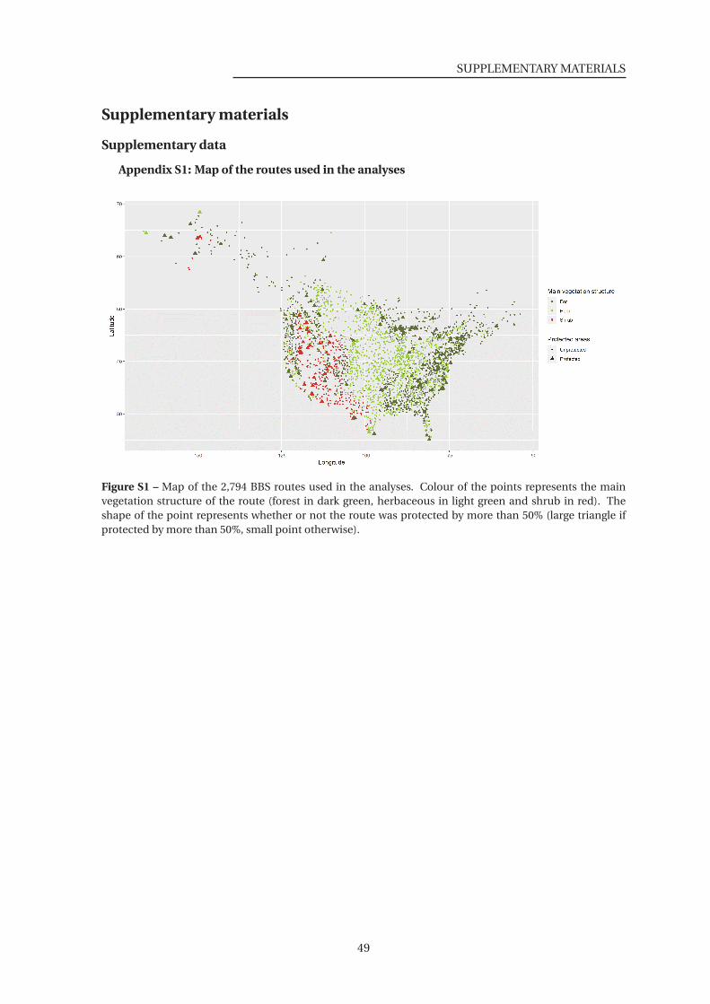
SUPPLEMENTARY MATERIALS
Supplementary materials
Supplementary data
Appendix S1: Map of the routes used in the analyses
Figure S1 – Map of the 2,794 BBS routes used in the analyses. Colour of the points represents the mainvegetation structure of the route (forest in dark green, herbaceous in light green and shrub in red). Theshape of the point represents whether or not the route was protected by more than 50% (large triangle ifprotected by more than 50%, small point otherwise).
49
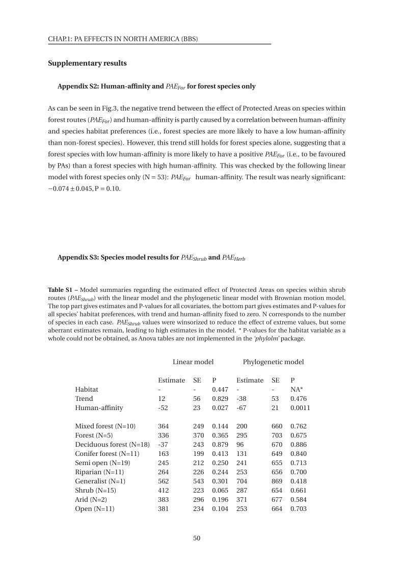
CHAP.1: PA EFFECTS IN NORTH AMERICA (BBS)
Supplementary results
Appendix S2: Human-affinity and PAEFor for forest species only
As can be seen in Fig.3, the negative trend between the effect of Protected Areas on species within
forest routes (PAEFor) and human-affinity is partly caused by a correlation between human-affinity
and species habitat preferences (i.e., forest species are more likely to have a low human-affinity
than non-forest species). However, this trend still holds for forest species alone, suggesting that a
forest species with low human-affinity is more likely to have a positive PAEFor (i.e., to be favoured
by PAs) than a forest species with high human-affinity. This was checked by the following linear
model with forest species only (N = 53): PAEFor human-affinity. The result was nearly significant:
−0.074±0.045,P = 0.10.
Appendix S3: Species model results for PAEShrub and PAEHerb
Table S1 – Model summaries regarding the estimated effect of Protected Areas on species within shrubroutes (PAEShrub) with the linear model and the phylogenetic linear model with Brownian motion model.The top part gives estimates and P-values for all covariates, the bottom part gives estimates and P-values forall species’ habitat preferences, with trend and human-affinity fixed to zero. N corresponds to the numberof species in each case. PAEShrub values were winsorized to reduce the effect of extreme values, but someaberrant estimates remain, leading to high estimates in the model. * P-values for the habitat variable as awhole could not be obtained, as Anova tables are not implemented in the ‘phylolm’ package.
Linear model Phylogenetic model
Estimate SE P Estimate SE PHabitat - - 0.447 - - NA*Trend 12 56 0.829 -38 53 0.476Human-affinity -52 23 0.027 -67 21 0.0011
Mixed forest (N=10) 364 249 0.144 200 660 0.762Forest (N=5) 336 370 0.365 295 703 0.675Deciduous forest (N=18) -37 243 0.879 96 670 0.886Conifer forest (N=11) 163 199 0.413 131 649 0.840Semi open (N=19) 245 212 0.250 241 655 0.713Riparian (N=11) 264 226 0.244 253 656 0.700Generalist (N=1) 562 543 0.301 704 869 0.418Shrub (N=15) 412 223 0.065 287 654 0.661Arid (N=2) 383 296 0.196 371 677 0.584Open (N=11) 381 234 0.104 253 664 0.703
50
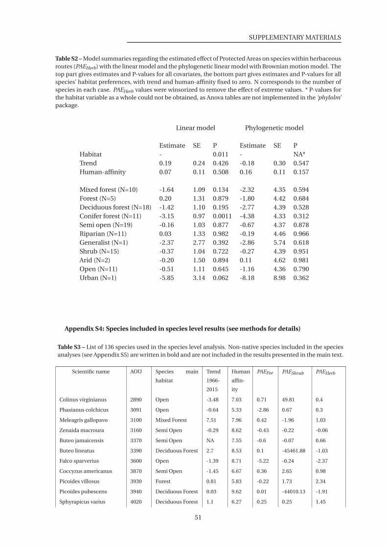
SUPPLEMENTARY MATERIALS
Table S2 – Model summaries regarding the estimated effect of Protected Areas on species within herbaceousroutes (PAEHerb) with the linear model and the phylogenetic linear model with Brownian motion model. Thetop part gives estimates and P-values for all covariates, the bottom part gives estimates and P-values for allspecies’ habitat preferences, with trend and human-affinity fixed to zero. N corresponds to the number ofspecies in each case. PAEHerb values were winsorized to remove the effect of extreme values. * P-values forthe habitat variable as a whole could not be obtained, as Anova tables are not implemented in the ‘phylolm’package.
Linear model Phylogenetic model
Estimate SE P Estimate SE PHabitat - 0.011 - NA*Trend 0.19 0.24 0.426 -0.18 0.30 0.547Human-affinity 0.07 0.11 0.508 0.16 0.11 0.157
Mixed forest (N=10) -1.64 1.09 0.134 -2.32 4.35 0.594Forest (N=5) 0.20 1.31 0.879 -1.80 4.42 0.684Deciduous forest (N=18) -1.42 1.10 0.195 -2.77 4.39 0.528Conifer forest (N=11) -3.15 0.97 0.0011 -4.38 4.33 0.312Semi open (N=19) -0.16 1.03 0.877 -0.67 4.37 0.878Riparian (N=11) 0.03 1.33 0.982 -0.19 4.46 0.966Generalist (N=1) -2.37 2.77 0.392 -2.86 5.74 0.618Shrub (N=15) -0.37 1.04 0.722 -0.27 4.39 0.951Arid (N=2) -0.20 1.50 0.894 0.11 4.62 0.981Open (N=11) -0.51 1.11 0.645 -1.16 4.36 0.790Urban (N=1) -5.85 3.14 0.062 -8.18 8.98 0.362
Appendix S4: Species included in species level results (see methods for details)
Table S3 – List of 136 species used in the species level analysis. Non-native species included in the speciesanalyses (see Appendix S5) are written in bold and are not included in the results presented in the main text.
Scientific name AOU Species main
habitat
Trend
1966-
2015
Human
affin-
ity
PAEFor PAEShrub PAEHerb
Colinus virginianus 2890 Open -3.48 7.03 0.71 49.81 0.4
Phasianus colchicus 3091 Open -0.64 5.33 -2.86 0.67 0.3
Meleagris gallopavo 3100 Mixed Forest 7.51 7.96 0.42 -1.96 1.03
Zenaida macroura 3160 Semi Open -0.29 8.62 -0.43 -0.22 -0.06
Buteo jamaicensis 3370 Semi Open NA 7.55 -0.6 -0.07 0.66
Buteo lineatus 3390 Deciduous Forest 2.7 8.53 0.1 -45461.88 -1.03
Falco sparverius 3600 Open -1.39 8.71 -5.22 -0.24 -2.37
Coccyzus americanus 3870 Semi Open -1.45 6.67 0.36 2.65 0.98
Picoides villosus 3930 Forest 0.81 5.83 -0.22 1.73 2.34
Picoides pubescens 3940 Deciduous Forest 0.03 9.62 0.01 -44010.13 -1.91
Sphyrapicus varius 4020 Deciduous Forest 1.1 6.27 0.25 0.25 1.45
51
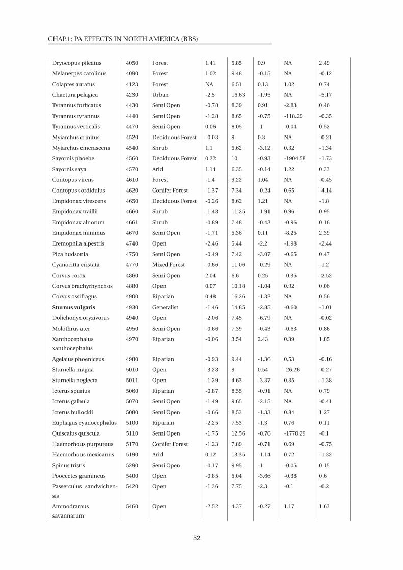
CHAP.1: PA EFFECTS IN NORTH AMERICA (BBS)
Dryocopus pileatus 4050 Forest 1.41 5.85 0.9 NA 2.49
Melanerpes carolinus 4090 Forest 1.02 9.48 -0.15 NA -0.12
Colaptes auratus 4123 Forest NA 6.51 0.13 1.02 0.74
Chaetura pelagica 4230 Urban -2.5 16.63 -1.95 NA -5.17
Tyrannus forficatus 4430 Semi Open -0.78 8.39 0.91 -2.83 0.46
Tyrannus tyrannus 4440 Semi Open -1.28 8.65 -0.75 -118.29 -0.35
Tyrannus verticalis 4470 Semi Open 0.06 8.05 -1 -0.04 0.52
Myiarchus crinitus 4520 Deciduous Forest -0.03 9 0.3 NA -0.21
Myiarchus cinerascens 4540 Shrub 1.1 5.62 -3.12 0.32 -1.34
Sayornis phoebe 4560 Deciduous Forest 0.22 10 -0.93 -1904.58 -1.73
Sayornis saya 4570 Arid 1.14 6.35 -0.14 1.22 0.33
Contopus virens 4610 Forest -1.4 9.22 1.04 NA -0.45
Contopus sordidulus 4620 Conifer Forest -1.37 7.34 -0.24 0.65 -4.14
Empidonax virescens 4650 Deciduous Forest -0.26 8.62 1.21 NA -1.8
Empidonax traillii 4660 Shrub -1.48 11.25 -1.91 0.96 0.95
Empidonax alnorum 4661 Shrub -0.89 7.48 -0.43 -0.96 0.16
Empidonax minimus 4670 Semi Open -1.71 5.36 0.11 -8.25 2.39
Eremophila alpestris 4740 Open -2.46 5.44 -2.2 -1.98 -2.44
Pica hudsonia 4750 Semi Open -0.49 7.42 -3.07 -0.65 0.47
Cyanocitta cristata 4770 Mixed Forest -0.66 11.06 -0.29 NA -1.2
Corvus corax 4860 Semi Open 2.04 6.6 0.25 -0.35 -2.52
Corvus brachyrhynchos 4880 Open 0.07 10.18 -1.04 0.92 0.06
Corvus ossifragus 4900 Riparian 0.48 16.26 -1.32 NA 0.56
Sturnus vulgaris 4930 Generalist -1.46 14.85 -2.85 -0.60 -1.01
Dolichonyx oryzivorus 4940 Open -2.06 7.45 -6.79 NA -0.02
Molothrus ater 4950 Semi Open -0.66 7.39 -0.43 -0.63 0.86
Xanthocephalus
xanthocephalus
4970 Riparian -0.06 3.54 2.43 0.39 1.85
Agelaius phoeniceus 4980 Riparian -0.93 9.44 -1.36 0.53 -0.16
Sturnella magna 5010 Open -3.28 9 0.54 -26.26 -0.27
Sturnella neglecta 5011 Open -1.29 4.63 -3.37 0.35 -1.38
Icterus spurius 5060 Riparian -0.87 8.55 -0.91 NA 0.79
Icterus galbula 5070 Semi Open -1.49 9.65 -2.15 NA -0.41
Icterus bullockii 5080 Semi Open -0.66 8.53 -1.33 0.84 1.27
Euphagus cyanocephalus 5100 Riparian -2.25 7.53 -1.3 0.76 0.11
Quiscalus quiscula 5110 Semi Open -1.75 12.56 -0.76 -1770.29 -0.1
Haemorhous purpureus 5170 Conifer Forest -1.23 7.89 -0.71 0.69 -0.75
Haemorhous mexicanus 5190 Arid 0.12 13.35 -1.14 0.72 -1.32
Spinus tristis 5290 Semi Open -0.17 9.95 -1 -0.05 0.15
Pooecetes gramineus 5400 Open -0.85 5.04 -3.66 -0.38 0.6
Passerculus sandwichen-
sis
5420 Open -1.36 7.75 -2.3 -0.1 -0.2
Ammodramus
savannarum
5460 Open -2.52 4.37 -0.27 1.17 1.63
52
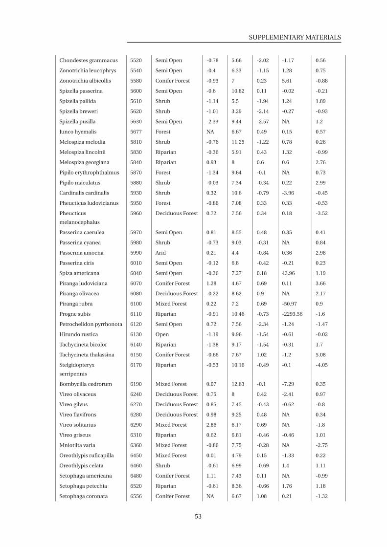
SUPPLEMENTARY MATERIALS
Chondestes grammacus 5520 Semi Open -0.78 5.66 -2.02 -1.17 0.56
Zonotrichia leucophrys 5540 Semi Open -0.4 6.33 -1.15 1.28 0.75
Zonotrichia albicollis 5580 Conifer Forest -0.93 7 0.23 5.61 -0.88
Spizella passerina 5600 Semi Open -0.6 10.82 0.11 -0.02 -0.21
Spizella pallida 5610 Shrub -1.14 5.5 -1.94 1.24 1.89
Spizella breweri 5620 Shrub -1.01 3.29 -2.14 -0.27 -0.93
Spizella pusilla 5630 Semi Open -2.33 9.44 -2.57 NA 1.2
Junco hyemalis 5677 Forest NA 6.67 0.49 0.15 0.57
Melospiza melodia 5810 Shrub -0.76 11.25 -1.22 0.78 0.26
Melospiza lincolnii 5830 Riparian -0.36 5.91 0.43 1.32 -0.99
Melospiza georgiana 5840 Riparian 0.93 8 0.6 0.6 2.76
Pipilo erythrophthalmus 5870 Forest -1.34 9.64 -0.1 NA 0.73
Pipilo maculatus 5880 Shrub -0.03 7.34 -0.34 0.22 2.99
Cardinalis cardinalis 5930 Shrub 0.32 10.6 -0.79 -3.96 -0.45
Pheucticus ludovicianus 5950 Forest -0.86 7.08 0.33 0.33 -0.53
Pheucticus
melanocephalus
5960 Deciduous Forest 0.72 7.56 0.34 0.18 -3.52
Passerina caerulea 5970 Semi Open 0.81 8.55 0.48 0.35 0.41
Passerina cyanea 5980 Shrub -0.73 9.03 -0.31 NA 0.84
Passerina amoena 5990 Arid 0.21 4.4 -0.84 0.36 2.98
Passerina ciris 6010 Semi Open -0.12 6.8 -0.42 -0.21 0.23
Spiza americana 6040 Semi Open -0.36 7.27 0.18 43.96 1.19
Piranga ludoviciana 6070 Conifer Forest 1.28 4.67 0.69 0.11 3.66
Piranga olivacea 6080 Deciduous Forest -0.22 8.62 0.9 NA 2.17
Piranga rubra 6100 Mixed Forest 0.22 7.2 0.69 -50.97 0.9
Progne subis 6110 Riparian -0.91 10.46 -0.73 -2293.56 -1.6
Petrochelidon pyrrhonota 6120 Semi Open 0.72 7.56 -2.34 -1.24 -1.47
Hirundo rustica 6130 Open -1.19 9.96 -1.54 -0.61 -0.02
Tachycineta bicolor 6140 Riparian -1.38 9.17 -1.54 -0.31 1.7
Tachycineta thalassina 6150 Conifer Forest -0.66 7.67 1.02 -1.2 5.08
Stelgidopteryx
serripennis
6170 Riparian -0.53 10.16 -0.49 -0.1 -4.05
Bombycilla cedrorum 6190 Mixed Forest 0.07 12.63 -0.1 -7.29 0.35
Vireo olivaceus 6240 Deciduous Forest 0.75 8 0.42 -2.41 0.97
Vireo gilvus 6270 Deciduous Forest 0.85 7.45 -0.43 -0.62 -0.8
Vireo flavifrons 6280 Deciduous Forest 0.98 9.25 0.48 NA 0.34
Vireo solitarius 6290 Mixed Forest 2.86 6.17 0.69 NA -1.8
Vireo griseus 6310 Riparian 0.62 6.81 -0.46 -0.46 1.01
Mniotilta varia 6360 Mixed Forest -0.86 7.75 -0.28 NA -2.75
Oreothlypis ruficapilla 6450 Mixed Forest 0.01 4.79 0.15 -1.33 0.22
Oreothlypis celata 6460 Shrub -0.61 6.99 -0.69 1.4 1.11
Setophaga americana 6480 Conifer Forest 1.11 7.43 0.11 NA -0.99
Setophaga petechia 6520 Riparian -0.61 8.36 -0.66 1.76 1.18
Setophaga coronata 6556 Conifer Forest NA 6.67 1.08 0.21 -1.32
53

CHAP.1: PA EFFECTS IN NORTH AMERICA (BBS)
Setophaga magnolia 6570 Conifer Forest 0.87 6.57 -0.94 -0.94 0.16
Setophaga pensylvanica 6590 Shrub -1.15 7.92 -0.11 NA 3.64
Setophaga fusca 6620 Conifer Forest 0.35 6.72 0.04 0.04 -24359.41
Setophaga dominica 6630 Conifer Forest 0.98 8.55 0.47 NA -1.59
Setophaga virens 6670 Mixed Forest 0.35 6.24 0.29 NA 2.61
Setophaga pinus 6710 Conifer Forest 0.88 7.56 0.83 NA 1.31
Seiurus aurocapilla 6740 Mixed Forest -0.07 6.86 1.18 1.18 -0.01
Parkesia noveboracensis 6750 Riparian 1.19 6.15 0.58 -4.67 0.5
Geothlypis philadelphia 6790 Shrub -1.18 6.27 -0.06 -0.06 -2.14
Geothlypis tolmiei 6800 Conifer Forest -1.66 4.83 -0.54 1.49 -4368.12
Geothlypis trichas 6810 Riparian -1.01 9.25 -0.24 1.87 1.45
Icteria virens 6830 Shrub -0.62 6.29 -0.25 2.01 2.29
Setophaga citrina 6840 Deciduous Forest 1.36 6.12 0.8 NA -10.44
Cardellina pusilla 6850 Riparian -1.8 6.33 -0.42 1.54 3.85
Setophaga ruticilla 6870 Deciduous Forest -0.28 8.67 1.08 -8.39 -2.28
Passer domesticus 6882 Generalist -3.61 12.24 -1.29 -1.59 -3.27
Mimus polyglottos 7030 Semi Open -0.46 10.02 -0.23 -0.76 -0.11
Dumetella carolinensis 7040 Shrub -0.01 14.09 -1.14 -0.82 0.47
Toxostoma rufum 7050 Shrub -1.04 9.5 -1.4 NA -0.27
Salpinctes obsoletus 7150 Arid -0.65 5.58 1.5 0.97 -0.27
Thryothorus ludovicianus 7180 Deciduous Forest 1.04 9.85 -0.12 NA -0.03
Thryomanes bewickii 7190 Shrub -0.9 7.4 1.34 -0.98 2.3
Troglodytes aedon 7210 Shrub 0.26 9.43 -0.78 -0.36 -0.16
Troglodytes hiemalis 7222 Conifer Forest 0.23 6.73 0.26 0.26 -35800.29
Sitta carolinensis 7270 Deciduous Forest 1.71 9.25 0.55 2.62 1.02
Sitta canadensis 7280 Conifer Forest 0.72 5.15 0.5 -0.14 2.11
Baeolophus bicolor 7310 Deciduous Forest NA 9.93 -0.39 NA -0.53
Poecile atricapillus 7350 Deciduous Forest 0.61 11.4 -0.53 1.45 1.01
Poecile carolinensis 7360 Mixed Forest -0.38 9.79 0.31 NA -2.36
Poecile gambeli 7380 Conifer Forest -1.34 4.5 0.61 1.07 -5.57
Regulus satrapa 7480 Conifer Forest -1.54 6.08 2.59 -37373.47 -32617.55
Regulus calendula 7490 Conifer Forest 0.47 4.83 -0.17 0.84 -25341.08
Polioptila caerulea 7510 Deciduous Forest 0.38 8.05 0.65 1.31 1.61
Hylocichla mustelina 7550 Deciduous Forest -1.91 9.6 0.56 NA 1.06
Catharus fuscescens 7560 Deciduous Forest -1.13 8.43 0.27 -0.42 -1.18
Catharus ustulatus 7580 Mixed Forest -0.84 6.27 0.21 -1.37 -0.81
Catharus guttatus 7590 Mixed Forest 0.33 4.99 1.09 0.05 -34475.37
Turdus migratorius 7610 Generalist 0.12 10.86 0.16 -0.24 -1.58
Sialia sialis 7660 Semi Open 1.5 10.25 -0.41 -1928.64 -0.81
Sialia currucoides 7680 Semi Open -0.54 4.05 -0.82 0.32 2.4
Streptopelia decaocto 22860 Semi Open 29.18 9.68 -1.06 -0.58 -5.17
54
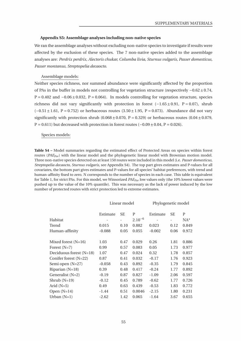
SUPPLEMENTARY MATERIALS
Appendix S5: Assemblage analyses including non-native species
We ran the assemblage analyses without excluding non-native species to investigate if results were
affected by the exclusion of these species. The 7 non-native species added to the assemblage
analyses are: Perdrix perdrix, Alectoris chukar, Columba livia, Sturnus vulgaris, Passer domesticus,
Passer montanus, Streptopelia decaocto.
Assemblage models:
Neither species richness, nor summed abundance were significantly affected by the proportion
of PAs in the buffer in models not controlling for vegetation structure (respectively −0.62±0.74,
P = 0.402 and −0.06±0.032, P = 0.064). In models controlling for vegetation structure, species
richness did not vary significantly with protection in forest (−1.65±0.91, P = 0.07), shrub
(−0.51±1.61, P = 0.752) or herbaceous routes (3.50±1.95, P = 0.073). Abundance did not vary
significantly with protection shrub (0.068±0.070, P = 0.329) or herbaceous routes (0.04±0.079,
P = 0.611) but decreased with protection in forest routes (−0.09±0.04, P = 0.026).
Species models:
Table S4 – Model summaries regarding the estimated effect of Protected Areas on species within forestroutes (PAEFor) with the linear model and the phylogenetic linear model with Brownian motion model.Three non-native species detected on at least 150 routes were included in this model (i.e. Passer domesticus,Streptopelia decaocto, Sturnus vulgaris, see Appendix S4). The top part gives estimates and P-values for allcovariates, the bottom part gives estimates and P-values for all species’ habitat preferences, with trend andhuman-affinity fixed to zero. N corresponds to the number of species in each case. This table is equivalentfor Table 1, for strict PAs. For this model, we Winsorized PAEFor low values only (the 10% lowest values werepushed up to the value of the 10% quantile). This was necessary as the lack of power induced by the lownumber of protected routes with strict protection led to extreme estimates.
Linear model Phylogenetic model
Estimate SE P Estimate SE PHabitat - - 2.10−6 - - NA*Trend 0.015 0.10 0.882 0.023 0.12 0.849Human-affinity -0.088 0.05 0.055 -0.002 0.06 0.972
Mixed forest (N=16) 1.03 0.47 0.029 0.26 1.81 0.886Forest (N=7) 0.99 0.57 0.083 0.05 1.73 0.977Deciduous forest (N=18) 1.07 0.47 0.024 0.32 1.78 0.857Conifer forest (N=22) 0.87 0.41 0.032 -0.17 1.76 0.923Semi open (N=27) -0.058 0.43 0.892 -0.35 1.79 0.845Riparian (N=18) 0.39 0.48 0.417 -0.24 1.77 0.892Generalist (N=2) -0.19 0.87 0.827 -1.09 2.06 0.597Shrub (N=19) -0.12 0.45 0.789 -0.62 1.77 0.726Arid (N=5) 0.49 0.63 0.439 -0.53 1.83 0.772Open (N=14) -1.44 0.51 0.0046 -2.15 1.80 0.231Urban (N=1) -2.62 1.42 0.065 -1.64 3.67 0.655
55

CHAP.1: PA EFFECTS IN NORTH AMERICA (BBS)
Appendix S6: Equivalent analyses when considering PAs Ia-IV only
As the effectiveness of PAs may depend on the protection level they offer, we repeated the exact
same analyses as those presented in the main text, but considering only PAs categorised by the
IUCN as categories Ia to IV (stricter conservation).
Assemblage models:
Neither species richness, nor summed abundance were significantly affected by the proportion of
PAs in the buffer in models not controlling for vegetation structure (respectively −0.042±0.092,
P = 0.665; −0.021±0.050, P = 0.692). In models controlling for vegetation structure, species
richness did not vary significantly with protection in forest (−1.22±1.19, P = 0.305), shrub
(−0.52±1.92, P = 0.787) but was increased by protection in herbaceous routes (8.04±2.52,
P = 0.0014). Abundance did not vary significantly with protection in forest (−0.028±0.052,
P = 0.590), shrub (−0.12±0.08, P = 0.153) or herbaceous routes (−0.16±0.113, P = 0.156).
Species models:
Table S5 – Model summaries regarding the estimated effect of strict Protected Areas (IUCN categories Ia toIV only) on species within forest routes (PAEFor) with the linear model and the phylogenetic linear modelwith Brownian motion model. The top part gives estimates and P-values for all covariates, the bottom partgives estimates and P-values for all species’ habitat preferences, with trend and human-affinity fixed to zero.N corresponds to the number of species in each case. This table is equivalent for Table 1, for strict PAs. Forthis model, we Winsorized PAEFor low values only (the 10% lowest values were pushed up to the value of the10% quantile). This was necessary as the lack of power induced by the low number of protected routes withstrict protection led to extreme estimates.
Linear model Phylogenetic model
Estimate SE P Estimate SE PHabitat - - 2.10−3 - - NA*Trend 0.009 0.11 0.932 4.10-4 0.11 0.997Human-affinity -0.008 0.05 0.862 0.087 0.05 0.084
Mixed forest (N=16) 0.37 0.48 0.445 -0.30 1.89 0.874Forest (N=7) 0.34 0.60 0.571 -1.03 1.94 0.596Deciduous forest (N=18) 0.18 0.50 0.716 -0.55 1.90 0.772Conifer forest (N=22) 0.362 0.42 0.391 -0.59 1.90 0.756Semi open (N=27) -0.90 0.46 0.048 -0.99 1.88 0.599Riparian (N=18) -0.58 0.50 0.246 -1.04 1.91 0.586Generalist (N=2) 0.43 1.24 0.729 -0.54 2.53 0.831Shrub (N=19) -0.65 0.48 0.179 -1.15 1.90 0.544Arid (N=5) 0.40 0.68 0.554 -0.50 1.95 0.798Open (N=14) -1.44 0.51 0.0046 -1.73 1.92 0.367Urban (N=1) -2.62 1.42 0.065 -4.16 3.92 0.289
56
SUPPLEMENTARY MATERIALS
Supplementary Discussion
Appendix S7: PA coverage differences between vegetation structure types in BBS routes
The better quality of sampling in forests results mainly from the fact that they are the most
common vegetation structure type (49% of the studied area) and well covered by BBS routes (61%
of the routes) and PAs (12% of the forests areas are protected and 7.6% of forest routes are protected
by more than 50%). In contrast, shrub areas are the rarest vegetation structure type (14% of the
studied area), they are even more rare in BBS routes (10% of the routes) but are well covered by
PAs (15% of the shrub area are protected in the studied area and 10.1% of the shrub BBS routes
are protected by more than 50%). Herbaceous areas, which include cultivated areas, represent
34% of the studied area and 40% of BBS routes. Although they are relatively well covered by PAs
in the studied area (10% protected), the first 5 stops of BBS routes do not intersect well with these
herbaceous PAs as only 1.6% of the herbaceous routes are protected.
57


60
Chapitre 2
Efficacité des aires protégées dans la conservation
des assemblages d’oiseaux des forêts tropicales
61

Dans le chapitre précédent, nous n’avons pas pu mesurer l’effet total qu’ont les aires protégées
sur la biodiversité puisque notre mesure n’incluait pas l’effet positif que peuvent avoir les aires
protégées en empêchant la conversion d’habitats. Cette limite majeure était principalement
induite par la diversité d’habitats originels présents sur la zone d’étude, qui rend difficile le
fait d’isoler l’effet des aires protégées sur les assemblages d’une différence qui serait due à une
hétérogénéité d’habitats originels (cf partie 4. de l’Introduction générale). Dans le deuxième
chapitre de cette thèse, nous avons cherché à dépasser cette limite. C’est pour cela que nous
avons fait le choix de nous concentrer sur un unique type d’habitat : les forêts tropicales. En
considérant que tous nos sites étaient originellement couverts de forêt tropicale humide, nous
pouvons supposer que leur différence actuelle est une résultante d’une pression différentielle
entre les sites. De ce fait, nous pourrons, grâce à un contrôle statistique, isoler ce que nous
appelons « l’efficacité des aires protégées ». De plus, grâce à l’accessibilité de données satellites
sur l’état des forêts à travers le monde, nous pourrons disséquer l’effet des aires protégées sur les
assemblages d’oiseaux entre l’effet qu’elles ont en atténuant la déforestation et celui qu’elles ont
en atténuant la dégradation des forêts restantes.
Au-delà de cet aspect méthodologique, la raison d’être de ce chapitre s’explique par les
latitudes étudiées. En effet, la majorité des études mesurant l’effet des aires protégées sur
les populations animales se concentre sur des pays à haut PIB par habitant (par exemple en
Amérique du Nord, Europe, Océanie) alors que les mesures de l’efficacité des aires protégées sont
extrêmement rares dans les zones tropicales. Nous profitons ici d’un jeu de données en plein essor,
"eBird", pour mesurer l’effet des aires protégées sur les populations d’oiseaux dans huit points
chauds de forêt tropicale humide à travers le monde.
62
THIS MANUSCRIPT HAS BEEN PEER-REVIEWED AND PUBLISHED
Effectiveness of protected areas in conserving trop-
ical forest birds
Victor Cazalis1, ∗, Karine Princé2,3,4, Jean-Baptiste Mihoub2, Joseph Kelly1,5, Stuart
H.M. Butchart6,7, and Ana S.L. Rodrigues1
Authors affiliation:1 CEFE, Univ Montpellier, CNRS, EPHE, IRD, Univ. Paul Valéry Montpellier 3, Montpellier, France2 Centre d’Écologie et des Sciences de la Conservation (CESCO), Muséum National d’Histoire Naturelle, Centre
National de la Recherche Scientifique, Sorbonne Université, CP 135, 43 rue Buffon, 75005 Paris, France3 Université de Lyon, F-69000, Lyon ; Université Lyon 1; CNRS, UMR5558, Laboratoire de Biométrie et Biologie
Evolutive, F-69622 Villeurbanne, France4 Department of Forest and Wildlife Ecology, University of Wisconsin-Madison, Madison, WI 53706, USA5 Center for Interdisciplinary Research on Ecology and Sustainability, College of Environmental Studies,
National Dong Hwa University, Shoufeng, Hualien 97401, Taiwan6 BirdLife International, David Attenborough Building, Pembroke Street, Cambridge CB2 3QZ, UK7 Department of Zoology, University of Cambridge, Downing Street, Cambridge CB2 3EJ, UK
∗ Corresponding author: [email protected]
Cite as: Cazalis, V., Princé, K., Mihoub, J.-B., Kelly, J., Butchart, S.H.M., Rodrigues, A.S.L. (2020).
Effectiveness of protected areas in conserving tropical forest birds. Nature Communications, DOI:
10.1038/s41467-020-18230-0
63
CHAP.2: PA EFFECTS IN TROPICAL HOTSPOTS (EBIRD)
Abstract
Protected areas (PAs) are the cornerstones of global biodiversity conservation efforts, but to fulfil
this role they must be effective at conserving the ecosystems and species that occur within their
boundaries. Adequate monitoring datasets that allow comparing biodiversity between protected
and unprotected sites are lacking in tropical regions. Here we use the largest citizen science
biodiversity dataset – eBird – to quantify the extent to which protected areas in eight tropical forest
biodiversity hotspots are effective at retaining bird diversity. We find generally positive effects of
protection on the diversity of bird species that are forest-dependent, endemic to the hotspots,
or threatened or Near Threatened, but not on overall bird species richness. Furthermore, we
show that in most of the hotspots examined this benefit is driven by protected areas preventing
both forest loss and degradation. Our results provide evidence that, on average, protected
areas contribute measurably to conserving bird species in some of the world’s most diverse and
threatened terrestrial ecosystems.
Key words: Protected areas; habitat loss; deforestation; forest degradation; conservation
effectiveness; citizen science; eBird
64
1. INTRODUCTION
1. Introduction
Hopes for halting and reversing the ongoing global biodiversity crisis are largely pinned on
protected areas (IPBES, 2019; UNEP-WCMC, IUCN and NGS, 2020). Defined as geographical
spaces that are recognised, dedicated and managed to achieve the long term conservation of
nature (UNEP-WCMC, IUCN and NGS, 2020), they are expected to buffer ecosystems and species
populations against some of the most destructive impacts of human activities, particularly those
resulting in habitat loss or degradation, or the overexploitation of wildlife. Already covering nearly
15.2% of the global land surface and 7.4% of the oceans (UNEP-WCMC, IUCN and NGS, 2020),
signatories to the Convention on Biological Diversity have committed through Aichi Target 11 to
expand protected area coverage to 17% and 10% respectively by 2020 (SCBD, 2010), and there are
calls to go even further (Pimm et al., 2018). However, protected areas can only fulfil their intended
role if they are effective.
Protected area effectiveness can be assessed through multiple, complementary approaches,
for instance, by evaluating whether they cover the diversity of species and ecosystems and the
most important sites, or by assessing their management adequacy in terms of staff or resources
(Pressey et al., 2015; UNEP-WCMC, IUCN and NGS, 2020). Here, we focus on effectiveness in
terms of biodiversity outcomes: the extent to which the establishment of protected areas makes a
difference to the trends and thus ultimately to the condition of the species and ecosystems within
their boundaries.
Evaluating outcomes is not straightforward, as it requires contrasting current state with a
counterfactual, i.e., an alternative scenario of what would have happened if the protected area had
not existed (Pressey et al., 2015). Simply contrasting any protected and unprotected sites would
not be an adequate counterfactual analysis, because it would conflate implementation effects
(the difference protected areas have made) with location biases (differences between protected
and unprotected sites prior to protected areas implementation; Joppa and Pfaff (2009), Pressey
et al. (2015)). Such location biases are inevitable because protected areas tend to be designated in
regions of little economic interest (i.e. greater remoteness, higher altitudes, and lower agricultural
suitability; Joppa and Pfaff (2009), Venter et al. (2018)), which are less likely to have suffered
from human pressure both before and after protection. These differences can be statistically
controlled for in counterfactual analyses of protected area effectiveness (Andam et al., 2008;
Cazalis et al., 2019; Gray et al., 2016), but this requires large datasets on the spatial distribution
of the biodiversity features of interest across many protected and unprotected sites.
Nowhere are effective protected areas more essential than in tropical regions, which host
a disproportionately large share of the world’s biodiversity (Barlow et al., 2018) and face rapid
habitat loss (Barlow et al., 2018) and degradation (Barlow et al., 2016; Lewis et al., 2015), both
major threats to biodiversity (Barlow et al., 2016; Newbold et al., 2013; Peres et al., 2006). Yet,
evaluating protected area effectiveness in these regions is particularly challenging, given that
the detailed biodiversity datasets required for counterfactual analyses are typically unavailable
(Chandler et al., 2017). Among the few analyses investigating biodiversity outcomes of tropical
protected areas, most focused on protected area effects on land-cover, finding that they mitigate
65
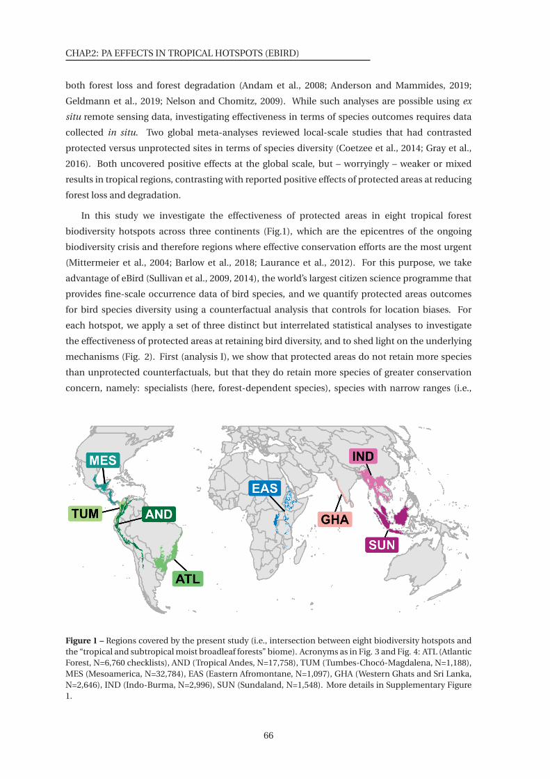
CHAP.2: PA EFFECTS IN TROPICAL HOTSPOTS (EBIRD)
both forest loss and forest degradation (Andam et al., 2008; Anderson and Mammides, 2019;
Geldmann et al., 2019; Nelson and Chomitz, 2009). While such analyses are possible using ex
situ remote sensing data, investigating effectiveness in terms of species outcomes requires data
collected in situ. Two global meta-analyses reviewed local-scale studies that had contrasted
protected versus unprotected sites in terms of species diversity (Coetzee et al., 2014; Gray et al.,
2016). Both uncovered positive effects at the global scale, but – worryingly – weaker or mixed
results in tropical regions, contrasting with reported positive effects of protected areas at reducing
forest loss and degradation.
In this study we investigate the effectiveness of protected areas in eight tropical forest
biodiversity hotspots across three continents (Fig.1), which are the epicentres of the ongoing
biodiversity crisis and therefore regions where effective conservation efforts are the most urgent
(Mittermeier et al., 2004; Barlow et al., 2018; Laurance et al., 2012). For this purpose, we take
advantage of eBird (Sullivan et al., 2009, 2014), the world’s largest citizen science programme that
provides fine-scale occurrence data of bird species, and we quantify protected areas outcomes
for bird species diversity using a counterfactual analysis that controls for location biases. For
each hotspot, we apply a set of three distinct but interrelated statistical analyses to investigate
the effectiveness of protected areas at retaining bird diversity, and to shed light on the underlying
mechanisms (Fig. 2). First (analysis I), we show that protected areas do not retain more species
than unprotected counterfactuals, but that they do retain more species of greater conservation
concern, namely: specialists (here, forest-dependent species), species with narrow ranges (i.e.,
Figure 1 – Regions covered by the present study (i.e., intersection between eight biodiversity hotspots andthe “tropical and subtropical moist broadleaf forests” biome). Acronyms as in Fig. 3 and Fig. 4: ATL (AtlanticForest, N=6,760 checklists), AND (Tropical Andes, N=17,758), TUM (Tumbes-Chocó-Magdalena, N=1,188),MES (Mesoamerica, N=32,784), EAS (Eastern Afromontane, N=1,097), GHA (Western Ghats and Sri Lanka,N=2,646), IND (Indo-Burma, N=2,996), SUN (Sundaland, N=1,548). More details in Supplementary Figure1.
66
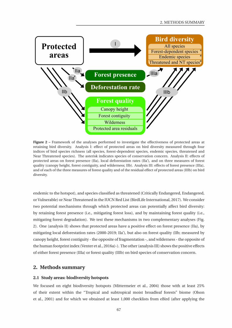
2. METHODS SUMMARY
Bird diversity
Forest presence
IIIb
IIIa
IProtectedareas
IIb
Forest quality
Canopy height
Forest contiguity
Wilderness
Protected area residuals
All species
Forest-dependent species
Endemic species
Threatened and NT species
Bird diversity
*
*
*
IIa
Deforestation rate
IIa'
Figure 2 – Framework of the analyses performed to investigate the effectiveness of protected areas atretaining bird diversity. Analysis I: effect of protected areas on bird diversity measured through fourindices of bird species richness (all species, forest-dependent species, endemic species, threatened andNear Threatened species). The asterisk indicates species of conservation concern. Analysis II: effects ofprotected areas on forest presence (IIa), local deforestation rates (IIa’), and on three measures of forestquality (canopy height, forest contiguity, and wilderness; IIb). Analysis III: effects of forest presence (IIIa),and of each of the three measures of forest quality and of the residual effect of protected areas (IIIb) on birddiversity.
endemic to the hotspot), and species classified as threatened (Critically Endangered, Endangered,
or Vulnerable) or Near Threatened in the IUCN Red List (BirdLife International, 2017). We consider
two potential mechanisms through which protected areas can potentially affect bird diversity:
by retaining forest presence (i.e., mitigating forest loss), and by maintaining forest quality (i.e.,
mitigating forest degradation). We test these mechanisms in two complementary analyses (Fig.
2). One (analysis II) shows that protected areas have a positive effect on forest presence (IIa), by
mitigating local deforestation rates (2000-2019; IIa’), but also on forest quality (IIb; measured by
canopy height, forest contiguity - the opposite of fragmentation -, and wilderness - the opposite of
the human footprint index (Venter et al., 2016a)-). The other (analysis III) shows the positive effects
of either forest presence (IIIa) or forest quality (IIIb) on bird species of conservation concern.
2. Methods summary
2.1 Study areas: biodiversity hotspots
We focused on eight biodiversity hotspots (Mittermeier et al., 2004) those with at least 25%
of their extent within the “Tropical and subtropical moist broadleaf forests” biome (Olson
et al., 2001) and for which we obtained at least 1,000 checklists from eBird (after applying the
67
CHAP.2: PA EFFECTS IN TROPICAL HOTSPOTS (EBIRD)
data selection procedure described below): Atlantic Forest, Tropical Andes, Tumbes-Chocó-
Magdalena, and Mesoamerica (Americas); Eastern Afromontane (Africa); Western Ghats and
Sri Lanka, Indo-Burma and Sundaland (Asia). Within each hotspot, we analysed only areas
overlapping the “Tropical and subtropical moist broadleaf forests” biome (Olson et al., 2001) (Fig.
1, Supplementary Figures 1,4,5), assumed to have been originally forested (see Supplementary
Methods 4D).
2.2 Data selection: eBird checklists
We obtained bird sightings from the eBird citizen science database (Sullivan et al., 2014). The
reporting system is based on checklists, whereby the observer provides: list of birds detected; GPS
location; sampling effort (whether or not all detected species are reported; sampling duration;
sampling protocol, e.g., stationary point, travel, banding; distance travelled in case of travelling
protocol); starting time of the sampling event; number of observers.
We used the eBird dataset released in December 2018 (eBird, 2018), focusing on records
from 2005 to 2018, as data collected prior to 2005 were too scarce for analysis. We filtered this
dataset to obtain high-quality checklists comparable in protocol and effort: we selected complete
checklists only (i.e., in which observers explicitly declare having reported all bird species detected
and identified); following either the ‘stationary points’ or the ‘travelling counts’ protocol; with
durations of continuous observation of 0.5-10 hrs; with observers travelling distances during the
checklist < 5 km; only from experienced observers (≥ 10 checklists; ≥ 30 species per checklist on
average; ≥ 100 different species in total); and removing potential duplicates (checklists made on
the same day at the same place). We applied some taxonomical transformation to eBird data in
order to fit with BirdLife International taxonomy (Supplementary Methods 1F).
After data filtering (more details in Supplementary Methods 1), we obtained the final dataset
used in the analyses, consisting of 66,777 checklists, covering 5,467 species, from 6,838 observers,
in eight hotspots (Supplementary Figures 4-5; Supplementary Table 2).
2.3 Site characteristics
Our analyses included two types of sites: checklist sites, corresponding to the coordinates of each
eBird checklist analysed (used in analyses I and III); and background sites, corresponding to the
centre points of a regular grid of 2x2 km covering the whole area of each hotspot evenly (used
in analysis II). We characterised each site according to six characteristics – calculated in a 1-km
radius buffer around its coordinates – two binary and four continuous: protected (if coordinates
fall within a protected area (UNEP-WCMC and IUCN, 2018); Supplementary Figure 6) versus non-
protected; forest (if > 60% of the 1-km buffer around the point is forested (ESA, 2015)) versus non-
forest (< 10% forested; sites with intermediate forest cover were removed from analyses); altitude
(National Geophysical Data Center, 1999); agricultural suitability (Zabel et al., 2014); remoteness
(Weiss et al., 2018), and the proportion of forest loss between 2000 and 2019 (Hansen et al.,
2013). In addition, we classified each forest site according to three continuous variables: canopy
height (Simard et al., 2011); forest contiguity (proportion of forest cover (ESA, 2015), 0.6 to 1); and
wilderness level (opposite of human footprint (Venter et al., 2016a)).
68
2. METHODS SUMMARY
Finally, checklist sites were also characterised according to four measures of local bird
diversity: overall species richness (total number of species detected in the checklist); richness in
forest-dependent species (high or medium dependency on forest habitats (BirdLife International,
2017)); richness in endemic species (at least 90% of their global distribution within a hotspot
(BirdLife International and HBW, 2017)); and richness in species of concern (classified as
Near Threatened or threatened, i.e., Vulnerable, Endangered, or Critically Endangered (BirdLife
International, 2017); more details in Supplementary Methods 2).
2.4 Index of observer expertise
Heterogeneity in observers’ birding skills, behaviours, and equipment increases data variability
and potentially introduces biases to the analyses (Dickinson et al., 2010; Johnston et al., 2018).
Heterogeneity is particularly high in citizen science datasets like eBird, where volunteers range
from those only familiar with a few common local birds to experienced observers capable of
detecting rare and cryptic species. As stated above, we only included checklists from relatively
experienced observers. To account for the remaining variability in observer expertise, we
calculated an observer expertise score (used as an explanatory variable in the statistical analyses),
adapted from Kelling et al. (2015) and from Johnston et al. (2018), and calculated separately for
each continent. It estimates the variation in the number of species that observers are predicted to
detect in similar conditions. To do so, we first ran a mixed General Additive Model (function gamm
from ‘mgcv’ R package (Wood, 2011)) modelling species richness of checklists against potential
confounding variables that are expected to affect either the number of species detected (sampling
protocol; n.observers number of observers; duration of sampling; time of the day) or the true
species richness (lat latitude; lon longitude; and Julian day), adding observer as a random effect:
g amm(r i chness ∼ pr otocol + n.obser ver s + s(dur ati on) + s(t i me) + te(lon, l at ,d ay) +
r andom = l i st (obser ver ∼ 1))
The notation s() indicates that the variable was used as a smoothed term; te() indicates that
the variables have been used as interacting smooth terms, allowing here species richness to vary
spatially during the year.
After fitting this model to each continental data subset, we used it to predict the logarithm of
species richness that each observer would report for a fictive stationary point with all variables
fixed to their median values. This resulted in an observer expertise score that we then assigned to
all checklists; assigning the observer score of the observer with the highest expertise score in cases
of multiple observers. This index ranged from 2.2 to 4.3 in Africa, from 2.3 to 4.4 in the Americas,
and from 2.8 to 4.5 in Asia (more details in Supplementary Methods 3).
2.5 Statistical analyses of protected area effectiveness
We investigated protected area effectiveness at retaining bird diversity through a set of three
connected statistical analyses (Fig. 2), undertaken separately for each hotspot, using GAM models
(Wood, 2011). The first analysis (I) directly estimated the effects of protection on bird diversity
while the two others (II and III) investigated the underlying mechanisms to explain the results of
the first analysis.
69
CHAP.2: PA EFFECTS IN TROPICAL HOTSPOTS (EBIRD)
Analysis I quantifies the effect of protected areas on bird diversity through models contrasting
bird diversity of checklist sites between protected versus unprotected sites, while controlling for
protected area location biases (and other potential confounding factors):
I : Bird_Diversity ∼ Protection+ locati on_bi ases + contr ol
Analysis II quantifies the effectiveness of protected areas at mitigating forest loss and forest
degradation, through models controlling for location biases and spatial autocorrelation. To
measure the effects of protection on forest loss (IIa), we built logistic models contrasting protected
versus unprotected background sites in their probability of being forested with land cover data:
IIa : Forest_presence ∼ Protection+ locati on_bi ases + te(l on, l at )
We have also run an analysis IIa’ comparing forest loss rates (log transformed to fit normal
distribution) between protected and unprotected sites:
IIa′ : log (0.001+Forest_loss) ∼ Protection+ l ocati on_bi ases + te(lon, l at )
To measure the effects of protected areas on forest degradation (IIb), we built Gaussian models
contrasting protected versus unprotected background forested sites in terms of forest quality
(canopy height, forest contiguity, or wilderness):
IIb : Forest_quality ∼ Protection+ l ocati on_bi ases + te(lon, l at )
Analysis III quantifies the effects of forest presence (IIIa) or of forest quality (IIIb) on bird
diversity, while controlling for potential confounding factors. In IIIa, we built models contrasting
bird diversity in forest versus non-forest checklist sites:
IIIa : Bird_Diversity ∼ Forest_presence+ contr ol
In IIIb, we modelled local bird diversity of forested sites against the three forest quality
variables, as well as protected status in order to capture other aspects of forest quality that could be
increased within protected areas (e.g. enforcement of hunting regulations; what we call protected
area residuals):
IIIb : Bird_Diversity ∼ scale(canopy)+scale(conti g ui t y)+scale(wi lder ness)+Protection+
contr ol
In analyses I and III, the response variable Bird_Diversity is one of the four metrics of local
bird diversity. We assumed Gaussian distribution for the overall richness, and a negative binomial
distribution for the richness in forest-dependent species, endemic species and threatened and
Near Threatened.
In analysis II, the response variable is either the binary Forest_presence (site forested or not) or
each of three measures of Forest_quality (canopy height, forest contiguity, or wilderness).
The term location_bias in analyses I and II corresponds to s(altitude) + s(remoteness) +
s(agricultural_suitability), supplemented by a control for spatial autocorrelation in analysis II
with the term + te(lon, lat). It controls for potential biases in protected area location in relation
to altitude, remoteness and agricultural suitability (Joppa and Pfaff, 2009; Venter et al., 2018)
(Supplementary Figures 7-9).
In analyses I and III, we controlled for other potential confounding factors that could affect the
70
3. RESULTS AND DISCUSSION
bird diversity reported in a checklist (Supplementary Figures 10-17). In particular, we controlled
for: heterogeneity in sampling effort (sampling duration; observer expertise; number of observers:
n.observers); temporal effects (year to account for possible trends; day to account for season);
spatial heterogeneity (lat latitude, lon longitude). lon, lat and day were used as interacting smooth
terms, enabling bird diversity variables to vary spatially across seasons (see Supplementary
Methods 2 and Supplementary Figures 10-17). The term control was thus:
s(dur ati on,k = 4) + s(exper t i se,k = 4) + s(n.obser ver s,k = 4) + s(year,k = 4) +
te(d ay, l at , l on)
When the response variable was richness in forest-dependent species, in endemic species or
in threatened and Near Threatened species, we also controlled for overall species richness, thus
using as control term:
log (over al l_r i chness)+ s(dur ati on,k = 4)+ s(exper t i se,k = 4)+ s(n.obser ver s,k = 4)+
s(year,k = 4)+ te(d ay, l at , lon)
In analysis I, altitude is already controlled for under the location_bias term; in analysis III, the
control term also includes a term controlling for it: s(altitude, k=6).
3. Results and discussion
3.1 Protected areas mitigate the replacement of species of concern
We found no consistent evidence across hotspots of an effect of protected areas on overall richness
in bird species (analysis I). Indeed, we obtained non-significant results for five out of the eight
hotspots tested, significant negative effects for two, and a significant positive effect for a single
one (Fig. 3A). Given that species richness is an intuitive and widely used measure of biodiversity
(Hillebrand et al., 2018), these results may appear worrying, by suggesting that protected areas
do not prevent local biodiversity loss. In fact, they agree with a wealth of previous evidence that
overall species richness is not a suitable indicator of local biodiversity impact, as species that go
locally extinct due to ecosystem alteration can be replaced by others – often of lower conservation
concern – with no or little impact on overall species richness (Dornelas et al., 2014; Hillebrand
et al., 2018). Accordingly, we also found that neither forest presence (Fig. 4A; Supplementary
Figure 3A; analysis IIIa) nor forest quality (Fig. 5A-C; Supplementary Figure 3B-D; analysis IIIb)
had a consistent positive effect on overall species richness, indicating that this diversity measure
is rather insensitive to habitat loss and degradation, at least at the temporal and spatial scales
considered in this study. Species richness is also known to temporarily increase at intermediate
levels of disturbance (Roxburgh et al., 2004), perhaps explaining the few observed negative effects
of protection (Fig. 3A), forest presence (Fig. 4A), and forest quality (Fig. 5) on overall species
richness.
Whereas we found no effect of protected areas on overall species richness, our results indicate
that protected areas are effective at retaining the three types of species of conservation concern
that were analysed: forest-dependent (i.e., specialists), endemics to each hotspot (i.e., narrow-
ranged), and threatened or Near Threatened (i.e., at greater risk of extinction). Indeed, controlling
for overall richness, we find for each of these three groups significant positive effects of protected
71
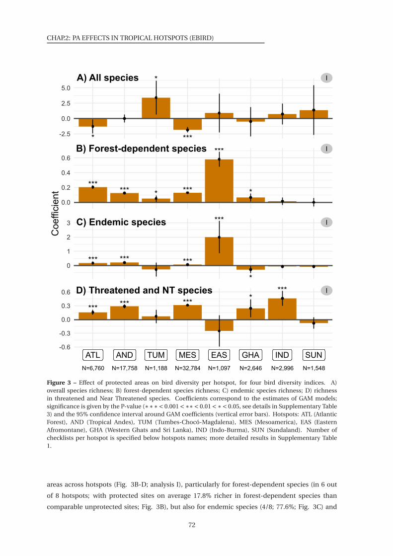
CHAP.2: PA EFFECTS IN TROPICAL HOTSPOTS (EBIRD)
* ***
*
***
***
******* *
***
***
*
******
***
****
******
ATL AND TUM MES EAS GHA IND SUN
-2.5
0.0
2.5
5.0
0.0
0.2
0.4
0.6
0
1
2
3
-0.6
-0.3
0.0
0.3
0.6
Coefficient
B) Forest-dependent species
A) All species
C) Endemic species
D) Threatened and NT species
N=6,76
I
I
I
I
ATL EAS GHA INDMES SUNAND TUM
N=6,760 N=17,758 N=1,188 N=32,784 N=1,097 N=2,646 N=1,548N=2,996
Figure 3 – Effect of protected areas on bird diversity per hotspot, for four bird diversity indices. A)overall species richness; B) forest-dependent species richness; C) endemic species richness; D) richnessin threatened and Near Threatened species. Coefficients correspond to the estimates of GAM models;significance is given by the P-value (∗∗∗< 0.001 <∗∗< 0.01 <∗< 0.05, see details in Supplementary Table3) and the 95% confidence interval around GAM coefficients (vertical error bars). Hotspots: ATL (AtlanticForest), AND (Tropical Andes), TUM (Tumbes-Chocó-Magdalena), MES (Mesoamerica), EAS (EasternAfromontane), GHA (Western Ghats and Sri Lanka), IND (Indo-Burma), SUN (Sundaland). Number ofchecklists per hotspot is specified below hotspots names; more detailed results in Supplementary Table1.
areas across hotspots (Fig. 3B-D; analysis I), particularly for forest-dependent species (in 6 out
of 8 hotspots; with protected sites on average 17.8% richer in forest-dependent species than
comparable unprotected sites; Fig. 3B), but also for endemic species (4/8; 77.6%; Fig. 3C) and
72
3. RESULTS AND DISCUSSION
threatened and Near Threatened species (5/8; 19.0%; Fig. 3D; Supplementary Table 1). The
consistency in these results may be derived from the partial overlap between the species classified
in these three classes of conservation concern (Supplementary Figure 2). Overall, our results
indicate that protected areas are effective at avoiding the replacement of species of conservation
concern (specialists, with small ranges, and at higher risk of extinction) by more widespread and
generalist species.
Our results corroborate studies in temperate regions that found that protected areas do not
protect all species and thus do not always affect species richness (Cazalis et al., 2019; Hiley et al.,
2016). However, they contrast with what was known in tropical regions from two previous global-
scale studies of protected area effectiveness, based on the meta-analysis of local-scale studies
contrasting protected versus unprotected sites. One of these studies found higher species richness
and abundances within protected areas in Africa and Asia but not in South America (Coetzee et al.,
2014); the other found higher overall richness within protected areas, but no significant effects on
the richness in rare and endemic species, including in the tropics (Gray et al., 2016). Nonetheless,
the present study provides a stronger test of protected area effectiveness in tropical forests by
focusing specifically on these biomes, using more comparable data (as emerging from a single,
coherent dataset), and by exploring the underlying mechanisms of habitat loss and degradation.
We have controlled for confounding variables in order to separate the implementation effects
of protected areas from potential location biases (see Supplementary Methods 4D), and have
also found that older protected areas tend to be more effective (in terms of conserving bird
diversity; analysis I), consistently with a cumulative implementation effect of protected areas
(Supplementary Methods 4E, Supplementary Figure 18).
3.2 Protected areas retain species of concern by mitigating forest loss
Our results suggest that protected area effectiveness at retaining species of concern is mainly
driven by their effectiveness at mitigating forest loss. First, we found significant positive effects
of protection on forest presence across all hotspots analysed, with a protected site having on
average a 17.8% higher probability of being forested than a non-protected counterfactual (Fig. 4A;
analysis IIa; Supplementary Table 1). Second, we confirmed the temporal effect of protected areas
on forests, showing across all hotspots that deforestation rates within protected areas were lower
(on average 46.7% so) than in non-protected counterfactuals (Fig. 4B; analysis IIa’; Supplementary
Table 1). These results confirm and extend previous works showing positive effects of protected
areas at reducing rates of tropical deforestation (Andam et al., 2008; Eklund et al., 2016; Nelson and
Chomitz, 2009). Third, we found that forested sites have higher richness in forest-dependent bird
species than comparable non-forested sites (across 8/8 hotspots; on average 74.9% more species),
as well as in endemic species (7/8; 250.0%) and in threatened and Near Threatened species (6/8;
122.1%; analysis IIIa; Fig.4A; Supplementary Table 1; Supplementary Figure 3A), in accordance
with the well-known devastating impact of deforestation on biodiversity (Barlow et al., 2018,
2016; Peres et al., 2006). Particularly in line with our results, Rutt et al. (2019), have highlighted
the replacement of forest-dependent bird species by generalist species following experimental
deforestation in the Amazon.
73
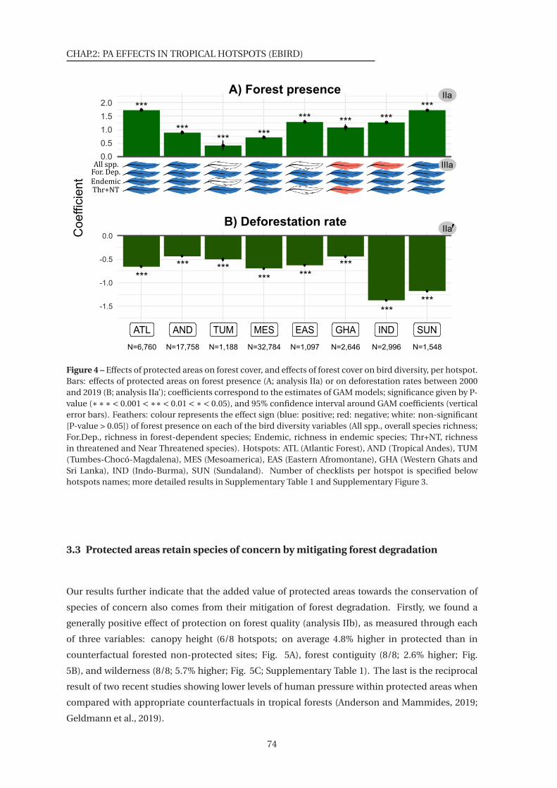
CHAP.2: PA EFFECTS IN TROPICAL HOTSPOTS (EBIRD)
*** *** ***
******
***
0.0
0.5
1.0
1.5
2.0 *** ***
-1.5
-1.0
-0.5
0.0
***
*** ****** ***
***
******
ATL AND TUM MES EAS GHA IND SUNATL AND TUM MES EAS GHA IND SUNATL EAS GHA INDMES SUNAND TUM
N=6,760 N=17,758 N=1,188 N=32,784 N=1,097 N=2,646 N=1,548N=2,996
IIa
IIIaAll spp.For. Dep.
EndemicThr+NT
A) Forest presenceCoefficient
B) Deforestation rateIIa'
Figure 4 – Effects of protected areas on forest cover, and effects of forest cover on bird diversity, per hotspot.Bars: effects of protected areas on forest presence (A; analysis IIa) or on deforestation rates between 2000and 2019 (B; analysis IIa’); coefficients correspond to the estimates of GAM models; significance given by P-value (∗∗∗< 0.001 <∗∗< 0.01 <∗< 0.05), and 95% confidence interval around GAM coefficients (verticalerror bars). Feathers: colour represents the effect sign (blue: positive; red: negative; white: non-significant[P-value > 0.05]) of forest presence on each of the bird diversity variables (All spp., overall species richness;For.Dep., richness in forest-dependent species; Endemic, richness in endemic species; Thr+NT, richnessin threatened and Near Threatened species). Hotspots: ATL (Atlantic Forest), AND (Tropical Andes), TUM(Tumbes-Chocó-Magdalena), MES (Mesoamerica), EAS (Eastern Afromontane), GHA (Western Ghats andSri Lanka), IND (Indo-Burma), SUN (Sundaland). Number of checklists per hotspot is specified belowhotspots names; more detailed results in Supplementary Table 1 and Supplementary Figure 3.
3.3 Protected areas retain species of concern by mitigating forest degradation
Our results further indicate that the added value of protected areas towards the conservation of
species of concern also comes from their mitigation of forest degradation. Firstly, we found a
generally positive effect of protection on forest quality (analysis IIb), as measured through each
of three variables: canopy height (6/8 hotspots; on average 4.8% higher in protected than in
counterfactual forested non-protected sites; Fig. 5A), forest contiguity (8/8; 2.6% higher; Fig.
5B), and wilderness (8/8; 5.7% higher; Fig. 5C; Supplementary Table 1). The last is the reciprocal
result of two recent studies showing lower levels of human pressure within protected areas when
compared with appropriate counterfactuals in tropical forests (Anderson and Mammides, 2019;
Geldmann et al., 2019).
74

3. RESULTS AND DISCUSSION
Figure 5 – Effects of protected areas on forest quality, and effects of forest quality on bird diversity, perhotspot. Bars: effects of protected areas on forest quality (A, canopy height; B, forest contiguity; C,wilderness; D, protected area residuals; analysis IIb); coefficients correspond to the estimates of GAMmodels; significance given by P-value (∗∗∗ < 0.001 < ∗∗ < 0.01 < ∗ < 0.05), and 95% confidence intervalaround GAM coefficients (vertical error bars). Feathers: colour represents the effect sign (blue: positive; red:negative; white: non-significant [P-value > 0.05]) of each habitat quality variable on each of the bird diversityvariables (All spp., overall species richness; For.Dep., richness in forest-dependent species; Endemic,richness in endemic species; Thr+NT, richness in threatened and Near Threatened species). Hotspots:ATL (Atlantic Forest), AND (Tropical Andes), TUM (Tumbes-Chocó-Magdalena), MES (Mesoamerica),EAS (Eastern Afromontane), GHA (Western Ghats and Sri Lanka), IND (Indo-Burma), SUN (Sundaland).Number of checklists per hotspot is specified below hotspots names (only forest checklists in this analysis);more detailed results in Supplementary Table 1 and Supplementary Figure 3.
75
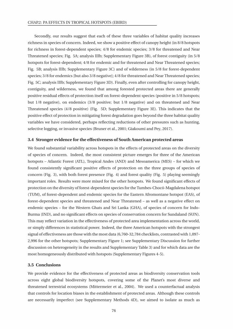
CHAP.2: PA EFFECTS IN TROPICAL HOTSPOTS (EBIRD)
Secondly, our results suggest that each of these three variables of habitat quality increases
richness in species of concern. Indeed, we show a positive effect of canopy height (in 8/8 hotspots
for richness in forest-dependent species; 4/8 for endemic species; 3/8 for threatened and Near
Threatened species; Fig. 5A; analysis IIIb; Supplementary Figure 3B), of forest contiguity (in 5/8
hotspots for forest-dependent; 4/8 for endemic and for threatened and Near Threatened species;
Fig. 5B; analysis IIIb; Supplementary Figure 3C) and of wilderness (in 5/8 for forest-dependent
species; 3/8 for endemics [but also 3/8 negative]; 4/8 for threatened and Near Threatened species;
Fig. 5C; analysis IIIb; Supplementary Figure 3D). Finally, even after controlling for canopy height,
contiguity, and wilderness, we found that among forested protected areas there are generally
positive residual effects of protection itself on forest-dependent species (positive in 5/8 hotspots;
but 1/8 negative), on endemics (3/8 positive; but 1/8 negative) and on threatened and Near
Threatened species (4/8 positive) (Fig. 5D; Supplementary Figure 3E). This indicates that the
positive effect of protection in mitigating forest degradation goes beyond the three habitat quality
variables we have considered, perhaps reflecting reductions of other pressures such as hunting,
selective logging, or invasive species (Bruner et al., 2001; Giakoumi and Pey, 2017).
3.4 Stronger evidence for the effectiveness of South American protected areas
We found substantial variability across hotspots in the effects of protected areas on the diversity
of species of concern. Indeed, the most consistent picture emerges for three of the American
hotspots – Atlantic Forest (ATL), Tropical Andes (AND) and Mesoamerica (MES) – for which we
found consistently significant positive effects of protection on the three groups of species of
concern (Fig. 3), with both forest presence (Fig. 4) and forest quality (Fig. 5) playing seemingly
important roles. Results were more mixed for the other hotspots. We found significant effects of
protection on the diversity of forest-dependent species for the Tumbes-Chocó-Magdalena hotspot
(TUM), of forest-dependent and endemic species for the Eastern Afromontane hotspot (EAS), of
forest-dependent species and threatened and Near Threatened – as well as a negative effect on
endemic species – for the Western Ghats and Sri Lanka (GHA), of species of concern for Indo-
Burma (IND), and no significant effects on species of conservation concern for Sundaland (SUN).
This may reflect variation in the effectiveness of protected area implementation across the world,
or simply differences in statistical power. Indeed, the three American hotspots with the strongest
signal of effectiveness are those with the most data (6,760-32,784 checklists, contrasted with 1,097-
2,996 for the other hotspots; Supplementary Figure 1; see Supplementary Discussion for further
discussion on heterogeneity in the results and Supplementary Table 3) and for which data are the
most homogeneously distributed with hotspots (Supplementary Figures 4-5).
3.5 Conclusions
We provide evidence for the effectiveness of protected areas as biodiversity conservation tools
across eight global biodiversity hotspots, covering some of the Planet’s most diverse and
threatened terrestrial ecosystems (Mittermeier et al., 2004). We used a counterfactual analysis
that controls for location biases in the establishment of protected areas. Although these controls
are necessarily imperfect (see Supplementary Methods 4D), we aimed to isolate as much as
76
4. ACKNOWLEDGEMENTS
possible the effects of implementation itself, i.e., the added value of protection. We found that
this value does not lie in preventing declines in overall local species richness, but in avoiding the
replacement of species that are most in need of conservation efforts: the forest specialists that are
most at risk from forest loss or degradation; the endemic species that make each hotspot globally
irreplaceable; and threatened or Near Threatened that are at higher risk of global extinction.
Our results contribute to the body of evidence supporting the effectiveness of protected areas
at avoiding forest loss (Andam et al., 2008; Nelson and Chomitz, 2009), focusing here on tropical
forests of biodiversity hotspots. Furthermore, they indicate that this is the main mechanism
through which protection has a positive effect on retaining bird species of concern. In addition,
we provide evidence that it is not the only mechanism, with protection also having a significant
effect on bird diversity by mitigating forest degradation, as measured through canopy height,
fragmentation and wilderness levels. Finally, we found evidence for a residual effect of protection
(once controlling for the effects on forest presence and quality) that may reflect management
measures of other pressures such as hunting, small-scale logging, or invasive species.
In this study, we found that protected areas are effective in the sense that they perform better
than comparable unprotected sites. We have, however, not demonstrated that they are sufficiently
effective to halt habitat loss and degradation (which previous studies found to be ongoing and
sometimes increasing within protected areas; Anderson and Mammides (2019), Geldmann et al.
(2019), Nelson and Chomitz (2009)) nor that they halt population declines (which are still ongoing
within many protected areas; Beaudrot et al. (2016), Craigie et al. (2010), Hallmann et al. (2017)).
Furthermore, our analysis does not address whether protected areas are sufficient in terms of
their extent or representativeness (while previous studies attest that they are not; Butchart et al.
(2015),Watson et al. (2014)). Nonetheless, our results indicate that protected areas are already
making a measurable difference in terms of biodiversity conservation in several regions of the
world where the conservation stakes are the highest. In this year of 2020 when Aichi Targets
are due to be reached (SCBD, 2010), yet some governments are announcing protected areas
degazettement and downsizing (Kroner et al., 2019), our results support the key role of protected
areas as global biodiversity conservation tools. We therefore join calls for the strategic expansion
of the global protected areas estate and increased investment to ensure that they are effectively
managed (Barnes et al., 2018; Maxwell et al., 2020; Visconti et al., 2019).
4. Acknowledgements
We are grateful to the numerous observers who contributed records to eBird, and to the eBird
team at Cornell Lab of Ornithology for creating and managing this database. J. Kelly was funded
by the European Union’s Horizon 2020 research and innovation programme under the Marie
Skłodowska-Curie grant agreement No 766417. This communication reflects only the authors’
view and the Research Executive Agency of the European Union is not responsible for any use that
may be made of the information it contains. K. Princé was funded by the French National Research
Agency under the grant agreement No ANR-17-CE04-0012.
77

CHAP.2: PA EFFECTS IN TROPICAL HOTSPOTS (EBIRD)
Supplementary materials
Supplementary Methods
1. Data selection: eBird checklists
A. Spatial filtering
We focused on global biodiversity hotspots (Mittermeier et al., 2004) which overlapped by more
than 25% of their extent the “Tropical and subtropical moist broadleaf forests” biome (boundaries
from Olson et al. (2001)). We obtained 16 hotspots: Atlantic Forest, Tropical Andes, Tumbes-
Chocó-Magdalena, Caribbean Islands, Mesoamerica, Guinean Forests of West Africa, Eastern
Afromontane, Coastal Forests of Eastern Africa, Madagascar, Western Ghats and Sri Lanka, Indo-
Burma, Sundaland, Philippines, East Melanesian Islands, and New Caledonia.
Of these, we ultimately analysed only eight hotspots for which we obtained more than 1,000
eBird checklists (after following the data filtering procedure detailed below). We first downloaded
the eBird checklists for the respective countries per hotspot (eBird codes between brackets):
• Atlantic Forest: Argentina [AR], Brazil [BR], Paraguay [PY].
• Tropical Andes: Argentina [AR], Bolivia [BO], Colombia [CO], Ec-uador [EC], Peru [PE],
Venezuela [VE].
• Tumbes-Chocó-Magdalena: Colombia [CO], Ecuador [EC], Panama [PA], Peru [PE].
• Mesoamerica: Belize [BZ], Costa Rica [CR], Guatemala [GT], Hon-duras [HN], Mexico [MX],
Nicaragua [NI], Panama [PA], El Salvador [SV].
• Eastern Afromontane: Burundi [BI], Democratic Republic of Congo [CD], Eritrea [ER],
Ethiopia [ET], Kenya [KE], Mozambique [MZ], Rwanda [RW], Sudan [SD], South Sudan [SS],
Tanzania [TZ], Uganda [UG].
• Western Ghats and Sri Lanka: India [IN], Sri Lanka [LK].
• Indo-Burma: Bangladesh [BD], Hong Kong [HK], India [IN], Cam-bodia [KH], Laos [LA],
Myanmar [MM], Malaysia [MY], Thailand [TH], Vietnam [VN], Chi-na [CN].
• Sundaland: Brunei [BN], Indonesia [ID], Malaysia [MY], Thailand [TW].
We then filtered the checklists to include only those overlapping both the hotspot and the
“Tropical and subtropical moist broadleaf forests” biome.
In the Indo-Burma hotspot, we excluded records from China [CN] (19% of the hotspot, 2% of
checklists) because no protected area data were available for this country in the publicly available
version of the World Database on Protected Areas (UNEP-WCMC and IUCN, 2018).
78
SUPPLEMENTARY MATERIALS
B. Filtering by sampling protocol
In order to be able to treat this dataset as presence/absence, we focused on checklists for which
observers stated that they reported every species detected (Sullivan et al., 2009). Accordingly, we
also removed checklists unlikely to capture all species because using particular protocols (e.g.
banding) or targeting specific groups (e.g. waders, nocturnal). We therefore used only checklists
for which the protocol reported was either ‘stationary points’ or ‘travelling counts’. In stationary
points, observers remain at the checklist location, and report both the starting time and the
duration of the sampling. In travelling counts, moving observers report the checklist location
(usually the mid-point of their itinerary), starting time, duration of the sampling and distance
travelled. We excluded travelling counts with a travel distance > 5km, as they may not represent
the local bird composition around the reported GPS location. To further increase comparability,
we excluded sampling events that were very short (< 30 minutes) or very long (> 10 hours).
We also included some data classified in the eBird dataset under the protocol category
‘historical counts’, which consist of sampling events for which birding was the primary focus but
for which the observer was not able to fill all fields required for reporting stationary points or travel
counts (e.g. starting time, duration, distance). We used historical counts if duration was known
and ranged from 30 minutes to 10 hours, and if distance was known and shorter than 5 km.
C. Observation filtering
We excluded observations that were disapproved by the eBird review process, corresponding to
exotic, feral or escaped individuals. Established introduced species were kept in the dataset.
Using the auk_r ol lup function from the above-mentioned R package ‘auk’ (Strimas-Mackey
et al., 2017), we brought all observations of subspecies to the species level.
D. Filtering checklists based on observer experience
To aim for complete checklists, we filtered observations to retain only those submitted by relatively
experienced observers. In order to identify these, we analysed checklists per observer across each
of the three continents, defined according to the following list of countries (eBird codes between
brackets):
• Americas: Antigua and Barbuda [AG], Anguilla [AI], Argentina [AR], Boliv-ia [BO], Brazil
[BR], Bahamas [BS], Belize [BZ], Chile [CL], Colombia [CO], Costa Rica [CR], Cuba [CU],
Dominica [DM], Dominican Republic [DO], Ecuador [EC] Falkland Islands [FK], Grenada
[GD], French Guyana [GF], Guadeloupe [GP], Guatemala [GT], Guyana [GY], Honduras
[HN], Haiti [HT], Jamaica [JM], Saint Knitts and Nevis [KN], Cayman Is-lands [KY], Saint
Lucia [LC], Martinique [MQ], Montserrat [MS], Mexico [MX], Nicaragua [NI], Panama [PA],
Peru [PE], Puerto Rico [PR], Paraguay [PY], Suriname [SR], El Savador [SV], Turks and Caicos
Islands [TC], Uruguay [UY], Saint Vincent and the Grenadines [VC], Venezuela [VE], British
Virgin Islands [VG], Virgin Islands [VI].
• Asia: Bangladesh [BD], Brunei [BN], Bhutan [BT], China [CN], Hong Kong [HK], Indonesia
[ID], India [IN], Cambodia [KH], Laos [LA], Sri Lanka [LK], Myanmar [MM], Malaysia [MY],
79
CHAP.2: PA EFFECTS IN TROPICAL HOTSPOTS (EBIRD)
Nepal [NP], Papua New Guinea [PG], Philippines [PH], Pakistan [PK], Thailand [TH], Taiwan
[TW], Vietnam [VN].
• Africa: Angola [AO], Burkina Faso [BF], Burundi [BI], Benin [BJ], Botswa-na [BW], Demo-
cratic Republic of Congo [CD], Central African Republic [CF], Congo [CG], Cote d’Ivoire [CI],
Cameroon [CM], Djibouti [DJ], Algeria [DZ], Egypt [EG], Western Saha-ra [EH], Eritrea [ER],
Ethiopia [ET], Gabon [GA], Ghana [GH], Gambia [GM], Guinea [GN], Equatorial Guinea
[GQ], Guinea-Bissau [GW], Kenya [KE], Liberia [LR], Lesotho [LS], Lib-ya [LY], Morocco
[MA], Madagascar [MG], Mali [ML], Mauritania [MR], Malawi [MW], Mozambique [MZ],
Namibia [NA], Niger [NE], Nigeria [NG], Rwanda [RW], Sudan [SD], Sierra Leone [SL],
Senegal [SN], Somalia [SO], South Sudan [SS], Sao Tomé and Principe [ST], Swaziland [SZ],
Chad [TD], Togo [TG], Tunisia [TN], Tanzania [TZ], Uganda [UG], South Africa [ZA], Zambia
[ZM], Zimbabwe [ZW].
Within each given continent, we defined as ‘experienced observers’ those who had submitted
≥ 10 checklists to eBird, with ≥ 30 species per checklist on average, and covering ≥ 100 different
species in total. We only retained the checklists by the observers who were classified as
‘experienced’ in the corresponding continent.
E. Removing duplicates
Multiple observations of the same birds can happen either because several observers travelled
together or because they came independently to the same site on the same day, both situations
creating pseudo-replication.
When submitting checklists, observers can specify if they were observing with others. For
checklists in this situation, we removed duplication by merging checklists, using the auk unique
function implemented in the R package ‘auk’ (a package specifically created to process eBird data
(Strimas-Mackey et al., 2017)) and keeping the number of observers as covariates for all analyses.
In addition, we filtered for other possible duplicates by independent observers: whenever two
checklists with equal dates were reported with less than 2 km between them, we randomly selected
one of them.
F. Taxonomic standardisation
The taxonomic classification used in eBird follows the Clements taxonomy (Clements et al., 2018).
In order to be able to cross the bird observation dataset with the species’ trait data (section 2
below) we have converted it to the taxonomy used by BirdLife International and HBW (BirdLife
International and HBW, 2017). For this, we used an unpublished table, kindly provided by the
Cornell Lab of Ornithology, which summarises relationships between the two taxonomies, by
applying the following rules:
• In the case of a simple difference in name, we applied the BirdLife name to the eBird records
(295 species).
• Whenever a single species in the BirdLife list was treated as multiple species in eBird, we
lumped the eBird records (92 species).
80
SUPPLEMENTARY MATERIALS
• Whenever multiple species in the BirdLife list were treated as a single species in eBird,
we split the eBird records based on the BirdLife distribution maps for the corresponding
species (358 species). Any records outside the BirdLife distribution maps were assigned to
the species whose distribution was the closest. In the extreme rare case of overlap between
distributions of these species (12 over the 5,467 species for a total of ∼ 1,500 observations),
observations falling within the distribution overlap were all assigned to a single of the two
species (randomly selected between both).
The lists of species in each case are detailed in the Supplementary Data 1.
G. Final dataset analysed
After the above steps, plus the removal of sites of intermediate forest cover (see section 2A below),
we obtained a total of 66,777 checklists, covering 5,467 species, from 6,838 observers, in eight
hotspots. The list of species per hotspot is available in Supplementary Data 2. This was the final
dataset used in the analyses. For further details, and a breakdown per hotspot, see Supplementary
Table 2 and Supplementary Figures 4-5.
2. Site characteristics
Our analyses include two types of sites: checklist sites, corresponding to the coordinates of
each eBird checklist analysed (used in analyses I and III, see below); and background sites,
corresponding to the centre points of a regular grid of 2*2 km covering evenly the whole area of
each hotspot (used in analysis II).
We characterised each site according to six variables: two binary (protected vs. non-protected;
forest vs. non-forest) and four continuous (altitude; agricultural suitability; remoteness; propor-
tion of forest loss between 2000 and 2019). For forest sites, we characterised them according to
three additional continuous variables (canopy height; forest contiguity; and wilderness level).
Checklist sites were also characterised according to four measures of local bird diversity
(richness of all species, of forest-dependent species, of endemic species, and of threatened and
Near Threatened species).
A. Protection (binary)
A site was considered ‘protected’ if its coordinates overlapped a protected area, as mapped in the
World Database on Protected Areas (UNEP-WCMC and IUCN, 2018). As is the standard protocol
in global analysis of protected area coverage (UNEP-WCMC and IUCN, 2019), we excluded: “Man
and Biosphere” reserves; protected areas without associated polygons; protected areas that did
not have as status “designated”, “inscribed” or “established”.
We would have obtained similar results if we had instead derived the protection status from
the proportion of area under protection within a 1-km buffer around the site, as the vast majority
of buffers are protected by either 0 or 100% (Supplementary Figure 6).
B. Forest habitat (binary)
To derive whether a site was forested or not, we used the 2015 version of Climate Change Initiative
Land Cover layer, with a resolution of 300m (ESA, 2015). We considered as forests all categories
81
CHAP.2: PA EFFECTS IN TROPICAL HOTSPOTS (EBIRD)
described as strict Tree Cover (i.e. codes 50-90, 160 and 170), and as non-forest all others (but
excluding from the analyses water bodies, code 210).
For each site, we first calculated the percentage of pixels overlapping the 1-km buffer that were
forest. We then classified as ‘forest’ the sites with > 60% forest, and as ‘non-forests’ those with <
10% forest. We thus obtained two types of localities very contrasting in their forest cover, removing
from the analyses all sites with intermediate (10 to 60%) cover.
C. Altitude (continuous)
Altitude data were obtained from the GLOBE Digital Elevation Model (National Geophysical Data
Center, 1999), which has a 0.008 degree resolution (∼ 930m at latitude 0). We calculated the
altitude per site as the median of the values intersecting a 1-km buffer around the site.
D. Agricultural suitability (continuous)
We used a global raster of resolution∼ 1-km mapping a value of agricultural suitability (Zabel et al.,
2014). Their model estimates for each cell the suitability of each of the 16 most important food
and energy crops in the world (based on climatic conditions, soil and topography) and assigns to
the cell the value of the crop with the highest suitability. It has no unit and is included in a 0 -
100 interval. We obtained a value of agricultural suitability per site as the median of the values
intersecting a 1-km buffer around the site.
E. Remoteness (continuous)
Remoteness was derived from the global accessibility map of resolution ∼ 1-km, which estimates
the travel time needed for a human to reach the nearest city with ≥ 1,500 inhabitants (Weiss et al.,
2018). We calculated a remoteness value per site as the median of the values intersecting a 1-km
buffer around the site.
F. Canopy height (continuous; forest sites only)
We used a global raster of canopy height at resolution ≥ 1-km, limited to maximum canopy heights
of 40m, derived from spaceborne light detection and ranging (lidar) data (Simard et al., 2011). We
calculated the canopy height value for all forest sites as the median of the values intersecting a
1-km buffer around the site.
G. Forest contiguity (continuous; forest sites only)
Using the above-mentioned forest layer (used to classify sites as forest or not), we assigned to each
forest site the proportion of forest cover (0.6 to 1) as an index of forest contiguity.
H. Wilderness level (continuous; forest sites only)
We used the 2009 global terrestrial human footprint map (Venter et al., 2016a), with a resolution
∼ 1-km, obtained by combining spatial information on human pressures including human
infrastructures, agricultural land use and population density. For each forest site, we obtained
a wilderness value as the opposite of the median human footprint (-1 * human footprint) across
pixels intersecting the 1-km buffer around the site.
82
SUPPLEMENTARY MATERIALS
I. Deforestation rates (continuous; all sites)
We used a global map of forest loss between 2000 and 2019 based on Landsat imagery, which
has a resolution of ∼ 30m (Hansen and DeFries, 2007). For each background buffer (regardless
of the Non-forest/Intermediate/Forest classification), we calculated the proportion of pixels that
experienced forest loss between 2000 and 2019.
J. Overall species richness
For each checklist site, we calculated the total number of species detected in the checklist.
K. Richness in forest-dependent species
For each checklist site, we calculated the total number of species classified as ‘forest-dependent’.
These are species classified as either highly- or medium-dependent in a pre-existing classification
by BirdLife International (2017) that includes five categories:
• Highly-dependent: Forest specialists; characteristic of the interior of undisturbed forest;
may persist in secondary forest and forest patches if their particular ecological requirements
are met, but where they do occur away from the interior, they are usually less common;
rarely seen in non-forest habitats; breeding is almost invariably within forest.
• Medium-dependent: Forest generalists; may occur in undisturbed forest but also regularly
found in forest strips, edges and gaps; likely to be commoner in such situations and in
secondary forest than in the interior of intact forest; breeding is typically within forest.
• Low-dependent: Often recorded in forest, but not dependent on it; almost always more
common in non-forest habitats, where most likely to breed.
• Non-forest species: Does not normally occur in forest.
• Unknown (none in the dataset): Occurs or probably occurs in forest, but dependency on it
is unknown, but could be high.
L. Richness in endemic species
For each checklist site, we calculated the total number of species that are classified as ‘endemic’
to the corresponding hotspot. This includes all species with at least 90% of its global distribution
(BirdLife International and HBW, 2017) contained within the boundary of the hotspot (considering
the whole area of the hotspot, not only the part included in the “Tropical and subtropical moist
broadleaf forests” biome).
M. Richness in threatened and Near Threatened species
For each checklist site, we calculated the total number of species classified as being either
threatened (Vulnerable, Endangered, or Critically Endangered) or Near Threatened in the
International Union for Conservation of Nature (IUCN) Red List of Threatened Species (BirdLife
International, 2017).
83
CHAP.2: PA EFFECTS IN TROPICAL HOTSPOTS (EBIRD)
3.Index of observer expertise
For each observer in our analysis, we derived an expertise score using an index adapted from
Kelling et al. (2015) and from Johnston et al. (2018). Calculated separately for each continent, the
index estimates the variation in the number of species that observers are predicted to detect in
similar conditions.
We first ran a mixed General Additive Model (function gamm from ‘mgcv’ R package (Wood,
2011)) modelling the species richness of checklists against several sampling variables that are
expected to affect species richness, adding observer (i.e., observer individual identifying number)
as a random effect:
g amm(r i chness ∼ pr otocol + n.obser ver s + s(dur ati on) + s(t i me) + te(lon, l at ,d ay) +
r andom = l i st (obser ver ∼ 1))
To control for differences in checklist sampling effort, we included both dur ati on (of
sampling, in minutes) and t i me (starting hour of sampling) as smooth terms, allowing non-linear
correlations. We included lon (longitude, in decimal degrees), l at (latitude, in decimal degrees)
and d ay (Julian date, from 1 to 365/366) as a smoothed three-way interaction, thus allowing
richness to vary across space and season of the year. We opted for a GAM (following Kelling
et al. (2015)) rather than a Generalised Linear Model (as Johnston et al. (2018)) because the former
allows for non-linear effects. For fitting issues, we only included a random effect on intercept,
rather than also on the slope between duration and richness, as in Kelling et al. (2015).
Following Johnston et al. (2018), we fitted this model to a nearly complete dataset per
continent (defined as in section 1D), i.e., before the filtering steps detailed in sections 1 and 2A. The
only filtering rules applied were to exclude: observations prior to 2005; disapproved observations;
checklists that did not report all species observed (because the model is based on richness). We
also removed checklists that did not report one of the covariates (about 15% of observations), given
that the GAMM cannot accommodate empty records.
We assumed that species richness followed a Poisson distribution, as in Kelling et al. (2015)
and Johnston et al. (2018), because the dataset includes many checklists with low richness,
making the distribution closer to a Poisson than a Gaussian distribution.
Having fitted the model to the data, we then used it to predict the species richness that each
observer would report for a fictive stationary point with all variables fixed to their median values.
The observer expertise score, measured as the logarithm of this predicted species richness, ranged
from 2.2 to 4.3 in Africa, from 2.3 to 4.4 in the Americas, and from 2.8 to 4.5 in Asia. We then
assigned to each checklist used in our analysis the expertise score of the observer. In case of
multiple observers, we assigned the score of the observer with the highest expertise score. This
score was then used as an explanatory variable in the statistical analyses below.
84
SUPPLEMENTARY MATERIALS
4. Statistical analyses of protected area effectiveness
We investigated protected area effectiveness at retaining bird diversity through a set of three
connected statistical analyses (Fig. 2). These analyses were undertaken separately for each hotspot
to allow for variations across hotspots in the relations between bird diversity and covariates (e.g.,
altitude, remoteness, protection), and because sampling effort is too heterogeneous between
hotspots. We used General Additive Models (GAMs) for all analyses, which are similar to
Generalised Linear Models, but accommodate nonlinear relationships between response and
explanatory variables (Wood, 2011; Zuur et al., 2009).
We implemented these models using the ‘mgcv’ R package (Wood, 2011), running an
independent model for each hotspot and for each response variable.
In analyses I and III, we assumed a negative binomial distribution for all models, except for
those where overall species richness was the response variable. For the later, the distribution
obtained after the filtering of checklists was closer to a Gaussian distribution, so we assumed
that instead. In analysis II, we assumed a Binomial distribution for forest presence and Gaussian
distributions for the three variables of forest quality.
A. Analysis I: effect of protected areas on bird diversity
Analysis I quantifies the effect of protected areas on the bird diversity reported in checklists,
controlling for site location biases and other potential confounding factors. The model has the
following structure:
Bird_Diversity ∼ Protection+ locati on_bi ases + contr ol
where:
• Bird_Diversity corresponds to one of the four bird diversity indices: overall richness;
richness in forest-dependent species; richness in endemics; richness in threatened and Near
Threatened species;
• Protection corresponds to the binary variable indicating whether the site is protected (1) or
not (0);
• locati on_bi ases corresponds to a term controlling for eventual spatial biases on
the location of protected areas, formalised as: s(al t i tude) + s(r emoteness) +
s(ag r i cul tur al _sui t abi l i t y), corresponding to the use of these three variables in
independent smoothed terms (allowing non-linear relationships) without limiting the
curves complexity (Supplementary Figure 8);
• contr ol corresponds to a term accounting for heterogeneity in sampling effort and poten-
tial spatiotemporal variation in bird diversity metrics. In models using the overall species
richness as response variable, this was formalised as: s(dur ati on,k = 4)+ s(exper t i se,k =
4) + s(year,k = 4) + te(d ay, l at , lon). For all other models, we also controlled for
overall species richness, so it became: log (over al l_r i chness) + s(dur ati on,k = 4) +
s(exper t i se,k = 4)+ s(n.obser ver s,k = 4)+ s(year,k = 4)+ te(l at , lon,d ay). Where:
85
CHAP.2: PA EFFECTS IN TROPICAL HOTSPOTS (EBIRD)
– s(dur ati on,k = 4) is the sampling duration in minutes, used here as an independent
smoothed term with the degree of the smoothing function fixed to 4, in order to limit
the curve complexity (Supplementary Figures 10-17). Results were robust to changes
in the degree of smoothing function;
– s(exper t i se,k = 4) is the observer expertise score for the checklist, used here as an
independent smoothed term with the degree of the smoothing function fixed to 4, in
order to limit the curve complexity (Supplementary Figures 10-17);
– s(n.obser ver s,k = 4) is the number of observers present during the sampling
– s(year,k = 4) is the year of observation, included to account for potential temporal
trends in the region, used here as an independent smoothed term with the degree of
the smoothing function fixed to 4, in order to limit the curve complexity (Supplemen-
tary Figures 10-17);
– te(l at , lon,d ay) are the site’s decimal coordinates and the Julian date of the observa-
tion (from 1 to 365/366), used as a three-way interaction smoothed-term, allowing bird
diversity indices to vary spatially during the year (e.g. a species can occur in a region
more often during the winter while occurring more often in another region during the
summer), thus enabling to account for migration patterns (Supplementary Figures 10-
17);
– log (over al l_r i chness) is the logarithm of the overall species richness. It was used in
all models with richness in forest-dependent species, endemic species, and threatened
and Near Threatened species as response variable (log-scaled because we assumed
Negative Binomial distributions for these three variables). Therefore, these models test
the effect of protection or habitat on the richness in forest-dependent species, endemic
species or threatened and Near Threatened species, for a given overall species richness
(Supplementary Figures 10-17).
B. Analysis II: effect of protected areas on forest quantity and quality
Analysis II quantifies the effect of protected areas at mitigating forest loss (analysis IIa and IIa’)
or forest degradation (analysis IIb), controlling for site location biases. Model were built from all
background sites (excluding Intermediate forests) within each hotspot. The model structure for
analysis IIa is:
Forest_presence ∼ Protection+ locati on_bi ases + te(l on, l at )
where:
• Forest_presence corresponds to the binary variable indicating whether the site is forested (1)
or not (0);
• Protection corresponds to the binary variable indicating whether the site is protected (1) or
not (0);
• locati on_bi ases corresponds to a term controlling for the possibility of location biases in
protected areas (as above) (Supplementary Figure 9);
86
SUPPLEMENTARY MATERIALS
• te(lon, l at ) corresponds to a two-way interaction smoothed term, used here to control for
spatial autocorrelation in habitat variables.
The model used for analysis IIa’ was identical in its explanatory variables but had as response
variable the proportion of forest lost between 2000 and 2019. Models were built from all
background sites (including Intermediate forests) with the following structure:
log (Deforestation_rates+0.001) ∼ Protection+ locati on_bi ases + te(lon, l at )
where:
• Deforestation_rates corresponds to the proportion of forest lost between 2000 and 2019.
This proportion was log-transformed [log (Deforestation_rates+ 0.001)] so that it fit with a
Gaussian distribution;
• Protection corresponds to the binary variable indicating whether the site is protected (1) or
not (0);
• l ocati on_bi ases corresponds to a term controlling for the possibility of location biases in
protected areas (as above) (Supplementary Figure 9);
• te(lon, l at ) corresponds to a two-way interaction smoothed term, used here to control for
spatial autocorrelation in habitat variables.
The models for analysis IIb were restricted to forest sites and have the following structure:
Forest_quality ∼ Protection+ l ocati on_bi ases + te(lon, l at )
where:
• Forest_quality corresponds to one of the three continuous variable used for forest quality:
canopy height, forest contiguity, and wilderness;
• Protection corresponds to the binary variable indicating whether the site is protected (1) or
not (0);
• l ocati on_bi ases corresponds to a term controlling for the possibility of location biases in
protected areas (as above) (Supplementary Figure 9);
• te(lon, l at ) corresponds to a two-way interaction smoothed term, used here to control for
spatial autocorrelation in habitat variables.
C. Analysis III: effect of forest presence and quality on bird diversity
Analysis III quantifies the effects of forest presence (IIIa) and forest quality (IIIb) on the bird
diversity reported in checklists. The model structure for analysis IIIa is:
Bird_Diversity ∼ Forest_presence+ contr ol
where:
• Bird_Diversity corresponds to one of the four bird diversity indices: overall richness;
richness in forest-dependent species; richness in endemics; richness in threatened and Near
Threatened species;
87
CHAP.2: PA EFFECTS IN TROPICAL HOTSPOTS (EBIRD)
• contr ol corresponds to a term accounting for heterogeneity in sampling effort and
potential spatiotemporal variation in bird diversity metrics. It corresponds to the term used
in analysis I, but supplemented with s(al t i tude,k = 6), the altitude in meters, used here
as an independent smoothed term with the degree of the smoothing function fixed to 4, in
order to limit the curve complexity;
The models for analysis IIIb were restricted to forest sites and have the following structure:
Bird_Diversity ∼ scale(canopy) + scale(conti g ui t y) + scale(wi lder ness) + Protection +
contr ol
where:
• Bird_Diversity corresponds to one of the four bird diversity indices: overall richness;
richness in forest-dependent species; richness in endemics; richness in threatened and Near
Threatened species;
• canopy , conti g ui t y , and wi lder ness respectively the canopy height, forest contiguity,
and wilderness of checklist sites;
• scale() indicates that the variable has been scaled (by subtracting the mean and dividing by
the standard deviation), so that their effect size are comparable;
• Protection corresponds to the binary variable indicating whether the site is protected (1) or
not (0);
• contr ol corresponds to a term accounting for heterogeneity in sampling effort and
potential spatiotemporal variation in bird diversity metrics. It corresponds to the term used
in analysis I, but supplemented with s(al t i tude,k = 6), the altitude in meters, used here
as an independent smoothed term with the degree of the smoothing function fixed to 4, in
order to limit the curve complexity;
D. Potential effects of differences in habitat between protected and non-protected sites
In analyses I and IIa, we contrasted protected versus unprotected sites in order to investigate the
effects of protection on either bird diversity or on the presence and quality of forest. For this to be a
perfect counterfactual analysis, the contrasts ought to have controlled for any confounding effects
that make protected sites distinct on average from unprotected ones, in ways besides protection.
We considered three types of biases: intrinsic differences in habitat type (e.g. protected sites
more likely to be in areas that are naturally forested); differences in deforestation pressure (e.g.,
if protected areas tend to be in locations with lower likelihood of deforestation, either prior to
protection or subsequently); and differences in bird diversity (e.g., if protected areas tend to be
located in sites of higher bird diversity). We attempted to reduce these biases by controlling for
factors affecting both the initial habitat and subsequent pressures.
Controlling for intrinsic differences in habitat
Observed differences in forest cover and bird community composition when contrasting protected
88
SUPPLEMENTARY MATERIALS
versus unprotected sites analysis I and IIa (Figs. 3, 4, 5) could reflect a bias in the location of
protected areas towards regions that are naturally forested.
To reduce this bias, we focused analyses within the “Tropical and subtropical moist broadleaf
forests” biome, which “contains the maximum extent of the world’s tropical and subtropical moist
broadleaf forests” (Nelson and Chomitz, 2009). In other words, we tried to ensure that both
protected and non-protected areas were naturally forested.
Nonetheless, it is unlikely that this biome would have been 100% forested, as assumed in the
analysis. To investigate limits to this assumption, we analysed other maps of historical habitat
cover for our study area. A global map of potential vegetation (Ramankutty and Foley (Ramankutty
and Foley, 1999); raster at a resolution of 5”, ∼ 9km at the Equator), representing the “vegetation
that would most likely exist now in the absence of human activities”, predicts that for five out
of eight hotspots the area we considered in these analyses would have been originally covered
by forests by >80%: Mesoamerica 87%; Tumbes-Chocó-Magdalena 92%; Western Ghats and Sri
Lanka 83%; Indo-Burma 90%; Sundaland 96% (considering as forest in the Ramankutty and Foley
map: “Tropical Evergreen Woodland”, “Tropical Deciduous Woodland”, “Temperate Evergreen
Woodland”, “Temperate Deciduous Woodland”, “Mixed Woodland”). For three other hotspots, it
estimates lower proportions of original forest: Atlantic Forest 69%, Tropical Andes 67%, Eastern
Afromontane 30%. Ramankutty and Foley (1999)’s method is however likely to underestimate
original forest cover by discounting old forest conversion. For the Atlantic Forest, we also analysed
a different map of predicted original vegetation produced by the Brazil Institute of Geography and
Statistics, according to which our study area was 90% originally covered forest (IBGE - EMBRAPA,
2001). We were unable to find another reconstruction of original habitat for the whole of the
Eastern Afromontane region, but a study focusing on the Eastern Arc Mountain (south-east part
of the hotspot) mapped the original forest using paleoecological data and found that it was
mostly covered by forest (Hall et al., 2009). In the Tropical Andes, much of the disagreement with
Ramankutty and Foley (1999) corresponds to high altitude grasslands (páramo) that were indeed
probably not forested (but we also control for altitude, see below). In summary, then, we have
high confidence that our study areas were largely (even if not completely) dominated by forest.
The differences that remain should be controlled for by our control for altitude in all models, or by
our control for spatial autocorrelation.
Controlling for differences in the likelihood of forest loss and degradation
Even if sites had similar intrinsic habitats, there may still be differences in habitats between
protected and unprotected sites caused by factors other than protection status. In particular,
protected areas may be located in regions with lower human pressure (e.g., areas of higher
altitude, with less agriculture interest). This in turn may result in differences at the time of
creation (protected areas tend to be in the remaining patches of reasonably intact habitat) as
well as a progressive separation between protected and unprotected sites, as the latter are more
exposed to human pressures. We accounted for this possible bias by controlling in our models
(analyses I and IIa) for altitude, agricultural suitability, and remoteness, variables often used in
analyses measuring protected area effects on habitat loss (Andam et al., 2008; Cuenca et al., 2016;
89
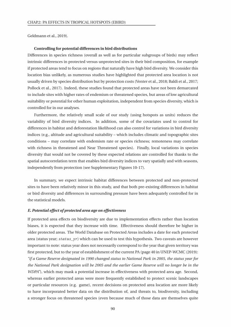
CHAP.2: PA EFFECTS IN TROPICAL HOTSPOTS (EBIRD)
Geldmann et al., 2019).
Controlling for potential differences in bird distributions
Differences in species richness (overall as well as for particular subgroups of birds) may reflect
intrinsic differences in protected versus unprotected sites in their bird composition, for example
if protected areas tend to focus on regions that naturally have high bird diversity. We consider this
location bias unlikely, as numerous studies have highlighted that protected area location is not
usually driven by species distribution but by protection costs (Venter et al., 2018; Baldi et al., 2017;
Pollock et al., 2017). Indeed, these studies found that protected areas have not been demarcated
to include sites with higher rates of endemism or threatened species, but areas of low agricultural
suitability or potential for other human exploitation, independent from species diversity, which is
controlled for in our analyses.
Furthermore, the relatively small scale of our study (using hotspots as units) reduces the
variability of bird diversity indices. In addition, some of the covariates used to control for
differences in habitat and deforestation likelihood can also control for variations in bird diversity
indices (e.g., altitude and agricultural suitability – which includes climatic and topographic sites
conditions – may correlate with endemism rate or species richness; remoteness may correlate
with richness in threatened and Near Threatened species). Finally, local variations in species
diversity that would not be covered by these expected relations are controlled for thanks to the
spatial autocorrelation term that enables bird diversity indices to vary spatially and with seasons,
independently from protection (see Supplementary Figures 10-17).
In summary, we expect intrinsic habitat differences between protected and non-protected
sites to have been relatively minor in this study, and that both pre-existing differences in habitat
or bird diversity and differences in surrounding pressure have been adequately controlled for in
the statistical models.
E. Potential effect of protected area age on effectiveness
If protected area effects on biodiversity are due to implementation effects rather than location
biases, it is expected that they increase with time. Effectiveness should therefore be higher in
older protected areas. The World Database on Protected Areas includes a date for each protected
area (status year; st atus_yr ) which can be used to test this hypothesis. Two caveats are however
important to note: status year does not necessarily correspond to the year that given territory was
first protected, but to the year of establishment of the current PA (page 40 in UNEP-WCMC (2019):
“if a Game Reserve designated in 1990 changed status to National Park in 2005, the status year for
the National Park designation will be 2005 and the earlier Game Reserve will no longer be in the
WDPA”), which may mask a potential increase in effectiveness with protected area age. Second,
whereas earlier protected areas were more frequently established to protect scenic landscapes
or particular resources (e.g. game), recent decisions on protected area location are more likely
to have incorporated better data on the distribution of, and threats to, biodiversity, including
a stronger focus on threatened species (even because much of those data are themselves quite
90
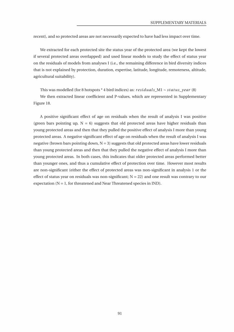
SUPPLEMENTARY MATERIALS
recent), and so protected areas are not necessarily expected to have had less impact over time.
We extracted for each protected site the status year of the protected area (we kept the lowest
if several protected areas overlapped) and used linear models to study the effect of status year
on the residuals of models from analyses I (i.e., the remaining difference in bird diversity indices
that is not explained by protection, duration, expertise, latitude, longitude, remoteness, altitude,
agricultural suitability).
This was modelled (for 8 hotspots * 4 bird indices) as: r esi dual s_M1 ∼ st atus_year (8)
We then extracted linear coefficient and P-values, which are represented in Supplementary
Figure 18.
A positive significant effect of age on residuals when the result of analysis I was positive
(green bars pointing up, N = 6) suggests that old protected areas have higher residuals than
young protected areas and then that they pulled the positive effect of analysis I more than young
protected areas. A negative significant effect of age on residuals when the result of analysis I was
negative (brown bars pointing down, N = 3) suggests that old protected areas have lower residuals
than young protected areas and then that they pulled the negative effect of analysis I more than
young protected areas. In both cases, this indicates that older protected areas performed better
than younger ones, and thus a cumulative effect of protection over time. However most results
are non-significant (either the effect of protected areas was non-significant in analysis 1 or the
effect of status year on residuals was non-significant; N = 22) and one result was contrary to our
expectation (N = 1, for threatened and Near Threatened species in IND).
91
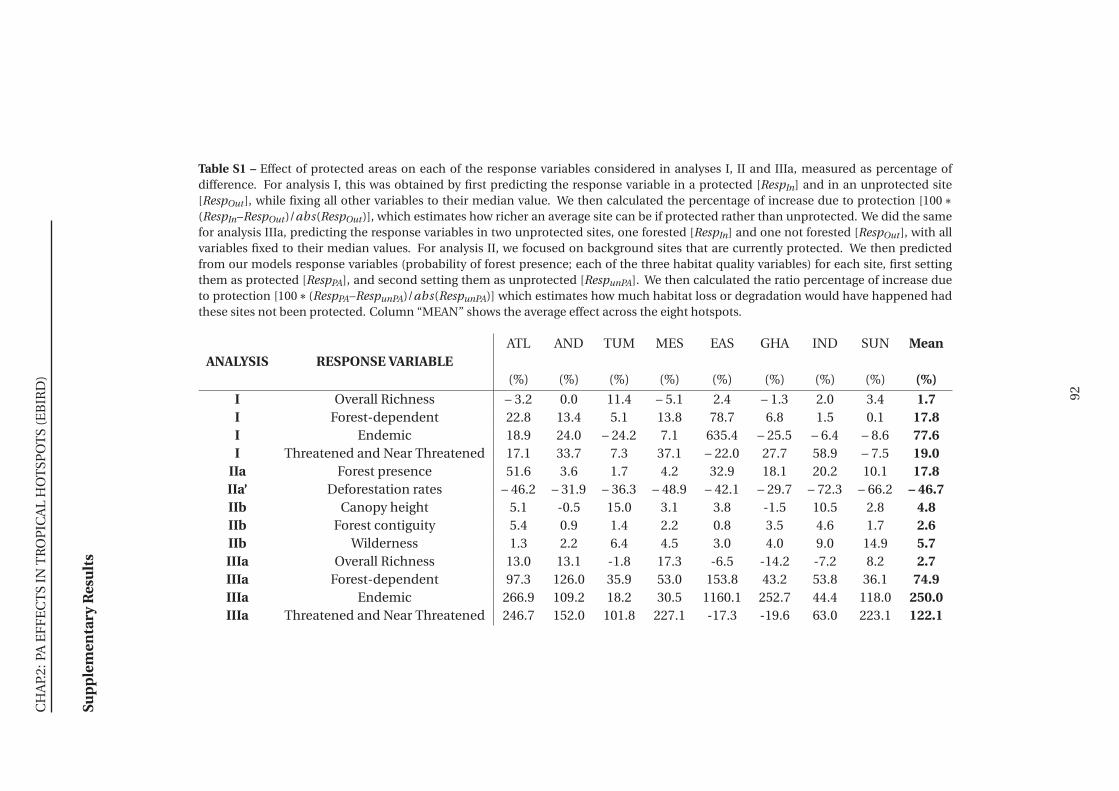
CH
AP.
2:PA
EF
FE
CT
SIN
TR
OP
ICA
LH
OT
SPO
TS
(EB
IRD
)
Sup
ple
men
tary
Res
ult
s
Table S1 – Effect of protected areas on each of the response variables considered in analyses I, II and IIIa, measured as percentage ofdifference. For analysis I, this was obtained by first predicting the response variable in a protected [RespIn] and in an unprotected site[RespOut ], while fixing all other variables to their median value. We then calculated the percentage of increase due to protection [100∗
(RespIn–RespOut )/abs(RespOut )], which estimates how richer an average site can be if protected rather than unprotected. We did the samefor analysis IIIa, predicting the response variables in two unprotected sites, one forested [RespIn] and one not forested [RespOut ], with allvariables fixed to their median values. For analysis II, we focused on background sites that are currently protected. We then predictedfrom our models response variables (probability of forest presence; each of the three habitat quality variables) for each site, first settingthem as protected [RespPA], and second setting them as unprotected [RespunPA]. We then calculated the ratio percentage of increase dueto protection [100∗ (RespPA–RespunPA)/abs(RespunPA)] which estimates how much habitat loss or degradation would have happened hadthese sites not been protected. Column “MEAN” shows the average effect across the eight hotspots.
ANALYSIS RESPONSE VARIABLEATL
(%)
AND
(%)
TUM
(%)
MES
(%)
EAS
(%)
GHA
(%)
IND
(%)
SUN
(%)
Mean
(%)
I Overall Richness – 3.2 0.0 11.4 – 5.1 2.4 – 1.3 2.0 3.4 1.7I Forest-dependent 22.8 13.4 5.1 13.8 78.7 6.8 1.5 0.1 17.8I Endemic 18.9 24.0 – 24.2 7.1 635.4 – 25.5 – 6.4 – 8.6 77.6I Threatened and Near Threatened 17.1 33.7 7.3 37.1 – 22.0 27.7 58.9 – 7.5 19.0
IIa Forest presence 51.6 3.6 1.7 4.2 32.9 18.1 20.2 10.1 17.8IIa’ Deforestation rates – 46.2 – 31.9 – 36.3 – 48.9 – 42.1 – 29.7 – 72.3 – 66.2 – 46.7IIb Canopy height 5.1 -0.5 15.0 3.1 3.8 -1.5 10.5 2.8 4.8IIb Forest contiguity 5.4 0.9 1.4 2.2 0.8 3.5 4.6 1.7 2.6IIb Wilderness 1.3 2.2 6.4 4.5 3.0 4.0 9.0 14.9 5.7IIIa Overall Richness 13.0 13.1 -1.8 17.3 -6.5 -14.2 -7.2 8.2 2.7IIIa Forest-dependent 97.3 126.0 35.9 53.0 153.8 43.2 53.8 36.1 74.9IIIa Endemic 266.9 109.2 18.2 30.5 1160.1 252.7 44.4 118.0 250.0IIIa Threatened and Near Threatened 246.7 152.0 101.8 227.1 -17.3 -19.6 63.0 223.1 122.1
92
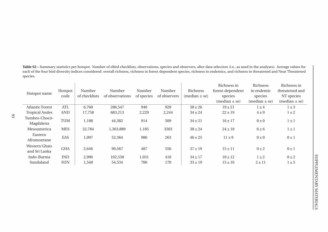
SUP
PL
EM
EN
TAR
YM
ATE
RIA
LS
Table S2 – Summary statistics per hotspot. Number of eBird checklists, observations, species and observers, after data selection (i.e., as used in the analyses). Average values foreach of the four bird diversity indices considered: overall richness, richness in forest-dependent species, richness in endemics, and richness in threatened and Near Threatenedspecies.
Hotspot nameHotspot
codeNumber
of checklistsNumber
of observationsNumber
of speciesNumber
of observersRichness
(median ± se)
Richness inforest-dependent
species(median ± se)
Richnessin endemic
species(median ± se)
Richness inthreatened and
NT species(median ± se)
Atlantic Forest ATL 6,760 286,547 940 928 38±26 19±21 1±4 1±3Tropical Andes AND 17,758 683,213 2,229 2,244 34±24 22±19 4±9 1±2
Tumbes-Chocó-Magdalena
TUM 1,188 44,382 914 509 34±21 16±17 0±0 1±1
Mesoamerica MES 32,784 1,363,889 1,185 3503 38±24 24±18 6±6 1±1
EasternAfromontane
EAS 1,097 52,364 986 263 46±25 11±9 0±0 0±1
Western Ghatsand Sri Lanka
GHA 2,646 99,567 487 556 37±19 15±11 0±2 0±1
Indo-Burma IND 2,996 102,558 1,031 418 34±17 10±12 1±2 0±2Sundaland SUN 1,548 54,534 706 170 33±19 15±16 2±11 1±5
93
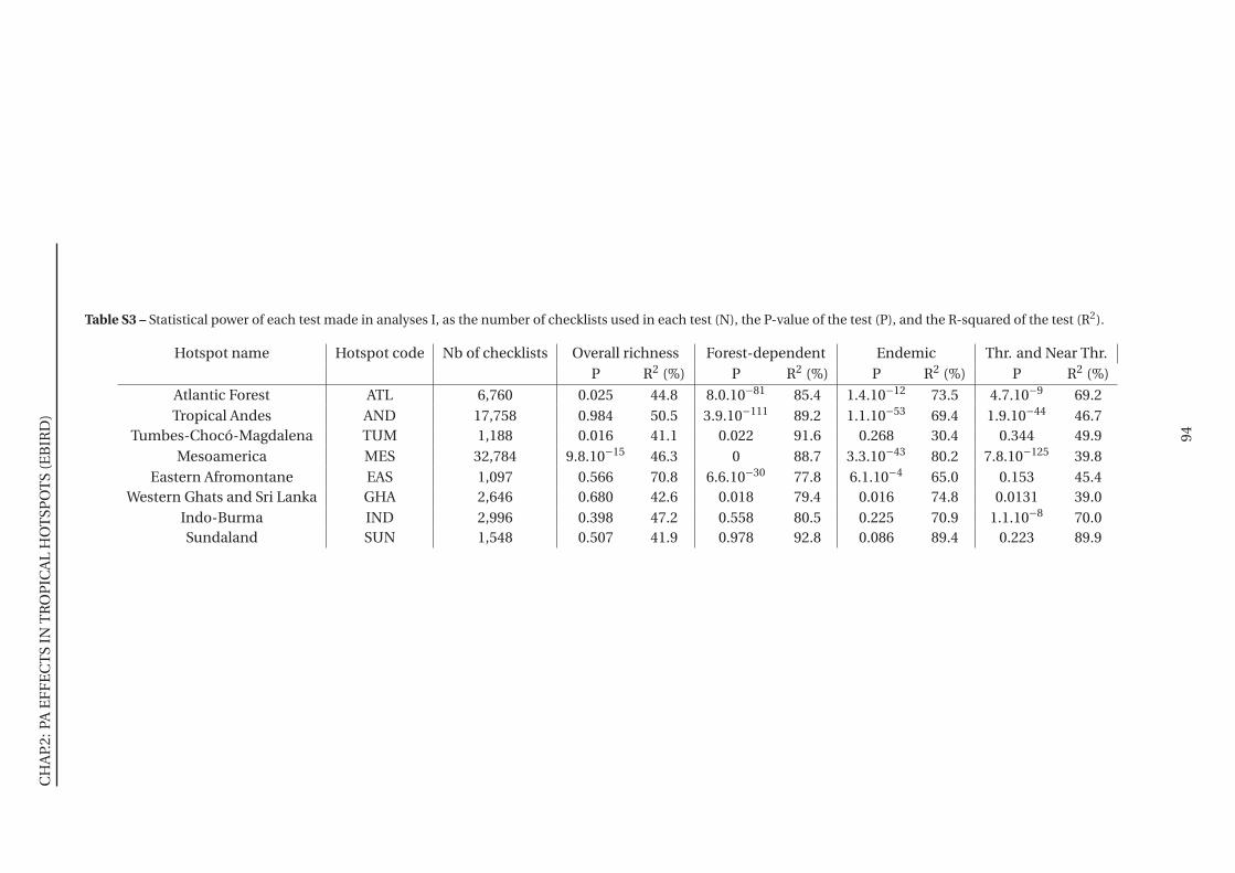
CH
AP.
2:PA
EF
FE
CT
SIN
TR
OP
ICA
LH
OT
SPO
TS
(EB
IRD
)
Table S3 – Statistical power of each test made in analyses I, as the number of checklists used in each test (N), the P-value of the test (P), and the R-squared of the test (R2).
Hotspot name Hotspot code Nb of checklists Overall richness Forest-dependent Endemic Thr. and Near Thr.P R2 (%) P R2 (%) P R2 (%) P R2 (%)
Atlantic Forest ATL 6,760 0.025 44.8 8.0.10−81 85.4 1.4.10−12 73.5 4.7.10−9 69.2Tropical Andes AND 17,758 0.984 50.5 3.9.10−111 89.2 1.1.10−53 69.4 1.9.10−44 46.7
Tumbes-Chocó-Magdalena TUM 1,188 0.016 41.1 0.022 91.6 0.268 30.4 0.344 49.9Mesoamerica MES 32,784 9.8.10−15 46.3 0 88.7 3.3.10−43 80.2 7.8.10−125 39.8
Eastern Afromontane EAS 1,097 0.566 70.8 6.6.10−30 77.8 6.1.10−4 65.0 0.153 45.4Western Ghats and Sri Lanka GHA 2,646 0.680 42.6 0.018 79.4 0.016 74.8 0.0131 39.0
Indo-Burma IND 2,996 0.398 47.2 0.558 80.5 0.225 70.9 1.1.10−8 70.0Sundaland SUN 1,548 0.507 41.9 0.978 92.8 0.086 89.4 0.223 89.9
94
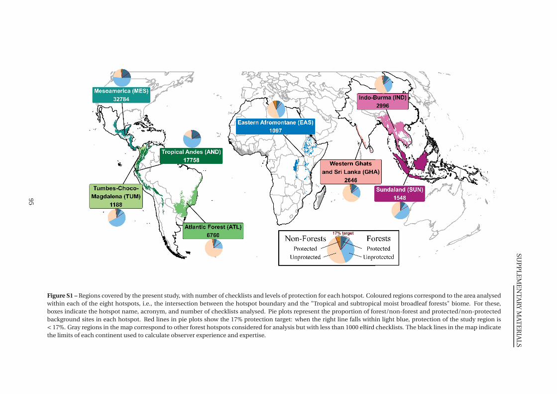
SUP
PL
EM
EN
TAR
YM
ATE
RIA
LS
Figure S1 – Regions covered by the present study, with number of checklists and levels of protection for each hotspot. Coloured regions correspond to the area analysedwithin each of the eight hotspots, i.e., the intersection between the hotspot boundary and the "Tropical and subtropical moist broadleaf forests" biome. For these,boxes indicate the hotspot name, acronym, and number of checklists analysed. Pie plots represent the proportion of forest/non-forest and protected/non-protectedbackground sites in each hotspot. Red lines in pie plots show the 17% protection target: when the right line falls within light blue, protection of the study region is< 17%. Gray regions in the map correspond to other forest hotspots considered for analysis but with less than 1000 eBird checklists. The black lines in the map indicatethe limits of each continent used to calculate observer experience and expertise.
95
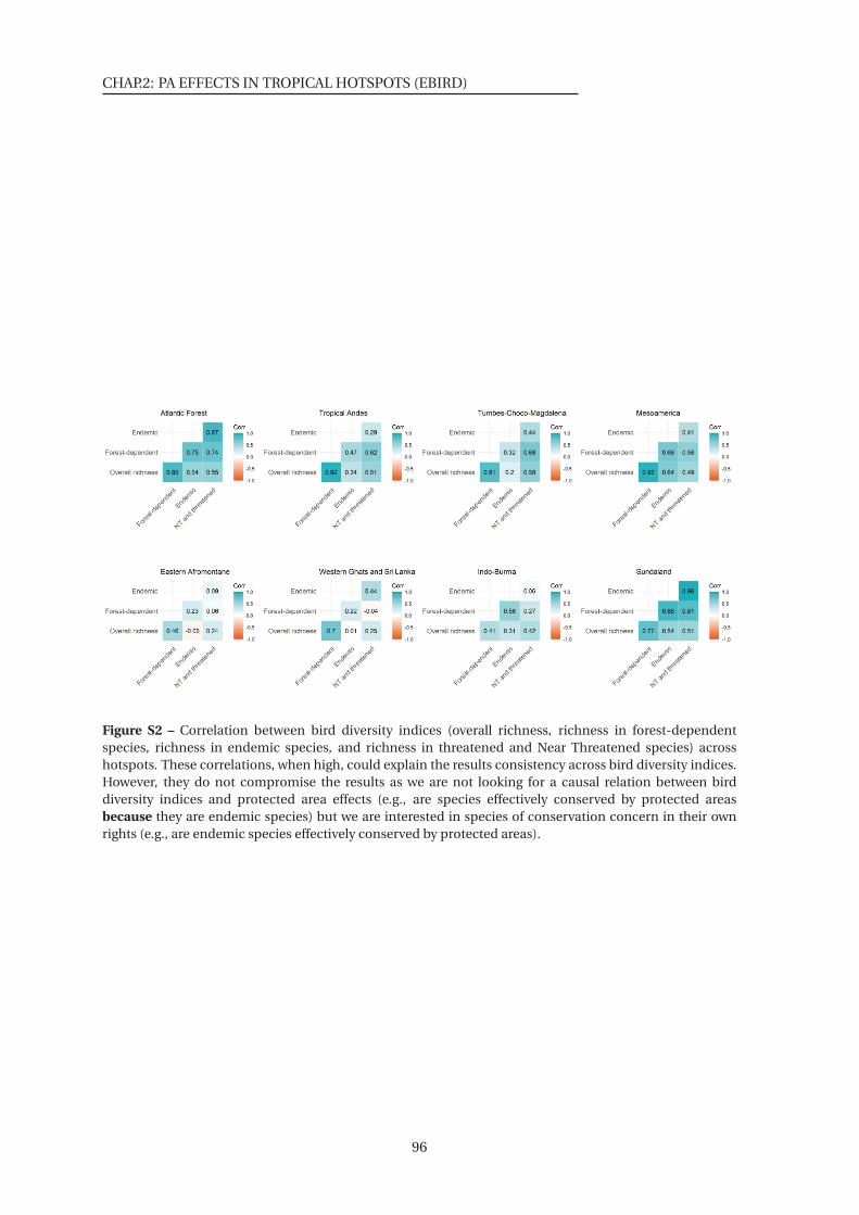
CHAP.2: PA EFFECTS IN TROPICAL HOTSPOTS (EBIRD)
Figure S2 – Correlation between bird diversity indices (overall richness, richness in forest-dependentspecies, richness in endemic species, and richness in threatened and Near Threatened species) acrosshotspots. These correlations, when high, could explain the results consistency across bird diversity indices.However, they do not compromise the results as we are not looking for a causal relation between birddiversity indices and protected area effects (e.g., are species effectively conserved by protected areasbecause they are endemic species) but we are interested in species of conservation concern in their ownrights (e.g., are endemic species effectively conserved by protected areas).
96
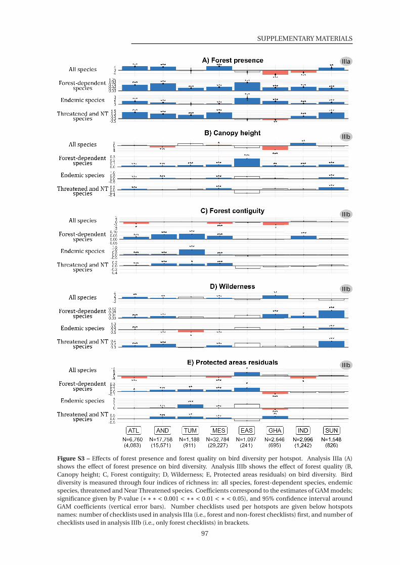
SUPPLEMENTARY MATERIALS
Figure S3 – Effects of forest presence and forest quality on bird diversity per hotspot. Analysis IIIa (A)shows the effect of forest presence on bird diversity. Analysis IIIb shows the effect of forest quality (B,Canopy height; C, Forest contiguity; D, Wilderness; E, Protected areas residuals) on bird diversity. Birddiversity is measured through four indices of richness in: all species, forest-dependent species, endemicspecies, threatened and Near Threatened species. Coefficients correspond to the estimates of GAM models;significance given by P-value (∗∗∗ < 0.001 < ∗∗ < 0.01 < ∗ < 0.05), and 95% confidence interval aroundGAM coefficients (vertical error bars). Number checklists used per hotspots are given below hotspotsnames: number of checklists used in analysis IIIa (i.e., forest and non-forest checklists) first, and number ofchecklists used in analysis IIIb (i.e., only forest checklists) in brackets.
97
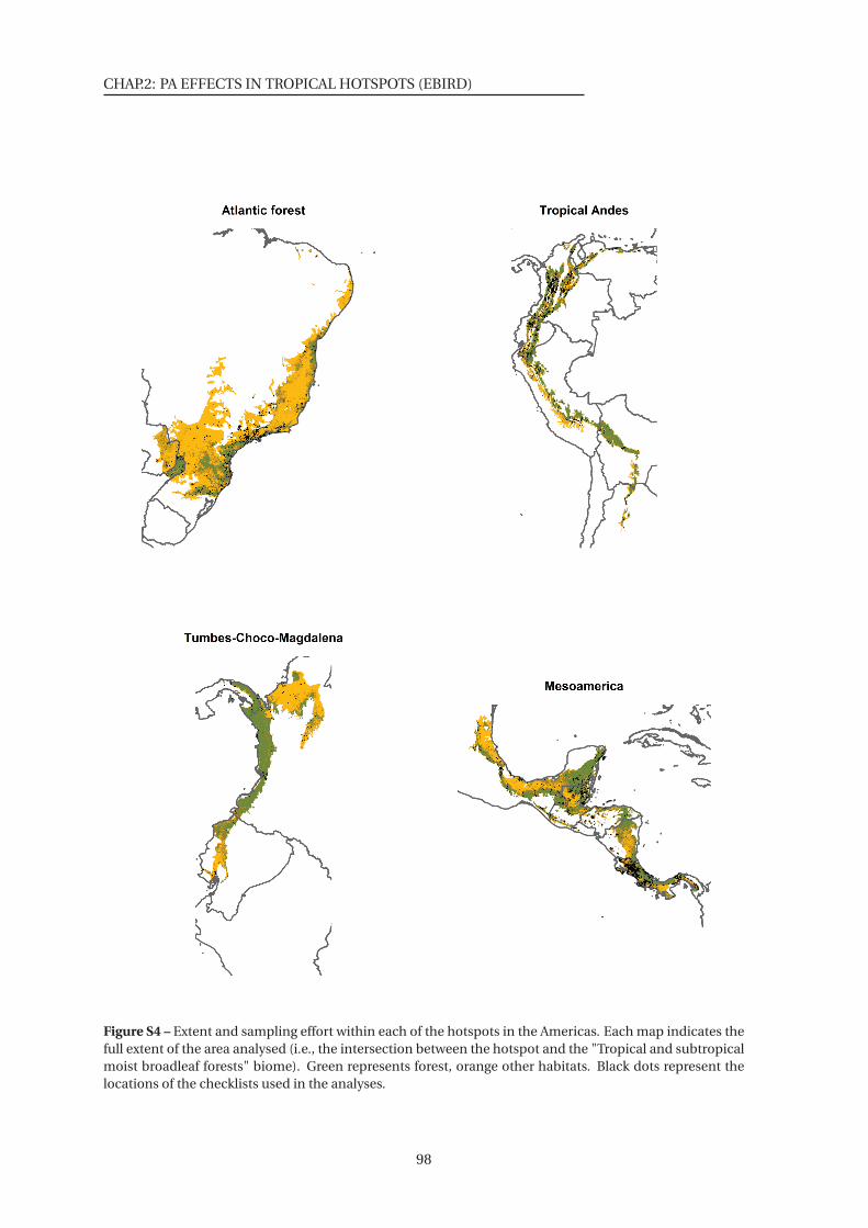
CHAP.2: PA EFFECTS IN TROPICAL HOTSPOTS (EBIRD)
Figure S4 – Extent and sampling effort within each of the hotspots in the Americas. Each map indicates thefull extent of the area analysed (i.e., the intersection between the hotspot and the "Tropical and subtropicalmoist broadleaf forests" biome). Green represents forest, orange other habitats. Black dots represent thelocations of the checklists used in the analyses.
98
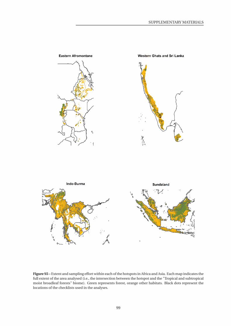
SUPPLEMENTARY MATERIALS
Figure S5 – Extent and sampling effort within each of the hotspots in Africa and Asia. Each map indicates thefull extent of the area analysed (i.e., the intersection between the hotspot and the "Tropical and subtropicalmoist broadleaf forests" biome). Green represents forest, orange other habitats. Black dots represent thelocations of the checklists used in the analyses.
99
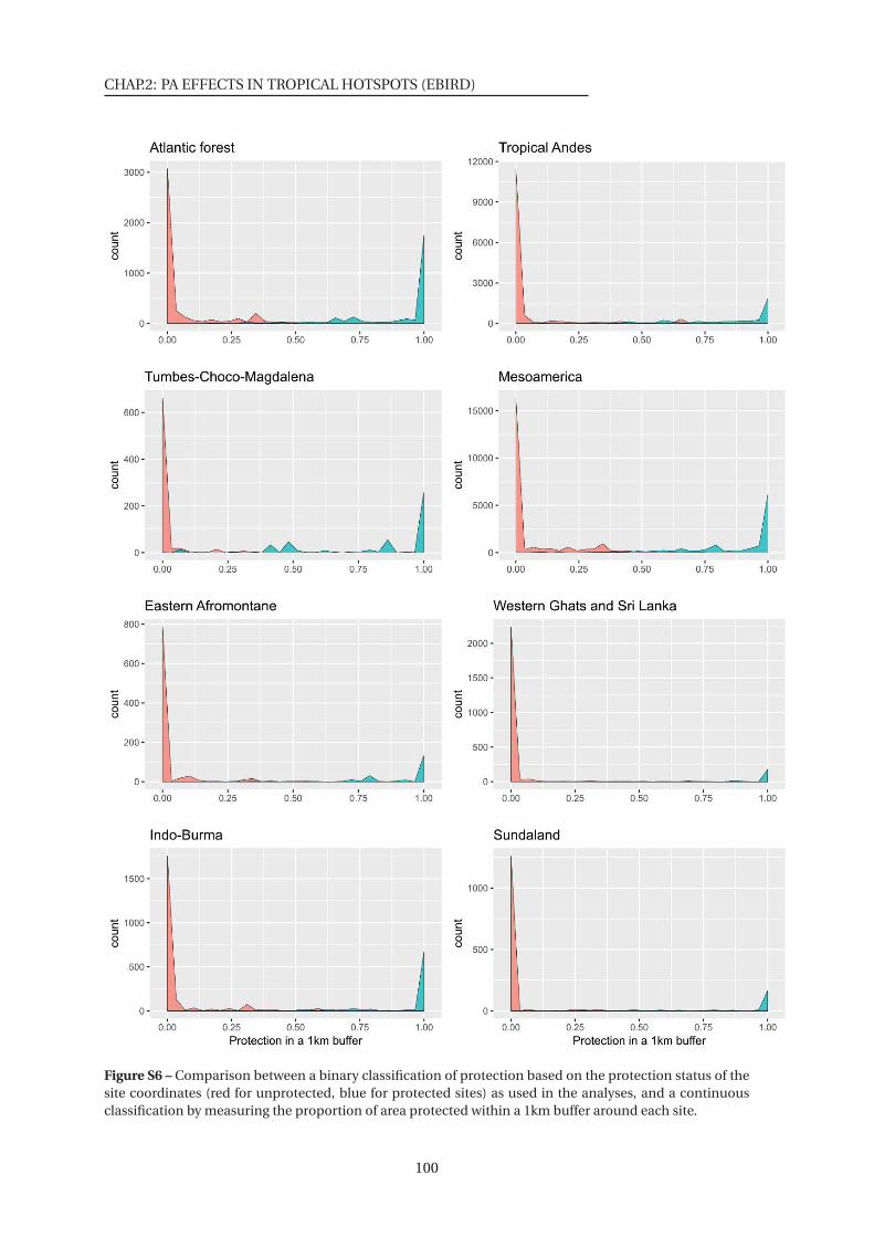
CHAP.2: PA EFFECTS IN TROPICAL HOTSPOTS (EBIRD)
Figure S6 – Comparison between a binary classification of protection based on the protection status of thesite coordinates (red for unprotected, blue for protected sites) as used in the analyses, and a continuousclassification by measuring the proportion of area protected within a 1km buffer around each site.
100
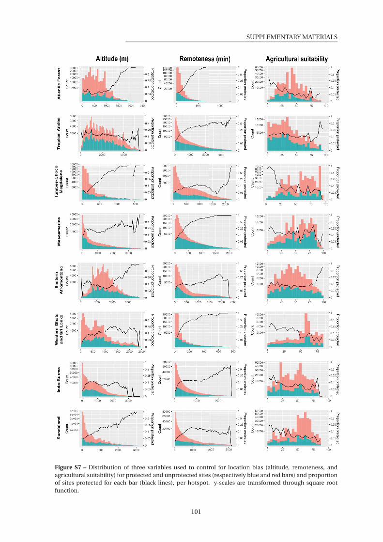
SUPPLEMENTARY MATERIALS
Figure S7 – Distribution of three variables used to control for location bias (altitude, remoteness, andagricultural suitability) for protected and unprotected sites (respectively blue and red bars) and proportionof sites protected for each bar (black lines), per hotspot. y-scales are transformed through square rootfunction.
101
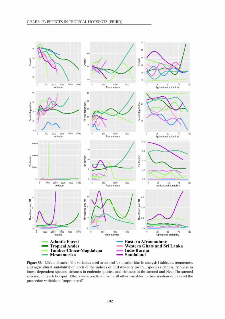
CHAP.2: PA EFFECTS IN TROPICAL HOTSPOTS (EBIRD)
Atlantic ForestTropical AndesTumbes-Chocó-MagdalenaMesoamerica
Eastern AfromontaneWestern Ghats and Sri LankaIndo-BurmaSundaland
10
20
30
40
0 1000 2000 3000 4000 5000
Altitude
Overa
ll
20
40
60
0 500 1000 1500
RemotenessO
vera
ll
30
35
40
45
50
55
0 25 50 75 100
Agricultural suitability
Overa
ll
0
10
20
30
40
0 1000 2000 3000 4000 5000
Altitude
Fore
st-
depend
ent
10
20
30
40
50
0 500 1000 1500
Remoteness
Fore
st-
depend
ent
10
20
0 25 50 75 100
Agricultural suitabilityF
ore
st-
depend
ent
0
2000
4000
6000
0 1000 2000 3000 4000 5000
Altitude
Endem
ism
0
5
10
15
0 500 1000 1500
Remoteness
Endem
ism
0.0
2.5
5.0
7.5
10.0
0 25 50 75 100
Agricultural suitability
Endem
ism
0
3
6
9
0 1000 2000 3000 4000 5000
Altitude
0
1
2
3
0 500 1000 1500
Remoteness
0.0
2.5
5.0
7.5
0 25 50 75 100
Agricultural suitability
Thre
ate
ned a
nd N
T
Thre
ate
ned a
nd N
T
Thre
ate
ned a
nd N
T
Figure S8 – Effects of each of the variables used to control for location bias in analysis I (altitude, remotenessand agricultural suitability) on each of the indices of bird diversity (overall species richness, richness inforest-dependent species, richness in endemic species, and richness in threatened and Near Threatenedspecies), for each hotspot. Effects were predicted fixing all other variables to their median values and theprotection variable to “unprotected”.
102
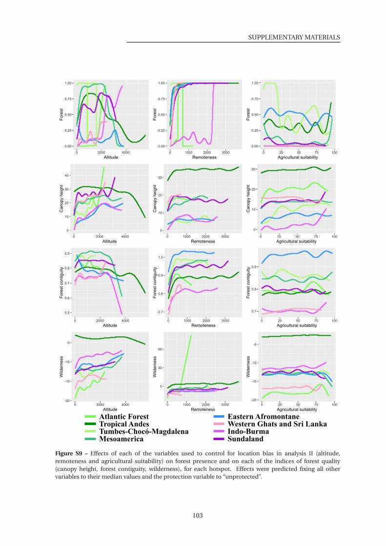
SUPPLEMENTARY MATERIALS
0.00
0.25
0.50
0.75
1.00
0 2000 4000
Altitude
Fore
st
0.00
0.25
0.50
0.75
1.00
0 1000 2000 3000
RemotenessF
ore
st
0.00
0.25
0.50
0.75
1.00
0 25 50 75 100
Agricultural suitability
Fore
st
0
10
20
30
40
0 2000 4000
Altitude
Ca
no
py h
eig
ht
0
10
20
30
0 1000 2000 3000
Remoteness
Ca
no
py h
eig
ht
0
10
20
30
0 25 50 75 100
Agricultural suitability
Ca
no
py h
eig
ht
0.5
0.6
0.7
0.8
0.9
0 2000 4000
Altitude
Fore
st contig
uity
0.7
0.8
0.9
1.0
0 1000 2000 3000
Remoteness
Fore
st contig
uity
0.7
0.8
0.9
0 25 50 75 100
Agricultural suitability
Fore
st contig
uity
-20
-15
-10
-5
0 2000 4000
Altitude
Wild
ern
ess
0
30
60
0 1000 2000 3000
Remoteness
Wild
ern
ess
-20
-15
-10
-5
0 25 50 75 100
Agricultural suitability
Wild
ern
ess
Atlantic ForestTropical AndesTumbes-Chocó-MagdalenaMesoamerica
Eastern AfromontaneWestern Ghats and Sri LankaIndo-BurmaSundaland
Figure S9 – Effects of each of the variables used to control for location bias in analysis II (altitude,remoteness and agricultural suitability) on forest presence and on each of the indices of forest quality(canopy height, forest contiguity, wilderness), for each hotspot. Effects were predicted fixing all othervariables to their median values and the protection variable to “unprotected”.
103
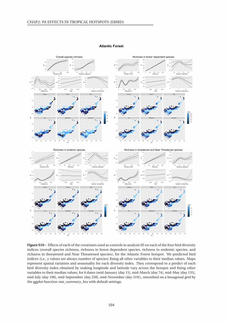
CHAP.2: PA EFFECTS IN TROPICAL HOTSPOTS (EBIRD)
Atlantic Forest
20
40
60
200 400 600
Duration (min)
fit
25
50
75
100
2.5 3.0 3.5 4.0
Observer expertise
fit
30
35
40
45
0 500 1000 1500
Altitude (m)
fit
32
34
36
38
40
42
2008 2012 2016
Year
fit
0
10
20
30
40
5 10
Number of observers
fit
July September November
January March May
−55 −50 −45 −40 −35 −55 −50 −45 −40 −35 −55 −50 −45 −40 −35
−30
−20
−10
−30
−20
−10
lon
lat
35
40
45
value
Overall species richness
13
15
17
200 400 600
Duration (min)
fit
0
25
50
75
100
0 50 100 150 200
Richness
fit
10
12
14
16
2.5 3.0 3.5 4.0
Observer expertise
fit
10
15
20
25
30
0 500 1000 1500
Altitude (m)
fit
13.5
14.0
14.5
15.0
2008 2012 2016
Year
fit
6
9
12
15
5 10
Number of observers
fit
July September November
January March May
−55 −50 −45 −40 −35 −55 −50 −45 −40 −35 −55 −50 −45 −40 −35
−30
−20
−10
−30
−20
−10
lon
lat
12.5
15.0
17.5
20.0
22.5
value
Richness in forest−dependent species
0.9
1.2
1.5
1.8
2.1
200 400 600
Duration (min)
fit
0
2
4
6
8
0 50 100 150 200
Richness
fit
0.4
0.6
0.8
1.0
1.2
1.4
2.5 3.0 3.5 4.0
Observer expertise
fit
2.5
5.0
7.5
0 500 1000 1500
Altitude (m)
fit
1.1
1.2
1.3
1.4
2008 2012 2016
Year
fit
0.5
1.0
1.5
5 10
Number of observers
fit
July September November
January March May
−55 −50 −45 −40 −35 −55 −50 −45 −40 −35 −55 −50 −45 −40 −35
−30
−20
−10
−30
−20
−10
lon
lat
1
2
3
value
Richness in endemic species
0.4
0.6
0.8
200 400 600
Duration (min)
fit
0
1
2
3
0 50 100 150 200
Richness
fit
0.25
0.50
0.75
1.00
2.5 3.0 3.5 4.0
Observer expertisefit
1
2
3
0 500 1000 1500
Altitude (m)
fit
0.45
0.50
0.55
2008 2012 2016
Year
fit
0.0
0.5
1.0
1.5
5 10
Number of observers
fit
July September November
January March May
−55 −50 −45 −40 −35 −55 −50 −45 −40 −35 −55 −50 −45 −40 −35
−30
−20
−10
−30
−20
−10
lon
lat
0.5
1.0
1.5
2.0
value
Richness in threatened and Near Threatened species
Figure S10 – Effects of each of the covariates used as controls in analysis III on each of the four bird diversityindices (overall species richness, richness in forest-dependent species, richness in endemic species, andrichness in threatened and Near Threatened species), for the Atlantic Forest hotspot. We predicted birdindices (i.e., y values are always number of species) fixing all other variables to their median values. Mapsrepresent spatial variation and seasonality for each diversity index. They correspond to a predict of eachbird diversity index obtained by making longitude and latitude vary across the hotspot and fixing othervariables to their median values, for 6 dates (mid-January [day 15], mid-March [day 74], mid-May [day 135],mid-July [day 196], mid-September [day 258], mid-November [day 319]), smoothed on a hexagonal grid bythe ggplot function stat_summary_hex with default settings.
104
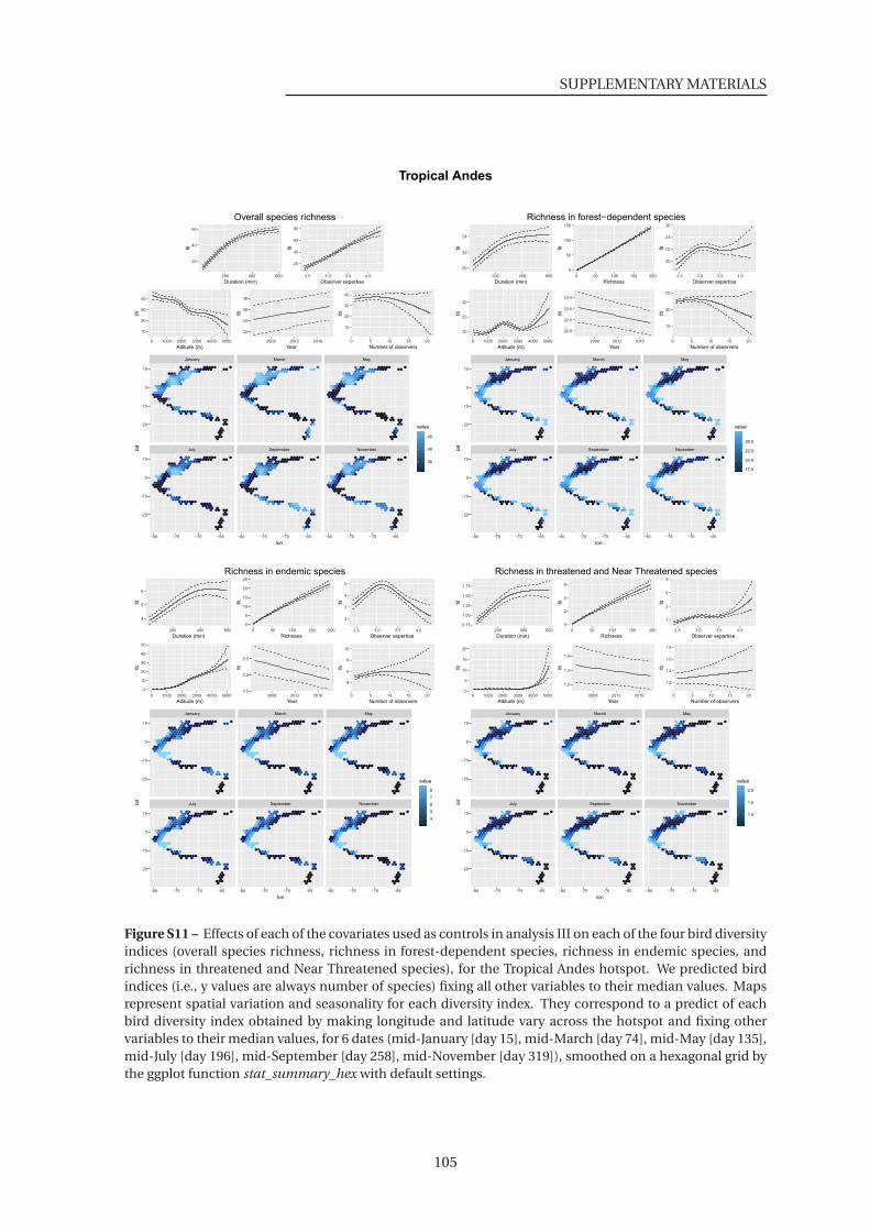
SUPPLEMENTARY MATERIALS
Tropical Andes
20
40
60
200 400 600
Duration (min)
fit
20
40
60
80
2.5 3.0 3.5 4.0
Observer expertise
fit
10
20
30
40
0 1000 2000 3000 4000 5000
Altitude (m)
fit
32
34
36
38
2008 2012 2016
Year
fit
10
20
30
40
0 5 10 15 20
Number of observers
fit
July September November
January March May
−80 −75 −70 −65 −80 −75 −70 −65 −80 −75 −70 −65
−20
−10
0
10
−20
−10
0
10
lon
lat
35
40
45
value
Overall species richness
20
22
24
200 400 600
Duration (min)
fit
0
50
100
150
0 50 100 150 200
Richness
fit
20
22
24
26
2.5 3.0 3.5 4.0
Observer expertise
fit
20
25
30
0 1000 2000 3000 4000 5000
Altitude (m)
fit
22.0
22.5
23.0
23.5
2008 2012 2016
Year
fit
15
20
25
0 5 10 15 20
Number of observers
fit
July September November
January March May
−80 −75 −70 −65 −80 −75 −70 −65 −80 −75 −70 −65
−20
−10
0
10
−20
−10
0
10
lon
lat
17.5
20.0
22.5
25.0
value
Richness in forest−dependent species
4
5
6
200 400 600
Duration (min)
fit
0
5
10
15
20
25
0 50 100 150 200
Richness
fit
2
3
4
5
2.5 3.0 3.5 4.0
Observer expertise
fit
0
10
20
30
40
50
0 1000 2000 3000 4000 5000
Altitude (m)
fit
4.5
5.0
5.5
2008 2012 2016
Year
fit
4
6
8
10
0 5 10 15 20
Number of observers
fit
July September November
January March May
−80 −75 −70 −65 −80 −75 −70 −65 −80 −75 −70 −65
−20
−10
0
10
−20
−10
0
10
lon
lat
4
5
6
7
8
value
Richness in endemic species
0.75
1.00
1.25
1.50
1.75
200 400 600
Duration (min)
fit
0
2
4
6
0 50 100 150 200
Richness
fit
1
2
3
4
2.5 3.0 3.5 4.0
Observer expertise
fit
0
5
10
15
20
0 1000 2000 3000 4000 5000
Altitude (m)
fit
1.2
1.3
1.4
2008 2012 2016
Year
fit
1.2
1.4
1.6
1.8
0 5 10 15 20
Number of observers
fit
July September November
January March May
−80 −75 −70 −65 −80 −75 −70 −65 −80 −75 −70 −65
−20
−10
0
10
−20
−10
0
10
lon
lat
1.0
1.5
2.0
value
Richness in threatened and Near Threatened species
Figure S11 – Effects of each of the covariates used as controls in analysis III on each of the four bird diversityindices (overall species richness, richness in forest-dependent species, richness in endemic species, andrichness in threatened and Near Threatened species), for the Tropical Andes hotspot. We predicted birdindices (i.e., y values are always number of species) fixing all other variables to their median values. Mapsrepresent spatial variation and seasonality for each diversity index. They correspond to a predict of eachbird diversity index obtained by making longitude and latitude vary across the hotspot and fixing othervariables to their median values, for 6 dates (mid-January [day 15], mid-March [day 74], mid-May [day 135],mid-July [day 196], mid-September [day 258], mid-November [day 319]), smoothed on a hexagonal grid bythe ggplot function stat_summary_hex with default settings.
105
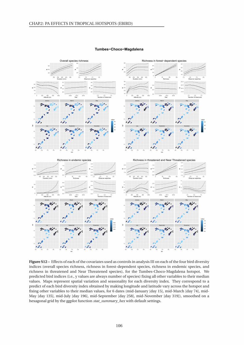
CHAP.2: PA EFFECTS IN TROPICAL HOTSPOTS (EBIRD)
Tumbes−Choco−Magdalena
20
40
60
100 200 300 400 500
Duration (min)
fit
20
40
60
2.4 2.8 3.2 3.6
Observer expertise
fit
0
10
20
30
0 300 600 900 1200
Altitude (m)
fit
20
25
30
35
2008 2012 2016
Year
fit
20
25
30
35
2.5 5.0 7.5
Number of observers
fit
July September November
January March May
−81 −79 −77 −75 −81 −79 −77 −75 −81 −79 −77 −75
0
4
8
0
4
8
lon
lat
30
35
40
45
value
Overall species richness
20
24
28
100 200 300 400 500
Duration (min)
fit
0
30
60
90
0 50 100 150
Richness
fit
15
20
25
30
2.4 2.8 3.2 3.6
Observer expertise
fit
15
20
25
30
35
0 300 600 900 1200
Altitude (m)
fit
20
22
24
2008 2012 2016
Year
fit
17.5
20.0
22.5
25.0
2.5 5.0 7.5
Number of observers
fit
July September November
January March May
−81 −79 −77 −75 −81 −79 −77 −75 −81 −79 −77 −75
0
4
8
0
4
8
lon
lat
15
20
25
value
Richness in forest−dependent species
0.0
0.5
1.0
1.5
100 200 300 400 500
Duration (min)
fit
0.0
0.5
1.0
0 50 100 150
Richness
fit
0.0
0.5
1.0
1.5
2.0
2.4 2.8 3.2 3.6
Observer expertise
fit
0
5
10
0 300 600 900 1200
Altitude (m)
fit
0.0
0.2
0.4
0.6
2008 2012 2016
Year
fit
0.0
0.2
0.4
0.6
2.5 5.0 7.5
Number of observers
fit
July September November
January March May
−81 −79 −77 −75 −81 −79 −77 −75 −81 −79 −77 −75
0
4
8
0
4
8
lon
lat
0.05
0.10
0.15
0.20
value
Richness in endemic species
1.5
2.0
2.5
100 200 300 400 500
Duration (min)
fit
0.0
2.5
5.0
7.5
0 50 100 150
Richness
fit
1.0
1.5
2.0
2.5
3.0
2.4 2.8 3.2 3.6
Observer expertisefit
1
2
3
4
5
0 300 600 900 1200
Altitude (m)
fit
1.2
1.6
2.0
2008 2012 2016
Year
fit
1
2
3
4
2.5 5.0 7.5
Number of observers
fit
July September November
January March May
−81 −79 −77 −75 −81 −79 −77 −75 −81 −79 −77 −75
0
4
8
0
4
8
lon
lat
0.6
0.9
1.2
1.5
1.8
value
Richness in threatened and Near Threatened species
Figure S12 – Effects of each of the covariates used as controls in analysis III on each of the four bird diversityindices (overall species richness, richness in forest-dependent species, richness in endemic species, andrichness in threatened and Near Threatened species), for the Tumbes-Choco-Magdalena hotspot. Wepredicted bird indices (i.e., y values are always number of species) fixing all other variables to their medianvalues. Maps represent spatial variation and seasonality for each diversity index. They correspond to apredict of each bird diversity index obtained by making longitude and latitude vary across the hotspot andfixing other variables to their median values, for 6 dates (mid-January [day 15], mid-March [day 74], mid-May [day 135], mid-July [day 196], mid-September [day 258], mid-November [day 319]), smoothed on ahexagonal grid by the ggplot function stat_summary_hex with default settings.
106
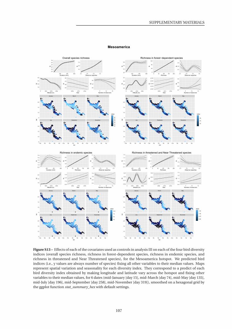
SUPPLEMENTARY MATERIALS
Mesoamerica
20
30
40
50
60
70
200 400 600
Duration (min)
fit
25
50
75
2.5 3.0 3.5 4.0
Observer expertise
fit
10
20
30
40
0 1000 2000 3000
Altitude (m)
fit
35
36
37
38
2008 2012 2016
Year
fit
25
30
35
5 10 15
Number of observers
fit
July September November
January March May
−100 −95 −90 −85 −80 −100 −95 −90 −85 −80 −100 −95 −90 −85 −80
5
10
15
20
5
10
15
20
lon
lat
32
34
36
38
40
42
value
Overall species richness
20
22
24
26
200 400 600
Duration (min)
fit
0
40
80
120
0 50 100 150 200
Richness
fit
23
24
25
2.5 3.0 3.5 4.0
Observer expertise
fit
20
24
28
32
0 1000 2000 3000
Altitude (m)
fit
22.50
22.75
23.00
23.25
23.50
2008 2012 2016
Year
fit
22
24
26
28
5 10 15
Number of observers
fit
July September November
January March May
−100 −95 −90 −85 −80 −100 −95 −90 −85 −80 −100 −95 −90 −85 −80
5
10
15
20
5
10
15
20
lon
lat
22
24
26
value
Richness in forest−dependent species
6.8
7.0
7.2
7.4
7.6
7.8
200 400 600
Duration (min)
fit
0
10
20
30
0 50 100 150 200
Richness
fit
6
7
8
9
2.5 3.0 3.5 4.0
Observer expertise
fit
10
20
30
0 1000 2000 3000
Altitude (m)
fit
6.8
7.0
7.2
7.4
2008 2012 2016
Year
fit
6.0
6.5
7.0
7.5
5 10 15
Number of observers
fit
July September November
January March May
−100 −95 −90 −85 −80 −100 −95 −90 −85 −80 −100 −95 −90 −85 −80
5
10
15
20
5
10
15
20
lon
lat
2.5
5.0
7.5
10.0
value
Richness in endemic species
0.7
0.9
1.1
1.3
1.5
200 400 600
Duration (min)
fit
0
1
2
3
4
0 50 100 150 200
Richness
fit
0.8
1.0
1.2
2.5 3.0 3.5 4.0
Observer expertise
fit
0.50
0.75
1.00
1.25
0 1000 2000 3000
Altitude (m)
fit
0.90
0.95
1.00
2008 2012 2016
Year
fit
0.9
1.0
1.1
1.2
1.3
5 10 15
Number of observers
fit
July September November
January March May
−100 −95 −90 −85 −80 −100 −95 −90 −85 −80 −100 −95 −90 −85 −80
5
10
15
20
5
10
15
20
lon
lat
0.50
0.75
1.00
1.25
value
Richness in threatened and Near Threatened species
Figure S13 – Effects of each of the covariates used as controls in analysis III on each of the four bird diversityindices (overall species richness, richness in forest-dependent species, richness in endemic species, andrichness in threatened and Near Threatened species), for the Mesoamerica hotspot. We predicted birdindices (i.e., y values are always number of species) fixing all other variables to their median values. Mapsrepresent spatial variation and seasonality for each diversity index. They correspond to a predict of eachbird diversity index obtained by making longitude and latitude vary across the hotspot and fixing othervariables to their median values, for 6 dates (mid-January [day 15], mid-March [day 74], mid-May [day 135],mid-July [day 196], mid-September [day 258], mid-November [day 319]), smoothed on a hexagonal grid bythe ggplot function stat_summary_hex with default settings.
107

CHAP.2: PA EFFECTS IN TROPICAL HOTSPOTS (EBIRD)
Eastern Afromontane
20
40
60
200 400 600
Duration (min)
fit
0
20
40
60
3.0 3.5
Observer expertise
fit
25
30
35
40
45
1000 2000
Altitude (m)
fit
25
30
35
40
2010 2015
Year
fit
30
35
40
45
2 4 6 8
Number of observers
fit
July September November
January March May
32 36 40 32 36 40 32 36 40
−5
0
5
10
−5
0
5
10
lon
lat
36
39
42
45
value
Overall species richness
6
9
12
15
200 400 600
Duration (min)
fit
0
5
10
15
20
0 30 60 90 120
Richness
fit
6
7
8
9
3.0 3.5
Observer expertise
fit
3
6
9
1000 2000
Altitude (m)
fit
6.5
7.0
7.5
8.0
8.5
9.0
2010 2015
Year
fit
8
10
12
2 4 6 8
Number of observers
fit
July September November
January March May
32 36 40 32 36 40 32 36 40
−5
0
5
10
−5
0
5
10
lon
lat
9
12
15
value
Richness in forest−dependent species
0.0000
0.0005
0.0010
0.0015
0.0020
200 400 600
Duration (min)
fit
0.0000
0.0005
0.0010
0.0015
0.0020
0 30 60 90 120
Richness
fit
0.0000
0.0005
0.0010
0.0015
3.0 3.5
Observer expertise
fit
0.00
0.01
0.02
0.03
0.04
0.05
1000 2000
Altitude (m)
fit
0.0000
0.0005
0.0010
0.0015
2010 2015
Year
fit
0.0000
0.0005
0.0010
0.0015
0.0020
2 4 6 8
Number of observers
fit
July September November
January March May
32 36 40 32 36 40 32 36 40
−5
0
5
10
−5
0
5
10
lon
lat
0.01
0.02
0.03
value
Richness in endemic species
0.05
0.10
0.15
0.20
200 400 600
Duration (min)
fit
0.0
0.1
0.2
0.3
0.4
0 30 60 90 120
Richness
fit
0.10
0.15
0.20
0.25
3.0 3.5
Observer expertisefit
0
1
2
3
1000 2000
Altitude (m)
fit
0.10
0.15
0.20
0.25
2010 2015
Year
fit
0.1
0.2
0.3
2 4 6 8
Number of observers
fit
July September November
January March May
32 36 40 32 36 40 32 36 40
−5
0
5
10
−5
0
5
10
lon
lat
0.3
0.6
0.9
value
Richness in threatened and Near Threatened species
Figure S14 – Effects of each of the covariates used as controls in analysis III on each of the four bird diversityindices (overall species richness, richness in forest-dependent species, richness in endemic species, andrichness in threatened and Near Threatened species), for the Eastern Afromontane hotspot. We predictedbird indices (i.e., y values are always number of species) fixing all other variables to their median values.Maps represent spatial variation and seasonality for each diversity index. They correspond to a predict ofeach bird diversity index obtained by making longitude and latitude vary across the hotspot and fixing othervariables to their median values, for 6 dates (mid-January [day 15], mid-March [day 74], mid-May [day 135],mid-July [day 196], mid-September [day 258], mid-November [day 319]), smoothed on a hexagonal grid bythe ggplot function stat_summary_hex with default settings.
108
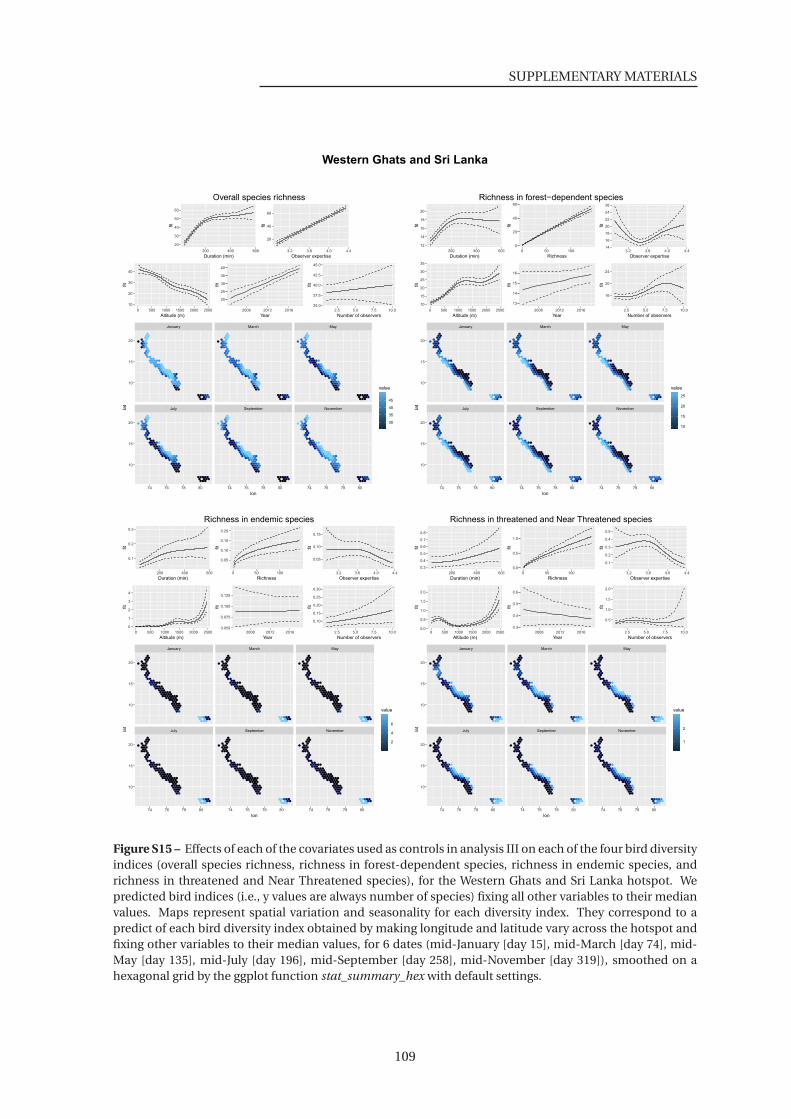
SUPPLEMENTARY MATERIALS
Western Ghats and Sri Lanka
20
30
40
50
60
200 400 600
Duration (min)
fit
20
40
60
3.2 3.6 4.0 4.4
Observer expertise
fit
10
20
30
40
0 500 1000 1500 2000 2500
Altitude (m)
fit
20
25
30
35
40
2008 2012 2016
Year
fit
35.0
37.5
40.0
42.5
45.0
2.5 5.0 7.5 10.0
Number of observers
fit
July September November
January March May
74 76 78 80 74 76 78 80 74 76 78 80
10
15
20
10
15
20
lon
lat
30
35
40
45
value
Overall species richness
12
14
16
18
20
200 400 600
Duration (min)
fit
0
20
40
60
0 50 100
Richness
fit
14
16
18
20
22
24
26
3.2 3.6 4.0 4.4
Observer expertise
fit
10
15
20
25
30
35
0 500 1000 1500 2000 2500
Altitude (m)
fit
13
14
15
16
2008 2012 2016
Year
fit
16
20
24
2.5 5.0 7.5 10.0
Number of observers
fit
July September November
January March May
74 76 78 80 74 76 78 80 74 76 78 80
10
15
20
10
15
20
lon
lat
10
15
20
25
value
Richness in forest−dependent species
0.1
0.2
0.3
200 400 600
Duration (min)
fit
0.05
0.10
0.15
0.20
0 50 100
Richness
fit
0.05
0.10
0.15
3.2 3.6 4.0 4.4
Observer expertise
fit
0
1
2
3
4
0 500 1000 1500 2000 2500
Altitude (m)
fit
0.050
0.075
0.100
0.125
2008 2012 2016
Year
fit
0.10
0.15
0.20
0.25
0.30
2.5 5.0 7.5 10.0
Number of observers
fit
July September November
January March May
74 76 78 80 74 76 78 80 74 76 78 80
10
15
20
10
15
20
lon
lat
2
4
6
value
Richness in endemic species
0.3
0.4
0.5
0.6
0.7
0.8
200 400 600
Duration (min)
fit
0.0
0.5
1.0
0 50 100
Richness
fit
0.1
0.2
0.3
0.4
0.5
3.2 3.6 4.0 4.4
Observer expertise
fit
0.0
0.5
1.0
1.5
2.0
0 500 1000 1500 2000 2500
Altitude (m)
fit
0.3
0.4
0.5
0.6
2008 2012 2016
Year
fit
0.5
1.0
1.5
2.0
2.5 5.0 7.5 10.0
Number of observers
fit
July September November
January March May
74 76 78 80 74 76 78 80 74 76 78 80
10
15
20
10
15
20
lon
lat
1
2
value
Richness in threatened and Near Threatened species
Figure S15 – Effects of each of the covariates used as controls in analysis III on each of the four bird diversityindices (overall species richness, richness in forest-dependent species, richness in endemic species, andrichness in threatened and Near Threatened species), for the Western Ghats and Sri Lanka hotspot. Wepredicted bird indices (i.e., y values are always number of species) fixing all other variables to their medianvalues. Maps represent spatial variation and seasonality for each diversity index. They correspond to apredict of each bird diversity index obtained by making longitude and latitude vary across the hotspot andfixing other variables to their median values, for 6 dates (mid-January [day 15], mid-March [day 74], mid-May [day 135], mid-July [day 196], mid-September [day 258], mid-November [day 319]), smoothed on ahexagonal grid by the ggplot function stat_summary_hex with default settings.
109
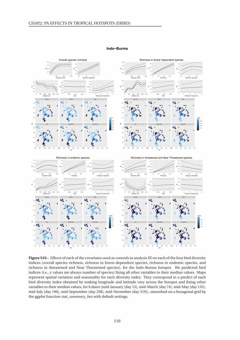
CHAP.2: PA EFFECTS IN TROPICAL HOTSPOTS (EBIRD)
Indo−Burma
30
40
50
60
200 400 600
Duration (min)
fit
20
30
40
50
3.2 3.6 4.0
Observer expertise
fit
10
20
30
40
0 500 1000 1500 2000 2500
Altitude (m)
fit
34
36
38
40
42
2008 2012 2016
Year
fit
35
40
45
50
55
2 4 6 8
Number of observers
fit
July September November
January March May
90 95 100 105 110 11590 95 100 105 110 11590 95 100 105 110 115
10
15
20
25
10
15
20
25
lon
lat
25
30
35
40
45
value
Overall species richness
10.0
12.5
15.0
17.5
200 400 600
Duration (min)
fit
0
10
20
30
0 30 60 90
Richness
fit
9
10
11
12
3.2 3.6 4.0
Observer expertise
fit
20
40
60
0 500 1000 1500 2000 2500
Altitude (m)
fit
9
10
11
12
2008 2012 2016
Year
fit
10
11
12
13
2 4 6 8
Number of observers
fit
July September November
January March May
90 95 100 105 110 11590 95 100 105 110 11590 95 100 105 110 115
10
15
20
25
10
15
20
25
lon
lat
7.5
10.0
12.5
15.0
value
Richness in forest−dependent species
2.0
2.4
2.8
3.2
200 400 600
Duration (min)
fit
0
2
4
6
8
0 30 60 90
Richness
fit
2.0
2.5
3.0
3.2 3.6 4.0
Observer expertise
fit
5
10
0 500 1000 1500 2000 2500
Altitude (m)
fit
2.0
2.5
2008 2012 2016
Year
fit
2.0
2.5
3.0
2 4 6 8
Number of observers
fit
July September November
January March May
90 95 100 105 110 11590 95 100 105 110 11590 95 100 105 110 115
10
15
20
25
10
15
20
25
lon
lat
0.5
1.0
1.5
2.0
2.5
value
Richness in endemic species
0.4
0.6
0.8
1.0
200 400 600
Duration (min)
fit
0.0
0.5
1.0
1.5
2.0
0 30 60 90
Richness
fit
0.3
0.4
0.5
0.6
0.7
3.2 3.6 4.0
Observer expertisefit
0.2
0.4
0.6
0 500 1000 1500 2000 2500
Altitude (m)
fit
0.3
0.4
0.5
2008 2012 2016
Year
fit
0.3
0.4
0.5
0.6
2 4 6 8
Number of observers
fit
July September November
January March May
90 95 100 105 110 11590 95 100 105 110 11590 95 100 105 110 115
10
15
20
25
10
15
20
25
lon
lat
0.5
1.0
1.5
2.0
value
Richness in threatened and Near Threatened species
Figure S16 – Effects of each of the covariates used as controls in analysis III on each of the four bird diversityindices (overall species richness, richness in forest-dependent species, richness in endemic species, andrichness in threatened and Near Threatened species), for the Indo-Burma hotspot. We predicted birdindices (i.e., y values are always number of species) fixing all other variables to their median values. Mapsrepresent spatial variation and seasonality for each diversity index. They correspond to a predict of eachbird diversity index obtained by making longitude and latitude vary across the hotspot and fixing othervariables to their median values, for 6 dates (mid-January [day 15], mid-March [day 74], mid-May [day 135],mid-July [day 196], mid-September [day 258], mid-November [day 319]), smoothed on a hexagonal grid bythe ggplot function stat_summary_hex with default settings.
110
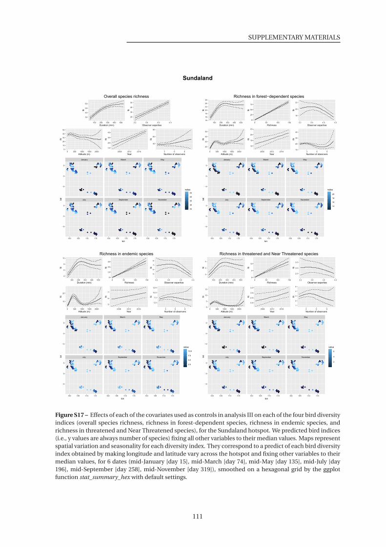
SUPPLEMENTARY MATERIALS
Sundaland
30
40
50
60
100 200 300 400 500
Duration (min)
fit
20
30
40
50
3.2 3.6 4.0 4.4
Observer expertise
fit
0
10
20
30
40
50
0 500 1000 1500 2000
Altitude (m)
fit
10
20
30
40
2008 2012 2016
Year
fit
40
60
80
3 6 9
Number of observers
fit
July September November
January March May
100 105 110 115 100 105 110 115 100 105 110 115
−5
0
5
−5
0
5
lon
lat
25
30
35
40
45
value
Overall species richness
14
16
18
20
22
24
26
100 200 300 400 500
Duration (min)
fit
0
25
50
75
0 50 100 150
Richness
fit
18
20
22
3.2 3.6 4.0 4.4
Observer expertise
fit
20
30
40
50
0 500 1000 1500 2000
Altitude (m)
fit
16
18
20
22
2008 2012 2016
Year
fit
10
20
30
40
3 6 9
Number of observers
fit
July September November
January March May
100 105 110 115 100 105 110 115 100 105 110 115
−5
0
5
−5
0
5
lon
lat
14
16
18
20
value
Richness in forest−dependent species
4
6
8
10
100 200 300 400 500
Duration (min)
fit
0
10
20
30
0 50 100 150
Richness
fit
5
6
7
8
3.2 3.6 4.0 4.4
Observer expertise
fit
10
20
0 500 1000 1500 2000
Altitude (m)
fit
5
6
7
2008 2012 2016
Year
fit
5.0
7.5
10.0
12.5
3 6 9
Number of observers
fit
July September November
January March May
100 105 110 115 100 105 110 115 100 105 110 115
−5
0
5
−5
0
5
lon
lat
2.5
5.0
7.5
10.0
value
Richness in endemic species
2
3
4
100 200 300 400 500
Duration (min)
fit
0
5
10
0 50 100 150
Richness
fit
2.5
3.0
3.5
3.2 3.6 4.0 4.4
Observer expertise
fit
0
5
10
15
0 500 1000 1500 2000
Altitude (m)
fit
2.0
2.5
3.0
3.5
2008 2012 2016
Year
fit
1
2
3
4
5
3 6 9
Number of observers
fit
July September November
January March May
100 105 110 115 100 105 110 115 100 105 110 115
−5
0
5
−5
0
5
lon
lat
2
4
6
value
Richness in threatened and Near Threatened species
Figure S17 – Effects of each of the covariates used as controls in analysis III on each of the four bird diversityindices (overall species richness, richness in forest-dependent species, richness in endemic species, andrichness in threatened and Near Threatened species), for the Sundaland hotspot. We predicted bird indices(i.e., y values are always number of species) fixing all other variables to their median values. Maps representspatial variation and seasonality for each diversity index. They correspond to a predict of each bird diversityindex obtained by making longitude and latitude vary across the hotspot and fixing other variables to theirmedian values, for 6 dates (mid-January [day 15], mid-March [day 74], mid-May [day 135], mid-July [day196], mid-September [day 258], mid-November [day 319]), smoothed on a hexagonal grid by the ggplotfunction stat_summary_hex with default settings.
111
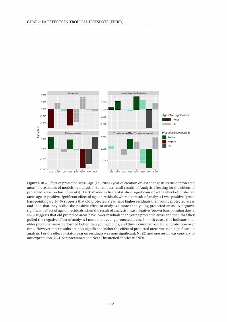
CHAP.2: PA EFFECTS IN TROPICAL HOTSPOTS (EBIRD)
P<0.05
NS
PAs effects (Analysis I)
Positive
Negative
NS
Endemic species Threatened and Near Threatened species
All species Forest-dependent species
ATL AND TUM MES EAS GHA IND SUN ATL AND TUM MES EAS GHA IND SUN
-0.010
-0.005
0.000
0.005
-0.005
0.000
0.005
-0.050
-0.025
0.000
0.025
0.050
-0.010
-0.005
0.000
0.005
Ag
e e
ffe
ct
Age effect significance
Figure S18 – Effect of protected areas’ age (i.e., 2020 - year of creation or last change in status of protectedareas) on residuals of models in analysis I. Bar colours recall results of Analysis I (testing for the effects ofprotected areas on bird diversity). Dark shades indicate statistical significance for the effect of protectedareas age. A positive significant effect of age on residuals when the result of analysis I was positive (greenbars pointing up, N=6) suggests that old protected areas have higher residuals than young protected areasand then that they pulled the positive effect of analysis I more than young protected areas. A negativesignificant effect of age on residuals when the result of analysis I was negative (brown bars pointing down,N=3) suggests that old protected areas have lower residuals than young protected areas and then that theypulled the negative effect of analysis I more than young protected areas. In both cases, this indicates thatolder protected areas performed better than younger ones, and thus a cumulative effect of protection overtime. However most results are non-significant (either the effect of protected areas was non-significant inanalysis 1 or the effect of status year on residuals was non-significant; N=22) and one result was contrary toour expectation (N=1, for threatened and Near Threatened species in IND).
112
SUPPLEMENTARY MATERIALS
Supplementary Discussion
When comparing across hotspots, we found some heterogeneity in our results, potentially induced
by three factors. First, failure to comply with our simplifying hypothesis that our study regions
(i.e., extent of biodiversity hotspots included in the “Tropical and subtropical moist broadleaf
forests” biome) were originally covered by homogeneous forest could explain some differences
in bird responses. For instance, responses of bird diversity indices in Western Ghats and Sri
Lanka were often low, sometimes the opposite of others. This could be due to the natural habitat
heterogeneity of this region, such as the presence of natural grasslands above the shola forests
and large variations in rainfall patterns (Mittermeier et al., 2004); this may also be the case in
the Tropical Andes, which include high natural grasslands such as Páramo (see Supplementary
Methods 4D for further information on this assumption), and perhaps Eastern Afromontane. This
corroborates with the high proportion of species with null dependency on forests in Western Ghats
and Sri Lanka, as well as Eastern Afromontane (respectively 33% and 38% of species detected,
against an average of 18% for other hotspots). Second, differences in protection regimes could
explain some of the variation found between hotspots. Indeed, the location of protected areas in
the Atlantic Forest is not highly biased towards remote and high areas (reactive approach (Brooks
et al., 2006), Supplementary Figure 7), which could explain the high effectiveness measured.
Conversely, protected areas in Sundaland are highly biased towards remote and high zones that
are less likely to suffer from human pressure in the short-term (pro-active approach (Brooks et al.,
2006), Supplementary Figure 7), which could explain the low effect we measured while controlling
for location biases. Finally, sampling effort greatly differed between hotspots (ranging from 1,097
checklists analysed in Eastern Afromontane to 32,784 in Mesoamerica; see Supplementary Table
3), which could affect the statistical power of tests. This could explain why hotspots in the
Americas showed clearer results than those from Asia and Africa. The consistency of results we got
across continents in analyses II and III (disentangling the mechanisms of protected area effects on
bird diversity) give high credit to this assumption.
113


116
Chapitre 3
Les aires protégées sont trop rares et dégradées
pour protéger les espèces les plus sensibles
117

Dans le chapitre 2, nous nous sommes intéressés aux espèces à fort enjeu de conservation
en désignant les espèces spécialistes des milieux forestiers, les espèces endémiques et les
espèces menacées. En réalité, de nombreuses espèces, notamment parmi les spécialistes et les
endémiques, ne sont pas à fort enjeu de conservation dans la mesure où elles peuvent très
bien s’accommoder de la pression humaine. C’est par exemple le cas du colibri rubis-émeraude,
Clytolaema rubricauda, espèce endémique de la Forêt Atlantique au Brésil et spécialiste des
milieux forestiers mais que l’on retrouve dans de nombreux sites anthropisés tels que des parcs
urbains, plantations, etc. Une mesure plus pertinente pour désigner les espèces qui ont besoin
d’une protection forte (c’est-à-dire d’avoir accès à des aires protégées dont l’habitat est intact,
sans pression humaine) serait une mesure de sensibilité des espèces aux pressions humaines.
Tirant profit de l’indice d’empreinte écologique (Human Footprint), nous utilisons dans le
chapitre 3 une méthode novatrice pour calculer la sensibilité à la pression humaine des espèces
d’oiseaux d’Amérique. Cette mesure nous permet de cartographier la répartition des espèces
sensibles aux pressions humaines et d’étudier l’adéquation entre cette sensibilité et les efforts de
protection actuels.
118
THIS MANUSCRIPT HAS NOT BEEN PEER-REVIEWED YET
Protected areas in the Americas inadequate and in-
sufficient to protect the most sensitive bird species
Victor Cazalis1, ∗, Megan D. Barnes2,3, Alison Johnston4,5, James E.M. Watson6,7, Cagan
H. Sekercioglu8,9, Oscar Venter10, and Ana S.L. Rodrigues1
Authors affiliation:1 CEFE, Univ Montpellier, CNRS, EPHE, IRD, Univ. Paul Valéry Montpellier 3, Montpellier, France2 Department of Natural Resources and Environmental Management, College of Tropical Resources and
Agriculture, University of Hawaii Manoa, Honolulu, HI 96822, USA3 Biodiversity and Conservation Science, Department of Biodiversity, Conservation and Attractions, Keiran
McNamara Conservation Science Centre, 17 Dick Perry Avenue, Kensington WA 6151, Australia4 Department of Zoology, University of Cambridge, The David Attenborough Building, Pembroke Street,
Cambridge, CB2 3QZ, UK5 Cornell Lab of Ornithology, Cornell University, 159 Sapsucker Woods Road, Ithaca, NY, 14850, USA6 Centre for Biodiversity and Conservation Science, School of Earth and Environmental Sciences, University
of Queensland, St Lucia, Queensland 4072, Australia7 Wildlife Conservation Society, Global Conservation Program, Bronx, New York 10460, USA.8 University of Utah, School of Biological Sciences, 257 South 1400 East, Salt Lake City, UT 84112, USA9 Koç University, Department of Molecular Biology and Genetics, Rumelifeneri, Sarıyer, Istanbul, Turkey10 Ecosystem Science and Management, University of Northern British Columbia, Prince George, Canada
∗ Corresponding author: [email protected]
Cite as: Cazalis, V., Barnes, M.D., Johnston, A., Watson, J.E.M., Sekercioglu, C.H., Venter, O.,
Rodrigues, A.S.L. (In prep). Protected areas in the Americas inadequate and insufficient to protect
the most sensitive bird species.
119
CHAP.3: PA INTACTNESS AND SENSITIVITY (EBIRD)
Abstract
Hopes to halt biodiversity declines mainly rely on protected areas, which aim at buffering natural
habitats from human pressure. While protected area coverage has significantly expanded in the
past decades, reaching today 15.0% of the land surface, there is increasing concern that many
of these protected areas are not able to conserve species effectively due to the intense human
pressure of their habitats. However, species vary widely in their sensitivity to human pressure,
and thus their need for intact habitats. Understanding the spatial distribution of this sensitivity
is crucial in order to understand where strict protection that maintains the long-term intactness
of habitats is the most needed. Here we use 60 million of observations from the eBird citizen
science platform to estimate the sensitivity to human pressure of every bird species breeding in
the Americas. To do so, we model the response of abundance to human footprint for 2,550 bird
species with sufficient field data to obtain a sensitivity measure, and then predict the sensitivity of
the other 1,874 species from their traits. We find that whereas every one of the 325 Americas’
ecoregions hosts high-sensitivity species, they are largely concentrated in tropical ecoregions.
We then compare the spatial distribution of high-sensitivity species across ecoregions with the
distribution of intact protected areas, finding no correlation between them. As a result, many
ecoregions, especially in the Andes and in Central America, host a large proportion of high-
sensitivity species but low extent of intact protected habitats. Hence, many high-sensitivity
species have no intact protected habitats within their distribution. Finally, we show that protected
area intactness is decreasing particularly quickly in ecoregions with many high-sensitivity species.
Our results suggest that different regions require different conservation strategies, with areas
with high concentration of high-sensitivity species requiring stricter forms of protection, whereas
others can more easily accommodate multiple uses. Current major mismatches between
protected area intactness and species sensitivity to human pressure jeopardize the capacity of
protected areas to retain species over the long-term in many ecoregions. In these, it is urgent to
increase the protection levels and ensure the adequate management of remaining intact patches,
alongside the habitat restoration efforts where needed.
Key words: Bird sensitivity; Protected area; Intactness; Habitat quality; eBird
120
1. INTRODUCTION
1. Introduction
Hopes to halt the ongoing decline of biodiversity largely rely on protected areas (Watson et al.,
2014), which aim at buffering habitats within their boundaries from human pressure, by restricting
or controlling human activities (UNEP-WCMC, IUCN and NGS, 2020). A growing number
of studies report that protected areas are effective in doing so, as they mitigate habitat loss
and degradation - particularly in forest ecosystems (Andam et al., 2008; Spracklen et al., 2015;
Anderson and Mammides, 2019; Geldmann et al., 2019; Cazalis et al., 2020) and retain species,
particularly specialists, endemic and threatened species (Cazalis et al., 2020; Gray et al., 2016;
Coetzee et al., 2014; Hiley et al., 2016). Protected areas have thus been and remain central
to international conservation strategies, especially those around the Convention on Biological
Diversity (SCBD, 2010, 2020). Already covering 15.0% of the global land surface, there has been
a consistent political wish to expand their coverage further, including through Aichi Target 11 to
expand this value to 17% by 2020 (SCBD, 2010) and likely even more ambitious targets beyond
this date (SCBD, 2020). However, protected areas vary substantially in both their intended
management (as legally defined) and their implementation, and not all can thus be presumed
to effectively protect all species within their boundaries (Rodrigues and Cazalis, 2020). For
this reason, concerns have been raised by previous authors regarding the risks of a focus on
simple protected area expansion, without guarantee of a concomitant quality, which can have the
perverse outcome of encouraging fast expansion into areas of little value to biodiversity, or with
little on-the-ground implementation efforts (Barnes et al., 2018; Visconti et al., 2019).
One important way in which protected areas vary is in the intactness of their habitats. Indeed,
because of differences in protected areas original habitats, in their management intentions and
in their effectiveness at mitigating human pressure, protected areas vary from highly pristine
habitats (e.g., primary tropical forest or intact deserts) to strongly modified landscapes (e.g.,
largely covered by agricultural habitats or dwellings). Indeed, a recent study found that 32.8%
of global protected land was under intense pressure, fully covering 57% of protected areas, with
only 10% of protected areas not including any intense pressure land (Jones et al., 2018). Not only
are intact protected areas not predominant, they are also getting scarcer as human pressure keeps
increasing. Indeed, human footprint index within protected areas has increased by 6% between
1993 and 2009 (compared to 9% across all land surface; (Venter et al., 2016b)), with for instance the
conversion of 280,000 km2 (1.5%) of protected land from low to intense human pressure (Jones
et al., 2018).
But even though it is generally assumed that the lower the human pressure (i.e., the higher the
intactness) of a site, the higher its biodiversity value (Di Marco et al., 2019; Watson et al., 2018;
Gibson et al., 2011), it does not necessarily follow that all protected areas need to be pristine.
Indeed, whereas many species are highly sensitive to human pressure (Barlow et al., 2016; Gibson
et al., 2011), many others can tolerate some levels of, or even benefit from, anthropogenic land
use change (Guetté et al., 2017; McKinney, 2006). At the broader landscape scale, and given
the need to also accommodate human activities, it may be argued that in some cases the best
conservation strategy is not necessarily to focus on separating highly intact protected areas while
121
CHAP.3: PA INTACTNESS AND SENSITIVITY (EBIRD)
concentrating human pressure elsewhere (a land sparing strategy), but to allow lower levels
of human pressure across larger areas, including across multiple use protected areas (a land
sharing strategy; (Green et al., 2005; Phalan et al., 2011; Williams et al., 2017). The best strategy
will depend on how species react to human pressure (Green et al., 2005). If their persistence
is strongly affected by even low levels of pressure, then their conservation requires protecting
sufficient expanses of intact habitats, and thus a concentration of human activities elsewhere.
Conversely, if species can tolerate low or even intermediate levels of human pressure, not only
they may not need pristine protected areas, but also they may benefit from having larger expanses
of partially modified habitat combining both conservation and economic goals (e.g., agro forestry
ecosystems, or extensive agriculture). The few studies quantifying species responses to increasing
human pressure (gradients of agriculture or urban intensification) in the context of the land
sparing/land sharing debate found that many species are strongly impacted by even low levels of
human pressure, providing support for the need to set aside intact protected areas (Phalan et al.,
2011; Williams et al., 2017; Collas et al., 2017).
Nonetheless, it seems plausible that the best conservation strategy will not be the same
everywhere. Indeed, species sensitivity is likely to vary across systems and across regions, either
as a result of ecological and evolutionary processes (e.g., leading to higher levels of habitat
specialization in some regions, or a fortuitous pre-adaptation of species to anthropogenic land
uses in others), or because historical extinction filters associated with ancient and long-lasting
human pressure have already deprived some regions from their sensitive species (Balmford, 1996;
Turvey and Fritz, 2011; Rodrigues et al., 2018). This prediction is coherent with the observation
that the distribution of threatened species is highly structured in space (IUCN, 2020), and not
simply driven by the distribution of human pressure. Understanding the spatial variation in
the sensitivity of species to human pressure is thus key to understand the extent to which
different regions are more or less dependent on the establishment of intact protected areas for the
conservation of their biodiversity. And understanding the extent to which regions concentrating
sensitive species are well covered by intact protected areas is key to assessing the adequacy of
ongoing protection efforts.
Here, we investigate large-scale spatial variation in the needs for strict protected areas based
on the sensitivity of bird species to human pressure, and contrast it with the intactness levels
of the existing protected areas, in order to highlight regions where strict intact protected areas
are most urgently needed. Taking advantage of the millions of field records collated through the
eBird citizen science platform, we focused on the American continents as a study region. We first
measured the sensitivity of 2,550 breeding species by modelling how their abundance responds
to increasing levels of human footprint, and then inferred the sensitivity of the remaining 1,874
species from their traits. Again using human footprint, we evaluated the intensity of protection
across the study area, defined as the coverage of intact protected habitats (i.e., within protected
areas and with human footprint < 4). Using ecoregions as spatial unit, we contrasted spatial
patterns in species sensitivity with protection intensity, in order to identify regions with a critical
mismatch between the two. In addition, we identified species that are highly sensitive to human
122
2. METHODS
pressure but have very little coverage by intact protected habitats and thus need immediate
conservation efforts. Finally, we analysed these results in the light of recent trends in human
footprint to understand if the mismatches between species sensitivity and species coverage by
intact protected areas are improving or worsening.
2. Methods
2.1 Study area
We focused on the American continents given their large concentration of bird observations
and wide ecological variation (major latitudinal gradients, representing all major biomes). We
analysed data across the Americas, delimited by the 325 terrestrial ecoregions from Olson et al.
(2001) that are located in these continents and are covered by human footprint maps (see Figure 2).
2.2 Bird data
2.2.1 Species distribution and abundance data
We used bird data from eBird (Sullivan et al., 2014), a unique online platform gathering millions
of bird observations across the globe, which consists in opportunistic and unstructured data
collection. However, as observers report their observations in checklists, providing information on
their sampling effort, eBird data can be transformed into a dataset enabling estimates of indices
of relative abundance (Sullivan et al., 2009). We used the dataset released in October 2019 (eBird,
2019).
2.2.1.1 Building a standard abundance dataset
We filtered the dataset following guidelines provided by the eBird team (Sullivan et al., 2009;
Strimas-Mackey et al., 2020), very similarly to the data filtering process described in Cazalis
et al. (2020). We restricted our dataset to recent (2010-2019) observations, in order to increase
synchronisation between bird records and landscape data. We kept only checklists for which
observers certified having reported all species identified, thus obtaining an abundance dataset
that includes non-detections. Furthermore, we filtered checklists based on sampling effort
and protocol to include only comparable checklists. Specifically, we kept only checklists that
reported a duration of sampling between 0.5-10 hours and less than 5 km distance travelled
arising from: the ‘Stationary Points’ protocol (i.e., the observer did not move during sampling);
the ‘Travelling’ protocol (i.e., the observer moved during sampling); or ‘Historical counts’ (if
they included information on duration and distance travelled). We removed protocols targeting
particular taxonomic groups (e.g., wader surveys, nocturnal protocols) or using specific methods
(e.g., banding).
Pseudo-replication of records in the database may occur when several observers are birding
at the same place at the same time. To eliminate these records, we first used the auk_uni que
function from the ’auk’ package (Strimas-Mackey et al., 2017), specifically designed to process
eBird data. This function combines checklists that several observers reported under the same
sampling event (e.g., two observers birding together and each reporting a checklist) in order to
123
CHAP.3: PA INTACTNESS AND SENSITIVITY (EBIRD)
create a single checklist for each sampling event, by combining species detected by both observers.
The number of observers of checklists, which increases the detection probability, will be controlled
for in further analyses. Second, because even observers who are not birding together can create
pseudo-replication if they overlap in space and time, whenever several checklists were less than
5 km apart on the same day we randomly and sequentially selected one checklist.
We excluded from the dataset disapproved observations (which correspond to exotic, escaped
or feral individuals), as well as domestic species, but we kept in the dataset established invasive
species. Using the auk_r ol lup function from the ’auk’ package, we removed subspecies details,
enabling us to have all observations at the species level. We also excluded marine species, defined
as species with ‘sea’ or ‘coastal’ as primary habitat (cf. Bird species traits section).
For each eBird observation, observers can provide an abundance value but are allowed to
report “X” individuals if they did not count them. This was the case for about 4% of observations,
which we excluded (given that they cannot be used as abundance in models; i.e., they were treated
as NA values).
2.2.1.2 Alignment with BirdLife International taxonomy
The bird taxonomies used by eBird and BirdLife International do not match perfectly. As we use
BirdLife International distribution maps in the analyses, we aligned the former with the latter
by: (1) replacing the species name used in eBird by the one in BirdLife International whenever
names have simply changed without taxonomical change; (2) merging different eBird species (and
summing their local abundance, if applicable) whenever they have been lumped in the BirdLife
International taxonomy; and (3) splitting single eBird species that correspond to multiple species
in the BirdLife International taxonomy, using species distribution maps (see Cazalis et al. (2020)
for more details).
2.2.1.3 Accounting for observer expertise
Even when the sampling protocol is similar, eBird checklists may greatly differ because of the
important heterogeneity in observers’ experience, skills, behaviours, and equipment (hereafter
merged under the term ‘observer expertise’). To ensure a minimum level of expertise, we only
considered observations made by observers who reported ≥ 50 checklists, encompassing ≥ 100
species during the study period (2010-2019). In addition, we calculated an index of individual
observer expertise that we included as control variable in all subsequent analyses using eBird
data. This index (closely related to the one calculated in Cazalis et al. (2020), following Kelling et al.
(2015) and Johnston et al. (2018)), uses a mixed model with random effect on observers to estimate
the log-scaled number of species each observer is expected to report in an average sampling event
(see details in Supplementary Methods 1).
2.2.1.4 Restriction to breeding season and grounds
We filtered observations to focus on records of potential breeding individuals, by restricting
records available to the breeding season and within the species’ breeding grounds. We focused on
the breeding season because this is when most species are the most territorial and discriminant
in terms of habitat requirements (Zuckerberg et al., 2016). As breeding season varies with latitude,
124
2. METHODS
and no adequate information was available per species, we inferred the broad breeding season
across all species based on the temporal distribution of records coded as ‘breeding’ in the eBird
database (e.g., between 6th April and 9th August for latitudes 50°N to 60°N; all year round for
latitudes 10°S to 10°N; see Supplementary Methods 2). Within these dates, we then focused on
observations made in the breeding grounds of each species, based on BirdLife International’s
distribution maps (BirdLife International and HBW, 2019) considering only polygons where the
species is likely present (excluding Presence coded as ‘Extinct’ or ‘Possibly Extinct’) and breeding
(including only Seasonality coded as ‘Resident’ or ‘Breeding season’). We considered a species
absent if it was not reported in the checklists that were made during the inferred breeding season
and within the breeding range of the species.
The final dataset consisted of 59,584,398 observations, structured into 3,449,486 checklists
made by 44,013 observers and representing 4,146 species.
2.2.2 Bird species traits
For each species, we obtained data on eight traits: four categorical (primary habitat, primary
diet, migratory status, and taxonomical order), and four continuous (body mass, specialisation,
quantitative Red List status and breeding range size in the Americas). Trait data came from two
sources: the trait database BirdBase, and BirdLife International datasets.
2.2.2.1 Data from BirdBase
BirdBase is a regularly updated global database of the ecology and life history traits of the world’s
bird species described in Sekercioglu et al. (2004) and in Sekercioglu et al. (2019). We extracted
from it the species’ primary habitat, structured into 10 classes (after exclusion of ‘coastal’ and
‘sea’ species): Artificial, Deserts, Forests, Grasslands, Riparian, Rocky, Savannahs, Shrublands,
Wetlands, Woodlands. Primary diet consisted of 8 classes (after combining ‘Carnivore’, ‘Scavenger’
and ‘Vertebrate’ under the ’Carnivorous’ category; combining ’Plant’ and ’Herbivore’ under
’Herbivorous’ category; and considering the 42 species with an ’unknown’ diet as ’Omnivorous’):
Carnivorous, Frugivorous, Granivorous, Herbivorous, Insectivorous, Nectarivorous, Omnivorous,
Piscivorous. In addition, we obtained from the same dataset: migratory status (strict, partial,
or sedentary); body mass; and species taxonomical order (e.g., Accipitriformes, Anseriformes).
A specialisation index was calculated for each species based on the number of different habitat
[HB] and diet [DB] categories suitable for each species, as in Sekercioglu (2011): log [100/(HB x
DB)]. We inferred specialisation and mass values of species for which it was unknown (respectively
43 and 358), by using the mean specialisation and mass of the documented species in the same
taxonomic family.
2.2.2.2 Data from BirdLife International
We extracted Red List status of species from BirdLife International (2019), and transformed it into
a quantitative variable as: Least Concern (LC) as 1, Near Threatened (NT) as 2, Vulnerable (VU) as
3, Endangered (EN) as 4, and Critically Endangered (CR) as 5 (Butchart et al., 2007). We considered
the 6 species for which the Red List status was Data Deficient as LC. We calculated each species’
breeding range size (as defined above; from BirdLife International and HBW (2019)), considering
125
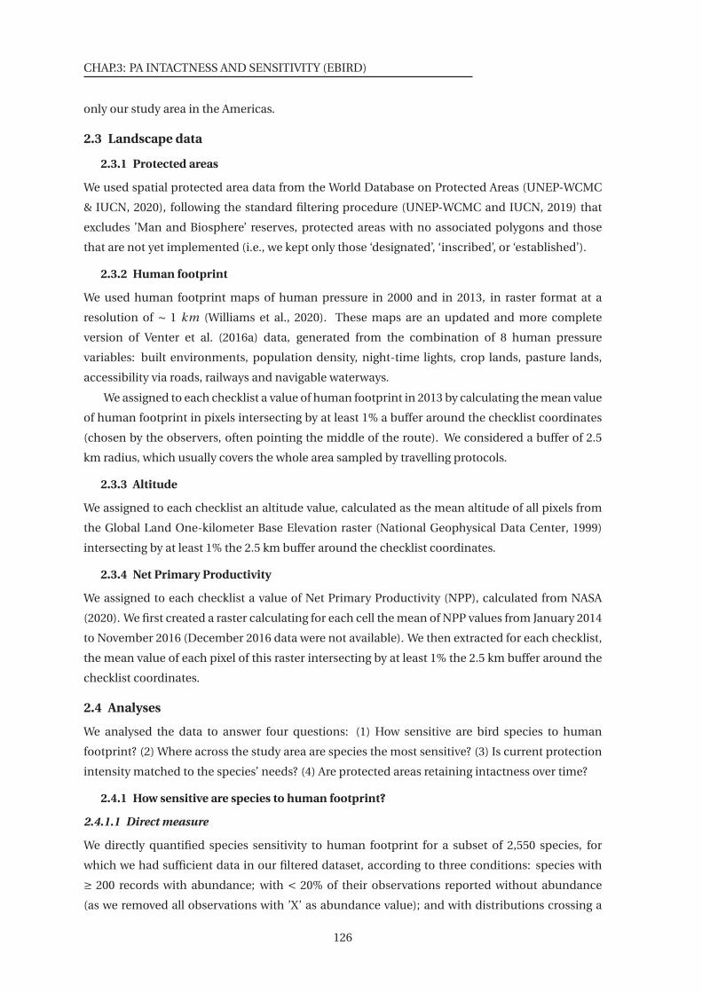
CHAP.3: PA INTACTNESS AND SENSITIVITY (EBIRD)
only our study area in the Americas.
2.3 Landscape data
2.3.1 Protected areas
We used spatial protected area data from the World Database on Protected Areas (UNEP-WCMC
& IUCN, 2020), following the standard filtering procedure (UNEP-WCMC and IUCN, 2019) that
excludes ’Man and Biosphere’ reserves, protected areas with no associated polygons and those
that are not yet implemented (i.e., we kept only those ‘designated’, ‘inscribed’, or ‘established’).
2.3.2 Human footprint
We used human footprint maps of human pressure in 2000 and in 2013, in raster format at a
resolution of ∼ 1 km (Williams et al., 2020). These maps are an updated and more complete
version of Venter et al. (2016a) data, generated from the combination of 8 human pressure
variables: built environments, population density, night-time lights, crop lands, pasture lands,
accessibility via roads, railways and navigable waterways.
We assigned to each checklist a value of human footprint in 2013 by calculating the mean value
of human footprint in pixels intersecting by at least 1% a buffer around the checklist coordinates
(chosen by the observers, often pointing the middle of the route). We considered a buffer of 2.5
km radius, which usually covers the whole area sampled by travelling protocols.
2.3.3 Altitude
We assigned to each checklist an altitude value, calculated as the mean altitude of all pixels from
the Global Land One-kilometer Base Elevation raster (National Geophysical Data Center, 1999)
intersecting by at least 1% the 2.5 km buffer around the checklist coordinates.
2.3.4 Net Primary Productivity
We assigned to each checklist a value of Net Primary Productivity (NPP), calculated from NASA
(2020). We first created a raster calculating for each cell the mean of NPP values from January 2014
to November 2016 (December 2016 data were not available). We then extracted for each checklist,
the mean value of each pixel of this raster intersecting by at least 1% the 2.5 km buffer around the
checklist coordinates.
2.4 Analyses
We analysed the data to answer four questions: (1) How sensitive are bird species to human
footprint? (2) Where across the study area are species the most sensitive? (3) Is current protection
intensity matched to the species’ needs? (4) Are protected areas retaining intactness over time?
2.4.1 How sensitive are species to human footprint?
2.4.1.1 Direct measure
We directly quantified species sensitivity to human footprint for a subset of 2,550 species, for
which we had sufficient data in our filtered dataset, according to three conditions: species with
≥ 200 records with abundance; with < 20% of their observations reported without abundance
(as we removed all observations with ’X’ as abundance value); and with distributions crossing a
126

2. METHODS
range of human footprint conditions (i.e., we calculated the 1% and the 99% quantiles of human
footprint from checklists sampled within each species distribution and excluded species for which
these quantiles differed by < 25). For these 2,550 species, we ran a General Additive Model
(GAM) per species modelling the link between local species abundance and human footprint per
checklist (assuming a negative binomial distribution of abundance and using the bam function
(Wood, 2011)). In order to enable a diversity of links, from linear to non-monotonous relations,
we used a smoothed term on human footprint, but we constrained the degree of the smoothing
function to 6 to avoid very complex functions (see examples of relations in Fig.1). In these models,
we controlled for differences in sampling effort (logarithm of sampling duration, logarithm of
number of observers, and observer expertise of the most experienced observer), differences in
ecological conditions (altitude and net primary productivity, both assuming parabolic responses),
and large-scale patterns of spatial autocorrelation (interacting smooth-term with longitude and
latitude), with the following structure:
Abundance_species ∼ s(human_ f oot pr i nt ,k = 6) + log (dur ati on) + log (N_observers) +
exper t i se+al t i tude+al t i tude2+pr oducti vi t y+pr oducti vi t y2
+ te(long i tude, l at i tude)
We then predicted the abundance of the species across a gradient of human footprint ranging
from 0 to the maximum value of human footprint observed within the species’ distribution,
with a step of 0.05 (and fixing duration and expertise to their median values) and extracted the
weighted average of this distribution. We measured species sensitivity (the variable used in
the following analyses) as the difference between 50 (i.e., maximum human footprint) and this
weighted average. High-sensitivity species have an abundance strongly biased towards sites with
low human footprint (e.g., Leuconotopicus borealis, Fig.1), medium-sensitivity species have an
abundance unrelated with human footprint or biased towards medium human footprint (e.g.,
Icterus gularis, Fig.1), low-sensitivity species have an abundance biased towards sites with high
human footprint (e.g., Turdus rufiventris, Fig.1).
2.4.1.2 Inferred sensitivity for missing species
We used information on traits to generalise from the 2,550 species for which sensitivity could be
measured directly to infer the sensitivity of the remaining 1,874 species that breed in the Americas
(for a total of N=4,424 based on BirdLife International and HBW (2019) distribution maps). To
do so, we first linked the measured values of species sensitivity to species traits using a linear
model. We included in the model the species’ primary habitat, primary diet, specialisation (log-
scaled), body mass (log-scaled), quantitative Red List status, breeding range size in the Americas
(log-scaled), migration status, and taxonomical order, with the following structure:
Sensitivity ∼ Primary_Habitat + Primary_Diet + speci al i sati on + log (Mass) + Red_List +
l og (Range)+Migration+Order
We then used this model to infer the sensitivity of the remaining species (see details in
Supplementary Methods 3). Our measure of species sensitivity cannot be compared in absolute
terms to human footprint (i.e., a sensitivity of 30 does not necessarily mean that the species is
tolerant to human pressure up to a human footprint of 20). This is due to a very strong bias in
sampling towards sites with high human footprint and, more importantly, a complete absence
127
CHAP.3: PA INTACTNESS AND SENSITIVITY (EBIRD)
of sampling events in sites with very low human footprint at every latitude (see Supplementary
Methods 4). Accordingly, we use values of measured or inferred sensitivity only in relative terms:
to investigate which species are more sensitive than others, and to contrast regions in terms of the
average relative sensitivity of their bird species.
2.4.2 Where are species the most sensitive?
For each ecoregion, we extracted from the species’ distribution maps BirdLife International and
HBW (2019) the list of species whose breeding distribution (as defined above) overlaps at least
partially the ecoregion polygon. We defined high-sensitivity species as the 25% most sensitive
species across the study area and calculated for each ecoregion the proportion of high-sensitivity
species in relation to the total number of breeding bird species in the ecoregion. For context, we
also mapped two potential alternative measures of sensitivity per ecoregion: median sensitivity
and absolute number of high-sensitivity species.
2.4.3 Is protection intensity matched to species’ needs?
2.4.3.1 At the ecoregional scale
We defined the protection intensity of an ecoregion as the proportion of its total area covered
by protected areas with intact habitats. This was calculated using the human footprint raster
from 2013, and considering as intact those pixels with values < 4 (following Williams et al.
(2020)) and as protected those pixels that were > 10% covered by protected areas. We then
studied the correlation between protection intensity and the proportion of high-sensitivity species
per ecoregion using the Pearson correlation coefficient and mapped the match between these
variables using a bivariate colouring. For comparison, we also mapped two potential alternative
measures of protection intensity per ecoregion: protected area extent (the percentage of ecoregion
covered by protected areas), and protected area intactness (the average intactness of protected
area pixels, defined as the inverse of human footprint).
2.4.3.2 At the species scale
For each high-sensitivity species, we quantified their coverage by intact protected areas. To do
so, we created a 0/1 raster of intact protected areas, as a transformation from the 2013 human
footprint raster, by assigning the value 1 to each pixel with human footprint value < 4 (i.e., intact
habitat) and whose centre felt within a protected area (0 otherwise). Given a pixel size of 1 km2,
we then calculated the area of intact protected areas per species by summing the raster values of
pixels whose centre felt within the species’ breeding distribution.
We then assessed whether high-sensitivity species were adequately covered by intact protected
areas, by comparing their coverage by intact protected areas against a predefined representation
target. For each species, this target was calculated based on a widely-used approach (e.g.,
Rodrigues et al. (2004a), Maxwell et al. (2020), Butchart et al. (2015)) whereby species with very
small ranges (< 1000 km2) have a 100% target, those with very widespread ranges (> 250,000 km2)
have a 10% target, with the target for species with ranges of intermediate size being interpolated
between these two extremes. A high-sensitivity species was considered inadequately covered by
intact protected areas if the coverage of protected areas falls below the representation target.
128
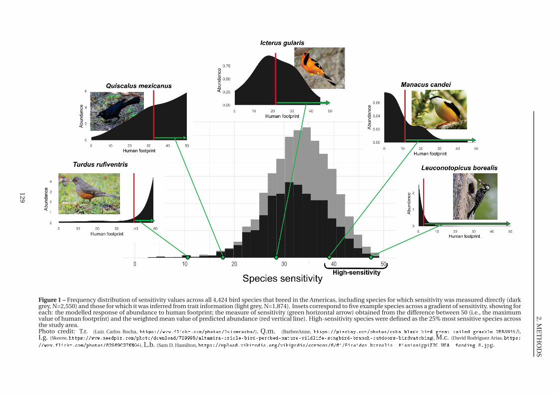
2.ME
TH
OD
S
Figure 1 – Frequency distribution of sensitivity values across all 4,424 bird species that breed in the Americas, including species for which sensitivity was measured directly (darkgrey, N=2,550) and those for which it was inferred from trait information (light grey, N=1,874). Insets correspond to five example species across a gradient of sensitivity, showing foreach: the modelled response of abundance to human footprint; the measure of sensitivity (green horizontal arrow) obtained from the difference between 50 (i.e., the maximumvalue of human footprint) and the weighted mean value of predicted abundance (red vertical line). High-sensitivity species were defined as the 25% most sensitive species acrossthe study area.Photo credit: T.r. (Luiz Carlos Rocha, ), Q.m. (BarbeeAnne, ),I.g. (Skeeze, ), M.c. (David Rodriguez Arias,
), L.b. (Sam D. Hamilton, ).
129
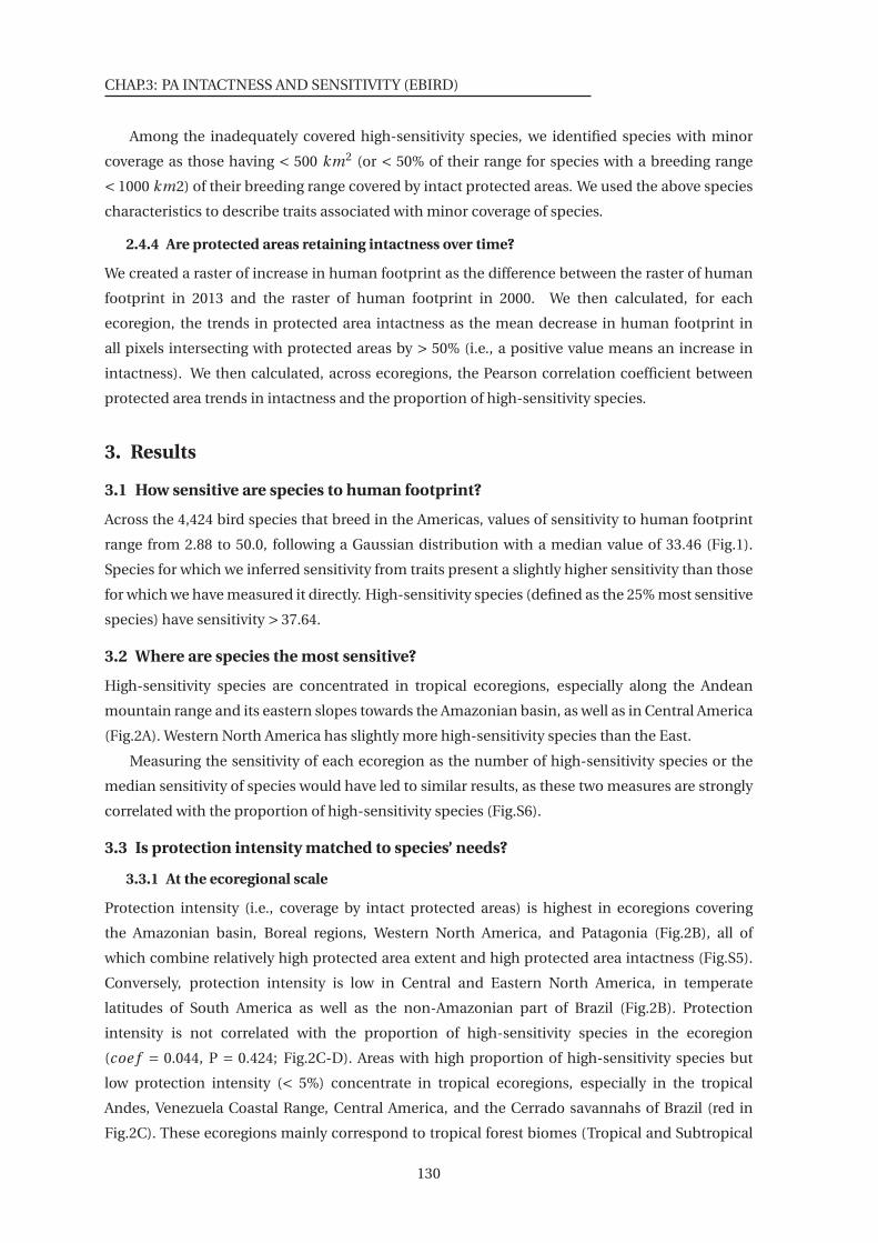
CHAP.3: PA INTACTNESS AND SENSITIVITY (EBIRD)
Among the inadequately covered high-sensitivity species, we identified species with minor
coverage as those having < 500 km2 (or < 50% of their range for species with a breeding range
< 1000 km2) of their breeding range covered by intact protected areas. We used the above species
characteristics to describe traits associated with minor coverage of species.
2.4.4 Are protected areas retaining intactness over time?
We created a raster of increase in human footprint as the difference between the raster of human
footprint in 2013 and the raster of human footprint in 2000. We then calculated, for each
ecoregion, the trends in protected area intactness as the mean decrease in human footprint in
all pixels intersecting with protected areas by > 50% (i.e., a positive value means an increase in
intactness). We then calculated, across ecoregions, the Pearson correlation coefficient between
protected area trends in intactness and the proportion of high-sensitivity species.
3. Results
3.1 How sensitive are species to human footprint?
Across the 4,424 bird species that breed in the Americas, values of sensitivity to human footprint
range from 2.88 to 50.0, following a Gaussian distribution with a median value of 33.46 (Fig.1).
Species for which we inferred sensitivity from traits present a slightly higher sensitivity than those
for which we have measured it directly. High-sensitivity species (defined as the 25% most sensitive
species) have sensitivity > 37.64.
3.2 Where are species the most sensitive?
High-sensitivity species are concentrated in tropical ecoregions, especially along the Andean
mountain range and its eastern slopes towards the Amazonian basin, as well as in Central America
(Fig.2A). Western North America has slightly more high-sensitivity species than the East.
Measuring the sensitivity of each ecoregion as the number of high-sensitivity species or the
median sensitivity of species would have led to similar results, as these two measures are strongly
correlated with the proportion of high-sensitivity species (Fig.S6).
3.3 Is protection intensity matched to species’ needs?
3.3.1 At the ecoregional scale
Protection intensity (i.e., coverage by intact protected areas) is highest in ecoregions covering
the Amazonian basin, Boreal regions, Western North America, and Patagonia (Fig.2B), all of
which combine relatively high protected area extent and high protected area intactness (Fig.S5).
Conversely, protection intensity is low in Central and Eastern North America, in temperate
latitudes of South America as well as the non-Amazonian part of Brazil (Fig.2B). Protection
intensity is not correlated with the proportion of high-sensitivity species in the ecoregion
(coe f = 0.044, P = 0.424; Fig.2C-D). Areas with high proportion of high-sensitivity species but
low protection intensity (< 5%) concentrate in tropical ecoregions, especially in the tropical
Andes, Venezuela Coastal Range, Central America, and the Cerrado savannahs of Brazil (red in
Fig.2C). These ecoregions mainly correspond to tropical forest biomes (Tropical and Subtropical
130
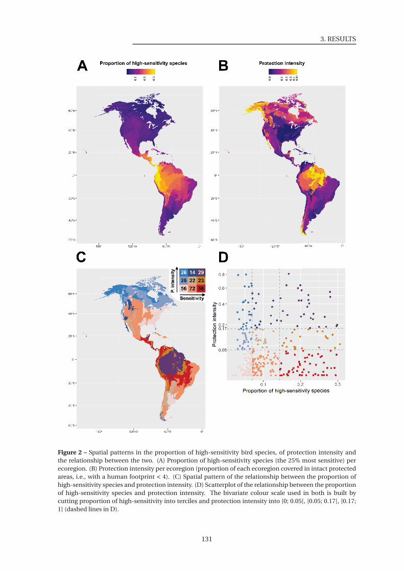
3. RESULTS
Figure 2 – Spatial patterns in the proportion of high-sensitivity bird species, of protection intensity andthe relationship between the two. (A) Proportion of high-sensitivity species (the 25% most sensitive) perecoregion. (B) Protection intensity per ecoregion (proportion of each ecoregion covered in intact protectedareas, i.e., with a human footprint < 4). (C) Spatial pattern of the relationship between the proportion ofhigh-sensitivity species and protection intensity. (D) Scatterplot of the relationship between the proportionof high-sensitivity species and protection intensity. The bivariate colour scale used in both is built bycutting proportion of high-sensitivity into terciles and protection intensity into [0; 0.05[, [0.05; 0.17[, [0.17;1] (dashed lines in D).
131

CHAP.3: PA INTACTNESS AND SENSITIVITY (EBIRD)
Moist broadleaf forests (N = 22), Tropical and Subtropical Dry broadleaf forests (N = 15),
Tropical and Subtropical Coniferous forests (N = 3), and Mangroves (N = 7)) but also include
Montane Grasslands and Shrublands (N = 6), Deserts and Xeric Shrublands (N = 3), Tropical
and Subtropical Grasslands, Savannahs and Shrublands (N = 1) and Flooded Grasslands and
Savannahs (N = 1; Fig.3; Olson et al. (2001)).
Additionally, 23 ecoregions have medium protection intensity (i.e., 5 – 17%) and high
proportion of high-sensitivity species, and are also found in tropical areas (caramel in Fig.2C-D),
and in Montane Grassland and Shrublands ecoregions (Fig.3). Ecoregions with medium sensitivity
and low protection intensity are mainly found in the centre of North America’s temperate
grasslands and in the Caribbean (salmon in Fig.2C-D).
Conversely, the eastern slopes of the Andes and the Amazonian basin have ecoregions with
high proportion of high-sensitivity species while being relatively well covered by intact protected
areas (purple in Fig.2C-D; 29 ecoregions), which mainly belong to Tropical and Subtropical Moist
Broadleaf forest biome and Mangroves biome (Fig.3).
Here we measured protection intensity as the proportion of intact protected areas, but neither
the total extent of protected areas nor the median intactness of protected areas per ecoregion
better correlate with the proportion of high-sensitivity species (Supplementary Figure S6).
Figure 3 – Biome distribution of the match between protection intensity and proportion of high-sensitivitybird species per ecoregion. Biome names and classification from Olson et al. (2001). Colours as in Fig.2.
132
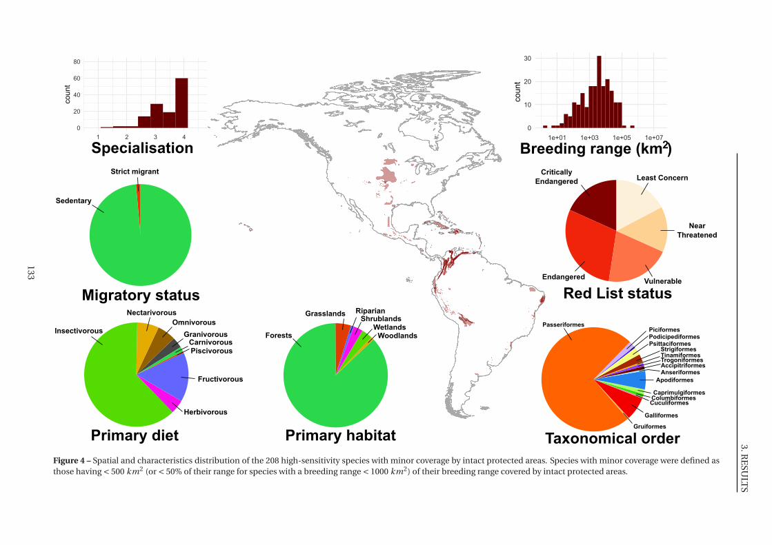
3.RE
SULT
S
0
20
40
60
80
1 2 3 4
count
0
10
20
30
1e+01 1e+03 1e+05 1e+07
count
Red List status
Least Concern
Near
Threatened
VulnerableEndangered
Critically
Endangered
PiciformesPodicipediformesPsittaciformes
StrigiformesTinamiformesTrogoniformesAccipitriformes
Apodiformes
CaprimulgiformesColumbiformesCuculiformes
Galliformes
Gruiformes
Passeriformes
Taxonomical order
Migratory status
Sedentary
Strict migrant
Insectivorous
Nectarivorous
Omnivorous
Granivorous
Herbivorous
Fructivorous
PiscivorousCarnivorous
Primary diet
Forests
Grasslands RiparianShrublands
WoodlandsWetlands
Primary habitat
Specialisation Breeding range (km )2
Anseriformes
Figure 4 – Spatial and characteristics distribution of the 208 high-sensitivity species with minor coverage by intact protected areas. Species with minor coverage were defined asthose having < 500 km2 (or < 50% of their range for species with a breeding range < 1000 km2) of their breeding range covered by intact protected areas.
133
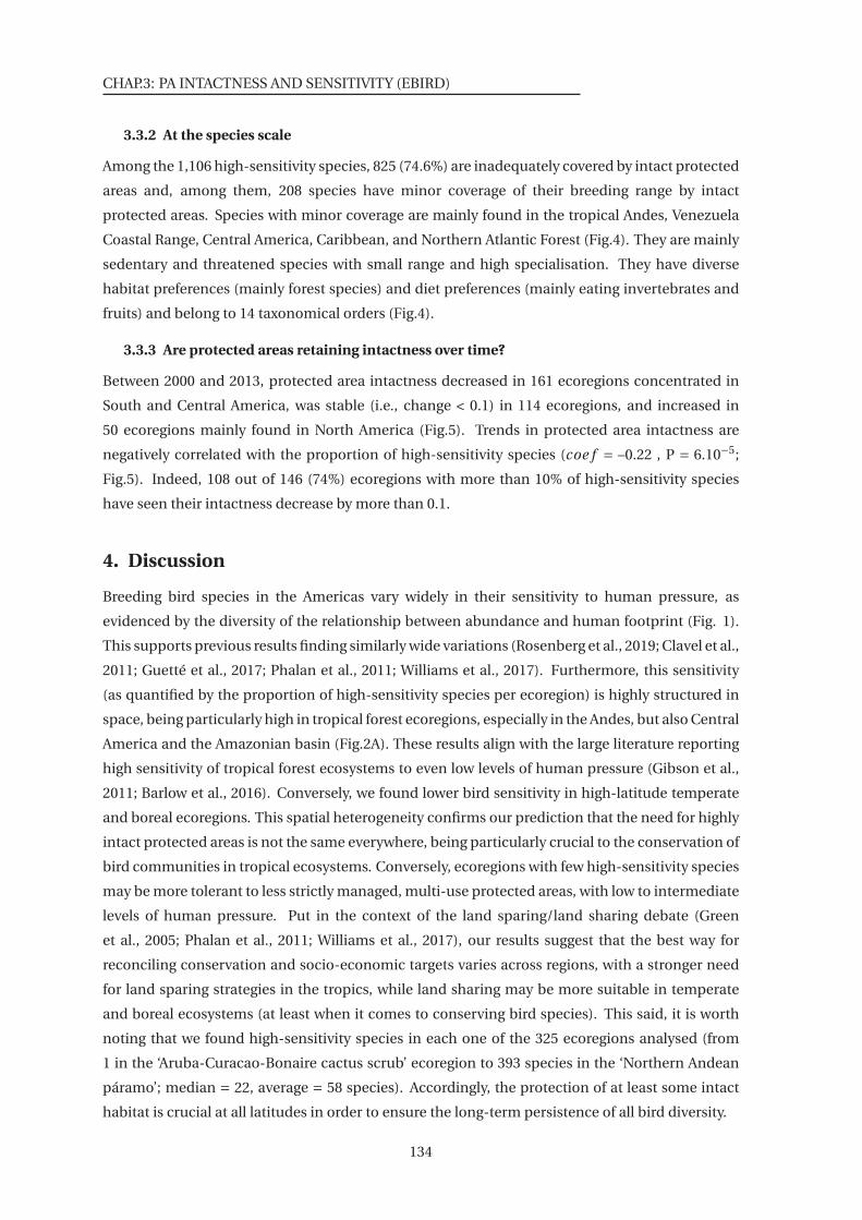
CHAP.3: PA INTACTNESS AND SENSITIVITY (EBIRD)
3.3.2 At the species scale
Among the 1,106 high-sensitivity species, 825 (74.6%) are inadequately covered by intact protected
areas and, among them, 208 species have minor coverage of their breeding range by intact
protected areas. Species with minor coverage are mainly found in the tropical Andes, Venezuela
Coastal Range, Central America, Caribbean, and Northern Atlantic Forest (Fig.4). They are mainly
sedentary and threatened species with small range and high specialisation. They have diverse
habitat preferences (mainly forest species) and diet preferences (mainly eating invertebrates and
fruits) and belong to 14 taxonomical orders (Fig.4).
3.3.3 Are protected areas retaining intactness over time?
Between 2000 and 2013, protected area intactness decreased in 161 ecoregions concentrated in
South and Central America, was stable (i.e., change < 0.1) in 114 ecoregions, and increased in
50 ecoregions mainly found in North America (Fig.5). Trends in protected area intactness are
negatively correlated with the proportion of high-sensitivity species (coe f = –0.22 , P = 6.10−5;
Fig.5). Indeed, 108 out of 146 (74%) ecoregions with more than 10% of high-sensitivity species
have seen their intactness decrease by more than 0.1.
4. Discussion
Breeding bird species in the Americas vary widely in their sensitivity to human pressure, as
evidenced by the diversity of the relationship between abundance and human footprint (Fig. 1).
This supports previous results finding similarly wide variations (Rosenberg et al., 2019; Clavel et al.,
2011; Guetté et al., 2017; Phalan et al., 2011; Williams et al., 2017). Furthermore, this sensitivity
(as quantified by the proportion of high-sensitivity species per ecoregion) is highly structured in
space, being particularly high in tropical forest ecoregions, especially in the Andes, but also Central
America and the Amazonian basin (Fig.2A). These results align with the large literature reporting
high sensitivity of tropical forest ecosystems to even low levels of human pressure (Gibson et al.,
2011; Barlow et al., 2016). Conversely, we found lower bird sensitivity in high-latitude temperate
and boreal ecoregions. This spatial heterogeneity confirms our prediction that the need for highly
intact protected areas is not the same everywhere, being particularly crucial to the conservation of
bird communities in tropical ecosystems. Conversely, ecoregions with few high-sensitivity species
may be more tolerant to less strictly managed, multi-use protected areas, with low to intermediate
levels of human pressure. Put in the context of the land sparing/land sharing debate (Green
et al., 2005; Phalan et al., 2011; Williams et al., 2017), our results suggest that the best way for
reconciling conservation and socio-economic targets varies across regions, with a stronger need
for land sparing strategies in the tropics, while land sharing may be more suitable in temperate
and boreal ecosystems (at least when it comes to conserving bird species). This said, it is worth
noting that we found high-sensitivity species in each one of the 325 ecoregions analysed (from
1 in the ‘Aruba-Curacao-Bonaire cactus scrub’ ecoregion to 393 species in the ‘Northern Andean
páramo’; median = 22, average = 58 species). Accordingly, the protection of at least some intact
habitat is crucial at all latitudes in order to ensure the long-term persistence of all bird diversity.
134
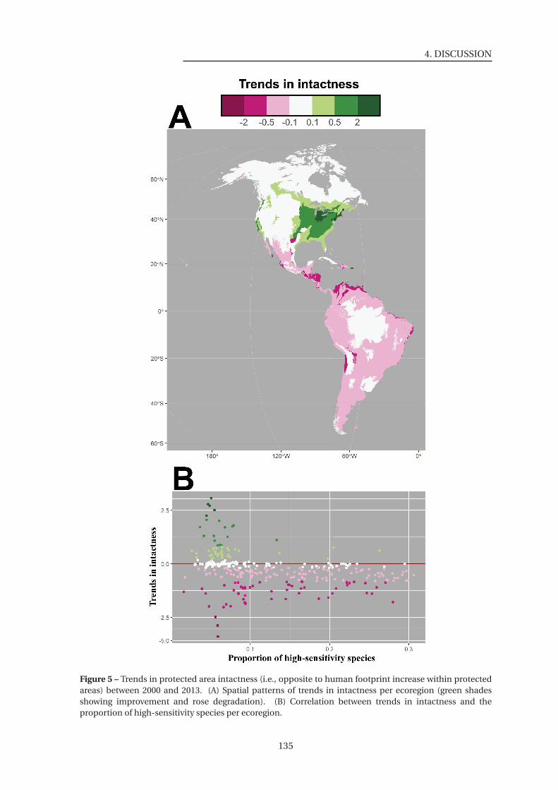
4. DISCUSSION
Figure 5 – Trends in protected area intactness (i.e., opposite to human footprint increase within protectedareas) between 2000 and 2013. (A) Spatial patterns of trends in intactness per ecoregion (green shadesshowing improvement and rose degradation). (B) Correlation between trends in intactness and theproportion of high-sensitivity species per ecoregion.
135
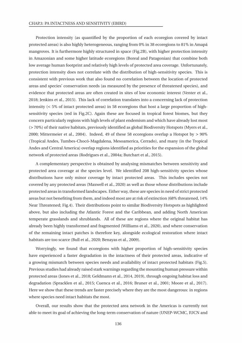
CHAP.3: PA INTACTNESS AND SENSITIVITY (EBIRD)
Protection intensity (as quantified by the proportion of each ecoregion covered by intact
protected areas) is also highly heterogeneous, ranging from 0% in 38 ecoregions to 81% in Amapá
mangroves. It is furthermore highly structured in space (Fig.2B), with higher protection intensity
in Amazonian and some higher latitude ecoregions (Boreal and Patagonian) that combine both
low average human footprint and relatively high levels of protected area coverage. Unfortunately,
protection intensity does not correlate with the distribution of high-sensitivity species. This is
consistent with previous work that also found no correlation between the location of protected
areas and species’ conservation needs (as measured by the presence of threatened species), and
evidence that protected areas are often created in sites of low economic interest (Venter et al.,
2018; Jenkins et al., 2015). This lack of correlation translates into a concerning lack of protection
intensity (< 5% of intact protected areas) in 58 ecoregions that host a large proportion of high-
sensitivity species (red in Fig.2C). Again these are focused in tropical forest biomes, but they
concern particularly regions with high levels of plant endemism and which have already lost most
(> 70%) of their native habitats, previously identified as global Biodiversity Hotspots (Myers et al.,
2000; Mittermeier et al., 2004). Indeed, 49 of these 58 ecoregions overlap a Hotspot by > 90%
(Tropical Andes, Tumbes-Chocó-Magdalena, Mesoamerica, Cerrado), and many (in the Tropical
Andes and Central America) overlap regions identified as priorities for the expansion of the global
network of protected areas (Rodrigues et al., 2004a; Butchart et al., 2015).
A complementary perspective is obtained by analysing mismatches between sensitivity and
protected area coverage at the species level. We identified 208 high-sensitivity species whose
distributions have only minor coverage by intact protected areas. This includes species not
covered by any protected areas (Maxwell et al., 2020) as well as those whose distributions include
protected areas in transformed landscapes. Either way, these are species in need of strict protected
areas but not benefiting from them, and indeed most are at risk of extinction (68% threatened, 14%
Near Threatened; Fig.4). Their distributions point to similar Biodiversity Hotspots as highlighted
above, but also including the Atlantic Forest and the Caribbean, and adding North American
temperate grasslands and shrublands. All of these are regions where the original habitat has
already been highly transformed and fragmented (Williams et al., 2020), and where conservation
of the remaining intact patches is therefore key, alongside ecological restoration where intact
habitats are too scarce (Bull et al., 2020; Benayas et al., 2009).
Worryingly, we found that ecoregions with higher proportion of high-sensitivity species
have experienced a faster degradation in the intactness of their protected areas, indicative of
a growing mismatch between species needs and availability of intact protected habitats (Fig.5).
Previous studies had already raised stark warnings regarding the mounting human pressure within
protected areas (Jones et al., 2018; Geldmann et al., 2014, 2019), through ongoing habitat loss and
degradation (Spracklen et al., 2015; Cuenca et al., 2016; Bruner et al., 2001; Moore et al., 2017).
Here we show that these trends are faster precisely where they are the most dangerous: in regions
where species need intact habitats the most.
Overall, our results show that the protected area network in the Americas is currently not
able to meet its goal of achieving the long-term conservation of nature (UNEP-WCMC, IUCN and
136
4. DISCUSSION
NGS, 2020) given the mismatches we highlight between species conservation needs in terms of
intact habitats and the coverage of these habitats by protected areas. Our results provide specific
guidance for expanding and reinforcing this network: by prioritising the protection of intact
habitat in ecoregions with high species sensitivity but low (current) protection intensity, as well as
its restoration where very little habitat remains. With these ecoregions located in several countries
with limited economic resources, international cooperation is key to meeting this goal.
More broadly, we recommend that species sensitivity is taken into account when possible
in future analyses of the effectiveness of protected areas in terms of covering species, including
in reporting towards policy goals (SCBD, 2010). Indeed, previous analyses focused on simple
coverage of species’ range (e.g., Rodrigues et al. (2004a), Butchart et al. (2015), Maxwell et al.
(2020)) can grossly overestimate the actual protection levels of high-sensitivity species. For
instance, Butchart et al. (2015) found that the Critically Endangered Santa Marta wren, Troglodytes
monticola, is protected in 99.7% of its range, and thus consider this species as adequately
covered. Yet we found that none of these protected areas include intact habitat (their human
footprint ranges from 5 to 16, mean = 7.3) for this high-sensitivity species (sensitivity = 41).
Our approach for calculating high sensitivity requires field information on species’ responses to
human pressure. Even though these data are not available for the vast majority of species in most
regions, citizen science datasets (e.g., eBird, iNaturalist) are creating increasingly large datasets
that are being brought together through data sharing platforms (e.g., GBIF). Treating these
datasets poses challenges given the lack of standardization in data collection. But these challenges
can be overcome when the datasets become sufficiently large to control for confounding factors.
Furthermore, we foresee that some of the general patterns obtained here – in particular that
tropical species are particularly sensitive to human pressure – are generalizable to other regions
and to other taxa.
137
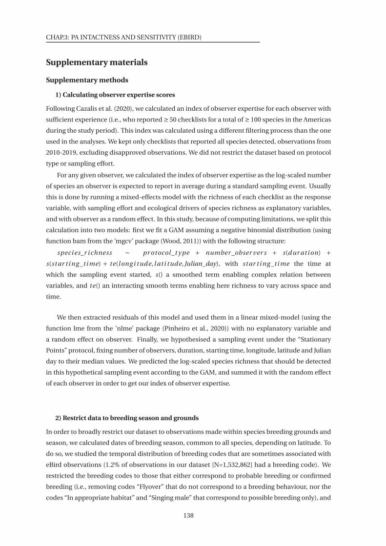
CHAP.3: PA INTACTNESS AND SENSITIVITY (EBIRD)
Supplementary materials
Supplementary methods
1) Calculating observer expertise scores
Following Cazalis et al. (2020), we calculated an index of observer expertise for each observer with
sufficient experience (i.e., who reported ≥ 50 checklists for a total of ≥ 100 species in the Americas
during the study period). This index was calculated using a different filtering process than the one
used in the analyses. We kept only checklists that reported all species detected, observations from
2010-2019, excluding disapproved observations. We did not restrict the dataset based on protocol
type or sampling effort.
For any given observer, we calculated the index of observer expertise as the log-scaled number
of species an observer is expected to report in average during a standard sampling event. Usually
this is done by running a mixed-effects model with the richness of each checklist as the response
variable, with sampling effort and ecological drivers of species richness as explanatory variables,
and with observer as a random effect. In this study, because of computing limitations, we split this
calculation into two models: first we fit a GAM assuming a negative binomial distribution (using
function bam from the ’mgcv’ package (Wood, 2011)) with the following structure:
speci es_r i chness ∼ pr otocol _t y pe + number _obser ver s + s(dur ati on) +
s(st ar t i ng _t i me) + te(long i tude, l at i tude, Julian_day), with st ar t i ng _t i me the time at
which the sampling event started, s() a smoothed term enabling complex relation between
variables, and te() an interacting smooth terms enabling here richness to vary across space and
time.
We then extracted residuals of this model and used them in a linear mixed-model (using the
function lme from the ’nlme’ package (Pinheiro et al., 2020)) with no explanatory variable and
a random effect on observer. Finally, we hypothesised a sampling event under the “Stationary
Points” protocol, fixing number of observers, duration, starting time, longitude, latitude and Julian
day to their median values. We predicted the log-scaled species richness that should be detected
in this hypothetical sampling event according to the GAM, and summed it with the random effect
of each observer in order to get our index of observer expertise.
2) Restrict data to breeding season and grounds
In order to broadly restrict our dataset to observations made within species breeding grounds and
season, we calculated dates of breeding season, common to all species, depending on latitude. To
do so, we studied the temporal distribution of breeding codes that are sometimes associated with
eBird observations (1.2% of observations in our dataset [N=1,532,862] had a breeding code). We
restricted the breeding codes to those that either correspond to probable breeding or confirmed
breeding (i.e., removing codes “Flyover” that do not correspond to a breeding behaviour, nor the
codes “In appropriate habitat” and “Singing male” that correspond to possible breeding only), and
138
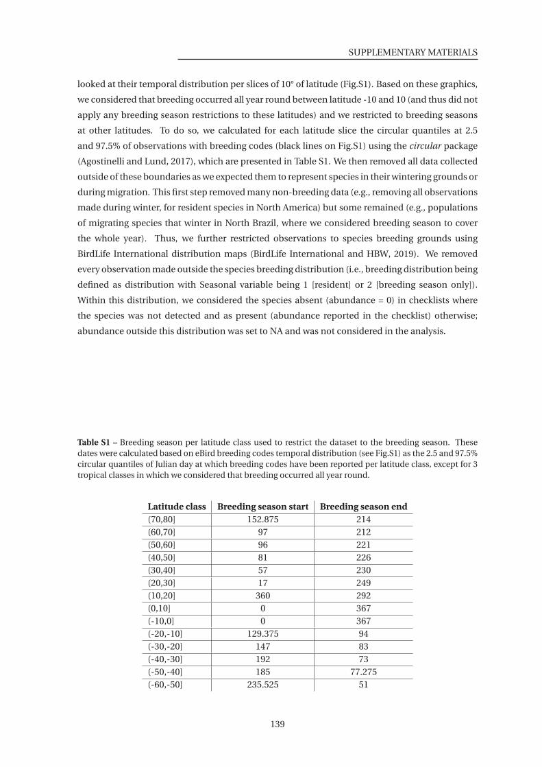
SUPPLEMENTARY MATERIALS
looked at their temporal distribution per slices of 10° of latitude (Fig.S1). Based on these graphics,
we considered that breeding occurred all year round between latitude -10 and 10 (and thus did not
apply any breeding season restrictions to these latitudes) and we restricted to breeding seasons
at other latitudes. To do so, we calculated for each latitude slice the circular quantiles at 2.5
and 97.5% of observations with breeding codes (black lines on Fig.S1) using the circular package
(Agostinelli and Lund, 2017), which are presented in Table S1. We then removed all data collected
outside of these boundaries as we expected them to represent species in their wintering grounds or
during migration. This first step removed many non-breeding data (e.g., removing all observations
made during winter, for resident species in North America) but some remained (e.g., populations
of migrating species that winter in North Brazil, where we considered breeding season to cover
the whole year). Thus, we further restricted observations to species breeding grounds using
BirdLife International distribution maps (BirdLife International and HBW, 2019). We removed
every observation made outside the species breeding distribution (i.e., breeding distribution being
defined as distribution with Seasonal variable being 1 [resident] or 2 [breeding season only]).
Within this distribution, we considered the species absent (abundance = 0) in checklists where
the species was not detected and as present (abundance reported in the checklist) otherwise;
abundance outside this distribution was set to NA and was not considered in the analysis.
Table S1 – Breeding season per latitude class used to restrict the dataset to the breeding season. Thesedates were calculated based on eBird breeding codes temporal distribution (see Fig.S1) as the 2.5 and 97.5%circular quantiles of Julian day at which breeding codes have been reported per latitude class, except for 3tropical classes in which we considered that breeding occurred all year round.
Latitude class Breeding season start Breeding season end(70,80] 152.875 214(60,70] 97 212(50,60] 96 221(40,50] 81 226(30,40] 57 230(20,30] 17 249(10,20] 360 292(0,10] 0 367(-10,0] 0 367(-20,-10] 129.375 94(-30,-20] 147 83(-40,-30] 192 73(-50,-40] 185 77.275(-60,-50] 235.525 51
139
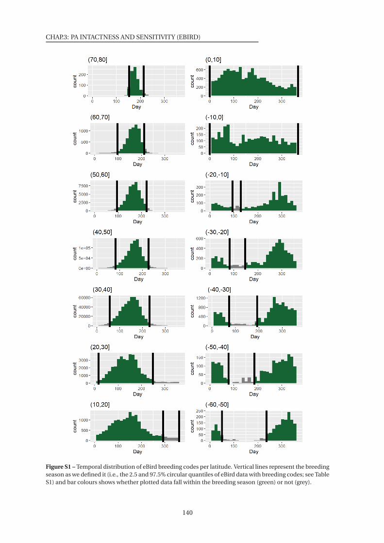
CHAP.3: PA INTACTNESS AND SENSITIVITY (EBIRD)
Figure S1 – Temporal distribution of eBird breeding codes per latitude. Vertical lines represent the breedingseason as we defined it (i.e., the 2.5 and 97.5% circular quantiles of eBird data with breeding codes; see TableS1) and bar colours shows whether plotted data fall within the breeding season (green) or not (grey).
140
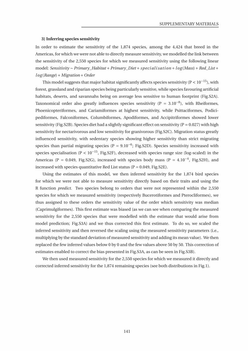
SUPPLEMENTARY MATERIALS
3) Inferring species sensitivity
In order to estimate the sensitivity of the 1,874 species, among the 4,424 that breed in the
Americas, for which we were not able to directly measure sensitivity, we modelled the link between
the sensitivity of the 2,550 species for which we measured sensitivity using the following linear
model: Sensitivity ∼ Primary_Habitat +Primary_Diet + speci al i sati on + log (Mass)+Red_List +
l og (Range)+Migration+Order
This model suggests that major habitat significantly affects species sensitivity (P < 10−15), with
forest, grassland and riparian species being particularly sensitive, while species favouring artificial
habitats, deserts, and savannahs being on average less sensitive to human footprint (Fig.S2A).
Taxonomical order also greatly influences species sensitivity (P = 3.10−8), with Rheiformes,
Phoenicopteriformes, and Cariamiformes at highest sensitivity, while Psittaciformes, Podici-
pediformes, Falconiformes, Columbiformes, Apodiformes, and Accipitriformes showed lower
sensitivity (Fig.S2B). Species diet had a slightly significant effect on sensitivity (P = 0.027) with high
sensitivity for nectarivorous and low sensitivity for granivorous (Fig.S2C). Migration status greatly
influenced sensitivity, with sedentary species showing higher sensitivity than strict migrating
species than partial migrating species (P = 9.10−6; Fig.S2D). Species sensitivity increased with
species specialisation (P < 10−15, Fig.S2F), decreased with species range size (log-scaled) in the
Americas (P = 0.049, Fig.S2G), increased with species body mass (P = 4.10−4, Fig.S2H), and
increased with species quantitative Red List status (P = 0.049, Fig.S2E).
Using the estimates of this model, we then inferred sensitivity for the 1,874 bird species
for which we were not able to measure sensitivity directly based on their traits and using the
R function predict. Two species belong to orders that were not represented within the 2,550
species for which we measured sensitivity (respectively Bucerotiformes and Pterocliformes), we
thus assigned to these orders the sensitivity value of the order which sensitivity was median
(Caprimulgiformes). This first estimate was biased (as we can see when comparing the measured
sensitivity for the 2,550 species that were modelled with the estimate that would arise from
model prediction; Fig.S3A) and we thus corrected this first estimate. To do so, we scaled the
inferred sensitivity and then reversed the scaling using the measured sensitivity parameters (i.e.,
multiplying by the standard deviation of measured sensitivity and adding its mean value). We then
replaced the few inferred values below 0 by 0 and the few values above 50 by 50. This correction of
estimates enabled to correct the bias presented in Fig.S3A, as can be seen in Fig.S3B).
We then used measured sensitivity for the 2,550 species for which we measured it directly and
corrected inferred sensitivity for the 1,874 remaining species (see both distributions in Fig.1).
141
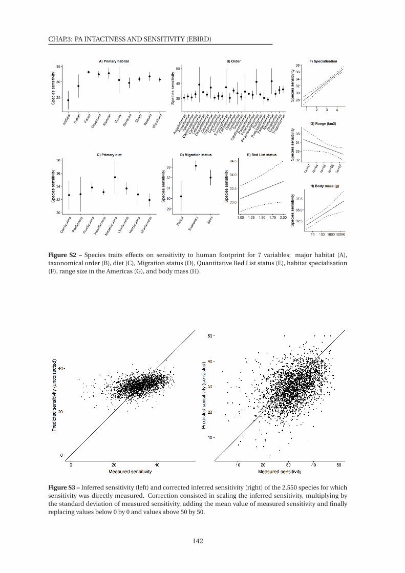
CHAP.3: PA INTACTNESS AND SENSITIVITY (EBIRD)
Figure S2 – Species traits effects on sensitivity to human footprint for 7 variables: major habitat (A),taxonomical order (B), diet (C), Migration status (D), Quantitative Red List status (E), habitat specialisation(F), range size in the Americas (G), and body mass (H).
Figure S3 – Inferred sensitivity (left) and corrected inferred sensitivity (right) of the 2,550 species for whichsensitivity was directly measured. Correction consisted in scaling the inferred sensitivity, multiplying bythe standard deviation of measured sensitivity, adding the mean value of measured sensitivity and finallyreplacing values below 0 by 0 and values above 50 by 50.
142
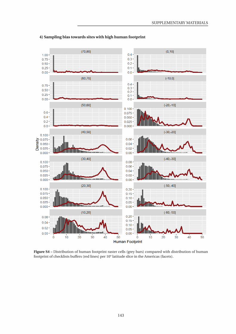
SUPPLEMENTARY MATERIALS
4) Sampling bias towards sites with high human footprint
Figure S4 – Distribution of human footprint raster cells (grey bars) compared with distribution of humanfootprint of checklists buffers (red lines) per 10° latitude slice in the Americas (facets).
143
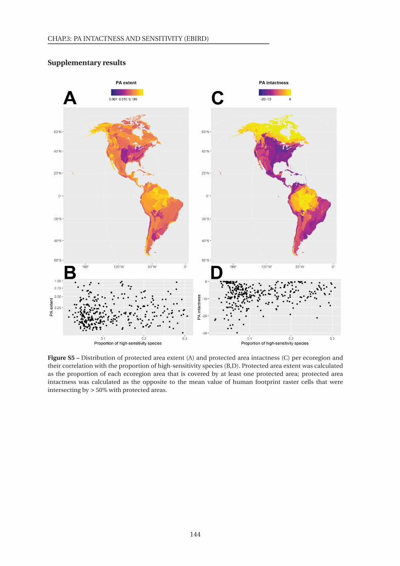
CHAP.3: PA INTACTNESS AND SENSITIVITY (EBIRD)
Supplementary results
Figure S5 – Distribution of protected area extent (A) and protected area intactness (C) per ecoregion andtheir correlation with the proportion of high-sensitivity species (B,D). Protected area extent was calculatedas the proportion of each ecoregion area that is covered by at least one protected area; protected areaintactness was calculated as the opposite to the mean value of human footprint raster cells that wereintersecting by > 50% with protected areas.
144
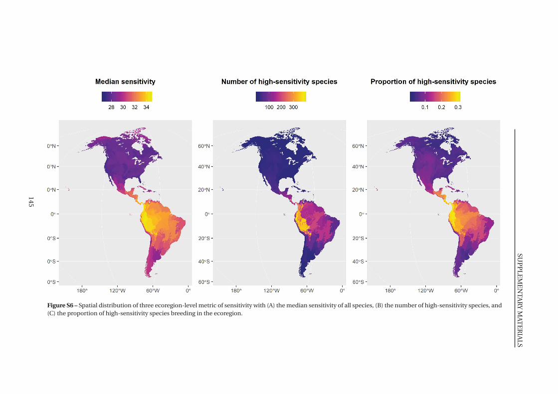
SUP
PL
EM
EN
TAR
YM
ATE
RIA
LS
Figure S6 – Spatial distribution of three ecoregion-level metric of sensitivity with (A) the median sensitivity of all species, (B) the number of high-sensitivity species, and(C) the proportion of high-sensitivity species breeding in the ecoregion.
145
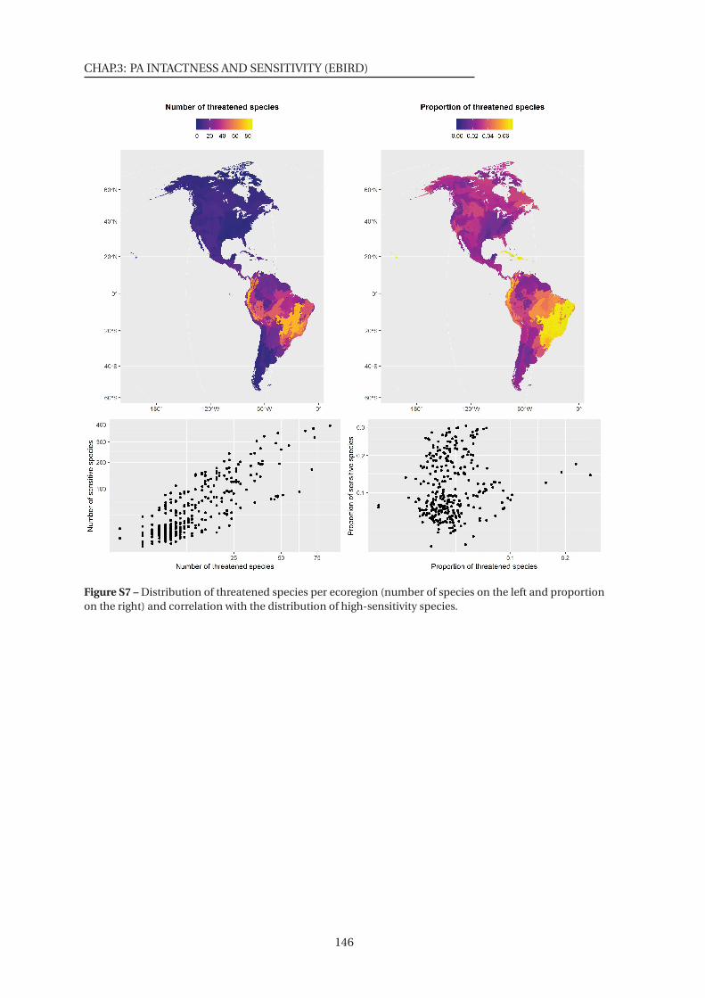
CHAP.3: PA INTACTNESS AND SENSITIVITY (EBIRD)
Figure S7 – Distribution of threatened species per ecoregion (number of species on the left and proportionon the right) and correlation with the distribution of high-sensitivity species.
146

148

Chapitre 4
Les aires protégées sont-elles efficaces dans la
conservation de la connexion des humains avec la
nature et la promotion de comportements
pro-environnementaux ?
149
Au cours de ces trois premiers chapitres de thèse, nous nous sommes intéressés à l’effet
local des aires protégées sur les assemblages d’oiseaux. Le mécanisme qui sous-tend toutes nos
hypothèses est un effet contraignant des aires protégées sur les activités humaines (par exemple
une limitation de la destruction d’habitat ou de la chasse) qui induit une réduction de la pression
et donc atténue le déclin de la biodiversité. Prenons le cas fictif de Valère, un habitant de Cauterets,
commune en bordure du Parc National des Pyrénées, qui a pour habitude de cueillir des fleurs,
dont certaines sont en déclin sur le massif pour confectionner des bouquets. La contrainte légale
du Parc National, interdisant la cueillette de toute fleur dans la zone cœur du parc, peut être un
moyen de faire diminuer cette pression en menaçant Valère de sanctions s’il est attrapé avec des
fleurs coupées. Cependant, une autre voie, moins directe, pourrait permettre à cette pression
de diminuer. En effet, nous pouvons imaginer que l’aire protégée permet à Valère de réaliser
qu’il vit dans un territoire d’exception mais menacé et de le sensibiliser aux problématiques
environnementales. Ainsi, nous pouvons conjecturer que la simple présence de l’aire protégée
et ses actions de sensibilisation pourront avoir un impact positif sur les comportements des
habitants.
Cette hypothèse a été testée dans ce chapitre 4 grâce à une collaboration avec Anne-
Caroline Prévot, chercheuse au MNHN en Psychologie de la Conservation. Nous avons exploré la
corrélation en France métropolitaine entre la distance des communes françaises à un parc naturel
(Parc National ou Parc Naturel Régional) et les comportements pro-environnementaux adoptés
par les habitants de ces communes.
150
THIS MANUSCRIPT HAS BEEN PEER-REVIEWED AND PUBLISHED
Are protected areas effective in conserving hu-
man connection with nature and enhancing pro-
environmental behaviours?
Victor Cazalis1, ∗, and Anne-Caroline Prévot2,3
Authors affiliation:1 CEFE, Univ Montpellier, CNRS, EPHE, IRD, Univ. Paul Valéry Montpellier 3, Montpellier, France2 Centre d’Ecologie et des Sciences de la Conservation (CESCO UMR7204), MNHN, CNRS, Sorbonne
Université, CP135, 57 rue Cuvier, 75005 Paris, France3 Laboratoire Parisien de Psychologie Sociale (LAPPS, EA4386), Université Paris Ouest, Dpt psychologie, 200
avenue de la république, 92000 Nanterre, France
∗ Corresponding author: [email protected]
Cite as: Cazalis, V., and Prévot, A.-C. (2019). Are protected areas effective in conserving human
connection with nature and enhancing pro-environmental behaviours? Biological Conservation
236, 548–555.
151
CHAP.4: PA EFFECTS ON HUMAN BEHAVIOURS (FRANCE)
Abstract
Halting the on-going biodiversity crisis requires large individual behavioural changes through
the implementation of more pro-environmental behaviours (PEBs) by every citizen. People’s
experiences of nature, such as outdoor activities, have been identified as great enhancers of such
behaviours. Yet, these experiences of nature got scarcer in the last decades, due to an increased
spatial segregation between human and nature, particularly in societies that follow a Western way
of life. In this context, we wondered if protected areas (PAs), because they offer more opportunities
for people to be in contact with natural landscapes and offer more ecological information and
governance than other places, could enlarge the implementation of PEBs for people living in
or close from them. We addressed this question by modelling the link between three types
of PEBs in Metropolitan France (i.e., voting for Green party candidates, joining or donating to
biodiversity conservation NGOs and participating in a biodiversity monitoring citizen science
program) and the proximity to large PAs. Innovatively, we addressed this question at national
level, with exhaustive data collected in more than 16,000 French municipalities with more than
500 inhabitants. All models controlled for difference in population size, average income and
proportion of retired people between municipalities. We found that each of the studied PEBs
decreased with distance of the municipality to PAs, even after having controlled by the naturalness
of municipalities’ surroundings. Our results suggest that, beyond their effect through exposure to
natural landscapes, PAs affect PEBs by the institutional context they create. Additionally, PEBs
were higher inside PAs than in close surroundings, suggesting that, besides restrictions brought
by PAs on inhabitants, a fraction of the population responds positively to their implementation.
Our results suggest that PAs can play a role in enhancing environmental friendly ways of life by
conserving human’s connection with nature.
152
1. INTRODUCTION
1. Introduction
We are currently facing the sixth mass extinction of biodiversity, with thousands of species
vanishing and the decline of many species’ populations, described as a time of biodiversity
annihilation (Ceballos et al., 2017). This crisis is mainly due to the human domination of Earth’s
ecosystems (Balmford and Bond, 2005; Dirzo et al., 2014), and threatens ecosystem services and
human well-being (Cardinale et al., 2012; Rockström et al., 2009).
Simultaneously with this decline in biodiversity, most societies are moving away from nature
and biodiversity. Indeed, the proportion of people living in cities increased in the last centuries
and decades, reaching 81.5% in high-income countries in 2018, a number that keeps increasing
(United Nations, 2018). This spatial segregation of human and nature, together with a reduction
of nature recreation activities (Soga and Gaston, 2016) dramatically reduced both desire and
opportunities to directly experience nature (Turner et al., 2004; Clayton et al., 2017). Pyle (2003)
characterised this on-going trend as the extinction of experience and defined it as an “inexorable
cycle of disconnection, apathy, and progressive depletion”.
Nonetheless, significant life experiences of nature are important to create sensitivity, concern
and knowledge about environmental issues (Prévot et al., 2018; Chawla, 1998). Indeed, numerous
studies have shown that they can increase concern about environmental issues and willingness to
take action against them (Clayton and Myers, 2015b; Gifford and Nilsson, 2014; Prévot et al., 2018).
Yet, changes in human behaviours and way of life are needed in order to reduce human impact on
biodiversity (Martin et al., 2016). Consequently, pro-environmental behaviours (PEBs) have been
of main interest in the field of conservation psychology, in order to understand which factors can
enhance them and therefore reduce human’s impact (Clayton and Myers, 2015c). This term of
PEB includes a wide variety of environmental-friendly human behaviours, with different impact
levels, from voting for Green party candidates or feeding birds in the winter, to environmental
activism or adopting of environment-friendly consumption (Larson et al., 2015). Some of them
have direct impacts on biodiversity, some have indirect impacts and some – considered sometimes
as symbolic –, are seen by some authors as a “foot in the door” of environmental-friendly way of
life, leading potentially to PEBs with bigger impact (Burger, 1999; Truelove et al., 2014).
One of the main tools used in conservation to halt biodiversity decline, is to define areas where
human activities are restricted and controlled: that is protected areas (PAs), which can have very
different protection levels. PAs currently represent about 15% of worldwide land area and should
reach 17% by 2020 (UNEP-WCMC, IUCN and NGS, 2018). Even if increasing in importance, PAs
alone cannot address the biodiversity crisis (Prévot-Julliard et al., 2011). However, aside from
their direct conservation impact, we can expect PAs to have an effect on the environmental
concern of nearby inhabitants. First, PAs are more natural than the average (Joppa and Pfaff,
2010), which allows nearby inhabitants to have more opportunities to experience nature than
other people do. Second, as PAs’ governance systems are particularly dedicated to biodiversity
(UNEP-WCMC, IUCN and NGS, 2018), inhabitants can be in contact with ecological information
through education initiatives of PAs (e.g., signs, activities, conferences, green tourism (Cetas and
Yasué, 2017; Laurens, 1995)). Hence, PAs inhabitants and neighbours can be directly affected by
153
CHAP.4: PA EFFECTS ON HUMAN BEHAVIOURS (FRANCE)
PAs, for instance by being more exposed to pro-biodiversity discourses in their daily lives than
other people are; we refer to this effect in the manuscript by “PAs’ institutional context”. With
these two processes, PAs may increase inhabitants opportunities to experience nature, knowledge
and awareness of environmental problems, and therefore their motivations to implement some
PEBs (Hinds and Sparks, 2008; Gifford and Nilsson, 2014). Conversely, PAs are often known to
raise opposition preceding implementation (Stoll-Kleemann, 2001; Stern, 2008; Cadoret, 2017).
Therefore, we could expect people living inside PAs to adopt fewer PEBs than people living outside
but close to PAs, as this former group will benefit from greater opportunities to experience nature
while they will not be subject to restrictions in their living location.
To our knowledge, few studies investigated the relationships between PAs and PEBs. Halpenny
(2010) conducted a survey study in Canada and showed that the place-attachment expressed by
PAs visitors enhanced their PEBs intentions. Ramkissoon et al. (2012) developed a conceptual
framework providing rationale for this relationship, splitting place-attachment in four items: place
dependence, place identity, place affect and place social bonding. Cetas and Yasué (2017) reviewed
cases where policy instruments were used in PAs to promote conservation behaviours in local
people. They found numerous papers studying such policies and found they were more efficient
when they targeted intrinsic motivations of PAs’ inhabitants (i.e., arisen directly from an individual
because of spontaneous interest in a particular activity) rather than extrinsic motivations such
as rewards or punishment. However, to our knowledge, no study has compared PEBs between
protected and unprotected areas, which is a way to address PAs impact on PEBs.
Here, we investigated the relationship between PEBs of French inhabitants and the distance
between their living location and PAs. To do so, we considered three types of behaviours,
as follows. First, we considered people’s implication in a biodiversity monitoring citizen
science program, which reflects a local interest in biodiversity and can be linked to concern
about biodiversity issues and the implementation of PEB (Cosquer et al., 2012; Prévot et al.,
2018). Second, we considered donations or membership to wildlife NGOs, which shows a
specific concern about biodiversity issues at national or global scales, and constitute a tangible
contribution to its conservation (Larson et al., 2015). Finally, we considered voting for Green
parties in elections, which reflects people’s willingness to act on environmental problems by a
broader, transversal, societal transformation (Gill et al., 1986; Larson et al., 2015). We gathered
exhaustive data for these three types of PEBs in each municipality in metropolitan France, and
modelled how they varied with distance to large French PAs (national parks and regional parks). As
PEB levels are known to differ between rural and urban populations (Gifford and Nilsson, 2014), to
vary with people age and to depend on social variables such as income (Hines et al., 1987; Gifford
and Nilsson, 2014), we controlled in the models for municipalities’ average income, proportion
of retired people and population size (in first approximation, we assumed a direct negative link
between population sizes and rurality level of the municipalities, but see Hart et al. (2005)). In
order to discriminate the effect PAs have by increasing opportunities to experience nature from
the effect of the institutional context, we have run all models with and without controlling for
exposure to nature. Indeed, as PAs surroundings are on average more natural, when we added a
154

2. METHODS
control for exposure to nature in our models, the measured effect of PAs only included institutional
context, allowing us to discriminate both parts of the effect. In a second time, we compared the
difference in PEBs between municipalities located inside PAs and the ones close to PAs, expecting
lower levels of PEBs inside PAs because of restrictions applied on inhabitants.
2. Methods
We collected data of pro-environmental behaviours (PEBs) and control variables in all metropoli-
tan France (i.e., excluding overseas departments and territories), for each of the 36,528 munic-
ipalities. In France, a municipality (‘Municipalité’) consists in an administrative division, often
including a village or a city and territories around the urban area, that extend to an invisible border
with adjacent municipalities (i.e., every place in France belongs to a municipality).
2.1 Pro-environmental behaviour data
2.1.1 Vote data
We downloaded public vote data from a French government official website (République
Française, 2018). We included in this study, only elections that have a unique clearly identified
Green party candidate in each municipality. This was not the case in local elections, nor in the
2017 presidential election, as ecology was incorporated in several candidates’ manifestos, while
none presented ecology as the first focus. We used the 2012 presidential election data where Eva
Joly was candidate for the Green party (‘Europe Ecologie Les Verts’), and the 2014 European election
data where there was a Green candidate in each of the seven constituency under the list ‘Europe
Ecologie Les Verts’. For both elections, we considered as PEB score the percentage of vote cast in
favour of the Green party candidate, excluding blank and invalid votes.
2.1.2 NGO data
We used the number of supporters per municipality for the two main French wildlife protection
NGOs, both doing tangible actions in favour of biodiversity: the WWF France and the LPO. These
data are not public and were provided directly by the organisations. The WWF France gets money
through either donations or purchases (e.g., books, textiles, goodies). Since its creation, 871,052
individuals have donated or purchased at least once to the organisation. We used as PEB score the
number of inhabitants per municipality that made at least one donation or purchase to the WWF
since its creation in 1973. The LPO (‘Ligue pour la protection des oiseaux’) is a NGO recognized as
being of public utility, defending and promoting nature (all fauna and plant species), and is the
official representative of BirdLife International in France. This association can count on a network
of 44,986 members (who outnumber the 20,000 donators). We used as PEB score the number of
members per municipality in 2016.
2.1.3 Citizen science data
We wanted to include data from a biodiversity monitoring citizen science program that was
widespread in France, did not require any naturalist background and that encourages people
to monitor biodiversity where they live. Among programs matching these criteria, the program
155
CHAP.4: PA EFFECTS ON HUMAN BEHAVIOURS (FRANCE)
‘Oiseaux des jardins’, managed together by the ‘Museum National d’Histoire Naturelle’ and the LPO,
is the most popular. It is the French equivalent of the UK Garden Birdwatch program, and monitors
birds seen in gardens with a checklist system: each observer registers its garden and reports,
opportunistically, a list of birds. No particular background in ornithology is required to participate
in this program. Between the creation in March 2012 and the 28th of February 2018, 30,233 gardens
have been registered. We used as PEB score the number of gardens per municipality. We did
not pool PEBs by type in order to facilitate interpretation and enable comparisons between PEBs.
Therefore, our dataset included five PEBs, of three types: voting for Eva Joly in the 2012 national
presidential election, voting for EELV in 2014 European elections, donating or purchasing items
to WWF France, being member of the LPO in 2016, participating in the French garden birdwatch
program.
2.2 Protected area data
Our main explanatory variable was the distance to a PA. We integrated two types of PA into this
study, national parks (‘Parcs nationaux’) and regional parks (‘Parcs naturels régionaux’). Both
of them cover fairly large areas and are well known to local people who are aware that they
live in or near such PAs, unlike some of the smaller PAs in France. These two types of PA
are nevertheless very different in terms of their objectives and means of nature conservation
(Laurens, 1995; Lepart and Marty, 2006). The primary objective of national parks is to protect
biodiversity, often concerning the presence of emblematic species. To achieve this objective, they
are spatially organized with two different zones: a “core area” where human activities are highly
restricted and regulated, i.e. PA category II in the IUCN classification, (UNEP-WCMC, IUCN and
NGS, 2018)), and a peripheral “adhesion area” that allows for more human activities (category
V). Because of their national status, their governance system includes nominated representatives
from the state (France), representatives from local authorities in an administrative council with
local stakeholders and experts (each park has a scientific commission). The ‘Parc national des
Cévennes’ is an exception as the core area includes habitations and human activities such as
hunting, the whole park is therefore considered as being a type V class by the IUCN. Regional
parks allow for human activities, often they contain several villages or small towns, and they do
not have a core area with regulatory control. Their primary aim is to protect both natural and
cultural heritages (often categorised V by the IUCN, sometimes IV). Their governance system is
composed of an administrative council with elected representatives of the local communities and
stakeholders; they also have a scientific commission. National and regional parks are therefore
different in their objectives, means and governances. However, peripheral adhesion areas in
national parks are similar to regional parks in terms of objectives and restrictions (i.e., same
IUCN category) and both follow a charter signed by all the local municipalities that adhere to the
National Park, or which are within the boundaries of the regional park. Local governance is thus an
important element of both types of PA, indeed local municipalities actually choose whether they
want to be included in the peripheral adhesion area of a national park or within a regional park or
not. As there are no inhabitants and villages inside core areas in all national parks, except in the
‘Parc national des Cévennes’, both types of parks might have similar effects on inhabitants.
156
2. METHODS
There are 7 national parks and 51 regional parks in metropolitan France. We included all
national parks except (1) the ‘Parc national de Port-Cros’, which is located on a small island and
(2) the most recently created, the ‘Parc national des Calanques’, created in 2012, because we
considered that its young age prevented any impact on most of the studied PEBs. In addition, the
latter has the city of Marseille that fringes the core zone of the park making any study of distance
from the PA difficult. We included all regional parks other than the ‘Parc naturel régional de la
Sainte-Baume’ and the ‘Parc naturel regional de l’Aubrac’, because they were created very recently,
respectively in 2017 and 2018. Selected parks are shown in Fig.1.
Among the 36,528 municipalities located in metropolitan France, we only considered the
16,825 municipalities with more than 500 inhabitants (Fig.1), in order to remove extreme values
(e.g., vote score can be very high in small villages, as a single individual will affect strongly the
municipality score). Among these selected municipalities, respectively 79 and 1,828 were located
inside national and regional parks.
We calculated the distance of each French municipality to the closest national or regional
park, as follows: we first calculated the coordinates of the barycentre of each municipality using
the shapefile from OpenStreetMap (2015). We then used the parks shapefile provided by MNHN-
INPN (2017) to determine the closest edge of the closest park for each municipality, considering
peripheral areas of national parks as parts of the park. Finally, we calculated the distance between
the municipality barycentre and the closest edge of this park; this distance was negative for
municipalities located inside a park.
2.3 Control variables
In order to control for social differences, we controlled in our analyses for municipality population
size, using municipality population size from 2014, available in a French official website
(République Française, 2018). We also controlled for income declared to the tax office by
households (‘Revenu fiscal de reference’). We extracted from the same website the summed ‘Revenu
fiscal de reference’ and the number of fiscal households of each municipality and calculated an
income index as the quotient of these two variables (i.e., the average ‘Revenu fiscal de reference’
of a tax household in the municipality). We extracted from the same dataset, the number of
retired inhabitants (‘Retraites et pensions, nombre’) and calculated the retirement proportion of
municipalities as the number of retired inhabitants divided by the total number of inhabitants.
In order to discriminate the effect of exposure to nature from the effect of the institutional
context, we have run models controlling for exposure to nature. Hence, in the first set of models
(without exposure to nature), the measured effect of PAs includes both a greater exposure to
nature and institutional context, while in the second set of models (with exposure to nature), the
measured effect of PAs only includes institutional context. We estimated exposure to nature using
the 2012 Corine Land Cover raster (CLC, 2012), calculating the proportion of pixels overlapping
with the municipality limits that represent natural land uses. We considered as natural land use:
pastures (CLC code = 231), forests (244-313), open natural habitats (321-324, 333), sandy areas
(331), bare rocks (332), burnt areas (334), glaciers and perpetual snow (335), and wetlands (411-
523).
157
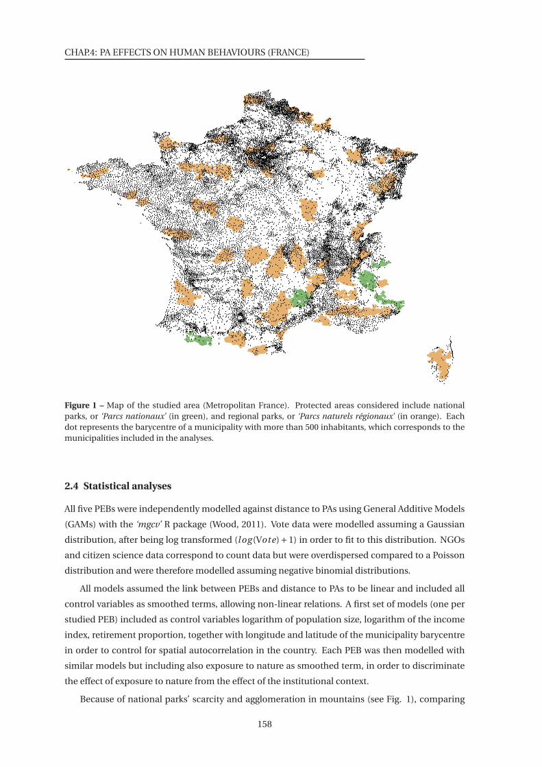
CHAP.4: PA EFFECTS ON HUMAN BEHAVIOURS (FRANCE)
Figure 1 – Map of the studied area (Metropolitan France). Protected areas considered include nationalparks, or ‘Parcs nationaux’ (in green), and regional parks, or ‘Parcs naturels régionaux’ (in orange). Eachdot represents the barycentre of a municipality with more than 500 inhabitants, which corresponds to themunicipalities included in the analyses.
2.4 Statistical analyses
All five PEBs were independently modelled against distance to PAs using General Additive Models
(GAMs) with the ‘mgcv’ R package (Wood, 2011). Vote data were modelled assuming a Gaussian
distribution, after being log transformed (log (Vote)+1) in order to fit to this distribution. NGOs
and citizen science data correspond to count data but were overdispersed compared to a Poisson
distribution and were therefore modelled assuming negative binomial distributions.
All models assumed the link between PEBs and distance to PAs to be linear and included all
control variables as smoothed terms, allowing non-linear relations. A first set of models (one per
studied PEB) included as control variables logarithm of population size, logarithm of the income
index, retirement proportion, together with longitude and latitude of the municipality barycentre
in order to control for spatial autocorrelation in the country. Each PEB was then modelled with
similar models but including also exposure to nature as smoothed term, in order to discriminate
the effect of exposure to nature from the effect of the institutional context.
Because of national parks’ scarcity and agglomeration in mountains (see Fig. 1), comparing
158

3. RESULTS
the impact of national and regional parks was not statistically straightforward. Rather than a
general quantitative comparison, we therefore decided to check that the effect of national and
regional parks were qualitatively similar. To do so, we ran the same 10 models (5 PEBs with
and without considering exposure to nature) but considering distance to regional parks only (see
Supporting Information Table S1). Then, we compared the percentage of deviance explained by
models considering distance to regional parks only with those considering distance to all types of
park (both regional and national). A higher percentage of deviance explained by the model when
all parks are considered would highlight that national and regional parks’ effect are qualitatively
similar (i.e., they affect PEBs in the same direction; see Supporting Information Table S2).
In order to test for the effect of living inside a PA rather than close to a PA, we made a subset of
our dataset, keeping only municipalities inside a PA or close to a PA (< 20km). This represents
about half of our dataset with 1,907 municipalities inside a PA and 7,002 municipalities close
to a PA. We ran GAMs modelling the five PEBs against a binary variable (inside or outside PA)
and controlling for population size, income, retirement proportion, longitude and latitude as in
previous models. We also ran the analyses controlling for exposure to nature.
3. Results
Models not controlling for exposure to nature showed a significant decrease in all five PEBs
with distance to PAs (Fig.2A, Table 1 first column). Thus, a municipality within or close to a PA
showed greater PEBs than a municipality far from PAs, the effects of population size, income,
retirement proportion and spatial autocorrelation being taken into account. In models controlling
for exposure to nature, all PEBs were positively correlated with exposure to nature (Fig.3D), leading
to a decrease in regression coefficients between PEBs and distance to PAs (Fig.2B, Table 1, second
column) emphasizing that part of PAs effect on PEBs is due to their more natural landscapes
than average. Yet, the negative effect of distance to PAs was still significant for all PEBs, meaning
that municipalities with equal population sizes, incomes, retirement proportion and exposure to
nature, still showed different PEB levels depending on their distance to a PA. This highlights that
PAs have a direct effect, aside from providing higher exposure to nature.
Population size of the municipality was strongly and inconsistently correlated with PEBs
(Fig.3A). Both, voting scores for Green party candidates and WWF donation were higher in
municipalities with larger population sizes. Conversely, participation in the French garden
birdwatch program was higher in municipalities with small populations. LPO membership
declined with population size - until ca. 10,000 inhabitants - before increasing for large
cities. Income level was also strongly, and mainly positively, correlated with PEBs (Fig.3B). The
proportion of retired inhabitants of municipalities was positively correlated with NGOs and citizen
science participation, but negatively with voting for Green parties (Fig. 3C). Longitude and
latitude plots in Fig.S2 and Fig.S3 (Supplementary Information) show that spatial autocorrelation
was rather high, especially for PEBs with limited data (i.e., LPO membership and French garden
birdwatch), highlighting that these PEBs have not homogeneously spread across the country.
The covariates effects for models not including exposure to nature are similar to the effects
159
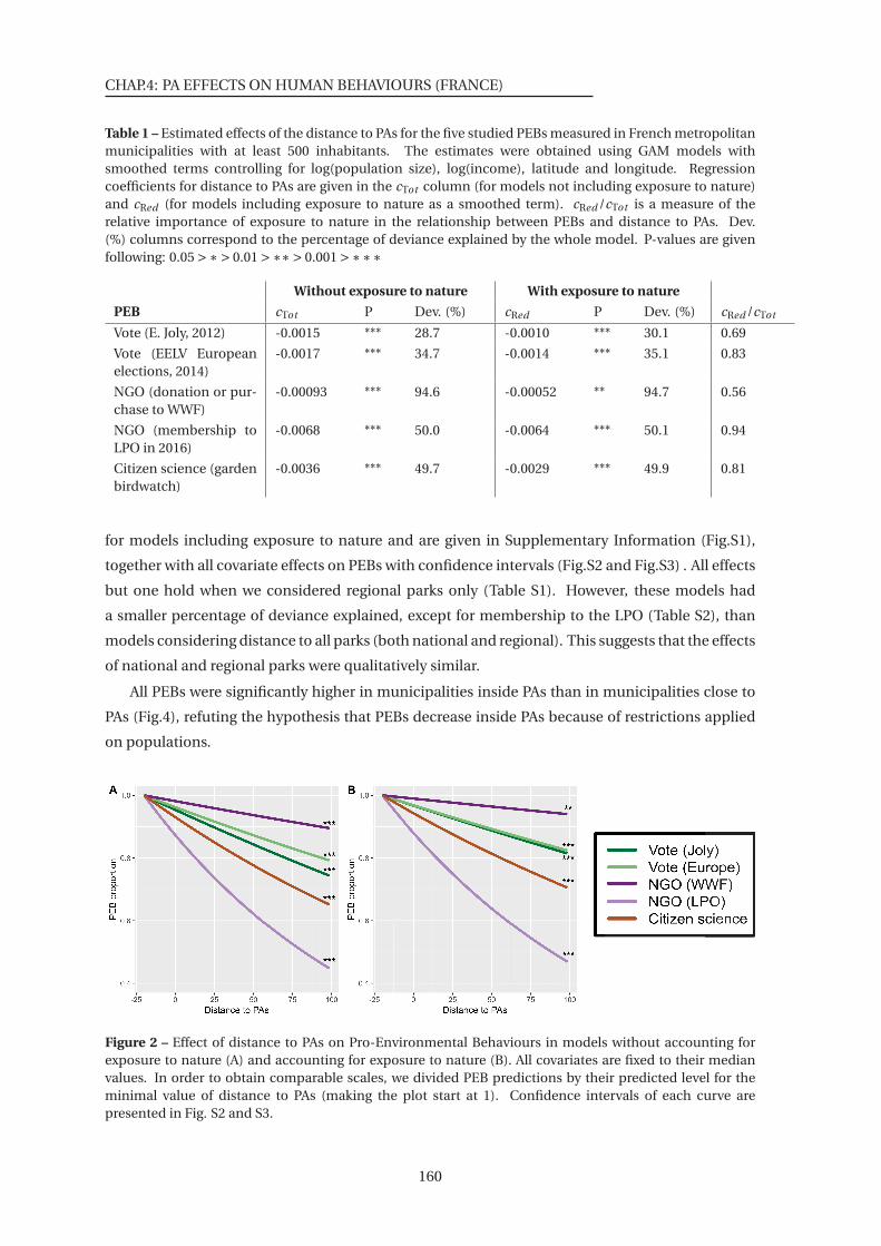
CHAP.4: PA EFFECTS ON HUMAN BEHAVIOURS (FRANCE)
Table 1 – Estimated effects of the distance to PAs for the five studied PEBs measured in French metropolitanmunicipalities with at least 500 inhabitants. The estimates were obtained using GAM models withsmoothed terms controlling for log(population size), log(income), latitude and longitude. Regressioncoefficients for distance to PAs are given in the cTot column (for models not including exposure to nature)and cRed (for models including exposure to nature as a smoothed term). cRed /cTot is a measure of therelative importance of exposure to nature in the relationship between PEBs and distance to PAs. Dev.(%) columns correspond to the percentage of deviance explained by the whole model. P-values are givenfollowing: 0.05 >∗> 0.01 >∗∗> 0.001 >∗∗∗
Without exposure to nature With exposure to nature
PEB cTot P Dev. (%) cRed P Dev. (%) cRed /cTot
Vote (E. Joly, 2012) -0.0015 *** 28.7 -0.0010 *** 30.1 0.69
Vote (EELV Europeanelections, 2014)
-0.0017 *** 34.7 -0.0014 *** 35.1 0.83
NGO (donation or pur-chase to WWF)
-0.00093 *** 94.6 -0.00052 ** 94.7 0.56
NGO (membership toLPO in 2016)
-0.0068 *** 50.0 -0.0064 *** 50.1 0.94
Citizen science (gardenbirdwatch)
-0.0036 *** 49.7 -0.0029 *** 49.9 0.81
for models including exposure to nature and are given in Supplementary Information (Fig.S1),
together with all covariate effects on PEBs with confidence intervals (Fig.S2 and Fig.S3) . All effects
but one hold when we considered regional parks only (Table S1). However, these models had
a smaller percentage of deviance explained, except for membership to the LPO (Table S2), than
models considering distance to all parks (both national and regional). This suggests that the effects
of national and regional parks were qualitatively similar.
All PEBs were significantly higher in municipalities inside PAs than in municipalities close to
PAs (Fig.4), refuting the hypothesis that PEBs decrease inside PAs because of restrictions applied
on populations.
Figure 2 – Effect of distance to PAs on Pro-Environmental Behaviours in models without accounting forexposure to nature (A) and accounting for exposure to nature (B). All covariates are fixed to their medianvalues. In order to obtain comparable scales, we divided PEB predictions by their predicted level for theminimal value of distance to PAs (making the plot start at 1). Confidence intervals of each curve arepresented in Fig. S2 and S3.
160
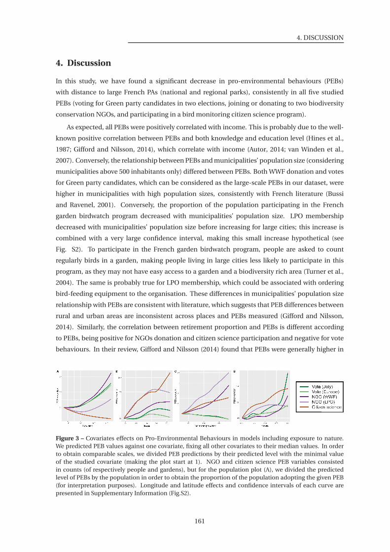
4. DISCUSSION
4. Discussion
In this study, we have found a significant decrease in pro-environmental behaviours (PEBs)
with distance to large French PAs (national and regional parks), consistently in all five studied
PEBs (voting for Green party candidates in two elections, joining or donating to two biodiversity
conservation NGOs, and participating in a bird monitoring citizen science program).
As expected, all PEBs were positively correlated with income. This is probably due to the well-
known positive correlation between PEBs and both knowledge and education level (Hines et al.,
1987; Gifford and Nilsson, 2014), which correlate with income (Autor, 2014; van Winden et al.,
2007). Conversely, the relationship between PEBs and municipalities’ population size (considering
municipalities above 500 inhabitants only) differed between PEBs. Both WWF donation and votes
for Green party candidates, which can be considered as the large-scale PEBs in our dataset, were
higher in municipalities with high population sizes, consistently with French literature (Bussi
and Ravenel, 2001). Conversely, the proportion of the population participating in the French
garden birdwatch program decreased with municipalities’ population size. LPO membership
decreased with municipalities’ population size before increasing for large cities; this increase is
combined with a very large confidence interval, making this small increase hypothetical (see
Fig. S2). To participate in the French garden birdwatch program, people are asked to count
regularly birds in a garden, making people living in large cities less likely to participate in this
program, as they may not have easy access to a garden and a biodiversity rich area (Turner et al.,
2004). The same is probably true for LPO membership, which could be associated with ordering
bird-feeding equipment to the organisation. These differences in municipalities’ population size
relationship with PEBs are consistent with literature, which suggests that PEB differences between
rural and urban areas are inconsistent across places and PEBs measured (Gifford and Nilsson,
2014). Similarly, the correlation between retirement proportion and PEBs is different according
to PEBs, being positive for NGOs donation and citizen science participation and negative for vote
behaviours. In their review, Gifford and Nilsson (2014) found that PEBs were generally higher in
Figure 3 – Covariates effects on Pro-Environmental Behaviours in models including exposure to nature.We predicted PEB values against one covariate, fixing all other covariates to their median values. In orderto obtain comparable scales, we divided PEB predictions by their predicted level with the minimal valueof the studied covariate (making the plot start at 1). NGO and citizen science PEB variables consistedin counts (of respectively people and gardens), but for the population plot (A), we divided the predictedlevel of PEBs by the population in order to obtain the proportion of the population adopting the given PEB(for interpretation purposes). Longitude and latitude effects and confidence intervals of each curve arepresented in Supplementary Information (Fig.S2).
161
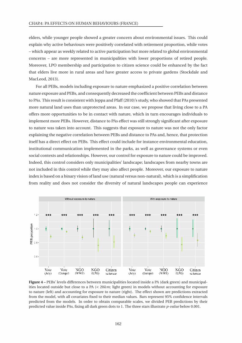
CHAP.4: PA EFFECTS ON HUMAN BEHAVIOURS (FRANCE)
elders, while younger people showed a greater concern about environmental issues. This could
explain why active behaviours were positively correlated with retirement proportion, while votes
– which appear as weekly related to active participation but more related to global environmental
concerns – are more represented in municipalities with lower proportions of retired people.
Moreover, LPO membership and participation to citizen science could be enhanced by the fact
that elders live more in rural areas and have greater access to private gardens (Stockdale and
MacLeod, 2013).
For all PEBs, models including exposure to nature emphasized a positive correlation between
nature exposure and PEBs, and consequently decreased the coefficient between PEBs and distance
to PAs. This result is consistent with Joppa and Pfaff (2010)’s study, who showed that PAs presented
more natural land uses than unprotected areas. In our case, we propose that living close to a PA
offers more opportunities to be in contact with nature, which in turn encourages individuals to
implement more PEBs. However, distance to PAs effect was still strongly significant after exposure
to nature was taken into account. This suggests that exposure to nature was not the only factor
explaining the negative correlation between PEBs and distance to PAs and, hence, that protection
itself has a direct effect on PEBs. This effect could include for instance environmental education,
institutional communication implemented in the parks, as well as governance systems or even
social contexts and relationships. However, our control for exposure to nature could be improved.
Indeed, this control considers only municipalities’ landscape; landscapes from nearby towns are
not included in this control while they may also affect people. Moreover, our exposure to nature
index is based on a binary vision of land use (natural versus non-natural), which is a simplification
from reality and does not consider the diversity of natural landscapes people can experience
Figure 4 – PEBs’ levels differences between municipalities located inside a PA (dark green) and municipal-ities located outside but close to a PA (< 20km; light green) in models without accounting for exposureto nature (left) and accounting for exposure to nature (right). The effect shown are predictions extractedfrom the model, with all covariates fixed to their median values. Bars represent 95% confidence intervalspredicted from the models. In order to obtain comparable scales, we divided PEB predictions by theirpredicted value inside PAs, fixing all dark green dots to 1. The three stars illustrate p-value below 0.001.
162
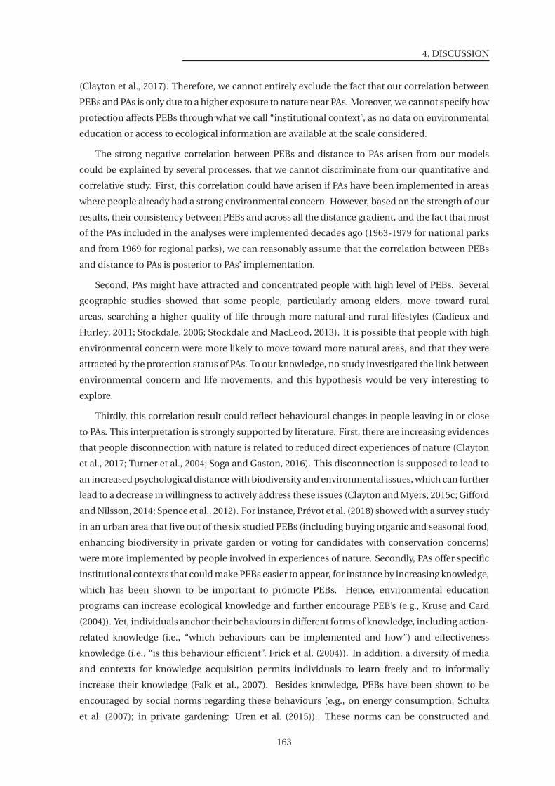
4. DISCUSSION
(Clayton et al., 2017). Therefore, we cannot entirely exclude the fact that our correlation between
PEBs and PAs is only due to a higher exposure to nature near PAs. Moreover, we cannot specify how
protection affects PEBs through what we call “institutional context”, as no data on environmental
education or access to ecological information are available at the scale considered.
The strong negative correlation between PEBs and distance to PAs arisen from our models
could be explained by several processes, that we cannot discriminate from our quantitative and
correlative study. First, this correlation could have arisen if PAs have been implemented in areas
where people already had a strong environmental concern. However, based on the strength of our
results, their consistency between PEBs and across all the distance gradient, and the fact that most
of the PAs included in the analyses were implemented decades ago (1963-1979 for national parks
and from 1969 for regional parks), we can reasonably assume that the correlation between PEBs
and distance to PAs is posterior to PAs’ implementation.
Second, PAs might have attracted and concentrated people with high level of PEBs. Several
geographic studies showed that some people, particularly among elders, move toward rural
areas, searching a higher quality of life through more natural and rural lifestyles (Cadieux and
Hurley, 2011; Stockdale, 2006; Stockdale and MacLeod, 2013). It is possible that people with high
environmental concern were more likely to move toward more natural areas, and that they were
attracted by the protection status of PAs. To our knowledge, no study investigated the link between
environmental concern and life movements, and this hypothesis would be very interesting to
explore.
Thirdly, this correlation result could reflect behavioural changes in people leaving in or close
to PAs. This interpretation is strongly supported by literature. First, there are increasing evidences
that people disconnection with nature is related to reduced direct experiences of nature (Clayton
et al., 2017; Turner et al., 2004; Soga and Gaston, 2016). This disconnection is supposed to lead to
an increased psychological distance with biodiversity and environmental issues, which can further
lead to a decrease in willingness to actively address these issues (Clayton and Myers, 2015c; Gifford
and Nilsson, 2014; Spence et al., 2012). For instance, Prévot et al. (2018) showed with a survey study
in an urban area that five out of the six studied PEBs (including buying organic and seasonal food,
enhancing biodiversity in private garden or voting for candidates with conservation concerns)
were more implemented by people involved in experiences of nature. Secondly, PAs offer specific
institutional contexts that could make PEBs easier to appear, for instance by increasing knowledge,
which has been shown to be important to promote PEBs. Hence, environmental education
programs can increase ecological knowledge and further encourage PEB’s (e.g., Kruse and Card
(2004)). Yet, individuals anchor their behaviours in different forms of knowledge, including action-
related knowledge (i.e., “which behaviours can be implemented and how”) and effectiveness
knowledge (i.e., “is this behaviour efficient”, Frick et al. (2004)). In addition, a diversity of media
and contexts for knowledge acquisition permits individuals to learn freely and to informally
increase their knowledge (Falk et al., 2007). Besides knowledge, PEBs have been shown to be
encouraged by social norms regarding these behaviours (e.g., on energy consumption, Schultz
et al. (2007); in private gardening: Uren et al. (2015)). These norms can be constructed and
163

CHAP.4: PA EFFECTS ON HUMAN BEHAVIOURS (FRANCE)
made salient by neighbourhood (Schultz et al., 2007), but also by personalities living in the
places (Uren et al., 2015), or by discourses and actions of local authorities (e.g., Skandrani
et al. (2015)). Based on this literature support, our results therefore suggest that PAs, through
the increase in opportunities to experience nature they provide and the effect of institutional
context, can reduce the disconnection of their inhabitants with nature and their psychological
distance with biodiversity and environmental issues. This can involve environmental education
- exposing inhabitants to ecological information (e.g., through popularisation activities or signs)-
, and making people feel they live in a biodiversity rich area (Laurens, 1995; Hinds and Sparks,
2008; Halpenny, 2010). In addition, the concepts of biodiversity and sustainable development are
more prone to be present in formal communication from the PAs’ institutions; this could produce
normative messages about environment, which may warrant individual implementation of PEBs.
As our study is correlative, we cannot definitively conclude that these behavioural changes caused
the described pattern. However, the statistical strength of our results, combined with pre-defined
hypotheses regarding the causal relationships on abundant existing literature, together give high
credit to this assumption. Only conducting survey experiments could allow to identify more
clearly the underlying processes of these correlations.
This effect of PAs on PEBs held when we zoomed in around PAs and compared municipalities
inside PAs with municipalities close to PAs. This result was not necessarily expected as PAs are
well-known to provoke opposition about inhabitants before implementation (Stoll-Kleemann,
2001; Stern, 2008; Cadoret, 2017). Therefore, we could have expected PAs to have a negative impact
on environmental concern of inhabitants, or at least to prevent people from being receptive to
the PAs’ institutional context. Yet, our analyses showed that PEBs were significantly higher for
municipalities inside PAs than municipalities close to PAs. This does not imply that PAs are well
received by all people, but rather that, beside restrictions, a part of the population is receptive to
PAs environment quality and discourses.
In this study, we gathered two types of natural parks that present relatively different objectives
(Lepart and Marty, 2006; Laurens, 1995). Indeed, national parks are mainly dedicated to
biodiversity and landscape protection, excluding people from their core area. Regional parks’
objectives rather include social aspects, promoting the coexistence of human and nature, and
are therefore less restrictive of human activities. However, national parks have a peripheral area,
which is less restrictive in terms of human activities than the core area and are therefore classified
by the IUCN in the same category as most regional parks (V). Moreover, municipalities decide
whether they want to be part of this peripheral area and, if so, sign a charter established by
the park. In all studied national parks but the ‘Parc national des Cévennes’, villages are only
present in these peripheral areas. This implies that the municipalities that we considered inside
national parks are only in this peripheral area, except for the ‘Parc national des Cévennes’, which
includes municipalities in the core area (18 municipalities, including two with more than 500
inhabitants have their barycentre inside the core area). Although we could not compare their
impact quantitatively, our analyses suggest that both national and regional parks enhance PEBs of
nearby municipalities’ inhabitants.
164
5. CONCLUSION
The studied PEBs have only indirect impacts on biodiversity and are implemented by only
0.05% (French garden birdwatch) to 2.6% (European elections) of the French population. Despite
their high internal consistency, our results cannot thus pretend to be generalized without any
caution. However, they open perspectives for further research at this national scale, which would
concern behaviours with more direct or bigger impacts on biodiversity, such as designing private
lands in order to favour biodiversity, changing consumption habits, or become an activist for
biodiversity NGOs or Green parties.
The correlations between PEBs and covariates could have been more precise if we had access
to individual data, which would have allow us to link geographical, social variables to PEBs directly.
Here, we used data with resolution at the municipality level, which is the best scale available for
the PEBs data we gathered, as well as income and retirement data. It is also important to remind
that we excluded municipalities with less than 500 inhabitants in order to limit extreme values in
PEBs, and therefore, we potentially excluded the most rural municipalities. The distribution of
these small municipalities is slightly biased toward PAs as 13.4% of municipalities with population
sizes below or equal to 500 are located inside PAs, against 11.3% for municipalities above 500
inhabitants.
5. Conclusion
With our study, we enlarged the potential roles of protected areas: besides the direct protection
of biodiversity through reservation, PAs can provide opportunities to experience nature through
different ways (e.g., by living in there, by visiting, but also by being exposed to natural settings
or ecological information). In addition, they provide local context where being involved in
biodiversity conservation could be socially encouraged and accepted. Therefore, even if this
is not the main objective of PAs, we suggest here that they can play a role in conserving
human’s connection with nature, and lead local inhabitants toward a higher care for nature
and biodiversity. We encourage the local governance system of protected areas to enlarge their
objectives by including social outcomes, notably by being aware of the social norms they support.
In these conditions, implementing new PAs would not only cause inhabitants’ opposition and
frustration, but could be positively received by other, potentially more discrete, inhabitants.
6. Acknowledgements
We deeply thank the LPO, WWF France and ‘Oiseaux des jardins’ teams who agreed to provide us
with non-public data, without which this study would not have been possible. We would also like
to thank Ana S.L. Rodrigues and John D. Thompson for their relevant comments and advices on
the manuscript.
165
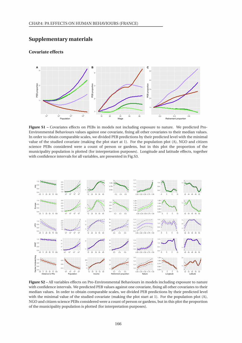
CHAP.4: PA EFFECTS ON HUMAN BEHAVIOURS (FRANCE)
Supplementary materials
Covariate effects
1
2
3
103
104
105
106
Population
PE
B p
rop
ort
ion
A
1
2
3
4
12 20 34 54 90
Wage
PE
B p
rop
ort
ion
B
1
2
3
4
5
0.2 0.4 0.6
Retirement proportion
PE
B p
rop
ort
ion
C
Figure S1 – Covariates effects on PEBs in models not including exposure to nature. We predicted Pro-Environmental Behaviours values against one covariate, fixing all other covariates to their median values.In order to obtain comparable scales, we divided PEB predictions by their predicted level with the minimalvalue of the studied covariate (making the plot start at 1). For the population plot (A), NGO and citizenscience PEBs considered were a count of person or gardens, but in this plot the proportion of themunicipality population is plotted (for interpretation purposes). Longitude and latitude effects, togetherwith confidence intervals for all variables, are presented in Fig.S3.
0.4
0.6
0.8
1.0
-25 0 25 50 75 100
Joly
1.0
1.5
2.0
2.5
3.0
103
104
105
106
1
12 20 34 54 90
0.50
0.75
1.00
0.2 0.4 0.6
1.1
1.3
1.5
1.7
0.00 0.25 0.50 0.75 1.00
0.6
0.8
1.0
-5 0 5 10
1
42 44 46 48 50
0.4
0.6
0.8
1.0
-25 0 25 50 75 100
Eu
rop
e
1.0
1.5
2.0
2.5
3.0
103
104
105
106
1
12 20 34 54 90
0.4
0.6
0.8
1.0
0.2 0.4 0.6
1.00
1.05
1.10
1.15
1.20
0.00 0.25 0.50 0.75 1.00
0.25
0.50
0.75
1.00
1.25
-5 0 5 10
1
42 44 46 48 50
0.4
0.6
0.8
1.0
-25 0 25 50 75 100
LP
O
1.0
1.5
2.0
2.5
3.0
103
104
105
106
1
3
7
12 20 34 54 90
2
4
6
8
0.2 0.4 0.6
0.9
1.0
1.1
1.2
1.3
0.00 0.25 0.50 0.75 1.00
0.4
0.8
1.2
1.6
-5 0 5 10
1
3
7
42 44 46 48 50
0.4
0.6
0.8
1.0
-25 0 25 50 75 100
WW
F
1
2
3
4
103
104
105
106
1
3
12 20 34 54 90
1
2
3
4
0.2 0.4 0.6
1.0
1.1
1.2
1.3
0.00 0.25 0.50 0.75 1.000.0
0.5
1.0
1.5
-5 0 5 10
1
42 44 46 48 50
0.4
0.6
0.8
1.0
-25 0 25 50 75 100
Distance to PAs
Gard
en b
irdw
atc
hin
g
0.3
0.6
0.9
103
104
105
106
Population
1
3
7
20
12 20 34 54 90
Income
1
2
3
0.2 0.4 0.6
Retirement proportion
1.0
1.2
1.4
1.6
0.00 0.25 0.50 0.75 1.00
Nature
0.25
0.50
0.75
1.00
1.25
-5 0 5 10
Longitude
1
3
42 44 46 48 50
Latitude
Figure S2 – All variables effects on Pro-Environmental Behaviours in models including exposure to naturewith confidence intervals. We predicted PEB values against one covariate, fixing all other covariates to theirmedian values. In order to obtain comparable scales, we divided PEB predictions by their predicted levelwith the minimal value of the studied covariate (making the plot start at 1). For the population plot (A),NGO and citizen science PEBs considered were a count of person or gardens, but in this plot the proportionof the municipality population is plotted (for interpretation purposes).
166
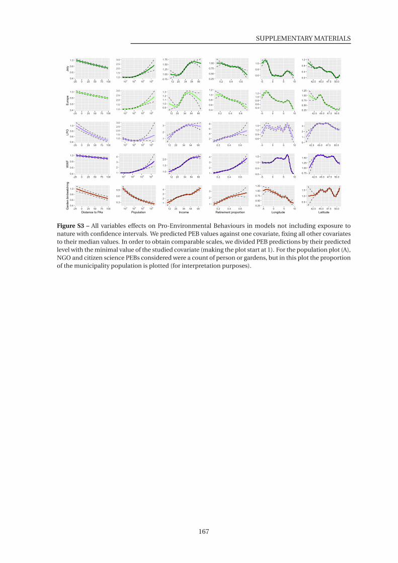
SUPPLEMENTARY MATERIALS
0.4
0.6
0.8
1.0
-25 0 25 50 75 100
Joly
1.0
1.5
2.0
2.5
3.0
103
104
105
106
0.75
1.00
1.25
1.50
1.75
12 20 34 54 900.25
0.50
0.75
1.00
0.2 0.4 0.6
0.6
0.8
1.0
-5 0 5 10
0.0
0.4
0.8
1.2
42.5 45.0 47.5 50.0
0.4
0.6
0.8
1.0
-25 0 25 50 75 100
Eu
rop
e
1.0
1.5
2.0
2.5
3.0
103
104
105
106
0.9
1.0
1.1
1.2
1.3
12 20 34 54 90
0.4
0.6
0.8
1.0
1.2
0.2 0.4 0.6
0.4
0.6
0.8
1.0
1.2
-5 0 5 10
0.25
0.50
0.75
1.00
1.25
42.5 45.0 47.5 50.0
0.4
0.6
0.8
1.0
-25 0 25 50 75 100
LP
O
1.0
1.5
2.0
2.5
3.0
103
104
105
106
1
2
3
12 20 34 54 90
2
4
6
8
0.2 0.4 0.6
0.6
0.9
1.2
1.5
-5 0 5 100
1
2
3
42.5 45.0 47.5 50.0
0.4
0.6
0.8
1.0
-25 0 25 50 75 100
WW
F
1
2
3
4
103
104
105
106
1.0
1.5
2.0
12 20 34 54 90
1
2
3
4
0.2 0.4 0.60.0
0.5
1.0
1.5
-5 0 5 10
0.75
1.00
1.25
1.50
42.5 45.0 47.5 50.0
0.4
0.6
0.8
1.0
-25 0 25 50 75 100
Distance to PAs
Gard
en b
irdw
atc
hin
g
0.3
0.6
0.9
103
104
105
106
Population
1
2
3
4
12 20 34 54 90
Income
1
2
3
0.2 0.4 0.6
Retirement proportion
0.25
0.50
0.75
1.00
1.25
-5 0 5 10
Longitude
0.5
1.0
1.5
42.5 45.0 47.5 50.0
Latitude
Figure S3 – All variables effects on Pro-Environmental Behaviours in models not including exposure tonature with confidence intervals. We predicted PEB values against one covariate, fixing all other covariatesto their median values. In order to obtain comparable scales, we divided PEB predictions by their predictedlevel with the minimal value of the studied covariate (making the plot start at 1). For the population plot (A),NGO and citizen science PEBs considered were a count of person or gardens, but in this plot the proportionof the municipality population is plotted (for interpretation purposes).
167
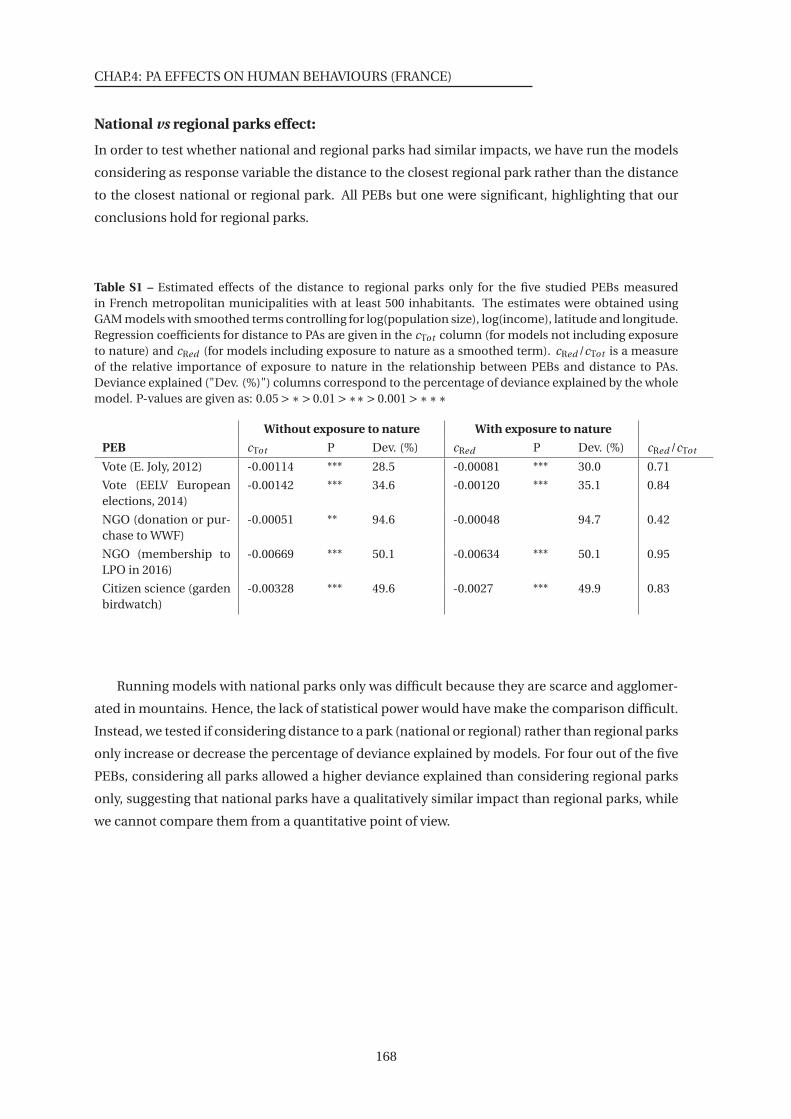
CHAP.4: PA EFFECTS ON HUMAN BEHAVIOURS (FRANCE)
National vs regional parks effect:
In order to test whether national and regional parks had similar impacts, we have run the models
considering as response variable the distance to the closest regional park rather than the distance
to the closest national or regional park. All PEBs but one were significant, highlighting that our
conclusions hold for regional parks.
Table S1 – Estimated effects of the distance to regional parks only for the five studied PEBs measuredin French metropolitan municipalities with at least 500 inhabitants. The estimates were obtained usingGAM models with smoothed terms controlling for log(population size), log(income), latitude and longitude.Regression coefficients for distance to PAs are given in the cTot column (for models not including exposureto nature) and cRed (for models including exposure to nature as a smoothed term). cRed /cTot is a measureof the relative importance of exposure to nature in the relationship between PEBs and distance to PAs.Deviance explained ("Dev. (%)") columns correspond to the percentage of deviance explained by the wholemodel. P-values are given as: 0.05 >∗> 0.01 >∗∗> 0.001 >∗∗∗
Without exposure to nature With exposure to nature
PEB cTot P Dev. (%) cRed P Dev. (%) cRed /cTot
Vote (E. Joly, 2012) -0.00114 *** 28.5 -0.00081 *** 30.0 0.71
Vote (EELV Europeanelections, 2014)
-0.00142 *** 34.6 -0.00120 *** 35.1 0.84
NGO (donation or pur-chase to WWF)
-0.00051 ** 94.6 -0.00048 94.7 0.42
NGO (membership toLPO in 2016)
-0.00669 *** 50.1 -0.00634 *** 50.1 0.95
Citizen science (gardenbirdwatch)
-0.00328 *** 49.6 -0.0027 *** 49.9 0.83
Running models with national parks only was difficult because they are scarce and agglomer-
ated in mountains. Hence, the lack of statistical power would have make the comparison difficult.
Instead, we tested if considering distance to a park (national or regional) rather than regional parks
only increase or decrease the percentage of deviance explained by models. For four out of the five
PEBs, considering all parks allowed a higher deviance explained than considering regional parks
only, suggesting that national parks have a qualitatively similar impact than regional parks, while
we cannot compare them from a quantitative point of view.
168

SUPPLEMENTARY MATERIALS
Table S2 – Comparison of percentage of deviance explained by models using as response variables distanceto regional parks only vs all parks for all models.
Without exposure to nature With exposure to nature
PEB Regional parks only All parks Regional parks only All parks
Vote (E. Joly, 2012) 28.4875 28.6969 30.0471 30.1281
Vote (EELV European elec-tions, 2014)
34.6145 34.7385 35.0529 35.1224
NGO (donation or pur-chase to WWF)
94.5997 94.6094 94.6894 94.6927
NGO (membership to LPOin 2016)
50.0559 50.0360 50.1378 50.1134
Citizen science (gardenbirdwatch)
49.6228 49.6565 49.8721 49.8934
169

Chapitre 5
Autres contributions scientifiques
171
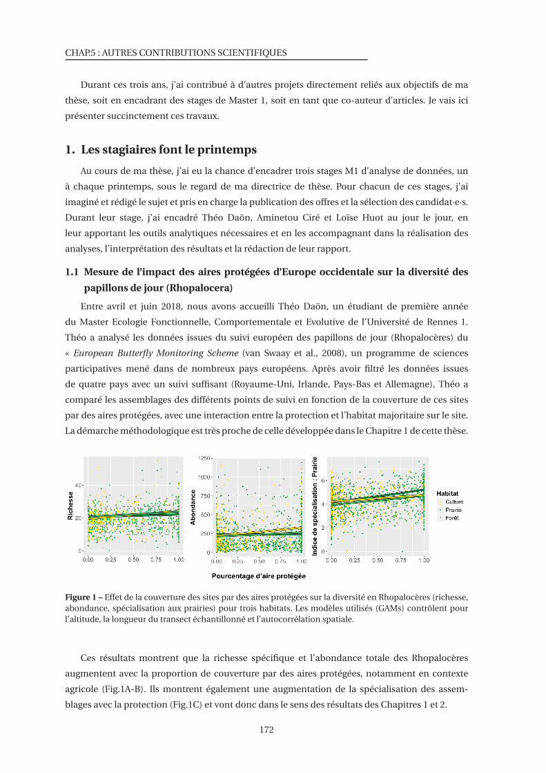
CHAP.5 : AUTRES CONTRIBUTIONS SCIENTIFIQUES
Durant ces trois ans, j’ai contribué à d’autres projets directement reliés aux objectifs de ma
thèse, soit en encadrant des stages de Master 1, soit en tant que co-auteur d’articles. Je vais ici
présenter succinctement ces travaux.
1. Les stagiaires font le printemps
Au cours de ma thèse, j’ai eu la chance d’encadrer trois stages M1 d’analyse de données, un
à chaque printemps, sous le regard de ma directrice de thèse. Pour chacun de ces stages, j’ai
imaginé et rédigé le sujet et pris en charge la publication des offres et la sélection des candidat·e·s.
Durant leur stage, j’ai encadré Théo Daön, Aminetou Ciré et Loïse Huot au jour le jour, en
leur apportant les outils analytiques nécessaires et en les accompagnant dans la réalisation des
analyses, l’interprétation des résultats et la rédaction de leur rapport.
1.1 Mesure de l’impact des aires protégées d’Europe occidentale sur la diversité des
papillons de jour (Rhopalocera)
Entre avril et juin 2018, nous avons accueilli Théo Daön, un étudiant de première année
du Master Ecologie Fonctionnelle, Comportementale et Evolutive de l’Université de Rennes 1.
Théo a analysé les données issues du suivi européen des papillons de jour (Rhopalocères) du
« European Butterfly Monitoring Scheme (van Swaay et al., 2008), un programme de sciences
participatives mené dans de nombreux pays européens. Après avoir filtré les données issues
de quatre pays avec un suivi suffisant (Royaume-Uni, Irlande, Pays-Bas et Allemagne), Théo a
comparé les assemblages des différents points de suivi en fonction de la couverture de ces sites
par des aires protégées, avec une interaction entre la protection et l’habitat majoritaire sur le site.
La démarche méthodologique est très proche de celle développée dans le Chapitre 1 de cette thèse.
Figure 1 – Effet de la couverture des sites par des aires protégées sur la diversité en Rhopalocères (richesse,abondance, spécialisation aux prairies) pour trois habitats. Les modèles utilisés (GAMs) contrôlent pourl’altitude, la longueur du transect échantillonné et l’autocorrélation spatiale.
Ces résultats montrent que la richesse spécifique et l’abondance totale des Rhopalocères
augmentent avec la proportion de couverture par des aires protégées, notamment en contexte
agricole (Fig.1A-B). Ils montrent également une augmentation de la spécialisation des assem-
blages avec la protection (Fig.1C) et vont donc dans le sens des résultats des Chapitres 1 et 2.
172
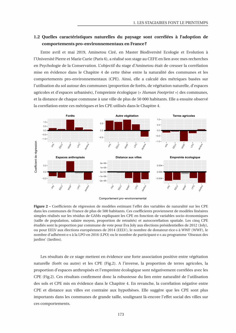
1. LES STAGIAIRES FONT LE PRINTEMPS
1.2 Quelles caractéristiques naturelles du paysage sont corrélées à l’adoption de
comportements pro-environnementaux en France?
Entre avril et mai 2019, Aminetou Ciré, en Master Biodiversité Ecologie et Evolution à
l’Université Pierre et Marie Curie (Paris 6), a réalisé son stage au CEFE en lien avec mes recherches
en Psychologie de la Conservation. L’objectif du stage d’Aminetou était de creuser la corrélation
mise en évidence dans le Chapitre 4 de cette thèse entre la naturalité des communes et les
comportements pro-environnementaux (CPE). Ainsi, elle a calculé des métriques basées sur
l’utilisation du sol autour des communes (proportion de forêts, de végétation naturelle, d’espaces
agricoles et d’espaces urbanisés), l’empreinte écologique (« Human Footprint ») des communes,
et la distance de chaque commune à une ville de plus de 50 000 habitants. Elle a ensuite observé
la corrélation entre ces métriques et les CPE utilisés dans le Chapitre 4.
−1.0
−0.5
0.0
0.5
1.0
Joly
EE
LV
WW
F
LP
O
Jard
ins
Forêts
−0.5
0.0
0.5
Joly
EE
LV
WW
F
LP
O
Jard
ins
Autre végétation
−1.0
−0.5
0.0
0.5
1.0
Joly
EE
LV
WW
F
LP
O
Jard
ins
Terres agricoles
−0.2
0.0
0.2
Joly
EE
LV
WW
F
LP
O
Jard
ins
Espaces anthropisés
−2e−06
−1e−06
0e+00
1e−06
2e−06
Joly
EE
LV
WW
F
LP
O
Jard
ins
Distance aux villes
−0.004
0.000
0.004Jo
ly
EE
LV
WW
F
LP
O
Jard
ins
Empreinte écologique
Comportement pro−environnemental
Co
eff
icie
nt
de
ré
gre
ssio
n
Figure 2 – Coefficients de régression de modèles estimant l’effet des variables de naturalité sur les CPEdans les communes de France de plus de 500 habitants. Ces coefficients proviennent de modèles linéairessimples réalisés sur les résidus de GAMs expliquant les CPE en fonction de variables socio-économiques(taille de population, salaire moyen, proportion de retraités) et autocorrélation spatiale. Les cinq CPEétudiés sont la proportion par commune de vote pour Eva Joly aux élections présidentielles de 2012 (Joly),ou pour EELV aux élections européennes de 2014 (EELV), le nombre de donateur·rice·s à WWF (WWF), lenombre d’adhérent·e·s à la LPO en 2016 (LPO) ou le nombre de participant·e·s au programme ‘Oiseaux desjardins’ (Jardins).
Les résultats de ce stage mettent en évidence une forte association positive entre végétation
naturelle (forêt ou autre) et les CPE (Fig.2). A l’inverse, la proportion de terres agricoles, la
proportion d’espaces anthropisés et l’empreinte écologique sont négativement corrélées avec les
CPE (Fig.2). Ces résultats confirment donc la robustesse du lien entre naturalité de l’utilisation
des sols et CPE mis en évidence dans le Chapitre 4. En revanche, la corrélation négative entre
CPE et distance aux villes est contraire aux hypothèses. Elle suggère que les CPE sont plus
importants dans les communes de grande taille, soulignant là-encore l’effet social des villes sur
ces comportements.
173
CHAP.5 : AUTRES CONTRIBUTIONS SCIENTIFIQUES
1.3 Évaluation de l’efficacité des aires protégées urbaines pour la conservation de
l’avifaune en Amérique latine
Au printemps 2020, en pleine période de confinement dû au Covid-19, Loïse Huot, en Master
Patrimoine Naturel et Biodiversité à l’Université de Rennes 1 a fait son stage de Master 1 dans notre
équipe dématérialisée. A l’origine de ce stage est le cas du «Parque Nacional de Tijuca», constitué
de 40km2 de forêt tropicale humide et situé en plein cœur de la ville de Rio de Janeiro au Brésil.
Nous nous sommes demandé quelle biodiversité pouvait persister dans de telles aires protégées,
dans ce contexte d’anthropisation extrême, par rapport à des aires protégées en contexte rural.
Loïse a identifié 12 aires protégées urbaines couvertes par de la forêt tropicale en Amérique
latine (en cœur de ville ou en périphérie immédiate) et a étudié leurs assemblages en utilisant
les données eBird utilisées dans le Chapitre 3 de cette thèse. Pour comprendre l’effet du contexte
urbain sur les aires protégées, Loïse a comparé ces aires protégées urbaines (APU) à des aires
protégées contrôle (APC). Ces APC étaient semblables à l’APU d’un point de vue écologique mais
étaient localisées en contexte non-urbain. Loïse a calculé différents indices de diversité sur les
assemblages d’oiseaux et a ensuite utilisé un modèle mixte expliquant les indices de diversité
mesurés dans les checklists en fonction du statut de l’aire protégée (urbain / contrôle), de variables
de contrôle (durée d’échantillonnage et expertise des observateur·rice·s), avec un effet aléatoire
sur les paires de sites.
Les résultats de ce stage suggèrent que les assemblages des APU sont en moyenne moins
diversifiés que ceux des APC mais qu’ils conservent tout de même une diversité importante
(Fig.3). En effet, la richesse spécifique est en moyenne 11% inférieure dans les APU, alors que
l’abondance est diminuée de 33%. De plus, les assemblages des APU présentent légèrement
moins d’espèces spécialistes des forêts (– 4%), et nettement moins d’espèces à petite distribution
(– 30%) et d’espèces menacées ou quasi-menacées (– 59%). En revanche, les assemblages des
APU contiennent plus d’espèces non-natives que les APC (+187%). Ces résultats mettent donc en
évidence l’importance du contexte dans lequel les aires protégées s’inscrivent et mettent en garde
contre la tendance actuelle visant à faire des aires protégées des îles d’habitats naturels inscrits
dans une matrice d’habitats fortement anthropisés. Néanmoins, ces résultats montrent que les
assemblages des APU sont relativement riches et méritent donc d’être préservés.
Loïse travaille actuellement sur la rédaction d’un article scientifique pour valoriser les résultats
de son stage, en collaboration avec Ana S.L. Rodrigues, David P. Edwards et moi-même.
2. Collaborations
2.1 Mesure de l’efficacité de la convention Ramsar dans la conservation des oiseaux
d’eau hivernants de Méditerranée
En début de thèse, j’ai été invité par Elie Gaget à collaborer à un article de sa thèse. Ce projet
visait à mesurer l’effet sur les populations hivernales d’oiseaux d’eau de la désignation de zones
humides en sites Ramsar. En utilisant les données des comptages d’oiseaux d’eau de Wetlands
International tout autour de la Méditerranée, cette étude compare les tendances de populations
174
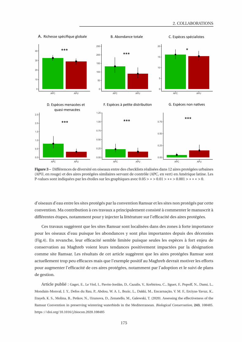
2. COLLABORATIONS
***
0
10
20
30
40
APC APU
***
0
50
100
150
200
250
APC APU
*
0
5
10
15
20
APC APU
***
0.0
0.5
1.0
1.5
2.0
2.5
APC APU
***
0.00
0.25
0.50
0.75
1.00
1.25
APC APU
***
0.00
0.25
0.50
0.75
APC APU
A. Richesse spéci que globale B. Abondance totale C. Espèces spécialistes
D. Espèces menacées et
quasi-menacées
F. Espèces à pe te distribu on G. Espèces non na ves
Figure 3 – Différences de diversité en oiseaux entre des checklists réalisées dans 12 aires protégées urbaines(APU, en rouge) et des aires protégées similaires servant de contrôle (APC, en vert) en Amérique latine. LesP-values sont indiquées par les étoiles sur les graphiques avec 0.05 >∗> 0.01 >∗∗> 0.001 >∗∗∗> 0.
d’oiseaux d’eau entre les sites protégés par la convention Ramsar et les sites non protégés par cette
convention. Ma contribution à ces travaux a principalement consisté à commenter le manuscrit à
différentes étapes, notamment pour y injecter la littérature sur l’efficacité des aires protégées.
Ces travaux suggèrent que les sites Ramsar sont localisées dans des zones à forte importance
pour les oiseaux d’eau puisque les abondances y sont plus importantes depuis des décennies
(Fig.4). En revanche, leur efficacité semble limitée puisque seules les espèces à fort enjeu de
conservation au Maghreb voient leurs tendances positivement impactées par la désignation
comme site Ramsar. Les résultats de cet article suggèrent que les aires protégées Ramsar sont
actuellement trop peu efficaces mais que l’exemple positif au Maghreb devrait motiver les efforts
pour augmenter l’efficacité de ces aires protégées, notamment par l’adoption et le suivi de plans
de gestion.
Article publié : Gaget, E., Le Viol, I., Pavón-Jordán, D., Cazalis, V., Kerbiriou, C., Jiguet, F., Popoff, N., Dami, L.,
Mondain-Monval, J. Y., Defos du Rau, P., Abdou, W. A. I., Bozic, L., Dakki, M., Encarnação, V. M. F., Erciyas-Yavuz, K.,
Etayeb, K. S., Molina, B., Petkov, N., Uzunova, D., Zenatello, M., Galewski, T. (2020). Assessing the effectiveness of the
Ramsar Convention in preserving wintering waterbirds in the Mediterranean. Biological Conservation, 243, 108485.
https ://doi.org/10.1016/j.biocon.2020.108485
175
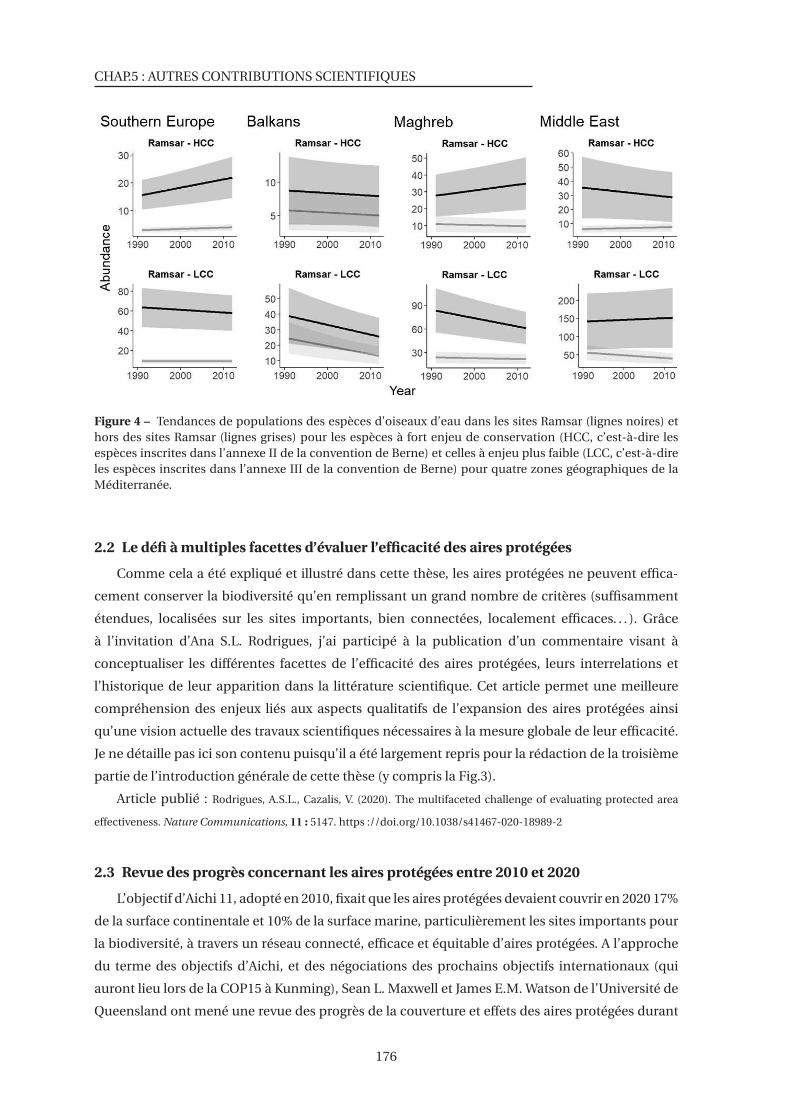
CHAP.5 : AUTRES CONTRIBUTIONS SCIENTIFIQUES
Figure 4 – Tendances de populations des espèces d’oiseaux d’eau dans les sites Ramsar (lignes noires) ethors des sites Ramsar (lignes grises) pour les espèces à fort enjeu de conservation (HCC, c’est-à-dire lesespèces inscrites dans l’annexe II de la convention de Berne) et celles à enjeu plus faible (LCC, c’est-à-direles espèces inscrites dans l’annexe III de la convention de Berne) pour quatre zones géographiques de laMéditerranée.
2.2 Le défi à multiples facettes d’évaluer l’efficacité des aires protégées
Comme cela a été expliqué et illustré dans cette thèse, les aires protégées ne peuvent effica-
cement conserver la biodiversité qu’en remplissant un grand nombre de critères (suffisamment
étendues, localisées sur les sites importants, bien connectées, localement efficaces. . . ). Grâce
à l’invitation d’Ana S.L. Rodrigues, j’ai participé à la publication d’un commentaire visant à
conceptualiser les différentes facettes de l’efficacité des aires protégées, leurs interrelations et
l’historique de leur apparition dans la littérature scientifique. Cet article permet une meilleure
compréhension des enjeux liés aux aspects qualitatifs de l’expansion des aires protégées ainsi
qu’une vision actuelle des travaux scientifiques nécessaires à la mesure globale de leur efficacité.
Je ne détaille pas ici son contenu puisqu’il a été largement repris pour la rédaction de la troisième
partie de l’introduction générale de cette thèse (y compris la Fig.3).
Article publié : Rodrigues, A.S.L., Cazalis, V. (2020). The multifaceted challenge of evaluating protected area
effectiveness. Nature Communications, 11 : 5147. https ://doi.org/10.1038/s41467-020-18989-2
2.3 Revue des progrès concernant les aires protégées entre 2010 et 2020
L’objectif d’Aichi 11, adopté en 2010, fixait que les aires protégées devaient couvrir en 2020 17%
de la surface continentale et 10% de la surface marine, particulièrement les sites importants pour
la biodiversité, à travers un réseau connecté, efficace et équitable d’aires protégées. A l’approche
du terme des objectifs d’Aichi, et des négociations des prochains objectifs internationaux (qui
auront lieu lors de la COP15 à Kunming), Sean L. Maxwell et James E.M. Watson de l’Université de
Queensland ont mené une revue des progrès de la couverture et effets des aires protégées durant
176
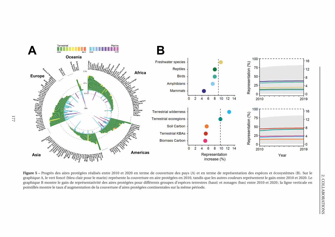
2.CO
LL
AB
OR
ATIO
NS
Africa
AmericasAsia
Europe
OceaniaA B
Figure 5 – Progrès des aires protégées réalisés entre 2010 et 2020 en terme de couverture des pays (A) et en terme de représentation des espèces et écosystèmes (B). Sur legraphique A, le vert foncé (bleu clair pour le marin) représente la couverture en aire protégées en 2010, tandis que les autres couleurs représentent le gain entre 2010 et 2020. Legraphique B montre le gain de représentativité des aires protégées pour différents groupes d’espèces terrestres (haut) et zonages (bas) entre 2010 et 2020 ; la ligne verticale enpointillés montre le taux d’augmentation de la couverture d’aires protégées continentales sur la même période.
177
CHAP.5 : AUTRES CONTRIBUTIONS SCIENTIFIQUES
cette décennie. J’ai été invité à collaborer à ce travail, participant notamment à la rédaction de la
partie révisant les progrès réalisés en terme d’efficacité des aires protégées et en apportant une
aide technique à la réalisation de certaines figures.
Cet article montre notamment que l’expansion des aires protégées a été moins importante
qu’attendue jusqu’à présent (Fig.5A). En effet, alors que la couverture terrestre des aires protégées
devaient atteindre 17% en 2020 d’après les engagements pris en 2010 (SCBD, 2010), elle
n’est actuellement que de 15.0% (UNEP-WCMC, IUCN and NGS, 2020), un chiffre qui devrait
augmenter dans les prochains mois suite d’après le Secrétariat de la Convention sur la Diversité
Biologique. De plus, il montre que l’expansion qui a été réalisée entre 2010 et 2019 s’est traduite
par une augmentation très faible de la représentation des espèces et des écosystèmes dans les aires
protégées (Fig.5B). L’article met également en évidence, en compilant les informations disponibles
dans la littérature, une connexion trop faible des aires protégées et un investissement trop faible
dans leur gestion, menant à une efficacité trop faible. Enfin, l’article suggère des points importants
à prendre en compte dans le choix des prochains objectifs internationaux concernant les aires
protégées, qui devraient être fixés à la COP 15 pour la biodiversité en mai 2021.
Article publié : Maxwell, S.L., Cazalis, V., Dudley, N., Hoffmann, M., Rodrigues, A.S.L., Stolton, S., Visconti,
P., Woodley, S., Maron, M., Strassburg, B.B.N., Wenger, A., Jonas, H.D., Venter, O., Watson, J.E.M. (2020). Area-Based
Conservation in the twenty-first century. Nature, 586 : 217-227. https ://doi.org/10.1038/s41586-020-2773-z
178


Discussion générale
DISCUSSION GÉNÉRALE
1. Rappel des principaux résultats
Les deux premiers chapitres de cette thèse avaient pour but de mesurer l’effet des aires
protégées sur les populations d’oiseaux. Le Chapitre 1, basé sur les données de la « Breeding
Bird Survey » aux Etats-Unis et au Canada, montre que les assemblages des aires protégées ne
présentent pas une richesse spécifique ni une abondance plus importante que les sites non-
protégés ayant un habitat similaire. En revanche, les assemblages des forêts protégées étaient
plus « typiques » que ceux des forêts non protégées, avec un effet positif de la protection sur les
abondances des spécialistes de forêts et un effet négatif sur les espèces spécialistes de milieux
ouverts. Le Chapitre 2, basé sur les données eBird dans huit points chauds de biodiversité en
forêt tropicale humide montre également que les aires protégées n’ont pas d’effet sur la richesse
spécifique des assemblages d’oiseaux mais qu’en revanche elles freinent l’homogénéisation
biotique (en favorisant les espèces spécialistes des habitats forestiers, endémiques et menacées).
Cet effet sur les espèces à fort enjeu de conservation est issu d’une action combinée des aires
protégées sur la perte d’habitat et sur la dégradation de l’habitat.
Le Chapitre 3 utilise également les données eBird pour mesurer la sensibilité des espèces
d’oiseaux d’Amérique aux activités humaines et confronter cette sensibilité aux stratégies
actuelles de conservation. Il montre que les espèces les plus sensibles, qui ont donc besoin d’aires
protégées avec des habitats intacts, se concentrent dans les forêts tropicales. Or nous ne trouvons
aucune corrélation entre la sensibilité des espèces habitant une écorégion et son intensité de
protection et identifions de nombreuses écorégions avec beaucoup d’espèces sensibles mais
très peu de couverture d’aires protégées intactes. De ce fait, de nombreuses espèces sensibles
ne disposent d’aucune aire protégée intacte dans leur aire de répartition. De plus, beaucoup
d’aires protégées subissent une dégradation des habitats, particulièrement dans les écorégions
où beaucoup d’espèces sont hautement sensibles.
Enfin, le Chapitre 4 s’intéresse à l’effet des aires protégées sur les comportements humains
en France. Nous y montrons que les habitants des communes abritées ou situées à proximité
d’un parc naturel adoptent en moyenne plus de comportements pro-environnementaux que les
habitants de communes éloignées des parcs. Nourris par des théories et résultats empiriques
de Psychologie de la Conservation, nous suggérons que les aires protégées permettent à leurs
habitants un contact privilégié avec la nature et les exposent à des actions de sensibilisation. Ces
deux processus induisent une meilleure connexion entre les habitants et la nature ce qui permet
l’augmentation des comportements pro-environnementaux.
Dans leur ensemble, ces travaux contribuent à l’augmentation des connaissances dans
différents domaines que sont la Biologie de la Conservation, l’Ecologie et la Psychologie de la
Conservation. Ils mettent également en évidence le rôle clé des sciences participatives dans
l’acquisition de connaissances, ainsi que l’importance des données spatiales publiques. Je vais ici
détailler les différents apports de cette thèse à ces disciplines, tout en identifiant des perspectives,
avant de conclure.
182
2. APPORTS DE CETTE THÈSE EN BIOLOGIE DE LA CONSERVATION
2. Apports de cette thèse en Biologie de la Conservation
La contribution de cette thèse à la littérature en Biologie de la Conservation porte principa-
lement sur l’efficacité individuelle des aires protégées. En effet, par les deux premiers chapitres,
nous renforçons la littérature méthodologique sur la mesure de l’efficacité des aires protégées à
partir de données de sciences participatives et apportons de nouvelles preuves de leur efficacité
en tant qu’outil de conservation. En particulier, nous montrons que les aires protégées sont un
rempart efficace contre l’homogénéisation biotique en évitant l’extinction locale des espèces
spécialistes, endémiques ou menacées (Chapitres 1, 2, 5). De tels résultats étaient déjà présents
dans la littérature (Hiley et al., 2016; Gray et al., 2016; Kerbiriou et al., 2018) mais restent peu
nombreux relativement à l’importance des aires protégées en tant qu’outil de conservation. De
plus, la focalisation du Chapitre 2 sur les zones tropicales qui sont des zones prioritaires pour
la conservation est assez novatrice puisque la majorité des connaissances se concentrent en
Amérique du Nord, en Europe, et Océanie pour des questions de disponibilité des données.
Ces résultats sont d’autant plus importants que les zones étudiées sont des points chauds de
biodiversité, combinant fort taux d’endémisme et de perte d’habitat, et doivent donc faire l’objet
d’une protection très efficace.
De nombreux travaux restent néanmoins nécessaires dans le futur, afin de comprendre plus
en finesse l’effet des aires protégées. Notons d’ailleurs qu’ils seront de fait toujours nécessaires. En
effet, l’efficacité des aires protégées étant dynamique, la mesure de leur effet devra régulièrement
être mise à jour.
Un premier axe à creuser, dans l’optique de mieux isoler l’effet des aires protégées des biais de
localisation, serait d’utiliser des tendances de populations plutôt que de comparer la biodiversité
entre sites protégés et non-protégés à un temps T. L’utilisation de tendances permettrait de
mesurer et distinguer l’effet du biais de localisation de l’effet des aires protégées de manière
plus fine. En effet, la différence de diversité lors de l’implémentation de l’aire protégée peut être
un indice du biais de localisation tandis que la différence de tendances sera liée à l’efficacité à
proprement parler des aires protégées. Cette approche temporelle permet également de mesurer
l’efficacité absolue des aires protégées afin de savoir si elles parviennent à stopper les déclins
de population ou seulement à les réduire. Au contraire, des approches statiques comme celles
utilisées dans les deux premiers chapitres de cette thèse ne permettent que de dire si les aires
protégées ont un effet positif relativement aux sites non-protégés. Ce type d’approche temporelle
a été utilisé dans quelques études mais qui sont principalement limitées à l’Europe car les données
permettant ces analyses sont très rares, par exemple sur les oiseaux communs (Gamero et al.,
2017; Pellissier et al., 2013) ou sur les oiseaux d’eau avec l’étude de Gaget et al. (2020) à laquelle
j’ai contribué (Chap.5-2.1). D’ici quelques années il sera possible de réaliser de telles études
temporelles dans les zones tropicales grâce aux données eBird, qui commencent à être utilisées
pour mesurer des tendances de populations (Horns et al., 2018; Robinson et al., 2018; Neate-Clegg
et al., 2020). Il convient toutefois de préciser que l’utilisation de données temporelles ne règle pas
le problème du choix du contrôle (développé en partie 4 de l’Introduction Générale). En effet, si les
183
DISCUSSION GÉNÉRALE
aires protégées sont localisées dans des sites peu convoités par l’activité économique, alors elles
montreront des tendances de populations moins négatives, même si leur création n’a aucun effet
réel sur le terrain.
Un second axe pour affiner nos connaissances sur l’efficacité des aires protégées consisterait à
mesurer une efficacité différenciée des aires protégées selon les caractéristiques de la protection,
afin de comprendre quel type de protection est la plus efficace. Cela a été exploré par exemple
par Geldmann et al. (2018) qui trouvent un effet plus positif des aires protégées sur les tendances
de populations dans les aires protégées qui sont jeunes et petites et celles qui ont des moyens
humains et financiers suffisants. C’est ce qui a été fait en marge du Chapitre 1 de cette thèse (en
comparant l’effet des aires protégées de manière stricte à l’effet de toutes les aires protégées), une
tentative qui illustre bien les difficultés de puissance statistique liées à cette démarche. Cette idée
peut être poussée plus loin en cherchant à mesurer l’efficacité des aires protégées à l’échelle de
chaque aire protégée (par exemple quelle est la différence faite par le Parc National des Ecrins).
Une telle mesure permettrait une meilleure compréhension de ce qui fait qu’une aire protégée
fonctionne et de mieux identifier les aires protégées nécessitant un renfort de protection. C’est
en partie ce qui a motivé la création de la base de données PAME (Protected Area Management
Effectiveness database) qui, pour l’instant, contient principalement des informations sur les
objectifs et moyens employés à la protection (Coad et al., 2019; UNEP-WCMC & IUCN, 2020).
Les jeux de données utilisés dans cette thèse, qu’ils contiennent des informations géographiques
(avec les occupations du sol, l’empreinte écologique ou les taux de déforestation) ou des données
d’abondance d’espèces d’oiseaux, pourraient potentiellement permettre de calculer de manière
systématique des indices d’efficacité pour chaque aire protégée et ainsi compléter cette base de
données. Par exemple, nous pourrions imaginer utiliser les rasters de déforestation développés
par Hansen et al. (2013) pour calculer le taux de déforestation de chaque aire protégée. Une
autre possibilité serait d’utiliser l’indice de sensibilité développé dans le Chapitre 3 pour mesurer
l’adéquation entre la sensibilité des espèces présentes dans une aire protégée et le niveau de
dégradation de ses habitats.
Une troisième perspective serait de s’intéresser à la variation de l’efficacité des aires protégées
en fonction du contexte autour de l’aire protégée. En effet, une aire protégée située au cœur de
la forêt amazonienne ne connaît pas les mêmes enjeux qu’une aire protégée située sur le front de
déforestation, en zone agricole, ou en bordure de ville. C’est ce qui a motivé le stage de Loïse Huot
(Chap.5-1.3), qui a montré que les aires protégées urbaines dans les forêts tropicales d’Amérique
latine abritent une diversité d’espèces d’oiseaux importante mais légèrement diminuée par
rapport aux aires protégées non-urbaines. En particulier, les aires protégées urbaines contiennent
moins d’espèces menacées, un peu moins d’espèces à petite distribution et de spécialistes,
tandis qu’elles contiennent plus d’espèces non-natives. Mesurer l’efficacité des aires protégées
en fonction du contexte de pression anthropique dans lequel elles s’inscrivent, de manière plus
générale, semble nécessaire.
En plus des contributions sur l’efficacité locale des aires protégées (Chapitres 1 et 2), ma thèse
a contribué à renforcer la littérature sur l’efficacité du réseau des aires protégées. Le Chapitre 3 met
184
3. APPORTS DE CETTE THÈSE EN ECOLOGIE
notamment en évidence une déconnexion spatiale entre les besoins d’habitats intacts des espèces
et la qualité des habitats des aires protégées. Ainsi, de nombreuses espèces à forte sensibilité aux
pressions humaines ne disposent pas d’aires protégées intactes dans leur aire de répartition, ce
qui rend les aires protégées incapables de préserver efficacement ces espèces. Cette étude montre
donc que la qualité des sites qui sont protégés est une dimension essentielle à considérer dans les
stratégies de conservation et dans la mesure de l’efficacité de ces stratégies. Elle suggère donc
que la qualité des sites devrait être plus présente dans les analyses sur l’efficacité des réseaux
d’aires protégées, notamment ceux liés à la couverture de la distribution des espèces par les aires
protégées (par exemple Butchart et al. (2015)).
En outre, ma thèse a contribué à la littérature sur les différentes facettes de l’efficacité des
aires protégées. En particulier, ma collaboration à un article mené par Ana S.L. Rodrigues m’a
permis de participer à un effort de conceptualisation des différentes facettes de l’efficacité des
aires protégées, de leur historique et de leurs interconnexions (Chap.5-2.2). L’article mené par
Sean L. Maxwell et James E.M. Watson, auquel j’ai également eu la chance de contribuer (Chap.5-
2.3), met en évidence la non-atteinte de l’objectif d’Aichi 11 (tant en terme de surface couverte
aujourd’hui par les aires protégées que par leurs aspects qualitatifs) et suggère des défis pour les
futurs objectifs internationaux sur les aires protégées. Ces deux articles pointent une perspective
majeure concernant la mesure de l’efficacité des aires protégées qui consiste à combiner les
différents aspects de l’efficacité. En particulier, combiner l’efficacité locale des aires protégées à
leur étendue globale et à leur couverture des sites les plus importants permettrait de quantifier
de façon unifiée leur contribution à la conservation de la biodiversité. Cette capacité à mesurer
de façon unifiée l’effet des aires protégées sur les espèces est d’autant plus importante que de
nombreux scientifiques appellent les gouvernements à adopter des objectifs basés sur les résultats
(par exemple « stopper le déclin de la biodiversité » ou « empêcher l’extinction des espèces
menacées ») plutôt que sur les efforts de protection (par exemple « protéger 17% de la surface
continentale »). C’est notamment ce que suggèrent Visconti et al. (2019) dans leur proposition
d’objectif post-2020 : « The value of all sites of global significance for biodiversity, including
key biodiversity areas, is documented, retained, and restored through protected areas and other
effective area-based conservation measures ». De tels objectifs, également plaidés par le comité
scientifique associé à la Convention pour la Diversité Biologique (le SBSTTA; SCBD (2019)), sont
très prometteurs mais présenteraient un défi majeur quant à la mesure de leur accomplissement.
En effet, cela nécessiterait de croiser l’efficacité des aires protégées sur la biodiversité (comme
nous l’avons mesurée dans les Chapitres 1 et 2) et leur étendue et couverture des sites importants
pour mesurer la perte de biodiversité qu’elles empêchent globalement.
3. Apports de cette thèse en Ecologie
Les trois premiers chapitres de cette thèse soutiennent des études précédentes mettant en
évidence l’homogénéisation des assemblages en soulignant le faible effet des activités humaines
sur la richesse spécifique malgré une transformation importante des assemblages. En effet, ils
montrent chacun à leur façon un impact plus important des activités humaines sur les espèces
185
DISCUSSION GÉNÉRALE
spécialistes, à faible distribution et menacées, ce qui est typiquement observé dans le processus
d’homogénéisation biotique (Clavel et al., 2011; McKinney and Lockwood, 1999; Finderup Nielsen
et al., 2019). Des résultats similaires ont été obtenus lors du stage de Théo Daön sur l’effet
des aires protégées sur les assemblages de Rhopalocères en Europe de l’Ouest (Chap.5-1.1).
Nos résultats se joignent donc naturellement aux nombreuses études suggérant que les indices
de richesse spécifique ou d’abondance totale ne sont pas des indices suffisants pour décrire
la dynamique de la biodiversité et les transformations des assemblages (Dornelas et al., 2014;
Hillebrand et al., 2018). Ces résultats mettant en évidence une stabilité de la richesse spécifique
posent d’importantes questions sur les processus écologiques sous-jacents et notamment sur
l’évolution temporelle de la composition des assemblages. En effet, nous pouvons nous demander
si l’apparition des espèces les plus adaptées à la pression humaine précède, succède ou est
simultanée à l’extinction locale des espèces les plus sensibles. Une perspective importante, pour
mieux appréhender la dynamique temporelle du processus d’homogénéisation biotique, serait
d’utiliser des données temporelles afin de comparer les dynamiques de populations des espèces
en déclin (par exemple les spécialistes) et des espèces en augmentation qui remplacent les
premières (par exemple les généralistes).
La mesure de sensibilité à la pression humaine, développée dans le Chapitre 3, pourrait
permettre une meilleure compréhension de l’hétérogénéité de l’impact des activités humaines
entre espèces. En effet, nous mettons en évidence la variabilité, au sein d’un même écosystème de
la réponse des espèces aux pressions humaines ainsi qu’une structuration spatiale et fonctionnelle
de cette sensibilité. Il pourrait être intéressant de chercher à mieux comprendre l’origine de cette
variabilité entre espèces et écosystèmes. Plus précisément, il serait pertinent de tester si cette
variabilité est due à une pré-adaptation de certaines espèces au dérangement ou si elle résulte
de processus de filtres d’extinction qui font que les espèces les plus vulnérables ont déjà disparu
de ces écosystèmes. Il serait donc intéressant de creuser les liens entre la sensibilité et les traits
fonctionnels des espèces pour comprendre l’origine biologique de cette variabilité. De plus, cet
indice de sensibilité pourrait s’avérer utile pour éclairer différents processus écologiques tels que
l’homogénéisation biotique (en regardant si l’homogénéisation biotique induit le remplacement
d’espèces sensibles par des espèces à faible sensibilité), la dette d’extinction (en étudiant si les
espèces les plus sensibles ont une dette d’extinction plus courte ; Kuussaari et al. (2009), Gibson
et al. (2013)), ou encore des aspects évolutifs de sensibilité écologique (en mesurant la corrélation
taxonomique de la sensibilité par exemple).
4. Apports de cette thèse en Psychologie de la Conservation
Le petit pas de côté vers la Psychologie de la Conservation réalisé dans le Chapitre 4 a
permis d’ouvrir légèrement le rôle actuel attribué aux aires protégées en les plaçant comme de
potentiels catalyseurs de changements normatifs. Ce travail pourrait ainsi permettre d’augmenter
l’importance des approches de sciences sociales dans les stratégies de conservation en montrant
l’impact positif que peuvent avoir les aires protégées sur les comportements humains.
Au-delà des résultats obtenus, ce chapitre ainsi que le stage d’Aminetou Ciré (Chap.5-1.2)
186
5. CONCLUSION SUBJECTIVE
peut apporter une ouverture méthodologique à la discipline en montrant l’utilité des approches
quantitatives pour faire émerger des patrons à large échelle dans une discipline qui utilise
principalement des enquêtes sociologiques réalisées sur un nombre d’individus restreint (Clayton
and Myers, 2015a). Bien sûr, l’approche quantitative et corrélative que j’utilise est accompagnée de
nombreuses limites. La principale est la difficulté de mettre en évidence des liens causaux entre
les variables, là où une approche plus individualisée permet une plus grande finesse d’analyse
sur les processus en jeu. Mais la combinaison de ces deux approches (l’une basée sur des études
approfondies sur quelques individus et l’autre quantitative sur un grand nombre d’individus)
semble prometteuse en permettant la vérification à large échelle de patrons identifiés par une
approche ciblée sur quelques individus.
5. Conclusion subjective
Pour conclure cette thèse, j’aimerais poser sur le papier quelques considérations plus
personnelles, avec une subjectivité assumée. En premier lieu, je souhaite prendre le temps
de discuter l’utilité concrète, si elle existe, de cette thèse. Ensuite j’aimerais évoquer quelques
considérations sociétales liées à mes travaux.
5.1 Finalement, à quoi ça sert?
Dès le début de mon parcours universitaire, j’ai été fortement attiré par la voie de la recherche
mais régulièrement frappé d’incertitude sur l’utilité des travaux réalisés en conservation. N’en
sait-on pas déjà assez ? Ne vaudrait-il mieux pas travailler sur la sensibilisation, l’influence de
politiques publiques ou simplement adopter un mode de vie correspondant à mes idéaux ? Après
de nombreuses réflexions et de riches discussions, j’ai finalement décidé de croire au travail
académique et en ce sujet proposé par Ana, je me suis inscrit en thèse. Il me semble aujourd’hui
essentiel de penser l’utilité réelle de ces travaux et d’exposer en toute transparence si je pense
avoir participé à quelque chose d’utile ou bien si ma thèse n’était en réalité qu’un exercice
intellectuel futile, aussi passionnant fût-il. Cela me semble d’autant plus important que l’utilité
de mes recherches n’a pas sauté aux yeux de toutes les personnes à qui j’ai exposé mon sujet. J’ai
été particulièrement frappé par cela au cours de l’été de vacances précédant le début de ma thèse,
quand mon ami Maël m’a dit avec humour « La réponse de ta thèse c’est : Oui, les aires protégées
protègent la nature. Je t’ai fait gagner trois ans » tandis qu’un chargé de mission en Camargue,
à qui j’ai probablement mal vendu mon futur sujet, m’a dit de façon péremptoire « Ta thèse ne
servira à rien, ça ne nous aidera pas à savoir quoi faire sur le terrain ».
Deux questions se posent pour penser l’utilité de ce travail de thèse : la connaissance issue des
travaux est-elle utile ? Cette connaissance peut-elle ensuite se traduire par des actions concrètes?
Commençons par la première question : a-t-on vraiment besoin d’analyses et d’articles
scientifiques pour savoir si oui ou non les aires protégées sont efficaces ? De mon point de
vue, nous n’en avons pas besoin pour valider l’idée que les aires protégées constituent un outil
pertinent pour la conservation. La logique suffit à valider cela : puisque les activités humaines
induisent le déclin de la biodiversité, restreindre localement ces activités doit permettre un
187
DISCUSSION GÉNÉRALE
meilleur état de la biodiversité. A mes yeux, la réelle question de ma thèse n’a donc jamais été de
savoir si les aires protégées sont un outil efficace face au problème du déclin de la biodiversité (un
peu comme on testerait l’efficacité d’un vaccin), mais plutôt de savoir si cet outil est bien utilisé.
Ainsi, si je n’avais trouvé aucun effet des aires protégées sur la biodiversité, je n’aurais pas conclu
qu’il fallait arrêter de créer des aires protégées, mais plutôt qu’un énorme effort de renforcement
des mesures de protection devait être fait en leur sein. C’est donc en tant que contrôle des efforts
de protection que l’efficacité des aires protégées me semble être quelque chose d’important à
mesurer. Cela est d’autant plus crucial que les aires protégées répondent à des engagements
internationaux des gouvernements, tels que l’objectif d’Aichi 11, qui ne peuvent être remplis que
si les aires protégées sont efficaces, c’est-à-dire si elles permettent la conservation de la nature. En
mesurant l’efficacité des aires protégées (comme dans les deux premiers chapitres de cette thèse),
en questionnant les choix de localisation des nouvelles aires protégées (comme dans le Chapitre
3) ou en étudiant les effets sociaux des aires protégées (comme dans le Chapitre 4), je considère
que mon travail est plutôt de vérifier l’effet réel des efforts de conservation mis en place par nos
sociétés. A ce titre, je considère donc que la connaissance résultant de ma thèse a sa raison d’être et
cela semble avoir à peu près convaincu Maël qui m’a dit récemment « Enfoncer une porte ouverte
t’aura au moins permis de passer de l’autre côté ». Reste à savoir si elle est cantonnée aux cercles
de lecture académiques ou si elle peut participer à des actions concrètes.
Ce point me paraît plus légitimement discutable mais plusieurs éléments me laissent
espérer qu’une transformation de l’exercice académique réalisé lors de ma thèse en actions de
conservation est possible. D’abord parce que j’ai vu que les travaux académiques servaient de
base de travail ou d’arguments à différentes institutions. En tête, le programme environnemental
des Nations Unies (UNEP) publie tous les deux ans un rapport sur les aires protégées (« Protected
Planet Report ») qui se base principalement sur des études académiques pour évaluer l’état du
réseau d’aires protégées et ainsi le succès des gouvernements à remplir leurs engagements. La
publication du premier rapport global de l’IPBES m’a également donné l’impression que nos
travaux pouvaient alimenter des messages importants à destination des décideurs politiques
et de nos sociétés. Ensuite, j’ai eu la chance de collaborer avec des membres d’organisations
internationales, notamment Stuart H.M. Butchart dans le Chapitre 2 et de nombreuses autres
personnes grâce au travail mené par Sean L. Maxwell, qui m’ont laissé voir que ces institutions
ont besoin d’études mettant en évidence l’effet des aires protégées, tant pour mettre en avant
ce qui fonctionne que pour pointer du doigt ce qui doit être amélioré. Les études académiques
me semblent donc un maillon important de la chaîne permettant d’influencer les politiques
publiques internationales. J’ai également vu qu’il était possible de raccourcir cette chaîne par
l’exemple de James E.M. Watson de l’Université de Queensland, avec qui j’ai eu le privilège
de collaborer sur deux articles. Ce chercheur, spécialisé sur les questions d’aires protégées, a
un impact direct sur les décisions internationales (notamment les objectifs post-2020) par son
investissement dans différentes instances institutionnelles, notamment liées à la Convention sur
la Diversité Biologique. Enfin, j’ai eu la chance d’expérimenter une autre façon de valoriser les
résultats académiques grâce à la publication de deux communiqués de presse, liés à mon Chapitre
188
5. CONCLUSION SUBJECTIVE
4 (printemps 2019) puis à mon Chapitre 2 (été 2020). Cela m’a fait toucher du doigt la position
privilégiée que peuvent avoir les chercheur·se·s pour dialoguer avec la société et m’a également
montré une porte d’entrée facilitée vers les instances publiques (par exemple l’OFB ou les conseils
scientifiques de parcs avec qui j’ai pu échanger suite à la publication du communiqué sur les
comportements pro-environnementaux).
Cette vision de l’utilité appliquée des travaux scientifiques, peut-être un peu restrictive, me
laisse toutefois quelques points de frustration. En particulier, j’ai parfois une légère impression
que la recherche sur ces thématiques consiste en une usine à gaz, réalisant des analyses
complexes, mobilisant de grandes quantités de données pour finalement alimenter les discussions
en conservation internationale par un message extrêmement simpliste, du type : « les aires
protégées, c’est bien » ou « il faut faire attention à ce qu’elles soient efficaces ». De ce fait, il
m’arrive encore de douter du besoin réel des analyses que je réalise. Ce doute m’atteint en général
durant la phase d’analyses, quand je ressens que mon véritable moteur pour les réaliser n’est pas
tellement ma conviction de leur nécessité mais plutôt un attrait ludique pour les jolies analyses, et
s’estompe lors de la rédaction où l’impression d’une potentielle utilité me regagne. C’est donc un
point de vigilance à garder, notamment au moment de la conceptualisation des analyses, l’idéal
étant d’impliquer dès cette étape des membres d’organisations non académiques de conservation.
5.2 Quelles aires protégées et quelle société pour satisfaire mes envies?
Mes travaux me placent dans la position, que j’accepte volontiers, d’un partisan de la création
des aires protégées et notamment d’aires protégées intactes avec un fort niveau de restriction
des activités humaines (dans le respect des besoins des populations locales bien évidemment).
Mais cette vision semble contradictoire avec la position tenue dans le Chapitre 4, qui prône
l’importance de la connexion entre humains et nature ainsi qu’avec mon positionnement
personnel régulier de défenseur de la vie rurale. M’étant régulièrement heurté à cet apparent
paradoxe durant ma thèse, j’aimerais ici en discuter rapidement. D’avance, je reconnais que les
considérations développées dans cette partie sont pour l’instant majoritairement instinctives, mes
recherches bibliographiques sur le sujet ayant été superficielles, mais j’espère pouvoir un jour m’y
pencher avec plus de rigueur et, pourquoi pas, participer à la littérature sur ces sujets.
Restons, dans un premier temps, concentrés sur les aires protégées. Je suis convaincu qu’il
est nécessaire d’avoir des aires protégées qui sont intactes de pression humaine comme défendu
dans le Chapitre 3. Bien qu’elles soient principalement nécessaires dans les milieux tropicaux,
je pense qu’elles doivent être présentes à travers le globe et ce afin de préserver les espèces les
plus sensibles, mais également pour permettre à nos sociétés un accès à une référence sauvage,
afin de nous rappeler ce qu’est l’altérité de la nature par rapport aux milieux anthropisés (Maris,
2018). Mais pour laisser de la place à la nature, le corollaire est qu’il faut concentrer nos activités
dans d’autres espaces, qui ne seront donc pas constitués de nature intacte. Cependant, cela ne
veut pas dire que cette nature intacte ne peut être visitée, au moins en partie. Une première voie
de résolution de mon paradoxe est donc de reconnaître le besoin d’un gradient dans les aires
protégées, avec une fraction complètement inaccessible (comme les réserves intégrales), d’autres
189
DISCUSSION GÉNÉRALE
où l’accès est limité à de la visite, reconnaissant là l’altérité de la nature tout en s’autorisant à en
profiter, comme on profite des tableaux d’un musée sans pour autant y ajouter notre touche de
peinture (comme les parcs nationaux) et d’autres enfin, qui accueillent des activités humaines
(les aires multi-usages).
Cet appel à créer des aires protégées intactes et à conserver une part de Terre sur laquelle les
humains ne peuvent pas vivre, a une répercussion inévitable pour la partie du monde accueillant
les humains : les concentrer. Pour autant, j’ai du mal à adhérer à l’idée qu’il faudrait, pour protéger
la nature, concentrer notre impact sur quelques espaces où l’anthropisation serait maximale
comme cela est souvent prôné par les défenseurs du « Land sparing ».
Ma principale réserve rationnelle sur ce sujet concerne l’idée que, pour minimiser les surfaces
agricoles, l’intensification de l’agriculture serait la solution. En effet, l’agriculture intensive
me semble très performante pour maximiser le rendement par heure de travail, mais pas
nécessairement pour maximiser le rendement par surface de production. Ainsi, il me semble
probable qu’une agriculture de petite échelle, moins mécanisée, plus diversifiée, en lien avec un
tissu économique local est une meilleure voie pour concentrer les surfaces de production. Je pense
donc que ce modèle agricole pourrait, contrairement à l’opposition souvent formulée dans le
débat « Land sparing / Land sharing », être moins néfaste à la biodiversité locale, tout en présentant
de meilleurs rendements par surface que l’agriculture intensive. Une condition importante de
cette réalisation, néanmoins, est la structuration spatiale des surfaces agricoles pour éviter une
fragmentation trop importante des espaces naturels.
Ma seconde réserve pour me positionner du côté du « Land sharing » est l’idée que la
consommation serait indépendante des méthodes de production et de distribution. En effet,
une hypothèse sous-jacente aux travaux du débat « Land sparing / Land sharing » est que
des personnes habitant dans une société complètement urbanisée (et donc où la production
est spatialement séparée des consommateur·rice·s) consommeront de la même façon que des
personnes habitant dans une société où les consommateur·rice·s vivent au sein des lieux de
production. Or, ayant encore la tête dans mes Cévennes natales, je ne peux croire à cela et je
pense que les normes de consommation (en termes d’alimentation, de loisirs, de vacances, de
mobilier, etc.) sont fortement influencées par notre milieu de vie et j’ai l’impression que les modes
de vie urbains sont plus difficilement adaptables à une logique de décroissance économique que
certains modes de vie ruraux. De ce fait, il me semble erroné de penser que la pression écologique
générée par une personne est indépendante de son mode de vie et qu’il suffirait donc de structurer
spatialement cette pression de manière optimale. Je suis donc là-encore réticent au fait d’opposer
un modèle où les terres seraient complètement ségrégées (entre nature, agriculture intensive
et milieux urbains) et un modèle où habitations et agriculture extensive seraient mélangées au
détriment de la nature sauvage.
Plus globalement, je pense qu’un positionnement sur ces questions de distribution spatiale
de la pression humaine ne peut s’abstraire d’un positionnement sur la source de la pression elle-
même. En effet, on peut considérer que le travail lié aux aires protégées revient à répondre à la
question : « comment structurer notre pression de manière à avoir le moins d’impact possible
190
5. CONCLUSION SUBJECTIVE
sur la biodiversité » comme si la pression elle-même ne pouvait être remise en question. C’est
pourquoi il me semble donc important de terminer cette thèse en exposant que la meilleure
façon d’empêcher les déclins de biodiversité serait d’adopter des modes de vie permettant de
diminuer cette pression, notamment en diminuant nos niveaux de consommation et en remettant
en question le paradigme de croissance économique (Büscher et al., 2017). C’est cette nécessité
de double positionnement des acteur·rice·s de la conservation qui est développée dans l’article
de Martin et al. (2016) : “The challenge for conservation scientists is thus to act on a day-to-day
basis under the current context but, at the same time, make clear that the long-term prospects for
conservation are dismal without a radical transition in attitudes and processes that govern our
interactions with the biosphere.”
5.3 Un rêve pour 2050, « living in harmony with nature »
Nous voilà maintenant en 2050, les humains ont enfin appris à laisser de l’espace à la
biodiversité, à respecter la part sauvage du monde. Ainsi, à Altamira au Brésil, les deux jeunes
aras hyacinthes, Anodorhynchus hyacinthinus, qui quittent pour la première fois la cavité dans
laquelle ils ont éclos n’ont pas à craindre d’être mis en captivité. Ils peuvent tranquillement passer
leur journée à casser des noix de Macadamia, en tentant d’échapper aux courses poursuites avec
la harpie qui niche dans le voisinage. En Inde, les populations d’outardes à tête noire, Ardeotis
nigriceps, ont retrouvé de belles tailles et il n’est pas rare d’observer des dizaines de mâles paradant
dans une même prairie, cherchant à devenir plus gros qu’un bœuf en gonflant leur cou. Plus au
sud, bien que certaines plages australiennes soient couvertes de béton, les sternes néréis, Sternula
nereis, peuvent compter sur la sanctuarisation de nombreuses plages d’Australie et de Nouvelle
Calédonie, leur promettant ainsi un avenir serein. Cap à l’ouest, dans les savanes africaines où les
groupes de vautours oricous, Torgos tracheliotos, trouvent quotidiennement quantité de carcasses
grâce aux dépôts des éleveur·se·s et à l’abondance persistante de grands mammifères sauvages. Il
leur arrive tout de même de dormir le ventre vide parfois, entraînant des bruits d’estomac si forts
que les impalas s’abritent dans les buissons, par crainte de l’orage. Les pies-grièches méridionales,
Lanius meridionalis, dont une femelle vient de passer au-dessus de mon pot de départ à la retraite,
ont elles aussi retrouvé de belles abondances grâce au retour en force de l’agriculture extensive
à petite échelle et à la protection de zones de garrigues. Tout au nord, le harfang des neiges,
Bubo scandiacus, mentionné dans l’introduction générale a laissé sa place à sa petite-fille qui
occupe le même territoire. Mais ce territoire a maintenant un nom : « Aulalangagnipugurvik » qui
signifie en Inuktitut « L’endroit où nous n’irons pas ». Enfin, la coquette de Guerrero, Lophornis
brachylophus, autrefois cantonnée à quelques dizaines de kilomètres carrés au Mexique a vu son
aire de répartition quintupler sur les deux dernières décennies et continue de s’étendre. C’est sur
les pentes de la Sierra Madre del Sur que se trouve le coulequin dont l’épanouissement d’une
fleur avait ouvert cette thèse. Les lueurs crépusculaires n’éclairant plus que la canopée incitent
la fleur de laquelle une coquette vient d’aspirer le nectar à refermer sa corolle. La coquette,
constatant amèrement qu’elle ne pourra plus se nourrir aujourd’hui retourne vers son nid à
quelques centaines de mètres de là et sur la route attrape un point de côté. Point qu’elle saisit
du bout du bec et qu’elle appose délicatement ici, sur cette feuille, en guise de conclusion.
191

Références
Agostinelli, C. and Lund, U. (2017). R package \textttcircular: Circular Statistics (version 0.4-93). CA: Department of
Environmental Sciences, Informatics and Statistics, Ca’ Foscari University, Venice, Italy. UL: Department of Statistics,
California Polytechnic State University, San Luis Obispo, California, USA.
Allan, J. R., Venter, O., and Watson, J. E. M. (2017). Temporally inter-comparable maps of terrestrial wilderness and the
Last of the Wild. Scientific Data, 4(1):1–8.
Andam, K. S., Ferraro, P. J., Pfaff, A., Sanchez-Azofeifa, G. A., and Robalino, J. A. (2008). Measuring the effectiveness of
protected area networks in reducing deforestation. Proceedings of the National Academy of Sciences, 105(42):16089–
16094.
Anderson, E. and Mammides, C. (2019). The role of protected areas in mitigating human impact in the world’s last
wilderness areas. Ambio.
Asefa, A., Davies, A. B., McKechnie, A. E., Kinahan, A. A., and van Rensburg, B. J. (2017). Effects of anthropogenic
disturbance on bird diversity in Ethiopian montane forests. The Condor, 119(3):416–430.
Autor, D. H. (2014). Skills, education, and the rise of earnings inequality among the "other 99 percent". Science,
344(6186):843–851.
Baldi, G., Texeira, M., Martin, O. A., Grau, H. R., and Jobbágy, E. G. (2017). Opportunities drive the global distribution of
protected areas. PeerJ, 5:e2989.
Balmford, A. (1996). Extinction filters and current resilience: the significance of past selection pressures for
conservation biology. Trends in Ecology & Evolution, 11(5):193–196.
Balmford, A. and Bond, W. (2005). Trends in the state of nature and their implications for human well-being: Trends in
the state of nature. Ecology Letters, 8(11):1218–1234.
Barlow, J., França, F., Gardner, T. A., Hicks, C. C., Lennox, G. D., Berenguer, E., Castello, L., Economo, E. P., Ferreira, J.,
Guénard, B., Leal, C. G., Isaac, V., Lees, A. C., Parr, C. L., Wilson, S. K., Young, P. J., and Graham, N. A. J. (2018). The
future of hyperdiverse tropical ecosystems. Nature, 559(7715):517.
Barlow, J., Lennox, G. D., Ferreira, J., Berenguer, E., Lees, A. C., Nally, R. M., Thomson, J. R., Ferraz, S. F. d. B., Louzada,
J., Oliveira, V. H. F., Parry, L., Ribeiro de Castro Solar, R., Vieira, I. C. G., Aragão, L. E. O. C., Begotti, R. A., Braga, R. F.,
Cardoso, T. M., Jr, R. C. d. O., Souza Jr, C. M., Moura, N. G., Nunes, S. S., Siqueira, J. V., Pardini, R., Silveira, J. M., Vaz-de
Mello, F. Z., Veiga, R. C. S., Venturieri, A., and Gardner, T. A. (2016). Anthropogenic disturbance in tropical forests can
double biodiversity loss from deforestation. Nature, 535(7610):144–147.
Barnagaud, J.-Y., Gaüzère, P., Zuckerberg, B., Princé, K., and Svenning, J.-C. (2017a). Temporal changes in bird functional
diversity across the United States. Oecologia, 185(4):737–748.
Barnagaud, J.-Y., Kissling, W. D., Tsirogiannis, C., Fisikopoulos, V., Villéger, S., Sekercioglu, C. H., and Svenning, J.-C.
(2017b). Biogeographical, environmental and anthropogenic determinants of global patterns in bird taxonomic and
trait turnover. Global Ecology and Biogeography, 26(10):1190–1200.
Barnagaud, J.-Y., Mazet, N., Munoz, F., Grenié, M., Denelle, P., Sobral, M., Kissling, W. D., Sekercioglu, a. H., and Violle,
C. (2019). Functional biogeography of dietary strategies in birds. Global Ecology and Biogeography, 28(7):1004–1017.
Barnes, M., Szabo, J. K., Morris, W. K., and Possingham, H. (2015). Evaluating protected area effectiveness using bird
lists in the Australian Wet Tropics. Diversity and Distributions, 21(4):368–378.
Barnes, M. D., Glew, L., Wyborn, C., and Craigie, I. D. (2018). Prevent perverse outcomes from global protected area
policy. Nature Ecology & Evolution, 2(5):759.
Beaudrot, L., Ahumada, J. A., O’Brien, T., Alvarez-Loayza, P., Boekee, K., Campos-Arceiz, A., Eichberg, D., Espinosa,
S., Fegraus, E., Fletcher, C., Gajapersad, K., Hallam, C., Hurtado, J., Jansen, P. A., Kumar, A., Larney, E., Lima, M.
G. M., Mahony, C., Martin, E. H., McWilliam, A., Mugerwa, B., Ndoundou-Hockemba, M., Razafimahaimodison,
J. C., Romero-Saltos, H., Rovero, F., Salvador, J., Santos, F., Sheil, D., Spironello, W. R., Willig, M. R., Winarni, N. L.,
193
RÉFÉRENCES
Zvoleff, A., and Andelman, S. J. (2016). Standardized Assessment of Biodiversity Trends in Tropical Forest Protected
Areas: The End Is Not in Sight. PLOS Biology, 14(1):e1002357.
Benayas, J. M. R., Newton, A. C., Diaz, A., and Bullock, J. M. (2009). Enhancement of Biodiversity and Ecosystem Services
by Ecological Restoration: A Meta-Analysis. Science, 325(5944):1121–1124.
Benítez-López, A., Alkemade, R., Schipper, A. M., Ingram, D. J., Verweij, P. A., Eikelboom, J. a. J., and Huijbregts, M. a. J.
(2017). The impact of hunting on tropical mammal and bird populations. Science, 356(6334):180–183.
Bihn, J. H., Verhaagh, M., Brändle, M., and Brandl, R. (2008). Do secondary forests act as refuges for old growth forest
animals? Recovery of ant diversity in the Atlantic forest of Brazil. Biological Conservation, 141(3):733–743.
Bingham, H. C., Bignoli, D. J., Lewis, E., MacSharry, B., Burgess, N. D., Visconti, P., Deguignet, M., Misrachi, M., Walpole,
M., Stewart, J. L., Brooks, T. M., and Kingston, N. (2019). Sixty years of tracking conservation progress using the World
Database on Protected Areas. Nature Ecology & Evolution, 3(5):737.
BirdLife International (2008). The Red List Index for internationally traded bird species shows their deterioration in
status. Downloaded from http://www.birdlife.org on 07/04/2020. Technical report.
BirdLife International (2017). IUCN Red List for birds. Version 2017.1. downloaded from <http://www.birdlife.org>.
Technical report.
BirdLife International (2019). IUCN Red List for birds. Version 2019.1. downloaded from <http://www.birdlife.org>.
Technical report.
BirdLife International and HBW (2017). Bird species distribution maps of the world. Version 7.0. Available at
<http://datazone.birdlife.org/species/requestdis>. Technical report.
BirdLife International and HBW (2019). Bird species distribution maps of the world. Version 2019.1. Available at
<http://datazone.birdlife.org/species/requestdis>. Technical report.
Boakes, E. H., Fuller, R. A., and McGowan, P. J. (2018). The extirpation of species outside protected areas. Conservation
Letters, page e12608.
Boulinier, T., Nichols, J. D., Sauer, J. R., Hines, J. E., and Pollock, K. H. (1998). Estimating species richness: the importance
of heterogeneity in species detectability. Ecology, 79(3):1018–1028.
Brooks, T. M., Bakarr, M. I., Boucher, T., Da Fonseca, G. A. B., Hilton-Taylor, C., Hoekstra, J. M., Moritz, T., Olivieri,
S., Parrish, J., Pressey, R. L., Rodrigues, A. S. L., Sechrest, W., Stattersfield, A., Strahm, W., and Stuart, S. N. (2004).
Coverage provided by the global protected-area system: is it enough? BioScience, 54(12):1081.
Brooks, T. M., Mittermeier, R. A., da Fonseca, G. A. B., Gerlach, J., Hoffmann, M., Lamoreux, J. F., Mittermeier, C. G.,
Pilgrim, J. D., and Rodrigues, A. S. L. (2006). Global Biodiversity Conservation Priorities. Science, 313(5783):58–61.
Brum, F. T., Graham, C. H., Costa, G. C., Hedges, S. B., Penone, C., Radeloff, V. C., Rondinini, C., Loyola, R., and Davidson,
A. D. (2017). Global priorities for conservation across multiple dimensions of mammalian diversity. Proceedings of
the National Academy of Sciences, 114(29):7641–7646.
Bruner, A., Gullison, R., Rice, R., and Fonseca, G. (2001). Effectiveness of parks in protecting tropical biodiversity.
Science, 291(5501):125–128.
Büscher, B., Fletcher, R., Brockington, D., Sandbrook, C., Adams, W. M., Campbell, L., Corson, C., Dressler, W., Duffy, R.,
Gray, N., Holmes, G., Kelly, A., Lunstrum, E., Ramutsindela, M., and Shanker, K. (2017). Half-Earth or Whole Earth?
Radical ideas for conservation, and their implications. Oryx, 51(03):407–410.
Bull, J. W., Milner-Gulland, E. J., Addison, P. F. E., Arlidge, W. N. S., Baker, J., Brooks, T. M., Burgass, M. J., Hinsley, A.,
Maron, M., Robinson, J. G., Sekhran, N., Sinclair, S. P., Stuart, S. N., Ermgassen, S. O. S. E. z., and Watson, J. E. M.
(2020). Net positive outcomes for nature. Nature Ecology & Evolution, 4(1):4–7.
Burger, J. M. (1999). The Foot-in-the-Door Compliance Procedure: A Multiple-Process Analysis and Review. Personality
and Social Psychology Review, 3(4):303–325.
Bush, E. R., Baker, S. E., and Macdonald, D. W. (2014). Global Trade in Exotic Pets 2006-2012: Exotic Pet Trade.
Conservation Biology, 28(3):663–676.
194
Bussi, M. and Ravenel, L. (2001). Ecologistes des villes et écologistes des champs : analyse spatiale de l’implantation en
France des partis écologistes et «Chasse Pêche Nature et Traditions». Cybergeo, 205.
Butchart, S. H. M., Clarke, M., Smith, R. J., Sykes, R. E., Scharlemann, J. P. W., Harfoot, M., Buchanan, G. M., Angulo, A.,
Balmford, A., Bertzky, B., Brooks, T. M., Carpenter, K. E., Comeros-Raynal, M. T., Cornell, J., Ficetola, G. F., Fishpool,
L. D. C., Fuller, R. A., Geldmann, J., Harwell, H., Hilton-Taylor, C., Hoffmann, M., Joolia, A., Joppa, L., Kingston, N.,
May, I., Milam, A., Polidoro, B., Ralph, G., Richman, N., Rondinini, C., Segan, D. B., Skolnik, B., Spalding, M. D., Stuart,
S. N., Symes, A., Taylor, J., Visconti, P., Watson, J. E. M., Wood, L., and Burgess, N. D. (2015). Shortfalls and Solutions
for Meeting National and Global Conservation Area Targets. Conservation Letters, 8(5):329–337.
Cadieux, K. V. and Hurley, P. T. (2011). Amenity migration, exurbia, and emerging rural landscapes: global natural
amenity as place and as process. GeoJournal, 76(4):297–302.
Cadoret, A. (2017). Des conflits territoriaux révélateurs d’efforts différenciés de protection de l’environnement : le cas
du Parc National des Ca-lanques (France). page 9.
Calenge, C. (2006). The package “adehabitat” for the R software: A tool for the analysis of space and habitat use by
animals. Ecological Modelling, 197(3-4):516–519.
Cardinale, B. J., Duffy, J. E., Gonzalez, A., Hooper, D. U., Perrings, C., Venail, P., Narwani, A., Mace, G. M., Tilman, D.,
Wardle, D. A., Kinzig, A. P., Daily, G. C., Loreau, M., Grace, J. B., Larigauderie, A., Srivastava, D. S., and Naeem, S.
(2012). Biodiversity loss and its impact on humanity. Nature, 486(7401):59–67.
Cazalis, V., Belghali, S., and Rodrigues, A. S. (2019). Using a large-scale biodiversity monitoring dataset to test the
effectiveness of protected areas at conserving North-American breeding birds. bioRxiv 433037, ver. 4peer-reviewed
and recommended by PCI Ecology.
Cazalis, V., Princé, K., Mihoub, J.-B., Kelly, J., Butchart, S. H., and Rodrigues, A. S. (2020). Effectiveness of protected areas
in conserving tropical forest birds. Nature Communications.
Ceballos, G., Ehrlich, P. R., and Dirzo, R. (2017). Biological annihilation via the ongoing sixth mass extinction signaled
by vertebrate population losses and declines. Proceedings of the National Academy of Sciences, page 201704949.
Cetas, E. R. and Yasué, M. (2017). A systematic review of motivational values and conservation success in and around
protected areas: Cetas & Yasué. Conservation Biology, 31(1):203–212.
Chandler, M., See, L., Copas, K., Bonde, A. M. Z., López, B. C., Danielsen, F., Legind, J. K., Masinde, S., Miller-Rushing,
A. J., Newman, G., Rosemartin, A., and Turak, E. (2017). Contribution of citizen science towards international
biodiversity monitoring. Biological Conservation, 213:280–294.
Chase, J. M., McGill, B. J., Thompson, P. L., Antão, L. H., Bates, A. E., Blowes, S. A., Dornelas, M., Gonzalez, A., Magurran,
A. E., Supp, S. R., Winter, M., Bjorkman, A. D., Bruelheide, H., Byrnes, J. E. K., Cabral, J. S., Elahi, R., Gomez, C.,
Guzman, H. M., Isbell, F., Myers-Smith, I. H., Jones, H. P., Hines, J., Vellend, M., Waldock, C., and O’Connor, M.
(2019). Species richness change across spatial scales. Oikos, 128(8):1079–1091.
Chawla, L. (1998). Significant Life Experiences Revisited: A Review of Research on Sources of Environmental Sensitivity.
The Journal of Environmental Education, 29(3):11–21.
Clavel, J., Julliard, R., and Devictor, V. (2011). Worldwide decline of specialist species: toward a global functional
homogenization? Frontiers in Ecology and the Environment, 9(4):222–228.
Clayton, S., Colléony, A., Conversy, P., Maclouf, E., Martin, L., Torres, A.-C., Truong, M.-X., and Prévot, A.-C. (2017).
Transformation of Experience: Toward a New Relationship with Nature: New experiences of nature. Conservation
Letters, 10(5):645–651.
Clayton, S. D. and Myers, G. (2015a). Conservation psychology: understanding and promoting human care for nature.
Wiley-Blackwell, Hoboken, second edition edition.
Clayton, S. D. and Myers, G. (2015b). Perceptions of environmental problems. In Conservation psychology:
understanding and promoting human care for nature, pages 114–129. WILEY-Blackwell, Chichester, West Sussex,
UK, second edition edition.
Clayton, S. D. and Myers, G. (2015c). Promoting sustainable behavior. In Conservation psychology: understanding and
195

RÉFÉRENCES
promoting human care for nature, pages 191–211. WILEY-Blackwell, Chichester, West Sussex, UK, second edition
edition.
CLC (2012). Copernicus land monitoring services, version 18.5.1. http://land.copernicus.eu/pan-european/corine-
land-cover/clc-2012. Accessed 20 April 2018. Technical report.
Clements, J., Schulenberg, T., Iliff, M., Roberson, D., Fredericks, T., Sullivan, B., and Wood,
C. (2018). The eBird/Clements checklist of birds of the world: v2018 [Downloaded from
<http://www.birds.cornell.edu/clementschecklist/download/>]. Technical report.
Coad, L., Watson, J. E., Geldmann, J., Burgess, N. D., Leverington, F., Hockings, M., Knights, K., and Marco, M. D. (2019).
Widespread shortfalls in protected area resourcing undermine efforts to conserve biodiversity. Frontiers in Ecology
and the Environment, 17(5):259–264.
Coetzee, B. W. T., Gaston, K. J., and Chown, S. L. (2014). Local scale comparisons of biodiversity as a test for global
protected area ecological performance: a meta-analysis. PLOS ONE, 9(8):e105824.
Collas, L., Green, R. E., Ross, A., Wastell, J. H., and Balmford, A. (2017). Urban development, land sharing and land
sparing: the importance of considering restoration. Journal of Applied Ecology, 54(6):1865–1873.
Cosquer, A., Raymond, R., and Prevot-Julliard, A.-C. (2012). Observations of Everyday Biodiversity: a New Perspective
for Conservation? Ecology and Society, 17(4).
Craigie, I. D., Baillie, J. E. M., Balmford, A., Carbone, C., Collen, B., Green, R. E., and Hutton, J. M. (2010). Large mammal
population declines in Africa’s protected areas. Biological Conservation, 143(9):2221–2228.
Cuenca, P., Arriagada, R., and Echeverría, C. (2016). How much deforestation do protected areas avoid in tropical
Andean landscapes? Environmental Science & Policy, 56:56–66.
da Silva, M. X., Paviolo, A., Tambosi, L. R., and Pardini, R. (2018). Effectiveness of Protected Areas for biodiversity
conservation: Mammal occupancy patterns in the Iguaçu National Park, Brazil. Journal for Nature Conservation,
41:51–62.
Devictor, V., Godet, L., Julliard, R., Couvet, D., and Jiguet, F. (2007). Can common species benefit from protected areas?
Biological Conservation, 139(1-2):29–36.
Devictor, V., Mouillot, D., Meynard, C., Jiguet, F., Thuiller, W., and Mouquet, N. (2010). Spatial mismatch and congruence
between taxonomic, phylogenetic and functional diversity: the need for integrative conservation strategies in a
changing world: Spatial mismatch between diversity facets. Ecology Letters, pages no–no.
Devictor, V., van Swaay, C., Brereton, T., Brotons, L., Chamberlain, D., Heliölä, J., Herrando, S., Julliard, R., Kuussaari, M.,
Lindström, k., Reif, J., Roy, D. B., Schweiger, O., Settele, J., Stefanescu, C., Van Strien, A., Van Turnhout, C., Vermouzek,
Z., WallisDeVries, M., Wynhoff, I., and Jiguet, F. (2012). Differences in the climatic debts of birds and butterflies at a
continental scale. Nature Climate Change, 2(2):121–124.
Di Marco, M., Ferrier, S., Harwood, T. D., Hoskins, A. J., and Watson, J. E. M. (2019). Wilderness areas halve the extinction
risk of terrestrial biodiversity. Nature, 573(7775):582–585.
Dickinson, J. L., Zuckerberg, B., and Bonter, D. N. (2010). Citizen Science as an Ecological Research Tool: Challenges
and Benefits. Annual Review of Ecology, Evolution, and Systematics, 41(1):149–172.
Dirzo, R., Young, H. S., Galetti, M., Ceballos, G., Isaac, N. J. B., and Collen, B. (2014). Defaunation in the Anthropocene.
Science, 345(6195):401–406.
Dornelas, M., Gotelli, N. J., McGill, B., Shimadzu, H., Moyes, F., Sievers, C., and Magurran, A. E. (2014). Assemblage time
series reveal biodiversity change but not systematic loss. Science, 344(6181):296–299.
Drummond, A. J., Suchard, M. A., Xie, D., and Rambaut, A. (2012). Bayesian Phylogenetics with BEAUti and the BEAST
1.7. Molecular Biology and Evolution, 29(8):1969–1973.
Duckworth, G. D. and Altwegg, R. (2018). Effectiveness of protected areas for bird conservation depends on guild.
Diversity and Distributions, 24(8):1083–1091.
Dudley, N. (2008). Guidelines for applying protected area management categories. International Union for Conservation
of Nature, Gland, Switzerland.
196
eBird (2018). eBird: An online database of bird distribution and abundance [web application]. eBird, Cornell Lab
of Ornithology, Ithaca, New York. Available: http://www.ebird.org. (Accessed: February 12, 2019, version Dec18).
Technical report.
eBird (2019). eBird: An online database of bird distribution and abundance [web application]. eBird, Cornell Lab
of Ornithology, Ithaca, New York. Available: http://www.ebird.org. (Accessed: November 30, 2019, version Oct19).
Technical report.
Sekercioglu, a. H., Mendenhall, C. D., Oviedo-Brenes, F., Horns, J. J., Ehrlich, P. R., and Daily, G. C. (2019). Long-term
declines in bird populations in tropical agricultural countryside. Proceedings of the National Academy of Sciences,
116(20):9903–9912.
Sekercioglu, a. H., Primack, R. B., and Wormworth, J. (2012). The effects of climate change on tropical birds. Biological
Conservation, 148(1):1–18.
Sekercioglu, C. H. (2011). Functional extinctions of bird pollinators cause plant declines. Science, 331:1019–1020.
Sekercioglu, C. H., Daily, G. C., and Ehrlich, P. R. (2004). Ecosystem consequences of bird declines. Proceedings of the
National Academy of Sciences, 101(52):18042–18047.
Eklund, J., Blanchet, F. G., Nyman, J., Rocha, R., Virtanen, T., and Cabeza, M. (2016). Contrasting spatial and temporal
trends of protected area effectiveness in mitigating deforestation in Madagascar. Biological Conservation, 203:290–
297.
Ellis, E. C., Antill, E. C., and Kreft, H. (2012). All Is Not Loss: Plant Biodiversity in the Anthropocene. PLOS ONE,
7(1):e30535.
Ellis, E. C., Klein Goldewijk, K., Siebert, S., Lightman, D., and Ramankutty, N. (2010). Anthropogenic transformation
of the biomes, 1700 to 2000: Anthropogenic transformation of the biomes. Global Ecology and Biogeography, pages
no–no.
ESA (2015). Climate Change Initiative - Land cover project map v2.0.7. Data from year 2015.
<http://maps.elie.ucl.ac.be/CCI/viewer/index.php>. Technical report.
Ewers, R. M. and Rodrigues, A. S. (2008). Estimates of reserve effectiveness are confounded by leakage. Trends in Ecology
& Evolution, 23(3):113–116.
Falk, J. H., Storksdieck, M., and Dierking, L. D. (2007). Investigating public science interest and understanding: evidence
for the importance of free-choice learning. Public Understanding of Science, 16(4):455–469.
Finderup Nielsen, T., Sand-Jensen, K., Dornelas, M., and Bruun, H. H. (2019). More is less: net gain in species richness,
but biotic homogenization over 140 years. Ecology Letters, 22(10):1650–1657.
Foley, J. A., DeFries, R., Asner, G. P., Barford, C., Bonan, G., Carpenter, S. R., Chapin, F. S., Coe, M. T., Daily, G. C., Gibbs,
H. K., Helkowski, J. H., Holloway, T., Howard, E. A., Kucharik, C. J., Monfreda, C., Patz, J. A., Prentice, C., Ramankutty,
N., and Snyder, P. K. (2005). Global consequences of land use. Science, 309(5734):570–574.
Forister, M. L., Pelton, E. M., and Black, S. H. (2019). Declines in insect abundance and diversity: We know enough to
act now. Conservation Science and Practice, 1(8):e80.
Fox, J. W. (2013). The intermediate disturbance hypothesis should be abandoned. Trends in Ecology & Evolution,
28(2):86–92.
Frick, J., Kaiser, F. G., and Wilson, M. (2004). Environmental knowledge and conservation behavior: exploring
prevalence and structure in a representative sample. Personality and Individual Differences, 37(8):1597–1613.
Frishkoff, L. O., Karp, D. S., M’Gonigle, L. K., Mendenhall, C. D., Zook, J., Kremen, C., Hadly, E. A., and Daily, G. C. (2014).
Loss of avian phylogenetic diversity in neotropical agricultural systems. Science, 345(6202):1343–1346.
Gaget, E., Le Viol, I., Pavón-Jordán, D., Cazalis, V., Kerbiriou, C., Jiguet, F., Popoff, N., Dami, L., Mondain-Monval, J. Y.,
Defos du Rau, P., Abdou, W. A. I., Bozic, L., Dakki, M., Encarnação, V. M. F., Erciyas-Yavuz, K., Etayeb, K. S., Molina, B.,
Petkov, N., Uzunova, D., Zenatello, M., and Galewski, T. (2020). Assessing the effectiveness of the Ramsar Convention
in preserving wintering waterbirds in the Mediterranean. Biological Conservation, 243:108485.
Gamero, A., Brotons, L., Brunner, A., Foppen, R., Fornasari, L., Gregory, R. D., Herrando, S., Horák, D., Jiguet, F.,
197
RÉFÉRENCES
Kmecl, P., Lehikoinen, A., Lindström, k., Paquet, J.-Y., Reif, J., Sirkiä, P. M., Škorpilová, J., van Strien, A., Szép, T.,
Telenský, T., Teufelbauer, N., Trautmann, S., van Turnhout, C. A., Vermouzek, Z., Vikstrøm, T., and Voríšek, P. (2017).
Tracking progress toward EU biodiversity strategy targets: EU policy effects in preserving its common farmland birds.
Conservation Letters, 10(4):395–402.
Gaüzère, P., Jiguet, F., and Devictor, V. (2016). Can protected areas mitigate the impacts of climate change on bird’s
species and communities? Diversity and Distributions, 22(6):625–637.
Geldmann, J., Barnes, M., Coad, L., Craigie, I. D., Hockings, M., and Burgess, N. D. (2013). Effectiveness of terrestrial
protected areas in reducing habitat loss and population declines. Biological Conservation, 161:230–238.
Geldmann, J., Coad, L., Barnes, M. D., Craigie, I. D., Woodley, S., Balmford, A., Brooks, T. M., Hockings, M., Knights,
K., Mascia, M. B., McRae, L., and Burgess, N. D. (2018). A global analysis of management capacity and ecological
outcomes in terrestrial protected areas. Conservation Letters, page e12434.
Geldmann, J., Joppa, L. N., and Burgess, N. D. (2014). Mapping Change in Human Pressure Globally on Land and within
Protected Areas. Conservation Biology, 28.
Geldmann, J., Manica, A., Burgess, N. D., Coad, L., and Balmford, A. (2019). A global-level assessment of the
effectiveness of protected areas at resisting anthropogenic pressures. Proceedings of the National Academy of
Sciences, 116(46):23209–23215.
Giakoumi, S. and Pey, A. (2017). Assessing the Effects of Marine Protected Areas on Biological Invasions: A Global
Review. Frontiers in Marine Science, 4.
Gibson, L., Lee, T. M., Koh, L. P., Brook, B. W., Gardner, T. A., Barlow, J., Peres, C. A., Bradshaw, C. J. A., Laurance, W. F.,
Lovejoy, T. E., and Sodhi, N. S. (2011). Primary forests are irreplaceable for sustaining tropical biodiversity. Nature,
478(7369):378–381.
Gibson, L., Lynam, A. J., Bradshaw, C. J. A., He, F., Bickford, D. P., Woodruff, D. S., Bumrungsri, S., and Laurance, W. F.
(2013). Near-Complete Extinction of Native Small Mammal Fauna 25 Years After Forest Fragmentation. Science,
341(6153):1508–1510.
Gifford, R. and Nilsson, A. (2014). Personal and social factors that influence pro-environmental concern and behaviour:
A review: Personal and social factors that influence pro-environmental behaviour. International Journal of
Psychology.
Gilg, O., Sittler, B., and Hanski, I. (2009). Climate change and cyclic predator–prey population dynamics in the high
Arctic. Global Change Biology, 15(11):2634–2652.
Gill, J. D., Crosby, L. A., and Taylor, J. R. (1986). Ecological Concern, Attitudes, and Social Norms in Voting Behavior.
Public Opinion Quarterly, 50(4):537.
Godet, L. and Devictor, V. (2018). What Conservation Does. Trends in Ecology & Evolution, 33(10):720–730.
Goulson, D. (2014). Pesticides linked to bird declines. Nature, 511(7509):295–296.
Gray, C. L., Hill, S. L. L., Newbold, T., Hudson, L. N., Börger, L., Contu, S., Hoskins, A. J., Ferrier, S., Purvis, A., and
Scharlemann, J. P. W. (2016). Local biodiversity is higher inside than outside terrestrial protected areas worldwide.
Nature Communications, 7:12306.
Green, R. E., Cornell, S. J., Scharlemann, J. P. W., and Balmford, A. (2005). Farming and the Fate of Wild Nature. Science,
307(5709):550–555.
Greve, M., Chown, S. L., van Rensburg, B. J., Dallimer, M., and Gaston, K. J. (2011). The ecological effectiveness of
protected areas: a case study for South African birds. Animal Conservation, 14(3):295–305.
Guetté, A., Gaüzère, P., Devictor, V., Jiguet, F., and Godet, L. (2017). Measuring the synanthropy of species and
communities to monitor the effects of urbanization on biodiversity. Ecological Indicators, 79:139–154.
Guetté, A., Godet, L., Juigner, M., and Robin, M. (2018). Worldwide increase in Artificial Light At Night around protected
areas and within biodiversity hotspots. Biological Conservation, 223:97–103.
Hall, J., Burgess, N. D., Lovett, J., Mbilinyi, B., and Gereau, R. E. (2009). Conservation implications of deforestation
across an elevational gradient in the Eastern Arc Mountains, Tanzania. Biological Conservation, 142(11):2510–2521.
198
Hallmann, C. A., Sorg, M., Jongejans, E., Siepel, H., Hofland, N., Schwan, H., Stenmans, W., Müller, A., Sumser, H.,
Hörren, T., Goulson, D., and de Kroon, H. (2017). More than 75 percent decline over 27 years in total flying insect
biomass in protected areas. PLOS ONE, 12(10):e0185809.
Halpenny, E. A. (2010). Pro-environmental behaviours and park visitors: The effect of place attachment. Journal of
Environmental Psychology, 30(4):409–421.
Hansen, A. J. and DeFries, R. (2007). Ecological Mechanisms Linking Protected Areas to Surrounding Lands. Ecological
Applications, 17(4):974–988.
Hansen, M. C., Potapov, P. V., Moore, R., Hancher, M., Turubanova, S. A., Tyukavina, A., Thau, D., Stehman, S. V., Goetz,
S. J., Loveland, T. R., Kommareddy, A., Egorov, A., Chini, L., Justice, C. O., and Townshend, J. R. G. (2013). High-
Resolution Global Maps of 21st-Century Forest Cover Change. Science, 342(6160):850–853.
Hart, L. G., Larson, E. H., and Lishner, D. M. (2005). Rural Definitions for Health Policy and Research. American Journal
of Public Health, 95(7):1149–1155.
Herremans, M. and Herremans-Tonnoeyr, D. (2000). Land use and the conservation status of raptors in Botswana.
Biological Conservation, 94(1):31–41.
Hiley, J. R., Bradbury, R. B., Holling, M., and Thomas, C. D. (2013). Protected areas act as establishment centres for
species colonizing the UK. Proceedings of the Royal Society B: Biological Sciences, 280(1760):20122310–20122310.
Hiley, J. R., Bradbury, R. B., and Thomas, C. D. (2016). Impacts of habitat change and protected areas on alpha and beta
diversity of Mexican birds. Diversity and Distributions, 22(12):1245–1254.
Hillebrand, H., Blasius, B., Borer, E. T., Chase, J. M., Downing, J. A., Eriksson, B. K., Filstrup, C. T., Harpole, W. S., Hodapp,
D., Larsen, S., Lewandowska, A. M., Seabloom, E. W., Waal, D. B. V. d., and Ryabov, A. B. (2018). Biodiversity change
is uncoupled from species richness trends: Consequences for conservation and monitoring. Journal of Applied
Ecology, 55(1):169–184.
Hinds, J. and Sparks, P. (2008). Engaging with the natural environment: The role of affective connection and identity.
Journal of Environmental Psychology, 28(2):109–120.
Hines, J. M., Hungerford, H. R., and Tomera, A. N. (1987). Analysis and Synthesis of Research on Responsible
Environmental Behavior: A Meta-Analysis. The Journal of Environmental Education, 18(2):1–8.
Hobbs, R. J., Valentine, L. E., Standish, R. J., and Jackson, S. T. (2018). Movers and Stayers: Novel Assemblages in
Changing Environments. Trends in Ecology & Evolution, 33(2):116–128.
Horns, J. J., Adler, F. R., and Sekercioglu, a. H. (2018). Using opportunistic citizen science data to estimate avian
population trends. Biological Conservation, 221:151–159.
IBGE - EMBRAPA (2001). Mapa de Solos do Brasil. Rio de Janeiro - Escala 1:5.000.000. The original vegetation map
(shapefile format) can be downloaded for Brazil or Brazilian Legal Amazon limits.
IPBES (2019). Global assessment report on biodiversity and ecosystem services of the Intergovernmental Science-
Policy Platform on Biodiversity and Ecosystem Services. E. S. Brondizio, J. Settele, S. Díaz, and H. T. Ngo (editors).
Technical report, IPBES Secretariat, Bonn, Germany.
IUCN (2016a). Anodorhynchus hyacinthinus: BirdLife International: The IUCN Red List of Threatened Species 2016:
e.T22685516A93077457. Technical report, International Union for Conservation of Nature. type: dataset.
IUCN (2016b). A Global Standard for the Identification of Key Biodiversity Areas, Version 1.0. Technical report, IUCN,
Gland, Switzerland.
IUCN (2016c). Torgos tracheliotos: BirdLife International: The IUCN Red List of Threatened Species 2019:
e.T22695238A155542069. Technical report, International Union for Conservation of Nature. type: dataset.
IUCN (2017a). Bubo scandiacus: BirdLife International: The IUCN Red List of Threatened Species 2017:
e.T22689055A127837214. Technical report, International Union for Conservation of Nature. type: dataset.
IUCN (2017b). Lanius meridionalis: BirdLife International: The IUCN Red List of Threatened Species 2017:
e.T22729533A118845180. Technical report, International Union for Conservation of Nature. type: dataset.
199
RÉFÉRENCES
IUCN (2018a). Ardeotis nigriceps: BirdLife International: The IUCN Red List of Threatened Species 2018:
e.T22691932A134188105. Technical report, International Union for Conservation of Nature. type: dataset.
IUCN (2018b). Lophornis brachylophus: BirdLife International: The IUCN Red List of Threatened Species 2018:
e.T22687196A130649157. Technical report, International Union for Conservation of Nature. type: dataset.
IUCN (2018c). Sternula nereis: BirdLife International: The IUCN Red List of Threatened Species 2018:
e.T22694691A132568135. Technical report, International Union for Conservation of Nature. type: dataset.
IUCN (2020). The IUCN Red List of Threatened Species. Version 2020-1. https://www.iucnredlist.org. Downloaded on
19 March 2020. Technical report.
Ives, A. R. and Garland, T. (2010). Phylogenetic logistic regression for binary dependent variables. Systematic Biology,
59(1):9–26.
Jenkins, C. N., Van Houtan, K. S., Pimm, S. L., and Sexton, J. O. (2015). US protected lands mismatch biodiversity
priorities. Proceedings of the National Academy of Sciences, 112(16):5081–5086.
Jenouvrier, S. (2013). Impacts of climate change on avian populations. Global Change Biology, 19(7):2036–2057.
Jetz, W., Thomas, G. H., Joy, J. B., Hartmann, K., and Mooers, A. O. (2012). The global diversity of birds in space and time.
Nature, 491(7424):444–448.
Jiguet, F., Gregory, R. D., Devictor, V., Green, R. E., Vorisek, P., Van Strien, A., and Couvet, D. (2010). Population trends of
European common birds are predicted by characteristics of their climatic niche. Global Change Biology, 16(2):497–
505.
Johnston, A., Fink, D., Hochachka, W. M., and Kelling, S. (2018). Estimates of observer expertise improve species
distributions from citizen science data. Methods in Ecology and Evolution, 9(1):88–97.
Jones, K. R., Venter, O., Fuller, R. A., Allan, J. R., Maxwell, S. L., Negret, P. J., and Watson, J. E. M. (2018). One-third of
global protected land is under intense human pressure. Science, 360(6390):788–791.
Joppa, L. N. and Pfaff, A. (2009). High and far: biases in the location of protected areas. PLOS ONE, 4(12):e8273.
Joppa, L. N. and Pfaff, A. (2010). Global protected area impacts. Proceedings of the Royal Society of London B: Biological
Sciences, 278:rspb20101713.
Keenan, R. J., Reams, G. A., Achard, F., de Freitas, J. V., Grainger, A., and Lindquist, E. (2015). Dynamics of global forest
area: Results from the FAO Global Forest Resources Assessment 2015. Forest Ecology and Management, 352:9–20.
Kelling, S., Johnston, A., Hochachka, W. M., Iliff, M., Fink, D., Gerbracht, J., Lagoze, C., La Sorte, F. A., Moore, T., Wiggins,
A., Wong, W.-K., Wood, C., and Yu, J. (2015). Can Observation Skills of Citizen Scientists Be Estimated Using Species
Accumulation Curves? PLOS ONE, 10(10):e0139600.
Kendall, W. L., Peterjohn, B. G., and Sauer, J. R. (1996). First-time observer effects in the North American breeding bird
survey. The Auk, 113(4):823–829.
Kerbiriou, C., Azam, C., Touroult, J., Marmet, J., Julien, J.-F., and Pellissier, V. (2018). Common bats are more abundant
within Natura 2000 areas. Biological Conservation, 217:66–74.
Kroner, R. E. G., Qin, S., Cook, C. N., Krithivasan, R., Pack, S. M., Bonilla, O. D., Cort-Kansinally, K. A., Coutinho, B., Feng,
M., Garcia, M. I. M., He, Y., Kennedy, C. J., Lebreton, C., Ledezma, J. C., Lovejoy, T. E., Luther, D. A., Parmanand, Y.,
Ruíz-Agudelo, C. A., Yerena, E., Zambrano, V. M., and Mascia, M. B. (2019). The uncertain future of protected lands
and waters. Science, 364(6443):881–886.
Kruse, C. K. and Card, J. A. (2004). Effects of a Conservation Education Camp Program on Campers’ Self-Reported
Knowledge, Attitude, and Behavior. The Journal of Environmental Education, 35(4):33–45.
Kuussaari, M., Bommarco, R., Heikkinen, R. K., Helm, A., Krauss, J., Lindborg, R., Öckinger, E., Pärtel, M., Pino, J., Rodà,
F., Stefanescu, C., Teder, T., Zobel, M., and Steffan-Dewenter, I. (2009). Extinction debt: a challenge for biodiversity
conservation. Trends in Ecology & Evolution, 24(10):564–571.
Larson, L. R., Stedman, R. C., Cooper, C. B., and Decker, D. J. (2015). Understanding the multi-dimensional structure of
pro-environmental behavior. Journal of Environmental Psychology, 43:112–124.
200
Laurance, W. F., Useche, D. C., Rendeiro, J., Kalka, M., Bradshaw, C. J. A., Sloan, S. P., Laurance, S. G., Campbell, M.,
Abernethy, K., Alvarez, P., Arroyo-Rodriguez, V., Ashton, P., Benítez-Malvido, J., Blom, A., Bobo, K. S., Cannon, C. H.,
Cao, M., Carroll, R., Chapman, C., Coates, R., Cords, M., Danielsen, F., Dijn, B. D., Dinerstein, E., Donnelly, M. A.,
Edwards, D., Edwards, F., Farwig, N., Fashing, P., Forget, P.-M., Foster, M., Gale, G., Harris, D., Harrison, R., Hart,
J., Karpanty, S., Kress, W. J., Krishnaswamy, J., Logsdon, W., Lovett, J., Magnusson, W., Maisels, F., Marshall, A. R.,
McClearn, D., Mudappa, D., Nielsen, M. R., Pearson, R., Pitman, N., Ploeg, J. v. d., Plumptre, A., Poulsen, J., Quesada,
M., Rainey, H., Robinson, D., Roetgers, C., Rovero, F., Scatena, F., Schulze, C., Sheil, D., Struhsaker, T., Terborgh, J.,
Thomas, D., Timm, R., Urbina-Cardona, J. N., Vasudevan, K., Wright, S. J., Arias-G, J. C., Arroyo, L., Ashton, M., Auzel,
P., Babaasa, D., Babweteera, F., Baker, P., Banki, O., Bass, M., Bila-Isia, I., Blake, S., Brockelman, W., Brokaw, N., Brühl,
C. A., Bunyavejchewin, S., Chao, J.-T., Chave, J., Chellam, R., Clark, C. J., Clavijo, J., Congdon, R., Corlett, R., Dattaraja,
H. S., Dave, C., Davies, G., Beisiegel, B. d. M., Silva, R. d. N. P. d., Fiore, A. D., Diesmos, A., Dirzo, R., Doran-Sheehy, D.,
Eaton, M., Emmons, L., Estrada, A., Ewango, C., Fedigan, L., Feer, F., Fruth, B., Willis, J. G., Goodale, U., Goodman, S.,
Guix, J. C., Guthiga, P., Haber, W., Hamer, K., Herbinger, I., Hill, J., Huang, Z., Sun, I. F., Ickes, K., Itoh, A., Ivanauskas,
N., Jackes, B., Janovec, J., Janzen, D., Jiangming, M., Jin, C., Jones, T., Justiniano, H., Kalko, E., Kasangaki, A., Killeen,
T., King, H.-b., Klop, E., Knott, C., Koné, I., Kudavidanage, E., Ribeiro, J. L. d. S., Lattke, J., Laval, R., Lawton, R., Leal,
M., Leighton, M., Lentino, M., Leonel, C., Lindsell, J., Ling-Ling, L., Linsenmair, K. E., Losos, E., Lugo, A., Lwanga, J.,
Mack, A. L., Martins, M., McGraw, W. S., McNab, R., Montag, L., Thompson, J. M., Nabe-Nielsen, J., Nakagawa, M.,
Nepal, S., Norconk, M., Novotny, V., O’Donnell, S., Opiang, M., Ouboter, P., Parker, K., Parthasarathy, N., Pisciotta,
K., Prawiradilaga, D., Pringle, C., Rajathurai, S., Reichard, U., Reinartz, G., Renton, K., Reynolds, G., Reynolds, V.,
Riley, E., Rödel, M.-O., Rothman, J., Round, P., Sakai, S., Sanaiotti, T., Savini, T., Schaab, G., Seidensticker, J., Siaka, A.,
Silman, M. R., Smith, T. B., Almeida, S. S. d., Sodhi, N., Stanford, C., Stewart, K., Stokes, E., Stoner, K. E., Sukumar, R.,
Surbeck, M., Tobler, M., Tscharntke, T., Turkalo, A., Umapathy, G., Weerd, M. v., Rivera, J. V., Venkataraman, M., Venn,
L., Verea, C., Castilho, C. V. d., Waltert, M., Wang, B., Watts, D., Weber, W., West, P., Whitacre, D., Whitney, K., Wilkie,
D., Williams, S., Wright, D. D., Wright, P., Xiankai, L., Yonzon, P., and Zamzani, F. (2012). Averting biodiversity collapse
in tropical forest protected areas. Nature, 489(7415):290–294.
Laurens, L. (1995). Les Parcs naturels, du concept à la pratique d’une agriculture environnementale. Annales de
Géographie, 104e Année, (584):339–359.
Lavergne, S., Evans, M. E. K., Burfield, I. J., Jiguet, F., and Thuiller, W. (2013). Are species’ responses to global
change predicted by past niche evolution? Philosophical Transactions of the Royal Society B: Biological Sciences,
368(1610):20120091.
Lee, T. M., Sodhi, N. S., and Prawiradilaga, D. M. (2007). The importance of protected areas for the forest and endemic
avifauna of Sulawesi (Indonesia). Ecological Applications, 17(6):1727–1741.
Lepart, J. and Marty, P. (2006). Des réserves de nature aux territoires de la biodiversité L’exemple de la France. Annales
de géographie, 651(5):485.
Leverington, F., Costa, K. L., Pavese, H., Lisle, A., and Hockings, M. (2010). A global analysis of protected area
management effectiveness. Environmental Management, 46(5):685–698.
Lewis, S. L., Edwards, D. P., and Galbraith, D. (2015). Increasing human dominance of tropical forests. Science,
349(6250):827–832.
Maris, V. (2018). La part sauvage du monde - Penser la nature dans l’Anthropocène. Paris, France, editions du seuil
edition.
Martin, J.-L., Maris, V., and Simberloff, D. S. (2016). The need to respect nature and its limits challenges society and
conservation science. Proceedings of the National Academy of Sciences, 113(22):6105–6112.
Maxwell, S. L., Cazalis, V., Dudley, N., Hoffmann, M., Rodrigues, A. S. L., Stolton, S., Visconti, P., Woodley, S., Kingston, N.,
Lewis, E., Maron, M., Strassburg, B. B. N., Wenger, A., Jonas, H. D., Venter, O., and Watson, J. E. M. (2020). Area-based
conservation in the twenty-first century. Nature, 586(7828):217–227.
McCarthy, J. L., McCarthy, K. P., Fuller, T. K., and McCarthy, T. M. (2010). Assessing variation in wildlife biodiversity in
the Tien Shan mountains of Kyrgyzstan using ancillary camera-trap photos. Mountain Research and Development,
30(3):295–301.
201
RÉFÉRENCES
McClure, C. J. W., Westrip, J. R. S., Johnson, J. A., Schulwitz, S. E., Virani, M. Z., Davies, R., Symes, A., Wheatley, H.,
Thorstrom, R., Amar, A., Buij, R., Jones, V. R., Williams, N. P., Buechley, E. R., and Butchart, S. H. M. (2018). State of
the world’s raptors: Distributions, threats, and conservation recommendations. Biological Conservation, 227:390–
402.
McGill, B. J., Dornelas, M., Gotelli, N. J., and Magurran, A. E. (2015). Fifteen forms of biodiversity trend in the
Anthropocene. Trends in Ecology & Evolution, 30(2):104–113.
McKinney, M. L. (2006). Urbanization as a major cause of biotic homogenization. Biological Conservation, 127(3):247–
260.
McKinney, M. L. and Lockwood, J. L. (1999). Biotic homogenization: a few winners replacing many losers in the next
mass extinction. Trends in Ecology & Evolution, 14(11):450–453.
McRae, L., Freeman, R., and Marconi, V. (2016). ’The Living Planet index’ in: Living Planet Report 2016: Risk and
resilience in a new era (ed. Oerlemans N). Technical report, Gland, Switzerland.
Mittermeier, R. A., Robles Gil, P., Hoffmann, M., Pilgrim, J., Brooks, T., Mittermeier, C. G., Lamoreux, J. F., and
Da Fonseca, G. A. B. (2004). Hotspot revisited. Technical report, Cemex, Mexico.
MNHN-INPN (2017). Cartes et information géographique. Technical report.
Mobley, J. (2020). Tropical Kingbird (Tyrannus melancholicus). In Del Hoyo, J., Elliott, A., Sargatal, J., Christie,
D., and de Juana, editors, Handbook of the Birds of the World Alive. Lynx Edicions, Barcelona. (retrieved from
https://www.hbw.com/node/57478 on 17 April 2020).
Moore, J. F., Mulindahabi, F., Masozera, M. K., Nichols, J. D., Hines, J. E., Turikunkiko, E., and Oli, M. K. (2017). Are
ranger patrols effective in reducing poaching-related threats within protected areas? Journal of Applied Ecology,
pages 99–107.
Mouillot, F. and Field, C. B. (2005). Fire history and the global carbon budget: a 1ox 1o fire history reconstruction for the
20th century. Global Change Biology, 11(3):398–420.
Murphy, G. E. P. and Romanuk, T. N. (2014). A meta-analysis of declines in local species richness from human
disturbances. Ecology and Evolution, 4(1):91–103.
Myers, N., Mittermeier, R. A., Mittermeier, C. G., da Fonseca, G. A. B., and Kent, J. (2000). Biodiversity hotspots for
conservation priorities. Nature, 403(6772):853–858.
Naidoo, R. (2004). Species richness and community composition of songbirds in a tropical forest-agricultural landscape.
Animal Conservation, 7(1):93–105.
NASA (2017). Net Primary Productivity (Terra/Modis) NASA Earth Observations (monthly data 2004-2015). [down-
loaded 08.03.2017] <https://neo.sci.gsfc.nasa.gov/view.php?datasetId=MOD17A2_m_psn>.
NASA (2020). Net Primary Productivity (TERRA / MODIS) maps. Technical report, Downloaded at:
https://neo.sci.gsfc.nasa.gov/ on the 25 May 2020.
National Geophysical Data Center (1999). Global Land One-kilometer Base Elevation (GLOBE), version 1.
<https://www.ngdc.noaa.gov/mgg/topo/gltiles.html>.
Neate-Clegg, M. H. C., Horns, J. J., Adler, F. R., Kemahlı Aytekin, M. i., and Sekercioglu, a. H. (2020). Monitoring the
world’s bird populations with community science data. Biological Conservation, 248:108653.
Nelson, A. and Chomitz, K. (2009). Protected area effectiveness in reducing tropical deforestation. Evaluation Brief 7,
Independent Evaluation Group, The World Bank, Washington DC, USA.
Newbold, T., Hudson, L. N., Contu, S., Hill, S. L. L., Beck, J., Liu, Y., Meyer, C., Phillips, H. R. P., Scharlemann, J. P. W.,
and Purvis, A. (2018). Widespread winners and narrow-ranged losers: Land use homogenizes biodiversity in local
assemblages worldwide. PLOS Biology, 16(12):e2006841.
Newbold, T., Hudson, L. N., Hill, S. L. L., Contu, S., Lysenko, I., Senior, R. A., Börger, L., Bennett, D. J., Choimes, A.,
Collen, B., Day, J., De Palma, A., Díaz, S., Echeverria-Londoño, S., Edgar, M. J., Feldman, A., Garon, M., Harrison, M.
L. K., Alhusseini, T., Ingram, D. J., Itescu, Y., Kattge, J., Kemp, V., Kirkpatrick, L., Kleyer, M., Correia, D. L. P., Martin,
C. D., Meiri, S., Novosolov, M., Pan, Y., Phillips, H. R. P., Purves, D. W., Robinson, A., Simpson, J., Tuck, S. L., Weiher,
202
E., White, H. J., Ewers, R. M., Mace, G. M., Scharlemann, J. P. W., and Purvis, A. (2015). Global effects of land use on
local terrestrial biodiversity. Nature, 520(7545):45–50.
Newbold, T., Scharlemann, J. P. W., Butchart, S. H. M., Sekercioglu, a. H., Alkemade, R., Booth, H., and Purves, D. W.
(2013). Ecological traits affect the response of tropical forest bird species to land-use intensity. Proceedings of the
Royal Society of London B: Biological Sciences, 280(1750):20122131.
Noss, R. F., Dobson, A. P., Baldwin, R., Beier, P., Davis, C. R., Dellasala, D. A., Francis, J., Locke, H., Nowak, K., Lopez,
R., Reining, C., Trombulak, S. C., and Tabor, G. (2012). Bolder Thinking for Conservation. Conservation Biology,
26(1):1–4.
Olson, D. M., Dinerstein, E., Wikramanayake, E. D., Burgess, N. D., Powell, G. V. N., Underwood, E. C., D’amico, J. A.,
Itoua, I., Strand, H. E., Morrison, J. C., Loucks, C. J., Allnutt, T. F., Ricketts, T. H., Kura, Y., Lamoreux, J. F., Wettengel,
W. W., Hedao, P., and Kassem, K. R. (2001). Terrestrial Ecoregions of the World: A New Map of Life on EarthA new
global map of terrestrial ecoregions provides an innovative tool for conserving biodiversity. BioScience, 51(11):933–
938.
OpenStreetMap (2015). Découpage administratif communal français - Export simple de janvier 2015 vérifié et simplifié
à 5 m. https://www.data.gouv.fr/fr/datasets/decoupage-administratif-communal-francais-issu-d-openstreetmap.
Technical report.
Pacifici, K., Simons, T. R., and Pollock, K. H. (2008). Effects of vegetation and background noise on the detection process
in auditory avian point-count surveys. The Auk, 125(3):600–607.
Pardieck, K. L., Ziolkowski, D. J., Lutmerding, M., Campbell, K., and Hudson, M.-A. R. (2017). North American
Breeding Bird Survey Dataset 1966 - 2016, version 2016.0. U.S. Geological Survey, Patuxent Wildlife Research Center.
<https://www.pwrc.usgs.gov/bbs/RawData/>; doi:10.5066/F7W0944J.
Pellissier, V., Schmucki, R., Pe’er, G., Aunins, A., Brereton, T. M., Brotons, L., Carnicer, J., Chodkiewicz, T., Chylarecki,
P., Moral, J. C. d., Escandell, V., Evans, D., Foppen, R., Harpke, A., Heliölä, J., Herrando, S., Kuussaari, M., Kühn,
E., Lehikoinen, A., Lindström, ., Moshøj, C. M., Musche, M., Noble, D., Oliver, T. H., Reif, J., Richard, D., Roy, D. B.,
Schweiger, O., Settele, J., Stefanescu, C., Teufelbauer, N., Touroult, J., Trautmann, S., Strien, A. J. v., Swaay, C. A. M. v.,
Turnhout, C. v., Vermouzek, Z., Voríšek, P., Jiguet, F., and Julliard, R. (2020). Effects of Natura 2000 on nontarget bird
and butterfly species based on citizen science data. Conservation Biology, n/a(n/a).
Pellissier, V., Touroult, J., Julliard, R., Siblet, J. P., and Jiguet, F. (2013). Assessing the Natura 2000 network with a common
breeding birds survey: Assessing Natura 2000 with a common breeding birds survey. Animal Conservation, 16(5):566–
574.
Peres, C. A., Barlow, J., and Laurance, W. F. (2006). Detecting anthropogenic disturbance in tropical forests. Trends in
Ecology & Evolution, 21(5):227–229.
Phalan, B., Onial, M., Balmford, A., and Green, R. E. (2011). Reconciling Food Production and Biodiversity Conservation:
Land Sharing and Land Sparing Compared. Science, 333(6047):1289–1291.
Phillips, A. (2004). The history of the international system of protected area management categories. Parks, 14:4–14.
Pimm, S. L., Jenkins, C. N., and Li, B. V. (2018). How to protect half of Earth to ensure it protects sufficient biodiversity.
Science Advances, 4(8):eaat2616.
Pinheiro, J., Bates, D., DebRoy, S., Sarkar, D., and R Core Team (2020). nlme: Linear and Nonlinear Mixed Effects Models.
R package version 3.1-144, <URL: https://CRAN.R-project.org/package=nlme>. Technical report.
Pollock, L. J., Thuiller, W., and Jetz, W. (2017). Large conservation gains possible for global biodiversity facets. Nature,
546(7656):141–144.
Pressey, R. L., Visconti, P., and Ferraro, P. J. (2015). Making parks make a difference: poor alignment of policy, planning
and management with protected-area impact, and ways forward. Philosophical Transactions of the Royal Society B:
Biological Sciences, 370(1681):20140280.
Pringle, R. M. (2017). Upgrading protected areas to conserve wild biodiversity. Nature, 546(7656):91–99.
Prévot, A.-C., Cheval, H., Raymond, R., and Cosquer, A. (2018). Routine experiences of nature in cities can increase
203
RÉFÉRENCES
personal commitment toward biodiversity conservation. Biological Conservation, 226:1–8.
Prévot-Julliard, A.-C., Clavel, J., Teillac-Deschamps, P., and Julliard, R. (2011). The Need for Flexibility in Conservation
Practices: Exotic Species as an Example. Environmental Management, 47(3):315–321.
Pyle, R. M. (2003). Nature matrix: reconnecting people and nature. Oryx, 37(02).
QGIS Development Team (2017). QGIS Geographic Information System. Open Source Geospatial Foundation Project.
http://qgis.osgeo.org. Technical report.
Ramankutty, N. and Foley, J. A. (1999). Estimating historical changes in global land cover: Croplands from 1700 to 1992.
Global Biogeochemical Cycles, 13(4):997–1027.
Ramkissoon, H., Weiler, B., and Smith, L. D. G. (2012). Place attachment and pro-environmental behaviour in national
parks: the development of a conceptual framework. Journal of Sustainable Tourism, 20(2):257–276.
Revilla, E., Palomares, F., and Delibes, M. (2001). Edge-Core Effects and the Effectiveness of Traditional Reserves in
Conservation: Eurasian Badgers in Doñana National Park. Conservation Biology, 15(1):148–158.
Robinson, O. J., Ruiz-Gutierrez, V., Fink, D., Meese, R. J., Holyoak, M., and Cooch, E. G. (2018). Using citizen science data
in integrated population models to inform conservation. Biological Conservation, 227:361–368.
Rockström, J., Steffen, W., Noone, K., Persson, s., Chapin, F. S., Lambin, E., Lenton, T. M., Scheffer, M., Folke, C.,
Schellnhuber, H. J., Nykvist, B., de Wit, C. A., Hughes, T., van der Leeuw, S., Rodhe, H., Sörlin, S., Snyder, P. K.,
Costanza, R., Svedin, U., Falkenmark, M., Karlberg, L., Corell, R. W., Fabry, V. J., Hansen, J., Walker, B., Liverman,
D., Richardson, K., Crutzen, P., and Foley, J. (2009). Planetary Boundaries: Exploring the Safe Operating Space for
Humanity. Ecology and Society, 14(2).
Rodrigues, A. S., Akçakaya, R., Andelman, S., Bakarr, M., Boitani, L., Brooks, T., Chanson, J., Fishpool, L., Da Fonseca,
G., Gaston, K., Hoffmann, M., Marquet, P., Pilgrim, J., Pressey, R., Schipper, J., Sechrest, W., Stuart, S., Underhill, L.,
Waller, R., Watts, M., and Yan, X. (2004a). Global gap analysis: priority regions for expanding the global protected-
area network. BioScience, 54(12):1092–1100.
Rodrigues, A. S. L., Andelman, S. J., Bakarr, M. I., Boitani, L., Brooks, T. M., Cowling, R. M., Fishpool, L. D. C., da Fonseca,
G. A. B., Gaston, K. J., Hoffmann, M., Long, J. S., Marquet, P. A., Pilgrim, J. D., Pressey, R. L., Schipper, J., Sechrest, W.,
Stuart, S. N., Underhill, L. G., Waller, R. W., Watts, M. E. J., and Yan, X. (2004b). Effectiveness of the global protected
area network in representing species diversity. Nature, 428(6983):640–643.
Rodrigues, A. S. L. and Cazalis, V. (2020). The multifaceted challenge of evaluating protected area effectiveness. Nature
Communications, 11(1):5147.
Rodrigues, A. S. L., Charpentier, A., Bernal-Casasola, D., Gardeisen, A., Nores, C., Pis Millán, J. A., McGrath, K., and
Speller, C. F. (2018). Forgotten Mediterranean calving grounds of grey and North Atlantic right whales: evidence
from Roman archaeological records. Proceedings of the Royal Society B: Biological Sciences, 285(1882):20180961.
Rosenberg, K. V., Dokter, A. M., Blancher, P. J., Sauer, J. R., Smith, A. C., Smith, P. A., Stanton, J. C., Panjabi, A., Helft, L.,
Parr, M., and Marra, P. P. (2019). Decline of the North American avifauna. Science, 366(6461):120–124.
Roxburgh, S. H., Shea, K., and Wilson, J. B. (2004). The intermediate disturbance hypothesis: patch dynamics and
mechanisms of species coexistence. Ecology, 85(2):359–371.
République Française (2018). Datagouv: Plateforme ouverte des données publiques françaises (Datagouv: Open
plateform for french public data). http://www.data.gouv.fr [consulted 5.03.2018]. Technical report.
Runge, C. A., Watson, J. E. M., Butchart, S. H. M., Hanson, J. O., Possingham, H. P., and Fuller, R. A. (2015). Protected
areas and global conservation of migratory birds. Science, 350(6265):1255–1258.
Rutt, C. L., Jirinec, V., Cohn-Haft, M., Laurance, W. F., and Stouffer, P. C. (2019). Avian ecological succession in the
Amazon: A long-term case study following experimental deforestation. Ecology and Evolution, 9(24):13850–13861.
Sacre, E., Bode, M., Weeks, R., and Pressey, R. L. (2019). The context dependence of frontier versus wilderness
conservation priorities. Conservation Letters, 12(3):e12632.
Sauer, J. R., Niven, D. K., Hines, J. E., Ziolkowski, D. J. J., Pardieck, K. L., Fallon, J. E., and Link, W. A. (2017). The North
American breeding bird survey, results and analysis 1966 - 2015. Version 2.07.2017. Technical report, USGS Patuxent
204
Wildlife Research Center, Laurel, MD.
Saura, S., Bastin, L., Battistella, L., Mandrici, A., and Dubois, G. (2017). Protected areas in the world’s ecoregions: How
well connected are they? Ecological Indicators, 76:144–158.
Saura, S., Bertzky, B., Bastin, L., Battistella, L., Mandrici, A., and Dubois, G. (2018). Protected area connectivity: Shortfalls
in global targets and country-level priorities. Biological Conservation, 219:53–67.
SCBD (2010). Aichi Biodiversity Targets. In: COP 10 Decision X/2: Strategic Plan for Biodiversity 2011-2020. Technical
report, Secretariat of the Convention on Biological Diversity, Nagoya, Japan.
SCBD (2019). Recommendation adopted by the Subsidiary Body on Scientific, Technical and Technological Advice.
CBD/SBSTTA/REC/23/1, Twenty-third meeting, Montréal, Canada. Technical report.
SCBD (2020). Zero draft of the post-2020 global biodiversity framework. CBD/WG2020/2/3. Technical report, Kunming
China.
Schorger, A. (1955). The passenger pigeon: its natural history and extinction. University of Oklahoma Press.
Schultz, P. W., Nolan, J. M., Cialdini, R. B., Goldstein, N. J., and Griskevicius, V. (2007). The Constructive, Destructive,
and Reconstructive Power of Social Norms. Psychological Science, 18(5):429–434.
Simard, M., Pinto, N., Fisher, J. B., and Baccini, A. (2011). Mapping forest canopy height globally with spaceborne lidar.
Journal of Geophysical Research: Biogeosciences, 116(G4):G04021.
Sinclair, A., Mduma, S., and Arcese, P. (2002). Protected areas as biodiversity benchmarks for human impact: agriculture
and the Serengeti avifauna. Proceedings of the Royal Society of London Series B-Biological Sciences, 269(1508):2401–
2405.
Skandrani, Z., Daniel, L., Jacquelin, L., Leboucher, G., Bovet, D., and Prévot, A.-C. (2015). On Public Influence on People’s
Interactions with Ordinary Biodiversity. PLOS ONE, 10(7):e0130215.
Small, M. F., Veech, J. A., and Jensen, J. L. R. (2012). Local landscape composition and configuration around North
American Breeding Bird Survey routes: Ecological Archives E093-215. Ecology, 93(10):2298–2298.
Soga, M. and Gaston, K. J. (2016). Extinction of experience: the loss of human-nature interactions. Frontiers in Ecology
and the Environment, 14(2):94–101.
Soulé, M. (1985). What Is Conservation Biology? BioScience, 35(11):727–734.
Spence, A., Poortinga, W., and Pidgeon, N. (2012). The Psychological Distance of Climate Change: Psychological
Distance of Climate Change. Risk Analysis, 32(6):957–972.
Spracklen, B. D., Kalamandeen, M., Galbraith, D., Gloor, E., and Spracklen, D. V. (2015). A Global Analysis of
Deforestation in Moist Tropical Forest Protected Areas. PLOS ONE, 10(12):e0143886.
Stern, M. J. (2008). The Power of Trust: Toward a Theory of Local Opposition to Neighboring Protected Areas. Society &
Natural Resources, 21(10):859–875.
Stockdale, A. (2006). The role of a ‘retirement transition’ in the repopulation of rural areas. Population, Space and Place,
12(1):1–13.
Stockdale, A. and MacLeod, M. (2013). Pre-retirement age migration to remote rural areas. Journal of Rural Studies,
32:80–92.
Stoll-Kleemann, S. (2001). Opposition to the Designation of Protected Areas in Germany. Journal of Environmental
Planning and Management, 44(1):109–128.
Strimas-Mackey, M., Hochachka, W. M., Ruiz-Gutierrez, V., Robinson, O. J., Miller, E. T., Auer, T., Kelling, S., Fink, D., and
Johnston, A. (2020). Best Practices for Using eBird Data. Version 1.0. https://cornelllabofornithology.github.io/ebird-
best-practices/. Cornell Lab of Ornithology, Ithaca, New York. https://doi.org/10.5281/zenodo.3620739. Technical
report.
Strimas-Mackey, M., Miller, E., and Hochachka, W. (2017). auk: eBird Data Extraction and Processing with AWK.
Sullivan, B. L., Aycrigg, J. L., Barry, J. H., Bonney, R. E., Bruns, N., Cooper, C. B., Damoulas, T., Dhondt, A. A., Dietterich,
T., Farnsworth, A., Fink, D., Fitzpatrick, J. W., Fredericks, T., Gerbracht, J., Gomes, C., Hochachka, W. M., Iliff, M. J.,
205
RÉFÉRENCES
Lagoze, C., La Sorte, F. A., Merrifield, M., Morris, W., Phillips, T. B., Reynolds, M., Rodewald, A. D., Rosenberg, K. V.,
Trautmann, N. M., Wiggins, A., Winkler, D. W., Wong, W.-K., Wood, C. L., Yu, J., and Kelling, S. (2014). The eBird
enterprise: An integrated approach to development and application of citizen science. Biological Conservation,
169:31–40.
Sullivan, B. L., Wood, C. L., Iliff, M. J., Bonney, R. E., Fink, D., and Kelling, S. (2009). eBird: A citizen-based bird
observation network in the biological sciences. Biological Conservation, 142(10):2282–2292.
Supp, S. R. and Ernest, S. K. M. (2014). Species-level and community-level responses to disturbance: a cross-community
analysis. Ecology, 95(7):1717–1723.
Truelove, H. B., Carrico, A. R., Weber, E. U., Raimi, K. T., and Vandenbergh, M. P. (2014). Positive and negative spillover
of pro-environmental behavior: An integrative review and theoretical framework. Global Environmental Change,
29:127–138.
Tung Ho, L. s. and Ané, C. (2014). A linear-time algorithm for Gaussian and non-Gaussian trait evolution models.
Systematic Biology, 63(3):397–408.
Turner, W. R., Nakamura, T., and Dinetti, M. (2004). Global Urbanization and the Separation of Humans from Nature.
BioScience, 54(6):585.
Turvey, S. T. and Fritz, S. A. (2011). The ghosts of mammals past: biological and geographical patterns of global
mammalian extinction across the Holocene. Philosophical Transactions of the Royal Society B: Biological Sciences,
366(1577):2564–2576.
UNEP-WCMC (2019). User Manual for the World Database on Protected Areas and world database on other effective
area-based conservation measures:1.6. Available at: http://wcmc.io/WDPA_manua. Technical report, UNEP-
WCMC, Cambridge, UK.
UNEP-WCMC and IUCN (2018). Protected Planet: [WDPA-shapefile-polygons; The World Database on Protected Areas
(WDPA)/The Global Database on Protected Areas Management Effectiveness (GD-PAME)] [On-line, downloaded
02/10/2018], Cambridge, UK. <www.protectedplanet.net>. Technical report.
UNEP-WCMC and IUCN (2019). Calculating protected area coverage. [On-line, consulted 06/02/2019].
<www.protectedplanet.net/c/calculating-protected-area-coverage>. Technical report.
UNEP-WCMC & IUCN (2020). Protected Planet: [WDPA-shapefile-polygons; The World Database on Protected Areas
(WDPA)/The Global Database on Protected Areas Management Effectiveness (GD-PAME)] [On-line, downloaded
16/01/2020], Cambridge, UK. <www.protectedplanet.net>. Technical report.
UNEP-WCMC IUCN (2016). Protected Planet Report. Technical report, UNEP-WCMC and IUCN, Cambridge UK and
Gland, Switzerland.
UNEP-WCMC, IUCN and NGS (2018). Protected Planet Report 2018. Technical report, UNEP-WCMC, IUCN and NGS,
Cambridge UK; Gland, Switzerland and Washington, D.C., USA.
UNEP-WCMC, IUCN and NGS (2020). Protected Planet Live Report 2020. Technical report, UNEP-WCMC, IUCN and
NGS, Cambridge UK; Gland, Switzerland and Washington, D.C., USA.
United Nations (2018). World Urbanization Prospects: The 2018 revision. Technical report, New-York.
Uren, H. V., Dzidic, P. L., and Bishop, B. J. (2015). Exploring social and cultural norms to promote ecologically sensitive
residential garden design. Landscape and Urban Planning, 137:76–84.
van Swaay, C. A. M., Nowicki, P., Settele, J., and van Strien, A. J. (2008). Butterfly monitoring in Europe: methods,
applications and perspectives. Biodiversity and Conservation, 17(14):3455–3469.
van Winden, W., van den Berg, L., and Pol, P. (2007). European Cities in the Knowledge Economy: Towards a Typology.
Urban Studies, 44(3):525–549.
Venter, O., Magrach, A., Outram, N., Klein, C. J., Possingham, H. P., Marco, M. D., and Watson, J. E. M. (2018). Bias in
protected-area location and its effects on long-term aspirations of biodiversity conventions. Conservation Biology,
32(1):127–134.
Venter, O., Sanderson, E. W., Magrach, A., Allan, J. R., Beher, J., Jones, K. R., Possingham, H. P., Laurance, W. F., Wood,
206
P., Fekete, B. M., Levy, M. A., and Watson, J. E. (2016a). Global terrestrial Human Footprint maps for 1993 and 2009.
Scientific Data, 3:160067.
Venter, O., Sanderson, E. W., Magrach, A., Allan, J. R., Beher, J., Jones, K. R., Possingham, H. P., Laurance, W. F., Wood,
P., Fekete, B. M., Levy, M. A., and Watson, J. E. M. (2016b). Sixteen years of change in the global terrestrial human
footprint and implications for biodiversity conservation. Nature Communications, 7:12558.
Vié, J.-C., Hilton-Taylor, C., and Stuart, S. N. (2009). Wildlife in a changing world: an analysis of the 2008 IUCN red list
of threatened species. IUCN ; Lynx Edicions, Gland, Switzerland : Barcelona, Spain. OCLC: ocn406142674.
Virkkala, R., Heikkinen, R. K., Lehikoinen, A., and Valkama, J. (2014). Matching trends between recent distributional
changes of northern-boreal birds and species-climate model predictions. Biological Conservation, 172:124–127.
Visconti, P., Butchart, S. H. M., Brooks, T. M., Langhammer, P. F., Marnewick, D., Vergara, S., Yanosky, A., and Watson, J.
E. M. (2019). Protected area targets post-2020. Science, page eaav6886.
Wasiolka, B. and Blaum, N. (2011). Comparing biodiversity between protected savanna and adjacent non-protected
farmland in the southern Kalahari. Journal of Arid Environments, 75(9):836–841.
Watson, J. E. M., Dudley, N., Segan, D. B., and Hockings, M. (2014). The performance and potential of protected areas.
Nature, 515(7525):67–73.
Watson, J. E. M., Evans, T., Venter, O., Williams, B., Tulloch, A., Stewart, C., Thompson, I., Ray, J. C., Murray, K., Salazar,
A., McAlpine, C., Potapov, P., Walston, J., Robinson, J. G., Painter, M., Wilkie, D., Filardi, C., Laurance, W. F., Houghton,
R. A., Maxwell, S., Grantham, H., Samper, C., Wang, S., Laestadius, L., Runting, R. K., Silva-Chávez, G. A., Ervin, J., and
Lindenmayer, D. (2018). The exceptional value of intact forest ecosystems. Nature Ecology & Evolution, 2(4):599–610.
Weiss, D. J., Nelson, A., Gibson, H. S., Temperley, W., Peedell, S., Lieber, A., Hancher, M., Poyart, E., Belchior, S., Fullman,
N., Mappin, B., Dalrymple, U., Rozier, J., Lucas, T. C. D., Howes, R. E., Tusting, L. S., Kang, S. Y., Cameron, E., Bisanzio,
D., Battle, K. E., Bhatt, S., and Gething, P. W. (2018). A global map of travel time to cities to assess inequalities in
accessibility in 2015. Nature, 553(7688):333–336.
Williams, B. A., Venter, O., Allan, J. R., Atkinson, S. C., Rehbein, J. A., Ward, M. S., Marco, M. D., Grantham, H. S., Ervin, J.,
Goetz, S., Hansen, A. J., Jantz, P., Pillay, R., Rodríguez-Buriticá, S., Supples, C., Virnig, A. L. S., and Watson, J. E. (2020).
Change in terrestrial human footprint drives continued loss of intact ecosystems. preprint, Ecology.
Williams, D. R., Alvarado, F., Green, R. E., Manica, A., Phalan, B., and Balmford, A. (2017). Land-use strategies to balance
livestock production, biodiversity conservation and carbon storage in Yucatán, Mexico. Global Change Biology,
23(12):5260–5272.
Wood, S. N. (2011). Fast stable restricted maximum likelihood and marginal likelihood estimation of semiparametric
generalized linear models: Estimation of Semiparametric Generalized Linear Models. Journal of the Royal Statistical
Society: Series B (Statistical Methodology), 73(1):3–36.
Wunderle, J. M., Henriques, L. M. P., and Willig, M. R. (2006). Short-term responses of birds to forest gaps and
understory: an assessment of reduced-impact logging in a lowland amazon forest: reduced-impact logging effects
on amazon birds. Biotropica, 38(2):235–255.
WWF (2018). Living Planet Report - 2018. Aiming higher. Grooten, M. and Almond, R.E.A. (Eds). WWF, Gland,
Switzerland.
Zabel, F., Putzenlechner, B., and Mauser, W. (2014). Global Agricultural Land Resources – A High Resolution Suitability
Evaluation and Its Perspectives until 2100 under Climate Change Conditions. PLoS ONE, 9(9):e107522.
Zuckerberg, B., Fink, D., Sorte, F. A. L., Hochachka, W. M., and Kelling, S. (2016). Novel seasonal land cover associations
for eastern North American forest birds identified through dynamic species distribution modelling. Diversity and
Distributions, 22(6):717–730.
Zuur, A. F., Ieno, E., Walker, N., Saveliev, A., and Smith, G. (2009). Mixed effects models and extensions in ecology with R.
Statistics for biology and health. Springer, New York, NY. OCLC: 288985460.
207


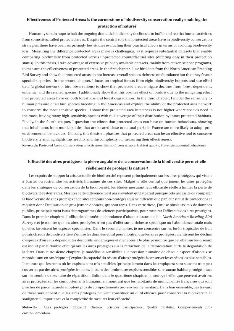
Effectiveness of Protected Areas: is the cornerstone of biodiversity conservation really enabling the
protection of nature?
Humanity’s main hope to halt the ongoing dramatic biodiversity declines is to buffer and restrict human activities
from some sites, called protected areas. Despite the central role that protected areas have in biodiversity conservation
strategies, there have been surprisingly few studies evaluating their practical effects in terms of avoiding biodiversity
loss. Measuring the difference protected areas make is challenging, as it requires substantial datasets that enable
comparing biodiversity from protected versus unprotected counterfactual sites (differing only in their protection
status). In this thesis, I take advantage of extensive publicly available datasets, mainly from citizen science programs,
to measure the effectiveness of protected areas. In the first chapter, I use bird data from the North American Breeding
Bird Survey and show that protected areas do not increase overall species richness or abundance but that they favour
specialist species. In the second chapter, I focus on tropical forests from eight biodiversity hotpots and use eBird
data (a global network of bird observations) to show that protected areas mitigate declines from forest-dependent,
endemic, and threatened species. I additionally show that this positive effect on birds is due to the mitigating effect
that protected areas have on both forest loss and forest degradation. In the third chapter, I model the sensitivity to
human pressure of all bird species breeding in the Americas and explore the ability of the protected area network
to conserve the most sensitive species. I show that protected area intactness is not higher where species need it
the most, leaving many high-sensitivity species with null coverage of their distribution by intact protected habitats.
Finally, in the fourth chapter, I question the effects that protected areas can have on human behaviours, showing
that inhabitants from municipalities that are located close to natural parks in France are more likely to adopt pro-
environmental behaviours. Globally, this thesis emphasises that protected areas can be an effective tool to conserve
biodiversity and highlights the need to, and the complexity of, measuring their effectiveness.
Keywords: Protected Areas; Conservation effectiveness; Birds; Citizen science; Habitat quality; Pro-environmental behaviours
Efficacité des aires protégées : la pierre angulaire de la conservation de la biodiversité permet-elle
réellement de protéger la nature ?
Les espoirs de stopper la crise actuelle de biodiversité reposent principalement sur les aires protégées, qui visent
à écarter ou restreindre les activités humaines de ces sites. Malgré le rôle central que jouent les aires protégées
dans les stratégies de conservation de la biodiversité, les études mesurant leur efficacité réelle à limiter la perte de
biodiversité restent rares. Mesurer cette différence n’est pas si évident qu’il y paraît puisque cela nécessite de comparer
la biodiversité de sites protégés et de sites témoins non-protégés (qui ne diffèrent que par leur statut de protection) et
requiert donc l’utilisation de gros jeux de données, qui sont rares. Dans cette thèse, j’utilise plusieurs jeux de données
publics, principalement issus de programmes de sciences participatives, pour mesurer l’efficacité des aires protégées.
Dans le premier chapitre, j’utilise des données d’abondance d’oiseaux issues de la « North American Breeding Bird
Survey » et je montre que les aires protégées n’ont pas d’effet sur la richesse spécifique ou l’abondance totale mais
qu’elles favorisent les espèces spécialistes. Dans le second chapitre, je me concentre sur les forêts tropicales de huit
points chauds de biodiversité et j’utilise les données eBird pour montrer que les aires protégées ralentissent les déclins
d’espèces d’oiseaux dépendantes des forêts, endémiques et menacées. De plus, je montre que cet effet sur les oiseaux
est induit par le double effet qu’ont les aires protégées sur la réduction de la déforestation et de la dégradation de
la forêt. Dans le troisième chapitre, je modélise la sensibilité à la pression humaine de chaque espèce d’oiseaux se
reproduisant en Amérique et j’explore la capacité du réseau d’aires protégées à conserver les espèces les plus sensibles.
Je montre que les zones où les espèces sont très sensibles (principalement dans les tropiques) sont souvent trop peu
couvertes par des aires protégées intactes, laissant de nombreuses espèces sensibles sans aucun habitat protégé intact
sur l’ensemble de leur aire de répartition. Enfin, dans le quatrième chapitre, j’interroge l’effet que peuvent avoir les
aires protégées sur les comportements humains, en montrant que les habitants de municipalités françaises qui sont
proches de parcs naturels adoptent plus de comportements pro-environnementaux. Dans leur ensemble, ces travaux
de thèse soutiennent que les aires protégées peuvent constituer un outil efficace pour conserver la biodiversité et
soulignent l’importance et la complexité de mesurer leur efficacité.
Mots-clés : Aires protégées ; Efficacité ; Oiseaux ; Sciences participatives ; Qualité d’habitat ; Comportements pro-
environnementaux