Effects ofAll-Terrain Vehicles on Forested Lands and Grasslands

United StatesDepartment of Agriculture

Forest Service

National Technology & Development Program

RecreationManagement

0823 1811—SDTDC

December 2008

U.S. Departmentof TransportationFederal HighwayAdministration

AcknowledgmentsWithout the spirited cooperation and volunteer contributions from many forests, other Federal

agencies, industry, and volunteer organizations this project woud have been impossible to

complete. We offer a special thanks to: The Minnesota Department of Natural Resources, The

Federal Highway Administration, The Specialty Vehicle Institute Of America, The National Off-

Highway Vehicle Conservation Council, and all of the participating forests.

The information contained in this publication has been developed for the guidance of employees of the Forest Service, U.S. Department of Agriculture, its contractors, and cooperating Federal and State agencies. The Forest Service assumes no responsibility for the interpretation or use of this information by other than its own employees. The use of trade, firm, or corporation names is for the information and convenience of the reader. Such use does not constitute an official evaluation, conclusion, recommendation, endorsement, or approval of any product or service to the exclusion of others that may be suitable.

The U.S. Department of Agriculture (USDA) prohibits discrimination in all its programs and activities on the basis of race, color, national origin, age, disability, and where applicable, sex, marital status, familial status, parental status, religion, sexual orientation, genetic information, political beliefs, reprisal, or because all or part of an individual’s income is derived from any public assistance program. (Not all prohibited bases apply to all programs.) Persons with disabilities who require alternative means for communication of program information (Braille, large print, audiotape, etc.) should contact USDA’s TARGET Center at (202) 720-2600 (voice and TDD). To file a complaint of discrimination, write USDA, Director, Office of Civil Rights, 1400 Independence Avenue, S.W., Washington, D.C. 20250-9410, or call (800) 795-3272 (voice) or (202) 720-6382 (TDD). USDA is an equal opportunity provider and employer.

Effects of All-Terrain Vehicles on Forested Lands and Grasslands

Dexter Meadows, Landscape Architect,

San Dimas Technology & Development Center

Randy Foltz, Research Engineer,

Rocky Mountain Research Station, Moscow, Idaho

Nancy Geehan, Recreation Planner, San Dimas Technology & Development Center

December 2008

i

Table of Contents

Executive Summary ..............................................................................................................................................iii

Introduction ........................................................................................................................................................... 1

Chapter 1. Methodology ....................................................................................................................................... 3 Experimental Approach ...................................................................................................................................... 3 Disturbance Classes ........................................................................................................................................... 3 Disturbance Class Matrix ................................................................................................................................... 4 Soils Characterization ......................................................................................................................................... 6 ATV Equipment ................................................................................................................................................... 7 Measurement Parameters and Data-Collection Devices ................................................................................... 7 Test Locations .................................................................................................................................................... 9

Chapter 2. Analysis of Findings .........................................................................................................................11 Disturbance Classes ..........................................................................................................................................11 Analysis of Disturbance Classes ...................................................................................................................... 12 Rut-Depth Analysis ........................................................................................................................................... 13 Erosion Determination Methods ....................................................................................................................... 13 Weather Measurements ................................................................................................................................... 15 Results Weather Measurements ................................................................................................................................... 15 Disturbance Class Results ............................................................................................................................... 16 Rainfall Simulations .......................................................................................................................................... 20 Erosion Parameters .......................................................................................................................................... 27 Statistical Analysis ............................................................................................................................................ 28 Recommended Erosion Parameters ................................................................................................................ 31

Chapter 3. Study Sites ........................................................................................................................................ 33 Arizona-Tonto National Forest .......................................................................................................................... 35 Kentucky-Land Between the Lakes .................................................................................................................. 41 Louisiana-Kisatchie National Forest ................................................................................................................. 49 Minnesota-Department of Natural Resources Lands ....................................................................................... 55 Missouri-Mark Twain National Forest ............................................................................................................... 61 Montana-Beaverhead-Deerlodge National Forest ........................................................................................... 69 Washington-Wenatchee National Forest .......................................................................................................... 75

Chapter 4. Conclusions and Management Implications ................................................................................. 83

Appendix A. Tables A1-A7 .................................................................................................................................. 87Appendix B. ATV and Rider Effects .................................................................................................................. 91Appendix C. Monitoring Fugitive Dust Emmissions From Off HighwayVehicles Traveling On Unpaved Roads: A Quantitiative Technique .............................................................. 95

References ......................................................................................................................................................... 109

iii

EXECUTIVE SUMMARY

One goal of the Forest Service, U.S. Department

of Agriculture, is to provide outdoor recreation

opportunities with minimized impacts to natural

resources (USDA Forest Service 2006). All-terrain-

vehicle (ATV) use on public lands is a rapidly

expanding recreational activity. An estimated 11

million visits to national forests involve ATV use.

This constitutes about 5 percent of all recreation

visits to national forests (English 2003). When

repeated ATV use occurs on undesignated

trails, the impacts can exceed the land’s ability

to rehabilitate itself. The challenge for recreation

managers is to address the needs—and conflicting

expectations—of millions of people who use and

enjoy the national forests while protecting the land’s

health and integrity.

In addition to a new travel management policy

that restricts travel on undesignated trails, the

Forest Service studied previously unused trails to

determine the effects of ATV traffic on the natural

resource. The study’s three main questions were:

Are natural resources being affected by ATV use; to

what degree are natural resources being affected;

and does the ATV’s design make a difference

in the effects? To answer these questions on a

nationwide scale, the study was performed at

seven locations within representative ecoregions.

The ecoregions included Desert, High-elevation

Western Mountains, Gulf Coastal Plains, and

Eastern Broadleaf.

Yes, natural resources were affected by ATV

traffic. At all seven locations, some portion of the

previously unused trail transitioned from a low

to medium disturbance class in 20 to 40 passes.

Medium-disturbance occurred when two of the

following three conditions were present: sixty-

percent loss of original ground cover, trail-width

expansion to 72 inches, or wheel ruts up to 6 inches

deep. At each location some portion of the trail

transitioned from medium to high disturbance in 40

to 120 passes. High disturbance occurred when two

of the following three conditions were present: more

than 60-percent loss of original ground cover, trail

width exceeding 72 inches, or wheel ruts deeper

than 6 inches.

Disturbance levels were caused by three

independent variables: sites, trail features, and

vehicles and tires. There was a statistically

significant difference between the number of

passes required to transition from the low to

medium disturbance class for the seven sites.

Desert and Eastern-broadleaf ecoregions were

the most susceptible to ATV traffic, and the Gulf

Coastal Plain ecoregion was the least susceptible.

Each ecoregion trail section that required wheel-

spin or slip moved quickly to increasing levels of

disturbance. Compared to tight-radius curves,

nearly eight times as many passes were required

to produce equal impacts on straight sections, and

nearly five times as many passes were required for

uphill or downhill sections.

There were no statistically significant differences

for the sport and utility ATVs equipped with either

original equipment manufacturer tires or after

market tires with ¾-inch lugs. The study concluded

that the impacts from the four combinations of

vehicles and tires were indistinguishable.

Following any level of disturbance, runoff and

sediment generated on the ATV trails increased by

56 percent and 625 percent, respectively, compared

to the undisturbed forest floor. ATV trails are high-

runoff, high-sediment producing strips on a low-

iv

runoff, low-sediment producing landscape. Frequent diversions of the trail runoff onto the forest floor will

reduce the amount of sediment and runoff as it infiltrates into the forest floor.

The study demonstrated that ATV traffic does have an impact on natural resources. The levels of

disturbance can be reduced by proper trail design and maintenance and by focusing efforts on trail sections

that require extra attention. Application of this study should assist managers in planning, designing, and

implementing decisions related to ATV management.

1

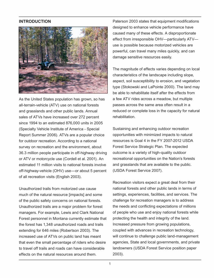
INTRODUCTION

As the United States population has grown, so has

all-terrain-vehicle (ATV) use on national forests

and grasslands and other public lands. Annual

sales of ATVs have increased over 272 percent

since 1994 to an estimated 876,000 units in 2005

(Specialty Vehicle Institute of America - Special

Report Summer 2006). ATVs are a popular choice

for outdoor recreation. According to a national

survey on recreation and the environment, about

36.3 million people participate in off-highway driving

or ATV or motorcycle use (Cordell et al. 2001). An

estimated 11 million visits to national forests involve

off-highway-vehicle (OHV) use—or about 5 percent

of all recreation visits (English 2003).

Unauthorized trails from motorized use cause

much of the natural resource [impacts] and some

of the public safety concerns on national forests.

Unauthorized trails are a major problem for forest

managers. For example, Lewis and Clark National

Forest personnel in Montana currently estimate that

the forest has 1,348 unauthorized roads and trails

extending for 646 miles (Robertson 2003). The

increased use of ATVs on public land has meant

that even the small percentage of riders who desire

to travel off trails and roads can have considerable

effects on the natural resources around them.

Paterson 2003 states that equipment modifications

designed to enhance vehicle performance have

caused many of these effects. A disproportionate

effect from irresponsible OHV—particularly ATV—

use is possible because motorized vehicles are

powerful, can travel many miles quickly, and can

damage sensitive resources easily.

The magnitude of effects varies depending on local

characteristics of the landscape including slope,

aspect, soil susceptibility to erosion, and vegetation

type (Stokowski and LaPointe 2000). The land may

be able to rehabilitate itself after the effects from

a few ATV rides across a meadow, but multiple

passes across the same area often result in a

reduced or complete loss in the capacity for natural

rehabilitation.

Sustaining and enhancing outdoor recreation

opportunities with minimized impacts to natural

resources is Goal 4 in the FY 2007-2012 USDA

Forest Service Strategic Plan. The expected

outcome is a variety of high-quality outdoor

recreational opportunities on the Nation’s forests

and grasslands that are available to the public.

(USDA Forest Service 2007).

Recreation visitors expect a great deal from their

national forests and other public lands in terms of

settings, experiences, facilities, and services. The

challenge for recreation managers is to address

the needs and conflicting expectations of millions

of people who use and enjoy national forests while

protecting the health and integrity of the land.

Increased pressure from growing populations,

coupled with advances in recreation technology,

will continue to challenge public land-management

agencies, State and local governments, and private

landowners (USDA Forest Service position paper

2003).

2

The Forest Service has responded to these

pressures by establishing a new travel management

policy. The Forest Service also conducted a study

to determine the effects of ATVs on the natural

resources. This publication documents that study

and provides field managers with information and

tools to make good, science-based decisions in

managing the effects of ATVs, as they implement

policies and plans related to travel management in

the national forests and grasslands.

Chapter 1 discusses the methodology behind the

study, as well as, its design and implementation.

It also discusses the assessment tool used to

measure the effects on natural resources.

Chapter 2 includes an analysis of the data collected

during the test period and answers the three

questions that framed the study:

1. Are natural resources being affected by ATV use? In other words, is change occurring?

2. If change is occurring, to what degree are natural resources affected?

3. If natural resources are affected, does the design of the ATV (or the way that it is equipped) make a difference?

Chapter 2 also contains a discussion of ATV

performance, rider behavior, and their effects.

Chapter 3 includes descriptions of the settings and

habitats for the seven study sites. The changes to

natural resources as a result of repetitive ATV traffic

also are included.

Chapter 4 contains recommendations to assist

managers in planning, designing, and implementing

decisions related to ATV management.

3

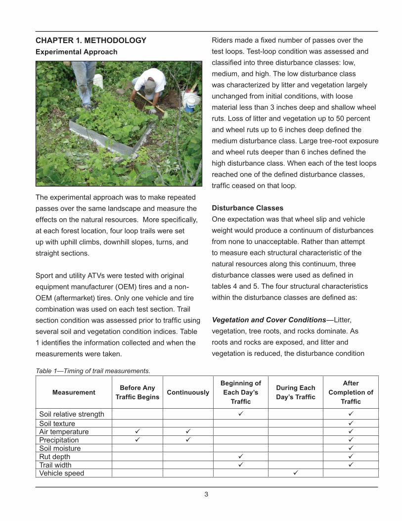
CHAPTER 1. METHODOLOGY

Experimental Approach

The experimental approach was to make repeated

passes over the same landscape and measure the

effects on the natural resources. More specifically,

at each forest location, four loop trails were set

up with uphill climbs, downhill slopes, turns, and

straight sections.

Sport and utility ATVs were tested with original

equipment manufacturer (OEM) tires and a non-

OEM (aftermarket) tires. Only one vehicle and tire

combination was used on each test section. Trail

section condition was assessed prior to traffic using

several soil and vegetation condition indices. Table

1 identifies the information collected and when the

measurements were taken.

Table 1—Timing of trail measurements.

MeasurementBefore Any

Traffic BeginsContinuously

Beginning of Each Day’s

Traffic

During Each Day’s Traffic

After Completion of

Traffic

Soil relative strength ¸ ¸Soil texture ¸Air temperature ¸ ¸ ¸Precipitation ¸ ¸ ¸Soil moisture ¸Rut depth ¸ ¸Trail width ¸ ¸Vehicle speed ¸

Riders made a fixed number of passes over the

test loops. Test-loop condition was assessed and

classified into three disturbance classes: low,

medium, and high. The low disturbance class

was characterized by litter and vegetation largely

unchanged from initial conditions, with loose

material less than 3 inches deep and shallow wheel

ruts. Loss of litter and vegetation up to 50 percent

and wheel ruts up to 6 inches deep defined the

medium disturbance class. Large tree-root exposure

and wheel ruts deeper than 6 inches defined the

high disturbance class. When each of the test loops

reached one of the defined disturbance classes,

traffic ceased on that loop.

Disturbance Classes

One expectation was that wheel slip and vehicle

weight would produce a continuum of disturbances

from none to unacceptable. Rather than attempt

to measure each structural characteristic of the

natural resources along this continuum, three

disturbance classes were used as defined in

tables 4 and 5. The four structural characteristics

within the disturbance classes are defined as:

Vegetation and Cover Conditions—Litter,

vegetation, tree roots, and rocks dominate. As

roots and rocks are exposed, and litter and

vegetation is reduced, the disturbance condition

4

moves toward high. The high disturbance class

is characterized by greater than 60 percent

bare soil and exposed roots and rocks.

Trail Conditions—Depth of rutting and

trail width are the key indicators in the trail

conditions. A trail width greater than 54

inches and ruts greater than 6 inches deep

are indicative of a high disturbance class.

Erosion Conditions—Rill networks and dust

are used as indicators of erosion conditions.

Rills on more than one-third of the trail

length, sediment movement off the trail, and

a dust cloud more than 6 feet high are used

to indicate a high disturbance class.

Soil Conditions—The depth of the A-

horizon is the soil indicator for disturbance

classes. A loss of more than 50 percent of

the A-horizon is cause for classifying a trail

section in the high disturbance class.

Disturbance Class Matrix

The idea behind a trail-condition class matrix

is well established. The Forest Service (1975)

used a Stream Reach Inventory and Channel

Stability Evaluation matrix with stability indicators

of excellent, good, fair, and poor. There are 15

descriptions for these conditions that correspond

to the proposed 9 descriptions in table 2. Using

this classification matrix, the verbal description

most closely matching the actual conditions on the

Table 2—Trail disturbance class matrix for trails.

Trail Disturbance Class Matrix For New Trail

Low Disturbance Medium Disturbance High Disturbance

Vegetation and Cover ConditionsLitter and vegetation 0-30% bare soil. 30-60% bare soil. Greater than 60% bare soil.

Tree roots Small roots exposed. Small roots exposed and broken.

Large roots exposed and damaged.

RocksNo more exposed or fractured rocks than natural conditions.

Exposed and fractured rocks.

Large rocks worn around or displaced.

Trail Conditions

Trail width (both tread and displaced material)

54 inches or less.Between 54 and 72 inches. Some trail braiding. Evidence of width increasing.

72 inches or greater. Braided trails evident. Trail width is growing.

Trail tread/surface Loose material up to 3 inches deep and wide.

Loose material 3 to 6 inches deep.

Loose material deeper than 6 inches.

ATV rut depth Ruts less than 3 inches deep. Ruts 3 to 6 inches deep. Ruts greater than 6 inches

deep. Erosion Conditions

Rill networksLittle or no rilling, less than 1/3 of trail between water breaks has rills.

More than 1/3 of trail between water breaks has rills.

Rills evident on more than 1/3 of trail between water breaks.

DustLess than 3 feet high. Traffic does not slow down. Does not obstruct visibility.

3- to 6-foot cloud. Causes traffic to slow down. Partially obstructs visibility.

Greater than 6 feet. Causes traffic to slow or stop. Very thick cloud that obstructs visibility.

Soil Conditions

Depth of A horizon Greater than 70% of natural. 70 to 50% of natural. Less than 50% of natural.

TOTALS

5

ground was checked, the number of checks in each

class added together, and the condition class rating

was determined by the total score. This procedure is

illustrated in table 3.

Application of the Disturbance Class Matrix

Table 3 illustrates how the disturbance class matrix

was used. An observer walks along a trail section

and makes a qualitative judgment, or in a few cases

a quantitative measurement, for each entry in the

matrix by circling the appropriate description. After

all the descriptors have been rated, the circles

(disturbance class) are totaled at the bottom of

each column. The disturbance class corresponding

to the column with the highest total is deemed the

condition of that trail section. Ties are rounded

down.

In table 3 the total of the factors in the low

disturbance class was five, in the medium class

was three, and in the high class was one. Since the

class receiving the highest total was low, the section

was classified as low disturbance.

Two techniques were used for assessing changes

to the natural resources as ATVs made repeated

passes over the loops. The first assessment was

made using the condition-class matrix described

Table 3—Example of trail disturbance class matrix for trails.

Trail Disturbance Class Matrix For New Trails

Low Disturbance Medium Disturbance High Disturbance

Vegetation & Cover Conditions

Litter and vegetation 0-30% bare soil. 30-60% bare soil. Greater than 60% bare soil.

Tree roots Small roots exposed. Small roots exposed and broken.

Large roots exposed and damaged.

RocksNo more exposed or fractured rocks than natural conditions.

Exposed and fractured rocks.

Large rocks worn around or displaced.

Trail Conditions

Trail width (both tread and displaced material)

54 inches or less.

Between 54 and 72 inches. Some trail braiding. Evidence of width increasing.

72 inches or greater. Braided trails evident. Trail width is growing.

Trail tread/surface Loose material up to 3 inches deep and wide.

Loose material to depth of 3 to 6 inches.

Loose material deeper than 6 inches.

ATV rut depth Ruts less than 3 inches deep. Ruts 3 to 6 inches deep. Ruts greater than 6 inches

deep.

Erosion Conditions

Rill networksLittle or no rilling, less than 1/3 of trail between water breaks has rills.

More than 1/3 of trail between water breaks has rills.

Rills evident on more than 1/3 of trail between water breaks.

Dust

Less than 3 feet high. Traffic does not slow down. Does not obstruct visibility.

3- to 6-foot cloud. Causes traffic to slow down. Partially obstructs visibility

Greater than 6 feet. Causes traffic to slow or stop. Very thick cloud that obstructs visibility.

Soil Conditions

Depth of A horizon Greater than 70% of natural. 70 to 50% of natural. Less than 50% of natural.

TOTALS 5 3 1

6

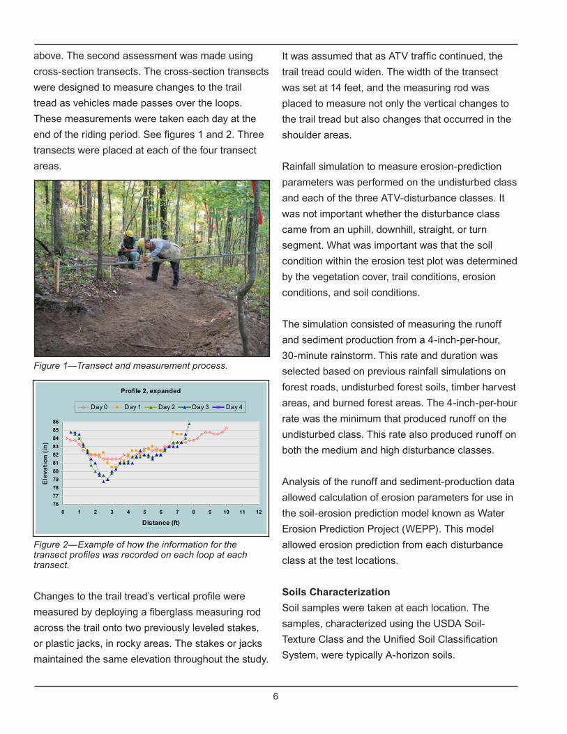
above. The second assessment was made using

cross-section transects. The cross-section transects

were designed to measure changes to the trail

tread as vehicles made passes over the loops.

These measurements were taken each day at the

end of the riding period. See figures 1 and 2. Three

transects were placed at each of the four transect

areas.

Figure 1—Transect and measurement process.

Figure 2—Example of how the information for the transect profiles was recorded on each loop at each transect.

Changes to the trail tread’s vertical profile were

measured by deploying a fiberglass measuring rod

across the trail onto two previously leveled stakes,

or plastic jacks, in rocky areas. The stakes or jacks

maintained the same elevation throughout the study.

Profile 2, expanded

76

77

78

79

80

81

82

83

84

85

86

0 1 2 3 4 5 6 7 8 9 10 11 12

Distance (ft)

Elevation (in)

Day 0 Day 1 Day 2 Day 3 Day 4

It was assumed that as ATV traffic continued, the

trail tread could widen. The width of the transect

was set at 14 feet, and the measuring rod was

placed to measure not only the vertical changes to

the trail tread but also changes that occurred in the

shoulder areas.

Rainfall simulation to measure erosion-prediction

parameters was performed on the undisturbed class

and each of the three ATV-disturbance classes. It

was not important whether the disturbance class

came from an uphill, downhill, straight, or turn

segment. What was important was that the soil

condition within the erosion test plot was determined

by the vegetation cover, trail conditions, erosion

conditions, and soil conditions.

The simulation consisted of measuring the runoff

and sediment production from a 4-inch-per-hour,

30-minute rainstorm. This rate and duration was

selected based on previous rainfall simulations on

forest roads, undisturbed forest soils, timber harvest

areas, and burned forest areas. The 4-inch-per-hour

rate was the minimum that produced runoff on the

undisturbed class. This rate also produced runoff on

both the medium and high disturbance classes.

Analysis of the runoff and sediment-production data

allowed calculation of erosion parameters for use in

the soil-erosion prediction model known as Water

Erosion Prediction Project (WEPP). This model

allowed erosion prediction from each disturbance

class at the test locations.

Soils Characterization

Soil samples were taken at each location. The

samples, characterized using the USDA Soil-

Texture Class and the Unified Soil Classification

System, were typically A-horizon soils.

Ele

va

tio

n (

in)

7

Table 4—ATV Characteristics

Sport Type Utility TypeWeight (pounds) 350 – 450 540 – 610 Stroke cycle 4 4Transmission/drive Manual or automatic AutomaticNumber of drive wheels 2 4Final drive Chain drive, solid axle Shaft drive, rear differentialFront suspension type Double A-arm Double A-armRear suspension type Swing arm Double wishbone

The characterization tests included moisture content

and bulk dry density, soil texture (classification)

requiring gradation analyses (sieve and hydrometer

analysis) and Atterberg Limits, and shear strength

testing (using a direct-shear device) to evaluate

soil strength parameters cohesion and internal-

friction angle. The testing provided uniform sets of

results that can be compared to results from other

locations.

Relatively undisturbed samples were obtained

using a hand-drive sampler (2.0 or 2.5 inches in

diameter) in areas generally free of coarse gravel,

cobble, and shale fragments. In areas of coarse

materials, grab samples were collected. All testing

was performed using standardized methods in

accordance with Forest Service specifications

established by the American Association of State

Highway and Transportation Officials (AASHTO)

and the American Society for Testing and Materials

(ASTM).

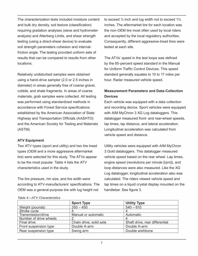
ATV Equipment

Two ATV types (sport and utility) and two tire tread

types (OEM and a more aggressive aftermarket

tire) were selected for this study. The ATVs appear

to be the most popular. Table 4 lists the ATV

characteristics used in the study.

The tire pressure, rim size, and tire width were

according to ATV-manufacturers’ specifications. The

OEM was a general-purpose tire with lug height not

to exceed ½ inch and lug width not to exceed 1½

inches. The aftermarket tire for each location was

the non-OEM tire most often used by local riders

and accepted by the local regulatory authorities.

Consequently, different aggressive-tread tires were

tested at each site.

The ATVs’ speed in the test loops was defined

by the 85-percent speed standard in the Manual

for Uniform Traffic Control Devices. This speed

standard generally equates to 10 to 17 miles per

hour. Radar measured vehicle speed.

Measurement Parameters and Data-Collection

Devices

Each vehicle was equipped with a data collection

and recording device. Sport vehicles were equipped

with AIM MyChron 3 XG Log dataloggers. This

datalogger measured front- and rear-wheel speeds,

lap times, lap distance, and lateral acceleration.

Longitudinal acceleration was calculated from

vehicle speed and distance.

Utility vehicles were equipped with AIM MyChron

3 Gold dataloggers. This datalogger measured

vehicle speed based on the rear wheel. Lap times,

engine speed (revolutions per minute [rpm]), and

loop distances were also measured. Like the XG

Log datalogger, longitudinal acceleration also was

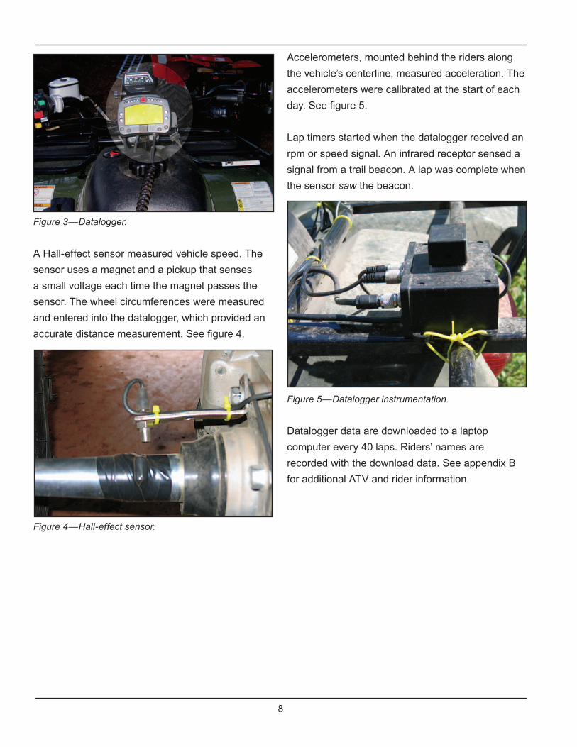
calculated. The riders viewed vehicle speed and

lap times on a liquid crystal display mounted on the

handlebar. See figure 3.

8

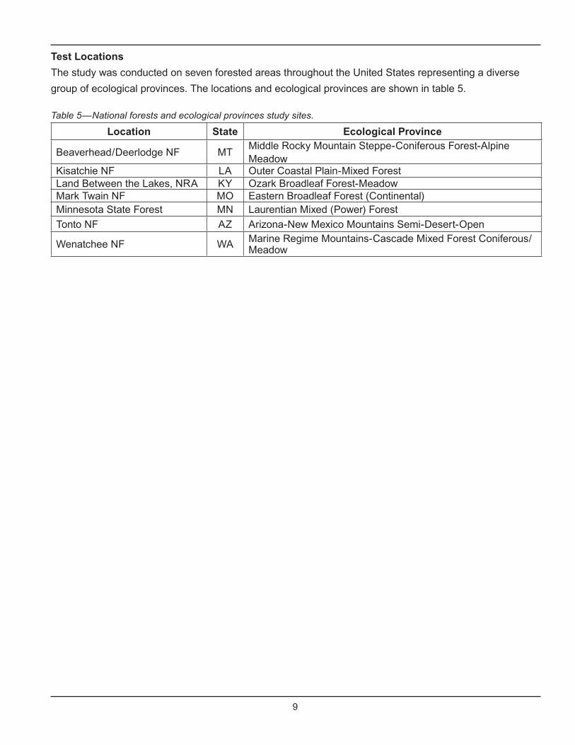
Accelerometers, mounted behind the riders along

the vehicle’s centerline, measured acceleration. The

accelerometers were calibrated at the start of each

day. See figure 5.

Lap timers started when the datalogger received an

rpm or speed signal. An infrared receptor sensed a

signal from a trail beacon. A lap was complete when

the sensor saw the beacon.

Figure 5—Datalogger instrumentation.

Datalogger data are downloaded to a laptop

computer every 40 laps. Riders’ names are

recorded with the download data. See appendix B

for additional ATV and rider information.

Figure 3—Datalogger.

A Hall-effect sensor measured vehicle speed. The

sensor uses a magnet and a pickup that senses

a small voltage each time the magnet passes the

sensor. The wheel circumferences were measured

and entered into the datalogger, which provided an

accurate distance measurement. See figure 4.

Figure 4—Hall-effect sensor.

9

Table 5—National forests and ecological provinces study sites.

Location State Ecological Province

Beaverhead/Deerlodge NF MTMiddle Rocky Mountain Steppe-Coniferous Forest-Alpine Meadow

Kisatchie NF LA Outer Coastal Plain-Mixed ForestLand Between the Lakes, NRA KY Ozark Broadleaf Forest-MeadowMark Twain NF MO Eastern Broadleaf Forest (Continental)Minnesota State Forest MN Laurentian Mixed (Power) Forest

Tonto NF AZ Arizona-New Mexico Mountains Semi-Desert-Open

Wenatchee NF WA Marine Regime Mountains-Cascade Mixed Forest Coniferous/Meadow

Test Locations

The study was conducted on seven forested areas throughout the United States representing a diverse

group of ecological provinces. The locations and ecological provinces are shown in table 5.

11

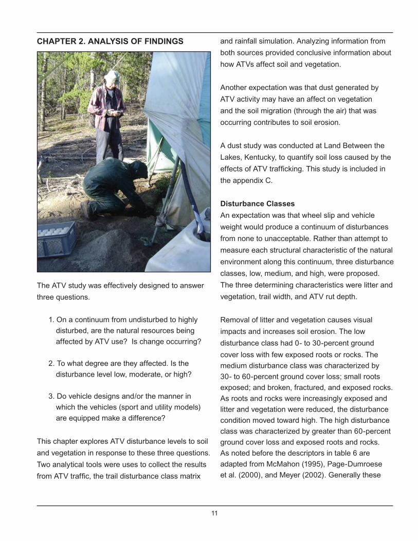
CHAPTER 2. ANALYSIS OF FINDINGS

The ATV study was effectively designed to answer

three questions.

1. On a continuum from undisturbed to highly

disturbed, are the natural resources being

affected by ATV use? Is change occurring?

2. To what degree are they affected. Is the

disturbance level low, moderate, or high?

3. Do vehicle designs and/or the manner in

which the vehicles (sport and utility models)

are equipped make a difference?

This chapter explores ATV disturbance levels to soil

and vegetation in response to these three questions.

Two analytical tools were uses to collect the results

from ATV traffic, the trail disturbance class matrix

and rainfall simulation. Analyzing information from

both sources provided conclusive information about

how ATVs affect soil and vegetation.

Another expectation was that dust generated by

ATV activity may have an affect on vegetation

and the soil migration (through the air) that was

occurring contributes to soil erosion.

A dust study was conducted at Land Between the

Lakes, Kentucky, to quantify soil loss caused by the

effects of ATV trafficking. This study is included in

the appendix C.

Disturbance Classes

An expectation was that wheel slip and vehicle

weight would produce a continuum of disturbances

from none to unacceptable. Rather than attempt to

measure each structural characteristic of the natural

environment along this continuum, three disturbance

classes, low, medium, and high, were proposed.

The three determining characteristics were litter and

vegetation, trail width, and ATV rut depth.

Removal of litter and vegetation causes visual

impacts and increases soil erosion. The low

disturbance class had 0- to 30-percent ground

cover loss with few exposed roots or rocks. The

medium disturbance class was characterized by

30- to 60-percent ground cover loss; small roots

exposed; and broken, fractured, and exposed rocks.

As roots and rocks were increasingly exposed and

litter and vegetation were reduced, the disturbance

condition moved toward high. The high disturbance

class was characterized by greater than 60-percent

ground cover loss and exposed roots and rocks.

As noted before the descriptors in table 6 are

adapted from McMahon (1995), Page-Dumroese

et al. (2000), and Meyer (2002). Generally these

12

references used either a set of descriptions for

unacceptable conditions or had four to six classes

of disturbance. The present study chose three

classes.

Trail width was a key indicator of trail conditions. A

trail width of 54 inches or less was rated as a low

disturbance class. As the width increased from 54

to 72 inches, the condition was rated a medium

disturbance class, and a width greater than 72

inches was rated a high disturbance class.

ATV rut depth was the final indicator of trail

conditions. A low rating was from no ruts up to 3-

inch-deep ruts; a medium rating was 3- to 6-inch-

deep ruts; and a high rating was greater than 6-

inch-deep ruts.

To use the disturbance class matrix, an observer

walked along a trail section and made a qualitative

judgment, or in a few cases a quantitative

measurement, for each entry in the matrix by

circling the appropriate description. After all of the

descriptors had been rated, the number of circles

in each column (disturbance class) was totaled.

The disturbance class corresponding to the column

with the highest total was deemed the condition of

that trail section. Ties between low and medium

or between medium and high were rounded down.

Any observation of high resulted in a condition

classification of at least medium.

Analysis of Disturbance Classes

The experimental design for the ATV traffic was

one loop for each combination of vehicle and tire

type, for a total of four loops at each site. Each loop

had four trail features, and each feature was rated

with the condition class matrix after approximately

every 40 passes. While this results in a large

number of observations, there are no replications

in the experimental design. Further, the number of

ATV passes was not the same on each loop, and

the goal of reaching the high condition was not

achieved at all sites.

Frequently, the data say only that riding stopped

after 500 passes and the trail condition was

medium. From this information one can conclude

only that it would have taken more than 500 passes

to reach the high condition. There are instances

where a similar statement has to be made for the

medium class, as well. It is not possible to average

an observation of 150 passes and one of greater

than 500 passes.

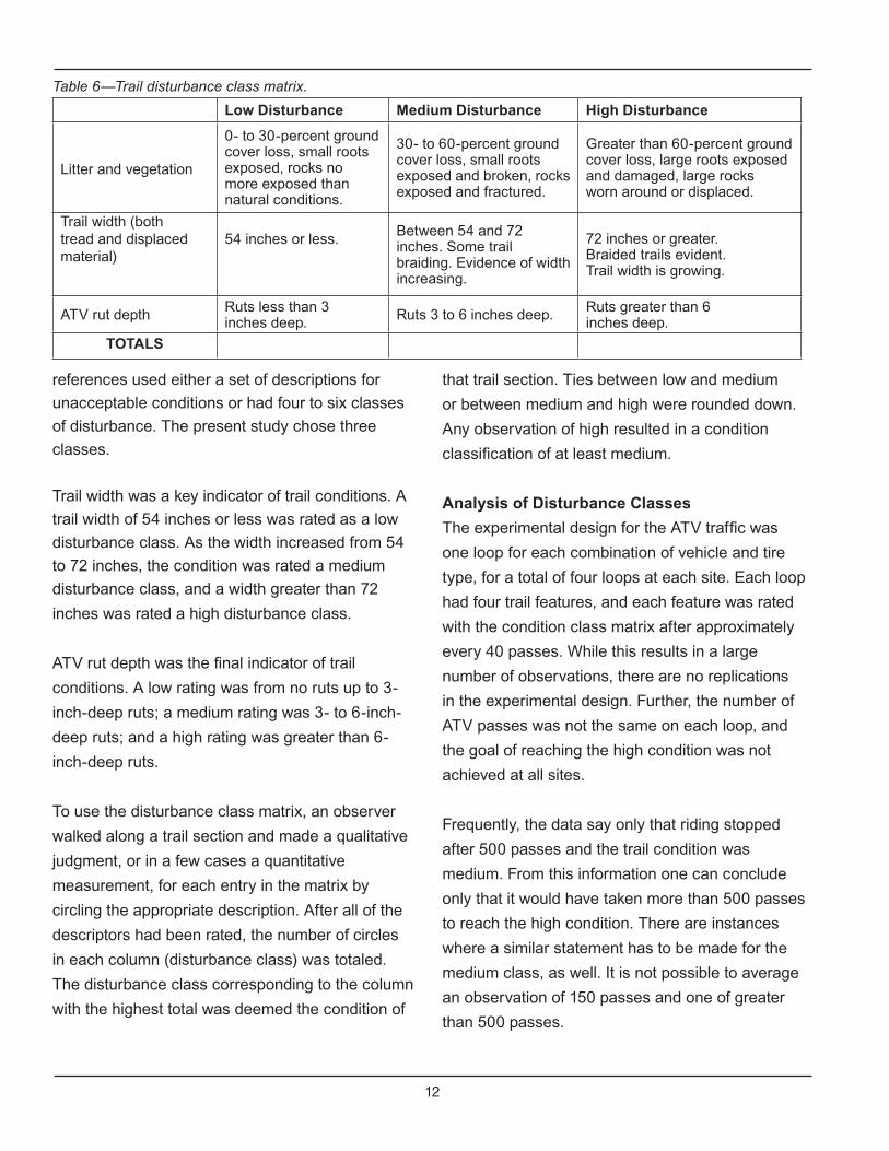
Table 6—Trail disturbance class matrix.

Low Disturbance Medium Disturbance High Disturbance

Litter and vegetation

0- to 30-percent ground cover loss, small roots exposed, rocks no more exposed than natural conditions.

30- to 60-percent ground cover loss, small roots exposed and broken, rocks exposed and fractured.

Greater than 60-percent ground cover loss, large roots exposed and damaged, large rocks worn around or displaced.

Trail width (both tread and displaced material)

54 inches or less.Between 54 and 72 inches. Some trail braiding. Evidence of width increasing.

72 inches or greater. Braided trails evident. Trail width is growing.

ATV rut depth Ruts less than 3 inches deep. Ruts 3 to 6 inches deep. Ruts greater than 6

inches deep.

TOTALS

13

Data that measure lifetime—or the length of time

until the occurrence of an event—are called lifetime,

failure time, or survival data. Classic examples

are the lifetime of diesel engines, the length of

time a person stays on a job, or the survival

time for heart-transplant patients. An intrinsic

characteristic of survival data is the possibility for

censoring observations, that is, the actual number

of passes until leaving a class was not observed.

A large percentage of censored values results

in a low statistical validity. In the ATV study, the

corresponding variable of interest is the number of

passes before leaving the low or medium condition

class. There were occasional censored values for

leaving the low condition and a large number of

censored ones for leaving the medium condition.

The first step in the analysis of survival data is an

estimation of the distribution of survival times, which

are often called failure times. Uncensored survival

times (i.e., times at which the event actually occurs)

are called event times. The survival-distribution

function (SDF) is used to describe the lifetimes of

the population of interest. The SDF evaluated at t

is the probability that an experimental unit from the

population will have a lifetime exceeding t, or

)Pr()( tTtS >=

where S(t) denotes the SDF and T is the lifetime of

a randomly selected experimental unit. For the ATV

study, times were synonymous with passes.

To make an SDF, two of the three independent

variables (i.e., trail feature, vehicle and tire

combination, and sites) have to be combined in

order to investigate changes in the third variable.

The condition-class-matrix results were used to

determine the survival distribution function for (1)

sites where trail feature and vehicle type were

combined, (2) trail feature where sites and vehicle

type were combined, and (3) vehicle type where

trail feature and sites were combined. There was an

insufficient number of uncensored passes to make a

statistical analysis of the transition from medium to

high condition class, so only the transition from low

to medium is presented.

The median number of passes required to

transition from low to medium condition class will

be considered to be that corresponding to the 0.50

value of the SDF. When comparing one SDF to

another, a lower number of passes for the same

value of the SDF is indicative of fewer passes to

achieve the same disturbance and, hence, a greater

sensitivity to ATV traffic.

Rut-Depth Analysis

Each trail feature had three cross sections

measured at the end of each driving day, resulting

in replicated rut depth data. The wheel rut depth

was measured from top of the berm to bottom of

the rut. The depth of any initial rills or ruts was

subtracted from that caused by ATV traffic. The

three replications were averaged to determine a

representative rut depth.

Erosion Determination Methods

Rainfall simulation on 1-meter-square bordered

plots was used to determine infiltration and

raindrop-splash parameters. The rainfall simulator

used a Spraying Systems Veejet 80100 nozzle to

approximate the raindrop distribution of natural

rainfall.

Rainfall-simulation plots consisted of an upper

border and two side borders of 16-gauge sheet

metal driven into the soil 2 inches deep. The lower

border consisted of a runoff apron flush with the

soil surface that drained into a collection trough

14

with a centrally located 1-inch opening. The runoff

apron was placed on top of a 1/4-inch-thick layer of

bentonite to prevent any water from flowing under

the apron. Dimensions of the exposed soil inside the

plot were 1 meter by 1 meter.

Two rainstorms with an intensity of 4 inches per

hour with 30-minute duration were applied to each

plot. The two rainstorms were applied 3 hours apart.

The 4 inches per hour, 30-minute-duration storm

had a return period varying from 5 years at the

Louisiana site to 450 years at the Arizona site. This

rainfall intensity and duration were chosen not to

represent a specific design storm, but to exceed the

expected infiltration rate at each site, thus allowing

the entire plot to contribute to runoff. Entire-

plot contribution to runoff is a requirement when

determining infiltration and erosion parameters from

simulated rainfall.

Two soil-moisture samples from each side of the

plot were taken at a depth of 0 to 1½ inches before

and after each simulated storm. These soil samples

were oven-dried overnight at 105 degrees Celsius

(°C).

Once runoff began on a plot, timed grab-samples

in 500-milliliter bottles were taken each minute

for the runoff’s duration. These runoff samples

were oven-dried overnight at 105 °C to determine

sediment concentrations. Water-runoff rates,

sediment concentrations, and sediment-flux rates

were calculated based on these samples. There

were three repetitions of each soil-disturbance class

at each site.

Ground cover was measured by counting the

number of grid points above vegetation, rocks,

or duff in simulation-plot photographs. Each plot

photograph was counted twice using different grid

orientations.

The WEPP model was used to determine the

infiltration and erosion characteristics from the ATV

study. The WEPP model (Flanagan and Livingston

1995) is a physically based soil erosion model that

provides estimates of runoff, infiltration, soil erosion,

and sediment yield considering the specific soil,

climate, ground cover, and topographic conditions.

The WEPP model uses the Green-Ampt Mein-

Larson model for unsteady intermittent rainfall to

represent infiltration (Stone et al. 1995). The primary

user-defined parameter is hydraulic conductivity.

Interpretation of this parameter is straightforward.

Higher values indicate a more rapid infiltration rate

and hence, less runoff. The parameter also is an

indication of the maximum-rainfall rate that a soil

can absorb without producing runoff.

Raindrop splash in the WEPP model is

characterized by an interrill-erodibility coefficient,

which is a function of rainfall intensity and runoff

rate (Alberts et al. 1995). Interpretation of the

interrill-erodibility coefficient is also straightforward,

although the units of kg·s·m-4 are not intuitive.

Higher values indicate higher raindrop-splash

erosion.

15

Table 7—Precipitation and temperatures during ATV traffic and rainfall-simulation activities for all sites.

Site

ATV-traffic period Rainfall-simulation period5-day

antecedent precipitation

(in)

Total precipitation

(in)

Average temperature

(°F)

5-day antecedent precipitation

(in)

Total precipitation

(in)

Average temperature

(°F)

AZ 0 0 91 0 0 86KY 0.34 0 59 0.4 2.84 76LA 3.36 0.95 78 2.09 10.59 79MN 0.10 0.38 56 0 2.98 60MO 0 0.72 64 no rainfall simulationMT 0.34 0 61 0 0.67 63

WA 0 0 64 0 0.28 67

From the rainfall-simulation data, the WEPP

parameters of hydraulic conductivity and interrill

erosion were determined for each run. The resulting

six values (first and second rain for each of the

three repetitions) were averaged to determine

values for each treatment class at each site. Prerain

soil saturation, bulk density, and ground cover as

well as plot geometry were entered into the WEPP

model. Hydraulic conductivity was determined by

minimizing the objective function in equation 1.

The objective function (Objhc

) gave equal weight to

matching the total rainfall-simulation runoff volume

and the peak flow and is shown below.

Equation 1.

Objhc

= (ROmeas

– ROWEPP

)2 + (Peakmeas

– PeakWEPP

)2

where ROmeas

was the measured runoff, ROWEPP

was the WEPP-predicted runoff, Peakmeas

was

the measured-peak runoff, and PeakWEPP

was the

WEPP-predicted peak flow. When the appropriate

value of hydraulic conductivity was determined, the

interrill-erosion parameter was found in a similar

iterative manner until the WEPP-predicted soil loss

matched the measured-sediment loss. Calculated

hydraulic conductivity and interrill-erosion

parameters were averaged to represent values for

each treatment class at each site.

Weather Measurements

Hourly air temperature and breakpoint precipitation

were taken during and after traffic. National Weather

Service records from nearby stations were used to

supplement locally measured values.

Results

Weather Measurements

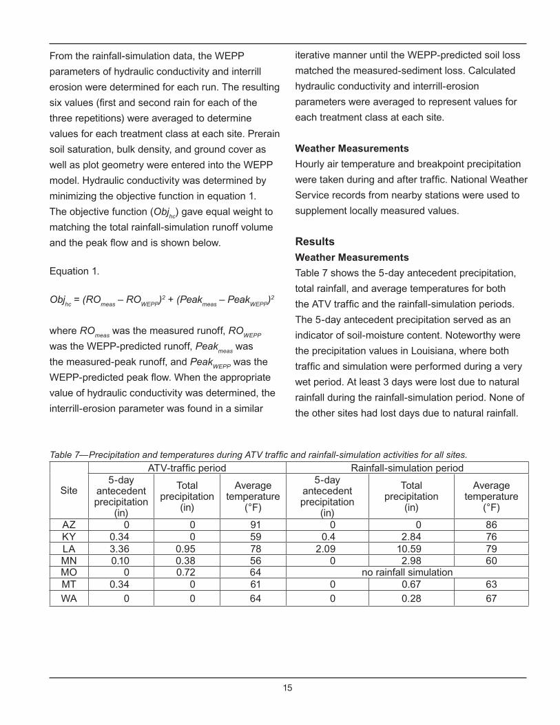
Table 7 shows the 5-day antecedent precipitation,

total rainfall, and average temperatures for both

the ATV traffic and the rainfall-simulation periods.

The 5-day antecedent precipitation served as an

indicator of soil-moisture content. Noteworthy were

the precipitation values in Louisiana, where both

traffic and simulation were performed during a very

wet period. At least 3 days were lost due to natural

rainfall during the rainfall-simulation period. None of

the other sites had lost days due to natural rainfall.

16

Disturbance Class Results

The number of passes required to leave the low

and medium condition for each site and each trail

feature is shown in appendix A. The transition from

low to medium and from medium to high was not

achieved on some loop-treatment combinations. In

these cases, the final number of passes is preceded

by a “greater than” symbol (e.g., >160).

Question 1 – Are the natural resources being

affected by ATV use?

One of the goals of the study was to answer the

question “Are the natural resources being affected

by ATV use?” An inspection of the disturbance-

class results will be used to answer this question.

Table 8 contains data showing the minimum

number of passes required to remain in both low

and medium classes and the range of passes

to achieve medium and high condition classes.

For table 8, vehicle and tire combinations were

combined as were trail features with only the sites

displayed separately. For this level of analysis,

these combinations are appropriate. On real trails,

there would be a mix of vehicle types and tires. No

trail could exist without a mix of curves, straights,

uphill, and downhill, so this combination is also

appropriate. The minimum number of passes to

remain in low represents how quickly some portion

of the trail transitioned from the low disturbance

class to the medium class. Similarly, the minimum

number of passes to remain in medium represents

how quickly some portion of the trail transitioned

from the medium class to the high-disturbance

class. The range of passes to remain in low and

medium classes is included.

At all seven sites, some portion of the trail

transitioned from low to medium disturbance

class in 20 to 40 passes. While the number of

days required to achieve this number of passes

varies from location to location, this level of ATV

traffic could be achieved in one weekend from a

moderate-sized ATV group. Not all of the trail had

left the low disturbance class, but some combination

of vehicle and tire and trail feature was no longer

in the low class. Similarly, all seven sites had some

portion of the trail transition from the medium to high

disturbance class in 40 to 120 passes. This level of

ATV traffic could be achieved in less than a month,

depending upon trail usage.

Our conclusion is that the natural resources

are being affected by ATV use as exhibited by

the impacts achieved during the study. It is also

reasonable to expect that similar impacts would

result to similar natural resources on any national

forest and grasslands where similar ATV riding

occurs.

Table 8—Minimum and range of ATV passes to remain in low and medium condition classes for all trail features and all vehicle and tire combinations.

SiteMinimum number of passes to Range of passes to

Remain in Low Remain in Medium Remain in Low Remain in MediumAZ 40 60 40 to >160 60 to > 160KY 40 40 40 to >320 40 to > 800LA 30 70 30 to >630 70 to > 730MN 40 120 40 to >600 120 to > 700MO 40 80 40 to >560 80 to > 560MT 40 120 40 to >640 120 to >1,000WA 20 80 20 to >480 80 to > 960

17

Question 2 – To what degree are the natural

resources being impacted?

The second goal of the study was to answer the

question “To what degree are the natural resources

being impacted?” This study uses the condition-

class matrix to quantify the degree of natural

resource impacts. The impacts were caused by

three independent variables, namely, sites, trail

features, and vehicles and tires. Vehicles and

tires will be considered separately in question 3.

Combinations of the remaining two impacts, sites

and trail features, and the causative agents will be

discussed by considering the number of passes

required to remain in the low disturbance class.

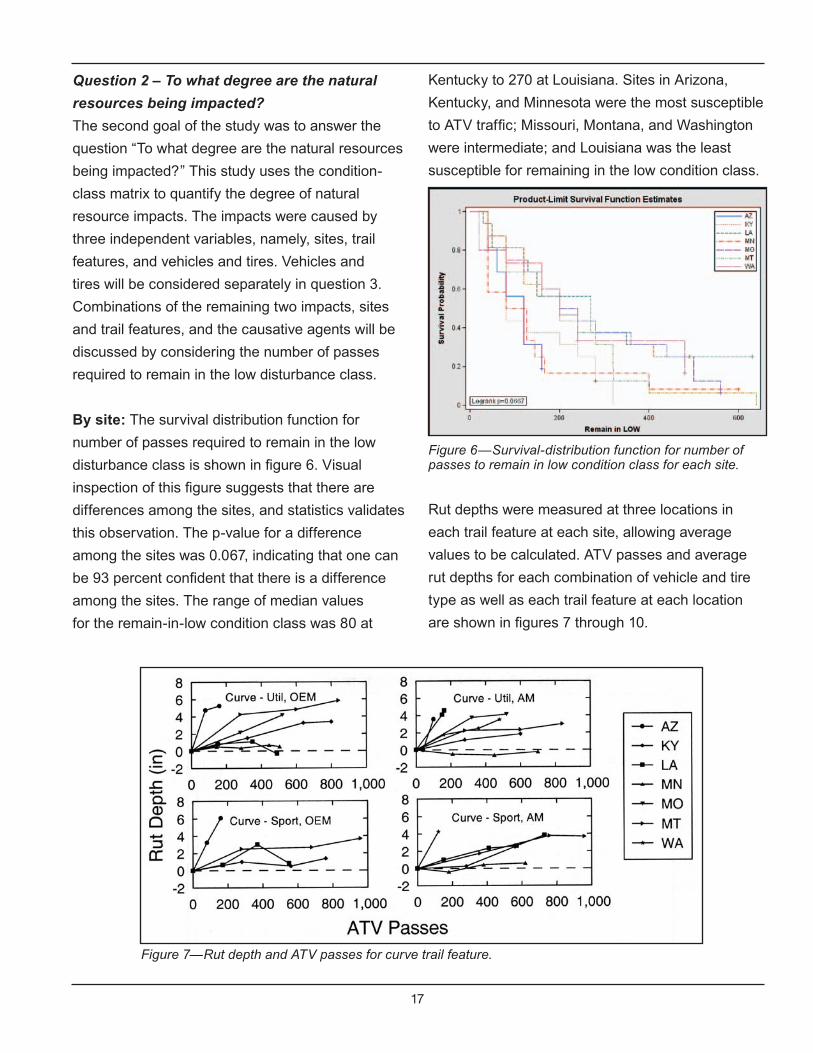
By site: The survival distribution function for

number of passes required to remain in the low

disturbance class is shown in figure 6. Visual

inspection of this figure suggests that there are

differences among the sites, and statistics validates

this observation. The p-value for a difference

among the sites was 0.067, indicating that one can

be 93 percent confident that there is a difference

among the sites. The range of median values

for the remain-in-low condition class was 80 at

Kentucky to 270 at Louisiana. Sites in Arizona,

Kentucky, and Minnesota were the most susceptible

to ATV traffic; Missouri, Montana, and Washington

were intermediate; and Louisiana was the least

susceptible for remaining in the low condition class.

Figure 6—Survival-distribution function for number of passes to remain in low condition class for each site.

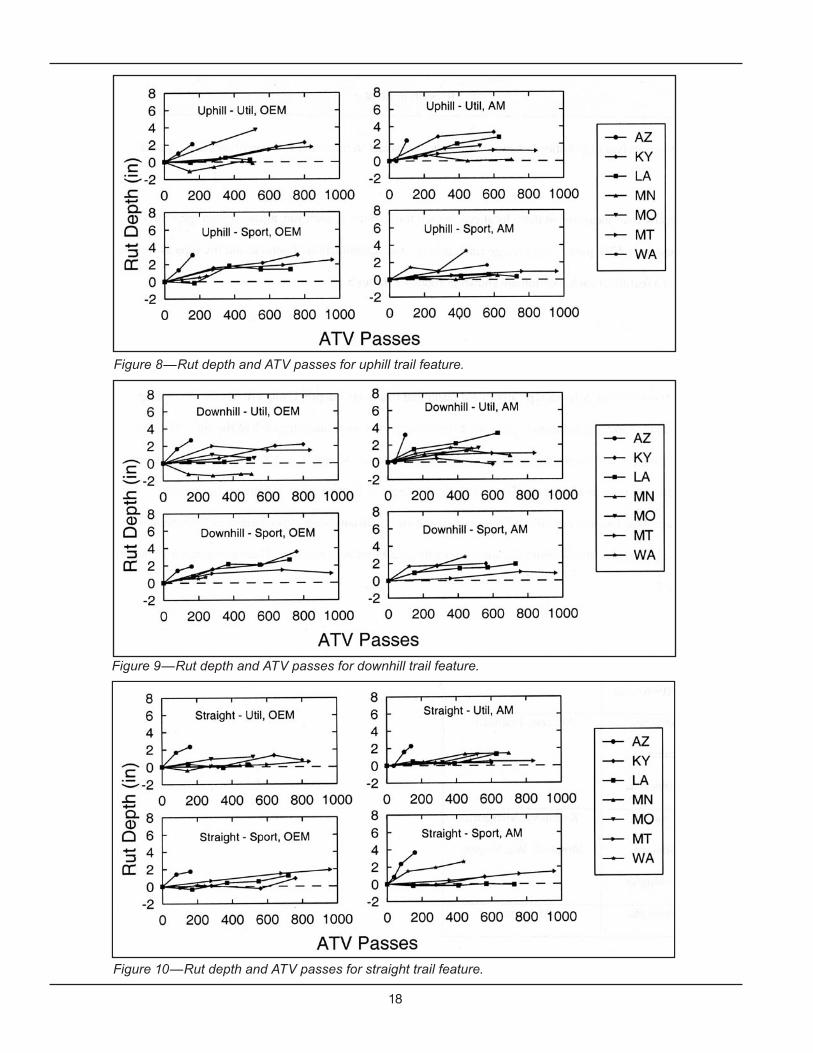
Rut depths were measured at three locations in

each trail feature at each site, allowing average

values to be calculated. ATV passes and average

rut depths for each combination of vehicle and tire

type as well as each trail feature at each location

are shown in figures 7 through 10.

Figure 7—Rut depth and ATV passes for curve trail feature.

18

Figure 8—Rut depth and ATV passes for uphill trail feature.

Figure 9—Rut depth and ATV passes for downhill trail feature.

Figure 10—Rut depth and ATV passes for straight trail feature.

19

median passes to remain in the low-condition class

was 40 for the curve to 320 for the straight. Both the

uphill and the downhill had median values of 200

passes.

Figure 11—Survival-distribution function for number of passes to remain in low condition for each trail feature.

Using figures 7 through 10, the number of instances

of 3-inch-deep or greater ruts was 14 for the curve,

6 for the downhill, 4 for the uphill, and 1 for the

straight trail features. The groupings for trail features

based on rut depths were (1) curve, (2) downhill and

uphill, and (3) straight.

Table 10 displays the rutted condition groups

for the overall condition class and the rut depth.

The authors conclude that the trail features, in

decreasing order of impact, are curves, uphill,

downhill, and straight.

Table 10—Trail feature groupings based on similar characteristics to remain in low disturbance condition and susceptibility to rutting. Order is highest to lowest.

Remain in low condition class Susceptibility to rutting

Curve Curve

Uphill, Downhill Uphill, Downhill

Straight Straight

It is noteworthy that Arizona typically rutted faster

and to a deeper depth. Using criteria of 3-inch-deep

ruts, counts of rutted conditions at the end of the

riding period were made for each of the sites. The

counts ranged from six at Arizona; five at Louisiana;

four at Kentucky, Montana, and Washington; three

at Missouri; and none at Minnesota. There were

three categories that the authors characterize as

high-, moderate-, and low-susceptibility to rutting.

Arizona and Louisiana were characterized as high;

Kentucky, Missouri, Montana, and Washington

were moderate; and Minnesota was low. These

groupings are shown in table 9.

Table 9—Site groupings based on similar characteristics to remain in low disturbance condition and susceptibility to rutting. Order is highest to lowest.

Remain in low condition class

Susceptibility to rutting

Arizona, Kentucky, Minnesota

Arizona, Louisiana

Missouri, Montana,

Washington

Kentucky, Missouri, Montana, Washington

Louisiana Minnesota

By trail features: The four trail features tested

were curves, downhill, straight, and uphill. Figure

11 presents the survival-distribution function for

number of passes to remain in the low-condition

class. It is clear that the curve feature required

fewer passes before it was no longer in the “remain

in low condition.” Results of the statistical analysis

were that one could be +99 percent confident that

there was a difference among the trail features (p-

value of >0.0001). The curve was no longer in the

low condition in nearly 5 times fewer passes than

in the next highest impacted trail feature (40 for the

curve compared to 200 for the uphill). The range of

20

Question 3 – Do the vehicle and tire

combinations tested make a difference in

impacts to the natural resources?

The impacts considered are trail condition class and

rut generation.

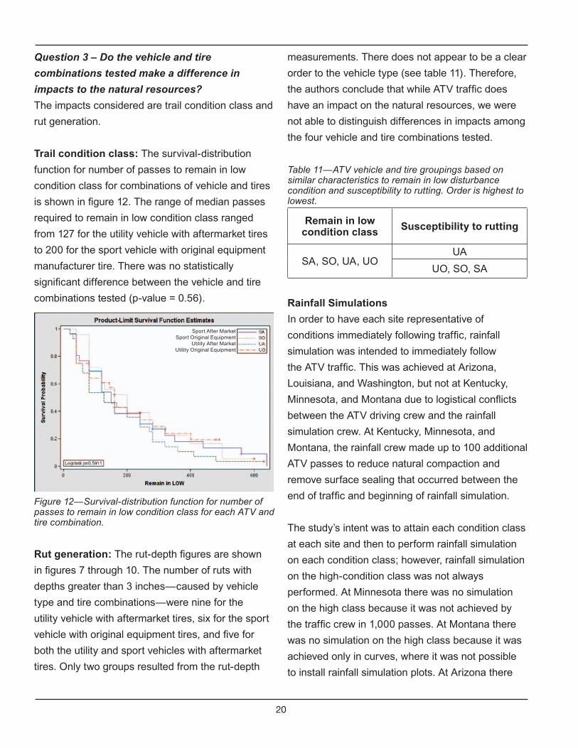
Trail condition class: The survival-distribution

function for number of passes to remain in low

condition class for combinations of vehicle and tires

is shown in figure 12. The range of median passes

required to remain in low condition class ranged

from 127 for the utility vehicle with aftermarket tires

to 200 for the sport vehicle with original equipment

manufacturer tire. There was no statistically

significant difference between the vehicle and tire

combinations tested (p-value = 0.56).

Figure 12—Survival-distribution function for number of passes to remain in low condition class for each ATV and tire combination.

Rut generation: The rut-depth figures are shown

in figures 7 through 10. The number of ruts with

depths greater than 3 inches—caused by vehicle

type and tire combinations—were nine for the

utility vehicle with aftermarket tires, six for the sport

vehicle with original equipment tires, and five for

both the utility and sport vehicles with aftermarket

tires. Only two groups resulted from the rut-depth

measurements. There does not appear to be a clear

order to the vehicle type (see table 11). Therefore,

the authors conclude that while ATV traffic does

have an impact on the natural resources, we were

not able to distinguish differences in impacts among

the four vehicle and tire combinations tested.

Table 11—ATV vehicle and tire groupings based on similar characteristics to remain in low disturbance condition and susceptibility to rutting. Order is highest to lowest.

Remain in low condition class Susceptibility to rutting

SA, SO, UA, UOUA

UO, SO, SA

Rainfall Simulations

In order to have each site representative of

conditions immediately following traffic, rainfall

simulation was intended to immediately follow

the ATV traffic. This was achieved at Arizona,

Louisiana, and Washington, but not at Kentucky,

Minnesota, and Montana due to logistical conflicts

between the ATV driving crew and the rainfall

simulation crew. At Kentucky, Minnesota, and

Montana, the rainfall crew made up to 100 additional

ATV passes to reduce natural compaction and

remove surface sealing that occurred between the

end of traffic and beginning of rainfall simulation.

The study’s intent was to attain each condition class

at each site and then to perform rainfall simulation

on each condition class; however, rainfall simulation

on the high-condition class was not always

performed. At Minnesota there was no simulation

on the high class because it was not achieved by

the traffic crew in 1,000 passes. At Montana there

was no simulation on the high class because it was

achieved only in curves, where it was not possible

to install rainfall simulation plots. At Arizona there

Sport After MarketSport Original Equipment

Utility After MarketUtility Original Equipment

21

Table 12—Date of traffic, rainfall simulation, and condition classes with simulation.

Site Traffic Dates Rainfall Simulation Dates Und Low Med HighAZ May 24-26, 2005 May 25-June 7, 2005 ¸ ¸ ¸KY Oct. 3-5, 2004 May 21-June 3, 2004 ¸ ¸ ¸ ¸LA June 4-6, 2004 June 7-July 2, 2004 ¸ ¸ ¸ ¸MN June 20-23, 2004 July 20-Aug 2, 2004 ¸ ¸ ¸MO Oct. 7-10, 2004 no rainfall simulationMT July 22-24, 2004 Aug 11-21, 2004 ¸ ¸ ¸WA June 14-16, 2005 June 16-July 2, 2005 ¸ ¸ ¸ ¸

Table 13—A horizon soil characteristics at rainfall simulation sites sorted by soil texture.

Site Soil textured

84

(mm)

d50

(mm)

d16

(mm)LA Loamy sand 0.35 0.19 0.05WA Gravelly loamy sand 2.86 0.50 0.05KY Gravelly sandy loam 3.24 0.48 0.02MN Gravelly sandy loam 3.22 0.96 0.02MT Gravelly sand 2.40 0.89 0.27AZ crust Gravelly sand 2.97 0.95 0.15AZ Gravelly sand 3.26 1.38 0.49

was no simulation on the medium class because of time constraints. Table 12 summarizes the dates of

traffic and rainfall simulation as well as condition classes with rainfall simulation.

The soil texture and grain size measurements for each site are shown in table 13. Textures ranged from

loamy sand for Louisiana to gravelly sand for Arizona and Montana. All sites had less than 6-percent clay

and, with the exception of Louisiana, had more than 15-percent rock fragments. Mean grain size (d50

)

ranged from 1.38 millimeters (Arizona) to 0.19 millimeter (Louisiana).

Average ground cover (plants, litter, and rock) for each site and disturbance class for the rainfall simulation

plots is shown in table 14. Changes in ground cover with ATV traffic were a major impact. Visually, the

reduction of cover distinguishes an ATV trail from the undisturbed forest. Additionally, the ground cover loss

increases raindrop-splash erosion because there are fewer plant leaves to absorb the raindrop impacts.

Continued ATV use also inhibits plant regrowth in much the same manner as vehicle traffic inhibits plant

regrowth on unpaved forest roads. Noteworthy were (1) the decrease in cover from undisturbed to low,

(2) the continuing decrease in cover from low through high, and (3) the lower covers at Montana and

Washington for all disturbance classes. Montana sites were on a high-elevation forest with less rainfall and,

hence, less cover. The Washington site was in a burned area, on a compacted logging road, and at high

elevation. Cover at the Arizona site appears unusually high, but was visited in the spring following a wet

winter.

22

Inspection of table 14 suggests that the ground covers for the disturbed classes were not consistent

with the definitions of 0- to 30-percent removal, 30- to 60-percent removal, and greater than 60-percent

removal. Values in table 13 were taken from the rainfall simulation plots centered on the wheel tracks.

These 1-meter-square plots were samples taken from the entire 54- to 72-inch-wide trail where the trail

condition assessment was performed. When the area outside the wheel tracks was included, the reduction

in cover was consistent with the definitions.

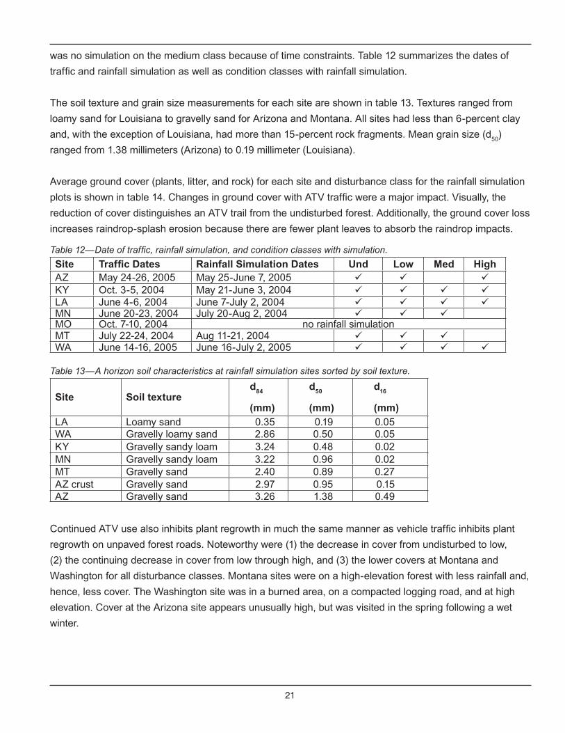
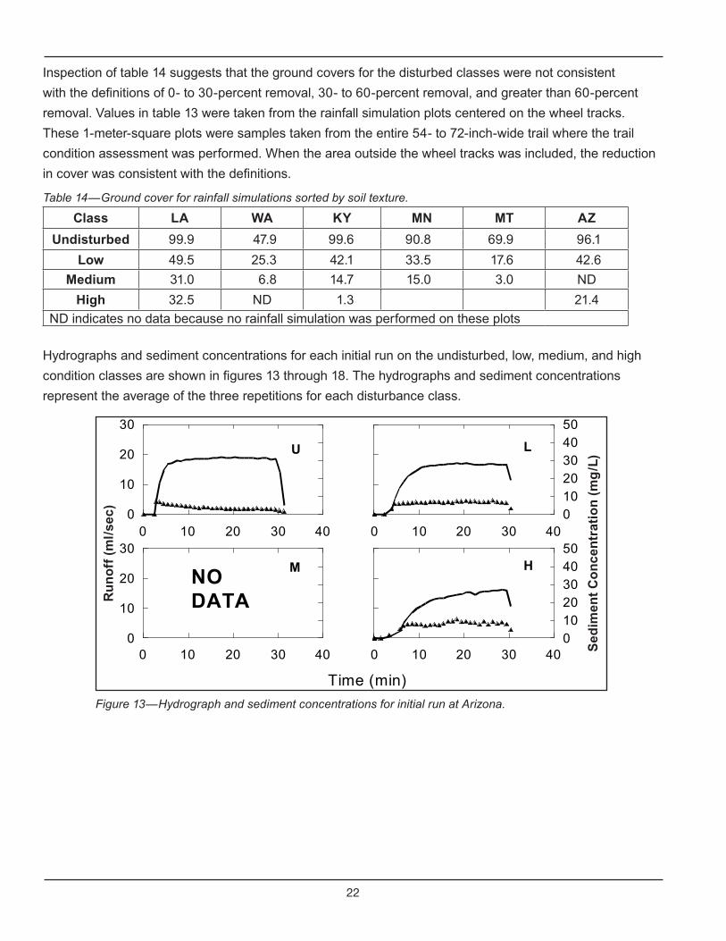
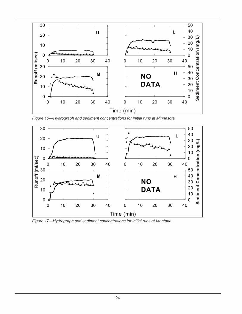
Hydrographs and sediment concentrations for each initial run on the undisturbed, low, medium, and high

condition classes are shown in figures 13 through 18. The hydrographs and sediment concentrations

represent the average of the three repetitions for each disturbance class.

Figure 13—Hydrograph and sediment concentrations for initial run at Arizona.

Table 14—Ground cover for rainfall simulations sorted by soil texture.

Class LA WA KY MN MT AZ

Undisturbed 99.9 47.9 99.6 90.8 69.9 96.1

Low 49.5 25.3 42.1 33.5 17.6 42.6

Medium 31.0 6.8 14.7 15.0 3.0 ND

High 32.5 ND 1.3 21.4

ND indicates no data because no rainfall simulation was performed on these plots

0 10 20 30 40

Time (min)

0

10

20

30

Runoff (ml/sec)

0 10 20 30 4001020304050

Sediment Concentration (mg/L)

0 10 20 30 400

10

20

30

0 10 20 30 4001020304050

U L

M HNODATAR

un

off

(m

l/se

c)

Sed

imen

t C

on

cen

trat

ion

(m

g/L

)

23

Figure 14—Hydrograph and sediment concentrations for initial runs at Kentucky.

Figure 15—Hydrograph and sediment concentrations for initial runs at Louisiana.

0 10 20 30 40

Time (min)

0

10

20

30

Runoff (ml/sec)

0 10 20 30 4001020304050

Sediment Concentration (mg/L)

0 10 20 30 400

10

20

30

0 10 20 30 4001020304050

U L

M H

0 10 20 30 40

Time (min)

0

10

20

30

Runoff (ml/sec)

0 10 20 30 4001020304050

Sediment Concentration (mg/L)

0 10 20 30 400

10

20

30

0 10 20 30 4001020304050

U L

M H

Ru

no

ff (

ml/

sec

)

Sed

imen

t C

on

cen

trat

ion

(m

g/L

)

Ru

no

ff (

ml/

sec

)

Sed

imen

t C

on

cen

trat

ion

(m

g/L

)

24

Figure 16—Hydrograph and sediment concentrations for initial runs at Minnesota

Figure 17—Hydrograph and sediment concentrations for initial runs at Montana.

0 10 20 30 40

Time (min)

0

10

20

30

Runoff (ml/sec)

0 10 20 30 4001020304050

Sediment Concentration (mg/L)

0 10 20 30 400

10

20

30

0 10 20 30 4001020304050

U L

M HNODATA

0 10 20 30 40

Time (min)

0

10

20

30

Runoff (ml/sec)

0 10 20 30 4001020304050

Sediment Concentration (mg/L)

0 10 20 30 400

10

20

30

0 10 20 30 4001020304050

U L

M HNODATA

Ru

no

ff (

ml/

sec

)

Sed

imen

t C

on

cen

trat

ion

(m

g/L

)

Ru

no

ff (

ml/

sec

)

Sed

imen

t C

on

cen

trat

ion

(m

g/L

)

25

Figure 18—Hydrograph and sediment concentrations for initial runs at Washington.

0 10 20 30 40

Time (min)

0

10

20

30

Runoff (ml/sec)

0 10 20 30 4001020304050

Sediment Concentration (mg/L)

0 10 20 30 400

10

20

30

0 10 20 30 4001020304050

U L

M H

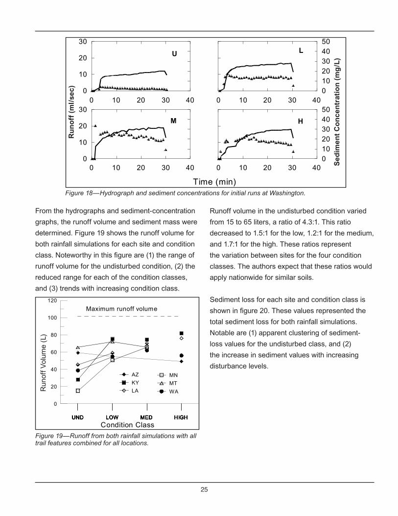
From the hydrographs and sediment-concentration

graphs, the runoff volume and sediment mass were

determined. Figure 19 shows the runoff volume for

both rainfall simulations for each site and condition

class. Noteworthy in this figure are (1) the range of

runoff volume for the undisturbed condition, (2) the

reduced range for each of the condition classes,

and (3) trends with increasing condition class.

Figure 19—Runoff from both rainfall simulations with all trail features combined for all locations.

Runoff volume in the undisturbed condition varied

from 15 to 65 liters, a ratio of 4.3:1. This ratio

decreased to 1.5:1 for the low, 1.2:1 for the medium,

and 1.7:1 for the high. These ratios represent

the variation between sites for the four condition

classes. The authors expect that these ratios would

apply nationwide for similar soils.

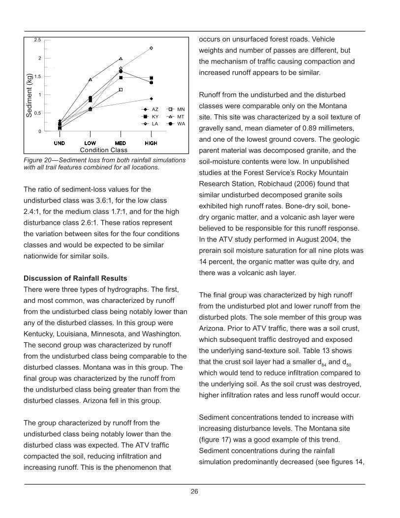
Sediment loss for each site and condition class is

shown in figure 20. These values represented the

total sediment loss for both rainfall simulations.

Notable are (1) apparent clustering of sediment-

loss values for the undisturbed class, and (2)

the increase in sediment values with increasing

disturbance levels.

UND LOW MED HIGHUND LOW MED HIGHUND LOW MED HIGHUND LOW MED HIGHUND LOW MED HIGHUND LOW MED HIGH

Condition Class

0

20

40

60

80

100

120

Runoff Volume (L)

AZ

KY

LA

MN

MT

WA

Maximum runoff volume

Ru

no

ff (

ml/

sec

)

Sed

imen

t C

on

cen

trat

ion

(m

g/L

)

Run

off V

olum

e (L

)

26

UND LOW MED HIGHUND LOW MED HIGHUND LOW MED HIGHUND LOW MED HIGHUND LOW MED HIGHUND LOW MED HIGH

Condition Class

0

0.5

1

1.5

2

2.5

Sediment (kg)

AZ

KY

LA

MN

MT

WA

Figure 20—Sediment loss from both rainfall simulations with all trail features combined for all locations.

The ratio of sediment-loss values for the

undisturbed class was 3.6:1, for the low class

2.4:1, for the medium class 1.7:1, and for the high

disturbance class 2.6:1. These ratios represent

the variation between sites for the four conditions

classes and would be expected to be similar

nationwide for similar soils.

Discussion of Rainfall Results

There were three types of hydrographs. The first,

and most common, was characterized by runoff

from the undisturbed class being notably lower than

any of the disturbed classes. In this group were

Kentucky, Louisiana, Minnesota, and Washington.

The second group was characterized by runoff

from the undisturbed class being comparable to the

disturbed classes. Montana was in this group. The

final group was characterized by the runoff from

the undisturbed class being greater than from the

disturbed classes. Arizona fell in this group.

The group characterized by runoff from the

undisturbed class being notably lower than the

disturbed class was expected. The ATV traffic

compacted the soil, reducing infiltration and

increasing runoff. This is the phenomenon that

occurs on unsurfaced forest roads. Vehicle

weights and number of passes are different, but

the mechanism of traffic causing compaction and

increased runoff appears to be similar.

Runoff from the undisturbed and the disturbed

classes were comparable only on the Montana

site. This site was characterized by a soil texture of

gravelly sand, mean diameter of 0.89 millimeters,

and one of the lowest ground covers. The geologic

parent material was decomposed granite, and the

soil-moisture contents were low. In unpublished

studies at the Forest Service’s Rocky Mountain

Research Station, Robichaud (2006) found that

similar undisturbed decomposed granite soils

exhibited high runoff rates. Bone-dry soil, bone-

dry organic matter, and a volcanic ash layer were

believed to be responsible for this runoff response.

In the ATV study performed in August 2004, the

prerain soil moisture saturation for all nine plots was

14 percent, the organic matter was quite dry, and

there was a volcanic ash layer.

The final group was characterized by high runoff

from the undisturbed plot and lower runoff from the

disturbed plots. The sole member of this group was

Arizona. Prior to ATV traffic, there was a soil crust,

which subsequent traffic destroyed and exposed

the underlying sand-texture soil. Table 13 shows

that the crust soil layer had a smaller d84

and d50

which would tend to reduce infiltration compared to

the underlying soil. As the soil crust was destroyed,

higher infiltration rates and less runoff would occur.

Sediment concentrations tended to increase with

increasing disturbance levels. The Montana site

(figure 17) was a good example of this trend.

Sediment concentrations during the rainfall

simulation predominantly decreased (see figures 14,

Sed

imen

t (kg

)

27

16, 17, and 18 for Kentucky, Minnesota, Montana,

and Washington, respectively). The Arizona site

(figure 13) had sediment concentrations that

remained relatively constant during the simulation.

At Louisiana (figure 15) the undisturbed, low, and

medium classes decreased during the simulation,

while the high class had increasing sediment

concentrations.

A decreasing sediment concentration was indicative

of the flow removing sediment faster than it could

be generated by raindrop splash, concentrated flow,

or small-bank sluffing. This is the condition usually

encountered on native-surface roads and is often

called armoring. A constant sediment concentration

rate was caused by either of two mechanisms.

One was a balance between sediment removal

by flow and generation by splash, concentrated

flow, or bank sluffing. The other was by sediment

being generated more rapidly than it could be

removed. Due to the higher slopes of the ATV trails,

generation likely exceeded the removal rate. The

increasing sediment concentration found on the

high disturbance class at Louisiana was caused by

needle-dams breaking and releasing their dammed

up water and sediment into the overland flow.

A trend of increasing runoff with increasing

disturbance class was exhibited by four of the six

sites, namely Kentucky, Louisiana, Minnesota, and

Washington. These are the same four that were

grouped together by hydrograph appearance and

can be explained by increased compaction and

reduced infiltration caused by ATV traffic. The

Montana site showed an increase from undisturbed

to low followed by a decrease from low to medium.

These changes are attributable to removal of the

water-repellent duff layer and breakup of the water

repellent conditions of the dry soil by ATV traffic.

The Arizona site showed a continuing decrease in

runoff from undisturbed to low to high due to the

breaking of the soil crust by ATV traffic.

All six sites had increasing sediment loss with

increasing condition class from undisturbed through

low to medium. Only Washington had less sediment

loss on the high condition class than the medium,

with the remaining five sites continuing to have

increasing sediment loss as the condition class

increased.

Erosion Parameters

Erosion parameters of hydraulic conductivity and

interrill erosion were determined for each set

of rainfall-simulation tests. The purpose was to

eliminate differences in runoff and sediment loss

due to differences in plot slope and antecedent

moisture condition. Comparison of hydraulic

conductivity and interrill-erosion coefficients

between sites is an improvement over comparing

runoff and sediment loss because differences in

plots have been taken into account. Additionally,

these erosion parameters are needed for the WEPP

model to make erosion predictions.

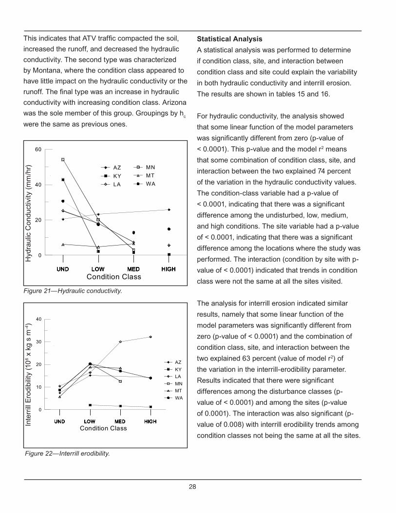
Figures 21 and 22 display the hydraulic conductivity

(hc) and interrill-erodibility coefficient (K

i) for each

site and each condition class. Smaller values of

hydraulic conductivity (hc) result in less infiltration

and more runoff, while larger values of Ki result in

more sediment loss.

There were three hydraulic conductivity responses

to increasing condition classes. The most

prevalent one was a continuing decrease in hc as

the condition class went from undisturbed to low

to medium to high. Sites in this category were

Kentucky, Louisiana, Minnesota, and Washington.

28

This indicates that ATV traffic compacted the soil,

increased the runoff, and decreased the hydraulic

conductivity. The second type was characterized

by Montana, where the condition class appeared to

have little impact on the hydraulic conductivity or the

runoff. The final type was an increase in hydraulic

conductivity with increasing condition class. Arizona

was the sole member of this group. Groupings by hc

were the same as previous ones.

Statistical Analysis

A statistical analysis was performed to determine

if condition class, site, and interaction between

condition class and site could explain the variability

in both hydraulic conductivity and interrill erosion.

The results are shown in tables 15 and 16.

For hydraulic conductivity, the analysis showed

that some linear function of the model parameters

was significantly different from zero (p-value of

< 0.0001). This p-value and the model r2 means

that some combination of condition class, site, and

interaction between the two explained 74 percent

of the variation in the hydraulic conductivity values.

The condition-class variable had a p-value of

< 0.0001, indicating that there was a significant

difference among the undisturbed, low, medium,

and high conditions. The site variable had a p-value

of < 0.0001, indicating that there was a significant

difference among the locations where the study was

performed. The interaction (condition by site with p-

value of < 0.0001) indicated that trends in condition

class were not the same at all the sites visited.

The analysis for interrill erosion indicated similar

results, namely that some linear function of the

model parameters was significantly different from

zero (p-value of < 0.0001) and the combination of

condition class, site, and interaction between the

two explained 63 percent (value of model r2) of

the variation in the interrill-erodibility parameter.

Results indicated that there were significant

differences among the disturbance classes (p-

value of < 0.0001) and among the sites (p-value

of 0.0001). The interaction was also significant (p-

value of 0.008) with interrill erodibility trends among

condition classes not being the same at all the sites.

Figure 21—Hydraulic conductivity.

Figure 22—Interrill erodibility.

UND LOW MED HIGHUND LOW MED HIGHUND LOW MED HIGHUND LOW MED HIGHUND LOW MED HIGHUND LOW MED HIGH

Condition Class

0

10

20

30

40

Interrill Erodibility (106 x kg s m

-4)

AZ

KY

LA

MN

MT

WA

Inte

rrill

Ero

dibi

lity

(10

6 x

kg s

m-4

)

UND LOW MED HIGHUND LOW MED HIGHUND LOW MED HIGHUND LOW MED HIGHUND LOW MED HIGHUND LOW MED HIGH

Condition Class

0

20

40

60

Hydraulic Conductivity (mm/hr)

AZ

KY

LA

MN

MT

WA

Hyd

raul

ic C

ondu

ctiv

ity (

mm

/hr)

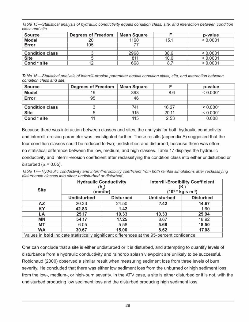
29

Table 15—Statistical analysis of hydraulic conductivity equals condition class, site, and interaction between condition class and site.

Source Degrees of Freedom Mean Square F p-valueModel 20 1160 15.1 < 0.0001Error 105 77

Condition class 3 2968 38.6 < 0.0001Site 5 811 10.6 < 0.0001Cond * site 12 668 8.7 < 0.0001

Table 16—Statistical analysis of interrill-erosion parameter equals condition class, site, and interaction between condition class and site.

Source Degrees of Freedom Mean Square F p-valueModel 19 393 8.6 < 0.0001Error 95 46

Condition class 3 741 16.27 < 0.0001Site 5 915 20.11 < 0.0001Cond * site 11 115 2.53 0.008

Because there was interaction between classes and sites, the analysis for both hydraulic conductivity

and interrrill-erosion parameter was investigated further. Those results (appendix A) suggested that the

four condition classes could be reduced to two; undisturbed and disturbed, because there was often

no statistical difference between the low, medium, and high classes. Table 17 displays the hydraulic

conductivity and interrill-erosion coefficient after reclassifying the condition class into either undisturbed or

disturbed ( = 0.05).

One can conclude that a site is either undisturbed or it is disturbed, and attempting to quantify levels of

disturbance from a hydraulic conductivity and raindrop splash viewpoint are unlikely to be successful.

Robichaud (2000) observed a similar result when measuring sediment loss from three levels of burn

severity. He concluded that there was either low sediment loss from the unburned or high sediment loss

from the low-, medium-, or high-burn severity. In the ATV case, a site is either disturbed or it is not, with the

undisturbed producing low sediment loss and the disturbed producing high sediment loss.

Table 17—Hydraulic conductivity and interrill-erodibility coefficient from both rainfall simulations after reclassifying disturbance classes into either undisturbed or disturbed.

Site

Hydraulic Conductivity(h

c)

(mm/hr)

Interrill-Erodibility Coefficient(K

i)

(106 * kg s m-4)Undisturbed Disturbed Undisturbed Disturbed

AZ 20.33 24.50 7.42 14.67KY 42.83 1.42 1.60LA 25.17 10.33 10.33 25.94MN 54.17 17.25 8.67 18.92MT 6.05 5.58 5.68 18.50WA 30.67 15.00 8.62 17.08

Values in bold indicate statistically significant differences at the 95-percent confidence

30

hydraulic conductivity was approximately halved

after traffic, and Ki was approximately doubled after

traffic. These sites and ones with similar soils would

be expected to have increased runoff and increased

sediment loss in excess of that due to the increased

runoff when compared to undisturbed areas.

Hydraulic conductivity decreased and interrill

erosion remained unchanged at Minnesota and

Kentucky. Soil texture for both of these sites was

gravelly sandy loam. Here, runoff would increase

due to impacts of ATV traffic. At Minnesota and

Kentucky, post-traffic hc’s were 1/3 and 1/40 of

their original values, respectively. Both sites would

be expected to have large increases in runoff from

ATV trails. The increased runoff would potentially

increase erosion in proportion to the increase

in runoff. These sites—and ones with similar

soils—would be expected to have increased runoff

and increased sediment loss proportional to the

increased runoff when compared to undisturbed

areas.

At the Arizona and Montana sites, hc was

unchanged and Ki increased, indicating that runoff

would be unchanged but sediment loss would

potentially increase due to the soil’s increased

erodibility. Both Arizona and Montana had soil

textures of gravelly sand that did not compact during

ATV traffic. Additionally, Arizona had a soil crust

on the undisturbed condition, which ATV-traffic

destroyed. Because the sand was not compacted,

there was no statistically significant change in hc

from the undisturbed to the disturbed condition. The

soil erodibility at Arizona doubled, while at Montana,

it tripled. These sites—and ones with similar

soils—would be expected to have similar runoff

and increased sediment loss in excess of the runoff

when compared to undisturbed areas.

Sediment loss is a combination of runoff and

raindrop-splash erosion. Investigation of changes

in both hydraulic conductivity (hc) and raindrop

splash (Ki) can indicate how erosion changes as

a result of ATV traffic. It is possible for hc and K

i

to independently increase, decrease, or remain

the same, resulting in a total of nine combinations.

A decrease in hc results in an increase in runoff.

This additional runoff has the potential to increase

sediment loss solely due to the increased runoff. In

combinations where the Ki also increases, sediment

loss has the potential to increase in excess of that

from just the increase in runoff alone. Actual erosion

increases would, however, depend on the transport

capacity of the runoff, which is primarily a function

of the slope steepness.

The combination that results in the greatest

increase in erosion would be a decrease in hc and

an increase in Ki. Runoff would increase and the

erodibility of the soil would increase, resulting in an

increase in sediment loss due to both the runoff and

the more erosive soil. The least impact, and in fact

a reduction in sediment loss, would result from hc

increasing and Ki decreasing. In this case, runoff

would decrease and the soil’s erodibility would

decrease, resulting in less sediment than before the

ATV traffic.

In this study there were only four of nine possible

combinations of changes in hc and K

i. The sites with

the largest potential increase in sediment loss were

Louisiana and Washington, where hc decreased and

Ki increased. Both of these sites had a rock-free soil

texture of loamy sand. Note that Washington had a

sufficiently high fraction of rock fragments to make

its classification a gravelly loamy sand. At these

locations, ATV traffic would be expected to increase

runoff and increase sediment loss in excess of that

caused by increased runoff. At both of these sites,

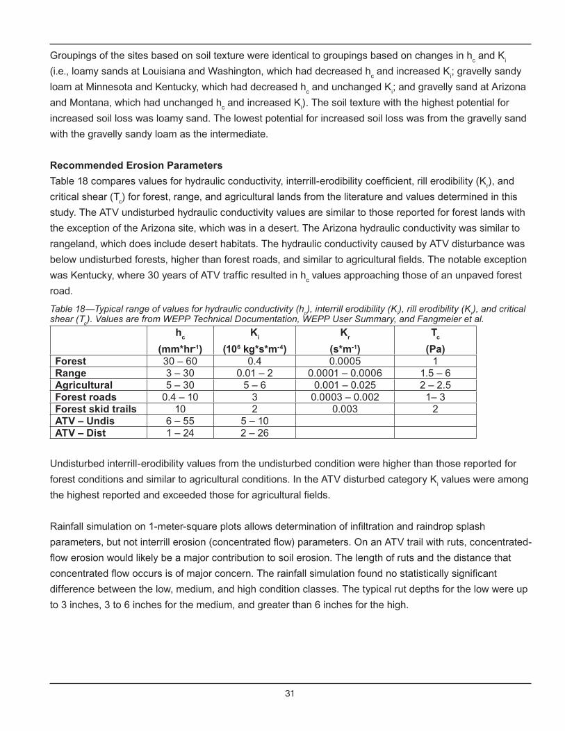
31

Groupings of the sites based on soil texture were identical to groupings based on changes in hc and K

i

(i.e., loamy sands at Louisiana and Washington, which had decreased hc and increased K

i; gravelly sandy

loam at Minnesota and Kentucky, which had decreased hc and unchanged K

i; and gravelly sand at Arizona

and Montana, which had unchanged hc and increased K

i). The soil texture with the highest potential for

increased soil loss was loamy sand. The lowest potential for increased soil loss was from the gravelly sand

with the gravelly sandy loam as the intermediate.

Recommended Erosion Parameters

Table 18 compares values for hydraulic conductivity, interrill-erodibility coefficient, rill erodibility (Kr), and

critical shear (Tc) for forest, range, and agricultural lands from the literature and values determined in this

study. The ATV undisturbed hydraulic conductivity values are similar to those reported for forest lands with

the exception of the Arizona site, which was in a desert. The Arizona hydraulic conductivity was similar to

rangeland, which does include desert habitats. The hydraulic conductivity caused by ATV disturbance was

below undisturbed forests, higher than forest roads, and similar to agricultural fields. The notable exception

was Kentucky, where 30 years of ATV traffic resulted in hc values approaching those of an unpaved forest

road.

Undisturbed interrill-erodibility values from the undisturbed condition were higher than those reported for

forest conditions and similar to agricultural conditions. In the ATV disturbed category Ki values were among

the highest reported and exceeded those for agricultural fields.

Rainfall simulation on 1-meter-square plots allows determination of infiltration and raindrop splash

parameters, but not interrill erosion (concentrated flow) parameters. On an ATV trail with ruts, concentrated-

flow erosion would likely be a major contribution to soil erosion. The length of ruts and the distance that

concentrated flow occurs is of major concern. The rainfall simulation found no statistically significant

difference between the low, medium, and high condition classes. The typical rut depths for the low were up

to 3 inches, 3 to 6 inches for the medium, and greater than 6 inches for the high.

Table 18—Typical range of values for hydraulic conductivity (hc), interrill erodibility (K

i), rill erodibility (K

r), and critical

shear (Tc). Values are from WEPP Technical Documentation, WEPP User Summary, and Fangmeier et al.

hc

(mm*hr-1)

Ki

(106 kg*s*m-4)

Kr

(s*m-1)

Tc

(Pa)Forest 30 – 60 0.4 0.0005 1Range 3 – 30 0.01 – 2 0.0001 – 0.0006 1.5 – 6Agricultural 5 – 30 5 – 6 0.001 – 0.025 2 – 2.5Forest roads 0.4 – 10 3 0.0003 – 0.002 1– 3Forest skid trails 10 2 0.003 2ATV – Undis 6 – 55 5 – 10ATV – Dist 1 – 24 2 – 26

32

Observations by the authors on native surface forest roads are that deeper ruts tend to be longer than

shallow ones. This would also be expected on ATV trails and would likely increase the sediment loss on the

medium and high disturbance classes. Such an increase could result in a statistically significant difference

between the low, medium, and high disturbance classes. Determination of concentrated-flow-erosion

parameters is straight forward and should be performed.

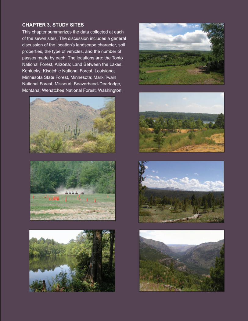
33

CHAPTER 3. STUDY SITES

Chapter summarizes the data

collected at each of the seven

sites. The discussion includes a

general discussion of the location's

landscape character, soil properties,

the type of vehicles, and the number

of passes made by each. The

locations are: the Tonto National

Forest, Arizona; Land Between the

Lakes, Kentucky; Kisatchie National

Forest, Louisiana; Minnesota

State Forest, Minnesota; Mark

Twain National Forest, Missouri;

Beaverhead-Deerlodge, Montana;

Wenatchee National Forest,

Washington.

CHAPTER 3. STUDY SITES

This chapter summarizes the data collected at each

of the seven sites. The discussion includes a general

discussion of the location's landscape character, soil

properties, the type of vehicles, and the number of

passes made by each. The locations are: the Tonto

National Forest, Arizona; Land Between the Lakes,

Kentucky; Kisatchie National Forest, Louisiana;

Minnesota State Forest, Minnesota; Mark Twain

National Forest, Missouri; Beaverhead-Deerlodge,

Montana; Wenatchee National Forest, Washington.

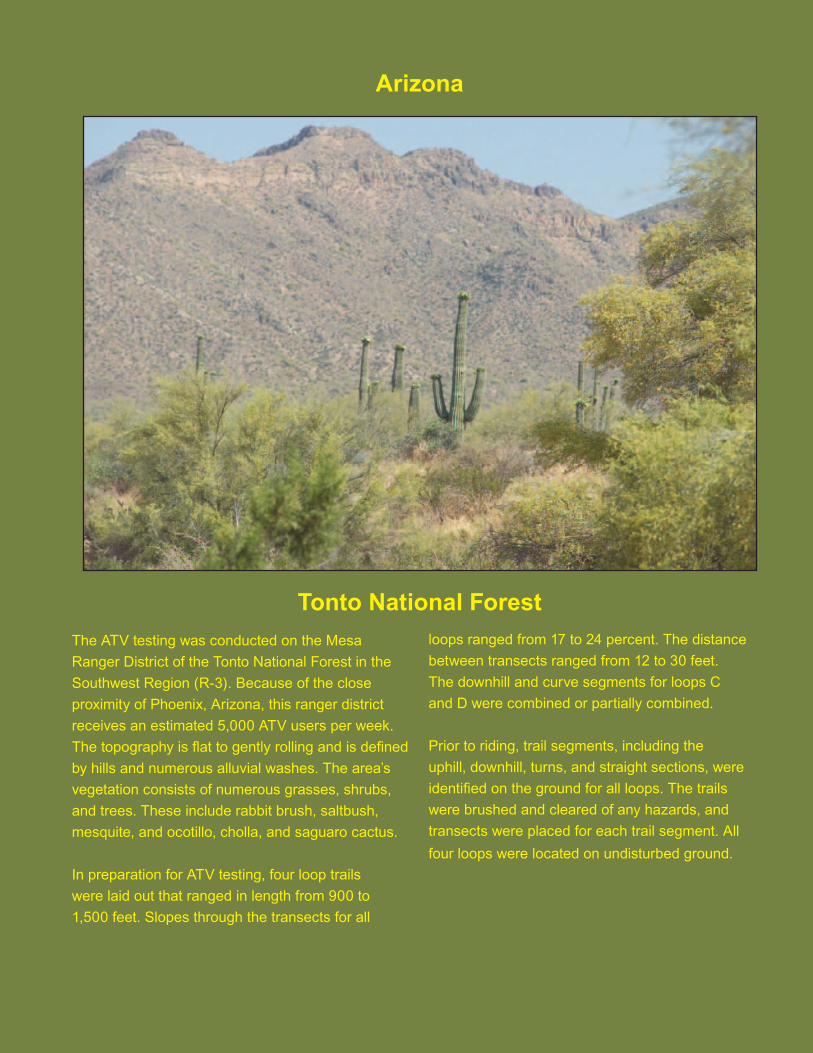
35

The ATV testing was conducted on the Mesa

Ranger District of the Tonto National Forest in the

Southwest Region (R-3). Because of the close

proximity of Phoenix, Arizona, this ranger district

receives an estimated 5,000 ATV users per week.

The topography is flat to gently rolling and is defined

by hills and numerous alluvial washes. The area’s

vegetation consists of numerous grasses, shrubs,

and trees. These include rabbit brush, saltbush,

mesquite, and ocotillo, cholla, and saguaro cactus.

In preparation for ATV testing, four loop trails

were laid out that ranged in length from 900 to

1,500 feet. Slopes through the transects for all

loops ranged from 17 to 24 percent. The distance

between transects ranged from 12 to 30 feet.

The downhill and curve segments for loops C

and D were combined or partially combined.

Prior to riding, trail segments, including the

uphill, downhill, turns, and straight sections, were

identified on the ground for all loops. The trails

were brushed and cleared of any hazards, and

transects were placed for each trail segment. All

four loops were located on undisturbed ground.

Tonto National Forest

Arizona

36

Soil Properties

Representative soil samples from the four loop trails were taken for analysis. These soils were classified as

poorly graded sand. They are characterized as medium strength and have a medium-to-high susceptibility

to surface erosion. Other soil properties are shown in table 19.

Vehicle Types

Table 20 provides the model, ATV type, and total number of passes for each loop.

Table 20—Loops, vehicle characteristics, and total number

of passes.

LoopVehicleModel/Type

OEM/AM

TotalPasses

A Honda Sport OEM 160

BKawasaki

Prairie Utility

OEM 160

CKawasaki

Prairie Utility

AM 60

D Honda Sport AM 160

Condition Class Summary

One study objective was to determine if ATVs affect the natural resources and, if so, to what degree.

Table 21 provides a summary of the condition-class assessments and, specifically, how condition classes

changed over time with subsequent passes.

Table 19—Soil properties for Tonto NF study site.

ForestUSCS Group

Symbol-Description

Surface Erosion

Dry Strength

Saturated Strength

Rutting(Saturated) Raveling Dust

TNF SP-poorly-graded sand

Medium-high Medium Medium-

high Low High Low-medium

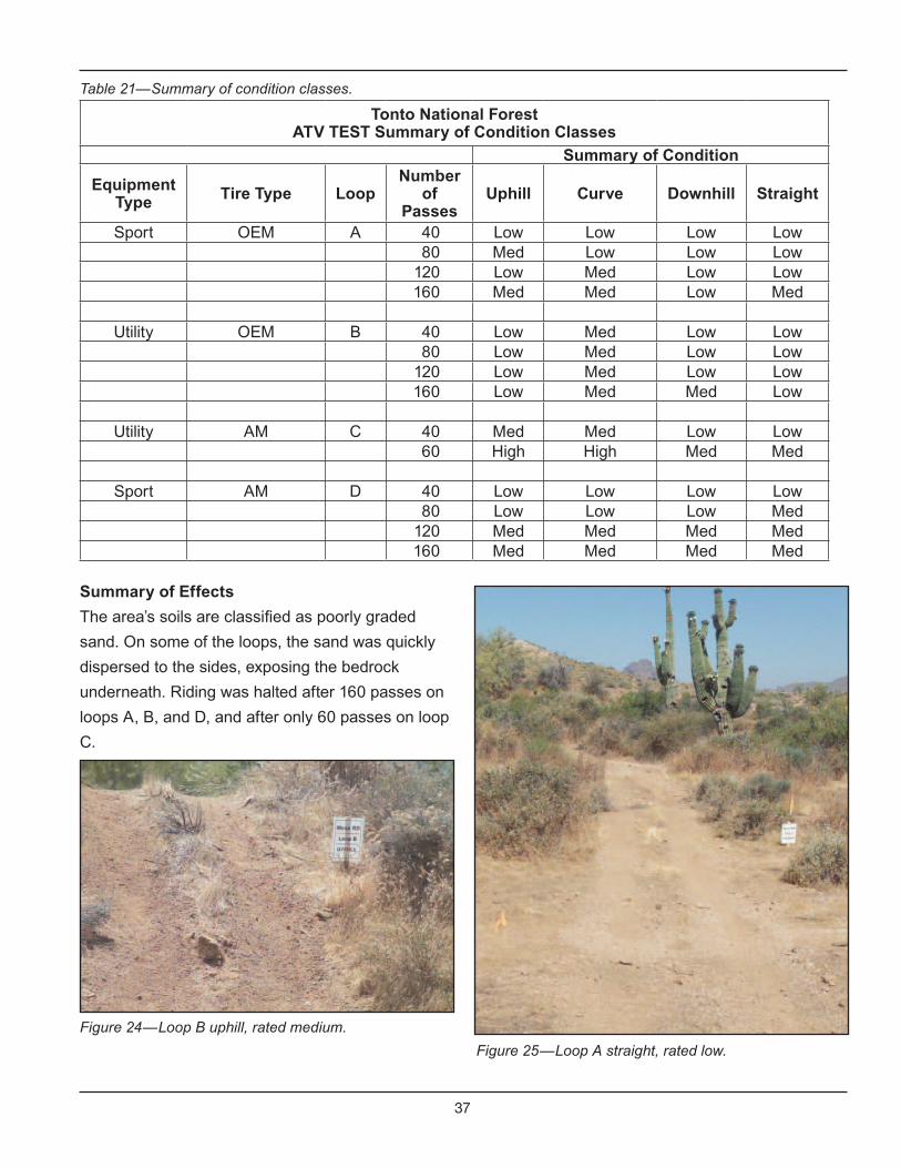
37

Summary of Effects

The area’s soils are classified as poorly graded

sand. On some of the loops, the sand was quickly

dispersed to the sides, exposing the bedrock

underneath. Riding was halted after 160 passes on

loops A, B, and D, and after only 60 passes on loop

C.

Figure 24—Loop B uphill, rated medium.

Table 21—Summary of condition classes.

Tonto National Forest ATV TEST Summary of Condition Classes

Summary of Condition

Equipment Type Tire Type Loop

Number of

PassesUphill Curve Downhill Straight

Sport OEM A 40 Low Low Low Low80 Med Low Low Low

120 Low Med Low Low160 Med Med Low Med

Utility OEM B 40 Low Med Low Low80 Low Med Low Low

120 Low Med Low Low160 Low Med Med Low

Utility AM C 40 Med Med Low Low60 High High Med Med

Sport AM D 40 Low Low Low Low80 Low Low Low Med

120 Med Med Med Med160 Med Med Med Med

Figure 25—Loop A straight, rated low.

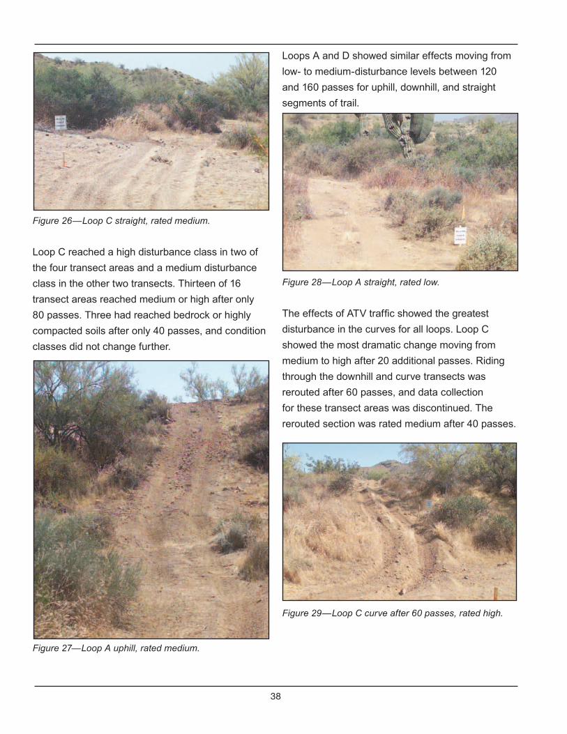
38

Loops A and D showed similar effects moving from

low- to medium-disturbance levels between 120

and 160 passes for uphill, downhill, and straight

segments of trail.

Figure 28—Loop A straight, rated low.

The effects of ATV traffic showed the greatest

disturbance in the curves for all loops. Loop C

showed the most dramatic change moving from

medium to high after 20 additional passes. Riding

through the downhill and curve transects was

rerouted after 60 passes, and data collection

for these transect areas was discontinued. The

rerouted section was rated medium after 40 passes.

Figure 29—Loop C curve after 60 passes, rated high.

Figure 26—Loop C straight, rated medium.

Loop C reached a high disturbance class in two of

the four transect areas and a medium disturbance

class in the other two transects. Thirteen of 16

transect areas reached medium or high after only

80 passes. Three had reached bedrock or highly

compacted soils after only 40 passes, and condition

classes did not change further.

Figure 27—Loop A uphill, rated medium.

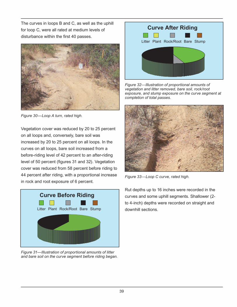
39

The curves in loops B and C, as well as the uphill

for loop C, were all rated at medium levels of

disturbance within the first 40 passes.

Figure 30—Loop A turn, rated high.

Vegetation cover was reduced by 20 to 25 percent

on all loops and, conversely, bare soil was

increased by 20 to 25 percent on all loops. In the

curves on all loops, bare soil increased from a

before-riding level of 42 percent to an after-riding

level of 50 percent (figures 31 and 32). Vegetation

cover was reduced from 58 percent before riding to

44 percent after riding, with a proportional increase

in rock and root exposure of 6 percent.

Figure 31—Illustration of proportional amounts of litter and bare soil on the curve segment before riding began.

Figure 32—Illustration of proportional amounts of vegetation and litter removed, bare soil, rock/root exposure, and stump exposure on the curve segment at completion of total passes.

Figure 33—Loop C curve, rated high.

Rut depths up to 16 inches were recorded in the

curves and some uphill segments. Shallower (2-

to 4-inch) depths were recorded on straight and

downhill sections.Litter StumpBareRock/RootPlant

Curve Before Riding

Litter StumpBareRock/RootPlant

Curve After Riding

41

Land Between the Lakes

Kentucky

Land Between the Lakes (LBL) National

Recreational Area site is located near Cadiz,

Kentucky, at Turkey Bay, a 2,200-acre, off-highway

vehicle (OHV) area open to trail and cross-country

riding. The OHV area is centrally located within the

LBL and consists of three seventh-level watersheds

that contribute 3,166 acres to Turkey Bay. The

watershed consists of the North Forks of Turkey and

Turner Creeks. The streams of these main channels

are intermittent, and the headwaters are ephemeral.

The topography of the area is moderately dissected

because of the nearby Tennessee and Cumberland

Rivers. The slopes range from 6 to 50 percent

and, due to steep slopes and narrow, closely

spaced drainage valleys, surface-water runoff has

contributed to the erosion process. Streambeds

are filled with chert gravels transported from upper

slopes. Annual rainfall for LBL averages 46 inches.

Cretaceous gravels, sands, and clays are overlain

by a thin layer of brown Tertiary-Quaternary-age

cherty gravels. The gravels have a matrix of reddish

sandy clay and are interbedded with reddish-brown

argillaceous sand. The upland is veneered with tan-

to-buff colored Quaternary-age loess. The loess is

generally believed to have a wind-blown origin and

is probably related to past glaciations.

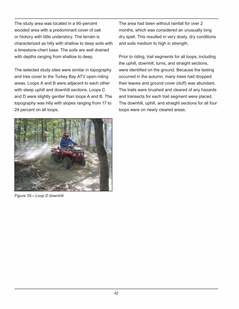
42

The study area was located in a 90-percent

wooded area with a predominant cover of oak

or hickory with little understory. The terrain is

characterized as hilly with shallow to deep soils with

a limestone-chert base. The soils are well drained

with depths ranging from shallow to deep.

The selected study sites were similar in topography

and tree cover to the Turkey Bay ATV open-riding

areas. Loops A and B were adjacent to each other

with steep uphill and downhill sections. Loops C

and D were slightly gentler than loops A and B. The

topography was hilly with slopes ranging from 17 to

24 percent on all loops.

Figure 35—Loop D downhill.

The area had been without rainfall for over 2

months, which was considered an unusually long

dry spell. This resulted in very dusty, dry conditions

and soils medium to high in strength.

Prior to riding, trail segments for all loops, including

the uphill, downhill, turns, and straight sections,

were identified on the ground. Because the testing

occurred in the autumn, many trees had dropped

their leaves and ground cover (duff) was abundant.

The trails were brushed and cleared of any hazards

and transects for each trail segment were placed.

The downhill, uphill, and straight sections for all four

loops were on newly cleared areas.

43

Soil Properties

Representative soil samples from the four loop trails were taken for analysis. These soils were classified as

silt and silty sand. They are characterized as medium strength and have a medium to high susceptibility to

surface erosion. Other soil properties are shown in table 22.

Table 22—Soil properties for LBL study site.

ForestUSCS Group

Symbol-Description

Surface Erosion

Dry Strength

Saturated Strength

Rutting(Saturated)

Raveling Dust

LBLSM-silty sand

Medium-high

Low-medium

Low-medium

Low-mediumMedium-

highMedium-

highLBL

ML-silt HighLow-

mediumLow High Low High

Vehicle Types

Table 23 provides the model, ATV type, and total number of passes for each loop.

Table 23—Loops, vehicle characteristics, and total number

of passes.

Loop Vehicle Model/Type

OEM/AM

Total Passes

AKawasaki

PrairieUtility

OEM 800

BKawasaki

PrairieUtility

AM 800

C Honda ReconSport OEM 760

D Honda ReconSport AM 280

Condition-Class Summary

One study objective was to determine if ATVs affect the natural resources and, if so, to what degree. Table

24 provides a summary of the condition-class assessments and specifically how condition classes changed

over time with subsequent passes.

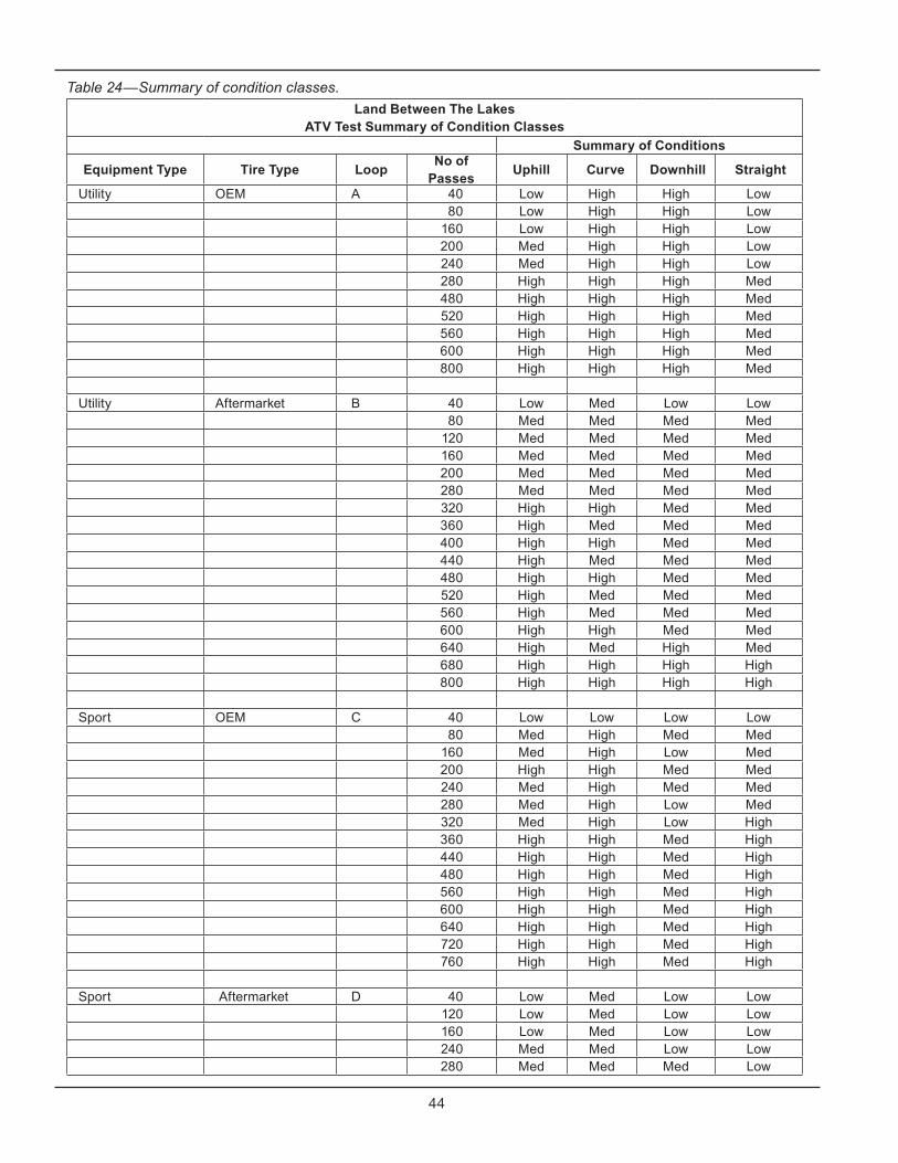
44

Table 24—Summary of condition classes.

Land Between The LakesATV Test Summary of Condition Classes

Summary of Conditions

Equipment Type Tire Type LoopNo of

PassesUphill Curve Downhill Straight

Utility OEM A 40 Low High High Low 80 Low High High Low 160 Low High High Low 200 Med High High Low 240 Med High High Low 280 High High High Med 480 High High High Med 520 High High High Med 560 High High High Med 600 High High High Med 800 High High High Med Utility Aftermarket B 40 Low Med Low Low 80 Med Med Med Med 120 Med Med Med Med 160 Med Med Med Med 200 Med Med Med Med 280 Med Med Med Med 320 High High Med Med 360 High Med Med Med 400 High High Med Med 440 High Med Med Med 480 High High Med Med 520 High Med Med Med 560 High Med Med Med 600 High High Med Med 640 High Med High Med 680 High High High High 800 High High High High Sport OEM C 40 Low Low Low Low 80 Med High Med Med 160 Med High Low Med 200 High High Med Med 240 Med High Med Med 280 Med High Low Med 320 Med High Low High 360 High High Med High 440 High High Med High 480 High High Med High 560 High High Med High 600 High High Med High 640 High High Med High 720 High High Med High 760 High High Med High Sport Aftermarket D 40 Low Med Low Low 120 Low Med Low Low 160 Low Med Low Low 240 Med Med Low Low 280 Med Med Med Low

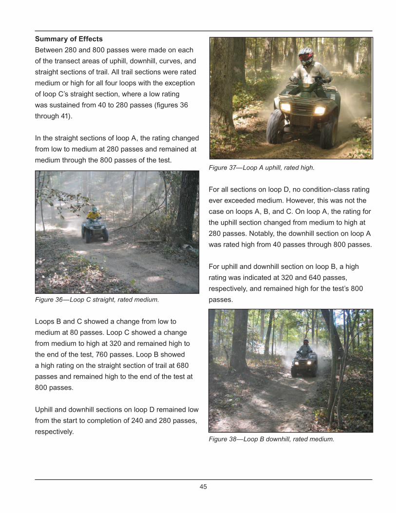
45

Summary of Effects

Between 280 and 800 passes were made on each

of the transect areas of uphill, downhill, curves, and

straight sections of trail. All trail sections were rated

medium or high for all four loops with the exception

of loop C’s straight section, where a low rating

was sustained from 40 to 280 passes (figures 36

through 41).

In the straight sections of loop A, the rating changed

from low to medium at 280 passes and remained at

medium through the 800 passes of the test.

Figure 36—Loop C straight, rated medium.

Loops B and C showed a change from low to

medium at 80 passes. Loop C showed a change

from medium to high at 320 and remained high to

the end of the test, 760 passes. Loop B showed

a high rating on the straight section of trail at 680

passes and remained high to the end of the test at

800 passes.

Uphill and downhill sections on loop D remained low

from the start to completion of 240 and 280 passes,

respectively.

Figure 37—Loop A uphill, rated high.

For all sections on loop D, no condition-class rating

ever exceeded medium. However, this was not the

case on loops A, B, and C. On loop A, the rating for

the uphill section changed from medium to high at

280 passes. Notably, the downhill section on loop A

was rated high from 40 passes through 800 passes.

For uphill and downhill section on loop B, a high

rating was indicated at 320 and 640 passes,

respectively, and remained high for the test’s 800

passes.

Figure 38—Loop B downhill, rated medium.

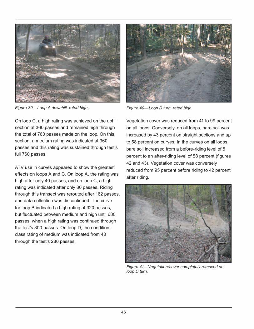
46

Figure 40—Loop D turn, rated high.

Vegetation cover was reduced from 41 to 99 percent

on all loops. Conversely, on all loops, bare soil was

increased by 43 percent on straight sections and up

to 58 percent on curves. In the curves on all loops,

bare soil increased from a before-riding level of 5

percent to an after-riding level of 58 percent (figures

42 and 43). Vegetation cover was conversely

reduced from 95 percent before riding to 42 percent

after riding.

Figure 41—Vegetation/cover completely removed on loop D turn.

Figure 39—Loop A downhill, rated high.

On loop C, a high rating was achieved on the uphill

section at 360 passes and remained high through

the total of 760 passes made on the loop. On this

section, a medium rating was indicated at 360

passes and this rating was sustained through test’s

full 760 passes.

ATV use in curves appeared to show the greatest

effects on loops A and C. On loop A, the rating was

high after only 40 passes, and on loop C, a high

rating was indicated after only 80 passes. Riding

through this transect was rerouted after 162 passes,

and data collection was discontinued. The curve

for loop B indicated a high rating at 320 passes,

but fluctuated between medium and high until 680

passes, when a high rating was continued through

the test’s 800 passes. On loop D, the condition-

class rating of medium was indicated from 40

through the test’s 280 passes.

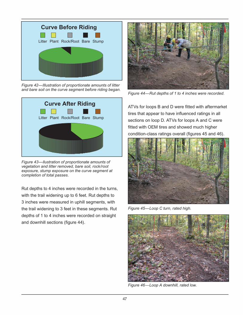
47

Figure 44—Rut depths of 1 to 4 inches were recorded.

ATVs for loops B and D were fitted with aftermarket

tires that appear to have influenced ratings in all

sections on loop D. ATVs for loops A and C were

fitted with OEM tires and showed much higher

condition-class ratings overall (figures 45 and 46).

Figure 45—Loop C turn, rated high.

Figure 46—Loop A downhill, rated low.

Figure 42—Illustration of proportionate amounts of litter and bare soil on the curve segment before riding began.

Figure 43—llustration of proportionate amounts of vegetation and litter removed, bare soil, rock/root exposure, stump exposure on the curve segment at completion of total passes.

Rut depths to 4 inches were recorded in the turns,

with the trail widening up to 6 feet. Rut depths to

3 inches were measured in uphill segments, with

the trail widening to 3 feet in these segments. Rut

depths of 1 to 4 inches were recorded on straight

and downhill sections (figure 44).

Litter StumpBareRock/RootPlant

Curve After Riding

Litter StumpBareRock/RootPlant

Curve Before Riding

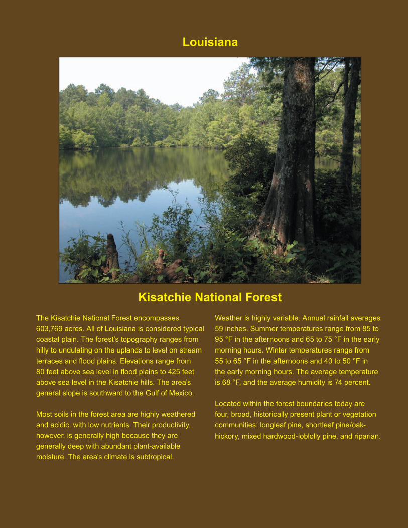
49

Kisatchie National Forest

Louisiana

Weather is highly variable. Annual rainfall averages

59 inches. Summer temperatures range from 85 to

95 °F in the afternoons and 65 to 75 °F in the early

morning hours. Winter temperatures range from

55 to 65 °F in the afternoons and 40 to 50 °F in

the early morning hours. The average temperature

is 68 °F, and the average humidity is 74 percent.

Located within the forest boundaries today are

four, broad, historically present plant or vegetation

communities: longleaf pine, shortleaf pine/oak-

hickory, mixed hardwood-loblolly pine, and riparian.

The Kisatchie National Forest encompasses

603,769 acres. All of Louisiana is considered typical

coastal plain. The forest’s topography ranges from

hilly to undulating on the uplands to level on stream

terraces and flood plains. Elevations range from

80 feet above sea level in flood plains to 425 feet

above sea level in the Kisatchie hills. The area’s

general slope is southward to the Gulf of Mexico.

Most soils in the forest area are highly weathered

and acidic, with low nutrients. Their productivity,

however, is generally high because they are

generally deep with abundant plant-available

moisture. The area’s climate is subtropical.

50

The study area was located on an old military base on the Kisatchie National Forest’s Calcasieu Ranger

District. Much of the area was roaded and covered with mature pines and a tall grass understory. Prior to

riding, four trail loops were identified that ranged in length from 900 to 1,500 feet. Loops were selected

that had similar characteristics: uphill and downhill of approximately 10 percent, a sharp hairpin turn, and a

straight section to allow for acceleration and higher speed.

Soil Properties

Representative soil samples from the four loop trails were taken for analysis. These soils were classified as

silt and silty sand. They are characterized as medium strength and have a medium-to-high susceptibility to

surface erosion. Other soil properties are shown in table 25.

Table 25—Soil properties for Kisatchie NF study site.

ForestUSCS Group

Symbol-Description

Surface Erosion

Dry Strength

Saturated Strength

Rutting(Saturated) Raveling Dust

KNFSM-silty sand

Medium-high

Low-medium

Low-medium

Low-mediumMedium-

highMedium-

high

KNFML-silt High

Low-medium

Low High Low High

Vehicle Types

Table 26 provides the model, ATV type, and total number of passes for each loop.

Table 26—Loops, vehicle characteristics, and total number

of passes.

Loop Vehicle Model/Type

OEM/AM

Total Passes

ASuzuki Vinson

4 by 4500 Utility

OEM 480

BHonda Foreman

Rubicon500 Utility

AM 640

C Suzuki OzarkSport OEM 720

D Suzuki OzarkSport AM 600

Condition Class Summary

One study objective was to determine if ATVs affect the natural resources and, if so, to what degree. Table

27 provides a summary of the condition-class assessments and specifically how condition classes changed

over time with subsequent passes.

51

Table 27—Summary of condition classes.

Kisatchie National ForestATV Test Summary of Condition Classes

Summary of Condition

Equipment Type Tire Type LoopNo. of

PassesUphill Curve Downhill Straight

Utility OEM A 40 Low Low Low Low 80 Med High Low Low 120 Low Med Low Low 160 Low Med Low Low 200 Low Low Low Low 240 Low Med Low Low 360 Low Med Low Low 400 Med Med Low Low 480 Low Med Low Low Utility Aftermarket B 40 Low Med Low Low 80 Low Med Low Low * Stopped riding at 162 passes 160 Low High* Low Low in Curve 240 Low Low Low 280 Med Low Low 360 Med Low Low 400 Low Med Low 440 Med Med Low 520 Med Med Low 500 Med Med Low 560 Med Med Low 640 Med Med Low Sport OEM C 40 Low Low Low Low 80 Low Low Med Low 120 Med Med Low Low 200 Med Low Med Med 240 Med Med Med 580 Low Low Low 640 Low Low Low 720 Low Low Low Sport Aftermarket D 40 Low Low Low Low 120 Low Med Low Low 200 Med High Med Low 240 Med High Med Low 280 Med High Med Low 320 Med High Low Low 360 Low High Med Med 400 Med High Med Med 560 Med High Med Low 600 Med High Med Med 640 Med High Med Med 680 Med High Med Med 720 Med High Med Med 740 High High Med Med

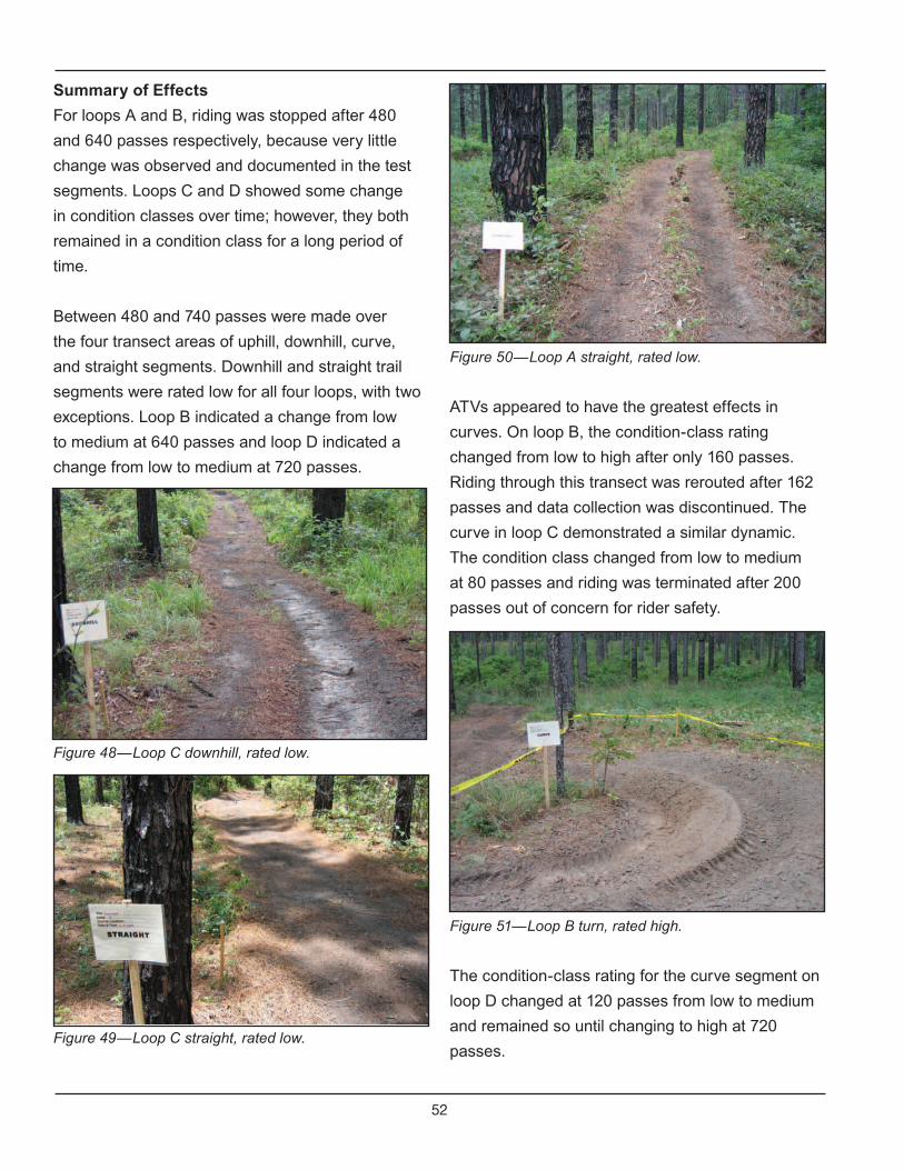
52

Figure 50—Loop A straight, rated low.

ATVs appeared to have the greatest effects in

curves. On loop B, the condition-class rating

changed from low to high after only 160 passes.

Riding through this transect was rerouted after 162

passes and data collection was discontinued. The

curve in loop C demonstrated a similar dynamic.

The condition class changed from low to medium

at 80 passes and riding was terminated after 200

passes out of concern for rider safety.

Figure 51—Loop B turn, rated high.

The condition-class rating for the curve segment on

loop D changed at 120 passes from low to medium

and remained so until changing to high at 720

passes.

Summary of Effects

For loops A and B, riding was stopped after 480

and 640 passes respectively, because very little

change was observed and documented in the test

segments. Loops C and D showed some change

in condition classes over time; however, they both

remained in a condition class for a long period of

time.

Between 480 and 740 passes were made over

the four transect areas of uphill, downhill, curve,

and straight segments. Downhill and straight trail

segments were rated low for all four loops, with two

exceptions. Loop B indicated a change from low

to medium at 640 passes and loop D indicated a

change from low to medium at 720 passes.

Figure 48—Loop C downhill, rated low.

Figure 49—Loop C straight, rated low.

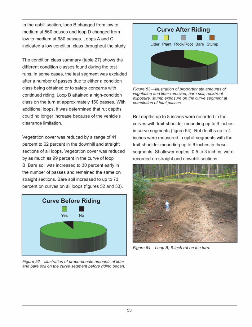
53

Figure 53—Illustration of proportionate amounts of vegetation and litter removed, bare soil, rock/root exposure, stump exposure on the curve segment at completion of total passes.

Rut depths up to 8 inches were recorded in the

curves with trail-shoulder mounding up to 9 inches

in curve segments (figure 54). Rut depths up to 4

inches were measured in uphill segments with the

trail-shoulder mounding up to 6 inches in these

segments. Shallower depths, 0.5 to 3 inches, were

recorded on straight and downhill sections.

Figure 54—Loop B, 8-inch rut on the turn.

In the uphill section, loop B changed from low to

medium at 560 passes and loop D changed from

low to medium at 680 passes. Loops A and C

indicated a low condition class throughout the study.

The condition class summary (table 27) shows the

different condition classes found during the test

runs. In some cases, the test segment was excluded

after a number of passes due to either a condition

class being obtained or to safety concerns with

continued riding. Loop B attained a high-condition

class on the turn at approximately 150 passes. With

additional loops, it was determined that rut depths

could no longer increase because of the vehicle’s

clearance limitation.

Vegetation cover was reduced by a range of 41

percent to 62 percent in the downhill and straight

sections of all loops. Vegetation cover was reduced

by as much as 99 percent in the curve of loop

B. Bare soil was increased to 30 percent early in

the number of passes and remained the same on

straight sections. Bare soil increased to up to 73

percent on curves on all loops (figures 52 and 53).

Figure 52—Illustration of proportionate amounts of litter and bare soil on the curve segment before riding began.

Yes No

Curve Before Riding

Litter StumpBareRock/RootPlant

Curve After Riding

54

Vehicles for loops B and D were fitted with aftermarket tires that achieved a high condition class in the

curve, uphill, and downhill segments. They achieved a medium rating on the uphill segments of loop B.

Vehicles for loops A and C used OEM tires. They achieved a low rating for the entire test for all trail

segments except the curve on loop A. The turn for loop A indicated a medium condition class.

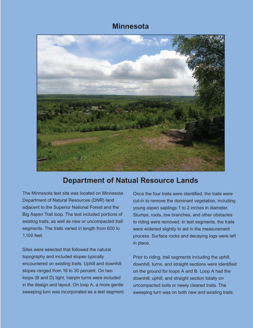
55

Department of Natual Resource Lands

Minnesota

The Minnesota test site was located on Minnesota

Department of Natural Resources (DNR) land

adjacent to the Superior National Forest and the

Big Aspen Trail loop. The test included portions of

existing trails, as well as new or uncompacted trail

segments. The trails varied in length from 600 to

1,100 feet.

Sites were selected that followed the natural

topography and included slopes typically

encountered on existing trails. Uphill and downhill

slopes ranged from 16 to 30 percent. On two

loops (B and D) tight, hairpin turns were included

in the design and layout. On loop A, a more gentle

sweeping turn was incorporated as a test segment.

Once the four trails were identified, the trails were

cut-in to remove the dominant vegetation, including

young aspen saplings 1 to 2 inches in diameter.

Stumps, roots, low branches, and other obstacles

to riding were removed. In test segments, the trails

were widened slightly to aid in the measurement

process. Surface rocks and decaying logs were left

in place.

Prior to riding, trail segments including the uphill,

downhill, turns, and straight sections were identified

on the ground for loops A and B. Loop A had the

downhill, uphill, and straight section totally on

uncompacted soils or newly cleared trails. The

sweeping turn was on both new and existing trails.

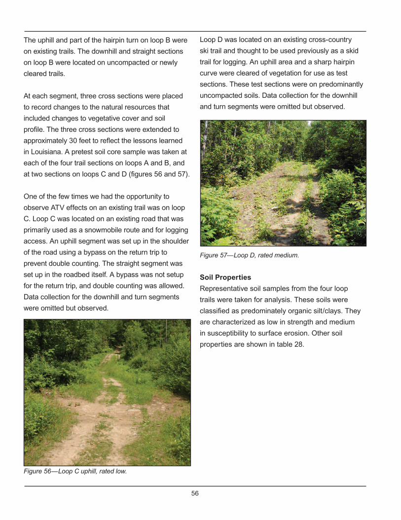
56

Loop D was located on an existing cross-country

ski trail and thought to be used previously as a skid

trail for logging. An uphill area and a sharp hairpin

curve were cleared of vegetation for use as test

sections. These test sections were on predominantly

uncompacted soils. Data collection for the downhill

and turn segments were omitted but observed.

Figure 57—Loop D, rated medium.

Soil Properties

Representative soil samples from the four loop

trails were taken for analysis. These soils were

classified as predominately organic silt/clays. They

are characterized as low in strength and medium

in susceptibility to surface erosion. Other soil

properties are shown in table 28.

The uphill and part of the hairpin turn on loop B were

on existing trails. The downhill and straight sections

on loop B were located on uncompacted or newly

cleared trails.

At each segment, three cross sections were placed

to record changes to the natural resources that

included changes to vegetative cover and soil

profile. The three cross sections were extended to

approximately 30 feet to reflect the lessons learned

in Louisiana. A pretest soil core sample was taken at

each of the four trail sections on loops A and B, and

at two sections on loops C and D (figures 56 and 57).

One of the few times we had the opportunity to

observe ATV effects on an existing trail was on loop

C. Loop C was located on an existing road that was

primarily used as a snowmobile route and for logging

access. An uphill segment was set up in the shoulder

of the road using a bypass on the return trip to

prevent double counting. The straight segment was

set up in the roadbed itself. A bypass was not setup

for the return trip, and double counting was allowed.

Data collection for the downhill and turn segments

were omitted but observed.

Figure 56—Loop C uphill, rated low.

57

Table 28—Soil properties for Minnesota DNR study site.

Forest

USCS Group

Symbol-Description

Surface Erosion

Dry Strength

Saturated Strength

Rutting(Saturated) Raveling Dust

MDNR PT,OL/OH-peat, organic

silt/claysMedium Low Low High Low Medium-

high

Vehicle Types

Table 29 provides the model, ATV type, and total number of passes for each loop.

Table 29—Loops, vehicle characteristics, and total number

of passes.

Loop Vehicle Model/Type

OEM/AM

Total Passes

AKawasaki

PrairieUtility

OEM 500

BKawasaki

PrairieUtility

AM 700

C Suzuki OzarkSport OEM 1,200

D Suzuki OzarkSport AM 620

Condition-Class Summary

One study objective was to determine if ATVs affect the natural resources and, if so, to what degree.

Table 30 provides a summary of the condition-class assessments and, specifically, how condition classes

changed over time with subsequent passes.

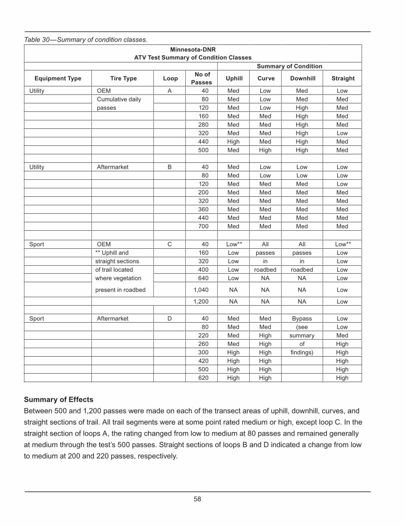
58

Table 30—Summary of condition classes.

Minnesota-DNRATV Test Summary of Condition Classes

Summary of Condition

Equipment Type Tire Type Loop No of

Passes Uphill Curve Downhill Straight

Utility OEM A 40 Med Low Med Low

Cumulative daily 80 Med Low Med Med

passes 120 Med Low High Med

160 Med Med High Med

280 Med Med High Med

320 Med Med High Low

440 High Med High Med

500 Med High High Med

Utility Aftermarket B 40 Med Low Low Low

80 Med Low Low Low

120 Med Med Med Low

200 Med Med Med Med

320 Med Med Med Med

360 Med Med Med Med

440 Med Med Med Med

700 Med Med Med Med

Sport OEM C 40 Low** All All Low**

** Uphill and 160 Low passes passes Low

straight sections 320 Low in in Low

of trail located 400 Low roadbed roadbed Low

where vegetation 640 Low NA NA Low

present in roadbed 1,040 NA NA NA Low

1,200 NA NA NA Low

Sport Aftermarket D 40 Med Med Bypass Low

80 Med Med (see Low

220 Med High summary Med

260 Med High of High

300 High High findings) High

420 High High High

500 High High High

620 High High High

Summary of Effects

Between 500 and 1,200 passes were made on each of the transect areas of uphill, downhill, curves, and

straight sections of trail. All trail segments were at some point rated medium or high, except loop C. In the

straight section of loops A, the rating changed from low to medium at 80 passes and remained generally

at medium through the test’s 500 passes. Straight sections of loops B and D indicated a change from low

to medium at 200 and 220 passes, respectively.

59

The straight segment of loop C remained low

through the 1,200 passes completed. The straight

segment has a higher number of passes recorded

because of the double counting as the vehicle

passed back and forth over the same area as it

completed each lap.

The uphill sections on loop C remained low from the

start to completion of 640 passes. Loop D indicated

a high rating on the straight section of trail at 260

passes and remained high through the end of the

test at 620 passes. Uphill sections on loops A, B,

and D indicated a medium condition class at 40

passes. Loop B remained at medium throughout the

test of 700 passes on the uphill section.

Loop A indicated a medium condition class in the

uphill section of trail until 440 passes, when a high

condition class was indicated. This condition class

changed back to medium at the end of the test, 500

passes. Loop D indicated a change from medium to

high at 300 passes and remained at this condition

class until the end of the test, 620 passes.

On the downhill section of loop A, a medium

condition class was indicated at 40 and 80 passes.

At 120 passes, a high was indicated and remained

the condition class for the downhill section of loop

A through the end of the test, 500 passes. On

loop B, the condition class was low at 40 and 80

passes and then indicated medium at 120 passes,

remaining the same throughout the test, 700

passes.

On loop C, the downhill section was conducted in

an existing roadbed and on loop D, a bypass for

the downhill section was used that replicated the

conditions on the uphill section of trail on this loop.

Only the curves on loop A and loop D reached a

high condition class. On loop A, a low was indicated

from 40 through 120 passes. Then, at 160 passes

through 440 passes, a medium was indicated. At

500 passes and to the end of the test on this loop,

the condition class was high. This gradual change

in condition class was not the case in the curve

section of loop D. A medium rating was indicated

from 40 through 220 passes. However, at 220

passes through the end of the test at 620 passes, a

high condition class was indicated.

On loop B, a low was indicated at 40 through 80

passes in the curve. The condition class changed

to medium at 120 passes and remained the same

through the test’s 700 passes on this loop. Loop

C was located in a roadbed where vegetation was

present.

Overall, the effects of ATV use on loop B were

never rated high on any one of the trail sections.

This result is most striking in comparison to the

straight sections of loops C and D where high

condition class was indicated at 400 and 260

passes, respectively.

The percentage of ground cover disturbed ranged

from a low of 47 percent on the straight section of

loop D, to 96 to 100 percent on all other sections

of all loops. As an example, vegetation cover was

reduced from 37 to 14 percent in the curve on loop

D. Bare soil was increased from none before riding

to 10 percent after riding.

Root/rock exposure changed from a before-riding

level of 1 percent to an after-riding 3 percent. Litter

increased from 62 percent prior to riding to 73

percent after riding in the curve on loop D. This

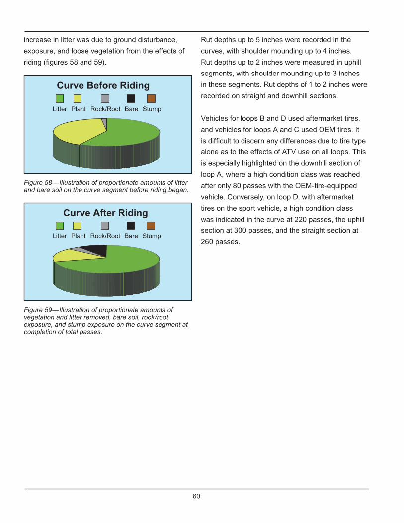
60

increase in litter was due to ground disturbance,

exposure, and loose vegetation from the effects of

riding (figures 58 and 59).

Figure 58—Illustration of proportionate amounts of litter and bare soil on the curve segment before riding began.

Figure 59—Illustration of proportionate amounts of vegetation and litter removed, bare soil, rock/root exposure, and stump exposure on the curve segment at completion of total passes.

Rut depths up to 5 inches were recorded in the

curves, with shoulder mounding up to 4 inches.

Rut depths up to 2 inches were measured in uphill

segments, with shoulder mounding up to 3 inches

in these segments. Rut depths of 1 to 2 inches were

recorded on straight and downhill sections.

Vehicles for loops B and D used aftermarket tires,

and vehicles for loops A and C used OEM tires. It

is difficult to discern any differences due to tire type

alone as to the effects of ATV use on all loops. This

is especially highlighted on the downhill section of

loop A, where a high condition class was reached

after only 80 passes with the OEM-tire-equipped

vehicle. Conversely, on loop D, with aftermarket

tires on the sport vehicle, a high condition class

was indicated in the curve at 220 passes, the uphill

section at 300 passes, and the straight section at

260 passes.

Litter StumpBareRock/RootPlant

Curve Before Riding

Litter StumpBareRock/RootPlant

Curve After Riding

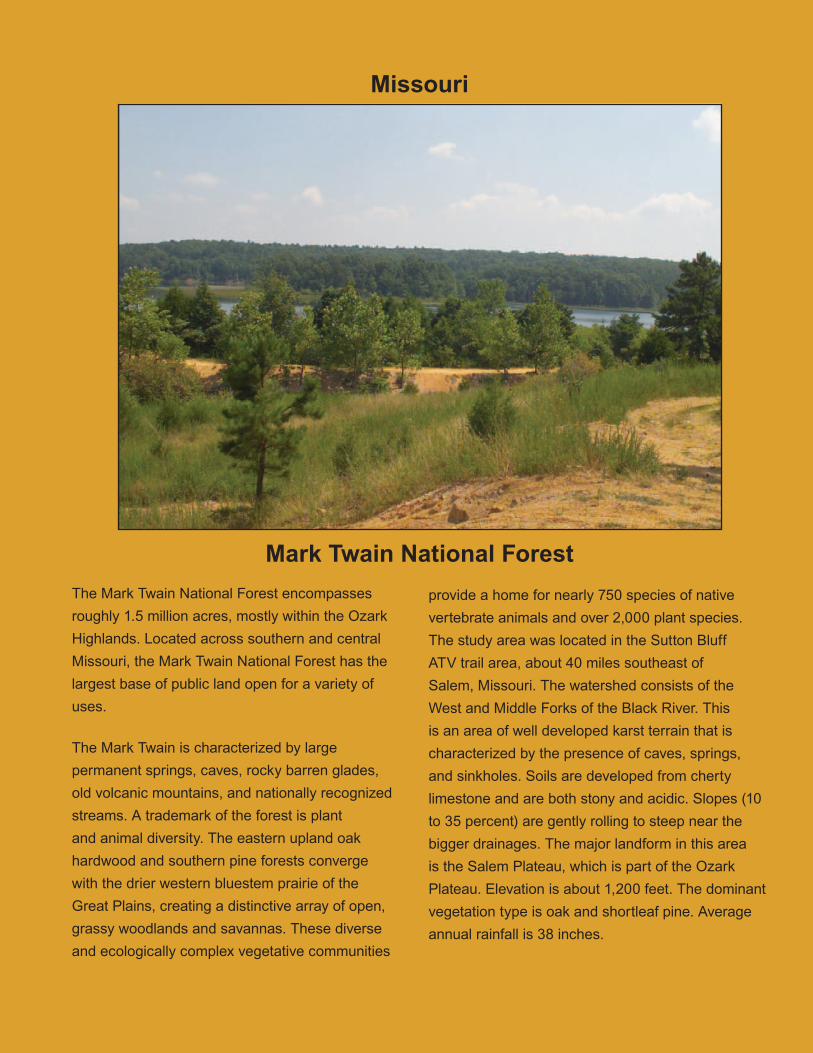
61

Mark Twain National Forest

Missouri

provide a home for nearly 750 species of native

vertebrate animals and over 2,000 plant species.

The study area was located in the Sutton Bluff

ATV trail area, about 40 miles southeast of

Salem, Missouri. The watershed consists of the

West and Middle Forks of the Black River. This

is an area of well developed karst terrain that is

characterized by the presence of caves, springs,

and sinkholes. Soils are developed from cherty

limestone and are both stony and acidic. Slopes (10

to 35 percent) are gently rolling to steep near the

bigger drainages. The major landform in this area

is the Salem Plateau, which is part of the Ozark

Plateau. Elevation is about 1,200 feet. The dominant

vegetation type is oak and shortleaf pine. Average

annual rainfall is 38 inches.

The Mark Twain National Forest encompasses

roughly 1.5 million acres, mostly within the Ozark

Highlands. Located across southern and central

Missouri, the Mark Twain National Forest has the

largest base of public land open for a variety of

uses.

The Mark Twain is characterized by large

permanent springs, caves, rocky barren glades,

old volcanic mountains, and nationally recognized

streams. A trademark of the forest is plant

and animal diversity. The eastern upland oak

hardwood and southern pine forests converge

with the drier western bluestem prairie of the

Great Plains, creating a distinctive array of open,

grassy woodlands and savannas. These diverse

and ecologically complex vegetative communities

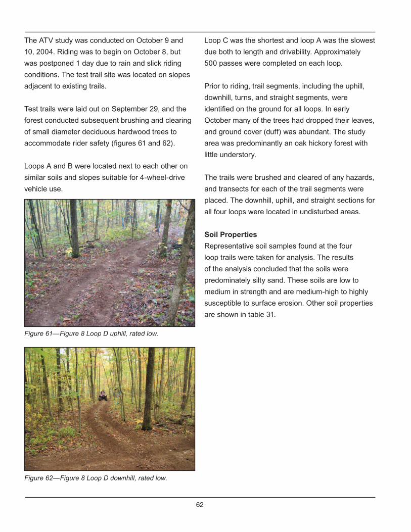
62

The ATV study was conducted on October 9 and

10, 2004. Riding was to begin on October 8, but

was postponed 1 day due to rain and slick riding

conditions. The test trail site was located on slopes

adjacent to existing trails.

Test trails were laid out on September 29, and the

forest conducted subsequent brushing and clearing

of small diameter deciduous hardwood trees to

accommodate rider safety (figures 61 and 62).

Loops A and B were located next to each other on

similar soils and slopes suitable for 4-wheel-drive

vehicle use.

Figure 61—Figure 8 Loop D uphill, rated low.

Figure 62—Figure 8 Loop D downhill, rated low.

Loop C was the shortest and loop A was the slowest

due both to length and drivability. Approximately

500 passes were completed on each loop.

Prior to riding, trail segments, including the uphill,

downhill, turns, and straight segments, were

identified on the ground for all loops. In early

October many of the trees had dropped their leaves,

and ground cover (duff) was abundant. The study

area was predominantly an oak hickory forest with

little understory.

The trails were brushed and cleared of any hazards,

and transects for each of the trail segments were

placed. The downhill, uphill, and straight sections for

all four loops were located in undisturbed areas.

Soil Properties

Representative soil samples found at the four

loop trails were taken for analysis. The results

of the analysis concluded that the soils were

predominately silty sand. These soils are low to

medium in strength and are medium-high to highly

susceptible to surface erosion. Other soil properties

are shown in table 31.

63

Table 31—Soil properties for Mark Twain NF study site.

Forest

USCS Group

Symbol-Description

Surface Erosion

Dry Strength

Saturated Strength

Rutting(Saturated) Raveling Dust

MTNF SM-silty sand

Medium-high

Low-medium

Low-medium

Low-medium

Medium-high

Medium-high

Vehicle Types

Table 32 provides the model, ATV type, and total number of passes for each loop.

Table 32—Loops, vehicle characteristics, and total number

of passes.

Loop Vehicle Model/Type

OEM/AM

Total Passes

AKawasaki

PrairieUtility

OEM 480

BKawasaki

PrairieUtility

AM 520

C Honda ReconSport OEM 500

D Honda ReconSport AM 500

Condition-Class Summary

One study objective was to determine if ATVs affect the natural resources and, if so, to what degree.

Table 33 provides a summary of the condition-class assessments and, specifically, how condition classes

changed over time with subsequent passes.

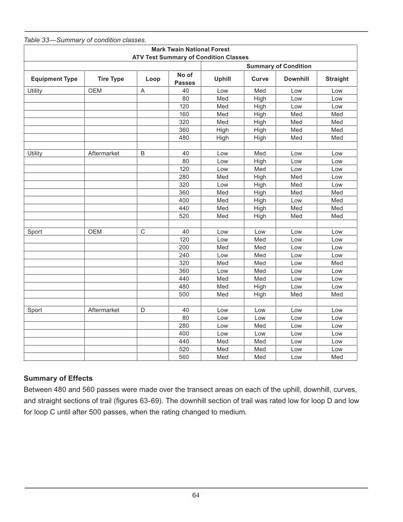
64

Table 33—Summary of condition classes.Mark Twain National Forest

ATV Test Summary of Condition Classes

Summary of Condition

Equipment Type Tire Type LoopNo of

PassesUphill Curve Downhill Straight

Utility OEM A 40 Low Med Low Low 80 Med High Low Low 120 Med High Low Low 160 Med High Med Med 320 Med High Med Med 360 High High Med Med 480 High High Med Med Utility Aftermarket B 40 Low Med Low Low 80 Low High Low Low 120 Low Med Low Low 280 Med High Med Low 320 Low High Med Low 360 Med High Med Med 400 Med High Low Med 440 Med High Med Med 520 Med High Med Med Sport OEM C 40 Low Low Low Low 120 Low Med Low Low 200 Med Med Low Low 240 Low Med Low Low 320 Med Med Low Med 360 Low Med Low Low 440 Med Med Low Low 480 Med High Low Low 500 Med High Med Med Sport Aftermarket D 40 Low Low Low Low 80 Low Low Low Low 280 Low Med Low Low 400 Low Low Low Low 440 Med Med Low Low 520 Med Med Low Low 560 Med Med Low Med

Summary of Effects

Between 480 and 560 passes were made over the transect areas on each of the uphill, downhill, curves,

and straight sections of trail (figures 63-69). The downhill section of trail was rated low for loop D and low

for loop C until after 500 passes, when the rating changed to medium.

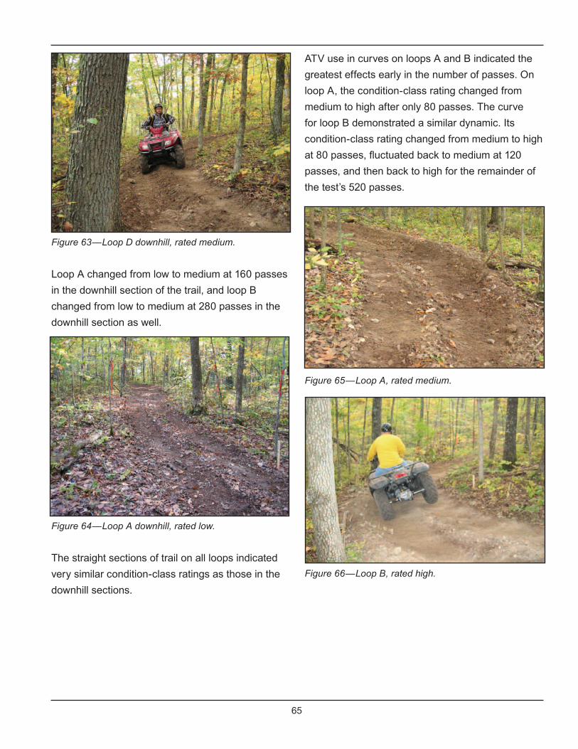
65

Figure 63—Loop D downhill, rated medium.

Loop A changed from low to medium at 160 passes

in the downhill section of the trail, and loop B

changed from low to medium at 280 passes in the

downhill section as well.

Figure 64—Loop A downhill, rated low.

The straight sections of trail on all loops indicated

very similar condition-class ratings as those in the

downhill sections.

ATV use in curves on loops A and B indicated the

greatest effects early in the number of passes. On

loop A, the condition-class rating changed from

medium to high after only 80 passes. The curve

for loop B demonstrated a similar dynamic. Its

condition-class rating changed from medium to high

at 80 passes, fluctuated back to medium at 120

passes, and then back to high for the remainder of

the test’s 520 passes.

Figure 65—Loop A, rated medium.

Figure 66—Loop B, rated high.

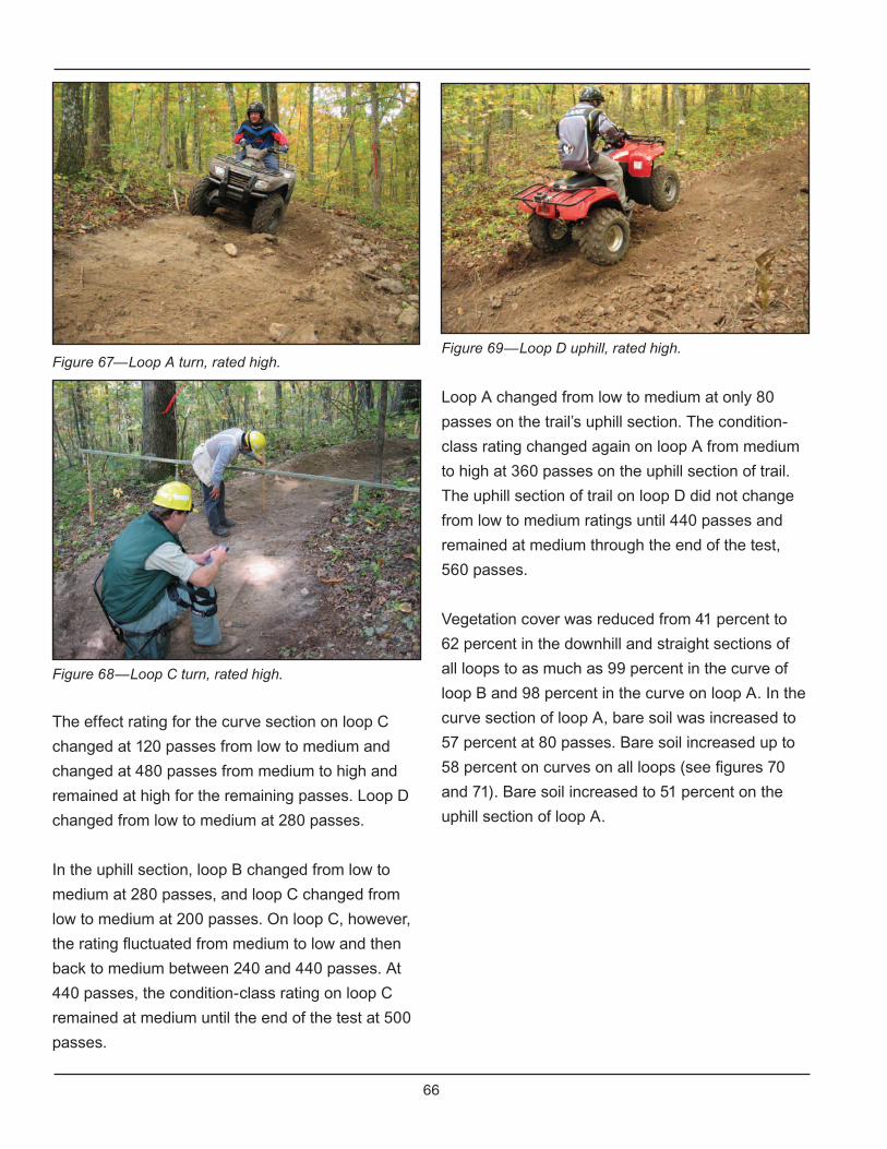
66

Figure 67—Loop A turn, rated high.

Figure 68—Loop C turn, rated high.

The effect rating for the curve section on loop C

changed at 120 passes from low to medium and

changed at 480 passes from medium to high and

remained at high for the remaining passes. Loop D

changed from low to medium at 280 passes.

In the uphill section, loop B changed from low to

medium at 280 passes, and loop C changed from

low to medium at 200 passes. On loop C, however,

the rating fluctuated from medium to low and then

back to medium between 240 and 440 passes. At

440 passes, the condition-class rating on loop C

remained at medium until the end of the test at 500

passes.

Figure 69—Loop D uphill, rated high.

Loop A changed from low to medium at only 80

passes on the trail’s uphill section. The condition-

class rating changed again on loop A from medium

to high at 360 passes on the uphill section of trail.

The uphill section of trail on loop D did not change

from low to medium ratings until 440 passes and

remained at medium through the end of the test,

560 passes.

Vegetation cover was reduced from 41 percent to

62 percent in the downhill and straight sections of

all loops to as much as 99 percent in the curve of

loop B and 98 percent in the curve on loop A. In the

curve section of loop A, bare soil was increased to

57 percent at 80 passes. Bare soil increased up to

58 percent on curves on all loops (see figures 70

and 71). Bare soil increased to 51 percent on the

uphill section of loop A.

67

Figure 70—Illustration of proportionate amounts of litter and bare soil on the curve segment before riding began.

Figure 71—Illustration of proportionate amounts of vegetation and litter removed, bare soil, rock/root exposure, stump exposure on the curve segment at completion of total passes.

Rut depths up to 7 inches were recorded in the

curves, with the trail widening up to 6 feet in curve

segments on all loops and in the uphill section of

loop D. Rut depths up to 6 inches were measured

in uphill segments, with the trail shoulder mounding

up to 10 inches in these segments. Shallower

depths—1 to 2 inches—were recorded on straight

and downhill sections.

ATV use in turns appeared to show the greatest

effects on loops B and D. On loop B, the rating was

high after only 80 passes and, on loop D, a high

rating was achieved after only 40 passes. Riding

through this section was discontinued after 80

passes, as a high-condition class was reached and

sustained. The turn for loop A indicated a high rating

at 240 passes, after a medium rating was sustained

from 40 through 200 passes.

Yes No

Curve Before Riding

Litter StumpBareRock/RootPlant

Curve After Riding

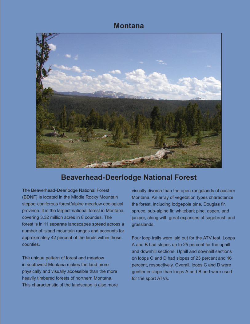
69

Beaverhead-Deerlodge National Forest

Montana

The Beaverhead-Deerlodge National Forest

(BDNF) is located in the Middle Rocky Mountain

steppe-coniferous forest/alpine meadow ecological

province. It is the largest national forest in Montana,

covering 3.32 million acres in 8 counties. The

forest is in 11 separate landscapes spread across a

number of island mountain ranges and accounts for

approximately 42 percent of the lands within those

counties.

The unique pattern of forest and meadow

in southwest Montana makes the land more

physically and visually accessible than the more

heavily timbered forests of northern Montana.

This characteristic of the landscape is also more

visually diverse than the open rangelands of eastern

Montana. An array of vegetation types characterize

the forest, including lodgepole pine, Douglas fir,

spruce, sub-alpine fir, whitebark pine, aspen, and

juniper, along with great expanses of sagebrush and

grasslands.

Four loop trails were laid out for the ATV test. Loops

A and B had slopes up to 25 percent for the uphill

and downhill sections. Uphill and downhill sections

on loops C and D had slopes of 23 percent and 16

percent, respectively. Overall, loops C and D were

gentler in slope than loops A and B and were used

for the sport ATVs.

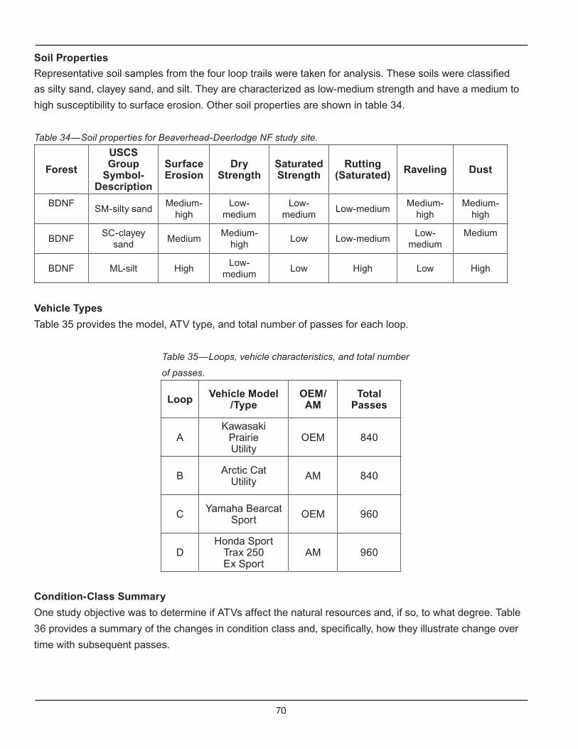
70

Soil Properties

Representative soil samples from the four loop trails were taken for analysis. These soils were classified

as silty sand, clayey sand, and silt. They are characterized as low-medium strength and have a medium to

high susceptibility to surface erosion. Other soil properties are shown in table 34.

Table 34—Soil properties for Beaverhead-Deerlodge NF study site.

Forest

USCS Group

Symbol-Description

Surface Erosion

Dry Strength

Saturated Strength

Rutting(Saturated) Raveling Dust

BDNFSM-silty sand

Medium-high

Low-medium

Low-medium

Low-mediumMedium-

highMedium-

high

BDNFSC-clayey

sandMedium

Medium-high

Low Low-mediumLow-

mediumMedium

BDNF ML-silt HighLow-

mediumLow High Low High

Vehicle Types

Table 35 provides the model, ATV type, and total number of passes for each loop.

Table 35—Loops, vehicle characteristics, and total number

of passes.

Loop Vehicle Model/Type

OEM/AM

Total Passes

AKawasaki

PrairieUtility

OEM 840

B Arctic CatUtility AM 840

C Yamaha BearcatSport OEM 960

DHonda Sport

Trax 250 Ex Sport

AM 960

Condition-Class Summary

One study objective was to determine if ATVs affect the natural resources and, if so, to what degree. Table

36 provides a summary of the changes in condition class and, specifically, how they illustrate change over

time with subsequent passes.

71

Table 36—Summary of condition classes.

Beaverhead-Deerlodge National Forest ATV Test Summary of Condition Classes

Summary of Condition

Equipment Type Tire Type Loop No of

Passes Uphill Curve Downhill Straight

Utility OEM A 40 Low Low Low Low 80 Low Med Low Low 120 Low Med Low Low 240 Med Med Low Low 320 Med Med Med Low 360 High Med Med Low 400 High Med Med Med 520 High Med Med Med 640 High High Med Med 840 High High Med Med Utility Aftermarket B 40 Low Low Low Low 80 Low Med Low Low 120 Low Med Low Low 200 Med Med Low Low 280 Med Med Med Low 320 Med Med Med Med 360 Med Med Med Low 400 Med Med Low Med 440 Med High Med Med 520 Med Med Med Med 560 Med Med Med Med 640 Low Low Low Low 680 Med Med Low Low 720 Med Med Low Low 760 Med Med Med Med 840 Med Med Med Med Sport OEM C 40 Low Med Low Low 120 Low High High Med 200 High High High Low 320 High High High Med 400 High High High Med 560 Low High High Med 720 High High High Med 960 High High High Med Sport Aftermarket D 40 Low Med Low Low 120 Low High Low Low 160 Med High Low Low 240 Med High Low Low 320 Med High Low Med 360 Med High Low Low 400 Med High Low Low 560 Med High Low Med 640 Med High Med Med 800 Med High Med Med 960 Med High Med Med

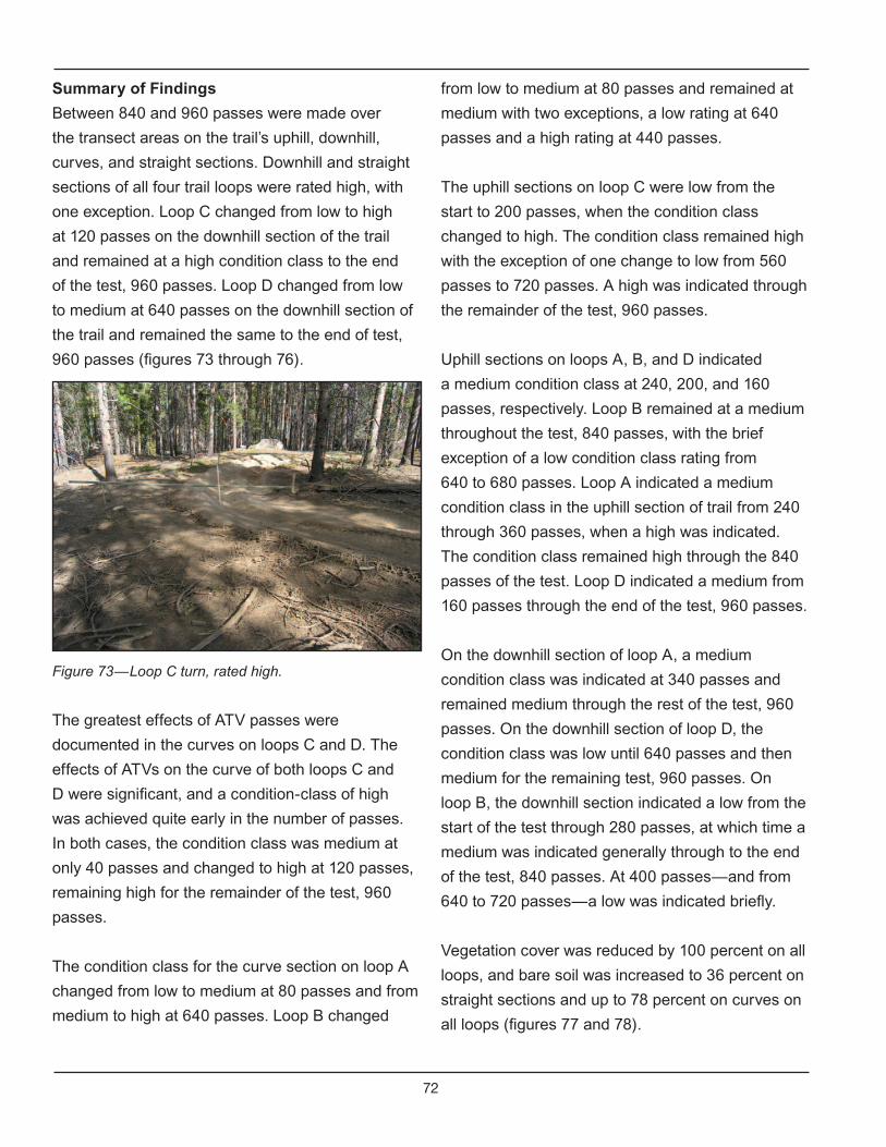
72

from low to medium at 80 passes and remained at

medium with two exceptions, a low rating at 640

passes and a high rating at 440 passes.

The uphill sections on loop C were low from the

start to 200 passes, when the condition class

changed to high. The condition class remained high

with the exception of one change to low from 560

passes to 720 passes. A high was indicated through

the remainder of the test, 960 passes.

Uphill sections on loops A, B, and D indicated

a medium condition class at 240, 200, and 160

passes, respectively. Loop B remained at a medium

throughout the test, 840 passes, with the brief

exception of a low condition class rating from

640 to 680 passes. Loop A indicated a medium

condition class in the uphill section of trail from 240

through 360 passes, when a high was indicated.

The condition class remained high through the 840

passes of the test. Loop D indicated a medium from

160 passes through the end of the test, 960 passes.

On the downhill section of loop A, a medium

condition class was indicated at 340 passes and

remained medium through the rest of the test, 960

passes. On the downhill section of loop D, the

condition class was low until 640 passes and then

medium for the remaining test, 960 passes. On

loop B, the downhill section indicated a low from the

start of the test through 280 passes, at which time a

medium was indicated generally through to the end

of the test, 840 passes. At 400 passes—and from

640 to 720 passes—a low was indicated briefly.

Vegetation cover was reduced by 100 percent on all

loops, and bare soil was increased to 36 percent on

straight sections and up to 78 percent on curves on

all loops (figures 77 and 78).

Summary of Findings

Between 840 and 960 passes were made over

the transect areas on the trail’s uphill, downhill,

curves, and straight sections. Downhill and straight

sections of all four trail loops were rated high, with

one exception. Loop C changed from low to high

at 120 passes on the downhill section of the trail

and remained at a high condition class to the end

of the test, 960 passes. Loop D changed from low

to medium at 640 passes on the downhill section of

the trail and remained the same to the end of test,

960 passes (figures 73 through 76).

Figure 73—Loop C turn, rated high.

The greatest effects of ATV passes were

documented in the curves on loops C and D. The

effects of ATVs on the curve of both loops C and

D were significant, and a condition-class of high

was achieved quite early in the number of passes.

In both cases, the condition class was medium at

only 40 passes and changed to high at 120 passes,

remaining high for the remainder of the test, 960

passes.

The condition class for the curve section on loop A

changed from low to medium at 80 passes and from

medium to high at 640 passes. Loop B changed

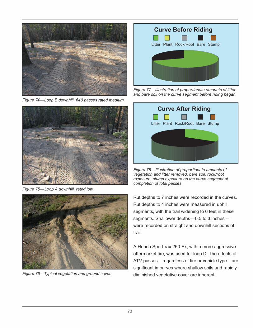
73

Figure 74—Loop B downhill, 640 passes rated medium.

Figure 75—Loop A downhill, rated low.

Figure 76—Typical vegetation and ground cover.

Figure 77—Illustration of proportionate amounts of litter and bare soil on the curve segment before riding began.

Figure 78—Illustration of proportionate amounts of vegetation and litter removed, bare soil, rock/root exposure, stump exposure on the curve segment at completion of total passes.

Rut depths to 7 inches were recorded in the curves.

Rut depths to 4 inches were measured in uphill

segments, with the trail widening to 6 feet in these

segments. Shallower depths—0.5 to 3 inches—

were recorded on straight and downhill sections of

trail.

A Honda Sporttrax 260 Ex, with a more aggressive

aftermarket tire, was used for loop D. The effects of

ATV passes—regardless of tire or vehicle type—are

significant in curves where shallow soils and rapidly

diminished vegetative cover are inherent.

Litter StumpBareRock/RootPlant

Curve Before Riding

Litter StumpBareRock/RootPlant

Curve After Riding

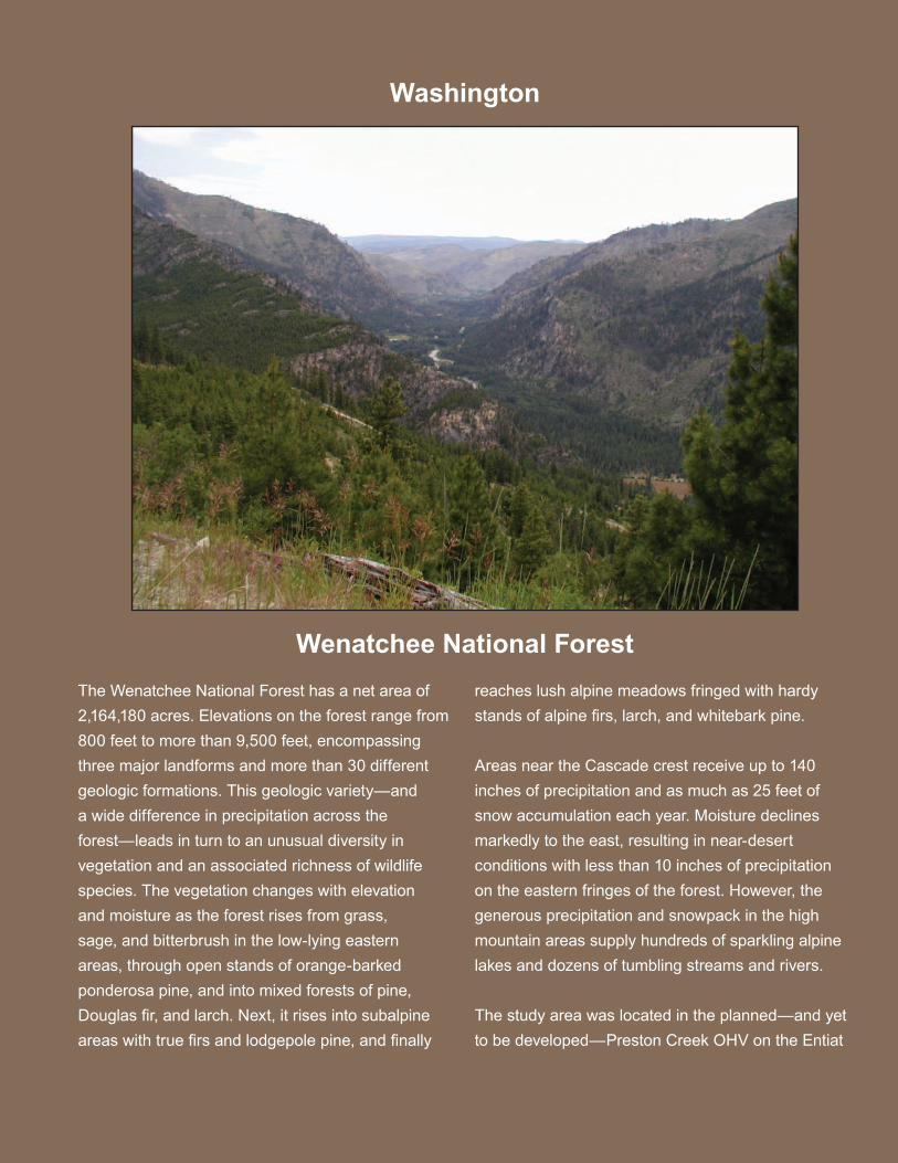
75

Wenatchee National Forest

Washington

The Wenatchee National Forest has a net area of

2,164,180 acres. Elevations on the forest range from

800 feet to more than 9,500 feet, encompassing

three major landforms and more than 30 different

geologic formations. This geologic variety—and

a wide difference in precipitation across the

forest—leads in turn to an unusual diversity in

vegetation and an associated richness of wildlife

species. The vegetation changes with elevation

and moisture as the forest rises from grass,

sage, and bitterbrush in the low-lying eastern

areas, through open stands of orange-barked

ponderosa pine, and into mixed forests of pine,

Douglas fir, and larch. Next, it rises into subalpine

areas with true firs and lodgepole pine, and finally

reaches lush alpine meadows fringed with hardy

stands of alpine firs, larch, and whitebark pine.

Areas near the Cascade crest receive up to 140

inches of precipitation and as much as 25 feet of

snow accumulation each year. Moisture declines

markedly to the east, resulting in near-desert

conditions with less than 10 inches of precipitation

on the eastern fringes of the forest. However, the

generous precipitation and snowpack in the high

mountain areas supply hundreds of sparkling alpine

lakes and dozens of tumbling streams and rivers.

The study area was located in the planned—and yet

to be developed—Preston Creek OHV on the Entiat

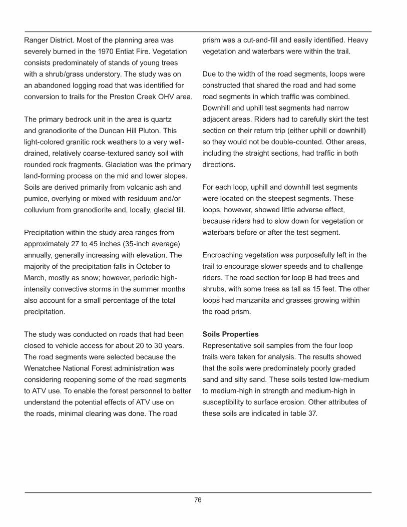
76

Ranger District. Most of the planning area was

severely burned in the 1970 Entiat Fire. Vegetation

consists predominately of stands of young trees

with a shrub/grass understory. The study was on

an abandoned logging road that was identified for

conversion to trails for the Preston Creek OHV area.

The primary bedrock unit in the area is quartz

and granodiorite of the Duncan Hill Pluton. This

light-colored granitic rock weathers to a very well-

drained, relatively coarse-textured sandy soil with

rounded rock fragments. Glaciation was the primary

land-forming process on the mid and lower slopes.

Soils are derived primarily from volcanic ash and

pumice, overlying or mixed with residuum and/or

colluvium from granodiorite and, locally, glacial till.

Precipitation within the study area ranges from

approximately 27 to 45 inches (35-inch average)

annually, generally increasing with elevation. The

majority of the precipitation falls in October to

March, mostly as snow; however, periodic high-

intensity convective storms in the summer months

also account for a small percentage of the total

precipitation.

The study was conducted on roads that had been

closed to vehicle access for about 20 to 30 years.

The road segments were selected because the

Wenatchee National Forest administration was

considering reopening some of the road segments

to ATV use. To enable the forest personnel to better

understand the potential effects of ATV use on

the roads, minimal clearing was done. The road

prism was a cut-and-fill and easily identified. Heavy

vegetation and waterbars were within the trail.

Due to the width of the road segments, loops were

constructed that shared the road and had some

road segments in which traffic was combined.

Downhill and uphill test segments had narrow

adjacent areas. Riders had to carefully skirt the test

section on their return trip (either uphill or downhill)

so they would not be double-counted. Other areas,

including the straight sections, had traffic in both

directions.

For each loop, uphill and downhill test segments

were located on the steepest segments. These

loops, however, showed little adverse effect,

because riders had to slow down for vegetation or

waterbars before or after the test segment.

Encroaching vegetation was purposefully left in the

trail to encourage slower speeds and to challenge

riders. The road section for loop B had trees and

shrubs, with some trees as tall as 15 feet. The other

loops had manzanita and grasses growing within

the road prism.

Soils Properties

Representative soil samples from the four loop

trails were taken for analysis. The results showed

that the soils were predominately poorly graded

sand and silty sand. These soils tested low-medium

to medium-high in strength and medium-high in

susceptibility to surface erosion. Other attributes of

these soils are indicated in table 37.

77

Table 37—Soil properties for Wenatchee NF study site.

Forest

USCS Group

Symbol-Description

Surface Erosion

Dry Strength

Saturated Strength

Rutting(Saturated) Raveling Dust

OW SP-poorly-graded sand

Medium-high Medium Medium-

high Low High Low-medium

OW SM-silty sand

Medium-high

Low-medium

Low-medium

Low-medium

Medium-high

Medium-high

Vehicle Types

Table 38 provides the model, ATV type, and total number of passes for all loops.

Table 38—Loops, vehicle characteristics, and total number

of passes.

Loop Vehicle Model/Type

OEM/AM

Total Passes

A Arctic Cat Utility OEM 240

B Honda 2 WDSport AM 960

C Honda 2 WDSport OEM 240

D Kawasaki 650Utility AM 440

Condition-Class Summary

One study objective was to determine if ATVs affect the natural resources and, if so, to what degree.

Table 39 provides a summary of the condition-class assessments and, specifically, how condition classes

changed over time with subsequent passes.

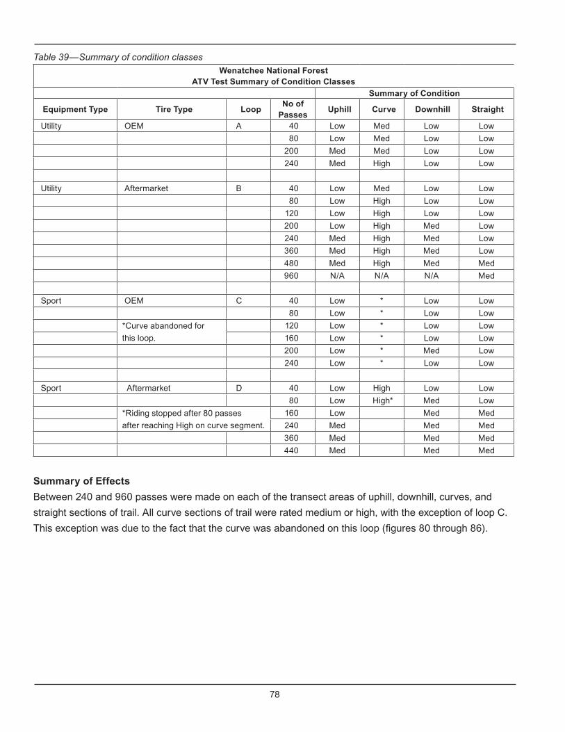
78

Table 39—Summary of condition classes

Wenatchee National ForestATV Test Summary of Condition Classes

Summary of Condition

Equipment Type Tire Type LoopNo of

Passes Uphill Curve Downhill Straight

Utility OEM A 40 Low Med Low Low

80 Low Med Low Low

200 Med Med Low Low

240 Med High Low Low

Utility Aftermarket B 40 Low Med Low Low

80 Low High Low Low

120 Low High Low Low

200 Low High Med Low

240 Med High Med Low

360 Med High Med Low

480 Med High Med Med

960 N/A N/A N/A Med

Sport OEM C 40 Low * Low Low

80 Low * Low Low

*Curve abandoned for 120 Low * Low Low

this loop. 160 Low * Low Low

200 Low * Med Low

240 Low * Low Low

Sport Aftermarket D 40 Low High Low Low

80 Low High* Med Low

*Riding stopped after 80 passes 160 Low Med Med

after reaching High on curve segment. 240 Med Med Med

360 Med Med Med

440 Med Med Med

Summary of Effects

Between 240 and 960 passes were made on each of the transect areas of uphill, downhill, curves, and

straight sections of trail. All curve sections of trail were rated medium or high, with the exception of loop C.

This exception was due to the fact that the curve was abandoned on this loop (figures 80 through 86).

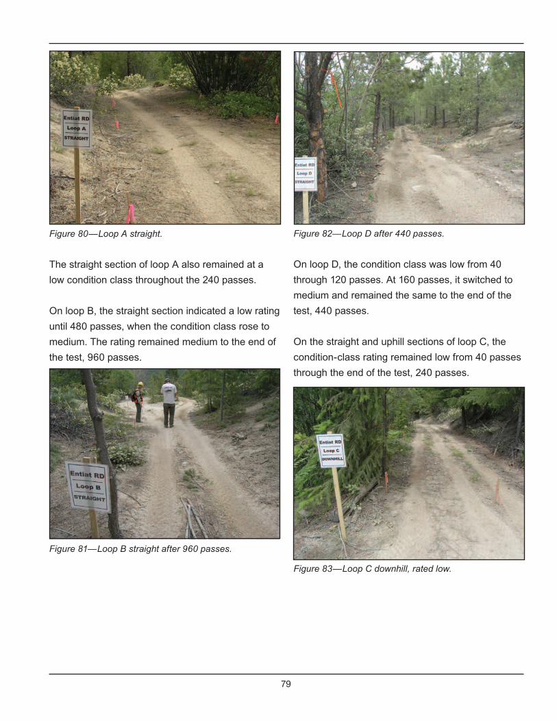
79

Figure 80—Loop A straight.

The straight section of loop A also remained at a

low condition class throughout the 240 passes.

On loop B, the straight section indicated a low rating

until 480 passes, when the condition class rose to

medium. The rating remained medium to the end of

the test, 960 passes.

Figure 81—Loop B straight after 960 passes.

Figure 82—Loop D after 440 passes.

On loop D, the condition class was low from 40

through 120 passes. At 160 passes, it switched to

medium and remained the same to the end of the

test, 440 passes.

On the straight and uphill sections of loop C, the

condition-class rating remained low from 40 passes

through the end of the test, 240 passes.

Figure 83—Loop C downhill, rated low.

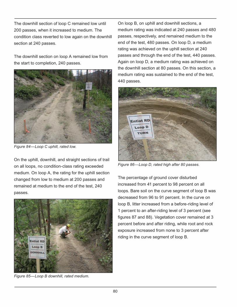
80

The downhill section of loop C remained low until

200 passes, when it increased to medium. The

condition class reverted to low again on the downhill

section at 240 passes.

The downhill section on loop A remained low from

the start to completion, 240 passes.

Figure 84—Loop C uphill, rated low.

On the uphill, downhill, and straight sections of trail

on all loops, no condition-class rating exceeded

medium. On loop A, the rating for the uphill section

changed from low to medium at 200 passes and

remained at medium to the end of the test, 240

passes.

Figure 85—Loop B downhill, rated medium.

On loop B, on uphill and downhill sections, a

medium rating was indicated at 240 passes and 480

passes, respectively, and remained medium to the

end of the test, 480 passes. On loop D, a medium

rating was achieved on the uphill section at 240

passes and through the end of the test, 440 passes.

Again on loop D, a medium rating was achieved on

the downhill section at 80 passes. On this section, a

medium rating was sustained to the end of the test,

440 passes.

Figure 86—Loop D, rated high after 80 passes.

The percentage of ground cover disturbed

increased from 41 percent to 98 percent on all

loops. Bare soil on the curve segment of loop B was

decreased from 96 to 91 percent. In the curve on

loop B, litter increased from a before-riding level of

1 percent to an after-riding level of 3 percent (see

figures 87 and 88). Vegetation cover remained at 3

percent before and after riding, while root and rock

exposure increased from none to 3 percent after

riding in the curve segment of loop B.

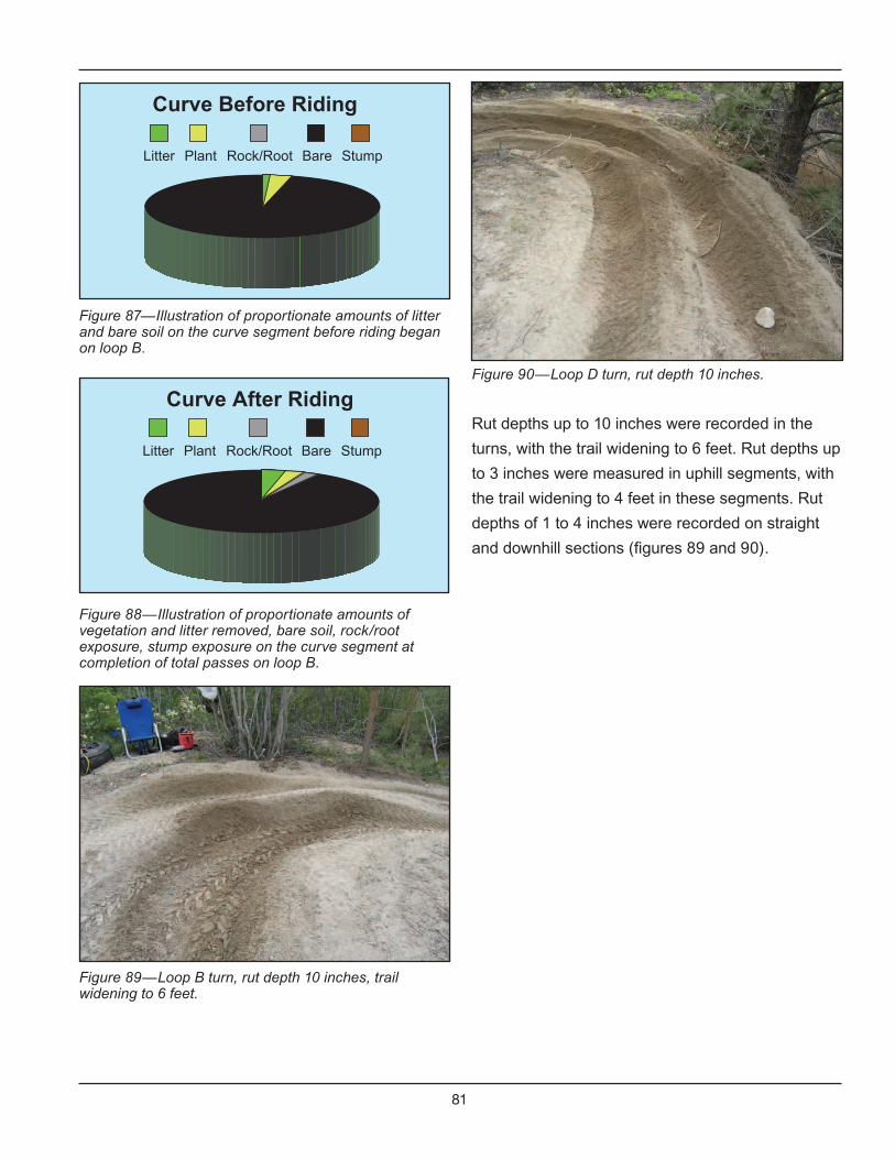
81

Figure 87—Illustration of proportionate amounts of litter and bare soil on the curve segment before riding began on loop B.

Figure 88—Illustration of proportionate amounts of vegetation and litter removed, bare soil, rock/root exposure, stump exposure on the curve segment at completion of total passes on loop B.

Figure 89—Loop B turn, rut depth 10 inches, trail widening to 6 feet.

Litter StumpBareRock/RootPlant

Curve Before Riding

Litter StumpBareRock/RootPlant

Curve After RidingFigure 90—Loop D turn, rut depth 10 inches.

Rut depths up to 10 inches were recorded in the

turns, with the trail widening to 6 feet. Rut depths up

to 3 inches were measured in uphill segments, with

the trail widening to 4 feet in these segments. Rut

depths of 1 to 4 inches were recorded on straight

and downhill sections (figures 89 and 90).

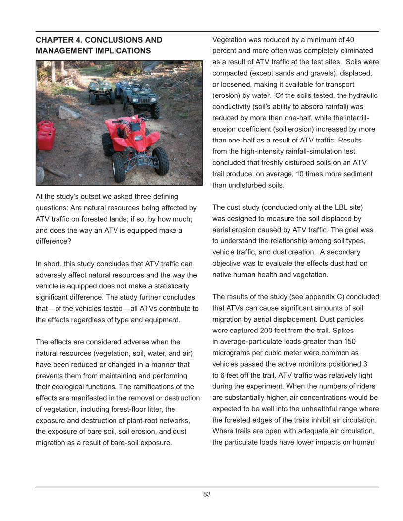
83

CHAPTER 4. CONCLUSIONS AND

MANAGEMENT IMPLICATIONS

At the study’s outset we asked three defining

questions: Are natural resources being affected by

ATV traffic on forested lands; if so, by how much;

and does the way an ATV is equipped make a

difference?

In short, this study concludes that ATV traffic can

adversely affect natural resources and the way the

vehicle is equipped does not make a statistically

significant difference. The study further concludes

that—of the vehicles tested—all ATVs contribute to

the effects regardless of type and equipment.

The effects are considered adverse when the

natural resources (vegetation, soil, water, and air)

have been reduced or changed in a manner that

prevents them from maintaining and performing

their ecological functions. The ramifications of the

effects are manifested in the removal or destruction

of vegetation, including forest-floor litter, the

exposure and destruction of plant-root networks,

the exposure of bare soil, soil erosion, and dust

migration as a result of bare-soil exposure.

Vegetation was reduced by a minimum of 40

percent and more often was completely eliminated

as a result of ATV traffic at the test sites. Soils were

compacted (except sands and gravels), displaced,

or loosened, making it available for transport

(erosion) by water. Of the soils tested, the hydraulic

conductivity (soil’s ability to absorb rainfall) was

reduced by more than one-half, while the interrill-

erosion coefficient (soil erosion) increased by more

than one-half as a result of ATV traffic. Results

from the high-intensity rainfall-simulation test

concluded that freshly disturbed soils on an ATV

trail produce, on average, 10 times more sediment

than undisturbed soils.

The dust study (conducted only at the LBL site)

was designed to measure the soil displaced by

aerial erosion caused by ATV traffic. The goal was

to understand the relationship among soil types,

vehicle traffic, and dust creation. A secondary

objective was to evaluate the effects dust had on

native human health and vegetation.

The results of the study (see appendix C) concluded

that ATVs can cause significant amounts of soil

migration by aerial displacement. Dust particles

were captured 200 feet from the trail. Spikes

in average-particulate loads greater than 150

micrograms per cubic meter were common as

vehicles passed the active monitors positioned 3

to 6 feet off the trail. ATV traffic was relatively light

during the experiment. When the numbers of riders

are substantially higher, air concentrations would be

expected to be well into the unhealthful range where

the forested edges of the trails inhibit air circulation.

Where trails are open with adequate air circulation,

the particulate loads have lower impacts on human

84

health. The passive samplers deployed at head-

height confirm a substantial atmospheric loading

that could affect the riders’ respiratory systems.

The evaluation of dust effects on vegetation

suggests that ATVs cause only minor perturbations

(disturbances). Some stomatal (pore) blockage

was observed, as were surface accumulations of

dust that may periodically inhibit photosynthesis

and respiration, but little superficial damage to

the cuticle was evident in the images captured by

a scanning electronic microscope. Because of

frequent rainfall at the test site, it is unlikely that

the effects are long lasting or a cause for serious

concern (Padgett 2006).

There are two surprising results from the study.

First, sport-model vehicles (lighter weight ATVs)

cause as much disturbance as the heavier

utility-model vehicles. There were no significant

differences between the level of disturbance caused

by sport- or utility-model vehicles. The heavier,

more powerful utility vehicles reached the targeted

disturbance levels in fewer passes than the sport

two-wheel-drive models; but, when the number of

passes was the same, the levels of disturbance

were the same for each vehicle type.

Second, there were no distinguishable differences

between the level of disturbance caused by a

vehicle with standard manufacturer-issued tires or a

vehicle equipped with more aggressive after-market

tires. Ultimately, all tire and vehicle combinations

tested caused the same levels of disturbance.

Four trail features were tested: a curve, downhill,

uphill, and straight runs. For all soil types, curves

were most susceptible to soil displacement, followed

by uphill and downhill runs regardless of soil type.

Straight runs showed the least amount of soil

displacement. The difference in soil displacement

for an uphill or downhill section was five to eight

times greater than on level-straight sections.

Therefore, trail managers should make monitoring

and maintaining curves and turns a high priority,

followed by uphill and downhill sections of trail.

Curves require extra attention to ensure that they

are designed and constructed for proper armoring

and drainage.

The data also imply that straight sections of trail

will require less maintenance, especially if these

sections are located away from weaker soils. This

is an important distinction to manage as forests

involve and work with volunteer groups to make

their contributions meaningful and effective.

Perhaps the most important management

implication of this study is that ATV traffic should

be limited to trails. The data gathered in this study

overwhelmingly support this direction. Areas that

continue to allow cross-country travel can only

expect to see a further reduction in the ability of

natural resources to maintain their composition and

structure and perform their natural functions. Other

studies related to soil and vegetation disturbance

indicated that the rehabilitation of these areas will

take many years, especially those in arid climate

zones (Cole 1986). Some may never recover

without assistance.

The study also suggests that limiting ATV traffic to

trails is not enough to protect the natural resources.

Trail planning and design, particularly the trail’s

location, are key considerations for limiting natural-

resource disturbances. The primary objective of a

well-designed ATV trail is to protect and conserve

the natural resources while providing an enjoyable

85

and challenging experience. The experience is

the purpose of the trip! The design phase should

identify destinations as well as areas to avoid, such

as soils that are easily disturbed, wet areas (riparian

zones), ridge tops, and sensitive wildlife habitats

and archeological sites.

Trail alignments should be curvilinear with short

sight distances. Avoid tight turns and steep climbs,

as these trail features are susceptible to high levels

of soil disturbance and erosion. Use contours and

the vertical alignment to facilitate drainage across

and away from the trail. Avoid constructing trails

on the fall line. Use water diversions as often as

necessary to move water off the trail and onto the

forest floor. These practices will significantly reduce

erosion and sedimentation.

The data also suggest setting limits or developing

natural-resource tolerance levels as a way to

manage and reduce the effects of ATV traffic on

the natural resources. Consider for example the

hydraulic conductivity, interrill coefficient, and dust-

migration data. The hydraulic conductivity of soil

(soil’s ability to absorb rainfall) is a way of estimating

soil saturation and when overland flow begins. This

information is very useful for establishing natural-

resource tolerances and developing trail-closure

parameters based on scientific principles (i.e.,

the rainfall rate at which soils begin to experience

runoff, and the magnitude of rainfall events). The

Kisatchie National Forest sets a rainfall limit of 2

inches before closing its ATV trails, and they remain

closed until the soil regains its absorption capacity.

Similar parameters have been developed for other

forests.

Information that describes the effects of dust

migration as a result of ATV traffic could also prove

to be an effective tool for monitoring trail use and

keeping natural resources in balance. Managers

could use such information to establish seasonal

closures, employ dust abatement techniques, and

design better trails to reduce soil migration.

Casual observations made during the study also

suggest a need to develop sustainable riding

practices to assist riders to improve their riding

habits and information to enhance their knowledge

about the affects of ATV traffic on natural

resources. Riding practices would include: slower

speeds through curves, avoiding wheel spins and

fish tailing, and avoiding travel through wet areas.

Information should also be provided about why it is

important to avoid these sensitive areas.

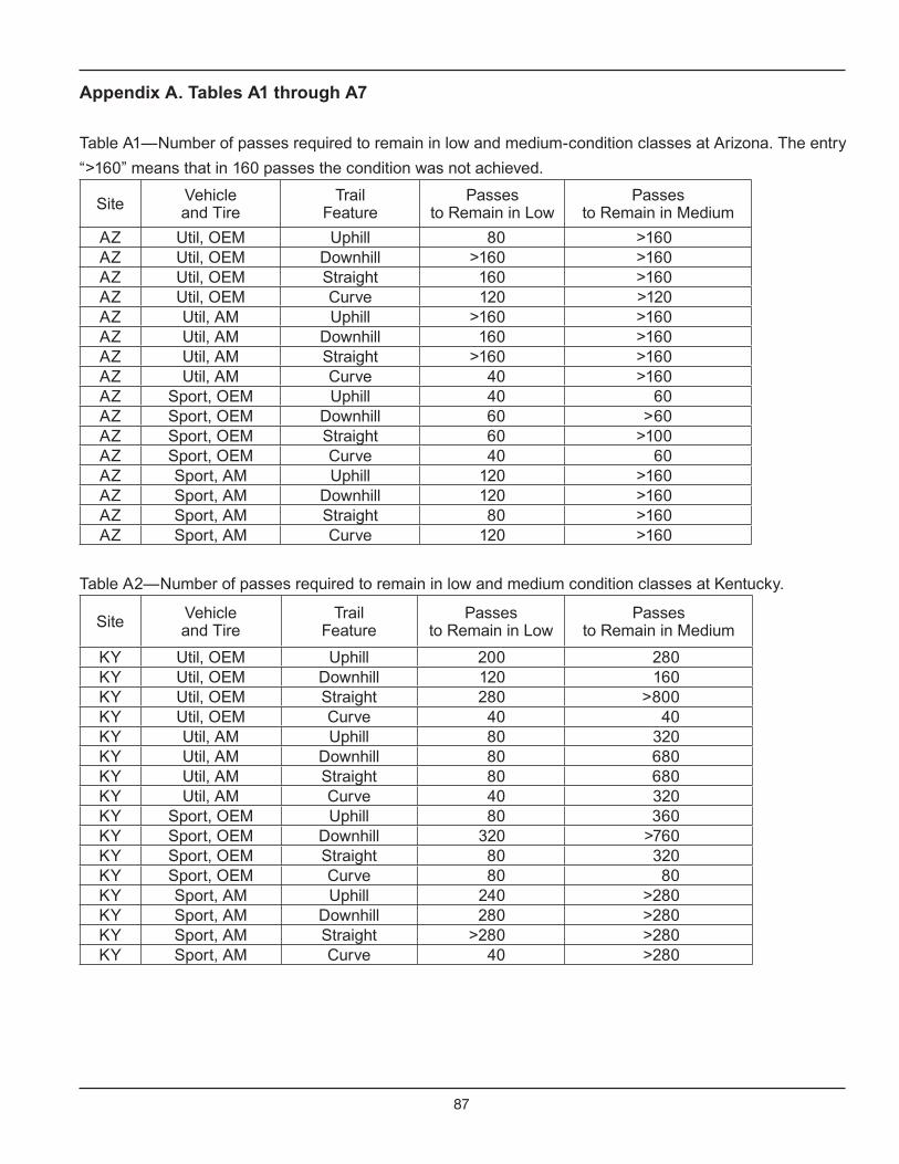
87

Appendix A. Tables A1 through A7

Table A1—Number of passes required to remain in low and medium-condition classes at Arizona. The entry

“>160” means that in 160 passes the condition was not achieved.

Site Vehicleand Tire

TrailFeature

Passesto Remain in Low

Passesto Remain in Medium

AZ Util, OEM Uphill 80 >160AZ Util, OEM Downhill >160 >160AZ Util, OEM Straight 160 >160AZ Util, OEM Curve 120 >120AZ Util, AM Uphill >160 >160AZ Util, AM Downhill 160 >160AZ Util, AM Straight >160 >160AZ Util, AM Curve 40 >160AZ Sport, OEM Uphill 40 60AZ Sport, OEM Downhill 60 >60AZ Sport, OEM Straight 60 >100AZ Sport, OEM Curve 40 60AZ Sport, AM Uphill 120 >160AZ Sport, AM Downhill 120 >160AZ Sport, AM Straight 80 >160AZ Sport, AM Curve 120 >160

Table A2—Number of passes required to remain in low and medium condition classes at Kentucky.

Site Vehicleand Tire

TrailFeature

Passesto Remain in Low

Passesto Remain in Medium

KY Util, OEM Uphill 200 280KY Util, OEM Downhill 120 160KY Util, OEM Straight 280 >800KY Util, OEM Curve 40 40KY Util, AM Uphill 80 320KY Util, AM Downhill 80 680KY Util, AM Straight 80 680KY Util, AM Curve 40 320KY Sport, OEM Uphill 80 360KY Sport, OEM Downhill 320 >760KY Sport, OEM Straight 80 320KY Sport, OEM Curve 80 80KY Sport, AM Uphill 240 >280KY Sport, AM Downhill 280 >280KY Sport, AM Straight >280 >280KY Sport, AM Curve 40 >280

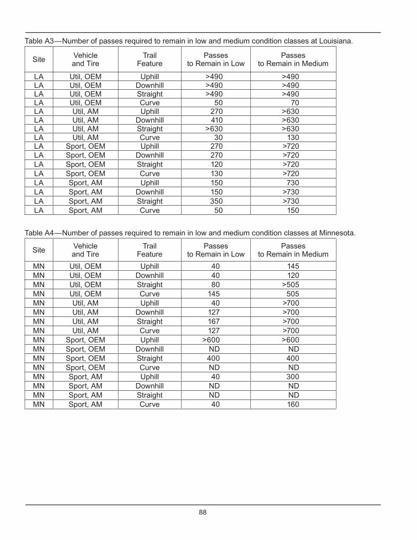
88

Table A3—Number of passes required to remain in low and medium condition classes at Louisiana.

Site Vehicleand Tire

TrailFeature

Passesto Remain in Low

Passesto Remain in Medium

LA Util, OEM Uphill >490 >490LA Util, OEM Downhill >490 >490LA Util, OEM Straight >490 >490LA Util, OEM Curve 50 70LA Util, AM Uphill 270 >630LA Util, AM Downhill 410 >630LA Util, AM Straight >630 >630LA Util, AM Curve 30 130LA Sport, OEM Uphill 270 >720LA Sport, OEM Downhill 270 >720LA Sport, OEM Straight 120 >720LA Sport, OEM Curve 130 >720LA Sport, AM Uphill 150 730LA Sport, AM Downhill 150 >730LA Sport, AM Straight 350 >730LA Sport, AM Curve 50 150

Table A4—Number of passes required to remain in low and medium condition classes at Minnesota.

Site Vehicleand Tire

TrailFeature

Passesto Remain in Low

Passesto Remain in Medium

MN Util, OEM Uphill 40 145MN Util, OEM Downhill 40 120MN Util, OEM Straight 80 >505MN Util, OEM Curve 145 505MN Util, AM Uphill 40 >700MN Util, AM Downhill 127 >700MN Util, AM Straight 167 >700MN Util, AM Curve 127 >700MN Sport, OEM Uphill >600 >600MN Sport, OEM Downhill ND NDMN Sport, OEM Straight 400 400MN Sport, OEM Curve ND NDMN Sport, AM Uphill 40 300MN Sport, AM Downhill ND NDMN Sport, AM Straight ND NDMN Sport, AM Curve 40 160

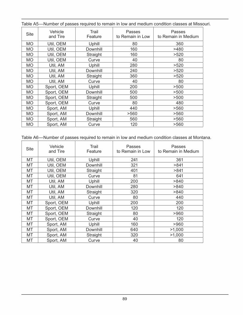
89

Table A5—Number of passes required to remain in low and medium condition classes at Missouri.

Site Vehicleand Tire

TrailFeature

Passesto Remain in Low

Passesto Remain in Medium

MO Util, OEM Uphill 80 360MO Util, OEM Downhill 160 >480MO Util, OEM Straight 160 >520MO Util, OEM Curve 40 80MO Util, AM Uphill 280 >520MO Util, AM Downhill 240 >520MO Util, AM Straight 360 >520MO Util, AM Curve 40 80MO Sport, OEM Uphill 200 >500MO Sport, OEM Downhill 500 >500MO Sport, OEM Straight 500 >500MO Sport, OEM Curve 80 480MO Sport, AM Uphill 440 >560MO Sport, AM Downhill >560 >560MO Sport, AM Straight 560 >560MO Sport, AM Curve 120 >560

Table A6—Number of passes required to remain in low and medium condition classes at Montana.

Site Vehicleand Tire

TrailFeature

Passesto Remain in Low

Passesto Remain in Medium

MT Util, OEM Uphill 241 361MT Util, OEM Downhill 321 >841MT Util, OEM Straight 401 >841MT Util, OEM Curve 81 641MT Util, AM Uphill 200 >840MT Util, AM Downhill 280 >840MT Util, AM Straight 320 >840MT Util, AM Curve 80 440MT Sport, OEM Uphill 200 200MT Sport, OEM Downhill 120 120MT Sport, OEM Straight 80 >960MT Sport, OEM Curve 40 120MT Sport, AM Uphill 160 >960MT Sport, AM Downhill 640 >1,000MT Sport, AM Straight 320 >1,000MT Sport, AM Curve 40 80

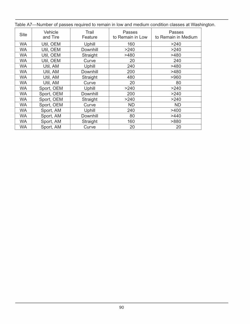
90

Table A7—Number of passes required to remain in low and medium condition classes at Washington.

Site Vehicleand Tire

TrailFeature

Passesto Remain in Low

Passesto Remain in Medium

WA Util, OEM Uphill 160 >240WA Util, OEM Downhill >240 >240WA Util, OEM Straight >480 >480WA Util, OEM Curve 20 240WA Util, AM Uphill 240 >480WA Util, AM Downhill 200 >480WA Util, AM Straight 480 >960WA Util, AM Curve 20 80WA Sport, OEM Uphill >240 >240WA Sport, OEM Downhill 200 >240WA Sport, OEM Straight >240 >240WA Sport, OEM Curve ND NDWA Sport, AM Uphill 240 >400WA Sport, AM Downhill 80 >440WA Sport, AM Straight 160 >880WA Sport, AM Curve 20 20

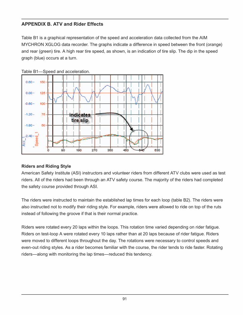
91

APPENDIX B. ATV and Rider Effects

Table B1 is a graphical representation of the speed and acceleration data collected from the AIM

MYCHRON XGLOG data recorder. The graphs indicate a difference in speed between the front (orange)

and rear (green) tire. A high rear tire speed, as shown, is an indication of tire slip. The dip in the speed

graph (blue) occurs at a turn.

Table B1—Speed and acceleration.

Riders and Riding Style

American Safety Institute (ASI) instructors and volunteer riders from different ATV clubs were used as test

riders. All of the riders had been through an ATV safety course. The majority of the riders had completed

the safety course provided through ASI.

The riders were instructed to maintain the established lap times for each loop (table B2). The riders were

also instructed not to modify their riding style. For example, riders were allowed to ride on top of the ruts

instead of following the groove if that is their normal practice.

Riders were rotated every 20 laps within the loops. This rotation time varied depending on rider fatigue.

Riders on test-loop A were rotated every 10 laps rather than at 20 laps because of rider fatigue. Riders

were moved to different loops throughout the day. The rotations were necessary to control speeds and

even-out riding styles. As a rider becomes familiar with the course, the rider tends to ride faster. Rotating

riders—along with monitoring the lap times—reduced this tendency.

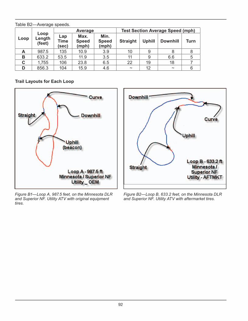
92

Table B2—Average speeds.

LoopLoop

Length(feet)

Average Test Section Average Speed (mph)Lap Time (sec)

Max. Speed (mph)

Min. Speed (mph)

Straight Uphill Downhill Turn

A 987.5 135 10.9 3.9 10 9 8 8B 633.2 53.5 11.9 3.5 11 9 6.6 5C 1,755 106 23.8 6.5 22 19 18 7D 856.3 104 15.9 4.6 ~ 12 ~ 6

Trail Layouts for Each Loop

Figure B1—Loop A, 987.5 feet, on the Minnesota DLR and Superior NF. Utility ATV with original equipment tires.

Figure B2—Loop B, 633.2 feet, on the Minnesota DLR and Superior NF. Utility ATV with aftermarket tires.

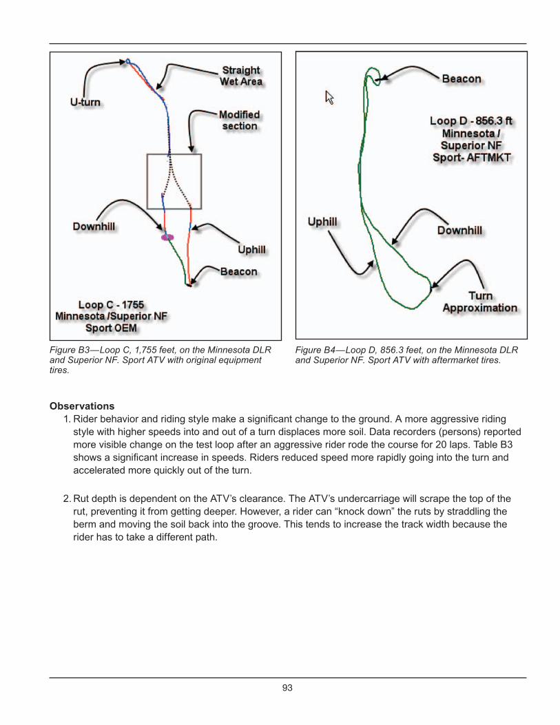
93

Observations1. Rider behavior and riding style make a significant change to the ground. A more aggressive riding

style with higher speeds into and out of a turn displaces more soil. Data recorders (persons) reported more visible change on the test loop after an aggressive rider rode the course for 20 laps. Table B3 shows a significant increase in speeds. Riders reduced speed more rapidly going into the turn and accelerated more quickly out of the turn.

2. Rut depth is dependent on the ATV’s clearance. The ATV’s undercarriage will scrape the top of the rut, preventing it from getting deeper. However, a rider can “knock down” the ruts by straddling the berm and moving the soil back into the groove. This tends to increase the track width because the rider has to take a different path.

Figure B3—Loop C, 1,755 feet, on the Minnesota DLR and Superior NF. Sport ATV with original equipment tires.

Figure B4—Loop D, 856.3 feet, on the Minnesota DLR and Superior NF. Sport ATV with aftermarket tires.

95

APPENDIX C

Monitoring fugitive dust emissions from off highway vehicles traveling on unpaved roads: a quantitative technique

Pamela Padgett, Ph.D.USDA Forest Service, Riverside Fire Lab

Atmospheric Deposition Unit.

Final Report To the Recreation Unit – San Dimas Technology CenterAugust 2, 2006

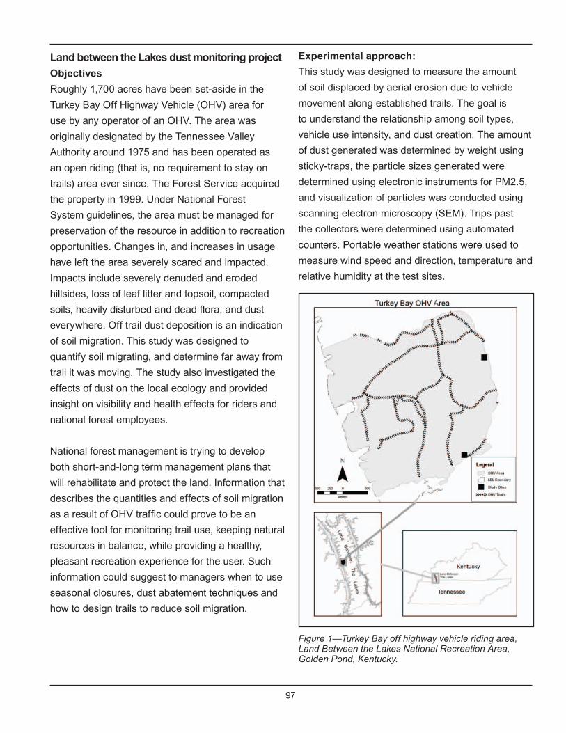
97

Land between the Lakes dust monitoring project

Objectives

Roughly 1,700 acres have been set-aside in the

Turkey Bay Off Highway Vehicle (OHV) area for

use by any operator of an OHV. The area was

originally designated by the Tennessee Valley

Authority around 1975 and has been operated as

an open riding (that is, no requirement to stay on

trails) area ever since. The Forest Service acquired

the property in 1999. Under National Forest

System guidelines, the area must be managed for

preservation of the resource in addition to recreation

opportunities. Changes in, and increases in usage

have left the area severely scared and impacted.

Impacts include severely denuded and eroded

hillsides, loss of leaf litter and topsoil, compacted

soils, heavily disturbed and dead flora, and dust

everywhere. Off trail dust deposition is an indication

of soil migration. This study was designed to

quantify soil migrating, and determine far away from

trail it was moving. The study also investigated the

effects of dust on the local ecology and provided

insight on visibility and health effects for riders and

national forest employees.

National forest management is trying to develop

both short-and-long term management plans that

will rehabilitate and protect the land. Information that

describes the quantities and effects of soil migration

as a result of OHV traffic could prove to be an

effective tool for monitoring trail use, keeping natural

resources in balance, while providing a healthy,

pleasant recreation experience for the user. Such

information could suggest to managers when to use

seasonal closures, dust abatement techniques and

how to design trails to reduce soil migration.

Experimental approach:

This study was designed to measure the amount

of soil displaced by aerial erosion due to vehicle

movement along established trails. The goal is

to understand the relationship among soil types,

vehicle use intensity, and dust creation. The amount

of dust generated was determined by weight using

sticky-traps, the particle sizes generated were

determined using electronic instruments for PM2.5,

and visualization of particles was conducted using

scanning electron microscopy (SEM). Trips past

the collectors were determined using automated

counters. Portable weather stations were used to

measure wind speed and direction, temperature and

relative humidity at the test sites.

Figure 1—Turkey Bay off highway vehicle riding area, Land Between the Lakes National Recreation Area, Golden Pond, Kentucky.

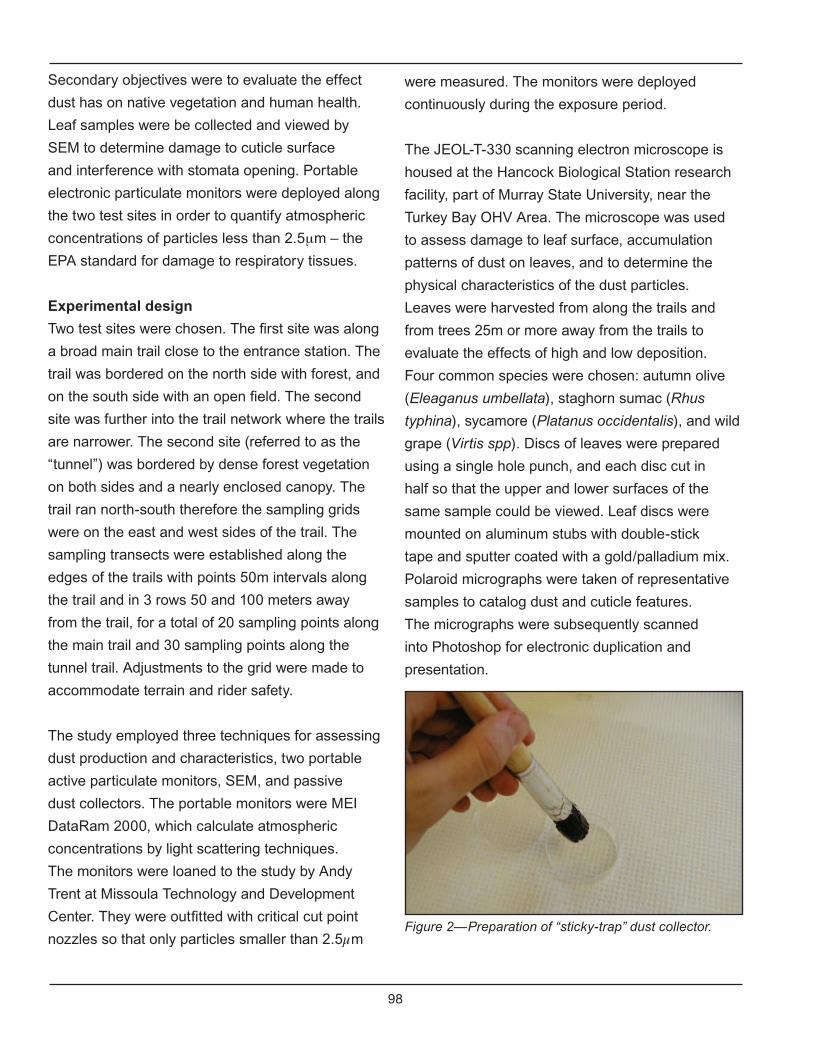
98

Secondary objectives were to evaluate the effect

dust has on native vegetation and human health.

Leaf samples were be collected and viewed by

SEM to determine damage to cuticle surface

and interference with stomata opening. Portable

electronic particulate monitors were deployed along

the two test sites in order to quantify atmospheric

concentrations of particles less than 2.5μm – the

EPA standard for damage to respiratory tissues.

Experimental design

Two test sites were chosen. The first site was along

a broad main trail close to the entrance station. The

trail was bordered on the north side with forest, and

on the south side with an open field. The second

site was further into the trail network where the trails

are narrower. The second site (referred to as the

“tunnel”) was bordered by dense forest vegetation

on both sides and a nearly enclosed canopy. The

trail ran north-south therefore the sampling grids

were on the east and west sides of the trail. The

sampling transects were established along the

edges of the trails with points 50m intervals along

the trail and in 3 rows 50 and 100 meters away

from the trail, for a total of 20 sampling points along

the main trail and 30 sampling points along the

tunnel trail. Adjustments to the grid were made to

accommodate terrain and rider safety.

The study employed three techniques for assessing

dust production and characteristics, two portable

active particulate monitors, SEM, and passive

dust collectors. The portable monitors were MEI

DataRam 2000, which calculate atmospheric

concentrations by light scattering techniques.

The monitors were loaned to the study by Andy

Trent at Missoula Technology and Development

Center. They were outfitted with critical cut point

nozzles so that only particles smaller than 2.5µm

were measured. The monitors were deployed

continuously during the exposure period.

The JEOL-T-330 scanning electron microscope is

housed at the Hancock Biological Station research

facility, part of Murray State University, near the

Turkey Bay OHV Area. The microscope was used

to assess damage to leaf surface, accumulation

patterns of dust on leaves, and to determine the

physical characteristics of the dust particles.

Leaves were harvested from along the trails and

from trees 25m or more away from the trails to

evaluate the effects of high and low deposition.

Four common species were chosen: autumn olive

(Eleaganus umbellata), staghorn sumac (Rhus

typhina), sycamore (Platanus occidentalis), and wild

grape (Virtis spp). Discs of leaves were prepared

using a single hole punch, and each disc cut in

half so that the upper and lower surfaces of the

same sample could be viewed. Leaf discs were

mounted on aluminum stubs with double-stick

tape and sputter coated with a gold/palladium mix.

Polaroid micrographs were taken of representative

samples to catalog dust and cuticle features.

The micrographs were subsequently scanned

into Photoshop for electronic duplication and

presentation.

Figure 2—Preparation of “sticky-trap” dust collector.

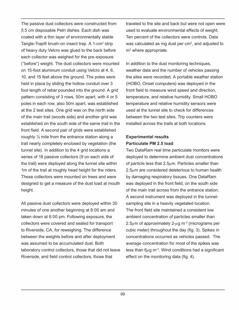
99

The passive dust collectors were constructed from

5.5 cm disposable Petri dishes. Each dish was

coated with a thin layer of environmentally stable

Tangle-Trap® brush-on insect trap. A 1-cm2 strip

of heavy duty Velcro was glued to the back before

each collector was weighed for the pre-exposure

(“before”) weight. The dust collectors were mounted

on 15-foot aluminum conduit using Velcro at 4, 6,

10, and 15 feet above the ground. The poles were

held in place by sliding the hollow conduit over 3

foot length of rebar pounded into the ground. A grid

pattern consisting of 3 rows, 50m apart, with 4 or 5

poles in each row, also 50m apart, was established

at the 2 test sites. One grid was on the north side

of the main trail (woods side) and another grid was

established on the south side of the same trail in the

front field. A second pair of grids were established

roughly ½ mile from the entrance station along a

trail nearly completely enclosed by vegetation (the

tunnel site). In addition to the 4 grid locations a

series of 18 passive collectors (9 on each side of

the trail) were deployed along the tunnel site within

1m of the trail at roughly head height for the riders.

These collectors were mounted on trees and were

designed to get a measure of the dust load at mouth

height.

All passive dust collectors were deployed within 30

minutes of one another beginning at 8:00 am and

taken down at 6:00 pm. Following exposure, the

collectors were covered and sealed for transport

to Riverside, CA, for reweighing. The difference

between the weights before and after deployment

was assumed to be accumulated dust. Both

laboratory control collectors, those that did not leave

Riverside, and field control collectors, those that

traveled to the site and back but were not open were

used to evaluate environmental effects of weight.

Ten percent of the collectors were controls. Data

was calculated as mg dust per cm2, and adjusted to

m2 where appropriate.

In addition to the dust monitoring techniques,

weather data and the number of vehicles passing

the sites were recorded. A portable weather station

(HOBO, Onset computers) was deployed in the

front field to measure wind speed and direction,

temperature, and relative humidity. Small HOBO

temperature and relative humidity sensors were

used at the tunnel site to check for differences

between the two test sites. Trip counters were

installed across the trails at both locations.

Experimental results

Particulate PM 2.5 load

Two DataRam real time particulate monitors were

deployed to determine ambient dust concentrations

of particle less that 2.5µm. Particles smaller than

2.5µm are considered deleterious to human health

by damaging respiratory tissues. One DataRam

was deployed in the front field, on the south side

of the main trail across from the entrance station.

A second instrument was deployed in the tunnel-

sampling site in a heavily vegetated location.

The front field site maintained a consistent low

ambient concentration of particles smaller than

2.5µm of approximately 2-µg m-3 (micrograms per

cubic meter) throughout the day (fig. 3). Spikes in

concentrations occurred as vehicles passed. The

average concentration for most of the spikes was

less than 6µg m-3. Wind conditions had a significant

effect on the monitoring data (fig. 4).

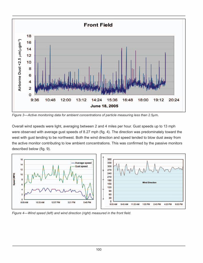
100

Figure 3—Active monitoring data for ambient concentrations of particle measuring less than 2.5µm.

Overall wind speeds were light, averaging between 2 and 4 miles per hour. Gust speeds up to 13 mph

were observed with average gust speeds of 8.27 mph (fig. 4). The direction was predominately toward the

west with gust tending to be northwest. Both the wind direction and speed tended to blow dust away from

the active monitor contributing to low ambient concentrations. This was confirmed by the passive monitors

described below (fig. 9).

Figure 4—Wind speed (left) and wind direction (right) measured in the front field.

Air

bo

rne

Du

st <

2.5

m

(g

m-3

)

N--

----

----

---E

----

----

----

-S--

----

----

--W

----

----

----

----

--N

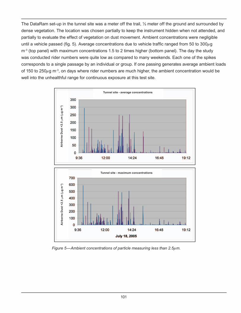
101

The DataRam set-up in the tunnel site was a meter off the trail, ½ meter off the ground and surrounded by

dense vegetation. The location was chosen partially to keep the instrument hidden when not attended, and

partially to evaluate the effect of vegetation on dust movement. Ambient concentrations were negligible

until a vehicle passed (fig. 5). Average concentrations due to vehicle traffic ranged from 50 to 300µg

m-3 (top panel) with maximum concentrations 1.5 to 2 times higher (bottom panel). The day the study

was conducted rider numbers were quite low as compared to many weekends. Each one of the spikes

corresponds to a single passage by an individual or group. If one passing generates average ambient loads

of 150 to 250µg m-3, on days where rider numbers are much higher, the ambient concentration would be

well into the unhealthful range for continuous exposure at this test site.

Figure 5—Ambient concentrations of particle measuring less than 2.5µm.

Air

bo

rne

Du

st

<2

.5

m (

g

m-3

)A

irb

orn

e D

us

t <

2.5

m

(

g m

-3)

Tunnel site - average concentrations

Tunnel site - maximum concentrations

102

Total particulate loads estimated by the passive

monitors deployed at the riders’ head height (about

4 feet off the ground) was 0.433 mg cm2, or roughly

4.33 g of dust per meter of trail over the 10 hour

sampling period.

Ambient particulate loading and human

health

The EPA has shifted from an absolute concentration

metric for determining concern levels for human

health to an index system. The index is based on

a 24-hour average concentration and has a scale

of 0 to 500 for all criteria pollutants (those that

EPA has established health risks for). Above 100

is considered unhealthy for sensitive groups. An

index of 100 is equivalent to 40-µg m-3 PM 2.5.

An index of 150 is unhealthy for all individuals

and corresponds to 65.4-µg m-3. A calculator to

converting concentration to index and visa-a-versa

can be found at:

http://cfpub.epa.gov/airnow/index.cfm?action=aqi.aqi_conc_

calc

The current EPA method does not account for very

high, but short acute exposures. On the day of the

experiment the air quality at both sites was good

with short episodes of very unhealthful air.

Although dust was visible for longer periods than

were recorded by the particulate monitors, based

on images of particulates accumulating on leaf

surfaces, most of the dust particles generated

by OHVs are larger than 2.5µm (fig. 6). Based

on this limited information and the current EPA

interpretation, particles sent airborne by OHV traffic

do not pose any long-term health concerns at the

rider densities encountered on June 18, 2005.

Vegetation

Leaf samples from autumn olive (Eleaganus

umbellata), staghorn sumac (Rhus typhina),

sycamore (Platanus occidentalis), and wild grape

(Virtis spp) were collected next to the main trail and

25 meters away from the trail. The sampling day

followed several days of heavy rain so only small

amounts or dust was visible to the naked eye. Dust

deposition assessments were made using a JEOL-

T-330 scanning electron microscope. Images were

assessed for:

1. Physical damage such as abrasions, broken

trichomes and punctures.

2. Percent surface area occupied by dust

particles.

3. Blocked stomata.

4. Estimated size of particles.

In comparing samples on and off the trail, the

leaves collected along the trail did have a higher

number of particles on the surface, but there was

no observed difference in lesions or superficial

damage. Particles were observed on both sides of

the leaves (fig. 6). All four of the species examined

had stomata on the underside of the leaves

exclusively, which is common for temperate zone

plants, and important for dust interference with leaf

respiration. A few examples of particles blocking

stomata were observed and captured in images,

but there were no consistent patterns of stomatal

blockage due to dust deposition (figs. 6 and 7).

Based on a visual assessment, it does not appear

that plants growing along the roads and trails are

severely impacted by dust generated by OHVs,

as long as heavy traffic is followed by rain. We

did not do a physiological assessment where

photosynthesis and respiration were measured, but

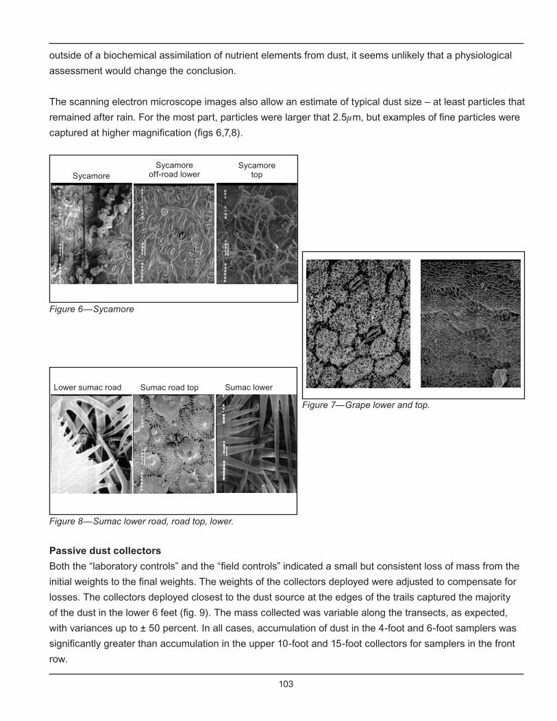
103

outside of a biochemical assimilation of nutrient elements from dust, it seems unlikely that a physiological

assessment would change the conclusion.

The scanning electron microscope images also allow an estimate of typical dust size – at least particles that

remained after rain. For the most part, particles were larger that 2.5µm, but examples of fine particles were

captured at higher magnification (figs 6,7,8).

Passive dust collectors

Both the “laboratory controls” and the “field controls” indicated a small but consistent loss of mass from the

initial weights to the final weights. The weights of the collectors deployed were adjusted to compensate for

losses. The collectors deployed closest to the dust source at the edges of the trails captured the majority

of the dust in the lower 6 feet (fig. 9). The mass collected was variable along the transects, as expected,

with variances up to ± 50 percent. In all cases, accumulation of dust in the 4-foot and 6-foot samplers was

significantly greater than accumulation in the upper 10-foot and 15-foot collectors for samplers in the front

row.

Figure 7—Grape lower and top.

Figure 8—Sumac lower road, road top, lower.

Lower sumac road Sumac road top Sumac lower

Figure 6—Sycamore

SycamoreSycamore

off-road lowerSycamore

top

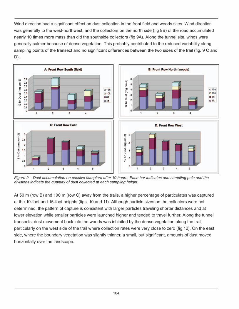
104

Wind direction had a significant effect on dust collection in the front field and woods sites. Wind direction

was generally to the west-northwest, and the collectors on the north side (fig 9B) of the road accumulated

nearly 10 times more mass than did the southside collectors (fig 9A). Along the tunnel site, winds were

generally calmer because of dense vegetation. This probably contributed to the reduced variability along

sampling points of the transect and no significant differences between the two sides of the trail (fig. 9 C and

D).

Figure 9—Dust accumulation on passive samplers after 10 hours. Each bar indicates one sampling pole and the divisions indicate the quantity of dust collected at each sampling height.

At 50 m (row B) and 100 m (row C) away from the trails, a higher percentage of particulates was captured

at the 10-foot and 15-foot heights (figs. 10 and 11). Although particle sizes on the collectors were not

determined, the pattern of capture is consistent with larger particles traveling shorter distances and at

lower elevation while smaller particles were launched higher and tended to travel further. Along the tunnel

transects, dust movement back into the woods was inhibited by the dense vegetation along the trail,

particularly on the west side of the trail where collection rates were very close to zero (fig 12). On the east

side, where the boundary vegetation was slightly thinner, a small, but significant, amounts of dust moved

horizontally over the landscape.

12 h

r D

us

t (m

g c

m-2

)

12 h

r D

us

t (m

g c

m-2

)

12 h

r D

us

t (m

g c

m-2

)

12 h

r D

us

t (m

g c

m-2

)

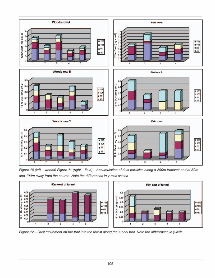
105

Figure 10 (left – woods) Figure 11 (right – field)—Accumulation of dust particles along a 200m transect and at 50m

and 100m away from the source. Note the differences in y-axis scales.

Figure 12—Dust movement off the trail into the forest along the tunnel trail. Note the differences in y-axis.

12 h

r D

us

t (m

g c

m-2

) 12

hr

Du

st

(mg

cm

-2)

12 h

r D

us

t (m

g c

m-2

)

12 h

r D

us

t (m

g c

m-2

) 12

hr

Du

st

(mg

cm

-2)

12 h

r D

us

t (m

g c

m-2

) 12

hr

Du

st

(mg

cm

-2)

12 h

r D

us

t (m

g c

m-2

)

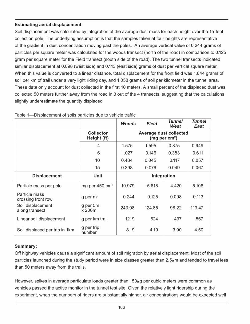
106

Estimating aerial displacement

Soil displacement was calculated by integration of the average dust mass for each height over the 15-foot

collection pole. The underlying assumption is that the samples taken at four heights are representative

of the gradient in dust concentration moving past the poles. An average vertical value of 0.244 grams of

particles per square meter was calculated for the woods transect (north of the road) in comparison to 0.125

gram per square meter for the Field transect (south side of the road). The two tunnel transects indicated

similar displacement at 0.098 (west side) and 0.113 (east side) grams of dust per vertical square meter.

When this value is converted to a linear distance, total displacement for the front field was 1,844 grams of

soil per km of trail under a very light riding day, and 1,058 grams of soil per kilometer in the tunnel area.

These data only account for dust collected in the first 10 meters. A small percent of the displaced dust was

collected 50 meters further away from the road in 3 out of the 4 transects, suggesting that the calculations

slightly underestimate the quantity displaced.

Table 1—Displacement of soils particles due to vehicle traffic

Woods Field TunnelWest

TunnelEast

CollectorHeight (ft)

Average dust collected (mg per cm2)

4 1.575 1.595 0.875 0.949

6 1.027 0.146 0.383 0.611

10 0.484 0.045 0.117 0.057

15 0.398 0.076 0.049 0.067

Displacement Unit Integration

Particle mass per pole mg per 450 cm2 10.979 5.618 4.420 5.106

Particle mass crossing front row g per m2 0.244 0.125 0.098 0.113

Soil displacement along transect

g per 5m x 200m 243.98 124.85 98.22 113.47

Linear soil displacement g per km trail 1219 624 497 567

Soil displaced per trip in 1km g per trip number 8.19 4.19 3.90 4.50

Summary:

Off highway vehicles cause a significant amount of soil migration by aerial displacement. Most of the soil

particles launched during the study period were in size classes greater than 2.5µm and tended to travel less

than 50 meters away from the trails.

However, spikes in average particulate loads greater than 150µg per cubic meters were common as

vehicles passed the active monitor in the tunnel test site. Given the relatively light ridership during the

experiment, when the numbers of riders are substantially higher, air concentrations would be expected well

107

into the unhealthful range where the forested edges of the trails inhibit air circulation. Where the trails are

open with adequate air circulation, such as along the main trail by the entrance station, the particulate loads

have lower impacts on human health. The passive samplers deployed at head-height confirm a substantial

atmospheric loading that could have effects on the rider’s respiratory systems.

The evaluation of dust effects on vegetation suggests that OHVs cause only minor perturbations.

Some stomatal blockage was observed, and surface accumulations of dust that may periodically inhibit

photosynthesis and respiration, but little superficial damage to the cuticle was evident in the images

captured by SEM. Because of frequent rainfall, it is unlikely that the effects are long lasting or a cause

for serious concern. Vegetation naturally tends to be thickest along the sides trails because of reduced

competition for nutrients and water in the trails (this is typically called an edge effect). This density tends

to shelter understory plants off the trail from large deposits of dust and any subsequent deleterious effects,

and therefore should be maintained or encouraged.

Overall, the results of this study demonstrate the success of using a low-tech particulate trap for

determining soil migration and atmospheric loading due to vehicle traffic on unpaved roads.

109

REFERENCES

Alberts, E. E.; Nearing, M. A.; Weltz, M. A.; Risse, L. M.; Pierson, F. B.; Zhang, X. C.; Laflen, J. M.;

Simanton, J. R. 1995. Soil Component. In USDA - Water Erosion Prediction Project Hillslope Profile and

Watershed Model Documentation, 7.1 - 7.47. D. C. Flanagan and M. A. Nearing, eds. NSERL Report No.

10. West Lafayette, IN: U.S. Department of Agriculture, Agriculture Research Service, National Soil Erosion

Research Laboratory.

Cordell, H. Ken and others. 2000. American’s participation in outdoor recreation: Results from the national

survey on recreation and the environment. Athens, GA: U.S. Forest Service, Southern Research Station.

Elliot, W. E.; Foltz, R. B.; Luce, C. H. 1993. Validation of the WEPP model for forest roads. ASAE Paper No.

932502. St. Joseph, MI: American Society Agricultural Engineers

English, D. 2003. Personal communication. U.S. Forest Service, Southern Research Station.

Fangmeier, D. D.; Elliot, W. J.; Workman, S. R.; Huffman, R. L.; Schwab, G. O. 2006. Soil and Water

Conservation Engineering, 5th Edition. Thomson Delmar Learning, 502 p.

Flanagan, D. C.; Livingston, S. J. (eds.). 1995. WEPP user summary. NSERL Report No. 11. West

Lafayette, IN: National Soil Erosion Laboratory. 131 p.

Foster, G. R.; Flanagan, D. C.; Nearing, M. A.; Lane, L. J.; Risse, L. M.; Finkner, S. C. 1995. Hillslope

erosion component. In USDA - Water Erosion Prediction Project Hillslope Profile and Watershed Model

Documentation, 7.1 - 7.47. Flanagan, D. C. and Nearing, M. A. eds. NSERL Report No. 10, West Lafayette,

IN: U.S. Department of Agriculture, Agriculture Research Service, National Soil Erosion Research

Laboratory.

Knowlton, J. 2003. Personal communication. Washington, DC: U.S. Forest Service, Office of

Communication.

McMahon, S. 1995. Accuracy of two ground survey methods for assessing site disturbance. Journal of

Forest Engineering 6(2).

Page-Dumroese, D.; Jurgensen, M.; Elliot, W.; Rice, T.; Nesser, J.; Collins, T.; Meurisse, R. 2000. Soil

Quality Standards and Guidelines for Forest Sustainability in Northwestern North America. Forest Ecology

and Management. Vol. 138, p 445-462.

Padgett, P. 2006. Monitoring fugitive dust emissions from off highway vehicles traveling on unpaved roads:

a quantitative technique. Riverside, CA: U.S. Forest Service, Riverside Fire Lab, Atmospheric Deposition

Unit. 15p.

Paterson, R. 2003. Personal communication. Washington, DC: U.S. Forest Service, Assistant Director,

Recreation, Heritage, and Wilderness Resources.

110

Robertson, R. 2003. Personal communication. Great Falls, MT: U.S. Forest Service, Northern Region,

Lewis and Clark National Forest.

Specialty Vehicle Institute of America. 2007. Special report summer 2007. Web site: http://www.svia.org/

sviapressreleases/SVIA_A2_Final_Low.pdf

Stokowski, P. A.; LaPointe, C. B. 2000. Environmental and social effects of ATVs and ORVs: An annotated

bibliography and research assessment. Burlington, VT: University of Vermont, School of Natural Resources.

32p.

Stone, J. J.; Lane, L. J.; Shirley, E. D.; Hernandez, M. 1995. Hillslope surface hydrology. In USDA - Water

Erosion Prediction Project Hillslope Profile and Watershed Model Documentation, 4.1 - 4.20. Flanagan,

D. C. and Nearing, M. A. eds. NSERL Report No. 10. West Lafayette, IN: U.S. Department of Agriculture,

Agricultural Research Service, National Soil Erosion Research Laboratory.

U.S. Department of Agriculture, Agriculture Research Service. 1995. Technical Documentation, USDA

– Water Erosion Prediction Project (WEPP). NSERL Report No. 10. West Lafayette, IN: U.S. Department of

Agriculture, Agriculture Research Service, National Soil Erosion Research Laboratory.

U.S. Department of Agriculture, Agriculture Research Service. 1995. WEPP user summary. NSERL Report

No. 11. West Lafayette, IN: U.S. Department of Agriculture, Agricultural Research Service, National Soil

Erosion Research Laboratory. 131 p.

U.S. Department of Agriculture, Forest Service. 1975. Stream reach inventory and channel stability

evaluation - a watershed management procedure. Missoula, MT: U.S. Department of Agriculture, Forest

Service, Northern Region.

U.S. Department of Agriculture, Forest Service. 2003. Changing the debate on managing national forests

and grasslands. Available at: http://www.fs.fed.us/news/2003/speeches/09/change-debate.shtml. 3 May 2006.

U.S. Department of Agriculture, Forest Service. 2004. On the right trail! Managing off-highway vehicles.

Available at http://www.fs.fed.us/recreation/programs/ohv/ohv_use.pdf .

U.S. Department of Agriculture, Forest Service. 2007. Strategic plan for fiscal years 2007-2012. Web site:

http://www.fs.fed.us/publications/strategic/fs-sp-fy07-12.pdf

Forest Service and U.S. Department of the Interior Bureau of Land Management employees also can view

videos, CDs, and SDTDC’s individual project pages on their internal computer network at: http://fsweb.sdtdc.

wo.fs.fed.us/

For additional information on the ATV study, contact Dexter Meadows at SDTDC. Phone: 909–599–1267

ext 276. E-mail: dmeadows@fs.fed.us