Effect of viscoelasticity in a second-grade fluid under the action of an electric

CASIRJ Volume 1 Issue 2 ISSN 2319 – 9202

International Research Journal of Commerce Arts and Science http:www.casirj.com 53

Effect of viscoelasticity in a second-grade fluid under the action of an

electric field

S Chandra*

Department of Mathematics, Jadavpur University,

Kolkata 700 032, India

Abstract

This article presents an analysis for blood flow through a channel under the influence of

an alternating electric field. The blood vessel is modeled as a channel and the nature of

blood is accounted through a second grade fluid model. The influence of rheological

parameters like Reynolds number and fluid viscoelasticity has been plotted in 3-D

graph. The effect of stern and diffuse layer (EDL) formed near the vicinity of the walls

has been well understood in the flow pattern of blood flow with the change in

viscoelasticity.

Keywords: Blood flow; Second-grade fluid; Viscoelasticity.

1 Introduction

It is now well known that the flow through human circulatory system can vary to a certain extent under the

application of a magnetic field as well as en electric field. Several investigations have been carried out in

the past regarding the change in blood flow velocity under the influence of a magnetic field [1, 3]. But

there are very few works where the blood flow is taken into account under the action of an electric field

considering blood as non-Newtonian fluid. With the progress of micro lab-on-a-chip-devices and its wider

necessity in recent days draws the attention of many researchers [4,5] for electroosmotic flow of a fluid

where it is possible to have a minute and accurate variation of blood flow in a microchannel.

When a solid surface comes in contact with an aqueous solution of an electrolyte, electrical Double

Layer (EDL) is formed near the vicinity of the walls. This EDL has sizeable effects onto the flow of blood.

The practical relevance of this electroosmotic flow is also available in many scientific literatures. Some

recent works about electroosmotic flow demonstrates the effect of electroosmotic flow in case of a non-

Newtonian fluid [6,7].

Among various non-Newtonian fluid models the second grade fluid model is capable to describe the

complex behaviour of viscoelastic fluid. To understand the effect of viscoelasticity and the effect of

Reynolds number under the purview of second grade fluid model the present study is motivated toward

searching for a flow behavior of blood under the action of an alternating electric field. Framing appropriate

constitutive equations, a mathematical analysis has been obtained to study the effect of the viscoelastic

parameter in the ionized motion of a viscoelastic fluid.


International Research Journal of Commerce Arts and Science http:www.casirj.com Page 154

2. Mathematical Formulation:

Let the electroosmotic flow be confined in the channel 0 ≤ y ≤ h, where h, the channel height be

considered to be much smaller than width w and the length of the channel. Gravitational effect and the

joule heating effect being small are neglected during the solution of this problem.

Taking into consideration the Boussinesq incompressible fluid model, the boundary-layer equations for

the second grade viscoelastic fluid in the presence of a time-periodic electric field can be given by

𝜕𝑢

𝜕𝑡= −

1

𝜌

𝜕𝑝

𝜕𝑥+ 𝜈

𝜕2𝑢

𝜕𝑦2 + 𝑘𝜕3𝑦

𝜕𝑡 𝜕𝑦2 +𝜌𝑒

𝜌(𝐸𝑥𝑒

𝑖𝜔𝑒 𝑡) ……………… (1)

and

0 = −1

𝜌

𝜕𝑝

𝜕𝑦 ……………………………..(2)

Gauss's law of charge distribution states that

𝜕2𝜓

𝜕𝑦2 = −𝜌𝑒

𝜀, ……………………………….. (3)

Where 𝜌𝑒 = 2𝑛0𝑒𝑧 sinh(𝑒𝑧

𝐾𝐵𝑇𝜓) is net electric charge density and we is the angular frequency of the AC

electric field, Ex is the amplitude of the electric field and t denotes the time. The electrical double layers

are assumed to be thin. The symbols ν, k, and ρ represent the kinematic viscosity, viscoelastic co-

efficient, and density respectively. .

Setting non-dimensional variables like

𝑥∗ =𝑥

ℎ ; 𝑦∗ =

𝑦

ℎ ; 𝑢∗ =

𝑢

𝑈𝐻𝑆 ; 𝜔∗ =

𝜔𝑈𝐻𝑆

ℎ

; 𝜔𝑒∗ =

𝜔𝑒𝑈𝐻𝑆

ℎ

; …………………..(4)

𝑅 =𝑈𝐻𝑆 ℎ

𝜈 ; 𝑘∗ =

𝑘𝑈𝐻𝑆

𝜈ℎ ; 𝑝∗ =

𝑝ℎ

𝜌𝜈𝑈𝐻𝑆 ; 𝜓∗ =

𝜓

𝜁 ; 𝑡∗ =

𝑡ℎ

𝑈𝐻𝑆

…………………….(5)

UHS is the Helmholtz-Smoluchowski electroosmotic velocity and can be given by,

𝑈𝐻𝑆 = −𝑀𝐸𝑥 = −𝜁𝜀𝐸𝑥

𝜇 , …………………… . (6)

in which M is the mobility, 𝜁 is the zeta potential, ε is the dielectric constant of the medium and 𝜇 =

𝜌𝜈 , represents the dynamic viscosity.

In terms of the dimensionless variables, equations (1)-(3) can be written as

𝑅𝜕𝑢∗

𝜕𝑡∗= −

𝜕𝑝∗

𝜕𝑥∗ +𝜕2𝑢∗

𝜕𝑦∗2 + 𝑘∗ 𝜕3𝑢∗

𝜕𝑡∗𝜕𝑦∗2 +𝜕2𝜓∗

𝜕𝑦∗2 (𝑒𝑖𝜔𝑒∗𝑡∗) ………………………… (7)



𝜕𝑝∗

𝜕𝑦 ∗ = 0 …………………………………….. (8)

and 𝜕2𝜓∗

𝜕𝑦∗2 = −2𝑛0𝑒𝑧ℎ

2

𝜁𝜀𝑠𝑖𝑛ℎ

𝑒𝑧𝜁

𝐾𝐵𝑇𝜓∗ , …………………………………………(9)

R is the Reynolds number and is given by =𝑈𝐻𝑆 ℎ

𝜈 , h is the half-width of the channel.

As we know that the electric potential energy is small in comparison with the thermal energy of the ions,

we can write 𝑒𝑧𝜁𝜓∗ < 𝐾𝐵𝑇 , the equation (9) reduces to

𝜕2𝜓∗

𝜕𝑦∗2= 𝑚2𝜓∗ …………………… . . (10)

where m represents Debye-Huckel parameter (in non-dimensional form) and is defined by

𝑚2 =ℎ2

𝜆2=

2𝑛0𝑒2𝑧2ℎ2

𝐾𝐵𝑇𝜓∗

λ is the thickness of the Debye layer.

The solution of equation (10) subject to the boundary conditions

𝜓∗ 0 = 0 , 𝜓∗ ±1 = 1

and

(𝜕𝜓∗

𝜕𝑦∗)𝑦∗=0 = 0

is given by

𝜓∗ 𝑦∗ =𝑐𝑜𝑠ℎ(𝑚𝑦∗)

𝑐𝑜𝑠ℎ(𝑚 )……………………………… (11)

Dropping the superscript “*” and assuming

velocity u as 𝑢 = 𝑢𝑠𝑒𝑖𝜔1𝑡 , where us represents the steady part of the velocity (independent of time)

and with the boundary conditions,

𝜕𝑢

𝜕𝑦= 0 𝑎𝑡 𝑦 = 0 and

𝑢 = 0 𝑎𝑡 𝑦 = ±1 …………………………….(12)



and considering 𝜔𝑒 − 𝜔1= 𝜔 , after solving we get

Solving under the above boundary conditions, we obtain,

𝑢𝑠 = 2𝐶 cosh 𝑚1𝑦 +𝐵(1 + 𝑘𝑖𝜔)

𝑅𝑒 𝑖𝜔−

𝑚2

2 cosh(𝑚)

𝑒𝑚𝑦 + 𝑒−𝑚𝑦

𝑚2 −𝑅𝑒 𝑖𝜔

1 + 𝐾𝑖𝜔

, ………… (13)

where,

𝑚1 = 𝑅𝑒 𝑖𝜔

1 + 𝐾𝑖𝜔

and

𝐶 =1

2 cosh(𝑚1) −

𝐵 1 + 𝐾𝑖𝜔

𝑅𝑒 𝑖𝜔+

𝑚2

𝑚2 −𝑅𝑒𝑖𝜔

1 + 𝐾𝑖𝜔

From the expression of 𝑢 = 𝑢𝑠𝑒𝑖𝜔1𝑡 , the fluid velocity u is determined using Mathematica and the result

is presented graphically to get the snap shot view of the variation in u with the Reynolds number R and

the viscoelastic coefficient k.

3 Results

Variation in velocity distribution as time (t) progresses or as the distance from the mid-channel (y)

increases has been computed and graphs are drawn using the software MATHEMATICA. In order to

have an idea about blood flow dynamics under electric field the physical parameters are chosen

commensurate with that of blood.

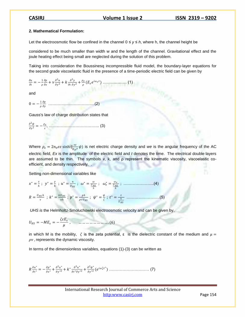
Fig. 1 Variation in blood flow velocity during electroosmotic flow with the change in

Reynolds number R, when m=50, t=5, B=30, k=0.05, we = 50, 𝜔1 = 20.



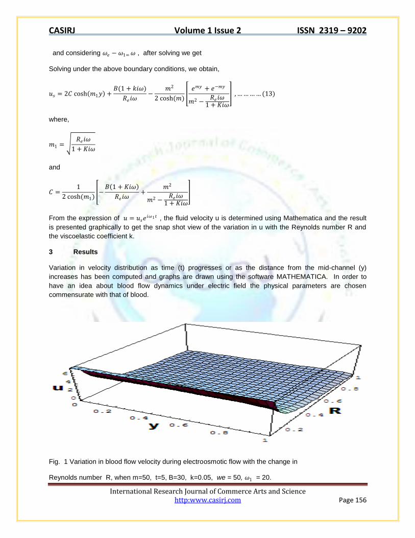
Fig. 2 Variation in blood flow during electro-osmotic flow as time t progresses with the change in

Reynolds number R, when m=50, t=5, B=30, k=0.005, we = 50, 𝜔1 = 20.

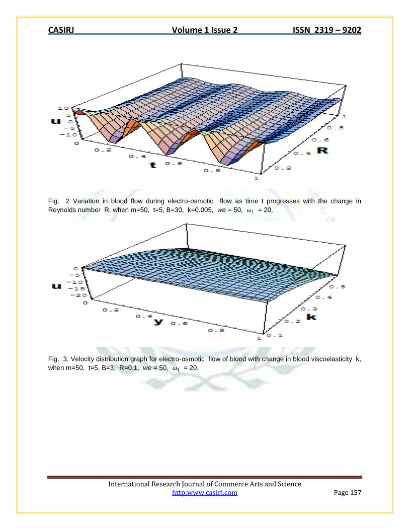
Fig. 3. Velocity distribution graph for electro-osmotic flow of blood with change in blood viscoelasticity k,

when m=50, t=5, B=3, R=0.1, we = 50, 𝜔1 = 20.



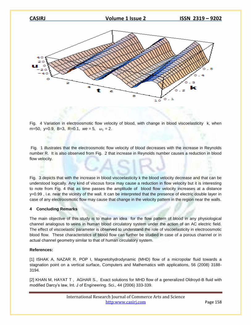
Fig. 4 Variation in electroosmotic flow velocity of blood, with change in blood viscoelasticity k, when

m=50, y=0.9, B=3, R=0.1, we = 5, 𝜔1 = 2.

Fig. 1 illustrates that the electroosmotic flow velocity of blood decreases with the increase in Reynolds

number R. It is also observed from Fig. 2 that increase in Reynolds number causes a reduction in blood

flow velocity.

Fig. 3 depicts that with the increase in blood viscoelasticity k the blood velocity decrease and that can be

understood logically. Any kind of viscous force may cause a reduction in flow velocity but it is interesting

to note from Fig. 4 that as time passes the amplitude of blood flow velocity increases at a distance

y=0.99 , i.e. near the vicinity of the wall. It can be interpreted that the presence of electric double layer in

case of any electroosmotic flow may cause that change in the velocity pattern in the region near the walls.

4 Concluding Remarks

The main objective of this study is to make an idea for the flow pattern of blood in any physiological

channel analogous to veins in human blood circulatory system under the action of an AC electric field.

The effect of viscoelastic parameter is observed to understand the role of viscoelasticity in electroosmotic

blood flow. These characteristics of blood flow can further be studied in case of a porous channel or in

actual channel geometry similar to that of human circulatory system.

References:

[1] ISHAK A, NAZAR R, POP I, Magnetohydrodynamic (MHD) flow of a micropolar fluid towards a

stagnation point on a vertical surface, Computers and Mathematics with applications, 56 (2008) 3188-

3194.

[2] KHAN M, HAYAT T , AGHAR S., Exact solutions for MHD flow of a generalized Oldroyd-B fluid with

modified Darcy’s law, Int. J of Engineering. Sci., 44 (2006) 333-339.



[3] KHAN M, ALI S H, HAYAT T, FETECAU C, MHD flows of a second grade fluid between two side walls

perpendicular to a plate through a porous medium, Int. J of Non Linear Mech. , DOI : 10.1016/

j.ijnonlinmec.2007.12.016.

[4] HERR A.E., MOLHO J.I., SANTIAGO J.G., MUNGAL M.G., Kenny T.W., Electro- osmotic

capillary flow with non-uniform zeta potential Anal. Chem. 72(2000) 1053-1057.

[5] YANG R.J., FU L.M., LIN Y.C., Electro-osmotic flow in microchannels, J. Colloid

Interface Sci. 239 ( 2001) 98-105.

[6] TANG G.H., LI X.F., HE Y.L., TAO W.Q., Electro-osmotic flow of non-Newtonian fluid in

microchannels. J. Non-Newt. Fluid Mech, 157 (2009) 133-137.

[7] ZHAO C, ZHOLKOVSKIJ E, MASLIYAH J.H, YANG C, Analysis of electroosmotic flow of

Effect of viscoelasticity in a second-grade fluid under the action of an electric

Documents

Transcript of Effect of viscoelasticity in a second-grade fluid under the action of an electric