EEG classification of imagined syllable rhythm using Hilbert spectrum methods

This article has been downloaded from IOPscience. Please scroll down to see the full text article.

2010 J. Neural Eng. 7 046006

(http://iopscience.iop.org/1741-2552/7/4/046006)

Download details:

IP Address: 128.200.38.28

The article was downloaded on 17/06/2010 at 23:16

Please note that terms and conditions apply.

View the table of contents for this issue, or go to the journal homepage for more

Home Search Collections Journals About Contact us My IOPscience

IOP PUBLISHING JOURNAL OF NEURAL ENGINEERING

J. Neural Eng. 7 (2010) 046006 (13pp) doi:10.1088/1741-2560/7/4/046006

EEG classification of imagined syllablerhythm using Hilbert spectrum methodsSiyi Deng, Ramesh Srinivasan, Tom Lappas and Michael D’Zmura1

Department of Cognitive Sciences, University of California, Irvine, SSPA 3151, Irvine,CA 92697-5100, USA

E-mail: mdzmura@uci.edu

Received 29 April 2010Accepted for publication 11 May 2010Published 16 June 2010Online at stacks.iop.org/JNE/7/046006

AbstractWe conducted an experiment to determine whether the rhythm with which imagined syllablesare produced may be decoded from EEG recordings. High density EEG data were recorded forseven subjects while they produced in imagination one of two syllables in one of threedifferent rhythms. We used a modified second-order blind identification (SOBI) algorithm toremove artefact signals and reduce data dimensionality. The algorithm uses the consistenttemporal structure along multi-trial EEG data to blindly decompose the original recordings.For the four primary SOBI components, joint temporal and spectral features were extractedfrom the Hilbert spectra (HS) obtained by a Hilbert–Huang transformation (HHT). The HSprovide more accurate time-spectral representations of non-stationary data than doconventional techniques like short-time Fourier spectrograms and wavelet scalograms.Classification of the three rhythms yields promising results for inter-trial transfer, withperformance for all subjects significantly greater than chance. For comparison, we testedclassification performance of three averaging-based methods, using features in the temporal,spectral and time–frequency domains, respectively, and the results are inferior to those of theSOBI-HHT-based method. The results suggest that the rhythmic structure of imagined syllableproduction can be detected in non-invasive brain recordings and provide a step towards thedevelopment of an EEG-based system for communicating imagined speech.

(Some figures in this article are in colour only in the electronic version)

1. Introduction

Recent advances in EEG technology have caused a surgeof interest in the development of a brain–computer interface(BCI). BCI research often focuses on finding a substitute for abroken mind–body chain that can help paralysed patients moveand communicate. Much research has been directed towardsbuilding a brain–computer interface which would allow its userto avoid the need for motor output by allowing direct corticalcontrol of prostheses or machines (e.g. Donchin et al 2000,Birbaumer et al 2000, Craelius 2002, Blankertz et al 2004).Research on classifying mind states using various forms ofbrain-imaging data has contributed to these advances. Forexample, scientists have successfully predicted the properties

1 Author to whom any correspondence should be addressed.

of unseen visual stimuli using fMRI signals from the primaryvisual cortex (Haynes and Rees 2005). EEG signals recordedduring imagined movement may also be classified (Ince et al2006, Wang and Makeig 2009) and used for real-time control(Pfurtscheller et al 2006, Leeb et al 2007, Zhao et al 2009).Such results confirm that the human cortex generates signalsobservable extracranially which may be used to infer theinternal state of the subject.

Research on decoding verbal thoughts from brain signalscan be dated back to the 1960s, when attempts were madeto transmit letters using Morse code extracted from EEG(Dewan 1967). BCI text generation based on the P300oddball paradigm has been a particularly successful approachto communication based on brain signals alone (Wolpaw et al2000, Schalk et al 2004). There are also potential non-clinicalapplications of BCIs for communication. In situations where

1741-2560/10/046006+13$30.00 1 © 2010 IOP Publishing Ltd Printed in the UK

J. Neural Eng. 7 (2010) 046006 S Deng et al

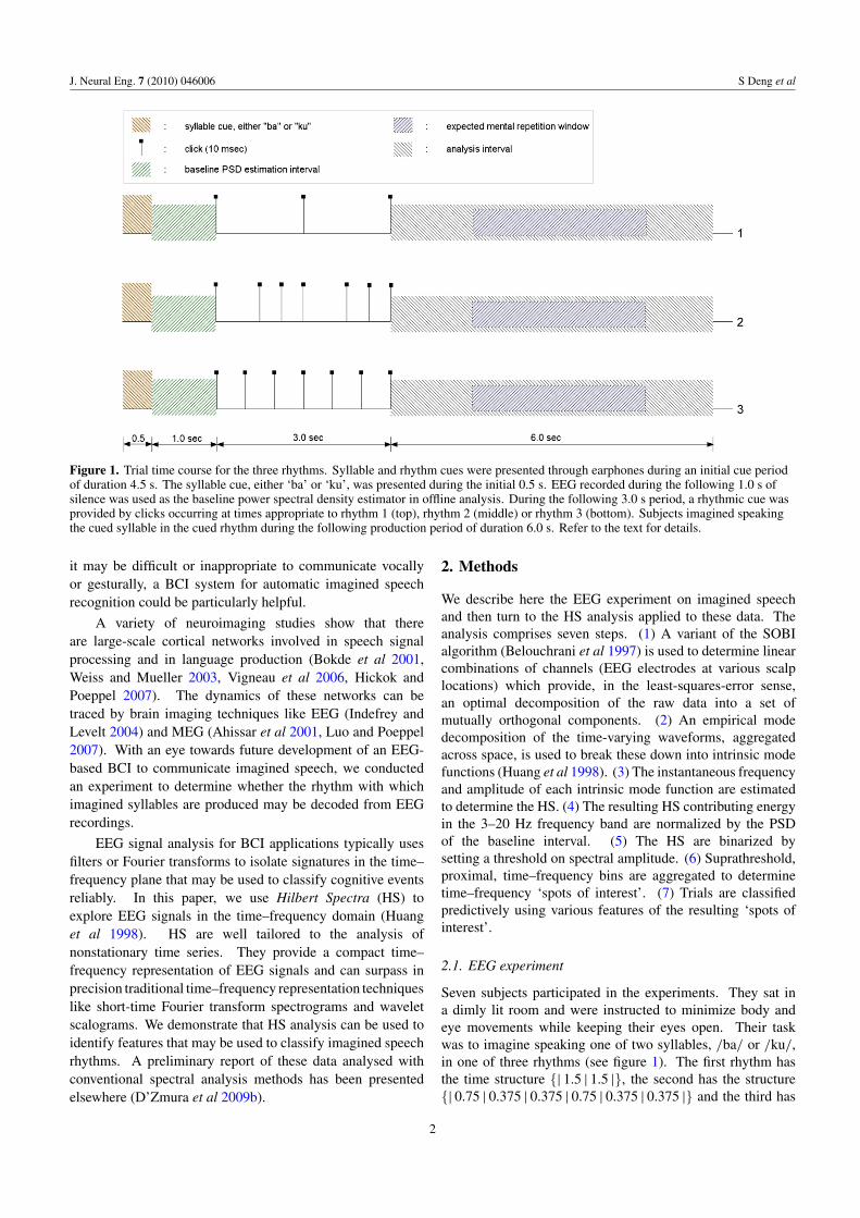
Figure 1. Trial time course for the three rhythms. Syllable and rhythm cues were presented through earphones during an initial cue periodof duration 4.5 s. The syllable cue, either ‘ba’ or ‘ku’, was presented during the initial 0.5 s. EEG recorded during the following 1.0 s ofsilence was used as the baseline power spectral density estimator in offline analysis. During the following 3.0 s period, a rhythmic cue wasprovided by clicks occurring at times appropriate to rhythm 1 (top), rhythm 2 (middle) or rhythm 3 (bottom). Subjects imagined speakingthe cued syllable in the cued rhythm during the following production period of duration 6.0 s. Refer to the text for details.

it may be difficult or inappropriate to communicate vocallyor gesturally, a BCI system for automatic imagined speechrecognition could be particularly helpful.

A variety of neuroimaging studies show that thereare large-scale cortical networks involved in speech signalprocessing and in language production (Bokde et al 2001,Weiss and Mueller 2003, Vigneau et al 2006, Hickok andPoeppel 2007). The dynamics of these networks can betraced by brain imaging techniques like EEG (Indefrey andLevelt 2004) and MEG (Ahissar et al 2001, Luo and Poeppel2007). With an eye towards future development of an EEG-based BCI to communicate imagined speech, we conductedan experiment to determine whether the rhythm with whichimagined syllables are produced may be decoded from EEGrecordings.

EEG signal analysis for BCI applications typically usesfilters or Fourier transforms to isolate signatures in the time–frequency plane that may be used to classify cognitive eventsreliably. In this paper, we use Hilbert Spectra (HS) toexplore EEG signals in the time–frequency domain (Huanget al 1998). HS are well tailored to the analysis ofnonstationary time series. They provide a compact time–frequency representation of EEG signals and can surpass inprecision traditional time–frequency representation techniqueslike short-time Fourier transform spectrograms and waveletscalograms. We demonstrate that HS analysis can be used toidentify features that may be used to classify imagined speechrhythms. A preliminary report of these data analysed withconventional spectral analysis methods has been presentedelsewhere (D’Zmura et al 2009b).

2. Methods

We describe here the EEG experiment on imagined speechand then turn to the HS analysis applied to these data. Theanalysis comprises seven steps. (1) A variant of the SOBIalgorithm (Belouchrani et al 1997) is used to determine linearcombinations of channels (EEG electrodes at various scalplocations) which provide, in the least-squares-error sense,an optimal decomposition of the raw data into a set ofmutually orthogonal components. (2) An empirical modedecomposition of the time-varying waveforms, aggregatedacross space, is used to break these down into intrinsic modefunctions (Huang et al 1998). (3) The instantaneous frequencyand amplitude of each intrinsic mode function are estimatedto determine the HS. (4) The resulting HS contributing energyin the 3–20 Hz frequency band are normalized by the PSDof the baseline interval. (5) The HS are binarized bysetting a threshold on spectral amplitude. (6) Suprathreshold,proximal, time–frequency bins are aggregated to determinetime–frequency ‘spots of interest’. (7) Trials are classifiedpredictively using various features of the resulting ‘spots ofinterest’.

2.1. EEG experiment

Seven subjects participated in the experiments. They sat ina dimly lit room and were instructed to minimize body andeye movements while keeping their eyes open. Their taskwas to imagine speaking one of two syllables, /ba/ or /ku/,in one of three rhythms (see figure 1). The first rhythm hasthe time structure {| 1.5 | 1.5 |}, the second has the structure{| 0.75 | 0.375 | 0.375 | 0.75 | 0.375 | 0.375 |} and the third has

2

J. Neural Eng. 7 (2010) 046006 S Deng et al

the structure {| 0.5 | 0.5 | 0.5 | 0.5 | 0.5 | 0.5 |}; the verticallines ‘|’ represent the expected times of imagined syllableproduction onset, while the numbers indicate the time intervalsin seconds between imagined syllables. Each experimentaltrial started with a period during which the syllable and rhythmwere cued; the cue period was followed by a period duringwhich the subject imagined saying the cued syllable in thecued rhythm without any vocalization (D’Zmura et al 2009a).

Each trial lasted 10.5 s. During the first 4.5 s, the cues tosyllable and rhythm were presented through earphones. Thesyllable cue, a spoken ‘ba’ or ‘ku’, was presented during theinitial 0.5 s of each trial. Clicks presented during the next 3.0 sinterval provided the cue to the rhythm. The cue period wasfollowed by an imagined speech production period of duration6.0 s. The subjects were instructed to imagine the cued syllableusing the cued rhythm and tempo identical to that indicated bythe cue period clicks.

Syllable and rhythm cues were presented using STAXelectro-static earphones. These headphones do not interferewith EEG recordings. EEG was recorded simultaneouslyusing a 128-channel Geodesic Sensor Net (ElectricalGeodesics Inc.) in combination with an ANT-128 (AdvancedNeuro Technology) amplifier. The EEG was sampled at1024 Hz and online average referenced. The presented cuesignals were accompanied by sinusoidal markers which werefed directly into the EEG amplifier to mark the onset times ofcue and imagined speech production periods of each trial.

Each subject performed 120 trials for each of the threerhythms and two syllables, for a total of 720 trials recordedper subject. During data analysis, we performed classificationon the data for all six conditions and for just three rhythms; thelatter analysis was conducted by pooling trials of two syllablesof the same rhythm to get 240 trials per rhythm. In our primaryanalysis, data from the 6.0 s long imagined speech periodswere analysed to determine whether one can decode imaginedspeech rhythm from EEG signals. In a second analysis, weused EEG data from the 3.0 s long click cue period of eachtrial to find out whether the cue sensory signals can be decodedfrom EEG.

2.2. Blind source separation using SOBI

For each subject, we used a variant of second-order blindidentification (SOBI) algorithm (Belouchrani et al 1997) todecompose the raw EEG data into a set of mutually orthogonalcomponents. The classical SOBI algorithm can be describedas follows. Consider an n-channel EEG time series x withmean zero. Each sample is assumed to be an instantaneouslinear mixture of n unknown sources s, where the mixingoccurs through some unknown linear mixing matrix A:

x = As. (1)

This can be written equivalently as

s = A−1x. (2)

In order to calculate the unknown separation matrix A−1,the data are first pre-whitened by finding a whitening matrixW so that the auto-correlation of x is normalized to identity:

z = Wx (3)

Rz,0 = E[(Wx)(Wx)T ] = WE[xxT ]WT

= WRx,0WT = I. (4)

In equations (3) and (4), z is the whitened time series, Rz,0 isthe (auto) correlation matrix of z at delay 0, E[] denotes theexpectation operator and I is an identity matrix of the samesize as the autocorrelation.

The whitening matrix W can be found by diagonalizingRx,0 as follows:

Rx,0 = PDP T (5)in which D is a diagonal matrix, whereby

W = D−1/zP T . (6)After pre-whitening, a set of cross-correlation matrices Rz,τ

is calculated for certain time delay values τ . We chose timedelay values that spanned a wide range, up to and includingthe Nyquist frequency (Tang et al 2005a). In this study we usethe values of

τ = {2, 4, 10, 20, 40, 80, 120, 250, 400, 512}. (7)These numbers of samples may be converted to delays (s)

using the sampling rate 1024 samples s−1. The key procedureof SOBI is to find a unitary transformation V that jointlydiagonalizes Rz,τ by minimizing the criterion (Cardoso 1998)∑

τ

∑i �=j

(V T Rz,τV )2i,j . (8)

The estimate of the separation matrix A−1 is thus providedby the product of the whitening matrix W (equation (6))and the unitary transformation matrix V that provides jointdiagonalization (equation (8)):

A−1 = V T W. (9)A problem which limits the application of classical SOBI

is that the transformation basis of recovered components is notconsistent across trials. By assuming a stationary distributionfor the neural basis, we can extend classical SOBI to multi-trialrecording by determining a single, approximate, pre-whiteningsolution and by jointly diagonalizing the cross-correlationmatrices for the same set of time delays across trials. First, theacross-trial pre-whitening solution is computed as

E[Rz,0] = WE[Rx,0]WT = I. (10)Second, the within-trial cross-correlation term Rz,0 is changedto the across-trial expectation E[Rz,τ ] for each time delayτ ; the joint diagonalization is then performed on theexpectations. Finally, after estimating the separation matrix,SOBI components are estimated separately for each trial byprojecting the raw data onto the SOBI space.

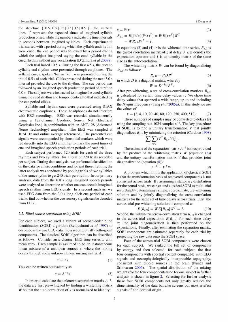
Four of the across-trial SOBI components were chosenfor each subject. We ranked the full set of componentsby energy and then selected, for each subject, the firstfour components with spectral content compatible with EEGsignals and neurophysiologically interpretable topography,consistent with dipole sources in the brain (Nunez andSrinivasan 2006). The spatial distribution of the mixingweights for the four components used for one subject in furtheranalysis is shown in figure 2. Selecting for further analysisthese four SOBI components not only greatly reduces thedimensionality of the data but also screens out most artefactsignals of non-cortical origin.

3

J. Neural Eng. 7 (2010) 046006 S Deng et al

Figure 2. Cortical distributions of the four SOBI components of the mixing weights for subject 6. Values are normalized to the range of[−1 1]. The regions bounded by solid black contour lines indicate positive mixing weights, while those regions bounded by dashed contourlines indicate negative mixing weights; mixing weight polarity is arbitrary.

2.3. Hilbert spectrum

The HS is an emerging method of joint time–frequencyrepresentation of signals. Unlike classical time–frequencyanalysis methods, HS does not employ a constant or lineartime versus frequency resolution window. It adaptively tracksthe evolution of the time–frequency basis in the original signaland can provide much detailed information at arbitrary time–frequency scales (Huang et al 1998). The fundamental stepin calculating an HS is the empirical mode decomposition(EMD). The EMD expresses a signal x in terms of a finite (andusually small) set of mathematically well-defined componentsc, called intrinsic mode functions (IMFs), and a residue term:

x =n∑

k=1

ck + γ . (11)

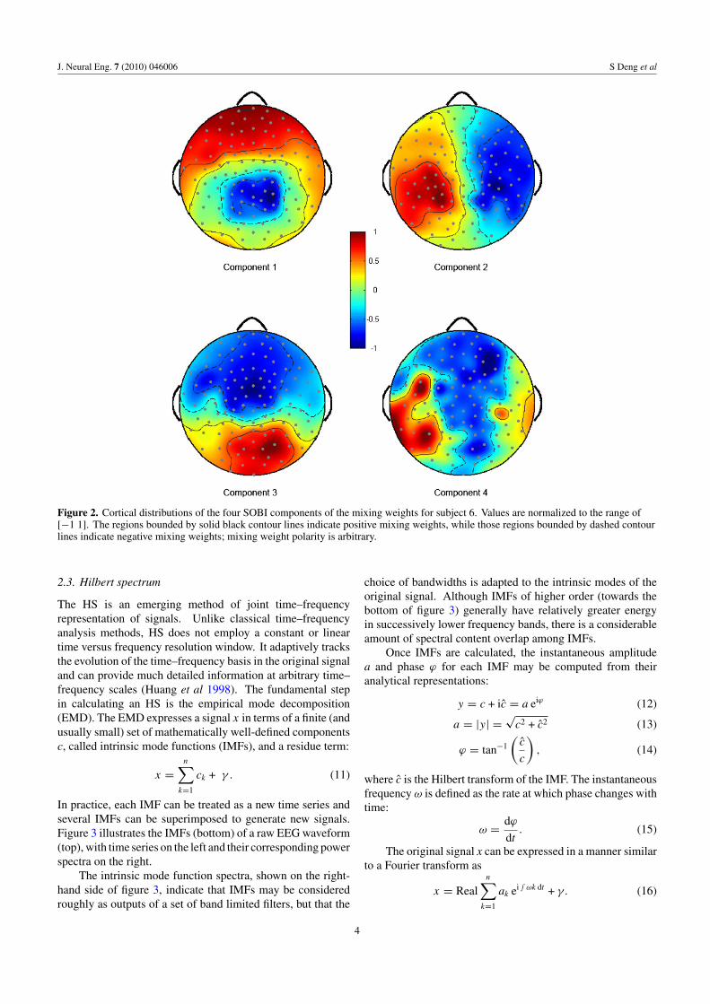
In practice, each IMF can be treated as a new time series andseveral IMFs can be superimposed to generate new signals.Figure 3 illustrates the IMFs (bottom) of a raw EEG waveform(top), with time series on the left and their corresponding powerspectra on the right.

The intrinsic mode function spectra, shown on the right-hand side of figure 3, indicate that IMFs may be consideredroughly as outputs of a set of band limited filters, but that the

choice of bandwidths is adapted to the intrinsic modes of theoriginal signal. Although IMFs of higher order (towards thebottom of figure 3) generally have relatively greater energyin successively lower frequency bands, there is a considerableamount of spectral content overlap among IMFs.

Once IMFs are calculated, the instantaneous amplitudea and phase ϕ for each IMF may be computed from theiranalytical representations:

y = c + ic = a eiϕ (12)

a = |y| =√

c2 + c2 (13)

ϕ = tan−1

(c

c

), (14)

where c is the Hilbert transform of the IMF. The instantaneousfrequency ω is defined as the rate at which phase changes withtime:

ω = dϕ

dt. (15)

The original signal x can be expressed in a manner similarto a Fourier transform as

x = Realn∑

k=1

ak ei ∫ωk dt + γ. (16)

4

J. Neural Eng. 7 (2010) 046006 S Deng et al

Figure 3. Example of the EMD and corresponding spectra for 4.5 s of EEG data for one electrode. The top-left panel shows the time courseof the raw EEG. The bottom-left panel shows all IMFs from the EMD, ranked downwards with successive order, and the residue, which isthe bottom-most component. The corresponding power spectra are shown in the right panels, on a logarithmic scale. The spectra of IMFsoverlap and differ from band pass-filtered spectra.

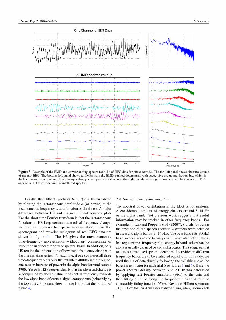
Finally, the Hilbert spectrum H(ω, t) can be visualizedby plotting the instantaneous amplitude a (or power) at theinstantaneous frequency ω as a function of the time t. A majordifference between HS and classical time–frequency plotslike the short-time Fourier transform is that the instantaneousfunctions in HS keep continuous track of frequency change,resulting in a precise but sparse representation. The HS,spectrogram and wavelet scalogram of real EEG data areshown in figure 4. The HS gives the most economictime–frequency representation without any compromise ofresolution in either temporal or spectral basis. In addition, onlyHS retains the information of how trend frequency changes inthe original time series. For example, if one compares all threetime–frequency plots over the 3500th to 4000th sample region,one sees an increase of power in the alpha band around sample3900. Yet only HS suggests clearly that the observed change isaccompanied by the adjustment of central frequency towardsthe low alpha band of certain signal components (primarily bythe topmost component shown in the HS plot at the bottom offigure 4).

2.4. Spectral density normalization

The spectral power distribution in the EEG is not uniform.A considerable amount of energy clusters around 8–14 Hzor the alpha band. Yet previous work suggests that usefulinformation may be tracked in other frequency bands. Forexample, in Luo and Poppel’s study (2007), signals followingthe envelope of the speech acoustic waveform were detectedin theta and alpha bands (3–14 Hz). The beta band (16–30 Hz)has also been suggested to carry cognitive-related information.In a regular time–frequency plot, energy in bands other than thealpha is usually dwarfed by the alpha peaks. This suggests thatone uses normalized spectral densities if activities in differentfrequency bands are to be evaluated equally. In this study, weused the 1 s of data directly following the syllable cue as thebaseline estimator for each trial (see figures 1 and 5). Baselinepower spectral density between 3 to 20 Hz was calculatedby applying fast Fourier transform (FFT) to the data andthen fitting a spline along the frequency bins to determinea smoothly fitting function M(ω). Next, the Hilbert spectrumH(ω, t) of that trial was normalized using M(ω) along each

5

J. Neural Eng. 7 (2010) 046006 S Deng et al

Figure 4. Comparison of the spectrogram, wavelet scalogram and Hilbert spectrum of a same time series. Top row: Original signal fromSOBI output. Second row: short-time Fourier transform spectrogram. Third row: wavelet scalogram, using a Morlet mother wavelet.Bottom row: Hilbert spectrum, projected onto a [3–20] Hz × 384 time-point grid. Instantaneous frequency trends from different IMFs arecoded with different colours but the intensity scale is kept the same (see figure 5 for the intensity scale).

time frame over the frequency window of 3–20 Hz to providethe spectral-density normalized Hilbert spectrum H :

H = H(ω, t)

M(ω). (17)

2.5. Energy normalization

The total energy in H can vary dramatically across trials,partly from the task and especially in a way which dependson the alertness of the subject. Such energy variation can beproblematic when setting thresholds on multiple trials. Toensure comparable spectral energy across different trials, wefurther normalized the total energy in each HS by the firstquartile Q1 of its power distribution:

¯H = H (ω, t)

Q1. (18)

We use Q1 instead of the median because the power distributionin EEG is skewed (Weineke et al 1980) and we expect Q1 to be amore robust estimator of the spontaneous EEG activities.

2.6. Binary transform and feature extraction

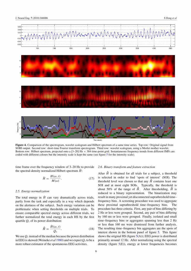
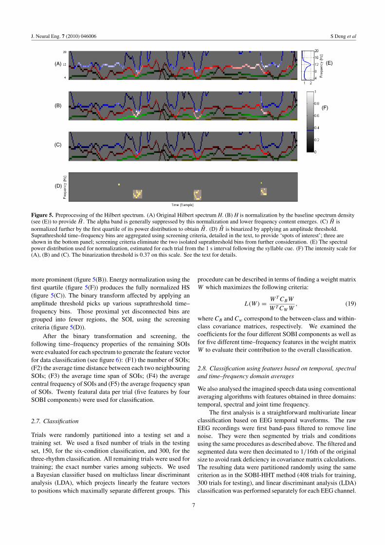
After ¯H is obtained for all trials for a subject, a thresholdis selected in order to find ‘spots of interest’ (SOI). Thethreshold level was chosen so that any ¯H contains least oneSOI and at most eight SOIs. Typically, the threshold isabout 50% of the range of ¯H . After thresholding, ¯H isreduced to a binary representation. The binarization mayresult in many proximal yet disconnected suprathreshold time–frequency bins. A screening procedure was used to aggregatethese proximal suprathreshold time–frequency bins. Theprocedure has three criteria. First, any pair of bins differing by2 Hz or less were grouped. Second, any pair of bins differingby 160 ms or less were grouped. Finally, isolated and smalltime–frequency bins or aggregates spanning less than 2 Hzor less than 160 ms were dismissed from further analysis.The resulting time–frequency bin aggregates are the spots ofinterest shown in the bottom panel of figure 5. This figureshows the original HS (figure 5(A)); EEG power is distributedprimarily around 12 Hz. After normalizing using the spectraldensity (figure 5(E)), energy at lower frequencies becomes

6

J. Neural Eng. 7 (2010) 046006 S Deng et al

(A)

(B)

(C)

(D)

(E)

(F)

Figure 5. Preprocessing of the Hilbert spectrum. (A) Original Hilbert spectrum H. (B) H is normalization by the baseline spectrum density(see (E)) to provide H . The alpha band is generally suppressed by this normalization and lower frequency content emerges. (C) H isnormalized further by the first quartile of its power distribution to obtain ¯H . (D) ¯H is binarized by applying an amplitude threshold.Suprathreshold time–frequency bins are aggregated using screening criteria, detailed in the text, to provide ‘spots of interest’; three areshown in the bottom panel; screening criteria eliminate the two isolated suprathreshold bins from further consideration. (E) The spectralpower distribution used for normalization, estimated for each trial from the 1 s interval following the syllable cue. (F) The intensity scale for(A), (B) and (C). The binarization threshold is 0.37 on this scale. See the text for details.

more prominent (figure 5(B)). Energy normalization using thefirst quartile (figure 5(F)) produces the fully normalized HS(figure 5(C)). The binary transform affected by applying anamplitude threshold picks up various suprathreshold time–frequency bins. Those proximal yet disconnected bins aregrouped into fewer regions, the SOI, using the screeningcriteria (figure 5(D)).

After the binary transformation and screening, thefollowing time–frequency properties of the remaining SOIswere evaluated for each spectrum to generate the feature vectorfor data classification (see figure 6): (F1) the number of SOIs;(F2) the average time distance between each two neighbouringSOIs; (F3) the average time span of SOIs; (F4) the averagecentral frequency of SOIs and (F5) the average frequency spanof SOIs. Twenty featural data per trial (five features by fourSOBI components) were used for classification.

2.7. Classification

Trials were randomly partitioned into a testing set and atraining set. We used a fixed number of trials in the testingset, 150, for the six-condition classification, and 300, for thethree-rhythm classification. All remaining trials were used fortraining; the exact number varies among subjects. We useda Bayesian classifier based on multiclass linear discriminantanalysis (LDA), which projects linearly the feature vectorsto positions which maximally separate different groups. This

procedure can be described in terms of finding a weight matrixW which maximizes the following criteria:

L(W) = WT CBW

WT CWW, (19)

where CB and Cw correspond to the between-class and within-class covariance matrices, respectively. We examined thecoefficients for the four different SOBI components as well asfor five different time–frequency features in the weight matrixW to evaluate their contribution to the overall classification.

2.8. Classification using features based on temporal, spectraland time–frequency domain averages

We also analysed the imagined speech data using conventionalaveraging algorithms with features obtained in three domains:temporal, spectral and joint time frequency.

The first analysis is a straightforward multivariate linearclassification based on EEG temporal waveforms. The rawEEG recordings were first band-pass filtered to remove linenoise. They were then segmented by trials and conditionsusing the same procedures as described above. The filtered andsegmented data were then decimated to 1/16th of the originalsize to avoid rank deficiency in covariance matrix calculations.The resulting data were partitioned randomly using the samecriterion as in the SOBI-HHT method (408 trials for training,300 trials for testing), and linear discriminant analysis (LDA)classification was performed separately for each EEG channel.

7

J. Neural Eng. 7 (2010) 046006 S Deng et al

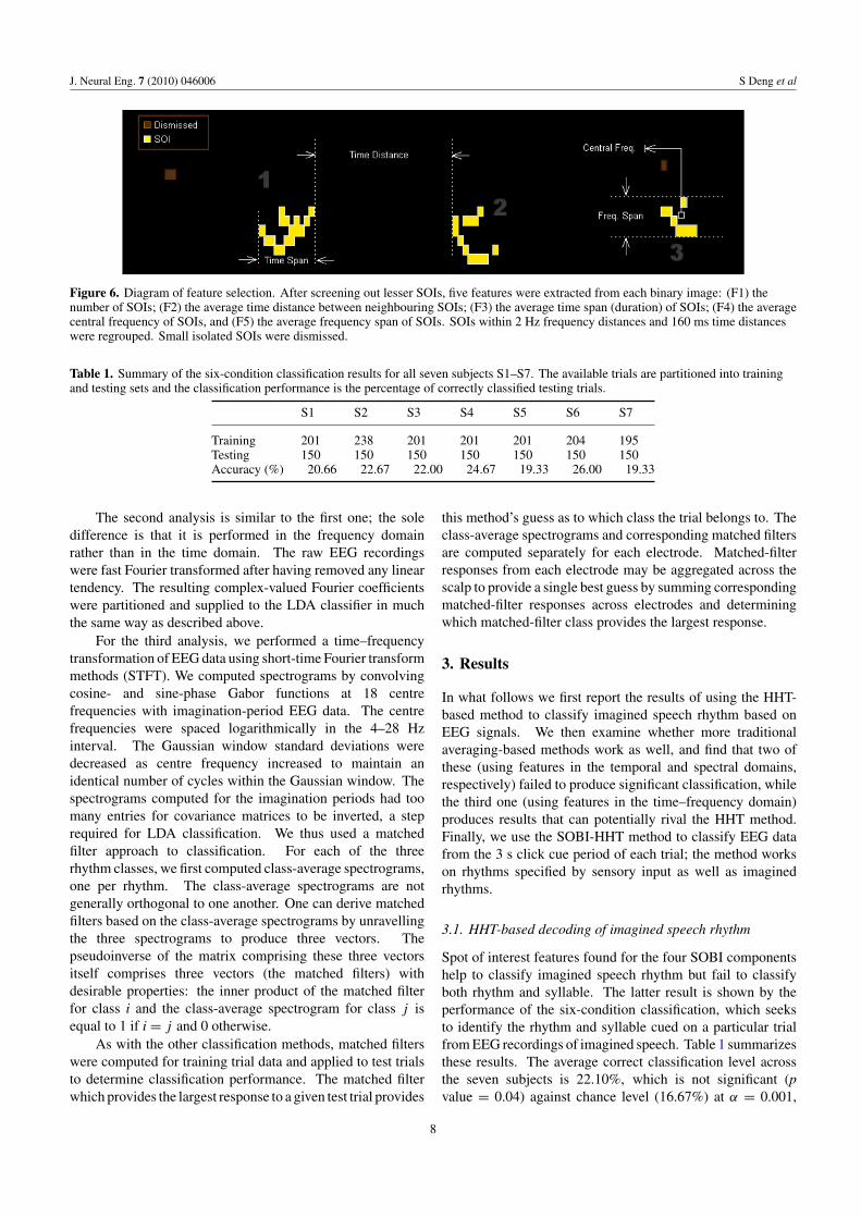
Figure 6. Diagram of feature selection. After screening out lesser SOIs, five features were extracted from each binary image: (F1) thenumber of SOIs; (F2) the average time distance between neighbouring SOIs; (F3) the average time span (duration) of SOIs; (F4) the averagecentral frequency of SOIs, and (F5) the average frequency span of SOIs. SOIs within 2 Hz frequency distances and 160 ms time distanceswere regrouped. Small isolated SOIs were dismissed.

Table 1. Summary of the six-condition classification results for all seven subjects S1–S7. The available trials are partitioned into trainingand testing sets and the classification performance is the percentage of correctly classified testing trials.

S1 S2 S3 S4 S5 S6 S7

Training 201 238 201 201 201 204 195Testing 150 150 150 150 150 150 150Accuracy (%) 20.66 22.67 22.00 24.67 19.33 26.00 19.33

The second analysis is similar to the first one; the soledifference is that it is performed in the frequency domainrather than in the time domain. The raw EEG recordingswere fast Fourier transformed after having removed any lineartendency. The resulting complex-valued Fourier coefficientswere partitioned and supplied to the LDA classifier in muchthe same way as described above.

For the third analysis, we performed a time–frequencytransformation of EEG data using short-time Fourier transformmethods (STFT). We computed spectrograms by convolvingcosine- and sine-phase Gabor functions at 18 centrefrequencies with imagination-period EEG data. The centrefrequencies were spaced logarithmically in the 4–28 Hzinterval. The Gaussian window standard deviations weredecreased as centre frequency increased to maintain anidentical number of cycles within the Gaussian window. Thespectrograms computed for the imagination periods had toomany entries for covariance matrices to be inverted, a steprequired for LDA classification. We thus used a matchedfilter approach to classification. For each of the threerhythm classes, we first computed class-average spectrograms,one per rhythm. The class-average spectrograms are notgenerally orthogonal to one another. One can derive matchedfilters based on the class-average spectrograms by unravellingthe three spectrograms to produce three vectors. Thepseudoinverse of the matrix comprising these three vectorsitself comprises three vectors (the matched filters) withdesirable properties: the inner product of the matched filterfor class i and the class-average spectrogram for class j isequal to 1 if i = j and 0 otherwise.

As with the other classification methods, matched filterswere computed for training trial data and applied to test trialsto determine classification performance. The matched filterwhich provides the largest response to a given test trial provides

this method’s guess as to which class the trial belongs to. Theclass-average spectrograms and corresponding matched filtersare computed separately for each electrode. Matched-filterresponses from each electrode may be aggregated across thescalp to provide a single best guess by summing correspondingmatched-filter responses across electrodes and determiningwhich matched-filter class provides the largest response.

3. Results

In what follows we first report the results of using the HHT-based method to classify imagined speech rhythm based onEEG signals. We then examine whether more traditionalaveraging-based methods work as well, and find that two ofthese (using features in the temporal and spectral domains,respectively) failed to produce significant classification, whilethe third one (using features in the time–frequency domain)produces results that can potentially rival the HHT method.Finally, we use the SOBI-HHT method to classify EEG datafrom the 3 s click cue period of each trial; the method workson rhythms specified by sensory input as well as imaginedrhythms.

3.1. HHT-based decoding of imagined speech rhythm

Spot of interest features found for the four SOBI componentshelp to classify imagined speech rhythm but fail to classifyboth rhythm and syllable. The latter result is shown by theperformance of the six-condition classification, which seeksto identify the rhythm and syllable cued on a particular trialfrom EEG recordings of imagined speech. Table 1 summarizesthese results. The average correct classification level acrossthe seven subjects is 22.10%, which is not significant (pvalue = 0.04) against chance level (16.67%) at α = 0.001,

8

J. Neural Eng. 7 (2010) 046006 S Deng et al

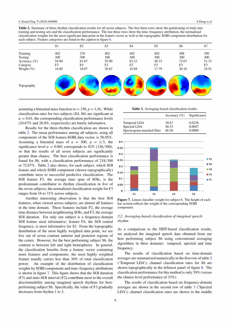
Table 2. Summary of three-rhythm classification results for all seven subjects. The first three rows show the partitioning of trials intotraining and testing sets and the classification performance. The last three rows show the time–frequency attribution, the normalizedclassification weights for the most significant data point in the feature vector as well as the topographic SOBI component distribution foreach subject. Feature categories are listed in the caption to figure 6.

S1 S2 S3 S4 S5 S6 S7

Training 402 276 402 402 402 408 390Testing 300 300 300 300 300 300 300Accuracy (%) 54.00 61.67 55.00 63.33 48.33 72.67 51.33Category F3 F4 F3 F2 F3 F3 F3Weight (%) 16.80 18.07 30.82 16.88 17.79 20.16 24.91

Topography

assuming a binomial mass function (n = 150, p = 1/6). Whileclassification rates for two subjects (S4, S6) are significant atα = 0.01, the corresponding classification performance levels(24.67% and 26.0%, respectively) are barely informative.

Results for the three-rhythm classification are shown intable 2. The mean performance among all subjects, using allcomponents of the SOI feature-SOBI data vector, is 58.05%.Assuming a binomial mass of n = 300, p = 1/3, thesignificance level α = 0.001 corresponds to 42% (126/300),so that the results of all seven subjects are significantlygreater than chance. The best classification performance isfound for S6, with a classification performance of 218/300or 72.67%. Table 2 also shows, for each subject, which SOIfeature and which SOBI component (shown topographically)contribute most to successful predictive classification. TheSOI feature F3, the average time span of SOIs, is thepredominant contributor to rhythm classification in five ofthe seven subjects; the normalized classification weight for F3ranges from 16 to 31% across subjects.

Another interesting observation is that the best SOIfeatures, when viewed across subjects, are almost all featuresin the time domain. These features include F2, the averagetime distance between neighbouring SOIs, and F3, the averageSOI duration. For only one subject is a frequency-domainSOI feature most informative; feature F4, the SOI centralfrequency, is most informative for S2. From the topographicdistribution of the most highly weighted data point, we seefive out of seven contrast anterior and posterior regions ofthe cortex. However, for the best performing subject S6, thecontrast is between left and right hemispheres. In general,the classification benefits from a feature vector containingmore features and components; the most highly weightedfeature usually carries less than 30% of total classificationpower. An example of the distribution of classificationweights by SOBI components and time–frequency attributionsis shown in figure 7. This figure shows that the SOI duration(F3) and inter-SOI interval (F2) contribute most to the overalldiscriminability among imagined speech rhythms for best-performing subject S6. Specifically, the value of F3 graduallydecreases from rhythm 1 to 3.

Table 3. Averaging-based classification results.

Accuracy (%) Significance

Temporal LDA 38.67 0.0226Spectral LDA 40.33 0.0047Spectrogram matched filter 66.50 0.0000

Figure 7. Linear classifier weight for subject 6. The height of eachbar section reflects the weight of the corresponding SOBIcomponent.

3.2. Averaging-based classification of imagined speechrhythm

As a comparison to the HHT-based classification results,we analysed the imagined speech data obtained from ourbest performing subject S6 using conventional averagingalgorithms in three domains: temporal, spectral and timefrequency.

The results of classification based on time-domainaverages are summarized numerically in the first row of table 3(‘Temporal LDA’); channel classification rates for S6 areshown topographically in the leftmost panel of figure 8. Theclassification performance for this method is only 39% (versusthe chance-level performance of 33%).

The results of classification based on frequency-domainaverages are shown in the second row of table 3 (‘SpectralLDA’); channel classification rates are shown in the middle

9

J. Neural Eng. 7 (2010) 046006 S Deng et al

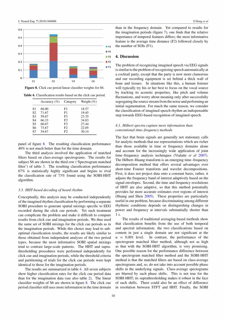
Figure 8. Click cue period linear classifier weights for S6.

Table 4. Classification results based on the click cue period.

Accuracy (%) Category Weight (%)

S1 68.00 F1 18.57S2 71.67 F1 19.45S3 59.67 F3 23.35S4 66.33 F2 34.83S5 60.67 F3 27.44S6 73.67 F2 22.05S7 54.67 F2 30.14

panel of figure 8. The resulting classification performance40% is not much better than for the time domain.

The third analysis involved the application of matchedfilters based on class-average spectrograms. The results forsubject S6 are shown in the third row (‘Spectrogram matchedfilter’) of table 3. The resulting classification performance67% is statistically highly significant and begins to rivalthe classification rate of 73% found using the SOBI-HHTalgorithm.

3.3. HHT-based decoding of heard rhythm

Conceptually, this analysis may be conducted independentlyof the imagined rhythm classification by performing a separateSOBI procedure to generate spatial mixings specific to EEGrecorded during the click cue periods. Yet such treatmentcan complicate the problem and make it difficult to compareresults from click cue and imagination periods. We thus usedthe same set of SOBI mixings for the click cue periods as inthe imagination periods. While this choice may lead to sub-optimal classification results, the results are likely similar tothose obtained from independent analyses of the two periodtypes, because the most informative SOBI spatial mixingstend to contrast large-scale patterns. The HHT and supra-thresholding procedures were performed independently forclick cue and imagination periods, while the threshold criteriaand partitioning of trials for the click cue periods were keptidentical to those for the imagination periods.

The results are summarized in table 4. All seven subjectsshow higher classification rates for the click cue period datathan for the imagination data (see also table 2). The linearclassifier weights of S6 are shown in figure 8. The click cueperiod classifier still uses more information in the time domain

than in the frequency domain. Yet compared to results forthe imagination periods (figure 7), one finds that the relativeimportance of temporal features differs; the most informativefeature is the average time distance (F2) followed closely bythe number of SOIs (F1).

4. Discussion

The problem of recognizing imagined speech via EEG signalsis similar to the problem of recognizing speech automatically ata cocktail party, except that the party is now more clamorousand our recording equipment is set behind a thick wall ofbone and tissues. In situations like this, a human listenerwill typically try his or her best to focus on the vocal sourceby tracking its acoustic properties, like pitch and volumefluctuations, and worry about meaning only after successfullysegregating the source stream from the noise and performing aninitial segmentation. For much the same reason, we considerthe classification of imagined speech rhythm an indispensablestep towards EEG-based recognition of imagined speech.

4.1. Hilbert spectra capture more information thanconventional time–frequency methods

The fact that brain signals are generally not stationary callsfor analytic methods that use representations which are richerthan those available in time or frequency domains aloneand account for the increasingly wide application of jointtime–frequency analysis techniques (Vialatte et al 2007).The Hilbert–Huang transform is an emerging time–frequencydecomposition method that offers several advantages overshort-time Fourier transform and wavelet decompositions.First, it does not project data onto a constant basis; rather, itadjusts the frequency band of interest adaptively based on thesignal envelopes. Second, the time and frequency resolutionsof HHT are also adaptive, so that this method potentiallyprovides far more accurate estimates over regions of interest(Huang and Shen 2005). These properties are particularlyuseful in our problem, because discriminating among differentrhythmic conditions depends on distinguishing changes inpower and frequency at intervals substantially shorter than1 s.

The results of traditional averaging-based methods showthat classification benefits from the use of both temporaland spectral information; the two classifications based oncontent in just a single domain are not significant at theα = 0.001 level. In contrast, the performance of thespectrogram matched filter method, although not as highas that with the SOBI-HHT algorithm, is very promising.One possible reason for the performance difference betweenthe spectrogram matched filter method and the SOBI-HHTmethod is that the matched filters are based on class-averagespectrograms and, so, do not take into account possible phaseshifts in the underlying signals. Class-average spectogramsare blurred by such phase shifts. This is not true for theSOBI-HHT; its suprathresholding makes it robust in the faceof such shifts. There could also be an effect of differencein resolution between STFT and HHT. Finally, the SOBI

10

J. Neural Eng. 7 (2010) 046006 S Deng et al

step in our method congregates more informative channelsto outperform any single one.

The computational complexity of HHT is orders ofmagnitude greater than that of classical spectral analysismethods such as FFT. This remains a major hindrance tothe implementation of HHT in real-time analysis. With thedevelopment of faster computers and better algorithms, weexpect that this problem will diminish. Yet we investigatedalso a spectrogram matched filter method, which is based onclass-average spectrograms. This method classified imaginedspeech rhythm in these experiments well, if not as well as theHHT method. Its major advantage is far less computationalcomplexity. We expect that HHT method classificationperformance can be improved. For example, the thresholdsthat were used to binarize the HS were determined ad hoc. Weexpect better classification performance if these parametersare determined quantitatively for each subject using a largerset of training data.

4.2. SOBI provides automatic spatial mixing and noisereduction

Due to the superficial positions of EEG electrodes onthe scalp, the true signals of neuronal origin are almostalways contaminated by noise of various sorts. Blind-source separation techniques have proven very effective atremoving statistically uncorrelated noise and at boosting SNRto facilitate further analyses (Tang et al 2005, Cichocki andThawonmas 2000). In this study, the SOBI procedure iscrucial to the success of the further joint time–frequencydecomposition because it acts not only to reduce artefactsbut also to automatically generate specific spatial patternswhich help contrast different cortical regions (Dornhege et al2006). We use SOBI instead of other PCA and ICA algorithmsbecause SOBI takes account of the time-variant nature of oursignal. However, for the purpose of reducing artefact, ICAis likely also sufficient as a preprocessing step before jointtime–frequency decomposition of the data. We extended theclassical SOBI algorithm to process multi-channel multi-trialrecordings, and although the current analysis is completelyoffline, we expect that the SOBI filters generated from trainingsessions can be readily used during online classifications aswell.

The SOBI algorithm provides an automatic scheme tomix all channels in a way that maximizes cross-lag inter-component separation (Delorme et al 2007). In most cases,the performance of single channels will fall behind that ofthe SOBI components. Yet, just as is found with most datarotation methods, the automatically generated spatial patternsmay vary across subjects, which can make them difficult tointerpret. The most significant of the automatically generatedweight maps usually vary slowly across space, as is shown bythe topographies in figure 2 and in table 2. For example, themost significant component for four of our subjects, S1, S3,S5 and S7, contrasts the occipital and lower temporal-parietalregions with mid-frontal regions. Contrast between left andright temporal-parietal channels can also produce valuableresults, as shown in S6. Conceivably, this specific pattern

(component 2 of figure 2) contrasts responses of auditoryorigins, and is consistent with ERP and BCI literature (Osmanet al 2006, Kruif et al 2007). In addition, although thedistributions of SOBI component vary across subjects, ourexperience is that on the same subject the pattern is generallyconsistent across trials within the same recording session. Forinstance, we compared the patterns contrasting the occipitaland frontal regions for different trials of the same subject, andthe correlations are in the range of 0.8–0.9. Such consistencyensures that for the same subject the SOBI analysis only needsto be performed once and the resulting loading patterns maypotentially be used in future recordings or BCI applications.

4.3. A step towards EEG-based classification of imaginedspeech

Our results suggest that information extracted from time–frequency representations of EEG data can be used to predictimagined speech rhythm. The temporal information is moreinformative; in six of the seven subjects, we found that themost significant type of feature is in the temporal domain.This finding confirms one’s intuition that brain activity duringimagined speech should bear some similarity to the temporalstructure of the speech itself. Among temporal features, theaverage time span of SOIs proved to be the most informativeone. For the subject providing the greatest accuracy inpredictive classification, increasing the rate at which syllablesare produced is correlated with decreasing SOI duration.This result suggests that certain features of EEG signalsrecorded during imagined speech production carry informationconcerning the temporal structure of the underlying neuronaldynamics, and that this structure is highly consistent with thatof its overt, vocalized, counterpart. Given enough temporalresolution and signal gain, we expect to be able to eventuallyuse this isomorphism to recognize more complex rhythmsin a real-time fashion and to provide concrete steps towardsthe development of EEG-based communication of imaginedspeech.

Previous research shows that sensory responses to heardspeech might be decoded from both MEG (Numminen et al1999, Houde et al 2002, Luo and Poeppel 2007) and EEG(Deng and Srinivasan 2010). We used the SOBI-HHT methodto classify EEG generated during the click trains which wereused at the beginning of each trial to cue the rhythm withwhich imagined speech was then generated. EEG responses tothese heard clicks could be classified using the HHT methodwith greater accuracy than EEG responses produced duringimagined speech. The features which proved most informativefor classifying click train rhythm differed from those mostinformative for classifying imagined speech (of the samerhythms). The change in feature weight distribution is likely tobe closely related to the phase locking of responses evoked byrhythmic sensory inputs (Snyder and Large 2005, Zanto et al2006). During imagination periods, such evoked responsesare absent. Instead, the endogenously driven modulation ofperception induces less precisely time-locked responses whichare characterized better by their overall time spans.

The classification of implicit thoughts has a self-contradictory nature, since objective verification that subjects

11

J. Neural Eng. 7 (2010) 046006 S Deng et al

are performing the desired tasks in some manner independentof the brain-imaging data is not forthcoming. Althoughwe obtained 72.67% classification performance of imaginedspeech rhythm for our best subject, there is some extent towhich we do not know whether this number represents theclassification of genuine EEG due to imagination or representsclassification based on interference factors like artefacts orsustained evoked responses from cueing. Nevertheless,researchers should not be daunted by these technical ormethodological issues, as they may only be answered byfurther exploration in this field.

Acknowledgments

We thank David Poeppel for proposing that such an experimentbe performed and Samuel Thorpe for his help with theexperiment. This work was supported by ARO 54228-LS-MUR.

References

Ahissar E, Nagarajan S, Ahissar M, Protopapas A, Mahncke Hand Merzenich M M 2001 Speech comprehension is correlatedwith temporal response patterns recorded from auditory cortexProc. Natl Acad. Sci. USA 98 13367–72

Belouchrani A, Abed-Meraim K, Cardoso J F and Moulines E 1997A blind source separation technique using second-orderstatistics IEEE Trans. Signal Process. 45 434–44

Birbaumer N, Kubler A, Ghanayim N, Hinterberger T,Perelmouter J, Kaiser J, Iversen I, Kotchoubey B, Neumann Nand Flor H 2000 The thought translation device (TTD) forcompletely paralyzed patients IEEE Trans. Rehabil. Eng.8 190–3

Blankertz B et al 2004 The BCI Competition 2003: progress andperspectives in detection and discrimination of EEG singletrials IEEE Trans. Biomed. Eng. 51 1044–51

Bokde A L, Tagamets M A, Friedman R B and Horwitz B 2001Functional interactions of the inferior frontal cortex during theprocessing of words and word-like stimuli Neuron30 609–17

Cardoso J F 1998 Blind signal separation: statistical principlesProc. IEEE 86 2009–25

Cichocki A and Thawonmas R 2000 On-line algorithm for blindsignal extraction of arbitrarily distributed, but temporallycorrelated sources using second order statistics Neural Process.Lett. 12 91–8

Craelius W 2002 The bionic man: restoring mobility Science295 1018–21

Delorme A, Sejnowski T and Makeig S 2007 Enhanced detection ofartifacts in EEG data using higher-order statistics andindependent component analysis Neuroimage 34 1443

Deng S and Srinivasan R 2010 Semantic and acoustic analysis ofspeech by functional networks with distinct time scales BrainRes. to be published

Dewan E M 1967 Occipital alpha rhythm eye position and lensaccommodation Nature 214 975–7

Donchin E, Spencer K M and Wijesinghe R 2000 The mentalprosthesis: assessing the speed of a P300-basedbrain–computer interface IEEE Trans. Rehabil. Eng.8 174–9

Dornhege G, Blankertz B, Krauledat M, Losch F, Curio Gand Muller K R 2006 Combined optimization of spatial andtemporal filters for improving brain–computer interfacingIEEE Trans. Biomed. Eng. 53 2274–81

D’Zmura M, Deng S, Lappas T, Thorpe S and Srinivasan R 2009aToward EEG sensing of imagined speech Human–ComputerInteraction, Part I, HCII 2009 (Lecture Notes in ComputerScience no 5610) ed J A Jacko (Berlin: Springer) pp 40–8

D’Zmura M, Deng S, Lappas T, Thorpe S and Srinivasan R 2009bEEG Classification of Imagined Syllable Rhythm Using HilbertSpectrum Methods (Chicago, IL: Society for Neuroscience)

Haynes J D and Rees G 2005 Predicting the orientation of invisiblestimuli from activity in human primary visual cortex Nat.Neurosci. 8 686–91

Hickok G and Poeppel D 2007 The cortical organization of speechprocessing Nat. Rev. Neurosci. 8 393–402

Houde J F, Nagarajan S S, Sekihara K and Merzenich M M 2002Modulation of the auditory cortex during speech: an MEGstudy J. Cogn. Neurosci. 14 1125–38

Huang N E and Shen S S P 2005 Hilbert–Huang Transform and ItsApplications (London: World Scientific)

Huang N E, Shen Z, Long S R, Wu M C, Shih H H, Zheng Q,Yen N C, Tung C C and Liu H H 1998 The empirical modedecomposition and the Hilbert spectrum for nonlinear andnon-stationary time series analysis Proc. Math. Phys. Eng. Sci.454 903–95

Ince N F, Arica S and Tewfik A 2006 Classification of single trialmotor imagery EEG recordings with subject adaptednon-dyadic arbitrary time–frequency tilings J. Neural Eng.3 235–44

Indefrey P and Levelt W J M 2004 The spatial and temporalsignatures of word production components Cognition92 101–44

Kruif B J, Schaefer R and Desain P 2007 Classification of imaginedbeats for use in a brain–computer interface 29th Ann. Int. Conf.of the IEEE Engineering in Medicine and Biology Society(2007) p 678

Leeb R, Lee F, Keinrath C, Scherer R, Bischof H andPfurtscheller G 2007 Brain–computer communication:motivation, aim, and impact of exploring a virtual apartmentIEEE Trans. Neural Syst. Rehabil. Eng. 15 473–82

Luo H and Poeppel D 2007 Phase patterns of neuronal responsesreliably discriminate speech in human auditory cortex Neuron54 1001–10

Numminen J, Salmelin R and Hari R 1999 Subject’s own speechreduces reactivity of the human auditory cortex Neurosci. Lett.265 119–22

Nunez P L and Srinivasan R 2006 Electric Fields of the Brain: theNeurophysics of EEG (Oxford: Oxford University Press)

Osman A, Albert R and Ridderinkof K R 2006 The beat goes on:rhythmic modulation of cortical potentials by imagined tappingJ. Exp. Psychol. Hum. Percept. Perform. 32 986–1005

Pfurtscheller G, Leeb R, Keinrath C, Friedman D, Neuper C,Guger C and Slater M 2006 Walking from thought Brain Res.2006 145–52

Schalk G, McFarland D J, Hinterberger T, Birbaumer N andWolpaw J R 2004 BCI2000: a general-purpose brain–computerinterface (BCI) system IEEE Trans. Biomed. Eng.51 1034–43

Snyder J S and Large E W 2005 Gamma band activity reflects themetric structure of rhythmic tone sequences Cogn. Brain Res.24 117–26

Tang A C, Liu J Y and Sutherland M T 2005a Recovery ofcorrelated neuronal sources from EEG: the good and bad waysof using SOBI Neuroimage 28 507–19

Tang A C, Sutherland M T and McKinney C J 2005b Validation ofSOBI components from high-density EEG Neuroimage25 539–53

Vialatte F B, Martin C, Dubois R, Haddad J, Quenet B, Gervais Rand Dreyfus G 2007 A machine learning approach to theanalysis of time–frequency maps, and its application to neuraldynamics Neural Netw. 20 194–209

Vigneau M, Beaucousin V, Herve P Y, Duffau H, Crivello F,Houde O, Mazoyer B and Tzourio-Mazoyer N 2006

12

J. Neural Eng. 7 (2010) 046006 S Deng et al

Meta-analyzing left hemisphere language areas: phonology,semantics, and sentence processing Neuroimage 30 1414–32

Wang Y and Makeig S 2009 Predicting intended movement directionusing EEG from human posterior parietal cortex AugmentedCognition, HCII 2009 (Lecture Notes in Computer Science no56380) ed D D Schmorrow et al (Berlin: Springer) pp 437–46

Weineke G H, Deinema C H A, Spoelstra P, Storm van Leeuwen Wand Versteeg H 1980 Normative spectral data on alpha rhythmin males adults Electroencephalogr. Clin. Neurophysiol.49 636–45

Weiss S and Mueller H M 2003 The contribution of EEG coherenceto the investigation of language Brain Lang. 85 325–43

Wolpaw J R, McFarland D J and Vaughan T M 2000Brain–computer interface research at the Wadsworth CenterIEEE Trans. Rehabil. Eng. 8 222–6

Zanto T P, Syder J S and Edward W L 2006 Neural correlates ofrhythmic expectancy Adv. Cogn. Psychol. 2 221–31

Zhao Q, Zhang L and Cichocki A 2009 EEG-based asynchronousBCI control of a car in 3D virtual reality environments Chin.Sci. Bull. 54 78–87

13