INSTITUTE OF PHYSICS PUBLISHING INVERSE PROBLEMS

Inverse Problems 18 (2002) 1873–1889 PII: S0266-5611(02)37551-8

Eddy-current evaluation of three-dimensional flaws inflat conductive materials using a Bayesian approach

Denis Premel1 and Alexandre Baussard

Laboratoire Systemes et Applications des Technologies de l’Information et de l’Energie (UMRCNRS 8029), Ecole Normale Superieure de Cachan 61, avenue du President Wilson, 94235Cachan, France

E-mail: denis.premel@cea.fr and baussard@satie.ens-cachan.fr

Received 29 May 2002Published 8 November 2002Online at stacks.iop.org/IP/18/1873

AbstractThis paper deals with quantitative eddy-current non-destructive evaluationof volumetric flaws. The inversion of eddy-current data leads to detection,localization, sizing and shape reconstruction of a flaw. The eddy-currentprobe is constituted by a driving coil which is placed at an adapted fixedposition and a pick-up coil which scans the surface above the flawed regionin order to collect the data. The eddy-current probe response is linked to thelocal variations of the electrical conductivity of the inhomogeneous material.A numerical model follows from the discretization of the coupled integralequations by using a method of moments. To solve the resulting nonlinearinverse problem, an inversion scheme is proposed within a Bayesian estimationframework. Lack of information due to the band-pass behaviour of the forwardoperator is compensated by introducing prior knowledge. The advantages ofthis approach result from combining the information contained in the data andthe a priori knowledge on the solution to be estimated. The inversion problem istransformed into an optimization problem which is dealt with using a sequenceof local minimizations performed via a standard descent algorithm. In orderto illustrate the behaviour and the efficiency of the proposed approach, severalreconstructions from simulated data are presented.

1. Introduction

The examination of conductive materials using eddy-current non-destructive evaluation (NDE)techniques is a central problem in the inspection of structures or products involved in nuclearpower plants, in the aircraft industry, for pipelines, motors, . . . . Quantitative non-destructiveevaluation (QNDE) methods are becoming increasingly important as the capabilities of

1 Current address: DRT/DECS/SISC/LCME CEA Saclay 91191 Gif/Yvette, France.

0266-5611/02/061873+17$30.00 © 2002 IOP Publishing Ltd Printed in the UK 1873

1874 D Premel and A Baussard

computers progress. Indeed, the goal of the QNDE methods is not limited to detecting andlocalizing an anomaly or a defect but it also consists in the determination of the shape and thesize of the defect or a cluster of defects from probe responses measured at different positionsand eventually at different frequencies. This paper focuses on electromagnetic methods whichinvolve eddy currents in conductive materials and imply the reconstruction of an electricalparameter which can reveal the defects inside a structure: the conductivity distribution. Weinvestigate the problem of evaluating a (three-dimensional) volumetric flaw from observeddata such as the variations of the magnetic field above the damaged zone inspected. Thisproblem successively requires one to design a suitable system for generating eddy currents inthe workpiece and for collecting data, to construct an efficient numerical model which linksthe collected data to the spatial variations of the conductivity, and finally to solve the inverseproblem by an appropriate optimization procedure. At each level of the above sequence, weare faced with a number of difficulties.

One way to reduce the complexity of the problem is to assume that the defect ishomogeneous; for example, it is a void cavity or a uniform inclusion. The inverse problem maythen be specified as a search for the flaw boundary. Another possibility lies in assuming thatthe flaw is an ideal crack with zero thickness. The inverse problem then becomes a problem ofevaluating the shape of the crack in a known plane from a set of probe measurements (Bowleret al 1994). In contrast to this previous work, in this paper, the flaw is represented by acontrast function (or an object function) which is defined in terms of the relative variationsof the conductivity distribution depending on the position in the conductive material. Thecontrast function is then approximated by a piecewise constant function on a three-dimensionalrectangular grid and the inverse problem consists of estimating the conductivity of each volumeelement from a set of probe responses.

In eddy-current NDE, a flaw is usually detected and localized from the observation ofprobe impedance changes due to the interaction between the induced currents and the flawwhen the probe is scanning the surface above the damaged zone. This type of probe is usuallycalled a common function probe since emission and reception are realized by the same coil.In this situation, only one observation for each position of the probe is obtained. Moreover, inorder to solve the inverse problem, the scattered field must be evaluated for each emitting probeposition; this experimental set-up leads to a significant increase in the computational cost ofthe inverse problem since the number of unknowns is much larger than the amount of collectedexperimental data. In this work, another type of probe has been adopted, which separatesthe emission function and the reception function. The response of flaws or cracks may beobserved by the changes in the normal component of the magnetic field which is measured bya pick-up coil moved above the workpiece which is to be examined. The driving coil is fixedat one appropriate position. Therefore, each position of the driving coil provides us with a setof observed data as with an imaging device in tomographic image reconstruction.

Many forward models have already been discussed in the literature (Badics et al 1998,Sabbagh and Sabbagh 1986). In this paper, a numerical model has been built on a set of coupledintegral equations by using Green dyads. This formulation has the advantage that only theinvestigated zone needs to be discretized and many computations can be performed analytically.Consequently, the number of unknowns remains tolerable in solving the inverse problem.However, the required dyadic Green functions are only available in explicit geometries suchas a layered half-space, for example, in the plane geometry. Consequently, in this paper,an isotropic, homogeneous half-space conductor is considered. The integral equations arediscretized by using the method of moments (Harrington 1968). The flaw region is subdividedinto volumetric cells and the adopted approach uses a conventional Galerkin scheme. Theforward problem may be fully solved by a conjugate gradient algorithm from the resulting

Eddy-current evaluation of 3D flaws 1875

system of linear equations. Though some approximations can be applied to reduce thecomputational time (Habashy et al 1993, Zdhanov and Fang 1996), the full solution has beenkept to study the best capabilities of the proposed inversion algorithm.

It is well known that the retrieval of an unknown conductivity distribution from eddy-current data is a nonlinear inverse problem, since both the conductivity distribution and theinternal electromagnetic field in the zone under inspection are both unknown. Moreover, inspite of the often large quantity of observed data, the nonlinear inverse problem is ill-posed,and therefore, we propose to solve it within a Bayesian estimation framework.

This approach enables us to introduce a priori knowledge on the contrast function to beretrieved. We propose to combine two kinds of priors in order to efficiently take into accountthe relevant properties of the sought contrast function. First, the contrast function may besubjected to strong transitions near the edge of a flaw and if we consider that the conductivityof the inclusion is smaller than that of the surrounding conductive zone, the values of thecontrast function may vary from zero (as in a healthy zone) to one (as in a void cavity). Thisfeature can be taken into account by considering the beta law model. Second, the damagedzone is often constituted by homogeneous patches, so, in order to take into account the localcorrelation property between nearby cells, the weak membrane model (Blake and Zisserman1987) is considered. Then, the inverse problem is iteratively solved by minimizing a criterioncombining a quadratic data fitting term and the two regularization functionals. Although theconvergence of the algorithm cannot be rigorously demonstrated, the numerical experimentsconsidered here show that the algorithm is effective for a variety of flaws.

This paper is organized as follows: in section 2, the forward problem is discussed and insection 3 the validity of the numerical model is illustrated by comparisons with other sets ofsimulated data provided by a well known eddy-current code. In section 4 the inverse problemand the regularization scheme are considered. Section 5 describes the initial guess. In section 6,typical numerical reconstructions are presented. The conclusion follows in section 7.

2. The forward problem

In this section, the coupled integral equations which govern the forward problem are presented.The flaws or anomalies are detected and localized in a conductive material by means of eddycurrents. They are represented by an electrical parameter which differs from that of the hostmaterial. A normalized contrast function is defined as follows:

f (r) = σ0 − σ(r)

σ0(1)

in order to characterize them. The host material surrounding the flawed region is isotropic,homogeneous, non-magnetic and its conductivityσ0 is assumed to be known. The quantity σ(r)

denotes the variations of conductivity of the damaged zone. The physical system considered isshown in figure 1; it consists of a driving coil and an auxiliary pick-up coil which successivelyoccupies a number of locations in a mesh above the anomalous region. A Cartesian (x, y, z)coordinate system is used with vertical axis z normal to the flat workpiece parallel to the (x, y)

plane.The driving coil generates the incident electric field denoted by E0(r) within the

workpiece. Induced currents interact with the flaw and denoting by E2(r) the total electricfield inside the anomalous domain D. Taking into account a time dependence in exp(−jωt),the state equation can be written as:

E0(r) = E2(r) + iωµ0σ0

∫D

G22(r, r′) · f (r′)E2(r′) dr′. (2)

1876 D Premel and A Baussard

Figure 1. The physical system: a driving coil creates eddy currents in the flat conductive workpiece,a pick-up coil is scanning above the anomalous domain denoted D representative of the volumetricflaw.

The dyadic Green functions are of electric type, both the observed field and the sources being ofelectrical nature. The subscripts denote the regions which are coupled by the Green functions:the left one denotes the region containing the observed field point r(x, y, z), and the right onedenotes the region which contains the source point r′(x ′, y ′, z′). The dyadic Green functionsare formed from the three components of the electric field due to an electric current pointsource orientated along the x, y, z unit vectors. From Chew (1995) the expressions for thedyadic Green functions are derived and implemented for a conductive half-space.

In order to obtain observational data, another integral equation must be derived from themeasurement procedure. In contrast to typical non-destructive devices which measure theperturbed probe impedance, we have chosen to measure the emf which is directly related tothe normal component of the magnetic field inside the air region R1. Defining the position ofthe pick-up coil by the measurement point rm(xm, ym, zm), the perturbed electrical field insidethe air region R1 is given by:

E1(r) = iωµ0σ0

∫D

G12(r, r′) · [ f (r′)E2(r′)] dr′. (3)

The subscripts of the electric–electric dyadic Green function G12(r, r′) denote that thecomponents of the electric field are observed at the point r in the region R1 whereas thepoint source is located in the region R2. Then the emf induced in one turn of the pick-up coilof contour C has the form:

emf(rm) =∮CE1(r) · dl. (4)

Finally, the pick-up coil, centred at rm , scanning above the flawed region provides a set ofdata, denoted by y(rm) related to the contrast function:

y(rm) =∫

DΓ12(rm, r′) · J2(r

′) dr′ (5)

where J2(r′) = f (r′)E2(r

′) is the normalized current density within the domain D. Fromequations (3) and (4) the dyadic function Γ12(rm, r′) is given by:

Γ12(rm, r′) =∫

pick-up coil

∮CG12(rm, r′) · dl drm . (6)

The incident field is also computed by another integral equation:

E0(r) = iωµ0

∫coil

G21(r, r′) · Je(r′) dr′, (7)

Eddy-current evaluation of 3D flaws 1877

where Je(r′) is the current density within the driving coil and G21(r, r′) is the electric–electric

dyadic Green function with the point source in the region R1 and the observation point in theregion R2.

The discretization of the coupled equations is then performed by subdividing the flawedregion into a regular mesh of N = Nx × Ny × Nz volumetric cells, each of size (δx × δy × δz),and by expanding the electric field and the contrast function using pulse basis functions:

E(r) =∑

i

∑j

∑k

Ei jk Pi (x/δx)Pj (y/δy)Pk(z/δz), (8)

f (r) =∑

i

∑j

∑k

fi jk Pi (x/δx)Pj (y/δy)Pk(z/δz), (9)

where the pulse basis function is given by:

Pi, j,k(r) ={

1 if r ∈ cell (i, j, k)

0 otherwise.(10)

Then, the integral equation is ‘tested’ with the same pulse functions. This variant of the methodof moments is the Galerkin method, and it leads to a system of coupled matrix equations whichread, in abbreviated form, as follows:

e0 = e2 + G22 · F · e2. (11)

y = Γ12 · F · e2, (12)

where e0 is the [3N × 1] incident field vector and e2 is the [3N × 1] total field vector, thenumber of components of these vectors come from the three components of each [N × 1]electric field vector ex, ey, ez . Denoting by f the [N × 1] vector which contains all valuesof the unknown contrast, and denoting by diag(f) a diagonal matrix whose elements are thevalues of f , the block matrix F can be built up as:

F =[ diag(f) 0 0

0 diag(f) 00 0 diag(f)

]. (13)

The [M × 1] vector y is the observation vector containing the values of M complex valuesresulting from the scanning of the pick-up coil according to a regular grid M = Nxm × Nym .The matrices Γ12 and G22 are, respectively, the [M × 3N] and [3N × 3N] matrices derivedfrom the Green functions. The forward problem is finally stated here as follows:

• compute the incident field e0 within the anomalous bounded domain D. This computationonly depends on the geometry of the inducer and the mesh of the anomalous region in theworkpiece,

• build up the matrix F from the values of the contrast function,• solve the state equation by computing the total electric field, then compute the observed

data.

The resulting equation has the following form:

y = Γ12 · F · (I + G22 · F )−1 · e0. (14)

This forward problem can be extended by considering that the driving coil is moved in the(x, y) plane. For each position l (1 � l � L) of this coil, the full forward problem mustbe solved to obtain the [M × L] observed data matrix. Each position of the driving coilmust be well considered in order to provide complementary information about the flawedregion. L is the number of views (meaning positions of the probe) as in usual tomographicimaging. The resulting numerical model, built up from these coupled matrix equations,

1878 D Premel and A Baussard

involves prohibitive computations and large memory requirements as the number of unknownsN increases. Therefore, another numerical model can be implemented by exploiting theconvolutional structure of the Green functions which is kept in the discrete form of the integralequations. Therefore, given an arbitrary number of layers (1 � k � Nz), let us denote the totalnormalized current density J2k(r) = fk(r)E2k(r) for z ∈ Ik = [zk −�k/2, zk +�k/2], whichis of finite support �k around the discrete depth zk . The equation of state can be rewritten as:

E0(r) = E(r) + iωµ0σ0

∑k′

∫Ik

G22(z, z′) ∗ J2k(z′) dz ′, (15)

where ∗ denotes the convolution product. Another form of the state equation results from theintroduction of the incident normalized current density: J0(r) = f (r)E0(r) which yields:

J0(r) = J2(r) + iωµ0σ0 f (r)∑

k′

∫Ik

G22(z, z′) ∗ J2k(z′) dz ′. (16)

This last equation can be discretized as previously, by using the expansion onto pulse basisfunctions. So, in abbreviated form:

J0 = J2 + iωµ0σ0f∑

k′

∫Ik

Γ22(z) ∗ J2k(z) dz (17)

where the matrix Γ22(z) results from the discrete form of G22(z, z′).This last formulation enables a strong reduction in storage requirements because the

resulting matrix Γ22(z) is of size [(2Nx − 1) × (2Ny − 1) × Nz × Nz ].The resulting scattered field can be computed by means of a conjugate gradient scheme

by using spatial convolution products or FFTs. In this case, the size of the cells (δx , δy) inthe region where the field is computed must be equal to the size of the cells (δ′

x , δ′y) in the

region where the sources are located. The full matrix equation (12) has been kept in order tocompute the observed data. The total normalized current density J2(x, y, zk) is substitutedinto the observation equation:

y = Γ12x · J2x(x, y, zk) + Γ12y · J2y(x, y, zk) + Γ12z · J2z(x, y, zk), (18)

where J2x (x, y, zk),J2y(x, y, zk),J2z(x, y, zk) are [N × 1] density vectors containing thevalues of the x, y, z components of the normalized density function.

3. Validation of the forward model

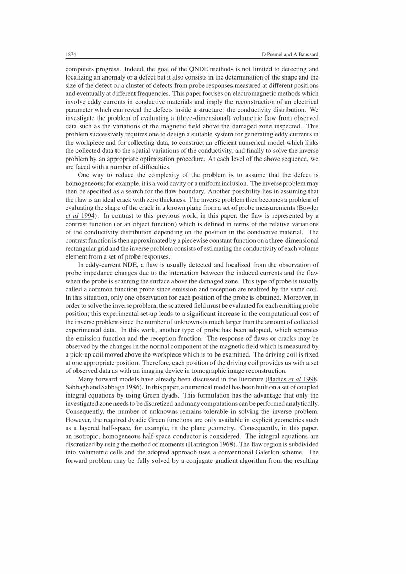
The resulting numerical model has been validated for a large number of cells discretizing theanomalous region. This section gives some numerical results to illustrate its behaviour. Ourgoal is to validate the solution of the forward problem by a comparison with simulated dataprovided by another model. Though synthetic data are available (Burke 1988,Takagi et al 1994,1996), several tests have been carried out using simulated data calculated using the volumeintegral code VIC3D (Sabbagh et al VIC-3D�) for electromagnetic NDE. Computations wereperformed in order to obtain the emf picked up by the pick-up coil for a number of locationsin a given grid above the anomalous region due to a volumetric flaw (opening in air) in ahalf-space conductive medium. The parameters of the probe and the flaw are given in table 1.Comparisons between our data sets and those provided by VIC3D lead to a RMS error whichis lower than 3.32%. The sets of data are so close that only one is displayed in figure 2.

This validation has been carried out with a 100 kHz operating frequency as usual inNDE experiments since the sensitivity of the probe becomes better as the frequency increases.However, for the retrieval of flaws in the following sections, the frequency is decreased to8 kHz to generate a set of simulated data that minimize the pernicious effects of the skin effectduring the reconstruction procedure.

Eddy-current evaluation of 3D flaws 1879

– 5

0

5

– 5

0

5

– 0.05

0

0.05

xm [mm] ym [mm] – 5

0

5

– 5

0

xm [mm]ym [mm]

5

– 0.02

0

0.02

(a) (b)

Figure 2. Real (a) and imaginary (b) parts of the calculated emf at f = 100 kHz.

Table 1. Parameters of the probe and the flaw opening in air.

Driving coil parameters Flaw parameters

Inner radius r1 12 mm Length L 3 mmOuter radius r2 16 mm Width W 3 mmHeight h 0.5 mm Depth D 0.5 mmLift-off l0 0.5 mmNumber of turns of the winding 75Frequency 100 kHz

Receiver coil parameters The workpiece parameters

Inner radius rm1 0.1 mm Conductivity σ0 106 S m−1

Outer radius rm2 0.2 mmHigh hm 0.3 mmNumber of turns 40

4. The inverse problem

4.1. Analysis of the ill-posedness

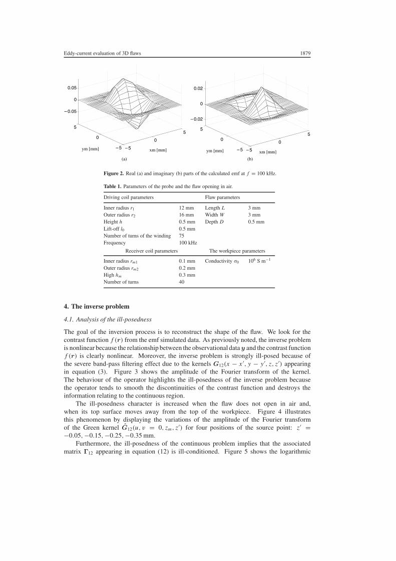
The goal of the inversion process is to reconstruct the shape of the flaw. We look for thecontrast function f (r) from the emf simulated data. As previously noted, the inverse problemis nonlinear because the relationship between the observational data y and the contrast functionf (r) is clearly nonlinear. Moreover, the inverse problem is strongly ill-posed because ofthe severe band-pass filtering effect due to the kernels G12(x − x ′, y − y ′, z, z′) appearingin equation (3). Figure 3 shows the amplitude of the Fourier transform of the kernel.The behaviour of the operator highlights the ill-posedness of the inverse problem becausethe operator tends to smooth the discontinuities of the contrast function and destroys theinformation relating to the continuous region.

The ill-posedness character is increased when the flaw does not open in air and,when its top surface moves away from the top of the workpiece. Figure 4 illustratesthis phenomenon by displaying the variations of the amplitude of the Fourier transformof the Green kernel G12(u, v = 0, zm, z′) for four positions of the source point: z′ =−0.05,−0.15,−0.25,−0.35 mm.

Furthermore, the ill-posedness of the continuous problem implies that the associatedmatrix Γ12 appearing in equation (12) is ill-conditioned. Figure 5 shows the logarithmic

1880 D Premel and A Baussard

–1 – 0 .5 0 0. 5 10

0. 5

1

1. 5

2

2. 5

u × 10 4 [ m–1 ]

Mag

nitu

de

(a) (b)

Figure 3. (a) The amplitude of the Fourier transform G12(u, v, zm , z ′ = −0.05 mm) of the Greenfunctions G12xx (x − x ′, y − y′, zm , z ′ = −0.05 mm), where u and v are the spatial wavenumbers.(b) Slice view for v = 0 and z ′ = −0.05 mm.

–1 – 0.5 0 0.5 10

0.5

1

1.5

2

2.5

u × 104 [ m– 1]

Mag

nitu

de

← z’= – 0.05 mm← z’= – 0.15 mm← z’= – 0.25 mm← z’= – 0.35 mm

– 0.4 – 0.2 00

0.5

1

1.5

2

2.5

3

z’ [mm]

Max

of

Mag

nitu

de

(a) (b)

Figure 4. (a) A slice of the amplitude of the Fourier transform G12(u, v = 0, zm , z ′). (b) Theattenuation of the maximum of the amplitude along the z axis.

decrease of the singular values of the symmetrized matrix (ΓT12Γ12) for a [15 × 15 × 2] mesh.

In this case, for instance, the size of ΓT12Γ12 is [1350 × 1350].

Due to the skin effect, the induced currents suffer from the same attenuation. Figure 6shows the eddy-current distribution in the workpiece around the flawed region at a frequencyof 8 kHz (the skin depth is estimated at 3.15 mm for a plane wave).

Because of the attenuation phenomenon, the conductivity perturbations of deep cells areless weakly represented in the data than those of shallow cells. To yield a stable and physicallyplausible solution, an efficient regularization scheme must be introduced to overcome the ill-posedness of the inverse problem. This is done by introducing suitable priors into the inversionstage in order to compensate for the lack of information on the flaw to be retrieved.

4.2. The Bayesian approach

Regularization in a Bayesian framework allows one to combine both the information containedin the data and a prior probability distribution function. In this approach, the first step consists

Eddy-current evaluation of 3D flaws 1881

0 500 1000 1500 2000 2500 3000 3500index

log1

0 si

ngul

ar v

alue

s

– 25

– 20

– 15

– 10

– 5

Figure 5. Logarithmic decrease of the singular values of the [1350 × 1350] symmetrized matrix(ΓT

12Γ12).

– 5 0 5 10 15 20 x [mm]

z [

mm

]

0

0.5

1

1.5

– 1

– 0.5

8 12 16 20 x [mm]

y [

mm

]

(a) (b)

– 8

– 6

– 4

– 2

0

2

4

6

8

Figure 6. (a) Slice view of the physical system: the driving coil, the pick-up coil above theworkpiece and the grey level map of the eddy-current distribution. (b) Map of the eddy-currentdistribution in the (x, y) plane at zk = −0.05 mm.

of evaluating the plausibility of a solution f (see equation (14)) to fit the data considering theexistence of errors due to modelling or measurement errors. When the errors are assumedcentred, white and Gaussian, the maximum of the likelihood p(y/f) gives a solution whichreduces to the least-squares solution:

fM L = arg maxf∈RN

p(y/f) = arg minf∈RN

Q(f) (19)

with

Q(f) = ‖y − Γ12 · F · (I + G22 · F )−1e0‖2. (20)

In the context of Bayesian estimation (Box and Tiao 1972), we may assign a prior law on theimage of the form:

p(f) = 1

Zexp[−γ U(f)] (21)

1882 D Premel and A Baussard

where U(f) denotes a prior energy which introduces the prior knowledge and Z is anormalization factor. The information about the image or the flaw is summed up in theposterior law:

p(f/y) = p(y/f)p(f)

p(y)∝ 1

Zexp[−Up(f)], (22)

where Up(f) is the posterior energy defined as:

Up(f) = Q(f) + γ U(f). (23)

In such a large problem with many unknowns, the MAP estimator appears to be the best suitedfor flaw reconstructions:

fM AP = arg maxf∈RN

p(f/y) = arg minf∈RN

[Q(f) + γ U(f)]. (24)

One can note that U(f) in (24) can be seen as a regularization term and γ is a weightingparameter. The main problem is now to translate the prior knowledge regarding the flaw to bereconstructed in a prior energy.

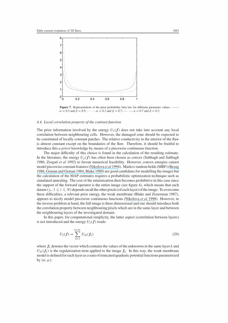
4.3. The beta law

The sought object function f (r) is the relative conductivity f (r) = σ0−σ (r)

σ0. When the interior

of the flaw is air (σ(r) = 0) f (r) is equal to 1 in the flaw region and equal to 0 in the healthyregion (σ (r) = σ0) of the investigated domain D. Thus the components of the object vector f(the discretized equivalent of the contrast function f (r)) take mostly one of these two valuesand the other ones belong to the interval ]0, 1[ with a strong probability of being close to oneor zero. This a priori knowledge can be approached and formalized by assigning a beta lawto each pixel of the image (Venard et al 1997):

p( fi ) ∝ f −αi (1 − fi )

−β, fi ∈ ]0, 1[ and α, β > 0. (25)

Moreover, by assuming that the cells are a priori independent, the prior law is given by:

p(f) =i=N∏i=1

p( fi ) (26)

and the related energy can be written:

U1(f) = − ln p(f) = constant + α

i=N∑i=1

ln( fi ) + β

i=N∑i=1

ln(1 − fi ). (27)

The constant is a normalized factor which comes from the beta law. This last one which isillustrated in figure 7 has one drawback. The resulting criterion from the MAP estimator:

J (f) = Q(f) + γ1U1(f) (28)

goes to −∞ when fi tends to 0 or 1. Therefore, the support of the object function is restrictedto the interval [ε, 1 − ε], ε > 0. The value of ε is chosen in order to keep a better sensitivityof the reconstruction results to the parameters α and β rather than to ε. The parameters α

and β belong to the interval ]0, 1[ and the balance between them depends on the size of theflaw compared to the size of the anomalous area. Weak variations of these parameters remainineffective. In order to obtain the reconstructions presented in this paper, the values of theparameters have been taken as α = 0.3, β = 0.7 and ε = 10−3 (see figure 7).

Eddy-current evaluation of 3D flaws 1883

0 0.2 0.4 0.6 0.8 10

1

2

3

4

5

6

7

8

Figure 7. Representation of the prior probability beta law for different parameter values: ——,α = 0.5 and β = 0.5; · · · · · ·, α = 0.3 and β = 0.7; — · —, α = 0.7 and β = 0.3.

4.4. Local correlation property of the contrast function

The prior information involved by the energy U1(f) does not take into account any localcorrelation between neighbouring cells. However, the damaged zone should be expected tobe constituted of locally constant patches. The relative conductivity in the interior of the flawis almost constant except on the boundaries of the flaw. Therefore, it should be fruitful tointroduce this a priori knowledge by means of a piecewise continuous function.

The major difficulty of this choice is found in the calculation of the resulting estimate.In the literature, the energy Up(f) has often been chosen as convex (Sabbagh and Sabbagh1986, Zorgati et al 1992) to favour numerical feasibility. However, convex energies cannotmodel piecewise constant features (Nikolova et al 1994). Markov random fields (MRF) (Besag1986, Geman and Geman 1984, Blake 1989) are good candidates for modelling the images butthe calculation of the MAP estimates requires a probabilistic optimization technique such assimulated annealing. The cost of the minimization then becomes prohibitive in this case sincethe support of the forward operator is the entire image (see figure 4), which means that eachdatum (yi, 1 � i � N)depends on all the other pixels (of each layer) of the image. To overcomethese difficulties, a relevant prior energy, the weak membrane (Blake and Zisserman 1987),appears to nicely model piecewise continuous functions (Nikolova et al 1998). However, inthe inverse problem at hand, the full image is three dimensional and one should introduce boththe correlation property between neighbouring pixels which are in the same layer and betweenthe neighbouring layers of the investigated domain.

In this paper, for computational simplicity, the latter aspect (correlation between layers)is not introduced and the energy U2(f) reads:

U2(f) =k=Nz∑k=1

U2k(fk) (29)

where fk denotes the vector which contains the values of the unknowns in the same layer k andU2k(fk) is the regularization term applied to the image fk . In this way, the weak membranemodel is defined for each layer as a sum of truncated quadratic potential functions parametrizedby (α,µ):

1884 D Premel and A Baussard

U2k(fk) =N∑

i=1

hα,µ( fi − fi−1) (30)

where the functional hα,µ(.), defined by:

hα,µ(t) ={

α2t2 if |t| < T

µ if |t| � T, T =

õ

α, (31)

involves an implicit contour process. α is a scale parameter which defines the spreading outof the homogeneous zone, while µ fixes the prior discontinuity detection threshold T .

This functional is not differentiable at |t| = T , so the criterion cannot be optimized insuch a form. Therefore, in order to implement this energy, the functional is approximated byusing a relaxation scheme based on the graduated non-convexity (GNC) principle (Blake andZisserman 1987). The functional hα,µ is modified as follows:

hα,µ,ζ (t) =

α2t2 if |t| < q

µ − ζ(|t| − r)2

2if q � |t| < r

µ if |t| � r.

(32)

The threshold expressions of r and q are given by:

r2 = µ

(2

ζ+

1

α2

)and q = µ

α2r. (33)

The parameters α and h0 (h0 =√

2µ

α), the discontinuity threshold, depend on the a priori

size of the homogeneous area and the amplitude of the contrast function; for instance, toobtain the reconstructions presented in figure 9; they have been experimentally chosen asα = 4 and h0 = 0.4. The parameter ζ (∈ [ζ0,∞[) is the relaxation parameter such thatlimζ→∞ hα,µ,ζ (t) = hα,µ(t) (in practice, only a small number of relaxations is necessary).This parameter has been adjusted according to a geometric progression from 1/32 to 1 with astep equal to 2.

4.5. Joint criterion

Two regularization functions U1(f) and U2(f) can be introduced at the same time. Theenergy U1(f) forces the solution of the inverse problem to be concentrated near 0 and 1. Theenergy U2(f) leads to solutions with homogeneous patches. Here, in accord with the previousanalysis, we propose the use of the weak membrane model and the beta law. The final criterionis then such that:

f = arg minf∈RN

[J (f)] with J (f) = Q(f) + γ1U1(f) + γ2U2(f). (34)

In effect, this allows us to introduce most of the prior knowledge we are able to expressregarding the physical aspects of the flawed region.

The resulting criterion J (f) is then minimized as follows: starting with an initial guess,successive sequences of local minimizations are carried out where each minimum is evaluatedby a local descent via a conjugate gradient algorithm.

The weighting parameters γ1 and γ2 (regularization parameters) are chosen to provide acompromise between the functionals. They have been experimentally estimated.

Eddy-current evaluation of 3D flaws 1885

5. Initial estimate: backpropagation technique

To start the algorithm, a back propagation solution denoted by F0 was considered. The processcan be summarized in three steps:

(i) Estimation of Wl = F0 · e2,l , 1 � l � L. Let yl be the observation vector for each viewl with 1 � l � L; the sought solution has the form:

Wl = γlΓ†12 · yl (35)

where † denotes the conjugate transpose of the matrix and γl minimizes the cost functionF(γ ):

F(γl) = ‖yl − Γ12 · Wl‖2. (36)

This parameter γl resulting from the condition (36) is given by:

γl = 〈Γ12Γ†12 · yl,yl〉

‖Γ12 Γ†12 · yl‖2

. (37)

(ii) Estimation of the total field e2,l . From Wl and by using the state equation (11) one candeduce an initial guess for the total field:

e2 = e0 − G22 · Wl . (38)

(iii) Estimation of the contrast function. Given the prior that the contrast vector f is strictlypositive, let F = τ , the following relation must be satisfied:

l=L∑l=1

(Re(W †

l · e2,l)

τ‖e2,l‖2− τ‖e2,l‖

)2

= 0. (39)

Finally, the initial guess is calculated as follows:

F0 =

l=L∑l=1

{Re(W †xl

e2xl +W †yl

e2yl +W †zl

e2zl )}2

‖e†2xl

e2xl +e†2yl

e2yl +e†2zl

e2zl ‖2

l=L∑l=1

‖e†2xl

e2xl + e†2yl

e2yl + e†2zl

e2zl ‖2

. (40)

6. Numerical results

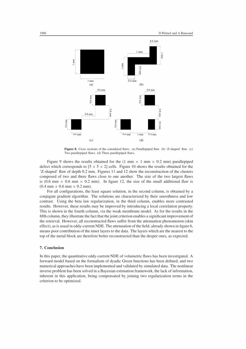
In this section, a few results using simulated data are given in order to illustrate the behaviourof the previous algorithm. These data are generated by solving the forward problem(equations (17) and (18)) for different contrast functions. The mesh of the damaged zoneis [16 × 16 × 4] with sampling steps (0.2 mm × 0.2 mm × 0.1 mm) while the data arecollected according to a [41 × 21] grid with sampling steps (0.5 mm × 0.25 mm). For allsimulations, the operation frequency is set to 8 kHz.

In what follows, for each considered flaw (see figure 8) the results are presented in afigure where the first column corresponds to the flaw to be reconstructed and where eachrow corresponds to a certain depth zone (z′ = −0.05, −0.15, −0.25, −0.35 mm). Thesecond column shows the results obtained without regularization. Results obtained by betalaw regularization are presented in the third column and the results obtained with the weakmembrane model are given in the fourth column. The fifth column shows the results obtainedusing the global criterion which combines the weak membrane model and the beta a priorilaw.

1886 D Premel and A Baussard

1 mm

1 m

m

0.4 mm

1 mm 1 mm

0.6 mm

. mm

1 m

m

0.6 mm.

mm0.8 mm

. m

m

.0.

6 m

m

0.6 mm

. m

m

1 mm 0.4 mm

.

0.6

mm

. mm

. m

m

0 6 mm

0 4

0 6

08

06

06

08

(a) (b)

(c) (d)

0 m

m6

Figure 8. Cross sections of the considered flaws. (a) Parallepiped flaw. (b) ‘Z-shaped’ flaw. (c)Two parallepiped flaws. (d) Three parallepiped flaws.

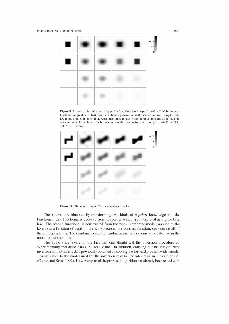
Figure 9 shows the results obtained for the (1 mm × 1 mm × 0.2 mm) parallepipeddefect which corresponds to [5 × 5 × 2] cells. Figure 10 shows the results obtained for the‘Z-shaped’ flaw of depth 0.2 mm. Figures 11 and 12 show the reconstruction of the clusterscomposed of two and three flaws close to one another. The size of the two largest flawsis (0.6 mm × 0.6 mm × 0.2 mm). In figure 12, the size of the small additional flaw is(0.4 mm × 0.6 mm × 0.2 mm).

For all configurations, the least square solution, in the second column, is obtained by aconjugate gradient algorithm. The solutions are characterized by their smoothness and lowcontrast. Using the beta law regularization, in the third column, enables more contrastedresults. However, these results may be improved by introducing a local correlation property.This is shown in the fourth column, via the weak membrane model. As for the results in thefifth column, they illustrate the fact that the joint criterion enables a significant improvement ofthe retrieval. However, all reconstructed flaws suffer from the attenuation phenomenon (skineffect), as is usual in eddy-current NDE. The attenuation of the field, already shown in figure 6,means poor contribution of the inner layers to the data. The layers which are the nearest to thetop of the metal block are therefore better reconstructed than the deeper ones, as expected.

7. Conclusion

In this paper, the quantitative eddy-current NDE of volumetric flaws has been investigated. Aforward model based on the formalism of dyadic Green functions has been defined, and twonumerical approaches have been implemented and validated by simulated data. The nonlinearinverse problem has been solved in a Bayesian estimation framework, the lack of information,inherent in this application, being compensated by joining two regularization terms in thecriterion to be optimized.

Eddy-current evaluation of 3D flaws 1887

0.75

0.5

0

Figure 9. Reconstruction of a parallelepiped defect. Grey level maps (from 0 to 1) of the contrastfunctions: original in the first column, without regularization in the second column, using the betalaw in the third column, with the weak membrane model in the fourth column and using the jointcriterion in the last column. Each row corresponds to a certain depth zone (z ′ = −0.05, −0.15 ,−0.25, −0.35 mm).

0.75

0.5

0

Figure 10. The same as figure 9 with a ‘Z-shaped’ defect.

These terms are obtained by transforming two kinds of a priori knowledge into thefunctional. One functional is deduced from properties which are interpreted as a prior betalaw. The second functional is constructed from the weak-membrane model, applied to thelayers (as a function of depth in the workpiece) of the contrast function, considering all ofthem independently. The combination of the regularization terms seems to be effective in thenumerical simulations.

The authors are aware of the fact that one should test the inversion procedure onexperimentally measured data (i.e. ‘real’ data). In addition, carrying out the eddy-currentinversion with synthetic data previously obtained by solving the forward problem with a modelclosely linked to the model used for the inversion may be considered as an ‘inverse crime’(Colton and Kress 1992). However, part of the proposed algorithm has already been tested with

1888 D Premel and A Baussard

0.75

0.5

0

Figure 11. The same as figure 9 with two parallelepiped defects.

0.75

0.5

0

Figure 12. The same as figure 9 with three parallelepiped defects.

good success in microwave tomography using laboratory-controlled data (Baussard et al2001).Furthermore, collecting experimental data remains a demanding task (Premel et al 1998).

In addition to future works regarding the instrumentation problem, the authors intend touse the proposed method for the retrieval of buried flaws. Also, since the skin effect stronglyreduces the contributions that are expected from deep cells, whereas the hyper-parameters sofar remain the same for each layer, the attenuation tends to modify the balance between thedata fitting term and the regularizing terms. The authors expect to weight the hyper-parametersaccording to the loss of energy in order to reach the same level of regularization for each layer.

Acknowledgments

The authors gratefully acknowledge fruitful discussions with, and useful readings ofthe manuscript by, D Lesselier, ‘Departement de Recherche en Electromagnetisme’ and

Eddy-current evaluation of 3D flaws 1889

A Mohammad-Djafari, ‘Groupe Problemes Inverses’, both at the Laboratoire des Signauxet Systemes (LSS, Gif-sur Yvette, France).

References

Badics Z, Komatsu H, Matsumoto Y and Aoki K 1998 Inversion scheme based on optimization for 3-D eddy currentflaw reconstruction problems J. Non-Destructive Eval. 17 67–78

Baussard A, Premel D and Venard O 2001 A Bayesian approach for solving inverse scattering from microwavelaboratory-controlled data Inverse Problems 17 1659–69

Besag J 1986 On the statistical analysis of dirty pictures J. R. Stat. Soc. B 48 259–302Blake A 1989 Comparison of the efficiency of deterministic and stochastic algorithms for visual reconstruction IEEE

Trans. Pattern Anal. Mach. Intell. 11 2–12Blake A and Zisserman A 1987 Visual Reconstruction (Cambridge, MA: MIT Press)Bowler J-R, Norton S-J and Harrison D-J 1994 Eddy-current interaction with an ideal crack. The inverse problem

J. Appl. Phys. 75 8138–44Box G and Tiao G 1972 Bayesian Inference in Statistical Analysis (Reading, MA: Addison-Wesley)Burke S 1988 A benchmark problem for computation of delta-Z in eddy-current NDE J. Non-Destructive Eval. 7

35–41Chew W-C 1995 Waves and Fields in Inhomogeneous Media (Piscataway, NJ: IEEE)Colton D and Kress R 1992 Inverse Acoustic and Electromagnetic Scattering Theory (New York: Springer)Geman S and Geman D 1984 Stochastic relaxation, Gibbs distributions, and the Bayesian restoration of images IEEE

Trans. Pattern Anal. Mach. Intell. 6 721–41Habashy T-M, Groom R-W and Spies B-R 1993 Beyond the Born and Rytov approximations: a nonlinear approach

to electromagnetic scattering J. Geophys. Res. 98 1759–75Harrington F R 1968 Field Computation by Moment Methods (New York: Macmillan)Harrison D-A, Jones L-D and Burke S-K 1996 Benchmark problems for defect size and shape determination in

eddy-current non-destructive evaluation J. Non-Destructive Eval. 15Nikolova M, Idier J and Mohammad-Djafari A 1998 A Inversion of large-support ill-posed linear operators using a

piecewise Gaussian MRF IEEE Trans. Image Process. 7 571–85Nikolova M, Mohammad-Djafari A and Idier J 1994 Inversion of large-support ill-conditioned linear operators using

a Markov model with a line process ICASSP 5 357–60Norton S-J and Bowler J-R 1993 Theory of eddy current inversion J. Appl. Phys. 3Premel D, Madaoui N, Venard O and Savin E 1998 Proc. 7th European Conf. on Non-Destructive Testing (Copenhagen,

1998) p 2584Sabbagh H-A, Radecki D-J, Barkeshli S, Shamee B, Treece J-C and Jenkins S-A 1990 Inversion of eddy-current data

and the reconstruction of three dimensional flaws IEEE Trans. Magn. 26 626–9Sabbagh H-A, Sabbagh E-H and Murphy R-K VIC-3D�, Eddy-current NDE software, Victor Technologies, LLC,

PO Box 7706, Bloomington, IN 47407-7706, USASabbagh H-A and Sabbagh L-D 1986 An eddy-current model for three dimensional inversion IEEE Trans. Magn. 22

282–91Takagi T, Bowler J-R, Nagawaga N and Pavo J 1996 Benchmarks from the Center for Non-Destructive Evaluation

(IA, USA) http://www.cnde.iastate.edu/ec/Projects/BenchMark/Bench mark.htmlTakagi T, Hashimoto M, Fukutomi H, Kurokawa M and Miya K 1994 Benchmarks models of eddy current testing for

stream generator tube:experiment and numerical analysis Int. J. Appl. Electromagn. Mater. 5 149–62TEAM Benchmarks: (http://ics.ec-lyon.fr/team.html)Venard O, Premel D and Mohammad-Djafari A 1997 Eddy current tomography: a Bayesian approach with a compound

weak membrane-beta prior model 3rd Int. Workshop—Advances in Signal Processing for NDE of Materials(Qu ebec, Canada) vol 3 (Quebe: American Society for Nondestructive Testing) pp 155–61

Zdhanov M-S and Fang S 1996 Quasi linear approximation in 3-D electromagnetic modeling Geophysics 61 646–65Zorgati R, Duchene B, Lesselier D and Pons F 1992 Eddy-current testing of anomaies in conductive materials: II.

Quantitative imaging via deterministic and stockastic inversion techniques IEEE Trans. Magn. 28 1850–62