ED 210 418

AUTHORTITLE

INSTITUTION

SPONS AGENCY

PUB DATENOTE

AVAILABLE FROM

DOCOHENT RESUME

CE 029 973

Freeman, Richard 8.4 And OthersThe Youth Employment Problem -- Dimensions, Causes andConsequences. Research on Youth Employment andEmployability Development. Youth KnowledgeDevelopment Report 2.9.National Bureau of Economic Researcl, Cambridge,Mass.Employment and Training Administration (DOL),Washington, D.C. Office of Youth Programs.May 80744p.: For related documents see note of CE 029 968.Some pages may not reproduce clearly because of faintor small print.Superintendent of Documents, U.S. Government PrintingOffice, Washington, DC 20402 (Stock No.029-014-00132-5, S11.00).

EDFS PRICE MF04/PC30 Plus P- stage.DESCRIPTORS Adolescents: Comparative Analysis; Data Collection:

Demography: Economic Factors; Employment Experience:*Employment Level: Employment Opprtunities;*Employment Patterns; *Employment Problems; EntryWorkers; Family Influence: Females: GeographicLocation: High Schools: Individual Characteristics;Labor Force; Labor Force Nonparticipants: LaborMarket; Labor Turnover; minimum Wage; Promotion(Occupational); Research Reports: SecondaryEducation; Surveys: *Unemployment: Yotng Adults;*Youth Employ-sent; South Opportunities; *YouthProblems

IDENTIFIERS Great Britain; *United States

ABSTRACTThis collection of capers on the youth employment

problem consists of 15 papers that Cover the dimensions, clauses, andconsequences of youth unemployment and that also focus cn problems inmeasuring the extent of the prohlesv the dynamic aspects of youthlabor force participation, and problems associated with adequatelyassessing the consequences of youth labor market Experiences.Included among those topics discussed are teenage unemployment, theyouth labo%! market problem in the United States, and the relationshipof labor market turnover to youth unemployment. The reasons fordifferences among rates of youth labor force activity across surveysare analyze!. Also examined are time series in youth joblessness,economic determinants of geographics and individual variation in thelabor market position of youth, and the dynamics of youthunemployment. The effects of familp, dead-end jobs, minimum wage andjob turnover, and high school preparation and early labor forceexperience on youth employment are described. Compared rext is theextent of youth unemployment in Britain and the United States. Theeffects of teenage unemployment on the individual and the employmentand wage consequences of teenage womer's nonemployment are alsoinvestigated. (MN)

J S Department of LaborRay Marshall, Secretary

Employment and Training AdministrationErnest G Green, Assistant Secretary forEmployment and Training AdministrationOffice of Youth Programs

Material contained in this publication isin the public domain and may bereproduced, fully or partially, withoutpermisSion of the Federal GovernmentSource credit is requested but notrequired Permission is required onlyto reproduce any-copyrighted materialcontained herein

3

YOUTH KNOWLEDGE DEVELOPMENT REPORT 2.9

THE YOUTH EMPLOYMENT PROBLEM- -DIMENSIONS, CAUSES AND CONSEQUENCES

National Bureau of Economic Research

May 1980

For sale by the Superintenden. of Documents. U 8 Jos ernment Printing officeWashington, D C. 2C402

4

OVERVIEW

There is, by now, a small library of analyses of the dimensions,causes and consequences of youth employment problems. This set of papers,

developed witn funding from the Office of Youth Pograms by the NationalBureau of Economic Research, covers much familiar territory but alsoprovides fresh perspective on three key dimensions:

First, the measurement uncertainties are clearly identified. It is

fairly well proven that the official employment and unemployment sta-tistics, frequently relying on secondhand reporting about the status ofyouth, yield a much different picture than direct interviews with youth;for teenagers, students and nonwhites, the direct interviews tend to yieldhigher rates of employment and unemployment. Moreover, the definitionsthemselves are suspect. The analyses document the similarities in behaviorbetween youth counted as out of the labor force and those counted asunemployed, as well as the statistical relationship between labor forceparticipation and job availability. On the other hand, if education isincluded as an activity on a par with work--and it is clearly an option- -then the trends and current conditions do not look so serious.

Second, there is penetrating analysis of the dynamic aspects of youthlabor force participation and the factors which affect transition prob-abilities. The picture is very complex but tends to suggest that forout-of-school youth, job-hopping or voluntary unemployment is not sig-nificantly different from the patterns of adults who are in the secondary

labor market. Certainly differences in volitional behavior do not explainthe significant varied differentials which exist.

Third, the assessment of the consequences of youth labor market

experiences go further than previous analyses in controlling for the

characteristics of individuals which may be correlated with employment inthe teen years and subsequently, so that the impact estimates are morerealistic. Work during the school years significantly increases the

probability of employment in the immediate post-school period. Joblessness

in the immediate post-school period does not.leav' "scars" as measured byenduring unemployment but does leave "scars" as measured by lower wagesrelated to the later start in the labor market.

The specific findings are well summarized in the opening paper.

Perhaps of most importance, however, is what is implicit rather thanexplicit. Underlying the complex analyses and the carefully reasonedarguments, there are a range of value judgments which usually emerge whenmoving from findings to conclusions. The most difficult task of all is to

determine what is policy significant rather than statistically sig-

nificant- -what is "new," "surprising," "large" or "small." For instance,

some of the papers dismiss the importance of the job needs of in-schoolyouth, yet others document that work during the school years is highlycorrelated with earnings and emloyment in the post-school period. Those

studies focusing on high school graduates and comparing the composition ofyouth unemployment to adult unemployment find the youth employment problemto be less serious than those focusing on racial problems or long-term andrecurring spells of nonemployment. The "big" picture is that the labor

5

market functions reasonably and that the problems are transitional for mostyouth. The more focused and less sanguine picture is that the prospectsfor certain significant segments are abhorrent and cannot be explainedaway. Most spells of youth unemployment arc! quite short, but most are alsobracketed by labor force nonparticipation and most of the aggregate weeksof unemployment are experienced by a minority of the unemployed. Whetherconcentration makes the problem more or less serious is a matter of debate.Some analysts conclude from the volatility of labor force participationthat, youth do not want to work or have tentative attachments; othersconclude from the cross-sectional and time series correlations betweenlabor market tightness and youth employment that job deficits are sig-nificaAs and the real problem. Post school employment rates are notcorm;ated with future unemployment for males, but are correlated withfuture earnings; this may be variously interpreted as minimizing the"scarring" effe:ts or documenting their importance.

Another implicit issue is the limitation in analytic methods and thediminishing returns from increasingly sophisticated analysis. One exampleis in the assessment of the consequences of youth unemployment. Themethodologies used to adjust for differences in individuals which are notcaptured by demographic variables available for regression analysis- -differences which persist from period to period and have an impact onfuture choice--are rather arcane. A basic shortcoming is that the statusvariables run over time periods, producing spurious correlations. Forinstance, those youth out of the labor force in year one will likely be outin year two simply because some are youth in this status in the last weekof the first year. Another example is that what may be.. considered achar.cteristic of individuals is, in fact, enforced by realit s, forinstance, a lagging work ethic in response to limited or seconda,f labormarket opportunities. Where the employment experience affects othervariables such as family status, then regression or clustering techniquescorrecting for differences in these variables leaves questions. In otherwords, first order regression analyses find impacts of work on futureearnings and employment. Second order or more complex analyses reducethese impacts by compensating for unreported differences between in-dividue:s. The second cut is subject to many theoretical uncertainties andwith different assumptions could range from zero to the upper bound offirst order opt-relations. Third order analysis will adjust for un-certainties in the techniques of the second order. Unfortunately, thedependability of the data--given the massive problems which have beennoted--do not support these ever more sophisticated cuts at the in-formation. The work is surely worth doing to measure inputs, but theinformation yield diminishes. There are similar problems in dealing withtime series relationships, with residual measures of discrimination andwith interaction of key variables. The most sophisticated techniquesshould be used if they do not exceed the power of the data base and as longas they do not obfuscate. These papers clearly seek to explain assumptionsand make reasonable interpretations, but there is some question about "whatit all means" when interpreting the sum of all these assumptions andmulti-faceted findings.

This study is one of "knowledge development" activities mounted inconjunction with research, evaluation and development activities fundedunder the Youth En;ployment and Demonstration Projects Act of 1977. The

ii

t;

knowledge development effort will result in literally thousands of writtenproducts. Each activity has been structured from the outset so that it isself-standing but also interrelated with a host of other activities. The

framework is presented in A Knowledge Development Plan for the Youth Em-ployment and Demonstration Projects Act of 1977,_ A Knowledge DevelopmentPlan for the Youth Initiatives Fiscal 1979 and Completing the Youth Agenda:A Plan for Knowledge Develo. ent Dissemination and Ai.lication for Fiscal

1980.

Information is available or will be coming available from thesevarious knowledge development efforts to help resolve an almost limitlessarray of issues. However, policy and practical application will usuallyrequire integration and synthesis from a wide range of products, which, inturn, depend on knowledge and availability of these products. A majorshortcoming of past research, evaluation and demonstration activities hasbeen the failure to organize and disseminate the products adequately toassure the full exploitation of "e findings. The magnitude and structureof the youth knowledge development effort puts a premium on structuredanalysis and wide dissemination.

As part of its knowledge development mandate, therefore, the Office ofYouth Programs of the Department of Labor will organize, publish anddisseminate the written products of all major research, evaluation anddemonstration activities supported directly by or mounted in conjunctionwith OYP knowledge development efforts. Some of the same products may alsobe published and disseminated through other channels, but they will be

included in the structured series of Youth Knowledge Development Reports inorder to facilitate access end integration.

The Youth Knowledge Development Reports, of which this is one, aredivided into twelve broad categories:

1. Knowledge Development Framework: The products in this categoryare concerned with the structure of knowledge development activities, theassessment methodologies which are employed, the measurement instrumentsand their ialidation, the translation of knowledge into policy, and thestrategy for dlssemination of findings.

2. Research on Youth Employment and Employability Development: Theproducts in this category represent analyses of existing data, presentationof findings from new data sources, special studies of dimensions of youthlabor market problems, and policy issue assessments.

3. Program Evaluations: The products in this category includeimpact, process and !ienefit-cost evaluations of youth programs includingthe Sumer Youth unployment Program, Job Corps, the Young Adult Con-servation Corps, Youth Employment and Training Programs, Youth CommunityConservation and Improvement Projects, and the Targeted Jobs Tax Credit.

4. Service and Participant Mix: The evaluations and demonstrationssummarized in this category concern the matching of different types ofyouth with different service combintAions. This involves experiments withwork vs. work plus remediation vs. straight remediation as treatment

options. It also includes attempts to mix disadvantaged and more affluentparticipants, as well as youth with older workers.

iii

7

5. Education and training Approaches: The products in this categorypresent the findings of structured experiments to test the impact andeffectiveness of various education and vocational training approachesincluding specific education_ methodologies for the disadvantaged, al-ternative education approaches and advanced career training.

6. Pre-Employment and Transition Services: The products in thiscategory present the findings of structured experiments to test the impactand effectiveness of school-to-work transition activities, vocationalexploration, job-search assistance and other efforts to better prepareyouth for labor market success.

7. Youth Work Experience: The products in this category address theorganization of work activities, their output, productive roles for youth,and the impacts of various employment approaches.

8. Implementation Issues: This category includes cross-cuttinganalyses of the practical lessons concerning "how-to-do-it." Issues suchas learning curves, replication processes and programmatic "battingaverages" will be addressed under this category, as well as the comparativeadvantages of alternative delivery agents.

9. Design and Organizational Alternatives: The products in thiscategory represent assessments of demonstrations of alternative program anddelivery arrangem:nts such as consolidltion, year-round preparation forsummer programs, the use of incentives, and multi-year tracking ofindividuals.

10. Special Needs Groups: The products in this category presentfindings on the special problems of and the programmatic adaptations neededfor significant segments including minorities, young mothers, troubledyouth, Indochinese refugees, and the handicapped.

11. Innovative Approaches: The products in this category present thefindings of those activities designed to explore new approaches. Thesubjects covered include the Youth Incentive Entitlement Pilot Projects,private sector initiatives, the national youth service experiment, andenergy initiatives in weatherization, low-head hydroelectric dam resto-ration, windpower, and the like.

12. Institutional Linkages: The products in this category includestudies of institutional arrangement-, and linkages as well, as assessmentsof demonstration activities to encourage such linkages with education,volunteer groups, drug abuse, and other youth serving agencies.

In each of these knowledge development categories, there will be arange of discrete demonstration, research and evaluation activities focusedon different policy, program and analytical issues. In turn, each discreteknowledge development project may have a series of written productsaddressed to different dimensions of the issue. For instance, allexperimental demonstration projects have both process and impact eval-uations, frequently undertaken by different evaluation agents. Findingswill be published as they become available so that there will usually be a

series of reports as evidence accumulates. To organize these products,

iv

each publication is classified in one of the twelve broad knowledge

development categories, described in terms of the more specific issue,activity or cluster of ajvities to which it is addressed, with an

identifier of the product and what it represents relative to other productsin the demonstrations. Hence, the multiple products under a knowledgedevelopment activity are closely interrelated and the activites in eachbroad cluster have significant interconnections.

This volume should be assessed in conjunction with A Review ofYouth Employment Problems, Programs and Policies, Between Two WorldsYoe,Transition from School to Work and Youth Unemployment--Its Measurement anr:Meaning.

Robert TaggartAdministratorOffice of Youth Programs

O

CONTENTS

Page

Overview

The Youth Employment Problem:Its Dimensions, Causes andConsequences

Richard B. Freeman and David A. Wise 1

Teenage Unemployment: What is the Problem?Martin Feldstein and David Ellwood 29

The Youth Labor Market Problem in theUnited States: An Overview

Richard B. Freeman and J.L. Medoff 58

Labor Turnover and Youth UnemploymentLinda S. Leighton and Jacob Mincer 93

Why Does the Rate of Youth Labor Force ActivityDiffer Across Surveys?

Richard B. Freeman and J.L. Medoff 159

Time Series Changes in Youth JoblessnessMichael L. Wachter and Choongsoo Kim 200

Economic Determinants of Geographicsand Individual Variation in theLabor Market Position of Young Persons

Richard B. Freeman 259

The_Dynamics of Youth UnemploymentKim B. Clark and Lawrence H. Summers 298

Family Effects in YouthEmploymentAlbert Rees and Wayne Gray 343

Dead-End Jobs and Youth UnemploymentCharles Brown 358

Youth Unemployment in Britain and theU.S. Compared

Richard Layard 387

The Minimum Wage and Job Turnoverin Markets for Young WorkersRobert E. ..... 451

High School Preparation and EarlyLabor Force Experience

Robert H. Meyer and David A. Wise 477

viii

Teenage Unemployment: Permanent Scars orTemporary BlemishesDavid Ellwood

Page

584

The Employment and Wage Consequencesof Teenage Women's Nonemplovment

Mary Corcoran649

1j

THE YOUTH EMPLOYMENT PROBLEM:

ITS DIMENSIONS, CAUSES, AND CONSEQUENCES

by

Richard B. Freeman and David A. Wise

Youth and young adults have traditionally worked less than

older persons. While some youth work less than ack,its because

they are devoting e major portion of their time to schooling

or to leisure activities, others work less because they have

great difficulty obtaining jobs or because they are in the midst

of switching their primary activity from schooling to employment,

a process that involves considerable searching and job changing

before settling into more or less permanent employment.

in recent years, as large numbers of youths ha.,e entered

the job market, and because some groups of young persons have lower

employment rates than comparable youth of the past, there has

been rising concern about.the operation of the youth labor market.

Youth unemployment has become a major issue, as evidenced by

Congressional legislation such as the Youth Employment and

Demonstration Projects Act of 1977.

Under the auspices of the National Bureau of Economic Research

(NBER), for the past year economists from several universities have

been engaged in extensive investigation of the nature of youth

employment, the causes of changes in youth employment rates over

time, the causes of individual differences in employment experi-

ences, and the consequences of youth unemployment. This paper

-2-

represents a distillation of the findings of that work. It summa-

rizes briefly (pp. 2-6) the principal results of the NBER analysis

and then describes the nature of these results in greater detail.

Dimensions of the Youth Employment Problem

1. One of the most important lessons from our analysis is

that standard published statistics may n ' adequately measure the

dimensions of youth employment and joblessness. First, different

sources of employment information lead to widely differing

estimates of the number of employed youth. The Current Popula-r.

tion Survey (CPS), which provides the official government statistics,

reports a smaller number of youth employed than do other government-

financed surveys

Second, the traditional distinction between being unemployed

(out of work and looking f,r a. job) and being out of the labor force

(out of work and not looking for a job) appears less clear for

young persons than for older workers. Many youth are on the border-

line between seeking work dnd not seeking work, and switch from one

group to the other frequently.Some youth who are out of the labor

force may in fact desire to work but have simply given up looking.

On the other hand,.some youth who are classified as unemployed may

not be seeking work as actively as unemployed adults. In addition,

many youth who are classified as unemployed are also in school full

time, an activity that many would consider as productive as work.

While for all age groups, the differencebetween unemployment and

-3-

being out of the labor force is ambiguous, the ambiguity is especially

great for youth.

2. Constant references to the youth employment problem, as if

all or the majority of young persons have difficulty obtaining

jobs, appear to misinterpret the nature of the difficulty. Youth

joblessness is in fact concentrated, by and large, among a small

group whu lack work for extended periods of time. Over half of the

male teenage unemployment is, for example, among those who are out

of work for over six months, a group constituting less than 10 per-

cent of the youth labor force and only seven percent the youth

population. The concentration of joblessness among a small group

means that lack of employment is a major problem for that group,

but also that the bulk of youth have little difficulty obtaining

work.

3. The relatively small group of youth who are chronically

without work have distinct characteristics. They are disproportion-

ately black; disproportionately high school dropouts, and dispropor-

tionately residents of poverty areas. Over time, the percentage of

black youth with jr°' has fallen while the proportion of white youth

with jobs has not, . yiying a deterioration in the employment chances

of black youth. Despite the extremely high rate of unemployment

among black youth, though, the fact is that since there are many

more whites than blacks in the population, most unemployment in even

this chronic group is accounted for by whites.

14

-4-

While the employment rate of black youth has fallen sharply

over the past decade, the wages of young blacks have risen rela-

tive to those of Oite youth. By the mid 1970's the wage rates

of black and white youth with comparable levels of education were

approximately equal.

The Causes of Youth Employment Problems

4. One of the most important determinants of youth employment

is the strength of the economy as a whole. When the aggregate level

of economic activity and the level of adult employment is high,

youth employment is also high. Quantitatively, the employment of

youth appears to be one of the most highly sensitive variables in

the labor market, rising substantially during boom periods and

falling substantially during less.active periods.

Another oft - mentioned determinant of youth employment is the

proportion of youth in the population. According to our analysis,

however, while the increase in the relative number of young people

in recent yeras has adversely affected youth employment, its

priwry impact has seen to depress youth wages relative to adult

wages.

A third important determinant of youth employment is the minimum

wage; our evidence confirms previous findings that by making youth

labor more expensive, increases in the minimum wage reduce youth

employment.

5. At any given time, youth with certain background character-

-5-

istics tend to have lower employment rates than youth with other

characteristics. Some of the characteristics associated with

lower employment appear to be unrelated to wages. Youth from poor

families frequently tend to be employed less often than youngsters

from wealthier families, although once employed, both groups earn

about the same wages. As noted earlier, blacks are employed less

often than whites, but earn about the same wages when employed.

The sizeable increase in black youth wage rates may have contributed

to the relative deterioration in employment of black youth.

6. Some forms of preparation during high school are related

to subsequent labor market experiences of youth while others are not.

Vocational training in high school shows little, if any, relation-

ship to labor market success, even among youth who obtain no

further education afte high school. Academic performance in high

school, on the other hand, is positively related to both employment

and wages after graduation and entry into the labor force. And most

important and possibly surprising, youth who work in high school work

much longer per year when they enter the labor force full time than

teenagers who do not work while in high school, and they earn more

per hour as well.

The Consequences of Youtn Employment and Unemployment

7. Much of the recent discussion about youth unemployment is

focused on the fear that lack of work in one's youth will contribute

substantially to unemployment later in life. This fear appears to be

-6-

greatly exaggerated. We have found that unemployment immediately

following school completion has virtually no effect on employment

three or four years later. Indeed, initial wage rates have almost

no effect on later wage rates. However, early unemployment has a

sizeable negative effect on later wage rates.

8. While the precise links have yet to be established, the

changing employment situation of young black persons as been

associated with other widespread social developments: increases

in youth crime, drug use, violence in schools, and youth suicide,

suggesting that the consequences and correlates of thi problem go

beyond standard economic issues. The finding that youth unemploy-

ment is concentrated among a small group of youth in itself suggests

that this group may also have other social problems.

In short, the NBER study has found that many commonly-held views

about the youth employment problems are erroneous and that many

critical aspects of the problems have been inadequately understood:

youth unemployment, rather than being widespread among a large pro-

protion of youth, is in fact concentrated among a small group of

youngsters; the nature of youth employment and unemployment differs

substantially from that of adult employment and unemployment; and

youth unemployment generally does not have the major long-term con-

sequences on later employment that some have feared though it does

affect later wages.

-7..

THE NATURE OF THE YOUTH EMPLOYMENT PROBLEM

A few basic statistics will motivate and provide background

for our subsequent discussion. Employment and unemployment rates

for selected years by race, sex, and age are shown in the tabulation

below.1

EMPLOYMENT AND UNEMPLOYMENT RATES 1954-1977

---

WHITE i'ILACK AND OTHER

Men1954 1964 1969 1977 1954- 1964 1969 1977

Percent Employed

Age: 16-17 40.6 36.5 42.7 44.3 40.4 27.6 28.4 18.9

e 18-19 61.3 57.7 61.8 65.2 66.5 51.8 51.1 36.9

20-24 77.9 79.3 78.8 80.51, 75.9 78.1 77.3 61.2

25-54 93.8 94.4 95.1 91:3 86.4 87.8 89.7 81.7

Percent of LaborForce UnemployedAge: 16-17 14.0 16.1 12.5 17.6 13.4 25.9 24.7 38.7

18-19 13.0 13.4 7.9 13.0 14.7 23.1 19.0 36.1

20-24 9.8 7.4 4.6 9.3 16.9 12.6 8.4 21.7

25-54 3.9 2.8 1.5 3.9 9.5 6.6 2.8 7.8

WomenPercent EmployedAge: 16-17 25.8 25.3 30.3 37.5 19.8 12.5 16.9 12.5

18-19 47.2 43.0 49.2 54.3 29.9 32.9 33.9 28.0

20-24 41.6 45.3 53.3 61.4 43.1 43.7 51.5 45.4

25-54 40.1 41.0 46.2 54.1 49.0 52.7 56.3 57.4

Percent of Labor

Force Unemployed

Age: 16-1718-19

12.0

9.4

17.1

13.2

13.8

10.018.2

14.2

19.1

21.6

36.:,

29.2

31.2

25.7

44.7

37.4

20-24 6.4 7.1 5.5 9.3 13.2 18.3 12.0 23.6

25-54 5.0 4.3 3.2 5.8 8.3 8.4 5.0 9.8

1. Freeman and Medoff (b).

-8-

These data show divergent levels and trends in the percentages of

youth with jobs and the percentage unemployed; they describe the

primary characteristics of the youth labor market.

Although youth unemployment is sometimes perceived and por-

trayed as a crisis of youth in general, these data do not support

this interpretation. The employment rate of white mole youth has

changed only modestly in the past two decades; indeed the trend has

been upward since the mid 1960's. The percent of white females

employed has also risen substantially, even in the 1970's.

On the other hand, since 1954, the percent of black youth with

jobs has fallen dramatically and there has been a correspondingly

large increase in the black unemployment rate. This disturbing

trend is even more troublesome in light of the fact that it is a

relatively recent one. In 1954, approximately equal percentages

of black and white youth were employed. Since that time, unem-

ployment rates for black youth have risen and their employment po-

sition has deteriorated greatly. As can be seen in the preceding

figures, the unemployed proportion of black youth has increased

relative to black adults as well as relative to white youth. (In

1954, the unemployment rate of black youth was about 1.5 times the

rate for black adults; by 1977, the youth rate was almost 4 times

the adult rate).

Thus, to the extent that trends in the dita signify a deteri-

oration in the employment of youth, that deterioration is concen-

trated among black youngsters. Nonetheless, because a much greater

19

-9-

proportion of the population is white, the vast majority of un-

employed youth are white.

What the numbers in the tables above do not reveal is that

almost half of the teenagers classified as unemployed are also in

school. The unemployment of a young person in school, most would

agree, represents less loss to society than that of an adult seeking

full time work.

The Bureau of Labor Statistics defines unemployment as the

ratio of persons looking for work the number employed plus the

number looking. AcCording to this (BLS) definition, 18 percent of

male teenagers, aged 16 to 19, were unemployed in October 1976.

Since most full time students are not included in the youth labor

force, however, this figure overstates the fraction of young persons

who are ready to work but have no productive way to spend their time.

Just 4.9 percent of teenagers are both unemployed and not in school.

On the other hand, the unemployment data ignore youth who are not

in the labor force. In October 1976, 9 percent of male teenagers,

16 to 19 years old, were either unemployed or out of the labor force

and not in school. Moreover, only 70 percent of the out-of-school

teenagers (many of whom were high scho%)1 dropouts) held jobs, ac-

cording to the Current Population Survey data.1

Whichever groups are considered, unemployment is concentrated

1. Feldstein and Ellwood, based on data from October, 1976 (CurrentPopulation Survey). Wachter and Kim give comparable figures usingannual averages, including summer months, for 1978.

-10-

among those with the lowest levels of education. Among out-of-

school teenagers, for example, persons with less than 12 years of

school account for 58 percent of the unemployed. Unemployment rates

are much higher among high school dropouts than among high school

graduates. Moreover, unemployment is also concentrated among rela-

tiv,ly few persons; those unemployed for very long periods. If we

add up all periods of nemployment for male teenager-, for example,

we find that 54 percent of the total is composed'of persons who are

unemployed for more than six months of the year. Even more striking,

10 percent of all teenagers account for more than half of total

teenage unemployment) The majority of young persons move in and

out of the labor force and-obtain zobs with ease; many youth either

experience no unemployment at all between transitions or are un-..

employed only for very short spells. However, the concentration of

unemployment among a small fraction of youth has presumably higher

social costs than if unemployment were evenly distributed among all

youth.

In short, the data suggest that most teenagers do not have sub-

stantial employment difficulties, but that for a minority of youth,

there are long periods without work thrt constitute severe problems.

This group is composed in large part of high school dropouts and

contains black youth in numbers disproportionatt to their represen-

1. Feldstein and rllwoo.1 Clark and Summers.

21

tation in the population.

It is commonly believed that young persons have Much more diffi-

culty in finding jcbs than their adult counterparts. Measured by the

lengths of spells of unemployment, the evidence does not support this

view. The average duration of periods of unemployment for teenagers

_is about the same as the average for adults.1

However, many spells

of teenage unemployment end not when a job is found but when the

young person drops out of the labor force. Teenagers average as

much as five months between loss of a job and attainment of a new

job.2 (The volatility of the youth labor force, with persons fre-

quently entEring and leaving the officially measured labor force,

raises questions about the adequacy of the data in distinguishing

between the two states.)

Unemployment rates can be decomposed into two components:

the rate at which persons change jobs or switch from out of the

labor force into the labor fcrce, multiplied by the rate at which

the changers or switchers are unemployed. Analysis,of these two

components of unemployment shows that young persons are unemployed

more than adults because they change jobs or situations more often

than adults, not because they have a greater chance of unemployment

given a change in status.

1. Mincer and Leighton find duration to be longer for adults thanyoung persons in their analysis.

2. Clark and Summers.

-12-

About one fourth of young men, aged 18 to 24, change jobs in a

year, compared to less than one tenth of men aged 35 to 54. The

differential proportion of job changers by age is itself largely

attributable, according to Mincer and Leighton's calculations, to

differfaces in seniority by age. Low-seniority workers, of necessity

primarily young workers, change *nbs frequently while high-seniority

workers, of necessity primarily older workers, change less frequently

and are as a result less likely to be unemployed. One of the key

factors behind the high rate of youth joblessness is the high mobility

and short job tenure of the young. 1

Finally, we emphasize that the interpretation of all these data

is complicated by uncertainty about the accuracy of their magnitudes.

Recent large scale surveys that interview young persons themselves,

rather than resident adults in a household, as in common in the

widely used Current Population Survey, reveal higher rates of em-

ployment and different rates of unemployment than the official

government statistics.

For example, for October 1972, employment rates for out-of-

school male high school graduates, based on the National Center for

Educational Statistics study of the High School Class of 1972, 'here

88% for whites and 78% for blacks.2

The comparable Current Popula-

1. Mincer and Leighton.

2. Meyer and Wise.

ti

-13-

tion Survey data, the basis for official Bureau of Labor statistics

numbers) implied substantially lower unemployment rates of 82% and

68% respectively. Similar differences arise in comparing the

Current Population Survey rates with those based on the National

Longitudinal Survey of Young Men. A large portion of the difference

among the various rates can. be attributed to who answers the survey

questions in each case. Youth report more employment activity for

themselves than is reported by the household member most likely to

respond to government population surveys, the youth's mother. The

differences in reports are larger for in-school youths with fu'.1

time jobs.1

It is important to remember that until the discrepancy

in survey results is completely resolved and the 'correct' rate of

youth employment determined, there will be ambiguity about the

causes and consequences of the problem.

THE CONSEQUENCES: MARKET DETERMINANTS OF YOUTH EMPLOYMENT

Whether z youth is employed or not depends partly on the strength

of the economy and on broad demographic conditions, and partly on

individual characteristics of the youths themselves. The aggregate

determinants are those that influence the average level of youth

employment at a given time; the individual influences are those that

determine differences among individuals at a given time. We shall

1. Freeman and Medoff.

0 4tix

-14-

discuss the broader influences on the average youth employment rate

in this section, and individual differences in the next section.

The most important aggregate determinant is the level of

economic activity. There is strong eivdence that when the economy

is strong, youth as well as adult workers are better off. A widely

used indicator of the level of aggregate economic activity is the

unemployment rate for adult males. Young persons living in areas

where the local unemployment rate is high have more spells of un-

employment than comparable youth in areas with strong economies)

Analysis of differences among metropolitan areas, based on

1970 Census data, indicates that an increase in the adult male

unemployment rates is associated with disproportionately large

decreases in the proportion of youth who are employed. When the

adult unemployment rate rises by one percertage point, the pro-

portion of youth who are employed drops by the following percentage

amounts:2

All Young Men Out-of-School Young Men

Aged: 16 to 17 5%

18 to 19 2%

20 to 24 3%

Aged: 16 to 17 5%

18 to 19 3%

20 to 24 3%

Evidence based on changes in adult unemployment over time

1. Mincer and Leighton.

2. Freeman.

1111=111111111

-15-

confirms these findings. The time series data show that a one per-

centage point increase in the adult male unemployment rate is asso-

ciated with a five percent decrease in the proportion of young men

aged 16 to 19 who are employed. 1

Thus youth employment is highly

sensitive to cyclical movements in the economy.

A second indicator of aggregate economic activity, the growth

rate of personal income, also shows a substantial positive relation-

ship to youth employment, according to our comparative analysis of

metropolitan areas. If these indicators reflect aggregate demand,

then demand forces have a substantial effect on youth employment.

Two other measures of aggregate economic conditions are also

strongly related to youth employment. One is the "industrial mix"

in the area where the young person lives, and the other is the

average income level in the area. Based on comparisons across'

metropolitan areas, youth employment is higher in those areas with

a large number of industries that traditionally employ many young

workers. Some of these industries have large numbers of jobs that

do not require extensive training; other industries may simply have

developed production processes, and organized their work forces, in

such a way that large numbers of young persons are accommodated.

The "industrial mix" has an approximately equal effect on the employ-

'pent of teenagers aged 16 to 19 as the effect of aggregate economic

activity (as measured by the adult unemployment rate) but has smaller

1. Clark and Summers. A comparable estimate for non-whites in thisage group is over 6 percent. Estimates obtained from a separate timeseries analysis are also consistent with this gereral order of mag-nitude (Wachter and'Kim).

-16-

effects on those aged 20 to 24.1

In addition, the extent of poverty in an area affects the

employment chances of youth. Those areas with greater proportions

of families living in poverty, and those youths living in officially

designated poverty areas, tend to have lower rates of youth employ-

ment.2

This is true even among areas with similar levels of adult

unemployment, personal income growth rates, and industrial mix.

Thus some characteristics of youth, or the demand for young workers

in poor areas, are not captured by these other geographic character-

istics.

Another oft-mentioned aggregate determinant of the percent of

youth who are employed is the proportion of the total population

wno are young. Over the past decade and a half, this proportion

has increased dramatically. It is argued that production techno-

logie3 and institutional arrangements may make the economy'slow to

adapt to large chaages in the relative numbers of younger versus

older workers, thereby increasing unemployment and reducing the

fraction of youths who work.

Our evidence suggests that while there may be some such effects,

especially for 16 to 17 year olds, the large increase in the number

of the youths relative to adults in the labor fcr,...e has affected

wage rates more than employment. The fact that during the period

1., Freeman.

2. Rees and 'ay; Freeman.

27

-17-

of rapid increase in the youth proportion of the population the

fraction of youth employed did not fall (see p. 7) casts doubt

on the importance of the number of young persons as a major deter-

minant of their employment.

The large increases in the youth labor force in the summer

months without a corresponding increase in youth unemployment also

brings into question the effect of the proportion of youth in the

population on their employment rate. During the summer months, the

labor market absorbs large numbers of teenagers. Although teenage

labor force participation has been almost 40 percent higher in July

than the annual average, in July the teenage unemployment rate has

been somewhat lower \ttlan the annual average.1

Evidence from geographic areas with different fractions of

young persons, however, suggests that a one percentage increase in

the proportion of the population who are young may lead to a

noticeable reduction in the employment rate of 16 to 17 year olds,

but not those aged 18 to 19, or those aged 20 to 24. Additional

evidence based on movements over time in the employment of youth,

suggests that. increases in the relative number of youth are, in

general, associated with declines in the employment ratio f most

youth groups,2

though not by enough to dominate the other factors

contributing to youth employment.

1. Clark and Summers.

2. Wachter and Kim.

-18-

Perhaps the greatest effect of the increasing proportions of

youth in the population has been a decrease in youth wages relative

to adult wages, rather than a decrease in youth employment. The

earnings of black and white male youth, as a percent of earnings

of adult males, are shown in the tabulation below for 1967 and 1977

and for selected age groups.1

1967White

1977Black and Other1967 1977

18 54 49 44 4420 66 58 63 5222 79 63 59 5424 87 75 60 63

The earnings of young white men in all age groups declined rather

dramatically relative to adult wages between 1967 and 1977. On the

other hand, the earnings of black youth have not changed much, on

average, relative to adult earnings. Thus, the market adjustment

to larger numbers of youth has been reflected to some extent in a

relative decline in yorith wages. Indeed, for white youth, wages may

have been the primary equilibrating mechanism, allowing the employment

rate to be maintained in.the face of large increases in the relative

number of youth in the population. Traditional supply and demand

analysis suggests that whenever the supply of any group of workers

increases relative to the demand for them, the larger numbers will

be employed only at a lower wage rate. In contrast to the decline

1. Wachter and Kim.

-19-

in the white youth wage rates relative to adult wages, the wages of

black youth--both male and female--rose relative to the wages of

white yOuth. At the same time, black youth were finding It increas-

ingly difficult to find jobs. It is likely that the change.in the

relative wages of the two groups contributed to the deterioration

in black versus white employment.

There is also a wide body of evidence showing that the employ-

ment of both white and youth is handicapped by the minimum

wage, pr=sumably because the minimum wage is higher than employers

are willing to pay some youth. Since the number of young persons

looking for jobs can change when the minimum wage changes, the

minimum wage has a more systematic effect on employment than on

unemployment of the young. Some results suggest larger effects on

employment for 16-17 year olds, and for black youth in general, than

for other groups.1

Both the evidence on the relationship between

youth employment and yoirth wage rates and the evidence on the effect

of the minimum wage are consistent with evidence from the United

Kingdom where youth employment appears to be quite sensitive to the

level of youth wages.2

The downward trend in youth wages relative

to adult wages in the U.S., may however, have been a more important

determinant of youth employment in the 1970's than changes in the

legal minimum. In addition, although most discussions of the

1. Wachter and Kim.

2. Layard.

30

-20-

minimum wage focus on its likely effects on youth employment and

wages, it is also possible, in theory, for the minimum wage to

shorten the duration of teenage jobs and thus increase the frequency

with which youths change jobs.1

Though some headway has been made in determining the causes of

changes in youth employment experiences, it is important to stress

that major questions remain unanswered, and in particular the

differential pattern of change between white and black youth.

THE CAUSES: INDIVIDUAL DETERMINANTS AND CORRELATES OF YOUTH EMPLOY-MENT AND WAGES

We now turn to individual characteristics that ^ontribute to

41fferences in employment experience among youth. These are at-

tributes that influence the experience of one youngster relative to

another at a given point in time. It is important to realize from

the start that most of the variation in employment and wages among

individuals cannot be explained by differencei among them that we

can observe and measure, such as education or family income. Most

of the variation is due to factors, such as individual tastes,

opportunities, or chance that we are unable to explain. Nonetheless,

the effect of some characteristics is very substantial. Among the

most important determinants of youth employment and wages are:

Education: As we have already emphasized, high school dropouts

are employed fewer weeks per year on average than high school grad-

1. Hall.

31

-21-

uates. More generally, out-of-school youths of any age with educa-

tion below the average for their age group are employed noticeably

less than other out-of-school youth in that age group.1

Particular educational experiences may also affect employment

and wages. Much public discussion and policy has centered on the

potential influence of job training on later ability to find and do

jobs. Yet, we have found that vocational training in high school is

virtually unrelated to subsequent employment and wage rates, even for

persons who obtain no further education after leaving high school.

Academic performance, on the other hand, seems to be positively re-

lated both to the number of weeks per year that youth are employed

and to their wage rates after entering the labor force full time. 2

But most important, and possibly surprising, there is a very

strong relationship between-hours worked while in high school and

later employment and wage rates, with persons who work in high school

employed many more weeks per year and having higher wage rates when

they enter the labor force full time than those who do not work in

high school.3

We hive as yet not adequately differentiated between

two possible explanations for these relationships: that working in

high school reflects an underlying commitment and ability to perform

well in the market, that the work experience itself enhances these

1. Rees and Gray.

2. Meyer and Wise.

3. Meyer and Wise.

32

characteristics, or most likely, that both of these possibilities

interact. The relationship suggests, however, that high school

work experience may hold significant potential for enhancemx!it of

later work experience and at the sane time raises the possibility

that unemployment among in-school youth, while different from that

of out-of-school youth, may result in lost preparation for future

work.

Family Background: It is widely accepted that early family

experiences are likely to affect later employment as well as edu-

cational attainment of youth. We have no knowledge of the early family

experiences of youth, but we do have access to measures of some family

characteristics, such as income. We have found that such measures are

related to toth school and labor force experiences, but the relation-

ships are not entirely what we expected. For all youth, family blck-

ground, as measured by parents' income, shows Tittle relationship to

employment. Thus family income apparently has little to do with the

inclination of youth to seek employment or with their ability to find

jobs, although it may affect inclination and ability to find wink in

an offsettipg way. However, youth whose bfothers and sisters have

jobs are more likely to have jobs themselves) This finding is subject

to several -interpretations. It may reflect local labor market con-

ditions or characteristics common to all family members, or it could

mean that employed siblings help other youth in the family to secure

jobs.

Though children from wealthier families seem to be no more

successful in finding jobs than those from poorer families, we !lave

1. Rees and Gray.

33

-23-

found that youngsters from wealthier families obtain jobs that pay

more per hour.1

The reasons for this pattern have yet to be deter-

mined.

We have also found that youth in female-headed households and

in households on welfare tend to have jobs less often than youth

from other families, though the differences are not sizeable. Apin,

while this result is not surprising, it is not clear why this rela-

tionship is observed. Youth in families where the adult heads are

less likely to have jobs may themselves be less likely to seek em-

ployment. On the other hand, youngsters from such families may

simply have fewer job opportunities. Here too, however, once a youth

is employed, family characteristics are not related to wage rates.

It is possible, of course, that those who are the most productive on

jobs are also the most likely to seek employment and the most likely

to be hired.

Race: As noted earlier, black youth have noticeably lower chances

cif working than white youth, although the magnitude of black/white

differences in employment differ by survey; in some surveys the

differences are modest for high school graduates. In contrast, black

and white youth wages tend to be quite similar for all educational

levels, so that employed young blacks earn about as much as employed

young whites. One reason for the downward trend in black youth

employment has been a marked increase in the school attendance of

1. Meyer and Wise.

3.1

young blacks. The increase in black schooling, however, explains

only a small proportion of the black/white differences in employment

that have arisen since 1954.

We find it implausible to explain the decreased employment in terms

of disalmination of the traditional type, particularly in view of in-

creased legal and other preisures placed on discriminators. Perhaps

other factors having to do with the social conditions in inner city

slums have worsened and have contributed to the weakened employment

experiences of blacks. No empirically verified explanation presently

exists.

THE CONSEQUENCES

Many persons have expressed the fear that periods of unemployment

early in one's working career could have substantial adverse effects

on employment in future years. We have found that these fears are

largely unfounded, and that the evidence has often been misinterpreted

to imply that there were large effects. In fact, there is little

evidence that time spent out of work early in a youngster's career

leads to recurring unemployment) Rather, the cost of not working is

the reduction in wages persons suffer later because they failed to

accumulate work experience which employers reward. That early un-

employment has little effect on later unemployment does not mean

that young men and women who have unusually low levels of employment

early in their working lives are unlikely to work less in later years.

1. Meyer and Wise; Ellwood.

`"),"..0 t)

-25-

Young men who do not enroll in college and spend some time unemployed

their first year out of school, for example, are twice as likely to

experience unemployment again than are their peers who escaped early

unemployment.1

But this effect is due almost entirely to persistence

of individual differences like education, academic ability, and moti-

vatiOn. The existence of such characteristics creates a positive

correlation between time worked in one year and that worked inAhe

next and subsequent years. To isolate the effect of unemployment

itself on future unemployment, it is necessary to control for these

individual differences. Once individual differences are controlled

for, so that persons can be compared only on the basis of early work

experiences, there is little relationship between employment experi-

ence after high school and employment four years later.

This conclusion holds for widely differing groups of young men

and probably for young women as well. It is supported by evidence

on young men who do not enroll in college, including high school

dropouts, who were followed in the National Longitudinal Survey of

Young Men.2

It is also supported by evidence on a large national

sample of high school graduates surveyed as part of the National

Longitudinal Study of the High School Class of 1972.3 Comparable

evidence based on young women in the National Longitudinal Survey

of Young Women supports this conclusion as well.4

This does not

1. Ellwood.

2. Ellwood.

3. Meyer and Wise.

4. Corcoran.

-26=

mean, of course, that we should be unconcerned that some persons will

always tend to have poorer labor force experience than others. But

it does mean that initial employment in itself does not increase or

decrease employment over the long run. Thus, for example, simply

creating jobs for persons right after high school should not be ex-

pected to increase the number of weeks that they will be employed

four years hence.

Since wage rates increase with experience, there is, however, a

cost of not working today. Individuals who are unemployed in their

youth obtain lower wages in subsequent years because they have

accrued fewer years of experience. The effect for high school grad-

uates three or four year Ater appears to be modest, and it is some-.

what less for women than for men.1

Evidence for young men with less

than 14 years education showed considerably higher estimates of the

effects of early experience on wage rates three or four years later,

upwards of 15 percent per year out of work! All of this evidence

is consistent with previous research findings on the relationship

between earnings and experience. in short, unemployment does not by

itself foster later unemployment, but the effect of unemployment is

felt in lower future wages, and this effect may be quite substantial.

Not only is there little, effect of early employment on subse-

quent employment but initial wage rands in themselves have'little

1. Meyer and Wise; Corcoran.

2. Ellwood.

;3'7

-27-

effect on subsequent wage rates. Once persistent individual differ-

ences are controlled for, there is virtually no relationship between

wage rates early in a person's labor force experience and wages

earned several years later.1

After allowing for individual character-

istics, a low paying job one year will not by itself lead to a low

paying job three or four years later, according to our fin:ings.

Thus the fear that a low level job one year--as indicated by a low

wage rate--will harm one's chances of obtaining a better job in later

years appears' to be unfounded.

These findings are distinct from the observation that unemploy-

ment varies according to occupational characteristics. Young persons

working in occupations with high initial wages but slow wage growth,

and in-occupations whose work force is highly mobile across in-

dustries also have higher rates of unemployment. 2

CONCLUSIONS

The NBER research has illuminated several aspects of youth em-

ployment and unemployment. We have found that severe employment

problems are concentrated among a small proportion of youth with

distinctive characteristics but that for the vast majority of youth,

lack of employment is not a severe problem. Thus, the youth un-

employment crisis should be thought of as one specific to only a

small proportion of youth, not as a general problem. Black youth

. Meyer and Wise

2. Brown.

-28-

are less likely than white youth to be employed, but once employed thetwo groups have similar wage rates; this rough equality is a recent

development. While work experience and academic performance in school

have been found to be related to employment and wages, vocational

training in school has not. tggregate economic activity has been

found to be a majordeterminant of the level of youth employment.

Early employment experience has virtually no effect on later

employment, after controlling for persistent characteristics of

individuals, like education: SiMilarly, wages earned upon entry

into the labor force have no effect themselves on wage rates earned

a few years later. But not working in earlier years has a negative

effect on subsequent wages because wage increases are related to

experience.

Finally, we have found large differences between employment

and unemployment rates based on Current Population Survey data--the

traditional source for such information--andevidence based on two

other recent large scale surveys. This uncertainty not only ds

to questions about the basic magnitude of youth employment.a

unemployment but also complicates analysis of youth employment

experiences as well.

a,f)

29 -

Teenage Unemployment: bat is the Problem?

Martin Feldstein*

David Ellwood**

An individual is officially classified as unemployed if he is not working

an& 13 seeking a full-time or part-z4me job," In recent years, 51 percent of

the unemployed ware less than 25 years old. Teenagers alone accounted for

half of tids youth unemployment 'r 25 percent of total unemployment. In 1978,

an average of 1.56 million teenagers were classified as unemployed, implying an

average unemployment rate of 16.3 percent of the teenage labor force. I

It is clear therefore that teenagers account for a large share of the

high unemployment rate in the United States. But how much of this teenage

unemployment represents a serious economic or social problem? How many of

these unemployed are students or others seeking part-time work'? How much of

all teenage unemployment represents very short spells of unemployment by those

who move from job to job and how much represents really long-term unemployment

of those who cannot find any job or any job that they regard as acceptable?

*President, National Bure:u of Economic Research, and Professor of Economics,Harvard University

**Research Analyst, National Bureau of Economic Research, and Graduate Studentin Economics, Harvard University.

This study vas prepared-as a background paper for the NBER Project on YouthJoblessness and Employment. We are grateful for comments on our earlierdtaft, especially the suggestions of Jacob Mincer, Linda Leighton and LawrenceSummers. The views expreozed are those of the authors and should not toattributed to any organization.

'Individuals who ere on layoff from a job to which they expect4.:to be recalledare also classified as unemployed even if they are not activellc seeking work.

2The unemployment rate for a denographic group is calculaced as the percentageof the correzponding labor force wao are currently classified as unemployed.The labor force is defined as everyone in that demographic group who is eitheremployed or unemployed. kn individual ray be both attending school and in thelabor force if he or she is working part-tine or full -time or is looking forsuch work.

40

-30-

Among those who are not officially classified as unemployed but-are neither

wgrking nor in school, how many should really be regarded as "unemployed but too

dtscouraged to look" an, how many should be classified as just "not currently

interested in working"? And even among those who are officially classified as

unemployed, how many Ere unemployed by the official definition but not really

interested in work at the current time?

To shed light on tt_se questions, we have analyzed the detailed infor-

mation on youth employment and unemployment that is collected in the

Department of Labor's monthly Current Population Survey. We have not relied

on the published surnaries of this survey but have examined and tabulated the

basic records on more than 5,000 individual teenage boys about whom information

was obtained in the Current Population Surveys of March 1976 and a similar

size sample in October 1976. Analyzing the raw data has the very impor ant

advantage of permi;ting us to examine a variety of special subgroups that can-

not be studied with the published summaries.

In particular, we decided quite early in our study to limit our attention

to male teenagers who are not enrolled in school. 1 We believe that the problems

end experience of the in-school and out-of-school groups of unemployed teenaeers

ale very diffL ent and must be studied sepa-ately.2 Since, as we show below,

half of the male unemployed teenagers are still in school, looking at both;

41n the earlier version J.,f this paper, ve focussed on the male teenagers who donot report attending school as their "major activity." M individual may beenrolled but also working. For most purposes, the two method% of classificationgive similar results but we were convinced by subsequent comment and analysisthat classifying by enrollment is more appropriate, especially for 16 and 17year olds.

2We are of course aware that remaining in school represents an economic decisionand should in principle be regarded as endogenous to the problem we are

studying. It would be interesting to extend the current analysis to examine therelation between work availability and the decision to remain in school.

41

- 31 -

groups together can obscure much that is important. Moreover, the social and

economic problems of unemployment may be of greater significane* for the out -of-

school group then for those who are still in school. Limiting Sur analysis to

bc5Ys also reflects a view that the problems and experiences of the boys are

likely to differ substantially from those of girls of the same age so that the

two should be studied separately.

Even with the study limited to out-of-school young men, we have a sample

of 1,451 individuals in October 1976. This is large enough to make statisti-

cally reliable estimates of unemployment and employment rates for most major

groups? In some cases, however, e.g., when nonwhites are classified by family

income, the sample becomes too small to permit estimates to be made with great

confidence. In these cases, as in others where a larger sample is desirable, it

would be useful in the future to pool data from several monthly surveys.

Since our analysis refers primarily to the unemployment experienced in

October 1976 and, in some cases, during the preceding year, it is useful to

describe briefly the state of the labor market during that period. In October

1976, the overall unemployment rate for the population as a whole vas a rela-

tively high 7.2 percent. Unemployment had been falling from a peak rate of

9.1 percent in June 1975. The mean durations of unemployment were therefore

very long; the 14.2 week mean duration of unemplJyment for all the unemployed in

the October 1976 survey was roughly 25 percent longer than the average duration

of 11.5 weeks that prevailed in the years from 1960 through 1975. Our study

should therefore be seen as an anal sis of the experience of out-cf-school

young men during a time in which the labor market was depressed but improving.

In estimating unemployment and employment rates, a sample of 100 yields a stan-iard error of no more than 0.005. Appendix Table A-1 presents selected samplesizes. Table A-2 presents the standard errors for probabilities based onselected sample sizes.

42

- 32 -

This shoo:_.! be remembered in interpreting any of our findings, a warning that

will not te repeated. It would clearly be interesting -N rep,Zt our an.:.lysis

for a year like 1974 when the unemployment rate for all perso4was only 5.6

percent az well as for 1979 when those data became available.1

Our finding may be summarized very briefly:

Unem=loyment is not a serious problem for the vast majority of teenage

boys. Less than 5 percent of teenage boys are unemployed, cut of school, and

looking fcr full-time work. Many out of school teenagers are neither working

nor looki:Ig for work and most of these report no desire to work. Virtually

all teenszers who are out of work live at home. Among those who do seek work,

unemployment spells tend to be quite short; over half end within one month

when these boys find work or stop looking for work. Nonetheless, much of the

total ama=t of unemployment is the result of quite long spells among a slaall

portion of those who experience unemployment during the year.

Althc)..:gh nonwhites have considerably higher unemployment rates than whites,

the overwl:elming majority of the teenage unemployed are white. Approximately

half of tom= difference between the unemployment rates of whites and blacks can

be accounted for by other demographic and economic differences.

There is a small group of relatively poorly educated teenagers for whom

unemploymem-t does seem to be a serious and persistent problem. This group slit-

ters much the teenage unemployment. Although their unemployment rate impro-

lees markedly as they move into their twenties, it remains very high relative to

tha unemplrJTment rate of better educated and more able young men.

TieThave rtptated the analysis for the two other recent years for which data areavailable, :975 and 1977. The results are quite similar to those for 1976reported the text of this paper. Tables for these years are available fromthe authorr.

- 33 -

1. More than 90 percent of all rale teenagers are either k school,

working or both. Most unemployed teenagers tire either- in schqg or seekins

onry part-time work. Only 5 1,ercent of teenage boys are uneroloyedt out of

school and looking for full-time work.

Although the unemployment rate among teenage boys was 18.3 percent in

October 1976, this figure is easily misinterpreted for two reasons. First since

most teenagers are in school and neither working nor looking for work, the labor

force size on which this unemployment rate is calculated is only a fraction of

the teenage population. The unemployed therefore represent a much smaller per-

centage of the teenage population than they do of the teenage labor force.

Second, more than half of the une=oloyed teenagers are actually enrolled in

school and generally interested only in some form of part-time work.

It is reasonable to classir,,, prime age men into the "employed" and "not

employed" and to regard the station of the first group as satisfactory from

a social and economic standp'5nt and that of the second group as unsatisfac-

tory. This is clearly inappropriate (or teenagers. The "satisfactory" group

for teenagers incluOes hose in school as wall as the 1 at work and therefore

more than 90 percent of this age group, almost the samg4as the "satisfactory

status" rate for prime age males. Less than 5 percent of teenage boys are

uqemployed, out of school and looking for full-time work. The problem of

unemployment affects only a very small fraction of teenagers.

The detailed statistics on which these statements Ere based are presented

in Table 1. Nearl,,, 70 percent of male teenagers were enrolled 4n school in

October 1976. Among the teenage boys who are officially classifed as

unemplo.'d, more than half (52.7 percent) are enrolled in school. There are

PopulationIn School

Employed 1,307,233

Unemployed 317,419

Full Time 22,000

Part Time 295,419

Not -In-Labor-Force 2,174,278

Total Population 3,798,930

Not in School

Table 1

Activities of Male Teenagers, March 1976

16.01718-19 16-19of

% ofofPopulation Population Population Popvlation Population

Employed 209,259

Unemployed 82,454

Full Tim, 74,949

Part Time 7,505

Not-In-Labor-Force 10j,996

Total Population 397,709

Total Civilian

4,196,639Po^.,1fttion

31.1

7.5

0.5

7.0

5.0

2.0

1.8

0.2

2.5

9.6

100.0

731,300 18.5 2,038,533

126,520 3.2 444,039

28,399 0.7 50,399

98,221 2.5 393,640

1,048,669 26.5 3,222,A7

1,906,589 48.35,705,519

1,506,038 38,1 1,715,297

316,251 8.0 398,705

304,355 7.7 379,30

11,896 0.3 19,401

226,980332,976

2,049,269 51.T 2,446,978

" 955,858 100.0 8,152,497M...U.Owelm,.. . %., inT4 1:4~1w4.4^^ qn.1ray.

25.0

5.4

0.6

4.8

39.5

69.9

21.0

4.9

4.1

0.2

4.i

30.1

100.0

- 35

only 79,000 boys who are out of school and seeking full time wwk.1 Of

equarse, the fact that half the teenage unemployed are in school.does not mAan

that the unemPloymest rate among out -of- school teenage boys is half of the

unemployment rate for all teenage boys. The two rates are in fact quite

similar: 18.3 percent overall and 18.9'percent allong out-of-school boys.

It is also clear that the expeience of 16 and 17 year olds is very dif-

ferent from that of 18 and 19 year olds. While 90 percent of the younger

boys are in school, only 48 percent of the older boys are. Among the 16 and

17 year olds who are classified as ,unemployed, nearly 80 percent are in school

and less than 25 percent are seeking full-time work. In contrast, among the

18 and 19 year olds who are clasSified as unemployed, only 29 percent are in

school and more than 75 percent are seeking full-time work. Only 1.8 percent

of the 16 and 17 years olds are out of school, unemployed and seeking full

time work. We are reminded that the official unemployment rate once included

the experience of 14 and 15 Tear olds but that the age limit was raised to

reflect the growing school enrollment of this group. It may again be time to

raise the age threshold for official labor force participation. Excluding 16

and 17 year olds, with their official unemployment rate of more than 20 per-

cent, would reduce the overall unemployment rate for Men of all ages from 7.2

percent to 6.9 percent.

These comments should not be taken as minimizing the importance of

unemployment for some young people. The figures dOriholilOvever that only a

very small fraction of teenagers are unemployed and that only )6 percent of

1Recall that we classify as "in school" anyone who is enrolled, whether or notschool is his major activity. If we use the "major activity" basis of classifi-cation instead, the number of out-of-school boys vho are seeking full-time workis essentially unchanged at 394,000. The total unemployed and out-of-schoolgroup (seeking part-time or full-time work) is 399,000 based on "enrollment" and416,000 based on "major activity."

- 36 -

the unemployed are both not in school and looking for full-time employment.

Less than 5 percent of teenage boys are out of school, withoutework, and

&eking full-time employment.

2. Most spells of teenage unemtloyment are quite short and most teenage

jobseekers have relatively little trouble in finding work. The bulk of

unemployment is experienced by a relatively small group of teenagers with long

spells of unemployment.

Short spells are characteristic of most out-of-school male teenagers

who become unemployed. In October 1976, 45.5 percent of the unemployed in

this group had been unemployed for four weeks or less. The survey also found

that 16.2 percent of the unemployed in this group had been unemployed for be-

tween 5 and 8 weeks. Only-10.7 percent of all the unemployed in the survey had

been unemployed for as long as 26 weeks. Because those who find work relati-

vely quickly are less likely to be counted in the distribution of unemployed,

these figures actually overstate the fraction of longer spells. In fact, con-

siderably more than one-half of all the teenage boys who become unemployed

areno longer so within just one month.1

The experience of young people during the summer also implies that

finding employment is not difficult for most young people. Although detailed

data is not available by sex and the level of school attainment, the published

awes permit us to trace the overall experience of teenagers of both sexes

cip a month by month basis.2 In March 1976, 3.8 million 16 to 39 year olds

were in the full-time labor force. This rose to 7.0 million,44 June, 8.3

IT5RiWd Summers report that 70 percent of spells end in one month; some ofthese spells end w;th the teenagers leaving the labor force. See Kim Clark andLawrence Summers, 'The Dynamics of Youth Unemployment," NBER Working Paper, No.274, 1979.

2These figures cone from the 1977 Handbook of Labor Statistics (U.S.Department of Labor 1978).

An

- 37 -

million in July and 7.5 million in August before dropping back to approxima-

.tely 4 million for the rest of the year. Of the 4.5 million extva entrants to

the=full-tidie labor force between :arch and July, 4.0 million o-r.:69 percent

were working in July. Although the number of unemployed rose between the

spring and summer, the unemployment rate actually fell sharply from 22.6 per-

cent in March to 16.3 percent in July and 15.3 percent in August. It is clear

that this comparatively able group of teenage boys and girls had relativrly

little difficulty finding work.

The labor market's ability to increase teenage employment by more than 100

percent between May and July is certainly remarkable. Employers clearly anti-

cipate a seasonal increase in the supply of. teenagers and organize production

to take advantage of their availability. We are struck by the contrast be-

tween this experience and the claim that much of the current high teenage

unemployment rate is due to the demographic shift that increased teenagers

from 7 percent of the labor force in 1958 to 10 percent today. If production

can adjust so rapidly the seasonal shift in the demographic composition of

the labor force, it would be surprising if it could not adjust to the much

slower change in demography over the past two decades. This leads us to

believe that too much weight has generally been given to the demographic

explanation of the rising teenage unemployment rate.

While most teenagers have little problem with unemployment, teenage

unemployment is concentrated in a group that experiences long periods of

unemployment. Table 2 presents information on the distribution-of

I ar. s fo

unemployment in 1975 based on the responses of the 8dt-of-school group in the

March 1976 Current Population Survey.' Table 2 reveals that in 1975 nearly

Tine March survey is used for these calculations because info - oration on

unemployment in the previous year is not collected in October.

4!)

Table 2

Distribution of Population and Total Unemploymentby Weeks Unemployed in the Previous Year

Weeks UnemployedLast Year

Percent ofPopulation,

Percent of Thosewith Some

Umemploynent

Pecent of AllUnenploymentin the Year

None 63.7 0.0 0.0

1-4 8.5 23.5 3.8

5-8 4.9 13.5 5.o

9-13 5.2 14.4 9.3

14-26 9.3 25.7 31.3

26+ 8.3 22.9 50.7

Source: Tabulations of the larch 1976 Current Population Survey. All figuresrefer to male teenagers whose major activity in March 1975 was not classified asattending school.

- 39 -

two - thirds of these teenagers experienced no unemployment at all. Another 13

percent were unemployed for a total of less than two months. Orfly one

teenager in twelve was out of work for a total of more than 26 weeks during

the year, but this high unemployment group accounted for 52 percent of all the

weeks of unemployment among these teenagers. Thus about half of all

unemployment among male out-of-school teenagers in a year is concentrated in a

group of roughly 250,000 boys.

3. Many of the teenagers who are out-of-school and out-of-work are not

officially classified as "unemployed." Most of this "out of the labor force"

Group show relatively little interest in finding work. For many of the there

is relatively little pressure or incentive to find work.

More than 45 percent of the out-of-school but not employed teenage boys

are officially classified as out-of-the-labor-force rather than unemployed.'

This means they reported ha,ing no work-seeking activity during the previous

four weeks, including such things as asking friends or looking in the

newspaper. The evidence that we present later in this section indicates that

only a relatively small proportion of these young men would really like to

work.

Kim Clark and Larry Summers2 have shown that a substantial fraction of

all measured spells of unemployment end with the individual leaving the labor

force. They argue that the distinction between youngsters who are out of work

and seeking a job and those who are out of work but not seeking-employment is

LAn individual is classified as out of the labor force if he neither employed

nor seeking work. The figures in Table 1 indicate that there iere 333,000teenage boys who were not in the labor force in October 1976. By comparison

there were 399,000 unemployed boys. The out-of-the-labor-force group thus

accounted for rare than 45 percent of those who were out of school but notworking.

2Kim Clark and Lawrence Summers, "The Dynamics of Youth Unemployement," NBERWorking Paper No. 274, 1979.

- 40 -

questionable and suggest further that most persons without work might be

regarded as unemployed. According to this interpretationcurtnt unemployment

Figures understate the magnitude of the problem. While we agile that the dis-

tinction between the unemployedsand those out of the labor force may be poorly

captured in the data, our evidence suggests that the vast majority of those

out of the labor force cannot reasonably be classified as "unemployed" with

its implication of active interest in finding work. Indeed it is quite

possible that current unemployment figures overstate the problem since many

unemployed move frequently to the out of the labor force status where few

report a desire for work.

Our interpretation of this evidence reflects our conclusion that the young

men who are out of the labor force are not "discouraged workers" who have

stopped looking because they believe,no work is available. We have reached this

conclusion after analyzing the data about the out of the labor force group that

vas collected in the ilarcb 1976 survey. These data are of two types- (1)

questions about the individual's interest in working and beliefs about job

availability) and (2) evidence on the financial incentives and pressures to

seek work.

When the out-of-school teenagers who had not done anything to look for

work during the past four weeks were asked, "Do you want a job now?", only 37

percent answered yes.2 Forty-six percent said no and 17 percent said they did

*These questions are asked only of a random subsample of the out:of-the-labor-forge group. Some of this information is available for Marcb ani not forOctober.

2rfhe question in the CPS may be answered by one adult in the household for allpersons in the household. The questions about a teenager are typically answeredby his mother although the group that is out-of-school and out-of-work may bemore likely than usual to be present at the interview.

- 41 -

not know.'

Among the out-of-tLe-labor-force group, only 3.5 percent said they :anted

er "job but believed there was no work, and 2.8 percent said that-lhe prospeo-

tiTte employers thought they were too young. Thus no more than 21 percent of

those in the out of the labor force group desire employment but believe that

search would not result in finding a job. In 63 percent of the cases, the

individ'ial just did not want a job. An additional 7.1 percent said they did

not look because they were attending school even though school was not given

as their major activity.

We believe that much of the high unemployment and noneployment rates anong the

out-of-school young non reflect the lack of pressure or incentive to find work.

Although unemployment insurance is relatively unimportant for this2age

group,2 the family acts as an alternative source of income when young people

are not working.3 more than 87 percent of the unemployed in this group live

with parents (80.5 percent) or other relatives (7.0 percent). Only 7.5 per-

cent live alone or with a family of their own. Among the group that is not in

the labor force, 97 percent live with parents (89.6 percent) or other relati-

illthough the sample of individuals who were asked this,question was so smallthat these percentages cannot be regarded as precise estimates of the true per-centages for all teenagers who were out of the labor force, there are enoughobservations to assert that there is less than one chance in 10 of observing anestimated "yes" response rate as low as 37 percent if the "true" traction ofpdtential "yes" responses is even 50 percent or higher. (Evidence for October1976 further supports this conclusion since an even lower fraction of the out-of-the-labor-force group expressed interest in working.)

2Data on the receipt of unemployment benefits were collected iri a special May1976 survey. Only 10 percent of unemployed male teenagers not schoolreceived unemployment benefits.

3It would be very interesting to have more data on the way in which a youngperson's unemployment affects his family's cash and in-kind gifts to him and hisexpected contribution to the overall family budget.

53

- 42 -

Yes (7.4 percent). 2,,While the unemployed teenagers come disproportionately

from lover inconie families, nearly two-thirds of the unemployed were in fami-

lies with incomes above $10,000 in 1976 and 22 percent were ialfamilies with

incomes over $20,000.

4. asjroblem of unemployment and nonennlar_ent is concentrated in a

group with little education. The une-nployment and nonemnloynent rates in this

group drop sharply as they move into their early twenties. Nevertheless, the rates

remain very high among those who do not complete hi-h school.

Since unemployment is concentrated in a group of teenagers with relatively

little schooling, it is worth emphasizing that nearly 70 percent of 16 to 19

year old males are still in school. The out-of-school group whose unemployment

we are studying therefore left school before tw. Thirds of those in their age

cohort. Moreover', for our out-of school group, unemployment rates are much

higher among those who did not complete high school (12 years of education).

Table 3 shows that these school dropouts accounted for 57.5 percent of the

unemployed and 58.0 percent of the nonemployed. They had an unemployment rate

of 28.2 percent and a nonemployment rate of 42.1 percent. The rates for

nonwhite dropouts were even higher.

Table 4 compares the unemployment rates of teenagers with the unemployment

rates of 20 to 24 year olds at each level of education.Among those with less

than 12 years of education, the unemployment rate drops from 0.282 to 0.175, a

atop of 38 percent. The decreases for_the two groups with more years of

schooling is relatively smaller (a 20 percent decline for both. groups), but

the final unemployment rates are substantially lower. Among 20 to 24 year

olds, those who did not complete high school have'hearlx,twice the0

unemployment rate of those who did. Note that the unemployment rate for ap.

5 1

- 43 -

Table 3

Education and Unemnloymnt

Percentage

Less than12 Years

Years of Schooling

12 Years

More than12 Years All

Distribution of

Population 41.2 53.6 5.1 100.0

Labor Force 38.4 56.9 4.7 100.0

Unemployed 57.5 40.2 2.3 100.0

- Nonemployed 58.0 37.3 4.7 /r.0

Unemployment Rates

Whites .26h .105 .069 .161

Nonwhites .412 .396 .513 .406

All .282 .133 .093 .189

Nonesployment Rates -

Whites .386 .171 .216 .2,9

Nonwhites .618 .501 .796 .571

All .421 .208 .277 '99

Source: Tabulations of the October 1976 Current Population Survey. All figures

relate to teenage boys who were not enrolled in school at the time of the survey.

- 44 -

Table 4

Uaemployment Rates by AF,e and Education

Years of

Schooling Age

Whites

Age and Race

Nonwhites

16-19 20-24 16-19 20-24 16-19 20-24

Les.: than

12 Years .282 .175 .264 .151 .412 .276

12 Years .133 .106 .105 .098 .396 .168

More than12 Years .093 .074 .069 .063 .513 .184-

All .189 .110 .163 .097 .406 .207

Source: 'Tabulations of the October 1976 Current Population Survey. All figuresrelate to males who were not enrolled in school at the tine of the survey.

- 45 -

20 to 24 year olds (0.110) is actually 42 percent lower than the teenage rate,

reflecting the chance in the mix of the labor force to those wit,* more educa-

ticiP and lower unemployment rates as well as the eecline in rate* within each

4edographic group.

A similar pattern is, seen for each race group. Amon those with less

than 12 years of education, the white unemployment rate drops by 43 percent

and the nonwhite uncmployment rate drops by 33 percent. For the groups wit)

more education, the gains are relatively greater for nonwhites but the sample

is too small to regard these differences as statistically significant.

Table 5 presents comparable figures for nonemployment. It will again be

seen that the rates for the lowest education group improve substantially with

time but still remain quite high. Once again, the total rate declines by more

than the decline at each education level because the out-of-school population

changes to include a higher fraction of young men with more education.

Although these two tables show that there is a substantial improvement in the

condition of the low education teenagers as they age, the figures should also

serve as a warning that the problem of high unemployment and nonemployment

among the low education group does not fully correct itself as these problem

teenagers get older.

.

5. Nonwhites have considerably higher rates pflUneliployment and nonemployment

thin whites do. However, since nonwhites ere a relatively small fraction of

th teenage population,_ they account fcr only a small_portion of unemployment

and non employment. Lowering the unemployment rate of the nonwhite group to

the rate of the white group would eliminate less than 60,000 Aemployed

teenagers in the whole country and would only lower the unemployment rate for

all out-of-school male teenagers from 19 percent to 16 _percent.

- 46

Table 5

Nonemployment Rates by Are and Education

Years ofSchooling Age Age and Race

Whites Nonwhites

16-19 20-24 16-19 20-24 16-19 20-24

Less than12 Years .421 .264 .386 .215 .618 .436

12 Years .208 .147 .171 .129 .501 .286

More than12 Years .277 .112 .216 .101 .796 .235

All .299 .162 .259 .137 .571 .330

Source: Tabulations of the October 1976 Current Population Survey. All figuresrelate to males who were not enrolled in school at the time of the survey.

sir

1

i

1

- 47 -

Nonwhite teenagers suffer very high rates of unemployment and non-

employment. Forty percent were unemployed in October 1976; neatly 6o percent

very without work. While these figures clearly show a serious employment

problem for nonwhite teenagers, it should be remembered that since the bul'r: of

teenagers are white, the bulk of the out-of-school teenage unemployed arc also

white.

Table 6 summarizes the racial compositl.on of unemployment and nonemplofment

among out-of-school male teenagers. Since nonwhites constitute only 12.7 per-

cent of the 2.45 million boys in this group, they account for only a small frac-

tion of the overall unemployment and nonenployment despite their relatively high

unemployment and nonemplo:ment rates. In October 1976, whites represented 77

percent of the unemployed, 76 percent of the not employed and 74 percent of

those not in the labor force. Even among those out of work for 23 weeks or

more, whites accounted for 77 percent.

By using the March 1976 survey, it is possible to obtain additional infor-

mation on the relative magnitudes of white and nonwhite unemployment. (This

requires using the "major activity" criteria of classifying an individual's

"school" status; this decreases the in school population and raises the share

of whites in the unemployed from 77 percent to 81 percent.) The March survey

figures indicate that whites accounted for 79 percent of those who experienced

at least 26 weeks of unemployment in 1975 and 80 percent of the weeks of

unemployment in that year. The March survey also provides evidence on

unemployment in the central cities of Standard Metropolitan Statistical Areas.

Because nonwhites constituted 24.3 percent of the male teenage out-of-school

labor force in the central cities of Standard Metropolitan Statistical Areas (in

comparison to 24.2 percent nationally), they accounted for a larger share of

- 48 -

Table 6

Unemployment Experience of White and Nonwhite Out-of-Schooi*aleTeenagers

Number of Persons

White Nonwhite

Proportion of Perscns

White Nonwhite

Unemployment andNonemployment Rates

White Nonwhite

Unemployed* 307,214 91,491 77.1 22.9 .163* .406

Not Employed** 553,382 y78,299 75.6 24.4 .259** .571Not in Labor**

Force 246,168 86,808 73.9 26.1 .115** .278

Long Term

Unemployed(more than 13seeks in thecurrent spell) 81,619 23,973 77.3 22.7 N/A N/A

Source: Tabulations of the October 1976 Current Population*Survey. All figuresrelate to teenage boys who were not enrolled in school at the time of the survey.

Rate as a percent of labor force.

** Rate as a percent of population.

r

- 49 -

total unemployment in central cities. But even there, nonwhites represented

oily 36 percent of the unemployed. Whites accounted for 64 percent of the

unemployment in the central cities and 84 percent outside the S::SA's.1 even among

familiet with incomes of less than .$10,000, whites accounted for 70 percent of

the unemployment nationally and 50 percent in central cities. The stereotyped

image of an unemployed teenager as a black cente,1 city resident corresponds to

less than 15 percent of the unemployed.

The figures in Table 6 imply that reducing the nonwhite unemployment rate

from 40.6 percent to the 16.2 percent that prevailed among whites would cut

nonwhite unemployment from 91,491 to 36,732, a reduction of 54,759.. This

accounts for only 13.4 percent of the total of 40e,705 unemployed male out-of-

school teenagers. Reducing the nonwhite unemployment rate to the white rate

would therefore only lover the total unemployment rate from 18.9 percent to

16.3.

Again, we want to stress that we are not minimizing the importance of the

high rates of unemployment and nonemployment among the nonwhite teenagers. With

57 percent not employed, there is clearly a serious employment problem among

nonwhite out-of-school teenagers. It is important, however, to recognize that

the vast majority of employed and nonemployed teenagers are white. Reducing the

unemployment rate of nonwhite teenagers to the corresponding rate for whites

would eliminate less than 15 percent of all the current unemployment among

teenage boys who are not in school.

6. Approximately half of the difference between the uneloyment rates of

white and nonwhites can be accounted for by other demographic and economic

differences. Among the very low income household the unemployment rates of

TATZIiithe 370,273 unemployed whites, 97,701 lived in central cities of SM34's.For nonwhites, the corresponding figures are 88,964 and 55,781.

Cl

- 50 -

whites and nonwhites are similar. Rising family income auears to be associated

ydth a much greater fall in the unemployment rate for ':kites than for non.whites.

We have examined how unemployment rates dif:er within each race by

schooling, family income, and age. More tei,ecifically, we have divided the

population into 48 non-overlapping p:oups based on all interactions among

these. three factors. Thus, one group contains only those 17 year olds with

exactly 12 years of schooling who live in a family whose income (excluding

that of the teenagers) is between $10,000 and $20,000. Each group is further

divided into whites and nonwhites, and the unemployment rate is calculated for

each subgroup. On the basis of this detailed information, we can calculate how

much of the white-nonwhite difference in unemployment rates is due to differences

between the rates in each of the 48 demographic groups and how much is due

to differences in the demographic composition of the white and nonwhite groups.'

The results are summarized in the first two columns of Table 7.

The actual unemployment rate for white, male teenage boys who are out of

school is 16.3 percent; the corresponding rate for nonwhites is 40.6 percent. If

nonwhites had the same demographic composition as whites but retained their

annual unemployment rates in each demographic group, their overall unemployment

-ate would fall from 40.6 percent to 27.9 percent. This is shown in Table 7 as

the unemployment rate based on "white weights and nonwhite rates." These

figures imply that the difference in the demographic composition of the two race

'group accounts for 12.7 percentage points of the 24.3 percentage point dif-

ference in the overall unemployment rates, i.e. for more thad 50 percent of the

difference between the races.

riii1111 the number of observations in each of the 48 cells is small, the

standard error of the mean depends essentially on the total number of obser-

vations. Similar results are obtained with the data for the March Sufvey.

C`)

White

Nonwhite

- 51 -

Table 7

Demoz.raphically Adjusted Unernloynent End Nonemploymmt Ratesof Whites ans Non.-1.itcs

Unemployment Rates. Nonemployncnt Pates

White Nonwhite White NonwhiteWeights Weights Weights Weights

.163 .210 .259 .325

.279 .ho6 .469 .571

Source: Tabulations of the October 1976 Current Population Survey. All figuresrefer to out-of-school rale teenagers.

C"

- 52 -

Table 7 also shows the implications of reversing this procedure and calcu-

lating the unemployment rate that whites would have if they retained their

actual unemployment rate in each demographic group but had thesame demographic

ebmposition as the nonwhites. With the nonwhite demographic weights, the white

unemployment rate would rise from 16.3 percent to 21.0 percent, an increase of

4.7 percentage points or only about 20 percent of the difference between the

observed unemployment rates.

Similar calculations for nonemployment rates are also presented in Table 7.

The first type of adjustment, i.e., using the white detographic composition,

results in a decrease in the nynwhite nonemployment rate from 31.2 percentage

points to 21.0 percentage points, a reduction of 33 percent. Similarly,

applying nonwhite weights to white unemployment rates raises the white

nonemployment rate from 25.9 percent to 32.5 percent, and accounts for only 21

percent of the race difference in nonemployment rates.

In short, a limited set of demographic factors can account for a substan-

tial part of the racial difference in unemployment rates and a smaller part of

the difference in nonemployment rates. Changing the demographic weights is more

important for the nonwhite population than for whites.

We have extended our analysis of the relationship between race and

unemployment by examining the unemployment rates of white and nonwhite teenagers

to families at different income levels.1 Two interesting conclusions emerge

Atom this analysis. First, among low income families there is relatively little

difference in the unemployment rates of whites and nonwhites. More precisely,

in families with incomes below $10,000 (excluding any income of the teenager)

white out-of-school boys had an unemployment rate of 0.26 while nonwhites had a

1We use the :arch 1976 survey to obtain more detailed income information.

53

rate of 0.30. Similarly, the nonemployment rates.for whites wa% 0.39 while that

foj nonwhite3 va4 0.45.

y. Our second finding is that rising family income appears to be associated

with a much greater fall in unemployment rates for whites than for nonwhites.

Among white teenazers,.the unemployment rate drops from 0.26 in families with

incomes leiow $10,000 to 0.14 in families with incomes of $10,000 to $20,000.

The.nonwhites show no decline at all; the unemployment rate actually rises

slightly from 0.30 to 0.33. The same lack of improvement with income is seen

in the nonemployment rates of nonwhites; while the white nonemployment rate

drops from 0.39 to 0.22, the ncnwhite rate rises from 0.45. to 0.54. Only when

family incomes rise to more than $20,000 does the experience of whites and

nonwhites become sindlar. The unemployment rates for this income group are 0.26

and 0.18 for whites and nonwhites respectively while the corresponding

nonemployment rates are 0.24 and 0.25.

The poor employment of middle income nonwhites remains a puzzle to us. Our

sample is too small to pursue this by further disaggregation but we believe that

much could be learned by pooling samples in order to explore whether this

apparent difference'. between middle income whites and nonwhites was just due to

chance in our sample and, if not, whether it can be explained by such things

as location or education.

11 Conclusion.

It is our conclusion tnat unemployment is not a serious problem for the

vast majority of teenage boys. School is the predominant actibity i* the young.

For many of the out of school but not employed group, the data provide evidence

or weak labor force attachment and little incentive or pressure to find work.

Most youngsters who do seek work re=in unemployed only a short time.

65

- 54 -

Nonwhites suffer disproportionately high unemployment rates, but whites

still represent the vast majority of unemployed young people. '-Atearly half of

the differences in white and nonwhite unemployment rates are 6Aributable to

demographic differences in age, schooling, and family income. Unemployment

rates of whites and nonwhites appear to be much more similar at the high and

low ends of the income distribution than in the middle. The mystery is the

middle class nonwhite teenagers who suffer far more unemployment than their

white counterparts.

There is a small group of relatively poorly educated young men for whom

teenage unemployment is a serious problem. Hign school dropouts suffe- over

half of the teenage unemployment and these persons show only a slow improement

as they reach their twenties.

In considering these findings, it should be borne in mind that the

results reported in this paper are based on samples for 1976 only. As we

noted above, ve have repeated the analysis by examining data from 1975 and

1977 and found quite similar results. It would nevertheless be useful to

extend these calculations to other years in which economic conditions were

substantially different from 1975 through 1977.

This paper is not the place to discuss the implications of our evidence

for appropriate policies to deal with youth unemployment. It is appropriate

However to conclude with a few words of caution. Since ye have emphasized that

the real problem of teenage unemployment is currently concentrated in the rela-

tively small grow) that experiences lofts periods Qf.unemploy*t, it may be:

tempting to believe that the problem could be solved by a program of targeted

Job creation. The 250,000 boys with long periods of unemployment who currently

account for more than half of the year's unemployment among out-of-school

- 55 -

teenage boys could in principle be hired fOr a cost of 0 billion even if they

were paid more than twice the minimum wage. The primary danger, in such an

ifproftch is that the provision of relatively attractive public-ftector.jobs

could induce a very much larger number of boys to seek such positions. This

could detour many of those who have little or no problem with unemployment

away from more productive jobs or from additional schooling. The challenge to

public policy is thus to create opportunities for employment and on-the-job

training for those who would.otherwise experience long periods of

nonemployment without providing adverse incentives to the vast majority of

young people.1

.1

/Fee the discussion of such policies in Martin Feldstein, "Lowering thePerranent Rate Of Unem2loyment," Joint ECAMOTAC Committee, U.S. CongressToOnment Printing Office: Washington, 1973) and Martin Feldstein, "Economics ofthe New Unemployment," The Public Interest, 1973.

67

- 56 -

SelectedNot Enrolled

16-19

Table A-1

Males

1976

20-24

Sample Sizes ofin School - October

October White Von-White Write Non-White

All education levels

Population 1250 201 3460 1461

Labor force 1106 154 3305 396

Under 12 years educationPopulation 507 97 654 166Labor force 1421 68 604 132

12 years educationPopulation 680 96 1757 202Labor force 632 82 1696 176

Over 12 years educationPopulation 63 8 1049 93Labor force 53 4 1005 88

1;

- 57 -

Table A-2

Titble of Standard Errors for Probabilities

Estimated Probability of Rate

Sam le Size .1 or .9 .2 or .8 .3 or .7 .4 or .6 .5 or .5

10 .10 .13 .15 .16 .17

25 .06 .08 .09 .10 .10

50 .04 .06 .07 .07 .07

100 .03 .04 .05 '.05 .05

250 .02 .03 .03 .03 .03

500 .01 .02 .02 .02 .02

1000 .01 .01 .01 .01 .01

CD

- 58 -

The Youth Labor Market Problem in theUnited StatAgy An Overview

Richard B. FreemanJ. L. Medoff*

The unemployed young person has replaced the unemployed breadwinner as

the focus of much concern about joblessness in the United States and other

countries. In part, the upsurge of interest reflects the major demographic

development of the 1960's and 1970's -- the increased proportion of young

persons in the population -- which has raised the youth share of the unemployed.

In part also, it reflects an upward trend in rates of joblessness among some

groups of young persons, notably blacks, relative to the population as a whole.

Considerable social concern has also been expressed about the correlates of

youth joblessness -- crime, drug abuse, suicide, and illegitimate births --

and about potential longterm consequences in the form of a 'lost generation'

of young workers. What are the quantitative dimensions of the youth jobless-

ness problem in the United States? Irhat ways is youth unemployment similar

or dissimilar to adult unemployment? How concentrated is the problem among

minorities? To what extent is the lack of employment associated with other

major social problems? What questions and topics must be addressed if we are

to understand the nature of the youth labor market problem?

This paper addresses these questions with quantitative data from various

national sources. It presents an overview of the nature of the youth labor

market problem in the U.S., sets out the principal petterns in the data, and

develops the questi,ms to which they give rise. Section I focuses on job

market phenomena, as depicted in Current Population Survey (CPS) and related

data. It shows that the problem of high and increasing joblessness is

concentrated among black youth and the less educated and is intimately associated

with movements into and out of the lab',r force and that the youth market

problem has wage as wf.'1 as employment dimensions.

*We have benefitted from the research assistance of Wayne Gray,Elizabeth Philipp, Martin Van Derrborgh, David Mandelbaum,Alison Hopfield and Ana Preston

Section II turns to associated social problems, which place youth un-

employment at the. center of major national socioeconomic problems:

crime, the family structure, illegitimate births, and so on. Regardless of

how one views the job market difficulties of the young, the interrelation

between employment problems and other social ills clearly merits serious atten-

tion. Section III considers briefly the research questions to which the quanti-

tative analysis directs attention.

I. Quantitative Dimensions of Job M,Arket Problems:Current Po ulation Survey Evidence

There are several alternative ways in which to measure the labor market

position of young workers: through indicators of the amount of labor, the type

of jobs held, rates of pay, and so on. Each of the measures has both advantages

and disadvantages for analysis, highlighting some aspects of the position of the

young at the expense of others. The most widely used indicator, the rate of

unemployment, provides a measure of the divergence between supply and demand at

a point in time but has the disadvantage of being highly dependent on the self-

reported job search of persons. Labor participation rates offer evidence on the

available supply of labor but suffer from the same problem. Because the young

move into and out of the work force more frequently than many other g:oups,

the distinction between being unemployed and in the labor force or being out

of the labor force is tenuous, making these rates potentially misleading indi-

cators of the position of the young. The ratio of employment to population is a

"harder" statistic as it reflects "objective" numbers : employment can be measured with

establishment as well as household survey data. The disadvantage of the employ-

ment/population raze is that it can vary for reasons that have little to do

- 60 -

with labor market "problems." With respect to other indicators, measures of

the wages and type of job held by young persons are not as easy to interpret

as the comparable measures for older workers due to the fact that the young

seek employment for different reasons: to obtain short-term cash or for

longer run career purposes. To the extent that wages on jobs that offer good

future prospects are lower than those on other jobs, the usual measure of

the value of employment, wages, can be misleading. For some purposes at least,

it is important to obtain information on several characteristics of youth

jobs, such as their permanent er temporary status, whether they have a

"future," the extent of learning involved, as well as wage rates.

The various indicators of the posiLinn or the young in the market are,

it should be stressed, interrelated. Decreases in the wages of the young are

likely to increase employment;increased participation due to exogenous supply

shifts will lower wages; and so forth. For this reasor and because of the

multifaceted nature of the employment relation, a variety of indicators of the

youth labor market are examined in this section. The amount of labor is mea-

sured with the rate of unemployment, labor participation, weeks worked, and

the employment to population ratio, with particular attention given the latter

two statistics. Characteristics of jobs are measured by the broad industry

and occupation of workers, which are associated with diverse employment charac-

teristics, and by wages.

In addition to different indicators of labor market position, there are

also several different surveys of persons whicl, provide information on the

young. The most widely used survey is the Current population Survey of

tne U.S. Bureau of the Census, which obtains infra-nation by a random sample

of over 50,000 households. Two other surveys which provide information on

young workers are the National Longitudinal 'urvey of Young Men (NLS) and

the National Longitudinal Survey of the Hirsh School Class of 1972 (NLS72).

74 ')

- 61 -

These surveys follow individuals over time, whereas the CPS is primarily

a cross-sectional survey. In this section we examine the picture of the

youth labor market given by CPS data, leaving to section II the important

issue o" differences in statistics among the surveys.

Amount of Labor

Young workers have traditionally had higher rates of unemployment,

lower rates of labor force participation, and lower employment/population

ratios than other workers. While some of these differences reflect enrollment

in school, even out of school youth have long exhibited lower rates of work.

Figure 1 graphs the pattern of utilization rates over the post-war period

for young men and young women and for young men not enrolled in school aged

16-17, 18-19, and 20-24 and gives the rates for youths predicted by

regressions of their rates on those of "prime age men," aged.35-44.

Deviations between the actual and predicted rates provide some indication

of changes in traditional youth utilization patterns.

The figure highlights two important aspects of the young male employment

problem in the United States. First, with respect to rates of unemployment,

the pattern of residuals from the regressions reveals a distinct upward trend

in youth rates relative to adult rates, particularly in the 1970's. Among

16-17 year 'Jld men, for exam?le, actual rates of unemployment average about

3 percentage points above predicted in the 1970's compared to over 3-4

percentage points below predicted in the 1950's. Addition of a simple time

trend to the regression of the rate of unemployment of the young on the rate

of unemployment of older men yields the following estimated trend coefficients

and standard errors (in parentheses):

- 62 -

Male Female

16-17 .31 (.02) .34 (.03)

18-19 .17 (.02) .32 (.02)

20-24 .10 (.02) .18 (.01)

Second, however, in contrast to the clear picture of change in unemploy-

ment rates, the figure tells a more mixed and uneven story about trends in

participation and employment ratios. Among all young men (panel A) the

participation of 16-17 and 18-19 year olds drops in the 1960's but rises in the

1970's, while the participation rate of 20-24 year olds varies only modestly through-

out the period, giving an overall picture of stability in participation.

Similarly, the employment/population ratios show increased rather than

reduced labor market activity in the 1970's, following reductions in the

1960's, which runs counter to the picture of marked deterioration found

in the unemployment data. The Situation for out-of-school young men, on the

other hand, shows a more definite pattern of deterioration, with participation

and Employment ratios trending downward and falling below the predicted

ratios for much of the late 1960's and the 1970's. As far as can be told

from these graphs, utilization of all young men did not worsen.

markedly in the 1970's while that of the out-of-school group did.

The measures of the labor market position of women in panel C of the

table show greater divergences between unemployment rates and participation

and employment rates. Unemployment rises absolutely and compared to the rate

predicted from the regression on the unemployment rate of prime age men.

Employment and participation ratios, however, also rise, absolutely, and

relative to the male rates, implying more rather than less utilization of

teenage and young women workers.

In sum, while the rai:e of unemployment among the young shows a

deterioration relative t- older male workers, the employment ratios and

74

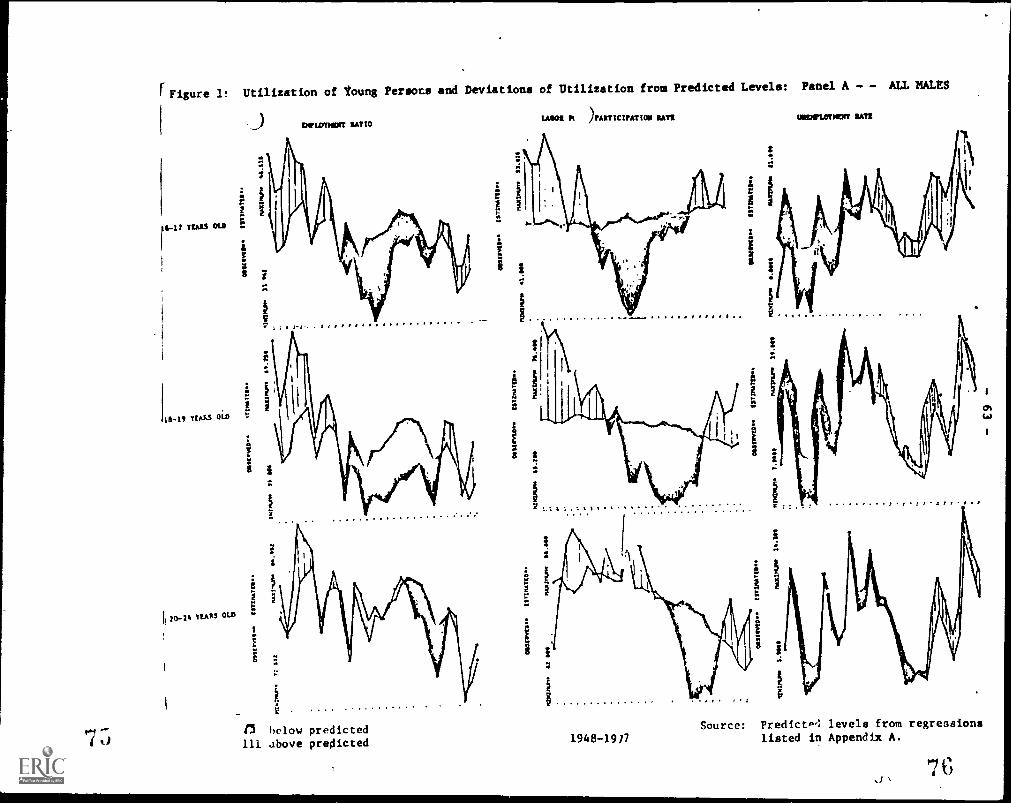
Figure 1: Utilization of toung Persocs and Deviations of Utilization from Predicted Levels: Panel A - - ALL MALES

16-17 TZARS OLD

1111-19 YtDAS OLD

INDLOYNDOT RATIO

13 below predicted111 above predicted

jrAIITICIDATION RATS amprtaness RATS

1948-1917Source: Predict' levels from regressions

listed in Appendix A. '

11IPLOTTITIT SATIO

Panel 1 - - OUT OF SCHOOL MALES

WOO MA trittC111411011 SAMvitormnsirt RATS

ti16.11 Tomas Oli 1 I

(1954.4977ii

1 Ii

1

1 .

18-110 Tara Old

20.21 Tierra Old

i1

I

.'.....

I

1\1

3..:

&.. ttttttttttttttttttt :1:: 1

I 1i

I

i

:::..:::...:..

1948-19771, -

i i

Tura Old I

E

8

oncrywarr PATIO

Panel C - - ALL FEMALES

M1011 I'01111 PAITICITATICIO MT. IDIOPPLOTNENT (ATP

E

7

8

V

IS-11. Toots Old A I

20-24 Tsars 014

I

li.11:1111S::131:81:1:::: !WS:-

7 ti

1948-1977

In

participation ratios tell a different story, particularly for women.

Overall, the data raise doubts about the existence of "job crisis" for

all young workers.

Black Youth Joblessness

The absence of a definite deterioration in the employment of all

young workers does not, however, mean that there is no youth employment

crisis, but rather that the problem is more localized. Data on'the employment,

unemployment, and labor force of young workers by race from the Current

Population Survey show a striking deterioration in the utilization of

young blacks, which can be viewed as the essence of the youth employment problemin the U.S. This claim is documented by the evidence on the overall magnitude.of employment and joblessness among black and other and white youth from t:le

early 1950's to the 1970's given in table 1. First, the employment to popula-

tion ratios given in line 1 for young men show a marked drop for blacks compared

to the rough stability for whites. Among 16-17 and 18-19 year old black men,,

the ratios drop sharply from 1954 to 1964, stabilize in the late 1960's, and

then drop sharply in the 1970's recession. Among 20-24 year old black men,

the ratios hold steady until the 1970'e, but then drop noticeably.

Regressions linking the black employment ratios to those for comparably aged

whites and a time trend make clear the e-4-tent of deterioration. The trend

coefficients and standard errors (in parentheses) are: -.94 (.04), -.96 (.08),

and -.25 (.11), for 16-17, 18-19, and 20-24 year olds, respectively. As a

result of the downward trend in utilization, the ratio of black to white employ-

ment rates drops from rough equality with those of whites in the early 1950's to

.43 (16-17 year olds), .57 (1g-1: year olds) and .76 (20-24 year olds) by 1977.

The decline in the employment rate of young black men has two components:

a marked rise in the fraction out of the labor force (line 2), which contrasts

Table 1

Dimensions of the Minority Black and Other Youth Employment Problem

Black and Other Male White Male

1954 1964 1969 1977 1954 1964 1969 1.977

1. Percent with JobAge: 16-17 40.4 27.6 28.4 18.9 40.6 36.5 42.7 44.3

18-19 66.5 51.8 .51.1 36.9 61.3 57.7 61.0 65.2

20-24 75.9 78.1 77.3 61.2 77.9 79.3 78.8 80.5

2. Percent is Labor ForceAge: 16-17 46.7 37.3 37.7 30.8 47.1 43.5 48.& 53.8

18-19 78.4 67.2 63.2 57.8 70.4 66.6 66.3 74.9

20-24 91.1 89.4 84.4 78.2 86.4 85.7 82.6 86.8

3. Percent of LaborForce UnemployedAge: 16-17 13.4 26.0 24.9 38.7 13.9 16.1 12.5 17.6

18-19 15.2 22.9 19.2 36.1 12.9 13.3 7.9 13.0

20-24 16.7 12.6 8.4 21.7 9.9 7.4 4.6 9.3

4. Percent WithoutWork ExperienceAge: 16-19

(b)32.7 55.3

(a) (b)24.5

37.2(a)20-24 9.7 12.8 20.8

(a)7.2 9.8

Black and Other Female White Female

5. Percent with JobAge: 16-17 19.8 12.4 16.8 12.5 25.8 23.6 30.3 37.5

18-19 29.6 32.9 33.7 28.0 47.2 43.1 49.1 54.3

20-24 43.1 43.8 51.6 45.4 41.6 45.3 53.3 61.4

b()I

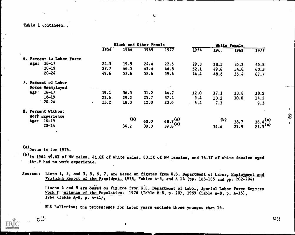
L.

Table 1 continued. ,

Black and Other Female White Female1954 1964 1969 1977 1954 19c, 1969 1977

6. Percent in Labor ForceAge: 16-17 24.5 19.5 24.4 22.6 29.3 28.5 35.2 45.6

18-19 37.7 46.5 45.4 44.8 52.1 49.6 54.6. 63.320-24 49.6 53.6 58.6 59.4 44.4 48.8 56.4 67.7

7. Percent of LaborForce UnemployedAge: 16-17 19.1 36.5 31.2 44.7 12.0 17.1 13.8 18.2

18-19 21.6 29.2 25.7 37.4 9.4 13.2 10.0 14.220-24

8. Percent WithoutWork Experience

13.2 18.3 12.0 23.6 6.4 7.1 9.3

orco

Age: 16-19(b)

60.0 68.7(a) (b)

38.7 36.4(a)

1

20-24 34.2 30.3 39.8(a)

34.4 25.9 21.5(8)

(a)Datum is for.1976.

(b)In 1964 49.6% of NW males, 41.6% of white males, 63.5% of NW females, and 56.1% of white females aged14--9 had no work experience.

Sources: Lines 1, 2, and 3, 5, 6, 7, are based on figures from U.S. Department of Labor, limlumnt andTraining Report of the President 1978, Tables A-3, and A-14 (pp. 183-185 and pp. 202-204)

Liness 4 and 8 are based on figures from U.S. Department of Labor, Special Labor Force RepsctsWork F-rerience of the Population: 1976 (Table B-8, p. 20), 1969 (Table A-8, p. A-15),1964 (rsbie A-8, p. A-11),

BLS Bulletins; the percentages for later years exclude those younger than 16.

- 69 -

with stable fractions for young whites; and an increase in the fraction in

the labor force lacking jobs (line 3), which also occurs among whites. The

relative importance of the two adverse developments can be gaged by decompottng

the identity that links the employment (E) to population (P) ratio to the labor

force (L) and to unemployment (U L-E):

(1) E/P E (L/P)(1-U/L)

or in log differential form:

(2) dln E/P E dln L/P t dln (1-13/L)

For the period 1954-1977, equation (2) yields the following deomposition of

the secular change in the employment to population ratio for young black men

in the three age groups:

16-17 18-19 20-24

Aisii vr -.76 -.59 -.22

Alm L/P -.42 -.30 -.15

pin (1-U/L) -.34 -.29 -.67

The drop in labor participation is, by these statistics, as or more important in

the falling employment ratio than is the increased rate of unemployment.

This implies that changes in unemployment rates understate the extelt 'f the

unemployment problem facing young blacks and that the behavior of ncnpartici-

pants is critical to understanding the black youth employment problen.

Line 4 of Table 1 examines the lack of employment among blacks from a different

perspective: in terms of the fraction of young peraons who obtain no work exper-

ience over a year. In contrasc to the employment, labor force, and unemployment

figures, which are based on monthly surveys of activity during a week, these

s

- 70 -

figures are obtained from a retrospective question (on the March CPS) regarding

activity over an entire year. What stands out is the marked increase in the

proportion of blacks without work for a whole year: from 10 percent of 20-24

year old blacks in 1964 to 21 percent in 1976, which contrasts to the rough

stability in the proportion of white men aged 20-24 without work experience.

Lines 5-8 present comparable figures for black and white women. While

the employment to ripulation and labor participation rates of young black women

do not trend downward in absolute terms, they drop sharply relative to the rates

for white women. In 1954, the ratio of black to white female employment rates

were .77 for 16-17 year olds, .63 for 18-19 year olds, and'1.04 for 20-24 year

olds. By 1977, the increased employment of white women brought the ratios down

to .45, .52, and .74, respectively.

The marked deterioration in the relative employment of young black

workers shown in Table 1 constitutes one of the major puzzles about the

youth labor market in the United States and thus one of the prime questions

for research: Why has the utilization of young black workers declined

relative to that of young white workers?

The striking difference in the labor force participation of 16-24 year

old blacks and whites in the 1970's, which accounts for much of the differ--

ence in employment/populationratios, is examined further in Table 2, which

gives the percentage distribution of blaA and white young persons by various

exclusive labor market categories in 1974-1975. Three basic differences

between blacks and whites stand out in the table. First is the sizeable dif-

ferential in the proportion of young persons working. In each age group the

proportion of whites working exceeds that of blacks by upwards of 25 percentage

points. From May 1974 to May 1975, when the economy entered a sizeable reces-

sion, the differentialsincrease noticeably for 18-19 and 20-24 year olds.

Second is the extent to which the differentials are associated with differences

,S5

- 71 -

in the fraction not in the labor force, as opposed to unemployed. In 1974, 82

percent of the 25.2 percentage point gap in the fraction working among 16-17

year olds is due to the fraction not in the work force; 85 percent of the 20.9

point gap among 18-19 year olds and 4.6 percent of the 9.0 gap among 20-24 year

oldsare alo associated with persons not in the labor force. The possibility

that the labor force participation differences between young blacks and whites

are due to differential propensities to enroll in school is, it should be

stressed, rejected by the data. As can be seen in columns 7 and 8 or Table 2,

even larger differences are found between blacks and whites out of school

than are found in the overall-population.

The differential patterns and trends in the employment of young blacks

and whites are examined further in table 3, which treats the employment, labor

force, and unemployment rate; of out-of-school high school graduates and drop-

outs. Lines 1 and 2 deal with all 16-24 year old male high school graduates

or dropouts while lines 3 and 4 treat males and females who either graduated

or dropped out in the given year. The figures in lines 1 and 2 show that the

percentage of black male high school graduates or dropouts with jobs is much

below the percentages for comparable young white men and that the differentials

grew sharply from 1964 to 1976, particularly in the 1970's, when black labor

participation rates fell and unemployment rates rose. Lines 3 and 4 tell a

similar story for persons in the relevant graduating class or dropout popula-

tion. The Magnitudes of some of the differences in 1976 are remarkable, to

say the least. According to the CPS survey, only 39 percent of black high

school graduates in the class of 1976 who were not enrolled in college were

employed in October 1976 compared to 73 percent of their white peers; the

black participation rate uas 15 points below that for whites and the unemploy-

ment rate three times as high. Among dropouts only 22 percent of black youth

compared to 49 percent of white youth were employed, with a 17 point difference

in participation rates and twofold differential in unemployment rates.

- 72 -Table 2: Percentage Distribution of Black and White Young Persons

by Labor Market Status: Hay 1973. 1974, and 19758

All Young PersonsOut of SchcolYoung'rerso-t,

May 1973 May 1974 May 197 5 "cy 197

Black WhiteArmand Status Black White Black White Black White

Working 14.5 3.7.9 13.2 38.4 11.9 36.1 34.1 66.8Not Working 85.6 6 21 86.8 61.6 83.1 6 3. 9 65.9 33.2With Jobsb 0.8 1.3 0.3 1.3 1.2 1.7 0.0 2.1Without Jebs 84.7 60.8 86.6 60.3 86.9 62.2 65.9 31.1

Have Looked 13.6 11.4 16.6 11.0 17.0 14.0 22.3 8.4Available 9.5

for Workand Looking

6.6 9.5 6.2 9.6 8.0 19.4 7.5

Not Lookin3 0.2 0.5 0.6 0.3 0.1 0.4 1.3 0.4

ActivelyNot Available 3.9

for Work d4.2 6.6 4.6 7.2 5.6 1.6 0.4

Not in Labor Force 71.1 49.5 69.9 49.3 69.9 48.2 43.6 22.7

18-19Working 32.7 54.8 34.7 55.6 26.8 53.3 48.6 70.1Not Working 67.3 45.2 65.3 44.4 73.2 46.7 51.4 29.9With Jobsb 1.6 2.3 1.5 2.6 2.0 3.6 2.6 2.8Without Jobs 65.7 42-9 63.7 41.8 71.2 43.1 48.7 27.]Have Looked 16.7 10.4 15.1 10.9 22.1 14.1 16.5 9.2

Available 11.1for Workand Looking

5.9 13.1 7,0 17.4 9.6 15.8 8.5

Not Looking 0.3 0.2 0.3 0.2 0.7 0.3 2.5 0.2Actively

Not Available 5.2

for Workd4.3 .1.6 3.7 3.9 4.2 0.3 0.5

Not in Labor Force 49.0 M .6 48.7 30.9 49.1 29.0 32.3 17.8

20-24

Working 54.8 65.0 57.0 66.0 47.6 62.9 62.0 72.2Not Working 45.2 75.0 43.0 34.0 52.4 37.1 35.0 27.8With Jobs b 2.8 2.8 3.3 3.5 4.3 4.9 3.5 3.5Without Jobs 42.3 32.2 39.7 30.5, 48.1 3.2.2 34.4 24.3

Have Looked 12.3 6.2 11.3 6.3 17.4 9.2 11.0 5.0

Available 10.8

for WJrkmid Locking

4.4 9.7 4.5 16.1 7.3 9.6 4.4

Not LL,oking 0.3 0.1 0.9 0.2 0.7 0.3 1.0 0.4

Activel)Not Available 1.2 1.7 0.8 1.5 0.7 1.0 0.4 0.2

for Work d ,

Not in Labor force. 30.0 26.0 'R.4 24.3 30.7 23.0 23.4 19.2

10. Based on welthted cot.n.,s witn

b) Includes emoloycJ worle,-; nctor I -' "

1,ta. a n'.!w

tee ..p',..-o;sriate Current Population Surveys.-,r- of 11. ss, vacation, bad oenr.

'0 Jr inoofinite .11:;off or at,c-: to

c) Incled.,:s job losers, job quirl,n--. who .114t school and those w4ritini:temporary work.

d) Includes. people who alrculy 11-:v j. , and thorn unavailable because of school

qt tevoratv Illness.

- 73 -

Table 3

f7p1,17ent of 0; h School Grai-aces ari Dropouts

1. All =Ale acrcolgrac.atea not earollsd

to college 16-24aa. Percent with a jobb. Percent in labor forcec. Percent of labor force

mimmtployed

2. !tale high school dropouts

16-2..41

a. Percent with a jobb

S. Peroenc in labor forcec. 'arcs= of labor force

mnimplo)ed

3. `talc mr.4 femali high schoolSrsd.ates in reportai yearoot enrolled in collegea. Percent with a jobb. Percent in labor forcec. Pezi-uic of labor force

uneeployed

4. male on1 fe:ala schoold ::;..: - :s

a. Percsat with a jobb. Pa:4enc in Labor forcec. Percent of labor force

unezplo:si

!jacks and Othsr Races Whites

1964 1969 1976 1960 1964 1969 1976

75.8 81.6 67.3 86.5 8E1 87.0

93.3 91.5 86.1 94.9 93.8 95.4

18.8 11.3 22.0 8.9 6.0 8.9

70.3 72.7 50.4 76.1 74.7 71.1

85.8 83.0 73.6 88.1 83.7 88.5

18.1 12.4 31.5 13.6 10.8 19.7

52.3 50.0 39.0 67.0 64.6 73.4 72.9

81.1 72.6 70.3 77.0 77.5 80.2 85.9

35.6 31.2 44.5 13.0 16.7 8.5 15.1

49.3 49.3 21.6 48.7 39.2 52.1 48.6

63.4 62.7 50.9 59.7 52.8 60.9 67.1

22.2 21.3 56.9 18.4 25.7 15.5 27.5

call f.; -:.s are zaxaa frog E=olorment of Huth School Graduates and Dropouts. 1960 (Table 2,

p. .:3), t:AS:e A. F. A75); 1964 (Toole 1, p. 639. Table 4, p. 642); 1969 (Table 2 and

Table 1. ?. is); 1$.o Ciaaie 1, p. A-13, Table 8, p. A-18).

Slit: :11.res in line 2 and line 3 include female graduates as well as male graduates.

alit. flg.res in line 2 include male graduates ages 16-21.

- 74 -

Because a sizeable proportion of black/white differences in youth employ-

ment result from differences in labor force behavior, it is important to

examine the poiition of nonparticipants from the CuLr,nit Population

Survey. The table records the percentage of 16-19 and 20-24

year old nonparticipants in and out of school and the percentage of these

20-24 year old nonparticipants in and out of school and the percentage of these

groups who report that they do or do not wanta job in the survey week and their

activity or reason for not seeking employment. For men, the data suggest that

most nonparticipants, including those out of school, do not in fact want a

job in the survey week, but does not elucidate the reasons why they are not

seeking work. Two-thirds of 16 -19 year old out of school male participants

do not want a job for "other" (unknown) reasons while half of 20-24 year old

out of school male nonparticipants are also reported as not wanting a job

for "other" reasons. Even among 16-19 year old women, the proportion who do

not welt a job for "other reasons" is about one-third. Among 20-24 year

olds, however, it is clear that choice of household activities leads persons

to be out of the work force.

The figures in columns 5 and 6 of the table show a much higher proportion

of out-of-the labor force blacks actively wanting a job now but "discouraged"

because they think they cannot get a job or for "other reasons." Thirty-six

percent of out of school 16-24 year old back nonparticipants desire a job com-

pared to 19 percent of their white peers. While inclusion of women in the data

by race makes keeping house the main reason for not wanting a job now, one-

quarter of both black and white groups do not want a job for "other reasons."

The sizeable differences in labor participation rates between young blacks

and whites, the declining rate of participation among young blacks, and the lack

of information about not enrolled nonparticipants directs attention to a second

Sti

- 7 5 -

loble 4

OfstrIbutIon of Nonparticipants In the labor Force,by s41 1 status and desire for work. 197/

Male Workers Female Workers

Both Seselmark

White

13F-TG=7Eand Other

71W-IF=74Age 16-19 Age 20-14 As 10-19 Aga 20-24

Total. Out of Labor Force 100.0 100.0 100.0 100.0 100.0 100.0

In school 80.8 71.1 67.6 23.5 58.9 60.3wont job now 21.4 15.7 19.6 lr 10.3 2.1.6do not want job now 78.6 84.3 80.4 83.8 81.7 76.4

Out of school

want a job now but111. disabled

19.2 28.9 RA22.5

76.5 11.1

14.7

39.7

27.1 34.6 18.7 35.7think cannot get job 1.3 6.3 .9 .9 1.4 1.3household responsibility 1.3 12.2 6.9 3.6 4.8 11.6other rosaon 14.5 16.1 7.7 9.3 5.5 12.9

7.0 4.9 7.1 9.9

do not want job now 72.9 64.3 77.5 81.2 111.3 64.3111. disabled 3.8 15.6 1.5 2.4 3.3 3.9keeping house 2.4 1.0 43.9 71.4 53.2 35.3other 66.7 48.7 32.2 7.4 24.8 25.1

Sources U.S. Department of Labor. Employment and Earnines. Vol 25. No.1 Surrey 1978Table 39, p. 167Table 40. p. 168

9U

- 76 -

major research question whose answer is needed to understand the youth labor

market problem in the United States: What are the out-of-the-labor-force youth

doing and why have they left the work force?

While much of the difference between the employment of young black and

white workers is associated with differences in labor force participation,

there are also sizeable racial differences in the proportion of young persons

available for work and looking, particularly in the older age groups. According

to table 2, 13.1 percent of 18-19 year old blacks, for example, were available

and looking in 1974 compared to 7.0 percent of 18-19 year old whites while 9.7

percent of 20-24 year old blacks were looking compared to 4.5 percent of 20-24

year old whites.

Table 5 presents data designed to illuminate this differential. It

records the proportion of black and white labor force unemployed for several

"direct" reasons: loss of job; quits; entrance into the labor force, divided

between re-entrants, defined as those who previously worked at a full-time

job lasting 2 weeks or longer but who were out of the labor force prior to

beginning to lzak for work, and new entrants, defined as persons who never

worked at a full-time job lasting 2 weeks or longer. The figures direct

attention to two factors in the high unemployment rate of black youngsters:

difficulty in obtaining an initial job upon entry to the work fbrce, which is

thE: prime cause of black/white differences among 16-17 year olds and 18-19 year

olds; and loss of jobs, which explains the bulk of differences among 20-24 year

olds.

The differences in the proportion of black and white teenagers who are

unemployed entrants are remarkable. In 1969 11.0 of the 12.1 percentage

point difference between the unemployment rate of 16-17 year old blacks and whites vas

attributable to entrants; 5.5 points of the 10.9 percentage point differential be-

tween 18-19 year olds was also due to entrants; in 1978, the relevant differences wt-re

25.3 of 25.6 points (16-17 year olds) and 14.5 of 20.1 points (18-19 year olds).

By contrast differential rates of job leaving h'id very little impact on the

- 77 -

Lit., 5 barect CI,Ises of luu,o Un.opl.):_ht4

Black l'hitob

1969 IS7S 197db 1969 1975 1978

1:-17

Total C.I.:4;1.7,:_o-t Rate 24.6 39.2 46.4 12.5 19.7 19.7

lasses 2.1 4.8 4.5 1.6 3.4 3.2

leavers 1.6 1.1 1.4 1.0 1.4 1.2

total entrant* 20.9 33.9 40.6 9.9 15.0 15.3

re-enttalts 10.2 15.3 15.7 4.3 5.9 6.1

new entrants 10.7 18.5 25.1 5.6 9.0 9.2

1S-1;a

To:al Uner.71e,..rert :ace 18.8 32.9 33.5 7.9 17.1 13.4

losers 5.9 13.0 10.2 2.0 8.1 5.4

leavers 3.3 2.3 2.6 1.5 1.7 1.8

total entraa:s 10.0 17.9 20.7 4.5 7.2 6.2

re-entrants 7.0 10.1 10.6 3.0 4.3 3.7

r.. entrants 3.0 7.5 10.2 1.5 3.0 2.5

To:al 1.r:rp1-ynenc Rate 8.4 23.0 22.8 4.6 13.2 10.7

losrs 3.9 14.9 11.4 1.8 8.6 6.2

leavers 1.7 1.4 1.6 0.9 1.4 1.9

teca: got:an:$ 2.7 6.7 9.8 1.9 3.2 2.6

re-C....riAtt 1.8 4.8 7.3 1.7 2.7 7.2

r.. c-:rants 0.9 1.9 2.5 0.3 0.5 0.4

Nocos: a. Unem;lcyvnt vcin4ted :nto:; ore taken from unpublished data provided

ms. !,Jra1 Fore, ru.-1.r. tt taken Crop E-_?la-ent_and Tr:00911.71.

.1 t, 1. L, -7, .. . (0. 13J-193).

b. 1;7,3 r:rcentzt,% Jr nerogcs of percentages for the first

t .1

92

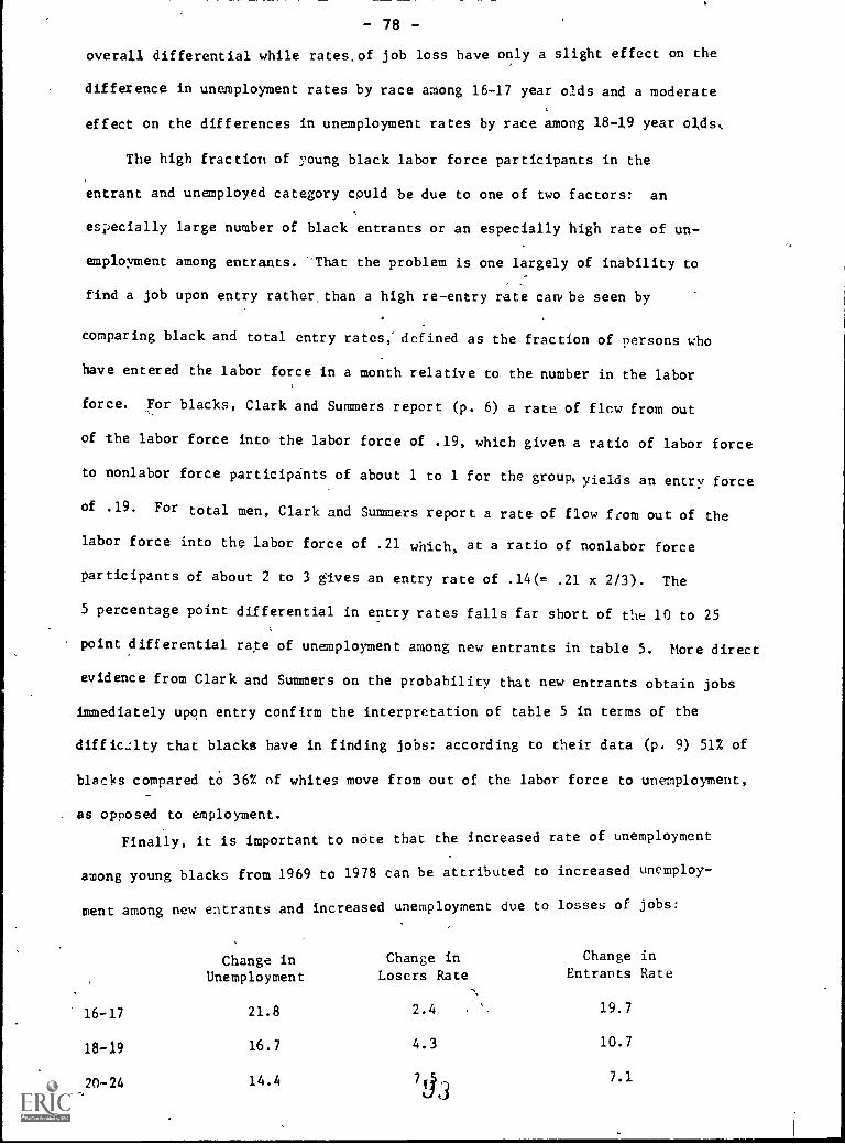
- 78 -

overall differential while rates.of job loss have only a slight effect on the

difference in unemployment rates by race among 16-17 year olds and a moderate

effect on the differences in unemployment rates by race among 18-19 year cads,.

The high fraction of young black labor force participants in the

entrant and unemployed category could be due to one of two factors: an

especially large number of black entrants or an especially high rate of un-

employment among entrants. That the problem is one largely of inability to

find a job upon entry rather than a high re-entry rate can, be seen by

comparing black and total entry rates,' defined as the fraction of persons who

have entered the labor force in a month relative to the number in the labor

force. For blacks, Clark and Summers report (p. 6) a rate of flow from out

of the labor force into the labor force of .19, which given a ratio of labor force

to nonlabor force participants of about 1 to 1 for the group, yields an entry force

of .19. For total men, Clark and Summers report a rate of flow from out of the

labor force into the labor force of .21 which, at a ratio of nonlabor force

participants of about 2 to 3 gives an entry rate of .14(= .21 x 2/3). The

5 percentage point differential in entry rates falls far short of the 10 to 25

point differential rate of unemployment among new entrants in table 5. More direct

evidence from Clark and Summers on the probability that new entrants obtain jobs

immediately upon entry confirm the interpretation of table 5 in terms of the

diffic.lty that blacks have in finding jobs: according to their data (p. 9) 51% of

blacks compared to 36% of whites move from out of the labor force to unemployment,

as opposed to employment.

Finally, it is important to note that the increased rate of unemployment

among young blacks from 1969 to 1978 can be attributed to increased unemploy-

ment among new entrants and increased unemployment due to losses of jobs:

16-17

18-19

20-24

Change inUnemployment

21.8

16.7

14.4

Change inLosers Rate

2.4

4.3

7J3

Change inEntrants Rate

19.7

10.7

7.1

79 -In short, the evidence on direct causes of unemployment suggests that

failure to obtain a job rapidly upon entrance into the market and a high job loss

rate constitute major labor market problems for black youngsters, raising alditional

questions regarding the youth labor market problem: Why do young blacks have

greater problems in finding a first ob than oun whites? Wh are oung blacks

laid off more frequently than young whites?

Characteristics of Employment

The labor market position of workers depend. not only on whether they hold

a job or not but also on the type of job and rate of pay. In this section we

compare the industrial and occupational distribution of young and all male workers,

the percent of young and all workers with part-time as opposed to full --time

positions, and the earnings of young and all workers. The data show that the

young are concentrated in a different sat of jobs than other workers, are

especially likely to work part-time, and have experienced sizeable declines in

relative earnings in the period studied.

Evidence on the industrial and occupational position of young and all

male workers is given in Table 6', which records percentages employed in

one-digit industries and occupations from the decennial Censuses of Population

and from Current Population Surveys. The divergence between the employment

distributions of young and all workers is summarized with an Index of

Structural Differcnces, defined as the sum of the absolute values of the

percentage point differences between the groups, formally, if aij

is the

percentage of workers in age group i in the jth category and a.j is the

percentage of all workers in the category, the index is defined as

E .

The industry employment figures reveal an enormous difference between the

sectors of employment of "-17 year old men and all male workers, a sizeable

'difference between the industries hiring 18-19 year olds and all men but only

a modest difference between the industrial distribution of 20-24 year olds

Takao b TM lodustrial ad 04cuutlft641

34-17 11-19 70-74 To141 (A)

bIstrIbatInn et tIm ImployanniC.10.4

14"18 AAA All MA"

(4)

Hurl."" 3950.1417

3'.70

)19-19 20-1414.17 11-19

1940

30.74.1.7,LLEth.11100S11111.4

Agrivature 39.1 24.3 15.0 15.9 18.1 11.6 7.4 9.0 8.8 3.7 3.4 ,.:

Milting .3 3.3 2.2 2.2 .2 .8 2.2 1.4 .2 .7 1.1 1.?C448trticgieft 4.0 6.6 8.0 8.7 3.5 3.9 8.4 8.4 3.3 6.$ 6.4 9.1

Manufacturing MO 26.5 30.0 27.0 15.5 25.5 32.6 30.2 12.1 25.7 31.0 2',..

Iransp.. etc. 2.4 5.1 8.9 9.2 1.8 3.8 6.6 8.3 2.0 4.8 7.7

Trade 23.7 22.6 18.8 17.1 40.3 24.1 19.6 17.0 52.3 37.0 21.3 111.E

inane. .3 1.6 2.0 2.8 .6 1.7 2.8 3.4 1.1 1.7 3.) 4.0line 4 Oneair 1.8 2.3 3.4 3.0 2.4 3.3 3.3 2.8 3.6 3.8 3.9 3.1.

Pere. Sarnia* 2.4 2.6 2.4 2.8 4.3 2.8 2.; 2.3 3.6 2.2 1.8 2.1

Rat. 6 bet. 4.4 2.0 1.2 1.0 3.5 1.6 .11 .8 3.2 1.7 1.0 .',

Prof. & Rel. 1.6 4.4 3.5 4.8 3.6 3.4 6.1 6.9 7.2 9.2 12.0 10.4Public Aditio. .4 .11 3.2 4.6 .4 1.3 3.3 3.3 1.0 .1.9 4.2 6.1let Xisparted 3.4 1.7 4.4 1.3 4.7 3.7 3.1 3.6

1441 48.8 27.3 10.8 74.3 34.9 12.1 82.1 38.3 10.4

coOCCUPATIONS O

iProf, Ttb.6 kindred .3 2.1 3.3 7.3 1.3 3.3 9.8 10.3

farmers . 1.7 4.2 14.3 14.4

6 shearers 2.7 3.6 5.6 10.4 1.1 1.7 2.0 3.3Managers .4 .3 .9 2.8

as faruera .3 1.2 3.4 10.3___-,/

--'' .3 1.3 3.$ 10.6Clerical 4.8 9.4 9.4 6.3-` -7.8 11.3 10.3 7.0 .7 1.6 4.9 11.2

Ileleo -10.7 7.5 6.9 6,4 13.8 7.8 6.2 6.9 7.9 11.4 11.0 7.6

Craftsmen 9.3 6.7 6.2. 6.9

6 fames 3.4 8.1 14.8 1/.7 4.6 10.1 1.5.4 18.3Oisratives 13.9 23.8 28.1 20.1 18.3 24.0 26.5 19.9 5.6 12.4 18.5 21.2

Para,* boussbeld .2 .1 .1 .2 .3 .2 .1 .1 18.1 26.7 24.1 19.5

SerifiCO OS MX 9.7 6.0 4.4 3.9 11.3 8.0 5.6 6.0 .3 .1 .1 .1

Pass laborers 33.7 20.0 8.6 4.4 14.7 8.8 4.4 '2.7 24.8 14.1 8.1 8.0

Laborers as faro 7.0 4.1 2.1 1.7

6 sloe 13.0 14.5 11.5 4.1 19.1 14.2 9.4 6.9lot Mow 114 2.6 1.7 1.3 1.1 3.8 7.3 6.6 4.6 24.1 18.1 9.3 6.6

Ile 114.5 63.3 37.4 76.4 56.3 29.983.1 61.1 21.8

%sloe 14 years sod alder Sourest Gassr data lodustrial Cbarectrriatics, 1930,

%s1.. ' years aod older. Table 3; 1440, fables 2, A; 1470, Tables 32, 34.

Occuppflooal Cba tette., 1930, Table 6; 1940,61811 'Wan of structural differences, dleflood as sum .t Tab14. 2, 6; 1470, Tables 39, 40.absolute deviattome berme.. pareastages for yours markersuid...fax44aiarsockers

0"

- 81 -

Tails it 994 ladmarial sad 096969614441 1109164M.. 0 94p1o9...4t 01 16699 6r4 Aii MANI 14.8r4, 15'.6 At"

P44.1 1.21..1..1 16/.1.09.1.

1167 1174

16-17 18-11 10-24 To141(6)

14-17 19-11 10-16 T097(4) 16-57 14-1q 70-16

.1 .6 .9 1.2 .2 .5N16143Caoscrweglas 5.6 9.5 CS 9.4 7.4 10.1 7.) 1.2 .1 1.1 3.11".4461acgmt144 14.0 32.6 29.9 34.3 11.2 29.4 12.0 10.4 6.9 11.9 24.1 16..

1rump.. 814. 2.4 5.1 7.2 8.1 2.3 5.2 36. 30.0 11.8 22.9 29.2 14.4Trod. 53.4 34.6 19.8 18.9 55.4 34.3 9.0 9.1 2.5 4.5 6.9Mass. 1.6 1.5 3.1 4.2 1.4 1.1 23.0 19.0 54.4 34.7 25.9 26.194 i Repair 3.4 3.1 2.7 3.4 4.1 4.4 3.8 4.6 1.4 1.7 3.3fors. masa 2.9 2.0 2.0 2.1 2.7 1.6 4.3 4.0 3.8 5.2 5.i 4 4Lag. i 119e. 5.1 2.6 1.1 1.0 4.2 2.3 1.5 1.7 1.1 1.7 1.4 JPref. i Isl. 9.3 4.0 1.0 1.6 7.4 7.4 1.6 1.1 4.8 2.7 1.9 1.1

Publis Male. 1.9 2.6 4.0 6.6 1.5 1.9 11.0 11.5 6.4 4.3 9.9 12.5

Mt Maenad 4.2 6.6 1.4 1.6 3.5 6.5

23e 79.5 35.o 14.2 41.2 32.4 11.5 44.2 44.6 14.1

ICWATIOVSaft siptigs(b) Ata ()

725.91. 1111:17Wf.1tPref. Tech.6 bistro/ramose4 manses

2saegersea Issuers

ClarlealSelo.Craltause

forsJoa@voraciousPrivate householdService on 11111

Peru laborersLaborers en lens4 'doe

Mc Sepersoduse

3.3 13.0 2.4

.5 3.9 .5

.11 13.3 1.4

11.5 7.1 6.57.0 5.5 5.3

6.7 20.1 10.925.3 20.4 22.1

.2 .1 .2

144 7.0 14.31.4 2.2 7.4

1

22.4 7.2 21.3

77.4 72.4

mit 2.0 14.6

3.0 .3 13.1

13.6 1.2 2.56.6 6.4 6.36.1 6.3 6.0

20.8 10.7 20.118.8 20.0 17.6

.0 .4 .1

7.9 22.0 9.71.4 6.5 1.7

7.7 24.1 7.6

75.3

aCPS escludos &stimulate sad Seeress CPS dates Isdostrial Chanciest's'''. 1950.privet' budsobslA wallows Table 3; 11060. Tables 2. 4; 1970. Table& 32. 34.

%sloe 16 yam and older Occupatissol Charas eeeee ties. ISSN Table 61 1140.Te41es 2 6' 1170. Tibiae 30. 40.

4240 . 5a441Ldf structural different... Selland ea sou ofshy/Auto dce1atieue between pereumases for 'swag unbarsand for aim workers

1;

- 82 -

and all men. Both the Census data and the CPS data (which are limited to

nonagricultural industries) show 16-17 year olds to be largely concentrated

in trade and substantially underrepresented in manufacturing, among other

sectors. From 1950 to 1970 the employment of 16-17 year olds as well as other

men in agriculture dropped sharply. Men in the next age bracket, 18-19 year

olds, are also relatively overrepresented in trade but much less so than 16-17

year olds. The 18-19 year olds tend to find a relatively large number of jobs

in manufacturing. Overall, the index of structural differences is reduced

by about 50% as the group increases in age from 16-17 to 18-19. In contrast

to teenage groups, the industrial distribution of 20-24 year olds closely

mirrors that of all male workers, suggesting that by that age the young are

beginning to enter what may be called adult job markets. From 1974 to 1977,

however, the ISD grew for 20-24 year olds, as well as for the teenagers.

Divergences in job distributions are considerably greater along

occupational dimensions, with 16-17 year olds highly concentrated in laborer

and service jobs and 18-19 year olds in laborer, service, operative and clerical

jobs. For 20-24 year olds, the divergences are smaller and appear to have

fallen from 1950 to 1970.

Whether the marked difference in the industrial and occupational

distribution of employment of teenagers and all male corkers does, in fact,

reflect differences in job markets depends, of course, on the link between

the jobs obta.ned by the teenagers and adult jobs. The wide divergences

shown in Table 6 are, at the least, suggestive of significant differences

between the teenage and adult job markets.

The data on part-time versus full-time work given in Table 7 lends some

support to the separate market interpretation of the divergences in job

distributions. According to the table, nearly half of teenage workers and

over 3/4ths of those aged 16-17 are either employed part-time or are on

part-time schedules. By contrast, the proportions of all workers employed

part-time and on part-time schedules is much smaller. Among the unemplcyed

- 83 -

Table 7

e - ..i_:.oc Y.-Eh and All Workers, by Part -lire Job Status, 1976

?odle Frzale

TztalHale and Female

Percentage of Percentzee of Percentw,e onEmployed Working Unemployet; Seeking Full-TinePart-Tie. Part-Tine Wo:k Schedules

46.4 41.9

14.3 19.4

S=ag7..1:-1t4ra1

Hale E:playees

All 10.616-17 76.418-14 20.9

h:n4iri:-It4ra1TOM31t Emplo)eas

All 28.816-17 84.415 -2. 29.0

Socrze. U.S. Department of Labor, Handbook of L.bor Statistics 1977Tables 20, 21, pp. 63-67

88

- 84 -

over 40% of unemployed teens are seeking part-time jobs compared to less than

20% of all unemployed workers. To the extent that the markets for full-time

and part-time workers are at least reasonably sepavlble, these figures

support the contention that there are substPmtive differences between the

youth, especially the teen, and adult job markets.

Wages

On the price side of the youth labor market, two major developments

stand out: a sharp drop in the relative earnings of young workers in the period

under study; and an increase in the earnings of young blacks compared to

young white workers. Columns 1-2 of table 8 document the marked fall in

the relative earnings of the young in terms of the ratio of usual weekly

earnings of out of school white men aged 16-24 to the usual weekly earnings

of all white men 25 and over. These data are taken from the May Current

Population Survey, which provides the best CPS figures on rates of pay from

1967 to the present. The data show drops in the rates of earnings for each

age group on the order of 10 points or so. Corroboratory information on the

annual earnings of year round and full-time workers ft= the March CPS reveals

similar patterns of change (see Freeman, 1978): a twist in the age-earnings

profile against young workers. Because a fairly sizeable number of young

persons are employed part-time, columns 3 and 4 of the table record the ratio

of the earnings of part-time young white men to the earnings of full-time

workers. All but two of these earnings ratios drop, though by a smaller

magnitude than the ratios for full-time workers, presumably because of their

initially low levels. If the full-time and part-time workers are joined into

a single group, the deterioration in the earnings position of the young becomes

even more marked. This is because the fraction of 16 to 24 year old out of school

men working part-time doubled over tie period covered from 8% to 16% in 1977.

(11)Ui

Table 8

Percentages of the Median Usual Weekly Earnings ofOut of School Men to Workers Aged 25 and Over, by Race 1967-77

Earnings of Full-TimeYoung White Men/Earnings of Full-TimeWhite Men, 25+

ChangeinEarningsRatios

Earnings of Part-TimeYoung White Men/Earnings of Full-TimeWhite Men, 25+

Changein

EarningsRatios

Earnings of Full-TimeBlack Workers/Earnings of Full-TimeWhite Men, 25+

ChangeinEarningsRatios

J967 1977 1967-77 1967 1977 1967-77 1967 1977 1967-77

Age

16 .38 .34 -.04 .19 .14 -.05 .33 .32 -.0917 .49 .39 -.10 .21 .19 -.02 .39 .32 -.07

118 .54 .49 -.10 .22 .20 -.02 .44 .44co

19 .61 .52 -.09 .22 .24 .02 .42 .43 -.0120 .66 .58 -.08 .35 .26 -.09 .63 .52 -.1121 .73 .61 -.12 .22 .23 .01 .57 .50 -.0722 .79 .63 -.16 .41 .24 -.17 .59 .54 -.0523 .84 .71 -.13 .38 .32 -.06 .59 .54 -.05

.

24 .87 .75 -.12 .37 .26 -.11 .60 .63 -.03

Source: U.S.Department of Labor, Unpublished Tablulations from May 1967 and May 1977, Current Population Survey

19f7 refers to voluntary part-time unless out of school1977 refers to all part time workers

bNo whites in 1969

101

- 86 -

exacerbating the drop in relative earnings.

Finally, the last two columns in table 8 reveal a pattern of drops in

the earnings of young blacks relative to full-time white male workers of a

smaller magnitude than those obtained for young white men, indicative of Ln

improvement in the earnings of young blacks vis-a-vis young whites. This

contrasts with the worsened employment record of young blacks relative to

young whites, possibly indicative of movement along a relative demand schedule.

Summary

The evidence from the Current Population Survey on the labor market

position of young workers in this section has yielded several findings

regarding the changing market for the young. We have found: that the un-

employment rate of all young workers deteriorated relative to older workers;

that, by contrast, the employment to population ratio did not decline,

except for not enrolled young men; that all indicators of employment --

unemployment rates, labor participation rates, and employment/population

rates -- show a worsened labor market position for young blacks while, by

contrast, their relative earnings position improued; that a large proportion

of the drop in black employment is associated with nonparticipation in the

work force, about which relatively little is known; that much of black un-

employment is due to problems in finding a first job and much to job loss;

that the occupational and industrial distribution of teenage employment

diverges sharply from that of adult males, suggesting a reasonably distinct

job market, while the iistribution of jobs of 20-24 year old men is quite

similar to that of all men; that relatively many teenagers are part-time

employees; and that the relative earnings of young workers have droppad

sharply in the pericd studied.

1'

- 87 -

II Associated Social Problems (Preliminary)

Concern wi 1 youth unemployment arises in part for two basic reasons:

fear that initially high rates of joblessness among the young will have

long term consequences for the economic well-being of the young; fear that

youth unemployment is associated, perhaps causally, with related major

social problems, such as youth crime, drug abuse, and the like. The potential

long term effect of youth unemployment has been examined by Ellwood. This

section focuses on the second issue. It presents data on several social

problems relating to youth that are a priori linked with joblessness and

then examines the lick itself. The evidence suggests a significant

worsening in these 'related social rroblems' which deserves serious attention.

The social problems

1. Increased youth crime.

Tables 9 and 10 demonstrate that youth arrest rates for both violent

crimes and property crimes have risen dramatically since the mid-1960's.

This appears to be truo for black and white youth, although the changes

in rates are substantially higher for blacks.

2. Violence in school

Table 11 shows sharp increases in violence and disruption in school

from 1964 to 1968 and from 1970 to 1973. Over the same periods school

enrollments rose much more modestly.

3. Increased illegal births

As can be seen in table 12 the number of births to unmarried women

aged 15-19 has risen among whites and nonwhites.

The preceding social statistics reveal substantial changes in several

important social indicators regarding youn. While cause and effect are

1O3

- 8d -

difficult to unentangle, the increase in -Jicide, illegitimacy, violence

in school, and youth crime are undoubtedly linked to the labor market

problems of the young. We plan to investigate these links in the next

few months.

4. Increased youth suicide rates

Table 13 documents a sharp rise in the suicide of young nonwhite and

white youth from 1950 to 1976, which compares with rough stability in the

suicide rate of the entire population. In 1950 the suicide rate for 20-24

year old nonwhi,es and for 20-24 year old whites were below the population

average. In 1976 both suicide rates exceeded the population average.

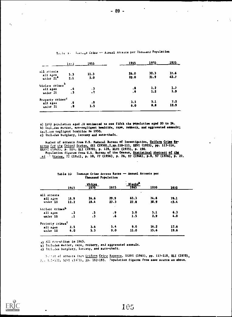
- 89 -

1. Crime -- AAnual Arrests per Thousand Population

1955 1965 1970 1975

All Jr:es:aall as 5.3 11.3 26.0 32.3 37.6

under 21a

crisesb

all ages

2.1

.6

S.0

.3

20.0

.6

31.9

1.2

42.7

1.7

under 21 .3 .1 .6 1.2 1.9

Property crimescall ages .9 .9 3.5 5.1 7.2

under 21 -3 1.5 6.0 6.6 12.9

a) 100 population aged 20 estimated is one fifth the populctioo aged 20 to 24.

b) murder, non-negligent homicide, rape, robbery, and aggravated assault;

inzl-res negligent hualcide in 1950.c) Includes burglary, larceny and auto theft.

Dumber of arrests from U.S. Federal Bureau of Investigation, Uniform Crime Re-- its fzr the rnitei Stares. XXI (1950),24P.116-111, MI (1955). pp. 113 -114,X3 V1 (19n3), p. 114, ILI (1970), p. 123, XLVI (1975). p. 190.

Population figures from U.S. Bureau of the Census, Statistical Abstract of the

ni States 72 (1951), p. 10, 77 (1956). p. 26, 67 (1966). p.8, 93 (1976). p. 27.

Table 10: Teenage Crime Across Races -- Annual Arrests per

Thousand Population

Whites--Ira--

Macke1963 1975 IVEY-- 1970

All arrestsall ages 13.9 24.6 29.9 65.3 74.6 79.1

under 13 12.2 13.4 27.3 27.6 38.9 i:S.4

Violent crimesball ages .3 .s .9 3.0 5.1 6.3

under 16 .1 .3 .6 1.5 2.9 4.0

Property :rimesc

all ages 2.5 3.6 5.4 9.0 14.2 17.6

under 13 4.0 5.3 9.0 11.0 15.6 19.6

,) All rzn-whites in 1965.b) In:16Jes murder, rape, robbery, and aggravated assault.

c) In:1-Jes burglary, larceny. and auto-theft.

of arretts Iron Uriforn Crime Reports, Mal/ (1965). pp. 117-113, XL/ (1970)

I.:-13:. MAI 01475), pp. 192-193. r'opulation figures from same source as above.

105

Violence and Disruption in the Schools

Percentage Increase in Crime in Schools in

110 Urban School Districts, 1964-1968

Category__ 1964 1958 Increase__

15 -26 73

Forcible Rap.- 51 81 61

PDbbery 396 1,508 376

Auravated Assault . 475 680 43

aiglary, Larceny 7,604 14,102 85

1:eaptinsCffenses 419 1,009 135

narcotics 73 854 1,059

Drunkenness 370 1,035 179

Crimes by Nonstuecnt3 142 3,894 2,600

%7anialism Incidents 185,184 250,549 35

Assault on Teachers 25 1,081 7,100

.k sr on Students 1,601 4,267 167

Otticr 4,796 8,824 84

Source: Senate SI:bcc.-..-.ittee on Juvenile Delinquency Survey, 1970, reported

In J. M. Tier,, C-...1-Le/!:1-renrent Tarczets.

Percentage Increase in Crime in Schoolsin 516 School Districts, 1970-1973

Catc;eryPercentageIncrease

Emicide 18.5

Rape and Atte7pted Rape 40.1

Pobbery 36.7

Assault on Students 85.3

Assault Teache: 77.4

Eurglary of School Buildings 11.8

Drug and Alcohol Offenses on School Property 37.5

Cr:;:jco

Source: CA:r Nation Srhoels..., Preliminory Itr:T.:ort of the Sennte Suh-

ccxmittco17:tig:to ju:vhile MiAlquency, 1975.

1 u6

- 91 -

Table 12:

Fertility Rates: 1955-1976: Unmarried Women

15-19 Years Old

births per 1,000 Unmarried Women

YEAR WHITES NONWHITES

1955 6.0 77.6

1960 6.6 76.5

1965 7.9 75.8

1970 10.9 90.8

1975 12.1 88,1

1976 12.4 84.6

Source: National Center for Health Statistics.

107

- 92 -

Table 13:

Suicide Rates: 1950-1976

Suicides per 100,000 individuals

AgesYear

Non-White White Population15-19 20-24 15-19 20-24 All

1950 1.9 4.9 2.8 6.4 11.4

1955 2.4 5.8 2.7 5.5 10.2

1960 2.4 4.5 3.8 1.4 10.6

1965 3.9 8.3 4.1 9.0 11.1

1970 4.2 12.0 6.2 12.0 11.6

1975 4.6 14.4 8.1 16.9 12.7

1976 5.4 13.8 7.7 16.8 17.5

Source: National Center for Health Statistics

1 Li

- y3 -

Labor Turnover and Youth UnemploymentLinda S. Leighton

andJacob Mincer

1. Introduction: The Youth Unemployment Problem

Public conceta abou'L youth employment problems in the U.S. derives from

three facts: (1) th2 unemployment rate of young people is high:in absolute

numbers, in relation to adult unemployment, and in comparison with other

countries, (2) unemployment rates of black youth are much higher and a large

fraction of black youth does not even search for jobs, (3) youth unemploy-

ment rates have increased in recent years. The trend is not pronounced

among whites, but the rate for black youth has risen from levels comparable

to white rates in the 1950 s to the present depression -like leielo.

In this paper we do not address the problem of trends. It is an imporLc:.t

question for assessing the plight of black youth and a smaller one for the

white population beyond the adverse, but temporary conjunction of the business

and demographic cycles. Rather, our question refers to the more permanent

fact of high youth unemployment. Why is it so high? Are t'Aere criteria by

which we can judge that it is too high? Why does it decline with age in a

particular fashion?

Recent developments in the economics of labor markets provide two

complementary a,proaches to the under q of differential unemployment.

Search models are applicable, in principle, to the analysis of duration of

uaemployment, as they highlight the conditions under which job search term-

inates. On the other hand, episodes of unemployment originate in the context

of job or inter-labor force moves, so that models of labor turnover are most

useful in understanding the incidence of unemployment. Since age differences

in the incidence of unemployment are even larger than differences in unemploy-

ment rites, we emphasize labor turnover as the main framework for analyzing

109

- 94 -

the relation between age and unemployment. We also employ a search model

which captures some relevant aspects of the age differentials in job sep-

aration and in the duration of unemployment.

Our data sets are the panels of men in the National Longitudinal Surveys

(NLS) and in the Michigan Ircome Dynamics surveys (MID). The data lend them-

selves to several analyses with which we hope to illuminate the structure of unemploymer

(1) We can decompose the "unemployment rate" observed in a period

into incidence, or proportion of persons experiencing unemployment some time

during the period, and average duration of unemployment during the period.

This enables us to assess the relative importance of each component in

creating unemployment differentials among age or any other population sub-

gro.lps.

(2) Incidence and duration of unemployment can be observed in pericds longer

than a year. The rate at which incidence and duration increase as the period

is lengthened indicates the degree of persistence of unemployment or its

converse the degree of turnover among the unemployed. Time (tenure) dependerce

or heterogeneity can ,-,-.oduce the observed degree of persistence. Both are

predicted by job sorting and specific capital theories of labor mobility.

These categories cannot be distinguished by lengthening the period, but are

explored in regression analyses (section V ).

(3) We relate current unemployment incidence co current labor mobility.

According to the

identity P(u) = P(s)P(u1s), factors underlying labor mobility P(s) ought to

acclunt for some of the patterns of incidence 1)(u). We explore the factors

underlying both probabilities in regression analyses.

(4) Further insights into differences in conditional unemployment znd in

duration of unemployment are obtained in a search model which also carries

implications for quit/layoff behavior and for wage changes connected with

separations and unemployment.

- 95 -

11. Components of Unemployment

The same rat, of unemployment is observed during a survey week when a

certain proportion of the labor force is unemployed two months on average

or when only one third of that proportion is unemployed for a period of six

months. The rate does not tell us whether a large number of those affected

share a small burden cr whether the opposite is the case. If the observation

period is sufficiently long, the rate can be decomposed into incidence arc

duration of unemployment. Whether or not time spent in unemployment is to be

interpreted as distress or as productive activity, we want to know whether it

is incidence or duration which is mainly responsible for the differences

in particular comparisons of population groups.

To do this we may define a personal unemployment rate during the period

by the ratio of weeks spent in unemployment to weeks spent in the labor force:

W u .

= l1 Wli

(1)

A 'simple average of ui would measure the group weekly unemployment rate

if each person spent the same number of weeks in the labor force. Otherwise

the individual ui must be weighted by their time in thz> labor force WLi in

averaging. As a result the group rate is obtained in:

/W,Jl.%Ll _

z wL 1 w wui

Ciu

L____

E WIA iL 1

.

N Clu

L 52 1 - cjo(2)

Where N is the number or persons unemployed some time during the period, L the

number of people in the labor force some time during the period, tau the average

number of weeks spent in unerplor,en by the unemployed, W. the average number

of weeks spent in the labor farce by the la:,or force group, and i'v'o the average

111

- 96 -

number ofweeks of non-participation by the group. The first comp..nert L = P(u)

:represents incidence of unemployment,that is,the probability of expeeencing

unemployment during the period. The second is the fraction of the yea: spent

in unemployment, and the last is the inverse of the fraction of ttua year spent

in the labor force.

Table 1 provides decompositions of unemployment experience by the NLS

samples of young and mature men in the year 1969-71. The young men raiged in age

between 16 and 27, the older men were 48 to 62 years old. The men are

classified by school enrollment status, educational attainment, and race.

Unemployment is restricted to the permanent unemployed, that is, to those whose

unemployment represents, ex cost, A job loJs. The left-hand panel shows the

components of levels of unemployment. The non-participation component is the

major one among students. It is followed by incidence and duration in

relative importance. Among the young incidence exceeds duration in producing

the unemployment total, while the opposite is true in the older gr.,,ups.

Roth inciden-_ and duration are larger among blacks than whites and among the

less educated youth compared to the more educated. In the right-hand panel,

per:ent differentials in the unemployment rate and its components are calculated

for selected groups. Clearly, higher unemployment rates of the young are attributable

to higher probabilities of unemployment; duration actually works in the opposite

direction. While duration always increases with age in the white sample, the

age differential for blacks is quite small in 1966-67 and 1967 -69 (Appendix tables 1-4 ).

On average, almost 4C% of all unemployed older men were on temprary layoffs and

were recalled by the employer, while about 25% of the non-student young unemployed

workers were recalled. Inclusion of recall unemployment in Appendix table 5

shows a narrowing of the age differential in both the incidence and duration

components of unemployment. This is because of the greater proportion of recall

unemployment among the old.

- 97 -

TAIL). I

fg114MTIfill or I1ir'11411, It, 14111ATIII4 u.).4-1,ANTICIPATioil, 1469-714140444htly !Ayr

vacant Difterenti o

11N

4Wu 7 7V)

U LWu

11 -Du)

Yhtsmi Water .0'.2 .320 .136 1.15 Young Mauls', minus

121641 Vous) Whitton .545 .3)2 .19i .02.'

Enrolled ,Or. .455 .127 1.36 19mullod .524 .243 .229 .041

(0'.0)Hun-cobra/led .648 .470 .127 .049

Mtn-enrolled .041 .257 .151 1.06

(1514) Young Whites mimes

Ednc.0-21 .056 .327 .156 1.10 Natnre Whites 1.02 1.29 -.354 .007

12 .043 .261 .154 1.06

>13 .045 .101 .135 1.04 Won-enrollvd YoungWhites sinus Mature

Yovesq blauku .009 .450 .165 1.10 Whites .001 1.04 -.250 .006

II (0)5)

inorollud .127 .51)1 .153 1.43 Youog Blacks mine

n (217)Mature blacks 1.10 1.36 .25t .091

Nun-unrolled .079 .414 .172 1.11

to (ON) Won-enrollod Youngslacks minus Motors

Nature Whites .019 .090 .194 1.06 Slacks .976 1.26 -.319 .032

n (2167)

Educ.0-11 .022 .099 .209 1.07 Nature Slacks minor;

12 .013 .000 .160 1.01 Mature Whits* .473 .217 .103 .019

>33 .016 .081 .189 1.04Educations

mature ,_lacks .030 .117 .236 1.00 Less than H.S.

n (967)minus H.V.Moe-ourol/ed Wh. .273 .226 .011

Nature Whites .SIS .200 .264

M.N. minus > N.S.ilou-onro/led lib. .S22 .367 .126 .018

Mature Whites -.192 -.012 466 -.000

Notes Wuproportion of time spout unemployed by unemployed.

fie proportion of time spent out of the labor force by

labor force participants.incidosa of unemployment

i.

- 98 -

Decomposition$ for the period 1966-67 and 1967-59 are shown in

the Appendix tablas. A comparison of the 1967 -69 and 1969-71 provides information

about cyclical effects, since overall unemployment was higher in 1969-71

than in the tight labor markets of 1967-69. We note that in the recession

years duration of unemployment shows 4 greater increase 'proportionately

twice as large) than incidence of unemployment, and that the age differentials

widen in incidence and wirrow in duration,

111. Short and ton- -Run Unemployment Experience

The longitudinal data enable us to observe the incidence and the amount

of time spent in unemployment over periods of several years. As indicated in

Table 2 the average incidence in a single year (pi) in the 1966-69 period

was 15.6% for young white non-students. Over the 3-year period it was P3 =t

32.5%. For the same group the average number of weeks spent in unemployment

during a single year was 7.2 It was 10.4 over the 3-year period. Clearly,

if unemployment were completely persistent E3 = andand W3 = 3W1, At the other

extreme, with complete turnover of the unemployed, P3 = 2p, and W3 W,. The

actual figuz'''es are in between the extremes, so that a significant degree of

persistence coexists with a great deal of turnover.

There are two possible, and not mutually exclusive reasons why the miaber

of people experiencing unemployment some time in an n-year period is less than

n-times the number of unemployed in a single year First, the experience of

unemployment in one period increases the probability of becoming unemployed the

next year. The events are .dependent in probability because of time or tenure

dependence: the longer a person stays in the job the less likely he is to

separEce, hence to become unemployed. The other possibility is independence

in probability, but differences in sizes of probability across people in the

- 99 -

group: those with higher probabilities are mote likely to be found unemployed

at any time than a-e others. Both possibilities give rise to the persistence

(positive serial correlation) in observed incidence, so that Pn < np and

Wn > Wl

Let us considetkthe two cases separately:

(1) The assumption of homog eneity, that is, pi = p for all individuals i,

with time independent probabilities yields an upper limit for Pn (It is clearly

less than np, which would require a negative serial correlation). Denote the

A Aupper limit by Pn, P

n= 1 - (1 - p)

n. the observed n-year incidence is

^Pn < Pn, and a natural meastdof degree of persistence is 1 - X, where

x = ;p=E. When x = 1, there is no persistence in the unemployment experience.

Pn ,

In Taole Zg A a 69.5i, so the degree of,persistence is 30.5% for young white

non-students, but it is 42%'for old NLS whites. when broken down by education,

it appears that the increase in degree of persistence with age is a property

of the less educated groups. It is higher in groups with education levels

above high school and it does not change with age. Apparently, tenure dependence

is weaker and/or heterogeneity lower in the young less educated than in the

more educated groups. This is reasonable if the less educated acquire less

specific capital on the job. Over time there is a differentiation in these

groups into people who acquire job attachments and others who continue to drift.

The result` is a growth of tenure dependence and of heterogeneity with age.

(2) Assume independence, but heterogeneity. Here the group consists of indiv-

iduals whose pi differ. Define p = E(pi). Then E(Pni) - (1 - poril <

1 - (1 - p)n,and 1 - ENO n 4 1 - qn. The inequality hclds because, as is well

,knowntEt7.--(ci)1 LEgib

n. In other words, if homogeneity and independence

obtained within each of the subgroups differing in pi , the observed Pn would

Abe smaller than Pn

expected on the assumption o. .1cmcgeneity of the whole group.

1. This measure has sampling properties akin to the likelihood ratio,according to R. Shakotk-1 We do not erplcre there issues.

115

- 100 -

Young Molt et,

I, Pft

lurnovvr and Persist/pude et Unewpfnyment

11ndludtd iteporsrr 1.0V011h)

0 A wln

1i1G6-10,1

wI.

I. m HIlHol .301 .114 .440 1021 .737 6.02 9.44Ilea-nftrolled .156. .125 .394 403.1 .64S 1.24 10.41,Ldues.tinoti-11 .:*40 .500 .561 110 .009 0.20 11.014-11 .144 .14U .476 14(. .743 U.S/ 12.S412 .129 .211 .134 377 .67) 5.qlt U.'.i.13-15 .127 .250 .136 60 .504 5.77 0.11:16. .036 .114 .104 44 1.04. 1.20 3.24Young blacks

kftrulled .100 .625 .657 291 .911 6.29 11.93Uon-enrolled .26(. .502 .604 135 .697 9.95 15.02

Mature WhAeskducstio0

11.0

.09)

.127

.167

.245

.254

.335

3495

1274

.501

.566

12.62

12.79

10.90

19.929 -11 .006 .170 .2)7 700 .552 12.67 19.63la .07) .151 .202 en .607 12.46 17.9413.15 .090 .195 .245 298 .675 11.14 15.36164 .0)6 .000 .104 143 .755 13.27 16.30

Mature blacks .134 .266 .350 1491 .607 11.68 17.67

Motu: the observed probability In in it year period.. an average of the n year single probabilities

Pn 1 - (1 - On sesuming p is sn independent yearly probabilityW, the average total weeks spent unemployed by the unemployed

In an n year period.w . weighted averaya of the E single year average total weeks unemployed.a Ph P

- 101 -

Of course, the observed Pnwill be even smaller if time dependence (or

heterogeneity) obtains within the subgroups. The data in Table 2

cannot distinguish whether it is heterogeneity or time dependence which

produce a less than proportionate increase in incidence and in tine spent in

unemployment. Regression analyses described in section (V) explores these

matters further and suggests that both factors are at work in

producing the result.

1V. Incidence of Unemployment and Labor Turnover

Since it is incidence that is responsible for high levels of youth

unemployment we direct our attention primarily to the analysis ofP(u) and second-

arily to the question why adult men experience longer spells of unemployment.2

Spells of unemployment occur, if at all, at the instance of job change or of

movement between the non-market (household, school, the military) and the

labor market. They also occur without job change in the case of recalled

workers on temporary layoffs.

Unemployment incidence is definitionally related to labor turnover in the

probability formula P(u) = P(s)'P(u)s) when recall unemployment is excluded.

For the sake of completeness we present our findings both excluding and

including recall unemployment.

Published data classified by age show that the high rates of youth

unemployment drop quite sharply to relatively low levels beyond the first half-

decade of working life. Table 3 shows that the age-profile of unemployment

incidence is very much a reflection of the typical shape of the age-mobility

profiles. In the upper panel we see that in 1961 almost ha:f of the job

2. While our tables provide information on weeks of unemployment curing

the year, rather than average duration cf a sr,ell, the results are very much

the same when measured by duration of spell (LeIghtor, 1978).

1 1 '-7A i

rop. of Job Changers

P(U/JC)

(L/JC)

(Q/JC)

Table 3JOB MOBILITY AND UNEMPLOYMENT

(Men, 19b1)

18-19

23.5

47 1

41.5

58.5

20-24 25-34 35-44 45-54 55-64

24.4 14.9 10.2 7.1 4.0

50.1 46.0 4E, ' 49.2 54.2

43.6 43.8 49.8 58.4 70.6

56.4 56.2 50.2 41.6 29.4

Source: SLF No.35, Job Mobility in 1961

(Men, .1972)

19-19 20-24 25-34 35-44 45-54 55-64

Prop. with Job Tenure 1

67.5less than a Year inJan. 1973.a

Prop. with Unemploy-ment during 1972b .

49.3

30.8 28.9

25.0 13.7

16.3 10.4

9.7 7.1

9.4 8.8

Sources: SLF No.172, Job Tenure of Workers, January 1973, and SLF No.162, Work Experienceof the Paulution in 1972.

aIncludes entrants, reentrants, and retireesbIncludes temporary layoffs and labor force dropouts

1' 3

- 103 -

changers became unemployed during the year although this proportion increased

somewhat with age. In the lower panel mobility is defined more broadly as

the proportion of the labor force who have been on the current job (with the

current employer) less than a year in January 1973. Incidence of all men in

the labor force and not merely of job changers is shown in the lower row of

the lower panel. Here the age curve of incidence is also convex (starting at

age: 20) as is the mobility curve, but quite a bit flatter, expecially beyond

age 35. This is because (a) temporary layoff unemployment is included in the

figures which almost doubles the incidence at older ages, and (b). even when

temporary layoffs are excluded, the quit/layoff ratio declines with age.

(See rows 3 and 4 of Panel 1). Since the probability of unemployment is higher

following layoffs than quits, unemployment Conditional on separations increases with

age. In view of the._:elatively minor changes in conditional unemployment, the

steep decline of youth unemployment in the early years of experience can be

attributed to the convex shape of the age curve in labor mobility.

We have shown elsewhere (Mincer & Jovanovic, 1979) that the-age decline in

job separations is due primarily to the fact that the probability of separating

declines with tenure of the current job, whether or not the separation is

initiated by the worker or the employer. The theory underlying this relation

is that the informational process of job matching and the accumulation of

specific capital en the job create growing differences between worker prod-

uctivity in the current job and elsewhere as well as differences between wages

in current and alternative employments. The convexity of the tenure-mobility

profile is due to the eventual completion of specific capital accumulation in

the firm. The experience (age) piofile of mobility is easily derived from the

tenure profile: Given s = f(T,X), where s is the mobility (separation) rate,

:ent

- 104

T length of tenure, and X length of experience in the labor market:

ds Zs dT Isdx dT ax (3)

The negative slope Is diminishes with T, and er is positive and non-dx3

increasing. The convexity of the age mobility curve s(x) is thus due to the

convexity of the tenure curve. The "aging effect", 1-3 , steepens the slopeax

of the experience profile but does not affect its convexity. This aging

effect reflects declines of mobility with age at fixed levels of tenure, and

is pronounced in quits but not in layoffs (M-J, Table 1).

The longer a worker stays in the firm the less likely he is to

separato. Consequently he is less likely to become unemployed, unless

separations after a longer stay in the firm carry a sufficiently higher risk

of unemployment. This may be true of permanent layoffs which are less expected

by higher-tenured employees, while the opposite ought tc hold for quits since

the opportunity cost of unemployment increases wl.th *enure. These predictions

are weakly confirmed in our MID regressions4the opposing signs of unemploy-

conditional.on quit-and layoff cancel in total separaticns6so that Nu's) shows

no clear pattern with tenure as is shown in Table 4.

Consequently, the tenure profile of unemploymentshould reflect the profile

of separation, and the analyses of the age(experience) profile of unemployment

incidence can berepresented equivalently in:

d7(u) ;7(u) dT 4. ap(u)(4)dx dx a x

Decline and convexity of the age profile of unemployment is'thus due, as was

3. dTd2T

dxdx,

. (1 - s) . Ts > 0, and r< 0. For argument and evidence see(Mincer and Jovanovic, pp.14 )

4 Not shown here.

- 105 -

true of separations, to the sharp decline and convexity of the tenure profile

of Incidence.

The tenure profile:, of incidence and of separations are shown in Taole 4.

Over the first few years of tenure, the decline in unemployment incidence

appears to be somewhat nore rapid than the decline in separation for both age

and race groups. Aside_from a first year decline, the provability of unemploy-

meet conditional on separation P(u(s) does not change systematically. Hcwever,

as we already noticed in Table Z P(u s) is higher at older ages..

Among blacks the age differential in P(u1s) varies over the cycle. It is

observable in 1969-71, but not in 1967-69. As noted before, a smilar

pattern was observed in age differentials in duration. The age increese in

P(uis) arises largely as a result of the increase in the layoff/quit ratio

(shown in Table 2), but also because of an increase in the probaoility of

unemployment conditional or. layoff P(1111.). However, P(uQ) decreases slightly

with age.5

The age increase in the conditional probability ?(uls) is the reason for

the praCtical absence of an aging effect OP (u) 'n eq. 4) in unemployment in the(7.x

face of a significant aging ."4"-t in separations. At given levels of tenure

the difference in P(u) between the young and the old white men is small although

the difference is evident among the blacks who shcw a stronger "aging effect"

in separations (temporary layoffs excluded)., The age differences also increase

in the recession period 1969-71 (see Appendix table 7 ).

We check on the age effect with the MID data which covers the complete age

range. The absence of an aging effect in the probability of unemployment of whites

is confirmed in the MID data even though the period cc 'erect (1975-76) was a period

of high unemployment. A regression of Pu) on experience (years spent

in the labor force) x yields the equation (t-ratios is parentheses):

P(ul. = .162 - .006Cx + .0001x2 (5)

(2.7) (1.8)

When job tenure T is included in the equation, the effect of x vanishes.

-106-

1r63,. 4

jut .ori# r or inlriirliv0001' IN i'11,7-la IIY 11.14111/1

'NNW* 6at 144.7

11011 IAN:. 71 Mlq 0/del UM I :)

V Nl Wile KIM Yosing Wink Mn Matutn White Me,' 0Ickp4Uf P(41 P10/L1 p11t1 PIUM 1'(U) 1'(6) 1.1U/:;) 1'(U1 P(L) 190/:,)

n .21.2 .606 .301 .440 .751

1--."4

.244 .472 .491 .264 .472 .,,Lti

1 .134 .444 .133 .216 .561 .312 .090 .265 .317 .121 .2'.0 .471

2 .107 .193 .271 .126 .262 .454 .001 .208 .300 .300 .303 .0114

3 .067 .278 .240 .231 .577 .400 .053 .117 .206 .167 .200 .600

4 .096 .327 .294 .091 .546 .167 .092 .277 .333 .119 .190 .621.

S .077 .462 .167 .167 .333 .500 .050 .117 .429 .161 .355 .454

6 .359 .118 .500 .000 .313 .000 .051 .136 .375 .154 .231 .667

7 .325 .250 .500 .000 .500 .000 .046 .197 .231 .050 .100 .500

6 .000 .400 .000. .000 .333 .000 .052 .121 .429 .069 .10.1 .8u7

9 3.00 1.00 1.00 - - - .050 .175 .286 .059 .176 .333

10-14 .500 .500 1.00 .500 .500 1.00 .026 .069 .320 .046 .110 .417

1549 .029 .089 .292 .028 .042 .500

20 -24 .044 .064 .625 .050 .115 .438

>25- .024 .081 .235 .032 .105 .231

Total .178 .518 .342 .337 .642 .525 .066 .163 .302 .09S .179 .510n 11065) (552) (410) (263) (20041 (340) (092) (1801

Um*: Students ere excluded.

Young wimples become very small for whites and tdcks at seven and thrce years of torture respectively.

p.

o4, 4

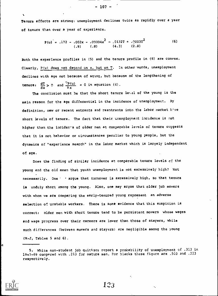
- 107 -

ti

Tenure effects are strong: unemployment declines twice as rapidly over a year

of tenure than over a year of experience.

P(u) = .172 - .002x - .00004x2

- .0132T + .(:)003T2

(.9) (.8) (4.3) (2.8)

(6)

Both the experience profiles in (5) and the tenure profile in (6) are convex.

Clearly, ?(u) does not depend on x, but on T. In other words, unemployment

declines with age not because of aging, but because of the lengthening of

tenure: dT> 0 and ^P(u) = 0 in equation (4).

dx ax

The conclusion, must be that the short tenure le,,a1 of the young is the

main reason for the age differential in the incidence of unemployment. By

definition, new or recent entrants and reentrants into the labor market h-ve

short levels of tenure. The fact that their unemployment incidence is not

higher than the inciden-e of older men at comparable levels of tenure suggests

that it is not behavior or circumstances peculiar to young people, but the

dynamics of "experience search" in the labor market which is largely independent

of age.

Does the finding of similar incidence at comparable tenure levels of the

young and the old mean that youth unemployment is not excessively high? Not

necessarily. One argue that turnover is excessively high, so that tenure

is unduly short among the young. Also, one may argue that older job movers

with whom we ate comparing the early-tenured young represent an adverse

selection of unstable workers. There is some evidence that this suspicion is

correct: older men with short tenure tend to be persistent movers whose wages

and wage progress over their careers are lower than those of stayers, while

such differences (between movers and stayers) are negligible among the young

(M-J, Tables 5 and 6).

5. White non-student job quitt3rs report a probability of unemployment of .313 in

1907-69 compAred with .213 for mature men. For blacks these figure are .503 and .333

respectively.

l`';3

- 108 -

Is it excessive turnover or is it newness in the labor market that produces

the high early unemployment of the young? It is possible that among workers

of ceppArable quality a first encounter with the labor market produces more

turnover and unemployment than at early levels of tenure on any subsequent

job. Being new in a labor market is an experience not restricted to the

young. We may,for instance,compare the young with international and internal

migrants of all ages who also encounter a new labor market. Since migrants

do not represent an adverse selection -indeed the opposite is argued and shown

6to be the cast in migration studies - their unemployment is not likely to

reflect excessive turnover.

Table S presents comparisons between the unemployment experience of

migrants (of all ages) and of young natives: while unemployment rates

of young non-migrants (age 18-24) are over twice as high as the r etes of

adult men, the rates of men who arrived in the U.S. from abroad were twice

as high as the youth rate in all age groups (Panel A). The reason the immigrant

rates are higher is because they had at most only a year of experience in the

U.S. labor market certainly less than the (18-24) youth had on average. Rates of theimmigrants

Aare comparable to the unemployment rates of men who entered or reentered the

labor force during the year (Panel B), and, indeed, are somewhat higher than the

mates of young (18-24) men who have less than a year of experience in the labor

market.

In Panel (C) immigrants (regardless of age) 'are compared with natives of

the same (modal HS) educational level by years of experience in the U.S. labor

market. During the first 2 years the unemploym:-t rate of immigrants is some-

what higher than of the young natives but it declines more zapidly. Initial

handicaps (language?) in settling in a job are overcome more quickly by immigrants.

The slower rate of decline among the young reflects the change from single to

6. Chiswick (1978)

- 109 -

married status and from part-time part-period to full-time, full-period work.

Thus, although the high initial turnover and unemployment of the young men

no greater than that of immigrants, a group that is highly motivated and

committed to the labor market, the decline in turnover and unemployment is

slower. The growth of commitment to the labor market takes time in the

transition from dependent member of parental household to head of own family,

with thr mix of school, le.sure, and work shifting toward the latter in the

allocation of time. The significance of these factors in affecting unemploy-

ment incidence is shown in regression analyses to be described in the

next section.

Internal migrants represent a group which is intermediate, in an inform-

ational and cultural sense,between immigrants and native experienced (non-

migrant) workers. Their unemployment rates are lower than those of immigrants

during the first year in the new location and comparable to the rate of young

.ion- migrants (row 2 of Panel A). Ac,in this comparison is biased because the

young nonmigrants have had more than one year of labor market experience,

while the migrants have been only a year or less in the new lcration.

Table 5A, drawn from the NLS data, compares the incidence of unemployment of

migrants during the first four years in the new labor market with the unemployment of

young men with at most 4 years of labor market experierce in 1967

Migrants who were unemployed at origin just before

,sere eliminated from the sample so as to avoid a possible adverse

selection which would bias upward the destination unemployment of migrants.

Within-firm geographic transfers were also eliminated to avoid an opposite bias.

Temporary layoffs were excluded, and the sample restricted to non-student, white

men. The results 37.7e": incidence of at married migrants was (14%) about t.he

dame is for the young, married men and 191$ for the non-married adult migrants

TABLE 5

(A) UNEMPLOYMENT OF NEWLY ARRIVED MIGRANTS, MEM, MARC!! 1963, (Migration after March 1962)(Rates)

All 18-24 25-44 45-64

Non-migrants 5.5 11.2 4.8 4.8

Migrants 12.2 15.5 9.2 16.4

Immigrants 22.1 22.9 18.0 22.5

(B) UNEMPLOYMENT OF LABOR FORCE ENTRANTS,(Nnt in Labor Force, MARC!! 1962; In Labor. Force, MARCH(Rates)

AII 10-24 25-44 45-64

1963)

ONon-migrants 20.0 19.6 10.5 23.0

Migrants 10.6 21.5 15.0 22.4

Note: U rate of 10-19 year old men was 16% in October 1963.

Source; SLF No. 44, Geographic Mobility and Emp:-Iyment Status

(C) UNEMPLOYMENT RATES OF IMMIGRANTS AN!) NATIVES BY EXPERIENCE, 1970 CENSUS WEEK

Experience 0-2 2-4 4-6 6-0 at

Natives 9.3 6.0 4.7 4.1 2.0

lmlOgrants 11.4 3,5 2.5 3.4 1.9

- 111 -TABLE 5A

INCIDENCE OF UNEMPLOYMENT, 19C7-69, NLS WHITE MEN

ALL MARRIED NOT MARRIED(EXCLUDING TEMPORARY LAYOFFS)

Mature Men0-4 YearsResidence in1967 .148

n 859

Young Non-Students 0-4Experiencein 1967 .189

n 644

.141 .187

786 73

.128 .260

344 300

(INCLUDING TEMPORARY LAYOFFS)

Mature Men .168 .165 .188

Young Non -

Students .230 .160 .310

Note: Respondents with unerployment in place of origin are deleted.

1'1

- 112 -

compared to 26% for young, single men. Inclusion of temporary layoff un-

employment raises the figures for the young somewhat more than for the old

migrants, the reverse of the general case.

We think it is fair to conclude that the major circumstance responsible

for high youth unemployment is newness in the labor market, rather than young

age and unstable behavior. This is not to say, however, that the frequency

of unemployment among the young stands in an irnutable ratio to that of the

adults. Increases in young cohorts consequent on,the "baby boom" create

larger proportions of young workers with short tentlre. Similarly, lengthening

of school enrollment produces shortening of tenure in fixed age groups, so

that unemployment of young non-students is more prevalent (relative to adult

unemployment) in countries with higher educational attainment. Of course, the

partial labor market commitment of youth in transition in school and family

status is a factor in greater turnover as is the interruption of work experience

by military service. Minimum wage legislation may also be important although its

impact on employment and labor force participation is stronger than on unemploy-

ment or on turnover. Note that black youthwere not included in our comparisons

with migrants and we have already seen that their unemmloyment incidence exceeds

not only that of whites but also of black adults of con arable :evels of tenure,

especially in early tenure where most unemployment is concentrated

V. Factors affecting the Incidence of Unemployment

The apparently close relation between turnover and unemmloyment sugges,:s

that sore or most of the variables which affect sei,arstions are factors which

also affect unemployment. We ascertLin these factors and the similarity of

their effectsin parallel regressions of separations and of unemployment

incidence on the same set of independent variables.

113

As is well understood in the analysis of labor mobility the observed

reduction of separation probabilities as tenure lengthens may be a statistical

illusion rather than a description of individual behavior. Suppose that indiv-

idual propensities to move are not reduced by tenure yet they differ among

workers. In that case the estimated tenure profile of mobility S(T) observed

across a sample of workers will have a downward slope and will be convex as

well: Persons with high propensities to move separate at early levels of

tenure while those with lower propensities stay on for longer periods. As

only stayers remain in long tenure classes, the apparently declining tenure

curve would level off at low separation rates in the long-tenured classes.

Much the same phenomenon may be expected to appear in the statistical

treatment of unemployment incidence. Unemployment risk may not be related to

duration cf job tenure, yet heterogeneity-differences among individuals in

the unemployment risk to which they are subject- can create exactly the same

spuriousness in the tenure profile, given the relation between separation and

unemployment. Actually, heterogeneity and "tenure dependence" are not mutually

exclusive hypotheses regarding labor mobility and unemployment incidence.

Indeed, the theory of job sorting and of acquisition of specific human capital

(cf. M-J pp.9-13implies heterogeneity in levels and slopes of tenure profiles.

Therefore, the heterogeneity bias does not fabricate an unreal tenure curve.

It merely steepens the slope of the real (average) tenure curve.

Differences in levels of tenure profiles can be indexed by observations

on past mobility behavior. If so, their inclusion in the regression reduces

the bias in the tenure slope. Other measured factors represent heterogeneity

not captured by the limited observations on past mobility. Their inclusion

further reduces the tenure slope while increasing the explanatory power of

the regressions.

A comparison of the separation and unwrployment regressions

Shows that the probability of unemployment is lust as labor mobility, subject

to tenure ,11renl,rc. Pr.r4. 'at individual characteristics, such as education,

1 ,2 t9

- 114 -Aealth, marital status, local unemployment rate, and job training, affect the

probabilities of separation and of unemployment, given tenure. These regressions

appear in Tables 6A and 6B for NLS young white non-students (1959-71), in

Tables 6C and 6D for the MID (1975-76), and in Tables 6E and 6F for mature NLS

men (1969-71). For the NLS, the dependent variables are defined as number of

separations and number of unemployment-spells during the period; for the

MID survey, as the probability of separation and the probability of unemployment

respectively. Temporary layoffs are excluded. Comparable regressions including

recall unemployment appear in the appendix. Results are similar for

both number and incidence of events; however, we refer to both as incidence of

unemployment and separation. (See Appendix tables 17, 18)

As we noted before, an experience profile which acpears :n the first

column of the regression disappears once tenure (and its square) are added.

This means, that within the observed age range (which is limited in the NLS),

probabilities of both separation and unemployment are the same at given levels

of tenure regardless of age. In the complete age range (available in the MID

data), the inclusion of tenure reduces but does not eliminate experience

effects, on separations. However, such "aging effects" are eliminated in the

unemployment incidence equations.

Next, the inclusion of heterogeneity indices (of past behavior) and of

heterogeneity factors reduces the tenure slope both in separations and in

unemployment incidence. Indeed, in the NLS data the slope is cut in half in

the longest equation, though more than half of the reduction is achieved when

prior mobility inaices are added to tenure. Tenure remains significant after

all other variables are included. Both prior separations (per year) and prior

unemployment (conditional on separations) were used as such indices in NLS.

Prior unemployment incidence is unconditional in MID.

130

- 115 -

The coefficients of tenure are quite similar in both the separation and

unemployment equations in elasticity terms. The coefficients on prior variables

are, in this sense, larger in the unemployment equation. Past motility,

especially if it fiequently results in unemployment, predicts the risk of

unemployment in the future more strongly than it predicts the probability of separat!on

Three training variables were used in the young NLS regressions: company

training on the current job, training prior to the current job, and off-the-

lob training. Of these only the first approaches statistical significance and,

as would-be expected on specific capital grounds, it reduces both separations

and unemployment incidence. Unemployment incidence is positively affected

by the local level of unemployment which, however, does not affect separations.

This is as interesting finding. It suggests that the c)...servea geographic

differences in unemployment reflect differences in local "aggrigate demand"

conditions (these are likely to be sectoral from the point of view of the

entire economy) rather than differences in frictional unemployment. In the

former case fewer :nits atrnpensate for greater layoffs as unemployment increases,

in the latter case higher unemployment is associated with higher ql.:its and

layoffs hence higher separations. Indeed, the local unemployment rate

affects layoffs positively and quits negatively (as appears in appendix tables.:9 and 2:

Both separations and unemployment incidence are negatively related to

education and to marital status. Short hours (part-time work) and non-particr

ipation some time during the year (or in prior years) are associated with higher

probabilities of separation and of unemployment in the young and old NLS data.

(In MID part-timers appear to have fewer separations and the effect of part-

time work on unemployment incidence disappears.)

Union membership reduces,seprraticns, and has no significant effect on

incidence, unless temporary layoff unemployment is included when the effect

becomes positive. Employment in the government sector has a weak negative

effect on separation and on unemployment in the young NLS, but both effects aze

stronger at older ago= :':ID and NL54.

- 116 -

Bag health hay no clear effects on separations and a posit-LIE effect on

unemployment incidence in 1967-69 in the young NLS sample. Both effects

are positive in the MID but rot clear in the older FLS samples.

The following conclusions may be drawn. Regression results strongly

support the turnover hypothesis of unemployment incidence. To the extent

that differences in lob sorting and specific canital processes underlie

variation in labor mobility across people, they are important in creating

differential unemployMent. Therefore, both tenure dependence and heterogeneity

are characteristic of unemployment incidence as they are of separations.

Factors which account for the convex (decelerating) decline of the incidence

of unemployment with Rage are: lengthening of tenure with age, change from

single to marital ,status, and the shift from part-tine and part - period work

activities to full-time work.

we should note the relevance of marital status, part-time work, and non-

participation in understanding the comparison with migrants in Table 5 (Panel C).

The transition from school to market and from parental to own household which

is observed in a cross-section of young people is gradual. It results in a

slower decline of separation (lengthening of tenure) compared to the experience

of largely adult migrants whose work in the new labor market was the major

reason for migration.

A comparison of unemployment P(u) regressions with separation regressions

leaves out questions about the conditional probability of unemployment. This

probability ?(uls) enters the product in P(u) = P(s)-P(u1s). It was shown to

increase with age in contrast to both P(s) and P(u). What are the factors

associated with P(u1s) and wIW dces it increase with age? We try to estimate factors

affecting Pfuls) in two wa,:s. In "a'.2g7ented regressions" we add separation

''

-

variables to all the others (col.4 of the Tables) and study factors affecting

unemployment. given separations. The alternative procedure is to restrict

the regressions to workers who moved, that is to job separators as well as to

entrants and reentrants. These we call "restricted regressions".

In both kinds of r?Iressions(co114,6)the variables which remain signif-

icant are: the local unemployment rate, prior conditional unemployment,

marital status, education, and less clearly part-titme work. Union membership

becomes positive and significant at least in the 1969-71 period. Similar

results are found in MID regressions. The variables show higher tscores in

the restricted regressions (col. 6), but the bulk of "explanatory power" in

the augmented regressions is due to the turnover variables. Indeed, in the

1969-71 sample these variables produce an adjusted 112=.505 which increases only to

.521 When all the factors are added.

Table 3 suggested that both separations and unemployment are more

heavily weighted by layoffs than by quits at older ages. Some of the va-4.^1Ps

which .are significant in-affecting conditional unemployment in the regressions

are apparently more closely associated with layoff unemployment. This is

true of the local unemployment rate, as already noted. Prior conditional

unemployment must be weighted toward layoff, since unemployment conditional, on

layoffs is twice as high as unemploymen5,conditional on quit. The same holds

for unemployment of union members. However, education, marital status, and

short hours affect both quits and layoffs and so affect the conditional in

each type of separation. Interestingly, bad health which is not a factor in

conditional unemployment of tLe young NLS, nor in MID, does appear in oldest

groups (NZ.`_') as a factor which increases .7uits but not layoffs.

118

REGRESSION VARIABLES

VARIABLE DEFINITION

X - Number of years since beginning the first jo3 after leaving

full-time school

T - Duration of job held at beginning of interval

JTRAIN - 1 if respondent attended company training school in the-job

held at beginning of interval

PTRAIN - 1 if respondent received any training aside from regula

school prior to job held at beginning of interval

GTRA/N - 1 if respondent received any training other than company

training school while employed on job held at beginning

of period

- Unemployment rate for labor market of current residence

- Prior separations per year since 1966 (NLS); probability

of separation per #4 since 1968 (MID)

PC 'D - Ratio of prior unemployment spells to prior separations

(NLS); priorylemployment incidence (MID)

ED C - Completed years of education

1 if health is poor

GOV - 1 if public employee

UNION - 1 if wages are Set by coliec ive bargaining in 1969

MARRY

LOCRATE

PSEP

PTIME

OLF

POLF-

SEP

ENTRY

- 1 if married, spouse present,

- 1 if 34 hour workweek or less

- 1 if incidence of unemployment in current period

- 1 if incidence of unemployment in prior years (MID)

- Number of job separations

- Number of periods o! non-Part4cipation

13,i

ITCONST

X2XTT-

JTRAINPTRAINGTRATNLCCRATEPSEPPC0111)

1:01.1c

!MTh

UN 1(10

t-1 /00tv

PT1(11;

)

tX

tl

TARLE 6A

THE DETERMINANTS OF SEPARATIONS, 1969-11, YOUNG WHITE MEN, NLS

B

(EXCLUDING TEMPORARY. LAYOFF'S)

t B

(1) (2) (3)

1.12 .749 1.50-.110 3.23 .064 1.76 .054 1.42.007 2.61 -.003 1.16 -.003 1.06

-.310(7) 6.45 -.221 4.70.026 4.15 .018 3.01

-.2i6 2.59 -.129 1.24.083 .611 .091 .924.017 .202 .090 1.12.016 .669 .008 .345.039 4.58 .036 4.41.147 1.80 .045 .573

-.064 3.83-.202 1.16-.113 .999-.159 2.10-.261 3.28.279 2.74.607 7.87

.008 .102 .173

.852

i 1351

ot)

)

B

G

'.. 1LE 613

TILE DETERMINANTS OF , ?ELLS OF UNEMPLOYMENT, 1969-71, YOUNG WHITE MEN, NLS(EXCLUDING TEMPORARY LAYOFFS)

t B t B t B t 8

CONST .642 .115 .650 -.064 .007X2 -.068 2.61 .029 1.03 .025 .854 -.004 .173

.004 1.79 -.002 .13:i4 -.002 .889 -.000 .219T -.171 4.59 -.120 3.24 -.016 .562T2 .014 2.88 .010 2.03 .001 .315JTRAIN -.111 1.34 -.016 .200 .043 .713P; RAIN .117 1.47 .118 1.52 .072 1.25CTRAIN -.016 .257 .037 .585 -.018 .382

LOcRATE .064 3.41 .056 3.03 .054 3.94PSCP .023 3.56 .021 3.31 .002 .512PCOND .244' 3.84 .169 2.71 .153 3.30EDUC -.043 3.29 -.011 1.17HLTH -.117 .854 .002 .000GOV -.010 1.12 -.C46 .696OHBA .078 1.32 .151 3.4rmARkY -.242 3.87 -.101 2.17vrimE .355 1.94 .001 .032oLF .348 5.75 - -

srp .d' 13.53 .434 14.79SEP2

.0 4.43 .017 3.95ENTRY .0,J. 1.12 .063 2.31

2R .007 .082 .133 .S21 .5055i2

.452

n 1351

.14,

) 1.0

1%.)

0.1.Incidence amongmovers and entre:

B t(6)

.484

.019 .97*

-.002 1.28-.045 1.68.003 .70;

.091 1.51

.056 1.03-.009 .20'

.039 3.28

.007 1.97

.099 2.92-.021 2.38.039 .46'

.014 .20!

.350 1.27-.120 2.96.089 1.73

-.030 .81.

.084

.445

706

'COUST

:X

!X2

1;2I

IIKICRATE

IPSEP

PC0ND11.1-02

HLTHGOVUNION,MARRY

primeP01 I'

-2R

X

n

TABLE 6C

THE DETERMINANTS OF SEPARATIONS , 1975-76, WUITE MEN, MiD

D

(EXCLUDES TEMPORARY LAYOFFS)

t B t B(1) (2)

t

(3)

.266 .228 .452-.010 3.92 -.007 2.37 -.007 2.42.0002 2.58 .0001 1.98 .010 1.70

-.010 2.51 -.012 3.07.0002 1.44 .0003 1.95.001 .200 .001 .480.166 3.02 .136 2.44.124 2.05 .094 2.05

-.010 2.74

.090 2.64

-.027 1.22

-.024 1.18

-.073 2.38-.122 2.24-.070 1.59

.024 .056 .075

.149

1562

1

TABLE

THE DETE1MINANTS OF THE INCIDENCE OF UNEMPLOYMENT, 1975-76, WHITE MEN, MID(EXCLUDES TEMPORARY LAYOFFS)

B t

(1)

B t

(2)

CONSTx2

r.

.162

-.006

.0001

2.73

1.74

.099

-.003

.0001

1.26

1.08

-.008 2.58T2 .0002 1.63LOCRATE .003 1.20PSEP .100 2.10PCOND .246 7.01EDUC

HLTHGOVUNiONmANPYPTiME

P(JLF

SEP

-21

R .012 .047i .094

n 1562i

I

INCIDENCEAMONG MOVERS

B

(3)

t B t B(4)

t(5)

B t(6)

.296 .090 .018 .769-.001 .574 -.0001 1.28 .013 1.17-.000 .005 .002 .985 -.0003 1.28-.007 2.06 -.001 .469 -.0001 .000.0001 1.32 .000 .332 -.000 .452.004 1.60 .003 1.62 .020 1.69.114 2.52 .052 1.40 .076 .473..209 5.68 .166 5.43 .387 2.86

-.010 3.53 -.006 2.38 -.034 2.36.050 1.82 .010 .424 -.009 .008

-.043 2.37 -.030 2.04 -.042 .4-16 I

-.015 ' .943 -.005 .374 .051 .692-.084 3.40 -.052 2.49 -.204 2.20

.768 .087 2.40 -.125,0134

.705 3.00 .131 4.48466.239

1,33.451 26.50 475 28.08.018 1.10 .034 2.01

.103 .383 .336 .112

.498

231

TABLE 0

THE DETERMINANTS OF SEPARATIONS , 1969-71, MATUk WAITE MEN, NL4

B

(EXCLUDES TEMPORARY

t 3 t

(1) (2)

LAYOFFS)

B t

(3)

CONST .478 .480 .294

X -.019 1.71 -.016 1.62 -.005 .560

X2

.0004 2.19 .000 1.89 .000 .477

-.019 4.85 -.014 3.9',r ? .0004 4.08 .0003 3.20LOCRATE .003 .354 .004 .438

PSEP .177 18.66 .164 18.31

/COW .080 2.32 .021 .628

k1 RUC .003 .621

nun .042 1.35

Govtin TON

-.083 2.40

.000

MARRY 1.41I TLI4E .078 1.69

OLF .505 15.22I

-2It .004 .235 .326

x .278

II 1957

111

TABLE

THE DETERMINANTS OF SPELLS OF UNEMPLOYMENT, 1969-71, MATURE WHITE MEN, NLS(EXCLUDES TEMPORARY LAYOFFS)

1CONST .248Ix -.011 1.411 2X .0002 1.62

,T2

LOCRATEPSFP

,FCOND!LDUCilLTH

!GOV

111t41al

NAPRYIFTImEoLFSEPsEP2

-2.001

X .112

1957

B

(1) (2)

.245

-.010 1.42

.0002 1.51

-.006 2.41

.0001 1.63

.001 .095

.098 14.74

.097 4.00

.163

14 ;

.266

-.088.0001

-.005

.001

.0091

.096

.086

.01:-.015

-.007.008

-.063

i -.011.110

1

.174

1-

INCIDENCE

t

(3)

B t

(4)

B t

(5)

Niglig -P.E.PNIATMSB t

(6)

1.26

1.25

1.99

1.18.164

14.34

3.49.604.632

2.70.397

1.87.311

4.45

.147

-.006.000

.000

-.000-.001.014

.077

.001

.-.027

.-.029-.003

.-.036-.043-.089

.302

.054

.528

1.22

1.34

.032

.641

.276

2.54

4.14.344

1.541.56

.176

1.411.664.37

13.05

8.91

!

E

.000

.286

.061

.516

13.7710.35

.653

1---005.000

1-.007.0001

.005

.023

j .093

.007

-.081

-.130.009

1-.123

-.040:-.137

.

1

!

.097

.386

391

.31a

.200

1.01

.263

.379

2.452.06

.9431.561.77

.176

1.68

.5912.65

M.4

IV

i

125

Altogether, the NLS regressions are not very helpful in explaining the

age increases in conditional unemployment. Lower levels of education and

of health and more frequent union membership among the old account for a part of

it. The other variables have no or opposite effects on age patterns, That

the variables we mere abl- to measure lo not account for the growth of

conditional unemployment with age is apparent in observing the effects of

experience on incidence in the regressions restricted to job movers. The

effect is positive in the older NLS (ages 45 and over), and: less so in MID

{average age near 40) before and after all other variables are included.

There are no experience effects in the restricted regressions within the

first decade of work experience (the young NLS sample), Evidently, the

probability of unemployment when separating increases at adult ages

within each of the classes (levels) of the variables we have measured.

Vl. Conditional Unerplovment and Ace Di"=.-,.-ces in the Duration of Unemployent

Although we are not able to ascribe much of the higher conditional unemploy-

ment at older ages to the factors we have reasured, we know that it is largely

an outcome of the increased layoff/quit ratio. ,Why do quits decline more

rapidly at older ages than layoffs?

At given tenure levels a worker's incentives to quit decline as he ages

because the payoff period to whatever benefit the quit produces is getting

v.

shorter. More importantly, we suggest That potential job changers encounter

a diminished probability of finding a job at older ages. There are several

possible reasons for this. Short prospective tenure inhibits hiring by

employers in the presence of hiring or training costs. A record of )ob mob-

ility at older ages is a (!eterrent to hiring for the same reasons, insofar as

it suggests a higher probability or future 5,?paration, as it does in our

- 126 -

findings. On the supply side, workers'hunan capital even if not specific to

the firm becomes progressively more specialized to a narrower cluster of

firms within an industry or occupation. The proportion of job changers who also

change industry and occupation does diminish at older ages.

In the terminology of search models we argue that, on average, older

workers who separate from jobs have a lasser probability of finding a job per

unit of search time, not because they are holding cut for a higher acceptance

wage within the relevant wage offer distribution -though it is true of some-,

but because the probability of getting any offer, that is the probability of

finding a vacancy, is smaller. On this assumption we can show that older

workers who separate will search longer when unemployed and quit less frequently

while their acceptance cage will be relatively lower, so the wage gain will be

smaller (or negative) for older job movers than for yc*anger ones.

In the standard sear c:1 model the individual samples from his wage offer

distribution f;w) receiving one offer per unit of time. The worker decides

on an optimal wage floor which equates the gain from an addit'onal unit of

search to the cost of it. The resulting rule is

PaC;ia Wa) = c = Wa 4 (7)

where W1 is the lowestacc,!ptablo wage, -',a is the probability of getting an

.acceptable wage offer, that is of W ?.. Wa, :4a the mean of all acceptable wage

offers; c is the (marginal) cost of search which includes direct and opportunity

costs'nehighestopporturiltycostorforegonewagei"-.Income offsets0

which are co-tingent on continued searcn such as unerp;.c.::-ent compensation

or the cl:rrent wage when searching on the' :oh enter costs with a negative

sign. ::',_:ration of search is inverse to in in this 7odel search is longer

t.o higher the acceptance wage ..high is n1.-:her the lower the cost of search.

1 .4., 5

- 127 -

Now the probability of accepting a wage offer cwt be redefined given

that the probabiiity of finding any offer in a (calendar) unit period can be

less than 1. A lesser frequency of vacancies may be a result of depressed

business conditions in general, or depressed markets for a particular type of

labor, or 4 function of lesser efficiency or intensity of sear:h. The

optimum conditions become:

p.Pa

".7,7

a- Wa ) = c = Wa - z (8)

Here p is the probability of finding a job offer, the probability of

findi.ig an acceptable job conditional on finding a vacancy, and pPa is the

D is now the inverse of the product pPa.probability of finding an acceptable job. - As Yoefore, changes in c

produce a positive relation between Wa and D. However,

changes in p over the business cycle or otherwise, cr differences in p

across people tend to produce a negative correlation between Wa and D.

A reduction in p leads to a downward revision of Wa, hence to an increase

in Pa. The question is whether pPa will rise or fall in (3). No perfectly

general answer can be given to this question, but a most plausible answer is

that (pPa) will fall, hence the duration of search will lengthen even though

Wa is revised downward in consequence of a fall in p. It is easy to see that

the difference (5;a

- Wa

) increases as Wa

is lowered in a uniform or triangular

wage, offer distribution. When wa is reduced, eta is reduced by a smaller

amount, so that pPa must fall, if c is fixed or reduced. Actually, c will

be reduced since lowering of Wa will lead to a fall in foregone wages when

search is continued. By the same token, an exponentially declining function

(here log f is linear in W) wi'l show an increase in the ratio3 as Wa

Wa

is reduced. Consequently pPei will fall since!

128

pPa( 71a - 1) = 1 -

a Wa(9)

Only an unusually high skew in the distribution, such as in the Pareto

distribution yields a fixed 1..1 whatever the position of Wa. Even thenWa

p-Pa will fall as the right hand expression does. It is difficult to

imagine that typical workers face a wage offer distribution which is as

skewed and long-tailed as Pareto.

The conclusion that-a lower p is very likely to produce longer search

and lower acceptance wages holds both for unemployed and for employed searchers.

In the latter case c Wa - Wo, where W is the wage paid on the job. An

increased duration of search on the ;oo, of course, means a reduction in the

frequency of quit.

In sum, workers facing fewer vacancies in their search may be expected.

to have a longer duration of search and a lesser wage gain when unemployed,

and to inhibit their job change (quit) when employed. These conclusions are

Consistent with worker behavior during the business cycle: duration of unem-

ployment increases and quits decline while layoffs increase, partly because

employment demand declined and'partly to substitute for a decline in attrition

(T.lits). Note that in contrast to other models, this explanation of behavior

7during tne business cycle does not assume nvcpia, or lags of adjustment.

Apping the sane model to the life-cycle we may argue that either p or c

decline at older ages. A decline in c is not plausible except very early

when labor marke:: entrants become eligible for unemployment compensation. A

decline in c would lead to increases in We and in wage gains, but the opposite

7 Cf Al Chian in the Phelps volume (1970).

14-1

tO

TABLE

CONDITIONAL UNEMPLOYMENT AND DURATION, 1967-69

P(U1S)

(EXCLUDES TEMPORARY LAYOFFS)

P(UIL) Q/L Average TotalDuration Duration

aw

Non-enrolled

--1.,

Whites .342 .573 4.66 5.30 8.84 .785

bluc.fl-11 .423 .641 4.26 5.74 9.91 .734

12 .329 .546 4.78 5.20 8.30 .772

>13 .218 .471 5.36 3.93 6.46 .881

Non-enrolledBlacks .525 .607 3.03 6.33 11.87 .578

Mature Whites .382 .623 1.62 9.99 16.17 .593

Educ.0-11 .443 .655 1.25 9'.90 16.76 .466

12 .313 .640 2.20 10.29 15.34 .561

>13 .268 .385 3.00 10.03 14.13 1.00

Ma Dire h1dcks .519 .725 1.17 11.35 17.86 .414

14S

- 130 -

is implied by a fall in p, and is observed. The implications that older men

have a longer duration of unemployment, a reduced - ratio, and a lower Wa

when changing jobs are strongly confirmed by the data in Table 7. The shorter

duration-of unemployment of the young is also due partly to relatively frequent

inter-labor force mobility. Again, this is characteristic of very early labor

force behavior and cannot account for the age-uptrend in duration of adult

unemployment. Nor can this upturn be ascribed to the somewhat longer duration

of layoff than of quit unemployment. Duration increases with age in both

cases. Table 7 shows that a similar search interpretation can be given to

unemployment differentials by race Ad, somewhat less clearly, by education.

We elaborate on the race differentials in the next section.

Although we have no direct evidence on the reduction of p at older ages,

MIL) may be a good index of it. It increases with age, is inverse to educ

ation and is higher for blacks. The only exception is that ?(uJL) is less for

the older, more educated whites compared to young whites in the same category.

In sum, as large as they are, age differentials in unemployment rates

are attenuated by the longer duration of unemployment and higher probability

of unemployment of older movers. Both the longer duration and the higher

conditional probability of unemployment of older men can be ascribed to the

decline in the probability of finding vacancies at older ages. Young white

job changers face, on average, a more favorable environment in this respect.

V11. Black-White Differences in Youth Unemelovment

Black youth unemploymenthas grown relative to white youth unemployment

over the past two decades or longer. A fuller understanding of the present

differential, therefore, requires an analysis of this trend. This is beyond

the scope of our present work. We did replicate some of the statistical

analyses on black data, and report some of the findings.

14:)

- 131 -

The salient features in the unemployment differentials are: higher

incidence, longer duration, and greater non-participation among black youth

as shown in Table 1. Those dVferences hold for both srdents and nonstudents.

As the age comparisons in 1966-67 an4 1967.69 (Appendit tables) show, the duration of

black youth unemployment is not much :hurter than the duration of unemployment of

older blacl Since the race differential in duration of older M03.8 unemplqe-

ment is smell, it is not clear whether our N1.6 sample of older blacks under-

state their adverse position, or whether cur findings about the young are,

indeed, an indication of deterioration of labor market conditions in present

cohorts of black youth. But these inferences are not mutually exclusive.

The longer duration of black youth anemployment romparet with whi'e y.juth,mirror

Table 4 in higher conditional unemployment at each level of tenure. The higher

incidence cf unemployment or clack youth is due both to tle higher separation

rates and to . r conditional unemployment at fixed levels of tenure. The

result is that while the tack separation rates are 20% higher than the white

rates, the black incidence of unemployment is ice as high as the white.

Table 7 shows also that the black conditional unemploynent Pfu!s) is

higher then the white lcrgely because 2 , the quit/layoff rtic is lower, and also because

both conditionals P(u /L) and P(u /Q) are higher.8 By a search model argument of the

preceding section, we may infer that: if 'blacks face a lower probability

of finding vacancies than whites dc, their duration of unemployment is longer

wage gain less, and quit/layoff ratio lower. It has been noted that black

quit rates are not higher than rates of whites.'a

In our interpretation this

does not suggest an equally stable work experience: tital separations

blacks are higher, but quits are inhibiteu because of an adverse labor market,

and some of the excess layoff is in part a substitution for reduced quit.

8. See footnote 4.9. Flanagan, (1978).

- 132 -

Sows of the factors that appear to influence the higher black separation

rotes and their slower decline with experience are suggested in comparisons

of black awl white regreacinne (Tables 8A _and 3B).

The tenure effects are somewhat weaker, end the effect of t:ainil+e en the

current job are, if anything, positive, rather than negative in the black sample. This

suggests that blacks receive not only lead training, bit also a lesser' specific training

component of it. Marital status which reduces separations of whites has little

effect on blacks. At the same time prior unemployment conditional on separ-

ation predicts future separations more sharply among blacks than among whites,

that is, black movers who encounter unemployment are more likely to separate

from jobs than are those who wove without unemployment and more than comparable whites.

Taken together, these effects may also explain why over the early years of

experience the decline in separations and in unemployment incidence is'not

pronounced among non-enrolled blacks, when it is for whites.

So much for the differential regression effects as esti'ated in the

regression coefficients. differential characteristics of black youth also

contribute to the higher unemployment. On average, black youths had less

tenure, leas training, lower education, fewer married, more working part-

time and intermittently.

In our regressions designed to spot factors influencing conditional un-

employment the cues for understanding wv= such nemploynent is higher for

blacks are sparse Education has no e' ect on blacks while it was negative for

whiter Poor Health and non-partic' _tion increase black (conditional) unemploy-

ment. They had no effect on whites, gain the likely conclusion is that the

conditional unemployment of blacks is hig'rer because their quit/layoff ratio

is lower at all levels of the factors.

TABLE 8A

TNE DETERMINANTS OF SEPARATIONS, 1969-71, YOUNG BLACK MEN, NLS(EXCLUDES TEMPORARY LAYOFFS)

B

(1) (2) i (3)

CON ST

X

X

TTJTRAINPTRAINGTRAINLOC2RATE

1.32

-.072 1.24

.000 .000

.482

.129

-.012

-.222.019

-.115

..154

.125

.012

2.02

2.36

3.59

3.04

.558

.669

.869

383

.432

.150

-.014

-.155

.013

-.027.257

.243

.005

2.38

2.772.59

2.22

.138

1.16

1.72

.164

PST .070 4.71 .074 5.21PCOND .267 2.66 .244 2.46EDUC -.012 .539

111 ;n i -.264 .682

GOV -.346 1.94

UNDAN -.489 4.17MARRY .003 .032

111 ME .377 2.60OLF .528 4.77

.023 .126 .203

1.01

504

TABLE 8"

THE DETERMINANTS OF SPELLS OF UNEMPLOYMENT, 1969-71, YOUNG BLACK MEN, NLS(EXCLUDES TEMPORARY LAYOFFS)

INCIDENCE AtioNGMOVERS AND

B t

(1)

B t

(2) (3)

B(4) (5)

ENTRANTS

(6)

COST .931 .230 -.200 -.404 .038 .280X -.045 .869 .117 2.50 .167 2.95 .082 1.77 .019 .477X 2 -.001 .195 -.011 2.44 -.014 3.15 -.006 1.75 -.002 .746T -.196 3.53 -.149 2,76 -.062 1.39 -.123 3-67T2 .0/7 3.14 .014 2.66 .007 1.59 .011 2.97..VVRA I II .284 1.53 .332 1.84 .362 2.47 j .092 .898PTR AI N .123 .594 .113 .565 -.015 .089 -.015 .130GTRA I t4 .156 1.21 .193 1.56 .058 .562 .051 .736CRATE .016 .559 .020 .756 .020 .892 .033 2.18PSEP .046 3.40 .051 3.96 .012 1.11 .009 1.28I COND .265 2.94 .185 2.07 .049 .665 .054 1.18Et UC.014 .717 .018 1,17 .004 .367III.TH.868 2.50 1.00 3.55 .411 2.25(INV

o: al

-.158-.185

,990

1.75.222

.090

.1/0

1.04.076

-.047.746

.787I-,

t...v.c.or,v1i

-.23/ 2.30 -.250 2.98. -.070 1.34 1PTInE

.220 1.69 .019 .179 .066 .948()EV

.523 5.26 - -.122 2.00SEP,

.637 9.07 .673 9.85SEP'-.023 Lit/ -.026 1.93ENTRY.0.17 1.59 .313 2,04

-2.018 .102 .179 .458 4135 .099.708

.576504314 )

r'

- 135 -

Our findings convey some impressions of greater job instability of blacks

which is partly due to lesser training and to specific components of job

experience, to greater non-participation, to weaker effects of education

and of family status. Greater difficulties in job finding are consistent with

longer duration of unemployment, inhibition of quits, and augmentation of lay-

offs. We do not know, however, how much of the difficulties are matters of

discrimination, of perception of potential productivities by employers or of

informational efficiency of job search. In contrast to the whites, unemploy-

ment of young blacks is higher than unemplor.ent of older blacks at fixed tenure

levels as we noted in Table 4. Also, the race differential in

duration is larger at young than at older ages. Both of these findings may be

a reflection of the deterioration in labor market conditions of recent cohorts

of young blacks.

La r,,lus ca change...?

A 1969 survey of research on youth labor markets concluded that "The

normally high level of teenage unemployment is due primarily to the fact that so

many teenagers are labor market entrants or reentrants rather than to their

deficiency or instability as employees."" We amend this conclusion by interposing

a continuum of job experience (job tenure running from 0 onwards to T) and showing

how it translates into a rapid and decelerating age decline in the incidence of

unemployment.

Our evidence is based on far richer data than .ere availakle to the researchers

in the 1960s. But we do face a question of data compa:.abilit;: the NLS shows

lower unemployment rates for young non-students, consequently a smaller age-

differential than the CPS does. Yet our findings of no "aging effects" are also

11. Kalachek (1969), p.2.

- 136 -

reproduced in the ?4I data,, apirt from being consistent with the spirit

of the conclusion reached a decade acio on the basis of fragmentary, cross-

sectional CPS aggregates.

- 131 -

REFERENCES

Alchian, Armen. "Information Costs, Pricing, and Resource Unemployment."

In Phelps, Edmund S. -et al. Micrceconcmic Foundations of Employment and

Inflation Theory. New York: W.W. Norton & Co., 1970.

Chiswick, Barry. "The Americanization of Earnings." Journal of Political

Economy (October 1978).

Flanagan, Robert J. "Discrimination Theory, Labor Turnover, and Racial

Unemployment Differentials." Journal of F=an Resources 13 (1978)1 187-207.

Kalachek,-Edward. The Youth Labor Yarket.Policy papers in Human Resources and Industrial Relations No.12. Ann

Arbor, Mich.: The Institute of Labor and Industrial Relations, University

of Michigan and Wayne State University, 1969.

Jovanovic, Boyan and Mincer, Jacob. "Labor :'ability and Wages."

Conference on Low Income Labor Markets. Universities-National Bureau

Coins itte for Economic Research. June 1978.

Leighton, Linda. "Unemployment over the Work History." Ph.D. Dissertation,

Columbia University, 1973.

- 138 -

Appendix Tables

Young Whitesn

Enrolledn

Non - enrolled

n

Fdue.0-1112

>13

Young Blacksn

Lnrotledn

Non-enrolled

n

Mature Whitesn

Educ.0-11

12

>11

mature Blacksn

TA' ',F. 1

DECOMPOSITION OF INCIDENCE DURATION AHD NON-PARTICIPATION, 1966-67(EX,:LUDES TEMPORARY LAYOFFS)

Levels Percent Differentials

UN_

L Wu1

U14

L Wu1

(1-k) (1-io)

.033 '.178 .144 1.28 Young Blacks minus

(2293) Young Whites .880 .562 .256 .062

.046 .207 .139 1.61 Enrolled .937 .545 .232 .160

(1151) Non-enrolled .934 .622 .263 .050

.024 .150 .152 1.06

(1142) Young Whites minus

.038 .209 .170 1.06 Mature Whites .475 .979 -.729 .223

.018 .122 .140 1.06

.012 .100 .114 1.06 Non-enrolled YoungWhites minus Mature

.000 .313 .187 1.36 Whites .166 .804 -.676 .0361

(875)

.118

(3137)

.357 .175 i..137 Yount] Blacks minus

Vatnre Blacks ,,,,...... 1.12 -.476 .267

wwv,

i

.062 .279 .198 1.12

(488) Non-enrolled Young

.021 . .067 .300 1.02 , Blacks minus Mature

(2477) Blacks .655 1.00 -.416 .068

.028 .091 ,.305 1.03

.011 .045 .238 1.02 Mature Blacks minus

.912 .030 .382 1.02 Mature Whites .44i .421 .003 .010

.032 .102 .301 1.04 Education:

(1136) Less than H.S.minus It. S.

Non-enrolled Wh. .739 .539 .195 .006

Mature Whites .967 .704 .247 .014

H.S. minus >B.S.Mon- enrolled .397 .201 .201 -.007

Mature Whites -.01)4 .411 -.472 -.001

160,-.

Append T £ 2

DECOMPOSITION OF IM.ADENCE DUPATION AND NON-PARTICIPATION, 1966-67(IN 2LUOES TEMPORARY LAYOFFS)

Levels; Percent Differentials

N

1. u1

(1-N0)

N

L

Young Whites .037 .208 .138 1.28 Young Blacks minusn (2293) Young Whites .867 .527 .277

Cnralled .049 .217 .139 1.60 Enrolled .918 .545 .214n (1151) Non-enrolled .895 .521 .331

Non-enrolled .029 .200 ,138 1.06n (1102) Young Whites minus

Educ.0 -1l .044 .257 .160 1.06 Mature Whites .327 .682 -.57812 .024 .185 .120 1.06>13 .013 .115 .108 1.06 Non-enrolled Young

Whites minus MatureYoung Blacks .088 .353 .183 1.26 Wites .090 .639 -.585

n (875)

Enrolled .122 .378 .173 1.87 Young Blacks minusn (387) Mature Black? .723 .752 -.295

Non-enrolled .071 .336 .192 1.12n (1142)

Non-enrolled YoungMature Whites .027 .105 .247 1.02 Maas minus Mature

li :2477) Blacks .521 .703 -.248Edur.0-11 .037 .143 .252 1.03

12 .014 .065 .218 1.02 Mature Blacks minus?'13 ,011 .053 .258 1.02 Mature Whites .471 .457 -.005

Mature Blacks .043 .166 .246 1.04 Education:(1136)

Less than U.S.minus U.S.

Non-enrolled Wh. .612 .325 .284

Mature Whites .944 .791 .141

H.S. minus >M.S.

Non-enrolled .581 .476 .112

Mature Whites .035 .199 -.166

1

(1-i0)

.062

.160

.050

.223

.0361-ao

.267 I

.068

.018

1

.006

.014

-.007

-.0001

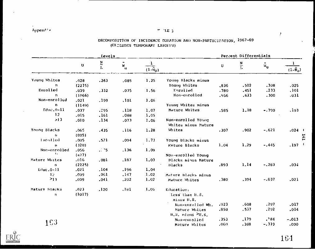
Appene'v

Young Whitesn

Enrolled

n

Non-enrolledn

Educ.0-1112

)13

Young Blacksla

lnrolled

n

Non-enrolledm

Mature Whitesn

Educ.0-1112

>13

Mature ntacksn

1e3

'1.E 3

DECOMPOSITION OF INCIDENCE DURATION AND NON-PARTICIPATION, 1967-69(EXCLUDES TEMPORARY LAYOFFS)

Levels Percent Differentials

UN 1 N -

ti

1

(1-C10) (1 -W0)

.028 .263 .085 1.25 Young Blacks minus(2215) Young Whites ,836 .502 .308 .025

.039 .332 .075 1.56 Enrolled .780 .451 .233 .101

(1066) Non-enrolled .966 .633 .300 .031

.021 .199 .101 1.06

(1149) Young Whites minus

.037 .295 .118 1.07 Mdture Whites .585 1.18 -.790 .193

.015 .161 .088 1.05

.010 .134 .073 1.06 Non-enrolled Young

Whites minus Mature.06S .435 .116 1.28 Whites .307 .902 -.621 .024 1

(805).P.

.005 .521 .094 1.73 Young Blacks minus i-,

(328) ature Blacks 1.04 1.29 -.445 .197 I

.056 .: '5 .136 1.09(477) Non-enrolled Young.016 .081 .187 1.03 Blacks minus Mature(2225) Blacks .893 1.14 -.283 .034

.021 .104 .196 1.04

.009 .061 .147 1.02 Mature Blacks minus

.009 .041 .202 1.02 Mature Whites .380 .394 -.037 .021

.023 .120 .181 1.06 Education;(1017) Less than B.S.

minus H.S.

Non-enrolled Wh. .923 .608 .297 .017

Mature WhiLes .850 .537 .292 .014

II. S. minus )11.S.

Non-eniolled .353 .179 .'84 -.013

Mature Whites .060 .388 -.319 .000

1 .1

Amendix TAlALE 4

...

DECOMPOSITION OF INCIDENCE DURATION AND NON-PARTICIPATION, 1967-69(IN:LUDES TEMPORARY LAYOFFS)

Levels Percent Differentials

UN_I Wu

1

11

N

L Wu(1-50)

Young Whites .030 .288 .082 1.25 Young Blacks minusn (2215) Young WhiteL .829 .477 .325

Enrolled .040 .342 .074 1.56 Enrolled .771 .435 .236n (1066) Non-enrolled .945 .568 .344

Non-enrolled .023 .238 .092 1.06n (1149) Young Whites minus

Educ.0-11 .041 .337 .113 1.07 Mature Whites .308 .721 -.60712 .016 .207 .076 : JS>13 .0111 .153 .069 1.06 Non-enrolled Young

whites minus MatureYoung Blacks .068 .463 .114 1.28 Whites .067 .530 -.486

n (805)

Enrolled .086 .527 .094 1.73 Young Blacks minusn (328) Mature Blacks .776 .847 -.267

Non-ep- Iled .060 .419 131 1.09

(477) Non-enrolled Young!haute Whites .022 .140 .150 1.03 Blacks minus Mature

n (2225) Blacks .652 .747 -.128Lduc.0-11 .030 .177 .162 1.04

11 .012 .106 .111 1.02 Mature Blacks m'lus>13 .012 .081 .151 1.02 Mature Whites .360 .351 -.014

t:ature Blacks .031 .199 .148 1.06 Education:n (1017) Less than H.S.

minus U.S.Non-enrolled wh. .909 .488 .402

Mature Whites .890 .509 .372

H.S. minus >11.S.

Non-enrolled .390 .301 .098

Mature Whites -.024 .278 -.304

1

.025

.101

.031

.193

.024

.197

.6a4

.021

1 f:i;

.017

.014

-.013

.000

ArrenA. Ti "F. 5

DE(OMPOSITION OF INCIDENCE DURATION AND NON-PARTICIPAT1ON, 1969-71(i14:LUDES TEMPORARY LAYOFES)

Levels Percent Differentials

N

1,

W 1U

N

I.ci

1

(1 -too) t1 -1o)

Young Whites .055 .339 .184 .022 Young Blacks minusIl (2364) Young Whiles .545 .339 .184 .022

Enrolled .077 .476 .120 1.36 Enrollej .500 .257 .214 .052n (850) Non-enrolled .647 .470 .132 .044

Non-enrolled .045 .293 .143 1.06n (1514) Young Whites minus

Edu,:.0-11 .062 .376 .150 1.10 Mature Whites .909 1.18 -.364 .08712 .046 .304 .143 1.06>13 .027 .195 .132 1.04 Non-enrolled Young

Whites minus MatureYoung Blacks .094 .504 .159 1.18 Whites .707 .982 -.283 .006

II (835)i-

Enrolled .128 .604 .148 1.43 Young Blacks minus w.p.n (217) Vatuce Blacks 1.02 1.26 -.328 .091

Non-enrolled .085 .469 .164 1.11

n (618) Non-enrolled YoungNature Whites .022 .110 .190 1.06 Blacks minus Mature

II (2167) Blacks .924 1.19 -.298 .032Educ.0-11 .027 .123 .208 1.07

12 .015 .100 .147 1.03 Mature Blacks minus>13 .017 .086 .187 1.04 Mature Whites .429 .262 .147 .018

Nature Blacks .094 .504 .159 1.18 Education:n (835) Less than H.S.

minus B.S.

icon -enrol led Wh. .305 .215 .042 .036

Mature Whites .596 .212 .346 .039

H.S. inub >H.S.

Non-enrolled .533 .442 .084 .018

Mature Whiles .101 .148 -.240 -.009

1C7-.1

AppendTrAll

INCIDENCE OF UNEMPLOYMENT IN 1967-69 BY TENURE(INCLUDES TEMPORARY LAYOFFS)

Tenure as Young White Men Youu Black Men Mature White Men Mature Black Menof 1967 P(0) P(S) P(U/S) P(U) P(S) P(U/S) P(U) P(S) P(U/S) P(U) P(S) P(U/S)

q .295 .716 .412 .494 .795 .621 .337 .565 .576 .368 .576 .640

1 .184 .493 .373 .270 .635 .426 .160 'S4 .451 .212 .348 .609

2 .187 .473 .394 .154 .308 .500 .167 .292 .500 .367 .433 .846

3 .100 .311 .321 .269 .615 .438 .093 .227 .412 .292 .333 .875

4 .096 .327 .294 .182 .636 .286 .123 .308 .400 .143 .214 .667

5 .077 .462 .167 .500 .667 .750 .133 .200 .667 .258 .452 .571

6 .059 .118 .500 .000 .333 .000 .085 .170 .500 .154 .231 .667

7 .125 .250 .500 .000 .500 .000 .091 .242 .375 .250 .300 .833

fi .200 .600 .333 .000 .333 .000 .172 .241 .714 .241 .276 .875

9 1.00 1.00 1.00 - - .100 .225 .444 .059 .176 .333

10-14 .500 .500 1.00 .750 .750 1.00 .078 .139 .564 .083 .147 .562

15-19 .081 .140 .553 .120 .134 .842

20-24 .096 .116 .793 .130 .194 .667

>25 .076 .133 .536 .145 .218 .630

Total .219 .558 .392 .388 .690 .562 .126 .223 .547 ' .182 .266 .675n (1065) (594) (410) (283) (2084) (464) (892) (237)

Note: (a) P(S) equals the probability of separating or of being temporarily laidoff from the job held at thethe htqinninq )f the I" rind.

(1,1 'of plc )come., very wall for young whiter; and hla,ks at !;even and four yeors of tenure Lesp,2ctivuly.

TAIM.E 7

INCIDE "ICE OF UNEMPLOYMNT IN 1969-71 BY TENURE, NLS(EXCLUDING TEMPORARY LAYOFFS)

Tenure asof 19f9

Young White Mena

Young Black Mena Mature White Men Mature Black MenP(U) P(s) P(U/S) P(U) P(S) P(U/S) P(U) P(S) P(U/S) P(U) P(S) P(U/S)

0 .351 .600 .586 .444 .647 .686 .252 .447 .556 .192 .416 .461

1 .195 .418 .467 .345 .536 .644 .081 .184 .419 .123 .217 .565

2 .120 .267 .450 .269 .385 .700 -

3 .164 .262 .625 .033 .233 .143 .072 .217 .333 .175 .300 .583

4 .087 .217 .400 .087 .174 .500 .114 .143 .800 .000 .111 .000

5 .068 .186 .364 .100 .300 .333 .038 .135 .286 .000 .188 .000

)-6 .029 .143 .200 .000 .200 .000 .000 .086 .000 .125 .208 .600 r

ul

7 .071 .214 .333 .250 .250 1.00 .026 .103 .250 .059 .412 .143I

A .000 .125 .000 .000 .3:3 .000 .023 .136 .167 .125 .125 1.00

9 .154 .231 .667 .000 1.00 .000 .038 .115 .333 .000 .091 .000

10-14 .000 .250 .000 .000 .000 .030 .104 .N16 .062 .112 .556

15-10 .500 .500 1.00 .039 .108 .360 .044 .104 .417

20-24 .030 .098 .304 .029 .096 .300

>25 .024 .136 .176 .035 .124 .286

Total .229 .426 .538 .347 .532 .652 .077 .106 .410 .096 .217 .4421128 481 256 1957 866

a: not enrolled

- 146 -

TABLE 8

SAMPLE MEANS FOR TURNOVER AND CNEMPLOYMENT REGRESSIONS

::LS 1969-71 MID 1975-76

YoungWhites

MatureWhites

YoungBlacks

MatureBlacks

X 4.63 35.64 4.45 37.02 18.65

X2 33.31 1317.16 30.05 1424.30 515.59

T 1.61 13.15 1.10 10.89 7.18

T2 6.95 313.83 4.84 236.73 112.13

JIRAIN .145 ,.081PTRAIN .167 - .066

GTRAIN .299 .190

DOCRATE 4.88 3.30 5.24 4.35 8.33PSEP 3.81 .496 4.19 .570 .093

PCOND .163 .068 .328 .111 .113

EDUC 12.21 10.53 10.35 7.31 12.65

HLTH .042 .222 .020 .192 .074

coy .114 ,187 .109 .231 .196

UNION .318 .378 .323 .457 .3C8

MARRY .626 .912 .448 .800 .908

PTIYE .137 .086 .167 .137 .030

OLF .328 .200 .405 .253

POLE - - - .051SEP .852 .278 1.01 .323 -

E'.."P 2.63 .5411 2.73 .589 -

EL-.7°Y .472 - .601 -

1351 1957 504 866 1562

TABLE 9

THE DETERMINANTS OF JOB SEPARATION,1969-71, YOUNG WHITE MEN, NLS

U t

11)

(INCLUDING TEMPORARY IAYOFFS)

ft

(21 . (3)CONST

.757 1.60X -.101 2.99 .078 2.15 .060 1.58X2

.00L 2.28 -.004 1.59 -.004 1.38T-.307 6.40

i-.216 4.6512

.026 4.08 .0) 8 2.97JTRAIN-.281 2.64 t -.128 1.24PTRAIN.102 .995 1.09GIPAIN.011 .130 i .090 1.12EOCRATE.015 .616 .005 .217psEP.044 5.15 .040 4.9711CrIID.182 2.23 .076 .96612141c:

-.072 4.32Itr.T11

-.118 .679GOV-.115 1.02Utl ow

; -.077 1.03NAPRY-.244 3.08PTHIE.258 2.55OLF.612 7.98

R- .007 .110 ;183.9061351

MI

17 4

bppundix

1

COUSTX

X2

T2JTRAINPTRAINGTRAINLOCRATEPSEPPCONDEDUCHLTHGOV

UNIONMARRYITWE0LF

!;EP

UNTRY

.687-.060

.003

! R2

.007

.506

1

1351

TABLE 3"

THE DETERMINANTS OF SPELLS OF UNEMPLOYMENT 1969-71, YOUNG WHITE MEN, NLS

(1)

(INCLUDING TEMPORARY LAYOFFS)

(2) 3) (4) (5)

.123 .749 .107 .0822.24 .043 1.50 .031 1.04 .004 .1611.34 -.003 1.38 -.003 1.28 -.001 .776

-.167 4.42 -.116 3.10 -.023 .781

.014 2.73 .CO9 1.94 .002 .452-.116 1.38 -.016 .187 .038 .592.136 1.67 .133 1.69 .092 1.49

-.022 .346 .037 .573 -.018 .358

.063 3.29 .052 2.84 .052 3.55

.028 4.20 .257 3.94 .008 1.57

.279 4.32 .200 3.17 .187 3.80-.051 3.84 -.022 2.11-.033 .237 .084 .771-.101 1.12 -.053 .755.159 2.66 .223 4.76

-.224 3.55 -.090 1.82.134 1.66 -.137 .214.354 5.77

.334 10.43 .371 11.78

.026 5.54 .023 4.89

.058 1.98 .100 3.39

.089 .146 -.18 .450

1

TABLE 11

THE DETERMINANTS OF JOB TURNOVU 19G9-71, MATURE WHITE MEN, NLS(INCLUDES TEMPORARY LAY01'ES)

13 t11)

B

(2)

t B

(3)

CONSTX

X 2

-2

LoCRATEPSEP

PCOUD

.517

-.021 1.81

.0004 2.30

.541

-.017 1.70

.0003 2.00-.020 5.14.0005 4.26

-.002 .190.180 18.59

.099 2.80

.377

-.007

.000

-.016.0004

-.001.166

.037

.775

.693

4.40

3.55

.173

18.07

1.10COW .002 .476HEIN .060 1.86GOV -.096 2.82Mori .040 1.44MARRY -.066 1.411-1144E .00S 1.82()LE

14.12

-2k .004 .241 .325

.30111 1957

17

TABLE 1.1

TM DETERMINANTS OF SPELLS OF UNEMPLOYMENT, 1969-71, MATURE WRITE MEN, NLS

B

(INCLUDES TEMPORARY LAYOFFS)

t B t B

(1) (2)

t

(3)

B t B(4)

t

(5)

CONST .287 .306 .350 .241 .028X. -.012 1.51 I -.011 1.48 -.01! 1.48 -.009 1.45X2 .0002 1.7.) .0002 1.60 .0002 1.47 .0001 1.56T -.008 2.77 -.007 2.54 -.002 1.00T2 .0002 1.88 .0001 1.53 .000 .152LO CRATE -.004 .641 -.004 .619 -.006 1.18PSEP .101 A.21 .097 13.68 .020 3.18PC011D .116 4.47 .102 3.90 .094 4.41

.001 .399 .0003 .126111.T11 .003 .110 -.008 .395GOV -.080 3.04 -.045 2.10

.040 2.24 , .036 2.091tARRY -.064 1.00 1-.040 1.36num: -.003 .084 -.032 1.10OLF .084 3.19 ;-.097 4.16SEP .259 9.77 .258 10.80SEP' .058 8.39 .065 9.66

-2R .001 .162 .173 .453 .434

.135

n 1957

17

TABLE 1'

Ti

THE DETEP.1INANTS OF JOB SEPARATIONS, 1969-71,

(INCLUDING TEMPORARY LAYOFFS)

t I3

(1) (2) (3)

YOUNG BLACK MEN,

CON ST 1.39 .514 1 .607-.069 1.20 : .125 1.99 1 .141 2.30-,000 .000 -.012 2.40 1-.013 2.78

T2

-.208 3.42 1-.138 2.35.1)18 2.94 .012 2.06

JTRAIN -.168 .829 -.000 .306PTRAIN .186 .818 .300 1.37GTRAIN .120 .843 .250 1.81I.6CRATE .021 .671 .011 .379PSEP .069 4.69 .073 5.22PCOND .288 2.92 i .259 2.66ED0C 1-.024 1.15MTH -.328 .868GDV !-.374 2.350111(44 1-.486 4.'3mARRY -.001 .000PTIE .366 2.58oLF .538 4.96

-2.025 .127 .213

X 1.08

504

NLS

1s

TABLE 3"

THE DETERMINANTS OF SPELLS OF UNEMPLOYMENT, 1969-71, YOUNG BLACK MEN, NLS(INCLUDING TEMPORARY LAYOFFS)

B t B t B t B t B(1) (2) (3) (4) (5)

t

lconsr .998

X -.041 .810;X

2-.001 .290

T2

JTRAINPTRAIN

GTRATN'1)0.:PATF

PSEP:14_,OND

ILDUC

inlxmCO.'

'VARRY

;Pr=()IF

!AA,

WITY

2 .020

./78

11 504

.262

.113 1.98

-.011 2.44

-.182 3.29

.017 2.98

.230 1.25

.150 1.17

.154 .748

.024 .875

.044 3.30

.286 3.19

-.024

.158 2.81

-.014 3.11-.132 2.46

.013 2.45

.299 1.67

.205 1.62

.156 .783

.027 .992

.049 3.87

.199 2.24

.003 .122

.803 2.32

-.186 1.17

-.182 1.73

-.242 2.35.209 1.61.532 5.38

.100 .178

-.159 .166

.082 1.69

.006 1.82

-.060 1.30

.007 1.52

.316 2.06

.041 .239

.080 .733

.025 1.09

.013 1.15

.078 1.01

.007 .436

.937 J.17

.028 .200

.063 .694

.259 2.96

.029 .263

.516 7.02 .563 7.90-.740 .531 -.011 .791.909 1.79 .118 2.35

.401 .379

181

TABLE lc

THE DETERMTNANTS OF JOB IUPNOVER, 1969-71, MATURE BLACK MEN, NLS(EXCLUDES TEMPORARY LAYOFFS)

(1) (2) (3)

CONST .588 .376 .231

X -.034 2.16 -.022 1.52 -.012 .86)

X 2 .001 3.07 .001 2.43 .0003 1.48

-.019 2.86 -.011 1.697

T- .0o04 1.71 .000 .794

LoCRATE .018 1.48 .010 .835

PSEP .120 7.47 .098 6.41

1t20N0 .076 1.56 .082 1.78

iDUc -.003 .578

!MTH .089 1.68

GOV -.020 .390

UMON -.037 .871

mAPRY -.035 .686

vrImE .253 4.08()LE .426 8.67

p2.028 .167 .260

X .323

n 866

1 c'Jar

ilf,It'IY.

TABLE lf

THE DETERMINANTS OF SPELLS OF UNEMPLOYMENT, 1969-71, MATURE BLACK MEN, NLS

I

CONSTIX.

X2

TT2

LOCRATEPSEP

ICOHDLime

HLTHr,OV

UNIoNflARYvrimr

1:i'

s:)

!,F

i-(

2

;..:

t1

B t B t(1) (2)

.373

-.022 2.10.0004 2.63

.012

.132

866

(EXCLUDES TEMPORARY LAYOFFS)

-.017 1.68J

.0003 2.20

-.004 .870

-.004 .870

.000 .122

.150 1.77

.055 4.91

.059 1.77

.080 .097

B

(3)

t

.241

-.015 1.49

.0003 1.81

-.001 .013

-.000 .043.011 1.23

.048 4.40

.056 1.70

-.003 .616

.043 1.15

-.026 ,685

-.027 .934

-.006 .158

.130 2.94

.091 2.57

lt3

1

:

:

INCIDENCEAMONG SEPARATORS

B t B t B t

(4) (5) (6)

.135

-.009 1.20

.0001 1.12

.004 1.22

,-.0001 1.21

.006 :906

.003 .386

.019 .728-.001 .332

.002 .009-.016 .573-.116 .490

.010 .360

.015 .422

-.104 3.u0

.458 11.39

.000 .000

1

.009 .750

11.51 -.008.800: .000

.002

-.000-.000.016

-.009-.004-.018-.050-.013-.049.063

-.246-.415

.010

.464 .461 .012

.415

200

.427

.409

.219

.459

.000

.883

.164

.385

.217

.492

.176

.611

.754 ,,,,

3.31

181

TABLE 1

THE DETERMINANTS OF THE PROBABILITY or sErARATInc, 1969-71, YOUNG WHITE MEN, NLS(EXCLUDES TEMPORARY LAY0FS)

B I E

(1)

t 6

(2)

t

(3)

COAST .567 .471 .660X -.054 4.46 .007 .513 .000 .000X2

.003 3.44 -.MOO .253 .000 .10JT -.134 7.90 -.101 6.08T2 .011 e..75 .007 3.49JTRAIN -.126 3.34 -.078 2.13!TRAIN .006 .182 .009 .268CTPAIN -.019 .656 .004 .145I ricRATE .016 1.89 .013 1.61psrp .004 1.38 .003 1.12WOAD .039 1.36 .008 .290

-.017 2.96

.019 .300GoV -.072 1.81

MioN -.08/ 3.26mAI.RY -.054 1.93MAME .050 1.61(.LF .243 8.96

-2k .017 .116 .187

.429

n 1351

.s.

.11 P t.

TABLE 1

THE DETERMINANTS OF THE INCIDENCE OF UNEMPLOYMENT, 1969-71, YOUNG WHITE MEN, NLS(EXCLUDES TEMPORARY LAYOFFS)

B t B(1)

t B(2)

t

(3)

B t B

(4)

t

(5)

!CONST .316 .110 .331 .040 .018X -.026 2.48 .015 1.31 .011 .962 .004 .042,X

2.001 1.34 -.001 1.38 -.001 1.29 -.001 1.02

-.075 5.11 -.047 3.32 -.002 .182T2 .006 3.08 .004 1.90 -.000 .110JTRAIN -.035 1.07 .010 .332 .040 1.56PTRATN .030 .959 .131 1.02 .015 .640GTRAIN -.022 .877 .001 .003 -.004 .224UPRATE .028 3.76 .024 3.42 .020 3.59L'S :P .007 2.66 .006 2.42 -.000 .000PC 0N0 .125 5.00 .092 3.80 .078 4.00Lh0C -.020 3.86 -.008 2.06H1110 .005 .009 .031 .727Go./ -.034 .997 -.011 .401

-.002 .100 .040 2.18rAvRy -.086 3.57 -.049 2.52

.063 2.05 .022 .900orF .197 8.41 I - -sEP .287 22.73 .299 24.25sLP- -.021 11.70 -.022 12.19I,NTPY

.029 2.51 .043 3.70-2

.010 .098 .174 i .462 .442* .234

11 1351

41%.11,i1A

TABLE lc

THE DETERMINANTS OF QUIT AND QUIT UNEMPLOYMENT, WHITE MEN

NLS Young Men 1969-71 1,11.E; Mature Men 1969-71 MID 1975-76P(Q) t P(unQ) t

(1) (2)

13

(3)

P(Q) t B P(unQ) t II

(4)

P(Q) t 13

(5)

P(unQ)t(6)

(CONST .432 .197 .002 -.015 .273 .122X -.018 1.43 -.004 .412 -.000 .000 .003 1.11 -.004 1.68 -.001 .922

'X2 .001 1.42 .0001 .212 .000 .499 -.000 .894 .0001 1.19 .000 .592'I' -.047 2.97 -.014 1.25 -.006 3.05 -.002 2.04 -.0013 2.65 -.003 1.522 .003 1.37 ,001 .456 .0002 3.10 .00004 1.27 .0002 1.90 .0001 1.1131TAIN -.085 2.46 -.007 .266 - - - -PTRAIN .004 .122 .017 .700 - - - -GMAIN -.045 1.65 -.033 1.69 - - - -U"xPATr.: .004 .537 .003 .488 I .002 .528 -.002 .848 -.002 .650 -.0001 .100P:-.1i, -.0004 .134 .002 .807 .003 .632 .005 1.97 .170 3.98 .114 3.71Pc0:H) -.065 2.42 -.007 .377 .0004 .003 .032 3.58 .041 1.58r1,0,' -.005 .800 -.006 1.24 .003 1.28 .002 1.65 -.009 3.09 -.006 3.2201111 .013 .200 -.014 .332 .043 2.70 .008 .093 .033 1.16 -.008 .336 1

W,V -.002 .006 -.007 .247 .004 .224 . -.013 1.41 -.036 1.96 -.01G 1.27 1-+

inii,14 -.141 5.57 -.054 2.92 -.058 4.20 -.023 3.15 -.027 1.64 -.009 .781kJ,

-4111.1 ICI -.030 1.16 -.064 3.28 -.004 .161 -.013 1.10 -.674 2.62 -.035 2.00 1

'1li-i: .020 .574 .f35 1.40 .003 .145 -.002 .152 .002 2.54 .001 2.17Ho r .222 8.50 .185 9.72 .300 17.70 .014 1.60 - -P(LC -.055 1.56 .005 .224

17`) .11/ .112 .176 .028 .066 .048X

n

.271

1207

.118,

1207.109

1928.023

1928.086

1454.036

1454

'(g) equals the probability of quittini the job held at the beginning of the interval.equal!1 the probability of quitting the job held at the beginning of the interval and experiencingunemployment during the interval.

lc ori5a

X

x2

iTTRATN

IqtRAIN

G'i EAT N

I p

I ( '00

To:

8f:Fit

r,(A/

Uri

rAvior

nu:

(1

PoLE

-2 v.

11

TABLE 20

TILE DETERMINANTS Or lAYrIT AN!. lAYOFF UNEMPLOYMENT, WHITE MEN

NTS YOUNG MEN 1969-71 NT.S MATURE TIrM 1969-71

P(L)

B t

(1)

.184

.021 2.08

-.001 1.82

-.052 4.10.004 2.81.014 .492

.008 .316

.046 2.13

.011 1.72

.004 2.05

.083 3.86-.013 2.95.021 .435

_.061 2.00.050 2.46

-.011 .496

.034 1.23

.029 1.40

-

.0R2

.14111297 I

I,

1

B

P(unL)t

(2)

P (L) P (unL)

B t l3 t

(3) (4)

.127 .112t

087.017 1.85 .001 .219 --.001 .346

-.001 1.93 : -.000 .458 .000 .017-.037 3.30 i -.004 2.27 -.003 1.95.003 2.22 ! .J3001 1.50 .0001 1.30.025 1.02 -

.008 .332 : - -

.013 1.71 - . -

.019 3.32 .0005 .138 .003 .954

.004 2.10 , .053 13,27 .040 11.80

.092 4.77 .014 .985 .008 .693-.014 3.46 -.001 .714 .0002 .141.036 .825 -.009 .648 -.011 .949

-.011 1.16 -.045 3.08 -.Oil 2.9.050 2.76 .009 .794 .010 1.02

-.012 .608 -.036 1.80 -.028 1.67

.031 1.26 .027 1.32 -.001 .005

.022 1.17 .111 7.60 .066 5.28- - -

.088 .178 .128

.110 .079 .0537397 1928 1928

1

MID 1975-76

P(L)

13 t 13

(5)

P(unL)

t

(6)

.175 .167

-.004 2%01 -.001 .781.0001 1.41 .000 .200

-.005 1.31 -.0u) 1.25.0001

-

1.02 .000 .583

-

-

.003 1.56 .002 1.46

.137 4.04 .166 6.19-.003 1.12 -.004 1.96 ,

.081 3.02 .062 2.64

.003 .173 -.011 .818-.002 .141 -.008 .671

-.031 1.25 -:065 3.30-.073 1.75 -.044 1.")6

-

-.027 .818 .012 .436

.047 .068

.075 .0441437 1437

1:3 P(L) equals the probability of being laid off from the job held at the beginning of the interval.4'(ur14 equals the probability of being laid oil- from the job held at the beginning of the interval and

experiencing unemployment during the interval.

- 159 -

Why Does the Rate of Youth Labor ForceActivity Differ Across Surveys?

Richard B. FreemanJ.L. Medoff

One prerequisite for analysis of the.economic problem of youth is

a set of sound estimates of the employment and labor force status of the

young. Yet, existing estimates of the extent of labor market involvement

and the extent of work activity of the young based on the monthly Current

Population Survey (CPS), the source of official government figures on this

subject, and from special longitudinal surveys of the young, notably the

National Longitudinal Survey of Yourg Hen (NLS) and the National Longitudinal

Survey of the High School Class of 1972 (NLS72), give strikingly different

pictures of the labor market for young men.1 Labor force participation rates,

employment to population ratios and weeks worked are noticeably higher in

both longitudinal surveys than in the CPS. Unemployment rates differ

significantly but are neither higher nor lower consistently across surveys.

The differences in the recorded activity rates constitute a major problem

in evaluating the magnitude and nature of the la or force prellem for young men Tf

the CPS data are incorrect, and understate the employment to population ratio

for young individuals, standard discussions of youth employment problams are

exaggerated. If the longitudinal data are incorrect, studies which vse the longitudi-

nal surveys to ascertain the causes and effects of the youth employment prcblemmay be invt.1-

id. What explains the large differences in rates of male youth labor force activity

found in the different surveys? Can the observed differences be traced to

specific differences in survey procedures or questions?

The purpose of this study is to answer these questions by providing a

detailed quantitative analysis of the divergences between the rates ef labor

force activity for male youths indicated by these surveys. Sectton I describes

the three surveys providing the youth labor force information on which we

focus: the CPS, NLS, and NLS72. The second section com es t.e cr

force participation rates, ratios of employment to opulation, rates ou

employment, and rates of school enrollment giv- by the surveys. Sectiot\ III

100OA*

- 160 -

uses a matched mother-son sample drawn from the NLS and other

information to examine three potential causes of survey differences: (1)

the fact that youths report their own activity in the NLS and NLS72 while parents

or other adults typically -report the activities of youths in the CPS; (2)

differences in the samples studied; and (3) differences in the survey methods

employed. In the fourth section,some suggestions for further investigations

of alternative measures of the employment of young persons are offered.

Our analysis indicates that there are significant differencis betweenAO

rates of activity for yo.4.g males calculated with surveys in which youngpeople

respond for themselves and those calculated with surveys in which they are unlikely to

do so. Of particular importance is the fact that the responses of young male

self- respondents imply s_5,1gnificantly higher employment to population ratio

than is implied by the responses of proxy-respondents. Who is questioned

about the activity of young men appears to be a major determinant of the

responses obtained, which raises important questions about current: ways of

obtaining information about the youth joblessness problem.

I. Survey Procedures and Questions

In this section we compare the questions asked and survey methods em-

ployed in the CPS, NLS, and NLS72. Each of the surveys seeks information

about labor force activity, weeks worked in the previous year, and enrollment

in school. While the questions are reasonably similar across surveys, the

survey methods, in particular the relative importance of proxy versus self-

responses, differ. These differences must be understood if the large dispa-

rities in the picture of the youth labor market given by the surveys are to

be explsined.

The CPS2interviews approximately 56,000 households (47,000

before July 1975) using a stratified sample. Part of the sample is

changed each month to avoid problems of noncooperation when a person is inter-

- 161 -

viewed for many months in a row. The method of rotation of the Sample is such

that a group will be interviewed for 4 consecutive months one year, deleted from

the CPS for 8 months and then interviewed in the same 4 months of the following

year. As a result, 75 percent of the sample is common from month to month and

50 percent is common from year to year. Each months during the calendar week

containing the 19th day, interviewers contactsome"responsible persorrin each of the

sample households. Personal visits are used to obtain 90 percent or more of

the responses in the first and fifth month that the household is in the sample

And about 50 to 60 percent in the second month; other months more than 75

percent of the responses come from telephone interviews. Roughly half of the

households in any month are interviewed by phone. Though the questions are

asked for every individual in the household, it is important to understand that

voun individuals do not usuall res ond for themselves. This is because

one "responsible person" per family, usually not a teen,3 answers for every

household member.

Tabulated results from the CPS are derived using responses

to calculate a "composite estimate" of the status of individuals by

taking the unweighted mean of two separate estimates: the "actual"

value for the current month and a figure obtained

by adding to the preceding month's composite estimate the change in the actual

value of each item between the precedin4 month and the )resent month based on the

part of the sample that is common to both months. oy using raw data for most of our

analysis we have taken into account the possible bias caused by this Procedure.

To determine the labor force status of an individual, the CPS asks a

standard set of interrelated questions which are designed to classify a person

as a member of one of three categories: employed, unemployed, end out of the

labor force. Figure 1 gives this set of questions from the CPS survey.

To determine weeks worked over the previous year the CPS asks (in its March

questionnaire only):

In 19 how many weeks did . . . work either full time or parttime not

counting work arm: the house? Include paid vacation and paid sick leave.

1 34

Figure 1: The CPS Labur Force Questions - 162 -II. LINE NUett!.1

h. ssi ... 401.40 alLAST WEEK

WI111.01

KIITS;q3 %MIs stiles'

se sohe es*' a(S1., se Me AK

Adh s r ore .. 7

Lseelel It, LXRawl; hayse N :Coln to sex' S :1)Pcb:* tt'e 1:;., Sr :1) U :Rood R

'04te CT :

20C. Cut ... USUALLY **/11 35bows or ran .lei r firs obiYes sense es Ile itliSs

oe,tei less Av. 35boon LAST AtEKI

Ni Oet nees.,

USUALLY .r4s lession IS 1.010 "esti?

31 el, Vrersatir Nrs**1

Slack rb

tsbe.:1 shtetale

Plot r crt sr:1N.. itS Ie : vvi

ire' row; .r%

OA'S fW, get'. /set..-* or:

hoh.17.y /Lepel

*.spit.

led ..est`r

()n Moots

OR *Era.Tao rus vor .

s:r301. res:a' :.s..

0 4 m a i nor follow* , .

P.11,,orb "ft, 3! ,.es

Odor mews teeeese.

Iffy is it ma own el. Gid1 era

25 . is try ...PI 1113LAST %EEC st es.esola stint! the :nose/Am e S..... es.draw 4.vsarl 041

1Yes N : Irr ta 111

21111 lbw/1110y hlwel1. . .LAST IIEVIat ell jots'

201. INTERvIECHICK ITEM

buy enkw- :J)

41 ere

1.31 'or :0C1

33J3 7. gess MO

100. Dig ... lose en. hoe enli ae1 1 oN LAST

MEEK Iff any 'eras'welt is ilbess. Ankh,At slut woIi?

Yes Ns. Awry hisI.f...sole ofCle

ICrtect 4 if 1,. Dimle:roi. le Ism,.

e; :34 ettlget el :11.4.

tenor :Of es/ .m'C.eleeftess, oil 11.1

Nts :

20E. Dal ... look itle cote -t R se it woe -hen wej*S-S1 SEW

1411 : Mew rimy Corokeen 14 .

Na

11.0011111=

timid 30 4 ea/ .VA011111141 of ewe ire.4.0 deed. melded sal.1.# is al

1$10 a.

21. Hi IS. *11., le I /6icws tab en

teee's hos yeleecee 114

IS Itnlecls ebeentloyfil LAST *E DO

'Ns 'la 7. n,/-M. %pi Own

firm fterk LAST SEEK!

(:)...w

01 , (3

Bed *w.- 0

Leroy d.stnott

i 73 ft :54.11 84/

.A jJ data : did

Tr-r leery ity:N 11C:1

%h. J4 ie,,i ;elp

!,:t;1;10 le,atf 21Cll1.1.11 sr

IN de f. well easel

Olive arm./d..

21e. I.. . setl.al ws;ss so

501:e far etome 11 LAST SEEK'

Yes

NA

Sell .realovel

0

21C. tees ... vsvelle ne.1,33 herb e, wens weel,of Ibis job?

Ytts CNo 0

iFia I. JJ ..... pi£.I I.., 6,1,41

errict USE ONLY

INDUSTRY

U

.W..400mimmUmw

C

0EP

c:

K :L:V

OCCUPATION

N

P

?<L 0

t3. 34. RS .2)

?5S TSSG 3.. . v=41 4: X

Y

0` Z

" t)

21. til LA n, so, flu, ::t /Nes &eel leslas kt .,.bietots the post 1 et:si

Yes No 3 K. se 11).I1

nA. 0.81 hes . try% faun IR m lee114 .v0.044 d

n4e4li ..el. 1. ...1 list,Cho: be.I orn:loy.

enplay.

lopterr 'Lordly

friends co selolees

Placed se bnered Als

1%4 ;1; to. 2,,t;.-4Cfpere4 is arm. , C/ It.

MAIO. 'true% M.;

//B. Vil gym test.'; Jo,sei? Was a breast feet

or sod job of AV hale 0a41Of wet Intee $ IMI 'thee Sees s +?

Lest jobGeis job

Leh schoolWanted re -poi :-

Other (Seeeth

22C. Hew men), .telra

has ... beenWiling for ...al

H.. many leettLVest

leolrm for .ad?

21 How merry ...la

Sc. ... 1.4off/

a

22D. Nos ... beenen,seit.Anse .enk!

Poll 3 Poo Z0

22E. Is ig Inv reason .11 .401 Idle 06 LAST *EEff.2

Yes .; 'Aireadir has seb

4%4 Ttictrry ,Gott.; le uhc..21

si C0111, erred. .*14

//F. sow f.f . , seful:hrte 1.1 c- vsntss !on

CPlttyleve will/11V ~II

1971 .1944 Wee world dr

ISoA

NSe:wir. :,:4741,4 Ali. ofNeer *Mei et eN

014 5, ;# 1 Sim 1.11tegri IOU". : ..I. wr14.,, dot, ...Ave.. I -4.,r1

- 163 -

The CPS has two questions regarding enrollment in school. Each October

the CPS asks:

Is attending or enrolled in school?

In each month, the oajor activity question:

What was . . .doing most of last week?

provides information on attendance at school (see question 19 in Figure 1).

The National Longitudinal Survey5is a survey that covers about 5,000

persons in several specified age groups: young men aged 14 to 24 in 1966

(more accurately, as of April 1, 1966); ;'Dung women aged 14 to 24 in

1968; women between the tages of 30 and 44 in 1966; and men 45 to 59 in 1966.

The original samples were chosen through a multi-stage probability sampling

procedure. To ensure that reliable information on blacks could be derived from

the surveys, this group was eversampled. The NLS interviews the same persons repeat-

ully as they age over a ten year neriod. In- nprcnn interviews were conductorl from

1966 to 1971, telephone interviews were generally employed in 1973 and_1975,-

and no interviews_ were conducted in 1972 and 1974.

The weeks worked question in the NLS varies only slightly from that in

the CPS:

In how many different weeks did you work either full- or part-time

in the last 12 months, (not counting work around the house)? Count

any week where you did any work at all (Include*paid vacations

and paid sick leave.)

The NLS asks two questions to ascertain the enrollment status of individuals.

At one point it inquires:

Are you attending or enrolled in regular school?

At another point it asks a question regarding the major activity of the indi-

vidual to which one answer is "going to school."

The NLS and CPS surveys are reasonably similar. Both are administered

by experienced CPS interviewers. Both use the standard set of CPS Libor

force questions to determine whether a person is employed or out of the labor

113G

- 164 -

force. The NLS differs from the CPS, however, in that each individual in .he

V-,S describes his/her own labor force experience rather than typically having

it described by someone else in the household and in that the NLS is part of

a larger battery of labor force questions. 6

The NLS72 is a very different rurvey. 7It is based on'n stratified national

probability sample of 1,200 high schools (later slightly amended) from which

18 persons in the class of 1972 per school were selected for the survey., An ini-

tiAl base year survey of studenta was administered followed by several "follow-up"

questionnaires designed to track each individual' -s progress over time. Most of

the information is obtained by mail, with between one quarter and one third of the

respondents interviewed by telephone. The response rate to the NLS72 was ex-

tremely high, with 95.5 percent of an initial base group of 23,457 students

responding to either the base-year or first follow-up.questionnaires and

with a large percentage responding to ensuing follow-up surveys.

To obtain information on the individual's labor force status in October

1972, the interviewer asked:

Now please think back to about a year ago. Did you hold a job

of any kind during the month of October 1972?

Yes, same job as in October 1973 1

Yes, but different job than in October 1973 2

No 3

What were the reasons you were not working during the month of

October 1972? (Circle one number on each line.) Applies

Does not

applyto me to me

Did not want to work1 2

On temporary layoff from work or waiting to report to work 1 2

Was full-time homemaker1 2

Going to school1 2

Not enough job openings available 1 2

Union restrictions .1 2

Would have required moving 1 2

1(V1ti

- 165 -

Required work experience I did not have. 1 2

Jobs available offered little opportunity for career development.1....2

Health problems or physical handicap 1 2

Could not arrange child care 1 2

Other family responsibilities (including pregnancy) 1

Waiting to enter or in Armed Forces 1 2

Not educationally qualified for types of work available 1 2

Did you look for work dU-iing Ottober 1972?

Yes 1

No 2

To obtain information on the weeks worked by the individual in the year,

the following question was asked:

Each part of this question refers to the entire 52-week period

from October 1972 to October 1973.

About how many different weeks did you work altogether during

this period? (Count all weeks in which you did any work at all

or were on paid vacation.) Number of weeks

To ascertain the enrollment status of the former'high school seniors in

October 1972 (a period for which comparable CPS data on the high school class

of 1972 is available), the students"ere asked (in 1973):

Now please think back a year to the Fall of 1972. Were you taking

classes or courses at any school during the month of October 1972?

Yes

No

1

2

166TO summarize, the CPS and NLS use roughly the same set Of questions bu't

employ survey methods which differ in a number of potentially important respects.

It seems that the primary difference in interview piocedures is that individuals.

self-repprt activity in the NLS but are often reported for by proxy-respondents

in the CPS. The CPS and NLS72 differ in more fundamental ways, both in terms of

questions ana survey procedures. The NLS and NLS72 have one basic similarity:

eacil seeks self-responses as opposed to proxy- responses.

II. Estimates of Differences in Youth Activity AAong Surveys

This section documents the basic "fact" under study: the strikingly

different rates of labor force activity reported for young males in the

NLS and NLS72 from those in the CPS. Our study reveals generally large differ-

ences in employment to population ratios, labor force Participation rates, and

weeks worked, and occasionally substantial differences in unemployment rates.

Basically, both the NLS and NLS72 show greater work activity among male youths

than does the CPS.

CPS vs. NLS

First, we examine differences in the patterns of labor force and

school activity for young males indicated by the CPS and the NLS. Table 1

compares the percentage of young persons in school, employment to population

ratios, labor force participation rates, unemploymont rates, and weeks worked,

as defined by the Bureau of Labor Statistics, for males in the civilian, non-

institutional population aged 16-17, 12-19, and 20-24 as indicated by

the two surveys. The NLS figures are based on weighted counts of individuals

interviewed in the 1966-71 surveys, with the number of respondents as given

in the table. In addition to the NLS sampling weights, a second set of wdigbts

was applied to people of different ages to correct for a problem with reporting

on the age of NLS respondents. Because NLS codes the are of resnordents as

of Lprii i and incervie::s the respondents Primarily in lovember,' there is a seven

month lag between the reported age and the time of the employment stetul question. This

lag means that roughly seven-twelfthsof the sample changes years of age between w'en

4,1

167 -

Table 1: Comparison of Rates of School and Labor Force Activity

for Young Men, 1966-1971: NLS vs. CPS

No. in NLS % in School `Trap /Pope LFrc Onemploymentc Weeks Worked

sample NLS CPS NLS CPS NLS CPS NLS CPS :'LS CPS

TOTAL MALES

16-17yr. olds

1966 1966 89.8 89.9 47.6 36.4 59.2 40.9 19.7 11.1 18.8 14.7

1967 1976 90.2 91.0 44.9 35.2 56.3 42%0 20.3 16.1 ° ?0.4 15.5

18-19yr. olds

1966 1519 61.8 57.8 63.5 54.271.0 59.9 10.5 9.6 29.2 24.4

1967 1622 63.0 56.3 62.3 52.3 70.5 59.5 11.6 12.1 29.3 24.8

1968 J1619 59.0 60.4 54.2 54.3 70.3 59.84 8.7 9.2 30.0 25.2

1964 1621 59.6 59.4 60.9 56.3 70.0 61.9 13.1 9.2 29.4 3').4

20 -24

vr. oldsU

1966 4056 30.1 29.2 83.6 79.5 56.3 83.1 3.1 4.3 38.8 37.7

1967 197e. 31.9 30.8. 82.1 77.8, 85.4 81.7 3.8 4.8 38.6 35.1

1968 1909 33.5 30.5 80.3 76.8 83.2 80.4 3.5 4.4 39.0 24.6

1969 1970 1 31.1 32.0 80.4 76.9 84.7 80.8 5.1 4.9 38.0 23.9

1970 2283 29.2 29.3 77.9 74.3 84.9 82.2 8.3 9.5 41.6 33.5

19712600 28.7 29.2, 79.9 73.5 87.4 81.5 8.6 9.8 31.3 33.2

jAThe nubers in this column are onweighted counts of the observations

used in generating the relevant row 'estinates. Thus, for example, the

sixteen to seventeen year old figures includes all males who were fifteen

to seventeen years old in April of the given year. The NLS numbers in all

other columns are base:1 on counts weighted in accordance with age. (See

pages 8 and 10 for a discussion of the weighting procedure.)

bU.S. Bureau of the Census, Current Population Reports, Series P-20, "School

Enrollment," October 1966-1971, numbers 167, 190, 206, 222, 241. Table:

"Enrollment Status of the Population 3 to 34 Years Old, by Age, Race, Sex,

and Selected Educational Characteristics, for the United States."

cU.S. Bureau of Labor Statistics, Employment andLlernigEs, December 1966-1971.

Table: "Employment Status of the Noninstitutional Population by Age, Sex, and

Color."dU.S. Bureau of Labor Statistics, Work Experience of the Population, Special

Labor Force Reports 91, 107, 115, 127, 141, 162. Table: "Age: Persons with

Work Experience, by Sex."

4.;

1

- 368 -their age is recorded and When their labor market status is ascertained. Inlight of this problem, we applied different

weights to people of differentrecorded ages in the ALS (unless otherwise stated). These weights were chosenso that we could derive NLS figures !or "X-Y" year olds which are comparableto cps figures for "X-Y" year olds. For example, in constructing an NLS averagefor 16-17 year olds, we attached to 15 year olds a weight of 7/12 (the proballityof their having turned 16 by the interview

date), to 16 year olds (all of whomwuld be either 16 or 17) a weight of one, and to 17 year olds a weight of 5/12(the probability of their not having turned 18 by the interview date). The finalweight applied to a respondent in the NLS was the product of this weightand the individual's sampling weight.

The CPS data are obtained from publishea documents, with enrollment figures

relating to November, and weeks worked information covering the calendar year.

Because of the timing of the surveys, the NLS figures do not refer to the same

time periods. While most of the NLS interviews occur in November, some take

place in the surrounding months. Also, while the NLS weeks worked question

covers the preceding 12 months, the CPS question relates to the calendar year,

creating a divergence of 1 to 2 months. While these slight differences in

timing may have some effects,there is typically not ,side enough variation in

rates of activity across CPS surveys in the relevant months to suggest any major

problems in comparison. We did, however, attach different weights to those of

different ages (11/12 or 1/12 using the method described above) for the NLS weeks

worked data because CPS weeks worked and age questions are asked in March while

the NLS age pertains to April of the preceding year.

The figures in Table 1 reveal five differencesbetween, the NLS ane CPS

descriptions of youth activity:

First, and most important, the NLS indicates a much higher proportion of

young males employed than does the CPS. The employment to population rat4os

diverge by 9.7 to 11.2 points among 16-17 years cads. by 4.6 to in.o points amens 18-1cyear olds, and by 3.5 to 6.4 points among 20-2::, fear olds. Since individuals

either have job or do not, the employment to ratio is a more

- 169 -

reliable measure. Thus, the difference in the reported levels is striking..

Second, rates of unemployment also differ between the surveys, with the

NLS showing typically higher rates among the youngest males ane generally lower

rates among the older males. The unemployment rates for 16-17 year olds diverge

by 4.2 to 8.6 points; those for 18-19 year olds by -').5 to 3.9 points; those for 20-24

year olds by -1.2 to 0.2 points.

Third, the higher employment to population ratios and differing rates of

unemployment translate into even larger difierenc. in labor force participation

rates LFPR's) between the surveys although the differences narrow with age.

For 16-17 year old males, the NLS LFPR's are 14.3 to 18.3 points above the CPS LFPR's;

for 1849 year old males, the NLS LFPR's are 8.1 to 11.1 points higher; and for 20-24

year old males, the NLS rates dominate by 2.7 to 5.9 points.

Fourth, consistent with the employment to population ratio evidence, the

evidence on weeks worked i- the previous year also shows divergences, with

the CPS indicating that young males work fewer weeks than is indicated by the NT.c

Fifth, although the NLS and CPS report strikingly different patterns of

work 1ctivity, they report similar proportions of young men in shcool.

And sixth, differences in reported labor force activity tend to be less

for older males than for younger.

Racial Differences

Does the pattern of higher rates of work activity in the NLS than in the CPS

hold for nonwhite males as well as for all young men? To what extent does the

magnitude of white- nonwhite difLerenceinwork activity differ between the wirveys?

Table 2 contains the basic data needed to answer these questions: rates of

activity disaggregated by race. The figures in the table show that the pattern

of higher work activity rates in the NLS than in the CPS is found among nonwhite

males as well as among slhite males. More importantly, comparison of the rates

of activity of nonwhite and white young men estimated with the two surveys

reveals a general pattern of much smaller absolute differences in employment to

population ratios between nonwhite and white male youths in the NLS thhn in

the CPS, especially for younger nen:

20')

- 170 -

Table 2: Comparison of Ra:cs of School and Labor Force Activity

for Young Men by Race, 1966-1971: NLS vs. CPS

No. in NLSa

in Schoolb

Emp/Popc

LF UnemploymentSample NLS CPS NLS CPS NLS CPS NLS CPS

16-17

yr. olds

WHITE MALES

1966 1310 90.7 90.3 48.4 NAe 59.4 NA 18.6frA

1967 1319 91.7 91.4 0.6 36.7 56.1 42.8 18.7 14.4

18-19vr. olds

1966 1093 63.3 59.0 64.1 NA 70.6 NA 9.1 NA

1967 1099 64.3 57.2 62.8 56.7 70.0 63.4 10.3 10.6

i968 1085 60.0 61.5 64.6 55.7 70.2 60.2 7.9 7.5

1969 1103 62.0 60.9 61.2 56.8 69.9 61.: 12.5 7.6

20-24

yr. olds

1966 1570 32.2 31.6 83.1 NA 85.8 NA 3.1 NA

1967 1496 33.9 32.2 81.8 78.0 84.5 81.2 3.2 4.0

1968 1410 35.4 37.5 79.7 76.5 82.6 79.8 3.4 4.1

1969 1402 32.8 33.6 80.8 76.7 84.6 80.3 4.6 4.5

1970 1619 30.6 30.9 78.2 75.0 84.5 82.2 7.4 8.8

1971 1869 30.0 30.3 80.5 74.1 87.5 81.8 8. 0 9.3

NNWITE MALES16-17yr. olds1966 656 84.9 87.2 43.0 NA 58.2 NA 26.2 NA1967 657 84.4 8S.0 40.6 26.2 57.8 36.7 29.8 28.8

18-19yr. olds1966 426 49.1 58.5 NA 74.0 NA 20.9 NA1967 523

... 50.5 59.7 47.0 74.0 60.1 19.4 21.71968 534 53.3 53.5 61.7 45.6 71.3 57.2 13.5 20.31969 518 43.5 49.8 59.0 52.6 70.9 65.1 16.9 19.0

20-24

yr. olds1966 486 15.3 12.3 8Q.9 NA 90.1 NA 3.5 NA

1967 480 16.2 18.9 84.876.9 91.9 85.7 7.8 10.3

1968 499 18.5 16.3 84.579.0 87.9 84.7 3.7 6.7

1969 568 18.1 20.5 784 78.2 85,5 84.7 8.7 7.7

1970 664 18.9 18.1 75.169.0 87.9 81.2 14.6 15.0

1971 731 19.1 21.7 75.3 69.5 86.7 79.9 13.2 13.0

Notes: a'b'c'dSee comparable note in Table 1.

Not available.

203

- 171 -

Difference in Employment to Population Ratios for Young White ?'.ales

Versus Young Nonwhite Males from Table 2

(White Minus Nonwhite)

1b-17 year olds

1967 1968 1969 1970 1971

CPS 10.S

NLS 5.0 .11.we

18-19 year olds

CPS 6.2 10.0 4.2 --

NLS 3.1 2.9 2.1 -- --

20-24 year olds

CPS 1.1 -2.5 -1.4 6.0 4.6

NLS -3.0 -4.9 2.7 3.1 5.2

If the NLS figures are correct and the CPS figures incorrect, the differences in

employment to population ratios for nonwhite young men and for white young men is

much smaller than is generally believed. Alternatively, if the ['PS figures are

correct and the NLS figures incorrect, studies of the causes and effects of

nonwhite -white differences in employment using the NLS tapes are questionable.

Inspection of other variables in Table 2 reveals that while the CPS yields

white labor force participation rates that are higher in five of nine cases than

the comparable nonwhite rates, the NLS gives nonwhite participation rates which are

typically above the comparable white rate. White-nonwhite differences in percen-

tages in school are larger in the NLS than in the CPS, while differences in unem-

ployment rates tend to be somewhat smaller in the NLS than in the CPS, at least

for younger men,, as :town below:

Differences in Unemployment Rates for Young While MalesVersus Young Nonwhite Males from Table 2

(Nonwhite Minus White)

1967 1968 1969 1970 1971

16-17 year oldsCPS 14.4

NLS 11.1

18-19 year oldsCPS 11.1 12.9 11.4 -- --

NLS 9.1 5.6 4.4 -- --

20-24 year olds6.3 2.6 3.2 6.2 3.7CPS4.6 0.3 4.1 7.2 5.2

- 172 -

School Status

How do the differences in work activity between the NLS and CPS vaLy by

the school status of the young? Given the differences by age group presented

in Table 2, one would expect greater divergences among those whose major

activity is reported as being in school than among those whose activity is

not being in school. Table 3 presents evidence for the 16-21 year old group

of males for whom the Census publishes data on work activity by school status

which is consistent with this expectation. The table shows three things.

First, NLS-CPS differences between the employment to population ratios

and labor force participation rates for young men are greater for those youth

whose major activity is school than for others. Employment to population

figures differ by 10.9 to 1^.3 points for the in school young men compared to 4.8

to 10.6 points for other young men.

Second, mean weeks worked for 16-21 year old males are higher by 4.1 to 7.1

weeks in the NLS than in the CPS for those sample members whose major activity

is school and by about 2.6 to 3.4 weeks for the other sample members

Third, the direction of differences between the unemployment rates calculated

from young men with the NLS and those calculated with the CPS depends critically

on the major activity of persons. For 16-21 ye:ir old males whose major activity

is other than being in school, the NLS shows much lower rates of unemployment

than the CPS. For those males whose major activity was school, however, the

NLS shows much higher rtes of unemployment than the CPS.

21 ti

1

- 173 -

Table 3: Comparison of Rates of School and Labor Force Activity

for Young Men, by Major Activity, 1967, 16-21 Year °Ids:

NLS vs. CPS

No. in nenmajor Activityb Emp/Pepc Unemplojrmentc Weeks VcrkeddSample NLS CPS NLS CPS NLS CrS NI.S CPS NLS

TOTAL MALES

Major activit,.school 2284 65.2 64.7 42.8 31.7 52.7 36.5 18.8 13.1 11.5 17,1

M:ajor activity:

other 1246 34.8 35.3 87.8 82.1 92.8 91.3 5.3 10.2 37.1 33.7

WHITE MALES

Major activity:school S:657 66.3 66.1 43.Q 33.0 52.9 37.5 17.0 11.9 22.0 17.9

".ajcr activity.

other786 33.7 33.9 88.6 83.8 92.5 91.6 4.2 8.5 38.0 34.6

NONWHITE MALES

'ajor activity:

school 627 57.5 55.8 33.9 21.6 51.0 28.8 33,7 25.2 17.4 10.3

-:ajor activity:

Dther 14.7 4/ c r4.283.7 7-s.1 94.2 90.1 11.1 18.9 32.4 29.8

:wtes: a,o,c,dSee comparable note in Table 1.

20G

- 174 -

Overall, the greater differences in work activity or desired work

activity for those in school suggest that much of the difference: between

surveys occur among those who are going to school and are thus most likely to

have a more marginal commitment to the work force.

CPS vs. NLS72

Table 4 compares the October 1972 rates of work activity for young males

indicated by the,National Longitudinal Survey of the Class of 1972 with the

rates for young men indicated by the CPS study of graduates and dropouts

in the class of 1972. The principal finding in the table is that the NLS72,

like the NLS, reports higher employment to population ratios among young males

not enrolled in school than does the CPS, somewhat smaller differences in

employment to population ratios between nonwhite and white young men, and much

smaller rates of unemployment for both white and nonwhite male youths. With

respect to labor market activity, the figures based on the NLS72 differ

from the figures based on the CPS data in the same eirection as the NLS-

based estimates differ from the CPS-based estimates.

III. What Explains the Difference?

There aie three major potential sources of differences in the youth activity

rates reported in the CPS and those reported in the longitudinal surveys.

First, the surveys could yield different results because of differences in

respondents--the fact that on the longitudinal surveys youths report theirel),",

- 175 -

Table 4: Comparison of School and Labor Force Activity

for Young Men, by Race, October 1972: NLS 72 vs.

CPS Survey of the High School Class of 1972

White Youth Nonwhite YouthNLS72a CPS' NLS72a CPSb

1. Percent enrolled in school 57.6 52.8d 46.7 52.5

2. Percent not enrolled 42.4 47.2 53.3 47.5

3. Percent employed of nou enrolled 88.0 81.5 78.4 68.0

4. Percent in labor force of notenrolled

92.9 91.6 90.2 88.0

5. Percent unemployed of notenrclled youth

5.3 11.0 13.0 22.7

Notes:aMeyer and Wise, "High School Preparation and Early Labor ForceParticipation," Table 1: 'Percent Male Youths in School and WorkCategories, and Leber Force Statistics, by Year and Race, Octoberof Each Year.'

bU.S. Department of Labor, Bureau of Labor Statistics, Employmentof High School Graduates and Dropouts: October 1972, SpecialLabor Force Report 155. Table 1: 'College Enrollment and LaborForce Status of 1972 High School Graduates, October 1972,' p. 27.

eFull and part time students.

dEnrolled in college.

2u',J

- 176 -

own activity, whereas in the CPS, proxy respondents report what youths do.

Young men report themselves doing relatively more work than proxies

report them doing. They may tend to exaggerate their work time or they

may actually hold jobs unknown to other household members. Whatever

the cause, at least some of the CPS-NLS and CPS-NLS72 differences could

reflect "respondent bias."

Second, the surveys could yield different results because of the differences

in the population covered. The longitudinal surveys may be subject to

selectivity bias due to the unwillingness of some young men to participate,P

particularly as time proceeds. If the male youths who do not participate

have a lower probability of being employed than those who do, the longitudinal

surveys would yield higher employment to population ratios than the CPS.

Third, the differences in work activity estimates across surveys could

also be due to differences in the way in which the surveys are conaucted.

For instance, differences in the extent of reliance on telephone versus

in-person interviews or differences in the number of times that an individual

is interviewed in a given year could affect the responses yielded by the

various surveys.

This section attempts to ascertain the relative importance of each of

these three potentially relevant factors. The main finding is that

a very substantial portion of the CPS-NLS differences in the estimated

probability that a teenage male is employed seems to be explicable by the fact

that the CPS relies primarily on proxy responses while the NLS does not.

Respondent Bias

The *post direct way of evalmitiut, the extent to which "proxy-respondent

bias" contributes to the CPS and longitudinal survey differences in rates of

school and labor force activity among young males is to compare the self-

reported labor force activity of young men with the activity reported for them

- 177 -

by other household members. If some of the differences in results with the

CPS and longitudinal surveys arc due to resnondent bias, then we would exnect to finu

males giving self-responses which indicate more employment than do the

proxy-responses that are given by their parents. The information needed

for this type of experiment was collected in the NLS; to save on sampling11,

cost, the survey queried more thar one member of a substantial number of

families. In particular, both sothers and sons were asked about the work

activity and enrollment of the sons. Thus, with these data it was possible

to develop a matched sample for comparing thb activity reported by a young man

with the activity ascribed to the youngster by his mother, the most likely

proxy-respondent. We used the family record numbers on the tapes to create

a matched file of this nature; it contains information on 1,541 mother-son

pairs in 1966, 1,094 pairs in 1968, and 734 pairs in 1970. While the mothers

were not asked the labor force status of their sons at a moment in time,

they were asked:

In all how many weeks did . . . work either full or part time

(not counting work around the house)?

which is comparable to the weeks worked question on the yoUng men's survey.

Weeks Worked Comparisons

A comparison with NLS data of the weeks worked by a grouo of young men as

reported by their mothers and by themselves must be done carefully because of modest

differences in the time period to which the relevant questions relate. As

indicated below, mature women were asked about the activity of their sons

over a calendar year whilt their sons were asked about their own activity over

a slightly different period, covering the 12 months prior to the survey.

2io

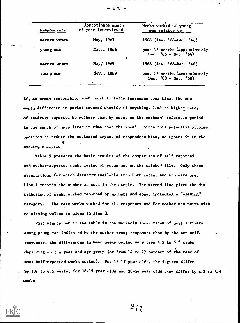
- 178 -

Approximate month Weeks worked a youngRespondents ofjear interviewed wen relates to

mature women May, 1967

young men Nov., 1966

mature women May 1969

young men Nov.,-1969

1966 (Jan. '66-Dec. '66)

past 12 months (approximatelyDec. '65 - Nov. '66)

1968 (Jan. '68-Dec. '68)

past 12 months (approximatelyDec. '68 - Nov. '69)

If, as seems reasonable, youth work activity increases over time, the one-

month difference in period covered should,- if anything, lead to higher rates

of activity reported by mothers than by sons, as the mothers' reference period

is one month or more later in time than the sons'. Since this potential problem

operates to reduce the estimated impact of respondent bias, we ignore it in the

9ensuing analysis.

Table 5 presents the basic results of the comparison of self-reported

and mother-reported weeks worked of young men on the matches file. Only those

observations for which data ucre available from both mother and son were used

Line 1 records the number of sons in the sample. The second line gives the dis-

tribution of weeks worked reported by mothers and sons, including a "missing"

category. The mean weeks worked for all responses and for mother-son pairs with

no missing values is given in line 3.

What stands out in the table is the markedly lower rates of work activity

among young men indicated by the mother proxy-responses than by the son self-

responses; the differences in mean weeks worked vary from 4.2 to 6.5 weeks

depending on the year and age group (or from 14 to 27 percent of the mean-of

sons self-reported weeks worked). For 16-37 year olds, the figures differ

by 5.6 to 6.5 weeks, for 18-19 year olds and 20-24 year olds they differ by A.2 to 6.4

weeks.

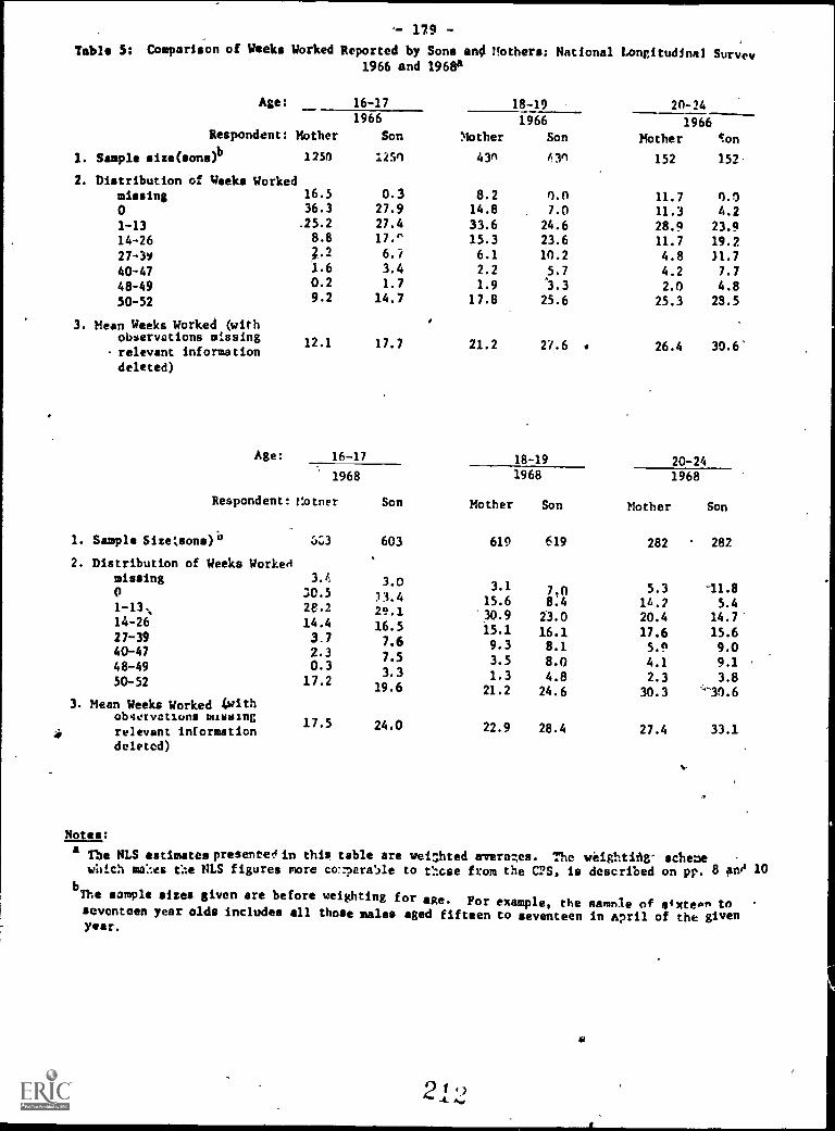
- 179 -

Table 5: Comparison of Weeks Worked Reported by Sons and Mothers: National Longitudinal Survey1966 and 19684

Age: 16-17 18-19 20-241966

Respondent: Mother Son *other

1966

Son1966

Mother !on

1. Sample size(sons)b 1250 lev, 43n t3n 152 152°

2. Distribution of Weeks Workedmissing 16.5 0.3 8.2 rhn 11.7 0.10 36.3 27.9 14.8 7.0 11.3 4.21-13 .25.2 27.4 33.6 24.6 28.9 23.914-26 8.8 17.n 15.3 23.6 11.7 19.227-3Y 3,.2 6./ 6.1 10.2 4.8 11.7

40-47 1.6 3.4 2.2 5.7 4.2 7.7

48-49 0.2 1.7 1.9 *3.3 2.0 4.8

50-52 9.2 14.7 17.8 25.6 25.3 28.5

3. Mean Weeks Worked (withobservations missing

12.1relevant informationdeleted)

17.7 21.2 27.6 26.4 30.6'

Age: 16-17 18-19 20-241968 1968 1968

Respondent: Motner Son Mother Son Mother Son

1. Sample Sizetsons)b 3;3 603 619 619 282 282

2. Distribution of Weeks Worker!missing 3.4 3.0 3.1 7.0 5.3 -11.80 30.5 33.4 15.6 8.4 11..? 5.41-13; 2e.2 29.1 30.9 23.0 20.4 14.714-26 14.4 16.5 15.1 16.1 17.6 15.627-39 3.7 7.6 9.3 8.1 5.9 9.040-47 2.3 7.5 3.5 8.0 4.1 9.148-49 0.3

3.3 1.3 4.8 2.3 3.850-52 17.2 19.6 21.2 24.6 30.3 30.63. Mean Weeks Worked With

obsylvsttuns missing17.5

relevant informationdeleted)

24.0 22.9 28.4 27.4 33.1

Notes:a

The NLS estimates presentee in this table are weishted ameranes. The weightlAg- schemewhich mo::es Cae NLS figures more co::pera5le to t:lose from the CPS, is described on pp. 8 any' 10

b7be sample sizes given are before weighting for ime. For example, the aamnle of extegm toseventeen year olds includes all those males aged fifteen to seventeen in April of the givenYear.

- 180 -

To what extent can the differences in weeks worked between mothers

and sons explain the differences in weeks worked between the NLS and CPS?

The following table presents the data from tables 4 and 5 desinned to answer

this question:

Comparison of Differences in Mean Weeks Worked asReported by the NLS and the CPS and by the NLS Mother-Son Matched File

16-17 year olds

(1)

Difference in

Mean Weeks Worked(NLS-CPS)

(2)

Difference inMean Weeks Worked

(Sons-mothers)

1966 4.1 5.6

18-19 year olds.

1966 4.8 6.41968 4.8 5.5average 4.8 6.0

20-24 year olds1966 1.1 4.21968 4.4 5.7average 2.8 5.0

According to these calculations, the difference in mother-dOn renorting could

easily explain the divergence between weeks worked reported in the NLS and in the

CPS and indeed tends to "overexplain" the differences. The anomolous over-

explanation could be rationalized by the fact that the mother-son differences in

Table 5 relate only to those males living at home, while the CPS-NLS differences in

Table 1 relate to all males. By the respondent bias hypothesis, differences

between the CPS and NLS arise when a proxy reports a young male's status

on the CPS and the individual reports his status on the NLS. For males not

living in their paren=s' home, we would expect smaller differences in rates

of activity between the surveys than are found for young men living at home.

One would expect that overexplanation would be more prevalent for older

males in the sample since they are less likely to live at home. Indeed, our

21

- 181 -

results show that for 20-24 year old males, roughly half of whom reside

outside their parents' home, the averexplanation is substantially larger

than for the younger males.

This argument suggests that we tabulate weeks worked for 20-24 year old males

who are unmarried heads of households and for those who are not heads oc

households and use the resultant figures to reestimate the effect of respon-

dent bias on the CPS-NLS difference. The former group will presumably give

self-responses in bo'h the CPS and NLS. The latter group will tend to have

the mother as proxy-respondent for the CPS-. In the tabulation below

NLS observations have been weighted (using the weighting procedure described on pages

C and 10), so that NLS interviewee ages are comparable to those in tho CPS. Powever,

the Census weeks worked figures relate to the preceding oalendar year (January

1968-December 1968) while the NLS figures relate to the twelve months prior to

interview (arproxf.rzzely December 1967 November 1968). Thus, there is one month dif-

difference in the time span to which the question pertains. Resolution of this probler

has been ignored in tabulation below:

Mean Weeks Worked from Mean Weeks Worked in DifferenceDec. 67 - Nov. 68; 1968 1968; March 1969 CPS in meanNLS 20-24 year old males 20-24.year old males Weeks Worked

Unmarried Heads 41.1 37.3 3.8

Not Heads 33.9 29.8 5.1

As expected, the differenct for unmarried heads is much smaller than

that for young men who are not heads.

Matrix of Responses

Analysis of the differences in responses between mothers and sons is

pursued further in Table 6, which cross-classifies the weeks worked,by the

21,1

- 182 -

son as reported by the mother with the son's weeks worked as reported by the

son. Each element an the matrix gives the percentage of mother-son pairs

reporting a given pair of weeks-worked values. If there were perfect agreement

between mothers And sons, all of the elements of the matrix would fall

along the main diagonal and would equal 100. (If there were no relation

between the weeks worked reported by mothers and sons, all

columns would be identical.) While there is

a definite concentration at or near the diagonals, a very large proportion

of the sample lie off the diagonal: only 63 percent of mothers whose

sons self-report working 0 weeks last year also report their sons as

working 0 weeks; only 41 5 percent of mothers whose sons report themselves

as working 52 weeks report their sons in that category, and so forth.

The divergences provide evidence of potentially large response bias

and measurement error in the weeks worked data, which supports the respondent

bias hypothesis. In addition, they suggest the value of a detailed analysis

of why some mother-son pairs are in agreement and others are not, A question

which we address to some extent in this section.

Employment Activity of Heads vs. Others

If respondent bias is the major cause of the differences in the labor force

activity rates of young males implied by the NLS and CPS, one would expect only

negligible survey differences for young males who are themselves unmarried heads

of households. The activity of these persons in the CPS is more likely to be

reported by the individual hiroself than by others, raking the results from the CPS

more likely to be consistent with those from the NLS.

To loot this inplication of the respondent bias hypothesis, the rates

of labor force activity of 20-24 year old males who are unmarried

heads of households and those who are not heads of households were

tabulated for 1969 with the NLS and CPS tapes. The results of the

calculations, shown in Table 7, yield a striking conclusion: for 20-24

215

g

Tehle 6: Comparison of Weeks Worked Reported

by Mothers and their Sons; 1966 NLS Data for Males Aged 16-24a

Percent of Mothers Reporting Weeks Worked

Weeks WorkedNumber of Sons

0 1-13 14-26 27-39 40-47 48-49 50-52 Missing TotalReporting

0

1-13

14-26

27-39

47

48 9

50- 2

Total

Missing

327

405

295

121

67

36/I

)

287

3 /

63."

30.4

16.3

/19.0

14.9

2.3

13.2

29.2

33.3

ihn

44.5

30.3

28.1

28.4.

13.9

16.4

27.3

66.7

7.8

8.4

17.3

17.4

14.0

13.9

11.5

10.6

--

.3

1.0

5.4

8.3

7.5

5.6

4.7

3.2

__

.1

--

2.4

3.3

9.0

5.6

:i.5

1.9

__

.3

--

.3

--

1.5

8.3

2.1

.8

__

.9

3.5

7.5

12.4

13.4

41.7

41.5

12.8

__

71.4

16.3

12.5

11.6

10.4

8.3

7.7

14.2

__

1n0."

111.n

1n0.0

100.0

1nn.n

inn.n

100.0

100.0

100.0

allote:As of April 1, 1966.

216217

- 184 -yeerold -unmarried heats of houscLolds there are no effective differences

in the ratio of employment to population or in the rate of labor force

pirticipation, whereas for comparable individuals who are not heads

there are sizeable differences. It appears that the bulk of the differentials

reported earlier is attributable to those whose status is self-reported

in the NLS but likely to be reported by the mother in the CPS.

In sum, there appears to be considerable support in the data for

the hypothesis that much of the NLS-CPS difference shown in section I

is attributable to respondent bias.

Differences in Samples and Methods

Since detailed information on persons designated to be included

in the NLS or in the CPS who were not represented is missing, it is difficult

to assess accurately the importance of sample differences in explaining the

observed differences in the employment experience-of young men. However, an

examination of the NLS-arid-CPS sampling procedures and the characteristics

----Of-their samples yields some insights into the possible magnitude of

sample survey bias.

We examine first the sampling procedures. One major difference between

the CPS and NLS cethods is that the former uses a one stage screening procedure

to obtain households for surveying, whereas the latter used a two stage procedure.

During the first stage of the NLS process, each of the four NLS samples young

men aged 14-24, young women aged 14-24, women aged 30-44, and men aged 45-59)

was designated to represent the civilian noninstitutional population of the

flj

185 -

Table 7: Comparison of Labor Force Batas by

Vousehold Status of Men Aged 20-24a

National Current Difference bete:eau

Longitudinal Population NLS Fall 68 and

Survey Survey CPS March 69

Fall 1968 March 1969

Unverried Heads

Employment/Population 82.7 83.0 -0.3

Labor Force Participation 83.9 84.9 -1.0

Onemployment(UNE) 3.2. 4.3 -1.1

Out of Labor Force 9.7 9.3 0.4

Major Activity is Being

in School

Not Meads

Employeent/Population 66.1 61.0 5.1

Labor Force Participation 68.3 63.0 5.3

Unemployment 4.7 5.5 -0.8

Out of Labor Force 22.1 26.2 -4.1

Major Activity isBeing in School

NntP:O Although the NLS observations Were weighted in accordance with age to facilitate com-

parability between the CPS and the NLSHestlestes (see mensal and 10),..thore Is still

difference between the two sets of figures.. loth sets of data refer to the survey week

The NLS however, takes place in November while the CPS is administered in ''arch. Thus,

there is approximately a four sant(' difference in the period referred to by the /ALS

and the CPS under analysis. The figures in the table were based on weighted

counts with the CPS March 1969m1crodataand NLS microdata.

21 j

- 186 -

United States. An initial group of 42,000 households from the primary sampling

units of the Census was selected by the NLS; a sample of this size was

drawn so that no age-sex-color group would be underrepresented. The 42,000

households were screened by interviews conducted in March and April of

1966, and adequate numbers of-each age-sex-color group were identified for

each of the four NLS samples.

In the fall of 1966, however, a second stage of screening was under-

taken to insure that during the months since April-the sample size for

young men had not become inadequate due to the mobility of male youths.

From these two screenings, 5,713 young men were designated to be interviewed;

of these 5,225 were actually interviewed, giving a non-interview rate oflu

8.6 percent. By contrast the non-interview rate on the CPS is considerably

lower, ranging from 4.1 to 4.4 percent annually in the 1974-1976 period.11

If the employment to population ratio for noninterviewees (thoie

designated to be interviewed who were not) in_the NIS- is less than for

-Interviewees12, and it the employment to population ratio for young males

in noninterviewee CPS families is less than for young men in the interviewee

families by the same amount, the differential noninterviewee rates in the

NLS and the CPS that were observed would cause the estimated NLS employment

SD population ratio to be higher than the estimated CPS ratio;

this would explain part of the difference in employment to population ratios

between the NLS and CPS. If, because

the CPS is based on proxy as opposed to self responses, the employment

to population ratio for young males in noninterviewee CPS families is

closer to the rate in interviewee families than the NLS non-

interviewee rate is to the NLS interviewee rate, then the higher NLS

noninterviewee rate might account for an even larger proportion of the

- 187 -

NLS -CPS young male employment to population ratio differential. In the absence

of information on the employment of noninterviewees, only the crudest

estimates of the magnitude of the effects can be made.

The calculations that can be made do, however, indicate that noninterviewee

bias most likely cannot explain a major fraction of the observed differences

in the NLS and CPS employment to population ratios for young men. Under

the totally unrealistic assumption that absolutely none of the NLS non-

interviewees worked and the assumption that young men in noninterviewee

CPS families have the same employment to population ratio as do those in interviewee

CPS families, there are still substantial differences in the NLS and CPS

young male employment to population ratios to be explained: a 7.1 percentage

point differential for 16-17 year olds in 1966 and a 3.8 percentage point

differential for 18-19 year olds in the same year. Under the seemingly more

realistic assumption that tUe NLS noninterviewees worked only half as much

as the NLS interviewees, the comparable differentials are 9.1 and 6.6

percentage points. Thus noninterviewee bias could only account for a part of the

11.2 and 9.3 percentage point differentials for 16-17 and 18-19 year old males

in 1966 shown in table 1.

In the NLS72, 21,350 of 23,451 students responded to the first follow-

up survey, giving a noninterview rate of 9.0 percent, which is comparable

to the NI,S ratePAs argued above in discussing sample bias with the NLS,

this noninterview rate could also explain some, but Certainly not all of the

differences between the surveys.

An alternative method for assessing important sample differences is to

compare the non-work characteristics of the samples. The NLS two-stage

screening process described above was specifically designed to compensate

for the high mobility of young men. It seems that young men who passed

through this double screen would be more stable than those

selected through a single screening process (such as that found in the CPS).

-f the NLS sample does have a larger fraction of young persons with stable

2'1 1

- 188 -

characteristics, then we would expect some of the estimated differences in

employment to population ratios to be attributable to characteristics

of the sample respondents.

Information on the household status of individuals in the NLS and CPS

suggests that the surveys' samples include similar fractions of high-

propensity-to-work individuals. In the CPS 46 percent of 20-24 year old men

are heads of households; in the NLS 48 percent of the comparable group are

heads, a negligible 2 percentage point difference. If the CPS heads-others

difference in employment to population ratios giNeen in Table 7

is assumed valid, the 2 percentage point difference in the relative

importance of heads and others implies a .57 (28.3 x .02) point

BLS -CPS differential in the overall ratios. If the NLS heads-others__difference in employment to population ratios given in Table 7 is used,

the 2 percentage point difference translates into a .47 ('R73.6 x .'12)

point differential. By contrast, the difference in the employment to

population ratio for others in the table predicts about a 3.0 point

differential nu utter which estimate of tbe atio of oners to others plus heads

is used. Thus, sample differences appear to account for a relatively tiny

fraction of the NLS-CPS difference in employment to population ratios.

There are two other potentially important differences in the way the NLS

and CPS surveys are carried out. These involve the rotation pattern and the

method of interview.

Under the CPS, a respondent will appear in a survey for four months, be

dropped for eight months, interviewed for another four months, and then be

dropped permanently. During any month, one-eighth of the sample will be inter-

wti

- 189

viewed for the first time, one-eighth for the second time, and so on. Under

the NLS, the same young male sample group is interviewed once each year for

the duration of the survey.

The other difference concerns interview technique. The CPS primarily

uses telephone interviews to collect its data. The NLS data on young persons

(fo. the time periods discussed in this study) were gathered using face to

face interviews nearly exclusively.

It is likely that these two differences in survey methods will lead

to a difference in the employment to population ratios observed between the

NLS and CPS. This contention is supported by analyses of the National Crime

Survey (NCS) currently being conducted by R. Lerman and H. Woltman.14

The NCS surveys 14,000 households each month. A total of 72 .non

households are selected for interview over a three year period. They are

interviewed one month, left out of the sample for five months, interviewed twin,

left out for another five months, and so on for the three year period.

There are two other important characteristics of the NCS. First, more

than 90 percent of the survey responses are self-reported, which makes the NCS

similar to the NLS and NLS731. Second, about 80 percent of the NCS interviews

are personal interviews, in contrast to the CPS 1.n which the majority of inter-

views are done by telephone. Therefore, the most important differences between

the NCS and CPS are that the NCS is self-response as opposed to proxy-reSponse.

Ss based primarily on personal rather than telephone interviews, and uses,a

a rotation pattern under which sample members are never surveyed two months

in a row. In all- these respects, the NCS methodology is similar to the

NLS methodology.

223

- tyu -

In analyzing the NCS data, Lerman looks separately at young persons

broken down by age, race, and SPX. His age groups are 16-17 year olds,

18,19 year olds, 20-21 year olds, and 22-24 year olds. Lerman's tabulations

reveal that the employment to population ratios among young males (especially

nonwhites) based on the NCS are significantly higher than those derived

with the CPS. However, the Lerman employment to population rates for young

fetales show substantially smaller differences than those observed for males.

In fact, for Lerman's largest group of females (white females aged 22-24), the CPS

employment to population ratio is higher than it is with the NCS. These findings

suggest somewhat different patterns of response bias for women than for men.

Woltman examined samples of people who were coming into the NCS or

CPS for the first time. He limited his sample to in-coming survey members

in an effort to control for potential differences in rates caused by differences

in tare surveys' rotations and in the extent to which the surveys rely unon telephone

and personal interviews. This could be accomplished since in both surveys

the first interview conducted with a sample member is done in person.

Woltman did his calculations for two age groups (16-19 year olds and 20-24

year olds) but did not cross-classify individuals by age and either race or sex.

He found virtually identical employment to population ratios for each age

group for ngw members of the NCS and new members of the'CPS. Part of

Woltman's result can be explained by the fact that he, unlike Lerman and

um, did not focus just on young molem, inc',m accerdino to Lernan'a an/Or:yes,

there appear to be much smaller and even differently signed differentials

for young females. Nevertheless, it is unlikely that this fact can fully

explain the Woltman findings. Thic leads us to believe that the nature of

a survey', rotation pattern and its reliance on personal versus telephone

interviews affects the estimates that it obtains of the employment to

population ratios for young males. The numbers derived by Lerman and Waltman

do not appear to refute our belief that ete 1ei. factor causing differences

2A.,

- 191 -

in the employment to population ratios among young males estimates with various

surveys is whether or not the surveys relied on self-responses as opposed to

proxy-responses. They do, however, underscore the need for more data collection

and analysis concerning the issue at hand.

IV. Future Research

The finding that much of the cross-survey differences in reported male youth

work activity depends on the way in which these surveys are conducted raises many

important questions. What factors explain the differences in the responses that

young ma/es give concerning their work activity and the responses that proxies

give about the work activity of these youths? Whit additional research is needed

to confirm or disconfirm the respondent bias hypothesis? How can we discover

whether young persons or their parents are providing more accurate :information on

actual activity? What should be done to improve our data base?

Why responses differ

There are two basic reasons for expecting differences between self-reported

work activity and proxy-reported work activity: first, differences in knowledge

of the facts; second, differences in the accuracy of reporting a given set of

facts, possibly for reasons of.self-esteem.

NLS matched mother-son file can be used to analyze the factors which

affect the mother's report of son's weeks worked. To do this, we

ran regressions of the son's weeks worked as reported by his

mother in 1966 on the seemingly relevent and available characteristics

of the son, his mother, and their household. The estimated coefficients for 1966

of the most complete equation fit and the mean and standard deviation-of each of

the model's variables are given in Table 8. These figures indicate several .InterestIng

results.

- 192 -

Table 8: Factors Affecting Number of 'Weeks Worked for Sonas Reported by Mother, 1966 NLS Data for Males Aged 16-24a

(N 474)

0

Independent Variables:

Dependent Variable:Son's weeks worked in 1966 reported by mother

Mean Coefficient'(S.D.) (Standard error)

Reported by Sonson's weeks worked 25.10 .576

(18.73) (.040)

son's enrollment status .723 -2.634(in school 1) (.44e) (1.754)

.,

son's_usual hours worked per week 28:52 .076(17.49) 4.043)

son's hourly wage in 1.370 -.541current or last job (.853) (.946)

,

son's agea

17.41 .207(1.680) (.461)

son's race

(nonwhite = 1)

Reported by Mother

.418

( .494)

mother's weeks workd 24.22

(23.33)

mother's usual hours worked 22.16per week (19.79)

other's education 10.12

(2.737)

number in household 5.97

(2.517)

1966 family income 8.659(in thousands of dollars) (6.008)

R2

aAs of April 1, 1966.bThe mean (S.D.) of the dependent variable is 19.61 (18..75).

cA constant was included' in the regression estimated.

-2.827(1.587)

.008

(.052)

.031

(.060)

.096

(.285)

4-.367

(.300)

.000

(.000)

2 2E;

.393

s

- 193 -

First, the coefficient relating the young males' weeks worked reported

by mothers to the weeks worked reported by sons is markedly less than 1. While

increases in sons' reported weeks worked raise mothers' reported weeks worked, the

effect is just .6 weeks for every 1 week increase reported by sons. Thus, the

_absolute difference in weeks worked grows with weeks worked.

Second, the race of the family affects the number of weeks worked the

mother reports for her son. The mother tends to report a much smaller number

of weeks worked for the son if the family is nonwhite. The minus 2.8 weeks

etle-0 of race is a 15% difference in weeks worked at the mean of the sample.

Third, son's enrollment status has a large negative (though insignificant)

effect on his mother's proxy-response: if the son is enrolled in school the

mother's reported response will be much smaller than if he is not enrolled.

Fourth, the mean of the son's reported usual weekly hours worked is

large (28.5), indicating that our typical young male labor force member with

a job is working more than just a couple of hours a day; the estimated coeffi=

cient of this variable is positive (but insignficant).

In contrast, family income has no partial relationship to the number of weeks

worked reported by a mother for her son. Neither do

mother's educational background, her current labor market status, and the

size of her household seem to be partially related to her nroxy-response.

Overall, the principal finding is that the divergence between self- and

proxy-responses appears to be larger for youths whose attachment to the labor

force is weaker while, except for race, the demographic characteristics of

individuals does not greatly affect the divergence.

20-,

- 194 -

Improving the data base

The cross-survey differences in rates of young male work activity reported in

this study suggest that the magnitude, let alone nature, of youth jobieSsness is

known with less certainty than is currently believed. If the estimates from

relevant surveys other than the CPS are correct, more young males hold jobs than is

reported in government statistics, and some aspects of the youth joblessness problem

are exaggerated. If the CPS data are correct, analyses of youth joblessness based

on the longitudinal surveys could be seriously flawed. Because valid scientific

analysis and policy prescription require data which accurately deal with the

issue at hand, improving our information about what youth in our society are

actually doing should be a top priority for those concerned with the youth

unemployment problem. In this section we offer some suggestions about

ways in which improvementi might be made.

First, it is important to obtain better estimates of the extent to which

respo dent bias affects estimates of the work activity of the younz. While useful,

our a alyses of the matched mother-son WLS sample suffer from various problems,

as d scribed earlier, and should be corroborated (or disproved) with actual CPS-

deri ed data. We recommend that the Bureau of the Census survey youths whose

falai ies are included in the CPS and compare the youths' self-reportedi

work activity to that reported by proxy respondents. If such a study sub-

stantiates our findings, it will be necessary to devise new methods of ob-

taining information about youth work activities, either through new

questions designed to elicit more accurate information about the employment

of the young, or through CPS

supplements answered by the young (and other relevant individuals) themselves.

Whatever approach is taken, the Bureau of the Census should undertake a

major analysis of the responsent bias problem as it relates to youth.

Second, a substantial effort should be devoted to determining whether self-

2:21j

- 195 -

reported or proxy-reported youth work activity rates are more accurate. This can

be done by requesting information on the putative employer of the youth and

verifying the reported job with the employer. Such an analysis would go far

beyond what we have been able to do in this study and significantly improve our

knowledge of basic labor force activity. Tnus, we recommend that the Bureau of

the Census requeit)names of employers from young persons, particularly those

reporting employment when a proxy-respondent does not report the youth with a

job and attempt to verify the position of the youth.

Third, we believe that serious attention should be given to the development

of entirely new questions and concepts for analysis of the activity of youth

(and others who are not typically heads of households). The current set of CPS

questions were developed i large measure to determine the employment status of

adult heads of households and are not well-suited toward understanding the

economic problems of youth. Current cgs questions provide very little information

on the activities of jobless persons w%o are cut of le.-.031, essentially defining their

status negatively: they are not employed and not in school. What is needed is a

set of questions evaluating what these people do with their time, possibly

oriented in part toward whether their current activity is likely to increase or

decrease their chances for employient in ensuing periods. We recommend that the

Bureau of the Census ex7eriment with new sets of cjlestions to find out what persons are

doing who are out of school and not em1 yed. Such questions should sack to determine the

way, in which time is allocated by the young (and others in this state) between

unpaid work in the home, part-time school,"loafing,",and so forth. It is difficult

to understand the problems faced.by the not-employed, not-enrolled young

person when we have so little information about what they are doing. What

is needed, we wish to stress, is not additional questions designed to

differentiate discouraged from other young workers on the basis of possible

work plans, but rather objective information on what people actually do

when they are not employed and not in school.

j

- 196 -

Basically, ue believe that to adequately deal with new economic

problems like youth joblessness we need new data. The payoff from obtaining

more inftrwation about what teenagers are really doing and why they are

really doing it will most likely be extremely high.

2;4j

,...=yanaMAY111/.111111

- 197 -

Footnotes

1 The divergence between youth labor market conditions as depicted in the NLS

and the CPS was noted in the important study by Borus, Mott and Nestel. An

earlier but much less complete discussion of the phenomenon is found in Parnes.

2For an in -depth discussion of the CPS see Hanson.

3This information was gathered inia telephone conversation with Paul Flaim

:of the Bureau of Labor Statistics.

U.S. Bureau of Labor Statistics, BLS Handbook of Methods, Bulletin 1910.

For an in -depth discussion of the NLS see Ohio State University.

6 Another difference, pointed out by Borus et al., exists between the 1966 CPS

and NLS. The NLS adopted changes in the definitions of employment and un-

employment in 1966 which were not adopted by the CPS until 1967.

7 For a discussion of the NLS72 survey see U.S. Department of Health, Education

and Welfare.

8This information was gathered in a telephone conversation with Gilbert Nestel

of Ohio State University.

9 Another possible source of discrepancy exists because mothers are interviewed

about their son's activity from four to six months after the end of the reference

period. Sons, however, are interviewed immediately after the reference

period. The direction of the bias introduced by this discrepancy is unclear.

10These data were calculated with NLS tapes.

11 See Hanson, p. 23. for a discussion.

12See Borus et al., p. 18 for more information.

13These figures were derived from data in Levinsohn et al.

14 :his discussion is based on telephone conversations with Robert Lerman and

Henry Holtman and on a memorandum by Holtman.

231

- 198 -

Bibliography

Borus, Michael-E., Frank L. Mott, and Gilbert Nestel. "Counting Youth:

A Comparison of Youth Labor Force Statistics in the Current Population

Survey and the National Longitudinal Surveys." Conference Report on

Youth Unemployment: Its Measurement and Meaning. U.S. Department of

Labor; Office of the Assistant Secretary for Policy, Evaluation and

Research; and the Employment and Training Administration, 1Q78, pp. 15-34.

Hanson, Robert H. The Current Population Survey: Design and Methodology.

U.S. Department of the Census. Technical Paper #40. Washington, D.C., 1978.

Levinsohn, Jay R. et al. National Longitudinal Study Base Year, First Second

and Third Followup Data File Users Manual, Washington, D.C., National

Center, for Education Statistics, April, 1978.

Meyer, Robert H. and David A. Wise. "High School Preparation and Early

Labor Force Experience," pi).

Ohio State University, College of Administrative Science, Center for Human

Resources Research. The National Longitudinal Surveys Handbook.

November, 1977.

Parnes, Herbert S., et al. Career Thresholds. Manpower Reserach Monograoh

Vol. I, No. 16, Appendix E. Washington, D.C.: GPO, 1970.

U.S. Bureau of the Census. Current Population Reports. Series P-20.

"School Enrollment," October 1966-October 1971. Washington, D.C.:

Glv, 1967-1972.

U.S. Bureau of the Census. "National Longitudinal Surveys, Survey of Work

Experience of Males 14-24." Forms LGT-201, 211, 221, 231, 241, 251.

Washington, D.C.: GPO. 1966-1971.

U.S. Bureau of Labor Statistics. BLS Handbook of Methods, Bulletin 1910.

Washington, D.C. U.S. GPO, 1976.

711111=1=11i

- 199 -

U.S. Bureau of Labor Statistics. Employment and Earninn.s. December 1966-1971.

Washington, D.C.: GPO, 1966-1971.

U.S. Bureau of Labor Statistics. Employment of High School nraduates and

Dropouts: October 1972. Special Labor Force Report 155. Washington

D.C.: GPO, 1972.

U.S. Bureau of Labor Statistics. Work Experience of the Population. Special

Labor Force Reports 91, 107, 115, 127, 141, 162. Washington, D.C.:

GPO, 1966-1971.

U.S. Department of Health, Education, and Welfare, Office of Education.

National Longitudinal Study of the High School Class of 1972. Final Report,

Washington, D.C.: GPO, June 1073.

Woltman, Henry. "Memorandum for Tom Walsh, Comparison of Youth Employment

Estimates from the CPS and Of., NCS." Washington, D.C.: U.S. Bureau

of the Census, StaListical Methods Division. ?arch 30, 1979.

- 200 -Time Series Changes in.Youth Joblessness

Michael L. WachterChoongsoo Kim

Introduction

Youth unemployment has increased over the past two decades

in absolute terms relative to prime-age male unemployment. More

recently the unemployment rates for most youth groups have begun

to level off and move in parallel with prime-age male unemployment

rates. This is especially true for white males.

Explaining these developments in a statistical sense presents

major' problems. First, the underlying developments appear to be

due to economic-demographic swings of intermediate-run duration.

Hence, the length of the time series data base is woefully short.

Second, many of the most interesting and potentially important

explanatory variables, such as government policy variables, have

major measurement problems.

Our view stresses the role of "cohort overcrowding" which

results from an imbalance between younger and older workers. The

model is based on two central assumptions. Thettirst is that

younger and older workers are imperfect substitutes for each other.

The main difference between them reflects their relative amounts

of specific training. Given the "putty-clay" nature of physical

and human capital and the transient nature of the cohort bulge,

the economy's adjustment process may be slow and incomplete. In

the short-run,elasticities of substitution are relatively low so

that large relative wage adjustments can occur.

The second is that aspiration levels or desired standards of

living are formed-when the younger workers are living with their

parents. This is an endogenous taste or habit formation model

234

- 201 -

where past living standards influence current desired standards.

In addition, young families are assumed to treat their desired

standard of living as a necessity. Hence, in the event of lower

wage levels, families will increase the number of workers and/or

hours worked. The increase in labor force participation rates of

the young workers can thus be traced directly to the population

demographics. In addition, the induced change in participation

rates serves to aggravate the existing oversupply problem of

younger workers, further driving down relative wages.

As relative wages fall for the oversized cohort, institutional

constraints, such as government transfer programs, minimum wage

levels, etc., become relevant and cause an increase in unemployment

rates as well as or instead of the increase in participation rates.

If the unemployment effects are large enough, employment may

actually decline.

Although some previous studies have attempted to isolate the

effects of government programs, for example minimum wage legis-

lation and manpower programs, data problems make this task almost

impossible. Besides the data problems, there are important con-

ceptual problems as well. The government's social welfare pack-

age, whether intentional or not, is an integrated program. The

parameters of the various programs tend to change together

reflecting common political pressures and the need to complement

each other An example is the parallel increase in minimum wage

coverage and government transfer payments (in relative terms)

- 202 -

during the late 1960's. Since almost all studies concentrate

on one government program at a time, they miss these crucial

interrelationships and, hence, attribute too much to the single

program under study. We also find that "relative wages" have

some explanatory power, but cannot separate minimum wage prom

government transfer effects. In addition, attempts to include

direct job creation effects ilivariably yield the wrong sign.

Our empirical work focuses on two approaches. The first

attempts to measure unemployment in different ways by altering

the numerator and/or the denominator of the unemployment rate

term. For example, we argue that the variable which is closest

to the traditional measure of unemployment would give school at-

tendence equal status with employment. Hence, the numerator would

exclude those who were unemployed and whose primary activity was

school and the denominator would include all of those who were in

actooI. The second approach focuses on disaggregating_youth acti-

vities into four categories - unemployment, empldyment, school,

an! a residual (all as a ratio to the population) for each of the

age-sex-race groups. Equations are then estimated using the same

explanatory variables and adding the constraint that the four ratios

sum to unity.

Since black males pose a particular problem, we concentrate

somewhat on the deterioration in the unemployment and employment

ratios of this group relative to other youth groups. Why should

this group suffer a deterioration in labor market position rela-

.2 to other youth groups, including black females?

236

- 203

The paper is organized in the following manner: Section I

presents the basic model of cohort overcrowding. Section II

provides the basic age-sex-race youth unemployment equation.

Section III analyzes alternative measures of youth unemployment.

Section IV provides the justification and estimates for our

four activity equation system. Section V analyzes the puzzle of

the deteriorating labor market position of black males, age

16-24.

- 204 -

I. The Basic Model of Cohort Overcrowding

A. The Underlying Workings of the Model

In some earlier work by the authors and others, the youth

unemployment problem was explained in the context of c. broader

economic-demographic model.' The basis of the model is a "cohort

overcrowding" effect which results from an imbalance between

younger and older workers. We shall utilize this approach to

explore the developments in youth unemployment over the past fif-

teen years. It was during this period that the baby boom cohort

was passing through the 16-24 age category.

This type of model can generate cyclical swings of inter-

mediate length in unemployment rates. A fertility increase in

generation t causes a large cohort of entry level workers in t + 1.

In the short-run, elasticities of substitution are relatively

low so that large relative wage adjustments occur. This deterio-

ration in the income potential of young people causes a decline

in fertility and family formation rates and an increase in the

labor force participation rates of secondary workers. The

increase in young workers' labor force participation rates can

thus be traced directly to the population demographics. In

addition, the induced change in participation rates serves to

aggravate the existing oversupply problem of younger workers. 2

As relative wages fall for the oversized cohort, institutional

constraints become relevant and cause an increase in unemployment

rates as well as or instead of the increase in participation rates.

2

- 205 -

If the unemployment effects are large enough, employment may

actually decline.

The institutional constraints which cause unemployment

can exist on both the demand and supply side of the market. For

example, since minirm wage levels are informally indexed on

average economy wide wages, a decline in the relative wage for

youth may cause the_ market clearing wage to fall below the mini-

mum wage. Youth, of course, form a heterogeneous skill group

with a wage distribution rather than a single wage. The decline

of the relative wage, in this case, causes an adverse shift in

the distribution of Sages. That is, the probability of any

outh having a skill and associated wage level that falls below

the minimum wage is increased by the demographic overcrowding.

On the supply side, a different institutional factor is

operating but with a similar pyotential result. In both neo-

classical labor supply literature as well as institutional

literature, workers are viewed as having a reservation wage; when

market wages are below that reservation wage, individuals choose

not to work. The ne-)classical theory tends to specify a contin-

uous trade-off between hours of work and wage rates. It is only

at the corner of the indifference map that the wage rate is

sufficiently low so that individuals will offer zero hours of

work. The likelihood of a corner solution is increased by the

existence of public assistance and government transfers in general.

These programs have high implicit tax rates. Indeed, it is

generally acknowledged that the eligible poverty population

2')td j

- 206

for these programs face higher implicit marginal tax rates than

do the wealthiest individuals. The result of these programs is

to considerably flatten the budget constraint.3

The likelihood of a corner solution is also determined by

the mechanism through which individuals form their reservation

wage. Specifically, individuals' attitudes towards an acceptable

wage are determined by wages paid elsewhere in the economy. Of

particular importance in defining the indifference map, or "taste"

for work is the minimum income level dictated by the government

social welfare programs and minimum wage laws. These programs

signal what constitutes an acceptable minimum wage to the voting

public and policymakers. That is, government programs,clmost

certainly influence the shape of the indifference map as they

alter the budget constraint. A liberalization of benefits shifts

both the indifference map and the budget constraint toward the

corner solution of zero work. 4

It should be noted that the fluctuations in unemployment

discussed in this model, are solely related to changes in the

equilibrium rate of unemployment. Cyclical unemployment may be

positive or negative in the short-run. But the above demographic

cycle is an intermediate swing and averages out the peaks and

troughs of the short-run business cycle.

B. A Simple Expositional Model5

The major factors that we use in our empirical work can be

captured in a simple expositional model. The model is oriented

0

- 207 -

towards the specific empirical factors involved in the demographic

shift. To start, assume a production function that recognizes

two different categories of labor - older workers who have accumu-

lated specific training (LA) and younger workers who lack such

training (LB). For our purposes we can view LA as skilled workers

and LBas unskilled workers. In the long run, the production

function can be written as:

(1) Xs = fs (LAS, LBs' X),

where K is the capital stock, X is the level of output, and the

superscript s refers to supply. In the short-run, there appear to

be significant lags in achieving desired absolute and relative

levels of factor inputs. The lags may arise for a number of

reasons including adjustment and expectional factors. The lite-

rature on investment functions indicates that long lags are

especially relevant to the capital input. If the capital stock

is "putty-clay," the input coefficients are fixed as part of the

capital endowment. These coefficients may vary for different

vintages but, to the extent that they are empirically important,

they impart a difficulty in substituting against scarce factors

in the short run.

For our purposes, aggregate demand can be viewed as being

controlled by monetary (M) and fiscal (F) policies, subject to

unanticipated changes in demand frpm the private sector (Xo):

(2) Xd fd (M,F,X0).

The derived demand for labor is constrained by either the

211

- 208 -

level of the demand for or supply of output X and by relative

factor prices. For B workers, the relevant own wage is either

the minimum wage (MW) or a market wage, whichever is higher.

The labor supply for both LA and LB is a function of the

population in each cohort and the factors that determined the

labor force participation rates. For A workers, we assume that

the participation rate (rA) is constant in the short run. Abstr-

acting from influences such as school enrollment and fertility,

the main forces determining participation for B workers are the

market wage rates for these workers (WB),) the government transfer

payments for being unemployed (T91, the effective minimum wage

(MW), and some unspecified trend factors that capture changes in

life-style. That is,

(3) L As = LAs(rA, POP A) ,

and

(4) LBs = Lias (POPB, TREND, g {WB, Tg, MW)).

The relationship between WB and Tg determines the cost of

being unemployed. The level of governmental transfers depends

upon unemployment compensation and public assistance. The supply

of labor relevant to the production function, denoted Las, is

(5) Las = LBO - g (W Tg,

MW).

That is, we distinguish between an observed labor supply,

LFsl

and an effective labor supply, LBs, which is available for

eLtployment. The discrepancy, measured by the g function, is a type

cf structural unemployment.6

212

- 209 -

Equations (1) througrt (5) indicate a number of reasons for

unemployment. The most obvious is cyclical unemployment which

results from Xs

Xd

. In addition, unemployment will vary with

(a) the distribution of the labor force between A and B workers,

(b) the cost of being unemployed and minimum wage effectiveness,

and (c) the bottlenecks of either skilled workers or capital.

Over the longer run, when coefficients of production are more

flexible, bottlenecks gradually lose their importance as,a cause

of unemployment. On the other ?rand, traditional wage equations

indicate another source of unemployment. As bottlenecks loosen,

relative wages must adjust if the surplus of B workers is to be

absorbed. The evidence suggests, however, that the adjustment

is very imperfect. Minimum wages prevent employers from moving

down their demand curve for B workers and/or alter the reser-

vation wage of B workers. In addition, government transfer

programs help to maintain a high reservation wage (relative to

their market wage) for the unskilled workers. These latter

workers are in the labor force, but are not willing or able to

work at the market clearing wage.

2 '3

- 210 -

II. The educed Form Unemployment Equation

A. Basic Considerations

Estimating an unemployment function can be done in several

ways given the basic building blocks of labor supply and employ-

ment functions. For our purposes it is useful to start by

estimating a reduced form relative unemployment equation. In

section IV below, we shall estimate both unemployment and employ-

ment functions. In this case the unemploymen4- equations serve the

role of a labor supply equation. This approach is compatible with

the theory ouzlined above and the fact that prime-age male unemploy-

mezt is an independent variable. Specifically, it highlights our

view that youth unemployment is largely structural in nature and

dominated by fluctuations on the supply rather than demand side

of the market. For reasons associated with government policy

and the dynamics of the overcrowding model, supply side shifts

do not induce adjustments in labor demand.

A reduced form relative unemployment equation can be obtained

from equation (51 With the Additional as.umption that fluctu-

ations inB8'

are captured by a cyclical aggregate demand vari-

able. For most of our calculatiGns, we used the prime-age mal4'

unemployment rate.?

A large number of alternative proxies were attempted for

the government policy variables. None were particularly satis-

factory because of measurement errors; essentially most of the

data were simply not collected. Our various attempts at repre-

senting policy impact are described below. No single policy

- 211 -

variable provided the best fit among the 18 age-sex-race groups.

Rather than use different policy variables in each equation, we

adopted a compromise variable that performed as well as the othe s

but could be viewed as representing severaY effects. The unemploy-

ment rate equations for the various age-sex groups are estimated

in the general form:

(6) Ui = a0 + ai (Si) + a2 ln(Upm) + a3 1nZRPy)+a4

ln(W/MW) +a5(1n(AF/POP)) or TREND

where (Si) is a vector of seasonal dummies, RPy is the proportion

of the civilian population age 16 to 24 to the population age

16+, AF/POP is the military/population ratio (added to the male

equations), and TREND is a time trend (added to the female

equations).

The RPy variable represents the cohort overcrowding referred

to above. Several different specifications of the RPy variable

were tried, varying the treatment of the military, individuals

over 65 years of age and defining youth over the age span of 16

to 34. The results were largely unchanged. Given this inability

to differentiate mpirically, the choice of the RPy variable was

dictated by usage in earlier studies. It is important to note

that this cohort variable assumes that young workers are substi-

tutes for each other and define a distinct labor input. Needless

to say, 'ny age division of the labor market into two distinct

components 'has-to-be arbitrary. The difference between a 24 and

a 25 year old is not large. On the other hand, labor market

attachment, employment patterns, unemployment rates, etc. differ

215

- 212 -

considerably for a 20 year old compared with a 30 year old.

Some recent studies have used separate supply or cohort

variables (denoted RPyi) for each of the youth age-sex groups.

For example, the black male population age 18-19 as a percentage

of the population age 16+ would be used to explain unemployment of

that age-sex-race group. Our view is that this is too limiting

a view of the degree of substitution across inputs. Labor market

behavior over the past two decades shows more similarities than

differences across youth age-sex-race groups. Where the RPyi

variable has been successful, it was only capturing the worsening

unemployment position of black youth relative to white youth As

shall be discussed below, however, black youths are not doing

worse than comparable white. groups by all economic yardsticks.

Black school enrollment rates and relative wages, for example,

show significant relative improvement. This suggests that RPyi

will not provide a consistent answer to the changing white-black

differential.

B. The Government Policy Variable

Although a properly specified unemployment ezuation should

contain separate variables to represent transfer payments, direct

job creation, and minimum wages, data and conceptual problems

make this impossible. After considerable, but largely unsuccessful

experimentation with different proxies for the various programs,

the actual government variable utilized in the equations is a

"compromise variable" of the form W/MW where W is the average

0 4Af

- 213 -

hourly earnings of workers 16-24 years of age and MW is the mini-

mum 4 age.10

Measurement problems are complicated by the fact that the

social legislation programs including transfers, minim,_Am wages,

and direct job creation are not made independently of each other.

That is, policy innovations in one program are likely to be

reflected in others. Basically, political and social pressures

do not become concentrated in one area. Rather, as was clearly

the case during the 1960's and 1970's, the forces that can yield

changes in one policy area are also likely to cause similar

changes in other areas.

Most of the literature dealing with federal welfare initia-

tives investigates only one program at a time. There are studies

on minimum wages, public assistance, direct job creation, etc.,

but few of these studies attempt to integrate the direct labor

market impact of that single study into the overall package of

programs. The limited range of individual studies is easily

explainable given the data problems for each single study. The,

problem, however, in evaluating the overall effect of the various

government programs on unemployment is that the programs interact.

The sum of the impacts of the individual studies does not equal

11the overall effect of the variety of programs evaluated together.

The data problems are due to the fact that the major change

in the minimum wage is the change in coverage in 1967. Until the

1978 a, however, littl, other meaningful variation in that

variable is evident. Many of the increases in coverage did not

21

- 214 -

affect lcw wage workers and the staggered catch-up increase in

the minimum wage created a saw-tooth pattern in the data with,

if anything, a slightly declining trend of the MW relative to

W. That is, the time series minimum wage variable is largely a

spike in 1967. This, of course, is difficult enough to repre-

sent using time series data. Suppose, however, as is likely,

that firms adjusted with a lag to this sweeping change in coverage.

One possibility is an exponential declining distributed lag re-

sponse. Depending upon the speed of decay, this would move the

mean of the response outward in time, probably to 1968 or 1969.

Alternatively, firms may have responded very slowly at first.

This may have included low levels of compliance or incomplete

compliance in the year immediately after 1967. With a compliance

lag and an employment response lag conditional on compliance, the

distributed lag structure could resemble a parabola with a mean

lag into 1970 or beyond.

Given these possible time profiles for W /MW, and the diffi-

culty of isolating the best fit in the various equations, it is

possible for WNW to move in near precision with transfer, supply

side variables. Moreover, as mentioned above, this multicol-

linearity may be a conceptual as well as a data problem. To the

extent that individuals form their reservation wages as a function

MW and transfer payments are adjusted to conform to the same

uraerlying inflation And real income changes effects, the MW

construct may be a good approximation of the reservation wage.

Tr the extent that the minimum wage helps to determine the reser-

vation wags of low wage workers, the greater the difficulty in

differentiating supply and demand effects.12

C. Empirical Results for the Reduced _Poi; Unemployment Equation

Given a lack of agreement or data on the control variables,

especlally government policy variables, to be introduced into

the unemployment equation, it is useful to start with the simplest

equation. Shown in Table 1, this equation only includes RPy, Upm

and the seasonal dummies. As can be seen, the coefficients of

RPy are all positive and indicate higher elasticities for females

and blacks.

Since the "cohort overcrowding" effect operated like a

trend variable for half of the sample period, namely between 1958

and 1972, it is useful to see if RPy is simply picking up a trend

effect. Prior to 1958, RPy is either stable or declining and

after 1972 it remains largely unchanged. The question is whether

youth unemployment, after controlling for Upm, is best approxi-

mated by a TREND or a cohort overcrowding variable. Of the 18 age-

sex-race groups, the equation with RPy instead of a TREND yields

a higher R2 in 15 equations. his provides mild support for the

RPy variable. Given their collinearity, it is not possible to

distinguish between RPy and TREND to the desired extent. Beginning

in the late 1970's, however, these two variables diverge sharply.

The RPy variable tends to be strongest in female and white male

equations and weakest in black male equations. This pattern will

appear with consistency regardless of the exact specification

2 1 !,1

-

Table 1

Unemp/cyment Equations with DemographicOvercrowding Variable:

1954:1 - 1978:4

Age-race RPy

MALE-2/bWR

FEMALE2

R /DWPM RPyPM

16-17Total 1.0424 .3347 .796/1.832 1.1466 .2382 .748/1.908

(14.82) (12.37) (11.77) (6.36)

White .8592 .3528 .760/1.808 1.0103 .2667 .707/2.078(9r.34)7 (6.41)(11.22)

Black 2.2524 .2879 .728/1.478 2.0174 .1515 .658/1.490(16.19) (5.38) (13.37) (2.61)

18-19Total .4446 .5576 .843/1.337 1.2097 .2881 .743/1.188

(5.40) (20.8E) (14.24) (8.82)

White .2386 .5862 .836/1.404 1.1605 .3137(3.13) (19.97) (11.31) (7.95)

Black 1.4952 .4938 .638/1.140 1.2334 .2403 .617/1.589(10.99) (9.43) (11.90) (6.02)

20-24Total .5090 .8548 .910/.702 1.1347 .5098 .891/1.360

(6.68) (29.16) (19.67) (22.97)

White .4733 .8629 .893/.728 1.2004 .5158 .874/1.388(5.51) (26.12) (18.43) (20.59)

Black .7793 .8352 .760/.879 .9269 .4782 .652/1.1u1(6.06) (16.87) (8.77) (11.76)

2,-,

- 217 -

and/or the sample period of the equation.

These results suggest that secular or intermediate swings

in female and white youth unemployment rates do track well with

RPy. The implication is that the unemployment rates of youth

groups have largely peaked, relative to prime-age male unemploy-

ment rates. Needless to say, we would be more comfortable with

this conclusion if "the data period were longer and included

several complete intermediate swing cycles. The unemployment

data by race, however, does not predate the 1950's and the unem-

ployment data by age and sex is only available after the late

1940's.

The black male,16-24 age groups, are the major exceptions to

the notion that youth unemployment rates may have peaked. Since

their unemployment rates continue to rise, the TREND variable

has a larger t statistic than RPy in the black male equations.

A major problem is to explain this divergence between black male

youth unemployment rates and those of other youth groups.13

0

- 218 -

III. Other Indicators of the Labor Market Status of Youth

Youth unemployment is a more complex phenomenon than is

unemployment for other age groups. Essentially, the unemployment

rate construct is not attuned to the unique features of the youth

labor market. Rather, it is based on the type of frictional and

cyclical unemployment which is most relevant to prime-age males

and, in general, to workers with a strong labor market attachment.

Youth unemployment, on the other hand, is much more difficult

to categorize. The key difference is that prime-age males tend

to be in the labor force year-round, full-time'(either employed

or unemployed), and youths are frequently moving among jobs or

into and out of the labor force. Of the 4.24 million males age

18-19, for example, only 2.37 million were ii. the labor force

and not in school in 1978. Of the 4.23 million males age 16-17,

only 1.12 million were in the labor force and not in school.

Furthermore, since these numbers are annual averages, (and thus

include tha summer months when many youths are not in school),

they overstate the number that is in the labor market and not in

school for the remainder of the year.

Essentially there are many options, besides being in the

labor market, open to youths that fit into traditional roles.

Young people, for example, can be in school, in the military, or

at home beginning to raise their own families. In addition, they

can combine these different activities; for example, a dispro-

portionate number of youths who are in the labor market are part-

211";

- 219 -

time workers. An increasing percentage of these combine being

full-time stud-mts and part-time workers. Moreover, the choice

of activities shifts frequently over the years. Relatively few

young people age 16 to 19 work year-round, full-time. One

traditional pattern for this group is to work full-time only

during the summer months. Yet even for those who are not in

school, changes in.status between being employed, unemployed and

out of the labor force can occur several times over the year.

Of importance for an evaluation of the unemployment issue

is that, from society's perspective, working year-round, full-

time is not necessarily the most desirable activity for a young

person. Particularly for teenagers, attending school may be

preferable to working. For some male youths, serving one's

military obligation ranks above civilian employment. For young

females, staying home and raising a family may be viewed favorable

to working.

Given this perspective, the youth unemployment rate has four

major problems. First, since many,if not most, youths are not in

the labor force at any given point in time, the unemployment rate

is a very incomplete measure of that group's economic position

and well-being. Second, since youths move frequently between

employment, unemployment and various non-labor market activities,

and are disproportionately part-time workers when they work,

their unemployment incidence should be higher than for other

workers who have stronger attachments to their jobs. Third,

since having a job is not necessarily, the preferred activity and

25J

- 220 -

-for some youth age groups is likely to be inferior to schooling,

changes in the unemployment rate may provide incorrect information

as to the nature and extent of changes in the economic conditions

in youth labor markets. Fourth, since many youths do not have

a firm labor market attachment, the question of whether they

are "actively" seeking work (and thus are unemployed by the BLS

definition), is often a judgment call and this leads to a consid-

erable measurement error.'

Our initial approach is to develop alternative unemployment

rate indicators and analyze how they vary over time. These new

indicators for 1978 are shown in Table 2. The point is not that

one is better than the other, but rather that they each provide

a different and useful perspective on the problem. Our U1

measure simply adds the military to the denominator of the unemploy-

ment rate. Including the military in the denominator of U1 is an

obvious additon since that construction is used by the Bureau of

Labor Statisticsand is referred to as the total (as distinct

from civilian) labor force. Dur U2 measure is constructed by

adding those in school and those in the military to the denomin-

ator of the unemployment rate; that is U2 = U/(L+M+S-(SnL),

including individuals in school (but not including these indivi-

6uals in the labor force since they are already included in L) is

coltroversial, but useful. Schooling can be viewed not only as a

true of employment, involving general human. capital training,

but also as the preferred activity for many of the youth groups.

:.'Auding schooling and military in the denominator, to

15

1-

- 221 -

Table 2

Alternative Measures of Unemployment:1978

U or U orBLS Unemploy- Utlemploymentment Fate a1 Divided by

Labor Force+ Military (b)

U2or

Unemploy-.ment Dividedby Labor Force+ School t,Military 'cl

U3or

Unemploy-ment ofNonenrollecsDivided byLabor.

Force +School +Military

Male

White16-17 17.1 16.9 10.1 4.8

18 -19 10.9 10.0 8.0 6.1

20-24 7.6 7.1 6.4 5.8

Black16-17 40.7 39.9 15.4 7.8

18-19 30.9 26.3 18.5 14.2

20-24 20.1 17.3 15.2 13.6

Female

White16-17 17.1 17.1 9.8 4.8

18-19 12:3 12.3 9.5 7.6

20-24 0.3 8.2 7.5 6.9

Black16-17 41.9 41.9 14.8 8.7

18-19 36.8 36.4 23.8 18.4

20-24 21.6 21.3 18.6 16.8

a) Measured as U/L where U is the number of upcmployed and L is thecivilian tabor force:.

b) Measured as UAlt+M) where M is the number in the military

c) Measured as tt/(L+M+S-(SAL)) where S is the number in school and(SAL) indicaten those who arc both in school and in the civilianlab6r force.

, d) Measured as (U- tuns) ) /(L u1 s- (sm.) ) .

2 4J

- 222 -

yield an augumented labor force (ALF) , hglps to control for

shifts among these activities which result in fluctuations in

the unemployment rate that may be related to labor demand

conditions.

The U3 construct, also depicted in Table 2, moves further

in treating schooling, on a par with employment. Workers, specifi-

cally those who want to moonlight and work at more than one job,

can be both employed at the first job and unemployed while looking

for the second job. According to the definition of unemployment,

however, such a worker is counted as employed, but not counted as

unemployed. The same issue arises when schooling is included.

If an individual is in school, should they also be counted as

unemployed if they are looking for a job as well? The U2 measure

does count them as unemployed. It is useful, however, to estab14sh

a U3

measure which excludes this group from the unemployment pool,.

The U3variable is defined as (u-(uns1)/(L+m+s-(snL));

The justification for this is that individuals whose major

activity is school are likely to be part-time workers with a

relatively marginal attachment to a job. The fact thty they are

in school indicates that they will soon be looking for a different

kind of job. Moreover, reporting errors far this group are

especially large. What constitutes active job search for full-

time students who are looking for part-time jobs?

Whether or not one agrees with this argument, U3 is still an

interesting measure of unemployment. Correctly interpreted, it

is the non-enrolled unemployed youth as a percentage of the popu-

lation that is in school, the military, or the labor force. The

- 223 -

difference between U and U 3 is even larger than that for U and

U2. First, the unemployment rates are again reduced considerably

with the largett reductions affecting the youngest age group.

For example, for white youth age 16-17, the U3 rate is 4.8 per-

cent. If schooling is viewed as a job (an investment in human

capital for futuie productivity), then this age group'is nearly

,fully empldyed. Furthermore, one can make a good argument that

the U3definition is closer to the meaning of unemployment for

nonyouth than is the BLS unemployment definition.

Essentially, white youth age 16-17 are largely in school.

The school enrollment rate for white males age 16-17 as an annual

average was 63.7 percent in 1978. But as mentioned above, teen-

age labor force statistics need to be inspected for the nonsummei

period as well along with the annual average. For example, during

the first qurter of 1978, the school enrollment rate for white

males age 16-17 was 81.4 percent. The U3 rate in the first

quarter of 1978 was 2.6 percent while the rate in the third quarter

was 9.0 percent. That is, most of the 16-17 year old white males

are in school in the winter anu many of these are unemployed

during the summer. The U3 rate for white males age 16-17 during

the winter, however, is below the unemployment rate for white

prime-age males.

Even for blacks age 16-17, unemployment is largely a summer-

time phenomenon. For black males age 16-17, U3 is only 7.8 per-

cent compared-with a BLS measured unemployment rate of 40.7

percent. Looking at the first quarter of 1978, instead of the

annual data, the U3 rate falls to 4.0 percent.

25

- 224 -

An important result of Table 2 is to show that black unemploy-

ment for the 18-24 age group remains a problem even after moving

from a ) to a U3

construct. Having narrowed the definition so

that it on2y covers the non-enrolled unemployed as a percentage of

the school and work forces, it is disturbing that the resulting

U3measure is still approximately 15 percent for nonwhites. More-

over, the black U3rates for the 18-24 age groups are still mere

than- double the white U3 rates for comparable groups.

The basic equations containing RPy and UPM as independent

variables were estimated for the various unemployment constructs.

Since the schooling data at the desired level of disaggregation

are only available from 1962, the sample period is shortened to

1962:4 through 1978:4. For comparison purposes, the U equations

of Table 1 are reestimated for the shorter time period.

The results support the notion that the alternative unemploy

ment rate indicators, and especially U3, may be a better cyclical

indicator of youth unemployment than the BLS unemployment rate

measure. For example, in all but one male equation, the coeffi-

cient of UPM is higher when U

3 rather than U is the dependent

variable. In the female equation, the coefficient of Upm is

also larger for U3 than U for all the younger groups (where the

school population is a significant percentage of the total).

Only for the female age 20-24 groups are the coefficients insigni-

ficantly different from each other.16

- 225 -

The Alternative Activity Equations - Employment, Unemployment,School, Residual

Background

Analyzing the labor market and general economic status of

youth by focusing on unemployment has severe problems. The Bureau

of Labor Statistics divides the youth population into four cate-

gories on the basis of major activity. The categories are

employment, unemployment, schooling, and residual (denoted R).

Of these four divisions, the unemployment category is the smallest.

Furthermore, the response error for unemployment is considerably

larger than for employment and schooling. Especially for youth

who may be either in school and looking for a part-time job or

out of school for the summer ana interested in working, the BLS

question that refers to "actively" seeking work is ambiguous.

Indeed, for most youth groups and particularly for teenagers, the

notion of unemployment and hence labor force is sufficiently

flawed and is a weak statistic for policy pur7oses.

To avoid concentrating solely on unemployment, we suggest

a strategy of studying employment, unemployment, schooling, and

the residual categrries together. This allows for the observation

of flows across categories. For example, it is useful to know

yhether a change in Upm causes a net increase in the schooling

%Si or residual (RI categories.17

One problem with the alternative activity equation approach

is that the residual category, R, includes both some of society's

aLvnItaged an disadvantaged youth 18 At one extreme, it

25:j

- 226 -

includes -high school dropouts who have a low skill level, such

that they cannot find a job, youths from welfare families who

would cost their families their eligibility if they accept a

job, and youths who are in poor health. On the other hand,it

alsO includes a large number'of young females who are beginning

to raise their families, teenagers who are taking the summer off,

and relatively skilled youths who are pursuing other activities

for a short period of time between jobs and/or school.

There is a tendency among some researchers to interpret an

increase in E/P as a positive development, especially if it

does not parallel a decrease in S/P. The work ethic aside, there

's little basis for this view. Although it would be an easier

problem if R only included problem nonworkers, our inspection of

the data suggests that this is not the case.

In the equations, we disaggregate the age-sex-race youth

population into four mutually exclusive categories. The cate-

gories are U/P, (E+M)/P, (S- (SAL)) and R/P. These dependent

variables were regressed with the same set of independent variables,

as indicated in equation (6), with the exceptions that the percent-

age in the military were included in the male equations and a time

trend was included in the female equations.

By construction, the sum of the four dependent variables

should be equal to one. The problem when estimating these depen-

dent variables by single equation techniques is that the linear

restriction across equations may not be satisfied. In n-dcl to

estimate the coefficients of the explanatory variables for these

-, 227 -

Table 3

Implicit Coefficients Derived FromConstrained Equations

Age-Race

Table '3AImplicit Coefficients of. RPy: 1978:3

MALE

S- (SAL) -U E R- S-(SriL)

FEMALE

R___

P1,4

U E

P .. P

P1 P2P

P3P P P

P4 P1 P2PP3

16-17Total -.5909 .8093 .2441 -.3843 .8157 .0371 -.0525 -.44-

White -.9068 1.0256 .4418 -.7449 .7697 .2165 -.08A4 -.38C

Black 1.0749 -.3633 -1.5747 .7839 1.6187 -.6933 -.3870 -.75!

18-19Total .3485 .3224 -.4480 2.5670 1.7067 .3337 -.5336 .4'

White .1132 .4435 -.3748 2.5505 1.5159 .4852 -.474F .52"

Black 1.5348 -.5643 -1.0509 3.1120 3.5698 -.0459 -1.6399 .31"

20-24Total 1.4642 .7323 -.3195 2.6901 1.0297 -.2925 -.3222 .64

White 1.1024 .8918 -.2889 2.7870 .7907 .5532 -.4256 .83

Black 5.4521 -.1343 -.6818 2.1400 2.8986 -2.3216 .2857A 0

. 1...0

2'

- 228 -

Table 3B

Age -

RaceS- (SAL)

Implicit

MALE

Coefficients of Upm: 1978:3

E R. S- (SAL) U

P2

FEMALE

U

P2P1 P3 P4 P1 P3

16-17Total .1051 .2411 -.1001 .0254 .01C0 .2273 -.0958 .osn

White .1093 .3160 -.0858 -.0097 .0271 .2710 -.0872 .031

Black .0897 -.1031 -.1872 .1631 -,0369 .0528 -.1830 .12t

18-19Total .0155 .5534 -.0963 .1544 -.0505 .3350 -.0819 .08'

White -.0074 .6405 -.0826 .1137 -.0790 .3993 -.0728 .09

Black .1227 .2558 -.2043 .3296 .0835 .1556 -.1684 .05

20-24Total .0600 .7820 -.0824 .1745 -.0599 .4918 -.0618 .01

White .0415 .8370 -.0736 .1718 -.0905 .5376 -.0440 -.0C

Black .2345 .5909 -.1527 .2104 .1207 .3387 -.1908 .1:

Mhsuliv

- 229 -

Implicit

MALE

Table 3C

Coefficients of W/MW: 1978:3

FEMALE

Age- s-(snL) U E it S-(SAL) U E

Race P P P P P P P_R-ir

P1 P2 P3 P4 P1 P2 P3 P4

16-17Total -.4774 -.2136 .2570 -.0707 -.5827 -.4211 .2082 .20C

White -.4453 -.4525 .2851 -.1431 -.4966 -.4343 .1844 .335

Black -.7215 .6640 .2238 .1209 -1.0165 -.4865 .9728 .n*5

10-19Total -.4771 -.6632 .1911 -.2976 -.6243 -.2121 .1622 -.C3

White -.4762 -.7328 .1491 -.1151 -.5837 -.1601 .1303

slack -.4212 -.3860 .4460 -.7857 -.8797 -.2416 .4702 .nor

20-24Total -.5435 -1.2411 .1825 -.6549 -.0539 -.1235 .0831 -.157

White -.4791 -1.2867 .1576 -.6283 .0216 -.0401 .1137 -.791

Black - 1.0187 -.9860 .3465 -.6807 -.5657 -.3967 -.1476 .590

2 Okj

- 230 -

Table 3D

Implicit Coefficients of AF/POP: 1978:3

s-(sno

MALE

E RUP

P1

P

P2

P

P3

P

P4

16-17Total .1535 -.1499 .0165 -.0944

White .1979 -.1134 .0129 -.1351

Black -.0022 -.3133 .1300 .0347

18-19Total .2845 -.1509 -.0441 .1914

White .3158 -.1082 -.0534 .2297

Black / .1484 -.2810 .0060 .1768

20-24Total .2354 -.3668 .0185 -.0174

White .2666 -.3181 .0035 .0767

Black .0940 -.4651 .1108 -.2696

231 -

four choices, subject to the linear constraint across equations,

we used the logarithm of the pairwise odds as the dependent

variables. To illustrate, denote the four youth categories as

4

P., 03< P.<1, i = 1,2,3,4, and EP.=1. The dependent vari-

i=11

able are then In (Pi/Pi), i= 2,3,4. The regressions determine

the ratios of the probabilities. The absolute values can then

be estimated using the condition that the sum of probabilities

is equal to unity. The implicit coefficients of the respective

independent variables can be obtained by numerical estimation.

Based on the coefficients from the P.1 /P1equations, the prob-

abilities were computed by changing one specific right-hand-side

variable by one percent. These computed probabilities were

compared with the corresponding original estimates to derive the

implicit elasticities at a given period. These numerically

derived elasticities for the third quarter of 1978 a.).e reported '

19..-

in Table 3 by each variable.

B. The Impact of RPy

For the constrained U/: equations, 6 of the male and 5 of

th,i female equations had the anticipated sign of RPy. It is

interesting that the incorrect signs appeared in the black

equations in all but one case. Does this suggest that the

'e or market position for black youths has improved with demo-

graphic overcrowding?

To analyze this puzzling result, it is necessary to evaluate

ri=2 other three activity equations. The equations indicate that

nr?gative coefficients of RPy in the U/P equations do not

- 232 -

indicate an improvement in blacks' labor market position. Of

particular importance are the E/P equations. For all but three

of the eighteen equations, E/P is negatively related to RPy. The

only equation for blacks where the coefficient is positive is

females age 20-24. Moreover, the implied elasticities of RPy in

the E/P equations are considerably larger for blacks than for whites.

The public policy debate on youth unemployment invariably is

in terms of the BLS unemployment rate variable, U/L. It is there-

fore useful to convert the U/P and E/P equations of Table 3 so

that their implications for the more traditional_unemployment rate

variable can be analyzed. The results are shown in Table 4.

Column 1 of Table 4 shows that the elasticity of U/L with respectto RPy ha: the anticipated positive sign in all but two equations

(black females age 16-17 and 20-24).

The results of Tables 3 and 4 make it clear that both black

and white youth labor market positions are adversely affected by

demographic overcrowding. However, the response pattern of the

two groups differs. For white youth, unemployment increases are

large and are not offset by changes in labor force partici-

pation rates. For black youth, the unemployment response to

RPy appears low, hut this is mainly because of a sharp decline

in participat;on rates.

Given the linear restriction across equations, an increase

in one of the 13;'s reiaires a reduction :n another. What happens

to those workers who are not L-Iployed as a result of cohort

overcrowding? The implicit coefficientt, of RPy in the (S-(snL))/P

and R/P equations prc.vide an answer.

- 233-

Table 4

Percent (t) Change in UnemploymentRates* due to One Percent Change in RespectiveExplanatory Variable in 1978:3, Derived From

Constrained Equations

Unemployment Rates

AgeRace RPy

MALE

W/MW RPy

FEMALE

W/MWUPM AF/POP UPM

16-17Total .4694 .2844 7.1387 -.3916 .0695 .2567 -.5133

White .4956 .3430 -.1078 -.6284 .2511 .2879 -.5268

Black .8095 .0556 -.2928 .2896 -.1867 .1407 -.8876

18-19Total .6835 .5744 -.0944 -.7545 .7408 .3638 -.3109

White .7403 .6523 -.0495 -.7951 .8408 .4122 -.2473

Black .3703 .3472 -.2166 -.6260 1.0294 2070 -.4498

20-24Total. .9804 .7962 -.3548 -1.3103 .0281 .4964 -.1873

White 1.1025 .8486 -.2998 -1.3451 .9174 .5505 -.12620

Black .4660 .6293 -.4872 -1.1259 -2.0224 .4125 -.1907

0

*Unemployment Rates a U /(E +U +M)

2

- 234 -

Essentially, an increase in RPy, ceteris paribus, leads to

an increase in U/P, a decrease in E/P, an increase in (s-(snL))/pand an increase in R/P. The displaced employed workers largelymigrate to full-time school and/or to household activities. Thisis not, however, the complete story of the demographic overcrowdingbecause of the ceteris paribus assumption. For example, govern-ment policy, responding to the effects of demographic over-cr)wding, may also affect the distribution of the youth population

across the four activity categories. When the AF/POP and W/MW

are removed from the 'schooling equation, the sign on RPy becomes;.

negative for white males. In addition, the TREND term poses

obvious problems in the female equations. Since the intermeelace-

run demographic swings are highly correlated with a trend variable

over the short estimation period, it is likely, that TREND will

capture some of these affects. That is, RPy does not reflect

the full effect of demographic overcrowding because changes in

other variables should also be anticipated.

C. The Impact of UPM

The cyclical variable, Upm, produced the anticipated results.

As illustrated in. Table 3, increases in UPM are associated with

little change in schooling, an increase in U/P, a decrease in E/Pand an increase in R/P.

The elasticities of U/P with respect to UPM are the largest

for white males. In aaaition, the elasticities tend to be

larger for whites than for blacks, males than for females, and

older than for younger workers. For all age-sex-race categories

2

- 235 -

the elasticities are less than unity.

The overall results suggest a ranking of youth groups in

terms of the cyclical vs. structural sensitivity of their unemploy-

ment rates (U/P). In general, youths are more structualiy than

. cyclically sensitive in comparison with non-youth. Females and

the youngeet youth groups are the most sensitive group to struc-

tural, rather than-cyclical, swings in unemployment.

The ranking is also reflected in industry employment. For

examplif the older male groups have a high concentration of

employment in the_ high wage, cyclically 'sensitive industries

such as mining, manufacturing and construction. The younger and

female groups are more heavily represented in the low wage,

acyclical industries such as retail and service. Industry

employment patterns,-however, cannot be viewed simply as a causal

factor in the unemployment behavior of these groups. Rather,

the underlying structural features of these groups' labor market

behavior is likely to determine their industry employment. For

example, the 16-17 age group, looking for part -time, after

school work, is most suited for employment in the retail and

'service sectors. Training costs and work scheduling in indust-/

ries such as manufacturing are not suitable for this group's

casual labor market attachment.

The ranking of black and white groups, in terms of the

cyclical vs. structural issue, is more difficult than ranking

age-sex groups. Although blacks have a lower elasticity of1

U/P with respect to Upm, it is necessary to inspect the E/P as

well as the U/P equation. Of particular interest is that black

2Sii

- 236 -

youths have a considerably higher E/P sensitivity to the business

cycle than whites. That is, black youths have a lower U/P, but

a higher E/P elasticity with respect to Since blacks and

whites tend to be equally employed, in percentage terms, in the

high and low wage industries, the cyclical nature of different

industries cannot be a factor.

One possible interpretation is that the black youth labor

market response is more closely related to fluctuations in lay-

offs and hires. On the other hand, changes in the labor market

status for white youth, as reflected in reentrant and new' entr-

ant rates may be relatively more important. In any case, the'

ranking across races is more complex than across age and sex

groups.

D. The Impacc of W/MW

The relative wage term exhibits the consistent and antici-20

pated signs in the constrained equations. Por all but one

demographic group, changes in schooling, unemployment and the

residual category are inversely related, while changes in employ-

ment are directly related to movements in W/MW. In other words,

an Lcrease in the youth market wage, ceteris paribus, is related

to a shift into employment and out of all other activities`:'

Of particular interest is the relationship between unemploy-

ment (U/P) and W/MW. As previously suggested, the youth unemploy-

ment rate depends upon the cost of being unemployed. Inter-

preting MW as a proxy for the reservation wage, an increase in

the market wage, W, leads to an increase in the cost of unemploy-

- 237 -

ment and hence a decrease in the unemployment rate. lo the

extent that W/MW represents a minimum wage variable, however,

the decrease in U/P, following an increase in W/MW, would be in-

tepreted,as a demand side effect. These two views cannot be

isolate;cd on the basis of the time series data.

The one category which shows a mixed pattern with respect

to W/MW is the residual category, R. For the female equations,

the three black groups and one white group are positively related,

while the two white groups are negatively related to W/MW. Given

the composition of R, a priori predictions of the signs of the

coefficients are not obvious. One factor, however, is that the'

female R category contains many more home-workers that are raising

families than the male R category. The resulting sign pattern is

thus compatible with a demographic overcrowding interpretation. In

particular, a deterioration in W/MW may reduce completed family

Itize and lead to an exit from R on the part of females. Since

this household behavior response is not likely to be a factor in

the male equatiOns, the cost of unemployment argument should be

dominant and explain the negative coefficient of W/MW.

E. The Impact of AF/POP

The armed forces variable has an important role in distin-

guishing between the unemployment rate patterns for whites and

b]acks. First, this variable has had a large variance over the

v..4rnatiOn--period, rising sharply during the Vietnam War and

then declining close to its pre-war lc..vels during the mid to

1:te 1970's. Second, the black and white male groups respond

- 238 -

differently to AF/POP. Unfortunately given the data period

variation in AF/POP, especially its sharp increase to a peak

value in the early 1970's parallels RPy. This may reduce the

confidence that can be placed in separately interpreting these

I-wo quite independAnt variables.

In the unemployment equations, the implicit coefficient

of AF/POP was negative in each of the nine male equations.

The white and black equations, however, indicate a much greater

sensitivity of black unemployment to military employment. This

may help to explain the fact that black youth unemployment has

increased since 1970 relative to white youth. Since both the

percentage of the military that is black and the percentage of

blacks in the military have increased since the change to all

volunteer forces, the decline in AF/POP cannot be blamed for the

unemployment trends.

The major differences in employment response also reflect

the greater sensitivity of black labor market conditions to the

level of military employment. For employment, the coefficient

differences between whites ant'_ blacks are particularly large.

Indeed, white employment in the 18-19 age group actually declines

with ircreases in military employment. This is particularly sur-

prising since E/P includes M as being employed. In other words,

an increase in the military is associated with a decline in

civilian employment for whites, age 18-19 that is larger than the

number of whites who enter the military.

The differential white-black response pattern also holds for

schooling. The increase in AF/POP is associated with a Ich

239 -

larger increase in white than in black schooling. This is prob-

ably capturing behavior during the draft period when increases in

AF/POP encouraged youth to remain or return to school to secure

student deferments.

- 240

V. Considerations in the Deterioration of the Black Youth LaborMarket

N. Unemployment and Labor Force Developments

Two basic factors suggest a deterioration in the labor market

position for black relative to white youth during the 1970's. The

first is that black youth une,n,2loyment increases throughout the

1970As. The second is that black youth E/P ratios fell over most

of the past decade while white E/F ratios were increaf,ing.21

Since increases in unemployment may be less of a problem

if attributable to increases in participation rates, it is

important to consider labor force and unemployment developments

togethex. For black males, the participation rates decreased

substantially for all age groups, while the rates for whites

increased for all age groups. For females, the situation is some-

what different. Both whites and blacks showed increasing parti-

cipation rates during the period. However, the percentage growth

in participation rates were much smaller for blacks than for

whites for all female cohorts. In sum, these changes in unemploy-

ment and participation rates suggest a deterioration in labor

market conditions for blacks, especially for black males. (See

Table 5)..

We have generally attributed the youth unemployment develop-

ments of the past decade to supply side factors. In the case of

black males, however, the data on U/L and E/P may indicate a

possibly different picture. Presumably, increases in U/L combined

with decreases in L/P give, at least the impression, of a

-7 4

- 241 -Table 5

Unemployment Rates and Employment/Populationilatios:by Age-Race-Sex

Unemployment Ratesa

1965 1972 1978

Employment

1965

Ratiosb

1972 1978.

WhiteMALE

16-17 14.84 16.55 17.08 38.91 42.44 46.31

18-19 11.53 12.54 10.92 63.53 65.17 69.18

20-24 5.95 8.55 7.65 83.36 79.93 82.00

Black16-17 27.78 36.66 40.71 28.97 22.52 20.47

18-19 20.13 26.40 30.90 56.87 48.61 46.59

20-24 9.29 14.79 20.13 83.38 72.81 66.29

FEMALE

White16-17 15.17 16.90 17.08 24.47 32.57 40.64

18-19 13.63 12.27 12.34 43.76 50.48 56.81

20-24 6.31 8.16 8.27 46.16 54.61 63.79

Black16-17 39.67 35.56 41.87 12.55 13.23 16.03

18-19 28.01 38.64 36.81 28.88 27.01 31.41

20-24 13.75 17.44 21.56 47.71 47.04 49.u1

a) The unemployment rates are defined asU/L

b) The employment ratios are defined as E/P where both E and Pinclude the military.

- 742 -

deterioration in demand conditions. To what extent has the demand

for black males shifted adversely relative to whites and black

females.

B. Trends in Secular Wages

Whereas the employment situation has worsened for blacks

relative to whites, the relative wages for blacks have increased

continuously during the last decade. The overall white median

usual weekly earnings for full-time,wage and salary workers in-

creased by 6.7 percent per year between 19E7 and 1977. However,

the corresponding wage growth for blacks was 8.0 percent on

average during the same period. The black-white wage ratios In-

creased from 0.692 to 0.776 for males and from 0.797 to 0.936

for females during this period.

The full-time usual weekly earnings for youth whose major

activities are other than school also show a similar pattern.

Here again, the gap between black and white wage differentials

has narrowed over time. Except for females age 16-17, the wage

of all black groups rose more than those of the comparable white

groups. The black-white wace ratios increased from 0.832, 0.735

and 0.740 to 0.973, 0.799 and 0.868 for males age 16-17, 18-19

and 20-24 groups respectively between 1967 and 1978. For

females, the corresponding ratios changed from 1.125, 0.829 and

0.830 respectively to 0.914, 1.034 and 0.928. The puzzling

development is that the groups with the most unfavorable

unemployment-employment indicators enjoyed the best earnings

growth.

- 243 -

C. Trends in Industry Employment

To further explore the issue of deteriorating U/L and E/P

rates coupled with increasing relative wages, for black youth,

it is useful to explore the industry employment of black and

white youth. For ease of analysis, we use the percentage of

each youth group which is employed in the retail and service

sector, compared with total employment of each demographic

group. The retail and service sectors are the major employers

of youth Fild are the lowest wage sectors. The data, presented

in Table 6, illustrate twc overall developments. First, the

percentage of black employment that is found in the lowest wage

sectors is approximately equal to the percentage of white

employment in these sectors. There are slightly more black

males but many fewer black females (as a percentage), in com-

parison with white groups, in the low wage sectors. Second,

changes in the percentage of low wage employment has worsened

for black relative to white males, but improved for black relative

to white females.

What is clear about these statistics is that they are not

of great help in clarifying the puzzle. As a compositir)nal issue,

the improvement in black relative wages :annot be explained by

fact that their occupational status was unchanged. However,

there is also no evidence of a significant deterioration in the

eployment status of black males that could explain their

,!.clining employment-population ratios and rising unemployment

244 -

Table 6

Proportion of Each Group's Employment that is inLow Wage Industries

MALE

(i.e. Service and Retail)

FEMALE

1968 197, 1978 1968 1972 1978

White

16-17- .7270 .7392 .7290 .8239 .8422 .8706

18-19 .4763 .5298 .5105 .5440 .6554 .6810

20-24 .3232 .3787 .3804 .5287 .5975 .6148

16 -21 (out

of school) .3650 .4657 .4446 .4914 .6129 .6399

16-21(in-school) .7765 .7833 .7929 .8881 .8967 .9051

16+ I .3037 ,3317 .3449 .5755 .6124 .6200

Black

16-17 .6617 .7013 .7435 .8291 ,.7655 .8315

18-19 .4583 .4393 .5429 .5738 .6126 .6514

20-24 .3012 .3500 .3816 .5453 .5267 .5536

16-21(outof school) .3519 .4220 .4583 .5277 .5519 .6150

16-21 ',In-

school) .7603 .7831 .8167 .8537 .8511 .8513

16+ I .3256 .3307 .345' .6429 .6350 .6121

4. 3

.

-?"

245

For those who believe that each age-sex-race gro'Jp has its

own RPyi variable as the proper cohort overcru wing variable,

there is no problem in explaining the declining black male

employment ratios. Specifically, the ratio of black youth employ-

ment to white youth employment (where employment includes he

military) has been virtually unchanT:d since 1965. According to

the"RPy."model, the entire detericIation in E/P ratios for

black males can thus be associated with their increasing percent-

age in the youth population. Since we believe that overcrowding

is better defined over youth as a single group, we do find this

result a,compelling explanation. Moreover, the puzzle of

declining E/P ratios for black males combined with increasing

relative wage rates cannot be attributed to the higher growth

rate of the black youth population.

D. Trerds in School Enrollment

One of the main distinctive features between white and black

groups over the last decade is that the school enrollment rates

for all black groups increased substantially mote than those for

whites. Except for females a,e 20-24, the enrollment rates forwhitP1,.

decreased for all acie-ex (yon:-,5 ',etween 1965 and 197g. During

the same period, the enrollm,nt rates for blacks consistuntly

increased. Furthermore, althoucjh the enrollment rates fur all

black age-sex groups were lower t:.lan those for the corresponding

white groups in 1965, the situation was reversed by 1q78. That

is, by 1978, the enrollment rates for ali black age-sex groups

were higher than the comparable white groups.

- 246

Does the increase in school enrollment rates for black males

equal the decline in their E/P rates? The answer can be seen by

comparing Tables 5 and 7. The increase in school enrollment

captures almost all of the decline in E/P for black males age

16-17. For black males age 18-14, it picks up 4 of the 10 per-t-

centage point decline. For the black male group, age 20-24, a

17 percentage point decline in E/P is reduced to 10 percentage

points when S/P is added. Perhaps as important, is that the

wide gap between E/P rates for whites and blacks becomes a very

narrow gap for most age-sex groups when (E+(SAE))/P is used as

an indicator of labor market position.

The nature of the problem depends upon how one evaluates

schooling vs. employment for youth. In level terms as of 1978,

white youths enjoy an advantage in the combined employment plus

schooling ratio. over comparable black youths. The trend is less

obvious. The increase in white employment ratios is, in part,

due to their declining school enrollment and increasing part-time

work while in school. The decrease in black employment ratios

is, in part, due to their increasing school enrollments. In

addition, black enrollment has gained without a significant in-

crease in after-school work (comparable to that found for white

enrollees).

- 247 -

Table 7

Employment + Schoola)Populktlon1965 and 1978

Male , White

16-17

18-19

20-24

Male , Black

16-17

18-19

20-24

Female , White

16-17

18-19

20-24

Female , Black

16-17

18-19

20-24

a) The specific

.

it

1965 1978

88.0 87.6

91.0 90.0

94.0 91.1

83.2 82.0

83.0 77.0

88.9 78.5

80.0 83.1

71.0 77.6

52.7 71.2

74.0 77.0

56.9 61.4

52.5 59.5

measure is : E+M-S-(SnE)P

- 248 -

VI. Summary

In this paper we have advanced the argument that the dete-

rioration in the absolute and relative youth unemployment ratios

is due primarily to a cohort overcrowding eftect. Other variables

that seem to have a role are the declines in the size of military.

'service since the Vietnam War, the decline in the market wage

for youth relative to some combination of minimum wages and govern-

ment transfer programs, and a cydlical variable representing

changes in demand. Since we control for the business cycle, which

does not have a secular trend, the deterioration in the labor market

position for youth over the past two decades can be attributed to

labor supply fadtors. That is, the increasing unemployment rate

of this group represents an increase in their equilibrium unemploy-

r..ent rate due to overcrowding and the effects of government labor

market and social welfare programs.

The BLS measured unemployment rate is usually the main piece

of evidence indicating the declining labor market position of

youth. Although we agree that an important decline has taken

place, the magnitude of the job decline is. overstated by the BLS

statistics. Indeed, we argue that the BLS youth unemployment

rate is a very weak statistic for policy purposes. Other mea-

sures of unemployment and/or employment ratios show less decline

than do the BLS measures. For example, the percentage of youths

dho are either-employed or in school is only slightly down from

the 1965 levels. We argue that this variable, or an unemploy-

ment rate construct which treats schooling as equivalent in

2

- 249 -

status to employment, is more useful as an indicator of the labor

market position of youth with respect to jobs.

Whereas the job decline is less serious than the BLS unemploy-

ment rate indicates, the decline in the relative wage of youth

may be more central to the relevant issues. That is, the labor

market problem of youth is more a problem of low skill and hence

low wage levels than of a lack of jobs. The increasing employ-

ment-population ratios for most youth groups, in spite of thet

high increase in their population, is one source of evidence of

the ability of the economy to create large numbers of youth jobs.

4Black males are the one sex-race youth group that combines

steadily deteriorating unemployment and employment ratios. There.

are problems, however, in determining to what extent the overall

position of this group has declined. First, the relative wage

for black youths, both males and females, has improved relative

to white youths. Second, the decline in employment and increase

in relative wages have rot been matched by a significant change

in the proportion of black males in the low wage industries.

-"the percentage of black male employment reffiains approximately the

same as the percentage of white male employment in the low wage

sectors. Finally, school enrollment rates have been increasing

for blacks and decreasing for whites. As a result, the ratios

of `hose employed plus those in school, as a percentage of the

rtlevant,population, show less of a difference between black and

white youth than the employment ratios alone. But, from a social

;fare perspective, it is difficult to weigh the increase in

25'3

- 250-

joblessness against the increase in relative wages and school

enrollment.

The increase in the percentage of black males who are both

Nrout of school and not employed implies that a component of the

black male youth population has suffered a significant decline in

their relative economic status. This suggests for black males,

age 16-24, there may be a growing divergence in labor market per-

formance.

/

.-

- 251 -

Footnotes

1See, for example, Wachter (1972), (1976b), (1977), Kim

(1979). This work builds upon Easterlin (1968). Several relevant

studies and a detailed bibliography are contained in Espenshade

and Serow, eds. (1978). More recent work which develops this

approach includes Ehrenberg (1979), Welch (1979), and Reubens

(1979).

2For a detailed discussion of the endogenous taste model for

explaining economic-demographic variables, see Easterlin, Pollak

and Wachter (forthcoming). The relative income model is pre-

sented in Easterlin (1968) and Wachter (1972),;1976b).

3See, for example, Cain and Watts, eds. (1973).

4The statistical problems of measuring the youth labor

force is stressed by Clark and Summers (1979).

5This model is drawn from Wachter and Wachter (1978).

6In equations (3) and (4) it isfassumed that experience or

skill can only be acquired with age. The result is that the

number of A workers only increases with the population and parti-

cipation rates of A workers. In fact, the rate of accumulation

of skill can be increased by more intensive training. The cost

for training is likely to be upward slopim and steeper in the

short than in the long run. Cdnsequently, the accumulation of

human capital will be slowed as workers spread their training to

avoid the higher short-run costs. (This factor of increasing

2&

- 252 -

cont'dFootnotes

short-run supply costs is also a factor in the lag of actual

capital behind its optimal level.

7An alternative measure of labor market pressure, denoted

UGAP, yielded similar results. The UPM variable was used instead

of UGAP because the latter contains the unemployment rate of

youth. For a discussion of UGAP, see Wachter (1976a).

8See, for example, Ragan (1977).

9In this paper, the terms blacks and nonwhites are used

interchangeably.

10An alternative variable, W/MW*C, where C is the coverage

rate, did not perform as well across equations. Especially given

the lack of success of the coverage variable, our W/MW cannot be

interpreted as a straight minimum wage effect. As indicated, it

cannot be empirically differentiated, in most equations, from a

supply side variable that measures changes in government transfer

programs.

11For a detailed discussion of the prLblems with measuring

gcvernment policy variables, see the original NBER discussion

paper.

12The impact of ,welfare programs has received relatively

limited attention until recently. See, Levitan et. al. (1972)_

Garfinkel and Orr (1974), Saks (1975), Williams (1975), Levy

- 253 -

cont'dFootnotes

(1979) and the Studies in Public Welfare of the Joint Economic

Committee (1973).

Major studies of minimum wage laws include Moore (1971),

Kosters and Welch (1972), Goldfarb (1974), Gramlich (1976),

Mincer (1976), Welch (1976), (1977), Ashenfelter and Smith (1979),

and U.S. Department of Labor (1970).

For several relevant models on the impact of direct job

creation see Yillingsworth and Killingsworth (1978) and Palmer

(1979).

13Some of the relevant papers that provide an empirical

framework for the youth unemployment problem include Kalachek

(1969), Doeringer and Piore (19C710, R.A. Gordon (1973), R.J.

Gordon (1977), and Adams and Mangum (1978).

Recent empirical time series studies on youth unemployment

which address this same phenomenon include Freeman and Medoff

(1979, Ragan (1977), Thurow (1977), and the conZerence on Youth

Unemployment (1978).

14Conceptual problems with the defi ition of the unemploy-

ment rate for youth are stressed by R.A. Gordon (1973), Levitan

and Taggart (1974), and Clark and Summers (1979).

15The n notation indicates the intersection of two variables.

Hence, SnL indicates those who are in school and in the labor

force.

16The results were included in the original NBER working

paper prepared for the conference.-)

- 254 -

cont'dFootnotes

17Relevant studies on schooling include Freeman (1976) and

the recent comment by Smith and Welch (1978). Kim (1979) in-

vestigates the complexities of the military and schooling relation-

ship with the youth labor market. A very useful collection of

essays is found in the NCMP Volume., From School to Work: Improving

the Transition.

18One of the major questions concerning the R c#tegory

involves the issue of discouraged workers. The view that the

number of disadvantaged potential workers in the R group is

significant is stressed by, among others, Doeringer and Piere

(1971) and Harrison (1972).

19For those who prefer to analyze estimated coefficients

directly, the equations for the four activities, unconstrained by4E P.=1i= 1 were presented in the original NBER- working paper.

20In the unconstrained equations, the pattern of the signs

is unchanged, but the variable is only marginally significant.

21Studies which focus on minority unemployment include

Doeringer and Piord (1971), Harrison (1972), Wallace (1974),

the Congressional Budget Office (1976), Adams and Mangum (1978),

and Osterman (1978).

111.."....

- 255 -

bibliography

Adams, Arvil V. and Mangum, Garth. 1978. The LingeringCrisis of Youth Unemployment, Yalamazoo, Michigan, W.E.Upjohn Innt.ltute.

Ashenfelter, Or)ey, and Smith, Robert S. April 19.79._"Compliance with the Minimum Wage Law", Journal ofPolitical Economy, 333-350.

Cain, Glen G. and Watts, Harold W. eds. 1973. Income Maintenanceand Labor. Supply, Institute for Research on Poverty Mono-graph Series.

Clark, Kim and Summers, Larence. 1:1979, forthcoming."Labor Market Dynamics and UnemployMent: A Reconsideration,"Brookings Papers on Economic Activity:

Congressional Budget Office 1976. The Teenage UnemploymentProblem: What are the Options? Washington, D.C. U.S.Government Printing Office.

Doeringer, Peter B., and Piore, Michael. 1971. Internal LaborMarkets and Manpower Analysis. Lexington, Mass.: D.C. Heath.

Easterlin, Richard A. 1968. Population, Labor Force and LongSwings in Economic Growth: The American Experience, ColumbiaUniversity Press .for the National Bureau cf Economic Research.

, Pollak, Robert A. and Wachter,Michael L. "Toward aMore General Economic Model of Fertility Determination:Endogenous Preferences and Natural Fertility," Populationand Economic Change in Less Developed Countries, New York:National bureau of Economic Research, forthcoming.

Ehrenberg, Ronald G. 1979. "The Demographic Structure of Unemploy-ment Rates and Labor Market Transition Probabilities," paperprepared for the National Commission for Manpower Policy.

Espenshade, Thomas J. and Serow, William J, eds. 1978. TheEconomic Consequences of Slowing Population Growth, Academic

Press.

Freewan, Richard:B. 197G. The Overeducated American, Academic

Pidrs

, April 1'178. "The Effects of Demographic Factors onthe Age-Earnings Profile in the U.S."

256 -Bibliography cont'd

Freeman, Richard B., and Medoff, J.L. May 16-17, 1979. "TheYouth Labor Market Problem in the United Stites: An Over-view," paper prepared for a National Bureauof EconomicResearch Conference on Youth Unemployment.

Garfinkel, Irwin, and Orr, Larry L. July 1974. "Welfare Policyand the Employment Rate of AFDC Mothers," National TaxJournal 27, 275-284.

Goldfarb, Rob,t S. "The Policy Content of Qualitative MinimumWage Res-rch," IRRA 27th Annual Winter Proceedings, 261-268.

Gordon, R.A. 3473. "Some Macroeconomic Aspects of Manpower Policy."In Ulma'i, -Jloyd, ed., Manpower Pro rams in the Policy Mix.Baltimo Johns Hopkins Press.

Gordon, Robes; J. 1977. "Structural Unemployment and the Pro-' ductiv.;:.., of Women", Carnegie- Rochester Conference Series

On Pu'a;i(. Policy: Stabilization of the Domestic and inter-national Econothy, Karl Brunner and Allin Meltzer, eds.,181-22).

Gratliph, Edward M. 1976. "Impact of Minimum Wages on OtherWages,I.Employment, and Family Income," Brookings Papers onEconomic Activity, 2. 4D9-.7,461.

Harrison, Bennett. 1972. Education, Training, and the UrbanGhetto. Baltimore, Md.: Johns Hopkins University Press.

Kalachek, Edward. 1969. "Determinants of.Teen Age Unemployment."Journal of Human Resources. 3-21.

Killings.orth, Charles C., and Killingsworth, Mark R. 1978."Direct Effects of Employment and T:aining Programs onEmrwoymer'e, and Unemployment: New Estimates and Implicationsfor Employment Policy," In Conference Report on YouthUnemployment: Its Measurement and Meaning, Washington: U.S.Government Printing Office, 249-286.

Kim, Choongsoo. 1979. unpublished manuscript. "AelStudy of theMilitary Labor Market," University of Pennsylvania.

, 1979. unpublished manuscript. "A Study of the SchoolEnrollment Rate: An Empirical and Theoretical Investigation,"University of Pennsylvania.

Kosters, Marvin and Welch, Finis. June 1972. "The Effects ofMinimum Wages on the Distribution of Changes in AggregateEmployment," American Economic neview, 323 -334.

Levitan, Sar A; Rein, Martin: and Marwich, David. 1972.Work and Welfare Go Tociether. Baltimore, Md.: Johns Hopkins'Universi ty Pre5f

- 257 -

Bibliography cont'd

Levitan, Sar A. and Taggart, Robert III. 1974. Employmentand Earnings Inadequacy: A New Social IndicatOITYiitimore,Johns Hopkins Press.

Levy, Frank. Winter 1979. "The Labor Supply of Female HouseholdHeads, or AFDC Work Incentives Don't Work Too Well," Journalof Human Resources.

Mincer, aacob.August 1976. "Unempl.,yment Effects of MinimumWages" Jourfial of Political Economy, Part 2, S87-S104.

Moore, Thomas G. July/August 1971. "The Effect of Minimum Wageson Teenage Unemployment Rates," Journal of Political Economy,897-903.

National Commission for Manpower Policy, 1976. From School toWork: Improving the Transition, Washington: U.S. GovernmentPrinting Office.

Osterman, Paul. 1978. "Racial Differentials in Male 'outh Unemploy-ment", Conference Report on Youth Unemployment. Its Measure-ment and Meaning. Washington: U.S. Government PrintingOffice.

Palmer, John L. 1978. Creating Jobs: Public Employment Programsand Wage Suosidies, The Brookings Institution.

Perry, Charles R., Anderson, Bernard Rowan, Richard L. andNorthrup, Herbert R. 1975. The Impact of Government ManpowerPrograms. Philadelphia. Industrial Relations Unit. Universityof Pennsylvania.

Ragan, James F. Jr. May 1977. "Minimum Wages and the Youth LaborMarket", Review of Economics and Statistics, 129-136.

Reuhens, Beatrice G. February 1978. The Measurement and Inter-pretation of Teenage Unemployment in the United States andOther Countries, U.S. Department of Labor, ASPER, NTISP13284161/AS.

Saks, Daniel H. 1975. Public Assistance for Mothers in UrbanLabor Market, Industrial Relations Section, PrincetonUniversity.

Smith, James P. and Welch, Finis. November 1978. "The Over-educated American? A Review Article", The Rand Paper Series.

2(41.11

- 258 -

Bibliography cont'd

Studies in Public Welfare: Staff Studies Prepared foi the Use oftheSpbcomMittee on Fiscal Policy o4f the Joint EconomicCommittee Congress of the United States, Washington: U.S.Government Printing Office.

Thurow, Lester C. Pali 1977. "Youth Unemployment," RockefellerFoundation Working Paper.

U.S. Department of Labor, 1970, Youth Unemployment and MinimumWages, Bulletin 1657, Washington: Government PrintingOffice.

Wachter, Michael L. May 1972. "A Labor Supply Model for SecondaryWorkers," Review of Economics and Statistics, 141-151.

, 1:1976. "The Changing,Cyclical Responsiveness of Wage In-flation Over the Postwar Period" Brookings Papers onEconomic Activity, 115-159 (a).

, December 1976. "The Demographic Impact on Unemployment:Past Experience and the Outlook for the Future," DemographicTrends and Full Employment, National Commission for ManpowerPolicy, Special Report No. 12, 27-99. (b)

2:1977. "Intermediate Swings in Labor-Force Participation",Brookings Papers on Economic Activity, 545-570.

, and Wachter Susan M. 1978. "The Fiscal Policy Dilemma:Cyclical Swings Dominated by Supply-Side Constrain,In The Economic Consequences of Slowing Population Growth,edited by Thomas J. Fspenshade and William J. Serow, AcademicPress, Inc., 71-99.

Wallace, Phyllis A. 1974. Pathways to Work-Unemployment AmongBlack Teenage Females. Lexington, Mass.: Health Lexington Books,

Welch, Finis, 1977. "Minimum Wage Legislation in the United States,"In Evaluating the Labor-Market Effects of Social Programs,edited by Orley Ashenfelter and James Blum, IndustrialRelations Section, Princeton University.

, January 1979. "Effects of Cohort Size on Earnings: TheBaby Boom Babies' Financial Bust", University of California,Los Angeles, Working Paper.

Williams, Robert G. 1975. Public Assistance and Work Effort: TheLabor Supply of Low-Income Female Heads of Household,'Industrial Relations Section, Princeton University.

- 259Economic Determinating of ;Geographic and

Individual Variation in the Labor Market Positioned by PersonsRichard B. Freeman

Relatively high and increasing rates of joblessness and decreasing

earnings for young persons relative to older persons constitute one of

the major labor market problems in the United States and other countries

in the 1970's. Several hypotheses have been offered to explain the de-

teriorated economic position of young persons. Some cite macro-economic

factors and the general weakening of the job market as the major cause of

high youth unemployment rates. Othersemphasize the role of the minimum

wage and related market rigidities. Yet *there have Stressed the demo-

graphic changes of the period, which took the form of sizeable increases

in the relative number of young workers.1 While the issue is one of changes

over time, the available time series, though useful, lacks sufficient

variation to provide strong tests of the competing hypotheses or to provide

estimates of the impact of the full set of possible explanatory factors.

This paper uses evidence on variation'in the labor force activity of

young persons across Standard Metropolitan Statistical Areas (SMSA's) and

evidence on the variation in labor force activity wrong individuals to analyze

2

the determinazts of the labor market for young persons. The geographic and

individual data offer different and, it can be argued, somewhat better

"experiments" for testing various proposed causal forces,than,do often

collinear time series. The data on geographic areas provides a reasonably

large sample of observations with considerable variation in measures of

the labor market position of the young and in explanatory variables.

The major disadvantage of the geographic evidence is that variation

across regions may reflect regional differences in 'competitiveness'--the

performance-of one SMSA versus another--that provides little insight into

the possible causes of aggregate problems. Another potential problem is

that correlations of factors across areas can give a misleading picture of

the determinants of the positinn of individuals (i.e., ecological correlation

2D'

- 260 -

bias). Blacks could, for example, hay lower labor participation rates

than whites within every SMSA but reside in SMSA's having (for unknown

reasons) high labor force participation rates. This would produce a

positive correlation between the percent black in an area and participation,

when in fact blacks have lower participation rates than whites. Data

on individuals provides a better means of analyzing the effect of individual

characteristics on the labor market position of-the young and is used

for that purpose.

The paper begins with a brief review of the ways several proposed

Causes of youth labor market problems can produce joblessness and then

analyzes the differences in youth employment, unemployment, and labor

force participation across.SMSA's and among individuals.

There are four basic findings:

1) Geographic variation in the employment, unemployment, and labor

force participation-of,young workers depends in large measure on

idenfifiable supplj, and demand conditions in local labor markets, including

the relative number of young persons, the ratio of homes below the poverty

level, the rate of unemployment of prime age men, the rate of growth of

personal income, and the proportion of jobs in young- worker - intensive

industries.

2) The employment and wages of young persons depend xi different

personal and background factors. Being black or coming from families

with certain socioeconomic problems affects the probability of employment

does not affect wages. The different effect of variables on employment than on

wages highlights the extent to which there is a distinct youth employment

problem.

3) Determinants of youth employment often have the same directional

impact on youth labor force participation rates, with the result that

2 (1 4

- 261 -

they have little effect or occasionally a contradictory,effect on un-

employment rates. This suggests that analyses focusing on unemployment can

give misleading inferences about the determinants of the youth labor

market position.

A) While the cross-SMSA regression models tell a roughly similar

story About the determinants of the youth labor market as comparable

time series regressions, neither cross-section nor time aeries analyses

explain the performance of the youth labor market in the 1970s, when

employment to population rates held steady and labor participation rates

rose, despite adverse changes in their putative determinants. Widespread

concern about youth joblessness notwithstanding, the story of the 1970s is not

one of reduced youth work activity, with the marked exception of young blacks.

Causes of Youth Labor Market Problems

The factors that underly youth employment problems can be examined

with standard partial equilibrium models of the job market, in which

supply and demand determine equilibrium employment and gages and in which

joblessness (above frictional levels) results from failure to attain

market clearing wages, either because wages respond relatively slowly

for diverse reasons) to rapid changes in demand or supply or because of

rigidities such as legislated minima. To illustrate the way in which

dynamic shifts in demand or supply and sluggish wages adjustments can

produce joblessness, consider the following simple model:

(1) Supply: 1nS = clnW + Bt

(2) Demand: lnD = -nlnW + At

(3) Wage Adjustment: AlnW = 11)(1nD - 1nS)

where S = supply of labor; D = demand for labor; W = wage; A = shift in

demand per uLit time; B = shift in supply per unit time, c = elasticity

of supply; and n elasticity of demand.

111

- 262 -

Joblessness occurs in the system (l) -(3) because wages respond to

disequilibrium with a lag. Since lnD - 1nS - -(n + c)1nW + (A-B)t,

A(lnD - 1nS) = -(n + c)8lnW + (A-B). Solving for the "equilibrium°

level of unemployment we get 1nS - lnD = (B-A)/(o + 0*. When supply increases

more rapidly than demand (B > A), the slow adjustment of wages produces

unemployment in the relevant time period. Relatively slow movement

in wages could result from the normal process of wage determination in an

economy with long term contracts and unexpected or uncertain shocks or _

from any other factors which might limit the extent of adjustment in a given

period,

The analysis of shifts in the schedules directs attention to the

factors causing the supply of young workers to increase significantly

or causing the demand for young workers to decrease significantly.

The -major potential cause of increased supply is the sizeable expan-

sion of the youth population, which resulted from the baby boom of the

fifties and sixties. The''demographic hypothesis' seeks to explain many

of the labor market problems of young workers as a result of their number

relative to the number of older workers, given noninfinite elasticities

of substitution among workers by age. If the hypothesis is-correct, many

of the problems will diminish in the 1980s as the number of young persons

declines as a share of the total population.

Two basic types of shifts in demand are likely to contribute to the

joblessness problem. First are shifts due to changes in the overall

level of economic activity, such as cyclical declines cr a longer-run

slowdown in the rate of growth. When aggregate demand declines or grows

slowly, the relatively permanent status of older workers, seniority layoff

polic4es, and the reduction in new hires will have significant effects on

the demand for the young. The second type of shifts involve structural

2"

AIM

- 263 -

... changes in the mix of industries and occupations or in the supplies

) of workers who can substitute for the young, such as illegal aliens

willing to undertake unpleasant tasks for low wages, and/or adult

women, who at existing wages may be preferred by employers for certain

entry-level positions.

Failure of wages to attain market-clearing levels due to rigidities

ke the minimum wage represents another potential cause of youth joblessness.li

In contrast,tO failure to clear due to sluggish adjustment, failure to clear

becau

and d

se of the minimum can produce joblessness even in periods of stable supply

nd if the minima is above the equilibrium rate.

addition to shifts in demand and supply due to eneral marketIn

or demographis factors, the labor market for some groups of youths may

be adversely

difficult to

affected by more complex social forces, whose impact is

measure with the type of data currently available. One

such set of factors pertains to opportunities for work and earnings

outside the mainline economy, ranging from casual street jobs to

'crime, which offer a viable alternative to normal labor force activity.

Anuther set of fact rs relates to possible dittlarities between the-skills

of young persons from disadvantaged backgrounds and their aspirations and

willingness to take 'undesirable jobs. Yet another relates to the

conditions of the individual's family or community: for diverse reasons,

those from welfare homes or from communities with extreme welfare or

poverty may have greater problems in obtaining jobs than other youngsters.

Finally, for discriminatory o

known to face especially poor

r other reasons, black youngsters are well-

employment prospects.

The current study focuses 1argely:on the contribution of differences

in broad supply and demand forces

briefly on the more complex social

to youth joblessness and touches only

actors mentioned above. The geographic

data set is well-suited to analyze the effect of broad market forces on youth

- 264 -

because these forces vary substantively across SMSA's and can be viewed

as appropriate indicators of labor market conditions. The data set

on individuals provides appropriate information with which to assess

the incidence of joblessness among young persons wits different characteristics

but lacks the information on incentives, skills, attitudes, ane employment

policies that is needed to determine the causal forces behind any

observed relations.

Geographic Variation in Youth Employment and Joblessness

The effect of some of the proposed explanatory factors on the youth

labor market can be analyzed with information on the work activity

of youths across SMSA's using data from the U.S. Census of Population of

1970. The Census has sufficiently large samples to provide information

on the activity of youths by age, sex, and enrollment status in 125

SMSA's. More limited information on certain explanatory factors reduces

the sample to 114 SMSA's.

The state of the youth labor market in each SMSA is measured by

three related variablest the ratio of youth employment to the youth

civilian population, which reflects the overall impact of supply and

demand forces on the amount of work from the group; the labor force

participation rate of the young; and the rate of unemployment among the

young. The employment to population ratio is given the greatest ;tress,

as it is the clearest measure of objective behavior. The high mobility

of young persons into and out of the work force (see Clark and Summers)

And the possibility of significant encouraged-discouraged imrker behavior

makes the lairr force and unemployment mea-4,ires of activity looser and

subject to greater potential error.

The analysis differentiates between males and females and among three

2

- 265 -

age groups, 16-17 year olds, most of whom are in school, 18-19 year olds;

and 20-24 year olds. Because of significant differences in work activity

by school status, calculations relating to the total youth group always

contain a variable for the fraction of the group enrolled in school. In addition

separate calculations are made for young persons out of and in school.

The three measures of youth labor market activity show considerable

differences in employment and joblessness across SMSA's, providing the

variation that is a prerequisit-. for fruitful analysis. As can be seen in

line 1 of Table 1, the standard deviation of the employment to population

ratio across SMSA's for all young men range from .069 for 16-17 year olds

to .059 for 20-24 year olds. The standard deviations of labor par-

ticipation rates are similar while those for unemployment are lower,

but with lower means.

Data on the explanatory factors were obtained from the Census of

Population of 1970, from the U.S. Statistical Abstract, which contains

a special section on SMSA's, and from other sources, as described in the

data appendix.

Differences in the relative supply of young persons are measured by

the ratio of the number of young civilians in a specified age-sex group

to the number of civilian men 16 and over. Sizeable differences in the

eistribution of workers by age among industries and occupations

suggests the value of separate analysis for each age-sex group.4

The ratio of

young persons to men 16 Pnd over varies considerably across areas, in part

because of differing fertility, mortality and migration patterns and in

part, it should be noted, because the Census enumerates college students

at their area of residence during college.5

Differences in demand for young workers due to differences in the

overall level of economic activity across SMSA's are measured by the

unemployment rate of 30-34 year old men, and by the rate of growth of

20

- 266 -

total personal income.

To take into account the likely impact of an SMSA's industrial mix

on the demand for young workers, a fixed weight index of the favorableness

of each SMSA's industrial composition to youth employment was estimated,

using national figures on youtn employment in industries. Specifically,

let ai - ratio of the number of young persons in a specified age-sex group

working in industry i to total employment in industry i in the U.S. as a

whole; let Wij = share of employment in SMSA j accounted by industry i

and let a = ratio of the number of young persons in the age-sex group

employed in the U.S. to total employment. Then the :Index of industrial

mix is defined by:

(4) Ij

/a)Wij

where a is used as a scaling factor.

The market imperfection most likely to affect demand, the federal

minimum does not, of course vary across areas. Since the minimum might

be expecte! to have a bigger impact on low wage than high wage SMSA's,

average hourly earnings in an area can be used as a crude proxy measure

of the effect of the minimum: the higher the earnings, the less effective

the minimum should be. Since earnings measure other characteristics of

an area, however, this provides at most a weak test of the effect of the minimum.

State minimum wages do of course differ across areas but have low levels

and are weakly enforced. A 0-1 dummy variable for the presence,of a state

minimum is entered in the calculations.

In the SMSA data set it is difficult to measure more complex determinants

of youth labor market problems, such as lack of skills, motivation,

aspirations, and the like. Current governmental survey data contains

little information on the activities of those most likely to be affected by

these factors, the out-of-school out-of-the-labor-force young persons.

AI best, one can include measures of some area characteristics which may,

oU1,1

- 267 -

be associated with these factors. The following measures are examined:

the proportion of one parent/female headed homes in the area; the

fraction of homes in the SMSA that are below the official poverty line;

the fraction of young persons in the SMSA who are black; and the number

of AFDC recipients per person in the SMSA. The fraction of homes in

poverty turns out to be the most important of this set of variables.

Unfortunately, there are two possible interpretations which can be placed

on its effect: it could be an indicator of inadequate demand in the

area in which the individual resides or alternatively, it could reflect

inadequate work skills and "human capital" formation in disadvantaged

homes. Because of this dual interpretation and because both poverty

and youth unemployment may be simultaneously determined by other area

characteristics, the variable is deleted from some calculations.

Since the welftre, one-parent female, poverty, and black variables

measure area characteristics, interpretation of their coefficients in

regressions is subject to the 'ecological correlation' problem referred

to earlier. The variables provide information on the incidence of youth

joblessness across SMSA's with different characteristics, not necessarily

about the incidence among persons.

Empirical Analysis: Young Men, 16-24

The effect of the explanatory variables described above on the employ-

cent to population rate, labor force participation rate and rate or unemploy-

ment of young workers is examined with ordinary least squares (OLS)

regressions of the following form:

3')

(5)

- 268 -

Yi LaiXi + Ui

where Y the relevant measure of labor force activity

Xi explanatory variable

residual01

The calculations use a linear form despite the fact that the dependent

variables are ratios ranging from 0 to 1. Experiments with the variables in

log odds ratio form yielded sufficiently similar results to those from the

linear form to make the latter, which is easier to interpret directly,

more desirable.

Table 1 contains the basic regression results for young men aged 16-17,

18-19, and 20-24. The regressions include controls for region and size of

SMSA (measured by number of persons), as well as the explanatory factors

described earlier. Regional dummies are included to control for potential

omitted factors that vary among major regions and lead to different labor

market conditions for youth. Size of SMSA is included to evaluate the

possible concentration of youth joblessness in the larger areas. The

figures in the odd columns show the results of regressions which exclude

the fraction of homes below the poverty level while the figures in the

even columns show results with that variable included as an explanatory

factor.

71,e calculations accord a substantial role to the supply and demand

forces under study. In the odd column equations, the relative number of

young persona obtains a substantial impact on the employment-to-population

rate and on the labor force participation rate of 16-17 and 18-19 year olds

and on the unemployment rate of 16-17 year olds though not on the position

of 20-24 year olds nor on the unemployment rate of 18-19 year olds. One

explanation for the differential effect by age is that the wages of the younger

- 269 -

groups have less room for downward adjustment to supply increases than

the wages of the older group because the teenage wages are closer to

legislated minima.6

The evfm numbered equations, which include the percent

families below the poverty line as an explanatory factor show reduced

effects for the demographic variable amongst teenagers, particularly

16-17 year olds.

The two measures of the level of economic activity in an SMSA, the

rate of unemployment of prime age (30-34 year old) men and the rate of

growth of total personal income in an area, have powerful effects on

the position of young workers in nearly all of the equations. The prime age

male unemployment rate significantly reduces the employment ratio and labor

force participation rate in all three age groups and raises the unemployment

rates of 18-19 and 20-24 year olds though not the unemployment rate of 16-17

year olds, for whom the reduction in participation is especially large. The

rate of growth variable is also accorded generally significant non-negligible

coefficients, which suggest that growing areas tend to have more jobs for the

young than declining areas. The measure of the favorableness of industry

mix to youth employment also turns out to be a major determinant of the

position of the young. The index is strongly positively related to the

employment rate and participation rate. By contrast, the log of average

hourly earnings in manufacturing and the dichotomous dummy variable for

presence of a state minimum did not noticeably affect the various

indicators of the labor market.

Two of the measures of social characteristics used in the calculations

have substantial impacts on the employment, labor participation, and

unemployment rates. When the fraction of families below the poverty lcvel is

excluded as an explanatory variable, the fraction of homes headed by women

has a significant depressent effect on youth labor market activity (odd

I

Table 1: Regression Coefficients and Standard Errors for the Effect of Explanatory Factors on the Labor Market Position of Toung Nen, 1970

Employment Ratio Labor Force Participation Rate Unemployment Rate

KJ,jcn

-Moons and Standard ()aviation.16-17

.32318-19.527

20.24

.74316-17.369

18-19.587

20-24

.79716-17

.12518-19

.10220-24 1

.068

Variables(.069) (.065) (.059) (.072) (.S67) (.055) (.024) :.036) (.028)

Relative Number -2.52 -.82 -1.51 -1.36 -.07 -.09 -2.16 -.26 -1.73 -1.60 -.31 -.33 1.78 1.52 -.12 -.19 -.29 -.29of Young People (.77) (.75) (.62) (59) (25) (.24) (.83) (.80) (.64) (.62) (.25) (.24) ( 43) (.47) (.38) (.38) (.11) (.11)

Prime Age Mole -1.50 -1.01 -1.28 -1.06 -2.01 -1.88 -1.59 -1.04 -.57 -.38 -.65 -.55 .28 .20 1.21 1.11 1.70 1.66Unemployment Rate (.55) (.50) (.47) (.45) (.37) (.35) (.60) (.53) (.48) (.47) (.36) (.35) (.31) (.31) (.29) (.28) (.16) (.16)

2 Annual Growth .62 .23 1.01 .77 .40 .25 .62 .18 .88 .68 .35 .23 -.20 -.14 -.37 -.26 -.11 '.07Personal Income(x100) (.37) (.34) (.32) (.51) (.25) (.24) (.40) (.36) (.33) (.32) (.24) (.24) (.21) (.21) (.20) (.20) (.11) (.11)

Indsa of .21 .14 .42 .39 .26 .27 .26 .313 .41 .39 .25 .26 .03 .04 -.07 -,06 -.0i -.04Industrial Mix (.09) (.08) (.12) (.12) (.12) (.11) (.09) (.08) (.13) (.12) (.12) (.11) (.05) (.05) (.08) (.07) (.05) (.05)

2 Moses Headed -1.81 -.42 -1.43 -.53 -.82 -.07 -1.73 -.18 -1.17 -.41 -.65 -.06 .68 .46 .67 .27 .26 .02by Females(x100) (.51) (.52) (.41) (.47) (.31) (.37) (.55) (.56) (-.42) (.49) (.30) (.37) (.29) (.33) (.25) (.30) (.14) (.17)

2 Families Below Low -1.61 -.84 -.65 -- -1.80 -- -.71 -- -.50 -- .24 -- .37 -- .21in.ww. LJ;e1(4100) (.30) l (.24) (.20) (.32) (.25) (.19) (.19) (.15) (.09)

Additional Controls \

Log Average Hourly I \E.:rains in Md..ufacturing

AFDC Recipl.-nts/ VPopulation

Dummy for State I

Minimum Wage

Log of City Site V /

Percent Black /

Percent in School / V

Region Diard.ies 8 8 8 8 8 8 8 8 8 8 8 8 8 8 8 8 8

Intercept / V V

Summary Statistics

R2 .71 .78 .77 .80 .82 .84 69 .77 .76 .78 .80 .82 .62 .63 .71 :72- .85 .86

Source: See Data Appendix

3!1

- 271 -

equations). When the fraction of families helcw the poverty level is included

it dominates the calculations, reducing the fraction of homes headed by

women to insignificance. If the fraction of families below the poverty

level is viewed as a measure of family background, and thus of "supply"

factors, the equations accord supply a major role in the youth market.

Altentatively, if the variable reflects demand conditions in the SMSA -

not captured by other variables, the equations accord demand factors

a bigger role. The AFDC recipients/population variable and, surprisingly,

percentage black had, by contrast, no discernible impact on the dependent

variables. Because these are measures of area characteristics rather

than measures of individual characteristics, however, it should not be

concluded that those from welfare homes or blacks are not especially

hard hit by joblessness.

As for the remaining variables in the analysis, the size of city has

little impact on the calculations, the percentage in school reduces labor

market activity noticeably, while the coefficients on the regional dumiay

variables indicate that the yqung tend to do better in the Midwest and New

England and relatively worse in the Pacific, the South, and the North

Atlantic.

It should be emphasized that in many of the calculations in Table 1,

explanatory variables have a stronger impact on employment to population

rates than on unemployment rates. For example, the relative number of

young persons significantly reduces the employment ratio of 18-19 year

olds but has no effect on their rate of unemployment, while the

prime age male unemployment rate, the percent annual growth of personal

income, and the index of industrial mix have larger impacts on employment

ratios than on unemployment rates. The reason for this pattern is that

variables which alter employment rates have comparable, sometimes larger

and sometimes smaller, effects on participation rates due to 'encouraged'

l'e.4)

- 272

or 'discouraged' worker behavior and thus uncertain effects on unemployment.

The tendency for ex lanator factors to affect emilo ent and artici ation

in the same way and mute their impact on unemployment raises serious

doubts about the emphasis usually placed on unemployment as the key

indicator of the outh market and as the main de endent variable with-

which to study the market effects of diverse supply and demand forces.

Labor Market Position, by Enrollment Status

Thus far the analysis has used a single variable, the fraction of young

persons in school, to differentiate between the behavior of persons enrolled

in school and perions not enrolled in school. This assumes that the major

difference between the two groups lies in the level of labor force activity

rather than in the effect of explanatory factors. As the response of

young persons to conditions may differ depending on enrollment status and

as lack of work is presumably a more serious problem for those out of

School, it is important to examIn2 the determinants of the employment/

population, labor force part4,Apation, and unemployment rates for the

two groups separately. Accordingly, Table 2 presents regressions in

which the dependent variables relate solely to either out of school or

in school youth. The independent variables are identical to those

used in Table 1, except that the percent of youth in school is deleted

as an explanatory factor.

While selected coefficients differ, the results for the out of school

and in school youth are qualitatively similar, suggesting roughly

comparable market processes at work. The ratio of young men to all

men obtains negative coefficients on the employment and participation rates

of all groups save 18-19 year olds out of school. As a set, the demand

aide variables obtain generally comparable regression coefficients, though

Means and StandardDeviations

eilablesRelative *umberof Young People

Prime Age HaleUnemployment Rate

2 Annual CrowtbPersonal Income (*100)

Index of Indus-trial Mix

2 Homes Headedby Females(x100)

Femmes BelowLow Income Level

Additional ControlsLog Average HourlyEarnings in Hsnufac.

AFDC Recipients/Pop.

Dummy for State Min. Wage

Log of City Sise

Percent Slack

Percent in School

'Region Dummies

Intercept

Summery Statistics17.

3

Table 2s Regression Coefficients and Standard Errors for the Effect of Explanatory Factorso the Labor Market Position of Out-of-School and In-School You.i Hen. 1970

Employment Ratio

.438(.094)

-1.92(1.45)

-2.23(1.00)

-.22(.67)

.32

(.16)

-2.00(1.06)

-.36(.58)

OtIT-OF-spirxx IM-SCA00L

Labor Force Unemployment Rate Employment Ratio Labor Force Unemployment RateParticipation late Participation Rate

18-19 20-24 16-17 18-19 20-24 16-17 18-19 20-24 16-17 18-19 20-24 16-17 18-19.700 .830 .555 .804 7b95 .232 .073 mu- 753Y- 74W-

(.074) (.0S1) (.092) (.054) (.034) (.070) (.053) (.032) (.071) (.074) (.083) (.075) (.079)

.88 -.32 -.58 .87 -.38 2.81 -.17 -.05 -.95 -2.80 -1.34 -.48 -2.77(.57) (.16) (1.55) (.57) (.13) (1.06) (.45) (.09) (.70) (.63) (.40) (.76) (.68)

-1.99 -2.22 -1.42 -.69 -.62 1.88 _1.66 1:81 -.45 -1.35 -1.04' -.14(.57) (.35) (1.07) (.A7) (.29) (.73) (.42) (.20) (.46) (.58) (.88) (.52) (.63)

.01\ .12 .18 -.18 -.01 .84 -.21 -.At/ .37 1.41 1.37 .26 1.29(.39) (.24) (.72) (.32) (.20) (.49) (.29) (.13) (.33) (.40) (.60) (.35) (.43)

,54 .33 .35 .48 .27 -.05 -.12 -.09 .14 .30 .26 .17 .29(.14) (.11) (.17) (.12) (.09) (.12) (.11) (.06) (.08) (.15) (.28) (.08) (.16)

-.84 .01 -1.71 -.57 .00 .36 .36 .00 -.25 -.41 .07 -.02 -.35(.60) (.36) (1.13) (.49) (.31) (.77) (.44) (.21) (.51) (.61) (.93) (.55) (.66)

-.92 .52 -.60 -.70 -.39 .07 .42 .17 -1.66 -.71 -.72 -1.85 -.70(.30) (.19) (.62) (.25) .16) (.42) (.22) (.11) (.28) (.32) (.49) (.30) (.34)

8

.48

20-24 16-17 18-10. 20-247 7--ar- 535-(.087) (.034)1.030) (.022)

-1.33 1.45(.41) (.44)

-.74 .05

(.91) (.31)

1.36 -.29K.62) (.20)

.26 ,04'_

(.29) (.05)

-.04 .47

(.96) (.32)

-.67 .23

(.51) (.18)

.36 .07(.28) (.07)

.70 1.35(.26) (.17)

-.30 -.16(.18) (.11) hj

-.07 ..(16 _Ag_

(.05)(.07)

.29 -.12(.27) (.17)

.26 .17

(.14) (.06)

1

8 8 8 8

I

8 8 8 8 8 8 8 8 8 8 8 8

.74 .78 .19 .66 .63 .50 .72 .84 .79 .72 .46 .79 .71 .48 .63 .65 .74

- 274 -

particular variables have different impacts: the rate of unemployment of men

30-34 has a somewhat larger effect on out of school than in school young men

while the growth of personal income has a larger effect on the in school

group. The family and related social characteristics variables also tell

much the same story for both groups of young men.

To what extent is the division of the youth population between in

school and out of school also affected by the demand and supply variables

under study

Beca se the Census enumerates college students by their plate of

college r idence(whose labor market conditions presumably do not influence

enrollment de sions),this important question can be analyzed with

existing Census"data only for 16-17 year olds who are unlikely to be

in college as yeti For that group, the labor market variables obtain

reasonable coefficients: the relative number of young persons and average

hourly earnings in the area raise the proportion in school while the rate

of growth of personal income, the industry mix, and the fraction of female

headed homes or with incomes below the poverty line reduce the proportion

in school:7

Estimated Effect of Variables on Percent in School, 16-17 Year OldsCoefficient Standard Error

Relative number of young 1.25 .40

Average Aourly earnings .04 .02

Growth of personal income -.37 .19

induotry mix -.08 .04

Percent with Incomes below poverty line -.56 .02

These results suggest that the fraction of young persons vho drop out

of school rises-when the labor market is stronper. vor 1A-1cs and

20-24 year olds, comparable regressions tell a similar story, with even

larger coefficients on the labor market variables but, as noted, with less

- 275 -

clear causal connections. We conclude that the same factors that influence

the labor market for youths as a whole have roughly comparable effects

on dew out of school gnd those in school, which implies that inferences

based on the entire youth population are reasonably likely to hold for

either subgroup, and may also possibly affect the division between the

two groups.8

The Impact of Supply and Demand Factors

In terms of our initial analysis of youth joblessness as reflecting

differing supply and demand schedules (coupled with sluggish wage

adjustments). to what extent are the observed differences in youth

joblessness across SMSA's attributable to supply factors or to demand

factors?

2--To answer this question I have calculated, the incremental R when

supply or detand factors are added to regressions that include the other

relevant variables and have also calculated standardized regression coefficients,

which show how much change in dependent variables is associated with standard

deviation changes in explanatory factors. Because of the significance

of the percent of families below the poverty line in the analysis and

the problems of interpretation noted earlier, calculations are made

with that variable included and excluded from the analysis. Table 3

presents the reaults. The columns labelled (a) are based on calculations

which exclude the percent of families below the poverty line trcm the analysis,

while those labelled (b) include that variable, either as part of the supply

set or as a control variable in the calculations. In the (a) calculations

supply factors tend to be more important than demand factors for 16-17

year olds, about equally as important as demand for 18-19 year olds and

less important for 20-24 year olds. In the (b) calculations, the percent

of families below the poverty line dominates the regressions for the younger

'311

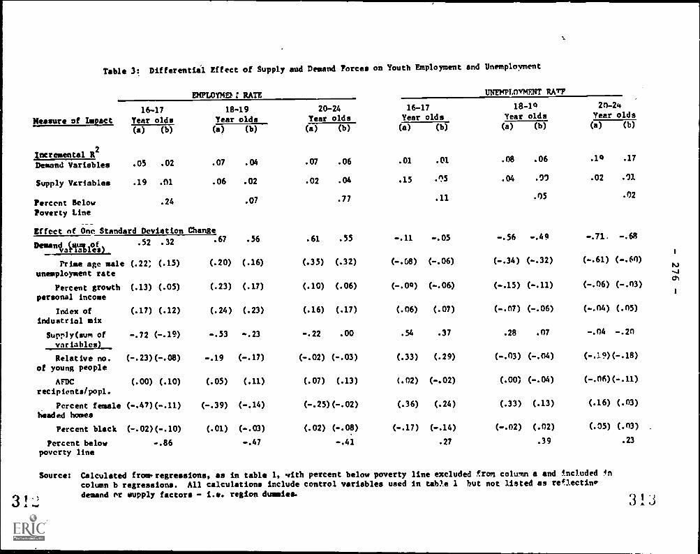
Table 3: Differential Effect of Supply and Demand Forces on Youth Employment and Unemployment

DIPLOYME) r RATE UNEMPLOYMENT RATF

16-17 18-19 20-24 16-17 18-10 20-24

Measure of Impact Year olds Year olds Year olds Year olds Year olds Year olds

(a) (b) (a) (b) (a) (b) (a) (b) (a) (b) (a) (b)

Incremental R2

Demand Variables .05 .02 .07 .04 .07 .06 .01 .01 .08 .06 .14 .17

Supply Variables .19 .01 .06 .02 .02 .04 .15 .in .04 .01 .02 .01

Percent Below .24 .07 .77 .11 .05 .02

Poverty Line

Effect of One Standard Deviation Change

Demantac Iualg).52 .32 .67 .56 .61 .55 -.11 -.05 -.56 -.49 -.71. -.68

Prime age maleunemployment rate

(.22; (.15) (.20) (.16) (.35) (.32) (-.08) (-.06) (-.34) (-.32) (-.61) (-.60)

Percent growthpersonal income

(.13) (.05) (.23) (.17) (.10) (.06) (-.09 (-.06) (-.15) (-.11) (-.06) (-.03)

Index ofindustrial mix

(.17) (.12) (.24) (.23) (.16) (.17) (.06) (.07) (-.07) (-.06) (-.04) (.05)

Supnly(sum ofvariables)

-.72 (-.19) -.53 -.23 -.22 .00 .54 .37 .28 .07 -.04 -.20

Relative no.of young people

(-.23)(-.08) -.19 (-.17) (-.02) (-.03) (.33) (.29) (-.03) (-.04) (..,19)(-.18)

AFDCrecipients/popl.

(.00) (.10) (.05) (.11) (.07) (.13) (.02) (-.02) (.00) (-.04) (...06)(-.11)

Percent femaleheaded homes

(-.47)(-.11) (-.39) (-.14) (-.25)(-.02) (.36) (.24) (.33) (.13) (.16) (.03)

Percent black (-.02)(-.10) (.01) (-.03) (.02) (-.08) (-.17) (-.14) (-.02) (.02) (.05) (.03)

Percent belowpoverty line

-.86 -.47 -.41 .27 .39 .23

Source: Calculated froarregressions, as in table 1, with percent below poverty line excluded front column a and included :In

column b regressions. All calculations include control variables used in table 1 but not listed as refl.ectino

demand or supply factors - i.e. region dummies.

- 27,7 -

age groups, so that its inclusion as a demand or supply variable is critical in

determining the relative importance of the two sets of forces. Even

with the percent below poverty variable, howeVer, demand factors continue

to be the dominant factor for 20-24 year olds and remain more important

than supply factors for 18-19 year olds as well. Perhaps the safest

conclusion to reach is that supply or background factors are relatively

more important determinants of the position of teenagers while demand

factors are more important for those in their early twenties.

Work Activity of Young Women

To see whether the labor market position of young women is influenced

by the same factors that determine the position of young men, the employ-

ment to population rate, labor participation rate, and rate of unemployment

of women aged 16-17, 18-19, and 20-24 are regressed on essentially the same

variables as in tables 1 and 2, with two exceptions: the relative number

of young persons is measured by the ratio of the number of young women

in each group (rather than the number of young men) to the number of

civilian men 16 and over, and the index of industrial mix is based on

the ratio of young women to all workers in the industry in the U.S.

(rather than by the ratio of young men to all workers). Table 4 summarizes

the results of the regressions for young women in terms of the OLS coefficients

and standard errors of the major variables and the summary statistics and

presents comparable information from the regressions for young men.

The regression results reveal considerable similarities between the

sexes in the labor market effects of most variables. The relative number

of young persons is an exception: it does not reduce the employment to

population rate and labor participation ratio of 16-17 and 18-19 year old

women with the same significance and magnitude as it does for 16-17 and

18-19 year old men. In contrast, the prime age male unemployment rate

31 .1

- 278 -Table 4; Comparison

Employment

Male16-17

of the

Economic Position

RatioFemale

-.17(.79)

-1.38

(.53) .

.37

(.36)

.14

(.06)

-.10(.57)

-1.30

(.33)

.78

-.10

(.64)

-.88(.50)

.54

(.34)

.26

(.11)

.35

(.54)

-1.62(.28)

.81

.16

(.21)

-1.10(.42)

.27

(.29)

.29

(.14)

.86

(.45)

-1.55(.23)

.71

Effects of Major Economic Variables on theof Young Men and Women

Labor Force Participation Rate Unemployment Rate

4

-Male

-.26(.80)

-1.04

(.53)

.18 1

(.36)*

.18

(.08)

-.18(.56)

-1.80(.32)

.77

-1.60(.62)

-.38(.47)

.68

(.32)

.39

(.12)

-.41

(.49)

-.71

(.25)

.78

-.33(.24)

-.55(.35)

.23

(.24)

.26

(.11)

- 06

(.37)

-.50(.19)

.82

Female

-.07.

(.85)

-1.32

(.57)

.35

(.39)

.17

(.07)

-.07

(.62)

-1.43(.35)

.77

-1.18

(.65)

-.34(.51)

.42

(.34)

.22

(.11)

.52

(.54)

-1.51(.28)

.79

.19(.19)

-.74

(.39)

.15

(.27)

.17

(.13)

.93

(.42)

-1.52

(.22)

.74

Male

1.52

(.47)

.20

(.31)

-.14(.21)

.04

(.05)

.46

(.33)

.24

(.19)

.63

-.19

(.38)

1.11

(.28)

-.26(.20)

-.06(.07)

-.07(.15)

.27

(.30)

.72

-.29(.11)

1.66(.16)

-.07

(.11)

.04

(.05)

.02

(.17N

.21

(.09)

.86

Female

.26

(.58)

.74

(.39)

-.24(.26)

.01

(.05)

-.14

(.42)

.96

(.24)

.70

-.64

(.40)

1.04

(.31)

-.39(.21)

-.12(.07)

-.16(.17)

.02

(.34)

.76

.05

(.09)

.70

(.18)

-.24

(.12)

-.21

.00

(.20)

.28

'0)

.77

Relative Number -.82of Young People (.75)

Prime Age Male -1.01Unemployment Rate (.50)

Percent Growth of .23

Personal Income (.34)

Index of .14

Industrial Mix (.08)

Percent of Female -.42Needed Households (.52)

Percent families -1.61

Below Low-Income (.30)

Level

R2

.78

18-19Relative Number -1.36of Young People (.59)

Prime Age Male -1.06Unemployment Ratc (.45)

Percent Growth of .77

Personal Income (.31)

Index of .38

Industrial Mix (.12)

Percent of Female -,53

Headed Households (.47)

Percent Families -.84

Below Low-Income (.24)

Level

R2 .80

20-24

Relative Number -.09of Young People (.24)

Prime Age Male -1.88Unemployment Rate (.35)

Percent Growth of .25

Personal Income (.24)

Index of .27

Industrial Mix (.11)

Percent Fiaele -.07

Headed Houselolds (.37)

Percent Families -.65Below Low-Income (.20)

Level

R2

.d4

- 279 -

has as sizeable impacts on the employment/population, labor force

participation and unemployment rate of women as on those for men.

The growth of personal income, the index of industrial mix, and the

fraction of families below low-income level also have roughly comparable

effects. The fraction of one parent/female homes has a somewhat

smaller effect on the employment of 16-17 year old women than on 16-17

year old men. But has comparable effects in the other age groups.

Although there are differences, the overall impression from the table

is that similar area factors are associated with geographic variation in

the employment of young women as of young men.

Relevance to Changes Over Time

The questioh naturally arises as to the relevance of the cross-

sectional calculations to observed changes in youth labor force activity

over time. Are the es;:imated effects of variables in the cross-section

consistent with comparable estimates from time series data? Do the

estimates help explain observed trends in the youth labor market?

To compare the effect of variables in cross-section and time series

data, it is best to estimate their coefficients with identical controls.

Since the time series has fewer observations and less information about

some variablep, a relatively simple set of comparable regressions was

estimated for the SMSA data set and the time series. The employment to

population rate, labor force participation rate, and rate of unemployment of

young male workers 16-17, 18-19, and 20-24 was -egressed on three explanatory

variables: the rate of male unemployment; the ratio of the number of young men

in each age group relative to the number of men 16 and over; and neasures of the

minimum wage, ln average earnings in private industry in the cross-section

data and ln of the federal minimum divided by average earnings in private

316

- 280

industry in the time series. The cross-section data are taken from the

basic SMSA data set. The sources of the time series data are described

in the data appendix. Because of the danger of mistaking similar trends

in time series variables for causal relations, the time series regressions

are estimated in two different specifications: without a time trend

variable and with a trend variable included.

Table 5 presents the estimated coefficients from the time series and

cross -SMSA regressions. While there are some differences in the estimated

effect of variables, the general pattern is of broad similarity in the

regression coefficients. The relative number of young pergons has a roughly

similar qualitative impact on employment to population and labor

participation and unemployment rates in the two sets of calculations. Note

however that the magnitude cf the estimated coefficients in time series

regressions is quite sensitive to inclusion or exclusion of trend, a

pattern that highlights the problem of inferring the effect of demographic

factors from the time series data. The unemployment rate of men reduces

the employment to population-rato and raises the linemployment rate of all

groups by similar magnitudes and has comparable effects on the labor force

participation of 16-17 year olds (though not on those of 18-19 and 20-24

year olds). The third explanatory factor, the minimum wage variable is

negative, of comparable magnitude in the regressions for 16-17 and

18-19 year olds, where it obtains significant effects on the employment

to population and labor force participation rates but has no discernible

impact on the unemployment rate. The minimum wage variable is, or the

other hand, accorded different effects on the 20-24 year olds in the cross-

section and time series. Overall, however, the coefficients from the

two sets of regressions are roughly consistent, enhancing the believability

of each. 3 I -7,

Table .5: Cmrarison of Om Fatimat#41 Effect of Seleerspd VerimMee

on Youth Work Activity, 1948-77 Time Series Regressions vs. Cross-SMSA Regressions

Variable16-17 year olds

cross -SMSA time series

A) Eaployaent to Population Rate20-24 year olds

cross-SMSA time series18-19 year olds

cross-SMSA time seriesTotal unemploy- -2.25 -2.05 -2.44 -2.28 -1.94 -1.72 -3.41 -1.49 -1.51ment rate (.60) (.36) (.36) (.52) (.51) (.54) (.42) (.32) (.25)

Rel. no. of -3.57 -3.33 -6.09 -3.38 -3.18 -1.27 -1.66 -.94 -.20young persona (.83) (.48) (1.12) (.58) (.64) (1.83) (.21) (.20) (.24)

"Minimum wage" -.12 -.09 -.11 -.15 -.14 -.10 - .11 -.01 .06

proxy (.04) (.03) (.03) (.04) (.04) (.05) (.03) (.03) (.03)

Time trend .26 -.18 -.19(.10) (.17) (.05)

R2 (.25) .75 .80 .33 .60 .62 .49 .65 .79

B) Labor Force Participation Rate

Total uneaploy- -2.03 -1.07 -1.69 -1.08 .13 .21 -1.70 .56 .55

aent rateRel. no. of

(.63)

-3.10(.46)

-1.78(.41)

-6.19(.53) (.51)

-3.43 -2.18 -1.45(.41)

-1.72

(.24)

-.61(.22)

-.15 corr

young persons (.89) (.60) (1.28) (.59) (.64) (1.85) (.21) (.15) (.20)

"Minimum wage" -.15 -.09 -.12 -.18 -.13' -.12 -.12 .00 .04

proxy (.05) (.04) (.03) (.04) (.04) (.05) 603) (.02) (.02)

Time trend -- .41 -- -.07 -.11(.11) (.17) (.04)

.21 .42 .63 .33 .44 .44 .42 .49 .62

C) Unemployment Rate

Male unemploy- 1.24 2.32 2.07 2.20 2.90 2.70 2.28 2.34 2,,35

ment rate (.26) (.18) (.16) (.26) (.19) (.18) (.15) (.16) (.12)Rel. no. of 2.41 3.65 1.88 .48 1.72 -.05 .06 .45 .06young persona (.37) (.24) (.49) t.29) (.24) (.60) (.08) (.10) (.12)

"Minimum wage" -. 03 .02 .01 -.02 .03 .00 .no .01 -.02proxy (.02) (.01) (.01) (.02) (.02) (.02) (.01) (.01) (.01)

Time trend .17 ' -- .17 .09(.04) (.04) (.02)

R2

.41 .93 .96 .44 .90 .93 .70 .90 .94

ine minimum wage variable in the croes-SMSA deta set is the In of the inverse of average hourly earnings in the area.Tne minimum wage var4able i" the time series data set is the In of the ratio of the federal minimum to Average hourlyearnings.

Source:

31-')

Cross-SMSA figures based on regressions using 114 SMSA data set.described in data appendix.

Time series figures based or data

319

- 282 -

While the cross-section and time series regressions yield roughly

similar estimates, it is important to note that neither analysis explains

developments in the youth labor market in the 1970s. As Table 6 shows,

from 1969 to 1977 the employment/population ratio of 16-17 year olds

changed modestly while their labor force participation and unemployment

rates rose. There was a marked divergence from 1969 to 1977 between

actual changes in youth work activity and the changes predicted by either

the cross-section or time series models. Because the adult male un-

employment rate increased sharply while the relative number of young

persons either changed only slightly (teenagers) or increased (20-24 year

old workers), dwarfing the effects of a decline in the ratio of the minimum

wage to the average wage, the cross section and time series regressions

predict a marked decline in the employment/population and labor

participation rates, and a sizeable increase in unemployment rates. In

fact, employment/population ratios changed unevenly while labor participation

rates rose sharply so that only the unemployment rates followed the

predicted pattern. Despite concern over the inability of the labor

market to generate jobs for youth, youth work activity did not_ decline or

decreased only slightly in the 1970s, despite adverse cyclical and other

developments, for reasons that are unclear. While our time series and

cross-section regressions yield comparable results, neither adequately

tracks the performance of the youth market in the 1970s. 9

Individual Variation

The analysis thus far has treated area data which, while well-

suited for investigating the effects of broad market factors in the

position of youth, provides only weak information on individual differences

in youth participation or unemployment. To obtain a better under-

standing of the incidence of youth labor market problems among individuals

and of the social characteristics of the individuals lacking employment,

it is necessary to obtain data on indiiiiduals.rather than on SMSA's.

34:u

Table 6: Predicted

Explanatory Factor

and Actual Changes in Youth Work Activity, 1969-1977

Actual Value Actual Change Predicted Cnanges, 1969-1977

1969 1977 1969-1977 Using cross-section model

Using time-series modelwithout

Using time-serieo modelwith trend

Rate of Unemployment of .015 .035 .020 trend

Adult Men

Relative No. of Young Persons16-17 year olds .059 .057 -.002

18 19 year olds .051 .053 .002

20-24 year olds .101 .124 .023

Ln(Minimum Wage/Average Wage) -.734 --.821 -.087

Trend 22 30 8

Dependent VariablesEmployment/Population

16-17 year olds 40.8 40.5 -.3 -2.7 -2.5 -0.4 haCO18-19 year olds 59.7 61.2 1.5 -3.9 -3.7 -4.5 14

20-24 year olds 78.6 76.5 -2.1 -9.7 -5.1 -5.4

Labor Force Participation Rate16-17 year olds 47.3 50.3 3.0 -2.1 -0.9 2.418-19 year olds 65.9 72.5 6.6 -1.3 0.7 0.420-24 year olds 82.8 85.7 2.9 -6.3 -0.3 -0.4

Unemployment Rate16-17 year olds 13.8 19.5 5.7 2.3 3.6 4.918-19 year olds 9.4 15.6 6.2 4.7 6.0 6.820-24 year olds 5.1 10.7 5.6 4.7 5.6 5.8

3.213,..,4) 2

- 284 -

The Survey of Income and Education, conducted in the spring of 1976,

provides an especially valuable sample for such an investigation. The

survey contains about 3 times as many respondents on the standard

Current Population Survey monthly samples and a variety of information

on family background that is unavailable in most CPS months.' Of particular

importance, the SIE has data on wages and hours worked over a year; as

well as on employment status, which permits comparison of the effect of

variables on rates of pay as opposed to the amount of work activity..

The SIE data are examined in two stages, First,'a linear probability

model is fit linking dichotomous dummy variables for employment and fors'

unemployment in Spring 1976 to various characteristics of the individual

and his or her family. Since the linear model is additive, the effect of

variables on the probability of labor force participation can be obtained

by adding the coefficients on employment and unemployment. While the linear

model is not entirely appropriate for analysis of 0-1 variables, the advan-

tage of a more complex curvilinear form, such as the logistic, is likely

to be modest. Second, In earnings eauations are estimated linking hourly

and annual earnings in 1975 to the same set of measures of individual

characteristics. The earnings equations provide information on the

wage side of the youth labor market. Comparison of the effect of variables

on hourly earnings and on the probability of employment or annual earnings

(which depends critically on the probability of employment over the year)

can cast considerable light on the extent to which youth labor market

problems are asscriated with joblessness as opposed to, or in conjunction

with, low rates of pay.

The rnalyses examine the impact of the following characteristics of

individuals or their families:

3"

.1 285 -

-race, measured by a dichotomous variable (=1 when the individual is black);

-receipt of welfare by the household of residence, a dichotomous

variable which takes the value 1 if the family obtained welfare in 1975;

-receipt of food stamps, a dichotomous variable which takes the value 1

if the family obtained food stamps in 1975;

-residence in public housing, a dichotomous variable which takes the

value of 1 if the family was living in public housing when surveyed;

-residence in a one parent/female home, a dichotomous variable which

takes the value 1 if the individual's parental family contained a female

head of household;

-yearst! education;

-school activity status, a dichotomous variable which takes the value 1

if the person's major'activity at the time of the survey was being in, school;

-other family income, a continuous measure of total family income in

1975 minus the individual's earnings in 1975;

- region of residence, consisting of 7 dummy variables for region;

-urban status, a dichotomous variable which takes the value 1 if a

person lived in an urban area in 1976}

- family income below the poverty line; a 0-1 variable-which takes

the value 1 if the family income in 1975 fell below the official poVerty line.

Since some of the respondents are no loriger living with their'parents or

other adults, the measures of family background do not always relate to

the position of the home in which they were brought up: for,1.4 7 and

-18-19 year olds, of whom only 0.6% and 8% reside outside the home

of their parent or other adult, the problem is not severe; for 20-24

year olds, of whom about half are themselves heads of households and .

for many of those out of school, however, the family variables relate

to parental homes fora significant fraction and to homes headed by

the individual for a significant fraction, which;confuses

To deal with this problem, a dummy variableofor those who

3'.4

the interprektion.

are themsAves

- 286 -

heads of households was included in all of the calculations, and the

variable was interacted with other family income. In addition, for

20-24 year olds, separate calculations for those residing in homes headed

by others were estimated. The results are sufficiently similar to those

reported in the table as to suggest that the head of household dummy

variable suffices to deal with the problem.

The calculations yield one striking result: the factors that influence

the employment status of young workers are not the same as the factors

that influence their wage rates. Being black, for example, lowers the

probability of being employed substantively but has little or no effect

on wages. In one sense, this result justifies analysis of youth job-

lessness as a labor market problem distinct from standard analysis of

wages. While presumably related, the determinants of employment chances

and earnings differ enough as to constitute separate Subjects-of study.

Evidence for the claim the personal characteristics have very

different effects on employment status than on earnings is given in tables

7 and 8. Table 7 summarizes the results of the linear

probability estimates of the detertinants of the employment and joblessness

of all young men aged 16-17, 18-19 and 21-24, and for 18-19 and 20-24 year

10old men out of school. The first column in each heading records means

of the relevant variables while the next two colUMns give the regtession

coefficients and standard errors from the linear probability model.

Not surprisingly, the calculations show that black youth,,those with

fewer years of Wicioling, and those whose major activity is schbolvturn

out to have much lower rates of employment and higher rates of unemployment.

The measures of family otatus--- being in a female headed home, family

receipt of welfare or food stamps, and residence in public bousing,'the

income of the household exclusive of the young person himself and whether

the family is or is not below the poverty litie--also'have some effect, with

3 2711

3`' t;

Table 11 Linear Probability of Estimates of Determinants of the Deployment of YouaR Men. 1976

Out of School J.Jat_School.All 16-17 year olds All 18-19 year old, ilpivarzi, All 20-24 year olds 41r.-1': year 014

Measpro of: means empl. unemp.,

.11

.06

(.01)

-.007(.003)

-.10(.01)

.01

(.01)

.08

(.01)

.31(.01)

.06

(.02)

-.021(.017)

-.02(.01)

.05

.31

9297

means empl. unemp.

.63 .11

.09 -.21 .11

(.02) (.01)

11.6 .02 -.01(.003) (.002)

.36 -.34 -.08(.01) (.01)

.11 -.05 .02

(.02) (.01)

.06 -.02 -.01(.02) (.02)

.10 -.07 .07

(.02) (.01)

.02 -.12 .09

(.03) (.02)

17.437 -.001 .003

(.0004)(.003

.11 -.08 .01

(.02) (.01)

8

/.17 .23

.44 .31

8476 8476

means

.09

11.1

.12

.08

.14

.02

13.500)

.14

emp .

.75

-.19(.03)

.033

(.015)

-.03(.03)

-.04(.03)

-.08(.03)

-.16(.05)

.000(.001)

-.04(.02)

8

.09

.42

3185

unemp.

.15

.12(.02)

-.02(.004)

.02

(.02)

-.00(.03)

.10(.02)

.11

(.04)

-.001(.0007)

.007(.02)

8

.07

.35

3185

means

.08

12.8

.06

.04

.10

.02

11.973

.09

empl. unemp..74 .09

-.12 .05

(.01 (.01)

.012 -.005(.001) (.001)

-.43 -.05(.01) (.01)

-.05 .05

(.01) (.01)

-.08 .06

(.02) (.01)

-.04 .08

(.01) (.01)

-.11 .00

(.02) (.02)

-.001 .002(.0003)(.000)

-.OS .03

(.01) (.01)

a 8

.11 .05

.40 .29

18.395 18,395

means

.08

12.2

.06

.05

.12

.02

9.793

-.08

eiii17-7Eiln.

.81 .10

-.10 .04

(.01) (.01)

.014 -.007(.002) (.001)

MAIN.

-.05 .05

(.01) (.01)

-.08 .06

(.02) (.01)

-.06 .07

(.01) (.01)

-.12 -.On

(.02) i.02)

-.001 -.001

(.005)(.0004)

-.08 .04

(.01) (.01)

8 8

.07 .05

.38 .29

12,513 12,513

11114111ULTLIEUWA .47,,

Individual statusblack .10. -.20

(.02)

years cf schooling 10.0 .044(.005)

major activity .67 -.20is in school (.01)

Family statusfemale headed .13 -.02

home (.02)

family receives .08 -.05welfare (.Q2)

food stamps .12 -.04(.02)

public housing .02 -.02(.04)

other family $18.305 .047income(in thou- (.026)

sands of $)

family below .11 -.06poverty line (.02)

Other Controls

head of householdinteraction: headof household andother family incomeregion 8

urbansubsidised rent

Summary StatisticsR2 .12

SEE .47

n 9291

'The numbers in this Column represent a smaller fraction of the youth than the proportion whose major activity is "in school."This is because a otrictur definition of schooling is used. Persons out of school are not enrolled at all. Since some persons

whose major activity is reported as other than being in school are enrolled, rs i.the numben the out of school columns representa smaller fraction of the total than would be obtained from the Major activity question.

sources Survey of Income and Education

- 288 -

a general pattern that those from more disadvantaged backgrounds have

lower probabilities of employment and higher probabilities of unemployment

than those from more advantaged backgroundL The seat noticeable

exception to this generalization is that other family income is accorded

little or no impact on employment or unemployment in the bulk of the

calculations. Even so, the regressions suggest youth joblessness is con-

centrated among persons from more disadvantaged homes and, with all other

characteristics fixed, among blacks.

The In hourly earnings in table 8 tell a very different story about

the determinant of the 'wages of the young. First, and perhaps most

importantly, being black is not a major depressent of wages. Among 16-17

year olds, being black is actually associated with higher wages while in

the other age groups, blacks are estimated to have only a 5 to 6 percent

disadvantage. Second, with the exception of the poverty line variable,

the measures of family status also fail to evince the negative effects

found in the employment and unemployment regressions. Being in school and

years of schooling also have much smaller impacts on wage rates than on

employment status. Since being below the poverty line is partially

determined by wages, particularly for 20-24 year olds, making its strong

effect on wages questionable in terms of the direction of causality,11

the main conclusion is that the background factors which adversely affect

employment chances have much diminished or in some cases opposite effects

on wage rates.

Since the calculations in table 8 are limited to persons who worked

and reported earnings in 1975 while those in table 7 refer to a larger

sample which includes those who did not work, it is possible that some of

the differential effects are attributable to differences in the samples.

To check this possible bias, as well as to expand the analysis to a

3''

Table 8: Regression Coefficient Estimates of the Eackground Determinants of the Ln of Sourly and Annual Earnings of

Young Men, 1975

16-17 year olds 18-19 year olds 20-24 year olds

mean in hrlyearnings

lba Measure of

ln 4anlearnings

6.37

impliedln annlhrs wkd5.84

mean In hrlyearning,

.80

ln annlearnings

7.36

impliedin annlhrs wkd

6.56

mean ln hrlyearnings

1.16

ln annlearnings

8.29

impliedln analhrs rkkd

7.16ckground Status .53

black .07 .14 -.17 -.31 .07 -.06 -.33 -.27 .07 -.05 -.14 -.09-

(.04) (.06) (.04) (.051) (.02) (.03)

years of schooling 10.2 .04 .09 .05 11./ -.04 -.01 .03 12.8 .007 -.04 -.03

(.01) (.02) (.02) (.01) (.002) (.004)

major activity is .66 -.01 -.26 -.25 .34 -.05 -.50 -.45 .13 -.08 -.70 -.62

in school (.02) (.03) (.02) (.03) (.01) (.02)

female headed home .13 ,08 .01 -.07 .10 .04 -.08 -.12 .06 -.00 -.08 -.oe

(.03) (.05) (.03) (.02) (.02) (.03)

family receives .07 .05 -.12 -.17 .05 .01 -.14 -.10 .04 -.06 -.22 -.16

welfare (.05) (.07) (.04) (.06) (.03) (.04)

food stamps .10 .05 .07 .02 .09 .00 -.09 -.09 1

(.04) (.06) (.03) (.05)

public housing .02 .07 .26 .21 .02 .13 .11 -.02 .02 -.04 -.24 -.20 .°D)

(.08) (.12) (.07) (.10) (.01) (.031s

other family income $18.994 .003 .002 -.001 17.815 .002 -.002 -.004 11.924 -.003 -.008 -.003

(in thousands of $) (.001) (.001) (.001) (.001) (.005) (.0n1)

!amily below 1975 .08 -.16 -.43 -.27 .09 -.37 -.72 -.25 .07 -.56 -1.25 -.79.

poverty line (.04) (.06) (.03) (.05) (.Q2) (.03)

'ever Controlsrags-head of household-interaction: head

of household andother family income

-region 8 8 8 8 8 8

-urban-subsidised rent

!ummary SuatisticR1 .03 .10 .20 .06 .34

SEE .73 1.05 .95 .66 .58 .83

n 5240 5240 6728 6728 15 430 15 43n

:ounce: Survey of Income and Education

3 3 u

- 290 -

more continuous measure of time worked, the log of annual earnings was

also repressed on the independent variables in the sample reporting earnings.

Differences between the impact of variables on log of hourly and log ofa

annual earnings reflect effects on annual hours worked. As can be seen

in table 8, these calculations confirm the basic conclusion that rates

of pay are largely unaffectedor affected differently by the background

factors under study than is time worked. Whereas, for example, being

black reduces the log of hourly earnings of 18-19 year old blacks by

.06 la points, it reduces the log of annual earnings by .33, implying

a .27 reduction in annual hours worsted.

The divergent effect of race and background factors on time worked

and rates of earnings per hour (or week) highlights an important aspect

of the youth labor market: striking differences between its employment

and wage dimensions. The disadvantaged groups that bear the brunt

of joblessness obtain roughly similar pay to other youngsters

upon receipt of employment. While it may be argued that the concentration

of youth joblessness among certain groups, whose pay is the same as

that of others, could be alleviated by wage differentials (tying the

employment and wage findings together), perhaps the safest conclusion to

reach is that the labor market problem for the disadvantaged is largely

one of generating jobs. Once employed, blacks and other disadvantaged

youth have roughly as high earnings as other young persons.

IV Summary of Findings

The results of our analysis of geographic and individual differences

in youth employment, unemployment, and earnings can be summarized

briefly: :trim, the employment of young workers across areas depends

in a reasonably comprehensible way on demand and supply factors, notably

the overall level of economic activity, as reflected in rates of unemployment

3

- 291 -

of prime age men and growth of personal income, the industrial composition

of employment, the number of young persons relative to the number of older

persons (for teenagers only) and the poverty status of an area. Second,

variables that influence employment often have comparable effects on labor

participation, leading to smaller or even contrary effects on unemployment.

Analyses which focus strictly on unemployment rates may, as a result, be

highly misleading. Thic4, the cross-i,ntion calculations, while yielding

results consistent with comparable time series regressions, do not provide

an explanation of youth labor market developments in the 1970s, when

employment to population rates did not fall and participation rates increased

in the face of adverse economic changes. Fourth, the correlates of youth

joblessness are not the same as the correlates of low wages, with blacks

and others from disadvantaged backgrounds having higher incidences of job-

lessness but obtaining similar wages to other workers.

3

- 292 -

Footnotes

'Between 1967 and 1977 the number of persons aged 16-24 increased by 37%

while the population 16 and over increased by 23Z, as calculated from

U.S. Department of Labor, Em lo ent and Trainin: Report of the President,

1978, table A-2, pp. 181-182.-

2The SKSA data set is described in the data appendix. For a detailed

description of the SIE survey see U.S. Department of Commerce and U.S.

Department of Health Education and Welfare, "Assessment of the Accuracy

of the Survey of Income and Education" A Report to Congress Moderated

by the Education Amendment of 1974 (Jan. 1967).

3To solve for the equilibrium set A(lnD-lnS) = 0.

4See R. Freeman and J. Medoff, "The Youth Labor Market Problem: An Overview,",

table 6, where significant differences in the distribution of the 16-17,

18-19 and 20-24 year olds among industries and occupations are shown.

5The coefficients of variation for the ratio of young men to men 16 and

over are: 16-17 year olds, .113; 18-19 year olds, .16; 20-24 year olds, .17.

6Another possible explanation is that 20-24 year olds migrate to areas

with low rates of youth joblessness, which would mute or reverse, any

adverse, effect of relative numbers on joblessness. By contrast the

bulk of teenagers reside with parents who are unlikely to migrate to areas

where job opportunities are better for the young.

in these regressions I have included all of the control variables used

in Table 1.

- 293 -

8Analysis of the in-school and out-of-school youth can be developed

further through estimation of the structural supply and demand equations

which presumably underly the relations examined in the text. Such an

analysis would seek to determine the degree of substitutability between

in-school and out-of-school youth in the job market among other things.

9For a similar conclusion see Burt Barnow, "Teenage Unemployment and

Demographic Factors: A Survey of Recent Evidence" (U.S. Department of

Labor, March 21, 1979).

10As described in the table note, persons in the out-of-school group are

limited to those not enrolled in school and do not include enrolled persons

who report their major activity as being other than in school.

11Regressions with the poverty variable excluded, reported in an earlier

version of this paper, yield results on other variables comparable to

those in tables. Hence inclusion of the variable does not mar inter-

pretation of the other regression coefficients.

- 294 -

DATA APPENDIX

Cross-SMSA Data

1. AFDC recipients

Source: Bureau of the Censma, Statistical Abstract of the United

States, 1971, section 33: Metropolitan Area Statistics.

2. Average annual rate of growth of personal income, 1958-1969

Source: Bureau of the Census, Statistical Abstract of the United States,

1971, section 33: Metropolitan Area Statistics.

3. Average hourly earnings 197C of production workers on manufacturing

payrolls

Source: Bureau of Labor Statistics, Employment and Earnings

States and Areas 1939-74, Bulletin 1370-11.

4. Black population as percentage of total population

'Source: Bureau of the Census, 1970, Census of Population, General

Characteristics of Population, 1970, table 24: Age by Race and Sex, for

Areas and Places: 1970.

5. City size (population of central city)

Source: Bureau of the Census, Statistical Abstract of the United

States, 1973, secAion 34: Metropolitan Area Statistics.

6. Demographic variables

Source: Bureau of the Census, 1970, Census of Population, state

volumes, Detailed Characteristics, 1970, table 164: Employment Status

by Race, Sex, and Age: 1970.

Calculations: 16-17 year olds demographic variable 16-17 year old

male civilian population/total male civilian population. Demographic

variables for 18-19 year olds and 20-24 year olds calculated in the same way.

- 295 -

7. Employment variables (employment rat', unemployment rate, labor force

participation rate)

Source: Bureau of the Census, 1970 Census of Population, Detailed

Characteristics, 1970, table 164: Employment Status by Race, Sex, and Age:

1970 for total group table 166 Employment and Status and Hours Worked of

Persons 14 to 34 year olds, by school enrollment, age, race, and sex:

1970; for persons not enrolled in school.

8. Female headed households as percentage of all households

Source: Bureau of the Census, County and CIty Data Book, 1972:

Statistical Abstract Supplement, table 3: Standard Metropolitan Statistical

Areas.

9. Industry indices

Sources: Percentages of civilian labor force employed in each industry,

by SMSA: Bureau of the Census, County and City Data Book, 7972:

Statistical Abstract Supplement, table 3: Standard Metropolitan Statistical

Areas. Persons employed in each age group as percentage of total persons

employed by industry: Bureau of the Census, 1970 Census of Population,

Detailed Characteristics: United States Summary, table 239: Age of

Employed Persons by Industry and Sex: 1970.

Calculations: Industry index for 16-17 year old males (industryall industries

share of labor force in SMSA x fraction of industry labor force that is 16 -1.7

years old)/ fraction of total U.S. labor force that is 16-17 years old.)

10. Percent of families below low-income level

Source: U.S. Bureau of the Census, Statistical Abstract of the United

States 1973, Section 34: Metropolitan Area Statistics.

- 296 -

11. State minimum wage laws

Source: Bureau of Labor Statistics, Youth Unemplcymert and Minimum

Wages, Bulletin 1657, 1970, pp. 133-134, Chapter IX Append4x B: Basic

adult minimum wage rates and specified differential rates by 3tete,

June 1969.

Time Series Data

12. Time-series average hourly earnings of production workers on private

payrolls

EoUrce: Employment and Training Report of the President, 1978, p. 265,

table C-3, Gross Average Weekly Hours, Average Hourly Earnings, and Average

Weekly Earnings of Production or Nonsupervisory Workers on Private

Payrolls, by Industry Division: Annual Averages, 1947-1977.

13. Time-series minimum wage

Source: Bureau of Labor Statistics, Youth Unemployment and Minimum Wages,

Bulletin 1657, 1970, p. 182, table 12.2: Proportion of earnings covered

by the Federal minimum wage.

14. Time-series demographic variables

Source: p11ertoftEmloentandTrairprEj31.dent, 1978,

p. 183, table A-3: Civilian Labor Force for Persons 16 Years and Over,

by Sex, Race, and Age: Annual Averages, 1948-1977; p. 186 table A-4:

Civilian Lebo: thce Participation Rates for Persons 16 Years and Over,

by Race, Sex, and Age: Annual Averages, 1948-1977.

Calculation: Male civilian population fcr each age group and total

number of persons in civilian labor force for cohort x 100)/Civilian labor

force participation rate for cohort.

- 16-17 year olds demographic variable = 16-17 year old

male civilian population. Demographic variables for 18-19 year olds and

20-24 year olds calculated in the same way. or

Ig

- 297 -

15. Time-series labor force participation rate

Source: Employment and Training Report of. the President, 1978, p. 186,

table A-4: Civilian Labor rorce Participation Rates for Persons 16

Years and Over, by Race, Sex; and Age; Annual_Averiges, 1948-77.

16. Time-series unemployment rate

Source: Employment and Training Report of the President, 1978,. p. 212

table A-19: Unemployed Persons 16 Years and Over and Unemployment Rates,

by Sex and Age: Aanual Averages, 1948-77.

17. Time-series employment ratio

Calculations: Employment Ratio (1 - unemployment rate/100) x

labor force participation rate.

-'298 -

The Dynamics of Youth UnemploymentKim B. Clark

Lawrence H. Summers*

Introduction

At any given moment appto]Zieaeely 2 million teenagers are unemployed.

Another 600 thousand are out of school and neither working nor looking for work.

Only about 60 percent of all teenagers and 23 percent of black youth who are

out of school are employed. These high rates of joblessness have been a source

of concern to both economists and policy mikere. This paper seeks to clarify

the dimensions of the youth empryment problem, by analyzing the distribution

4of unemployment and related patterns of labor force mobility. We are led to

fcur priaeiry conclusions.

First, most youth ioblessness is due to a small part of the Population

who are out of work Eor extended periods. Normal. turnover accounts for a

neglIzible fraction of youth unemployment. In March of 1976, for example,

the average unemployed teenager had been out of work almost four months a.td

could expect to wait an additionel 3.5 months before finding work- He could

expect to experience over 8 months of joblessness during the calendar year.

The evident concentration of joblessness suggests the existence of a serious

social problem.

Second, for the vast majority of youna_ziale the labor m'rket functions

exceptionally well. Almost half of all job changes among teenagers occur with-

out intervening unemployment. Close to two thirds of entrances into employment

occur without measured unemployment. Most spells of unemployment are qtite

brief. It is important to understand that the etse with which most transitions

occur says little about the experience of the extensively unemployed population

who account for most of the youth employment problem.

*We are grateful to James Buchal, James Poterba and Daniel SmithEor assistance with computation.

339

Third, the_uneryiument/tiot-in-laber force distinction is virtually

madjuless fcr young, _people. The behavior of most of the unemployed and many

persons outside the labor force is functionally indistinguishable. Indeed,

for men out of schuol, the probability of moving into employment is only

slightly greater for the unemployed than it is for persons outside the labor

farce. The evidence suggests tftat attention should be focused on the youth

non-employment problem, lather than merely on unemployment.

Fourth, the level of emulam,iut among teenagers depends cri:ieally on

available emplmentopnertonities. The sharp cyclical sensitivity of youth

employment belies the sueii,esti4a that the unemployed do not really want work,

or that they are incapable of working productively. The cyclical evide* -e

suggests that a shortage of attractive jobs is the root cause of the youth

non-employment problem.

- 300 -

I

Characteristics of the Teenage Labor Market

In recent years it has become fashionable to view youth unemployment as the

result of high rates of turnover. On this view, youth unemployment is not due

to a shortage of jobs for young people. Rather, it occurs because young peoplE7,

especially teenagers, are unwilling or unable to hold jobs for very long and

thus move from job to job with brief intervening spells of unemployment.

Presentations of this "turnover" view of youth unemployment typically focus on

flows between unemployment and emrloyment. Less attention is devoted to move-

ments into and out of the labor force. This section tries to present a fuller

picture of the youth labor market by examining in a systematic way movements

between all three labor market states (i.e. employment, unemployment, and not in

the labor farce (NIL?)). -We extend previous work on the dynamics of the youth

labor market.by focusing on the differences in behavior between young people who

are in and out of school. After presenting the basic data characterizing the

dynamics of youth labor markets, we examine the relative importance of tran-

sistions into ane out of the labor force as well as the duration of completed

spells in eac= of the labor market states.

The Basic Data

The dynamics of the youth labor market are examined in this section using the

BLS gross changes data. Individuals included in the Current, Population Survey

rre in the sample for four months, then out for eight months, and then in the

sample for four months before leaving for good. The data in this study are

derived from a special file which matches the March, April, May, and June

Surveys taken in 19'(6. It is possible to follow one rotation group over tae

'I

- 301 -

entire period and several rotation groups over shorter intervals. From th-se

data it is poss:,.ble to find the number of individuals who =wed, for example,

from unemployment to employment dUring the preceding -nonth. Since there are

three possible laoor market states, nine monthly flows may be calculated.

We summarize the available information in a 3 x 3 matrix of transition pro-

babilities and a vector of three stocks.

groups we consider the matrix:

Thus, for each of several demographic

Pee Peu Pen

P Pue Puu Pun

Pne Pnu Pnn

where, for example, represents the proportion of employed workers last

month who are unemplovi in the current month. Since a worker must always be in,

one of the three labor force states, the rows of ? sum to 1. Therefore, if any

two of the transition probabilities out of a state are known, it is easy to

compute the third. In order to calculate aggregate flows between states, we

multiply the transition probabilities by appropriate initial stocks. This may

be conveniently represented in matrix form as:

Fee

Fue

Fne

r.

' eU

Fuu

Fnu

''en

Fun

Fnn

Se

0

0

0

Su

0

0

0

Sn

P (2)

wheT. Fij represents the flow of workers into state j from state i and Se,

Su, and Sn refer to the stock of workers employed, unemployed and not in the

labor force (NILF) respectively.

302

Since much of the emphasis in this stuc:v is on labor force transitions, it

vill be convenient to define a state L, for labor force, which includes both E

and U. It is clear that:

Fnl

= Fne

+ Fnt

(3)

Fin = Fen + Fun

The transition probabilities may then be represented as:

Pnl

= Pne

+ Pnu

E(1) Pen U(-1) Pun(4)

P =In L(-1) 17:17

Transition Patterns

In Table 1.1, we report average flow rates and transition probabilities

for teenagers and mature adults as calculated from the 'arch- April and the

April-Nay CPS 'samples. Except for in-school youths it does not appear that the

results are seasonally aberrant. For the total male and female teenagers, the

probabilities are consistent with average of values from 1968-1976.

An important feature of these data is the enormous magnitude of all the

flows. For example, the results suggest that about 15 percent or 645 thousand

young men withdrew from the labor, force. At the spme time about 20 percent of

those outside the labor force entered the market.

The differences between persons who are in-and out of school are par-

ticularly striking. Among young men who were in school, a very large propor-

tion, almost half the unemployed, drop out of the labor force within a ,nonth.

Slightly more than one-fifth find jobs. Almost one-third of the out of school

;roup find jobs, while only 18 percent withdraw from the labor force. It is

noteworthy that in the out of school group the job finding probabilities or

a 4 .1atj

- 303 -

Table 1.1

Omplormont. Unemployment and Labor 'MT* Transitions North-Mar 19/1

Domusrophic/irkuuJicrGroupe

1 11 1.11

N1619 Total

.105 .042 .272 .107 .074 .129 .201 .1,7

la School

350.3 147.0 237.3 294.6 F.J.8 450.5 704.4

.173 .033 .217 .479 .061 .111 .172 .24r.

241.1 46.0 1143 209.6 709.1 380.4 569.5 450.5

Out of School

.053 .049 .310 .185 .134 .210 .344 .077109.2 101.0 142.4 85.0 44.7 70.1 114.9 194.0

71619 Total

.131 .024 .254 .357 .070 .101 .171 .174

la School

411.2 72.9 115.0 257.2 298.1 438.6 736.6 669.1

.209 .023 .163 .313 .057 .090 .147 .272265.5 29.2 54.3 171.6 201.3 317.8 519.1 437.8

Out of School

P .080 .024 .333 .218 .103 .131 .236 .1047 145.7 43.7 130.7 85.6 116.8 120.11 217.5 231.3

M2559 Total

.009 .010 .323 .081 .053 .082 .135 .013332.2 349.1 685.1 171.1 162.6 251.6 414.2 504.0

4559 Total

7 .044 .009 .187 .305 .036 .071 .109 .P511033.1 211.3 293.0 491.1 767.3 1433.7 2201.0 1524.9

Note; f irodicotws flow is thousands; P indicates probability; on indicate' employment not in the labor fore.; ito indicatesemployment to unemployment. and so forth.

*puree* TabnIorf000 or Thu Mar.th-4prIl-nor-Tune 1976 Cf9 MAtch F110: The flows I:Jse hi.4# ad!mted to conjoin to the ,.tort'Ia. The pr"o i1,1 III le, ore f..r

3'A A

304

persons who are out of the labor force are quite close to those of the

unemployed. While 32 percent of unemployed young men accept employment within a

month, almost 22 percent of those outside the labor force find a job. Since the

probabilities of exit from unemployment declines quite sharply with duration, it

appears that persons outside the labor force have as much chance of moving into

employment as do persons unemployed for a significant period. As one would

expect, the labor force distinction appears to be much more meaningful in the

case of in-school youth, where only 11.1 percent find jobs within a month.

The differences between male and female transition probabilities are quite

small. The largest difference is that young women appear to be much less likely

to re-enter tne labor force than young men. When they leave eiaplcfment they ar'!

also more likely to withdraw from the labor force rather than becoming

unemployed. Not surprisingly, there are large differences between youth and

adult transition probabilities. While the differences are much less pronounced

for the out -of- school group, young people appear to be much more likely to enter

and withdraw from the labor force. For example, 14.7 percent of male teenagers

withdraw from the labor force each month compared to 1.3 percent of mature men.

Similarly 20.3 percent of persons outside enter contrasted with 13.5 percent for

adults.

It is clear from Table 1.. that observed changes in the participation and

unemployment of young people, reflecta net of large gross movements into and out

of the labor force. The importance of labor force entrance and exit in

explaining youth employment and unemployment is documented in Table 1.2. The data

in line 1 illustrate the importance of flows from outside the labor force in

changes in employment. Between 60 and 70 percent of all entrances into

- 305 -

1.101 1.1

Nelailve nova Into an4 0.sI of 100-10-Laber tierce. March-May 19/6

Flow Category

1. Proportiu of floesinto employment OuseNIL/ (V

nuf(F ))

me me

2. proportion t flowswt ill ooploymontfats NILYOf /if of ))

em es es

3. proportion-of flossowl of unemploymentlotto MILT

(Pull

/Psae+P ) )

Ye

4. proportion f flowsloco unemploymentfrom NIL/(y

owI? o? ))ow am

5. proportion of flowsInto the labor ferret

which Tomah ismplysient(F IF ))

we we ee

total

Innaurrepidc/St Wel inc Group.

Haler 16-19

in-schonl out of school total

Female. 1649

to school out of school

Males

25-59 29.5

.655 .100 .130 .703 .854 .430 '.269 .636

.714 .140 .520 .845 .901 .769 .474 .1.11,

.530 .61111 .374 .584 .760 .396 400 .626

.633 .820 .307 .804 .873 .689 .306 .784

.633 .643 .610 .391 .612 .333 .607 .631

looms nos labial

3 A tI

306

employment occur from outside the labor force. The second line indicates

that most of teenagers who leave employment leave the labor force rather

than becoming unemployed. Among out of school women, this pattern is par-

ticularly pronounced; over 80 percent of employment exiters withdraw.

Lines 3 and 4 indicate that labor force transitions are almost ac important

in determining flows into and out of unemployment. A large fraction of un-

employment spells appear to begin and end outside the labor force.

These results indicate the artificiality of the not-in-labor-force

unemployment dist'nction for your, people. Given the frequency of movements

between unemployment and not in labor force, it is difficult to distinguish bet-

ween these two states. Most of the newly employed did not search long enoueh to

be recorded as unemployed. The evidence suggests the possibility that for many

teenagers, job search is a passive process in which the rain activity is waiting

for a job o:)portunity to be presented. This conclusion is especially true of

enrolled young people. Their extremely high, withdrawal rate (30 percent)

suggests that their job search is extremely casual. The ease with which most

young people enter the labor force, documented in line 5 of the table, sup-

ports this view. While only about-third of the unemployed find a ,c)b within a

month, almost two-thirds of labor force entrants are successful within a month.

This strongly suggests that many people only enter the labor force vhe a ,lob is

presented.

The patterns of entrance suggest that the availability of sobs is an impor-

tant element in determining movements into and out of the labor force. At the

same time, the evidence indicating tha.,, most teenagers end spells of employment

by withdrawing from the labor force provides some indication that teenage unemploy-

ment arises from voluntary turnover. Among unemployed teenagers, the quit rate is

3 4

- 307 -

$,bolt hal' the jot Howe-!e', Y. seems reas.)ni::.le tG ocnjere

lr pc=.1-ort4o1 of t.,o,e who wJtdr....-: tLe labo,. force ftolowing

arc quicers. If, for ex-unnle, it t' assumecl that SO 1:ers:ent o: thLn grour is

made 1.1.7: of quitters, i. follovs thst about two-thirds of teena-ge emrloyment

spell?, end in quits. For males in the 2C-24 a,se group, about 60 percent of

employment sepafations end in quits. This illustrative calculation underscores

how mislendLig sole focus on unemployrent can be. Of course, quits Lay ref_eot

the perceivel low quality of availa'ple er..1.1oThent oppoltunities, as well as

variation n tne return from alternitive uses of time.

Du-ations

The resllts on flows an rates of tr,..ncition in 7es 1.1 and 1.2

character o: =he youth mar%o%.

volatility 1r tne 'cehsvior your s 72ers,-)ns may 2_..so be sonvyal sy ex3.-

mining th,: mean suraton of cor.1:-1eted are 12s-in each o` the states. :t should

be emphal"ni that th estates 7)resented below differ from the me:n d'uraticn

of thos.i currently in each state. As Kaitz (1.973) has shown, the former csonxert

will yield lower estimate=, than th,-! latter. Table 1.3 presents estimates of mean

duration of comple:ed spells in each state. The brevity of mean durations fcr

most groups is quite striking. Male teenagers, for example, have an average

duration of a spell of employment of only about 6.5 months.

Out of school young people have longer durations on the job, about 9

months, compared to about four months for enrolled teenagers. Since perscns can

remain employed but change Jobs, these figures overstate the expected duration

of a job. The only available evilence, from a 1963 3LS survey, suggests athat

about 54 percent of teenage Job changes occur without intervening non-

employment. id,:usti-,; for this flow yields the estimates of the mean lura'..on

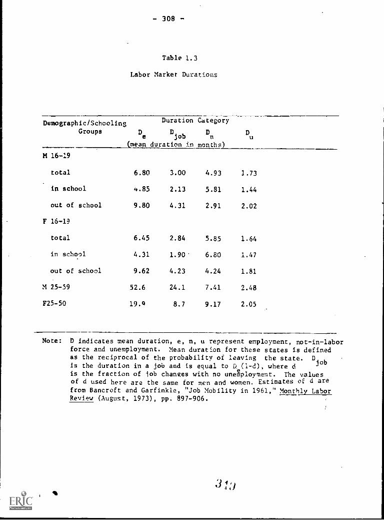
- 308 -

Table 1.3

Labor Market Durations

Demographic/SchoolingGroups

Duration Category

De

Djob

Dn

Du

(mean duration in months)

M 16-19

total 6.80 3.00 4.93 1.73

in school 4.85 2.13 5.81 1.44

out of school 9.80 4.31 2.91 2.02

F 16-19

total 6.45 2.84 5.85 1.64

in school 4.31 1.90' 6.80 1.47

out of school 9.62 4.23 4.24 1.81

M 25-59 52.6 24.1 7.41 2.48

F25-50 19.9 8.7 9.17 2.05

Note: D indicates mean duration, e, n, u represent employment, not-in-laborforce and unemployment. Mean duration for these states is definedas the reciprocal of the probability of leaving the state. D

jobis the duration in a job and is equal to De(1-d), where dis the fraction of -lob changes with no unemployment. The valuesof d used here are the same for men and women. Estimates of d are

from Bancroft and Garfinkle, "Job Mobility in 1961," Monthly LaborReview (August, 1973), pp. 897-906.

,j,

" 4 1)4

. - 309 -

of jobs shown in column 2. Jobs held by young people do not appear to last very

long. The mean duration of u job for all male teenagers was 3 months. '7ven for

cut of school men the average Job lasted a little over 4 months. In

interpreting these figures, several factors should be recognized. First, the

figures are based on exit probabilities calculated from March-April and April-

May transitions. Hence, they are unaffected by brief summer jobs. Second,

these estimates overstate the mean duration of jobs and employment because of

the sampling interval. Individuals who are unemployed for less than a month may,

never appear as unemploy0-3 in the survey, so their employment may incorrectly

appear unbroken. Similarly, very brief employment spells which would bring down

the averace, nay never be recorded. It appears, tnen, that the typical teenage

job may last much less than the 3 month estimate reported here. telow, we will

examine some :mplic3L4.ons of the brevity of employment spells.

ColurAs 3 and 4 ill:,4trate the brevit.of unemployment and out of the

labo fz;rce spells. Perhaps the most surprising result is the brevity of

spells outside the labor force for out-of-school youth. The average NIL?

spell for this group lasts three months, which is only slightly longer than

the average spell length of the unemployed. This is further evidence that

these states are functiorally almost indistinguishable. There appear to be

relatively small differences between men and women, with somewhat more per-

sistence in withdrawal among women. A striking feature of the results !s

that the mean duration of unemployment is, not much different for teenagers

and adults. The much higher teenage unemployment rate results from a larger

frequency rather than a longer duration of unemployment. For most teenagers,

the labor market functions well.

- 310 -

Seasonal Variation in Labor Market Flows

Perhaps the most scriking evidence of the success of the youth labor market

in meeting the needs of most young people comes from evidence on seasonal fluc-

tuations. In Table 1.4, we examine the changes over the year in various key

labor _market rates for males 16-19. Seasonal patterns do not vary much among

youth groups, and the iaale 16-19 group is fairly typical. The first line provi-

des the unemployment rate for the summer months and the remainder of the year.

No signititant increase in the unemployment rate occurs during the summer

,months. Irideed, the rates in May, July, August and September are actually lower

than the rate over the rest of the year. Cf course, the number of unemployed

persons rises substantial] because as the se,:ond row F!1OWS, the participation

rate soars. The particiintion rate in July is almost 40 percent moie than its

average. As line 3 indicates, a parallel rise in the employed protor-

tion also takes place. lot surprisingly the vast majority of thin increase

in employment is due to summer-only workers. In the fourth line of the table,

we present the proportion of the population who enter the labor force each

month. In June, almost 21 percent of the male teenage population enters the

labor force. This figure represents close to 50 percent of the NILF category.

Another 12 percent of tne population enter the labor force in July. Of course,

a certain amount of labor force entrance occurs in all months, averaging about

percent of the population. Contrasting this figure with the entry rates for

May, Junetrd July one finds that during the summer months about an extra 20

percent of the population enter the labor force. Note that this is a substan-

tia,. underestimate of the extent of the increase in youths' labor supnly, since

Table 1.4

Seasonal Variation in Labor Oarket Stocks and Flgwe

Male 16-19, 1968-1976

Stock/Flow Category

1. unemployment rate

2. participation rate

3. employment ratio

4. labor force inflowas a percent of thepopulation

5. labor force outflowas 4 percent of thepopulation

6. probability cf

successful laborforce entry (P

ns)

7. unemployment inflowas percent ofpopulation

8. probability offinding a job if

unemployed (Pue)

AVERAGE FOR:

May June July August September Pest of Year

,--

.129 .182 .152 .122 .149 .160

.541 .704 .758 .701 .541 .527

.471 .575 .643 .615 .459 .442

.086

.077

.213

.054

.117

.067

.060

.118

.057

.217

.073

.071

.711 .655 .670 %676 .630 .622.

.025 .073 .039 .019 .021 .028-\ f

.269 .332 186 :312 .280 .249

Annual

.155

.578

.438

.037 1

L.3

o-,

o-,

.086

.641

.031

.277

Source: Unpublished tabulations by the Bureau of Labor Statistics, adjusted by the Urban Institute asdescribed in J. E. Vanski, "Recession and the Employment of Demographic Croups: Adjustments toGross Change Data," in Holt, C. C., et al, labor Markets Inflation', andlganpower Policies,Final Report to the Department of Labor, Washington, D.C.: The Urban Institute (May, 1975).

3

- 312 -

many teenagers shift from desiring part time to seeking full tine work during th

summer months: Comparisons of the seasonality in teenage labor market behavior

with the patterns observed for other demographic-groups leads us to conclude

that about three-quartera Of summer entrances are due to school ending rather

---than fluctuations in employment opportunities.

Not surprisingly, the high rates of labor force entrance in June and July

are mirrored by high rates of labor force exit in August and September. During

these months, about 33 percent of the teenage population exits from the labor

force. Since the rate of withdrawal in a typical month is about 7 percent, the

extra labor force exits during August and September almost exactly offset the

extra entrances in the early summer months. Thus, both the flow and the stock

data suggest that employment only during the summer :ontns characterizes the

behavior of about 20 percent of male teen,laets.

The lab.,r market appears to adapt very well to the surge in those see:zing

employment. In June when the inflow is at its peak, about two-thirds of labor

force entra is find jobs. This figure is actually greater oy about 5 percent

than the rate of successfo' entry during the remainder of the year. Those who

do become unemployed during t!-e summer months fare much better than the unem-

ployed in other months, as the job finding rate Pue in May, June, and July fEl.r

exceeds the rate in the non-summer months. The fact that these flow rates are

significantly higher during the summer months suggests that the additional

members of the labor force may have an unemployment :ate much lower than that

of full year workers. Clearly, the average unemployment rate over the summer

months is lover than during the rest of the year. This suggests that the sum-

mer !nflux )f teenagers actually reduces the average annual unemployemnt rate,

3,7

- 313 -

since the additional workers appear to fare substantially better both as labor

force entrants and as unemployed job seekers than do other teenagers. This

quite striking fact bears further comment.

Undoubtedly, public employment and training policy affects the behavior

of labor market flows during the summer months. Over the first 6 years of the

period covered in Table 2.1, (1968-1973), the federal government provided about

600 thousand summer jobs through the Neighborhood Youth Corps. The NYC was

eliminated with the enactment of CETA in 1973, but summer jobs remain a compo-

nent of the decentralized employment and training system. In 1976, for example,

just over 820 thousand jobs were provided in the CETA summer program. The great

majority of participants were classed as economically disadvantaged (95.9

percent),

drawn frcm the unemployed or from outside the labor force (98.7 percent), and

were full time students (87.8 percent). A comparison of the size of the federal

summer program with the average flow into the labor force reveals the relative

importance of the summer jobs program. From 1968-1976, an average of 600

thousand summer jobs were provided through NYC and CETA. The data in Table 2.1

suggest that about 3 million teenagers left school and entered the labor market

each summer. Given the estimated probability of entering with a job (about .6

on average), en the order of 1.2 million teenagers would remain without employ-

ment if no adjustments were made. Thus, about 50 percent of this group were

moved into employment through the federal jobs program. This calculation is

likely to overstate, perhaps substantially, the contribution of public policy.

We have assumed that the federal jobs constitute net Job creation. It is likely

l'awever, that *-,e federal program funds some Jobs which would have existed

314

anyway. This is more liely to be tne case under Cr:1A, where the program

largely is run through state and local gol'ernmInt units. Unfortunately, estima-

tes of the net jobs created under the summer prograns are not available. We

plan to examine the impact of the summer jobs policy in future research.

The limited size of the summer jobs program clearly suggests that a large

number of young people are able to find jobs in the private sector. The ability

of the job market to accommodate an almost 50% increase in those desiring work

without any increase in the unemployment rate is testament to an impressive set

of institutional and market adaptations. The most important of these is undoub-

tedly the scheduling of vacations to coincide with the availability of addi-

tional workers. is likely that to some extent firms schedule certain kinds

of relatively menial work for the summer, when suitable workers become

available. Undoubtedly, some adjustment in wage rates also takes place.

The ability of the labor market to deal with the large inflow of workers in

summertime should lead one to question demographic explanations of recent

increases in youth unemployment. As Table 1.4 shows, the labor market is able

to deal with a three-fold increase in the proportion of the population newly

seeking work, without an appreciable increase in individual's difficulty in

finding employment. It seems improbable that the same labor market should be

incapable of adapting to the easily forseen, persistent, and much smaller

increase in the labor force due to demographic shifts. Indeed, the problem

should be much simpler because in this case the time frame is much longer and

there is no need to create very temporary jobs. while adaptations such as

replacing vacationing workers ani work scheduling, are less feasible in this

case, the longer run should permit much greater flexibility.

315

Taken together, the results in this section convey a picture of an

enormously dynamic labor market. It is apparent that most teenagers move

easily between labor market states. More than half of all job changes

occur without intervening unemployment. Most labor force entrants find

jobs without ever being measured as unemployed. Most incidents of unem-

ployment are quite brief. There appears to he no evidence that most teen-

agesrs have serious problems. Yet we did observe in March of 1976 that

almost one-fifth of all young people who wanted jobs did not have then,

and that an equal number were out of school and jobless, but had chosen

not to search. The key question then is whether these average probabilities,

which suggest that ::.ovement in all directions is quite easy, are relevant to

a large part of non-employment . We turn to this question in the next section.

- 316 -

II

The Experience of the Non-Employed

There are at least three reasons why the picture of the labor market preseated

in the preceding section may be a misleading guide to the experience of the

unemployed population at a point in time. First, even if most unemployment

spells are short, most unemployment may be contained la long spells. To see

this, consider the following example. Smppose thar, each week 20 spells of

unemployment began lasting one week, and one began with a duration of twenty

weeks. The mean duration of a completed spell of unemployment would be 1.05

weeks, but half of all unemployment would be accounted for by spells lasting 20

weeks. Equivalently, in a steady state, the expectation of the lengtn of time

until a Job as found, among all those unemployed at any instant would be 9.5

weeks. Sole focus on the reap duration of a completed spell could clearly be

quite misleading.

Second, as we have already emphasized, there is reason to doubt the sali-

ence of the unemployment not-in-the labor force distinction for young people.

UnEmployment durations appear to be short in large part because of high

rates of labor force withdrawal. The brevity of many spells outside the

labor force suggests that many of those who withdraw are in fact sensitive

to labor market cnnditi,,,. Indeed, it appears that our official statistics fre-

quently record two brief spells of unemployment, broken by a period outside the

labor force, when a tingle spell of Joblessness would be more a_7ropriate.

The third sense in which it is necessary to go beyond the average transi-

tion probabilities Is the need to study the incidence of multiple spells. As

Richard Layard has emphasized in his contribution to this volume, one's view

about the welfare consequence of you non-employment should depend on its

3 L

317

(111:7,prItr.:.tinn, If th. burden 1. quite ...%,r,nly ri4$11Priai, individuals are unli-

kely to suffer greatly and the economy may even benefit from a better matching

between workers and jobs. On the other hand, if the distribution of

unemployment is very uneven, the welfare cost to individuals is likely to be

greater, and tie social benefit much more dubious.

In this section, we try to deal with these three issues by studying

the distributions of unemployment and non-employment weeks. Basically, we

seek to answer two questions. First, how long can we expect the teenagers

who are unemployed at a point in time to wait before entering employment?

Second, how much une:-*loyment and non-employment can they expect to suffer

within the year? It is crucial to realize that we seek to answer these two

questions for all those unemployed at a point in time, rather than all those

who flow into unemployment over some interval. This procedure gives more

weight to long spells than to short ones, since persons suffering lengthy

spells are more likely to appear in the sample at a point in time. In

assessing the nature of the unemployment problem, one wants to study the un

employed population, not the experience of persons flowing into unemployment.

This key point is illustrated by the numerical example above in which much

of unemployment was due to long spells eventhough the vast majority of spells

were short.

:tow long does it take to find a Joo?

In Table ll,we present various estimates of how long it takes young people

to find jobs. The first row displays the mean duration of completed une:aploy-

ment spells. he durations of unemployment, as we have already noted, are quite

3

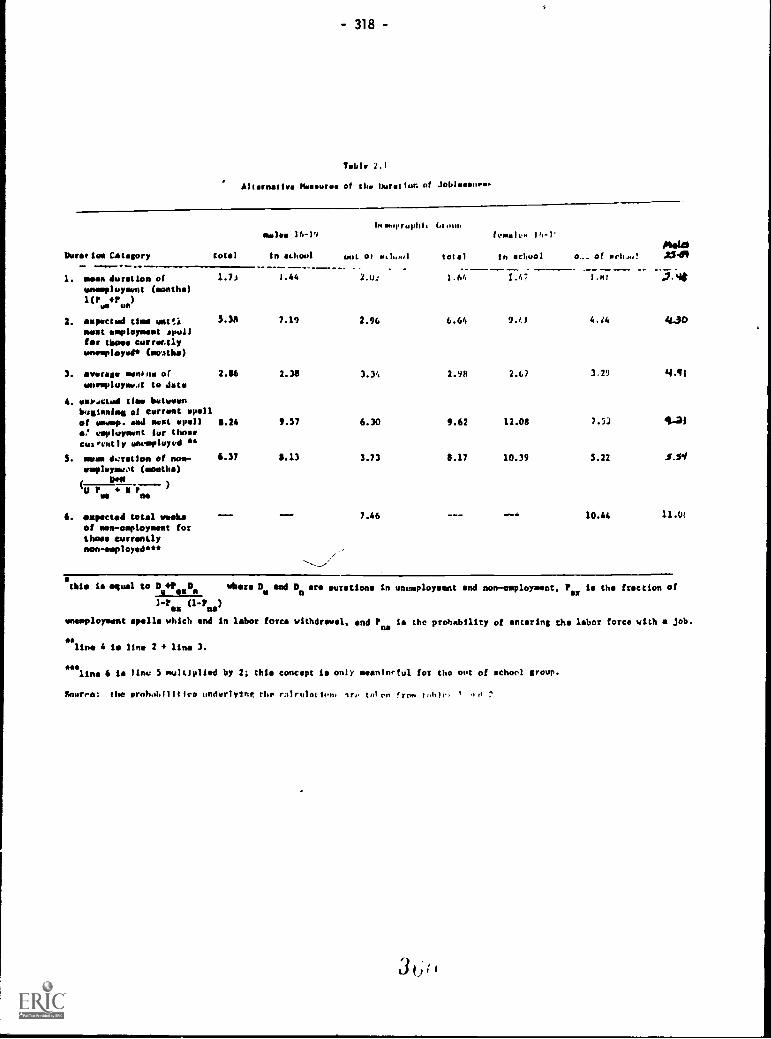
Duration Category- ----- -

1. mean duration ofwneoployownt (months)icr r )

WO tan

2. mpectud time unttimost soploymest pullfor those currentlyunemployed* (maths)

3. average room, ofImemploymeat to Jots

4. usw.otted 1.1mo betweenbuglaning of current *pallof ~op. sod mat smelle.' vepIumeent fur thorrmotel:n(1y emempluyed *

S. mom M:ratlen of now-rimpleymeA (mouths)

WM(U r

WO111,

WO)

6. expected total weeksof rem- employment fortheme currentlynon-esployed

- 318 -

Toblt. 2.1

Alternative MO f for Duration of Johloosnow,

total

melee 16-19

in 8000

Ino.rreohl,

uut ot mh..,1

Giono

total

______-___

female. 14-1'

in school 0..: of och,o!0910.1544

_ _1.7i

____.1.44 2.0: 1.64 1.47 1.81 .7.*-

3.38 7.19 2.96 6.64 9.41 4.14 430

2.86 2.38 3.34 2.98 2.0 3.29 4.11

8.24 9.37 6.30 9.62 12.08 7.51 1-21

6.37 8.13 3.73 8.17 10.39 5.22 5.84

7.46 10.44 11.01

tbls is equal to D 4, D where Da and D0 are Durations in unemployment and non-employment. Pax IS the fraction of

1-Pea (1-Paa)

mneoployment spells which end in labor forte withdrawal, and Pam Is the probability of entering the labor force with a job.

line 4 is line 2 4 line 3.

line 6 Is lino I multiplied by 2; this concept is only meentneful for the out of school group.

Bourret the prnhahIlitleo undetivinv, the ralrolottom 1r tnler fern. f.h)p, '

319

short. Ar we have noted, however, labor force withdrawal makes Lhis a

Aisleading indicator of the ease of job finding. In line 2 we attempt to answer

the more meaningful question of how long the unemployed must wait until a job is

found. This calculation recognizes the possibility of labor force withdrawal

and th.. attendant decline in the probability of finding a job. The possibi] ity

of labor force re-entrance into unemployL;ent is also taken into account. The

average unemployed male teenager in March of 1976 could expect to wait 5.4 more

months before finding a job. Line 3 notes that the average male 16-19 had been

unemployed for months. Hence, the average unemployed person was in the midst

of a spell of over 2.86 months of joblessness. The notion that most of those

currently unemployed can and will find ,jobs quickly is si:;Iply false. Y.cst are

in the midst of lengthy spells without work.

Even the large estimates above nay understate the ease of rove ;.e-.t

into Jobs. We have argued that many persons who are out of the labor force

behave in ways which are functionally equivalent to the unemployed. In line

5 we report the expected length of time until a job is found for currently non-

employed young people. Doubling this figure yields the mean total duratica

of joblessness for the non-employed. The results indicate that it takes most

persons a long time to find a job. The average non-employed young men who is

in school will have been out of work for about 7.5 months before returning to

employment. The corresponding figures for women are even larger reflecting

greater persistence of labor force withdrawal. All of the estimates in Table 4

are conservative since they do not take account of the fact that continuation

probabilities decline with duration.

- 320 -

How extensive is Unemployment?

While the evidence suggests that joblessness is frequently prolonged, we

have not yet considered multiple spells. The annual March Work Experience

Survey asks all civilian non-institutional respondents in the CPS to describe

their work and unemployment experience in the preceeding year. We have used the

Work Experience Data to calculate two measures of joblessness. The first is the

official definition of unemployment as weeks looking for work or on layoff. This

concept is referred to as "non-employment." It is important to note that non-

employment excludes weeks out of the labor force for those citing illness,

fmaily responsibilities, or "other" as the principal reason for part year work.

For these individuals, non-employment is defined as weeks of unemployment. In

both calculations, persons who did not participate in labor force are excluded

from the sample.

The distribution of unemployment and non-employment for selected demo-

graphic groups is shown in Table 2.2 .0f the approximately 6 million young people

with labor force experience, about 1.7 million experience unemployment,

averaging about three months during the year. The average number of weeks is

almost 50 percent greater for the out of school group. While the number of per-

sons experiencing non-employment is not different from the number with

unemployment in this sample, weeks of joblessness are significantly greater when

time out of the labor force is included. Out of school youth average 6 months

of non-employment per person becoming non-employed.

In line 6 of the table we examine the experience of the unemployed papule,"

tion as of a point in time by focusing on the distribution of unemployment an

non-employment weeks. ?ecause unemployment weeks are captured randomly by tIle

I

ti

'fittriertliniUrrarresesporieece (utilioes)

total with unemployment(eilliees)

Average weeks of weerploymost per personwith unemployment

total with sommnpley-mot (millions)

Amoroso weeks of nos-employment per parseswith mm-osplement

51strlhotfon ofIndividuate endvftehm by Migrim,

1-4 veuk3

- 321 -

Table 2.2

The Coaceetratios of Osemploymant sad Moo-Maployment

for Toesumma "-- 1974DemogrJALc Groups

Mal.. Femalue

total out of school total out of school

Mon-WhiteMales Females oat

out of school of school

5.99 2.82 5.27 2.44 .31 .30

1.71 .91 1.56 .85 .14 .17

12.7 18.6 10.4 14.9 20.1 16.4

1.71 .91 1.56 .85 .14 .17

16.2 25.2 15.4 24.1 29.0 30.3

U NV U N1! U NE U NE U ME

of labor Wee 11.2 10.1 4.2 4.2 14.4 12.6 10.9 6.9 7.3 4.6 17.1 9.0

7. of total. woke 6.2 4.4 2.1 1.0 4 4 1.$ 4.2 1.6 1.6 .7 3.7 1.0

1-14 woksof !ober force 9.0 7.9 9.7 7.3 5.1 7.2 9.9 7.7 143 11.3 17.5 8.0

7 of total veeks 24.1 17.0 16.0 9.0 26.4 15.5 19.1 9.1 17.5 3,5 111.5 4.6

15 -26 yal's

,41 'abut 1.rre 4.1 2.1$ /1.1. 5.1 4.0 2.4 4.2 4.5 o.4 2.2 :.3

Z of total wuuke 21.5 12.7 18.2 13.7 27.1 11.0 31.2 12.0 i4.6 1.4 :11.6 S.3

/1-19 weeklahfor forre 2.3 1.1 4.4 7.2 1.5 7.1 1.i 5.1 m.0 9.0 .4 7.3

WrpitN !I.) 24./ 16.1 211.9 54.2 /7.1 ?0.1 :11.6 1'2.4 1)4

4011

I 1 th.or

t..1.1 wv,km

1.0/4.0

4.141.1

1.61/.4

M.44/.4

1.711.1

4.741.4

/.411.5

10.1

:1.7

/.5

u.1

11 /

"1.0

-.322-

survey, the statements that "x percent of unemployment weeks are suffered by

persons with y weeks of unemploymentduring the year," and "x percent of the currently

unemployed will experience y weeks of unemployment during the year" are equiva-

lent. Both the unemployment and non-employment distributions exhibit substan-

tial concentration, with the preponderance of unemployment attributable to per-

sons out of vork more than half the year. Among out of school male teenagers,

54 percent of unemployment, and 76 percent of non-employment were due to

persons out of work more than six months. Among young black men who were

not enrolled in school, 65.0 percent of the unemployed were out of work more

than 40 weeks during the year. As one would expect from these figures, indi-

viduals with brief, infrequent unemployment experience contribute only negligibly

to overall unemployment. For example, persons out of work less t%do three months

accounted for only 21 percent of non-employment among young men who were

out of school. While many teenagers experience short periods of unemployement

in moving between jobs, these are of little consequence in explaining total

weeks non-employment.

The statistics in Tables 5 and 6 tell a consistent story. Youth unem-

ployment is properly understood in terms of a fundamental failure of the labor

market. A small portion of the population finds itself chronically unable to

locate satisfactory work. They do not have the same ease of transition which

characterizes the remainder of the population. Rather, they wai, long periods

between jobs. Moreover, they experience frequent unemployMent because o'7

frequency with which they leave employment.

Employment exit and Extensive UneTployment

Many observ,4 regard the brevity of employment spells emphasized

in Section I as the root cause of the youth non-employment problem. The

323

results here call tent interpretation into question. For most young people

frequent job change appears to be possible without extensive unemployment.

The median length of unemployment spells is probably about three,weeks.

Half of all job changes occur without any unemployment at all. A person

who held five jobs dqrins the year, and was unemployed during each change

for the median length of time, would sLffer only 12 weeks of unemployment

during the year. Persons with this little unemployment contribute less than

one-fourth of all youth unemployment. it is therefore clear that without

serious difficulty in job-finding even extreme employment instability

could not account for observed patterns of concentrated joblessness.

A similar conclusion is obtained by exP.mining in more detail the experi-

ence of young people reporting extensive joblessness. Among persons with

over 26 weeks of non - employment, who accounted for 76 percent of jobless-

neso, the average number of unemployment spells was less than two. In many

cases these spells were separated by periods outside the labor force rather

than by jobs. Hence, this is an overstatement of the average number of em-

ployment spells during the year. Even neglecting this correction the average

spell length of the extensively non-employed appears to last close to 5 months.

Thus, for this group, where the real problem lies, the difficulty prolonged

unemployment rather than frequent joblessness.

Nothing in the preceding paragraphs is inconsistent with the common

observation that differences in demographic group unemployment rates are

largely due to differences in the frequency of spells rather than their

duration. The point here is that for the problem population, it is very

difficult to locate a suitable job. The demographic observation simply

addresses the incidence of "problem" people in different subgroups of the

324

population. Once iL is recognized that noi-employment is largely a matter of

small minority of all demcrrauhic grOupi with serious job finding problems,

the fallacy of inferring the nature of individual problem unemployment, from

comparisons of demographic averages becoales clear.

'

325

III

Cyclical Variations in Ersloyment

The cyclical behavior of youth employment and unemployment can shed light

on the nature of the non-employment problem. If extensive Joblessness occurs

only because come young people are essentially unemployable, one would expect

changes in aggregate demand to have smell effects. On the other hand, a finding

that changes in aggregate demand has a large impact on young people would imply

the existence of a chronic shortage of attractive jobs. Of course, a finding

that aggregate demand has a potent effect on the youth labor market need not

-,imply the desirability of expansionary macro economic policy, which has other

perha;s undesirable consequences.

Ehnloyment, Unemplovnent and Participation

The cyclical sensitivity of unemployment is the reflection of two luite

different phenomena. Unemployment can ...ncrease either because fewer jobs are

available or because more workers decide to seek the available jobs. These

two sources of unemployment obviously have quite different welfare implications.

While the former is almost certainly indicative of a worsening of labor market

performance, the latter may reflect an improvement in conditions. Focus only

on unemployment rates is thus very likely to be misleading. Moreover, the

results in Section I suggest that NILF-unemploved distinction is quite arbi-

trary. These considerations indicate the importance of examining the cyclical

behavior of employment, unemployment, and participation.

These three measures summarize tre labor market experience of a given

demographic group. They are related by the following identit _

E E

Ni Li Ni (3.1)

- 326 -

wnere E is employment, fl is population, L is labor force, and i indexes demo-

graphic gfoups. Taking logs and differentiating yields:

d In = d InL

+ d In ()(3.2)

Thus charges in the employment ratio may be decompose] into changes in employ-

ment and participation rates. Since persons in the labor force are either

employed or unemployed it is clear that:

d ln = d In (1 - UR). + d ini N (3.3)

where UR is the unemployment rate.

The results of the decomposition in Tal.le 3.1 show clearly the importance

of fluctuations in participation during the past few years. For young women,

changes in participation are generally much larger than changes in the rate of

utemployment. While movements in participation are less pronounced for young

men, they still account for a significant part of movements In employment. It

is thus clear that serious studies of the youth labor market mu5t examine both

unemployment and participation. This point has been drifen'home by recent

expe.ience. Over Go percent of the increase in youth employment which occurred

between 1976 and 197T was due to increases in employment rather than reductions

in unemployment. For black youth, the situation is even more striking. The

black male unemployment rate has risen, while at the same time the employment

ratio has cicreased due to the surge in participation.

- 327 -

Tale 3.!

el Cian4es in the Er.ploy=ent Ratio

ie in

Em- lc -r_ :it Ratio

Percent Change in Percent Change in

Participation Rate Employment Rate

:.0 i. ;,

lr

lilt -3 4.8 2.4 2.4

1973-4 -0.5 1.5 -2.0

1974-5 -8.2 -2.6 -5.6

1375-i 1.8 6.6 1.2

l9,i-7

ibz= 1J-li

5.3 3.0 2.3

Tc.:

372-3 5.8 4.1 1.7

1373-4 1.5 3.1 -1.5

1974-5 -4.0 -0.1 -3.9

1975-i 2.9 1.6 1.3

1976-7 3.4 2.9 I 0.5

Sots: Calculations as described in the text.

3 C:J

- 328 -

A Sirole Model

The cyclical responsiveness of the youth labor market is estimated using

a quite simple model. For each group we postulate that the unemployment rate

and participation rate are functions of aggregate demand, seasonal factors,

and time. The time trends are included to reflect the impact of slowly changing

social trends, and other gradually moving variables omitted from the equation.

Seasonal movements are captured with monthly dummies. The basic equations to

be es:ieafed are:

wheee

8 11

ln( ?R). = ao +E UPRIMEt-j

. ZOSk +S1 T+ T67 + V.i =0 k =1k=.1

it -j k 2

8 11UR. T. ao E a

t-

. UPRIME . + E Y, S + ,IT + 2T67 + uit1=0

lt t-3 K k

,-went rate of men 35-44, T is the tine trend, T6-

(3.4)

(3.5)

is a second tine trend which begins in 1967, and Si are monthly dummies.

The specification of (3.4) is traditional in analyses of participation.

The prime male unemployment rate is assumed to measure variation in Job oppor-

tunities and the ease of job finding. Since workers may respond to changes in

the availability of Jobs with a delay, lagged unemploymenti3 also included in

the equation. ',Mile equations of thin sort have not been extensively used in

studying the cyclical behavior of group unemployment rates, they are Justified

by essentially the same arguments.

The model is not designed to provide the best or most detailed explanation

of the participation (unemployment) rate of each group. Our purpose is to esti-

mat_ a comacn :ncdel for each group which capt,res the response of participation

(unemployment) to cyclical fluctuations in aggregate demand. Thus some poten-

tial explandt-Jry varlales have 'Jee- eYcl;-!el because they vary

3

- 32Q -

"cyclically. Others have been omitted because they are essentially orthogonal

to the variables included.

The specification appears to be quite robust. The results presented below

are almost completely insensitive to changes in the measure of aggregate demand,

and variations in the way in which the second time trend is entered.

Our experimentation suggests that neither demographic variables, inflationary

expectations, or measures of household wealth and liquidity have any systematic

effect on participation. Moreover, our results decisively reject theories of

labor supply which emphasize the timing of participation and the intertemporal

substitution of leisure and work, and which explain unemployment as a voluntary

phenomenon. In any event, these variables have little impact on the estimate

of cyclical effects. We have also experimented with a minimum wage variable.

While it is sometimes significant, it has litt2e impact on the estimated

cyclical effects and so the results are not reported here.

The interpretation of the coefficients of the model is straightforward.

For example, the cyclical responsiveness of the participation rate of the ith

group is measured by'fiR

E8t-j

A value of 1.0 implies that a 1 percent

P

increase in aggregate demand (e.g., UPRIME declines from .06 to .05) produces

a 1 percent increase in the participation rate of the ith group (e.g., .430

to .434). Equations (3.4) and (3.5) have been estimated using both annual and

monthly data for the period (1948-1977) for trarious demographic groups. The

identity (1) along with the properties of ordinary least squares insures that

the relationship between the employment ratio, aggregate demand and time is

given by:

111n(EN)

it= So - ao + Z(3 -a ,)UPRIME + r (0

k)S

t-j t-jk=1

k k

+ (SI - 41)t + (62 - h)T67 *ti

(3.6)

330 -

It follows immediately that the equations presented here can be used to

decompose cyclical movements in the employment ratio into unemployment and

;artist-cation cc.mponents since:

Y. YEN YN PR UR(3.7)

In order to insure that this identity is exactly satisfied we have estimated

all the equations using ordinary least squares without correcting for serial

correlation. The results for individual equations, however, are not sensitive

to this choice. The estimated equations are shown in Table 3.2.

The crincinal conclusion which emerges'is the tremendous responsiveness

of youth employment to aggregate demand. For men 16-19, each (.11.0 point decrease

in the prime male unemployment rate increases the employed proportion of the

copulation by about 4.5 percent. About two-thirds of the response comes through

unemployment, with the remainder due to increases in participation. For women

15-19, the cyclicalrespon6iveness estimates are comparable, with participation

somewhat more responsive, and unemployment somewhat less responsive to aggregate

demand. In line with the traditional view of disadvantaged youth as likely to

be "last hired" and "first fired," black youth employment is even more

cyclically senstive than the total group. For black men 16-19, each point

reduction in the unemployment rate raises the employment ratio by close to 6.3

percent. A comparable figure obtains for black women.

The substantial cyclic response to changes in aggregate demand suggests

that 3 shortage of job opportunities characterizes the youth labor market. If

there were not a dearth of good jobs, aggregate demand would not be expected to

have a significant impact on youth employment. The very strong response of par-

ticipation to unemplOyment confirms the importance of focusing on employment

3 ".)

331

rather than unemployment in assessing labor market conditions. It also

supports the argument of Section I that much of the high rate of labor

force withdrawal among the unemployed is attributable to discouragement.

The strong cyclic response of employment and participation to aggregate

demand reflects the large inflows and outflows described in the first section.

The surges in employment and participation which accompany increaecc in

aggregate demand may be due either to increased inflows or decreased outflows.

That is, low unemployment may raise employment either by helping workers get

jobs or by helping them hold jobs. In order to examine this issue we :_d -e

estimated equations describing the time series movements in the monthly flow

probabilities. In addition to trend, cycle, and seasonal variables, we also

studied the effects of minimum wage legislation and Federal youth employment

programs. Since we were unable to isolate a significant effect of eitlier

of tnese measures on transition probabilities, the results of estimating the

equations in which they were included are not reported here.

Table 3.3 summarizes the results of the flow probability equations.

The first set of equations describesthe probability of employment entrance.

For all groups, especially men, the rate of entrance is very sensitive to

demand. For men, a one point increase in the prime male inemployment rate

reduces the probability of entry by , or about 9 percent. It is changes

in entry rather than exit behavior which are the prime cause of employnent

fluctuations among young men. The rate of exit does not appear to exhibit

significant cyclical fluctuations. The reasons for this difference are not

clear. Cne possibility is that women are the first to be laid off in downturns.

A more plausible explanation is that the entrance rate does not fall as unem

ployment rises, because more women enter the labor force as their family

income falls.3 $ k.1

- 332 -

3.2

i : . :a1..ci;.:tcn and EtTloysent

by Ienaae Dtacirapnic Gr.:vt

3r:41Deier.2tt %-tiabls

CeN5

1. )g.:% :9-19: Total

une:plaFttant rate .02

(.005)

participation rata -.47

(.01)

t=p1:y-vet ratio -.50(.01)

2. )lea 16-19: San-hitt

unerplo)manc rate -.046(.03)

partitipation race -.35

((.03)

eav::y:-.2c: ratio -.30

(.04)

3. U:ten 1c-14: Tota!

nnt-p:..1!-eat raze -.009(.007)

participation rats -.83(.01)

esplzyzoac Esti* -.81

(.01)

4. U:m.gn It-19: Non-...bite

untnployzenc rate -.04(.04)

participation rats -1.11(.05)

employ -enc ratio -1.07(.07)

Independent Variabl's

MIME(121102)

I SEE OW

2.77 .35 -.15 .84 .018 .85

(.10) (.02) (.06)

-1.87 -1.11 2.82 .95 .035 .73

(.19) (.04) (.11)

-4.64 -1.45 2.9$ .95 .037 .72

(.20) (.046) (.12)

4.29 1.14 -.21 .69 .051 1.32(.36) (.12) (.23)

-1.99 -2.12 .84 .90 .064 1.13(.45) (.14) (.28)

-6.29 -3.26 1.05 .87 .085 1.27

(.59) (.0) (.37)

1.72 .32 -.36 .82 .021 .94

(.11) (.03) (.07)

-2.29 -.44 3.48 .93 .039 .69

(.22) (.05) (.12)

-4.07 -.96 3.84 .89 .045 .60(.24) (.06) (.14)

3.45 1.58 -.99 .58 .070 1.44(.49) (.16) (.31)

-2.96 -.22 1.02 .75 .105 .115

(.74) (.24) (.46)

-6.41 -1.80 2.00 .65 .131 .932

(.92) (.29) (.58)

Sots: the ccmffitieri: on LIMA is the sus of the coefficients obtained (con a nine monthA1mon leg (first Jest**. tar restriction).

3 7'

- 333 -

TJblz 3.3

of Trarsition

1968-1976

(,tariatd crrors in parentheses)

Independent Variables

UPR12

SEETr_ - ?.'t

U 2It

rc7-,:(12x10 )

1.

_it Varlle

pr31:::ilicy of

e7i.:2=ante:..tra-ee

Mli19 .093 -1.44 -.185 .937 .019 -.050

(.073) (.257) (.105) (.105)

:in-...1; .112 -1.420 -.264 .856 .024 .002

(.032) (.357) (.146) (.105)

:1013 .051 -.273 .169 .930 .010 -.293

(.011) (.110) (.048) (.100)

:-'4 .110 -.246 -.206 .796 .017 .029

(.023) (.254) (.104) (.104)

2. pr_:, :-:icy of

r111 -ell: 23[1:

Niclv .229 .213 -.317 .946 .015 -.105

(.018) (.194) (.079) (.104)

2.'1-li .134 -.696 .216 .839 .030 .002

(.051) (.551) (.218) (.104)

Vloli .250 .591 -.535 .940 .015 -.154

(.017) (.184) (.075) (.104)

E..: '.'3 .364 -.493 -.714 .793 .048 -.060

(.059) (.642) (.262) (.104)

3. prhiltry of11"_3t force entrance

M17.13 .063 -.760 .378 .961 .020 -.122

(.024) (.266) (.109) (.104)

151oli .170 -1.148 -.115 .932 .02%

(.039) (.435) (.178)

41:19 .032 -.036 .324 .959 .012 -.258

(.013) (.142) (.OSS) (.101)

S61i14 .104 .291 -.064 .885 .023 -.018

(.030) (.317) (.133) (.105)

(Continued...)

:43/4e 4 3 z,utilLe4

- 334 -

Independent V -fables

CONS MIME T a SEE1. (12x102)

Cr:Jp

2C,c3.:::-.0 Variable

4. Prabaility cfLabar farce exit

M:619 .255 .578 -.541 .940 .014 -.041

(.017) (.190) (.077) (.104)

1M1619 .173 .498 .026 .851 .029 .112(.043) (.478) (.195) (.104)

1.1619 .280 .627 -.592 .920 .014 -.158(.016) (.173) (.071) (.104)

r..1o19 .238 1.23 -.149 .753 .036 -.004(.047) (.515) (.211) (.106)

NJ:a: the czeffirient en MIK': is the sum of nine month Almon lag (first degree, farrestriction); earn regression vas estimated with seasonal dummies, end correv.:.::for first order aLtocomlecian.

335

The rates of labor force entry and exit also vary cyclically. The rate

of exit fells daring recessions lar3ely because the probability of withdrawal

is rack greater for the unemployed than it is for those who are employed.

For the rale groups the probability of labor forte entrance is strongly

cyclical. It is much less cyclical for women because of the added worker beha-

vior noted above.

On balance, the flow probability equations bear out the basic conclusions

of this section. They demonstrate that both labor force entry and employment

entry become siz,nificantly easier during peak periods. This is completely

)cons stent with the findings about the responsiveness of non-employment to

the state of local labor markets, noted by rreeman. Taken together with

the evilence that most unemployed teenagers are in the midst of spells of

prolonzed joblessness, these findings su2zest that a shortage of attractive

jobs accounts for much of teenage unemployment.

"*-1t 1 ,

- 336 -

IV

Conclusions and Implications

In this section, we discuss the implications of our results for policies

designed to combat youth unemployment. Our argument can be stated in quite

bold terms. Expansionary aggregate demand policy is the only proven way of

enlarging the employment opportunities open to young people. A consistent

effort to keep the unemployment rate near its full employment level would do

more to help young people find jobs than almost any other conceivable govern-

mental policy. Of course, Other considerations might suggest that, on balance,

such a policy is not workable. While certain structural policies might have

salutory effects, it is highly unlikely that they could succeed except in a

full employment economy. After discussing the positive effects of a tint

labor market, we tui to an examination of potential structural initiatives.

The '1acro-Economy and the Youth Labor d'arket

As Section III showed, both teenage unemployuent and participation respond

strongly to labor market conditions. A reduction of one point in the prime-age

male unemployment rate raises the proportion of teenagers who are employed y

about ! percent, which is split about 2:1 between a reduction in unemployment

and an increase in participation. For black youth the proportion rises about

6.5 percent split in a similar way. These figures imply that the 1975 recession

cost young workers about 800,000 jobs. The growth in the economy during the

late 1960's created close to 300,000 sobs for young workers. Fvidence from

cross-section data underscores- the responsiveness of teenage unemployment to

changes in demand. Freeman (1978) and Clark and mummers (1973) have shown that

the youth employment ratio is much higher in strong tnan in weak local labor

markets.

- 337 -

Expansion of aggrega`e demand is esi.eclally potent in making available

opportunities for those who are most disadvntaged. Between 1969 when the

aggregate unemployment rate was 3.6 percent, and 1976 '.hen it was 7.7 percer,t,

the proportion of 15 and 19 year olds suffering more than 6 months of unemplov-

ment rose fourfold. For black youth the same figure increased by almost 6

times. The treelandous impact of demand on the amount of long-term unemployment

is particularly important in light of the results of Section I. The evidence

presented there suggests that while most teenagers experience little difficulty

in moving into and out of employment, most unemployment is concentrated among

those who face serious difficulties in obtaining jobs. The teenage unemployment

problem is not the lack of desire to hold Jobs, but the inability to find work.

A shortage of Jobs atteaes to be the only explanation for the large respon-

siveness of enpfoyment to changer: in _e :and. If unemployment were simply a

matter of instability, there would be little reason to expect, it to respond

strongly to aggregate demand.

We conclude that the existence of a job shortage must be the central

reality dominating efforts to evaluate or design structural initiatives to

improve the labor market for youth. It seems clear, for example, that the

existence of a Job shortage is of fundamental importance in assessing the

policy implications cf the instability view of teenage unemployment.We

have noted the allegation that high turnover is the principal culprit in

high youth unemployment rates which yields policy prescriptions designed to

improve school to work transitions and upgrade teenage workers. However,

in the face of a Job shortage, reduction of turnover will only redistribute

the burden of unemployment. Without job vacancies to be filled, or a..1 increase

- 338 -

in the number of jobs, reduced instability wouci- simply reduce the frequency

and increase the duration of unemployment spells.

Before ve turn to an evaluation of potential structural initiatives. it

is usef41 to review the extent to which erong aggregate de1and can achieve

structural goals. A key objective of almost all structural programs is to

aid youth -in ghtaining the skills acid employment expfrience decessafy to sucI,

ceed in the adult world. These goals are accomplisl-ed to a large extent by

expansionary macro - economic policies. Between 1969 and 1976 t6e rate of job

loss rose by about 75 percent, substantially reducing the ability of young

people to accumulate experience. ,Cyclical decreases in the youth employment

rate also cause reductions in on-the-job training. Spndard estimates (e.g.

Mincer) suggest that an` extra year's expe-rience raises earnings by about 2-3

percent. Ell rood's results in this volume appear to be consistent with this

figure. This figure suggests that the 1975-1976 recession reeducel/by a

significant amount the lifetime earnings of the youth cohort,. Since each year

o2 youth non - employment costs about $20,000, this implies;tAt the extra non-.

employment had a present value cost of about 16 billion dollars. This

calculation is a substantial underestimate of the true difference which cyclical

conditi,,ns can make in human capital forzation. It ignores the benefits of both

worker upgrading and the_likelihood that if labor was in short supply employers

would compete at least in part, by offeringtrainng. When these factors are

considered, it is clear that expansionary macroeconomic policy can do a great

4Ib

deal to achieve -structural Foals. .

The Role of Str iral Policies

The resits In Section III bear out Feldstein and Wright's 1 1710 concl

339

sion that even if the prime-age male unemployment rate were reduced to 1.112r,2-

cedented levels, teenage unemployment rates would remain relatively hi,z11.

This fact has led many to conclude th4 only structural measures can make an

effective dent in the youth unemployment ;problem. As we have argued elsewherc,

this inference is misleading. Youth unemployment rates remain so high

aggregate demand increases in large part because of increases participatIbu

In Clark and Summers (1979) we show that if the mature'mle une loymer.t rite

were driven down to its 1969 level, and participation were not allowed to expand,

the teenage unemployment rate would fall to close to 6 percent. The question

remains as to whaif any contribution structural measures can make. These

policies may be divi]ed into three broad categories: 1) programs to ail

workers in searching for jobs through job matching or improved informat:on;

2) job training programs designed to provide 'orkers with necessary sk-ii

3) job creation programs designed to make available s-)ecial jobs for you`h

groups.

A detailed review of the evidence and discussion of the effectiveness of

job matching, job training and job creation programs is beyonl the scct'e of

this paper. Our results, howeier, _suggest the following observations. First,

given a shortage of jobs, training and Job matching programs offer little

prospect for making a significant contribution to the solution of the youth

unemployment problem. Aidi ig any single worker through training or improvel

transition to work will improve his chances at the expense of others. 4s

long as there are only a fixed number of jobs, total employment cmnot be

increased by helping all workers augment skills or search more efficient17.

Each worker's additional sear.:11, for example, detracts from the

3c4

340

open to other workers and so generates a negative externality. Und.!r these

circumstances, belief in training and job matching reflects the fallacy of

composition. Matching and training programs cannot have the desired effects

unless coupled with an expansion in the number of jobs. If such a- expansion

is forthcoming, and employers experience difficulty in filling vacancies,

training and market transition programs could prove useful.

Second, direct job creation through public employment or private sector

subsidies appears to offer the most promising structural approach to the youth

unemployment probleri. Like training programs, the impact of policy can be

focused on those groupS who account for t' bulk of teenage unemployment.

Moreover, the policy is directed at the root of the problem: a shortage of good

jobs. The success of such programs, however, depends on the extent of net

job creation and the provision of skills and experience useful to young persons

over the longer term. The evidence presented in Section II suggests that

governmental efforts to provide Seasonal jobs for disadvantaged in-school youth

have met with some success. The eff_ct of other government programs like the

Youth Conservation Corps, the Job Corps and Public Service Employment remains an

open question in need of further research.

Conclusion

This paper has presented evidence on the characteristics znd sources of

teenage unemployment. Our results underscore the dynamic character of the youth

labor market, but suggest that market dynamics cannot account for the bulk of

youth joblessness. The job instability - turnover view of unemployment is

applicable to the majority of teenagers who experience little difficulty in

moving into and out of the labor force. Most unemployment, however, is con-

3

centrated among those people who are ure!mployed for extended periods, and vho

face serious difficulty in o'Dtaining employment. The results suggest that the

problem of teenage uncriployx,eNt arises fires: a shortage of attrat_tive jobs. The

evidence in Section III indicates that aLgregate demand has a potent impact on

the job prospects and market experience of teenagers.

342

References

Clark, K. B. and L. H. Summers, "Labor Force Transitions and Unemployment,"April, 1978, unpublished.

Feldstein, M. S. and Brian Wright, High Unemployment Groups in Tizht LaborMarkets, H.I.E.R. Discussion Paper 11488, June, 1976.

Hilaski, H., "The Status of Research on Gross Changes in the Labor Force,Employment and Earninzs, October, 1968.

Kaitz, H., Monthly Labor Review, 1970.

Marston, Stephen, "Employment Instability and high Unemployment Rates,"Brookings Payer on Economic Activity, 1976: 1, p. 169.

Mincer, Jacob, Schooling. Experience and Earnings (New York: National Bureauof Economic Research, 1969).

Vanski, jean, "Recession and the Employment of Demographic Groups, Adjust-ments to the Gross Changes Data," unpublished.

.)0 ,.., '1

- 34 3 -

FAMILY EFFECTS IN YOUTH EMPLOYNEW

Alberc Rees and Wayne Gray

I. Introduction

Recent work on youth unemployment has advanced two contrasting

models of the yoilth labor market. One view emphasizes high turnover

rather than the shortage of jobs for young people. It can be illus-

trated by the fallaing quotation from Bally and Tobin: "Much teenage

unemployment, it is often observed, comes from dissatisfaction with

the avilable job options, a gap between expectations or aspirations

and the realities of low wages and poor working conditions. One

consequence is high turnover. Even when jobs are available, therefore,

unemployment is high."'

The other view stresses the shortage of jobs, noting that "The

substantial cyclic response to changes in aggregate demand suggests

that a shortage of job opportunities characterizes the youth labcr

narket."2

1Martin Neil a:lily and James Tobin, "Inflation-Unemolovmmt Consequencesof Jet; Croati5n Policies," in John L. Palmer, ed., C-1eating

Public ihr,loim,2ht Pri,-)maras and Wa'-e Subsidies (ashington: Brcol:ings,

7978), p. 6J

2Kim B. Clark and Laysrrence H. armerE., "The Dina:Ides of Youth Une:-:loyment",

NBER Par No. 274, p. 52

- 344 -

In Keynesian terms, the first view sees much youth unemployment

as voluntary at prevailing wages; the second sees it as primarily

involuntary. The first vicar suggests that youth unemployment could

be reduced by raising the ratio of youth to adalt wages; the second

implies that it could be reduced by lowering this ratio.

This paper provisionally adopts the second view and seeks to

test one of its implications. If there is a shortage of jobs for young

workers at prevailing wages, then there must be one or more nonprice

rationing mechanisms that determine which young people get the available

jobs. Our special hypothesis is that the family of the young person

furnishes such a mechanism; those young people get jobs whose parents

or siblings have jobs, particularly jobs in which they can influence

hiring decisions. Same support for this view oan be found in rsarlier

studies of the labor-force participation of young people. Bowen and

Finegan, who found that after controlling for other forces the labor-

force participation of married women falls with husband's income, were

surprised to find that the adjusted labor-force participation rate of

males 14 to 17 in school in urban areas in 1960 rcse thrcIgh the range

of other family income between $4,000 and $11,000. In seeking to

explain this, they wrote "We suspect that part of the explanation

turns on the comparative advantage that youngsters in these families

have in finding part-tithe jobs. For one thing, their parents are more

frequently able to help, mainly as a result of their business and

social contacts. "` It is this suspicion that we explore further here.

3 .

Wiliam G. Bowen and T. Aldrich Fine^,an, The Economics of Labor ForceParticipation, ( Princeton, N.J.: Princeton UhlvLIsity Pnss, hic,), p.337.

3

- 345 -

II. The Data Set

The results presented in this paper are from the cross-sectional

data set celled the "Survey of Income and Education", collected in the

spring of 1976 (April through July). The full sample is a national

stratified probability sample of households in which 151,000 households

were interviewed. This makes the sample roughly three times the size

of the CUrrent Population Survey. The interview includes most of the

information available from CPS interviews, plus a good deal of additional

detail on sources of 1975 income and on education.

We have analyzed data for men and women aged 17 to 20 living in

nonfarm households where they are the children of the head. This ex-

cludes those young people who have moved out of their parents' household

to live by themselves or establish their own families. The group that

was 17 to 20 in 1976 was 16 to 19 in 1975, and one of our dependent

variables measures work experience in 1975. Using the ages 17 to 20

in 1976 rather than 16 to 19 also gives us a less unequal division of

the ..sample between those in scnool and those not in school.

The distinction made here between these in scnool and those not

in school is based on whether or not the person had attended school

since February, 1976. The alternative of using major activity in the

survey reference week is only viable for those observations collected

in April and May, since many June and July observations were collected

during school vacations.

The regressions presented in the next section are based cn a

data file w2 have created that mertes observation-:; on the young person

- 346 -

with observations on household income and individual data on other

members of the household 16 years of age and older.

III. Regression Results

We have been persuaded by the work of Clark and Summers, among

others, that for young people the distinction between being unemployed

and being out of the labor force is not always meaningful, since the

boundary between these states'is so blurred. Accordingly, we use

measures of employment as our dependent variables. The two measures

shown here are: (a) estimated total hours worked last year (the product

of weeks worked and usual hours per week) and (b) a dichotomous variable

taking the value of one if the teenager was employed in the survey

reference week. The models using both dependent variables are estimated

by ordinary least squares, so that the second model is a linear prob-

ability model.

We recognize that this model is not strictly appropriate, since

the estimated probabilities are not necessarily confined to the zero-

one interval. In future work we will re-estimate the final model by .

logit methods. We have also run regressions using weeks worked in 1975

as the dependent variable. These are very similar to those using

estimated hours in 1975, but the fits are not quite a: good.

Table 1 shows our estimates of the determirants of timated

hours worked last year for males and females in school andlout of

school. Table 2 shows the corresponding estimates of the 'determinants

of employment in the reference week.

3 L'

In general, we get significant effects (at the 5 percent level)

for variables measuring schooling, race, being in a female-headed

household, and being in a poverty'area. We also estimate significant

effects for the employment status of siblings, but generally not for

the employment status of the head.

Schooling

Since we are dealing with people whose schooling has often not

been completed, we measure years of school completed relative to the

mean for all people of the same age in the main SIE sample. The

variable "education gap 1" measures the number of years above the

overall mean for those who are above. " Education gap 2" measures the

number of years below the overall mean for those below. Having less

education than the average of cne's age group lowers employment signi-

ficantly in all eight regressions.

The three negative signs on "Education gap 1" in Table 1 seem

to be an anomaly arising because those people with more education than

their age group had a gr(ater than average probability of being in

school last year. In Table 2, where the schooling status and dependent

variables both refer to the same year, the signs on "Education gap 1:

are all positive.

Income

A second set of variables explored measures family income. The

one used here) other family income, is the income of the household in

1975 minus the earnings of the young persln whose behavior is being

measured. This has a consistently negative effect (not always signi-

- 348 -

ficant) on the employment of young people in school, and a positive

effect (not always significant) on the employment of young people Who

are not in school. In earlier work we used a number of additional

variables indicating whether the household received income in 197E from

various kinds of transfer payments. At some stages-of our work, a

few of these variables showed significant negative effects on some

measure; of youth employment. However, they did not remain signigicant

in the :resence of the other variables included in the final model.

Geographical variables

A third set of variables deals with various geographical aspects

of the labor market. The data set places obser.'ations in one of-nine

regions of the country. Me have included a set of eight regional

dummy variables in all regressions as control variables, and there are

always some significant differences in youth employment by region.

Variables indicating whether or net the household lived in an SMSA

or in the central city of an SMSA were not significant. The final

model includes a dummy variable taking the value of one if the house-

hold lives in an area designated by the Census Bureau as a poverty area.

In our sample 12 to 13 percent of youth in school and 17 to 18 percent

of youth not in school lived in such areas. This variable has an

effect that is consistently negative and ustlally clearly significant.

For youths in school of both sexes, living in a poverty area reduces

the probability of employment by 9 percent, other thilgs equal. Since

other family income and race appear in the regressions, this should

probably be interpreted as measuring the availability of job opportun-

,-\

- 349 -

ities in the locality.

We also tried using a variable measuring the total unemployment

rate in the SMSA for SMSA's that could be identified in the data set.

The unemployment rate was taken from a published external source

(Department of Labor estimates for May, 1976) and merged into the data

set. Only about one-third of our observations were in areas for which

we could use this information. The variable did not have a significant

effect eves-,0 regressions confiped.to observations for which the

variable could be used. We might have gotten bet-tel.' results by gener-

ating unemployment rates by area for spring 1976 from our own data set.

However, this Would have required processing data on all households, we

have used only households including youth.

Pace

We have used two variables to identify youth by race, dumry var-

iables identifying blacks and Hispanics. Both are consistently negative

and usually significant, with the effect of being black being generally

substantially larger than that of bei4Edspanic. For regressions

whote dependent variable is "employed laetyfeek", being black lowers

the probability of employment by 17 to 24 percent even after controlling

for schooling, other family incOme, and location in a poverty area.

Fcr youth not in school, in the regressions TZle 1, negative coeffi-

cients on the variable identifying blacks are about one-third the size

of the mean of the dependent variable. With other measured variables

equal, we estimate that black youth not in school worked one-third

fewer hours ir) 1975 than white youth.

I

- 350 -

We have tried using a variable measuring whether or not the

principal language spoken in the household is English; this is less

successful than the variable identifying Hispanics.

Family influences

When we started our research, we expected-to find.powerful

influences of the position of the head of the household'on the employ-

ment status of youth living at home. The effects we'find are much

weaker than we :expected. Living in a household with a femalehead

has a negative effect in all eight. regressions, and a significant

one in four. Living iria household with a self-employed male head

generally has a positive effect, but this is significant only oncet-

at the 5 per&nt level and twice at the 10 percent level.

Sets of dummy 'variables identifying male heads who were not

employed and the major industry or occupation of the employed male

heads perfo'rmed very poorly. So did an index of three-digit occupa-

tions sealed by median income in the occupation in 1969. Education

of the male head was tried and entered with a negative sign -- that is,

it acted like an index of,permanent income rather than a measure of

-access to jobs. In short, we find very little direct support in this

data set for our original hypothesis that many youths find employment

through contacts generated by their parents. At the same time, we

find other family effeCts that we had not anticipated.

Our second set of variables measuring family effects identifies

the employment status of siblings between the ages of 16 and 24 who are

in the household. Within this large set, there are four subsets, for

i,

- 351 -

older brother, older sister, younger brother, and younger sister. In

each of these subsets, there are two dummy variables, e.g. "older brother

not employed" and "older brother employed;" the base or omitted variable

of the subset is "no older brother living at home."

EMployment decisions within the household are presumably made

simultaneously, and our single equation model does not permit us to

analyze the simultaneity. If we have an observation on a youth named

John who is employed and he has an older brother named Fred who is also

employed, we detect the association, but we cannot tell whether John

found Fred a job, Fred found John a job, or both were subject to some

common parental or environmental influence that increased the probabil-

ity that they are employed. It should also be noted that if both of

them are between 17 and 20, observations for both will appear somewhere

in our regressions with many (though not all) of the independent var-

iables being identical. However, the scheme should permit us to sep-

arate the effects of job contacts and the family's work ethic from

income effee'is by examining the signs of the coefficients. The income

effect of Fred's working on the probability that John will work is

presumably negative.

As shown in Tables 1 and 2, the positive association of employ-

ment status among siblings is very strong. For males in school, having

an employed sibling significantly increases the dependent variable

4 This scher;.e of classifying sib:ings b; sex and birth-order wa-s

suggested by the work of Claudia ,;o]uin cn the L71-.7,1c%7::nt ofaith

in Philadelphia in 1380.

- 352 -

in all eight cases in the two tables. Having a sibling not employed

significantly decreases the dependent variable in all eig-e cases.

For females and males not in school the effects are not always signi-

ficant, though the signs are almost always the same. Some the

effects for females are also quite large. For example, other measured

variables held constant, having a younger brother employed increases

the chances of a female in school being employ i by 15 percent, or

increases her estimated hours worked last year by 104 relative to a

mean of 440.

The differences in coefficients for siblings of different sexes

may support the interpretation that the sibling variables reflect

information networks in the labor market, rather than local job

availability or parental influence. Because many occupations or

industries still employ workers predominantly of one sex, d youth may

be better able to help a sibling of the same sex find work. The dif-

ferences in coefficients may also arise from stronger demonstration

effects or closer personal relationships between siblings of the same

sex.

The pattern of differences in coefficients is clearest for youth

not in school in Table 1. Having a younger brother employed increases

estimated hours last year for a male by 185, but for a female by only 29.

Having a younger sister employed increases estimated hours last year

by 166 for a female, but by only 64 for a male. In both cases the

larger figure is clearly significant at the 5 percent level and the

smaller is not.

3 EJ

1

I

1

- 353 -

However, we do not want to regard these sex differences as more

than uggestive. Clearly, the results still are subject to several

possible interpretations, and more work is needed to sort them out.

- 354 -

Table 1

Determinants of Total Hours Worked Last Year

Youth 17 - 20

Independent Variables Coefficients and t-ratios

Male

In School

Female

Not in School

Male Female

ELacation gap 1 -17.6 3.52 -155.8 -89.4(-2.16) (0.50) -(4.87) (-2.99)

Education gap 2 -5P.0 -34.0 -62.9 -68.9(-7.54) (-5.14) (-5.85) (-5.66)

Other family income x 10-4 -15.3 -1.58 34.7 43.3(-3.23) (-0.37) (2.28) (2.66)

Black -151,0 -122.4 -343.3 -369.1(-7.18) (-6.55) -(6.99) (-7.40)

Spanish -70.4 -60.5 -230.3 -194.2(-2.22) (-2.24) (-3.38) (-2.58)

Female head -45.5 -3.6 -70.2 8.2(-2.67) (-0.24) (-1.60 (0.20)

Male head sell-employed 34.9 -0.34 44.3 46.8(1.96) (-0.02) (0.94) (0.92)

Poverty area -82.0 -68.2 -37.1 -133.8(-4.45) (-4.06) (-0.92) (-3.00)

Older brother not employed -91.8 -43.6 -183.5 -52.6(-4.95) (-2.60) (-3.38) (-0.88)

Older brother employed 32.8 26.0 90.1 -23.5(2.21) (1.95) (2.30) (-0.59)

Older sister not employed -60.2 -40.4 -107.0 -57.8(-2.97) (-2.15) (-1.69) (-0.85)

Older sister employed 35.9 17.7 2.8 78.7(2.15) (1.18) (0.05) (1.75)

continued...

Table 1 continued. - 355 -

In School

Male Female

Not in School

Male Ferna'e

Younger brother not employed -46.1 -20.5 -178.0 -64.8

(-2.60) (-1.24) (-4.75) -1.65)

Younger brother employed 132.1 104.4 185.5 19.2

(6.94) (5.94) (4.79) (0.45)

Younger sister not employed -40.1 -52.2 -93.5 -30.6

(-2.37) (-3.38) (-2.53) (0.78)

Younger sister employed 135.6 137.2 63.9 166.0

(6.40) (7.53) (1.44) (3.43)

Controls for:

Single years of age 3 3 3 3

Health status 2 2 2 2

Marriage 1 1 1 1

Region 8 8- 8 8

Number of observations 9196 8385 3534 2604

R2

.115 .109 .164 .205

SEE 511.1 440.0 786.7 709.0

Mean of dependent variable 511.9 400.0 1064.2 925.8

- 356 -

Table 2

Determinants of Employment Last Week

Youth 17 - 20

Independent Variables Coefficients and t- ratios

In School

Male Female

Not in School

Male Female

Education gap 1 .023 .008 .013 .091

(3.07) (1.05) (0.74) (5.20)

Education gap 2 -.037 -.027 -.038 -.053

(5.60) (-3.69) (-6.42) (-7.36)

Other family income x 10-5 -.175 -.053 .066 .010

(-3.98) (-1.14) (0.80) (0.10)

Black -.215 -.171 -.172 -.238(-10.95) (-8.35) (-6.41) (-8.13)

Spanish -.122 -.087 -.008(-4.13) (-2.93) (-0.20) (-1.64)

Female head -.069 -.016 -.056 -.063(-4.31) (-0.96) (-2.68) (-2.68)

Male head self-employed .0012 .0055 .047 .072

(0.07) (0.31) (1.82) (2.38)

Poverty area -.087 -.091 -.025 -.117(-5.09) (-4.92) (-1.14) (-4.49)

Older brother no, employed -.139 -.069 -.073 -.057

(-8.03) (-3.72) (-2.46) (-1.62)

Older brother employed .037 .019 .024 .023

(2.64: (1.31) (1.10) (0.38)

Older sister not employed -.079 -.103 -.070 -.052

(-4.18) (-4.99) (-2.01) (-1.31)

Older sister employed .039 .050 .042 .038

(2.54) (3.08) (1.55) (1.42)

continued...

3 " ,tJ

Table 2 continued.- 357 -

In School

Male Female

Not in School

Male Female

Younger brother not employed -.080 -.053 -.072 -.019(-4.84) (-2.94) (-3.52) (-0.82)

Younger brother employed .121 .146 .062 .039

(6.83) (7.54) (2.91) (1.56)

Younger sister not employed -.054 -.076 -.011 -.002(-3.41) (-4.51) (-0.56) (-0.07)

Younger sister employed .087 .130 .046 .109

(4.41) (6.52) (1.89) (3.84)

Controls: Same as in Table 1

Number of observations 9196 8385 3534 2604

h .088 .069 .108 .224

SEE .477 .483 .431 .416

Mean of dependent variable .539 .481 .710 .672

358

Dead-End Jobs and Youth UnemploymentCharles Brown

The hypothesis that one's job affects one's chances .of unemployment

is neither new nor very controversial. In every year since 1958, unemploy-

ment rates of craft workers have exceeded those of white collar workers,

while those of nonfarm laborers have been double those of craft workers.

Moreover, a substantial fraction of these differences among broad occupa-

tional groups persists after controlling for differences in "personal"

characteristics (age, sex, race, education, location) of the workers in

them (MarstOn, 1976, p. 196).

These observations suggest two alternative strategies fcr further

research: (1) improving the controls for differences in personal character-

istics with more such variables or more sophisticated statistical techniques;

(2) attempting to characterize occupations in a parsimonious way which

gives some clues as to why such differences exist. This paper is based on

the second strategy. It focuses on young males: young people because their

unemployment rates are so high, males to reduce complications which those

not in the labor force introduce.

Recent analyses of youth unemployment have emphasized "dead end"

jobs as an important factor in youth unemployment, even in relatively pros-

perous times. Feldstein (1973, p. 14) argued that

high turnover rates and voluntary un "mployment are also aresponse to the unsatisfactory type of job that is available tomany young workers. These are often dead-end jobs with neitheropportunity for advancement within the firm nor ',raining andexperience that would be useful elsewhere.

Similarly, a Washington Post report on unemployment among black teenagers

in Washington D.C. .asserted that they

359

sometimes refuse to take low level jobs aS busboys, dishwashers,and janitors because they feel that these jobs cannot offer them

money, status, or an ooportunitv for advancement....(T)eeoagers

often stay at those joos only -Gig enough to buy a certain thing

or qualify for unemployment [benefits]. (emphasis added)

The importance of the conceptual distinction bctween "low- wage" jobs

and those which offer no chances for advancement was noted by Hall (1970,

p. 395): "trainees in banks and workers in service stations receive about

the same hourly wages, but the trainees have an incentive to work hard

and steadily that is absent for the service station men."

While the relationship between wages and unemployment has received

considerable attention, the independent impact of opportunities for advance-

ment has received less attention. Two factors appear to be responsible for

this mission. First, while the notion that disadvantaged workers may end

up in jobs with low wages and little prospect of advancement is.present in.

the writings of human capital theorists (e.g., Posen, 1972, p. 338), it has

received much greater emphasis in dual labor market theories (Piore, 1971;

Gordon, 1972, Chapter 4). Because both attributes are seen as common to

the "secondary" labor market, the dichotomy between low-wage, no-advancement

jobs and high-wage jobs with opportunities for advancement has been stressed,

to the exclusion of separate analysis of each component. Second, existing

occupational indices -- e.g., the Ducan index, the Dictionary of Occupational

Titles' General Educational Development ar Specific Vocational Preparation

scales -- measure current position rather than opportunities for advancement.

"Apprentice' classifications receive low ratings, becauSe they measure what

a job requires, not what. it promises)

11n the NLS Young Fen's file, SVP scores range from 0-9 years; apprentice

occupations are coded 2 months. For the Ducan index (1OO-point scale),

the median score for apprentice occupations was 33.

u

- 360 -

In this paper, occupational characteristics which are intended to

capture "dead-end" or "secondary market" attributes are used to explain

unemployment among young men. The data--occupational characteristics

based on the 1970 Census and labor-force status and personal character-

istics of individuals from the Current Population Survey--are described in

section 1. Characteristics rellted to opportunities for advancement are

emphasized. In section 2, the relationship between these characteristics

and youth unemployment is explored. Some support for the "dean -end" job

hypothesis is found, but several puzzles also emerge. Conclusions are

offered in section 3.

- 361

Data

The 1970 Census ascertained individual's occupation and industry

in 1965 as well as in 1970, making it a unique source of data on the

(realized) prospects for advancement in each occupation. The aspect of

dead-end jobs emphasized in the introduction was the lack of orderly

career advancement. This suggests that, whatever the average wage which

such occupations pay, those who are in them can't expect future wages to

be much higher.

The average current wage in the occupation can be measured by Wi,

the average 1970 wage of those in occupation i with less than 10 years of

labor market experience.2

The future prospects of those now in occupation

i are measured by the actual 1970 wage of those -who were in the occupation

five years earlier. Thus, WI is the average 1970 wage of tnose who were in

occupation i (with less than 10 years of experience) in 1965, regardless

of 1970 occupations.

More precisely, let Wi(t, t0, j) be the period t wage of those who

are/were in occupation i, with j periods 'of experience, in period t0. Real-

ized"opportunitiesforadvancement"ihvolveacomparisohof Wi .0965, 1965, j)

and W1(1970, 1965, j). If wages grow uniformly at rate g within each occu-

pation- experience cell from 1965 to 1970, W1(1965, 1965, j) = (l+g)-1

W1(1970, 1970, j). In the simpler notation of the previous paragraph,

W1(1970, 1970, j; W. and Wi(1970, 1965, j) = W..

2Labor market experience since school-lea.in is -Tasured by age rJ,inus esti-

ated school-leaving age. School-lc,aving .-.22.: for each revel of schooling

are from Mincer (1974, p. 3).

- 362 -

Knowing the previous occupation of each individual is critical when

occupation-changing is comm '.3 Without such information, one is forced

to infer opportunities for advancement from a purely cross-sectional wage-

experience profile (e.g., Landes, 1977, p. 529). But this compares, for

example, apprentice carpenters five years out of school with apprentice

carpenters ten years out of school, mis ,g the fact that much of the return

to being an apprentice carpenter depends on not being an apprentice carpen-

ter (i.e., being a "regular" carpenter) fiVe years later.

V. and VP were tabulated by 3-digit occupation from the 1/100 PubliCW.

Use File. Average weekly wages were calculated as the ratio of total earn-

ings to total weeks worked in the year preceeding the Census.4

Average

hourly wages were calculated as total earnings divided by total hours worked,

the latter being approximated by weeks worked last year times hour worked

in the week preceeding the Census. These averages were cased cn roughly 200

out-of-school men with less than 10 years experience per occupational cell --

a sample size unattainable with any other data source.

Having calculated Wi and Wi one can ask which occupations provide

the best prospects for future wages, given the level of current wages. A

31n the 60 most common occupations (i.e., those in Table 1), occupation-

changing was quite important for those with less than ten years of ex-perience. The fraction of those in an occupation in 1965 who were in thesane occupation in 1970 ranged from 17 to 96 percent, the median being only54 percent.

4The actual calculation was slightly more complicated. W was calculated

separately by occupation for those with 0-4 and 5-9 years of experience.Tne "final" W was computed as a weeks-weichted average off the two ex-

perience groups, corrected for differences in experience composition.

4 ,11-

363

simpler answer is provided by regressing ln(Wi) on 11(1.1i) and calculating

the residuals.5

Dead-end occupations are expected to have Jbstantial

negative residuals, while those in occupations which promise advancement

should have positive residuals. Table 1 lists the 60 largest occupations

by this criterion, using hourly wage data. The list is restricted to "large"

occupations in order to minimize the importance of sampling variation.

It it notclearivhich occupations shguld be rated high or low on

such an index on a pri ri grounds. My own a priori candidates for high-

advancement jobs -- a prentice categories not appear in Table 1 be-

cause no apprentice category achieved sufficient cell size. Other was of

generating Table 1 (using weekly wages or a non-logarithm estimating func-

tion) produced similar(though certainly not identical rankings.

One disturbing feature of Table 1 is the high rating given to a few

occupations which seem dopbtful as sources of training or other avenues

of advancement (farm laborers, gas station, attendants). A plausible expla-1

nation for'these "outliers" is that initial wages are so low in these occu-, .

_pations_that the individual is likely to advance subsequently simp'4 by

leaving them.6

Thus, if some occupations have substantial negative transitory

50ccupations were included in the regression if W! and Wi were each based on

at least 10 observations; occupations_ ware weighted according to number of

individuals uses, in calculating5An analysis of the occupational transitions made by those intially in these

occupations was consistent with this interpretation. Less than half of the

workers in these two occupations wefe in the same occupation five years later,

and.there was little evidence of systematic movement to related occupations._

(In Treral, the occupational transitions revealed only two patterns: re-

maining in one's prior occupation was the most frequent single outcome, and

scme workers in most occupations moved to supervisory (foreman, msnager,

n.'e.c.) positions. Movements to :kill- related occupations seemed surprisingly

infrequent.)_

3-0tAliCode Oceepatioe

TablOccupation, by Wage o

Tth Residual

Residual N 3-Olgit ()MINIUMCode r SegiAal

65 PHYSICIANS:MED..OSTEO. .1678 554. 410 MRICKMASONS.STONEMASONS -.0057 263.305 440KKEEPERS .1422 274. 694 NISC.OPERAT. -.0071 957.552 PHONE INS1.,REPAIRNEN .1023 438. 680 WELDERSOLAMECUTTERS -.0092 !04.'22 FARM LAtOR..wAGE wORK. .0968 1052. 643 PACKERS.WRAP?ERS:X MEAT.PRODUCE -.0103 267.621 OARAGE hORK..GAS STATION ATTEND. .0942 606. 11 CIVIL E,.G. -.0105 322.31 LAWYERS .0865 586. 231 SALES PGR..DEPT.HEADS:RETAIL -.0106 291.

233 SALES PIGR.,K RETAIL .0775 315. 522 PLUNDERS.PIPEFITTERS -.0118 555.265 INS.AGENTS,DROKERS.UNDERwRITERS .0744 870. 23 ENC..NEC -.0129 357.

1 ACCOUNTANTS .0601 978._ 610 CHECKERS.EXAMINERS.INSPEC.:MANU. -.0131 529.374 SHIPPING.RECEIVING CLERKS .0524 620. 715 TRUCK DRIVERS -.0160 2474.430 ELECTRIANS .0495 727. 395 NOT SPEC. CLERICAL WORK. -.0221 591.153 ELFC..ELECTRONIC ENG.TECHNIC. .0460 349. 602 ASSENOLERS -.0223 1127.152 DRAFTSMEN .0433 652. 751 CONST.LAOOR.:* CARPENTERS' HELPERS -.0230 1091.311 FARNERSIOJNERS.TENAHTS .0324 1254. 401 HEAVY EQUIP.NECH.,INCL.DIESEL -.0265 613.202 RANK OffICERSJINAN.MGR. .0313 525. 12 ELEC.ALECTRON1C ENG. -.0293 589.643 NINE OPERAT..NEC .0197 323. 144 SEC.SCH.TEACH. -.0331 788.140 TEAEt..COLL..UNIV. .0169 275. 142 ELEM.SCH.TEACH. -.0558 797.510 PAINTI95:CONST..NAINT. .0167 406. 690 NACH.OPtRAT.:MISC..SPEC. -.0'..,2 1243.033 JANITORS.SEATONS .0154 682. 415 CARPENTERS -.0390 1103.935 NARLIER; .0106 269. 441 FONEMINOEC -.0399 1459.705 DtLINtRYPEN,ROUTENEN .0095 821, 692 0ACH.OPERAT.:NOT SPEC. -.3437 910.912 COOvS:R PRI.HHOLO. .0091 4'3. 964 POLICENEN.DETECTIVES -.3459 632.245 mc.o..ADPIN..NEC .079 3735. 895 NOT SPEC. OPERAT. -.3495 727.473 AUTO YECII. .0033 1492. 14 LCit6N1CAL ENG. -.050S 318.631 "EAT CUTTERS.UUTCHERS:11 MANU. .0023 325. 706 FORK LIfT,TOw MOTOR OPERAT. -.0561 329.351 STOCK fLERKS.STOREKEEPERS .0011

.463. 461 VACHIHISTS -.3567 752.

162 ENG..SCIENCE TECHNIC..NEC .0006 306. 436 EKCAVATING.GRADING.ROAD NACH.OPER. -.0635 358.785 401 SPEC. LIAO*. .0005 882. 753 FREIGHT.MATERIAL HANDLERS -.0667 605.762 STOCK HANDLERS -.0030 475. 755 GARDENERS.GROUNDSKEEPt9S:x FARM -.0673 294.422 CONPOSITORS.TYPESETTERS -.0048 298. 86 CLERGYMEN -.0072 388.

IL"42(1

365

effects (low W1) they might mistakenly show substantial, positive advance-

ment (ln 41! - In W.). This possibility should be kept in mind when con-

sidering the results in se:tion 2.7

A second, somewhat more tentative index can also be constructed. To

the extent that what is "learned" on the job is industry-specific, those

who are on career paths should remain in the same industry, even if they

change occupational title or accept a position with a different employer.

Those in jobs where-such learning is absent have no particular incentive to

find a new job in the same industry. Thus, a plausible index of advancement

opportunities in an occupation is the probability that a worker in that

occupation will be in the same industry at some point (five years) in the

future. This probability was computed directly from the 1970 Census 1/100

File, using 3-digit industries.

Table 2 presents the 60 largest occupations according to this inenx.

The rankings seem,(to me) more plausible than those in Table 1, but that

may be due largely titt, fact that this index is not constructed to be un-

correlated with the logarithm of currert wages, so that low-wage occupations

are more prominently represented among the "worst" occupations according to

this index. However, ln(W,) is held constant in the regressions in section 2.

Thrce other occupational.characteristics were taken from published

1970 Census data: median years of schooling, percent and percent

black. (U.S. Census Bureau, 1973, Tables 1 and 38.) They are most easily

interpreted as measures of the labor-. arket disadvantage of the members.cf

each occupation. They may also reflect the relative opportunities for advance-

7RegressingW-on the characteristics of nose in each occupation is not ain.sclIllo

helpful first step/ since negative reslouals %/Quid be exacted for both

high-training and negative-transitory occupations.

4 "

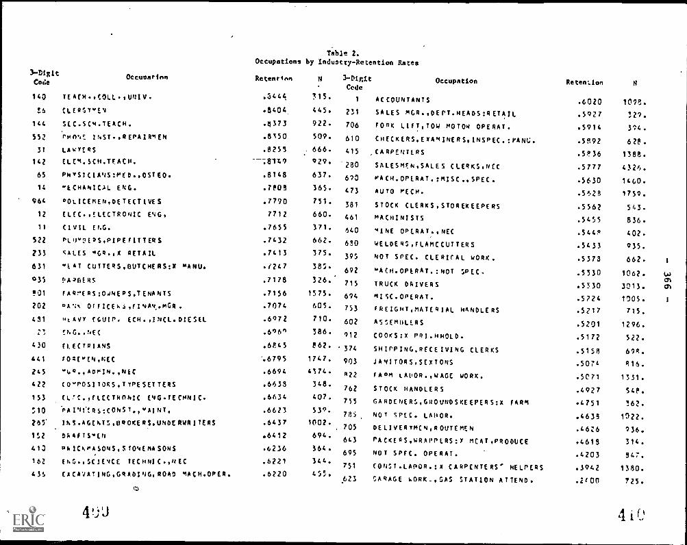
Table 2.

Occupations by Industry-Retention Rates

3 -Digit

Code

143

es

144

557

31

142

65

14

964

12

11

522

233

631

035

!O1

202

431

,,Cl

430

441

245

422

153

7,10

26./

152

413

162

435

OccuoArinn

11AF/4.0:DLL.UNIX.

CLER5TmE4

SEC.SCH.TEACH.

Plq(1%E 1NST.O/EPAIPIEN

LA',YtRS

ELEm.SCH.TFACH.

PHYSICIANS:m(0..05TE°.

mECHANIUL C46.

POLICEmEN,DETECTIVES

ELEC.,ELECTRONIC ENG,

CIVIL E.G.

PLIPDEPS,PIPEFITTERS

GALES "GR.,x RETAIL

"EAT CUTTERS,OUTCHERS:X mANU

!,A2FIERS

FAR:ERS:OdNEPS,TENANTS

0A%k OFFIcF1,,EI4A4,.mGR.

wtAvv EQUIP. ECH.,INCL.DIESEL

tNGO4NE(

ELECTRIA4S

tO4EmEN,NEC

v40.,A0m14.,NEC

CO"POSITORS,TYPESETTERS

ECC.,ELECTRONIC E4G.TECHNIC.

PA141CAS:CONST,,mAINT.

INS.AGENTS,OROKERS.UNDERWRITERS

67.4FTSmEN

PhICAmASONS,S104EmASONS

ENG..SCIE4CE TECHN1C.,NEC

EACAVATING,GRADI4G,ROAD MACH.OPER.

Retenti nn

.5444.

8404

.$373

.8150

.8255

.0141

.877187409880

7712

.7655

.7432

.7413

./247

.7156

.7074

.6972

.606'

.6845

.6795

:::::

.6634

.6623

.6437

.6412

.6236

.6221

.6220

N

315.

445.

922.

569670623596971..

365.

660.

371.

662.

375.

385.

326.

1575.

605.

710.

386.

862.

147147::

348407.

539.

1002.

633496454445.

3-Digit

CodeOccupation

1 ACCOUNTANTS

231 SALES mGR.,DEPT.HEADS:RETAIL

706 FORK LIFT,TOW MOTOR OPERAT.

610 CHECKERS,ExAmINERS,INSPEC.:MANU.415 ,CARPENTERS

280 SALESMEN.SALES CLERKS,NEC

670 mACR.0PLRAT.:MISC.,SPEC.

473 AUTO mECH.

381 STOCK CLERKS,STOREKEEPERS

461 MACHINISTS

640 MiNE OPERAT.,NEC

680 WELDERS,FLAMCCUTTERS

395 NOT SPEC. CLERICAL WORK.

692 mACH.OPERAT.:NOT SPEC,

715 TRUCK 041VERS

694 MISC.OPERAT.

753 FREIGHT,mATERIAL HANDLERS

602 ASSEmOLLRS

912 COOKS:X PRI.MHOLD.

374 SHIPPING.RECEIVING CLERKS

903 JANITORS,SEXTONS

022 FAOM LAUOR.,wAGE WORK.

762 STOCK HANDLERS

755 GARDENERS,GROUNDSKEEPERS:X FARM

78) NOT SPEC. LAHOR.

705 DELIVERFPIEN,ROUTEmEN

643 PAEKERS,wilAppERSOt mCAT,PRODUCE

695 NOT SPEC. OPERAT.

751 EONsi.LApOR.:x CARPENTERS' HELPERS

623 GARAGE voORK.,GAS STATION ATTEND.

RetenLion N

.6020 10.78.

.5927 329.

.5914 394.

.5P,92 628.

.5836 1388.

.5455 836.

402.

....555576:73267082

935.

.5555443:7:30 1062.

.57.30 3013.

.5724 1005.

:55221071 1296.

.5172

.5074

.5158

1331.

548.

.4751

,5444096672321786 lE.4618

.4203

1380.

.2/00

LIcyC15

I

4":)..., 4 t U

367

ment in occupations, to the extent that blacks, womell and those with less

education choose low- training occupations (Rosen, 1972, p. 338) or are

crowded into them (Bergmann, 1971).

These occupational characteristics were matched to the 1973-75 May

Current Population Survey according to the individual's 3-digit occupation

code. Apart from the restrictions noted above (male, not in school, less

than 10 years of experience), the matching process imposes the additional

requirement that the individual ,?ort an occupation. This excludes

(1) all those who have never worked, whether they are unemployed or out of

the labor force at the time of survey; (2) most of those not in the labor

force.8

The first exclusion is inherent in the study of "occupation effects";

the second leads to tne exclusion of all those not in the labor force from

the regressions presented elow.9

In addition to whether the individual was unemployed at time of sur-

vey, the CPS determined the reason for unemployment. Those who report they

"have a job or business from which [they were)...on layoff last week" are

counted as having "lost" their last job. Those who reported they started

looking for work because they "lost or quit a job at that time" are counted

as "lost" or "quit", respectively, Consequently, those who dropped out of

the labor force between quitting or losing their previous job and beginning

their current spell of unemployment probably aren't captured in either the

8Those in "rotation groups" 4 and 8 who had worked in the last 5 years are

asked their octupation by the CPS.

9Those in "small" occupations--those in which published characteristics

were unavailable or with less than 13 individuals in the 1/100 file--were

also deleted.

4r:

368

'lost" or "quit" categories, though they are counted as unemployed.

Finally, the CPS files provided several potentially important in-

dividual characteristics: race, education, age (and hence experience),

location, marital and veteran statuses. Moreover, hourly earnings and

union membership were'deterMined for those who were working, who had a job

but were absent or on layoff, or who had worked in the last three months.

4 ' .)..,

369

2. Results

Equations in which personal and job chatacteristics are used to

explain unemployment are presented in Table 3. The dummy variables

indicating being unemployed at time of survey are multiplied by 100,

se that each regregglon coefficient can be interpreted as that variable's

"effect" on the unemployment rate, measured in pe7 cent. The number

in parentheses below each coefficient is the standard error. The number

in brackets is the product of the regression coefficient and the

variable's standard deviation. It reflects the impact of a one standard

deviation change in the independent variable on the unemployment rate

and can, in that.sense, be compared across variables.

4!

370

The equation in column 1 of Table 3 includes only "personal" char-

acteristics as independent variables. There are few surprises. The co-

efficients of the three regional variables show that unemployment is

considerably lower in the South than elsewhere, but there is very little

difference among the three other regions (NorLh East, North Central, and

West). Living in an SMSA or a poverty area is associated with a higher

unemployment rate, and a standard deviation difference in the area poverty

rate has a considerable impact. Even with other personal characteristics

controlled, whites have an unemployment rate nearly five percentage points

lower than nonwhites. Married men with spouses present enjoy considerably

lower unemployment, while vetrrans' unemployment rate is almost one percent-

age point higher than others'. Schooling has a considerable impact, with

the unemployment rate declining one point per year of schooling. Perhaps

the strongest surprise is the failure of the two experience variables to

achieve "significance." Experience was defined as years since estimated

school Leaving, following Mincer (1974, p. 48). The tv.o exoerience variables

allow the experience-unemployment relationship to have a different slope in

the first two years than Teter on, in response to Ornstein's (1971, p. 417)

finding that young workers appear to spend roughly two years finding their

place in the labor market. The standard errors of these vcr4..ibles' coef-

ficients are increased by the sample selection, which limits the range of

experience, and the estimated effect in the first two years is probably re-

duced by eliminating those without work experience.

Columns 2-5 reflect the addition of various occupational character-

istics ;nto the equation. The coefficients of the personal characteristics,

.11 4I I

i

- 371 -

Cable 3Unemployment Equations

Hales with Less than 10 Years Expecience

(1) (2) (3) (4) (5) (6) (7) (8)

Dependent Variable Dependent VariableUnemsloved(x 100) Unemployed(x 100)

Mean All Lost Quit Mean All Wet Quit

Constant 67.7 21.6 7.90*

45.9 11.9 7.40

(5.23) (3.00) (2.12) (5.66) (3.85) (2.30)

North Central .284 -2.43 .354 .034 .285 .408 .024 .338*

(.451) (.448) (.257) (.181) (.452) (.393) (.267) (.160)( -.110] (.160) (.0151 (.184] (.0111 (.153)

South .308 -2.97* -1.08* -.238 .319 -.721 -.457 .039

(.462) (.458) (.262) (.186) (.446) (.402) (.273) (.164)(-1.37) 1-.5041 (-.110] ( -.322) ( -.204] (.017)

West .184 -.337 -.668* -.227 .187 .197 -.179 -.072(.388) (.498) (.286) (.202) (.390) (.435) (.296) (.177)

( -.131] ( -.259) ( -.088) (.077) (-.0701 (-.0281

In S)SA .697 .753 -.344 .254 .699 -.194 -.681* .184

(.459) (.379) (.218) (.154) (.459) (.328) (.222) (.133)(.3461 ( -.158] (.117) ( -.089) ( -.313) (.084)

Per Cent Poor in Area 11.3 .0774 -.013 .012 11.2 .026 -.014 .001

(10.8) (.018) (.010) (.007) (10.7) (.015) (.011) (.006)

(.832] ( -.140] (.1301 (.278] (-.150) (.0111

Schooling 13.0 -.747* 7.213* -.189* 12 9 -.343* -.159* -.071*

(2.59) (.088) (:051) (.036) (2.55) (.082) ( 056) (.033)(-1.931 (-.552] (-.490) 1-.1'751 (-.4051 (-.1811

Experience 4.15 -.245 -.167 .204 4.16 -.335 -.129 .099

(2.87) (.279) (.160) (.113) (2.84) (.243) (.165) (.099)(-.7031 ( -.480] (.585) 1-.95 ] (-366) (.281)

flax(0. Experience-2) 2.51 -.030 .145 -.258 2.51 .230 .034 -.106(2.44) (.322) (.185) (.131) (2.42) (.280) (.191) (.114)

( -.073) (.354] ( -.629] (.557) (.082] (-.256)

White .895 -3.91 -.472 .093 .901 -.771 -.309 .291

(.306) (.552) (.317) (.224) (.299) (.486) (.330) (.198)

( -1.20) 1-.144) (.028) (-.230) (-.092] (.087]

Aarried,Spouse Present .640 -4.59 -.300 -1.07 .676 -1.80 -.400 .347*

(.480) (.364) (.208) (.148) (.468) (.320) (.218) (.130)

(-2.20) (-.1441 ( -.514] (-.842) (- 187] [ -.162)

Veteran 351 .742* -.044 .106 .357 .000 .155 .122

(.477) (.351) (.201) (.142) (.479) (.302) (.205) (.122)

(.354] ( -.021] (.051] (.000] (.074] (.058)

In(Hourly Earnings) 6.02 -.504 .475 -.673*(.489) (.379) (.258) (.154)

( -.246) (.232] ( -.329)

Union Members .284 .402 1.31 -.306(.451) (.332) (.226) (.135)

(.181) (.591] (-.1381

Median Schooling in Occupation 12.3 -.709* -.377* -.019 12.4 -.554* -.161 -.037

(2.11) (.165) (.095) (.067) (2.11) (.145) (.099) (.059)

1-1.501 ( -.648) (-.040] 1-1.171 ( -.340) (-.078)

Per Cent female in Occupation 17.8 .012 .003 .008* 18 0 .004 .002 .004

(20.6) (.009) (.005) (.004) (20.7) (.006) (.005) (.003)

(.247) (.062) (.165) (.0831 (.042) (.083)

Per Cant Slate in Occupation 8 64 .14d* .046*

.019 8.81 .023 .025 -.005

(7.03) (.012) (.019) (.013) (7.00) (.029) (.01°) (.012)

11-041 (.323) (.134) (.161) (.175) (-.0351

In(Curcent Wage in Occupation) -3.4. 11.9* 7.68 .237 -3.45 9.60* 5.49 -1.14

(.299) (2.26) (1.29) (.915) (.277) (2.16) (1.47) (.881)

(3 56) (.2301 (.0211 (2.6'.) (1.52) (-.3161

In(Futort Wage in Occupation) -3.23 -1.4$ -5.14* .735 -3.23 -4.05 -3.35* 1.58

193) (2.1) (1.39) (.983) (.223) (2.24) (2.52) (.312)

( -1.1 *] (-1.51) (.215) (-1 111 (-1 09) (.434

Retention Rate 61.2 -.142* -.031 -.020* 61.1 -.094. -.024' -.010(12.5) (.019) (.011) (.0081 (12 41 (.017) (.012) ( 007)

(-1-781 1-.388) (- (-1.16) (- 3601 (- 124)

Mean of ;:pendent Var(ohle a.h0 1.99 .983 3.57 1.o0 566

Numher of Obser..ati..ms 2;71 21714 2)7(4 2371' 18261 18361 18361 18)61

et4n).1.4 neelf1 II tinlir4 4ow11-fon of of.161, 16 nrace.to. .C-4tittYLLGgreitor than 2.0 in )6e'1lt

- 372 -

taken as a group, are not greatly affected by the additional

variables. Even granting the crudeness of the occupation variables,

the small change in the coefficients of the poverty area and race

coefficients is striking. Schooling does lose up to 40 percent of its

estimated effect (column 5 vs. column 1), suggesting that a non-

negligible fraction of the advantage of those with more schooling

comes from access to "better" occupations.

In colum 2, each occupation's current and future wage, and its

three-digit retention rate are added to the equation. Each is highly

significant. A higher current wage is associated with a higher

unemployment rate (when personal characteristics are held constant).10

However, if only the current wage is added to the personal

characteristics, its coefficient is .156 (.864). The future wage has an

almost equally large negative coefficient, as predicted by the

"opportunities for advancement" hypothesis. Where the size of this

coefficient relative to those of the personal characteristics is, of

course, sensitive to scaling, the impact of a one standard deviation

difference (three percentage points) is quite large. Finally, 'he

occupation's retention rate" is negative and significant: Individuals

in occupations in which industry-switching is less common (higher

retention rate) have lower unemployment rates.

A sterner test of the three occupational characteristics is permitted

10Marston (1976, p. 192) found the probability of becoming unemployed

positively related to the individual's wage; Bartel and Borjas

(1977, Table 10) found a negative relationship between wage and

probability of separation (quit or layoff) for those with "long"

tenure, and a non-significant positive relationship for those

with short tenure, in the NLS Mature Men sample.

- 373 -

in column 3, where 10 dummy variables for Census broad occupation

(e.g., "clerical workers") are added to the equation. The occupation's

current wage and retention rate are not significantly affected, but the co-

efficient of the future wage variable falls to one third its previous value

and is no longer "significant" at conventional levels. The ten dummy vari-

ables are jointly significant at the 1 percent level. These broad-occupa-

tion dummies consistently outperformed an alternative set (white collar,

blue collar, and farm, with service worker the omitted group) in the sense

that one could reject the restrictions of the ten-dummy set's coefficients

which the alternative set implied.

Three additional occupational characteristics are added, with and

without the broad-occupation dummies, in columns 4 and 5. Once again, ,he

effect of tne current wage and retention rate are not Gramatically affected,

but the coefficient of the future wage is considerably reduced (column 4 vs.

column 2) or eliminated (column 5). The standard error of the future wage

variable rises with the addition of the other occupation variables, but the

increase.is_ not very large. Two of the three new variables (the occupation's

median years of schooling and the fraction of its workers who are black)

have substantial effects on the unemployment rate, while the fraction who

are female does not.

Modest experimentation with the specification produced similar re-

sults. Deletion of the retention rate reduced the current wage variable's

impact (though it remained positive and generally "significant") but had

little impact on the other occupation characteristics' coefficients. The

effect of the current wage variable was significantly positive when weekly

wages replaced hourly wages, or when the future wage Was deleted. An in-

4 1

374 -

dustry-retention rate based on (about 20) broad industries produced similar,.

slightly weaker results. Median years of schooling, percent female, and

percent black were little ffected by these experiments.

The relationship between occupational characteristics and unemploy-

ment which emerges from these regressions is a good deal more complicated

than implied by the discussions ciced in the introduction. The three major

findings are: (1) A consistent relationship between three measures of oc-

cupational advantage (retention rate, median schooling, and racial composi-

tion) and-unemployment is evident. Whether this reflects the current posi-

tion or future opportunities provided by the occupation is unclear, since

quite plausible a priori arguments can be made for either. (2) The coef-o

ficient of the future wage variab as quite sensitive to the other occu-

pational characteristics included, ranging from being a quite i:rportant

factor to a thoroughly negligible one. The rQasurement difficulties noted

in Section 1 may help to explain its demise as other, correlated variables

are added, but this remains a matter of conjecture until these difficulties

can be overcome. (3) The broad-occupation dumwies were consistently signi.fi-

cant when added to any of the equations. This suggests that significant oc-

cupational differences in unemployment exist, independent of the variables

discussed above. With service workers as the omitted category, white-collarit

and farm workers had uniformly lower unemployment. Among blue collar workers,

craft workers and transport operatives had consistently lower unerroloyment

. .

rates, while unemployment among other operatives and nonfarm laborers was

similar to that of service workers.

Table 4 iecomposes unemployment bj reason for leaving last job.

Columns 1, 4, and 7 reproduce colur.ns 1, 2, and 5 from Table 3, and relate

.1 t,

Constant

North Central

South

West

In SMSA

Pet Cent Poor in Area

Schooiing

Experience

Max(O.Experience -2)

White

- 375 -

Unesployment Equations

Males with No College and Less than 5 Years Experience

(1) (2) (3) (4)

Dependent variable -Unemolcned (x 100)

Mean All Lost Quit

116.* 22.8' 10.4

(16.4) (8.96) (6.83)

1.26 ,603(.555) (.423)

(.571) (.2731

.288 .659

:1.01)

(.7981(.453)

.338 -,.19* -.985 -.474

(.473) (1.05) (.575) (.438)

(-2.45) (-,466) (-.224)

.152 -1.82 -1.00 -.347

(.359) (1.20) (.653) (.498)

1-.653) 1-.3591 ( -.1241

.642 .115 -.012 .118

(.419) (.823) (.449) (.342)

(.342) (-.034) (.056)

13.6 049 -.002 .001

(11.8) (.0)7) (.020) (.015)

14281 (-4024) (.012)

11.3 -1.99* -.078 -.661*

(1.36) (.288) (.157) (.120)

1=2.711 (-.106) ( -.8991

1.86 -.234 -.216 .465*

(1 43) (.545) (.297) (.221)

(-.3351,(-.304) (.665)

.544 -.090 .309 -.709

( 181) (.968) (.528) (.402)

(- 070) (.241) 5541

.871 -7.02 .960 -.186

.33s) (1 18)1-2.351 (.122)

.421(.122) (-(.0692)

(5) (6) (7) (8)

Dependent Variable 0

Unemployed (e

Mean- All Lost Quit

79.5 4.74 18.7

(16.2) (10.6) (6.50)

.284 1,66- .009 .941*

(.451) (.904) (.593) (.363)

(.749) (.004) (.424)

.359 -.143 -.450 .168

( 480) (.925) (.601) (.372)

(-.351) 1-.2161 (.081)

.155 -.493 -.567 -.130

(.362) (1.04) (.685) (.420)

(-.1781 (-.2051 (-.P'')

.635 -.32I -.844 .241

(.481) (.708) 1.465) (.285)

(1.3.47) ( -.406) (.1161

13.6 -.001 -.004 -.002

(11.8) (.032) (.021) (.013)

(-.012) ( -.041) (1-.0241

11.3 -1.21* -.247 -.479*

(1.32) ( 264) (.173) (.106)

( -1.60) (-.326) (-:632)

1.91 -.316 -%024 .201

(1.42) (.471) (.313) (.192)

(-.449) f-..034) (.285)

.563 .124 -.256 -.204

(.746) (.831) (.545) (.334),

(.1191) ( -.201) (- 160)

.832 -1.35 .584 .452

( 323) (1.05) (.689)

(-.436) (.1691 (.146)

Married.57ouse Present .424 -5.44* - 034 ,-I.45 .484 -1 88 -.261 - 303

(.494) (.794) (.433) (.330) (.500) (.618) (.445) ( 213)

(-2.69) (-.017) ( -.716) (-.940) (-.134) ( -.152)

Veteran .186 3.15* -.286 .797 .194 .412 .450 .487

(.389) (.979) (.534) (.407) (.395) (.835) (.548) (.336)

(1.221 ( -.111) (.3101 (.163) (.1781 (.192)

In(Nourly Earnings)5.78 .076 1.25 -,689

(.434) (.915) (.600) (.368)

(.0)71 (.5421 ( -.299)

Union Meober.294 .488 1.62 -.781

(.456) (.756) (.496) (.304)

(.222) (.739) ( -.1281

1111

Median Schooling in Occupation 11.2 -.496 -.149 11 2 -1.09* -.065 -.317

(1.13) (.581) (,317) (.241) (1.12) (.505) (.331) (.203)

(-1.601 (-.5601 ( -.1681 (-1.22) (-.073) (-.355)

Per Cent Female in Occupation 16.2 .042* .015 016 15,7 .026 -.00a .019

(20 1) (.021) ( 011) (.309) (19.6) (.018) (.012) (.007)

1.844/ (.3021 (.32i1 (.510) ( -.09P) (.372)

Per Cent Black in Occupation 11 8 .173 .083* .002 11.9 .067 .081 -.030

(7.16) ( 016) (.041) (.012) (1.12) (.066) (.041) ( 021)

(1.24) (.594) (.014) (.477) 1.577) (-.214)

ln(Current Wage in Occupation) -3.60 10.9* 6.47* 2.02 -3.59 8 61 2 91 -2.32

(.227) (4 85) (2.65) (2.02) (.205) (4.91) (3.22) (1.97)

(2.47) (1.471 (.458) (1 76) (.596) ( -.416)

In(Future Wage in Occur.cion) -3.38 322 -2 83 -.504 -3.38 2.74 -1.40 3.71

( 192) (6,44) (3.5r) (2 68) (.184) (6.00) (3.94) (2.41)

(.6181 1- 4431 (-.091) (.504) ( -.258) (.6431

Retention Races 55.0 - 179* -.024 -.042* 55.2 -.122* - 022 -.028

(10.9) (.043) ( 023) (.018) (10.8) (.038) (.024) (.015)

1-1.951 (- 262) 4581 ( -1.321 (- 238) (-.302)

lain of Desenuont Variable 10.9 2.86 1.65 5.63 2.32 .864

ionber of Obaervations 7266 7:46 7266 7266 3555 5555 5555 5555

-*Indira err...of .n paranC)artpa, coetfIctent x otan4erJ 4ottat!on ot vartoble in 6rac4et7. r-stztistio

r,,r ,In 2 1 0-.11ut,, 411.e

4 1-J

376 -

to total unemployment. The remaining columns relate to unemploymnt due

to losing or quitting one's previous job. Thus, in column 2, the dependent

variable was one (times the scaling factor 100) if the individual was un-

employed due to losing his previous job, and zero otherwise (including

other types of unemployment). The difficulties in defining such categories

of unemployment in these CPS data should be recalled when interpreting

the results.

Given that less than half of the unemployed fall into either the

lost or quit category, one expects estimated coefficients to be smaller

than in column 1. Indeed, the effect of each variable on "other" unemploy-

ment can be gotten by subtracting column 2 and 3 from column 1. In general,

the variables which had substantial effects on overall unemployment have

substantial effects on this residual category.

Meng the personal variables (columns 2 and 3), Southern ana Western

locations are associated with lower "lost" unemployment, but have negligible

effects an the "quit" component. Living in a poverty area has little effect

on either component. The large overall advantage of whites does not appear

to be attributable to differences in either the "lost" or "qui," components.

.being married substantially reduces the "quit" component, but has much less effect on

the "lost" component. Schooling remains a significant, negative determinant

of both components.

The coefficients of the occupational characteristics vary with the

type of unemployment (columns 5, 6, 8, and 9). The positive effect of the

occupation's current wage is concentratec on the "lost" category of unem-

ployment, consister,t with an equalizing d:fference interpretation. The lack

1

377

of impact of occupation's wage on quit unemployment is s-urprising.11

A

higher future wage in an occupation is associated with lower "lost" unem-

ployment, "significantly" in column 5 and nearly so in column 8. This is

consistent with the notion that jobs which offer advancement for the worker

are also those which involve investing in the worker by the firm. The

future wage has no impact on quit unemployment, and a mildly positive im-

pact on non-layoff unemployment (column 7 - column 8). Thus, there is no

evidence that the promise of higher future wages has a significant impact

on the more "voluntary" components of unemployment. At a minimum, this

_ contradicts the emphasis of the "opportunities for advancement" hypothesis

on quits. The occupation's industry retention rate was significant and

negative for both components of unemployment. Omitting this variable

tended to increase the other occupational cnaracteristics' coefficients,

but not dramatically. ;.ledian schooling has a modest coefficient in the

"lost" unemployment equation, and the racial composition of the occupation

is related to both components. Deletion of the retention rate once again

had little effect on the other coefficients.

11Related previous research has used the individual wage as the independent

variable: Marston (1976, Table 7: positive, non-significant relationship

to probability of becoming unemployed due to layoff and negative, non-

significant relationship to becoming unemployed by quitting); Bartel and

Borjas (1977, Tables 7 and 4: positive, non-significant relationship to

probability of layoff and significant negative relationship to quitting);

Leighton (1978, Table 15: positive, significant relationsY4 to probability

of layoff); Feldstein (1978, Table 2: positive, sometimes significant re-

lationship to probability of being on temporary layoff unf2Tployrent).

- 378 -

The individuals in Tables 3 and 4 are "young" in the sense of having

/

limited labor market experience, but they are not necessarily young in the

mare usual sense. A high schc'l graduate with. 9 years of experience or a

college graduate with 4 years of experience would each be 27 years old --

beyond the age which bounds the "youth unemployment problem." Thus, Table

5 is restricted to those who are most likely to be part of "the-problem":

those with no more than 12 years of schooling, and less than 5 years of

post-school experience.

Comparison of Table 5 with Table 4 shows frequently larger coeffi-

cirnts (with greater unemployment, there is more room for sensitivity Ty

the various factors) and much larger standard errors (due to a smaller sample

and less variation in independent variables). The most striking differences

are the reduced impact of living in roverty area, the almost coTolete con-

centration of the racial effect in the residual unemployment category, and

the lack of any effect of the future wage in the last three _ctions. In

general; however, the earlier findings -- both expected and anomolous --

remain.

:ur about 80 percent of the full sample (i.e., of those in Tables 3

and 4), two additional variables are available in the CPS file; union mem-

bership and the individual's hourly wage rate.12 However, those unemployed

who hadn't "lost" their last job were over-represented among the remaining

20 percent. Consequently, among the 18,361 observations for whom union

memtership and hourly wage were known, the total and "quit" unemployment

rates were less than 60 percent of these in the full sample.

12If en hourly wage was not reported directly, the ratio of usual weekly wage

to usual hours worked per week wt.s used as fhe hourly wage.

423

TableElnenployment Equations. by Type of Unemployment

(Males lose than 5 years )or sthool-leovIng, no college)

VariableMain (1) All (2) Lost (3) Quit (4) All (5) Lost (6) Quit (7) All (6) Lost (9) Quit

(l.0.)

CONSTANT(1:224) ( 1:3;t; ( 1:i1i) (s2:ffl; ( ('1:348) (4:20) ( (1:17,S)

,.

`\ '1':7401-A1911:41BP:MillleilMli'Ml:?11:118.264 .610 1.315REGIONRAWN CENTRAL .436 1.190: .560 .616 1.240. .553 .5416

REGIONSOUTN . CR -3.236. -1.029 -.496 -5.243. -1.009 -.492 - 5.251. -.969 4.463

( . 62) ( 1.057) ( .575) ( .437) ( 1.055) ( .575) ( .439) f 1.053) ( .574) ( .4310

E-2.419) C -.4753 C -.230) (-2.442) C -.406) C -.227) (- 2.426) C ...4433 C -.214)

AEGIONuEST .184 -1.534 -.901 -.301 -1.65A 4.333 41.719 -1.033...939 -.294

l .3E8) ( 1.201) ( .653) l . .49?) 4 1.199) ( .653) ( .493) C 1.19P) 4 .653) C .445)

o C -.595) C- C -OM C- C- E -.129) C -.667) C -.441) C -.115)

---J.6C? 4.122LIVES IN SRSA .13?

( .4591 ( .81A) ( .445) ( 039) ( .340) C .26) ( .450) (

.13? .43? -.02C:9!63;

C.302) C-.056)(.0613(1)E-01C.063) C .2213 ( -.013) C .0101( iN) ( -11116)

PER CENT POOR IN AREA 11.3C0(10 540)

.047

.017).n01 .000 .002 .056 .031

A ( ( 065)( ...AB) ( .020)C

.015)C.504C-.0195t4115t$M002) C .021) C .604) ( -.076) t .01334 .:ii5,1)

IIACEswHITE .595 -R.n54. .71? -.259 -6.622. .916 .-.164t .458) t 1.165) 4 .446) ( .4.3)

-.355 -7.591.4 .3(6) ( 1.174) ( :!11) , ..6, ( 1.175) ( .6.0)

(- 2.465) ( .173) C -.100] (-2.3233 C .215) C -.079) (-2.05?) ( .260) C ...056)

H ARR1Si. SPOUSE PRESENT( :tta) 4-5:;06) ( .Ai) 4-1:1)t (-':42; ( %Ili) (1:11;) (-':IiI) ( :134) (-1:11i7

(.2.771] c -.049] C -.717) (- 2.702) ( -.054) C -.710) (-2.652) C ...0:61 C -.7451

( :In) t 3:;1!) (

Ow.VETEPA94 3:4ia; ( -:iil q(1)) t 3:330; ( -:M) .1?7)

( 1.535)( .4u?)

i .3:43C -.1243 C .191) E 1.505) C -.134 1 .00)

SCHOOLING -.691. -2.101. -.122

C 1.45?) C -.179)

-.642. 4-2.141.4

-.66e. 2.020. ...C10f .116) f .267) f .156) f .119) f .269) 1 .153) 4 .12C)

C -.314) (-1.7693 f-5.442) C -.316) C-1.7151 (-5.231) ( -.20) C-1.711) 4I.4

EAERIE%CE -.071 .440 -.171 .4)5 1.0(:I:::::: :-;:i.iii: i -:it;3 1 1:iiti i -..IfAi c

-...:76176

.40.i ,:mi

C

.50) 1 -:T) .2471...5 3) C 1.2)0) 1

n at(0. ESPERIENCI.4) -.723 .-.6792.510( 2.440) l .971) t .;)71)

.2:6491-.1.6 63.1:;2flt.-_,Aiwp31..ailf .96R) 1 .52.) 1 .4t3)

C -.726) C .503 -.12!)

6.0531.160LNIOCCS CURRENT h WAGE) 17.724 9.399 1.371 -.237( 4.469) 4 2.4.151 ( 1.655) ( t9....:13:) ( ( 7.3)6)t .2i9)f 5.299) C 2.810) ( .560) ( 1.910) ( 1010) ( -.071)

1.360 -/1.961 -9.043. -1.0)2Lf440CCS FUTURE N WAGE) .227C .21.3) f 5.,55) ( 6.4.31) ( 3.752) ( 2.161)

1

2.920)4.3.:051 E-2.650) I Niiii ( 2.910) C .332) C .CLO

OCC'S REFENTiON RATEt :ST)

-22.44.0. -3.,35...4_ 4.151

( 41911 i 1.iosil 1 .1.5oli i- :4 1 C -:1'Xi C 2:3191C-2. 70

OCC'S NEOIAN YRS SCHOOL41i.n a) 4

-1.013 -.197 -.113.664) ( .162) 4 aro/

C-2.1383 C -.416) C -.2003

OcC'S PER CENT FErALE(11r.:E8) ( -M) ( liZ)

C -.1521 C ...OM C ....2201:!1

Ott 'S PER CENT eLACA 8.640 .197. .115i

1.347)( .0.,1) ( .0.0)( 7.030)

73 C .512) C .4343

10 Occupation Dummy Variable.?

fi

2

No No No No No No Us Yell Yes

.034 .004 .011 .039 .006 .012 .047 .012 .015

4r)1

380

The restricted sample is inferior to the full sample as a source of

information about the relationship between une,!ployment and occupational

characteristics already discussed, but one is limited to the restricted

sample for the two "new" variables. Consequently, only the results of

these two variables in the restricted sample will be discussed in any

detail.13

The equation in Table 6 corresponds to those in Table 4, apart from

the addition of union membership and hourly wage. Thus, the equation in

any column of .able 6 uses the sample dependent variable as the correspond-

ing column in Table 4, and included the independent variables 'Acluded in

that column of Table 4. The results here are fairly insenEitive to the

addition of other occupation variables, and are consistent with previous

research. Union membership is associated with greater "lost" Aemployment

i and less "quit" unemployment; its coefficient in the total unemployment

equations is positive but non-signifi(Ant (though not negligible in columns

1 and 4). The same pattern consistently emerges for the coefficient of the

indivioual's hourly wage: positive for "lost", and negative for "quit", and

insignificant for "total" unemployment. When only union membership is

---- added to the personal characteristics, its coefficient also followed the,...

pattern in Table 6 -- positive for "lost", negative for "quit" unemployment,

positive non-significant overall. Thus, while unionization may be a

--__13In general, the absolute value of the occupational characteristics' coef-

ficients declined. Estimating the "Table 4" equations using the restricted

sample but riot adding union membership and hourly wage led to similar de-

clines in these coefficients, so it was the sample selection rather than

the addition of the new variables which was pr:rarly responsible for the

__,change.

4,:.-,..4)

Table 6

Union Membership and Individual Wage Coefficients in Unemployment Equations(Males less than 10 years after school-leaving)

VariableMean

(S.D.)(1) All (2) Lost (3) Quit (4) All (5) Lost (6) Quit (7) All (8) Lost (9) Quit

Union Membership .284 .448 1.405* -.340* .530 1.362* -.299* .003 1.060* -.348*(.451) (.323) (.219) (.131) (.330) (.224) (.134) (.342) (.233) (.139)

[ .202) [ .634) [-.153) [ .239] f .614) [-.135) [ .001] [ .478) [-.157]

Ln(Hourly Wage) 1.42 -.169 .549* -.681* -.324 .538* -.684* -.576 .433 -.685*(.489) (.357) (.242) (.145) (.375) (.255) (.153) (.380) (.255) (.155)

[-.082) [ .268] [-.333] [-.158) [ .263) j -.334] [-.282) [ .214) [-.335]

10 Occupation No No No No No No Yee Yes YenDummy Variables?

R2

.014 .007 .006 .018 .009 .006 .020 .011 .307

Number of 18361Observations

O

4

382

. "primary" labor market in many respects, it does not seem to be a source

of lower unemployment rates for young workers.

4 ) j

383

3. Conclusions

Occupational characteristics did prove significantly related to

the unemployment of young workers with given personal characteristics.

This result is not very surprising, given previous research and the limited

menu of personal characteristics in the CPS. The more interesting ques-

tion As the more narrow one: Is there evidence of a relationship between

lack of opportunities for advancement and youth unemployment? Unfortunately,

the results presented above are too weak to justify either a confident "yes"

or a confident "no".

One fairly straightforward way to measure opportunities for advancement

is from the wage gains which different occupations provide. The main

reservation about this approach is that if transitory variation in earnings-

is occupation related -- as seems almost certain -- individuals in some

occupations will have "low" initial earnings due to these transitory

influences, while others will have "loe initial earnincs because they are

"buying" opportunities for advancement. This measure7.ent problem clearly

tends to obscure the effect of opportunities for advancement on unemplc:,ment,

if they exist. When we turn to the data, we find that tne "future

wage" variable designed to capture these influences exhibits a non-trivial

relationship to unemployment, but it is not very sturdy in the presence of other

occupational characteristics, and confined to unemployment of job losers.

(The bias noted above might be expected to be stronger for quitters than for

job losers, since those with low earnings due to transitory factors would have

an incentive to quit.)

An alternative strategy is to ass'ine (plausibly, I belie,,e) that

opportunities for advancer.art should leaf", in 7--,st cases, tc tin individdal

384

remaining in his current 'industry. Industry-retention rates of occupations did

prove consistently (negatively) related to unemployment, controlling both for

personal characteristics and average wages of young workers in the occupation.

The problem here is that an occupation's industry-retention rate is influenced

by other factors besides opportunities for advancement. Indeed, any desirable

job characteristic (apart from the wage, which is included separately; would

be likely (other things equal) to reduce quits, quit-related unemployment,

and industry-switching; whatever it is that reduces layoffs would also be

likely to reduce layoff-related unemployment and layoff-induced industry

switching.14 One should not overstate the "automatic-ness" of these relation-

ships, however: turnover and unemployment are not synonymous, and lack of

opportunities for advancement would increase the likelihood that one would leave

one job without having another line up.

To end on a more positive note, two conclusions do not seem warrar.i.ed:(1) Tne

industry retention rate is clearly measuring something which wages in the

occupation and broad-occupation dummy variables do not. (2) While jobs in

unionized firms may be desiraL,ie jobs for young workers for other reasons,

improving access to these jobs is an unpromising approach to solving youth

unemployment. Their greater layoff rates more than compensate for their

lower quit rates.

14 A piece of information which supports this interpretation is the fact that

a very high percentage of industry stayers are also firm stayers. Among out-of-

school NLS young men, the percentages of industry stayers who were also firm

stayers were 81.9% (1971 vs. 1966) and 86.3% (1973 vs. 1968).

a 0

$

- 385 -

References

Bartel, Ann P., and Borjas, George J., "Middle-Age Job Mobility: Its

Determinants and Consequences," in Seymcur L. Wolfbein, ed., Men in

the Pre-Retirement Years (Philadelphia: Temple University School of

Business Administration, 1977), pp. 39-96.

Bergmann, Barbara, "The Effect on White Incomes of Discrimination in Em-

ployment," Journal of Political EconomyT vol. 79, no. 2, March/April

1971, pp. 294-313.

Feldstein, Martin, "The Economics of the New Unemployment," Public Interest,

Fall 1973, pp. 3-42.

Feldstein, Martin, "The Effect of Unemployment Insurance on Temporary Layoff

Unemployment," American Economic Review, vol. 68, no. 5, December 1978,

pp. 834-845.

Gordon, David, Theories of Poverty and.Underemployment (Lexington, Mass.:

Lexington Books, 1972).

Hall, Robert E., "Why Is the Unemployment Rate So High at Full Employment,"

Brookings Papers on Economic Activity, 1970:3, pp. 39G-410.

Landes, ,Elisabeth M., "Sex Differences i^ Wages and Employment: A Test of

the Specific Capital Hypothesis," Economic Inquiry, vol. 15, no. 4,

October 1977, pp. 523-533.

Leighton, Linda, "Unemployment over the Work History: Structure, Determinants,

and Consequences," Ph.D. Thesis, Columbia University, 1978.

Marston, Steven T., "Employment Listability and High Unemployment," Brookings

Papers on Economic Activity, 1976:1, pp. 169-210.

Mincer, Jacob, Schooling, Experience, and Earnings (New York: National

Bureau of Economic Research, 1974).

Ornstein, !'ichael, Entry Into the Am,arican Labor Force (8altim3re: Center

for Social Organization of Schools, 1971).

386

Piore, Michael, The Dual Labor Market: Theory and Implications," in DavidGordon, ed., Problems in Political Econcmy: An Urban Perspective(Lexington, Mass.: Lexington Books, 1971).

Rosen, Sherwin, "Learning and Experience in the Labor' Market," Journal ofHuman Resources, vol. /, no. 3, Summer 1972, pp. 326-342.

U.S. Census Bureau, 1970 Census of Population: Occupational Characteristics(Washington: U.S. Government Printing Office, 1973).

- 387 -

Youth Unemployment in Britain and the U. ComponentRichard Layard

British unemployment differs markedly from U.S. unemployment in two

ways:

1. Youth unemployment has been much lower relative to adult unemployment,

for decades.

2. Spells of unemployment last on average about twice as long (at a given

point of the cycle), with the difference being greater for adults.

There are also two points of similarity:

3. In both countries youth unemployment rises relative to adult unemployment

in slumps.

4. And in both countries the demand for young workers is very sensitive to

wage levels.

In the four sections of the paper I examine these- phenomena.

Why is youth unemployment relatively loci in Britain? It seems likely that

both equilibrium and disequilibrium factors are involved (see Section 1). An

equilibrium approach to unemployment leads one to look mainly for supply-

side factors which might affect the choice of whether to be 'unemployed',

rather than employed. I find good evidence that the higher relative youth

unemployment in the U.S. reflects in part higher U.S. incomes, which also explain

the remarkably low U.S. levels of labour-force participation, compared with

Britain. Supply behaviour is also influenced by price effects: income

maintenance for adults is less generous in the U.S. than in Britain and this

tends to reduce the relative unemployment of adults. Another price effect in

supply comes from the rigidity of the British labour market, which refuses

adm43sion to apprenticeship programmes to most pecple over the age of 16; this

provides a strong incentive for youths to be employed.

I next explorevhether differential disequilibrium ah help to explain

higher relative youth employment in the States. The obvious influence here is the

minimum wage law, which does not exist in Britain. Though there is some non-

')

- 388 -

compliance, it seems probable that the minimum wage las contributed- to youth

unemployment in the.U.S. But the structure of age-wage profiles does not reveal,

any sharp differences between the countries.

Finalrfthere is an important differene in information. Almost every.school-

leaver in Britain is interviewed by the Careers Service before leaving school and

nearlya quarter find their first job through the Service; By contrast inAhe

U.S. the state plays little more role in the,placement of youths thin ih the

ylacement of adults.

All the factors I have mentioned probably affect the relative rates of

unemployment in the different age groups, though I cannot say by how much.

Going on, one would like to be able to assess the efficiency cost of the

unemployment in each age group and the impact of unemployment upon inequality.

To do this one needs to look at duration (see Section 2). If unemployment

arises from disequilibrium job-rationing, its cost (relative to the gross

output lost) is approximately proportional to the average duration of the

uncompleted spells.

Taking all age groups at a giveW point in the cycle, average durations

are about twice as high in Britain as in the U.S. And the average number of

spells per year among those experiencing any unemployment has been about the

same. Thus, e"en though average levels of unemployment have been higher in

the U.S. than in Britain, the efficiency,cost (relati.ve to GNP) has been lower.

Furthermore, annual unemployment has been more evenly distributed across people.

As between youth's and adults, the higher relative-rate of youth unemployment

in the U.S. turns out to be mainly due to higher relative durations. Thus the

share of youth unemployment in the total efficiency cost of unemployment may be

higher in the U-.S. Onthe other hand the less generous scales of unemployment

benefit may mean that adults suffer more when they are unemployed than youths

do. Thus while the British worry particularly about youth unemployment (and

now about long-terM adult unemployment), the Americans may be right to worry

particularly about adult male unemployment. However the British experience

389 -

1. Why is :Illative youth unemployment higher in the U.S.?

The puzzle

In the U.S., unemployment rates for young people are much higher relative

to rates for adults than they are in Britain. There are various ways of

looking at this. A crude way is to examine the unemployment rate of, say,

all tie under 25s relative to the unemployment rate of the over 25s. For a

meaningful comparison one should probably exclude students, since in Britain

full-time students do not generally work (except in vacations) and, even if

they do, they are not included in labour force statistics (except in vacrcions).1

In Britain survey - based unemployment data are collected-at tensuses,2 when

the form of question and methods of data collection are very similar for both

countries. Table 1 shows the latest Census data. For males the youth rate

is nearly twice as high (relative to the adult rate) in the U.S. as in Britain.

There is less difference for women, but still some.

However, these differences could be misleading. For the U.S. labour force

aged under 25 is much more recently out of school thin the British labour force

under 25; so one might expect that fewer of its members would have been absorbed

into employment. However by the same reasoning one would expect that the

proportion of the total'unemployed who were under 25 would be much smaller in

the U.S. than in Britain.3

But in fact the proportiOns are very similar,

although the proportions of the labour farce who are under 25 are wildly

dissimilar:

Men

U.S.A.

Women

U.S.A.Britain Britain(1971) (1970) (1971) (1970

X of unemployed aged under 25+ 31 30 34 31

of labour force aged under 25 20 11 25 19

Excluding students.

49. 4'

- 390 -

does suggest that a good case can be made for a Careers Service for youth.

Feldstein argued scum years ago that the U.S. should have such a service. Given

the market failures that arise in the presence of asymmetrical information,

there does seem to be a case for this proposal.

Next there is the question of the time-series behaviour of youth unemploy-

ment rates (see Section 3). In Britain, as in the U.S., the age-structure

of unemployment rates can be well explained by the state of the cycle, by

relative youth earnings and by demographic factors. However in the late 1970s

youth unemployment has been much higner in Britain than ever before. This

phenomenon has led to endless speculati about structural change. But in

fact it is due almost entirely to cyclical factors. In addition the size

of the youth cohort has increased, as have relltive youth earnings. These

three factors taken together tend, if anything, to overpredict recent levels

of youth unemployment. There is no clear evidence that Britain is engaged

in secular movement towards the A-lrican pattern of age-specific unemployment

rates.

Across towns,- the level of youth unemploym-t varies with the level of

adult unemployment, in Britain as in Americk. But, as one might expect, the

elasticity of youth unemployment with respect to adult unemployment is much

less in the cross-section (0 6) than in the time series (1.4).

Across towns, the ratio of youth unemployment toadult unemployment falls

as adult unemployment rises.

Finally, in Section 4, I confirm that It is reasonable 3 find wage

effects on youth unemployment, by looking at the effect of wages on youth

employment. I estimate the demand system derived from the trans-log cost

function on time series data for British manufacturing (April and October 1949-69).

Holding constant output and capital, the own wage elasticity of demand is

around -1.3 flr youths, -1.6 for women and -0.3 for girls and men. Thus, if

there must be minimum wages, the case for a separate youth rate seems over-

wholeint.

4 Li

b- 391 -

A further vay of checking the point is to compare the unemployment rates

of people with similar periods of experience since leaving school. This

comparison can be made in T4b1.1 2.4 For example, if one wants to compare

British youth with U.S. whites 5S(iii7, one notes that a half of 16-year-olds

in Britain were out of school, as were a half of 19-year-old U.S. whites;

and in each case about one-third had left school in OA last year. If we now

compare the unemployment rates of these groups for males, we find they were

8.82 in Britain and 11.22 for U.S. whites. By contrast the adult unemployment

rates (age 30-34) were in the opposite crder: 3.92 in Britain and only 2.62

for U.S. whites.

For women the difference in age-profiles between Britain and the U.S. is

less striking. This may be because the concept of unemployment is more

slippery for adult women than for any other group. In any case there are no

comprehensive data on female unemployment in Britain except at Census years,

so I shall henceforth confine my remarks to men. For unemployed men the

regular data come from registrations at unemployment exchanges (most unemployed

men register). These data show that at any point in the cycle the youth

unemployment rates are lower relative to the adult rate than they are in the

U.S. (see Tables 3 and 4).

In passing one show',; note the profound implications of this for the

comparison of aggreg2 unemployment rates between Britain and the U.S. The

normal assertion that the British rate of registered unemployed needs to be

raised by a fifth or less to allow for unregistered female unemployment and

thus to get it onto a 'survey basis' comparable with the U.S. rate.5

This

comparison always makes the U.S. rate fook awfully high. For example in 1976

the BLS estimate that British unemployment adjusted to U.S. concepts was 6.4

per cent, compared with the published British figure of 5.6 per cent and the

U.S. figure of 7.7 per cent. 'Mies the U.S. rate is still 1.3 per cent higher.

But at the same time the prime aye male rate (ages 25-54) was about 0.8 per cent

lower in the U.S. than in Brit:in.° In fact seem, 1;kCly that in every year

4 .)

- 392 4.

in the 1970s except 1976 the U.S. prime-age male rate was below the British.

It is therefore well to remember ho( much the aggregate U.S. rate is bootNid

not only by the relatively high rate of female unemployment but also by the

relatively high rate of youth unemployment.7

4

The question is why the youth rates should be so mulh higher (relative to

adult rates) than in Britain? At least five possible stories come to mind.

11)7 Income effects in labour supplyc,

The U.S. is a richer society. To investigate the effects of income I

shall begin by looking at labour force participation. Participation rates

are dramatically lower at all ages in the U.S. (except among the old) - see

Table 2 for the under 35s and Table 5 for the over 35s. Whereas virtually all

British males who are not incapacitated participate, the number of U.S. males

not in the labour force is greater a.: every age than the number who are

unemployed. (This has been true in most years, except for the those aged

25-34 in a few recent years.)

If income accounts for this difference between the two countries, it should

also have produced a decline in age-specific participation rates over time

-within the U.S., which we do indeed oboerve. It should also lead to lower

participation rates in higher income groups, which we again observe for adults.

But for youths, cross-sectional data show the reverse pattern. I believe that

this can be explained by the role of job-rationing in the youth labour market.

Suppose that family connections have an important effect on a teenager's ability

to find a job, and thus in turn on his willingness to participate. If

family connections can be represented by income relative to the mean (y/y) then

the probability of participation might be approximated by some function such as

P " f[-a 11

If 1 > 0 - a > 0, we should observe

f' >0

393 -

(a) that in a cross-section high income youths participated more than low

income youths and

(b) that over time and across countries, participation fell as average income

rose.

However our main concern is with the participation rate of youths relative

to adults. This is much lower in America than in Britain (where it is roughly

unity).8

Can this be explained by income levels? It seems quite likely.

?or over time youth participation rates (of non-students) have fallen by a

greater oportion than adult participation rates.9

Thus it may well be that

higher ea s to disproportionate reduction in working-time at the

beginning of life. Otherwise, it is difficult to explain why so many American

parents are willing to support children Iiho are not even looking for work.10

It is hard to imagine such a phenomenon occurring in a much poorer country.

Turning to unemployment, we again find that the unemployment rate of

youths relative to adults has an upward trend in the U.S. This is consistent

with the notion that the U.S./British difference may be partly a function of

the difference in income levels.11

However the story is much more complicated

than this and, w.ile arguing that income effects are a part of the story, I now

turn to other possible explanations.12

(ii) Price effects in labour supply: social security

Does social security help to explain the lower relative unemployment of

adults in the U.S.? Quite possibly. For adults the key variable is net income

out of work relative to net income in work. This is much lower in the U.S. than

in Britain. Ir. Britain the average male replacement ratio is .75 for all those

currently unemployed and .69 for those currently employed.13

In the U.S. the

only d I can find are Feldstein's, which relate to individuals aged 25 to 55

excludi.4 labour force entrants and re-entrants.14

Nearly all of these were

394 -

entitled to UI, which would not be true of many younger people nor of many

labour force entrants and re-entrants. Yet even for the relatively 'privileged'

group the average replacement ratio was .59 for the unemployed and .55 for the

population as a whole. Thus the U.S. system is less generous than the British

system to the adult unemployed. 15

But the U.S. system is also of course less generous to youths (see Annex 1).

However, for youths it is not the income replacement ratio that-matters. What

matters is the consumption "replacement ratio", and, given the indulgence of

American parents, this may be quite high.ifi

Thus the lower adult income replacement ratios in the MS.-are probably

an important reason for relatively high youth unemployment rates. But it is

sometimes suggested that in addition Aid to Families with Dependent Children

(AFDC) claimed by the family head raises relative youth rates. The argument is

this. In Britain a child not in school is treated as an independent economic

unit, even if living with the family. Thus the income received by a single parent

mother with dependent children will be independent of the work behaviour of the

older child. The fact that she is subsidized will have an income effect on the

youth's behaviour, but that is all. In the U.S., however, a single-parent mother

on AFDC has her AFDC income reduced (at a 2/3 marginal tax rate) for any income

earned by a child who contributes to the family expenses. This would set up a sub-

stitution effect against the child working,as well as an income effect. Moreover, if

AFDC is lost due to excessive family earnings, the family also loses its Medicaid

entitlement. However, one would expect the mother would normally say the youth

did not contribute to family expenses.17

In this case AFDC sets up a substitution

effect in favour of the child's working, since the parent's earnings are taxed,

the child's are not, and the child's and parent's leisure must be substitutes.

In any case, the data show clearly that welfare is not a major part of the

teenage unemployment story. For in families where the head is not on welfare

- 395 -

the ratio of unemployment to employment is 97 per cent of the overall ratio

(including those on welfare); for blacks the comparable figure is 88 per cent.18

I conclude that AFDC does not explain the high relative you..h unemployment

rate, but the lower level of adult benefits may help to explain the low relative

level of U.S. adult unemployment.

(iii) Price effects in labour supply: age limits for apprenticeship

Labour supply is affected not only by the cost of being unemployed, but

by the returns to being employed. For many British teenagers these returns

are very high. To become a skilled worker you still generally have to serve

an apprenticeship, and most apprenticeships have to be entered at the age of 16.

Thus, the discounted cost of not getting a job at 16 is very high. This helps

to explain low unemployment rates and high participation rates for young males.

It does not apply to young women, few of whom become apprentices. This may

explain why the U.S./British age-profiles of unemployment differ -'ore for men

than for women (see Table 1).

In the more flexible U.S. situation the youth market is less separated

off and less institutionalised than in Britain. It may be disadvantageous to

be in a somewhat separated market in the face of business cycle variations in

demand, but it may be an advantage to be separated, when it comes to the effect

of exogenous increases in youth wages. This brings me to the question of the

minimum wage.

(iv) Price effects in labour demand

The U.S. has statutory minimum wages (identical for young and old) now

covering most of the labour force. Britain only has statutory minima in a feu

industries (mainly retailing and catering), though most other wages are covered

by collective bargaining, which may also introduce rigidities into the structure.19

However, in both statutory sectors and those covered by bargaining, youths and

girls have special rates that are lower than those for adults.

'1

- 396 -

It is difficult to draw any conclusions about the effects of minimum wages

on relative youth unemployment by comparing the slope of British and American

age-wage profiles, since so many cetera are not para. However, Table 6 shows

hourly earrings for manual workers of each age relative to the average for all

ages. This does not suggest that on average American youths are relatively

overpaid. As a further check, Table 7 shows the average weekly earnings of youth

relative to the all-age average. The median age of U.S. non-student workers

aged under 25 is about 22, and British workers with cow -rable-work experience

are aged about 19. Again it does not seem that young U.S. workers have higher

relative pay than young British workers. 20

But of course there is always the problem that we never observe the wage

that would have been paid to those who do not get employed. The same problem

arises when we look at the relation between the distribution of youth wages and the

minimum wage. According to Ashenfelter and Smith, in the covered sector the

proportion of workers aged 17-19 paid the Federal minimum wage or less was only

8 per cent in 1973 and 12 per cent in 1975.21The proportion in the uncovered

sector was about one half in 1973, but this sector was small. the fraction

of employed workers who would have been paid less than the minimum wage is not

enormous; and, in addition, for employed workers the minimum wage is not paid

in about a third of such cases. However, against this we have not allowed for

the possible employment effects of the minimum wage, which could have ejected

many low wage workers from the population being observed. It is therefore

interesting to compare the shape of the British and U.S. wage distributions for

young people, to see whether the U.S. distribution looks as though it is missing

its lower tail. For males, the lower quartile was about 80 per cent of the median

for both U.S. whites aged 16-19 and for British youths aged under 18 and 18-20,22

providing no evidenceda reduced lower tail in the U.S. Unfortunately the published

figures do not permit a similar calculation for U.S. blacks. Given the good time

,1 4

- 397 -

series evidence for the effect of minimum wages on youth employment and unemployment

(Welch, Mincer), i am inclined to conclude that minimum wages may contribute a

little toward the higher rates of white youth unemployment in the U.S. and a lot

to the higher still rates of black youth unemployment.

(v) The British Careers Service

Finally, we consider an important institutional feature of the British youth

labour market: the Careers Service. About 97 per cent of school leavers register

with the Careers Service.23

Most of them are interviewed by a Careers Officer

wtile they are in school and about a quarter get their first job through the

Service. The state apparatus makes much more effort to find jobs for school

leavers than it does for adults.

The following shows the process by which school leavers find jobs. Each

year over 650,000 youngsters leave school aged under 18, most of them in June

and July. The number who had still not found jobs is as follows (thousands)24

1973 1974 1975 1976 1977 1978

September 13 33 118 142 166 131

October 5 13 65 78 93 76

November 2 8 40 N.K. 69 53

December 2 N.K. 32 48 54 40

(1 have not been able to find similar data for the U.S.) Since the school-

leaving age was raised to 16 (with effect from 1973), the vast majority of all

school-leavers have been leaving at the age of 16. Yet the unemployment rate

has been hardly any higher for people aged 16-17 than for those aged 18-19 or

20-24 (see Table 3). This suggests a relatively successful initial absorption

of school leavers, but considerable proLlems arising after the first job is oven.

- 398 -

2. Duration as an indicator of the cost and distribution of unemployment

We have not so far compared the economic cost of unemployment in Britain

and the U.S. To assess the economic cost of a given stock of unemployment

one needs to know how long it has lasted. The key statist1c is the distribution

of those currently unemployed by the length of time they have been unemployed

to date (i.e. the distribution of "interrupted spells"). Since this is not

universally agreed, I should perhaps first justify this focus on interrupted

spells.

It seems reasonable to suppose that the value of additional leisure varies

with the amount of leisure already experienced. Thus if we want to cost the

unemployment experienced in a particular, week we look at the amount of unemploy-

ment already experienced by the unemployed. If a person could produce W per week

(gross) and values his tth

week's leisure at Vt, then the economic cost of the

tth

week of unemployment is

Ct = W - Vt

Thus the total cost of unemployment per week is

» N

NtCt m N.[ t C

t=1 t=1N t

(1)

where Nt

are the numbers with t weeks unemployment experience and N = ENt

.

25

The significance of a given stock of unemployment (N) thus depends on the

distribution of the uninterrupted durations (Nt/N).

This applies equally in a steady or a non- steady state. However for those

who are naturally inclined to think of 'unemployment in terms of flows, there is

of course an analogous expression which shows how in a steady state the

significance of a given flow of unemployment (F) depends on the distribution of

completed durationi. Suppose F is the flow per period of entrants whose

completed duration will be d periods, and Td is the total cost of a completed

spell lasting d weeks. Then the total cost per week in a steady state is4 4 4

- 399'.

E Fd T-(1-1

'

Fd

-1 4c1

.

(2)

where F EFd. However most members of the public (and even most academics)

have no idea what the flow into unemployment is, and it seems much better to

focus on the average cost of the stock of unemployment rather than of the flow.26

To measure this average cost it is probably sufficient to concentrate on

the mean spell length, at any rate on the assumption that unemployment is

involuntary. For then, in the case of a person who has been unemployed so far

for t weeks and who is normally paid his marginal product27

tCtW-V

tw

52 c

when c is the compensated elasticity of supply of annual weeks. The total cost

relative to potential labour earnings is

(tW)U 1

u52 c -

WT

where u is the unemployment rate, U relates to the unemployed and T to the total

labour force. If duration and wages are independent, this reduces to

ut- 1 1

WU

3 g

Thus assuming the term in brackets to be similar in the U.S. and Britain, ut is

a good index of the cost of unemployment relative to potential earnings.

This index is shown in Table 8. Since duration in Britain is generally

twice as large as in the U.S. (at a similar point in the cycle), the relative

cost is higher even though the rates are generally lower. This is why people

worry about unemployment more in Britain.

14

- 400 -

Another possible reason for being interested in the mean uncompleted

duration is that it is also equal to the mean time which those currently

unemployed will remain unemployed from now on.28 The length of the uncompleted

duration may thus give some idea of the plausibility of viewing workers as

engaged in search rather than (as we have hitherto assumed) as being rationed.

There certainly appears to be more search unemployment in the U.S. than in

Britain.

Of course if a given stock of unemployment is associated with a longer

duration, this Means not only that it is more costly but also that it is more

unequally distributed. Fewer people will be experiencing more unemployment

(if we ignore for the time being the T"roblem of repeated spells). Table 9

gives some relevant figures, for all age groups combined.29 We find for 1972-77

an average male completed duration of about 7 weeks in the U.S. and 13 weeks

in Britain, with corresponding differences in probability of an individual's

becoming unemployed. These differences are consistent with the picture of a

more mobile society in which all durations are shorter (job tenure, housing

tenure, marital tenure). For example the monthly turnover rate in manufacturing

in 1977 was 3.8 in the U.S. and 2.1 in Britain. However addition the

shorter duration may be due to the fact that UI normally expires after some

months. Public assistance may then be available at a much lower rate. In

Britain social security is in effect paid indefinitely, though at a lower rate

after the first 26 weeks and a slightly lower average rate after a year.

This reminds us that duration,though it may be the main determinant of the

efficiency cost of a given unemployment rate, is not the only thing affecting the

distributional consequences of unemployMent. The social security system is

probably more important. In the U.S.,income out of work is lower relative to

income in work than in Britain. Thus the disequalizing effect of unemployment

is probably at least as high in the U.S. as in Britain. But it is relatively

greater for adults than for youths, so far as consu7p;ion is concerned. Thusconsume ; ion

f)

- 401 -

it is not obvious in the U.S. that there is any greater equity case for measures

to relieve youth unemployment than adult unemployment. In fact it is possible

that the relative absence of measures to combat youth unemployment in the U.S.,

compared with Europe, can be explained by the comparatively loy levels of income

maintenance for adults in the U.E.

However there is one obvious qualification to be made to all of the

preceding: the problem of repeated spells. If leisure in every week of one's

life was a perfect substitute for leisure in every other period, the efficiency

cost of unemployment would depend on the amount of unemployment that each

individual had had so far over his whole life. And the fairness with which

unemployment was distributed would depend on the distribution of lifetime

unemployment. But leisure in more closely adjacent weeks is in fact more closely

substitutable than leisure in weeks more widely separated. So we could think

of the efficiency cast as depending on the distribution of unemployment

accumulated over a year, and equity also as depending on the distribution of annual

unemployment. A key statistic is therefore the amount of repetition. Are

the short U.S. durations associated with more repetition? Apparently not.

Unfortunately the only British data are available for 1971/2 (the highest post-

war unemployment year before the oil price rise). In that year the average

number of spells per unemployed person was 1.8 - almost the same as in the

U.S. in 1975, 1976 and'1977 (see Table 10). In both countries the average

number of spells was almost the same for young people as for the population at

large.31

Finally we can return to the basic question of Section 1 and ask whether

the higher youth unemployment (relativeto adults) is due to higher relative

flow or to higher relative duration. In Table* the British duration figures

(for January) overstate the relative duration of teenagers on an all-year basis

(see Table 12). It follows that the durations of youths in the U.S. are

- 402 -

definitely higher relative to adults than they are in Britain. And indeed for

people aged 20-24 differences of duration alone seem to explain the higher

relative unemployment rate. For teenagers there is in addition a disproportionately

high inflow into unemployment in the U.S., but this must be largely due to the

high proportion of teenagers who have recently left school. 32

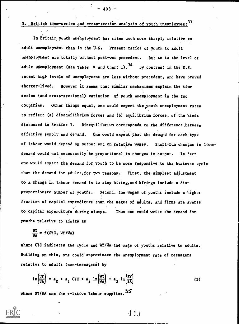
- 403

. British time-series and cross - section anal sis of outh une o .ent33

In Britain youth unemployment has risen much more sharply relative to4'7

adult unemployment than in the U.S. Present ratios of youth to adult

unemployment are totally without poit-war precedent. But so is the level of

adult unemployment (see Table 4 and Chart 1),34

By contrast in the U.S.

recent hist, levels of unemployment are less without precedent, and have proved

shorter-lived. However it seems that similar mechanisms explain the time

series (and cross-sectional) variation of youth unemployment in the two

coupiries. Other things equal, one would expect thetyouth unemployment rates

to reflect (a) disequilibrium forces and (b) equilibrium forces, of the kinds

discussed in Section 1. Disequilibrium corresponds to the difference, between

effective supply and demand. One would expect that the demjd for each type

of labour would depend on output and on relative wages. Short-run changes in labour

demand would not necessarily be proportional to changes in output. In fact

one would expect the demand for youth to be more responsive to the business cycle

than the demand for adults,for two reasons. First, the simplest adjustment

to a change in labour demand is to stop hiring, and hirings include a dis-

proportionate number of youths. Second, the wages of youths include a higher

fraction of capital expenditure than the wages of adults, and firms are averse

to capital expenditure during slumps.

youths relative to adults as

DIY

DA- f(CYC, WY/WA)

Thus one could write the demand for

where CYC indicates the cycle and WY/WA,the wage of youths relative to adults.

Building on this, one could approximate the unemployment rate of teenagers

relative to adults (non-teenageri) by

lnHuy sy0

+ a1CYC + a

2 WA1n1/1 + a

3ln

SA11A

where SY/SA are the relative labour supplies.14.

a

(3)

In addition equilibrium forces should be.at work. Relative income support

levels for the two groups should be important, but the Supplementary Benefit

for a youth relative to an adult rarely had a t-value above unity.

Equation (3) is therefore our estiu.ating equation. The analysis is confined to

males, since the rate of registered unemployment of adult females is particularly

difficult to interpret.

Before presenting the results we must briefly discuss the explanatory

variables, and their movement over time.

(i) The cycle (VAC or UA)

This is rrobably best measured by the number of vacancies registered at

employment exchanges (VAC). Alternatively can be measured by the adult

male unemployment rate (UA), but we are then explaining youth unemployment by

adult unemployment which is a highly trended variable, whose significance has

probably altered ove time. Vacancies are relatively untrended but have almost

identical turning points to adult unemployment (up to 1976).

(ii) Relative wage rates (RY/RA)

The hourly earnings of men under 21 relative to those over 21 are shown in

Chart 2. Relative youth earnings rlse steadily up till 1972. Then in 1971

they shot up, and have continued shooting up since. The main explanat:on seems

fairly clear. The compulsory minimum schoc4-leaving age was raised from 15 to

16 for everyone becoming 15 after September 1972. About two-thirds of children

wert forced to stay an extra year at school. This of course had a profound

effect on the quality of the teenage labour force. In the first place it removed

from the labour force all people with schooling up to age 15 and no work experience.

But in addition in the higher age groups (16, 17, 18, and 19) people who had

left school at 15 were progressively replaced by people who had left at 16

(beginning in 1974 and ending in 1977). Thus the efficiency units per teenager

increased. Suppose I'm treat a 15-year-old leaver with no work experience as

- 405 -

1 erg, and assume that 1 year of work-experience and 1 year of schooling each

1.1 ergs in an additive fashion. Then the number of ergs per teenager in

36t-Jc edy state changed as follows.

.

Ergs per teenage workerTeenage ergs at work

if population constant (1972 6.0)

1972 1.20 6.0

1973 1.25 5.0

1974 1.275 5.1

1975 1.30 5.2

1976 1.3275 5.3

1977 1.35 5.4

So one would expect some rise in relative teenage wages, but not by as much as

the 16 per cent which occurred. If we standardise earnings to allow for the

above changes in ergs per teenager, we get the dotted line shown in Chart 2.

This (which is the variable we use) continues the trend rise in earnings observed

before 1972.

Why these relative earnings have risen is not clear. If the earnings

changes was due to changes in the balance of supply and demand, then one could

hardly use them to explain movements in unemployment. However this does not

seem to be the case. Let us begin with the period since 1972. Due to the

raising of the school- leaving age there would of course have been a reduction

in the number of teenage ergs at work (relative to adults) if population

structure had remained ranstant. However, as Chart 3 shows, the teenage

population rose between 1972 and 1976 by 10 per cent - just enough by that date

to offset the effect of the raised school leaving age on the number of teenage

ergs as recorded above. Moreover s raised school leaving age would not create

much marked shortage of youth at existing wages if people in their younger 20s

Jere good substitutes for teenagers. Given that there must be a good deal of

substitut:on, I am willi to accept the conventional view that youth wages have

risen due to an unexplained tendency in collectively-bargained wage agreements

.1

- 406 -

There is also the puzzle of the rise in relative youth earnings before

1972. Could this be due to quality improvement? During the period, the

proportion of youngsters who stayed on rose continuously. This staying-on,

if independent of ability levels, would raise quality, whether the extra

staying-on was voluntary or compulsory. However the voluntary staying-on was

in fact selective. So the average 'natural ability' of the teenage work-force

declined, as the abler people reduced the fraction of their teenage years spent

in the labour force more rapidly than the less able people did. One cannot

quanitify this effect, but there seems no obvious reason to reject the null

hypothesis that the quality of the teenage work force remained constant relative

to the adult work force (which was itself immroving in quality). Thus one

would expect the series in Chart 2 (including the dotted section) to help

t- explain relative teenage unemployment. Further confirmation of the power

of this series to explain the teenage employment is provided in Section 4.

(iii) Relative labour supply (POPY/POPA)

There are two possible ways of measuring demographic movements:

(a) the fraction of the total population aged 15-60 who are aged

15-19 (POPY/POPA), shown in Chart 3;

(b) the fraction of the total labour force aged 15-19.38

The second of these appears to reflect more accurately the labour supply of

teenagers, but is subject to two drawbacks. First, if teenage labour supply

is reduced (for example by the raising of the school-leaving age) one would

not necessarily expect less teenage unemployment if people in their early 20s

are close substitutes for teenagers. In fact the youth labour market may be

better considered as a market for people in their first five years of work

experience. In such a case variable (i) is more relevant.39

Second, labour

supply may respond lo unemployment, whereas population is exogenous. I

therefore use variable (1).

- 407 -

One must of course remember that over time the teenage labour force

(wI-ase unemployment we are studying) has got increasingly close to the time

when it left school. This means that its members have had less time for a

succe3sful job-search and job-matching. One might suppose this would have

produced an upward trend in relative youth unemployment, but no such trend

appears in the regressions. However, as Table 3 shows the youth unemployment

problem is not primarily one of initial absorption, so this may not be an

especially important aspect of the situation.

Turning to the results, these are estimated on annual data (males only).

As Table 13 shows, the effect of the cycle is transparent. The youth unemploy-

ment rate goes up relative to the adult unemployment rate during a slump.

In fact it rises 40 per cent faster than 'the adult unemployment. Given

that the youth unemployment rate is on average over the period close to the

adult rate, it follows that youth employment falls in a slump faster than

adult employment falls. The estimated effect is robust with respect to the other

included variables, but falls as the sample period is extended forwards. This

is because youth unemployment in 1976 was much lower than predicted by amp.

equation. For example Chart 4 shows the remarkable tracking power of the top

equation in Table 13 but also shows how it overpredicts in 1976. Since all our

exploratory variables have high values in 1976, their estimated coefficients all

fall when that year is included.

The estimated effect of relative wages seems to vary in addition according

to how demand is specified, though it is always positive and reasonably

significant. If, as I prefer, demand is measured 1- vacancies, the effect of

relative wages is very large - with an elasticity of 4-5. In this case relative

wages are being made to explain most of the time trend in UYNA. If, instead,

adult unemployment is the explanatory variable, then it itself picks up a part

of the time trend in UY/UA. By contrast, the effect of population size is

unaffected by which demand variable is included.

- 40R -

One can therefore conclude that there is nothing surprising about recent

high levels of youth unemployment. The world is still the same, except that

we are in a protracted slump.

Cross-section of towns

It is interesting to compare the time-series relation between youth and

adult unemployment with the cross-sectional relation. In a cross-section of

towns, one would expect the youth unemployment rate to vary positively with

the adult unemployment rate. But one would also expect the elasticity of the

youth rate with respect to the adult rate to be lower in the cross-section than

in the time-series. For over time youths are not hired in a downturn, whereas

in a 'steady state' it is not obvious that a bad economic climate would affect

youths more than adults. Indeed, since youths can more readily migrate, one

might expect the youth rates (for the current work force) to vary less than the

adult rate. One cannot of course claim that the 1971 data for 78 county

boroughs (towns) represented a completely 'steady state', however defined.

Even so, the cross-sectional structure of unemployment rates has been fairly

stable.

The data support our prediction: the cross-section elasticity of the youth

rate with respect to the adv't rate is only .6, compared with 1.4 for the time-

series. The exact estimate is (s.e. in brackets)

In UT 1.19 + .61 In UA R2

0.61(.06)

where youths are teenabc men as before and adults are an aged 25-59. Adding as

a variable the relative supply of youths does not appear to add significantly to

the explanatory power of the equation.

- 409 -

4. Time-series analysis of the demand for labour by age in British manufacturin

Finally we can examine whether wage movements are a plausible explanation

of relative unemployment rates, by looking at the effect of relative wages on

the age composition of employment (rather than unemployment). The only

available data on labour demand by age in Britain relate to manual workers in

manufacturing, which I take to be a price-taking sector. I use the data for

April and October in the years 1949-1969. These are shown in Charts 5 - 8,

together with once-yearly data for 1970-1976.

The Charts 5A - 8A show the man-hours of youths, girls, full-time women

and part-time women, all measured relative to the man-hours of men. Charts

5B - 8B show the hourly wages of each type of labour relative to the hourly

wages of men. Taking youths first, there was an increase in relative employ-

ment lasting into the 1960s, followed by a relative decline that began well

before the raising of the school-leaving age ih 1972. By contrast the relative

wage rose more or less continuously, as we have already seen. The relative

number of girls employed (always smaller than the number of boys) fell more or

less continuously, indicating that the rise in the number of boys in the mid-

60s cannot be simply explained by the rise in the number of young people in the

labour force resulting from the post-War baby boom. The relative wage of girls

was more or less flat until its recent surge, which was. affected by the forces

already mentioned plus equal pay legislation for females. The relative

employment of women has fallen more or less continuously, with the rise in part-

time women-hours insufficient to compensate for the fall in full-time women-

hours. Relative wages of women were more or less flat until a recent spurt,

partly due to equal pay legislation.

To assess the effect of wages on labour demand requires a fully-specified

demand system. The most tractable general demand system is that derived from

the translog cost function. In using this I shall not attempt to explain the

pattern of investment and will therefore take the capital stock as a predetermined

- 410 -

variable (K) affecting labour costs (C). The general cost function can then

be written as

in C f(ln P1, In Pn, In K, T, In Y)

thwhereP.is the price of the .

type of labour, T is time and Y is output.

Taking a Taylor series expansion around zero values of all right-hand variables,

we get

where

Since

In C = ao + Egi In Pi + g.K1hK + giT + gylnY + In Pi In Pj

+ 1/24KK (InK)2 + Vi72 + 1/2.4dyy (lnY)2

+ id. In P. IriK + Ed.IT Pi .TP.TK

+ Ed.y ln Pi lnY + d. InK. T + dKy InK InY + d

2

d In C.,

11 alnP.UnP.3

1d3 ..

0

ac BlnC x.P.= xi ,

i C

thor the share of the

.

factor in total labour cost (C). Hence, differentiating

1nC by 1nPi we find that

x.P.1 1C

In addition

gi + E di3 In Pj + diK In K+ diTT + diyln Y

(i= 1, n) (4)

81nCgK 1iKinPi dKK 1nK

1KTT 1KY la (5)

and

=g1 + E diT 1nPi + 44.KT InK + d.T + dTy lnY (6)

and alncmy= gy + Edit 1nPi +dKY InK + dTiT + dyy (7)

'

- 411 -

Since shares add to a constant (unity),

I d E dI.i

d.t

0iK T Y

Since shares do not vary when all prices change by a common multiple,

I d.. 0

3 "

(8)

(all i) (9)

One could estimate the preceding system as a whole, though this would

11.4require fairly strong assumptions about the value of

3mgwhich needs to be

measurable for the estimation of equations (5) and (6).40

Or one could

confine oneself to the system (4), as I shall do. Using restriction (9)

we find that

xiP. n-1

g.+Ld..(111P.-1nP)+ & 111K+ T+ .da 111Y31 n

diT

(i 1, n) (4')

where n is some factor taken as numeraire. In addition, since the shares

must add up, one need only estimate (n-1) equations for (n-1) shares. This

is our estimating system, with the requirement thatt

d..tj

di.. imposed upon it.

The Allen elasticities of substitution are then evaluated as42

S

dii+ 1 -

1

iiAi2

Ai

d44St. + 1

j A A.i 3

(1 3)

where Ai

xiPievaluated at the mean. The price-elasticities of demand (with

output and capital constant) are

et .

SitA.

j i

- 412 -

Estimates

System (11) was estimated using the TSP's iterative version of Zellners's

minimum distance estimator (see Table 14).43

The variables are defined in Annex 7

Unfortunately we have no data on non-manual workers,so the assumption is that

the relative demand for manual workers of different age and sex is independent

of the number of non-manual workers. (Part-time women were amalgamated with

full-timers in order to reduce the number of parameters.) 44The results are

fairly sensible and suggest quite high -short-run elasticities of demand for

youths (but not girls), linked to quite high substitutability between categories

of labour (except, rather oddly, girls and women). Girls are very good

substitutes for youths, and women are less good substitures. As one would

expect, youths and girls are not good substitutes for men, women being rather

better substitutes. These findings are similar to those of Anderson, and

Freeman for the U.S.45

Noneof the effects of capital, output or time were1

well-determined. But, given the significance of the price effects, one has

some confidence in supposing that youth wages are highly relevant to the problem

of youth unemployment."

- 413 -

Annex 1

Income maintenance for young people

Income if unemployed as a fraction of income in full-time work is

probably higher for youths relative to anults in Britain than in the U.S.

A registered unemployed British youth, even if he.ot she has never worked

and,is living at home, can claim Supplementary Benefit. This is currently paid

to someone living at home and aged 16 to 17 at a rate equal to about 30 per

cent of gross male weekly earnings at that age (and a higher percentage of

net earnings). With a minimal work record an 18-19 year old can claim

unemployment benefit equal to about 30 per cent of the equivalent gross male

earnings. About two-thirds of unemployed youths under 18 in Britain personally

receive social security payments.47

In the U.S. it is more difficult for a youth to obtain benefit in his

own right. Only 112 of unemployed under 20's (out of school and looking for

full-time work) were on U.I. in May 1976. In some states other youths

would be receiving personal welfare payments, but there is no information on

the numbers.

I

- 414 -

Annex 2

Definitions of variables in Section 4

P hourly earnings: from survey of Earnings and Hours of Manual

Workers in Manufacturing in April and October (to 1969) and

October (1970 onwards).

X manual manhours: from the same source

fixed assets in manufacturing. Gross value at constant prices

(replacement cost). The series is rebased a number of times

over the period and I have grafted one series onto the next.

T time (1 unit 6 months; April 1948 1)

index of manufacturing production (this is a value-added measure)

Footnote No.

1

2

4

5

- 415 -

FOOTNOTES

Excluding students from the U.S. data also involves excluding part-

time students, who are included in the British data. However the

age-specific unemployment rates of students in the U.S. are very

similar to those of non-students.

The General Household Survey is too small for disaggregated

comparisons with the CPS.

This assumes that the age structure of the population is not totally

dissimilar.

One should ignore the figure for unemployed 15-year-olds in. Britain,

since nearly all 15-year-olds in the labour force had left school

a month before the Census.

See U.S. D.O.L., B.L.S., International Comparisons of Unemployment,

Bulletin 1979, 1978, p.19.

6 A formula which would adjust the British aggregate rate so that in

1976

British aggregat3 adjusted rate,,- U.S. aggregate rst-e.

s. British prime male rate - U.S. prime male rate

would be to multiply the British aggregate rate by 1.5. The

multiple would of course differ between years.

7 It is also 'boosted' by the inclusion c4 unemployed students (some

14 per cent of U.S. unemployed).. Such people cannot be inc uded

when other countries are adjusted to U.S. concepts due to lack of

data (and the absence of any large numbe.k of such people). Inc)uding

them raises the U.S. rate by a multiple of between 1.05 and 1.10.ti

- 416 -

Footnote No.

In addition in 1970/1 of employed males under 20 not in school

21Z in the L.S. worked part-time (under 35 hours) compared with

under 7% in Britain. (There were few differences here for

women.) However some of the part-timers may have been looking

for full-time jobs. (Source: Britain, 1971 Census Economic

Activity Table 23; U.S., Ac for Table 2).

9 ETRP 1978, p.242 and p.186-7.

10 C.P.S. analyses by D. Ellwood and M. Feldstein show that of males

under 20 out of school and out of the labour force, only 37 per cent

say they would definitely like a job, and of these only 37 per cent

are-rot)looking because they do not think they could find one. Of

the whole group (r,les under 20 out of school and out of labour

force) 28 per cent say they will' not look for work in the next 12

months (or their intentions are so reported).

11 I would explain the fact that individual youth unemployment is

negatively correlated with income by the same type of expression

as used to explain individual youth participation in the labour force.

12 Not all differences found in cross-sectional data for individuals

are found repeated in a comparison of U.S.: and Britain.

(a) The hours of work of full-time workers are not lower in the

U.S. (1977): for men 43 hours in Britain and 45 in the U.S.,

and for women 38 hours in Britain and 40 in the U.S. (see

D.E. New Earnings Survey, 1977, p.A18-19 and B.L.S. Employment

and Earnings, July 1978, vol. 25, No. 7, p.19).

(b) Female participation is higher in Britain than the U.S.

13 R. Layard, D. Piachaud and M. Stewart, The Causes of Poverty,

Royal Commission on the Distribution of Iacome and Wealth, Background

Paper No. 5, HMSO, 1978, and S.J. Nickell, 'The effect of unemployment,

and related benefits on the duration of unemployment', Economic Journal,

- 417 -

Footnote No.

14 M. Feldstqin, 'The effect of unemployment insurance on temporary

layoff unemployment', A.E.R. Dec. 1978.

15 The previous comparison is complicated by two factors. First,

FeIdstoin's figures include women but he also shows a figure of

.54 for the subsample of (predominantly male) union members.

Second, his figures are individual income replacement ratios and

ours are family income replacement ratios. On average women's

earnings account for under one-fifth of family income so the

British individual income replacement ratios for all males could

not be as low as the U.S. ratios for 'privileged' males. (Most

international comparative statistics on unemployment relief fail to

mention the British Supplementary Benefit system which determines th

income maintenance levels of 5Q% of the unemployed, compared with

302 whose income maintenance is determined by National Insurance),1

16 A youth in a family characterized by an altruistic head does not

face the full cost of his actions. If he decides his own labour

force behaviour, he may make choices which do not maximi4 family

income.

17 She is unlikely to say this if the youth is under 18. For if the

youth is under 18, the AFDC entitlement includes a child allowance

only payable (for a non-student) if the child is working or

registered unemployed. This constitutes a strong pressure to

participate (though not to take a job). Bus: under a quarter of

unemployed teenagers out of school are under 18.

18 1975 SIE analysis by R. Freeman. Data relate to 18-19 year-cld

males'(including students?).

19 75 per cent of men are covered.

t itJ

- 418 -Footnote No,

20 Another approach is to look at the shape of estimated experience-

earning profiles. If male annu.-.1 earnings are regressed on

schooling, experience and experience squared, earnings at the peak

are 280 per cent higher than starting earnings in Britain and

288 per cent higher in the U.S. (G. Psacharopoulos and R. Layard,

'Human capital and earnings: British evidence and a critique',

Review of Economic Studies, forthcoming; J. Mincer, Schooling,

Experience and Earnings, 1c74.)

21 0. AshEnfelter and R. Smith, 'Compliance with the Minimum Wage Law',

Industrial Relations Section, Princeton University, Working Paper 98,

June 1977.

22 D.E. New Earnings Survey, 1977, Table 126. For U.S. as in Table 6.

23 Formerly known as the Youth Employment Service, this is run by

local education authorities and has primary responsibility for the

placement of school leavers. 22% of a random sample of 3,000

15 -i9 year-olds interviewed in November 1976 said they got their

first job through the Careers Service (Manpower Services Commission,

Young People and Work, Manpower Stndies No. 1S1781, 1978).

24 D.E. GazEtte regular statistics. Relate to number of school-leavers

r4istereo as unemployed. A 'school-leever' is anyone under 18 who

has never had a full-time job. From January 1961 to January 1975 the

number of unemployed people under 18 who had not yet found a first job

never rose above 10,000 in any January. In January 1976 it was 38,000.

25 I am as-uming unemployment always lasts a whole number of weeks.

- 419 -Footnote No.

26 Expressions (1) and (2) are of course eqivalent since

4, ft d(E F

dTd

a E(F E C0

dal dal t -1

(F1C1 F2(C1 C2) F3(C1 C2 C3)

C1(F1 + F2 + F3 + ...) + C2(F2 + F3 + ...) + C3(F3 + ...) +

E Ct Nt

since Nt a E Fd.

d -t

27 This assumes no repeated spells in a year. If a worker's

annual weeks are held to lG HI below their equilibrium level,

the compensated supply price falls from W to V where

W - V a 1; IAHI

.H AH IH 1 Lo 1 wHence W-V .17hr4 71- " H

28 See S. Salant, 'Search theory and duration data: a theory of

sorts , ILLE., 91, Feb. 1977, pp.39-57.

29 The U.S. duration figures are taken from Akerlof and Main since

Clark and Summers' figures do not reflect short spells beginning

and ending betwren CPS interviews. (The clerk and Sminwrs'

figures are 9.4 for 1974, and 11.3 for 1976, see K. Clark and

L. Summers, Labour force transitions and unemployment, N.B.E.R.,

mimeo, April 1978.) However I rely on the Clark and Sunawa

finding cf almost identical,durations for men and women in assuming

that Akerlof and Main's figures for both sexes also apply to men.

30 ETRP 1978 p.275 and D.E. Gazet*e May 1978 p.577. It would be

interesting to compare the distribution of establishments by their

annual changes in employment, in order to see to what extent the

labour turnover reflects demand-side as opposed to supply-side

- 420 -Footnote No.

30 forces. British data are available -- are there U.S. data?(contd.)

It would also help if the CPS would ask how unemployed re-entrants

left/lost their last job (British data are available).

31 For Britain see S. Owen, 'Do the faces in the dole queue change?',

University College, Cardiff, mimeo, Summer 1978.

U.c. data are special tabulations relating to non-students and show

average numbers of spells in 1977 of 1.83 for men aged 16-19 and

1.72 for men aged 20-24. Of course the distribution of cumulated

spells depends not only on the frequency of repetition but on the

way in which spell lengths differ for repeaters and others. I have

not been able to investigate thisfor Britain (on the U.S. see

Akerlof-and-Main).

32 In both countries of course the inflow of youths into unemployment

is much higher than f adults, though, perhaps interestingly, the

difference in Britain seems rather less than the differential turnover

rate. The percentage of employees who have been with their current

employer for less than 12 months is (April 1976)

Under 18 281420 21-24 25-29 30-39 40-49 50-59 AllMales 57 21 20 14 1,0 6 4 11

Females 60 25 21 16 15 9 5 lE

(New Earnings Survey).

33 This whole section is based on data generously supplied by Peter

Makeham of the Department of Employment from his forthcoming study

of youth unemployment, summarised in D r Gazette, August 1978.

Full details of the time-series source3 are available in the

Technical Annex to his article in the D.E. Gazette, August 1978,

obtainable from the Department of Empla;,ment. The following

eat

421 -

33 definition is important. Unemployment rates are measured in July

(contd.)

34

35

but exclude school leavers in order to avoid problems to do with

changes in school-leaving dates. Adult students are also excluded.

The cross-section data are based on the 1971 Census Table 18,

unemployment rates being measured by total out of employment as

percentage of all economically active.

The same has happened in France and Germany (see H. Gallis, Youth

unemployment: a statistical analysis, ENP 47-1/W7 2, I.L.O. Oct. 1977).

Since UY and UA are small

= ln (111,/ lnUY

But in addition since UY/UA is not far from unity

ln =UY UY DA

UA 2 .11 (DY+ ln =f (iv + ln (17-1

Sa SA

with f' > O.

36 This is based on the assumption that (n_arly) all who do not leave

at the minimum age stay till 19 or over. Unfortunately, no more

subtle exercise is worthwhile since there is no fine breakdown of

teenage wages by age, let alone by age and education. The best

data are in the source to Table 6.

37 In so far as unemployment affected pay, I assume the relationship

has a lag so that current pay is predetermined.

38 See for example D.E.G., April 1978, p.427.

39 It might be better still to taasure the fraction aged (15 + D) to

(19 + D) where D is unity from 1973 onwards and 0 before.

40 To estimate (6) we need a measure of ainC , which can be

111"measured using the following identity:

dInC E alriC dinPi alnC dInK aInC aInC dlnYdr 51315. dr 1-0Z. "fr CirOise could assume on the basis of zero excess profits that

alniC 3C K rK H alnC II

- = and my = 1 -

4c;

- 422 -

Footnote No.

41 Constant returns requires

diK a+ d. = 0

But, as we are omitting non-manual workers from the demand system

(for lack of information) there is no virtue in imposing this

constraint.

42 See H. Binswanger, 'A cost function approach to the measurement

of elasticities of factor demand and elasticities of substitution',

American Journal of Agricultural Economics, May 1974.

43 To reduce the autocorrelation of residuals, the system was estimated

as follows:

Ai = gi + Edij(lnPi In Pn) + diK In K+ diT' T

EdijanPi_,+ diK InK_i +

Here p is the autocorrelation coefficient in the equation

u. = + e.1 1,-1 1

It has to be constrained to be the same for all i in order to

ensure that the factor shares add up to unity For simplicity

consider the following proof in the case of two shares, Al and A2,

and one right-hand variable (X)

= Xpl + ul

A2 = X/2 + u2

Since A. + A2 = 1 , we require 6]. xi,32 = 1, and therefore

ul + u2 = 0 . Now suppose ul

I* follows that

u2 = u,

=

5P1u2,-1

Thus the autocorrelation coefficient is the same in the equation for A2

as for Al. I am grateful to Larry Lau for pointing this constraint out

_ _a

Footnote No.

44

- 423 -

Up to 1956 I assume part-time woman-hours to be proportional to

full-time, and part-time hourly earnings to be proportional to

full-time.

45 J.M. Anderson, 'Substitution among age groups in the U.S. labor

force', Williams College, mimeo, December 1978. He used four

factors in a translog production function - capital, and workers

aged under 25 (Y), 25-55 (M) and over 55 (0). The price elasticities

(with capital variable) were

0

Y -2.5 1.9 .6

H .3 -.9 .4

0 .3 1.7 -2.7

R. Freeman, 'The effect of demographic factors on age-earnings

profiles', NBER Working Paper No. 316, February 1979. He used four

factors - capital, men 20-34 (Y), men 35-64 (M) and women 20-64 (W).

The own-price elasticities (with capital variable) were

Y -2.14 1.64 .19

.76 -1.21 .29

W .29 .94 -1.25

46 The model reported here includes no adjustment mechanism. But I have

also estimated the model with ln P replaced by .5 ln P + .33 In P_1

+ .17 ln P_2. The estimated price elareicities were very similar.

However, I am currently, with John Abowd, estimating a fuller model

which includes a fully-specified zdjustment mechanism and distinguishes

between people and people-hours.

47 Department of Employment, British Labour Statistics Year Book, 1976

Table 119.

424 -

Table 1

Age-specific unemployment rates for non-studentsin Britain (1971) and U.S. (1970)

Percentage

Under 25

25+

Men Women

Britain U.S. Britain U.S.

6.6

3.6

9.6

2.8

5.1

3.2

8.2

4.1

Total 4.2 3.6 3.7 4.9

(Under 25 rate

divided by 25+ rate) (1.8) (3.4) (1.6) (2.0)

Source and Notes: See Table 2.

- 425 -Table 2

Schooling, labour force participation and unemploymentin Britain (1971) and U.S. (1970)

of populationwho are

non-students

% of non-stu2.-ntswho are inlabor force

of non-studentsin civilian labor forcewho are unemployed

Age Britain US(W) US(B) Britain US(W) US(B)Britain US(W) US(B)

(1) (2) (3) (4) (5) (6) (7) (8) (9)

Males

(15) (31.4) (4.4) (7.6) (87.3) (32.5) (26.5) (21.7) (16.0) (20.6)

16 52.3 7.9 11.8 97.1 48.6 34.7 8.8 21.6 27.0

17 71.0 13.3 20.5 97.9 65.3 48.0 6.7 19.0 27.1

18 78.8 30.2 45.0 98.1 82.8 71.8 7.2 i2.9 20.8

19 83.6- 48.2 61.6 98.0 86.4 71.8 7.1 11.2 18.6

20 85.5 59.8 77.8 97.8 88.3 76.0 6.9 9.6 14.6

21-24 92.8 75.8 87.5 98.2 92.4 82.1 5.4 6.4 10.4

25-29 98.2 89.5 93.3 98.3 95.6 87.3 4.2 3.3 6.0

30-34 99.2 94.7 95.3 98.2 96.2 89.1 3.9 2.6 4.7

Females

(15) (31.7) (5.0) (8.4) (87.0) (19.5) (16.7 (14.9) (15.9) (25.4)

16 52.0 8.5 13.1 94.1 26.5 20.7 6.8 21.9 33.E

17 69.7 15.0 22.2 91.6 35.2 29.2 5.3 19.3 31.1

18 79.6 38.9 46.9 86.5 59.6 44,4 5.0 11.7 24.4

19 85.2 54.9 63.6 80.9 63.1 50.6 4.8 9.3 21.0'

20 87.2 67.6 79.5 74.4 62.4 55.3 4.5 7.8 15.9

21-24 95.9 85.6 89.8 61.1 56.9 58.9 4.1 5.7 11.8

25-29 99.2 95.4 95.5 43.1. 43.1 58.3 4.3 4.9 8.5

30-34 99.4 96.6 96.3 44.8 41.8 59.1 4.2 4.6 7.0

Source and notes: See next page.

- 416 -

Source: Britain: 1971 Census, Economic Activity Table 3.

U.S.: U.S. Department of Commerce, Bureau of the Census,

1970 Census of Population, Detailed Characteristics,

Final Report, PC(1)-D1, U.S. Summary, Table 217.

Notes: 1. Britain re.lates to 24 April 1971; U.S. relates to 1 April 1970.

U.S. (W) relates to whites and U.S. (B) to blacks.

2. Non-students in Britain include part-time students; in the U.S. they

do not. In Britain a student is someone who will.be studying in the

following April/May term; in the U.S. a student is someone who has

studied at all since 1 February.

3. The labor force is the employed (defined identically) plus the

unemployed. The employed labour force includes those who worked at

any time for pay or profit during the week (including unpaid family

work) plus those temporarily away from their job due to holiday,

sickness, or industrial dispute. In Britain, unlike the U.S.,

temporary layoffs are treated as employed, but the maximum number of

such people since 1973 has been 34,000 and the usual number is

under 10,000.

4. In Britain the unemployed include those persons currently "seeking work

or waiting to take up i job". In the U.S., the unemployed include

all who have looked for work in the last 4 weeks or due to take up

a job within a month, or on temporary lay-off. The unemployed include

those looking for part-time work, in both countries.

,1".)4.,

- 427 -

Table 3

Male unem lo ..ent rates for non-students: by age (1976)

Age j Britain (Jan.) Britain (July) U.S. (All year)

16-17 12.4 26.8 28.4

18-19 11.1 10.6 17.3

20-24 10.0 9.3 11.0

25-34 6.6 6.2 6.2

35-44 5.5 5.2 4.1

45-54 4.6 4.5 4.0

55-59 4.9 4.9

}4.2

60-64

9.5

19.5

65+ 5.2

Total 6.9 7.3 7.0

Source: Department of Employment Gazette, January 1979, p. 40.

Employment and Training Report of the President, 1978, Tables A3,.A19 and B7.

Notes: 1. U.S. data include persons in school if they were also in the labour force.

2. A fine age breakdown of youth unemployment is only available in Britainin January and July and in the U.S. in October. The first three U.S.figures relate to October, but other-data show that for those aged 16-21not in school the October rate is quite close to the annual average(B.L.S. Handbook of Labor Statistics 1977 p.57)*. There is surprisinglylittle month to month variation in the unemployment rate for such people,though in January it is higher than the annual average by about the sameproportion as the all-age unemployment rate is p.57 and 63).

3. In Britain the pattern of male unemployment was very similar inJanuary 1976, 1977 and 1978.

- 428 -

Table 4

Unemployment rates: by age

Males Yemales

Britain U.S. Britain

Under 20* All ages

U.S.

18-19 1 All agesUnder 20*1 All ages 18-19 All ages

1959 1.6 2.2 15.1 5.3 0.8 1.5 13.1 1 5.9

1960 1.0 1.7 16.5 I 5.4 0.6 ,1.2 0.0 5.9

1961 0.8 1.5 15.2 6.4 0.5 1.0 14.5 7.2

1962 1.7 2.1 13.0 5.2 1.1 1.3 12.3 6.2

1963 1.9 2.6 14.8 5.2 1.4 1.5 14.9 6.5

1964 1.3 1.8 13.3 4.6 0.8 1.1 15.3 6.2

1965 1.1 1.6 10.4 4.0 0.7 0.9 1'3.7 5.5

1966 1.2 1.7 8.4 3.2 0.7 0.8 12.6 4.8

1967 2.6 2.E 10.7 3.1 1.3 1.1 1 16.1 5.2

1968 2.6 3.1 9.5 2.9 1.2 1.0 12.9 4.8-

1969 2.7 3.1 8.9 2.8 1.1 0.9 11.0 4.7

1970 3.4 3.4 14.1 4.4 1.4 1.0 16.4 5.9

1971 5.4 4.5 14.6 5.3 2.4 1.3 16.7 6.9

1912 6.8 4.9 11.9 4.9 . 3.1 1.5 15.2 6.6

1973 3.3 3.5 9.9 4.1 2.0 1.1 13.8 6.0

1974 3.6 3.5 15.3 4.8 2.0 1.0 16.9 6.7

1975 7.4 5.2 18.6 7.9 5.3 1.9 19.0 9.3.

1976 9.1 6.7 17.3 7.0 8.0 3.0 18.5 8.6

1977 9.6 7.0 - 6.2 9.4 3.8 - 8.2

Scarce and notes: See next page.

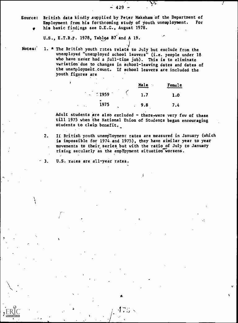
- 429 -

Source: British data kindly supplied by Peter Makeham of the Department ofEmployment from his forthcoming study of youth unemployment. For

his basic finc4ngs see D.E.G., August 1978.

U.S., E.T.R.p. 1978, Tables 87 and A 19.

Notes:" 1. * The British youth rates relati to July but exclude from theunemployed " unemployed school leavers" (i.e. people under 18who have never had a full -time job). This is to eliminatevariation due to changes in school-leaving dates and dates ofthe unetploymeht count. If school leavers are included theyouth figures are

1959

1975

Male FemaleFemale

1.7 1.0

9.8 7.4

Adult students fire also excluded - there.weretill 1975 when the National Union of Studentsstudents to claim benefit.,,

2. If British youth unemployment rates are measured in January (whichis impossible for 1974 and 1975), they have similar year to yearmovements to their series but with the ratio of July to Januaryrising secularly as the emprpyment situation worsens.

very few of these

began encouraging

3. U.S rates are all-year rates.

a

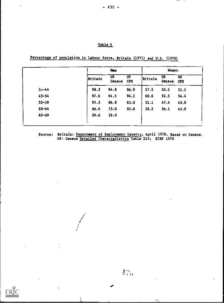
- 43C -

Table 5

Percentage of population in labour force, Britain (1971) and U.S. (1970)

3-44

45-54

55-39

60-64

65-69

Britain

Men Women

US US

Census CPSBritain

US USCensus CPS

98.3

97.6

95.3

86.6

30.6

94.8

94.5

86.8

73.0

39.0

96.9

94.2

83.0

83.0

57.5

60.6

51.1

28.2

50.2

52.5

47.4

36.1

51.1

54.4

43.0

43.0

Source: Britain: Department of Employment Gazette, April 1978. Based on Census.US! Census Detailed Characteristics Table 215; ETRP 1978

Table 6 - 431 -Average hourly earnings of manual workers within each age

group as percentage of average hourly earnings ofall manual workers in the same column 1976/7

Britain U.S.

Age Males Females Age Males Females

Under 18 51 68

18-20 76 90 16-19 56 74

21-24 96 100 20-24 82 97

Note: U.S. data relate to workers paid at hourly rates (including part-timers

and students) in May 1976. British data relate to full-time manual

workers in April 1977.

Source:Britain: DE, New Earnings Survey 1977, p. A18 and A19.-

U.S.: U.S. Department of Labor, B.L.S. Weekly and Hourly Earnings Datafrom the Current Copulation Survey, Special Labor Force Report 195,

1977, Table 4.

Table 7

Average weekly earnings within each age group asRercentageof average weekly earnings of workers

of all ages in the same colurn 1976/7.

Britain U.S.

Males I Females Males Females

Under 18 42 38.

18-20 63 78 9 80

21-24 84 96 59 80

25-29 98 116 89 104

I I

Note: U.S. data relate to annual earnings of year-round, full-time workers.British data relate to weekly earnings of full -time employees in the surveyweek or month.

Source:gritain :DE New Earnings Survey 1977 p. A18 and 19.

U.S.: Department of Commerce, Bureau of the Census, Ci_irret'otilationReport, Series P-60 No. 114.,Money Income in 1976 of Families and Persons in the U.S. 1978 p.203-204

- 432

Table 8

Average uncompleted duration ofrpit,ai22naleuttemloetidthearoximatecost of male unemployment relative to potential male earnings

Average uncompletedduration (Weeks)

Unemploymentrate (%)

Approximate cost ofunemployment relative

to potential maleearnings (Index)

(1) (2) (3)

Britain (July)

1971 23.4 4.5 1051972 27.8 4.9 1361973 30.8 3.5 1071974 26.4 3.5 921975 22.3 5.2 1161176 26.5 6.7 1771977 28.1 7.0 1901978 29.5 6.7 197

U.S. (All year)

1971 11.3 5.3 601972 12.0 4.9 591973 10.0 4.1 411974 9.7 4.8 461975 14.1 7.9 1121976 15.8 7.0 1101977 14.3

Source: Britain: D.E. Gazette, September 1978, p. 1049 and Table 4 ofthis paper.

U.S.: G. Akerlof and B. Main, 'Unemployment spells and unemploymentexperience', Federal Reserve Board, Washington D.C., SpecialStudies Paper No. 123, October 1978, and Table 4 of this paper.

Note: U.S. data assume duration to be the same for men as tor men and women.This slightly understates duration (see Table 12).

- 433 -

Table 9

Completed duration of unemployment (weeks), (men)

Average completedduration (Weeks)

Probability ofentering unemployment

(% per week)

Unemploymentrate (Z)

(1) (2) (3)

Britain

1972 13 0.38 4.91973 10 0.35 3.51974 9 0.39 3.51975 14 0.37 5.21976 16 0.42 6.71977 17 0.41 7.0

U.S.

1972 6.2 0.79 4.91973 7.0 0.59 k.11974 5.6 10.86 4.81975 9.1 0.87 7.91976 8.0 0.88 7.01977 7.2 0.86 6.2

Source: Col. (1) - 1. U.S. data from Akerlof and Main, (see Table 8).They are got b; applying the Salant method to theuncompleted durations.

2. The British data come from inflow data divided bystock data. Department of Employment Gazette, September1978. They relate only to registered unemployment -most male unemployment is registerri.

Col. (3) - Sources are ETRP and DE Gazette.

Col. (2) - Col. (3) divided by Col. (1).

434 -

Table 10

Distribution of males unemployed sometimeduring a 12 month period: by number of spells

1 2 3 4-9 10+ All Average numberof spells

Britain June 71-72 66 20 7 5 2 100 1.8

1/4.-..---..------)U.S. Jan. 75-76 64 18 18 100 1.53

Jan. 76-77 61 19 20 100 1.67

Jan. 77-78 62 20 18 100 1.66

Source: Britain: DHSS study of claimants cited in D. Metcalf and S. Nickell,'The plain man's guide to the out of work: the nature andcomposition of male unemployment in Britain', LSE Centre forLabour Economics, Discussion Paper No. 6.

U.S. : B.L.S., Work Experience of the Population, Special Tabulations.Data exclude students. The average figure is based on theassumption that average spells in the 3+ category are 3.5, asnormally assumed by B.L.S.

0.

435 -

Table 11

Age specific indices (male, non-students) (All ages 1.0)

Average completed''.oration (Weeks)

Probability ofentering

unemployment(Z per week)

Unemploymentrate (Z)

(1) (2) (3)

Britain (Jan. 1978)

16-17 0.53 3.38 1.7918-19 0.70 2.11 1.4820-24 0.80 1.71 1.37

All ages 1.00 1.00 1.00

U.S. (1976)

16-17 0.75* 5.41 4.0618-19 0.75* 3.29 2.4720-24 1.06 1.48 1.57

All ages 1.00 1.00 1.00

Source: Col.(1) - Britain: D.E. Gazette, February 1978, p. 205.

U.S.: K. Clark and L. Summers, 'Labour Force Transitionsamd Unemployment', Table 3. They get very similar resultsfor 1974 - and also for 1968-76 in 'The dynamics of youthunemployment', Table 1.3.

Col.(3) - Britain: D.E. Gazette, March 1979, p. 262.

U.S.: Elq, 1977.

Col.(2) - Col.(3) divided by Col.(1).

Note: * Separate figures not available.

4L'

- 436 -

Table 12

Uncompleted duration of unemployment (weeks)

Men

Under 18

18-19

20-24

All ages

Women

Under 18

18-19

20-24

All ages

Aggregateunemployment rate

Mean duration

Britain U.S.

Percentage unemployed over13 weeks (Britain) 15 weeks (U.S.)

Britain U.S.

Jan.1976

July1976

Jan.

1976

July1976

Jan.

1976

July1976

Jan.

1976

July1976

13.6

16.6

19.5

25.4

6.910.3

18.0

22.5 14.9

26.5 15.9

6.0

10.0

12.3

41

44

48

56

11

42

51

54

Men

Women

Source:

Note: 1.

2.

13.1

15.2

16.1

18.0

6.7

3.0

9.5

10.9

12.6

6.1

8.1.

9.5

6.2

8.2

ql 12

40 40

42 45

45 38

21

30

32 29

10

2010

20 16

25 21

11

11

29

D.E., British labour Statistics Year Book, 1976, Tate 113.

B.L.S., Employment and Earnings, July 1978, p. 32, and Handbook

Statistics, 1977.

British data relate to period registered at exchange; U.S. data

reported period looking for work.U.S. data include students but other data suggest that, holding

duration of students and non-students are similar.

of Labor

relate to

age constant,

- 437 -

Tab- le 13

Time-series regressions (all variables in logarithms)

Dep. Var. Period VAC UA WY/WA PCPY/POPA Const. R2

DW SE

UY/UA 59-72 -.54 4.62 1.29 -18.7 .96 2.63 .048(.06) (.52) (.40)

UY/UA 59-74 -.50 5.01 1.43 -20.7 .96 2.55 .046(.05) (.43) (.40)

UY/UA 59-76 -.38 4.07 .42 -15.1 .93 1.49 .071(.06) (.41) (.43)

UY/UA 59-72 .40 1.52 1.64 -10.1 .94 2.11 .060(.06) (.88) (.52)

UY/UA 59-74 .43 .60 1.46 - 6.5 .91 1.88 .066(.06) (.70) (.53)

UY/UA 59-76 .38 .71 .96 - 5.7 .93 1.90 .073(.C7) (.69) (A40)

Note: Standard errors in brackets. All regressions estimated by Cochrane-Orcuttprocedure; the Hildreth-Liu procedure gave very similar results.

'14

- 438 -

Table 14

Demand elasticities and elasticities of substitution

Youthsi

Girls Women Men

.

e.. YouthsGirls

WomenMen

.

-1.25.82

.12

.02

_

.29

-.31-.07.01

.50

-.85-1.59

.32

.47

.34

1.55

-.35

s.. YouthsGirls

WomenMen

-33.622.1

3.1

.6

22.1-23.5-5.3

.4

3.1-5.3-9.92.0

.6

.4

2.0

-.4

t-ratio Youths

GirlsWomenMen

5.82.5

1.8

1.3

i

2.5

.9

2.0

.7

1.82.0

10.5

9.5

1.3.7

9.59.2

Note: 1. The elasticities are for given capital and output.The t-ratios apply equally to eij and sib.

2. In the equations for Ay, AG and the implied values

of DW and R2

were as follows:

AYAG AW

R2

.96 .92 .92

DW 1.11 1.8-i .90

- 439

CHART 1

Unemployment rates of males aged under 20(excluding school leavers) and all males 1959-1976

% Unemployment Rate

10

9

all males (excluding school leavers

fmales aged under 20 (excludingschool leavers)

1

1

I

1

1

1

1

1

/ 1

FPI

I I II

1

JU

$1

440

CHART 2

hourly earnings of aged under 21 as a per cent

prf adult male hourly earnings 1948-1976 - manual workers all industries, UK

61

SO

49

47

46

44

11146 49 SO 61 52 63 54 55 55 67 69 59 60 61 62 63 64 65 OS 67 68 69 70 71 72 73 74 75 V, 77

Source: Department of Employment Gazette, October earnings survey.

4 i;

Adjusted forquality

- 441 -

CHART 3

Males aged 15 -19 as percentage of males aged 15-60

.71-77.. 1

- . I

1- -

14.0

13;5

13.0

--12.0

11.5

4L,

Source: Estimatessu?pliec by the Department of Employment.

CTuAL Flyli.**

IP

-.2107..3657-.4620-.1278...1270-.2231-.2231-.13930.4..9431E-01-.40A2E-01.7696E-31.2624.2624

O..1044'

3E153 0.' .3507

4..

CHART 4

Top equation of Table 13, estimated for periods 1-14

.4)7.1 4,,,

Lls.E nP. .;.e..

s7-,.. =.0.

1, .la.. .E'.:.

4. i

+..

I ' 1 ( I:) V/ l i!.. i

qt.SVIJAL

nor OF RESIOUAL310)

0.0.Sbs .

.113 . . a

-.56pr-01 . A

1 stiLAEVI. It .0,4} weei5E..C1 0

*16Ar01 II .0 4,

.15:er7.-4-,1 . U 1.4 -.1AT-)1 . 0,, 4,

I. 4 ..h7oz-01 . 0 . .

+ -.413r-31 . 0. .

Ot4 ..6t.'YE.9:1. a ea .

f A, .D7LIE"1 0

... te .4:-AF../...1 0

+. ./1;1:.1,1 0 .

+ , .7x97 -C1 . 0

4... .672=-C1 . . 0

+ -.9o1 -!1 .0

+ -.563 0 . .

i

443

atMIMUM

0.074776

MAXIMUM

0.106026'

Apr

-48

Oct

48

t .tg

t 21: S.

.7.

I

10 .

11 .

It .

13 .

14 .

IS

1617

10 .

1,

20 .

21 .

22

23 .

24 .

26 .

26 27

.

a

aaa

a

a

a

a4

a .

it .

30 .

31 .

32

r.

33.

CD

34IS

36

37

IS .

30 .

4041

69 ,42 3

.A

pr D

4O

ct 6

9 44

Oct

70

45 .

Oct

71

"

Oct

72

47.

Oct

73

44 *

Oct

74

4.!

Oct

75

Oct

76

aa

a

a

U.

*a

aa

a

a

0 rt

MINIMUM'

fir

ti.

Apr

49

1O

ct 4

9 I .

6 .

7 .

$ .

le .

11 it .

13 .

14 .

15 .

16 .

417 .

14.

It

20 .

21 .

31 .

10 .

32 .

25U.

22 .

-

23

#'48,

24.

26

27

24P .

2 33 .

la .

35 .

is )7 .

3$ 3 .

40 .

et

0.422474

a a

444

MAXIMUM

.605516 06

. . . .a

. . . .

;-

4.121- 0 .

. .4 0 re a. .... W 0

41 .

12 .

..

WIN g; :: . .

a. .

Oct

70

4.3

.O

ct 7

1 41

* .

Oct

72

7.

Oct

73

IS .

Oct

.74

.O

ct 7

5 Is

Oct

76

51

ItIta

illits

Apr

48

1 .

34

Apr

Oct

13

49O

ct 4

9 4 5 6. 7. 8. e IS

.11

.12 13

.14

..15 16 17

.is

.19 to

.at

.22

.23

.24

.25

1. 2

6C

.1.,

27 20.

t..)

2 .

30 .

31 .

32 .

33 .

34 .

35 .

33 .

37 .

38 .

30 .

60 .

41 .

42A

pr 6

9 43

Oct

69

44Q

ct 2

945

.O

ct/1

46

.

Oct

72

47 .

Oct

73 4

t .O

ct 7

4 41

PO

ct 7

5 30

0O

ct 7

6 51

a

.522

661

MA

XIM

UM

*

4.a

0

6.11

5754

3 .0

'

a

%

a

a a

-

I

a

a

.

a

*

es

.

r r I

- 41

6 -

MINIMUM*

0.357333

MAXIMUM

0.408627

ttt. ti : ,

rO

ctA

p499

43,. s. 6 .

._

7 .

S . .

10 .

11 .

12 .

*.

13 .

*.

14 .

.

IS .

. . . - . . .

IS .

a.

VP .

a.

30 .

31 .

32 .

.

33 .

34 .

35 .

.

36 .

.

'CZ , - w

16 .

17 .

IS

IV .

10 .

21 .

12 .

23 .

14 .

2316 .

27 .

a

37 .

30 .

3,

40 .

41 .

42 .

fr 2

12 :

tO

ct 7

045

Oct

714

6

Oct

724

7.

Oct

pa.

449

Oct

5so

Oct

76s

t .

a

ow .

447

MINIMM*

0.171636

MAXIMUM'

0.388342

Apr

48

1.2g

a3

Oct

49

4 .

s .

6.

7.

6. 10.

11 .

11 .

13 .

14 .

aa a

a aa.

IS .

16 .

17 .

16 .

19 .

20 .

11 .

22 .

23 .

24 . .

a

a

aa

a

C.3

4 27.

18.

29

.

30

.a

31

. .a

33

.

34

.

IS

.a

36

.

37

.a

38

.

39

.

40

.a

41

.

42

.a

Apr

69

43

.a

Oct

69

44

.

Oct

70

43

.

Oct

71

46

.a

3 0 Lt 1 a

Oct

72 47 .

Oct

73

48 .

a

Oct

74

«s4

9O

ct 7

5 o

Oct

76

51 *

Alm

mm

wsI

IIIIM

EN

IMIN

I

MIN

IMU

M0.

3475

4elAXIMUlla

0.701732

Oct

41

1O

t 4t

r 4

.O

ct 4

9. I. 6

.

7.

4. 9.10 .

11 .

12

.13 .

14 .

IS .

16 *

17 10 .

19 .

20 .

21 .

i...

22 .

CZ

23 .

:4 .

2.

526 .

t7 .

211

.:,

.30

.31

.3233 .

34 . 0

3336 37 .

3S .

39 .

40 .

41 .

42

.A

pr 6

9 43

.O

ct 6

944 .

Oct

70

45.

Oct

71

4

Oct

72

47.

Oct

73

*1 .

Oct

74

49 . -

Oct

75 5

0 .

Oct

76

$1

a

a

:

- 449 -

8A. Man hours : P.T. Women/Men

MINIMUM* 0.03018S warm= 0.068255

Apr 56 17 . *Oct 56 le -

19 .20..21 .22 .2324 .25 .26 ;

27 .

28 .

29 .

30 .

31 .

32 .

33 .

34 .

35 .

36 .

37 .

38 .

39 .

40 .

41 .

42 .

Apr-62 43 .

OCt 69 44 .

Oct 70 45 .

Oct 71 46 .

Oct 47 .

Oct3

48 .

OCt 49 .

Oct 75 50 .Oct 76 S1 .

4 9 G

- 450 -

83. Hourly Wa es : P.T. Women/Hen

MINIMS' 0.535230flAXIMMI 0.654907

Apr 5617 .Oct 5618

19 .to.. *21 .22 . *23 . *24 .

tS . *26 . *27 . *28 . *29 .30 .31 .32 .33 .34 .3S .*16 *37 .se. .

39 *40 .*41 .*42 .

Apr 69 TI-7Oct 69 44 . *

Oct 70 4S .

OCt 71 46 .

OCt 72 47

8Ct ct 32 3 :Oct 75 so .

Oct 76 51 .

4 ti

- 451 -

The Iinimum Wage and Job Turnoverin Markets for Young Workers

Robert E. Hall

By the standard analysis, the minimum wage ought to create a shortage

of jobs for young workers. The minimum sets a reward to work which draws

the young into the labor market in numbers beyond the level of employment

which employers are willing to provide. With large numbers of job-hunters

looking for a small number of actual jobs, jobs become exceedingly hard to

find, according to this view. The excessive effort required for young

workers to find jobs in such a market is one of the important social costs

of the minimum wage and is starkly evident in high unemployment rates for

the young. This analysis has one important discrepancy from the actual

experiences of American youths: In fact, jobs paying the minimum wage are

quite easy to find. Millions of jobs are filled every year by a never-

ending stream of youths. The young tale no longer than mature workers to

find jobs, even though they are clearly differentially influenced by the

minimum wage. It is by now firmly established that high unemployment of

youths is associated with high frequency of unemployment, not long duration

of unemployment. To put it another way, the problem of jobs for the young

is not that they are hard to find, but that they do not last very long.

This paper presents an alternative analysis cf the effects of the

minimum wage within a labor market where both job turnover and the avail-

ability of new jobs are determined through the interaction of the preferences

of young workers, the costs of turnover and recruiting faced by employers,

and the minimum wage set by the gn,,ernment. The essential hypothesis is

that the arrangements observed in markets for the young are an adaptation

that is as efficient as it can be in the face of the distortion imposed by

the minimum wage. The paper argues that the principal effect of the

minimum wage is to increase job turnover rather than make it more difficult

for the unemployed to find work. Through their recruiting and layoff

498

- 452 -

policies, firms can push the market toward a point where the trade-off

between turnover costs and job-finding benefits is efficient. This point

involves roughly the same degree of job-finding effort no matter how far

the minimum wage distorts the market, at least up to a certain level. The

markets most seriously affected by the minimum wage will have the highest

rate of turnover, but the participants in them will not think of them as

markets where work is hard to find.

The analysis presented here should help to square the economic

analysis of the effects of the minimum wage with the facts about the

operation of modern labor markets for the young. It does not alter in any

important way the criticisms emerging from the standard analysis about the

economic inefficiency of the minimum wage. The excessive turnover caused

by the minimum wage is a waste of resources. High unemployment brought

about by the minimum wage is just as costly when we understand that it

comes from high turnover as it was when we mistakenly associated it with

difficulties in finding work.

Data on Turnover and Employment

Table 1 presents data from U.S. surveys comparing turnover and

unemployment among teenagers and adults. These data strongly confirm

thaZ the important difference between the two groups is in their rates

of job separation, not in their rates of job finding. The first two lines

measure two different aspects of the job-finding process; teenagers and

adults are similar in both. The first line shows the proportion of job-

changers who do not experience any unemployment between jobs. If jcbs for

teenagers were harder to find than jobs for adults, the proportion of job-

changers without unemployment would be lower for teenagers, but, in fact,

199

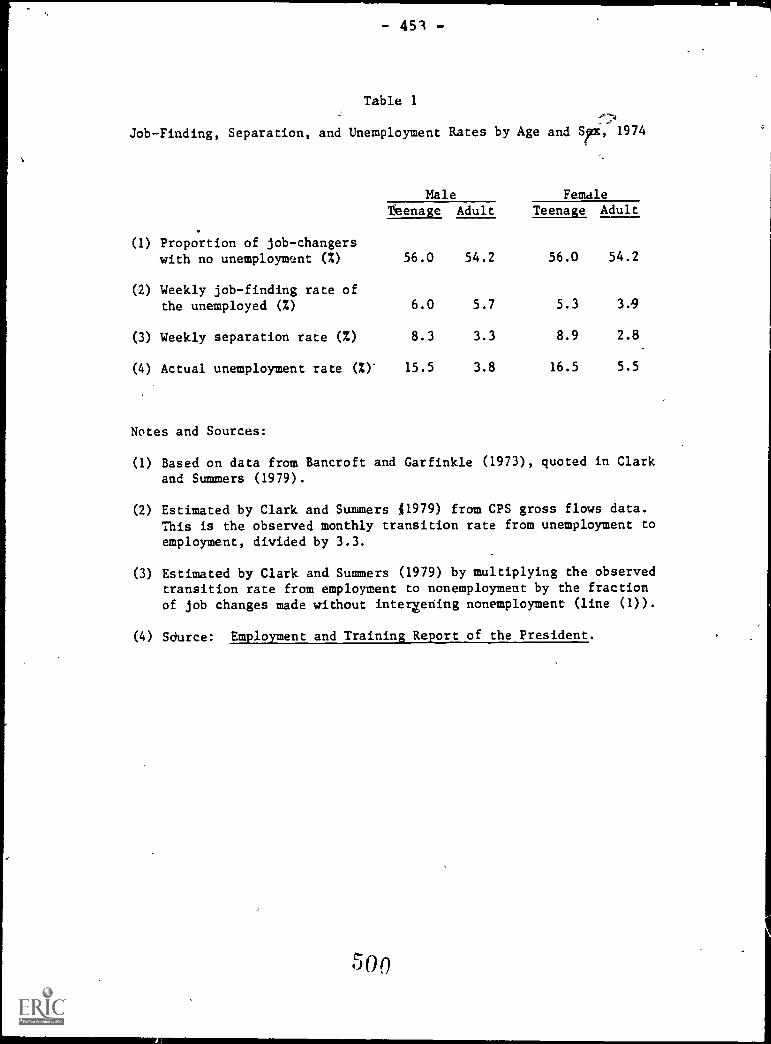
- 451 -

Table 1

Job-Finding, Separation, and Unemployment Rates by Age and Spx, 1974

(1) Proportion of job-changers

Male Female

Teenage Adult Teenage Adult

with no unemployment (%) 56.0 54.2 56.0 54.2

(2) Weekly job-finding rate ofthe unemployed (%) 6.0 5.7 5.3 3.9

(3) Weekly separation rate (%) 8.3 3.3 8.9 2.8

(4) Actual unemployment rate ay 15.5 3.8 16.5 5.5

Notes and Sources:

(1) Based on data from Bancroft and Garfinkle (1973), quoted in Clarkand Summers (1979).

(2) Estimated by Clark and Summers 11979) from CPS gross flows data.This is the observed monthly transition rate from unemployment toemployment, divided by 3.3.

(3) Estimated by Clark and Summers (1979) by multiplying the observedtransition rate from employment to nonemployment by the fractionof job changes made without intergehing nonemployment (line (1)).

(4) Sdurce: Employment and Training Report of the President.

500

%-' 454 -

the proportions are slightly higher for teenagers survey upon which

this finding is based is not tabulated by sex). The second line shows the

percent of the unemployed who take jobs each week. Again, if teenage

markets were slacker, this percent would be lower than for adults, but, in

fact, it is higher, especially among women. Note that the evidence from

the first two lines of Table 1 does not involve the mistake of trying to

infer rates of job-finding from data on the duration of unemployment. As

Marston (1976) and Clark and Summers (1939) have pointed out, much of the

explanation of the brief duration of unemployment among teenagers comes

from their high propensity to drop out of the labor force while unemployed.

However, the correct comparison in terms of actual success in finding work

shows that teenagers are on a par with adults.

The third line of Table 1 presents data on the weekly rate of departure

from jobs among the four age-sex groups., Between 8 and 9- percent of teen -

agers loselose or quit their jobs each week,'compared to about 3 percent of

adults. Teenage jobs are brief--they last about 12 weeks on the average.

The dramatic difference in separation rates stands in' sharp contrast to

the virtual equality of job-finding rates. The well-known large g4p in

unemployment rates, shown in the fourth line of Table I, is due largely

to the difference in job separation rates. Table 1 does not attempt a

full description of the dynamic process by which workers move in and out

of the labor force, which would be necessary to give a complete account

of the differences in unemployment between teenagers and adults. For such

an account, see Marston (1976) and Clark and Summers (1979).

Investigation of possible causes of high separation rates among young

workers is the main purpose of this pape,F. Obviously, there are important

normal influences toward brief jobs, including the fact that a fraction of

- 455 -

employment takes the form of summer jobs. But the impression remains that

much turnover is pathologi:al. Consequently, the paper spends a good deal

of effort investigating the possible role of the minimum wage in stimulating

excessive job turnover.

Determination of Turnover, Job-Finding Rates, and Unemployment in the

Presence of a Minimum Wage

The analysis presented in this section is closely related to an earlier

paper of mine (Hall, 1979), modified suitably to take the minimum wage into

account. The discussion here is intended to stand on its own, however,

The first component of the model describes the mechanical operation of

the recruiting and job-finding process. The unemployed are viewed simply

as a group of people who have'not yet found work, but are confident of

finding work eventually. Bach of the unemployed has the same chance of

locating a job each week. All unemployment is "frictional"; nobody is

permanently unemployable. The state of tightnes3 or slackness of the

market is described by a single variable, the job-finding rate, which I

will call f. It is the weekly probability that an unemployed worker will

find a job. Tighter markets have higher values of f and are preferred by

workers. On the other hand, slacker markets with lower values of f are

preferred by employers for the following reason: Employers compete with

each other for the workers who are available. When an employer extends a

job offer in a tighter market, it is lesg likely to be accepted because

the worker way also receive an offer from another employer at the same

time. In formal terms, this consideration is emb,died in a recruiting

cost function, p(f), which gives the number of offers that need to be

made, on the average, to hire one new worker. As f approaches one, p(f)

J02

456

Approaches infinity-- guaranteed instantaneous job-fin4ing would make

recruiting prohibitively expensive. In very slack markets with f near

zero, p(f) will be only slightly more than one. In my earlier paper, I

der.wed an exact form, p(f) s - lcg(1 -f) /f, for the recruiting cost function,

based on some further simple assumptions.

The job-finding rate is one of two major dimensions of conditions in

the labor market; it does not by itself determine the unemployment race.

A very slack market where it is nearly impossible to find work could have

a low unemployment rate because few workers came to it t.o search. Similarly,

a tight market could have a high unemployment rate because there was a

large continuing flow of newly unemployed workers into it. The latter is a

good description of markets for youths in the modern U.S. economy. Thus

the other dimension of labor market conditions is the separation rate--the

weekly probability that an employed worker will become unemployed. In

stochastic equilibrium, where the flow of workers into the pool of unemploy-

ment via job separations balances the flow out of the pool through finding

new jobs, the unemployment rate will be

us f/(1-f)

The job-finding rate, f, the separation rate, s, and the unemployment rate,

u, are linked by this relation. Given the values of any two of these

measures, the third is fully determined by it. In this paper, the job-

finding and separation rates are considered explicitly and the corresponding

unemployment rate is then derived. Of course, it is also true that unem-

ployment is the difference between the supply of laoor and the demand for

it. Further discussion of determination of unemployment will continue

- 457 -

after the principles of the efficient combination of separation and job-

finding rates are presented.

It has already been established that both parties to the employment

contract are concerned about the job-finding rate. Workers favor high

rates and employers low rates. It is equally true that both parties are

concerned about the separation rate. The rate is the reciprocal of the

duration of employment: High separation rates mean jobs are brief. Both

very long and very short jobs are generally undesirable from the employer's

point of view. If an employer promises virtually permanent jobs to workers,

it will be difficult to adjust total employment downward in the event of an

adverse shift in demand. Permanent commitments also limit the employer's

power to retain only the most productive of a group of new recruits. For

these reasons, it is costly or employers to promise lengthy employment.

On the other hand, very high turnover implies excessive recruiting and

training costs. This second consideration has dominated most discussions

of the economics of turnover. In markets for young workers, though, rasher

high turnover rates may actually be efficient, especially in lines of work

where training costs c. be made low. In these markets employers profit

from the flexibility they enjoy in adj.isting employment to each minor_ -

fluctuation in demand. The occasional redundancy of labor that is typical

under more or less permanent employment arrangements is unnecessary where

separation rates are high:

The hypothesis pursued in this paper is that emplc,7ment terms adjust

to mediate the conflicting attitudes of employers and workers about ,ob-

finding and separation rates. Specifically, the two parties should equalize

their trade-offs between the two aspects of the arrangement. The minimum

wage does not impose any limitations r- these dimensions of the employment

504

- 458 -

package. In a market unaffected by the minimum wage, the parties ought to

equalize their trade-offs between cash wages and the separation or job-

finding rates. The fully efficient outcome is described in my earlier

paper. The influence /of an effective minimum wage in the present analysis

is to prevent employi4rs from offering better duration terms to workers in

exchange fo_ lower cash wages.

In analytical terms, the efficient combination of separation rates

and job-finding rates occurs at the point of tangency of an indifference

curve and an isocost curve. The indifference curve describes the alterna-

tive combinations of separation and job-finding rates that achieve the same

level of satisfaction, on the average, for workers. It presumably slopes

upward, since workers will need to be rewarded with higher job-finding

rates iu order to induce them to accept higher turnover. The isocost curve.

embodies the considerations about the costs and benefits to employers men-

tioned earlier. Its slope is positive for low separation rates, where the

added flexibility of higher turnover is a benefit, and then turns negative

for high separation rates, where recruiting and training costs begin to

dominate. All this can be summarized in a diagram:

305

job-

finding

rate

459

betterindifference worse

curve indifferencecurve

expansion path

better isocost curve

worse isocost curve-

separationrate

The outcome of this analysis is an expansion path of alternative efficient

combinations of separation rates and job-finding rates; call it f 8(8).

Different points on the path correspa* to different levels of satisfaction

achieved by workers and costs incurred by employers. If the market is

operating at separation and job-finding rates that are not on this path,

employers' costs can be reduced and workers' level of satisfaction improved

by a suite!) movement to a point on the path. Along the path, cost can be

reduced only by making workers worse off by raising the separation rate.

5O6

- 460 -

The forces of supply and demand determine which of the efficient

combinations of separation and job-finding rates will prevail in the

market, and thus determine the unemployment rate. Since costs are sensi-

tive to the separation and job-finding rates through recruiting and

training costs, the total demand for labor in a market will be a function

LD(w,s,f) of the hourly wage, w, and the separation and job-finding rates,

s and f. Higher wages end higher job-finding rates depress the demand for

labor, while higher separation rates stimulate it, at least over the range

of variation that is consideree tare. Further implications of and justifi-

cations for the latter proposition are presented in the subsequent section

of the paper.

The supply side of the market is a little more complex because the

presence of unemployment even in equilibrium means that there are two

different concepts of supply. The first, gross supply, corresponds to

labor force participation--it consists of all the workers attracted to the

market, including those looking for work who have not yet found it. Gross

supply is a function, LS(w,s,f) of the terms of employment offered by the

market. The other concept is net supply, which does not count the unem-

ployed. If u is the unemployment rate implied by the separation and job-

finding rates, net supply is (1-u)LS(w,s,f). Recall that u is a simple

function of s and f, so that another way to express net supply is

(1-f)s + f LS(w,s,f)

Equilibrium occurs in the market when demand and net supply are in balance:

D(w,s,f) e LS(w,s,f)(1-fs + f

507

- 461 -

The equilibrium that concerns this paper is the constrained one that

occurs when the government sets the wage through an effective minimum wage

at level W. The wage itself cannot participate in the process of clearing

the market, but variations in the separation and job-finding rates can

bring about a constrained equilibrium in the market. I wilt assume that

they move in tandem, so as to preserve the effici=mt combination of the

two rates; that is, the job-finding rate is 8(s) and not a free variable.

This condenses the market-clearing process to a single dimension, the

separation rate:

L OW,s,e(s)) =13(s) ,S r

(1-8(s)is 8(s) Ow,s,e(s))

This can be portrayed in a somewhat unconventional supply-and-demand

diagram:

separation

ratedemand

gross supply

employment unemployment

5O

labor

462

The demand curve is shown as nearly vertical on the assumption that the

benefits to the employer of higher turnover and the associated change in

recruiting costs are not very large. On the other hand, gross labor sursply

may be reasonably sensitive to the separation rate--given the fixed wage

tate, young workers will choose activities other than work in preference

to the high unemployment rates that accompany high turnover rates., This

is even more pronounced when supply is measured net of unemployment.

Higher separation rates mean fewer workers are available for work at any

one time. both because the work is less attractive and because more of

their time is spent finding new work.

When the wage is held fixed by minimum wage legislation, the separa-

tion rate assumes the role of clearing the market. Equality of supply and

demand is achieved subject to the constraint of the minimum wage; in this

sense, the market is in equilibrium. It is important to note, however,

that this equi'dbrium is not efficient. Because the minimum wage does not

try to peg either the separation rate or the job-finding rate, private

economic arrangemeLts yield an efficient trade-off between the two. How-

ever, the minimum wage does interfere with the trade-off between the

separation rate and the cash wage rate. Separation rates (and therefore

unemployment rates) are excessive under the minimum wage because employers

are prohibited from offering a set of employment terms with lower wages

and longer jobs, even though those terms would make workers better off and

reduce employers' costs at the same cime.

Ii a labor market unaffected by the minimum wage, the separation and

job-finding rates are largely unaffected by shifts in supply or demand.

Unemployment remains at a fixed "natural" rate when, say, demand increases.

The wage rises to clear the market. This analysis of a free labor market

009

463

is amplified in my earlier paper. In the presence of a minimum wage, the

impact of an increase in demand is rather different. Because the wage

cannot respond, the separation rate falls as demand rises:

separationrate

E4

E'

gross supply

net1supply

I laborE+U E' +U'

The increase in employment, from E to is somewhat less than the amount

of the rightward shift c: the demand curve (just as it would be if the wage

were permitted to rise). Unemployment, which is held above the natural

-rate by the minimum wage, falls toward the natural rate.

The same apparatus will help to explain the effect of an increase in

the minimum wage itself. For a given separation rate, a higher minimum

wage means lower labor demand and higher net supply, so the demand schedule

shifts to the left and the net supply schedule to the right:

51()

separationrate

s'

- 464 -

D'

I

I

D

s'

labor

The combination brings about a decrease in employment from E to E' and an

increase in the separation rate from s to s'. Unemployment rises as well,

as the following diagram shows:

separationrate

net

gross

grossnet

U

labor

- 465 -

In the traditional analysis of the minimum wage, employment falls by

the full amount of the downward shift in labor demand brought about by a

higher minimum. Demand alone determines-employment. The gap between

s:ipply and demand appears as unemployment. In the analysis presented here,

the equilibrating role of the separation rate dampens the adverse effect

of the minimum wage on employment. The rise in separations makes the labor

market more attractive to employers and so helps to offset the disincentive

of higher cash wages. A stricter minimum wage must raise unemployment,

however. Most, or perhaps all, of the increase comes from higher turnover

rather than from lower job-finding rates and longer duration of unemployment.

This conclusion is rather different from one reached by Finis Welch

(1976). In a brief discussion of the theory of the effect of the minimum

wage on unemployment, he concludes that it is ambiguous because the shortage

of jobs will decrease turnover among those lucky enough to find work.

Implicit in Welch's discussion is the belief that jobs terminate at the

initiative of workers, and that employers would prefer lower turnover.

This situation would represent a failure of the market to achieve -n effi-

cient turnover rate where workers and employers' have equalized their

trade-offs between turnover and other aspects of the employment bargain.

Under the hypothesis of an efficient trade-off, pursued in this paperf is

seems likely that turnover and unemployment ari stimulated by a minimum

wage.

Another discussion of the effect of the minimum wage on unemployment

appears in Mincer (1976). In his analysis, the job turnover rate is taken

as constant, unaffected by the minimum wage. He does consider the influence

of unemployment on labor supply.

Turnover and Labor Costs

All of the novelty in the previous section rests on the hypothesis

that employers can operate at lower costs when turnover rates are higher,

given a fixed hourly cash wage. To see this, consider the opposite case

where turnover above a certain critical level is undesirable from the

point of view of the employer. Since turnover is assumed always to be

undesirable to the worker, efficient arrangements will never involve a

separation rate above the critical level. In this case, the efficient

job-finding rate, f = e(s), wild rise rapidly as the separation rate

approaches the critical level (say, s*):

- 466 -

The supply-and-demand diagram under a wage fixed by minimum wage legis-

lation is, in this case,

13

separation

rate

- 467 -

demand

net

supply gross supply

E E+Ulabor

Here the net supply curve bends far to the left of the gross supply curve

becm.:se the job-finding rate drops rapidly as the separation rate approacheM

s*. If market equilibrium occurs at a separation rate near s*, it will

involve high rates of unemployment in the traditional sense of a stagnant

market: The unemployed will consist of people who are having a great deal

'bfAroublesfinding jobs. The jobs they find eventually will last a reason-.,

able length of time. This is the kind of influence of the minimum wage

depicted in the standard analysis. To .the extent that the minimum wage

raises the wage above its full market-cleating level, it creates a shortage

of jobs, and jobs are rationed among job -- seekers by the increased difficulty

in finding work.

My point in this paper is the theoretical and practical possibility

that a.minimumwage operates in the Opposite way, to stimulate job turnover

514

468

rather than to depress job-finding. The most convincing part of the case

favoring this hypothesis is the evidence presented earlier of very high

job separation rates and rapid flows of workers into jobs in markets

influenced by the minimum wage. This section of the paper gives some

further reasons to think that the minimum wage has most of its effect in

raising job turnover.

First, it may be useful to exhibit a class of utility functions and

cost functions where the efficient job-finding rate is literally constant,

independent of the minimum wage, and, indeed, independent of the supply

andidemand for labor generally. Within this class, workers' concerns.

about separation rates and job - finding operate through Lhe unemployment

rate. In other words, a worker is indifferent between two labor markets

where wages and unemployment are the same, but one has higher separation

and higher job-finding rates than the other. It is also necessary to say

something about workers' willingness to trade off cash earnings against

unemployment, which will depend on the level of public unemployment

insurance and workers' attitudes about the value of time spent out of

work. A reasonable approximation is that there is a constant, A, equal

to 0 for workers who are indifferent between work and unemployment (either

because of full unemployment insurance or high value of time in nonworking

activities) and equal to 1 for workers for whom unemployment is a pure

waste of time and who receive no unemployment insurance. Then a utility

function capturing all of this is

w(1-Xu)

or, in terms of separation and job-finding rates,

w(1s f /(1 f))

r.

- 469 -

The indifference curve along which workers achieve a certain level of

satisfaction, say, y, can be written

On the cost side,

the sum of

less

s 1--1-f - (1-A)

t eems reasonable to approximate total cost as

1. costs not related td the type of lablunder consideration, say,

A.

2. regular hourly employment say, aw.

3. recruiting costs, proport)nal to the rate at which jobs are,

filled, s, the effott-rkuired to fill one job, p(f), and the

hourly wage, w.

4. the benefit, say, bws, of the flexibility associated with the

separation rate, net of training costs.

/The resulting cost function has the form

C(w,s,f) m A+ Bw(a +p(f)s - ba)

It is only a useful approximation over the range of separation rates where

it is plausible that rising rates convey benefits to the firm, on net.

An efficient employment arrangement that yields a level of satisfac-

tion y to each worker can be described mathematically as the minimum of

cost subject to the constraint that utility equal y:

1,1in A+ BW(a + (Os -bs)s,f

subject to s -w -y

1-f y - (1 -A)*

The minimum wage prevents achievement of the fully efficient arrangement,

where the minimum would be taken over the wage rate as well. Now the

516

- 470 -

constraint can be substituted into the minimand to restate the problem as

Min A+Bw(a - (8- OM) fw-y

1-f y- (1- )wf

But minimization of this over the job-finding rate, f, is equivalent to

maximizing the expression

- p (1)) 1.7.7

The maximum occurs somewhere between f..0 and the critical job-finding

rate, f*, where the recruiting costs, p(f)% begin to outweigh the net

benefits of turnover, b:

(b-P(f)1)1-f

f

The important point is that the efficient job-finding rate is determined

by the narrow consideration of balancing the employer's benefits from

turnover against the worker's costs. Both are propo4ional to the hourly

wage, so the efficient job-finding rate is independent of the level at

which the government sets the minimum wage. It is also independent of

the level of satisfaction achieved by workers and so independent of the

{supply of and demand for labor.

- 471 -

It seems reasonable to expect that the efficient job-finding rate is

fairly close to constant over a range of market conditions, even if the

exact mathematical conditions set forth above do not hold. Obviously,

the range includes only t ose separation rates where turnover has net

benefits to employers. A sufficiently aggressive minimum wage will

inevitably push the market close to the point where turnover becomes

costly to employers, and the conventional analysis where the minimum

creates a shortage of jobs will begin to apply. On the other hand, the

effect of a minimum wage that pushes the cash wage only moderately above

its equilibrium may well be to stimulate turnover rather than to depress

job-finding.

The core of the argument that turnover can benefit employers, as I

have emphasized earlier, is the flexibility that brief job commitments_

provide to employers. At the most basic level, the minimum wage induces

turnover by inhibiting employers .rom holdi:.g overhead labor. Instead of

paying a lowe age to long-term workers through thick ain, employers

subject to a minimum wage pay &high hourly wage to shot. term workers who

must finance themselves (at least Tartly) in times of slack. Only a tiny

fraction of the fluctuations in demand that lie behind this process are

,,zregate--most affect just the firm itself. They are not necessarily

purely random, _ither. A highturnover emplo:ment policy makes it easier

to accommodate seasonal swings in demand as well, for example.

Other adaptations to the minimum wage are more subtle and probably

take longer to respond to changes in the minimum. The scope for taking

athantage of a high-wage, high-turnover employment policy depends on the

technical organization of work within a firm. Training costs must be low

in order to benefit from high turnover. Jobs must be highly standardized.

518

- 472 -

The fast-food industry, which is a major source of employment at the

minimum wage, is the leading example of this kind of adaptation. Workers

can be trained in a few hours. They need not even memorize the prices of

items on the menu because each item has a separate button on the cash

register. Job turnover is a way of life in this industry, and the industry

has learned to profit from it. Though obviously many forces have contrib-

uted to the evolution of the high-turnover practices of the fast-food

industry, my suggestion here is that the minimum wage is important among

them.

Achievement of the Efficient Job-Fifting and Separation Rates within theLabor Market

The analysis of this paper pictures employers and workers agreeing on

three aspects of the employment arrangement: the cash hourly wage, the

separation rate, and the job-finding rate. Only the first of these is

considered in the conventional analysis of employment bargains. Is it

meaningful to speak of an agreement about separation or job-finding rates?

Job separation is under the joint control of the two partly to an

employment arrangement. Separations can occur unilaterally as quits or

layoffs. Alternatively, they may occur by prearrangement, as when a summer

or other temporary job comes to an end. Evidence from the United States

suggests that the latter case is particularly important for teenagers (Hall,

1978). In cases where there is no advance agreement. about the duration of

the job, there are generally understandings about how the job will come to

an end. It is fairly easy for workers to find out the past layoff rates of

employers and reasonable assume that these are guides to the future.

Similarly, employers can inquire about the employment histories of

519

- 473 -

potential workers to avoid those who have deviated from the norm for the

market. Though neither party gives up the right to bring about a separa-

tion unilaterally in any one instance, both face penalties for systematic

departures from the prevailing employment terms.

Agreement about job-finding rates is a harder issue. A very general

argument can be made that a market operating at an inefficient job-finding

rate will be displaced by one operating at the efficient rate. In the

second market, everyone can be made better off than in the first. But

this leaves the important question unanswered about how the market deter-

mines its job - finding, rate. This point is discussed in my earlier paper.

A market operating away from the efficient job-finding rate presents

arbitrage opportunities for an entrepreneur willing to offer employment

at alternative, efficient terms and to sell his workers' services to

employers. Temporary - employment firms could have exactly this function

in clerical and other markets, though, of course, there are many other

reasons for their existence as well. Alternatively, a market with an

inefficient, high job-finding rate offers arbitrage profits to an

employer who makes special efforts to advertise that jobs are readily

available, but on terms favorable to the employer. As in the case of

conventional supply-and-demand theory, the model presented in this paper

does not provide a fully worked-out story of how the market moves toward

its equilibrium, but restricts its attention to the equilibrium itself.

While this discussion may lend some plausibility to the notion that

the market does move eventually to the efficient equilibrium, it seems

unlikely that the process is a speedy one. In particular, the prediction

that the effect of a higher minimum wage is to stimulate turnover rather

than to make jobs harder to find 13 a prediction for the long run. In

520

- 474 -

the short run, the minimum wage seems likely to push the market into

disequilibrium with an inefficiently low job-finding rate. The resulting

lags are a potential complication in any empirical analysis of the effect

of the minimum wage.

Concluding Remarks

Jobs for young workers are readily available in the U.S. economy, in

spite of minimum wage legislation that affects youth much more than any

other segment of the labor force. Young workers find jobs just as fast as

their olAer counterparts. The conventional analysis of the potential

effects of a minimum wage suggests that it creates a shortage of jobs and

so should make it more difficult for any one worker to find a job. Taken

together, these constitute an apparent case against any important effect

of the minimum wage. It seems that high unemployment rates of youths have

to be blamed on something else.

This paper has sho,,n that a minimum wage can bring about high unem-

ployment without causing a sho tage of jobs or reducing the job-finding

rate. Rather, in the long run, an effective minimum wage can induce the

evolution of employment practices and arrangements that raise turnover.

The minimum wage does not block the market from achieving an efficient

degree of tightness, that is, an efficiently high job-finding rate. In

fact, under reasonable assumptions about turnover and recruiting costs,

the efficient job-finding rate is a constant, unaffected by the minimum

wage or the supray of and demand for labor. The adverse effects of the

minimum wage are then concentrated in inefficiently high separation rates.

The shockingly low average duration of jobs held by teenagers--less than

three months--may be an important consequence of the minimum wage. If so,

- 475 -

high unemployment among youths can be traced in part to the minimum wage,

which makes them become unemployed too often even though it does not

inhibit job-finding once they are unemployed.

C ()(3,...,4,

- 476 -

References

Gertrude Bancroft and Stuart Garfinkle, "Job Mobility in 1961," MonthlyLabor Review, August 1973.

Kim Clark and Lawrence Summers, "Labor Market Dynamics and Unemployment:A Reconsideration," Brookings Papers on Economic. Activity, 1:1979,forthcoming.

Robert E. Hall, "A Theory of the Natural Unemployment Rate and theDuration of Employment," Journal of Monetary Economics, Vol. 5,pp. 1-17, April 1979.

Stephen Marston, "Employment Instability and High Unemployment Rates,"Brookings Papers on Economic Activity, 1:1976, pp. 169-203.

Jacob Mincer. "Unemployment Effects of Minimum Wages," Journal of PoliticalEconomy, Vol. 84, pp. 87-104, August 1976.

Finis Welch, "Minimum Wage Legislation in the United States," inOrley Ashenfelter and James Blum (eds.), Evaluating the Labor-MarketEffects of Social Programs, Industrial Relations Section, PrincetonUniversity, 1976, pp. 1-38.

- 477 -

HIGH SCHOOL PREPARATION

and

EARLY LABOR FORCE EXPERIENCE

by

Robert H. Meyer and David A. Wise

Many kinds of preparation and ,!xpe;ience are presumed to prepare

youth to find jobs, to do them, to keep them. At least three are often

mentioned. One is general academic education -- reading, writing,

arithmetic. A second is vocational training intended to develop the

skills necessary to perform particular tasks. A third is work experi-

ence itself, emphasized as the way to learn what it's like to work, to

acquire the habits and attitudes that persons who work have, that draw

one to want to work, and that those who hire want to-find in those they

pay. Motivated by these common hopes, we have investigated the relation-

ships between early labor force experience and the three kinds of high

school preparation that emphasize them. The paper analyzes the relation-

ship between high school curriculum, work experience, and academic

achievement on the one hand and early labor force employment and wage

rates on the other. We find that work experience while in high school

is strongly related to later employment. Academic performance in high

school is also related to successful labor market experience. But we

find no significant effect of current forms of high school vocational

training on early labor force experience. Thus the weight of Our evi-

dence implies that programs that emphasize work experience for youth,

52.1

478

tog(ther with general academic education, have the greatest chance of

.enhancing their subsequent labor force experiences.

The analysis is based on male youth whu graduated from ht0 school.

A large portion of young persons enter the labor force immediately upon

graduation from high school. Many receive no further formal education.

For these youth, as well as those who continue their education, high

school preparation is a potentially important determinant of early labor

force experience. Because the study is limited to high school graduates,

its implications for high school dropouts must be indirect. Among all

groups of youth, high school dropouts, and in particular black school

dropouts, have the poorest labor force experiences. Nonetheless, labor

force statistics suggest a high youth unemployment rate, even among high

school graduates. And nur results for high school graduates we think

have strong implications for future generations of persons like those

who now drop out, if these future generations were to remain in school.

The Analysis is based on data collected by the National Center for

Educational Statistics through the National Longitudinal Study of 1972

High School Seniors. The Study collected a wide range of school, family

background, attitude and aspiration information from approximately 23,000

high school seniors in the Spring of 1972. The 1972 base survey was

based on a nation-wide sample of high schools, stratified in such a way

that schools in lower socioeconomic areas were somewhat oversampled.

In addition to the base survey, the Study included three follow-up

surveys in 1973, 1974, and 1976. The follow-up surveys were used to

obtain information on nost-secondary school and work choices ai well

as labor force experiences.) Unlike most other data sources, this one

479

allows us to follow a single cohort in their transition from school to

work.

Most male youths in the years immediately after high school are

either in the labor force or are attending a post-secondary-ichool;

some are in the labor force and going to school. Because the labor

force aspirations of persons while the"), are students, their labor force

behavior, their access to the labor market, and thus their realized

experiences are likely to differ substantially from persons who are not

in school, we have sought to obtain estimates that represent the experi-

ence that we would expect to find among persons not in school. To obtain

such estimates, however, we must consider simultaneously both the deci-

sion to enter the labor force, rather than go to school, and the expected

experience of those who enter the labor force. In a strictly statistical

sense, this may be thought of as correcting for sample selection bias.

But in our case, the determinants of school attendance, as well as the

determinants of labor force experience, are of considerable substantive

interest. In fact, the decision to attend school may be expected to be

determined in part by expected labor force experience. Although our

primary emphasis will be on labor force experience we will give some

attention to the determinants of school attendance as well. The

outline of the paper is preceded by a summary of our major findings.

We have foufld a strong relationship between hours of work while in

high school and weeks worked per year upon graduation. Persons who work

while in high school also receive higher hourly wage rates than those

who don't. The combined effect on earnings is very substantial. For

example, with other individual charpteristics equal to the average fin

the sample, persons who worked 16 to 20 hours per week in high school

JtiG

- 480 -

are estimated to earn annually about 12 percent more than those who

didn't work at all in high school. Depending upon the amount of work

in high school and estimated weeks worked based on other chaftcter-

istics, the estimated "effect" on annual earnings of high scfidol work

could be as high as 30 or 35 percent. On the other hand, we find

almost no relationship between any measure of high school vocational

training and later weeks worked or wage rates. This has led us to

raise the possibility that programs that emphasize work experience in

high school may well have a greater impact on later labor market

experience than programs that emphasize job skill training without

work experience. Our evidence, however, establishes only a strong

correspondence between work while in high school and later employment;

it cannct be used to infer a cause and effect relationship of the

same magnitude.

Traditional measures of academic achievement are also positively

related to early success in the labor market. In particular, class rank

is related to both weeks worked after graduation and to wage rates, after

controlling for test scores reflecting a combination of aptitude and achieve-

ment. Combined with the results on hours worked in high school, this

*lies to us a substantial carry-over to the labor market of individual

attributes associated with or developed through work effort in and out

of school. Class rank may also measure general academic knowledge. And

together with the positive estimated effect of test scores on both weeks

worked and wage rates implies a significant effect of traditional mea-

sures of academic aptitude and achievement on labor market pfrformance

upon leaving school. Thus both high school academic performance and work

527

481

experience seem to dominate specific vocational training as preparation

for successful early experience in the labor market.

In contrast to the lasting relationship between high school work

experience on weeks worked and wage rates over the next four years,

there is little relationship between random -- as distinct from indivi-

dual specific -- determinants of weeks worked in the first. year after

graduation and weeks worked four years later, and little relationship

between random determinants of wage rates upon graduation and wage rates

four years later. After controlling for individual specific characteris-

tics, we find little lasting effect of unusually few weeks worked in the

first year or two on weeks worked three or four years later. Similarly,

after controlling for individual specific terms, we find lIttle lasting

effect of random fluctuations in initial wage rates on wages four years

later. Whatever the determinants of wages and weeks worked, other than

individual specific attributes, they do not lead to long-run persistence

of initial experience. (On the other hand, wage rates increase with job

experience so that weeks not working contribute to lower wage rates in

the future.) And much if not most of work while in high school, that has a

substantial positive relation to later labpr market experience, must

have been on jobs with limited direct relation to future job ladders,

although our data do not provide any indication of the quality of high

school jobs. Thus our findings suggest that the oft-expressed worry

that poor initial jobs and initial jobs without a future should be

avoided, for fear that they will contribute to lasting poor labor force

experience, may be misplaced. Our evidence on persons graduating from

high school suggests, albeit indirectly, that this worry is unfounded

52

482

and in fact should be dominated by policies to encourage early work

experience, possibly without exaggerated initial concern forjts rela-

tionship to a well defined hierarchy of future jobs. We find no evi-r-

dence tliat persons on average were hindered by the work expettence that

they had in high school; on the contrary, the evidence suggests that

they may well have been helped. And, our evidence is that low-wage

jobs after graduation do not in themselves increase the likelihood of

low wage jobs a few years hence.

We have distinguished weeks worked in the four years following

high school by the year in which the experience was had. Thus after

four years for example, we know how much an individual worked in each

of the three preceding years. As expected, we find that wage rates

at any given date are determined in part by previous experience.

Thus although there is no lasting effect of non-employment in one

year on employment in subsequent years, there is a cost associated

with early non-employment; it is lower wages in future years. The

effect of early labor force experience on subsequent wages is not

obviously different in magnitude from the effect of work experience

while in high school. But the effect of work experience while in high

school does not decline over the first five years in the labor force,

whereas there is some evidence that the effect of early labor force

experience on subsequent wages may decline over time. Thus high school

work experience may be capturing attributes that are in part at least

distinct from those associated with later labor market experience.

Ite pattern of the relationships between work while in high ithool and

weeks worked in subsequent years in the labor force provides0further

evidence of this. Indeed the latter finding suggests strongly that

0 2!)

483

high school work experience is associated with individual attributes

that persist over time.

The average wage rates of whites and non-whites in the 1eor market

are quite close, with whites earning a bit more per hour after the first

year. But after controlling for other variables, non-whites seem to earn

a bit more per hour than whites. On the other hand, non-whites work

fewer weeks per year than whites on the average but we find little dif-

ference between the two groups after controlling for other variables.

After controlling for other variables, the probability that non-whites

are in school in each of the four years after high school is about 0.10

higher than the corresponding probability for whites.

In general, summary statistics based on the National Longitudinal

Study do not suggest severe employment problems for these high school

graduates. On the contrary, they suggest a group of persons moving

rather smoothly into the labor force.

Finally, employment ratios of both white and non-white high school

graduates based on these data are considerably higher than those calcu-

lated from Current Population Survey data, and unemployment rates much

lower. Although employment ratios of non-whites are lower than those

of whites, and unemployment rates higher, four years after high school

graduation they are close. The October 1976 white employment ratio

is .909 and the, non-white ratio .875. Unemployment rates are .665 and

.081 respectively. Very few persons in the sample are chronically out

of school and unemployed.

530

484

The general outline of the paper is as follows: Section I contains

some general descriptive statistics on the transition from school ;c1

work. Empirical estimates of weeks worked and wage equations.are pre-

sented in Section II. They are accompanied by non-school attendance

equations: Section III is an analysis of the extent of persistence of

individual experience over time. Concluding remarks are contained in

Section IV.

J21

485

I. Some Descriptive Statistics on the Transition from School to Work.

Through the National Longitudinal Study of 1972 high School Seniors

data were obtained on almost 23,000 persons from over 1,300 high schools.

The high schools were a stratified sample of all public, private, and

church affiliated schools in the country. To increase the number of

"disadvantaged" students in the sample, high schools located in low income

ar'as and schools with a high proportion of minority enrollment were

sampled at approximately twice the sampling rate used for the other schools.

The summary statistics reported below have not been adjusted to reflect

population proportions. They are reported, however, for whites and non-

whites separately. Both groups probably reflect more persons from low

income families than would be found in a random sample of the population.

We will present summary statistics in three groups: the first

on work and school status by year, the second on the likelihood of selecte5

sequences of school and work status over time, and the third on weekly

earnings and hours worked and annual employment and by year.

A. School and Work Status by Year.

The distribution of white and non-white males in the survey sample

by school and work status, together with some summary labor force statistics,

is shown in Table 1. (More detailed L'istributions by (' school and 5 work

classifications are presented for five consecutive Octobers beginning in

1972 in tables available from the authors.) We will point out first some

general findings based on an examination of Table 1 and then indicate the

kind of detail that can be found in the more detailed tables, Nithout

presenting an extensive discussion of it.

532

Table I. Percent Male Youths in School and Work Categories, and Labor ForceStatistics, by Year and Race, October of Each Year.

White Non-White

1972 1973 1974 1975 1976 1972 1973 1974 .1975 1976

In School, Full-Time a 53.6 43.3 38.2 35.2 22.1 42.3 30.3 26.5 23.3 17.7

In School, Part-Time 4.6 7.2 6.2 6.6 7.7 4.4 1.4 6.5 7.4 7.0

Not in School, Total 42.4 49.5 55.7 58.2 70.2 53.3 62.3 67.i 69.4 75.3

Working Full- 71.9 76.2 74.1 77.5 80.1 60.1 67.7 63.3 68.7 '71.9

Ti-n

Working Part- 9.2 5.1 4.9 4.2 4.1 11.4 6.2 5.1 5.2 5.1

Time

Military 7.7 11.2 11.9 10.8 7.4 8.8 14.2 16.1 15.7 12.1

Out of Labor 6.6 4.5 2.3 2.7 2.7 9.0 6.2 2.9 3.1 4.1

Force

Looking for 4.6 2.8 6.7 4.7 5.7 10.7 6.8 12.6 7.3 6.9

Work

Labor ForceStatistics:

Employment .380 .914 .898 .916 .909 .784 .860 .840 .877 .875

Ratio

Labor Force .929 .946 .974 .969 .972 .902 .928 .965 .964 .953

Par%icioAtton06.1'1.1

Unemployment .053 .035 .079 .053 .065 .130 .073 .155 .090 .081

Ratio1

d. Include small number of persons in graduate school in 1975 and 1976.

:3a. For persons not in school and not in the military.5 3

- 487 -

The most striking statistics in Table 1 are the comparatively low

unemployment rates and high employment ratios, as compared with those

based on Current Population Survey data. (See Freeman and Medoff [this

volume].) Although we cannot provide a direct comparison for lach

October, we can for 1972. In October of 1972, the Census Bureau conducted

a special survey of Spring 1972 high sc)ool graduates. (See Bureau of

Labor Statiscics [1973], p. 27.) A comparison of unemployment and other

labor force statistics based on the two data sources is presented in the

tabulation below (for persons not in school).

National Longitudinal Current Population

Statistic Study Survey, October 1972

White Non-White White Non-White

Employment Ratio .880 .784 .815 .68C

Labor ForceParticipation

.929 .902 .916 .880

Unemployment Rate .054 .130 .110 .227

An investigation of the definitions used in the two surveys does

not reveal any differences that would suggest such apparently contradictory

results, although the survey questions are not identical. Although the

NLS survey is weighted to oversample low income youth, this should tend

to raise implied unemployment rates, not to lower them. The survey

respondent, however, is the individual youth in the NLS survey, but is

likely to be the mother or father of the youth in the CPS survey. The

NLS data is collected through a mailed questionnaire (together with some

mail and telephone reminders), while the CPS data is obtained by interview

with a household member, often the female head. Freeman and Medoff find

a large portion of the difference between the CPS numbers and those

L ad on the Parnes National Longitudinal Survey can be attributed to the

different respondents.

- 488 -

The summary statistics also reveal several differences between

white and non-white youth. The percent of white youth in school full -

time is approximately 12 percentage points higher than the percent of

non-whites until 1976, when many youth would have finished four_years of

college. Of those not in school, the percent working full-time is about

8 to 10 poiats higher for whites than for non-whites. By 1976, the

percentages were about 80 and 72 respectively. The proportions working

part-time do not differ substantially in any of the years, although in

each year the percent for non-whites is somewhat higher than for whites.

It declines between 1972 and 1976 from 9.2 to 4.1 for whites and from 11.4

to 5.1 for non-whites. A larger proportion of non-whites than whites are

in the military. In 1974, the year of highest military participation

for both groups, about 12 percent of whites and 16 percent of non-whites

were in the armed forces.

More blacks than whites are out of the labor force, but the differ-

ences are not large. The proportion "looking for work," however, is about

twice as high for non-whites as for whites in 1972 through 1974. The

differences decline in 1975 and 1976. The percent of whites looking for

work in 1976 was 5.7, versus 6.9 for non-whites.

The labor force participation rates are high for both groups and

do not differ substantially. Between 1972 and 1976 they moved from .93

to .97 for whites and .90 to .95 for non-whites. The employment ratio is

higher for whites than non-whites in 1972, .88 versus .78; but by 1976

the two ratios were much closer, .91 versus .88. This closing of the

gap between the two groups is reflected in the unemployment rate

which was more than twice as high for non-whites as for whitessln 1972;

489

but by 1976, the two rates were rather close, .065 versus .081

In short, these numbers suggest a cohort of youth moving rather

smoothly into the labor force. Although there are differences between

the statistics for whites and non-whites, they do not seem to us to be

striking. In particular, the unemployment rates, although higher for non-

whites than whites, are not shocking to us for either group in any year.

By 1976, somewhat more than four years after graduation from high school,

labor force participation and employment ratios are high for both groups

and the unemployment rates are modest for both groups. Youth unemployment

does not appear from these data to be a severe problem for this group

of high school graduates.#

From the statistics in the tables available from the authors, one

can find more detail within this more general picture. For example, it

can be seen that most youth who are working part-time are also in school

full-time, although the proportion is lower for non-whites than for

whites. Also, many persons looking for work are full-time students.

They were not included in the unemployment statistics reported above.

- 490 -

B. Sequences of School and Work Status.

The average statistics reported above do not reveal extremely high

unemployment rates. But it could be that there are some youth who are

often unemployed. As a worst case, we have lumped together the persons

out of the labor force with those who are unemployed. In Table 2 are

reported the percent of persons not in school ano not working (in either

civilian or military jobs) for each possible number and sequence of time

periods. For example, the sequence 10101 indicates not in school and not

working in October 1972, October 1974, and October 1976; but not in this

category in October 1973 nor in October 1975. The left digit pertains

to 1972.

Examination of Table 2 reveals that 81 perc.Int 'f the sample were

not in this category in any. of the five October periods. (The data per-

tain to the first full week in October of each year.) Only one-tenth

of one percent were out of school and not working in all of the periods.2

For whites and non-whites together, this represents 5 persons out of 9115.

Three-tenths of one percent were in this category 4 out of the 5 periods,

and one-tenth of one percent in 3 out of the 5. Only 14 percent were so

classified in 1 of the 5 periods. We do not find a large group of chroni-

cally not in school and not working youth. More non-whites than whites

were in this status for one, two, three, and four periods; but over 72,

percent of non-whites were never out of school and without work in these

October periods. These data do suggest, however, that some youth are

much more likely to be in this category than others; there is tgtero-

geneity among the group. For example, based on Table 1, about 5 percent

of white youngsters are in this category in any year. If a person had a

.05 probability of being In this category in any period and the

538

491

probabilities were independent over time, the likelihood of being in this

status three out of the five periods, for example, would be only .001,

much less than the observed proportion of .008 for all white males.

Similarly defined sequences and associated percentages4or full-

time school and full-time work are reported in Tables 3 and 4 respectively.

Table 3 figures reveal that 36 percent of the sample were never in school

full-time, 35 percent for whites and 44 percent for non-whites. (While

these numbers suggest that whites are more often in school than non-whites;

the estimates below of the probability of attending school suggest a

higher probabilitysfor non-whites than whites, after controlling for

other relevant variables such as test scores and family background.)

Although there is some movement into and out of school, it is net

the norm. Of persons who go to school at all, 69 percent begin in the

first year after high school and attend only in consecutive years.

Eighty-four percent of those who attend at all, attend during the year

immediately after high school. The in and out possibility that is

sometimes emphasized, possibly more often for older persons, is not the

norm among th's group.

While 36 percent of the sample were never in school full-time, only

24 percent worked full-time in each of the five periods, as can be seen in

Table 4. As could be inferred from the school attendance figures, we see

in Table 4, that a relatively large number of persons work the last 4, the

last 3, the last 2, or the last year; but none of the prior years.

539

- 492 -

Table 2. Percent of Male Youths Not in School and NotWorking, October 1972-76, by Sequence and Race c

Sequent*Percent of Total

All Males White Non-White

0.1 0.1 0.1 0.1 0.1 0.1

0.3

0.10.00.00.00.1

0.1

0.00.00.00.00.1

0.5

0.30.1

0.00.1

0.4

111000111000111110101100101101

10110100110101110101

11000

011004000110

000I1101000101000101100100100110001

1000001000001000001000001

0000n

1.0

0.20.1

0.20.00.1

0.00.1

0.1

0.1

0.0

0.8

0.1

0.1

0.20.0

0.10.00.00.1

0.1

0.1

2.0

0.60.1

0.5

0.0 .-

0.30.00.20.3

0.1

0.0

3.1

0.60.50.5

0.50.30.1

0.40.2

0.20.2

3.1

0.60.0

0.4

0.00.30.1

0.3

0.1

0.2

0.2

6.3

1.01.0

0.90.70.40.1

0.90.50.4

0.3

14.1

3.1

1.)

2.7

2.5

3.9

13.2

2.3

1.8

2.5

2.3

3.9

18.6

5.4

2.53.9

3.2

3.7

81.0 81.0 82.7 82.7 72.2 72.2

Total

Missing

9115

2052

7639

1448

1475

522

c. The percents have been rounded to the nearest tenth. Differences between thesum of the numbers in the groups and the group totals reported to the left in eachcolumn are due to rounding. A "1" indicates not in school and not working. The leftdigit pertains to October 1972.

453 -

Table 3. Percent of Male Youths in School Full-Time,October 1972-76, by Sequence and Race d

.

SequencePercent of Total

All Males White Non-White

11111 11.7 12.4 8.1

11110 12.1 13.2 6.3

11101 1.3 1.3 1.2

11011 1.2 1.1 0.6

10111 1.2 1.2 1.3

01111 1.0 1.0 1.0

11100 3:8 3.9 3.3

01110 0.6 0.6 0.4

00111 0.5 0.5 0.5

11010 0.8 0.8 0.5

11001 0.4 0.5 0.3

01101 0.2 0.2 0.1

10110 1.1 1.1 0.9

10011 0.6 0.6 0.5

01011 0.2 0.2 0.1

10101 0.2 0.2 0.2

11000 7.1 7.0 7.3

01100 0.9 0.9 0.8

00110 0.5 0.5 0:7

00011 0.8 0.7 1.6,,

10100 1.2 1.1 1.2

01010 0.1 0.1 0.1

00101 0.1 0.1 0.1

10010 0.7 0.7 0.6

01001 0.1 0.1 0.1

10001 0.6 0.6 0.7

10000 9.5 9.2 11.2

01000 1.6 1.6 1.7

00100 1.5 1.4 1.9

00010 1.1 1.0 1.5

Q0001 1.3 1.2 2.0

00000 36.4 34.9 44.0

Total (..-152 7659 1492

Missing 2052 1428 505

d. The percents have been rounded to the nearest tenth. Differences between

the sum of the numbers in the groups and the group totals reported to the left ineach column are due to rounding. A "1" indicates in school full-time. The left

digit pertains to October 1972.

- 494 -

Table 4. Percent of Male Youths Wcrking Futl-Time,October 1972 -7b, by Sequence and Race e

Sequente Percent of TotalAll Males White Non-White

11111 23.7 23.7 24.1

11110 1.5 1.6 1.311101 1.2 1.1 1.511011 2.8 2.7 2.910111 2.9 2.9 3.201111 9.7 9.5 10.7

11100 1.0 0.9 1.501110 1.0 1.0 1.300111 7.6 7.2 9.711010 0.4 0.3 0.611001 0.8 0.8 0.901101 0.7 0.7 1.010110 0.5 0.4 0.910011 1.2 1.2 1.301011 1.8 1.7 2.110101 0.3 . 0.3 0.5

11000 1.0 0.9 1.201100 0.7 0.6 0.700110 1.3 1.3 1.200011 4.5 4.3 5.510100 0.4 0.4 0.301010 0.3 0.3 0.400101 1.4 1.4 1.410010 0.2 0.2 0.301001 0.9 0.9 0.910001 0.7 0.7 0.7

10000 1.2 1.2 1.301000 1.6 1.5 1.800100 1.6 1.6 1.400010 1.5 1.5 1.600001 9.9 10.6 6.5

00000 15.6 16.4 11.4

Total 9208 7689 1518Missing 1959 1398 479

e. The percents have been rounded to the nearest tenth. Differences betweenthe sum of the numbers in the groups and the group totals reported to the left ineach column are due to rounding. A "1" indicates working full-time. The leftdigit pertains to October 1972.

512

- 495 -

C. Weekly Earnings and Hours, Annual Employment and Unemployment, andNumber of Employers.

Average hourly wage rates, weekly earnings and weekly hours worked

for persons not in school and for those in school are shown in Table 5.

They cover all persons in the sample who were working in the first full

week of October of the year indicated. Persons working full-time or

part-time are included. Fo... persons out of school, wage rates for the

two groups are virtually identical right after graduation. After four

years, whites earn about 6 percent more per hour than non-whites, pre-

sumably due irr part at least to the different schooling patterns of the

two groups and post-high school work experience. Non-whites also work

about 2 hours per week less than whites in each of the time periods and

thus have lower weekly earnings -- about 8 percent in the first year and

10 or 11 percent in each of the subsequent years.

On the other hand, non-whites who are in school work 1.5 to 3 hours

per week more than whites, earn somewhat more per hour in all but the

last period, and have higher weekly earnings in each of the periods --

between 5 and 19 percent depending on the period.

We also calculated the percent of persons with wage rates below

the Federal minimum. The results for October of each year are shown in

the tabulation below. These numbers presumably reflect in large part

YearMinimum

Wage Rate Total

Percent Below MinimumWhite Non-White

1972 $1.60 10.98 11.02 10 76

1973 $1.60 5.89 5.93 5.59

1974 $2.00 8.06 8.35 6.68

1975 $2.10 8.14 8.14 7.99

1976 $2.3u 5.76 5.39 47.73

4

Table 5. Average Hourly Wage Rates, Weekly Earnings, and Weekly Hours Workedfor Persons Working in October, by School Status, Race, and Yeari

Item and RaceOut of School In School

1972 1973 1974 1975 1976 1972 1973 1974 1975 1976

Hourly Wage Rate

All Males 2.67 3.18 3.69 4.14 4.56 2.34 2.66 3.06 3.49 4.04(3040) (3752) (4199) (4039) (4950) (2153) (2223) (1892) (1725) (1347)

White 2.68 3.22 3.73 4.17 4.61 2.34 2.65 3.00 3.47 4.06(2471) (3001) (3403) (3271) (4097) (1866) (1938) (1625) (1473) (1162)

Non-White 2.67 3.02 3.53 3.99 4.35 2.49 2.74 3.42 3.59 3.91

(550) (731) (796) (753) (841) (276) (273) (267) (248) (181)

Weekly Earnings

All Males 108.68 133.61 154.21 173.48 192.15 62.96 74.34 89.25 103.77 130.80

White 110.32 137.04 157.41 176.47 195.52 61.85 73.43 86.94 101.47 129.74

Non-White 101.69 119.79 140.53 160.85 176.18 69.29 78.93 103.29 115.95 136.48

Weekly HoursWorked -

All Males 41.50 42.79 42.47 42.53 42.63 26.83 27.47 27.95 28.88 31.45

White 41.90 43.21 42.80 42.86 42.95 26.57 27.24 ?7.58 28.39 31.06

Non-White 39.65 41.14 41.02 41.09 41.09 _8.09 28.62 30.20 31.60 33.73

f. The data pertain to the first full week in October of each year. The numbers reporting figmres in eachyear are in parenthesis under the wage rates. They are the same for weekly earnings and weekly hours worked.

54 5

54 4

Table 6. Average Annual Weeks Worked, Weeks Looking for Work, Weeks Out of the Labor Force,and Number of Employers, for Male Youths, by School Status, Race, and Year.9

Item and RaceOut of School In School

1972-73 1973-74 1974-75 1975-76 1972-73 1973-74 1974-75 1975-76

Weeks Worked

All Males

White

Non-White

39.91

(4374)

41.03(3433)

35.77(899)

43.32(4214)

44.18(3364)

39.91

(850)

43.66(5031)

44.26(4087)

41.05(944)

44.08(5470)

44.52(4424)

42.14(1030)

28.17(5541)

28.55(4742)

25.70(779)

30.03(4253)

30.22(3703)

28.78(549)

30.82(3923)

30.86(3432)

30.58(490)

31.55(3708)

31.54(3236)

31.60(463)

Weeks Looking for

All Males 3.57 3.00 3.78 3.51 2.21 2.16 2.77 2.90(3960) (3941) (5061) (5470) (5140) (3987) (3913) (3730)

White 3.06 2.77 3.60 3.42 1.98 1.99 2.59 2.75i

Non-White

(3112)

5.55

(3158)

3.93

(4091)

4.54

(4411)

3.88

(4438)

3.70

(3462)

3.25

(3418)

4.03

(3251)

3.92

4.kg)

-4(807) (783) (970) (1042) (683) (524) (494) (470)

1

Weeks Out of theLabor Force

All Males 8.39 5.86 4.47 4.25 21,73 20.04 18.41 17.58(3925) (3899) (4898) (5313) (5093) (3948) (3815) (3646)

White 7.72 5.17 4.02 3.89 21.59 20.00 18.59 17.71(3089) (3131) (3980) (4303) ;4408) (3431) (3339) (3186)

Non-White 10.79 8.66 6.39 5.84 22.84 20.32 17.09 16.63(795) (768) (918). (994) (276) (516) (475) (451)

(continued)

547

Table 6. Average Annual Weeks Worked, Weeks Looking for Work, Weeks Out of the Labor Force,and Number of Employers, for Male Youths, by School Status, Race, and Year,g completed)

Item and RaceOut of School In School

1972-73 1973-74 1974-75 1975-76 1972-73 1973-74 1974-75 1975-76

Number ofEmployers

All Males 1.85 1.59 1.43 1.41 1.76 1.64 1.43 1.56(4342) ('0409) (5306) (5732) (5496) (4399) (4019) (3837)

White 1.89 1.60 1.43 1.41 1.78 1.67 1.43 1.57(3418) (3509) (4290) (4611) (4726) (3822) (iL03) (3335)

Non-White 1.72 1.55 1.43 1.41 1.66 1.46 1.43 1.47(884) (900) (1016) (1105) (748) (576) (515) (493)

g. The number of respondents is shown in parenthesis under each average. The numbers for non-white andwhite may not add to the total because race is sometimes unknow..

54b 549

499

wages of persons in jobs exempt from minimum wage legislation.

Average annual weeks worked, weeks looking, weeks out of the labor

force, and number of employers, by school status, are shown in-Table 6.

Among persons out of school, non-whites work fewer weeks per year than

whites, but the difference declines continuously over the four-year

period. Non-whites work 13 percent less in the first year, 10 percent

in the second, 7 percent in the third, and 5 percent in the fourth. The

differences are accounted for by both weeks looking for work and weeks

out of the labor force. Differences among whites and non-whites in school

are somewhat less in general, although as among persons not in school

non-whites who are in school spend more weeks than whites looking for work.

- 500 -

II. High School Training and Labor Force Experience

Our goal is to estimate the effects of personal characteristics,

particularly high school preparation, on labor force experiences in the

years following high school graduation. The measures of labor force

experience we shall use are weeks worked and wage rates. We have annual

weeks worked for four years following high school graduation and wage

rates for five consecutive October periods, as described above. We

have estimated a week's worked equation separately for each of the four

years and a separate wage equation for each of the five October periods.

Jointly with each of the weeks worked and wage equations we have esti-

mated a "school non-attendance" equation. That is, the probability of

being in the sample, and thus having recorded wage or weeks worked

measures as defined below. We have followed this procedure in the first

instance to correct for possible bias in the parameters of the weeks

worked and wage equations. But the non-school attendance equations have

a behavioral interpretation in this case and the associated parameter

estimates are of interest distinct from their relationship to the weeks

worked and wage equation estimates. In addition, the procedure we have

used to estimate weeks worked accounts for the upper limit of 52 weeks

in a year. A large proportion of respondents report working a full 52-

week year. Parameter estimates obtained without recognizing this limit

tend to underestimate the effects of explanatory variables on weeks

worked. (An analogy would be the effect 'f knowledge about a subject

on an examination score in that subject if the exam is very easy. After

some level of knowledge, more doesn't help. You can't score_above 100.)

Thus we have combined a Tobit specification for weeks worked with a Probit

- 501 -

non-school attendance specification. Finally, in Section III, we shall

discuss the relationships between weeks worked and wage rates. over time.

A more precise description of the approach we have followed to

estimate weeks worked is presented in Section A below. The variant

of this procedure used to estimate wages is iescribed in Section B. The

results are then discussed in turn, beginning with estimates of the

probability of school attendance, followed by parameter estimates for

the weeks worked and wage rate equations.

A. The Weeks Worked Estimation Procedure

Suppose that weeks worked in each of 4 years are indicated by Yl

through Y4. Assume also that in each period there are vectors of

"exogenous" variables X1 through X4. In practice, these vectors will

be composed largely of variables like test scores and family background

that do not change over time, although some like schooling and work

experience do. Let the relationships between weeks worked and the exo-

genous variables for individuals in the population, should they decide

to work, be described by,

(1)

V11 = Xli 1

+ Eli,

Y.X +E21 2 2i'

Y 2 X . + E41 41 4 4i'

where the Eti are random terms and the et vectors of parameters. It

is important in our case that the at be allowed to vary. We-do not

want to restrict the influence of variables like high school work

- 502 -

experience to be constant over time. On the contrary, we would like

to see if their effects change, and if so, how.

Two groups of individuals are distinguished -- those who. are in

school and those who are not. Persons included in our out of school

group were not in school in either the October beginning the year, nor

in the following October. Although one might well consider the deter-

minants of weeks worked for persons in either group, we will concen-

trate on those not in school. We judged that the labor market behavior

of the two groups would be quite different and we did not want estimates

that confounded the decisions of both. 3Each of the equations (1) is

presumed to describe the work experience of persons in the population

should they decide not to go to school in the year indicated by the sub-

scripts 1 through 4.

Suppose that there are four unobserved variables St'

one for each

of the four time periods. Define them by

(2)

S = Z d1

+ n11'

S21Z + n

21 21 2 2i'

S4i

= A!

3i(5

4+ n

4i1

where the Zt are vectors of exogenous variables, the 6t are vectors of

parameters, and the nt are random terms. Let sti be an indicator

variable with sti

.th1 if the individual is not in school in year

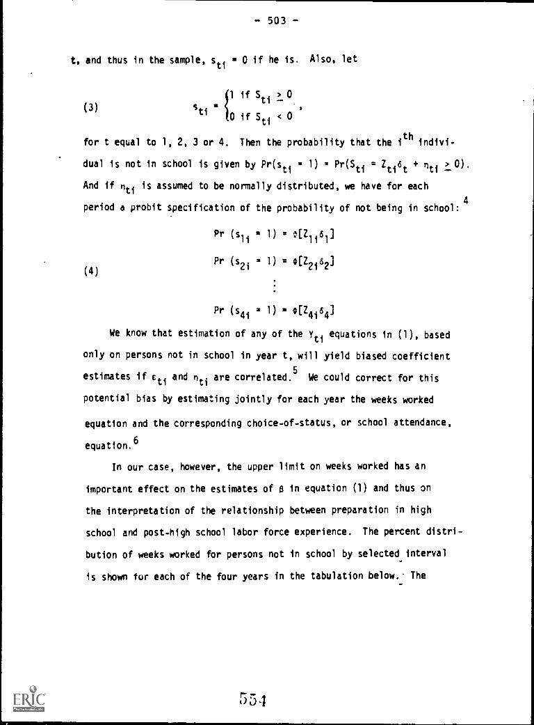
503

t, and thus in the sample, so = 0 if he is. Also, let

(3)

1 if Sti 10

sti0 if S

ti< 0

for t equal to 1, 2, 3 or 4. Then the probability that the 1th indivi-

dual is not in school is given by Pr(sti 1) Pr(sti = Zo6t + no > 0).

And if no is assumed to be normally distributed, we have for each

period a probit specification of the probability of not being in school:4

(4)

Pr (sli = 1) = t[Zlity

Pr (s2i . 1) = .(2202]

Pr (s4i = 1) 142404]

We know that estimation of any of the yti equations in (1), based

only on persons not in school in year t, will yield biased coefficient

estimates if Eti

and nti

are correlated.5

We could correct for this

potential bias by estimating jointly for each year the weeks worked

equation and the corresponding choice-of-status, or school attendance,

equation.6

In our case, however, the upper limit on weeks worked has an

important effect on the estimates of 0 in equation (1) and thus on

the interpretation of the relationship between preparation in high

school and post-high school labor force experience. The percent distri-

bution of weeks worked for persons not in school by selected interval

is shown for each of the four years in the tabulation below.. The

504

Weeks Worked Percent Distribution

Interval 1973 1974 1975 1976

0 to 10 5.2 5.3 4.6 4.6

11 to 20 4.8 3.1 3.6 3.5

21 to 3C 8.0 5.9 5.7 5.5

31 to 40 12.5 12.0 9.9 10.2

41 to 51 30.3 32.3 24.2 24.7

52 39.2 41.4 52.0 51.5

percent reporting fifty-two weeks of work ranges from 39 in 1973 to 52

in 1976. It is apparently the case that many persons are prepared to

work, and have work opportunities, that exceed the time available con-

straint as measured in weeks.7

Thus we have changed the specification in equation (1), interpret-

ing capital Yi as an unobserved "propensity" to work, with observed

weeks worked given by,

(5)

yli

Y4i*

X1101 + Eli if X1181 + en < 52,

52 if xlial + Eli > 52,

X4184 + co

52

if X4184 + c4i 1

52,

if X41

04

+ c41

> 52.

The maximum likelihood procedure we have used estimates 0 in (5) jointly

with 6 in (2), for each of the four years individually. It is explained

in more detail in Appendix A. The relationship between the expected

value of Y given by X0 and the expected value of weeks work0r, E(y),

may be seen in the figure below, in which one right-hand var4able is

assumed.

52

545

AE(Y),E(y)

tE(Y) X$

43 _____ _ _________

Figure 1

E(y) . Expected weeks worked

At low levels of X8, the estimated parameter 8 represents the approxi-

mate effect of a change in X on the expected number of weeks worked.

As X increases, its effect on weeks worked approaches zero.8 For exam-

ple, our results reported below suggest that $ is about twice as large

as the derivative of E(y) with respect to X, evaluated at X. At the

mean of the variables in our sample, the expected number of weeks worked

is about 44, and the expected value of the unobserved Y is somewhat

greater than 52. The derivative of E(y) with respect to X at X is approx-

imately equal to the estimate of $ from a specification that does not

distinguish employment at the limit of 52 weeks from observations below 52.

There were also a few persons each year who did not work at all.

We obtained some initial estimates that accounted for this by specifying

weeks worked to be bounded at zero, as well as 52. It did not signifi-

cantly affect our results and we did not incorporate it in the results

55E

-: 506

presented below.

An alternative to separate estimates for each year is to divide

the sample into two groups:. one composed of persons who were never in

school, and the other composed of everyone else. But for our p'poses

the procedure outlined above has at least two advantages over this one.

First, it allows us to make use of as much of the data as possible.9

Examination of Table 3 shows that the number of persons out of school in

all years is much smaller than the number in any single year.10

Also,

even if the group with weeks worked is defined in the alternative way,

a sample selection correction must still be made to obtain unbiased

estimates of the population parameters in the weeks worked equations.

This presumably would be done by estimating a probit equation pertaining

to the probability of never being in school. Such an equation could be

used to correct each of the weeks worked equations for the sample selec-

tion bias.11

But it is difficult to think of a behavioral interpretation

for this sample selection equation, since in a given year one group in-

cludes persons who are in school as well as some who are not. Our status

equations can be interpreted in each year as estimating the determinants

of school attendance in that year.

B. The Wage Rate Estimation Procedure

Wage rate equations were also estimated jointly with non-school

attendance equations. There are five wage equations, however, one for

each of the October survey periods. But there is no limit problem as

with weeks worked. Parameters in equations like (1) and (2) for-weeks

worked were estimated jointly, with the logarithm of the wage seb-

stituted for weeks worked.12

There is, however, a complication that

does not arise in the weeks worked equation.

507

Wage rates are presumed to depend on years of schooling, as well

as other variables. For example, persons who were working in the fourth

October period may have been in school during some or all of the pre-

li:ous periods, and their wage rates may be expected to depend=on the

amount of schooling. Suppose that the logarithm of the wage is given

by,

W4i X4i14 + alAii + a2A2i + a3A3i + v4i ,

where Al equals 1 if individual i was in school during period 1 and

zero if not, and similarly for A2 and A3. The potential bias resulting

from the possibility that E(v411s41 = 1) may not be zero is corrected

for by estimating the equation jointly with the probability of non-school

attendance. But if the vt's are correlated with the error in the non-

school attendance equations, and the nt's or the vt's are correlated

over time, then Al through A3 may be correlated with the error v4 in the

wage equation. To overcome this problem, we experimented with an

instrument for prior schooling 13 In practice, we found that the use of

an instrument for schooling did not substantially alter the character

of our conclusions.14 A similar problem may pertain to work experience

that is also assumed to determine the wage rate. We did not attempt to

correct for it. (In subsequent work we will estimate a more appropriate

moael for solving this problem. It will allow joint estimation of weeks

worked, wage, schooling, and a sample selection equation.)

Finally, the sample selection equations estimated with the wage

rate equations are not precisely non-school attendance equations, al-

though in practice the two are almost interchangeable. The weeks worked

-2 508 -

equation for a given year included all persons who were not in school

during that year. Thus the status or sample selection equations are

equivalent to school attendance equations. Students were also excluded

from the wage equations. But we do not have wage rates for all persons

who were not students. Some non-students were also not employed. To

correct the wage equation for sample selection bias we need to consider

all ,persons without a recorded wage rate, whatever the reason.15

The variables used in the analysis are defined below.

Weeks Worked: Annual weeks worked, October to October.

Wage Rate: Earnings divided by hours worked, first full week in

October.

Test Scores Total: Sum of scores on six tests - vocabulary, read-

ing, mathematics, picture-number, letter groups, mosaic comparisons:

Class Rank in High School: Percentile ranking relative to other

persons in individual's high school.

Job Training in High School: One if the individual received in

high school "any specialized training intended to prepare you for

immediate employment upon leaving school? (For example, auto

mechanics, secretarial skills, or nurses aid)," zero otherwise.

Hours Worked during High School: Response to the question, "On

the average over the school year, how many hours per week do you

work in a paid or unpaid job? (Exclude vacation.)" The response

'was by interval: 0, 1-5, 6-10, ..., 26-30, over 30.

509

Parents' Income: Annual income of parents, in thousands.

Education of Mother (Father) less than High School: One if the

youth's mother (father) had less than a high school education and

zero otherwise.

Education of Mother (Father) College Degree or More: One if the

youth's mother (father) had a college degree or more education,

and zero otherwise. The excluded category is a high school degree

but less than a college degree.

Race: One if non-white, zero otherwise.

Dependents: Number of persons dependent on the individual for

income.

School Years: Number of Octobers in which the individual said

he was in school.

On the Job Training: Months of on-the-job training.

Experience: Work experience, in years. Excludes work

while attending a post-secondary school. Experience is disZin-

guished by the year in which it occurred.

Part-Time Wor' la: One if the individual is working part-time,

zero otherwise.

Rural, Urban: One if the individual's residence location corre-

sponds to the one indi:ated, zero otherwise. The excluded category

is suburban and town.

West: One if the person lives in the Wrist, zero otherwise.

State Wait: Annual average wage in manufacturing.

56U

- 510 -

State Unemployment: Average annual unemployment rate.

Missing Variable Indicators: For test sores, class rank, parents'

income, experience. Each is one if the designated variable is

missing and zero otherwise. The corresponding variable takes

the value zero if it is missing and the recorded value if it is

not.

The means and standard deviations of these variables are given in

Appendix Table C.

511

C. School Attendance

As a concomitant of the procedure used to estimate both the weeks

worked and the wage equations we estimated school attendance equations,

or more precisely, the probability of not attending school. Before

presenting results on the central questions of our analysis, we will

summarize briefly the implications of the estimated attendance pro-

bability parameters.

Non-school attendance equations estimated with the weeks worked

equations are presented in Table 7B; those estimated with the wage equations

are shown in Table 88. The two sets of parameter estimates are necessarily

very similar. The discussion in this section is based on those estimated

with weeks worked. Recall that the parameter estimates in Table 7B are

analogous to the parameters 6 in equations (2) and (4). The variables

used in the probability equ Lions are easily identifiable by glancing

at the table. They need no further explanation. The first two groups

of variables pertain to school achievement and family background. All

are measured with considerable precision, as shown in the table.

To get a better idea of the importance of the variables, however,

we have calculated estimated differences in the probability of attending

school for persons who have different values of a specified variable,

but the same values for all the others. All other variables were assumed

to have values equal to their respective means. The specified differences

and the associated differences in estimated school attendance probabili-

ties are shown in the tabulation below.

562

512

Difference inAcademic orSocial Background 1972-73

Associated Differences in theProbability of School Attendance

1973-74 1974-75 1975-76 1976h

Test scores oneS.D. above themean, versus oneS.D. below

Class rank oneS.D.above the mean,versus one S.D. below

Parents income oneS.D. above the mean,versus me S.D. below

Education of Father& Mother college ormore, versus lessthan h.s. graduate

Non-white, versuswhite

.242

.341

.103

.254

.279

.104

.247

.097

.247

.288

.096

.319

.091

.230

.292

.104

.323

.109

.181

.165

.059

.230

.136

Possibly the most notable finding is that the probability that non-

whites are in school, controlling for other variables. is considerably

16higher than for whites, at least .10 in each of the five years. (Recall

that the summary numbers in Table 1 show that in each of the first four

years following high school, the percent of non-whites in school full-

time was between 11 and 13 percentage points less than the percent for

whites.) This could result from relatively fewer opportunities in the

labor force. But as indicated in the wage equation estimates, discussed

below, after controlling for other variables, there is little difference

between the wage rates of whites and non-whites in the first three years;

in the last two, non-whites are estimated to earn about 4 percent more

than whites.17 And the weeks worked equations inuicate that afir

h. Based on the non-school attendance equation estimated with the1976 wage equation. See Table 8B.

5 63

513

controlling for other variables non-whites lork about the same number of

weeks per year as whites. It could also reflect higher returns to educa-

tion for nor-whites than for whites, as discussed by Freeman 0976a,

1976b], for example.

The other academic and family background variables are all related

in the expected way to school attendance, although the relative mag-

nitudes may not be widely known. Parents' income seems to have much less

effect on school attendance than either of the measures of academic

achievement. Parents' income n'y be the least important of all the

variables listed. Class rank seems somewhat more important than the

test scores, although our comparison is only suggestive. Recall that

the tests measure a range of abilities and achievements, some more

academically oriented than others. Also, we have made no attempt to

distinguish types of school. The relative importance of academic'ability

is likely to increase with the quality of schoolY Finally, there are

large differences in expected probability of school attendance asso-

ciated with extremes in parents' education.

In an alternative specification of the school attendance equations

in Table 78 we also included the number of hours worked per week in high

school -- measured - -as one of seven intervals, 1 to 5, 6 to 10, . . . ,

over 30--and a variable indicating whether or not the individual had job

training during high school. It is questionable whether the job train-

ing variable (and possibly hours worked in high school) should be in-

cluded in a school attendance equation. The question arises because

564

- 514 -

job trtining in high school may indicate a "non-college trait" and thus

.a prier decision not to go to school--it may be more an indicator of

post-secondary school attendance rather than a determinant of -it. But

because the relationship between these choices while in high school and

later school attendance may be of interest we have reported the results

when they are included. Their inclusion has a negligible effect on the

other parameter estimates. 19

Persons who work more than about twenty hours per week in high

school are considerably less likely to be in school in any of the four

years than these who work less, according.to the estimates of the coeffi-

cients on hours worked in high school. The average effect on the proba-

bility of school attendance of working 21 to 25, 26 to 30, or more than

30 hours per week is about .10, with the probability evaluated at the

means of the other variables. Persons who work less than twenty hours

per week are also less likely to be in school during the first year after

high school than those who don't work at all, but the relevant coeffi-

cients are not measured very precisely. 20 In the remaining three years,

the estimates indicate little relationship between poit-secondary school

attendance and hours worked in high school until hours worked exceeds

20 hours per week approximately.

Recall that these are estimates after controlling for high school

achievement and family background. We will show below that, with a few

notable exceptions, the number of hours worked : ring high school is not

strongly related to most measures of socioeconomic background aor to

school achievement. It is largely an indeptndAnt personal characteristic.

515

Recall that only for persons who work many hours per week during high

school is such work significantly related to later school attendance.

There is a tendency for persons who work a lot to be less inclined to

continue their formal schooling. Possibly some have made a prior

decision to work rather than go to school. We will see, however, that

hours worked in high school are strongly related to weeks worked per

year after graduation. As expected, persons who get job training in

high school are considerably_less likely to go to school later than

those who don't.

Only two of the other variables in Table 8B need be mentioned; the

others may be thought of simply as controls. One might suppose that school

attendance would depend on expected wage if not in school and the ease

of finding work; thus the state wage and unemployment variables have

been included in the probability equations. They could be considered

as rough instruments for individual wage and unemployment rates. Neither

is significantly different from zero in most years, although the wage

rate in each year is negatively related to school attendance and the

unemployment rate positively related. The wage rate is significantly

different from zero by standard criteria during the first two years.

It could be that labor force opportunities are important determinants

of school attendance right after high school, but that in the later

years, once in school, persons don't drop out due to changes in the

wage rate, and they are less likely to enter school having not attended

previously. The marginal lifetime return to an additional year of

school probably increases as one nears college graduation.

566

516

Finally, persons who go to rural t-.1gh schools are less likely to

be in school after graduation--the difference 4r1 probability s about

.06 in the first two years and .12 and .13 respectively in the third

and fourth years.

, .s) ti .7

s

- 517 -

Table 7A. Estimates of Weeks Worked EquationParameters, by Year

Variable

October 1972to

October 1973

October 1973to

October 1974

October 1974to

October 1975

October 1975to

October 1976

Hours Worked duringHigh School:

1 to 5 0.1700 1.1246 0.9006 3.4239

(1.1629) (1.6710) (2.0376) (1.9529)

6 to 10 2.5027 2.2662 0.4056 3.0490

(1.1893) (1.7883) (1.9750) (1.7620)

11 to 15 7.3619 1.7668 4.0527 4.4541

(1.3896) (1.9820) (2.2907) (1.9907)

16 to 20 6.8180 4.2688 5.9215 6.5548

(1.1109) (1.5694) (1.9135) (1.7884)

21 to 25 7.8500 5.1503 4.2531 7.3057

(1.2329) (1.7854) (1.9096) (1.7893)

2b to 30I

10.9685(1.3189)

6.1313(1.7165)

5.9604(1.9496)

7.1673

(1.8737)

31 or more 12.5225 7.6769 8.9859 8.1603

(1.1273) (1.5174) (1.8231) (1.6714)

Class Rank in 0.2323 0.2120 0.1914 0.2044

High School (0.0267) (0.0276) (0.0294) (0.0270)

Test Score Total 12.1144 10.8146 9.7233 6.7031

(1.4197) (1.6811) (1.7978) (1.6649)

Job Training during -1.4376 1.4486 0.5983 3.0389

High School (0.7151) (1.0539) (1.2593) (1.23E8)

Race -1.9184 0.1898 0.3935 -0.9848

(1.3714) (1.6311) (1.736') (1.5666)

Parents' Income 0.6370 0.4868 0.5015 0.3137

(0.1168) (0.1211) (0.1401) (0.1218)

Dependents 4.2551 1.6987 1.3027 1.8420

(0.5997) (0.7739) (0.7485) (0.6702)

(continued)

yes

- 518 -

Table 7A. Estimates of Weeks Worked EquationParameters, by Year. (completed)

VariableOctober 1972

to

October 1973

October 1973to

October 1974

October 1974:to t.

October 1975-1'

October 1975to

October 1976

On the Job 0.6600 0.3335 0.3680Triining Years (0.2667) (0.1885) (0.1653)

Rural -2.5912 0.1617 -2.7939 0.0897(0.9628) (1.3651) (1.4721) (1.3027)

Urban -1.4913 -2.2115 -1.2479 0.3683(0.8016) (1.0583) (1.2458) (1.1566)

State Wage -2.1755 -1.0422 -1.9233 -1.6065(0.9391) (1.1206) (1.0218) (0.8324)

State Unemployment -1.0645 -0.4019 -0.8878 -0.7279(0.4069) (1.1206) (0.4418) (0.2826)

Test Score Missing 33.0777 29.6297 26.4883 19.3229(4.3147) (5.1682) (5.5833) (5.1371)

Class Rank Missing 10.1779 6.8823 6.6354 7.1726(1.9191) (2.2285) (2.5529) (2.2480)

Parents' Income 6.6426 6.8539 3.2212 2.2059Missing (1.7567) (1.9804) (2.2199) (2.2028)

Constant 27.2947 23.4604 36.8182 40.9972(5.3019) (6.3969) (7.0262) (6.5931)

r-5C9

- 519 -

Table 7B. Estimates of Non-School Attendance Equation Parageters,by Year (Estimated with Weeks Worked Equation))

October 1972to

October 1973

October 1973to,

October 1974

October 1974to

October 1975

October 1975to

October 1976

Test Scores Total

Class Rank inHigh School

-0.7411(0.0504)

-0.0154(0.0008)

-0.7704(0.0684)

, -0.0133

(0.0010)

-0.7180(0.0694)

-0.0132

(0.0010)

-0.6714(0.0674)

-0.0136(0.0010)

Race -0.2792 -0.2509 -0.2297 -0.2726

(0.0519) (0.0687) (0.0696) (0.0678)

Parents' Income -0.0284 -0.0254 -0.0228 -0.0247

(0.0039) (0.0051) (0.0051) (0.0049)

Education of Mother 0.1358 0.0509 -0.0067 0.0372

Less than High School (0.0275) (0.0488) (0.0511) (0.0511)

Education of Mother -0.2534 -0.1325 -0.1540 -0.1759

College Degree or More (0.0449) (0.0628) (0.0703) (0.0687)

Education of Father 0.2503 0.2808 0.2560 0.2295

Less than, High School (0.0277) (0.0466) (0.0494) (0.0504)

Education of Father -0.2890 -0.1772 -0.3991 -0.3675

College Degree or More (0.0377) (0.0554) (0.0631) (0.0607)

Rural 0.1708 0.1542 0.3022 0.3186

(0.0341) (0.0529) (0.0551) (0.0554)

Urban -0.0456 -0.0174 -0.0071 -0.0387

(0.0278) (0.0439) (0.0475) (0.0470)

State Wage 0.1444 0.0658 0.0063 -0.0030

(0.0333) (0.0437) (0.0397) (0.0339)

State Unemployment -0.0191 -0.0156 -0.0195 0.0008

(0.0140 (0.0179) (0.0167) (0.0112)

Test Score Missing -2.1016 -2.1982 -2.115 - 2.0005

(0.1579) (0.2177) (0.2237) (0.2169)

Class Rank Missing -0.5491 -0.4709 -0.5977 -0 -6305

(0.0704) (0.0941) (0.0980) (0.0940)

Parents' Income -0.2979 -0.3408 -0.2796 -0.3026

Missing (0.0643) (0.0845) (0.0868) (0.0836)

(continued)

5 70

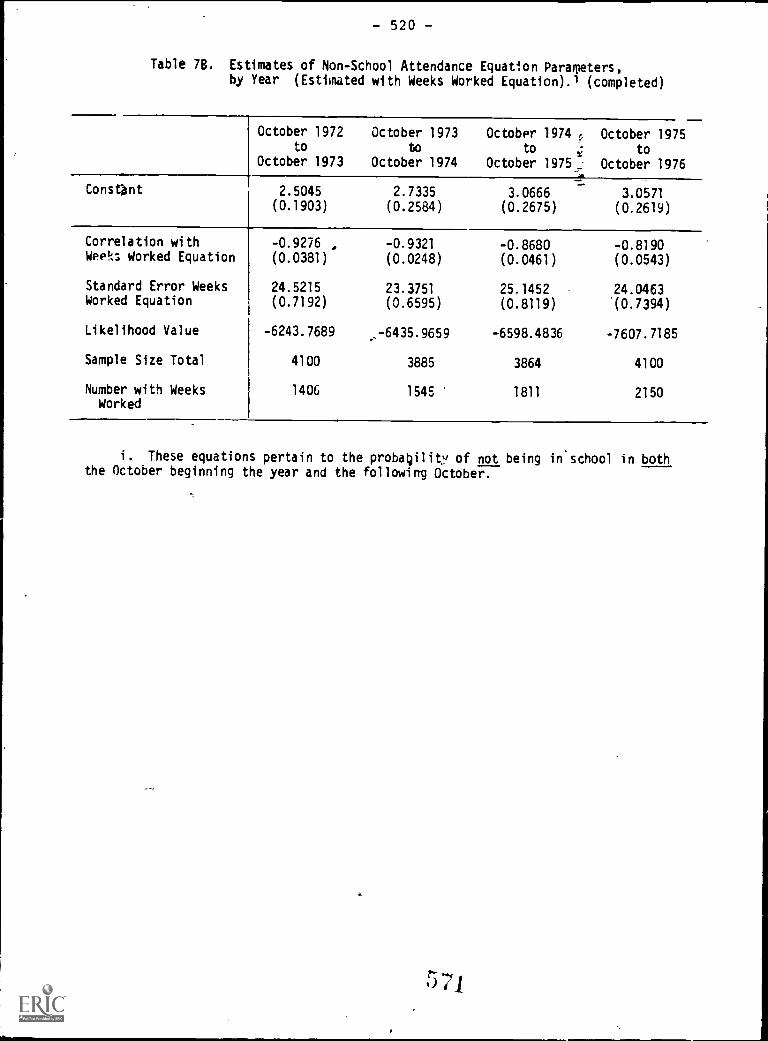
- 520 -

Table 78. Estimates of Non-School Attendance Equation Parameters,by Year (Estimated with Weeks Worked Equation).1 (completed)

October 1972to

October 1973

October 1973to

October 1974

October 1974to

October 1975:

October 1975to

October 1976

Constbnt 2.5045(0.1903)

2.7335(0.2584)

3.0666(0.2675)

3.0571

(0.2619)

Correlation with -0.9276 , -0.9321 -0.8680 -0.8190Weeks Worked Equation (0.0381) (0.0248) (0.0461) (0.0543)

Standard Error Weeks 24.5215 23.3751 25.1452 24.0463Worked Equation (0.7192) (0.6595) (0.8119) (0.7394)

Likelihood Value -6243.7689 -6435.9659 -6598.4836 -7607.7185

Sample Size Total 4100 3885 3864 4100

Number with Weeks 1406 1545 1811 2150Worked

i. These equations pertain to the proba4ility of not being in school in boththe October beginning the year and the following October.

- 521 -

D. Weeks Worked

Estimates of the parameters in the weeks worked equations are

shown in Table 7A. The most significant finding is that hours worked

while in high school bear-a substantial relationship to weeks Worked

per year in the years immediately following high school graduation.

The estimated coefficients corresponding to hours worked intervals in

high school are reproduced in the tabulation below. As can be seen in

Table 7A, they are measured with considerable precision. Recall that

they represent an upper bound on the effect of high school work. They

are slightly larger than the estimated effect of high school hours

worked on expected weeks worked, evaluated at Xa close to zero. As

the expected value of Y rises, and thus the expected value of weeks

worked, the marginal effect of hours worked in high school falls. In-

deed, as the expected number of weeks worked approaches 52, the marginal

effect of a change in any variable declines, and must ultimately approach

zero.

To give an idea of the magnitude of the decline, we have evaluated

the estimated effects of high school work at two additional points. One

is the expected value of weeks worked evaluated at the mean of X for

all persons in the sample, whether they were in fact in the labor force

or in school. These values are shov4n in the second portion of the tabu-

lation. In addition, the expected value of weeks worked is shown for

each year, along with an "adjustment factor." The adjUstment factor

indicates the multiple by which the estimates in the first portion of the

table must be multiplied to get the estimates in the second portion.21

5 "101 ti

- 522 -

The other evaluation point is tne mean of X for persons who were in

the labor force and conditional on knowing that they were. The esti-

mated effect on,weeks worked over the four year period is shown in

the last column.

Hours Worked Estimated Effect on Weeks Workedin High School 1973 1974 1975 197b Total

1 to 56 to 1011 to 1516 to 2021 to 2526 to 30over 30

Effect at Zero Weeks Worked (Estimate of 8)

/d 0.17 1.12 0-90 3.42 5.612.50 2.27 0.41 3.05 8.237.36 1.77 4.05 4.45 17.636.82 4.2.7 5.92 6.55 23.567.85 5.15 4.25 7.21 24.56

10.97 5.13 5.96 7.17 30.2312.52 7.68 8.99 8.16 37.35

Effect at Mean of X in Total Sample

Expected Weeks 47.20 47.26 47.36 47.04Adjustment Factor 0.270 0.287 0.270 0.297

1 to 5b tO 10

11 to 1516 to 2021 to 2526 to 30over

0.06 0.32 0.24. 1.02 1.640.68 0.65 0.11 0.91 2.351.99 0.51 1.09 1:32 4.911.84 1.22 1.60 1.95 6:612.12 1.48 1.15 2.17 6.922.96 1.76 1.61 2.13 8.463.38 2.20 2.43 2.42 10.43

.,-

Effect at Mean of X for Persons in Labor Force

Expected Weeks 44.17 43.26 44.42Adjustment Factor 0.484 0.567 0.461

1 to 5 0.08 0.64 0.416 to 10 1.21 1.29 6.19

11 to 15 3.56 1.00 1.8716 to 20 3.30 2.42 2.7321 to 25 3.80 2.92 1.9626 to 30 5.31 3.48 2.75over 30 6.06 4.35 4.14

5 73

44.41

0.45e_./

1.57 2.701.40 4.092.04 8.443.00 11.45.3.35 12.03.3.28 14.823.74 18.28

a

523

Estimates of the 0 coefficients on hours worked range from zero

for hours between 1 and 5 to over twelve for hours greater than 30.

Even in the fourth year, the estimated values of 0 are very_large,

ranging from 3 for the fewest hours category to over 8 for the largest.

It is notable, that after four years, the relationship of even a little

work in high school to work after high school is substantial. Over the

four year period, the sum of the estimates range continuously upward

from 6 weeks to 37 weeks.

Expected weeks worked per year evaluated at the mean of the right-

hand variables averaged over all persons in the sample is about 47

weeks in each of the four years. Even at this level, the estimated

relationship to work in high school is ry large. The average ove.'

the four years of the effect of working between 16 and 20 hours per

week is about 1.5 weeks per year. For persons who worked over 30 hours,

the average of the estimated effects is almost 3 weeks per year. The

sums of the effects for the four years range from 2 to 11 weeks.

Possibly the most intuitively meaningful results pertain to persons

who did in fact choose to work rather than go to school. Expected

weeks worked evaluated at the mean of X over persons observed to be in

the labor force is about 44 weeks in each of the four years. The

sums of the effects over the four years range from almost 3 to close to

18 weeks. Sixteen to twenty hours of work in high school is associated

with an average of almost 3 weeks per year in weeks worked during

the four years after graduation.

Estimates Jf the marginal relationship between hours worked in

high school and weeks worked, evaluated at any other expected value of

5 74

524

weeks worked, can be obtained by multiplying the numbers in the top por-

tion of the tabulation by the appropriate adjustment factor. For example,

the appropriate multiple when the expected value of weeks worked [E(y)]

Is thirty is approximately .86 in each of the four years. 22---

How to interpret this finding is open to question. It is possible

that persons who work in high school gain skills and other attributes,

through their work, that give them an advantage in the labor market

after graduation. Demand may be greater for them than for persons who

do not work. This is consistent with the finding that wage rates are

also higher for persons who work in high school, although the relation-

ship is not nearly as strong as that between weeks worked and work in

high school. But we might expect such an advantage to diminish over

time, as post-high school experience becomes an increasingly larger pro--

portion of total experience. And although the estimated effect declines

som 'what, it is still very Importznt four years after graduation. This

suggests that working in high school may be an indication of personal

characteristics not gained through work, but leading to work in high

school as well as greater labor force participation following graduation.

That is, it is not that the demand is greater for persons who work in

high school, but that these persons have a greater propensity to work.

That wage rates are not so greatly affected by high school work seems

to add to the evidence for this interpretation.

Even this latter interpretation, however, would not rule out the

possibility that work experience while in high school, for parsons

like those in our sample who did not work, would increase their

employment after high school. Working may in fact enhance it these

325

persons attributes that were associated with high school work of

persons in our sample. And, as we shall see below, work experience

while in high school may increase subsequent wage rates in much the

same way that work experience upon graduation increases later wage

rates in the labor market.

It is informative to consider these findings and possible inter-

pretations of them, in conjunction with the relationship between work in

high school and other school and family characteristics. We shall returi

to that after some discussion of some of the other results shown in

Table 7A.

Class rank in high school is strongly related to weeks worked in

each of the four post-high school years. The estimates indicate that a

50 point increase in class rank i3 associated with an-increase of about

10 in the expected value of Y, or say 3 in the expected value of weeks

worked, over the total sample. This result is based on holding constant

the test score. The test score appears to measure a combination of

aptitude and achievement. No matter what the interpretation of test

score, conditional on nolding it constant, class rank is likely to reflect

effort directed to doing well in high school. Effort in school, like

the characteristic reflected in high school work, is related to later

labor force participation at least for the next four years. Both hours

worked and class rank may capture what is sometimes referred to as the

"work ethic." Those who work harder in high school also work more in

subsequent years. Or, those who become accustomed to working at a young

age maintain the habit. Or, if they have or develop early in life

characteristics associated with working, they maintain them.

We also find that high test scores are associated with more employ-

576

516 --

ment after graduation, but the effect diminishes over the four years

following graduation. An increase of one standard deviation--about

.4--in tt2 sum of the test scores is associated with a 11/2 week increase

in expected weeks worked in the first year and declines continuous to

about 1 week in the fourth. It may be that persons with greater ability

or achievement, as reflected in the test scores have an advantage in

the labor market, but as time goes on the skills that are associated

with the test scores are in part compensated for by skills developed

on the job or elsewhere. That their effect diminishes over time sug-

gests that the reason is not entirely a permanent underlying individual

characteristic. (The wage equation estimates suggest some advantage

to higher test scores, but there is no distinct time pattern.)

We could find no measure of high school vocational or industrial

training that was significantly related to employment, or wage rates, after

graduation. The variable included in the results in Table 7A is high

school training for a particular job. We assumed that if any high school

training mattered, this training should. It doesn't. We experimented

with many other measures of job related training -- semesters of various

vocational courses, acadrmic versus non-academic tracking, and others.

We found none that was relate° to subsequent employment. It could be

that the least able are directed to vocational training courses, or self-

selected into them. But our results are conditional on controlling for

traditional measures of school performance -- class rank and test scores.

527

This cannot be interpreted to mean that no training matters; but it does

indicate strongly that none of the training in current high School

curricula, or at least that systematically measured in the survey, is

related to later labor force participation after high school. We were

not able to distinguish vocational high schools from others. In sub-

sequent work we will. It is possible that the effect of training in

a vocational high school is different from the effect of training

received in schools whose curricula are not primarily directed to job

training.

Non-whites are employed about the same number of weeks per year

as whites during the first years following high school graduation. The

differences between the expected value of weeks worked for non-whites

and whites, evaluated at the mean of X in the sample, are -.52, .05, .11,

and -.29 respectively in the first four years following high school grad-

uation. None is significantly different from zero by standard criteria

Remember that these results are partial effects after controlling for

other variables, unlike the summary statistics in the first section of

the paper. (The simple averages in Table 6 indicate fewer weeks worked

by non-whites than whites during the first two years after high school,

but little difference in he third and almost none in the last.) The

wage estimates below indicate that after controlling for other variables,

wage rates of whites and non-whites are quite close in the first three

October periods and in the last two that non-whites earn about 4 percent

more per hour than whites. And the averages in Table 5 indicate whites

and non-whites who are not in school have very similar weekly earnings

and hours worked, as well as wages.

Parents' income bears a substantial positive relationship to weeks

528

worked during each of the first four years after graduation. In the

first year, an increase in parental income of $5,000--about t standard

deviation--is associated with an increase in weeks worked of over 3

weeks. The relevant coefficient declines over time to about half of its

original size her the fnurth year. If children whose parents have higher

paying jobs have an advantage in finding work, the advantage apparently

diminishes as the youth cohort gains labor market experience.

In sum, the most important determinants of weeks worked seemed to

be characteristics associated with effort pursuant to succeeding in high

school, as measured by class rank after controlling for ability, and to

effort devoted to outside work while in high school, in particular the

latter. It may be informative therefore to consider the relationship

between hours of work while in high school and other personal and family

characteristics.

For descriptive purposes, we have obtained coefficient estimates

from a least squares regression of hours worked per week on several vari-

ables. The coefficients and standard errors pertaining to the variables

Variable coefficient Standard Error

Test Score TotalRaceParents' Income

Education of MotherLess than High School

Education of MotherCollege Degree or More

Education of FatherLess than High School

Education of FatherCollege Degree or More

-2.81

-5.33

0.22

0.49

-0.85

0.36

-1.58

(0.92)

(0.87)

(0.07)

(0.69)

(1.51)

(0.68)

(1.2)

579

Class Rank in High SchoolJob Training duringHigh School

Extracurricular Participationin High School

0.01

0.37

0.51

(0.01)

(0.66)

(0.29)

of most interest are listed above. 2: There are two groups of variables:

one that can be interpreted as composed of predetermined personal and

family characteristics; the second group is composed of measures of the

individuals' high school experience other hours worked while in

high school. There seems not to be a substantial tradeoff between any

of these latter measures and hours worked. For example, working does

not seem to take the place of studying, as reflected in class rank after

controlling for test scores. Comparable results were found by Griliches

[1977).

Race is the only variable that stands out. Non-whites work con-

siderably less in high school than whites, given the measures of parents'

income and education. This may result either from differences between

the two groups in job opportunities, or from differences in work habits,

or some combination of the two. Whatever the reason, 5 hours less work

in high school is associated with a maximum of about 1.5 fewer weeks

worked in the years following graduation, according to the weeks worked

results. Recall that after controlling for hours worked in high school

as well as other variables, non-whites work about the same number of

weeks per year es whites.

In addition, persons with higher test scores work a bit less and

those with higher parents' income a bit more (The standard deviation

of test scores is .4 and of parents' income is 5.7, in thousands.)

The latter may result from more job possibilities if one's patients have

better jobs, or it may reflect cultural differences related to income.

560

- 530 -

Possibly persons with higher test scores, given class rank, foresee a

greater- probability of going to college and thus are somewhat less

inclined to take jobs in high school. This is consistent with the non-

school attendance results.

Thus we have in hours worked in high school a personal characteris-

tic that is somewhat related to race, test scores, and parents' income.24

But after controlling for these variables hours worked in high school

is strongly related to weeks worked after graduation. Hours worked

captures an individual attribute that is not simply a reflection of other

personal and family socioeconomic characteristics. It reflects a largely

independent personal attribute that persists over time.

We shall mention briefly the effects of the remaining variables

in Table 7B. The estimated effect of on-the-job training is always

positive, but it declines over time. This result may be due to training

agreements or employment expectations that lead to training for persons

who expect to continue in the same job, or who employers expect to con-

tinue. The effect might be expected to die out over time as persons are

increasingly likely to have charged jobs.

Persons living in urban areas are employed liSs than others. Accord-

ing to our imprecise estimates, the maximum neoative effect is 2.2 weeks;

in the last year when a larger proportion of those working are college

graduates the estimated urban effect is in fact positive. although not

significantly different from zero. College graduates may have relatively

greater work opportunities in urban areas. As expected, state unemploy-

ment is negatively related to employment of youth. Roughly speaking, if

the unemployment rate increases by a percentage point expected weeks

worked by these youth falls by about half a week, about one percent of the

5S1

531

mean value of weeks worked. The higi4r the state wage as we have

measured it, the lower the number of weeks worked by youth.25

Finally, for each year our procedure estimates the correlation

between the random term in the weeks worked equation and the7:random

term in the probability of non-school attendance equation. They are

reported for each year in the last section of Table 7B. Recall that a

zero correlation coefficient indicates no :ample selection bias. Our

estimates (and standard errors) for the four consecutive years are

-.93 (.03), - 33 (.02), -.87 (.05), and -.82 (.05). that is, in each

year unmeasured determinants of college attendance bear a very strong

positive relationship to unmeasured determinants of weeks worked.

Holding constant the variables we have measured, persons who choose to

go to school would work more if they were in the labor force than those

who choose not to go to school after high school. The relationship is

very striking. The results seem to indicate that the motivations or

drives that characterize persons who continue their education are also

attributes that are related to increased employment if not attending

school. In practice, correction for sample selection, by estimating

jointly weeks worked and the probability of non-school attendance, in-

,

creases substantially the estimated coefficients on class rank, test

scores, and parents' incoma, but yields coefficients on the other vari-

ables that are close to Tobit results. For purposes of comparison, weeks

worked parameter estimates by method of estimation are presented in

Appendix Table B.

We have not in this specification of weeks worked incluled a

schooling variable. One might suppose, however, that if the proba-

5 S 9

532

bility of school attendance in a given year is positively related to

the number of weeks a person would work if he were in the labor force,

then also the number of years of schooling prior to a given year would

-be likely to affect weeks worked in that year if a person were in the

labor force. When prior schooling is included in the weeks worked

equations, however, its effect is not significantly different from

zero, even with prior schooling also included in the sample selection

equation. This suggests that the large correlation between unmeasured

determinants of school attendance and measured determinants of weeks

worked reflects the difference between persons who attend school foie

several years after high school graduation--possibly long enough to

obtain a degree and those who don't. Apparently persons who move in

and out of school during the first four years after graduation are in

th,, respect much like persons who don't attend school at all.

5 3

E. Wage Rates

The wage rate parameter estimates are reported in Table 8A. Some

have been referred to already. Work experience in high school is posi-

tively re;ated to post-hign school wage rates, as well as to weeks worked.

In gOneral, during the last four periods, persons who worked in high

school earned roughly 5 to 9 percent more per hour than those who didn't.

Thus not only are additional hours of work in high school associated

with additional weeks worked after graduation, but higher earnings

per hour as well. But although there is an increasing relationship

between the number of hours worked in high school and weeks worked

later; given 5 or 10 hours per week, additional hours in high school

are not associated with increments in wage rates until high school hours

exceed 30 per week.26

For these reasons, we have used only three high-

school-work intervals instead of the seven used in the weeks worked

equations.

To evaluate the relationship between hours worked in high school

and annual earnings, we need to consider the association between high

school work and both weeks worked and the wage rate. (We have not con-

sidered the possible effect on hours worked per week.) In addition,

accord-ng to our specification the marginal effect of any variable on

weeks worked depends on the number of weeks worked at which the marginal

effect is evafUa-bad. (See pages 29 and 46.) Consider, for example,

persons in the labor force who otherwise -- if not for high school work

experience -- would have worked 44 weeks per year. This is approxi-

mately the average number of weeks worked by persons who were in the

labor force (see page 4E). According to cur estimates, those who worked

534

between 16 and 20 hours in high school earned about 12 percent more than

those who didn't work at all in high school. Persons who wopked over

30 hours earned about 18 percent more. The effect could be _much greater

for persons who would otherwise work less. For example, consider persons

who yiould work only 30 weeks per year. Those who worked 16 to 20 hours

in high school would, earn about 25 percent more than those who didn't

work at all. Those whb worked more than 30 hours, would earn about 35

percent More. These litter figures should be considered only as indica-

tive because the estimates do not allow interactions among the variables

and therzfore imply substantial extrapolation based on estimated coeffi-

cients. Nonetheless, the relationship between earnings and work in high

school is certainly large even for persons who are working most of the

time and is probably much larger for persons who, based on other charac-

tertstics, woUld work much less.

As with weeks worked, it seems likely that at least part of the

effect results from personal characteristics associated with or devel-

oped through high school work as distinct from later work. If higher

wage rates were tne result simply of the additional experience or

associated acquired skills one would expect both to be dominated

eventually by post-high school work experiehi_e, and the estimated effect

to decline over time.27

Note that the estimated coefficients on high

school work do not simply reflect the fact that persdn's who work while

in high school also are employed more upon graduation and thus have

higher wage rates because of more cumulated post-high school txperience.

The measured effect of high school experience is in addition...to work

experience after high school, also included in the equations.

- 535 -

Test scores and class rank are also positively related to wage rates.

The effect of class rank seems to diminish somewhat with time, but. the

test score coefficients follow no apparent pattern. A standard deviation

increase in the test scores total is associated with an average of

estimated wage rate increases over the five periods of about 3 percent.

The corresponding class rank effect is about 2 or 3 percent. The total

effect of a standard deviation increase in both would be something

like 5 or 6 percent. Together these measures may be assumed to repre-

sent some combination of academic aptitude, academic achievement, and

academic success. Controlling for test score, class rank may also

reflect effort in school comparable to hours worked as a measure of

effort outside of school, as discussed in the section above on weeks

worked. Any one of these attributes would presumably increase productiv-

ity per unit of time.

While traditional measures Of academic success are positively related

to wage rates, as are attribuLes associated with actual work experience

in high school, high school training which is presumably closely directed

to the development of job skills is not. The estimated coefficients on

job training during high school are not significantly different from

zero. This suggests that time taken from academic courses and devoted

to job training instead, has a negligible effect on future wage rate..

If high school training contributes to the development of job=related

skills, they are at least offset by the loss in traditional academic

training related to job performance. It is also possible that rersons

who are relatively poor academic performers and would be relatively

poor job performers are self-selected into job training courses in

5 5I)

536

high school. But as mentioned above, our estimates are conditional on

class rank and test scores, possibly the most common measures of high

school performance.

One might suppose that the effect of hioh school training would

be greater for persons who left school after high school graduation

than for those who obtained further education. Vocational training,

for example, may be more important in jobs filled by high school

graduates than in those typically filled by college graduates.

Our wage data for 1972 includes only high school graduates; for that

year the coefficient on high school training is negative but not

statistically different from zero. In subsequent years, the sample with

observed wage rates includes high school graduates as well as those with

more education. Thus for 1974 and 1976 we reestimated the equations for

high school graduates only; the coefficients on high school training

were 'positive for each of these years bf,t not statistically different

from zero by standard criteria.28

While non-whites worked about the same number of weeks as whites

after controlling for other variables (Table 7A), the wage rates of

non-whites are a bit higher than those of whites, according to our esti-

mates. The coefficient on race is positive in each of the five periods

and significantly' different from zero by standard criteria in the last

two periods. In the fourth ano time periods, non-whites are es-

timated to earn about 4 percent more per hour than whites. (The summary

statistics in Tables 5 and 6 show that the average wage rates of non-

whites were slightly lower than the white averages in all but.the first

period and non-whites worked somewhat fewer weeks per year thin whites

in each year, not controlling for other variables.)

537

Parents' income tics a substantial effect on wage rates. An increase

of tan thousand dollars in parents' income is associated with an increase

in wage rates of 8 to 12 percent. It may be that children of wealthier

parents have different skills, values, or ambitions than those from

poorer families. And presumably, wealthier parents are able to find, or

help to find, better paying jobs for their children. The preponderance

of young persons say that their jobs were found through family contacts

or through friends. The effect of this benefit as reflected in wage

rates seems not to decline much over our five periods; the advantage is

maintained for at least these first four years.29

Recall that the

positive relationship between parents' income and weeks worked declined

over time.

Persons with dependents not only are employed more, but earn more

per hour as well -- approximately 3 percent per dependent in each period.

This may result from greater pressure to find higher paying jobs, as

well as to work more. Persons without dependents may be more willing

to accept lower wages, at least temporarily, possibly while looking

for another job.

On-the-job training does not yield appreciably higher wage rces

during the first year or two after high school. But after that, when

training has presumably paid off in better jobs, the effect shows up.

By the fifth time period, the return to a year of on-the-job training

is estimated to be 7.2 percent.30

In the second, third, and fourth

periods the estimated returns are 1.4, 2.5, and 6.1 percent respectively.

While the estimated effect of on-the-job training increases over

time, our estimates suggest a decline over time in the return to years

of post-secondary schooling. The estimates shown were obtained using

nominal years of schooling.31 As explained in Section II, these esti-

5 5 s

538

mates should be expected to be biased. Indeed the positive relation-

ship between the unobserved determinants of wage rates and school attend-

ance, together with the positive correlation among the wage disturbance

(discussed in the next section), imply that the estimates are biased

upward.32

In the second, third, fourth, and fifth time periods -- one,

two, three and four years after high school graduation -- the schooling

coefficients imply returns of 7.4, 5.5, 4.3 and 1.1 percent respectively.

The results for the last period may be somewhat confounded because college

graduates just entering the labor force are included in the sample.

College graduates are likely to be in jobs with wage structures substan-

tially different from persons without college degrees. There may not

have been enough time for a college degree to pay off in terms of pro-

gression up the hierarchy associated with higher level jobs.33 In addi-

tion, the result may reflect declines in the return to college education.34

The estimated returns to experience are substantially greater than

to schooling during these first years following high school graduation.35

Unlike the effect of hours worked in high school, the effect of early

experience on later wage rates declines according to this specification.

For example, a year of experience during the first year after graduation

is associated with a 13 percent increase in wage rates in the second time

period (the second October after graduation). The effect declines to

10 percent by the third, 6 percent by the fourth and 4 percent by the

fifth period. In general, the effect on wage rates of recent expe-

rience is greater than the effect of earlier experience. Reletive to the

second, third, and fourth time periods -- for which experience is

relevant -- the estimated effect of previous experience in the last time

539

period is quite low, 4 percent for experience during the first two years

and 5 or 6 percent for experience in the third and fourth years. Lest

this pattern of results be taken too literally, we hasten to,add two

qualifications. The first is that the relative effect of experience

across the time periods is dependent in part on changes in aggregate

market conditions over the time period. Experience during the recession

years is likely to have contributed less to earnings than expLIAence .n

more expansive years. These results are of course determined in part by

changes in aggregate market conditions over the 1972 to 1976 time period.36

Second, the specification as shown distinguishes experience by

calendar year, but not by the number of years since leaving school.

Thus, for example, experience in the "second year" may represent expe-

rience during the second year in the labor force for some persons, but

during the first year in the labor force for others -- those who went to

school for one year after high school and then entered the labor force.

We tried two other formulations to check the sensitivity of the results

to changes in specification. For 1974 we distinguished a separate

experience variable for each possible schooling-labor force sequence.

Thus for persons who didn't go to school after high school we allowed

one experience variable for the first year in the labor force and another

for experience in the second; these estimates (and standard errors)

were .062 (.051) and .071 (.059) respectively. For persons who went to

school the first year and entered the labor force the second, the

coefficient on this first year of experience was .034 (.037). For those

who were in the labor force the first year but went'to school the second,

the coefficient on the first year of experience was .042 (..059).

As mentioned above, for 1974 and 1976 we also estimated wage equations

590

- 540 -

for Rersons with no post-secondary education. (Of course, persons in

the sample in 1972, had no education past high school.) For this group,

the estimated experience coefficients for 1974 were .116 (.057) and

.134 (.074) respectively, as compared with .100 (.032) and .074 (.035)

in Table 8 A. For 1976, the coefficients were measured very imprecisely

but tended to be somewhat larger than those shown in the table. Thus it

seems clear that early experience affects later wage rates. The precise

patterns of the effects shifts with'the sample and the specification

although the differences are not statistically significant. Finally,

we noted above that vocational training in high school was not signifi-

cantly different from zero, even for persons with no post-secondary

education. These estimates for 1974 and 1976 do reveal, however, that

work experience in high school has a somewhat greater effect on wage

rates for persons who got no further education than for the group as a

whole.

The effect of experience as well as other variables is reflected

of course in the small difference between the average ridge rates of

whites and non-whites shown in Table 5. For example, the average wage

rate for whites is about percent higher than for non-whites in 1976.

Our estimated coefficient on race for 1976 implies that non-whites

earn about 4 percent more than whites after controlling for other

variables. But non-whites work fewer weeks than whites in each year,

as shown in Table 6. Using these differences, the effect of fewer

weeks worked per year on non-white wages would be about 1.3 percent in

1976, according to the estimated coefficients on experience in that year.

We also find that while part-time workers do not receive lower

wages than fell-time workers immediately after graduation, they do a

5;11

541

few years later. By 1976, part-time workers were earning 15 percent

less per hour than those working full-time. It is likely that part-time

jobs are less likely to be characterized by ladder movement -and associated

wage increases than full-time ones. This may not affect infIial wage

rates much, but would after some time when many full-time workers would

have moved up the ladder.

We experimented with several regional and residential location vari-

ables. Only a rural indicator and an indicator for the western region

are included in the specification shown. After controlling for an aver-

age state wage measure, none of the other controls for aggregate market

conditions affected youth wages.

We will not comment on the "non-school attendance" estimates in

Table 8B. They are essentially comparable to those in Table 7B, that

were discussed above.

At the bottom of Table 8B, however, are shown the estimates of the

correlations between the wage rate and non-school attendance disturb-

ances. As in the weeks worked results, we find a positive correlation

between unmeasured determinants of school attendance and the disturb-

ances in the wage rate equations, although the relevant correlations are

much smaller. Thus, according to our results, persons who go to school

if they were working would earn more than those w"o in fact elect to work,

even if the two groups of individuals had the same measured characteristics.

The estimated correlation is .21 in 1972 and then rises to .36 in 1973.

After that, they decline rather evenly to .19 in 1976. It is reasonable

to expect them to decline as more and more persons enter the labor fOrce

after having been in school for one or more years.

590

- 542 -

Table 8A. Estimates of Wage Equation Parameters by 'iear.J

VariableOctober1972

October1973

October1974

October1975

October1976

Hours Worked during

-Hig1T.School:-7_

to 15 0.0446 0.0593 0.0627 0.0446 0.0610(0.0297) (0.0294) (0.0255) (0.0274) (0.0238)

16 to 30 -0.0127 0.0407 0.0209 0.0637 0.0411(0.0284) (0.0252) (0.0244) (0.0250) (0.0209)

31 or more 0.0202 0.0971 0.0541 0.0876 0.0904(0.0342) (0.0293) (0.0284) (0.0287) (0.0251)

Class Rank in 0.0011 0.0013 0.0009 0.0007 0.0008High School (0.0009) (0.0006) (0.0006) (0.0006) (0.0004)

Test Score Total 0.0294 0.1002 0.0363 0.0529 0.0996(0.0358) (0.0351) (0.0300) (0.0325) (0.0271)

Job Training during -0.0272 -0.0481 -0.0152 -0.0221 0.0196High School (0.0297) (0.0266) (0.0257) (0.0236) (0.0215)

Race 0.01b4 0.0160 0.0078 0.0479 0.0431(0.0322) (0.0287) (0.0256) (0.0297) (0.0272)

Parents' Income 0.0095 0.0077 0.0113 0.0101 0.0083(0.0026) (0.0022) (0.0021) (0.0021) (0.0019)

Dependents 0.0221 0.0306 0.0336 0.0318 0.0326(0.0143) (0.0131) (0.0109) (0.0120) (0.0091)

On the Job -- 0.0012 0.0021 0.0041 0.0060Training Months (0.0041) (0.0023) (0.0026) (0.0022)

School Years -- 0.0735 0.0547 0.0433 0.0166(0.0429) (0.0247) (0.0202) (0.0082)

Experience:

First Year -- 0.1266 0.0997 0.0540 0.0385(1972-73) (0.0471) (0.0323) (0.0307) (0.0219)

Second Year -- -- 0.0741 0.1055 0.0275(1973-74) (0.0345) (0.0330) (0.0231)

Third Year .0 40 O. . MI/ 0.1168 0.0602(1%74-75) (0.0289) (0.0239)

Fourth Year -- -- -- OW 0.0513(1575-76) (0.0247)

(continued)

5 :3

- 543 -

Table 8B. Estimates of Non-School Attendance Equation Parameters,

by Year (Estimated with Wage Equations).

VariableOctober1972

October1973

October1974

October1975

October1976

Test Scores Total -0.4809 -0.5913 -0.6648 -0.5853 -0.5618

(0.0697) (0.0757) (0.0774) (0.0790) (0.0818)

Class Rank in -0.0160 -0.0145 -0.0136 -0.0134 -0.0083

High School (0.0011) (0.0011) (0.0011) (0.0011) (0.0011)

Race -0.3242 -0.2732 -0.2534 -0.3473 -0.3863

(0.0705) (0.0765) (0.0797) (0.0814) (0.0831)

Parents' Income -0.0209 -0.0201 -0.0151 -0.0201 -0.0153

(0.0054) (0.0057) (0.0056) (0.0057) (3.0058)

Education of Mother 0.1406 0.2221 -0.0123 -0.0087 -0.0019

Less than High School (0.0563) (0.0619) (0.0641) (0.0653) (0.0690)

Education of Mother -0.2725 -0.0607 -0.1357 -0.2226 -0.1247

College Degree or More (0 0911) (0.0812) (0.0840) (0.0835) (0.0808)

Education of Father 0.2712 0.2179 0.2848 0.3237 0.1985

Less than High School (0.0549) (0.0588) (0.0621) (0.0640) (0.0670)

Education of Father -0.2385 -0.2521 -0.3495 -0.3798 -0.3068

College Degree or More (0.0778) (0.0735) (0.0742) (0.0742) (0.0702)

Hours Worked during 0.1184 0.0998 0.1147 0.0786 0.0710

High School (0.0199) (0.0209) (0.0214) (0.0220) (0.0219)

1.-

Job Training during 0.4921 0.5072 0.4238 0.3498 0.1924

Nigh School (0.0576) (0.0655) (0.0708) (0.0721) (0.0748)

Rural 0.1195 0.1157 0.3155 0.2781 0.3078

(0.0597) (0.0632) (0.0646) (0.0676) (0.0692)

Urban -0.0605 -0.0747 0.0450 0.0520 -0.0817

(0.0551) (0.0570) (0.0576) (0.0580) (0.0582)

State Wage 0.1520 0.0815 0.0288 -0.0311 0.0029

(0.0443) (0.0447) (0.0424) (0.0388) (0.0352)

(continued)

597

- 544 -

Table 8A. Estimates of Wage Equation Parameters by Year.i (completed)

VariableOctober1972

October1973

October1974

October1975

October1976

Part-time Working -0.0141 0.0762 -0.0961 0.0045_ -0.1456

(0.0242) (0.0280) (0.0344) (0.0317) (0.0305)

Rural 0.0101 -0.0287 -0.0542 -0.0029 -0.0514

(0.0238) (0.0208) (0.0210) (0.0220) (0.0193)

West -0.0153 -0.0301 -0.0014 0.0950 0.0814

(0.0242) (0.0237) (0.0218) (0.0234) (0.0213)

State Wage 0.0582 0.1218 0.0885 C.0855 0.0775

(0.0209) (0.0174) (0.0147) (0.0145) (0.0111)

Test Score Missing 0.0713 0.2851 0.1144 0.2148 0.3366

(0.1072) (0.1032) (0.0887) (0.1003) (0.0856)

Class Rank Missing 0.0106 0.0215 0.0181 0.0053 0.0361

(0.0438) j0.0378) (0.0383) (0.0388) (0.0326)

Parents' Income 0.0896 0.0720 0.0891 0.1192 0.0786

Missing (0.0399) (0.0364) (0.0331) (0.0368) (0.0305)

Experience Missing 0.0549 0.0408 0.0786 0.0275

(0.0484) (0.0335) (0.0277) (0.0204)

Constant 0.5374 0.1421 0.5558 0.4187 0.4897

(0.1108) (0.1165) (0.1115) (0.1288) (0.0981)

3 The data pertain to the first full week in October of each year.

11.7-t-if)

- 545 -

-Table 8B. Estimates of Non-School Attendance Equation Parameters,by Year (Estimated with Wage Equations). (completed)

ViriableOctober1972

October1973

October1974

October1975

October1976

Test Score Missing -1.3909 -1.7156 -1.9021 -1.7546 -1.7570

(0.2196) (0.2393) (0.2499) (0.2542) (0.2666)

Class Rank Missing -0.6499 -0.4990 -0.5336 -0.5836 -0.3744

(0.0960) (0.1041) (0.1043) (0.1094) (0.1133)

Parents' Income -0.2448 -0.2928 -0.2539 -0.3713 -0.2019

Missing (0.0891) (0.0944) (0.0972) (0.1021) (0.1026)

-Constant 1.1362 1.9271 2.4743 2.7925 2.6646

(0.2678) (0.2945) (0.3024) (0.3086) (0.3146)

Correlation with -0.2115 -0.3610 -0.3557 -0.1932 -0.1937

Wage Equation (0.1632) (0.1414) (0.1233) (0.1416), (0.1641)

Variance of Wage 0.3542 0.3496 0.3509 0.3649 0.3482

Error (0.0100) (0.0127) (0.0102) (0.0076) (0.0070)

Likelihood Value -2538.7109 -2321.7729 -2354.3789 -2441.3557 -2444.0023

Sample Size Total 4000 3400 3300 3200 3100

Number with Wage 1402 1489 1659 1728 2070

5DG

546

III. The Persistence of Early Labor Force Experience

Early labor force experience may be related to later experience

for at least four reasons: (1) Measured attributes of individuals are

similar from period to periOd. For example, we have found that persons

from wealthy families earn more per hour than those from poor families.

And that persons with higher academic aptitude or measured achievement

command higher wage rates than those with lower scores. (2) Some

unmeasured attributes of individuals persist over time and.are related

to labor force experience. This reason is often referred to as hetero-

geneity. Now much youth are helped by their families, for example, or

difficult to define characteristics like motivation may fall into this

category. (3) Random factors that affect labor force experience,

although not constant over time, may be related from one time period to

the next. The fortunes or misfortunes of a large firm in a small town

may be an example. (4) Finally, labor force experience due to random

occurrences or shifts in exogenous variables in one period may effect

outcomes in later periods. This possibility is often referred to as

state dependence.37

The first we have analyzed in Section II. The last three are the

subject of this section, although we will not be able to distinguish

each of them from all of the others. Our analysis will concentrate on

inferences that can be drawn from relationships among the disturbance

terms in the wage equations, and from relationships among nominal weeks

worked as well as disturbances from the weeks worked equations. Because

we have estimated weeks worked and wage equations separately for each

year, and because we have obtained -Age equation estimates allowing for

547

Although subsequent analysis will use estimated covariance terms,

it is informative to look first at estimates of the correlations between

the disturbances in the wage equations." They are reproduced below,

together with a correlation matrix of the logarithm of nominal wages.41

October 72 1Correlation Matrix of Disturbances

in the Wage EquationsOctober 73 .538 1

Actober 74 .304 .505 1

October 75 .287 .373 .56S 1

October 76 .282 .412 .519 .727 1

October 72 1 Correlation Matrix of the Logarithm

October 73 .563 1, of Nominal Wages

October 74 .342 .544 1

October 75 .323 .411 .590 1

October 76, .329 .458 .558 .752 1

The pattern of correlations suggests that unmeasured influences on

wage rates are to a large degree temporary ones that do not persist from

early to later years. The correlation between the first and the fifth

wage disturbances is only .282. The correlations also suggest increas-

ing consistency over time. For example, the correlation between the

first and second disturbance is .538; but .727 between the fourth and the

fifth. The correlations drop rapidly with increases _in the time inter-

val between periods. This can be seen by a glance at the laSt row of

5 84'

- 548 -

sample selection and weeks worked equations allowing for both sample

selection and a limit of 52 weeks, it is cumbersome to estimate uncondi-

tional correlations among the population disturbances -- as specified

in equations (1) and (5), for example. It i; not straightforward to use

the residuals because the independent variable is observed only for

persons not in school and in the case of weeks worked because the inde-

pendent variable is limited. For simplicity we will limit our discussion

to the relationships over time, conditional on being in the labor force.

This allows a rather straightforward variance components description of

the structure of the correlations among the wage disturbances. We will

consider them first. In addition to the variance components decomposi-

tion, we have used another method to describe the relationships among

weeks worked over time, we will consider them second.38

For the wage rate disturbances we will be able to distinguish per-

sistence over time due to heterogeneity from that caused by the last two

reasons listed above. But we will not formally be able to distinguish

the third from the fourth; that is, serial correlation from state

dependence as they are interpreted here. What will show up as serial

correlation in our analysis'could result from what we would like to

distinguish as state dependence. But we will be able to say something

about the possible magnitude of a state dependence effect. Because our

analysis relies primarily on inferences based on the estimated correlations

(or covariances) among the disturbances, we will not give much attention

to the subsequelit effects of changes in labor force experience due to

shifts in exogenous variables in earlier periods (included under our

fourth reason).39

549

the correlation matrix, where the correlations between the last year's

disturbance and those for prior years are recorded. Whatever the cause

of the observed persistence, it declines rapidly over time to,a floor

of about .3 (that we will see in a moment can be attributed to per-

sistent individual specific characteristics.) A casual comparison of

the correlations suggests that the iffect of individual specific

characteristics on wage rates is dominated by random components

that are serially correlated. We shall be more precise about that.

Suppose that the wage equation disturbances can be decomposed into

individual specific and random terms. Let each disturbance be written as

eti

= ui

+ eti '

where u is an individual specific term, presumed to persist over the

period of our data, and e is a random term. Suppose that the variance

of u over individuals is a2 and the variance of e, allowed to differ

from period to period, is given by at. Also, assume that the terms eti

follow a first order auto regressive process. Then the variances among

the disturbances can be written as:

2 + c2all au 1

2 2

°12 au PG1

(72u p24

2 3 2

014 aupalP al

2 2022 = a u + u

2

2 2023 = o

u+ pa

2

2 2 2

G24 Gu+P

GOO

550

a3302

+2

u a3

2 2a34 au aa3

2 2+ J

a44 4

We have estimates of the 0ii, based on residuals from the equations

estimated above. Using a maximum likelihoLd procedure, we fitted these

estimates to the specification just described. That is, we estimated

02, p, of, ..., (1.42

There are several special cases of this more

general model. We shall mention two. One is obtained by supposing that

the random components are not serially correlated, so that p is zero.

(This would of course rule out state dependence.) In this case, all the

covariances would be equal. The corresponding correlations would be the

same, except to the extent that the variances of the random terms differ.

The second constrains 02 to be zero; it rules out heterogeneity. Then

the correlations between disturbances one period apart are given by

PraTi a2 , and for two periods apart by 02,g / , etc... Ift t+1 t t+2

the random term variances are equal, the correlations become p, p2, etc...

Estimates of the components of variance for the wage disturbances,

based on the unconstrained model, are recorded below.

601

551

Components of Variance Estimates and Standard

Errors for the Wage Rate Covariance Structure

Individual specific variance, vi 0.032 (0.009)

Random variance, period 1, 0.1 0.089 (0.013)

Random variance, period 2, c2 0.086 (0.008)

Random variance, period 3, 1 0.093 (0.013)

P*ndom variance, period 4, 04 0.107 (0.012)

Random variance, period 5, ai 0.090 (0.013)

Serial correlation coefficient, p 0.454 (0.082)

We have also estimated a components of variance specification of

the wage disturbances with the random component variances constrained

to ae equal. The results are as follows:

Constrained Components of Variance Estimates and Standard

Errors for the Wage Rate Covariance Structure

Individual specific variance 0.034 (0.009)

Random variance 0.091 (0.009)

Serial correlation coefficient, p 0.430 (0.090)

k. These are asymptotic standard errors based on the maximum like-lihood estimation procedure and the associated information matrix. They

should be considered only as illustrative. A more efficient, and con-

sistent, procedure would take account of the variance-covariance matrix

of the initial covariance matrix estimates. Such a procedure is described

in Hausman and Wise [1978]. Because our original sample is so large,

we suspect that the marginal gains from using this procedure would not

be great.

602

- 552 -

They suggest the same general conclusions as those based on the uncon-

strained model, although we reject the hypothesis of equal variances.

It is clear that both individual specific and random terms are important

determinants of variance. These estimates suggest that between 23 and

27 percent of the error variances can be ascribed to individual specific

characteristics that persist over the five time periods. The bulk of

the variance, however, remains in the additive random teems. Those

random terms are correlated over time. The estimated serial correlation

coefficient in the unconstrained model is .454. We conclude that what-

ever the cause of this correlation over time, its effect is not lasting.

The estimated effedt of serial correlation on the aggregate correlations

in the matrix above declines rapidly. Ignoring differences in random

term variances, without tl individual specific terms the estimated cor-

relations between the disturbances one, two, three, and four periods

apart would be .454, .206, .094, and .042 respectively. 43

Thus we conclude that whatever causal effect there may be of early

wage rate experience on later wage rates, it does not last very long;

it is essentially absent after four or five years.

The correlations among the weeks worked disturbances for persons

not in school are shown in the first tabulation below. The correlations

among nominal weeks worked are shown in the second.44

October 72 to October 73

October 73 to October 74

October 74 to nct-iber 75

October 75 to October 76

1 Correlation Matrix of Weeks

.351 1Worked Disturbances

.240 .333 1

.170 .270 .640 1

- 553 -

ble state dependence effect -- it is not lasting. These results based

on weeks worked residuals are similar to those obtained for wage dis-

turbances.

But in this case, the disturbances, like nominal weeks worked,

are limited by the upper bound on total weeks worked. In practice, the

estimated correlations are not affected much by the truncation of weeks

worked. Correlation matrices of nominal weeks worked, and of weeks

worked disturbances, based only on observations with weeks worked less

than 52 are very close to those presented above. Nonetheless we found

it more informative to describe relationships among weeks worked through

a series of transition matrices, than to describe the relationship by

an estimated components of variance structure. Our procedure was the

following.

For each year we classified weeks worked into four intervals:

0 to 20, 21 to 40, 41 to 51, and 52. For each pair of years we calcu-

lated the transition probabilities of moving from an interval in the

earlier year to each of the intervals in the second year. They are

presented in Table 9, with the entries shown as percents. For example,

the matrix headed "1974-75" in the middle of the table says that 71

percent of the persons who worked 52 weeks in 1974 also worked 52 weeks

in 1975; 4 percent worked between 0 and 20 weeks. The numbers below

and'to the left of each matrix are marginal proportions (percents).

All entries have been rounded to the nearest percent.

The table can also be used to calculate for each pair of years

604

554

October 72 to October 73 1 Correlation Matrix of

October 73 to October 74 .394 1Weeks Worked

October 74 to October 75 .285 .373 1

October 75 to October 76 .196 .302 .655

For comparison with the results for the wage disturbances, we fit

the same variance components specification to the weeks worked residual

covariance structure. The results are as follows:

Components of Variance Estimates and Standard

Errors for the Weeks Worked Covariance Structure

Individual specific variance, (31 26.19 (19.14)

Random variance, period 1, at 130.52 (26.76)

Random variance, period 2, a2 125.52 (16.84)

Random variance. period 3, ai 139.74 (25.60)

Random variance, period 4, 04 128.04 (26.48)

Serial correlation coefficient, p .343 (.133)

The estimates are quite similar to those pertaining to the wage dis-

turbances, although the proportion of variance due to individual specific

'arms is smaller -- between 16 and 18 percent, depending on the year.

As with the wage disturbances, without individual specific terms, the

correlations among the errors would be quite small. Ignoring differ-

ences in random term variances, the implied correlations onel two, and

three periods apart are .343, .118, and .040 respectively. :hus,

whatever the reasons for the correlation over time -- including a possi-

9

20

31

40

1973-74

30 *24 23 24Table 9. Transition Probabilities (Percent) by

11 33 33 21 Weeks Worked Interval, for Each Two-Year

2 12 42 43 Combination, 1974-1976.

4 8 26 62

7 16 32 46--

N = 1045

1973-75 1974-75Weeks Workeo

Interval

27 27 16 30 7 31 27 15 27 0 to 20

9 25 25 41 18 15 29 21 35 21 to 40

6 12 29 53 32 6 14 34 46 41 to 51

6 8 19 66 44 4 8 18 71 52

8 14 23 54 8 15 23 54

N = 868 N . 1164

1973-76 1974-76 1975-76

13 26 20 41 7 24 24 20 32 8 50 33 9 8

13 24 23 40 17 14 25 22 39 15 12 40 22 26,

4 15 29 53 32 5 15 35 46 25 3 13 61 h5 8 22 65 44 4 8 20 68 53 1 5 11 83

7 15 24 54 / 14 25 53 7 14 24 54

N = 892 N . 1093 N = 1581

606

- 556 -

the joint probability of each of the interval combinations. For

example, the matrix headed "1973-76" in the lower left of the table

says that 1 percent of the 892 persons who were not in school in both

1973 and 1976 worked less than 20 weeks in each of those years (13 per

cent of 8 percent).

Recall that some persistence over time is due to measured attributesof individuals that are similar from one period to the next. The slightly

higher correlations among annual weeks worked than among the weeks worked

residuals reflects the effect of these variables. It can be seen from

the matrices above, hodver, that this difference is small. Only a small

proportion of the variance in weeks worked is explained by measured indi-

vidual attributes. The transition matrices in Table 9 present a blowup

of the information contained in the nominal weeks worked correlation

matrix. Thus persistence is somewhat higher than that due to unobserved

components alone, but not much.

The transition matrices reveal several phenomena. The upper bound

on weeks worked is reflected in the large probabilitiesof remaining in

the 52-week "interval" from one period to the next, much larger than

for any other interval. This is apparently because many persons who

work 52 weeks are indeedconstrained by this limit. Any who "would work"

52 weeks or more are observed to remain at the limit. Even persons

observed to work 52 weeks in one year may still be at 52 weeks in the

second even if their "unobserved propensity" to work declined between

the two time periods. From the diagonal matrices it can be seen that

those who remain at the limit for consecutive years increases, from 62

percent between the first and the second to 83 percent between the third

557

and the fourth.

Persistence in, general increases over time, as can be seen from a

comparison of the diagonal elerents of the three diagonal matrices. For

example, 30 percent of persons who are in the lowest interval in the

first year are also in that interval in the second. But 50 percent who

are in this interval in the third year are also there in the fourth.

Apparently individual patterns become increasingly established. 45

While experience in the fourth year seems strongly related to that

in the third, the relationship between experience in the last year and

earlier years declines rapidly with increasingly distant time periods.

This pattern can be seen best by looking at the last row of matrices in

in 1976. Of persons in the four intervals in 1975; 50, 12, 3, and 1 per-

cent respectively are in the lowest .interval in 1976. Of persons in the

four intervals in 1973, the corresponding percents are 13, 13, 4, and 5.

Whereas the likelihood that a person who was in the lowest interval in

1975 was also there in 1976 was 50 times as high as if he worked 52

weeks in 1975; if he were in the lowest interval in 1973, the likeli-

hood of being in the lowest interval in 1976 was only about 2.5 times

as high as if he had worked 52 weeks in 1973. These numbers are con-

sistent with the simple correlations among weeks worked.

The numbers of persons who remain in the lowest intervals also can

be inferred directly from Table 9. For example, 1 percent of persons

who were not in school in both the first and the last year worked 20

weeks or less in each of the years.

We conclude, as with wage rates, that whatever the determinants of

weeks worked, they do not for the most part persist over these four

608

- 558 -

years. Recall that a small part of the relationship seen in the tran-

sition matrices is due to measured individual attributes. They are not

distinguished in the matrices from unmeasured individual attributes,

individual specific terms, commonly referre' to as representing hetero-

geneity. Both measured and unmeasured individual specific characteristics

oroduce some persistence over time. (The proportion of the residual

variance due to individual specific terms, implied by the "residual"

covariance matrix, was presented above.) The remainder of the rela-

tionship over time may be due to a true state dependence effect or to

serial correlation induced by correlation over time of other factors

that affect weeks worked. Whatever the reason, however, there seems to

be very little room for a state dependence effect of labor force

experience in the first year on experience in the last. Any effect

there may be dies out rapidly.

As youngsters age their patterns of labor force experience become

increasingly stable, as we might expect to find among persons moving

from full-time school to full-time work, a process that is likely to

involve considerable searching, job changing, am the like before

settling into more or less permanent employment. 46

Unmeasured determinants of wage rates in the early periods show

little re%tionship to unmeasured determinants it later years. Un-

measured determinants of weeks worked in the earliest period show

little relationship to those in the last. There is, however, a

dependence between the two. As shown in Table aA, experience in

earlier years does affect wage rates in later years. 47

559

IV. Summary and Conclusion

We have used the National Longitudinal Study of 1972 High School

Seniors to analyze the relationship between high school preparation

and other personal characteristics on the one hand and early libor

force experience on the other.

In general, the data do not suggest to us severe employment pro-

- blems for this sample of high school graduates. There are very few

persons who are chronically out of school and unemployed. Estimated

unemployment rates are moderate and employment ratios high. The implica-

tions that we draw from these data are at variance with those based on

the Current Population Survey data, ,t suggest substantially higher

unemployment rates for high school graduates and considerably lower

employment ratios.

Average wage rates of employed whites and non-whites who are not

in school are very similar. Wage equation estimates reveal that after

controlling for other variables, non-whites earn slightly more per hour

than whites. But average weeks worked per year are less for non-whites

than whites although annual weeks worked equations that control for

other variables indicate that non-whites are employed about as many

weeks per year as white's with similar characteristics. At the same

time, non-whites are more likely than whites to be in school; control-

ling for other variables, the probability of being in school is at

least .10 higher for non-whites in each of five periods covering four

post-high school years.

ei 0

- 560

Although traditional measures of academic success -- standardized

test scores and class rank -- are related to employment and wage rates

following high school, measures of vocational and industrial-training

are not. Training presumably directed toward job related tacks does

not enhance post-high school labor force experience, but attributes

associated with traditional measures of academic success do.

Hours of work while in high school are very strongly related to weeks

worked in particular and also to wage rates in each of the four years

following graduation. An additional five hours of work per week in high

school, at least up to 20, is associated with as much as 1.5 more weeks

worked per year in each of the four post-high school years. The

evidence suggests that this is due to individual attributes associated

with working while in high school; these attributes may or may not be

developed by this experience. Together with the effect on the hourly

wage rate, the effect on earnings is quite substantial. This suggests

to us that training only, without the attributes associated with work

effort and or doing well in school, will not increase one's chances in

the labor force. On the other hand, on-the-job training after high

school is associated with higher wage rates. Possibly none of these

findings should be 'specially surprising. They reinforce the oft-

mentioned claim that ill-defined attributes associated with working

hard and "doing well", maybe the work ethic, are important determinants

of labor force "success". This idea seems to come through strongly in

our statistical result'.

The results should not be interpreted to mean that vocational

training will not help persons do joc: better. It seems to Ms more

561

likely that the kinds of training in current high school curricula does

not. On-the-job training, for examPe, does have a significant effect

on later wage rates. This is o'f course training combined with work.

We were unable to distinguish training in vocational high schools from

training in other high schools. Vocational high schools may provide

better training, and attract different kinds of students. More detailed

`investigation could reveal particular types of students for whom high

school vocational training does enhance subsequent labor force exper-

iences. We will pursue both of these possibilities in future research.

It may `also be_that selection and tracking mechanisms in high school

channel those Yeast likely to succeed, either in or out of school,

into non - academic, courses. Our results, however, are conditional on

test scores and class rank, both common measures of high school per-

formance.

Finally, we addressed the question of persistence over time of early

;labor force experience. An important question is whether or not early

realized experience itself, after controlling for individual characteris-

tics of persons, has an effect on later experience. Is tnere a "state

dependence" effect? Our analysis suggests that if there is such an

effect, it does not last long. There seems to be almost no relationship

of this kind between weeks worked during the first year after high school

graduation and weeks worked four years later. That is, we find no rela-

tionship other than that due to individual specific attributes. And

random fluctuations in wage rates in the first year or two, resulting

from non-individual specific attributes, have almost no relationship

to wages three or four years later. Thus our findings do not motivate

or increase concern that there may be something intrinsically damaging

6 1 0k4,,

- 562 -

about particular kinds of'early labor force experience. After control-

ling for measured characteristics of individuals, we cannot identify

a-lasting effect of initial realized employment on later employment or

of 4nitial realized wage rates on later wage rates. We do find, how-

ever, that early weeks worked have an effect on wage rates; but even

this effect may be rather small after four years.

Although early random fluctuations in weeks worked have little

effect on later weeks worked and early random fluctuations in wages

little effect on later wages, our results show 3 distinct trend of

greater consistency between one year and the next as persons age.

Employment patterns in the third year, for example, are much more like-

ly to carry over to the fourth than are first year patterns to carry

over to the second. We find a concomitant increasing wage penalty

associated with part-time work, as persons age.

. Along with the lasting re]ationship between high school work

experience and later wage rates, as well as employment, we find that

the effect of weeks worked in the first year after graduation has a

substantial effect on wage rates in subsequent years, although the

effect may decline over time.

There are three distinct findings here and we will put them all

together. One, the estimated "effects" of high school work expe-

rience on weeks worked and wage rates after high school are about the

same over the four post-high school years. Two, the effect of early

post-high school weeks worked on wage rates in subsequent yea is

substantial but may decline over time, with weeks worked in the most

recent year being more important than experience in earlier years in'

563

the determination ,jf current wages. Three, we find no lasting effect

of non-individual specific random disturbances in early post-high

school weeks worked on weeks worked in later years. And there is no

lasting effect of non-individual specific random disturbances in initial

wage rates on later wages. Although weeks worked in early years hage an

effect on later wage rates, as the second finding describes.

Thus our findings suggest, albeit indirectly, that to prepare

persons for the labor force, programs that emphasize work experience

for youth may be the most likely to succeed. And indirectly, that the

concern that low-level or dead-end jobs will hinder subsequent labor

market performante is likely to be misplaced. Even though we cannot

be sure that the characteristics of those who now work in high school

will be gained by those who don't, should future generations.of them

be got to work, the weight of our evidence is that it offers the best

chance of enhancing future labor market experience. Certainly cur

evidence suggests that it should be given precedence over speci.

job training in high school. If therE is a second priority, our

evidence suggests that general academic preparation has a greater

payoff than current high school vocational training as well.

61 4

David A. Wise- 564 -

Appendix A: Estimation

Consider the weeks worked and the non-school attendance;*quation--

even in equations (5) 4nd (2) in the text--for any one of the four

annual time perio-d-s:-._

= .

iX0 if X.0 + c. < 52,

52 if Xio + Ei > 52,

Si = Zi6 + ni , with

1 if Si 1

0,

Si

2

0 if Si

< 0, and

Id

a2 pa

its[

N (1

where small yi is observed weeks worked and capital Yi is the unobserved

propensity to work and p is the correlation between Yi and Si.

There are three possibilities: Individual i is in school so that

Si < 0; he is not in school and is working less than 52 weeks so that

Si > 0 and yi is observed with yi < 52; he is not in school and is work-

ing 52 weeks so that Si > 0 and yi = 52. The probabilitis of these

outcomes, given Xi and Zi, are represented respectively by:

1) Pr(Si < 0) = 1 - m[Zid] = Pli

565

2) Pr(Si > 0 and yi observed, with yi < 52)

= Pr(Si > OlYi)f(Yi)

+ 1:7 tyi-Xiii)

CJ /4 k

1171:72

aP2i

3) Pr(Si > 0 and yi . 52)

Pr(Si > 0 and Yi > 52)

= Pr(n1 < Zi6 and ei < Xi0 - 52)

i 1- 52

f(ni, eddeidni

0[Zi6,(X0 - 52)/a; P],

where f is a bivariate normal density function and 0 must now be

interpreted as,, standardized bivariate normal distribution function

with correlation parameter p. The log-likelihood function for the

complete sample of observations is given by,

N1 N2

N3

L 1 lnPli + 1nP2i + 1nP3i ,

i

where the three summations distinguish the groups corresponding to the

three possible outcomes. This likelihood function is maximized to

obtain estimates of 0, 6, a, and p.

There are three expectations that it is useful to distinguish,

together with the derivatives with respect to the variables x. They

are given by:

61

566

1) E(YIX) = X0,

2) E(yIX) Pr(Y > 52).52 + Pr(Y < 52)E(YIY < 52)

452-X9 52 +4552-X6] xo 0(521;x0)a L a

3) E(yIX and s=1) = Pr(Y > 521s=1).52 + Pr(Y < 52Is=1)E(YIY < 52, s=1)

/1-41§1:11 . 52 +4,[52-u*] . * * 452-0.)a

a

* a* a

where p* and a* are the mean and standard error respectively of Y given

E.1 (the individual is not attending school. They are given by:

II* 2 X0 + pa(olZZ6

is

and

a* [1..p2(z61/2

t tadj2

the derivatives of the expected values with respect to Xj are given by:

a) aE(0)/aXj = oi,

b) aE(Y0)/aXi = oj .452;

c) alE(yd)( and sal) '2 03 "ITa211Q

j

Recall that our.maximuiti likelihood procedure estimates si. The derivative

of the expected value/bf observed weeks worked is given by 0i times

the probability that Y is less than 52. At X0 = 0, this derivative is

approximately equal to a4 in our sample since 452/a] is close to 1. It

is informative to evaluate the derivative b at say the mean of X.

In our sample, E(j!X) is about 43 weeks. Thus the derivative of y at

6'1?

567

this point gives a reasonable indication of the effect of a change in

an X value, when y is approaching its maximum. Finally, to obtain the

effect of a change in an X value on y for persons who elect not to go

to school, the derivative c may be used.

The wage specification prescribes only two possible outcomes,

analogous to the first two presented above for weeks worked. An individual

is either not in the sample with a measured wage ("in school") so that

Si < 0; or is not in school and has an observed wage, Si > 0 and Wi

is observed. These probabilities are given by:

1) Fr(Si < 0) = 1 - o[Zid]

2) Pr(Si > 0) and Wi observed) t= Pr(Si > 01Wi) f(Wi)

2 4,+ a (Wi-Xie) (Wi-XioN

a(00\ ) ,

j-177

where a here i

the right-hand

corresponds to

tion is formed

p, and a.

s the standard deviation of Wi

given Xiand X

irepresents

side variables in the wage equation, not all of which

those in the weeks worked equation. The likelihood func-

as above. Maximization of it yields estimates of 8, 6,

6.18

- 568 -

Appendix Table B: Estimates of Weeks Worked Equation Parametersfor 1973, by Method of Estimation.

variable

Method of Estimation

Tobit withSample

Selection,Persons noin School 1

Tobit withoutLeast Squares,Persons notin School

Least Squares,Persons in

School

Sample.Selection,Persons notin School

Hours Worked duringHigh School:

1 to 5 0.1700 0.4522 1.0774 4.3217(1.1629) (1.9881) (1.2973) (1.0991)-

6 to 10 2.5027 2.8743 2.8273 4.9857(1.1893) (2.0018) (1.2663) (1.1254)

11 to 15 7.3619 1.6174 5.5637 9.1464(1.3896) (2.2155) (1.3636) (1.2168)

16 to 20 6.8180 7.5513 5.8188 11.2879(1.1109) (1.8405) (1.1591) (1.0926)

21 to 25 7.8500 8.1490 6.2343 11.1932(1.2329) (1.9460) (1.1950) (1.1718)

26 to 30 10.9685 12.3107 8.9362 12.7374

(1.3169) (2.0724) (1.2203) (1.3088)

31 or more 12.5225 13.8282 9.1276 13.4815

(1.1273) (1.6996) (1.0468) (1.1888)

Class Rank in 0.2323 0.0205 -0:0176 -0.0709High School (0.0267) (0.0258) (0.0151) (0.0147)

Test Score Total 12.1144 2.8301 2.4563 -1.0417(1.4197) (1.5196) (0.9271) (1.0616)

Job Training during -1.4376 0.8732 1.3674 2.8242High School (0.7151) (1.1221) (0.6967) (1.0530)

Race -1.9184 -4.2791 -3.4964 -3.8434(1.3714) (1.3949) (0.9061) (1.0742)

Parents' Income 0.6370 -0.0120 -0.0615 -0.3025(0.1168) (0.1179) (0.0730) (0.0673)

Dependents 4.2551 2.8608 1.8077 3.1252(0.5997) (0.7401) (0.5091) (0.8161)

(continued)

619

- 569 -

Appendix Table B: Estimates of Weeks Worked Equation Parametersfor 1973, by Method of Estimation. (completed)

'Variable

Method of Estimation

Tobit withSampTi--

Selection,Persons notin School

Tobit withoutLeast Squares,Persons notin School

least Squares,Persons in

School

Samp le

Selection,Persons not

1in School

On the Job -- -- -- --

Training Years

Rural -2.5912 -0.7243 -0.3656 2.0630

(0.9628) (1.3676) (0.8149) (1.0417)

Urban -1.4913 -2.1925 -1.2437 0.5384

(0.8016) (1.1968) (0.7210) (0.6827)

State Wage -2.1755 -0.0931 0.1629 1.5083

(0.9391) (1.0075) (0.5938) (0.6341)

State Unemployment -1.0645 -1.4112 -0.9576 -0.0160

(0.4069) (0.4399) (0.2604) (0.2551)

Test Score Missing 33.0777 6.6222 5.9033 -3.34J2(4.3147) (4.4468) (2.8358) (3.5306)

Class Rank Missing 10.1779 1.9033 -0.3888 -2.4658(1.9191) (1.8276) (1.2259) (1.5017)

Parents' Income 6.6426 0.4868 -0.7339 -4.6648

Missing (1.7567) (1.7427) (1.0865) (1.2153)

Constant 27.2947 40.2316 -- --

(5.3019) (5.8471)

1. Reproduced from Table 7A, October 1972 to October 1973.

690

570

Appendix Table C: Means and Standard Deviations of Variables.

Variable MeanStandardDeviation Samplem

Hours Worked duringHigh School:

1 to 5 0.088 0.2832 A

6 to 10 0.113 0.3161 A

11 to 15 0.083 0.2763 A

16 to 20 0.127 0.3335 A

21 to 25 0.127 0.3324 A

26 to 30 0.110 0.3132 A

31 or more 0.191 0.3929 A

Class Rank in 35.833 25.8589 A

High School

Test Score Total 2.677 0.8367 A

Job Training during 0.232 0.4219 A

High School

Race 0.162 0.3683 A

Parents' Income 8.846 5.8960 A

Dependents 0.504 0.7817 A

On the Job 1.337 3.0180 A

Training Weeks

C2

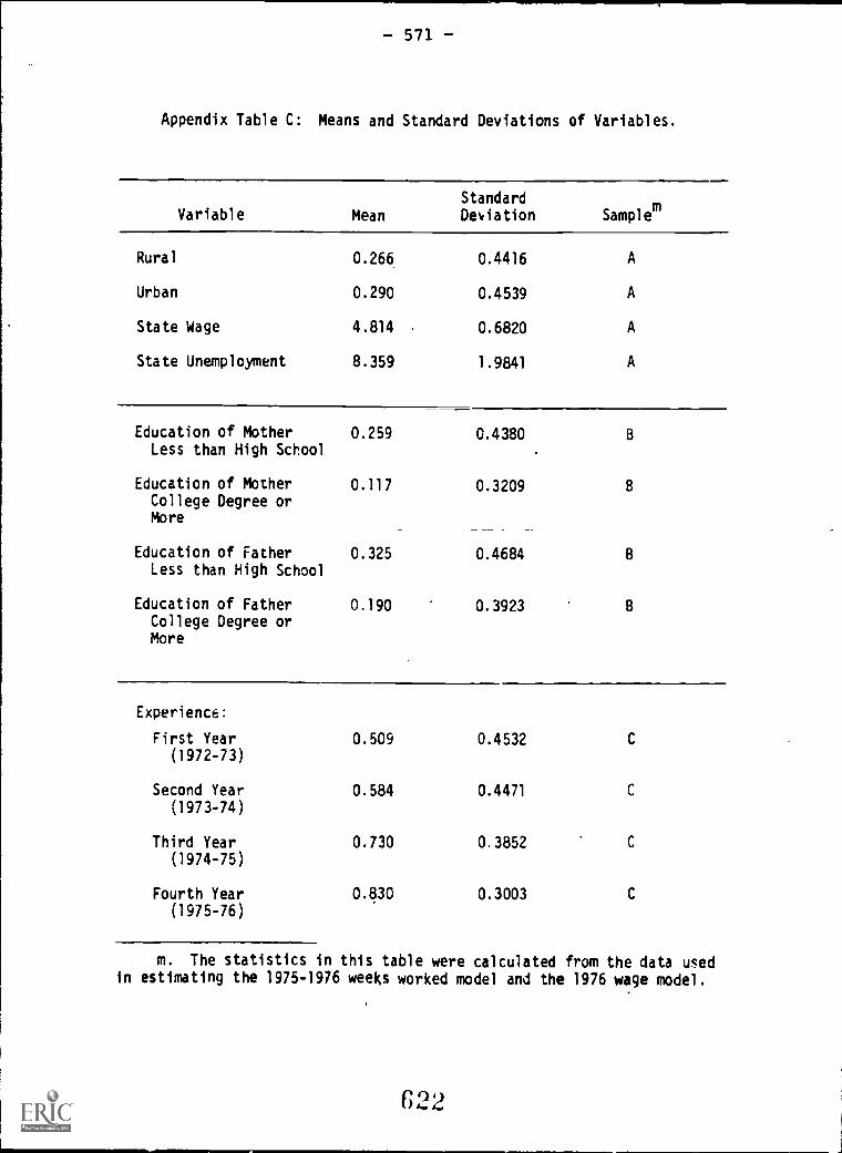
571

Appendix Table C: Means and Standard Deviations of Variables.

Variable MeanStandard

Deviation Samplem

Rural 0.266 0.4416 A

Urban 0.290 0.4539 A

State Wage 4.814 0.6820 A

State Unemployment 8.359 1.9841 A

Education of Mother 0.259 0.4380Less than High School

Education of Mother 0.117 0.3209College Degree orMore

Education of Father 0.325 0.4684Less than High School

Education of Father 0.190 0.3923College Degree orMore

Experience:

First Year 0.509 0.4532(1972-73)

Second Year 0.584 0.4471

(1973-74)

Third Year 0.730 0,3852(1974-75)

Fourth Year 0.830 0.3003(1975-76)

m. The statistics in this table were calculated from the data usedin estimating the 1975-1976 weeks worked model and the 1976 wage model.

C22

- 572 -

Appendix Table C: Means and Standard Deviations of Variables.(Completed)

m. (continued)

The particular sample used in ctIculating the mean and standard deviationof each variable is indicated by A, B, or C.

A. Persons working and used in estimation of the 1975-76 weeksworked equation, 2150 observations.

B. Persons used in estimation of the school attendance equationestimated in conjunction with the 1975-76 weeks worked equa-tion, 3100 observations.

C. Persons used in estimation of the 19Th wage equation,"2070observations.

.44

573

REFERENCES

David A. Wise

Adams, Arvil V. and Mangum, Garth L. 1978. The lingering crisis of

youth unemployment. Kalamazoo, Michigan: The W. E. Upjohn

Institute for Employment Research

Brown, Charles [this volume].

Bureau of.Labor Statistics. 1973. Employment of high school graduates

and dropouts October 1972: the high school class of 1972.

Special Labor Force Report 155. Washington, D.C.: Bureau of

Labor Statistics, Department of Labor.

Ellwood, David= [this volume].

Freeman, Richard B. 1975a. The overeducated American. New York

Academic Press, Inc.

1976b. Black elite, tsc new market for highly edu-

cated black Americans. The Carnegie Commission on Higher Education.

New York: McGraw-Hill Book Company

. 1978. Black economic progress after 1964: who has

gained and why. Cambridge, Massachusetts: National Bureau of

Economic Research. Working Paper No. 282.

Freeman, Richard B. and Medoff, James L. [this volume].

Griliches, Zvi. 1977. Schooling interruption, work while in school, and

the return from schooling. Cambridge, Massachusetts: Harvard

Institute of Economic Research, Discussion Paper Number 529.

Griliches, Zvi; Hall, Bronwyn; and Hausman, Jerry A. 1978. Missing

data and self-selection in large panels. Annales de L'Insee,

Number 30-31.

624

574

Griliches, Zvi and Mason, William M. 1972. Education, income, and

ability. Journal of Political Economy 80: 74-103.

Hausman, Jerry A. and Wise, David A. 1978. AFDC participation.: measured

variables or unobserved characteristics, permanent or transitory.

Working paper.

. 1979. Attrition bias in experi-

mental and panel data: the Gary income maintenance experiment.

Econometrica 47, Na. 2, March 1979, pp. 455-473.

Kohn, Mier; Manski, Charles; and Mundel, David. 1976. An empirical

investigation of factors influencing college-going behavior.

Annals of Economic and Social Measurement; alto Rand Corporation

Report, F-1470-NSF, 1974.

Levinsohn, Jay R. et al. 1978. National longitudinal study base year,

first, second, and third follow-up data file users manual,

Volumes I and II, April 1978. Washington, D.C.: National Center

for Education Statistics.

Manski, Charles F. and Wise, David A. 1978. Experiences of recent

high school graduates. Lexington, Massachusetts: D. C. Heath

and Co. pp. 1:9-162.

Radner, Roy and Miller, Leonard S. 1975. Demand and supply in U. S.

higher education. Berkeley: The Carnegie Commission on Higher

Education.

Wise, David A. 1975. Academic achievement and job performance. The

American Economic Review. June 1975. pp. 350-366.

. 1975. Personal attributes, job performance, am pro-

bability of promotion. Econometrica 43, No. 5-6, September-

November 1975, pp. 913-931.

David A. Wise

575

FOOTNOTES

1. For more detail, see Levinsohn et al. [1978].

2. The number is in 'fact .063.

3. In Appendix Table B, we have presented an example of estimates

for persons in school. For some parameter estimates, differences between

the two groups are substantial.

4. We can give a behavioral interpretation to this model by supposing

that in each year t each individual attaches some value Ut0 to going to

school and some value Utl

to staying out of'school. The values may depend,

for example, on the expected effect of each of the choices on future

earnings. Suppose that both Litt) and Ut1 depend on individual characteris-

ticszand random terms e so that U =zt b +e and Ut1 =tO tO tO ztbt1 etl.

Then assume that the no-school alternative is chosen if Utl

- UtO

zt(bi-bo) + (etl et0) is greater than zero. If we define St UM UtO,

t t,6t

= btl

- bt0, and nt eta - etO1

we can attach a random choice

model interpretation to the specifications defined in equations (3). (4)

and (5), with the individual profit specifications interpreted as yielding

reduced form parameter estimates. This is similar to the more elaborate

specification used by Willis and Rosen [1978].

5. See for example Hausman and Wise [1977]. The expected value of

Yi'

given that individual i is in the sample is given by:

,(Zid)

E(Y.is. = i) = X.0 + pa0[Ii6]

626

- 576 -

6. A maximum likeli ood method for doing this is laid out by

Hausman and Wise [1977].

7, We have not considered hours irked per week.

8. The expected value of week work is given by, E(y) --Pr(Y>52)

52 + Pr(Y<52)E(YIY<52).

9.- This could be done by estimating the four weeks worked equations

jointly with the four sample selection equations. Such a procedure would

also yield estimates of the correlations among the random terms in equations

(2) and (5). But it also presents substantial computational complexity.

10. Fven though we have used only a subsample of the whole data set,

to-get a given number with "good" weeks worked data, we have to have a

much larger total sample size if only persons never in school are con-

sidered to have observations on the yt.

11. By forming for example the appropriate inverse Mills ratio and

entering it as a variable in each of the weeks worked equations.

12. It may be technically inconsistent to use weeks worked while at

the same time using the logarithm of wages, since earning is usually

assumed to be lognormal. That is,

E = YHW, and lnE = lnY + lnH + lnW,

where E is annual earnings, H is hours per week, and W is the hourly wage

rate. But since our weeks worked results suggest a slightly better fit

using weeks rather than their logarithms, we have reported these results.

13. We predicted the conditional expectation of S1, S2, and 53,

given that a person was in the sample. We also predicted the ium of the

schooling variables, conditional upon being in the sample.

577

14. Griliches, Hall, and Hausman [1978], found that corrections for

the endogeneity of schooling increased the coefficient for schooling in

their wage equation, even after correcting for sample belectiow Our

attempts to instru,ent schooling suggested, however, that the schooling

..oefficient in our model may be biased upward.

15. We experimented with two approaches. One was to include in

the no-wage group all persons without a wage, whether they were students

or unemployed non-students. The status equations in this case are

simply sample selection equations; they cannot be interpreted as school

attendance equations. The other approach was to eliminate altogether

from consideration non-students who were also unemployed in the October

period being considered. The status equations may again be interpreted

as school attendance equations, but the wage equation estimates are

biaf',1 to the extent that they are affected by the elimination of

unemployed non-students. In practice, the two procedLres led to very

similar wage equation estimates. (In fact, even the estimates in the

status equations were affected very little by the selection procedure

used.) The results reperted below were based on the'second method.

16. This is consistent with the findings of Freeman [1978] in a

current NBER working paper.

17. The appropriate comparison may be the high school wage versus

the wage with additional schooling -- say a college degree. 3ut the

appropriate high school wage may be local, while the college wage may

reflect a national market.

18. For a detailed discussion of the determinants of college going

behavior, see Manski and Wise [1978], Radner ana Miller [1975], or Kohn,

578

Manski and Mundell [1974]. Work of Manski and Wise currently in progress

suggests that blacks, once admit.ed to schools, are less likely than

whites to choose four-year colleges, after controlling for SAT scores,

parents' income, and other variables.

19. The estimated effects of hours worked in high school are some-

what lower with than without them and the Pstimated effects of high school

training somewhat lower as well. The school attendance equations esti-

mated with the wage rate equations as shown in Table 8B include these two

variables. Their inclusion in the wage sample selection equation has

little effect on the wage equation parameters.

2G. More precisely, the estimates indicate a substantial relation-

ship if hours worked exceed 15.

21. For more details, see Figure 1 and the text discussion of it,

and Appendix A.

22. 4[(52-X0)/o] s[(52- 30)/20] [1.1] = .8643, if XB is 30

and a is 20. Sigma is close to 20 in each of the four years. For

more details see Appendix A.

23. The other variables included in the regression are: Number

of Siblings 0.01 (0.01), Sti. e Wage -1.62 (0.90), State Unemployment

-0.03 (0.38), Rural -1.8- ,1.03), Town -1.85 1,0.99), Urban -1.88 0.98),

South -0.19 (1.25), L...)t -1.32 (1.19), West -0.55 (1.38), Test Score

Missing -9.37 (2.76), Class Rank Missing 0.55 (.18), and Parents'

Income Missing 1.63 (1.05).

24. Griliches [1977], in an analysis of the Parnes National.

Longitudinal Survey, as well as National Longitudinal Study date, also

found that work in high school was virtually unrelated to family socio-

economic variables.

679

25. At least in the first two years the estimates are not precisely

measured. The state wage may be considered as an instrument for the

individual wage. Possibly it is too weakly related to individual wages

to pick up any labor supply effect that might be preser0.. A more highly

parameterized instrumental variable!: specification of the model might

yield a different result. One interi.retation of our results is that the

higher the "going" wage the less likely are employers to be willing to

fill jobs with youths.

26. Indeed the estimates imply a relationship that is slightly

U-shaped, with hours between 16 and 30 generally associated with

slightly lower wage rates than high school hours of either more than

30 or greater than zero but less than 16.

27. Of course, high school work could enhance of.e's ability to

learn from later work experience, and thus a decline in the effect

would not necessarily be expect''

28. If the same specification as shown in Table 8A is used, but

with two high school training variables -- one for persons with a high

school degree only, and a second for persons with post-secondary educa-

tion -- the results are similar; the relevant coefficients are not

significantly different from zero for either group.

29. We cannot rule out the possibility that family income captures

individual attributes contributing to joa performance and associated with

income, although we think this is unlikely having controlled for school

performance and other characteristics. Wise [1975a, 1975b] found that

family background was not related to earnings or performance in a given

corporate fob setting, after individual academic and non-academic

characteristics were controlled for.

F3!)

- 580

30. This Is consistent,with other estimates of this type. See, for

example, Griliches and Mason [1972] or Hausman and Wise [1972]. A

ctmparable monthly coefficient in Hausman and Wise, for example, is

_.0063, versus our estimate of .0060 in 1976.

31. In fact, the number of October time periods that the person

was in school.

32. We experimented with the instrumental variable approach des-

clbed in Section II -- using the expected value of school in a given

year, conditional on being in the labor force in that year. It did

indeed yield lower estimates, but because we were not satisfied with

the procedure in general, we have reported the uncorrected estimates.

In subsequent work, we will set up a more highly specified simultaneous

equations model that allows for the simultaneous determination of school

and work experience, together with a sample selection equation. Such

a system is cumbersome to apply over repeated years when the 0 para-

meters are estimated separately for each year. Because this was a pri-

mary concern of our analysis, we elected to work with a less complicated

specification in this investigation.

33. The increase in salary with experience is generally higher for

white collar workers than for blue collar workers.

34. See, for example, Freeman [1976a].

35. If there is an endogeneity bias with respect to experience, its

sign is not clear. Because schooling is positively related to the error

in the wage equation, and experience is cumulated only if a person is

not in school, the estimates would tend to be biased downward. On the

other hand the error in weeks worked is positively related to.school

attendai Experience may also be endogenous in that it may be deter-

581

mined in part by past wages and the wage disturbances are correlated

over time.

36. And again, there may be some compounding of results because of

the entry of recent college graduates, in the last time period.

37. Although this terminology is intuitively appealing when there

are discrete distipci. states that are not artificial divisions of a

continuous measure, it may be a misnomer here. Still we will stick

with it.

38. A straightforward way to estimate the population covariance is

to obtain joint maximum likelihood estimates of the parameters, incl'ud-

ing a covariance term, for each pair of years. This is expensive when

different e parameters are allowed for each year. An easier and less

expensive procedure is to use estimates for individual years (like ours)

to obtain consistent estimates of the B parameters for each year; and

then to use them in a second maximum likelihood stage to estimate co-

variances, assuming the means implied by the i's from the first stage.

On the basis of preliminary analysis, however we concluded that these

alternatives would not change the conclusions that we reach on the basis

of covariance estimates conditional on being in the labor force.

These same alternatives could be used to obtain population co-

variances among the weeks worked disturbances, with the added complication

of the upper limit on weeks. We will pursue this in subsequent work.

But as with the wage disturbances, we concluded that the substance of our

conclusions would not be changed by a more precise and detailed analysis.

39. For a more detailed analysis of state dependence following a

somewhat different procedure, see Ellwood [this volume]. Related

analysis is also contained in Brown [this volume].

6 ')ti

582

40. The correlation for any two periods is based on persons who were

in the sample in both periods. The residuals are calculated conditional

on being in the sample (not in school).

41. We also calculated a correlation matrix for the logarithm of

nominal wages/based on the sample of persons who had a recorded wage

rate in each period (447 out of 3280 who worked in at least one of the

five periods). The correlations are quite close to those shown here

although the correlations between adjacent years are a bit larger in

the later years -- .811 between 1975 and 1976 -- indicating somewhat

greater stability after four years than for the sample as a whole. The

correlation between 1972 and 1976 is .319, slightly smaller than the one

shown in the text.

42. Although our procedure is consistent, it is not efficient. A

correct procedure would use a minimum modified x2procedure analorous

to generalized least squares. Given our purpose and relatively large

sample size, we did not pursue this approach.

43. Recall that if all variation were due to individual specific

terms, correlations over time would be one; they would also be one if

state dependence were extreme so that persons could not "change states".

44. The correlation matrix of weeks worked disturbances is based on

an earlier set of statistical results that are substantially the same as

those reported in Table 7. A correlation matrix based on nominal weeks

worked for persons always in the sample--?28 out of 2933 who were not in

school in any of the years--reveals no systematic differences from those

shown here.

45. These conclusions remain unchanged if the matrices are based

only on persons who were not in school in any of the four years.

- 583 -

46. Relationships like those described in this section hold as

well for persons who were in the labor force in each of the periods,

who had no post-high school training.

47. See greater elaboration on this point in Ellwood [this volume].

- 584 -

Teenage Unemployment: Permanent,Scars on Temporary Blemishes

David Ellwood

Teenage unemployment poSes a puzzle for economists. Its causes and

consequences are not well understood because of conflicting economic

analyses. The human capital model suggests that since investment should

be quite heavy in the early years, teenage unemployment carries with it

heavy costs. But search theory suggests that shopping around is a

necessary and desirable Activity, particularly for those with little

information about opportunities in the labor market. There is also

concern that early labor force attachment may be weak, raising the

possibility that early unemployment may just represent consumption of

leisure. This paper focuses on the longer term consequences of early

spells out of work for male teenagers.

The fundamental problem in capturing the long-term effects of

unemployment is separating differences in employment and wages which are

causally related to early unemployment from the differences which are

due to unobserved personal characteristics correlated with early unem-

ployment. Whereas elsewhere in economics, researc%ers routinely assume

homogeneity of tastes and preferences, heterogeneity lies at the very

heart of the issue here. Separating the individual component is the

primary challenge faced in this paper.

This paper is divided into three sections. The first simply

describes the early labor market experience of the young men in this

sample. Strangely there is little published data which trace the

experience of a complete cohort over four years. In most other work

the high rates of attrition and re-entrance into the sample over the

period at least open the possibility of distorting the underlying pattern.

- 585 -

The second section extends the work of Heckman and Chamberlain to test

the long term effects of early employment on future employment. The

final section uses a Sims type causality model to measure the impact of

work experience on wages.

I conclude that the effects of a period without work do not end

with that spell. A teenager who spends time out of work in one year

will probably spend less time working in the next than he would have

had he worked the entire year. Furthermore the last work experience

will also be reflected in lower wages. At the same time, my data

provide no evidence that early unemployment sets off a vicious cycle

of recurrent unemployment. The reduced employment effects die off very

quickly. What appears to persist are effects of lost work experience

on wag.--t.

Scars -- In Theory and Practice

It is useful to begin by examining the implications of early

unemployment according to several more common labor theories. Perhaps

most prominent in its prediction of long-term effects is human capital

-theory. While the theory isn't concerned with early unemployment

inducing later unemployment, its emphasis on human investment early in

the job career to explain the concave pattern of aggregate age-earnings

profiles implicitly imposes heavy costs on the unfortunate young person

who misses out on early investment opportunities. If no investment

takes place during the period without employment, the entire profile

is shifted back. Even if retir07,-nt is also delayed, the present value

of the entire earnings streams mu:_ row be discounted over the lost time.

6 3 6

- 586 -

The dual labor market theorists paint ar equally bleak picture.

Poor work habits develop over the periods of discouragement, catalyzing

weak labor force attachment and alienation. The result is a vicious

cycle of unemployment followed by deterioration followed by more un-

employment. Pervading the institutional literature is the related

notion of tracking. Teenagers face only a limited rumher of entry-

level jobs which lead to better jobs. Those who miss good jobs early

are permanently tracked onto inferior ladders.

One troubling question is whether early unemployment is largely

a result of a job shortage or of weak labor force attachment. Most

theories which predict long-term impacts of unemployment emphasize the

involuntary nature of early unemployment. If much of it is "voluntary,"

it still may be reasonable to consider whether there are long -term

consequences. Teenage unemployment cannot be strictly voluntary since

it is so strongly counter-cyclical. But it is possible that some por-

tion of the problem is due to weak attachment. Young people may take

jobs only when they are readily available. Early experience may quicken

labor force attachment and reinforce desirable work skills. If it

is considered socially desirable to hasten the assimilation process,

then it would be desirable to make jobs readily available to the young.

A slightly more sophisticated argument emphasiz.. a the severe

informational problems of the young in the labor market. Teenagers

and employers are involved in an elaborate game of mixing .end matching

skills and jobs, but there is -relatively little information available

to either party. The employers rely rt-avily on evidence of past work

experience in making hiring decisio,,, li,ecdur,c they need to separate

- 587 -

persons with poor work skills and weak attachment from those with

superior work qualities. Employers avoid hiring workers who have been

out of school for some time but have little experience, so those workers

who were involuntarily unemployed are inappropriately typed as poor

workers. The problems may be exacerbated in recessionary times. If

employers are slow to adjust their expectations for experience from

young applicants, cohorts entering a weak labor market will suffer. Of

course, permanent damage need not occur at all. Early unemployment

may simply be productive job search or simple consumption of leisure.

There is a small but rapidly growing literature testing the long-

term effects of early spells of unemployment. (See for example Becker

and Hill, 1978; Stevenson, 1)79). These papers conclude that early unemploy-

ment has sizeable long-term effects. The methodology usually involves

regressions of wages or weeks worked of persons beyond their teens on

duration Au/or spells of teenage unemployment several years earlier.

Although most pay lip service to the difficulty of controlling for

individual differences, it is typical to include several background

variables as a control in the equations. This methodology is troubling.

If there is a true job shortage employers are likely to hire the highest

quality w.:,rkers first. It early unemployment is in part a reflection

of weak attacIlment, then some persons with unemployment are also low

quality workers. In either case, early unemployment is certain to be

highly correlated with aspects of worker quality. The findings of

these stuiiien document persistence very convincingly but serious clues-

rion: about ..01f1,er ras causal effects in 141'-er

economic 1_enavior.

- 588 -

It is the conclusion of this paper that while long-term effects

do exist, they may be a good deal smaller than the literature suggests.

The Data

Current published data tends to obfuscate early patterns of market

experience. Data from the Current Population Survey are currently

published by age group and school enrollrent status. Throughout this

paper, I will concentrate only on those persons out of school. I see

much fewer possibilities for long-term effects of unemployment during

school. The composition of the 16-19 year old out of school labor force

is very different from that of the 20-24 age group. The 16-19 year old

group includes early dropouts and high school graduates. The 20-24

year old group includes persons with little school but 8 years of exper-

ience along with recent college graduates. To look across different

age groupe and to draw conclusions about the patters of unemployment

as persons age is to invite error.

Ideally, one should like to follow a cohort of persons permanently

out of school over five or ten years. The National Longitudinal Survey

of Young Men -- the so-called "Parnes data" -- allows such an examination.

Some 5225 young meh between the ages of 14 and 24 were interviewed in

1966. They were than reinterviewed annually through 1971, then again

in 1973, and again in 1975. Typically, respondents were interviewed in

November about their current labor force status and most recent wage

as well as about their experience over the past year. The sample

chosen for analysis here was a group of roughly 750 young nen who left

- 589 -

school "permanently" in 1965, 1966 or 1967 with less than 14 years of

\

education. Unfortunate y, this period was the height of the Vietnam

war. Thus, slightly over alf the sample is not observed in the four

full years after they left School, primarily because of military service.

The 364 young men who remain do appear to be somewhat less prone to

unemployment and time out of the labor force. Persons who were

observed in the first full year out of school but were not observed in

some later year had a labor force participation rate of-$4.1 percent,

an unemployment rate of 7.1 percent and an employment rate of 78.2 percent.

Persons who remained in the sample had rates of 86.1 percent, 5.0 percent,

and 81.8 percent respectively. This sample selection is an obvious

source of potential bias and will be addressed in more detail later.

Another well known "problem" with the Parnes data is that they

show very different rates of employment and unemployment than do pub-

lished statistics derived for the CPS. The longitudinal data used here

show much higher employment rates and lower unemployment rates than

the` CPS data. For a discussion of the likely reasons for these differ-

ences see Freeman and Medoff (1979b). The sample selection and, CPS

comparison suggests that the NLS sample may miss some of the longer-

term unemployed persons, for whom unemployment could have the most

serious consequences. Thus, the current sample could serve to undar-

represent the long-term consequences of early labor mr-ket experience.

Few of the young men in the survey data leave school in November.

In the year of leaving school, retrospective labor force figures cover

both time in and out of school. After nur.crous attempts to adjust for

/

590 -

the problem, I finally decided to simply omit the first part-year of

experience. In later sections when I refer to the first year of exper-

ience, I refer to the first full survey year after graduation or drop-

out.

I. THE EARLY LABOR MARKET EXPERIENCE

The labor market position of young men improves dramatically during

the first,four years out of- school. Table 1 shows that while an average

of nearly 20 percent, are without work in the first year, only 10 percent

are not working 3 years later. Labor force participation rates rise

precipitously, from 86 percent to 95 percent. The markeu improvement

is countercyclical in this case since for roughly two-thirds of the sample

(those leaving school in 1966 and 1967) the fourth full year out of

school comes during 1970 or 1971 -- recessionary years. Indeed, if the

overall economic picture had remained stable over this period, even more

rapid improvement would likely have occured. Almost immediately, however,

the unemployment rate shows up as a poor indicator of labor market

performance for this group. While the other statistics, most notably,

the employment ratio, show clear improvement over time, the unemployment

1

rate follows no clear pattern. This latter statistic badly misrepresents

the trend in labor force position. In these retrospective figures,

unemployment appears to mean something different to persons one year

out of school than to persons four years out. As the young men age,

they may become increasingly reluctant to report themselves as out of the

labor force even if they are not El-pending time in productive job search.

591

Table 1

oyment Rate, Employment Ratio and Labor Force Participation

Rate For Young Men During First Four Years After

Leaving chool in 1965, 1966, or 1967 With Less Than 13 Years of Schooling

UnemploymentRate*

EmploymentRate**

Labor ForceParticipation Rate***

Year 1 5.0 81.8 86.1

Year 2 6.4 84.7 90.5

Year 3 4.8 89.3 93.8

Year 4 5.4 90.0 95.0

* average weeks unemployed/average weeks in labor force

** average weeks employed/52

*** average ,:eek in labor force/52

- 592 -

Ant" alternative is that in later years only a hard core cannot find

jr !_,:se persons become discouraged and drop out of the labor force.

ithar way the distinction between unemployment and time out of the

labor forcr is blurred.

The steady improvement of the cohort masks remarkably dynamic labor

force patterns. The initial years of employment experience are pocketed

with spells of unemployment and time out of the labor force. Only 18

percent of all young men in this sample have four year employment his-

tories unmarred by a spell out of work. Table 2 shows that nearly 40

percent of all young men spend time out of the labor force in their

first year, while just over one quarter report unemployment. Overall,

57 percent of these young men spent some time out of work. The prob-

abilities of adverse experiences decline substantially over the period.

Yet even in the fourth year out of school when the overall employment

ratio is 90 percent, almost 40 percent spend some time not employed.

And while the labor force participation rate is hovering at 95 percent

in that fourth year, one quarter spend some time neither working nor

looking for work. These results reinforce those of Clark and Summers

(1978) who have shown that CPS data suggest extremely dynamic labor

market behavior.

Perhaps the most dramatic result in these first few tables is the

prominence of time out of the labor force. Nearly 40 percent of the

sample self report time spent neither working nor looking in the first

years. These 40 percent report average spells of 18 weeks -- more than

fou months -- during a period of very 10 unemployent. Perhaps these

are discouraged workers. e.t three quarters of them spent no time

C1.7

-593-

Table 2

Probability of Unemployment, Time Out of the Labor Force

and Time Not Employed During First Four Years After Leaving School

Probability ofUnemployment

Probabill*- of TimeOut of Labor Force

Probability of TimeNot Employed

Year 1 26.9% 40.1% 56.6%

Year 2 27.5 31.9 51.1

Year 3 23.0 23.6 40.9

Year 4 21.9 24.1 38.2

- 594 -

unemployed at all during that first full year! Of course, some may have

had severe unemployment problems in the part year preceding the first

survey year. Still, four months is a remarkably long time to be dis-

couraged, particularly when one's peers are reporting a 5 percent

unemployment rate. The sample selection rues, which appear to discrim-

inate against the non-employed, make the results seem even more dramatic.

The rapid rise in labor force participation rates and employment rates

during the downward swing of the business cycle must almost certainly

indicate increasing labor force attachment.

One important concern is whether to regard unemployment as a

separate experience from time out of the labor force. The evidence

cited thus far suggests little distinguishes the two. Retrospective

unemployment figures do not appear to capture the essence of the

employment situation. While the distinction between those actively

seeking work and those who are not seems particularly important in

this group, the line is poorly drawn using retrospective employment

figures. Of course, few labor force statistics are derived from retro-

spective data. Still, the standard CPS question about whether the teen-

ager has done anything to look for work in the past four weeks (a speci-

fic method must be listed) may not separate them too much more efficiently.

Unfortunately, if it is difficult to separate the truly unemployed

from those with weak labor force attachment in surveys, it may be

equally difficult for employers. Thus, those persons who are seriously

searcl .; for work but have been unable to find it may suffer from

gu)lt association.

This brief section has pz.int. a pa;_tern of change and

595

diversity. Early in their career young men spend a great deal of time

without work. By their forth year, however, most workers are settling

into a more staple and presumably permanent work situation. The next

section shows that while the early years are periods of rapid improve-

ment for the young men overall, adverse experiences persist.

The Persistent Pattern of Adverse Labor Market Experiences

Early labor market experiences foretell future ones. Persons who

escape unemployment early will likely escape it later. Figures 1, 2,

and 3 are probability trees for unemployment, time out of the labor

force, and time not employed for the four periods. Each branch corres-

ponds to one period. A 1 indicates that unemployment or non-employment

was experienced in the period, a 0 indicates that it was not. Above the

line in any branch is the probability of being in that state conditional

on being at the previous branch. Below the line in parenthesis is the

unconditional probability of being on that branch (or the proportion of

all persons who are found on that branch). The bottom number is the

average weeks of unemployment in that period by persons on that branch.

Thus in Figure 1, 53.1 percent of persons who had been unemployed in

their first year were unemployed in 'neir second year. 14.3 percent

of all persons had unemployment both periods and these persons averaged

14.2 weeks of unemployment in the second year.

All three figures demonstrate striking persistence in the labor

force experiences. The probability of unemployment (non-employment)

in tho :;coond perio:1 conditic,n,D1 on fir7L ;..crlod spells is .531 (.631),

while those who escaped early prob11-:-.3 ha:, only a .180 (.354) probability

596

Figure 1: Probahiliry Tree of

Weeks Unemployed in First Four Full Years Out of School

N = 364

.511(.10114.2 WS

.315(.0515.7 WKS

J61

4

(.034)14.0 (KS

4

(.01410.0 WKS

(.030111.0 WKS

.047

.060)0.0 WKS

.447

.0 WKS

.S10

(.00.0 WKS

.171

(.011177.4 WKS

.87,4

.06011.0 WKS

7.1 WKS.500

(.010)0.0 WKS

.400

(.0111.6 (KS

CONKS

412._4.347113.0 WKs

6,1

Figure 2: Probability Tree of - 597 -

Weeks Out of the Labor Force in First Four Full Years Out of School

.414.0 MKS

N..364

414.148120.3 WKS

771.043122.1 WKS

1.10410.011M

.235

0

.522

33

14.8 MKS

.47$

.030)

6.0 WKS

.310

13.4 1413

.582

0.0 *3

4.8 WS

.2731.041111.7 WS

10.3 *1

.484

.0 1

0.0 MKS

.250. 422.1 WKS

.750

0.8 MKS

.215

4. MKS

(.1401$.0 WKS

.252/.131)10.4 MKS

,841

1.390.0 10.3--,..

11.0 WS

.0$.014113.2 MKS

.440

.025)

$.130113

1.022)9.4 *3

.8001.000)

0.0 WKS

.3571.01714.7 WKS

(3 4 5'5

644

1.31314.0 *3

Figure 3: Probability Tree of 598

Weeks Not Employed in First Four Full Years Out of School

N - 364

.411

.611

.225116.6 MKS

ali9L---1.137117.3 w(S

10.7 WKS

16.7 WKS

.169

.305

.041)0.0 WS

.331344T-11.0 WK3

1.0 WKS.667

.0.0 WKS

.333

717iirr7.0 WS

316

(.044.) 0.1 60(3

.361(.226)0.0 WS

.667441CO WKS

.217

GAWKS

(.13410.3 41(3

.834

.56/

0.0 WS

.303(.027r

0.4 WS

4-.011) -.., 0

. 61)

1.0 WS

0.0 W(S

1.0 WS

8043T.,

3.0 W(3'\.743

00 I.YS

7

.4001.021)

S.1 WKS

60041/0.0~x3

.207f.o%Tr

I.'. WKS

599

of unemployment (non-employment). By the fourth period, boys with

three straight years with unemployment are 7 times more likely to

become unemployed than those with three straight years without it.

This sort of probability tree is common in the literature (see

Heckman and Willis, 1977; Heckman, 1978a and 1978b); however, the patterns

can be misleading. If spells are long, say 10 weeks, and if spells

are distributed randomly throughout the year, then 20 percent of all

the unemployed in one year will have spells which overlap into the

next one. This would cause a much higher probability of unemployment

in the second year conditional on having experienced it in the first,

regardless of the underlying pattern. In this sort of table, there is

no straightforward way of making an adjustment for this problem

Happily, overlap problems do not affect probabilities of third

or fourth period events conditional on the first period event. Table 3

reveals that persons with poor first period records are likely to have

poor records three or four years later. Persons who spent time out of

work in the first period have a .447 probability of similar problems

in the final year as contrasted to a .297 probability for those persons

with uninterrupted work histories in the first year.

A somewhat more appealing measure of persistence is a simple

correlation matrix. Table 4 provides the correlations for weeks of

unemployment over the first four years anc: for the weeks not employed.

Once again the persistence is prominent, but not quite so prDminent as

might be expected. Weeks not ernloyed shows a one year correlation of

about .S, but it dc3y- :-_:]1... the alu_ fa12- to

around .25. E2markably, %.:-.-k, u:. -,r icss 1,erence and

- 600 -

Table 3

Probabliity of Adverse Market Experiences

in Later Years Conditional on Early Experience

Unemployment Time OLF Time Not Employed

P(1 in year 2/1 in year 1) .531 .418 .631

P(1 in year 2/0 in year 1) .180 .252 .354

P(1 in year 3/1 in year 1) .327 .294 .514

Pil in year 3/

0 in year 0) .194 .197 .272

P(1 in year 4/1 in year 1) .345 .294 .447

P(1 in year 4/0 in year 1) .172 .205 .297

65 1

- 601 -

Table 4

Correlation Matrix for Weeks Unemployed and Weeks

Not Employed During the First Four Years Out of School

Weeks Unemployed Year 1

Weeks Unemployed

Year 2 Year 3 Year 4

Year 1

Year 2

Year 3

Year 4

Weeks Not Employed

1.00 .27 .20 .08

1.00 .27 .26

1.00 .39

1.00

Year 1

Weeks Not Employed

Year 2 Year 3 Year 4

Year 1

Year 2

Year 3

Year 4

1.00 .54 .34 .25

1.00 .46 .34

1.00 .47

1.00

II #)l) ,)

- 602 -

the pattern of decay is erratic. Adjacent year correlations

(a12

a23

, 034

) show some stability, but hover at only about .3, a

figure roughly comparable to the correlation between weeks not employed

one or two years removed. The correlation between unemployment in the

first and third year (013), shows evidence of slight decay, but 024

shows no such evidence. Then, dramatically, 014 falls to .08. The

unorthodox behavior of the unemployment figures reinforces once again

the earlier concerns about the quality of unemployment measures (at

least this retrospective measure) for this age group.

Both the unemployment and non-employment correlations are more

stable than would be generated by a first order Markov process. The

stability suggests that individual differences are an important part

of the underlying process or that the process is of higher order. Unem-

ployment and non-employment are not events randomly distributed over

this population of young men. If early unemployment or non-employment

is nothing more than, search and matching of workers and jobs, then for

some at least, the process is quite protracted. Since adverse employment

patterns are a problem of a sub-class of youngsters, programs to aid

them ought to be targeted to those with early problems

The critical question of this paper still remains: is the persis-

tence a reflection only of individual differences or is future employ-

ment causally related to past experience?

603

II. THE IMPACT OF EARLY UNEMPLOYMENT ON FUTURE UNEMPLOYMENT --

HETEROGENEITY AND STATE DEPENDENCE

Persistence of labor market.- behavior has been noted in numerous

other settings, most notably in the labor force participation Of

married women. A newly developing literature seeks to separate the

effects of individual differences in behavior -- heterogeneity --

from changes in behavior induced by a previous event -- state dependence.

The unique character of longitudinal data allows one to control for

unobserved individual characteristics in a way that no strictly,

cross-sectional data set does. Although there are serious concep-

tual problems with this formulation, the following model in contin-

uous time will help illustrate the methodology currently employed

in the literature. The problems will be considered later.

Yi = X. B Yt it-1Y + Si + U.

t t t it

Here!it

the time person i was in a particular state during periodis

t(i.e.weeksworked),Xitit

isavectorofevogenousvariables,6is

an individual constant, Uit is a random component. This is simply

a model of a first-order Markov process with an individual component

In this example, Sit is the control for heterogeneity, yt is the test

of state d,2endence. Such an equation cannot be e.--imated from cross:A

sectional data because there will be more parameters than observations

since each individual is accorded his own intercept. Cross-sectional

cstir2tesnalewithouttheirclusicnoit

will create upward bias

inthestatedeperidEncocoeffic,,E.ntunlesstAlatpartofLit which

654

- 604 -

correlated with Yit-1

is fully captured by a linear combinaticn of

the X's.

By imposing restrictions on dit, one can estimate yt from longi-

tudinal data. The individual component can be controlled using data

from previous years. The simplest assumption ist,tfa fix the individual

component over time, 6 = 6 . To simplify the example further,

assume $t = 8, yt = y and that Cov (Uit, Uit_i) = 0. Simple differ-

encing eliminates the nuisance parameter 6i

. Thus:

Yit

- Yit-1 --(= (Xi - Xit-1 )8 + Y( Yit-1 - 'it-2

) + Uit - U.t it-1

Of course all exogenous variables which are invariant over time are

also eliminated with this approach. Since the focus here is with the

state dependence parameter, y, this is a source of no concern. The

term (Yit-1 Yit-2)

is now negatively correlated with the error term,

so OLS results will be negatively biased. However, and Xit_i

can be used to instrument this term and consistent results will be

generated. Note that absolutely no distributional restrictions are

imposed on the 6. across individuals since they are simply'differenced

away.

Heckman (1978a, 1978b) has

developed an appealing and more general counterpart to this model for

the discrete case. Heckman's model transforms the dichotomous variable

into a continuous one by assuming the event occurs whenever a

uousljtentvariable(Y*.)crosscs -- here assumed to beit

- 605 -

zero. A dummy variable dit

is assumed to be one when Y*it

> 0 and zero

otherwise. Exogenous variables Xit

are allowed. Using a variance

components error structure in Heckman's model, we can allow each indi-

vidual to have his owt, individual component, dit, freely varying over

time for the moment. One case of Heckman's somewhat more general model

is then:

Setting1t-j t-j it i 1 it

are

iid normal provides for an estimable model. Heckman offers a heuristic

proof of identifiability which relies on the ordering of unconditional

probabilities. Suppose t = 2 and the Xs are constant over time. Then

concitionalonX.1 and (S.1 , in the absence of state dependence, the probability

of the sequence (1,0) (one in first period, zero in the second) is equal

tothe probability of the sequence (0,1). In the presence of state

dependence however P(.,0) e P(0,1). State dependence increases the

likelihood that persons who experience the event in the first ,period

will experience it again 11 the second. Therefore P(1,11 is increased

and P(1,0) is reduced. P(0,1) on the other hand is unaffected since

the event was not experienced in the first period. This relation holds

for each individue; it must hold in aggregate. Thus simple run

sequences alone allow testing for the 1.resence of state dependence

under particular functional form assumptions. Obviously run sequences

coverin-3 more time period: allow testing of less restrictive functional

forms.

656

- 606 -

Heckman suggests this approach can be usefully applied to a

variety of situations, including spells of unemployment. Several

features of the Heckman model make its usefulness it this and related

situations questionable. For purposes of this discussion, let us

divide early job history into only two states -- employed and not

employed. The fundamental problem is that the model breaks a con-

tinuous time event into artificial periods. When the chosen interval

is long relative to average length of stay in a state, there is

inevitably an assymetry in the definition of states. Often periods

are chosen to be one year long. A person is observationally reported

to have been in a particular state for that period if and only if he

or she experienced the state at any time during the period. In the

current example persons who experience time out of work any time

over a year recei e l's, persons who do not receive 0's. Thus to be

in a :ate, one need experience only one week of non-employment, but

to be out of the state one need experience 52 weeks of employment.

If we simply re-define state 1 as having experienced any employment

a very different pattern of states emerges. Virtually everyone is

always in state 1. The presence or absence of state dependence may

depend on which state is accorded the special privilege of being

designated as the 1.

On the other hand, if the periods are short relative to the

spells, then state dependence exists almost by assumption. If spells

tend to be longer than periods then the probability of being in the

state conditional on having !:,,con in 14 in the previous period is

high. Indeed, even if spells tend to be four or five times shorter

7

- 607 -

than the periods, one can predict with certainty that at least 20-25%

of persons who experience the event one period will experience it

again in the next period simply because spells overlap.

The arbitrary designation of time periods and states means an

observed data point (1,1) may represent a host of very different

histories. One person may have been in the state continuously for

two periods. Another may have been in it only a few day's but those

days happened to overlap two periods. Still a third person might

have had several spells in the state in each period. These problems

represent more than just lost efficiency. They imply peculiar results.

The problem of overlapping spells is particularly troubling in the

current treatment. If spells last an average of 13 weeks, then one-

fourth of all spells in one yei,e will overlap into another. This

implies that even if the spell has no long term effect, P(1,1) is

increased. Since the P(111) > P(110) there appears to be state de-

pendence where there is none. Although these problems are particu-

lerly acute in the Heckman formulation using yeats as periods, they

are also present to some degree in the continuous model presented

earlier, as we shall see below.

Obviously, the notion of state dependence is a confusing one.

In the next few paragraphs I present a non-technical discussion in

an attempt to clarify some of the concepts. For a more technical

treatment see Ellwood and Summers (in preparation) and Chamberlain

( 1978) and (1979).

A cumplete analysis of heLorc:,_neity and state dependence would

treat each event in continuous time with a particular starting and

658

- 608 -

ending date. We must separate two distinct types of state dependence.

Once a person has entered a particular state -- say employment --

there is a tendency to remain there for some period of time. The

probability of remaining in some state is always higher than the prob-

ability of entering it from another if the time interval is short

enough. Virtually all persons who work one minute will work the next,

regardless of their underlying propensity to work over a month, year,

or decade. Tr iitionally this inertia has been captured with a Markov

model. Conditional on being in a state, a person has a certain escape

probability over a given period of time which may be suite independent

of his past history of spells or states.

For example, a young black male teenager who is unemployed this

week could be far more likely to be unemployed next week than if he

had been employed this week, simply because it is hard for young blacks

to find jobs. It could be that nothing about his work history or his

length of turrer% unemployment duration influences his ability to get

a job; yet being unemployed now indicates that he is less likely to be

employed next week. Unemployment doesn't change the individual per se,

it is just a difficult state for the teenager to escape. Heterogeneity

must imply that each individual has his or her own escape probability

from each state. Let us label this form of state dependence simple

Markov type persistence. The key notion is that it is what state one

is in that caants, not his past history. This persistence is unques-

tionably present in all human endeavors to some degree.

If the force of escape from one or another state is influenced

65!)

- 609 -

by previous experience, then the second form of state dependence --

experience dependence -- is present. Exit probabilities may rise

or fall with time in the current spell. Work history may influence

the likelihood of, employment when a teenager is unemployed. Experience

dependence corresponds most closely to the conception of state depen-

dence described in the literature. A person is actually "changed" by

a particular event. Models which postulate that the accumulation

or depreciation of human capital or of information or even of signals

of worker quality alters the likelihood of work all imply an altered

force of escape from one state or anther because of the individual's

past experience. Ideally it is this form of state dependence that we

seek to capture.

Simple Markov type persistence certainly is not uninteresting.

The distribution of forces of escape will strongly influence the con-

centration of unemployment across individuals. Macro-economic poli-

cies can alter escape rates and may provide great benefit to those

with otherwise very low rates of escape from unemployment. But if

experience dependence is not present, once a spell is over so is its

impact,

Unfortunately the current models capture both Markov type

persistence and experience d- pendence simultaneously. Markov per-

sistence requires two heterogeneity parameters: the force of escape

from each state. In the Heckman fcrTulation this implies an indivi-

dual intercept diand an individual coefficient on the person's state

last period. This can be modeled :c7itt1ng the Xs):

660

- 610 -

kY* = 6 + *.d

i+ E y di + Uit i 1 t-1 t-j t-j itj2

If the time periods are quite short, then 6i effectively captures the

Markov type probability of entering the 1 state; Ti, the probability

of remaining in it. With short periods dit_i captures the persons

most recent state -- the "current state" while the next state is

being determined Markov persistence virtually guarantees that Ti

will be positive as the period shrinks. Experience dependence requires

previous job history -- not just the current state alter the probability

of entering or remaining in a state. Thus coefficients on dit_2, dit_3...

are non -zero. The Yt-j here capture this experience dependence. *

Estimation of this model is complicated by the fact that the

L1 amiligiarehighlYcorrelatedwithdit_lit-

andthedsince highj

values of the individual compone.lts increase the likelihood that any

d..ij = 1. Estimating the equation assuming 4 = '' may substantially

upwardbiastheyt_icoefficientsbecausetheomittedtermW-Tdit_i

is positively correlated the dit-j

. Previous work using this model

have over-estimated experience dependence for two reasons. First,

_ the coefficient on the once lagged dit inevitably reflects not only

experience dependence but also Markov persistence. Second, because

the coefficient on dit-1

is constrained to equality across individuals,

.Actually 4; captures both the experience depandence from period t-1plus the Markov type probability of remaining in :. *ate 1. This is ofno serious concern if the periods are short. If periods are long,anyrretric definition of periods i-nlies a serious loss of efficiency.

661

- 611 -

the yt_i also capture some Markov type persistence. Heterogeneity has

simply not been properly controlled for.

The continuous model described at the beginning of this section

Oso inadvertently captures some Markov type persistence in the state

dependence parameter. Suppose weeks worked is the dependent variable.

Then it is tempting to regard c i as the expected weeks worked in year

t given a-. individual's two escape probabilities. However, even in

the presence of Markov persistence alone, the individual's expected

weeks worked will be greater if he begins the period working than if

he enters without work. Last year's weeks worked helps predict the

person's state at the end of that year and therefore at the start of

the current year. Anyone who worked 52 weeks in year t-1 was working

at the start of year t. He will certainly be expected to have more

weeks worked in year t than an identical individual who begins year t

outofwork.Evencorditionalon6weeks worked in one year is

correlated' with weeks worked in the next because they help predict

the person's state at the start of the ne;:t. period. The correct

model is thus:

Y. = 6. + 'IP.1bit + yy. + U.

it 1 it-1 it

Where bit

is now a dummy variable capturilg the person's state at the

beginning of year t. In this model and re reflective of the two

Markov escape probabilities and y is a measure of true experience

dependence. Even if we know 3 with certainty, we could not estimate

thisequation-becausevaries each 1n::i7idual and is highly

correlated with bit and 1%41_1.

662

- 612 -

When we difference, however, the advantages of this continuous

formulation become clearer:

Yit Yit-1 41(kit bit-1) Y(Yit-1 Yit-2) Uit Uit-1

There is only a bias problem for persons who change their beginning

state from one period to the next. Otherwise (bit - bit-1) = 0 and

*i vanishes. One cannot estimate the equation for these persons only

because ht

Uit_iis correlated with and conditioning on it will

introduce bias.* But in the present sample, nearly 90% of all persons

are observed in'the same state at the start of any two consecutive

years, so the bias on y may be quite small.

Including ditdit-1

(instrumenting it with dit-1) will reduce

the bias, but will not fully eliminate it. Actually y does not fully

capture experience dependence because di and *i are average yearly

probabilities which will'in part reflect some experience dependence

if the underlying forces of escape are high. It seems quite reasonable

then to regard y as a rough measure of experience dependence. Any

better measures require complete work histories and present serious

methodological problems. (See Ellwood and Summers.)

In this continuous model, identification was achieved with the

imposition of three important restrictions: dit 6i, Oit = *i and

Cov(Uit, Uit_1)-

O. if any of these restrictions are false, spurious

Actually it can be proven that if we assume complete stationarity(exclude all Xs), we can legitimately test the null hypothesis of nostate dependence by conditioning on dit

-1= dit = d

it+1.

6 C,3

- 613 -

state dependence can be generated. Probably tht most serious concern

for this group is non-stationarity of the individual components di and

*i. If weeks worked is the endogenous variable, di and *i might be

seen as that part of maturity, ability, or labor force attachment not

captured by the Xs. Since these may grow or decay over time, it seems

desirable to free up the individual components. Although we cannot

let the components decay or grow at different rates, a model allowing

dit Atdi andit

At*i can be estimated using four years of data.

We solve for di

in the third year equations and substitute it into

the fourth.

So

Y = A d + A *.b. +y3

+ X. 0 + UY.3 i 3 1 13 3 12 13 3 i3

1

6ib

3i3+'Al (Y

i3- y

3Yi2

- X.13

03

- U.13

)

Substituting into the equation for Yi4

Y A *. (bi4

b )

(Y42:4) y

i14

i4 4 1 i4 i3 4 A -T YY3 3 A3 3 i2

X4X. 8 -

Xi 3B3U U.

14 4 A3 13 3 i4 A3 13

The effects of the first term have been discussed earlier. The only

other problem is that Y13 is correlated with the error term; Yil is

not however, and serves as a natural instrument for Y13

. If we constrain

y4

= y3we can obtain estimates of , and although we cannot tell which

A3

is which;

664

614

The restriction Covillit, Uit_1) = 0 helps to highlight an important

distinction between state dependence and serial correlation. In the

absence of strong X's which change over time, there is no meaningful

distinction between serial correlation and state dependence. However,

in the presence of X's_ the distinction is important. State dependence

implies that a change in X will cause a change in Y not only in the

present period but in future periods as well, because the initial

increase om Y induces future increases in Y. If serial correlation is

present, a change in X will have its full force immediately, with no

damped response into the future. In the case of unemployment, one

might ask whether a weak labor market now induces more unemployment

in the future. even when the labor market regains its strength. If

the answer is yes, then state dependence is present. Otherwise,

state dependence probably is not present. Unfortunately, it is likely

to be virtually impossible to capture both serial correlation ana a

non - stationarity of individual specific constant. The only reasonable

approach I can see is to assume that both serial correlation and non-

stationarity are captured using a time specific coefficient en the

individual effect. These models then were used to estimate the long

run effects of unemployment.

- 615 -

Empirical Results

Before performing the more complicated tests for state dependence

described above, we might try to fin&"natural experiments" which would

reveal it much more simply. Local unemployment rates vary dramatically

over time and across locales. One natural experiment would be to

test whether persons who enter a weak labor market which later turns

strong, fare less well than those who enter a strong market which remains

strong. A unique feature of the "Parnes data" is the availability of

an area unemployment rate for most persons in each year. The rate for

small local areas about the size of an SMSA was derived from a 12 month

average of monthly local unemployment rates from the Current Population

Survey. Presumably the area unemployment is only slightly correlated

with individual effects, so with a few controls for individual charac-

teristics, we might simply test the importance of lagged unemployment

rate in equations with both current and lagged unemployment rates. If

entering a weak labor market left long term scars, then the lagged

rate should be negative and significant. Unfortunately the area rate

behaved very poorly. Even in equations without the lagged rate, the

coefficient on the current rate, though usually of the correct sign, was

rarely significant and was highly unstable. When the lagged rate was

included, the results were invariably insignificant and occasionally

even the sign on the current rate was perverse.

Even though the area rates performed poorly on this data, this

experiment definitely ought to be performed on other samples if pos-

sible. Ultimately a conclusion reing on such a sample methodology

would be the most compelling test for the long-run effects of short-ran

macro polio,.

6

- 616 -

The techniques described in the previous section were.applied to

weeks worked and to weeks unemployed. Weeks worked was chosen over

weeks not worked only because it seems conceptually easier to deal with.

Obviously since weeks not worked is simply 52 less weeks worked the

results would be identical except for the constant term and a sign

change on the coefficients of the exogenous variables if the alterna-

tive variable was used. There were 298 observations in the final

sample.

There is a purely statistical problem associated with the use of

the various controls for heterogeneity in equations predicting weeks

worked or weeks unemployed. Both are limited dependent variables;

they cannot exceed 52 nor fall below zero. The importance of the problem

is most evident in the case of weeks worked. As weeks worked approach

52 the estimate of state dependence will approach zero if controls are

made for heterogeneity. Statistically the limited variable will induce

an artificially negative correlation between once lagged weeks and the

error term. The result follows from the fact that if lagged weeks are

large the positive end of the distribution of the error term is likely

to be truncated. Intuitively once weeks worked approaches 52, regard-

less of the true, strength of state dependence, the next years' weeks

cannot be pushed above 52. This problem is of greater concdrn in later

years when more and more of the young men approach 52 weeks employment.

There are well known methodologies to correct truncated dependent var-

iables. These typically do not apply to situations where a lagged

dependent variable is correlatei with the error term for reasons ot!.cr

than truncation. Hetercgsneity further complicates the problem. No

66'

617

attempt was made to develop the appropriate truncation corrections for

theeequations. It should be remembered that persons who remain at

52 weeks in all three years do not bias the results, they simply provide

no information because yit 0.v

The wage rate normally appears in labor supply equa,tions. At the

same time human capital theory suggests that work experience will be

associated with higher wages as individuals invest in on the job

training. To prevent the wage variable from capturing any effects of

increased investment, the variable LWit

reflects the wage at the beginning

of period t while WWt equals weeks worked during year t. To eliminate

potential bias, the various equations (because weeks worked in year t-1

and therefore Ut-1

alters the wage in year t) the wage variables were

always instrumented with LWit-1 LWit-2

and. in equations controlling for

heterogeneity. All strictly exogenous variables are measured at the

beginning of each period.

Table 7 presents the results of regressions of weeks worked and

weeks unemployed on th, once lagged counterparts. The only correction

for heterogeneity is the inclusion of a few personal characteristics

like age, race, and level of schooling. As anticipated, lagged values

of weeks worked and weeks unemployed have sizeable coefficients and

small standard errors. As in previous examples in this paper the

results for weeks worked are far more stable than those,for weeks

unemployed.

When all years are estimated as a system and the coefficient on

lagva weeks unemployed is constrain to equality over all three years,

the coefficient is .27; the coefficient on weeks worked, .39. The results

again suggest substantial perisitence of earlyvxcerience. Still, even

AGEt

- 618 -

Table 5

Definitions of Variables Used in Regressions

- Age at start of year t.

AREA - Area unemployment rate at start of year t

BLACK - Race dummy (1 = non-white)

LWt

- Employment dummy (1 - employed) at start of year t

- Log of wage at start of year t

MARL - Marriage dummy (1 = married) at start of year t

SCHOOL - Years of school completed

SMSAt

- SMSA dummy (1 = resides in SMSA) at start of year t

SOUTHt - South dummy (1 = resides in South) at start of year t

UNt

- Unemployment dummy (1 = unemployed) at start of year t

WWt

WUNt

- Weeks worked in year t

- Weeks unemployed in year t

Dxxxx - Change in variable xxxx

- 619 -

Table 6

Means & Standard Deviations for Variables Used in Regressions

MEAN S.D.

AGE 2 18.8 1.98

AREA 2 4.33 1.72

AREA 3 4.22 1.85

AREA 4 4.59 1.93

BLACK .383 .487

EM 2 .899 .301

EM 3 ,932 .251

EM 4 .946 .225

LW 2 .673 .491

LW 3 .826 .442

LW 4 .947 .433

MAR 2 .292 .455

MAR 3 .446 .498

MAR 4 .507 .500

SCHOOL 11.2 1.51

SMSA 2 .634 .482

SMSA 3 .664 .473

SMSA 4 .668 .472

SOUTH 2 .446 .497

SOUTH 3 .432 .496

SOUTH 4 .422 .495

UN 2 .060 .238

UN.3 .050 .219

UN 4 .037 .189

WW 1 43.4 12.77

WW 2 45.2 11.45

WW 3 47.1 9.78

WW 4 47.2 10.64

WUN 1 2.53 6.28

WUN 2 2.88 7.27

WUN 3 2.33 6.33

WUN 4 2.41 7.44

670

- 620 -

Table 7

Regressions of Weeks Worked and Weeks

Unemployed on Once Legged Values

DEPENDENT VARIABLESWeeks Worked Weeks Unemployed

WW4

WW3 WW

2WUN

4WUN

3WUN2.

(t=4) (t=3) (t=2) (t=4) (t 3 (t 2

BLACK -.442 .596 -1.54 .370 .328 1.25(1.31) ,(1.16) (1.40) (.945) (.847) (.961)

' SCHOOL .348 .239 .541 -.364 -.497 -.073

AGE2

(.431) (.384) (.450) (.310) (.278) (.306)

.140 .048 .442 -.154 -.369 .005(.326) (.293) (.355) (.235) (.211) (.242)

SMSAt -2.55 -1.78 .910 .824 -.331 1.08(1.33) (1.19) (1.37): (.943) (.867) (.932)

SOUTHt

MARt

AREAt

-.082 .298 3.48 -.768 -1.01 -2.23(1.38) (1.26) (2.33) (1.00) (.914) (1.03)

2.96 .667 1.45 -1.25 -1.11 -1.?6(1.22) (1.09) (1.43) (.875) (.789) (.967)

.193 -.236 -.464 -.148 .042 .356(.308) (.291) (.372) (.222) (.211) (.255)

LWt .686 2.54 1.31 -.741 1.00 -1.18

(1.64) (1.54) (1.49) (1.16) (1.12) (1.01)

WWt-1 .378 .399 .354 --

(.062) (.046) (.049)

WUNt -1

SEE

R2

OWN/0

9.54

.23

8.44

.28

10.1

.25

(3

.359 .163 .300(.067) (.051) (.065)

.87 6.12 6.89

.18 .10 .13

- 621 -

without controlling for heterogeneity, the coefficient on weeks unemployed

is low. Even if this were the correct estimate of state dependence, a

26 week spell of unemployment would induce less just two extra weeks of

unemployment two years later. An equal spell without work would induce

a four week spell two years -later according to these results. With

appropriate corrections for heterogeneity, state dependence estimates

should fall to even lower levels.

One control for heterogeneity is differencing. This eliminates any

stationary person effects. The second is to include the state at the

beginning of each period. Difference equation results are displayed

on Tables 8 and 8, In equations (1) and (2), twice lagged weeks

unemployed and weeks employed, and once lagged lag wage and beginning

state dummies, serve as the principle instruments to the lagged dif-

ferences on weeks unemployed, weeks worked, lag wageo and beginning

states respectively. The equations also include changes in residence,

marital status, and area unemployment rate. The personal character-

istic variables remain to capture any systematic changes in the de-

pendent variables.

Efficiency can be gained, however, with the use of three stage

least squares because both error_, terms contain the residuals from the

third year. Equations (3) and (4) are the unconstrained three stage

least squares results. For these equations weeks worked and weeks unem-

ployed in the first year were used as the primary instruments. Finally,

in equation (5) the coefficients on all variables shown were constrained .

to equality across the two years.

6'2

- 622

Table 8

Difference Equation Results for Weeks Unemployed

VARIABLE

IV*

(1)

DWUN

METHOD AND DEPENDENT VARIABLE

(2)

DWUN3

3SLS**(3) (4)

DWUN4

DWUN3

Constrained 3SLS**

(5)

DWUN4, DWUN3

DSMSA -4.51 0.28 -4.41 0.48 -1.89t(1.78) (1.94) (1.88) (1.94) (1.29)

DSOUTHt -2.75 2.18 -2.89 2.07 -0.26

(4.99) (4.61) (4.91) (4.59) (3.32)

DMARt -0.43 1.30 '-0.78 1.33 0.69(1.57) (1.24) (1.65) (1.24) (0.97)

DAREAt -0.68 0.06 -0.64 0.07 -0.35(0.36) (0.46) (0.38) (0.46) (0.28)

DLWt 7.34 1.12 7.24 0.51 1.15(3.07) (2.20) (5.15) (1.99) (1.77)

DUN 2.06 -2.45I -2.21 -2.14 -1.39t

(2.67) (2.2n) J (6.99) (2.20) (2.04)

D WU N -0.05

(0.07)-0.002(0.102)

I -0.09(0.07)

0.001(0.10)

-0.04(0.09)

z;)

Standard errors in parentheses.

All equations include year dummies, AGE2, BLACK, and SCHOOL.

* Instruments include all past and future values of WWt-2, WUNt-2.

** Instruments include all past and future values of SMSA, SOUTH, MAR, AREA,

WW1, WUN1.

- 623 -

Table 9

Difference Equation Results for Weeks Worked

VARIABLE(1)

DWW4

METHOD AND DEPENDENT VARIABLE

3SLS**

(5)

DWW4, DWW3

IV*

(2)

DWW3

3SLS**

(3) (4)

DWW4

DWW3.

Constrained

DSMSAt

4.36 4.54 5.61 3.77 3.97(2.66) (2.60) (2.75) (2.58) t (1.79)

DSOUTHt 13.75 1.64 15.57 1.75 7.31

(7.50) (6.17) (7.18) (6.10) (4.56)

DMAR -0.69 -1.75 0.76 -1.59 -1.22,t(2.36) (1.68) (2.40) (1.67) (1.35)

DAREAt

0.47 -0.12 0.48 -0.12 0.25(0.53) (0.62) (0.54) (0.62) (0.39)

_DLW 1.06 -1.98 -3.14 -1.06 -0.54t(4.54) (2.68) (7.72) (2.65) (2.39)

DEM 3.54 4.92 3.75 5.34 4.63t(3.18) (2.40) (7.35) (2.39) (2.22)

DWWt -1

0.19 0.12 0.08 0.14 0.13(0.10) (0.08) (0.25) (0.08) (0.07)

Standard errors in parentheses.

All equations include year dummies, AGE2, BLACK, and SCHOOL.

* Instruments include all past and future values of S1SA, SOUTH. MAR, AREA,

WWt-2' 1114t-1.

** Instruments include all past and future values of SMSA, SOUTH, MAR, AREA,

WW1, WUN1, LW2, EM2.

674

- 624 -

The results in the unemployment equations are quite striking. All

evidence of state dependence is eliminated. The coefficients on the

lagged change in weeks unemployed is rarely positive and never signifi-

cant. Indeed, there is even a hint in the results of negative state

dependence. Persons with unusually high unemployment one year will

hay, unusually low unemployment the next. Note also the poor performance

of the change in beginning state dummies, DUNt

. The standard errors

are always quiteohigh and in four of five cases the sign is incorrect.

Very 'ew persons change states so DUNt is virtually always zero and the

variab'e is always instrumented. These facts no doubt explain a, large

part of the perverse results. Nonetheless there appears to be relatively

litilef.larkovrersistermeinunemploymentnotcapturedbyL.Even with-

out controlling for non-stationarity or serial correlation th,a, persis-

tence of unemployment -- as distinguished from non-employment -- can be

entirely attributed to heterogeneity not state dependence.

The results for weeks worked'are quite different. Although correction5

for heterogeneity substantially reduce the coefficient on the lagged

dependent variable, some experience dependence remains. The experience

dependence parameter varies from .08 to .19 across years and specifications.

In the constrained 3SLS equation its value is .13 and is nearly twice its

standard error in spite of being instrumented. This coefficient indicates

that persons who work an extra 30 weeks one year will work an additional

4 during the next as a direct result of this extra employment.

There is also strong evidence for the presence of Marlov persis-

tence. On average, persons who are workinzi at the beginning of a year

are expected to work an additional 5 weeks more in that year than if

675

- 625 -

they had been out of work. Excluding this parameter does upward bias

the experience dependence parameter. In the constrained 3SLS equation

with this omitted, the dependence parameter it 0.21.

In sharp contrast to the results for unemployment then, controls

for heterogeneity do not eliminate the experience dependence estimate and

the beginning state variable performs well. This is perhaps the most

conclusive evidence that the retrospective unemployment rates have little

meaning. Unemployment as r-,qured here does not beget unemployment.

Non-employment begets non-employment. Or, even more convincingly,

employment begets employment. The results suggest real gains from work.

One disappointment in the results is the poor showing of the

exogenous variables. Most were insignificant in the constrained

three stage equations. The SMSA, SOUTH-and MAR variables were not

expected to perform-well as few persons moved or got married. But the

performance of the area variable was unanticipated. Its sign was

often incorrect; its magnitude was usually low: and its standard error

was always high. The lack of strong exogenous variables prevents certain

isolation of serial correlation and state dependence. Corrections for

more stationarity, however, should capture much of the effects, of serial

correlation.

A second surprise was the very weak performance of the wage in

all equations and specifications. Even in the equations which don't

control for heterogeneity (Table 7) the coefficients on LWt are quite

small and never significant. At most a 10% increase in wage increases

weeks worked by a trifling 2 days! In the difference equations, the

standard errors are inevitoLly niqh and moat signs are incorrect.

Using the change in wage rather than the absolute level does little to

6 76

O

626

improve the performance of this measuro. Although perplexing, these

results are strongly verified in the next sect!on. Measured wage of

course may be quite different from potential wage if the youngster is

investing in on-the-job training.Atel`

Non-stationarity might be a source of serious bias in the results.

Sharply changing employment rates rearing from,rising or decaying

heterogeneity unrelated to employment could be spuriously picked up as

-experience dependence. Inclviding age, race, marital status, and an

intercept in the difference equations captures systematic changes and

helps to minimize the problem. Corrections for non-stationarity requires

four years of data. Thus non-stationarity can only be tested between

the third and fourth year.

=Table 10 presents the results for weeks unemployed and weeks worked

designed to isolate the effects of non-stationarity and state dependence.

Once again the unemployment equation behaves badly, WUN3 failing even to

change sign. The weeks worked equation, however, performs surprisingly

well. Although tle standard error in the twice lagged weeks worked is

large, so too is its magnitude. The coefficients imply a non-stationarity

parameter(ratio of the individual effects in year three and four) of 0.76

and artate dependence parameter of 0.11. (Although the specification

allows either parameter to be 0.76 or 0.11, it is clear from context

.which is which.) The heterogeneity parameter does show some decay

(capturing some serial correlation no doubt), but the experience

dependence parameter is nearly identical to that derived in the con-

strained 3SLS specification.

6' ' I

- -627 -Table 10

Instrumental Vadeblet Equations ing

Non-axationitj.tv9f Individual Component)

DEPENDENT VARIABLE

WW 4 'WUN 4

SMSA 4 4.42- -4.03

(2.71) (2.08)

SMSA 3 -5.67 4.70

(2.59) (1.99)

SOUTH 4 15.37 -3.92(6.65) (4.94)

SOUTH 3 -16.97 4.47

(6.84) (3.10)

1a1C-4 2401 -2.16-

(2.42) (1.75)

MAR 3 1.23 0.25(2.29) a,66)

AREA 4 0.30 0.04

(0.50) (0.39)

AREA 0.31 0.08

(0.54) (0.39)

LW 4 -7.13 11.96(6.67) (5.23)

LW 3 1.65 -7.08(3.45)

DEM 4 3.64 *woo

(3.01)

WW 3 0.87 - _(0.19)

WW 2 -0.084 OWN=

(0.098)

DUN 4

WUN 3

WUN 2

SEE

=KW

10.5

-0.04(3.03)

0.43

(0.20)

0.081(0.072)

7.84

equations also include BLACK, SCHOOL, AGE 2.

Instruments include SMSA 4, SMSA 3, SOUTH 4, SOUTH 3, MAR 4, MAR 3, AREA 4, AREA 3,BLACK, SCHOOL, AGE2, WW2, WW1, WUN2, WGN1, LW3, LW2, EM3, E42, UN3, UN2.

678

..-

-"628 -

This analysis illustrates the critical importance of controlling

for heterogeneity. Controls eliminated all of the apparent state depen-

dence in unemployment equations. They reduced by twothirds the depen-

dence parameter in the weeks worked equations. Previous studies,which

used only a itional"demographic variables to control for heterogeneity

have seriousl overstated the true lOng-term impact of teenage unemploY-.

\

.went oquture labor market practide.

The conclusion then is that working does have some benefit beyond

the current year. Someone working an extra 30 weeks this year will

perhaps work an extra 4 in the next. This result does not distinguish,

between voluntary and involuntary time out of work. Work may improve

skills, open new options for employment, or simply increase work

attachment.

Nonetheless', in absolute terms the long-run impact is relatively

small. Even 30 weeks out of work has virtually no impact after one or

two years. For this group of youngsters there is no evidence of a long-

term cycle of recurring periods without employment induced by an early

episode out of work. Experience dependence yes, but a serious "permanent

scar" no.

These estimates are not 'perfect. There are potential biases in

both directions. Nevertheless, I find the evidence that teenage non-

employment exhibits short-term state dependence quite compelling. There

are, however, three important caveats. First, this evidence is from a

group of teenagers who entered the labor force in extremely favorable

times. In this period it may haVe been the case that jobs were reaclily

available for most youngsters. The seventies has brought a substantially

6 2.tiv

. woxse j611 outlook.* In this 'enviroguant the effects of employment and

the lack of it maybe very different. Second, this is not a random

sample of young persons. Some of the long term non-employed may have been

excluded from the sample. These persbni may gain and, lose more from

being in or out or work. Finally, the sample here is too small to

separate effects on specific groups. It may be that one can isolate

stronger effects among, blacks,, or low income, persons.

These concerns notwithstanding, the current evidence is clear.

Teenage-non-employment has real but short lived adverse effects on

teenage employment prospects.-

68u'

- 630 -

III. THE IMPACT OF WORK EXPERIENCE ON WAGES

The second potential cost of being out of work is that the lost

experience will translate into reduced wages. In the lops run, reduced

wages could be a far more important cost of unemployment. Lost exper-

ience could travel with the worker over his life. Each job may serve

as a stepping stone to another. Lost experience-at least delays the

start of the young worker's climb. Worse, it may track the worker into

a lesstesirable chain of jobs. This final section attempts to separate

theycamst of lost experience from differences in individual earning cap-

acity corielated with work experience.

Assessing the true impact of work experience in a particular year

apart from heterogeneity is a very complex problem. The triangular

structure of wages whereby work experience influences wages which in

turn influences future work experience, in combination with the direct

experience dependence of work experience creates a hopelessly tangled

collection of heterogeneity terms with coefficients which vary over time.

The problems can best be understood by starting with a multi -

equation system. Let LWit be the natural log of wages if individual i

at the start of year t, Xit a vector of exogenous variables, and WWit

be weeks worked in year t. One model of wages and employment is:

t-1

(1)i

LW = X a + E a WWi + Alt E.it it t tt-j t-j it t

j=1

4 (2) WWi = X. Bt y Wwi + w LW + 6 + Tit +Uitit t t t-1 t it it it it it

Cs

- 631 -

Here equation (1) is just a straightforward human capital type

wage equation; equation (2) is just the labor supply relation from

the previous section. Ait is a heterogeneity term in the wage equation,

6it

and Tit

are the individual components in the weeks worked model.

Note that att-j

is almost certainly not going to be constant across

weeks worked in different years' sin(' the flattening profile suggests

diminished investment over time.

Oniy lagged weeks worked appear in the wage equation. Thus the

system is triangular and a reduced form equation can be derived in a

straight-forward fashion. If we assume Ait X1 .,it

d =i

, and Tit = Ti

and if we condition on WWil, the reduced form equation will have the

following form.

t t t

LW. = E X..A. BtWW + C

t6. + E D

t 1T.d. + E

t 1A. + E

Ft ti.+

t 13 3 1 itj=2 j=2 j=2

t

E Gt it

j=2

The coefficient on WWil in the correctly estimated reduced form equation

captures the full impact of early unemployment on the wage in year t.

Previous authors have estimated equations of this type in the past but

have included few controls for heterogeneity or Markov persis..ence.

The reduced form equation helps moint out the dual biases present

in OLS estimation of this equation. Early experience may be correlated

with the individual component in wages, Ai, ("ability"), upward biasing

the coefficient on 17a This bias grows over time because Ai

682

- 632 -

wages each year which alters future weeks worked which in turn influences

future wages. At the same time, early experience is correlated with

later experience in part because of the individual components cf exper-9p

ience,i' i'

("work attachment" and "case of finding a job"). Since

experience yields positive benefits, the coefficient on WWil is

further biased because early experience inappropriately captures some

of the effects of later experience. This effect also grows over time,

each year brings new experience correlated with first year's

experience. (In practice, of course, most workers eventually hit roughly

52 weeks employment each year so the correlaticn is not perpetual.)

Thus, previous estimates of the long-term impacts of :..arly employment

experience may be severely biased. One other feature of the equation

should be noted. The equation includes all X's between year 2 and

year t. Exclusion of these is yet another source of potential bias.

Yet even this rather complicated model leaves much to be desired.

,Human capital theories suggest persons may se3ect diZferent shaped pro-

files. Persons with early unemployment and non-employment may have

flatter schedules. Blue-,collar workers have slower wage growth than

their white-col ., mterparts. If the return to experience is sys-

tematically lower for persons lacking some early work experience, the

coefficient will be further biased upward. Similarly, the individual

components may not be stationary over time, introducing even more bias.

Even ignoring the inadequacies with the current model, however,

it is virtually impossible to get consistent estimates of the coeffi-

cient on weeks worked in the first year. Simple differencing does not

- 633 -

eliminate the heterogeneity components since the coefficients on all

are changing over time. Equally troubling, WWil is fixed over time.

Differencing yields only the change in its coefficient, not its over-

all magnitude. The only hope for estimation is to find an in,trument

withis

such instrument might be the area unemployment rate in year 1. It is

not currently in the equations and the inclusion of race and residence

dummies along with schooling may eliminate most of its correlation with

the individual effects. Unfortunately, we have already seen that the

area rate performed poorly in weeks worked equations. Thus it is an

unlikely instrument.

Although isolation of the full long-term impact of non-employment

in this data set is infeasible then, a more modest attempt can be made

to isolate the impact of heterogeneity. Let us concentrate solely on

equation (1), the regression ofIlog wages in an individual constant and

weeks worked in previous years. If we treat weeks worked in each year

as exogenous, then simple differencing eliminates the nuisance parameter

and leaves the last weeks worked parameter intact. Thus,

t-1(1) = x $' + E a WW. + A + U

it it t ti-j lt-jA.

itj=1

t-7(1') LWit - = X $' - X 8' + E (a . - a

) wit -.+

j=2lt-1 it t it-1 t-1 tx-j t-lt-j t-)

WW. 4 U - Uatt-1 wit -1 it it-1

684

- 634 -

As long as the weeks worked are strictly exogenous att-lfthe coef-

ficient on the weeks worked in year t-1 represents its impact in '..hat

year. One can also difference wages separated by two years. In that

case, the coefficients on the last two years of experience could be

captured.

The exogeneity assumption however is highly suspect. Even if

we assume that WWt-1

was uncorrelated with Uit'

the presence of LWt-1

in the labor supply equation determining WWt-1 guarantees that

Cov(WWIL...1, > 0. OLS estimates of the difference equation will

then understate the true impact of WWt on wages. In the previous labor

supply results the coefficient on LWt-1

was often small, occasionally of

wrong sign and invLriably insignificant. Still, without stronger evidence of

exogeneity, we must be concerned that OLS estimates will be biased.

There are two reasonable approaches to this problem. First Sims

(1972) has suggested a very simple methodology to test for exo--

1 geneity -- simply regress the dependent variable on all past and future

values of the independent variable. Strict exogeneity in the absence

of heterogeneity implies that the coefficient on future values will

be zero; those on past values, non-zero. If causality is uni-directional,

east values of the independent variable will influence the dependent

variable, but the current dependent variable will not influence future

values of the independent variables. Unfortunately, even if the indepen-

dent variable is'strictly exogenous, in the presence of heterogeneity

the expectation of the future coefficients will be non-zero if the.,

future values are correlated with any part of the heterogeneity not

captured by other variables in the equation. See Chamberlain (1979).

- 635 -

The common sense notion is that any variable partially correlated with

an omitted stationary heterogeneity term will have a non-zero coeffi-

cient even in equations where the variable would otherwise have a zero

coefficient, because it will be serving as a proxy for the omitted

variable. If weeks worked in year 2 is capturing heterogeneity in

the year 2 wage equation, it ought to capture the same heterogeneity

in year 1. E!:sentially, Sim's is a test for true causality as opposed to

spurious co:relation due to endogeneity or omitted variables.

If, as seems likely, the Sim's test fails, we are forced to seek

an instrument Ppr WWit-1 in equation (1'). If we assume that impact

work experience in some year j raises wages in years t-1 and t by a

egualamount,atrat_ijandwecanwithdrawWWiifrom the equation

and use it to instrument Wit. wit-2

for instance, might serve as

an effective instrument.

Many authors have previously sought to remove heterogeneity or

"ability" bias from wage equations. (See for example Chamberlain 1978a,

Griliches and Mason 1972). These efforts typically were not aimed at

deriving the coefficient on work experience as distinct from age, nor

did they focus particularly on the very early years of experience. None-

theless it would be surprising in light of all the previous efforts if

we did not find a substantial effect of work experience on wages.

Empirical Results in Wage Equations

To roughly replicate previous studies of the effects of unemployment

on wages, wage equations were first estimated for 1975 and 1973 with no

experience variables included other

6S

- 636 -

than weeks worked in the first year. The data base, was the same

sample of young men who left high school in 1965 to 1967. The results

were similar to those reported by other authors. The coefficient on

WW1was .00452 on 1975 and .00478 in 1973. Both coefficients were

quite significant. If the values actually reflected the time effect

of early non-employment on future wages, the impact is staggering.

Youngsters missing out on 26 weeks employment experience in their

first year out of school are left with 12 percent lower wages even

ten years later! Cumulated over a lifetime, the cost could be enor-

mous. These results are not purged of heterogeneity, of course. The

large size of the possible losses thus makes the separation of the

true impact quite importrt.

At the very least, the results do show dramatic persistence in

wages for persons with early time not employed. Even if non-employment

had no important impact of its own, early unemployment can be used

to single out persons who will dopoor24 in the future. They could

be the recipients of special aid. The result is also important

because it suggests early experience could be used as a signal of

"quality" or "ability" by employers. This is not to say that employers

in 1975 look at what happened in 1966, but employers in 1967 or 1968

could. And employers in the next year can look back to 1968 and so

forth. In a market with great uncertainty, those persons who genuinely

tried but failed to get work may be inadvertently classed as poor

workers. It may take these workers some real time to recover from

this early adverse signal. a

The issue at hand, however, is whether this early experience or

- 637 -

lack thereof actually has ill effects. The previous section described

why the only possible hope of capturing the very long-term effects

was with an effective instrument on WW1.

The area unemployment rate

in year 1 was suggested. As expected, however, instrumental variable

equations behaved poorly. The results were erratic; standard errors,

very high. Thus, I chose to focus more narrowly on the effects of

experience in the first four years of experience.

Table 11 presents regression results of wages at the end of each

of the first four full years out of school as a function of weeks

worked in-previous years. These were estimated as seemingly unrelated

equations since the error terms will almost certainly be correlated.

With only 271 observations, the results are plagued by rather high

standard errors. Nonetheless the coefficients on past weeks worked are

quite sizeable. Furthermore, the results seem quite stable until

year 4 when collinearity seems to be excessive. The numbers suggest

that each year of experience.is associated with a 10-20 percent wage

increase in these first four years. Although reserving some concern

for the low significance of some estimates, I shall concentrate on

determining whether the high point estimates appear to be the result

of heterogeneity or state dependence.

The Sims test for true causality is to include future work

experience in current wage equations. Strict exogeneity implies

'zero coefficients on future variables so that the coefficients on

WW2, WW3, and WW4 wound be zero in the LW2 regression; WW3 and WW4,

in the LW3

nreoressio, and so forth.' (Recall that LWt

is wage at the

6S&

- 638

TABLE 11: Wage Equations for the

First Four Years Out of School

LWAGE2

(t = 2)

LWAGE3

(t = 3)

- Dependent VariablLs -

LWAGE4

LWAGEs

(t = 4) (t = 5)

SCHOOL .040 .051 .046 .060(.017) (.414) (.015) (.014)

AGE2

.040 .038 .018 .027

(.017) (.011) (.012) (.011)

BLACK -.114 -.125 -.124 -.Q70(.053) (,045) (.048) (.045)

SMS At .135 .145 .171 .138(.048) (.039) (.041) (.038)

SOUTH -.275 -.216 -.197 -.264t

(.055) (.045! (.047) (.044)

MAR -.078 .105 .078 .085

(.046) (.033) (.035) (.034)

AREAL .010 .005 -.003 -.012 ,

(.013) (.009) (.008) (.007)

WW1

.0030 .0036 .0034 .0049(.0019) (.0017) (.0019) (.0017)

WW2

.0028 .0035 .0010

(.0018) (.0021) (.0020)

WW3

.0043 .0019

(.0020) (.0022)

WW4

.0017(.0017)

INTERCEPT -.675 -.742 -.433 -.487(.258) (.221) (.237) (.226)

All equations estimated as seemingly unrelated equations.

4

- 639 -

beginning of year t or end of year t-1)-. Table 12 displays wags equa-

tions for years 2,3, and 4, when weeks worked in year 1 to 4 are included

in each regression. The results are striking. In spite of a high degree

of multicollinearity, in each of the equations the coefficients on past

experiences remain strongly positive. The coefficients on future ex-

perience tend to be small or of incorrect sign. Incredibly neither

endogeneity nor heterogeneity may seriously bias the coefficients on

WW2, WW3 or WW4. A likelihood ratio test that the coefficients on future

values are zero is not rejected. Twice the natural log of the likelihood

ratio is 7.7 while the critical value of x2(6) is 12.6. A similar test

that the coefficients on past values are zero is overwhelmingly rejected.

(Likelihood ratio = 126.3.)

This evidence for the one-way causality of weeks worked on wages

is quite surprising, although the very weak vrformance of the wage

variables in the labor supply equation portended this exogeneity. The

minimal bias resulting from heterogeneity is perhaps even more remark-

able. It should be remembered though, that these results in no way

indicate that heterogeneity is absent. They show instead that the

portion of heterogeneity correlated with WW2, WW3 and WW4, is fully

captured by WWI, SCHOOL, AGE, and the other controls. The coefficients

on these latter variables are undoubtedly biased by the presence of

heterogeneity.

The very powerful conclusion from this exercise is that at least

in these fow: years the coefficients axe a good reflection of the

causal re2ationship between experience and wages. Not s..Irprisingly :ne

difference results confirm these findings. Differencing elevates any

690

- 640 -

TABLE 12: Wage Equations with Weeks Worked

in First Four Years Included in All Regressions*

LWAGE. 2

(t = 2)

- Dependent Variables -

LWAGE LWAGE43

(t = 3) (t = 4)

WW1 .0031 .0036 .0034(.0021) (.0018) (.0019)

WW2 -.0005 .0025 .0032(.0026) (.0022) (.0023)

WW3 .0014 .0014 .0047(.0031) (.0026) (.0028)

WW4 -.0019 -.0015 .0009(.0026) (.0022) (. ')024)

All equations include SCHOOL, AGEt'

BLACK, SMSAt'SOUTHt, MARL, AREA

t.

All equations estimated as seemingly unrelated equations.

6 D 1

641

stationary effects correlated with weeks worked. If heterogeneity were

a serious problem we should expect the coefficients on work experience

accumulated between the differenced years' wages to fall. At the same

time, endogeneity would induce a negative correlation between this

experience and the error term causing a further fall.

Since the coefficients in year 4 showed that multi-collinearity

may be excessive, I will concentrate on the first three years' wage

equations. (The results for year four are quite similar.) Table 14

presents the estimated coefficients in three difference equations:

In the first column, first year wages are subtracted from those of the

second year. The second column presents results of the regressions

on the difference in wages between years 2 and 3. The final column

provides differences between years 3 and 1. Once again, the data

strongly suggest that heterogeneity and endogeneity are relatively

small parts of the measured association between experience and wages

in the 'second and third years. The impact of weeks worked in year 1

is neutralized in all of the difference equations as would be predicted,

since the coefficient represents the difference in the effects of exper-

ience on wages in two future years. The coefficient on weeks worked

in the second year is effectively zero in the second equation, again

as predicted. However, the coefficients on weeks worked in the second

and third years in equations where those effects were not differenced

out remain quite large. The coefficients are much more stable across

equations than they were in Table 11. Their magnitude is if anything

greater and their significance is increased. The results are thus highly

supportive of a causal relationship between experience and wages. The

692

642 -

TABLE 13: Ditferenced Wage Equations*

- Dependent Variables -

LWAGE3

- LWAGE2

LWAGE4.'-, LWAGE3

LWAGE4

- LWAGE2

(t1= 3, t

2= 2) (t

1= 4, t

2= 3 ) (ti = 4, t2 = 2)

WW1

WW2

WW3

.0002

(.0019)

.0035(.0022)

-.0001(.0016)

.0006

(.0020)

.0041

(.0021)

.0002

(.0020)

.0040

(.0025)

.0040

(.0021)'

All equations include: SCHOOL, AGE2, BLACK, SMSAti, SMSAt2, SOUTHtl'

SOUTHt2, MARti, MARt2,-AREAt1, AREAt2.

All equations estimated as seemingly unrelated equations.

=90

- 643 -)

increase in the significance is reassuring that the effects of experience

are not purely s ?urious.

One possible problem may be that we have tested the wrong

model. Jobi with the highest wage zoth may have very stable employ-

ment requirements. This model would imply that if a Sims type test was

performed using the change in wages on the left hand side, future weeks

Worked would enter significantly since workers would presumably remain

with--their jobs. Note also that past weeks worked would likely enter

significantly since there is a good chance that persons with good jobs

nowlas measured by wage growth, had them in the previous year. Neither

result was prominent in the data. Moreover, it is quite possible that

the largest single year wage changes will be associated with job changes.

Presumably some young men find new jobs offering better pay. The movers

probably hav4 fewefweeks worked than the stayers. These persons down-

wardebias the results.

The results presented here strongly suggest that in the very

early years; experience increases wages by as much as -10 -20 percent

per year. Zile biggest cost of being out of work therefore may well be

the lost work experience. These data do not reveal whether this is

the result of the accumulation of general or specific human captial or

even if they merely reflect signaling. Nor do they reveal what skills

might be gained from early experience. They do reveal, however, that

lost work experieAce really can be quite costly.

Tbese data de) not allow good tests for a catch-up effect. It

is possible that the loss in wages due to previously lost experience

is compensated for when the individu;'.1 finally gets a steady job.

Interaction terms simply make the results unstable. This is an imp

69

644

possibility which merits attention in future work.

'The results here imply that early experience increases wages

by 12-20 percent. 1 regard these wage equations as preliminary results

requiring verification from other sources. Still, they provide surprisingly

strong evidence that at least in the short run, work experience really

does make a difference. Just how long the effect persists requires

other analyses. Ultimately, the final cpnclusion awaits the availability

of a good area unemployment rate measure so that WW1

can be properly

instrumented.

- 645 -

Conclusion: Perman'nt Scars or Temporary Blemishes?

The first part of this paper examined the early pattern of labor

market performance of young men. Several important conclusions arise.

The early years of labor market experience are timesof substantial change. -EMployment rates rise, as do

participation rates. There is considerable evidence ofweak labor force attachment early in many young men's

careers.

Although the distinction between time out of the laborforce and time unemployed is conceptually appealing, thedivision is not accurately captured in this retrospective

data. Unemployment rates behave erratically over time for

this group. All of the results in this paper suggest thattime not employed is a far better measure of the labor market

performance of young men.

o Even though there is a general improvement in employmentrates for these young men over time, early labor marketpatterns persist. Young men with poor records early willtypically have comparatively poor records later.

The next section revealed that much of the persistence in employ-

ment patterns could be directly attributed to heterogeneity.

Controls for heterogeneity eliminates at least two-thirds

of the observed persistence in employment, but evidence of

experience' dependence remains. That is, even controlling

for individual differences in the propensity to work, exper-

ience dependence remains. However the absolute magnitude of

the effect is small. Even a six month spell out of worktends to generate.only an additional 3 to 4 weeks out of

wurk one year later. There is no evidence in this data that

time out of work sets off a long term cycle ofrer:urring

"non-employment."

Finally, the effects of work experience on wages was examined.

Apparently, neither heterogeneity nor endogeneity induce important

biases in the estimated i:-?act of work experience in the second, third,

ani fourth years out of school on the wares of youngsters in the first

696

- 646 -

few years afterward. The impact of early experience on wages is quite

large.

Early work experience has a sizeable impact on wages.

Controlling for individual iffects, experience in thesecond, third, or fourth years out of school tends to beassociated with wage increases of between 10 and 20 per-cent a year.

The data did not allow testing for the possibility of catch-up,

nor to test how long these wage differentials persist.

There is a strong asymmetry in the problem of isolating the real

effects of early labor market experience on future employment and wages

from the differences in wages and employment that are the natural result

of differences in people within the labor market. There are many reasons

to expect unobserved differences in people will be correlated both with

employment and wages. Thus a finding suggesting that early experience

has real impact is always suspect. On the other hand, a finding of no

impact is considered quite convincing since-the deck was stacked against

such a conclusion. The results in this paper lead me to the former more

suspect finding. Early experience really does seem to make a differ-

ence, particularly on wages. Even after rather elaborate controls for

heterogeneity, both wages and labor supply seem to be diredtly related

to past work experience in the short run, although the effects on-labor

supply is quite small.

As with all research, many caveats remain. This research was con-

ducted on a small select sample in a period of tight labor markets,

quite unlike the present situation. It may be that these findings are

peculiar to this group or this era. No separate analysis has been 6cnc

for the central city poor. The cleanest experiment -- testing

647

whether past unemployment rates predic`. future wages and employment,

could not be performed. The ultimate answer to the question of the

long-term impact must await these results. Until such time as high

quality local unemployment data are available, we will have to rely

on statistical methods of removing heterogeneity.

In this group of young men the heavy cost of time out of work

was the impact of the lost work experience on wages. The data does

not show whether working generates better work habits, either general

or firm specific skills, or even just positive signals. Policy makers

should keep in mind, however, that many forms of public employment

may not generate the desirable human capital or worker quality signals.

Employers may regard public employment quite differently than private

employment. The challenge for public policy is to design aid programs

which help young people accumulate the important labor experience,

rather than simply provide programs which makes the government the

employer of last resort.

69s

648

REFERENCES

Becker, Evans E. and S. Mills,1978 "Teenage Unemployment: Some Evidence ofthe Long Run Effects" Draft.

Chamberlain, G.,1978-"Omitted Variable Bias in Panel Data: Estimating the-Returns to Schooling" Annales de l'INSEE; It--3,0-31, April -,September 1978.

Chabberlain, G.1197§ "Heterogeniety, Omitted Variable Bias and Duration Dependence"HIER Discussion Paner No. 691.

Clark, K. and L. Summers, J °79 "The Dynamics of Youth Unemployment", NBER WakingPaper No. 274.

Ellwood, D. and L. Surmaars "Markov Persistence vs. Experience Dependence - A,Continuous Time Frameimadk in preparation.

Grilliches, Z. and W. Mason, 1972 "Education Income and Ability" Journal ofPolitical Economy Vol. 80, No. 3.

Heckman, J., 1978a "Dummy Endogenous Variables in a SimultaneoUs EquationSystem," Econometrica No. 46.

Heckman, J., 1978b "Sample Statistical Nbdels for Discrete Panel Data Developedand Applied to Test the Hypothesis of True State Dependence Against theHypothesis of Spurious State Detperideme' Annales de l'INSEE No. 30-31.

Heckman, Jr. and Willis, R., 1977 "A Beta-logistic Nbdel for the Analysis ofSequential Labor Force Participation by Married 'Amen," Journal of PoliticalEconomy, No. 85.

Lillard, L. and R.-Willis_1977_"Eynamic Aspects of Earning Mbbility" NBERWorking Paper No. 150 (revised).

Sims, C., 1972 "Money, Income and Casualty" American Economic Review, Vol. 62.

Stevenson, W., 1978 "The Relationship Between Early WOrk Experience and FutureEmployability" in Adams, A. and G. Mangum - The Lingering Crisis of YouthUnemployment,Upjohn Institute for Empirical Research.

69!)

- 649 -The Employment and Wage Consequences of

Teenage Women's NonemploymentMary Corcoran

INTORDUCTION

Teenage unemployment has risen dramatically in the last few years and has

become an increasingly visible national problem, causing widespread concern.

However, little is known about its causes and consequences. Some argue that

being without work in what should be the early years of one's career does

permanent harm by typing an individual as an unreliable worker, weakening labor

force attachment and depriving him or her of valuable opportunities to invest

in work skills. Search theory, on the other hand, suggests that teenage unem-

ployment may be a necessary consequence of the process by which young workers

look for the jobs most appropriate to their skills. Others argue that lack of

employment in the teenage years is the result either of weak work attachment or

(in the case of women) of rational and voluntary decisions to trade off wages

and employment for family work.

I propose to examine the ways in which lack of employment as teenagers

affects employment and wages of women in later years. I will concentrate on

perhaps the most serious problem in capturing the consequences of not working,

that of separating the differences in employment and wages which are causally

related to teenage nonemployment from the differences which are due to unobserved

personal characteristics correlated with it.1

Most analyses in this paper do not separate unemployment time from time out

of the labor force. This has the advantage of being comparable with Ellwood's

analysis feheptegji-Le-thie.-ualume). More importantly, while teenage woren

who are actively seeking work may differ in important ways from those who

are not, it is not clear that either retrospective reports of unemployment or

the standard CPS unemployment questions allow one to distinguish between these

70

- 650 -groups. Results reported by Clark and Summers and

Ashenfelcer (1978) suggest that unemployment statistics fail to capture the

labor market activity ofyoungworkers adequately, and do not appear to differ-

entiate nonworkers who are seeking work from those who are not. Moreover,

unemployment forms a small part of teenage women's reported nonwork time.

Understanding how nonwork in the teenage years affects women's later life

changes is crucial, whether or not such nonwork is voluntary.

This paper has three sections. First I describe teenage women's work

activity in the years following school completion. Next I investigate whether

early nonemployment reduces women's chances of later employment once we adjust

for individual differences that are stable over time and aftect employment.

Because of data restrictions, this section concentrates on short-run employment

effects. In the last section, I estimate the long-run wages costs associated

with early nonwork.

This paper has six conclusions:

1) Young women's early labor market behavior is quite dynamic. Six out of

seven women spent some time working and some time out of work in the four

years following school completion.

2) In the four years following school completion, young women's employment

rates and participation rates dropped, the duration of nonempleyment

increased, and the probability that a woman did not work at all doubled.

This is the reverse of the pattern observed by Ellwood for young men.

3) Early labor market experiences persisted. Young women with poor early re-

cords typically had relatively poor records later. Heterogeneity accounted

for great deal of this persistence. The odds that a woman works given

she worked last year were 14.8 times higher than if she did not work last

year. Adjustments for heterogeneity halve these odds. Thus, even after

701

- 651 -

controlling for individual differences in women's propensity to work, not

working in one year is associated with a much lower probablity of working

in the next year.

4) There is also evidence that employment effects persist beyond adjacent

years. Even given her current work status, a woman's past work history is

significantly related toter future work. Because of data restrictions, I

could not estimate the magnitude of this relationship or how soon it dies

out.

5) Early nonwork involved considerable opportunity costs--in the form of lower

wages. Ten years after school completion, a woman who spent two years out

of work in the years following school completion earned three to five per-

cent less per hour than did an otherwise similar woman who had worked

continuously since leaving school. Moreover, for white women, the losses

associated with nonwork are greater if that nonwork occurs at the beginning

of one's career. This finding must be queified in two ways. First, at

least part of the cost of teenage nonemployment may result from individual

differences which are correlated with early nonemployment and later wages.

However, controls for differences in women's labor force attachment did

not reduce he long-run wage costs associated with teenage nonemployment.

Second, some women may be voluntarily electing there costs in order to

pursue other goals. But whether voluntary or not, a prolonged period of

nonemployment early in one's career is associated with considerably lower

wages - even 20 years later. This pattern of long-term reductions in

earnings potential is consistent with the results for young men reported by

Ellwcod, and Meyer and Wise.

Nonemployaent in women,' teenage years is an important policy issue. A

sizeable proportion of young women reported extended periods of nonemployment

702

- 652 - .

in the years following school. Whether voluntary or not, this nonemployment

had considerable opportunity costs. It was associated with a lover probability

of employment in the short run with lower wages throughout a woman's work

career. Choices made about work and nonwork in the teenase years were

clearly important to women's life chances.

She Consequences of Early-ronwork; Theoretical Predictions

Patterns of teenage labor market activity in the years following school

completion are quite dynamic with the majority spending some time unemployed,

out-of-the labor force or both. This continual movement in and out of paid

work is more striking for women than for men. Also, women's employment rates,

unlike those of men, declined rather than grew in the years following school

completion.

Opinions about the consequences of early nonwork vary considerably with

some claiming that it may seriously harm an individuarslong-term economic

prospects while others argue either that long-run effects are minor or that

both any negative consequences associated with early nonwork and early nonwork

itself merely reflect unobserved differences in worker quality or in workers'

tastes for work. This latter argument has been applied to women in- particu-

lar since some argue that many young women voluntarily decide to drop out of

the labor force because of a preference for home versus market work. Others

argue that such "preferences" may be conditioned or encouraged by sex discrim-

nation, either perceived or actual, combined with a shortage of decent jobs.

loth human capital and crowding theories of women's labor market behavior

lead to the conclusion that the long-term effects of an early lack of work nay

be less serious, on average, for women than for men. Human capital theorists

stress the importance of early investments in on-the job-training for men, but

argue that a woman's optimal investment strategy may differ (see Mincer and

703

- 653 -Polachek, 1974). Underlying this argument are two assumptions. The first is

that. many women will choose at sone time to withdraw from the work force to

meet family responsibilities; the second is that work skills depreciate` during

such withdrawals. If thede assumptions hold, women might choose to defer

investments in their future - such as on-the-job training - until after all

their expected withdrawals have been completed. This might make the first

few years of work less crucial for women than for men.

"Crowding" theorists argue that women tend to be segregated into "female"

jobs and that these jobs provide few opportunities for on-the-job training.

(Bergmann, ,1971; Stevenson,) 973). This job segregation need not be involun-

tary. Polachek (1975) argues that some women will choose jobs where future

movement in and out of the labor force will not be penalized. If women are

disproportionately concentrated in jobs with few training opportunities, then

delays in entering the labor market should have few permanent effects on

women's careers since most women will not be missing out on valuable investment

opportunities.

Even if we accept this reasuning, a number of factors :ay be operating to

increase the harmful effects for women of not working in their early years. As

women's participation in the labor force increases and fertility rates decrease,

incentives .o defer investment and/or to enter occupations which Jo not

penalizethem for frequent entries and exits should drop. This should also

occur if yuunger women's perceptions of appropriate sex roles in the labor

force and at home are less sex - stereotyped than those of previous generations.

Similarly if equal opportunity and affirmative action policies are widening

the range of jobs available to women, then early work behavior night becmoe A

more important determinant of women's economic life chances.

Using Panel data, empirical researchers haVe estimated measures of

704

- 654 -

persistence in work participation of married women aged 30 to 50 years, which

allow for individual differences (Heckman and Willis, 1977; Heckman 1978b, d;

Chamberlain, 1978c.). Cross-sectional analyses of wage determination suggest

that periods of nonwork are associated with lower wages for married women

aged 30 to 50 years (Mincer and Polachek, 1974; Corcoran 1979). But analysts

have not made such a thorough investigation of the determinants and conse-

quences of teenage nonemployment, particularly among teena7ft women. Yet--

economic theories suggest that the teenage years may be important decision

years and that decisions about family and work are interrelated. Suppose, fir

instance, young women respond to a lack of decent jobs by getting married,

bearing a child or by staying home to raise a child; these decisions will in

turn shape future work decisions.

DATA AND SAMPLES

I examined the employment consequences of early nonwork for teenage girls

using subsamples of the National Longtitudinal Survey (NLS) of Young Women.

This is a national sample of 5159 young women between the ages of 14 and 24 who

were interviewed annually from 1968 to 1973, and then wire interviewed again

in 1975. Each year women reported on the past year's labor market experiences.

used this data to track employment experiences for a cohort of young women

who left school in 1966, 1467, 1968 and remained out of school for at least-

four consecutive years. Women still in school were eliminated from analysis

since nonwork during school may be less likely to have permanent effects on

later employment or wages. Analysis is restricted to women with less than

14 years of schooling in order to avoid confounding the effects of age and

education. The group of women aged 15-19 years who are out of school includes

dropouts and high school graduates, while a group of women aged 20 to 24 years

and out of school' includes college graduates with little experience and high

705

- 655

school dropouts with as much as eight years of experience. There is a potential

selection bias here since education is.a powerful predictor of women's labor

supply. Finally by only including women who reported their work behavior in

each of the four years following school the sample was reduced from 829 to 634

women. This may cause some selection bias problem since the 634 women who

reported on their work behavior were apparently more likely to be employed

and less likely to be out of the labor force (See Table 1).

Thus my major sample consists of those 634 young women in the NLS who left

school permanently in 1966, 1967, or 1968 with less than 14 years of education

and who reported on their work behavior in each of the next four full years.

Parallel analyses are also reported for those 401 women in this group who re-

ported work behavior over five full years.

The NLS data show h; ar employment rates and lower unemployment rates than

do the CPS data (See Ellwood and Meyer and Wise). Part of this difference

probably reflects differences in respondents; in the NLS, the teenager reports

on her work status; in the CPS, a parent reports on their child's work status.

Freeman. and Medoff fftsprer-VY7111" This vvinme) show that if we compare reports

of parents and teenagers in the same family, the teenagers' reports show more

employment and less unemployment than do the parents' reports. However, part

of the difference in NLS and CPS statistics could occur because the long-term

unerlployed are less likely to participate in or remain in longitudinal surveys.2

Both the sample selection procedures and the CPS comparison suggest that

some women with long-term records of nonwork may be omitted from our sample of

634 women. Analysis performed on this sample may underestimate the long -r':4

costs associated with nonemployment in the teenage years.

I. WOMEN'S EARL' EMPLOYMENT PATTERWS

Women's employment and labor force participation declined steadily in the

706

- 656 -

Table 1

EFFECTS OF ADJUSTMENTS FOR MISSING DATA

(For women who left school'in 1966, 1967 or 1968 who had

less than 14 years of schooling)

Respondents Who Reported

Their Labor'Force Statusin Years 1 to 4 at

the Time of the Interview

Percentout of

Percent Percent the

Year Employed Unemployed Labor Force

Respondents Who Reported

Their Past Year's WorkHistory for: Years 1 to 4

After School Completion

Percent

out of

Peicent Percent -tireEmployed Unemployed Labor Force

1 58.5 8.3 33.2 65.0. 8.2 26.8

2 56.6 8.2 . 35.3 63.1 7.7 29.1

3 56.6 6.5 36.9 63.1 6.1 30.8

4 52.4 6.1 41.5 57.7 6.1 36.2

N 770 770 770 634 634 634

There are 829 women in the Parnes who left school in 1966, 1967 or 1968 and whohad less than 14 years of school; 770 of these women reported their labor force

status at the t!_me of the interview in the next four years.

70 7

- 657 -

first four years Out of school. Women's participation and employment rates

dropped from 68 and 64 percent in the first year'to 60 and 57 percent by the

fourth year. (Table 2) This is in marked contrast to young men whose

employment and participation rates rose steadily over the same period to 90 and

95 percent by the fourth year: (See Ellwood, Table 1) The decreases in women's

participation and employment rates were the result of increases in the amount

of time women stayed out when they were employed. The average time spent out

of the labor force by those with any such time increased from 27 to 34 weeks

over the period, and the proportion of women who did not work at all in a

given year almost doubled from 12 percent in the first year to 24 percent in

the fourth year.

The diversity and change apparent in teenage women's labor force patterns

is striking. Women move continually between work and nonwork in the four years

following school. Almost all women spend some time not employed (90 percent)

d some time employed (96 percent) over this period. Even in a single year,

aZ

a least three out of four women reported some work and six out of ten re-

orted a period of nonworle (table 3).

Tracking the unemployment rate over tint provides little information about

hanges in women's labor, force activities. Although employment and partici.-

ipartion rates decreased in the four years following school completion, there was

no clear time trend in unemployment rates. Moreover, time unemployed formed

less than one-seventh of women's total nonemployment time.

Women clearly spend a great deal of time not working in the years following

school completion. Almost one-quarter of all women did not work at all in the

fourth year following school and, in any given year more than two-thirds

reported some.nonwork time. In addition, nonwork time per person out of work

increased from an average of 27.4 weeks in the first year after school.

708

- 658 -

Table 2

UnemploymeLt Rate, Employment Rate and Labor ForceParticipation Pate for Young Women During First Five Yearsa After

Leaving School in 1965, 1967, or 1968 with Less than 14 Years of Schooling

Year lb

Year 2b

Year 3b

Year 4b

Year 12.

Unemployment Employment Labor ForceRatec Rate** Participation Rate***

5.8

4.8

5.6

5.4

3.6

63.9

62.9

60.5

56.8

58.1

67.8

66.0

64.1

60.0

60.3

a nthA year here is not a single calendar year. Instead, the n. yearrepresents the n'th full year following school completion. Thus forwomen who left school in 1966, year 1 is 1967; while for women wholeft school in 1968, year 1 is 1969.

141..634

aNis401

*Average weeks unemployed/average weeks in laboi: force**Average weeks employed/52

***Average weeks in labor forte/52

Table 3

__Percent of Women with. Unemployment Time, Time Out of Labor Force,_and Time not_Employed,_and Who Never Worked During the First Four Years After Leaving School

PerdentUnemployed

Percent with TimeOut-of Labor Force

Percent withTime Not Employed

Percent.Who NeverWorked in Year t

Year 1 25.6 62.1 68.5 11.8

Year 2 22.0 61.5 66.3 17.2

Year 3 22.8 61.8 68.2 20.4

t_Year 4 16.2 62.6 66.7 23.9.

N634

710 711

- 660 -

to an average of 32.3 in the fourth year. Given that the procedures for

&clang with missing data and that NLS/CPS comparisons suggest that these data

are likely to underrepresent nonwork time, these results are quite dramatic.

Understanding the extent to which this nonwork time hinders women's future

economic life chances is the central issue of this paper.

The Persistence of Labor Market Experiences

Early labor market. experiences predict later ones. This section documents

the extent of this persistence in work experience. The next section will

investigate whether or not this persistence is due to personal differences in

worker characteristics or to a causal link between past and current employment.

Figures 1, 2, 3 and 4 are probability trees for unemployment, time out of

the labor force, time not employed, and whether never employed over the four

-year period. Each branch corresponds to one year ---4.1111" indicates that-a

women was unemployed, spent time out-of-the labor force, was not employed or

was never employed in that year; a "0" indicates the opposite. Above the line

at a branch is the estimated probability of being in that state given you were

at the previous branch. Below the line in parentheses is the proportion of

all people who are found on that branch. The bottom number under a branch

is the length of time spent in a particular state. Thus in Figure 1, 34.4

percent of women who were unemployed in their first year were also unemployed

in the second year; 8.8 percent of all women were unemployed in both years

and these women averaged 9.3 weeks out of work.

There is considerable persistence in young women's labor market p::prr.ences.

For instance, the estimated probability that a woman did nct. work at all in year

two is .608 if she did not work in the previous year and .116 if she worked

(See Figure 4). By the fourth year after school completion, women who bad

never worked were eight times

7 1 9A 4,

- 661 -

713

- 662 -

Nom a

Immaluip Tess GO 11011 ass li bilme amY MN for fe11 Ism ar ad MEM

lie" 1

Omporisese II dos mg at tram Om=

Smear& posbabillaiss aim liss .Ilmaimonel pamildillease Ss NovelissesMow asst an at Wow bass Woe

S. de

- 663 -

Plow j

hvbiallity Ins of tita'. Ifteftlevel !aWee Pee VW/ firs 1114 at Meal

bwompotirkend troplaysa ofUm am el ohs &aim him

CasinAgerbobilittem alms Itiopembebillaias parmealmme

meow mil w ampgsped War

715

1114 rYe

Swim Wog seas

- 664 -

nrow4 4hubstilty Um fe ism Inks believedY Vase Ws All Tomes ass of Most

ta.

Inittimeml probatillitte Om Urlbsseaslinsi proballitialso IS pepossimposMow waft main" balof

71 r;

- 665 -as likely not to work as were women who had worked in each of the previous

years (.767 to .089).

But, such patterns can be misleading (See Ellwood). If spells of un-

employment are long, say 13 weeks, and are distributed randomly throughout the

-year, then one-quarter of all the unemployed in one year would have spells

which overlap into the next one. Table 4 gives the estimated probabilities

of being unemployed, out of the labor force, not employed, or never working in

the third, fourth and fifth years, given one's work experiences in year one.

Again, labor market behavior persists. Women who spent some time not employed

in the first year were 1 1/2 times as likely to miss some work in the fifth

year as were women who had worked continuously in the first year. And, women

who did not work at all in year one were 1.8 times as likely not to work at

all in the fifth year as were women who had worked in the first year.

Cress-year correlations for weeks not employed in the first four and five

years following school completion also indicate that employment behavior per-

sists (See Table 5). Estimates of the one-year correlation range from .6 to

.7 and the correlation between the first and fifth years is .26. Persistence

in weeks not employed is stronger for young women than for young-men (Ellwood).

There is also a slight tendency for correlations to- increase over time.

Women's weeks unemployed show far less persistence. Adjacent year cor-

relations range from .12 to .35 and drop quickly. The correlations between

weeks unemployed one year removed range from .05 to .21.

The cross-year correlations for weeks not employed are more stable than

would be generated by a first order Markov process. Individual differences

could be an important part of the underlying process. The next section of

this paper invest gates whether persiitence in employment merely reflects

differences in workers' traits or whether furture employment is causally

71'

- 66_6

Table 4

Probability of Unemployment, Time Out of Labor Force, Time Not Em-ployed and Never Working in Later Years Conditional on First Full Year Out of School

P(1 in ygar 2/1 inyear 1)P(1 in ylar.2/0 inyear 1)P(1 in year 3/1 isyear 1)

P(1 in ygaryear 1).

P(1 in year 4/1 inyear 1)

P(1 in year 4/0 inyetri)a

P(1 in ygar 5/1 inyear 1)

P(1 in ygar 5/0 inyear 1)

*N634bWw401

Unemployment Time OffTime NotEmployed

NeverWorking

.344 .748 .786 .608

.177 .396 .370 .116

.362 .721 .793 .542

.182 .449 .440 .159

.278 .702 .744 .508

.499 .-198-A50' .499r

.242 .719 .758 ..408

.187 .519 .485 .221

718

- 667 -

Table 5

Correlation Matrix for Weeks Not WorkingDuring First Five Years Out of School

N=401

WeeksNot

Working Year 1 Year 2

Weeks Not Working

Year 3 Year 4 Year 5

Year 1 1.00 ,.57 .46 .32 .26

Year 2 / 1.00 .67 .49 .45

Year 3 1.00 .67 .54

Year 4 1.00 .74

Year 5 1.00

Weeks Weeks Unemployed

Unemployed Year 1 Year 2 Year 3 Year 4 Year 5

Year 1 1.00 .35 .05 .11 .00'

Year 2 1.00 .15 .15 .03

Year 3 1.00 .12 .21

Year 4 1.00 , .29

Year 5 1.00

719

related to-past eaperience. - 668 -i

II. SOURCES OF rERSISTENCE IN YOUNG WOMEN'S EMPLOYMENT DECISIONS

Past and current employment decisions show a positive and strong associa-

tion, but several quite different processes could generate this_associatien.

It could be seen as a "mover-stayer" problem; unobserved differences in women's

talents, motivations or preferences--"heterogeneity"--might b2 correlated with

their past and prtsent employment behavior-(Heckman and Willis, 1977). Ai

second possibilit' is that women's past and present work behavior is affected

J.by unobserved var ables which are serially correlated over time. For instance,

1

i

.

a woman may,not work in two adjacent years because the, local market is depressed

both years. Finally early work (or nonwork) may have a "real" effect on later

work behavior--"state dependence." This could arise for several reasons.

Women's preferences for market or home work may be altered as a result of early

employment -(or-home pre-duct-ISO activirkwavi.e., working may reinforce the

desire to work. Similarly women's work skills and hence their ability to find

employment and/or demand high wages may grow as a result of employment (through

investment in on-the-job training, accumulation of seniority, etc.) and depreci-

ate during periods of nonwork (See Mincer and Polachek).. Finally, even if worker

skills and motivations are unaltered by early nonwork or employment experiences,

employers may use past behavior as an indicator of future behavior when hiring.

Distinguishing heterogeneityfrem serial correlation and state de ?endence

is not straightforward. Economists have routinely dealt with heterogeneity by

assuming it away--i.e., by assuming that unmeasured tastes, preferences and/or

talents are uncorrelated with included independent variables (in this case with

past work behavior). The ways in which panel data are collected further compli-

cates this task.' Apparent persistence in employment behavior over.time.could

occur simply because a single employment spell spans two data collection periods.

74," t;

669 -

Heterogeneity vs. State Lependence-Some Econometric Models

Heckman (1978b, 1978d ) and Chamberlain (1978c) have developed

models to explore persistence in behavior over time. I will use Chamberlain's

autoregressive logistic model-to investigate the extent to which a wqman's work

history influences her current work behavior. This model eliminates effects

of unobserved person factors by comparing the likelihood that a woman works

given she worked in the previous year to the likelihood that the same woman

works given she did not work in the previous year.

The model is:

i =exP Y1, -1t = 1,...T

(equation 1)Prob(Yitm llYi t-1-

)

1+expti"el-tYivt-ii

}it Am 1 if person i is employed anytime in period t

= 0 otherwise

0i

unobserved personal characteristics which raise the ith

person's

propensity to work i =1...N

In this model, tLe conditional probability th ;t the ith

woman works this year,

given her last year's employment status depends on an individual specific

-constant (0 ) and on her employment status in the previous year. This model

has N + 1 unknowns: N individual-specific constants (04) and y, the coef-

ficient on last year's employment status. If unmeasured person effects (at)

completely accounted for the observed association between past and present

employment behavior then y should equal "0". We can test th is by calculating

a confidence interval for y.

Note three characteristics of this model. First, the individual traits

which influence a woman's probability of work (at) do not vary over the tinp

period considered _(in this case over the five years following school comple-

! tion). Second, this model assumes that y is constant over the time period

721

- 670 -

considered; that is, the relationship between employment in two adjacent years

does'not change over time. Taken together thee- two assumptions imply that

the distyibutions of transitional employment probabilities should be similar

across time. 'We can check this by seeing whether the estimated_ conditional

employment probabilities change much over the five-year period. The

estimated mean values of p(110), the probability cf working this year given one

did not work last year, were quite similar across the five-year period ranging

from .106 to .120. But estimated values of P(111),.the conditional probpbility

of employment this year given employment last year, increase over the five year

period from .549 in years 1 and 2 to .680 in years 4 and 5: This suggests that

there may be a time trend in employment behavior. Third, there are no X's

(exogenous predictors) in this model. Constant X's will be captured in , but

the model cannot capture effects of changing X's. This means that we cannot

differentiate serial correlation from state dependence with this model. In

practice, this may not be such a serious limitation. I attempted to predict

women's employment decisions using a number of demographic and demand variables

which changed over-time.3

Only one of-these consistently and significantly

influenced women's probability of employment, 7number of dependents." But if

.lack of early work reduces the probability of later, work by increasing women's

incentives to bear and raise children, then we should not control for family

size when estimating state dependence.

If we illow each individual to have their own individual specific perm-

eter (ai), maximizing the joint likelihood function over and *44)6111Nnot in

general provide a consistent estimator of Y. But berlain sho s that we ca,..

get a consistent estimator of Y if we use a conditional likelihood function.

The basic idea is that the itMber of years a women was employed over the

period, si E (yit) and her employment status in the last year (yiT) providet -1

- 671 -

sufficient statistics for the omitted person factor, (xi). Holding fixed si

and.yiT, oi'drops from the likelihood function. Initfal conditions are dealt

with by conditioning on a woman's employment status in the first full year

following school completion (yid.4

This gives:

Prob(yil "' 'YiTlYil, 1.1y it'YiT)

E exp(yE dt dt -1)

de B t-2

exp t(YLT.2 Y1tYit -1)

where Ri - (d - (d1, ...,dT)Idt - 0 or 1, d1 yiT, E dt yit, dT = yiT

, 4re,

Sill 4-2YitYi,t -1 is a sufficient statistic for Y.

t=

For T> 4, there are conditional probabilities that depend upon Y. Since

not all conditional prpbabilities will depend upon y, this procedure uses only

a subset of any given sample to estimate y. For-instance, when T -5, 18 of the

31 possible sequences depend upon y. (See Chamberlain, 1978c for a 'Igor*

detailed discussion of this model.)

Even if Y Caere significantly different from zero we still cannot conclude

that a woman's past work behavior is causally related to her current work

behavior. Such persistence could also be due to unmeasured factors which

influenced her chances of working and which were serially correlated over time

(e.g., local demand conditions).5 In addition, the measure Y depends upon the

period of observation. Even if women's past and current behavior were not

causally related, we Would expect 7,to be non-zero simply because a Konemploy -

went spell may span two years. To see this, suppose our period of observation

was one day; the probability that a person who worked yesterday will work today

will be very close, to one,

723

- 672 -

To completely describe a wor.an's work history we would want to know the

length and timing of all spells of work and nonwork. If her past work history

did not help us to predict her future, given her current state then this is a

Harkov process. Chamberlain (1978c) calls deviations from the ilarkov property

"duration dependence". He points out that duration independence would imply

that a woman's employment history prior to the current spell should not affect

the distribution of the length of the current spell; and the amount of_time

spent in the current spell should not affect the distribution of remaining time

in that spell. This implies that the duration of the spells should be inde-

pendent of each other and the distribution of time in a state should be ex-

ponentiel. If we assumed that all spells of employment have the same distri-

bution, that all-spells of noiwork have the same distribution and that the

exponential rate parameter for each of the states is the same for all spAls,

then we would have an ...._ernating Poisson process. In this case, ele

stationaryheterogeneity, model implies that each woman is characterft.d by the

two parameters of an alternating ?oisson process. Departure from t model

would be evidence of duratior-dependence at the individual level; i.e., even

given her current state, a woman's past history helps predict her future.6

Chaumerlain has developed tests for duration dependence based, in binary

employment sequences generated by questions like "Did you wnrk last year"? The

basic idea underlying these tests is that stationary heterogeneity implies that

a woman's probability of working in period t depends upon the number of consec-

utive periods-immediately preceding period t in which that woman worked. the

reasoning goes as follows. If a woman is following an alternating Poissor.

process then only her state at the end of the past year is relev.Int. If

101, we know only that she worked sometime last year. 'Ate do not know

whether she worked at the end of the past year, and yt-2 will affect the

72,1

- 673 -

probability that she worked early in the'year rather than late in the year.-

But if yt_i 0, then the woman never worked last year Thus, we know her

state at the end of that year and yt_2, yt_3, ... are irrelevant.

This gives

Prob(ytIlYt-1'Yt-2'

) Prob(yt 1lYt-1 -Yt-J

0) Prob(yt 11J),

where J the number of consecutive preceding years that the woman was

employed.

That is, the probability that a woman works n year t depends only on how many

consecutive years she worked immediately preceding year t. This would give the

following logistic model:

Ai

Prob(yit

lly'") e

Ai

' 1+e

where Ai

tx +k1 Jnl '

*ik Yi, t-joe

Here, each woman has her own set of parameters ui and Tut. Chamberlain extends

this model to test for duration dependence as follows.

(equation 2) exp(Ai + y2 yiit-2)Prob(yit llyiit_liyiit_2,...)

1 + exp(A + y y )i 2 i,t-2

For T>6 large MI, we can consistently estimate'2 using a conditional lit.t-

lihood function. For T5, Chamberlain's model has some equality predictions

for particular sets of conditional probabilities which enable us to tell

whether or not /2 significantly differs from zero.

725

- 674 -

Empirical Results: Employment Effects of Early Ionwork

The techniques described in the previous section were used to analyze the

persistence of employment. I looked at employment behavior rather than par-,

ticipation behavior because results of other studies (Ashenfelter, Summers and

Clark) suggest that for young women time unemployed and time out of the labor

force are not conceptually distinct.

I began-by obtaining in estimate-of first-order dependence that is based

on Chamberlain's autoregressive logistic model, where each woman is assigned

her own employment probability (equation 1). Using Chamberlain's conditional

likelihood function on five year employment sequent'es, gives v82.05 with a

standard error of .33. This estimate is based on the employment sequences of

80 women (19.9 percent of the five year sample).,7

A woman's employment behavior in one year is a good predictor of her

employment behavior in *he next year--even after we allow each woman to have

her own employment probability. The odds that the same woman works, given she

worked in the previous year are e2.05

m 7.8 times higher than if she did not

work last year. While high, these odds are only about half as large as the

odds we would get if we ignored heterogeneity. Not allowing for unobserved

person factors would increase these odds to 14.8.8

AThis estimate of adjacent year persistence in work behavior (y) assumes

stationary heterogeneity, invariance of y over time and does not control fox

changing X's. Yet the estimates of P(111), the conditional probability of a

woman being employed this year if she was employed last year, rose consider-

ably in the five year period following school from .549 for yt..cs one and

two to .680 for years four and five. This suggests employment transition

probabilities say be increasing over time. Our estimate of persistence may

pick up some of this time trend.

74f;

- 675 -

The following model suggested by Chamberlain 0979) allows us to include

a tine trend:

14YItmilYi,t-1)exp(oi+ 0,)

YYi,t-11+ex p (ni +My

wheret

t-1 t 1, T

Here the term "03(t" allows us to pick up a time trend. Consistent estimated ofA

B can be obtained using a conditional likelihood function. By comparing the

value-of y that obtains when we set 00 to the value of y that obtains when

is estimated we can get a rough idea of how much our estimate of adjacent-year

persistence will drop if we allow for a time trend.

ANot allowing for a time trend (i.e., setting 00) gives y .47, this

estimate is significant (p< .05). Not allowing for state dependenceA

(setting yu0), gives O .30, this estimate is not very significant (p.25). IfA

we estimate both 0 and y, the estimate of y Is still large, y=.31, but is notA

very,significant 1p.25); the estimate of is quite small, O .09 and is

quite insignificant (p=.86). Thus allowing for a time trend reduces estimatesA

of adjacent year persistence (y) by about one-third.9

The NLS data did not provide strong predictors of the work decision which

also changed over time and'which were not proxies for expectations. Itried

area demand variables (whether South, whether lived in a city and the local

unemployAint rate) and a measure of husband's income as predictors of the

decision to work in the second, third, fourth, and fifth years following school

completion. None of these consistently and significantly predicted the

decision toiork. Given this I did not attempt to differentiate between serial

correlation and state dependence on these analyses.

Recall, that we would expect to observe some persistence in women's work

behavior simply because of the way in which the NLS employat information

727

- 676 -

is recordee.. That is, past and current employment will be associated,simply

because a single work (or no:uork) spell may span two years. Instead of asking

whetner a woman's previous year's employment status helps to predict her current

year's employment status we nay want to ask whether given her current employ-

ment status, her employment history enables us to predict her future. That is,

does, employment behavior follow a Markov process? Departures from this Markov

property are evidence of duration dependence,-- i.e.-, evidence-that-given-a

woman's current employment Status, her past employment history is informative

abopt her future.

I tested for departures from this Markov property using Chamberlain's

second - order autoregressive logistic model (equation 2). Chamberlain has

shown that when T=5, probabilities of certain binary employmentsequences

should be equally likely whenever there is no duration dependence. Alikeli-hood ratio test comparing those probabilities which obtain under the assump-

tion of no duration dependence (y1 =0) to the probabilities in the data (unre-

stricted model) gives X2(5)=10.9, based on 30 women. This is significant at

the .05 level, suggesting a departure from an alternating Poisson process. That

is, we can not conclude that given a woman's current state, her past work history

will'not influence her future.

Taken together, these results strongly reject the notion that unexplained

personal differences entirely account for the strong link between women's

present and past employment behavior. The odds that a woman works given she

worked last year are 7.8 times higher than if she did not work last year--even

if we allow each woman to have her own employment probability. Further, even

- 677 -

after we adjisst for data collection procedures, there is still a link between

past and current employment. Given a woman's current employment status, her

past work history still predicts her future. This finding was significant even

though based on only a small number-Of cases.

Given the small number of cases I could not estimate the magnitude of this

duration dependence, nor could I estimate how quickly the predictive power of

early employment dies out over time. Finally, it may be that women who do not

work early in their careers "catch-up" by working more later. Eecause of data

restrictions I do not investigate this possibility.

These findings are not inconsistent with those reported by Ellwood and by

persistsMeyer and Wise. We both find employment behavior in the short run. Ellwood

and Neyer and Wise further show that these employment effects diminish after

several years; because of data restriction I did not investigate ttis for women.

III. LONG-RUN WAGE LOSSES ASSOCIATED WITH EARLY NONWORK

The previous section documents and explores the persistence of employment

in the short-run. In thelong run lost wages may be a more serious cost of

early nonenployment. Losing early work experience may impose costs in addition

to delaying the Start of a career. If employers evaluate a worker's potential

by her past work behavior, women who spent considerable time out of work in the

years following school completion may be permanently tracked into less de-

sirable career ladders. If scrking (or not working) reinforces the tprdency to

work (or not to work) and/or if human capital depreciates during periods of

nonwork, then women's expected lifetime earnings may be permanently lowered "oy

extended periods of nonwork in their early careers. Even if *tar:, of the wage

loss were "voluntary" (in the sense that women trade off wages for flexibility,

and/or time to engage in home work), it would still be useful to know the

"opportunity costs" associated with early nonemployment.

72 *J

- 678 -

I explore the longrun opportunity costs of early nonwork using a sample

of 2067 employed women aged 18 to 64 years (1326 whites and 741 blacks) from

the 1976 wave of the Panel Study of Income Dynamics (PSID). In 1975, these

women reported about their wages and current jobs and gave retrospective

reports of their employment histories. Using this data, I constructed the

experience and non-work measures. '(Elsewhere, Corcoran, 1979, I describe in

detail how these measures were constructed). Note that these measures differ-

entiate nonwork "which occurs early in a woman's career", "number of years not

employed in the period following school completiod: from nonwork which'bccurs

later in a woman's career, "other nonwork time." A large percentage of these

women (29 percent of the whites and 42 percent of the blacks) experienced a

year or more of nonwork early in their careers. And. this nonwork was often

quite extensive; the average duration was 9.6 years for white women and 7.2

years for black women.

This analysis involves 7 pairs of equations. First I regress the natural

logarithm of wages on experience and nonwork measures with controls for educa-

tion, city size and region for employed black and white women (Table 6, columns

1 and 2). Some economists (Heckman, 1974; Gronau, 1974) have argued that

restricting analysis to employed women could lead to selection bias if the

independent variables in the wage equation influence a woman's market wage

relative to her reservation wage. So next I reestimate the wage equation using

a procedure described by Heckman (1977) which corrects parameter estimates

for selection bias10

(Table 6, columns 3 and 4). This is followed by a modest

attempt to control for heterogeneity by adjusting for individual differences

in women' labor force attachment. The PSID provides four indicators of labor

force

- 679

attachment:. absenteeism due to own illness; absenteeitm due to others'

illness; self-imposed restrictionsoa work hours and/or job location and

whether the respondent plans to leave work in the near future for reasons

other than training. If womensith less experience earn less than other women

because low attachment to the labor force both decreases wages and leads to

11less work, then controlling for attachment should reduce the observed effect

of work and nonwork measures on wages. Table 6, columns 5 and 6 present the

results when these four indicators of attachment are added to the regression of

experience and nonwork measures on wages. But to the extent that these measures

of labor force attachment are subject to random measurement errors, use of_OLS

may still understate the influence of attachment on wages (Criliches, and

Mason, 1973), and hence overstate the influence of experience and nonwork. To

correct for this problem I use a two-stage procedure to get predicted values

of the labor force attachment measures, Table 6, columns 7 and S.

Finally, work experience is not obviously an exogenous variable since a

woman's expected market wage will presumably influence her decision to work.

Table 7 compares results of three sets of equations. In the first (columns

1 and 2), experience is assumed exogenous; in the second.(columns 3 and 4),

experience is assumed to be endogenous; and in the third experience is assumed

endogenoui12 and corrections are made for selection bias.

Results were consistent across all sets of equations. Both black and

white women's wages increased with experience; this increast was large for,ths

first few years and then dropped off over time. In addition not working for

prolonged periods early in one's career lowered white women's exoected wages

by .7 percent for each of the nonworking years in addition to lowering wages

indirectly by lowering total experiencel3'

None of the observed influences of

early nonwork and experience on wages were reduced when I adjusted for selection

7 31

680

Table'

Veit Experience, laxly Nom-work ad Vases for EmployedWas Mod 16-64 Ube Wire Hives or ludo of Nomseholds is 1973

(111326 Vhitsea, 741 Olathe)

llepeadest Variable La (1975 hourly mese)

nuArgel Sea White ilsik chit. Sid White PAik

tdweetlee .0633** .0921** .0236** .0902** .0142** .0920** .0611v* .0730**(.0233) (.0070) (.0233) (.0073) (.0054) (.0073) (.003'I (.0091)

Total Vert Ispiatisirce .0290* .0231* .0300* .0284* .0266* .0142* .0363* .0264*(4043) (.0033) (.0034) (.0034) (.0046) (.0032) (.0033) (-0099)

Total Vert //Waimeacomiged -.0005 ...0003* -.0006* ...COOS* -.0006* -.000$* .4007* -.0006*

(.0001) (.0001) (.0001) (.0001) (.0001) (.0001) (.0001) (.0042)

Member el Tsars VetZapleyed la the Period , ..,0067+ .0016 -.0071* ...0016 -.0066* .0027 -.0072* .0016ToLlartug Scheel Camelot/ea' (.4023) (.0026) (.0030) (.0030) (.0023) (.0030) (.0023) (.0032)

Othar Nos -Nark Tiesb

- . - - .. - -

City Sire, - - - - - - - .

&nth .. .. - .. - - -Parson of Cork .. - - - . - . .raPellamee &Kase hal-ting

Labarrorcw/Ateclassat Measures

lietf-Imposed Limits

Os .lehllearler Location*Days Absent la 197541

Due to Out !liaiseDays Abseil is 1173 forCare fey OthersExpect to leave workis leer ricers for bIsaTralaissresseas

Cerrectioms for semseriage

LabosINerdmArtschamatNeemei.a us Instrwmasted

f

-hems 'tots variable was laeleded

aA waits is defined as a mom -WeekbSae Careers* (1979) ler details is how the.* 'measures were coaetrweted.

alb alb alb

alb 411.

411. 411.

es.. Hu (Is») toirs....ia. se how these measures were emestruated.

dies Coe (1679) for details 'n. how these measures ware coestructad.

anis wee deem by estia14106 s ambit alysis of the decision te work for all 'STD wows 'elms the voltasperiamme. and asewesk mousses, admeatisa, .icy aims, region, fraily tweet ovelveits of the Twilospdeve*samisen marital status sal the amber of .Mid -on lass Una 3 you're, 2-6 pure, 7-11 years, aid 12-17 years.I awed this equities ts cosetswes the Hills ratio and included it La ay resressios. Sae MAckmas (1977) fora detailed description Of this precede:a.

t/ lastruseets4 the labor fame ettachaeat warlablos amiss a two-stage least squares routiss. Instrumentsincluded tea S mod apes of thfldrem, marital status, family income =awl's, of respoadomes earnings.whoa., expect mere children ewe health problems, *Anchor amts. is the family Deeded extra cars, madfertility plass.

*Sissifieset at .03 level

681

Table 7

Work Experiences and WagesCorrections for Endogeneity(fcr employed women aged 18-64 who were wives or heads of household in 1975)

(N1326 Whites,a 741 Blacks)

Dependent Variable-.I.n (1975 hourly wage)

Work Experience Measuresb

White Black White Black White Black

Total work experience .0271* .0236* .0292* .0217* .0301* .0360*(.0047) (.0052) (.0056) (.0073) (.0056) (.0085)

Total work -.0005* -.0055* -.0007* -.0006* -.0008* -.0010*experience squared (.0001) (.0001) (.0002) (.0002) (.0002) (.0003)

Corrections for4endogeneityof experiencesc

Corrections for censoringd

eans the procedure was followed.aA white ,is defined as a non-black.bControls were included for education, city size and region.

elliperience as a fraction of time since leaving school was estimated as a functionof education, family income exclusive of respondent's own earnings, marital statusand number and ages of'children. Expected experience was estimated to be the productof this fraction and time since leaving school.

was done by estimating a probit analysis of the decision to work for all PSIDwives and female heads using instrumented experience, education, city size, region,marital status, number and ages of children, and family income exclusive of therespondent's own earnings. I used this equation to construct the Mills ratio andincluded it in the regression.

Significant at .05 level.

733

682

bias. This is consistent with other research (Heckman, 1977a, Corcoran, 1979).

Similarly, treating experience as endogenous did not reduce the estimated

effects of experience or early nonwork:on wages. The magnitude of these in-

fluences also remained unchanged when controls were added for labor force

attachment. But, of course, these procedures provide very Crude adjustments

for unmeasured personal traits which influence early experience and wages so

we may be overestimating the long-term wage costs that are causally associated

with early nonwork.

Two kinds of opportunity costs are associated with early nonwork; fore-

gone earnings and the reduction in later earnings which is associated with

lower experience and extended nonwork. I estimated this latter cost by com-

paring the expected 1975 earnings of women who have worked continuously to

those of otherwise similar women (in terms of education, age, race, residence

and on our measures of labor f'orce attachment) who did not work for a year or

more in the period immediately following school completion. (See Table

8) Note that these estimated costs are for nonwork- which occurs in the

years following school completion.14 These costs are quite large even many

years later. Ten years after school completion a two-year period of nonwork

lowers white women's expected wages by five percent and lowers black women's

expected wages by three percent. Even twenty years later, a four-year spell

of nonwork lowers white women's wages by 5.8 percent and lowers black women's

expected wages-by 2.5 percent.

It might be more useful to estimate the expected wage reductions associa-

ted with an early spell of 9.6 years of nonwork for white women and vli-n one

of 7.2 years of nonwork for black women (these are the average durations of

early nonwork time for women with any such time). Twenty years after school

completion, these expected wage reductions are 16.8 percent for white women

683

Table 8

Expected Percentage Wage Differences Between Women Who Worked

Continously Since School Completion and Women Who Experienced a

Spell of Nonwork in the Period Immediately Following School

Length ofNonwork

Spell (in Years)

White Women

Number of Years Since LeAvingSchool (Maximum Potential Experience)

5 10 15 20 25

1 3.1 2.5 1.9 1.3 7

2 6.3 5.1 3.9 2.7 1.5

4 13.0 10.6 8.2 5.8 3.4

8 23.2 18.4 13.6 8.8

12 30.5 23.3 16.1

16 34.9 25.3

aThese figures are estimated using the coefficients in Table 6, Column 6.

This gives the effects of experience when education, city size, region,

part-time work, self-imposed limits on jobs hours or location, days absent

to care for oneself or others, and expectations' about leaving work are

held fixed.

684

Black Womenh

Table 9

Expected Percentage Wage DiffeAnces Between Black Women Who WorkedContinuously Since School Completion and Black Women Who Experienced

a Spell of Nonwork in the Period immediately Following School

Length of

NonworkSpell (in Years) v

-0,

Number of Years Since Leaving School5--

1

2

4

8

12

16

5 10 15

-,2.0 1.5 '-1.0

4.0 3.Q 2.0

0.5 6.5 4.5

14.6 10.6

18.2

20_

25

0

0

.5

2,6

6.2

11.5

.5

1.0

2.5

6.6

12.2

18.7

%hese figures are estimated using the coefficients in Table 6,-column 6.This gives the when education, city size, region, part-time work, self-imposed Unita on ,obs hours or location, days absent to carefor oneself or others, and expectations about leaving work are held fixed.

685and 5.6 percent for black women.

,Given differences in sample populations and in methodology, it is diffi-

cult to compare these wage costs with those;estimated by Ellwood and by Meyer

and Wise. Nonetheless, the consistency across studies is quite remarkable.

These authors also found that early nonwork was associated with significantly

lower wages later on. Their estimates of men's wage losses were larger than

those estimated on this sample of women.15

The wage losses associated with not working in the years following school

completion are large and persist over time. I suspect, however, that a part

of the wage costs associated with lower experience and early nonwork could be

due to unobserved factors (e.g., "ability"; propensity to work) which differ

across women and which are correlated with both employment behavior and wages,

and which are inadequately capturedby the included labor force attachment

measures. In addition, even if all the observed wage losses were.causally

related to early nonwork, women may be voluntarily electing to trade off these

wage gains for other desired goals. Nonetheless, it is evident from these

data that women miss a great deal of nonwork early in their careers and that

this loss of work is associated with lower lifetime earnings. Women forego

earnings by not working, and early nonwork is associated with lower hourly

wages throughout most of a woman's career.

Summary and Conclusions

Young women moved continuously in and out of employment in the four years

following school. Almost all the young women in this sample spent some time

not employed over this period, and it appears that these women's 111:,,,r force

attachment weakened somewhat over this period.

Many of these young women were not employed for a prolonged period of time.

Descriptive results showed evidence of considerable persistence in women's

737

686

employment behavior. Further analysis suggested that a part of this persis-

tence is due to unmeasured individual differences which influenced a woman's

propensity to work. Nonetheless, even allowing each woman to have here own

employment probability, the odds that a woman worked given that she worked

last year were 7.8 times higher that if she did not work in the previous year.

Since the BLS data did mit provide good exogenous predictors of employment

behavior, (Could not test whether this-persistence was due to a causal re-

lationship between past and present employment or to exogenous variables which

were serially correlated over time.

Part of this persistence could, of course, be caused by the way the NLS

collects and records employment behavior. That is, we would observe some

first-order serial correlation simply because a single employment spell may

span two years. However, even given a woman's current employment status, her

past work history is informative about her future. Due to the small sample

size, I could not ostimate the magnituJe of this association.

Evidence also suggests that early nonemployment is associated with lower

future wages--even as long as twenty years later. Moreover, for white women,

the wage losses associated with prolonged nonwork are greatest when it occurs

at the beginning of their careers. While part of these wage losses may result

from individual differences which are correlated both with early nonwork and

with wages, controls for a number of behavioral indicators of labor force

attachment did not decrease the estimated long-run wage losses associated with

early nonwork. Whether of not it is voluntary, not working for a prolonged

period during the teenage years is associated with considerably lower wages

later on.

Nonewsloyment is pervasive and prolonged among teennge women with less than

fourteen years of schooling. It is associated with a lowered probability of

'7')8

687

employment in the short-run and with lower wages throughout women's work

careers._ voluntary or not, early employment behavior apparently

has lasting implications for women's future economic careers.

739

- 689 -

Footnotes

1. This piper uses a set of techniques developed by Gary Chamberlain to

examine e=ployment persistence. Chamberlain has been extremely generous

with both time and advice. Chamberlain helped me plar an analysis

strategy for examining employment persistence and provided useful Assis-

tance at every stage of the analysis. I am also grateful for discussions

with Joan Brinser, Greg Duncan, David Ellwood, Elizabeth Phillips and

David Wise.

2. This does not appear to be the case for the NLS 74 (See Meyer and Wise).

3. I did this by estimating whether a woman worked in the ith

year follow-

school completion as a function of region, urban residence, local unem-

ployment rate, husband's income, marital status and number of dependents

with controls for age, race and schooling.

4. This affects the distribution of a, but since we are conditioning one, a

no problems arise.

5. Theoretically we can distinguish serial correlation from "true" state de-

pendence when we have strong predictors (X's) of employment behavior which

change over time. If all the remaining persistence in women's work be-

havior (after adjusting for heterogeneity) were due to exogenous factors

that were serially correlated over time, then a change in X should have

its full effect on work behavior immediately with no damped response into

the future. On the other hand, if past and present work behavior were

causally related, then a change in X should affect the probability a

working now and should alter the probability of worlng in the future

because the initial change in work behavior will induce future changes.

To test this we need to introduce current and lagged values of predictors

(X's) into a model which predicts the current decision to work, which

omits the lagged decision to work, and which adjusts for heterogeneity.

740

- 690 -

6. This paragraph is a brief summary of a more elaborate argument developed

by Chamberlain (1978b, 1978c).

7. Applying Chamberlain's model to four-year employment sequences gives much

the same results. The estimate of first order dependence is large andA

significant (y -1.81 with a standard error of .41), again stiggesting that

past employment is assoc ted with significantly higher chances of

future employment, even after adjustments for heterogeneity.

8. We calculate these odds as follows. For each year after the first, cal-

culate the probability that a woman works, given she worked in the

previous year. The average of these probabilities over years 2..T is

equal to the average value of P(111). Similarly calculate the average

value of P(310). For five years, these average values are .C90 and .354.

The odds are: 0.=(.8901.110) (.6461.354)..14.8. Here y would equal 2.84.

9. Chamberlain, (1979), in response to a question about time trends, very

generously developed this procedure and used the NLS four year sample

as an example.

10. This procedure involves estimating a probit function of the decision to

work for all women, employed and unemployed, calculating the Mills ratio

for each employed woman using the probit estimates, and including this

Mills ratio in the regression equation.

11. Note, that this test will not allow us to distinguish between two quite

different hypotheses. The first is that both work behavior and wages

are causally related to attachment, but not to one another. The second

is that work behavior alters attachment which, in turn, influences wages.

7.1

- 691 -

12. In order to treat work experience as endogenous, I assumed that fertility

was exogenous. As Cain (1976) points out, this assumption is difficult to

justify.

13. It should be noted that this result is consistent with nanr different

hypotheses. This penalty to early nonwork could be due to the deprecia-

tion of human capital, to stere6Yping by employers on the basis of early

work behavior; or to reinforcement of "good" work attitudes by work and

"ioad" work attitudes by nonwork; I will not attempt to differentiate among

these competing hypotheses, although each has quite different implications

for our understanding of the wage determination process for women.

Instead my purpose is in a more limited--to assess the opportunity coats

associated with early nonwork.

14. It might also be useful to ask the question"Are labor force withdrawals,

which occur -in the period following school completian more costly than

labor force withdrawals which occur after beginning a career?" This is

true for white women, but not for black women (See Corcoran, 1979).

15. Ellwood attempted to remove heterogeneity from the relationship between

experience and wages by differencing using the NLS data. To do this, he

assumed that wages and experience were not simultaneously determined and

that problems of selection bias could be ignored since almost all young

men worked in both years 3 and 4. These assumptions become such :sore

suspect if applied to women. Researih on women's labor force partici-

pation typically assume8 that wages influence time worked. In the NLS

four-year subsample of women, About 30 percent of the woLan did not work

either in year 3 or in year 4 and so do not have wage measures for one

or both years. Given problems of simultaneity and selection bias, I

chose not to examine heterogeneity with the NLS data.

712

ry

- 692 -

Refesences

Ashenfelter, Orley. 1978. What do teenage employment statistics measure?

In Supplementary papers from the conference on youth unemplament: I's

measurement and meaning. Washington, D.C. U.S. Department of Labor.

Bergmann, Barbara R. 1971. Occupational segregation, wages, and profits when

employers discriminate by sex and race. College Park, MD.: EcOnomies

of discrimination project, University of Maryland. Mimeographed.

Cain, Glen G. 1976. The challenge of segmented labor market theories' to

orthodox theory: A survey. Journal of Economic Literature, XIV:

1215-1257.

Chamberlain, G. 1978a. Omitted variable bias in panel data: Estimating

the returns to schooling. Annales de l'INSEE.

. 1978b. Analysis of covariance with qualitative data. Harvard

University, mimeographed.

. 1978c. On the use of panel data. Harvard University, mimeo-

graphed.

. 1979. Unpublished communication on time trends in women's

employment behavior.

Corcoran, Mary. 1979. Work experience, labor force withdrawals and women's

wages. In Andrews, Gilroy and Lloyd, eds. Women in the Labor Market.

Columbia University Press. for:bcoming.

Grilliches, Zvi and Mason, Williams. 1973. Education, income and ability. In

Goldberger and Duncan eds., Structural Equation Models in the SOCiA

Sciences. New York: Seminar press.

Cronau, R. 1974. Wage comparisons--a selectivity bias. Journal of Political

Iconomy, 82, No. 6:1119-43.

- 693

Heckman, James A. 1977. Sample selection bias as a specification error.

Unpublished paper, the University of Chicago.

. 1978a. A partial survey of recent research on the labor supply

of women. American Econonic Review, Papers and Proceedings. MMy:200-12.

. 1978b. Heterogeneity and State Dependence in Dynamic Models of

labor supply. University of Chicago, mimeographed.

1978 . Statistical models for discrete panel data developed and

applied to test the hypothesis of true state dependence against the

hypothesis of spurious state dependence. Annales de 1'INSEE.

. 1974. Shadow prices, market wages and labor supply. Econometrics

42:679-94.

Heckman, J. J., and Willis, R. 1977. A beta logistic model for analysis

of sequential labor force participation by married women. Journal of

Economy 85:.27-581 (b)

Mincer, J. 1962. Labor force participation of married women: A study of

labor supply. In Lewis, H. C. ed., Aspects of Labor Economics,

Princeton University Press.

."* .

Mincer, J. and Polachek, S. 1974. lewd

01iithuman capital:

Earnings of women. In Schultz, T. ti. ed., The Economics of the Family,

Chicago: University of Chicago Press.

Polachek, S. 1975. Differences in expected post school investment as a

determinant of market wage differentials, International Economic Review

16, No. 2, 451-70.

Stevenson, Mary. 1973. Women's wages and job segregation, Politics any!

Society, Fall:83-95.

7 1.1

* u.s. 1.)voortF-Irr tRittrire F FICF 198-, - '7F-5