Economic Studies 195

Olle Hammar

The Mystery of Inequality

Department of Economics, Uppsala University

Visiting address: Kyrkogårdsgatan 10, Uppsala, SwedenPostal address: Box 513, SE-751 20 Uppsala, SwedenTelephone: +46 18 471 00 00Telefax: +46 18 471 14 78Internet: http://www.nek.uu.se/_______________________________________________________

ECONOMICS AT UPPSALA UNIVERSITY

The Department of Economics at Uppsala University has a long history. The first chair in Economics in the Nordic countries was instituted at Uppsala University in 1741.

The main focus of research at the department has varied over the years but has typically been oriented towards policy-relevant applied economics, including both theoretical and empirical studies. The currently most active areas of research can be grouped into six categories:

* Labour economics* Public economics* Macroeconomics* Microeconometrics* Environmental economics * Housing and urban economics_______________________________________________________

Additional information about research in progress and published reports is given in our project catalogue. The catalogue can be ordered directly from the Department of Economics.

Olle Hammar

The Mystery of InequalityEssays on Culture, Development, and Distributions

Dissertation presented at Uppsala University to be publicly examined in Hörsal 2,Ekonomikum, Kyrkogårdsgatan 10, Uppsala, Friday, 4 June 2021 at 13:15 for the degreeof Doctor of Philosophy. The examination will be conducted in English. Faculty examiner:Ingvild Almås (Institute for International Economic Studies, Stockholm University).

AbstractHammar, O. 2021. The Mystery of Inequality. Essays on Culture, Development, andDistributions. Economic studies 195. 210 pp. Uppsala: Department of Economics, UppsalaUniversity. ISBN 978-91-506-2873-9.

Essay I (with Daniel Waldenström): We estimate trends in global earnings dispersion acrossoccupational groups by constructing a new database that covers 68 developed and developingcountries between 1970 and 2018. Our main finding is that global earnings inequality hasfallen, primarily during the 2000s and 2010s, when the global Gini coefficient dropped by 15points and the earnings share of the world’s poorest half doubled. Decomposition analyses showearnings convergence between countries and within occupations, while within-country earningsinequality has increased. Moreover, the falling global inequality trend was driven mainly byreal wage growth, rather than changes in hours worked, taxes or occupational employment.

Essay II: I analyze the relationship between individualism and preferences for redistribution,using variation in immigrants’ countries of origin to capture the impact of cultural valuesand beliefs on personal attitudes towards income redistribution and equality. Using globalindividual-level survey data, I find strong support for the hypothesis that more individualisticcultures are associated with lower preferences for redistribution. At the same time, culturalassimilation in this dimension seems to take place relatively fast.

Essay III (with Paula Roth and Daniel Waldenström): We provide new evidence onincome inequality levels and trends in Sweden from 1968 to 2016. By combining data from taxand population registers, we construct a new dataset that includes the distribution of pre-tax totaland post-tax disposable income for the full Swedish population since 1968. Our results indicatethat the 1980s was the decade with the lowest level of overall income inequality in Sweden,while income inequality as measured by top income shares for the very top has increased steadilyover the studied period.

Essay IV (with Katarzyna Burzynska): We apply a panel of 331 microfinance institutionsfrom 37 countries to investigate the relationship between social beliefs and microfinancefinancial performance over the period of 2003–2011. We find that microfinance institutionsin countries with higher levels of trust and more collectivist culture have lower operating anddefault costs and charge lower interest rates. These results provide the first large cross-countryevidence that social beliefs are important determinants of microfinance performance.

Keywords: Inequality, Culture, Development

Olle Hammar, Department of Economics, Box 513, Uppsala University, SE-75120 Uppsala,Sweden.

© Olle Hammar 2021

ISSN 0283-7668ISBN 978-91-506-2873-9urn:nbn:se:uu:diva-440036 (http://urn.kb.se/resolve?urn=urn:nbn:se:uu:diva-440036)

Online defence: https://uu-se.zoom.us/j/62038295914.

For Emma, and all our kids

Acknowledgments

Eight years is a long time. Although this time has not been solely devoted to

doctoral studies, the list of people who—either directly or indirectly—has

contributed to this thesis has steadily increased over the years.

First and foremost, I would like to thank my main supervisor Daniel Wal-

denström. You’re the person from whom I’ve learnt the most about research

and economics over these years. Despite our distance relationship (first on

Skype; now on Zoom), I think our cooperation has worked out extremely well.

This has resulted in two co-authored papers in this thesis (the first also pub-

lished in the Economic Journal), and I’m sure our joint work will continue

even after these years of formal supervision have ended.

I would also like to thank my second supervisor, Niklas Bengtsson. You’ve

been a stable contact point in Uppsala and always provided insightful com-

ments on my work. You’ve also shown great confidence in my teaching skills

and acted as a reminder of my interest in development issues, the reason why

I started studying economics from the beginning.

Two other crucial contributors to this thesis are my other co-authors: Paula

Roth (in Chapter 3) and Katarzyna Burzynska (in Chapter 4). I’ve learnt a lot

from working with you, and you’ve both been key to moving these two pro-

jects forward. For Chapter 4, I would also like to thank my master thesis su-

pervisor in Lund, Sonja Opper, for being the one who motivated me to con-

tinue with graduate studies. I would also like to thank my co-authors of other

ongoing research projects that did not end up in this dissertation: Mounir

Karadja, Akib Khan, Felicia Doll, Sebastian Escobar and Gabriel Zucman.

Along the way, I’ve also been fortunate to become part of various research

groups: Uppsala Immigration Lab (UIL), Uppsala Center for Fiscal Studies

(UCFS), Uppsala Center for Labor Studies (UCLS), the Association of Swe-

dish Development Economists (ASWEDE) and the IMCHILD project.

Thanks to all participants in these groups, I’ve really enjoyed discussing re-

search projects and ideas with you. The second part of my PhD studies, I’ve

also been affiliated with the Research Institute of Industrial Economics (IFN),

which has become a second research home to me. Thanks to Magnus Henrek-

son for giving me this opportunity, and to all colleagues at IFN for being so

friendly and welcoming. For this final semester, I would also like to thank Bi

Puranen and Gustaf Arrhenius for recruiting me to the Institute for Futures

Studies (IFFS). I’m looking forward to our future together.

During these years, I’ve also been very lucky to have spent two semesters

abroad: one at Columbia University in New York and one at the University of

California in Berkeley. Many thanks to Wojtek Kopczuk and Gabriel Zucman

for inviting and introducing me to your great institutions. These visits would

also not have been possible without the generous funding from Handels-

banken’s Research Foundations, Annika and Gabriel Urwitz’ Foundation,

Smålands Nation in Uppsala and Sylff.

Moreover, for excellent comments on my licentiate and final seminars, I’m

indebted to Markus Jäntti and Andreas Bergh. I’m also very grateful to Ingvild

Almås for agreeing on being the opponent at my public defence.

The number of fellow PhD students and other colleagues at the Department

of Economics in Uppsala who have made my life easier over these years are

too many to name here. Nevertheless, a special shout-out goes out to the won-

derful cohort that I started this journey together with: Aino-Maija, Dagmar,

Franklin, Henrik, Lucas, Maria and Paula. Thanks for the many pancake din-

ners, and for always being so genuinely supportive. Also, a special thanks to

my office partners over the years (Henrik, Irina and Lucas), my first-year men-

tor (Anna) as well as my fellow job market candidates (André, Charlotte, Da-

vide, Kerstin, Lucas, Melinda, Sebastian and Vivika).

Of course, the greatest support has come from family and friends. To my

parents, Per and Susanna, for always believing in my and for being my biggest

fans. To my sister Lotten, and Erik, for your constant support and by now

professionalized baby-sitting skills. To my brother Tomas for taking the big-

brother stress away by becoming a doctor faster than me, and for your com-

forting advice that “nobody will read the thesis anyway.” To my grandfather

Nenne for actually reading (at least some early parts of) my thesis. To my

friends David, Martin, Martin and Oskar for being the perfect combination of

break and boost to research.

Another important supporter for this dissertation has been my father-in-

law, and great economist, Ingemar Hansson. Your curiosity and genuine in-

terest in economics and research have been a big inspiration. You were also

the best morfar our kids could have. You’re deeply missed.

To my wonderful children: Noa, Bill and Viola, the three of you are the

reason this thesis has taken so long for me to write. You’re also the best mo-

tivation for writing this thesis at all. You’re the future, and you’re the real

values in life.

Finally, Emma, thanks for always supporting me, in highs and lows. For

being my best friend and true love.

Enskede, April 2021

Olle Hammar

Contents

Introduction ................................................................................................... 13 Global Inequality ...................................................................................... 13 Individualism–Collectivism, Attitudes to Redistribution, and Migrant

Assimilation ............................................................................................. 14 Top of the Global Distribution: Income Inequality in a Nordic Welfare

State .......................................................................................................... 14 Culture and Microfinance in Developing Countries ................................ 15 Concluding Remarks ................................................................................ 16 References ................................................................................................ 16

1. Global Earnings Inequality, 1970–2018 .............................................. 17 1.1 Data and Estimation Procedure .................................................. 21

1.1.1 Earnings, Taxes, Working Hours and Prices ......................... 22 1.1.2 Occupational Employment Statistics ..................................... 24 1.1.3 Estimation Procedure ............................................................. 26

1.2 Main Results .............................................................................. 28 1.3 Decomposing Global Inequality Trends .................................... 34

1.3.1 Country and Regional Decompositions ................................. 35 1.3.2 Decompositions by Occupations and Sectors ........................ 35 1.3.3 Counterfactual Analysis ........................................................ 35 1.3.4 Within-Group Dispersion Adjustment .................................. 39

1.4 Conclusions ................................................................................ 41 References ................................................................................................ 42 Appendix 1.A Constructing the Database .......................................... 44

1.A.1 UBS Earnings Data ................................................................ 44 1.A.2 UBS Prices Data .................................................................... 48 1.A.3 ILO Occupational Employment Data .................................... 50 1.A.4 OWW Agricultural Earnings Data ........................................ 53 1.A.5 Imputations and Estimation Procedure .................................. 53

Appendix 1.B Validating the Data .................................................... 70 1.B.1 Cross-Country Correlations with Other Datasets .................. 70 1.B.2 Top Earnings Correlations ..................................................... 72 1.B.3 Occupational Earnings Correlations ...................................... 73 1.B.4 City Size, Earnings and Inequality ........................................ 76

1.B.5 Country Inequality Time-Series Comparisons ...................... 78 1.B.6 LIS Occupational-Means Inequality Time-Series

Comparisons ........................................................................................ 86 Appendix 1.C Robustness Checks, Sensitivity and

Heterogeneity Analyses ........................................................................... 94 1.C.1 Alternative Inequality Indices ............................................... 94 1.C.2 Kernel Densities .................................................................... 94 1.C.3 International Earnings and Income Inequality ...................... 95 1.C.4 The “Elephant Curve” of Global Earnings ............................ 97 1.C.5 Regional Earnings Inequality ................................................ 98 1.C.6 Occupational Earnings Inequality ....................................... 100 1.C.7 Counterfactual Analysis by Country-Occupation ............... 101 1.C.8 Using Different PPP-Adjustments ....................................... 102 1.C.9 Restricting the Analysis to Global Urban and Working

Populations ........................................................................................ 104 1.C.10 Adding Top Earnings ...................................................... 104 1.C.11 Gender Composition Adjustment ................................... 105 1.C.12 Robustness Checks Using Alternative Imputations ........ 107

Appendix References ............................................................................. 111

2. The Cultural Assimilation of Individualism and Preferences for

Redistribution ............................................................................................. 113 2.1 Introduction .............................................................................. 114 2.2 Previous Research and Hypothesis .......................................... 115 2.3 Data and Empirical Approach .................................................. 117

2.3.1 Epidemiological Approach .................................................. 117 2.3.2 Global Survey Data ............................................................. 118

2.4 Main Results ............................................................................ 124 2.4.1 Relation between Individualism and Redistributive

Preferences ........................................................................................ 124 2.4.2 Cultural Assimilation Analysis ............................................ 127

2.5 Robustness Checks ................................................................... 133 2.5.1 Pronoun-Drop IV Approach ................................................ 133 2.5.2 Heterogeneity Analyses ....................................................... 135 2.5.3 Matching Estimators ............................................................ 138

2.6 Conclusion ............................................................................... 139 References .............................................................................................. 140 Appendix 2.A ......................................................................................... 142

3. The Swedish Income Distribution, 1968–2016 ................................. 149 3.1 Introduction .............................................................................. 150 3.2 Database Construction ............................................................. 152

3.2.1 Population: Individuals and Households ............................. 152 3.2.2 Incomes, Taxes and Transfers ............................................. 155

3.3 Results ...................................................................................... 156 3.3.1 Inequality Trends ................................................................. 157 3.3.2 Gini Coefficient Decompositions ........................................ 160 3.3.3 Top Income Shares .............................................................. 165

3.4 Comparison with Previous Series ............................................ 171 3.5 Conclusions .............................................................................. 173 References .............................................................................................. 174 Appendix 3.A ......................................................................................... 175

4. The Impact of Social Beliefs on Microfinance Performance ............ 177 4.1 Introduction .............................................................................. 178 4.2 Microfinance and Social Beliefs .............................................. 179

4.2.1 Trust ..................................................................................... 179 4.2.2 Collectivist Cultural Norms ................................................. 180

4.3 Data .......................................................................................... 181 4.3.1 Microfinance Institution Data .............................................. 181 4.3.2 Social Beliefs ....................................................................... 183 4.3.3 Country-Specific Variables ................................................. 185

4.4 Estimation Methodology .......................................................... 187 4.5 Empirical Results ..................................................................... 189

4.5.1 Baseline Results of the Impact of Social Beliefs on

Microfinance Institution Performance ............................................... 189 4.5.2 Impact of Social Beliefs on Performance of Larger versus

Smaller Microfinance Institutions ..................................................... 192 4.5.3 Impact of Social Beliefs on the Performance of Non-

Governmental Organisations versus Banking Institutions ................ 194 4.5.4 Impact of Social Beliefs with Alternative Formal

Institutional Variables ....................................................................... 196 4.5.5 Impact of Social Beliefs Including Historical Heritage ...... 197 4.5.6 Impact of Social Beliefs Including Economic Freedom

and Country Income Groups ............................................................. 199 4.5.7 Impact of Social Beliefs Including Religion ....................... 201

4.6 Conclusion ............................................................................... 203 References .............................................................................................. 204 Appendix 4.A ......................................................................................... 207

13

Introduction

“It’s the mystery of iniquity, Said it’s the history of inequity” —Lauryn Hill

The world in an unequal place. At the same time, the world has become a

better place in many ways over the past half-century. But has it become more

or less unequal? Who has been the winners and losers from this development?

And how are views on equality and redistribution related to our culture? How

do they change if you migrate from one country to another? In this thesis, I try

to contribute to our understanding of some of these big questions related to

inequality, culture, and development.

In order to study such broad questions, it would be hard (and most likely

unethical) to conduct a random experiment that would allow us to perfectly

identify the causal effect of ! on ". Nevertheless, since I believe these are

important issues, I think it is still important to investigate these kinds of de-

scriptive questions. It is my hope and belief that descriptive work, such as the

main part of this thesis, can push our understanding of these topics at least a

small step further.

This thesis consists of four self-contained essays. The papers are primarily

empirical, and use a wide variety of data sources ranging from global survey

data to administrative records.

Global Inequality In Chapter 1, Global Earnings Inequality, 1970–2018, Daniel Waldenström

and I build on the pioneering work by Branko Milanovic (2015, 2016) and

others studying the global distribution of incomes—that is, the levels and

trends of global inequality among all citizens on this planet. By focusing on

incomes from labor for different occupational groups around the world, our

paper provides the first study of the global distribution of earnings and wages

(Hammar and Waldenström, 2020). Doing so, we find that the level of global

earnings inequality is high, but has fallen over the last 50 years. While the

average inequality within countries has increased over this period, the de-

crease in inequality between countries has been larger. The main decline in

global earnings inequality has taken place since the turn of the millennium,

14

and we find that it is mainly driven by high wage growth in China and India.

Our results also imply that the main determinant of your position in the global

earnings distribution is which country you live in.

Individualism–Collectivism, Attitudes to Redistribution, and Migrant Assimilation

In Chapter 2, The Cultural Assimilation of Individualism and Preferences for Redistribution, the area of study is still the world, but the question I now

ask is on the relationship between individualistic–collectivistic cultures and

people’s attitudes to inequality and redistribution. The study of culture and its

relationship with different social and economic outcomes is a relatively new

field within economics. As found in the seminal work by Daron Acemoglu

and James A. Robinson (2012), the institutional environment matters for de-

velopment and many other outcomes. In their defining work on institutions,

however, Douglass C. North (1991) and Oliver E. Williamson (2000) have

often referred to culture has something relatively vaguely categorized into ‘in-

formal institutions’ or the ‘embeddedness level’. In this chapter, I thus focus

on one specific cultural dimension, namely that of individualism versus col-

lectivism. This cultural dimension has a long history within cultural psychol-

ogy, but it is only more recently that is has gained attention within econom-

ics—through early theoretical work by Avner Grief (1994), and more recent

empirical studies by Yuriy Gorodnichenko and Gérard Roland (2011, 2017).

In a couple of very recent papers it has also been linked to migration (Knud-

sen, 2019) and political preferences (Bazzi, Fiszbein and Gebresilasse, 2020).

I try to expand this analysis by studying the relationship between individu-

alism–collectivism and preferences for redistribution in a global sample of

migrants, and how these preferences are related to the culture in the country

of origin as well as destination. I find that people who come from more indi-

vidualistic countries on average have lower preferences for redistribution, but

also that people seem to adapt their preferences to the new cultural environ-

ment relatively fast. This latter finding also relates to recent work on cultural

assimilation by Ran Abramitzky, Leah Platt Boustan and Katherine Eriksson

(2017, 2020).

Top of the Global Distribution: Income Inequality in a Nordic Welfare State

In Chapter 3, The Swedish Income Distribution, 1968–2016, focus is shifted

back to studying inequality levels and trends. In this chapter, Paula Roth, Dan-

iel Waldenström and I focus on the income distribution of one very rich

15

country, Sweden, over the past 50 years. Has inequality within Sweden in-

creased over this period—in accordance with the average within-country ine-

quality that we saw in Chapter 1? To study this, we construct a new database

covering detailed income records of all individuals and households in Sweden

since 1968. Moreover, this extremely detailed administrative data allows us to

study the very top of the global income distribution, such as the income share

of the top 0.001% (that is, approximately the richest 100 persons in Sweden).

We find that the income and household concepts one use, can make a big dif-

ference to the pattern found. In general, however, we see that income inequal-

ity in Sweden fell quite dramatically during the late 1960s and 1970s, was at

its lowest level during the 1980s, and has increased since then. Comparing the

levels of pre-tax total income inequality with post-taxes-and-transfers dispos-

able income, we also document the redistributions that take place through the

welfare system. Finally, this study is also related to a broader research project

about income and wealth inequality around the world, through the World Ine-quality Database (WID.world). As such, it builds on a long tradition of meas-

uring and studying income distributions, following the great work by Simon

Kuznets, Tony Atkinson and, most recently, Thomas Piketty.

Culture and Microfinance in Developing Countries While Capital in the Twenty-First Century (Piketty, 2014) has been an im-

portant inspiration for Chapter 3, inspiration for the final chapter first came

from another book on capital, namely The Mystery of Capital by Hernando de

Soto (2000). In response to poor people’s lack of access to capital in many

developing countries, microfinance has come across as a potential solution.

Since Muhammad Yunus and the Grameen Bank won the Nobel Peace Prize

for this idea and implementations, a lot of research has been conducted on

studying the effects of microfinance, where it seems to work and where it does

not.

In Chapter 4, The Impact of Social Beliefs on Microfinance Perfor-mance, the focus is thus shifted from Sweden to the other end of the global

income distribution—that is, to people living in developing countries who do

not have enough money or resources to get a formal bank loan. In this final

chapter, Katarzyna Burzynska and I study to what extent informal institutions,

or culture, can serve as a substitute for weak formal institutions, and whether

or not social capital can work as a substitute for physical capital. Our results

suggest that microfinance can work better in more collectivistic countries and

countries with higher levels of trust (Berggren and Burzynska, 2015).

16

Concluding Remarks To summarize, the overall takeaways from this dissertation is that the world

remains an unequal place, but less so than it was 50 years ago. Culture seems

to matter; but it is not deterministic. Hopefully this thesis has provided some

new insights into the mysteries of inequality. More importantly, I hope it has

spurred—and will continue to spur—many ideas for future research on these

topics.

References Abramitzky, R., Boustan, L.P. and Eriksson, K. (2017). ‘Cultural assimilation during

the age of mass migration’, Working Paper, NBER, no. 22381. Abramitzky, R., Boustan, L.P. and Eriksson, K. (2020). ‘Do immigrants assimilate

more slowly today than in the past?’, American Economic Review: Insights, vol. 2(1): 125–141.

Acemoglu, D. and Robinson, J.A. (2012). Why Nations Fail: The Origins of Power, Prosperity, and Poverty, New York: Crown Business.

Bazzi, S., Fiszbein, M. and Gebresilasse, M. (2020). ‘Frontier culture: the roots and persistence of “rugged individualism” in the United States’, Econometrica, vol. 88(6), pp. 2329–2368.

Berggren, O. and Burzynska, K. (2015). ‘The impact of social beliefs on microfinance performance’, Journal of International Development, vol. 27(7), pp. 1074–1097.

de Soto, H. (2000). The Mystery of Capital: Why Capitalism Triumphs in the West and Fails Everywhere Else, New York: Basic Books.

Gorodnichenko, Y. and Roland, G. (2011). ‘Which dimensions of culture matter for long-run growth?’, American Economic Review: Papers & Proceedings, vol. 101 (3), pp. 492–498.

Gorodnichenko, Y. and Roland, G. (2017). ‘Culture, institutions, and the wealth of nations’, Review of Economics and Statistics, vol. 99 (3), pp. 402–416.

Greif, A. (1994). ‘Cultural beliefs and the organization of society: a historical and theoretical reflection on collectivist and individualist societies’, Journal of Polit-ical Economy, vol. 102(5), pp. 912–950.

Hammar, O. and Waldenström, D. (2020). ‘Global earnings inequality, 1970–2018’, Economic Journal, vol. 130(632), pp. 2526–2545.

Hill, L. (2002). ‘Mystery of iniquity’, MTV Unplugged No. 2.0. Knudsen, A.S.B. (2019). ‘Those who stayed: selection and cultural change during the

age of mass migration’, Job Market Paper. Milanovic, B. (2005). Worlds Apart: Measuring International and Global Inequality,

Princeton: Princeton University Press. Milanovic, B. (2016). Global Inequality: A New Approach for the Age of Globaliza-

tion, Cambridge: Belknap Press of Harvard University Press. North, D.C. (1991). ‘Institutions’, Journal of Economic Perspectives, vol. 5(1), pp.

97–112. Piketty, T. (2014). Capital in the Twenty-First Century, Cambridge: Belknap Press. Williamson, O.E. (2000). ‘The new institutional economics: taking stock, looking

ahead’, Journal of Economic Literature, vol. 38, pp. 595–613.

17

1. Global Earnings Inequality, 1970–2018

with Daniel Waldenström

Published 2020 in The Economic Journal, vol. 130(632), pp. 2526–2545.

Acknowledgments: We have received valuable comments from Ingvild Almås,

Tony Atkinson, Niklas Bengtsson, Mikael Elinder, Nils Gottfries, Markus Jä-

ntti, Christoph Lakner, Branko Milanovic, Jørgen Modalsli, Thomas Piketty,

Jukka Pirttilä, Martin Ravallion, Paul Segal, the editor Morten Ravn, two

anonymous referees, and seminar participants at ASWEDE Stockholm School

of Economics Workshop, Columbia University, CUNY Graduate Center,

EALE Conference Uppsala, EEA ESEM Manchester, IFN, IIES and SOFI at

Stockholm University, IIPF Annual Congress Tokyo, IT14 Winter School

Alba di Canazei, Labex OSE Aussois Workshop, LISER, LMU Munich, Paris

School of Economics, Statistics Norway, University of Copenhagen, UC

Berkeley, UCLS Members Meeting and Uppsala University. We thank the

Swedish Research Council for financial support.

18

The world economy has undergone tremendous change over the past decades

and questions about distributional consequences are often heard: Has the

world become a more or less equal place? What are the main patterns under-

lying this development? Answering questions about global inequality is diffi-

cult since distributional data around the world are not always well-measured

or comparable across countries and time. Despite this, a small research litera-

ture has estimated a global household income distribution by combining avail-

able information from household surveys, national accounts and administra-

tive tax records (Milanovic, 2002, 2005, 2016; Anand and Segal, 2008, 2015,

2017; Bourguignon, 2015; Lakner and Milanovic, 2015; Alvaredo et al., 2017).1 The results so far are uncertain, but they suggest that global household

income inequality (as measured by, for instance, the Gini coefficient) has de-

creased since the late 1990s, despite high income growth in the global top.

They also find that a key driver behind this development has been an income

convergence between poorer and richer countries.

In this paper, we construct a new global inequality dataset by using previ-

ously unexploited data on labour earnings in the working population that have

been collected consistently around the world over the past fifty years. Our aim

is to estimate the trend in global earnings inequality from 1970 to 2018 and

to analyse underlying patterns and potential driving factors. Our contribution

to the literature is threefold. First of all, we are the first to focus on labour

earnings and wages among the global workforce, rather than on total incomes

among households, when measuring global inequality. Second, we use data

that were created with the explicit purpose to be comparable and consistent

over both time and space, which contrasts with previously used global income

datasets that are composed by mixing observations from distinct sources.

Third, we observe labour market variables that allow us to decompose previ-

ously unexplored dimensions of global inequality, for example, by occupa-

tions and sectors, comparing real wage rate growth with changes in labour

supply, and pre- versus post-tax differences.

Our new database is based on two main sources: earnings survey data from

the Union Bank of Switzerland’s (UBS) Prices and Earnings (1970–2018)

reports and labour market statistics from the International Labour Organiza-

tion (ILO). The earnings data have been collected by the UBS using the same

methodology in a total of 89 cities around the world, every three years since

1970. These data contain homogenous information about earnings, working

hours and taxes in a total of 19 different occupations in 68 countries, which

represents about 80% of the world’s population and over 95% of the world’s

gross domestic product (GDP). The UBS data also contain local prices

1 These studies, as well as ours, focus on relative inequality. For a discussion on absolute ine-quality, see Niño-Zarazúa et al. (2017) and Ravallion (2018b). Moreover, we follow the general practice within this literature by taking a cosmopolitan (rather than nationalistic) view on global inequality, which means that we value all people equally regardless of where they live.

19

collected in the exact same location and time frame as the earnings data, which

means that we can adjust for local price level differences. We create the global

labour force by matching these UBS occupations to occupational employment

statistics from the ILO (2010, 2018), using the International Standard Classi-fication of Occupations (ISCO), together with unemployment data and coun-

try working age populations from the World Bank’s (2018) World Develop-ment Indicators (WDI).

There are some important limitations with the UBS earnings data. First, in

the UBS data, the observational units within a country are occupations, not

individuals. This means that we will underestimate inequality both nationally

and globally since we do not observe the individual earnings variation within

each country-occupation.2 A closely related problem is also that we only have

earnings for a limited number of occupations and therefore lack variation both

within and between missing occupations. Our main approach to examine how

these issues affect our results is to compare our within-country series to cor-

responding microdata estimates for all countries with available data in the

Luxembourg Income Study (LIS, 2017) and similar sources. These compari-

sons confirm that our levels of inequality are lower than the estimates using

individual-level data, but also that we match the microdata-based within-coun-

try inequality trends remarkably well. Based on estimates from these compar-

isons, we are able to adjust our global inequality series for the missing disper-

sion within occupational groups (that is, both for missing occupations and for

missing variation within occupations). We find that these adjustments increase

our estimated level of global earnings inequality by relatively little (between

one and four Gini points).

Second, another main limitation is that the UBS data have only been col-

lected in major cities. The first implication of this urban coverage is that we

lack certain rural-specific occupations, of which we add the most important

one, namely agricultural sector earnings, from Freeman and Oostendorp’s

(2012) Occupational Wages around the World (OWW) database. The other

implication is that we might still miss earnings variation, both within and be-

tween countries, if earnings levels within given occupations differ systemati-

cally between urban and rural areas. Our main approach to deal with this issue

is to purchasing power parity (PPP)-adjust for urban prices at the local city

level. Our (relatively strong) assumption is thus that any systematic differ-

ences in earnings between rural and urban areas would be fully captured by

corresponding price differences. This assumption is supported by within-sam-

ple checks, where we compare price-adjusted earnings and inequality in cities

of different sizes within the same country, and find no relationship between

2 Note that the previous global inequality literature also uses grouped data but where, instead of country-occupations, their lowest level of observation is a country-decile or ventile. Since our baseline estimations include 20 occupations this means that the number of observational units are similar.

20

city population and earnings or inequality in our data. Nevertheless, it is still

possible that, for example, urban earnings are relatively higher than rural earn-

ings in developing, compared to developed, countries. If so, this would imply

that we underestimate global inequality.

A third, and final, potential issue with the UBS data is limited coverage of

top and bottom earnings. Comparisons with top earnings data from the World Inequality Database (WID, 2018) show that our data seem to cover top earn-

ings reasonably well up to the top five percentiles. Moreover, when we add

national top earnings from the WID to our data, we find that this has a very

limited effect on our global earnings inequality estimates (which then increase

by approximately one Gini point). At the lower end of the earnings distribu-

tion, we add the unemployed population in each country, which we assign zero

earnings. However, our data and estimations do not include any earnings from

the informal sector. While we cannot check the implications of this explicitly,

we believe that it is plausible to assume that some of the workers who were

officially registered as unemployed had some form of informal-sector earn-

ings. If this is the case, this means that in our baseline analysis we ascribe

them too low earnings and, as such, overestimate both country- and global-

level earning inequality. In an alternative analysis, we therefore exclude the

unemployed, instead focusing exclusively on the employed global workforce,

finding that this yields only a slightly lower level of global inequality (approx-

imately two Gini points lower).

Our main finding is that global earnings inequality has fallen during the

past decades, after being stable at a high level from the 1970s until the 1990s.

The decline occurred during the 2000s and 2010s, with the global Gini coef-

ficient decreasing by 15 points (from 65 to 50) and the earnings share of the

bottom half of the global distribution more than doubling (from 9% to 19%).

Global inequality is lower for yearly earnings than for hourly wages, which

suggests a negative relationship between earnings and hours worked at the

global level. We also find that global post-tax inequality is approximately two

Gini points lower than global pre-tax inequality. When decomposing global

inequality into within- and between-country contributions, we find that earn-

ings convergence across counties accounts for the entire fall in global inequal-

ity, primarily driven by high earnings growth in China and India. However,

inequality within countries has increased since the 2000s, from representing

about one-fifth to one-third of total global inequality. Counterfactual analyses,

where we hold the 1970 values of different variables constant, show that the

declining global inequality trend is driven mainly by relative changes in real

wage rates rather than in labour supply, as reflected by hours worked and oc-

cupational employment shares, or in demographics. When we decompose the

global earnings inequality trend across occupations and sectors, we find that

the earnings growth of agricultural workers in China and low-skilled workers

in India are particularly important and only slightly offset by rising managerial

earnings in the United States. Finally, we observe a stronger earnings

21

convergence in the traditionally traded (industrial) sector than in the non-

traded (services) sector. While such an analysis lies outside the scope of this

paper, this could indicate that trade globalization matters for global inequality

trends.

The results of the study are robust to a number of sensitivity checks and

alternations, including using alternative samples, inequality measures, impu-

tation methods, populations, and PPP-adjustments (see the accompanying Ap-

pendix for further details). Comparing our results with the previous literature,

we find that global inequality in earnings and wages are lower than global

inequality in total incomes. The trends are similar, but with a slightly larger

inequality decline for global earnings. While these deviations could be due to

capital incomes, pensions and other transfers included in total household in-

comes, the overall similarities suggest that labour market outcomes stand for

most of overall global inequality.

The remainder of the paper is organized as follows. Section 1.1 describes

the data and construction of our Global Earnings Inequality Database. Section

1.2 presents the main trends, Section 1.3 their decomposition in different di-

mensions, and Section 1.4 concludes. Further details and validations as well

as sensitivity and heterogeneity analyses are presented in the supplementary

Appendix.

1.1 Data and Estimation Procedure Our analysis builds on previous attempts to estimate global inequality by con-

structing an income distribution of the global population. Early attempts to do

so used population-weighted national per capita incomes to measure the global

distribution of income (for example, Deaton, 2010). This “Concept 2” of in-

ternational inequality (Milanovic, 2005) captures between-country inequality,

but neglects inequality within countries.3 The more recent literature has in-

stead used household income and consumption surveys from different coun-

tries compiled into a unified global population (Anand and Segal, 2015, 2017;

Lakner and Milanovic, 2015).4 In this paper we follow this latter “Concept 3”

approach of global inequality (Milanovic, 2005), albeit with a slightly differ-

ent focus. That is, we build on the measurement approaches of, for example,

Lakner and Milanovic (2015), but construct a unified global distribution of

earnings and wages (rather than total incomes or consumption) among occu-

pational groups (instead of household quantiles). As such, our dataset is con-

structed by combining earnings data from the UBS surveys with occupational

3 A comparison of this “Concept 2” of international (between-country) inequality in terms of labour earnings versus total income is presented in Figure 1.C3 in the Appendix. 4 A combination of the two concepts is used by, for example, Sala-i-Martin (2006). An overview of the early literature is provided in Anand and Segal (2008), whereas Ravallion (2018a) pro-vides a review of two recent volumes by Bourguignon (2015) and Milanovic (2016).

22

employment statistics from the ILO and country populations from the World

Bank.5 This section briefly describes these data and the construction of our

dataset. More detailed descriptions of the database are given in the Appendix.6

The key advantage of using the UBS earnings data is the comparability and

consistency they offer across both time and space. Previous estimations of

global inequality have merged household surveys from various countries and

sources that often differ in sample definitions, observational unit (individuals

or households), outcome measure (income or consumption), or time of meas-

urement (Anand and Segal, 2008, 2015). Household surveys are also a fairly

recent phenomenon which is why previous studies usually begin their analyses

in the late 1980s. Our database covers a significantly longer time period as it

includes the entire 1970s and 1980s as well as the most recent decade.7

Another advantage of the UBS data is that we can study global inequality

along dimensions that have not been investigated before. For instance, we can

compare the outcomes using yearly earnings versus hourly wages (that is, ac-

counting for average weekly working hours) and pre- versus post-tax earnings.

The previous global inequality studies differ from us in that they examine total

income or consumption, which usually include earnings, pension income and

also capital income, typically after taxes and transfers, and how they are dis-

tributed among all households including both working age adults and old-age

pensioners. For this reason, if we were to encounter similar global inequality

trends using our earnings data, this would quite plausibly rule out strong in-

fluences from top capital incomes, pensions or other transfers. Another moti-

vation for focusing solely on earnings and wage rates could, for instance, be

that these outcomes are more closely connected to the distribution of human

capital. As for the limitations with our data and analyses, we discuss them in

the following sections.

1.1.1 Earnings, Taxes, Working Hours and Prices The Prices and Earnings reports, collected by the UBS every third year be-

tween 1970 and 2018, represent a standardized price and earnings survey con-

ducted locally by independent observers in a large number of cities around the

5 A database somewhat similar to ours is the University of Texas Inequality Project (UTIP), which contains data on pay inequality within and between different countries and regions around the world (see, for example, Galbraith, 2007). That project, however, differs from us by focusing primarily on industrial wages and comparing national inequality levels rather than estimating a global earnings distribution. Moreover, the UTIP project estimates inequality be-tween different manufacturing branches, rather than occupations. 6 Appendix 1.A contains details about the database and how we have constructed it. Appendix 1.B presents a number of validation tests where we compare our data and inequality estimations with those available from other sources. Finally, Appendix 1.C presents sensitivity analyses regarding the robustness of our findings. 7 There are previous studies on global inequality that cover much longer time spans, but that use other data sources such as national accounts (for instance, Bourguignon and Morrisson, 2002, and Atkinson and Brandolini, 2010).

23

world. In the latest edition (UBS, 2018), more than 75,000 data points were

collected for the survey evaluation. The UBS data have previously been used

by, for example, Braconier et al. (2005) to construct measures of wage costs

and skill premia, and of selected wage gaps by Milanovic (2012). To our

knowledge, our study is the first to use these data to construct broader

measures of earnings inequality.

The UBS data collection involved questions on salaries, income taxes (in-

cluding employee social security contributions) and working hours for a num-

ber of different occupational profiles that represent the structure of the work-

ing population in Europe. The underlying individual data were collected from

companies deemed to be representative, and the occupational profiles were

delimited as far as possible in terms of age, family status, work experience and

education. In total, the UBS survey provides an unbalanced panel of up to 89

cities in 68 countries (35 OECD members and 33 non-OECD countries) from

17 specific years covering a period of 48 years (that is, every third year be-

tween 1970 and 2018). The surveys cover four countries in Africa, 22 in Asia,

30 in Europe, eight in Latin America, two in Northern America and two in

Oceania.8 The data on gross and net yearly earnings in current United States

dollar (USD) as well as weekly working hours cover 19 occupations in total

(six from the industrial sector and 13 from the services sector), of which

twelve occupations have available observations for all decades from the 1970s

to the 2010s. For further description of the UBS Prices and Earnings data

coverage, see Appendix 1.A.

Because we want to compare real earnings both within and across coun-

tries, we need to adjust these for any differences in local price levels, or PPP.

Fortunately, the UBS has compiled a price level index based on a common

reference basket of more than 100 goods and services collected locally in all

surveyed cities and years (where prices in New York City = 100). By dividing

our earnings data by that index and deflating all years for inflation in consumer

prices for the United States using WDI data (World Bank, 2018), we obtain

earnings in constant New York City PPP-adjusted 2015 USD for all available

occupations, cities and years.9

As discussed in the introduction, the UBS earnings data come in the form

of occupational units and not individuals. Since we thereby lack earnings var-

iation both within and between different occupations within these occupa-

tional groups, this is likely to bias the earnings dispersion downwards both

8 Throughout this paper, we use the United Nations’ classification of macro geographical con-tinental regions and geographical sub-regions (see Table 1.A1 in the Appendix). 9 As our baseline, we use this UBS price level index excluding rent. In alternative specifications, we instead use price level data from the International Comparison Program (ICP) 2011 in the Penn World Tables (PWT) as an alternative PPP source, as well as the UBS price level index including rent. We also report our results without PPP-adjustments (using current market ex-change rates). While the choice of PPP seems important, it does not affect our overall results (see Figure 1.C9 in the Appendix).

24

within countries and at the global level. We examine the extent of this bias by

comparing the country-level earnings inequality estimates in our data with

equivalent estimates constructed from actual microdata in the LIS, the Inte-grated Public Use Microdata Series (IPUMS) and other sources. These com-

parisons reveal two main patterns: i) occupational inequality is lower than in-

dividual inequality within countries, and ii) this wedge appears to be stable

over time (see Sections 1.B.5 and 1.B.6 in the Appendix for comparisons in

all countries with available microdata). We also apply Modalsli’s (2015) cor-

rection method that adjusts for within-group inequality by imputing within-

group dispersions, based on dispersion levels observed in the country micro-

data comparisons (see Section 1.3.4 below). This adjustment leads to an in-

crease in the global Gini coefficient by a relatively small change, up to four

points.

1.1.2 Occupational Employment Statistics To construct population-wide measures of earnings inequality, such as the

Gini coefficient, we combine the occupational earnings with information

about the relative proportions of each occupational group in the labour force

of each country and over time, which implies that we are able to account for

the changing occupational structure within each individual country. Data on

employment by occupation are available in the ILO (2010, 2018) databases

LABORSTA and ILOSTAT, where the economically active population in each

country is disaggregated by occupational groups according to the latest ver-

sion of the ISCO available for that year. We match each of our 19 UBS occu-

pations with the most relevant of the ISCO categories and assign that cate-

gory’s population to the corresponding occupation.10 Since the ILO occupa-

tional employment statistics include both paid employees and self-employed,

this means that we assume that the UBS full-time employment earnings are

representative for both of these groups.11

Because the UBS data are built on surveys conducted in cities, our earnings

data lack representation of rural earnings and, in particular, occupations as-

signed to the ISCO agricultural category. To adjust for this and to make our

earnings data representative for the total workforce within each country, we

do several things: First, we add the occupational category “agricultural work-

ers”, to which we assign the average agricultural sector earnings in the OWW

database (Freeman and Oostendorp, 2012). This makes a total of 20 occupa-

tional groups with earnings and population data for our broad panel of

10 See Table 1.A2 in the Appendix. We have at least one occupation with UBS earnings data for each ISCO category, except for the agricultural group. 11 For example, if self-employed workers in developing countries earn less than those that are dependently employed (within the same occupation), while self-employed workers in devel-oped countries earn more than their dependently employed counterparts, this would mean that we underestimate the level of global earnings inequality.

25

countries and years. Each country’s occupational populations are then

weighted so that they sum to the country’s total employed working age popu-

lation (aged 15–64), to which we also add an unemployed category with zero

earnings (corresponding to the country’s unemployed working age popula-

tion), based on the World Bank’s (2018) WDI.12 Second, we PPP-adjust earn-

ings using local city prices, collected at the same urban locations as the earn-

ings. If, for example, urban earnings are higher than rural earnings, our as-

sumption is thus that these differences will be captured by corresponding dif-

ferences in prices. Finally, in the countries for which our UBS data cover more

than one city, we compare earnings and inequality between cities of different

sizes, and find no systematic relationship between city size and PPP-adjusted

earnings or inequality (see Section 1.B.4 in the Appendix). However, there

could still be urban-rural differences that we do not capture by these adjust-

ments and tests. Our guess is that a potential remaining bias would be in the

direction of underestimating global inequality, as we expect such a real urban-

rural earnings gap to be relatively larger in developing countries.13

An implication of the limited number of occupations in the UBS data is that

we do not have full coverage of the very top and bottom of the earnings dis-

tributions. In the case of missing top earnings, we can compare our data with

administrative top earnings data in the WID. This comparison shows that our

observed professions represent top earnings levels relatively well up to the

95th percentile, and adding national top earnings from the WID does not

change our results (except for yielding higher earnings growth in the absolute

top of the global distribution).14 In the bottom of the distribution, we add the

unemployed and assign them zero earnings. Related to this, an important cat-

egory that we do not capture is informal-sector earnings. To the extent that

these workers are part of the unemployed population in the official statistics,

we underestimate their actual earnings and thus overestimate inequality both

nationally and at the global level.15 In one of the sensitivity analyses, we ex-

clude the unemployed and focus exclusively on the employed global working

age population, which results in a slightly lower global inequality (see Section

1.C.9 in the Appendix).

12 For 2018, we use data from 2017, because the 2018 WDI data were not yet available to use. For Taiwan, which is not included in the WDI, we instead use data from National Statistics Taiwan (2018). 13 Few studies have systematically examined urban-rural inequality gaps around the world, but Eastwood and Lipton (2000) conclude that urban-rural income gaps in developing countries seem to follow overall inequality at the country level but to be trendless at the global level. 14 See Sections 1.B.2, 1.C.4 and 1.C.10 in the Appendix. 15 Estimates of the informal sector and its development around the world are scarce, but a survey by Charmes (2012) suggests that its relative importance has not changed much since the 1970s.

26

1.1.3 Estimation Procedure In the original UBS data (Sample I), we have 836 country-year observations

(for our 20 occupations, that makes 16,720 country-year-occupation observa-

tions).16 Because this is an unbalanced panel, we need to ensure that our find-

ings about global earnings inequality are not driven by an increasing sample

of countries over time.17 To obtain a balanced panel, we extrapolate the miss-

ing country-occupation observations by the corresponding occupational earn-

ings growth in neighbouring countries (or, more precisely, the average sub-

regional or regional change for each occupation).18 As such, we obtain full

sample coverage with observations from all 68 countries for all 17 time peri-

ods, that is, every third year from 1970 to 2018 (Sample II). This gives a total

of 1,156 country-year observations for each of the 20 occupations, and alto-

gether 23,120 observations for each earnings and population measure.

In Table 1.1, we present the database coverage separating the two data sam-

ples just described.19 Sample II covers approximately 80% of the world’s pop-

ulation and over 95% of its GDP. Note that despite being smaller, the original

observed UBS sample (Sample I) covers on average almost 60% of the global

population and over 90% of the world’s GDP.

16 This coverage refers to country means of the included cities, after linear interpolation for missing values within a series, with full occupational coverage and including the added agri-cultural category. In the very raw UBS data we have 11,806 city-year-occupation observations. 17 This kind of adjustment is not done by, for instance, Anand and Segal (2015) and Lakner and Milanovic (2015), who instead use their unbalanced country sample as the baseline and then include estimates based on a balanced, common sample over time as a robustness check. A similar approach to ours, however, is used by Modalsli (2017). 18 For a more detailed description of this procedure, see Appendix 1.A. In alternative specifica-tions, we instead extrapolate the missing observations with country GDP per capita growth, as well as using average and earliest or latest observed country-occupation growth rate, with sim-ilar results (Appendix Section 1.C.12). 19 For coverage in all years, see Table 1.A4 in the Appendix.

27

Table 1.1. Coverage of the Dataset. Sample 1970 1994 2018 Mean a) Number of countries represented in the database

World I 27 48 63 49.2 II 68 68 68 68.0

Africa I 1 4 4 3.1 II 4 4 4 4.0

Asia I 3 16 18 14.4 II 22 22 22 22.0

Europe I 16 19 30 21.8 II 30 30 30 30.0

Latin America I 4 6 7 6.5 II 8 8 8 8.0

Northern America I 2 2 2 2.0 II 2 2 2 2.0

Oceania I 1 1 2 1.4 II 2 2 2 2.0

b) GDP (% of regional GDP represented in the database)

World I 82 92 94 90.5 II 97 97 96 96.5

Africa I 24 47 46 40.1 II 53 47 46 47.7

Asia I 44 87 92 82.0 II 95 96 95 95.5

Europe I 87 92 99 92.8 II 100 100 99 99.4

Latin America I 67 83 82 81.6 II 84 89 90 87.0

Northern America I 100 100 100 100.0 II 100 100 100 100.0

Oceania I 83 82 98 89.5 II 97 96 98 97.1

28

Sample 1970 1994 2018 Mean c) Population (% of regional population represented in the database)

World I 25 51 75 59.3 II 85 83 79 82.4

Africa I 6 33 32 25.3 II 34 33 32 33.2

Asia I 5 46 81 58.3 II 89 89 88 88.7

Europe I 54 55 96 71.5 II 97 95 96 95.9

Latin America I 67 73 75 74.7 II 80 81 80 80.5

Northern America I 100 100 100 100.0 II 100 100 100 100.0

Oceania I 65 62 72 67.2 II 79 75 72 75.1

Notes: First row for each region only includes the original UBS data (Sample I). Second row also includes the imputed data (Sample II). Last column shows average number of countries, current GDP and total population coverage over all years. Sources: Authors’ calculations based on data described in the text; World Bank (2018).

However, since our ultimate goal is to study global inequality, we also need

to account for countries not in the original sample. We do this by imputing

earnings for our missing countries, using GDP-per-capita-weighted average

sub-regional or regional occupational earnings. This sample (Sample III)

yields a total of 29,580 country-year-occupation observations for each of our

different statistics (or 31,059 observations including the unemployed cate-

gory), and has 100% global coverage. Sensitivity analyses show that our find-

ings are not changed by excluding these latter imputations (see Figure 1.C13

in the Appendix).

From these earnings and population data, we estimate the inequality of

global, regional and country earnings over the entire period 1970–2018. Our

main index of inequality is the Gini coefficient, but we have also assessed the

inequality trends using other measures, such as top earnings shares and gen-

eralised entropy (GE) indices. Finally, we also estimate our different inequal-

ity indices for gross and net, yearly and hourly earnings (where hourly earn-

ings inequality corresponds to what we will refer to as wage inequality). We

have also validated our data by comparing them with those from other sources,

finding relatively strong correlations (see Appendix 1.B).

1.2 Main Results The evolution of global earnings inequality between 1970 and 2018 is pre-

sented in Figure 1.1. Gini coefficients for three different earnings concepts are

29

shown: gross annual earnings, net annual earnings, and net hourly wages. The

level of inequality in gross earnings is approximately two Gini points higher

than the inequality in net earnings. Inequality in hourly wages is consistently

higher than inequality in yearly earnings over this period, which suggests a

negative correlation between earnings and hours worked at the global level

(which is in line with the findings of Bick et al., 2018). Looking at the trends

over the period, all three measures offer a similar picture. Global earnings in-

equality was virtually flat over the 1970s, 1980s and 1990s. During these three

decades, the global net earnings Gini coefficient was stable around 65%. A

large decline is then recorded during the 2000s and 2010s. The fall over this

period is sizeable: the net earnings Gini dropped from 65% in 2000 to 50% in

2018, that is, by 15 points in two decades.

Figure 1.1. Global Earnings Inequality, 1970–2018.

Notes: Calculations based on PPP-adjusted earnings using UBS price levels in 2015 USD, weighted by working age populations and including the unemployed. Earnings refer to yearly earnings and wages to hourly earnings. Source: Authors’ calculations based on data described in the text.

As a complement to the Gini coefficient, we present in Figure 1.2 two other

inequality measures which illustrate the evolution of global earnings inequal-

ity in different parts of the global distribution: the global earnings shares of

30

the global top decile and the global bottom 50%.20 These series both display a

decline in global earnings inequality, or an increase in global earnings equal-

ity, over the studied period. The top decile share trend looks similar to the Gini

trend, except for some more volatility during the 1970s and 1980s as well as

a flatter trend during the 2010s. The share of the bottom half has more than

doubled, from 9% of global earnings in 1970 to 19% today. As such, these

series also indicate that the overall decline in global earnings inequality comes

both from a relative decline of the top and a relative increase of the bottom of

the global earnings distribution.

Figure 1.2. Top and Bottom Global Earnings Shares.

Notes: Calculations based on net yearly earnings (if nothing else specified), PPP-adjusted using UBS price levels in 2015 USD, and weighted by working age populations, excluding the un-employed. Earnings refer to yearly earnings and wages to hourly earnings. Source: Authors’ calculations based on data described in the text.

Next, we examine how our global earnings inequality series relate to other

estimates of global inequality: Figure 1.3 contrasts our gross and net earnings

and wage Gini coefficients with the Gini coefficients for global income or

consumption, as presented by Lakner and Milanovic (2015), Bourguignon

(2015), and Anand and Segal (2017).21 Some interesting results emerge from

this comparison. First, the level of inequality we find in earnings is markedly

lower than in surveyed income and consumption, with Gini coefficients being

approximately seven percentage points lower. One important explanation for

this gap is that our focus on the working age population implies that we

20 Figure 1.C1 in the Appendix also shows the global earnings inequality trend using two other inequality indices, namely the GE and Atkinson indices, which yields very similar results. Moreover, Figure 1.C2 presents another view of the evolution of inequality, depicting kernel densities of absolute earnings over this period. 21 We use their inequality indices based on household surveys without imputed top income shares in order to increase the comparability across sources. While Anand and Segal (2017) PPP-adjust using the 2011 ICP round, Bourguignon (2015) uses the 2005 ICP round. As argued by Deaton and Aten (2017), using the ICP 2005 PPP is likely to overestimate global inequality. For Lakner and Milanovic (2015), we present their results using both the 2005 and 2011 ICP rounds.

31

exclude many low- or zero-earners such as students and retirees. Another rea-

son is that our earnings data do not include incomes from capital, which are

more unevenly distributed than income from labour, and transfers. Moreover,

our data are based on occupational group averages instead of averages in in-

come groups such as deciles.

Second, the trend in inequality is relatively similar and points in the same

direction: A decrease in recent decades from high and relatively stable levels

in the late 1980s and 1990s to a lower level in the late 2000s and early 2010s.

A main takeaway from these comparisons is thus that the overall levels and

trends of global inequality are strikingly similar when we only include labour

earnings (that is, excluding incomes from capital, pensions and other transfers)

among the global workforce instead of total incomes among households. Yet,

looking at magnitudes, the decrease is larger in earnings than in total income

and consumption. A plausible explanation for this difference could be an in-

creasing role of capital that counteracts the convergence in earnings. Another

possible explanation could be welfare system expansions in developing coun-

tries where, for example, old people do not have to work but instead get pen-

sions (and hence lower incomes). A related analysis is also presented in Sec-

tion 1.C.3 in the Appendix, where we compare the “Concept 2” of interna-

tional inequality (Milanovic, 2005) using country-mean earnings versus GDP

per capita to estimate between-country inequality for labour earnings and total

incomes, respectively. This analysis confirms that the convergence between

countries has also been larger for labour earnings than for GDP per capita.

32

Figure 1.3. Global Earnings versus Income Inequality.

Notes: Net and gross earnings and wage inequality refer to this study and are based on yearly and hourly earnings, respectively, which are PPP-adjusted using UBS price levels in 2015 USD and weighted by working age populations including the unemployed. “L&M” refers to Lakner and Milanovic’s (2015) estimations using the ICP 2005 and 2011 PPP, respectively. “A&S” refers to Anand and Segal’s (2017) estimations without top incomes (using the ICP 2011 PPP). “B” refers to Bourguignon’s (2015) estimations based on household surveys and data rescaled by GDP per capita, respectively (using the ICP 2005 PPP). Sources: Authors’ calculations based on data described in the text; Anand and Segal (2017); Bourguignon (2015); Lakner and Milanovic (2015).

Growth incidence curves (GIC), showing the rate of earnings growth across

the distribution, offer another way of examining the evolution of inequality

(Ravallion and Chen, 2003). Figure 1.4 depicts a so-called non-anonymous

GIC by country-occupation, measured as the average annual percentage

growth of each country-occupation’s mean earnings between the 1970s and

2010s, ordered according to their initial 1970s rank in the global earnings dis-

tribution. To facilitate interpretation, we have marked some country-occupa-

tions that illustrate the earnings dispersion both within and across countries.

During this long period, on average, global real (PPP-adjusted) earnings grew

by approximately 1% annually. However, seen over the entire earnings distri-

bution in the 1970s, the growth rates differ considerably. The lower half of the

global distribution recorded mostly above-average earnings growth. In con-

trast, earnings growth in the upper half of the distribution was more often be-

low average and, quite notably, for some country-occupations, real PPP-

33

adjusted earnings growth was zero or even negative.22 The anonymous GIC,23

depicted in Figure 1.C4 in the Appendix, shows a similar pattern with above-

average growth in the lower part of the global earnings distribution and below-

average growth in its upper part. Because the UBS data are likely to lack ob-

servations in the very top of the distribution, we have also done this analysis

adding national top earnings from the WID, which generates a pattern similar

to Lakner and Milanovic’s (2015) “elephant curve” with relatively high

growth rates in the very top of the global distribution (see Section 1.C.4 in the

Appendix).

Figure 1.4. Non-Anonymous Growth Incidence per Country-Occupation, 1970s–2010s.

Notes: Average annual country-occupation growth rate 1970s–2010s in net yearly earnings (PPP-adjusted using UBS price levels in 2015 USD), where each observation represents a coun-try-occupation. Dashed line shows average annual earnings growth rate 1970s–2010s for all country-occupations, and solid line a smoothed local polynomial. Horizontal axis ranked ac-cording to country-occupation earnings ranks in 1970s. Decade averages for 1970s and 2010s correspond to the years 1970–1979 and 2009–2018, respectively. “Manager” refers to depart-ment managers and “Worker” to construction workers. Source: Authors’ calculations based on data described in the text.

22 While perhaps surprising, a recent study by Sacerdote (2017) similarly found that, since the 1970s, the growth of real wage rates in the United States has been close to zero (with some variation due to the choice of price index). 23 The corresponding GIC for global incomes or consumption, as depicted in Lakner and Mila-novic (2015), is sometimes referred to as the “elephant curve” (Corlett, 2016; Lakner and Mi-lanovic, 2016).

34

1.3 Decomposing Global Inequality Trends The next part of our analysis is to account for the potential drivers of the global

earnings inequality trends, as documented above. Our approach to this is to

study how different sub-components contribute to this evolution. We begin by

statistically estimating the relative contributions from inequality within and

between countries and world regions and, for the first time in this literature,

occupational groups and sectors. Then we do counterfactual analyses by hold-

ing different factors and variables constant at their 1970 value in order to iso-

late their relative importance for the trends over time. Finally, we examine

how global earnings inequality responds to simulating earnings dispersion

within the occupational groups within countries. Some further analyses and

more fine-grained decompositions, for instance, depicting the evolution of

earnings inequality within each of the different regions as well as within the

different occupations, are presented in Appendix 1.C.

Figure 1.5. Decomposing Inequality by Countries, Regions, Occupations and Sec-tors.

Notes: Calculations based on net yearly earnings (PPP-adjusted using UBS price levels in 2015 USD) and weighted by working age populations including the unemployed. Gini decomposi-tions calculated using Yitzhaki and Lerman’s (1991) method as described in Frick et al. (2006), with overlapping index included in “within”. Decompositions calculated excluding the unem-ployed but scaled by total global Gini coefficient including the unemployed. b) Regional de-composition refers to Africa, Asia, Europe, Latin America, Northern America and Oceania. d) Sector decomposition refers to agricultural, industrial and services sectors. Source: Authors’ calculations based on data described in the text.

35

1.3.1 Country and Regional Decompositions The two upper panels of Figure 1.5 present Gini decomposition results with

respect to countries and regions, respectively.24 Looking first at the country-

based decomposition in Figure 1.5a, the major part of the inequality can be

attributed to earnings differences between countries. Over time, however, this

between-inequality component has become less important, while the relative

importance of the within-country component has increased. Over the investi-

gated period, between-country inequality fell by 24 Gini points while, at the

same time, within-country inequality increased by nine points, leading to the

total decrease in global earnings inequality of 15 Gini points. Note also that

since our earnings data are based on occupational group averages and thus

lack within-group dispersion, the within-country inequality is likely to be un-

derestimated (see Section 1.3.4). Analysing the decomposition trends within

and between world regions, we can also see in Figure 1.5b that the between-

region component seems to be driving most of the falling global earnings in-

equality trend, although it has a lower level than the within-region counterpart.

1.3.2 Decompositions by Occupations and Sectors A unique aspect of our global database is its labour market variables. We ex-

ploit them to decompose global earnings inequality by occupations (Figure

1.5c) and sectors (Figure 1.5d). Both within- and between-occupation inequal-

ity have decreased over this period, and the decline in within-occupation ine-

quality accounts for most of the fall in global earnings inequality. Between

1970 and 2018, inequality within occupations fell by twelve Gini points, and

between-occupation inequality by three points. This result goes well with the

country-based analysis, since the large within-occupation inequality also re-

flects large earnings differences across countries.25 The sectoral decomposi-

tion divides the world’s workers into the agricultural, industrial and services

sectors. It shows that the within-sector component dominates the between-

sector level of inequality, but that most of the fall in the inequality trend can

be explained by earnings convergence between sectors.

1.3.3 Counterfactual Analysis An alternative way to examine the role of explanatory factors is by counter-

factual analysis. We do this by keeping different components of the global

24 Gini decompositions calculated using Yitzhaki and Lerman’s (1991) method as described in Frick et al. (2006), with the overlapping term included in the within component. For an alter-native decomposition method, see Modalsli (2017). Theil index decompositions give qualita-tively the same results (Appendix Table 1.A7). 25 For the evolution of earnings inequality within each different occupation, see Figure 1.C7 in the Appendix.

36

earnings inequality trend fixed at their initial 1970 value, one at a time, and

then analyse the difference between the actual global inequality outcome and

the counterfactual outcome if this factor had not changed during the 1970–

2018 period. The results in Figure 1.6 show that the most dominant component

behind the fall in global earnings inequality is changes in earnings, or more

exactly, gross hourly wages. If gross wages had remained at their 1970 values

during this period, the global net earnings inequality trend would have been

essentially flat. Changes in prices, influencing through their role for PPP-ad-

justments, matter during some periods, but less when considering the full pe-

riod impact. Within-country occupational employment shares (that is, changes

in the occupational structure) have also contributed to the fall in global ine-

quality since the mid-1990s, albeit to a relatively small extent. Changes in

country-level populations have a small but opposing impact, driving the ine-

quality trend upwards. Changes in taxes and working hours have almost no

impact on the global trend. The 2018 difference between the actual outcome

and the counterfactual is minus 15 Gini points for wages, minus four points

for prices, minus two points for occupational employment and plus one points

for country populations. Since changes in gross hourly wages thus seem to be

the main driver behind the global earnings inequality decline, in the rest of

this section we focus solely on that dimension.

37

Figure 1.6. Counterfactual Analysis: Impact of Holding Factors Constant at 1970 Values.

Notes: Figure shows difference between actual baseline global earnings inequality and coun-terfactual inequality keeping 1970 values fixed for the different variables. Calculations based on net yearly earnings (PPP-adjusted using UBS price levels in 2015 USD), weighted by work-ing age populations and including the unemployed. Source: Authors’ calculations based on data described in the text.

As a next step, we keep the 1970 wages fixed for the different regions, coun-

tries, sectors and occupations, one at a time. Figure 1.7 shows differences be-

tween the actual global inequality outcome and each of these inequality coun-

terfactuals holding gross hourly wages constant. As clearly illustrated by this

figure, earnings changes in Asia are by far the most important regional driver

behind the fall in global earnings inequality. If Asian gross wages had re-

mained constant since 1970, global inequality would have been 27 Gini points

higher today. The most important countries are China and India, whose wage

changes, ceteris paribus, have reduced global inequality by twelve and eight

Gini points, respectively. Wage changes in the United States, and Northern

America, have had the opposing effect, driving global inequality up by three

Gini points. Among the sectors, all three sectors contribute to the global ine-

quality decrease, although their relative importance has changed over time.

During the 1970s and 1980s, wage changes in the agricultural sector contrib-

uted most to the global inequality decline, while during the late-1990s and

early-2000s industry was the dominant sector, followed by services during the

most recent decade. Wage changes among agricultural and construction

38

workers represent the most important occupational groups, implying a global

inequality decrease of six and five Gini points, respectively, while changes

among department managers have had an upward-driving impact on global

inequality. Doing the same analysis for each country-occupation separately

further emphasises the special role played by agricultural workers in China

and construction workers in India (see Figure 1.C8 in the Appendix).

Figure 1.7. Difference between Actual Gini and Counterfactual Gini with Fixed 1970 Wages.

Notes: Figure shows difference between actual global earnings inequality and counterfactual inequality with 1970 gross hourly wages held constant. Calculations based on net yearly earn-ings (PPP-adjusted using UBS price levels in 2015 USD), weighted by working age populations and including the unemployed. Source: Authors’ calculations based on data described in the text.

To summarize, cross-country convergence and real wage growth, especially

in China, seem to account for most of the global earnings inequality trend and,

in particular, the fall in global inequality since the turn of the millennium. We

check the robustness of these findings by conducting a variety of sensitivity

and heterogeneity analyses (presented in Appendix 1.C).26 Overall, these

checks show that our results seem to be robust, but that the early-period esti-

mates are associated with a higher degree of uncertainty.

26 These include, but are not limited to, analyses using different PPP-adjustments, workforce and population definitions, top-earnings and gender-gap adjustments, as well as alternative samples and imputations.

39

1.3.4 Within-Group Dispersion Adjustment Finally, we examine how sensitive our results are for the lack of earnings dis-

persion within the country-occupational groups. Because our data emanate

from occupational averages, they do not capture any earnings differences

among workers within the same occupation in the same country, nor between

the occupations included and not included in our data.27 While we cannot know

exactly how large the bias from this omitted within-group dispersion is at the

global level, Modalsli (2015) suggests a correction method to adjust for this

(applied to historical social tables). His method imposes a number of distribu-

tional assumptions, but could still be informative about plausible implications

of our missing within-group dispersion.

The method begins by assuming a log-normal distribution within each

group. It then assigns a within-group dispersion in terms of the coefficient of

variation (CV), given by the standard deviation divided by the mean.28 In order

to estimate the size of this within-group dispersion, we use the country-level

microdata available from Krueger et al. (2010), the LIS (2017) and IPUMS

International (Minnesota Population Center, 2018). Comparing the levels of

microdata-estimated inequality with our estimations based on occupational

groups, we find that the former is, on average, eleven Gini points higher for

earnings (and five Gini points higher for wages), for the 41 countries available

in the microdata sources (see Figure 1.B6 in the Appendix). If we assume that

this difference corresponds to the mean inequality within the country-occupa-

tional groups,29 the corresponding within-group CVs would be approximately

0.2 for earnings and 0.1 for wages (thus indicating a positive relationship be-

tween earnings and hours worked within country-occupations). Constructing

comparable country-inequality series by calculating mean earnings per ISCO

group from the LIS microdata yields some support for this assumption and do

not show any systematic trend in this within-group dispersion (see Section

1.B.6 in the Appendix).

Figure 1.8 presents global earnings inequality adjusted for within-country

occupational-group dispersion using this method.30 As is immediately visible,

27 Note that this problem is not unique to our dataset, as essentially all studies of global ine-quality are based on grouped data (usually in the form of country-deciles or ventiles) and, in this regard, also underestimate within-country-group dispersion. 28 Modalsli (2015) finds that most modern-day social groups have coefficients of income vari-ations between 0.5 and 1 (corresponding to within-group Gini coefficients of 26% and 44%, respectively). However, since earnings are generally less dispersed than income, and since oc-cupational groups might be more narrowly defined than other social groups, it is plausible that the within-group dispersion in our data would rather be somewhere between the lower CV of 0.1 (corresponding to a within-group Gini coefficient of 6%) and 0.5. 29 We thus assume that our occupational data capture the within-country between-occupations inequality and that the microdata estimations capture the total within-country inequality (both within and between occupations), while the overlap category is assumed to be negligible. 30 We first compute the adjustments excluding the unemployed, then weight total inequality (with the unemployed) by the ratio between the adjusted estimates and our unadjusted measures of inequality (without the unemployed).

40

assuming a within-group CV of 0.1 does not change the global Gini coeffi-

cients at all, while CVs of 0.2 and 0.5 increase the global earnings inequality

by approximately one and four Gini points, respectively. Even if this suggests

that total earnings inequality is somewhat higher than our baseline estimates

show, it does not change the overall picture that global earnings inequality has

decreased over time.

Figure 1.8. Within-Group Dispersion Adjustments.

Notes: Calculations based on net yearly earnings, PPP-adjusted using UBS price levels in 2015 USD, and weighted by working age populations including the unemployed. CV implies that country-occupations are assigned within-group earnings distributions with CVs of 0.1, 0.2 and 0.5, respectively. For the adjustment method applied, see Modalsli (2015). Sources: Authors’ calculations based on data described in the text and using Modalsli’s (2015) correction method.

41

1.4 Conclusions The purpose of this study has been to shed further light on global inequality

by studying new and previously unexploited data on occupational earnings in

a large panel of countries covering the past fifty years. Our focus on the global

distribution of labour earnings and wages appears to be a unique contribution

to the literature, and it also allows us to decompose global inequality and its

trend in various dimensions that have not been analysed before.

Our main finding shows that global earnings inequality was stable during

the 1970s–1990s, after which it fell during the 2000s–2010s. In 2018, the

global earnings Gini coefficient was 15 points lower than it was in 1970,

which accounts to a fall by around one quarter. Decomposing this inequality

decline, we found that it was mainly driven by earnings convergence between

developed and developing countries. Over the same period, within-country

dispersion increased and counteracted the convergence impact (that is, while

between-country inequality fell by 24 Gini points, within-country inequality

rose by 9 points). When decomposing inequality trends across occupational

and sectoral dimensions, we found that the inequality decline was largely

driven by rising earnings among agricultural and low-skilled industrial work-

ers, especially in China and India, while rising earnings among American and

European top-earnings professions only slightly offset this equalization.

Moreover, industry-sector occupations experienced stronger earnings conver-

gence than those in services, which suggests that trade could potentially have

an important impact on global inequality. To identify the determinants of

global inequality more rigorously would require complementary data and

other analytical approaches, which lies beyond the scope of the present study.

In ongoing work, we hope to shed further light on these and related issues.

What we have shown in this study, however, is that it seems to be real wage

growth rather than changes in labour supply or demographics that dominates

the global inequality trend. To conclude, we thus find that, over the investi-

gated period, global earnings and wage growth has been pro-poor.

Altogether, we hope that our study and the new database that we have con-

structed will spur further analysis on the links between national, regional and

global labour markets and their role for global distributional outcomes.

42

References Alvaredo, F., Chancel, L., Piketty, T., Saez, E. and Zucman, G. (2017). World Ine-

quality Report 2018, WID.world. Anand, S. and Segal, P. (2008). ‘What do we know about global income inequality?’,

Journal of Economic Literature, vol. 46(1), pp. 57–94. Anand, S. and Segal, P. (2015). ‘The global distribution of income’, in (A.B. Atkinson

and F. Bourguignon, eds.), Handbook of Income Distribution 2A, pp. 937–979. Anand, S. and Segal, P. (2017). ‘Who are the global top 1%?’, World Development,

vol. 95, pp. 111–126. Atkinson, A.B. and Brandolini, A. (2010). ‘On analyzing the world distribution of

income’, World Bank Economic Review, vol. 24(1), pp. 1–37. Bick, A., Fuchs-Schündeln, N. and Lagakos, D. (2018). ‘How do hours worked vary

with income? Cross-country evidence and implications’, American Economic Re-view, vol. 108(1), pp. 170–199.

Bourguignon, F. (2015). The Globalization of Inequality, Princeton: Princeton Uni-versity Press.

Bourguignon, F. and Morrisson, C. (2002). ‘Inequality among world citizens: 1820–1992’, American Economic Review, vol. 92(4), pp. 727–744.

Braconier, H., Norbäck, P.-J. and Urban, D. (2005). ‘Multinational enterprises and wage costs: vertical FDI revisited’, Journal of International Economics, vol. 67, pp. 446–470.

Charmes, J. (2012). ‘The informal economy worldwide: trends and characteristics’, Margin – The Journal of Applied Economic Research, vol. 6(2), pp. 103–132.

Corlett, A. (2016). Examining an Elephant: Globalisation and the Lower Middle Class of the Rich World, Resolution Foundation, September 2016.

Deaton, A. (2010). ‘Price indexes, inequality, and the measurement of world poverty’, American Economic Review, vol. 100(1), pp. 5–34.

Deaton, A. and Aten, B. (2017). ‘Trying to understand the PPPs in ICP2011: why are the results so different?’, American Economic Journal: Macroeconomics, vol. 9(1), pp. 243–264.

Eastwood, R. and Lipton, M. (2000). ‘Rural-urban dimensions of inequality change’, Working Paper, UNU/WIDER, no. 200.

Freeman, R.B. and Oostendorp, R.H. (2012). ‘Occupational wages around the world database’, http://www.nber.org/oww/ (last accessed: October 15, 2018).

Frick, J.R., Goebel, J., Schechtman, E., Wagner, G.G. and Yitzhaki, S. (2006). ‘Using analysis of Gini (ANOGI) for detecting whether two subsamples represent the same universe’, Sociological Methods & Research, vol. 34(4), pp. 427–468.

Galbraith, J.K. (2007). ‘Global inequality and global macroeconomics’, Journal of Policy Modeling, vol. 29, pp. 587–607.

International Labour Organization (2010). ‘LABORSTA Internet’, http://la-borsta.ilo.org (last accessed: October 24, 2016).

International Labour Organization (2018). ‘ILOSTAT database’, http://www.ilo.org/ilostat (last accessed: October 8, 2018).

Krueger, D., Perri, F., Pistaferri, L. and Violante, G.L. (2010). ‘Cross-sectional facts for macroeconomists’, Review of Economic Dynamics, vol. 13(1), pp. 1–14.

Lakner, C. and Milanovic, B. (2015). ‘Global income distribution: from the fall of the Berlin wall to the great recession’, World Bank Economic Review, vol. 30(2), pp. 203–232.

43

Lakner, C. and Milanovic, B. (2016). ‘Response to Adam Corlett’s “Examining an elephant: globalisation and the lower middle class of the rich world”’, September 2016, http://www.gc.cuny.edu/CUNY_GC/media/CUNY-Graduate-Center/LIS %20Center/elephant_debate-4,-reformatted.pdf (last accessed: December 11, 2018).

LIS (2017). ‘LIS cross-national data center in Luxembourg: Luxembourg income study database’, http://www.lisdatacenter.org (last accessed: November 15, 2018).

Milanovic, B. (2002). ‘True world income distribution, 1988 and 1993: first calcula-tions based on household surveys alone’, Economic Journal, vol. 112(476), pp. 51–92.

Milanovic, B. (2005). Worlds Apart: Measuring International and Global Inequality, Princeton: Princeton University Press.

Milanovic, B. (2012). ‘Global inequality: from class to location, from proletarians to migrants’, Global Policy, vol. 3(2), pp. 125–134.

Milanovic, B. (2016). Global Inequality: A New Approach for the Age of Globaliza-tion, Cambridge: Belknap Press of Harvard University Press.

Minnesota Population Center (2018). ‘Integrated public use microdata series, interna-tional: version 7.1’, Minneapolis: University of Minnesota, https://interna-tional.ipums.org (last accessed: November 13, 2018).

Modalsli, J. (2015). ‘Inequality in the very long run: inferring inequality from data on social groups’, Journal of Economic Inequality, vol. 13, pp. 225–247.

Modalsli, J. (2017). ‘Decomposing global inequality’, Review of Income and Wealth, vol. 63(3), pp. 445–463.

National Statistics Taiwan (2018). ‘Statistical yearbook of the Republic of China 2017’, http://eng.stat.gov.tw (last accessed: October 7, 2018).

Niño-Zarazúa, M., Roope, L. and Tarp, F. (2017). ‘Global inequality: relatively lower, absolutely higher’, Review of Income and Wealth, vol. 63(4), pp. 661–684.

Ravallion, M. (2018a). ‘Inequality and globalization: a review essay’, Journal of Eco-nomic Literature, vol. 56(2), pp. 620–642.

Ravallion, M. (2018b). ‘What might explain today’s conflicting narratives on global inequality?’, Working Paper, WIDER, no. 141.

Ravallion, M. and Chen, S. (2003). ‘Measuring pro-poor growth’, Economics Letters, vol. 78, pp. 93–99.

Sala-i-Martin, X. (2006). ‘The world distribution of income: falling poverty and … convergence, period’, Quarterly Journal of Economics, vol. 121(2), pp. 351–397.

Sacerdote, B. (2017). ‘Fifty years of growth in American consumption, income, and wages’, Working Paper, NBER, no. 23292.

UBS (1970–2015). Prices and Earnings, Zurich: UBS Switzerland AG. UBS (2018). ‘Prices and earnings 2018’, https://www.ubs.com/microsites/prices-

earnings/en/ (last accessed: September 13, 2018). United Nations Statistics Division (2018). ‘Demographic statistics database’,

http://data.un.org (last accessed: October 1, 2018). World Bank (2018). ‘World development indicators’, https://data.worldbank.org (last

accessed: October 3, 2018). World Inequality Database (2018). ‘World inequality database’, https://wid.world

(last accessed: November 9, 2018). Yitzhaki, S. and Lerman, R.I. (1991). ‘Income stratification and income inequality’,

Review of Income and Wealth, vol. 37(3), pp. 313–329.

44

Appendix 1.A Constructing the Database In this section, we provide a more detailed description of the data used in the

paper and our procedure for constructing the Global Earnings Inequality Da-tabase.

1.A.1 UBS Earnings Data The UBS recently released their data as open data on https://www.ubs.com/.

However, for some countries and years, these data were incomplete. Our anal-

ysis is thus based on the original data published in the printed versions of the

Prices and Earnings reports (UBS, 1970–2015). For 2018, however, we have

used the UBS online dataset (version: 13 September 2018), since the 2018

version of the report (with data collected between January and April, 2018)

was only available in electronic form. For 1970–2015, we have also validated

the data in the printed reports with those available online. The coverages of

these data are presented in Tables 1.A1 and 1.A2. For a graphical illustration,

see Figure 1.A1. Countries with full 1970–2018 coverage are Argentina, Aus-

tralia, Austria, Belgium, Brazil, Canada, Colombia, Denmark, Finland,

France, Germany, Greece, Hong Kong, Italy, Japan, Luxembourg, Mexico,

Netherlands, Norway, South Africa, Spain, Sweden, Switzerland, the United

Kingdom and the United States.

45

Figure 1.A1. Average Country Earnings Inequality around the World, 1970s and 2010s.

Notes: Average country-level Gini coefficients based on net yearly earnings, weighted by oc-cupational group populations, and including the unemployed. Decade averages for 1970s and 2010s correspond to the years 1970–1979 and 2009–2018, respectively. Cities included in the UBS data are marked as points. Sources: Authors’ calculations based on data described in the text.

The UBS data on earnings, taxes and working hours cover 19 occupations in

total, of which twelve occupations are covered in all decades from the 1970s

to the 2010s. The included occupations are bank credit clerks, bus drivers, call

centre agents, car mechanics, carpenters, construction workers, cooks, depart-

ment managers, engineers, female factory workers, female sales assistants, fi-

nancial analysts, medical doctors, hospital nurses, doctor’s assistants, primary

school teachers, product managers, secretaries, and skilled industrial workers.

For a detailed description of the different occupational profiles and their back-

ground characteristics, see Table 1.A3. To these occupations we also add ag-

ricultural workers from Freeman and Oostendorp’s (2012) OWW database

(see Section 1.A.4), which gives us a total of 20 occupations.

46

Table 1.A1. Countries Included in the UBS Data. Country Cities Years Africa Eastern Africa Kenya Nairobi 1988–2018 Northern Africa Egypt Cairo 1982–1991, 2000, 2009–

2018 Southern Africa South Africa Johannesburg 1970–2018 Western Africa Nigeria Lagos 1985–1994, 2003, 2018 Asia Eastern Asia China Beijing, Shanghai 1997–2018 Hong Kong Hong Kong 1970–2018 Japan Tokyo 1970–2018 South Korea Seoul 1982–2018 Taiwan Taipei 1991–2018 South-Eastern Asia Indonesia Jakarta 1979–2018 Malaysia Kuala Lumpur 1985–1991, 1997–2018 Philippines Manila 1976–2018 Singapore Singapore 1973–2009 Thailand Bangkok 1979–1988, 1994–2018 Vietnam Hanoi 2018 Southern Asia India Mumbai, New Delhi 1973, 1982–2018 Iran Tehran 1976–1979 Pakistan Karachi 2003 Western Asia Bahrain Manama 1976–1988, 1994–2018 Cyprus Nicosia 1988–2000, 2006–2018 Israel Tel Aviv 1973–2003, 2009–2018 Lebanon Beirut 1970–1973 Qatar Doha 2009–2018 Saudi Arabia Jeddah, Riyadh 1979–1988, 2018 Turkey Istanbul 1973–1988, 1997–2018 United Arab Emira-tes

Abu Dhabi, Dubai 1979–1988, 1994–2018

47

Country Cities Years Europe Eastern Europe Bulgaria Sofia 2003–2018 Czechia Prague 1994–1997, 2003–2018 Hungary Budapest 1994–2018 Poland Warsaw 1997–2018 Romania Bucharest 2003–2018 Russia Moscow, Saint Petersburg 1997–2018 Slovakia Bratislava 2003–2018 Ukraine Kiev 2003–2018 Northern Europe Denmark Copenhagen 1970–2018 Estonia Tallinn 2003–2018 Finland Helsinki 1970–2018 Ireland Dublin 1976–2018 Latvia Riga 2003–2018 Lithuania Vilnius 2003–2018 Norway Oslo 1970–2018 Sweden Stockholm 1970–2018 United Kingdom London 1970–2018 Southern Europe Croatia Zagreb 2018 Greece Athens 1970–2018 Italy Milan, Rome 1970–2018 Portugal Lisbon 1970–1976, 1982–2018 Slovenia Ljubljana 2003–2018 Spain Barcelona, Madrid 1970–2018 Western Europe Austria Vienna 1970–2018 Belgium Brussels 1970–2018 France Lyon, Paris 1970–2018 Germany Berlin, Düsseldorf, Frankfurt, Mu-

nich 1970–2018

Luxembourg Luxembourg 1970–2018 Netherlands Amsterdam 1970–2018 Switzerland Basel, Geneva, Lugano, Zurich 1970–2018

48

Country Cities Years Latin America Central America Mexico Mexico City 1970–2018 Panama Panama City 1976–2000, 2018 South America Argentina Buenos Aires 1970–2018 Brazil Rio de Janeiro, São Paulo 1970–2018 Chile Santiago de Chile 2000–2018 Colombia Bogotá 1970–2018 Peru Lima 2003–2018 Venezuela Caracas 1973–2012 Northern America Northern America Canada Montreal, Toronto 1970–2018 United States Chicago, Houston, Los Angeles,

Miami, New York City, San Fran-cisco

1970–2018

Oceania Australia and New Zealand Australia Sydney 1970–2018 New Zealand Auckland 2000–2018

Source: UBS (1970–2018).

1.A.2 UBS Prices Data The UBS price level index is based on a standardized basket of 128 goods and

services, representing the monthly consumption habits of a European three-

person family (UBS, 2018). When products were not available or deviated too

far, local representative substitutes were used. Changes in consumer habits

stemming from technological developments were also accounted for. For

1970 and 1973, the UBS does not report any composite index, so we instead

use their index for food prices. When there are earnings observations from

more than one city in a country and year, we first PPP-adjust at the city level

and then calculate population-weighted country-level averages for each occu-

pational group using city population data (agglomeration averages) from the

United Nations Statistics Division’s (2018) Demographic Statistics Database.

This is the case for eleven countries: Brazil, Canada, China, France, Germany,

India, Italy, Russia, Spain, Switzerland and the United States. To obtain our

PPP-adjusted earnings in constant New York City 2015 USD, we divide our

nominal earnings by the UBS price index and then deflate for United States

inflation in consumer prices using data from the WDI (World Bank, 2018).

For 2018, we deflate using the consumer price index of 2017 since the 2018

49

inflation statistics were not available yet. For alternative PPP-adjustments, see

Section 1.C.8 in Appendix 1.C.

Table 1.A2. Occupations Included in the UBS Data. Occupation Years ISCO-58 ISCO-68 ISCO-88 ISCO-08

Industrial sector

Managers Department manager 1973–2018 1 2 1 1 Professionals Engineer 1979–2015 0 0–1 2 2 Craft and related trades workers Skilled industrial worker 1976–2018 7–8 7–9 7 7 Carpenter 2018 7–8 7–9 7 7 Plant and machine operators and assemblers Female factory worker 1976–2015 7–8 7–9 8 8 Elementary occupations Construction worker 1976–2018 7–8 7–9 9 9

Services sector

Managers Product manager 2003–2018 1 2 1 1 Professionals Primary school teacher 1970–2018 0 0–1 2 2 Financial analyst 2012 0 0–1 2 2 Hospital nurse 2015–2018 0 0–1 2 2 Medical doctor 2018 0 0–1 2 2 Technicians and associate professionals Bank credit clerk 1970–2015 2 3 3 3 Doctor’s assistant 2018 0 0–1 3 3 Clerical support workers Secretary 1970–2018 2 3 4 4 Call centre agent 2006–2018 6 3 4 4 Services and sales workers Female sales assistant 1979–2018 3 4 5 5 Cook 1979–2018 9 5 5 5 Craft and related trades workers Car mechanic 1970–2018 7–8 7–9 7 7 Plant and machine operators and assemblers Bus driver 1970–2018 6 7–9 8 8

50

Occupation Years ISCO-58 ISCO-68 ISCO-88 ISCO-08

Agricultural sector (added from OWW)

Skilled agricultural, forestry and fishery workers Agricultural worker 1983–2008 4–5 6 6 6

Note: Agricultural worker earnings added from Freeman and Oostendorp’s (2012) OWW data-base. Sources: Freeman and Oostendorp (2012); ILO (2010, 2018); UBS (1970–2018).

1.A.3 ILO Occupational Employment Data Using the ILO (2010, 2018) databases LABORSTA and ILOSTAT, we cate-

gorize each of the 19 UBS occupations (as well as the added OWW agricul-

tural occupation) into the most relevant of the nine (or ten, depending on year)

ISCO categories and assign that category’s employment, or economically ac-

tive population, to the corresponding occupation. If there is more than one

occupation assigned to the same ISCO category, we assign them equal pro-

portions of that category’s population. For the cases where ISCO level 2 data

were available, we have also tried weighting them by their relative proportions

using the second level of the ISCO data instead, which gave very similar re-

sults (available upon request). If there is more than one ISCO categorization

for the same year, we use their average. If there are missing values, we first

use linear interpolation and, second, extrapolation where we let the country-

occupation with missing observations follow the occupational employment

trend of (in order of priority): its sector within the same country, its country

average, its occupation within the same sub-region or region, or its occupation

average, depending on which data that are available. As an alternative extrap-

olation approach, we have also extrapolated missing observations using the

earliest or latest available observation, assuming it to be constant over the

missing period and finding that this does not change the results (see Figure

1.C12 in Appendix 1.C). For Taiwan, which lacks employment data for four

occupations, we add these using sub-regional employment by occupation av-

erages. For 2018, we use data from 2017 since the 2018 ILO data were not yet

available to use.

51

Table 1.A3. Description of Occupational Profiles in the UBS Data.

Industrial sector

Department manager Head of production department with more than 100 employees in a sizable company in the metal processing, machinery, or tool-making industry. Full vocational training and consider-able professional experience. Approximate age and status: 40, married, two children. Engineer Employed by an industrial firm in the electrical equipment, electric power, or similar indus-try. Completed studies at a university or institute of higher technical education. At least five years of practical experience. Approximate age and status: 35, married, two children. Skilled industrial worker Skilled mechanic with vocational training and considerable experience with a large com-pany in the metal-working and tool industry. Approximate age and status: 35, married, two children. Carpenter

Unskilled or semi-skilled worker in a carpentry. Approximate age and status: 25, single.

Female factory worker Unskilled or semi-skilled operator in a medium-sized plant in the textile industry. Approxi-mate age and status: 25, single. Construction worker Unskilled or semi-skilled labourer without technical training. Approximate age and status: 25, single.

52

Services sector

Product manager Manager in pharmaceutical, chemical or food industry, about five years of experience, ter-tiary educational degree, middle management. Approximate age and status: 35, married. Primary school teacher Teaching for about 10 years in government-operated schools. Approximate age and status: 35, married, two children. Financial analyst Employed at a major bank with completed studies (university, technical institute, possibly also an institute of higher technical education) and at least 5 years of work experience. Ap-proximate age and status: 30-35, single. Hospital nurse Completed apprenticeship or studies, at least 10 years of experience. Approximate age and status: 35, married, two children. Medical doctor General practitioner in a public hospital with completed M.D. or equivalent and at least 10 years of experience. Approximate age and status: 35-40, married, two children. Bank credit clerk Completed apprenticeship, at least 10 years of experience. Approximate age and status: 35, single. Doctor’s assistant Practice assistant to medical doctor in a private medical practice with finished bachelor’s degree and five years of work experience. Approximate age and status: 30, single. Secretary Secretary of a department manager in an industrial firm, at least five years of experience. Knowledge of PCs and one foreign language. Approximate age and status: 25, single. Call centre agent Trained agent at an inbound call/service centre in the telecommunications or technology sector. Approximate age and status: 25, single. Female sales assistant Sales in the ladies’ apparel department of a large department store, specialised training in sales, several years of experience. Approximate age and status: 25, single. Cook Cook in a kitchen with a fairly large staff in a respected restaurant or hotel, deputy of the head chef or chef de partie, who supervises two to three cooks, has completed vocational training as a cook, about 10 years of experience. Approximate age and status: 30, single. Car mechanic Completed training or apprenticeship, at least five years of experience. Approximate age and status: 25, single. Bus driver Employed by a municipal transport system, at least 10 years of driving experience. Approxi-mate age and status: 35, married, two children.

Notes: There are some minor variations in the exact occupational description between different editions of the UBS Prices and Earnings reports. The descriptions above are taken from the 2012–2018 editions. Source: UBS (1970–2018).

53

1.A.4 OWW Agricultural Earnings Data The OWW database contains normalized occupational wage data derived

from the ILO (2010) by Freeman and Oostendorp (2012) from 1983 to 2008.

The data are given for hourly and monthly wages (where we convert the

monthly wage rates to yearly earnings by multiplying them by twelve). We

use these data for the agricultural workers, to which we assign the average

earnings within the agricultural production, plantation, forestry, logging, and

deep-sea and coastal fishing industries. When there are missing observations

within this period, we use the same imputation methods as for the UBS occu-

pational earnings data, that is, linear interpolation and extrapolation using the

sub-regional or regional earnings growth by occupation (see Section 1.A.5).

For missing countries (France, Greece, Hong Kong, Israel, Lebanon, Luxem-

bourg, Panama, Qatar, Saudi Arabia, South Africa, Spain, Switzerland, Tai-

wan, Thailand, the United Arab Emirates and Vietnam), we use GDP-per-cap-

ita-weighted sub-regional or regional averages. For the years before 1983 and

after 2008, we extrapolate the series by letting them follow the country’s

GDP-per-capita trend. In two alternative specifications, we impute missing

observations by using the weights and trends of country mean earnings (in-

stead of GDP per capita), as well as by the earnings of elementary occupations,

finding that this does not change the overall results (see Figure 1.C12 in Ap-

pendix 1.C). For our observed observations, the correlation between agricul-

tural earnings and GDP per capita is 83%, and between agricultural and con-

struction worker earnings 84% for gross earnings (and 85% for gross wages).

Finally, we convert gross earnings to net earnings by using either the country

mean or the construction worker tax rate, depending on specification. Note

that, similarly to the UBS data, our use of mean earnings per occupational

group (in this case, agricultural sector workers) is likely to underestimate ine-

quality as it neglects within-group earnings dispersion (we try to adjust for

this bias: see Section 1.3.4 in the main paper).

1.A.5 Imputations and Estimation Procedure Our Global Earnings Inequality Database is constructed as follows: First, we

use the UBS (to which we later also add the OWW) data on yearly earnings

before (gross) and after (net) taxes and employee social security deductions,

as well as weekly working hours, for our 19 different occupational profiles

and all cities, countries and years available in the UBS Prices and Earnings

reports. We check for potential errors in the original data by calculating the

change in city-occupational earnings between all consecutive periods. Doing

so, we identify three cases where the three-year change in earnings is tenfold

or more and where the city-occupation trend and the overall country earnings

trend suggest that there is a zero missing at the end of the earnings figure. The

three earnings observations that we thus adjust accordingly are for car

54

mechanics and construction workers in Hong Kong in 1994 and skilled indus-

trial workers in Jakarta in 1991. In a robustness check, we also try adjusting

for more outliers, finding that this does not affect the results (see Figure 1.C12

in Appendix 1.C).

Second, if a gross or net earnings observation is missing, we linearly inter-

polate the tax rate (calculated as the difference between gross and net earnings

divided by gross earnings) and then use that to compute the missing earnings

observation. For 2015 and 2018, the UBS only report taxes and working hours

as city averages. We thus assume that the distributions of tax rates and work-

ing hours among the different occupations within a city were the same in 2015

and 2018 as they were in 2012, but weighted by changes in the city’s average

tax rate and hours worked. Twelve of the occupations are available from the

1970s, while product managers and call centre agents are added during the

2000s, and financial analysts, hospital nurses, carpenters, medical doctors and

doctor’s assistants are added during the 2010s. Moreover, some of the occu-

pations that have data from the 1970s lack data during the earliest years and

some during the latest (see Table 1.A2), which we then extrapolate with the

corresponding change in average earnings for that occupation’s sector in each

city. If an occupation is missing completely for a city, we use sub-regional (or

regional) averages for that city-occupation, weighted by the relative difference

in mean sector earnings. In alternative specifications, instead of extrapolating

all occupation to cover the full period, we also exclude the “new” occupations

that are added during the 2000s and 2010s and, alternatively, include these

“new” occupations gradually as they are added to the data. We find that this

does not affect the overall results (see Figure 1.C12 in Appendix 1.C).

Third, after PPP-adjusting at the city level, we calculate city-population-

weighted country-occupation averages. We then balance our sample: In the

original country-level UBS data, we have 827 country-year observations. For

a few countries, there are missing observations within the country’s time

trend, and we linearly interpolate them, increasing our sample size to 836

country-year observations (16,720 country-year-occupation observations for

our sample of 20 balanced occupations). To obtain a balanced panel, we then

extrapolate the missing country-occupation observations by the corresponding

average sub-regional (or regional) change for each occupation. In all such im-

putations, we always use average data on the sub-regional level if they are

available and regional level averages only when we do not have any observa-

tions at the sub-regional level (using the United Nations’ classification of ge-

ographical regions). As such, we obtain full sample coverage with observa-

tions from all 68 countries for all 17 time periods, that is, every third year from

1970 to 2018, which gives a total of 1,156 country-year observations for each

of the 20 occupations (23,120 observations for each of our earnings, taxes,

working hours, and the matched ILO occupational population measures). The

coverages of the original and balanced data samples are presented in Table

1.A4. In addition to adding agricultural worker earnings from the OWW, we

55

also add an unemployed category with zero earnings and populations given by

the country’s unemployed working age population from the World Bank’s

(2018) WDI. Based on population data from the WDI, we also weight each

country’s occupational populations so that they sum to the country’s total em-

ployed working age population (aged 15–64 years). Weighting this by total,

instead of working age, country populations does not alter the results (see Fig-

ure 1.C12 in Appendix 1.C). Because the 2018 WDI data were not yet availa-

ble to us, for 2018 we use data from 2017.

Tabl

e 1.

A4.

Cov

erag

e of

the

Dat

aset

.

Wor

ld

Afri

ca

Asia

Eu

rope

L.

Am

eric

a N

. Am

eric

a O

cean

ia

S1

S2

S1

S2

S1

S2

S1

S2

S1

S2

S1

S2

S1

S2

N

umbe

r of c

ount

ries r

epre

sent

ed in

the

data

base

19

70

27

68

1 4

3 22

16

30

4

8 2

2 1

2 19

73

32

68

1 4

7 22

16

30

5

8 2

2 1

2 19

76

36

68

1 4

9 22

17

30

6

8 2

2 1

2 19

79

40

68

1 4

13

22

17

30

6 8

2 2

1 2

1982

41

68

2

4 13

22

17

30

6

8 2

2 1

2 19

85

43

68

3 4

14

22

17

30

6 8

2 2

1 2

1988

45

68

4

4 15

22

17

30

6

8 2

2 1

2 19

91

46

68

4 4

16

22

17

30

6 8

2 2

1 2

1994

48

68

4

4 16

22

19

30

6

8 2

2 1

2 19

97

51

68

4 4

17

22

21

30

6 8

2 2

1 2

2000

53

68

4

4 17

22

21

30

7

8 2

2 2

2 20

03

63

68

4 4

18

22

29

30

8 8

2 2

2 2

2006

62

68

4

4 17

22

29

30

8

8 2

2 2

2 20

09

63

68

4 4

18

22

29

30

8 8

2 2

2 2

2012

62

68

4

4 17

22

29

30

8

8 2

2 2

2 20

15

61

68

4 4

17

22

29

30

7 8

2 2

2 2

2018

63

68

4

4 18

22

30

30

7

8 2

2 2

2 M

ean

49.2

68

.0

3.1

4.0

14.4

22

.0

21.8

30

.0

6.5

8.0

2.0

2.0

1.4

2.0

W

orld

A

frica

A

sia

Euro

pe

L. A

mer

ica

N. A

mer

ica

Oce

ania

S1

S2

S1

S2

S1

S2

S1

S2

S1

S2

S1

S2

S1

S2

GD

P (%

of r

egio

nal G

DP

repr

esen

ted

in th

e da

taba

se)

1970

82

97

24

53

44

95

87

10

0 67

84

10

0 10

0 83

97

19

73

85

97

26

51

65

96

87

100

75

86

100

100

80

96

1976

84

96

21

51

66

95

87

10

0 80

86

10

0 10

0 86

97

19

79

87

96

21

48

79

95

87

100

80

85

100

100

84

96

1982

86

96

31

48

76

95

86

99

80

85

10

0 10

0 86

97

19

85

87

96

41

43

73

95

86

99

80

84

100

100

85

97

1988

89

97

44

44

84

97

88

10

0 81

86

10

0 10

0 81

96

19

91

90

97

41

41

85

94

90

100

84

89

100

100

86

97

1994

92

97

47

47

87

96

92

10

0 83

89

10

0 10

0 82

96

19

97

95

97

49

49

93

96

98

99

83

89

100

100

84

97

2000

96

97

48

48

94

96

98

99

86

88

10

0 10

0 97

97

20

03

96

97

47

47

94

96

99

99

85

85

100

100

98

98

2006

95

96

47

47

91

95

99

99

87

87

10

0 10

0 98

98

20

09

95

96

45

45

91

95

99

99

88

88

100

100

98

98

2012

94

95

51

51

90

95

99

99

89

89

10

0 10

0 98

98

20

15

93

95

52

52

91

95

99

99

79

87

100

100

98

98

2018

94

96

46

46

92

95

99

99

82

90

10

0 10

0 98

98

M

ean

90.5

96

.5

40.1

47

.7

82.0

95

.5

92.8

99

.4

81.6

87

.0

100.

0 10

0.0

89.5

97

.1

W

orld

A

frica

A

sia

Euro

pe

L. A

mer

ica

N. A

mer

ica

Oce

ania

S1

S2

S1

S2

S1

S2

S1

S2

S1

S2

S1

S2

S1

S2

Popu

latio

n (%

of r

egio

nal p

opul

atio

n re

pres

ente

d in

the

data

base

) 19

70

25

85

6 34

5

89

54

97

67

80

100

100

65

79

1973

41

85

6

34

33

90

54

97

72

80

100

100

65

79

1976

43

85

6

34

36

89

54

96

72

80

100

100

64

79

1979

47

84

6

34

44

89

53

96

72

80

100

100

64

78

1982

48

84

15

34

44

89

53

96

73

81

10

0 10

0 64

77

19

85

50

84

30

34

45

89

53

96

73

81

100

100

63

76

1988

50

83

34

34

45

89

53

96

73

81

10

0 10

0 63

76

19

91

51

83

34

34

46

89

52

95

73

81

100

100

63

75

1994

51

83

33

33

46

89

55

95

73

81

10

0 10

0 62

75

19

97

75

82

33

33

81

89

81

95

73

81

100

100

62

74

2000

75

82

33

33

81

88

82

95

76

81

10

0 10

0 74

74

20

03

79

81

33

33

84

88

95

95

81

81

100

100

73

73

2006

76

81

32

32

80

88

95

96

81

81

10

0 10

0 73

73

20

09

75

80

32

32

80

88

95

96

81

81

100

100

72

72

2012

75

80

32

32

80

88

95

96

81

81

10

0 10

0 72

72

20

15

74

79

32

32

79

88

95

96

76

80

100

100

72

72

2018

75

79

32

32

81

88

96

96

75

80

10

0 10

0 72

72

M

ean

59.3

82

.4

25.3

33

.2

58.3

88

.7

71.5

95

.9

74.7

80

.5

100.

0 10

0.0

67.2

75

.1

Not

es: F

irst c

olum

n fo

r eac

h re

gion

onl

y in

clud

es th

e or

igin

al U

BS d

ata

(Sam

ple

1). S

econ

d co

lum

n al

so in

clud

es th

e im

pute

d da

ta (S

ampl

e 2)

. So

urce

s: A

utho

rs’ c

alcu

latio

ns d

escr

ibed

in th

e te

xt; W

orld

Ban

k (2

018)

.

59

Fourth, we obtain full global coverage by imputing occupational earnings for the countries that are not in our original sample. We do this last imputation by using the average sub-regional or regional earnings levels of each occupation, weighted by the GDP per capita of the excluded countries relative to that of the whole sub-region or region. This sample has 100% global coverage and includes a total of 29,580 country-year-occupation observations (31,059 in-cluding the unemployed category) for each of our different statistics.

Finally, the last step in our estimation procedure is to compute the different inequality measures using these earnings and population data, where our hourly wage measure is calculated as yearly earnings divided by weekly work-ing hours times 52. For average country-level Gini coefficients of the different measures, see Table 1.A5. For country inequality trends, see Table 1.A6. Fi-nally, the main global and regional inequality measures are presented in Table 1.A7.

Table 1.A5. Average Earnings Inequality per Country. Gini coefficient (%)

Country Net earnings Gross earnings Net wages

Sweden 17.8 20.0 18.3

Denmark 18.1 19.7 17.7

Switzerland 19.9 21.1 20.6

Norway 20.0 21.2 19.5

Netherlands 20.6 22.3 20.9

Finland 20.9 23.4 21.6

Czechia 22.3 23.1 22.6

Australia 22.6 24.7 22.5

New Zealand 22.8 24.2 22.6

Slovenia 23.7 24.9 24.8

Japan 23.8 24.1 23.2

Belgium 23.9 26.4 24.0

Austria 24.7 26.6 24.8

Germany 25.1 26.2 25.1

Hong Kong 25.4 26.5 27.2

Hungary 25.6 28.5 25.7

United Kingdom 25.9 26.7 26.4

Italy 26.0 27.5 26.0

Croatia 26.1 26.7 26.9

60

Country Net earnings Gross earnings Net wages

Ireland 26.6 28.0 27.4

Greece 28.2 29.4 28.2

Taiwan 28.3 29.1 29.3

Luxembourg 28.7 29.3 29.7

South Korea 28.7 29.1 30.3

Estonia 28.7 29.3 29.0

Poland 28.9 29.5 28.6

Nigeria 29.2 29.1 30.4

China 29.4 29.9 30.2

Portugal 29.8 31.9 31.6

Canada 29.9 31.4 29.9

United States 30.1 30.9 29.8

France 30.6 31.7 30.4

Peru 31.4 33.1 32.9

Spain 32.2 33.6 32.6

Ukraine 32.2 33.6 32.9

Saudi Arabia 32.9 33.0 33.8

Singapore 32.9 34.1 33.7

Israel 34.1 37.1 34.0

Cyprus 34.6 35.9 35.6

Slovakia 35.4 36.7 35.0

Malaysia 35.6 37.0 37.2

Romania 36.6 38.5 36.5

Mexico 37.1 38.7 39.3

Latvia 37.7 37.8 37.6

Bulgaria 38.1 39.2 37.7

Turkey 38.5 39.1 38.9

Iran 38.6 40.9 38.7

Lithuania 39.0 39.3 39.5

Indonesia 39.1 39.7 41.7

Argentina 39.6 40.1 39.8

Egypt 39.7 40.6 43.2

Chile 39.9 41.1 40.6

Venezuela 40.2 41.2 40.0

61

Country Net earnings Gross earnings Net wages

Bahrain 40.9 40.8 41.9

Colombia 41.2 43.5 41.9

India 41.6 43.2 42.5

United Arab Emirates 42.3 42.3 42.9

Thailand 42.5 43.1 42.6

Qatar 44.1 44.0 46.3

Brazil 44.9 46.9 45.5

Russia 45.1 46.1 45.3

Pakistan 45.5 46.9 45.4

South Africa 45.6 48.4 46.3

Panama 45.9 46.6 47.4

Lebanon 46.0 46.2 46.2

Philippines 47.5 48.7 47.9

Vietnam 49.7 49.7 49.5

Kenya 50.3 50.6 51.0

Notes: 1970–2018 averages. Calculations based on earnings weighted by occupational group populations including the unemployed. Earnings refer to yearly and wages to hourly earnings. Source: Authors’ calculations based on data described in the text.

Tabl

e 1.

A6.

Cou

ntry

Ear

ning

s Ine

qual

ity, 1

970–

2018

.

Gin

i coe

ffici

ent,

net e

arni

ngs (

%)

Coun

try

1970

19

73

1976

19

79

1982

19

85

1988

19

91

1994

19

97

2000

20

03

2006

20

09

2012

20

15

2018

Arg

entin

a 44

.9

45.4

43

.4

45.1

44

.3

35.9

43

.6

45.8

47

.1

43.9

45

.9

48.4

36

.2

29.3

24

.7

21.8

26

.6

Aus

tralia

15

.6

17.6

16

.6

20.6

23

.9

22.4

23

.0

25.4

26

.7

25.9

23

.7

21.9

23

.4

26.1

23

.9

24.3

22

.9

Aus

tria

26.8

27

.8

23.7

22

.5

20.0

22

.7

24.2

26

.1

25.5

25

.0

23.8

24

.6

23.9

27

.3

25.6

24

.3

25.7

Bahr

ain

43.9

37

.6

39.5

39

.1

36.5

36

.3

34.8

38

.5

48.1

46

.7

46.7

45

.2

45.2

41

.8

32.9

41

.7

41.6

Belg

ium

20

.2

20.2

23

.0

23.5

26

.0

27.5

26

.9

25.5

26

.2

29.4

25

.8

25.3

24

.2

21.7

21

.4

19.6

19

.0

Braz

il 47

.0

44.5

40

.3

42.7

43

.0

43.9

39

.2

45.8

47

.9

52.1

48

.2

46.3

44

.5

45.2

41

.9

45.6

45

.8

Bulg

aria

45

.6

45.7

47

.5

48.0

49

.3

40.4

33

.4

39.3

41

.0

38.7

37

.7

31.1

30

.8

24.5

32

.4

31.9

30

.8

Cana

da

29.1

28

.6

29.6

29

.9

32.6

32

.9

29.9

33

.0

30.7

31

.2

27.8

30

.5

29.5

28

.8

27.5

29

.0

28.3

Chile

42

.0

42.3

42

.9

41.3

44

.9

41.3

43

.5

41.7

43

.3

40.2

43

.3

45.4

34

.4

37.4

31

.7

29.3

33

.1

Chin

a 14

.9

15.3

17

.2

19.8

20

.4

20.0

23

.3

23.6

34

.0

39.1

44

.4

57.4

39

.4

41.8

34

.6

26.6

27

.5

Colo

mbi

a 47

.9

42.9

45

.0

39.2

34

.1

37.5

42

.9

47.1

40

.1

43.8

48

.1

42.6

38

.4

39.0

35

.9

39.0

36

.1

Croa

tia

23.8

23

.2

17.2

15

.9

17.5

20

.5

27.8

27

.3

29.1

31

.4

34.6

29

.9

27.4

26

.0

32.7

31

.1

28.6

Cypr

us

54.5

46

.5

39.5

26

.0

27.2

30

.0

26.4

29

.8

30.4

32

.2

31.7

33

.5

34.7

33

.1

38.7

39

.5

34.5

Czec

hia

21.3

20

.9

23.3

24

.0

24.5

22

.5

21.4

24

.6

24.7

26

.5

24.1

21

.6

19.1

22

.5

22.8

18

.0

17.2

Den

mar

k 15

.4

13.7

17

.0

17.4

20

.6

17.5

22

.0

19.2

18

.2

16.2

15

.1

15.5

17

.9

18.8

20

.1

21.8

21

.0

Egyp

t 22

.8

23.9

23

.6

26.4

26

.5

25.4

28

.9

36.0

39

.9

45.9

48

.2

55.0

56

.7

55.0

61

.9

50.8

48

.1

Esto

nia

25.5

26

.2

26.9

26

.2

26.2

26

.9

28.2

27

.6

33.9

34

.5

34.6

31

.9

25.4

29

.6

31.7

27

.8

25.0

Coun

try

1970

19

73

1976

19

79

1982

19

85

1988

19

91

1994

19

97

2000

20

03

2006

20

09

2012

20

15

2018

Finl

and

17.6

17

.8

18.1

19

.7

19.5

17

.5

18.1

19

.5

24.8

24

.2

23.9

23

.0

23.6

23

.2

20.8

22

.5

21.4

Fran

ce

25.7

27

.0

26.8

26

.5

25.5

31

.4

31.4

27

.0

35.0

34

.2

32.6

36

.2

34.0

33

.6

32.5

29

.7

30.5

Ger

man

y 19

.0

19.6

21

.3

19.8

23

.0

26.3

25

.0

26.4

28

.6

27.6

25

.9

29.0

28

.1

27.2

26

.6

26.7

27

.0

Gre

ece

24.3

22

.2

22.3

21

.6

19.4

23

.6

28.9

28

.8

25.3

27

.4

30.8

32

.9

27.0

26

.1

38.8

39

.8

40.3

Hon

g K

ong

35.9

36

.1

32.2

25

.4

31.7

23

.9

21.7

20

.1

17.5

17

.9

18.8

29

.6

24.8

22

.9

27.2

23

.0

22.5

Hun

gary

18

.6

18.7

19

.7

19.8

20

.2

22.9

24

.5

30.5

30

.3

26.8

25

.2

31.9

27

.8

32.6

31

.6

28.0

25

.4

Indi

a 26

.7

40.6

42

.0

37.9

35

.6

29.6

32

.6

48.4

44

.9

44.5

48

.1

47.9

55

.5

46.9

48

.7

40.7

37

.0

Indo

nesia

47

.2

51.7

35

.1

35.5

25

.7

31.1

40

.4

46.1

38

.0

45.2

42

.8

48.6

34

.6

38.3

39

.5

31.8

32

.4

Iran

27.3

26

.2

34.7

41

.7

44.4

45

.0

35.7

35

.9

36.7

31

.1

36.7

41

.1

44.0

43

.9

50.1

41

.7

39.5

Irela

nd

19.3

19

.7

25.4

22

.8

26.8

29

.0

29.1

31

.0

32.1

28

.4

24.8

26

.0

24.5

27

.7

33.2

27

.5

24.1

Isra

el

40.0

29

.9

30.9

27

.0

32.7

33

.1

31.9

37

.6

36.3

35

.8

36.8

41

.0

36.4

33

.6

33.3

31

.9

31.3

Italy

25

.3

26.2

24

.9

22.3

24

.0

25.8

26

.0

25.7

26

.3

26.9

26

.7

24.9

23

.1

24.3

31

.3

29.5

28

.9

Japa

n 25

.3

21.8

21

.9

22.0

20

.9

23.4

22

.9

21.5

23

.3

25.9

25

.1

27.9

25

.7

23.4

25

.4

24.0

24

.3

Ken

ya

45.3

45

.6

44.1

41

.3

51.1

47

.7

46.0

63

.5

59.6

59

.9

58.7

52

.0

43.3

46

.3

47.3

45

.5

58.2

Latv

ia

36.6

36

.4

39.5

38

.6

40.9

41

.0

40.0

44

.5

42.9

41

.7

39.2

37

.5

39.8

36

.6

31.7

29

.4

24.7

Leba

non

49.0

48

.7

50.4

45

.3

45.3

47

.0

46.7

49

.1

49.6

48

.1

47.8

46

.6

43.9

40

.4

41.5

40

.5

41.7

Lith

uani

a 38

.6

39.8

41

.3

39.9

40

.3

40.3

39

.8

40.8

44

.3

42.0

40

.6

39.6

31

.9

40.6

35

.5

34.7

32

.7

Luxe

mbo

urg

21.9

23

.1

24.7

26

.2

22.1

30

.4

24.2

28

.6

30.2

30

.1

29.5

28

.4

32.4

31

.9

35.6

34

.4

33.8

Mal

aysia

34

.3

36.0

32

.9

27.1

31

.4

37.2

37

.2

36.5

43

.1

45.1

39

.8

39.2

38

.5

36.4

30

.7

29.3

29

.9

Mex

ico

48.7

47

.8

48.8

43

.7

34.5

22

.5

18.5

18

.4

37.0

37

.3

33.4

32

.2

39.5

46

.1

42.6

46

.8

32.8

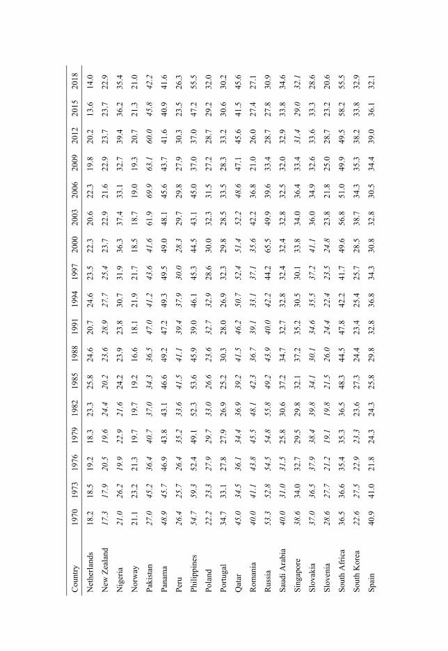
Coun

try

1970

19

73

1976

19

79

1982

19

85

1988

19

91

1994

19

97

2000

20

03

2006

20

09

2012

20

15

2018

Net

herla

nds

18.2

18

.5

19.2

18

.3

23.3

25

.8

24.6

20

.7

24.6

23

.5

22.3

20

.6

22.3

19

.8

20.2

13

.6

14.0

New

Zea

land

17

.3

17.9

20

.5

19.6

24

.4

20.2

23

.6

28.9

27

.7

25.4

23

.7

22.9

21

.6

22.9

23

.7

23.7

22

.9

Nig

eria

21

.0

26.2

19

.9

22.9

21

.6

24.2

23

.9

23.8

30

.7

31.9

36

.3

37.4

33

.1

32.7

39

.4

36.2

35

.4

Nor

way

21

.1

23.2

21

.3

19.7

19

.7

19.2

16

.6

18.1

21

.9

21.7

18

.5

18.7

19

.0

19.3

20

.7

21.3

21

.0

Paki

stan

27.0

45

.2

36.4

40

.7

37.0

34

.3

36.5

47

.0

41.2

43

.6

41.6

61

.9

69.9

63

.1

60.0

45

.8

42.2

Pana

ma

48.9

45

.7

46.9

43

.8

43.1

46

.6

49.2

47

.2

49.3

49

.5

49.0

48

.1

45.6

43

.7

41.6

40

.9

41.6

Peru

26

.4

25.7

26

.4

35.2

33

.6

41.5

41

.1

39.4

37

.9

30.0

28

.3

29.7

29

.8

27.9

30

.3

23.5

26

.3

Phili

ppin

es

54.7

59

.3

52.4

49

.1

52.3

53

.6

45.9

39

.0

46.1

45

.3

44.5

43

.1

45.0

37

.0

37.0

47

.2

55.5

Pola

nd

22.2

23

.3

27.9

29

.7

33.0

26

.6

23.6

32

.7

32.9

28

.6

30.0

32

.3

31.5

27

.2

28.7

29

.2

32.0

Portu

gal

34.7

33

.1

27.8

27

.9

26.9

25

.2

30.3

28

.0

26.9

32

.3

29.8

28

.5

33.5

28

.3

33.2

30

.6

30.2

Qat

ar

45.0

34

.5

36.1

34

.4

36.9

39

.2

41.5

46

.2

50.7

52

.4

51.4

52

.2

48.6

47

.1

45.6

41

.5

45.6

Rom

ania

40

.0

41.1

43

.8

45.5

48

.1

42.3

36

.7

39.1

33

.1

37.1

35

.6

42.2

36

.8

21.0

26

.0

27.4

27

.1

Russ

ia

53.3

52

.8

54.5

54

.8

55.8

49

.2

43.9

40

.0

42.2

44

.2

65.5

49

.9

39.6

33

.4

28.7

27

.8

30.9

Saud

i Ara

bia

40.0

31

.0

31.5

25

.8

30.6

37

.2

34.7

32

.7

32.8

32

.4

32.4

32

.8

32.5

32

.0

32.9

33

.8

34.6

Sing

apor

e 38

.6

34.0

32

.7

29.5

29

.8

32.1

37

.2

35.2

30

.5

30.1

33

.8

34.0

36

.4

33.4

31

.4

29.0

32

.1

Slov

akia

37

.0

36.5

37

.9

38.4

39

.8

34.1

30

.1

34.6

35

.5

37.2

41

.1

36.0

34

.9

32.6

33

.6

33.3

28

.6

Slov

enia

28

.6

27.7

21

.2

19.1

19

.8

21.5

26

.0

24.4

22

.4

23.5

24

.8

23.8

21

.8

25.0

28

.7

23.2

20

.6

Sout

h A

frica

36

.5

36.6

35

.4

35.3

36

.5

48.3

44

.5

47.8

42

.2

41.7

49

.6

56.8

51

.0

49.9

49

.5

58.2

55

.5

Sout

h K

orea

22

.6

27.5

22

.9

23.3

23

.6

27.3

24

.4

23.4

25

.4

25.7

28

.5

38.7

34

.3

35.3

38

.2

33.8

32

.9

Spai

n 40

.9

41.0

21

.8

24.3

24

.3

25.8

29

.8

32.8

36

.8

34.3

30

.8

32.8

30

.5

34.4

39

.0

36.1

32

.1

Coun

try

1970

19

73

1976

19

79

1982

19

85

1988

19

91

1994

19

97

2000

20

03

2006

20

09

2012

20

15

2018

Swed

en

16.0

15

.6

15.0

15

.5

15.8

15

.2

16.4

14

.8

20.6

17

.6

17.1

17

.2

21.3

21

.4

22.1

21

.1

20.4

Switz

erla

nd

15.7

15

.7

16.7

17

.7

17.4

19

.4

20.4

18

.8

24.0

23

.2

22.4

22

.7

22.6

19

.3

19.5

22

.4

21.3

Taiw

an

26.2

28

.2

25.1

26

.7

28.0

28

.1

25.5

22

.9

30.0

23

.5

24.4

31

.9

26.9

32

.3

32.9

35

.7

33.4

Thai

land

45

.4

50.1

42

.7

39.7

47

.9

42.0

37

.3

43.9

43

.9

49.4

44

.7

41.1

41

.7

44.7

37

.2

34.9

35

.2

Turk

ey

34.7

38

.6

37.1

23

.4

35.9

32

.2

44.8

37

.9

38.4

38

.3

34.8

47

.4

38.3

40

.2

40.5

49

.0

42.4

Ukr

aine

25

.1

26.3

29

.1

30.8

33

.0

30.1

30

.2

36.7

32

.3

39.1

37

.3

40.4

29

.9

34.2

28

.6

32.9

31

.7

Uni

ted

Ara

b Em

irate

s 38

.1

40.4

39

.0

36.8

34

.3

37.4

35

.9

43.3

47

.3

40.5

41

.3

41.8

45

.0

46.1

50

.6

49.7

51

.9

Uni

ted

Kin

gdom

20

.2

19.8

22

.6

23.2

27

.3

27.5

27

.8

29.8

29

.0

27.9

27

.5

25.1

23

.9

26.2

28

.2

28.4

25

.5

Uni

ted

Stat

es

30.7

29

.9

30.2

28

.3

31.8

31

.3

30.0

31

.0

29.2

28

.6

26.9

29

.6

26.8

32

.1

30.2

33

.5

31.7

Ven

ezue

la

42.7

43

.0

42.6

39

.8

37.7

54

.8

48.1

50

.6

41.5

33

.2

35.7

44

.9

34.3

31

.8

35.4

31

.8

36.4

Vie

tnam

54

.1

57.7

47

.6

38.9

40

.5

41.1

44

.7

52.5

51

.0

55.8

56

.0

54.3

48

.0

57.3

50

.9

46.9

47

.7

Not

es: C

alcu

latio

ns b

ased

on

net y

early

ear

ning

s wei

ghte

d by

occ

upat

iona

l gro

up p

opul

atio

ns in

clud

ing

the

unem

ploy

ed. I

mpu

ted

obse

rvat

ions

in it

alic

s. So

urce

: Aut

hors

’ cal

cula

tions

bas

ed o

n da

ta d

escr

ibed

in th

e te

xt.

66

Table 1.A7. Global Earnings Inequality, 1970–2018.

a) Global inequality

Gini coefficient (%) GE index (%)

Net earnings

Gross earnings

Net wages

GE(0) Theil-L (MLD)

GE(1) Theil-T

GE(2)

1970 65.3 67.9 67.4 80.3 78.7 138.7

1973 64.3 66.5 66.7 79.6 73.4 117.1

1976 64.7 67.0 66.7 81.3 72.6 109.0

1979 65.3 67.4 66.8 84.3 73.3 105.5

1982 64.2 67.0 65.8 78.9 69.8 100.2

1985 64.5 67.4 65.8 77.3 71.3 107.0

1988 63.8 67.3 65.4 74.0 71.0 111.1

1991 63.7 66.1 65.0 73.1 68.3 102.4

1994 65.0 67.4 66.3 78.6 71.5 108.4

1997 65.5 67.8 67.1 81.8 72.3 110.6

2000 64.7 66.6 66.4 79.0 69.4 102.6

2003 61.3 63.3 62.6 67.2 60.0 84.9

2006 56.1 58.3 57.1 52.5 49.2 68.1

2009 54.3 56.4 55.5 47.4 45.4 62.7

2012 52.4 54.6 53.2 43.4 42.2 58.9

2015 52.3 54.6 54.0 42.6 43.2 63.5

2018 50.2 52.6 52.2 39.0 39.2 56.6

1970–2018 change (%)

-23.1 -22.5 -22.5 -51.4 -50.2 -59.2

67

b) Regional Gini indices (%)

Africa Asia Europe Latin America

Northern America

Oceania

1970 45.3 47.1 46.2 51.2 31.2 21.2

1973 47.2 55.5 46.6 51.4 30.1 23.1

1976 46.0 59.0 46.0 47.3 30.5 21.6

1979 45.2 63.1 46.7 45.8 28.7 25.6

1982 49.6 60.4 48.0 43.0 32.2 30.5

1985 46.7 58.9 51.2 46.2 31.6 29.3

1988 48.1 56.1 52.8 44.5 30.2 29.2

1991 55.8 59.8 52.1 48.1 31.4 30.8

1994 62.1 60.3 53.3 46.6 29.4 31.4

1997 60.1 61.8 52.6 50.4 29.3 31.9

2000 58.9 62.5 50.3 48.9 27.4 31.2

2003 55.9 61.2 43.7 49.4 29.9 36.1

2006 54.6 55.5 39.9 44.8 27.4 37.1

2009 54.1 51.9 36.6 44.6 32.1 40.3

2012 56.7 49.6 37.4 41.6 30.5 39.5

2015 54.9 46.3 37.4 44.2 33.3 39.2

2018 55.2 44.2 38.2 41.7 31.7 38.3

1970–2018 change (%)

21.9 -6.2 -17.4 -18.4 1.7 80.8

68

c) Global Theil index decomposition within and between countries and occupations (%)

GE(1) by countries GE(1) by occupations

Within country

Between country

Between (%) contribution

Within occupation

Between occupation

Between (%) contribution

1970 15.7 62.9 80.0 44.8 33.9 43.0

1973 15.9 57.5 78.3 39.2 34.2 46.6

1976 14.4 58.1 80.1 39.9 32.6 44.9

1979 13.3 60.0 81.9 42.0 31.3 42.7

1982 13.4 56.4 80.9 39.5 30.3 43.4

1985 13.7 57.6 80.7 39.1 32.2 45.2

1988 13.5 57.5 81.0 38.9 32.1 45.2

1991 16.3 52.0 76.1 35.4 32.9 48.2

1994 16.1 55.4 77.5 38.1 33.4 46.7

1997 17.1 55.2 76.3 38.0 34.3 47.4

2000 18.2 51.2 73.8 37.3 32.0 46.2

2003 23.4 36.6 61.0 29.2 30.8 51.3

2006 22.3 26.9 54.7 22.7 26.5 53.9

2009 20.5 24.9 54.9 22.3 23.1 50.9

2012 20.5 21.8 51.5 23.5 18.7 44.3

2015 17.1 26.1 60.4 25.6 17.5 40.6

2018 16.7 22.5 57.3 22.8 16.3 41.7

1970–2018 change (%)

6.3 -64.3 -28.3 -49.1 -51.7 -3.1

69

d) Global percentile earnings shares and average net yearly earnings (in PPP-adjusted 2015 USD)

Top and bottom earnings shares (%) Top and bottom earnings (2015 USD)

Bottom 50%

Top 10%

Top 1%

Bottom 50%

Top 10%

Top 1%

1970 9.4 50.1 8.8 1,957 52,822 130,618

1973 9.0 46.5 8.5 2,247 59,082 133,108

1976 8.1 45.2 8.2 1,924 53,747 110,977

1979 7.5 43.8 8.2 1,779 53,540 98,311

1982 8.2 43.4 8.2 1,677 44,549 83,842

1985 9.2 44.9 7.1 2,049 51,570 99,682

1988 9.4 45.9 9.0 1,955 47,844 96,994

1991 9.4 43.8 8.8 1,976 46,284 93,324

1994 8.8 44.7 8.9 2,015 52,118 104,365

1997 8.7 45.5 6.6 1,860 48,391 106,296

2000 9.2 43.7 8.7 2,088 50,862 95,721

2003 10.9 40.4 7.7 3,040 57,830 112,722

2006 13.8 36.7 6.8 3,952 52,093 106,791

2009 15.0 35.5 7.0 4,872 57,921 113,946

2012 16.8 35.0 7.0 6,384 67,121 134,435

2015 17.6 36.4 7.3 5,782 60,786 121,724

2018 18.9 34.5 6.9 5,827 53,403 107,040

1970–2018 change (%)

102.4 -31.1 -21.9 197.7 1.1 -18.1

Notes: Calculations based on net yearly earnings (if nothing else specified), which are PPP-adjusted using UBS price levels in 2015 USD and weighted by working age populations. Earn-ings refer to yearly earnings and wage to hourly earnings. Gini indices include the unemployed; GE indices and percentiles exclude the unemployed. Source: Authors’ calculations based on data described in the text.

70

Appendix 1.B Validating the Data In this section, we present comparisons and correlations between our data and those from other sources. Overall, we regard the correspondence between our new earnings inequality database and previous evidence from other sources as good. In the cases of deviations, most of the discrepancies seem to be level differences potentially explained by the within-occupational-group dispersion that was omitted in our original data.

1.B.1 Cross-Country Correlations with Other Datasets Figure 1.B1 shows country-average correlations between our data and other sources for incomes, prices and inequality. In Figure 1.B1a, we plot average country-level gross earnings in the UBS data against the mean level of GDP per capita income from the WDI, which shows a strong positive correlation (90%). In Figure 1.B1b, we compare the country-average price levels based on the UBS data with prices based on the ICP 2011, which also shows a strong correlation (79%). Note, however, that the indices here have different base values, where the ICP price index is relative to the United States’ average price level in 2015, while the UBS price index is relative to the 2015 prices in New York City. In Figure 1.B1c, we plot average country-level Gini coefficients for our net earnings measure against those for income or consumption in Mi-lanovic’s (2016) All the Ginis (ALG) dataset. Again, there is a positive and significant correlation, although this is somewhat weaker than the others (59%). The level of inequality is generally lower for earnings than for income or consumption. This is as expected since earnings do not include income from capital, which is generally more skewed than income from labour. Finally, there is also a relatively strong correlation (61%) between the average coun-try-level top 10% earnings in our dataset and the corresponding figures in the WID (2018), as shown in Figure 1.B1d.

71

Figure 1.B1. Cross-Country Correlations: Earnings, Prices and Inequality.

Notes: a) Country-level earnings and income per capita averages for 1970–2018 in current USD. UBS gross yearly earnings weighted by occupational group populations, including the unemployed. b) Country-level price levels in 2015. For UBS, prices excluding rent (where New York City 2015 = 100). For ICP 2011, prices from the WDI (where the United States 2015 = 100). c) Country-level inequality averages for 1970–2018. UBS net yearly earnings inequality refers to this study with calculations based on net yearly earnings weighted by occupational group populations, including the unemployed. ALG income inequality refers to interpolated values of Milanovic (2016) ALG dataset. d) Country-level top 10% gross yearly earnings aver-ages for 1970–2018 in current USD. “UBS top 10% mean gross yearly earnings” refers to this study with calculations based on gross yearly earnings weighted by occupational group popu-lations, excluding the unemployed. “WID top 10% mean earnings” refers to the WID. Sources: Authors’ calculations based on data described in the text; Milanovic (2016); WID (2018); World Bank (2018).

The country-level pairwise correlations (using all available years) between our measures of inequality, earnings and prices, and income inequality in the ALG dataset, GDP per capita incomes from the WDI and price levels from the ICP 2011, respectively, are shown in Table 1.B1.

72

Table 1.B1. Country-Level Pairwise Correlations: Inequality, Earnings and Prices.

a) Inequality correlation (%) ALG income inequality

Gini net earnings inequality 48.2*** (814)

b) Income and earnings correlation (%) GDP per capita

Gross earnings 91.3*** (1,156)

c) Price levels correlation (%) ICP 2011 PPP

UBS PPP 84.3*** (680)

Notes: * ! < 0.1, ** ! < 0.05, *** ! < 0.01. Number of observations in parentheses. Mean earnings and inequality calculations weighted by occupational group populations including the unemployed. a) Country-level inequality measured by Gini coefficient. ALG refers to interpo-lated values of Milanovic (2016). b) GDP per capita and gross yearly earnings in current USD. c) For UBS, prices excluding rent, where New York City 2015 = 100. For ICP 2011, prices from the WDI using the 2011 ICP round, where United States 2015 = 100. Sources: Authors’ calculations based on data described in the text; Milanovic (2016); World Bank (2018).

1.B.2 Top Earnings Correlations Figure 1.B2 shows some further correlations between top occupation earnings in our data and the WID top earnings data. The correlations indicate that the highest-earnings occupations in the UBS data (managers and medical doc-tors), except for some outliers (particularly Qatar), have earnings around or even above the mean in the WID top decile and, in many cases, also the top ventile. This means that we have fairly good coverage in the top, although the very top (above the top 5%) may still not be well covered in our data. In one of our robustness analyses, we have therefore added the national top earnings from the WID to our baseline data, finding that this does not change our results (see Section 1.C.10 in Appendix 1.C).

73

Figure 1.B2. Top Earnings Cross-Country Correlations.

Notes: Correlations between top earnings in the WID and top occupation earnings in the UBS data, with gross yearly earnings averages for 1970–2018 in current USD. Solid line indicates 45-degree line, with equal earnings in the WID and the UBS data; observations above this line indicate higher mean earnings in the UBS than in the WID data. Medical doctors refer to general practitioners, and managers to department and product managers. Sources: Authors’ calculations based on data described in the text; WID (2018).

1.B.3 Occupational Earnings Correlations Next, we also check how well the UBS occupational earnings correspond to another international dataset of occupational wages, namely Freeman and Oostendorp’s (2012) OWW database. In Figure 1.B3, we thus plot the occu-pational gross hourly wages in the UBS versus OWW datasets (where each observation represents the earnings of an occupation in a country and year) for all occupations that are available for the full 1970s–2010s period. The oc-cupations are matched as follows (in the UBS and OWW datasets, respec-tively): bank credit clerks with bank tellers; bus drivers with motor bus driv-ers; car mechanics with automobile mechanics in the repair of motor vehicles industry; construction workers with labourers in the construction industry; cooks with cooks; department managers with supervising or general foremen in the manufacture of industrial chemicals industry; engineers with electronics engineering technicians; female factory workers with labourers in the spin-ning, weaving and finishing textiles industry; female sales assistants with salespersons in the retail trade (grocery) industry; primary school teachers

74

with first-level education teachers; secretaries with office clerks in the print-ing, publishing and allied industries industry; and skilled industrial workers with mixing- and blending-machine operators in the manufacture of industrial chemicals industry. For wage correlations per occupation, see Figure 1.B4.

Figure 1.B3. Occupational Earnings Correlations.

Notes: Country-occupation gross hourly wages in current USD in the UBS and the OWW da-tasets. Each point corresponds to an occupation in a country in a specific year. Sources: Authors’ calculations based on data described in the text; Freeman and Oostendorp (2012).

The correlation between occupational hourly wages in the two datasets is very high (88%), and similarly for yearly earnings (86%). We can also see that, on average, the wages and earnings levels are slightly higher in the UBS than in the OWW data. A potential explanation for this is that the UBS data are only collected in cities and, as such, lack rural wages and earnings, which are likely to be lower than their urban counterparts. To deal with this limitation, we PPP-adjust at the local city level for urban price levels instead of a mix of rural and urban prices.

75

76

Figure 1.B4. Earnings Correlations per Occupation.

Note: Country-occupation gross hourly wages averages for 1970–2018 in current USD in the UBS and the OWW datasets. Sources: Authors’ calculations based on data described in the text; Freeman and Oostendorp (2012).

1.B.4 City Size, Earnings and Inequality To check our assumption about local price adjustments, we do a within-sam-ple test using the city-level data within countries (Figure 1.B5). By comparing all within-country between-city pairs available in our data (that is, the coun-tries for which we have earnings data from more than one city in the same year), we see that after PPP-adjusting at the city level, average earnings within one city in a country seems to be strongly correlated with earnings in another city within the same country (Figure 1.B5a). The same also seems to be the case for city earnings inequality (Figure 1.B5b). While some earlier studies have argued for a potential relationship between inequality and city size (for example, Glaeser et al., 2009, who find this association to be negative, and Baum-Snow and Pavan, 2013, who find it to be positive), we do not see such within-country correlation between city population and earnings inequality in our data (Figure 1.B5d). Nor do we see any significant within-country corre-lation between city size and average earnings, after PPP-adjusting at the city level (Figure 1.B5c). It should be noticed, however, that this analysis only covers a limited sample of (relatively large) cities. It could still be the case that there is a real earnings gap between urban and rural areas that we do not

77

capture with our data and local price adjustments. In one of our heterogeneity analyses, we hence focus exclusively on global urban earnings inequality (see Section 1.C.9 in Appendix 1.C).

Figure 1.B5. Within-Country Between-City Correlations: Earnings, Inequality and City Size.

Notes: a) Average net yearly earnings (PPP-adjusted using UBS price levels in 2015 USD) correlations for each within-country between-city pairs in our data. b) Average net yearly earn-ings inequality correlations for each within-country between-city pairs in our data. c) Within-country correlations between city population and average net yearly earnings (PPP-adjusted using UBS price levels in 2015 USD), excluding the unemployed, for all countries with more than one city in our data. d) Within-country correlations between city population and average net yearly earnings inequality excluding the unemployed, for all countries with more than one city in our data. Source: Authors’ calculations based on data described in the text; UN (2017).

As a validity check of using the OWW agricultural earnings data for missing data on rural earnings, we have also compared the ratio between OWW agri-cultural and UBS mean gross earnings in China to the corresponding rural/ur-ban fiscal income ratio as provided for China by the WID. Over the available period, the mean ratio between agricultural earnings in the OWW and mean urban (industrial and services) earnings in the UBS data for China is 35%, and the mean WID rural/urban income ratio for China is 38%. Although these two measures are not fully comparable, we can at least see this as indication that the relation between our urban earnings data from the UBS and the added ag-ricultural earnings data from the OWW seems reasonable in the case of China.

78

1.B.5 Country Inequality Time-Series Comparisons Another consistency check is to compare the levels and trends of our country-level earnings Gini coefficients with other microdata sources. Figure 1.B6 pre-sents such comparisons for 41 countries with available series from three other, microdata-based, sources for country-level earnings and wage inequality: i) Krueger et al.’s (2010) special issue of the Review of Economic Dynamics (RED) containing earnings and wage inequality series for nine countries (for an earlier compilation of long-run trends in earnings dispersion in rich coun-tries, see Atkinson, 2008); ii) estimates based on microdata over earned in-come, wages and salaries available for ten countries from the Minnesota Pop-ulation Center’s (2018) IPUMS International; and, iii) estimates based on har-monized microdata for 39 countries from the LIS (2017) database, using per-son-level data on labour income for all individuals with positive earnings. For comparison, our earnings inequality trends here also include the series with top 5% earnings added from the WID (see Section 1.C.10 in Appendix 1.C). Moreover, Figure 1.B6 also includes comparisons with country-level income or consumption inequality series from various sources, as collected by Mila-novic (2016) and reported in the ALG dataset, which are available for 60 of our 68 covered countries (the ALG dataset lacks data for Bahrain, Lebanon, Qatar, Saudi Arabia and the United Arab Emirates, while Croatia, Pakistan and Vietnam only have been included in the UBS for one year). Overall, our estimated earnings inequalities are reassuringly similar to those available in the other sources in both levels and trends. However, there are several exam-ples of imperfect overlaps, but notably not only between our series and the others, but also between the other estimates. Some discrepancy is also ex-pected given that the series might differ in the definitions of population, and possibly due to the omitted within-occupational-group dispersion in our data.

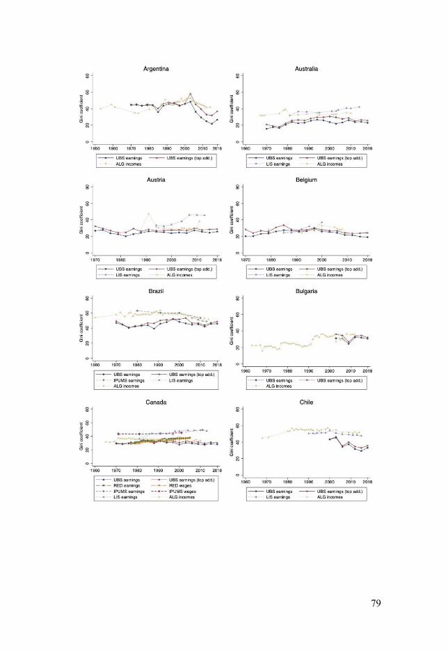
79

80

81

82

83

84

85

86

Figure 1.B6. Country-Specific Inequality Trends and Time-Series Comparisons.

Notes: UBS earnings refer to this study and are country-level Gini coefficients based on net yearly earnings weighted by occupational group populations including the unemployed, where “top add.” means that the top 5% earnings are added from the WID. Extrapolated years are excluded. RED earnings and wages refer to the country-level microdata studies available in the RED special issue “Cross-sectional facts for macroeconomists” (Krueger et al., 2010). IPUMS earnings and wages, and LIS earnings, refer to the authors’ own calculations based on microdata available in the IPUMS International and LIS databases, respectively. ALG incomes refer to Milanovic’s (2016) estimations and compilation of country-level income and/or consumption inequality. Sources: Authors’ calculations based on data described in the text; Binelli and Attanasio (2010); Blundell and Etheridge (2010); Brzozowski et al. (2010); Domeij and Flodén (2010); Fuchs-Schündeln et al. (2010); Gorodnichenko et al. (2010); Heathcote et al. (2010); Jappelli and Pistaferri (2010); LIS (2017); Milanovic’s (2016); Minnesota Population Center (2018); Pijoan-Mas and Sánchez-Marcos (2010); WID (2018). Source data for IPUMS International are pro-vided by the following national statistical offices: Institute of Geography and Statistics for Bra-zil, Statistics Canada, Ministry of Statistics and Programme Implementation for India, BPS Statistics Indonesia, Central Bureau of Statistics for Israel, National Institute of Statistics, Ge-ography, and Informatics for Mexico, Census and Statistics Directorate for Panama, Bureau of the Census for United States, and National Institute of Statistics for Venezuela.

1.B.6 LIS Occupational-Means Inequality Time-Series Comparisons

As an attempt to estimate the size of the omitted within-occupational-group dispersion in our data, we also use the LIS (2017) microdata to estimate com-parable country-level earnings inequality series, using occupational-group av-erages instead of individual-level earnings data. Using the harmonized person-

87

level microdata from the LIS, we thus compute weighted average labour in-come for each of the nine ISCO categories (see Table 1.A2 in Appendix 1.A) in each of the 35 of our countries for which these data are available in the LIS. We then re-estimate the country-level earnings inequality series using occu-pational group means instead of the individual-level data from the LIS. To make these series as comparable as possible, we only include working age (ages 15–64) individuals with positive earnings from the LIS, and only the employed population’s earnings from occupations that are not added to the data during the 2000s–2010s from the UBS. In Figure 1.B7, we compare our country-level earnings inequality series with these comparable estimates from the LIS database. The microdata estimates seem to be highly consistent with our series, both in terms of levels and trends. Our occupational-group-based trends follow the individual-based trends very well, and the level difference that exists seems to be due to the omitted within-group dispersion among the occupations-based estimates. As such, we also do an analysis where we adjust our global inequality estimates for such within-group dispersion (see Section 1.3.4 in the main paper).

88

89

90

91

92

Figure 1.B7. Country Earnings Inequality Comparisons using Occupational-Group Averages.

Notes: “UBS (groups)” refers to this study and are country-level Gini coefficients based on net yearly earnings, weighted by occupational group populations, excluding the unemployed and “new” occupations that are added to the UBS data during the 2000s–2010s. Extrapolated years are excluded. “LIS (ind.)” refers to the authors’ own calculations based on person-level labour income microdata available in the LIS database, weighted by the working age populations (ages 15–64) with positive labour income, and “LIS (groups)” implies that average labour income for the ISCO occupational groups 1–9 are used instead of the individual-level data. Sources: Authors’ calculations based on data described in the text; LIS (2017).

The average difference between our country-level earnings inequality series and the corresponding series based on the LIS in only one Gini point (see Figure 1.B8), which in turn could be due to the fact that our series are based on 13 rather than nine occupational groups. Moreover, the data do not show evidence of any consistent trend in the difference between our and the LIS estimates over time, why we assume this dispersion to be constant over time in our adjustments. As further illustrated in Figure 1.B8, our estimations using occupational group means in the UBS and the LIS data are on average 20 and 21 Gini points lower than the corresponding estimations using individual-level microdata from the LIS. Comparisons between all microdata sources (that is, the IPUMS, LIS and RED) and our baseline country-level earnings inequality (that is, now including the unemployed and all UBS occupations) show that our inequality estimations are on average eleven Gini points lower than those using individual-level data. For wage inequality, the corresponding difference is five Gini points. We use these numbers as empirical examples when we

93

adjust our global estimates for the omitted within-country occupational-group dispersion (see Section 1.3.4 in the main text).

Figure 1.B8. Microdata Comparisons: Mean Earnings Inequality Differences.

Notes: Average country-level Gini coefficient differences between different microdata sources. Solid line shows the mean difference between individual-level earnings inequality in the IPUMS, LIS and RED microdata sources and our baseline net yearly earnings inequality, weighted by occupational group populations and including the unemployed. Dashed lines show comparisons between earnings inequality estimated from the LIS data, where “LIS groups” implies that occupational group means (that is, average labour income for the ISCO occupa-tional groups 1–9) are used instead of individual-level data, and our UBS data estimations of net yearly earnings inequality weighted by occupational group populations (where, for compa-rability, our “UBS groups” exclude the unemployed and the “new” occupations that are added to the UBS data during the 2000s–2010s). Sources: Authors’ calculations based on data described in the text; Krueger et al. (2010); LIS (2017); Minnesota Population Center (2018).

94

Appendix 1.C Robustness Checks, Sensitivity and Heterogeneity Analyses In this section, we present various robustness checks, sensitivity and hetero-geneity analyses of the results in our main paper. In summary, we find that our results are robust to numerous alternations.

1.C.1 Alternative Inequality Indices Figure 1.C1 presents the global earnings inequality trend using two other ine-quality indices instead of the Gini coefficient. Figure 1.C1a shows GE indices, GE('), where a higher parameter ' reflects a higher sensitivity to disparities in the top of the distribution, and where GE(0) corresponds to the mean log deviation (MLD), GE(1) to the Theil-T index and GE(2) to half the squared CV. Figure 1.C1b shows Atkinson indices, A((), where ( is society’s aversion to inequality and makes the index more sensitive to earnings differences at the bottom of the distribution. The levels of inequality vary across these measures, which is as expected since the specific parameter values differ, but the trends are quite similar to our baseline global Gini coefficient trend, showing a de-cline in global earnings inequality over the studied period.

Figure 1.C1. Other Measures of Global Earnings Inequality.

Notes: Calculations based on net yearly earnings, PPP-adjusted using UBS price levels in 2015 USD, and weighted by working age populations, excluding the unemployed. Source: Authors’ calculations based on data described in the text.

1.C.2 Kernel Densities Figure 1.C2 presents the evolution of earnings inequality in a different way, depicting kernel densities of absolute earnings of occupations across countries in 1970, 1994 and 2018. Comparing these densities over time shows that the distribution has drifted upwards, especially since 1994, signalling an overall increase in real earnings across the world during this period. The relatively thick left tail (that is, sizeable mass of low-earners) is especially visible in

95

1970 and 1994, but is then almost gone in 2018 when earnings instead became more concentrated around the centre (or lower middle) of the distribution. This once again underlines the decline in global earnings inequality. Other studies of the global income distribution over time have found that it was bimodal before 1970 and then became unimodal between 1980 and 2000 (for example, Moatsos et al., 2014). We see a similar trend for the global earnings distribu-tion.

Figure 1.C2. Kernel Densities over Time.

Notes: Density of log net yearly earnings (PPP-adjusted using UBS price levels in 2015 USD) and weighted by working age populations, excluding the unemployed. Horizontal axis in log scale. Gaussian smoothing. Source: Authors’ calculations based on data described in the text.

1.C.3 International Earnings and Income Inequality Milanovic (2005) defines world inequality in terms of three different concepts: “Concept 1” is unweighted international inequality, “Concept 2” is popula-tion-weighted international inequality, and “Concept 3” is the “true” global inequality (which includes both within- and between-country inequality). While most of our analysis in this paper focuses on the “Concept 3” of global inequality, it could also be informative to compare the “Concept 2” of inter-national (that is, between-country) inequality for labour earnings versus total incomes. Such a comparison is illustrated in Figure 1.C3, in which we have estimated population-weighted international inequality using average

96

country-level i) net yearly earnings from the UBS data, and ii) GDP per capita from the PWT 9.1 (Feenstra et al., 2015). For the former we use our baseline sample, population-weights and PPP-adjustments, and for the latter a balanced sample of the 156 countries with available GDP per capita, population and PPP (ICP 2011) data for the 1970-2017 period.

First, comparing the series in Figure 1.C3 shows that ignoring within-coun-try inequality results in lower levels of inequality. This is shown by the lower level of “international earnings inequality” than the level of “global earnings inequality” (our baseline). Second, over this period, the fall in international inequality has been much larger for earnings than for total income. That is, between countries, average earnings levels have converged more than GDP per capita, and today, the difference is almost 12 Gini points. A possible ex-planation for this could be an increased role of capital income (which is in-cluded in GDP but not in labour earnings) in richer countries.

Figure 1.C3. Comparing International Earnings versus Income Inequality.

Notes: Global earnings inequality includes both within- and between-country inequality, and is based on net yearly earnings using the UBS and ILO data, which are PPP-adjusted using UBS price levels in 2015 USD and weighted by working age populations including the unemployed. International inequality only includes between-country inequality, which is estimated using population-weighted country averages, where earnings inequality is based on average net yearly earnings (using the UBS and ILO data), and income inequality on GDP per capita (using data from the PWT 9.1 with ICP 2011 PPP-adjustments, for a balanced sample of 156 countries). Sources: Authors’ calculations based on data described in the text; Feenstra et al. (2015).

97

1.C.4 The “Elephant Curve” of Global Earnings Figure 1.C4 shows an anonymous GIC, depicting the average annual earnings growth of each percentile of the global earnings distribution between the 1970s and 2010s. This figure corresponds to Lakner and Milanovic’s (2015) anonymous GIC, sometimes referred to as the “elephant curve”, but here for global earnings instead of income or consumption (note also that our figure covers a longer time period). Because the UBS data are likely to lack very top earnings, here we have also included our results with national top earnings added from the WID (see Section 1.C.10). When national top earnings are included, the GIC pattern that we find is strikingly similar to that found by Lakner and Milanovic (2015, 2016), in particular to their quasi non-anony-mous GIC. If anything, compared to income or consumption, the global earn-ings growth that we find seems to be even more concentrated to the bottom half, as well as to the more extreme top (that is, the top 0.1%–0.2%), of the global distribution. Potential explanations for this could be incomes from pen-sions and capital, which are included in Lakner and Milanovic’s (2015) meas-ure of global income or consumption but not in our labour earnings.

98

Figure 1.C4. Anonymous GIC, 1970s–2010s.

Notes: Average annual percentile growth rate 1970s–2010s in net yearly earnings (PPP-ad-justed using UBS price levels in 2015 USD), weighted by working age populations excluding the unemployed. Horizontal axis ranked according to percentile earnings ranks in 1970s. Top percentile divided into ten groups. Decade averages for 1970s and 2010s correspond to the years 1970–1979 and 2009–2018, respectively. “Adding national top earnings” implies that the national top 5% earnings are added from the WID. Sources: Authors’ calculations based on data described in the text; WID (2018).

1.C.5 Regional Earnings Inequality Figure 1.C5 displays regional earnings inequality trends in Africa, Asia, Eu-rope, Latin America, Northern America and Oceania (see Table 1.A1 in Ap-pendix 1.A for country coverage in each of the regions). A similar regional inequality analysis, albeit for total incomes instead of labour earnings, has for instance been conducted by Ravallion (2014), however, focusing only on the developing world. As illustrated in Figure 1.C5, there is a large heterogeneity in both levels and trends of earnings inequality across continents. Asia and Europe experienced lowered inequality, with the latter experiencing almost a level shift in the 2000s. Regional decomposition shows that both of these in-equality decreases were due to falls in between-country inequality, which might be explained by exceptionally high earnings growth rates among the low-income Asian countries and earnings convergence among European countries, for example, with the expansion of the European Union and the in-troduction of the euro. Africa and Latin America also have high levels of

99

regional earnings inequality, where the level in Latin America and the increas-ing trend in Africa are more dominated by the within- than between-country inequality. The smaller regions, Northern America and Oceania, have lower levels of initial regional earnings inequality and exhibit flat and increasing trends, respectively.

Figure 1.C5. Earnings Inequality in World Regions and Their Country Decomposi-tions.

Notes: Calculations based on net yearly earnings (PPP-adjusted using UBS price levels in 2015 USD) and weighted by working age populations including the unemployed. Gini decomposi-tions calculated using Yitzhaki and Lerman’s (1991) method as described in Frick et al. (2006), with overlapping index included in “within”. Decompositions calculated excluding the unem-ployed but scaled by total global Gini coefficient including the unemployed. Source: Authors’ calculations based on data described in the text.

100

The regional earnings inequality trends for our different sub-regions are fur-ther illustrated in Figure 1.C6 (missing sub-regions according to the United Nations’ geographical classification are Middle Africa, Central Asia, Carib-bean, Melanesia, Micronesia, and Polynesia).

Figure 1.C6. Earnings Inequality in Sub-Regions around the World.

Notes: Calculations based on net yearly earnings (PPP-adjusted using UBS price levels in 2015 USD) and weighted by working age populations including the unemployed. Sub-regions de-fined according to the United Nations’ classification of macro geographical sub-regions. Ex-trapolated sub-regional observations are excluded. Source: Authors’ calculations based on data described in the text.

1.C.6 Occupational Earnings Inequality In Figure 1.C7, we examine the earnings inequality between countries within different occupations in the industrial, agricultural and services sectors. We document a large variation in the level of earnings inequality across occupa-tions. For example, there is larger earnings dispersion among the world’s con-struction workers than among the department managers of the world, and sec-retaries in the world are more homogenously paid than primary school teach-ers. Looking at trends, almost all occupations (except for bank credit clerks) have experienced decreased global occupational inequality over this period, which matches the overall global trend. However, the decrease is more pro-nounced in the industrial sector than for the services professions. A possible explanation for this might be trade globalization: Since the industrial sector

101

has typically been more exposed to international competition, industrial earn-ings would then have become more compressed by globalization. By contrast, services sector earnings might to a larger extent have been determined by na-tional conditions and, therefore, responded less to rising globalization. Further analyses (which are outside the scope of this paper), however, are needed in order to test this hypothesis.

Figure 1.C7. Occupational Inequality.

Note: Calculations based on net yearly earnings (PPP-adjusted using UBS price levels in 2015 USD) and weighted by working age populations, excluding the unemployed. Source: Authors’ calculations based on data described in the text.

1.C.7 Counterfactual Analysis by Country-Occupation Figure 1.C8 shows the differences between the actual global Gini coefficient and the counterfactual Ginis with fixed 1970 gross hourly earnings for each of the different country-occupations. The most important country-occupations are agricultural workers in China and construction workers in India, whose gross wage changes, ceteris paribus, have reduced global inequality by four and one Gini points, respectively. Wage changes among department managers in the United States have had a smaller but opposing impact, driving global inequality up by 0.3 Gini points.

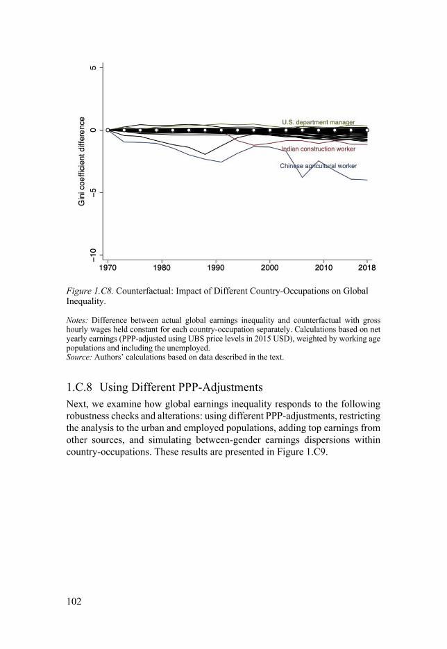
102

Figure 1.C8. Counterfactual: Impact of Different Country-Occupations on Global Inequality.

Notes: Difference between actual global earnings inequality and counterfactual with gross hourly wages held constant for each country-occupation separately. Calculations based on net yearly earnings (PPP-adjusted using UBS price levels in 2015 USD), weighted by working age populations and including the unemployed. Source: Authors’ calculations based on data described in the text.

1.C.8 Using Different PPP-Adjustments Next, we examine how global earnings inequality responds to the following robustness checks and alterations: using different PPP-adjustments, restricting the analysis to the urban and employed populations, adding top earnings from other sources, and simulating between-gender earnings dispersions within country-occupations. These results are presented in Figure 1.C9.

103

Figure 1.C9. Prices, Populations, Top Earnings and Gender-Gap Adjustments.

Notes: Calculations based on net yearly earnings, PPP-adjusted using UBS price levels in 2015 USD (if nothing else specified), and weighted by working age populations including the unem-ployed (if nothing else specified). a) Baseline implies UBS PPP excluding rent. For PWT PPP, prices are compared across countries using the 2011 ICP round. Market exchange rates imply no PPP adjustments. b) Baseline implies total rural and urban working age population. Urban means that urban working age populations are used as country population weights instead of total working age populations and that the agricultural sector is not included. Employed means that the unemployed are excluded. c) National top earnings are added from the WID (not added in baseline). d) Gender-gap adjustment means that UBS sectoral earnings gender gaps are used, and ILO gender-gap adjustment that ILO occupational earnings gender gaps (1992–2017) are used. Sources: Authors’ calculations based on data described in the text; Feenstra et al. (2015); ILO (2018); WID (2018); World Bank (2018).

Previous studies have found that adjusting incomes for PPP has a large impact on global inequality assessment (see, for example, Deaton, 2010; Deaton and Heston, 2010; Almås, 2012; Deaton and Aten, 2017). In Figure 1.C9a, we therefore re-estimate the global earnings Gini coefficients using different price indices. The results show that it does not make a big difference whether we include or exclude rents in our UBS price index. Furthermore, we find that our preferred adjustment, based on local prices collected homogenously by the UBS for all cities and years in direct correspondence with the earnings infor-mation, delivers a long-run pattern that is somewhat similar to, although gen-erally higher than, what we obtain when using the ICP 2011 PPPs from Feenstra et al.’s (2015) PWT 9.0 (if there are missing values, we use the same imputation methods as above, namely by linear interpolation and sub-regional

104

means extrapolation). The main difference when using this alternative PPP source is that the global earnings inequality trend then gets a lower level dur-ing the 1970s–1990s. Note, however, that the ICP price index adjusts for av-erage country (and not city) prices. This mix of urban and rural prices in the ICP should bias our results since the UBS earnings are given for urban areas only. Finally, as expected the global earnings inequality in current market prices (that is, using market exchange rates and no adjustments for local price differences) is consistently higher than our PPP-adjusted measures of global earnings inequality, but still follows a relatively similar declining trend.

1.C.9 Restricting the Analysis to Global Urban and Working Populations

Heterogeneity analyses with respect to populations, where we focus exclu-sively on the global urban and global employed earnings inequalities, are pre-sented in Figure 1.C9b. Weighting each country by its urban, instead of total, working age population and excluding our added agricultural workers yields lower levels of earnings inequality. Moreover, the global urban workforce has experienced a somewhat smaller inequality decline during this period. When instead excluding the unemployed populations, we obtain a lower level, but similar trend, of global earnings inequality. That is, as expected earnings ine-quality among the global labour force participants is lower than inequality among the total global workforce. The difference between including and ex-cluding the unemployed has increased over this period, suggesting that global unemployment has increased, or that the relative labour force participation in developed countries, relative to that in developing countries, has increased.

1.C.10 Adding Top Earnings One potential concern with our earnings data is their insufficient coverage of earners at the very top of the distribution. Correlations between our data and the WID top earnings data are positive and significant, and we seem to cover the top decile and ventile relatively well (see Figure 1.B2 in Appendix 1.B). Still, we know that by construction (since we do not have full occupational coverage), we are likely to miss the very highest-paid professions and their earnings in our estimations. Hence, to account for earnings in the highest in-come top, in the next analysis, we have added national top earnings using data from the WID.

Our method for adding national top earnings data from the WID is as fol-lows: First of all, because our analysis focuses on earnings, we only include the top incomes in the WID that come from wages, salaries and labour income, or corresponding estimates. That is, we adjust the recorded national top total incomes into earnings by using evidence on earnings shares in the WID. We

105

separately add the national top 1%, 5%, and 10%, treat them as their own oc-cupational group and reduce the other employed working age population by the corresponding percentage. When missing, we impute these data using the same methods as for our baseline data, by linear interpolation and sub-regional or regional extrapolation. In total, there are 42 countries with data both in our sample and top earnings data in the WID. For countries that are not included in the WID, we use sub-regional or regional means, weighted by the country-to-region relative mean GDP per capita. Similarly, we use country mean taxes to calculate net yearly earnings. We have also done these top adjustments in various alternative ways, by adding national top incomes instead of earnings, by adding the top 1%, 5% and 10% simultaneously and on top of all the other earnings and population data, as well as by regression imputations, finding very similar results (available upon request).

The results from the top earnings additions are shown in Figure 1.C9c, and do not seem to make a big difference to our baseline results. The Gini coeffi-cient increases somewhat, from 50 to 52 in 2018, and this relatively small effect appears to be roughly the same regardless of whether we add the na-tional top 1%, 5% or 10% earnings. In our GIC analysis, however, we find that adding national top earnings from the WID does make a difference to the growth rate that we find in the very top (top 0.1%) of the global earnings dis-tribution (see Section 1.C.4).

1.C.11 Gender Composition Adjustment Furthermore, we have also done an analysis where we adjust our main series for the lack of within-group between-gender earnings dispersion, arising from the gender composition in our country-occupational data. That is, instead of having male earnings for some occupations and female earnings for other oc-cupations, we separate each country-occupational group into a male and a fe-male group of workers. In contrast to studies using income data on the house-hold level, we are thus able to make a gender-gap adjustment to our inequality estimations.

We make this within-occupation between-gender inequality adjustment as follows. First, we use the gender composition in ILO’s (2010, 2018) data on employment by sex and occupation. That is, after separating each occupational group into its male and female components, we weight the population of each group by the male/female employment share of that particular country-year-occupation. For missing observations, we use the same approach as for the other ILO occupational population data (linear interpolation and extrapolation using sectoral and regional changes). Second, we use the sectoral gender earn-ings gap in the UBS data. These UBS gender earnings gaps are estimated by using the earnings ratio of occupational groups that are similar in terms of skills, experience, education, age and family status but differ in terms of gen-der. The industrial (and agricultural) sector gender earnings gap is calculated

106

as the mean earnings of male construction workers divided by the mean earn-ings of female factory workers, and the services sector gender earnings gap as the mean earnings of male secretaries and car mechanics divided by the mean earnings of female sales assistants. We then weight the earnings of each male and female country-year-occupational group by the corresponding earnings ratio. Because the UBS male-female earnings gap is only available on the sec-toral level, as an alternative, we also use three-year averages of ILO’s (2018) data on earnings by sex and occupation to estimate occupational-level gender earnings gaps (using the same imputation approach as above). These ILO oc-cupational earnings data, however, are only available for the years 1992–2017.

Figure 1.C9d shows the global earnings inequality trend adjusted for this within-group between-sex earnings dispersion, using the UBS and the ILO sources of the gender earnings gaps. As we can see, this adjustment has a small but slightly increasing effect on global earnings inequality. Our two measures of the global gender earnings gap are further illustrated in Figure 1.C10, where we can see that the between-gender earnings inequality has fallen over this period.

Figure 1.C10. Global Gender Earnings Gap.

Notes: “UBS” refers to the mean UBS sectoral net yearly earnings gender gap, where the in-dustrial earnings gender gap is calculated as the average earnings of male construction workers divided by the average earnings of female factory workers, and the services gender earnings gap as the average earnings of male secretaries and car mechanics divided by the average earn-ings of female sales assistants. “ILO” refers to the mean ILO occupational earnings gender gap. Sources: Authors’ calculations based on data described in the text; ILO (2018).

107

1.C.12 Robustness Checks Using Alternative Imputations Finally, in this section, we present some further robustness checks where we use alternative extrapolations, imputations and samples when generating the database. As shown in Figures 1.C11 and 1.C12, our baseline results seem to be robust to using various alternative extrapolation and imputation ap-proaches. Extrapolating missing earnings observations using only observed within-country information (that is, the earliest or latest observed country-oc-cupation growth rate, as well as the mean observed country-occupation growth rate), yields a slightly higher global earnings inequality level during the first half of the covered period, but a similar decline during the second half (in this analysis, we exclude Croatia, Iran, Lebanon, Pakistan and Vietnam because they have none or only one observed growth period and, in the first case, we also censor negative growth rates at zero). Similarly, extrapolating missing observations with changes in the country’s GDP per capita instead of sub-regional changes also yields a slightly higher level of global earnings inequal-ity during the 1970s–1990s, but then yields a very similar trend from the mid-1990s onwards (see Figure 1.C11). This indicates that the inequality decline that we observe might actually be even somewhat larger than what our base-line estimates suggest.

108

Figure 1.C11. Robustness Checks: Extrapolations.

Notes: Calculations based on net yearly earnings, PPP-adjusted using UBS price levels in 2015 USD, and weighted by working age populations including the unemployed. For “constant growth extrapolation”, missing earnings observations are extrapolated using the first or last observed country-occupation growth rate for the previous or following periods, where negative growth rates are censored at zero and only countries with observations from more than two three-year periods are included. For “mean growth extrapolation”, missing earnings observa-tions are extrapolated using average observed country-occupation growth, and only countries with observations from more than two three-year periods are included. For “GDP per capita growth extrapolation”, missing earnings are extrapolated using GDP per capita growth. Sources: Authors’ calculations based on data described in the text; World Bank (2018).

Figure 1.C12 shows robustness checks using a number of alternative imputa-tions, which all seem to have very little impact on our baseline results. This includes using total instead of working age country population weights; grad-ually including or excluding the “new” occupations that are added to the UBS data during the 2000s and 2010s; extrapolating the agricultural earnings that we add from the OWW by using country mean earnings or unskilled elemen-tary occupational earnings instead of GDP per capita; as well as extrapolating missing occupational employment observations by using the earliest or latest available observation instead of sectoral and regional changes. Finally, we also check that our results are not driven by extreme outliers by excluding all earnings observations that have changed by more than 100% over a three-year period, and instead linearly interpolate these observations, finding that this does not affect the results either.

109

Figure 1.C12. Robustness checks: Imputations.

Notes: Calculations based on net yearly earnings, PPP-adjusted using UBS price levels in 2015 USD, and weighted by working age populations including the unemployed (if nothing else specified). “Total population weights” imply that total country populations are used as weights instead of working age populations. “New occupations” refer to occupations that are added to the UBS data during the 2000s and 2010s (that is, product managers, call centre agents, financial analysts, hospital nurses, carpenters, medical doctors and doctor’s assistants), where gradual inclusion means that they are gradually included as they are being added to the data, and ex-cluding means that they are excluded altogether. “Country mean agriculture” and “Unskilled agriculture” mean that the agricultural earnings that we add from the OWW are extrapolated by using country mean earnings or unskilled construction worker earnings, respectively, instead of GDP per capita. “Constant employment extrapolation” means that missing occupational em-ployment observations are extrapolated using the earliest or latest available observation, assum-ing it to be constant over the missing period. “Outliers interpolation” implies that we drop all earnings observations with a three-year change larger than 100%, and instead interpolate these observations linearly. Sources: Authors’ calculations based on data described in the text; World Bank (2018).

Finally, Figure 1.C13 shows some more robustness checks, using different samples. First of all, we can see that whether or not we include our GDP-per-capita-weighted regional proxies for the countries that are not in the original UBS data (that is, to get global coverage by using Sample III) does not seem to have an important impact on our results. Moreover, we find that using only the balanced non-extrapolated sample of country-occupations available for the full 1970–2018 period yields a significantly lower level and flatter trend of global earnings inequality. This, however, is as expected since this sample only includes 26, mainly developed, countries and five occupations (see

110

Tables 1.A1 and 1.A2 for country and occupational period coverage). If we instead use the balanced 1997–2018 sample, which for instance includes both China and agricultural workers, we find a global earnings inequality trend that is very similar to our baseline estimation.

Figure 1.C13. Robustness checks: Samples.

Notes: Calculations based on net yearly earnings, PPP-adjusted using UBS price levels in 2015 USD, and weighted by working age populations including the unemployed. “UBS country sam-ple” means that countries not included in the UBS data are not imputed. “1970 sample” only includes the balanced non-extrapolated sample of country-occupations available for the full 1970–2018 period. “1997 sample” includes the balanced sample of country-occupations ob-served for the full 1997–2018 period. Sources: Authors’ calculations based on data described in the text.

111

Appendix References Almås, I. (2012). ‘International income inequality: measuring PPP bias by estimating

Engel curves for food’, American Economic Review, vol. 102(1), pp. 1093–1117. Atkinson, A.B. (2008). The Changing Distribution of Earnings in OECD Countries,

Oxford: Oxford University Press. Baum-Snow, N. and Pavan, R. (2013). ‘Inequality and city size’, Review of Economics

and Statistics, vol. 95(5), pp. 1535–1548. Binelli, C. and Attanasio, O. (2010). ‘Mexico in the 1990s: the main cross-sectional

facts’, Review of Economic Dynamics, vol. 13(1), pp. 238–264. Blundell, R. and Etheridge, B. (2010). ‘Consumption, income and earnings inequality

in Britain’, Review of Economic Dynamics, vol. 13(1), pp. 76–102. Brzozowski, M., Gervais, M., Klein, P. and Suzuki, M. (2010). ‘Consumption, in-

come, and wealth inequality in Canada’, Review of Economic Dynamics, vol. 13(1), pp. 52–75.

Deaton, A. (2010). ‘Price indexes, inequality, and the measurement of world poverty’, American Economic Review, vol. 100(1), pp. 5–34.

Deaton, A. and Aten, B. (2017). ‘Trying to understand the PPPs in ICP2011: why are the results so different?’, American Economic Journal: Macroeconomics, vol. 9(1), pp. 243–264.

Deaton, A. and Heston, A. (2010). ‘Understanding PPPs and PPP-based national ac-counts’, American Economic Journal: Macroeconomics, vol. 2(4), pp. 1–35.

Domeij, D. and Flodén, M. (2010). ‘Inequality trends in Sweden 1978-2004’, Review of Economic Dynamics, vol. 13(1), pp. 179–208.

Feenstra, R.C., Inklaar, R. and Timmer, M.P. (2015). ‘The next generation of Penn world table’, American Economic Review, vol. 105(10), pp. 3150–3181.

Fuchs-Schündeln, N., Krueger, D. and Sommer, M. (2010). ‘Inequality trends for Ger-many in the last two decades: a tale of two countries’, Review of Economic Dy-namics, vol. 13(1), pp. 103–132.

Freeman, R.B. and Oostendorp, R.H. (2012). ‘Occupational wages around the world database’, http://www.nber.org/oww/ (last accessed: October 15, 2018).

Frick, J.R., Goebel, J., Schechtman, E., Wagner, G.G. and Yitzhaki, S. (2006). ‘Using analysis of Gini (ANOGI) for detecting whether two subsamples represent the same universe’, Sociological Methods & Research, vol. 34(4), pp. 427–468.

Glaeser, E.L., Resseger, M. and Tobio, K. (2009). ‘Inequality in cities’, Journal of Regional Science, vol. 49(4), pp. 617–646.

Gorodnichenko, Y., Peter, K.S. and Stolyarov, D. (2010). ‘Inequality and volatility moderation in Russia: evidence from micro-level panel data on consumption and income’, Review of Economic Dynamics, vol. 13(1), pp. 209–237.

Heathcote, J., Perri, F. and Violante, G.L. (2010). ‘Unequal we stand: an empirical analysis of economic inequality in the United States, 1967-2006’, Review of Eco-nomic Dynamics, vol. 13(1), pp. 15–51.

International Labour Organization (2010). ‘LABORSTA Internet’, http://la-borsta.ilo.org (last accessed: October 24, 2016).

International Labour Organization (2018). ‘ILOSTAT database’, http://www.ilo.org/ilostat (last accessed: October 8, 2018).

Jappelli, T. and Pistaferri, L. (2010). ‘Does consumption inequality track income ine-quality in Italy?’, Review of Economic Dynamics, vol. 13(1), pp. 133–153.

Krueger, D., Perri, F., Pistaferri, L. and Violante, G.L. (2010). ‘Cross-sectional facts for macroeconomists’, Review of Economic Dynamics, vol. 13(1), pp. 1–14.

112

Lakner, C. and Milanovic, B. (2015). ‘Global income distribution: from the fall of the Berlin wall to the great recession’, World Bank Economic Review, vol. 30(2), pp. 203–232.

Lakner, C. and Milanovic, B. (2016). ‘Response to Adam Corlett’s “Examining an elephant: globalisation and the lower middle class of the rich world”’, September 2016, http://www.gc.cuny.edu/CUNY_GC/media/CUNY-Graduate-Center/ LIS%20Center/elephant_debate-4,-reformatted.pdf (last accessed: December 11, 2018).

LIS (2017). ‘LIS cross-national data center in Luxembourg: Luxembourg income study database’, http://www.lisdatacenter.org (last accessed: November 15, 2018).

Milanovic, B. (2005). Worlds Apart: Measuring International and Global Inequality, Princeton: Princeton University Press.

Milanovic, B. (2016). ‘All the Ginis dataset’, October 2016, https://www.gc.cuny.edu/Page-Elements/Academics-Research-Centers-Initia-tives/Centers-and-Institutes/Stone-Center-on-Socio-Economic-Inequality/Core-Faculty,-Team,-and-Affiliated-LIS-Scholars/Branko-Milanovic/Datasets (last accessed: November 12, 2018).

Minnesota Population Center (2018). ‘Integrated public use microdata series, interna-tional: version 7.1’, Minneapolis: University of Minnesota, https://interna-tional.ipums.org (last accessed: November 13, 2018).

Moatsos, M., Baten, J., Foldvari, P., van Leeuwen, B. and van Zanden, J.L. (2014). ‘Income inequality since 1820’, in (J.L. van Zanden, J. Baten, M.M. d’Ercole, A. Rijpma, C. Smith and M. Timmer, eds.), How Was Life? Global Well-Being since 1820, OECD Publishing, pp. 199–215.

Pijoan-Mas, J. and Sánchez-Marcos, V. (2010). ‘Spain is different: falling trends of inequality’, Review of Economic Dynamics, vol. 13(1), pp. 154–178.

Ravallion, M. (2014). ‘Income inequality in the developing world’, Science, vol. 344(6186), pp. 851–855.

UBS (1970–2015). Prices and Earnings, Zurich: UBS Switzerland AG. UBS (2018). ‘Prices and earnings 2018’, https://www.ubs.com/microsites/prices-

earnings/en/ (last accessed: September 13, 2018). United Nations Statistics Division (2018). ‘Demographic statistics database’,

http://data.un.org (last accessed: October 1, 2018). World Bank (2018). ‘World development indicators’, https://data.worldbank.org (last

accessed: October 3, 2018). World Inequality Database (2018). ‘World inequality database’, https://wid.world

(last accessed: November 9, 2018). Yitzhaki, S. and Lerman, R.I. (1991). ‘Income stratification and income inequality’,

Review of Income and Wealth, vol. 37(3), pp. 313-329.

113

2. The Cultural Assimilation of Individualism and Preferences for Redistribution

Acknowledgments: I am grateful to Niklas Bengtsson, Niclas Berggren, An-dreas Bergh, Christian Bjørnskov, Isabelle Bonjean, Konstantin Büchel, Mag-dalena Domínguez, Mikael Elinder, Per Engström, Martín Fernández-Sánchez, Jérôme Gonnot, Yuriy Gorodnichenko, Lisa Sofie Höckel, Markus Jäntti, Gustav Karreskog, Anne Sofie Beck Knudsen, Martin Ljunge, Joël Ma-chado, Dagmar Müller, Suresh Naidu, Therese Nilsson, Ola Olsson, Bi Pura-nen, Emmanuel Saez, Torsten Santavirta, Mary M. Shirley, Daniel Walden-ström, and seminar participants at ASWEDE, AYEW, Berkeley, Columbia, EALE SOLE AASLE, EEA, EUDN (Leuven), Gothenburg, IBF, IFN, ifo In-stitute (Warsaw), IIES, IIPF (Glasgow), IMCHILD, Immigration in OECD Countries, Junior Migration Seminar, LISER, Lund, NCDE (Copenhagen), PSE, Ratio, Scandinavian PhD Seminar, SNS, SSE, SUDSWEC, Södertörn, UCFS, UCLS, Uppsala, Växjö, ZEW and Örebro, for valuable comments and discussions.

114

2.1 Introduction There is large variation in the amount of income equality and redistribution people support around the world, both on the individual and country level (Alesina and Angeletos, 2005; Almås et al., 2020). Recent studies have found culture31 to be an important determinant of such variations in preferences for redistribution (Luttmer and Singhal, 2011; Alesina and Giuliano, 2015). Less studied, however, is which cultural dimensions that affects our preferences and attitudes towards equality and redistribution? In this study, I will focus on the relationship between one particular cultural dimension, individualism ver-sus collectivism, and preferences for redistribution.

In a recent paper by Bazzi, Fiszbein and Gebresilasse (2020), they find that the expansion of the U.S. border fostered “rugged individualism”, i.e., a com-bination of individualism and opposition to government intervention and re-distribution. In this paper, I will empirically test whether this combination of individualism and opposition to redistribution is a more general phenomenon that also holds among a global sample of migrants around the world today. To my knowledge, this study is the first to test this relationship on a broader scale.

A second, related question is what happens with people’s preferences after they have migrated into a new culture. Will their preferences and attitudes converge with the new cultural environment and, if so, how fast? By analyzing people that migrated at different ages and have lived differently long in their country of destination, I will study the cultural assimilation of individualism and preferences for redistribution by comparing the cultural origin versus cul-tural destination impact over the life course of migrants.

While individualism versus collectivism has been considered a main di-mension of cross-country cultural variation in the psychology literature since long (see, e.g., Hofstede et al., 2010; Heine, 2020), and although Greif (1994) argued for its economic importance more than 25 years ago, it is only more recently that this cultural dimension has gained recognition in empirical eco-nomics (e.g., Gorodnichenko and Roland, 2011, 2017, 2020). Also, most pre-vious studies on individualism highlight its (positive) correlation with, for in-stance, economic growth (e.g., Gorodnichenko and Roland, 2011). At the same time, however, whether a society is more individualistic or collectivistic, i.e., whether people’s self-image is defined in terms of “I” or “we”, is also likely to affect how individuals value equality. This potential link, I believe, is something that has not been investigated before, and studying this relation-ship is thus important for our understanding of the cultural roots of preference

31 In this paper, I will follow Fernández (2011) and Alesina and Giuliano (2015) use of the term culture when referring to, e.g., social values and beliefs. This concept, however, is also closely related to what, e.g., North (1991) and Williamson (2000) refer to as informal institutions. Cul-ture can be defined as “the set of values and beliefs people have about how the world (both nature and society) works as well as the norms of behavior derived from that set of values” (Gorodnichenko and Roland, 2017).

115

differences. Moreover, these preferences will eventually also have implica-tions for actual redistribution and welfare around the world.

In order to test whether individuals from more individualistic cultures pre-fer less income redistribution,32 I will use variation in immigrants’ country of origin to capture the impact of culture on individual preferences (i.e., using the so-called “epidemiological” approach), using individual-level survey data from a large set of countries around the world using the integrated World Val-ues Survey (WVS, 2016) and European Values Study (EVS, 2016), and the European Social Survey (ESS, 2016). As robustness checks, I will also apply matching estimators as well as an instrumental variables (IV) approach where I use the pronoun drop dummy from Abdurazokzoda and Davis (2016)’s new linguistic dataset as an instrument for collectivism. Doing so, I find a robust and statistically significant negative relationship between individualism and preferences for redistribution. Heterogeneity analyses confirm this association for both individuals born in another country and with another citizenship, while there seems to be assimilation into the new cultural environment over time as the impact is not persistent for second- generation immigrants. When individuals have spent approximately half their life in the new country, the impact of the country-of-residence culture starts to dominate that of their country of origin. Moreover, I find no statistically significant impact of the culture of origin if migration took place before the age of 10.

The rest of the paper is organized as follows. In the next section I will give a brief overview of some previous empirical research that has been conducted on this topic. Thereafter, I will present the empirical approach and data used in this paper, followed by its main results, including an analysis of cultural assimilation. Finally, I will also present some robustness and heterogeneity analyses, before I conclude.

2.2 Previous Research and Hypothesis Quite a few earlier studies have tried to use cross-country data to analyze the determinants of preferences for redistribution or equality. However, a problem with many of these studies is that they use too aggregated data and thereby risk averaging away potentially important individual determinants of prefer-ences. Also, the relationships could be different on the cross-country and in-dividual levels. As a response to this, more recent studies have instead used individual-level survey data and, as such, been able to also take individual characteristics into account. Yet, when trying to establish causal relationships

32 While there is a difference between preferences for redistribution and preferences for equal-ity, both conceptually and empirically, in my main analysis I will use these concepts inter-changeably as the survey data that I use include measures of both. In the sensitivity analysis, however, I will make a distinction between these two questions.

116

a number of problems, including endogeneity issues such as reverse causality, simultaneity and omitted variables, remain. As a potential solution to some of these problems, the so-called epidemiological approach has become popular over the last years. In such a study, Luttmer and Singhal (2011) find that im-migrants’ redistributive preferences are positively related to the average pref-erence in their birth countries, and that cultural determinants of preferences for redistribution are persistent across generations. This means that redistrib-utive preferences cannot be fully explained by economic self-interest or by the current economic, political or social environment. In other words, culture seems to matter. But which aspects of culture are important in shaping prefer-ences for redistribution and equality? This is an important question that re-mains yet to be answered.

The individualism-collectivism cleavage is one such particular aspect of culture, which has been claimed to be the most important cross-country di-mension in cultural psychology (Heine, 2020), as well as the primary cultural dimension affecting long-run economic growth (Gorodnichenko and Roland, 2011, 2012, 2017). While individualism emphasizes personal freedom and achievement, collectivism emphasizes embeddedness of individuals in larger groups. Because an individualistic culture implies stronger preferences for personal freedom, it seems plausible that individuals in such a culture should prefer less income redistribution, and possibly also less income equality. A collectivistic culture, on the other hand, is associated with considerations be-yond the individual self, i.e., for the group, and is thus likely to imply more egalitarian preferences. My hypothesis is thus that more individualistic socie-ties should foster preferences for more income inequality, and vice versa.

Other potential determinants of redistributive and equality preferences that have been found significantly (and negatively) associated with preferences for redistribution in previous studies include the individual characteristics of age, being male, income, right-wing ideology, education and employment (Alesina and Giuliano, 2011). Moreover, preferences for redistribution have also been found to be affected by country-level and time-specific determinants such as political regimes (Alesina and Fuchs-Schündeln, 2007), macroeconomic shocks (Giuliano and Spilimbergo, 2014) and changes in income inequality (Olivera, 2015; Schmidt-Catran, 2016). Finally, social trust has been found to affect income equality in previous studies (e.g., Bergh and Bjørnskov, 2014), and a potential mechanism for this relationship could be via redistributive preferences.

117

2.3 Data and Empirical Approach

2.3.1 Epidemiological Approach The idea behind the epidemiological approach is that culture affects prior be-liefs, which in turn affect economic outcomes (Guiso et al., 2006). As such, it analyzes the variation in outcomes across different (first- or second-genera-tion) immigrant groups residing in the same country, thus making it possible to separate the impact of culture from the, otherwise endogenously deter-mined, economic and institutional environment. The assumptions underlying this approach is that cultural beliefs vary across immigrant groups in a sys-tematic fashion reflecting culture in the country of origin, and that individuals who live in the same country face similar economic and formal institutional environments (Fernández, 2011). As an example of the epidemiological ap-proach, Alesina and Giuliano (2011) and Luttmer and Singhal (2011) have found that culture, as measured by the mean preferences for redistribution in the immigrants’ country of origin, appears to be an important determinant of preferences for redistribution.

Following this approach, my baseline estimation equation is given by:

)*(+(*(,-(.!"#$ = 0% + 0&234# + 0'5# + 0(6! + 7" + 8$ + 9!"#$

where )*(+(*(,-(.!"#$ is the preferences for redistribution of individual :, living in country ; and coming from country - (- ≠ ;); in year =; 234# is the individualism index in the individual’s country of origin; 5# is a vector of country-of-origin-level controls; 6! is a vector of individual controls; 7" and 8$ are country of residence and year fixed effects, respectively; and 9!"#$ is an error term. The country of residence fixed effect captures the institutional en-vironment and all other unobserved characteristics that apply to all individuals living in that country. It also implies that the cultural variable captures the difference between the social beliefs in the individual’s country of origin rel-ative to the country of residence (i.e., the cultural component; see, e.g., Dine-sen, 2012). The regressions are run using ordinary least squares (OLS), but using ordered logistic or probit regressions yields qualitatively the same re-sults. The results are shown with robust standard errors clustered on country of origin, but the results also hold with country-of- residence clustering.

In a robustness analysis, I will also use propensity score matching to com-pare individuals with an individualistic culture to similar individuals with the main difference being that they have a collectivistic culture instead. This ap-proach has previously been used in a similar context by, e.g., Dinesen (2012) comparing the level of trust of migrants and comparable non-migrants. More-over, I will also use an IV approach as an alternative identification strategy trying to disentangle the effect of individualism from other cultural

118

components. As instrument for individualism-collectivism I will then use a linguistic measure of the grammatical rule on pronoun drop, which was first collected by Kashima and Kashima (1998) and recently expanded by Abdura-zokzoda and Davis (2016). As an example of such a pronoun drop you can, e.g., in Spanish say both “yo hablo” (“I speak”) or only “hablo” (dropping the subject pronoun “yo”), while such a pronoun drop is not permitted in, e.g., English. The intuition behind this instrument is that more individualistic soci-eties tend to emphasize the importance of the individual in the context of speech and thus have kept the pronoun, while more collectivistic societies more often have dropped it. Previous studies using the pronoun drop as similar instrument are Licht, Goldschmidt and Schwartz (2007), Tabellini (2008) and Alesina and Giuliano (2010). This linguistic feature is then assumed to affect preferences for redistribution only through its relationship with individualism.

2.3.2 Global Survey Data Most previous studies analyzing the determinants of preferences for redistri-bution or equality only use data from one specific survey, country or region. I broaden this approach by using a combined dataset of the integrated World Values Survey (WVS, 2016) and European Values Study (EVS, 2016) and the European Social Survey (ESS, 2016), thus obtaining a wide set of countries and individuals from all around the world. The coverage of this dataset is shown in Table 2.1. In the full sample, the WVS (2016) includes 341,271 in-dividuals in 98 countries over the years 1981–2014, the EVS (2016) includes 164,997 individuals in 46 countries for 1981–2009, and the ESS (2016) in-cludes 336,964 individuals in 36 countries for 2002–2014.

Table 2.1. Coverage of the Dataset.

Individuals Residence countries

Origin countries

Years

Migrant sample: other cultural origin

63,511 46 214 2002–2014

First-generation immigrants

Other citizenship 15,310 45 174 2002–2014

Other country of birth 35,383 45 204 2002–2014

Second-generation immigrants Other origin mother 44,654 46 204 2004–2014

Other origin father 45,790 46 198 2004–2014

Full sample: both migrants and non-migrants

843,232 108 214 1981–2014

Note: Other cultural origin is defined as having another citizenship, another country of birth or both parents having another country of birth than the country of residence. One individual can belong to multiple groups. Origin countries also include regions. Sources: ESS (2016); EVS (2016); WVS (2016).

119

Most of my analysis will focus on the sample of all individuals with another cultural origin than their country of residence, in which I will include both first-generation immigrants (i.e., individuals with another nationality or coun-try of birth) and second- generation immigrants (i.e., individuals whose mother and/or father has another country of origin). In some heterogeneity analyses, however, I will also compare and analyze these different samples and datasets separately.

As dependent variable, I will use individuals’ responses to the survey ques-tion on income equality values, i.e., self-selection on a 10-point scale ranging from “We need larger income differences as incentives” to “Incomes should be made more equal” (EVS, 2016; WVS, 2016). In the ESS (2016), this ques-tion is phrased slightly differently, namely as “The government should take measures to reduce differences in income levels”, with selection on a 5-point scale ranging from “Agree strongly” to “Disagree strongly”. Conceptually, the EVS/WVS question is thus closer to the concept of income equality pref-erences, while the ESS question is closer to that of preferences for income redistribution. In my baseline analysis, I will use both sources and thus recode this variable into an index ranging from 0 to 100, where a higher value indi-cates stronger preferences for income equality or redistribution, and vice versa. Sensitivity analyses, however, show that the results do not depend on the wording of this question and hold for each survey separately. Country cov-erage and the average preferences for redistribution are illustrated in Figure 2.A1 in the Appendix.

The individualism-collectivism explanatory variable is collected from Hof-stede, Hofstede and Minkov (2010) and their later extensions,33 whose indi-vidualism index is the most commonly used empirical measure of this cultural dimension (Alesina and Giuliano, 2015; Gorodnichenko and Roland, 2017). This dimension has also been included in recent research using the epidemio-logical approach, albeit looking at other outcomes (Berggren et al., 2019; Ljunge, 2017). The individualism index is given at the country level for 102 countries (see Figure 2.1 for country coverage and individualism values) and assumed to be constant over the analyzed time period, which should be rea-sonable given that cultures usually change only slowly over time (Williamson, 2000). The index is based on factor analysis using survey questions (initially for IBM employees, but later expanded) and has been validated in a number of studies (see, e.g., Gorodnichenko and Roland, 2017; Hofstede et al., 2010).34 It ranges from 0 to 100, with 0 representing maximum collectivism,

33 Available at https://geerthofstede.com. 34 The index formula used by Hofstede, Hofstede and Minkov (2010) to calculate the individu-alism index (IDV) is given by: 234 = 35(@(',A4 −@(',A1) + 35(@(',A9 −@(',A6) + GH,.=',=, where @(',A6 is the mean score of question 6 in the following: “In choosing an ideal job, how important would it be for you to: 1) have sufficient time for your personal or home life; 4) have security of employment; 6) do work that is interesting; 9) have

120

i.e., “a society in which people from birth onwards are integrated into strong, cohesive in-groups, which continue to protect them throughout their lifetime in exchange for unquestioning loyalty”, and 100 maximum individualism, i.e., “a society in which the ties between individuals are loose: a person is expected to look after himself or herself and his or her immediate family only” (Hof-stede and Minkov, 2013). In the main analysis, immigrants are assigned the individualism index value of their country of origin (i.e., country of national-ity, country of birth, mother’s or father’s country of origin, if different than country of residence).35 In the heterogeneity analysis, however, I analyze these different samples separately.

Figure 2.1. Individualism versus Collectivism around the World.

Source: Hofstede et al. (2010).

The individual-level control variables taken from the WVS (2016), the EVS (2016) and the ESS (2016) include the (recoded) survey measures of trust (1 meaning that the individual answered “Most people can be trusted”, in con-trast to 0 “Can’t be too careful”), satisfaction with life (ranging from 0 “Dis-satisfied” to 100 “Satisfied”), self positioning in political scale (ranging from 0 “Left” to 100 “Right”), highest educational level attained (ranging from 0 “Inadequately completed elementary education” to 100 “University with de-gree”), employment status (where 0 means “Unemployed”, 1 “Other” and 2 “Employed”), monthly household income (in constant euros), a sex dummy (where 0 indicates male and 1 indicates female), age, and number of years lived in country (grouped into less than 1 year, 1–5 years, 6–10 years, 11–20 years, and more than 20 years).

a job respected by your family and friends”, ranked on a 5-point scale, ranging from 1 “of utmost importance” to 5 “of very little or no importance”. 35 If an individual has both another nationality and country of birth, I simply use their average. Similarly, for second-generation immigrants, I use the average value of both parents. If an in-dividual is both a first- and second-generation immigrant, I use the value of his or her own country of origin.

121

In the baseline specification, I will control for the level of inequality and income in the country of origin and use fixed-effects for the country of resi-dence. In alternative specifications, however, I will control for a broader set of variables in the country of origin, including the mean level of social trust and equality preferences, ethnolinguistic fractionalization and democratic rights. The sources for these country-level control variables are the following: the actual level of income inequality is measured by the Gini coefficient as collected by Milanovic (2016)’s All the Ginis (ALG) dataset; the country- level income is measured by the log of GDP per capita (in PPP-adjusted con-stant 2011 international dollars) taken from the World Bank (2016)’s World Development Indicators (WDI); the average ethnic, linguistic and religious fractionalization is measured by Alesina, Devleeschauwer, Easterly, Kurlat and Wacziarg (2003); and, as an indicator of democracy and autocracy, I use the revised combined polity score (rescaled into a 0–100 index) from the Pol-ity IV Project (Marshall et al., 2016). Moreover, as further controls, the survey values for social trust and equality preferences above are averaged at the coun-try level. The pronoun drop instrument is taken from Abdurazokzoda and Da-vis (2016) new linguistic dataset (where 1 indicates that the language allows pronoun drop and 0 that it does not), covering 56 languages in 94 countries (the country-level averages of this dummy is illustrated in Figure 2.A2 in the Appendix). Some summary statistics for the different variables and samples are presented in Table 2.2.

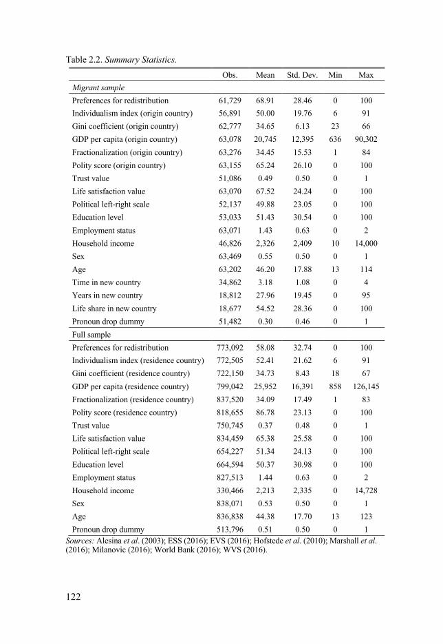
122

Table 2.2. Summary Statistics. Obs. Mean Std. Dev. Min Max

Migrant sample

Preferences for redistribution 61,729 68.91 28.46 0 100

Individualism index (origin country) 56,891 50.00 19.76 6 91

Gini coefficient (origin country) 62,777 34.65 6.13 23 66

GDP per capita (origin country) 63,078 20,745 12,395 636 90,302

Fractionalization (origin country) 63,276 34.45 15.53 1 84

Polity score (origin country) 63,155 65.24 26.10 0 100

Trust value 51,086 0.49 0.50 0 1

Life satisfaction value 63,070 67.52 24.24 0 100

Political left-right scale 52,137 49.88 23.05 0 100

Education level 53,033 51.43 30.54 0 100

Employment status 63,071 1.43 0.63 0 2

Household income 46,826 2,326 2,409 10 14,000

Sex 63,469 0.55 0.50 0 1

Age 63,202 46.20 17.88 13 114

Time in new country 34,862 3.18 1.08 0 4

Years in new country 18,812 27.96 19.45 0 95

Life share in new country 18,677 54.52 28.36 0 100

Pronoun drop dummy 51,482 0.30 0.46 0 1

Full sample

Preferences for redistribution 773,092 58.08 32.74 0 100

Individualism index (residence country) 772,505 52.41 21.62 6 91

Gini coefficient (residence country) 722,150 34.73 8.43 18 67

GDP per capita (residence country) 799,042 25,952 16,391 858 126,145

Fractionalization (residence country) 837,520 34.09 17.49 1 83

Polity score (residence country) 818,655 86.78 23.13 0 100

Trust value 750,745 0.37 0.48 0 1

Life satisfaction value 834,459 65.38 25.58 0 100

Political left-right scale 654,227 51.34 24.13 0 100

Education level 664,594 50.37 30.98 0 100

Employment status 827,513 1.44 0.63 0 2

Household income 330,466 2,213 2,335 0 14,728

Sex 838,071 0.53 0.50 0 1

Age 836,838 44.38 17.70 13 123

Pronoun drop dummy 513,796 0.51 0.50 0 1 Sources: Alesina et al. (2003); ESS (2016); EVS (2016); Hofstede et al. (2010); Marshall et al. (2016); Milanovic (2016); World Bank (2016); WVS (2016).

123

From Table 2.2, the immigrant sample seems fairly representative for the full sample, even though it covers a smaller sample of residence countries and years. Pairwise correlations for the individual and country-of-origin-level characteristics are presented in Table 2.A1 in the Appendix. These correla-tions indicate that, on the individual level, preferences for more equal income distributions seem to be correlated with higher trust, lower life satisfaction, more left-wing political preferences, lower educational, employment and in-come levels, time spent in the new country, and being female and older. On the country level, focusing on the cultural component, individual preferences for redistribution and equality seem to be negatively related to individualism, social trust, actual income equality, GDP per capita, fractionalization and democratic rights in the immigrants’ country of origin. The correlation be-tween individualism index in country of origin and individual preferences for redistribution is illustrated in the binned scatterplot in Figure 2.2 (correspond-ing correlations separated into the different immigrant samples are shown in Figure 2.A3 in the Appendix). However, these are only simple correlations and, hence, I turn now to the regression results.

Figure 2.2. Correlation between Cultural Individualism and Individual Preferences for Redistribution: Binned Scatterplot.

Sources: ESS (2016); EVS (2016); Hofstede et al. (2010); WVS (2016).

124

2.4 Main Results

2.4.1 Relation between Individualism and Redistributive Preferences

I first run a standard OLS regression estimating individuals’ preferences for redistribution by the level of individualism in their country of residence (in-cluding the full sample of both immigrants and non-immigrants) and a set of individual and country-level controls. These results are presented in Table 2.A2 in the Appendix (together with the same estimation using ordered lo-gistic and ordered probit regressions, respectively, instead of OLS), and show a negative and statistically significant relationship between individualism and preferences for redistribution also when controlling for a large number of in-dividual and country-of-residence-level characteristics. Most of the individual variables also remain statistically significant and in the same direction as the pairwise correlations, except for trust, which is now found to have a negative conditional correlation with redistributive preferences. When controlling for the other variables, income inequality in the country of residence is positively related to preferences for redistribution and equality, while country- of-resi-dence-level income has a positive, but not statistically significant, association with preferences for income redistribution.

However, since all individuals living in a country are assumed to have the same individualism-collectivism cultural beliefs in the regression above, I cannot control for country fixed effects, and this specification could poten-tially suffer from a number of endogeneity issues. Thus, I now turn to the epidemiological approach, exploiting variation in immigrants’ country of origin to better capture variation in the cultural dimension of individualism versus collectivism within the country of residence, i.e., applying country-of-residence fixed effects to control for the economic and institutional environ-ment in which these individuals live. In particular, this should solve for any unobservable characteristics at the country-of-residence level, as well as for potential reverse causality since the individual preferences of a person living in a new country are not very likely to affect the individualism-collectivism ranking of his or her country of origin. These OLS regression results are pre-sented in Table 2.3.36

36 Running ordered logit or probit regressions instead of OLS yields qualitatively the same re-sults (results available upon request).

125

Table 2.3. Baseline OLS Regression Results, Immigrant Sample. Preferences for redistribution (1) (2) (3) Std. Coef. Origin country Individualism index –0.057*** –0.068*** –0.081*** –0.049*** (0.018) (0.025) (0.027) (0.017)

Gini coefficient –0.074 –0.015 –0.003 (0.057) (0.079) (0.015)

Log GDP per capita 0.672 –0.597 –0.014 (0.568) (0.879) (0.020)

Mean social trust 0.052 0.023 (0.035) (0.015)

Mean preferences for redistribution 0.015 0.004 (0.049) (0.014)

Fractionalization –0.064* –0.030*

(0.038) (0.018)

Polity score 0.030 0.024

(0.023) (0.019)

Individual characteristics Trust value 1.219 1.133 0.017 (0.838) (0.862) (0.013)

Life satisfaction value –0.054*** –0.060*** –0.047*** (0.014) (0.014) (0.011)

Political left–right scale –0.175*** –0.174*** –0.128*** (0.019) (0.019) (0.014)

Education level –0.080*** –0.078*** –0.074*** (0.013) (0.013) (0.012)

Employment status –0.674* –0.809** –0.016** (0.384) (0.388) (0.007)

Household income –0.001*** –0.001*** –0.052*** (0.000) (0.000) (0.014)

Time in new country 1.243*** 1.184*** 0.039*** (0.331) (0.337) (0.011)

Sex 2.584*** 1.847*** 1.929*** 0.029*** (0.207) (0.472) (0.480) (0.007)

Age 0.107*** 0.050*** 0.048*** 0.029*** (0.014) (0.018) (0.018) (0.010)

Residence country FE Yes Yes Yes Yes

Year FE Yes Yes Yes Yes

Number of obs. 55,085 12,143 11,805 11,805

I-squared 0.117 0.153 0.158 0.158

126

Notes: Robust standard errors clustered on origin country in parentheses; *! < 0.1, **! <0.05, ***! < 0.01.

Sources: Alesina et al. (2003); ESS (2016); EVS (2016); Hofstede et al. (2010); Marshall et al. (2016); Milanovic (2016); World Bank (2016); WVS (2016).

The results in Table 2.3 show a negative and statistically significant relation-ship between individualistic cultural beliefs in the country of origin and im-migrants’ preferences for income redistribution, even after controlling for their country of residence. That is, more individualistic cultures seem to be associated with less egalitarian values, where an increase of 10 percentage points on the individualism index is associated with a decrease of approxi-mately 0.6–0.8 percentage points on the preferences for redistribution scale. Also, preferences for redistribution are found to be statistically significantly related to having lower life satisfaction, political preferences more to the left, lower levels of education, employment and income, more years spent in the new country, and being female and old. It could also be noted that none of the other country-of-origin-level variables are statistically significant (except for fractionalization, which is marginally significant), when controlling for the cultural individualism impact. The last column of Table 2.3 shows the same results but where the values of all variables have been standardized to having mean 0 and standard deviation 1. In other words, a one standard deviation increase of the individualism index (which corresponds, e.g., to the difference between Sweden with an individualism index value of 71 and the United States with a value of 91) is associated with a 0.05 standard deviation decrease of the preferences for redistribution measure (corresponding roughly to, e.g., the difference between the average redistributive preferences value in Sweden, which is 62.3, and in Poland, which is 60.6). This standardized coefficient magnitude is similar to that of household income and the life satisfaction measure, and the only variables with larger standardized coefficients are po-litical preferences and the education level.

127

Figure 2.3. Estimated Impact of Individualism on Preferences for Redistribution by Immigrant Sample.

Note: Estimated standardized coefficients for individualism on preferences for redistribution, with 95 percent confidence intervals, controlling for origin country characteristics, individual characteristics, residence country and year fixed effects. Source: See Table 2.A5 in the Appendix.

2.4.2 Cultural Assimilation Analysis Separating the sample into first- and second-generation immigrants (see Sec-tion 2.5.2), the association between country-of-origin individualism and indi-vidual preferences for income inequality is not found statistically significant among second-generation immigrants. The corresponding results for an even finer division of the immigrant subsamples are shown in Table 2.A3 in the Appendix, and the standardized estimated coefficients of these regressions are illustrated in Figure 2.3. A potential explanation for this is that, with time spent in the new cultural environment, immigrants might also adapt the culture of their new country of residence (i.e., direct horizontal socialization, as opposed to vertical parental socialization; see, e.g., Bisin and Verdier, 2011). In order to further check whether or not this seems to be the case, I will, instead of the country-of-residence fixed effects, include the country-of-residence individu-alism index as well as income and inequality controls in my baseline regres-sion. Because such cultural assimilation is also likely to depend on the relative time that the individual has lived in the new environment, I will calculate the country-of-residence life-share as the total number of years lived in the

128

country-of- residence divided by the individual’s age. Since the number of observations for each year lived in the country is quite limited, I will group this variable into three categories: those immigrants that have lived i) less than one third, ii) between one and two thirds, and iii) more than two thirds of the life in the new country of residence. The results for these three groups are presented in Table 2.4 and illustrated by their standardized coefficient esti-mates in Figure 2.4.

Tabl

e 2.

4. C

ompa

ring

Cou

ntry

-of-O

rigin

ver

sus C

ount

ry-o

f-Res

iden

ce C

ultu

ral I

mpa

ct.

Pref

eren

ces f

or re

distr

ibut

ion

Li

fe sh

are

in re

side

nce

coun

try

(1

) (2

) (3

) <13⁄

13⁄ <23⁄

>23⁄ O

rigi

n co

untr

y

Indi

vidu

alism

inde

x –0

.083

***

–0.0

70**

–0

.070

* –0

.142

***

–0.0

98*

–0.0

38

(0

.017

) (0

.029

) (0

.036

) (0

.050

) (0

.052

) (0

.053

) G

ini c

oeffi

cien

t

–0.0

92

–0.0

92

–0.3

45**

* –0

.228

* –0

.130

(0

.061

) (0

.075

) (0

.112

) (0

.130

) (0

.126

) Lo

g G

DP

per c

apita

0.61

9 –0

.275

0.

929

2.03

9 –0

.385

(0

.818

) (0

.976

) (1

.459

) (1

.586

) (1

.519

) M

ean

soci

al tr

ust

–0.0

10

(0.0

47)

Frac

tiona

lizat

ion

–0.0

79*

(0.0

44)

Po

lity

scor

e

0.

027

(0.0

28)

Resi

denc

e co

untr

y

Indi

vidu

alism

inde

x –0

.203

***

–0.1

38**

* –0

.123

***

–0.1

13

–0.1

80**

–0

.267

***

(0

.031

) (0

.037

) (0

.043

) (0

.073

) (0

.083

) (0

.061

) G

ini c

oeffi

cien

t

0.69

6***

0.

627*

**

0.58

9*

0.69

4***

0.

318*

*

(0

.121

) (0

.119

) (0

.328

) (0

.224

) (0

.156

) Lo

g G

DP

per c

apita

–2.7

46

–3.0

70

–6.5

01*

1.27

8 3.

347

(1.9

62)

(2.1

34)

(3.6

11)

(4.4

92)

(3.6

48)

Mea

n so

cial

trus

t

–0

.001

(0

.039

)

Frac

tiona

lizat

ion

0.02

0

(0

.030

)

Polit

y sc

ore

–0.0

54

(0.0

99)

Indi

vidu

al c

hara

cter

istic

s

Tr

ust v

alue

1.66

4**

1.77

5**

2.47

7 –1

.485

–0

.400

(0

.753

) (0

.782

) (1

.696

) (1

.091

) (1

.119

) Li

fe sa

tisfa

ctio

n va

lue

–0

.064

***

–0.0

69**

* –0

.010

–0

.049

**

–0.0

43

(0.0

15)

(0.0

16)

(0.0

39)

(0.0

24)

(0.0

38)

Polit

ical

left–

right

scal

e

–0.1

75**

* –0

.171

***

–0.2

09**

* –0

.176

***

–0.1

37**

*

(0

.019

) (0

.020

) (0

.036

) (0

.032

) (0

.026

) Ed

ucat

ion

leve

l

–0.0

85**

* –0

.082

***

–0.0

10

–0.0

81**

* 0.

002

(0.0

15)

(0.0

15)

(0.0

27)

(0.0

23)

(0.0

24)

Empl

oym

ent s

tatu

s

–1.3

53**

* –1

.533

***

–1.3

66

0.59

4 –2

.800

**

(0.4

46)

(0.4

43)

(1.0

57)

(1.1

60)

(1.0

77)

Hou

seho

ld in

com

e

–0.0

01**

–0

.001

**

–0.0

01**

* –0

.001

***

–0.0

01*

(0.0

00)

(0.0

00)

(0.0

00)

(0.0

00)

(0.0

00)

Tim

e in

new

cou

ntry

0.87

2**

0.86

4**

(0

.336

) (0

.327

)

Sex

2.66

9***

1.

637*

**

1.72

7***

2.

623

1.87

7 1.

986*

(0.2

18)

(0.6

12)

(0.6

30)

(1.5

82)

(1.2

54)

(1.0

24)

Age

0.

125*

**

0.06

1**

0.05

4**

0.00

8 0.

079

0.07

1*

(0

.013

) (0

.025

) (0

.025

) (0

.071

) (0

.052

) (0

.039

) Re

siden

ce c

ount

ry F

E N

o N

o N

o N

o N

o N

o Y

ear F

E Y

es

Yes

Y

es

Yes

Y

es

Yes

N

umbe

r of o

bs.

52,7

67

8,75

9 8,

470

1,21

1 1,

503

1,96

0 -s

quar

ed

0.06

8 0.

136

0.13

9 0.

188

0.19

6 0.

281

Not

es: R

obus

t sta

ndar

d er

rors

clu

stere

d on

orig

in c

ount

ry in

par

enth

eses

; *<0.1,

**<0.05

, ***

<0.01.

132

While these cultural assimilation results are admittedly crude, I believe that they do give some support to the idea that immigrants are assimilated or adapted to their new cultural environment quite “rapidly”, i.e., after spending approximately the same amount of time in the new country as spent in the origin country. Moreover, the country of residence impact seems to be rela-tively stronger, with a coefficient size that is almost the double, compared to the culture of origin impact.

Figure 2.4. Comparing Country-of-Origin versus Country-of-Residence Impact of Individualism on Preferences for Redistribution.

Note: Estimated standardized coefficients for individualism on preferences for redistribution, with 95 percent confidence intervals, controlling for origin country characteristics, residence country characteristics, individual characteristics and year fixed effects. Source: See Table 2.7.

Finally, I will also perform the same cultural assimilation analysis as above, but instead separating the sample by the individuals’ age when they migrated. These results are presented in Figure 2.5, and indicate that there seems to be no statistically significant impact of the culture of origin on current prefer-ences for redistribution if migration took place approximately before the age of 10. Culture in the current country of residence, however, seems to have a statistically significant impact regardless of the age at migration.

133

2.5 Robustness Checks

2.5.1 Pronoun-Drop IV Approach

Although none of the included country-of-origin controls are significant in the OLS regressions above, it could still be the case that there are some other omitted or unobserved variables driving the results. As an alternative strategy, I will thus use the pronoun-drop dummy as an instrument for individualism versus collectivism, i.e., to check whether it is actually individualism, rather than some other cultural variable in the country of origin, that drives the re-sults. The assumption here is that the grammatical rule on pronoun drop af-fects preferences for redistribution only through its language-culture relation-ship, i.e., through its association with individualistic-collectivistic cultural be-liefs. The results from these two-stage least squares (2SLS) regressions are shown in Table 2.5, where I have used the individual responses to the "lan-guage at home" question in the WVS (2016), the EVS (2016) and the ESS (2016), combined with pronoun-drop information from Abdurazokzoda and Davis (2016)’s new linguistic dataset.

134

Table 2.5. IV Regression Results, Immigrant Sample.

Individualism

(origin)

Preferences for

redistribution

Individualism

(origin)

Preferences for

redistribution (1) (1) (2) (2) 1st stage 2nd stage 1st stage 2nd stage Individualism (origin) –0.355*** –0.279***

(0.065) (0.098)

Pronoun drop dummy –12.168*** –9.483***

(4.085) (3.100)

Residence country

Gini coefficient –0.593*** 0.656*** (0.214) (0.146)

Log GDP per capita 12.188*** –6.457*** (2.943) (2.134)

Individual characteristics

Trust value 0.515 –0.889 (0.664) (0.545)

Life satisfaction value 0.030* –0.036*** (0.016) (0.011)

Political left–right scale –0.002 –0.179*** (0.011) (0.023)

Education level 0.014 –0.044*** (0.024) (0.010)

Employment status –0.483 –0.450 (0.482) (0.443)

Household income 0.000*** –0.001*** (0.000) (0.000)

Sex –0.210 1.618*** (0.438) (0.569)

Age 0.106*** 0.129*** (0.034) (0.022)

Number of obs. 45,129 45,129 13,130 13,130

!-squared 0.079 0.195

Notes: Robust standard errors clustered on origin country in parentheses; *" < 0.1, **" <0.05, ***" < 0.01. Individualism index (IDV) measured in country of origin, and pronoun drop dummy for home language. Sources: Abdurazokzoda and Davis (2016); ESS (2016); EVS (2016); Hofstede et al. (2010); Milanovic (2016); World Bank (2016); WVS (2016).

135

The 2SLS regression results in Table 2.5 show that i) the pronoun drop seems to be a valid instrument for individualism-collectivism in the respect that it is negatively and statistically significantly related to the individualism index, and ii) using this instrument confirms the baseline results of a statistically sig-nificant negative association between individualism and an individual’s pref-erences for redistribution. Here, the estimated impact is even stronger than for the OLS results, indicating that an increase of 10 percentage points on the individualism index is associated with a decrease of approximately 3 percent-age points on the preferences for redistribution scale. Moreover, since the baseline results are confirmed also when using this alternative individualism-collectivism measure, potential measurement error in the main survey-based individualism index does not seem to be driving the results.

2.5.2 Heterogeneity Analyses

Using the epidemiological approach, another robustness check includes ana-lyzing the different surveys separately (see Table 2.A4 in the Appendix). The results hold for both surveys separately, but the individualism coefficient size is somewhat larger for the integrated EVS (2016) and WVS (2016) sample than for the ESS (2016). Since the wording of the survey question differs be-tween these two samples, this indicates that the association between individu-alism and preferences for equality is slightly stronger than the association with preferences for redistribution.

Furthermore, I can also analyze the impact within different immigrant sub-samples. These results are presented in Table 2.6.

Tabl

e 2.

6. H

eter

ogen

eity

Ana

lysis

, Diff

eren

t Im

mig

rant

Sam

ples

.

Pref

eren

ces f

or re

distr

ibut

ion

Mor

e in

divi

dual

ist

orig

in

Mor

e co

llect

ivis

t or

igin

Be

twee

n-re

gion

m

igra

tion

With

in-r

egio

n m

igra

tion

1st-g

ener

atio

n im

mig

rant

2n

d-ge

nera

tion

imm

igra

nt

Ori

gin

coun

try

Indi

vidu

alism

inde

x –0

.180

***

–0.0

69**

–0

.078

***

–0.0

65*

–0.0

65**

–0

.035

(0.0

46)

(0.0

34)

(0.0

29)

(0.0

38)

(0.0

26)

(0.0

32)

Gin

i coe

ffici

ent

–0.1

39

–0.0

47

0.00

9 –0

.042

–0

.067

0.

016

(0

.148

) (0

.058

) (0

.067

) (0

.116

) (0

.054

) (0

.084

) Lo

g G

DP

per c

apita

6.

255*

**

0.39

5 –0

.803

1.

451

0.51

0 0.

321

(1

.551

) (0

.547

) (0

.737

) (1

.663

) (0

.572

) (0

.698

)

Indi

vidu

al c

hara

cter

istic

s

Tr

ust v

alue

0.

360

1.45

3 2.

179*

* 0.

727

1.08

5 –0

.092

(0.8

37)

(0.9

95)

(0.9

73)

(1.0

83)

(0.7

86)

(0.5

88)

Life

satis

fact

ion

valu

e –0

.077

**

–0.0

47**

* 0.

008

–0.0

85**

* –0

.058

***

–0.0

84**

*

(0.0

31)

(0.0

14)

(0.0

23)

(0.0

20)

(0.0

13)

(0.0

14)

Polit

ical

left–

right

scal

e –0

.206

***

–0.1

65**

* –0

.146

***

–0.1

96**

* –0

.179

***

–0.1

87**

*

(0.0

26)

(0.0

25)

(0.0

23)

(0.0

22)

(0.0

19)

(0.0

25)

Educ

atio

n le

vel

–0.0

86**

* –0

.075

***

–0.0

45**

* –0

.092

***

–0.0

86**

* –0

.085

***

(0

.021

) (0

.015

) (0

.014

) (0

.016

) (0

.011

) (0

.012

) Em

ploy

men

t sta

tus

–0.3

20

–0.7

83

–1.0

11

–0.5

12

–0.7

87*

–0.5

70

(0

.625

) (0

.483

) (0

.674

) (0

.399

) (0

.439

) (0

.477

) H

ouse

hold

inco

me

–0.0

01**

–0

.001

***

–0.0

01**

* –0

.001

* –0

.001

***

–0.0

01**

*

(0.0

00)

(0.0

00)

(0.0

00)

(0.0

00)

(0.0

00)

(0.0

00)

Tim

e in

new

cou

ntry

0.

629

1.36

2***

2.

166*

**

0.89

8**

(0

.492

) (0

.445

) (0

.511

) (0

.407

)

Sex

2.77

1***

1.

717*

**

1.40

5 2.

004*

**

1.93

0***

2.

730*

**

(0

.951

) (0

.549

) (0

.881

) (0

.557

) (0

.411

) (0

.526

) A

ge

0.07

3*

0.05

4**

0.01

0 0.

065*

* 0.

097*

**

0.10

0***

(0.0

38)

(0.0

23)

(0.0

27)

(0.0

24)

(0.0

15)

(0.0

18)

Resid

ence

cou

ntry

FE

Yes

Y

es

Yes

Y

es

Yes

Y

es

Yea

r FE

Yes

Y

es

Yes

Y

es

Yes

Y

es

Num

ber o

f obs

. 3,

349

8,73

6 3,

919

8,22

4 13

,161

10

,705

-s

quar

ed

0.20

6 0.

139

0.15

6 0.

157

0.16

0 0.

182

Not

es: R

obus

t sta

ndar

d er

rors

clu

stere

d on

orig

in c

ount

ry in

par

enth

eses

; *<0.1,

**<0.05

, ***

<0.01.

138

The results in Table 2.6 show that the negative relation between individualism and preferences for income redistribution is robust to looking separately on immigrants who have emigrated from a more individualistic culture relative to their country of destination, as well as from a relatively more collectivistic culture, respectively; from another country within the same geographical re-gion, and those who have emigrated from another geographical region, respec-tively.37 The relationship, however, is strongest among those who have mi-grated from one region to another, and to a relatively more collectivist region. The association is also robust to looking only on the sample of first-generation immigrants (i.e., those with another nationality and/or country of birth than their country of residence). Analyzing the sample of second-generation immi-grants separately, however, there seems to be no statistically significant im-pact of individualism in the parents’ country of origin on their children’s pref-erences for redistribution. These results again indicate the existence of an as-similation or integration process such that the cultural impact of individualism on redistributive preferences is not persistent across generations and possibly weakens off with time spent in the new institutional and cultural environment. Notably, this insignificant relationship among the second-generation immi-grants is in contrast to what has been found by, e.g., Luttmer and Singhal (2011).

2.5.3 Matching Estimators As a final sensitivity analysis, I will also check if the results are robust to using matching as an alternative estimation strategy. I hence use the propensity-score matching method, where I compare individuals that are similar in a num-ber of observable characteristics but differ in their individualism versus col-lectivism cultural belonging. I thus create a dummy variable in which I define individuals that have a country-of-origin individualism index value above 50 as individualists and those with a value below 50 as collectivists. For a com-parison of the mean values in the two samples, see Table 2.A5 in the Appen-dix. The estimation results when matching and comparing immigrant individ-ualists to collectivists are shown in Table 2.7.

37 Using the United Nations’ classification of regions.

139

Table 2.7. Propensity-Score Matching Results, Immigrant Sample.

Preferences for redistribution ATE Individualist dummy –1.267** (0.569)

Number of obs. 26,743 Notes: Average treatment effects (ATE). Robust standard errors in parentheses; *! < 0.1, **! < 0.05, ***! < 0.01. Matching variables are individual-level trust value, life satisfaction value, political left–right scale, education level, employment status, household income, sex, age, and residence country FE. Sources: ESS (2016); EVS (2016); Hofstede et al. (2010); Milanovic (2016); World Bank (2016); WVS (2016).

As seen in Table 2.7, using this matching method I also find a negative and statistically significant relationship between individualism and preferences for redistribution. More specifically, the average treatment effect of having an in-dividualistic, as opposed to collectivistic, culture is a reduction of approxi-mately 1.3 percentage points on the preferences for redistribution scale.

2.6 Conclusion In this study, I have analyzed the association between individualism versus collectivism and individuals’ preferences for income redistribution and equal-ity, using variation in immigrants’ country of origin to separate the effect of culture from the otherwise endogenously determined institutional environ-ment. Doing so, I have found strong support for a negative relationship be-tween individualistic cultural beliefs and redistributive preferences, i.e., indi-vidualistic societies seem to foster preferences for income inequality. These results were confirmed using matching estimators as well as the grammatical rule on pronoun drop as a linguistic instrument for individualism-collectivism. Heterogeneity analyses also showed that the cultural impact of individualism on redistributive preferences is not significantly persistent over generations. Moreover, the impact of cultural origin only seems to be statistically signifi-cant if migration took place after the age of 10. More research would be needed in order to better understand the workings of such cultural adaption and its relation to institutional and cultural change. It would also be interesting to analyze the association between other cultural dimensions and egalitarian preferences, as well as the impact of individualism on actual redistribution and income equality.

140

References Abdurazokzoda, F. and Davis, L.S. (2016). ‘Language, culture and institutions: evi-

dence from a new linguistic dataset’, Journal of Comparative Economics, vol. 44, pp. 541–561.

Alesina, A. and Angeletos, G.-M. (2005). ‘Fairness and redistribution’, American Economic Review, vol. 95(4), pp. 960–980.

Alesina, A., Devleeschauwer, A., Easterly, W., Kurlat, S. and Wacziarg, R. (2003). ‘Fractionalization’, Journal of Economic Growth, vol. 8, pp. 155–194.

Alesina, A. and Fuchs-Schündeln, N. (2007). ‘Good-bye Lenin (or not?): the effect of communism on people’s preferences’, American Economic Review, vol. 97(4), pp. 1507–1528.

Alesina, A. and Giuliano, P. (2010). ‘The power of the family’, Journal of Economic Growth, vol. 15, pp. 93–125.

Alesina, A. and Giuliano, P. (2011). ‘Preferences for redistribution’, in (J. Benhabib, A. Bisin and M.O. Jackson, eds.), Handbook of Social Economics 1A, Amster-dam: North-Holland, pp. 93–132.

Alesina, A. and Giuliano, P. (2015). ‘Culture and institutions’, Journal of Economic Literature, vol. 53(4), pp. 898–944.

Almås, I., Cappelen, A.W., Sørensen, E.Ø. and Tungodden, B. (2020). ‘Fairness across the world: preferences and beliefs’, Presentation, IFN Brown Bag Seminar (May 11, 2020).

Bazzi, S., Fiszbein, M. and Gebresilasse, M. (2020). ‘Frontier culture: the roots and persistence of “rugged individualism” in the United States’, Econometrica, vol. 88(6), pp. 2329–2368.

Berggren, N., Ljunge, M. and Nilsson, T. (2019). ’Roots of tolerance among second-generation immigrants’, Journal of Institutional Economics, vol. 15, pp. 999–1016.

Bergh, A. and Bjørnskov, C. (2014). ‘Trust, welfare states and income equality: sort-ing out the causality’, European Journal of Political Economy, vol. 35, pp. 183–199.

Bisin, A. and Verdier, T. (2011). ‘The economics of cultural transmission and social-ization’, in (J. Benhabib, A. Bisin and M.O. Jackson, eds.), Handbook of Social Economics 1A, Amsterdam: North-Holland, pp. 339–416.

Dinesen, P.T. (2012). ‘Does generalized (dis)trust travel? examining the impact of cultural heritage and destination-country environment on trust of immigrants’, Political Psychology, vol. 33(4), pp. 495–511.

European Social Survey (2016). ‘European social survey’, http://www.europeanso-cialsurvey.org (last accessed: January 4, 2017).

European Values Study (2016). ‘European values study’, http://www.europeanval-uesstudy.eu (last accessed: September 12, 2016).

Fernández, R. (2011). ‘Does culture matter?’, in (J. Benhabib, A. Bisin and M.O. Jackson, eds.), Handbook of Social Economics, vol. 1A, pp. 481–510, Amster-dam: North-Holland.

Giuliano, P. and Spilimbergo, A. (2014). ‘Growing up in a recession’, Review of Eco-nomic Studies, vol. 81, pp. 787–817.

Gorodnichenko, Y. and Roland, G. (2011). ‘Which dimensions of culture matter for long-run growth?’, American Economic Review: Papers & Proceedings, vol. 101 (3), pp. 492–498.

141

Gorodnichenko, Y. and Roland, G. (2012). ‘Understanding the individualism-collec-tivism cleavage and its effects: lessons from cultural psychology’, in (M. Aoki, T. Kuran and G. Roland, eds.), Institutions and Comparative Economic Develop-ment, New York: Palgrave Macmillan, pp. 213–236.

Gorodnichenko, Y. and Roland, G. (2017). ‘Culture, institutions, and the wealth of nations’, Review of Economics and Statistics, vol. 99 (3), pp. 402–416.

Gorodnichenko, Y. and Roland, G. (2020). ‘Culture, institutions and democratiza-tion’. Public Choice, forthcoming.

Greif, A. (1994). ‘Cultural beliefs and the organization of society: a historical and theoretical reflection on collectivist and individualist societies’, Journal of Polit-ical Economy, vol. 102(5), pp. 912–950.

Guiso, L., Sapienza, P. and Zingales, L. (2006). ‘Does culture affect economic out-comes?’, Journal of Economic Perspectives, vol. 20(2), pp. 23–48.

Heine, S.J. (2020). Cultural Psychology, 4th ed., New York: W. W. Norton & Com-pany.

Hofstede, G., Hofstede, G. J. and Minkov, M. (2010). Cultures and Organizations: Software of the Mind, 3rd ed., New York: McGraw-Hill.

Hofstede, G. and Minkov, M. (2013). Values Survey Module (VSM) 2013 Manual. Kashima, E.S. and Kashima, Y. (1998). ‘Culture and language: the case of cultural

dimensions and personal pronoun use’, Journal of Cross-Cultural Psychology, vol. 29(3), pp. 461–486.

Licht, A.N., Goldschmidt, C. and Schwartz, S.H. (2007). ‘Culture rules: the founda-tions of the rule of law and other norms of governance’, Journal of Comparative Economics, vol. 35, pp. 659–688.

Ljunge, M. (2017). ‘Cultural determinants of gender roles: “pragmatism” as an under-pinning attitude toward gender equality among children of immigrants’, in (J. Costa-Font and M. Macis, eds.), Social Economics: Current and Emerging Ave-nues, Cambridge: MIT Press, pp. 197–232.

Luttmer, E.F.P. and Singhal, M. (2011). ‘Culture, context, and the taste for redistri-bution’, American Economic Journal: Economic Policy, vol. 3(1), pp. 157–179.

Marshall, M.G., Gurr, T.R. and Jaggers, K. (2016). ‘Polity IV project: political regime characteristics and transitions, 1800–2015’, http://www.systemicpeace.org/in-scrdata.html (last accessed: May 30, 2017).

Milanovic, B. (2016). ‘All the Ginis dataset’, https://www.gc.cuny.edu/Page-Ele-ments/Academics-Research-Centers-Initiatives/Centers-and-Institutes/Stone-Center-on-Socio-Economic-Inequality/Core-Faculty,-Team,-and-Affiliated-LIS-Scholars/Branko-Milanovic/Datasets (last accessed: January 5, 2017).

North, D.C. (1991). ‘Institutions’, Journal of Economic Perspectives, vol. 5(1), pp. 97–112.

Olivera, J. (2015). ‘Preferences for redistribution in Europe’, IZA Journal of European Labor Studies, vol. 4(14).

Schmidt-Catran, A.W. (2016). ‘Economic inequality and public demand for redistri-bution: combining cross-sectional and longitudinal evidence’, Socio-Economic Review, vol. 14(1), pp. 119–140.

Tabellini, G. (2008). ‘Institutions and culture’, Journal of the European Economic Association, vol. 6(2–3), pp. 255–294.

Williamson, O.E. (2000). ‘The new institutional economics: taking stock, looking ahead’, Journal of Economic Literature, vol. 38, pp. 595–613.

World Bank (2016). ‘World development indicators’, http://databank.worldbank.org (last accessed: January 5, 2017).

World Values Survey (2016). ‘World values survey’, http://www.worldvaluessur-vey.org/wvs.jsp (last accessed: September 12, 2016).

142

Appendix 2.A

Figure 2.A1. Mean Preferences for Redistribution around the World.

Sources: ESS (2016); EVS (2016); WVS (2016).

Figure 2.A2. Mean Pronoun Drop around the World.

Source: Abdurazokzoda and Davis (2016).

143

Figure 2.A3. Correlation between Individualism and Preferences for Redistribution by Cultural Origin Source: Binned Scatterplots.

Note: Bins based on a) 13,374, b) 28,806, c) 37,119 and d) 37,963 observations in total. Sources: ESS (2016); EVS (2016); Hofstede et al. (2010); WVS (2016).

144

Table 2.A1. Correlation Matrix.

Pref’s for redist.

IDV (origin)

Mean social trust (origin)

Mean pref’s for redist (origin)

Origin country

Individualism index –0.080***

Mean social trust –0.081*** 0.608***

Mean pref’s for redist. 0.002 0.119*** 0.225***

Gini coefficient 0.015*** –0.237*** –0.353*** –0.227***

Log GDP per capita –0.068*** 0.706*** 0.600*** 0.475***

Fractionalization –0.018** –0.234*** –0.112*** –0.347***

Polity score –0.091*** 0.612*** 0.496*** 0.414***

Individual characteristics

Trust value 0.054*** 0.134*** 0.196*** –0.020***

Life satisfaction value –0.051*** 0.148*** 0.138*** 0.004

Political left–right scale –0.131*** –0.016*** 0.007 –0.037***

Education level –0.143*** 0.057*** 0.106*** –0.018***

Employment status –0.069*** 0.029*** 0.055*** 0.026***

Household income –0.089*** 0.168*** 0.188*** 0.041***

Time in new country 0.077*** 0.031*** 0.068*** 0.017***

Sex 0.050*** –0.011*** 0.003 –0.005

Age 0.122*** 0.055*** 0.035*** 0.019*** Note: *! < 0.1, **! < 0.05, ***! < 0.01. Sources: Alesina et al. (2003); ESS (2016); EVS (2016); Hofstede et al. (2010); Marshall et al. (2016); Milanovic (2016); World Bank (2016); WVS (2016).

145

Table 2.A2. OLS, Ordered Logistic and Ordered Probit Regression Results, Full Sample.

Preferences for redistribution OLS Ordered logit Ordered probit Residence country

Individualism index –0.144*** –0.010*** –0.006*** (0.006) (0.000) (0.000)

Gini coefficient 0.262*** 0.017*** 0.010*** (0.018) (0.001) (0.001)

Log GDP per capita 0.362 –0.006 0.006 (0.229) (0.015) (0.009)

Individual characteristics

Trust value –0.395** –0.045*** –0.024*** (0.156) (0.010) (0.006)

Life satisfaction value –0.089*** –0.007*** –0.004*** (0.004) (0.000) (0.000)

Political left–right scale –0.181*** –0.012*** –0.007*** (0.003) (0.000) (0.000)

Education level –0.111*** –0.007*** –0.004*** (0.003) (0.000) (0.000)

Employment status –1.148*** –0.075*** –0.044*** (0.130) (0.009) (0.005)

Household income –0.001*** 0.000*** 0.000*** (0.000) (0.000) (0.000)

Sex 2.656*** 0.154*** 0.092*** (0.144) (0.009) (0.006)

Age 0.055*** 0.004*** 0.002*** (0.004) (0.000) (0.000)

Residence country FE No No No

Year FE Yes Yes Yes

Number of obs. 147,110 147,110 147,110

'-squared 0.146 0.037 0.036 Notes: Robust standard errors in parentheses; *! < 0.1, **! < 0.05, ***! < 0.01. Sources: ESS (2016); EVS (2016); Hofstede et al. (2010); Milanovic (2016); World Bank (2016); WVS (2016).

146

Table 2.A3. Sensitivity Analysis, Different Immigrant Samples. Preferences for redistribution

Citizen- ship

Birth country

Mother’s origin

Father’s origin

Origin country

Individualism index –0.098** –0.065** –0.035 –0.026 (0.043) (0.027) (0.023) (0.024)

Gini coefficient –0.165** –0.062 –0.040 –0.048 (0.082) (0.060) (0.056) (0.058)

Log GDP per capita 0.597 0.574 0.535 0.229 (1.232) (0.639) (0.573) (0.583)

Individual characteristics

Trust value 0.499 1.142 0.476 0.163 (1.016) (0.752) (0.615) (0.750)

Life satisfaction value –0.062*** –0.055*** –0.066*** –0.070*** (0.022) (0.012) (0.016) (0.014)

Political left–right scale –0.201*** –0.176*** –0.168*** –0.170*** (0.025) (0.019) (0.020) (0.021)

Education level –0.091*** –0.084*** –0.085*** –0.081*** (0.013) (0.012) (0.012) (0.013)

Employment status –0.096 –0.699* –0.466 –0.597 (0.516) (0.396) (0.372) (0.420)

Household income –0.001*** –0.001*** –0.001*** –0.001*** (0.000) (0.000) (0.000) (0.000)

Sex 1.512** 1.976*** 2.117*** 2.568*** (0.719) (0.482) (0.383) (0.408)

Age 0.107*** 0.087*** 0.080*** 0.081*** (0.019) (0.018) (0.015) (0.014)

Residence country FE Yes Yes Yes Yes

Year FE Yes Yes Yes Yes

Number of obs. 5,662 12,110 15,976 16,360

'-squared 0.173 0.153 0.168 0.163 Notes: Robust standard errors clustered on origin country in parentheses; *! < 0.1, **! <0.05, ***! < 0.01. Sources: ESS (2016); EVS (2016); Hofstede et al. (2010); Milanovic (2016); World Bank (2016); WVS (2016).

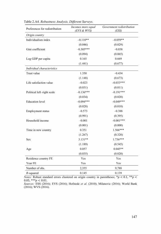
147

Table 2.A4. Robustness Analysis, Different Surveys.

Preferences for redistribution Incomes more equal (EVS & WVS)

Government redistribution (ESS)

Origin country

Individualism index –0.110** –0.059** (0.046) (0.029)

Gini coefficient –0.305*** –0.038 (0.094) (0.065)

Log GDP per capita 0.165 0.669 (1.441) (0.677)

Individual characteristics

Trust value 1.350 –0.434 (1.148) (0.673)

Life satisfaction value –0.023 –0.033*** (0.031) (0.011)

Political left–right scale –0.136*** –0.191*** (0.034) (0.020)

Education level –0.094*** –0.049*** (0.028) (0.010)

Employment status –0.573 –0.388 (0.991) (0.395)

Household income –0.001 –0.001*** (0.001) (0.000)

Time in new country 0.351 1.566*** (1.267) (0.320)

Sex 3.131** 1.736*** (1.189) (0.545)

Age 0.057 0.045** (0.035) (0.020)

Residence country FE Yes Yes

Year FE Yes Yes

Number of obs. 2,355 9,788

'-squared 0.145 0.139 Notes: Robust standard errors clustered on origin country in parentheses; *! < 0.1, **! <0.05, ***! < 0.01. Sources: ESS (2016); EVS (2016); Hofstede et al. (2010); Milanovic (2016); World Bank (2016); WVS (2016).

148

Table 2.A5. Means Comparison, Immigrant Sample.

Sources: ESS (2016); EVS (2016); Hofstede et al. (2010).

Individualists (()* > 50) Collectivists (()* < 50) Obs. Mean Std. Dev. Obs. Mean Std. Dev. Preferences for redistribution 29,645 66.64 28.47 31,841 70.99 28.32

Individualism index (origin) 25,714 68.98 10.23 30,925 34.23 9.10

Trust value 24,589 0.54 0.50 26,303 0.43 0.50

Life satisfaction value 30,202 71.16 22.62 32,617 64.10 25.19

Political left–right scale 26,645 49.31 22.44 25,264 50.35 23.61

Education level 25,071 52.19 30.63 27,762 50.73 30.48

Employment status 30,131 1.44 0.62 32,690 1.42 0.64

Household income 23,348 2,660 2,562 23,320 1,988 2,193

Sex 30,332 0.55 0.50 32,885 0.56 0.50

Age 30,211 46.78 17.89 32,739 45.76 17.85

149

3. The Swedish Income Distribution, 1968–2016

with Paula Roth and Daniel Waldenström

Acknowledgments: We are grateful to Sebastian Escobar for important contri-butions to this project. Financial support from the Swedish Research Council and Urwitz’ Foundation is gratefully acknowledged. We thank seminar par-ticipants at IFN and Uppsala University for valuable comments.

150

3.1 Introduction The Swedish income distribution has attracted considerable attention among researchers and policymakers alike over the recent years. The interest stems partly from reports about rising inequality since the 1980s and discussions about the role of market liberalizations, privatizations and lowered tax pro-gressivity in this increase.38

One problem with the data underlying most estimates of income inequality trends in Sweden is that the comparability over time has not always been per-fect for several reasons. First, the official income distribution series produced by Statistics Sweden (SCB) begins only in 1975 and there are no annual ob-servations until the 1980s. Second, relatively small population samples have been surveyed in order to generate the estimates up until the 2010s, which could give rise to measurement errors related to sample size and top or bottom coverage. Third, several variables in the Swedish income tax registries are not fully comparable over time, which creates inconsistencies unless accounted for. For example, imputed income from owner-occupied housing was imputed in total taxable income according to a progressive scale up to 1990 but it was not imputed at all from 1991 onwards. Non-taxable benefits were not recorded before 1978 and some of them have been added gradually in the 1980s, 1990s and 2000s, potentially causing problems with the comparison of disposable income over time. Fourth, the 1991 tax reform brought several breaks in both variable definitions and collection routines, which potentially affected income inequality levels and trends.

In this paper, we present a new Swedish income distribution database that covers the full Swedish population in all years since 1968, the first year with electronic administrative registries in Sweden. The main contribution of the study is the development of this new population-wide registry database with individual and household incomes during 1968–2016. The database expands the current set of income inequality statistics by almost a decade, and adds over four decades of full-population inequality statistics. To construct our new database, we compile population and tax registers from the onset of electronic registers in 1968, covering both non-working spouses and children, which al-lows us to compute proper consumption households. Finally, we homogenize income, tax and transfer variables over all years in order to obtain consistent income inequality estimates. Naturally, some of these estimations contain problematic aspects, and we point out a number of areas where further work is needed.

Using our new database, we compute and present some preliminary results on Sweden’s income inequality trends over the past decades. The results are preliminary in the sense that the database is still not complete in all respects,

38 See, for example, Björklund and Freeman (1997), Lindbeck (1997), Björklund and Palme (2000), Roine and Waldenström (2008, 2010), and Björklund and Jäntti (2019).

151

with some additional adjustments and robustness checks of the measurement of a few income componentsare needed. The first main result is that our series confirm the main, U-shaped pattern of Swedish income inequality over the past half-century. The Gini coefficient for disposable income of equivalized households fell from 28 in 1968 down to 18 in 1983, increased in the early 1990s to 25 and thereafter further to 32 in 2007, a level around which it has remained ever since. The main factor driving the falling Gini coefficient in the 1970s was an equalization of labor earnings, which in turn was driven by in-creased female labor force participation and more equal earnings among all workers.39 The increase in inequality around the economic crisis of the early 1990s seems more driven by a smaller redistributive effect of taxes than by increased inequality in labor earnings. The inequality increase from 1995 on-wards is primarily driven by increased weight of relatively unequally distrib-uted capital incomes, muted somewhat by a slight fall in labor earnings ine-quality. Taxes reduced the Gini coefficient by around ten Gini points in all years since 1990, but with an increasing trend in the Gini coefficient this means that the relative redistributive effect of taxes decreased during this pe-riod. Cash benefits, taxable and non-taxable, has not contributed significantly to the evolution of the Swedish disposable-income Gini coefficient in any pe-riod during the past half-century.

We also examine the evolution of Swedish top incomes, previously studied by Roine and Waldenström (2008, 2010, 2012). Our series corroborate the previous patterns, but extend them in several dimensions. We offer the first series of top disposable income shares that are based on the same measurement approach as the previous pre-tax income shares. The results suggest a strong similarity in the evolution of pre- and post-tax top income shares, which is largely explained by the fact that capital incomes, and especially realized cap-ital gains, are part of both income concepts. During the last decades, top in-come shares were at low levels in the 1970s and 1980s, but increased rapidly in the 1990s and 2000s due to large increases in top capital incomes. As a token of the size of our new database, we even measure the share of incomes going to the top 100,000th in the population in terms of income, which is the 80–100 highest-earning individuals. Their share increased from about 0.1 (100 times the average income) before 1990 to 0.3–0.6 (300–600 times average income) in the latter part of the period.

The remainder of the paper is organized as follows. Section 3.2 describes the main sources of the database and computation approaches used. Section 3.3 outlines the main results of the income inequality trends, and Section 3.4 presents comparisons between our new series and previous series from Statis-tics Sweden and other researchers. Finally, Section 3.5 concludes.

39 We are at this point unable to separate between the relative role of wage compression and equal working hours, but the analysis in Björklund and Freeman (1997) suggests that hours mattered more.

152

3.2 Database Construction n this section, we describe the main steps in the construction of our new full-population individual database of income distribution statistics.

3.2.1 Population: Individuals and Households Up until the 2010s, the official Swedish income distribution data were based on household surveys in the so-called HINK (Inkomstfördelningsun-dersökningen), and later HEK (Hushållens ekonomi), surveys. These surveys sampled 10,000–20,000 adult individuals (about 0.2–0.4 percent of the popu-lation) and added all household members to the surveyed individuals. Income and tax information was collected from the Swedish tax register. From this, income inequality measures were estimated.

Our database covers everyone registered as living in Sweden, which con-sists of both citizens and non-citizens. We start out by compiling the full tax and population registers in order to construct homogeneous individual and household populations for each year since 1968. It is crucial to include both tax and population records since otherwise there would be serious coverage gaps for women, children and old-age retirees. Sweden had a relatively low female labor force participation up until the 1980s. In fact, before 1971, most married couples filed taxes jointly and only primary-earners were noted as taxpayers. Children did typically not file taxes before the 1990s when the tax reform changed the rules. Some old-age pensioners with only basic pension income (folkpension), were for administrative reasons not recorded as income earners in the tax registers despite receiving taxable pension income. The total Swedish population and its age distribution over the study period is shown in Figure 3.1.

153

Figure 3.1. Total Individual Population in Sweden, by Age, 1968–2016.

Note: Population data from the total population register (RTB), Censuses (Folk- och bos-tadsräkningar) and complementing household information from the income and tax register (IoT).

A specific contribution is the construction of households over the entire pe-riod. In the early decades, only tax-unit households (consisting of married cou-ples, and their children) are directly observed in the registers. In these house-holds non-married couples are treated as separate households, and adult chil-dren living at home are treated as a separate household from the parent’s household. As such, there are many challenges to constructing households from Swedish administrative registers before 2011, when the current Census-based “dwelling household” (or housekeeping units, basically consisting of all individuals that lives in the same house or apartment) was started being rec-orded thanks to the new apartment register, and especially before 1998, when a new household concept, the family-unit household (RTB-familj), was intro-duced. The family-unit household has the advantage of also identifying non-married couples with joint children, as well as adult children still living with their parents, within the same household. To improve these household defini-tions, and to construct a consistent series of both tax- and family-unit house-holds, we use data from the real property register (Fastighetsregistret), the multi-generation register (Flergenerationsregistret), the population Censuses in 1970, 1975, 1980, 1985, 1990 and 2011, as well as the apartment register (Lägenhetsregistret) since 2012. Our preferred household concept is the

154

family-unit household, since it has the advantages discussed above, and since it is observed over the whole period. In the following series, if nothing else is mentioned, this household definition will be our baseline.

The total number of households as well as the average household size in Sweden between 1968 and 2016 are shown in Figure 3.2. The database con-sists of 7.9 million individuals and 3.5 households in 1968, and 10.0 million individuals and 5.3 million households in 2016. In total, our dataset includes 428 million observations.

Figure 3.2. Total Swedish Household Population and Mean Household Size.

Note: Population data from the total population register (RTB), Censuses (Folk- och bos-tadsräkningar), the income and tax register (IoT), the real property register (Fastighetsregis-tret), the multi-generation register (Flergenerationsregistret) and the apartment register (Lägenhetsregistret).

Equivalizing households is common in income distribution analysis and equivalized family households are our primary income-earning unit when an-alyzing income inequality (we will study adult individuals when doing com-parisons with old top-income series, and in future analyses of labor earnings and gender decompositions). The reason to use equivalized households is that scale advantages prevail in household economics, which means that the aver-age incomes of multi-person households are higher than what a simple per-capita adjustment would suggest. When equivalizing household incomes, we use the common square-root equivalence scale, which means that the summed household income is divided by the square root of the number of household members (including children), and we then distribute this income equally to all household members.40

40 We have also used the equivalence scale that Statistics Sweden uses (based on a 2004 house-hold consumption survey analysis), as well as the OECD scale, which consist of somewhat different weightings of children. The results are practically identical to the ones we present. See Figure 3.A1 in the Appendix.

155

3.2.2 Incomes, Taxes and Transfers We use data from the Swedish income tax registries to study three main in-come concepts: i) pre-tax factor income, ii) pre-tax market income, and iii) post-tax-and-transfers disposable income. All of these income concepts in-clude all labor, business and capital incomes. Factor income is total income before all cash-based taxes and transfers, meaning that it also includes social security contributions, but excludes pensions and any benefits (taxable and non-taxable).41 Market income is pre-tax income after social securitycontri-butions, meaning that it instead includes pensions and taxable benefits.42 Fi-nally, disposable income is income after all taxes, and including any transfers (that is, both taxable and non-taxable benefits).43 In addition to these three main income concepts, we can also study their different sub-components, such as labor earnings or capital incomes (with or without realized capital gains), separately. The average, per-capita income for our different income concepts are shown in Figure 3.3.

Constructing comparable income concepts from the Swedish micro regis-tries over the period 1968–2016 is difficult. The reason is that incomes are defined according to legal requirements and tax-collection procedures rather than economic principles. The tax reform of 1991 brought several changes with respect to the collection of income micro data. For example, in-kind earn-ings remunerations (free meals, company car usage) were typically excluded from taxable earnings before 1991 but included thereafter. Realized capital gains were only partially taxable before the reform (long-term holdings were partly or fully exempt) but fully taxable thereafter. Income from owner-occu-pied housing was imputed in the official income measure before the reform but not afterwards. Income from interest earnings and dividends was not re-ported separately before 1988, and interest payments were split up and re-ported together with the different income sources to which they adhered (mortgage rent payments were deducted from housing income, farm loan ex-penses from farm income, other interest payments from capital income).44

There are also gaps in the availability of various register variables during certain periods that need to be addressed. Unemployment and sickness insur-ance transfers are not reported before 1974. For disposable income, non-taxed benefits are not reported in micro registries prior to 1978 and in subsequent years new benefits are added gradually with a timing that sometimes corre-sponds more to administrative collection routines than when the benefits in questions were actually introduced. For these components, we collect

41 Factor income = Capital income + Business income + Wages and salaries + Social security contributions. 42 Market income = Factor income – Social security contributions + Pensions + Taxable bene-fits. 43 Disposable income = Market income – Taxes + Non-taxable benefits. 44 In future extensions of this work, we plan to examine these definitional changes and their impact on the distributional outcomes.

156

information about macro sums in the government budget each year. Moreover, in some cases, the statutory rules for allocating these transfers are known. To allocate these components at the individual level, we use the macro sums and statutory rules.

We have thus made a number of adjustments to make incomes comparable over all years in our study period. While we have managed well in most of the major variables, some unresolved issues remain. One problem is the income-definition changes of the 1990–1991 tax reform. This reform extended the definition of taxable income and made previously non-taxed and non-reported benefits from meals and company cars and tax-exempt savings accounts a part of the income tax base. We are in the process of incorporating these pre-reform non-counted components into the incomes. Another case is imputed income from owner-occupied housing which we are in the process of calculatingho-mogeneously over the entire period.

Figure 3.3. Average Incomes in Sweden, 1968-2016.

Note: Income data from the income and tax register (IoT). Total Swedish population averages (per capita). Inflation-adjusted incomes.

3.3 Results This section presents income inequality trends in Sweden, 1968–2016. We begin with presenting the broad trends for the Gini coefficient among

157

equivalized family household incomes, for both disposable and pre-tax in-comes. We then decompose the Gini coefficients into their different income components. Thereafter, we present results for different top income shares, and their decompositions.

3.3.1 Inequality Trends Figure 3.4 shows the evolution of the Swedish income distribution measured as the Gini coefficient for disposable income of equivalized family house-holds. This figure shows that Sweden experienced a relatively drastic equali-zation of incomes from the late 1960s until the early 1980s, with the Gini co-efficient dropping ten points, from 28 to 18. The 1980s was a relatively stable period, with the Gini coefficient hovering around 20 over several years. The early 1990s saw a period of economic turmoil, resulting in the profound eco-nomic and financial crisis in 1991–1993, during which unemployment in-creased from two percent to twelve percent over just a couple of years. The Gini coefficient increased somewhat during this era, from 20 to 23–24 Gini points. However, the period from 1995to 2007 saw the sharpest increase in the Swedish disposable income Gini coefficient of almost ten points, from 23 to 32. From the late 2000s until 2016, the Gini coefficient has been at a stable level a bit above 30 Gini points.

158

Figure 3.4. Income Inequality in Sweden, 1968–2018.

Note: The figure shows full-population Gini coefficients for equivalized households in Sweden. Disposable income is defined as the sum of pre-tax labor, business and capital income (includ-ing realized capital gains) plus all taxed and non-taxed transfers and benefits, minus all personal taxes.

As mentioned above, the computation of households in the Swedish popula-tion registers is one of our important contributions when building this new full-population database. Our main household concept consists of families in-cluding both adult children living at home and non-married couples with joint children (regardless if their children still live at home or not). Adult individu-als would be another possible income-earning unit, which is the main unit in the Swedish tax system and also a unit that is sometimes used in inequality research. Figure 3.5 shows the Gini coefficient for disposable income when adult individuals is used. The level of inequality is markedly higher in the individual distribution during the entire period, which is in line with prior ex-pectations. The difference is relatively large in the 1960s and 1970s when the Gini coefficient for individuals falls more than the Gini coefficients for house-holds, which is partly explained by increased female labor force participation. In Figure 3.5 we also see the difference between using our modern family-household concept compared to the older married-household definition. The level of disposable income inequality is consistently lower for family house-holds, and since the 1990s the difference between the two household defini-tions is almost as large as that between family households and individuals.

159

Figure 3.5. Income Inequality in Sweden: Individuals versus Households.

Note: Disposable income is defined as the sum of pre-tax labor, business and capital income (including realized capital gains) plus all taxed and non-taxed transfers and benefits, minus all personal taxes.

Turning to the pre-tax income distribution, Figure 3.6 displays Gini coeffi-cients for our three main income concepts. Factor income is the sum of pre-tax labor earnings, including social security contributions and payroll taxes, business and capital incomes. Market income is the sum of pre-tax labor in-come, excluding social security contributions and payroll taxes but instead in-cluding pensions and taxable benefits, business and capital incomes. Looking at the graph, the trends in the Gini coefficient are quite different across income concepts. The factor-income Gini coefficient increases steadily during the 1970s and the 1980s, but then stabilizes at a high level from the 1990s to the 2010s. The market-income Gini coefficient is relatively flat during the 1970s and 1980s, and then increases gradually from the 1990s to the 2010s. The dis-posable-income Gini coefficient is lower than both pre-tax income Gini coef-ficients, but follows a similar trend as the market-income Gini coefficient, even if it exhibits a clearer decrease in the 1970s and a sharper increase in the 1990s and 2000s.

160

Figure 3.6. Inequality in Three Income Concepts: Factor, Market and Disposable In-come.

Note: Factor income is pre-tax labor (including social security contributions and payroll taxes), business and capital incomes. Market income is pre-tax labor (excluding social security contri-butions and payroll taxes, but including pensions and taxable benefits), business and capital incomes. Disposable income is post-tax market income plus non-taxable benefits.

3.3.2 Gini Coefficient Decompositions

We now turn to decomposing the Gini coefficient into the relative contribution of different income sources (earnings, business and capital income, pensions, taxes and transfers). We use the decomposition methodology of Frick et al. (2006) and Lerman and Yitzhaki (1985) and run the analysis on each of the three main income concepts studied above: factor income, market income and disposable income, for the full population of equivalized households. Figure 3.7 shows the factor income decomposition, where the Gini coefficient was increasing during the 1970s and 1980s. The decomposition shows that this increase was driven by labor earnings, mainly through higher social security contributions. The flat inequality level from the early 1990s masks a gradual decline in the contributions of labor earnings, shown in the contributions from both wages and salaries and from social security contributions, and a gradual increase in the contribution from capital income.

161

Figure 3.7. Factor Income Inequality Decomposition.

Note: The figure shows decomposition of the Gini coefficient in factor incomes of equivalized households in the full Swedish population using the method of Frick et al. (2006).

The market income Gini coefficient decreased in the 1970s and its decompo-sition in Figure 8 shows that it was mainly due to the contribution from earn-ings and in the early years also from business incomes. The increase in the Gini coefficient during the 1990s and 2000s are mainly driven by an increas-ing inequality-contribution from capital incomes, but to a small extent also from labor earnings. Pensions have on average a small contribution to the mar-ket income Gini coefficient, but it is interesting to note that it had an equaliz-ing effect in the middle of the 1970s but a clearly disequalizing effect from the 1990s onward. Whether this shift is associated with a higher relative im-portance of occupational pensions, increasingly in defined-contribution plans, is a question worthy of further inquiry.45

45 See Roine and Waldenström (2012) for an analysis of the role of realized capital gains for Swedish top income shares.

162

Figure 3.8. Market Income Inequality Decomposition.

Note: he figure shows decomposition of the Gini coefficient in market incomes of equivalized households in the full Swedish population using the method of Frick et al. (2006).

The decomposition of the Gini coefficient for disposable income, our main income concept of interest, is shown in Figure 3.9. Its time-series patterns re-semble those of the market income Gini coefficient decomposition, with the decreasing trend in the 1970s being largely driven by earnings and business income contributions and the increase in the post-1990 period largely reflect-ing the contribution from capital incomes. However, in addition to these gen-eral trends, Figure 3.9 reveals several other interesting results. One is that the redistribution contribution from income (and some other) taxes has been rela-tively constant over the entire 50-year period, hovering between a reducing effect on the Gini coefficient between 15 and 20 points. A notable jump in the contribution from taxes on the Gini coefficient is 1991, when it went from reducing the Gini coefficient by 20 points in 1990 to 12–13 points in 1991. This decreasing redistributive effect has been discussed previously, reflecting the intentions of the progressivity-reducing tax reform of 1991 in combination with the large realization of capital gains that are taxed by a flat 30 percent rate, even for high-income earners, instead of a much higher marginal income tax rate in 1990. Another result is the marginal importance of benefits, taxable as well as non-taxable, for the overall disposable income Gini coefficient. Non-taxable benefits are always redistributive, having a negative marginal contribution to the Gini coefficient in all years (although only around 2–3 Gini

163

points). By contrast, taxable benefits, mainly unemployment and sickness in-surance income, has had a slight positive impact on the Gini coefficient in several years and zero effect during several periods. Pensions have also had a small relative contribution, except around the early 1990s when it became no-table and positive, raising the Gini coefficient by around five points (at this time the Gini was between 20 and 25).

Figure 3.9.Disposable Income Inequality Decomposition.

Note: The figure shows decomposition of the Gini coefficient in disposable incomes of equiv-alized households in the full Swedish population using the method of Frick et al. (2006).

Digging deeper into the different income components, we can also look sepa-rately on the role played by realized capital gains as a part of capital incomes. Realized capital gains is sometimes included and sometimes excluded from the income concept in studies of income inequality. However, to include real-ized capital gains in studied incomes is problematic for several reasons. Most importantly, realized capital gains are highly transitory, reported on tax returns in a single year despite the fact that they often refer to incomes accruing during a longer period. In the case of sales of primary homes, this period can amount to several decades. Compressing such gradual capital gains into a single year’s income can result in a boost of the income of households and move them from the bottom or middle of the distribution to its very top during that single year. This results in larger income inequality during single years, and it can also

164

lead to spurious increasing trends in cross-sectional inequality just because the aggregate amounts of capital gains is increasing.46

Figure 3.10 shows the Gini coefficient for pre-tax market incomes when these either exclude or include realized capital gains. The reason for using market incomes at this stage is that subtracting both realized capital gains and the capital income taxes they are associated with is more difficult in the pre-1991 period when all incomes were jointly taxed. We plan to make such cal-culations in future versions of the paper. The figure shows that realized capital gains have little impact on the pre-tax Gini coefficient in the 1970s and 1980s, which relates to the low overall levels of asset price gains in the housing and financial markets during this period. By contrast, the 1990s, 2000s and 2010s are periods of considerable price increases in asset markets and in aggregate realized capital gains. The pre-tax Gini coefficient is clearly higher during this period when realized capital gains are included, between 2 and 5 Gini points, which roughly represents a 10 percent increase of the Gini coefficient.

Figure 3.10. The Role of Realized Capital Gains in Income Inequality.

Note: Total pre-tax market income consists of the sum of pre-tax labor, business and capital incomes plus taxed transfers (mainly unemployment and long-term sickness insurance income). The figure is for equivalized family households.

46 See Roine and Waldenström (2012) for an analysis of the role of realized capital gains for Swedish top income shares.

165

3.3.3 Top Income Shares Top income shares reflect a specific aspect of income inequality, namely the share of all incomes going to a certain share of the highest-earning individuals or households. Throughout, we will compute these shares using the population and incomes in our database, which means that the total income reference will be the one contained in the income tax registries, and no further adjustments will be made for exempt incomes such as in-kind incomes or tax-evaded in-comes. We will compute new top income shares in the pre-tax income distri-bution which replicate and extend the series produced by Roine and Walden-ström (2008, 2010). We will also present new long-run series of the post-tax and transfer top income shares.

Figure 3.11 displays the income share of the highest-earning top decile dis-played for the three pre- and post-tax income concepts reported above: factor income, market income and disposable income. The series exhibit a remarka-ble similarity in time series trends as the corresponding Gini coefficients in Figure 3.6. All series show flat or falling shares in the 1970s and 1980s, then increasing shares in the 1990s and 2000s, followed by a relatively flat trend in the 2010s. However, the levels are relatively spread out, with almost 10 per-centage points differences, where the factor-income top decile goes from 25 percent in the 1980s to almost 35 percent in the 2010s, and the disposable-income top decile share goes from 17 percent to 25 percent over the same years.

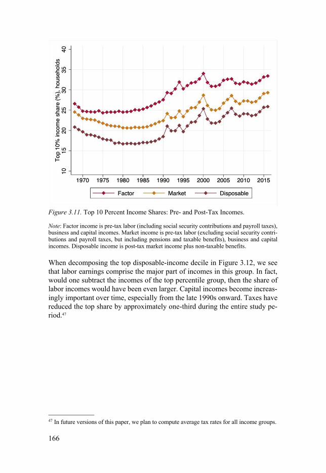
166

Figure 3.11. Top 10 Percent Income Shares: Pre- and Post-Tax Incomes.

Note: Factor income is pre-tax labor (including social security contributions and payroll taxes), business and capital incomes. Market income is pre-tax labor (excluding social security contri-butions and payroll taxes, but including pensions and taxable benefits), business and capital incomes. Disposable income is post-tax market income plus non-taxable benefits.

When decomposing the top disposable-income decile in Figure 3.12, we see that labor earnings comprise the major part of incomes in this group. In fact, would one subtract the incomes of the top percentile group, then the share of labor incomes would have been even larger. Capital incomes become increas-ingly important over time, especially from the late 1990s onward. Taxes have reduced the top share by approximately one-third during the entire study pe-riod.47

47 In future versions of this paper, we plan to compute average tax rates for all income groups.

167

Figure 3.12. Decomposing the Top 10 Percentiles Income Share.

Turning to the top 1 percent share of pre-tax market income and post-tax-and-transfer disposable income in Figure 3.13, the pattern looks broadly similar to the top decile in terms of time-series trends. The income share falls during the 1970s and is almost flat in the 1980s, then jump up sharply in 1991 and there-after continues to increase. The disposable-income top percentile share was down at three percent in the 1980s and has hovered between six and eight percent during the 2010.

168

Figure 3.13. Top 1 Percent Income Shares: Pre- and Post-Tax Incomes.

Note: Market income is pre-tax labor (excluding social security contributions and payroll taxes, but including pensions and taxable benefits), business and capital incomes. Disposable income is post-tax market income plus non-taxable benefit.

The composition of the top 1 percentile incomes is shown in Figure 3.14. The most striking difference with the top 10 percent incomes is the substantially larger relative importance of capital income in the top percentile over the re-cent years. From having comprised less than one-twentieth in the 1970s and 1980s, realized capital gains rose to represent approximately half of all top percentile income from the mid-1990s onward. Interest and dividend income have become increasingly important in the 2010s and represent one-third in 2016, which means that total capital income makes up two thirds of the top 1 percentile income today. The surge in dividend income during the late 2000s and 2010s is related to substantial tax cuts of dividend income in closely held corporations.48

48 For a discussion of the role of the tax changes referring to closely held corporations in 2006, and the possible effects on income shifting from labor to capital income among the owners of these firms, see Alstadsæter and Jacob (2016)).

169

Figure 3.14. Decomposing the Top 1 Percentile Income Share.

Finally, our population-wide data allow us to stretch the measurement of top income shares into the extreme top of the income distribution, the top 0.001 percentile—that is, the top 100,000th of the income distribution. This exclu-sive group comprises the 80–100 highest-earning individuals in the economy (although not necessarily being the same ones from one year to another), as measured by equivalized household incomes. Figure 3.15 shows an extraordi-nary increase in the share of incomes going to this small top group. From a share around 0.1 percent in the 1970s and 1980s, the share increased rapidly after 1995 to reach a peak level in the year 2000 of 0.8 percent, which is 800 times the average income and almost 1,000 times the median income. The share has been between 0.3 and 0.6 in the 2010s.

170

Figure 3.15. Top 0.001 Percent Income Share: Pre- and Post-Tax Incomes.

Note: Factor income is pre-tax labor (including social security contributions and payroll taxes), business and capital incomes. Market income is pre-tax labor (excluding social security contri-butions and payroll taxes, but including pensions and taxable benefits), business and capital incomes. Disposable income is post-tax market income plus non-taxable benefits.

Looking at the income composition of the top 0.001 percentile group in Figure 3.16, the role of capital income among top income earners is taken to the ex-treme. Virtually all income in this small group is capital income. Realized capital gains comprise most of this for most years, which indicates that the transitory income component in this group is relatively large. However, divi-dend income has become notably larger in this top group since the mid-2000s.

171

Figure 3.16. Decomposing the Top 0.001 Percentile Income Share.

3.4 Comparison with Previous Series One important aspect of the analysis of our new income database is how the inequality estimates it produces stand up against the official series of Statistics Sweden (SCB). Over time, different series have been used, mainly depending on the quality of household information. Up until the 2010s, the household survey HINK (Inkomstfördelningsundersökningen), later renamed HEK (Hushållens ekonomi), was used. This survey used income data from the same registries as we use, but the households were generated from telephone inter-views and as a sample, whereas our households are fully register-generated and have full-population coverage.49 From 2011, Statistics Sweden has used the new apartment register (Lägenhetsregistret) to create a full-population in-come database (Inkomster och skatter, IoS). Figure 3.17 compares the dispos-able-income Gini coefficient for equivalized households in our database with the different series from Statistics Sweden.

49 For a longer discussion, see Björklund (1998) and Björklund and Jäntti (2019).

172

Figure 3.17. Gini Coefficient Comparison with Statistics Sweden.

Note: Gini coefficients showing disposable income inequality for equivalized households. “Hammar, Roth and Waldenström” refers to this study; IoS to Inkomster och skatter; and HEK to Hushållens ekonomi. The new HEK series includes adjustments for the 1991 tax reform in-come base broadening. Note that some variation in household definitions and equivalence scales across the different series remain.

The top income share series presented by Roine and Waldenström (2008) cov-ered a long time period stretching back to the beginning of the twentieth cen-tury. For this rea- son, the series was based on pre-tax incomes excluding most transfers and allowances in the redistributive system. Furthermore, the nature of the historical data was such that household adjustments were not possible to any greater extent, and the postwar statis- tics underlying their data was individual-based, which implied that their top income shares was also based on individuals. The top income shares of Roine and Waldenström were also not based on microdata, but tabulated distributions with income thresholds that did seldom match the exact percentile shares of interest. For this reason, top in- come shares were generally interpolated using Pareto interpolation.

In Figure 3.18, we compare the series of Roine and Waldenström (2008) with our new series. We select our top share of pre-tax market incomes among adult individuals and the incomes including realized capital gains. The com-parison shows a great deal of congruence, with both levels and trends closely matching each other across the two sources. There is a tendency of an over-estimation of post-1990 top income shares by Roine and Waldenström, but the difference is small.

173

Figure 3.18. Top Income Share Comparison.

Note: “Hammar, Roth and Waldenström” denotes data from this paper; and “Roine and Wal-denström” denotes data from Roine and Waldenström (2008) and later updates.

3.5 Conclusions The main contribution of this paper is the presentation of a new population-wide database on incomes, taxes and transfers in Sweden that spans the recent five decades, 1968– 2016. This database extends the existing Swedish income inequality statistics in several dimensions. We add over four decades of full-population inequality estimates, the late 1960s through the early 2010s, to the current survey-population estimates. We pre- date the initial year of inequality estimates from 1975 to 1968. We present annual data from 1968 instead of 1980 as in the current survey-based statistics. In addition to this, our database will contain more consistent income variables than the current inequality da-tasets offer.

As the analysis is preliminary because of the need for some additional ad-justments in the data, the results of the series presented here should be inter-preted with caution. Having said this, we conclude that our new series do not change the overall trends and inequality patterns found in the official series of Statistics Sweden. We find that the trends in disposable-income inequality ex-hibited lower levels in the 1970s and 1980s than they do today, but also that the level of inequality has been almost trendless during the 2010s. Our data allow us to look into the very top of the distribution, and there we find that income shares relative the rest of the population have trended upwards, but also that virtually all of the incomes among these groups is made of capital returns. Further analyses are needed to gain a deeper understanding of these patterns and the forces that underlie them. We intend to pursue such analysis in future work.

174

References Alstadsæter, A. and Jacob, M. (2016). ‘Dividend taxes and income shifting’, The

Scandinavian Journal of Economics, vol. 118(4), pp. 693–717. Björklund, A. (1998). ‘Income distribution in Sweden: what is the achievments of the

welfare state?’, Swedish Economic Policy Review, vol. 5, pp. 39–80. Björklund, A. and Freeman, R.B. (1997). ‘Generating equality and eliminating pov-

erty, the Swedish way’, in (R.B. Freeman, R. Topel and B. Swedenborg, eds.), The Welfare State in Transition: Reforming the Swedish Model, Chicago: Univer-sity of Chicago Press.

Björklund, A. and Jäntti, M. (2019). ’Kapitalinkomster och inkomstspridningens ut-veckling’, in Bilaga 3, Långtidsutredningen 2019, SOU 2019:62.

Björklund, A. and Palme, M. (2000). ‘The evolution of income inequality during the rise of the Swedish welfare state 1951 to 1973’, Nordic Journal of Political Econ-omy, vol. 26(2), pp. 115–128.

Frick, J.R., Goebel, J., Schechtman, E., Wagner, G.G. and Yitzhaki, S. (2006). ‘Using analysis of Gini (ANOGI) for detecting whether two subsamples represent the same universe: the German socio-economic panel study (SOEP) experience’, So-ciological Methods and Research, vol. 34, pp. 427–468.

Lerman, R. and Yitzhaki, S. (1985). ‘Income inequality effects by income’, Review of Economics and Statistics, vol. 67(1), pp. 151–156.

Lindbeck, A. (1997). ‘The Swedish experiment’, Journal of Economic Literature, vol. 35(3), pp. 1273–1319.

Roine, J. and Waldenström, D. (2008). ‘The evolution of top incomes in an egalitarian society: Sweden, 1903–2004’, Journal of Public Economics, vol. 92(1–2), pp. 366–387.

Roine, J. and Waldenström, D. (2010). ‘Top incomes in Sweden over the twentieth century’, in (A.B. Atkinson and T. Piketty, eds.), Top Incomes over the Twentieth Century: Volume II, A Global Perspective, Oxford: Oxford University Press.

Roine, J. and Waldenström, D. (2012). ‘On the role of capital gains in the Swedish income inequality’, Review of Income and Wealth, vol. 58(3), pp. 569–587.

175

Appendix 3.A

Figure 3.A1. Comparing Different Household Equivalence Scales.

177

4. The Impact of Social Beliefs on Microfinance Performance

with Katarzyna Burzynska

Published 2015 in Journal of International Development, vol. 27(7), pp. 1074–1097.

Acknowledgments: We gratefully acknowledge the helpful comments of Sonja Opper and Fredrik N.G. Andersson. We also thank the participants at the Workshop on Banking and Finance in Emerging Markets in Strasbourg, the PhD Nordic Finance Workshop in Stockholm, the 6th IFABS Conference in Lisbon, and the Comparative Institutional Analysis research group seminars at Lund University.

178

4.1 Introduction Since the late 1980s, microfinance institutions (MFIs) have developed as a key way to solve the financial exclusion problem of poor people in developing countries, and the so-called “microfinance revolution” quickly gained popu-larity around the world.50 Both theory and empirical studies suggest that finan-cial exclusion can hamper economic development and lead to persistent in-come inequality (Banerjee and Newman, 1993; Ray, 1998). The major ad-vantage of MFIs is thus to ensure easier access to credit services through the offering of small loans without monetary or physical collateral demands. Nev-ertheless, there is a substantial variation between countries in terms of the suc-cess and performance of MFIs (Armendáriz and Morduch, 2010; Cull et al., 2007).

Various cross-country studies have attempted to explain the uneven micro-finance performances by differences in economic and organisational indica-tors, such as MFIs’ legal status, regulation and corporate governance (Cull et al., 2011; Hartarska and Nadolnyak, 2007; Mersland and Strøm, 2009; Rob-erts, 2013). More recently, microfinance studies also started to take the impact of formal institutional arrangements into account. These studies suggest that MFIs may perform better in countries where the traditional financial system is underdeveloped (Vanroose and D’Espallier, 2013) and where formal insti-tutions are weak (Ahlin et al., 2011).

We take the analysis one step further and shift attention to informal ar-rangements. Because MFIs imitate informal lending practices and rely strongly on personalised interactions and communal norms, their operations should be deeply embedded in a country’s social and cultural context (Epstein and Yuthas, 2011). Through the use of group lending and social collateral, microfinance is therefore likely to rely more on informal institutions such as trust rather than on the formal institutional environment. Building on this in-formal institutional perspective, we examine the role of social beliefs on MFIs’ operational and financial performance across countries. To our knowledge, this study provides the first large cross-country analysis of the impact of social beliefs on microfinance performance.

For the purpose of this study, we construct a dataset of 311 MFIs located in 37 countries based on the information provided by the Microfinance Infor-mation Exchange (MIX, 2012), which we complement with survey data on trust from the World Values Survey (WVS, 2012) and the Global Barometer Surveys (GBS, 2009) as well as the individualism versus collectivism index developed by Hofstede, Hofstede and Minkov (2010). To distinguish the im-pact of social beliefs from that of other factors, we select a large set of control variables based on previous studies and theoretical considerations.

50 From 2000 to 2011, the total number of MFIs increased from 218 to 1529, and the number of active borrowers increased from 9 million to 98 million according to the MIX Market data-base (MIX, 2012).

179

We find evidence in support of our hypothesis that social beliefs affect MFIs’ financial performance. Our results show that MFIs in countries with higher levels of trust have significantly lower default risks and charge lower interest rates. Moreover, a higher degree of collectivist cultural values is as-sociated with significantly lower costs per borrower and costs per dollar loaned. Ancillary tests indicate that while the effect of collectivism is most significant for smaller MFIs, the positive correlation between trust and MFI financial performance holds for MFIs of all sizes.

The remainder of this paper proceeds as follows. In Chapter 4.2, we explain the relationship between MFI performance and social beliefs and develop our hypotheses. In Chapter 4.3, we describe the dataset and discuss the choice of variables. In Chapter 4.4, we present the methodology. In Chapter 4.5, we re-port the results on the relationship between MFI performance and social be-liefs. Finally, Chapter 4.6 concludes the paper.

4.2 Microfinance and Social Beliefs The idea that informal institutions, such as culture, customs, beliefs, norms and religion, affect organisational performance is strongly supported by a wide range of theoretical and empirical studies (Ménard and Shirley, 2005; Williamson, 1998). In our paper, we focus particularly on trust and collectivist cultural norms. Microfinance lending schemes rely on collective action, coop-eration and coordination for mutual benefit, all of which depend strongly on reciprocity and trust (Beilmann and Realo, 2012). We therefore conjecture that the level of trust as well as the degree of collectivist cultural norms, as features of communities and nations, should have a pivotal role in the development and performance of microfinance.

4.2.1 Trust Trust plays an important role in any type of financial exchange, and while formal contracts and legal regulations can serve as its substitute, they come at the expense of transaction costs (Howorth and Moro, 2012). Because trust is present at multiple levels of interactions within microfinance relationships, both between borrowers and between borrowers and loan officers, its amount can critically affect the outcomes (Epstein and Yuthas, 2011). MFIs can use trust to minimise the need for formal contracts and regulations and to serve as an alternative control mechanism. This allows an MFI to save money and re-sources on transaction and monitoring costs, to provide lower interest rates and, eventually, to fulfil its mission to offer financial services to the poorest and most disadvantaged clients.

Moreover, microfinance repayment relies on joint liability, social connec-tions, informal networks and other features of informal group lending

180

schemes, implying that MFIs operate in a credit market that relies on credible promises instead of formal collateral. Trust and social collateral, which en-compasses borrowers’ reputation and the social networks to which they be-long, can solve problems of imperfect information and credible commitment (Karlan et al., 2009; Keefer and Knack, 2005). Peer pressure, joint liability and the threat of social sanctions can decrease the risks of opportunistic be-haviour by contracting parties, while social connections between borrowers promote savings in screening and mutual monitoring (Bastelaer and Leathers, 2006). Consequently, the higher the level of trust, the better the MFI perfor-mance should be.

Epstein and Yuthas (2011) develop a theoretical model that incorporates trust as an important determinant of MFI performance. The positive impact of higher levels of trust on MFI performance is explained by three main mecha-nisms. First, trust motivates borrowing group members to cooperate and to share information and resources, which increases loan repayment (Bastelaer and Leathers, 2006; Karlan, 2007). Second, trust improves the sustainability of borrowing groups over time, thus decreasing the risk of default (McEvily et al., 2003). Third, trust is necessary in order to form the relationship between loan officers and clients and for loan officers to obtain important information from clients, which in turn allows loan officers to charge lower interest rates (Uchida et al., 2012).

Previous experimental and country-specific micro-level studies also sug-gest that social ties can reduce moral hazard behaviour within groups (e.g. Hermes et al., 2005, in Eritrea) and that clients with stronger social connec-tions, a similar culture and higher trust tend to have higher repayment rates (Al-Azzam et al., 2012, in Jordan; Bastelaer and Leathers, 2006, in Zambia; Cassar et al., 2007, in South Africa and Armenia; Karlan, 2007, in Peru). If such relationships exist on the micro level, there is reason to believe that they should also be decisive in explaining variation in cross-country comparisons of organisational performance.

Given the discussed benefits of higher trust, we propose the following hy-pothesis:

Hypothesis 1. The higher a country’s level of trust: (a) the higher its MFI repayment rates, (b) the lower its MFI costs and (c) the lower its MFI interest rates.

4.2.2 Collectivist Cultural Norms Another important dimension of social beliefs is that of cultural variation, par-ticularly the aspect of collectivist versus individualist cultural norms (Markus and Kitayama, 1991). In more collectivist societies, individuals are more will-ing to subordinate their personal goals to collective ones and regard

181

themselves as strongly connected with other members of the group. In con-trast, individuals in more individualistic societies see each other as autono-mous beings pursuing their personal goals (Oyserman et al., 2002).

The sociocultural environment in which MFIs operate, which includes ob-ligations, expectations, norms and self-imposed rules of conduct, can influ-ence financial management and the choice of guarantors, thus affecting MFI lending practices. In a highly collectivist country, where obligations to the well-being of the extended family and kinship network are valued higher than the individual’s private benefit, group welfare is part of the individual mem-ber’s self-identity and reputation. As such, individuals in more collectivist countries not only work hard to repay their own debts but also encourage other group members to do the same (Gould, 2010).

Moreover, compared with individualist societies, collectivist societies rely more on informal institutions, which can allow MFIs to take better advantage of the existing informal environment. Collectivist cultural norms enhance the group’s ability to use the threat of non-financial social and moral sanctions against the individual group member, which in turn should reduce moral haz-ard and lead to lower default rates in repayment (Greif, 1994). With improved peer monitoring and the increased effectiveness of peer pressure as an enforce-ment mechanism, MFIs in collectivist societies should be able to achieve higher repayment rates, reduce operating costs and charge lower interest rates. This is also supported by a comparative study of microfinance in Bangladesh and the USA, in which Gould (2010) attributes the relative success of Bang-ladeshi MFIs to their reliance on collectivist cultural norms, which are stronger in Bangladesh compared with the USA.

Our second hypothesis is therefore the following:

Hypothesis 2. The higher a country’s degree of collectivist cultural norms: (a) the higher its MFI repayment rates, (b) the lower its MFI costs and (c) the lower its MFI interest rates.

4.3 Data

4.3.1 Microfinance Institution Data Our MFI performance data come from the MIX Market database (2012). The MIX Market reports data from approximately 2000 MFIs from more than 100 countries. We focus on the period 2003–2011 and match these data with the available information on social beliefs. Because of concerns about the relia-bility of self-reported data such as that provided by the MIX Market, we de-cide to base our study on MFI reports that are audited by a third party and to

182

only include observations that correspond to a calendar-year fiscal year (as in Ahlin et al., 2011). Moreover, we require each institution to be exclusively focused on microfinance, that is, the percentage of its operations composed of microfinance to be 80% or higher. Finally, in our analysis, we only include observations of the dependent variables that are available for at least four con-secutive years. In all, this leaves us with 331 MFIs from 37 countries with available information on both social beliefs and MFI performance.

Because our results are conditioned on MFIs that have reported their per-formance to the MIX Market, we cannot make inference about MFIs that are not included in this sample. Nonetheless, the MIX Market is considered the largest online database of MFIs, and it is widely used in the microfinance lit-erature (Cull et al., 2011; Roberts, 2013; Vanroose and D’Espallier, 2013). The summary statistics presented in Table 4.1 indicate that the MFIs included in our sample are very comparable with those included in the study by, for example, Ahlin, Lin and Maio (2011) in terms of MFI characteristics. Because large MFIs might, however, be overrepresented in the MIX Market database (Mersland and Strøm, 2009), we also investigate subsamples based on MFI size.

Table 4.1. Summary Statistics of MFI Variables Used in the Study.

Variable , Mean SD P25 Median P75

Average interest rate 1,514 0.40 0.24 0.27 0.35 0.47

Cost per dollar loaned 1,513 0.28 0.25 0.13 0.21 0.34 PAR30 1,464 0.07 0.09 0.02 0.05 0.08 Cost per borrower 1,513 414.68 852.49 129.66 247.01 451.93 Average loan size 1,524 2,623.67 8,205.80 450.15 1,012.56 2,818.66 Age 1,524 15.27 8.54 9.00 14.00 20.00 Borrowers./0 (1,000s) 1,524 142.61 738.99 3.18 11.57 38.62 Assets per loan./0 1,521 1.55 4.02 1.14 1.25 1.44 Bank 1,524 0.09 0.29 0.00 0.00 0.00 Credit union/cooperative 1,524 0.11 0.31 0.00 0.00 0.00 NBFI 1,524 0.31 0.46 0.00 0.00 1.00 NGO 1,524 0.44 0.50 0.00 0.00 1.00 Rural bank 1,524 0.04 0.19 0.00 0.00 0.00

Note: The sample consists of data from 331 MFIs in 37 countries. We require each MFI in our sample to have at least 80% of its operations composed of microfinance.

Our sample coverage is not geographically balanced, which relates to the fact that MFIs are mostly active in developing countries with relatively low levels of financial and economic development.51 Nevertheless, there is a fair degree of variation between those countries, not only in terms of social beliefs but

51 The regional distribution of our sample coverage includes 13 countries from Latin America and the Caribbean, 9 countries from Africa, 4 countries from East Asia and the Pacific, 4 coun-tries from Eastern Europe and Central Asia, 4 countries from Middle East and North Africa, and 3 counties from South Asia (see Table 4.A1 in the Appendix).

183

also in terms of economic and financial development. These countries range from Ethiopia, with a gross domestic product (GDP) per capita of 341 US dollars in 2010, to Chile, with a GDP per capita of 12,671 US dollars. Zambia has the lowest level of financial development, with domestic credit to the pri-vate sector at 12% of GDP in 2010, while China ranks at the top, with domes-tic credit to the private sector at 130% of GDP.

Because social beliefs are hypothesised to facilitate MFI transactions by raising repayment rates and reducing costs to both lenders and borrowers, our main dependent variables are the commonly used drivers of MFI financial performance, namely the average interest rate, cost per borrower, cost per dol-lar loaned and portfolio at risk. Following Ahlin, Lin and Maio (2011), we calculate the average interest rate as the ratio of financial revenue to the aver-age gross loan portfolio, and we calculate the cost per borrower as the ratio of operating expenses to the average number of active borrowers.52 As an indica-tor of default problems, we use the standard international measure of portfolio quality, that is, portfolio at risk (PAR30), which is the fraction of the loan portfolio overdue for more than 30 days.

Following Ahlin, Lin and Maio (2011), we control for the following MFI-specific characteristics: age, institutional type, and size decomposed into the number of active borrowers, the average loan size and the ratio of assets to loans.53 Table 4.1 presents the summary statistics of the MFI variables used in the analysis. In total, we consider 331 MFIs, of which 44% are operating under non-governmental organisation (NGO) status, 31% are registered as non-bank financial institutions (NBFIs), 11% as cooperatives or credit unions, 9% as commercial banks and 4% as rural banks. To evaluate the representativeness of this sample, we compare it with the broader sample used by Ahlin, Lin and Maio (2011). With median MFI having an average loan size of 1,013 dollars and charging an average interest rate of 35%, we find our sample very similar.

4.3.2 Social Beliefs Our two key measures of social beliefs are trust and the value of collectivism relative to individualism in a society. The most common measure of trust ap-plied in cross-country studies is based on the standard survey question “Gen-erally speaking, would you say that most people can be trusted or that you need to be very careful in dealing with people?” and uses the percentage of people who answer, “most people can be trusted” as an indicator of the

52 We recalculate the cost per borrower in constant 2005 international dollars per borrower in constant 2005 international dollars. 53 All MFI size controls (i.e. the average loan size, assets to loans ratio and number of active borrowers) are converted to natural logarithms.

184

country’s general level of trust.54 The three latest waves of the WVS (2012) covers the period 1995–2008 and provides information on 44 countries match-ing our MFI data, while the GBS (2009) provide data on 24 additional coun-tries over the period 1995–2010.55 The data are matched with available infor-mation on collectivism, which leaves us with 37 countries. Within this sample, the countries with the highest levels of trust are China (with an average trust score of 56%), Pakistan (40%), Vietnam (39%) and Jordan (32%), while Bra-zil (7%), the Philippines (10%), Kenya (10%) and Tanzania (11%) are the countries with the lowest trust scores (see Table 4.A1 in the Appendix).

We base our indicator of the collectivism versus individualism cultural di-mension on the survey-based individualism index (IDV) developed by Hof-stede, Hofstede and Minkov (2010). This individualism index is the most com-monly used measure of collectivism and has been validated in a number of studies (e.g. Chui et al., 2010; Weber et al., 1996). The original index takes values from 0 to 100, where a high value indicates a high degree of individu-alism and a low value indicates a high degree of collectivism. For the conven-ience of easier interpretation of the results, we subtract the IDV’s original val-ues from 100 such that a high value indicates a high degree of collectivism and a low value indicates a high degree of individualism. Within our sample, the countries characterised by the highest collectivism values are Guatemala (with a collectivist score of 94 points), Ecuador (92 points), Panama (89 points) and Colombia (87 points), while Argentina (54 points), Lebanon (60 points), Russia (61 points) and Brazil (62 points) are the most individualist ones (see Table 4.A1 in the Appendix).

The summary statistics of the social beliefs variables are presented in Table 4.2, together with the description of the other country-specific variables used in the analysis.

54 We calculate the average trust scores when scores from more than one survey are available. As an alternative measure, we also use the latest available score for each country. This alterna-tive measure is correlated with the average measure at 87% and gives very similar results. 55 The GBS (2009) database includes the Latinobarómetro (2012), the Afrobarometer (2009), the AsiaBarometer (2012), the East Asian Barometer (2009) and the Arab Barometer (2007). The surveys ask the same question as the WVS (2012) to approximately the same number of individuals in each country.

185

Table 4.2. Social Beliefs and Descriptions of Country-Specific Variables.

Variable , Mean SD P25 Median P75 Min Max

Trust level 1,524 0.21 0.08 0.15 0.21 0.25 0.07 0.56

Collectivism 1,524 80.00 9.00 70.00 81.00 86.00 54.00 94.00 Rule of law 1,524 –0 .57 0.44 –0.86 –0.61 –0.39 –1.43 1.31 Control of corruption 1,524 –0.46 0.41 –0.79 –0.49 –0.24 –1.49 1.50 Regulatory quality 1,524 –0.14 0.52 –0.43 –0.13 0.26 –1.32 1.54 Government effectiveness 1,524 –0.30 0.36 –0.58 –0.29 –0.02 –0.97 1.27 Political stability 1,524 –0.69 0.68 –0.99 –0.74 –0.15 –2.73 0.86 Ethnic fractionalisation 1,524 0.48 0.21 0.24 0.54 0.66 0.05 0.86 Language fractionalisation 1,459 0.32 0.29 0.06 0.24 0.46 0.02 0.90 GDP growth 1,524 0.03 0.03 0.01 0.04 0.06 –0.08 0.14 Laborforce 1,524 0.68 0.08 0.65 0.69 0.73 0.42 0.91 Manufacturing 1,524 0.17 0.05 0.14 0.17 0.20 0.03 0.33 Private credit 1,524 0.36 0.21 0.24 0.29 0.43 0.08 1.30 GDP per capita./0 1,524 6.06 3.36 3.36 6.10 7.97 0.53 14.77 Unfree dummy 1,524 0.60 0.49 0.00 1.00 1.00 0.00 1.00 Colony dummy 1,524 0.84 0.37 1.00 1.00 1.00 0.00 1.00 Low income 1,524 0.07 0.25 0.00 0.00 0.00 0.00 1.00 Lower-middle income 1,524 0.38 0.49 0.00 0.00 1.00 0.00 1.00 Upper-middle income 1,524 0.55 0.50 0.00 1.00 1.00 0.00 1.00 Agriculture 1,524 0.12 0.08 0.07 0.08 0.14 0.03 0.48 Services 1,524 0.56 0.08 0.54 0.57 0.60 0.24 0.81 FDI 1,524 0.04 0.04 0.02 0.03 0.05 –0.00 0.31 Inflation 1,508 0.06 0.05 0.03 0.05 0.08 –0.01 0.51 Population below poverty line

1,517 0.28 0.21 0.15 0.17 0.43 0.01 0.90

Settler mortality 1,278 4.47 0.53 4.26 4.26 4.36 3.26 7.60 English legal origin 1,524 0.13 0.34 0.00 0.00 0.00 0.00 1.00 French legal origin 1,524 0.77 0.42 1.00 1.00 1.00 0.00 1.00 Socialist legal origin 1,524 0.09 0.29 0.00 0.00 0.00 0.00 1.00 Catholic 1,524 64.21 41.31 6.80 91.60 95.80 0.00 96.60 Muslim 1,524 14.39 29.19 0.00 0.10 7.20 0.00 99.40 Protestant 1,524 3.83 5.80 0.90 2.40 3.80 0.00 31.90 Other religions 1,524 17.57 27.91 1.70 3.70 17.80 0.40 97.60

Note: The sample consists of data from 37 countries. We require each country in our sample to have a score on trust and collectivism.

4.3.3 Country-Specific Variables In addition to social beliefs and MFI characteristics, we explore a large num-ber of other variables used in the literature to explain cross-country variation in MFI performance.

Existing empirical research on MFIs suggests that their financial perfor-mance is related to the macroeconomic and institutional environment in which they operate (Ahlin et al. 2011). We use per capita economic growth and GDP per capita to account for a country’s economic situation (as in Ahlin et al., 2011; Hartarska and Nadolnyak, 2007; Mersland et al., 2013). Because MFI

186

performance is affected by access to the traditional financial system (Vanroose and D’Espallier, 2013), we also include the ratio of private sector domestic credit to GDP (Private credit) as a determinant of financial sector develop-ment. Following Ahlin, Lin and Maio (2011), we further control for the prev-alence of labour opportunities in the economy using the ratio of the total la-bour force to the population aged 15 years and above (Laborforce) and the manufacturing value added to GDP ratio (Manufacturing). All of the eco-nomic control country-level data come from the World Bank’s World Devel-opment Indicators (WDI, 2013).

To control for the formal institutional setting, we consider a number of in-dicators, including the rule of law, control of corruption, regulatory quality and political stability indicators, from the World Bank’s Worldwide Govern-ance Indicators (WGI, 2013).

Another concern is that the level of a society’s cultural heterogeneity can potentially drive the indicators of social beliefs and therefore affect our out-come variables (Glaeser et al., 2000). To account for this, we complement our set of base controls with a measure of ethnic fractionalisation. The ethnic frac-tionalisation index comes from Alesina, Devleeschauwer, Easterly, Kurlat and Wacziarg (2003), in which a higher value indicates a higher degree of frac-tionalisation within the country.

A larger set of country controls encompasses various aspects of institu-tional conditions that could be potentially correlated with social beliefs and MFI financial outcomes. First, based on the study by Acemoglu, Johnson and Robinson (2001), we construct a dummy indicating whether a country is a former colony or not, of which 84% of the countries included in our sample are. We also consider the natural logarithm of settler mortality as a proxy for the degree of extractive institutions and the protection against risk of expro-priation index as an alternative proxy for the quality of current institutions. Second, a country’s score on the Heritage Foundation’s (2013) Index of Eco-nomic Freedom serves as a proxy for the development of market institutions. Based on 2010 country evaluations of this index, we construct a dummy indi-cating whether a country is considered to have a “mostly unfree” economy, of which 60% of the countries in our sample do.56 Third, we group countries ac-cording to their 2010 income levels into low-income, lower-middle income or upper-middle income countries based on the World Bank’s (2013) classifica-tion.57 Upper-middle income countries dominate our sample, followed by lower-middle income countries. Fourth, La Porta, Lopez-de-Silanes, Shleifer and Vishny (1999) and Beck, Demirgüç-Kunt and Levine (2003b) suggest that national legal traditions are correlated with certain characteristics of financial systems, such as the access to equity finance and the government ownership

56 The group of “mostly unfree” economies remains largely unchanged during our investigation period 2003–2011. 57 Group members remain largely unchanged during our investigation period 2003–2011.

187

of banks, and thus influence their development. To control for this aspect, we include dummies for English common law, French civil law and socialist law. Fifth, from the study by La Porta, Lopez-de-Silanes, Shleifer and Vishny (1999), we also obtain another aspect of culture, that is, the percentage of the population in each country belonging to different religious affiliations sepa-rated between Catholic, Protestant, Muslim and others. Finally, we investigate whether our measures of social beliefs could capture the general effect of pov-erty. As a proxy for poverty, we use the average levels of the poverty head-count ratio at 2 dollars per day, based on the WDI (World Bank, 2013).58 The percentage of the population below the poverty line varies in our sample from less than 1% in Russia to approximately 80% in Tanzania.

4.4 Estimation Methodology Empirical analyses of MFI performance usually specify performance as a function of MFI-specific variables as well as macroeconomic and institutional factors (Ahlin et al., 2011; Hartarska and Nadolnyak, 2007; Mersland et al., 2013), which we complement with social beliefs. Formally, the estimated equation takes the following form:

1!"# = 3 + 5$6"# + 5%7"# + 5&8!# + 9!"#

where 1!"# is the performance variable for MFI : in country ; at time <; 6"# captures the impact of social beliefs; 7"# are macroeconomic and formal in-stitutional country-specific variables; 8!# is a vector of MFI-specific variables; and 9!"# is an error term.

Our main performance indicators are interest rates, operating costs and de-fault rates, while trust and collectivism are the focal explanatory variables. In our baseline specification, we then follow Ahlin, Lin and Maio (2011). Mac-roeconomic controls consist of GDP per capita growth, labour force participa-tion, manufacturing share, private credit and lagged levels of GDP per capita in linear and quadratic forms. We add rule of law as a proxy for formal insti-tutional development. Finally, we include age, institutional-type dummies, and a lagged number of borrowers, average loan size and assets per loan as MFI control variables.

Our initial analysis of the data reveals the presence of severe outliers and indicates that the residuals are not normally distributed. We therefore follow Ahlin, Lin and Maio (2011) and estimate the model using a quantile regres-sion, which has several useful properties. First, its objective function is a weighted sum of absolute deviations, which gives a vector of coefficients that

58 An alternative measure is the poverty headcount ratio at 1.25 dollars a day, which gives sim-ilar results.

188

are robust to outlier observations (Koenker and Bassett, 1978).59 Second, when the standard assumption of normality of the error term does not hold, quantile regression estimators are more efficient than least square estimators (Buchinsky, 1998). Finally, in contrast to ordinary least squares (OLS), which estimate the mean effect of explanatory variables, quantile regression allows for estimations of the entire conditional distribution of the dependent variable. By calculating coefficient estimates at various quantiles of the conditional dis-tribution, we are therefore able to study the effects of social beliefs on MFIs with varying levels of financial performance.

We compute standard errors robust to heteroskedasticity and misspecifica-tion following Angrist, Chernozhukov and Fernández-Val (2006). Further-more, because within-MFI standard errors can be correlated because of MFI-specific shocks, we verify the need to cluster standard errors at the MFI level by testing for intra-cluster correlation using the Parente and Santos Silva (2013) test. In the case of detected intra-cluster correlation, we compute robust standard errors as proposed by Parente and Santos Silva (2013), which serve as an alternative to bootstrap, offering faster computation times.

Given scarce comparable data and surveys covering trust and collectivism measures for a large country sample, we cannot use time-variant indicators that would allow us to apply country fixed effects. To minimise the risk of unobserved heterogeneity across countries, we thus control for a wide range of country characteristics, including income, poverty, labour force, manufac-turing, financial sector development, formal institutional setting, ethnic frac-tionalisation and religion. Nonetheless, there is still a potential risk of unob-served heterogeneity left, which we need to keep in mind in considering our findings. For robustness, we also estimate OLS regressions where we, one at a time, eliminate the top and bottom 5% of the sample based on the dependent variables, which gives similar results.60

To check for multicollinearity, we compute variance inflation factors (VIF) for each regression. The VIF scores range from 1.14 to 29.42, with an average of 6. All the variables of interest have low VIFs of about 2.5, and the only variables with high VIFs are the controls for income due to the inclusion of powers. As the values are below the problematic 10 proposed in the literature (O’Brien, 2007), the results suggest that multicollinearity should not be a con-cern. Moreover, there is no strong correlation between the major country and MFI variables (see Table 4.A2 in the Appendix).

59 For robustness, we drop 5 or 10 extreme outliers based on Cook’s distance measure and run median regressions in each case. The main results hold. 60 Results available upon request.

189

4.5 Empirical Results

4.5.1 Baseline Results of the Impact of Social Beliefs on Microfinance Institution Performance

We first determine the appropriate model specification by testing for intra-cluster correlation using the Parente and Santos Silva (2013) test. The results of this test indicate that there is intra-cluster correlation. We therefore apply standard errors that are robust under heteroskedasticity and intra-cluster cor-relation. Table 4.3 presents the estimation results obtained from the quantile regression with robust standard errors clustered on MFI.

As shown in Table 4.3, we find a significant negative correlation between trust and default risk. That is, the fraction of actual loans at risk in MFI port-folios is significantly lower in countries where there is higher trust. A value of 0.146 suggests that the PAR30 of MFIs in countries with higher levels of trust is typically 0.146 percentage points lower. This is consistent with Hy-pothesis 1a, implying that trust improves microloan default rates by strength-ening the borrowers’ repayment discipline. Contrary to our expectations in Hypothesis 1b, we do not find significant effects of trust on MFI operating costs. Consistent with Hypothesis 1c, however, there is a significant negative correlation between a country’s level of trust and MFIs’ average interest rates, indicating that microcredit is less expensive for borrowers in higher-trust so-cieties. An additional percentage point of trust is associated with a 0.341 per-centage point lower average interest rate. This result is consistent with the findings of Howorth and Moro (2012), which show that trust decreases the cost of bank credit for small businesses. By reducing transaction and agency costs, higher trust can also influence the lending decisions of MFI loan offic-ers, encouraging them to offer lower interest rates to their clients.

190

Table 4.3. Trust, Collectivism and MFI Performance (Quantile Regression with Ro-bust Standard Errors Clustered on MFI).

Variables Average

interest rate Cost per borrower

Cost per dollar loaned

PAR30

Trust level –0.314*** 63.021 –0.418 –0.146***

(0.096) (126.129) (0.126) (0.041) Collectivism –0.001 –3.695*** –0.003** 0.001** (0.001) (1.250) (0.001) (0.000) Rule of law –0.024 –6.946 –0.029 0.001 (0.026) (29.570) (0.025) (0.008) Ethnic fractionalisation 0.043 –140.535 –0.002 0.004 (0.031) (40.296) (0.030) (0.018) GDP growth –0.141 –302.115*** –0.294** –0.138*** (0.115) (147.425) (0.121) (0.042) Private credit –0.177*** –175.543*** –0.135*** –0.005 (0.037) (44.544) (0.042) (0.013) Laborforce –0.252*** 240.482*** –0.136* –0.017 (0.086) (85.891) (0.080) (0.025) Manufacturing 0.507** –170.878 0.110 0.204*** (0.210) (265.543) (0.232) (0.070) GDP per capita./0 –0.001 –15.981 –0.002 –0.010*** 0.009 (12.083) (0.010) (0.003) GDP per capita./0= 0.001** 1.525* 0.001 0.001*** (0.001) (0.922) (0.001) (0.000) Age –0.000 0.003 0.000 –0.000 (0.000) (0.039) (0.000) (0.000) Age= 0.002 –3.877 –0.005 0.003** (0.004) (4.625) (0.003) (0.001) ln Borrowers./0 –0.014*** –27.473*** –0.021*** –0.002 (0.003) (4.788) (0.003) (0.001) ln Average loan./0 –0.080*** 150.226*** –0.075*** 0.007*** (0.007) (14.727) (0.006) (0.002) ln Assets ⁄ Loans./0 0.052*** 65.198*** 0.081*** 0.011** (0.014) (18.422) (0.014) (0.005) Observations 1,519 1,513 1,518 1,464 '-squared 0.409 0.209 0.472 0.131 MFIs 331 331 331 329 PSS test 26.28 20.36 26.28 18.95

! value 0 0 0 0

Note: Standard errors in parentheses. ***! < 0.01; **! < 0.05; *! < 0.1. Included in all re-gressions are MFI institutional-type dummies.

Contrary to Hypothesis 2a, collectivism seems to be related to higher default rates. The estimated effect, however, is small, with MFIs in more collectivist countries having 0.001 percentage points higher PAR30.61 Consistent with

61 The correlation becomes insignificant altogether if we exclude from our analysis those MFIs that provide information that they do not provide group loans (giving us a subsample of 99 MFIs that certainly offer group loans). A potential interpretation of this may be that a higher

191

Hypothesis 2b, MFIs in more collectivist societies tend to have lower costs both in terms of cost per borrower and cost per dollar loaned. An additional point in the collectivism measure is associated with a reduction in the costs per borrower of 3.69 dollars and a reduction in the costs per dollar loaned of 0.3 basis points. These results are consistent with the view that MFIs in col-lectivist societies can benefit from the increased effectiveness of peer moni-toring and peer pressure compared with those in more individualist countries. However, we find no support for Hypothesis 2c, as we do not find any signif-icant relationship between collectivism and MFIs’ average interest rates. This suggests that MFIs do not pass on the cost savings of having more collectivist cultural values in terms of lower interest rates to their customers.

To rule out the possibility that our measures of trust or collectivism could capture the effect of a country’s cultural homogeneity, we control for ethnic fractionalisation in all of the regressions. Our results suggest that a society’s heterogeneity has a significant negative effect on MFIs’ cost per borrower only. A potential explanation for this is that with increased fractionalisation, societies have larger informal sectors (Lassen, 2007), which in turn could in-crease competition among MFIs and thereby lead to lower costs. As for other controls, the main indicators of the macroeconomic environment have the ex-pected sign, where both economic growth and financial development are sig-nificantly correlated with better MFI performance, as also found by Ahlin, Lin and Maio (2011).

Even though we control for the economic environment, rule of law and ethnic heterogeneity in our model specifications, there is still a possibility that our measure of generalised trust is not exogenous. To address this potential omitted variable bias, we also consider a larger set of control variables, in-cluding services, agriculture and manufacturing shares of GDP, inflation and population below the poverty line. We add each of these variables, one at a time, to our baseline specification. Moreover, we check for possible time ef-fects by estimating our base model with added time dummies. For each spec-ification, the negative correlation between generalised trust and MFIs’ aver-age interest rates and default costs remains statistically significant and of the similar order of magnitude. Similarly, the negative correlation between col-lectivism and operating costs remains statistically unaffected. To allow for a potential interaction between trust and collectivism, we also include interac-tion terms in the empirical estimates, which are found to be insignificant.62

degree of individualism could be associated with better repayment rates of loans taken by indi-viduals but not by groups. 62 Results available upon request.

192

4.5.2 Impact of Social Beliefs on Performance of Larger versus Smaller Microfinance Institutions

Social beliefs are hypothesised to work best in small, close-knit communities, and their influence should wither as the group size increases. As such, we are interested in whether social beliefs can enhance the financial performance of smaller MFIs better than that of larger MFIs. To investigate whether social beliefs have different impacts across different MFI sizes, we divide our sam-ple into two groups according to the number of active borrowers. An MFI is classified as large (small) if its number of borrowers is above (below) the sam-ple median.63

Table 4.4. Effect of Trust on Average Interest Rates and Portfolio at Risk among Smaller versus Larger MFIs. Small MFIs Large MFIs

Variables Average

interest rate PAR30

Average interest rate

PAR30

Trust level –0.431*** –0.136** –0.457*** –0.144**

(0.139) (0.058) (0.150) (0.061) Collectivism –0.001 0.001 0.001 0.001 (0.001) (0.001) (0.002) (0.001) Rule of law –0.067** 0.006 0.016 0.003 (0.033) (0.010) (0.041) (0.010) Ethnic fractionalisation 0.077 0.020 0.014 –0.002 (0.055) (0.053) (0.043) (0.014) GDP growth 0.076 –0.190* –0.247 –0.172*** (0.149) (0.106) (0.198) (0.052) Private credit –0.112** –0.001 –0.169** –0.006 (0.055) (0.020) (0.069) (0.021) Laborforce –0.323** –0.093 –0.239 –0.001 (0.126) (0.085) (0.147) (0.031) Manufacturing 0.412 0.247** 0.722*** 0.146** (0.273) (0.117) (0.275) (0.066) Observations 735 713 759 728 '-squared 0.509 0.079 0.624 0.162 MFIs 243 242 192 189 PSS test 13.70 10.15 17.43 11.72

! value 0 0 0 0

Note: Standard errors in parentheses. ***! < 0.01; **! < 0.05; *! < 0.1. Included in all re-gressions are GDP per capita controls, MFI size and age controls and MFI institutional-type dummies.

Table 4.4 presents the effect of trust on the average interest rates and portfolio at risk. Contrary to our expectations, we do not find differences in the signifi-cance of the trust effect between smaller and larger MFIs, and the magnitude

63 As an alternative specification, we divide our sample into two groups according to asset size, which gives similar results.

193

of coefficients is similar. Trust therefore plays a significant role in reducing interest rates and the probability of loan defaults for MFIs of all sizes.64 This result is in line with those of La Porta, Lopez-de-Silanes, Shleifer and Vishny (1997), who argue that trust is especially important in supporting cooperation in larger organisations, and with those of Howorth and Moro (2012), who find significant effects of trust on the performance of small banks, which are more similar to larger MFIs. Therefore, the size of an MFI is not the main determi-nant of the effectiveness of trust.

In contrast, collectivism clearly lowers the costs of smaller MFIs while having no significant effect among larger MFIs (Table 4.5). These results can be explained by cooperative norms being most effective for smaller groups or communities with long-standing relationships, where the sanctioning against violators of such norms is most severe, while trust can still play a significant role in more complex, multiple-network societies (Hechter and Opp, 2001).

Table 4.5. Effect of Collectivism on Average Interest Rates and Portfolio at Risk among Smaller versus Larger MFIs. Small MFIs Large MFIs

Variables Cost per borrower

Cost per dollar loaned

Cost per borrower

Cost per dollar loaned

Trust level 136.857 –0.051 –30.350 –0.297*

(257.780) (0.171) (180.554) (0.159) Collectivism –4.836*** –0.003** –1.384 –0.001 (1.820) (0.001) (1.795) (0.002) Rule of law –42.500 –0.042 10.731 –0.021 (36.402) (0.033) (19.664) (0.058) Ethnic fractionalisation –187.140** –0.013 –89.838* 0.020 (86.918) (0.048) (53.316) (0.053) GDP growth –363.153 –0.109 –307.357 –0.368** (317.352) (0.172) (200.401) (0.148) Private credit –141.049 –0.167** –137.478 –0.094* (93.272) (0.067) (100.702) (0.053) Laborforce 159.419 –0.263** 270.838** –0.140* (206.570) (0.134) (125.396) (0.078) Manufacturing –515.076 –0.110 104.591 0.522** (345.873) (0.284) (229.774) (0.207) Observations 733 737 756 758 '-squared 0.346 0.546 0.528 0.566 MFIs 243 243 190 191 PSS test 10.72 13.64 13.45 15.51

! value 0 0 0 0

Note: Standard errors in parentheses. ***! < 0.01; **! < 0.05; *! < 0.1. Included in all re-gressions are GDP per capita controls, MFI size and age controls and MFI institutional-type dummies.

64 When we group MFIs based on assets, the only difference in the results is that the effect of trust on interest rates in larger MFIs is insignificant.

194

4.5.3 Impact of Social Beliefs on the Performance of Non-Governmental Organisations versus Banking Institutions

In our baseline results, we control for the effect of legal status by including institutional type dummies (Table 4.3). To determine whether our results hold for more specific groups of MFIs, we distinguish between NGOs, which are typically not regulated by a banking supervisory agency, and more formal, supervised banking institutions (banks and NBFIs).

Table 4.6 reports the results of these split-sample regressions. Our findings indicate that the two organisational types of MFIs benefit from social norms in somewhat different ways. While both NGOs and banking institutions have better repayment rates thanks to higher trust, only banking institutions benefit from trust in terms of lowered interest rates. For NGOs, collectivism is asso-ciated with lower interest rates instead. As such, we find that more institution-alised organisations such as banks benefit more from trust, while NGOs rely more on collectivism, which seems reasonable given the more informal nature of NGOs compared with banking institutions.

Tabl

e 4.

6. S

plit-

Sam

ple

Regr

essio

n fo

r Diff

eren

t Org

anisa

tiona

l Typ

es (N

GO

s and

Ban

king

Insti

tutio

ns).

Ba

nkin

g in

stitu

tions

N

GO

s

Var

iabl

es

Ave

rage

in

tere

st ra

te

Cost

per

borro

wer

Co

st pe

r do

llar l

oane

d PA

R30

Ave

rage

in

tere

st ra

te

Cost

per

borro

wer

Co

st pe

r do

llar l

oane

d PA

R30

Trus

t lev

el

–0.3

96**

31

3.65

8 0.

005

–0.2

82**

* –0

.207

14

.449

–0

.007

–0

.130

**

(0

.198

) (2

72.8

39)

(0.1

91)

(0.0

57)

(0.1

82)

(99.

486)

(0

.256

) (0

.051

) Co

llect

ivism

0.

002

–6.2

52*

0.00

0 –0

.001

* –0

.005

***

–2.5

18

–0.0

06**

* 0.

001

(0

.002

) (3

.237

) (0

.002

) (0

.001

) (0

.002

) (1

.539

) (0

.002

) (0

.001

) O

bser

vatio

ns

611

608

610

593

669

668

669

641

-squ

ared

0.

333

0.24

5 0.

517

0.09

1 0.

450

0.18

0 0.

444

0.11

9 M

FIs

128

128

128

128

141

141

141

140

PSS

test

17.4

5 11

.70

13.0

3 10

.68

16.9

5 14

.78

17.4

4 11

.92

val

ue

0 0

0 0

0 0

0 0

Not

e: S

tand

ard

erro

rs in

par

enth

eses

. ***

<0.01; *

*<0.05

; *<0.1.

Incl

uded

in a

ll re

gres

sions

are

all

base

line

cont

rols

(Tab

le 4

.3).

196

4.5.4 Impact of Social Beliefs with Alternative Formal Institutional Variables

When we control for trust and collectivist cultural norms, a “good” formal institutional environment as proxied by the rule of law does not seem to play a significant role in the financial performance of MFIs. This result is con-sistent with those of Ahlin, Lin and Maio (2011), who find the rule of law indicator to be insignificant for MFI performance. However, they also find some other institutional determinants to be detrimental to MFI performance. Because the rule of law is not the only possible proxy for the quality of formal institutions, we assess the robustness of our results to different aspects of for-mal institutions by replacing the rule of law with other governance indicators, including the control of corruption, regulatory quality, government effective-ness and political stability indicators from the WGI (World Bank, 2013).65 Ta-ble 4.7 presents the results with government effectiveness used as the alterna-tive institutional determinant.66

In contrast to Ahlin, Lin and Maio (2011), we do not find any negative effects of formal institutional quality on MFI performance. In fact, these cor-relations only hold when social beliefs are not controlled. Once we include them in our analysis, the negative effects of the formal institutional setting on MFI performance disappear. Moreover, the beneficial effects of social beliefs on MFI performance remain significant under all alternative specifications.

65 We exclude from our analysis the last of the six indicators provided by the WGI (World Bank, 2013), that is, voice and accountability, because of its high correlation with the trust measure. 66 Results with control of corruption, regulatory quality and political stability are available upon request.

197

Table 4.7. Government Effectiveness, Social Beliefs and MFI Performance.

Variables Average interest rate

Cost per borrower

Cost per dollar loaned PAR30

Trust level –0.302*** 58.232 –0.100 –0.167*** (0.111) (117.239) (0.112) (0.043) Collectivism –0.001 –3.507*** –0.002** 0.001** (0.001) (1.116) (0.001) (0.000) Government effectiveness –0.005 4.846 0.029 –0.009 (0.030) (32.690) (0.030) (0.010) Ethnic fractionalisation 0.041 –145.335*** –0.017 0.008 (0.032) (40.450) (0.032) (0.018) GDP growth –0.192* –288.156** –0.425*** –0.132*** (0.110) (142.316) (0.107) (0.046) Private credit –0.195*** –180.370*** –0.179*** 0.005 (0.041) (41.344) (0.041) (0.014) Laborforce –0.207*** 256.984*** –0.058 –0.023 (0.077) (77.438) (0.060) (0.025) Manufacturing 0.434 –167.438 –0.049 0.238*** (0.284) (253.218) (0.290) (0.080) Observations 1,519 1,513 1,518 1,464 !-squared 0.407 0.209 0.468 0.134 MFIs 331 331 331 329 PSS test 26.84 20.01 25.64 18.89 " value 0 0 0 0 Note: Standard errors in parentheses. ***" < 0.01; **" < 0.05; *" < 0.1. Included in all re-gressions are GDP per capita controls, MFI size and age controls and MFI institutional-type dummies.

4.5.5 Impact of Social Beliefs Including Historical Heritage Recent studies stress the importance of colonial experience on current institu-tions (Beck et al., 2003a; Acemoglu et al., 2001; La Porta et al., 1999). In particular, colonisation policies adopted by colonising European countries de-pended on the conditions in the colonies and left long-lasting effects on the quality of institutions in now-independent states. The argument is that the col-onisers created better institutions in environments in which they could settle safely. To explore the importance of this historical aspect, we control for ex-tractive institutions using the logarithm of settler mortality as a proxy.

198

Table 4.8. Colonialism, Social Beliefs and MFI Performance.

Variables Average interest rate

Cost per borrower

Cost per dollar loaned PAR30

Trust level –0.182 9.000 –0.043 –0.177*** (0.149) (182.135) (0.144) (0.057) Collectivism –0.002 –3.025*** –0.002 0.001** (0.002) (1.122) (0.001) (0.000) Settler mortality 0.060** 49.894 0.072*** –0.003 (0.029) (30.402) (0.017) (0.007) Rule of law –0.072** –39.642* –0.075*** 0.001 (0.031) (21.164) (0.027) (0.009) Ethnic fractionalisation 0.013 –155.210*** –0.015 –0.006 (0.037) (49.884) (0.038) (0.024) GDP growth 0.047 –286.617** –0.070 –0.133*** (0.131) (144.300) (0.117) (0.051) Private credit –0.172*** –170.957*** –0.134*** –0.004 (0.049) (58.012) (0.050) (0.016) Laborforce –0.340*** 191.551 –0.273*** –0.042 (0.089) (116.551) (0.083) (0.041) Manufacturing 0.365* –39.596 0.289 0.174 (0.200) (376.595) (0.194) (0.108) Observations 1,274 1,270 1,273 1,229 !-squared 0.411 0.212 0.492 0.181 MFIs 281 281 281 280 PSS test 25.25 15.77 23.24 18.73 " value 0 0 0 0 Note: Standard errors in parentheses. ***" < 0.01; **" < 0.05; *" < 0.1. Included in all re-gressions are GDP per capita controls, MFI size and age controls and MFI institutional-type dummies.

As shown in Table 4.8, the effects of social beliefs on the costs per borrower and PAR30 hold both with and without settler mortality controls. Moreover, extractive institutions tend to have statistically significant negative effects on MFI performance by increasing interest rates and the costs per dollar loaned. Although the effect of trust on the average interest rate becomes insignificant, informal institutions might still be especially important for MFIs operating within extractive institutions working as a viable substitute for a more favour-able environment. Indeed, if we include the interaction term between trust and settler mortality, we find that the more extractive the institutions are, the more trust lowers MFI costs, which is significant at the 5% level.67 In an alternative specification, we control for political heritage by including dummies for legal origin and find the effects of social beliefs significant and of similar magnitude as in the baseline results (Table 4.9).

67 Results available upon request.

199

Table 4.9. Legal Origin, Social Beliefs and MFI Performance.

Variables Average interest rate

Cost per borrower

Cost per dollar loaned PAR30

Trust level –0.221** –91.454 –0.052 –0.124** (0.094) (154.230) (0.141) (0.052) Collectivism –0.002* –3.032** –0.003** 0.001* (0.001) (1.216) (0.001) (0.000) Rule of law –0.042 6.354* –0.033 –0.003 (0.028) (25.839) (0.024) (0.009) Ethnic fractionalisation 0.061** –143.804*** 0.005 –0.008 (0.029) (35.207) (0.030) (0.019) GDP growth –0.003 –397.674*** –0.287** –0.126*** (0.101) (154.023) (0.124) (0.041) Private credit –0.150*** –251.966*** –0.132*** 0.008 (0.040) (70.869) (0.045) (0.013) Laborforce –0.213** 68.938 –0.067 0.013 (0.094) (121.117) (0.091) (0.030) Manufacturing 0.358 –28.493 0.007 0.215*** (0.222) (326.933) (0.231) (0.068) English legal origin –0.086** 55.653 –0.051* 0.018 (0.038) (46.758) (0.026) (0.013) Socialist legal origin –0.065** 155.230* –0.042 –0.017 (0.026) (79.172) (0.036) (0.011) Observations 1,519 1,513 1,518 1,464 !-squared 0.416 0.204 0.478 0.136 MFIs 331 331 331 329 PSS test 25.02 19.62 26.53 19.09 " value 0 0 0 0 Note: Standard errors in parentheses. ***" < 0.01; **" < 0.05; *" < 0.1. Included in all re-gressions are GDP per capita controls, MFI size and age controls and MFI institutional-type dummies.

4.5.6 Impact of Social Beliefs Including Economic Freedom and Country Income Groups

We further investigate if our results hold when we take the development of market institutions and the current economic situation into account. To control for the degree of economic freedom, we include a dummy indicating re-pressed, or “mostly unfree”, economies, which we base on the Index of Eco-nomic Freedom 2010 (Heritage Foundation, 2013). The results are presented in Table 4.10.

200

Table 4.10. Economic Freedom, Social Beliefs and MFI Performance.

Variables Average interest rate

Cost per borrower

Cost per dollar loaned PAR30

Trust level –0.295*** 96.070 –0.065 –0.140*** (0.099) (118.136) (0.120) (0.044) Collectivism –0.001 –3.596*** –0.003** 0.001** (0.001) (1.108) (0.001) (0.000) Rule of law –0.023 –2.683 –0.031 0.001 (0.024) (26.134) (0.021) (0.008) Unfree –0.057* –34.777 –0.086** –0.005 (0.033) (24.395) (0.034) (0.007) Ethnic fractionalisation 0.020 –157.562*** –0.032 0.004 (0.037) (41.218) (0.030) (0.018) GDP growth –0.115 –258.485* –0.221** –0.136*** (0.105) (141.090) (0.106) (0.043) Private credit –0.190*** –186.648*** –0.158*** –0.005 (0.037) (43.282) (0.039) (0.014) Laborforce –0.228** 264.547*** –0.094 –0.016 (0.104) (86.363) (0.071) (0.027) Manufacturing 0.447** –229.647 –0.032 0.197*** (0.225) (269.781) (0.213) (0.074) Observations 1,519 1,513 1,518 1,464 MFIs 331 331 331 329 PSS test 26.11 19.94 26.88 18.94 " value 0 0 0 0 Note: Standard errors in parentheses. ***" < 0.01; **" < 0.05; *" < 0.1. Included in all re-gressions are GDP per capita controls, MFI size and age controls and MFI institutional-type dummies.

There is some indication that MFIs operating in the environments where there is less market freedom have lower interest rates and lower costs per dollar loaned. To control for country effects, we include dummies indicating those groups based on economic development, that is, low-income countries, lower-middle income countries and upper-middle income countries. These results are presented in Table 4.11.

201

Table 4.11. Income Group, Social Beliefs and MFI Performance.

Variables Average interest rate

Cost per borrower

Cost per dollar loaned PAR30

Trust level –0.383*** 71.651 –0.184 –0.132*** (0.099) (120.021) (0.121) (0.048) Collectivism –0.001 –3.732*** –0.003** 0.001** (0.001) (1.244) (0.001) (0.000) Rule of law –0.047* –6.498 –0.042* 0.003 (0.024) (29.536) (0.022) (0.009) Low income –0.141** –43.276 –0.121** 0.035 (0.057) (50.249) (0.048) (0.024) Lower-middle income –0.006 –17.406 –0.003 0.009 (0.022) (34.523) (0.024) (0.013) Ethnic fractionalisation 0.043 –160.246*** 0.009 0.010 (0.035) (47.542) (0.027) (0.021) GDP growth –0.066 –353.314** –0.231** –0.131*** (0.103) (162.896) (0.115) (0.044) Private credit –0.172*** –182.716*** –0.135*** –0.007 (0.032) (44.632) (0.040) (0.013) Laborforce –0.267*** 249.609*** –0.160** –0.013 (0.088) (83.464) (0.077) (0.028) Manufacturing 0.387* –224.702 –0.040 0.212*** (0.209) (282.487) (0.205) (0.079) Observations 1,519 1,513 1,518 1,464 MFIs 331 331 331 329 PSS test 25.21 20.09 25.61 18.40 " value 0 0 0 0 Note: Standard errors in parentheses. ***" < 0.01; **" < 0.05; *" < 0.1. Included in all re-gressions are GDP per capita controls, MFI size and age controls and MFI institutional-type dummies.

Microfinance institutions in low-income countries charge lower interest rates and bear lower costs per dollar loaned compared with middle-income coun-tries. Nevertheless, in both specifications, the effects of social beliefs on MFI performance remain significant. The better performance of MFIs in the poor-est countries with less-developed market economies can be an indication that clients there are most dependent on MFI services, which improves the repay-ment discipline. Moreover, such economic environments can be more condu-cive for economic actors to rely on informal institutions.

4.5.7 Impact of Social Beliefs Including Religion Finally, religion could conducively be another possible determinant of MFI performance. Because Islamic principles generally prohibit interest, MFIs op-erating in such settings may report interest rates inaccurately. Furthermore, Mersland, D’Espallier and Supphellen (2013) find that Christian MFIs have significantly lower costs of funds and interest rates than secular ones.

202

However, because of a high correlation between the religion indicators and trust, we cannot directly include them in the regressions. Instead, we exclude the four countries with the highest shares of Muslim populations (Jordan, Mo-rocco, Pakistan and Senegal). Table 4.12 presents the results.

Table 4.12. Social Beliefs and MFI Performance (Sample Excluding Countries with the Percentage of Muslim Population above 90%).

Variables Average interest rate

Cost per borrower

Cost per dollar loaned PAR30

Trust level –0.356*** 8.087 –0.168 –0.134*** (0.119) (128.210) (0.198) (0.045) Collectivism –0.001 –3.498*** –0.002* 0.001** (0.001) (1.327) (0.001) (0.000) Rule of law –0.040 –6.398 –0.042 0.000 (0.034) (33.846) (0.032) (0.008) Ethnic fractionalisation 0.054 –200.535*** 0.029 0.026 (0.046) (55.494) (0.077) (0.026) GDP growth –0.123 –262.403* –0.273* –0.140*** (0.129) (147.256) (0.139) (0.042) Private credit –0.159*** –202.197*** –0.142 0.008 (0.054) (53.129) (0.094) (0.013) Laborforce –0.332** 369.203*** –0.095 –0.080* (0.148) (99.231) (0.228) (0.044) Manufacturing 0.587*** –253.159 0.073 0.237*** (0.217) (277.363) (0.371) (0.078) Observations 1,415 1,411 1,414 1,364 !-squared 0.403 0.208 0.471 0.141 MFIs 308 308 308 307 PSS test 26.34 19.27 26.36 17.92 " value 0 0 0 0 Note: Standard errors in parentheses. ***" < 0.01; **" < 0.05; *" < 0.1. Included in all re-gressions are GDP per capita controls, MFI size and age controls and MFI institutional-type dummies.

Social beliefs continue to exert significant favourable influence on MFI per-formance, with only the effect of collectivism on the cost per dollar loaned being weakened, yet not eliminated. Similarly, the exclusion of the four coun-tries with the highest shares of Christian populations does not qualitatively affect the results.68

68 Results available upon request.

203

4.6 Conclusion Despite microfinance’s strong similarity to informal, relationship-based lend-ing and its deep embeddedness in social and cultural contexts, there has been little empirical analysis of the effects of social beliefs on MFI performance. To address this gap in the literature, we employ a dataset of 331 MFIs from 37 countries and combine it with cross-country survey data on trust and col-lectivism.

We find that social beliefs help explain the observed differences in the fi-nancial performance of MFIs over the investigated period, 2003–2011, even when the economic environment, quality of formal institutions, historical fac-tors and ethnic fractionalisation are taken into account. Our results show that there is a negative and statistically significant relationship between the level of trust in a country and MFIs’ average interest rates and default costs. We also find a significant, negative relationship between collectivist cultural norms and MFIs’ operating costs.

The evidence in this paper indicates that social beliefs have a significant effect on MFIs’ performance, allowing them to save on monitoring and default costs and to offer lower interest rates to their clients. This is consistent with the idea that MFIs are able to take advantage of a society’s higher level of trust and stronger collectivist cultural norms, which improve cooperation and in-crease the within-group sense of responsibility and to use them as viable sub-stitutes for traditional, formal institutions.

Our findings provide further insights for MFI development across coun-tries. First, MFI financial performance not only relies on the macroeconomic and formal institutional environment, as the current empirical literature sug-gests, but is also closely related to social beliefs, particularly trust and norms of cooperation. Therefore, the informal institutional setting in which an MFI is situated should be taken into account when evaluating MFI performance. Second, social beliefs are more important to MFI performance than the formal institutional setting, and more formal institutions are not necessarily detri-mental to MFI performance if the informal setting is taken into account. This result can explain the negative effect of good regulations and government on MFI performance found by Ahlin, Lin and Maio (2011). Third, our results confirm that social collateral, supported by trust and collectivist cultural norms, can work as a substitute for physical collateral in MFIs. Finally, our results suggest that it is advisable for MFIs operating in countries with weak social beliefs to develop appropriate strategies that help substitute for weak social norms of trust and cooperation.

204

References Acemoglu, D., Johnson, S. and Robinson, J.A. (2001). ‘The colonial origins of com-

parative development: an empirical investigation’, American Economic Review, vol. 91(5), pp. 1369–1401.

Afrobarometer (2009). ‘Afrobarometer online data analysis’, http://www.afrobarom-eter.org, (last accessed: November 26, 2012).

Ahlin, C., Lin, J. and Maio, M. (2011). ‘Where does microfinance flourish? Micro-finance institution performance in macroeconomic context’, Journal of Develop-ment Economics, vol. 95, pp. 105–120.

Al-Azzam, M., Hill, R.C. and Sarengi, S. (2012). ‘Repayment performance in group lending: evidence from Jordan’, Journal of Development Economics, vol. 97, pp. 404–414.

Alesina, A., Devleeschauwer, A., Easterly, W., Kurlat, S. and Wacziarg, R. (2003). ‘Fractionalization’, Journal of Economic Growth, vol. 8, pp. 155–194.

Angrist, J., Chernozhukov, V. and Fernández-Val, I. (2006). ‘Quantile regression un-der misspecification, with an application to the U.S. wage structure’, Economet-rica, vol. 74(2), pp. 539–563.

Arab Barometer (2007). ‘Arab barometer’, http://www.arabbarometer.org (last ac-cessed: November 26, 2012).

Armendáriz, B. and Morduch, J. (2010). The Economics of Microfinance, 2nd ed., Cambridge: MIT Press.

AsiaBarometer (2012). ‘AsiaBarometer’, http://www.asiabarometer.org (last ac-cessed: November 26, 2012).

Banerjee, A.V. and Newman, A.F. (1993). ‘Occupational choice and the process of development’, Journal of Political Economy, vol. 101(2), pp. 274–298.

Bastelaer, T.V. and Leathers, H. (2006). ‘Trust in lending: social capital and joint liability seed loans in Southern Zambia’, World Development, vol. 34(10), pp. 1788–1807.

Beck, T., Demirgüç-Kunt, A. and Levine, R. (2003a). ‘Law, endowments, and fi-nance’, Journal of Financial Economics, vol. 70(2), pp. 137–181.

Beck, T., Demirgüç-Kunt, A. and Levine, R. (2003b). ‘Law and finance: why does legal origin matter?’, Journal of Comparative Economics, vol. 31, pp. 653–675.

Beilmann, M. and Realo, A. (2012). ‘Individualism–collectivism and social capital at the individual level’, Trames, vol. 16(3), pp. 205–217.

Buchinsky, M. (1998). ‘Recent advances in quantile regression models: a practical guideline for empirical research’, Journal of Human Resources, vol. 33, pp. 88–126.

Cassar, A., Crowly, L. and Wydick, B. (2007). ‘The effects of social capital on group loan repayment: evidence from field experiments’, Economic Journal, vol. 117, pp. 85–106.

Chui, A.C.W., Titman, S. and Wei, K.C.J. (2010). ‘Individualism and momentum around the world’, Journal of Finance, vol. 65(1), pp. 361–392.

Cull, R., Demirgüç-Kunt, A. and Morduch, J. (2007). ‘Financial performance and out-reach: a global analysis of leading microbanks’, Economic Journal, vol. 117, pp. 107–133.

Cull, R., Demirgüç-Kunt, A. and Morduch, J. (2011). ‘Does regulatory supervision curtail microfinance profitability and outreach?’, World Development, vol. 39(6), pp. 949–965.

Epstein, M.J. and Yuthas, K. (2011). ‘The critical role of trust in microfinance suc-cess: identifying problems and solutions’, Journal of Developmental Entrepre-neurship, vol. 16(4), pp. 477–497.

205

East Asian Barometer (2009). ‘East Asia barometer: a comparative survey of democ-ratization and value changes’, http://www.eastasiabarometer.org (last accessed: November 26, 2012).

Glaeser, E.L., Laibson, D.I., Sheinkman, J.A. and Soutter, C.L. (2000). ‘Measuring trust’, Quarterly Journal of Economics, vol. 115(3), pp. 811–846.

Global Barometer Surveys (2009). ‘GBS—Global barometer surveys’, http://www.globalbarometers.org (last accessed: November 26, 2012).

Gould, C.L. (2010). ‘Grameencredit: one solution for poverty, but maybe not in every country’, Pacific Basin Law Journal, vol. 28(1), pp. 1–24.

Greif, A. (1994). ‘Cultural beliefs and the organization of society: a historical and theoretical reflection on collectivist and individualist societies’, Journal of Polit-ical Economy, vol. 102(5), pp. 912–950.

Hartarska, V. and Nadolnyak, D. (2007). ‘Do regulated microfinance institutions achieve better sustainability and outreach? Cross-country evidence’, Applied Eco-nomics, vol. 39, pp. 1207–1222.

Hechter, M. and Opp, K.D. (2001). Social Norms, New York: Russell Sage Founda-tion.

Heritage Foundation (2013). ‘Index of economic freedom’, http://www.herit-age.org/index/ (last accessed: December 1, 2013).

Hermes, N., Lensink, R. and Mehrteab, H.T. (2005). ‘Peer monitoring, social ties and moral hazard in group lending programs: evidence from Eritrea’, World Develop-ment, vol. 33(1), pp. 149–169.

Hofstede, G., Hofstede, G.J. and Minkov, M. (2010). Cultures and Organizations: Software of the Mind: Intercultural Cooperation and Its Importance for Survival, 3rd ed., New York: McGraw-Hill.

Howorth, C. and Moro, A. (2012). ‘Trustworthiness and interest rates: an empirical study of Italian SMEs’, Small Business Economics, vol. 39, pp. 161–177.

Karlan, D., Mobius, M., Rosenblat, T. and Szeidl, A. (2009). ‘Trust and social collat-eral’, Quarterly Journal of Economics, vol. 124(3), pp. 1307–1361.

Karlan, D.S. (2007). ‘Social connections and group banking’, Economic Journal, vol. 117, pp. 52–84.

Keefer, P. and Knack, S. (2005). ‘Social capital, social norms and the new institutional economics’, in (C. Ménard and M.M. Shirley, eds.), Handbook of New Institu-tional Economics, Dodrecht: Springer, pp. 701–725.

Koenker, R. and Bassett, G.J. (1978). ‘Regression quantiles’, Econometrica, vol. 46(1), pp. 33–50.

La Porta, R., Lopez-de-Silanes, F., Shleifer, A. and Vishny, R. (1999). ‘The quality of government’, Journal of Law, Economics, Organization, vol. 15(1), pp. 222–279.

La Porta, R., Lopez-de-Silanes, F., Shleifer, A. and Vishny, R.W. (1997). ‘Trust in large organizations’, AEA Papers and Proceedings, vol. 87(2), pp. 333–338.

Latinobarómetro (2012). ‘Latinobarómetro: opinion pública latinoamerica’, http://www.latinobarometro.org (last accessed: November 26, 2012).

Lassen, D.D. (2007). ‘Ethnic division, trust, and the size of the informal sector’, Jour-nal of Behavior Organization, vol. 63, pp. 423–438.

Markus, H.R. and Kitayama, S. (1991). ‘Culture and the self: implications for cogni-tion, emotion, and motivation’, Psychological Review, vol. 98(2), pp. 224–253.

McEvily, B., Perrone, V. and Zaheer, A. (2003). ‘Trust as an organizing principle’, Organization Science, vol. 14(1), pp. 91–103.

Ménard, C. and Shirley, M.M. (2005). Handbook of New Institutional Economics, Dodrecht: Springer.

206

Mersland, R., D’Espallier, B. and Supphellen, M. (2013). ‘The effects of religion on development efforts: evidence from the microfinance industry and a research agenda’, World Development, vol. 41, pp. 145–156.

Mersland, R. and Strøm, R.Ø. (2009). ‘Performance and governance in microfinance institutions’, Journal of Banking and Finance, vol. 33, pp. 662–669.

Microfinance Information Exchange (2012). ‘MIX market: financial data and social performance indicators for microfinance’, http://www.mixmarket.org (last ac-cessed: November 26, 2012).

O’Brien, R.M. (2007). ‘A caution regarding rules of thumb for variance inflation fac-tors’, Quality & Quantity, vol. 41, pp. 673–690.

Oyserman, D., Coon, H.M. and Kemmelmeier, M. (2002). ‘Rethinking individualism and collectivism: evaluation of theoretical assumptions and meta-analyses’, Psy-chological Bulletin, vol. 128(1), pp. 3–72.

Parente, P.M.D.C. and Santos Silva, J.M.C. (2013). ‘Quantile regression with clus-tered data’, Discussion Paper No. 728, Department of Economics, University of Essex.

Ray, D. (1998). Development Economics, Princeton: Princeton University Press. Roberts, P.W. (2013). ‘The profit orientation of microfinance institutions and effec-

tive interest rates’, World Development, vol. 41, pp. 120–131. Uchida, H., Udell, G.F. and Yamori, N. (2012). ‘Loan officers and relationship lend-

ing to SMEs’, Journal of Financial Intermediation, vol. 21, pp. 97–122. Vanroose, A. and D’Espallier, B. (2013). ‘Do microfinance institutions accomplish

their mission? Evidence from the relationship between traditional financial sector development and microfinance institutions’ outreach and performance’, Applied Economics, vol. 45, pp. 1965–1982.

Weber, Y., Shenkar, O. and Raveh, A. (1996). ‘National and corporate cultural fit in mergers/acquisitions: an exploratory study’, Management Science, vol. 42(8), pp. 1215–1227.

Williamson, O.E. (1998). ‘Transaction cost economics: how it works; where it is headed’, De Economist, vol. 146(1), pp. 23–58.

World Bank (2013). ‘World DataBank: world development indicators and worldwide governance indicators’, http://data.worldbank.org (last accessed: December 1, 2013).

World Values Survey (2012). ‘World values survey’, http://www.worldvaluessur-vey.org (last accessed: November 26, 2012).

207

Appendix 4.A Table 4.A1. List of Countries Included in the Study (2003–2011).

Country Trust level, average (%)

Collectivism index (100 – IDV)

Number of MFIs included in study

Albania 24 80 5 Argentina 21 54 8 Bangladesh 24 80 8 Brazil 7 62 15 Bulgaria 25 70 7 Burkina Faso 15 85 2 Chile 15 77 3 China 56 80 2 Colombia 17 87 21 Costa Rica 16 85 10 Dominican Republic 27 70 4 Ecuador 21 92 42 Egypt 28 75 8 El Salvador 23 81 13 Ethiopia 24 80 1 Ghana 12 85 10 Guatemala 25 94 16 Honduras 20 80 16 Indonesia 30 86 14 Jordan 32 70 7 Kenya 10 75 11 Lebanon 16 60 2 Malawi 26 70 2 Mexico 22 70 26 Morocco 20 75 2 Nigeria 16 70 2 Pakistan 40 86 13 Panama 21 89 3 Peru 15 84 34 Philippines 10 68 38 Romania 15 70 3 Russia 25 61 4 Senegal 27 75 4

208

Country Trust level, average (%)

Collectivism index (100 – IDV)

Number of MFIs included in study

Sri Lanka 18 65 6 Tanzania 11 75 4 Vietnam 39 80 13 Zambia 14 65 2

Tabl

e 4.

A2.

Cor

rela

tion

Tabl

e fo

r Mai

n Va

riabl

es.

A

vera

ge

inte

rest

rate

Co

st pe

r do

llar l

oane

d PA

R30

Cost

per

borro

wer

A

vera

ge lo

an

Age

Bo

rrow

ers

Ass

ets ⁄ loan

s Co

st pe

r dol

lar l

oane

d 0.

70**

PAR3

0 0.

02

0.02

Co

st pe

r bor

row

er

–0.0

4 –0

.02

0.01

Ave

rage

loan

–0

.15*

**

–0.1

5***

–0

.01

0.86

***

Age

–0

.16*

**

–0.2

3***

0.

07**

* –0

.01

0.04

Borro

wer

s –0

.08*

**

–0.1

0***

–0

.02

–0.0

7***

–0

.04*

0.

18**

*

A

sset

s ⁄ loans

0.09

***

0.11

***

–0.0

2 –0

.02

–0.0

2 –0

.02

–0.0

1

Trus

t lev

el

–0.1

7***

–0

.09*

**

–0.0

7***

–0

.03

–0.0

2 –0

.13*

**

0.10

***

–0.0

1 ID

V

0.31

***

0.33

***

0.02

0.

02

–0.0

3 –0

.16*

**

0.01

0.

02

Rule

of l

aw

0.00

0.

01

–0.0

1 0.

10**

* 0.

12**

* –0

.10*

**

–0.0

5**

0.02

**

Ethn

ic fr

actio

nalis

atio

n 0.

04

0.01

0.

06**

–0

.02

–0.0

3 –0

.10*

**

–0.2

2***

0.

02

GD

P gr

owth

–0

.10*

**

–0.1

0***

–0

.12*

**

–0.0

3 –0

.03

0.00

0.

07**

* –0

.01

Labo

rforc

e –0

.09*

**

–0.0

6***

–0

.02

–0.0

1 0.

00

0.07

***

0.11

***

0.02

M

anuf

actu

ring

0.08

***

0.05

* 0.

11**

* –0

.05*

* –0

.03

0.00

0.

03

0.00

Pr

ivat

e cr

edit

–0.2

8***

–0

.25*

**

–0.0

8***

0.

05*

0.07

***

0.02

0.

09**

* –0

.04

GD

P pe

r cap

ita

0.12

***

0.06

**

–0.0

6***

0.

24**

* 0.

19**

* –0

.04*

–0

.16*

**

–0.0

6***

Tr

ust l

evel

ID

V

Rule

of l

aw

Ethn

ic fr

act.

GD

P gr

owth

La

borfo

rce

Man

nfac

turin

g Pr

ivat

e cr

edit

IDV

–0

.21

Ru

le o

f law

–0

.07*

**

0.39

***

Ethn

ic fr

actio

nalis

atio

n –0

.14*

**

–0.3

4***

–0

.27*

**

G

DP

grow

th

0.07

***

0.03

0.

11**

* 0.

00

Labo

rforc

e –0

.16*

**

–0.2

4***

–0

.26*

**

0.23

***

0.20

***

M

anuf

actu

ring

0.29

***

0.31

***

0.15

***

–0.5

1***

0.

08**

* –0

.18*

**

Priv

ate

cred

it 0.

44**

* 0.

13**

* 0.

39**

* –0

.45*

**

0.09

***

–0.1

3***

0.

22**

*

GD

P pe

r cap

ita

–0.1

3***

0.

20**

* 0.

20**

* –0

.03

–0.1

5***

–0

.03

–0.0

4*

0.01

N

ote:

***

<0.01; *

*<0.05

; *<0.1.

Economic Studies ____________________________________________________________________ 1987:1 Haraldson, Marty. To Care and To Cure. A linear programming approach to national

health planning in developing countries. 98 pp. 1989:1 Chryssanthou, Nikos. The Portfolio Demand for the ECU. A Transaction Cost

Approach. 42 pp. 1989:2 Hansson, Bengt. Construction of Swedish Capital Stocks, 1963-87. An Application of

the Hulten-Wykoff Studies. 37 pp. 1989:3 Choe, Byung-Tae. Some Notes on Utility Functions Demand and Aggregation. 39

pp. 1989:4 Skedinger, Per. Studies of Wage and Employment Determination in the Swedish

Wood Industry. 89 pp. 1990:1 Gustafson, Claes-Håkan. Inventory Investment in Manufacturing Firms. Theory and

Evidence. 98 pp. 1990:2 Bantekas, Apostolos. The Demand for Male and Female Workers in Swedish

Manufacturing. 56 pp. 1991:1 Lundholm, Michael. Compulsory Social Insurance. A Critical Review. 109 pp. 1992:1 Sundberg, Gun. The Demand for Health and Medical Care in Sweden. 58 pp. 1992:2 Gustavsson, Thomas. No Arbitrage Pricing and the Term Structure of Interest Rates.

47 pp. 1992:3 Elvander, Nils. Labour Market Relations in Sweden and Great Britain. A Com-

parative Study of Local Wage Formation in the Private Sector during the 1980s. 43 pp.

12 Dillén, Mats. Studies in Optimal Taxation, Stabilization, and Imperfect Competition. 1993. 143 pp.

13 Banks, Ferdinand E.. A Modern Introduction to International Money, Banking and

Finance. 1993. 303 pp. 14 Mellander, Erik. Measuring Productivity and Inefficiency Without Quantitative

Output Data. 1993. 140 pp. 15 Ackum Agell. Susanne. Essays on Work and Pay. 1993. 116 pp. 16 Eriksson, Claes. Essays on Growth and Distribution. 1994. 129 pp. 17 Banks, Ferdinand E.. A Modern Introduction to International Money, Banking and

Finance. 2nd version, 1994. 313 pp.

18 Apel, Mikael. Essays on Taxation and Economic Behavior. 1994. 144 pp. 19 Dillén, Hans. Asset Prices in Open Monetary Economies. A Contingent Claims

Approach. 1994. 100 pp. 20 Jansson, Per. Essays on Empirical Macroeconomics. 1994. 146 pp. 21 Banks, Ferdinand E.. A Modern Introduction to International Money, Banking, and

Finance. 3rd version, 1995. 313 pp. 22 Dufwenberg, Martin. On Rationality and Belief Formation in Games. 1995. 93 pp. 23 Lindén, Johan. Job Search and Wage Bargaining. 1995. 127 pp. 24 Shahnazarian, Hovick. Three Essays on Corporate Taxation. 1996. 112 pp. 25 Svensson, Roger. Foreign Activities of Swedish Multinational Corporations. 1996.

166 pp. 26 Sundberg, Gun. Essays on Health Economics. 1996. 174 pp. 27 Sacklén, Hans. Essays on Empirical Models of Labor Supply. 1996. 168 pp. 28 Fredriksson, Peter. Education, Migration and Active Labor Market Policy. 1997. 106 pp. 29 Ekman, Erik. Household and Corporate Behaviour under Uncertainty. 1997. 160 pp. 30 Stoltz, Bo. Essays on Portfolio Behavior and Asset Pricing. 1997. 122 pp. 31 Dahlberg, Matz. Essays on Estimation Methods and Local Public Economics. 1997. 179

pp. 32 Kolm, Ann-Sofie. Taxation, Wage Formation, Unemployment and Welfare. 1997. 162

pp. 33 Boije, Robert. Capitalisation, Efficiency and the Demand for Local Public Services. 1997.

148 pp. 34 Hort, Katinka. On Price Formation and Quantity Adjustment in Swedish Housing

Markets. 1997. 185 pp. 35 Lindström, Thomas. Studies in Empirical Macroeconomics. 1998. 113 pp. 36 Hemström, Maria. Salary Determination in Professional Labour Markets. 1998. 127 pp. 37 Forsling, Gunnar. Utilization of Tax Allowances and Corporate Borrowing. 1998. 96

pp. 38 Nydahl, Stefan. Essays on Stock Prices and Exchange Rates. 1998. 133 pp. 39 Bergström, Pål. Essays on Labour Economics and Econometrics. 1998. 163 pp.

40 Heiborn, Marie. Essays on Demographic Factors and Housing Markets. 1998. 138 pp. 41 Åsberg, Per. Four Essays in Housing Economics. 1998. 166 pp. 42 Hokkanen, Jyry. Interpreting Budget Deficits and Productivity Fluctuations. 1998. 146

pp.

43 Lunander, Anders. Bids and Values. 1999. 127 pp. 44 Eklöf, Matias. Studies in Empirical Microeconomics. 1999. 213 pp. 45 Johansson, Eva. Essays on Local Public Finance and Intergovernmental Grants. 1999.

156 pp. 46 Lundin, Douglas. Studies in Empirical Public Economics. 1999. 97 pp. 47 Hansen, Sten. Essays on Finance, Taxation and Corporate Investment. 1999. 140 pp. 48 Widmalm, Frida. Studies in Growth and Household Allocation. 2000. 100 pp. 49 Arslanogullari, Sebastian. Household Adjustment to Unemployment. 2000. 153 pp.

50 Lindberg, Sara. Studies in Credit Constraints and Economic Behavior. 2000. 135 pp. 51 Nordblom, Katarina. Essays on Fiscal Policy, Growth, and the Importance of Family

Altruism. 2000. 105 pp. 52 Andersson, Björn. Growth, Saving, and Demography. 2000. 99 pp. 53 Åslund, Olof. Health, Immigration, and Settlement Policies. 2000. 224 pp. 54 Bali Swain, Ranjula. Demand, Segmentation and Rationing in the Rural Credit Markets

of Puri. 2001. 160 pp. 55 Löfqvist, Richard. Tax Avoidance, Dividend Signaling and Shareholder Taxation in an

Open Economy. 2001. 145 pp. 56 Vejsiu, Altin. Essays on Labor Market Dynamics. 2001. 209 pp. 57 Zetterström, Erik. Residential Mobility and Tenure Choice in the Swedish Housing

Market. 2001. 125 pp. 58 Grahn, Sofia. Topics in Cooperative Game Theory. 2001. 106 pp. 59 Laséen, Stefan. Macroeconomic Fluctuations and Microeconomic Adjustments. Wages,

Capital, and Labor Market Policy. 2001. 142 pp. 60 Arnek, Magnus. Empirical Essays on Procurement and Regulation. 2002. 155 pp. 61 Jordahl, Henrik. Essays on Voting Behavior, Labor Market Policy, and Taxation. 2002.

172 pp.

62 Lindhe, Tobias. Corporate Tax Integration and the Cost of Capital. 2002. 102 pp. 63 Hallberg, Daniel. Essays on Household Behavior and Time-Use. 2002. 170 pp. 64 Larsson, Laura. Evaluating Social Programs: Active Labor Market Policies and Social

Insurance. 2002. 126 pp. 65 Bergvall, Anders. Essays on Exchange Rates and Macroeconomic Stability. 2002.

122 pp.

66 Nordström Skans, Oskar. Labour Market Effects of Working Time Reductions and Demographic Changes. 2002. 118 pp.

67 Jansson, Joakim. Empirical Studies in Corporate Finance, Taxation and Investment.

2002. 132 pp. 68 Carlsson, Mikael. Macroeconomic Fluctuations and Firm Dynamics: Technology,

Production and Capital Formation. 2002. 149 pp. 69 Eriksson, Stefan. The Persistence of Unemployment: Does Competition between

Employed and Unemployed Job Applicants Matter? 2002. 154 pp. 70 Huitfeldt, Henrik. Labour Market Behaviour in a Transition Economy: The Czech

Experience. 2003. 110 pp. 71 Johnsson, Richard. Transport Tax Policy Simulations and Satellite Accounting within a

CGE Framework. 2003. 84 pp. 72 Öberg, Ann. Essays on Capital Income Taxation in the Corporate and Housing Sectors.

2003. 183 pp. 73 Andersson, Fredrik. Causes and Labor Market Consequences of Producer

Heterogeneity. 2003. 197 pp. 74 Engström, Per. Optimal Taxation in Search Equilibrium. 2003. 127 pp. 75 Lundin, Magnus. The Dynamic Behavior of Prices and Investment: Financial

Constraints and Customer Markets. 2003. 125 pp. 76 Ekström, Erika. Essays on Inequality and Education. 2003. 166 pp. 77 Barot, Bharat. Empirical Studies in Consumption, House Prices and the Accuracy of

European Growth and Inflation Forecasts. 2003. 137 pp. 78 Österholm, Pär. Time Series and Macroeconomics: Studies in Demography and

Monetary Policy. 2004. 116 pp. 79 Bruér, Mattias. Empirical Studies in Demography and Macroeconomics. 2004. 113 pp. 80 Gustavsson, Magnus. Empirical Essays on Earnings Inequality. 2004. 154 pp.

81 Toll, Stefan. Studies in Mortgage Pricing and Finance Theory. 2004. 100 pp. 82 Hesselius, Patrik. Sickness Absence and Labour Market Outcomes. 2004. 109 pp. 83 Häkkinen, Iida. Essays on School Resources, Academic Achievement and Student

Employment. 2004. 123 pp. 84 Armelius, Hanna. Distributional Side Effects of Tax Policies: An Analysis of Tax

Avoidance and Congestion Tolls. 2004. 96 pp. 85 Ahlin, Åsa. Compulsory Schooling in a Decentralized Setting: Studies of the Swedish

Case. 2004. 148 pp. 86 Heldt, Tobias. Sustainable Nature Tourism and the Nature of Tourists' Cooperative

Behavior: Recreation Conflicts, Conditional Cooperation and the Public Good Problem. 2005. 148 pp.

87 Holmberg, Pär. Modelling Bidding Behaviour in Electricity Auctions: Supply Function

Equilibria with Uncertain Demand and Capacity Constraints. 2005. 43 pp. 88 Welz, Peter. Quantitative new Keynesian macroeconomics and monetary policy 2005. 128 pp. 89 Ågren, Hanna. Essays on Political Representation, Electoral Accountability and Strategic

Interactions. 2005. 147 pp. 90 Budh, Erika. Essays on environmental economics. 2005. 115 pp. 91 Chen, Jie. Empirical Essays on Housing Allowances, Housing Wealth and Aggregate

Consumption. 2005. 192 pp. 92 Angelov, Nikolay. Essays on Unit-Root Testing and on Discrete-Response Modelling of

Firm Mergers. 2006. 127 pp. 93 Savvidou, Eleni. Technology, Human Capital and Labor Demand. 2006. 151 pp. 94 Lindvall, Lars. Public Expenditures and Youth Crime. 2006. 112 pp. 95 Söderström, Martin. Evaluating Institutional Changes in Education and Wage Policy.

2006. 131 pp. 96 Lagerström, Jonas. Discrimination, Sickness Absence, and Labor Market Policy. 2006.

105 pp. 97 Johansson, Kerstin. Empirical essays on labor-force participation, matching, and trade.

2006. 168 pp. 98 Ågren, Martin. Essays on Prospect Theory and the Statistical Modeling of Financial

Returns. 2006. 105 pp.

99 Nahum, Ruth-Aïda. Studies on the Determinants and Effects of Health, Inequality and Labour Supply: Micro and Macro Evidence. 2006. 153 pp.

100 Žamac, Jovan. Education, Pensions, and Demography. 2007. 105 pp. 101 Post, Erik. Macroeconomic Uncertainty and Exchange Rate Policy. 2007. 129 pp. 102 Nordberg, Mikael. Allies Yet Rivals: Input Joint Ventures and Their Competitive Effects.

2007. 122 pp. 103 Johansson, Fredrik. Essays on Measurement Error and Nonresponse. 2007. 130 pp. 104 Haraldsson, Mattias. Essays on Transport Economics. 2007. 104 pp. 105 Edmark, Karin. Strategic Interactions among Swedish Local Governments. 2007. 141 pp. 106 Oreland, Carl. Family Control in Swedish Public Companies. Implications for Firm

Performance, Dividends and CEO Cash Compensation. 2007. 121 pp. 107 Andersson, Christian. Teachers and Student Outcomes: Evidence using Swedish Data.

2007. 154 pp. 108 Kjellberg, David. Expectations, Uncertainty, and Monetary Policy. 2007. 132 pp. 109 Nykvist, Jenny. Self-employment Entry and Survival - Evidence from Sweden. 2008. 94 pp. 110 Selin, Håkan. Four Empirical Essays on Responses to Income Taxation. 2008. 133 pp. 111 Lindahl, Erica. Empirical studies of public policies within the primary school and the

sickness insurance. 2008. 143 pp. 112 Liang, Che-Yuan. Essays in Political Economics and Public Finance. 2008. 125 pp. 113 Elinder, Mikael. Essays on Economic Voting, Cognitive Dissonance, and Trust. 2008. 120 pp. 114 Grönqvist, Hans. Essays in Labor and Demographic Economics. 2009. 120 pp. 115 Bengtsson, Niklas. Essays in Development and Labor Economics. 2009. 93 pp. 116 Vikström, Johan. Incentives and Norms in Social Insurance: Applications, Identification

and Inference. 2009. 205 pp. 117 Liu, Qian. Essays on Labor Economics: Education, Employment, and Gender. 2009. 133

pp. 118 Glans, Erik. Pension reforms and retirement behaviour. 2009. 126 pp. 119 Douhan, Robin. Development, Education and Entrepreneurship. 2009.

120 Nilsson, Peter. Essays on Social Interactions and the Long-term Effects of Early-life Conditions. 2009. 180 pp.

121 Johansson, Elly-Ann. Essays on schooling, gender, and parental leave. 2010. 131 pp. 122 Hall, Caroline. Empirical Essays on Education and Social Insurance Policies. 2010. 147 pp. 123 Enström-Öst, Cecilia. Housing policy and family formation. 2010. 98 pp. 124 Winstrand, Jakob. Essays on Valuation of Environmental Attributes. 2010. 96 pp. 125 Söderberg, Johan. Price Setting, Inflation Dynamics, and Monetary Policy. 2010. 102 pp. 126 Rickne, Johanna. Essays in Development, Institutions and Gender. 2011. 138 pp. 127 Hensvik, Lena. The effects of markets, managers and peers on worker outcomes. 2011.

179 pp. 128 Lundqvist, Heléne. Empirical Essays in Political and Public. 2011. 157 pp. 129 Bastani, Spencer. Essays on the Economics of Income Taxation. 2012. 257 pp. 130 Corbo, Vesna. Monetary Policy, Trade Dynamics, and Labor Markets in Open

Economies. 2012. 262 pp. 131 Nordin, Mattias. Information, Voting Behavior and Electoral Accountability. 2012. 187 pp. 132 Vikman, Ulrika. Benefits or Work? Social Programs and Labor Supply. 2013. 161 pp. 133 Ek, Susanne. Essays on unemployment insurance design. 2013. 136 pp. 134 Österholm, Göran. Essays on Managerial Compensation. 2013. 143 pp. 135 Adermon, Adrian. Essays on the transmission of human capital and the impact of

technological change. 2013. 138 pp. 136 Kolsrud, Jonas. Insuring Against Unemployment 2013. 140 pp. 137 Hanspers, Kajsa. Essays on Welfare Dependency and the Privatization of Welfare

Services. 2013. 208 pp. 138 Persson, Anna. Activation Programs, Benefit Take-Up, and Labor Market Attachment.

2013. 164 pp. 139 Engdahl, Mattias. International Mobility and the Labor Market. 2013. 216 pp. 140 Krzysztof Karbownik. Essays in education and family economics. 2013. 182 pp.

141 Oscar Erixson. Economic Decisions and Social Norms in Life and Death Situations. 2013. 183 pp.

142 Pia Fromlet. Essays on Inflation Targeting and Export Price Dynamics. 2013. 145 pp. 143 Daniel Avdic. Microeconometric Analyses of Individual Behavior in Public Welfare

Systems. Applications in Health and Education Economics. 2014. 176 pp. 144 Arizo Karimi. Impacts of Policies, Peers and Parenthood on Labor Market Outcomes.

2014. 221 pp. 145 Karolina Stadin. Employment Dynamics. 2014. 134 pp. 146 Haishan Yu. Essays on Environmental and Energy Economics. 132 pp. 147 Martin Nilsson. Essays on Health Shocks and Social Insurance. 139 pp. 148 Tove Eliasson. Empirical Essays on Wage Setting and Immigrant Labor Market

Opportunities. 2014. 144 pp. 149 Erik Spector. Financial Frictions and Firm Dynamics. 2014. 129 pp. 150 Michihito Ando. Essays on the Evaluation of Public Policies. 2015. 193 pp. 151 Selva Bahar Baziki. Firms, International Competition, and the Labor Market. 2015.

183 pp. 152 Fredrik Sävje. What would have happened? Four essays investigating causality. 2015.

229 pp. 153 Ina Blind. Essays on Urban Economics. 2015. 197 pp. 154 Jonas Poulsen. Essays on Development and Politics in Sub-Saharan Africa. 2015. 240 pp. 155 Lovisa Persson. Essays on Politics, Fiscal Institutions, and Public Finance. 2015. 137 pp. 156 Gabriella Chirico Willstedt. Demand, Competition and Redistribution in Swedish

Dental Care. 2015. 119 pp. 157 Yuwei Zhao de Gosson de Varennes. Benefit Design, Retirement Decisions and Welfare

Within and Across Generations in Defined Contribution Pension Schemes. 2016. 148 pp. 158 Johannes Hagen. Essays on Pensions, Retirement and Tax Evasion. 2016. 195 pp. 159 Rachatar Nilavongse. Housing, Banking and the Macro Economy. 2016. 156 pp. 160 Linna Martén. Essays on Politics, Law, and Economics. 2016. 150 pp. 161 Olof Rosenqvist. Essays on Determinants of Individual Performance and Labor Market

Outcomes. 2016. 151 pp. 162 Linuz Aggeborn. Essays on Politics and Health Economics. 2016. 203 pp.

163 Glenn Mickelsson. DSGE Model Estimation and Labor Market Dynamics. 2016. 166 pp. 164 Sebastian Axbard. Crime, Corruption and Development. 2016. 150 pp. 165 Mattias Öhman. Essays on Cognitive Development and Medical Care. 2016. 181 pp. 166 Jon Frank. Essays on Corporate Finance and Asset Pricing. 2017. 160 pp. 167 Ylva Moberg. Gender, Incentives, and the Division of Labor. 2017. 220 pp. 168 Sebastian Escobar. Essays on inheritance, small businesses and energy consumption.

2017. 194 pp. 169 Evelina Björkegren. Family, Neighborhoods, and Health. 2017. 226 pp. 170 Jenny Jans. Causes and Consequences of Early-life Conditions. Alcohol, Pollution and

Parental Leave Policies. 2017. 209 pp. 171 Josefine Andersson. Insurances against job loss and disability. Private and public

interventions and their effects on job search and labor supply. 2017. 175 pp. 172 Jacob Lundberg. Essays on Income Taxation and Wealth Inequality. 2017. 173 pp. 173 Anna Norén. Caring, Sharing, and Childbearing. Essays on Labor Supply, Infant Health,

and Family Policies. 2017. 206 pp. 174 Irina Andone. Exchange Rates, Exports, Inflation, and International Monetary

Cooperation. 2018. 174 pp. 175 Henrik Andersson. Immigration and the Neighborhood. Essays on the Causes and

Consequences of International Migration. 2018. 181 pp. 176 Aino-Maija Aalto. Incentives and Inequalities in Family and Working Life. 2018. 131 pp. 177 Gunnar Brandén. Understanding Intergenerational Mobility. Inequality, Student Aid

and Nature-Nurture Interactions. 2018. 125 pp. 178 Mohammad H. Sepahvand. Essays on Risk Attitudes in Sub-Saharan Africa. 2019. 215

pp. 179 Mathias von Buxhoeveden. Partial and General Equilibrium Effects of Unemployment

Insurance. Identification, Estimation and Inference. 2019. 89 pp. 180 Stefano Lombardi. Essays on Event History Analysis and the Effects of Social Programs

on Individuals and Firms. 2019. 150 pp. 181 Arnaldur Stefansson. Essays in Public Finance and Behavioral Economics. 2019. 191 pp. 182 Cristina Bratu. Immigration: Policies, Mobility and Integration. 2019. 173 pp. 183 Tamás Vasi. Banks, Shocks and Monetary Policy. 2020. 148 pp.

184 Jonas Cederlöf. Job Loss: Consequences and Labor Market Policy. 2020. 213 pp. 185 Dmytro Stoyko. Expectations, Financial Markets and Monetary Policy. 2020. 153 pp. 186 Paula Roth. Essays on Inequality, Insolvency and Innovation. 2020. 191 pp. 187 Fredrik Hansson. Consequences of Poor Housing, Essays on Urban and Health

Economics. 2020. 143 pp. 188 Maria Olsson. Essays on Macroeconomics: Wage Rigidity and Aggregate Fluctuations.

2020. 130 pp. 189 Dagmar Müller. Social Networks and the School-to-Work Transition. 2020. 146 pp. 190 Maria Sandström. Essays on Savings and Intangible Capital. 2020. 129 pp. 191. Anna Thoresson. Wages and Their Impact on Individuals, Households and Firms. 2020.

220 pp. 192. Jonas Klarin. Empirical Essays in Public and Political Economics. 2020. 129 pp. 193. André Reslow. Electoral Incentives and Information Content in Macroeconomic

Forecasts. 2021. 184 pp. 194. Davide Cipullo. Political Careers, Government Stability, and Electoral Cycles. 2021.

308 pp. 195. Olle Hammar. The Mystery of Inequality: Essays on Culture, Development, and

Distributions. 2021. 210 pp.