Economic Report

of the President

Transmitted to the Congress

January 1987

TOGETHER WITH

THE ANNUAL REPORTOF THE

COUNCIL OF ECONOMIC ADVISERS

UNITED STATES GOVERNMENT PRINTING OFFICE

WASHINGTON : 1987

For sale by the Superintendent of Documents, U.S. Government Printing OfficeD.C. 20(02

C O N T E N T S

Page

ECONOMIC REPORT OF THE PRESIDENT 1

ANNUAL REPORT OF THE COUNCIL OF ECONOMICADVISERS* 9

CHAPTER 1. GROWTH AND ADJUSTMENT IN THE UNITED STATESECONOMY 19

CHAPTER 2. BUDGET CONTROL AND TAX REFORM 65

CHAPTER 3. GROWTH, COMPETITIVENESS, AND THE TRADE DEFI-CIT. 97

CHAPTER 4. OPENING INTERNATIONAL MARKETS 125

CHAPTER 5. TOWARD AGRICULTURAL POLICY REFORM 147

CHAPTER 6. RISK AND RESPONSIBILITY 179

CHAPTER 7. WOMEN IN THE LABOR FORCE 209

APPENDIX A. REPORT TO THE PRESIDENT ON THE ACTIVITIES OFTHE COUNCIL OF ECONOMIC ADVISERS DURING 1986 227

APPENDIX B. STATISTICAL TABLES RELATING TO INCOME,EMPLOYMENT, AND PRODUCTION 237

*For a detailed table of contents of the Council's Report, see page 13.

Ill

ECONOMIC REPORT

OF THE PRESIDENT

ECONOMIC REPORT OF THE PRESIDENT

TO THE CONGRESS OF THE UNITED STATES:

For 6 years, my Administration has pursued policies to promotesustained, noninflationary growth and greater opportunity for allAmericans. We have put in place policies that are in the long-termbest interest of the Nation, policies that rely on the inherent vigor ofour economy and its ability to allocate resources efficiently and gen-erate economic growth. Taming the Federal Government's propensi-ty to overtax, overspend, and overregulate has been a major elementof these policies.

THE CURRENT EXPANSION

Our market-oriented policies have paid off. The economic expan-sion is now in its fifth year, and the growth rate of the gross nationalproduct, adjusted for inflation, should accelerate to 3.2 percent in1987. By October, the current expansion will become the longestpeacetime expansion of the postwar era.

Since the beginning of this expansion, the economy has createdmore than 12 million new jobs. In each of the past 2 years, the per-centage of the working-age population with jobs was the highest onrecord. Although I am encouraged by the fall in the overall unem-ployment rate to 6.6 percent in December 1986, I will not be satis-fied until all Americans who want to work can find a job.

Our efforts to reduce taxes and inflation and to eliminate excessiveregulation have created a favorable climate for investing in newplant and equipment. Business fixed investment set records as ashare of real gross national product in 1984 and 1985, and remainshigh by historical standards.

Despite the economy's tremendous gains in employment and pro-duction, inflation has remained below or near 4 percent for the past5 years and, in 1986, declined to its lowest rate in 25 years. Althoughlast year's low inflation rate in part reflected the substantial declinein energy prices during 1986, we expect inflation in 1987 to continueat the moderate pace experienced during the first 3 years of the ex-pansion. The financial markets have acknowledged our progress inreducing inflation from its double-digit levels, and interest rates de-clined during 1986, reaching their lowest levels in 9 years. To sustainthese developments, the Federal Reserve should continue to pursue

monetary and credit policies that serve the joint goals of growth andprice stability.

In short, since 1982, we have avoided the economic problems thatplagued our recent past—accelerating inflation, rising interest rates,and severe recessions. Production and employment have grown sig-nificantly, while inflation has remained low and interest rates havedeclined. This expansion already has achieved substantial progresstoward our long-term goals of sustainable economic growth and pricestability.

THE ECONOMIC ROLE OF GOVERNMENT

Government should play a limited role in the economy. The Fed-eral Government should encourage a stable economy in which peoplecan make informed decisions. It should not make those decisions forthem, nor should it arbitrarily distort economic choices by the way ittaxes or regulates productive activity. It should not and cannot con-tinue to spend excessively, abuse its power to tax, and borrow to livebeyond its means.

The Federal Government should provide certain goods and serv-ices, public in nature and national in scope, that private firms cannoteffectively provide—but it should not try to provide public goods andservices that State or local governments can provide more efficiently.When government removes decisions from individuals and privatefirms, incentives to produce become dulled and distorted; growth,productivity, and employment suffer. Therefore, to the greatestextent possible, the Federal Government should foster responsibleindividual action and should rely on the initiative of the privatesector.

TAX REFORM

My 1984 State of the Union Message set tax reform as a nationalpriority. After more than 2 years of bipartisan effort, we achieved ourgoal last fall when I signed into law the Tax Reform Act of 1986.Tax reform broadens the personal and corporate income tax basesand substantially reduces tax rates. These changes benefit Americansin at least three ways.

First, by reducing marginal tax rates, tax reform enhances incen-tives to work, save, and invest. Second, by reducing disparities in taxrates on income from alternative capital investments, tax reform en-courages more efficient deployment of investment funds. Investmentdecisions will now reflect the productive merits of an activity morethan its tax consequences, leading to a more efficient allocation ofresources, higher growth, and more jobs. Finally, tax reform makesthe tax system more equitable. The simpler, lower rate structure will

make compliance easier and tax avoidance less attractive. Americanswill know that everyone is now paying his or her fair share and is nothiding income behind loopholes or in unproductive shelters. Taxreform will especially benefit millions of working poor by removingthem from the Federal income tax rolls.

REMAINING CHALLENGES OF ECONOMIC POLICY

We have successfully reformed the tax code, controlled inflation,and reduced government intervention in the economy. The result hasbeen an expansion of production and employment, now in its fifthyear, which we fully expect will continue with greater strength in1987. Although much has been accomplished, we must and will ad-dress the remaining challenges confronting the economy. We mustcontinue to reduce the Federal budget deficit through spending re-straint. We must reduce the trade deficit, while avoiding protection-ism. We must strengthen America's productivity and competitivenessin the world economy. And we must reform our costly, inefficient,and unfair agricultural programs.

Control Federal Spending

For the first time since 1973, Federal spending in 1987 will fall inreal terms. As a result, the Federal budget deficit will decline from its1986 level by nearly $50 billion. My budget for 1988 continues thisprocess by meeting the Gramm-Rudman-Hollings deficit target of$108 billion.

Deficit reduction must continue and must be achieved by restrain-ing the growth of Federal spending—not by raising taxes, whichwould reduce growth and opportunity. Large and persistent Federaldeficits shift the burden of paying for current government spendingto future generations. Deficit reduction achieved through spendingrestraint is essential if we are to preserve the substantial benefits oftax rate reduction and tax code reform; it is also essential for reduc-ing our international payments imbalances. Finally, spending onmany programs exceeds the amounts necessary to provide essentialFederal services in a cost-effective manner.

Besides exercising spending restraint, we must reform the budgetprocess to build a check on the Federal Government's power to over-tax and overspend. I support a constitutional amendment providingfor a balanced peacetime budget, and I ask the Congress to give thePresident the same power that 43 Governors have—the power toveto individual line items in appropriations measures.

Maintain Free and Fair Trade

One of the principal challenges remaining for the U.S. economy isto reduce our trade deficit. However, we cannot accomplish this, or

make American firms more competitive, by resorting to protection-ism. Protectionism is antigrowth. It would make us less competitive,not more. It would not create jobs. It would hurt most Americans inthe interest of helping a few. It would invite retaliation by our trad-ing partners. In the long run, protectionism would trap us in thoseareas of our economy where we are relatively weak, instead of allow-ing growth in areas where we are relatively strong.

We cannot gain from protectionism. But we can gain by workingsteadfastly to eliminate unfair trading practices and to open marketsaround the world. This year, I will continue to press to open foreignmarkets and to oppose vigorously unfair trading practices whereverthey may exist. In addition, I will ask the Congress to renew thePresident's negotiating authority for the Uruguay Round under theGeneral Agreement on Tariffs and Trade. These talks offer an im-portant and promising opportunity to liberalize trade in areas criticalto the United States; trade in services, protection of intellectualproperty rights, fair rules governing international investment, andworld trade in agricultural products.

More remains to be done to end our trade deficit. We must sustainworld economic growth, increase productivity, and restrain govern-ment spending. For U.S. exports to grow, the economies of our trad-ing partners must grow. Therefore, it is essential that our tradingpartners enact policies that will promote internally generated eco-nomic growth. At the Tokyo Economic Summit last year, the leadersof the seven largest industrial countries continued efforts, begun atthe Versailles Economic Summit in 1982, to increase internationalcoordination of economic policies. We must also continue to encour-age developing countries to adopt policy reforms to promote growthand restore creditworthiness.

Here in the United States, we must restrain government spending.Our trade deficit in goods and services reflects that, over the pastseveral years, we have spent more than we have produced—and wehave spent too much because of the profligacy of the Federal Gov-ernment. As the Congress reviews my proposed 1988 budget, itshould remember that a vote for more government spending is avote against correcting our trade deficit.

Strengthen Productivity and Competitiveness

We must work to improve our international competitivenessthrough greater productivity growth. The depreciation of the dollarsince early 1985 has done much to restore our competitiveness.However, we do not want to rely on exchange-rate movements alone.Productivity growth provides the means by which we can strengthenour competitiveness while increasing income and opportunity. Since

1981, U.S. manufacturing productivity has grown at a rate 46 percentfaster than the postwar average. This is a solid accomplishment, butstill more remains to be done. We must encourage continuedproductivity growth in manufacturing and in other sectors of oureconomy.

One way to strengthen our global competitiveness is to free Ameri-can producers from unnecessary regulation. My Administration hassought to deregulate industries in which increased competition willprovide greater benefits to consumers and producers. It has alsostreamlined the Federal Government's regulatory structure. Ameri-cans have benefited significantly from the deregulation of airlines, fi-nancial services, railroads, and trucking. I will resist any attempt toreregulate these industries. Our economy will benefit further if weeliminate natural gas price controls, remaining trucking regulations,and unnecessary labor market restrictions. Also, without compromis-ing the Nation's air quality, we should eliminate the bias that exists incurrent air pollution regulations against cleaner and more efficientnew factories and power facilities. Where regulation is necessary, itscosts should be balanced against its benefits to ensure that regulatoryefforts are applied where they do the most good and to avoid placingAmerican firms at a competitive disadvantage in the world market-place.

Privatization shifts the production of goods and services from gov-ernment ownership to the private sector. Privatization can also im-prove American competitiveness because private firms can producebetter quality goods and services, and deliver them to consumers atlower cost, than can government. For these reasons, Americans bene-fit when government steps aside. Like deregulation and federalism,privatization embodies my Administration's belief that the FederalGovernment should minimize its interference in the marketplace andin local governance. We must return more government activities tothe competitive marketplace by selling or transferring government-owned businesses. In 1986, the Congress authorized the Departmentof Transportation to sell Conrail in a public offering, which we hopewill take place this year. Other businesses suitable for privatizationinclude the Naval Petroleum Reserves, the Alaska Power Administra-tion, and Amtrak.

Reform Agricultural Policies

Another high priority in 1987 must be to reform our agriculturalprograms. Besides costing taxpayers $34 billion this year alone, theseprograms divert land, labor, and other resources from their mostproductive uses. Most farm programs are costly and unfair becausethey give literally millions of dollars to relatively few individuals and

corporations while many family farmers—who are those most often inneed—receive little. In the process, farm programs raise the prices ofmany food items for all Americans, rich and poor.

Farm income support should not be linked to production throughdirect subsidies or propped-up prices for agricultural products. MyAdministration will seek a market-oriented reform package with twogoals: gradually separating farm income support from farm produc-tion, and focusing that income support on those family farmers whoneed it most.

CONCLUSION

The economic policies of my Administration have created greatereconomic freedom and opportunity for men and women, privatefirms, and State and local governments to pursue their own interestsand make their own decisions. These policies have produced a sus-tained economic expansion with low inflation, lower tax rates and asimpler tax code, the unshackling of industries from regulation, asurge in investment spending, and more than 12 million new jobs.

The American people demand a sound, productive, growing econ-omy. Therefore, I shall continue to pursue policies to encouragegrowth, reduce the Federal budget deficit, correct the trade deficit, andstrengthen the competitiveness of American producers. The Americanpeople will not tolerate a replay of the failed economic policies of thepast. Therefore, I shall resist proposals to adopt any economic policythat abandons the accomplishments of tax reform, stymies growth,fuels inflation, perpetuates needless government interference in themarketplace, or fosters protectionism. With the help and cooperationof the Congress, we can sustain and strengthen the current economicexpansion, and preserve and extend the economic achievements of thepast 6 years.

January 29, 1987

(j \ cnAJ^aA. \ CjL-tKjQ^-v

THE ANNUAL REPORT

OF THE

COUNCIL OF ECONOMIC ADVISERS

LETTER OF TRANSMITTAL

COUNCIL OF ECONOMIC ADVISERS,Washington, D.C.January 23, 1987.

MR. PRESIDENT:The Council of Economic Advisers herewith submits its 1987

Annual Report in accordance with the provisions of the EmploymentAct of 1946 as amended by the Full Employment and BalancedGrowth Act of 1978.

Sincerely,

Beryl W. SprinkelChairman

Thomas Gale MooreMember

Michael L. MussaMember

11

C O N T E N T S

Page

CHAPTER 1. GROWTH AND ADJUSTMENT IN THE UNITED STATESECONOMY 19

Overview of the Report 19The Macroeconomic Setting 20Fiscal Policy 21International Imbalances 21Free and Fair Trade 22Reform of Agricultural Policies 23Risk, Regulation, and Safety 23Women in the Labor Force 23

The U.S. Economy in 1986 24Components of Demand 24The Oil Price Decline 25Sectoral Performance 26Regional Developments 27This Expansion in the Postwar Context 29

Relative Prices and Structural Change 31Relative Farm Product Prices 31Relative Import and Export Prices 32Relative Capital Goods Prices 33Effects of Relative Price Changes 34

Real Interest Rates, Net Worth, and Saving 35The Behavior of Real Interest Rates 36Real Asset Values and Net Worth 41Debt and Saving 43

Productivity Growth and Real Per Capita GNP 45Labor Productivity Growth 46Sectoral Productivity Performance 47Prospects and Policies for Productivity Growth 48

Economic Policies and Outlook 50Financial Deregulation, Velocity, and Monetary Policy. 50The Macroeconomic Effects of Deficit Reduction 56Economic Forecast for 1987 57Economic Projections 1988-92 60Underlying Trends in Economic Growth 62

Conclusion 63

13

Page

CHAPTER 2. BUDGET CONTROL AND TAX REFORM 65Spending Restraint and Deficit Reduction 66

Reasons for Deficit Reduction 66Growth of the Federal Budget Deficit 69Prospects for Deficit Reduction 70Proposals for Spending Reductions 72Other Revenue Measures 73Budget Concepts and Fiscal Authority 74

Tax Reform 79Overview 79The Conditions Leading to Tax Reform 79Marginal Tax Rates and Economic Efficiency 82A Microeconomic Analysis of the Tax Reform Act 83TRA's Effect on Long-Run Economic Growth 90The Short-Run Macroeconomic Effects of TRA 93Summary 95

Conclusion 96CHAPTER 3. GROWTH, COMPETITIVENESS, AND THE TRADE DEFI-

CIT 97The Macroeconomic Character of the U.S. Payments Posi-

tion 98Economic Growth and the Trade Deficit 101

Foreign Industrial Countries 103Developing Countries 105Growth and the Trade Deficit 106

The Saving-Investment Balance 107The Private Saving-Investment Balance 108The Government Deficit 109International Capital Flows I l l

Exchange Rates and Competitiveness 113Sources of Real Exchange-Rate Movements 113Productivity and Competitiveness 116

Policy Coordination and Exchange-Rate Stability 119Current Requirements for Policy Coordination 120

CHAPTER 4. OPENING INTERNATIONAL MARKETS 125The Case for Free Trade 127Sectoral Market Opening Initiatives 131

Section 301 Actions 131Market-Oriented, Sector-Selective Talks 136Reciprocal Market Opening Initiatives 136Free-Trade Area Negotiations 137The New GATT Round 139Administration Aims in the New GAIT Round 140

Conclusion 145

14

Page

CHAPTER 5. TOWARD AGRICULTURAL POLICY REFORM 147Changes in U.S. Agriculture 147

Market, Government, and Resource Risk 149The Structure of American Farms 151

Current Agricultural Policy: Problems and Outlook 152Financial Stress and Economic Waste 157Promising Developments 160

Global Distortions in Agriculture 163International Costs of Agricultural Policies 168Export-Market Responsiveness 170

Reform of U.S. Agricultural Policy 170Supply Management Bias 173A Coherent Long-Term Agricultural Policy 174

Conclusion 177CHAPTER 6. RISK AND RESPONSIBILITY 179

Protection Against Risk 181Government Management of Risk 182Personal Responsibility 184

Smoking: The Greatest Avoidable Risk 184Automobile Safety 187

The Tort System 190The "Liability Crisis" 191Tort Reform 192

Consumer Products and the Workplace 192Consumer Product Safety 192The Regulation of New Drugs 194Occupational Safety 195

Environmental Risk 201Control of Air and Water Pollution 201Control of Environmental Risks 202

Conclusion 207CHAPTER 7. WOMEN IN THE LABOR FORCE 209

Employment 210Unemployment 212Home Work Versus Market Work 213

Occupational Choice 217Occupational Distributions 218

Earnings Differential 220Trends in the Pay Gap 221

Conclusion 225APPENDIXES

A. Report to the President on the Activities of the Councilof Economic Advisers During 1986 227

B. Statistical Tables Relating to Income, Employment,and Production 237

15

List of Tables and ChartsTables

1-1. Real Household Assets and Liabilities, 1965-86 421-2. GNP, Productivity, and Employment Measures, 1948-86 451-3. Labor Productivity Growth Rates by Sector, 1948-86 461-4. Economic Outlook for 1987 581-5. Administration Economic Assumptions, 1987-92 611-6. Accounting for Growth in Real GNP, 1948-92 622-1. Marginal Personal Income Tax Rates for Four-Person

. Families, Selected Years, 1965-88 802-2. Effects of the Tax Reform Act of 1986 on Federal Tax Li-

abilities and Average Federal Tax Rates, by IncomeClass, 1988 85

2-3. Percent Change in Cost of Capital under the TaxReform Act of 1986 87

2-4. Within-Sector and Between-Sector Variation in the Costof Capital 89

2-5. The Cost of Capital under the Tax Reform Act of 1986for an 8-Percent Inflation Rate: Percent Change fromCase of 3-Percent Inflation 90

2-6. Average Marginal Tax Rates on Labor Income, CapitalIncome, and Output 91

2-7. The Long-Run Simulated Effect of the Tax Reform Actof 1986 92

3-1. U.S. Trade in Manufactures, 1982 and 1985 1003-2. U.S. Exports and Imports of Goods and Services, 1980-

86 1013-3. Growth in Real Domestic Demand and Real GNP in

Major Industrial Countries, 1970-86 1043-4. Real GNP Growth in Developing Countries 1053-5. Private Saving and Investment 1083-6. National Saving, Investment, and Net Capital Inflow 1123-7. U.S. and Foreign Unit Labor Costs, 1980-85 1184-1. Summary of Cases under Section 301 1325-1. Direct Government Payments for 1986 Agricultural Pro-

grams 1575-2. Annual Gains and Losses from Income-Support Pro-

grams under the 1985 Food Security Act and TradeRestrictions 159

5-3. Sources of Producer Support Equivalents for SelectedCountries and Major Commodities, 1982-84 164

5-4. Who Bore the Cost of Support to Producers, 1982-84 ... 1676-1. Estimated Risks of Various Activities 184

16

List of Tables and Charts—ContinuedTables

7-1. Labor Force Participation Rates of Women, by Age,1890-1986 211

7-2. Labor Force Participation Rates of Women by Age ofYoungest Child, March of Selected Years, 1970-86 211

7-3. Young Women's Work Expectations for Age 35: Trendsand Current Participation Rates 215

7-4. Percent Female in Selected Occupations, 1970, 1980,and 1986 219

7-5. Earnings of Females as Percent of Earnings of Males, byAge, 1979, 1982, and 1985 222

Charts

1-1. Manufacturing Shares in Real GDP and Employment 271-2. Nonfarm Payroll Employment by State 281-3. Relative Price Movements 321-4. Proxy Measure of Real Long-Term Interest Rates 371-5. Ex Ante Real Long-Term Interest Rates 391-6. Velocity of Ml 522-1. Federal Outlays and Receipts as Percent of GNP 672-2. Federal Outlays as Percent of GNP 703-1. U.S. Trade and Current Account Balances 993-2. Real Domestic Demand in Selected Industrial Countries 1023-3. Private Saving-Investment Balance, Government Deficit,

and Current Account Balance 1103-4. Real Exchange Rate and Relative Price of Imports 1145-1. Corn: Target Price, Loan Rate, and Market Price 1545-2. Average Direct Government Payments per Farm by

Sales Class, 1985 1565-3. Distribution of Financially Distressed Farms by Sales

Class 1585-4. Carryover Stocks of Coarse Grains and Wheat 1605-5. Shares of Total U.S. Consumption of Sweeteners 1666-1. Rates of Accidental Deaths by Cause 1806-2. Rates of Home and Work Deaths Due to Accidents 1816-3. Motor Vehicle Deaths as Percent of Total Work Deaths . 2007-1. Women's Real Annual Earnings 2147-2. Percent of Earned Degrees Received by Women 2167-3. Ratio of Female to Male Earnings for Full-time Workers 2217-4. Ratio of Black and Other Women's Earnings to White

Women's Earnings 224

17

CHAPTER 1

Growth and Adjustmentin the United States Economy

THE UNITED STATES ECONOMY is in the fifth year of the cur-rent expansion, and an acceleration of real growth with continuedmoderate inflation is projected for 1987 and beyond. While the paceof economic growth remained moderate in 1986, expansion proceed-ed on a broad front. Real gross national product (GNP) rose by 2.2percent during the year, with output expanding in most sectors. Duein large part to a sharp decline in energy prices, inflation fell to thelowest rate in more than two decades. Rising real personal incomeand significantly lower interest rates contributed to strong growth ofconsumption and of residential investment. Despite a decline in busi-ness fixed investment and further deterioration of the trade balance,the unemployment rate fell to 6.6 percent and total employmentgrew by more than 2Va million persons. In each year of this expan-sion, more jobs were created in the United States than in the combinedeconomies of the next six largest industrial democracies.

More than 4 years of economic expansion, with the inflation rateremaining near or below 4 percent and interest rates declining totheir lowest levels in 9 years, have laid the foundation for sustainablereal growth with moderate inflation. The problems that remain in theU.S. economy are primarily sectoral and structural: the Federal Gov-ernment controls too much of the Nation's resources; a large tradedeficit adversely affects many trade-sensitive industries and encour-ages protectionist sentiment; the domestic oil and gas industry andlocal areas heavily dependent on it are suffering the consequences ofthe decline in world oil prices; conditions remain depressed in muchof American agriculture; and excessive and inappropriate regulationcontinues to burden business and consumers.

OVERVIEW OF THE REPORT

This Report analyzes the structural and sectoral problems thatremain in the U.S. economy. It assesses policies to deal with theseproblems, while maintaining a sustainable rate of overall growth and

19

making continued progress in moderating inflation. This chapterbegins with a summary of the Report.

THE MACROECONOMIC SETTING

The broad economic forces that shape the overall performance ofthe U.S. economy and of its major sectors are the focus of Chapter 1.This chapter first reviews the main economic developments of 1986in the context of the current expansion and in comparison with pastexpansions and with economic performance in other countries. Thisleads to an examination of the main forces that have influenced theperformance and current problems of important sectors of the U.S.economy.

Wide swings in relative product prices are among these forces. Theoil and gas industry and agriculture benefited from increases in therelative prices of their products in the 1970s, and have suffered asthese relative prices declined in the 1980s. The problems of manytrade-sensitive industries are directly related to the 28 percent de-cline in the relative price of imports between 1980 and 1986 and tothe downward pressure of a strong dollar on the relative price ofU.S. exports. On the positive side, lower relative prices of oil, agri-cultural products, and imports have benefited consumers. Also, a de-clining relative price of capital goods during this expansion has per-mitted strong growth of real investment without a correspondingdrain on national saving.

Another critical factor influencing sectoral problems and structuralchange is the wide swing in real interest rates and real asset valuesthat occurred in the 1970s and 1980s. During the period of rising in-flation in the 1970s, real interest rates—the difference between nomi-nal interest rates and anticipated inflation rates—were low and some-times even negative. Borrowers benefited from low real borrowingcosts and real values of tangible assets rose, while holders of fixed-interest rate instruments and equities experienced real capital losses.As often happens during periods of disinflation, during the 1980s realinterest rates have been high by postwar standards. Borrowers haveoften suffered, while holders of financial assets including equities haveenjoyed large gains that have contributed to substantial increases inreal household net worth.

Differential productivity growth also drives important structuralchanges. Since 1981, productivity growth in manufacturing has accel-erated above the postwar trend, while productivity growth in theservice sector has remained sluggish. These differential rates of pro-ductivity growth, together with the relative constancy of the share ofmanufacturing output in real GNP, have induced a decline in the

20

share of manufacturing in total employment—a development thatmight be less decried if its underlying causes were better understood.

Advancing technology and wide swings in interest rates and infla-tion rates, together with financial deregulation, have contributed tostructural change in the banking and financial services industry andto instability in the relationship between money growth and nominalincome growth. This instability has complicated the conduct of mon-etary policy in its dual tasks of restraining inflation and avoiding dis-ruption of real economic growth.

The prospect of gradual resolution of the economy's structural andsectoral problems contributes to the forecast of stronger economicgrowth discussed at the end of this chapter. The growth rate of realGNP is projected to increase to 3.2 percent in 1987 and somewhathigher in 1988-89. Because of the wearing off of the temporary, in-flation-reducing effects of the decline in oil prices and the delayedeffects of dollar depreciation on import prices, the inflation rate isprojected to rise moderately in 1987. Subsequently, the inflation rateshould resume its decline, provided that the Federal Reserve contin-ues to manage monetary policy in a manner consistent with sustain-able real economic growth and with gradual reduction of the infla-tion rate toward the long-run goal of price stability.

FISCAL POLICY

Chapter 2 examines two elements of fiscal policy, budget controland tax reform, that influence both the sectoral and overall perform-ance of the U.S. economy. Better control of the Federal budget is re-quired to reduce the Federal deficit, primarily by reducing the shareof Federal spending in GNP. Realization of the long-run benefits ofthe Tax Reform Act of 1986 is one of the many important reasonsfor pursuing this approach to deficit reduction. This Act improvesoverall incentives for economic activity and reduces disparities inrates of taxation on different forms of economic activity. In the longrun, after the transition problems of some sectors are resolved, thisAct is estimated to increase net national product by approximately 2percent. Evaluated at current levels of national income and product,this implies approximately a $600 gain in the annual income of theaverage American family, without any loss of Federal revenue.

INTERNATIONAL IMBALANCES

Chapter 3 demonstrates that the large U.S. trade deficit is primarily amacroeconomic phenomenon. This phenomenon is fundamentallyrelated to the rapid growth of domestic demand in the United Statesrelative to the growth of U.S. output and relative to demand andoutput growth in the rest of the world. It is also related to the

21

appreciation of the U.S. dollar between 1980 and 1985, which re-duced the international competitiveness of U.S.-produced goods andservices. And it is related to the deterioration of the U.S. nationalsaving-investment balance, which reflects not abnormal behavior ofthe private saving-investment balance, but rather the persistence of alarge Federal deficit late into the current expansion.

Stronger internally generated growth in other industrial countries,reduction of the Federal deficit through spending restraint, andpolicy reforms that encourage growth and restore credit worthinessin developing countries are critical elements in the global strategy toreduce international trade imbalances. Stronger internally generatedgrowth in foreign countries is essential to maintain satisfactory ratesof real growth in the world economy. This is especially importantduring a period when the growth of domestic demand is slowing inthe United States and when improvements in the relative competitiveposition of U.S. tradable goods industries are shifting world demandtoward U.S. products. International coordination of economic poli-cies, especially among the leading industrial countries, can help toensure that payments imbalances decline in an environment of great-er exchange-rate stability and sustainable, noninflationary growth inthe world economy.

FREE AND FAIR TRADE

Protectionism is a false solution to the U.S. trade imbalance. How-ever justified are the claims of unfair trade practices by other coun-tries, the massive deterioration of the U.S. trade balance clearly hasnot occurred primarily because foreign trade practices have becomevastly more unfair. Moreover, starting a world trade war by resortingto protectionism would be especially imprudent at a time when theimproving competitiveness of U.S. industries appears likely to bringsignificant expansion of U.S. exports.

As is discussed in Chapter 4, the Administration's policy of freeand fair trade is to avoid protectionism at home while opening mar-kets to U.S. products abroad. This policy fits well with the broaderstrategy of reversing the tide of macroeconomic forces principally re-sponsible for the deterioration of the U.S. trade balance. Administra-tion efforts to improve market access have brought significant resultsin bilateral negotiations with Japan on sector-specific trade problemsand in cases initiated by the Administration against unfair foreigntrade practices under Section 301 of the Trade Act of 1974.

Major initiatives to extend the Administration's trade policy in-clude bilateral discussions with Canada to move toward a free-tradearea and the new round of multilateral trade negotiations under theGeneral Agreement on Tariffs and Trade (GATT). The agreed pur-

22

pose of the new GATT round is to secure a standstill or rollback ofexisting protectionist policies, to improve GATT procedures for en-forcing fair rules of international trade, and, most importantly, to en-hance or extend GATT rules in areas of critical interest to theUnited States: trade in services, protection of intellectual propertyrights, rules governing international investment, and trade in agricul-tural products.

REFORM OF AGRICULTURAL POLICIES

The problems of U.S. agriculture are the focus of Chapter 5. Gov-ernment policies have directly or indirectly subsidized agriculturalproduction in the United States and in many other industrial coun-tries. These policies have stimulated excess production that has de-pressed agricultural product prices in world markets. Governmentintervention has wasted resources by encouraging farmers to incurcosts in order to produce commodities for which only the govern-ment provides a market. Much of the money spent on agriculturalsupport programs has been dissipated in outright waste or deliveredto owners of large farms that invariably receive the largest subsidypayments.

The solution is to reform agricultural programs by gradually de-coupling farm income support from farm production and linking it tofinancial need. Simultaneous reform of agricultural policies in theUnited States, the European Community, and Japan would reducethe economic waste and budgetary cost of agricultural support pro-grams for all countries.

RISK, REGULATION, AND SAFETY

Regulation is another mechanism through which the governmentinfluences the performance of different sectors of the economy andbroader aspects of individual behavior. Chapter 6 discusses examplesof excessive and inappropriate regulations that unduly limit individ-ual choice, raise costs, and discourage economic activity. In somecases, regulations even work against their intended purposes. Rigidrules, such as some designed to reduce workplace hazards, canreduce production and employment opportunities without a corre-sponding gain in occupational safety. In this and other areas wheregovernment intervention may be indicated, the costs of regulationsshould be weighed against their likely benefits. Reliance on personalresponsibility and market incentives often provides the best methodsfor reducing risk.

WOMEN IN THE LABOR FORCE

The final chapter of this Report examines one of the most impor-tant structural changes in the U.S. economy—increasing participation

23

of women in the labor force. Over the past decade, women have ac-counted for 62 percent of total labor force growth. Increasing laborforce participation of women has not led to large increases in unem-ployment rates for either men or women, and has made an importantcontribution to growth of real per capita income. Because manywomen now plan longer careers and acquire the requisite education,experience and skills, wages of women relative to those of men havebeen rising in the 1980s. These developments testify to the flexibilityof U.S. labor markets and to the capacity of the market-oriented U.S.economy to generate productive and rewarding jobs for an expand-ing labor force.

THE U.S. ECONOMY IN 1986

Economic growth proceeded at a moderate pace in 1986, while sig-nificant declines were recorded in both the inflation rate and interestrates. Between the fourth quarter of 1985 and the fourth quarter of1986 (preliminary estimate), real GNP rose by 2.2 percent. While theunemployment rate declined by only 0.3 of a percentage pointduring the year and remained relatively high by postwar standards,the employment-population ratio for persons over 16 years of agereached a new postwar peak of 61.3 percent at the end of 1986.Given the impact of declining oil prices, the inflation rate, measuredby the consumer price index (CPI), turned negative in the first quar-ter. Over the entire year, the CPI rose by only 1.1 percent, the lowestinflation rate in more than 20 years. Nominal interest rates fell sharp-ly early in the year and by yearend were near their lowest levels forthe year and since 1977.

COMPONENTS OF DEMAND

On the demand side, real GNP may be decomposed into real con-sumption spending, real investment spending, real governmentspending, and real net exports. Strong growth of real consumptionspending was the driving force behind demand growth for most of1986. Real consumption spending rose at a 4.0 percent annual ratein 1986, fourth quarter to fourth quarter.

After rising nearly $14 billion in the fourth quarter of 1985, realnonresidential fixed investment declined by $19 billion in the firstquarter of 1986 and then fell an additional $6.8 billion in the nextthree quarters. Real residential investment grew strongly, recording a9.8 percent increase during the year. The continuing congressionaldebate over tax reform and final passage of the Tax Reform Act of1986, together with the effect of lower oil prices on the domesticenergy industry, apparently affected the pace and pattern of invest-

24

ment spending in 1986. Anticipated repeal of the investment taxcredit, with an effective date of January 1, 1986, may have contribut-ed to the sharp rise in real nonresidential fixed investment in thefourth quarter of 1985 and to its decline in the first quarter of 1986.The likelihood of an increase in business taxes and uncertainty aboutthe final shape of tax reform may have helped to depress this catego-ry of real investment spending for the remainder of 1986. Lowermortgage interest rates contributed to strong growth of residentialinvestment during 1986.

Real purchases by State and local governments grew 4.6 percentduring 1986. Real Federal purchases followed a somewhat erraticpath primarily because of fluctuations in defense purchases and pur-chases by the Commodity Credit Corporation, and ended the year1.8 percent above their level in the fourth quarter of 1985. Overall,growth of real government purchases contributed 0.7 percent to realGNP growth in 1986.

Real net exports of goods and services improved by $6.1 billion inthe first quarter of 1986, and then declined by $28 billion in thesecond quarter and by a further $9.4 billion in the third quarter,before recovering by $7.7 billion in the fourth quarter. Net exportsin nominal terms showed much less deterioration during 1986 thanreal net exports. Specifically, between the fourth quarter of 1985 andthe third quarter of 1986, real net exports declined by $31.3 billionof 1982 dollars, while nominal net exports declined by only $3.6 bil-lion of current dollars. The reason for this difference is the low rela-tive price of imports and the further decline in this relative priceduring 1986, attributable primarily to the decline in the price of im-ported oil.

THE OIL PRICE DECLINE

Probably the most important special factor affecting the U.S. econ-omy in 1986 was the sharp drop in world oil prices, which waspromptly reflected in domestic oil prices. Between November 1985and April 1986, the spot price of West Texas Crude fell from $30.90to $13.75 per barrel. A further $2.45 per barrel decline in domesticoil prices occurred between April and July, before prices recoveredto $17.60 per barrel in December. The sharp decline in oil priceshad pronounced adverse effects on the domestic oil and gas industry.Real investment in this industry declined by more than $10 billion inthe first half of 1986, accounting for more than half of the decline inreal business fixed investment. Employment in the domestic oil andgas industry fell by nearly 150,000, mainly in the first half. Furtheremployment losses occurred in regions heavily dependent on the oiland gas industry.

25

For the rest of the economy, the decline in oil and gas prices hadimportant beneficial effects. The CPI fell at an annual rate of 4.3 per-cent between January and April, the first significant decline in thisindex since 1954. The decline in consumer prices was clearly attrib-utable to lower oil and gas prices, because the CPI excluding energyrose at an annual rate of 2.9 percent between January and April. Thedecline in consumer prices contributed to strong gains in real dispos-able personal income that, in turn, fueled the strong growth of con-sumer spending, which was the mainstay of overall economic growth.

The fall in oil prices, inflation, and inflationary expectations alsoplayed a critical role in the sharp decline in nominal interest rates.Interest rates on 10-year Treasury securities fell from 9.26 percent inDecember 1985 to 7.30 percent in April 1986, and declined a further19 basis points by yearend. Interest rates on 91-day Treasury billsfell somewhat less, moving down from 7.10 percent in December1985 to 6.06 percent by April 1986 and to 5.53 percent by yearend.The sharp decline of interest rates spread rapidly to mortgage inter-est rates.

Assuming no further substantial change in domestic oil prices,most of the negative effects of lower oil prices have probably beenabsorbed, while the beneficial effects are yet to be fully realized.Lower energy costs will contribute to lower production costs in manyimportant domestic industries. Productivity growth may be enhancedin the long run as firms adopt more efficient energy-using technol-ogies, partially reversing the adverse productivity effects of higherenergy prices in the 1970s.

SECTORAL PERFORMANCE

The effects of economic advance were widespread across industriesand regions. Output expanded at about the same rate in goods-pro-ducing and service-producing industries. Industrial production datashow increases in output in 18 of the 28 major industries for whichresults are reported. Because of strong productivity gains in manu-facturing industries, however, employment increases were concentrat-ed primarily in service-producing industries.

The relative constancy of the share of manufacturing in totaloutput, combined with a declining share of manufacturing in totalemployment, is a longstanding phenomenon. It does not reflect along-term weakness in the growth of output of manufacturing indus-tries relative to the total economy. Rather, it reflects the generaltendency (discussed later in this chapter) for labor productivitygrowth in manufacturing to exceed labor productivity growth for therest of nonfarm business.

26

For analytical purposes, this phenomenon is most appropriately as-sessed by comparing the behavior of the ratio of value added in man-ufacturing to real nonagricultural gross domestic product (GDP) withthe ratio of manufacturing employment to nonfarm employment, asillustrated in Chart 1-1. Data for value added by industry, which areavailable annually through 1985, were used to construct the chart.Data on final expenditure by sector, which are available quarterlythrough 1986, confirm the general relationship illustrated in Chart 1-1. Specifically, in 1986, when labor productivity growth in manufac-turing remained substantially above that in total nonfarm business,the share of final expenditures on goods output (which are dominat-ed by manufacturing) remained essentially constant, while the shareof manufacturing in nonfarm employment continued to decline.

Chart 1-1

Percent32

Manufacturing Shares rn Real GDP and Employment

30

28

26

24

22

Employment Share ̂

20

n< . . . . I

Real GDP Share &

i i I I I i I i i1960 1965 1970 1975 1980 1985

-is Manufacturing as percent of nonfarm payroll employment.-̂ Manufacturing as percent of real gross domestic product less agriculture, forestry, and fisheries.Sources: Department of Commerce and Department of Labor.

REGIONAL DEVELOPMENTS

While GNP data are not available on a regional basis, data on em-ployment by State provide a reasonably good impression of the re-gional economic performance of nonagricultural business. The re-

27

gional pattern of employment gains for 1986 is illustrated in Chart1-2. The chart is constructed using data from the establishmentsurvey on employment in nonfarm business by State. The change inemployment from the same month a year ago is used to control forseasonal factors, and the results for the 3 most recent months forwhich data are available (September, October, and November) areaveraged in order to limit the effects of sampling error.

Chart 1-2

Nonfarm Payroll Employment by StatePercent Change September-November 1985 to September-November 1986

Percent Change

jj] 2 and above

^ Oto2

Q] Less than 0 to-1

ill -1 and below

Source: Department of Labor.

In 39 States and the District of Columbia, increases in employmentwere recorded for the period covered by Chart 1-2. In 36 States, em-ployment increased by at least 1 percent, and in 24 States, employ-ment increased by at least 2 percent. In 11 States, employment felland in 6 States the decline in employment exceeded 1 percent. Notsurprisingly, States where the oil and gas industry is important,Alaska, Louisiana, Oklahoma, Texas, and Wyoming, are among thosethat recorded significant employment losses. If Chart 1-2 were ex-tended to cover the period since the last cyclical peak (July 1981 toNovember 1986), employment gains would be shown in all but 5States. Employment gains of 10 percent or more would be shown in

28

24 States and gains exceeding 5 percent would be shown in 40States.

Widespread employment gains across most of the country do notimply an absence of economic problems in some industries and re-gions. Agriculture, mining, the oil and gas industry, and other trade-sensitive industries have experienced problems for some time, andparticularly for the oil and gas industry, these problems have recentlydeepened. In areas heavily dependent on declining firms and indus-tries, economic problems have spread to the support and service in-dustries. However, assertions that the United States is becoming a"bicoastal economy" with broad areas of economic depression acrossthe Nation's midsection, are greatly exaggerated. Economic progresshas been widespread. Remaining economic problems tend to be con-centrated in particular industries and in specific areas of the country.

THIS EXPANSION IN THE POSTWAR CONTEXT

The performance of the U.S. economy in 1986 should be assessedin the broader context of the current expansion, in comparison witheconomic performance in other industrial countries, and with earlierpostwar expansions in the United States. Viewed in this context, it isimportant to note that despite a moderate pace of overall growthsince mid-1984 and continuing problems in some sectors, steadyprogress has been made in reducing inflation and interest rates. Thefoundation for sustainable real economic growth, with continuedmoderate inflation, has been strengthened.

In other leading industrial countries, substantial progress has alsobeen made in reducing the rate of inflation during the 1980s. As isdiscussed in Chapter 3, however, other industrial countries have gen-erally recovered less strongly from the worldwide recession of theearly 1980s than has the United States. This is especially the casewhen recovery is calibrated in terms of growth of real domesticdemand, which measures total real spending by the residents andgovernment of a country. Moreover, the deterioration of U.S. realnet exports during the current expansion contributed significantly toeconomic growth in other countries, while limiting real GNP growthin the United States. In contrast, during earlier postwar expansions,growth rates of real GNP in most other industrial and in many devel-oping countries typically exceeded the U.S. growth rate.

Comparison of unemployment rates in the United States and West-ern Europe dramatically illustrates the relative strength of U.S. eco-nomic performance during the current expansion. At 6.6 percent, thetotal U.S. unemployment rate remains relatively high by postwarstandards, but is well down from its cyclical peak of 10.7 percent inDecember 1982. In Western Europe, unemployment rates typically

29

ran well below U.S. rates during the 1960s and 1970s. During the1980s, despite recovery from the recession of 1980-82, the averageunemployment rate in the major countries of the European Commu-nity has risen persistently, reaching 12 percent in early 1986.

The situation in the U.S. economy today should also be comparedwith that prevailing at similar stages of earlier postwar expansions. Inthe later stages of the long expansion of the 1960s, real growth re-mained strong. However, after the slowdown in 1967, the inflationrate and interest rates (although still low by recent standards) re-sumed their upward movement. Tightening of monetary and fiscalpolicy undertaken to curb rising inflation at the end of the expansionof the 1960s probably contributed to the recession of 1969-70. Theexpansion that began in 1970 was barely a year old when rising infla-tion and a deteriorating balance of payments led to the imposition ofprice and wage controls and to devaluation of the dollar. With theremoval of controls, the inflation rate and interest rates rose in 1973,exacerbated at the end by the surge in world oil prices. Shortly there-after, the economy collapsed into one of the deepest recessions ofthe postwar period.

In the recovery from the 1974-75 recession, the inflation rate andinterest rates continued on a downward path for the first six quartersof the expansion, and short-term interest rates kept falling for an ad-ditional two quarters. However, by the fourth year of the expansion(comparable to 1986 during the current expansion), the inflation rateand short-term interest rates were more than 3 percentage pointsabove their minimum levels for the expansion, and this was beforethe second oil price shock (in early 1979) contributed to a furtherupsurge of inflation and interest rates.

This expansion ended in a double crescendo of rising inflation andinterest rates and falling economic activity. The tightening of mone-tary policy in late 1979 and early 1980 and the brief recession in1980 brought only temporary respite from high inflation and interestrates at the cost of a sharp rise in unemployment. Following the re-acceleration of monetary growth in mid-1980, the inflation rate andinterest rates rose to new peaks in 1981, while economic activity col-lapsed into a deep recession.

Fortunately, the cure applied in 1981 proved more enduring, evenif more painful, than that attempted and aborted in 1980. Averageannual real GNP growth during the first 4 years of the current ex-pansion has been 0.7 of a percentage point below that for the 4 yearsfrom 1975 to 1979 (4.0 versus 4.7 percent). However, the inflation rateand interest rates have continued to decline during the current expan-sion, in contrast with behavior in the late 1970s. Currently, there are

30

no signs of the developments associated with the unfortunate conclu-sions of earlier expansions. The destructive sequence of businesscycles with progressively rising inflation rates and interest rates,punctuated by severe recessions, has been broken. With appropriatemacroeconomic policies, the U.S. economy need not suffer, onceagain, the painful process of wringing entrenched inflation out of theeconomic system.

RELATIVE PRICES AND STRUCTURAL CHANGE

The 1970s and 1980s saw not only wide swings in the overall rateof price inflation, but also dramatic movements in relative pricesamong important sectors of the economy. Such relative price move-ments are generally associated with important structural changes andwith adjustment problems for particular sectors of the economy. Sec-tors experiencing relative price increases usually enjoy rapidly grow-ing output and employment with rising incomes and asset values,while sectors facing relative price declines often suffer stagnatingoutput and employment with falling incomes and asset values.

Movements in relative prices for several important sectors of theU.S. economy over the past 30 years are illustrated in Chart 1-3. Foreach sector, the relative price is the ratio of that sector's implicitprice deflator to the implicit price deflator for total GNP. The impor-tant message conveyed by Chart 1-3 is that relative price movementshave been much larger in the 1970s and 1980s than they typicallywere between 1955 and 1970.

RELATIVE FARM PRODUCT PRICES

After 15 years of modest fluctuations, the relative price of farmproducts rose sharply in the early 1970s, declined substantially in themid-1970s, and then rose again until 1979, as shown in Chart 1-3(top panel). Since 1979, the relative price of farm products has beenon a declining path, and in 1986 was below the 1955-70 average.These movements in the relative price of farm products in the UnitedStates were correlated with similar relative price movements in worldmarkets.

The rise in the relative price of farm products in the 1970s wasassociated with substantial gains in real farm incomes and large in-creases in the real value of farmland. This development encouragedlarge-scale and sometimes excessive borrowing to finance purchasesof farm equipment and farmland. With the decline of the relativeprice of farm products in the 1980s, however, farm incomes and landvalues fell. Many farmers who borrowed heavily in the late 1970s

31

Chart 1-3

Index, 1982 = 1.00

Relative Price Movements

1.60

1.40

1.20

1.00

.80

.60

Farm Products —W \

Index, 1982 = 1.00 (Enlarged scale)1.30

1.20

1.10

1.00

.90

.80

.70

Personal Consumption Expendituresfor Services

Capital Goods__ (Nonresidential Fixed Investment)

t I 1 I I 1 1 I 1 I t 1 I i I t i I i I i t i i

1̂=̂ % -X\\

1 1 1 1 1 11955 1960 1965 1970 1975 1980 1985

Note.—Ratio of component implicit price deflator to GNP implicit price deflator.

Sources: Department of Commerce and Council of Economic Advisers.

with the expectation of rising farm incomes and land values have ex-perienced severe economic difficulties. The role of governmentpolicy in creating these problems, and in correcting them, is dis-cussed in Chapter 5.

RELATIVE IMPORT AND EXPORT PRICES

Movements in the relative price of products imported into and ex-ported from the United States followed a pattern broadly similar tothat of farm products. The relative prices of imports and exportswere quite stable during the late 1950s and the 1960s, before risingsharply in the early 1970s. After declining moderately between 1974

32

and 1976, the relative prices of imports and exports rose again in thelate 1970s. Since 1980, the relative prices of imports and exportshave been declining and relative export prices are now near levelstypical of the period around 1960.

Increases in the relative price of imported oil contributed signifi-cantly to the sharp rise in the relative price of all imports in 1973^-74and again in 1979-80. However, movements in the relative price ofimported oil do not account for all of the movement in relativeimport prices; the same general pattern is observed in the relativeprice of non-oil imports (also shown in the top panel of Chart 1-3).An important exception is that the relative price of non-oil importsstarted to rise modestly in 1986, but the sharp decline in the price ofimported oil caused the relative price of total imports to continue todecline.

As is discussed further in Chapter 3, movements in the relativeprices of both imports and exports have tended to mirror movementsin the real foreign exchange value of the U.S. dollar. The deprecia-tion of the dollar in 1971 and especially in 1973 contributed to in-creases in the relative price of imports and eased the competitive sit-uation of U.S. exporters relative to their foreign rivals. The veryweak dollar in the late 1970s and 1980 had similar effects. In con-trast, the strong real appreciation of the dollar between 1980 andearly 1985 was associated with a sharp decline in relative importprices and placed U.S. exporters under severe pressure vis-a-vis for-eign competitors. The substantial decline in the real foreign ex-change value of the dollar that started in early 1985 began to be re-flected in a higher relative price of non-oil imports only in 1986, andis not yet clearly apparent in relative export prices. This may bepartly because relative import and export prices never fully reflectedthe very high dollar, as well as because of longer than normal delaysin the adjustment of relative goods prices to a lower dollar.

RELATIVE CAPITAL GOODS PRICES

After 25 years of only very modest movements (Chart 1-3, bottompanel), the relative price of capital goods (nonresidential fixed invest-ment) fell by 12 percent between 1982 and 1986. This decline isprobably related to the same forces that depressed the relative pricesof many manufactured goods, especially those linked strongly tointernational trade. The decline in the relative price of capital goodsmade possible very strong growth of real business fixed investmentduring the current expansion without correspondingly strong growthof demand for investment financing. Specifically, between the fourthquarter of 1982 and the fourth quarter of 1985, the ratio of real busi-ness fixed investment to real GNP rose from 11.2 percent to a post-

33

war peak of 13.2 percent. Over this period, the share of nominalspending on business fixed investment rose from 11.0 to only 11.6percent. Thus, the decline in the relative price of capital goods al-lowed the share of real business fixed investment spending in realGNP to rise by 2 percentage points, while the share of such spendingin nominal GNP rose by only 0.6 of a percentage point.

The lower relative prices of capital goods presumably made invest-ment spending more attractive by reducing the cost of acquiring pro-ductive assets. This contributed to the strong growth of real invest-ment during the current expansion. As is discussed in Chapter 3, thedecline in the cost of capital goods allowed a given increase in realinvestment to be financed with a smaller drain on national saving andhence a smaller demand for foreign borrowing than would otherwisehave been the case.

EFFECTS OF RELATIVE PRICE CHANGES

In assessing the effects of relative price changes, it is important toremember that the weighted average of the relative prices of allthe components of GNP or of total domestic spending is always con-stant. If the relative prices of some components increase, this mustbe offset by declines in the relative prices of other components. Inparticular, as is shown in Chart 1-3, the relative price of services(which constitute about one-third of GNP and of total domesticspending) generally moves in the opposite direction from the otherrelative prices (which refer to components of smaller magnitude).This relationship is especially apparent in the 1980s, when all of theother relative prices in this chart are declining.

The economic fortunes of particular industries have been stronglyinfluenced by movements in their own relative prices. Agriculture didvery well when the relative price of farm products and farm exportsrose in the 1970s, and has suffered with their decline in the 1980s.The domestic oil and gas industry boomed during the period of highrelative oil prices, and has experienced severe difficulties since therecent sharp decline in oil prices. Consumers of food and energyhave been on the other side, losing during the period of rising rela-tive prices of these products in the 1970s, and gaining during theperiod of falling relative prices in the 1980s.

A similar story applies generally for many U.S. manufacturing in-dustries that must compete with imports of foreign products at homeor that seek to export their products to foreign markets. Under theshelter of the weak dollar and high relative import prices in the1970s, many of these industries prospered. Despite sluggish produc-tivity growth in many manufacturing industries, output, employment,and exports of many manufacturing industries expanded substantially

34

in the 1970s. This situation reversed during the period of the strongdollar and declining relative import and export prices in the 1980s.Many U.S. manufacturing industries came under heavy pressure fromforeign competitors in both domestic and foreign markets, despite anacceleration of productivity growth. Consumers of manufacturedproducts, of course, suffered from higher prices of these productsthan probably would have prevailed if the dollar had remainedstronger in the 1970s. Consumers have recently benefited from sig-nificantly lower relative prices of these products supplied by bothforeign and domestic producers.

Although movements of relative prices are often associated with prob-lems of particular industries, they play an essential role in the effec-tive and efficient functioning of the economic system. When real eco-nomic conditions change because of changes in taste or technologyor the availability of productive resources, relative price changessignal the need to alter patterns of consumption and production.However, wide swings in relative prices that are associated with theprocess of inflation and disinflation generate significant problems notonly for individual industries, but also for the economy as a whole.To attempt to restrain relative price movements by any direct meansis no solution. Such attempts often generate surpluses or shortagesof products whose relative prices are controlled. They injure theeconomy by limiting its flexibility to respond to economic and tech-nological change. In the end, they create worse problems than theyresolve. The solution to the excessive and unnecessary volatility ofrelative prices generally associated with inflation and disinflation is toavoid the macroeconomic policies that contribute to inflation and tothe subsequent need to disinflate.

REAL INTEREST RATES, NET WORTH, AND SAVING

In addition to wide swings in relative goods prices, the past 15years have witnessed substantial movements in real asset values andrates of return. Anticipated real rates of return are important factorsin decisions about borrowing and lending and about saving and in-vesting. Wide swings in the real values of assets strongly influencereal household net worth and therefore consumption and saving aswell. The causes and effects of these movements in real interest ratesand real asset values need to be understood within the context of theprocess of inflation and disinflation that has dominated economicevents since the late 1960s.

35

THE BEHAVIOR OF REAL INTEREST RATES

The real rate of interest on a loan or security is the nominal inter-est rate less the inflation rate realized over the life of the loan or se-curity. Thus the real rate of interest is the return paid by borrowersto lenders, measured in real goods and services. The ex ante real in-terest rate is the nominal rate of interest on the loan or securityminus the rate of inflation that is anticipated when the loan is madeor the security is purchased. Ex ante real interest rates, however, areoften difficult to measure because of the lack of reliable and consist-ent information about expected inflation. A useful proxy measure ofex ante real interest rates can be constructed by assuming that theanticipated rate of future inflation corresponds reasonably closely torecent past rates of inflation. This proxy measure of ex ante real in-terest rates is probably most reliable during periods when the actualinflation rate is stable, and anticipated rates of future inflation arelikely to correspond reasonably closely to recent past inflation rates.

The long-run behavior of this proxy measure of ex ante real inter-est rates is illustrated in Chart 1-4. The yield on railroad bonds isused to measure nominal interest rates from 1857 to 1936, augment-ed by a composite of long-term government bond yields since 1919.The annualized rate of increase in the CPI over the preceding 2 yearsis subtracted from these nominal interest rates to construct the proxymeasure of the real interest rate. The CPI for early years is not com-pletely comparable with the index used today, but this is not likely toaffect seriously the main results discussed below. For the past twodecades, the behavior of the proxy measure of real interest rates de-picted in Chart 1-4 is broadly consistent with that shown by othermeasures of real interest rates.

The real interest rate on long-term government bonds shown inChart 1-4 was in the range of 2 percent during the 1960s before de-clining, sometimes to negative levels, in the middle and late 1970s.Starting in 1981, real interest rates rose substantially above the levelsof the 1960s; the proxy measure shown in Chart 1-4 reached a peakof 8.25 percent in 1984. Although high by postwar standards, thelevel of real interest rates in the 1980s is not unprecedented over alonger historical period. Over the period since 1857, the proxy reallong-term rate shown in Chart 1-4 averaged 3.11 percent; in the1982-86 period, it averaged 6.13 percent. However, during a pro-longed period in the late 1800s, real long-term rates were higherthan in the 1980s; during the 15-year period ending in 1880, thereal rate on railroad bonds shown in the chart averaged 10.44 per-cent. Since 1900, there have been two periods (in the early 1920sand again in the early 1930s) when real rates rose to levels as high asin the early 1980s. There have also been several periods when the

36

Chart 1-4

Proxy Measure of Real Long-Term Interest Rates

Percent per annum

2-Year Change in CPI

Real U.S. GovernmentComposite Bond Rate J/Real Railroad Bond Rate-!/

II III I I'll IIII ll III11II! IIIII ill I! Ill III IIIII11IIII! III III! I III III II Illll 111 II III I III 1111 ill III III 111 I 111 It IIII III 111 III! III t i l l I!

1857 1872 1887 1902 1917 1932 1947 1962 1977 1986

^ Nominal yield minus the average annual percent change in the consumer price index over thepreceding 2 years.

Sources: Department of Commerce, Department of Labor, and Department of the Treasury.

proxy measure of real interest rates was significantly negative, as oc-curred in the 1970s.

High real interest rates in the second half of the 19th century aresometimes attributed to the rapid growth in the U.S. economy andhigh prospective rates of return on investment that attracted capitalfrom overseas to finance the industrial boom. Similarly, the rise inreal interest rates in the early 1980s has been attributed to an im-proved climate for capital investment in the United States, resultingfrom the business tax cuts enacted in 1981, the decline in the infla-tion rate, and strong real economic growth early in the expansion.

Other explanations relate high real rates in the early 1980s to theemergence of large actual and prospective budget deficits and to ashift to disinflationary monetary policy. Although most analysts agreeon the direction of the influence of budget deficits on interest rates,the evidence of the strength of that influence is by no means unam-biguous. The budget deficit increased in 1980 and 1981, but verylarge budget deficits did not emerge until 1982, after much of the

37

apparent rise in real interest rates had taken place. The increase inreal interest rates before 1982, therefore, would need to be relatedto expectations of large future budget deficits.

It is plausible that restrictive monetary policy contributed to higherreal interest rates in 1980-82 and perhaps again in the second half of1984. However, given rapid monetary growth over most of the expan-sion, it is difficult to see restrictive monetary policy as the persistentand predominant cause of high real interest rates (except insofar asmonetary policy has continued to contribute to the moderation of in-flation). Moreover, the rising stock market and the boom in invest-ment spending since 1982 are somewhat difficult to reconcile withlarge budget deficits or disinflationary monetary policy as the exclu-sive explanations of high real interest rates.

One apparent regularity in the behavior of the proxy measure ofreal interest rates illustrated in Chart 1-4 is the strong inverse rela-tionship between movements in the real interest rate and movementsin the inflation rate. During periods of rapidly changing inflationrates, expectations of future inflation may differ substantially fromrecent past inflation. Hence, caution is called for in interpretingmeasures of the ex ante real rate such as those shown in Chart 1-4.Recognizing this limitation, it is nevertheless the case that since1857, all periods of high or rising inflation, including the middle andlate 1970s, were associated with sharp declines in the proxy measureof the real interest rate. During all periods of sharply declining infla-tion or deflation, including the early 1920s, the early 1930s, and theearly 1980s, the real interest rate turns strongly positive. Whenplaced in a longer historical context, neither the negative real inter-est rates in the 1970s nor the rise of real interest rates in the 1980sis particularly unusual, given the sharp movements in the inflationrate that were also occurring. Although many factors have probablycontributed to movements of real interest rates in the past decade,the evidence suggests that these movements are consistent with pastexperience and should be viewed as normal concomitants of theprocess of inflation and disinflation.

Adjustment of Inflation Expectations

The relationship between changes in the inflation rate and theproxy measure of the real interest rate is consistent with a lag in theadjustment of inflation expectations behind the actual inflation rate.The potential effect of this adjustment lag is illustrated in Chart 1-5,which compares two measures of the ex ante real long-term interestrate during the past 8 years. The "proxy measure" is constructed bysubtracting the annual rate of change in the CPI over the preceding2 years from the nominal yield on 10-year Treasury securities. The"expectations measure" is calculated by subtracting from the same

38

nominal yield a measure of 10-year inflationary expectations takenfrom a survey of financial experts. Both measures of the ex ante realinterest rate in Chart 1-5 indicate that long-term real interest ratesrose sharply in the early 1980s and that real long-term interest rateshave been declining since 1984.

Chart 1-5

Percent per annum10

Ex Ante Real Long-Term Interest Rates

10-Year Treasury Securities

Expectations Measure J/

-2I i i I I I I i i I i i 1 I I I I I I i I I i i

19781V 19801V 19821V 19841V 19861V

-l/ The expectations measure is the yield on 10-year Treasury securities (constant maturity) minus 10-yearinflation expectations from the Decision-Makers Poll by Richard B. Hoey, Drexel Burnham Lambertjnc.

-2/The proxy measure is the yield on 10-year Treasury securities (constant maturity) minus theaverage annual percent change in the consumer price index over the preceding 8 quarters.

Sources: Department of the Treasury and Department of Labor, except as noted.

The relative movement in the two measures of the ex ante interestrate indicates a lag in the adjustment of long-term inflation expecta-tions to actual inflation rates. During the period of high inflation, andeven 2 years after the inflation rate began to fall, the long-term ex-pected inflation rate remained below the 2-year moving average ofthe CPI. Accordingly, through 1982 the expectations measure of thereal interest rate remained above the measure based on actual infla-tion. Long-term inflationary expectations began declining in 1981;but because of the lag in the adjustment of such expectations, they fellless rapidly than the 2-year moving average of the CPI. Since 1982, theexpected inflation rate has been consistently above the 2-year averageactual inflation rate. Accordingly, after 1982, the proxy measureof the real interest rate is above the expectations measure.

39

Thus, the divergence of the two measures of ex ante real interestrates depicted in Chart 1-5 reflects the failure of inflation expecta-tions to adjust quickly both to the rise in actual inflation in the 1970sand to its subsequent decline in the 1980s.

The lag in the adjustment of inflationary expectations helps to ex-plain why nominal interest rates remain relatively high in comparisonwith actual inflation rates during periods of disinflation, and whynominal interest rates tend to decline only gradually with the persist-ence of lower actual inflation rates. Borrowers and lenders who con-tinue to anticipate relatively high future inflation rates agree to loanswith nominal interest rates that reflect these expectations, rather thanlower actual rates of current inflation. As evidence of lower inflationaccumulates, inflation expectations are revised downward, and thistranslates into lower nominal interest rates.

The steady and substantial decline since mid-1984 in the real inter-est rates shown in Chart 1-5 reflects this process of the decline innominal interest rates in the context of a gradual, albeit uneven,downward adjustment of inflation expectations. The expectationsrate in Chart 1-5 remains considerably below the real interest ratemeasured with current inflation, reflecting the persistence of inflationexpectations that exceed recent actual inflation. To a large extent,the difference between current and anticipated inflation in 1986 canbe attributed to the effects of the oil price declines on current infla-tion, which are largely temporary. During the last 6 months of 1986,10-year inflation expectations of 5 to 5Vi percent are apparently in-corporated into nominal rates, which implies a 10-year anticipatedreal interest rate of just over 2 percent. This is generally consistentwith the level of the proxy measure of the real long-term interest raterecorded in the 1960s.

Consequences of Real Interest Rate Changes

The wide swings in real interest rates associated with the inflationand disinflation of the past 15 years have had important, often ad-verse, effects on the economy and on the financial system. In the1970s, when actual inflation accelerated ahead of what had been an-ticipated, lenders earned lower real rates of return than they had ex-pected and suffered large capital losses as increases in nominal inter-est rates depressed the market value of existing fixed-rate securities.Borrowers generally benefited from paying lower (even negative) realinterest rates than they had anticipated, and enjoyed capital gainsfrom the reduced real value of their debts.

These wealth transfers between borrowers and lenders did not di-rectly affect total wealth, but such arbitrary and unexpected redistri-butions may have interfered significantly with the efficient function-ing of national and international credit markets. Lenders, having ex-

40

perienced losses, likely became less willing to extend credit unlesscompensated for the uncertainty about future inflation. The borrow-ers most willing to continue to borrow at higher nominal rates im-plicitly assumed continued high future inflation.

With disinflation in the 1980s, the situation of the 1970s was re-versed. Borrowers experienced capital losses and lenders realizedgains as the real cost of credit rose above what had been anticipated.When borrowers could not fulfill their obligations, lenders also facedlosses. In many cases (including loans to energy producers, agricul-ture, and developing countries) debt problems were exacerbated bydeclining relative commodity prices associated with disinflation.

The general association of wide swings in real interest rates withthe process of inflation and disinflation suggests that the high realinterest rates and associated difficulties of the 1980s are intimatelyrelated to the inflation of the 1970s. In an environment of variableinflation, it is more difficult for the public to foresee accuratelychanges in the inflation rate. Hence, the public is likely to base lend-ing, borrowing, saving, and investment decisions on informationabout future real rates of interest that turns out to be incorrect. Theresult is unanticipated capital gains and losses that can distort incen-tives to borrow and lend or save and invest. The prescription to di-minish the likelihood of a recurrence of these problems is to avoidpolicies that contribute to a return of high inflation and therefore tothe painful consequences of subsequent disinflation.

REAL ASSET VALUES AND NET WORTH

Wide swings in real asset values have been another importantcounterpart of the process of inflation and disinflation. Generally,tangible assets such as farmland and owner-occupied housing thatprovide reasonably good hedges against inflation rose substantially inreal value during the 1970s. During the 1980s, real farmland valueshave declined, and the real value of owner-occupied housing has lev-eled off. In contrast, the real value of financial claims against the pro-ductive assets used by nonfarm businesses (the real value of bondsand equities) declined during the period of rising inflation, and re-covered strongly during the period of disinflation.

These swings in real asset values are reflected in the compositionof household net worth, as reported in Table 1-1. Between the thirdquarter of 1965 (when the inflation rate was still under 2 percent)and the third quarter of 1978 (just before the second oil price shockand second surge of double-digit inflation), the ratio of householdnet worth to GNP declined from 321 percent to 290 percent. Amongthe components of net worth, the value of owner-occupied housinggrew more rapidly than GNP, while the values of consumer durables,

41

noncorporate businesses (farm and nonfarm), pension fund and lifeinsurance reserves, other financial assets, and total household liabil-ities maintained essentially constant ratios to GNP. Thus, the declinein the ratio of the value of household holdings of corporate equitiesto GNP more than accounted for the decline in the ratio of house-hold net worth to GNP. Indeed, the real value of such holdings fellabsolutely by $755 billion of 1982 dollars between the third quartersof 1965 and 1978.

TABLE \-\.—Real household assets and liabilities, 1965-86

[Outstanding, end of period]

Item

Total assets

Owner-occupied housingConsumer durablesOther tangible assets

Total financial assets

Equity in noncorporate businesses:FarmNonfarm

Corporate equitiesPensions and life insuranceOther financial assets

Total liabilities

Home mortgagesInstallment and other consumer creditOther liabilities

Household net worth

ADDENDUM:

Net Federal Government debt2

Level1

(billions of 1982 dollars)

1965 III

7,763

1,102685436

5,540

527805

1,809753

1,647

1,028

618294116

6,735

627

1978 III

10,675

2,0171,091

955

6,611

8381,1691,0541,1222,428

1,577

954432191

9,098

670

1986 II

14,273

2,1751,2611,197

9,640

4911,6252,0741,9013,550

2,253

1,335608310

12,021

1,317

Percent of real GNP

1965 III

370

533321

264

2538863679

49

29146

321

30

1978 III

340

643530

211

2737343677

50

30146

290

21

1986 II

390

593433

263

1344575297

62

36178

328

36

1 Deflated by GNP implicit price deflator.2 Debt of Federal Government held by the public less Federal debt held by the Federal Reserve System.Note.—Data include households, personal trusts, and nonprofit institutions.Sources.- Department of Commerce (Bureau of Economic Analysis) and Board of Governors of the Federal Reserve System.

Next, consider the changes in net worth and its components be-tween the third quarter of 1978 and the second quarter of 1986(each the 14th quarter of its respective expansion). Real householdnet worth rose by $2.9 trillion of 1982 dollars in just under 8 years,exceeding its real gain during the 13 years between 1965 and 1978.The ratio of household net worth to GNP rose to 328 percent, morethan recovering the ground lost between 1965 and 1978. Among thecomponents, consumer durables maintained a constant ratio to GNP.The ratio of owner-occupied housing to GNP declined modestly, butremained above that recorded in 1965. The real value of equity innoncorporate farm business fell absolutely and as a share of GNP. Li-abilities grew more rapidly than GNP, but so did total assets. Thevalue of financial assets primarily representing claims on nonfarmbusiness (equity in nonfarm noncorporate business, corporate equi-

42

ties, pension and life insurance reserves, and other financial assets)all grew significantly more rapidly than GNP. The combined increasein the real value of these financial assets exceeded the gain in realhousehold net worth.

To some extent, gains in the real value of holdings of these finan-cial assets reflected household saving and business retained earnings.However, a substantial part of these gains was due to increases in thereal market value of existing financial claims against nonfarm busi-ness. These capital gains reflect substantial increases in the real valueof the existing stock of productive capital employed by nonfarm busi-ness. Thus, the reversal of the earlier downward movement in thereal value of claims on business enterprises played the key role in therecent growth of real household net worth and in the recovery of theratio of net worth to GNP. As will be discussed below, this gain inreal household net worth has implications for the recent behavior ofhousehold consumption and saving.

The nature and source of this gain also has potentially importantimplications for business investment. One prominent theory of busi-ness investment holds that when the market value of claims againstexisting businesses is high relative to the cost of new investment,there is a strong incentive for further business investment. Accordingto this theory, therefore, the combination of strong gains in the realvalue of financial claims against nonfarm businesses with the recentlow relative price of capital goods (discussed earlier in this chapter)implies the likelihood of renewed strength of business investment.

DEBT AND SAVING

In the second quarter of 1986, the ratio of household debt to dis-posable personal income was at a postwar high of 86.2 percent. Theratio of total consumer debt to disposable personal income was alsoat a postwar high. Over the 4 years of the current expansion, the per-sonal saving rate (the ratio of personal saving to disposable personalincome) has averaged only 5.2 percent, versus a postwar average of6.8 percent. In 1986, the personal saving rate was only 3.9 percent—the lowest personal saving rate since 1949. The concern is often ex-pressed that with high levels of debt and low saving rates, house-holds may not be able to sustain the growth of consumption spend-ing that has been the mainstay of the current expansion. Even moreworrisome, in the event of an economic downturn, households mightbe forced to cut back sharply on consumption, and difficulties mightarise for the financial system if debtors could not meet their financialobligations in a timely manner.

Although these concerns have merit, especially for some heavily in-debted households, their importance for the general economy should

43

not be exaggerated. Real household net worth—the excess of the realvalue of household assets over the real value of household liabil-ities—has been growing strongly. The current ratio of household networth to GNP or to disposable personal income is high by thestandards of the 1970s. For the aggregate of all U.S. households,increased borrowing over the past 8 years has, in effect, financedincreased gross asset holdings, rather than increased consumption. Forthe reverse to be true, real household net worth would need to havefallen, rather than risen both absolutely and relative to GNP anddisposable personal income. The fact that some of the growth of realhousehold net worth has been accounted for by nonprofit institutionssomewhat diminishes, but does not overturn, the force of this point.

In assessing saving behavior, it is important to take account ofbusiness saving from retained earnings and depreciation that is notcounted as part of personal saving, but is part of private saving andof national saving. During this expansion, gross business saving hasaveraged 13.5 percent of GNP, exceeding the postwar average of12.0 percent. The ratio of gross private saving (personal saving plusgross business saving) to GNP in this expansion, has averaged 17.3percent, versus a postwar average of 16.7 percent.

Further, in assessing private saving behavior, it is important to takeaccount of significant changes in real household net worth. Studieshave shown that at a given level of disposable personal income,higher household net worth induces higher consumption spending.Alternatively, it might be that when households enjoy gains in networth due to increases in the value of assets they already own, theydecide to save less of their income. Either story fits reasonably wellwith the recent experience of large gains in real household networth, strong growth of real consumption expenditures, and a lowpersonal saving rate.

Some potential remains for further capital gains on existing pro-ductive assets. For example, the ratio of the New York Stock Ex-change Common Stock Price Index to the GNP implicit price deflatorincreased 77 percent between 1982 and 1986, but is still below thepeaks recorded in the 1960s. However, much of the recovery of realasset values, due to the decline in inflationary expectations and re-newed optimism in future U.S. economic performance, may alreadyhave been realized. Moreover, in the 1950s and 1960s, when house-holds enjoyed significant capital gains on equity holdings and the ratioof net worth to disposable personal income was as high as it is now, thepersonal saving rate was above levels recorded recently.

At some point, therefore, the measured rate of personal saving willprobably need to rise above its 1986 level to maintain strong gains inreal household net worth. This suggests that while growth of con-

44

sumer spending can continue to make significant contributions tototal demand growth, at some point real consumer spending willneed to grow less rapidly than real disposable personal income andreal GNP. The economic projections discussed at the end of thischapter take account of these likely developments.

PRODUCTIVITY GROWTH AND REAL PER CAPITA GNP

Productivity growth is the main determinant of the economy'slong-run capacity to generate increases in real living standards, asmeasured by the growth of real per capita GNP. When labor produc-tivity (output per hour) was growing at a relatively strong 2.8 percentannual rate between the cyclical peak in 1948 and the cyclical peak in1973, real per capita GNP grew at a relatively strong 2.2 percentannual rate. However, as reported in Table 1-2, when the growthrate of labor productivity fell after 1973, so did the growth rate ofreal per capita GNP.

TABLE 1-2.—GNP, productivity, and employment measures, 1948-86

[Average annual percent change]

Period

1948 IV to 1973 IV

1973 IV to 1981 III

1981 III to 1986 III

RealGNP

37

22

2.5

Realper capita

GNP

22

1.1

1.5

Laborproductivity1

28

.7

1.2

Employment-total population

ratio2

03

.9

.8

1 Output per hour of all persons engaged in the business sector.2 Ratio of business sector employment to population including Armed Forces overseas.Sources: Department of Commerce (Bureau of Economic Analysis), Department of Labor (Bureau of Labor Statistics), and

Council of Economic Advisers.

Factors other than labor productivity growth also influence growthof real per capita GNP and hence growth of real living standards.The broadest aggregate for which labor productivity is measured isthe business sector of the economy, which currently accounts forabout 80 percent of real GNP. Changes in the relative size of thebusiness sector affect the relationship between growth of measuredlabor productivity and growth of real per capita GNP. This relation-ship is also affected by changes in average hours worked and in theratio of people employed to the total population. In particular, since1973, the growth rate of the ratio of employment to total populationhas exceeded the rate of decline of average hours worked. This hascontributed to stronger growth of real per capita GNP than of laborproductivity. Demographic developments suggest, however, that thissource of growth of real per capita GNP will not be much strongerover the next decade than it has been over the past decade. Hence,prospects for maintaining the growth rate of real per capita GNP,

45

and for securing increases in this measure of the growth of real livingstandards, depend critically on maintaining and strengthening growthof labor productivity.

LABOR PRODUCTIVITY GROWTH

Labor productivity is influenced by several important factors: thehuman capital of the labor force (education, training, experience, andskill); the amount of physical capital, land, and other resources avail-able to cooperate with labor in the production of goods and services;and the technical efficiency of production processes. In the short run,labor productivity is also affected by cyclical fluctuations becausebusinesses typically cut output more than employment during reces-sions and achieve large increases in output without comparable in-creases in employment during strong expansions. To assess underly-ing trends in labor productivity, it is useful to abstract from these cy-clical influences. This calculation is provided in Table 1-3 by com-paring periods whose endpoints correspond to business cycle peaks(treating the third quarter of 1986 as an end point).

TABLE 1-3.—Labor productivity growth rates by sector, 1948-86

[Average annual percent change]

Period

1948 IV to 1973 IV

1973 IV to 1981 III

1981 III to 1986 III

Postwar trend:

1948 IV to 1986 III . .

Total

2.8

.7

12

2.2

Farm

5.1

4.3

13

45

Business sector

Total

2.3

.6

1 1

18

Nonfarm

Manu-facturing

2.7

1.5

38

26

Nonmanu-facturing

2.1

.1

1

1.5

Note.—Data are for output per hour of all persons.

Sources: Department of Labor (Bureau of Labor Statistics) and Council of Economic Advisers.

Several factors contributed to the slowdown in labor productivitygrowth that began in the early 1970s. Entry into the labor force oflarge numbers of new workers who, on average, were less skilled andless experienced than existing workers, tended to depress labor pro-ductivity. Growth of capital-labor ratios in the private business sectorslowed somewhat during the 1970s. Large increases in the price ofenergy in the middle and late 1970s diminished the economic effi-ciency of much existing capital, and required that new investmentand research and development be directed toward improving energyefficiency.

The general rate of technological advance also appears to haveslowed since the early 1970s. Although difficult to measure, this

46

slowdown in technological progress seems to have affected most in-dustrial countries. Other factors, such as slower growth of real out-lays for research and development, and the rising costs of regulatorycompliance, have also been linked to the decline in productivitygrowth during the 1970s. Most economists conclude, however, that alarge portion of the decline in productivity growth remains unex-plained, except by a decline in technological progress that is difficultto attribute to any identifiable source.

SECTORAL PRODUCTIVITY PERFORMANCE

In the current business cycle, the labor productivity growth in bothtotal business and in nonfarm business has picked up from the pre-ceding two cycles, but remains well below the postwar average. Inmanufacturing, the increase in labor productivity growth has beenmuch more dramatic. Over the past 5 years, the annual rate of laborproductivity growth in manufacturing has been 46 percent above thepostwar average and is more than double the rate of increase record-ed in the previous two cycles.

Labor productivity growth in manufacturing is critical for the inter-national competitiveness of the U.S. economy because exports andimports of manufactures dominate U.S. trade. As is discussed inChapter 3, weak productivity growth is not the cause of the deterio-ration of the international competitive position of U.S. manufactur-ing, although stronger productivity growth could always help im-prove this position. In fact, the combination of strong labor produc-tivity growth and restrained wage growth (in comparison with pro-ductivity and wage developments in other leading industrial coun-tries) has reduced the relative unit labor costs of U.S. manufacturers—a fact that has been concealed until recently by the strong appreciationof the U.S. dollar between 1980 and early 1985.

During the current cycle, productivity growth remained near zeroin nonfarm business outside manufacturing. Although no official esti-mates are published, very sluggish productivity growth in service-pro-ducing industries (which produce nearly 90 percent of real GDPof nonfarm nonmanufacturing industries) must primarily account forthis poor performance. The addition of large numbers of younger,less-experienced, less-skilled workers to service sector employmentprobably contributed to sluggish productivity growth in this sector.Although many employees in service sector industries (such as healthcare, and banking and finance) are high-skill, high-wage workers,wage rates in service sector industries are generally below averagewage rates in manufacturing, indicating that skill levels are alsolower. Specifically, wage rates are relatively low in the two service

47

sector industries (retail trade and personal and business services) thathave recorded the strongest employment gains since 1981.

Problems in measuring productivity in service-producing industriesmay be partly responsible for low measured productivity growth inthis sector. To measure productivity growth, it is necessary to divideincreases in the nominal value of an industry's product into increasesin price and quantity. It is difficult to make this distinction when thecomposition and quality of an industry's output is changing, particu-larly for service-producing industries where no easy way exists todefine and measure a unit of output of constant quality. Indeed, forsome service industries, such as certain types of medical care and pri-vate education and research, it is assumed that labor productivitygrowth is zero. There is little evidence, however, that the slowdownin measured service-sector productivity growth since the early 1970sis attributable to more severe measurement problems. Nevertheless,it should be recognized that a shift of output toward lower productiv-ity service industries would reduce measured productivity growth forall business.

PROSPECTS AND POLICIES FOR PRODUCTIVITY GROWTH

Slower measured labor productivity growth since mid-1984, rela-tive to that recorded earlier in this expansion, probably partly reflectsthe usual cyclical effect of slower output growth on productivitygrowth. If real output growth accelerates in accord with Administrationprojections (discussed in the next section), then productivity growthshould increase. Thus, the macroeconomic developments and policiesthat underlie the Administration's forecast of moderately stronger realGNP growth are critical for near-term prospects for stronger produc-tivity growth.

Four important developments also seem likely to contribute tostronger long-term productivity growth. First, as the labor force onaverage grows older and more experienced over the next 15 years,labor productivity is likely to advance more rapidly. Second, therecent decline in energy prices should allow for some labor produc-tivity improvement, especially in energy-intensive industries. Third,expenditures on research and development, which declined as ashare of GNP in the 1970s, have been increasing since 1978 andshould contribute to a higher rate of technological progress. Fourth,as is discussed in Chapter 2, tax reform may have a small negativeeffect on the long-run capital stock, which would tend to depresslabor productivity. However, tax reform will also reduce distortionsaffecting the distribution of capital among productive activities. Amore efficient distribution of capital should contribute to higher pro-ductivity.

48

Productivity can be promoted by avoiding policies that inhibit theefficient functioning of private businesses and competitive markets.For example, productivity is impeded by subsidies that keep unprofit-able and inefficient firms in business, at the expense of more profita-ble and efficient firms that must ultimately finance such subsidies.This applies not only to direct subsidies, but also to tax subsidies andto protectionist measures that provide subsidies by forcing consum-ers to pay higher prices. Particularly troublesome are protectionistmeasures applied to intermediate products. They increase productioncosts and diminish economic efficiency for industries that use theseproducts, injuring their ability to compete with foreign firms, as isdiscussed further in Chapter 4. Government can also contribute tostronger productivity growth by eliminating or reducing burdensomeand inappropriate regulation. A number of initiatives in this area arediscussed in Chapter 6.

Government has a critical role to play in education, which equipsindividuals with the basic knowledge and skills to be productiveworkers and lays the basis for much scientific and technical advance.The key governmental responsibility in education is that of State andlocal governments that fund and operate most of the Nation's pri-mary and secondary schools, as well as its public colleges and univer-sities. In this regard, it is noteworthy that standardized measures ofeducational performance in the Nation's primary and secondaryschools have been improving for about the past 10 years, following along period of decline during the 1960s and 1970s. Improved incen-tives for educational performance through enhanced merit pay forteachers might contribute to these developments. Increased parentalinfluence over school performance through tuition voucher systemsalso might contribute to this end.

The Federal Government has an important role in funding basicscientific research. Such research can contribute to technological ad-vance in the longer term. However, its benefits are often too diffuseand difficult to profit from for it to be undertaken by private business.Included in this category are basic and some applied research inbiomedicine that not only contribute directly to human welfare, butalso help to improve the health component of human capital.

The ultimate objective of policies to improve productivity is toenhance human welfare and increase real living standards. Govern-ment policies serve these objectives by encouraging investment inhuman and physical capital, improvement of productive technology,and allocation of resources to their highest valued uses. The Presidentwill soon present initiatives to enhance the Federal Government'scontribution in these areas. This will aid in the reversal that is alreadyunder way of the forces that previously limited productivity growth.

49

There is good reason to believe that rising labor productivity and afalling unemployment rate will further raise real per capita GNP andthe real living standards of Americans in 1987 and beyond.

ECONOMIC POLICIES AND OUTLOOK

The future performance of the U.S. economy depends primarily onthe productive activities of individuals and businesses. Governmentpolicies enhance economic performance by allowing the private en-terprise system to function as freely as possible, by maintaining astable macroeconomic environment, by providing essential publicgoods and services and support for the needy, and by correcting ex-ternalities, distortions, and deficiencies in the operation of the eco-nomic system. Policies that serve these vital purposes are examinedthroughout this Report. Two broad areas of macroeconomic policy—monetary policy and fiscal policy—require specific discussion beforepresenting the Administration's economic projections.

FINANCIAL DEREGULATION, VELOCITY, AND MONETARY POLICY

The movements in real interest rates, inflation, and asset prices, aswell as structural and regulatory changes in the financial services in-dustry, have altered the institutional environment in which monetarypolicy is conducted. Apparently as a result of both deregulation anddisinflation in the 1980s, the velocity of money has behaved unusual-ly, and measures of the monetary aggregates that historically havebeen most reliable have become less dependable guides to monetarypolicy. The velocity of money is the ratio of nominal GNP to themoney supply. If velocity behavior is reasonably predictable, thencontrol of monetary aggregates is a useful approach to the conductof monetary policy, and measures of the monetary aggregates canprovide important information about the likely economic impact ofmonetary policy. The unusual behavior of velocity and the monetaryaggregates in recent years implies increased uncertainty about themeaning and appropriateness of a given rate of money growth.

With higher inflation and nominal interest rates in the 1970s, theeffectiveness of interest rate ceilings and other restrictions on depos-its was gradually eroded. In many cases, competitive market forcesfound ways to circumvent these regulations, and the effects of exist-ing regulations were widely perceived as inequitable or destabilizing.In response, the Depository Institutions Deregulation and MonetaryControl Act of 1980 and the Garn-St Germain Depository Institu-tions Act of 1982 mandated elimination of most of the regulations ondeposit interest rates that had been in place since the 1930s. The de-regulation of deposit interest rates was largely completed in 1986

50

when the remaining regulations on consumer-owned transactions ac-counts were removed in January and the interest rate ceiling on pass-book savings accounts was removed in March. Depository institutionsare now free to pay market-determined rates on all consumer-owneddeposits, and no legal restrictions remain on the maturity or mini-mum size of such deposits.

These and previous regulatory changes, as well as shifts in con-sumer preferences in response to changes in inflation and interestrates, have altered the composition of the monetary aggregates. Forexample, interest-bearing transactions deposits accounted for lessthan 10 percent of Ml (currency plus transactions deposits) before1981; since then, interest-bearing transactions deposits have grownto nearly one-third of M1, while non-interest-bearing demand depos-its have declined from their historical share of 75 to 80 percent ofMl to approximately 40 percent at the end of 1986. Similarly, thecomposition of the broader monetary aggregate, M2, has been affect-ed by the availability of interest-bearing transactions deposits and therelaxation of interest rate ceilings on time deposits. Passbook savingsdeposits, for example, accounted for more than one-half of M2 in themid-1960s, but for only about 13 percent of M2 by the end of 1986.

The Behavior of Velocity

As illustrated in Chart 1-6, for most of the postwar period untilrecently, the growth of Ml velocity has been reasonably stable. On aquarter-to-quarter basis, of course, Ml velocity has always experi-enced sizable fluctuations, and Ml velocity historically has shown acyclical component. Nevertheless, over longer periods, Ml velocityhas not deviated very far from its long-term trend. However, in the1980s and particularly since the cyclical trough of 1982, Ml velocityhas fallen markedly below its postwar growth path. For the broadermonetary aggregates, velocity was typically less stable than Ml veloci-ty earlier in the postwar period, and a sharp downturn in velocity forthese broader aggregates has also occurred in the 1980s.

The recent aberrant behavior of velocity raises important questionsfor the conduct of monetary policy. Is the behavior of velocity in the1980s evidence of a permanent breakdown of any reliable relation-ship between money and income growth? Or, is that basic relation-ship intact, with its characteristics altered (temporarily or permanent-ly) by deregulation of bank deposits, declining inflation and interestrates, or some combination of the two? If so, can a measure of themoney supply be devised that preserves a reliable relationship be-tween it and GNP growth? Although considerable empirical researchhas investigated these and related questions, it offers no completelysatisfactory explanation of recent velocity behavior. However, someinferences can be drawn from the evidence currently available.

51

Chart 1-6

Ratio9

Velocity of M1Ratio of Nominal GNP to M1

imiiiimiiiimiiiimiii^

Trend Fit 1948 IV Peak to 1981 III Peak_ (3.4 Percent at Annual Rate)

1947 1953 1959 1965 1971 1977 1983 1986

Sources: Department of Commerce and Board of Governors of the Federal Reserve System.

The available evidence does not justify the conclusion that thebasic money-income relationship has become permanently unreliable.To the contrary, some researchers have specified stable demand formoney functions or expressions for velocity that are robust tochanges in income variables, interest rate variables, and sample peri-ods. For example, recent empirical research identifies a break in thetrend growth of velocity in the third quarter of 1981, and once thatchange is accounted for statistically, the relationship is stable.

It is much less clear, however, what caused the shift in the trend ofvelocity. The change in the trend of velocity apparently occurred toolate to be attributable to the 1979 change in Federal Reserve operat-ing procedures. Similarly, the shift is not closely associated in timewith increased volatility of interest rates. Also, the evidence suggeststhat the record trade deficits of the 1980s have contributed little tothe observed decline in velocity.

A number of empirical studies indicate that the decline in Ml ve-locity in the 1980s is not primarily a reflection of shifts of funds intoMl induced by the introduction of new types of deposit accounts.This view is supported by the fact that a similar shift in the trend

52

growth of velocity is observed if velocity is calculated using eithercurrency held by the public or the monetary base. In addition, if ve-locity is measured using a monetary aggregate that excludes the in-terest-bearing accounts now included in Ml, some evidence remainsof a decline in velocity, albeit a less steep decline. Moreover, eventhough M2 would be expected to be less distorted by financial de-regulation, M2 velocity has also behaved atypically during the 1980s,although its aberration has been less pronounced than that for Ml.

It appears that inclusion of interest-bearing deposits in Ml has in-creased the interest-elasticity of the demand for money. With an in-creased interest-elasticity, declining interest rates of the past 4 yearswould explain more of the decline in velocity than can be explainedwith lower interest-elasticities. It is also possible that the decline inexpected inflation in recent years has exerted additional downwardpressure on velocity growth, beyond the effect of expected inflationon interest rates. Much of the empirical evidence available at thistime suggests that an increased interest-elasticity of the demand formoney in combination with the fall in interest and inflation rates maywell in time provide the best explanation of the unusual velocity be-havior of the 1980s.

Finally, the demand for money balances is presumably affected bythe spread between market interest rates and those paid on deposits.After a long history of legal restrictions on deposit interest rates,these rates have been relatively slow to adjust to changing marketconditions since the restrictions were removed. It is therefore plausi-ble that part of the Ml growth that occurred in 1985 and 1986 isrelated to declines in market interest rates that reduced the opportu-nity cost of holding Ml balances. Over time, additional changes inmarket rates relative to deposit rates would be expected to affect thedemand for Ml. But with only limited experience in a deregulatedenvironment, it is difficult to predict how deposit rates will be adjust-ed to changes in market interest rates and how the public will re-spond to changes in relative interest rates.

Federal Reserve Policy

Two opposing types of risk are inherent in the conduct of mone-tary policy. One risk is that monetary policy might be too expansion-ary and that excess monetary growth will ultimately generate higherinflation and the subsequent need to disinflate. The second risk isthat inadequate monetary growth might constrain the growth of realeconomic activity. While the balancing of these two types of risk isnever easy, the task has been made more difficult in recent years bythe unusual pattern of velocity behavior, which reflects a less reliablerelation between money and nominal GNP growth.

53

In 1986, monetary policy was influenced by a wide range of eco-nomic and financial market developments. In the first 4 months of1986, market interest rates declined substantially as the oil price de-clines and other price developments had favorable effects on thenear-term outlook for inflation. In this period, the Federal ReserveBoard reduced the discount rate twice in order to realign it withlower market rates. Money growth was relatively modest early in theyear as M1 expanded along the upper bound of its target range andthe broader aggregates were within or below their prescribed ranges.As evidence of economic weakness emerged in the second quarterand inflation remained subdued, the Federal Open Market Commit-tee (FOMC) voted in July to ease reserve conditions and the FederalReserve Board approved another cut in the discount rate, againlargely in response to additional downward movements in market in-terest rates that had occurred in June. Even though Ml growth accel-erated rapidly beginning in the spring, these accommodative policyactions were judged appropriate in light of the fact that the broadermonetary aggregates remained within their target ranges, and uncer-tainty continued about the reliability of the linkage between Ml andnominal income growth.

Similar policy actions were adopted again in August as economicactivity continued to appear sluggish and the broader aggregates stillgrew at moderate rates, despite very rapid Ml growth. Because eachof the discount rate cuts in 1986 occurred after general declines inmarket interest rates, the discount rate followed, rather than led, in-terest rate movements. However, following the April and August dis-count rate cuts, market interest rates generally increased. In addition,in the 2 months immediately following the August discount rate cut,long-term interest rates rose both absolutely and relative to short-term rates, resulting in a steepening of the yield curve. This illus-trates the limitations on the capacity of discount rate cuts to securelasting reductions in market interest rates.

By the summer of 1986, the broader monetary aggregates werealso growing more rapidly and M2 reached the upper bound of itstarget range in August. The FOMC appeared to become more con-cerned about the inflationary potential of money growth, a concernthat had been apparently discounted earlier in the year when Mlalone was growing rapidly. Implicit in these decisions was the judg-ment that with the uncertainty about Ml velocity, the broader mone-tary aggregates were more reliable guides to monetary policy thanMl. From the fourth quarter of 1985 to the fourth quarter of 1986,Ml growth averaged more than 15 percent, well above the FederalReserve's target range of 3 to 8 percent. M2 growth from the fourth

54

quarter of 1985 to the fourth quarter of 1986 was just at the upperbound of its 6 to 9 percent target range.

Although the full consequences of monetary policy actions areoften not felt for more than a year afterwards, the record in 1986suggests that the Federal Reserve did a reasonably good job in bal-ancing the risk of inadequate money growth against the long-term in-flationary risk of too much money creation. As the economy expand-ed more slowly than expected during the year and inflation contin-ued to be moderate, the Federal Reserve allowed Ml growth toexceed its predefined target range and relied more heavily on abroader range of economic data. Further depreciation of the dollar in1986 was apparently not interpreted as a signal of the need forslower money growth, probably because real dollar depreciation waswidely regarded as desirable to improve U.S. international competi-tiveness, and because the lower dollar had little visible effect on theinflation rate. In the context of moderate real growth, very lowinflation, and falling inflation expectations and given the uncertaintyabout the behavior of velocity, the de-emphasis of Ml in favor of othervariables to gauge the conduct of monetary policy appears to havebeen an appropriate judgment.

Despite weaker-than-expected economic growth in 1986, no evi-dence suggests that the Federal Reserve has erred on the side ofmonetary restriction. Based on money growth, interest rates, or ex-change rates, it is not reasonable to conclude that monetary policywas "too tight" in 1986. The failure of the real economy to performas well as most forecasters had predicted is clearly related to sectoralproblems, and is not the result of inadequate monetary expansion. Inparticular, the adverse effects on the energy sector of the oil pricedeclines, the further deterioration of the trade balance, and the con-tinued stress in the agricultural sector together appear to have limit-ed economic growth in 1986.

One cannot dismiss the fact, however, that by historical standards,Ml growth in 1986 was high. It substantially exceeded the FederalReserve's own target range, as well as most analysts' a priori views ofappropriate money growth. Until a more reliable relationship be-tween Ml and nominal income growth is reestablished, however, theimplications of this rapid Ml growth remain uncertain. Given the var-ious factors discussed above that appear to be working to alter—atleast temporarily—the relationship between money and GNP growth,rates of monetary expansion that would have previously implied a re-surgence of inflation appear to have been necessary in recent yearsto satisfy an increase in the demand for real money balances relativeto income. Although the nature of the change in velocity behavior isnot fully understood at this time, no plausible assessment of the

55

change in velocity growth would imply a permanent need for suchrapid money growth. Analysts agree that at some point the rate ofmonetary growth must be reduced if the ultimate goal of price stabil-ity is to be achieved. The difficult policy issue is one of timing—toassess when sufficient money growth has been provided to satisfy in-creased demand for money balances and to determine the extent towhich money growth should be decelerated.

From the outset, the Administration has emphasized the impor-tance of promoting sustainable real economic growth within an envi-ronment of long-run price stability. With a continuation of slowerthan expected economic growth, moderate inflation, and seriousstress in some sectors of the economy, the dangers of a monetary re-striction of economic activity are real and important. Given the eco-nomic dislocation associated with the rise of inflation in the 1970sand its reduction in 1981-82, the Nation also cannot afford to ignorethe dangers of allowing a reacceleration of inflation and the inevitableeconomic cost of disinflation.

THE MACROECONOMIC EFFECTS OF DEFICIT REDUCTION

In fiscal 1986, the Federal deficit amounted to 5.3 percent of GNP.Under the provisions of the Balanced Budget and Emergency DeficitControl Act of 1985, commonly referred to as Gramm-Rudman-Hol-lings (GRH), the deficit is scheduled to decline gradually to zero byfiscal 1991. As outlined in the President's 1988 budget, it is assumedthat deficit reduction will be achieved primarily through restrainingFederal spending, not by raising taxes. In the long run, this approachto deficit reduction should contribute to economic growth by freeingresources that would have been used by the Federal Government formore efficient use by the private sector. Also, by avoiding tax in-creases, this approach protects private incentives to work, save, andinvest.

The analysis of the prospects for reducing the Federal deficit, pre-sented in Chapter 2 of this Report, provides several facts relevant forassessing the probable short-term macroeconomic effects of deficitreduction. First, net interest expense of the Federal Government as ashare of GNP will decline by 1 percentage point, implying an equalreduction in the Federal deficit as a share of GNP. This decline innet interest expense will occur provided that the economy grows andinterest rates decline in accord with the Administration's projections,and provided that growth of the stock of Federal debt is slowed byreducing the Federal deficit in accord with the GRH targets. Second,Federal receipts as a share of GNP are projected to rise by 0.9 of apercentage point between fiscal years 1986 and 1991. A small part ofthis rise is due to already scheduled increases in social security pay-

56

roll taxes, but most is due to the expected revenue benefits of con-tinued economic growth. Third, excluding net interest expense andsocial security benefits (which are projected to maintain approximate-ly a constant share of GNP), the composite of all other Federalspending amounted to $655 billion in fiscal 1986, or 15.7 percent ofGNP. If real spending on this composite stayed constant at fiscal1986 levels, projected real economic growth between fiscal years1986 and 1991 would reduce the share of such spending in GNP by2.4 percentage points.

It is plausible to suppose that these three sources of deficit reduc-tion, which jointly account for 81 percent of the required reductionin the Federal deficit as a share of GNP, will not generate any signifi-cant, short-run, negative macroeconomic effects. Reaching the GRHtarget of a balanced budget by fiscal 1991, however, will requiremore than holding constant real government spending on the com-posite that excludes net interest and social security benefits. It willalso require a cut of about $39 billion in real spending from thiscomposite. As is discussed in Chapter 2, achieving such real expendi-ture reductions while providing for increased real Federal spendingin critical areas of national need will require hard political choices.However, this magnitude of real Federal spending cuts, spread overseveral years, should not have serious adverse consequences for over-all economic activity.

Further, it should be recognized that at some time, the Federaldeficit must be reduced as a share of GNP. The potential negativemacroeconomic consequences of deficit reduction are minimized byachieving deficit reduction gradually, when other economic forcesappear likely to sustain economic expansion. As improved U.S. inter-national competitiveness contributes to a smaller trade deficit, thelikelihood increases that resources that might otherwise be used tosatisfy rising Federal expenditures will find other uses. A noninfla-tionary monetary policy that fosters permanent reduction in interestrates also eases the task of deficit reduction by contributing to lowernet interest expense for the Federal Government.

ECONOMIC FORECAST FOR 1987

The Administration forecasts a strengthening of economic growthwith continued moderate inflation in 1987. The impediments to eco-nomic growth that brought past expansions to a halt are not evident:inflation and interest rates remain low, inventory stocks are relativelylean, and resource constraints and production capacity pressures areabsent. Table 1-4 summarizes key aspects of the Administration'sforecast for 1987. The Administration's estimate of real GNP growththis year is 3.2 percent, measured fourth quarter to fourth quarter,

57

compared with a growth rate of 2.2 percent in 1986. For 1987,strong growth in employment is forecast to continue and the totalunemployment rate is predicted to be 6.5 percent in the fourth quar-ter. An improved balance of trade, an increase in inventory invest-ment, and cessation of the economic deterioration caused by thedrop in oil prices should contribute to stronger growth in 1987.

The inflation rate in 1987 is forecast to return to the 3.5 to 4 per-cent range of recent years, before the decline in oil prices temporari-ly depressed the inflation rate in 1986. Specifically, the GNP deflatoris forecast to rise at a 3.6 percent annual rate during 1987, after a2.2 percent rate of increase during 1986. During 1987, the CPI is ex-pected to increase at a slightly faster rate than the GNP implicit pricedeflator, reversing the pattern in 1986. This is because the CPI em-bodies import prices more directly than does the GNP implicit pricedeflator, and import prices are expected to rise more rapidly thandomestic prices because of the continuing effects of depreciation ofthe dollar.

TABLE 1-4.—Economic outlook for 1987

Item

Real gross national product.. .

Personal consumption expendituresNonresidential fixed investmentResidential investmentFederal purchases of goods and servicesState and local purchases of goods and services

GNP implicit price deflator

Compensation per hour2

Output per hour2

Unemployment rate (percent)3.

Housing starts (millions of units, annual rate)

19861 1987forecast

Percent change, fourth quarter to fourth quarter

2.2

4.0549.81.84.6

2.2

2.6

1.1

3.2

2.32.51.5252.7

3.6

4.8

1.9

Fourth quarter level

6.8

1.7

6.5

1.8

1 Preliminary.2 Nonfarm business, all persons; fourth quarter 1986 estimated.3 Unemployed as percent of labor force including resident Armed Forces.

Sources: Department of Commerce (Bureau of the Census and Bureau of Economic Analysis), Department of Labor (Bureau ofLabor Statistics), and Council of Economic Advisers.

The Administration's forecast embodies the following assessmentsfor the four main components of GNP: consumption, investment,government spending, and net exports. First, growth of real con-sumption spending is forecast to slow from the 4.0 percent annualgrowth rate in 1986, but is still expected to make a substantial contri-bution to real GNP growth in 1987. As discussed earlier, a rapid in-crease and high level of real household net worth tend to raise con-

58

sumption spending. However, the relatively low personal saving ratein 1986 suggests that households may wish to hold growth of con-sumption spending below that of disposable personal income inorder to restore personal saving rates to more normal levels. More-over, the boost to real disposable personal income, and hence to realconsumption spending, from the sharp decline in oil prices in 1986, isunlikely to be repeated in 1987.

Second, real investment is expected to strengthen because of gainsin nonresidential fixed investment and inventory investment, despite asubstantial slowdown in residential investment growth. Real nonresi-dential fixed investment fell in 1986, partly because of the problemsof the oil and gas industry and perhaps also because of some short-run adverse effects of the tax reform process. Lower interest rates,rising corporate profits, stronger economic growth, and (as previous-ly explained) a high ratio of the market value of financial claims forownership of business enterprises to the price of capital goodsshould contribute to some strengthening of real nonresidential fixedinvestment in 1987. Real residential investment, however, seems un-likely to repeat the strong growth performance of 1986. In particular,high vacancy rates and the effects of tax reform may inhibit growthof multifamily housing construction. Concerning inventory invest-ment, it is noteworthy that manufacturing inventories have generallybeen falling for more than a year and a half and the inventory-salesratio is currently low for other sectors as well. With continuedgrowth of domestic sales and improvement in net exports, producersshould begin accumulating inventories at a faster pace.

Third, given their relatively strong budget positions, continuedmodest growth of real spending by State and local governmentsseems probable. In contrast, the program to reduce the Federal fiscaldeficit should lead to a modest reduction in real Federal purchases ofgoods and services in 1987.

Fourth, after deducting 0.7 percent from economic growth in 1986,real net exports are expected to contribute a similar amount togrowth in 1987. The falling dollar appears finally to be influencingthe prices of non-oil imports. The fixed-weighted price index fornon-oil imports rose 9.4 percent during 1986 and further increasesare expected in 1987. Higher relative prices for goods imported intothe United States and lower relative prices of U.S. exports in foreignmarkets should improve U.S. net exports.

A special factor that should aid real GNP growth in 1987 is the endof the decline of production and investment in the domestic oil andgas industry. Following the oil price drop in early 1986, drilling op-erations for gas and oil plummeted, pulling down nonresidentialfixed investment for most of the year. If oil prices remain near year-

59

end levels, declining activity in the domestic oil and gas industryshould not continue to detract from real GNP growth in 1987. Whilethe direct effects of lower oil prices were largely completely absorbedby the economy in 1986, secondary benefits may still be forthcoming.

ECONOMIC PROJECTIONS FOR 1988-92

The Administration's longer term economic projections representexpected trends and should not be interpreted as year-to-year fore-casts. They reflect the long-run economic policy goals of the Admin-istration and long-run trends in the economy. Specifically, it is as-sumed that the incentives for economic activity embodied in the re-duced marginal tax rates contained in the Tax Reform Act of 1986are preserved and that further gains are made in reducing govern-ment spending and the burden of government regulation. Also, theFederal Reserve is assumed to continue a policy that is both consist-ent with gradual achievement of the long-term goal of price stabilityand not so restrictive as to impair economic growth.

The Full Employment and Balanced Growth Act of 1978 requiresthe Economic Report of The President, together with the Annual Report ofthe Council of Economic Advisers, to include an Investment Policy Reportand review progress in achieving goals specified in the Act. The pro-jections for 1987 through 1992 summarized in Table 1-5 constitutethe "...annual numerical goals for employment and unemployment,production, real income, productivity and prices...", prescribed bythis Act. The projections go far in achieving the goals specified in theAct for unemployment and inflation, while achieving many other aimsof the legislation such as balanced growth, reduced Federal spending,adequate productivity growth, an improved trade balance, and in-creased competitiveness of agriculture, business, and industry. Al-though the goal of 4 percent unemployment, specified in the legisla-tion, is not attained by 1992, this does not indicate a lack of commit-ment to achieving full employment. On the contrary, the Administra-tion is dedicated to bringing about full employment and stable pricesby creating an environment conducive to healthy and sustained eco-nomic growth. There are no quick fixes to reach the legislation'sstated goals; government best serves these goals by allowing privateenterprise to flourish, thereby generating long-term growth and fullutilization of resources in a noninflationary environment.

Specifically, the Administration's economic projections detailed inTable 1-5 show real GNP growth rising to 3.6 percent in 1989 anddeclining slowly to 3.4 percent in 1992. Stronger real growth reflectsthe long-term benefits of tax reform, as well as factors that will im-prove growth in the current year and carry forward in later years.Further improvements in real net exports are expected, especially in

60

TABLE 1-5.—Administration economic assumptions, 1987-92

[Calendar years]

item

Real GNP

Real compensation per hour1

Output per hour1

Consumer price index2

Employment (millions)8

Unemployment rate (percent)4

1987 1988 1989 1990 1991 1992

Percent change, year to year

2.7

.8

.9

3.0

3.5

2.0

2.2

3.6

3.6

1.8

2.0

3.6

3.6

1.7

1.9

3.2

3.5

1.8

1.9

2.8

3.4

1.9

1.9

2.2

Annual level

113.5

6.7

115.8

6.3

118.0

6.0

120.2

5.8

122.0

5.6

123.9

5.5

1 Nonfarm business, all persons.2 For urban wage earners and clerical workers.3 Includes resident Armed Forces.4 Unemployed as percent of labor force including Armed Forces.

Source: Council of Economic Advisers.

1988. Higher production will lift incomes and consumption, andbusiness investment should strengthen further in 1988 and beyond.Production is projected to grow sufficiently rapidly to lower the un-employment rate to 5.5 percent by 1992. Consistent with gradualachievement of the long-term goal of price stability, the inflation rateis projected to decline to 2.2 percent by 1991. Productivity growth isprojected to improve from recent levels because of the normal cycli-cal effect of stronger output growth and because of expected im-provements (discussed earlier) in the trend rate of growth of laborproductivity. Coincident with this improvement in productivitygrowth, increases are expected in real compensation per hour.

These projections reflect the Administration's policies to promotelong-term, noninflationary growth by encouraging investment inphysical and human capital and improvements in productive technol-ogy. The Administration believes that creating an economic environ-ment that provides strong incentives for work and production is thebest policy for promoting investment and productivity growth. Re-ducing disparities in the rate of taxation on different economic activi-ties contributes to this result by encouraging resources to be allocat-ed to activities where they can be used most productively. Chapter 2describes how the Tax Reform Act of 1986 promotes these goals.Also, as is discussed in Chapter 2, Federal spending restraint will freeresources to be invested more productively to support growing do-mestic and foreign demands for U.S. products. Chapters 3 and 4 de-scribe policies to improve the U.S. trade balance.

61

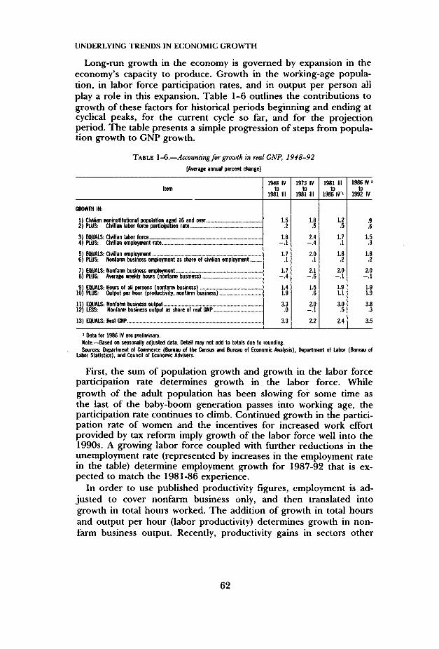
UNDERLYING TRENDS IN ECONOMIC GROWTH

Long-run growth in the economy is governed by expansion in theeconomy's capacity to produce. Growth in the working-age popula-tion, in labor force participation rates, and in output per person allplay a role in this expansion. Table 1-6 outlines the contributions togrowth of these factors for historical periods beginning and ending atcyclical peaks, for the current cycle so far, and for the projectionperiod. The table presents a simple progression of steps from popula-tion growth to GNP growth.

TABLE 1-6.—Accounting for growth in real GNP, 1948-92

[Average annual percent change]

Item

GROWTH IN:

1) Civilian noninstitutional population aged 16 and over2) PLUS- Civilian labor force participation rate

3) EQUALS- Civilian labor force . .4) PLUS: Civilian employment rate

5) EQUALS: Civilian employment6) PLUS: Nonfarm business employment as share of civilian employment

7) EQUALS- Nonfarm business employment8) PLUS* Average weekly hours (nonfarm business)

9) EQUALS: Hours of all persons (nonfarm business)10) PLUS- Output per hour (productivity, nonfarm business)

11) EQUALS: Nonfarm business output12) LESS- Nonfarm business output as share of real GNP

13) EQUALS- Real GNP

1948 IVto

1981 III

152

18

1.7.1

1.7-4

1.41.9

3.30

33

1973 IVto

1981 III

18.5

24-.4

2.0.1

2.16

1.5.6

2.01

22

1981 IIIto

1986 IV •»

12

1.7

1.8.2

2.0_ 1

1.91.1

3.05

24

1986 IV ito

1992 IV

96

1.5

1.8.2

2.01

1.91.9

3.83

35

1 Data for 1986 IV are preliminary.Note.—Based on seasonally adjusted data. Detail may not add to totals due to rounding.Sources: Department of Commerce (Bureau of the Census and Bureau of Economic Analysis), Department of Labor (Bureau of

Labor Statistics), and Council of Economic Advisers.

First, the sum of population growth and growth in the labor forceparticipation rate determines growth in the labor force. Whilegrowth of the adult population has been slowing for some time asthe last of the baby-boom generation passes into working age, theparticipation rate continues to climb. Continued growth in the partici-pation rate of women and the incentives for increased work effortprovided by tax reform imply growth of the labor force well into the1990s. A growing labor force coupled with further reductions in theunemployment rate (represented by increases in the employment ratein the table) determine employment growth for 1987-92 that is ex-pected to match the 1981-86 experience.

In order to use published productivity figures, employment is ad-justed to cover nonfarm business only, and then translated intogrowth in total hours worked. The addition of growth in total hoursand output per hour (labor productivity) determines growth in non-farm business output. Recently, productivity gains in sectors other

62

than manufacturing have been disappointing. Expectations of futuregains, although above recent productivity growth, have been scaledback somewhat from previous projections. Productivity is projectedto increase at approximately 1.9 percent, on average, over the 1987-92 period, up 0.8 of a percentage point from rates experienced in thecurrent cycle to date. After adjustment for the stronger relative rate ofgrowth of the nonfarm business sector, the growth rate of real GNP isgiven in the last line of Table 1-6. The calculations in the table indicatethat the projected improvement in productivity growth (output perhour) from 1.1 to 1.9 percent per year is the key to stronger real GNPgrowth and to the gains in real living standards that this growth willgenerate.

CONCLUSION

Although 1986 was not an outstanding year in terms of real GNPgrowth, the economic expansion proceeded on a broad front throughits fourth year, and important progress was made in expanding em-ployment and reducing inflation and interest rates. The problemsthat kept overall growth below expectations were largely sectoral: adecline in world oil prices that depressed employment and invest-ment in the domestic oil and gas industry; continued difficulties inU.S. agriculture; and a further deterioration of the U.S. trade bal-ance. Nowhere evident were the problems that usually portend theend of expansions. Rather, the economic developments of 1986affirm that the destructive sequence of progressively rising inflationrates and interest rates, interrupted by severe recessions, has beenbroken. The foundation for sustainable growth of production andemployment, accompanied by gradually declining inflation and un-employment, has been strengthened.

For the future, real economic growth is projected to accelerate. In-flation is projected to resume its gradual decline, after a modestupturn because of erosion of the temporary effects of the recent oilprice decline. Continuation of stable macroeconomic policies is es-sential to realizing these projections and to avoiding cycles of infla-tion and disinflation that are associated with unnecessary swings inrelative prices, real interest rates, and real asset values, and ultimatelywith many of the structural and sectoral problems that still beset theU.S. economy. In particular, monetary policy faces a difficult task in aperiod when the traditional guideposts for its conduct have becomeless reliable. It must continue to tread cautiously between the risk ofinadequate money and credit creation that would jeopardize econom-ic expansion in the short run, and the risk of excessive monetary

63

growth that would reignite inflation and seriously damage economicperformance in the long run.

Ultimately, the long-run growth rate of the economy and thegrowth of real living standards depend primarily on the produc-tivity of individuals and businesses operating in the private sector. Asdiscussed here and in later chapters of this Report, government has animportant role to play in enhancing the efficiency and productivity ofthe economic system. Its principal contribution is to maintain a stablemacroeconomic environment and to allow the natural incentives ofthe flexible, private enterprise system to stimulate individuals andbusinesses to increase the quantity and enhance the quality of pro-ductive resources, to improve the efficiency of production processes,and to deploy the Nation's resources to their highest valued uses.

64

CHAPTER 2

Budget Control and Tax Reform

GOVERNMENT TAX AND EXPENDITURE POLICIES stronglyinfluence the economy's long-run performance. Government-provid-ed goods and services improve economic performance if their valueexceeds their cost, as measured by the value of the private goods andservices they displace. The cost of government-provided goods andservices, in turn, depends on the efficiency of the tax system. An effi-cient tax system entails low and unvarying marginal tax rates thathave minimal effects on private investment and consumption choices.

The Administration is committed to a policy of restructuring Fed-eral fiscal activities to serve the national interest more effectively.Tax reform, the Administration's number one domestic priority forthe past several years, has been accomplished. The Tax Reform Actof 1986 significantly lowers tax rates and will decrease tax-induceddistortions in private economic decisions. Progress has also beenmade in Federal spending restraint. The upward trend in FederalGovernment expenditures as a share of gross national product (GNP),which had persisted for most of two decades, was reversed in 1984. Forthe first time since 1973, real Federal Government expenditure isprojected to fall in fiscal 1987. Further spending restraint, however,will be necessary to achieve the future deficit targets set in theBalanced Budget and Emergency Deficit Control Act of 1985 (popular-ly known as Gramm-Rudman-Hollings), targets to which the Adminis-tration is firmly committed.

This chapter surveys both the Administration's accomplishmentsand its future agenda concerning the restructuring of Federal fiscalactivities. The chapter begins with a discussion of the Federal budgetdeficit, the need for Federal spending restraint, and proposedchanges in the budgetary process. It argues that the objective of bal-ancing the budget by 1991 can be achieved without a general tax in-crease and without sacrificing programs essential to the national in-terest. This task will require uncompromising efforts to eliminate allunnecessary Federal spending, efforts that could be aided by appro-priate reforms of the budgetary process. The chapter then turns toan assessment of the economic effects of the Tax Reform Act of1986. It finds that tax reform, while entailing minor transition costs,

65

significantly improves the economy's long-run economic perform-ance. Specifically, it is estimated that national net output of goodsand services increases approximately 2 percent because of the long-run consequences of tax reform. In 1986, this would have amountedto an increase of approximately $600 in the income of the averageAmerican family.

SPENDING RESTRAINT AND DEFICIT REDUCTION

The current economic expansion marks the first occasion in thepostwar period when Federal deficits have exceeded 5 percent ofGNP, and when very large deficits have persisted into thethird and fourth years of an expansion. At comparable periodsduring the expansions of the 1960s and 1970s, the Federal deficit asa share of GNP was generally less than one-half the level of 1985 and1986. The underlying cause of the growing Federal deficit is illustrat-ed in Chart 2-1. The share of Federal spending in GNP has contin-ued on an upward trend, while the secular trend in the share of Fed-eral revenues has remained virtually flat.

Under the provisions of Gramm-Rudman-Hollings, significant defi-cit reduction will occur in fiscal 1987. With moderately good eco-nomic performance and absent large new spending initiatives, theOffice of Management and Budget projects that the Federal deficitwill decline by almost $50 billion between fiscal 1986 and fiscal 1987,equivalent to more than a full percentage point of GNP. The Admin-istration's proposed budget for 1988 provides for another importantstep in the process of deficit reduction, to the target of $108 billion,along a path to reach a balanced Federal budget by 1991. Five criti-cal reasons explain why this process of deficit reduction must contin-ue and why deficit reduction should be achieved primarily throughspending restraint.

REASONS FOR DEFICIT REDUCTION

First, persistent large Federal deficits, except during periods ofsevere economic difficulty or extraordinary national need, constitutean unfair burden on future generations. The principle that "there isno free lunch" applies to lunches charged on Uncle Sam's creditcard. In the end, all Federal spending must be paid for by some formof explicit or disguised taxation. Finance of current expendituresthrough the issuance of Federal debt merely postpones the inevitableday when the bill for current services (plus accumulated interest)must ultimately be paid, either through higher taxes or through re-duced public services. More specifically, interest payments on theFederal debt must ultimately be financed by some combination of re-

66

Chart 2-1

Federal Outlays and Receipts as Percent of GNP

Percent of GNP25

24

23

22

21

20

19

18

17

nI

Outlays/\

v \

Outlays Trend / ^-^\ >

\--"f ~~V

Receipts

i i I i i I i I i i i i i i i i I

1960 1963 1966 1969 1972 1975 1978 1981 1984Fiscal Years

Note.—Data for 1987 are estimates.Sources: Department of Commerce, Office of Management and Budget,

and Council of Economic Advisers.

1987

during the growth of noninterest Federal outlays below the growth ofGNP or by higher future taxes relative to GNP. The longer largedeficits persist, the larger grows the outstanding stock of Federaldebt and hence the greater is the ultimate required adjustment infuture noninterest outlays or taxes. Thus, the choice is not whetherto reduce the budget deficit, but rather when and by what means.

Second, deficit reduction through spending restraint is essential topreserve the long-term economic benefits of the low marginal taxrates established in the Tax Reform Act of 1986. This chapter lateranalyzes the gains to national income and national welfare from taxreform. These long-run benefits will begin to emerge, however, onlyif marginal tax rates are lowered as promised in 1988, and only ifindividuals and businesses believe that these tax rates will not be in-creased in the future.

Third, persistent large Federal deficits throughout an economic ex-pansion could pose a difficult dilemma for macroeconomic policy inthe event of a significant economic downturn. In such a downturn,Federal receipts automatically decline and transfer payments expand.

67

Either a sharply contractionary fiscal policy would need to be adopt-ed during a recession to prevent a further increase in the Federaldeficit, or the share of the deficit in GNP would have to be allowedto expand to levels not previously experienced in the United Statesin peacetime. As is discussed in Chapter 1, there is no reason now toexpect a recurrence of the economic difficulties that contributed tothe steep recessions of 1974-75 and 1980-82. Nevertheless, it wouldbe imprudent to permit the persistence of large Federal deficitsthroughout an economic expansion in light of the dilemma such defi-cits could create in the future.

Fourth, reduction of the Federal deficit through spending restraintis an essential component of the strategy to reduce internationalpayments imbalances. Substantial progress has already been made onone component of this strategy—exchange-rate realignments that im-prove the international competitive positions of many U.S. industriesand promise significant reductions in the U.S. trade deficit in 1987 andbeyond. As is discussed in Chapter 3, however, reduction of the U.S.trade deficit and of the corresponding trade surpluses of other coun-tries also requires that domestic demand in the United States growmore slowly than U.S. GNP and conversely for foreign countries. Si-multaneously, the United States must improve its national saving/in-vestment balance (private saving less the sum of private investmentand the government deficit). Reduction of the Federal budget deficitthrough spending restraint is a key U.S. contribution to achievingthese results in a manner consistent with sustainable, noninflationarygrowth of the world economy. Furthermore, as discussed in Chapter1, significant reductions in the trade deficit increase the likelihoodthat resources that might otherwise be used to meet the demandsarising from Federal purchases will shift rapidly to meet the demandsof sectors producing exports and import substitutes.

Fifth, deficit reduction through spending restraint is required be-cause Federal spending in many areas remains above levels necessaryto provide essential Federal services on an efficient and cost-effectivebasis. Much has been accomplished during the past 6 years in cuttingback inessential, ineffective, and inefficient Federal programs. Largercutbacks can and should be made in a number of Federal programsthat serve special interests but whose benefits to the Americanpeople do not justify the costs imposed on current or future taxpay-ers. Equally important, new spending initiatives should be limited tocritical areas of national need in the realm of Federal responsibility.

Deficit reduction is ultimately an issue of priorities. The long-runbenefits of stronger economic growth from the relatively low margin-al tax rates provided in the Tax Reform Act of 1986 can be pre-

68

served only if the share of Federal spending in GNP is gradually re-duced. Alternatively, Federal spending can be maintained and ex-panded on programs that serve a variety of special interests, at theexpense of current and future consumption by American families andinvestment by American businesses. In making the politically difficultchoices required for deficit reduction, however, damage to Federalprograms that promote peace, maintain national security, or provideessential support to the poor and elderly is neither necessary nor de-sirable.

GROWTH OF THE FEDERAL BUDGET DEFICIT

The tax rate reductions mandated by the Economic Recovery TaxAct of 1981 (ERTA) reduced the share of Federal receipts in GNP tothe average of the 1960s and 1970s. In 1986, this share stood at 18.5percent, virtually the same as in 1978 (also the fourth year of an eco-nomic expansion). Between 1978 and 1981, the share of Federal taxcollections rose to a postwar high of 20.1 percent, primarily as theresult of bracket creep. A significant contribution of ERTA was theindexation of tax brackets, standard deductions, and personal exemp-tions, effective in 1985, which ensured that future inflation could notonce again push up the share of Federal revenues without an explicitand visible decision to raise tax rates.

On the spending side of the Federal budget, total spending growthhas not been adequately restrained, but the distribution of Federalspending has changed in important respects. Between 1978 and1986, Federal spending rose from 21.1 to 23.8 percent of GNP. Thekey changes in the distribution of Federal spending that occurred be-tween 1978 and 1986 are illustrated in Chart 2-2 and may be sum-marized as follows:

• The share of defense spending increased from 4.8 percent ofGNP to 6.6 percent, ending the long period of erosion of nation-al defense capabilities.

• The share of social security benefits increased by 0.5 percent ofGNP, maintaining a critical commitment to older and disabledAmericans and their families.

• The share of medicare expenditures increased by 0.7 percent ofGNP, reflecting both increased health care benefits and the par-tial success of efforts to limit the increasing cost of providingsuch benefits.

• The share of net interest payments increased by 1.7 percent ofGNP, reflecting higher interest rates and the growing stock ofFederal debt.

• The share of general nondefense programs (except social securi-ty, medicare, and net interest) declined by 1.8 percent of GNP.

69

Chart 2-2

Percent11

10

9

S

7

6

5

4

3

2

1

Federal Outlays as Percent of GNP

National Defense

'X / ̂

Social Security

A---"

. i1960 1962 1964 1966 1968 1970 1972 1974 1976 1978 1980 1982 1984 1986

Fiscal Years

Sources: Department of Commerce and Office of Management and Budget.

• Within the broad category of general domestic programs, fundswere reallocated away from inefficient, ineffective, low-priorityprograms and toward programs serving important nationalneeds. For example, funding for community and regional devel-opment was reduced substantially and general revenue sharingwas eliminated, while outlays for health research and Federal lawenforcement activities increased significantly.

Despite the substantial progress already achieved in reorientingbudget priorities, important work remains to be done. Elimination orcurtailment of inessential, inefficient, and ineffective Federal pro-grams is required to contribute to reduction of the share of Federalspending in GNP and to allow room for expansion of programs thatserve critical national needs.

PROSPECTS FOR DEFICIT REDUCTION

The Administration is committed to achieving the targets for defi-cit reduction prescribed by Gramm-Rudman-Hollings (GRH). Thefirst important step in this process will be taken during the currentfiscal year, with a reduction of the Federal deficit to almost $50 bil-

70

lion below its fiscal 1986 level. Meeting the GRH deficit targets for1988 and later fiscal years will not be an easy task, even with the con-tinuation of reasonably strong economic growth and with furthermoderation of inflation and interest rates. However, as the followinganalysis suggests, the task is achievable provided the economic cli-mate remains favorable.

In fiscal 1986, Federal spending amounted to 23.8 percent of GNP,while Federal receipts absorbed 18.5 percent of GNP, leaving a defi-cit of 5.3 percent of GNP. Under the Administration's economic pro-jections, continued economic growth and previously legislated in-creases in social security payroll taxes will increase the share of Fed-eral receipts to 19.4 percent of GNP by 1991. These projectionsimply that spending restraint must reduce the share of Federalspending in GNP by 4.4 percent by 1991 to achieve a balancedbudget without general tax rate increases.

The President is firmly committed to no reductions in social securi-ty retirement benefits. Fulfilling this commitment means that theshare of social security expenditures will remain virtually unchangedat 4.5 percent of GNP. Reductions in the share of total Federalspending in GNP must come from other sources.

Net interest payments amounted to 3.3 percent of GNP in fiscal1986. If the economy grows and interest rates decline as projected,and if growth in the outstanding stock of Federal debt is slowed bydeficit reduction in accord with GRH targets, then net interest ex-pense will decline by at least 1 percentage point of GNP by 1991.This process is the reverse of that through which a rapidly growingstock of Federal debt (fed by large Federal deficits) and rising inter-est rates contributed to the growth of net interest expense as a shareof GNP. To reverse this process, however, it is absolutely essential toplace the ratio of Federal debt to GNP on a descending path, mainlythrough progress in spending reduction in categories other than netinterest expense. The sooner this task is accomplished, the easier willbe the subsequent task of deficit reduction.

The projected reduction of 1 percent in the share of net interestexpense and the relative constancy in the share of social security ben-efits imply that to reach a balanced Federal budget, the combinedshare of all other categories of Federal expenditure must declinefrom 15.7 percent of GNP in 1986 to roughly 12.5 percent in 1991.Total Federal spending in this broad composite amounted to $655billion in fiscal 1986. If real spending in this composite remainedconstant at the 1986 level, projected economic growth between 1986and 1991 would reduce its share in GNP from 15.7 to 13.3 percent.Thus, an absolute reduction of real spending in this composite of

71

about $39 billion of 1986 dollars is required to achieve a balancedbudget.

Cutting $39 billion or 6.0 percent from composite spending of$655 billion should not be an insurmountable task. The difficulty ofthis task is heightened, however, by the need to accommodate realspending increases in areas of critical national need and primary Fed-eral responsibility. In particular, in the 1988 budget, the Presidenthas identified the following major areas as requiring increased ex-penditures: national defense, foreign affairs (including foreign aidand embassy protection), scientific and health research (including ac-quired immune deficiency syndrome research), drug abuse controland treatment, space exploration, and implementation of the new im-migration law. Increasing expenditures in these critical areas will re-quire deeper cuts in less essential Federal programs if the deficit re-duction targets are to be met.

PROPOSALS FOR SPENDING REDUCTIONS

The Administration's proposals for program reductions and termi-nations are described in detail in the President's 1988 budget. Abrief review of some of these proposals helps to place the economicissues associated with deficit reduction into proper perspective.

Spending on farm support programs has been the most rapidlygrowing major category of Federal spending, increasing from $4 bil-lion in 1981 to $25.8 billion in 1986. The desire to assist farm fami-lies during a period of severe economic difficulty accounts for muchof this increased spending. However, total farm support spending hasnow reached a level that would finance a direct payment of morethan $16,000 annually to each of 1.6 million farm families, or anannual payment of more than $42,000 for each of the 619,000 com-mercial-sized farms in the United States. By comparison, medianincome for all U.S. families is less than $30,000. Moreover, mostfarmers receive little or no financial assistance from Federal farmprice-support programs. Of the 34 percent of American farmers whodid receive direct assistance in 1985, one-fifth received almost 70percent of the payments. In the cotton program in 1986, 12 percentof the participants received more than one-half of the total payments,with some receiving millions of dollars. The 50 largest rice producerswill each receive more than $1 million in 1986 payments.

As is discussed in Chapter 5, Federal farm support programs arenot only expensive to the taxpayer and ineffective in channeling sup-port to the most needy, but they also generate huge economic waste.Because current Federal programs link financial support to farmoutput, they encourage production of crops for which there is no ef-fective market. Appropriate reform of farm support programs can

72

reduce economic waste and lower Federal expenditures while main-taining income support for distressed farm families.

The Federal Government continues to subsidize activities for whichthe original rationale has disappeared or where no persuasive casefor Federal involvement can be made in the first place. For example,mass transit systems can provide important benefits in the local areaswhere they operate, but generally no good rationale exists for Feder-al subsidies that distort local choices concerning the construction andoperation of such systems. The Administration proposes eliminationof discretionary grants for new mass transit systems.

Another example is the Rural Electrification Administration (REA),which has gone well beyond its original purpose of encouraging ex-tension of electrical supply in rural areas. Since 1935, when theAgency was founded, farms receiving electric service through REAhave increased from 12 percent of all farms to 99 percent. Rural tele-phone service (added as an REA responsibility in 1949) now extendsto 95 percent of all farms. REA's original goals have been achieved,but it lives on, offering subsidized loans to electric cooperatives serv-ing prosperous urban and suburban areas such as Atlanta, Georgia;Denver, Colorado; Manassas, Virginia; and Minneapolis, Minnesota.Loans have also been provided for electrification in exclusive resortssuch as Aspen, Steamboat Springs, and Vail in Colorado, and HiltonHead Island, Kiawah Island, and Myrtle Beach in South Carolina.The Administration proposes to curtail these practices by imposingappropriate limits on REA lending and loan guarantees.

OTHER REVENUE MEASURES

The Administration's proposals for deficit reduction also involveincreasing Federal revenues by levying equitable user fees for Federalservices provided to identifiable beneficiaries, by selling some feder-ally owned assets, and by instituting other relatively minor programsto generate revenues. Both user fees and asset sales serve the dualpurpose of raising revenue for the Federal Government and encour-aging economic efficiency. Efficiency in the use of services providedby the Federal Government that are similar to services provided byprivate business is encouraged when the user of the service, ratherthan the general taxpayer, pays the cost of providing the service.Economic efficiency is also often advanced when business-like oper-ations are shifted from the Federal Government to the private sector,where the profit motive and force of competition promote efficiency.

Major Administration proposals concern increased user fees forguaranteed student loans and for home loans guaranteed by the Vet-erans Administration (VA) and the Federal Housing Administration(FHA), and for mortgage-backed securities guaranteed by the Gov-

73

ernment National Mortgage Association (GNMA). Costs associatedwith defaults on guaranteed student loans have run well ahead ofrevenues from current fees—a situation that should be corrected.The same is true for VA home loans. For FHA and GNMA, evidencesuggests that their association with the government provides an im-plicit subsidy that allows them to charge less for their services than aprivate business would have to charge for the same service.

In addition to continuing sales from the Federal Government'sloan portfolio, major proposals for asset sales include the sale ofAmtrak and the phaseout of subsidies to Amtrak, sale of the NavalPetroleum Reserve, and sale of the Alaska Power Administration.Transfer of these programs to the private sector would lead to moreefficient operation, as well as generating revenue.

Asset sales are a one-time source of revenue. Indeed, sales of loansfrom the Federal portfolio and sales of government enterprises thatearn a profit increase current revenue at the expense of future reve-nue. Such asset sales effectively transfer part of the task of deficit re-duction from the present to the future. If adequate progress is beingmade in attacking the core of the deficit problem, however, partialtransfer of this problem into the future through asset sales may bedesirable.

Once the budget is balanced on a cash basis, the nominal stock ofFederal debt will not grow and the ratio of Federal debt to GNP willdecline. As the ratio of Federal debt to GNP declines (assuming con-stant interest rates), the share of net interest expense in GNP will de-cline at a moderate pace. This development will allow room for othercategories of Federal spending to rise, absolutely and as a share ofGNP, without any increase in tax rates. Lost revenues from priorasset sales can be made up under these circumstances without abso-lute cuts in spending programs or tax rate increases. This strategyworks, however, only if asset sales play a limited role in the totalstrategy of deficit reduction, as they do in the President's 1988budget, and if the other elements of that strategy are pursued con-sistently and effectively.

BUDGET CONCEPTS AND FISCAL AUTHORITY

Gramm-Rudman-Hollings significantly alters the congressionalbudget process. It imposes targets for the Federal budget deficit ineach of fiscal years 1986-91 as well as a timetable and procedures formeeting these targets. A number of other proposals have recentlybeen made to reform the process by which budget decisions are de-liberated and implemented as well as to change the coverage andcontent of the budget itself. Proposals to modify the coverage andcontent of the Federal budget are motivated by the concern that the

74

current budget does not adequately reflect the economic costs ofFederal credit programs or capital investments made by the govern-ment. The line-item veto and a balanced budget amendment to theConstitution are proposed reforms of the budget process that aremotivated by the fact that, absent the temporary Gramm-Rudman-Hollings procedures that expire in 1991, congressional decisions toincrease outlays are not directly related to decisions affecting expect-ed tax receipts.

Federal Credit Programs

The accounting for Federal credit programs is a major weakness inthe present budget. Currently, the budget costs of direct loan pro-grams are measured by the net outlays of those programs, that is,total disbursements and interest paid minus repayments and interestreceived. Congressional appropriations for direct loan programs aregenerally only necessary when new disbursements exceed repay-ments. Loan guarantees do not result in recorded outlays except incase of default. A loan guarantee represents a contingent liability ofthe government that induces lenders to invest in particular loans,thus allocating capital for federally determined purposes. Thus, aloan guarantee may provide as large a subsidy as a direct loan obliga-tion.

The budget neither measures nor controls the most salient aspectof Federal credit—the size of the subsidy offered the borrower. With-out some means of measuring and controlling this subsidy, neitherthe executive branch nor Congress can make informed decisionsabout Federal credit programs, either by comparing one with theother or by comparing them with noncredit expenditure programs.

Some inadequacies of the budget treatment of Federal credit pro-grams were rectified by introduction of the Federal credit budgetin 1980. The Federal credit budget measures direct loan obligationsand guaranteed loan commitments. Although it is a step forward, thecredit budget does not restrain the total volume of Federal credit ef-fectively. Only about 55 percent of the credit budget totals for 1985were capped by appropriation act limitations. Moreover, the creditbudget does not measure the subsidy costs, nor does it directly re-strict the level of subsidy that a program offers the borrower.

The Administration proposes to change the budget treatment ofdirect loans and loan guarantees. Legislation for this purpose will besent to the Congress in the spring of this year. The Administration'sproposal would divide the face value of a new direct loan into twoparts: the market value of the loan and the present value of Federalsubsidies. A Federal Credit Revolving Fund would be establishedunder the direction of the Treasury. Before an agency could makedirect loans, Congress would have to appropriate funds to that

75

agency for the provision of direct loan subsidies. As loans weremade, the agency would provide the Fund with the information re-quired to estimate the present value of the direct loan subsidies. Thecentral revolving account would be charged for the market value, ornonsubsidized component, of direct loans. The agency would then becharged for the subsidy component of direct loans.

In the case of loan guarantees, Congress would first make appro-priations to the agency. As the agency granted loan guarantees, itwould provide the Fund with the information necessary to estimatethe present value of the guarantee subsidies. The agency would becharged for the value of the subsidy and would also transmit to theFund any fees paid by the borrowers. The Fund would then assumethe contingent liability for the guarantees.

To establish an objective measure of direct loan subsidies, newlymade direct loans would be sold to the public without recourse. Simi-larly, new loan guarantees would be reinsured with private insurers.

Adoption of the Administration's proposal would ensure that thebudget reflected the true economic costs of Federal credit programs.It would provide the President and Congress with the informationnecessary to make informed decisions about the allocation of budgetresources to these programs.

A Capital Budget

The Federal budget is a comprehensive statement of expected cashoutlays and cash receipts. The budget includes both operating andinvestment outlays, but does not report separate operating and cap-ital budget subtotals. However, details of Federal investment outlaysare presented in a special analysis that is published with the budget.The comprehensive outlay and receipt totals are indispensable forevaluating the effect of Federal policies on the level and compositionof aggregate economic activity. The unified budget deficit, which is thedifference between total Federal outlays and receipts, figures promi-nently in macroeconomic analysis precisely because it measures thegovernment's demand for private domestic and foreign saving as wellas the change in the outstanding stock of government debt.

For many years, proposals have been made to separate the unifiedFederal budget into an operating budget and a capital budget. Al-though the proposals differ in important respects, all share the essen-tial feature that Federal receipts and outlays would be disaggregatedinto their operating and capital components. In general, investmentoutlays would not be charged against operating receipts in the calcu-lation of the operating deficit, and only the subsidy component ofdirect loans and loan guarantees would be considered an operatingoutlay. Investment expenditures and the market value of direct loans

76

would constitute the outlays used in calculating the capital budgetdeficit.

Several arguments have been made in favor of a capital budget.First, it would provide the information and incentives necessary topromote economically efficient government capital planning. Second,borrowing to finance capital outlays would spread the cost of govern-ment investments more equitably among current and future benefici-aries and thus link the payment for a government investment with itsuse. For this reason, it has been argued that operating and capitalbudget subtotals should be calculated separately so as to distinguishbetween Federal borrowing that finances current operations fromborrowing that finances capital investments yielding future benefits.

Opponents argue that the capital budget would not promote eco-nomically efficient capital planning. Because capital outlays wouldnot be deducted from receipts in the calculation of the operating def-icit, the constraint on capital outlays might be relaxed to such anextent that budget decisions would be biased in favor of capitalspending. Furthermore, technical disagreement over the definition ofcapital outlays would likely occur, such as whether expenditures forresearch and development or education should be included in thecapital budget and thus not be charged against receipts in calculatingthe operating budget deficit. More generally, opponents argue that aunified budget is needed to hold public officials accountable for ap-propriations of tax receipts. Separate capital and operating budgetswould, according to this view, invite manipulation to hide andexpand Federal spending.

It is important that the long-term benefits of government capitalinvestments be adequately assessed against the current budget costof the resulting capital outlays. However, it is at least equally criticalthat budget deliberations take into account the effect of proposedpolicies on total outlays, receipts, and the unified budget deficit.

The Line-Item Veto

The line-item veto would authorize the President to veto individualline items in appropriation bills, subject to the current provisions foroverriding a veto of any bill. Governors in 43 States now have suchauthority. Congress has approved such authority for the Governorsof the Commonwealth of Puerto Rico and the Trust Territories andfor the Mayor of the District of Columbia—but not for the President.

For more than a century, Congress has rejected Presidential re-quests for this authority in order to maintain the opportunity to pack-age spending proposals that the President would otherwise veto inbroader appropriations that the President would approve. Appropria-tions are presented to the President in only 13 general appropriationbills. Indeed, last year Congress did not pass a single one of the 13

77

appropriation bills, but instead passed one 389-page omnibus spend-ing bill. Because Congress had not completed action on the annualappropriation bills, the President was compelled by law to shut downthe Federal Government. Such abrogation of a responsible budgetprocess by Congress not only discourages careful, prudent legisla-tion—it encourages excessive spending and waste.

Effective use of the line-item veto would change the compositionand level of Federal expenditure. A Member of Congress is electedby voters in a specific congressional district or State, while the Presi-dent is elected by the voters of the Nation. As a consequence, aMember of Congress has stronger preferences for programs andprojects that benefit his or her regional constituency, especially be-cause only a fraction of the cost of such programs and projects areborne by his or her constituency. The expected result of granting ap-proval for a line-item veto would be a decrease in expenditures onprograms and projects whose regional benefits do not exceed thecost to the Nation's taxpayers. This result should be a sufficient basisfor early approval of Presidential authority for a line-item veto.

Balanced Budget Amendment

The President has endorsed the concept of a balanced budget/taxlimitation amendment to the Constitution. The objective is to changethe rules by which decisions are made to borrow or to increase thesize of Federal outlays and receipts relative to national income. Al-though several amendments have been proposed, two that have beenconsidered in the Senate share the following provisions:

• A requirement that total outlays be no greater than total re-ceipts, unless three-fifths of the whole number of both Houses ofCongress decide otherwise in a vote devoted solely to that sub-ject;

• A prohibition on increases in the public debt, absent approval bythree-fifths of the whole number of both Houses of Congress;

• A requirement that all or some revenue-increasing bills be en-acted by a majority of the whole number of both Houses of Con-gress by roll call vote; and

• The authority for Congress to waive these requirements in theevent of war.

Approval of this proposed amendment would be a recognition thateach generation may need to bind itself to responsible fiscal deci-sions in the interests of the current and future American community.

The line-item veto and a balanced budget amendment cannot sub-stitute for the hard choices necessary to restrain the growth of Feder-al expenditure and to reduce the Federal deficit. Early approval ofthese proposals, however, could force a resolution of the choices nec-essary to resolve major near-term fiscal issues.

78

TAX REFORM

This section assesses the economic effects of the Tax Reform Actof 1986. The purpose of this assessment is twofold: to forecast theeffects that tax reform will have on future macroeconomic activityand, by demonstrating the substantial benefits of tax reform, toguard against possible future changes in the tax code that wouldundo the important progress that has been made.

OVERVIEW

The Tax Reform Act of 1986 fundamentally alters the structure ofthe Federal income tax. It broadens the personal and corporateincome tax bases and substantially lowers tax rates. These changeswill significantly alter private incentives and, accordingly, will influ-ence the economy's performance through three principal channels:

• Lower marginal tax rates on personal income, in conjunctionwith a broader tax base, will increase labor effort and reduce theexploitation of tax loopholes.

• More uniform tax rates on income from alternative capital in-vestments will induce a more efficient allocation of investmentfunds.

• A somewhat higher overall marginal tax rate on capital incomewill modestly reduce the economy's long-run capital intensity.

The analysis in this section indicates that tax reform will significantlyimprove the economy's long-run performance. This improvement willcome from several sources, most of which have not been explicitlyquantified. Estimates that have been made, however, suggest that theNation's output of goods and services will permanently increase byapproximately 2 percent because of the long-run consequences of taxreform.

This section begins with a discussion of the conditions leading totax reform and a brief explanation of the importance of marginal taxrates for economic efficiency. The chapter then turns to an assess-ment of the Tax Reform Act of 1986 (TRA). This assessment beginswith a description of the major provisions of TRA and an analysis oftheir microeconomic implications. Finally, the chapter explores theimplications of TRA for long-run economic growth and short-runmacroeconomic activity.

THE CONDITIONS LEADING TO TAX REFORM

Despite legislated "tax reductions" during the 1960s and 1970s,marginal tax rates rose substantially as inflation pushed taxpayersinto higher tax brackets. As is shown in Table 2-1, a family of fourwith median earnings in 1965 paid 17 cents in tax on the last dollar

79

of income earned. Such a family, therefore, had a marginal tax rateof 17 percent. The marginal tax rate for a similar family in 1980, incontrast, had risen to 24 percent due to bracket creep. The growth inmarginal tax rates was more dramatic at higher incomes: a familywith twice the median income in 1980 had a marginal tax rate almostdouble that of a similar family in 1965.

TABLE 2-1.—Marginal personal income tax rates for four-person families, selected years,1965-881

[Percent]

Year

1965

1970

1975

1980

1986

1988 (TRA) ...

One-halfmedian income

14

15

17

18

14

15

Family income

Median income

17

20

22

24

22

15

Twice medianincome

22

26

32

43

38

28

1 Excludes social security taxes and State and local income taxes.

Source: Department of the Treasury, Office of Tax Analysis.

For income from capital gains, inflation not only increases the stat-utory rate of tax because of bracket creep, but it also causes the ef-fective tax rate to exceed the statutory tax rate. This phenomenonwas particularly important in the 1970s, when inflation rates werehigh. In 1979, for example, a 1-year investment yielding a 10 percentnominal capital gain yielded, after 9 percent inflation, a 1 percentreal capital gain. Federal taxes, however, are levied on nominal cap-ital gains. A taxpayer in the 70 percent tax bracket who received a 10percent nominal capital gain, therefore, earned a 7.2 percent nominalafter-tax return (taking the 60 percent capital gains exclusion into ac-count). After 9 percent inflation, this translates to a minus 1.8 per-cent real after-tax return. Hence, for this hypothetical investor, infla-tion increased the effective tax rate on the 1 percent real pretax cap-ital gain from 28 percent to 280 percent. This phenomenon is entire-ly independent of bracket creep and, for the taxation of capital gains,is quantitatively much more important.

Inflation also distorts the taxation of corporate bond interest. Thenominal rate of return on bonds includes an inflation premium thatis not distinguished, for tax purposes, from the real return. Corpora-tions can deduct nominal bond interest paid from their taxableincome and individual bondholders must include nominal bond inter-est received in their taxable income. Inflation, therefore, decreases(increases) the effective rate of tax on debt-financed corporate invest-

80

ment if the corporate tax rate exceeds (is less than) the marginal taxrate of the marginal bondholder. Because of the offsetting effects ofthe corporate and personal tax systems, inflation affects the taxationof real corporate bond interest much less than it does the taxation ofreal capital gains.

The high inflation rates of the 1970s distorted the taxation of cap-ital income in still another way. Deductions for the depreciation of acapital asset, which are properly subtracted from gross capital incometo determine taxable income, are set in accordance with the purchaseprice of the asset. Inflation therefore reduces the real value of depre-ciation deductions. This phenomenon, in addition to the taxation ofinflationary capital gains, caused the effective rate of tax on equity-financed investments to rise substantially during the 1970s.

It became increasingly apparent in the late 1970s that these infla-tion-induced increases in effective tax rates were stifling private in-centives to work and to save and were impeding economic growth.To restore private production incentives, therefore, the Administra-tion proposed, and Congress passed, the Economic Recovery TaxAct of 1981. ERTA called for a phased reduction in personal taxrates that, when completed in 1984, substantially reduced personalmarginal tax rates (see the 1986 tax rates in Table 2-1). The topmarginal tax rate was reduced from 70 to 50 percent. ERTA also ex-tended eligibility for individual retirement accounts (IRAs) to individ-uals with other pension plans. Beginning in 1985, the rate schedule,the zero bracket amount, and the personal exemption were indexedto the price level. ERTA also included substantial investment incen-tives. Although these incentives were scaled back somewhat byTEFRA, the Tax Equity and Fiscal Responsibility Act of 1982, ERTAand TEFRA together significantly lowered the effective tax rate onincome from most capital investments.

ERTA-TEFRA substantially reduced marginal tax rates but left twoparticularly undesirable features of the income tax. First, ERTA-TEFRA's investment incentives increased the opportunities for taxavoidance. Second, ERTA-TEFRA did not help to equalize marginaltax rates on alternative capital investments. In particular, investmentsin corporate equipment retained their tax advantages over invest-ments in corporate structures. Uneven tax rates on income from al-ternative capital investments result in a misallocation of capital and alower value of output than would otherwise be obtainable.

To correct these problems and others, and to reduce marginal taxrates further, the President submitted to Congress detailed proposalsfor income tax reform in May 1985. These proposals became thebasis for congressional deliberations that culminated in TRA. Thislaw differs somewhat from the President's proposals but retains their

81

overall thrust. TRA lowers marginal tax rates, broadens the personaland corporate tax bases, and helps to equalize marginal tax rates onalternative income-producing activities.

MARGINAL TAX RATES AND ECONOMIC EFFICIENCY

Marginal tax rates—the rates paid on the last dollar earned fromincome-producing activities—influence the incentives to engage inproductive activities and, hence, are extremely important elements ofthe tax system. The marginal tax on labor income, for example,drives a tax wedge between the value of output that an additionalunit of labor produces and the after-tax wage received by workers,thereby discouraging additional labor effort. A reform of the taxsystem that lowers the marginal tax rate on labor income, while rais-ing the same total revenue, therefore increases labor effort and eco-nomic well-being. Economic well-being is increased because the valueof total output is increased by more than the total value of leisure isdecreased. Likewise, the marginal tax on investment income drives atax wedge between the pretax return to investment and the after-taxreturn to saving. Additional saving that would be induced by a lowermarginal tax rate on capital income increases the total value ofoutput by more than it increases the inconvenience cost of postpon-ing consumption.

A uniform tax on investment income distorts the overall savingsdecision. A nonuniform tax on capital income introduces an addition-al distortion in the allocation of saving and investment. Because in-vestment funds tend to be directed toward assets with the highest ex-pected after-tax returns and because the return to a particular assettype declines with its quantity, alternative investments tend, in equi-librium, to yield equal after-tax returns. Hence, the pretax return ona particular investment tends to be higher, the higher is the effectivemarginal tax rate. Unequal marginal tax rates on alternative capitalinvestments, therefore, result in an output loss. That is, the value ofoutput would be increased if investment funds were shifted awayfrom investments with low marginal tax rates and low pretax returns,and toward investments with high marginal tax rates and high pretaxreturns. The greater are the differentials among marginal tax rateson alternative capital investments, the greater is the resulting outputloss.

High marginal tax rates on labor income also encourage excessiveconsumption of untaxed employee fringe benefits. A worker with a30-percent marginal tax rate, for example, gives up 70 cents in take-home pay for each dollar of (untaxed) fringe benefits he or she re-ceives. The worker, or the worker's union, therefore rationally seeks

82

an amount of fringe benefits that have a value, at the margin, equalto only 70 percent of their true cost.

More generally, high marginal tax rates increase incentives toengage in tax avoidance and evasion. Tax avoidance occurs when tax-payers make legitimate investment or consumption choices that areinfluenced by the desire to reduce tax liabilities. As was demonstrat-ed for the case of untaxed employee fringe benefits, tax avoidanceleads to an inefficient allocation of resources and is apt to increasewith the marginal tax rate on ordinary income. Tax evasion, con-versely, is the failure to comply with the tax laws. The incentive tohide income from the tax authorities, so as to evade taxes, increaseswith the marginal tax rate. Tax evasion, like tax avoidance, ordinarilyresults in wasteful expenditures of time, energy, and tangible re-sources.

A MICROECONOMIC ANALYSIS OF THE TAX REFORM ACT

The Personal Income Tax

TRA significantly lowers tax rates on personal income. When thelaw is fully effective in 1988, two tax brackets, set at 15 and 28 per-cent, will replace the 14 that ranged from 11 to 50 percent. The 15-percent bracket and the personal exemption are phased out for high-income returns, which results in an implicit 33-percent tax rate for abroad income range. As is shown in Table 2-1, TRA reduces margin-al tax rates to levels that are similar to those that prevailed in 1965.

These rate reductions are made possible, in part, by TRA's base-broadening measures. TRA broadens the personal tax base, or tax-able personal income, to include the following: all long-term capitalgains, State and local sales taxes, IRA contributions for high-incomeindividuals with employer-provided pension plans, nonmortgage con-sumer interest payments, miscellaneous itemized deductions less than2 percent of adjusted gross income, net losses from passive invest-ments, and net losses from active real estate investments for high-income taxpayers. These base-broadening measures are partiallyoffset by substantial increases in the standard deduction and personalexemption. By 1988, the personal exemption is nearly doubled andthe standard deduction is increased 36 percent for joint returns and21 percent for single returns.

An important feature of TRA is its strong limitations on tax-shel-tered activities, which have grown greatly over the past several years.Two factors are largely responsible for the recent growth in tax shel-ters; first, the high inflation rates of the late 1970s and early 1980sincreased the real value of nominal interest deductions on leveragedinvestments, and second, ERTA-TEFRA substantially accelerated de-preciation deductions. These factors increased the opportunities for

83

claiming early losses in exchange for later capital gains that have theadvantages of tax deferral and a lower tax rate.

TRA limits tax shelters directly and indirectly. The elimination ofthe capital gains preference, the deceleration of tax depreciation de-ductions, more stringent limitations on investment interest deduc-tions, and the lowering of marginal tax rates all serve indirectly tomake tax shelters less attractive. Moreover, any remaining tax avoid-ance opportunities are subjected to TRA's provisions concerning pas-sive business losses and real estate losses. In particular, net lossesfrom passive business investments and real estate investments forhigh-income taxpayers cannot be deducted from ordinary income;they must be carried forward and deducted from net income fromlike activities in later years.

These tax-shelter limitations not only make the personal incometax more equitable, but they should also result in more economicallyefficient investment decisions. Investments that previously providedopportunities for tax avoidance are put on a more equal footing withother investments. Investment funds, therefore, should have a great-er tendency to flow to their most highly valued uses.

The elimination of the nonmortgage consumer interest deductionshould also improve the current allocation of investment funds. Con-sumer durables yield a flow of services that, unlike alternative invest-ments yielding monetary income, is untaxed. By disallowing non-mortgage consumer interest deductions, TRA partially eliminates thetax preference that is currently afforded to consumer durables. TRA,therefore, puts consumer durables on a more equal footing with al-ternative investments and should lead to more efficient investmentdecisions.

Allowing State and local taxes to be deducted from the Federalincome tax base is both inefficient and inequitable. It is inefficientbecause it reduces the perceived cost of State and local governmentservices and, except possibly in cases where State spending generatesappreciable spillover benefits, encourages excessive State and localspending. It is inequitable because it causes residents of low-tax lo-calities, who enjoy relatively small amounts of State and local govern-ment services, to pay a disproportionate share of Federal taxes. TRAameliorates these problems in two ways: it disallows the State andlocal sales tax deduction, and, by lowering the marginal Federal taxrate, it lowers the value of other State and local tax deductions.

TRA disallows IRA deductions for high-income individuals withemployer-provided pension plans. However, TRA still allows mostworking individuals to deposit $2,000 (nondeductible) each year inIRAs and defer tax on accrued interest until the funds are withdrawn

84

at retirement. This tax advantage is substantial, accounting for alarge portion of the tax savings afforded by deductible IRAs.

Although TRA significantly limits itemized deductions, it substan-tially raises the standard deduction. As a result, TRA is estimated toreduce the number of itemized personal Federal income tax returnsin 1988 by 11.5 million, thereby yielding an approximate $1.3 billionreduction in compliance costs.

Equity. TRA will cut total personal income taxes by about 6.6 percentin 1988. Table 2-2 gives the percentage tax cut for eight incomeclasses. The estimates are based on an expanded definition of incomethat equals adjusted gross income plus such items as excluded capitalgains, passive business losses, and tax-exempt bond interest.

TABLE 2-2.—Effects of the Tax Reform Act of 1986 on Federal tax liabilities and average Federaltax rates, by income class, 1988

Income class (1986 dollars)1

0 to 10 000

10,000 to 15,000

15 000 to 20 000

20 000 to 30 000

30 000 to 50 000

50,000 to 100,000

100,000 to 200,000

200 000 and over

ALL INCOME CLASSES

Percent changein income

tax liability

-56.2

-27.8

-14.8

-8.5

-7.1

-.9

-1.0

-.9

-6.6

Average tax rate (percent)

Prereform

2.0

5.4

7.0

8.9

11.0

13.9

17.4

13.6

10.3

TRA

0.9

3.9

6.0

8.1

10.3

13.7

17.1

13.4

9.6

1 The income concept (modified expanded income) is one of many possible income classifiers and was used by the JointCommittee on Taxation to present the distributional effects of the Tax Reform Act of 1986. An alternative measure, "economicincome," was used in the Treasury Department's The President's Tax Proposals in 1985.

Note.—Distributions reflect most but not all of the provisions of the individual income tax code.Source: Department of the Treasury, Office of Tax Analysis.

The percentage tax cut under TRA is largest for low-income re-turns. The number of poor families paying Federal income tax is esti-mated to fall by 4.3 million in 1988 under TRA. With one smallexception, the estimated percentage tax cut under TRA steadily falls forhigher income returns. Thus, these estimates indicate that TRA actuallyincreases the effective progressivity of the personal Federal income taxdespite a less graduated rate structure. This result is shown in thelast two columns of Table 2-2, which give the estimated average taxrate for each income class under TRA and the prereform tax law.TRA cuts the average tax rate much more for taxpayers with incomeless than $50,000 than it does for higher income taxpayers.

Table 2-2 concerns only personal Federal income taxes. Becauseall taxes are ultimately paid by individuals, a complete analysis of tax

85

incidence would allocate undistributed corporate income and Federalcorporate taxes to the various income classes. Exactly how thisshould be done, however, is uncertain. Current evidence is not con-clusive, but it suggests that part of the corporate tax burden is borneby workers and that the majority is borne by owners of capital. If thisinference is correct, it would imply that high-income taxpayers, whoearn a disproportionate share of capital income, bear a relativelylarge share of the corporate tax burden. Because TRA shifts 6.6 per-cent of the individual income tax burden to corporations, it wouldfollow that a proper imputation of corporate taxes to the variousincome classes would probably reinforce the conclusion that TRA en-hances the effective progressivity of the Federal income tax.

TRA increases the long-run horizontal equity of the Federalincome tax. Horizontal equity concerns the degree to which taxpay-ers with equal amounts of economic income have equal tax liabilities.Because of TRA's limitations on tax preferences, including the elimi-nation of the capital gains preference, the limitations on tax shelters,and a stricter minimum tax, it substantially reduces the variation inthe amount of tax paid by taxpayers with the same real income.

As does any significant reform of the tax system, TRA will cause aone-time change in asset values that will redistribute wealth. Existingassets that received tax preference under ERTA-TEFRA and havetheir tax preferences curtailed under TRA suffer capital losses. Con-trariwise, any existing assets that are taxed less heavily under TRAthan they were under ERTA-TEFRA enjoy capital gains. Special tran-sition rules make these changes in asset values less severe in somecases. The deductions for passive business losses and real estatelosses attributable to assets acquired prior to tax reform, for exam-ple, are phased out gradually over 4 years. The same is true for de-ductions of interest payments on preexisting nonmortgage loans.

This phenomenon of changing asset values is one reason whychanges in the tax law should be infrequent and implemented onlyfor compelling reasons. Investments tend to be inherently risky; fur-ther riskiness introduced by frequent changes in the tax law unneces-sarily destabilizes the business environment.

Business Taxes

The proper measurement of economic income from investments inreal assets requires that deductions be made for the decline in realasset values attributable to depreciation. Since 1954, tax law has al-lowed investors to deduct for more rapid depreciation on most assetsthan actually occurs. Accelerating depreciation in this manner lowersthe cost of capital, which is defined as the minimum pretax invest-ment return that is profitable. The cost of capital has also been re-duced by the investment tax credit, which applied primarily to equip-

86

ment assets and allowed investors to deduct a percentage of anasset's purchase price immediately from tax liabilities.

TRA repeals the investment tax credit, allows less accelerated de-preciation, and lowers the corporate tax rate from 46 to 34 percent.These provisions taken together have two general effects: they tendto raise the cost of capital overall, and they tend to equalize the costof capital for alternative capital investments. The latter effect is dueprimarily to more equal effective rates of tax on investments in cor-porate equipment and corporate structures.

Table 2-3 gives the estimated percent change in the cost of capitalbrought about by TRA for three sectors of the economy and for vari-ous assets within the corporate sector. For the corporate sector, thecalculations take into account corporate, property, and personaltaxes. Investments are taxed differently depending on whether theyare financed with debt or equity. Table 2-3 gives results for threedifferent modes of finance; for debt, equity, and a combination ofdebt and equity.

TABLE 2-3.—Percent change in cost of capital under the Tax Reform Act of 1986

Sector

Corporate sector

EquipmentNonresidential structuresPublic utilities . . .Residential structuresInventoriesNonresidential landResidential land

Noncorporate business sector

Owner-occupied housing

Total business

TOTAL

Financing mode

Debt

48.6

197.344.547.924.221.119.316.5

4.7

3.3

22.1

16.8

Equity

Old view1

48

26.61.06.5

-5.7-18.6-18.0

170

.6

1.6

28

-2.1

Newview1

4.7

43.710.616.22.1

110-10.6-9.9

.6

1.6

3.0

2.7

Debt and equity

Old view1

2.8

43.77.7

13.3-.4130

-12.5116

1.9

2.2

2.4

2.3

view1

11.9

62.216.622.26.5

-5.8-5.5

51

1.9

2.2

7.4

6.2

1 See text for explanation of the old view and the new view of dividend taxation.Note.—Changes are relative to the prereform tax law. The computations take into account corporate taxes, property taxes, and

personal taxes at all levels of government.Source: Department of the Treasury, Office of Tax Analysis.

As is shown in the first column of the table, TRA substantially in-creases the cost of debt-financed capital investments. This result fol-lows largely because the value of interest deductions falls with thefall in corporate and personal tax rates.

There are currently two views in the economics profession con-cerning the relative importance of taxes on capital gains and on divi-dends for determining the cost of equity capital. The "new view" ofdividend taxation maintains that taxes on capital gains are very im-portant, while taxes on dividends are nearly irrelevant, for determin-

87

ing the cost of equity capital. The "old view" of dividend taxation,conversely, maintains that taxes on dividends, as well as taxes on cap-ital gains, are important for the cost of equity capital. It follows thatTRA, which raises the marginal tax rate on capital gains and lowersthe marginal tax rate on dividends, increases the cost of capital moreunder the new view of dividend taxation than under the old view. Noconsensus has formed as to which of these two views is correct. Al-though the new view gained wide acceptance when first introduced,recent empirical evidence does not uniformly support either viewover the other.

The estimates in Table 2-3 indicate that the overall cost of equity-financed investment falls under the old view and rises under the newview. The cost of corporate equipment rises much more than the costof corporate structures. This finding also applies to the noncorporatesector and is attributable to the repeal of the investment tax credit.Because TRA reduces corporate and personal tax rates, the cost ofcapital falls dramatically for nondepreciable capital assets, such as in-ventories and land.

Historically, approximately one-third of investment is financed withdebt and two-thirds with equity. The last two columns of Table 2-3use these weights to obtain overall percentage changes in the cost ofcapital for both views of dividend taxation. These calculations indi-cate that the overall cost of capital rises by 2.3 to 6.2 percent. Be-cause debt finance becomes relatively more expensive under TRA,and the financing shares are not allowed to respond to this change,these estimates tend to overstate the rise in the cost of capital. Onthe other hand, these estimates do not incorporate tax-shelter limita-tions or changes in accounting rules, provisions of TRA that raise thecost of capital.

TRA substantially evens the cost of capital across assets withineach sector. This effect is shown in the first part of Table 2-4, whichconcerns the variation in the cost of capital within the corporatesector. For every asset, TRA is estimated to reduce the magnitude ofthe percentage deviation of the cost of capital from the overall aver-age cost of capital in the corporate sector. Because relative costs ofcapital within each sector depend primarily on the investment taxcredit and depreciation allowances, and these features of the tax laware the same for the corporate and the noncorporate sectors, theseconclusions also apply to the noncorporate sector.

However, TRA does not alleviate the intersectoral distortions inthe capital income tax, as is shown in the second part of Table 2-4.The corporate sector is taxed most heavily, followed, in order, by thenoncorporate sector and owner-occupied housing.

88

TABLE 2-4.— Within-sector and between-sector variation in the cost of capital

Sector

Corporate sector:

EquipmentNonresidential structuresPublic utilitiesResidential structuresInventories .Nonresidential landResidential land

Corporate sector

Noncorporate business sector

Owner-occupied housing

Old view1

Prereform TRA

New view1

Prereform TRA

Percent deviation from averagecorporate cost of capital

-34.969

-8.821.921.426.035.4

-8.9-2.5

.518.12.77.4

16.5

-37.2-6.3-7.624.821.527.037.9

-8.9-2.3

.918.82.47.3

17.0

Percent deviation from overallaverage cost of capital

16.3

-5.9

-17.6

16.8

-6.2

-17.7

7.2

.5

-12.0

12.9

36

-15.3

1 See text for explanation of the old view and new view of dividend taxation.

Note.—Assumes financing is one-third debt and two-thirds equity.

Source: Department of the Treasury, Office of Tax Analysis.

A recent study indicates that eliminating the uneven taxation ofassets within sectors, and retaining the intersectoral distortions,would cause investment funds to be reallocated so as to increase realnet national product—real GNP less capital depreciation—perma-nently by about 0.2 percent. Because TRA reduces the within-sectorvariance in the cost of capital by about 60 percent, this finding sug-gests that this particular feature of TRA will, after a period of adjust-ment, permanently increase net national product by about 0.1 per-cent.

This estimate of the neutrality gains under TRA omits two impor-tant factors. First, the cost-of-capital estimates do not take into ac-count the possible "churning" of assets. Churning occurs when aused asset is sold and redepreciated, for tax purposes, by the newowner. Under ERTA-TEFRA, this investment strategy was viable onlyfor assets that have an active resale market, most particularly com-mercial structures and rental housing. TRA's limitations on tax shel-ters substantially reduce the tax preference afforded to such assets.Therefore, the quantified neutrality gains under TRA are mismeas-ured to the extent that TRA's neutrality gains associated with churn-able structures are different than TRA's neutrality gains associatedwith other structures. Second, TRA increases the relative tax prefer-ence given to intangible assets, such as expenditures on marketing,advertising, and research and development. This result follows fromthe fact that TRA increases the overall cost of tangible capital, andincome from intangible capital assets is entirely untaxed (at themargin) at the corporate level under both ERTA-TEFRA and TRA.

89

Because intangible assets are not included in the cost of capital com-putations, the quantified neutrality gains from TRA tend to be over-stated.

Under both TRA and the prereform tax law, corporations are ableto deduct interest payments. Because dividend payments are not de-ductible, equity finance is put at a disadvantage relative to bond fi-nance, which presumably encourages corporate borrowing. The esti-mates of the cost of capital indicate that TRA reduces the tax advan-tage of financing corporate investments with debt rather than equityby about 25 percent. TRA, therefore, should reduce the incentive forcorporate borrowing, thereby reducing bankruptcy costs and othereconomic costs attributable to the issuance of corporate debt.

Under TRA as well as the prereform tax law, inflationary returnsto capital investments are taxed. Also, depreciation allowances arenot indexed for inflation. The cost-of-capital estimates in Tables 2-3and 2-4 assume that the inflation rate is 3 percent. If the inflation rateshould rise, the cost of capital would increase. Table 2-5 gives thepercentage change in the cost of capital under TRA caused by a 5-percentage-point increase in the inflation rate. The overall cost ofcapital rises 3.2 percent under the new view of dividend taxation and5.1 percent under the old view. Higher inflation would also exacerbatethe tax-induced distortion in the choice of debt and equity finance.Inflation must be kept low, therefore, to maintain appropriate invest-ment and financing incentives.

TABLE 2-5.—The cost of capital under the Tax Reform Act of 1986 for an 8-percent inflation rate:Percent change from case of 3- percent inflation

Financing mode

Debt „

Equity:

Old view1

New view1

Debt and equity:

Old view1

New view1

Percentchange

-13.8

12.095

5132

1 See text for explanation of the old view and the new view of dividend taxation.Source: Department of the Treasury, Office of Tax Analysis.

TRA'S EFFECT ON LONG-RUN ECONOMIC GROWTH

It has been argued that TRA will lead to more efficient consump-tion and investment decisions and, for fixed aggregate quantities ofproductive inputs, will lead to an increase in output and economicwell-being. This section analyzes TRA's effects on the long-run sup-plies of capital and labor and the implications for economic growth

90

and economic well-being. This section abstracts from issues concern-ing the composition of the capital stock and of output, topics thatwere discussed in earlier sections.

Table 2-6 gives the marginal tax rate (averaged over taxpayers) forall levels of government on labor income, capital income, and outputunder TRA and the prereform tax law. So as to estimate conserv-atively the long-run gains under TRA, the effective marginal tax rateon capital income assumes that the new view of dividend taxation ap-plies. The average marginal tax rate on labor income takes accountof the social security and medicare payroll taxes. In so doing, thelinkage between these payroll taxes and future benefits is assumed tobe sufficiently weak and uncertain that these payments are regardedas taxes. As is shown in the table, TRA lowers the marginal tax rateon labor and raises it on capital. The marginal tax rate on output,which is a weighted average of the marginal tax rates on labor andcapital, falls 4.3 percent under TRA.

TABLE 2-6.—Average marginal tax rates on labor income, capital income, and output

Item

Labor income

Federal income taxState and local income and sales tax *Social security and medicare payroll tax 2

Capital income 3

Output 4

Prereform

41.6

25.84.9

109

345

398

TRA

38.0

21.75.4

10.9

38.4

381

1 Rate is the statutory tax rate (measured as State and local income and sales taxes divided by net national product in 1985)adjusted down in accordance with the deducibility of State and local taxes (except sales taxes under TRA) from the Federalincome tax base.

2 Social security and medicare payroll tax rate, for both employees and employers, multiplied by the portion of total laborincome earned by individuals who are subject to the payroll tax at the margin.

3 Includes taxes at all levels of government.4 Tax rate on labor income multiplied by .labor's share of income (0.75) plus the tax rate on capital income multiplied by

capital's share of income (0.25).Sources: Department of the Treasury (Office of Tax Analysis) and Council of Economic Advisers.

The immediate effect of TRA will be to raise the net wage by 6.2percent and lower the net return to saving by 5.9 percent. Thesechanges will increase labor effort and depress saving as a portion ofan enlarged pool of labor income. Relative to their baseline growthpaths, therefore, labor input will increase and capital input may in-crease or decrease. Capital input is more likely to increase the morelabor compensation, and hence total income, increases. In any case,the ratio of capital to labor is decreased.

The long-run economic effect of TRA is most appropriately meas-ured in terms of real net national product. The effect of TRA on netnational product depends on its effects on capital and labor input.Net national product is more likely to rise the more labor supply re-sponds to the after-tax wage, and the less the supply of savings re-

91

spends to the after-tax return to capital. The change in economicwelfare, or individual well-being, depends on changes in consump-tion and leisure. Because changes in net national product and con-sumption may come at the expense of less leisure, net national prod-uct is an imperfect measure of economic welfare.

These factors have been analyzed in the context of a formal modelof economic growth. The assumptions of the model, among themthat population and productivity grow at constant rates, are extreme-ly simple. None of the assumptions, however, is expected to lead tobiased results. That is, no a priori reason exists to believe that plausi-ble alternative assumptions would yield qualitatively different conclu-sions. The model therefore gives useful guidance, but the precisionof its estimates should not be overstated.

Table 2-7 summarizes the results of this analysis. The point esti-mates of TRA's long-run effects are given in the first column of thetable. Relative to their baseline growth paths, it is estimated that realnet national product rises 2.2 percent, aggregate consumption rises3.6 percent, capital input falls 0.4 percent, and labor input rises 3.1percent. Because the value of consumption is raised more than thevalue of leisure is decreased, economic welfare is increased. In fact,TRA is estimated to increase individual well-being by as much aswould an annual distribution, from an outside source, equal to 1.2percent of net national product.

TABLE 2-7.—The long-run simulated effect of the Tax Reform Act of 19861

Item

Percent change in:

Net national productConsumption

Capital inputLabor input

Net capital return

Annual welfare change as percent of net national product

Point estimate2

223.6

_.43 1

2649

1.2

Plausible

04 -1.5 -

-4.6 -20 -

34 -42 -

.4 -

range3

294.3

1.338

652

1.9

1 The simulation model is adapted from Lawrence H. Summers, "Capital Taxation and Accumulation in a Life Cycle GrowthModel," American Economic Review, September 1981. The Summers model is extended to allow for endogenous labor supply andan unfunded social security system.

2 Elasticity of substitution in production (ESP) = 0.75. Elasticity of intertemporal substitution (EIS) = 0.20. Theuncompensated elasticity of labor supply is zero for all cases.

3 ESP varies between 0.5 and 1.0 and EIS varies between 0.05 and 1.0.

Source: Council of Economic Advisers.

The point estimates incorporate assumptions about productiontechnology and behavior that, while consistent with the existing em-pirical literature, are subject to error. The second column of Table2-7 gives ranges for the long-run changes under TRA that corre-spond to alternative plausible assumptions. All plausible assumptions

92

lead to the conclusion that TRA increases economic welfare, net na-tional product, and consumption.

An important factor that has been omitted in this analysis is TRA'seffect on productivity growth. The returns to education come, inlarge part, through higher future wages. Because TRA decreases themarginal tax rate on labor income, the incentive to invest in educa-tion and other forms of human capital is increased. Hence, TRAshould lead to more human capital investment and consequently tohigher levels of productivity and output growth.

Also, the model underlying the long-run simulations assumes aclosed economy with no trade. The tax rates reported in Table 2-6,however, reflect on TRA's effect on U.S. production costs relative tothose of other countries. The average marginal tax rate on output inthe United States is estimated to decline by 4.3 percent under TRA.Hence, while TRA may cause the composition of U.S. exports to shifttoward labor-intensive goods and away from capital-intensive goods,it should not adversely affect the overall U.S. current account tradebalance for given exchange rates and given after-tax returns to U.S.factors of production.

THE SHORT-RUN MACROECONOMIC EFFECTS OF TRA

Although TRA will increase long-run economic growth, it maycause some short-run adjustment problems. First, TRA will slow thegrowth of investment to a modest extent as the capital stock adjuststo its new long-run equilibrium growth path. Hence, unless consump-tion or net exports takes up the slack, aggregate demand growth willbe dampened somewhat. Second, TRA will cause a reallocation of in-vestment that, in the short run, will cause some industries to growless rapidly. Other industries, of course, will grow more rapidlyunder TRA, but possibly with a short lag.

Aggregate Investment

The long-run simulation results illustrate the relationship betweeninvestment and changes in the long-run equilibrium capital stock. Ifthe point estimates given in Table 2-7 are correct, TRA will induce a0.4 percent decline in the long-run capital stock relative to its base-line growth path. This result would imply that net and gross invest-ment also fall 0.4 percent in long-run equilibrium. In the transitionto the long-run equilibrium, however, net investment would fall anadditional amount equal to 0.4 percent of the current capital stock,or a total of about $50 billion. Assuming a short 5-year adjustmentperiod, this result would imply that TRA will cause gross investmentto fall by less than 2 percent from baseline in each of the next 5years. After this initial period of adjustment, however, TRA shouldhave a minimal effect on investment.

93

This method of estimating TRA's effect on short-term investmentencounters two problems. First, it assumes that the economy is cur-rently on the long-run equilibrium growth path associated with thesubstantial investment incentives included in ERTA-TEFRA. Recentestimates, however, suggest that only about one-half of the additionaldesired capital accumulation induced by ERTA-TEFRA has beencompleted. This finding implies that Table 2-7 overestimates thepercentage decline in the long-run capital stock. Second, the simula-tion results give a broad range for the probable change in the long-run capital stock. In fact, a relatively small change in assumptionsraises the implied decline in the long-run capital stock from 0.4 to1.0 percent. However, the conclusions regarding changes in econom-ic welfare and net national product are robust with respect to alterna-tive assumptions.

An alternative upper-bound estimate of TRA's effect on investmentis suggested by the observation that the equilibrium capital stockpath under TRA is significantly above that which would have pre-vailed under the 1980 tax law, prior to ERTA. This conclusion fol-lows from estimates indicating that, relative to the 1980 tax law, TRAresults in a similar cost of capital (the cost of equity capital, however,is much lower under TRA) and a substantially lower cost of labor.The resulting higher supply of labor under TRA, relative to whatwould have prevailed under the 1980 tax law, will simultaneously in-crease the demand for investment and the supply of savings. It fol-lows that TRA only partially scales back the investment incentives in-cluded in ERTA-TEFRA. An extreme upper-bound estimate of thefall in the equilibrium capital stock under TRA, therefore, is the netaddition to the capital stock that has been induced by ERTA-TEFRAover the past 6 years.

A recent econometric study concludes that ERTA-TEFRA's busi-ness tax cuts increased gross nonresidential fixed investment byabout $28 billion in the first 2 years of the current economic expan-sion. Extrapolating this result to each of the past 6 years, and assum-ing the same proportionate effect on multifamily housing investment,leads to the conclusion that ERTA-TEFRA's business tax cuts in-creased gross investment by about $90 billion over the past 6 years.After adjustment for depreciation, this change in gross investmentimplies a $64 billion increase in the capital stock. TRA, therefore,will cause the equilibrium capital stock to decline, relative to base-line, by much less than $64 billion. Assuming a short 5-year adjust-ment period, the implied upper-bound reduction in annual gross in-vestment from baseline over the next 5 years is less than 2 percent.An investment decline of this magnitude amounts to only 0.3 percentofGNP.

94

Investment in 1987 will be influenced by two additional factors.Because the corporate tax rate is 40 percent in 1987 and 34 percentthereafter, an incentive exists to shift investment from 1988 to 1987so that the first year's depreciation allowances are written off againstthe higher 1987 tax rate. On the other hand, some investment thatwould have been made in 1987 may have been shifted to 1986 totake advantage of more accelerated depreciation allowances.

It is important not to confuse the short-run effects of TRA with itslong-run effects. In the long run, investment will be little affected byTRA and, because of an increased labor supply and more efficientinvestment decisions, output and economic welfare will increase.

Transition Costs

A major advantage of TRA is that it evens effective marginal taxrates on alternative capital investments, thereby improving theeconomy's long-run allocative efficiency. Unfortunately, this eveningof tax rates entails short-run transition costs.

TRA will cause investment to shift away from assets that enjoyedfavorable tax treatment under ERTA-TEFRA. This shifting will di-rectly affect producers of capital inputs. Construction, in particular,will be adversely affected because the new tax rules will limit the abil-ity of individuals to deduct net losses on investments in commercialstructures and rental housing in exchange for later capital gains.These provisions of TRA have probably contributed to the recentslowdown in the construction industry. New nonresidential construc-tion expenditures were unchanged between 1985 and 1986 afterhaving risen at a 7-percent annual rate between 1982 and 1985. Like-wise, multifamily housing starts in 1986 were down 12 percent fromthe pace of 1985.

TRA may also induce a minor restructuring of the market for finalgoods and services. The general increase in business taxes under TRAdoes not significantly affect the relative cost of capital for the variousproducers of final goods and services, but it will raise the relative costof capital-intensive goods and services. The mix of goods and services,therefore, will shift toward more labor-intensive goods. The magni-tude of this change, however, will be small. The overall cost of capitalrises less than 7 percent, which sets an upper limit on the increase inthe price of one industry's output relative to another.

SUMMARY

TRA will lead to substantial long-run increases in economic wel-fare. Relative to net national product, the approximate changes ineconomic welfare that have been quantified are 0.1 percent for amore efficient allocation of investment funds and 1.2 percent forchanging long-run factor supplies. Additional welfare gains, whichhave not been quantified, will result from greater levels of humancapital investment; from less tax bias toward corporate debt; fromless excessive consumption of employee fringe benefits, consumer

95

durables, and State and local government services; and from less taxevasion.

TRA will increase the long-run fairness of the income tax. Allincome classes receive a personal income tax cut and the percentagetax cut tends to be largest for low-income taxpayers. TRA also se-verely limits the opportunities for tax avoidance and will tend toequalize effective tax rates within income classes.

TRA will inflict some short-run costs on the economy as resourcesare reallocated to more highly valued uses. However, these transitioncosts will be minor relative to the permanent long-run gains.

CONCLUSION

The Tax Reform Act of 1986 is perhaps the most importantreform of the Federal income tax since its inception in 1913. TRArestores incentives to work, save, and invest, and will substantiallyboost economic growth and individual well-being.

Important progress has recently been made in restraining thegrowth in Federal spending. More must be done. It is imperative thatthe Federal budget deficit be brought under control in accord withthe provisions of Gramm-Rudman-Hollings. To preserve the gains oftax reform, and to free more resources for use in the private sector,deficit reduction should be accomplished primarily through addition-al spending restraint. This task will be difficult but it can be achievedwithout sacrificing essential government services. The effort could beaided by appropriate reforms of the budgetary process.

96

CHAPTER 3

Growth, Competitiveness, and the TradeDeficit

THE DETERIORATION OF THE U.S. TRADE BALANCE hasbeen a disturbing feature of the current recovery. From a surplusequivalent to almost 1 percent of real gross national product (GNP)in 1982, U.S. real net exports of goods and services declined sharplyto a deficit equivalent to more than 4 percent of real GNP in 1986,far larger than the deficit recorded in any postwar year before 1984.The growing U.S. trade deficit is often cited as a principal cause ofthe slowdown of real GNP growth since mid-1984 and of the prob-lems of many trade-sensitive industries. This chapter assesses thecauses and effects of the growing U.S. trade deficit and discussespolicies adopted by the United States and other countries that willgradually reduce international trade imbalances in a manner consist-ent with sustainable growth in the world economy.

The increase in the U.S. trade deficit is a macroeconomic phe-nomenon. Imports have grown strongly and exports have stagnatedprimarily because of the strong growth of the U.S. economy (espe-cially in terms of demand growth) relative to other countries, the dif-ficulties faced by many developing countries in managing their exter-nal debts, and the fall in U.S. price competitiveness associated withthe large appreciation of the dollar between 1980 and early 1985.Underlying these developments are several macroeconomic imbal-ances, including the deterioration in the U.S. saving-investment bal-ance that has resulted from the failure of the Federal Government tobring its expenditures in line with revenues.

Initially, the deterioration of the U.S. trade balance was associatedwith developments that had favorable effects for the U.S. economy(reduced inflation because of dollar appreciation and reducedupward pressure on interest rates because of a capital inflow). It cer-tainly had favorable effects for the rest of the world, which was suf-fering from sluggish economic growth. More recently, however, largetrade and payments imbalances have been recognized to pose sub-stantial problems for the world economy, including the stimulation ofprotectionist sentiments.

97

Important policy actions have been taken in the United States andother countries to reduce international trade and payments imbal-ances. Better convergence of performance and policies and efforts atpolicy coordination have brought about exchange-rate adjustmentsthat improve the price competitiveness of U.S. industries. However,there is a lag in the effect of exchange-rate adjustments on tradeflows.

Further efforts are needed to reduce current payments imbalances.The United States must press forward in reducing the Federal fiscaldeficit through restraint on the growth of Federal spending. At thesame time, other industrial countries must undertake policies thatwill strengthen internally generated economic growth. Developingcountries need to adopt growth-oriented strategies for resolving theireconomic difficulties. The overall strategy is to reduce internationalimbalances in a manner consistent with sustainable economic growth,in the United States, in other industrial countries, and in the devel-oping countries, rather than by moving toward protectionism thatwould injure all countries.

THE MACROECONOMIC CHARACTER OF THE U.S.PAYMENTS POSITION

By any measure, the United States has experienced an unprece-dented deterioration in its international payments position. The U.S.current account deficit—i.e., the excess of imports of goods and serv-ices over exports, plus net transfers made to foreign residents—wid-ened from $9 billion in 1982 to an estimated $145 billion in 1986(Chart 3-1). Almost all of this change is attributable to the increasein the merchandise trade deficit, which rose to an estimated record$150 billion in 1986.

The deterioration of the U.S. trade balance has been across-the-board. Between 1982 and 1986, the U.S. merchandise trade balance(census basis) worsened in 9 of the 10 major product groups used toclassify trade, including such disparate sectors as chemicals, food andlive animals, and machinery and transport equipment. Among thesemajor product groups, the U.S. merchandise trade balance improvedonly in the mineral fuels and lubricants sector. This exception, how-ever, has clearly resulted from special factors, the most importantbeing the decline in oil imports following the 1979-80 oil shock andthe recent drop in petroleum prices.

Similarly, deteriorations in U.S. bilateral trade balances have beenwidespread. Between 1982 and 1986, the U.S. bilateral trade positionworsened against all of the top 10 U.S. trading partners (based ontotal trade) and 19 of the top 20. The widening of the U.S. bilateral

98

Chart 3-1

U.S. Trade and Current Account Balances

Billions of dollars40

Current Account Balance20

0

-20

-40

L Merchandise Trade Balance \

-80 -

-100 -

-120 -

-140 -

1601 I I I I I I l I I I I I I I I l I I I I I I I I I I I 1 I I I I I I I I1950 1955 1960 1965 1970 1975 1980 1985

Note.—Data for 1986 are first 3 quarters at an annual rate; seasonally adjusted.Source: Department of Commerce.

trade deficit with Japan from $19 billion in 1982 to more than $55billion in 1986 has attracted the most public attention, but this dete-rioration is not unique. The change in the U.S. bilateral trade bal-ance with Western Europe has been about as large, falling from asurplus of $5 billion to a deficit of more than $30 billion. Substantialdeteriorations in U.S. bilateral trade positions have also been record-ed with Latin America and the newly industrializing countries of EastAsia, in each case exceeding $10 billion.

Special factors have undoubtedly influenced bilateral trading pat-terns and some markets are more open to U.S. exports than others.It is not correct, however, to place primary blame for the more than$100 billion increase in the U.S. trade deficit over the past 4 years onunfair trading practices by U.S. trading partners. The deterioration ofthe U.S. trade balance is too pervasive to be credibly explained byanalyses focused on a product-by-product, country-by-country, basis.Rather, the great bulk of the widespread deterioration must beviewed as a product of general macroeconomic developments in theUnited States and the rest of the world.

99

This point is demonstrated by recent developments in U.S. trade inmanufactures. Between 1982 and 1985, the U.S. deficit in manufac-tures trade widened by $101 billion. Imports of manufactures in-creased $112 billion. This increase in manufactures imports has beena focus for protectionist pressures in the United States, especially re-garding Japan. However, as shown by Table 3-1, most of the changein U.S. bilateral balances in manufactures trade during this period re-flects general movements in imports and exports, not country-specif-ic changes in bilateral trading relations. Although the U.S. balance ofmanufactures trade with Western Europe deteriorated by $21 billionbetween 1982 and 1985, Western Europe provided virtually the samepercentage of total U.S. imports of manufactures and absorbed thesame percentage of total U.S. exports of manufactures in both peri-ods. Japan supplied a somewhat higher share of U.S. imports of man-ufactures in 1985 than in 1982. This increase in market share, how-ever, accounts only for about one-sixth of the $32-billion increase inJapanese exports of manufactures to the United States during thisperiod. At the same time, the share of total U.S. exports going toJapan increased. Clearly, general movements in U.S. imports and ex-ports, not changes in bilateral trade relations, represent the properfocus for understanding the deterioration of the U.S. internationalpayments position.

TABLE 3-1.—U. S. trade in manufactures, 1982 and 1985

Country/Area

Canada

Japan .

Western Europe

Latin America

East Asian NICs1

Change inbilateralbalances,1982 to

1985(billions of

dollars)

-4.6

298

-21.1

-10.4

-16.4

Percent share in

U.S. imports

1982

20.1

25.1

26.0

6.1

14.6

1985

18.8

26.6

26.1

6.2

15.0

U.S. exports

1982

19.8

6.6

26.7

12.2

7.0

1985

26.2

7.6

26.7

12.9

7.2

1 Newly industrializing countries: Hong Kong, Singapore, South Korea, and Taiwan.Source: Department of Commerce, Bureau of the Census.

The general movements in U.S. imports and exports are summa-rized in Table 3-2. Growth of U.S. spending on imports, whilestrong, has not been especially rapid given the growth of the U.S.economy. Imports of goods and services (on a national income andproduct accounts basis) rose from 10.6 percent of nominal GNP in1982 to 11.4 percent in 1986. Non-oil imports grew more rapidly,but this was partly offset by a decline in the oil import bill. This"normal" growth of import expenditures, however, masks a substan-tial increase in import volumes. Import prices have fallen sharply rel-

100

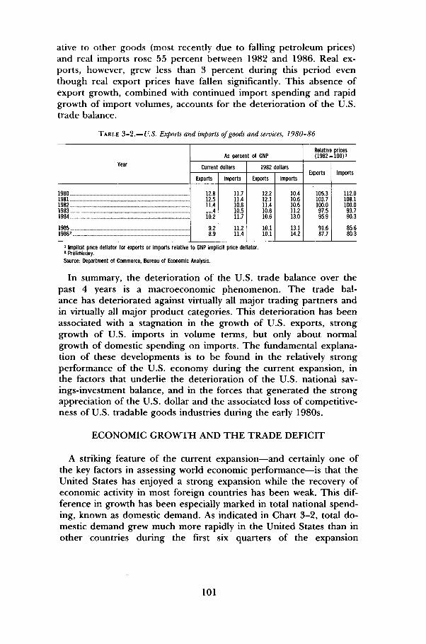
ative to other goods (most recently due to falling petroleum prices)and real imports rose 55 percent between 1982 and 1986. Real ex-ports, however, grew less than 3 percent during this period eventhough real export prices have fallen significantly. This absence ofexport growth, combined with continued import spending and rapidgrowth of import volumes, accounts for the deterioration of the U.S.trade balance.

TABLE 3-2.—U.S. Exports and imports of goods and services, 1980-86

Year

19801981198219831984

198519862

As percent of GNP

Current dollars

Exports

12.812.511.4,w.410.2

9.28.9

Imports

11.711.410.610.511.7

11.211.4

1982 dollars

Exports

12.212.111.410.610.6

10.110.1

Imports

10.410.610.611.213.0

13.114.2

Relative prices(1982 = 100) 1

Exports

105.3103.7100.097.595.9

91.687.7

Imports

112.0108.1100.093.790.3

85.680.3

1 Implicit price deflator for exports or imports relative to GNP implicit price deflator.2 Preliminary.

Source: Department of Commerce, Bureau of Economic Analysis.

In summary, the deterioration of the U.S. trade balance over thepast 4 years is a macroeconomic phenomenon. The trade bal-ance has deteriorated against virtually all major trading partners andin virtually all major product categories. This deterioration has beenassociated with a stagnation in the growth of U.S. exports, stronggrowth of U.S. imports in volume terms, but only about normalgrowth of domestic spending on imports. The fundamental explana-tion of these developments is to be found in the relatively strongperformance of the U.S. economy during the current expansion, inthe factors that underlie the deterioration of the U.S. national sav-ings-investment balance, and in the forces that generated the strongappreciation of the U.S. dollar and the associated loss of competitive-ness of U.S. tradable goods industries during the early 1980s.

ECONOMIC GROWTH AND THE TRADE DEFICIT

A striking feature of the current expansion—and certainly one ofthe key factors in assessing world economic performance—is that theUnited States has enjoyed a strong expansion while the recovery ofeconomic activity in most foreign countries has been weak. This dif-ference in growth has been especially marked in total national spend-ing, known as domestic demand. As indicated in Chart 3-2, total do-mestic demand grew much more rapidly in the United States than inother countries during the first six quarters of the expansion

101

(through mid-1984). Since then, differentials between U.S. and for-eign demand growth have narrowed considerably, but a large cumu-lative gap in domestic demand growth remains. This gap reflects thefact that the current recovery of U.S. domestic demand is one of thestrongest of the postwar period. It also reflects the fact, however,that the recovery of domestic demand abroad has been one of theweakest.

Chart 3-2

Real Domestic Demand in Selected Industrial Countries

Index, 1982=100

125 ~

120

115

110

105

100

95

Four Largest European~ .**• Countries-!/

"T i I i i i I i i i I i i i I i i i I i i i I i i1980 1981 1982 1983 1984 1985 1986

-I/France, Italy, United Kingdom, and West Germany, weighted by GNP.

Note.—Domestic demand is the sum of personal consumiinvestment, and government purchases of goods and serv

Sources: Department of Commerce and country sources.

Note.—Domestic demand is the sum of personal consumption expenditures, gross private domesticinvestment, and government purchases of goods and services.

These differences in output and demand growth have contributedto the deterioration of the U.S. international payments position inseveral ways. At an accounting level, the U.S. deficit on goods andservices trade signifies that total expenditures on goods and servicesin the United States (domestic demand) exceed U.S. production ofgoods and services (GNP), and that the United States is importingthe difference. Intuitively, the strong U.S. recovery—especially interms of domestic demand—has boosted expenditures on imports aswell as on domestically produced goods. Relatively weak growthabroad, however, has limited the expansion of U.S. export markets.

102

Weak foreign growth has been a critical problem for the worldeconomy. Assessments of the U.S. recovery and the deterioration ofthe U.S. payments position must take account of this weakness and ofthe importance of the U.S. expansion to sustaining world growth.Similarly, domestic demand growth abroad needs to be assessed notonly in terms of its effect on the U.S. trade balance, but also in itsrole in sustaining foreign growth as the U.S. economy adjusts. Thissection, therefore, reviews the recent economic performance of for-eign industrial countries, developing countries, and the UnitedStates, and analyzes the deterioration of the U.S. trade balance inthis regard.

FOREIGN INDUSTRIAL COUNTRIES

In the 1980s, the industrial countries faced critical economic chal-lenges of reducing inflation rates generally from double-digit levels,adjusting to the second oil shock of 1979-80, recovering from theworld recession, and halting or reversing the growth in governmentexpenditures. All countries achieved substantial reductions in infla-tion, but experienced varying success in meeting other challenges.

Western Europe's recovery from world recession has been slack.Between 1982 and 1985, real GNP in Western Europe grew at an av-erage annual rate of about 2.2 percent, one-half of the growth rateexperienced in the United States, Canada, or Japan (Table 3-3).Annual growth of domestic demand was slightly weaker, averagingonly about 1.8 percent. This slow growth has coexisted with risingunemployment during much of the recovery. In 1986, the averageunemployment rate for the four largest European countries (France,Italy, the United Kingdom, and West Germany) was about 10 per-cent, roughly double its 1980 rate.

This slow growth is especially disappointing given the stimulus toworld growth provided by the strong U.S. recovery and the apprecia-tion of the dollar (which increased these countries' relative competi-tiveness). Most Western European countries, however, generallycoped successfully with the depreciation of the dollar in 1986. Therapid passthrough of lower petroleum prices increased consumer in-comes and both consumption and investment strengthened. Thisstrengthening of domestic demand enabled many Western Europeancountries to enjoy a slight acceleration of GNP growth despite aweakening of real net exports. The cumulative growth rate of West-ern European domestic demand over the course of the expansion,however, remains low, especially for West Germany (despite stronggrowth in 1986), where the level of domestic demand in 1985 wasonly slightly above its 1980 level.

103

TABLE 3-3.—Growth in real domestic demand and real GNP in major industrial countries,1970-86

[Average annual percent change]

Country

United States

Canada

Japan

France

Germany

Italy

United Kingdom

1970 t(

Realdomes-

ticde-

mand1

25

49

42

37

27

2.9

1.7

) 1980

RealGNP2

28

46

47

36

27

3.1

1.9

1980 t

Realdomes-

ticde-

mand1

34

21

28

12

2

.4

1.9

) 1985

RealGNP2

24

25

39

12

13

.9

1.9

1982 t(

Realdomes-

ticde-

mand1

56

42

31

8

19

1.5

3.1

) 1985

RealGNP2

4.2

42

4.3

1.2

2.4

1.7

3.1

1985tc

1986

Realdomes-

ticde-

mand1

3.6

33

38

(3)

36

4.5

3.3

III

III

RealGNP2

2.3

3.5

2.3

(3)

23

3.0

2.0

1 Domestic demand is the sum of personal consumption expenditures, gross private domestic investment, and governmentpurchases of goods and services.

2 Data for Canada, France, Italy, and United Kingdom are real GDP.3 Not available.Sources: International Monetary Fund and country sources.

Unlike Western Europe, Japan grew at a 4.3 percent annual ratebetween 1982 and 1985. Much of this growth, however, was export-led. Following the 1979 oil shock, domestic demand in Japan slowedmarkedly as the country adjusted to the higher oil import bill. Duringthe first half of the 1980s, the average rate of domestic demandgrowth was only about one-half its 1970-79 average. Rising exports,however, enabled GNP to grow more than 1 percentage point higherthan domestic demand. This excess of output over demand growthwas reversed in 1986 as real Japanese exports fell in the wake of thesharp appreciation of the yen. Japanese internal demand increasedsomewhat, but not enough to offset the decline in exports, andJapan's rate of GNP growth slowed to under 3 percent.

Despite differences in their growth rates, Western Europe andJapan shared similar policies and challenges. They both faced thesudden increase in petroleum prices while shifting to anti-inflationarymonetary policies. They both moved generally toward fairly austerefiscal policies by restraining government expenditures. While the re-sulting reduction in inflation and increased budgetary room for taxcuts should provide a good foundation for stronger growth in thelong run, the initial effect of these developments was to depress eco-nomic activity.

In Western Europe, these developments interacted with structuralrigidities that, in addition to reducing long-run growth, intensifiedand prolonged the effect of macroeconomic shocks. Substantial non-wage labor costs and excessively expensive job security arrangements

104

discouraged labor mobility and new hiring. High marginal tax rates,various regulatory burdens, and large subsidies to declining indus-tries and to agriculture impeded adjustment and growth by retardingthe flow of investment toward high-growth sectors.

In Japan, structural rigidities did not prevent the economy fromgrowing strongly over much of the 1980s. They did, however, holddomestic demand below what it could have been, giving the economya bias toward export-led growth. Restrictions that have prevented theefficient use of scarce land, combined with mortgage instruments thatrequire substantial downpayments, have made housing less afford-able. Limitations on consumer credit markets have dampened thedemand for consumer durables, discouraging investment aimed atproducing for local markets.

DEVELOPING COUNTRIES

Slack growth of output and demand during the 1980s has not beenconfined to foreign industrial countries. With the exception of devel-oping countries in Asia, growth in the developing world has beenparticularly weak. Between 1980 and 1986, annual real GNP growthin Latin America averaged 1 percent, less than one-fifth the averagegrowth rate enjoyed during the 1970s (Table 3-4). Real GNP grewequally slowly in Africa over this period; in the Middle East, realGNP declined. This slow growth has depressed U.S. exports. Devel-oping countries are important trading partners for the United States.In 1981, developing countries purchased 41 percent of all U.S. mer-chandise exports. By 1985, however, their trade share had fallen to34 percent.

TABLE 3-4.—Real GNP growth in developing countries

[Average annual percent change]

Region

Western Hemisphere

Africa

Middle East

Asia.

1970to

1980

58

64

1980to

19861

10

10

4

47

1980to

1983

1 1

6

1983to

1986 l

32

1.7

4.1

1 Preliminary estimates.Source: International Monetary Fund.

The slow growth of many developing countries is the product ofmany forces. The recession in the industrial countries in the early1980s, followed by the slack recovery of domestic demand in Japanand Europe, reduced the demand for many exports by developingcountries. Exporters of primary commodities suffered particularly, asthe shift from the inflation of the 1970s to the disinflation of the

105

1980s, combined with sluggish world growth, depressed prices forthese products. Since 1980, the dollar price of raw agricultural com-modities has fallen 20 percent; mineral prices have declined 30 per-cent.

With the appreciation of the dollar, the real burden of the dollar-denominated debt of many developing countries increased consider-ably. Much of this debt was contracted at floating rates, making debt-service payments highly sensitive to the sharp rise in nominal andreal interest rates in the early 1980s. These developments causedmany lenders to doubt the capacity of several developing countries tomeet their obligations, and to end abruptly the access of these coun-tries to international capital markets.

The policies of many developing countries were an importantcause of the interruption of voluntary lending flows. Overvalued ex-change rates, price controls, arid schemes to boost real wages by leg-islative fiat made the production of many goods unprofitable and re-duced the international competitiveness of many developing coun-tries. Maintenance of substantially negative real interest rates, as wellas tax and regulatory policies that discouraged investment, inducedcapital flight instead of encouraging the inward flows of capitalneeded to promote more rapid development. Reliance on inefficientpublic enterprises to produce a wide variety of goods and servicescontinued to be important drains on government budgets. Thesedrains further increased external deficits in these countries while fail-ing to engender the productive investment needed to increase theircapacity to service the associated external debts.

Whatever the cause, the cessation of voluntary lending flows forceddeveloping countries with debt-management problems to cut importspending rapidly in order to reduce their borrowing needs. Between1981 and 1983, the value of U.S. merchandise exports to Mexico fell$9 billion, a drop of almost 50 percent. Exports to the rest of LatinAmerica fell nearly 37 percent, or about $8 billion. In contrast, U.S.exports to industrial countries fell 10 percent. Since 1983, exports toLatin America have recovered somewhat but still remain below 1980levels.

GROWTH AND THE TRADE DEFICIT

The strong recovery in the United States—and the resulting dete-rioration of the U.S. international payments position—was a powerfulstimulant to growth in both industrial and developing countries. Thisgrowth, which took place against the background of world recession,provided a vibrant market for foreign exporters at a time when manydeveloping countries, suddenly facing credit constraints, needed toexpand exports to finance imports sufficient to maintain politically

106

acceptable levels of output and income. In contrast, sluggish growthin most other industrial countries limited increases in their imports.Between 1982 and 1984, the United States absorbed about 95 per-cent of the increase in merchandise exports by Latin American coun-tries to industrial countries, much more than would be implied by thenormal 50 percent U.S. share of Latin American exports to industrialcountries.

At Crst, the deterioration of the U.S. payments position helped aswell as hurt the U.S. economy. During the first six quarters of theexpansion, real GNP grew at a healthy 6.8 percent annual rate; do-mestic demand grew even faster, averaging 8.8 percent. In effect,growing net imports allowed desired increases in spending to be sat-isfied without pushing production growth to levels that would havecaused bottlenecks. Although the strong appreciation of the dollarreduced U.S. international competitiveness, the resulting decline inimport prices boosted real incomes in the United States and helpedto ameliorate inflationary pressures.

Since mid-1984, domestic demand has grown at a 3.1 percentannual rate. However, despite this slowing of demand growth tomore sustainable levels, increases in imports continued to outpaceexports, and the annual rate of real GNP growth from the secondquarter of 1984 to the fourth quarter of 1986 averaged only 2.4 per-cent. Insofar as the expanding capacity of the U.S. economy wasmore than sufficient to meet increases in total U.S. demand, the ex-pansion of the U.S. trade deficit during this period was an importantfactor limiting growth. This negative consequence has stimulatedprotectionist sentiment in the United States, especially because theburden of the resulting adjustment has not been spread evenlythrough the economy. Industries that account for about 70 percentof U.S. GNP produce either services that do not enter into interna-tional trade or products that are largely nontradable. The deteriora-tion in the U.S. balance in goods and services trade between 1980and 1986, amounting to 5.7 percent of real GNP, was thereforeconcentrated in sectors of the economy that account for only about 30percent of GNP. Moreover, the distribution of the adjustment withinthese sectors was not even.

THE SAVING-INVESTMENT BALANCE

The deterioration of the U.S. international payments position hasalso been closely associated with movements in national saving andinvestment. As discussed in the previous section, the U.S. deficit ingoods and services trade signifies that total spending in the United

107

States on goods and services exceeds U.S. production of goods andservices. This necessarily implies that the United States is absorbingforeign saving to finance the difference between expenditures andincome or, equivalently, that U.S. investment exceeds U.S. saving.For example, in 1986, gross national saving in the United States was$537 billion; gross private investment was $686 billion. The differ-ence was financed by a net capital inflow of nearly $150 billion fromabroad.

THE PRIVATE SAVING-INVESTMENT BALANCE

The national saving-investment balance is the excess of the privatesaving investment balance—the difference between gross privatesaving and gross private domestic investment—over the general (Fed-eral, State, and local) government deficit. Between 1982 and 1986,the private saving-investment balance fell from 3.5 percent of GNP to—0.1 percent. This decline reflected the strength of consumptionand investment growth, as is normal for a recovery. Given the lengthof the current expansion, the current level of the private saving-investment balance is not unusually low. The private saving-investmentbalance was lower in 1969 and 1979 than it was in 1986.

Between 1982 and 1985, the gross private saving rate—defined asgross private saving divided by GNP—fell less than one-half percent-age point (Table 3-5). The ratio of private saving to GNP fell signifi-cantly, but this decline was more than offset by increases in net busi-ness saving. Such offsetting movements in household and businesssaving are not surprising, since households are the ultimate owners ofall wealth, including the capital owned by businesses.

TABLE 3-5.—Private saving and investment

Year

1979

19801981198219831984

198519864

As percent of GNP

Private saving

Gross1

17.8

17.518.017.617.417.9

17.216.2

Personal

4.7

5.05.24.93.84.5

3.62.8

Business(net)2

2.5

1.41.4.6

1.92.4

2.72.8

Gross privatedomestic investment

1982dollars

18.0

16.016.814.115.418.7

18.117.9

Currentdollars

18.1

16.016.914.114.717.6

16.516.3

Relative priceof investment(1982=100)8

100.6

100.1100.6100.096.094.1

91.890.9

1 Gross private saving is personal saving plus net business saving and capital consumption.2 Net business saving is undistributed corporate profits plus inventory valuation and capital consumption adjustments.3 Implicit price deflator for gross private domestic investment relative to GNP implicit price deflator.4 Preliminary.

Source: Department of Commerce (Bureau of Economic Analysis) and Council of Economic Advisers.

The gross private saving rate fell sharply in 1986. However, evenwith the drop in private saving, most of the decline in the private

108

saving-investment balance during the current expansion is accountedfor by strong investment growth. Real gross private domestic invest-ment rose 46 percent between 1982 and 1984, boosting the share ofreal investment in real GNP from a near record low of 14.1 percent to anear record high of 18.7 percent. Although investment growth hasbeen sluggish since 1984, the share of real investment in real GNP hasremained near cyclical highs.

This strength in real investment spending, however, was partiallyoffset by a substantial decline in the relative price of investmentgoods. As reported in Table 3-5, the relative price of investmentgoods fell 9.1 percent between 1982 and 1986. In 1986, nominal ex-penditures on gross private domestic investment accounted for 16.3percent of GNP, well below 1978-79 levels and only 0.3 percentagepoint above the average share of nominal investment expendituresexperienced over the past 25 years. Thus, the lower relative price ofinvestment goods allowed large increases in real investment to occurwith only moderate demands on nominal saving. This developmentproduced a normal cyclical decline in the private saving-investmentbalance, despite the decline in the gross private saving rate and thestrength of real investment.

THE GOVERNMENT DEFICIT

The large increase in the general government budget deficit, how-ever, stands in marked contrast to its normal cyclical behavior. Thegeneral (Federal, State, and local) government budget deficit aver-aged 3.4 percent of GNP in 1986. This deficit/GNP ratio, althoughlarge, is not the largest experienced during the past 15 years. Thegeneral government budget deficit exceeded 3.4 percent of GNP inboth 1975 and 1982. The 1975 and 1982 deficits, however, occurredduring sharp recessions; the current large deficit comes in the fourthyear of an expansion.

As indicated in Chart 3-3, until recently the general governmentbudget deficit has tended to track the private saving-investment bal-ance during cyclical expansions and declines. National saving has ap-proximated national investment and the current account balance hasbeen small. In recessions, government budget deficits typically widenas a result of declining tax revenues and increased expenditures asso-ciated with income support. The private saving-investment balance,however, usually increases by more than the cyclically induced de-cline in the general government budget deficit (because of weak in-vestment and consumption spending), and the current account bal-ance tends to improve. In the sharp 1975 recession, for example, thelargest general government budget deficit in the postwar era (meas-

109

ured as a percent of GNP) coincided with one of the largest U.S.current account surpluses.

Chart 3-3Private Saving-Investment Balance, Government Deficit,

and Current Account Balance

Percent of GNP

2 -

-2

Private Saving-Investment Balance

4

2

0

-2

-4

~^^ /\

_ Current Account Balance \

I I I I 1 I I I t 1 I I I I 1 I I I I i I i i I 1 I I I I 1 I1955 1960 1965 1970 1975 1980 1985

Note.—For current account balance, data for 1986 are first 3 quarters at an annual rate; seasonally adjusted.

Source: Department of Commerce.

Similarly, strong investment growth during an expansion usuallyoutstrips increases in private saving, and the private saving-invest-ment balance declines. The associated growth in tax revenues, how-ever, traditionally lowers the general government budget deficit, andthe deterioration in the U.S. current account deficit usually remainsmodest. This pattern has not been followed in the current expansion.The increased surpluses of State and local governments have beenmore than offset by the large growth of the Federal Governmentbudget deficit. This unprecedented deterioration of the U.S. fiscalposition during an expansion, combined with a normal cyclical de-cline in the private saving-investment balance, has been reflected inan unprecedented deterioration in the U.S. current account balance.

It is important to emphasize that the government budget deficitand the U.S. international payments position are the product of manyforces and that the link between them is complex. As noted above,increases in the government budget deficit that result from a cyclical

110

decline are typically associated with improvements in the U.S. inter-national payments position. Clearly it is incorrect to say that move-ments in budget deficits always cause equal movements in the U.S.current account balance. It is equally clear, however, that the persist-"ence of the Federal deficit late into the current expansion is one ofthe most important factors contributing to the growth of the tradedeficit.

It is also important to emphasize that the desirability of any fiscalmeasure taken to reduce the current large budget and trade deficitsdepends critically on whether the measure is desirable in its own right.Federal outlays have remained at a high percentage of GNP. Sustainedefforts to control Federal spending are needed not only to preserve thebenefits of tax reform but also to reduce the U.S. internationalpayments imbalance. The key point is that a substantial reduction inthe U.S. current account deficit will require restraint of U.S. domesticdemand growth relative to GNP growth. If this restraint does not comefrom controlling government spending, it must come from the othercomponents of domestic demand—consumption and investment. Taxincreases are not the answer. Higher tax rates would not only lowerGNP growth in the short run, but would also continue to dull economicincentives and to reduce growth far into the future. This would makeeven more painful the necessary adjustment of consumption andinvestment to bring domestic demand in line with GNP in the long run.

INTERNATIONAL CAPITAL FLOWS

The link between the current account balance and the nationalsaving-investment balance also helps to emphasize the importance ofinternational capital markets and net capital flows in the developmentof the U.S. current account deficit. The counterpart to the U.S. currentaccount deficit is a capital account surplus; developments influencingone account significantly influence the other. On the one hand, deep,liquid international capital markets have represented a ready source offinancing for the large shortfall of U.S. saving relative to U.S. invest-ment. On the other hand, changes in the desirability of holding U.S.assets, particularly dollar-denominated assets, have had substantialeffects on exchange rates, thereby affecting the current account.

International capital markets channel resources from the ultimatesavers in the world economy to those countries that offer the mostattractive opportunities to invest. For example, through most of the19th century, the inflow of capital from abroad helped the UnitedStates to exploit its vast productive potential much more quickly thanif U.S. capital formation had been limited to U.S.-based saving. In

111

this case, the associated current account deficit was part of a processthat invigorated a then-young economy.

Similarly, the capital inflows now associated with the U.S. currentaccount deficit have once again become an important source of in-vestment financing. Several factors have made the United States oneof the most attractive places in which to invest funds. The stronggrowth of the U.S. economy during the first six quarters of thisexpansion stood in marked contrast to the sluggish performanceabroad, especially in Europe. This growth, combined with the reduc-tion in capital taxation embodied in the Economic Recovery Tax Act of1981 (ERTA), surely increased the relative attractiveness of investmentin the United States.

It is important to recognize, however, that the development of theU.S. current account deficit has also been associated with a sharp dropin the national saving rate (relative to the cyclical peak in either 1979or 1981). Between 1981 and 1986, the national saving rate fell morethan 4 percentage points (Table 3-6). This drop has made theUnited States increasingly dependent on net capital inflows to fi-nance U.S. investment. In 1986, net capital inflows—and the associat-ed buildup of foreign claims on the United States—equaled one-halfof U.S. net capital formation. To the extent that the drop in the na-tional saving rate is not desirable, this dependence on net capital in-flows to finance U.S. investment is also not desirable. Part of the de-cline in the national saving rate has resulted from the failure to bringgovernment expenditures in line with revenues. Part of the increaseddependence on capital inflows to finance U.S. investment, therefore,ought to be viewed as a by-product of a fiscal stance that should becorrected by gradually reducing the share of Federal expenditures inGNP.

TABLE 3-6.—National saving, investment, and net capital inflow

[Percent of GNP]

Year

1979

19801981198219831984

198519864

Grossprivatesaving

178

175180176174179

172162

Governmentsaving1

05

-1.3-10

35-38

27

-3434

Grossnationalsaving

183

16.317114 113.6152

138128

Netcapitalinflow2

01

-.3_ 2

o1.124

2735

Grossprivate

domesticinvestment3

181

16.016914 114.7176

165163

1 Federal, State, and local governments.2 Includes statistical discrepancy.3 Nominal prices.4 Preliminary.

Source: Department of Commerce, Bureau of Economic Analysis.

112

This conclusion, however, in no way minimizes the role capitalmarkets have played in driving the current account. Exchange ratesare determined in asset markets. As is discussed in the next section,the strong increase in the demand for dollar-denominated assetsduring the first half of the 1980s, and the consequent appreciation ofthe dollar between 1980 and early 1985, was a key factor underlyingthe deterioration of the U.S. current account balance.

EXCHANGE RATES AND COMPETITIVENESS

Exchange-rate changes are a direct channel through which interna-tional divergences in economic policy are transmitted to domesticeconomic performance. Exchange-rate movements that persistentlyexceed international inflation differentials—real exchange-rate move-ments—change the prices of a country's imports relative to domesti-cally produced goods and alter the ability of its producers to com-pete in world markets. This section reviews the behavior of the realforeign exchange value of the dollar and the relative price of U.S. im-ports over the past decade, investigates the sources of these real ex-change-rate movements, and assesses the effect of these exchange-rate movements on the international cost competitiveness of U.S.manufacturers.

SOURCES OF REAL EXCHANGE RATE MOVEMENTS

The past decade has been characterized by wide swings in the for-eign exchange value of the dollar and in the relative price of imports.Chart 3-4 presents an index of the foreign exchange value of thedollar against a trade-weighted basket of currencies from 18 other in-dustrial and 22 developing countries. The index is adjusted for dif-ferences in wholesale price inflation in each country and thus meas-ures changes in the real foreign exchange value of the dollar. Alsopresented is an index of the relative price of non-oil imports, com-puted as the ratio of the import price deflator excluding petroleumto the total GNP price deflator. As can be seen from the chart, broadmovements in the dollar's real exchange rate and the relative price ofimports over the past decade can be divided into three phases.

During the late 1970s, the real value of the trade-weighted dollardepreciated and the relative price of imports increased by roughly 10percent. According to many observers, the weakness of the dollar inthe late 1970s was directly related to the perception that the UnitedStates was embarked on significantly more inflationary policies thanwere Japan and many West European countries. This perception ledto depreciation of the dollar not only in nominal terms, but also inreal terms. The nominal foreign exchange value of the dollar fell

113

Chart 3-4

Real Exchange Rate and Relative Price of Imports

Index, 1977:1=100140

130

120

110

100

90

80

Real Exchange Rate1'/

Relative Price of ImportsLess Petroleum1/

-4.I I I i I I I I I I I I i I I i I I I I I I I

1977 1979 1981 1983 1985

-VTrade-weighted value of the dollar adjusted by relative wholesale prices.

-2/Ratio of implicit price deflator for imports less petroleum to GNP implicit price deflator.

Sources: Morgan Guaranty Trust Company of New York and Department of Commerce.

more than was justified by the actual excess of inflation in the UnitedStates over inflation in other countries, because the exchange rate re-sponds to expected future inflation as well as to current and past in-flation.

The relatively weak dollar during the late 1970s benefited manytrade-sensitive industries in the United States. The real depreciationof the dollar shielded these industries from their foreign competitorsbecause, as is shown in Chart 3-4, import prices increased faster thandid the prices of domestically produced goods and services. This al-lowed some manufacturing industries to remain profitable while in-creasing real wage rates substantially more rapidly than in the rest ofthe United States economy, despite slow productivity growth. The in-sulation from foreign competition that the weak dollar provided tomany trade-sensitive industries in the United States in the 1970s leftmany of these industries poorly prepared to deal with such competi-tion in the 1980s.

114

The first half of the 1980s was marked by an unprecedented surgein the real foreign exchange value of the dollar. From the third quar-ter of 1980 through the first quarter of 1985, the real value of thetrade-weighted dollar appreciated by some 47 percent and the rela-tive price of imports declined by 22 percent. Although some observ-ers have claimed that the dollar's appreciation can be attributed to asingle cause, several factors contributed to the sustained rise in thedollar between 1980 and early 1985.

The shift in monetary policy from one of perceived ease and ac-commodation to an actual and ultimately perceived anti-inflationarystance in the early 1980s was likely critical to the reversal during1981 and 1982 of the real depreciation of the dollar that had oc-curred in the late 1970s. Between the third quarter of 1980 and thefourth quarter of 1981, the dollar appreciated in real terms back toits early 1977 level. The dollar appreciated an additional 12 percentin real terms in 1982. This appreciation was likely due, at least inpart, to increasingly persuasive evidence that the Federal Reserve wascommitted to an anti-inflationary monetary policy.

From the trough of the recession in the fourth quarter of 1982through the first quarter of 1985, the dollar appreciated an addition-al 15 percent in real terms. The initial dramatic decline and subse-quent stability of inflation, in conjunction with the strong growth inreal GNP in comparison with both past expansions and growth inmost other industrial countries, probably played an important role inthe further appreciation of the dollar during 1983-84.

The excess of real domestic demand over real domestic output thathas characterized the current expansion translates into an excess ofreal domestic investment over real domestic saving that, in turn,equals the real net inflow of foreign capital. At least a portion of thiscapital inflow and the appreciation of the dollar during 1983-84 likelyresulted from the increase in the after-tax profitability of physical in-vestment in the United States during this period. The increase in theafter-tax profitability of investment resulted from the interaction ofthe ERTA tax reductions with the decline in inflation, which in-creased the value of original cost depreciation.

Real business fixed investment grew much more rapidly relative toreal GNP in the first 2 years of the expansion than in previous cycli-cal upswings. Indeed, the share of real business fixed investment inreal GNP achieved a postwar record in 1984. This strength occurreddespite high real interest rates and concern that the Federal budgetdeficit would crowd out private investment. Furthermore, the realvaluation of the corporate capital stock by the equity markets alsosurged during this period. As discussed in previous Economic Reports,these facts are consistent with the view that changes in the tax law

115

raised the value in equity markets of new physical capital and the at-tractiveness of foreign investment in the United States.

Since the first quarter of 1985, the real value of the trade-weighteddollar has fallen by 20 percent, back to its late 1981 level. Although thecauses of this steep depreciation of the dollar are difficult to isolatewith precision, the decline in real GNP growth in the United Statessince mid-1984 likely contributed to the dollar's fall. In addition, theannounced intentions of the Group of Five to seek a lower dollar inthe Plaza Agreement and subsequent actions to back up these inten-tions, especially the continuation of the easing of U.S. monetarypolicy that began in late 1984, probably contributed to further dollardepreciation after September 1985. More generally, the convergenceof economic performance and economic policies of the leading indus-trial countries in 1985 and 1986 was probably necessary to support asignificant adjustment of exchange rates.

So far, little evidence exists of the effect of the substantial depre-ciation of the dollar on U.S. trade flows. Several factors help to ex-plain this limited impact. Existing empirical evidence indicates thatimport prices respond with a lag of up to 2 years to even largechanges in exchange rates. This phenomenon results from the choiceof foreign producers to boost profit margins as their currencies de-preciate against the dollar and to allow these margins to narrow so asto maintain market share as their currencies appreciate against thedollar. According to one study, foreign producers widened theirprofit margins considerably during the 1980-84 appreciation of thedollar. This provided them ample room to narrow profit margins bylimiting price increases and thus maintain market share as the dollardepreciated. Indeed, as is shown in Chart 3-4, non-oil import pricesactually declined in 1985 and began to rise only in 1986.

Another factor that has limited the immediate effect of the deprecia-tion of the dollar on U.S. trade flows is that the dollar has not in factdepreciated substantially against the currencies of several importanttrading partners. Total imports from Canada, Korea, and Taiwanexceed imports from Western Europe or Japan, yet the dollarhas depreciated less than 7 percent against the currencies of Canadaand Taiwan and has actually continued to appreciate against theKorean won.

PRODUCTIVITY AND COMPETITIVENESS

Declining international competitiveness of the U.S. economy, espe-cially manufacturing industries, is often cited as an important causeof the deterioration of the U.S. trade balance. Programs to revivesupposedly sagging productivity growth are often recommended as ameans of improving competitiveness and reducing the trade deficit.

116

In fact, as is discussed in Chapter 1, productivity growth in manu-facturing during the current cycle has exceeded the postwar averageand substantially exceeded the sluggish rate of productivity growthduring the 1970s. Since the business cycle peak in the third quarterof 1981, output per hour in manufacturing has grown at an averageannual rate of 3.8 percent, 46 percent faster than the postwar aver-age of 2.6 percent per year and more than twice the annual averagerate of 1.5 percent recorded between 1973 and 1981. Furthermore,real wage growth in the manufacturing sector has exhibited notablerestraint during the current cycle. Since the business cycle peak, realhourly compensation in manufacturing has grown at an averageannual rate of 1.0 percent, 50 percent slower than the postwar aver-age annual rate of 2.0 percent.

As the result of restrained wage increases and strong productivitygrowth, unit labor costs in manufacturing have increased at an aver-age annual rate of only 0.7 percent since the 1981 peak and have ac-tually declined at an average annual rate of 0.8 percent since the re-cession trough in the fourth quarter of 1982. By contrast, unit laborcosts in manufacturing have grown at an average annual rate of 3.4percent over the entire postwar period and grew at an averageannual rate of 8.2 percent between 1973 and 1981.

Table 3-7 compares movements in unit labor costs in the UnitedStates with a trade-weighted average of unit labor costs in 11 of thelargest foreign industrial countries. As is shown in the secondcolumn of the table, when measured on a national currency basis,growth in unit labor costs during the first half of the 1980s was 5percentage points higher abroad than in the United States. In the ab-sence of other developments, the relatively better U.S. perform-ance—which was a product of surging productivity growth and re-strained wage increases—would have improved U.S. internationalcost competitiveness. However, the cost competitiveness of U.S. man-ufacturers also depends upon the dollar exchange rate. Foreign im-porters can charge a lower dollar price to cover the same level of na-tional currency costs when the dollar appreciates against their owncurrencies.

As indicated by the third column of Table 3-7, the appreciation ofthe dollar during the first half of this decade overwhelmed the otherdeterminants of international cost competitiveness. In national cur-rency terms, unit labor costs in the 11 largest foreign industrial coun-tries rose more than 16 percent during the first half of the 1980s; indollar terms, foreign unit labor costs fell nearly 20 percent. Insteadof experiencing a 5 percent improvement in U.S. international costcompetitiveness between 1980 and 1985, the strong appreciation of

117

TABLE 3-7.—U. S. and foreign unit labor costs, 1980-85

[1980=100]

Year

1980

1981

1982

1983 .

1984

1985

UnitedStates

100.0

107.3

114.0

111.1

110.5

111.2

Eleven foreign industrial countries1

Nationalcurrency basis

100.0

108.2

114.4

115.4

115.1

116.3

Dollarbasis

100.0

96.9

91.6

88.5

81.9

80.3

1 Trade-weighted average of Belgium, Canada, Denmark, France, Germany, Italy, Japan, Netherlands, Norway, Sweden, andUnited Kingdom.

Source: Department of Labor (Bureau of Labor Statistics) and Council of Economic Advisers.

the dollar boosted the ratio of U.S. unit labor costs to foreign unitlabor costs by 39 percent.

This gap between the unit labor costs in U.S. manufacturing indus-tries relative to manufacturing industries in most other industrialcountries has been narrowed significantly by the depreciation of thedollar that began in early 1985. According to the International Mon-etary Fund, the ratio of unit labor costs in the United States to atrade-weighted average of unit labor costs expressed in dollars inother industrial countries fell almost 30 percent to its 1981 level be-tween the first quarter of 1985 and the second quarter of 1986.

In sum, the deterioration of international cost competitiveness inU.S. manufacturing during the first half of this decade was the resultof the real appreciation of the dollar, not sagging productivity growthor excessive wage increases. This fact does not imply, however, thatthe United States can or should rely solely on exchange-rate move-ments to improve further its international cost competitiveness. Ex-change-rate depreciation can increase competitiveness in the interme-diate run by making foreign-produced products more expensive, butat the cost of slower real income growth. By contrast, improvinginternational cost competitiveness through greater productivity andeconomic efficiency increases real income growth. The United Statesshould seek to strengthen international competitiveness by imple-menting policies that increase productivity. The President is sendingto the Congress a package of initiatives to enhance further U.S. pro-ductivity and competitiveness, including increased funding for basicand applied scientific research, reforms of Federal regulations toreduce business costs while continuing to serve important regulatorygoals, and efforts to improve access for U.S. products and services inforeign markets.

118

POLICY COORDINATION AND EXCHANGE RATE STABILITY

There is general agreement among economists that better conver-gence of economic performance and better coordination of economicpolicies among the leading industrial countries is both desirable andessential for achieving greater stability of exchange rates. At theTokyo Economic Summit, the leaders of the seven largest industrialcountries agreed to a flexible approach to improving the internation-al monetary system by providing more effective procedures for thecoordination of economic policies. The approach adopted in Tokyorepresents an important step down the path to greater convergenceof economic performance and better coordination of economic poli-cies—a path that was charted at earlier Economic Summits and Minis-terial Meetings, including especially the Versailles Economic Summitand the Group of Five meeting of September 1985. Three features ofthe approach outlined at the Tokyo Summit deserve particular em-phasis.

First, efforts at policy coordination will not focus narrowly onachieving specific values or ranges for exchange rates. Policymakersare to consider a broad class of indicators of economic performanceand economic policy: GNP growth rates, inflation rates, interest rates,unemployment rates, fiscal deficit ratios, current account and tradebalances, monetary growth rates, reserves, and exchange rates. Thisapproach should help to avoid the inherent weakness of pegged ex-change-rate systems: rigid commitments to particular exchange-ratevalues or ranges become too expensive in terms of other importantpolicy objectives and ultimately collapse under the pressure of policyconflicts. The Tokyo Summit leaders explicitly stated that the objec-tives of policy coordination are much broader than limiting ex-change-rate movements. Objectives include "promoting non-infla-tionary economic growth, strengthening market-oriented incentivesfor employment and productive investment, opening the internation-al trading and investment system and fostering greater stability of ex-change rates."

Second, individual nations are responsible for formulating theireconomic objectives and forecasting the critical indicators of econom-ic policy and performance. Collective assessment of the mutual com-patibility of objectives and forecasts is required as the essence ofpolicy coordination, and the managing director of the InternationalMonetary Fund is assigned his traditional role in assisting multilateralsurveillance. However, no agency is asked to undertake the essential-ly impossible task of forcing sovereign nations to pursue policies con-trary to their perceived national interests. Instead, the onus is on in-dividual nations to live up to their own commitments and forecasts.

119

Third, when significant deviations from the intended and agreedupon course arise, individual nations are pledged "to make their bestefforts to reach understanding on appropriate remedial measures. . . ."This pledge is not an effort to fine-tune the world economy to cor-rect for all of the minor and inevitable deviations from its forecastedpath. The emphasis is on "significant deviations from intendedcourse." Further, the Summit leaders agreed that remedial effortsshould "focus first on underlying policy fundamentals. . . ." This agree-ment does not preclude official intervention in foreign exchangemarkets, when such intervention would be useful. However, it doesplace the emphasis for policy coordination where it belongs—on theeconomic policies that ultimately influence important developmentsin the world economy.

Experience with the operation of this new system of policy coordi-nation will contribute to its further development. Even at this stage,however, it is clear that better policy coordination offers the promiseof more stable exchange rates, reduced external imbalances, and amore favorable economic environment for developing countries.

CURRENT REQUIREMENTS FOR POLICY COORDINATION

In the period ahead, the principal challenge of policy coordinationis to reduce present international payments imbalances in a mannerthat will support sustained, noninflationary growth in the world econ-omy. Unilateral actions by the United States are not sufficient to ac-complish this goal. Although a sharp U.S. recession would probablyimprove the U.S. trade balance, it would not only injure economicwell-being in the United States, but would also sharply curtail pros-pects for growth in the rest of the world. Massive dollar depreciation,by shifting world demand toward U.S.-produced goods, would helpreduce the U.S. external deficit but at a cost of increased inflationarypressures in the United States and depressed output growth in themain U.S. trading partners. Put simply, reduction of the U.S. currentaccount deficit requires that real GNP in the United States growmore strongly than domestic demand. This implies that real GNPgrowth abroad will fall short of foreign domestic demand growth.Unless foreign domestic demand strengthens, improvement in theU.S. current account balance will necessarily be associated with re-duced foreign growth. Given the size of the potential adjustment inthe U.S. current account, the risk is that foreign growth would besharply reduced.

An essential element of any program to reduce current externalimbalances, therefore, is that other industrial countries must achievestronger, domestic-led growth. Stronger domestic demand growth isneeded primarily to maintain satisfactory output and employment

120

growth in these countries while the United States adjusts. It is alsoneeded to engender the much needed expansion of U.S. export mar-kets without having to rely on further massive depreciation of thedollar. Finally, strengthened foreign domestic demand is needed tomaintain the growth of demand for the exports of many developingcountries. Many of these countries, especially those with debt serviceproblems, face considerable pressures to improve their external posi-tions. The United States, however, will be reducing, not increasing,its external deficit; thus, further improvements of the developingcountries' payments positions must come from the other industrial-ized countries.

Because the reduction of the U.S. current account deficit will taketime, strengthened foreign growth must be sustained over themedium term. Achieving such long-lasting improvements requires theelimination of those structural (i.e., microeconomic-based) distortionsthat have impeded growth. In particular, to ease adjustment in thetraded goods sectors, efforts must be redoubled to eliminate not onlythose practices that have restrained domestic demand but also thoserigidities that have reduced the mobility of labor and capital betweensectors. In Western Europe, where the recent economic recovery hascoexisted with sustained rises in unemployment—in some countriesto depression levels—there is a clear need to reform those policiesthat have reduced labor flexibility and have rendered employmentunprofitable. In Japan, where the emphasis has been on export-ledgrowth, the need is to eliminate those policies that have hindered do-mestic demand. In many countries there is a need to consider tax re-forms that would substantially lower marginal tax rates, without nec-essarily reducing government revenues in the long run. These meas-ures are desirable not simply because they would indirectly helpreduce present external imbalances; they are desirable because theywould improve long-term economic performance and well-being.

Efforts by foreign industrial countries to effect a growth-orientedreduction in external imbalances must be matched by correspondingefforts by the United States. Reductions in the U.S. current accountdeficit require that domestic demand in the United States grow lessrapidly than GNP and that national saving increase by more than na-tional investment. The United States can make a critical contributionto achieving these results by reducing the Federal deficit through ex-penditure restraint. Restraint on Federal spending would help slowdomestic demand growth, but the effects of this slowing would notsignificantly reduce GNP growth, provided that stronger growth ofdemand abroad and the lagged effects of dollar depreciation boostU.S. exports.

121

The preferred approach to unwinding current external imbalancescalls for continued growth of world demand, but with a smaller con-tribution coming from the United States and a larger contributionfrom surplus countries. Domestic demand growth abroad wouldexpand faster than potential GNP, while domestic demand in theUnited States would grow more slowly than potential output. Move-ments in exchange rates would offset the effect of these changes inthe sources of world demand for any one country's products. In the•United States, the reduced size of the government would allow for agreater percentage of the Nation's output to be devoted toward pri-vate investment and consumption.

Two other elements are also essential for the effective implementa-tion of this program. First, developing countries, especially thosewith external debt problems, need to adopt more growth-orientedpolicies. The critical issue here is really for developing countriesthemselves to make the reforms necessary to support long-termgrowth. However, the industrial countries and the international finan-cial system have an important role to play in assisting countries thatare moving toward more growth-oriented reforms. This role is theessence of the program articulated by the Secretary of the Treasuryin October 1985 to deal with the problems of debtor countries. Thelong-term goal of this approach is to restore the access of thesecountries to international capital markets by increasing their capacityto service their debts. By taking the measures needed to restore theiraccess to international credit markets, these countries will not only bepursuing policies that will promote long-term growth with existingresources, but will also restore the capital inflows needed to under-write additional investment and growth. These developments wouldprimarily benefit the developing countries themselves. They wouldalso expand markets for the products of the industrial countries.Meanwhile, industrial countries can contribute to growth-oriented ad-justment in developing countries by sustaining a growing market fortheir exports. (For a detailed analysis of this subject, see EconomicReport of the President: 1986, Chapter 2.)

Finally, all countries must avoid new protectionist measures andwork to reduce and eventually dismantle existing barriers to interna-tional trade in both goods and services. Much attention has recentlyfocused on growing protectionist sentiment in the United States.Progress in reducing the U.S. trade deficit, combined with effortsabroad to reduce protectionism in foreign markets, are clearly impor-tant in resisting protectionist actions in the United States.

Similarly, efforts in the United States to resist protectionism areneeded to prevent the awakening of protectionist forces abroad.International trade, after all, is dominated by trade in goods. Just as

122

most of the deterioration of the U.S. trade balance was in manufac-tures, improvements in the U.S. trade balance will come about large-ly from a swing in manufactures trade. This development will presentserious adjustment problems for U.S. trading partners, especially asthe performance of manufactures output in many countries, notablyWestern European countries, has been weak. It would be singularlyunfortunate, therefore, if the United States were to suggest—just asits trade position was beginning to improve—that protectionist meas-ures were an acceptable response to these adjustment pressures. Inthe end, all countries share an important common interest in the lib-eral system of international trade and must work to protect andexpand that system.

International policy coordination will always be made difficult byintercountry differences in economic situation and policy priorities.At a minimum, however, it is important to identify those situations inwhich joint actions will reinforce efforts to achieve individual as wellas common goals. Clearly, it is in every nation's interest that interna-tional payments imbalances unwind in an environment of continuedworld growth. Actions by other nations to strengthen their domesticdemand and to reduce structural rigidities that have impeded adjust-ment, combined with resolute action by the United States to restrainFederal spending, offer a means of accomplishing this goal.

123

CHAPTER 4

Opening International MarketsONE OF THE MORE REMARKABLE FEATURES of the past 40

years has been the rapid increase in real income per capita in manyparts of the world. This economic expansion has been fueled in largepart by a tremendous growth in world trade. In turn, growth in worldtrade has resulted from a major effort led by the United States andother countries to reduce global barriers to international commerce.

These events stand in direct contrast with the decade precedingthe start of World War II. Then, stagnation in the domestic econo-mies of major nations was compounded by the spread of import bar-riers, export subsidies, trade wars, and a general emphasis on closingdomestic markets to foreign competition.

Determined not to see this scenario unfold again after the war, theUnited States sparked a move to establish a world trade system com-plete with firm rules to govern trade practices and to ensure thattrade policies would not degenerate into beggar-thy-neighbor protec-tionism. International organizations were created to guide the worldeconomy along this new path. Among them was the General Agree-ment on Tariffs and Tra<Jt? (GATT)^et up to initiate a reduction oftrade barriers and to mediate-commercial disputes between membernations.

GATT has presided over seven multilateral rounds of negotiationsthat have produced historic global tariff reductions. As tariffs havecome down, the volume of international trade has increased muchfaster than world production. Unfortunately, while GATT has beenexpanding trading opportunities among countries, largely throughtariff reductions, these efforts have been undermined by new andmuch less transparent protectionist measures.

The world thus stands at a crossroads similar to the one it faced 40years ago. The commercial playing field is littered with governmentpolicies aimed at protecting various industries from the rigors ofinternational competition. Trade in major product sectors—includingsteel, automobiles, electronics, textiles, apparel, and footwear—is be-coming increasingly regulated by measures such as voluntary exportrestraints and orderly marketing agreements. The cost of these poli-cies is enormous while the benefits reach only a few. Unless some-

125

thing reverses the trend toward government-sponsored trading ar-rangements, the growth enjoyed by world economies over the pastfour decades could be severely curtailed.

The United States, as the largest participant in world trade and asa long-time champion of free trade, stands in a unique position tofight this move toward greater protectionism. From its start, the Ad-ministration has supported free trade. Most recently, it reaffirmedthis position in a policy statement issued on September 23, 1985,which contained a multipronged program to enhance and strengthenthe international trading environment. Elements of the program in-cluded macroeconomic policies aimed at dollar realignment, fiscaldeficit reduction, and an effort to ease the debt burden of developingcountries.

With respect to trade policy, the statement proposed that theUnited States undertake a number of bilateral measures aimed at re-ducing foreign trade barriers. A second thrust of U.S. trade policywould be to rekindle the GATT process by urging fellow members toenter into a new round of multilateral trade talks.

More than a year has passed since these policies were announced.Using a series of self-initiated cases under Section 301 of the TradeAct of 1974, the Administration has sought to eliminate certainunfair trading practices of foreign governments. A fund of money hasbeen established to support Export-Import Bank loans as part of aneffort to persuade foreign countries to restrict and eliminate com-mercial subsidy elements of their foreign aid grants. Bilateral talksaimed at establishing free-trade areas have been concluded withIsrael and begun with Canada.

And because of a leading role taken by the Administration, a newround of multilateral trade liberalization talks—held under the aus-pices of GATT—has commenced in Geneva. This new round pre-sents an important opportunity for rolling back interventionist meas-ures and for strengthening rules of conduct in international trade.Indeed, it offers prospects to rein in the various new forms of protec-tion that have arisen because of current weaknesses in the GATTprocess. The new round also provides the opportunity to extendrules of commercial relations to areas previously exempted from ornot covered by GATT, including agriculture, services, direct foreigninvestment, and intellectual property rights.

This chapter reviews the Administration's trade policy initiatives ofthe past year, especially as they relate to efforts to open foreign mar-kets. The fundamental premise behind these efforts is that free tradeoffers Americans the greatest hope for a prosperous future. Conse-quently, this chapter begins by reviewing the benefits of free trade.

126

THE CASE FOR FREE TRADE

Governments have long interfered with the exchange of goodsacross their boundaries. One purpose of their barriers was to collectrevenues through tariffs or tolls. Local industry usually supportedand benefited from the protective effect of these policies. Indeed, inmany instances, pressure from domestic producers induced govern-ments to shelter them from foreign competition with trade restric-tions. Another purpose was to achieve trade surpluses throughexport subsidies and import restrictions. These policies, whose osten-sible goal was to increase and preserve domestic wealth at the ex-pense of other countries, became known as mercantilism.

For more than 200 years, many economists have argued againstmercantilist policies and made the case for free trade. They generallybelieve that restrictions on commercial activity reduce wealth ratherthan increase it. Conversely, the argument for free trade is relativelysimple yet compelling.

The case for free international trade is much the same as the casefor free internal trade. Commerce between the United States andJapan benefits Americans as does commerce between New York andCalifornia. The exchange of goods, internally or internationally,arises as a natural outcome of specialization. Because of factors suchas climate, natural resource endowments, or technology, differenteconomic regions possess different abilities to produce certain goods.Individuals, firms, and industries within these regions tend to con-centrate their efforts in the goods and services that they are best ableto produce. Then their output is exchanged in the marketplace forthat of other economic agents.

Specialization allows for a more efficient use of scarce resourcesand permits improved productivity of the economy. The larger thesize of the market, the greater are the possibilities for specializationand for increasing the wealth of the community. The extent of spe-cialization in international trade is related to the forces of interna-tional competition. As barriers between markets are lowered, somedomestic producers will face increased competition from abroad.Other producers will exploit export opportunities as accessible mar-kets expand. Hence, production will tend to contract in industrieswhere foreign goods are superior relative to domestic goods on aprice and/or quality basis. In those industries where domestic goodsare relatively superior to foreign, local output will expand. Theselatter industries are said to have a comparative advantage.

In essence, comparative advantage means that an industry willexport if it is more efficient relative to other domestic industries. Anindustry's productivity relative to other industries within the same

127

country determines its ability to command scarce resources withinthat economy and, thereby, to export to the rest of the world. Thus,a local industry's efficiency compared with that industry in foreigncountries is not the main determinant of whether it exports or facesimport competition.

Because comparative advantage refers to an internal ranking ofproductivity, a country may import goods even if the local producingindustry is more efficient than its foreign rival. A country will tend toconcentrate production in those industries in which it has the great-est comparative advantage. Standards of living rise as resources areput to their most productive uses. One sign of rising standards ofliving, of course, is a rise in real wages.

A common misconception about international trade is that it isunfair. For instance, some argue that because U.S. wages are highrelative to wages in other countries, U.S. producers cannot compete.This argument is true for some industries, but not true in general.U.S. wages are high because American workers are in general rnqreproductive than their foreign counterparts. The relatively high U.S.productivity comes about from this Nation's enormous stock of physi-cal and human capital. As U.S. productivity levels increase, so dowages paid to workers. This puts upward pressure on wages even inrelatively inefficient sectors of the economy. But if wages rise andproductivity does not keep pace, then American firms will have trou-ble competing.

An instructive example comes from the U.S. steel industry. From1965 to 1981, wages rose much faster than labor productivity in steeland faster than wages and labor productivity in overall manufactur-ing. As a consequence, unit labor costs increased dramatically, andthe comparative advantage of U.S. steel products deteriorated badly.In other sectors where wages are relatively high but productivity re-mains strong, such as aircraft and computers, U.S. products competesuccessfully in world markets.

In addition to raising the general standard of living, the forces offree trade also produce dynamic gains for the economy. These bene-fits accrue because, in the absence of government intervention, in-vestment in new plant and equipment and in research and develop-ment tends to concentrate in the most efficient sectors of the econo-my. This increases the rate of growth of the economy. Conversely, inan economy riddled with protectionist policies, investment is oftendiverted from more efficient industries because of government-in-duced distortions in relative rates of return.

Finally, political gains arise from free-trade policies. As countriesrely more on each other for goods and services, they are more likelyto settle international disputes through negotiation rather than hos-

128

tile action. An example is the remarkable reduction in national ten-sions between the countries of Western Europe since the adoption ofinternal free-trade policies following World War II.

It is sometimes argued that the benefits of free trade depend uponspecial assumptions about economic behavior. But the case for freetrade is quite general. Early arguments for free trade assumed thatindustries were perfectly competitive and that trade arose from cli-matic or technological differences between countries. Later, econo-mists focused on trade resulting from relative differences in nationalendowments of factors of production, such as labor and capital. Inboth instances, the free-trade outcome was one where production ex-panded along the lines of comparative advantage and countries en-joyed the consequent gains of trade.

More recent theories of international trade flows stress the impor-tance of imperfectly competitive market structures arising from suchphenomena as increasing returns to scale and domestic barriers toentry. Even here, however, free international trade is beneficial. Ex-pansion of markets because of freer trade may allow a firm to realizeeconomies of scale from an output level higher than would be ex-pected in the absence of trade. These economies can then be passedon to the consumer as lower prices. Expansion of markets throughfree trade also leads to an erosion of monopoly power enjoyed bythose industries where both significant barriers to domestic entry andforeign competitors exist. Another source of gain is the benefit toconsumers from an increase in product diversity, in both quality andvariety.

The benefits of free trade are relatively independent of actionstaken by foreign countries. In particular, it is often argued that be-cause protectionist policies exist in foreign countries the UnitedStates must follow suit. This argument is generally false. The benefitsto the United States flow from buying goods and services for whichforeign producers have a comparative advantage and selling U.S.goods and services where U.S. companies have a comparative advan-tage. To the extent that foreign policies reduce these trade possibili-ties, those countries and the United States gain less.

Furthermore, the benefits of free trade do not require that tradebe balanced at any point in time. Indeed, overall trade balances andthe associated international capital flows allow countries the mutualbenefit of trading goods and services over time. Countries with over-all trade deficits borrow from the rest of the world. Such borrowingcan provide the requisite funds for financing investment expenditurescrucial to economic growth. Countries with overall surpluses lend tothe rest of the world. This lending raises the wealth of the country ifit is allocated to projects that earn higher rates of return than would

129

otherwise be possible. However, neither borrowing nor lending cango on indefinitely, and economic forces will work over time to ensurethat imbalances are closed. Thus, trade in goods and services be-tween any country and the rest of the world tends to be in balanceover the long run.

On the other hand, trade between any two countries may never bein balance. For a variety of reasons, countries tend to amass surplus-es with some countries and deficits with others. Unfortunately, inter-est in bilateral trade balances—essentially a mercantilist trait—re-mains great. In May 1986, the House of Representatives passed anomnibus trade bill, H.R. 4800, that called for the President to identi-fy countries that have "excessive" trade surpluses with the UnitedStates and then to negotiate with or take actions against these coun-tries, regardless of the underlying causes of the surpluses. The Presi-dent labeled the bill "kamikaze legislation" and promised to veto themeasure, but it died when the 99th Congress adjourned.

Despite the obvious benefits of a liberal trading order, variousforms of protection abound and are proliferating at an alarming rate.Why do governments continue to pursue these policies? Various jus-tifications have been put forward by governments to defend protec-tionist policies. Examples include government revenue, national de-fense, unfair foreign trade practices, preservation of certain ways oflife, and short-term aid to revitalize industry.

Whatever the motive, protection in any form redistributes incomeand wealth. And because the redistributive effects are usually notreadily apparent, special interest groups sometimes favor and govern-ments often choose these methods over other more visible and muchless costly forms of subsidy. Protection raises the price of importsand domestically produced import-competing products. But, consum-ers are seldom aware of the tax imposed upon them by protectionbecause they rarely have the opportunity to observe the differencebetween domestic and world prices. The cost of protection to con-sumers can be quite dramatic. For instance, the Council of EconomicAdvisers estimated that if Congress had been successful in its attemptto override the President's veto of the Textile and Apparel Trade En-forcement Act of 1985, Americans would have had to pay up to anadditional $44 billion for textiles and apparel over the next 5 years.

Given these considerations, the Administration supports policiesdesigned to improve the efficiency and productivity of the U.S. econ-omy. Such steps should make Americans more prosperous. Thesepolicies include retraining for displaced workers, reforming antitrustlaws, and strengthening property rights, both domestically andabroad. Other initiatives include the repeal or reform of regulationsthat unnecessarily impinge upon U.S. competitiveness.

130

SECTORAL MARKET OPENING INITIATIVES

SECTION 301 ACTIONS

Trade imbalances are largely macroeconomic phenomena, not re-lated directly to market access barriers or unfair trade practices byforeigners. But trade barriers and unfair practices distort economicactivity and generally harm economic efficiency. For this reason, theAdministration is committed to eliminating foreign trade policies thatpose a significant burden on U.S. exports.

Section 301 of the Trade Act of 1974, as amended, provides theauthority and procedures for the President to act against certainunfair trading practices of U.S. trading partners. The President mustfirst find that action is appropriate to enforce U.S. rights under anytrade agreement, or to respond to any act, policy, or practice of aforeign country that (a) is inconsistent with the provisions of, or oth-erwise denies the United States benefits under, any trade agreement,or (b) is unjustifiable, unreasonable, or discriminatory and burdensor restricts U.S. commerce. If he so finds, then he is authorized toact to enforce these rights or to eliminate the act, policy, or practice.

Unjustifiable practices are those that violate or are inconsistentwith U.S. international rights. The term "unreasonable" refers toacts, policies, or practices that are not necessarily illegal or inconsist-ent with U.S. international legal rights, but are viewed as beingunfair. The act applies not only to practices that harm U.S. trade ingoods and services, but also to actions against U.S. direct foreign in-vestment that affect trade in goods or services.

Section 301 is administered by the Office of the U.S. Trade Repre-sentative (USTR). Petitions may be filed by any interested party orthey may be "self-initiated" by USTR on its own or at the request ofthe President. Once an investigation has been opened, USTR, in co-operation with other U.S. Government agencies, determines theextent of harm to domestic interests and recommends action for thePresident. At the same time, USTR consults with the foreign govern-ment involved in the complaint and attempts to negotiate a settle-ment.

Depending upon the specific nature of the alleged practice, USTRhas up to 12 months to conclude the investigation and recommendaction to the President. If no solution is reached, USTR may recom-mend that the President impose duties or other restrictions on im-ports from the foreign country or take any other action authorized bylaw. Retaliatory actions taken under Section 301 may be nondiscrim-inatory or solely against the goods and services of the foreign coun-try involved in the dispute. The products subject to retaliation neednot correspond to the products related to the dispute.

131

Between January 1975 and November 1986, 57 cases had been ini-tiated under Section 301. Table 4-1 details the disposition of thesecases. In addition, numerous firms and industry groups have consult-ed with USTR regarding the Section 301 process or have filed andthen withdrawn their petitions before a case could be initiated. Morethan 60 percent of initiated cases were begun under the current Ad-ministration. Until 1985, all of these came as the result of privatelyfiled complaints. Recently, however, the role of Section 301 as anactive component of U.S. trade policy has grown, with the Presidentdirecting USTR to self-initiate four investigations and three trade ac-tions aimed at the practices of several U.S. trading partners. Five ofthe seven proceedings have been favorably resolved, while two arepending. Brief descriptions of the circumstances of these self-initiatedcases follow.

TABLE 4-1.—Summary of cases under Section 301

[January 1975 to November 1986]

Category

Petitions considered . . . ..

Petitions withdrawn

Cases terminated:

Due to resolution of disputeDue to other reasons

Cases resulting in retaliation

Cases suspended

Cases pending

Number

57

6

204

12

3

15

Note.—Case resolutions do not equal number of petitions considered because cases may fall into more than one category.Source: Compiled by Council of Economic Advisers from data provided by Office of the U.S. Trade Representative.

Self-initiated Section 301 Cases

On September 16, 1985, at the request of the President, an investi-gation was begun into practices that act as a barrier to U.S. cigarettesales in Japan. These practices included tariffs combined with inter-nal ad valorem excise taxes, an absolute prohibition on the manufac-ture of foreign cigarettes in Japan, discriminatory treatment in thecollection of excise taxes, and restrictions on the distribution of for-eign cigarettes. Bilateral consultations were held between representa-tives of USTR and the government of Japan. Japan promised to sus-pend altogether tariffs on cigarette imports. It also agreed to elimi-nate the discriminatory deferral in collecting excise taxes, terminatediscriminatory distribution practices, and make its price approvalsystem virtually automatic. On October 6, 1986, the President sus-pended the investigation with the intent that it be terminated uponfull implementation of the agreement.

132

In the autumn of 1985, the President directed USTR to self-initiatetwo Section 301 investigations against the practices of Korea. Thefirst involved restrictions on the ability of U.S companies to sell fireand life insurance in Korea. The second was aimed at the lack of ef-fective protection of U.S. intellectual property rights, such as copy-right protection for literary and artistic works, including computersoftware, and patent protection for chemical and pharmaceuticalproducts. Bilateral consultations resulted in agreements coveringboth complaints. The first increased U.S. market access to Korea's in-surance market by allowing U.S. insurers to underwrite both life andother insurance. The second promised to expand dramatically theprotection of intellectual property rights. The President approved theagreements in August 1986, and the investigations were terminated.

On August 1, 1986, the President determined that Taiwan's prac-tice of calculating customs duties based on prices listed in duty-paying tables violated a trade agreement or was unjustifiable and aburden on U.S. trade. In effect, this practice had led to increasedduties paid to Taiwan, because the prices in the tables often exceed-ed transactions values. Before USTR could recommend an appropri-ate method of retaliation, Taiwan agreed to stop the practice.

In October 1985, Taiwan agreed to provide greater market accessfor U.S. exports of beer, wine, and cigarettes within 6 to 12 months.In particular, Taiwan agreed to lift an import ban on beer and toallow U.S. products to be sold at all retail outlets where Taiwaneseproducts were sold. It also agreed to limit retail markups on U.S.products to the level applied to local products and to allow marketforces to determine the levels of importation of U.S. products.

On October 27, 1986, the President determined that Taiwan hadnot honored the agreement and accordingly found the Taiwanesepractices to be unreasonable and a burden on U.S. commerce. He di-rected USTR to retaliate. On December 5, 1986, before the retalia-tion could be implemented, Taiwan agreed to settle the dispute andthe President ordered the case terminated.

On March 31, 1986, the President announced his intention toimpose quotas on several European Community (EC) products in re-sponse to EC restrictions affecting U.S. exports of oilseeds andgrains to Portugal. He also vowed to increase tariffs on certain prod-ucts if the EC did not provide compensation for reduced U.S. ex-ports of corn and sorghum to Spain as a result of the replacement ofSpain's 20-percent tariff on these products by the EC's variable levy.The EC had taken its actions in connection with the accession ofSpain and Portugal to the EC.

On May 15, 1986, the President imposed quotas on EC imports inresponse to the Portuguese import restrictions. However, to date,

133

these actions have not restricted trade. On July 2, 1986, the EC andthe United States reached an interim agreement, and the quotas werelifted to permit continued sales of corn and sorghum to Spain for anadditional 6 months. Both sides had agreed to December 31, 1986,as a deadline for the final agreement. Unfortunately, subsequent ne-gotiations have failed to produce a settlement. Consequently, on De-cember 30, 1986, the President announced that ad valorem tariffs of200 percent would be placed on certain products, primarily importedfrom the EC, with a trade value approximately equal to the estimatedloss of corn and sorghum exports. The tariffs will be implementedno earlier than January 31, 1987, thus allowing additional time fornegotiations.

On September 16, 1985, at the President's direction, USTR begana Section 301 investigation into all aspects of Brazil's computer andcomputer-related (informatics) products policies. Included in the in-vestigation were practices concerning import restrictions, limitationson U.S. investment, and failure adequately to protect intellectualproperty rights. On October 6, 1986, the President announced thatBrazil's informatics policy was unreasonable and a burden or restric-tion on U.S. commerce, but ordered that the case be continued untilDecember 31, 1986, to give both sides more time to reach an agree-ment. In the meantime, he requested that USTR notify GATT ofU.S. intentions to suspend the application of tariff concessions toBrazil and to effect such suspensions when appropriate.

In the weeks that followed the Presidential announcement, someprogress was achieved on certain procedural aspects of Brazil's infor-matics policy. Consequently, on December 30, 1986, the Presidentsuspended those aspects of the investigation. In addition, he ordereda further extension, until July 1, 1987, to give negotiators additionaltime to settle remaining issues in the case.

Analysis of Section 301 Actions

The Administration's decision to self-initiate several Section 301cases has sent important signals. First, U.S. industries know that ifthey encounter unreasonable trade barriers in foreign markets, amechanism exists to help them overcome these barriers. Moreover,both the self-initiations and actions in cases initiated in response toindustry filings demonstrate U.S. concern to its trading partnersabout their commercial policies. The message of the Section 301process is that in the products and countries involved in the variouscases, the United States thinks its comparative advantage is being un-fairly denied.

Section 301 puts the weight of the President behind disputes overspecific, narrowly defined trade practices abroad. This attentionsharpens the focus of the dispute and allows pressure to build on a

134

clear and remediable problem. The threat of retaliation can provideleverage to negotiate an end to unfair foreign practices. Section 301also encompasses a greater range of issues (in goods, services, invest-ment, and intellectual property rights) than does GAIT.

Section 301 should be used with caution. Actions taken under it maybe perceived as an intrusion into the policies of a foreign government.And, while these policies may clearly be egregious and often lower theeconomic welfare of the foreign country, in some cases the threat ofretaliation may not provide the best incentive for successful resolutionof the issue.

Political leaders may not want to appear to be vulnerable to for-eign threats and may resist a mutually beneficial agreement to pre-serve national pride. Thus, Section 301 cases are most likely to suc-ceed in areas that have little economic and political significance toforeign governments, and retaliation is more likely in those caseswith significant foreign national interest.

The level of contentiousness is even higher when the process is ini-tiated at the President's direction without a petition filed by a U.S.firm or industry. In these cases, it is most unlikely that the investiga-tion will lead to any finding other than unreasonableness. The possi-bility of abandoning the case because the costs of retaliation are toohigh is limited.

U.S. retaliation may inflict as much or more harm on the Americaneconomy as it does on its target. In addition, unless carefully han-dled, it is likely to violate GAIT rules, undermining an already weakinternational dispute settlement process. Moreover, retaliation doesnot always stop with the issue at hand, but may escalate into furtherrounds of retaliation and counter-retaliation. The potential for mutu-ally destructive trade wars rises with the magnitude of the case andwith the size of the trading partner.

While the focus of a Section 301 case is usually on a specific prod-uct, the effects of a settlement may extend to other related areas. Forinstance, the recently concluded agreement with Japan over trade insemiconductor products has led, at least temporarily, to increases inthe prices of these products. As semiconductor prices rise, the com-petitiveness of industries using these products as inputs may dimin-ish.

Several proposed trade bills recently considered by the 99th Con-gress would have amended the Section 301 decisionmaking process.Most of these proposals are ill-advised. For instance, Senate billS.I860 would have mandated the President to self-initiate severalSection 301 investigations each year. It would also have required thePresident to retaliate if settlement were not reached after a fixedperiod of time. Such requirements add inflexibility to areas where

135

flexibility is vital, and do nothing to address the fundamental prob-lem of opening foreign markets. The decision to self-initiate raisesthe stakes in the negotiating process. Section 301 currently allows thePresident to lend the force of his office in those situations where itmost benefits the outcome of the process.

Finally, the credibility of U.S. complaints about foreign trade bar-riers depends in part on the extent of its own barriers. U.S. tariffs arelow on average, but tariffs on certain products remain high and non-tariff barriers affect a significant percentage of total imports. For ex-ample, the United States participates in the international MultifiberArrangement, which authorizes complex bilateral trade-restrictingagreements between exporters and importers of textiles and clothing.The United States has asked its trading partners to limit their exportsof steel and machine tools and uses nontariff barriers or high tariffsto restrict trade in sugar, dairy products, lumber products, motorcy-cles, and a number of other goods.

MARKET-ORIENTED, SECTOR-SELECTIVE TALKS

A much less confrontational approach to bilateral market openingis represented by a series of sectoral negotiations between the UnitedStates and Japan. Following the successful conclusion of talks to lib-eralize Japanese financial markets, both governments sought to ad-dress the often contentious issue of commercial trade with Japan. In1985, high-level discussions, called Market-Oriented, Sector-Selective(MOSS) talks, began with the purpose of identifying and removingimpediments to market access in Japan. Sectors initially chosen fordiscussion were telecommunications, electronics, medical equipmentand pharmaceuticals, and forest products. Transportation machinerywas added later.

The MOSS talks have shown substantial progress. Japan has imple-mented reforms in telecommunications, forest products, and medicalequipment and pharmaceuticals. MOSS discussions on electronicswere largely preempted by the semiconductor agreement. Negotia-tions in transport machinery, especially involving trade in automobileparts, still continue.

RECIPROCAL MARKET OPENING INITIATIVES

Opening markets on a piecemeal basis is difficult and inefficient. Amore fruitful approach is to enter into discussions with foreign gov-ernments to open all markets reciprocally. These discussions can occuron a bilateral or multilateral basis. Important progress was made onboth fronts in 1986.

136

FREE-TRADE AREA NEGOTIATIONS

A free-trade area (FTA) is an arrangement between two or morecountries to remove barriers to trade among themselves but to main-tain separate barriers with respect to nonmember countries. Thebenefits from FTAs resemble those attributed to free trade in gener-al: expansion of market size can lead to efficiency gains through spe-cialization. Consumers gain because they pay lower prices for certaingoods because of increased competition.

Conclusion of FTA agreements can help to maintain the momen-tum for liberalizing trade. When the international climate does notpermit widespread reductions of trade barriers, liberalization amonglike-minded nations promotes free trade. When nations that refuse toreduce their trade barriers see that others will achieve gains fromtrade by reducing barriers bilaterally, they might reconsider theircommercial policies and join the effort to open markets.

FTAs have their problems. The potential cost of FTAs relative tofreer trade in general arises from the fact that FTAs discriminate infavor of trade between member nations and against trade with non-member countries. Hence, the source of trade may be diverted awayfrom the lowest cost world producer in favor of a higher cost FTAmember.

Both the Administration and Congress, however, think that free-trade area arrangements are worthwhile. The Administration's 1985trade policy statement noted that bilateral negotiations are no substi-tute for multilateral negotiations, but that "such agreements couldcomplement our multilateral efforts and facilitate a higher degree ofliberalization, mutually beneficial to both parties, than would be pos-sible within the multilateral context/' Congress, for its part, hasgranted the Administration authority to enter into bilateral trade-lib-eralizing negotiations.

FTA Agreement with Israel

The Trade and Tariff Act of 1984 specifically authorized the Presi-dent to conclude an FTA agreement with Israel. Formal talks beganin January 1984. An agreement was signed in April 1985 and the firststage of liberalization went into effect in September 1985.

The agreement covers both tariff and certain nontariff barriers thatexist between the two countries. Although most substantive elementsof the agreement address liberalized trade in goods, some relate totrade in services and protection of intellectual property rights.

The U.S.-Israel FTA is the first such agreement reached by theU.S. Government. One motivating factor for negotiating this agree-ment was Israel's previous entry into a similar agreement with the ECcovering trade in manufactured products. By negotiating an FTA

137

with Israel, the United States regained the competitive advantage thatU.S. exporters had lost to their European competitors.

FTA Talks with Canada

More trade passes between the United States and Canada than be-tween any two other countries. In 1985, this trade totaled about $120billion. Canada is this country's largest foreign market, accountingfor 22 percent of total merchandise exports. The United States isCanada's largest market, purchasing more than 75 percent of totalCanadian exports. The two countries engage in substantial trade inservices. In addition, about 20 percent of U.S. direct foreign invest-ment is in Canada.

Over the course of U.S.-Canada relations, special trade pacts haveperiodically been considered. From 1855 to 1866, trade between thetwo countries was governed by special treaty. Since 1965, the UnitedStates and Canada have had a sectoral agreement covering trade inautomobiles. However, more comprehensive and longstanding agree-ments have eluded American and Canadian negotiators for decades.

Recently, a new effort to reinforce U.S.-Canada economic tiesbegan. On September 26, 1985, the Prime Minister of Canada calledfor negotiations between the United States and Canada to achieve"the broadest possible package of mutually beneficial reductions inbarriers to trade in goods and services." The Administration wel-comed this proposal and formally notified Congress in December1985 of its intent to enter into negotiations under the negotiating au-thority established in the Trade and Tariff Act of 1984. These nego-tiations were begun in May 1986.

After consultations with advisory committees representing industry,labor, and agriculture, the Administration developed objectives forthe talks. The first objective is the elimination of Canadian tariffs. Asecond broad goal is the elimination of nontariff barriers to certainU.S. exports. The United States is also interested in eliminating bar-riers to foreign investment in Canada, liberalizing trade in services,and protecting intellectual property rights.

Canadian objectives include reducing U.S. tariffs and improvingaccess to the government procurement process, both Federal andState, from which Canadian vendors have often been excluded be-cause of various Buy American provisions. Both sides seek a disputesettlement mechanism that could be used to enforce any agreementemerging from these negotiations and to deal with individual dis-putes in the future.

The mutual economic gains of liberalized trade with Canada arelikely to be substantial. The United States would benefit because Ca-nadian tariffs are quite high and hence reduction of these barrierscould lead to increased market access for U.S. exporters. Canada

138

would gain from taking advantage of the economies of scale that itcould achieve through producing for a market ten times larger thanits own. Both countries also stand to gain in many nonquantifiableways, not the least of which is the reduction of commercial tensions.

Since 1981, the Administration has concluded or examined com-prehensive bilateral trading arrangements with several countries. Al-though such arrangements are better, in general, than sectoral nego-tiations between countries—and far better than negotiations conduct-ed under threat of retaliation (such as Section 301)—multilateraltrade talks are the most efficient and all-encompassing means bywhich to reduce global trade barriers. Hence, the Administration hasplaced strong emphasis on a new round of GATT talks.

THE NEW GATT ROUND

An important Administration success in trade policy has been thelaunching of a new round of talks in GATT to reduce barriers tointernational trade and to strengthen and improve the global tradingsystem. The announcement of an agreement to begin this new roundwas made at an international gathering of trade ministers at Puntadel Este, Uruguay, on September 20, 1986. Organized discussionsbegan on October 27, 1986; the negotiations are scheduled to con-tinue for 4 years.

The Uruguay Round holds considerable promise for U.S. commer-cial interests. In addition to traditional areas, new topics that will beconsidered in the negotiations include trade in services, treatment offoreign investment, and protection of intellectual property rights.The Administration played a key role in ensuring that these issueswould be included in the talks.

History of GATT

GATT was created at the end of World War II as one of severalinternational agreements designed to promote world peace and de-velopment. It serves both as a forum for trade liberalization talks andinternational commercial dispute settlement and as a multilateralbody that sets rules of conduct in international commerce. Countriesthat agree to follow GATT rules are said to be contracting parties.As of December 1986, GATT comprised 92 contracting parties, in-cluding all developed Western economies. In addition, numerous de-veloping countries, as well as several Eastern-bloc countries, areGATT contracting parties. Together, GATT members account forabout 85 percent of international trade.

As a code of commercial conduct, GAIT prohibits quantitative re-strictions on trade in goods, and the GATT subsidies code outlawsgovernment export subsidies for nonagricultural products. It doespermit certain protective measures for balance of payments reasons,

139

to provide temporary relief for local industries in distress (i.e., safe-guards protection), or to promote infant industries in developingcountries. GATT has procedures for settling disputes arising be-tween members. The dispute settlement process may sometimes belong and problems over compliance with decisions may develop. Inthe Uruguay Round, the United States hopes to streamline andstrengthen the dispute settlement process.

Since 1947, GATT has served as a forum for seven rounds of talksaimed at reducing international barriers to trade. Perhaps the twomost successful and well-known are the Kennedy Round of the 1960sand the Tokyo Round of the 1970s. The major achievement of theKennedy Round was across-the-board tariff cuts, averaging 35 per-cent, on manufactured products. In the Tokyo Round, manufacturedgoods tariffs were cut again, this time an average of 31 percent. Inaddition, codes concerning nontariff barriers, such as governmentprocurement practices and customs valuation procedures, were estab-lished.

The operating principle underlying the agreements to cut tariffs isthe unconditional most favored nation (MFN) treatment among coun-tries. This notion holds that if a contracting party grants trade con-cessions to another contracting party or to a nonmember country, itmust grant the same concessions to all contracting parties. The eco-nomic basis for this principle is sound. Because all countries belong-ing to GATT are treated alike, and because GATT members accountfor most of world trade, trade flows will tend to occur along the linesof comparative advantage. Thus, potentially trade-distorting discrimi-natory treatment is minimized. The MFN rule also protects smallcountries by preventing big countries from negotiating exclusivemutual concessions. Thus, less developed countries benefit from thefull weight of U.S. influence in negotiating trade concessions. TheMFN rule is extremely efficient in that it enables countries to avoidthe huge administrative costs of conducting the thousands of bilateraltrade agreements that are the effective equivalent of a multilateralGATT round.

ADMINISTRATION AIMS IN THE NEW GATT ROUND

Talks in the new round will be conducted on the basis of a com-prehensive agenda in two parallel areas, one involving trade in goodsand the other trade in services. The negotiations involving trade ingoods represent an extension of previous negotiations. Topics to beaddressed include tariff and nontariff barriers, trade in tropical andnatural resource based products, textiles and clothing, agriculture,and trade-related investment and intellectual property rights issues.In addition, negotiations will seek to strengthen GATT rules related

140

to subsidies, dispute settlement, and safeguards protection. The talksinvolving trade in services represent the first multilateral negotiationsever undertaken on this issue.

Dispute Settlement

GATT acts as a forum for the settlement of disputes concerningthe rules and obligations set out in the GATT agreement. In the firstyears of GATT, the dispute settlement process was effective in inter-preting the rules of GATT and pressing countries to adhere toGATT rules. Beginning about 1960, however, confidence in GATTprocedures and compliance with its rules began to wane. The TokyoRound attempted to tighten the dispute settlement process, but sig-nificant problems remain.

Basic weaknesses pervade the settlement process. The fundamentalproblem is delay. It is not atypical for cases to drag on for severalyears. Under current arrangements, parties to a dispute can blockadoption of settlement recommendations, thereby compounding theproblem of unsuccessful resolutions. Furthermore, the process isleast effective where GATT rules themselves are weak or ambiguous,as with agriculture.

The United States is strongly committed to repairing and improv-ing the dispute settlement system. The Administration supports newrules and procedures designed to restore international confidence inthe system. Included in these rules would be the development of newarrangements to ensure compliance with GAIT rules and rulings.New and strengthened trade rules make no sense for the world trad-ing system without effective enforcement.

Trade in Services

From 1950 to 1985, the production of services increased as a shareof total U.S. output from 47 to 57 percent. As employment in manu-facturing was falling as a share of total employment, employment inthe services sector was rising faster than total employment. Today,about 60 percent of American jobs are in the nongovernmentalservices sector. Between 1950 and 1980, real service exports rosefaster than real GNP. Other developed economies have shared simi-lar experiences. In the economies of developed countries, on aver-age, services now account for about 50 percent of value added andconstitute approximately 20 percent of international trade.

Despite the growing • importance of the production and trade ofservices in the U.S. economy and the economies of other developedcountries, little has been done to limit government policies that re-strict or distort trade in services. A key element of the MinisterialDeclaration at Punta del Este was the establishment of a negotiating

141

group on services: the object is to fashion a legal framework toreduce barriers to and govern trade in services.

The agreement to consider trade in services required considerableeffort by U.S. negotiators. Opposition to negotiations over serviceswas largely related to issues of national sovereignty. Several countriesremain concerned about their ability, in the face of foreign competi-tion, to develop domestic services industries in such sectors as tele-communications and insurance. Moreover, these countries fear thatwithout domestically supplied services they will be at risk. These fa-miliar mercantilist arguments have no more validity in this instancethan they do with trade in goods.

The Administration has stated objectives regarding talks in serv-ices. It would like to see a legal framework that consists of at leastthe following elements: transparency of restrictions, so that all partiesto the agreement are aware of laws and regulations in place to pro-tect local industry; open regulatory procedures; limitations on the ac-tivities of local monopolies; a dispute settlement process; and a com-mitment to pursue liberalization in future talks.

Negotiators will still face the appropriate definition of the servicesectors. The Administration seeks a framework covering activitiesreadily traded internationally, including but not limited to, insurance,telecommunications, data processing, shipping, aviation, construc-tion, and engineering. A second and potentially more difficult prob-lem lies with the measurement of production and trade in services.For most countries, adequate data on trade in services do not exist.Developing better measures of activity in the services area could bean important by-product of the Uruguay Round.

Investment

The international diversification of capital through direct foreigninvestment raises economic welfare around the world. In countriesthat receive the investment, standards of living rise because realwages rise, resources are used more efficiently, and technology levelsincrease. Countries that export financial capital under free marketconditions also benefit because they allocate their capital to projectsthat earn higher rates of return than could have been earned other-wise. Thus, the international flow of capital between countries is mu-tually beneficial, in a fashion similar to the free exchange of goods.

Governments that unnecessarily restrict the location and operationof foreign capital lower the welfare of their citizens by lowering theirincomes. All investment policies that distort or impede trade alter thepattern of trade away from that dictated by comparative advantageand lower the economic well-being of both the countries that imposethe laws and the rest of the world.

142

The United States has traditionally welcomed foreign investmentand only limits it in a few sensitive areas, generally on essential na-tional security grounds. Many countries have established free-tradezones and offer incentives to potential foreign investors. In effect,they subsidize direct foreign investment in their countries and there-by distort capital and trade flows. Typical trade-distorting incentivesinclude performance requirements, which establish minimum exportlevels expected of the foreign corporation. Laws that require the useof domestic parts or labor, exchange controls, controls on technologytransfer, local equity requirements, and regulations on licensing, re-search, and development are other common restrictions. In the Uru-guay Round, the United States will seek to develop effective multilat-eral disciplines over the whole range of trade-distorting investmentmeasures.

Intellectual Property Rights

Economic growth is spurred through the inventive, innovative, andcreative activities of individuals and companies. When the resultingideas are disseminated widely, the ideas of one person often contrib-ute to the creative activities of others. In order to encourage thisprocess, countries establish systems of laws to promote and protectinventions, literary and artistic works, trademarks, and other forms ofintellectual property. These patent, copyright, and trademark lawsprovide incentives to create intellectual property by granting exclu-sive rights to their creators. For instance, patents afford inventorstime to recover their investment and the costs of creating and mar-keting inventions. Copyrights give authors control for a period oftime over the reproduction, dissemination, and public performanceof their works. Trademarks assure consumers about product character-istics such as quality.

Different countries provide different levels of intellectual propertyprotection. The United States seeks comprehensive protection for allforms of intellectual property. Certain other nations afford little pro-tection to foreign holders of intellectual property or limit protectionin several important areas. Some countries provide only minimal pro-tection and use compulsory licensing to acquire foreign technologyor reproduce copyrighted works. This problem is becoming increas-ingly important as U.S. producers expand the marketing of itemssuch as computer software and pharmaceutical products abroad.

The Administration hopes the conclusion of an enforceable multi-lateral trade agreement will eliminate trade-distorting practices aris-ing from inadequate protection of intellectual property. Part of thisagreement would seek the adoption by GATT members of minimumstandards of protection contained in existing international conven-tions where the United States perceives standards to be adequate. In

143

areas where no convention exists or the standards under existingconventions are considered inadequate, the Administration will seekgreater protection.Agriculture

Trade policies affecting agricultural products are perhaps the mostdifficult and contentious issues awaiting the new round. Virtually allcountries distort their trade in agriculture through tariffs, quotas, andexport subsidies.

Industrialized countries adopt domestic agricultural policies aimedat raising farm income. Instead of providing farmers with incometransfers decoupled from production, governments employ price-dis-torting policies that encourage agricultural production. In order tolimit the cost of these programs, governments typically will alsoimpose import tariffs or nontariff barriers, such as quotas or variablelevies, and may subsidize the export of unwanted surpluses of do-mestic production. Thus, a direct relationship exists between domes-tic agricultural policies and the distortion of agricultural trade.

The cost of these policies, to both consumers and taxpayers, is ex-ceedingly high. Consumers are often forced by their governments topay several times more than world price for the same product. Forinstance, the price of sugar in the United States has recently been300 percent above the world price. Japanese consumers currently payeight times the world price for rice. Beef prices in the EC are cur-rently more than twice world prices.

The budget costs are also enormous and are worsening. Trade inagricultural products should be determined by comparative advan-tage; instead it is determined by which government is willing to taxits own citizens the most in order to subsidize domestic producers.This situation has prompted competitive, countersubsidy trade warsamong the industrial countries in an effort to capture world markets.It is not surprising that the predominate source of all GAIT disputesettlement cases has been agricultural trade. The same is true forSection 301 cases. Current rules on agricultural trade are weak,vague, and easily circumvented. Practices are tolerated that GATThas elsewhere forbidden.

The keen interest of the United States in negotiating tougher rulesto govern agricultural trade stems in part from its role as a major ex-porter of agricultural products. In 1985, U.S. farm exports totaled$29.6 billion, accounting for 13.9 percent of U.S. merchandise ex-ports. U.S. agricultural exports have been declining rapidly, however.In 1981, the peak year for U.S. trade in this area, exports totaled$43.8 billion, 18.7 percent of all U.S. merchandise exports. Some ofthe loss of export markets can be attributed to the strength of thedollar. In addition, recent technological advances in agricultural pro-

144

duction have allowed countries that were only recently net importersof agricultural products to increase their production levels andbecome net exporters. High support prices in other countries havehad similar effects. For example, in the mid-1970s, the EC was a netimporter of 25 million tons of grains—20 percent of world trade inthese products. By 1985, largely because of its internal farm policies,the EC had become a net exporter of 16 million tons, a swing of 41million tons in the world market in a decade.

Some of the lost market for U.S. products has been caused by theproduction and export subsidy practices of certain competing na-tions. In order to stave off this reduction in markets, the UnitedStates has resorted to subsidizing exports. The Uruguay Roundoffers the opportunity to end this costly and counterproductive subsi-dy war. Stable, undistorted world agricultural markets offer the bestopportunity for America's farmers to export their products.

The United States seeks to improve the climate of international ag-ricultural markets by bringing them under effective and enforceablemultilateral rules. The United States hopes the Uruguay Round willmake progress in reducing import restrictions on agricultural prod-ucts, in outlawing export subsidies, and in reducing other forms ofmarket barriers in developed and developing countries alike. Clearly,the key to achieving fundamental reform in this area will be for coun-tries to agree to eliminate distorting domestic agricultural policies.

CONCLUSION

The Administration seeks to open foreign markets to U.S. export-ers. Administration actions include the increased use of Section 301,which attacks specific foreign trade practices; the initiation of negoti-ations leading to bilateral free-trade areas between the United Statesand several important trading partners; and the achievement of a newround of multilateral trade liberalization talks in GAIT.

The Administration's approach stands in sharp contrast to effortsproposed by some to attack the trade imbalance with protectionistpolicies. Instead of bilateral market opening, these forces recommendbilateral restrictions. Instead of multilateral trade liberalization, theycall for general import surcharges. Calls for protection ignore its costto consumers, its deadening effect on the efficiency of U.S. industryand the global economy, its invitation to counter-retaliation thatstings U.S. exporters, and the inspiration it gives to other industriesto seek government assistance in the guise of import relief. Raisingtrade barriers would only reduce the opportunities to open worldmarkets for American products. Through its efforts to contain andreverse the growth of protectionism both at home and abroad, theAdministration hopes to ensure that the postwar expansion continuesin the years to come.

145

CHAPTER 5

Toward Agricultural Policy Reform

U.S. AGRICULTURAL PROGRAMS have resulted in enormousbudgetary costs, benefits that do not reach those most in need, hugesurpluses of farm products, major trade disputes with other coun-tries, and great harm to well-functioning international markets. Pro-grams instituted at the Federal level have distorted economic incen-tives sufficiently to create serious long-term problems. Programs forsome commodities have imposed substantial losses on consumers.Chronic surpluses of major commodities exist throughout the world,largely because of high U.S. Government target prices and heavysubsidization of agricultural production by most other developedcountries.

Despite the massive taxpayer and consumer costs of current pro-grams, the U.S. agricultural sector faces its most severe economiccrisis since the 1930s. Instability within the sector continues, withlittle improvement apparent in the financial condition of many familyfarms and rural banks. Soil erosion and the pollution of surface andgroundwater with toxic waste continue with only moderate signs ofrelief.

Agricultural policies have become contentious issues of immenseimportance to all countries. The shift in U.S. agriculture from itsprosperous state in the inflationary period of the 1970s to its unset-tled existence in the 1980s is linked to events abroad and to the poli-cies pursued in both the agricultural sector and the U.S. economy ingeneral. For these reasons, this chapter focuses on the current stateof U.S. and world agriculture, how the Nation arrived at this state,and what public policies would foster a healthy U.S. farm economy.

CHANGES IN U.S. AGRICULTURE

Over much of the 20th century, agriculture has been one of themost innovative and productive sectors of the U.S. economy. In the1930s, no perceptible difference in crop yields was visible among theUnited States, England, India, and Argentina. In the subsequent 50years, however, U.S. agricultural productivity has increased dramati-

147

cally. It has grown faster than other industries and, until the mid-1970s, faster than agricultural productivity in other countries.

Farmers in the United States represent less than 3 percent of thecivilian labor force, but they produce enough food to feed the entiredomestic population, while maintaining the capacity to export largequantities to the rest of the world. Farming operations represent onlyone component of a total food and fiber system that embraces all ac-tivities from the provision of farm inputs through commodity produc-tion and on to final consumption. Defined in this fashion, the foodand fiber system accounts for approximately one-fifth of the Nation'sgross national product (GNP) and slightly more than one-fifth oftotal labor force employment.

Factors that affect U.S. agriculture can be categorized as follows:macroeconomic, financial, and exchange-rate factors; demand andsupply; and agricultural and food public policies. The interaction ofthese three forces, along with the inherent instability of the U.S. agri-cultural sector, explain the changes in the U.S. food and fiber system.

During the 1970s, the combination of these forces had the effect ofpushing agricultural prices and incomes to record levels. In the1972-73 period, the fall in the U.S. dollar, the emergence of a well-integrated international capital market to finance trade, the lack ofsupply response in many foreign countries due to trade barriers, andthe growth in real income around most of the world boosted demandsharply for U.S. farm output. The elimination of the huge U.S. gov-ernmental stocks in 1972 that had accumulated during the 1960smade the system more vulnerable to shocks.

Throughout the 1970s, supply and demand worked both to expandworld agricultural trade and to increase the U.S. share in trade at anunprecedented pace. Foreign food consumption grew by 34 milliontons per year while the annual average increase in foreign grain pro-duction was only 24 million tons. For the decade as a whole, worldtrade expanded -fourfold while U.S. exports increased sixfold. By1980, more than one-third of U.S. cropland was committed to pro-ducing for export, while 2 out of every 5 tons of farm productstraded were produced in the United States.

Rapid inflation in 1973-74 and again in 1978-80 boosted nominalagricultural prices and helped drive up the price of agricultural land.Higher land prices made additional borrowing more attractive, whichwas further stimulated during much of this period by negative realinterest rates.

In the early 1980s, the forces that stimulated the agricultural pros-perity of the 1970s reversed direction. The need to control inflationled to a mix of U.S. fiscal and monetary policies that drove ex postreal interest rates to postwar highs. The rise in the value of the

148

dollar in the first half of the 1980s, the worldwide recession that re-duced demand for U.S. exports, the increase in supplies of agricul-tural products from other countries, and record U.S. crops in 1981,1982, and 1985 all combined to reduce world prices and U.S. exportsales. The Food and Agricultural Act of 1981 made it more profitablefor U.S. farmers to forfeit their output to the Commodity Credit Cor-poration (CCC) at rigidly fixed loan rates than to export at lowerworld prices. This imbalance led to larger and larger stocks and, inturn, to larger and larger acreage reduction programs, which culmi-nated in 1983 with more cropland idled in the United States than allof Western Europe planted to crops.

The decline in the growth rate of worldwide consumption in the1980s was attributable to the low rate of income growth in much ofthe world and, in many countries, the high interest costs of large ex-ternal debt. The rate of growth of consumption decreased from 34million tons of grain to 19 million a year. With foreign grain outputincreasing 29 million tons per year during the 1980s, the 10-million-ton yearly increase in net foreign grain imports of the 1970s was re-placed by a 10-million-ton annual decline during the 1980s.

Throughout the developed world, increasing self-sufficiency has se-verely contracted available export markets. For example, during the1970s, the European Community (EC) was a large net importer ofgrains. In particular, in the mid-1970s, the EC imported about 25million tons of grain, a fifth of world trade. By 1985, the EC was ex-porting 16 million tons. That change reduced the annual size of theworld market available to the United States by 41 million tons a yearin a single decade.

With falling rates of return to agricultural production during the1980s and the increasing attractiveness of financial instruments, thevalue of agricultural assets, particularly land, dropped sharply. Thechange in asset values resulted in a loss of owners' equity since 1981of almost $300 billion. Owners' equity can no longer shield manyfarmers from their debt repayment problems, resulting in an in-creased frequency of farmer bankruptcies and rural bank failures.

MARKET, GOVERNMENT, AND RESOURCE RISK

The special characteristics of U.S. agriculture include inherent in-stability and uncertainty because of unpredictable weather patterns,the lack of complete insurance markets for sharing risk, the immobil-ity of certain resources in farming, and particular environmental ef-fects of farming on the Nation's resource base.

Some human resources are trapped in farming with few off-farmrural employment opportunities. Despite falling commodity pricesand widespread overcapacity, many farmers are reluctant to enter

149

other occupations. This reluctance is reinforced by government poli-cies that encourage an overcommitment of resources to the agricul-tural sector. However, the immobility of farmers has declined as adistinguishing characteristic of U.S. agriculture as farms have grownlarger and have become more integrated into the rest of the economy.

Macroeconomic developments induce increased volatility of com-modity prices. Because agricultural prices are generally more flexiblethan nonagricultural prices—due to product homogeneity, modernintegrated markets, biological time lags, and shorter contracts—mon-etary shocks cause agricultural prices to respond sharply while leav-ing other prices relatively unchanged. This phenomenon helped fuelthe explosion of agricultural prices in the 1970s and their dramaticfall in the early 1980s.

Public policies have been designed to reduce the risk associatedwith high variations in commodity prices and production in the agri-cultural sector. Farm policies, such as price stabilization schemes andcrop insurance, are supposed to help the agricultural sector copewith the capricious nature of its physical and economic environment.When the government guarantees farmers a certain price, for in-stance, it absorbs risk and eliminates some of the uncertainty facedby many in the agricultural sector.

While government policies have absorbed risk in many instances,government itself has also created risks by contributing to com-modity market instability. The Food and Agriculture Act of 1977changed commodity programs to permit a wider fluctuation in prices.The export embargo of 1980, variations on the rules of the Farm-Owned Reserve program since 1980, the payment-in-kind program of1983, and the issuance of generic certificates of 1986, to name but afew large government agricultural programs, make it clear that policyuncertainty can be a major contributor to private commodity marketinstability. In addition, the mere existence of governments is onereason why private stockholders may not store commodities for ex-treme contingencies and, thus, provide needed price stabilization.

If complete risk markets existed, the inherent instability and uncer-tainty within the agricultural sector would not be sufficient justifica-tion for public policy. One reason more comprehensive risk marketsdo not exist within the agricultural sector is because of heavy govern-ment involvement. So much of the risk is borne by the public sectorthat little incentive exists for the emergence of private institutions tomanage inherent instabilities and risk. For example, the introductionof commodity futures options markets has provided an importantmechanism for hedging risk. Options markets allow agricultural pro-ducers, merchants, and processors to take advantage of favorableprices while limiting the risk associated with harmful price move-

150

ments. These risk-transfer mechanisms offer distinct advantages toproducers relative to traditional futures markets because of the avoid-ance of margin calls and their associated demands on liquidity. How-ever, because of government policy most farmers have little if any in-centive to use these options markets.

Government policy, while perhaps achieving its direct goal, mayhave side effects and consequences that are unanticipated and unin-tended. Once it is known that the government intends to redistributeincome from one group to another, specific economic groups lobbythe government to gain these lucrative transfers for themselves. If,for instance, the government has reduced the downside risk in pro-ducing certain commodities, farmers will specialize in these commod-ities because they offer a less variable rate of return than was previ-ously the case. Farmers will then also have an economic incentive topush for the political maintenance of that government program fromwhich they benefit.

Environmental effects of farming activities justify some correctivepublic policy. Some lands currently under cultivation are highly erod-ible. Current irrigation levels with average precipitation result in"mining" of more than 22 million acre feet of water from aquifers inthe Western United States. Nationally, nearly a quarter of thegroundwater used by agriculture is not replenished. Groundwatercontamination from agricultural as well as nonagricultural sourceshas also become serious in many parts of the country. Western irriga-tion practices have raised groundwater salinity. Perhaps one-quarterof the lands currently under irrigation in the West depend heavily onnonrenewable water supplies, and the productivity of several millionadditional acres is threatened by rising salt levels. Excessive applica-tion of fertilizer, pesticides, and other chemical uses in agriculturalproduction generate much of these off-farm environmental risks andadversely affect the quality of groundwater and surface water.

THE STRUCTURE OF AMERICAN FARMS

Today, slightly more than 2 million farms in this country havegross sales exceeding $1,000, a third of the number 50 years ago. Al-though the rate of decline has slowed, fewer but bigger farms are ex-pected in the future. Over the past 50 years, average farm size hasincreased in terms of sales, acreage, and the real value of assets.

The population of farms can be divided into three groups. First, alarge number (1.6 million) of farms have gross sales under $40,000per year. More than one-third of all farms have sales less than$5,000, and three-fifths have sales less than $20,000. The farms withsales under $40,000 per year account for 72 percent of all farms,but only generate 10.3 percent of gross farm income. Net farm

151

income is usually a minor component of average income for thesefarms—in fact, averaging a $1,635 loss in 1985. But off-farm incomeaveraged $20,740 per farm. These farms are minimally affected byagricultural policies and, in fact, receive only 9.5 percent of govern-ment payments.

A second class of farms have sales from $40,000 to $250,000, con-stitute about a fourth of all farms (544,000), and account for 40.9percent of gross farm income. For these enterprises, farming is themajor occupation and livelihood of their owners, and family membersprovide most of the labor. Off-farm income amounts to 55 percent ofnet farm income, and they receive 58.6 percent of direct governmentassistance to agriculture.

Finally, a small number of farms (93,000, or only 4.1 percent of allfarms) have gross sales of more than $250,000 and account for 48.8percent of gross farm income. Off-farm income constituted only 10.2percent of net farm income for this group. The largest farms gaindisproportionately from government support. Those with sales over$250,000 receive 32 percent of government payments, while thosewith sales over $500,000, representing 1.2 percent of all farms, re-ceive 13.3 percent of such assistance.

In terms of income and assets, farming is not as badly off as issometimes popularly portrayed. Individual hardship cases do indeedexist. Compared with the past, however, poverty or low farm incomeis not as important a rationale for farm policy as it once was.Average net cash income per farm was $11,745 in 1960, or 58 per-cent of median family income, but, in 1985, stood at $19,256, 69 per-cent of median family income (all figures in 1985 dollars). In 1986,government payments were high enough to pay an equivalent of$42,000 to each U.S. commercial farm (those with sales above$100,000) while U.S. median family income was $27,735.

The current financial stress suffered by farmers has focused atten-tion on the debt/asset position of farming as a whole. The agricultur-al sector had $866.8 billion worth of assets, primarily in land, and$204.9 billion of debt as of December 31, 1985. Because of the dra-matic declines in land values and the large accumulation of debtduring the 1970s, the debt relative to net farm income currently isalmost twice as high as 15 years ago.

CURRENT AGRICULTURAL POLICY: PROBLEMS ANDOUTLOOK

Public policy has played a major and, in some instances, domi-nant role in U.S. agriculture over the past 50 years. The Food Securi-ty Act of 1985 is the most recent omnibus farm law that provides the

152

basic authority for implementing U.S. food and agricultural pro-grams. Like the 1981 act, the 1985 legislation provides income sup-port to farmers through deficiency payments. Deficiency paymentsare computed as the difference between the target price, which is setby law, and the higher of the basic loan rate or the average price re-ceived by farmers over the first 5 months of the marketing year. Loanrates for each commodity are announced by the Secretary of Agricul-ture before the commencement of the marketing year. The Secretaryhas some discretion in the case of feedgrains and wheat to lower theloan level up to 20 percent below the basic loan rate. For soybeans,the loan level can be lowered no more than 5 percent. For cottonand rice, the effective loan is set at world market prices. As a result,cotton and rice farmers participating in government programs canfirst pledge their output as collateral for a loan at the basic rate, andat maturity repay the loan at the then world market price if it is lowerthan the basic rate.

The payment base for each farmer is determined by base acreageand "program" yield (based on the individual's or county's pastyields), adjusted for any acreage reduction programs. For the 1987crop year, deficiency payments are limited to $50,000 and loan defi-ciency payments, based on the difference between the basic loan rateand the Secretary of Agriculture's announced loan rate, are limited to$200,000. For cotton and rice, the $200,000 limit pertains to the dif-ference between the basic loan and the marketing loan repaymentrate. Chart 5-1 shows the recent history and current legislative provi-sions for target prices, loan rates, and market prices for corn.

As with previous legislation, the 1985 act requires acreage reduc-tion programs in an attempt to manage total market supply. In es-sence, the government induces farmers to participate voluntarily byoffering subsidies in the form of deficiency payments. In return, thegovernment asks the farmer to idle some portion of the farm's land.By idling land, the government hopes to reduce supply to markets,thereby raising market prices and indirectly lowering the amount ofdeficiency payments.

Some features of the 1985 act allow market discipline to operatewhile other features have moved U.S. agriculture farther away fromthe free market. The former features include the dramatic reductionin operative loan rates for several important commodities. In the caseof cotton and rice, the introduction of the marketing loans has elimi-nated price supports. This particular feature, however, has increasedsignificantly the cost of these commodity programs to the govern-ment.

Moreover, the use of generic commodity certificates has reducedthe effectiveness of the loan rate as a price floor for corn and wheat.

153

Chart 5-1

Corn: Target Price, Loan Rate, and Market Price

Dollars per bushel3.60

3.20-

2.80-

2.40

1981 1982 1983 1984 1985 1986

Crop Years

-l/Set by the Secretary of Agriculture within mandated limits.Source: Department of Agriculture.

1987 1988 1989

The negotiable generic commodity certificate allows the holder ofthe certificate to take ownership within a specified period of time,usually 9 months, of most commodities that are held in CCC stocks.The certificates may also be exchanged for cash or used to redeemoutstanding commodity loans. The certificates are specified in dollarsand can be exchanged for a quantity of the commodity based onlocal market prices. Thus, CCC stocks can be placed on the marketeven when prices are below loan levels.

The reduction in price supports has made the United States morecompetitive internationally and, in the case of some commodities,lowered prices for U.S. consumers. Other features of the act alsogradually lower direct income support for some commodities. In par-ticular, the act allows a producer to receive deficiency payments on92 percent of permitted acreage if 50 percent or more of eligibleland is planted. In this instance, permitted acreage is defined as theacreage that remains after land has been idled under an acreage re-duction program.

The 50-92 provision provides a partial decoupling of the link be-tween deficiency payments and planted acreage. Because farmers can

154

collect payments on 92 percent of the permitted acreage, the onlyreason to plant more than 50 percent is if the market price or theloan rate exceeds variable production costs. However, if farmerschoose to plant less than 92 percent of eligible acreage, they cannotgrow other crops on the land that is idled. Very little use was madeof the 50-92 provision during the 1986 crop year, in part because ofthe large setup costs associated with planting any portion of a farm-er's acreage base.

Another instance of partial decoupling is the freezing of historicalprogram yields in the determination of deficiency payments. Thischange means that farmers no longer have an incentive to manipulatetheir yields in current and future years in order to increase the levelof production on which deficiency payments are determined.

Between 1981 and 1985, the Federal Government spent about $60billion on farm price and income-support programs. The original es-timate for farm program outlays for 1986 was significantly below theactual cost of $25.9 billion associated with CCC activities to supportthe agricultural sector. Other related programs also support agricul-tural production and rural America; in 1986 the outlays for theseprograms amounted to approximately $14 billion. The largest singleitem was Farmer Home Administration outlays at $8 billion.

Other features of current programs act directly or indirectly on thedemand for farm output. Major trade programs include amendmentsto the Agricultural Trade Development and Assistance Act of 1954(Public Law 480), short- and intermediate-term trade credit guaran-tees, targeted export assistance, and the export enhancement pro-gram. In fiscal 1986, the value of commodities exported under PublicLaw 480 (both Titles I and II) amounted to $1.4 billion; $2.5 billionof export guarantees were provided; and the export enhancementprogram that subsidizes U.S. agricultural sales abroad cost the U.S.Government nearly $0.75 billion. In the domestic market, food assist-ance programs cost $20.2 billion in fiscal 1986; the bulk of this ex-penditure supports the food stamp program and the women, infants,and children feeding program.

Target prices, the remaining partial coupling of deficiency pay-ments to production, and the implied export subsidies have contin-ued to cause distortions in economic incentives and further misallo-cations of economic resources. Moreover, the 1985 act has continuedto impose waste and economic losses on the American economy inother commodity programs, especially sugar and dairy. Over much ofthe 1980s, taxpayer costs of government programs designed to sup-port U.S. agriculture have been at record levels. In 1980, govern-ment outlays for corn, wheat, and rice represented less than 7 per-cent of the crop value. This share grew to about 57 percent by 1986.

155

Given the current level of the Federal budget deficit, growth in theoutlays for agriculture simply cannot be sustained. Unfortunately,program expenditures are not expected to improve much duringfiscal 1987 with CCC outlays for direct income and price supportsprojected to be between $23 billion and $28 billion.

Furthermore, the distribution of program benefits is viewed bymany as inequitable. The benefits provide little assistance to thosesuffering the greatest financial hardship. As is shown in Chart 5-2,government payments are concentrated among the larger farmingoperations, with the average payment to all farmers having annualsales exceeding $500,000 per year being almost $40,000. Since manylarge farms do not produce commodities eligible for governmentprograms, participating farms receive considerably more than this$40,000.

Chart 5-2Average Direct Government Payments per Farm

by Sales Class, 1985

Thousands of dollars40

30

20

10

Less than 10 to 20 20 to 40 40 to 100 100 to 250 to Over 50010 250 500

Farm Size by Annual Sales (Thousands of Dollars)

Source: Department of Agriculture.

The commodity programs with the largest outlays include corn,wheat, cotton, and rice. Table 5-1 shows how much is going to thegrowers of various crops and what proportion of farmers are receiving

156

large payments. One large California cotton producer is expected toreceive more than $12 million in CCC payments; the crown prince ofLiechtenstein as a partner on a Texas rice farm received a subsidy ofmore than $2 million; and 112 dairy producers in California, Florida,Idaho, Texas, and Arizona received payments exceeding $1 millioneach under the dairy termination program.

TABLE 5-1.—Direct government payments for 1986 agricultural programs

Program

Corn

Wheat

Cotton

Rice

Payments

Total(millions of

dollars)

6,147

3,454

1,523

814

Averagepayment toall payees

$8,000

6,000

14,000

25,000

Payees receiving over $50,000

Portionof

all payees

Portionreceived of

total payments

Percent

6

1

12

20

24

9

55

61

Note.—Data are estimates for 1986 crop year.

Source: Office of Management and Budget.

FINANCIAL STRESS AND ECONOMIC WASTE

Financial stress in U.S. agriculture continues to be a serious prob-lem. Approximately 11 percent of all farms were in serious trouble atthe beginning of 1986. The Department of Agriculture considers afarm to be financially distressed if its debt/asset ratio exceeds .40and it cannot generate sufficient cash to pay its bills. A comparisonof Chart 5-3 with Chart 5-2 shows that much of the money spent onFederal agricultural programs does not go to distressed farmers,partly because many farms are not eligible for commodity programs.Even though the participation rate among farms eligible for com-modity programs wras very high in 1986, only about 30 percent of allfarms had access to direct government payments. Financial stress isconcentrated among family-size commercial farms; farms with salesbetween $40,000 and $250,000 represent about 25 percent of thetotal number of farms, but include in their numbers more than 50percent of all financially stressed farms.

The benefits received by farmers include not only the governmentoutlays for agricultural programs, but also the gains from higherprices that are the result of government policies. Such policies, evenif they do riot entail government outlays, impose extra costs on con-sumers and taxpayers that exceed the amount of income transferred.

157

Chart 5-3

Percent

30

Distribution of Financially Distressed Farms by Sales ClassJanuary 1, 1986

25

20

15

10

Less than 10 to 20 20 to 4010

40 to100

100 to250

250 to500

Over 500

Farm Size by Annual Sales (Thousands of Dollars)

Note.- -Financially distressed farms are defined as those with debt/asset ratio over 40 percent andnegative cash flow.

Source: Department of Agriculture.

The higher prices result from price supports, acreage reduction pro-grams, or trade barriers.

The benefits to farms are directly tied to output. Taxpayer trans-fers are specifically tied to the acreage base of each farmer. Thelarger the stream of future subsidies, the higher the value of land.This feature of government programs increases the cost of produc-tion and makes the United States less competitive relative to otherexporting countries.

Table 5-2 summarizes estimates of the consumer and taxpayercosts and producer gains from the major commodity programs. In mostinstances, economic resources are wasted because producer gains areless than the sum of losses to consumers and taxpayers. Most ofthese estimates assume U.S. policies do not affect world prices, whenin fact the United States is an influential agricultural producer andconsumer whose public policies can affect world prices. For example,U.S. sugar policies have such a large influence on world prices thatTable 5-2 includes estimates of the costs and gains, taking account of

158

such changes. If U.S. sugar prices were determined by a free market,the world price would rise; thus, producer gains and consumer losseswould be lower because the gap between the internal and world pricewould be narrower.

TABLE 5-2. —Annual gains and losses from income-support programs under the 1985 Food SecurityAct and trade restrictions

[Billions of dollars]

Commodity

Corn

Sugar I3

Sugar II3

Milk

Cotton

Wheat

Rice ..

Peanuts

Tobacco

Consumerloss

05 11

18 - 2511 - 18

16 - 3 1

(2)

1 - 3

02 - 06

2 - 4

. 4 - 7

Taxpayercost1

105

00

10

2.1

4.7

1 1

o.1

Producergain

104 - 109

1.5 - 1.71.0 - 1.4

1 5 - 2 4

1.2 - 1.6

3.3 - 3.6

8 - 1.1

15 - 40

.1 - .2

Netloss

06 - 07

.3 .7

.1 - .4

1 1 - 1.7

.5 - .9

1.4 - 1.5

.06- .32

0 - 0 5

.4 - .6

1 Includes CCC expenses after cost recovery.2 Less than $50 million.3 Case I assumes U.S. policies do net affect world sugar prices. Case II takes into account the fact that U.S. policies reduce

world sugar prices. The value of sugar import restrictions to those exporters who have access to the U.S. market (that is, valueof quota rents) is $250 million.

Note.—All figures reflect Gramm-Rudman-Hollings.

Source: Compiled by the Council of Economic Advisers from various sources.

Given the incentives provided by agricultural policy in the UnitedStates, it is no surprise that surpluses have become burdensome. Atthe beginning of the 1981-82 crop year, the world's wheat exportersheld 49.5 million metric tons of wheat stocks, of which the UnitedStates held more than half. At the end of the 1985-86 year, stocks ofthe major world wheat exporters were estimated to be 83.2 milliontons, of which the United States held 62 percent (Chart 5-4) or theequivalent of about 2 years of domestic consumption. Of the amountstored in the United States, most was held by the government (32.6million tons). For coarse grains, at the end of 1986-87, it is estimat-ed that U.S. stocks, which will be about 76 percent of world stocks,will represent approximately 1 year's domestic consumption andalmost four times the amount of U.S. exports of coarse grains in anygiven year.

The overcapacity that exists and the chronic surpluses of majorcommodities continue to be sources of bad news for the future ofAmerican agriculture. During the 1980s, world stocks of sugar haverisen 45 percent; world butter stocks have soared to a massive 2.1million metric tons, which is approximately 33 percent of annual con-sumption, and prices have fallen by 50 percent; stocks of beef withinthe EC have risen to more than 30 percent of total world trade.

159

Chart 5-4Carryover Stocks of Coarse Grains and Wheat

Millions of metric tons300

250

200

150

100

50

Wheat

Coarse Grains

UnitedStates

UnitedStates

Rest ofWorld

UnitedStates

1980/81 1982/83 1986/87

Note.—Data are for crop years; 1986/87 data are preliminary estimates.Source: Department of Agriculture.

Within the United States, overcapacity is in the neighborhood of one-third of recent annual production of corn, wheat, and rice; and in1985 overcapacity in the dairy industry was approximately 10 percentof total milk production.

PROMISING DEVELOPMENTS

Several developments engender hope that the current overcapacityin the U.S. agricultural sector may begin to ease. The Tax ReformAct of 1986 eliminated or severely curtailed many of the tax shelterfeatures that led to an overcommitment of resources in agriculture.Special tax rates for capital gains have been eliminated, so the capitalgain benefits for breeding and dairy livestock no longer will apply.Opportunities provided by cash accounting have also been restricted.Farmers will be able to deduct the costs of prepaid feed, seed, fertil-izer, and similar supplies when they are purchased only to the extentthat they are 50 percent or less of total farm expenses; those exceed-ing 50 percent will have to be deducted when used. In addition, onlythose involved in farming on a regular, continuous, and substantialbasis can now use farm losses to offset wage and salary income.

160

Growth in the use of many inputs has fallen significantly. Invest-ment in machinery and structures has been below replacement levelssince 1981 and thus should act to curtail capacity. The demand fornew credit, which already has declined approximately 20 percent,should continue to slow as farmers pursue cost-cutting strategies.The dramatic drop in energy prices will offer farmers large savings inproduction costs. Furthermore, the changes in how government defi-ciency payments are computed should lead to reduced output.

The declines in interest and exchange rates have begun to improvethe outlook for the U.S. agricultural sector. Because farming is ex-tremely capital intensive and debt-to-asset ratios have risen steeply,movements in real interest rates have significant effects on the coststructure facing agricultural production. In 1985, interest accountedfor 16 percent of farm production expenses, excluding depreciation.Storable commodity prices are particularly sensitive to changes in in-terest rates; for nonstorable commodities (for example, cattle andhogs), breeding stocks are interest-rate sensitive.

The downturn in outstanding farm debt that began in 1983 contin-ued through 1986. The large drop in interest rates during 1986 ulti-mately should offer improved returns to farming by eliminating sev-eral billion dollars of interest expense. The fall in production ex-penses is expected to boost net cash income about 14 percent in1987 over 1986.

From a longer term perspective, existing overcapacity in the U.S.agricultural sector today can be altered by increases in demand or bythe introduction of new cost-reducing technologies. Unfortunately,relief from current surplus conditions is unlikely to come from agrowth in U.S. demand for food. Over the past quarter of a century,there has been no appreciable growth in per capita U.S. food con-sumption. On the other hand, U.S. agricultural productivity has beengrowing at a significant rate. The divergence between these twotrends highlights the need to find markets for U.S. agriculturaloutput beyond U.S. borders, or else experience further shrinkage ofthe farm sector. Fortunately, the rather steady growth in foreign foodmarkets since 1960 provides a major outlet for U.S. excess supply.

One major source of world trade growth is the developing coun-tries. Developing countries' effective demand for food has significant-ly outpaced their growth in food production. The result is large in-creases in trade; for example, during the period 1961-80, the 29 de-veloping countries with the fastest growth rates in staple food pro-duction increased net imports of staple foods SVa-fold. Between 1970and 1980, less developed country (LDC) net grain imports increasedfrom 18 million to 53 million tons. Unlike the EC and centrallyplanned countries, LDC imports have continued to grow in the

161

1980s, reaching 68 million tons in 1984. Even though growth hasstagnated over the past few years, the developing countries stillremain the major potential growth market for U.S. exports.

Foreign economic growth rates are likely to increase over the nextseveral years because of improved macroeconomic and financial con-ditions. Expanding incomes and global trade, declining inflation, andlower interest rates are providing the basis for recovery in purchasingpower. Moreover, the world will add another 80 million people peryear in the late 1980s. As a result, the growth rate of foreign demandfor agricultural products could more than double the early 1980s'rate of 1 to 1.5 percent per year.

To enhance their rate of growth, LDCs must be encouraged to im-plement effective strategies, including those that improve the per-formance of their own agricultural sectors. Recent studies have dem-onstrated that such policies do not lead to reduced export demandfor U.S. agricultural products. On the contrary, by fueling domesticgrowth and increasing rural income, many developing countriesbecome better customers for some agricultural products that only theUnited States and other developed countries can provide.

Another promising development is on the emerging technologyfront. The United States is at the threshold of a revolution in bio-technology and genetic engineering. This revolution has the poten-tial to increase agricultural productivity and reduce unit cost of pro-duction to levels that will significantly enhance U.S. trade competi-tiveness. The expected technological advances will result in somepainful adjustments that, when completed, should eliminate the over-capacity that exists within the industry, provided that market signalsare not distorted by government policies.

In addition, more intensive use of resources, more effective man-agement, and regional shifts in production patterns could, under theright circumstances, expand the production of agricultural productswithin the United States. These potential changes have led to a 2.4percent productivity growth rate forecast for U.S. agriculture as awhole, which is significantly above the rate of growth for the sectorsince 1950. Countries that allow market incentives to operate andthat effectively manage commercialization of biotechnology and ge-netic engineering are expected to lower their costs of production andreap substantial benefits as a result of their greater internationalcompetitiveness.

Conditions may now be in place for an eventual economic and fi-nancial recovery of the U.S. agricultural sector. Nevertheless, thepainful adjustment process currently underway will continue. Givenappropriate reforms in government policies, these adjustments willeventually lead to a lower cost structure for the sector, fewer farmers,

162

ultimately higher incomes per farmer, and an improved financialstructure for American agriculture.

GLOBAL DISTORTIONS IN AGRICULTURE

Not only has the United States subsidized its agricultural sector,but other developed countries have also pursued similar strategies.Until the Food Security Act of 1985, however, one major differenceexisted because of high and inflexible price supports within theUnited States: U.S. commodity programs frequently encouragedfarmers to turn their commodities over to the government. As aresult, much of this supply became locked up in public stocks and didnot enter the export market. Some countries, using the high U.S.price as an umbrella, promoted expansion of production and exportsthat would be otherwise unprofitable. Accordingly, U.S. agriculturalexports fell from their 1981 peak of more than $43 billion to a levelof $26 billion in 1986.

In fact, the net agricultural trade balance for the United States wasnegative for several months during 1986. Although this fact may besurprising, especially in light of the recent decline in the foreign ex-change value of the dollar, several reasons contributed to this deficit.The dollar fell against major currencies, but not against the curren-cies of major agricultural exporters such as Argentina, Australia,Brazil, and Canada. Also, the recession of the early 1980s, fromwhich many Third World countries have still not recovered, reducedeconomic growth abroad. Large harvests in a number of countries(e.g., Soviet Union) also played an important role. And because theFood Security Act of 1985 dramatically lowered price supports fromone crop year to another (1985 to 1986), major importers during thefirst half of 1986 had no incentive to purchase supplies from theUnited States until new dollar price supports took effect. For exam-ple, at the end of July 1986, cotton was priced in the United States atapproximately 64 cents per pound; at the beginning of the new cropyear, August 1, cotton cost about 31 cents.

But the fundamental difficulty behind U.S. export performance ispervasive government intervention in domestic agricultural markets.World agricultural markets have been distorted by government poli-cies in both the developed and the developing world. Policies insome industrial countries support and protect domestic farmers andshrink potential import markets. Sometimes the policies are so dras-tic as to turn net importers into net exporters. A dramatic rise in theyen against the dollar will have little impact on U.S. agricultural ex-ports to Japan if trade barriers restrict the flow of such goods, re-gardless of price.

163

As a general rule, developed countries raise farm prices abovemarket levels through policies that lead to an overcommitment of re-sources to agriculture. On the other hand, developing countries havetaxed the agricultural sector, forcing prices below levels that wouldbe generated by the market, often causing local shortages. Thus, de-veloped countries are pushed toward a net export position and devel-oping countries toward a net import position—regardless of underly-ing comparative advantages.

In the industrialized world, governments generally increase the sizeand scope of the agricultural sector. Often the underlying goal of in-dustrialized countries is to raise farm income, which is achievedthrough schemes that protect their small but sacred agriculturalsector against foreign competition. For example, Japan protects itsinefficient rice producers through trade barriers, the EC protectsalmost all of its farmers, arid the United States shields components ofits agricultural sector from import competition and assists its exportsthrough subsidization (Table 5-3).

TABLE 5-3.—Sources of producer support equivalents for selected countries and major commodities,1982-84

Commodity

Grains

Oilseeds

Dairy

Livestock

Sugar

Japan

State trading

Deficiency payments

Price supports throughgovernmentstockholding and tradebarriers

Some deficiencypayments

Beef-QuotasTariffDomestic pricestabilization

Pork:Variable levy

Poultry:Tariff

Price stabilizationImport levy

European Community

Price supports maintainedby interventionpurchases

Variable levyExport refunds

Deficiency payments

Price supports maintainedby interventionpurchases

Variable import leviesExport refunds

Price supports maintainedby interventionpurchases

Variable import leviesExport refunds

Price supports maintainedby interventionpurchases

Variable import leviesExport refundsProduction quotas

United States

Deficiency paymentsPIK entitlementsCCC inventory operations

and commodity loans

CCC inventory operationsand commodity loans

Price supports maintainedby tariffs, quotas, andgovernment purchases

Beef-Tariff

Other:General (research and

development,inspection, etc.)

Price supportsImport quotas

Source: Department of Agriculture, Economic Research Service.

The cost of the "common agricultural policies" in the EC is enor-mous, with about the same budgetary costs as in the United States.The direct subsidy cost of the EC agricultural policy during 1986 isestimated to have been $23 billion, with as much as $3 billion spent

164

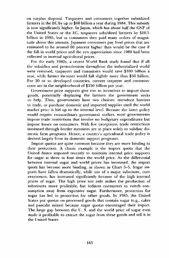
on surplus disposal. Taxpayers and consumers together subsidizedfarmers in the EC by up to $40 billion a year during 1984. This subsidyis now significantly higher. In Japan, which has about half the GNP ofthe United States or the EC, taxpayers subsidized farmers by $10.5billion in 1985, but as consumers they paid many orders of magni-tude above this amount. Japanese consumers pay food prices that areestimated to be around 60 percent higher than would be the case ifthe fall in world prices and the yen appreciation since 1980 had beenreflected in internal agricultural prices.

For the early 1980s, a recent World Bank study found that if allthe subsidies and protectionism throughout the industrialized worldwere removed, taxpayers and consumers would save $100 billion ayear, while farmer incomes would fall slightly more than $50 billion.For 20 or so developed countries, current taxpayer and consumercosts are in the neighborhood of $150 billion per year.

Government price supports give rise to incentives to import thosegoods, potentially displacing the farmers the government seeksto help. Thus, governments have two choices: introduce barriersto trade, or purchase domestic and imported supplies until the worldmarket price is bid up to the internal level. Because the latter policywould require extraordinary government outlays, most governmentsimpose trade restrictions that involve no budgetary expenditures butimpose losses on consumers. With few exceptions, trade restrictionsinstituted through border measures are in place solely to validate do-mestic farm programs. Hence, a country's agricultural trade policy isderived largely from its domestic support programs.

Import quotas are quite common because they are more binding intheir protection. A classic example is the impori quota that theUnited States imposed recently to maintain internal price supportsfor sugar at three to four times the world price. As the differentialbetween internal sugar and world prices has increased, the importquota has become more binding, as shown in Chart 5-5. Sugar im-ports have fallen dramatically, while use of a major substitute, cornsweeteners, has increased significantly because of the high internalprices of sugar. The high price not only makes the production ofsubstitutes more profitable, but induces consumers to switch con-sumption away from expensive sugar. Furthermore, protection forsugar has led to protection for other goods. In 1985, the UnitedStates put quotas on processed goods that contain sugar (e.g., cakesand pancake mixes) because sugar quotas encouraged their import.The large gap between the U. S. and the world price of sugar evenmade it profitable to extract the sugar from these goods and sell it inthe United States.

165

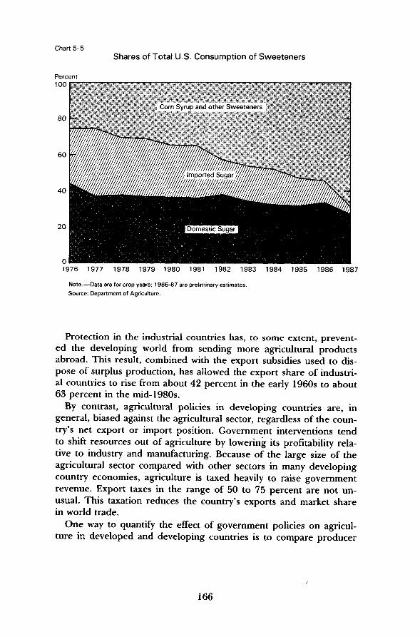
Chart 5-5Shares of Total U.S. Consumption of Sweeteners

Corn Syrup and other Sweeteners

20

Oi1976 1977 1978 1979 1980 1981 1982 1983 1984 1985 1986 1987

Note.—Data are for crop years; 1986-87 are preliminary estimates.Source: Department of Agriculture.

Protection in the industrial countries has, to some extent, prevent-ed the developing world from sending more agricultural productsabroad. This result, combined with the export subsidies used to dis-pose of surplus production, has allowed the export share of industri-al countries to rise from about 42 percent in the early 1960s to about63 percent in the mid-1980s.

By contrast, agricultural policies in developing countries are, ingeneral, biased against the agricultural sector, regardless of the coun-try's net export or import position. Government interventions tendto shift resources out of agriculture by lowering its profitability rela-tive to industry and manufacturing. Because of the large size of theagricultural sector compared with other sectors in many developingcountry economies, agriculture is taxed heavily to raise governmentrevenue. Export taxes in the range of 50 to 75 percent are not un-usual. This taxation reduces the country's exports and market sharein world trade.

One way to quantify the effect of government policies on agricul-ture in developed and developing countries is to compare producer

166

subsidy equivalent levels and consumer subsidy equivalent levels.These ratios indicate the net effect of government policies on pro-ducer and consumer incentives. Producer subsidy equivalents meas-ure, as a percent of crop revenues, the value to producers of tradeand domestic policies. The most recent producer subsidy equivalents(1982-84) indicate clearly that all developed countries subsidize theiragricultural producers. Across all commodities, the weighted produc-er subsidy equivalents (in percentage terms) for some of the majorindustrial countries over the period 1982-84 are as follows: Japan,70; EC, 41; U.S., 22; Canada, 24; and Australia, 6. In 1986, thesefigures for all countries have increased, especially the U.S. subsidyequivalents. In the case of wheat, beef, and dairy, the cost of produc-er support is borne mainly by consumers in the EC and japan, whilethe United States and other developed countries use budget contri-butions (except in dairy or sugar support) to assist producers (Table5-4).

TABLE 5-4,—Who bore the cost of support to producers, 1982-84

[Percent of producer support]

European Community

Borne by consumersBudget contribution

Japan

Borne by consumersBudget contribution

United States

Borne by consumersBudget contribution

Wheat

6734

6337

2971

Commodity

Beef

928

7624

4258

Dairy

7723

5842

955

Note.—Data are for crop years.

Sources: Department of Agriculture (Economic Research Service) and Council of Economic Advisers.

Consumer subsidy equivalents measure the value, as a percent ofconsumer costs, of government policies to consumers, with negativefigures indicating consumer taxation. Consumer subsidy equivalentsshow that developed countries tax consumers almost uniformlyacross commodities. For example, these equivalents for beef, pork,and poultry are around — 5 for the United States and range between— 1 and —25 for the EC. The developing countries are divided again:East Asian newly industrialized countries generally tax consumers,whereas some countries such as India, Argentina, and Nigeria oftensubsidize consumers.

The importance of the disincentives inflicted upon agriculture inLDCs can best be dramatized when those disincentives are removed.After two decades of sluggish growth, agricultural output in the Peo-

167

pies Republic of China has soared since 1978, when regulations wereliberalized and prices were allowed to rise and approach market-de-termined levels. This remarkable expansion, making China now thelargest wheat producer in the world, was achieved almost entirelythrough productivity gains. The amount of land (including irrigated)under cultivation and the use of tractors for farming declined be-tween 1978 and 1983; the major change was the incentive system.

Nations that have not liberalized their agricultural policies, particu-larly those in Africa, have suffered from food shortages and evenwidespread malnutrition and famine. When the enormous surplusesof the developed economies are juxtaposed with the situation ofpoorer LDCs, the world agricultural imbalance seems particularlygalling. The problem is not one of agricultural supply, however, butone of allocation. The poorer countries are not underfed becausethey need more agricultural production, but because they lack theincome to buy more food on world markets. By liberalizing their ag-ricultural policies and allowing market incentives to motivate theirfarmers, poorer LDCs can not only increase domestic production inproducts for which they have comparative advantage, but they canalso increase rural incomes so they may trade for the foodstuffs es-sential for a healthy populace.

INTERNATIONAL COSTS OF AGRICULTURAL POLICIES

Even though agricultural policies may be aimed at domestic con-cerns, their effects spill over to the rest of the world. For example,the distorted price incentives in industrialized countries stimulateproduction that directly or indirectly depresses world prices. The de-pressive effect is particularly pronounced when a government subsi-dizes the sale of stocks on the world market, makes concessionalsales, or simply donates the food as aid.

Sugar is a glaring example of the international cost of industrial-ized country policies. The EC and the United States have both guar-anteed high prices for domestic sugar producers, which has led togrowing domestic production. The EC sugar program turned theCommon Market from a net importer to a net exporter in 1977. TheUnited States, under its current sugar policy, may make the samechange soon. The U.S. and EC sugar policies have placed great bur-dens of adjustment on many developing countries. These sugar poli-cies have not only eliminated a major importing market for countrieswhose climate is more naturally suited for sugar production, but alsopromise to make the EC and the United States export competitors.One study estimates that industrialized countries' sugar policies costthe developing countries about $7.4 billion in lost export revenueduring 1983, reduced their real income by about $2.1 billion, and in-

168

creased price instability in the residual world market for sugar by ap-proximately 25 percent. The list of sugar-producing countries thatsuffer from these policies almost coincides with the list of countriesand regions that are of utmost interest to American policymakers,e.g., Philippines, Brazil, and Central America.

In essence, by expanding output and depressing domestic demand,the agricultural protectionist policies of industrialized countriesreduce world prices and distort the relative prices of agriculturalversus other goods. Prices for the most highly protected products aredepressed more than prices of other agricultural products. These dis-torted prices make the use of resources in world agriculture even lessefficient. If Japan were to reduce its protection of the rice varieties inwhich other Asian countries have a comparative advantage, they—and Japan—could achieve greater efficiency and higher income.When fanners in the Netherlands produce vegetables in greenhousesbecause energy costs are subsidized, they indirectly discourage farm-ers in Mediterranean countries from pursuing their natural advan-tages in the production of these products.

Differential rates of subsidization also create particular difficultiesfor LDCs when the rate of support for processed agricultural prod-ucts exceeds that for raw products. In industrialized countries, tariffand nontariff barriers tend to be higher on more processed forms ofa particular good. As a result, escalating support of agri-processingseverely disrupts economic development by blocking the most naturalstep toward industrialization. Such policies have resulted in industri-alized countries exporting larger quantities and importing smallerquantities of processed products than of related raw materials. Forexample, the EC accounts for 11.4 percent of world wheat exports,but 48.9 percent of wheat flour exports. Developing countries oftenrespond to such policies by subsidizing local processing industries,which inevitably encourages further inefficiencies and compounds thedirect harm arising from industrial countries' tariffs.

Any one country's competitiveness depends not only on its own ef-ficiency but also on the political decisions of other countries. The re-turns to a country from the world market may be undermined by in-creased direct and indirect subsidies. For example, high target pricesfor U.S. rice coupled with marketing loans have resulted in largeU.S. exports imposing significant costs on Thailand, a major rice ex-porter. The same basic policies for cotton have generated similar, al-though riot as dramatic, effects for Egypt, Bangledesh, Mexico, Gua-temala, Paraguay, and other cotton-exporting countries.

169

EXPORT-MARKET RESPONSIVENESS

During the policy debates on the Food Security Act of 1985, sup-porters of the legislation emphasized the dependence of the U.S. ag-ricultural sector on foreign markets. The general view was that ex-ports led to the boom of the 1970s and the bust of the early 1980s.As a result, if American agriculture were to escape its plight, exportswould have to lead the way once again. Unfortunately, the length oftime before lower price supports would improve U.S. agriculturalexport performance was underestimated.

The effectiveness of the new policy in enhancing exports of U.S.agriculture depends critically upon the responsiveness of exportdemand to price. The evidence shows that the short-run responsive-ness of export demand for many commodities from the United Statesis relatively weak. As a result, increases in export volume will lead tolower total values of exports in the short run because the fall inprices will be sharp enough to offset the increase in volume sold.Over the longer run, 3 to 5 years in the case of many commodities,lower prices can be expected to drive inefficient producers out of themarket, force some government policy changes, and stimulate greaterconsumption, thereby increasing export sales at higher prices.

Exports of agricultural products depend heavily on government be-havior throughout the industrialized world. Only if protectionist poli-cies are curbed will it be possible to increase demand for farm prod-ucts from those countries that have comparative advantages. Certain-ly over the next few years, major competitors of the United Statescan be expected to make some adjustments in their production. How-ever, if total market demand increases only moderately in response todeclining market prices and slow growth in foreign income, any sig-nificant increase in either the U.S. share of world trade or in thevolume of exports is unlikely. Some increase in share and some gainin volume might occur, of course, but they may not correspond tothe dramatic reduction in U.S. price support levels. The current pro-tectionist policies that are pursued throughout the world, the largeovercapacity in place, and the worldwide market fragmentation willserve to limit growth of U.S. exports over the balance of the 1980s.

REFORM OF U.S. AGRICULTURAL POLICY

The Food Security Act of 1985 and its predecessors have helped tocreate many new problems that afflict the U.S. agricultural sector,and have failed adequately to solve many old problems. Thefundamental flaw is that Federal farm subsidy payments are linked di-rectly to farm production. Because farmers are paid subsidies (explic-it or implicit) that are proportional to their output, they are encour-

170

aged to produce even more. Excess production must either be stock-piled by the government, dumped on v/orld markets, or restrainedthrough inefficient land or production restrictions.

To the extent that price supports are above market-clearing prices,government stocks accumulate while exports fall. This design hasalso contributed to instability and uncertainty on private markets. Forexample, government management of commodity generic certificatescan exacerbate the volatility of wheat and corn markets. If no furthergeneric certificates are released, the market will expect corn andwheat prices to rise above current loan rates, because most stockswill be held in government hands rather than by the private sector.In contrast, if the Department of Agriculture releases a large numberof generic certificates, market prices will fall below the loan rates.

Two of the major features of the Food Security Act of 1985 are thehigh target prices and the relationship between government income-support payments and production decisions. Under the act, targetprices are set at high levels and are not permitted to decline until1988 for feedgrains and wheat and 1987 for cotton and rice; further-more, the scheduled reductions in target prices are far too small (2,3, and 5 percent, respectively, for the years 1988, 1989, arid 1990 inthe case of feedgrains and wheat). The limited decoupling of govern-ment income payments and production decisions provided by the 50-92 provision is insufficient. This small step in the direction of decou-pling is not expected to have any major effect on the current chronicsurpluses and overcapacity within the sector.

The Administration seeks major revisions in the 1985 act in orderto reduce budget exposure, provide fairness, restore a sense of pro-portion to agricultural policy, attempt to set loan rates at or belowmarket-clearing levels, and move more meaningfully in the directionof decoupling production from payments. Specifically, the Adminis-tration proposes to extend the 50-92 provision to a 0-92 provision;administratively and legislatively tighten the definition of a "person"for purposes of the payment limitations; limit the total payments to$50,000 per person; reduce target prices from 1987 by 10 percentper year through 1990; and provide more flexibility in establishingloan rates for program crops.

Under the 0-92 provision, farmers would receive payments basedon historical acreage, without being required to plant the programcrop on those acres. To ease the adjustment from chronic surpluses,any land that might be idled under this provision could not be usedto produce any other crop. Hence, this provision does not allow totaldecoupling of program payments and farmer production decisions.The proposed revision simply means that participating farmers cancollect 92 percent of what their income subsidies would be under full

171

production, even though all of their land is idle. Current law requiresthat at least half of their land be planted.

The proposed $50,000-per-person payment limitation pertains todeficiency and land diversion payments, as well as to marketing loanpayments in the case of cotton and rice, and loan deficiency paymentsfor other program crops. Under current law, the 1987 limit is$250,000. Tightening the definition of a person will achieve consist-ency and fairness in the application of payment limitations by closingloopholes that circumvent current legislative intent. The currentloose definition of "person" has fostered a proliferation of overlap-ping partnerships and other farm reconstitutions in order to qualifyfor multiple payment limits.

The proposed reduction in target prices is expected to lead to adecline in agricultural program outlays by $13 billion over fiscal 1988through 1990. This action would reduce the current incentive tooverproduce and also contribute to reductions in the budget deficit.

If loan rates are above market prices, incentives will still remain toplant for the government and not the market. Thus, an importantstep in decoupling is to reduce loan rates to below market prices.Under the proposed revisions, the Secretary of Agriculture couldreduce loan rates by up to 10 percent per year. Current law estab-lishes loan rates by formula (75 percent of 5-year moving average,dropping the high and low price), but superimposes a limit on howfast annual adjustments can be made to the computed formula loanrate. The current limit is 5 percent, after a special provision of 20percent for some commodities. The proposed revision would allowU.S. prices to be more competitive, reduce incentives to produce forthe loan rate itself, and make the decoupling more effective.

Because the program for crop year 1987 has been largely deter-mined, many of the revisions can be adopted only for years 1988through 1990. The 0-92 decoupling provision could, however, be in-stituted immediately. The proposed revisions for the past 3 years ofthe current legislation would provide an effective transition to a morecomprehensive and coherent agricultural policy.

The Administration also proposes changes in the U.S. sugar pro-gram to deal with the distortions generated by current policy. Theproposed reform would lower the price-support loan rate to 12 centsa pound while providing transition payments to cane and beet pro-ducers over a 4-year period. Prices paid by domestic sugar consumerswill fall as a result. By modifying the incentives that distort domesticproduction and consumption, U.S. sugar policy moves slowly towarda more market-oriented position.

172

SUPPLY MANAGEMENT BIAS

The cornerstone of any comprehensive reform of agriculturalpolicy is the elimination of incentives to produce for governmentprograms rather than for the market. As long as such incentives exist,surpluses will be generated. As a consequence, the government willattempt to manage supply by acreage reduction programs, voluntarydiversion, acreage set-asides, or production quotas.

Given the changes that have occurred within agriculture, thesupply management bias of current programs is doomed to failure.The sector's capacity to produce under the stimulus of favorable eco-nomic conditions and large government subsidies is extremely high.As a result, the cost of agricultural commodity policies that attemptto restrain production and enhance prices through land controls arein short, toweringly expensive. Moreover, a program attempting tolimit supply by renting land from farmers, by outright purchases offarm commodities, or by mandatory supply controls cannot avoid di-recting its benefits to the largest producers. For a given supply re-duction, most of the idled land or the eliminated production mustcome from the 15 to 20 percent of all producers who account for ap-proximately two-thirds of total production.

Attempts to limit supply fail to exploit the continued growth inworld food markets. Although increases in the acreage reduction andthe voluntary diversion programs can provide some short-term assist-ance in reducing current chronic surpluses, this benefit can only beachieved by incurring other costs. These other costs include thelosses imposed upon consumers, the reduction in markets for thefarm supply industry, and the increase in costs for food processingand distribution. Moreover, acreage controls result in the excessiveuse of other inputs, which partially offsets the desired productioncutback. Such programs are not cost-effective in terms of governmentoutlays.

Mandatory acreage controls could be more effective than currentvoluntary programs in managing the total amount of land allocatedto a particular crop but at a high social cost. Recent Department ofAgriculture studies show that a 125-million-acre reduction in crop-land would be required to raise commodity prices 30 to 40 percent.This program would discourage domestic use, cut exports sharply,devastate the farm supply industry, raise costs for the entire foodprocessing and distribution chain, and impose huge losses on U.S.consumers. This option applied to feedgrains would reduce earningsfor livestock producers throughout the United States. Exports offarm commodities could be expected to fall 40 percent. This manda-tory control program would reduce GNP by $64 billion and eliminateapproximately 2.2 million jobs, a number almost equal to all the

173

farmers in the United States. The greatest impact would fall on thepoor, who spend the largest portion of their income on food. More-over, in comparison with current programs, the concentration of ben-efits among large producers would be even greater, with no effectivepayment limitation.

Subsidies could be offered to counteract some of the adverse ef-fects, such as those on the U.S. livestock industry and on exportsales. Such subsidies, however, would drive the cost of the mandatoryacreage control program above even the high costs that were in-curred during fiscal 1986.

All attempts to limit production will impede the international com-petitiveness of the U.S. agricultural sector, both in cost and output.In acreage reduction programs, for example, farmers must retire acertain fraction of their acreage base, e.g., 20 percent in the case ofcorn, to receive deficiency payments. Thus, every firm in the industryis asked to spread its total fixed cost over 80 percent of its potentialoutput. This scheme raises the average cost of production, relative tocompetitors who suffer from no such constraints. Moreover, supplymanagement policies create an artificial scarcity of farmland, biddingup its price to a higher level than otherwise would have occurred.

Finally, limiting output places the United States in the position ofbeing the residual supplier to world commodity markets. Whatevergrowth occurs in world food markets is allowed to be tapped bymajor competitors. Moreover, the supply management bias of agri-cultural programs in the United States lowers the costs to othercountries of subsidizing their agricultural sectors. As a result, U.S.programs operate to improve the position of major competitors interms of both their access to major markets and the cost of their agri-cultural policies.

A COHERENT LONG-TERM AGRICULTURAL POLICY

A comprehensive policy to foster and maintain a vital and progres-sive U.S. agricultural sector would contain four major components:complete decoupling, targeting, resource conservation, and negotia-tion and trade cooperation.

Complete Decoupling

Under complete decoupling, payments to farmers would not belinked to current production either through subsidies or artificiallyhigh prices. Production decisions would be based on economic incen-tives, not governmental policy. Set-asides and acreage reduction pro-grams could be phased out over a specified period of time. Distor-tions such as intensive use of inputs would diminish, and budgetaryoutlays would largely be known in advance.

174

Decoupling could be phased in by allowing increasing discretionwith regard to the use of idle land. For example, after a period oftime in which idle land could not be used for any other crop, 20 per-cent of the land could be planted in any crop, then 40 percent, andfinally 100 percent. Income support could also be decoupled fromprices. Farmers should receive a known payment regardless of whatthey plant and the market price they receive. The income supportthat has been decoupled from production and prices should bephased out.

Targeting

Separating payments from production and prices would make itpossible to target such transfers so as to preserve the family farm andrural communities while protecting the rural landscape. Targetedincome-deficiency payments would preserve some farms unable tomanage the riskiness of their operations, and would ease the costs oflabor adjustment from agriculture for other farmers. Income supportstargeted at those who rely more heavily on farm income and yet do nothave the immediate resources for retraining, job searching, etc., wouldease the inevitable pain of change and improve the long-term flexibilityof U.S. agriculture.

Targeted farmers should receive income supports unconditionally.Farmers could then employ their support in whatever fashion theyconsidered most appropriate—from retraining to remaining in farm-ing. One possible method of targeting would be to have paymentsbased on current acreage and historic yields with a limit to the quali-fying farm size.

Resource Conservation

One feature of the Food Security Act of 1985 that is in the long-run interest of the United States is the provision for placing highlyerodible land in the conservation reserve. Under the 1985 legislation,lands that pose significant off-farm environmental threats—for exam-ple, water quality damage—can also be included in the conservationreserve program. It is the largest conservation program in the historyof Federal agricultural policy, calling for the voluntary, gradual en-rollment of 40 million to 45 million acres of land. Under this pro-gram, landowners agree not to produce on qualifying cropland for 10years in exchange for an annual rental payment. Unfortunately, thisprogram is hampered by competing supply management programs.In essence, the government is bidding against itself to idle farmland.Currently, most farmers are better off collecting deficiency paymentsor diversion payments for idling acreage under commodity programs

175

than by idling land on a long-term basis under the conservation re-serve program.

Over the period that supply constraints are being phased out, diffi-culties stemming from the concurrent operation of the conservationreserve program and the price-support programs must be resolved.The joint operation could be effectively managed by the introductionof a land-targeting scheme. Lands declared eligible for the conserva-tion reserve program would be declared ineligible for the acreage re-duction program.

A redesigned conservation reserve program, combined with decou-pled and targeted income support, would reduce incentives for inten-sive land use that arise when farmers seek to increase their immedi-ate cash incomes. Finally and most significantly, the elimination ofcommodity programs that connect income supports to productionlevels would ease the extensive and intensive use of land and otherresources in production. The significant reductions in the use of pes-ticides and other chemical inputs resulting from these programchanges would also reduce environmental damage.

Negotiation and Trade Cooperation

The current state of agricultural trade can be described as one inwhich many countries feel trapped. If any country reduces its exportsubsidies or limits its farm support, it will lose market share. Its ownaction will rarely be sufficient to induce a significant rise in worldprices. Thus, the rewards to individual countries from unilateral agri-cultural policy reform often seem too little to encourage change.

Simultaneous action by many countries might break this trap. TheAdministration began a coordinated move to raise the issue of agri-cultural protectionism at the last economic summit. How to achievemultilateral, systematic rationalization of policies across sovereignstates with different resource endowments and policy mechanisms, ifnot policy objectives, remains a major challenge.

The difficulty of international cooperation in adjustments, howev-er, does not excuse delay in U.S. policy reform. Reform is in the self-interest of the United States and should be initiated regardless ofwhether trading partners act as well. In addition, the reformed policieswould eventually stimulate other protectionist countries to makesimilar adjustments.

Although sound economic grounds exist for greater market orien-tation even with no action by other countries, the chances of signifi-cantly reducing the degree of protection provided to U.S. agricultureare far better if coordinated moves also occur in other major agricul-tural exporting countries. The political feasibility of implementingdecoupled and targeted deficiency payments is greatly enhanced ifother industrialized countries would pursue similar actions,

176

A cooperative effort of major agricultural exporting countriescould involve coordinated and lockstep moves in decoupling. Thepossibility of such cooperative ventures is much higher in today's en-vironment because of the huge subsidization under the Food SecurityAct of 1985. In contrast with the U.S. legislation governing the early1980s, many exporting countries, including Australia, Canada, andArgentina, now have far more incentive to enter a cooperative effortto reduce worldwide protectionist trade policies.

CONCLUSION

Today's highly complex patchwork of agricultural policies hasbecome increasingly antiquated and unproductive. Agriculture andrural communities have become so vastly different in structure and intheir relationships to the domestic and world economies that thepremises underlying current policies are no longer valid. Besidescosting taxpayers and consumers billions of dollars and representinga significant portion of the Federal deficit, agricultural policies divertland, labor, and other resources from more to less productive uses.The huge surpluses generated in the United States and throughout theworld harm U.S. allies and less developed countries, while providinghuge windfalls to powerful economic interest groups. These programsare unfair, with some individuals receiving millions of dollars from thegovernment.

The policy reforms outlined here would correct the major imbal-ances that exist within U.S. agriculture. Other reforms are alsoneeded. For example, some Federal marketing orders attempt tomaintain or enhance commodity prices by restricting either theamount produced or the amount marketed. These market regulationstend to tax consumers in order to generate extra profits for estab-lished producers of the protected commodities. Such marketingorders should be deregulated. In contrast, marketing orders thatfocus on research, promotion, and providing timely information toproducers and consumers should continue to be supported. TheFarm Credit System faces huge losses and is currently unable to di-versify the risk of its loan portfolio; it needs to be restructured. Fed-eral and State governments must address problems such as depletedaquifers, groundwater contamination, water salinity, and the exces-sive use of irrigation water attributable to inappropriately adminis-tered prices. The challenge facing both the public and private sectoris to invent the means for enhancing agricultural productivity whilereducing the cost of environmental externalities.

To be sure, the Food Security Act of 1985 will not yield easily to amajor overhaul. These policies, after all, are tied to a long series of

177

legislative precedents, deeply embedded goals and objectives, andthe vested interests of powerful groups. Major opposition will doubt-less arise to the reforms outlined here, which are in the best interestof the U.S. taxpayer and consumer. Reforming agriculture would leadto huge gains not only here in the United States but in the rest of theworld.

178

CHAPTER 6

Risk and Responsibility

RISK IS A FACT OF LIFE. Every person balances risks of accidentand injury against the attainment of other goals, and trades off somekinds of hazards against others. Whether to smoke, take a particularjob, travel by automobile or airplane, use a safety belt while driving,or engage in a dangerous recreational activity are all decisions thatinvolve risk. People are subject to hazards from the actions of otherindividuals as well. Determination of the proper role of governmentwith regard to personal risk is a complex and important public policyissue.

Health and safety have improved dramatically in the United Statesduring the 20th century. Life expectancy at birth increased from 47.3years in 1900 to 62.9 years in 1940 and, by 1983, had risen to 74.7years. Much of this improvement is attributable to the decline ininfant mortality, but adult life expectancy has also increased. In 1900,a 40-year old could expect to live to age 67.9. This expectation in-creased to 71 by 1940, and rose further to 77.2 by 1983. This repre-sents a gain of 9.3 years, or a 33 percent increase in the expectednumber of years remaining at age 40.

Accident fatality rates have declined at the same time. Chart 6-1shows annual fatality rates from motor vehicle and all other acciden-tal causes. The rate from all causes other than motor vehiclesdropped from 82.4 per hundred thousand population in 1910 to 20.9in 1982. Motor vehicle deaths per hundred thousand population gen-erally have been steady since the late 1930s. Automobile travel hasincreased substantially over this period, however, and traffic fatalitiesper hundred million vehicle miles have fallen almost 80 percent,from 10.89 in 1940 to 2.47 in 1985.

Both the home and workplace have become safer. The home acci-dental death rate per hundred thousand population decreased from21.2 in 1948 to 8.6 in 1985. The accidental death rate at work hasfallen by more than two-thirds since the 1930s (Chart 6-2). Work-re-lated death rates differ across industries, and one cause of reductionsin the overall rate has been the change in employment patterns asproduction has shifted from agriculture and other relatively danger-

179

Chart 6-1Rates of Accidental Deaths by Cause

Deaths per 100,000 Population90

80

70

60

50

40

30

2C

10

ill l 1 1 1 1 1 i i 1 1 1 1 1 l l 1 1 l 1 1 1 1 1 1 1 1 1 1 1 1 l I 1 1 l 1 1 l i 1 1 1 1 l l l ! i l 1 1 ! l 1 1 l 1 1 i 1 1 I l 1 1 l 1 1 l l i I1910 1920 1930 1940 1950

Sources: Public Health Service and National Safety Council.

1960 1970 1980

cms goods-producing industries to the relatively safer service indus-tries.

The underlying source of these improvements in health and safetyis economic growth and a rising standard of living. Higher incomesenable people to purchase better nutrition, clothing, and shelter aswell as more and better medical care. A higher standard of living en-ables consumers to purchase safer products, safer forms of transpor-tation (including safer automobiles), and safer living environments.Increased wealth supports improved public health measures, fromvaccinations to water and sewage treatment. Economic progress hasbeen a major factor leading to advances in science and medicine thathave mitigated or eliminated many dread diseases and have improvedthe treatment of accident victims.

But accidents, injuries, and disease can never be avoided entirely.Individuals do not seek to avoid all risks, and the human lifespancannot be extended without limit. Increases in health and safety oftencannot be achieved without cost, and are only one way in which eco-nomic progress can be translated into greater well-being.

180

Chart 6-2Rates of Home and Work Deaths Due to Accidents

Deaths per 100,000 Persons40

35

30

25

20

15

Work (per 100,000 Workers)

"-•••'~--j/"

Home (per 100,000 Resident Population)10 '

I I I I I I I I i i I I I I I I I I I I I I I I I I I i i i I I I I I I I I I I I I I I I i I i I i I I1935 1940 1945 1950 1955 1960 1965 1970 1975 1980 1985

Note.—A change in classification resulted in a break in the home accident series in 1948.

Source: National Safety Council.

PROTECTION AGAINST RISK

Every individual can reduce risk by exercising personal care. If re-sponsible adults voluntarily undertake risky activities, such as hanggliding, their choices must be respected in a society that values indi-vidual liberty and autonomy. This general principle of respectingpersonal choice is compatible, however, with governmental action toreduce risk in particular circumstances, especially when the actions ofsome increase the risks to others.

The institutional means for increasing safety and reducing risk areprovided through three social arrangements—markets, the legalsystem, and government regulation. Markets create incentives for safebehavior and allow individual choice in decisions involving risk. Con-sumers can purchase reductions in risk directly by choosing saferproducts. Safety is a desirable product characteristic, like durabilityand energy efficiency. Companies that earn reputations for makingunsafe products face retribution in the marketplace, just as if theycharged excessive prices or offered shoddy goods. The market also

181

promotes safety in the workplace. All other things equal, employersmust pay higher wages for riskier jobs, which creates an incentive toreduce occupational hazards.

Private insurance enables individuals and firms to protect them-selves against the costs of various risks. Consumers purchase insur-ance against losses from death, illness and accidents, and some kindsof natural disasters. Manufacturers insure against product liabilitylawsuits, and professional practitioners insure against liability formalpractice. By spreading the costs of risk, insurance can also under-mine incentives for safe behavior; but where premiums are closelylinked to the likelihood of events insured against, safety incentivesare substantially preserved.

Markets cannot entirely protect an individual from being harmedby the actions of others. The legal system, specifically tort law, pro-vides victims the opportunity to be compensated. By transferring tothose who cause harm the costs they impose on others, tort law cre-ates incentives for individuals to behave responsibly.

GOVERNMENT MANAGEMENT OF RISK

Government provides the legal and judicial framework for themarket and tort systems, offers insurance against some risks, imposesregulatory standards, and operates programs to control risk directly.Government protects the integrity of the marketplace by prohibitingdissemination of false or fraudulent information by sellers. Govern-ment supports basic health research, and informs the public abouthealth and safety characteristics of products.

Several circumstances may provide a rationale for government reg-ulation. First, consumers may lack the information or the ability toassess particular risks accurately. Second, individuals or firms fail insome cases to take account of the costs of harm they impose onothers. The tort system may not be able to force a person whocauses harm to bear these costs if the person's wealth is insufficientto compensate the victim, the cost of using the tort system is toohigh, or the person who caused the harm cannot be identified. Third,if markets and the tort system cannot adequately control externalitiessuch as those leading to environmental pollution, government regula-tion may be warranted. Government regulates risk and safety throughagencies such as the National Highway Traffic Safety Administration(NHTSA), the Consumer Product Safety Commission (CPSC), theOccupational Safety and Health Administration (OSHA), and the En-vironmental Protection Agency (EPA).

Regulatory policy encompasses both risk assessment (determina-tion of the probabilities of harm) and risk management. Risk manage-

182

ment should reduce and not merely displace risk. If one dangerousproduct is banned, more harmful ones may be used. Substitutions ofthis sort can exchange known risks for unknown ones. Effective riskmanagement assesses the relative benefits and costs of actions toreduce particular risks. The benefits of regulation include avoidanceof deaths, injuries, and property damage, as well as saving resourcesthat otherwise would be used to mitigate these adverse conse-quences. Costs of regulation include the resources, both public andprivate, that must be devoted to meeting regulatory standards, aswell as reduced competition in some cases. Government regulationsometimes restricts freedom of individual choice by imposingcommon standards. Regulation may, in addition, retard innovationand investment, thus slowing economic growth.

If some regulations show a much lower cost per life saved or acci-dent avoided than others, adoption of the more cost-effective oneswould save more lives for a given level of risk-reduction costs. Regu-latory actions with the highest expected net gains should be under-taken first, leading to consistency in cost-effectiveness across regula-tions. A policy of consistency should apply to all activities of govern-ment that affect risk: for example, statutes and regulations; Federalprograms that directly affect safety, such as air traffic control and theoversight of aircraft maintenance; and State and local activities, suchas highway construction and firefighting. Complete consistency, how-ever, is neither attainable nor desirable. States determine their ownregulatory policies in many areas, in accordance with principles offederalism. Special significance may be attached to reducing particu-lar types of risks, such as those faced by children, or risks that arenot assumed voluntarily.

Statutory language sometimes impedes the realization of consisten-cy by setting goals that do not take account of costs. Examples areportions of the Clean Air Act, Clean Water Act, and OccupationalSafety and Health Act, as well as the Delaney Clause of the Food,Drug, and Cosmetic Act. Agencies may also fail to promote consist-ency in their rulemaking by implicitly assigning widely differingvalues to saving a life. A recent study shows that the average cost perlife saved varies across regulations from as little as $100,000 forNHTSA's 1967 steering column protection rule to $132 million forthe Food and Drug Administration's 1979 ban on diethylstilbestrol(DES) in cattle feed. Some proposed regulations have even highercosts, such as EPA's proposed restrictions on the disposal of dioxinsand solvents on land, estimated to cost $3.5 billion per life saved.The regulatory review and coordination process implemented by thisAdministration is designed to improve consistency across Federalregulations, to the extent permitted by law.

183

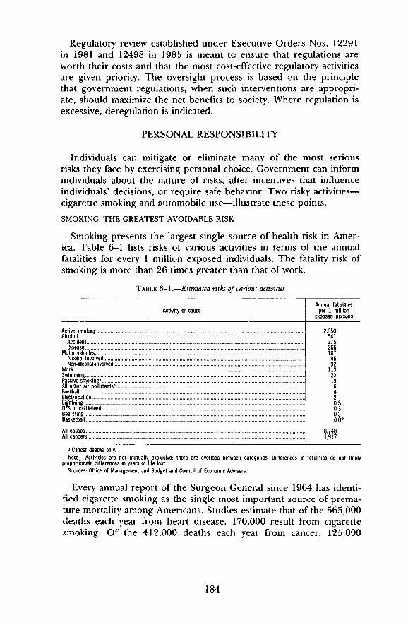
Regulatory review established under Executive Orders Nos. 12291in 1981 and 12498 in 1985 is meant to ensure that regulations areworth their costs and that the most cost-effective regulatory activitiesare given priority. The oversight process is based on the principlethat government regulations, when such interventions are appropri-ate, should maximize the net benefits to society. Where regulation isexcessive, deregulation is indicated.

PERSONAL RESPONSIBILITY

Individuals can mitigate or eliminate many of the most seriousrisks they face by exercising personal choice. Government can informindividuals about the nature of risks, alter incentives that influenceindividuals' decisions, or require safe behavior. Two risky activities—cigarette smoking and automobile use—illustrate these points.

SMOKING: THE GREATEST AVOIDABLE RISK

Smoking presents the largest single source of health risk in Amer-ica. Table 6-1 lists risks of various activities in terms of the annualfatalities for every 1 million exposed individuals. The fatality risk ofsmoking is more than 26 times greater than that of work.

TABLE 6-1.—Estimated risks of various activities

Activity or cause

Active smoking ,Alcohol

AccidentDisease

Motor vehiclesAlcohol-invoivedNon-alcohol-involved

WorkSwimming ,Passive smoking1

All other air pollutants1

FootballElectrocutionLightning ....DES in cattlefeedBee stingBasketball

All causes ,. .All cancers

Annual fatalitiesper 1 million

exposed persons

2,950541275266187959?

1132219662050302002

87481917

1 Cancer deaths only.

Note.—Activities are not mutually exclusive; there are overlaps between categories. Differences in fatalities do not implyproportionate differences in years of life lost.

Sources: Office of Management and Budget and Council of Economic Advisers.

Every annual report of the Surgeon General since 1964 has identi-fied cigarette smoking as the single most important source of prema-ture mortality among Americans. Studies estimate that of the 565,000deaths each year from heart disease, 170,000 result from cigarettesmoking. Of the 412,000 deaths each year from cancer, 125,000

184

result from cigarette smoking, with more than 100,000 of these fromlung cancer alone. A 25-year-old man who smokes one pack of ciga-rettes per day can expect to live 4.6 fewer years than one who doesnot smoke at all, and one who smokes two packs per day can expecthis life to be shortened by 8.3 years. Life insurance companies usual-ly charge smokers higher premiums reflecting their greater mortalityrisk. Some health insurance carriers have also introduced premiumdifferentials based on smoking.

The issue of smoking goes beyond matters of individual choice;secondary smoke affects others. The Surgeon General reports that anonsmoker whose spouse smokes more than one pack of cigarettesper day has a risk of lung cancer 1.3 to 1.9 times higher than a non-smoker whose spouse is a nonsmoker. Passive smoking results in anestimated 2,500 fatal cancers per year. Children of smokers havemore respiratory problems, and are more frequently hospitalized forbronchitis, pneumonia, and respiratory allergies. Smoking-relatedfires led to 1,500 deaths and another 4,000 injuries in 1984.

It is not clear whether the pleasures of smoking outweigh thehealth risks and other costs, even for smokers themselves. When sur-veyed, more than 90 percent of smokers say they want to quit, andthe majority of smokers have tried to quit at least once and failed.

Most smokers begin to smoke as adolescents. Studies of whypeople start smoking identify the influences of parents, siblings, andfriends as the most important causal factors. School curricula in thepast tried to discourage smoking by emphasizing its long-term healtheffects. Newer curricula, targeted at ages 10 through 14, focus on thesocial influences that encourage the initiation of smoking. Such pro-grams aim at helping children acquire the behavioral skills to resistthese influences and at changing perceptions that smoking is matureand sophisticated. Students who participate in these programs havestarted smoking at rates 15 to 50 percent lower than those in controlgroups.

The price of cigarettes also influences whether people smoke.Higher prices discourage young people from starting to smoke, buthave a much smaller effect on habitual users. The Federal excise taxon cigarettes was raised from 8 cents per pack to 16 cents per packin 1983, but was scheduled to revert to 8 cents in 1985. Instead, thetax was maintained at 16 cents, and as a result an estimated 1.9 mil-lion fewer people smoke, including more than a million fewer underage 25.

Current Federal agricultural policies toward tobacco do not under-mine public health efforts to discourage smoking. A system of allot-ments allows farmers to produce only specified quantities of tobaccoand limits the amount they can market. The net effect of the allot-

185

ments plus price supports and other subsidies is to hold tobaccoprices slightly higher, and quantities slightly lower, than they wouldbe in the absence of these programs.

Evidence suggests that information on the consequences of smok-ing influences behavior. The largest decline in per capita sales ofcigarettes, a fall of 8.9 percent, occurred during 1953-54, followingpublication of two retrospective epidemiological studies that linkedlung cancer to smoking and the first laboratory demonstration thatthe tar in cigarette smoke could cause cancer in animals. During thistime, tobacco companies competed vigorously by advertising pur-portedly less harmful brands, indirectly reminding smokers of thedangers of smoking. The second largest decline in per capita salesoccurred in 1968-69, during the height of the antismoking cam-paigns on television. The largest decline in the number of smokersfollowed the 1964 Surgeon General's report.

The effects of tobacco advertising are complex. There is little evi-dence that advertising results in additional smoking. As with manyproducts, advertising mainly shifts consumers among brands. Evi-dence from other countries suggests that banning tobacco advertisinghas not discouraged smoking. Four industrialized countries withmarket economies—Italy, Finland, Iceland, and Singapore—havecompletely banned advertising for tobacco products, yet have experi-enced a rise in the per capita consumption of tobacco, Sweden andDenmark enacted partial advertising bans, yet achieved greater suc-cess in reducing consumption than did Norway and Finland, whichimposed total advertising bans. After the broadcast advertising ban inthe United States, cigarette use continued to decline, but at a slowerrate than before the ban.

The ban on broadcast advertising was supported by the large to-bacco companies. Tobacco advertising expenses were about 35 per-cent lower in the 5 years following the ban. It is likely that reducedaccess to public attention made it harder for new brands of cigarettesto enter the market, thus solidifying the market shares of existingcompanies and brands. Moreover, with no tobacco advertising on tel-evision, the antismoking messages required under the Fairness Doc-trine were eliminated.

Increased awareness of the health risks of smoking has brought achange in public attitudes and government policies. Forty-two Statesand the District of Columbia restrict smoking in public places, includ-ing government workplaces. Twelve States restrict smoking by publicemployees and also by those in private businesses. New rules forFederal employees prohibit smoking in nearly all public work areas,including general office space, and permit smoking only in designat-ed areas.

186

AUTOMOBILE SAFETY

Many automobile deaths stem from avoidable behavior such asdrunk driving and failure to wear a safety belt. In 1985, about 44,000Americans died in motor vehicle accidents, including 6,800 pedestri-ans and 890 bicyclists. Nearly half of the fatalities involving occu-pants of motor vehicles occurred in single-vehicle crashes. Despitethis substantial loss of life, 1985 was the safest year on record formotorists: the death rate per hundred million vehicle miles traveled(HMVM) was 2.47, down from 5.50 in 1966 and 21.0 in 1923.

Drunk Driving

Alcohol impairs physical coordination and can increase aggressivebehavior. Alcohol contributes to many kinds of accidents and injuriesand is involved in more than 50 percent of fatal automobile acci-dents. Drunk driving is the leading cause of death for persons in the15-to-24 age group. About one-half of all single-vehicle crashes andtwo-thirds of nighttime single-vehicle crashes involve alcohol-intoxi-cated drivers. In 1982, 63 percent of those killed in alcohol-relatedautomobile accidents were drivers, bicyclists, or pedestrians who hadbeen drinking. Twenty percent were passengers (both drinking andsober) of drinking drivers. The remaining 17 percent, nearly 4,000people, were sober victims.

Evidence from other countries and recent experience in the UnitedStates suggest that programs to deter drivers from drinking by in-creasing penalties and enforcement tend to succeed in the short runto the extent that they alter drivers' perceptions of the certainty ofpunishment. But the ability of such programs to achieve lasting re-ductions in drunk driving fatalities has not been established. Thismay be because none of the programs or experiments to date hasbeen able to sustain an increase in the probabilities of apprehendingand punishing drunk drivers.

State and local actions to restrict the availability of alcohol toyoung people by raising the minimum drinking age have contributedto reduced traffic fatalities. In 1982, 31 States allowed people under21 to buy alcoholic beverages, but by 1985, only 7 States did. Inthose 3 years, motor vehicle fatality rates fell 3.0 percent for the gen-eral population, but 6.3 percent for drivers aged 24 and under. If thetraffic fatality rate for this group had fallen only by the same amountas for the general population, approximately 600 additional youngdrivers would have died in automobile accidents in 1985.

Higher alcohol taxes would also reduce fatalities. Federal excisetaxes on beer and wine have remained constant in nominal termssince 1951. As a result of this and other factors, the real price ofbeer fell 27 percent, of wine 21 percent, and of hard liquor 48 per-

187

cent between 1951 and 1983. Studies of teenage drunk driving indi-cate that if the real excise tax on beer were at its 1951 level, an esti-mated 1,000 fewer deaths per year would result, primarily of personsaged 18 to 21.

Safety Belts

Motor vehicle occupants who wear a safety belt are less than halfas likely to die in the event of an automobile accident as those whodo not. If all occupants of motor vehicles wore safety belts, 12,000 to15,000 fewer persons would die annually. Safety belt use is a clearexample of how an individual can reduce risk by taking a simple pre-caution. For this reason, some State courts, although not going so faras to hold that an accident victim's failure to wear a safety belt con-stitutes contributory negligence, have reduced the unbelted victim'sdamage award on the grounds of failure to mitigate the harm.

Even though voluntary safety belt use is an extremely low-cost wayto reduce deaths and injuries, as of 1984 only about 12.5 percent ofpassenger car drivers were estimated to use them. Usage amongteenagers appears to be particularly low. Since 1984, 26 States andthe District of Columbia have enacted laws requiring use of safetybelts (although two States recently repealed theirs). Safety belt usageincreases after passage of a belt law, but the longer term effect doesnot appear to be as great as the initial response.

Compliance with child safety seat laws has been much higher thancompliance with safety belt laws, and has been effective in reducingfatalities among young children. In 1977, the first child safety seatlaw went into effect. Now all 50 States require safety seats for smallchildren. Compliance rates are between 50 and 60 percent. Themotor vehicle fatality rate for the overall population fell 10 percentbetween 1975 and 1985, but for children under 5 it fell 32 percent.

Air bags and automatic safety belts are passive restraints that donot require the cooperation of the driver or passengers. Air bags aremore costly to install than either automatic or conventional safetybelts. Moreover, their cost-effectiveness relative to safety belts fallswith more widespread belt usage. Even if air bags were required inall new cars, they would not come into nearly universal use untilabout 10 years later. Current Department of Transportation regula-tions require phased installation of passive restraint systems unlessStates comprising two-thirds of the U.S. population enact safety beltlaws.

The 55-Miles Per Hour Speed Limit

The driver who speeds assumes a higher risk of death and injurybut also increases risk for others. It is because of this externality that

188

a maximum speed limit is in the interest of most drivers. The maincost of a lower speed limit is more time spent traveling.

The primary goal of the National Maximum Speed Limit Act of1974 was energy conservation. Today, with low real oil prices, debateconcerning the 55-miles per hour (MPH) speed limit focuses more onsafety than energy conservation. From 1973 to 1974, the overalldeath rate per HMVM dropped 14 percent from 4.12 to 3.53. (Asimilar drop of 13 percent in the death rate, from 3.17 to 2.76 perHMVM, occurred between 1981 and 1982.) Although drivers havegradually increased their average speed since the 55-MPH limit wasintroduced, they have not returned to the speeds at which they weredriving before the Federal limit was enacted. The fatality rate perHMVM, however, has continued to fall, suggesting that factors otherthan speed are important in the declining fatality trend.

Variations in fatality rates across States and types of roads suggestthat speed limits should be tailored to local conditions. In 1985, theautomobile accident fatality rate ranged from 4.1 deaths per HMVMin New Mexico to 1.6 in North Dakota. The safest roads are theinterstate highways in urban areas, with a fatality rate of 1.01 deathsper HMVM. Local rural roads are the least safe, with a fatality rate of4.99. Driving at night is three times more risky than driving duringthe day.

Although it left enforcement of the 55-MPH speed limit to theStates, the Federal Highway Safety Act of 1978 directed withholdinga portion (up to 10 percent) of a State's Federal highway funds if itfailed to achieve at least 50 percent compliance. As a result, Statesassign their highway patrol officers to enforcing the 55-MPH limit,diverting them from other efforts that would be more effective insaving lives. To reach compliance, States have an incentive to allocatemost officers to work during the day, when traffic is the heaviest, ratherthan at night, when a majority of motor vehicle deaths occur. Statediscretion in the regulation of highway speeds could improve safetymore than centralized Federal regulation.

The Unintended Hazards of Fuel Economy Regulation

Like the 55-MPH speed limit, the Corporate Average Fuel Econo-my (CAFE) regulations are a vestige of the "energy crisis/' TheCAFE standards (enacted as part of the Energy Policy and Conserva-tion Act of 1975) established minimum average levels of fuel econo-my for passenger cars sold by each automobile manufacturer. Tomeet the standards, manufacturers took a number of steps, includingswitching to lighter materials and reducing the weight and size ofcars. Market forces also shifted the automobile fleet in the directionof smaller cars while gasoline prices remained high. Automobiles

189

have become safer as design has improved. Other things equal, how-ever, small automobiles are less safe than large ones.

In single-vehicle crashes, occupant death rates are inversely relatedto car size. In multiple-car crashes involving cars of the same size,occupants of small cars have a death rate higher than occupants oflarge cars. In crashes between cars of different size, the occupants ofthe larger car have a better chance of survival than if they had beeninvolved in a crash with a car the same size, but occupants of thesmaller car have a worse chance of survival than if they had been in acrash with another small car.

There is evidence that drivers of small cars attempt to mitigatetheir increased risk by driving more carefully. One study indicatesthat, taking age into account, drivers of small cars are somewhat lesslikely to be involved in an accident than are drivers of larger cars.Even so, the fatality rate associated with small cars is higher than thatof large cars.

The "energy crisis" has passed, but Federal regulation of automo-bile fuel economy persists. To the extent that CAFE has reduced thesize of cars driven by Americans, it also has indirectly reduced auto-mobile safety.

THE TORT SYSTEM

In addition to self-inflicted injury, harm can result from the actionsof others. Tort law, the civil law governing harms other than breachof contract, serves to compensate persons injured by the negligent orwrongful conduct of others, and also to deter such conduct.

Two general rules of liability guide accident law—negligence andstrict liability. Negligence is determined by reasonableness of con-duct. If the injurer acted unreasonably, that is, failed to exercise duecare, then ordinarily the injurer would be required to compensate thevictim. Strict liability, on the other hand, focuses on whether a prod-uct that caused an injury was defective in such a way as to make itunreasonably dangerous for its intended use. Both standards seek toimpose a duty of care; strict liability, however, allows demonstrationof the breach of that duty by examination of the product itself.

The product user's degree of care also can affect the risk of acci-dents. In certain instances, the user can more easily eliminate orreduce the risk of injury than can the manufacturer. The rule of con-tributory negligence limits the scope of liability so that an injurer isnot liable for harm that could have been avoided had the victim notbeen negligent. Many States have adopted the rule of comparativefault, under which an injurer is liable only for that share of the harmcorresponding to the injurer's share of responsibility. Determining

190

the reasonableness of a party's conduct depends in part on the costsof avoiding the accident. When both parties can affect the probabilityor seriousness of an accidental injury, the rule of negligence (or therule of strict liability accompanied by the defense of contributorynegligence or comparative fault) leads both the potential injurer andpotential victim to behave reasonably to avoid accidents.

THE "LIABILITY CRISIS"

During the past several years, products and services as diverse asvaccines and skating rinks have been withdrawn from the market be-cause of the greatly increased price or unavailability of liability insur-ance. Investment in product innovations, such as new pharmaceuti-cals, has been retarded because of potential liability costs. Some ex-planations of the "liability crisis" attribute the scarcity of liability in-surance to an expansion in liability exposure under tort law. In par-ticular, the alleged crisis has been linked to trends in legal rules onfault and causation and to larger jury verdicts for damages.

In the early 1960s, courts began to replace traditional common lawrules of negligence with strict liability. It was argued that expandingliability would encourage the supplier of a good to prevent accidents;in addition, the supplier would provide insurance for unpreventableinjuries. Some courts went so far as to say that business defendantscould spread the cost of compensating victims across all consumerssimply by charging higher prices for their goods and services. Thisviewpoint assumed that society would benefit from replacing person-al responsibility for accidental injuries with expanded liability forthose supplying goods and services. Carried to its extreme, this ap-proach would entirely remove the issue of fault or wrongdoing fromthe determination of liability.

The growing trend toward no-fault liability has increased defend-ants' expected tort costs and, therefore, their need for insurance cov-erage. Historically, tort law required a plaintiff to prove a directcause-and-effect relationship between the defendant's act and theplaintiffs harm. This requirement of proximate cause eroded assome courts allowed plaintiffs to recover an entire judgment awardfrom any of a number of parties who might have contributed to theharm. This application of joint and several liability to product liabilitycases increased the potential financial exposure of defendants andfurther weakened the traditional legal requirements of fault andproximate causation. In practical terms, joint and several liabilitythreatens any defendant having substantial financial resources withthe risk of having to pay the entire damage award in a lawsuit involv-ing multiple defendants, even if this defendant was only slightly atfault for the plaintiffs injury.

191

TORT REFORM

Many States have enacted or are considering reforms in tort law.The Administration has also supported legislation to address the fac-tors that have led to the high price and scarcity of product liabilityinsurance. This legislation would ensure that fault remains a basis fordetermining legal liability for injury caused by a defective product.For a manufacturer to be found liable under strict product liability,the product would have to be defective and unreasonably dangerousbecause of its defect. This reform would limit strict product liabilityto situations in which the doctrine originally applied, before the ex-pansion of no-fault liability.

Another provision of the Administration's tort reform proposalwould make joint and several liability inapplicable to product liabilitycases. A manufacturer found liable for damages would be responsiblefor at most those damages directly attributable to its share of faultfor the injury; the manufacturer could not be held responsible fordamages arising from another party's share of fault. However, jointand several liability would still be available where two or more de-fendants consciously acted together in a common scheme or planthat directly caused the plain tiffs injury.

These proposals seek to ensure that fault and wrongdoing contin-ue to be essential to determining liability for defective products.These reforms should lessen the unpredictability of product liabilityawards for manufacturers and insurers and, by emphasizing the im-portance of personal responsibility, reduce accidents.

CONSUMER PRODUCTS AND THE WORKPLACE

Of the 92,500 accident fatalities in the United States in 1985,about half were caused by motor vehicle crashes, 22 percent by acci-dents at home, and 13 percent by accidents at work. In an effort toimprove safety, the government requires consumers and private firmsto devote resources to meeting regulatory standards, develops anddisseminates information, requires controlled testing of new drugs,and requires injury compensation insurance for workers. Governmentrules also modify market incentives for safe behavior.

CONSUMER PRODUCT SAFETY

Markets generate strong incentives for the production and safe useof consumer products. Safer products may be more expensive, be-cause of superior materials, product design, and quality control.Many consumers are willing to pay higher prices for safer products aslong as they perceive that the benefits of improved safety exceed theadditional costs. Consumers acquire safety information through per-

192

sonal experience and word of mouth, as well as from manufacturers,specialized testing laboratories, and consumer groups. The risks ofunsafe products generally are borne directly by consumers, with littlespillover of hazards beyond the immediate household. Thus, marketincentives will guide manufacturers to produce products as safe asconsumers' willingness to pay allows.

The Food and Drug Administration (FDA) regulates food, drugs,and cosmetics. Its standard-setting and inspection activities are de-signed to reduce hazards about which it is difficult to obtain informa-tion in the marketplace. Examples include the safety of food additivesand the safety and efficacy of pharmaceuticals.

The Delaney Clause of the Food, Drug, and Cosmetic Act has beeninterpreted to ban all food additives found by the FDA "to inducecancer in man or animal." In effect, this restriction has grown morestringent over the years, as advances in chemistry have permitted thedetection of extremely small amounts of substances in additives. In1985, the FDA proposed that methylene chloride be banned in hairspray, but that it be allowed as a decaffeinating agent in coffee be-cause its risk in that use is negligible. This de minimis interpretationof no-risk statutory provisions is intended to reduce regulation that isoverly costly. Recognizing the excessively restrictive nature of theDelaney Clause, Congress has exempted saccharin from its reach.

The Consumer Product Safety Commission (CPSC) has broad au-thority to set standards and order bans, recalls, and modifications. Itspurpose is to reduce hazards by improving products' technologicalsafety characteristics. Such activities, however, may fail to benefitconsumers and can have adverse effects. Sometimes safer productsare more costly, and regulation may impose higher safety levels thanconsumers are willing to purchase. To reduce the likelihood of thisresult, the law mandates cost-benefit analysis for formal CPSC rule-makings. The CPSC has adopted cost-benefit criteria for its other ac-tivities, such as implementing voluntary standards.

Even if a product standard meets a cost-benefit test, the marketmight have achieved an equivalent level of product safety. Moreover,even if the estimated costs of regulation match the benefits, regulat-ed product standards may not be desirable because benefits that stemfrom product diversity will be lost. Consumers value safety, like otherproduct characteristics, differently, in part because not all consumersuse products in the same way. If a household appliance is to be usedby children, parents may buy a safer model at a higher price thanthey would otherwise. Individuals benefit from the opportunity tomake their own tradeoffs based on price, quality, and safety.

When product regulation reduces competition and thereby in-creases prices, it restricts consumers' choices. For example, in 1975

193

fev.J

the CPSC issued a bicycle standard that imposed numerous technicaldesign features that would increase costs and exclude some bicyclesfrom the market. Some of these specifications, such as the one thathandlebars be between 14 and 28 inches wide, were overturned incourt for lack of evidence that their absence would pose an unreason-able risk of injury.

The effectiveness of product regulation in improving safety can beundermined and even reversed by risk displacement. For example,manufacturers of children's sleepwear used the flame-retardantchemical Tris to comply with the flammability standard issued in1973. Later, when it was discovered that Tris can be carcinogenic, thesale of Tris-coated sleepwear was banned. Some consumers may stopbuying products whose prices rise as a result of safety regulation,only to substitute alternatives that are more dangerous.

THE REGULATION OF NEW DRUGS

Advances in pharmacology have produced drugs that prolong lifeand improve health. Many diseases that took a substantial toll in thepast, such as polio and pneumonia, are now inexpensively preventedor treated with vaccines or drugs.

Regulation of the introduction and use of new drugs poses difficultpolicy questions. Government oversight of the testing and approvalof new drugs has both therapeutic benefits and costs. It is not in thepublic interest to introduce a drug with side effects or risks moresevere than the disease it is intended to treat. The relative efficacy ofa new drug compared with existing therapies cannot be establishedwithout controlled experiments, including clinical trials. However,the time spent in testing means that some potential beneficiaries of anew drug are not able to obtain it. Unnecessarily stringent regulatoryrequirements can lead to more deaths and lower health levels.

The 1962 amendments to the Food, Drug, and Cosmetic Actadded a proof-of-effectiveness requirement that expanded the experi-mental and testing procedures required by the FDA for new drug ap-proval. Some evidence indicates that the result was a delay in the in-troduction in the United States during the 1970s of certain innova-tive therapeutic drugs by as much as 3 to 6 years after their introduc-tion in Great Britain. The 1962 amendments increased costs to phar-maceutical companies of introducing a new drug, and also length-ened the approval process, shortening the time that a manufacturercould retain patent protection. Incentives to innovate were therebyreduced.

Recent legislative and administrative changes have expedited drugreview. Legislation in 1984 allowed an abbreviated approval processfor generic versions of drugs previously proven safe and effective,

194

and restored patent life lost during FDA review. In 1985, the FDArewrote approval procedures for new drugs to reduce paperwork andallow expanded use of valid data from foreign studies. The FDA hasalso allowed controlled use of experimental drugs that show substan-tial promise in treating fatal diseases. Limited use of azidothymidine(AZT) has been permitted for treatment of acquired immune defi-ciency syndrome (AIDS). In certain cases, the agency also allows useof experimental drugs by patients suffering from serious diseaseswhen there is no alternative treatment.

OCCUPATIONAL SAFETY

Risks of death from work accidents, along with other types ofsafety hazards, have declined sharply. Injury rates, which are less reli-ably measured than death rates, have also declined, but less rapidly.As people demanded better working conditions and safety on thejob, they also sought increased government regulation of workplacesafety. Among the many laws and regulations that address job safety,the major ones are State workers' compensation acts and the FederalOccupational Safety and Health Act. Both workers' compensationand the OSHA statute were expected to reduce work injuries, butmany of their possible effects on costs were overlooked.

Labor Market Safety Incentives

Work-related accidents and diseases impose costs on employeesthat include premature death and disability, suffering, loss of earn-ings, and medical expenses. Safety and health on the job are not pro-duced by employers alone, but are determined jointly by the actionsof workers and employers. Individuals can reduce job risks by acquir-ing information about job safety and using that information to bar-gain for safer working conditions, as well as by exercising personalcare. Workers and employers can enter into contracts or labor agree-ments that specify safe working conditions or payments to be madein the event of an injury.

The labor market provides strong incentives for employers to im-prove safety. In order to make a hazardous job attractive to workers,a firm must offer higher wages than it would have to pay otherwise.Wage premiums are a critical device for controlling job hazards be-cause they provide employers with incentives to reduce hazards inorder to reduce wage costs. Additional incentives for employers toincrease job safety include the desire to reduce work accidents andinjuries in their firms and the costs associated with job hazards—ab-sence from work, interruptions in production, and employee turnov-er. The level of workplace safety is determined in a way that equatesthe marginal cost of additional safety measures with their marginal

195

benefit to employers, as indicated by savings in wage premiums andother costs.

In efficient labor markets, wage premiums result in appropriatematching of workers and jobs based on risk and other factors. Work-ers who are more risk-averse will demand higher wage premiums forrisky jobs than workers who are less risk-averse, and thus will be lesslikely to take jobs with relatively high probabilities of injury. Similar-ly, the labor market offers incentives to both workers and employersto implement job matches based on differing personal vulnerabilitiesto job hazards. For example, if short police officers face greater risksof assault, smaller people will be less likely to take police jobs for agiven wage. To some extent, however, legal prohibitions against dis-crimination limit the ability of firms to screen workers on the basis ofvulnerability to job risks.

Imperfect information may militate against fully efficient labormarket outcomes, thus providing a rationale for regulation or othergovernment intervention. However, studies have found evidence thatjob safety information, although not perfect, is generally adequate.Workers have reasonably accurate perceptions of risks, and if they ac-quire new information suggesting risks greater than they originallyhad expected, their likelihood of quitting increases.

Workers' knowledge of health risks is probably less accurate thantheir knowledge of safety risks. It is more difficult to link disease andwork than accidental injuries and work because of the delayed onsetof symptoms, difficulty of detecting many harmful agents, multiplicityof causes, and uncertainties in the relationship between exposurelevels and health effects. Workers, however, are often aware of healthhazards, and in some cases perceive very high risks from possible car-cinogens in the workplace.

Government also has limited knowledge of occupational healthhazards, but it can improve the information available to both employ-ees and employers by supporting research on job safety and dissemi-nating the results. Government, however, has no clear advantageover workers, labor unions, and employers in using this informationto determine appropriate levels of workplace safety or the best wayto reduce hazards.

Pecuniary costs of job injuries are commonly shifted to the generalpublic by income transfers such as social security disability payments,welfare, and food stamps. This reduces firms' incentives to takesafety measures, by enabling them to pay lower wage premiums.Even where information is not perfect or pecuniary externalitiesexist, however, wage premiums serve a useful function in providingsafety incentives and in matching workers with jobs.

196

Workers' Compensation

Workers' compensation statutes were enacted in most States earlyin the 20th century. Before that, the principal recourse of workerswho suffered job injuries was to sue their employers for compensa-tion. Proving that the employer had been negligent and that theworker had not contributed to the accident was difficult, however,and damage awards were highly uncertain. Under workers' compen-sation, employers assumed no-fault but limited liability for work inju-ries, and industrial accident victims gained the right to prompt com-pensation for a portion of lost wages and medical expenses.

Except for the largest firms, which are allowed to self-insure, em-ployers must buy insurance from a private carrier or a State insur-ance fund to cover their workers' compensation liabilities. SomeState funds are exclusive carriers, but others compete with private in-surers. Premiums are experience-rated—that is, linked to past lossexperience—only for larger firms. The smallest firms generally arerated by industrial-occupational classifications; the degree of experi-ence rating increases with firm size. Most workers are employed byfirms that are either experience-rated to some degree or self-insured.

Although the impetus for adoption of workers' compensation wasto replace employers' tort liability with a no-fault system, safety in-centives were an additional consideration. Workers' compensationwas expected to induce employers to provide greater workplacesafety because each firm would assume the costs of its workers' inju-ries more predictably than under tort liability. The costs of industrialinjuries thus would be included among other business costs, and em-ployers would be motivated to reduce them by increasing job safety.This expectation of improved safety, however, overlooked factorsthat would undermine safety: reduced wage premiums in response tolower but more certain recovery of damages, and reduced incentivesfor employers to increase safety when workers' compensation premi-ums are not closely related to the injuries suffered by employees.

A growing body of research has found that workers' compensationbenefits have unfavorable effects on safety. Higher benefits appear toincrease both the frequency of work injuries and the number of com-pensation claims filed. One explanation for the positive connection isthe claim effect. Even if actual injuries remain constant, workers aremore likely to file claims when benefits are higher, thereby producingmore reported injuries.

Lack of experience rating of workers' compensation premiums re-duces an employer's incentives to invest in safety measures. A firmthat is not forced to bear the full costs of compensating its workersfor their injuries has a diminished incentive to make expendituresthat promote safety. Recent research has found that increased bene-

197

fits produce a smaller increase in injury rates in firms whose premi-ums are more highly experience-rated than in firms that pay classrates. Employers' safety incentives could be strengthened by requir-ing them to make a deductible payment and copayment on eachclaim. Many insurance companies maintain staffs that help their cli-ents correct occupational health and safety problems, such as work-site fire hazards. To the extent that private carriers provide more ac-cident-prevention services than exclusive State insurance funds, moreof such services would become available by allowing private insurersto compete with or supplant such funds.

Workers' compensation has improved the reliability of compensa-tion to injured workers. By replacing lost wages, it also has enabledinjured workers to recuperate more fully before returning to work.There is evidence, however, analogous to findings on the effects ofunemployment insurance, that higher levels of workers' compensa-tion benefits create work disincentives. Recipients whose benefits arerelatively high compared with their previous wages have longer dura-tions of work disability. Work disincentive effects can be important:because benefits are not taxable, the after-tax rate of wage replace-ment for some workers exceeds 100 percent of their prior wages.

Although one goal of workers' compensation was to reduce thehigh transactions costs of litigation, many workers' compensationclaims are still contested. Workers, moreover, are making liabilityclaims with increasing frequency against suppliers of inputs, com-monly in situations where adverse effects on health, such as those re-lated to cancer, may be delayed. Such suits are not barred under theno-fault workers' compensation system.

Regulation of Job Safety

The Occupational Safety and Health Act's sweeping mandate is toensure that "so far as possible every working man and woman in theNation [has] safe and healthful working conditions." OSHA hasissued several thousand workplace standards, the large majority ofwhich were adopted soon after OSHA's formation and formalized ex-isting industry practices. Some of the most obviously ineffective ofthese have since been revoked. Most of OSHA's rules deal with safetyrather than health hazards. Employers continue to complain thatOSHA's regulations are costly, but no comprehensive estimates ofcompliance costs have been made.

Compared with the magnitude of safety incentives provided in themarket, OSHA's fines and enforcement activities are small. One esti-mate of wage premiums generated by job risks is approximately $90billion per year, which compares with about $9 million in OSHAfines. By comparison, workers' compensation benefits are about $20billion annually.

198

A number of studies have found that OSHA's activities have notbeen effective in promoting workplace safety. Before the establish-ment of OSHA, evidence was lacking that working conditions weresafer or healthier in States with stricter regulatory standards. Overrecent decades, the job fatality rate has declined fairly steadily bymore than 2 percent per year. OSHA has not made an identifiabledifference in this rate of decline. One recent study, however, hasfound that OSHA's activities have resulted in a small reduction inwork injuries. It is more difficult to assess OSHA's effects on health,because of the time lag between a worker's exposure to a toxic chem-ical or environmental hazard and the manifestation of disease. ThisAdministration has taken steps to enhance the effectiveness andreduce the burdens of OSHA's inspections. Inspections are now lessconfrontational and are targeted toward high-risk firms and seriousworkplace hazards.

OSHA's effects on health and safety may be small because of thetype of regulations it has promulgated. Many require specific changesin the physical work environment rather than encouraging safe be-havior. For example, OSHA has not required the use of automobilesafety belts, although motor vehicle fatalities account for about one-third of total work deaths (Chart 6-3). Even in manufacturing, motorvehicle deaths are close to 20 percent of work deaths. ExecutiveOrder No. 12566, issued in 1986, requires safety belt use by Federalemployees.

Although precise causation of work injuries is difficult to establish,studies show that individual behavior is a major factor in many workaccidents. Studies of occupational fatalities have found that 9 to 40percent are alcohol-related.

Executive Order No. 12291 broadly requires the use of cost-benefitcriteria for agency rulemaking, to the extent permitted by law. TheSupreme Court has interpreted OSHA's legislative mandate as pro-hibiting the balancing of costs and benefits in formulating health reg-ulations. OSHA has adopted a restricted cost-effectiveness approachin accordance with this decision, allowing lowest cost methods ofcompliance in achieving a given technical standard. Studies of pastOSHA rules show that costs typically exceed expected benefits. Therecent OSHA hazard communication standard, requiring that workersbe informed of workplace hazards, is an important exception.

A major criticism of OSHA is that many of its regulations have un-necessarily increased costs by preventing employers from using flexi-ble means to meet health and safety goals. In contrast, OSHA'shazard communication rule requires that workers be informed aboutchemical hazards, but leaves employers leeway in implementation.OSHA regulations have tended to specify technical characteristics of

199

Chart 6-3Motor Vehicle Deaths as Percent of Total Work Deaths

Percent40

35

30

25

20

15

10

I l I l I I I I i I I I I I l I I I I I I I I I I I I I I I I

1950 1955 1960

Source: National Safety Council.

1965 1970 1975 1980 1985

workplace design. Performance standards, which define acceptablelevels of workers' exposure to hazards and allow employers to findthe most cost-effective ways to meet them, are often at least as effec-tive. In the case of the cotton dust standard, for example, the risk oflung disease could be reduced by allowing the use of disposablemasks. OSHA's preference for engineering controls rather than per-sonal protective equipment is based, among other factors, on con-cerns that protective devices may be cumbersome, may not be usedconsistently, and may not provide adequate protection over long pe-riods of time.

OSHA's preference for engineering controls is particularly costly inthe case of noise control. Relatively inexpensive ear plugs can oftenprotect workers as effectively as reducing the noise level, which gen-erally can be achieved only through costly modifications in workprocesses, machinery, or plant design. It has been estimated that al-lowing greater flexibility in methods of compliance would reduce thecost of occupational health regulations by 20 to 80 percent.

Many of OSHA's standards increase costs and reduce productivityand competitiveness. Where OSHA's rules increase capital require-

200

ments, they also reduce employment opportunities, by encouragingthe substitution of capital for labor. Where OSHA's rules specifycharacteristics of workplace design, they impose fixed costs that tendto favor larger firms over smaller ones.

The evidence on whether workers' compensation and OSHA haveimproved safety is mixed at best. Most studies indicate that theseprograms have failed to reduce job injuries in the aggregate. Al-though workers' compensation achieved some of its goals, it also mayhave undermined safety incentives. Both workers' compensation andOSHA have generated costs and indirect effects that have tended toreduce productivity.

ENVIRONMENTAL RISK

Environmental externalities stem from the release of harmful sub-stances into a common resource, such as the air, a lake, a river, orthe ocean. Lack of private ownership of such resources makes it diffi-cult for those injured or inconvenienced to charge polluters for thelosses suffered. The costs of organizing those harmed by pollutionhampers the use of tort remedies. Also, the cause of the harm is fre-quently impossible to identify. The same pollutant may be producedby automobiles, utilities, industrial plants, and natural processes.

Management of environmental risk entails dealing with large un-certainties in the magnitude of potential losses. Environmental risksfrequently involve effects extending over a wide area or across inter-national boundaries, and sometimes include effects that may occurfar in the future.

CONTROL OF AIR AND WATER POLLUTION

Direct controls have been the most common regulatory strategy forreducing pollution in the United States. Alternatively, if emissionswere taxed or if permits for emissions were in a form that could betraded, emitters would take account of the costs of pollution theyproduce. Actual or implicit market valuation of these permits wouldinduce firms to include the costs of pollution among their other costsof production. A market in pollution permits would result in a reduc-tion of emissions to the required level at the lowest total cost. TheEnvironmental Protection Agency has begun to implement market-based control programs, including "bubbles," which allow severalsources to be considered as a group in meeting emissions targets.These emissions-trading strategies ensure that sources having thelowest costs of control will reduce emissions most.

The United States has devoted considerable resources to reducingpollution. In 1984, total public and private expenditures for pollution

201

abatement and control were approximately $68.5 billion (1984 dol-lars), or 1.8 percent of GNP. Of these expenditures, 45 percent wasfor control of air emissions and 38 percent for water pollution con-trol.

Measurable improvements in environmental quality have beenachieved. Average concentrations of the six atmospheric pollutantssubject to National Ambient Air Quality Standards (NAAQS) havedeclined over the past decade (1975-84). The NAAQS have beenreached in almost all parts of the country for sulfur dioxide, nitrogendioxide, and lead. In some areas, carbon monoxide and total sus-pended particulates standards have not been met. Surface-levelozone is the largest remaining problem, although most people live incounties that meet the ozone standard. Significant improvements inwater quality have also been reported. It is difficult to determine,however, whether these gains carry with them benefits larger thanthe costs of their attainment.

Misallocations of capital and reduced productivity result from cer-tain features of current environmental regulation. One example ofthis sort of distortion is the "new source bias." New plants mustmeet more stringent air emissions standards than old ones. Anotherexample is that regions with air that is cleaner than national stand-ards must regulate new sources to achieve "prevention of significantdeterioration" of their already superior air quality. The first of theserequirements gives an economic advantage to older plants comparedwith newer ones, while the second favors particular regions overothers. Both discourage investment in more modern facilities.

CONTROL OF ENVIRONMENTAL RISKS

Management of environmental risk addresses more than the failureof markets to motivate firms and individuals to take account of theeffects of their actions on the environment. Insufficient scientificknowledge often makes it difficult to balance the costs and benefitsof alternative environmental policies.

Stratospheric Ozone Depletion

Stratospheric ozone has been a focus of research and policy con-cern since the 1970s. Certain otherwise useful and harmless chemi-cals—primarily chlorofluorocarbons (CFCs)—released into the atmos-phere eventually diffuse to the stratosphere, where they may interactwith and break down the ozone layer. A reduction in the amount ofstratospheric ozone would allow more biologically damaging ultravio-let radiation to reach the Earth's surface. Increased ultraviolet radi-ation has been associated with deleterious effects on health, includingvarious forms of skin cancer, and with reductions in the yields of

202

some crops. CFCs also are greenhouse gases, like carbon dioxide,which may contribute to global warming.

CFCs and related compounds are stable chemicals used in refriger-ation, air conditioning, and fire extinguisher systems; in foam pro-duction; as aerosol propellants; and in electronics manufacture.Annual world output of the two most important CFCs increasedalmost fivefold from 1960 to 1985. Worldwide production of thesetwo chemicals peaked in 1974 and then declined until 1982, primarilybecause of reduction in their use as aerosol propellants in the UnitedStates (which banned nonessential aerosol applications in 1978) anda few other countries. Nonaerosol usage accounts for approximately70 percent of all CFG applications, however, and total world produc-tion of the main CFCs has grown since 1982 by approximately 5.3percent per year. Because of the long lifetime of the molecules, emis-sions may affect the ozone layer for many years.

Although the consequences of stratospheric ozone depletion maybe extremely serious, estimates of the magnitudes of the potentialdamages are highly uncertain. The largest unknowns involve fore-casts of future emissions of CFCs and other greenhouse gases, thephysical and chemical mechanisms of ozone depletion, and the ef-fects of increased ultraviolet radiation on living organisms. Therecent discovery of large changes in the seasonal pattern of ozonelevels over Antarctica raises doubts about the current state of knowl-edge about stratospheric ozone dynamics and chemistry. Some scien-tists claim that CFCs are the cause of these changes, but others be-lieve they have a natural cause.

Ozone depletion is a global issue. Most world CFC production isconcentrated in the industrialized countries, with the U.S. shareslightly over 30 percent in recent years. Unilateral action to controlCFCs is not likely to be effective, and could even reduce the oppor-tunity for international cooperation by removing some of the incen-tive for other nations to reduce CFC release. International agreementon controls would prevent the loss of competitiveness that couldresult if the United States were to act alone to control CFCs further.

In 1985, the United States signed the Vienna Convention for theProtection of the Ozone Layer, which provides for international co-operation in research, monitoring, and information exchange. TheUnited States is currently participating in negotiations to implementthis agreement, and has proposed a near-term freeze on ozone-de-pleting emissions, a long-term reduction of emissions, and periodicreview of controls. In view of the uncertainties regarding the extentand consequences of ozone depletion, it is appropriate that emissionsreduction policy provide for periodic reassessment of the levels andeffectiveness of controls as new information becomes available.

203

Acid Rain

Acid deposition, known as acid rain when it takes the form ofliquid precipitation, is another major environmental concern. Aciddeposition may have a number of adverse effects on the environ-ment, but few are well established. Emissions of some air pollutantscontribute to the acidification of certain sensitive lakes and streams,but other cause-and-effect relationships are not clearly understood.

Combustion of many types of fossil fuels produces oxides of sulfurand of nitrogen. These combustion products can be chemically trans-formed into acidic compounds, sometimes after being transportedhundreds of miles from their source. Rain is naturally acidic, butmanmade contributions to acid deposition are much greater than nat-ural sources in industrial regions such as the Eastern United Statesand Southeastern Canada.

Air pollutants that are precursors of acid deposition are regulatedunder the NAAQS. The direct effects of these pollutants, such assoot, smog, and haze, as well as their possible hazards to health, aredistinct from their indirect effects through acid deposition. Thus, re-ducing these primary pollutants would have benefits beyond thoseassociated with the resulting reduction of acid rain.

The mechanisms of atmospheric transport in the acid depositionprocess are not well understood. The areas of North America thatshow apparent effects of acid deposition are generally downwind ofthe power plants, smelters, and urban areas that are the main sourcesof precursor emissions. But it is not known specifically what fractionof acid deposition in the Adirondacks, for example, originates in par-ticular regions. Further, deposition varies from site to site and fromyear to year at the same site because of meteorological variations.

Uncertainty also surrounds the effects of acid deposition. Visibledamage to U.S. forests appears to be confined largely to trees in theEast, with most of the damage occurring at higher elevations. The hy-potheses that have been advanced to account for the decline of theseforests include the effects of climate cycles and other air pollutants aswell as acid deposition. The effects of acid precipitation on surfacewaters are complex. Damage to lakes and streams can occur only ifthey are sensitive to acidification, that is, only if they lack naturallyoccurring neutralizing chemicals in their watersheds. Most large lakesin the Eastern United States are not acidified, either because they arenot sensitive or are not located in areas of sufficient acid deposition.Although higher acid concentrations present a potential danger ofdissolving heavy metals in municipal water supplies, no such contami-nation has been established in the United States. Adverse effects ofacid rain on crops and soils have been suggested, but have not beenshown to be significant.

204

Transboundary deposition is of major concern to Canada. Theusual difficulties of assessing environmental risks and internalizingcosts are magnified because some costs and benefits occur in anothercountry. Acid rain has been the subject of high-level discussions be-tween the United States and Canada, and the U.S. Government hasendorsed a recommendation that it undertake a 5-year, $5-billionprogram in conjunction with private industry to develop a more ex-tensive set of commercial control technologies than is now available.

Some proposals to control acid precursor emissions have beenmade that go far beyond these demonstration projects. Acid raincontrol programs that have been proposed in Congress wouldimpose costs of $3 billion to $9 billion per year. Sulfur dioxide con-trol methods include switching to coal with lower sulfur content, re-moving some of the sulfur before combustion (coal washing), or re-moving the sulfur during or after combustion. Costs tend to be lowerfor programs that involve switching from high-sulfur to low-sulfurcoal, but switching would disrupt the regions that mine high-sulfurcoal.

Current regulations and laws might be modified to alleviate aciddeposition at relatively low cost. The Powerplant and Industrial FuelUse Act of 1978, for example, prohibits use of natural gas in new in-dustrial or electricity-generating facilities without a special exemp-tion. Natural gas combustion releases minimal levels of sulfur dioxideand fewer oxides of nitrogen than coal burning. Use of coal is alsoencouraged by obstacles to the construction of nuclear power plants.More stringent air quality emissions standards for new sources have,along with other factors, prolonged the useful lifetime of older powerplants, which produce relatively more acid precursors.

A large and rapid reduction in emissions nationwide would be veryexpensive. Low-cost options, such as liming of lakes, may be able tomitigate acidification in some cases. Identifiable economic benefits oflower levels of acid deposition in the United States appear to besmall, although reducing acid precursors might benefit urban areasby improving ambient air quality. For any large-scale control effort,questions remain as to how best to achieve the desired results. Forexample, better understanding of atmospheric transport mechanismsis necessary to decide whether to target emissions from particular re-gions. The costs of undertaking an ambitious emissions control pro-gram need to be balanced against the relatively low risks of waitingto resolve the scientific uncertainties surrounding the causes and ef-fects of acid deposition.

Biotechnology

Biotechnology is the use of biological systems and organisms inhousehold, agricultural, and industrial production. In its broadest

205

context, it is an ancient practice that includes such familiar applica-tions as the use of yeast in baking bread and brewing beer and theuse of cultures in making cheese and yogurt. The most recent ad-vances include genetic manipulation technologies, such as recombi-nant DNA, recombinant RNA, and cell fusion, that allow more pre-cise and predictable methods of producing old products or creatingnew ones.

The benefits of biotechnology to society are substantial, and in-clude opportunities for new and better medicines and therapies fordisease, more efficient food production, and pollution control. Bio-technology has already provided new drugs and improved existingdrugs and vaccines. It has reduced the cost of insulin and interferon.

Health and safety concerns related to use of living organisms in-clude the effects of accidental release from contained facilities andthe side effects of environmental applications. Releases that occurcommonly in facilities using low-risk microorganisms to produceproducts such as penicillin, tetracycline, or industrial enzymes are notharmful to persons or the environment. More stringent containmentconditions are employed for hazardous organisms.

Introduction of new plants, animals, and microorganisms into theenvironment has long been commonplace. It occurs whenever newcrop varieties are planted or animals are selectively bred. Microorga-nisms are released as pesticides and to improve plant growth. For ex-ample, large numbers of genetically improved nitrogen-fixing bacte-ria are added to agricultural soils in the United States each year.

The environmental risk from the release of a genetically engi-neered organism is that it may have unforeseen effects on plants, ani-mals, or human beings. Because living organisms are self-replicating,it might be difficult to control the spread of an organism whoseharmful effects were discovered only after its release. Adverse conse-quences from bringing an alien species into a new environment, how-ever, are not confined to cases of genetic manipulation. The kudzuvine was introduced to the United States for soil conservation, butrapidly spread, becoming a pest in some areas. Other imported spe-cies, such as the gypsy moth, have caused environmental damage.

A framework for coordinating Federal regulation of biotechnologywas established in 1986. This framework built on existing legislationand practices, but imposed additional levels of Federal review forcertain environmental applications, particularly of new microorga-nisms. To the greatest extent possible, responsibility for regulating aspecific product will be placed with a single agency. Regulatory co-ordination should reduce uncertainty, encourage consistency in therigor of scientific reviews across agencies, and provide the flexibilityto modify regulations as scientific knowledge advances. The aim of

206

the Administration's regulatory policy is to safeguard public healthand the environment without blocking the development and commer-cial use of this highly productive new technology.

CONCLUSION

Government regulation can reduce some risks significantly, but itcan also reduce productivity, personal income, and individual choice.Risks ordinarily cannot be controlled without cost. The resourcesused to reduce them are not available for alternative improvementsin safety or well-being. When government regulates, makes public ex-penditures, or requires private expenditures to reduce risk, the costof these actions should be weighed against their likely benefits.

It is not possible to eliminate all hazards to safety and health, noris it desirable for the government to attempt to reduce risks thatcould be controlled in less costly ways. In many cases, governmentcontrol of risk is neither efficient nor effective. Markets accommodateindividual preferences for avoiding risk and produce information thathelps people make informed choices. Markets and the legal systemprovide powerful incentives for reducing personal hazards; govern-ment regulatory actions should avoid diminishing the incentives forsafety that markets and tort law provide. Because many of the great-est risks are subject to personal control, government regulation cannever replace the need for responsible individual action.

207

CHAPTER 7

Women in the Labor Force

WOMEN NOW CONSTITUTE 44 percent of the U.S. labor force.They provide services that range from teaching, air traffic control,medicine, and legal advice to administrative and technical support.Women have always played a major productive role in American soci-ety. In this century, however, they have increasingly shifted their pro-ductive activities from the home to the marketplace. This shift wasaccomplished through market processes, without the intervention ofgovernment in either job training or job placement activities.

In the early 20th century, about 20 percent of women worked out-side the home, and those who did were typically single or widowed.By 1986, the majority of adult women (two-thirds of those betweenthe ages of 25 and 54) worked outside the home and most were mar-ried. Female employment increased throughout the century, but thepace has accelerated since World War II. In the postwar period, thenumber of women working in the United States has risen from 16million to 49 million. That this important structural change was ac-complished in an environment of rising real wage rates underscoresthe flexibility and resilience of the U.S. economy. The chapter exam-ines these extraordinary changes from an economic perspective.

Care and management of the home have always been important tosociety. One major reason that more women are able to enter thework force today is that household management requires less time thanit did in the early 20th century. Previously, it required one full-timeperson (generally the woman) to perform necessary household tasks.Improvements in technology have increased the number of labor-saving devices in the home, and more goods that were formerlyproduced in the home can now be purchased outside it. Moreover, thedecline in the birth rate has also reduced work demands in the homeand provided more time for work in the market.

As demands on women in the household were falling, women'swages in the market were rising. The changes in technology thatmade labor-saving devices in the home widely available also alteredthe nature of market work and increased the returns to labor. Physi-cal strength became less important in many jobs, service sector em-ployment grew, and wages and salaries increased.

209

Changes in the household and the market meant that the wageswomen could command outside the home rose relative to the valueof time spent in the home. This growing market opportunity encour-aged women to enter the labor force. Real earnings of men increasedthroughout the 1950s and 1960s, at a time when married womenwere rapidly entering the labor force, implying that family standardsof living would have risen even without the earnings of the wife.Thus, while higher real incomes for male wage earners meant less fi-nancial need for their wives to work, the attraction of higher wagesand less need for women to work at home drew women into thelabor market. In some years in the 1970s, however, real wages forboth men and women fell. Then, many married women probably didenter the labor market to maintain family incomes. The 1980s havebrought increases in both women's real earnings and women's earn-ings relative to men's, changes that further encouraged work in themarketplace.

The remainder of the chapter is divided into three sections. Thefirst section describes the increase in women's labor force participa-tion and the changes in their employment patterns. The second sec-tion discusses factors that affect occupational choice, and chronicleschanges in the occupational distribution of employed women. Thethird section analyzes earnings differentials, and examines the paygap between men and women.

EMPLOYMENT

The percent of the U.S. labor force that is female has risen from18 percent in 1900 to 29 percent in 1950 to 44 percent in 1986.Table 7-1 shows the rapid rise of women's participation in the laborforce since the turn of the century. As women entered the laborforce, the market responded and a variety of new opportunities werecreated. The market also accommodated the preferences of many ofthese women for part-time work or flexible scheduling of hours.

Dramatically increased participation of women in the labor marketis not a phenomenon confined to the United States. A recent studyof 12 major industrialized countries shows similar patterns of socio-economic change: urbanization, decreasing birth rates, increasingfemale education, and the growth of the service sector.

But the U.S. economy displayed a far greater capacity than theeconomies of other industrialized countries to absorb additionalworkers and create new jobs. Between 1960 and 1984, job growth inthe United States increased by an average of 2 percent per year,double the rate for Japan. Over the same time period, there was vir-

210

TABLE 7-1.—Labor force participation rates of women, by age, 1890-1986

[Percent]

Year

18901900

1920193019401950196019701980

1986

Women 20-64

All

17.419.3

22.925.429.433.342.350.060.8

66.4

White

14.916.5

20.723.327.932.240.949.160.5

66.3

Black andother

38.441.0

43.144.142.943.254.057.262.8

66.4

All women

20-24

30.231.7

37.541.845.643.646.157.768.9

72.4

25-34

16.819.4

23.727.133.332.036.045.065.5

71.6

Source: There is some controversy over the Census counts of women workers in the 1890-1940 time period. Data here for1890-1950 are from Bureau of the Census monograph, Gertrude Bancroft, The American Labor Force, New York, Wiley, 1958.Data for 1960-86 are from Department of Labor, Bureau of Labor Statistics.

tually no job growth in Great Britain or Italy, and employment inWest Germany fell.

In recent years, a pattern of increased employment of marriedwomen with young children has emerged in most industrialized coun-tries. As Table 7-2 shows for the United States, the historical patternof married women staying home to care for children, especially smallchildren, has changed considerably in recent decades. Women whomaintain families alone have had high rates of market participationthroughout the postwar period, and although participation rates forthese mothers have grown, the major increase in female employmentin recent decades has come from married women. The sharpest in-creases have been for wives with very young children. About 54 per-cent of wives with children under the age of 6 participate in the laborforce. The rate for wives with infants is almost 50 percent, more thandouble the percentage in 1970.

TABLE 7-2.—Labor force participation rates of women by age of youngest child, March of selectedyears, 1970-86

[Percent]

Presence and age of child

Total

With children under 18 years

Under 6 yearsUnder 3 years .. ..

1 year and under3-5 years

6-17 years ». . ..6-13 years

Wives, husband present

1970

40.8

39.8

30.325.824.036.949.247.0

1975

44.5

44.9

36.832.630.842.252.451.8

1980

50.2

54.3

45.341.539.051.762.062.6

1986

54.6

61.4

53.951.049.858.568.568.0

Womenmaintaining

familiesalone,1986

62.1

69.5

57.950.944.764.576.874.5

Source: Department of Labor, Bureau of Labor Statistics.

211

Although marital status and age of children are less important pre-dictors of market participation than they were in the past, they stillinfluence behavior, most notably for full-time employment. Inmonthly survey data for 1986, 36 percent of married women withchildren under 18 years of age worked full time, but 47 percent ofwidowed, divorced, separated, or never-married mothers with chil-dren in the same age group did so. The proportion of women whoworked full time was lowest for those with very young children.Among married women with children aged 6 to 17, 45 percent workfull time. But among those with children under 6, only one-thirdwork full time.

Probably because of family responsibilities, more women than menwork part time (fewer than 35 hours per week). Although the numberof women who are working part time has increased, the proportionof the adult female labor force that wants part-time jobs has notchanged since 1970. And, over this same time period, approximatelyone-third of all women who worked in a year worked part time. How-ever, the percent of women with the strongest time commitment tothe labor force (full-time and full-year) is rising, while the percentwith the weakest time commitment to the labor force (part-time andpart-year) is falling. In 1985, virtually half of women who worked inthe market worked full time for the entire year, while only 12 percentworked part time for part of the year.

UNEMPLOYMENT

In the 1950s and 1960s, unemployment rates were higher forwomen than men, even though women tended to be employed in in-dustries and occupations where layoffs were less common. Women'shigher unemployment rates can be attributed primarily to their morefrequent movement into and out of the labor force. Moreover, be-cause men tend to work in industries that are more affected by busi-ness cycles, differences between male and female unemploymentrates widened in upswings and narrowed during recessions. In thelate 1960s, a period of generally low overall unemployment, the un-employment rate for women was about 70 percent greater than thatfor men. In the 1980s, however, overall rates of unemployment arehigher than in the 1960s and male and female unemployment differ-ences have narrowed considerably. In 1982 and 1983, the female un-employment rate fell below the male rate for the first time in thepostwar period.

Seasonally adjusted unemployment rates were 6.6 percent for bothmen and women in December 1986. Equal male and female unem-ployment rates, however, reflect the outcome of two opposing forces:a higher proportion of female new entrants and reentrants, which in-

212

creases women's rates relative to those of men, and occupational andindustrial employment patterns that lower women's unemploymentrates relative to male rates.

HOME WORK VERSUS MARKET WORK

Individuals tend to split their hours between home and marketwork such that an additional hour spent in each will furnish roughlyequal benefits. Urban residence, fewer children, and labor-savinghousehold appliances decrease the time required to produce a givenlevel of benefits from work in the home, and thereby reduce thenumber of hours necessarily devoted to home work. More educationand previous labor market experience raise market productivity andthe value of market time, providing additional incentives for workoutside the home.

The marginal rate at which income is taxed influences decisionsabout market work, nonmarket work, and leisure. Taxes create a dif-ferential between the individual return to an hour of market work(the after-tax wage) and the productive return to society (the before-tax wage). In 1980, the top marginal Federal tax rate on laborincome was 50 percent, and in some special cases was even higher.With this marginal rate, individuals could have been considerablymore productive in market than in nonmarket work, but would havebeen better off working an extra hour in the home than in the work-place because the output was not taxed. Under the Tax Reform Actof 1986, the top marginal rate will be 28 percent, although a sur-charge on certain relatively high incomes will make it 33 percent.Therefore, the tax reforms that the Administration is implementingshould reduce the disincentives against market work built into previ-ous tax rates.

Although labor-saving devices played an important role in reducingthe number of hours women spent doing housework in the 1940sand 1950s, working wives still spend substantial time doing house-work. Survey estimates from the mid-1970s indicate that wives em-ployed full time averaged 25 hours of work in the home and 39hours of work in the market each week, while husbands employed fulltime averaged 13 hours of work in the home and 47 hours of work inthe market. (Work in the market includes commuting time.) Aswomen have increased their market work and reduced their nonmar-ket work over the past two decades, men have done the opposite. Be-tween the mid-1970s and the early 1980s, men aged 25 to 44 cuttheir market work by 1 hour a week and increased their work in thehome by almost 3 hours a week, while women in the same age groupincreased their market work by 4 hours and cut their work in thehome by a little more than an hour.

213

The Role of Wages in Increased Participation

Researchers estimate that over half the growth in female employ-ment between 1950 and 1980 was in response to the real wage in-creases illustrated in Chart 7-1. Real wage growth affected marketparticipation both directly, through the attraction of more income,and indirectly, through reductions in the number of births. The indi-rect effects were estimated to be as large as the direct effects. Thepeak of the postwar baby boom in 1957 was 3.8 births per woman,but over the past decade the rate has been about 1.8 births perwoman.

Chart 7-1

Women's Real Annual Earnings

Thousands of 1985 Dollars16

15

14

13

12

11

m i i i i I i i i i I i i i i I i i i i 1 i i i i I i i i i I I1955 1960 1965 1970 1975 1980 1985

Note.—Data are median wage or salary income of year-round, full-time, civilian workers (14 yearsand over through 1978 and 15 years and over after 1978). Self-employed persons areexcluded. Data beginning 1975 are not strictly comparable with earlier figures.

Data are converted to 1985 dollars using the consumer price index for all urban consumers.

Sources: Department of Commerce, Department of Labor, and Council of Economic Advisers.

The rest of the growth in female employment is related to factorssuch as decreases in the time required for household work andchanges in husbands' income. Between 1973 and 1981, husbands'real earnings fell about 10 percent and, in response, wives probablyincreased their work effort. In addition, as work expectations gener-ally increased, labor supply decisions were probably based moreon long-term individual wage expectations than on year-to-yearchanges in wages. Finally, some of the growth in women's participa-

214

tion can be attributed to the fact that proportionately more womenwere single, divorced, or widowed.

The Role of Expectations

Along with changes in labor market opportunities and in wages,people's attitudes about work have changed greatly. Questions con-cerning women working appeared in at least six polls in the 1930s,and fewer than 25 percent of the respondents in any of the polls ap-proved of married women working outside the home. In a 1960 na-tional survey, slightly more than one-third of husbands had either fa-vorable or qualifiedly favorable attitudes toward their wives working.By the 1980s, however, the overwhelming proportion—nearly two-thirds—of both men and women reported that it is less important fora wife to help her husband's career than to have one of her own.

Table 7-3 shows how young women's expectations about futurework in the market changed between 1968 and 1979. In 1985,women surveyed in 1968 would have been between 31 and 41 yearsold; thus, the table also shows 1985 labor force participation rates forwomen in these age groups. With the dramatic increase in laborforce participation rates, more women were working than had expect-ed to work. The differences between expectations and actual later be-havior were considerably greater for white than for black women,probably because the increase in labor force participation has beenso much greater for white women.

TABLE 7-3.— Young women's work expectations for age 35: Trends and current participation rates

[Percent]

Race

White

Black

Percent of young womenexpecting to work at age 35

1968 sample

27.5

55.6

1979 sample

71.7

85.9

1985 labor force participationrate by age

25-34

70.9

72.4

35-44

71.4

74.8

Sources: The 1968 data are from the 1968 National Longitudinal Survey of 5,000 women aged 14-24 years. The 1979 data arefrom the 1979 National Longitudinal Survey of Youth Labor Market Experience, a survey of over 12,000 young men and womenaged 14-21 years (over 6,000 women). The tabulations exclude those answering "don't know" or "other." All survey data wereweighted to a nationally representative sample. The 1985 labor force participation rates are from Department of Labor, Bureau ofLabor Statistics.

What and how long women study, what jobs they take, and whatoccupations they choose depend, in part, upon how long and remu-nerative they expect their careers to be. The dramatic increases inwomen's employment were unanticipated. Not surprisingly, manywomen seriously underestimated how many years they would work inthe marketplace. As a result, women, on average, were less trainedfor labor market activities than they would have been had they antici-pated their future work histories. Today, young women expect to

215

spend a much greater fraction of their adult lives working in thelabor market than their mothers did.

Young women are changing their training and initial job plans asthey anticipate greater commitment to the labor force. This is evidentin the increased proportion going to college. As Chart 7-2 illustrates,women now receive about half of the bachelor's and master's andmore than one-third of the doctoral degrees. The sharpest growth inthe past decade has been in professional degrees. In 1985, womenreceived 30 percent of the degrees in medicine (up from 13 percentin 1975), 21 percent in dentistry (up from 3 percent in 1975), and 38percent in law (up from 15 percent in 1975).

Chart 7-2Percent of Earned Degrees Received by Women

20 -

10 -

Bachelor'sDegrees

Master'sDegrees

DoctoralDegrees

ProfessionalDegrees

Note.—Data are for 12-month period ending June 30 of year shown. Data for professional degreesare for first professional degrees, and are primarily in law, medicine, and dentistry.Source: Department of Education.

Women's college major choices are converging toward those ofmen. In 1960, 46 percent of degrees awarded to women were in edu-cation. Since then, the increased commitment of women to the laborforce has led them to choose a greater variety of college majors. Inthe fall of 1985, only 10 percent of women beginning college intend-ed to major in education, while 28 percent opted for business,making it the most popular major for women as well as for men.

216

Roughly equal numbers of male and female college graduates nowmajor in the arts and humanities, as well as in the biological sciencesand management. Although considerably fewer women major in edu-cation than before, 76 percent of education majors are women.Women represent only 13 percent of engineering majors, but adecade earlier they represented a mere 2 percent.

OCCUPATIONAL CHOICE

Work performed in the home would, under paid circumstances, becategorized in the service sector. Women made an occupational shiftduring the postwar period, as many left full-time homemaking. Interms of the proportions of the labor market involved, the shift awayfrom homemaking is greater than the migration of the workforce outof agriculture that occurred earlier in this century. Both structuralshifts in employment were massive and, again, the market-orientedU.S. economy accommodated them in an environment of generallyrising wages.

Occupational choices seem to be driven not only by expectationsregarding lifetime hours of work, but also by tradeoffs among thecharacteristics of different occupations. For example, individuals bal-ance wages against job characteristics such as riskiness, effort, workenvironment, and fringe benefits. Characteristics such as amount oftraining required, usual hours, and rate of skill atrophy are also im-portant. Women who expect to have long and continuous work ca-reers make choices different from those who expect more disruptionsin their labor market work because of family demands. Women's di-vergent goals are reflected in the differing characteristics of the occu-pations they choose. And the market provides individuals with theopportunity to choose among occupations with very different fea-tures.

The amount and type of training women acquire signal expecta-tions for lifetime hours of work. Women who plan continuous careersare more likely to choose apprenticeship training or make specific in-vestments in schooling as preparation for a particular occupation.The amount of additional training undertaken while employed alsodepends on the expected length of labor market participation, aswomen who expect lengthy and continuous careers are more likely toundertake career investments that enhance future earnings.

The type of training also affects working wives' occupationalchoices. Some couples invest more heavily in the career of the hus-band than of the wife; if the wife chooses to work, she must find em-ployment wherever the family locates and is thus less likely to acquirejob-specific or nontransferable skills. Similarly, occupations in which

217

skills deteriorate or require knowledge of a rapidly changing body ofinformation, may not be good choices for women who plan substan-tial interruptions in their labor market careers for marriage or child-bearing. The cost of taking time off is much greater in engineeringthan in editing, because the decay of knowledge is much greater.

Job characteristics valued by many, especially women with children,are work-time flexibility and shorter work hours. Women have longdominated elementary and secondary school teaching, occupationsthat allowed them to spend summers and holidays with family.Workers in the clerical fields, where women have often been employedfull time throughout the year, generally work fewer hours per weekthan the average full-time worker.

Physical strength, access to financing, societal expectations, andlegal barriers constrain occupational choices for both men andwomen. Barriers to entry for women have included Federal regula-tions prohibiting certain work in the home, State "protective" legisla-tion barring entry into occupations requiring heavy or dangerouswork, certain military occupations (because of congressional bans onwomen in combat), and employer or union discrimination. Employeror union discrimination on the basis of sex, race, or age is nowagainst the law, and virtually all State "protective" legislation hasbeen repealed. Federal regulations still prohibit the manufacture ofsome types of goods within the home. The Department of Labor in1984 partially lifted the ban and in 1986 proposed further liberaliza-tion of these rules.

Some argue that women's occupational choices have also been af-fected by what is broadly called sex-stereotyping of occupations. Al-though occupational choices of women are changing, most employedwomen are still found in a relatively small cluster of occupations.Women have often chosen these occupations because they requiregeneral skills that were easily transferable and could be used in thehome, and because the occupations permitted the flexibility in hoursor labor force discontinuity that many women wanted. Few legallyvalid restrictions to occupational choice remain. And as women raisetheir expectations about their work time in the market, they are in-creasingly entering occupations considered nontraditional.

OCCUPATIONAL DISTRIBUTIONS

Women's tendency to choose clerical, service, and social servicefields over crafts and manufacturing is a phenomenon not confinedto the United States. A study of Great Britain, Sweden, the UnitedStates, and West Germany in the 1960s and 1970s indicated thatthese patterns were strongest in Sweden. Gender differences in occu-pational choice narrowed only slightly in the United States between

218

1950 and 1970. During the 1970s and increasingly in the 1980s,women have been choosing a greater variety of occupations. Table7-4 shows the percentage of women in the labor force, in the sixbroad census occupational groupings, and in a variety of more de-tailed occupations. Women are increasing their participation inhighly skilled occupations that traditionally had been almost exclu-sively male. For example, in 1970, when 38 percent of the total work-force was female, only 5 percent of lawyers and judges were female.By 1986, women constituted 45 percent of employed workers under35 years of age and 29 percent of lawyers and judges.

TABLE 7-4.—Percent female in selected occupations, 1970, 1980, and 1986

[Female workers as percent of total workers]

Occupation

Percent of employment that is female

Managerial and professionalMathematical and computer scientistsNatural scientistsHealth diagnosing occupations

PhysiciansHealth assessment and treating occupations

Registered nurses . ..Lawyers and judges . . .

Technical, sales, and administrative supportTechnicians and related support

Engineering and related technologists and techniciansSales occupationsAdministrative support, including clerical

Secretaries stenographers, and typistsMail and message distributing . . . . . . . . .

Service occupationsSheriffs bailiffs, other law enforcement officersBartenders . ..Waiters and waitresses ..Cooks except short-order . . .

Precision production, craft, and repairPrecision woodworking occupations

Operators fabricators, and laborersMotor vehicle operators

Bus driversPrinting machine operators

Farming forestry and fishing

1970

38

3417148

1085975

59349

41739725

606

219167

78

265

2814

9

1980

43

4126201213869614

64441749779830

5913448857

814

27g

4927

15

19

All

44

4336231518859418

65471848809834

6114498551

917

25115028

16

86

Under35 years

45

49412824(i)85(i)29

66482254809840

58(i)(i)(i)I1)

8(i)

2210(i)(i)

14

1 Not available.Note.—All data are based on the 1980 Census job classification system.Sources: Department of Commerce (Bureau of the Census) and Department of Labor (Bureau of Labor Statistics).

Women are also expanding their roles as entrepreneurs. Female-operated nonfarm sole proprietorships have grown about twice asrapidly as all such proprietorships since 1977. In 1983, female entre-preneurs operated 28 percent of nonfarm sole proprietorships, upsharply from earlier periods. Most of these businesses are in areassuch as retail trade, insurance, and real estate, but an increasingnumber are in areas considered nontraditional.

219

EARNINGS DIFFERENTIALS

Differences in earnings arise partly because of differences indemand for the goods and services provided by particular jobs, andpartly because of differences in the number of qualified individualswilling to take those jobs. Different skills that stem from past train-ing, work histories, motivation, and talent all contribute to variationin earnings. Continuous work histories and longer job tenures withparticular employers lead to higher earnings. Jobs that begin withcomparatively more on-the-job training also pay less at first than jobsthat offer no training; individuals seek jobs with training because ofthe potential for future wage growth.

Within race and sex categories, individual characteristics (hours ofwork, education, age, union membership, urban location, etc.) ex-plain some of the variation in earnings. Adding those factors to otherreadily measured characteristics—such as actual work experience,interruptions in work experience, tenure with employer, and occupa-tion, job, or industry characteristics—explains about half of the earn-ings variation.

The average employed man has more work experience, fewer inter-ruptions in that work experience, and longer tenure with his currentemployer than does his female counterpart of a comparable age.However, these differences are now beginning to narrow. For exam-ple, in 1963, women's median years of tenure with their current em-ployer were 2.7 years less than men's; 20 years later, in 1983, the dif-ference was 1.4 years. For women 25 to 34 years old, the tenure dif-ferences were 1.5 years and 0.6 years respectively.

Just as unexplained earnings differentials exist among men oramong women whose readily measured characteristics are identical,unexplained earnings differentials also exist between men andwomen. These pay differences can result from the failure to measureall of the gender differences that affect market productivity, or fromdiscrimination, or from both.

One example of a characteristic that is not generally measurable isanticipated future market work time. Such information, however, isavailable from the 1968 survey of young women discussed previouslyin this chapter. Because the survey was longitudinal and the samebasic question was asked each year, it was possible to compare theearnings of women who had consistently expected to be working atage 35 with those who had not. Recent analysis of these data showsthat the earnings in 1980 of women who had answered the questionin the affirmative throughout the first 7 years of the survey (1968through 1975) were almost 30 percent higher than the earnings ofwomen who had not, but who were comparable in other respects. No

220

doubt many of those who expected to be working continuously chosedifferent occupations and made greater investments in their skills andcareers than those who believed otherwise.

TRENDS IN THE PAY GAP

Two data series, illustrated in Chart 7-3, are often used to com-pare male and female earnings. The first series, the ratio of female tomale median wage or salary income for year-round, full-time workers,was 58 percent in 1939 (not shown), rose to 64 percent in the mid-1950s and then fell to 58 percent in the mid-1960s. From the mid-1960s to 1981, it drifted in a narrow range. Since 1981, it has begunto climb, reaching 64 percent in 1985. The ratio for the second dataseries, median usual weekly earnings of full-time wage and salaryworkers, shows a similar pattern for the available time period. Since1979, it has risen steadily, reaching 69 percent in 1986. Althoughboth series are for full-time workers, gender differences occur inhours worked even for full-time workers. In 1985, full-time womenworkers averaged 6 percent fewer hours than full-time male workers.

Chart 7-3

Ratio0.70

Ratio of Female to Male Earnings for Full-Time Workers

.68

.66

.64

.62

.60

.58

.56 tr

Usual Weekly Earnings-^

Annual Wage orSalary Earnings &

I I I I I I I l I 11955 1960 1965 1970 1975 1980 1985

_y Median usual weekly earnings of all full-time workers, 16 years and over. Excludes self-employed persons whose businesses are incorporated. For details on data consistency, seeBureau of Labor Statistics Bulletin 2239, February 1986.

-2/ Median wage or salary income of year-round, full-time, civilian workers (14 years and overthrough 1978 and 15 years and over after 1978). Self-employed persons are excluded.Data beginning 1975 are not strictly comparable with earlier data.

Sources: Department of Commerce, Department of Labor, and Council of Economic Advisers.

221

Recent research has examined the reasons why the ratio of medianearnings did not rise until the 1980s. The 1950s, 1960s, and 1970swere decades of increasing female participation in the labor force.The sharp increases in market participation by women with little pre-vious market work experience depressed the average experience levelof women workers for much of the postwar period, widening the ex-perience gap between the typical male and female worker. A modestreduction in the experience gap occurred in the 1970s, particularlyamong younger workers, but by 1980, a typical employed female hadonly a few months more experience than in 1940. Education played asomewhat similar role as the schooling levels of male workers in-creased relative to female workers in the 1950s and 1960s, stimulat-ed, in part, by the GI bill. As the work experience of women relativeto men as well as the educational differential between working menand women widened, the median earnings ratio fell. Because both ex-perience and educational differences are now narrowing, the ratio isrising, as Chart 7-3 shows. And the underlying trends in women'swork commitments discussed in this chapter suggest that the ratioshould continue to rise.

The pay gap is smaller for younger workers. Table 7-5 shows theratio of female to male earnings for full-time, year-round workers indifferent age groups. Earnings ratios are not only higher, but are in-creasing rapidly for younger workers.

TABLE 7-5.—Earnings of females as percent of earnings of males, by age, 1979, 1982, and 1985

[Percent]

Year

1979

1982 .

1985

Age of workers

20-24years

76.7

82.4

85.7

25-34years

67.5

72.0

75.1

35-44years

58.2

61.1

63.2

45-54years

57.0

60.0

59.6

Note.—Data relate to median usual weekly earnings of full-time wage and salary workers.Source: Department of Labor, Bureau of Labor Statistics.

As mentioned above, employed men and women differ in many ofthe basic characteristics that influence earnings, such as labor marketexperience and employee tenure. When these differences in charac-teristics are accounted for, almost half of the gap between men andwomen is explained. In general, studies that sample only youngerworkers or those in similar jobs find smaller pay gaps. Some recentresearch, incorporating work expectations of men and women into ananalysis of the pay gap, suggests that as much as 90 percent of thedifferences in male and female earnings can be explained when

222

gender differences in work expectations are included in the calcula-tions. Accurate measurement of work expectations, however, is ex-tremely difficult, and these results should be considered tentative.

Discrimination

Some observers attribute all, or almost all, of the unexplained por-tion of the wage gap between women and men to discrimination.Other observers attribute all, or almost all, to unmeasured or diffi-cult-to-measure differences in characteristics between men andwomen. There is no consensus on the magnitude of discrimination.Discrimination is illegal. The Equal Pay Act of 1963 and Title VII of theCivil Rights Act of 1964 contain remedies for discrimination. The EqualPay Act requires equal pay for equal work and thus outlaws gender wagediscrimination. The 1964 legislation prohibits gender barriers to entry,and thus outlaws discrimination in hiring or promotion.

Discrimination also reduces gross national product. Resources areallocated most efficiently when prices are determined by the freeinterplay of supply and demand. Barriers to entry based upon character-istics such as sex, age, or race, impede the workings of the market,reduce allocative efficiency, and retard economic growth. These bar-riers are also costly to business. A firm that hires or promotes a lesscompetent man over a more competent woman has higher costs ofproduction than one that hires or promotes the most competent person.Barriers may include unequal educational opportunity or occupational,union, and trade association restrictions. Breaking down barriers thatremain and promoting equal opportunity are commitments of thisAdministration.

The Earnings of Black Women

The relative constancy of the ratio of median earnings for all full-time workers disguises the sharp increases in earnings experienced-by black women in the postwar period. Since black women's earningsare not available in separate series until the late 1960s, Chart 7-4 il-lustrates the earnings ratio of black and other women to whitewomen from the mid-1950s to the present. (In years when black andother female earnings and black earnings are both available, the twoseries are virtually identical.) While Chart 7-1 showed sharp real in-creases in the earnings of all women, Chart 7-4 shows that the earn-ings of women in the black and other category were growing consid-erably faster than the earnings of all women.

There are at least three important reasons for this extraordinaryincrease in black women's earnings. First, black women had highlabor force participation rates throughout the postwar period, andthe increases in their participation were much smaller than those forwhite women. The median work experience of employed black

223

women grew during the period because it was not diluted by a highproportion of new entrants, and this contributed to the growth inblack women's earnings.

Chart 7-4

Ratio1.0

Ratio of Black and Other Women's Earnings toWhite Women's Earnings

.9

.8

.7

.6

.5 -

ril i i i i I1955 1960 1965 1970 1975 1980 1985

Note.—Data are median wage or salary income of year-round, full-time, civilian workers (14 yearsand over through 1978 and 15 years and over after 1978). Self-employed persons are excluded.Black women constitute the great majority of the category black and other women.

Data beginning 1975 are not strictly comparable with earlier data.

Sources: Department of Commerce and Council of Economic Advisers.

Second, and more important, schooling levels of black womenworkers increased sharply throughout the period. In 1940, onlyabout 7 percent of black women over the age of 25 had completedhigh school. By 1960, the percent had almost tripled and today it isabout 60 percent. Finally, in the early postwar period, a great majori-ty of employed black women worked in only two occupations, privatehousehold worker and farm laborer. While in 1940 more than 70percent of black working women were in these two occupations, by1960 the fraction had fallen to below 40 percent. By 1970, the frac-tion was below 20 percent; today it is about 5 percent.

The increase in black female education, and the changes in theiroccupational distribution in the past 40 years have been dramatic.Real wage changes for black women have been larger than those forany other group. In 1939, the earnings ratio depicted in Chart 7-4

224

was 0.38; by 1960, it was 0.70; and since the mid-1970s, the ratio hasfluctuated between 92 and 99 percent.

The growth in the real earnings of black and other women was asrapid in the late 1950s and the early 1960s as it has been since 1964.The increases in black women's schooling, and their movement outof the occupations of private household worker and farm laborer,contributed significantly to the growth in these earnings.

CONCLUSION

This chapter tells two stories. The first is about women and theirshift from work in the home to work in the market. The number ofwomen in the labor force has tripled, women's real earnings arerising, and women are increasingly entering higher paid occupations.Women have successfully integrated work in the market with work inthe home, making important contributions to both their family'sincome and the Nation's output.

The second story, which underlies the story of women's economicachievements, is about the adaptability and flexibility of U.S. labormarkets in accommodating such a major structural change. Not onlyhas the economy created over 30 million additional jobs filled bywomen since World War II, but it has also created jobs that interestand attract women: in business and the professions, science and tech-nology, and the service sector. The market produced these jobs whilestill providing rising real wages and incomes for both men andwomen.

The success of the responsive and flexible U.S. labor markets hasnot been confined to adapting to increasing numbers of women. Lastyear the Council of Economic Advisers chronicled the labor marketsuccess of immigrants. Since 1950, the United States has absorbedabout 13 million legal immigrants. During the same time, 4 millionworkers left farming and found other jobs. The market provided non-farm jobs for those who left agriculture, as well as jobs for immi-grants who often knew neither the English language nor Americancustoms. It did this without major government programs to force ac-commodation.

The central conclusion that can be drawn from this chapter, asfrom many other sections of this Report, is clear. The success of themarkets is reflected in their adaptability. In the labor market, as withall markets, it is important to retain this ability to respond to change.Regulations to mandate wages or benefits would, even if enactedwith the best of intentions, restrict this flexibility and inhibit the abili-ty of markets to adapt. In contrast, free and flexible labor markets

225

provide employment opportunities for new workers, even in the faceof enormous and rapid structural change.

As this Report demonstrates, the success of the U.S. economy increating employment opportunities, increasing national income, andraising real living standards begins with reliance upon private enter-prise and a competitive-market system. The incentives for individualeffort and initiative generated by this system provide the essentialstimulus for economic progress. By facilitating the operation of thissystem, government policy most effectively contributes to the goalsspecified 40 years ago in the Employment Act of 1946: ". . .maximumemployment, production and purchasing power."

226

Appendix A

REPORT TO THE PRESIDENT ON THE ACTIVITIES

OF THE

COUNCIL OF ECONOMIC ADVISERS DURING 1986

LETTER OF TRANSMITTAL

COUNCIL OF ECONOMIC ADVISERS,Washington, D.C., December 31, 1986.

MR. PRESIDENT:The Council of Economic Advisers submits this report on its

activities during the calendar year 1986 in accordance with therequirements of the Congress, as set forth in section 10(d) of theEmployment Act of 1946 as amended by the Full Employment andBalanced Growth Act of 1978.

Sincerely,

Beryl W. Sprinkel, ChairmanThomas Gale Moore, MemberMichael L. Mussa, Member

229

Council Members and their Dates of Service

Name

Edwin G NourseLeon H Keyseriing

John D Clark

Roy BloughRobert C TurnerArthur F. BurnsNeil H JacobyWalter W StewartRaymond J. Saulnier

Joseph S. DavisPaul W McCrackenKarl BrandtHenry C WallichWalter W HellerJames TobinKermit GordonGardner Ackley

John P LewisOtto EcksteinArthur M Okun

James S DuesenberryMerton J PeckWarren L SmithPaul W McCrackenHendrik S HouthakkerHerbert Stein

Ezra SolomonMarina v N WhitmanGary L SeeversWilliam J. Fellner . . ..Alan GreenspanPaul W. MacAvoyBurton G MalkielCharles L SchultzeWilliam D. NordhausLyle E GramleyGeorge C EadsStephen M GoldfeldMurray L WeidenbaumWilliam A NiskanenJerry L JordanMartin FeldsteinWilliam PooleBeryl W. SprinkelThomas Gale MooreMichael L Mussa

Position

ChairmanVice Chairman . ..Acting ChairmanChairmanMemberVice Chairman

MemberChairman

MemberMemberChairmanMemberMemberMemberMember .ChairmanMemberMemberMemberChairmanMemberMemberMemberChairmanMemberMemberMemberChairmanMemberMember . . .ChairmanMemberMemberMemberMemberChairmanMemberMemberChairmanMember

MemberMemberChairman . .MemberMemberChairmanMemberChairmanMemberMember

Oath of office date

August 9, 1946August 9, 1946November 2 1949May 10, 1950August 9 1946May 10, 1950June 29, 1950September 8 1952March 19, 1953September 15 1953December 2 1953April 4 1955December 3 1956May 2, 1955December 3, 1956November 1 1958May 7, 1959January 29 1961January 29, 1961January 29 1961August 3 1962November 16, 1964May 17 1963September 2, 1964November 16 1964February 15 1968February 2, 1966February 15 1968July 1, 1968February 4 1969February 4 1969February 4, 1969January 1 1972September 9, 1971March 13 1972July 23 1973October 31, 1973September 4 1974June 13, 1975July 22 1975January 22 1977March 18, 1977March 18 1977June 6, 1979August 20 1980February 27 1981 . . . .June 12 1981July 14, 1981October 14, 1982December 10, 1982April 18 1985 . . .July 1, 1985August 18 1986

Separation date

November 1, 1949.

January 20, 1953.

February 11, 1953.August 20, 1952.January 20 1953December 1, 1956.February 9 1955.April 29 1955

January 20 1961October 31, 1958.January 31, 1959.January 20 1961January 20, 1961.November 15, 1964.July 31, 1962.December 27, 1962.

February 15, 1968.August 31 1964.February 1, 1966.

January 20 1969June 30, 1968.January 20 1969.January 20, 1969.December 31, 1971.July 15 1971

August 31 1974March 26, 1973.August 15 1973.April 15 1975February 25, 1975.January 20 1977November 15, 1976.January 20 1977.January 20 1981February 4, 1979.May 27 1980January 20, 1981.January 20 1981.August 25 1982March 30 1985July 31, 1982.July 10, 1984.January 20 1985.

230

Report to the President on the Activities of theCouncil of Economic Advisers During 1986

The Council of Economic Advisers was established by the Employ-ment Act of 1946 to provide economic analysis and advice to thePresident and thus to assist in the development and implementationof national economic policies. The Council also advises the Presidenton other matters affecting the performance of the Nation's economy.

Beryl W. Sprinkel and Thomas Gale Moore continued to serve asCouncil Members in 1986, with Dr. Sprinkel as Chairman. Michael L.Mussa, the William H. Abbott Professor of International Business ofthe University of Chicago, became a Member of the Council onAugust 18, 1986.

MACROECONOMIC POLICIES

As is its tradition, the Council devoted much of its time during1986 to assisting the President in formulating economic policy objec-tives and designing programs to implement them. In this regard, theChairman kept the President informed on a continuing basis of im-portant macroeconomic developments and other major policy issues.This included briefings on various international issues in preparationfor the Tokyo Economic Summit.

The Council chaired an interagency forecasting group, also includ-ing the Department of the Treasury and the Office of Managementand Budget, which developed economic projections that were pre-sented to the President and used in the Federal budget. The Councilalso actively participated in discussions of macroeconomic policyissues before the Cabinet-level Economic Policy Council, includingthe economic effects of tax reform, the causes of and remedies fortrade and payments imbalances, and the need for international policycoordination, including the need for budget reform in the UnitedStates and for stronger, internally led economic growth abroad.

The Chairman of the Council continued to serve as the Chairmanof the Economic Policy Committee of the Organization for EconomicCooperation and Development (OECD). The Council also activelyparticipated in other OECD fora, working on a variety of issues, in-cluding an analysis of macroeconomic performance in a multinationalcontext, problems of international policy coordination and payments

231

imbalances, and barriers to economic development, including struc-tural rigidities.

The Council maintained particularly close attention to economicdevelopments in Japan. The Council participated in the ongoingU.S.-Japan Sub-Cabinet Meetings and the newly formed StructuralDialogue, and held its annual discussion with its Japanese counter-part, the Economic Planning Agency, in Tokyo.

MICROECONOMIC POLICIES

A wide variety of microeconomic issues received Council attentionduring the year. The Council actively participated in the Cabinet-level Domestic Policy Council and the Economic Policy Council, deal-ing with such issues as international trade policy and remedies forunfair trade practices, problems in the agricultural sector includingfarm credit, privatization, alternatives to Federal regulation, antitrustreform, catastrophic health insurance, welfare reform, tort reform,energy policy and security, financial markets and institutions, airportlanding rights and other transportation regulatory issues, communi-cations regulatory issues, and tax policy.

The Council also participated actively in various OECD commit-tees, working on a variety of issues including agricultural policy andtrade, tax policy, international financial market integration, and a va-riety of labor issues.

PUBLIC INFORMATION

The Council's Annual Report is the principal medium through whichthe Council informs the public of its work and its views. It is also animportant vehicle for presenting the Administration's domestic andinternational economic policies. Annual distribution of the Report inrecent years has averaged about 50,000 copies. The Council also as-sumes primary responsibility for the monthly Economic Indicators,which is issued by the Joint Economic Committee of the Congressand has a distribution of approximately 10,000. Information is alsoprovided to the public through speeches and other public appear-ances by the Council Chairman, Members, and senior staff.

ORGANIZATION AND STAFF OF THE COUNCIL

OFFICE OF THE CHAIRMAN

The Chairman is responsible for communicating the Council'sviews to the President. This role is performed through personal dis-cussions with the President, Cabinet-level meetings with the Presi-dent, and written reports to him on economic developments. TheChairman also represents the Council at Cabinet meetings, meetingsof the Economic Policy Council and Domestic Policy Council, daily

232

White House senior staff meetings, weekly issues lunches with thePresident, and at many other formal and informal meetings of seniorgovernment officials. The Chairman guides and oversees the work ofthe Council and exercises ultimate responsibility for the work of theMembers and the professional staff.

COUNCIL MEMBERS

Members of the Council are involved in the full range of issueswithin the Council's purview, and are responsible for the regular su-pervision of the work of the professional staff. Members representthe Council at a wide variety of interagency and international meet-ings and assume major responsibility for initiating issues for Councilattention.

The small size of the Council permits the Council Chairman andMembers to work as a team on most policy issues. There was, how-ever, an informal division of subject matter in 1986. Dr. Mussa hasbeen primarily responsible for domestic and international macroeco-nomic analysis and economic projections. Dr. Moore has been pri-marily responsible for microeconomic and sectoral analysis and regu-latory issues.

PROFESSIONAL STAFF

The professional staff of the Council consists of the Special Assist-ant, the Senior Statistician, 12 senior staff economists, 2 staff econo-mists, 4 junior staff economists, and 1 research assistant. The profes-sional staff and their respective areas of concentration at the end of1986 were:

Special Assistant to the Chairman

Margot E. Machol

Senior Staff Economists

Richard H. Clarida Macroeconomics and International FinanceStephen J. DeCanio Energy, Environment, and RegulationJ. David Germany International Finance and MacroeconomicsArlene S. Holen Labor, Health, and RegulationSteven L. Husted International Trade and FinanceCarol A. Leisenring Macroeconomics and Monetary PolicyRandall P. Mariger Public Finance and TaxationAline O. Quester Labor, Education, and WelfareGordon C. Rausser Agriculture, Trade, and FinanceJ. Gregory Sidak Law and EconomicsPeter M. Taylor Macroeconomics and ForecastingSusan E. Woodward Financial Markets and Institutions

233

Statistician

Catherine H. Furlong Senior Statistician

Staff Economists

Edward T. Gullason General Microeconomics and LaborEllen L. Hughes-Cromwick ... Macroeconomics and Money

Junior Staff Economists

Diana E. Furchtgott-Roth Public Finance and PrivatizationDouglas A. Irwin International Trade, Finance, and AgricultureMarjorie B. Rose International Finance and MacroeconomicsDarrell L. Williams Industrial Organization and Finance

Research Assistant

Lisa E. Bernstein General Economics and Regulation

Mrs. Furlong manages the Statistical Office assisted by Natalie V.Rentfro, Linda A. Reilly, and Deborah D. Miller. They administer theCouncil's statistical information system, overseeing the publication ofthe Economic Indicators and the statistical appendix to the EconomicReport, as well as the verification of statistics in memoranda, testimony,and speeches.

Joseph Foote provided editorial assistance in the preparation of the1987 Economic Report.

Three former staff members returned in January to assist in thepreparation of the 1987 Report: S. Dean Furbush (junior staff econo-mist), Rhonda L. Philopoulos (research assistant), and Hannah R.Hopkins (student aide). David K. Carlson (research assistant) alsocontinued to provide support through the Report's preparation. SarahE. Jeffries (research assistant), Daniel J. Mullarkey (student intern),and Dorothy Bagovich (statistical assistant) joined the staff in Januaryto work on the Report.

SUPPORTING STAFF

The Administrative Office, which provides general support for theCouncil's activities, consists of Elizabeth A. Kaminski, Staff Assistantto the Council, and Catherine Fibich, Administrative Assistant.

The secretaries for the Council during 1986 were Lisa D. Branch,Bonnie D. Brown, Audrey L. Carlson, Mary E. Jones, Sandra F.Medwid, Sheila J. Moat, Margaret L. Snyder, Suzanne M. Tudor, andAlice H. Williams.

DEPARTURES

The Council's senior staff economists, in most cases, are on leaveof absence from faculty positions at academic institutions, or are

234

from other government agencies or research institutions. Theirtenure with the Council is usually limited to 1 or 2 years. Many ofthe senior staff economists who resigned during the year returned totheir previous affiliations. They are: Dallas S. Batten (Federal Re-serve Bank of St. Louis), Robert G. Chambers (University of Mary-land), John H. Mutti (University of Wyoming), and Martin B. Zim-merman (University of Michigan). Others went on to new positions.They are: Lincoln F. Anderson (Bear, Stearns, and Co.), Joseph R.Antos (Department of Health and Human Services), Robert E.Keleher (Board of Governors of the Federal Reserve System), andCharles E. Stuart (Nationalekonomiska, Lund, Sweden).

Staff economists usually have recently completed their dissertationsand spend a year at the Council as preparation for their professionalcareers. Junior staff economists generally are graduate students whospend 1 year with the Council and then return to complete their dis-sertations. Those who returned to their graduate studies in 1986 are:David S. Bizer (Stanford University), Catherine A. Bonser-Neal (Uni-versity of Chicago), Phillip A. Braun (University of Chicago), S. DeanFurbush (University of Maryland), and James V. Stout (University ofMaryland). Anne Caple, research assistant, resigned to continue grad-uate studies at Southern Methodist University.

In addition, a number of other staff provided support to the Coun-cil during the year. Kim Finethy (Bates University) served as anintern during the spring of 1986 and David S. Clapp and John H.Neumiller (Lawrence University) served as interns during the fall of1986. David K. Carlson (University of Maryland) served as a researchassistant during the summer and fall of 1986 and Rhonda Philopou-los (Mt. Holyoke College) served as a research assistant during thesummer of 1986. Donald R. Brown served as an administrative aideduring the winter of 1986, Lorraine A. Ambrosio served as a studentaide during the spring of 1986, and Hannah R. Hopkins served as astudent aide during the summer of 1986.

235

Appendix B

STATISTICAL TABLES RELATING TO INCOME,EMPLOYMENT, AND PRODUCTION

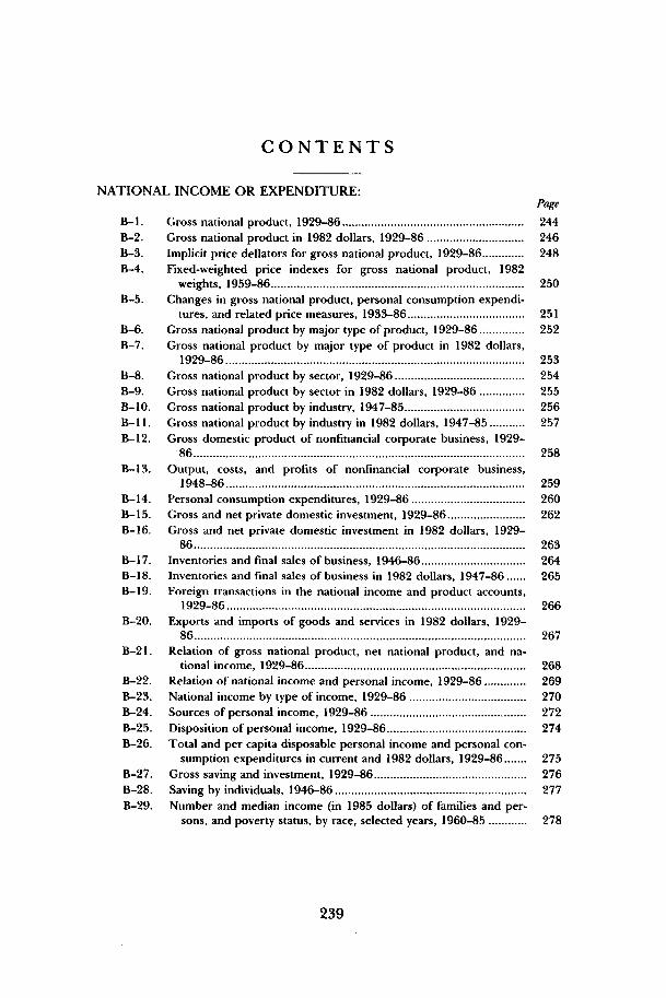
C O N T E N T S

NATIONAL INCOME OR EXPENDITURE:Page

B-l. Gross national product, 1929-86 244B-2. Gross national product in 1982 dollars, 1929-86 246B-3. Implicit price deflators for gross national product, 1929-86 248B-4. Fixed-weighted price indexes for gross national product, 1982

weights, 1959-86 250B-5. Changes in gross national product, personal consumption expendi-

tures, and related price measures, 1933-86 251B-6. Gross national product by major type of product, 1929-86 252B-7. Gross national product by major type of product in 1982 dollars,

1929-86 253B-8. Gross national product by sector, 1929-86 254B-9. Gross national product by sector in 1982 dollars, 1929-86 255B-10. Gross national product by industry, 1947-85 256B-ll. Gross national product by industry in 1982 dollars, 1947-85 257B-12. Gross domestic product of nonfmancial corporate business, 1929-

86 258B-l3. Output, costs, and profits of nonfinancial corporate business,

1948-86 259B-14. Personal consumption expenditures, 1929-86 260B-15. Gross and net private domestic investment, 1929-86 262B-l6. Gross and net private domestic investment in 1982 dollars, 1929-

86 263B-17. Inventories and final sales of business, 1946-86 264B-18. Inventories and final sales of business in 1982 dollars, 1947-86 265B-l9. Foreign transactions in the national income and product accounts,

1929-86 266B-20. Exports and imports of goods and services in 1982 dollars, 1929-

86 267B-21. Relation of gross national product, net national product, and na-

tional income, 1929-86 268B-22. Relation of national income and personal income, 1929-86 269B-23. National income by type of income, 1929-86 270B-24. Sources of personal income, 1929-86 272B-25. Disposition of personal income, 1929-86 274B-26. Total and per capita disposable personal income and personal con-

sumption expenditures in current and 1982 dollars, 1929-86 275B-27. Gross saving and investment, 1929-86 276B-28. Saving by individuals, 1946-86 277B-29. Number and median income (in 1985 dollars) of families and per-

sons, and poverty status, by race, selected years, 1960-85 278

239

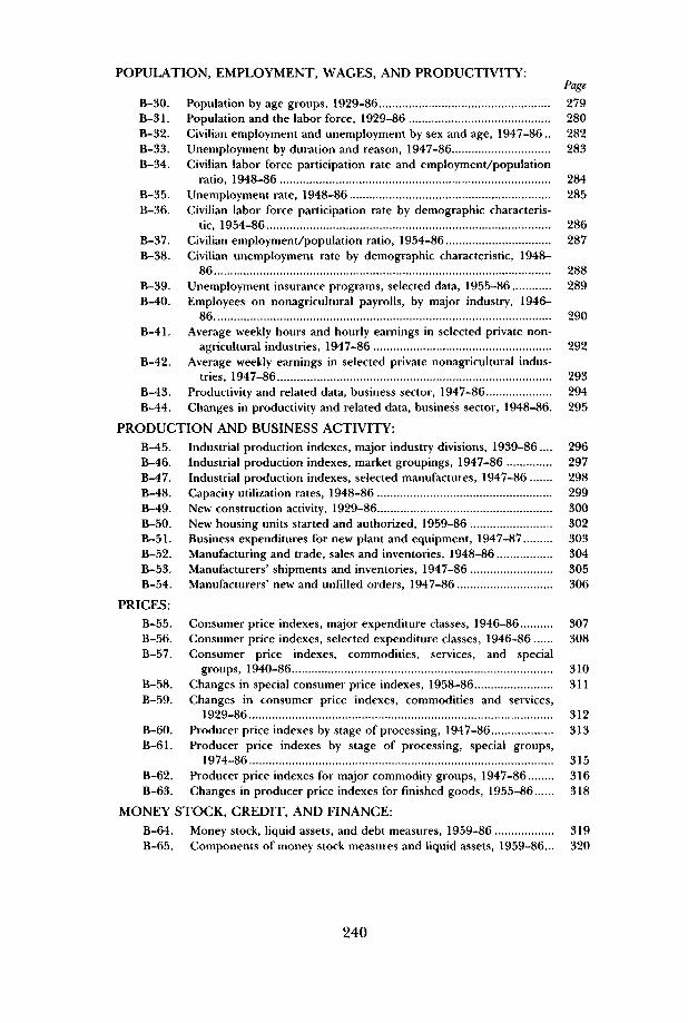
POPULATION, EMPLOYMENT, WAGES, AND PRODUCTIVITY:Page

B-30. Population by age groups, 1929-86 279B-31. Population and the labor force, 1929-86 280B-32. Civilian employment and unemployment by sex and age, 1947-86.. 282B-33. Unemployment by duration and reason, 1947-86 283B-34. Civilian labor force participation rate and employment/population

ratio, 1948-86 284B-35. Unemployment rate, 1948-86 285B-36. Civilian labor force participation rate by demographic characteris-

tic, 1954-86 286B-37. Civilian employment/population ratio, 1954-86 287B-38. Civilian unemployment rate by demographic characteristic, 1948-

86 288B-39. Unemployment insurance programs, selected data, 1955-86 289B-40. Employees on nonagricultural payrolls, by major industry, 1946-

86 290B-41. Average weekly hours and hourly earnings in selected private non-

agricultural industries, 1947-86 292B-42. Average weekly earnings in selected private nonagricultural indus-

tries, 1947-86 293B-43. Productivity and related data, business sector, 1947-86 294B-44. Changes in productivity and related data, business sector, 1948-86. 295

PRODUCTION AND BUSINESS ACTIVITY:B-45. Industrial production indexes, major industry divisions, 1939-86.... 296B-46. Industrial production indexes, market groupings, 1947-86 297B-47. Industrial production indexes, selected manufactures, 1947-86 298B-48. Capacity utilization rates, 1948-86 299B-49. New construction activity, 1929-86 300B-50. New housing units started and authorized, 1959-86 302B-51. Business expenditures for new plant and equipment, 1947-87 303B-52. Manufacturing and trade, sales and inventories, 1948-86 304B-53. Manufacturers' shipments and inventories, 1947-86 305B-54. Manufacturers' new and unfilled orders, 1947-86 306

PRICES:B-55. Consumer price indexes, major expenditure classes, 1946-86 307B-56. Consumer price indexes, selected expenditure classes, 1946-86 308B-57. Consumer price indexes, commodities, services, and special

groups, 1940-86 310B-58. Changes in special consumer price indexes, 1958-86 311B-59. Changes in consumer price indexes, commodities and services,

1929-86 312B-60. Producer price indexes by stage of processing, 1947-86 313B-61. Producer price indexes by stage of processing, special groups,

1974-86 315B-62. Producer price indexes for major commodity groups, 1947-86 316B-63. Changes in producer price indexes for finished goods, 1955-86 318

MONEY STOCK, CREDIT, AND FINANCE:B-64. Money stock, liquid assets, and debt measures, 1959-86 319B-65. Components of money stock measures and liquid assets, 1959-86... 320

240

B-66. Aggregate reserves of depository institutions and monetary base,1959-86 322

B-67. Commercial bank loans and securities, 1972-86 323B-68. Bond yields and interest rates, 1929-86 324B-69. Total funds raised in credit markets by nonfinancial sectors, 1977-

86 326B-70. Mortgage debt outstanding by type of property and of financing,

1939-86 328B-71. Mortgage debt outstanding by holder, 1939-86 329B-72. Consumer credit outstanding, 1950-86 330

GOVERNMENT FINANCE:B-73. Federal receipts, outlays, surplus or deficit, and debt, selected

fiscal years, 1929-88 331B-74. Federal receipts, outlays, and debt, fiscal years 1979-88 332B-75. Relation of Federal Government receipts and expenditures in the

national income and product accounts to the budget, fiscal years1986-88 334

B-76. Federal and State and local government receipts and expenditures,national income and product accounts, 1929-86 335

B-77. Federal and State and local government receipts and expenditures,national income and product accounts, by major type, 1929-86... 336

B-78. Federal Government receipts and expenditures, national incomeand product accounts, 1966-88 337

B-79. State and local government receipts and expenditures, nationalincome and product accounts, 1946-86 338

B-80. State and local government revenues and expenditures, selectedfiscal years, 1927-85 339

B-81. Interest-bearing public debt securities by kind of obligation, 1967-86 340

B-82. Maturity distribution and average length of marketable interest-bearing public debt securities held by private investors, 1967-86. 341

B-83. Estimated ownership of public debt securities, by private investors,1976-86 342

CORPORATE PROFITS AND FINANCE:B-84. Corporate profits with inventory valuation and capital consumption

adjustments, 1929-86 343B-85. Corporate profits by industry, 1929-86 344B-86. Corporate profits of manufacturing industries, 1929-86 345B-87. Sales, profits, and stockholders' equity, all manufacturing corpora-

tions, 1950-86 346B-88. Relation of profits after taxes to stockholders' equity and to sales,

all manufacturing corporations, 1947-86 347B-89. Sources and uses of funds, nonfarm nonfinancial corporate busi-

ness, 1946-86 348B-90. State and municipal and business securities offered, 1940-86 349B-91. Common stock prices and yields, 1949-86 350B-92. Business formation and business failures, 1945-86 351

AGRICULTURE:B-93. Farm income, 1929-86 352B-94. Farm output and productivity indexes, 1947-86 353B-95. Farm input use, selected inputs, 1947-86 354

241

Page

B-96. Indexes of prices received and prices paid by farmers, 1946-86 355B-97. U.S. exports and imports of agricultural commodities, 1940-86 356B-98. Balance sheet of the farm sector, 1939-86 357

INTERNATIONAL STATISTICS:B-99. U.S. international transactions, 1946-86 358B-100. U.S. merchandise exports and imports by principal end-use catego-

ry, 1965-86 360B-101. U.S. merchandise exports and imports by area, 1977-86 361B-102. U.S. merchandise exports and imports by commodity groups,

1966-86 362B-103. International investment position of the United States at year-end,

1978-85 363B-104. International reserves, selected years, 1952-86 364B-105. Exchange rates, 1967-86 365B-106. Industrial production and consumer prices, major industrial coun-

tries, 1962-86 366B-107. Civilian unemployment rate, and hourly compensation, major in-

dustrial countries, 1960-86 367B-108. Growth rates in real gross national product, 1961-86 368

242

General Notes

Detail in these tables may not add to totals because of rounding.Unless otherwise noted, all dollar figures are in current dollars.Symbols used:

p Preliminary.Not available (also, not applicable).

Data in these tables reflect revisions made by the source agencies during 1986.

243

NATIONAL INCOME OR EXPENDITURE

TABLE B-l.—Gross national product, 1929-86

[Billions of dollars, except as noted; quarterly data at seasonally adjusted annual rates]

Year or quarter

192919331939 .. ..19401941194219431944194519461947194819491950195119521953195419551956195719581959196019611962196319641965 .. .19661967196819691970 . .. .197119721973197419751976. .. . .19771978197919801981. ..19821983 .198419851986 p

1982: IV1983: IV1984- 1

IIIllIV

1985:1I II I IIV

1986- 1 .III l lIV "

Grossnationalproduct

103.956.091.3

100.4125.5159.0192.7211.4213.4212.4235.2261.6260.4288.3333.4351.6371.6372.5405.9428.2451.0456.8495.8515.3533.8574.6606.9649.8705.1772.0816.4892.7963.9

1,015.51,102.71,212.81,359.31,472.81,598.41,782.81,990.52,249.72,508.22,732.03,052.63,166.03,405.73,765.03,998.14,208.53,212.53,545.83,670.93,743.83,799.73,845.63,909.33,965.04,030.54,087.7

4,149.24,175.64,240.74,268.4

Personal consumption expenditures

Total

77.345.867.071.080.888.699.5

108.2119.6143.9161.9174.9178.3192.1208.1219.1232.6239.8257.9270.6285.3294.6316.3330.7341.1361.9381.7409.3440.7477.3503.6552.5597.9640.0691.6757.6837.2916.5

1,012.81,129.31,257.21,403.51,566.81,732.61,915.12,050.72,234.52,428.22,600.52,762.42,117.02,315.82,363.82,416.12,445.62,487.22,530.92,576.02,627.12,667.9

2,697.92,732.02,799.82,819.9

Dura-ble

goods

9.23.56.77.89.76.96.56.78.0

15.820.422.925.030.829.929.332.732.138.938.239.737.242.843.541.947.051.856.863.568.570.681.086.285.797.6

111.2124.7123.8135.4161.5184.5205.6219.0219.3239.9252.7289.1331.2359.3388.3263.8310.0321.2331.3331.8340.4347.7354.0373.3362.0

360.8373.9414.5404.2

Non-durablegoods

37.722.335.137.042.950.858.664.371.982.790.996.694.998.2

109.2114.7117.8119.7124.7130.8137.1141.7148.5153.2157.4163.8169.4179.7191.9208.5216.9235.0252.2270.3283.3305.1339.6380.9416.2452.0490.4541.8613.2681.4740.6771.0816.7870.1905.1932.7786.6837.9855.7870.3873.9880.3888.2902.3907.4922.6

929:7928.4932.8940.0

Services

30.420.125.226.228.331.034.337.239.745.450.655.558.463.269.075.182.188.094.3

101.6108.5115.7125.0134.0141.8151.1160.6172.8185.4200.3216.0236.4259.4284.0310.7341.3373.0411.9461.2515.9582.3656.1734.6831.9934.7

1,027.01,128.71,227.01,336.11,441.31,066.51,167.91,186.91,214.51,239.91,266.51,294.91,319.71,346.41,383.2

1,407.41,429.81,452.41,475.7

Gross private domestic investment

Total

16.71.69.5

13.418.310.36.27.7

11.331.535.047.136.555.160.553.554.954.169.772.771.163.680.278.277.187.693.199.6

116.2128.6125.7137.0153.2148.8172.5202.0238.8240.8219.6277.7344.1416.8454.8437.0515.5447.3502.3662.1661.1686.4409.6579.8659.5657.5670.3661.1650.6667.1657.4669.5

708.3687.3675.8674.5

Fixed investment

Total

14.93.19.1

11.213.88.56.98.7

12.325.135.542.439.548.350.250.554.555.764.068.069.765.174.475.174.781.587.394.2

106.2114.4115.4129.1143.4145.7164.7191.5219.2225.4225.2261.7322.8388.2441.9445.3491.5471.8509.4598.0650.0675.1469.5548.8564.0597.6605.8624.4625.2648.0654.3672.6

664.4672.8680.3682.7

Nonresidential

Total

11.02.56.17.79.76.35.47.4

10.617.323.526.824.927.831.831.935.134.739.044.547.542.446.348.848.352.555.261.473.183.584.491.4

102.3105.2109.6123.0145.9160.6162.9180.0214.2259.0302.8322.8369.2366.7356.9416.5458.2458.5354.9383.9388.2413.3421.8442.9439.8459.2459.8474.0

459.2457.5459.0458.1

Struc-tures

5.51.12.22.63.32.21.82.43.37.48.19.59.2

10.011.912.213.613.915.218.218.917.518.019.219.420.520.822.727.430.530.732.937.139.240.944.551.457.056.360.166.781.099.5

113.9138.5143.3124.0139.3154.8143.6137.6127.4129.7139.1141.4146.7150.7156.1155.0157.2

154.6141.5139.5138.6

Pro-ducers'

dur-able

equip-ment

5.51.43.95.26.44.13.75.07.39.9

15.317.315.717.819.919.721.520.823.926.328.624.928.329.728.932.134.438.745.853.053.758.565.266.168.778.594.5

103.6106.6119.9147.4178.0203.3208.9230.7223.4232.8277.3303.4314.9217.3256.5258.4274.1280.4296.2289.1303.1304.7316.8

304.6316.0319.5319.5

Resi-dential

4.0.6

3.03.54.12.21.4141.77.8

12.115.614.620.518.418.619.421.125.023.522.222.728.126.326.429.032.132.833.130.931.137.741.240.555.168.673.364.862.381.7

108.6129.2139.1122.5122.3105.1152.5181.4191.8216.6114.7164.9175.8184.4184.0181.5185.4188.8194.5198.6

205.3215.3221.3224.6

Changein busi-

nessinven-tories

1.7-1.6

.42.24.51.8

-.6-1.0-1.0

6.4-.54.7

-3.16.8

10.23.1

.4-1.6

5.74.61.4

-1.55.83.12.46.15.85.49.9

14.210.37.99.83.17.8

10.519.615.4

-5.616.021.328.613.083

24.0-24.5-7.164.111.111.4

-59.931.095.559.964.436.725.419.13.131

43.814.5

-4.5-8.3

See next page for continuation of table.

244

TABLE B-l.—Gross national product, 1929-86—Continued

[Billions of dollars, except as noted; quarterly data at seasonally adjusted annual rates]

Year or quarter

192919331939194019411942194319441945194619471948194919501951195219531954195519561957.195819591960196119621963.19641965196619671968196919701971197219731974197519761977197819791980198119821983198419851986 "1982: IV1983- IV1984:1

IIIllIV

1985:1||IIIIV

1986:1||IIIIV P

Net exports of goods andservices

Netexports

1.1.4

1.21.81.5.2

-1.917

"?!811.97.06.52.24.53.21.32.63.05.37.33.31.55.97.26.98.2

10.99.77.57.45.55.68.56.33.2

16.816.331.118.81.94.1

18.832.133.926.3

-6.1-58.7-78.9

-105.714.1

-25.8-45.6

632-60.0-66.1-49.4

771-83.71053

-93.7-104.5-108.9-115.6

Exports

7.12.44.65.46.15.04.65.57.4

15.220.317.516.414.519.819.218.118.821.125.228.224.425.029.931.133.135.740.542.946.649.554.860.468.972.481.4

114.1151.5161.3177.7191.6227.5291.2$51.0382.8361.9352.5382.7369.8373.0335.9364.7373.4382.1389.2386.2378.4370.0362.3368.2374.8363.0370.8383.4

Imports

5.92.13.43.74.74.86.57.27.97.38.3

10.69.8

12.315.316.016.816.318.119.920.921.123.524.023.926.227.529.633.239.142.149.354.760.566.178.297.3

135.2130.3158.9189.7223.4272.5318.9348.9335.6358.7441.4448.6478.7321.9390.5419.0445.3449.1452.2427.9447.1446.0473.6468.5467.5479.7499.0

Government purchases of goods andservices

Total

8.98.3

13.614.225.059.988.997.183.029.126.432.639.038.860.475.882.876.075.379.787.395.497.9

100.6108.4118.2123.8130.0138.6158.6179.7197.7207.3218.2232.4250.0266.5299.1335.0356.9387.3425.2467.8530.3588.1641.7675.0733.4815.4865.3671.8676.1693.2733.3743.8763.4777.3799.0829.7855.6836.7860.8874.0889.7

Federal

Total

1.52.25.26.1

17.052.081.489.474.819.213.617.321.119.138.652.757.948.444.946.450.554.554.654.458.264.665.766.468.780.492.7

100.1100.098.899.8

105.8106.4116.2129.2136.3151.1161.8178.0208.1242.2272.7283.5311.3354.1367.2293.2276.1283.4315.2317.2329.1333.7340.9360.9380.9355.7367.6369.3376.3

Nation-al

defense

1.32.3

13.849.479.887.573.716.410.011.313.914.333.846.249.041.639.040.744.646.346.445.347.952.151.550.451.062.073.479.178.976.874.177.477.582.689.693.4

100.9108.9121.9142.7167.5193.8214.4235.0259.4278.4205.4221.5227.1233.7234.5244.9248.9255.1265.5268.0266.4278.4286.8281.9

Non-de-

fense

3.93.93.22.61.62.01.12.83.66.07.24.74.86.58.96.86.05.75.98.38.29.2

10.212.614.216.017.718.319.321.021.122.025.828.428.933.639.642.950.352.956.165.474.878.969.176.294.788.987.754.656.381.682.784.284.885.895.5

112.989.389.282.694.4

Stateandlocal

7.46.18.38.18.07.87.57.68.29.9

12.815.318.019.821.823.124.827.730.333.336.940.843.346.150.253.558.163.569.978.287.097.6

107.2119.4132.5144.2160.1182.9205.9220.6236.2263.4289.9322.2345.9369.0391.5422.2461.3498.1378.7400.0409.8418.1426.6434.3443.5458.1468.8474.7480.9493.3504.7513.3

Finalsales

102.257.690.998.3

121.0157.2193.4212.3214.4206.0235.7256.9263.4281.4323.2348.6371.1374.1400.2423.6449.6458.3490.0512.3531.4568.5601.1644.4695.2757.8806.1884.8954.1

1,012.31,094.91,202.31,339.71,457.41,604.11,766.81,969.22,221.02,495.22,740.33,028.63,190.53,412.83,700.93,987.04,197.13,272.43,514.83,575.43,683.93,735.33,808.93,883.93,945.94,027.44,090.84,105.44,161.24,245.24,276.7

Percent changefrom preceding

period

Grossnation-

alprod-uct

-4.27.0

10.025.026.621.29.7

.9

ibis11.2

10.715.75.55.7

g'.o5.55.31.38.53.93.67.65.67.18.59.55.89.38.05.48.6

10.012.18.38.5

11.511.713.011.58.9

11.73.77.6

10.56.25.34.2

12.414.98.26.14.96.85.86.85.86.22.66.42.6

Finalsales

555.48.1

23.229.923.09.81.0

-3.914.49.02.56.8

14.87.96.5

.87.05.86.11.96.94.63.77.05.77.27.99.06.49.87.86.18.29.8

11.48.8

10.110.111.512.812.39.8

10.55.37.08.47.75.3

11.07.87.1

12.75.78.18.16.58.56.41.45.58.33.0

Source: Department of Commerce, Bureau of Economic Analysis.

245

TABLE B-2.—Gross national product in 1982 dollars, 1929-86

[Billions of 1982 dollars, except as noted; quarterly data at seasonally adjusted annual rates]

Year orquarter

19291933193919401941 . . .19421943194419451946194719481949195019511952195319541955195619571958 . . .195919601961196219631964196519661967196819691970197119721973 . . .197419751976 .1977197819791980198119821983198419851986 p

1982: IV1983: IV1984- 1

IIIllIV

1985: I||II IIV

1986: IIII l lIV P

Grossnationalproduct

709.6498.5716.6

772.9909.4

1,080.31,276.21,380.61,354.81,096.91,066.71,108.71,109.0

1,203.71,328.21,380.01,435.31,416.21,494.91,525.61,551.11,539.21,629.1

1,665.31,708.71,799.41,873.31,973.32,087.62,208.32,271.42,365.62,423.3

2,416.22,484.82,608.52,744.12,729.32,695.02,826.72,958.63,115.23,192.4

3,187.13,248.83,166.03,279.13,489.93,585.23,676.5

3,159.3

3,365.1

3,444.73,487.13,507.43,520.4

3,547.03,567.63,603.83,622.3

3,655.93,661.43,686.43,702.4

Personal consumptionexpenditures

Total

471.4378.7480.5

502.6531.1527.6539.9557.1592.7655.0666.6681.8695.4

733.2748.7771.4802.5822.7873.8899.8919.7932.9979.4

1,005.11,025.21,069.01,108.41,170.61,236.41,298.91,337.71,405.91,456.7

1,492.01,538.81,621.91,689.61,674.01,711.91,803.91,883.81,961.02,004.4

2,000.42,024.22,050.72,146.02,246.32,324.52,418.6

2,078.7

2,191.9

2,213.82,246.32,253.32,271.7

2,292.32,311.92,342.02,351.7

2,372.72,408.42,448.02,445.1

Durablegoods

40.320.735.7

40.646.231.328.126.328.747.856.561.767.8

80.774.773.080.281.596.992.892.486.996.9

98.093.6

103.0111.8120.8134.6144.4146.2161.6167.8

162.5178.3200.4220.3204.9205.6232.3253.9267.4266.5

245.9250.8252.7283.1318.9343.9368.9

262.0

300.5

311.1319.0318.8326.8

332.3338.8357.4347.0

345.4357.1391.6381.3

Non-durablegoods

211.4181.8248.0

259.4275.6279.1284.7297.9323.5344.2337.4338.7342.3

352.8362.9376.6388.2393.8413.2426.9434.7439.9455.8

463.3470.1484.2494.3517.5543.2569.3579.2602.4617.2

632.5640.3665.5683.2666.1676.5708.8731.4753.7766.6

762.6764.4771.0800.2828.6841.6872.4

778.6

812.7

819.7832.8831.7830.5

834.3841.3843.8847.2

860.6877.3875.4876.2

Services

219.7176.2196.7

202.7209.3217.2227.2232.9240.5262.9272.6281.4285.3

299.8311.1321.9334.1347.4363.6380.1392.6406.1426.7

443.9461.4481.8502.3532.3558.5585.3612.3641.8671.7

697.0720.2756.0786.1803.1829.8862.8898.5939.8971.2

991.91,009.01,027.01,062.71,098.71,139.01,177.3

1,038.1

1,078.6

1,083.01,094.61,102.81,114.4

1,125.81,131.81,140.81,157.5

1,166.61,174.01,181.01,187.6

Gross private domestic investment

Total

139.222.786.0

111.8138.876.750.456.476.5

178.1177.9208.2168.8

234.9235.2211.8216.6212.6259.8257.8243.4221.4270.3

260.5259.1288.6307.1325.9367.0390.5374.4391.8410.3

381.5419.3465.4520.8481.3383.3453.5521.3576.9575.2

509.3545.5447.3504.0652.0647.7659.7

408.8

577.2

649.3649.7658.9649.9

638.2655.6643.8653.2

684.0664.7651.3638.8

Fixed investment

Total

128.433.582.1

97.4111.164.749.761.684.9

150.2178.9196.0178.4

210.8204.3201.8213.8217.3243.5244.9240.4224.8253.8

252.7251.8272.4290.5310.2341.8353.7345.6370.7385.1373.3399.7443.7480.8448.0396.1431.4492.2540.2560.2

516.2521.7471.8510.4592.8638.6648.9

468.1

550.3

564.1592.7598.3615.9

615.0638.1643.1658.4

644.1649.6651.6650.3

Nonresidential

Total

93.025.853.2

65.076.647.439.452.674.2

105.5121.7127.4114.8

124.0131.7130.6140.1137.5151.0160.4161.1143.9153.6

159.4158.2170.2176.6194.9227.6250.4245.0254.5269.7

264.0258.4277.0317.3317.8281.2290.6324.0362.1389.4

379.2395.2366.7361.2422.2461.4455.0

352.3

390.4

394.4419.5427.1447.6

442.7463.0463.1476.9

457.8456.8454.4451.0

Struc-tures

54.714.325.2

28.533.420.915.620.427.050.947.550.549.3

52.856.557.362.364.969.475.575.270.671.9

76.177.781.381.687.9

101.8108.0105.4108.0112.9

111.1107.3109.5117.7115.2102.8104.4108.3119.3130.6

136.2148.8143.3127.2141.3152.2134.7

138.3

131.6

133.5141.3142.9147.5

149.9154.1152.3152.4

148.1132.9129.5128.4

Pro-ducers'durableequip-ment

38.411.528.0

36.543.226.523.832.147.254.774.276.965.5

71.275.273.377.712.181.784.985.973.381.7

83.380.588.995.1

107.0125.8142.4139.6146.5156.8

152.9151.0167.5199.6202.7178.4186.2215.7242.8258.8

243.0246.4223.4233.9280.9309.2320.3

214.1

258.8

260.9278.2284.2300.1

292.8308.9310.9324.5

309.7323.9324.9322.6

Resi-dential

35.47.7

28.9

32.534.417.310.49.0

10.744.757.268.663.6

86.772.671.273.879.892.484.479.381.0

100.2

93.393.6

102.2113.9115.3114.2103.2100.6116.2115.4

109.3141.3166.6163.4130.2114.9140.8168.1178.0170.8

137.0126.5105.1149.3170.6177.2193.9

115.8

159.9

169.7173.2171.2168.3

172.4175.1180.0181.5

186.3192.7197.2199.3

Change inbusiness

inven-tories

10.8-10.7

3.9

14.427.812.0

.7-5.2-8.427.9

-1.012.3

-9.7

24.230.810.02.8

-4.816.312.93.0

-3.416.5

7.77.3

16.216.615.725.236.928.821.025.1

8.219.621.840.033.3

-12.822.129.136.815.0

-6.923.9

-24.5-6.459.29.0

10.8

-59.3

27.0

85.157.060.633.9

23.217.4

.7-5.2

39.915.1-.3

-11.5

See next page for continuation of table.

246

TABLE B-2.—Gross national product in 1982 dollars, 1929-86—Continued

[Billions of 1982 dollars, except as noted; quarterly data at seasonally adjusted annual rates]

Year or quarter

19291933193919401941194219431944194519461947 ...194819491950 ..195119521953195419551956195719581959196019611962196319641965196619671968 ..19691970197119721973197419751976197719781979198019811982 .1983198419851986"1982- IV .1983: IV1984:1

II.IllIV

1985- 1IIIllIV

1986- 1IIIIIIV P

Net exports of goods andservices

Netexports

4.7-1.4

6.18.23.977

-23.0238

-18.927.042.419.218.84.7

14.66.9

-2.72.5

.04.37.0

103-18.2-4.0-2.7-7.5-1.9

5.9-2.7

-13.7169297

-34.9-30.0-39.8-49.4-31.5

.818.9

-11.0-35.5-26.8

3.657.049.426.3

-19.9-83.6

-108.2-149.7

11.7-46.2-68.6-87.2-85.7-92.7

-78.8-108.1-113.8-132.0-125.9

1539-163.3-155.6

Exports

42.122.736.240.042.029.125.127.335.269.082.366.265.059.272.070.166.970.076.987.994.982.483.798.4

100.7106.9114.7128.8132.0138.41436155.7165.0178.3179.2195.2242.3269.1259.7274.4281.6312.6356.8388.9392.7361.9348.1369.7362.3371.3336.0355.5361.3367.0375.5375.0

369.4361.2355.8362.9369.2359.8371.2385.3

mports

37.424.230.131.738.236.948.051.154.142.039.947.146.254.657.463.369.767.576.983.687.992.8

101.9102.4103.3114.4116.6122.8134.7152.11605185.3199.9208.3218.9244.6273.8268.4240.8285.4317.1339.4353.2332.0343.4335.6368.1453.2470.5521.0324.3401.6429.9454.2461.2467.7

448.2469.3469.6494.8495.1513.6534.5540.8

Government purchases of goods andservices

Totai

94.298.5

144.1150.2235.6483.7708.9790.8704.5236.9179.8199.5226.0230.8329.7389.9419.0378.4361.3363.7381.1395.3397.7403.7427.1449.4459.8470.8487.0532.65762597.6591.2572.6566.5570.7565.3573.2580.9580.3589.1604.1609.1620.5629.7641.7649.0675.2721.2748.0660.1642.2650.2678.2681.0691.5

695.3708.3731.8749.4725.2742.2750.4774.1

Federal

Total

18.327.053.863.6

153.0407.1638.1722.5634.0159.391.9

106.1119.5116.7214.4272.7295.9245.0217.9215.4224.1224.9221.5220.6232.9249.3247.8244.2244.4273.83044309.6295.6268.3250.6246.0230.0226.4226.3224.2231.8233.7236.2246.9259.6272.7275.1291.7323.6333.4289.5266.0271.2296.3295.6303.8

305.8311.4329.9347.2320.4328.9330.9353.5

Nation-al

de-fense

185.3171.0163.3161.1157.5159.2160.7164.3171.2180.3193.8206.9219.4235.7251.0201.4211.6214.4219.0218.4225.9

228.0233.5242.2239.3238.7249.3259.4256.5

Non-de-

fense

60.759.163.165.266.872.773.071.975.779.378.968.272.387.882.488.254.456.877.377.177.9

77.877.987.6

107.981.779.571.597.0

Stateandlocal

75.971.590.386.682.676.770.868.370.577.687.993.4

106.5114.2115.4117.3123.1133.4143.4148.3157.0170.4176.2183.1194.2200.1212.0226.6242.5258.8271.8288.0295.6304.3315.9324.7335.3346.8354.6356.0357.2370.4373.0373.6370.1369.0373.9383.5397.6414.5370.6376.2379.0381.8385.4387.7

389.5396.9401.9402.2404.8413.3419.5420.6

Finalsales

698.7509.2712.7758.5881.6

1,068.31,275.51,385.71,363.31,069.01,067.71,096.41,118.71,179.51,297.41,370.01,432.51,421.01,478.61,512.71,548.11,542.61,612.61,657.51,701.41,783.31,856.71,957.62,062.42,171.52,242.62,344.62,398.12,407.92,465.22,586.82,704.12,696.02,707.82,804.62,929.53,078.43,177.43,194.03,225.03,190.53,285.53,430.73,576.23,665.73,218.63,338.13,359.63,430.03,446.83,486.4

3,523.93,550.23,603.13,627.53,616.13,646.33,686.73,713.9

Percent changefrom preceding

period

Grossnation-

alprod-uct

-2.17.97.8

17.718.818.18.21.9

-19.02.83.9

.08.5

10.33.94.0

-1.35.62.11.7.8

5.82.22.65.34.15.35.85.82.94.12.4-.32.85.05.2-.5

-1.34.94.75.32.5

— .21.9

-2.53.66.42.72.5.6

7.39.85.02.31.5

3.12.34.12.13.8

.62.81.7

Finalsales

-3.16.36.4

16.221.219.48.6

-1.6-21.6

~2J2.05.4

10.05.64.6-.84.12.32.3

-.44.52.82.64.84.15.45.45.33.34.52.3

.42.44.94.5

.43.64.55.13.2

.51.01.13.04.44.22.57.13.82.68.62.04.7

4.43.06.12.7

-1.33.44.53.0

Source: Department of Commerce, Bureau of Economic Analysis.

247

TABLE B-3.—Implicit price deflators for gross national product, 1929-86

[Index numbers, 1982=100, except as noted; quarterly data seasonally adjusted]

Year or quarter

192919331939194019411942194319441945 .19461947 . . .194819491950195119521953195419551956195719581959I96019611962196319641965196619671968196919701971197219731974197519761977197819791980198119821983198419851986 "1982- IV1983- IV1984- 1

III l lIV

1985:1I II I IIV

1986- 1III l lIV

Grossnationalproduct

14.611.212.713.013.814.715.115.315.719.422.123.623.523.925.125.525.926.327.228.129.129.730.430.931.231.932.432.933.835.035.937.739.842.044.446.549.554.059.363.167.372.278.685.794.0

100.0103.91Q7.9HIT114.5101.7105.4106.6107.4108.3109.2110.2111.1111.8112.8113.5114.0115.0115.3

Personal consumptionexpenditures

Total

16.412.113.914.115.216.818.419.420.222.024.325.725.626.227.828.429.029.129.530.131.031.632.332.933.333.934.435.035.636.737.639.341.042.944.946.749.654.859.262.666.771.678.286.694.6

100.0104.1

_mL111.9114.2101.8105.7106.8107.6108.5109.5110.4111.4112.2113.4113.7113.4114.4115.3

Durablegoods

22.916.818.719.220.922.023.325.427.733.036.137.136.938.140.040.140.839.440.141.242.942.844.244.444.845.746.347.047.147.548.350.151.452.754.755.556.660.465.969.572.776.982.189.295.7

100.0102.1

___iQia104.5105.3100.7103.1103.3103.9104.1104.1104.6104.5104.5104.3104.5104.7105.9106.0

Non-durablegoods

17.812.214.214.315.518.220.621.622.224.026.928.527.727.830.130.530.430.430.230.631.532.232.633.133.533.834.334.735.336.637.539.040.942.744.245.849.757.261.563.867.171.980.089.496.9

100.0102.1-m106.9101.0103.1104.4104.5105.1106.0106.5107.2107.5108.9108.0105.8106.6107.3

Services

13.811.412.812.913.514.315.116.016.517.318.619.720.521.122.223.324.625.325.926.727.628.529.330.230.731.432.032.533.234.235.336.838.640.743.145.147.451.355.659.864.869.875.683.992.6

100.0106.2

-8K122.4102.7108.3109.6110.9112.4113.6115.0116.6118.0119.5120.6121.8123.0124.3

Gross private domestic investment J

Fixed investment

Total

11.69.4

11.111.512.413.213.814.214.516.719.821.722.222.924.625.025.525.626.327.829.028.929.329.729.729.930.130.431.132.433.434.837.239.041.243.245.650.356.960.765.671.978.986.394.2

100.099.8

JOO 3" 101.8

104.0100.399.7

100.0100.8101.3101.4101.7101.5101.7102.2103.2103.6104.4105.0

Nonresidential

Total

11.89.8

11.511.912.713.313.814.014.316.419.321.021.722.424.224.425.125.225.827.729.529.530.230.630.530.931.331.532.133.334.435.937.939.942.444.446.050.557.961.966.171.577.885.193.4

100.098.8

J&7— gfe100.8100.798.398.498.598.899.099.499.299.399.4

100.3100.2101.0101.6

Struc-tures

10.07.68.89.09.7

10.711.411.612.314.517.118.918.618.821.121.321.821.421.824.125.224.825.025.225.025.225.525.926.928.229.130.432.935.238.140.643.749.554.757.661.667.976.283.693.1

100.097.5

_98JL101.7106.699.596.897.198.599.099.5

100.6101.3101.8103.2104.4106.5107.8108.0

Pro-ducers'

dur-able

equip-ment

14.312.513.914.214.915.315.415.615.418.220.722.524.025.026.426.927.728.629.331.033.334.034.735.635.936.136.236.236.437.238.439.941.543.245.546.847.351.159.764.468.373.378.686.093.7

100.099.5

~£8J.- 98.1

98.3101.599.199.198.598.698.798.898.198.097.698.497.698.399.0

Residen-tial

11.28.1

10.510.911.912.813.814.915.817.521.122.823.023.725.426.126.326.427.027.928.028.028.028.228.228.328.228.529.029.930.932.535.637.039.041.244.849.854.258.064.672.681.489.496.6

100.0102.2IQ&3-108.2 •111.799.1

103.1103.6106.4107.5107.8107.6107.8108.1109.4110.2111.7112.2112.7

See next page for continuation of table.

248

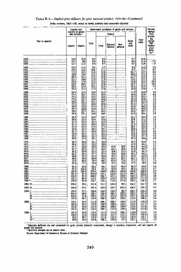
TABLE B-3.—Implicit price deflators for gross national product, 7929-86—Continued

[Index numbers, 1982=100, except as noted; quarterly data seasonally adjusted]

Year or quarter

19291933193919401941 !19421943194419451946. .1947194819491950195119521953195419551956195719581959I9601961196219631964196519661967196819691970197119721973197419751976197719781979198019811982 . ..198319841985 „1986 " .1982: IV1983- IV .1984- 1

IIIl lIV

1985:1||IIIIV

1986- 1IIIllIV

Export;imports o

and ser

Exports

16.810.712.713.614.617.218.520.221.122.024.626.525.224.427.427.427.026.927.528.629.729.629.930.430.931.031.131.432.533.734.535.236.638.740.441.747.156.362.164.868.072.881.690.297.5

100.0Wl.3103.5102.1100.4100.0102.6103.4104.1103.6103.0102.4102.4101.8101.5101.5100.999999.5

, andf goods/ices1

Imports

15.98.6

11.311.612.313.113.614.114.617.420.922.421.222.526.725.324.124.123.523.823.822.723.123.423.122.923.624124.725.726.226.627.429.030.232.035.550.454.155.759.865.877.196.0

101.6100.097.497.495,491.999.397.297.598.097.496.795.595.395.095.794.691.089.792.3

Government purchases of goods and services

Total

9.48.49.49.5

10.612.412.512.311.812.314.716.317.316.818.319.419.820.120.821.922.924.124.624.925.426.326.927.628.529.831.233.135.138.141.043.847.152.257.761.565.870.476.885.593.4

100.0104.0108.6113.1115.7101.8105.3106.6108.1109.2110.4111.8112.8113.4114.2115.4116.0116.5114.9

Federal

Total

8.18.09.79.7

11.112.812.812.411.812.014.816.317.616.318.019.319.619.720.621.522.524.224.624.725.025.926.527.228.129.430.532.333.836.839.843.046.251.357.160.865.269.275.484.393.3

100.0103.1106.7109.4110.1101.3103.8104.5106.4107.3108.3109.1109.5109.4109.7111.0111.8111.6106.5

Nationaldefense

I"::.":::."."

•'•""•

:::=::

4l'.845.350.655.659.363.467.874.283.492.9

100.0103.6107.1110,0110.9102.0104.7105.9106.7107.3108.4109.2109.3109.6112.0111.6111.7110.5109.9

Non-defense

i."""::::

"""'»•""•

46"848.953.360.664.369.172.478.086.494.3

100.0101.4105.5107.9107.899.5

100.399.2

105.5107.3108.2109.0110.2108.9104.6109.2112.1115.497.3

Stateandlocal

9.78.69.29.39.7

10.210.611.211.612.814.516.316.917.318.919.720.220.721.222.423.524.024.625.225.926.727.428.028.830.232.033.936.339.241.944.447.852.858.162.066.171.177.786.293.4

100.0104.7110.1116.0120.1102.2106.3108.1109.5110.7112.0113.9115.4116.6118.0118.8119.4120.3122.1

Finalsales

14.611.312.813.013.714.715.215.315.719.322.123.423.523.924.925.425.926.327.128.029.029.730.430.931.231.932.432.933.734.935.937.739.842.044.446.549.554.159.263.067.272.178.585.893.9

100.0103.9107.9111.5114.5101.7105.3106.4107.4108.4109.3110.2111.1111.8112.8113.5114.1115.1115.2

Percentchange

frompreced-

ingperiod,

GNPimplicit

pricedefla-tor2

""-2.2-.82.06.26.62.61.42.9

22.913.97.0

2.04.81.51.61.63.23.43.62.12.41.61.02.21.61.52.73.62.65.05.65.55.74.76.59.19.86.46.77.38.99.09.76.43.93.83.32.73.64.74.63.03.43.43.73.32.53.62.51.83.61.0

1 Separate deflators are not calculated for gross private domestic investment, change in business inventories, and net exports ofgoods and services.2 Quarterly changes are at annual rates.

Source: Department of Commerce, Bureau of Economic Analysis.

249

TABLE B-4.—Fixed-weighted price indexes for gross national product, 1982 weights, 1959-86

[Index numbers, 1982 = 100, except as noted; quarterly data seasonally adjusted]

Year or quarter

1959I9601961196219631964196519661967196819691970 . .19711972 . .1973197419751976197719781979198019811982 .. .19831984 .19851986"1982- IV1983: IV1984- 1

||I l lIV

1985:1I II I IIV

1986- 1I II l lIV p

Grossnationalproduct

37.638.138.438.739.139.640.141.142.143.745.647.248.850.353.157.261.865.168.472.778.886.194.1

100.0104.1108.3112.3115.4101.7105.7106.9107.8108.8109.8110.9111.9112.6113.7114.4114.9115.6116.4

Personalcon-

sumptionexpendi-

tures

35.235.736.136.436.837.237.738.539.541.042.844.746.648.351.055.860.163.567.572.278.686.894.6

100.0104.2108.4112.4115.2101.8105.8107.1107.9108.9109.9110.8112.0112.8114.1114.6114.5115.4116.4

Gross private domesticinvestment1

Fixed investment

Total

58.058.158.058.058.058.258.559.360.261.463.261.560.659.861.864.469.071.472.674.580.386.994.5

100.0100.4101.8103.3105.2100.2100.5100.6101.6102.2102.7102.7103.0103.4104.0104.2104.9105.5105.9

Nonresi-dential

65.966.166.066.166.266.466.767.468.469.571.068.466.665.066.668.573.175.274.975.080.186.193.9

100.099.9

100.5101.9103.3100.599.699.7

100.2100.7101.2101.3101.6102.0102.4102.5103.1103.6104.0

Residen-tial

30.230.330.229.929.529.630.030.831.633.136.037.439.541.645.150.154.658.464.872.581.289.496.6

100.0102.2106.3108.2111.599.1

103.3103.7106.4107.4107.7107.6107.8108.1109.4110.1111.4112.0112.5

Exportimports (

and ser

Exports

32.833.534.034.134.434.835.937.138.239.340.943.345.346.550.859.865.467.470.374.582.990.597.7

100.0101.6104.5104.0103.9100.0103.2104.0105.0104.7104.3104.1104.3103.8103.8104.3104.0103.5103.6

s and)f goods

Imports

27.027.327.026.727.127.728.129.129.530.131.233.435.637.842.454.559.761.366.171.380.996.3

101.5100.097.797.795.992.199.397.697.898.497.797.295.795.995.496.594.890.990.992.9

Government purchases ofgoods and services

Total

25.826.427.027.828.529.330.031.332.734.536.639.642.345.248.853.558.662.266.070.977.386.394.1

100.0104.5109.2114.1117.1102.0106.0107.7108.8109.6110.8112.6113.5114.4115.8116.4116.7117.1118.2

Federal

Total

26.927.327.828.429.330.130.832.032.834.536.439.542.446.050.154.859.462.465.870.676.886.494.9

100.0104.1107.9111.0111.8101.7105.4106.9107.7107.9108.9110.5110.5110.8112.1112.3112.0111.4111.5

Nationaldefense

44.347.451.456.559.763.568.675.184.793.8

100.0103.7107.5111.4112.8101.8104.7106.3107.2107.4108.9110.8110.7111.2112.9113.2112.7112.5112.6

Non-defense

50.556.963.366.669.071.575.581.090.697.4

100.0105.1108.8110.0109.5101.4107.0108.4109.1109.0108.8109.9110.0109.7110.3110.1110.1108.8108.9

Stateandlocal

24925.726.427.327.928.529.330.632.534.436.739.642.244.647.852.657.962.066.271.277.786.293.5

100.0104.8110.3116.0121.0102.2106.4108.2109.7110.9112.2114.1115.7117.0118.5119.4120.2121.3123.1

Percentchange

frompreceding

period,GNP fixed-weighted

priceindex2

1.4.7.8

1.01.21.42.52.63.74.43.63.52.95.57.88.05.35.16.28.59.39.36.24.14.03.72.84.04.04.73.63.53.64.23.62.84.02.51.72.62.6

1 Separate deflators are not calculated for gross private domestic investment, change in business inventories, and net exports ofgoods and services.

2 Quarterly changes are at annual rates.Source: Department of Commerce, Bureau of Economic Analysis.

250

TABLE B-5.—Changes in gross national product, personal consumption expenditures, and related price

measures, 1933-86

[Percent change from preceding period; quarterly data at seasonally adjusted annual rates]

Year or quarter

1933193919401941 ...194219431944194519461947194819491950195119521953 ..19541955 .1956195719581959196019611962196319641965 .19661967196819691970197119721973197419751976....19771978 ....19791980198119821983198419851986 "1982: IV1983- IV1984:1

IIIllIV . ...

1985:1||IIIIV

1986- 1IIIllIV »

Gross national product

Currentdollars

-4.27.0

10.025.026.621.29.7

.9

10.811.2-.510.715.75.55.7

.29.05.55.31.38.53.93.67.65.67.18.59.55.89.38.05.48.6

10.012.18.38.5

11.511.713.011.58.9

11.73.77.6

10.56.25.34.2

12.414.98.26.14.96.85.86.85.86.22.66.42.6

Con-stant

(1982)dollars

-2.17.97.8

17.718.818.18.219

-19.0-2.8

3.9.0

8.510.33.94.0

-1.35.62.11.7

-.85.82.22.65.34.15.35.85.82.94.12.4

32.85.05.2

5-1.3

4.94.75.32.5-.21.9253.66.42.72.5.6

7.39.85.02.31.53.12.34.12.13.8

.62.81.7

Implicitprice

deflator

-2.2-.82.06.26.62.61.42.9

22.913.97.0-.52.04.81.51.61.63.23.43.62.12.41.61.02.21.61.52.73.62.65.05.65.55.74.76.59.19.86.46.77.38.99.09.76.43.93.83.32.73.64.74.63.03.43.43.73.32.53.62.51.83.61.0

Chainpriceindex

1.51.01.21.31.51.83.02.84.35.05.24.84.25.98.99.25.96.17.28.79.09.46.34.14.03.62.54.13.94.83.63.63.53.93.52.53.91.91.52.52.3

Fixed-weight-ed price

index(1982

weights)

1.4.7.8

1.01.21.42.52.63.74.43.63.52.95.57.88.05.35.16.28.59.39.36.24.14.03.72.84.04.04.73.63.53.64.23.62.84.02.51.72.62.6

Personal consumption expenditures

Currentdollars

-5.74.66.0

13.89.7

12.28.8

10.520.412.58.01.97.78.35.36.23.17.54.95.43.37.44.63.16.15.57.27.78.35.59.78.27.08.19.5

10.59.5

10.511.511.311.611.610.610.57.19.08.77.16.2

10.39.78.69.15.07.07.27.38.26.44.65.2

10.32.9

Con-stant

(1982)dollars

-1.65.14.65.7-.72.33.26.4

10.51.82.32.05.42.13.04.02.56.23.02.21.45.02.62.04.33.75.65.65.13.05.13.62.43.15.44.2-.92.35.44.44.12.2

-.21.21.34.64.73.54.05.35.54.16.01.33.33.73.55.31.73.66.26.7-.5

Implicitprice

deflator

-4.2-.51.37.7

10.49.65.43.98.9

10.65.6-.12.26.12.22.1.6

1.31.93.21.82.21.91.21.81.51.71.73.12.54.54.34.64.74.06.2

10.58.05.76.57.39.2

10.79.25.74.13.83.52.14.44.34.23.03.43.73.33.72.94.31.1

-1.13.63.2

Chainpriceindex

1.71.11.11.41.21.52.72.54.04.44.74.33.66.0

10.38.05.76.47.29.2

10.99.25.74.24.03.62.44.84.14.53.03.73.73.54.02.84.71.4

~3.B3.6

Fixed-weight-ed price

index(1982

weights)

1.5.9.9

1.11.21.22.22.53.84.34.64.23.55.79.47.75.66.37.08.8

10.59.05.64.24.03.72.54.84.14.73.03.83.83.64.23.04.71.5

-.43.43.5

Source: Department of Commerce, Bureau of Economic Analysis.

251

TABLE B-6.—Gross national product by major type of product, 1929-86

[Billions of dollars; quarterly data at seasonally adjusted annual rates]

Year orquarter

192919331939

1940. .194119421943194419451946194719481949.

19501951195219531954195519561957... .19581959

1960196119621963196419651966196719681969

1970197119721973197419751976197719781979

1980.198119821983198419851986 p.

1982: IV

1983: IV

1984-.IIIIllIV

1985:1IIIllIV

1986:1IIIllIV P.

Grossnationalproduct

103.956.091.3

100.4125.5159.0192.7211.4213.4212.4235.2261.6260.4

288.3333.4351.6371.6372.5405.9428.2451.0456.8495.8

515.3533.8574.6606.9649.8705.1772.0816.4892.7963.9

1,015.51,102.71,212.81,359.31,472.81,598.41,782.81,990.52,249.72,508.2

2,732.03,052.63,166.03,405.73,765.03,998.14,208.5

3,212.5

3,545.8

3,670.93,743.83,799.73,845.6

3,909.33,965.04,030.54,087.7

4,149.24,175.64,240.74,268.4

Finalsales

102.257.690.9

98.3121.0157.2193.4212.3214.4206.0235.7256.9263.4

281.4323.2348.6371.1374.1400.2423.6449.6458.3490.0

512.3531.4568.5601.1644.4695.2757.8806.1884.8954.1

1,012.31,094.91,202.31,339.71,457.41,604.11,766.81,969.22,221.02,495.2

2,740.33,028.63,190.53,412.83,700.93,987.04,197.1

3,272.4

3,514.8

3,575.43,683.93,735.33,808.9

3,883.93,945.94,027.44,090.8

4,105.44,161.24,245.24,276.7

Inven-tory

change

1.716.4

2.24.51.8-.61 0

-1.06.4

~4>-3.1

6.810.23.1.41 65.74.61.4

-1.55.8

3.12.46.15.85.49.914.210.37.99.8

3.17.8

10.519.615.456

16.021.328.613.0

8324.0

-24.57 i

64.111.111.4

-59.9

31.0

95.559.964.436.7

25.419.13.1

-3.1

43.814.5-4.5-8.3

Goods

Total

Total

56.127.049.0

56.072.593.7

120.4132.3128.9125.3139.8154.4147.7

162.4189.9195.5204.6198.0216.3225.4234.7230.5250.8

257.2260.4281.5293.2313.5342.9380.1395.1427.4456.6

467.8493.0537.4616.4663.1714.7798.9882.0991.4

1,099.1

1,174.91,322.91,319.11,396.11,576.71,630.21,673.0

1,309.8

1,473.7

1,553.51,573.51,585.81,594.1

1,611.61,622.41,642.71,644.1

1,669.01,661.51,680.21,681.1

Finalsales

54.428.648.6

53.868.091.9

121.0133.3129.9118.9140.3149.7150.8

155.6179.6192.4204.2199.6210.6220.7233.3232.0245.1

254.1258.0275.4287.4308.1333.0365.9384.9419.5446.8

464.7485.2526.9596.8647.7720.3782.9860.7962.8

1,086.1

1,183.21,298.91,343.71,403.21,512.61,619.11,661.6

1,369.7

1,442.7

1,458.11,513.71,521.41,557.4

1,586.21,603.31,639.71,647.2

1,625.21,647.11,684.71,689.4

Inven-tory

change

1.716.4

2.24.51.8-.610

-1.06.4-.54.7

-3.1

6.810.23.1.4

-1.65.74.61.4

-1.55.8

3.12.46.15.85.49.914.210.37.99.8

3.17.810.519.615.4-5.616.021.328.613.0

-8.324.0

-24.5-7.164.111.111.4

-59.9

31.0

95.559.964.436.7

25.419.13.1

-3.1

43.814.5-4.5-8.3

Durable goods

Finalsales

16.15.4

12.4

15.423.834.554.258.550.131.844.448.050.0

56.266.472.678.074.181.786.291.784.891.1

93.893.1103.4110.0119.6132.4147.9154.5169.1180.1

182.1189.4209.7241.9257.2288.2323.6369.4416.9473.1

499.4541.1542.9574.3635.9693.6715.5

551.8

610.4

612.4632.2633.0666.0

671.1690.8713.0699.6

682.0703.2745.7731.1

Inven-tory

change

1.4-.5

.3

1.23.11.0.0

-.6-1.35.31.41.0

-1.8

3.66.11.21.5253.42.1.5

-2.83.1

1.6-.13.42.74.06.710.25.54.76.4

-.12.87.2

15.011.2-7.010.39.7

20.110.3

-2.96.8

-16.8-1.039.26.64.2

-42.7

16.7

45.636.844.829.5

17.32.3

-2.79.5

28.6-.1

-15.63.9

Nondurable goods

Finalsales

38.323.236.2

38.444.257.466.874.879.887.195.9101.7100.9

99.4113.2119.8126.2125.5128.9134.5141.6147.2154.0

160.3164.8172.0177.4188.5200.6218.1230.4250.4266.7

282.6295.8317.2354.9390.4432.2459.3491.3545.9613.0

683.8757.8800.8828.8876.7925.5946.1

817.9

832.3

845.7881.5888.4891.4

915.2912.6926.7947.7

943.1943.9939.0958.3

Inven-tory

change

0.31 1.1

1.01.4.7

-.63.2

1.1-1.93.7

-1.3

3.24.21.9

-1.1.92.32.5.91.32.6

1.42.52.73.11.43.24.04.83.23.4

3.24.93.34.64.31.35.711.68.62.7

-5.417.2-7.7-6.125.04.57.2

-17.2

14.3

49.923.119.67.2

8.116.75.8

-12.7

15.314.611.1

-12.2

Services

35.925.934.5

35.840.950.963.272.477.370.572.778.083.0

89.0104.4115.2123.4128.5138.5148.9161.6170.9183.5

197.4210.9226.4242.2261.1280.5307.2334.9368.0402.3

441.1484.9533.2586.6650.6725.2803.5895.9

1,003.01,121.9

1,265.01,415.41,547.51,682.51,813.21,959.82,105.5

1,598.9

1,730.1

1,760.31,792.91,832.31,867.1

1,906.31,935.41,971.92,025.5

2,057.72,087.42,125.22,151.7

Struc-tures

11.93.17.8

8.612.114.49.26.67.2

16.622.829.229.6

36.939.140.943.646.051.153.954.855.561.5

60.762.566.771.575.281.784.686.497.2105.1

106.5124.8142.1156.3159.1158.5180.4212.6255.3287.1

292.0314.4299.4327.1375.1408.1430.0

303.9

342.0

357.1377.3381.6384.4

391.4407.2415.9418.1

422.6426.7435.3435,7

Autooutput

7.28.811.9

15.413.312.016.114.721.216.919.414.519.4

21.317.822.425.125.931.130.227.835.034.7

28.538.941.446.038.840.355.264.368.366.9

60.169.466.588.6

103.5114.1114.8

64.5

102.1

108.397.199.7108.9

114.8111.4116.9113.3

113.2112.7112.0121.2

Source: Department of Commerce, Bureau of Economic Analysis.

252

TABLE B-7.—Gross national product by major type of product in 1982 dollars, 1929-86

[Billions of 1982 dollars; quarterly data at seasonally adjusted annual rates]

Year orquarter

192919331939

1940194119421943194419451946194719481949 ..

19501951195219531954 . .19551956195719581959

1960196119621963196419651966196719681969

1970197119721973197419751976197719781979

1980 ....1981198219831984 ..19851986 ".

1982: IV

1983: IV

1984:1IIIllIV

1985:1III l lIV

1986:1IIIllIV ".

Grossnationalproduct

709.6498.5716.6

772.9909.4

1,080.31,276.21,380.61,354.81,096.91,066.71,108.71,109.0

1,203.71,328.21,380.01,435.31,416.21,494.91,525.61,551.11,539.21,629.1

1,665.31,708.71,799.41,873.31,973.32,087.62,208.32,271.42,365.62,423.3

2,416.22,484.82,608.52,744.12,729.32,695.02,826.72,958.63,115.23,192.4

3,187.13,248.83,166.03,279.13,489.93,585.23,676.5

3,159.3

3,365.1

3,444.73,487.13,507.43,520.4

3,547.03,567.63,603.83,622.3

3,655.93,661.43,686.43,702.4

Finalsales

698.7509.2712.7

758.5881.6

1,068.31,275.51,385.71,363.31,069.01,067.71,096.41,118.7

1,179.51,297.41,370.01,432.51,421.01,478.61,512.71,548.11,542.61,612.6

1,657.51,701.41,783.31,856.71,957.62,062.42,171.52,242.62,344.62,398.1

2,407.92,465.22,586.82,704.12,696.02,707.82,804.62,929.53,078.43,177.4

3,194.03,225.03,190.53,285.53,430.73,576.23,665.7

3,218.6

3,338.1

3,359.63,430.03,446.83,486.4

3,523.93,550.23,603.13,627.5

3,616.13,646.33,685.73,713.9

Inven-tory

change

10.8-10.7

3.9

14.427.812.0

-5.2-8.427.9

-1.012.3

-9.7

24.230.810.02.8

-4.816.312.93.0

-3.416.5

7.77.3

16.216.615.725.236.928.821.025.1

8.219.621.840.033.3

-12.822.129.136.815.0

-6.923.9

-24.5-6.459.29.0

10.8

-59.3

27.0

85.157.060.633.9

23.217.4

.7-5.2

39.915.1_ 3

-1L5

Goods

Total

Total

308.1210.0331.7

370.3431.9504.1608.6664.6639.1521.0517.1531.7517.9

561.4623.0641.3676.6643.5683.9697.1699.3674.2716.6

726.8730.2773.5797.5845.2904.0974.7993.1

1,024.81,048.5

1,030.01,037.61,093.81,175.01,159.21,125.01,194.71,256.21,329.11,354.6

1,344.21,386.01,319.11,367.01,503.11,533.21,569.0

1,297.9

1,423.8

1,486.31,506.11,510.31,509.5

1,521.11,526.01,544.21,541.7

1,563.61,562.81,568.01,581.6

Finalsales

297.3220.7327.8

355.9404.2492.1607.9669.8647.5493.1518.1519.4527.6

537.2592.2631.3673.8648.2667.6684.1696.3677.6700.1

719.1723.0757.3780.8829.5878.8937.8964.3

1,003.71,023.3

1,021.71,017.91,072.11,135.01,125.91,137.81,172.51,227.11,292.41,339.6

1,351.11,362.21,343.71,373.41,443.91,524.21,558.2

1,357.1

1,396.8

1,401.21,449.11,449.71,475.6

1,497.91,508.61,543.61,546.9

1,523.71,547.61,568.31,593.2

Inven-tory

change

10.8-10.7

3.9

14.427.812.0

.7-5.2-8.427.9

-1.012.3

-9.7

24.230.810.02.8

-4.816.312.93.0

-3.416.5

7.77.3

16.216.615.725.236.928.821.025.1

8.219.621.840.033.3

-12.822.129.136.815.0

-6.923.9

-24.564

59.29.0

10.8

-59.3

27.0

85.157.060.633.9

23.217.4

-5.'2

39.915.1

-1L5

Durable goods

Finalsales

85.834.974.8

91.9122.9163.3254.4292.4263.1129.6164.7166.5166.8

180.0208.8229.8245.4230.6245.2248.3251.3229.1236.8

242.2239.2260.2273.4295.4322.2354.2363.6378.5389.7

381.7375.5409.4474.9476.0471.1490.9534.0572.5604.6

584.0578.5542.9565.4615.9670.0699.6

543.8

596.6

596.2614.1611.8641.5

643.8666.6689.3680.2

662.6688.3728.6718.7

Inven-tory

change

7.5-4.5

1.6

7.217.47.51.4

-3.8-7.823.12.83.4

-6.1

11.419.13.64.7

-7.79.56.31.9

-7.18.2

4.0-.18.47.1

11.217.426.314.411.815.2_ 57'.1

15.430.820.0

-11.415.914.227.513.3

-3.26.9

-16.812

37.55.93.7

-42.4

16.1

43.635.542.828.0

16.21.7

-2.98.4

26.0-.7

-14.43.9

Nondurable goods

Finalsales

211.5185.7253.1

264.0281.2328.8353.5377.4384.4363.5353.4353.0360.8

357.1383.4401.5428.4417.7422.3435.8445.0448.6463.4

476.9483.7497.1507.4534.1556.5583.6600.7625.3633.6

640.1642.4662.7660.1649.9666.7681.7693.1719.9735.1

767.1783.7800.8808.0828.0854.2858.6

813.4

800.2

805.0835.0837.9834.1

854.1841.9854.2866.7

861.1859.4839.7874.4

Inven-tory

change

3.3-6.2

2.3

7.210.34.5-.714

-.64.8

-3.88.8

-3.6

12.811.76.4

-2.02.96.86.71.13.78.3

3.77.37.79.54.57.8

10.614.49.39.9

8.812.56.49.2

13.3-1.4

6.314.99.31.7

3716.9

-7.752

21.73.27.1

-16.9

10.9

41.521.617.85.9

7.015.73.5

-13.6

13.915.914.1

-15.4

Services

290.0252.1306.4

318.1367.1460.4598.9665.0662.3472.0431.0438.1450.1

470.4537.7567.3577.6579.5601.0619.7645.4654.7681.5

709.9743.0777.0811.5852.8891.6942.7990.6

1,032.01,066.9

1,092.41,126.11,169.41,218.71,256.41,286.41,324.41,368.71,426.91,478.6

1,511.11,533.41,547.51,585.51,623.01,667.61,718.1

1,555.5

1,600.7

1,604.91,614.91,629.71,642.5

1,653.01,656.51,668.71,692.1

1,703.01,712.01,727.21,730.5

Struc-tures

111.436.578.5

84.5110.3115.868.750.953.5

104.0118.6138.9141.0

171.9167.5171.4181.2193.2210.0208.9206.5210.3231.0

228.5235.4248.9264.4275.3292.0291.0287.6308.8307.9

293.8321.2345.4350.4313.7283.6307.6333.7359.1359.2

331.8329.4299.4326.6363.9384.4389.4

305.9

340.6

353.5366.1367.4368.4

373.0385.1390.9388.5

389.4386.6391.3390.3

Autooutput

24.127.635.5

44.938.334.944.843.358.245.848.337.445.7

49.641.149.854.655.366.964.858.370.567.6

53.169.873.982.065.461.880.188.787.380.2

67.173.366.585.997.3

104.6102.5

63.3

96.4

102.392.293.5

101.4

105.7102.3107.6102.7

103.2101.698.3

106.8

Source: Department of Commerce, Bureau of Economic Analysis.

253

TABLE B-8.—Gross national product by sector, 1929-86

[Billions of dollars; quarterly data at seasonally adjusted annual rates]

Year or quarter

19291933.. .1939

19401941194219431944194519461947....19481949...

1950195119521953195419551956....195719581959

19601961....19621963...19641965....196619671968.1969

197019711972.1973...1974197519761977....197819791980...1981198219831984.19851986 p

1982: IV

1983: IV

1984: 1||I I IIV

1985: 1||IIIIV

1986: 1III l lIV "

Grossnationalproduct

103.956.091.3

100.4125.5159.0192.7211.4213.4212.4235.2261.6260.4

288.3333.4351.6371.6372.5405.9428.2451.0456.8495.8

515.3533.8574.6606.9649.8705.1772.0816.4892.7963.9

1,015.51,102.71,212.81,359.31,472.81,598.41,782.81,990.52,249.72,508.2

2,732.03,052.63,166.03,405.73,765.03,998.14,208.5

3,212.5

3,545.8

3,670.93,743.83,799.73,845.6

3,909.33,965.04,030.54,087.7

4,149.24,175.64,240.74,268.4

Gross domestic product

Total

103.255.790.9

100.1125.0158.5192.3210.9213.0211.6234.1260.1259.0

286.7331.4349.4369.5370.3403.3425.2447.7453.9492.7

511.8530.0570.1602.0644.4699.3766.3810.4885.9957.1

1,008.21,093.41,201.61,343.11,453.31,580.91,761.71,965.12,219.12,464.4

2,684.43,000.53,114.83,355.93,717.53,957.04,171.2

3,163.8

3,494.6

3,622.13,697.73,751.33,798.8

3,866.83,923.83,991.44,045.8

4,106.04,140.74,203.24,234.9

Business '

Total !

96.049.381.0

89.8113.0140.4163.4174.9173.5184.8211.3236.4232.9

259.0296.7310.7329.3329.1359.4378.1397.3399.5435.5

449.9463.9499.1526.0562.1610.7666.7699.7762.0820.1

856.3927.4

1,020.01,145.01,237.51,341.21,500.71,682.11,908.42,125.3

2,306.82,582.82,658.22,866.63,194.33,394.03,572.3

2,693.6

2,994.8

3,110.63,178.63,224.73,263.2

3,317.23,365.73,424.73,468.4

3,519.93,546.33,600.73,622.2

Nonfarm l

84.843.673.0

82.0103.4128.0149.8156.9153.5165.2189.3214.4213.3

238.3271.1286.7306.3306.7338.8361.4380.1378.9417.9

432.5445.0478.6506.2544.3590.0641.7677.8740.4798.8

831.2897.5988.8

1,098.31,190.01,288.41,448.71,631.71,850.02,054.52,236.42,498.92,581.32,802.13,117.23,324.03,498.7

2,607.7

2,932.7

3,022.73,102.43,148.23,195.3

3,247.43,301.33,357.83,389.4

3,451.73,470.13,524.03,549.3

Farm

9.74.66.3

6.48.9

13.015.315.316.018.820.223.318.8

20.022.922.220.319.718.818.618.420.719.0

20.220.220.420.519.321.922.822.222.725.2

26.328.132.851.049.250.348.550.460.371.8

65.579.877.059.379.075.568.1

79.0

59.6

82.979.477.076.6

76.176.172.477.5

71.871.666.462.6

Statis-tical

discrep-ancy

1.51.21.7

1.4.7

-.71 72.74.0

.71.8

-1.3.8

.82.71.82.62.71.8

-1.9-1.2-.1

-1.5

-2.812.06

-1.4-1.2

2.14

-1.139

-1.11.8

-1.643

-1.72.53.6

.0-1.9-1.0

4.94.1-.15.2

-1.9-5.5

5.4

6.8

2.5

5.032-.686

-6.4-11.7-5.5

1.6

-3.64.6

10.310.3

House-holdsand

insti-tutions

2.91.72.3

2.42.52.93.23.74.14.55.15.65.9

6.56.97.27.88.19.19.9

10.611.512.4

13.914.515.616.717.919.321.323.426.129.532.435.639.043.047.252.057.162.470.278.6

89.3101.0112.7122.9132.3142.1153.1

116.9

126.6

128.9131.3133.3135.9

138.2140.5143.4146.2

149.5152.0154.4156.6

Government2

Total

4.44.77.6

7.89.5

15.225.632.335.322.417.618.120.1

21.227.731.532.433.034.837.239.842.944.8

48.151.655.459.364.469.378.487.497.8

107.5

119.5130.3142.6155.0168.7187.7203.8220.5240.5260.4

288.3316.7343.9366.4390.9420.9445.9

353.4

373.1

382.6387.9393.4399.7

411.5417.6423.3431.2

436.7442.5448.1456.2

Federal

0.91.23.5

3.55.1

10.721.027.330.0L6.210.39.6

10.7

11.116.619.319.118.319.019.620.221.321.7

22.623.625.226.528.530.034.337.841.944.9

48.451.154.957.161.166.570.975.581.786.9

96.1107.4117.0124.7132.0140.7145.1

120.7

126.0

130.5131.4132.4133.7

139.1140.0140.5143.4

144.0144.7145.2146.4

Stateandlocal

3.53.54.2

4.34.44.54.74.95.46.27.38.59.4

10.111.212.313.314.715.817.619.621.623.1

25.527.930.232.935.939.344.149.555.962.6

71.179.387.797.9

107.6121.1132.9145.0158.9173.5192.2209.3226.9241.7258.9280.1300.8

232.6

247.2

252.1256.4261.0266.0

272.4277.6282.8287.8

292.6297.8302.9309.8

Restof theworld

0.8.3.4

.4

.5

.5

.4

.5

.4

.71.21.51.4

1.52.02.22.12.22.63.03.42.93.1

3.53.84.54.95.45.85.66.06.86.8

7.39.3

11.216.219.517.521.125.430.543.847.652.151.249.947.541.237.3

48.7

51.3

48.946.048.446.8

42.541.239.141.9

43.234.937.433.5

1 Includes compensation of employees in government enterprises.2 Compensation of government employees.Source: Department of Commerce, Bureau of Economic Analysis.

254

TABLE B-9.—Gross national product by sector in 1982 dollars, 1929-86

[Billions of 1982 dollars; quarterly data at seasonally adjusted annual rates]

Year or quarter

192919331939

194019411942194319441945194619471948..1949

1950195119521953195419551956.195719581959

196019611962. ..19631964. .19651966196719681969

19701971. .19721973.1974197519761977.19781979.

1980198119821983198419851986"1982: IV

1983: IV

1984:1I II l lIV

1985- 1||III .IV

1986: 1IIIllIV P

Grossnationalproduct

709.6498.5716.6

772.9909.4

1,080.31,276.21,380.61,354.81,096.91,066.71,108.71,109.0

1,203.71,328.21,380.01,435.31,416.21,494.91,525.61,551.11,539.21,629.1

1,665.31,708.71,799.41,873.31,973.32,087.62,208.32,271.42,365.62,423.3

2,416.22,484.82,608.52,744.12,729.32,695.02,826.72,958.63,115.23,192.43,187.13,248.83,166.03,279.13,489.93,585.23,676.5

3,159.3

3,365.13,444.73,487.13,507.43,520.4

3,547.03,567.63,603.83,622.3

3,655.93,661.43,686.43,702.4

Gross domestic product

Total

704.6496.1713.5

770.3906.0

1,077.11,273.41,377.71,352.61,093.31,061.61,102.51,103.4

1,197.41,320.31,371.71,427.41,407.81,485.51,515.01,539.71,529.71,619.1

1,654.11,696.61,785.61,858.51,957.12,070.62,192.52,255.02,347.92,406.2

2,399.12,464.12,584.92,711.82,693.52,665.72,793.72,921.23,073.03,136.63,131.73,193.63,114.83,231.23,446.03,548.33,643.8

3,111.3

3,316.6

3,399.13,444.43,462.93,477.6

3,508.53,530.53,568.83,585.2

3,617.93,630.63,653.83,673.1

Business »

Total1

611.6404.9586.8

635.5738.7832.9891.6934.3914.3866.3886.1925.4916.7

1,002.81,080.51,114.71,170.01,154.61,229.71,254.11,274.01,260.41,345.8

1,369.71,403.21,480.91,546.71,635.21,737.41,837.11,880.91,961.12,009.8

2,004.42,068.02,186.62,309.12,283.92,249.62,374.82,497.22,639.22,696.42,683.22,739.82,658.22,770.12,978.33,071.53,158.92,654.1

2,853.22,934.42,977.92,994.53,006.3

3,034.83,054.83,090.83,105.4

3,135.83,146.93,168.03,184.8

Nonfarm l

547.8338.7518.3

571.2675.8774.4841.6862.5839.3809.0828.6875.1858.5

941.41,014.91,050.91,101.31,084.21,161.51,199.61,219.01,199.71,291.6

1,317.21,346.71,421.11,488.71,581.61,681.81,776.51,824.21,908.31,962.1

1,946.42,001.42,128.02,256.62,226.52,180.62,306.62,434.92,581.02,633.2

2,613.12,659.62,581.32,703.72,910.42,998.93,080.7

2,567.1

2,795.3

2,860.92,912.72,925.62,942.2

2.965.62,988.03,016.93,025.0

3,061.63,067.53,087.33,106.3

Farm

54.156.656.4

54.658.162.459.257.253.754.049.955.255.0

58.356.057.259.360.962.060.758.861.258.8

61.160.259.859.857.759.054.757.755.757.260.762.362.061.160.764.862.562.261.064.6

64.275.777.061.369.677.673.4

80.3

55.6

68.768.269.472.1

75.077.578.979.0

77.475.371.569.4

Statisti-cal

discrep-ancy

9.79.6

12.1

9.74.8

-4.0-9.214.621.33.37.6

-4.93.2

3.19.76.59.49.56.262

-3.8

-"le87

-3.7

-L8-4.1-3.4

5.9-1.0-2.8

95-2.7

4.2-3.4-8.6-3.3

4.25.6.1

-2.8-1.4

5.94.4

l!o1 7504.86.7

2.34.7

-3.05

-8.0

-5.8-10.7-4.9

1.4

-3.24.09.19.1

House-holdsand

insti-tutions

34.427.133.3

35.835.836.934.334.334.435.437.941.242.4

45.046.146.247.748.453.256.157.760.762.7

67.468.070.772.574.677.480.483.185.688.2

87.088.891.293.493.996.497.098.0

101.0103.7

107.3109.9112.7114.9117.7121.2125.5

113.8

115.8116.2117.3118.0119.3

119.7120.6121.8122.9

124.1125.1126.0127.0

Government2

Total

58.664.093.4

99.0131.5207.4347.6409.1403.8191.6137.7135.8144.2

149.6193.7210.7209.7204.8202.6204.8208.0208.6210.6

217.1225.4233.9239.2247.3255.8275.0291.0301.2308.2

307.7307.4307.1309.3315.7319.6321.9326.0332.8336.5

341.2343.9343.9346.3350.0355.5359.4

343.5

347.5348.4349.2350.4352.0

354.0355.1356.2356.9

357.9358.7359.8361.3

Federal

13.216.238.9

44.176.2

152.9294.6357.5350.7135.076.773.277.1

80.3122.8137.5133.2125.0119.2116.1114.5109.5107.5

108.9111.5116.7116.1116.8117.3128.1138.5140.7141.0

133.2125.5118.3113.6113.5112.8112.7112.7113.9113.0114.4115.8117.0119.0120.7122.6123.2

117.6

119.4

120.0120.5120.8121.3

122.5122.6122.8122.6

122.9123.0123.2123.8

Stateandlocal

45.347.954.6

55.055.354.452.951.753.256.661.062.667.1

69.371.073.376.579.883.488.793.599.2

103.1

108.2113.9117.3123.1130.5138.5146.9152.4160.5167.2

174.5181.9188.8195.7202,1206.8209.2213.3219.0223.5226.8228.1226.9227.3229.3232.9236.2

225.9

228.1228.4228.7229.6230.6

231.6232.5233.4234.3

235.0235.7236.6237.5

Restof theworld

4.92.43.1

2.63.43.12.72.92.33.65.16.25.6

6.27.98.37.98.49.4

10.711.59.5

10.0

11.112.113.914.916.117.015.916.317.717.0

17.120.723.732.235.929.333.037.442.155.755.555.251.247.943.937.032.7

48.0

48.5

45.642.744.542.8

38.537.135.137.1

38.130.832.729.3

1 Includes compensation of employees in government enterprises.2 Compensation of government employees.Source.- Department of Commerce, Bureau of Economic Analysis.

255

TABLE B-10.—Gross national product by industry, 1947-85

[Billions of dollars]

Year

194719481949

19501951195219531954

19551956195719581959

19601961196219631964

19651966196719681969

19701971197219731974

19751976197719781979

198019811982198319841985

Grossnation-

alprod-uct

235.2261.6260.4

288.3333.4351.6371.6372.5

405.9428.2451.0456.8495.8

515.3533.8574.6606.9649.8

705.1772.0816.4892.7963.9

1,015.51,102.71,212.81,359.31,472.8

1,598.41,782.81,990.52,249.72,508.2

2,732.03,052.63,166.03,405.73,765.03,998.1

Gross domestic product

Agri-culture,forestry,

andfisheries

20.824.019.5

20.823.923.221.420.8

20.019.819.622.120.4

21.721.822.322.321.4

24.225.324.925.728.6

29.932.237.456.255.0

56.355.758.970.183.1

77.292.089.674.394.091.5

Mining

6.89.48.1

9.310.210.210.711.0

12.513.613.712.612.5

12.812.913.113.413.8

14.014.615.216.217.1

18.718.820.223.436.9

41.346.050.256.572.7

107.3143.7132.1118.4125.1122.8

Con-struction

9.111.511.5

13.215.616.917.517.7

19.121.322.221.823.7

24.325.327.128.931.6

34.737.939.743.548.7

51.456.563.070.474.5

76.586.297.9

115.6131.4

137.7138.4140.9149.6171.1182.2

Manufacturing

Total

66.274.772.2

84.099.0

103.3112.5106.7

121.3127.2131.8124.3141.8

144.4145.0158.6168.1180.2

198.4217.4222.9243.6257.1

252.3265.7292.5326.4338.5

357.3409.3465.3518.8561.8

581.0643.1634.6683.2766.9795.8

Dura-ble

goods

33.538.237.1

45.955.559.066.161.0

70.873.978.070.081.6

82.581.691.998.0

105.7

118.4130.8133.7146.1154.2

145.9153.8172.6195.4201.7

206.3239.7277.7317.4345.2

351.8385.8362.5385.6446.6463.1

Non-durablegoods

32.736.635.0

38.143.444.346.445.7

50.453.353.954.360.3

61.963.366.870.174.5

80.086.689.297.5

102.9

106.3111.9119.9131.0136.7

151.0169.7187.7201.4216.5

229.2257.3272.1297.6320.3332.8

Trans-portation

andpublic

utilities

21.023.723.9

26.630.232.234.233.8

36.839.641.741.945.1

47.348.951.954.858.3

62.667.470.776.482.6

88.497.1

108.0118.7129.1

141.7160.4178.9201.0216.1

240.8269.6288.4320.0350.9374.4

Whnlownoie-saleand

retailtrade

44.248.448.0

51.556.859.060.461.6

67.071.375.076.483.3

85.788.094.198.2

107.1

115.0124.1132.9146.8159.2

168.7183.7202.6225.6246.0

273.7299.7332.8373.5415.8

438.8483.1506.5542.9610.4652.5

Fi-nance,insur-ance,andreal

estate

23.826.929.2

32.235.539.143.347.0

50.754.358.563.168.2

72.876.981.786.592.0

98.9106.9115.6125.1136.3

145.8161.4174.8190.5206.7

221.7246.1280.3326.3363.3

400.6449.3475.1536.4577,0626.6

Services

20.221.922.6

24.226.428.130.231.6

35.138.741.744.048.3

51.454.959.263.369.0

74.682.590.699.1

110.5

120.2130.2144.6163.2179.4

199.8224.9253.4289.1328.7

374.0422.6463.6515.5581.6639.4

Govern-mentand

govern-mententer-prises

20.220.823.2

24.231.235.736.837.4

39.041.244.547.850.8

54.257.662.167.072.5

78.288.198.4

110.5121.0

134.0145.9160.1173.1189.0

210.1229.7247.4270.3292.4

322.1354.7383.9410.5442.3477.4

Statist!-palcai

discrep-ancy

1.8-1.3

.8

.82.71.82.62.7

1.8-1.9-1.2-.1

-1.5

-2.8-1.2

.0-.6

-1.4

-1.22.1-.4

-1.1-3.9

-1.11.8

-1.6-4.3-1.7

2.53.6.0

-1.9-1.0

4.94.1-.15.2

-1.9-5.5

PoetKcSlof theworld

1.21.51.4

1.52.02.22.12.2

2.63.03.42.93.1

3.53.84.54.95.4

5.85.66.06.86.8

7.39.3

11.216.219.5

17.521.125.430.543.8

47.652.151.249.947.541.2

Note.—The industry classification is on an establishment basis and is based on the 1972 Standard Industrial Classification.Source: Department of Commerce, Bureau of Economic Analysis.

256

TABLE B-ll.—Gross national product by industry in 1982 dollars, 1947-85

[Billions of 1982 dollars]

Year

194719481949

195019511952 .19531954

19551956195719581959

19601961196219631964

19651966196719681969

19701971197219731974

19751976197719781979

19801981198219831984

1985 ..

Grossnationalproduct

1,066.71,108.71,109.0

1,203.71,328.21,380.01,435.31,416.2

1,494.91,525.61,551.11,539.21,629.1

1,665.31,708.71,799.41,873.31,973.3

2,087.62,208.32,271.42,365.62,423.3

2,416.22,484.82,608.52,744.12,729.3

2,695.02,826.72,958.63,115.23,192.4

3,137.13,248.83,166.03,279.13,489.9

3,585.2

Gross domestic product

Agri-culture,forest-ry, andfisher-

ies

55.661.361.0

64.362.664.266.368.2

69.167.865.968.365.8

68.367.567.167.265.2

66.762.465.463.665.3

68.870.670.970.369.7

73.171.571.671.876.1

76.288.089.674.584.0

92.2

Min-ing

67.672.465.7

72.880.881.584.383.3

92.096.596.289.194.1

94.295.698.1

102.2105.7

109.4115.0120.2124.7128.9

134.5132.4134.4133.4130.3

125.6124.4126.2128.8130.0

135.6139.8132.1125.4133.0

130.6

Con-struc-tion

76.790.089.4

100.0110.9115.9119.9124.8

133.3142.7142.4147.5160.4

163.1165.1172.5177.5185.9

193.7194.4190.7190.2183.6

168.0162.7166.7170.4162.3

149.4158.1165.1176.7173.5

161.6147.4140.9147.3159.9

163.1

Manufacturing

Total

226.1238.5226.3

257.7288.4298.2319.9296.6

327.7330.6332.5303.5338.0

338.7339.4368.3397.4425.4

462.5497.9496.6522.0536.7

506.8515.5561.2621.3591.6

547.5600.6645.0683.4697.1

665.4676.1634.6675.5748.2

776.9

Dura-ble

goods

138.1145.0133.2

156.7181.4190.6208.4185.8

208.5207.3208.7180.1203.0

202.4199.9220.5238.9259.3

286.9312.3311.9326.2334.1

304.8305.5336.5377.0363.5

325.2357.4386.2415.9423.5

401.5404.9362.5390.4451.7

481.5

Non-durablegoods

88.093.593.1

101.0107.0107.6111.5110.8

119.2123.3123.8123.4135.0

136.3139.5147.8158.5166.2

175.6185.6184.7195.8202.6

202.0210.0224.8244.3228.1

222.2243.2258.9267.5273.5

263.9271.2272.1285.1296.4

295.4

Trans-por-

tationand

publicutil-ities

100.098.790.7

95.3104.9104.5106.7104.1

112.3117.7119.9116.1123.5

127.8130.0136.3143.8150.4

161.5174.2178.1189.5200.3

203.9209.8223.8243.0248.8

246.4257.1268.5284.8293.4

293.4296.2288.4300.8317.0

323.3

Whole-saleand

retailtrade

157.8161.9166.1

182.1183.7189.5195.6197.1

215.0221.5225.1225.0240.7

245.4247.8263.9273.9290.7

309.8326.5335.4354.8361.7

367.6385.7414.8437.0426.2

433.1454.4479.2502.3511.7

500.4507.3506.5529.1578.2

604.3

Fi-nance,insur-ance,andreal

estate

103.0107.7112.2

119.7126.4134.7142.2149.5

160.2168.8178.3184.5195.9

206.5215.0226.5235.9245.8

259.8271.1282.4296.0314.0

320.7335.9350.9367.7381.6

387.6403.1417.7442.5459.2

464.3474.2475.1489.0506.1

523.9

Serv-ices

124.7128.9129.0

133.8136.9139.4142.7145.9

153.0161.1168.6174.3183.5

190.2197.7207.7217.4230.7

240.4253.9265.2274.7287.8

295.7302.4320.0340.2347.5

352.4367.7388.4411.9429.8

442.6462.5463.6486.6519.6

538.5

Govern-mentand

govern-mententer-prises

156.2155.5164.0

169.2214.0231.9230.9225.4

223.4225.6229.2230.1232.8

240.3249.2258.4264.5274.0

284.3305.5322.3332.6340.2

339.6340.0340.5343.4350.6

355.0357.7362.9371.5376.2

382.7385.3383.9387.4392.3

399.4

Sta-tis-ticaldis-

crep-ancy

7.6-4.9

3.2

3.19.76.59.49.5

6.2-6.2-3.8

-~4l6

87-3.7

-L8-4.1

-3.45.9

-1.028

-9.5

-2.74.2

-3.4-8.6-3.3

4.25.6.1

-2.8-1.4

5.94.4-.15.0

-1.7

-5.0

Resid-ual 1

-13.6-7.5-4.2

-.62.05.39.43.5

66-11.1-14.7-8.1110

116-6.9133

-19.7-12.6

140-14.5

liS-2.7

-3.94.85.1

-6.2-11.8

-8.7-6.6-3.4

2.1-9.0

3.512.5

.010.69.6

1.1

Restof theworld

5.16.25.6

6.27.98.37.98.4

9.410.711.59.5

10.0

11.112.113.914.916.1

17.015.916.317.717.0

17.120.723.732.235.9

29.333.037.442.155.7

55.555.251.247.943.9

37.0

1 Equals GNP in constant dollars measured as the sum of incomes less GNP in constant dollars measured as the sum of gross productby industry.

Note.—The industry classification is on an establishment basis and is based on the 1972 Standard Industrial Classification.Source-. Department of Commerce, Bureau of Economic Analysis.

257

TABLE B-12.—Gross domestic product of nonfinancial corporate business, 1929-86

[Billions of dollars,- quarterly data at seasonally adjusted annual rates]

Year orquarter

192919331939194019411942 . ..1943194419451946194719481949195019511952195319541955195619571958 . .19591960.19611962.19631964 . .. .196519661967196819691970 .19711972197319741975197619771978197919801981198219831984 .19851986 p

1982: IV1983: IV1984- 1

III l lIV

1985: 1I II l lIV

1986: IIII l lIV

Grossdomes-

ticproduct

ofnon-

financialcorpo-ratebusi-ness

50.424.644.050.665.983.399.1

102.695.899.8

121.2138.9135.2153.6176.3184.0196.6193.5218.5233.6244.1238.0267.1277.6285.2311.1331.1357.7392.7430.2452.6499.7542.2560.4605.1671.8753.0812.8881.5995.5

1,126.11,274.11,417.4154081,738.41,782.21,914.22,143.72,275.12,361.51,779.42,012.52,081.72,135.92,160.32,196.82,226.02,259.12,301.32,314.12,343.62,341.52,370.0

Capitalcon-

sump-tion

allow-anceswith

capitalcon-

sump-tion

adjust-ment

5.34.24.85.05.46.06.16.26.37.49.0

10.511.212.113.914.915.916.817.920.122.123.224.325.326.027.028.229.631.634.537.841.745.750.255.160.565.676.892.5

103.0115.1130.8150.71725200.2223.0229.8239.5252.2262.9229.7232.2234.9238.1241.0244.1247.3250.7253.9256.8258.7261.9264.2267.0

Net domestic product

Total

45.120.439.145.660.577.393.096.489.592.4

112.2128.4123.9141.5162.4169.1180.7176.7200.7213.5221.9214.8242.8252.4259.1284.2303.0328.0361.1395.7414.8458.0496.6510.2550.0611.3687.4736.0789.0892.5

1,010.91,143.31,266.7136821,538.11,559.31,684.41,904.12,023.02,098.51,549.71,780.31,846.71,897.81,919.31,952.71,978.72,008.42,047.42,057.32,084.92,079.62,105.8

Indi-rectbusi-nesstax,etc.1

3.43.85.15.56.46.87.38.18.9

10.111.913.213.915.316.518.019.218.620.622.423.724.126.228.529.832.234.236.839.440.743.349.954.959.064.769.476.581.588.395.4

104.4114.1122.1138.5165.9166.9182.9203.7216.8226.7169.7189.6196.6203.3206.3208.7210.9217.1218.2221.1227.6220.1230.0229.1

Domestic income

Total

41.816.534.140.254.170.585.788.380.682.3

100.3115.2110.1126.2146.0151.1161.5158.1180.0191.1198.2190.7216.7223.9229.4252.0268.7291.2321.7355.0371.5408.1441.6451.2485.3541.9610.8654.5700.7797.1906.5

1,029.21,144.71,229.71,372.31,392.41,501.51,700.41,806.11,871.91,379.91,590.71,650.11.694.51,713.01,744.01,767.81,791.31,829.21,836.21,857.41,859.51,875.8

Com-pensa-tion ofemploy-

ees

32.316.728.231.239.851.062.265.161.967.279.187.785.294.7

110.2118.2128.6126.4138.4151.3159.0155.8171.5181.2185.3200.1211.1226.7246.5274.0292.3323.2358.8378.7402.0447.1505.9556.8580.4656.3741.0847.4962.0

1,051.11,160.51,203.91,266.11,401.11,491.51,555.71,206.51,319.71,361.21,389.31,414.41,439.61,461.81,482.21,498.41,523.51,542.81,545.71,557.01,577.1

Corporate profits with inventory valuation and capitalconsumption adjustments

Total

8.0-1.9

4.47.6

13.018.222.422.217.714.420.426.623.930.634.731.731.530.140.038.137.032.242.139.240.147.352.859.369.173.770.574.869.655.465.275.782.469.491.6

113.3134.9146.0139.1123.1144.2111.9165.6216.7224.2229.2100.1199.5214.3225.0212.5214.9214.6218.2240.8223.3225.5225.9232.7

Profits

Profitsbefore

tax

8.4.6

6.18.8

16.420.123.622.217.822.029.131.824.938.539.133.834.932.142.041.839.833.743.139.739.544.248.955.465.270.366.573.169.657.065.676.896.9

107.2109.2138.3160.5182.1195.8181.8181.5129.7159.3189.3170.3171.7116.3183.2202.2201.1179.6174.2164.9161.1177.5177.5156.3165.7176.8

Profitstax

liability

1.2

U2.77.5

11.213.812.610.28.6

10.811.89.3

16.921.217.818.515.620.220.119.116.220.719.219.520.622.824.027.229.527.833.633.327.229.933.840.242.241.553.059.967.169.667.063.946.359.474.466.575.741.070.681.580.869.166.263.661.570.570.368.771.777.9

Profits after tax

Total

7.3.1

4.76.19.08.99.89.67.6

13.418.320.015.621.617.916.016.416.421.821.820.717.522.420.520.123.526.231.438.040.838.639.536.229.835.643.056.765.067.785.4

100.6115.0126.2114.8117.683.499.9

114.9103.896.175.4

112.7120.6120.3110.5108.0101.3

99.6107.0107.287.694.098.9

Divi-dends

5.12.03.33.53.93.73.94.14.14.85.56.06.07.57.17.17.37.48.59.09.39.3

10.010.610.611.412.613.715.616.817.519.119.118.518.520.121.121.724.827.832.037.239.345.553.459.766.572.974.380.462.268.870.174.374.372.969.180.672.874.674.885.679.8814

Undis-tributedprofits

2.2-1.9

1.42.65.05.25.85.63.58.6

12.814.09.6

14.110.88.89.19.0

13.412.711.48.2

12.49.99.5

12.213.517.722.424.021.220.417.111.317.122.935.643.342.957.668.677.886.969.364.223.733.442.029.515.613.243.950.645.936.235.132.119.134.132.612.88.3

19.1

Inven-toryvalu-ation

adjust-ment

0.5-2.1-.7-.2

-2.5-1.2-.8-.3-.6

-5.3-5.9

221.9

-5.0-1.2

1.0-1.0

-7.7-2.7-1.5

3-.3-.2

.3

.0

.15

-1.2-2.1-1.6-3.7-5.9-6.6-4.6-6.6200

-39.5-11.0

149-16.6-25.3-43.2-43.1-24.2

104-10.9-5.5-.66.3

-13.4-8.1

-13.6-4.9-1.8-1.6-.51.66.1

-9.416.510.66.1

-8.0

Capitalcon-

sump-tion

adjust-ment

-0.9

-~LO-1.0-1.0-.7-.4

.3

-2.3-2.8

30-2.9-2.9-3.2-3.0

24-1.6

-~L1-1.2-1.2-.8_ 2

'.33.13.94.45.25.55.55.35.95.04.25.55.61.7

-6.6102

-9.0-10.9-13.5

155-13.1-7.517.132.954.551.1

-2.824.425.728.934.742.350.255.557.255.252.749.749.752.3

Netinter-est

1.41.71.51.41.31.31.11.01.0.7.8.9

1.0.9

1.11.21.31.61.61.82.22.73.13.54.04.54.85.36.17.48.8

10.113.217.118.119.222.528.328.727.530.635.943.555.567.576.669.882.690.487.073.471.574.680.286.189.591.490.989.989.389.187.886.185.0

1 Indirect business tax and nontax liability plus business transfer payments less subsidies.Source: Department of Commerce, Bureau of Economic Analysis.

258

TABLE B-13.—Output, costs, and profits of nonfinancial corporate business, 1948-86

[Quarterly data at seasonally adjusted annual rates]

Year orquarter

19481949

19501951 ... .19521953 ..195419551956195719581959

19601961196219631964196519661967 ..19681969

197019711972197319741975.. .1976197719781979

1980.. ..19811982 .. . .19831984 .. .19851986 *

1982- IV

1983: IV

1984- 1III l lIV

1985- 1III l lIV

1986: 1 .. .III l l "

Gross d<produ

nonfincorpcbusir

(billiodoll;

Currentdollars

138.9135.2

153.6176.3184.0196.6193.5218.5233.6244.1238.0267.1

277.6285.2311.1331.1357.7392.7430.2452.6499.7542.2

560.4605.1671.8753.0812.8881.5995.5

1,126.11,274.11,417.4

1,540.81,738.41,782.21,914.22,143.72,275.12,361.5

1,779.4

2,012.2

2,081.72,135.92,160.32,196.8

2,226.02,259.12,301.32,314.1

2,343.62,341.52,370.0

)mesticrt nfancialratelessns ofrs)

1982dollars

538.9515.7

570.4622.4637.3668.4650.8719.3747.0758.1725.2798.5

820.8839.1904.8964.4

1,029.01,111.71,189.51,217.01,286.51,339.6

1,325.21,360.61,461.11,569.71,533.41,488.11,583.51,686.61,789.81,840.4

1,807.91,837.21,782.21,886.02,030.82,105.52,144.9

1,760.2

1,940.5

1,993.82,031.62,038.42,059.4

2,075.72,094.42,124.62,127.3

2,141.02,135.32,142.2

Current-dollar cost and profit per unit of output (dollars) 1

Totalcostand

profit2

0.258.262

.269

.283

.289

.294

.297

.304

.313

.322

.328

.335

.338

.340

.344

.343

.348

.353

.362

.372

.388

.405

.423

.445

.460

.480

.530

.592

.629

.668

.712

.770

.852

.9461.0001.0261.0561.0811.101

1.011

1.037

1.0441.0511.0601.067

1.0721.0791.0831.088

1.0951.0971.106

Capitalconsump-

tionallow-anceswith

capitalconsump-

tionadjust-ment

0.019.022

.021

.022

.023

.024

.026

.025

.027

.029

.032

.030

.031

.031

.030

.029

.029

.028

.029

.031

.032

.034

.038

.040

.041

.042

.050

.062

.065

.068

.073

.082

.095

.109

.125

.123

.118

.120

.123

.131

.120

.118

.117

.118

.119

.119

.120

.119

.121

.121

.123

.123

Indi-rectbusi-nesstax,etc.3

0.025.027

.027

.026

.028

.029

.029

.029

.030

.031

.033

.033

.035

.035

.036

.035

.036

.035

.034

.036

.039

.041

.045

.048

.048

.049

.053

.059

.060

.062

.064

.066

.077

.090

.094

.098

.100

.103

.106

.096

.098

.099

.100

.101

.101

.102

.104

.103

.104

.106

.103

.107

Com-pen-

sationof

employ-ees

0.163.165

.166

.177

.185

.192

.194

.192

.203

.210

.215

.215

.221

.221

.221

.219

.220

.222

.230

.240

.251

.268

.286

.295

.306

.322

.363

.390

.414

.439

.473

.523

.581

.632

.676

.679

.690

.708

.725

.685

.680

.683

.684

.694

.699

.704

.708

.705

.716

.721

.724

.727

Corporate profits withinventory valuation and

capital consumptionadjustments

Total

0.049.046

.054

.056

.050

.047

.046

.056

.051

.049

.044

.053

.048

.048

.052

.055

.058

.062

.062

.058

.058

.052

.042

.048

.052

.053

.045

.062

.072

.080

.082

.076

.068

.078

.063

.089

.107

.106

.107

.057

.103

.107

.111

.104

.104

.103

.104

.113

.105

.105

.106

.109

Profitstax

liability

0.022.018

.030

.034

.028

.028

.024

.028

.027

.025

.022

.026

.023

.023

.023

.024

.023

.024

.025

.023

.026

.025

.021

.022

.023

.026

.028

.028

.033

.036

.037

.038

.037

.035

.026

.032

.037

.032

.035

.023

.036

.041

.040

.034

.032

.031

.029

.033

.033

.032

.034

.036

Profitsaftertax4

0.027.028

.024

.022

.022

.020

.022

.028

.024

.024

.022

.027

.024

.025

.029

.031

.034

.038

.037

.035

.032

.027

.021

.026

.029

.027

.018

.034

.038

.044

.044

.038

.031

.044

.037

.057

.070

.075

.072

.034

.066

.067

.071

.070

.072

.073

.075

.080

.072

.073

.072

.072

Netinterest

0.002.002

.002

.002

.002

.002

.002

.002

.002

.003

.004

.004

.004

.005

.005

.005

.005

.005

.006

.007

.008

.010

.013

.013

.013

.014

.018

.019

.017

.018

.020

.024

.031

.037

.043

.037

.041

.043

.041

.042

.037

.037

.039

.042

.043

.044

.043

.042

.042

.042

.041

.040

Outputper hour

of allemploy-

ees(1982

dollars)

12.05312.506

12.67213.05813.55014.13514.65514.97915.20515.34415.71515.700

15.71316.15816.49016.83216.33116.69116.S8617.25717.35817.221

17.09617.19417.31817.86718.22418.436

17.383

18.027

18.17218.27518.20118.250

18.28518.38418.60418.472

18.44918.43818.450

Compen-sation

per hourof all

employ-ees

(dollars)

2.5892.685

2.7972.8842.9973.0933.2293.3213.5023.6853.9484.206

4.4904.7745.0455.4255.9306.5107.0407.5818.2199.002

9.93910.86111.69912.12412.57413.060

11.915

12.259

12.40612.49812.63012.758

12.87813.01113.12113.229

13.29413.34713.407

1 Output is measured by gross domestic product of nonfinancial corporate business in 1982 dollars.2 This is equal to the deflator for gross domestic product of nonfinancial corporate business with the decimal point shifted twoplaces to the left.

3 Indirect business tax and nontax liability plus business transfer payments less subsidies.4 With inventory valuation and capital consumption adjustments.Sources: Department of Commerce (Bureau of Economic Analysis) and Department of Labor (Bureau of Labor Statistics).

259

TABLE B-14.—Personal consumption expenditures, 1929-86

[Billions of dollars; quarterly data at seasonally adjusted annual rates]

Year or quarter

192919331939

194019411942194319441945 .. ..1946194719481949

1950195119521953195419551956195719581959

196019611962196319641965196619671968 .1969

19701971 .19721973197419751976197719781979

1980198119821983198419851986 *

1982- IV

1983- IV

1984:1III l lIV

1985:1||I I IIV

1986: IIIIllIV

Personalconsump-

tionexpendi-

tures

77.345.867.0

7LO80.888.699.5

108.2119.6143.9161.9174.9178.3

192.1208.1219.1232.6239.8257.9270.6285.3294.6316.3

330.7341.1361.9381.7409.3440.7477.3503.6552.5597.9

640.0691.6757.6837.2916.5

1,012.81,129.31,257.21,403.51,566.8

1,732.61,915.12,050.72,234.52,428.22,600.52,762.4

2,117.0

2,315.8

2,363.82,416.12,445.62,487.2

2,530.92,576.02,627.12,667.9

2,697.92,732.02,799.82,819.9

Durablegoods

9.23.56.7

7.89.76.96.56.78.0

15.820.422.925.0

30.829.929.332.732.138.938.239.737.242.8

43.541.947.051.856.863.568.570.681.086.2

85.797.6

111.2124.7123.8135.4161.5184.5205.6219.0

219.3239.9252.7289.1331.2359.3388.3

263.8

310.0

321.2331.3331.8340.4

347.7354.0373.3362.0

360.8373.9414.5404.2

Non-durablegoods

37.722.335.1

37.042.950.858.664.371.982.790.996.694.9

98.2109.2114.7117.8119.7124.7130.8137.1141.7148.5

153.2157.4163.8169.4179.7191.9208.5216.9235.0252.2

270.3283.3305.1339.6380.9416.2452.0490.4541.8613.2

681.4740.6771.0816.7870.1905.1932.7

786.6

837.9

855.7870.3873.9880.3

888.2902.3907.4922.6

929.7928.4932.8940.0

Services

30.420.125.2

26.228.331.034.337.239.745.450.655.558.4

63.269.075.182.188.094.3

101.6108.5115.7125.0

134.0141.8151.1160.6172.8185.4200.3216.0236.4259.4

284.0310.7341.3373.0411.9461.2515.9582.3656.1734.6

831.9934.7

1,027.01,128.71,227.01,336.11,441.3

1,066.5

1,167.9

1,186.91,214.51,239.91,266.5

1,294.91,319.71,346.41,383.2

1,407.41,429.81,452.41,475.7

Durable goods

Motorvehicles

and parts

3.31.12.3

2.83.5

'.8.8

1.04.16.68.0

10.6

13.712.211.313.913.017.815.817.314.818.9

19.717.821.524.426.029.930.330.036.138.4

35.944.951.556.750.355.872.785.495.196.9

90.3100.5108.9130.4154.5169.2182.3

115.7

144.4

150.4155.8154.4157.6

162.3165.3182.8166.4

163.5172.0204.7189.0

Furnitureand

householdequip-ment

4.71.93.4

3.84.84.63.93.84.58.4

10.611.511.3

13.714.114.014.714.816.417.317.216.918.1

18.018.319.320.723.225.128.230.032.934.7

35.737.842.447.951.554.560.267.173.982.1

86.292.795.7

107.1118.9126.8137.0

99.1

112.4

115.6118.3119.2122.3

123.5125.9126.8130.9

132.1135.8140.0140.2

Other

1.2.5

1.0

1.11.31.61.92.12.53.23.33.43.2

3.33.63.94.14.34.65.05.25.45.8

5.85.86.36.87.68.4

10.010.612.013.2

14.114.917.220.122.025.028.532.036.640.0

42.846.648.151.657.863.369.0

49.0

53.2

55.257.258.360.4

61.962.863.764.7

65.366.069.875.0

, Nondurable goods

Food

19.511.519.1

20.223.428.433.236.740.647.452.354.252.5

53.960.764.165.466.868.671.475.177.980.7

82.784.887.189.594.6

101.0109.0112.3121.6130.5

142.1147.5158.5176.1198.2218.7236.2255.9282.2317.3

349.1376.5398.8421.9449.9469.3492.8

407.0

430.8

440.4447.9454.3456.9

461.2468.3470.4477.4

484.6490.3494.0502.2

Clothingand

shoes

9.44.67.1

7.58.8

11.013.414.616.518.218.820.119.3

19.621.322.022.222.323.324.424.524.926.4

27.027.629.029.832.434.137.439.243.246.5

47.851.756.462.566.070.876.684.194.8

102.2

109.0119.9124.4135.1147.2155.2164.8

126.5

141.1

144.4148.2146.6149.7

151.7155.0155.4158.7

161.3165.0166.6166.2

See next page for continuation of table.

260

TABLE B-14.—Personal consumption expenditures, 1929-86—Continued

[Billions of dollars; quarterly data at seasonally adjusted annual rates]

Year orquarter

192919331939

1940194119421943194419451946194719481949

19501951195219531954 . . .19551956195719581959

1960196119621963196419651966196719681969 .

197019711972 .. .19731974197519761977 ..19781979

1980 ...198119821983198419851986 ".

1982: IV

1983: IV

1984:1IIIllIV

1985:1||I I IIV

1986:1IIIllIV

Nondurable goods— cont'd

Gasolineand oil

1.81.52.2

2.32.62.11.31.41.83.44.04.85.3

5.56.16.87.47.88.69.4

10.210.611.3

12.012.012.613.013.614.816.017.118.620.5

21.923.224.428.136.139.743.046.951.366.1

83.792.789.190.290.791.978.7

89.8

91.9

92.091.789.489.9

89.692.892.493.0

87.678.174.274.9

Fuel oiland coal

1.61.21.4

1.51.71.92.02.02.22.53.03.43.1

3.43.53.53.43.53.83.94.14.24.0

3.83.83.84.04.14.44.74.84.74.6

4.44.65.16.37.88.4

10.111.112.015.8

18.019.418.617.517.915.714.0

18.2

18.1

18.918.317.716.6

15.915.315.516.2

14.913.713.713.5

Other

5.43.55.3

5.66.47.58.79.6

10.811.312.814.114.7

15.817.618.419.4W.320.421.723.224.226.1

27.729.231.433.135.037.641.443.547.050.2

54.156.460.866.672.778.586.092.4

101.4111.8

121.5132.2140.1152.1164.3172.9182.5

145.2

155.9

160.0164.2165.9167.3

169.9170.9173.6177.3

181.3181.2184.3183.2

Services

Housing 1

11.78.19.4

9.710.411.211.812.312.814.216.017.919.6

21.724.327.029.932.334.436.739.342.045.0

48.251.254.758.061.465.469.574.179.786.8

94.0102.7112.1123.1135.1148.4163.5182.4205.2231.1

261.5295.6321.1344.1372.2403.9438.5

330.3

353.8

360.2368.2376.6383.8

390.6399.1408.6417.4

424.8434.7442.8452.0

Household operation

Total

4.02.83.8

4.04.34.85.25.96.46.87.58.18.5

9.510.411.212.112.714.215.416.317.418.7

20.321.222.423.625.026.528.230.132.335.0

37.740.945.249.655.463.572.3|81.790.9

100.3

113.9127.5143.4156.0166.6175.0178.4

148.0

161.4

162.5166.6168.2169.3

175.0171.4175.1178.3

174.3177.6181.7180.0

Electricityand gas

1.21.11.4

1.51.51.61.71.81.92.12.32.62.9

3.33.74.14.55.05.56.16.57.17.6

8.38.89.49.9

10.410.911.512.213.014.0

15.216.618.420.023.528.532.537.642.146.8

56.463.572.880.084.889.987.3

74.8

84.1

81.584.786.286.9

93.186.588.791.3

86.386.989.286.8

Other

2.91.72.4

2.62.73.23.54.14.54.75.15.45.6

6.26.77.17.67.78.69.39.8

10.411.1

11.912.312.913.714.615.616.717.919.321.0

22.524.326.829.631.935.039.844.148.853.4

57.564.070.676.081.885.191.1

73.2

77.3

81.081.982.082.4

82.084.986.487.0

88.090.692.593.2

Transpor-tation

2.61.52.0

2.12.42.73.43.74.05.05.35.85.9

6.26.87.38.08.28.58.99.49.7

10.5

11.211.712.212.713.414.515.917.318.920.9

23.727.129.831.233.335.741.349.253.559.0

64.568.369.774.882.088.795.9

71.1

77.6

79.581.682.284.9

86.888.188.990.9

93.595.096.898.2

Medicalcare

2.21.52.1

2.22.42.72.93.33.64.65.66.36.5

6.97.48.39.3

10.210.811.712.814.015.3

16.417.519.421.024.125.928.331.135.740.9

46.151.857.864.472.484.295.9

111.5125.1141.4

164.2193.5217.8238.3263.2290.1315.9

226.9

246.9

252.1259.4267.0274.1

278.6287.7291.5302.5

307.9312.3318.1325.4

Other

9.96.38.0

8.28.99.6

11.012.012.915.016.317.417.8

18.820.121.422.924.626.528.930.732.535.4

38.040.342.445.348.953.158.563.569.975.8

82.588.296.5

104.7115.7129.3142.9157.5181.4202.7

227.9249.7275.1315.5342.9378.4412.6

290.2

328.1

332.5338.6346.0354.5

364.0373.4382.1394.1

406.9410.3413.0420.2

1 Includes imputed rental value of owner-occupied housing.Source: Department of Commerce, Bureau of Economic Analysis.

261

TABLE B-15.—Gross and net private domestic investment, 1929-86

[Billions of dollars; quarterly data at seasonally adjusted annual rates]

Year or quarter

192919331939194019411942194319441945194619471948194919501951195219531954195519561957195819591960 .19611962196319641965196619671968196919701971197219731974197519761977197819791980 ..198119821983 .198419851986".

1982- IV1983: IV. ..1984:1

||IIIIV

1985- 1 .III l lIV

1986- 1I II l lIV '

Grossprivate

domesticinvest-ment

16.71.69.5

13.418.310.36.27.7

11.331.535.047.136.555.160.553.554.954.169.772.771.163.680.278.277.187.693.199.6

116.2128.6125.7137.0153.2148.8172.5202.0238.8240.8219.6277.7344.1416.8454.8437.0515.5447.3502.3662.1661.1686.4

409.6579.8659.5657.5670.3661.1650.6667.1657.4669.5708.3687.3675.8674.5

Less:Capital

consump-tion

allow-anceswith

capitalconsump-

tionadjust-ment

9.97.69.09.4

10.311.311.612.012.414.217.620.422.023.627.229.230.932.534.438.141.142.844.646.447.849.451.453.957.462.167.473.981.488.897.5

107.9118.1137.5161.8179.2201.5229.9265.8303.8347.8383.2396.6415.1437.2455.1

393.2400.8405.5413.0418.5423.3427.8433.1441.3446.7447.1453.3457.6462.5

Equals: Net private domestic investment

Total

6.7-6.1

.54.18.0

-1.0-5.3-4.2-1.117.317.526.714.531.533.324.424.021.635.334.629.920.835.531.829.438.241.845.758.866.558.363.171.860.074.994.1

120.7103.457.898.4

142.5186.9189.1133.1167.764.1

105.7247.0223.9231.3

16.4179.0254.0244.5251.8237.8222.8234.0216.1222.8261.2234.0218.2212.0

Net fixed investment

Total

5.045.1

1.93.5

-2.7-4.7-3.2-.110.917.922.017.624.623.121.323.623.329.629.928.522.329.828.727.032.135.940.348.952.348.055.262.056.967.283.6

101.187.963.482.4

121.3158.3176.1141.5143.788.7

112.8182.9212.8219.9

76.3148.0158.5184.6187.4201.1197.4214.9213.0225.9217.4219.5222.7220.3

Nonresidential

Total

3.335

.72.0

-2.13.1

-1.31.76.9

10.711.88.7

10.311.610.111.910.213.215.615.99.6

12.113.411.914.916.020.329.335.832.334.239.836.834.540.556.255.837.540.958.682.298.988.998.665.545.892.0

117.2

Struc-tures

1.8-1.7-1.1

8-.317

-2.4-1.9-1.0

2.41.92.52.22.83.93.84.85.05.97.97.96.36.47.37.38.07.99.4

13.215.214.415.117.417.416.817.421.722.015.616.017.625.034.539.451.745.925.938.148.4

Pro-ducers'durableequip-ment

1.4-1.8

.41.52.3

5-.7

.52.84.58.79.36.57.57.76.47.15.27.37.78.13.25.76.14.66.98.1

10.916.120.718.019.022.419.417.723.134.433.721.924.841.057.264.549.546.919.619.953.968.8

Resi-dential

1.7-1.0

.81.21.5

-.6-1.6-1.9-1.8

4.07.3

10.28.9

14.411.511.211.713.016.414.412.612.717.715.415.117.219.920.019.616.515.721.022.220.132.743.145.032.225.941.662.676.177.252.645.023.267.090.895.6

Change inbusiness

inven-tories

1.7-1.6

.42.24.51.8

-.6-1.0-1.0

6.4-.54.7

-3.16.8

10.23.1.4

-1.65.74.61.4

-1.55.83.12.46.15.85.49.9

14.210.37.99.83.17.8

10.519.615.4

-5.616.021.328.613.0

-8.324.0

-24.5-7.164.111.111.4

-59.931.095.559.964.436.725.419.13.1

-3.143.814.5

-4.5-8.3

Source: Department of Commerce, Bureau of Economic Analysis.

262

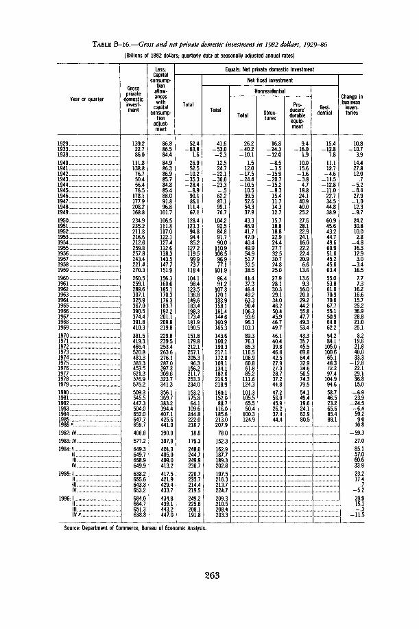
TABLE B-16.—Gross and net private domestic investment in 1982 dollars, 1929-86

[Billions of 1982 dollars,- quarterly data at seasonally adjusted annual rates]

Year or quarter

19291933193919401941194219431944194519461947194819491950195119521953195419551956195719581959196019611962196319641965196619671968196919701971197219731974197519761977197819791980198119821983198419851986 p

1982: IV1983- IV1984:1

III l lIV

1985:1I II I IIV ..

1986- 1I II I IIV P

Grossprivate

domesticinvest-ment

139.222.786.0

111.8138.8

76.750.456.476.5

178.1177.9208.2168.8234.9235.2211.8216.6212.6259.8257.8243.4221.4270.3260.5259.1288.6307.1325.9367.0390.5374.4391.8410.3381.5419.3465.4520.8481.3383.3453.5521.3576.9575.2509.3545.5447.3504.0652.0647.7659.7408.8577.2649.3649.7658.9649.9638.2655.6643.8653.2684.0664.7651.3638.8

Less:

consump-tion

allow-anceswith

capitalconsump-

tionadjust-ment

86.886.584.484.986.386.985.784.885.488.091.896.8

101.7106.5111.8117.0122.1127.4132.6138.3143.5147.7151.9156.3160.6165.1170.3176.3183.7192.2201.1209.8219.8229.8239.5253.4263.6276.1287.0297.3309.6323.7341.3356.1369.7383.2394.4407.1425.6441.0390.0397.9401.3405.0409.0413.2417.5421.9429.4433.7434.8439.1443.2447.0

Equals: Net private domestic investment

Total

52.46381.6

26.952.5

-10.2353

-28.489

90.186.1

111.467.1

128.4123.394.894.485.2

127.2119.599.973.7

118.4104.198.4

123.5136.8149.6183.4198.3173.4181.9190.5151.8179.8212.1257.1205.396.3

156.2211.7253.3234.0153.2175.864.1

109.6244.8222.0218.7

18.8179.3248.0244.7249.9236.7220.7233.7214.4219.5249.2225.6208.1191.8

Net fixed investment

Total

41.6-53.0-2.312.524.7

-22.1-36.0-23.3

B2.287.199.176.7

104.292.584.891.790.0

110.9106.596.977.1

101.996.491.2

107.3120.1133.9158.1161.4144.6160.9165.3143.6160.2190.3217.1172.0109.1134.1182.6216.5218.9160.1152.088.7

116.0185.6213.0207.9

78.0152.3162.9187.7189.3202.8197.5216.3213.7224.7209.3210.5208.4203.3

Nonresidential

Total

26.2402

-10.11.5

12.0-17.5-24.4-10.5

10.539.552.654.337.943.346.941.747.040.449.954.951.731.538.541.437.346.449.263.390.4

106.393.696.1

103.189.376.185.3

116.5106.960.861.885.2

111.6124.3101.3105.565.550.4

100.3124.9

Struc-tures

16.8243

-12.0-8.5-3.5

-15.9207

-15.283

15.411.714.312.715.718.818.822.924.427.732.530.724.825.027.928.130.329.134.046.250.445.946.749.746.140.439.846.842.527.927.328.737.244.847.256.045.926.237.444.4

Pro-ducers'durableequip-ment

9.4-16.0

1.910.015.6

-1.6384.7

18.824.140.940.025.227.628.122.924.116.022.222.420.96.6

13.613.69.3

16.020.129.244.255.847.749.353.443.335.745.569.864.432.934.656.574.379.554.149.419.624.162.980.5

Resi-dential

15.41287.8

11.112.7

-4.6115

-12.811022.734.544.838.960.945.643.244.749.660.951.645.245.663.455.053.861.070.970.667.755.150.964.862.254.284.1

105.0100.665.148.372.297.4

104.994.658.746.523.265.685.488.1

Change inbusiness

inven-tories

10.8-10.7

3.914.427.812.0

.7-5.2

8427.910

12.3-9.724.230.810.02.848

16.312.93.0

-3.416.57.77.3

16.216.615.725.236.928.821.025.1

8.219.621.840.033.3

-12.822.129.136.815.0

-6.923.9

-24.5-6.459.29.0

10.8-59.3

27.085.157.060.633.923.217.4

.7-5.239.915.1-.3115

Source: Department of Commerce, Bureau of Economic Analysis.

263

TABLE B-17.—Inventories and final sales of business, 1946-86

[Billions of dollars, except as noted; seasonally adjusted]

Quarter

Fourth quarter:1946194719481949

1950195119521953195419551956195719581959 .

1960196119621963196419651966196719681969

19701971197219731974197519761977 .19781979

198019811982 . .1983198419851986 p

1982: IV

1983- IV

1984: I . . . .I II I IIV

1985- 1 .I II l lIV

1986: 1||I I IIV P

Inventories *

Total2

71.080.385.677.5

96.7109.4108.6109.6107.3114.6123.4127.0126.2131.7

135.5137.2143.8149.6155.3169.1185.2197.4211.8232.4

240.3257.8285.6352.6423.3428.8463.3505.7588.2674.8

739.3789.0771.5787.2854.5862.6856.3

771.5

787.2

818.4832.8846.9854.5

859.0859.2856.4862.6

855.8857.0856.6856.3

Farm

19.621.019.316.7

22.524.923.322.021.219.919.921.222.622.1

23.323.825.225.724.528.027.427.929.131.8

31.135.444.365.562.464.360.259.373.780.7

84.581.679.279.481.274.071.0

79.2

79.4

86.185.883.481.2

81.179.076.874.0

71.573.874.871.0

Nonfarm

Total2

51.459.366.360.8

74.284.585.387.686.194.7

103.5105.8103.7109.6

112.2113.4118.6123.8130.9141.0157.8169.5182.6200.6

209.2222.4241.3287.1360.9364.5403.1446.4514.5594.1

654.8707.4692.2707.8773.3788.5785.3

692.2

707.8

732.3747.0763.6773.3

777.8780.2779.7788.5

784.3783.2781.8785.3

Manu-facturing

24.629.032.228.6

34.943.144.046.043.948.354.054.352.755.2

56.257.260.362.265.970.780.987.594.0

103.4

105.8107.3113.6136.1177.0177.8194.9210.6238.4281.1

310.7330.2316.1315.9342.5338.9328.1

316.1

315.9

325.2333.6341.2342.5

342.5341.5340.0338.9

330.5328.5327.2328.1

Whole-sale

trade

10.411.112.512.5

14.715.615.615.816.117.618.919.219.321.0

21.321.822.423.925.226.930.332.734.637.9

41.745.250.059.475.676.286.196.2

113.8133.7

154.8164.7162.2163.8178.0181.9184.0

162.2

163.8

168.4171.5176.0178.0

179.2180.4179.8181.9

179.9180.9182.5184.0

Retailtrade

12.814.516.615.4

19.219.719.420.020.222.823.725.025.126.2

27.527.028.329.631.033.736.236.940.744.5

45.852.357.766.474.674.782.793.3

107.8117.0

122.7134.0134.7148.2166.6176.7183.1

134.7

148.2

155.8157.8160.9166.6

168.9169.3170.5176.7

183.4183.0181.2183.1

Other

3.24.14.53.9

4.95.55.65.25.35.46.26.66.67.2

7.27.47.58.08.89.8

10.412.413.314.9

16.017.619.925.233.735.839.446.354.562.3

66.778.579.279.986.191.090.1

79.2

79.9

82.884.185.586.1

87.289.089.491.0

90.590.990.890.1

Finalsales3

15.818.419.819.7

21.824.926.427.528.030.231.933.334.336.2

37.539.541.844.547.152.155.358.864.868.8

72.478.987.796.8

104.6117.1128.5143.9165.1183.2

201.1217.8229.5247.0268.9289.3302.5

229.5

247.0

251.3259.9263.4268.9

274.3278.9285.1289.3

289.7294.3300.4302.5

Inventory-finalsales ratio

Total

4.484.364.333.94

4.444.404.113.983.843.803.873.823.683.64

3.613.473.443.363.303.243.353.363.273.38

3.323.273.263.644.053.663.603.513.563.68

3.683.623.363.193.182.982.83

3.36

3.19

3.263.203.223.18

3.133.083.002.98

2.952.912.852.83

Non-fa rm 4

3.243.223.353.09

3.413.403.233.183.083.143.243.183.023.03

2.992.872.842.782.782.702.852.882.822.91

2.892.822.752.973.453.113.143.103.123.24

3.263.253.022.872.882.732.60

3.02

2.87

2.912.872.902.88

2.842.802.732.73

2.712.662.602.60

1 End of quarter.2 Beginning 1959, inventories of construction establishments are included in "other" nonfarm inventories. Prior to 1959, they are

included in total and total nonfarm inventories, but not in the detailed categories shown.3 Quarterly totals at monthly rates. Business final sales equals final sales less gross product of households and institutions,

government, and rest of the world, and includes a small amount of final sales by farms.4 Ratio based on total business final sales, which includes a small amount of final sales by farms.Note.—The industry classification of inventories is on an establishment basis and is based on the 1972 Standard Industrial

Classification (SIC) beginning 1948 and on the 1942 SIC prior to 1948.Source: Department of Commerce, Bureau of Economic Analysis.

264

TABLE B-18.—Inventories and final sales of business in 1982 dollars, 1947-86

[Billions of 1982 dollars, except as noted; seasonally adjusted]

Quarter

Fourth quarter:194719481949

1950195119521953195419551956. .19571958.1959

1960196119621963196419651966196719681969

1970197119721973. .197419751976197719781979

198019811982 . .1983198419851986 p .

1982- IV ..

1983: IV

1984- 1III l lIV ..

1985: 1III l lIV

1986: 1II ...Il lIV P

Inventories *

Total2

251.3263.5253.9

278.1308.9318.9321.6316.9333.2346.1349.1345.7362.2

370.0377.2393.4410.1425.8451.0487.9516.6537.7562.8

571.1590.7612.4652.5685.7673.0695.1724.2761.0776.0

769.1793.0768.4762.0821.2830.2841.0

768.4

762.0

783.3797.6812.7821.2

827.0831.4831.5830.2

840.2844.0843.9841.0

Farm

43.345.444.4

47.751.554.654.355.956.053.754.957.358.1

59.460.863.565.864.066.366.167.768.269.0

69.873.475.981.481.382.679.177.277.882.4

77.882.681.274.979.877.877.7

81.2

74.9

79.079.479.879.8

81.483.383.277.8

78.679.681.777.7

Nonfarm

Total2

208.0218.1209.5

230.4257.4264.3267.4260.9277.1292.4294.2288.4304.2

310.5316.5329.9344.2361.8384.7421.7449.0469.4493.8

501.2517.3536.6571.0604.5590.3616.1647.0683.2693.6

691.4710.3687.2687.2741.4752.4763.3

687.2

687.2

704.3718.1733.0741.4

745.6748.0748.4752.4

761.6764.4762.2763.3

Manu-facturing

105.1108.6102.9

109.8133.2139.0142.7135.0142.5153.2152.1146.8153.5

154.7158.8167.2172.6180.9191.6213.6229.2239.0248.5

248.3246.1251.7267.9288.5281.9294.0301.9314.1324.7

326.8330.3315.2309.3329.9325.2322.3

315.2

309.3

315.5323.0329.5329.9

330.2329.3327.8325.2

323.9324.1322.5322.3

Whole-sale

trade

39.942.742.8

47.649.050.050.451.154.856.656.056.060.7

61.863.165.068.972.676.585.190.793.598.9

105.8110.7114.0118.4128.4124.0131.2140.5151.6156.1

161.6165.0161.5157.9171.3174.7180.1

161.5

157.9

161.0164.4168.9171.3

172.2174.0173.9174.7

176.4177.7180.1180.1

Retailtrade

39.643.742.8

49.549.649.650.851.257.157.859.859.461.9

65.264.267.570.373.479.284.384.290.596.4

96.6107.2114.0122.1121.1115.9122.3130.9139.1136.7

130.4135.5132.9142.4157.6165.0168.9

132.9

142.4

148.2150.1152.7157.6

159.1159.3160.5165.0

172.1171.0167.8168.9

Other

23.523.121.1

23.425.625.823.523.622.724.826.326.328.1

28.830.330.132.434.937.438.745.046.550.0

50.553.256.962.666.468.668.573.778.476.1

72.779.577.677.582.687.591.9

77.6

77.5

79.880.781.982.6

84.185.486.287.5

89.391.591.891.9

Finalsales3

74.877.177.3

82.690.493.998.097.7

102.5104.7105.9107.7111.4

114.1118.7123.4130.4136.3147.7150.2156.4163.7165.4

166.8172.6185.4188.9184.3191.5199.3209.0221.5225.6

225.3224.6226.1235.5247.7259.2266.4

226.1

235.5

237.4243.4244.5247.7

251.0253.1257.5259.2

258.0261.0264.0266.4

Inventory-finalsales ratio

Total

3.363.423.28

3.373.423.403.283.243.253.313.303.213.25

3.243.183.193.143.123.053.253.303.283.40

3.423.423.303.453.723.513.493.473.443.44

3.413.533.403.243.323.203.16

3.40

3.24

3.303.283.323.32

3.303.283.233.20

3.263.233.203.16

Non-farm4

2.782.832.71

2.792.852.812.732.672.702.792.782.682.73

2.722.672.672.642.652.602.812.872.872.98

3.003.002.893.023.283.083.093.103.083.08

3.073.163.042.922.992.902.87

3.04

2.92

2.972.953.002.99

2.972.962.912.90

2.952.932.892.87

1 End of quarter.2 Beginning 1959, inventories of construction establishments are included in "other" nonfarm inventories. Prior to 1959, they areincluded in total and total nonfarm inventories, but not in the detailed categories shown.3 Quarterly totals at monthly rates. Business final sales equals final sales less gross product of households and institutions,government, and rest of world, and includes a small amount of final sales by farms.4 Ratio based on total business final sales, which includes a small amount of final sales by farms.

Note.—The industry classification of inventories is on an establishment basis and is based on the 1972 Standard IndustrialClassification (SIC) beginning 1948 and on the 1942 SIC prior to 1948.

Source: Department of Commerce, Bureau of Economic Analysis.

265

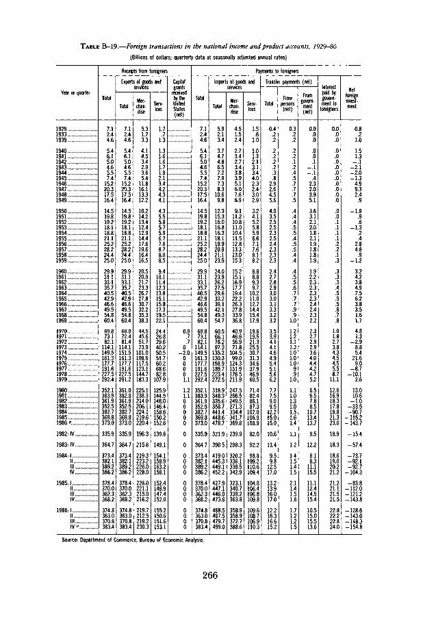
TABLE B-19.—Foreign transactions in the national income and product accounts, 1929-86

[Billions of dollars; quarterly data at seasonally adjusted annual rates]

Year or quarter

192919331939

1940194119421943194419451946194719481949

195019511952195319541955195619571958. ..1959

I9601961196219631964196519661967 ,19681969

1970197119721973197419751976197719781979

1980198119821983198419851986 p.

1982- IV

1983- IV

1984: 1III I IIV

1985:1||I I IIV. . . .

1986-1||III .IV

Receipts from foreigners

Total

7.12.44.6

5.46.15.04.65.574

15.220.317.516.4

14.519.819.218.118.821.125.228.224.425.0

29.931.133.135.740.542.946.649.554.860.4

69.873.182.1

114.1149.5161.3177.7191.6227.5292.4

352.1383.9361.9352.5382.7369.8373.0

335.9

364.7

373.4382.1389.2386.2

378.4370.0362.3368.2

374.8363.0370.8383.4

Exports of goods andservices

Total

7.12.44.6

5.46.15.04.65.574

15.220.317.516.4

14.519.819.218.118.821.125.228.224.425.0

29.931.133.135.740.542.946.649.554.860.4

68.972.481.4

114.1151.5161.3177.7191.6227.5291.2

351.0382.8361.9352.5382.7369.8373.0

335.9

364.7

373.4382.1389.2386.2

378.4370.0362.3368.2

374.8363.0370.8383.4

Mer-chan-dise

5.31.73.3

4.14.53.42.93.654

11.816.113.312.2

10.214.213.412.412.914.417.619.616.416.5

20.520.921.723.326.727.830.732.235.338.3

44.545.651.773.9

101.0109.6117.5123.1144.7183.3

225.1238.3214.0206.1224.1219.6220.4

196.3

215.6

219.3223.2226.0228.0

226.0221.1215.0216.2

219.7212.5219.2230.3

Serv-ices

1.7.7

1.3

1.31.61.61.71.9213.44.24.34.1

4.35.55.85.75.96.77.68.78.08.5

9.410.111.412.313.815.115.817.319.522.1

24.426.829.640.250.551.760.268.682.8

107.9

125.9144.5148.0146.4158.6150.2152.6

139.6

149.1

154.1158.9163.2158.1

152.4148.9147.4152.0

155.2150.6151.6153.1

Capitalgrants

receivedby theUnitedStates(net)

0.9.7.7

0-2.0

00001.1

1.21.100000

0

0

0000

0000

0000

Payments to foreigners

Total

7.12.44.6

5.46.15.04.65.57.4

15.220.317.516.4

14.519.819.218.118.821.125.228.224.425.0

29.931.133.135.740.542.946.649.554.860.4

69.873.182.1

114.1149.5161.3177.7191.6227.5292.4

352.1383.9361.9352.5382.7369.8373.0

335.9

364.7

373.4382.1389.2386.2

378.4370.0362.3368.2

374.8363.0370.8383.4

Imports of goods andservices

Total

5.92.13.4

3.74.74.86.57.27.97.38.3

10.69.8

12.315.316.016.816.318.119.920.921.123.5

24.023.926.227.529.633.239.142.149.354.7

60.566.178.297.3

135.2130.3158.9189.7223.4272.5

318.9348.9335.6358.7441.4448.6478.7

321.9

390.5

419.0445.3449.1452.2

427.9447.1446.0473.6

468.5467.5479.7499.0

Mer-chan-dise

4.51.52.4

2.73.42.73.43.83.95.16.07.66.9

9.111.210.811.010.411.512.813.313.015.3

15.215.116.917.719.422.226.327.833.936.8

40.946.656.971.8

104.599.0

124.3151.9176.5211.9

247.5266.5249.5271.3334.4341.7369.8

239.9

298.3

320.2336.1338.5342.9

323.1340.7339.2363.8

358.9358.9372.7388.6

Serv-ices

1.5.6

1.0

1.01.32.13.13.44.02.32.43.02.9

3.24.15.25.85.96.67.17.68.18.2

8.88.89.39.7

10.211.012.714.415.417.9

19.619.521.325.530.731.334.637.946.960.5

71.482.486.187.3

107.0106.9108.9

82.0

92.2

98.8109.2110.6109.4

104.8106.4106.8109.8

109.6108.7106.9110.3

Transfer payments (net)

Total

0.4.2.2

.2

.2

.2

.2

.3

.82.92.64.55.6

4.03.52.52.52.32.52.42.32.32.3

2.42.72.82.93.03.03.13.33.23.2

3.53.94.14.14.64.95.45.15.66.2

7.77.59.09.5

12.215.015.0

10.6

13.4

9.59.8

12.517.0

13.213.916.017.0

12.216.316.615.2

Frompersons

(net)

0.3.2.2

.2

.2

.1

.2

.4

.5

.7

.7

.7

.5

.4

.4

.4

.5

!4.5.5.4.4

.4

.5

.5

.6

'.7.7.9.9

1.0

1.21.21.11.31.01.01.0.9.9

1.0

1.11.01.31.01.51.61.4

1.1

1.2

1.41.51.41.5

2.11.41.51.6

1.71.21.21.5

Fromgovern-

ment(net)

0.0.0.0

.0

.0

.11

-.1.4

2.32.03.95.1

3.63.12.12.01.82.11.91.81.81.9

1.92.22.32.32.32.32.42.42.32.2

2.32.72.92.93.64.04.44.24.75.2

6.56.57.88.5

10.713.413.7

9.5

12.2

8.18.3

11.115.5

11.112.414.515.4

10.515.015.513.6

Interestpaid bygovern-ment to

foreigners

0.0.0.0

.0

.0

.0

.0

.0

.0

.0

.0

.0

.0

.0

.0

!i.1.1\2.1.3

.3

.3

A.5.5.5.6.7.8

1.01.82.73.84.34.54.55.58.7

11.1

12.616.918.317.819.821.323.0

18.9

18.3

18.619.020.221.2

21.221.121.521.5

22.822.222.824.0

Netforeigninvest-ment

0.8.2

1.0

1.51.3

21-2.0-1.3

4.99.32.4

.9

-1.8.9.6

-1.3.2.4

2.84.8

.9-1.2

3.24.23.84.97.56.23.83.51.61.7

4.81.3

-2.98.85.4

21.69.087

-10.12.6

13.010.6

-1.0-33.5-90.7

-115.2-143.7

-15.4

574

-73.7-92.1

927-104.3

-83.811? 0

-121.2-143.8

-128.6-143.0-148.3-154.8

Source: Department of Commerce, Bureau of Economic Analysis.

266

TABLE B-20.—Exports and imports of goods and services in 1982 dollars, 1929-86

[Billions of 1982 dollars,- quarterly data at seasonally adjusted annual rates]

Year orquarter

192919331939

1940194119421943194419451946194719481949

1950195119521953195419551956195719581959

1960196119621963196419651966196719681969

1970197119721973197419751976197719781979

198019811982198319841985..........1986 P.

1982: IV

1983: IV

1984:1III l lIV

1985:1I II l lIV

1986:1III l lIV P..

Exports of goods and services

Total

42.122.736.2

40.042.029.125.127.335.269.082.366.265.0

59.272.070.166.970.076.987.994.982.483.7

98.4100.7106.9114.7128.8132.0138.4143.6155.7165.0

178.3179.2195.2242.3269.1259.7274.4281.6312.6356.8

388.9392.7361.9348.1369.7362.3371.3

336.0

355.5

361.3367.0375.5375.0

369.4361.2355.8362.9

369.2359.8371.2385.3

Merchandise

Total

29.715.926.5

30.531.719.515.216.424.054.165.549.148.4

42.251.149.046.448.853.261.866.656.656.1

68.869.172.277.687.788.294.096.5

104.9110.0

120.6119.3131.3160.6175.8171.5177.5178.1196.2218.2

241.8238.5214.0207.6222.7227.4237.5

199.1

214.4

216.9219.1224.9230.1

230.8227.0223.9227.8

232.0227.2238.8252.2

Dura-ble

goods

12.34.5

13.3

18.920.213.410.511.012.623.134.424.524.1

21.023.825.325.826.930.334.437.231.030.5

37.938.039.842.148.250.053.658.864.869.5

74.372.980.099.3

113.9112.1112.9111.2121.9136.6

150.0143.8121.9117.5127.3133.5146,9

110.8

123.7

124.0125.0128.3132.1

132.6134.3133.6133.4

142.1142.7148.0154.7

Non-dur-able

goods

17.511.413.1

11.611.66.14.85.4

11.331.031.124.624.2

21.327.323.720.621.922.927.429.425.625.6

30.931.132.435.539.538.240.437.740.140.5

46.346.451.361.362.059.564.766.974.381.6

91.994.692.190.195.493.990.7

88.3

90.7

92.994.196.698.1

98.292.790.394.4

89.984.590.897.5

Services

Total

12.36.89.8

9.410.39.69.8

10.911.214.916.917.116.7

17.020.921.220.521.223.726.128.325.827.6

29.631.634.737.141.143.844.447.150.855.0

57.659.964.081.793.388.296.8

103.6116.4138.6

147.1154.3148.0140.5147.0135.0133.8

136.9

141.1

144.4147.9150.6144.9

138.6134.2132.0135.1

137.2132.6132.4133.1

Factorin-

come x

7.63.75.2

4.65.24.84.64.94.85.67.28.58.2

9.110.911.311.011.613.014.114.813.214.0

15.716.918.520.021.823.222.823.826.329.0

29.630.533.946.253.545.649.753.563.286.6

91.496.391.685.092.680.976.9

83.0

88.2

90.094.096.290.1

82.681.279.180.9

82.476.374.874.0

Other

4.83.14.5

4.85.14.95.26.06.59.49.78.68.5

7.910.09.99.59.6

10.712.013.512.613.5

13.914.716.217.219.320.621.623.324.526.0

28.029.430.135.439.842.647.150.153.252.0

55.757.956.355.554.454.056.9

53.8

52.9

54.453.954.454.8

56.053.052.954.3

54.856.357.659.0

Imports of goods and services

Total

37.424.230.1

31.738.236.948.051.154.142.039.947.146.2

54.657.463.369.767.576.983.687.992.8

101.9

102.4103.3114.4116.6122.8134.7152.1160.5185.3199.9

208.3218.9244.6273.8268.4240.8285.4317.1339.4353.2

332.0343.4335.6368.1453.2470.5521.0

324.3

401.6

429.9454.2461.2467.7

448.2469.3469.6494.8

495.1513.6534.5540.8

Merchandise

Total

29.319.224.0

25.629.421.025.026.526.030.029.333.933.3

40.940.441.944.642.148.353.656.158.168.0

67.569.078.981.286.397.0

109.1113.0135.7144.6

150.9166.2190.7218.2211.8187.9229.3259.4274.1277.9

253.6258.7249.5282.2350.0368.7420.4

242.7

311.6

334.0348.7354.8362.5

347.5367.7368.4391.3

392.6412.8436.0440.0

Dura-ble

goods

7.44.06.9

8.811.06.76.56.76.97.87.89.48.9

11.511.513.013.711.914.716.817.116.922.8

21.721.124.826.229.035.644.048.061.765.6

66.874.484.488.989.272.488.599.3

113.7115.7

116.1126.1125.3149.2199.3216.6246.8

117.1

171.3

186.7197.3204.5208.6

209.2213.8216.9226.7

237.4244.8249.5255.4

Non-dur-able

goods

22.015.217.0

16.818.414.318.519.719.122.221.524.524.4

29.528.928.930.930.333.536.839.041.345.3

45.847.954.055.057.461.465.265.074.079.0

84.191.8

106.4129.4122.5115.5140.8160.1160.4162.2

137.5132.6124.2133.0150.7152.1173.6

125.6

140.3

147.3151.4150.3153.9

138.3153.9151.4164.6

155.2168.0186.4184.6

Services

Total

8.04.96.1

6.28.8

15.823.024.628.212.010.613.113.0

13.617.121.425.125.428.630.031.834.633.8

34.934.335.535.436.537.743.047.549.655.2

57.452.753.955.656.652.956.157.765.375.3

78.484.786.185.8

103.3101.8100.7

81.6

90.1

95.8105.5106.4105.3

100.7101.7101.3103.6

102.5100.898.5

100.8

Factorin-

come *

2.61.32.2

2.01.91.71.92.12.51.92.12.32.6

2.83.12.93.13.33.63.43.43.74.0

4.64.84.65.15.66.27.07.58.6

12.0

12.59.8

10.213.917.716.316.716.121.130.8

35.941.140.537.148.744.044.2

35.1

39.7

44.351.351.647.3

44.144.144.043.7

44.345.542.244.7

Other

5.43.64.0

4.16.9

14.221.222.525.710.18.5

10.810.4

10.814.018.421.922.125.026.628.430.929.8

30.329.630.930.330.931.636.040.041.043.2

45.042.943.741.738.936.639.341.644.244.5

42.443.645.748.754.657.856.5

46.5

50.3

51.554.254.858.0

56.657.557.259.8

58.255.356.456.1

1 Factor income exports less factor income imports equals rest-oMhe-world product.Source: Department of Commerce, Bureau of Economic Analysis.

267

TABLE B-21.—Relation of gross national product, net national product, and national income, 1929-86

[Billions of dollars; quarterly data at seasonally adjusted annual rates]

Year or quarter

192919331939

19401941. .19421943194419451946194719481949

1950195119521953.19541955 . .1956195719581959

1960196119621963196419651966.196719681969

19701971 . . .197219731974.19751976197719781979

1980198119821983198419851986 "

1982: IV

1983: IV

1984-1 .IIIllIV

1985: 1||II IIV

1986- 1III I I . . . .

Grossnationalproduct

103956091.3

100.41255159.01927211421342124235226162604

288*3333435163716372.54059428.2451045684958

5153533857466069649870517720816489279639

101551 10271212813593147281598417828199052249725082

27320305263166034057376503998142085

32125

35458

36709374383799738456

39093396504,030.540877

4 14924,175.64240742684

Less:

consump-tion

allowanceswith

capitalconsump-

tionadjustment

99769.0

9.410311.3116120124142176204220

23627229230932.534438.141 142.8446

46447849451453957462 1674739814

888975

10791181137516181792201522992658

3038347838323966415143724551

3932

4008

4055413041854233

42784331441.34467

447 1453.345764625

Equals:Net

nationalproduct

94048482.3

91.1115.3147.7181 1199420101982217624122384

2646306.232253407340.03715390.14099414.04512

4689486.152525555595964777099749081878825

9266100511 104812412133541436616036178902019822424

2428127048278283009 1334993560937534

28193

31450

326543,330 73381234223

34815353193,589.336410

370213,722.33783138060

Indirectbusinesstax andnontaxliability

71719.4

10.111311.812814.2155171184201213

23425.327729729.632235.037438.6417

45348.0515546587625652701787863

9401034111 1120812901400151.71657178 11894

2133251 525882826312033143487

2645

2941

3029310.33153319.6

323.33319332.73377

3467340.835423531

Less:

Busi-ness

transferpay-

ments

067.5

.45.55555678

89

10121.1121.4151618

20202 124272830313439

414449555874798693

103

121124143160183209232

152

165

17217.9187194

20.020621.2217

22322.9235241

Statis-tical

discrep-ancy

15121.7

1.47

-.7172.740

718

-138

82 718262.718

-1.912

_.l15

28-1.2o-.614

-122 1

_ 41 1

-3.9

-1 11816

-4.3-17

253.6

01910

4941

_ 1

-195554

68

2 5

50-3.2

6-8.6

-6.4110

-5.516

-364.6

103

Plus:

lesscurrentsurplus

ofgovern-

mententer-prises

020.4

.41

j.6792

_ 13

1_ 1

3_ 5— 3

0.77

1.11

41.7181.1171.62516141.9

2926373.512241.03.03935

57678.7

14110.582

113

15.4

196

2304.545

10.0

12.51022.674

4122.4

1.0178

Equals:Nationalincome

84739471.2

79.61028136.21697182.61816180.71966221.52152

2398277.329163066306.33363356.33728375.04092

4249439.04733500.35376585.26420677.77391798.1

832.689819941

1,122.71 203.5128911,441.41,617.81,838.220473

2,203.5244352,518.4271953,032.0322233,387.4

2,548.2

2,851,5

2 963.23,010.3305233,102.0

3,157.03 201.43,243.43 287.3

3 340.73,376.43,396.1

Source: Department of Commerce, Bureau of Economic Analysis.

268

TABLE B-22.—Relation of national income and personal income, 1929-86

[Billions of dollars; quarterly data at seasonally adjusted annual rates]

Year or quarter

19291933193919401941194219431944194519461947194819491950195119521953195419551956195719581959196019611962196319641965196619671968196919701971197219731974197519761977197819791980198119821983198419851986"1982: IV.1983: I V .1984 1

I I .I l lI V .

1985 1I I .I I I .IV .

1986 1I II I IIV P

Nationalincome

84.739471.279.6

102.8136.2169.7182.6181.6180.7196.6221.5215.2239.8277.3291.6306.6306.3336.3356.3372.8375.0409.2424.9439.0473.3500.3537.6585.2642.0677.7739.1798.1832.6898.1994.1

1,122.71,203.51,289.11,441.41,617.81,838.22,047.32,203.52,443.52,518.42,719.53,032.03,222.33,387.42,548.22,851.52,963.23,010.33,052.33,102.03,157.03,201.43,243.43,287.33,340.73,376.43,396.1

Corporateprofits

withinventoryvaluation

andcapital

consump-tion

adjust-ments

9.6155.58.8

14.319.724.024.219.717.222.930.328.034.939.937.537.736.647.145.745.340.351.449.550.358.363.670.781.386.684.190.787.474.787.1

100.7113.3101.7117.6145.2174.8197.2200.1177.2188.0150.0213.7264.7280.7299.7146.1248.5262.5271.7259.8265.0266.4274.3296.3285.6296.4293.1302.0

Le

Netinterest

4.7413.63.33.33.12.72.32.21.82.32.42.63.03.53.94.45.25.86.57.89.5

10.211.312.914.616.318.220.924.327.429.834.641.246.351.059.675.583.888.8

105.3126.3158.3200.9248.1272.3281.0307.4311.4294.9266.9290.2292.5305.2316.1315.7316.8311.4309.7307.6304.9297.7292.92841

SS:

Contribu-tions for

socialinsurance

0.3.3

2.22.42.83.54.65.26.37.76.76.06.67.48.89.39.6

10.612.013.515.515.918.821.922.925.428.530.131.640.645.550.457.962.268.979.097.6

110.5118.5134.5149.8171.7197.8216.5251.2269.6291.0326.7355.7376.1273.0299.2318.8323.9329.0334.9350.0353.9356.8362.1371.5373.5376.63826

Wageaccruals

lessdisburse-

ments

0.0.0.0.0.0.0.2

-.2.0.0.0.0.0.0.1.0_ i'.0.0.0.0.0.0.0.0.0.0.0.0.0.0.0.0.0.6.0

_ 1

-'.5.1.1.1.3

-.2.0.1.0

-.4.2

-.2.0.0.0.2.2.0.6.1

-1.0.0.0.0.0.0.0

Govern-ment

transferpayments

topersons

0.91.52.52.72.62.72.53.15.6

10.811.210.611.714.411.612.213.115.316.417.520.324.725.727.531.532.634.536.039.143.652.360.667.581.897.0

108.4124.1147.4185.7202.8217.5234.8262.8312.6355.7396.2426.6437.3466.2490.5420.2429.0433.4436.7437.7441.6459.4463.5469.9471.8482.4487.2495.04976

Plu

Personalinterestincome

6.95.55.35.35.35.25.15.25.86.67.58.08.79.6

10.411.212.413.714.916.618.720.322.324.926.328.932.235.539.644.248.253.260.969.374.780.893.3

111.9122.5134.1155.4182.5221.5271.9335.4369.7393.1446.9476.2475.4366.2411.6421.4438.9460.6466.8473.8475.3475.2480.6480.8480.1473.8466.7

S:

Personaldividendincome

5.82.03.84.04.44.34.44.64.65.66.37.07.28.88.58.58.89.1

10.311.111.511.312.212.913.314.415.517.319.119.420.221.922.422.222.624.126.628.928.733.838.243.048.152.961.363.968.774.776.481.265.471.072.974.775.275.976.376.476.376.779.181.182.0827

Businesstransfer

payments

0.6.7.5.4.5.5.5.5.5.5.6.7.8.8.9

1.01.21.11.21.41.51.61.82.02.02.12.42.72.83.03.13.43.94.14.44.95.55.87.47.98.69.3

10.312.112.414.316.018.320.923.215.216.517.217.918.719.420.020.621.221.722.322.923.524.1

Equals:

Personalincome

84.346.372.177.695.2

122.4150.7164.5170.0177.6190.2209.2206.4228.1256.5273.8290.5293.0314.2337.2356.3367.1390.7409.4426.0453.2476.3510.2552.0600.8644.5707.2772.9831.8894.0981.6

1,101.71,210.11,313.41,451.41,607.51,812.42,034.02.258.52,520.92,670.82,838.6

! 3,110.23,314.53,487.02,729.22,941.83,034.2

; 3,077.4! 3,139.7

3,189.63,253.13,298.73,323.2

| 3,382.93,432.63,483.33,498.83,533.4

Source: Department of Commerce, Bureau of Economic Analysis.

269

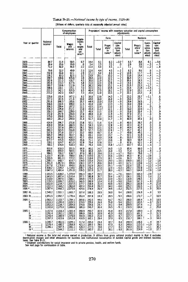
TABLE B-23.—National income by type of income, 1929-86

[Billions of dollars; quarterly data at seasonally adjusted annual rates]

Year or quarter

1929 .193319391940194119421943194419451946194719481949195019511952 .1953195419551956195719581959I96019611962196319641965196619671968196919701971.197219731974197519761977197819791980198119821983.19841985 .1986 P1982- IV1983- IV1984: I

I II l lIV

1985:1I II l lIV

1986- 1I II l lIV

Nationalincome l

84.739.471.279.6

102.8136.2169.7182.6181.6180.7196.6221.5215.2239.8277.3291.6306.6306.3336.3356.3372.8375.0409.2424.9439.0473.3500.3537.6585.2642.0677.7739.1798.1832.6898.1994.1

1,122.71,203.51,289.11,441.41,617.81,838.22,047.32,203.52,443.52,518.42,719.53,032.03,222.33,387.42,548.22,851.52.963.23,010.33,052.33,102.03,157.03,201.43,243.43,287.33,340.73,376.43,396.1

Compensationof employees

Total

51.129.648.252.264.885.3

109.6121.3123.3119.6130.1142.1142.0155.4181.6196.3210.4209.4225.9244.7257.8259.8281.2296.7305.6327.4345.5371.0399.8443.0475.5524.7578.4618.3659.4726.2812.8891.3948.7

1,057.91,176.61,329.21,491.41,638.21,807.41,907.02,020.72,214.72,368.22,498.31,931.12,092.72,153.72,195.42,234.72,275.02,316.32,352.12,380.92,423.62,461.52,480.22,507.42,544.2

Wagesand ,

salaries

50.529.046.049.962.182.1

105.8116.7117.5112.0123.1135.5134.7147.2171.6185.6199.0197.2212.1229.0239.9241.3259.8272.8280.5299.3314.8337.7363.7400.3428.9471.9518.3551.5584.5638.7708.6772.2814.7899.6994.0

1,119.61,251.91,372.01,510.41,586.11,676.21,837.01,965.82,073.81,603.71,739.41,784.11,820.51,854.81,888.61,922.41,952.21,976.02,012.82,044.12,058.82,081.12,111.1

Supple-ments

towages

andsal-

aries2

0.7.6

2.22.32.83.23.84.55.87.67.06.57.38.2

10.010.711.512.113.815.717.818.521.423.825.128.130.733.236.142.746.652.860.166.874.987.6

104.2119.1134.0158.3182.6209.7239.5266.3297.1320.9344.5377.7402.4424.5327.4353.4369.6374.9379.8386.3393.9399.8404.9410.9417.4421.3426.3433.1

Proprietors' income with inventory valuation and capital consumptionadjustments

Total

14.45.4

11.412.617.123.928.830.031.536.335.540.435.938.844.044.443.443.545.446.948.851.551.752.154.356.657.760.565.169.671.175.479.380.286.898.3

119.0118.8125.4137.7152.9176.2191.9180.7186.8175.5190.9236.9254.4278.9188.3207.8242.5229.6234.6240.7250.7255.5249.3262.1265.3289.1277.5283.7

Farm

Total

6.12.54.44.46.4

10.112.011.912.414.815.117.512.813.616.015.013.012.411.311.111.013.110.811.612.012.111.910.713.014.012.712.814.614.715.519.433.727.525.420.620.527.031.720.530.724.612.431.529.226.428.519.344.526.424.730.432.933.021.629.424.439.519.622.2

Propri-etors'

in-come3

6.32.54.54.56.5

10.312.212.212.615.215.618.213.514.316.815.913.913.212.112.011.914.011.712.412.812.912.611.413.714.813.613.715.816.016.821.135.630.129.024.625.132.438.028.139.433.921.840.838.034.638.028.553.735.834.139.541.841.930.337.932.747.927.730.1

Capitalcon-

sump-tion

adjust-ment

02.0

-.1

_~2-'.2-.2-.3-.3

4-.5

7-.7-.7

8-.9-.9

8-.8

9-.9-.9— .9-.8-.8-.8-.7

7-.7

8-.8_ 9

-U-1.3-1.3-1.7-1.9-2.6-3.6

40-4^6-5.3

63-7.6-8.7-9.3-9.4-9.3-8.8-8.2-9.4-9.3

9 2-9.4

94-9.1-8.9-8.8-8.7

8584

-8.382

-8.0

Nonfarm

Total

8.32.97.18.2

10.813.816.818.119.121.520.422.923.125.228.029.430.431.134.035.837.838.540.940.542.344.445.749.852.155.558.462.664.765.471.479.085.391.3

100.0117.1132.4149.2160.1160.1156.1150.9178.4205.3225.2252.5159.8188.6198.0203.2209.9210.3217.8222.5227.7232.7240.9249.6258.0261.6

Propri-etors'

in-come4

8.83.97.68.6

11.714.417.118.319.323.321.823.122.225.727.728.529.830.433.535.437.237.740.139.741.743.845.149.151.855.558.463.165.166.072.379.687.295.3

102.2119.6135.1152.8164.0164.3155.2148.5167.3183.9193.5217.5156.9172.7180.4183.5187.4184.4189.0191.2194.4199.1206.6215.5222.8224.9

Inven-tory

valua-tion

adjust-ment

0.1_ 5-2

.0-.6-.4_ 2-!i-.1

-1.7-1.5

4.5

-1.13.2

-.2.0

-.2_ 5-.3-.1

.0

.0

.0

.0

.0-.1

-.2-.2-.4-.5_ 5-'.B

-2.0-3.8

12-1.3-1.3-2.3-2.9-2.9-1.4-.5-.8-.4_ 2-19

6_ 7

-.9-.6-.2

.1_ 3-.3

-'.3-A

-1.0-1.1-1.0

Capitalcon-

sump-tion

adjust-ment

-0.6-.5-.4-.3

-'.3-.2-.1-.1-.1

.1

.2

.5

.6

.6

.7

.7

.8

.7

.9

.9

.9

.9

.8

.6

.6

.7

.7

.4

.3

-.'l.1.0

-.3.1.1

10-1.3-1.4-1.4-1.0-1.2

2.32.9

12.021.831.935.93.5

16.518.520.322.825.829.031.533.234.034.735.136.237.7

1 National income is the total net income earned in production. It differs from gross national product mainly in that it excludesdepreciation charges and other allowances for business and institutional consumption of durable capital goods and indirect businesstaxes. See Table B-21.2 Employer contributions for social insurance and to private pension, health, and welfare funds.

See next page for continuation of table.

270

TABLE B-23.—National income by type of income, 1929-86—Continued

[Billions of dollars; quarterly data at seasonally adjusted annual rates]

Year or quarter

19291933193919401941194219431944194519461947194819491950195119521953195419551956195719581959I96019611962196319641965196619671968196919701971 . ...197219731974197519761977197819791980198119821983198419851986 *1982- IV1983: IV1984:1

HIIIIV

1985- 1III l lIV

1986:1I II l lIV '

Rental income ofwith capital cons

adjustmer

Total

4.92.02.62.73.24.14.64.85.05.85.86.46.77.78.39.4

10.711.612.012.413.113.914.615.315.816.517.117.318.118.619.618.418.418.218.617.918.016.113.511.98.29.35.66.6

13.313.613.28.37.6

15.615.812.412.18.47.15.66.88.17.38.3

12.816.316.217.0

Rentalincome

ofpersons

5.62.13.23.34.05.15.76.16.57.58.29.19.4

10.511.512.713.914.915.315.916.517.318.018.719.119.820.320.521.322.223.522.924.224.625.926.528.128.928.628.928.834.235.741.452.254.455.051.752.460.656.554.354.051.951.149.650.451.553.054.757.261.361.562.5

persons

t

Capitalcon-

sumptionadjust-ment

-0.7-.1

6-.8

9-1.1

13-1.5

17-2.4

27-2.7-2.8-3.2-3.3

333.233

-3.535

-3.43434

-3.333

-3.2-3.2-3.3-3.6-3.9-4.5-5.8-6.4

74-8.6

-10.1-12.7-15.0-17.0

206-24.9-30.1

348-38.9-40.8-41.8

434-44.8-45.1

407-41.9

41.9435

-44.0440436

-43.4457

-46.4-44.4-45.1-45.3-45.5

Corporate profits with inventory valuation and capital consumption adjustments

Total

9.6-1.5

5.58.8

14.319.724.024.219.717.222.930.328.034.939.937.537.736.647.145.745.340.351.449.550.358.363.670.781.386.684.190.787.474.787.1

100.7113.3101.7117.6145.2174.8197.2200.1177.2188.0150.0213.7264.7280.7299.7146.1248.5262.5271.7259.8265.0266.4274.3296.3285.6296.4293.1302.0

Profits with inventory valuation adjustment and withoutcapital consumption adjustment

Total

10.5-1.2

6.59.8

15.420.524.524.019.319.625.933.431.137.943.340.640.238.447.546.946.641.652.349.850.155.259.866.276.281.278.685.481.469.582.794.9

107.199.4

123.9155.3183.8208.2214.1194.0202.3159.2196.7230.2222.6242.9150.7223.4235.7241.5223.3220.3213.3215.4235.3226.4239.0238.3246.5

Profits

Profitsbefore

tax

10.01.07.2

10.017.921.725.324.219.824.831.835.629.242.944.539.641.238.749.249.648.141.952.649.949.855.159.866.777.483.380.189.187.276.087.3

101.5T7.2138.9134.8170.3200.4233.5257.2237.1226.5169.6207.6235.7223.2236.6164.1231.5249.3246.5225.1221.9213.8213.8229.2235.8222.5227.7240.4

Prnfitctax

liability

1.4.5

1.42.87.6

11.414.112.910.79.1

11.312.410.217.922.619.420.317.622.022.021.419.023.622.722.824.026.228.030.933.732.739.439.734.437.741.949.351.850.964.273.083.588.084.881.163.177.295.491.8

102.859.888.1

102.9101.689.387.887.887.195.896.495.799.0

104.4

Profits after tax

Total

8.6.4

5.77.2

10.310.311.211.39.1

15.720.523.219.025.021.920.220.921.127.227.626.722.928.927.227.131.233.538.746.549.647.549.747.541.749.659.677.987.183.9

106.0127.4150.0169.2152.3145.4106.5130.4140.3131.4133.8104.3143.4146.4144.8135.8134.1126.0126.7133.4139.4126.9128.8135.9

Divi-dends

5.82.03.84.04.44.34.44.64.65.66.37.07.28.88.58.58.89.1

10.311.111.511.312.212.913.314.415.517.319.119.420.222.022.522.522.924.427.029.729.634.639.544.750.154.763.666.971.578.381.687.868.573.976.078.179.080.180.981.481.682.585.287.588.889.7

Undis-tributedprofits

2.8-1.6

2.03.25.86.06.76.74.5

10.214.216.211.816.213.411.812.111.916.916.615.211.616.714.313.716.818.021.427.430.227.327.725.019.226.635.250.857.354.371.487.9

105.2119.197.681.839.658.962.049.846.035.869.570.466.756.854.045.145.351.857.041.741.247.2

Inven-toryvalu-ation

adjust-ment

0.5-2.1

2-2.5

12-.8

3-.653

-5.9-2.2

1.9-5.0-1.2

1.0-1.0

l'y-2.7

15-.3

3

-.2.3.0.15

-1.2-2.1-1.6-3.7-5.9-6.6

46-6.6200

-39'.5-11.0-14.9

166-25.3-43.2

43 1-24.2-10.4-10.9

55-.66.3

-13.4-8.1

-13.649

-1.8-1.6

51.66.1

-9.416.510.66.1

-8.0

Capitalcon-

sumptionadjust-ment

-0.9-.3

-1.0-1.1-1.1-.8_ 5

'.2A

-2.4-2.9-3.2-3.0-3.0-3.4-3.2-2.5-1.8-.4

-1.2-1.3-1.3-.8-.3

.23.13.84.55.25.45.55.36.15.24.35.86.22.3

-6.2-10.1-9.0109

-14.0-16.8

144-9.217.034.558.156.845

25.126.730.236.544.753.258.961.059.257.354.855.559.5

Netinterest

4.74.13.63.33.33.12.72.32.21.82.32.42.63.03.53.94.45.25.86.57.89.5

10.211.312.914.616.318.220.924.327.429.834.641.246.351.059.675.583.888.8

105.3126.3158.3200.9248.1272.3281.0307.4311.4294.9266.9290.2292.5305.2316.1315.7316.8311.4309.7307.6304.9297.7292.9284.1

3 With inventory valuation adjustment and without capital consumption adjustment.4 Without inventory valuation and capital consumption adjustments.Source-. Department of Commerce, Bureau of Economic Analysis.

271

TABLE B-24.—Sources of personal income, 1929-86

[Billions of dollars; quarterly data at seasonally adjusted annual rates]

Year or quarter

1929193319391940.,1941194219431944194519461947194819491950195119521953 !195419551956195719581959196019611962196319641965.19661967196819691970197119721973197419751976.197719781979198019811982 .1983198419851986 "1982: IV1983- IV1984- 1

IIIll .IV

1985- 1IIIllIV

1986: 1||IIIIV p ....

Personalincome

84.346.372.177.695.2

122.4150.7164.5170.0177.6190.2209.2206.4228.1256.5273.8290.5293.0314.2337.2356.3367.1390.7409.4426.0453.2476.3510.2552.0600.8644.5707.2772.9831.8894.0981.6

1,101.71,210.11,313.41,451.41,607.51,812.42,034.02,258.52,520.92,670.82,838.63,110.23,314.53,487.02,729.22,941.83,034.23,077.43,139.73,189.63,253.13,298.73,323.23,382.93,432.63,483.33,498.83,533.4

Wage and salary disbursements l

Total

50.529.046.049.962.182.1

105.6116.9117.5112.0123.1135.5134.8147.2171.5185.6199.0197.2212.1229.0239.9241.3259.8272.8280.5299.3314.8337.7363.7400.3428.9471.9518.3551.5583.9638.7708.7772.6814.6899.5993.9

1,119.31,252.11,372.01,510.31,586.11,676.61,836.81,966.12,073.81,603.61,739.41,783.91,820.31,854.91,888.11,922.31,953.31,976.02,012.82,044.12,058.82,081.12,111.1

Commodity-producingindustries

Total

21.59.8

17.419.727.539.149.050.445.946.054.261.157.864.876.482.189.885.893.3

100.8104.4100.3109.9113.4114.0122.2127.4136.0146.6161.6169.0184.1200.4203.7209.1228.2255.9276.5277.1309.7346.1392.3441.4470.7512.2511.7523.1577.8607.7623.3501.8545.4563.5572.9582.9591.9600.1605.0608.3617.7622.0620.8621.8628.7

Manu-facturing

16.17.8

13.615.621.730.940.942.938.236.542.547.144.650.359.464.271.367.673.979.582.578.786.989.889.996.8

100.7107.3115.7128.2134.3146.0157.7158.4160.5175.6196.6211.8211.6238.0266.7300.1334.8355.6386.7384.0397.4439.1460.1471.3377.4415.5427.8435.8443.0449.9455.1457.3460.7467.5470.5468.8470.0475.8

Distrib-utiveindus-tries

15.68.8

13.314.216.318.020.122.724.831.035.237.537.739.944.447.049.950.353.658.060.761.165.168.669.673.376.882.087.995.1

101.6110.8121.7131.2140.4153.3170.3186.8198.1219.5242.7274.6307.8335.5366.8384.2404.2442.2469.8488.0389.3420.8429.2439.1446.7454.0460.2467.7472.4478.9485.2484.3488.3494.2

Serviceindus-tries

8.4527.17.58.19.09.9

10.911.914.316.117.918.519.921.623.225.026.228.731.533.835.938.841.744.447.650.754.959.465.372.080.490.699.4

107.9119.7133.9148.6163.4181.6202.8232.9266.8305.6346.9384.4425.1470.6516.4566.8398.5443.2453.1465.0476.1488.1498.8511.0521.1534.6549.6561.3572.6583.8

Govern-mentand

govern-mententer-prises

5.05.28.28.5

10.216.026.633.034.920.717.519.020.822.629.233.334.434.936.638.841.044.146.049.252.456.360.064.969.978.386.496.6

105.5117.1126.5137.4148.7160.9176.0188.6202.3219.4236.1260.2284.4305.9324.3346.2372.2395.7314.0330.0338.2343.4349.2354.0363.2369.6374.2381.6387.2392.5398.4404.4

Otherlabor

income 1

0.5.4.6.6.7.9

1.11.51.82.02.42.72.93.74.65.25.96.17.08.09.09.4

10.611.211.813.014.015.717.819.921.725.228.532.536.743.049.256.565.979.394.1

107.7122.7138.4150.3163.6173.6184.5196.9208.8168.0177.8181.0183.5185.5188.2191.7195.3198.8201.7204.5207.3210.4213.0

Proprietors' incomewith inventoryvaluation and

capitalconsumptionadjustments

Farm

6.12.54.44.46.4

10.112.011.912.414.815.117.512.813.616.015.013.012.411.311.111.013.110.811.612.012.111.910.713.014.012.712.814.614.715.519.433.727.525.420.620.527.031.720.530.724.612.431.529.226.428.519.344.526.424.730.432.933.021.629.424.439.519.622.2

Nonfarm

8.32.97.18.2

10.813.816.818.119.121.520.422.923.125.228.029.430.431.134.035.837.838.540.940.542.344.445.749.852.155.558.462.664.765.471.479.085.391.3

100.0117.1132.4149.2160.1160.1156.1150.9178.4205.3225.2252.5159.8188.6198.0203.2209.9210.3217.8222.5227.7232.7240.9249.6258.0261.6

1 The total of wage and salary disbursements and other labor income differs from compensation of employees in Table B-23 in that itexcludes employer contributions for social insurance and the excess of wage accruals over wage disbursements.

See next page for continuation of table.

272

TABLE B-24.—Sources of personal income, 1929-86—Continued

[Billions of dollars; quarterly data at seasonally adjusted annual rates]

Year or quarter

19291933193919401941194219431944194519461947194819491950195119521953195419551956195719581959196019611962196319641965196619671968196919701971197219731974197519761977197819791980198119821983198419851986 * .1982: IV1983: IV1984- 1

III l lIV

1985: 1||I l lIV ...

1986:1||I I IIV

Rentalincome

ofpersons

withcapital

con-sumption

adjust-ment

4.92.02.62.73.24.14.64.85.05.85.86.46.77.78.39.4

10.711.612.012.413.113.914.615.315.816.517.117.318.118.619.618.418.418.218.617.918.016.113.511.98.29.35.66.6

13.313.613.28.37.6

15.615.812.412.18.47.15.66.88.17.38.3

12.816.316.217.0

Personaldividendincome

5.82.03.84.04.44.34.44.64.65.66.37.07.28.88.58.58.89.1

10.311.111.511.312.212.913.314.415.517.319.119.420.221.922.422.222.624.126.628.928.733.838.243.048.152.961.363.968.774.776.481.265.471.072.974.775.275.976.376.476.376.779.181.182.082.7

Personalinterestincome

6.95.55.35.35.35.25.15.25.86.67.58.08.79.6

10.411.212.413.714.916.618.720.322.324.926.328.932.235.539.644.248.253.260.969.374.780.893.3

111.9122.5134.1155.4182.5221.5271.9335.4369.7393.1446.9476.2475.4366.2411.6421.4438.9460.6466.8473.8475.3475.2480.6480.8480.1473.8466.7

Transfer payments

Total

1.52.13.03.13.13.13.03.66.2

11.311.711.312.515.212.613.314.316.317.718.921.826.327.429.533.534.736.938.741.946.655.564.071.485.9

101.5113.3129.6153.2193.1210.7226.1244.0273.1324.7368.1410.6442.6455.6487.1513.7435.4445.5450.6454.6456.4461.8479.4484.1491.1493.6504.7510.1518.5521.7

Old-age,survivors,disability,

andhealthinsur-ance

benefits

0.0.0.1.1.2.2.3.4.5.6.7

1.01.92.23.03.64.95.77.38.5

10.211.112.614.315.216.018.120.825.530.232.938.544.549.660.470.181.492.9

104.9116.2131.8154.2182.0204.5221.7235.7253.4266.7216.6227.0231.2233.7235.8241.9249.3251.1256.5256.3263.2264.1269.6270.2

Govern-ment

unem-ployment

insur-ance

benefits

0.4.5.4.4.1.1.4

1.1.8.9

1.91.5

.91.11.02.21.51.51.94.12.83.04.33.13.02.72.31.92.22.12.24.05.85.74.46.8

17.615.812.79.79.8

16.115.925.226.315.815.716.331.820.017.315.615.115.516.715.815.115.315.516.316.916.5

Veteransbenefits

06.6.5.5.5.5.5

1.03.07.07.05.95.37.74.64.34.14.24.44.44.54.74.64.65.04.74.84.74.94.95.65.96.77.78.89.7

10.411.814.514.413.813.914.415.016.116.416.616.416.716.816.616.516.416.416.516.316.816.816.716.417.017.016.716.4

Govern-ment

employ-ees

retire-ment

benefits

01

'.3.3.3.3.4.4.5.7.7.7.9

1.01.11.21.41.51.71.92.22.52.83.13.43.74.24.75.26.16.97.68.7

10.211.813.816.019.022.726.129.032.736.943.049.454.658.760.866.670.656.160.261.161.862.557.765.366.267.068.069.170.171.072.1

Aid tofamilies

withdepend-

entchildren(AFDC)

0.3".4.5.6.6.5.5.6.6.6.7.8.9

1.01.11.31.41.51.71.92.32.83.54.86.26.97.27.99.2

10.110.610.711.012.413.013.314.214.915.416.213.614.515.015.014.614.915.115.315.615.716.016.216.316.4

Other

0.81.41.71.71.81.81.82.02.02.12.52.93.33.53.63.94.24.24.54.85.25.76.26.77.17.68.39.19.8

11.213.015.317.320.724.527.631.237.547.651.555.160.969.184.091.896.5

105.1112.0119.2127.1100.6107.3109.6112.0111.9114.6116.1118.9120.3121.3124.0126.5127.9130.1

Less:Personalcontribu-tions for

socialinsurance

0.1.2.6.7.8

1.21.82.22.32.02.12.22.22.93.43.84.04.65.25.86.76.97.99.39.7

10.311.812.613.317.820.622.926.227.930.734.542.647.950.455.561.269.881.088.6

104.5112.3120.1133.5150.2160.3113.5123.6130.3132.5134.7136.7147.8149.4150.7152.9158.6159.5160.8162.5

Nonfarmpersonalincome2

159.9172.0188.3190.6211.2237.1255.4274.2277.5299.6322.8341.9350.4376.2393.9409.9436.7460.0494.9534.0581.5626.3688.7752.1810.4871.8955.0

1,059.71,172.61,276.91,417.91,572.61,769.31,983.22,215.82,465.62,618.72,799.03,052.23,261.03,437.82,672.82,895.62,962.73,024.23,088.63,133.23,194.93,241.03,277.83,330.43,385.43,421.13,456.43,488.3

2 Personal income exclusive of farm proprietors' income, farm wages, farm other labor income, and farm net interest.Note.—The industry classification of wage and salary disbursements and proprietors' income is on an establishment basis and is

based on the 1972 Standard Industrial Classification (SIC) beginning 1948 and on the 1942 SIC prior to 1948.Source: Department of Commerce, Bureau of Economic Analysis.

273

TABLE B-25.—Disposition of personal income, 1929-86

[Billions of dollars, except as noted; quarterly data at seasonally adjusted annual rates]

Year or quarter

192919331939.194019411942194319441945194619471948194919501951195219531954195519561957195819591960196119621963196419651966196719681969197019711972197319741975197619771978197919801981.19821983198419851986 p

1982- IV1983- IV1984: 1

||I I IIV

1985- 1III l lIV

1986- 1I II I IIV P

Personalincome

84.346.372.177.695.2

122.4150.7164.5170.0177.6190.2209.2206.4

228.1256.5273.8290.5293.0314.2337.2356.3367.1390.7

409.4426.0453.2476.3510.2552.0600.8644.5707.2772.9831.8894.0981.6

1,101.71,210.11,313.41,451.41,607.51,812.42,034.02,258.52,520.92,670.82,838.63,110.23,314.53,487.0

2,729.2

2,941.83,034.23,077.43,139.73,189.6

3,253.13,298.73,323.23,382.93,432.63,483.33,498.83,533.4

Less:Personaltax andnontax

payments

2.61.42.42.63.35.9

17.818.920.818.721.421.018.520.628.934.035.532.535.439.742.442.246.150.552.257.060.558.865.274.982.497.7

116.3116.2117.3142.0152.0171.8170.6198.7228.1261.1304.7340.5393.3409.3410.5439.6486.5513.4

411.1413.9421.5431.2445.9460.0497.7456.4491.2500.7497.5504.8519.0532.2

Equals:Dispos-

ablepersonalincome

81.744.969.775.091.9

116.4132.9145.6149.2158.9168.8188.1187.9207.5227.6239.8255.1260.5278.8297.5313.9324.9344.6

358.9373.8396.2415.8451.4486.8525.9562.1609.6656.7715.6776.8839.6949.8

1,038.41,142.81,252.61,379.31,551.21,729.31,918.02,127.62,261.42,428.12,670.62,828.02,973.7

2,318.12,527.92,612.72,646.32,693.82,729.62,755.42,842.32,832.02,882.22,935.12,978.52,979.93,001.2

Less: Personal outlays

Total

79.246.567.972.081.989.5

100.2109.0120.5145.3163.6177.0180.6194.8211.0222.4236.7244.1262.8276.2291.2300.6322.8338.1348.9370.2391.2419.9452.5489.9516.9567.1614.5657.9710.5778.2860.8941.7

1,038.21,156.91,288.61,441.11,611.31,781.11,968.12,107.52,297.42,501.92,684.72,857.4

2,174.92,382.52,433.52,488.72,520.92,564.62,611.32,658.72,712.42,756.42,789.42,825.52,895.82,918.9

Personalcon-

sumptionexpendi-

tures

77.345.867.071.080.888.699.5

108.2119.6143.9161.9174.9178.3192.1208.1219.1232.6239.8257.9270.6285.3294.6316.3330.7341.1361.9381.7409.3440.7477.3503.6552.5597.9640.0691.6757.6837.2916.5

1,012.81,129.31,257.21,403.51,566.81,732.61,915.12,050.72,234.52,428.22,600.52,762.4

2,117.02,315.82,363.82,416.12,445.62,487.2

2,530.92,576.02,627.12,667.92,697.92,732.02,799.82,819.9

Interestpaid by

consum-ers tobusi-ness

1.5

.'7

.8

.9

.7

.5

.5

.5

LO1.41.72.32.52.93.63.84.45.15.55.66.17.07.37.88.89.9

11.112.012.513.815.616.717.719.522.324.124.426.630.536.743.547.452.055.561.972.382.693.6

56.865.568.271.173.975.878.481.283.887.089.892.394.997.5

Per-sonal

transferpay-

mentsto

for-eigners(net)

0.3

.2

.2

.2

.1

A.5.7.7.7.5.4.4.4.5

A.5.5.4.4.4.5

!e.7.7.7.9.9

1.01.21.21.11.31.01.01.0

.9

.91.01.11.01.31.01.51.61.4

1.11.21.41.51.41.52.11.41.51.61.71.21.21.5

Equals:Personalsaving

2.6-1.6

1.83.0

10.027.032.736.528.713.65.2

11.17.4

12.616.617.418.416.416.021.322.724.321.820.824.925.924.631.534.336.045.142.542.257.766.361.489.096.7

104.695.890.7

110.2118.1136.9159.4153.9130.6168.7143.3116.3

143.1145.4179.2157.6172.9165.0144.1183.6119.6125.8145.6153.184.182.3

Percent of disposablepersonal income

Personal outlays

Total

96.8103.697.496.089.176.875.474.980.891.496.994.196.193.992.792.792.893.794.292.892.892.593.794.293.493.594.193.093.093.292.093.093.691.991.592.790.690.790.892.493.492.993.292.992.593.294.693.794.996.1

93.894.293.194.093.694.094.893.595.895.695.094.997.297.3

Personalconsump-

tionexpend-itures

94.5102.196.294.787.976.174.874.480.290.695.993.094.992.691.491.491.292.092.590.990.990.791.892.191.391.491.890.790.590.889.690.691.089.489.090.288.288.388.690.291.190.590.690.390.090.792.090.992.092.9

91.391.690.591.390.891.191.990.692.892.691.991.794.094.0

Personalsaving

3.2-3.6

2.64.0

10.923.224.625.119.28.63.15.93.96.17.37.37.26.35.87.27.27.56.35.86.66.55.97.07.06.88.07.06.48.18.57.39.49.39.27.66.67.16.87.17.56.85.46.35.13.9

6.25.86.96.06.46.05.26.54.24.45.05.12.82.7

Source: Department of Commerce, Bureau of Economic Analysis.

274

TABLE B-26.—Total and per capita disposable personal income and personal consumption expenditures in

current and 1982 dollars, 1929-86

[Quarterly data at seasonally adjusted annual rates, except as noted]

Year or quarter

19291933193919401941194219431944194519461947. . .. .194819491950195119521953195419551956195719581959I9601961196219631964196519661967196819691970 ..19711972197319741975197619771978197919801981198219831984 .19851986"1982- IV1983- IV1984: I

IIIIIIV.

1985:1||IIIIV

1986- I....IIIllIV

Disposable personal income

Total (billions ofdollars)

Currentdollars

81.744.969.775.091.9116.4132.9145.6149.2158.9168.8188.1187.9207.5227.6239.8255.1260.5278.8297.5313.9324.9344.6358.9373.8396.2415.8451.4486.8525.9562.1609.6656.7715.6776.8839.6949.8

1,038.41,142.81,252.61,379.31,551.21,729.31,918.02,127.62,261.42,428.12,670.62,828.02,973.72,318.12,527.92,612.72,646.32,693.82,729.62,755.42,842.32,832.02,882.22,935.12,978.52,979.93,001.2

1982dollars

498.6370.8499.5530.7604.1693.0721.4749.3739.5723.3694.8733.1733.2791.8819.0844.3880.0894.0944.5989.4

1,012.11,028.81,067.21,091.11,123.21,170.21,207.31,291.01,365.71,431.31,493.21,551.31,599.81,668.11,728.41,797.41,916.31,896.61,931.72,001.02,066.62,167.42,212.62,214.32,248.62,261.52,331.92,470.62,528.02,603.72,276.12,392.72,446.92,460.32,481.92,493.12,495.72,550.82,524.72,540.72,581.22,625.82,605.52,602.3

Per capita(dollars)

Currentdollars

671357532568689863972

1,0521,0661,1241,1711,2831,2601,3681,4751,5281,5991,6041,6871,7691,8331,8651,9461,9862,0342,1232,1972,3522,5052,6752,8283,0373,2393,4893,7404,0004,4814,8555,2915,7446,2626,9687,6828,4219,2439,72410,34011,26511,81712.3129,92910,72511,06011,17811,35011,47111,55511,89311,81911,99912,19312,34812,32412,382

1982dollars

4,0912,9503,8124,0174,5285,1385,2765,4145,2855,1154,8205,0004,9155,2205,3085,3795,5155,5055,7145,8815,9095,9086,0276,0366,1136,2716,3786,7277,0277,2807,5137,7287,8918,1348,3228,5629,0428,8678,9449,1759,3819,7359,8299,7229,7699,7259,93010,42110-,56310,7809,74910,15110,35810,39210,45710,47710,46610,67410,53710,57710,72310,88610,77610,737

Personal consumption expenditures

Total (billions ofdollars)

Currentdollars

77.345.867.071.080.888.699.5108.2119.6143.9161.9174.9178.3192.1208.1219.1232.6239.8257.9270.6285.3294.6316.3330.7341.1361.9381.7409.3440.7477.3503.6552.5597.9640.0691.6757.6837.2916.5

1,012.81,129.31,257.21,403.51,566.81,732.61,915.12,050.72,234.52,428.22,600.52,762.42,117.02,315.82,363.82,416.12,445.62,487.22,530.92,576.02,627.12,667.92,697.92,732.02,799.82,819.9

1982dollars

471.4378.7480.5502.6531.1527.6539.9557.1592.7655.0666.6681.8695.4733.2748.7771.4802.5822.7873.8899.8919.7932.9979.4

1,005.11,025.21,069.01,108.41,170.61,236.41,298.91,337.71,405.91,456.71,492.01,538.81,621.91,689.61,674.01,711.91,803.91,883.81,961.02,004.42,000.42,024.22,050.72,146.02,246.32,324.52,418.62,078.72,191.92,213.82,246.32,253.32,271.72,292.32,311.92,342.02,351.72,372.72,408.42,448.02,445.1

Per capita(dollars)

Currentdollars

634365511538606657727782855

1,0181,1231,1931,1951,2671,3491,3961,4581,4771,5601,6081,6661,6921,7861,8291,8571,9402,0172,1332,2682,4282,5342,7522,9493,1213,3303,6093,9504,2854,6895,1785,7076,3046,9607,6078,3208,8189,51610,24310,86611,4379,0689,82510,00710,20610,30410,45310,61310,77910,96411,10711,20811,32611,57911,634

1982dollars

3,8683,0133,6673,8043,9813,9123,9494,0264,2364,6324,6254,6504,6614,8344,8534,9155,0295,0665,2875,3495,3705,3575,5315,5615,5795,7295,8556,0996,3626,6076,7307,0037,1857,2757,4097,7267,9727,8267,9268,2728,5518,8088,9048,7838,7948,8189,1399,4759,71310,0148,9049,2999,3729,4899,4949,5479,6139,6749,7759,7909,8579,98510,12510,088

Popula-tion(thou-sands) *

121,878125,690131,028132,122133,402134,860136,739138,397139,928141,389144,126146,631149,188151,684154,287156,954159,565162,391165,275168,221171,274174,141177,073180,760183,742186,590189,300191,927194,347196,599198,752200,745202,736205,089207,692209,924211,939213,898215,981218,086220,289222,629225,106227,754230,182232,549234,829237,067239,317241,522233,466235,707236,222236,742237,347237,953238,469238,985239,605240,206240,709241,215241,789242,376

1 Population of the United States including Armed Forces overseas; includes Alaska and Hawaii beginning 1960. Annual data are forJuly 1 through 1958 and are averages of quarterly data beginning 1959. Quarterly data are averages for the period.

Source: Department of Commerce (Bureau of Economic Analysis and Bureau of the Census).

275

TABLE B-27.—Gross saving and investment, 1929-86

[Billions of dollars; quarterly data at seasonally adjusted annual rates]

Year orquarter

192919331939194019411942194319441945194619471948194919501951195219531954 ...1955195619571958195919601961196219631964 .. .1965196619671968196919701971197219731974 ..1975197619771978197919801981 ..19821983198419851986 »1982- IV1983: IV1984- 1

||II IIV. .

1985:1II .IllIV

1986- 1II..IllIV P

Gross saving

Total

15.9.6

8.913.618.810.95.83.05.9

35.742.550.836.552.558.752.351.051.668.477.377.164.580.584.282.691.498.7

108.5123.5130.3129.5139.7158.8154.7171.9200.7251.9247.9238.7283.0335.4408.6458.4445.0522.0446.4463.6573.3551.5537.4387.4519.9580.7568.7578.2565.5573.2566.8541.7524.1583.2539.7517.2

Gross private saving

Total

14.91.9

11.114.322.642.350.054.945.430.328.142.439.944.552.656.158.058.865.272.176.177.182.181.186.895.297.9

110.8123.0131.6143.8145.7148.9164.5190.6203.4244.0254.3303.6321.4354.5409.0445.8478.4550.5557.1592.2674.8687.8680.5554.2632.8668.3662.6682.9685.4669.8722.4679.6679.2708.3713.0650.5

Per-sonalsav-ing

2.6-1.6

1.83.0

10.027.032.736.528.713.65.2

11.17.4

12.616.617.418.416.416.021.322.724.321.820.824.925.924.631.534.336.045.142.542.257.766.361.489.096.7

104.695.890.7

110.2118.1136.9159.4153.9130.6168.7143.3116.3143.1145.4179.2157.6172.9165.0144.1183.6119.6125.8145.6153.184.1823

Grosshnci

nesssav-ing1

12.33.69.3

11.312.615.317.318.416.816.723.031.332.531.836.038.739.642.349.250.853.552.960.360.362.069.373.379.388.795.698.6

103.3106.7106.7124.3142.0155.0157.6198.9225.6263.8298.9327.7341.5391.1403.2461.6506.1544.5564.2411.1487.3489.1505.0510.0520.3525.6538.8560.1553.4562.7560.0566.4

Government surplus or deficit(-), national income and

product accounts

Total

1.0-1.4-2.2-.7

-3.8-31.4-44.2-51.8-39.5

5.414.48.4348.06.1

-3.8-7.0-7.1

3.15.2

.9-12.6-1.6

3.1-4.3-3.8

.723

13-14.2-6.0

9.9-10.6-19.5

347.9

-4.3-64.9

384-m-.411.5

-34.5-29.7

-110.8-128.6

1015-13613-143.1-166.8

1129-87.5-93.9

-104.81199

-96.61556

-138.0-155.1-125.1-173.3-133.3

Federal

1.2-1.3

22-1.3-5.1

-33.1466

-54.5421

3.513.48.3

-2.69.26.53.7

-7.1-6.0

4.46.12.3

-10.3-1.1

3.0-3.9-4.2

-13.5

-1.8-13.2

608.4

-12.4-22.0

168-5.6

-11.6-69.4-53.5-46.0-29.3-16.1

613-63.8

-145.9-176.0-170.0-198.0-204.0-202.6-169.2

1540-163.9

1719-190.1-162.6-214.8

197.5-217.6

1950-232.2-197.4

Stateandlocal

-0.2-.1

.0

.61.31.82.42.72.61.91.0.17

-1.2-.4

.0

.1-1.1-1.3-.9

-1.4-2.4-.4

.1-.4

.5

i!o.0.5

-1.1

1.51.82.6

13.513.57.24.5

15.226.928.927.626.834.135.147.568.561.760.835.856.466.570.067.270.265.659.259.562.569.958.964.0

Capitalgrants

receivedby theUnitedStates(net)2

0.9.7.7

04 -2.000001.11.21.10000000000000000000

Gross investment

Total

17.41.7

10.615.019.510.24.15.8

10.036.444.349.637.353.261.454.253.654.370.275.475.964.579.081.481.391.598.1

107.1122.3132.4129.2138.6154.9153.6173.7199.1247.6246.2241.2286.6335.3406.7457.4450.0526.1446.3468.8571.4545.9542.8394.2522.4585.8565.5577.6556.8566.8555.0536.2525.7579.6544.3527.5519.7

Grossprivate

domesticinvest-ment

16.71.69.5

13.418.310.36.27.7

11.331.535.047.136.555.160.553.554.954.169.772.771.163.680.278.277.187.693.199.6

116.2128.6125.7137.0153.2148.8172.5202.0238.8240.8219.6277.7344.1416.8454.8437.0515.5447.3502.3662.1661.1686.4409.6579.8659.5657.5670.3661.1650.6667.1657.4669.5708.3687.3675.8674.5

Netforeigninvest-ment3

0.8.2

1.01.51.3

21-2.0

134.99.32.4

.9-1.8

.9

.6-1.3

.2

.42.84.8

.9-1.2

3.24.23.84.97.56.23.83.51.61.74.81.3

-2.98.85.4

21.69.0

-8.71012.6

13.010.6

-1.0-33.5-90.71152

-143.7-15.4-57.4-73.7-92.1-92.7

-104.3-83.8

-112.0-121.2-143.8-128.6-143.0-148.3

1548

Statis-tical

discrep-ancy

1.51.21.71.4.7

-.7-1.7

2.74.0

.71.8

-1.3.8.8

2.71.82.62.71.8

-1.9-1.2

-~L5-2.8

1.2.0

-1.4-1.2

2.1-.4

-1.1-3.9-1.1

1.81643

-1.72.53.6.0

-1.9-1.0

4.94.1

~5.2-1.9-5.5

5.46.82.55.0

-3.2

-lie-6.4

-11.7-5.5

1.6-3.6

4.610.3

1 Undistributed corporate profits with inventory valuation and capital consumption adjustments, corporate and noncorporate capitalconsumption allowances with capital consumption adjustment, and private wage accruals less disbursements.2 Allocations of special drawing rights (SDRs), except as noted in footnote 4.3 Net exports of goods and services less net transfers to foreigners and interest paid by government to foreigners plus capital grantsreceived by the United States, net.4 In February 1974, the U.S. Government paid to India $2,010 million in rupees under provisions of the Agricultural TradeDevelopment and Assistance Act. This transaction is being treated as capital grants paid to foreigners, i.e., a -$2.0 billion entry incapital grants received by the United States, net.

Source: Department of Commerce, Bureau of Economic Analysis.

276

TABLE B-28.—Saving by individuals, 1946-861

[Billions of dollars; quarterly data at seasonally adjusted annual rates]

Year orquarter

1946194719481949

1950195119521953195419551956195719581959

1960196119621963196419651966196719681969

1970197119721973197419751976197719781979

198019811982198319841985

1984: 1II.. . .I I I . .IV. .

1985: III . . .I I I . .IV. .

1986: II I . . .I I I . .

Total

25.220.625.421.8

31.935.331.733.128.635.737.836.634939.1

36.936.742.147.357.365.072.478.581.473.1

88.697.3

122.9140.5139.4158.5171.4183.1212.2220.5

249.0301.5330.9312.0422.3381.2

419.4427.5429.1413.3

358.5434.9368.8362.6

374.1428.1314.4

Increase in financial assets

Total

19.013.49.4

10.0

14.219.423.623.022.428.430.228.431538.1

31.735.139.746.755.858.957.569.875.265.2

82.499.8

134.0146.1148.0171.7208.9239.4281.7307.7

333.7363.7402.3468.3551.7560.5

503.2591.0541.0571.7

456.6596.7533.0655.9

434.3542.4428.4

Check-able

depos-its

andcur-

rency

5.6.1

-2.9-2.0

2.64.61.61.02.21.21.8

-.4381.0

1.0-.9

-1.24.25.37.62.49.9

11.1-2.5

8.912.313.613.36.55.9

16.019.622.425.9

12.830.019.339.519.145.1

29.926.4

-14.734.7

-.469.795.915.3

49.4125.662.4

Timeandsav-ingsde-

posits

6.33.42.22.6

2.44.77.88.19.18.69.4

11.913911.0

12.018326.126.226.127.819.035.331.19.1

43.667.773.963.456.176.8

107.6105.499.274.0

126.266.2

126.7198.6224.6140.0

226.5226.5214.6230.9

185.5127.0145.2102.4

143.278.9

125.9

Moneymarket

fundshares

»"'"

2.41.3

-.0.2

6.934.4

29.2107.524.7

-44.147.2

-2.2

44.915.420.5

107.9

-12.120.4

-21.24.0

27.030.949.8

Securities

Govern-ment

securi-ties2

151.61.31.8

-.62.52.51.05.83.92.3

-2.510.1

2.21.41.3.6

4.83.7

11.3-1.2

5.225.9

-5.4-12.2

.918.919.918.36.5

12.633.454.7

33.656.280.498.3

139.9120.1

115.8169.8178.495.5

50.5195.121.8

213.0

-91.970.6

-4.6

Corpo-rateequi-ties3

1.11.11.0.7

.71.81.61.0.8

1.02.01.51.5.5

-.6

-2^1-2.6-.2

-2.1-.7

-4.7-7.5-2.8

-1.7-5.5-9.9-4.3-.3

-7.4-2.4-7.2-6.3

-22.9

-6.3-29.0

2.114.8

-36.4-.8

-16.7-52.9-27.1-48.8

-14.7-23.1

7.926.5

133.950.780.5

Othersecuri-ties4

09-.8

.0-.4

-.7.3.0

-'.81.01.0.8

1.0-.2

2.3_ 2

~L3.4

• 1.32.45.27.9

10.0

6.96.6.1

9.513.0

-4.78.6

13.69.62.9

-13.9-12.6-7.3-8.3-3.960.9

-26.1-16.9

25.91.5

81.0-13.5

82.394.0

24.44.8

-121.2

Insur-anceand

pensionre-

serves5

5.35.45.35.6

6.96.37.77.97.88.59.59.5

10.411.9

11.512.112.713.916.116.919.218.619.821.5

23.927.447.839.142.770.555.278.088.5

106.1

118.5116.0127.3150.2134.3150.5

109.1193.4112.9121.9

135.5166.4165.9134.1

97.9157.8194.9

Otherfinan-cialas-

sets •

3.12.72.51.7

2.42.22.32.22.32.32.62.83.43.8

3.24.23.43.13.33.84.06.77.84.1

6.33.47.56.27.7

11.117.417.328.032.7

33.529.429.119.226.946.9

19.829.330.528.0

31.354.635.266.5

48.323.240.7

Net investment in 7

Owner-occu-pied

homes

3.87.09.58.7

12.112.111.712.713.117.316.213.812.817.0

15.713.514.015.515.715.314.512.617.017.2

14.622.329.233.127.927.541.961.077.886.7

66.659.735.667.894.698.1

90.295.197.495.6

94.696.899.6

101.3

104.2110.5112.6

Con-sumerdura-bles

6.79.4

10.210.9

14.911.48.7

10.37.0

12.78.87.93.77.7

7.34.58.6

11.915.120.223.221.326.926.2

19.925.734.841.229.928.442.953.358.854.0

31.937.437.262.792.7

102.9

87.695.492.195.6

98.1100.1114.898.7

92.9101.5137.4

Non-cor-

poratebusi-nessas-

sets8

2.01.36.92.0

7.24.41.9.8

1.72.91.02.12.94.3

3.24.97.09.28.7

12.49.8

10.79.9

13.3

13.019.526.631.914.97.62.7

15.118.912.4

-6.119.7

-3.8-7.219.813.6

36.416.516.410.1

19.124.614.0

-3.3

25.230.829.8

Less: Net increase indebt

Mort-gagedebton

non-farm

homes

3.64.74.64.4

6.76.66.27.68.7

12.211.28.99.5

12.8

11.712.213.816.617.517.013.812.417.018.6

13.425.338.344.634.838.259.489.7

108.6117.6

96.475.049.5

110.4129.3149.4

118.8145.6121.7131.1

124.7139.8162.4170.6

114.7182.1200.5

Con-sumercredit

3.13.73.23.2

4.81.65.34.21.57.13.92.9.5

8.0

4.42.56.38.99.8

10.66.55.7

11.510.9

5.514.819.824.09.99.1

24.238.146.742.7

4.522.617.756.895.096.6

83.2114.391.291.4

105.589.2

112.679.2

63.687.081.1

Otherdebt89

-0.42.22.82.2

5.03.72.61.95.56.33.23.86.07.2

5.06.67.3

10.510.914.212.217.819.219.4

22.629.943.543.236.629.341.357.969.780.1

76.381.473.2

112.5112.2147.9

96.0110.5104.9137.2

79.7154.2117.6240.2

104.288.1

112.1

1 Saving by households, personal trust funds, nonprofit institutions, farms, and other noncorporate business.2 Consists of U.S. savings bonds, other U.S. Treasury securities, U.S. Government agency securities and sponsored agency securities,mortgage pool securities, and State and local obligations.3 Includes mutual fund shares.4 Corporate and foreign bonds and open market paper.5 Private life insurance reserves, private insured and noninsured pension reserves, and government insurance and pension reserves.6 Consists of security credit, mortgages, accident and health insurance reserves, and nonlife insurance claims for households and ofconsumer credit, equity in sponsored agencies, and nonlife insurance claims for noncorporate business.7 Purchases of physical assets less depreciation.8 Includes data for corporate farms.9 Other debt consists of security credit, policy loans, and noncorporate business debt.

Source: Board of Governors of the Federal Reserve System.

277

TABLE B-29.—Number and median income (in 1985 dollars) of families and persons, and poverty status,by race, selected years, 1960-85

Year

ALL RACESI960196119621963196419651966 3..19671968196919701971197219731974 3

197519761977197819794

1980198119821983 3

19841985

WHITE1970197119721973....19743

19751976197719781979*

1980198119821983 3.19841985

BLACK1970....1971197219731974 3

19751976....19771978. ..19794

1980198119821983 3

19841985

Families »

Num-ber

(mil-lions)

45.546.447.147.548.048.549.250.150.851.6

52.253.354.455.155.756.256.757.257.859.6

60.361.061.462.062.763.6

46.547.648.548.949.449.950.150.550.952.2

52.753.353.453.954.455.0

4.95.25.35.45.55.65.85.85.96.2

6.36.46.56.76.86.9

Medianincome

$20,41520,62321,18121,95722,78323,72024,96725,56026,69127,680

27,33627,31928,58429,17228,14527,42128,26728,41929,08729,029

27,44626,48126,11626,64227,37627,735

28,35828,34729,69730,48929,24928,51829,36129,71730,28730,292

28,59627,81627,42027,89828,67429,152

17,39517,10617,65017,59617,46517,54717,46516,97617,93917,153

16,54615,69115,15515,72215,98216,786

Below poverty level

Total

Num-ber

(mil-lions)

8.28.48.17.67.26.75.85.75.05.0

5.35.35.14.84.95.55.35.35.35.5

6.26.97.57.67.37.2

3.73.83.43.23.43.83.63.53.53.6

4.24.75.15.24.95.0

1.51.51.51.51.51.51.61.61.61.7

1.82.02.22.22.12.0

Rate

18.118.117.215.915.013.911.811.410.09.7

10.110.09.38.88.89.79.49.39.19.2

10.311.212.212.311.611.4

8.07.97.16.66.87.77.17.06.96.9

8.08.89.69.79.19.1

29.528.829.028.126.927.127.928.227.527.8

28.930.833.032.330.928.7

Femalehouseholder

Num-ber

(mil-lions)

2.02.02.02.01.81.91.71.81.81.8

2.02.12.22.22.32.42.52.62.72.6

3.03.33.43.63.53.5

1.11.21.11.21.31.41.41.41.41.4

1.61.81.81.91.92.0

.8

.91.01.01.01.01.11.21.21.2

1.31.41.51.51.51.5

Rate

42.442.142.940.436.438.433.133.332.332.7

32.533.932.732.232.132.533.031.731.430.4

32.734.636.336.034.534.0

25.026.524.324.524.825.925.224.023.522.3

25.727.427.928.327.127.4

54.353.553.352.752.250.152.251.050.649.4

49.452.956.253.751.750.5

Pers(belc

poverty

Num-ber

(mil-lions)

39.939.638.636.436.133.228.527.825.424.1

25.425.624.523.023.425.925.024.724.526.1

29.331.834.435.333.733.1

17.517.816.215.115.717.816.716.416.317.2

19.721.623.524.023.022.9

7.57.47.77.47.27.57.67.77.68.1

8.69.29.79.99.58.9

)nsw

Rate

22.221.921.019.519.017.314.714.212.812.1

12.612.511.911.111.212.311.811.611.411.7

13.014.015.015.214.414.0

9.99.99.08.48.69.79.18.98.79.0

10.211.112.012.111.511.4

33.532.533.331.430.331.331.131.330.631.0

32.534.235.635.733.831.3

Median income of persons 14 years oldand over with income z

Males

Allpersons

$14,82215,06415,54815,84916,11717,12617,58817,89218,49118,86518,47918,33619,15719,50218,43817,69517,81317,97018,03117,45716,35815,93615,54715,83016,15716,311

19,42319,22320,09320,46319,31518,58918,77818,82318,88518,23717,40016,91016,43716,65417,05517,111

11,47211,35312,10112,37711,96711,11311,30611,17011,31311,28910,45610,0559,8509,7399,785

10,768

Year-round

full-timeworkers

$19,74020,36320,72121,32921,79322,49623,05523,48524,16225,43625,44425,58227,09827,76126,53125,85226,19026,75226,48525,90525,03124,47524,13424,30124,86124,999

26,17226,30228,07528,56527,04826,45026,97027,29926,97626,65325,74525,05024,77724,95025,71225,693

17,82817,98518,95919,25219,37819,68419,31718,82120,66119,20918,11417,72317,59817,78917,54817,971

Females

Allper-sons

$4,5824,6004,7734,8215,0255,1855,4315,8036,2436,2566,1976,3966,6836,7686,7236,7666,7586,9966,7086,4506,4236,4566,5616,9167,1137,217

6,2786,5026,7276,8346,8006,8366,8147,1036,7896,5116,4586,5286,6507,0377,1977,357

5,7155,6986,2856,1686,1396,2106,4216,1336,1135,9255,9795,7995,8666,0136,3846,277

Year-roundful l -time

work-ers

$11,97112,01512,29612,49412,86813,01213,34513,52614,12514,89815,07115,14315,56515,70615,65015,42815,70815,64715,89715,60815,13214,73415,22715,64415,97216,252

15,33715,31815,87115,97215,78315,46415,82815,74616,04715,74415,27814,98015,43215,85316,13116,482

12,56713,52513,57713,54414,56614,77514,79914,71614,87314,42614,25013,52913,79314,07214,53714,590

JThe term "family" refers to a group of two or more persons related by blood, marriage, or adoption and residing together; all suchpersons are considered members of the same family. Beginning 1979, based on householder concept and restricted to primary families.

2 Beginning 1979, data are for persons 15 years and over.3 Based on revised methodology; comparable with succeeding years.4 Based on 1980 census population controls; comparable with succeeding years.Note.—The poverty level is based on the poverty index adopted by a Federal interagency committee in 1969. That index reflected

different consumption requirements for families based on size and composition, sex and age of family householder, and farm-nonfarmresidence. Minor revisions implemented in 1981 eliminated variations in the poverty thresholds based on two of these variables, farm-nonfarm residence and sex of householder. The poverty thresholds are updated every year to reflect changes in the consumer priceindex. For further details see "Current Population Reports," Series P-60, No. 152.

Source-. Department of Commerce, Bureau of the Census.

278

POPULATION, EMPLOYMENT, WAGES, AND PRODUCTIVITY

TABLE B-30.—Population by age groups, 1929-86

[Thousands of persons]

July 1

1929

1933

1939

19401941194219431944

19451946194719481949

19501951195219531954... .

1955... .1956195719581959

1960... .1961196219631964

19651966196719681969

19701971197219731974

19751976. |1977 !

19781979

19801981198219831984....

1985.. .1986

Total

121 767

125 579

130 880

132 122133,402134 860136,739138 397

139 928141,389144 126146,631149 188

152 271154,878157 553160,184163,026

165,931168,903171,984174,882177,830

180 671183,691186 538189,242191 889

194 303196 560198,712200 706202,677

205,052207 661209 896211,909213 854

215,973218 035220 239222 585225,055

227 757230 138232,520234,799237 019

239 283241,489

Under 5

11734

10612

10418

1057910,8501130112,01612524

1297913,2441440614,91915607

1641017,3331731217,63818,057

1856619,0031949419,88720175

2034120,5222046920,34220165

1982419208185631791317376

17,1661724417 10116'85116487

16,12115617155641573516,063

164581693117,2981765017859

18037

5-15

26800

26897

25179

2481124,5162423124,09323949

2390724,1032446825,20925852

2672127,2792889430,22731480

3268233,9943527236,44537368

38494397654120541,6264? 297

4293843702442444462244840

4481644591442034358242989

42,50842099412984042839,552

3884438 190378763766837'657

37694

16-19

9127

9302

9822

98959,84097309,6079561

93619,11990978,9528788

85428,44684148,4608637

87448,91691959,54310215

106831102511 1801200712736

135161431114*2001445214'800

1528915688160391644616769

17,01717194172761728817,242

17 16016770162551570415 141

14818

Age (years)

20-24

10694

11 152

11519

1169011,8071195512,06412062

1203612,0041181411,79411700

1168011,5521135011,06210832

1071410,6161060310,75610969

11 13411483119591271413269

1374614050152481578616480

1720218 15918 15318'52118975

19,52719986204992094621,297

21 58421 8212180721 70021 535

21 207

25-44

35862

37319

39354

3986840,3834086141,42042016

4252143,0274365744,28844916

4567246,1034649546,78647001

47,19447,3794744047,33747192

4714047,0844701346,99446958

4691247001471944772148064

48,473489365048251 74953051

54,3025585257 5615940061,379

634946561967,8566997072046

74066

45-64

21076

22933

25823

2624926,7182719627,67128138

2863029,0642949829,93130405

3084931,3623188432,39432,942

33,50634,0573459135,10935663

3620336,7223725537,78238338

3891639534401934084641,437

41,9994248242,8984323543522

43,80144,008441504428644,390

445154456944,6014467844815

44931

65 andover

6474

7,363

8,764

9,0319,2889,5849,86710,147

10,49410,82811,18511,53811,921

12,39712,80313,20313,61714,076

14,52514,93815,38815,80616,248

16,67517,08917,45717,77818,127

18,4511875519,07119,36519,680

20,10720,56121,02021,52522,061

22,69623,27823,89224,50225,134

25,70426,23626,82727,42827,967

28,530

Note.—Includes Armed Forces overseas beginning 1940. Includes Alaska and Hawaii beginning 1950.

Source-. Department of Commerce, Bureau of the Census.

279

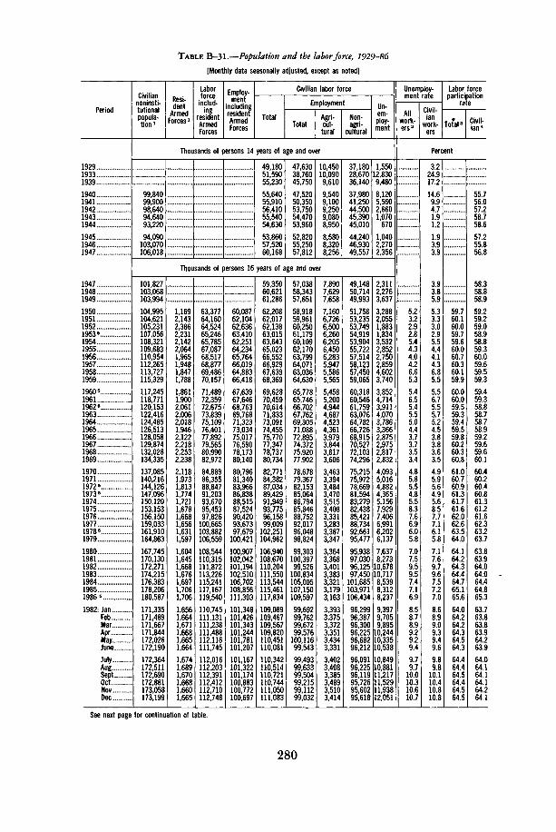
TABLE B-31.—Population and the labor force, 1929-86

[Monthly data seasonally adjusted, except as noted]

Period

192919331939

19401941194219431944

194519461947

194719481949

1950195119521953 5195419551956195719581959

I960519611962s19631964196519661967..19681969

1970.. .1971197251973 519741975197619771978s1979

1980198119821983198419851986s

1982: JanFebMarAprMayJune

J/yAugSeptOctNovDec

Civiliannon insti-tutionalpopula-tion1

Resi-dentArmedForces *

Laborforceinclud-ing

residentArmedForces

Employ-ment

includingresidentArmedForces

Civilian labor force

Total

Employment

TotalAgri-cul-tural

Non-agri-

cultural

Un-em-ploy-ment

Thousands of persons 14 years of age and over

99,84099,90098,64094,64093,220

94090103,070106,018

49,18051,59055,230

55,64055,91056,41055,54054,630

53,86057,52060,168

47,63038,76045,750

47,52050,35053,75054,47053,960

52,82055,25057,812

10,45010,0909,610

9,5409,1009,2509,0808,950

8,5808,3208,256

37,18028,67036,140

37,98041,25044,50045,39045,010

44,24046,93049,557

1,55012,8309,480

8,1205,5602,6601,070670

1,0402,2702,356

Thousands of persons 16 years of age and over

101,827103,068103,994

104,995104,621105,231107,056108,321109,683110,954112,265113,727115,329

117,245118,771120,153122,416124,485126,513128,058129,874132,028134,335

137,085140,216144,126147,096150,120153,153156,150159,033161,910164,863

167,745170,130172,271174,215176,383178,206180,587

171,335171,489171,667171,844172,026172,190

172,364172,511172,690172,881173,058173,199

1,1692,1432,3862,2312,1422,0641,9651,9481,8471,788

1,8611,9002,0612,0062,0181,9462,1222,2182,2532,238

2,1181,9731,8131,7741,7211,6781,6681,6561,6311,597

1,6041,6451,6681,6761,6971,7061,706

1,6561,6641,6711,6681,6651,664

1,6741,6891,6701,6681,6601,665

63,37764,16064,52465,24665,78567,08768,51768,87769,48670,157

71,48972,35972,67573,83975,10976,40177,89279,56580,99082,972

84,88986,35588,84791,20393,67095,45397,826100,665103,882106,559

108,544110,315111,872113,226115,241117,167119,540

110,745111,131111,238111,488112,116111,745

112,016112,203112,391112,412112,710112,748

60,08762,10462,63663,41062,25164,23465,76466,01964,88366,418

67,63967,64668,76369,76871,32373,03475,01776,59078,17380,140

80,79681,34083,96686,83888,51587,52490,42093,67397,679100,421

100,907102,042101,194102,510106,702108,856111,303

101,348101,426101,343101,244101,781101,207

101,167101,322101,174100,883100,772100,697

59,35060,62161,286

62,20862,01762,13863,01563,64365,02366,55266,92967,63968,369

69,62870,45970,61471,83373,09174,45575,77077,34778,73780,734

82,77184,38287,03489,42991,94993,77596,15899,009102,251104,962

106,940108,670110,204111,550113,544115,461117,834

109,089109,467109,567109,820110,451110,081

110,342110,514110,721110,744111,050111,083

57,03858,34357,651

58,91859,96160,25061,17960,10962,17063,79964,07163,03664,630

65,77865,74666,70267,76269,30571,08872,89574,37275,92077,902

78,67879,36782,15385,06486,79485,84688,75292,01796,04898,824

99,303100,39799,526100,834105,005107,150109,597

99,69299,76299,67299,576100,11699,543

99,49399,63399,50499,21599,11299,032

7,8907,6297,658

7,1606,7266,5006,2606,2056,4506,2835,9475,5865,565

5,4585,2004,9444,6874,5234,3613,9793,8443,8173,606

3,4633,3943,4843,4703,5153,4083,3313,2833,3873,347

3,3643,3683,4013,3833,3213,1793,163

3,3933,3753,3723,3513,4343,331

3,4023,4083,3853,4893,5103,414

49,14850,71449,993

51,75853,23553,74954,91953,90455,72257,51458,12357,45059,065

60,31860,54661,75963,07664,78266,72668,91570,52772,10374,296

75,21575,97278,66981,59483,27982,43885,42188,73492,66195,477

95,93897,03096,12597,450101,685103,971106,434

96,29996,38796,30096,22596,68296,212

96,09196,22596,11995,72695,60295,618

2,3112,2763,637

3,2882,0551,8831,8343,5322,8522,7502,8594,6023,740

3,8524,7143,9114,0703,7863,3662,8752,9752,8172,832

4,0935,0164,8824,3655,1567,9297,4066,9916,2026,137

7,6378,27310,67810,7178,5398,3128,237

9,3979,7059,89510,24410,33510,538

10,84910,88111,21711,52911,93812,051

Unemploy-ment rate

Allwork-ers2

Civil-ian

work-ers

Labor forceparticipation

rate

Total3 Civil-ian4

Percent

5.23.22.92.85.44.34.04.26.65.3

5.46.55.45.55.04.43.73.73.53.4

4.85.85.54.85.58.37.66.96.05.8

7.07.59.59.57.47.16.9

8.58.78.99.29.29.4

9.79.710.010.310.610.7

3224.917.2

14.69.9471.91.2

1.93.93.9

3.93.85.9

5.33.33.02.95.54.44.14.36.85.5

5.56.75.55.75.24.53.83.83.63.5

4.95.95.64.95.68.57.77.16.15.8

7.17.69.79.67.57.27.0

8.68.99.09.39.49.6

9.89.810.110.410.810.8

59.760.160.059.759.660.060.760.360.159.9

60.060.059.559.359.459.559.860.260.360.8

61.060.760.961.361.761.662.062.663.564.0

64.164.264.364.464.765.165.6

64.064.264.264.364.564.3

64.464.464.564.464.564.5

55.756.057.258.758.6

57.255.856.8

58.358.858.9

59.259.259.058.958.859.360.059.659.559.3

59.459.358.858.758.758.959.259.659.660.1

60.460.260.460.861.361.261.662.363.263.7

63.863.964.064.064.464.865.3

63.783.863.863.964.263.9

64.064.164.164.164.264.1

See next page for continuation of table.

280

TABLE B-31.—Population and the labor force, 1929-86—Continued

[Monthly data seasonally adjusted, except as noted]

Period

1983: JanFebMar

May'.".'""!!!June

JulyAugSeptOctNovDec

1984- JanFebMar .AprMayJune

JulyAugSeptOctNovDec

1985: JanFebMarAprway-June

JulyAugSeptOct. .NovDec

1986: Jan 5FebMar

ft:::::June

JulyAugSeptOctNovDec

Civiliannoninsti-tutionalpopula-tion1

Resi-dentArmedForces l

Laborforceinclud-ing

residentArmedForces

Employ-ment

includingresidentArmedForces

Civilian labor force

Total

Employment

TotalAgri-cul-tural

Non-agri-

cultural

Un-em-ploy-ment

Thousands of persons 16 years of age and over

173,354173,505173,656173,794173,953174,125

174,306174,440174,602174,779174,951175,121

175,533175,679175,824175,969176,123176,284

176,440176,583176,763176,956177,135177,306

177,384177,516177,667177,799177,944178,096

178,263178,405178,572178,770178,940179,112

179,670179,821179,985180,148180,311180,503

180,682180,828180,997181,186181,363181,547

1,6671,6641,6641,6711,6691,668

1,6641,6821,6951,6951,6851,688

1,6861,6841,6861,6931,6901,690

1,6981,7121,7201,7051,6991,698

1,6971,7031,7011,7021,7051,702

1,7041,7261,7321,7001,7021,698

1,6911,6911,6931,6951,6871,680

1,6721,6971,7161,7491,7511,750

112,361112,318112,256112,512112,492113,489

113,410113,878113,995113,621113,905114,037

113,923114,355114,400114,816115,365115,447

115,630115,369115,544115,723115,873116,283

116,494116,673117,017117,015116,991116,628

116,984117,003117,576117,780117,851118,031

118,485118,733118,880118,987119,274119,685

119,789119,821119,988120,163120,426120,336

100,835100,776100,853101,244101,340102,241

102,880103,279103,719103,744104,405104,668

104,885105,540105,650106,067106,909107,235

107,144106,876107,188107,351107,666107,898

107,988108,308108,666108,651108,700108,243

108,546108,862109,334109,492109,680109,847

110,583110,248110,500110,664110,852111,293

111,559111,764111,703111,941112,183112,387

110,694110,654110,592110,841110,823111,821

111,746112,196112,300111,926112,220112,349

112,237112,671112,714113,123113,675113,757

113,932113,657113,824114,018114,174114,585

114,797114,970115,316115,313115,286114,926

115,280115,277115,844116,080116,149116,333

116,794117,042117,187117,292117,587118,005

118,117118,124118,272118,414118,675118,586

99,16899,11299,18999,57399,671100,573

101,216101,597102,024102,049102,720102,980

103,199103,856103,964104,374105,219105,545

105,446105,164105,468105,646105,967106,200

106,291106,605106,965106,949106,995106,541

106,842107,136107,602107,792107,978108,149

108,892108,557108,807108,969109,165109,613

109,887110,067109,987110,192110,432110,637

3,4363,3853,3693,3433,3423,461

3,4813,4933,3453,3063,2783,330

3,2863,3623,2523,3163,3473,373

3,3373,2763,3793,2033,3803,386

3,3123,3363,2893,3373,2763,138

3,1313,1063,0443,0723,0553,151

3,2803,1053,2523,1993,1513,164

3,1243,0573,1423,1623,2153,161

95,73295,72795,82096,23096,32997,112

97,73598,10498,67998,74399,44299,650

99,913100,494100,712101,058101,872102,172

102,109101,888102,089102,443102,587102,814

102,979103,269103,676103,612103,719103,403

103,711104,030104,558104,720104,923104,998

105,612105,452105,555105,770106,014106,449

106,763107,010106,845107,030107,217107,476

11,52611,54211,40311,26811,15211,248

10,53010,59910,2769,8779,5009,369

9,0388,8158,7508,7498,4568,212

8,4868,4938,3568,3728,2078,385

8,5068,3658,3518,3648,2918,385

8,4388,1418,2428,2888,1718,184

7,9028,4858.3808,3238,4228,392

8,2308,0578,2858,2228,2437,949

Unemploy-ment rate

Allwork-ers2

Civil-ian

work-ers

Labor forceparticipation

rate

Total3 Civil-ian4

Percent

10.310.310.210.09.99.9

9.39.39.08.78.38.2

7.97.77.67.67.37.1

7.37.47.27.27.17.2

7.37.27.17.17.17.2

7.27.07.07.06.96.9

6.77.17.07.07.17.0

6.96.76.96.86.86.6

10.410.410.310.210.110.1

9.49.49.28.88.58.3

8.17.87.87.77.47.2

7.47.57.37.37.27.3

7.47.37.27.37.27.3

7.37.17.17.17.07.0

6.87.27.27.17.27.1

7.06.87.06.96.96.7

64.264.164.064.164.164.6

64.464.764.764.464.564.5

64.364.564.464.664.964.9

64.964.764.764.864.865.0

65.165.165.265.265.164.9

65.065.065.265.365.265.3

65.365.465.465.465.565.7

65.765.665.765.765.865.7

63.963.863.763.863.764.2

64.164.364.364.064.164.2

63.964.164.164.364.564.5

64.664.464.464.464.564.6

64.764.864.964.964.864.5

64.764.664.964.964.964.9

65.065.165.165.165.265.4

65.465.365.365.465.465.3

1 Not seasonally adjusted.2 Unemployed as percent of labor force including resident Armed Forces.3 Labor force including resident Armed Forces as percent of noninstitutional population including resident Armed Forces.4 Civilian labor force as percent of civilian noninstitutional population.5 Not strictly comparable with earlier data due to population adjustments as follows-. Beginning 1953, introduction of 1950 census

data added about 600,000 to population and 350,000 to labor force, total employment, and agricultural employment. Beginning 1960,inclusion of Alaska and Hawaii added about 500,000 to population, 300,000 to labor force, and 240,000 to nonagricuIturaI employment.Beginning 1962, introduction of 1960 census data reduced population by about 50,000 and labor force and employment by 200,000.Beginning 1972, introduction of 1970 census data added about 800,000 to civilian noninstitutional population and 333,000 to laborforce and employment. A subsequent adjustment based on 1970 census in March 1973 added 60,000 to labor force and to employment.Beginning 1978, changes in sampling and estimation procedures introduced into the household survey added about 250,000 to laborforce and to employment. Unemployment levels and rates were not significantly affected. Beginning 1986, the introduction of revisedpopulation controls added about 400,000 to the civilian population and labor force and 350,000 to civilian employment. Unemploymentlevels and rates were not significantly affected.

Note.—Labor force data in Tables B-31 through B-38 are based on household interviews and relate to the calendar week includingthe 12th of the month. For definitions of terms, area samples used, historical comparability of the data, comparability with other series,etc., see "Employment and Earnings."

Source: Department of Labor, Bureau of Labor Statistics.

281

TABLE B-32.—Civilian employment and unemployment by sex and age, 1947-86

[Thousands of persons 16 years of age and over; monthly data seasonally adjusted]

Year or month

1947194819491950195119521953 »1954 ..19551956195719581959I960119611962 »1963 ... .1964196519661967 .. .19681969197019711972 *1973 »19741975 . ..197619771978 »19791980198119821983198419851986 l

1985: Jan .FebMarAprMayJuneJulyAuesept ::.::..OctNovDec

1986: Jan l ...FebMar..AprMay ..June

JulyAugSeptOctNovDec

Civilian employment

Total

57,03858,34357,65158,91859,96160,25061,17960,10962,17063,79964,07163,03664,63065,77865,74666,70267,76269,30571,08872,89574,37275,92077,90278,67879,36782,15385,06486,79485,84688,75292,01796,04898,82499,303100,39799,526100,834105,005107,150109,597106,291106,605106,965106,949106,995106,541106,842107,136107,602107,792107,978108,149108,892108,557108,807108,969109,165109,613109,887110,067109,987110,192110,432110,637

Males

Total

40,99541,72540,92541,57841,78041,68242,43041,61942,62143,37943,35742,42343,46643,90443,65644,17744,65745,47446,34046,91947,47948,11448,81848,99049,39050,89652,34953,02451,85753,13854,72856,47957,60757,18657,39756,27156,78759,09159,89160,89259,57059.59059J8959,81759,95159,62959,76159,94960,11660,15360,20760,21360,85360,60360,68160,71260,66860,79360,88460,94260,96860,97561,24161,393

16-19years

2,2182,3442,1242,1862,1562,1072,1361,9852,0952,1642,1152,0122,1982,3612,3152,3622,4062,5872,9183,2533,1863,2553,4303,4093,4783,7654,0394,1033,8393,9474,1744,3364,3004,0853,8153,3793,3003,3223,3283,3233,4173,3713,4203,4313,3853,2653,3103,2953,2873,2373,2653,2853,2543,3073,2933,3203,3303,2713,3403,3573,3613,3803,3583,292

20yearsandover

38,77639,38238,80339,39439,62639,57840,29639,63440,52641,21641,23940,41141,26741,54341,34241,81542,25142,88643,42243,66844,29444,85945,38845,58145,91247,13048,31048,92248,01849,19050,55552,14353,30853,10153,58252,89153,48755,76956,56257,56956,15356,21956,36956,38656,56656,36456,45156,65456,82956,91656,94256,92857,59957,29657,38857,39257,33857,52257,54457,58557,60757,59557,88358,101

Females

Total

16,04516,61716,72317,34018,18118,56818,74918,49019,55120,41920,71420,61321,16421,87422,09022,52523,10523,83124,74825,97626,89327,80729,08429,68829,97631,25732,71533,76933,98935,61537,28939,56941,21742,11743,00043,25644,04745,91547,25948,70646,72147,01547,17647,13247,04446,91247,08147,18747,48647,63947,77147,93648,03947,95448,12648,25748,49748,82049,00349,12549,01949,21749,19149,244

16-19years

1,6911,6821,5881,5171,6111,6121,5841,4901,5471,6541,6631,5701,6401,7681,7931,8331,8491,9292,1182,4682,4962,5262,6872,7352,7302,9803,2313,3453,2633,3893,5143,7343,7833,6253,4113,1703,0433,1223,1053,1493,1363,2133,1543,1233,1092,9293,0953,0673,1283,0883,1603,0933,0873,1343,1923,1633,1623,1633,1343,1693,1143,1973,1243,186

20yearsandover

14,35414,93615,13715,82416,57016,95817,16417,00018,00218,76719,05219,04319,52420,10520,29620,69321,25721,90322,63023,51024,39725,28126,39726,95227,24628,27629,48430,42430,72632,22633,77535,83637,43438,49239,59040,08641,00442,79344,15445,55643,58543,80244,02244,00943,93543,98343,98644,12044,35844,55144,61144,84344,95244,82044,93445,09445,33545,65745,86945,95645,90546,02046,06746,058

Unemployment

Total

2,3112,2763,6373,2882,0551,8831,8343,5322,8522,7502,8594,6023,7403,8524,7143,9114,0703,7863,3662,8752,9752,8172,8324,0935,0164,8824,3655,1567,9297,4066,9916,2026,1377,6378,27310,67810,7178,5398,3128,2378,5068,3658,3518,3648,2918,3858,4388,1418,2428,2888,1718,1847,9028,4858,3808,3238,4228,3928,2308,0578,2858,2228,2437,949

Males

Total

1,6921,5592,5722,2391,2211,1851,2022,3441,8541,7111,8413,0982,4202,4862,9972,4232,4722,2051,9141,5511,5081,4191,4032,2382,7892,6592,2752,7144,4424,0363,6673,1423,1204,2674,5776,1796,2604,7444,5214,5304,6264,5784,5124,5634,4274,6144,5984,4294,4324,5704,4554,4114,2744,5954,5724,5174,6534,6194,5664,4284,6004,5654,5744,439

16-19years

270256353318191205184310274269300416398426479408501487479432448426440599693711653757966939874813811913962

1,0901,003812806779820816784772798767865798772897791794730799783829833811755794795751754714

20yearsandover

1,4221,3052,2191,9221,029980

1,0192,0351,5801,4421,5412,6812,0222,0602,5182,0161,9711,7181,4351,1201,060993963

1,6382,0971,9481,6241,9573,4763,0982,7942,3282,3083,3533,6155,0895,2573,9323,7153,7513,8063,7623,7283,7913,6293,8473,7333,6313,6603,6733,6643,6173,5443,7963,7893,6883,8203,8083,8113,6343,8053,8143,8203,725

Females

Total

619717

1,0651,049834698632

1,188998

1,0391,0181,5041,3201,3661,7171,4881,5981,5811,4521,3241,4681,3971,4291,8552,2272,2222,0892,4413,4863,3693,3243,0613,0183,3703,6964,4994,4573,7943,7913,7073,8803,7873,8393,8013,8643,7713,8403,7123,8103,7183,7163,7733,6283,8903,8083,8063,7693,7733,6643,6293,6853,6573,6693,510

16-19years

144153223195145140123191176209197262256286349313383385395405391412413506568598583665802780789769743755800886825687661675697663691630685635707575628680653700683701677719671691654635670663693645

20yearsandover

475564841854689559510997823832821

1,2421,0631,0801,3681,1751,2161,1951,056921

1,078985

1,0151,3491,6581,6251,5071,7772,6842,5882,5352,2922,2762,6152,8953,6133,6323,1073,1293,0323,1833,1243,1483,1713,1793,1363,1333,1373,1823,0383,0633,0732,9453,1893,1313,0873,0983,0823,0102,9943,0152,9942,9762,865

1 See footnote 5, Table B-31.Note.—See Note, Table B-31.Source: Department of Labor, Bureau of Labor Statistics.

282

TABLE B-33.—Unemployment by duration and reason, 1947-86

[Monthly data seasonally adjusted1]

Year or month

194719481949

19501951. . .195219531954195519561957 . .19581959

I9601961196219631964.. .1965196619671968.1969

197019711972197319741975..1976197719781979

19801981.. . .198219831984198519861985- Jan

FebMar*.AprMayJune

JulyAucsept::::::::::::::::::::::::::::OctNovDec

1986- JanFebMarAprMay .June

JulyAugSeptOct. . .NovDec

Unem-ploy-ment

Duration of unemployment

Lessthan 5weeks

5-14weeks

15-26weeks

27weeksandover

Thousands of persons 16years of age and over

2,3112,2763,637

3,2882,0551,8831,8343,5322,8522,7502,8594,6023,740

3,8524,7143,9114,0703,7863,3662,8752,9752,8172,832

4,0935,0164,8824,3655,1567,9297,4066,9916,2026,137

7,6378,27310,67810,7178,5398,3128,237

8,5068,3658,3518,3648,2918,385

8,4388,1418,2428,2888,1718,184

7,9028,4858,3808,3238,4228,392

8,2308,0578,2858,2228,2437,949

1,2101,3001,756

1,4501,1771,1351,1421,6051,3351,4121,4081,7531,585

1,7191,8061,6631,7511,6971,6281,5731,6341,5941,629

2,1392,2452,2422,2242,6042,9402,8442,9192,8652,950

3,2953,4493,8833,5703,3503,4983,448

3,6893,4813,5143,4803,5343,492

3,5303,4283,4993,4313,4843,417

3,3733,5343,5363,5653,6103,415

3,3993,4363,4153,4183,3823,355

704669

1,194

1,055574516482

1,116815805891

1,3961,114

1,1761,3761,1341,2311,117983779893810827

1,2901,5851,4721,3141,5972,4842,1962,1321,9231,946

2,4702,5393,3112,9372,4512,5092,557

2,5932,4842,4742,4892,5492,492

2,5352,5242,4932,5292,4452,507

2,5052,6152,6252,6502,6712,650

2,5212,4072,5242,5632,6132,389

234193428

425166148132495366301321785469

503728534535491404287271256242

428668601483574

1,3031,018913766706

1,0521,1221,7081,6521,1041,0251,045958

1,0601,0421,0131,0611,0361,0611,0221,0251,076912

1,005

1,0031,1421,078982

1,0651,038

1,0581,0681,110950

1,0451,023

164116256

3571378478317336232239667571

454804585553482351239177156133

235519566343381

1,2031,3481,028648535

8201,1621,7762,5591,6341,2801,187

1,3421,3481,3451,3561,2351,2731,2551,2261,2531,2001,2951,2041,1141,1901,1651,1481,1671,2611,1921,2041,2631,2181,1721,148

Aver-age

(mean)dura-tion inweeks

Mediandura-tion inweeks

8.610.0

12.19.78.48.0

11.813.011.310.513.914.4

12.815.614.714.013.311.810.48.78.47.8

8.611.312.010.09.8

14.215.814.311.910.8

11.913.715.620.018.215.615.0

15.915.916.216,415.315.515.515.315.315.315.615.2

15.015.214.614.714.815.2

15.115.615.515.214.815.0

4.54.4

4.96.36.25.25.28.48.27.05.95.4

6.56.98.7

10.17.96.86.96.87.17.06.96.86.77.07.16.87.06.96.8

6.86.96.86.66.87.2

7.17.17.17.07.07.1

Reason for unemployment

Joblosers

Jobleavers

Reen-trants

Newen-

trants

Thousands of persons 16years of age and over

1,2291,0701,017

1,8112,3232,1081,6942,2424,3863,6793,1662,5852,635

3,9474,2676,2686,2584,4214,1394,033

4,3074,2234,1444,2253,9104,1124,3274,1304,1264,0354,0983,996

3,8024,1474,2104,0354,2144,272

4,0633,8244,0443,9843,9473,890

438431436

550590641683768827903909874880891923840830823877

1,015864857853826871982887889857940807902

977985989

1,071979

1,009

1,025990

1,0411,0271,0561,036

945909965

1,2281,4721,4561,3401,4631,8921,9281,9631,8571,8061,9272,1022,3842,4122,1842,2562,160

2,2532,2182,3032,2802,3672,270

2,1762,1672,3562,2122,2212,251

2,0832,2632,1962,1882,2002,107

2,2052,1992,1452,1902,1192,019

396407413504630677649681823895953885817

872981

1,1851,2161,1101,0391,029

1,0481,0381,0791,0411,1301,0101,122955915

1,0621,0381,042

1,0291,0731,0061,0481,0461,050

9891,0141,038972

1,0761,015

1 Because of independent seasonal adjustment of the various series, detail will not add to totals.Note.—See footnote 5 and Note, Table B-31.Source: Department of Labor, Bureau of Labor Statistics.

283

TABLE B-34.—Chilian labor force participation rate and employment/population ratio, 1948-86

[Percent; monthly data seasonally adjusted]

Year or month

194819491950195119521953195419551956195719581959I96019611962196319641965196619671968. .196919701971197219731974197519761977197819791980198119821983198419851986

1985: JanFebMar

May!...!.".....June

JulyAugSeptOctNovDec

1986: JanFebMarAprMayJune

JulyAug

, SeptOctNovDec

Civilian labor force participation rate 1

Total

58.858.959.259.259.058.958.859.360.059.659.559.359.459.358.858.758.758.959.259.659.660.160.460.260.460.861.361.261.662.363.263.763.863.964.064.064.464.865.3

64.764.864.964.964.864.5

64.764.664.964.964.964.9

65.065.165.165.165.265.4

65.465.365.365.465.465.3

Males

86.686.486.486.386.386.085.585.485.584.884.283.783.382.982.081.481.080.780.480.480.179.879.779.178.978.878.777.977.577.777.977.877.477.076.676.476.476.376.3

76.476.376.476.476.376.1

76.276.176.376.476.276.1

76.376.376.376.276.376.3

76.276.176.276.176.476.3

Fe-males

32.733.133.934.634.734.434.635.736.936.937.137.137.738.137.938.338.739.340.341.141.642.743.343.443.944.745.746.347.348.450.050.951.552.152.652.953.654.555.3

54.254.454.654.554.454.1

54.354.254.654.654.754.9

54.854.955.055.155.255.5

55.555.655.555.655.555.4

Bothsexes16-19years

52.552.251.852.251.350.248.348.950.949.647.446.747.546.946.145.244.545.748.248.448.349.449.949.751.953.754.854.054.556.057.857.956.755.454.153.553.954.554.7

55.255.255.254.755.052.4

55.253.554.154.654.454.4

53.654.954.955.455.254.8

54.554.854.855.054.553.8

White

58.258.759.459.158.958.758.858.858.358.258.258.458.759.259.359.960.260.160.460.861.461.561.862.563.363.964.164.364.364.364.665.065.5

64.965.065.165.065.064.8

64.964.865.165.265.265.2

65.265.365.365.365.465.6

65.665.665.665.665.765.7

Blackand

other

64.064.264.964.464.864.364.564.163.263.063.162.963.062.862.262.161.860.960.260.560.359.659.860.462.262.261.761.361.662.162.663.363.7

63.663.163.563.663.463.0

63.363.063.263.163.363.7

63.863.664.063.964.064.0

63.663.363.663.863.863.5

Black

"59"960.259.858.859.059.861.561.461.060.861.061.562.262.963.3

63.263.162.762.962.862.5

62.862.762.862.862.963.4

63.363.363.563.763.863.6

63.062.763.163.363.263.1

Employment/population ratio2

Total

56.658.257.358.056.457.558.257.856.156.756.856.156.356.156.456.957.658.058.258.758.057.257.558.358.356.557.358.359.760.359.659.458.258.359.960.561.1

60.360.460.660.560.560.2

60.360.460.660.760.760.8

61.060.760.860.960.961.1

61.261.261.161.261.361.3

Civilian

Total

56.655.456.157.357.357.155.556.757.557.155.456.056.155.455.555.455.756.256.957.357.558.057.456.657.057.857.856.156.857.959.359.959.259.057.857.959.560.160.7

59.960.160.260.260.159.8

59.960.160.360.360.360.4

60.660.460.560.560.560.7

60.860.960.860.860.960.9

Males

83.581.382.084.083.983.681.081.882.381.378.579.378.977.677.777.177.377.577.978.077.877.676.274.975.075.574.971.772.072.873.873.872.071.369.068.870.770.971.0

70.870.871.071.071.170.6

70.770.971.071.071.070.9

71.371.071.070.970.870.9

70.970.970.970.871.171.2

Fe-males

31.331.232.033.133.433.332.534.035.135.134.535.035.535.435.635.836.337.138.339.039.640.740.840.441.042.042.642.043.244.546.447.547.748.047.748.049.550.451.4

50.150.350.550.450.35Q. 1

50.250.350.650.750.850.9

50.950.850.951.051.251.5

51.751.851.651.851.751.7

Bothsexes16-19years

47.745.245.547.946.946.442.343.545.343.939.939.940.539.139.437.437.338.942.142.242.243.442.341.343.545.946.043.344.246.148.348.546.644.641.541.543.744.444.6

44.945.145.145.144.842.8

44.344.044.443.744.444.1

43.944.544.844.844.844.5

44.845.044.745.344.544.5

White

55.256.557.356.855.355.955.955.355.455.355.556.056.857.257.458.057.556.857.458.258.356.757.558.660.060.660.060.058.858.960.561.061.5

60.761.061.161.061.060.6

60.860.861.161.261.361.3

61.461.261.361.361.461.6

61.661.861.661.761.761.8

Blackand

other

58.058.759.559.356.757.557.956.256.356.257.057.858.458.258.058.156.854.954.155.054.351.452.052.554.755.253.652.650.951.053.654.755.4

54.854.054.754.954.654.9

54.754.954.754.654.455.1

55.555.155.555.355.455.4

55.555.055.355.755.755.7

Black

•••••"• •

•••••••• •

"'53J54.553.550.150.851.453.653.852.351.349.449.552.353.454.1

53.552.953.253.453.153.6

53.353.953.453.553.253.9

54.153.954.254.354.354.2

54.153.553.854.254.254.4

1 Civilian labor force as percent of civilian noninstitutional population in group specified. See Table B-31 for total labor forceparticipation rate.

2 Employment as percent of noninstitutional population in group specified.Note.—Data relate to persons 16 years of age and over. See footnote 5 and Note, Table B-31.Source: Department of Labor, Bureau of Labor Statistics.

284

TABLE B-35.—Unemployment rate, 1948-86

[Percent; monthly data seasonally adjusted]

Year ormonth

19481949

1950195119521953195419551956195719581959

1960196119621963196419651966196719681969

1970197119721973197419751976197719781979

1980198119821983198419851986

1985: JanFebMar

MPay";"!June....

JulyAugSept ...OctNov....Dec....

1986: JanFebMar....AprMay....June-

July ....Aug....Sept...OctNov....Dec....

Unem-ploy-mentrate,

allwork-ers *

5.23.22.92.85.44.34.04.26.65.3

5.46.55.45.55.04.43.73.73.53.4

4.85.85.54.85.58.37.66.96.05.8

7.07.59.59.57.47.16.9

7.37.27.17.17.17.2

7.27.07.07.06.96.9

6.77.17.07.07.17.0

6.96.76.96.86.86.6

Unemployment rate, civilian workers 2

Allcivil-ian

work-ers

3.85.9

5.33.33.02.95.54.44.14.36.85.5

5.56.75.55.75.24.53.83.83.63.5

4.95.95.64.95.68.57.77.16.15.8

7.17.69.79.67.57.27.0

7.47.37.27.37.27.3

7.37.17.17.17.07.0

6.87.27.27.17.27.1

7.06.87.06.96.96.7

Males

Total

3.65.9

5.12.82.82.85.34.23.84.16.85.2

5.46.45.25.24.64.03.23.12.92.8

4.45.35.04.24.97.97.16.35.35.1

6.97.49.99.97.47.06.9

7.27.17.07.16.97.2

7.16.96.97.16.96.8

6.67.07.06.97.17.1

7.06.87.07.06.96.7

16-19

years

9.814.3

12.78.18.97.9

13.511.611.112.417.115.3

15.317.114.717.215.814.111.712.311.611.4

15.016.615.913.915.620.119.217.315.815.9

18.320.124.423.319.619.519.0

19.419.518.618.419.119.0

20.719.519.021.719.519.5

18.319.519.220.020.019.9

18.419.119.118.218.317.8

20yearsandover

3.25.4

4.72.52.42.54.93.83.43.66.24.7

4.75.74.64.53.93.22.52.32.22.1

3.54.44.03.33.86.85.95.24.34.2

5.96.38.88.96.66.26.1

6.36.36.26.36.06.4

6.26.06.16.16.06.0

5.86.26.26.06.26.2

6.25.96.26.26.26.0

Females

Total

4.16.0

5.74.43.63.36.04.94.84.76.85.9

5.97.26.26.56.25.54.85.24.84.7

5.96.96.66.06.79.38.68.27.26.8

7.47.99.49.27.67.47.1

7.77.57.57.57.67.4

7.57.37.47.27.27.3

7.07.57.37.37.27.2

7.06.97.06.96.96.7

16-19

years

8.312.3

11.48.38.07.2

11.410.211.210.614.313.5

13.916.314.617.216.615.714.113.514.013.3

15.617.216.715.316.619.718.718.317.116.4

17.219.021.921.318.017.617.6

18.217.118.016.818.117.8

18.615.816.718.017.118.5

18.118.317.518.517.517.9

17.316.717.717.218.216.8

20yearsandover

3.65.3

5.14.03.22.95.54.44.24.16.15.2

5.16.35.45.45.24.53.84.23.83.7

4.85.75.44.95.58.07.47.06.05.7

6.46.88.38.16.86.66.2

6.86.76.76.76.76.7

6.66.66.76.46.46.4

6.16.66.56.46.46.3

6.26.16.26.16.15.9

Bothsexes16-19

years

9.213.4

12.28.28.57.6

12.611.011.111.615.914.6

14.716.814.717.216.214.812.812.912.712.2

15.316.916.214.516.019.919.017.816.416.1

17.819.623.222.418.918.618.3

18.818.318.317.618.618.5

19.717.817.920.018.419.0

18.218.918.419.318.818.9

17.918.018.517.718.217.3

White

3.55.6

4.93.12.82.75.03.93.63.86.14.8

5.06.04.95.04.64.13.43.43.23.1

4.55.45.14.35.07.87.06.25.25.1

6.36.78.68.46.56.26.0

6.46.26.26.26.16.4

6.36.26.16.15.96.0

5.86.36.26.16.26.1

6.05.86.06.06.05.8

Blackand

other

5.98.9

9.05.35.44.59.98.78.37.9

12.610.7

10.212.410.910.89.68.17.37.46.76.4

8.29.9

10.09.09.9

13.813.113.111.911.3

13.114.217.317.814.413.713.1

13.914.413.913.713.913.0

13.612.813.613.514.113.5

13.113.313.413.513.513.5

12.713.113.112.712.712.3

Black

""io.4"9.4

10.514.814.014.012.812.3

14.315.618.919.515.915.114.5

15.216.115.215.215.414.2

15.114.115.014.815.515.0

14.614.914.814.814.814.9

14.214.614.614.314.213.7

Experi-encedwageand

salaryworkers

436.8

6.03.73.43.26.2484.44.67.35.7

5.76.85.65.65.04.33.53.63.43.3

4.85.75.34.55.38.27.36.65.65.5

6.97.39.39.27.16.86.6

7.06.86.76.86.76.8

6.86.86.86.76.66.6

6.36.86.76.76.86.6

6.66.56.56.66.56.3

Mar-riedmen,

spousepres-en t 3

3.5

4.61.51.41.74.0262.32.85.13.6

3.74.63.63.42.82.41.91.81.61.5

2.63.22.82.32.75.14.23.62.82.8

4.24.36.56.54.64.34.4

4.54.44.24.34.04.6

4.34.24.44.24.34.3

4.34.54.54.24.44.5

4.44.24.34.64.54.3

Womenwho

main-tain

fami-lies

••••""""

4.94.44.4

5.47.37.27.17.0

10.010.19.48.58.3

9.210.411.712.210.310.49.8

10.210.810.210.810.79.8

10.510.711.110.610.09.6

9.99.9

10.19.5

10.110.0

9.510.19.88.99.79.8

1 Unemployed as percent of labor force including resident Armed Forces.2 Unemployed as percent of civilian labor force in group specified.3 Data for 1949 and 1951-54 are for April; 1950, for March.Note.—Data relate to persons 16 years of age and over. See footnote 5 and Note, Table B-31.Source: Department of Labor, Bureau of Labor Statistics.

285

TABLE B-36.—Civilian labor force participation rate by demographic characteristic, 1954-86

[Percent;1 monthly data seasonally adjusted]

Year or month

195419551956195719581959

I96019611962 . .1963196419651966 . . .196719681969

1970197119721973197419751976 .197719781979

1980198119821983198419851986

1985- JanFebMar

fc=:June

JulyAugSeptOctNovDec

1986: JanFebMarAprfayJune

JulyAugSeptOctNovDec

Allcivil-ian

work-ers

58859.360059659559.3

59.459358858758.758959259659660.1

60.460260.460861.361.261662.363263.7

63.863964.064064.464865.3

64764.864.964.964.864.5

64.764.664.964.964.964.9

65065.165.165.165.265.4

65.465.365.365.465.465.3

Total

58258.759459158958.7

58.858858358258.258458759259359.9

60.260160.460861461.561862.563363.9

64164364.364364.665065.5

64965.065.165.065.064.8

64.964.865.165.265.265.2

65265.365.365.365.465.6

65.665.665.665.665.765.7

Total

85685485684884383.8

83.483082181581180880680680480?

80.079679.679479.478778478.578678.6

782779774771771770769

77077.077.077.077.176.9

76.976.876.977.177.076.8

77077076.976.876.876.9

76.876.876.976977.177.1

Males

16-19years

57658.660459256555.9

55.954553.853152.754155956355956.8

57.557960.162062961.962364.065064.8

637624600594590597593

60560.160.560.660.859.3

60.458.758.660058.658,9

57859.558.759.559.559.5

58.959.960.359.859.658.2

White

20yearsandover

87887.587686986686.3

86.085784984484283983683583283.0

82.882382.081681480.780380.2801801

798795792789787785785

78578578.578.578.578.5

78.378.478.678778.678.4

78678.678.578.378.478.5

78.478.278.478378.778.8

Total

33334.535735735836.0

36.536936737237538139240140741.8

42.6426432441452459469480494505

51251952452753354 1550

53954154.354.054.053.7

53.953.954.354454.454.6

54554654.754.754.955.2

55.355.455.255.355.255.1

Females

16-19years

40640.7431422401396

40.340639838737839242642543044.6

45.645448150151751.552854.5567574

562554550545554552563

55956656.354.555.152.6

55.253.655.755556.255.9

55356656.856.756.656.2

55.556.255.556.956.356.5

20yearsandover

32734.035.135235535.6

36236636537037538038839840441.5

42.242342743544445.3462473487498

506515522525531540549

53753954.154.053.953.8

53.853.954.254354.254.5

54454454.554.554.855.1

55.355.455.255255.155.0

Total

59.960259858859059.861561.4

610608610615622629633

63263162.762.962.862.5

62.862.762.862.862.963.4

63363.363.563.763.863.6

63.062.763.163.363.263.1

Total

73.673472970.970070.6715713

703700701706708708712

70971170.470.570.570.1

70.771.171.271070.671.0

71571.371.671.571.971.6

71.270.570.770.870.570.7

Males

16-19years

46.345746742.641343.244943.6

43241639.8399417446437

45043.043.544.543.141.7

46.546.444.946.243.645.7

44545.745.545.648.143.8

42.741.842.242.240.441.6

Black

20yearsandover

78.578477.676.075475.676276.3

751745747752748744748

74575074.174.174.274.0

74.174.474.774474.274.4

75274775.175.075.175.3

75.074.274.474.674.574.5

Total

48.749349048.849850.853153.1

53153553754255.2565569

56956.656.656.756.656.3

56.455.956.156.156.857.2

56656.857.057.357.257.2

56.456.456.957.257.356.9

Females

16-19years

32.234233.434.232932.937336.8

34.934033.533035.037939.1

37939.938.537.840.734.6

39.035.235.938.438.938.6

39639.942.041.538.442.1

34.835.939.740.038.238.1

20yearsandover

51.251651.451 152553 fi555554

55656056.256857.658658.9

59 158.458.658.958.458.8

58.458.358.358158.759.2

58558658.659.159.258.8

58.858.658.859159.358.9

1 Civilian labor force as percent of civilian noninstitutional population in group specified.Note.—Data relate to persons 16 years of age and over. See footnote 5 and Note, Table B-31.Source: Department of Labor, Bureau of Labor Statistics.

286

TABLE B-37.—Civilian employment/population ratio, 1954-86

[Percent*; monthly data seasonally adjusted]

Year or month

1954.19551956195719581959

1960196119621963196419651966196719681969

1970197119721973197419751976197719781979

19801981 .198219831984.19851986

1985: JanFebMarAprMayJune

JulyAugSeptOctNovDec

1986: JanFebMarAprMayJune

JulyAugSeptOctNovDec

Allcivil-ian

work-ers

55556757.557155.4560

56155455.555.455.756.256957.3575580

57456.657057857.856156857.959359.9

59.259057.857.959560160.7

59.960.160.260.260.159.8

59.960.160.360360.360.4

60.660.460.560.560.560.7

60.860.960.860.860.960.9

Total

55256557356855.3559

55955355.455.355.556056857.2574580

57556.857458258.356757558.660060.6

60060058.858.960561061.5

60.761.061.161.061.060.6

60.860.861.161 261.361.3

61.461.261.361.361.461.6

61.661.861.661.761.761.8

Total

81582282781879.2799

79478278477.777.877978378.4783782

76875.776076575973073474.175075.1

73472870670.472172372.3

72.272.272.472.472.672.0

72.172.172.472572.472.3

72.672.372.272.272.172.2

72.172.372.372.272.472.6

Males

16-19years

49952054152447.6481

48145946444.745.047150150.250351 1

49649.251554354450651 554.456355.7

53451347047.449 149949.6

50.649.950.851.150.849.8

49.948.849.448849.349.2

49.149.749.449.349.449.3

49.750.050.250.549.949.2

White

20yearsandover

84084785084181.8828

82481481581.181.381581781.7816814

80179.079079278675776076.577277.3

75675 173072.674374374.3

74.174.274.374.274.574.0

74.074.274.474674.5744

74.774.374.274.274.174.2

74.174.374.274.174.474.6

Total

31433034234233.6340

34634534735.035.536237538.338940 1

40339.940741842442043244.546347.5

47848348148.549850751.7

50.350.750.850.650.550.3

50.450.550.851 051 151 1

51.251.051.251.351.551.9

52.052.251.952.051.952.0

Females

16-19years

36437038938235.0348

35134634832.932.233737537.7378395

39538641343644342544245.948549.4

47946244644.547047 147.9

47.348.947.846.846.744.5

46.946.347.747 1480472

47.047.948.848.048.248.0

47.448.247.148.247.548.3

20yearsandover

31 132733833933.5340

34534534735.235.836537538.339140 1

40440.140641642241943 i44.446 147.3

47848548448.950051 052.0

50.550.851.050.950.850.7

50.750.951.1513513514

51.551.251.451.551.852.2

52.452.552.352.352.352.3

Total

53754553550150851.453653.8

52351349449.552353454.1

53.552.953.253.453.153.6

53.353.953.453553.2539

54.153.954.254.354.354.2

54.153.553.854.254.254.4

Total

66867565860660661.463363.4

60459 156056.359260060.6

59.959.659.559.659.659.9

60.061.360.460059.5601

60.860.460.960.961.160.7

60.659.960.060.360.461.2

Males

16-19years

31632831426325826.428528.7

27024620320.423926326.5

25.325.126.127.126.424.2

26.929.626.627423.727.0

26.227.726.126.828.626.4

25.425.525.926.226.326.6

Black

20yearsandover

73073771966566867.569 169.1

65864561461.664 164665.1

64.764.464.164.164.264.8

64.565.665.064464.364.6

65.564.865.565.465.465.3

65.364.564.564.865.065.7

Total

43043843541642843.345846.0

45745144.244.146748148.8

48.447.548.148.347.948.5

47.947.847.748248.148.8

48.548.648.748.948.948.8

48.848.348.949.349.249.0

Females

16-19years

19222020.920219218.522122.4

21.019717.717.020123 123.8

23.322.222.723.323.822.7

23.822.422.722824.422.1

23.023.724.323.822.825.5

22.620.824.526.524.124.0

20yearsandover

46547246.944946447.049349.3

49.148547.547.449850951.6

51.250.450.951.150.651.4

50.650.750.551 150.851.8

51.451.351.451.751.751.4

51.651.351.551.851.951.7

1 Civilian employment as percent of civilian noninstitutional population in group specified.

Note.—Data relate to persons 16 years of age and over. See footnote 5 and Note, Table B-31.

Source: Department of Labor, Bureau of Labor Statistics.

287

TABLE B-38.—Civilian unemployment rate by demographic characteristic, 1948-86

[Percent;J monthly data seasonally adjusted]

Year or month

19481949

195019511952195319541955 . .19561957 . . .19581959

1960196119621963196419651966196719681969

1970197119721973.. ..1974197519761977.. . .19781979 .

198019811982198319841985..1986

1985: JanFebMar

ftJune

JulyAucSeptOct...NovDec

1986: JanFebMar

ftJune

JulyAugsepf:oct :....:.::..:NovDec

Allcivil-ian

work-ers

3859

5333302955444143685.5

556.75.557524.5383.83635

4.9595.649568577716158

7176979.675727.0

747.3727.37273

73717.1717.070

6872727.17271

706870696967

Total

3556

4931282750393638614.8

506.04.95.0464.1343.43231

4.5545.143507870625251

6367868.465626.0

646.2626.26 164

63626.1615.960

5863626.16261

605860606058

Total

3456

4726252548373436614.6

48574.6474136282.72625

4.0494.538447264554645

61658888646160

6361606.15964

626159615958

56616 15.96161

605861616159

Males

16-19years

13411310511515714.0

14015.713.715914712910510.7101100

13.7151142123135183173150135139

162179217202168165163

16416916015.6165161

174170157187159164

15016615917.1170171

156166166157163155

White

20yearsandover

443.3303.2554.1

425.14.03.9342.9222.12019

3.2403.630356254473.736

53567879575453

565.4535.45 157

555352525251

5054545.25454

545154545453

Total

3857

534.2333.1554.3424.3625.3

53R")5.55.8555.0434.64342

5.4635953618679736259

65698379656461

6763656.46565

646364626063

6 166636.26261

605960605957

Females

16-19years

1049.1979.5

12712.0

12714.812.815.114914.012111.5121115

13.415114.2130145174164159144140

148166190183152148149

15413615114.2151154

150136144151146156

15115414115.4147146

147142151152157146

20yearsandover

513.9373.8564.7

465.74.74.8464.0333.83434

4.4534.943517568625250

56597369585754

6057585.85858

575757555355

5459575.55554

535253525250

Total

10.494

105148140140128123

143156189195159151145

15216115215.2154142

151141150148155150

14614914814.8148149

142146146143142137

Total

9.38098

148137133118114

145157201203164153148

15516215515.4154145

152137151155157153

15015215014.9150152

149149151149143135

Males

16-19years

31.727.8331381375392367342

37540748948.8427410393

43841.640039.2388421

422361408408457409

41 139542641.2405397

405388386378350361

Black

20yearsandover

7.06074

1251141079393

124135178181143132129

13114213513.5135124

129118130134134132

12913312812.8129133

12913213413112911 8

Total

11.811.111314814314913.8133

14015617618.6154149142

15016015014.9155139

150145149141152146

14314514514.7145146

135143142138141139

Females

16-19years

40.536.137441.041643440.8391

39842247148.242639239.2

38544.541 138.3416344

38936336.6406373427

41940742242.7405394

350419383338370369

20yearsandover

908.688

12211712311.2109

11913415416.5135131124

13313.713113.2134125

132130134121136126

12212512312.5127127

12 1125124124125123

1 Unemployed as percent of civilian labor force in group specified.Note.—See footnote 5 and Note, Table B-31.Source: Department of Labor, Bureau of Labor Statistics.

288

TABLE B-39.—Unemployment insurance programs, selected data, 1955-86

Year or month

1955 . ..19561957195819591960 .19611962196319641965196619671968196919701971197219731974197519761977 ..19781979198019811982 ...19831984 ..1985

1985- JanFebMarAprMayJuneJulyAugsept":Oct .NovDec

1986- JanFebMarApr . ..MayJuneJulyAugSeptOctNovDec

All programs

Coveredemploy-ment1

Insuredunemploy-

ment(weekly

aver-age) « >

Thousands

40,01842,75143,43644,41145,72846,33446,26647,77648,43449,63751,58054,73956,34257,97759,99959,52659,37566,45869,89772,45171,03773,45976,41988,80492,06292,65993,30091,62891,89896,474

8 99,186

1,3991,3231,5712,7731,8602,0712,9941,9467 1,9731,7531,4501,1291,2701,1871,1772,0702,6082,1921,7932,5584,9373,8463,3082,6452,5923,8373,4104,5943,7752,5612,692

3,3613,3393,1132,7672,4572,3402,5232,3612,2122,2272,4682,884

3,3703,2953,1442,7792,5562,4742,6322,4832,3352,2962,478

Totalbenefits

paid(millions

ofdollars) 2 4

1,560.21,540.61,913.04,290.62,854.33,022.84,358.13,145.13,025.92,749.22,360.41,890.92,221.52,191.02,298.64,209.36,154.05,491.14,517.36,933.9

16,802.412,344.810,998.99,006.99,401.3

16,175.415,287.123,774.820,206.213,109.614,495.1

1,631.31,495.51,503.81,395.91,257.81,039.21,213.91,128.71,019.61,120.91,049.81,383.3

1,715.11,543.51,585.01,516.71,297.51,224.41,361.31,204.81,184.41,195.01,075.4

State programs

Insuredunem-

ploymentInitialclaims

Exhaus-tions5

Weekly average; thousands

1,2651,2151,4462,5101,6841,9082,2901,7837 1,8061,6051,3281,0611,2051,1111,1011,8052,1501,8481,6322,2623,9862,9912,6552,3592,4343,3503,0474,0613,3962,4762,611

2,5902,6462,6202,5752,5622,5812,6092,5852,5602,5352,5602,564

2,5912,6102,6542,6122,6662,6812,6982,7052,6912,5962,5492,488

226221270369277331350302

7 298268232203226201200296295261247363478386375346388488460583438377396

385411394390389398391386384380382391

370392393380382381380387370354354363

25202350333146323026211517161625393529378163553939595780805050

525254575149514743454348

5252555853515454484946

Insured

ment aspercent

ofcoveredemploy-

ment

3.53.23.66.44.44.85.64.44.33.83.02.32.52.22.13.44.13.52.73.56.04.63.93.32.93.93.54.63.92.82.9

2.93.02.92.92.82.92.92.82.82.82.82.8

2.82.82.92.82.92.92.92.92.92.72.72.6

Benefits paid

Total(millions

ofdollars) 4

1,350.31,380.71,733.93,512.72,279.02,726.73,422.72,675.42,774.72,522.12,166.01,771.32,092.32,031.62,127.93,848.54,957.04,471.04,007.65,974.9

11,754.78,974.58,357.27,717.28,612.9

13,761.113,262.120,649.617,762.812,594.713,977.8

1,580.01,450.61,459.21,349.81,221.41,011.81,183.81,096.7

988.81,085.21,014.61,341.3

1,662.61,495.71,539.31,472.11,260.81,177.51,308.91,160.01,144.51,147.31,030.5

Averageweeklycheck

(dollars) 6

25.0427.0228.1730.5830.4132.8733.8034.5635.2735.9237.1939.7541.2543.4346.1750.3454.0256.7659.0064.2570.2375.1678.7983.6789.6798.95

106.70119.37123.59123.47128.23

127.47128.20128.21128.18127.00126.35125.82126.88128.37129.41130.90132.13

133.57135.00135.59135.23135.81135.61134.16135.03136.78136.73137.49

**Monthly data are seasonally adjusted.1 Includes persons under the State, UCFE (Federal employee, effective January 1955), and RRB (Railroad Retirement Board) programs.Beginning October 1958, also includes the UCX program (unemployment compensation for ex-servicemen).2 Includes State, UCFE, RR, UCX, UCV (unemployment compensation for veterans, October 1952-January 1960), and SRA(Servicemen's Readjustment Act, September 1944-September 1951) programs. Also includes Federal and State extended benefitprograms. Does not include FSB (Federal supplemental benefits), SUA (special unemployment assistance), and Federal SupplementalCompensation programs.3 Covered workers who have completed at least 1 week of unemployment.4 Annual data are net amounts and monthly data are gross amounts.5 Individuals receiving final payments in benefit year.6 For total unemployment only.7 Programs include Puerto Rican sugarcane workers for initial claims and insured unemployment beginning July 1963.8 Latest data available for all programs combined. Workers covered by State programs account for about 97 percent of wage andsalary earners.

Source-. Department of Labor, Employment and Training Administration.

289

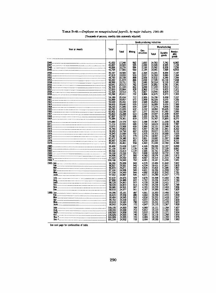
TABLE B-40.—Employees on nonagricultural payrolls, by major industry, 1946-86

(Thousands of persons; monthly data seasonally adjusted]

Year or month

19461947 . . .19481949195019511952 .19531954195519561957 .19581959I960196119621963196419651966196719681969197019711972197319741975197619771978 . .1979198019811982198319841985,1986 "1985: Jan

Feb .MarAprMayJuneJulyAugSept(£:::::::::::::::::::::::::::NovDec

1986: JanFebMarApr .. .itfay..: ..:: .r::::;r;: r: rJuneJulyAug ,Sept ...OctNoVDec*.

Total

41,65243,85744,86643,75445,19747,81948,79350,20248,99050,64152,36952,85351,32453,26854,18953,99955,54956,65358,28360,76563,90165,80367,89770,38470,88071,21473,67576,79078,26576,94579,38282,47186,69789,82390,40691,15689,56690,20094,49697,614100,16896,36696,50796,87097,10497,33897,44297,67297,89098,12898,42898,66698,91099,29699,42999,48499,78399,91899,843100,105100,283100,560100,826101,065101,334

Goods-producing industries

Total

17,24818,50918,77417,56518,50619,95920,19821,07419,75120,51321,10420,96419,51320,41120,43419,85720,45120,64021,00521,92623,15823,30823,73724,36123,57822,93523,66824,89324,79422,60023,35224,34625,58526,46125,65825,49723,81323,33424,72724,93024,94025,00824,93124,97124,99624,94924,89724,87524,88024,84324,90324,93124,97725,10125,03824,94525,03824,96524,85424,86924,88824,85824,86524,89524,932

Mining

862955994930901929898866791792822828751732712672650635634632627613606619623609628642697752779813851958

1,0271,1391,128952966930792948946945949944936928922917913907901897880852821790772768753743746743738

Con-struction

1,6832,0092,1982,1942,3642,6372,6682,6592,6462,8393,0392,9622,8173,0042,9262,8592,9483,0103,0973,2323,3173,2483,3503,5753,5883,7043,8894,0974,0203,5253,5763,8514,2294,4634,3464,1883,9053,9484,3834,6874,9614,5764,5544,6244,6914,6824,6714,6794,7024,7284,7544,7654,7874,9014,8644,8384,9724,9744,9474,9805,0125,0105,0014,9935,004

Manufacturing

Total

14,70315,54515,58214,44115,24116,39316,63217,54916,31416,88217,24317,17415,94516,67516,79616,32616,85316,99517,27418,06219,21419,44719,78120,16719,36718,62319,15120,15420,07718,32318,99719,68220,50521,04020,28520,17018,78118,43419,37819,31419,18719,48419,43119,40219,35619,32319,29019,26819,25619,19819,23619,25919,28919,30319,29419,25519,24519,20119,13519,12119,12319,10519,11819,15919,190

Durablegoods

7,7428,3858,3267,4898,0949,0899,34910,1109,1299,5419,8339,8558,8299,3739,4599,0709,4809,6169,81610,40511,28211,43911,62611,89511,20810,63611,04911,89111,92510,68811,07711,59712,27412,76012,18712,10911,03910,73211,50511,51611,34611,64211,61111,59511,55911,54211,51711,48311,47311,42111,44711,45311,46111,46611,45511,41811,41511,37811,30711,29411,30211,27111,26611,28311,298

Nondur-ablegoods

6,9627,1597,2566,9537,1477,3047,2847,4387,1857,3417,4117,3217,1167,3037,3377,2567,3737,3807,4587,6567,9308,0078,1558,2728,1587,9878,1028,2628,1527,6357,9208,0868,2318,2808,0988,0617,7417,7027,8737,7987,8417,8427,8207,8077,7977,7817,7737,7857,7837,7777,7897,8067,8287,8377,8397,8377,8307,8237,8287,8277,8217,8347,8527,8767,892

See next page for continuation of table.

290

TABLE B-40.—Employees on nonagricultural payrolls, by major industry, 1946-86—Continued

[Thousands of persons; monthly data seasonally adjusted]

Year or month

Service-producing industries

Total

Trans-portation

andpublic

utilities

Whole-saletrade

Retailtrade

Finance,insur-ance,

and realestate

Services

Government

Total FederalStateandlocal

1946 24,4041947 25,3481948 26,0921949 26,189

1950 26,6911951 27,8601952 28,5951953 29,1281954 29,2391955 30,1281956 31,2661957 31,8891958 31,8111959 , 32,857

1960 33,7551961 34,1421962 35,0981963 36,0131964 37,2781965 38,8391966 40,7431967 42,4951968 44,1601969 46,023

1970 47,3021971 48,2781972 50,0071973 51,8971974 53,4711975 54,3451976 56,0301977 58,1251978 61,1131979 63,3631980 64,7481981 65,6591982 65,7531983 66,8661984 69,7691985 72,6841986 p 75,228

1985: Jan 71,358Feb 71,576Mar 71,899Apr 72,108May 72,389June 72,545July 72,797Aug 73,010Sept 73,285Oct 73,525Nov 73,735Dec 73,933

1986: Jan 74,195Feb 74,391Mar 74,539Apr 74,745May 74,953June 74,989July 75,236Aug 75,395Sept 75,702Oct 75,961Nov" 76,170Dec P 76,402

4,0614,1664,1894,0014,0344,2264,2484,2904,0844,1414,2444,2413,9764,0114,0043,9033,9063,9033,9514,0364,1584,2684,3184,442

4,5154,4764,5414,6564,7254,5424,5824,7134,9235,1365,1465,1655,0824,9545,1595,2425,285

5,2195,2295,2205,2305,2415,2385,2415.2195,2575,2605,2725,277

5,2865,2775,2805,2665,2655,1675,2885,2555,3165,3165,3485,358

2,2912,4712,6052,602

2,6352,7272,8122,8542,8672,9263,0183,0282,9803,082

3,1433,1333,1983,2483,3373,4663,5973,6893,7793,907

3,9934,0014,1134,2774,4334,4154,5464,7084,9695,204

5,2755,3585,2785,2685,5555,7405,853

5,6695,6735,6915,7055,7215,7365,7405,7625,7775,7965,7965,8095,8305,8435,8415,8645,8725,829

5,8495,8635,8595,8645,8645,855

6,0846,4856,6676,662

6,7517,0157,1927,3937,3687,6107,8407,8587,7708,045

8,2488,2048,3688,5308,8239,2509,6489,917

10,32010,798

11,04711,35111,83612,32912,55412,64513,20913,80814,57314,989

15,03515,18915,17915,61316,54517,36017,976

16,98817,06617,18417,24017,32917,37917,40417,46417,48917,54317,58917,62217,73417,79517,82817,85117,91117,944

17,99218,03018,06518,14318,18618,187

1,6751,7281,8001,8281,8881,9562,0352,1112,2002,2982,3892,4382,4812,549

2,6292,6882,7542,8302,9112,9773,0583,1853,3373,5123,6453,7723,9084,0464,1484,1654,2714,4674,7244,9755,1605,2985,3415,4685,6895,9536,304

5,8215,8385,8645,8885,9135,9395,9645,9886,0146,0386,0706,0956,1236,1576,1846,2286,2616,2956,3346,3646,3886,4096,4316,466

4,6975,0255,1815,2405,3575,5475,6995,8355,9696,2406,4976,7086,7657,087

7,3787,6207,9828,2778,6609,0369,498

10,04510,56711,169

11,54811,79712,27612,85713,44113,89214,55115,30316,25217,112

17,89018,61919,03619,69420,79721,97423,073

21,45121,54121,66021,74121,83821,89321,99822,11522,21222,31322,41522,50122,58522,63822,70722,82522,92423,072

23,17623,25523,30023,35923,44423,586

5,5955,4745,6505,856

6,0266,3896,6096,6456,7516,9147,2787,6167,8398,083

8,3538,5948,8909,2259,596

10,07410,78411,39111,83912,195

12,55412,88113,33413,73214,17014,68614,87115,12715,67215,94716,24116,03115,83715,86916,02416,41516,738

16,21016,22916,28016,30416,34716,36016,45016,46216,53616,57516,59316,62916,63716,68116,69916,71116,72016,682

16,59716,62816,77416,87016,89716,950

2,2541,8921,8631,9081,9282,3022,4202,3052,1882,1872,2092,2172,1912,2332,2702,2792,3402,3582,3482,3782,5642,7192,7372,758

2,7312,6962,6842,6632,7242,7482,7332,7272,7532,773

2,8662,7722,7392,7742,8072,8752,8992,8372,8382,8522,8592,8692,872

2,8792,8862,8992,8952,9042,9132,9182,9182,9232,9142,8992,875

2,8662,8752,9012,8962,8992,901

3,3413,5823,7873,948

4,0984,0874,1884,3404,5634,7275,0695,3995,6485,850

6,0836,3156,5506,8687,2487,6968,2208,6729,1029,437

9,82310,18510,64911,06811,44611,93712,13812,39912,91913,174

13,37513,25913,09813,09613,21613,54013,839

13,37313,39113,42813,44513,47813,48813,57113,57613,63713,68013,68913,71613,71913,76313,77613,79713,82113,807

13,73113,75313,87313,97413,99814,049

Note.—Data in Tables B-40 through B-42 are based on reports from employing establishments and relate to full- and part-time wageand salary workers in nonagricultural establishments who worked during or received pay for any part of the pay period which includesthe 12th of the month. Not comparable with labor force data (Tables B-31 through B-38), which include proprietors, self-employedpersons, domestic servants, and unpaid family workers; which count persons as employed when they are not at work because ofindustrial disputes, bad weather, etc., even if they are not paid for the time off; and which are based on a sample of the working-agepopulation. For description and details of the various establishment data, see "Employment and Earnings."

Source: Department of Labor, Bureau of Labor Statistics.

291

TABLE B-41.—Average weekly hours and hourly earnings in selected private nonagricultural industries,

1947-86

[For production or nonsupervisory workers,- monthly data seasonally adjusted, except as noted]

Year ormonth

19471948194919501951195219531954195519561957195819591960196119621963196419651966196719681969 .. .19701971197219731974197519761977.197819791980198119821983198419851986 p

1985: JanFebMarAprMay....June.,.JulyAugSept....OctNovDec

1986: JanFebMar....

May"!'.!June....JulyAug....Sept.,Oct..,Nov..Dec P..

Average weekly hours

Totalprivate

non-agricul-tural1

40.340.039.439.839.939.939.639.139.639.338.838.539.038.638.638.738.838.738.838.638.037.837.737.136.937.036.936.536.136.136.035.835.735.335.234.835.035.234.934.8

35.034.935.034.935.034.934.834.934.934.934.834.9

35.034.934.934.834.834.734.734.834.734.734.834.6

Manufac-turing

40.440.039.140.540.640.740.539.640.740.439.839.240.339.739.840.440.540.741.241.440.640.740.639.839.940.540.740.039.540.140.340.440.239.739.838.940.140.740.540.7

40.540.140.540.340.440.540.440.640.740.740.740.9

40.840.740.740.740.740.640.640.840.840.740.840.9

Con-struction

38.238.137.737.438.138.937.937.237.137.537.036.837.036.736.937.037.337.237.437.637.737.337.937.337.236.536.836.636.436.836.536.837.037.036.936.737.137.837.737.5

37.637.938.137.937.737.337.637.637.837.937.437.2

38.436.536.837.737.537.137.437.637.737.537.337.4

Retailtrade

40.340.240.440.440.439.839.139.239.038.638.138.138.238.037.637.437.337.036.635.935.334.734.233.833.733.433.132.732.432.131.631.030.630.230.129.929.829.829.429.2

29.629.629.629.429.629.529.429.429.429.329.329.2

29.329.329.329.229.229.129.229.229.229.129.228.8

Average gross hourly earnings,current dollars

Totalprivate

non-agricul-tural1

$1.1311.2251.2751.3351.451.521.611.651.711.801.891.952.022.092.142.222.282.362.462.562.682.853.043.233.453.703.944.244.534.865.255.696.166.667.257.688.028.328.578.76

8.448.488.508.528.538.578.558.598.628.638.658.70

8.688.718.738.728.738.748.738.778.768.808.858.84

Manufac-turing

$1.2161.3271.3761.4391.561.641.741.781.851.952.042.102.192.262.322.392.452.532.612.712.823.013.193.353.573.824.094.424.835.225.686.176.707.277.998.498.839.199.539.73

9.409.439.459.499.509.539.549.579.589.619.639.68

9.659.689.709.689.729.719.739.769.749.779.779.80

Con-struction

$1.5401.7121.7921.8632.022.132.282.382.452.572.712.822.933.073.203.313.413.553.703.894.114.414.795.245.696.066.416.817.317.718.108.669.279.94

10.8211.6311.9412.1312.3112.42

12.2312.3212.2712.2912.2912.2912.2912.3212.3512.3312.3412.40

12.2512.2912.2312.3412.3812.4312.4012.4312.4312.5312.6512.63

Daioil

trade

$0.838.901.951.983

1.061.091.161.201.251.301.371.421.471.521.561.631.681.751.821.912.012.162.302.442.602.752.913.143.363.573.854.204.534.885.255.485.745.855.946.02

5.885.895.905.905.925.925.935.945.985.965.976.02

5.995.996.015.995.996.006.006.036.056.056.066.04

Adjusted hourly earnings, totalprivate nonagricultural2

Index,1977=100

Currentdollars

21.623.424.525.427.328.730.331.332.434.035.737.238.539.841.042.443.644.846.448.450.853.957.561.365.769.874.180.086.792.9

100.0108.2116.8127.3138.9148.5155.4160.3165.2169.2

162.7163.6163.8164.2164.4165.2165.0165.5166.4166.2166.8167.7

167.3168.2168.5168.4168.7169.2168.9169.3169.6170.0170.9170.8

1977dollars3

58.558.962.364.063.665.568.770.573.375.976.978.080.081.483.085.086.387.589.090.392.294.095.095.798.3

101.2101.198.397.699.0

100.0100.5

97.493.592.693.494.994.694.194.9

94.394.594.294.094.194.293.994.194.494.093.994.0

93.594.495.195.495.495.295.195.195.095.195.495.1

Percent changefrom a year

earlier*

Currentdollars

8.34.73.77.55.15.63.33.54.95.04.23.53.43.03.42.82.83.64.35.06.16.76.67.26.26.28.08.47.27.68.27.99.09.16.94.63.23.12.4

2.73.33.12.93.13.22.83.13.13.03.03.1

2.82.82.92.62.62.42.42.31.92.32.41.8

1977dollars

0.75.82.7-.63.04.92.64.03.51.31.42.61.82.02.41.51.41.71.52.12.01.1

.72.73.0-.128-.71.41.0

-3'.1-4.0-1.0

.91.6

-.5.9

-.5-.2-.8

-1.3-.9-.8

-1.0.1.4.1

-.4-.5

-.9-.2

.91.41.41.01.21.1.6

1.11.51.1

1 Also includes other private industry groups shown in Table B-40.2 Adjusted for overtime (in manufacturing only) and for interindustry employment shifts.3 Current-dollar earnings index divided by the consumer price index for urban wage earners and clerical workers on a 1977=100

base.4 Monthly percent changes are computed from indexes to two decimal places and are based on data not seasonally adjusted.Note.-See Note, Table B-40.Source: Department of Labor, Bureau of Labor Statistics.

292

TABLE B-42.—Average weekly earnings in selected private nonagricultural industries, 1947-86

[For production or nonsupervisory workers; monthly data seasonally adjustea, except as noted]

Year or month

194719481949195019511952195319541955195619571958 . .. .1959196019611962196319641965196619671968196919701971197219731974197519761977197819791980198119821983198419851986"1985- Jan

FebMarAprMayJuneJulyAugSeptOctNovDec

1986- JanFebMarAprMayJuneJulyAugSeptOctNovp

Decp

Average gross weekly earnings

Total privatenonagricultural 1

Currentdollars

$45.5849.0050.2453.1357.8660.6563.7664.5267.7270.7473.3375.0878.7880.6782.6085.9188.4691.3395.4598.82

101.84107.73114.61119.83127.31136.90145.39154.76163.53175.45189.00203.70219.91235.10255.20267.26280.70292.86299.09304.85295.40295.95297.50297.35298.55299.09297.54299.79300.84301.19301.02303.63303.80303.98304.68303.46303.80303.28302.93305.20303.97305.36307.98305.86

1977dollars2

$123.52123.43127.84133.83134.87138.47144.58145.32153.21157.90158.04157.40163.78164.97167.21172.16175.17178.38183.21184.37184.83187.68189.44186.94190.58198.41198.35190.12184.16186.85189.00189.31183.41172.74170.13168.09171.26172.78170.42171.07171.15170.97171.08170.30170.80170.62169.44170.43170.74170.45169.49170.20169.72170.58171.94171.93171.83170.67170.57171.46170.49170.78171.86170.30

Manufac-turing

(currentdollars)

$49.1353.0853.8058.2863.3466.7570.4770.4975.3078.7881.1982.3288.2689.7292.3496.5699.23

102.97107.53112.19114.49122.51129.51133.33142.44154.71166.46176.80190.79209.32228.90249.27269.34288.62318.00330.26354.08374.03385.97396.01380.70378.14382.73382.45383.80385.97385.42388.54389.91391.13391.94395.91393.72393.98394.79393.98395.60394.23395.04398.21397.39397.64398.62400.82

Construc-tion

(currentdollars)

$58.8365.2367.5669.6876.9682.8686.4188.5490.9096.38

100.27103.78108.41112.67118.08122.47127.19132.06138.38146.26154.95164.49181.54195.45211.67221.19235.89249.25266.08283.73295.65318.69342.99367.78399.26426.82442.97458.51464.09465.75459.85466.93467.49465.79463.33458.42462.10463.23466.83467.31461.52461.28470.40448.59450.06465.22464.25461.15463.76467.37468.61469.88471.85472.36

Retailtrade

(currentdollars)

$33.7736.2238.4239.7142.8243.3845.3647.0448.7550.1852.2054.1056.1557.7658.6660.9662.6664.7566.6168.5770.9574.9578.6682.4787.6291.8596.32

102.68108.86114.60121.66130.20138.62147.38158.03163.85171.05174.33174.64175.78174.05174.34174.64173.46175.23174.64174.34174.64175.81174.63174.92175.78175.51175.51176.09174.91174.91174.60175.20176.08176.66176.06176.95173.95

Percent change froma year earlier, total

privatenonagriculturar3

Currentdollars

7.52.55.88.94.85.11.25.04.53.72.44.92.42.44.03.03.24.53.53.15.86.44.66.27.56.26.45.77.37.77.88.06.98.54.75.04.32.11.92.02.12.71.42.42.61.52.32.12.72.32.53.12.52.42.11.91.11.71.81.01.42.0

.7

1977dollars

-0.13.64.7

.82.74.4

.55.43.1.1

-.44.1

.71.43.01.71.82.7

.6

.21.5

.9-1.3

1.94.1-.0

-4.1-3.1

1.51.2

.2-3.1-5.8-1.5-1.2

1.9.9

-1.4.4

-1.213

-1.2-2.6-1.5-1.5-2.2-.6-.6-.2

-1.1-1.1-.6-.5

.4

.9

.7_ 2

.5

.6-.3

.21.1.1

1 Also includes other private industry groups shown in Table B-40.2 Earnings in current dollars divided by the consumer price index on a 1977=100 base.3 Based on data not seasonally adjusted.Note.-See Note, Table B-40.Source: Department of Labor, Bureau of Labor Statistics.

293

TABLE B-43.—Productivity and related data, business sector, 1947-86

[1977=100; quarterly data seasonally adjusted]

Year orquarter

194719481949

1950 .1951195219531954

19551956 . .195719581959

196019611962... .19631964

196519661967 . .19681969

1970197119721973 . ..1974

19751976 .197719781979

19801981198219831984 .

1985

1982: IV

1983: IV

1984:1IIIllIV

1985:1IIIllIV

1986:1IIIll

Output per hourof all persons

Busi-ness

sector

44.947.247.7

51.753.855.457.558.4

60.160.962.564.466.5

67.670.072.575.478.7

81.083.285.587.887.8

88.491.394.195.993.9

95.798.3

100.0100.899.6

99.3100.7100.3103.0105.3

106.4

101.0

103.8

104.9105.6105.5105.5

105.7106.4107.3106.4

107.3107.4107.4

Nonfarmbusinesssector

51.453.354.2

57.759.460.762.163.0

64.865.266.568.070.2

71.073.275.678.381.4

83.485.287.189.489.0

89.391.994.796.494.3

96.098.5

100.0100.899.3

98.899.899.2

102.4104.3

104.8

99.7

103.3

103.9104.6104.4104.3

104.4104.9105.4104.5

105.6105.7105.8

Output1

Busi-ness

sector

36.238.337.4

41.043.945.347.446.5

49.751.151.750.754.4

55.456.559.462.165.9

70.073.675.678.981.1

80.382.587.792.991.3

89.494.5

100.0105.8107.9

106.7108.9105.5109.9118.8

122.7

105.0

113.6

116.9119.0119.5120.2

121.3122.3123.5123.8

125.3125.4126.2

Nonfarmbusinesssector

35.237.236.4

39.943.044.446.445.5

48.750.250.949.853.7

54.655.758.761.565.4

69.573.475.378.880.9

80.082.287.592.991.2

89.194.4

100.0106.0107.9

106.7108.5104.9110.1118.8

122.5

104.2

114.1

116.9119.1119.5120.2

121.1122.1123.3123.6

125.1125.3126.2

Hours of allpersons2

Busi-ness

sector

80.681.278.5

79.381.681.782.579.7

82.783.982.778.881.8

81.980.781.982.483.7

86.488.588.589.992.3

90.890.493.296.997.3

93.496.1

100.0104.9108.3

107.5108.2105.2106.7112.8

115.3

103.9

109.4

111.4112.7113.3114.0

114.8115.0115.2116.4

116.8116.7117.4

Nonfarmbusinesssector

68.669.867.0

69.172.373.074.872.2

75.177.076.673.376.4

76.976.077.678.580.3

83.386.286.488.190.9

89.789.492.396.396.7

92.895.9

100.0105.1108.7

108.0108.7105.7107.5114.0

116.9

104.5

110.5

112.5113.8114.5115.2

116.0116.4116.9118.2

118.5118.5119.3

Compensation perhour3

Busi-ness

sector

16.618.118.4

19.721.623.024.625.3

26.027.729.530.932.2

33.634.936.637.939.9

41.544.346.750.453.9

57.861.665.570.977.6

85.292.8

100.0108.5119.1

131.5143.7154.9161.5168.1

175.3

158.3

163.6

165.9167.1169.0170.6

172.3174.5176.4178.0

179.1180.4181.7

Nonfarmbusinesssector

18.019.620.2

21.423.324.626.026.8

27.829.531.232.533.8

35.336.538.039.341.1

42.545.047.551.154.4

58.262.066.071.278.0

85.692.8

100.0108.6118.9

131.3143.6154.8161.5167.9

174.6

158.2

163.4

165.6166.9168.7170.4

172.1174.0175.4177.0

178.3179.3180.4

Real compensationper hour4

Busi-ness

sector

45.245.546.7

49.650.552.555.657.2

58.861.863.664.867.1

68.970.873.275.178.0

79.682.784.887.889.1

90.292.194.996.795.4

95.998.7

100.0100.899.4

96.795.797.398.298.1

98.8

97.9

98.0

98.197.998.198.2

98.498.799.199.0

99.2100.3100.4

Nonfarmbusinesssector

48.949.351.3

53.954.356.158.860.5

62.965.867.268.170.3

72.373.876.077.780.3

81.684.086.289.090.0

90.892.895.797.195.9

96.498.8

100.0100.999.2

96.695.797.298.298.0

98.4

97.8

97.9

97.997.898.098.1

98.298.498.598.4

98.899.899.7

Unit labor costs

Busi-ness

sector

37.038.338.5

38.140.341.542.743.4

43.245.547.248.048.5

49.749.950.450.350.7

51.253.354.757.461.4

65.467.469.673.982.7

89.094.3

100.0107.6119.5

132.5142.7154.5156.8159.7

164.8

156.8

157.7

158.2158.3160.2161.7

163.1164.0164.4167.3

167.0168.0169.1

Nonfarmbusinesssector

35.136.737.2

37.139.240.541.942.6

42.945.347.047.748.2

49.749.850.250.250.5

50.952.854.557.161.2

65.267.469.773.982.7

89.294.3

100.0107.7119.7

132.9144.0156.0157.7161.0

166.7

158.7

158.2

159.4159.5161.5163.3

164.8165.9166.3169.3

168.8169.6170.5

implicit pricedeflator5

Busi-ness

sector

35.538.037.8

38.440.841.441.742.2

43.244.646.246.947.8

48.548.849.750.250.7

51.953.654.957.560.4

63.266.469.073.480.5

88.794.0

100.0107.3117.0

127.6139.8148.1153.0158.5

163.0

150.2

155.2

156.7157.7159.0160.3

161.4162.6163.4164.6

165.3165.8167.2

Nonfarmbusinesssector

34.036.436.9

37.539.640.441.141.8

43.144.546.146.647.8

48.548.849.750.250.8

51.953.555.057.560.4

63.466.669.072.379.7

88.393.8

100.0107.0116.5

127.8140.3149.2154.3159.3

164.6

151.4

156.2

157.2158.4160.0161.4

162.7164.1165.2166.2

167.1167.5168.9

1 Output refers to gross domestic product originating in the sector in 1982 dollars.2 Hours of all persons engaged in the sector, including hours of proprietors and unpaid family workers. Estimates based primarily onestablishment data.3 Wages and salaries of employees plus employers' contributions for social insurance and private benefit plans. Also includes anestimate of wages, salaries, and supplemental payments for the self-employed.4 Hourly compensation divided by the consumer price index for all urban consumers.5 Current dollar gross domestic product divided by constant dollar gross domestic product.

Source: Department of Labor, Bureau of Labor Statistics.

294

TABLE B-44.—Changes in productivity and related data, business sector, 1948-86

[Percent change from preceding period; quarterly data at seasonally adjusted annual rates]

Ynar nr

quarter

19481949

195019511952 .19531954

19551956195719581959

19601961196219631964

19651966196719681969

19701971197219731974

197519761977 .19781979

19801981198219831984

1985

1982: IV

1983: IV

1984:1III l lIV

1985:1III l lIV

1986:1III l l

Output per hourof all persons

Busi-ness

sector

5.01.1

8.34.03.13.61.6

3.01.32.63.03.3

1.73.53.64.04.3

3.02.82.72.7.1

.73.23.02.0

-2.1

2.02.81.7.8

-1.2

_ 3L4

-.42.72.3

1.0

3.0

2.8

4.42.6-.3-.1

.92.73.4

-3.2

3.3.5.2

Nonfarmbusinesssector

3.81.7

6.43.02.22.21.5

2.9.6

1.92.43.2

1.13.13.33.63.9

2.52.12.32.6-.5

.33.03.11.8

-2.2

1.82.61.6.8

-1.6

-.41.0

-.63.31.8

.5

2.4

1.3

2.42.9-.7-.4

.31.82.2

-3.5

4.3.5.2

Output1

Busi-ness

sector

5.9-2.3

9.57.13.24.6

-1.8

6.92.81.1

-1.87.3

1.81.95.24.66.0

6.35.22.74.42.7

-.92.76.36.0

-1.8

2 15.85.85.82.0

-1.12.1

-3.14.28.1

3.3

-.5

10.4

12.27.51.72.5

3.63.34.11.0

4.7.3

2.5

Nonfarmbusinesssector

5.6-2.3

9.77.73.24.620

7.13.11.3

-2.07.7

1.72.05.54.76.3

6.45.62.54.72.7

-1.12.76.46.2

-1.8

-2.36.05.96.01.9

-1.21.7

-3.34.98.0

3.0

-1.2

9.8

10.27.71.62.2

3.23.04.01.0

5.1.6

3.0

Hours of allpersons2

Busi-ness

sector

0.8-3.4

1.12.9.1.9

34

3.71.51 5

-4.73.8

.1-1.6

1.6.6

1.6

3.22.4-.01.72.6

-1.6

~3!l3.9

.4

-4.02.94.04.93.2

-.8.7

-2.81.55.7

2.2

-3.4

7.3

7.44.82.12.6

2.6.6.7

4.3

1.4-.22.3

Nonfarmbusinesssector

1.7-3.9

3.04.61.02.4

-3.4

4.02.5

5-4.3

4.3

.6-1.1

2.11.12.3

3.83.4

2'.03.2

-1.3-.33.34.3

.4

-4.03.44.35.13.5

-.7.7

-2.71.66.0

2.6

-3.5

8.4

7.64.72.32.6

2.91.21.84.6

.8

.12.8

Compensation perhour3

Busi-ness

sector

8.51.7

7.39.86.36.73.2

2.56.76.54.64.4

4.33.94.73.85.2

3.86.95.47.97.0

7.36.46.48.39.5

9.78.97.88.59.7

10.59.27.84.24.1

4.3

4.5

5.3

5.72.84.63.8

4.25.14.43.8

2.52.82.9

Nonfarmbusinesssector

8.53.0

6.18.75.65.73.3

3.66.25.74.14.1

4.43.34.13.54.6

3.45.95.57.66.6

7.06.56.57.99.6

9.78.47.78.69.5

10.59.47.84.34.0

4.0

5.1

4.4

5.43.24.34.2

3.94.63.23.7

3.12.32.3

Real compensationper hour4

Busi-ness

sector

0.72.7

6.31.74.05.92.8

2.95.13.01.83.5

2.72.83.52.53.8

2.13.92.53.51.6

1.22.13.01.9

-1.3

.52.91.3.8

-1.4

-2.7-1.0

1.61.0

-.1

.7

2.9

1.1

.5-.8

.8

.1

1.01.01.8

-.5

1.04.5

Nonfarmbusinesssector

0.84.0

5.1

3^34.92.8

4.04.62.21.33.3

2.82.22.92.33.3

1.72.92.63.21.1

.92.13.11.5

-1.3

.52.51.2.9

-1.6

-2.7-.91.51.1

-.3

.4

3.4

.1

.3-.4

.4

.5

.7

.5

.7-.6

1.64.0

_ 2

Unit labor costs

Busi-ness

sector

3.3.6

-.95.63.13.01.6

-.55.33.81.61.0

2.6.3

1.1_ 2

'.B

.94.12.65.06.9

6.53.13.36.2

11.9

7.65.96.07.6

11.1

10.97.78.31.51.8

3.2

1.5

2.4

1.2.2

5.03.9

3.32.41.07.2

-.72.32.7

Nonfarmbusinesssector

4.61.3

~5.B3.33.51.8

.75.53.81.6

.9

3.3

'.S-.1

.7

.83.73.24.87.1

6.73.43.46.0

12.0

7.85.76.17.7

11.2

11.08.38.41.12.1

3.5

2.6

3.0

3.0.3

5.14.6

3.62.71.07.4

-1.21.82.2

Implicit pricedeflator5

Busi-ness

sector

7.2-.6

1.56.31.3.7

1.2

2.63.23.51.62.0

1.4.5

1.9.9

1.0

2.33.32.54.65.1

4.74.94.06.49.6

10.35.96.47.39.0

9.09.65.93.33.5

2.9

2.4

4.8

4.02.63.43.2

2.73.01.93.0

1.81.23.4

Nonfarmbusinesssector

7.21.3

1.85.62.01.81.5

3.23.33.61.22.5

1.4.6

2.0.9

1.2

2.03.12.94.65.0

4.95.03.64.8

10.2

10.86.36.67.08.9

9.79.76.33.53.2

3.3

3.0

3.1

2.73.14.03.7

3.23.42.62.4

2.31.03.3

1 Output refers to gross domestic product originating in the sector in 1982 dollars.2 Hours of all persons engaged in the sector, including hours of proprietors and unpaid family workers. Estimates based primarily onestablishment data.3 Wages and salaries of employees plus employers' contributions for social insurance and private benefit plans. Also includes anestimate of wages, salaries, and supplemental payments for the self-employed.

4 Hourly compensation divided by the consumer price index for all urban consumers.5 Current dollar gross domestic product divided by constant dollar gross domestic product.Note.—Data relate to all persons engaged in the sector. Percent changes are based on original data and therefore may differ slightly

from percent changes based on indexes in Table B-43.Source: Department of Labor, Bureau of Labor Statistics.

295

PRODUCTION AND BUSINESS ACTIVITY

TABLE B-45.—Industrial production indexes, major industry divisions, 1939-86

[1977=100; monthly data seasonally adjusted]

Year or month

1977 proportion

19391940194119421943.. ..19441945194619471948 . . .194919501951195219531954195519561957195819591960196119621963196419651966196719681969 .19701971197219731974197519761977197819791980198119821983198419851986 "1985: Jan

FebMar .. . .AprMayJuneJulyAug . . .SeptOctNovDec

1986- JanFebMarAprMayJuneJulyAugSeptod':;.:::.::::.::.::.:::::::::::::":":::::::Nov"Dec "

Totalindustrial

production

100.00

16018423326.732434.929925.829.030.228.6

33.135937.240438.243044.945.542.647748849.153256.360.166172.073577.6812785796873944930848926

1000106511071086111010311092121412381251122712321234123312361236

123412441243123612481256

12621253123612471242124212491251124912531260126.6

Total

84.21

15818623827.734537.331225.928.930028.3

33.035637.140437.842644.444.941.747048048152455559.365771.773177.280677078286494092683.4919

1000107 111151082110510221102123412631292125012521258126112631261126312721270126312781282129412871272128712821283129212951295129913051314

Manufacturing

Dura-ble

49.10

13618124230.741846.134924429.030327.5

33.537740.045239.945647.147.441.547748547652856360.368676.277080.884077677386396394382.691 1

100010821139109 1111.1999

1077124.21273128012661264127312751274127012691281127412671282128712951287126812811270126212741275128112821287129.6

Non-durable

35.11

17918822723.725426.426327.128.229228.7

31.933033.635035.239141.141.842146347448.851854658.262166.068172.576376379486.590890284.5931

1000105510821070109.710551137122312511309

12261235123*7124112471248125412601264125812721275129312871277129.61299131.21317132.21314132313311338

Uin

ing

9.83

37641844445.746850.249248.354.657450.956.962461.963562.369573.173.267170271672.174177180.283187.689392.796498996498.499.398896.697.4

10001036106.41124117.510931029111 11088996

1100110011021097109511061075108110821069106910741081105.11030101.099898.9971964962959966970

lltili

ties

5.96

6976869.7

10711.411612.013.014515.517.620121.823625.428431.233.334.938441143.446649.854.157.461.864.970.276.481.185090.494.092.893.797.4

100.01031105.91073107.1104.8105.2110.7111.9109.7

113.311611127109.710971095110.01100113.31118111.911481125109.71093109.41085108.6

10971083108310951109110.6

Source: Board of Governors of the Federal Reserve System.

296

TABLE B-46.—Industrial production indexes, market groupings, 1947-86

[1977=100; monthly data seasonally adjusted]

Year or month

1977 proportion

194719481949. .. .1950195119521953195419551956195719581959196019611962196319641965196619671968196919701971 . .197219731974197519761977197819791980198119821983198419851986p

1985: JanFebMarAprMayJuneJuly. .AugSeptOctNovDec

1986: JanFebMarAprMayJuneJulyAugSeptOctNov.Dec"

Totalindustrial

production

100.00

29.030.228.633.135.937.240.438.243.044.945.542.647.748.849.153.256.360.166.172.073.577.681.278.579.687.394.493.084.892.6

100.0106.5110.7108.6111.0103.1109.2121.4123.8125.1122.7123.2123.4123.3123.6123.6123.4124.4124.3123.6124.8125.6126.2125.3123.6124.7124.2124.2124.9125.1124.9125.3126.0126.6

Final products

Total

44.77

29.030.129.132.935.538.140.738.541.644.145.443.347.549.149.553.756.759.965.872.175.078.681.178.278.985.692.091.786.392.4

100.0106.9111.0112.2115.2109.5114.7127.3131.1132.4129.0129.9130.0130.3131.0130.5130.6132.2132.2131.0133.1133.2133.9132.8130.6132.1131.6131.1132.0132.6132.2132.7133.4134.2

Consumer goods

Total »

25.52

29.930.830.635.034.635.437.537.341.643.144.243.848.049.850.954.357.360.565.368.670.374.577.376.480.887.391.288.484.993.3

100.0104.3103.9102.7104.1101.4109.3118.0120.2124.5118.0119.1119.3118.9119.7119.9119.4120.9121.1120.5122.7123.3123.8123.3121.8124.5124.3124.4125.2125.1124.2124.9125.8126.9

Auto-motive

products

2.98

25.827.026.733.629.826.833.931.541.934.536.128.736.041.237.645.649.952.364.464.256.467.267.556.872.478.186.274.570.287.1

100.0102.4

94.976.178.878.195.1

109.4114.0114.9113.9114.1113.2111.9112.7112.6113.0118.6116.2113.2115.6113.9116.2117.6110.4116.4113.2113.7116.4114.5117.0112.7113.2117.0

Homegoods

3.91

26.127.225.234.729.929.933.931.336.938.838.035.841.141.442.746.450.054.661.968.269.174.078.976.581.092.798.190.779.989.5

100.0104.7103.797.798.186.5

101.1114.3112.2116.8109.1111.3113.8111.4111.4112.7110.3111.4110.7111.6115.3116.4115.8115.8113.9115.5114.3114.8116.3116.7117.7119.7120.5121.2

Equipment

Total2

19.25

83.893.696.688.591.5

100.0110.3120.4124.7129.9120.2121.7139.6145.4142.9143.6144.3144.2145.4146.0144.6145.6147.1146.9144.9147.0146.4147.5145.4142.3142.3141.2140.0141.0142.5142.8143.1143.5143.9

Busi-ness

14.34

25.927.023.625.230.834.936.331.934.640.141.735.239.540.639.442.844.950.357.666.768.071.075.672.969.379.092.496.586.189.3

100.0112.2124.7125.1127.6113.6115.4134.2139.6138.8138.3139.2138.9140.7140.8138.5139.5141.0140.4138.3140.8140.0141.5140.5137.7138.6137.9136.6137.9139.3139.3139.2139.2139.3

De-fenseand

space

3.67

15.217.818.621.953.875.790.679.873.171.474.674.978.981.182.495.4

102.999.6

110.3129.6147.8148.1141.0119.4107.3104.3101.9100.498.5

100.1100.0101.2105.6115.4119.8133.0143.1156.4170.6180.2163.2164.2166.0167.1168.3169.9170.8173.3174.5174.8177.2178.5178.7176.3176.2178.0178.0178.4179.5181.0182.0183.6184.5186.2

Inter-mediateproducts

12.94

29.931.629.934.836.536.338.838.743.945.945.944.949.649.950.954.057.060.764.668.671.475.579.678.480.890.296.092.683.692.1

100.0106.9110.8106.9107.3101.7111.2124.7130.0136.3126.3127.2128.1128.7130.1130.9130.6131.7131.3131.2131.8132.0134.2133.4133.3134.5135.1137.0137.3137.8137.0138.4138.5139.2

Materials

Total3

42.28

28.830.027.332.736.236.740.837.744.645.745.741.147.448.148.152.455.860.367.273.272.577.381.979.080.288.496.894.883.293.0

100.0105.9110.3105.3107.7

96.7102.8114.2114.2113.9114.8114.9115.0114.1113.8114.1113.6113.9113.8113.4113.9115.4115.5114.8113.3113.8113.0113.1113.6113.2113.5113.4114.5114.7

Dura-ble

goods

20.50

28.529.326.333.137.638.444.938.747.447.647.540.047.748.347.152.455.960.969.876.974.278.682.775.175.485.297.494.678.890.8

100.0108.8114.4106.1109.794.2

103.7121.5121.4119.7123.6122.4122.9122.2120.8121.2120.1121.2119.9120.1121.2121.9122.2121.3119.3120.2118.4117.8118.8118.8118.9119.0120.6120.5

Non-durablegoods

10.09

29.133.334.834.734.539.440.141.745.247.952.157.261.862.969.174.875.278.486.492.793.282.993.9

100.0105.6109.3103.4107.196.6

106.2111.4112.2118.2110.4110.9110.8110.5111.1111.5113.3112.7114.2113.6113.3114.9116.2116.1114.8116.5116.5117.7118.9119.7120.6120.4120.3121.3

1 Includes clothing and consumer staples, not shown separately.2 Two components—oil and gas well drilling and manufactured homes—are included in total equipment, but not in detail shown.3 Includes energy materials, not shown separately.Source: Board of Governors of the Federal Reserve System.

297

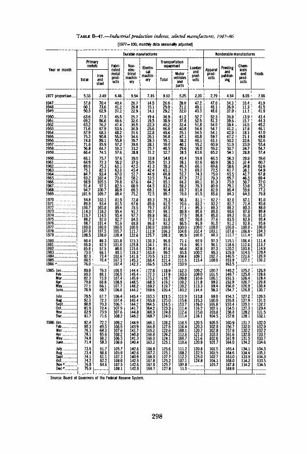
TABLE B-47.—Industrial production indexes, selected manufactures, 1947-86

[1977=100; monthly data seasonally adjusted]

Year or month

1977 proportion

19471948 .194919501951. .19521953195419551956195719581959I9601961196219631964 .. . .1965196619671968196919701971197219731974197519761977197819791980198119821983198419851986 '1985: Jan . .

FebMarAprMayJuneJulyAugSeptOct .NovDec

1986: Jan ..FebMar

MayJuneJulyAugSeptOctNovDec*

Durable manufactures

Primarymetals

Total

5.33

57.860.150.563.669.263.271.657.975.374.871.656.866.466.164.969.675.184.793.298.991.494.7

101.994.8899

100.7114.3110.788.298.7

100.0107.0108.590.495.065.873.082.380.576.080.980.282.379.877.178.978.582.380.881.982.981.782.480.376.378.174.871.473.673.474.174.276.875.9

Ironandsteel

3.49

70.473.662.977.586.676.287.968.390.889.185.964.774.575.772.375.382.193.4

102.4105.597.5

100.7109.7102.1934

103.8118.2114.592.0

101.4100.0107.5108.086.392.557.566.173.470.4

70.369.173.969.866.168.767.772.370.372.473.971.672.269.564.365.660.258.361.760.861.162.264.6

Fabri-catedmetalprod-ucts

6.46

40.441.237.245.548.647.453.548.255.055.857.251.357.657.656.261.163.167.073.678.882.586.988.481.981589.499.495.482.791.6

100.0105.7109.4101.8101.686.689.1

102.6107.3107.4106.5106.5107.4108.9107.7106.6106.4107.4106.7107.9107.6108.2109.2108.5107.6108.2106.5106.6105.7105.9107.3108.0107.5108.1

Non-elec-trical

machin-ery

9.54

26.726.822.925.732.635.536.931.634.639.739.633.238.839.037.942.545.451.758.267.668.969.575.272.867678.591.797.784.588.8

100.0111.7122.6123.3129.8115.6118.3141.8145.3142.3144.4145.4145.9148.5148.2144.2145.4145.4144.2141.7144.8146.2144.9143.9141.7140.8141.3140.4142.6142.6140.9142.9142.6142.9

Electri-cal

machin-ery

7.15

14.515.114.119.419.522.325.622.826.128.328.125.731.233.835.941.342.444.953.564.264.568.172.569.369679.790.789.877.286.8

100.0112.9125.7130.3134.1128.4143.8170.5168.4166.5172.8172.3173.2168.3169.2169.6165.5165.8164.5164.2166.9168.7166.1164.8165.2166.8166.0163.2166.8167.2166.9167.8167.9169.7

Transportationequipment

Total

9.13

26.629.029.234.938.945.256.849.456.855.159.046.552.754.651.359.365.166.879.485.183.290.489.775.381587.099.190.181.092.2

100.0106.3108.396.995.187.699.2

112.2121.4125.9118.9117.9118.7119.2119.7120.4121.5125.0124.5123.3124.8124.0128.2127.5122.6126.2124.1125.1125.6125.1127.7125.2125.7127.8

Motorvehicles

andparts

5.25

28.831.232.041.237.832.440.835.147.138.240.129.638.543.438.146.351.352.767.366.258.269.770.056.370677.189.877.565.786.5

100.0104.695.971.171.666.885.8

104.4111.5110.9112.3110.0109.8110.2110.2110.2111.9115.6113.7111.4112.6111.4116.5116.4108.1112.6108.7110.6111.2108.2112.2107.1107.811.5

Lumberand

prod-ucts

2.30

47.249.143.352.752.551.854.854.560.860.155.256.063.659.862.666.169.274.377.280.179.381.681.581.183295.395.686.880.891.9

100.0102.4102.092.990.182.8

100.2109.1113.4

109.2109.0110.6111.8113.3114.4113.8115.3116.0116.2115.0116.1120.5120.3120.7121.3121.6120.9120.8122.5125.0124.8

Nondurable manufactures

Apparelprod-ucts

2.79

47.049.148.652.351.354.054.754.159.761.160.959.265.266.566.969.672.575.079.381.380.982.985.682.283288.389.085.077.691.5

100.0103.198.397.396.187.395.3

102.7100.9

100.7101.5100.199.299.498.399.9

100.0101.8102.1103.8104.5105.5102.8102.8103.1102.6101.7102.5102.5102.7104.1105.7

Printingand

publish-ing

4.54

34.336.037.038.839.539.441.242.947.250.251.950.754.156.356.558.661.765.569.775.079.180.484.382.082788.290.689.283.591.2

100.0107.8112.7115.1118.6120.2129.8146.5153.9163.5149.2149.7151.3152.9156.0154.7154.3155.8153.4154.5156.8157.6160.9156.7157.8161.6161.9164.0165.4164.6163.0168.0167.81686

Chem-icalsand

prod-ucts

8.05

10.411.311.113.915.716.517.818.121.122.623.924.728.829.931.434.838.141.746.550.753.059.664.567.171480.387.891.082.992.8

100.0106.8111.4106.4112.6103.8114.0121.6127.1

125.2125.8126.4126.7126.9126.8127.2127.9129.1127.3128.2128.1131.7132.0130.2132.8131.5134.2134.1134.4133.9134.2134.2

Foods

7.96

41.941.541.943.444.345.246.147.049.852.653.454.757.459.060.762.664.967.869.472.075.277.279.881.083.688.089.891.090.495.6

100.0104.3106.7111.4113.7114.9120.4126.9130.2

126.9128.6128.4129.8130.4130.7130.5131.5132.2129.4131.5132.1132.0132.9132.2133.1133.7134.6134.3135.1134.3133.5134.5

Source: Board of Governors of the Federal Reserve System.

298

TABLE B-48.—Capacity utilization rates, 1948-86

[Percent; monthly data seasonally adjusted]

Year or month

19481949

19501951195219531954

195519561957 . . ..19581959

19601961196219631964

1965 . .1966196719681969

1970197119721973 . ..1974

19751976197719781979

19801981198219831984

19851986 p

1985: JanFebMar

N&y!'.!'.'.'.'.'.'.June

JulyAugSeptOctNovDec

1986: JanFebMar

MPary"l""":June

JulyAugSeptOct.Nov"Dec p.

Totalindustry

871874874

80.979084.087983.6

74.178.882484885.2

80979.972.174781.0

804794

80.680.880.880.580.580.4

80.180.680.379.780.380.6

80.980.279.079.579.179.0

79.279.279.079.179.479.6

Total

825742

82.885885.489380 1

87086 183.675081.6

80177381483.5856

89.591 186.787086.7

79.277482.887082.6

72.377.481484284.6

79378.370.374080.5

801798

80.280.280.480.480.380.0

79.980.380.079.480.180.2

80.880.279.179.979.479.3

79.779.779.679.779.980.3

Durablegoods

87.086786.1

76.173379.786281.6

69.674.879482984.1

77976.766.970378.6

782743

78.878.478.878.778.578.0

77.878.477.877.277.978.1

78.411176.577.176.375.7

76.376.276.476.476.576.9

Manufacturing

Non-durablegoods

86.787788.0

83.983587.488.184.2

76.381.484586.185.3

81380.775.579583.4

830854

82.482.882.782.883.082.9

83.183.383.382.783.583.5

84.583.983.084.184.184.7

84.885.084.384.785.085.2

Primaryprocessing

87.3762

88.590284.989.4806

92089484.775483.0

79877.981583.8878

91.091485.386987.7

80.979586.491.385.4

72.279.383186.086.6

77978.167.674281.6

821835

81.581.381.781.981.481.6

82.082.582.582.882.883.0

84.483.682.483.282.982.7

82.983.283.783.784.284.6

Advancedprocessing

800732

79.883485.9893800

84284483174981.1

80577281683.4846

88.891 187.687086.1

78.376181.185181.5

72.676.880583183.5

80078.371.773980.0

79278.1

79.579.679.679.779.879.2

79.079.378.977.978.979.0

79.278.677.478.578.0111

78.478.077.677.977.978.3

Mining

82984687.0

89.087390.291491.1

89.289.789990.390.7

93292.983.477984.0

82175.4

83.083.183.382.882.783.5

81.281.681.780.780.781.1

81.679.477.976.475.574.9

73.573.172.972.873.473.7

Utilities

93293995.6

95.193794.592886.8

84.385.385185.085.6

85484.281.480583.6

83179.9

85.087.084.381.981.781.4

81.681.583.882.682.584.5

82.780.480.180.079.379.2

79.978.878.779.480.380.0

Industrialmaterials

85186888.1

81.880486.091 186.1

73.480.384186.387.1

81181.171.775382.0

80278.5

81.481.381.280.580.180.2

79.779.879.579.179.480.3

80.179.678.578.778.178.0

78.377.978.177.978.578.6

Source: Board of Governors of the Federal Reserve System.

299

TABLE B-49.—New construction activity, 1929-86

[Value put in place, billions of dollars; monthly data at seasonally adjusted annual rates]

Year or month

19291933193919401941194219431944

19451946

New sprips

194719481949 . .

19501951195219531954

19551956195719581959

I960196119621963.

New series

1964

1965.1966196719681969

19701971197219731974

19751976197719781979 .. .

19801981198219831984 . .

1985

Totalnew

construc-tion

10.82.98.28.7

12.014.18.35.3

5.814.3

20.026.126.7

33.635.436.839.141.4

46.547.649.150.055.4

54.756.460.264.8

72.6

78.581.883.593.2

100.5

101.3117.9133.9147.4148.4

143.6161.3187.0224.7250.3

249.0257.8244.4279.2327.2

355.6

Private construction

Total

8.31.24.45.16.23.42.02.2

3.412.1

16.721.420.5

26.726.226.027.929.7

34.834.935.134.639.3

38.939.342.345.5

52.4

56.658.058.165.772.7

73.488.2

103.9115.0110.3

102.9122.4149.1179.0201.5

194.0204.4193.6228.5272.0

292.8

Residentialbuildings '

Total2

3.6.5

2.73.03.51.7.9.8

1.36.2

9.913.112.4

18.115.915.816.618.2

21.920.219.019.824.3

23.023.125.227.9

30.5

30.228.628.734.237.2

35.948.560.765.156.6

51.968.692.5

110.4117.2

101.1100.085.4

126.6155.1

158.8

Newhousing

units

3.0.3

2.32.63.01.4.7.6

.74.8

7.810.510.0

15.613.212.913.414.9

18.216.114.715.419.2

17.317.119.421.7

24.1

23.821.821.526.729.2

27.138.750.154.644.1

36.651.172.786.290.1

70.470.257.795.7

115.1

116.0

Nonresidential buildings and otherconstruction 1

Total

4.7.8

1.72.12.71.71.11.4

2.15.8

6.98.28.0

8.610.310.211.311.5

12.914.716.114.815.1

15.916.217.217.6

21.8

26.329.429.431.635.5

37.539.743.249.953.7

51.053.856.668.684.3

92.9104.4108.2102.0116.8

134.0

Com-mercial 3

1.1.1.3.3.4.2.0.1

.21.2

1.01.41.2

1.41.51.11.82.2

3.23.63.63.63.9

4.24.75.15.0

6.8

8.18.18.09.0

10.7

11.113.015.417.717.6

13.913.715.719.727.1

32.938.041.441.054.9

66.9

Indus-trial

0.9.2.3.4.8.3

'.I

.61.7

1.71.41.0

1.12.12.32.22.0

2.43.13.62.42.1

2.92.82.82.9

3.6

5.16.66.06.06.8

6.55.44.76.27.9

8.07.27.7

11.015.0

13.817.017.312.913.7

15.8

Other4

2.6.5

1.21.31.51.2.9

1.1

1.33.0

4.25.55.9

6.16.76.87.37.2

7.38.09.08.89.0

8.98.79.29.7

11.5

13.114.715.416.617.9

19.921.323.126.028.2

29.133.033.237.942.3

46.249.449.548.148.2

51.3

Public construction

Total

2.51.63.83.65.8

10.76.33.1

2.42.2

3.34.76.3

6.99.3

10.811.211.7

11.712.714.115.516.1

15.917.117.919.4

20.2

21.923.825.427.427.8

27.929.730.032.338.1

40.738.937.945.648.8

55.053.350.850.755.2

62.8

Federal

0.2

'.B1.23.89.35.62.5

1.7.9

.81.21.5

1.63.04.24.13.4

2.82.73.03.43.7

3.63.93.94.0

3.7

3.93.83.33.23.2

3.13.84.24.75.1

6.16.87.18.18.6

9.610.410.010.611.2

12.4

State andlocal5

2.31.13.12.42.01.3.7.6

.71.4

2.53.54.8

5.26.36.67.18.3

8.910.011.112.112.3

12.213.314.015.4

16.5

18.020.022.124.224.6

24.825.925.827.633.0

34.632.130.937.540.2

45.442.940.840.244.0

50.4

See next page for continuation of table.

300

TABLE B-49.—New construction activity, 1929-86—Continued

[Value put in place, billions of dollars; monthly data at seasonally adjusted annual rates]

Year or month

1985- JanFebMarAprMay ...June

JulyAugSeptOctNovDec

1986- JanFebMar .AprMay::::::::::::::::June

July .AugSeptOctNov"

Totalnew

construc-tion

343.6344.8352.7350.1352.0352.9

355.1353.3361.3374.0357.6365.6

373.4373.9368.0373.9374.5375.4

380.7382.6382.6379.7377.0

Private construction

Total

285.3287.7291.9289.3287.6288.4

290.3289.8296.0312.0294.4300.6

305.4305.7298.9303.3302.6304.6

309.0310.2308.6307.7306.2

Residentialbuildings1

Total2

159.4158.0161.0154.7151.6154.3

156.8154.9161.0174.8158.2161.8

163.4164.7165.6170.5172.5174.5

178.8178.8178.5178.6178.0

Newhousing

units

114.3114.7116.0115.6115.2115.4

115.3115.5116.1117.2117.5118.7

122.8124.7126.5129.4132.4135.2

136.6137.8138.5139.5139.5

Nonresidential buildings and otherconstruction l

Total

125.8129.7130.9134.6136.0134.1

133.5134.9135.0137.1136.2138.8

142.0141.0133.2132.8130.1130.1

130.2131.4130.1129.1128.2

Com-mercial3

63.264.866.166.967.365.7

64.966.868.568.268.971.7

72.671.168.167.365.165.3

66.468.566.164.864.4

Indus-trial

15.715.415.416.016.215.0

15.815.315.815.916.116.5

15.816.413.414.613.713.0

12.912.513.212.912.7

Other*

47.049.549.451.752.553.4

52.852.850.753.051.250.6

53.553.551.851.051.351.8

50.950.350.951.451.2

Public construction

Total

58.357.260.860.864.464.5

64.863.565.362.163.264.9

68.068.369.270.671.970.8

71.772.474.071.970.7

Federal

11.811.012.311.312.913.1

13.512.414.111.012.412.6

12.912.811.912.712.612.4

11.912.014.311.711.6

State andlocal5

46.646.248.549.551.551.4

51.351.151.351.050.852.3

55.155.557.257.959.358.4

59.860.459.760.359.1

1 Beginning 1960, farm residential buildings included in residential buildings; prior to 1960, included in nonresidential buildings andother construction.

2 Includes residential improvements, not shown separately. Prior to 1964, also includes nonhousekeeping units (hotels, motels, etc.)3 Office buildings, warehouses, stores, restaurants, garages, etc., and, beginning 1964, hotels and motels; prior to 1964 hotels and

motels are included in total residential.4 Religious, educational, hospital and institutional, miscellaneous nonresidential, farm (see also footnote 1), public utilities, and all

other private.5 Includes Federal grants-in-aid for State and local projects.

Source: Department of Commerce, Bureau of the Census.

301

TABLE B-50.—New housing units started and authorized, 1959-86

[Thousands of units]

Year or month

1959

19601961196219631964

19651966196719681969

19701971197219731974

19751976197719781979

19801981198219831984

19851986".

1985: JanFebMarAprMay::::::::::::;:::'::June

JulyAug ..SeptOctNov. .Dec

1986- Jan.. .FebMarAprMayJune

JulyAugSeptOctNovDecp

New housing units started

Private and public l

Total(farm andnonfarm)

1,553.7

1,296.11,365.01,492.51,634.91,561.0

1,509.71,195.81,321.91,545.41,499.5

1,469.02,084.52,378.52,057.51,352.5

1,171.41,547.6

1 2,001.72,036.11,760.0

1,312.61,100.31,072.11,712.51,755.8

1,745.01,808.3

105.495.8

145.2176.0170.5163.4

161.0161.1148.6173.2124.1120.5

115.9107.2151.1188.3186.8183.6

172.2163.8154.3154.9115.9114.1

Nonfarm

1,53

1,271,331,461,611,53

1,481,171,291,521,48

1.3

4.06.88.74.84.0

7.52.88.81.42.3

))

)

!

3

3

3

3

:;

3

3

3

3

3

3

3

3

( 3

Private (farm and nonfarm) l

Total

1,517.0

1,252.21,313.01,462.91,603.21,528.8

1,472.81,164.91,291.61,507.61,466.8

1,433.62,052.22,356.62,045.31,337.7

1,160.41,537.51,987.12,020.31,745.1

1,292.21,084.21,062.21,703.01,749.5

1,741.81,806.6

Type of structure

1 unit

1,234.0

994.7974.3991.4

1,012.4970.5

963.7778.6843.9899.4810.6

812.91,151.01,309.21,132.0

888.1

892.21,162.41,450.91,433.31,194.1

852.2705.4662.6

1,067.61,084.2

1,072.41,179.4

2 to 4units

283.0

2533*47]59C

108.4

86.661.171.680.985.0

84.8120.3141.3118.368.1

64.085.9

121.7125.0122.0

109.591.180.0

113.5121.4

93.483.7

5 unitsor more

'.41.7.5

).8450.0

422.5325.1376.1527.3571.2

535.9780.9906.2795.0381.6

204.3289.2414.4462.0429.0

330.5287.7319.6522.0544.0

576.1543.6

New private housing units authorized 2

Total

1,208.3

998.01,064.21,186.61,334.71,285.8

1,239.8971.9

1,141.01,353.41,323.7

1,351.51,924.62,218.91,819.51,074.4

939.21,296.21,690.01,800.51,551.8

1,190.6985.5

1,000.51,605.21,681.8

1,733.31,759.3

Type of structure

1 unit

938.3

746.1722.8716.2750.2720.1

709.9563.2650.6694.7625.9

646.8906.1

1,033.1882.1643.8

675.5893.6

1,126.11,182.6

981.5

710.4564.3546.4901.5922.4

956.61,073.6

2 t o 4units

77.1

64.667.687.1

118.9100.8

84.861.073.084.385.2

88.1132.9148.6117.064.3

63.993.1

121.3130.6125.4

114.5101.888.3

133.6142.6

120.1110.2

5 unitsor more

192.9

187.4273.8383.3465.6464.9

445.1347.7417.5574.4612.7

616.7885.7

1,037.2820.5366.2

199.8309.5442.7487.3444.8

365.7319.4365.8570.1616.8

656.6575.5

Seasonally adjusted annual rates

1,8041,6321,8491,8511,6841,693

1,6731,7371,6531,7841,6541,882

2,0342,0011,9602,0191,8531,852

1,7821,7951,6641,6281,5851,802

1,0391,1111,1471,1291,0411,036

1,0681,0711,0061,1181,0061,098

1,3351,2021,2211,2421,2411,230

1,1371,1861,1021,0851,0871,209

10596

10310610595

869785807683

10711584798380

8189598267

100

660425599616538562

519569562586572701

592684655698529542

564520503461431493

1,6401,6961,7541,6941,7271,717

1,7091,7821,8461,7031,6681,839

1,8611,8081,8341,8851,7881,792

1,7591,6731,6031,5651,6131,893

903976995940926958

961990956984932963

1,0601,0331,0431,1391,0921,121

1,0931,0391,0471,006

9911,144

131108139118127124

115123128109107114

127122107117118108

10310897

10392

115

606612620636674635

633669762610629762

674653684629578563

563526459456530634

1 Units in structures built by private developers for sale upon completion to local public housing authorities under the Department ofHousing and Urban Development "Turnkey" program are classified as private housing. Military housing starts, including those financedwith mortgages insured by FHA under Section 803 of the National Housing Act, are included in publicly owned starts and excluded fromtotal private starts.2 Authorized by issuance of local building permit: in 17,000 permit-issuing places beginning 1984; in 16,000 places for 1978-83; in14,000 places for 1972-77; in 13,000 places for 1967-71; in 12,000 places for 1963-66; and in 10,000 places prior to 1963.3 Not available separately beginning January 1970.

Source: Department of Commerce, Bureau of the Census.

302

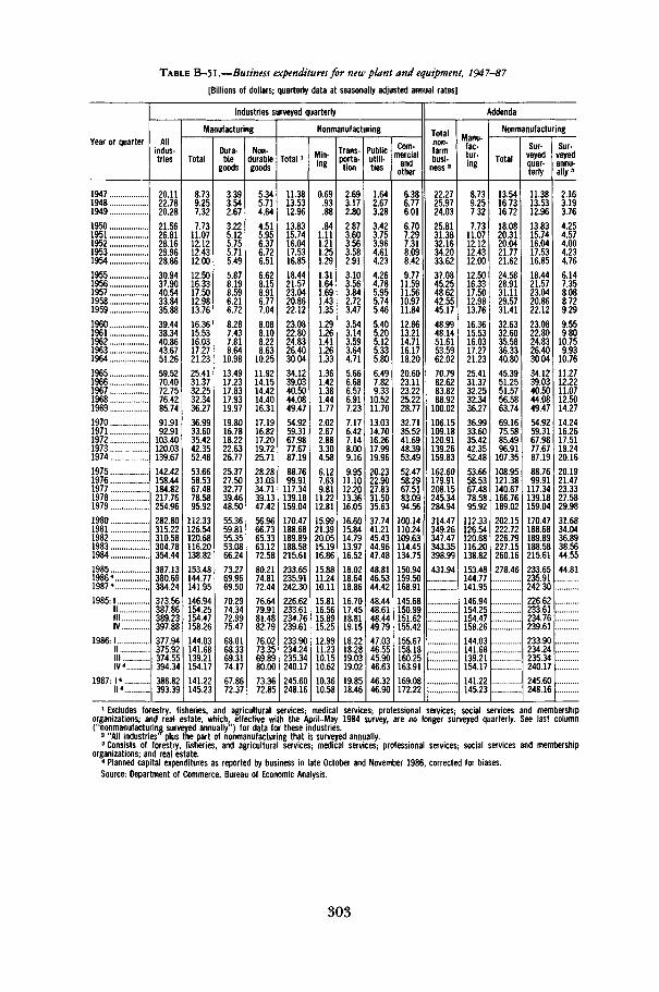
TABLE B-51.—Business expenditures for new plant and equipment, 1947-87

[Billions of dollars; quarterly data at seasonally adjusted annual rates]

Year or quarter

194719481949

19501951195219531954

19551956195719581959

19601961196219631964

19651966196719681969

19701971197219731974

19751976197719781979

19801981198219831984

19851986 4

1987 4

1985- 1I IIllIV

1986:1III I IIV 4

1987- 1 4I I 4

Industries surveyed quarterly

Allindus-tries

20.1122.7820.28

21.5626.8128.1629.9628.86

30.9437.9040.5433.8435.88

39.4438.3440.8643.6751.26

59.5270.4072.7576.4285.74

91.9192.91

103.40120.03139.67

142.42158.44184.82217.76254.96

282.80315.22310.58304.78354.44

387.13380.69384.24

373.56387.86389.23397.88377.94375.92374.55394.34

386.82393.39

Manufacturing

Total

8.739.257.32

7.7311.0712.1212.4312.00

12.5016.3317.5012.9813.76

16.3615.5316.0317.2721.23

25.4131.3732.2532.3436.27

36.9933.6035.4242.3552.48

53.6658.5367.4878.5895.92

112.33126.54120.68116.20138.82

153.48144.77141.95146.94154.25154.47158.26

144.03141.68139.21154.17

141.22145.23

Dura-ble

goods

3.393.542.67

3.225.125.755.715.49

5.878.198.596.216.72

8.287.437.818.64

10.98

13.4917.2317.8317.9319.97

19.8016.7818.2222.6326.77

25.3727.5032.7739.4648.50

55.3659.8155.3553.0866.24

73.2769.9669.50

70.2974.3472.9975.47

68.0168.3369.3174.17

67.8672.37

Non-durablegoods

5.345.714.64

4.515.956.376.726.51

6.628.158.916.777.04

8.088.108.228.63

10.25

11.9214.1514.4214.4016.31

17.1916.8217.2019.7225.71

28.2831.0334.7139.1347.42

56.9666.7365.3363.1272.5880.2174.8172.44

76.6479.9181.4882.79

76.0273.3569.8980.00

73.3672.85

Nonmanufacturing

Total »

11.3813.5312.96

13.8315.7416.0417.5316.85

18.4421.5723.0420.8622.12

23.0822.8024.8326.4030.04

34.1239.0340.5044.0849.47

54.9259.3167.9877.6787.19

88.7699.91

117.34139.18159.04

170.47188.68189.89188.58215.61

233.65235.91242.30

226.62233.61234.76239.61

233.90234.24235.34240.17

245.60248.16

Min-ing

0.69.93.88

.841.111.211.251.29

1.311.641.691.431.35

1.291.261.411.261.33

1.361.421.381.441.77

2.022.672.883.304.58

6.127.639.81

11.2212.81

15.9921.3920.0515.1916.86

15.8811.2410.11

15.8116.5615.8915.25

12.9911.2310.1510.62

10.3610.58

Trans-porta-tion

2.693.172.80

2.873.603.563.582.91

3.103.563.842.723.47

3.543.143.593.644.71

5.666.686.576.917.23

7.176.427.148.009.16

9.9511.1012.2013.3616.05

16.6015.8414.7913.9716.52

18.0218.6418.86

16.7017.4518.8119.1518.2218.2819.0319.02

19.8518.46

Publicutili-ties

1.642.673.28

3.423.753.964.614.23

4.264.785.955.745.46

5.405.205.125.335.80

6.497.829.33

10.5211.70

13.0314.7016.2617.9919.96

20.2322.9027.8331.5035.63

37.7441.2145.4344.9647.48

48.8146.5344.42

48.4448.6148.4449.7947.0346.5545.9046.63

46.3246.90

Com-mercial

andother

6.386.776.01

6.707.297.318.098.42

9.7711.5911.5610.9711.84

12.8613.2114.7116.1718.20

20.6023.1123.2225.2228.77

32.7135.5241.6948.3953.49

52.4758.2967.5183.0994.56

100.14110.24109.63114.45134.75150.94159.50168.91

145.68150.99151.62155.42155.67158.18160.25163.91169.08172.22

Addenda

Totalnon-farmbusi-

ness2

22.2725.9724.03

25.8131.3832.1634.2033.62

37.0845.2548.6242.5545.17

48.9948.1451.6153.5962.02

70.7982.6283.8288.92

100.02

106.15109.18120.91139.26159.83

162.60179.91208.15245.34284.94

314.47349.26347.47343.35398.99

431.94

Monu

fac-tur-ing

8.739.257.32

7.7311.0712.1212.4312.00

12.5016.3317.5012.9813.76

16.3615.5316.0317.2721.23

25.4131.3732.2532.3436.27

36.9933.6035.4242.3552.48

53.6658.5367.4878.5895.92

112.33126.54120.68116.20138.82

153.48144.77141.95

14694154.25154.47158.26144.03141.68139.21154.17

141.22145.23

Nonmanufacturing

Total

13.5416.7316.72

18.0820.3120.0421.7721.62

24.5828.9131.1129.5731.41

32.6332.6035.5836.3340.80

45.3951.2551.5756.5863.74

69.1675.5885.4996.91

107.35

108.95121.38140.67166.76189.02

202.15222.72226.79227.15260.16

278.46

Sur-veyedquar-terly

11.3813.5312.96

13.8315.7416.0417.5316.8518.4421.5723.0420.8622.12

23.0822.8024.8326.4030.04

34.1239.0340.5044.0849.47

54.9259.3167.9877.6787.19

88.7699.91

117.34139.18159.04

170.47188.68189.89188.58215.61

233.6523591242.30

226.62233.61234.76239.61233.90234.24235.34240.17

245.60248.16

Sur-veyedannu-ally3

2.163.193.76

4.254.574.004.234.766.147.358.088.729.29

9.559.80

10.759.93

10.76

11.2712.2211.0712.5014.27

14.2416.2617.5119.2420.16

20.1921.4723.3327.5829.98

31.6834.0436.8938.5644.55

44.81

:::::::::::

1 Excludes forestry, fisheries, and agricultural services; medical services; professional services; social services and membershiporganizations; and real estate, which, effective with the April-May 1984 survey, are no longer surveyed quarterly. See last column("nonmanufacturing surveyed annually") for data for these industries.

2 "All industries plus the part of nonmanufacturing that is surveyed annually.3 Consists of forestry, fisheries, and agricultural services; medical services; professional services; social services and membership

organizations; and real estate.4 Planned capital expenditures as reported by business in late October and November 1986, corrected for biases.Source: Department of Commerce, Bureau of Economic Analysis.

303

TABLE B-52.—Manufacturing and trade, sales and inventories, 1948-86

[Amounts in millions of dollars; monthly data seasonally adjusted]

Year or month

194819491950195119521953195419551956 . .195719581959 . ..1960196119621963196419651966196719681969197019711972197319741975197619771978 .. . .19791980198119821983198419851985- Jan. . .

Feb .MarAprMayJuneJuly. . .AugSeptOctNovDec

1986: JanFebMarAprMay. . .JuneJulyAugSeptOctNovDec

Total manufacturing andtrade

Sales ]

35,26033,78838,59643,35644,84047,98746,44351,69454,06355,87954,20159,72960,82761,15965,66268,99573,68280,28387,18790,41998,184105,088107,536116,110130,144153,566177,861182,404204,463230,000260,805298,334328,058356,919344,656368,724410,737424,091415,973418,218420,346423,215424,379418,219421,565428,205427,201426,123431,012432,679431,713426,854420,230428,455421,613425,475427,473429,310442,206435,848437,141

Inven-tories2

52,50749,49759,82270,24272,37776,12273,17579,51687,30489,05287,09392,12994,71395,594101,063105,480111,503120,907136,790144,920155,831169,482177,719187,929202,132233,419286,098288,651318,833351,459399,608451,460494,105528,105509,555520,328575,098583,148576,490578,541578,370578,533577,813580,107580,372579,486579,519581,986582,707583,148584,968585,176588,178588,599586,727588,908591,895590,141588,069591,556590,606

Ratio3

1.421.531.361.551.581.581.601.471.551.591.601.501.561.541.501.491.471.451.471.561.531.551.621.581.491.411.451.571.481.461.441.431.451.441.511.381.341.371.391.381.381.371.361.391.381.351.361.371.351.351.351.371.401.371.391.381.381.371.331.361.35

Manufacturing

Sales1

17,31616,12618,63421,71422,52924,84323,35526,48027,74028,73627,24730,28630,87930,92333,35735,05837,33140,99544,87046,48750,22853,50152,80555,90663,02772,93184,79086,58998,797113,202126,905143,936154,391168,129159,027170,441189,578195,102191,724192,261194,303193,509194,638193,871193,793196,593194,229197,229200,131199,084198,716196,274191.051196432193,068193,642193,294193,305196,281196,202198,232

Inven-tories2

28,54326,32131,07839,30641,13643,94841,61245,06950,64251,87150,24152,94553,78054,88558,18660,04663,40968,18577,95284,66690,61898,203101,653102,656108,237124,626157,792159,935175,195189,214210,509241,100264,281282,645264,909260,682285,709281,884285,785286,146286,171286,049284,900285,678285,036284,688284,030282,444281,993281,884280,357279,236279,571279,358278,352278,410278,613277,473276,574276,007276,588

Ratio3

1.571.751.481.661.781.761.811.621.731.801.841.701.751.741.701.691.641.601.621.761.741.771.901.831.671.581.651.841.691.611.571.571.661.641.731.521.451.461.491.491.471.481.461.471.471.451.461.431.411.421.411.421.461.421.441.441.441.441.411.411.40

Merchant wholesalers

Sales1

6,8086,5147,6958,5978,7829,0528,9939,89310,51310,47510,25711,49111,65611,98812,67413,38214,52915,61116,98719,52020,92622,69424,03126,35029,69538,17347,98946,80350,88556,36466,66979,47293,704102,01396,290100,424113,404114,494113,738114,022114,044115,450115,749110,880113,152115,263114,473113,947115,527116,852115,648113,380112,495114,608109,870112,873114,375114,482117,594117,991117,972

Inven-tories2

7,9577,7069,2849,88610,21010,68610,63711,67813,26012,73012,73913,87914,12014,48814,93616,04817,00018,31720,76524,95526,26828,76232,19935,21038,81645,55657,23956,97264,36572,80186,40599,262113,478118,259118,149120,265131,544135,940131,752132,917133,135132,984133,485134,696134,762134,732134,496135,038134,927135,940136,624136,561137,056137,083137,506138,793139,753139,742139,878139,211138,837

Ratio3

1.131.191.071.161.121.171.181.131.191.231.241.151.221.201.161.151.141.151.151.241.231.211.261.271.241.111.071.211.191.211.201.181.141.131.241.171.121.171.161.171.171.151.151.211.191.171.171.191.171.161.181.201.221.201.251.231.221.221.191.181.18

Retail trade

Sales !

11,13511,14912,26813,04613,52914,09114,09515,32115,81116,66716,69617,95118,29418,24919,63020,55621,82323,67725,33024,41327,03028,89330,70033,85337,42242,46245,08249,01254,78160,43467,23174,92679,96386,77789,33997,858107,755114,495110,511111,935111,999114,256113,992113,468114,620116,349118,499114,947115,354116,743117,349117,200116,684117,715118,675118,960119,804121,523128,331121,655120,937126,255

Inven-tories2

16,00715,47019,46021,05021,03121,48820,92622,76923,40224,45124,11325,30526,81326,22127,94129,38631,09434,40538,07335,29938,94542,51743,86750,06355,07963,23771,06771,74479,27389,444102,694111,098116,346127,201126,497139,381157,845165,324158,953159,478159,064159,500159,428159,733160,574160,066160,993164,504165,787165,324167,987169,379171,551172,158170,869171,705173,529172,926171,617176,338175,181

Ratio3

1.391.411.381.641.521.531.511.431.471.441.431.401.451.431.381.391.401.391.441.431.381.411.411.411.401.401.481.441.381.391.431.441.421.411.411.341.391.401.441.421.421.401.401.411.401.381.361.431.441.421.431.451.471.461.441.441.451.421.341.451.45

1 Monthly average for year and total for month.2 Seasonally adjusted, end of period.3 Inventory/sales ratio. For annual periods, ratio of weighted average inventories to average monthly sales; for monthly data, ratio of

inventories at end of month to sales for month.Note.—Earlier data are not strictly comparable with data beginning 1958 for manufacturing and beginning 1967 for wholesale and

retail trade.The inventory figures in this table do not agree with the estimates of change in business inventories included in the gross national

product since these figures cover only manufacturing and trade rather than all business, and show inventories in terms of current bookvalue without adjustment for revaluation.

Source: Department of Commerce, Bureau of the Census.

304

TABLE B-53.—Manufacturers' shipments and inventories, 1947-86

[Millions of dollars; monthly data seasonally adjusted]

Year ormonth

194719481949 ...195019511952 .19531954195519561957195819591960 ..1961196219631964196519661967196819691970197119721973197419751976 . ..1977197819791980198119821983198419851985: Jan

FebMar

May"!'.;;June....JulyAugSept....OctNovDec

1986: JanFebMar

May"!!June-July....Aug....Sept...OctNov....

Shipments l

Total

15,51317,31616,12618,63421,71422,52924,84323,35526,48027,74028,73627,24730,28630,87930,92333,35735,05837,33140,99544,87046,48750,22853,50152,80555,90663,02772,93184,79086,58998,797113,202126,905143,936154,391168,129159,027170,441189,578195,102191,724192,261194,303193,509194,638193,871193,793196,593194,229197,229200,131199,084198,716196,274191,051196,132193,068193,642193,294193,305196,281196,202198,232

Dura-ble

goodsindus-tries

6,6947,5797,1918,84510,49311,31313,34911,82814,07114,71515,23713,56315,60915,88315,61617,26218,28019,63722,22124,64925,26727,65929,43728,18829,95434,02739,68144,23043,65950,70059,26767,84876,06077,55083,87276,69384,95198,502103,649101,966101,724102,116102,068102,718102,657102,478105,311103,656106,479107,007105,777105,631105,545102,693106,592103,672104,553104,980104,154106,027107,443107,185

Non-durablegoodsindus-tries

8,8199,7388,9359,78911,22111,21611,49411,52712,40913,02513,49913,68414,67714,99615,30716,09516,77817,69418,77420,22021,22022,57024,06424,61725,95229,00033,25040,56042,93148,09753,93559,05767,87676,84184,25782,33485,49191,07691,45289,75890,53792,18791,44191,92091,21491,31591,28290,57390,75093,12493,30793,08590,72988,35889,54089,39689,08988,31489,15190,25488,75991,047

Inventories2

Total

25,89728,54326,32131,07839,30641,13643,94841,61245,06950,64251,87150,24152,94553,78054,88558,18660,04663,40968,18577,95284,66690,61898,203101,653102,656108,237124,626157,792159,935175,195189,214210,509241,100264,281282,645264,909260,682285,709281,884285,785286,146286,171286,049284,900285,678285,036284,688284,030282,444281,993281,884280,357279,236279,571279,358278,352278,410278,613277,473276,574276,007276,588

Durable goods industries

Total

13,06114,66213,06015,53920,99123,73125,87823,71026,40530,44731,72830,25832,07732,37132,54434,63235,86638,50642,25749,92055,00558,87564,73966,78066,28970,25081,398101,739102,874112,581121,601137,891160,533174,620186,347175,103171,629191,109189,164192,153192,030192,355192,475191,546192,239192,163192,037191,930190,508190,284189,164188,518187,644188,333188,031187,637187,148186,858186,045186,102185,358185,742

Mate-rialsand

supplies

8,9667,8949,19410,41710,60810,03210,77610,35310,27910,81011,06811,97013,32515,48916,45517,37618,69319,18219,75920,86026,02835,15133,92037,54840,25145,25252,68755,12157,92752,45451,60456,46953,52756,03355,76855,44555,63854,69354,71454,25754,21753,84453,64452,99953,52752,31751,92151,68851,86451,38751,55951,33850,87851,05250,56150,530

Workin

proc-ess

10,7209,72110,75612,31712,83712,38713,06312,77213,20314,15914,87116,19118,07521,93925,00527,33630,40829,84828,65030,78835,54542,60343,36946,34550,62058,63469,25476,99781,10577,81377,46388,10589,91288,67288,96789,68489,53789,65490,30691,38391,47392,18191,07291,02089,91290,47790,12591,23690,82590,71490,91890,51890,67390,89890,50790,030

Finishedgoods

6,2066,0406,3487,5658,1257,8398,2399,2459,0639,6629,92510,34410,85412,49113,54714,16315,63917,75117,88018,60119,82323,98525,58628,69030,73034,00538,59242,50247,31544,83642,56246,53545,72547,44847,29547,22647,30047,19947,21946,52346,34745,90545,79246,26545,72545,72445,59845,40945,34245,53644,67145,00244,49444,15244,29045,182

Nondurable goods industries

Total

12,83613,88113,26115,53918,3151740518,07017,90218,66420,19520,14319,98320,86821,40922,34123,55424,18024,90325,92828,03229,65931,74333,46334,87136,36837,98843,23056,05357,06062,61267,61372,61880,56789,66196,29889,80689,05394,60092,72093,63294,11693,81693,57493,35493,43992,87392,65192,10091,93691,70992,72091,83991,59291,23891,32790,71591,26291,75591,42890,47290,64990,846

Mate-rialsand

supplies

8,3178,1678,5568,9718,7758,6629,0809,0829,4939,8139,97810,13110,44811,15511,71512,28912,72413,15013,68314,67618,13223,69923,54225,83327,39829,31732,45136,20637,75835,16536,17036,63535,50336,73136,91436,40036,39936,10736,44835,91735,97435,43335,53935,05135,50335,50035,46235,11035,07834,88935,28935,68535,68435,36735,58035,457

Workin

proc-ess

2,4722,4402,5712,7212,8642,8282,9442,9463,1103,2963,4063,5113,8064,2044,4214,8485,1225,2745,6655,9826,7078,1758,8379,93311,00311,90713,74115,73216,07414,30814,48014,81114,56814,65614,64214,52414,35114,31814,33614,21614,16114,31014,60714,68014,56814,15014,19813,92113,79013,69713,93813,78813,50413,73713,90513,954

Finishedgoods

7,4097,4157,6668,6228,6248,4918,8459,3809,73810,44410,79611,26111,67412,67313,52314,60615,61716,44817,01917,33018,39124,17924,68126,84629,21231,39434,37537,72342,46640,33338,40343,15442,64942,24542,56042,89242,82442,92942,65542,74042,51642,35741,79041,97842,64942,18941,93242,20742,45942,12942,03542,28242,24041,36841,16441,435

1 Monthly average for year and total for month.2 Book value, seasonally adjusted, end of period.Note.—Data beginning 1958 are not strictly comparable with earlier data.Source: Department of Commerce, Bureau of the Census.

305

TABLE B-54.—Manufacturers' new and unfilled orders, 1947-86

[Amounts in millions of dollars; monthly data seasonally adjusted]

Year or month

194719481949195019511952195319541955195619571958195919601961196219631964196519661967196819691970197119721973197419751976197719781979198019811982.198319841985. ..1985: Jan

FebMarAprMayJuneJulyAugSeptOctNovDec

1986- JanFebMarAprMayJuneJulyAugsept::....::....:.:OctNov

New orders *

Total

15,25617,69315,61420,11023,90723,20423,58622,33527,46528,36827,55927,00230,72430,23531,10433,43635,52438,35742,10046,40247,05650,68753,95052,03855,98364,16776,05687,24485,22099,532115,032131,546147,403156,161167,752157,255173,259191,634195,803195,210193,057191,532191,081195,019198,261195,793198,782197,332195,381196,865201,213201,133198,559192,996193,151192,122191,795194,560192,836199,399192,502200,421

Durable goodsindustries

Total

6,3888,1266,63310,16512,84112,06112,14710,76814,99615,36514,11113,29016,00315,30315,75917,37418,70920,65223,27826,17725,82528,11629,87127,38829,99835,06442,72646,83542,09951,40361,08272,33979,45179,36083,55374,99687,631100,611104,305105,447102,46799,54499,839102,971106,780104,370107,661106,641104,495103,796107,531108,194107,545104,682103,747102,624102,730106,220103,845108,723103,569109,273

Capitalgoodsindus-tries,non-

defense

6,9037,6606,7387,4448,62210,97112,67311,01112,79115,29119,45823,23123,25924,05020,68122,76427,01727,21523,63329,49327,20625,46125,59427,98426,68527,55429,24027,09225,78830,56624,28828,63726,54026,17926,14526,42127,38726,32528,22226,91228,647

Non-durablegoods

industries

8,8689,5668,9819,94511,06611,14311,43911,56612,46913,00313,44813,71214,72014,93215,34516,06116,81517,70518,82320,22521,23122,57124,07924,65025,98629,10433,33040,40943,12248,12953,95059,20767,95376,80184,19982,26085,62791,02491,49989,76390,59091,98891,24292,04891,48191,42391,12190,69190,88693,06993,68292,93991,01488,31489,40489,49889,06588,34088,99190,67688,93391,148

Unfilled orders2

Total

34,47330,73624,04541,45667,26675,85761,17848,26660,00467,37553,18347,37052,73245,08047,40748,57754,32766,88280,07198,401104,547109,926115,422106,158107,147121,061158,884188,467172,037180,562203,475259,770302,145323,393319,094296,918330,924355,640363,809359,125359,926357,151354,731355,112359,502361,502363,691366,794364,946361,680363,809366,226368,511370,456367,475366,529364,682365,948365,479368,597364,897367,086

Durablegoods

industries

28,57926,61919,62235,43563,39472,68058,63745,25056,24163,88050,35244,55949,37342,51444,37545,96551,27063,69176,29894,575100,576105,950111,250101,566102,119114,725151,504182,925164,139172,273195,008249,483290,921312,648309,066287,796320,123345,443353,036348,924349,671347,096344,874345,127349,250351,142353,492356,477354,493351,282353,036355,599357,599359,588356,743355,695353,872355,112354,803357,499353,625355,713

Non-durablegoods

industries

5,8944,1174,4236,0213,8723,1772,5413,0163,7633,4952,8312,8113,3592,5663,0322,6123,0573,1913,7733,8263,9713,9764,1724,5925,0276,3367,3805,5427,8988,2888,46710,28711,22410,74510,0289,12210,80110,19710,77310,20110,25510,0559,8579,98510,25210,36010,19910,31710,45310,39810,77310,62710,91210,86810,73210,83410,81010,83610,67611,09811,27211,373

Unfilled orders— shipmentsratio3

Total

3.423.633.873.353.093.012.782.632.692.803.103.333.813.703.853.753.653.383.313.864.133.763.303.273.593.883.813.773.763.383.363.333.473.473.403.403.383.393.413.413.473.373.323.333.433.433.503.393.463.363.383.413.363.313.30

Durablegoods

industries

4.124.274.554.003.693.543.373.133.243.373.723.954.554.404.654.504.394.063.904.564.964.523.943.894.224.614.554.574.654.104.064.044.234.214.144.124.124.114.144.114.224.064.004.044.204.174.274.144.234.134.144.194.154.054.04

Non-durablegoodsindus-tries

0.961.121.04.85.86.94.72.79.68.73.72.80.76.73.69.69.77.77.88.93.64.84.76.70.78.76.67.59.53.55.49.50.49.50.48.48.47.49.49.49.48.50.49.50.48.50.50.49.50.47.48.47.48.49.49

1 Monthly average for year and total for month.2 Seasonally adjusted, end of period.3 Ratio of unfilled orders at end of period to shipments for period; excludes industries with no unfilled orders. Annual figures relate

to seasonally adjusted data for December.Note.—Data beginning 1958 are not strictly comparable with earlier data.Source: Department of Commerce, Bureau of the Census.

306

PRICES

TABLE B-55.—Consumer price indexes, major expenditure classes, 1946-86

[1967=100]

Year ormonth

194619471948194919501951195219531954195519561957195819591960 .19611962 ..1963196419651966196719681969....197019711972197319741975197619771978197919801981198219831984 .198519861985: Jan

FebMar

fezJuneJulyAugSeptOctNovDec

1986: JanFebMar

fezJuneJulyAugSeptOctNovDec

Allitems

58.566.972.171.472.177.879.580.180.580.281.484.386.687.388.789.690.691.792.994.597.2

100.0104.2109.8116.3121.3125.3133.1147.7161.2170.5181.5195.4217.4246.8272.4289.1298.4311.1322.2328.4316.1317.4318.8320.1321.3322.3322.8323.5324.5325.5326.6327.4328.4327.5326.0325.3326.3327.9328.0328.6330.2330.5330.8331.1

Foodbever

Total »

•••"•"••••

'"iboio"103.6108.8114.7118.3123.2139.5158.7172.1177.4188.0206.3228.5248.0267.3278.2284.4295.1302.0311.8299.3301.4301.6301.6301.0301.4301.6301.8302.1302.5303.6305.6307.9307.7307.8308.5309.4309.5312.2314.6315.1315.6316.4317.0

andages

Food

58.170.676.673.574.582.884.383.082.881.682.284.988.587.188.089.189.991.292.494.499.1

100.0103.6108.9114.9118.4123.5141.4161.7175.4180.8192.2211.4234.5254.6274.6285.7291.7302.9309.8319.7307.3309.5309.7309.6308.9309.3309.5309.7309.9309.8311.0313.2315.6315.3315.4316.1317.0317.1320.1322.7323.2323.7324.6325.0

Housing

Total2

60.665.269.870.972.877.278.780.881.782.383.686.287.788.690.290.991.792.793.894.997.2

100.0104.0110.4118.2123.4128.1133.7148.8164.5174.6186.5202.8227.6263.3293.5314.7323.1336.5349.9360.2342.0343.6344.7345.9348.5350.4351.6352.9353.8354.4355.0355.8356.8356.5357.0358.0358.5361.2361.5362.4363.7363.0361.7362.1

Shelter

76.578.279.180.483.485.186.087.888.589.690.792.293.896.8

100.0104.8113.3123.6128.8134.5140.7154.4169.7179.0191.1210.4239.7281.7314.7337.0344.8361.7382.0402.9371.2373.3374.3375.9379.5381.0383.2385.9386.9389.1391.3392.3393.8394.8397.0400.1400.9401.6403.5405.2407.6409.5410.2410.4

Fuel andother

utilities3

83.083.585.187.389.991.793.895.997.197.398.298.498.398.8

100.0101.3103.6107.6115.0120.1126.9150.2167.8182.7202.2216.0239.3278.6319.2350.8370.3387.3393.6384.7387.2386.5388.2388.7393.0399.4399.9398.9400.5395.6392.1393.3394.6390.0385.5381.8382.5393.8389.4389.5388.3379.1371.1371.0

House-hold

furnish-ingsand

oper-ation2

91.390.989.989.991.992.393.193.893.793.894.695.095.397.0

100.0103.8107.7111.5115.7118.3121.6135.3151.0160.1167.5177.7190.3205.4221.3233.2238.5242.5247.2250.4244.2246.2246.9247.9247.6247.1246.5247.0247.1248.4248.9248.8248.8249.0249.8249.6249.9250.2250.5250.5251.5251.6251.2252.4

Appareland

upkeep

67.578.283.380.179.086.185.384.684.584.185.887.387.588.289.690.490.991.992.793.796.1

100.0105.4111.5116.1119.8122.3126.8136.2142.3147.6154.2159.6166.6178.4186.9191.8196.5200.2206.0207.8199.8201.8205.3205.9205.3204.6202.8205.3209.6211.1211.2209.0205.0204.1206.3207.3206.4204.5203.2207.0212.1213.2213.1210.9

Trans-portation

50.355.561.866.468.272.577.379.578.377.478.883.386.089.689.690.692.593.094.395.997.2

100.0103.2107.2112.7118.6119.9123.8137.7150.6165.5177.2185.5212.0249.7280.0291.5298.4311.7319.9307.5314.7314.3316.7320.0321.4321.8321.8320.7319.7320.9323.2324.0323.9319.2309.6303.3305.7308.6304.7301.3302.2302.6304.3304.8

Medicalcare

44.448.151.152.753.756.359.361.463.464.867.269.973.276.479.181.483.585.687.389.593.4

100.0106.1113.4120.6128.4132.5137.7150.5168.6184.7202.4219.4239.7265.9294.5328.7357.3379.5403.1433.5391.1393.8396.5398.0399.5401.7404.0406.6408.3410.5413.0414.7418.2422.3425.8428.0429.7432.0434.8437.5439.7442.3444.6446.8

Enter-ainment

100.0105.7111.0116.7122.9126.5130.0139.8152.2159.8167.7176.6188.5205.3221.4235.8246.0255.1265.0274.1261.0261.3262.2263.3263.6264.8265.7265.7266.8268.4269.0268.3270.8272.0271.9272.3272.9273.9274.4274.7275.3276.5277.4277.4

Othergoods

andservices

100.0105.2110.4116.8122.4127.5132.5142.0153.9162.7172.2183.3196.7214.5235.7259.9288.3307.7326.6346.4319.1320.5321.1321.8322.3323.0325.0326.0333.3334.9335.3336.5339.1340.3341.1341.8342.1342.6344.9346.4353.3354.6354.9355.2

Ener-gy 3

90.190.391.894.294.494.795.094.696.397.8

100.0101.5104.2107.0111.2114.3123.5159.7176.6189.3207.3220.4275.9361.1410.0416.1419.3423.6426.5370.3414.5411.4416.6424.4431.7436.8437.1433.8432.6427.1425.1426.5424.7408.9381.3361.8367.6380.6366.5358.6360.6348.6341.7342.4

1 Includes alcoholic beverages, not shown separately.2 Series beginning 1967 not comparable with series for earlier years.3 See Tables B-56 and B-57.Note.—Data beginning 1978 are for all urban consumers; earlier data are for urban wage earners and clerical workers.Data beginning 1983 incorporate a rental equivalence measure for homeowners' costs and therefore are not strictly comparable with

earlier figures.Source: Department of Labor, Bureau of Labor Statistics.

307

TABLE B-56.—Consumer price indexes, selected expenditure classes, 1946-86

[1967 = 100]

Year or month

194619471948 .. . .19491950195119521953 .19541955195619571958 .. .19591960196119621963196419651966196719681969197019711972197319741975197619771978197919801981198219831984198519861985: Jan

Feb .MarMay'""'"""'JuneJulyAugSeptOctNovDec

1986- JanFebMarAprMayJuneJulyAugSeptOctNovDec

Food and beverages

Total »

100.0103.6108.8114.7118.3123.2139.5158.7172.1177.4188.0206.3228.5248.0267.3278.2284.4295.1302.0311.8299.3301.4301.6301.6301.0301.4301.6301.8302.1302.5303.6305.6307.9307.7307.8308.5309.4309.5312.2314.6315.1315.6316.4317.0

Food

Total

58.170.676.673.574.582.884.383.082.881.682.284.988.587.188.089.189.991.292.494.499.1

100.0103.6108.9114.9118.4123.5141.4161.7175.4180.8192.2211.4234.5254.6274.6285.7291.7302.9309.8319.7307.3309.5309.7309.6308.9309.3309.5309.7309.9309.8311.0313.2315.6315.3315.4316.1317.0317.1320.1322.7323.2323.7324.6325.2

Athome

73.579.876.777.686.387.886.285.884.184.487.291.088.889.690.491.092.293.295.5

100.3100.0103.2108.2113.7116.4121.6141.4162.4175.8179.5190.2210.2232.9251.5269.9279.2282.2292.6296.8305.3296.1298.6298.4297.7296.2296.0296.2295.9295.6295.3296.6299.3302.5301.5301.2301.5302.1301.6305.5308.9309.0309.5309.9310.2

Awayfromhome

68.970.170.872.274.977.279.381.483.285.487.388.990.995.1

100.0105.2111.6119.9126.1131.1141.4159.4174.3186.1200.3218.4242.9267.0291.0306.5319.9333.4346.6360.1339.9341.4342.6343.9345.1346.9347.3348.4349.9350.3351.3352.1353.1354.2355.5357.0358.8360.2360.8361.8363.3364.0365.8367.1

Shelter

Total

76.578.279.180.483.485.186.087.888.589.690.792.293.896.8

100.0104.8113.3123.6128.8134.5140.7154.4169.7179.0191.1210.4239.7281.7314.7337.0344.8361.7382.0402.9371.2373.3374.3375.9379.5381.0383.2385.9386.9389.1391.3392.3393.8394.8397.0400.1400.9401.6403.5405.2407.6409.5410.2410.4

Renters' costs

Total

"i03"b"108.6115.4121.9111.8112.4112.9113.5114.5115.1115.8116.6117.0117.9118.4118.3118.8119.0119.6120.9121.1121.6122.5122.9123.6124.0124.3124.2

Rent,resi-

dential

59.261 165.168.070.473.276280.383.284.385.987.589.190.491.792.994.095.095996.9982

100.0102.4105.7110.1115.2119.2124.3130.6137.3144.7153.5164.0176.0191.62082224.0236.9249.3264.6280.0257.1258.4259.2260.4262.6263.6265.0266.6267.7269.9271.7272.4273.4273.7275.0277.9278.4279.4281.2281.7283.2284.6285.6286.0

Home-owners'costs

'"ibis"107.3113.1119.4110.0110.7110.8111.3112.4112.8113.5114.3114.6115.1115.8116.3116.7117.0117.9118.7118.9119.0119.4119.9120.7121.3121.5121.6

Mainte-nanceand

repairs

71.272.474.177280.581.883.284.685.986.587.789.591.395.2

100.0106.1115.0124.0133.7140.7151.0171.6187.6199.6214.7233.0256.4285.7314.4334.1346.3359.2368.9373.8366.0366.8370.0368.0366.2367.6367.8370.6368.7368.5372.7373.7379.1379.6367.5367.6367.1366.6369.2376.4376.2379.0377.1380.0

Fuel and other utilities

Total

83.083.585.187.389.991.793.895.997.197.398.298.498.398.8

100.0101.3103.6107.6115.0120.1126.9150.2167.8182.7202.2216.0239.3278.6319.2350.8370.3387.3393.6384.7387.2386.5388.2388.7393.0399.4399.9398.9400.5395.6392.1393.3394.6390.0385.5381.8382.5393.8389.4389.5388.3379.1371.1371.0

Household fuels

Total

"ib'o'.b"101.4103.4107.9115.3120.1128.4160.7183.8202.3228.6247.4286.4349.4407.0446.2469.2485.5488.1463.1481.2480.8482.2483.0490.0497.7497.3494.4496.8488.4481.5483.6484.7476.3467.6459.6460.6477.0469.2469.0467.2450.3437.8438.1

Fuel oil,coal,and

bottledgas

51.358.468.670.372.776.578081.581.282.385990.388789.889291.091.593.292.794697.0

100.0103.1105.6110.1117.5118.5136.0214.6235.3250.8283.4298.3403.1556.0675.9667.9628.0641.8619.5501.5621.6623.4620.8623.5620.8612.0601.9594.6601.7615.3641.6657.3650.3591.2549.9518.3496.8486.6459.4447.3453.5451.9452.0460.6

Gas(piped)

andelec-

tricity

77.477.179.181.081.281.582684.285.387.588.489.392.494.798.699.499.499.499.499.499.6

100.0100.9102.8107.3114.7120.5126.4145.8169.6189.0213.4232.6257.8301.8345.9393.8428.7445.2452.7446.7444.1443.3445.5445.9454.7465.6467.1465.1466.5453.9440.5439.9442.6444.5442.3439.2444.6466.0462.3464.5461.1441.4426.7425.3

Otherutilities

andpubfic

services

100.0101.2104.0107.4114.7120.6124.1130.3137.1145.4152.0158.3159.5165.2181.0200.2213.7230.2240.7253.1235.3234.3236.3236.4236.8241.1242.8244.2244.6244.7245.9245.8247.3247.9249.0251.3251.5255.2255.6255.9255.6257.1255.4254.9

See next page for continuation of table.

308

TABLE B-56.—Consumer price indexes, selected expenditure classes, 1946-86—Continued

[1967=100]

Year or month

19461947194819491950195119521953195419551956195719581959I960196119621963196419651966196719681969197019711972 .1973197419751976197719781979 . . .19801981198219831984198519861985: Jan

FebMarAprMayJuneJulyAugSeptOctNovDec

1986- Jan .. .FebMarAprMayJuneJulyAug ...SeptCct . .NovD e c . . .

Transportation

Total

50.355.561.866.468.272.577.379.578.377.478.883.386.089.689.690.692.593.094.395.997.2

100.0103.2107.2112.7118.6119.9123.8137.7150.6165.5177.2185.5212.0249.7280.0291.5298.4311.7319.9307.5314.7314.3316.7320.0321.4321.8321.8320.7319.7320.9323.2324.0323.9319.2309.6303.3305.7308.6304.7301.3302.2302.6304.3304.8

Private transportation

Total 2

54.361.568.272.372.575.880.882.480.378,980.184.787.491.190.691.393.093.494.796.397.5

100.0103.0106.5111.1116.6117.5121.5136.6149.8164.6176.6185.0212.3249.2277.5287.5293.9306.6314.2299.5309.1308.7311.0314.6316.0316.3316.1314.9313.6314.7317.0317.8317.3312.2302.1295.3297.8300.8296.5292.8293.7294.1295.8295.9

Newcars

69.275.682.883.487.494.995.894.390.993.598.4

101.5105.9104.5104.5104.1103.5103.2100.999.1

100.0102.8104.4107.6112.0111.0111.1117.5127.6135.7142.9153.8166.0179.3190.2197.6202.6208.5215.2224.4213.1213.9214.1214.1214.5214.7214.7214.6214.5216.2218.4219.4219.9220.4220.3221.2223.0224.2224.7224.7224.5227.1230.7232.2

Usedcars

89.275.971.869.177.480.289.583.686.994.896.0

100.199.497.0

100.0

u£l104.3110.2110.5117.6122.6146.4167.9182.8186.5201.0208.1256.9296.4329.7375.7379.7363.2382.8384.6386.1386.4384.2380.3376.7374.0374.3375.3376.4375.6374.1370.7367.2364.8363.6362.5360.3358.0359.5360.6361.0356.6

Motorfuel3

54.962.270.472.371.873.975.880.382.583.686.590.088.889.992.591.491.991.891.494.997.0

100.0101.4104.7105.6106.3107.6118.1159.9170.8177.9188.2196.3265.6369.1410.9389.4376.4370.7373.8292.1357.6352.4360.6374.2381.6384.7385.5381.9377.7374.6376.7377.5373.3351.5308.5279.5289.3299.4280.2265.9271.1263.2260.9261.9

Auto-mobilemainte-nanceand

repair

52.056459.661 162.367.068672.374.876.579.582.483.785.587.289.390.491.692.894.596.2

100.0105.5112.2120.6129.2135.1142.2156.8176.6189.7203.7220.6242.6268.3293.6315.8330.0341.5351.4363.1346.9348.2348.5348.2349.6350.4351.1351.9353.5355.7355.8357.5357.9358.9359.3360.6361.3362.1363.4364.3365.0365.7368.4370.7

Other

""ibo.b"103.4109.7119.2128.4129.1127.8132.4141.2163.1177.3184.6198.6222.6241.3257.8260.8273.3287.6303.9283.9284.4284.5285.8285.6286.6287.6287.7285.8289.6293.9295.2297.7299.2301.5301.6301.3303.0304.5304.5302.3307.6311.6312.0

Publictranspor-

tation

34.436.040.745.248.954.057.561.365.567.470.072.776.178.381.084.687.488.590.191.995.2

100.0104.6112.7128.5137.7143.4144.8148.0158.6174.2182.4187.8200.3251.6312.0346.0362.6385.2402.8426.4394.5394.4397.3398.0398.4399.3402.4403.7408.0411.5412.8412.9419.6422.2421.2422.2423.7425.4428.0428.0428.5428.7431.7437.5

Medical care

Total

44.448.151.152.753.756.359.361.463.464.867.269.973.276.479.181.483.585.687.389.593.4

100.0106.1113.4120.6128.4132.5137.7150.5168.6184.7202.4219.4239.7265.9294.5328.7357.3379.5403.1433.5391.1393.8396.5398.0399.5401.7404.0406.6408.3410.5413.0414.7418.2422.3425.8428.0429.7432.0434.8437.5439.7442.3444.6446.8

Medicalcarecom-

modities

76.281.886.187.488.591.091.892.693.794.796.799.3

102.8104.4104.5103.3101.7100.8100.5100.2100.5100.0100.2101.3103.6105.4105.6105.9109.6118.8126.0134.1143.5153.8168.1186.5205.7223.3239.7256.7273.6248.2249.8251.9253.9255.2257.0257.8259.3260.2261.3262.7262.9264.5267.4269.4271.3272.3273.3275.4276.0276.7277.5278.2280.8

Medi-cal

careserv-ices

40.143.546.448.149.251.755.057.058.760.462.865.568.772.074.977.780.282.684.687.392.0

100.0107.3116.0124.2133.3138.2144.3159.1179.1197.1216.7235.4258.3287.4318.2356.0387.0410.3435.1468.6422.4425.3428.1429.4430.9433.0435.8438.6440.5443.0445.8448.0451.9456.2460.1462.3464.2466.8469.8473.0475.7478.8481.5483.4

1 Includes alcoholic beverages, not shown separately.2 Includes direct pricing of new trucks and motorcycles, beginning September 1982.3 Includes direct pricing of diesel fuel and gasohol beginning September 1981.4 Not available.Note.—Data beginning 1978 are for all urban consumers; earlier data are for urban wage earners and clerical workers.See also Note, Table B-55.Source: Department of Labor, Bureau of Labor Statistics.

309

TABLE B-57.—Consumer price indexes, commodities, services, and special groups, 1940-86

[1967=100]

Year ormonth

19401941194219431944194519461947 ... .194819491950... .19511952195319541955 . .1956195719581959196019611962196319641965196619671968196919701971197219731974. ..1975197619771978197919801981198219831984198519861985: Jan

FebMar....AprMay....June-July....Aug....Sept..Oct....Nov...Dec...

1986: Jan....Feb....Mar...Apr....May-June. .July...Aug...Sept..Oct....Nov...Dec...

Allitems

42.044.148.851.852.753.958.566.972.171.472.177.879.580.180.580.281.484.386.687.388.789.690.691.792.994.597.2

100.0104.2109.8116.3121.3125.3133.1147.7161.2170.5181.5195.4217.4246.8272.4289.1298.4311.1322.2328.4316.1317.4318.8320.1321.3322.3322.8323.5324.5325.5326.6327.4328.4327.5326.0325.3326.3327.9328.0328.6•'30.2330.5330.8331.1

Commodities

Allcom-

modities

40.643.349.654.054.756.362.475.080.478.378.885.987.086.785.985.185.988.690.690.791.592.092.893.694.695.798.2

100.0103.7108.4113.5117.4120.9129.9145.5158.4165.2174.7187.1208.4233.9253.6263.8271.5280.7286.7283.9282.7284.0285.3286.8287.0286.9286.5286.5287.1287.9289.2289.9290.1287.4283.7281.2282.1282.8281.9281.9283.5283.6284.0284.2

Food

35.238.445.150.349.650.758.170.676.673.574.582.884.383.082.881.682.284.988.587.188.089.189.991.292.494.499.1

100.0103.6108.9114.9118.4123.5141.4161.7175.4180.8192.2211.4234.5254.6274.6285.7291.7302.9309.8319.7307.3309.5309.7309.6308.9309.3309.5309.7309.9309.8311.0313.2315.6315.3315.4316.1317.0317.1320.1322.7323.2323.7324.6325.2

Commodities less food

All

48.050.456.058.461.664.168.176.882.781.581.487.588.388.587.586.987.890.591.592.793.193.494.194.895.696.297.5

100.0103.7108.1112.5116.8119.4123.5136.6149.1156.6165.1174.7195.1222.0241.2250.9259.0267.0272.5263.4267.8268.6270.6272.8273.4273.1272.4272.3273.1274.4275.7275.7274.7270.9265.2261.2262.1263.0260.2259.0261.1260.9261.2261.2

Durable

48.151.458.460.365.970.974.180.386.287.488.495.196.495.793.391.591.594.495.997.396.796.697.697.998.898.498.5

100.0103.1107.0111.8116.5118.9121.9130.6145.5154.3163.2173.9191.1210.4227.1241.1253.0266.5270.7270.2270.2271.4271.9272.6271.6270.4269.3268.6268.7270.2271.5271.4271.4270.5269.7269.2269.6269.9269.6269.0269.3270.5271.8271.7

Non-durable

44.746.751.653.856.658.662.972.277.876.376.282.082.483.183.583.585.387.688.289.390.791.291.892.793.594.897.0

100.0104.1108.8113.1117.0119.8124.8140.9151.7158.3166.5174.3198.7235.2257.5261.6266.3270.8277.2262.2269.7270.2273.2276.5278.0278.4277.9278.1279.6280.7282.0282.0280.4274.5265.6259.2260.5261.8257.3255.6258.9257.8257.4257.5

Services

Allservices

43.644.245.646.447.548.249.151.154.356.958.761.864.567.369.570.972.775.678.580.883.585.286.888.590.292.295.8

100.0105.2112.5121.6128.4133.3139.1152.1166.6180.4194.3210.9234.2270.3305.7333.3344.9363.0381.5400.5372.1373.5375.0376.2378.9381.3383.3384.9386.5387.7388.7389.53917393.3394.9396.8397.9401.0402.3403.7405.5406.1406.1406.6

Medi-cal

careserv-ices

32.532.733.735.436.937.940.143.546.448.149.251.755.057.058.760.462.865.568.772.074.977.780.282.684.687.392.0

100.0107.3116.0124.2133.3138.2144.3159.1179.1197.1216.7235.4258.3287.4318.2356.0387.0410.3435.1468.6422.4425.3428.1429.4430.9433.0435.8438.6440.5443.0445.8448.0451.9456.2460.1462.3464.2466.8469.8473.0475.7478.8481.5483.4

Serv-icesless

medi-cal

care

77.680.482.585.286.788.189.691.293.296.4

100.0104.9112.0121.3127.7132.6138.3151.0164.7177.7190.6206.9230.1266.6302.2328.6338.1355.6373.3390.6364.3365.5366.9368.1370.9373.3375.2376.7378.3379.3380.1380.8382.7384.0385.4387.2388.3391.3392.5393.6395.4395.7395.4395.8

Special indexes

Allitemslessfood

47.348752.153655.756.959464.969670.371.175.777579.079579.781.183.885.787.388.889.790.892.093.294.596.7

100.0104.4110.1116.7122.1125.8130.7143.7157.1167.5178.4191.2213.0244.0270.6288.4298.3311.3323.3328.6316.3317.4319.1320.8322.4323.6324.2325.0326.2327.4328.5328.9329.5328.5326.6325.7326.7328.6328.0328.1330.0330.2330.4330.6

Allitemsless

energy

83.986.387.088.389.390.491.692.994.397.3

100.0104.4110.3117.0122.0126.1133.8146.9160.2169.2179.8193.8213.1238.0261.7279.3289.3302.9314.8327.0309.2310.9312.0312.7313.3313.9314.5315.6316.8318.4319.8320.5321.8322.3323.3324.4325.0325.5326.9328.3330.0331.4332.3332.6

Allitemslessfoodand

ener-gy

83.385.287.088.389.390.591.693.094.396.6

100.0104.6110.7117.6123.1126.9131.3142.2155.3165.5175.8188.7207.0232.8257.1276.1287.0301.2314.4327.1307.9309.5310.8311.8312.8313.4314.1315.3316.9318.9320.4320.7321.6322.3323.6324.8325.3325.9326.9327.9329.9331.6332.5332.8

Ener-gy1

90.190.391.894.294.494.795.094.696.397.8

100.0101.5104.2107.0111.2114.3123.5159.7176.6189.3207.3220.4275.9361.1410.0416.1419.3423.6426.5370.3414.5411.4416.6424.4431.7436.8437.1433.8432.6427.1425.1426.5424.7408.9381.3361.8367.6380.6366.5358.6360.6348.6341.7342.4

1 Fuel oil, coal, and bottled gas; gas (piped) and electricity; and motor fuel. Motor oil, coolant, etc. also included through 1982.Note.—Data beginning 1978 are for all urban consumers; earlier data are for urban wage earners and clerical workers.See also Note, Table B-55.Source: Department of Labor, Bureau of Labor Statistics.

310

TABLE B-58.—Changes in special consumer price indexes, 1958-86

[Percent change]

Voar nr mnnth

19581959

I9601961196219631964

19651966196719681969

197019711972 . .19731974

19751976197719781979

19801981198219831984

19851986

1985- JanFebMar

fc: ::~JuneJulyAugSeptOctNovDec

1986- JanFebMar

W&y"'.l"'.!'.!!'.""'.JuneJuly.AugSeptocf. ::.::""NovDec

All items

Dec.to

Dec.1

1.81.5

1.5.7

1.21.61.2

1.93.43.04.76.1

5.53.43.48.8

12.2

7.04.86.89.0

13.3

12.48.93.93.84.0

3.81.1

Yearto

year

2.7.8

1.61.01.11.21.3

1.72.92.94.25.4

5.94.33.36.2

11.0

9.15.86.57.7

11.3

13.510.46.13.24.3

3.61.9

All items lessfood

Dec.to

Dec.1

1.62.3

1.01.11.21.61.0

1.63.33.54.95.7

6.53.13.05.6

12.2

7.16.26.38.5

14.0

12.99.94.04.14.0

4.0.5

Yearto

year

2.31.9

1.71.01.21.31.3

1.42.33.44.45.5

6.04.63.03.99.9

9.36.66.57.2

11.4

14.610.96.63.44.4

3.91.6

All items lessenergy

Dec.to

Dec.1

1.91.4

1.4.8

1.21.81.3

1.93.53.14.96.4

5.63.33.5

•8.311.5

6.74.66.89.2

11.1

11.78.64.24.44.5

4.03.8

Yearto

year

2.9.8

1.51.11.21.31.4

1.53.22,84.45.7

6.14.33.46.19.8

9.15.66.37.8

10.0

11.710.06.73.64.7

3.93.9

All iterrfoodene

Dec.to

Dec.1

1.82.2

.81.51.11.81.2

1.53.33.95.16.1

6.63.13.04.7

11.3

6.76.16.48.5

11.3

12.19.64.54.94.7

4.43.8

is lessandrgy

Yearto

year

2.32.1

1.51.11.31.21.5

1.42.43.54.65.8

6.24.73.13.58.3

9.26.66.27.39.7

12.510.47.43.94.9

4.44.0

All items less food,energy, and shelter

Dec.to

Dec.1

4.65.0

5.73.22.63.5

11.3

6.47.05.26.57.2

9.99.46.15.04.4

3.73.4

Yearto

year

4.64.8

5.14.92.43.07.6

8.97.06.05.76.9

8.89.57.75.25.0

3.83.4

Change from preceding month

Unad-justed

0.2.4.4

A.3

.2

.2

'.3.3

.3

-.5-.2

'.5

.0

.2

.5

.1

.1

.1

Sea-sonally

ad-justed

0.2.3.5.3

'.2

.2

'.2.4.6.4

.3-.4-.4-.3

.2

.5

.0

.2

.3

.2

.3

.2

Unad-justed

0.0.3.5.5

'.4

.2

.2

.4

.4

.3

.1

.23

-.6

'.3.6

-.2.0.6.1.1.1

Sea-sonally

ad-justed

0.2.3.5.4.3.3

.2

.2

.2

.4

.5

.3

.43

-.5_ 4

'.1.6

~'.o.3.1.2.3

Unad-justed

0.3.5.4

'.2.2

.2

.3

.4

.5

.4

.2

.4

.2

'.3

'.2

.4

.4

.5

.4

.3

.1

Sea-sonally

ad-justed

0.3.5.3

'.2.3

.2

.3

.2

.4

.5

.4

.4

.0

'.4.2.2

.5

.4

.3

.4

.4

.2

Unad-justed

0.2

'.4.3

'.2

.2

.4

.5

.6

.5

.1

.3

.2

.4

.4

.2

.2

.3

.3

.6

.5

.3

.1

Sea-sonally

ad-justed

0.3.6.4.3

'.3

.3

'.2.5.5

.4

.2

.4

.4

.1

.3

.4

.3

.3

.4

.3

.3

Unad-justed

0.2

'.5

o'.1

.1

.2

.6

.7

.4

.0

.2

'.3.2

'.2

.2

ie'.3.1

Sea-sonally

ad-justed

0.4.5.4.3

-.0.2

.2

.2

.2

'.5

.5

'.2.2.1.3

.3

.3

'.3

1 Changes from December to December are based on unadjusted indexes.Note.—Data beginning 1978 are for all urban consumers; earlier data areSee also Note, Table B-55.Source: Department of Labor, Bureau of Labor Statistics.

for urban wage earners and clerical workers.

311

TABLE B-59.—Changes in consumer price indexes, commodities and services, 1929-86

[Percent change]

Year

19291933193919401941194219431944194519461947194819491950195119521953195419551956195719581959196019611962196319641965196619671968196919701971197219731974197519761977197819791980198119821983198419851986

All items

Dec.to

Dec.1

0.25

_ 5

1.09.79.33.22.12.3

18.29.02.7

-1.85.85.9.9.6

-.5.4

2.93.01.81.51.5.7

1.21.61.21.93.43.04.76.15.53.43.48.8

12.27.04.86.89.0

13.312.48.93.93.84.03.81.1

Yearto

year

0-5.1

1 41.05.0

10.76.11.72.38.5

14.47.8

-1.01.07.92.2

.8

.5-.41.53.62.7

.81.61.01.11.21.31.72.92.94.25.45.94.33.36.2

11.09.15.86.57.7

11.313.510.46.13.24.33.61.9

Commodities

Total

Dec.to

Dec.1

1 01.2

13.513.04.02.22.9

24.910.41.7

-4.17.75.9-.7-.6

-1.4-.42.62.61.3.6

1.101.01.4.8

1.62.52.53.85.54.02.93.4

10.412.76.33.36.18.9

13.011.16.03.62.92.62.5

-2.0

Yearto

year

2 01.06.7

14.58.91.32.9

10.820.2

7.2-2.6

.69.01.3

-'.9— 9

!93.12.3.1.9.5.9.9

1.11.22.61.83.74.54 73.43.07.4

12.08.94.35.87.1

11.412.28.44.02.93.42.1

-1.0

Food

Dec.to

Dec.1

2.37.0

-2.52.6

16.417.53.1

.23.0

31.511.2-.8

-3.79.67.4

-1.1-1.3-1.6-.93.12.82.2-.83.1_ gL51.91.43.43.91.24.37.22 24.34.7

20.112.26.5

.68.0

11.810.210.24.33.12.63.82.73.8

Yearto

year

1.3-2.9

281.79.1

17.411.5

-1.42.2

14.621.58.5

-4.01.4

11.11.815

-.2-1.4

.73.34.2

-1.61.01.3

.91.41.32.25.0

.93.65.1553.04.3

14.514.48.53.16.3

10.010.98.67.94.02.13.82.33.2

Commcless

Dec.to

Dec.1

0.2.4

10.86.45.45.03.0

12.99.15.3

-4.85.74.6-.5

.2-1.4

02.52.2.8

1.5-.3

.6

.71.2

.4

.71.93.13.74.5482.32.55.0

13.26.25.14.97.7

14.311.56.73.83.12.02.4

-5.3

)ditiesFnnrl

Yearto

year

1 6.6

5.011.14.35.54.16.2

12.87.7

-1.51

7.5.9.2

-1.1-.71.03.11.11.3.4.3.7.7.8.6

1.42.63.74.24 13.82.23.4

10.69.25.05.45.8

11.713.88.64.03.23.12.1

-3.3

Services

Total

Dec.to

Dec.1

0.2.7

2.52.02.61.71.03.55.26.13.63.65.24.64.21.92.33.14.52.73.72.71.91.72.31.82.64.94.06.17.48.24.13.66.2

11.38.17.37.99.3

13.714.213.04.34.85.45.14.4

Yearto

year

0.2.2

1.43.21.82.41.51.94.16.34.83.25.34.44.33.32.02.54.03.82.93.32.01.92.01.92.23.94.45.26.98.15.63.84.49.39.58.37.78.5

11.015.413.19.03.55.25.15.0

Medical careservices

Dec.to

Dec.1

0.301.53.95.82.82.98.96.57.02.13.35.85.53.62.63.24.14.54.94.63.83.53.02.62.63.58.17.97.47.08.35.33.85.8

13.310.310.79.09.2

10.610.012.711.26.15.86.87.9

Yearto

year

0.30

.63.15.04.22.75.88.56.73.72.35.16.43.63.02.94.04.34.94.84.03.73.23.02.43.25.48.77.38.17.17.33.74.4

10.312.610.19.98.69.7

11.310.711.98.76.06.07.7

Energy2

Dec.to

Dec.1

-0.74.31.5

-1.12.1-.8-.22.01.81.41.73.14.53.12.8

16.821.611.66.97.28.0

37.418.111.91.3

-.5.2

1.8-19.7

Yearto

year

0.21.72.6

.2

.3

-'.A1.81.62.21.52.72.73.92.88.0

29.310.67.29.56.3

25.230.913.51.5.8

1.0.7

-13.2

1 Changes from December to December are based on unadjusted indexes.2 Fuel oil, coal, and bottled gas; gas (piped) and electricity; and motor fuel. Motor oil, coolant, etc. also included through 1982.Note.—Data beginning 1978 are for all urban consumers; earlier data are for urban wage earners and clerical workers.See also Note, Table B-55.Source: Department of Labor, Bureau of Labor Statistics.

312

TABLE B-60.—Producer price indexes by stage of processing, 1947-86

[1967=100]

Year or month

194719481949

195019511952195319541955195619571958 .1959

I96019611962196319641965-1966196719681969

1970197119721973197419751976197719781979

19801981198219831984198519861

1985: JanFebMarAprMayJune

July . .Augsept ::::::::::::::::.:OctNovDec

1986: JanFebMarAprMay:..::.:"::::::::::.::::..June

JulyAug l

SeptOctNovDec

Finished goods

Totalfinishedgoods

74.079.977.6

79.086.586.085.185.385.587.991.193.293.0

93.793.794.093.794.195.798.8

100.0102.8106.6

110.3113.7117.2127.9147.5163.4170.6181.7195.9217.7

247.0269.8280.7285.2291.1293.7289.6

292.1292.6292.1293.1294.1294.0

294.8293.5290.0294.7296.4297.2

296.0291.9288.0287.2288.9289.3

287.6288.1287.5290.5290.7289.9

Consumer foods

Total

82.890.483.1

84.795.294.389.488.786.586.389.394.590.1

92.191.792.591.491.995.4

101.6100.0103.6110.0

113.5115.3121.7146.4166.9181.0180.4189.9207.2226.2

239.5253.6259.3261.8273.3271.2278.0

273.7275.6273.7272.2269.5268.7

271.2268.7265.7268.2271.8275.0

275.0272.0271.6271.9274.8275.1

280.4284.0282.2282.9283.0282.9

Crude

99.4107.1101.3

92.2105.9112.8105.294.798.898.797.4

103.594.3

100.696.197.095.598.298.6

104.8100.0107.5116.0

116.3115.8121.2160.7180.8181.2193.9201.0216.8233.1

237.2263.8252.7258.7281.6260.0265.6

255.4279.4275.5279.9254.2237.0

261.5251.2243.5242.3259.2280.4

268.9245.9250.0265.3270.6255.2

262.3268.9259.6273.5284.5282.3

Proc-essed

80.287.680.1

83.493.291.386.787.684.484.387.993.189.5

90.790.991.790.790.894.9

101.0100.0103.0108.9

113.1115.1121.7143.9164.6181.3177.8187.3204.6223.8

237.8250.6257.7260.0270.3270.0276.7

273.1273.1271.3269.3268.7269.3

269.9268.1265.5268.3270.7272.3

273.2271.8271.1270.1272.9274.4

279.5282.9281.6281.3280.5280.6

Finished goods excluding consumer foods

Total

100.0102.6105.4

109.1113.1115.4120.1139.3156.2166.1177.7190.7213.3

247.8273.3285.8290.8294.8299.0291.1

296.0295.9296.0297.8300.1300.2

300.5299.5295.9301.3302.4302.4

300.7296.3291.2289.9291.2291.6

287.4286.8286.6290.5290.7289.7

Consumer goods

Total

79.084.082.2

83.589.588.389.189.490.192.394.694.795.9

96.396.296.096.095.996.698.1

100.0102.1104.6

107.7111.4113.5118.6138.6153.1162.6174.3186.7211.5

250.8276.5287.8291.4294.1297.3283.4

294.3293.5293.6295.9299.0299.0

299.2297.8294.7299.4300.7300.7

298.3291.8284.6282.2284.0284.4

278.3277.5278.1281.0281.1279.9

Durable

74.679.781.8

82.788.288.989.690.391.294.397.198.499.6

99.298.898.397.898.297.998.5

100.0102.2104.0

106.9110.8113.3115.4125.9138.2144.5152.8166.9183.2

206.2218.6226.7233.1236.8241.5246.9

240.2240.9240.4240.7241.4241.9

241.9241.8234.5244.9245.0244.3

243.5243.9243.7245.7245.5245.9

246.2245.8242.7253.6253.5252.9

Non-durable

80.785.882.3

83.690.087.888.688.989.491.193.292.694.0

94.794.794.895.194.895.997.8

100.0102.2105.0

108.3111.7113.6120.5146.8163.0174.8189.3200.0231.3

283.9319.6333.6335.3337.3339.3311.1

334.9332.7333.4337.4342.4342.1

342.4340.0340.3340.3342.6343.2

339.6328.0315.4309.8313.0313.5

302.6301.6304.8301.9302.1300.5

Capitalequipment

55.460.463.4

64.971.272.473.674.576.782.487.589.891.5

91.791.892.292.493.394.496.8

100.0103.5106.9

112.0116.6119.5123.5141.0162.5173.4184.6199.2216.5

239.8264.3279.4287.2294.0300.5306.5

297.4299.2299.3299.9300.3300.5

300.8301.0296.3303.5303.8303.7

303.9304.3304.3305.6305.7306.1

306.4306.2304.2310.1310.5310.1

Totalfinished

consumergoods

80.586.582.5

83.991.890.789.289.188.589.892.494.493.6

94.594.394.694.194.396.199.4

100.0102.7106.6

109.9112.9116.6129.2149.3163.6169.7180.7194.9217.9

248.9271.3281.0284.6290.3291.8284.9

290.6290.7290.1291.2292.4292.2

293.1291.4288.2292.3294.4295.4

293.8288.4283.4281.9284.1284.5

282.3283.0282.7284.9285.0284.2

See next page for continuation of table.

313

TABLE B-60.—Producer price indexes by stage of processing, 1947-86—Continued

[1967=100]

Year or month

194719481949

1950195119521953195419551956195719581959

1960196119621963196419651966196719681969

197019711972 .. . .1973197419751976.197719781979

1980198119821983198419851986 1

1985: JanFebMarAprMayJune

JulyAugSeptOctNovDec

1986: JanFebMarAprMayJune

JulyAug J

SeptOctNovDec

Intermediate materials, supplies, and components

Total

72478.375.2

78.688.185.586.086.588.192.094.194.395.6

95.695.094.995.295596.899.2

100.0102.3105.8

109.9114.1118.7131.6162.9180.0189.1201.5215.6243.2

280.3306.0310.4312.3320.0318.7307.6

319.5318.7318.6319.3319.9319.3

318.6317.9317.7317.6318.1318.9

317.4313.5309.5307.1306.7306.8

304.8304.5306.1304.9304.9305.0

Foodsand

feeds2

"ibb'.b"99.4

102.7

109.1111.7118.5168.4200.2195.3185.3190.5203.1226.1

252.6250.3239.4247.9253.1232.8230.2

240.7239.2236.7235.4232.6232.2

231.7227.1225.4228.6231.4232.7

232.6228.9227.8227.0229.3229.0

230.3232.1233.3229.8230.9231.7

Other

70.076.174.2

77.787.084.385.385.788.392.695.094.896.4

96.895.595.395.095.696.998.9

100.0102.5106.1

109.9114.3118.9128.1159.5178.6189.4202.3216.5244.4

282.3310.1315.7317.1325.0325.0313.3

325.4324.5324.7325.5326.4325.7

325.0324.5324.4324.1324.5325.3

323.6319.7315.5313.0312.4312.5

310.4309.9311.5310.4310.4310.5

Materials andcomponents

Formanufac-

turing

72.177.874.5

78.188.584.886.286.388.492.694.895.296.5

96.595.394.794.995.997.499.3

100.0102.2105.8

110.0112.8117.0127.7162.2178.7185.4195.4208.7234.4

265.7286.1289.8293.4301.8299.5296.1

300.6300.5300.0300.6300.5300.3

299.8299.1298.4298.0297.7297.9

297.1296.5296.4295.5295.4295.1

295.6296.0296.2296.5296.5296.2

Forcon-

struction

66.073.173.2

77.084.383.785.185.588.993.594.094.096.6

95.994.694.294.595.496.298.8

100.0105.0110.8

112.6119.7126.2136.7161.6176.4188.4203.4224.7247.4

268.3287.6293.7301.8310.3315.2317.5

313.4313.3313.5314.0315.9317.3

316.9316.5315.6315.5315.0315.7

316.2316.5317.0318.3318.3317.8

317.9317.6317.9317.3317.6317.0

Proc-essedfuelsand

lubri-cants

85.596.988.2

89.993.992.893.493.393.396.2

101.996.095.6

98.299.499.098.196.097.499.2

100.097.698.5

105.0115.2118.9131.5199.1233.0250.1282.5295.3364.8

503.0595.4591.7564.8566.2548.9430.3

556.3546.3547.9552.3558.0549.1

544.0539.8542.4542.6550.5557.2

540.8500.8453.4428.5424.2426.7

401.1395.0409.1395.1393.2396.2

Con-tainers

66.869.870.1

72.084.579.980.081.582.688.692.594.794.2

95.594.795.994.794.095.898.4

100.0102.4106.3

111.4116.6121.9129.2152.2171.4180.2188.3202.8226.8

254.5276.1285.6286.6302.3311.2315.1

311.1311.8313.1312.4311.7312.0

311.4310.3309.9310.4309.8310.6

311.2310.9312.3312.8313.6314.0

314.6316.2317.8318.4319.6319.7

Supplies

77.581.076.3

78.988.888.884.386.384.887.188.090.091.2

90.791.893.895.294.395.299.4

100.0101.0102.8

108.0111.0115.6140.6154.5168.1179.0188.7198.5218.2

244.5263.8272.1277.1283.4284.2287.3

283.9283.8283.8283.7283.4283.3

283.6284.1284.5285.1285.6285.7

286.6286.4286.8287.2287.1287.3

287.2287.1287.9287.5287.9288.3

Crude materials for further processing

Total

101.2110.996.0

104.6120.1110.3101.9101.097.197.699.8

102.099.4

97.096.597.595.494.599.3

105.7100.0101.6108.4

112.3115.1127.6174.0196.1196.9202.7209.2234.4274.3

304.6329.0319.5323.6330.8306.1280.0

318.9318.1312.3311.0309.1305.6

303.9295.3291.8297.8304.7304.3

301.0289.0281.1273.7279.4276.9

277.7276.3275.5276.7278.4274.8

Food-stuffsand

feed-stuffs

111.7120.8100.3

107.6124.5117.2104.9104.995.193.197.2

103.096.2

95.193.895.792.990.897.1

105.9100.0101.3109.3

112.0114.2127.5180.0189.4191.8190.2192.1216.2247.9

259.2257.4247.8252.2259.5235.0230.6

250.7250.0242.9239.9236.3233.7

231.6221.0215.4224.6236.6236.8

231.7227.2224.4220.3229.9227.1

234.4238.1231.9233.7235.9232.8

Other

Total

ibb.b102.2106.8

112.7117.0128.0162.5208.9206.9228.5245.0272.3330.0

401.0482.3473.9477.4484.5459.2386.8

466.0465.1462.0464.2466.0460.5

459.6454.7455.4455.3451.6450.0

450.6422.7403.9389.4386.9384.8

370.8358.3369.6369.8369.7365.1

Fuel

66.678.778.3

77.979.479.982.779.078.884.489.290.391.9

92.892.692.193.292.893.596.3

100.0102.3106.6

122.6139.0148.7164.5219.4271.5305.3372.1426.8507.6

615.0751.2886.1931.5931.3909.6817.3

916.6930.5910.8915.0938.8924.8

921.6904.0903.0898.6880.0871.6

871.9855.6891.8865.4859.5837.4

792.3783.9781.3773.2766.0729.4

Other

90.6100.791.6

104.7120.7104.6100.198.2

103.8107.6106.2102.2105.8

101.4102.5102.0100.7102.4104.5106.7100.0102.1106.9

109.8110.7121.9161.5205.4188.3206.7212.2233.1284.5

346.1413.7376.8372.2380.5355.3286.4

361.9358.2358.4360.2357.7354.0

353.5351.2352.2352.8352.0351.6

352.4321.8290.5278.8277.1279.5

272.6259.8273.5275.3276.7278.6

1 Data have been revised through August 1986 to reflect the availability of late reports and corrections by respondents. All data aresubject to revision 4 months after original publication.2 Intermediate materials for food manufacturing and feeds.

Source: Department of Labor, Bureau of Labor Statistics.

314

TABLE B-61.—Producer price indexes by stage of processing, special groups, 1974-86

[1967=100]

Year or month

19741975. . .1976197719781979

1980198119821983198419851986 2

1985: JanFebMarAprMayJune

JulyAugSeptOct..NovDec

1986: JanFebMar

fc=June

JulyAug 2

SeptOctNovDec

Finished goods

Total

147.5163.4170.6181.7195.9217.7

247.0269.8280.7285.2291.1293.7289.6

292.1292.6292.1293.1294.1294.0

294.8293.5290.0294.7296.4297.2

296.0291.9288.0287.2288.9289.3

287.6288.1287.5290.5290.7289.9

Foods

166.9181.0180.4189.9207.2226.2

239.5253.6259.3261.8273.3271.2278.0

273.7275.6273.7272.2269.5268.7

271.2268.7265.7268.2271.8275.0

275.0272.0271.6271.9274.8275.1

280.4284.0282.2282.9283.0282.9

Ener-gy

215.2252.4282.3326.7347.7469.9

701.3835.4822.9783.6750.3720.9518.5

711.7692.0693.2714.9746.1741.4

733.8719.9718.2716.5729.5733.8

700.9629.3554.1517.2534.1536.4

461.6456.2477.2454.9452.9446.8

Excluding foodenergy

Total

133.3148.5156.8166.3178.7194.7

216.4235.1248.6256.1262.3268.7274.9

266.0267.2267.2267.7268.2268.6

269.4269.4265.7271.6271.8271.4

272.1272.5272.5273.9274.0274.3

275.0274.8273.1278.8279.1278.5

Cap-ital

equip-ment

141.0162.5173.4184.6199.2216.5

239.8264.3279.4287.2294.0300.5306.5

297.4299.2299.3299.9300.3300.5

300.8301.0296.3303.5303.8303.7

303.9304.3304.3305.6305.7306.1

306.4306.2304.2310.1310.5310.1

Con-sumergoods

exclud-ing

foodsand

energy

129.1141.0148.1156.6168.0183.3

204.2220.1232.6239.9245.9252.1258.4

249.6250.5250.5251.1251.5252.0

252.9252.9249.6254.9255.0254.6

255.5256.0256.0257.3257.5257.7

258.7258.4256.9262.4262.7262.0

Intermediate materials, supplies,and components

Total

162.9180.0189.1201.5215.6243.2

280.3306.0310.4312.3320.0318.7307.6

319.5318.7318.6319.3319.9319.3

318.6317.9317.7317.6318.1318.9

317.4313.5309.5307.1306.7306.8

304.8304.5306.1304.9304.9305.0

Foodsand

feeds1

200.2195.3185.3190.5203.1226.1

252.6250.3239.4247.9253.1232.8230.2

240.7239.2236.7235.4232.6232.2

231.7227.1225.4228.6231.4232.7

232.6228.9227.8227.0229.3229.0

230.3232.1233.3229.8230.9231.7

Ener-gy

188.7220.8236.8267.3280.3348.6

484.9573.6570.8543.9545.0528.3414.5

535.7526.0527.5531.5536.7528.6

523.8519.8522.3522.2529.3536.2

520.0482.0437.0413.3409.1411.1

386.6380.7393.8380.5378.7381.3

Other

156.7174.7185.0196.1210.4234.2

261.8283.4290.1294.8303.6305.2304.4

305.1305.3305.2305.6305.9306.0

305.6305.5305.0304.6304.2304.5

304.3304.2304.5304.3304.0303.8

304.1304.2304.7304.9305.1304.8

Crude materials for furtherprocessing

Total

196.1196.9202.7209.2234.4274.3

304.6329.0319.5323.6330.8306.1280.0

318.9318.1312.3311.0309.1305.6

303.9295.3291.8297.8304.7304.3

301.0289.0281.1273.7279.4276.9

277.7276.3275.5276.7278.4274.8

Food-stuffsand

feed-stuffs

189.4191.8190.2192.1216.2247.9

259.2257.4247.8252.2259.5235.0230.6

250.7250.0242.9239.9236.3233.7

231.6221.0215.4224.6236.6236.8

231.7227.2224.4220.3229.9227.1

234.4238.1231.9233.7235.9232.8

Ener-gy

223.0266.9283.1323.5362.5439.9

586.1783.4801.5791.1785.2748.1575.8

757.5754.1746.4749.1760.7754.5

752.6742.9743.2743.1737.1735.6

732.8662.9614.5577.0570.6563.9

528.8520.4544.1539.2535.3519.5

Other

198.3165.0191.0190.1209.2253.0

269.4266.0238.1250.7266.1249.7245.6

254.4255.3255.4257.3252.3247.4

247.2245.8246.7246.5244.6242.9

245.8246.5247.9249.1249.3250.1

250.0235.9239.2242.3244.5246.9

1 Intermediate materials for food manufacturing and feeds.2 Data have been revised through August 1986 to reflect the availability of late reports and corrections by respondents. All data aresubject to revision 4 months after original publication.

Source: Department of Labor, Bureau of Labor Statistics.

315

TABLE B-62.—Producer price indexes for major commodity groups, 1947-86

[1967 = 100]

Year or month

19471948194919501951195219531954195519561957195819591960196119621963196419651966196719681969197019711972 .19731974 ..197519761977197819791980198119821983198419851986 2

1985: JanFebMarAprMayJune

JulyAueSeptOctNovDec

1986: JanFebMarAprMay ::rrJune

J u l y .A u g 2

SeptOctNovDec

Farm products and processedfoods and feeds

Total

94.3101.589.693.9

106.9102.796.095.791.290.693.798.193.593.793.794.793.893.297.1

103.5100.0102.4108.0111.7113.9122.4159.1177.4184.2183.1188.8206.6229.8244.7251.5248.9253.9262.4250.5252.0

257.6258.0254.6253.1250.2249.1

249.6244.0240.9245.1251.0252.6

251.5248.3247.3246.2250.8249.8

254.2255.5254.6255.4255.2254.6

Farmproducts

109.4117.5101.6106.7124.2117.2106.2104.798.296.999.5

103.997.597.296.398.096.094.698.7

105.9100.0102.5109.1111.0112.9125.0176.3187.7186.7191.0192.5212.5241.4249.4254.9242.4248.2255.8230.5224.7

243.2245.3238.8236.8230.4229.4

229.3218.0212.8219.9230.4232.2

227.4221.8220.2218.6227.0222.6

228.6227.0221.7225.4229.3226.8

Processedfoods and

feeds

82.988.780.683.492.791.687.488.985.084.987.491.889.489.591.091.992.592.395.5

101.2100.0102.2107.3112.1114.5120.8148.1170.9182.6178.0186.1202.6222.5241.2248.7251.5255.9265.0260.4265.1

264.4263.9262.3260.9260.0258.8

259.7257.3255.3257.8261.2262.8

263.3261.4260.7259.9262.3263.2

266.8269.6269.0268.2267.9268.4

Industr ial commodities

Total

70.876.975.378.086.184.184.885.086.990.893.393.695.395.394.894.894.795.296.498.5

100.0102.5106.0110.0114.1117.9125.9153.8171.5182.4195.1209.4236.5274.8304.1312.3315.7322.6323.8312.1

322.9322.2322.5323.8325.3324.8

324.4323.7322.3324.2324.7325.1

323.8318.9314.0311.6311.6311.8

308.5307.9308.8309.3309.8309.3

Textileproducts

andapparel

103.6108.198.9

102.7114.6103.4100.898.698.798.798.897.098.499.597.798.698.599.299.8

100.1100.0103.7106.0107.1109.0113.6123.8139.1137.9148.2154.0159.8168.7183.5199.7204.6205.1210.0210.4211.1

210.3210.6210.5210.7210.5210.2

210.2210.4210.3210.1210.6210.6

210.7210.9211.4211.1211.2211.1

211.4211.2210.9210.9211.3211.0

Hides,skins,

leather,and

relatedproducts

83.384.279.986.399.180.181.377.677.381.982.082.994.290.891.792.790.090.394.3

103.4100.0103.2108.9110.3114.1131.3143.1145.1148.5167.8179.3200.0252.4248.9260.9262.6271.1286.3286.1296.7

283.7283.7282.4284.7284.2285.5

284.6286.3287.2288.6290.0292.4

293.7294.1293.6295.0296.5297.9

297.4297.0297.1297.5299.1301.5

Fuels andrelated

products,and

power l

76.990.586.287.190.390.192.691.391.294.099.195.395.396.197.296.796.393.795.597.8

100.098.9

100.9106.2115.2118.6134.3208.3245.1265.6302.2322.5408.1574.0694.5693.2664.7656.8633.6483.5

636.8625.3625.3633.9647.3640.6

635.4627.6628.6628.0634.7639.6

620.3567.0512.1482.4483.8484.7

444.3438.4455.3440.1438.2435.9

Chemicalsand alliedproducts l

93.795.987.688.9

101.796.597.798.998.599.1

101.2102.0101.6101.8100.799.197.998.399.099.4

100.099.899.9

102.2104.1104.2110.0146.8181.3187.2192.8198.8222.3260.3287.6292.3293.0300.8303.2299.7

301.6302.2302.6303.3303.2303.7

304.6304.6304.7303.0302.6301.9

305.1303.7303.8300.2298.5298.4

298.4297.0297.1298.0298.5297.5

1 Prices for some items in this grouping are lagitems was eliminated beginning with the June 1981

See next page for continuation of table.

jed and refer to 1 month earlier than the index month; the lag for refined petroleumdata.

316

TABLE B-62.—Producer price indexes for major commodity groups, 1947-86—Continued

[1967=100]

Year or month

1947194819491950195119521953195419551956195719581959I96019611962196319641965196619671968196919701971197219731974 .197519761977197819791980198119821983198419851986 2 .

1985: J a n . . .FebMarAprMayJuneJulyAug ::::::::::::".:::SeptOctNovDec

1986: JanFebMarAprSay :::::::.::::::.: :r:::June

JulyAujt2

sept ::::.::...."....Oct . .NovDec

Industrial commodities— Continued

Rubberand

plasticproducts

70.572.870.585.9

105.495.589.190.4

102.4103.8103.4103.3102.9103.199.296.396.895.595.997.8

100.0103.4105.3108.3109.1109.3112.4136.2150.2159.2167.6174.8194.3217.4232.6241.4243.2246.8245.9246.1

246.7246.4246.5246.6246.4246.2245.8244.8245.1245.2245.5246.0

246.9247.5246.7246.7246.3246.1

245.4246.2246.3245.2244.4244.9

Lumberand

woodproducts

73.484.077.789.397.294.494.392.697.198.593.592.498.895.391.091.693.595.495.9

100.2100.0113.3125.3113.6127.3144.3177.2183.6176.9205.6236.3276.0300.4288.9292.8284.7307.1307.4303.6305.3

304.4303.4303.1301.5306.8313.1310.1305.5300.5299.4296.9298.1

298.9297.1301.2308.6308.1306.0

306.8307.2308.3307.0307.6306.7

Pulp,paper,

andallied

products

72.575.772.474.388.085.785.585.587.893.695.496.497.398.195.296.395.695.496.298.8

100.0101.1104.0108.2110.1113.4122.1151.7170.4179.4186.4195.6219.0249.2273.8288.7298.1318.5327.2335.3

327.1327.6327.7327.6327.3327.1326.8326.9326.6327.2327.3327.4

330.6331.1331.3332.8333.8334.2

335.2336.4337.9339.5340.5340.6

Metalsand

metalproducts

54.962.563.066.373.873.976.376.982.189.291.090.492.392.491.991.291.393.896.498.8

100.0102.6108.5116.6118.7123.5132.8171.9185.6195.9209.0227.1259.3286.4300.4301.6307.2316.1314.9311.3

315.0315.6315.4316.8316.4314.9314.5314.7314.4314.2313.3313.4

311.0311.2311.2311.0310.6310.7

310.4311.1311.8312.1312.2311.8

Machineryand

equipment

53.758.261.063.170.570.672.273.475.781.887.689.491.392.091.992.092.292.893.996.8

100.0103.2106.5111.4115.5117.9121.7139.4161.4171.0181.7196.1213.9239.8263.3278.8286.4293.1298.9303.3

297.0297.6297.8298.1298.4298.9299.2299.6299.8299.9300.1300.4

301.1301.6302.0302.7302.9303.1

303.9304.1304.3304.4304.9305.0

Furnitureand

householddurables

77.081.682.984.791.890.191.992.993.395.898.399.199.399.098.497.797.097.496.998.0

100.0102.8104.9107.5110.0111.4115.2127.9139.7145.6151.5160.4171.3187.7198.5206.9214.0218.7221.6223.9

220.3220.8221.1221.7221.7221.6222.0222.0221.9221.8222.2222.4

222.7223.0223.2223.6224.1224.2

224.1224.2223.9224.4224.6225.0

Non-metallicmineral

products

66.371.673.575.480.180.183.385.187.591.394.895.897.097.297.697.697.197.397.598.4

100.0103.7107.7112.9122.4126.1130.2153.2174.0186.3200.5222.8248.6283.0309.5320.2325.2337.3347.8352.0

341.7342.6343.9345.5348.1349.3349.7350.3349.9350.5350.5351.1

352.5352.3352.4352.8353.6353.0

352.9351.8351.1351.2350.9349.8

Transpor-tationequip-ment:Motor

vehiclesand

equip-ment3

64.170.875.775.379.484.083.683.886.391.295.198.1

100.398.898.698.697.898.398.598.6

100.0102.8104.8108.7114.9118.01192129.2144.6153.8163.7176.0190.5208.8237.6251.3256.8261.5267.3274.4

265.2266.7266.2266.2267.3267.5267.7267.7254.8273.3273.2271.9

270.3270.8270.2272.9272.6273.0

273.3272.0265.7284.4284.2282.9

Miscella-neous

products

73.576.578.079.283.983.485.686.486.587.690.292.092.293.093.393.794.595.295.997.7

100.0102.2105.2109.9112.9114.6119.7133.1147.7153.7164.3184.3208.7258.8265.7276.4289.6295.9302.3308.6

299.2300.7300.6301.6301.4301.3303.5303.4303.7304.2304.4304.0

307.3306.9307.2307.3307.2306.8

309.4309.7310.0310.4310.5309.9

2 Data have been revised through August 1986 to reflect the availability of late reports and corrections by respondents. All data aresubject to revision 4 months after original publication.3 Index for total transportation equipment is not shown but is available beginning December 1968.

Source: Department of Labor, Bureau of Labor Statistics.

317

TABLE B-63.—Changes in producer price indexes for finished goods, 1955-86

[Percent change]

Year or month

19551956195719581959196019611962196319641965196619671968196919701971197219731974197519761977197819791980. ..198119821983198419851986 2

1985: JanFebMar

fcJuneJulyAugSeptOctNovDec

1986: JanFebMar

MayiiiiiiJuneJulyAug 2SeptOctNovDec

Totalfinishedgoods

Dec. toDec.1

1.24.23.2

.5_ 4

1.8-.5

.1-.2

3.32.21.63.14.82.23.23.8

11.818.36.63.76.99.2

12.811.87.13.7.6

1.71.8

-2.5

Yearto year

0.22.83.62.3

.80

-is.4

1.73.21.22.83.73.53.13.19.1

15.310.84.46.57.8

11.113.59.24.01.62.1

.9-1.4

Finishedconsumer

foods

Dec. toDec.1

293.65.3

.4-3.7

5.2-1.8

-li3.4

9.11.4

-.44.88.2

-2.55.98.0

22.513.05.5256.9

11.77.47.51.42.12.33.5.5

2.9

Yearto year

-2.5-.2

5i8-4.7

2.2-.4

.9-1.2

3.86.5

-1.63.66.23.21.65.6

20.314.08.4

5.39.19.25.95.92.21.04.4-.82.5

Finished goods excluding consumer foods

Total

Dec. toDec.1

£43.44.32.12.16.6

21.27.26.26.98.3

14.813.38.84.1

.0

2.2-4.2

Yearto year

2.62.73.53.72.04.1

16.012.16.37.07.3

11.916.210.34.61.71.41.4

-2.6

Consumergoods

Dec. toDec.1

1.72.51.7.2.8.4

-.3

il9

1.72.12.02.93.92.02.07.4

20.56.76.06.78.5

17.514.28.54.2-.8

.82.0

-6.9

Yearto year

0.82.42.5

11.3.4

-.12

0-.1

71.61.92.12.43.03.41.94.5

16.910.56.27.27.1

13.318.610.24.11.3.9

1.1-4.7

Capitalequipment

Dec. toDec.1

5.68.34.31.31.0.1.2.3.5

153.93.13.04.64.92.42.05.3

22.68.26.47.37.98.8

11.49.23.91.91.82.72.1

Yearto year

3.07.46.2261.9

.2

.1

.4

.21.0122.53.33.53.34.84.12.53.3

14.215.26.76.57.98.7

10.810.25.72.82.42.22.0

Finishedenergygoods

Dec. toDec.1

16.411.512.18.5

58.027.814.1

1-9.2-4.1-.3

-39.1

Yearto year

17.311.815.76.4

35.149.219.1

-1.5-4.8-4.2-3.9

-28.1

Finished goodsexcluding foods

and energy

Dec. toDec.1

6.15.66.38.39.4

10.77.84.91.82.12.72.6

Yearto year

11.45.66.17.59.0

11.18.65.73.02.42.42.3

Percent change from preceding month

Unad-justed

0.0.2

-.2.3.3

-.0.3

-.4-1.2

1.6.6.3

_ 4-li4-1.3-.3

.6

.1-.6

.2-.21.0.1

-.3

Sea-son-

Sjusted

-0.10

.0

.5

-'.2.2

-.3-.5

.9

ie-.7

-1.6-1.0_ 5

is

-.6.3.5.3

o'

Unad-justed

0.0

-i7

-To-.3

.9-.9

-1.1.9

1.31.20

-1.1-.1

.11.1.1

1.91.3

-.6.2.0

-.0

Sea-son-

Sjusted

-0.4-.0-.4-.6-.8

.9-.7

-1.01.71.11.0

-.6-1.7

.1

.11.3

-.01.81.6

-.3.9

-.1-.4

Unad-justed

0.1-.0

.0

.6

.8

.0

.1-.3

-1.21.8.4

0-.6

-1.5-1.7-.4

.4

.1-1.4-.2-.11.4.1

-.3

Sea-son-

%justed

0.0-.0

.2

.9

.6-.3

.0-.2-.4

.7

.5

.5-.8

-1.6-1.3-.8

.2

.2-1.5

— 1i7.1.3.2

Unad-justed

-0.2-.3

.0

.81.00

.1-.5

-1.01.6

.40-.8

-2.2-2.5-.8

.6

.1-2.1

lio.0

-.4

Sea-son-

justed

-0.2-.2

.21.2

-i40-.3-.4

.6

'.6-1.0-2.3-2.0-1.2

.3

.1-2.2

— 1

-io.3.2

Unad-justed

0.6.6.0.2.1.1.1

-1.62.4.1

-.0.1.1

0.4.0.1.1

-.1-.71.9.1

-.1

Sea-son-

justed

0.4.6.2.1.1.1.1.2

lio.2.1

-.2.1

is.0.2.1.1.4.5

o'

Unad-justed

-3.3-2.8

.23.14.4-.6

-1.0-1.9-.2-.21.8.6

-4.5-10.2-11.9-6.7

3.3.4

-13.9-1.2

4.6-4.7-.4

-1.3

Sea-son-

%justed

-2.6-2.5-.96.13.0

-3.3-1.1-1.5-.4

.12.32.3

-4.4-9.9

-12.0-7.8

1.8.1

-13.9-.84.4

-4.3-.0

.2

Unad-justed

0.6.5

0.2.2.1.3

0-1.4

2.2.1

-.1.3.1

0.5.0.1.3

-.1-.62.1.1

Sea-son-

%justed

0.5.4.4

0.1.3.3.1_ 4is.2.2

-.10

.5

.3

.0

.1

.2

.0

.3

.7

.3

.1

1 Changes from December to December are based on unadjusted indexes.2 Data have been revised through August 1986 to reflect the availability of late reports and corrections by respondents. All data aresubject to revision 4 months after original publication.

Source-. Department of Labor, Bureau of Labor Statistics.

318

MONEY STOCK, CREDIT, AND FINANCE

TABLE B-64.—Money stock, liquid assets, and debt measures, 1959-86[Averages of daily figures; billions of dollars, seasonally adjusted]

Yearand

month

December:1959

19601961196219631964

19651966196719681969

19701971197219731974

19751976197719781979

19801981...198219831984

19851986 "

1986: JanFebMarAprMayJune

JulyAugSeptOctNov"Dec ".

Ml

Sum ofcurrency,demanddeposits,travelers

checks, andother

checkabledeposits(OCDs)

141.0

141.8146.5149.2154.7161.9

169.5173.7185.1199.4205.8

216.6230.8252.0265.9277.5

291.1310.4335.3363.0388.7

414.2441.1479.9527.1558.5

626.6730.4

627.2631.0638.4646.1658.7666.8

676.0687.6693.2701.2713.5730.4

M2

Ml plusovernightRPs and

Eurodollars,MMMF

balances(general

purpose andbroker/dealer),

MMDAs, andsavings andsmall timedeposits

297.8

312.3335.5362.7393.2424.8

459.4480.0524.3566.3589.5

628.2712.7805.1861.0908.4

1,023.11,163.61,286.61,388.91,497.5

1,630.31,792.81,952.62,186.02,373.8

2,566.52,804.7

2,569.92,577.72,592.42,622.22,649.72,670.8

2,699.22,724.32,740.82,765.22,781.42,804.7

M3

M2 pluslarge timedeposits,term RPs,

termEurodollars,

andinstitution-only MMMF

balances

299.8

315.3341.0371.4406.0442.5

482.2505.1557.1606.2615.0

677.5776.2886.0985.0

1,070.4

1,172.21,311.81,472.61,646.41,803.2

1,987.42,233.62,443.52,697.32,986.6

3,201.23,488.1

3,224.53,241.53,262.63,293.73,315.43,339.0

3,375.13,400.73,425.53,444.23,461.23,488.1

L

M3 plus •other liquid

assets

388.6

403.6430.8466.1503.8540.4

584.4614.8666.5728.9763.5

816.3903.1

1,023.01,141.71,249.2

1,366.61,515.91,704.11,909.02,114.8

2,323.32,593.72,850.13,162.73,532.4

3,839.5

3,862.23,881.33,895.13,918.63,951.03,973.5

4,003.54,031.14,059.34,082.04,111.8

Debt1

Debt ohdomestic

nonfinancialsectors

(monthlyaverage)

673.0

708.2750.4802.8858.5921.6

990.81.058.21,134.81,230.11,320.0

1,410.61,544.21,700.51,889.52,062.7

2,245.62,485.82,800.23,173.13,556.1

3,898.94,279.24,661.75,210.15,949.8

6,778.6

6,878.56,923.36,968.57,029.17,101.37,172.2

7,238.17,314.87,387.27,444.47,519.3

Percent change from year or 6months earlier2

Ml

0.63.31.83.74.7

4.72.56.67.73.2

5.26.69.25.54.4

4.96.68.08.37.1

6.66.58.89.86.0

12.216.6

10.78.99.0

10.712.813.2

16.218.717.917.817.320.0

M2

4.97.48.18.48.0

8.14.59.28.04.1

6.613.513.06.95.5

12.613.710.68.07.8

8.910.08.9

12.08.6

8.19.3

6.05.05.06.77.98.3

10.311.711.811.210.210.3

M3

5.28.28.99.39.0

9.04.7

10.38.81.5

10.214.614.111.28.7

9.511.912.311.89.5

10.212.49.4

10.410.7

7.29.0

7.37.27.28.28.68.8

9.610.110.29.39.09.1

Debt

8.0

5.26.07.06.97.4

7.56.87.28.47.3

6.99.5

10.111.19.2

8.910.712.613.312.1

9.69.88.9

11.814.2

13.9

16.015.214.714.614.012.0

10.711.612.412.212.1

1 Consists of outstanding credit market debt of the U.S. Government, State and local government and private nonfinancial sectors;data from flow of funds accounts.

2 Annual changes are from December to December, and monthly changes are from 6 months earlier at an annual rate.

Note.—The nontransactions portion of M2 is seasonally adjusted as a whole to reduce distortions caused by substantial portfolioshifts arising from regulatory and financial changes in recent vears, especially shifts to MMDAs in 1983. A similar procedure is used toseasonally adjust the remaining nontransactions balances in Ml See Table 6-65 for components.

Source: Board of Governors of the Federal Reserve System.

319

TABLE B-65.—Components of money stock measures and liquid assets, 1959-86

[Averages of daily figures; billions of dollars, seasonally adjusted, except as noted]

Yearand

month

December:1959

1960 .19611962 .19631964

19651966196719681969

19701971197219731974

197519761977.19781979

19801981198219831984

19851986".

1985: JanFebMarAprMayJune

JulyAugSeptOctNovDec

1986: JanFebMar . .AprMayJune

JulyAugsept...:.::.:::"::"::OctNov.Dec*

Currency

29.0

28.929.530.632.534.3

36.338.340.443.446.1

49.252.656.861.667.9

73.880.688.697.6

106.4

116.7124.1134.3148.3158.5

170.6183.5

159.6160.7161.3161.9163.2164.4

165.3166.9167.7168.7169.8170.6

171.9172.9173.9174.4175.8176.7

177.5179.0179.7181.2182.2183.5

Travelerschecks

0.4

.4

.4

.4

.5

.5

.6

.6

.8

.8

1.01.11.31.51.8

2.32.83.13.53.8

4.24.44.34.95.2

5.96.4

5.35.35.45.55.55.7

5.85.95.95.95.95.9

5.95.96.16.16.16.2

6.46.56.56.46.46.4

Demanddeposits

111.6

112.5116.5118.2121.7127.0

132.5134.6143.9155.1158.8

166.3176.9193.7202.4207.4

214.1224.3239.4253.5261.1

265.3234.6237.9242.7248.4

271.5307.8

249.0251.2251.4251.8255.4259.0

260.4263.1266.4266.0267.8271.5

268.9269.2273.2275.7281.6284.9

288.3291.8292.2293.2298.4307.8

Othercheckabledeposits(OCDs)

0.0

.0

.0

.0

.1

.2

.2

'A.9

2.74.28.5

17.4

28.078.0

103.4131.3146.3

178.6232.7

149.0152.2154.1156.5158.4161.8

164.8169.0171.5173.7176.7178.6

180.5183.1185.3189.9195.1199.0

203.8210.4214.8220.4226.4232.7

Overnightrepur-chaseagree-ments(RPs)

net, plusovernightEurodol-

larsNSA

0.0

.0

.0

.0

.0

.0

.0

.0

.0

.02.2

1.32.32.85.35.6

5.810.614.720.321.2

28.335.938.853.856.3

70.375.7

60.464.663.357.861.360.8

60.863.864.565.266.470.3

68.968.567.668.669.266.5

71.974.672.777.275.875.7

Money market mutualfund (MMMF)

balances

Generalpurpose

andbroker/dealer

NSA

0.0

.0

.0

.0

.0

.0

.0

.0

.0

.0

.0

.0

.0

.0

.11.7

2.72.42.46.4

33.4

61.6150.6185.2138.2167.5

176.5207.2

171.9175.1177.6176.2172.2175.4

175.8176.8176.7177.0176.8176.5

177.7181.0186.2191.4193.2197.3

199.7200.5202.2206.9207.0207.2

Institu-tion only

NSA

0.0

.0

.0

.0

.0

.0

.0

.0

.0

.0

.0

.0

.0

.0

.0

.2

.4

.6

.93.19.5

15.238.051.143.262.7

64.684.1

65.062.259.559.663.567.1

65.063.662.363.364.564.6

67.367.770.274.176.175.0

77.580.884.484.584.484.1

Moneymarketdeposit

accounts(MMDAs)

NSA

0.0

.0

.0

.0

.0

.0

.0

.0

.0

.0

.0

.0

.0

.0

.0

.0

.0

.0

.0

.0

.0

.0

.043.2

379.2417.0

512.0570.7

435.7450.5460.2462.5466.4478.1

487.2495.2499.8504.1509.5512.0

515.7516.3520.5525.2530.8540.4

546.1553.1558.3563.8568.1570.7

Savingsdeposits

146.4

159.1175.5194.8214.4235.2

256.9253.1263.7268.9263.7

261.0292.2321.4326.7338.5

388.8453.1492.2482.0423.9

401.4344.8357.9306.6289.7

303.6371.5

289.4289.9289.7289.0290.8293.6

296.7299.7300.3302.3303.7303.6

304.0304.9306.9311.4318.5325.0

331.2337.6344.4353.8363.3371.5

See next page for continuation of table.

320

TABLE B-65.—Components of money stock measures and liquid assets, 1959-86—Continued

[Averages of daily figures; billions of dollars, seasonally adjusted, except as noted]

Yearand

month

December:1959

I9601961196219631964

19651966196719681969

19701971197219731974 ...

19751976197719781979

19801981198219831984

19851986 p

1985: JanFebMarAprMayJune

JulyAugSeptOctNovDec

1986- JanFebMarAprMayJune

JulyAugSeptOctNov p

Dec p

Smalldenomi-nationtime

deposits *

11.4

12.514820.125.529.2

34555.0778

100.51204

151.1189.7231.62658287.9

337.9390.8445.7521.5635.3

7302825.18528785.28875

88038524

887.48852885.08876889.58903

8880880.9878387578760880.3

8859891.08947895989128856

88378772871.38618854.98524

Largedenomi-nationtime

deposits *

1.2

2.0397.0

10.815.2

21.223.130.937.420.4

45.257.773.3

111.1144.8

129.7118.1145.0195.1222.1

259.0301.83278329.94139

43654443

415.64169421.04259425.04227

4182421.04257429.84329436.5

4479451.3450545214464445 1

4459448 1447.24430442.94443

Termrepur-chaseagree-ments(RPs)

NSA

0.0

.0o

.0

.0

.0

.0

.0

.0

.02.6

1.62.73.56.87.9

8.214.019.126.629.5

34.036.034551.8622

66081 1

58.958558.659757.7571

55857.358759.763366.0

68870.671.6715742753

75075578.017 &81.881 1

TermEuro-

dollars

NSA

0.7

.8141.61.92.4

1.72.12.12.92.7

2.22.73.65.48.0

9.714.820.231.844.7

50.367.581.791.5831

767830

81.181384.780980.8782

77678.878978.278476.7

76079.282.7815798801

78678481.678779.9830

Savingsbonds

46.1

45.746.546.948.149.0

49.650.251.251.851.7

52.054.357.660.463.3

67.271.876.480.379.6

72.367.868.071.274.3

79.5

74.574.975.375.776.176.5

76.777.278.078.579.079.5

79.980.581.181.882.6834

84.385386.487.889.9

Short-term

Treasurysecurities

38.6

36.737.039.840.738.5

40.743.238.746.159.5

48.936.140.749.452.9

68.569.878.281.1

107.8

133.4149.6184.4214.1266.1

308.4

266.9270.5275.0276.3277.6282.8

280.1278.3281.6282.1300.7308.4

305.6307.8300.3299.1306.2300.2

292.5288.6289.4287.5298.6

Bankersaccept-ances

0.6

.91.11.11.21.3

1.61.81.82.33.3

3.53.83.55.0

12.6

10.710.814.122.027.2

32.139.944.344.543.6

41.1

43.345.047.047.546.344.5

43.743.643.243.943.141.1

41.642.441.741.040.140.3

39.437.336.738.137.7

Commer-cial

paper

3.6

5.15.26.87.79.1

10.214.417.822.534.0

34.532.735.241.950.1

48.051.762.979.297.0

98.1102.8109.9135.6161.8

209.5

159.5164.5169.0167.7168.6165.7

171.6182.9187.2192.5196.4209.5

210.6209.2209.5203.0206.7210.6

212.3219.3221.1224.4224.4

1 Small denomination and large denomination deposits are those issued in amounts of less than $100,000 and more than $100,000,respectively.

Note.—NSA indicates data are not seasonally adjusted.See also Table B-64.

Source: Board of Governors of the Federal Reserve System.

321

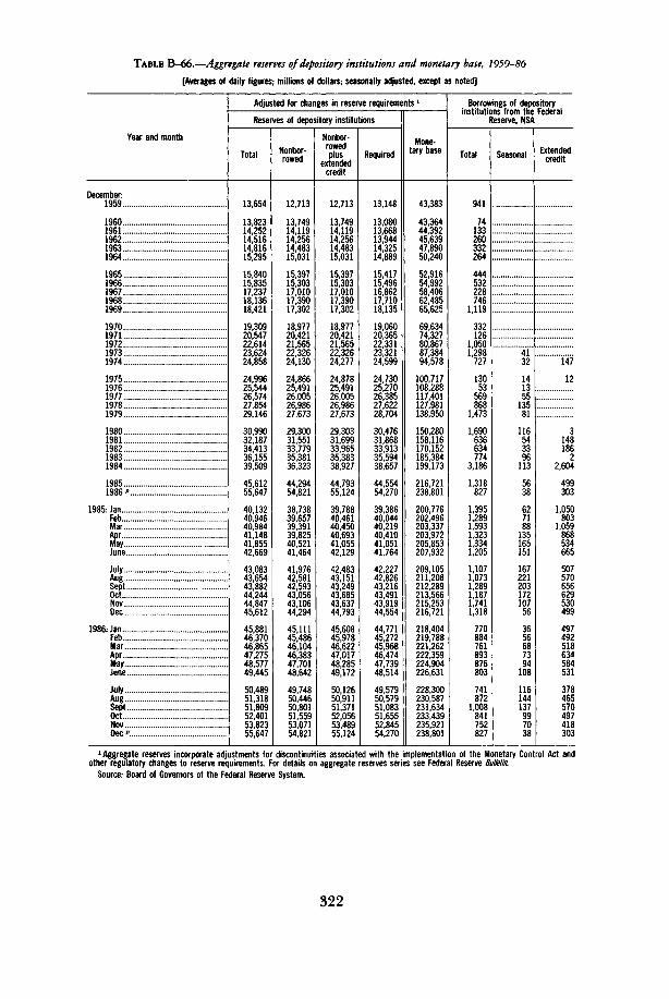
TABLE B-66.—Aggregate reserves of depository institutions and monetary base, 1959-86

[Averages of daily figures; millions of dollars; seasonally adjusted, except as noted]

Year and month

December:1959

I9601961196219631964

19651966196719681969

19701971197219731974

19751976197719781979

19801981198219831984

19851986 p

1985- JanFebMarAprMayJune

JulyAugSeptOctNovDec

1986: JanFebMarAprallay::::::::::::":::June

JulyAucSeptOctNovDec p . ..

Adjusted for changes in reserve requirements *

Reserves of depository institutions

Total

13,654

13,82314,25214,51614,81615,295

15,84015,83517,23718,13618,421

19,30920,54722,61423,62424,858

24,99625,54426,57427,85429,146

30,99032,18734,41336,15539,509

45,61255,647

40,13240,94640,98441,14841,85542,669

43,08343,65443,88244,24444,84745,612

45,88146,37046,86547,27548,57749,445

50,48951,31851,80952,40153,82355,647

Nonbor-rowed

12,713

13,74914,11914,25614,48315,031

15,39715,30317,01017,39017,302

18,97720,42121,56522,32624,130

24,86625,49126,00526,98627,673

29,30031,55133,77935,38136,323

44,29454,821

38,73839,65739,39139,82540,52141,464

41,97642,58142,59343,05643,10644,294

45,11145,48646,10446,38347,70148,642

49,74850,44650,80151,55953,07154,821

Nonbor-rowedplus

extendedcredit

12,713

13,74914,11914,25614,48315,031

15,39715,30317,01017,39017,302

18,97720,42121,56522,32624,277

24,87825,49126,00526,98627,673

29,30331,69933,96535,38338,927

44,79355,124

39,78840,46140,45040,69341,05542,129

42,48343,15143,24943,68543,63744,793

45,60845,97846,62247,01748,28549,172

50,12650,91151,37152,05653,48955,124

Required

13,148

13,08013,66813,94414,32514,889

15,41715,49616,86217,71018,135

19,06020,36522,33123,32124,599

24,73025,27026,38527,62228,704

30,47631,86833,91335,59438,657

44,55454,270

39,38640,04440,21940,41041,05141,764

42,22742,82643,21643,49143,91944,554

44,77145,27245,96846,47447,73948,514

49,57950,57951,08351,65552,84554,270

Mone-tary base

43,383

43,36444,39245,63947,89050,240

52,91654,99258,40662,48565,625

69,63474,32780,86787,38494,578

100,717108,288117,401127,981138,950

150,280158,116170,152185,384199,173

216,721238,801

200,776202,496203,337203,972205,853207,932

209,105211,208212,289213,566215,253216,721

218,404219,788221,262222,359224,904226,631

228,300230,587231,634233,439235,921238,801

Borrowings of depositoryinstitutions from the Federal

Reserve, NSA

Total

941

74133260332264

444532228746

1,119

332126

1,0501,298727

13053569868

1,473

1,690636634774

3,186

1,318827

1,3951,2891,5931,3231,3341,205

1,1071,0731,2891,1871,7411,318

770884761893876803

741872

1,008841752827

Seasonal

4132

14135513581

116543396113

5638

627188135165151

16722120317210756

3656687394108

116144137997038

Extendedcredit

147

12

3148186

2,604

499303

1,050803

1,059868534665

507570656629530499

497492518634584531

378465570497418303

1 Aggregate reserves incorporate adjustments for discontinuities associated with the implementation of the Monetary Control Act andother regulatory changes to reserve requirements. For details on aggregate reserves series see Federal Reserve Bulletin.

Source: Board of Governors of the Federal Reserve System.

322

TABLE B-67.—Commercial bank loans and securities, 1972-86

[Monthly average, billions of dollars, seasonally adjusted M

Year and monthTotal loans

andsecurities

Loans and leases

Total

Commercialand

industrialloans

U.S.Governmentsecurities

Othersecurities

December:1972 572.51973 647.91974 713.9

1975 745.31976 804.91977 891.91978 1,014.41979 1,136.2

1980 1,240.51981 1,308.21982 1,401.11983 1,553.51984 1,722.6

1985 1,900.41986 P. 2,079.7

1985: Jan 1,736.1Feb 1,751.1Mar 1,763.8Apr 1,773.6May 1,792.5June 1,808.5

July 1,822.2Aug 1,833.9Sept 1,847.2Oct 1,855.5Nov 1,876.0Dec 1,900.4

1986: Jan 1,930.0Feb 1,935.5Mar 1,944.6Apr 1,947.9May 1,957.5June 1,963.7

July 1,985.0Aug 2,007.7Sept 2,029.6Oct 2,034.0Nov 2,049.0Dec * 2,079.7

390.1460.3520.0

517.3555.1632.6747.5849.9

915.4968.4

1,033.91,123.71,319.7

1,449.71,576.9

1,329.21,340.51,355.11,365.71,377.61,388.2

1,398.21,408.01,418.01,424.01,436.81,449.7

1,469.31,473.71,491.81,495.81,501.51,505.3

1,513.41,524.51,534.71,537.71,549.51,576.9

137.1165.0196.6

189.3190.9211.0246.2291.3

327.4355.9392.5414.0472.9

499.5536.7

474.5478.4483.2483.9486.1487.6

488.5489.7492.1492.7495.7499.5

502.1502.4506.1507.8506.7508.7

508.7510.4512.1514.1520.3536.7

89.088.286.3

116.7136.3136.6137.6144.4

170.6179.2201.9259.7260.9

273.1309.4

262.8267.9268.1265.4270.2273.1

275.4275.1275.5274.2276.0273.1

268.2273.6269.5270.0274.1274.8

285.4290.9294.3299.6304.8309.4

93.499.4

107.5

111.2113.5122.7129.3142.0

154.5160.6165.3170.1142.1

177.6193.4

144.2142.7140.6142.5144.7147.2

148.5150.7153.6157.3163.3177.6

192.5188.1183.3182.1181.9183.6

186.1192.3200.7196.7194.8193.4

1 Data are prorated averages of Wednesday figures for domestically chartered banks and averages of current and previous month-enddata for foreign-related institutions. Lease financing receivables are included in total loans and investments and in total loans.

Note.—Data are not strictly comparable because of breaks in the series.

Source: Board of Governors of the Federal Reserve System.

323

TABLE B-68.—Bond yields and interest rates, 1929-86

[Percent per annum]

Year andmonth

192919331939

1940194119421943194419451946194719481949

19501951 .19521953195419551956195719581959

1960196119621963196419651966196719681969

1970197119721973197419751976197719781979

1980198119821983198419851986

1981:JanFebMar

May"!!JuneJulyAugSept ....OctNovDec

U.S. Treasury securities

Bills(new issues) l

3-month

0.515.023

.014

.103

.326

.373

.375

.375

.375594

1.0401 102

1.21815521.7661.931

.95317532.65832671.8393.405

2.9282.3782.7783.1573.5493.9544.8814.3215.3396.677

6.4584.3484.0717.0417.8865.8384.9895.2657.221

10.041

11.50614.02910.686

8.639.587.485.98

14.72414.90513.47813.63516.29514.55714.69915.61214.95113.87311.26910.926

6-month

ZZZ"

3.832'

3.2472.6052.9083.2533.6864.0555.0824.6305.4706.853

6.5624.5114.4667.1787.9266.1225.2665.5107.572

10.017

11.37413.77611.084

8.759.807.666.03

13.88314.13412.98313.43415.33413.94714.40215.54815.05714.01311.53011.471

Constantmaturities2

3-year

••— "

2.471.632.473.193.982.844.46

3.983.543.473.674.034.225.235.035.687.02

7.295.655.726.957.827.496.776.698.299.71

11.5514.4412.9210.4511.899.647.06

13.0113.6513.5114.0915.0814.2915.1516.0016.2215.5013.1113.66

10-year

2.852.402.823.183.653.324.33

4.123.883.954.004.194.284.925.075.656.67

7.356.166.216.847.567.997.617.428.419.44

11.4613.9113.0011.1012.4410.627.68

12.5713.1913.1213.6814.1013.4714.2814.9415.3215.1513.3913.72

Corporatebonds

(Moody's)

Aaa»

4.734.493.01

2.842.772.832.732.722.622.532.612.822.66

2.622.862.963.202.903.063.363.893.794.38

4.414.354.334.264.404.495.135.516.187.03

8.047.397.217.448.578.838.438.028.739.63

11.9414.1713.7912.0412.7111.379.02

12.8113.3513.3313.8814.3213.7514.3814.8915.4915.4014.2214.23

Baa

5.907.764.96

4.754.334.283.913.613.293.053.243.473.42

3.243.413.523.743.513.533.884.714.735.05

5.195.085.024.864.834.875.676.236.947.81

9.118.568.168.249.50

10.619.758.979.49

10.69

13.6716.0416.1113.5514.1912.7210.39

15.0315.3715.3415.5615.9515.8016.1716.3416.9217.1116.3916.55

High-grade

munici-pal

bonds(Stand-a rds

Poor's)

4.274.712.76

2.502.102.362.061.861.671.642.012.402.21

1.982.002.192.722.372.532.933.603.563.95

3.733.463.183.233.223.273.823.984.515.81

6.515.705.275.186.096.896.495.565.906.39

8.5111.2311.579.47

10.159.187.38

9.6510.0310.1210.5510.7310.5611.0312.1312.8612.6711.7112.77

New-'home

mortgageyields

(FHLBB)<

5.895.825.816.256.466.977.80

8.457.747.607.968.929.009.009.029.56

10.78

12.6614.7015.1412.5712.3811.5510.17

13.2613.5414.0214.1514.1014.6714.7215.2715.2915.6516.3815.87

Com-mercial

paper, 6months5

5.851.73.59

.56

.53

.66

.69

.73

.75

.811.031.441.49

1.452.162.332.521.582.183.313.812.463.97

3.852.973.263.553.974.385.555.105.907.83

7.715.114.738.159.846.325.345.617.99

10.91

12.2914.7611.898.89

10.168.016.39

15.1014.8713.5914.1716.6615.2216.0916.6215.9314.7211.9612.14

Prime ratecharged by

banks6

5.50-6.001.50-4.00

1.50

1.501.501.501.501.501.501.50

1.50-1.751.75-2.00

2.00

2.072.563.003.173.053.163.774.203.834.48

4.824.504.504.504.504.545.635.616.307.96

7.915.725.258.03

10.817.866.846.839.06

12.67

15.2718.8714.8610.7912.049.938.33

High-low

21.50-20.0020.00-19.0019.00-17.5018.00-17.0020.50-18.0020.50-20.0020.50-20.0020.50-20.5020.50-19.5019.50-18.0018.00-16.0015.75-15.75

Discountrate,

FederalReserveBank of

New York6

5.162.561.00

1.001.008 1.008 1.008 1.008 1.00

8 1.001.001.341.50

1.591.751.751.991.601.892.773.122.153.36

3.533.003.003.233.554.044.504.195.165.87

5.954.884.506.447.836.255.505.467.46

10.28

11.7713.4211.028.508.807.696.33

High-low

13.00-13.0013.00-13.0013.00-13.0013.00-13.0014.00-13.0014.00-14.0014.00-14.0014.00-14.0014.00-14.0014.00-14.0014.00-13.0013.00-12.00

Federalfundsrate7

•""••••"•

l'.782.733.111.573.30

3.221.962.683.183.504.075.114.225.668.20

7.184.664.438.73

10.505.825.045.547.93

11.19

13.3616.3812.269.09

10.238.106.81

19.0815.9314.7015.7218.5219.1019.0417.8215.8715.0813.3112.37

1 Rate on new issues within period; bank-discount basis.2 Yields on the more actively traded issues adjusted to constant maturities by the Treasury Department.3 Series excludes public utility issues for January 17, 1984 through October 11, 1984 due to lack of appropriate issues.4 Effective rate (in the primary market) on conventional mortgages, reflecting fees and charges as well as contract rate andassuming, on the average, repayment at end of 10 years. Rates beginning January 1973 not strictly comparable with prior rates.

See next page for continuation of table.

324

TABLE B-68.—Bond yields and interest rates, 1929-86—Continued

[Percent per annum]

Yearand

month

JanFebMar....AprMay....June ...July ....Aug ....Sept...OctNovDec

1983:JanFebMar ....AprMay....June ...July ....Aug ....

OctNovDec

1984:JanFebMar....AprMay....June...July....Aug....Sept...OctNovDec

1985:JanFebMar ....AprMay....June...July ....Aug ....Sept ...OctNovDec

1986:JanFebMar ....AprMay....June..July.. .Aug ...Sept ..Oct....Nov....Dec....

U.S. Treasury securities

Bills(new issues)1

3-month

12.41213.78012.49312.82112.14812.10811.9149.0068.1967.7508.0428.013

7.8108.1308.3048.2528.198.829.129.399.058.718.718.96

8.939.039.449.699.909.94

10.1310.4910.419.978.798.16

7.768.228.578.007.567.017.057.187.087.177.207.07

7.047.036.596.066.126.215.845.575.195.185.355.49

6-month

12.93013.70912.62112.86112.22012.31012.23610.1059.5398.2998.3198.225

7.8988.2338.3258.3438.208.899.299.539.198.908.899.14

9.069.139.589.83

10.3110.5510.5810.6510.5110.058.998.36

8.038.348.928.317.757.167.167.357.277.327.267.09

7.137.086.606.076.166.285.855.585.315.265.425.53

Constantmaturities2

3-year

14.6414.7314.1314.1813.7714.4814.0012.6212.0310.629.989.88

9.649.919.849.769.66

10.3210.9011.3011.0710.8710.9611.13

10.9311.0511.5911.9812.7513.1813.0812.5012.3411.8510.9010.56

10.4310.5511.0510.499.759.059.189.319.379.258.888.40

8.418.107.306.867.277.416.866.496.626.566.466.43

10-year

14.5914.4313.8613.8713.6214.3013.9513.0612.3410.9110.5510.54

10.4610.7210.5110.4010.3810.8511.3811.8511.6511.5411.6911.83

11.6711.8412.3212.6313.4113.5613.3612.7212.5212.1611.5711.50

11.3811.5111.8611.4310.8510.1610.3110.3310.3710.24

9.789.26

9.198.707.787.307.717.807.307.177.457.437.257.11

CorporatehrmHcuonas

(Moody's)

Aaa 3

15.1815.2714.5814.4614.2614.8114.6113.7112.9412.1211.6811.83

11.7912.0111.7311.5111.4611.7412.1512.5112.3712.2512.4112.57

12.2012.0812.5712.8113.2813.5513.4412.8712.6612.6312.2912.13

12.0812.1312.5612.2311.7210.9410.9711.0511.0711.0210.5510.16

10.059.679.008.799.099.138.888.728.898.868.688.49

Baa

17.1017.1816.8216.7816.6416.9216.8016.3215.6314.7314.3014.14

13.9413.9513.6113.2913.0913.3713.3913.6413.5513.4613.6113.75

13.6513.5913.9914.3114.7415.0515.1514.6314.3513.9413.4813.40

13.2613.2313.6913.5113.1512.4012.4312.5012.4812.3611.9911.58

11.4411.1110.4910.1910.2910.3410.1610.1810.2110.2410.079.97

High-grade

munici-pal

bonds(Stand-ard &

Poor's)

13.1612.8112.7212.4511.9912.4212.1111.1210.619.599.979.91

9.459.489.168.969.039.519.469.729.579.649.799.90

9.619.639.929.98

10.5510.7110.5010.0310.1710.3410.2710.04

9.559.669.799.489.088.788.909.189.379.248.648.51

8.067.447.077.327.677.987.627.317.147.126.866.93

New-home

mortgageyields

(FHLBB)4

15.2515.1215.6715.8415.8915.4015.7015.6814.9814.4113.8113.69

13.4913.1613.4112.4212.6712.3612.5012.3812.5412.2512.3412.42

12.2912.2312.0212.0412.1812.1012.5012.4312.5312.7712.7512.55

12.2712.2111.9212.0512.0111.7511.3411.2411.1711.0911.0110.94

10.8910.6810.5010.2710.2210.1510.3010.2610.1710.029.919.69

Com-mercial

paper, 6months5

13.3514.2713.4713.6413.0213.7913.0010.8010.869.218.728.50

8.158.398.488.488.319.039.369.689.288.989.099.50

9.189.319.86

10.2210.8711.2311.3411.1610.9410.169.068.55

8.158.699.238.477.887.387.577.747.867.797.697.62

7.627.547.086.476.536.636.245.835.615.615.695.88

Prime ratecharged by

banks6

High-low

15.75-15.7517.00-15.7516.50-16.5016.50-16.5016.50-16.5016.50-16.5016.50-15.5015.50-13.5013.50-13.5013.50-12.0012.00-11.5011.50-11.50

11.50-11.0011.00-10.5010.50-10.5010.50-10.5010.50-10.5010.50-10.5010.50-10.5011.00-10.5011.00-11.0011.00-11.0011.00-11.0011.00-11.00

11.00-11.0011.00-11.0011.50-11.0012.00-11.5012.50-12.0013.00-12.5013.00-13.0013.00-13.0013.00-12.7512.75-12.0012.00-11.2511.25-10.75

10.75-10.5010.50-10.5010.50-10.5010.50-10.5010.50-10.0010.00- 9.509.50- 9.509.50- 9.509.50- 9.509.50- 9.509.50- 9.509.50- 9.50

9.50- 9.509.50- 9.509.50- 9.009.00- 8.508.50- 8.508.50- 8.508.50- 8.008.00- 7.507.50- 7.507.50- 7.507.50- 7.507.50- 7.50

Discountrate,

FederalReserveBank of

New York6

High-low

12.00-12.0012.00-12.0012.00-12.0012.00-12.0012.00-12.0012.00-12.0012.00-11.5011.50-10.0010.00-10.0010.00- 9.509.50- 9.009.00- 8.50

8.50- 8.508.50- 8.508.50- 8.508.50- 8.508.50- 8.508.50- 8.508.50- 8.508.50- 8.508.50- 8.508.50- 8.508.50- 8.508.50- 8.50

8.50- 8.508.50- 8.508.50- 8.509.00- 8.509.00- 9.009.00- 9.009.00- 9.009.00- 9.009.00- 9.009.00- 9.009.00- 8.508.50- 8.00

8.00- 8.008.00- 8.008.00- 8.008.00- 8.008.00- 7.507.50- 7.507.50- 7.507.50- 7.507.50- 7.507.50- 7.507.50- 7.507.50- 7.50

7.50- 7.507.50- 7.507.50- 7.007.00- 6.506.50- 6.506.50- 6.506.50- 6.006.00- 5.505.50- 5.505.50- 5.505.50- 5.505.50- 5.50

Federalfundsrate7

13.2214.7814.6814.9414.4514.1512.5910.1210.319.719.208.95

8.688.518.778.808.638.989.379.569.459.489.349.47

9.569.599.91

10.2910.3211.0611.2311.6411.309.999.438.38

8.358.508.588.277.977.537.887.907.927.998.058.27

8.147.867.486.996.856.926.566.175.895.856.046.91

5 Bank-discount basis; prior to November 1979, data are for 4-6 months paper.6 For monthly data, high and low for the period. Prime rate for 1929-33 and 1947-48 are ranges of the rate in effect during theperiod.7 Since July 19, 1975, the daily effective rate is an average of the rates on a given day weighted by the volume of transactions atthese rates. Prior to that date, the daily effective rate was the rate considered most representative of the day's transactions, usuallythe one at which most transactions occurred.8 From October 30, 1942, to April 24, 1946, a preferential rate of 0.50 percent was in effect for advances secured by Governmentsecurities maturing in 1 year or less.

Sources: Department of the Treasury, Board of Governors of the Federal Reserve System, Federal Home Loan Bank Board (FHLBB),Moody's Investors Service, and Standard & Poor's Corporation.

325

TABLE B-69.—Total funds raised in credit markets by nonfina ncial sectors, 1977-86

[Billions of dollars; quarterly data at seasonally adjusted annual rates]

Item

Total net borrowing by domestic nonfinancial sectors...

U S Government

Treasury issuesAgency issues and mortgages

Private domestic nonfinancial sectors

Debt capital instruments .

Tax-exempt obligationsCorporate bondsMortgages

Home mortgagesMulti-family residentialCommercialFarm

Other debt instruments

Consumer creditBank loans n e eOpen-market paperOther

By borrowing sector: Total

State and local governmentsHouseholdsNonfinancial business

FarmNonfarm noncorporateCorporate

Foreign net borrowing in United States

BondsBank loans n.e.cOpen-market paperU S. Government loans

Total domestic plus foreign

Total funds supplied to domestic nonfinancial sectors ..

Private domestic nonfinancial sectors

Deposits and currency

Checkable deposits and currencyTime and savings depositsMoney market fund sharesSecurity repurchase agreementsForeign deposits

Credit market instruments

Foreign funds

At banksCredit market instruments

U.S. Government and related loans, netU.S. Government cash balancesPrivate insurance and pension reservesOther sources

1977 1978 1979 1980 1981 1982 1983 1984 | 1985

Net credit market borrowing by nonfinancial sectors

316.9

56.8

57.6-.9

260.2

171.3

20.322.9

128.1

93.38.4

18.28.2

88.9

38.126.51.6

22.6

260.2

10.5137.5112.2

13.429.569.3

13.5

5.13.1

.63.0

330.4

371.9

53.7

55.1-1.4

318.2

200.7

28.421.1

151.2

110.210.921.98.2

117.6

46.740.5

2.727.6

318.2

16.5167.2134.5

15.633.885.2

24.2

4.218.31.03.9

396.1

385.7

37.4

38.8-1.4

348.4

212.5

30.317.3

164.9

116.610.024.414.0

135.9

42.750.59.0

33.7

348.4

17.6173.7157.1

23.537.995.7

15.1

3.93.11.72.9

400.8

344.9

79.2

79.8-.6

265.7

189.1

30.327.7

131.2

94.27.6

19.210.2

76.6

4.537.84.0

30.3

265.7

17.2120.0128.5

15.231.881.5

23.8

.811.82.44.7

368.7

375.8

87.4

87.8-.5

288.5

155.5

23.422.8

109.3

72.24.8

22.210.0

133.0

22.657.014.738.7

288.5

6.8121.4160.3

16.638.5

105.2

23.5

5.43.03.94.2

399.3

387.4

161.3

162.1-.9

226.2

148.3

44.218.785.4

50.55.4

25.24.2

77.9

17.752.9

-6.113.4

226.2

21.588.4

116.2

6.840.269.2

16.0

6.7-5.5

1.94.5

403.4

548.8

186.6

186.7-.1

362.2

252.8

53.716.0

183.0

117.114.149.0

2.8

109.5

56.825.8-.827.7

362.2

34.0188.0140.2

4.376.659.3

17.4

3.13.66.54.3

566.2

756.3

198.8

199.0

557.5

314.0

50.446.1

217.5

129.925.163.3-.8

.243.5

95.080.121.746.6

557.5

27.4239.5290.6

97'.1193.4

6.1

1.3-6.6

6.24.3

762.4

869.3

223.6

223.7-.1

645.7

461.7

152.473.9

235.4

150.329.262.4

-6.4

184.0

96.641.314.631.4

645.7

107.8295.0242.9

-13.692.8

163.7

1.7

4.0-2.8

6.21.6

871.0

Direct and indirect supply of funds to credit markets

316.9

191.5

146.6

25.3116.9

.22.91.3

44.9

36.9

1.135.8

4.24.3

58.321.7

371.9

221.8

149.0

26.3108.3

6.95.52.0

72.8

33.4

7.326.1

3.06.8

75.731.2

385.7

248.6

150.8

28.176.534.46.75.1

97.8

18.9

26.475

16.7.4

79.521.6

344.9

237.0

183.9

16.8128.229.26.82.8

53.1

-4.0

-25.121.1

5.2-2.688.920.4

375.8

299.0

222.4

28.083.4

107.55.2

-1.7

76.6

-.7

-23.723.0

10.6-1.189.6

-21.4

387.4

320.7

204.5

28.3140.824.711.1

4

116.3

-7.3

-31.424.1

10.46.1

92.5-35.0

548.8

382.7

229.7

43.1209.044118.53.1

153.0

41.3

16.324.9

5.2-5.3110.614.4

756.3

517.4

321.1

36.4235.6

47.27.051

196.4

60.9

5.455.5

18.14.0

112.543.3

869.3

515.3

215.1

54.4151.5

2213.4

-2.1

300.2

80.1

17.762.4

37.710.3

107.0119.0

See next page for continuation of table.

326

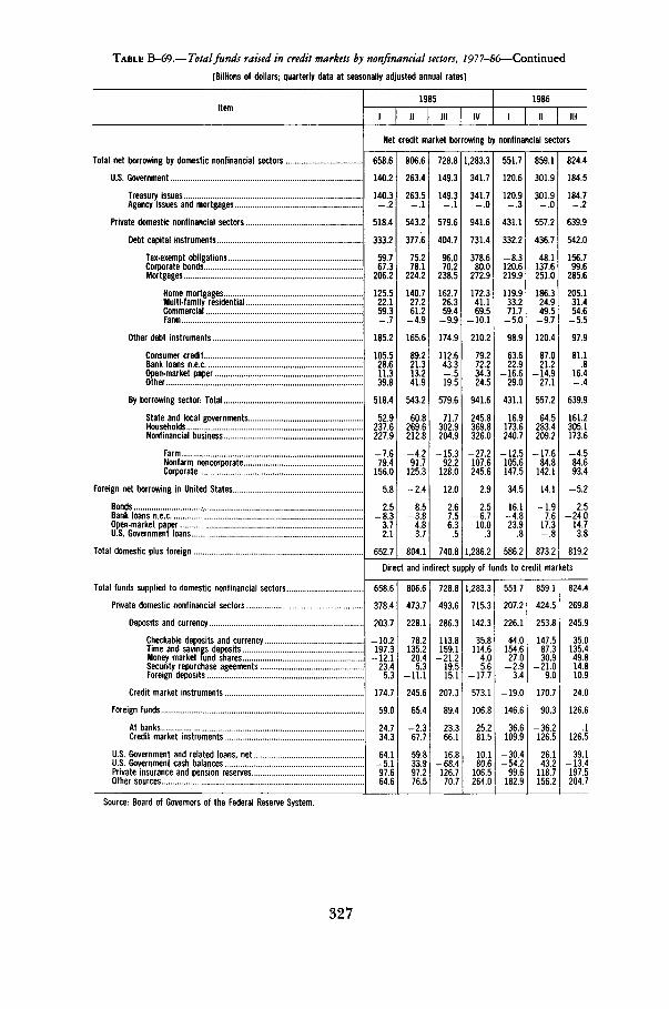
TABLE B-69.—Total funds raised in credit markets by nonfinancial sectors, 1977-86—Continued

[BilKons of dollars; quarterly data at seasonally adjusted annual rates]

Item

Total net borrowing by domestic nonfinancial sectors

U.S. Government

Treasury issuesAgency issues and mortgages

Private domestic nonfinancial sectors

Debt capital instruments

Tax-exempt obligationsCorporate bondsMortgages

Home mortgagesMulti-family residentialCommercialFarm . .

Other debt instruments

Consumer creditBank loans n.e.cOpen-market paperOther

By borrowing sector- Total

State and local governmentsHouseholds . . .Nonfinancial business

FarmNonfarm noncorporateCorporate

Foreign net borrowing in United States . .

Bonds .-Bank loans n e eOpen-market paperU.S. Government loans...

Total domestic plus foreign

Total funds supplied to domestic nonfinancial sectors

Private domestic nonfinancial sectors

Deposits and currency

Checkable deposits and currencyTime and savings depositsMoney market Fund sharesSecurity repurchase ageementsForeign deposits

Credit market instruments

Foreign funds

At banks . .Credit market instruments

U.S Government and related loans netU.S. Government cash balancesPrivate insurance and pension reservesOther sources

1985

1 II III IV

1986

1 II III

Net credit market borrowing by nonfinancial sectors

658.6

140.2

140.3-.2

518.4

333.2

59.767.3

206.2

125.522.159.3-.7

185.2

105.528.611.339.8

518.4

52.9237.6227.9

-7.679.4

156.0

58

2.5-8.3

3.72.1

652.7

806.6

263.4

263.5-.1

543.2

377.6

75.278.1

224.2

140.727.261.2

-4.9

165.6

89.221.313.241.9

543.2

60.8269.6212.8

-4.291.7

125.3

-2.4

8.5-3.8

4.83.7

804.1

728.8

149.3

149.31

579.6

404.7

96.070.2

238.5

162.726.359.4

-9.9

174.9

112.643.3-.519.5

579.6

71.7302.9204.9

-15.392.2

128.0

12.0

2.67.56.3

.5

740.8

1,283.3

341.7

341.70

941.6

731.4

378.680.0

272.9

172.341.169.5

-10.1

210.2

79.272.234.324.5

941.6

245.8369.8326.0

-27.2107.6245.6

2.9

2.5-6.710.0

.3

1,286.2

551.7

120.6

120.9-.3

431.1

332.2

83120.6219.9

119.933.271.7

-5.0

98.9

63.622.9

-16.629.0

431.1

16.9173.6240.7

-12.5105.6147.5

34.5

16.1-4.823.9

.8

586.2

859.1

301.9

301.90

557.2

436.7

48.1137.6251.0

186.324.949.5

-9.7

120.4

87.021.2

-14.927.1

557.2

64.5283.4209.2

-17.684.8

142.1

14.1

-1.97.6

17.3-.8

873.2

824.4

184.5

184.7-.2

639.9

542.0

156.799.6

285.6

205.131.454.6

-5.5

97.9

81.1.8

16.4-.4

639.9

161.2305.1173.6

-4.584.693.4

-5.2

2.524014.73.8

819.2

Direct and indirect supply of funds to credit markets

658.6

378.4

203.7

-10.2197.3

-12.123.4

5.3

174.7

59.0

24.734.3

64.151

97.664.6

806.6

473.7

228.1

78.2135.220.45.3

-11.1

245.6

65.4

-2.367.7

59.833.997.276.5

728.8

493.6

286.3

113.8159.1

-21.219.515.1

207.3

89.4

23.366.1

16.8-68.4126.770.7

1,283.3

715.3

142.3

35.8114.6

4.05.6

-17.7

573.1

106.8

25.281.5

10.180.6

106.5264.0

551.7

207.2

226.1

44.0154.627.0

-2.93.4

190

146.6

36.6109.9

304-54.2

99.6182.9

859.1

424.5

253.8

147.587.330.92109.0

170.7

90.3

-36.2126.5

26.143.2

118.7156.2

824.4

269.8

245.9

35.0135.449.814.810.9

24.0

126.6

.1126.5

39.1-13.4197.5204.7

Source: Board of Governors of the Federal Reserve System.

327

TABLE B-70.—Mortgage debt outstanding by type of property and of financing, 1939-86

[Billions of dollars]

End of yearor quarter

1939

19401941194219431944

19451946194719481949

19501951 .. .19521953 ..1954

195519561957 .19581959

1960196119621963 .. . .1964

19651966196719681969

19701971 . . .197219731974

19751976197719781979

1980198119821983 .1984

1985

1984: 1||I I IIV

1985:1IIIllIV.. .

1986: 1III l l

Allproper-

ties

35.5

36.537.636.735.334.7

35.541.848.956.262.7

72.882.391.4

101.3113.7

129.9144.5156.5171.8190.8

207.5228.0251.4278.5305.9

333.3356.5381.2410.9441.4

473.5524.0597.1672.3732.3

791.7878.5

1,009.81,161.91,327.3

1,457.51,564.01,631.31,813.92,034.6

2,266.3

1,863.81,926.81,983.72,034.6

2,080.92,139.62,200.62,266.3

2,315.02,381.22,456.5

Farmproper-

ties

6.6

6.56.46.05.44.9

4.84.95.15.35.6

6.16.77.27.78.2

9.09.8

10.411.112.1

12.813.915.216.818.9

21.223.125.127.429.2

30.332.235.139.544.7

49.755.363.571.685.6

95.8105.8110.0112.8112.0

105.6

112.3112.6112.6112.0

111.9110.9108.3105.6

103.9101.6100.1

Nonfarm properties

Total

28.9

30.031.230.829.929.7

30.836.943.950.957.1

66.775.684.293.6

105.4

120.9134.6146.1160.7178.7

194.7214.1236.2261.7287.0

312.1333.4356.1383.5412.2

443.2491.8562.0632.8687.5

742.0823.2946.4

1,090.21,241.7

1,361.81,458.21,521.21,701.01,922.6

2,160.7

1,751.51,814.31,871.01,922.6

1,969.02,028.82,092.32,160.7

2,211.12,279.62,356.3

1- to 4-familyhouses

16.3

17.418.418.217.817.9

18.623.028.233.337.6

45.251.758.566.175.7

88.299.0

107.6117.7130.9

141.9154.6169.3186.4203.4

220.5232.9247.3264.8283.2

297.4325.9366.5407.9440.7

482.1546.3642.7753.5870.5

963.91,038.51,074.71,189.81,318.9

1,466.1

1,217.01,254.21,288.11,318.9

1,346.61,383.21,425.41,466.1

1,493.81,541.51,595.3

Multi-familyproper-

ties

5.6

5.75.95.85.85.6

5.76.16.67.58.6

10.111.512.312.913.5

14.314.915.316.818.7

20.323.025.829.033.6

37.240.343.947.352.2

60.170.182.893.1

100.0

100.6105.7114.0124.9134.9

142.3142.1145.8160.8185.4

213.8

166.4174.2179.6185.4

190.9197.5203.6213.8

221.5228.3236.1

Com-mercialproper-

ties

7.0

6.97.06.76.36.2

6.47.79.1

10.210.8

11.512.513.414.516.3

18.320.723.226.129.2

32.436.541.146.250.0

54.560.164.8,71.41

76.9

85.695.9

112.7131.7146.9

159.3171.2189.7211.8236.3

255.5277.5300.8350.4418.3

480.7

368.0385.9403.3418.3

431.5448.1463.3480.7

495.9509.9524.9

Nonfarm properties by type of mortgage

Government underwritten

Total l

1.8

2.33.03.74.14.2

4.36.39.8

13.617.1

22.126.629.332.136.2

42.947.851.655.259.3

62.365.669.473.477.2

81.284.188.293.4

100.2

109.2120.7131.1135.0140.2

147.0154.1161.7176.4199.0

225.1238.9248.9279.8294.8

328.3

286.8290.5292.9294.8

299.7305.4323.8328.3

339.9349.7

1- to 4-family houses

Total

1.8

2.33.03.74.14.2

4.36.19.3

12.515.0

18.822.925.428.132.1

38.943.947.250.153.8

56.459.162.265.969.2

73.176.179.984.490.2

97.3105.2113.0116.2121.3

127.7133.5141.6153.4172.9

195.2207.6217.9248.8265.9

288.8

255.9260.5263.6265.9

270.6276.0282.6288.8

299.1308.3

FHAinsured

1.8

2.33.03.74.14.2

4.13.73.85.36.9

8.59.7

10.812.012.8

14.315.516.519.723.8

26.729.532.335.038.3

42.044.847.450.654.5

59.965.768.266.265.1

66.166.568.071.481.0

93.6101.3108.0127.4136.7

153.0

131.1133.6135.6136.7

139.8144.3148.3153.0

160.6168.9

VAguar-

anteed

0.22.45.57.28.1

10.313.214.616.119.3

24.628.430.730.430.0

29.729.629.930.930.9

31.131.332.533.835.7

37.339.544.750.056.2

61.667.073.682.092.0

101.6106.2109.9121.4129.1

135.8

124.8126.9128.0129.1

130.8131.6134.3135.8

138.5139.4142.7

Conventional 2

Total

27.1

27.728.227.125.825.5

26.530.634.137.340.0

44.749.154.961.569.3

78.086.894.6

105.5119.4

132.3148.5166.9188.2209.8

231.0249.3267.9290.1312.0

333.9371.1430.9497.7547.3

595.0669.0784.6913.9

1,042.7

1,136.71,219.31,272.41,421.21,627.8

1,832.3

1,464.71,523.81,578.21,627.8

1,669.31,723.41,768.41,832.3

1,871.31,929.9

l-to4-familyhouses

14.5

15.115.414.513.713.7

14.316.918.920.822.6

26.328.933.238.043.6

49.355.160.467.677.0

85.595.5

107.1120.5134.1

147.4156.9167.4180.4193.0

200.2220.7253.5291.7319.4

354.3412.8501.0600.2697.6

768.8830.9856.8941.0

1,053.0

1,177.3

961.1993.7

1,024.51,053.0

1,076.01,107.21,142.71,177.3

1,194.71,233.2

1 Includes FHA insured multifamily properties, not shown separately.2 Derived figures. Total includes multifamily and commercial properties, not shown separately.Source: Board of Governors of the Federal Reserve System, based on data from various Government and private organizations.

328

TABLE B-71.—Mortgage debt outstanding by holder, 1939-86

[Billions of dollars]

End of yearor quarter

1939

19401941194219431944

19451946194719481949

19501951195219531954

19551956195719581959

19601961196219631964

19651966196719681969

19701971197219731974

19751976197719781979

19801981198219831984

1985

1984: 1III l lIV

1985- 1I II l lIV

1986- 1I II l l

Total

35.5

36.537.636.735.334.7

35.541.848.956.262.7

72.882.391.4

101.3113.7

129.9144.5156.5171.8190.8

207.5228.0251.4278.5305.9

333.3356.5381.2410.9441.4

473.5524.0597.1672.3732.3

791.7878.5

1,009.81,161.91,327.3

1,457.51,564.01,631.31,813.92,034.6

2,266.3

1,863.81,926.81,983.72,034.6

2,080.92,139.62,200.62,266.3

2,315.02,381.22,456.5

Major financial institutions

Total

18.6

19.520.720.720.220.2

21.026.031.837.842.9

51.759.566.975.185.7

99.3111.2119.7131.5145.5

157.6172.6192.5217.1241.0

264.6280.8298.8319.9339.1

355.9394.2450.0505.4542.6

581.2647.5745.2848.2938.2

996.81,040.51,021.31,108.21,245.9

1,361.7

1,137.81,181.61,219.41,245.9

1,266.91,297.91,328.51,361.7

1,379.01,404.61,429.9

Savingsand loanassocia-

tions

3.8

4.14.64.64.64.8

5.47.18.9

10.311.6

13.715.618.422.026.1

31.435.740.045.653.1

60.168.878.890.9

101.3

110.3114.4121.8130.8140.2

150.3174.3206.2231.7249.3

278.6323.0381.2432.8475.7

503.2518.5483.6494.8555.3

583.2

503.5528.2550.1555.3

559.3569.3573.7583.2

574.7565.2558.4

Savingsbanks

4.8

4.94.84.64.44.3

4.24.44.95.86.7

8.39.9

11.412.915.0

17.519.721.223.325.0

26.929.132.336.240.6

44.647.350.553.556.1

57.962.067.673.274.9

77.281.688.295.298.9

99.9100.094.5

131.9154.4

177.3

139.1143.4146.1154.4

161.0165.7174.4177.3

188.2203.2214.2

Commer-cial

banks '

4.3

4.64.94.74.54.4

4.87.29.4

10.911.6

13.714.715.916.918.6

21.022.723.325.528.1

28.830.434.539.444.0

49.754.459.065.770.7

73.382.599.3

119.1132.1

136.2151.3179.0214.0245.2

262.7284.2301.3330.5379.5

429.4

343.9356.5367.9379.5

388.2400.7415.6429.4

441.3456.1472.0

Lifeinsur-ancecom-

panies

5.7

6.06.46.76.76.7

6.67.28.7

10.812.9

16.119.321.323.326.0

29.433.035.237.139.2

41.844.246.950.555.2

60.064.667.570.072.0

74.475.576.981.486.2

89.291.696.8

106.2118.4

131.1137.7142.0151.0156.7

171.8

151.3153.5155.4156.7

158.5162.1164.8171.8

174.8180.0185.2

Other holders

Federaland

relatedagen-cies2

5.0

4.94.74.33.63.0

2.42.01.81.82.3

2.83.54.14.64.8

5.36.27.78.0

10.2

11.512.212.611.812.2

13.517.520.925.131.1

38.346.454.664.882.2

101.1116.7140.5170.6216.0

256.8289.4355.4433.4491.1

582.0

448.4458.9472.3491.1

511.3531.7555.2582.0

605.7637.0680.6

Individ-uals andothers

11.9

12.012.211.711.511.5

12.113.815.316.617.5

18.419.320.421.723.2

25.327.129.132.335.1

38.443.146.349.552.7

55.258.261.465.971.2

79.383.492.5

102.2107.5

109.4114.3124.1143.1173.1

203.9234.1254.5272.2297.6

322.6

277.6286.3291.9297.6

302.6310.1316.9322.6

330.3339.6346.1

1 Includes loans held by nondeposit trust companies, but not by bank trust departments.2 Includes former Federal National Mortgage Association (FNMA) and new Government National Mortgage Association (GNMA), as wellas Federal Housing Administration, Veterans Administration, Public Housing Administration, Farmers Home Administration (FmHA), and inearlier years Reconstruction Finance Corporation, Homeowners Loan Corporation, and Federal Farm Mortgage Corporation. Also includesU.S.-sponsored agencies such as new FNMA, Federal Land Banks, Federal Home Loan Mortgage Corporation (FHLMC), and mortgagepass-through securities issued or guaranteed by GNMA, FHLMC, FNMA or FmHA. Other U.S. agencies (amounts small or current separatedata not readily available) included with "individuals and others."

Source: Board of Governors of the Federal Reserve System, based on data from various Government and private organizations.

329

TABLE B-72.—Consumer credit outstanding, 1950-86

[Amount outstanding (end of month); millions of dollars, seasonally adjusted]

Year and month

December:19501951195219531954... .19551956195719581959

1960196119621963196419651966196719681969

1970197119721973197419751976197719781979

198019811982198319841985

1985: JanFebMarAprMayJune

JulyAugSeptOctNovDec

1986- JanFebMarAprMayJune

JulyAugSeptOctNov

Totalconsumercredit

25,01826,57631,83035,92837,29344,31948,22451,13651,59559,432

63,92866,56972,83081,57891,279101,726108,227113,628124,915135,431

141,010155,537175,286200,894210,634217,428241,989279,428325,433366,854

371,219393,701411,709471,784568,127668,216

576,121584,896595,246604,592613,127619,473

628,255636,234647,776654,249660,462668,216

678,067682,855686,810694,403702,353708,541

715,112719,507727,128735,348739,208

Installment credit l

Total

15,16615,85920,12123,87024,47029,80932,66034,91434,73640,421

44,33545,43850,37557,05664,67472,81478,16281,78390,11299,381

103,905116,434131,258152,910162,203167,043187,782221,475261,976296,483

297,667314,321327,173376,239453,580535,098

459,843466,690474,989482,532488,862493,253

500,039506,090516,420522,978528,621535,098

542,753547,852550,939555,810562,267567,653

573,216576,609584,334591,542595,560

Automobile

6,0355,9817,6519,7029,75513,48514,49915,49314,26716,641

18,10817,65620,00122,89125,86529,37831,02431,13634,35236,946

36,34840,52247,83553,74054,24156,98966,82180,94898,739112,475

112,255120,020125,369145,908173,122206,482

175,845178,251181,514184,526187,533189,459

191,201192,923198,656201,994203,766206,482

210,661213,342214,361215,814218,965222,606

226,234228,814236,280240,548241,392

Revolving 2

2,0223,563

4,9008,2529,39111,31813,23214,50716,59536,68945,20253,357

54,89460,75066,00778,36998,514118,296

100,263102,373105,297107,417108,372109,260

110,904112,373113,850115,218117,050118,296

119,682120,724122,131123,442124,545124,720

125,577125,915126,012126,514128,102

Mobile home 3

2,4337,1719,46813,50514,58215,38815,73816,36216,92118,207

19,11920,38220,99822,19424,18425,461

24,13924,36024,46824,57024,67024,768

25,01525,17325,34125,32025,31525,461

25,37125,57325,58425,51325,56025,479

25,39825,21524,95824,99425,029

Other

9,1319,87812,47014,16814,71516,32418,16119,42120,46923,780

26,22727,78230,37434,16538,80943,43647,13850,64753,73858,872

60,22460,48964,56474,34780,14880,15988,62887,476101,114112,444

111,399113,169114,799129,768157,760184,859

159,596161,706163,710166,019168,287169,766

172,919175,621178,573180,446182,490184,859

187,039188,212188,863191,041193,197194,847

196,007196,665197,084199,485201,036

Noninstallmentcredit *

9,85210,71711,70912,05812,82314,51015,56416,22216,85919,011

19,59321,13122,45524,52226,60528,91230,06531,84534,80336,050

37,10539,10344,02847,98448,43150,38554,20757,95363,45770,371

73,55279,38084,53695,545114,547133,118

116,278118,206120,257122,060124,265126,220

128,216130,144131,356131,271131,841133,118

135,314135,003135,871138,593140,086140,888

141,896142,898142,794143,806143,648

1 Installment credit covers most short- and intermediate-term credit extended to individuals through regular business channels,usualrv to finance the purchase of consumer goods and services or to refinance debts incurred for such purposes, and scheduled to berepaid (or with the option of repayment) in two or more installments. Credit secured by real estate is generally excluded.

2 Consists of credit cards at retailers, gasoline companies, and commercial banks, and check credit at commercial banks. Prior to1968, included in "other," except gasoline companies, included in noninstallment credit prior to 1971. Beginning 1977, includes open-end credit at retailers, previously included in "other." Also beginning 1977, some retail credit was reclassified from commercial intoconsumer credit.

3 Not reported separately prior to July 1970.4 Noninstallment credit is credit scheduled to be repaid in a lump sum, including single-payment loans, charge accounts, and service

credit. Because of inconsistencies in the data and infrequent benchmarking, series is no longer published by the Federal Reserve Boardon a regular basis. Data are shown here as a general indication of trends.

Source-. Board of Governors of the Federal Reserve System.

330

GOVERNMENT FINANCE

TABLE B-73.—Federal receipts, outlays, surplus or deficit, and debt, selected fiscal years 1929-88

[Billions of dollars; fiscal years]

Fiscal yearor period

192919331939

19401941194219431944

19451946194719481949

19501951195219531954

19551956195719581959

19601961196219631964

19651966196719681969

19701971197219731974

19751976Transition

quarter ..197719781979

19801981198219831984

198519861987 3

1988 3

Total

Re-ceipts

3.92.06.3

6.58.7

14.624.043.7

45.239.338.541.639.4

39.451.666.269.669.7

65.574.680.079.679.2

92.594.499.7

106.6112.6

116.8130.8148.8153.0186.9

192.8187.1207.3230.8263.2

279.1298.1

81.2355.6399.6463.3

517.1599.3617.8600.6666.5

734.1769.1842.4916.6

Outlays

3.14.69.1

9.513.735.178.691.3

92.755.234.529.838.8

42.645.567.776.170.9

68.470.676.682.492.1

92.297.7

106.8111.3118.5

118.2134.5157.5178.1183.6

195.6210.2230.7245.7269.4

332.3371.8

96.0409.2458.7503.5

590.9678.2745.7808.3851.8

946.3989.8

1,015.61,024.3

Surplusor

deficit(-)

0.7-2.6

28

-2.9-4.9

-20.5-54.6-47.6

-47.6-15.9

4.011.8

.6

-3.16.1

-1.565

-1.2

-3.03.93.4

-2.8-12.8

.3-3.3-7.1-4.8-5.9

-1.4-3.7-8.6

-25.23.2

-2.8-23.0-23.4-14.9-6.1

-53.2-73.7

-14.7-53.6-59.2-40.2

-73.8-78.9

-127.9-207.8-185.3

-212.3-220.7-173.2-107.8

On-budget

Re-ceipts

5.8

6.08.0

13.722.942.5

43.838.137.139.937.7

37.348.562.665.565.1

60.468.273.271.671.0

81.982.387.492.496.2

100.1111.7124.4128.1157.9

159.3151.3167.4184.7209.3

216.6231.7

63.2278.7314.2365.3

403.9469.1474.3453.2500.4

547.9568.9628.4674.5

Outlays

9.2

9.513.635.178.591.2

92.655.034.229.438.4

42.044.266.073.867.9

64.565.770.674.983.1

81.386.093.396.4

102.8

101.7114.8137.0155.8158.4

168.0177.3193.8200.1217.3

271.9302.2

76.6328.5369.1403.5

476.6543.0594.3661.2686.0

769.5806.3821.1821.9

Surplusor

deficit(-)

-3.4

-3.5-5.6

-21.3-55.6-48.7

-48.7-17.0

2.910.5-.7

-4.74.3

-3.4-8.3-2.8

-4.12.52.6

-3.3-12.1

.5-3.8-5.9-4.0-6.5

-1.63 1

-12.6-27.7

-.5

-8.7-26.1-26.4-15.4-8.0

-55.3-70.5

-13.3-49.7-54.9-38.2

-72.7-73.9

-120.0-208.0-185.6

-221.6-237.5-192.7-147.4

Off-budget

Re-ceipts

0.5

.6

.7

.91.11.3

1.31.21.51.61.7

2.13.13.64.14.6

5.16.46.88.08.3

10.612.112.314.216.4

16.719.124.424.929.0

33.535.839.946.153.9

62.566.4

18.076.885.498.0

113.2130.2143.5147.3166.1

186.2200.2214.0242.1

Outlays

0.0

.0

.0

.1

.1

.1

.1

.2

.3

A

l'.31.72.32.9

4.05.06.07.59.0

10.911.713.515.015.7

16.519.720.422.325.2

27.632.836.945.652.1

60.469.6

19.480.789.7

100.0

114.3135.2151.4147.1165.8

176.8183.5194.5202.4

Surplusor

deficit(-)

0.5

.6

.7

.81.01.2

1.21.01.21.21.3

1.61.81.91.81.7

1.11.5.8.5

-.7

-.2.4

-1.3-.8

.6

.2-.64.02.63.7

5.93.03.1

L8

2.0-3.2

-1.4-3.9-4.3-2.0

-1.1-5.0-7.9

.2

9.416.719.539.7

Gross Federal debt(end of period)

Total

1 169*22.5

48.2

50.757.579.2

142.6204.1

260.1271.0257.1252.0252.6

256.9255.3259.1266.0270.8

274.4272.8272.4279.7287.8

290.9292.9303.3310.8316.8

323.2329.5341.3369.8367.1

382.6409.5437.3468.4486.2

544.1631.9

646.4709.1780.4833.8

914.31,003.91,147.01,381.91,576.7

1,827.22,132.92,372.42,585.5

Held bythe

public

41.4

42.848.267.8

127.8184.8

235.2241.9224.3216.3214.3

219.0214.3214.8218.4224.5

226.6222.2219.4226.4235.0

237.2238.6248.4254.5257.6

261.6264.7267.5290.6279.5

284.9304.3323.8343.0346.1

396.9480.3

498.3551.8610.9644.6

715.1794.4929.4

1,141.81,312.6

1,509.91,746.11,908.42,015.1

Adden-dum:Gross

nationalproduct

95.8113.0142.2175.8202.0

212.4212.9223.6247.8263.9

266.8315.0342.4365.6369.5

386.4418.1440.5450.2481.5

506.7518.2557.7587.8629.2

672.6739.0794.6849.4929.5

990.21,055.91,153.11,281.41,416.5

1,522.51,698.2

2 1,794.71,933.02,171.82,447.8

2,670.62,986.43,139.13,321.93,686.8

3,937.24,163.34,418.94,731.2

1 Not strictly comparable with later data.2 Annual rate.3 Estimates.Note.—Through fiscal year 1976, the fiscal year was on a July 1-June 30 basis; beginning October 1976 (fiscal year 1977), the fiscal

year is on an October 1-September 30 basis. The 3-month period from July 1, 1976 through September 30, 1976 is a separate fiscalperiod known as the transition quarter.

Refunds of receipts are excluded from receipts and outlays.See "Budget of the United States Government, Fiscal Year 1988" for additional information.Sources: Department of the Treasury, Office of Management and Budget, and Department of Commerce (Bureau of Economic

Analysis).

331

TABLE B-74.—Federal receipts, outlays, and debt, fiscal years 1979-88

[Millions of dollars; fiscal years]

Description

RECEIPTS AND OUTLAYS:

Total receiptsTotal outlays

Total surplus or deficit ( — )

On-budget receiptsOn-budget outlays

On-budget surplus or deficit (-)

Off-budget receiptsOff-budget outlays

Off-budget surplus or deficit ( — )

OUTSTANDING DEBT, END OF PERIOD:

Gross Federal debt

Held by Government agencies .Held by the public

Federal Reserve SystemOther . .

RECEIPTS: ON-BUDGET AND OFF-BUDGET .

Individual income taxes . ..Corporation income taxesSocial insurance taxes and contributions

On-budgetOff-budget

Excise taxesEstate and gift taxesCustoms dutiesMiscellaneous receipts:

Deposits of earnings by Federal Reserve System

OUTLAYS: ON-BUDGET AND OFF-BUDGET

National defenseInternational affairsGeneral science space, and technologyEnergyNatural resources and environment . ..Agriculture .Commerce and housing creditTransportation . . . .Community and regional developmentEducation, training, employment, and social servicesHealthMedicareIncome securitySocial security

On-budgetOff-budget

Veterans benefits and servicesAdministration of justiceGeneral governmentGeneral purpose fiscal assistanceNet interest . . . . .

On-budgetOff-budget

AllowancesUndistributed offsetting receipts

On-budgetOff-budget

1&79

463 302503,464

-40,162

365,309403 486

-38,178

9799499,978

-1,984

833,751

189,162644 589

115594528,995

463 302

217 84165,677

138 939

4094597994

18,74554117,439

8,327925

503,464

116 342745952359180

12135112364,686

175321048030,223204942649566359

104073

757103,316

199314,16939288,369

42615

448392224

17476

16362-1,114

1980

517,112590,920

-73,808

403,903476 591

72,689

113209114,329

-1,120

914,317

199,212715 105

120 846594,259

517,112

244 06964,600

157 803

44594113,209

24,32963897^174

11,767981

590,920

133 99512,7145832

1015613,85888399,390

21,3291125231,84323,1693209086540

118 547

675117,872

21,1854,5824,4488,582

52,512

548512339

19942

18738-1,204

Actual

1981

599,272678,209

-78,936

469,097543,013

-73,916

130 176135,196

-5,020

1,003,941

209,507794 434

124 466669,968

599,272

285,91761,137

182,720

52545130,176

40,83967878,083

12,834956

678,209

157 51313,1046,469

1516613,56811,3238,206

23,37910,56833,70926,86639,14999723

139,584

670138,914

22,9914,7624,5826,854

68,734

71,0222288

28041

-26,611-1,430

1982

617 766745,706

- 127,940

474,299594 302

-120,003

143 467151 404

-7937

1,146,987

217 560929 427

134 497794,930

617 766

297 74449,207

201 498

58031143,467

36,31179918,854

15,186975

745,706

185 30912,3007200

1352712,998159446,256

20,6258347

27,02927,44546567

107 717155 964

844155,120

23,9584,7034,5326,390

84995

870652071

-26 099

-24453-1,646

1983

600562808,327

-207,764

453,242661 219

-207,977

147 320147 108

212

1 381 886

240 1161 141 770

155 527986,243

600,562

288,93837,022

208 994

61674147,320

35,30060538,655

14,4921,108

808,327

209 90311,8487^359353

12,67222,9016,681

21,3347,560

26,60628,64152,588

122 598170,724

19,993150,731

24,8465,0994,7896,452

89,774

91,6191845

-33 976

-32 198-1,778

See next page for continuation of table.

332

TABLE B-74.—Federal receipts, outlays, and debt, fiscal years 1979-88—Continued

[Millions of dollars; fiscal years]

RECEIPTS AND OUTLAYS:

Total receipts . .Total outlays

Total surplus or deficit ( — )

On-budget receiptsOn-budget outlays

On-budget surplus or deficit ( )

Off-budget receiptsOff-budget outlays

Off-budget surplus or deficit ( )

OUTSTANDING DEBT, END OF PERIOD:

Gross Federal debt

Held by Government agenciesHeld by the public

Federal Reserve System . .Other

RECEIPTS: ON-BUDGET AND OFF-BUDGET

Individual income taxesCorporation income taxesSocial insurance taxes and contributions

On-budgetOff-budget

Excise taxesEstate and gift taxesCustoms dutiesMiscellaneous receipts:

Deposits of earnings by Federal Reserve System

OUTLAYS: ON-BUDGET AND OFF-BUDGET

National defenseInternational affairsGeneral science, space, and technologyEnergy...Natural resources and environmentAgricultureCommerce and housing creditTransportationCommunity and regional developmentEducation, training employment and social servicesHealth..MedicareIncome securitySocial security

On-budgetOff-budget

Veterans benefits and servicesAdministration of justiceGeneral governmentGeneral purpose fiscal assistanceNet interest

On-budgetOff-budget

AllowancesUndistributed offsetting receipts

On-budgetOff-budget

Actual

1984

666,457851,781

-185,324

500,382685,968

-185,586

166,075165,813

262

1,576,748

264,1591,312,589

155,1221,157,467

666,457

298,41556,893

239,376

73,301166,075

37,3616,010

11,370

15,6841,347

851,781

227,41315,8768,3177,086

12,59313,6136,917

23,6697,673

27,57930,41757,540

112,668178,223

7,056171,167

25,6145,6605,0536,770

111,058

114,368-3,310

31957

-29,913-2,044

1985

734,057946,316

-212,260

547,886769,509

-221,623

186,171176,807

9,363

1,827,234

317,3771,509,857

169,8061,340,051

734,057

334,53161,331

265,163

78,992186,171

35,9926,422

12,079

17,0591,480

946,316

252,74816,1768,6275,685

13,35725,5654,229

25,8387,680

29,34233,54265,822

128,200188,623

5,189183,434

26,2916,2775,2286,353

129,430

133,548-4,118

-32,698

-30,189-2,509

1986

769,091989,815

-220,725

568,862806,318

-237,455

200,228183,498

16,731

2,132,913

386,7721,746,141

190,8551,555,286

769,091

348,95963,143

283,901

83,673200,228

32,9196,958

13,327

18,3741,510

989,815

273,37514,1528,9764,735

13,63931,4494,448

28,1177,233

30,58535,93670,164

119,796198,757

8,072190,684

26,3566,6036,1026,431

135,969

140,298-4,329

33007

30150-2,857

Estimates

1987

842,3901,015,572

-173,182

628,372821,074

-192,702

214,018194,498

19,520

2,372,429

464,0401,908,389

842,390

364,002104,761301,460

87,442214,018

32,6025,998

14,445

15,8223,300

1,015,572

282,24614,6079,5233,787

13,85731,0849,300

27,0176,167

29,80839,66571,614

124,905207,865

5,008202,857

26,6798,2936,8401,944

137,461

142,544-5,084

37091

33816-3,275

1988

916,5711,024,328

-107,756

674,473821,900

-147,427

242,098202,427

39,671

2,585,466

570,3562,015,110

916,571

392,821117,207333,184

91,086242,098

33,4065,817

• 15,274

15,4503,413

1,024,328

297,55015,20911,4393,344

14,24126,333

2,53325,523

5,46328,42938,86573,032

124,784219,388

4,882214,506

27,1609,1707,5281,475

139,032

145,626-6,594

-77045,399

39,915-5,484

Note-Through fiscal year 1976, the fiscal year was on a July 1-June 30 basis. Beginning October 1976 (fiscal year 1977), the fiscalyear is on an October 1-September 30 basis. The 3-month period from July 1, 1976 through September 30, 1976 is a separate fiscalperiod known as the transition quarter.

Refunds of receipts are excluded from receipts and outlays.

See "Budget of the United States Government, Fiscal Year 1988" for additional information.Sources: Department of the Treasury and Office of Management and Budget.

333

TABLE B-75.—Relation of Federal Government receipts and expenditures in the national income andproduct accounts to the budget, fiscal years 1986-88

[Billions of dollars; fiscal years]

Receipts and expenditures

RECEIPTS

Total on-budget and off-budget receipts

Government contributions for employee retirement (grossing)Other netting and grossing .Timing adjustmentsGeographic exclusions.. .. . . .

Federal sector national income and product accounts receipts

EXPENDITURES

Total on-budget and off-budget outlays

Lending and financial transactionsGovernment contributions for employee retirement (grossing)Other netting and grossingDefense timing adjustment .Bonuses on Outer Continental Shelf land leasesGeographic exclusions. ..Other

Federal sector, national income and product accounts, expenditures

1986

769.1

33.812.3

.8-1.4

814.7

989.8

-12.533.812.33.22.0

-5.42.0

1,025.4

Estimate

1987

842.4

35.813.5

-15.6-1.5

874.6

1,015.6

-6.335.813.56.51.3

-5.6-.4

1,060.5

1988

916.6

41.517.7

-6.1-1.7

968.1

1,024.3

4.541.517.73.9

.8-5.5

1.5

1,088.6

Note.—See Note, Table B-73.See Special Analysis B, "Special Analyses, Budget of the United States Government, Fiscal Year 1988" for description of these

categories.

Sources: Department of Commerce (Bureau of Economic Analysis), Department of the Treasury, and Office of Management andBudget.

334

TABLE B-76.—Federal and State and local government receipts and expenditures, national income and

product accounts, 1929-86

[Billions of dollars; quarterly data at seasonally adjusted annual rates]

Yearor

quarter

1929193319391940194119421943194419451946194719481949195019511952195319541955195619571958 .195919601961196219631964196519661967196819691970197119721973197419751976.1977197819791980198119821983198419851986"1982: IV1983- IV1984- 1

III l lIV

1985: 1||IIIIV

1986- 1III l lIV

Total government

Receipts

11.39.4

15.417.825.032.749.251.253.452.657.859.656.669.485.690.595.090.4

101.6110.2116.7115.7130.3140.4145.9157.9169.8175.6190.2214.4230.8266.2300.1306.8327.3374.0419.6463.1480.0549.1616.6694.4779.8855.1977.2

1,000.81,061.31,173.71,265.41,341.01,008.41,095.31,146.11,167.01,179.51,202.21,258.81,229.31,276.61,296.91,311.41,318.11,354.2

Expendi-tures

10.310.717.618.528.864.193.4

103.192.947.243.451.160.061.479.594.3

102.097.598.5

105.0115.8128.3131.9137.3150.1161.6169.1177.8189.6215.6245.0272.2290.2317.4346.8377.3411.7467.4544.9587.5635.7694.8768.3889.6

1,006.91,111.61,189.91,275.21,401.71,484.11,175.31,208.21,233.61,260.91,284.31,322.11,355.41,385.01,414.51,452.01,436.51,491.41,487.51,520.8

Surplus ordeficit

nationalincome

andproductaccounts

1.0-1.4-2.2-.7

-3.8314

-44.2518

-39.55.4

14.48.4348.06.138

-7.0-7.1

3.15.2

.9-12.6

163.1

-4.3-3.8

.7-2.3

.5-1.3

-14.2-6.0

9.9-10.6

195-3.4

7.9-4.3

-64.9384

-19.1-.411.5

-34.5-29.71108

-128.6-101.5

1363-143.1-166.8

112 9-87.5-93.91048

-119.9-96.61556

/- 138.0^-155.1

-125.1-173.3-133.3

Federal Government

Receipts

3.82.76.88.7

15.523.039.341.142.740.744.143.939.450.464.667.770.464.273.178.582.579.390.696.999.0

107.2115.6116.2125.8143.5152.6176.9199.7195.4202.7232.2263.7293.9294.9340.1384.1441.4505.0553.8639.5635.3659.9726.5786.8826.2633.1675.5711.2721.7729.2743.9793.3755.8792.6805.8806.6813.5833.1

Expendi-tures

2.74.09.0

10.020.556.185.995.684.737.230.835.542.041.258.171.477.670.368.672.580.289.691.793.9

102.9111.4115.3119.5125.3145.3165.8182.9191.3207.8224.8249.0269.3305.5364.2393.7430.1470.7521.1615.1703.3781.2835.9896.5984.9

1,030.2835.7844.7865.2885.6901.1934.0955.4970.6990.1

1,023.41,001.51,045.71,030.51,043.0

Surplus ordeficit

nationalincome

andproduct

accounts

1.2-1.3-2.2-1.3-5.1

-33.1-46.6-54.5-42.1

3.513.48.3

-2.69.26.5

-3.7-7.1-6.0

4.46.12.3

-10.3-1.1

3.0-3.9-4.2

.333.5

-1.8132

-6.08.4

-12.4220

-16.8-5.6

-11.6-69.4

535-46.0-29.3-16.1-61.3-63.8

-145.9-176.0-170.0-198.0-204.0-202.6-169.2-154.0-163.9-171.9-190.1-162.2-214.8-197.5-217.6-195.0-232.2-197.4

State and localgovernment

Receipts

7.67.29.6

10.010.410.610.911.111.613.015.417.719.521.323.425.427.429.031.735.038.542.046.650.054.158.663.469.875.585.294.1

107.9120.8135.8153.6179.3196.4213.1239.6270.1300.1330.3355.3390.0425.6449.4487.7540.8577.5618.8459.8505.8526.5538.8542.9555.3561.3571.9584.2592.7608.3611.5629.1

Expendi-tures

7.87.29.69.39.18.88.48.59.0

11.114.417.620.222.523.925.527.330.232.935.939.844.447.049.954.558.262.968.875.584.795.2

107.8119.3134.0151.0165.8182.9205.9235.2254.9273.2301.3327.7363.2391.4414.3440.2472.4515.8557.9424.1449.5460.0468.7475.8485.0495.6512.6524.7530.2538.5552.6565.1575.5

Surplus ordeficit

nationalincome

andproduct

accounts

-0.2_ i!o.6

1.31.82.42.72.61.91.0.1.7

-1.2-.4

.0

-LI-1.3-.9

-1.4-2.4

.4

.1-.4

.5

1.0-.0

.51.1.1

1.51.82.6

13.513.57.24.5

15.226.928.927.626.834.135.147.568.561.760.835.856.466.570.067.270.265.659.259.562.569.958.964.0

Note.—Federal grants-in-aid to State and local governments are reflected in Federal expenditures and State and local receipts. Totalgovernment receipts and expenditures have been adjusted to eliminate this duplication.

Source: Department of Commerce, Bureau of Economic Analysis.

335

TABLE B-77.—Federal and State and local government receipts and expenditures, national income and

product accounts, by major type, 1929-86

[Billions of dollars; quarterly data at seasonally adjusted annual rates]

Year or quarter

19291933193919401941194219431944194519461947 .19481949195019511952195319541955195619571958195919601961196219631964 .1965196619671968196919701971197219731974197519761977197819791980198119821983198419851986p .. . .1982: IV1983: IV1984- 1

I II l lIV

1985:1I II I IIV

1986- 1 ... .I II l lIV p.

Receipts

Total

11.39.4

15.417.825.032.749.251.253.452.657.859.656.669.485.690.595.090.4

101.6110.2116.7115.7130.3140.4145.9157.9169.8175.6190.2214.4230.8266.2300.1306.8327.3374.0419.6463.1480.0549.1616.6694.4779.8855.1977.2

1,000.81,061.31,173.71,265.41,341.0'1,008.41,095.31,146.11,167.01,179.51,202.21,258.81,229.31,276.61,296.91,311.41,318.11,354.2,

Per-sonaltaxand

nontaxre-

ceipts

2.61.42.42.63.35.9

17.818.920.818.721.421.018.520.628.934.035.532.535.439.742.442.246.150.552.257.060.558.865.274.982.497.7

116.3116.2117.3142.0152.0171.8170.6198.7228.1261.1304.7340.5393.3409.3410.5439.6486.5513.4411.1413.9421.5431.2445.9460.0497.7456.4491.2500.7497.5504.8519.0532.2

Corpo-rate

profitstax ac-cruals

1.4.5

1.42.87.6

11.414.112.910.79.1

11.312.410.217.922.619.420.317.622.022.021.419.023.622.722.824.026.228.030.933.732.739.439.734.437.741.949.351.850.964.273.083.588.084.881.163.177.295.491.8

102.859.888.1

102.9101.6

89.387.887.887.195.896.495.799.0

104.4

In-directbusi-nesstaxandnon-taxac-

cruals

7.17.19.4

10.111.311.812.814.215.517.118.420.121.323.425.327.729.729.632.235.037.438.641.745.348.051.554.658.762.565.270.178.786.394.0

103.4111.1120.8129.0140.0151.7165.7178.1189.4213.3251.5258.8282.6312.0331.4348.7264.5294.1302.9310.3315.3319.6323.3331.9332.7337.7346.7340.8354.2353.1

Contri-butions

forsocialinsur-ance

0.3.3

2.22.42.83.54.65.26.37.76.76.06.67.48.89.39.6

10.612.013.515.515.918.821.922.925.428.530.131.640.645.550.457.962.268.979.097.6

110.5118.5134.5149.8171.7197.8216.5251.2269.6291.0326.7355.7376.1273.0299.2318.8323.9329.0334.9350.0353.9356.8362.1371.5373.5376.6382.6

Expenditures

Total !

10.310.717.618.528.864.193.4

103.192.947.243.451.160.061.479.594.3

102.097.598.5

105.0115.8128.3131.9137.3150.1161.6169.1177.8189.6215.6245.0272.2290.2317.4346.8377.3411.7467.4544.9587.5635.7694.8768.3889.6

1,006.91,111.61,189.91,275.21,401.71,484.11,175.31,208.21,233.61,260.91,284.31,322.11,355.41,385.01,414.51,452.01,436.51,491.41,487.51,520.8^

Pur-chases

ofgoodsand

serv-ices

8.98.3

13.614.225.059.988.997.183.029.126.432.639.038.860.475.882.876.075.379.787.395.497.9

100.6108.4118.2123.8130.0138.6158.6179.7197.7207.3218.2232.4250.0266.5299.1335.0356.9387.3425.2467.8530.3588.1641.7675.0733.4815.4865.3671.8676.1693.2733.3743.8763.4777.3799.0829.7855.6836.7860.8874.0889.7

Trans-fer

pay-ments

1.01.52.62.72.62.72.43.06.0

13.113.114.516.918.014.814.315.117.118.519.422.226.527.629.433.734.836.838.341.346.054.762.969.784.199.8

111.3127.0150.9189.6207.2221.6239.5268.0319.2362.2404.0435.1448.1479.5504.2429.7441.1441.4445.0448.8457.0470.5475.9484.4487.3492.9502.3510.5511.3

Net interest paid

Total

0.71.01.11.21.21.41.92.43.24.14.24.24.34.44.54.54.64.74.75.25.65.46.36.96.46.97.47.98.18.58.9

10.311.512.412.512.915.216.518.823.225.128.230.836.352.260.168.187.1

103.6109.8

61.474.279.381.690.996.499.9

103.8103.2107.5109.0112.4108.8109.2

Inter-estpaid

10.19.9

10.811.612.513.214.515.718.119.822.323.124.829.633.637.743.647.956.568.283.2

109.1128.3145.1173.3194.7206.4133.2154.7162.4167.8178.1184.9189.0193.8195.7200.4204.0207.8206.9206.9

Less-.Inter-

est re-ceived

bygovern-

ment

3.33.53.94.24.65.16.06.87.78.39.9

10.611.914.317.118.920.422.828.337.546.956.968.177.186.391.196.671.880.583.286.187.288.489.190.092.592.995.095.598.197.8

Less:Divi-

dendsre-

ceivedby

govern-ment

0.1.2.2.3.3.5.9.9.9

1.31.72.01.92.32.92.83.65.26.63.12.93.13.43.84.24.65.05.45.76.16.46.87.0

Subsi-dieslesscur-rentsur-

plus ofgovern-

mententer-prises

-0.2.0.4.4.1.1.1.6.7.9

_ 2— 1-.3

.11

-.3-.5-.3

.0

.7

.71.1.1.4

1.71.81.11.71.62.51.61.41.92.92.63.73.51.22.41.03.03.93.55.76.78.7

14.110.58.2

11.315.419.623.04.54.5

10.012.510.22.67.44.1

22.41.0

17.8

Surplusor

deficit(-),na-

tionalincome

andprod-

uct ac-counts

1.0-1.4-2.2_ i38

-31.4-44.2-51.8

3955.4

14.48.4

-3.48.06.1

-3.8-7.0-7.1

3.15.2

.9-12.6

1.63.1

-4.3-3.8

.7-2.3

.513

-14.2-6.0

9.9-10.6-19.5

347.9

-4.3-64.9-38.4-19.1

-.411.5

-34.5297

-110.8-128.6-101.5

1363-143.1-166.8-112.9

875-93.91048

-119.9-96.6

-155.6-138.0

1551-125.1-173.3-133.3

Adden-dum:

Grants-in-aid

toStateandlocal

govern-ments

0.1.5

1.0.9.8.9.9.9.9

1.11.72.02.22.32.52.62.82.93.13.34.25.66.86.57.28.09.1

10.411.114.415.918.620.324.429.037.540.643.954.661.167.577.380.588.787.983.986.293.699.0

104.084.586.091.593.492.696.995.798.3

100.2101.6103.5106.9108.097.7

1 Includes an item for the difference between wage accruals and disbursements, not shown separately.Source: Department of Commerce, Bureau of Economic Analysis.

336

TABLE b-/o.—reaerai Government receipts and expenditures, national income and product accounts,

1966-88

[Billions of dollars; quarterly data at seasonally adjusted annual rates]

Year orquarter

Fiscal: 21966196719681969197019711972197319741975.. .197619771978197919801981198219831984198519861987 3

1988 3

Calendar:1966196719681969197019711972197319741975..19761977197819791980198119821983198419851986 "

1982: IV1983: IV1984:1

IIIllIV

1985:1IIIllIV

1986:1

Ill"""IV'..

Receipts

Total

134.0148.1162.1192.5198.0196.2217.9245.3277.2290.5322.6374.7424.3491.2538.6623.8643.3645.7712.6774.6814.7874.6968.1

143.5152.6176.9199.7195.4202.7232.2263.7293.9294.9340.1384.1441.4505.0553.8639.5635.3659.9726.5786.8826.2

633.1675.5711.2721.7729.2743.9

793.3755.8792.6805.8806.6813.5833.1

Personaltax andnontaxreceipts

57.564.471.490.294.087.9

100.5107.5122.7127.5137.1165.9186.5222.9250.7289.6310.0292.5302.4340.2355.8368.7396.5

61.767.579.795.192.690.3

108.2114.7131.3125.9147.3169.8194.9231.0257.9298.9304.5294.5309.3345.6361.8

303.0291.9295.9301.7314.3325.5360.7316.6349.6355.6

350.3355.5365.8375.6

Corpo-rate

profitstax

accruals

30.830.333.136.832.931.934.240.943.442.152.159.067.875.770.269.452.155.776.371.783.0

108.9130.2

31.430.036.136.130.633.536.643.345.143.654.661.671.474.470.365.749.061.375.973.683.2

46.470.281.980.971.069.970.569.976.877.277.880.184.3

Indirectbusinesstax andnontax

accruals

15.415.717.018.619.120.019.820.621.322.124.224.527.129.035.353.450.050.254.956.552.253.856.6

15.516.217.918.919.220.319.921.121.623.823.325.028.029.338.856.248.151.655.756.152.3

47.653.654.655.856.355.955.159.353.956.052.750.753.452.5

Contri-butions

forsocialinsur-ance

30.237.740.646.952.056.563.476.389.898.8

109.1125.4142.9163.6182.3211.4231.1247.3279.0306.2323.7343.2384.8

34.938.943.249.652.958.767.584.695.9

101.6115.0127.7147.0170.3186.8218.8233.7252.5285.5311.5328.9

236.1259.8278.8283.3287.6292.6

306.9310.0312.2317.0325.8327.2329.6333.1

Expenditures

Total1

134.3156.7174.4187.3198.7216.8237.1260.4283.9335.7378.9419.6459.9506.4589.0682.4755.9832.4873.9962.1

1,025.41,060.51,088.6

145.3165.8182.9191.3207.8224.8249.0269.3305.5364.2393.7430.1470.7521.1615.1703.3781.2835.9896.5984.9

1,030.2

835.7844.7865.2885.6901.1934.0

955.4970.6990.1

1,023.4

1,001.51,045.71,030.51,043.0

Purchagoodsserv

Total

73.987.697.0

100.399.898.3

104.4105.3109.3123.9132.2146.8158.6173.1199.9231.8264.4287.4297.8341.1367.1384.8394.8

80.492.7

100.1100.098.899.8

105.8106.4116.2129.2136.3151.1161.8178.0208.1242.2272.7283.5311.3354.1367.2

293.2276.1283.4315.2317.2329.1333.7340.9360.9380.9355.7367.6369.3376.3

ses ofand

Nationaldefense

55.768.877.078.578.275.776.277.178.886.391.599.2

106.3117.7137.2160.7187.3210.4229.1253.6274.8291.0301.0

62.073.479178.976.874.177.477.582.689.693.4

100.9108.9121.9142.7167.5193.8214.4235.0259.4278.4

205.4221.5227.1233.7234.5244.9

248.9255.1265.5268.0266.4278.4286.8281.9

Transferpayments

Topersons

31.837.242.948.955.368.176.587.6

102.3131.9154.3167.1179.3198.5235.4274.6305.6339.8342.3360.8380.4395.3412.9

33.540.246.250.861.673.080.993.7

115.0146.8159.3170.1182.4205.6247.0282.1316.3340.1344.3367.0383.8

337.9340.3342.1343.4345.0346.7

363.1364.7369.6370.4

378.8381.6387.5387.4

To for-eign-ers

2.42.32.22.32.22.53.02.83.23.73.74.14.45.15.86.77.27.79.9

13.413.814.214.3

2.42.42.32.22.32.72.92.93.64.04.44.24.75.26.56.57.88.5

10.713.413.7

9.512.28.18.3

11.115.511.112.414.515.410.515.015.513.6

Grants-in-aid

toStateandlocalgov-ern-

ments

12.714.817.819.222.626.832.640.441.648.457.566.374.779.186.790.183.485.790.797.7

107.4104.6100.0

14.415.918.620.324.429.037.540.643.954.661.167.577.380.588.787.983.986.293.699.0

104.0

84.586.091.593.492.696.995.798.3

100.2101.6103.5106.9108.097.7

Netnter-estpaid

8.79.6

10.412.013.514.114.015.719.621.725.128.533.540.750.866.782.290.6

109.7128.3136.8138.5140.5

9.29.8

11.312.714.113.814.418.020.723.026.829.135.242.553.372.484.694.3

115.6130.5135.8

87.2101.0107.3110.4119.7124.9127.6130.9129.8133.9135.0138.1134.7135.4

Subsi-diesless

currentsurplus

ofgovern-

mententer-prises

4.85.24.14.75.57.06.59.17.75.96.26.99.79.9

10.412.513.020.923.520.919.925.126.1

5.54.74.55.26.56.37.97.85.66.95.88.29.59.2

11.512.316.022.921.320.725.6

23.429.132.915.015.621.524.422.315.121.118.036.515.432.5

Surplusor

deficit( ),

nationalincome

andproductaccounts

-0.3-8.6

-12.35.2

-2~il5-19.2-15.2-6.8

-45.3-56.3-44.8-35.6-15.2-50.4-58.5

-112.6-186.7-161.3-187.5-210.7-185.9-120.5

-1.8-13.2-6.0

8.4-12.4-22.0-16.8-5.6

-11.6-69.4-53.5-46.0-29.3-16.1-61.3-63.8

-145.9-176.0-170.0-198.0-204.0

-202.6-169.2-154.0-163.9-171.9-190.1-162.2-214.8-197.5-217.6

-195.0-232.2-197.4

1 Includes an item for the difference between wage accruals and disbursements, not shown separately.2 Through fiscal year 1976, the fiscal year was on a July 1-June 30 basis; beginning October 1976 (fiscal year 1977), the fiscal yearis on an October 1-September 30 basis. The 3-month period from July 1, 1976 through September 30, 1976 is a separate fiscal periodknown as the transition quarter.3 Estimates.

Sources: Department of Commerce (Bureau of Economic Analysis) and Office of Management and Budget.

337

TABLE B-79.—State and local government receipts and expenditures, national income and product accounts,

1946-86

[Billions of dollars; quarterly data at seasonally adjusted annual rates]

Yearor

quarter

19461947194819491950195119521953195419551956195719581959I96019611962196319641965196619671968196919701971197219731974197519761977197819791980198119821983198419851986 »1982- IV1983: IV1984: 1

IIIllIV

1985: 1||IIIIV

1986: 1IIIllIV

Receipts

Total

13.015.417.719.521.323.425.427.429.031.735.038.542.046.650.054.158.663.469.875.585.294.1

107.9120.8135.8153.6179.3196.4213.1239.6270.1300.1330.3355.3390.0425.6449.4487.7540.8577.5618.8459.8505.8526.5538.8542.9555.3

561.3571.9584.2592.7

608.3611.5629.1

Personaltax andnontaxreceipts

1.51.72.12.42.52.83.03.23.53.94.55.05.46.26.87.58.49.0

10.211.313.215.018.021.123.627.033.837.340.544.751.558.366.273.782.694.5

104.9116.1130.3140.9151.6108.1122.0125.5129.5131.7134.4137.0139.8141.6145.1147.2149.3153.1156.7

Corpo-rate

profitstax

accruals

0.5.6.7.6.8.9.8.8.8

1.01.01.01.01.21.21.31.51.71.82.02.22.63.33.63.74.35.36.06.77.39.6

11.412.113.614.515.414.015.919.518.219.613.417.921.020.818.318.017.317.219.019.217.918.820.1

Indirectbusinesstax andnontax

accruals

9.310.712.213.314.615.917.418,819.921.623.825.727.229.332.034.437.039.442.646.149.753.960.867.474.883.191.299.6

107.4116.2128.4140.7150.0160.1174.5195.3210.8231.0256.3275.4296.4

216.9240.5248.3254.4259.0263.7

268.2272.7278.8281.8294.1290.1300.8300.6

Contribu-tions for

socialinsurance

0.6

is.9

1.11.41.61.72.02.12.32.62.83.13.43.73.94.24.75.05.76.77.28.39.2

10.211.513.014.616.819.522,124.727.429.732.535.838.541.144.247.136.939.440.040.741.442.343.143.944.545.145.746.347.049.5

Federalgrants-m-

aid

1.11.72.02.22.32.52.62.82.93.13.34.25.66.86.57.28.09.1

10.411.114.415.918.620.324.429.037.540.643.954.661.167.577.380.588.787.983.986.293.699.0

104.084.586.091.593.492.696.995.798.3

100.2101.6103.5106.9108.097.7

Expenditures

Total »

11.114.417.620.222.523.925.527.330.232.935.939.844.447.049.954.558.262.968.875.584.795.2

107.8119.3134.0151.0165.8182.9205.9235.2254.9273.2301.3327.7

363.2391.4414.3440.2472.4

515.8557.9424.1449.5460.0468.7475.8485.0495.6512.6524.7530.2

538.5552.6565.1575.5

Pur-chases

ofgoodsand

services

9.912.815.318.019.821.823.124.827.730.333.336.940.843.346.150.253.558.163.569.978.287.097.6

107.2119.4132.5144.2160.1182.9205.9220.6236.2263.4289.9322.2345.9369.0391.5422.2461.3498.1378.7

400.0409.8418.1426.6434.3

443.5458.1468.8474.7

480.9493.3504.7513.3

Trans-fer

pay-ments

toper-sons

1.72.33.03.03.63.13.53.63.84.04.24.65.15.65.96.57.07.58.28.8

10.112.114.516.720.124.027.530.432.338.943.647.452.457.265.773.679.986.593.199.2

106.782.388.791.393.392.794.996.398.7

100.4101.4103.6105.6107.5110.2

Netinterest

paidlessdivi-

dendsreceived

0.2.1.1.1.1.0.0.0.1.1.1.1.1.1

.1

.1

.2

.1-.1

3

~'.9-1.1-1.3-2.0-1.6-1.8-3.3-5.0-5.1

45-5.3-8.7138

-18.9-22.4

274-29.0-32.1-32.1-32.6

289-29.7-31.2-32.2-32.6-32.6-32.3-32.1-32.0

321-32.2-32.2-32.7-33.3

Subsi-diesless

currentsurplus

ofgovern-

mententer-prises

-0.7-.8-.8

9

-.9-1.0-1.1-1.2-1.3

15-1.6-1.7

17-2.0-2.2-2.3-2.5-2.8-2.8

30-3.0-3.1-3.2

33-3.6-3.7-4.2-4.3-4.4-4.5-4.8-5.1-5.6-5.7-5.8-5.6-7.3-8.8

-10.7126

-14.3-8.0-9.4-9.9

-10.5-11.0-11.5-11.9-12.1-12.5-13.7-13.9-14.1-14.4-14.7

Surplusor

deficit(— ).

nationalincome

andproductaccounts

1.91.0.1

-.712

-.4.0.1

-1.113

-.9-1.4

24-.4

.1-.4

.5

.51.0.0.5

-1.1.1

1.51.82.6

13.513.57.24.5

15.226.928.927.626.834.135.147.568.561.760.835.856.466.570.067.270.265.659.259.562.569.958.964.0

1 Includes an item for the difference between wage accruals and disbursements, not shown separately.Source: Department of Commerce, Bureau of Economic Analysis.

338

TABLE B-80.—State and local government revenues and expenditures, selected fiscal years, 1927-85

[Millions of dollars]

Fiscal year *

1927

1932 .19341936 .1938

19401942194419461948

1950195219531954

19551956195719581959

1960196119621963

1962-631963-641964-65

1965-661966-671967-681968-691969-70

1970-711971-721972-731973-741974-75

1975-761976-771977-781978-791979-801980-811981-821982-831983-841984-85

General revenues by source2

Total

7,271

7,2677,6788,3959,228

9,60910,41810,90812,35617,250

20,91125,18127,30729,012

31,07334,66738,16441,21945,306

50,50554,03758,25262,890

62,26968,44374,000

83,03691,197101,264114,550130,756

144,927167,541190,214207,670228,171

256,176285,157315,960343,278382,322423,404457,654486,878542,847597,719

Propertytaxes

4,730

4,4874,0764,0934,440

4,4304,5374,6044,9866,126

7,3498,6529,3759,967

10,73511,74912,86414,04714,983

16,40518,00219,05420,089

19,83321,24122,583

24,67026,04727,74730,67334,054

37,85242,87745,28347,70551,491

57,00162,52766,42264,94468,49974,96982,06789,25396,457103,757

Salesandgrossre-

ceiptstaxes

470

7521,0081,4841,794

1,9822,3512,2892,9864,442

5,1546,3576,9277,276

7,6438,6919,4679,82910,437

11,84912,46313,49414,456

14,44615,76217,118

19,08520,53022,91126,51930,322

33,23337,51842,04746,09849,815

54,54760,64167,59674,24779,92785,97193,613100,247114,097126,281

Indi-vidualincometaxes

70

7480153218

224276342422543

788998

1,0651,127

1,2371,5381,7541,7591,994

2,4632,6133,0373,269

3,2673,7914,090

4,7605,8257,3088,90810,812

11,90015,22717,99419,49121,454

24,57529,24633,17636,93242,08046,42650,73855,12964,62370,097

Corpo-rationnet

incometaxes

92

7949113165

156272451447592

593846817778

744890984

1,0181,001

1,1801,2661,3081,505

1,5051,6951,929

2,0382,2272,5183,1803,738

3,4244,4165,4256,0156,642

7,2739,17410,73812,12813,32114,14315,02814,25817,04719,158

Revenuefrom

FederalGovern-ment

116

2321,016948800

945858954855

1,861

2,4862,5662,8702,966

3,1313,3353,8434,8656,377

6,9747,1317,8718,722

8,66310,00211,029

13,21415,37017,18119,15321,857

26,14631,34239,25641,82047,034

55,58962,44469,59275,16483,02990,29487,28289,98397,052106,193

Allother3

1,793

1,6431,4491,6041,811

1,8722,1232,2692,6613,685

4,5415,7636,2526,897

7,5848,4659,2529,69910,516

11,63412,56313,48914,850

14,55615,95117,250

19,26921,19723,59826,11829,971

32,37436,16240,21046,54151,735

57,19161,12468,43679,86495,466111,599128,926138,009153,570172,233

General expenditures by function 2

Total

7,210

7,7657,1817,6448,757

9,2299,1908,86311,02817,684

22,78726,09827,91030,701

33,72436,71140,37544,85148,887

51,87656,20160,20664,816

63,97769,30274,678

82,84393,350102,411116,728131,332

150,674168,550181,357198,959230,721

256,731274,215296,983327,517369,086407,449436,896466,421505,006554,161

Education

2,235

2,3111,8312,1772,491

2,6382,5862,7933,3565,379

7,1778,3189,39010,557

11,90713,22014,13415,91917,283

18,71920,57422,21623,776

23,72926,28628,563

33,28737,91941,15847,23852,718

59,41365,81469,71475,83387,858

97,216102,780110,758119,448133,211145,784154,282163,876176,108192,686

High-ways

1,809

1,7411,5091,4251,650

1,5731,4901,2001,6723,036

3,8034,6504,9875,527

6,4526,9537,8168,5679,592

9,4289,84410,35711,136

11,15011,66412,221

12,77013,93214,48115,41716,427

18,09519,02118,61519,94622,528

23,90723,05824,60928,44033,31134,60334,52036,65539,51645,022

Publicwelfare

151

444889827

1,069

1,1561,2251,1331,4092,099

2,9402,7882,9143,060

3,1683,1393,4853,8184,136

4,4044,7205,0845,481

5,4205,7666,315

6,7578,2189,85712,11014,679

18,22621,11723,58225,08528,155

32,60435,90639,14041,89847,28854,12157,99660,48466,41471,532

Allother4

3,015

3,2692,9523,2153,547

3,8623,8893,7374,5917,170

8,86710,34210,61911,557

12,19713,39914,94016,54717,876

19,32521,06322,54924,423

23,67825,58627,579

30,02933,28136,91541,96347,508

54,94062,59769,44678,09692,180

103,004112,472122,476137,731155,277172,941190,098205,406222,969244,921

1 Fiscal years not the same for all governments. See Note.2 Excludes revenues or expenditures of publicly owned utilities and liquor stores, and of insurance-trust activities. Intergovernmental

receipts and payments between State and local governments are also excluded.3 Includes other taxes and charges and miscellaneous revenues.4 Includes expenditures for libraries, hospitals, health, employment security administration, veterans' services, air transportation,

water transport and terminals, parking facilities, and transit subsidies, police protection, fire protection, correction, protective inspectionand regulation, sewerage, natural resources, parks and recreation, housing and community development, sanitation other than sewerage,financial administration, judicial and legal, general public buildings, other governmental administration, interest on general debt, andgeneral expenditures, n.e.c.

Note.—Data for fiscal years listed from 1962-63 to 1983-84 are the aggregations of data for government fiscal years which endedin the 12-month period from July 1 to June 30 of those years. Data for 1963 and earlier years include data for government fiscal yearsending during that particular calendar year.

Data are not available for intervening years.Source-. Department of Commerce, Bureau of the Census.

339

TABLE B-81.^—Interest-bearing public debt securities by kind of obligation, 1967-86

[Millions of dollars]

End of yearor month

Fiscal year:196719681969

19701971197219731974 .. ..

19751976197719781979

198019811982 .19831984

19851986

1985- JanFebMarAprMayJune

JulyAugSept....OctNov ..Dec

1986: JanFebMar

fci:June

JulyAUBSelf::::::::OctNovDec

Total »interest-bearingpublicdebt

securities

322,286344,401351,729

369,026396,289425,360456,353473,238

532,122619,254697,629766,971819,007

906,402996,495

1,140,8831,375,7511,559,570

1,821,0102,122,684

1,677,7851,696,1881,695,2231,730,6661,751,8381,759,826

1,798,9121,806,9051,821,0101,829,8851,888,8441,943,402

1,960,1291,976,7441,984,2242,005,8892,019,7732,056,726

2,071,9762,081,9612,122,6842,136,5962,167,0582,212,034

Marketable

Total 1

4210,672226,592226,107

232,599245,473257,202262,971266,575

315,606392,581443,508485,155506,693

594,506683,209824,422

1,024,0001,176,556

1,360,1791 1,564,329

1,259,4161,274,9091,271,6701,300,8951,314,3081,310,712

1,343,5501,347,7631,360,179U,375,619'1,411,4691 1,437,6531 1,449,8591 1,464,0941 1,472,8361 1,481,953'1,487,2261,498,229

1,519,7001 1,531,8351 1,564,3291 1,567,4921 1,591,8741 1,618,961

Treasurybills

58,53564,44068,356

76,15486,67794,648100,061105,019

128,569161,198156,091160,936161,378

199,832223,388277,900340,733356,798

384,220410,730

374,471376,760379,477379,851381,220381,872

384,462387,345384,220389,716397,561399,893

399,563397,505393,172393,714394,880396,650

400,727403,628410,730412,166423,759426,679

Treasurynotes

49,10871,07378,946

93,489104,807113,419117,840128,419

150,257191,758241,692267,865274,242

310,903363,643442,890557,525661,687

776,449896,884

712,778719,762713,836738,455745,124740,910

766,677760,882776,449777,687788,611812,488

820,299829,375842,473851,084845,884869,302

877,717872,796896,884898,631903,269927,459

Treasurybonds

97,41891,07978,805

62,95653,98949,13545,07133,137

36,77939,62645,72456,35571,073

83,77296,178103,631125,742158,070

199,510241,716

172,168178,387178,357182,589187,963187,930

192,411199,537199,510199,470211,103211,078

215,803223,045223,022222,986232,294232,278

232,256241,742241,716241,695249,845249,824

Nonmarketable

Total

111,614117,808125,623

136,426150,816168,158193,382206,663

216,516226,673254,121281,816312,314

311,896313,286316,461351,751383,015

460,831558,355

418,369421,279423,554429,771437,531449,114

455,362459,142460,831454,265477,375505,749

510,270512,650511,388523,936532,547558,497

561,276550,126558,355569,103575,184593,073

U.S.

bonds

51,21351,71251,711

51,28153,00355,92159,41861,921

65,48269,73375,41179,79880,440

72,72768,01767,27470,02472,832

77,01185,551

73,33673,72474,08974,53474,99275,426

75,92776,49077,01177,53678,11578,073

78,56779,18579,80780,53481,50982,278

83,05284,32285,55187,00589,92690,594

Foreigngovern-mentand

publicseries 2

1,5143,7414,070

4,7559,27018,98528,52425,011

23,21621,50021,79921,68028,115

25,15820,49914,64111,4508,806

6,6384,128

9,3788,5989,0878,8407,6638,333

8,1477r1536,6387,1567,0367,527

7,5437,0876,7265,7375,2535,260

4,6764,4704,1284,4684,2824,661

Govern-ment

accountseries

56,15559,52666,790

76,32382,78489,598101,738115,442

124,173130,557140,113153,271176,360

189,848201,052210,462234,684259,534

313,928365,872

290,527293,292292,219297,355302,536310,995

313,956314,849313,928302,625319,425332,174

336,203338,988335,956343,156348,672372,305

372,264358,380365,872374,109374,298386,867

Other 3

2,7312,8283,051

4,0685,7593,6543,7014,289

3,6444,88316,79727,06727,400

24,16423,71824,08535,59341,843

63,255102,804

45,12745,66448,15949,04352,33954,359

57,33260,64863,25566,94872,79987,975

87,95787,39188,89994,50997,11298,653

101,284102,953102,804103,521106,678110,951

1 Beginning October 1985, includes Federal Financing Bank securities, not shown separately: $8,747 million in October 1985, $14,194million in November 1985 through January 1986, $14,169 million in February through May 1986, $13,670 million in August 1986, and$15,000 in September through December 1986.

2 Nonmarketable certificates of indebtedness, notes, bonds, and bills in the Treasury foreign series of dollar-denominated and foreign-currency denominated issues.

3 Includes depository bonds, retirement plan bonds, Rural Electrification Administration bonds, State and local bonds, and specialissues held only by U.S. Government agencies and trust funds and the Federal home loan banks.

4 Includes $5,610 million in certificates not shown separately.Note—Through fiscal year 1976, the fiscal year was on a July 1-June 30 basis; beginning October 1976 (fiscal year 1977), the fiscal

year is on an October 1-September 30 basis.Source: Department of the Treasury.

340

TABLE B-82.—Maturity distribution and average length of marketable interest-bearing public debt securities

held by private investors, 1967-86

End of year or month

Fiscal year:196719681969

19701971197219731974 .

19751976197719781979

1980198119821983. .1984

19851986

1985: Jan ...FebMar....AprMayJune .

JulyAug....SeptOctNov....Dec

1986: JanFebMarAprMay...June .

JulyAugSept... .Oct....Nov...Dec ..

Amountout-

standing,privately

held

Maturity class

Withinlyear

Ito5years

5 to 10years

10 to 20years

20 yearsand over

Millions of dollars

150,321159,671156,008

157,910161,863165,978167,869164,862

210,382279,782326,674356,501380,530

463,717549,863682,043862,631

1,017,488

1,185,6751,354,275

1,099,8571,110,2721,106,7981,121,9771,145,2711,138,109

1,171,6621,173,5791,185,6751,193,3761,224,0741,237,340

1,251,8821,268,6481,277,3071,281,2101,286,9701,309,827

1,322,7001,328,8331,354,2751,358,1951,377,1411,388,733

56,56166,74669,311

76,44374,80379,50984,04187,150

115,677151,723161,329163,819181,883

220,084256,187314,436379,579437,941

472,661506,903

461,758462,955463,882457,352467,260465,310

470,538473,060472,661480,307492,916490,217

492,408496,927496,137498,504493,622496,114

501,204499,103506,903504,767513,311511,117

53,58452,29550,182

57,03558,55757,15754,13950,103

65,85289,151113,319132,993127,574

156,244182,237221,783294,955332,808

402,766467,348

372,608378,690366,843385,122392,430379,046

401,502398,089402,766407,877413,960423,625

429,808434,036435,704437,756438,261450,670

456,984456,689467,348477,871473,818481,772

21,05721,85018,078

8,28614,50316,03316,38514,197

15,38524,16933,06733,50032,279

38,80948,74375,74999,174130,417

159,383189,995

137,280136,490143,745143,704145,696153,878

155,237151,550159,383154,326156,262163,049

164,242165,187172,974173,434173,587181,384

182,860182,388189,995184,917190,631197,594

6,1536,1106,097

7,8766,3576,3588,7419,930

8,8578,0878,42811,38318,489

25,90132,56933,01740,82649,664

62,85370,664

56,35354,69954,72254,32058,37258,362

62,87262,86762,85362,85366,15466,003

66,04570,81070,80470,38970,79370,952

70,94670,94170..66470,92870,84770,657

12,96812,67012,337

8,2727,6456,9224,5643,481

4,6116,65210,53114,80520,304

22,67930,12737,05848,09766,658

88,012119,365

71,85877,43877,60681,47881,51381,513

81,51388,01388,01288,01394,78294,446

99,379101,688101,688101,127110,707110,707

110,706119,712119,365119,712128,534127,593

Average length

Years

544

33332

22233

34344

45

444444

454455

555555

555555

Months

152

8631

11

871137

901116

113

68881010

90111000

021143

253354

Note.—All issues classified to final maturity.Through fiscal year 1976, the fiscal year was on a July 1—June 30 basis; beginning October 1976 (fiscal year 1977), the fiscal year

is on an October 1—September 30 basis.Source-. Department of the Treasury.

341

TABLE B-83.—Estimated ownership of public debt securities by private investors, 1976-86

[Par values;1 billions of dollars]

End of month

1976:June . .Dec

1977:JuneDec

1978:JuneDec

1979:JuneDec

1980:JuneDec

1981:JuneDec

1982:MarJuneSeptDec

1983:MarJuneSeptDec

1984:MarJuneSeptDK

1985:MarJuneSeptDec

1986:MarJuneSept

Held by private investors

Total

376.4409.5

421.0461.3

477.8508.6

516.6540.5

558.2616.4

651.2694.5

733.3740.9791.2848.4

906.6948.6982.7

1,022.6

1,073.01,102.21,154.11,212.5

1,254.11,292.01,338.21,417.2

1,473.11,502.71.553.3

Com-mercialbanks2

91.4103.5

102.798.9

97.895.0

86.188.1

97.4112.1

119.7111.4

116.1116.1117.8131.4

153.2171.6176.3188.8

189.8182.3183.0183.4

195.0196.3196.9192.2

195.1197.2212.5

Nonbank investors

Total

285.0306.0

318.3362.4

380.0413.6

430.5452.4

460.8504.3

531.5583.1

617.2624.8673.4717.0

753.4777.0806.4833.8

883.2919.9971.1

1,029.1

1,059.11,095.71,141.31,225.0

1,278.01,305.51,340.8

Individuals3

Total

96.1101.6

104.9107.8

109.0114.0

115.5118.0

116.5117.1

107.4110.8

112.5114.1115.6116.5

116.7121.3128.9133.4

136.2142.2142.4143.8

145.1148.7151.4154.8

157.6157.2156.1

Savingsbonds"

69.672.0

74.476.7

79.180.7

80.679.9

73.472.5

69.268.1

67.567.467.668.3

68.869.770.671.5

72.272.973.774.5

75.476.778.279.8

81.483.887.1

Othersecurri-

ties

26.529.6

30.531.1

29.933.3

34.938.1

43.144.6

38.242.7

45.046.748.048.2

47.951.658.461.9

64.069.368.769.3

69.772.073.275.0

76.273.969.0

Insur-ance

compa-nies

14.416.2

18.119.9

19.720.0

20.921.4

22.324.0

26.429.0

32.132.534.839.1

43.747.451.256.7

60.763.468.476.4

80.485.088.693.2

95.8

marketfunds

0.81.1

.8

.9

1.31.5

3.85.6

5.33.5

9.021.5

25.722.438.642.6

44.828.322.122.8

19.414.913.625.9

26.724.822.725.1

29.922.824.9

Corpora-tions5

23.323.5

22.118.2

17.317.3

18.617.0

14.019.3

19.917.9

16.917.621.624.5

27.232.835.939.7

42.645.347.750.1

50.854.959.059.0

59.659.867.0

Stateandlocal

govern-ments6

34.240.9

50.358.1

70.076.1

78.781.7

83.387.9

94.296.8

99.0103.3109.0116.6

123.7135.2143.0150.5

157.7165.4172.4179.4

189.7198.9212.8

Foreignana

interna-tional7

69.878.1

87.9109.6

119.5133.1

114.9119.0

118.2129.7

136.6136.6

136.1137.2140.6149.5

156.2160.1160.1166.3

166.3171.6175.5192.9

186.4200.7209.8214.6

225.42398256.3

Otherinves-tors8

46.444.6

34.247.9

43.251.6

78.189.7

101.2122.8

138.0170.5

194.9197.7213.2228.2

241.1251.9265.0264.4

300.3317.1351.1360.6

380.0382.7397.0

1 U.S. savings bonds, series A-F and J, are included at current redemption value.2 Includes domestically chartered banks, U.S. branches and agencies of foreign banks, New York investment companies majority owned by foreign banks,

and Edge Act corporations owned by domestically chartered and foreign banks.3 Includes partnerships and personal trust accounts.4 Includes U.S. savings notes. Sales began May 1,1967, and were discontinued June 30,1970.5 Exclusive of banks and insurance companies.6 Includes State and local pension funds.7 Consists of the investment of foreign balances and international accounts in the United States.8 Includes savings and loan associations, credit unions, nonprofit institutions, mutual savings banks, corporate pension trust funds, dealers and brokers,

certain Government deposit accounts, and Government-sponsored agencies.Source: Department of the Treasury.

342

CORPORATE PROFITS AND FINANCE

TABLE B-84.—Corporate profits with inventory valuation and capital consumption adjustments, 1929-86

[Billions of dollars; quarterly data at seasonally adjusted annual rates]

Year or quarter

19291933 ..1939 .

1940194119421943194419451946 . .194719481949

195019511952 .19531954195519561957 .19581959

I9601961196219631964196519661967 ..19681969

197019711972197319741975..19761977.. ..19781979 .

1980198119821983198419851986 »

1982: IV

1983: IV

1984- 1 .IIIllIV

1985: 1||I I IIV

1986: 1II . . . .Ill

Corporateprofits with

inventoryvaluation

and capitalconsumptionadjustments

9.6-1.5

5.5

8.814.319.724.024.219.717.222.930.328.0

34.939.937.537.736.647.145.745.340.351.4

49.550.358.363.670.781.386.684.190.787.4

74.787.1

100.7113.3101.7117.6145.2174.8197.2200.1

177.2188.0150.0213.7264.7280.7299.7

146.1

248.5

262.5271.7259.8265.0

266.4274.3296.3285.6

296.4293.1302.0

Corporateprofits tax

liability

1.4.5

1.4

2.87.6

11.414.112.910.79.1

11.312.410.2

17.922.619.420.317.622.022.021.419.023.6

22.722.824.026.228.030.933.732.739.439.7

34.437.741.949.351.850.964.273.083.588.0

84.881.163.177.295.491.8

102.8

59.8

88.1

102.9101.689.387.8

87.887.195.896.4

95.799.0

104.4

Corporate profits after tax with inventoryvaluation and capital consumption adjustments

Total

8.2-2.1

4.0

5.96.78.39.9

11.29.08.0

11.717.817.8

17.017.318.117.419.025.123.823.821.427.8

26.827.634.337.442.750.452.951.451.447.7

40.349.358.864.149.966.781.0

101.8113.7112.1

92.4106.886.9

136.5169.3188.9196.9

86.3

160.4

159.6170.1170.5177.1

178.7187.2200.5189.2

200.7194.2197.6

Dividends

5.82.03.8

4.04.44.34.44.64.65.66.37.07.2

8.88.58.58.89.1

10.311.111.511.312.2

12.913.314.415.517.319.119.420.222.022.5

22.522.924.427.029.729.634.639.544.750.1

54.763.666.971.578.381.687.8

68.5

73.9

76.078.179.080.1

80.981.481.682.5

85.287.588.8

Undistributedprofits with

inventoryvaluation

and capitalconsumptionadjustments

2.4-4.1

.3

1.92.34.05.56.64.42.55.4

10.810.6

8.28.89.68.69.8

14.812.712.310.115.6

13.914.219.921.925.331.333.531.229.425.2

17.926.434.437.020.237.146.462.369.062.0

37.743.220.065.091.0

107.3109.1

17.9

86.5

83.592.091.597.0

97.8105.8118.8106.8

115.5106.6108.8

Source: Department of Commerce, Bureau of Economic Analysis.

343

TABLE B-85.—Corporate profits by industry, 1929-86

[Billions of dollars; quarterly data at seasonally adjusted annual rates]

Year or quarter

1929 . .1933. .. .193919401941194219431944194519461947194819491950195119521953195419551956195719581959196019611962 .1963196419651966196719681969197019711972.. ..19731974. .19751976.19771978.. .197919801981198219831984. .19851986 *1982- IV1983- IV1984- 1

II. .HIIV

1985- 1||IIIIV

1986- 1||III

Corporate profits with inventory valuation adjustment and without capital consumptionadjustment

Total

10.5126.59.8

15.420.524.524.019.319.625.933.431.137.943.340.640.238.447.546.946.641.652.349.850.155.259.866.276.281.278.685.481.469.582.794.9

107.199.4

123.9155.3183.8208.2214.1194.0202.3159.2196.7230.2222.6242.9150.7223.4235.7241.5223.3220.3213.3215.4235.3226.4239.0238.3246.5

Domestic industries

Total

10.2-1.2

6.19.6

15.020.124.123.518.918.924.932.229.936.741.538.738.436.445.144.143.539.149.646.746.851.555.861.871.576.773.979.974.862.675.185.592.682.4

109.5139.3165.5186.0180.4159.6173.8131.2166.6199.2190.8207.4121.6190.7205.2211.5191.3188.8182.6183.8205.3191.3200.6205.4211.8

Financial *

Total

1.3.3.8

1.01.11.21.31.61.72.11.72.63.13.13.64.04.54.64.85.05.25.76.87.27.07.36.86.97.58.59.0

10.411.212.214.115.415.814.711.215.921.629.127.821.016.511.818.115.421.029.318.715.516.615.413.416.118.221.121.723.227.829.128.9

Fed-eralRe-

servebanks

0.0.0.0.0.0.0.0.1.1.1.1.2.2.2.3.4.4.3.3.5.6.6.7

1.0.8.9

1.01.11.41.72.02.53.13.63.33.44.55.75.76.06.27.79.6

11.914.515.414.816.716.815.914.815.416.116.417.017.417.117.116.516.317.016.215.5

Other

1.3.3.8.9

1.01.21.31.61.62.01.62.32.93.03.33.74.14.34.54.54.65.16.06.26.36.45.85.86.26.87.07.98.18.6

10.712.011.28.95.59.9

15.421.418.29.01.9363.3

-1.34.3

13.43.9.1.5

-1.036

-1.21.14.05.26.9

10.813.013.4

Nonfinancial

Total

8.9-1.5

5.38.6

14.018.922.821.917.316.823.229.626.833.537.934.733.931.840.339.138.333.542.939.539.844.249.054.964.068.264.969.563.750.461.070.276.867.898.3

123.4143.9156.8152.6138.6157.3119.4148.5183.8169.7178.1102.9175.2188.6196.1177.8172.6164.4162.7183.6168.1172.8176.3182.9

Manu-fac-

turing2

5.2-.43.35.59.5

11.813.813.29.79.0

13.617.616.220.924.621.722.019.926.024.724.019.426.423.623.326.029.332.339.341.938.641.436.726.734.340.846.239.853.670.980.688.787.577.188.558.070.187.473.073.446.888.695.094.681.378.970.468.279.074.566.776.875.6

Trans-porta-tionand

publicutili-ties

1.8.0

1.01.32.03.44.43.92.71.82.23.03.04.04.64.95.04.75.65.95.85.97.07.47.88.49.3

10.011.011.810.710.810.38.28.59.08.56.7

10.314.817.920.915.217.619.519.328.532.633.038.816.331.334.634.731.129.931.730.936.632.736.838.640.3

Whole-saleand

retailtrade

1.0-.5

.71.21.42.23.03.23.33.84.65.54.55.05.04.83.83.85.04.54.44.65.94.95.05.85.97.58.18.29.1

10.410.59.6

11.713.413.912.922.223.027.527.328.721.632.534.638.949.749.750.733.643.146.251.151.050.748.851.154.245.052.146.353.3

Other

0.9_ 7

'.3.6

1.11.51.61.61.52.12.93.63.13.63.73.33.13.43.64.14.03.63.63.63.73.94.45.15.66.36.56.96.15.96.56.98.28.3

12.214.717.820.021.122.416.87.5

10.914.114.015.16.2

12.212.815.814.513.113.612.613.915.917.114.613.7

Restof theworld

0.2.0.3.3.4.4.4.4.3.7

1.01.31.11.31.71.91.82.02.42.83.12.52.73.13.33.74.04.44.64.44.75.56.56.97.69.3

14.517.014.416.018.322.233.734.428.528.030.231.031.835.529.132.730.630.032.031.530.631.630.035.138.432.934.7

1 Consists of the following industries: Banking; credit agencies other than banks; security and commodity brokers, dealers, andservices; insurance carriers; regulated investment companies; small business investment companies; and real estate investment trusts.2 See Table B-86 for industry detail.

Note.—The industry classification is on a company basis and is based on the 1972 Standard Industrial Classification (SIC) beginning1948, and on the 1942 SIC prior to 1948.

Source: Department of Commerce, Bureau of Economic Analysis.

344

TABLE B-86.—Corporate profits of manufacturing industries, 1929-86

[Billions of dollars; quarterly data at seasonally adjusted annual rates]

Year or quarter

19291933193919401941194219431944194519461947194819491950195119521953195419551956195719581959 . .I96019611962196319641965196619671968 .196919701971197219731974197519761977197819791980198119821983 .198419851986"1982: IV1983- IV1984:1

II ..I l lIV

1985-1IIIllIV

1986- 1IIIll

Corporate profits with inventory valuation adjustment and without capital consumption adjustment

Totalmanufac-

turing

5.24

335.595

11813.81329.790

13.617.616.220.924.621.722.019.926.024.724.019.426.423.623.326.029.332.339.341.938.641.436.726.734.340.846.239.853.670.980.688.787.577.188.558.070.187.473.073.446.888.695.094.681.378.970.468.279.074.566.776.875.6

Durable goods

Total

2.64

173.164728.1744.5245.87.58.1

12.013.211.711.910.514.312.813.39.3

13.711.611.414.016.317.923.023.821.022.219.010.216.422.524.714.619.831.338.644.637.321.321.02.1

17.234.828.031.6

-6.629.436.834.933.234.527.828.828.926.628.134.631.8

Pri-marymetalindus-tries

1.61.52.33.11.92.51.72.93.03.01.92.32.01.61.62.02.53.13.62.71.91.40.8

lie2.34.92.72.01.33.53.62.53.149

-4.9-2.6-3.6

2 0-5.1

44-2.6-1.8-3.3

27

-4.1-3.9-2.6-3.6-2.6-1.1-2.3

Fabri-catedmetalprod-ucts

0.8

1.11.31.01.0.9

1.11.11.1.9

1.1.8

1.01.11.31.42.02.42.42.32.01.11.52.12.61.63.13.94.44.95.24.34.42.43.04.64.15.0

.94.44.24.54.35.24.44.64.53.04.75.05.1

Machin-ery,

exceptelectri-

cal

1.21.31.62.32.31.91.71.72.12.01.42.11.81.92.32.53.33.94.54.14.13.73.02.94.34.73.14.86.78.99.69.17.78.64.13.14.73.63.41.34.75.35.64.04.11.53.54.64.72.24.92.8

Electricand

elec-tronicequip-ment

0.7.8

1.21.31.51.41.21.11.21.51.31.71.31.31.51.61.72.73.02.92.82.31.21.92.83.0

.32.43.75.86.75.24.74.11.73.75.24.95.4.1

6.25.75.15.24.84.35.26.04.34.77.24.9

Motorvehicles

andequip-ment

1.42.13.12.42.42.62.14.12.22.60.93.03.02.54.04.94.76.25.13.95.54.81.25.15.95.80.72.07.29.48.94.7

-2.5

-'$5.19.96.84.9

-2.78.7

11.57.9

10.210.19.07.64.26.66.44.94.1

Other

1.81.72.62.82.62.62.93.53.23.12.93.52.73.13.54.04.45.15.24.95.74.92.94.35.86.24.04.87.98.8

10.99.54.50.7-.47.2

13.112.114.9

-1.29.9

12.813.612.813.112.811.912.311.612.713.717.1

Nondurable goods

Total

2.6o1.72.4314.6575.95.26.678

10.08.18.9

11.49.9

10.19.4

11.811.910.710.012.712.011.912.013.114.416.318.117.619.117.716.517.918.321.625.233.839.642.044.050.255.867.555.953.052.645.041.953.559.258.259.748.144.442.639.450.147.938.642.243.9

Foodand

kindredprod-ucts

1.91.61.61.41.71.81.62.21.81.82.12.42.22.32.32.72.72.83.23.23.23.03.23.52.92.52.58.87.16.96.25.86.18.77.07.28.07.8

10.37.18.08.88.67.47.37.27.69.17.69.3

10.011.2

Chemi-calsand

alliedprod-ucts

1.71.82.32.82.32.22.23.02.82.82.53.53.13.23.23.64.04.64.94.35.24.63.94.55.26.05.16.48.27.88.27.25.48.25.26.77.54.77.33.27.88.88.37.06.05.45.35.32.86.36.48.3

Petro-leumandcoalprod-ucts

2.81.92.32.72.32.82.73.03.32.62.12.52.52.22.22.12.42.93.23.93.73.33.53.63.05.2

10.79.5

13.112.914.722.531.436.529.121.417.313.47.6

25.925.320.022.514.012.810.57.4

17.018.77.39.77.0

Other

3.72.82.74.43.63.32.93.64.13.63.34.34.24.14.34.65.36.06.86.37.06.95.96.47.27.97.09.1

11.214.414.914.712.914.114.517.719.719.116.717.318.120.620.319.718.319.619.118.718.915.716.117.4

Note.—The industry classification is on a company basis and is based on the 1972 Standard Industrial Classification (SIC) beginning1948, and on the 1942 SIC prior to 1948.

Source: Department of Commerce, Bureau of Economic Analysis.

345

TABLE B-87.—Sales, profits, and stockholders' equity, all manufacturing corporations, 1950-86

[Billions of dollars]

Year orquarter

195019511952 . . .19531954195519561957 . .19581959I960196119621963196419651966196719681969. .19701971197219731973: IVNew series:1973- IV

1974... .

19751976197719781979198019811982198319841985

1984- 1III l lIV

1985: IIII l lIV

1986: 1IIIll

All manufacturing corporations

Sales(net)

181.9245.0250.2265.9248.5278.4307.3320.0305.3338.0345.7356.4389.4412.7443.1492.2554.2575.4631.9694.6708.8751.1849.5

1,017.2

275.1

236.6

1,060.6

1,065.21,203.21,328.11,496.41,741.8

1,912.82,144.72,039.42,114.32,335.02,331.4

566.1597.9577.1594.0

565.3594.1578.0593.9

558.4581.1561.2

Profits

Beforeincometaxes J

23.227.422.924.420.928.629.828.222.729.727.527.531.934.939.646.551.847.855.458.148.152.963.281.421.4

20.6

92.1

79.9104.9115.1132.5154.2145.8158.6108.2133.1165.6137.0

42.548.538.536.1

35.537.333.530.7

31.439.431.3

Afterincometaxes

12.911.910.711.311.215.116.215.412.716.315.215.317.719.523.227.530.929.032.133.228.631.036.548.113.0

13.2

58.7

49.164.570.481.198.792.6

101.370.985.8

107.687.6

26.731.025.724.3

22.523.621.420.1

19.727.118.9

Stock-holders'equity2

83.398.3

103.7108.2113.1120.1131.6141.1147.4157.1165.4172.6181.4189.7199.8211.7230.3247.6265.9289.9306.8320.8343.4374.1386.4

368.0

395.0

423.4462.7496.7540.5600.5668.1743.4770.2812.8864.2866.2

850.9857.0865.1883.6

861.4864.0868.8870.7

874.3888.4891.0

Durable goods industries

Sales(net)

86.8116.8122.0137.9122.8142.1159.5166.0148.6169.4173.9175.2195.3209.0226.3257.0291.7300.6335.5366.5363.1381.8435.8527.3

140.1

122.7

529.0

521.1589.6657.3760.7865.7889.1979.5913.1973.5

1,107.61,142.6

264.6284.8270.7287.5

276.3293.6281.1291.6

278.7297.7283.9

Profits

Beforeincometaxes 1

12.915.412.914.011.416.516.515.811.415.814.013.616.818.521.226.229.225.730.631.523.026.533.643.610.8

10.1

41.1

35.350.757.969.672.457.467.234.748.775.561.5

18.922.916.617.2

15.518.613.314.0

13.217.912.0

Afterincometaxes

6.76.15.55.85.68.18.37.95.88.17.06.98.69.5

11.614.516.414.616.516.912.914.518.424.86.3

6.2

24.7

21.430.834.841.845.235.641.621.730.048.938.6

11.714.611.211.4

9.511.48.59.1

8.012.06.9

Stock-holders'equity 2

39.947.249.852.454.958.865.270.572.877.982.384.989.193.398.5

105.4115.2125.0135.6147.6155.1160.4171.4188.7194.7

185.8

196.0

208.1224.3239.9262.6292.5317.7350.4355.5372.4395.6420.9

386.5392.1297.2406.7

414.1420.4423.7425.6

436.3441.2445.6

Nondurable goods industries

Sales(net)

95.1128.1128.0128.0125.7136.3147.8154.1156.7168.5171.8181.2194.1203.6216.8235.2262.4274.8296.4328.1345.7369.3413.7489.9

135.0

113.9

531.6

544.1613.7670.8735.7876.1

1,023.71,165.21,126.41,140.81,227.51,188.8

301.5313.1306.4306.5

289.1300.5296.9302.3

279.7283.4277.3

Profits

Beforeincometaxes 1

10.312.110.010.49.6

12.113.212.411.313.913.513.915.116.418.320.322.622.024.826.625.226.529.637.810.6

10.5

51.0

44.654.357.262.981.888.491.373.684.490.075.6

23.625.621.919.0

20.018.720.216.7

18.221.519.3

Afterincometaxes

6.15.75.25.55.67.07.87.56.98.38.28.59.2

10.011.613.014.614.415.516.415.716.518.023.36.7

7.0

34.1

27.733.735.539.353.556.959.649.355.858.849.1

15.016.414.513.0

13.012.212.911.0

11.715.111.9

Stock-holders'equity2

43.551.153.955.758.261.366.470.674.679.283.187.792.396.3

101.3106.3115.1122.6130.3142.3151.7160.5172.0185.4191.7

182.1

199.0

215.3238.4256.8277.9308.0350.4393.0414.7440.4468.5445.3

464.5464.5467.9476.9

447.3443.6445.1445.1

438.0447.2445.4

1 In the old series, "income taxes" refers to Federal income taxes only, as State and local income taxes had already been deducted.In the new series, no income taxes have been deducted.2 Annual data are average equity for the year (using four end-of-quarter figures).

Note.—Data are not necessarily comparable from one period to another due to changes in accounting procedures, industryclassifications, sampling procedures, etc. For explanatory notes concerning compilation of the series, see "Quarterly Financial Report forManufacturing, Mining, and Trade Corporations,' Department of Commerce, Bureau of the Census.

Source-. Department of Commerce, Bureau of the Census.

346

TABLE B-88.—Relation of profits after taxes to stockholders' equity and to sales, all manufacturing

corporations, 1947-86

Year or quarter

194719481949

19501951195219531954

195519561957 .19581959

19601961196219631964

19651966 . .196719681969

1970197119721973

1973- IV

New series:1973: IV

1974

19751976197719781979

198019811982. .19831984 ..

1985

1984- 1 .III I IIV

1985:1III l lIV

1986- 1III l l

Ratio of profits after income taxes (annualrate) to stockholders' equity— percent *

Allmanufacturingcorporations

15.616.011.6

15.412.110.310.59.9

12.612.310.98.6

10.4

9.28.99.8

10.311.6

13.013.411.712.111.5

9.39.7

10.612.8

13.4

14.3

14.9

11.613.914.215.016.4

13.913.69.2

10.612.5

10.1

12.514.511.911.0

10.510.99.99.3

9.012.28.5

Durablegoods

industries

14.415.712.1

16.913.011.111.110.3

13.812.811.38.0

10.4

8.58.19.6

10.111.7

13.814.211.712.211.4

8.39.0

10.813.1

12.9

13.3

12.6

10.313.714.516.015.4

11.211.96.18.1

12.4

9.2

12.114.911.311.2

9.210.98.08.6

7.310.96.2

Nondurablegoods

industries

16.616.211.2

14.111.29.79.99.6

11.411.810.69.2

10.4

9.89.69.9

10.411.5

12.212.711.811.911.5

10.310.310.512.6

14.0

15.3

17.1

12.914.213.814.217.4

16.315.211.912.712.5

11.0

12.914.112.410.9

11.711.011.69.9

10.713.510.7

Profits after income taxes per dollar ofsales— cents

Allmanufacturingcorporations

6.77.05.8

7.14.94.34.34.5

5.45.34.84.24.8

4.44.34.54.75.2

5.65.65.05.14.8

4.04.14.34.7

4.7

5.6

5.5

4.65.45.35.45.7

4.84.73.54.14.6

3.8

4.75.24.44.1

4.04.03.73.4

3.54.73.4

Durablegoods

industries

6.77.16.4

7.75.34.54.24.6

5.75.24.83.94.8

4.03.94.44.55.1

5.75.64.84.94.6

3.53.84.24.7

4.5

5.0

4.7

4.15.25.35.55.2

4.04.22.43.14.4

3.4

4.45.14.14.0

3.43.93.03.1

2.94.02.4

Nondurablegoods

industries

6.76.85.4

6.54.54.14.34.4

5.15.34.94.44.9

4.84.74.74.95.4

5.55.65.35.25.0

4.54.54.44.8

5.0

6.1

6.4

5.15.55.35.36.1

5.65.14.44.94.8

4.1

5.05.24.74.2

4.54.04.33.6

4.25.34.3

1 Annual ratios based on average equity for the year (using four end-of-quarter figures). Quarterly ratios based on equity at end ofquarter only.

Note.—Based on data in millions of dollars.See Note, TaWe B-87.Source: Department of Commerce, Bureau of the Census.

347

TABLE B-89.—Sources and uses of funds, nonfarm nonfinancial corporate business, 1946-86

[Billions of dollars; quarterly data at seasonally adjusted annual rates]

Yearor

quar-ter

1946...1947...1948...1949...

1950...1951...1952...1953...1954...1955...1956...1957...1958...1959...

1960...1961...1962...1963...1964...1965...1966...1967...1968...1969...

1970...1971...1972...1973...1974...1975...1976...1977 ...1978..1979..

1980..1981..1982..1983..1984..1985..

1984:.1II....III. . .IV...

1985:.1II....III . . .IV...

1986:.1II....III . . .

Sources

Total

19.127.429.420.5

42.537.030.528.630.153.445.243.542.356.8

48.856.060.368.574.192.998.494.8

114.7117.9

102.2126.4153.4195.5194.1158.4219.1261.4328.5352.6

347.6382.5327.6431.3503.4483.1

527.3485.1443.7557.5

432.2421.9505.0573.2

413.5456.0389.6

Internal

Total

8.513.319.720.0

18.520.822.522.324.429.930.132.030.736.4

35.936.943.247.052.359.163.364.265.865.2

62.874.786.493.989.3

124.8142.0165.1182.3197.6

200.1239.5242.3285.7326.3352.5

314.1326.2329.0335.8

339.4350.3365.2355.1

361.7355.6359.6

Domes-tic

undis-ributedprofits

8.112.113.28.7

13.19.67.88.07.6

11.810.99.66.5

10.6

8.07.29.6

11.014.619.121.218.117.113.4

7.612.718.128.834.136.449.158.466.971.5

53.750.211.622.231.517.9

39.537.326.222.9

15.214.521.420.6

-1.43.78.0

Inven-tory

aluationand

capitalcon-

umptionadjust-ments

-7.6-8.7-5.2-1.0

-7.9-4.4-2.0-3.3-1.9-2.0-3.7-2.7-1.5-1.0

-.4.6

3.13.93.93.93.33.91.7.0

-1.6-.5

-1.2-14.7-38.1-17.9-25.4-26.0-36.6-57.2

-59.2-38.0-18.7

5.125.952.1

10.822.531.339.0

47.955.261.444.0

67.558.754.2

Capitalcon-

sumptionallow-ances

7.49.0

10.411.2

12.013.814.815.916.817.820.022.023.124.1

25.125.926.828.029.431.534.337.641.445.4

49.954.860.165.276.391.9

102.3114.3129.8149.6

171.3198.8221.4228.2237.9250.6

233.3236.5239.4242.5

245.7249.1252.3255.2

257.1260.3262.6

Foreignearn-ings1

0.71.01.31.1

1.31/71.91.82.02.42.83.12.52.7

3.13.33.74.14.44.74.54.65.56.5

6.97.69.3

14.517.014.416.018.322.233.7

34.428.528.130.231.031.9

30.529.932.131.5

30.631.530.035.3

38.532.934.8

External

Total

10.614.19.8

.4

24.016.28.06.35.7

23.415.211.511.620.3

13.019.117.121.521.833.835.130.648.952.6

39.551.767.0

101.6104.833.677.196.3

146.3155.1

147.5143.085.3

145.6177.1130.6

213.2158.9114.8221.6

92.871.6

139.8218.1

51.8100.3

30.0

Credit market funds

Total

6.98.46.53.1

8.110.59.55.86.5

10.412.711.910.412.4

11.812.212.512.013.719.023.927.328.033.8

34.237.143.857.670.327.155.072.085.087.8

94.393.780.687.6

116.482.1

116.289.677.7

182.3

71.758.253.0

145.6

87.567.115.4

Securi-tiesand

mort-gages

3.65.46.74.9

4.26.48.16.26.86.67.4

10.110.58.3

7.410.59.08.17.87.6

14.319.215.014.6

26.332.826.420.726.438.538.436.033.321.0

53.122.844.057.3

-10.015.3

-26.9-59.7-1.047.6

-10.129.417.024.8

51.850.017.4

Loansand

short-termpaper

3.33.0

-.2-1.8

3.94.11.5

-.4-.33.85.31.8.0

4.2

4.41.73.53.95.9

11.49.58.1

13.019.2

7.94.3

17.436.943.9

-11.516.736.151.866.9

41.270.936.630.3

126.566.8

143.1149.378.7

134.7

81.828.836.0

120.8

35.717.0

-2.0

Other *

3.75.83.3

-2.7

15.95.7

-1.5.5

-.813.12.5-.41.27.9

1.26.94.69.58.0

14.811.23.3

20.918.8

5.314.623.244.034.56.5

22.124.361.267.3

53.249.3

4.758.060.748.5

97.169.337.039.3

21.113.486.872.5

-35.733.314.6

Uses

Total

17.526.525.618.4

40.437.930.028.528.149.141.140.038.652.1

41.850.756.160.364.983.491.987.5

106.0115.0

98.0121.9145.1189.5190.8153.4210.4242.2309.4362.8

343.2349.2292.0399.1469.1438.5

497.6478.4410.8489.6

407.8406.6417.3522.3

393.0430.9344.7

Capitalexpendi-tures 3

18.818.120.714.9

24.030.625.426.223.332.537.235.727.838.0

37.836.543.844.650.161.775.371.275.483.3

79.385.295.0

119.0138.6112.2156.9179.7216.9238.3

244.1286.3256.3274.8371.2353.1

360.3372.4377.4374.9

340.1349.8349.0373.5

380.2354.4336.3

ncreasein

inancialassets

-1.48.45.03.5

16.47.44.62.34.9

16.54.04.2

10.814.2

3.914.212.315.714.821.816.616.330.631.6

18.736.750.170.552.241.253.562.592.4

124.5

99.162.835.7

124.397.985.4

137.3106.033.4

114.6

67.856.868.3

148.8

12.876.48.4

Discrep-ancy

(sourcesess uses)

1.61.03.82.1

2.2-1.0

.5

.11.94.34.13.63.74.6

7.05.34.28.29.19.46.47.38.62.9

4.24.58.36.03.35.08.7

19.319.2

-10.1

4.433.335.632.234.344.6

29.76.7

32.967.9

24.315.387.750.9

20.625.145.0

1 Foreign branch profits, dividends, and subsidiaries' earnings retained abroad.2 Consists of tax liabilities, trade debt, and direct foreign investment in the United States.3 Plant and equipment, residential structures, inventory investment, and mineral rights from U.S. Government.

Source: Board of Governors of the Federal Reserve System.

348

TABLE B-90.—State and municipal and business securities offered, 1940-86

[Millions of dollars]

Year or quarter

19401941194219431944194519461947 .. ..19481949

1950 ..1951195219531954195519561957 .19581959

1960196119621963196419651966196719681969 ...

197019711972197319741975197619771978 61979

198019811982198319841985

1986: First threequarters

1985:1IIIllIV

1986: 1 ...IIIll

Stateand

municipalsecuritiesofferedfor cash(princi-

palamounts)

1,238956524435661795

1,1572,3242,6902,907

3,5323,1894,4015,5586,9695,9775,4466,9587,4497,681

7,2308,3608,55810,10710,54411,14811,08914,28816,37411,460

17,76224,37022,94122,95322,82429,32633,84545,06046,21542,261

47,13346,13477,17983,348101,882203,954

102,830

21,84834,79038,888108,430

12,40636,92153,503

Business securities offered for cash l

Totalofferings

2,6772,6671,0621,1703,2026,0116,9006,5777,0786,052

6,3627,7419,5348,8989,51610,24010,93912,88411,5589,748

10,15413,16510,70512,21113,95714,78217,38524,01421,26125,997

37,45143,22939,70531,68037,82053,63253,31454,22929,94937,248

67,12665,43473,291102,40685,828129,085

160,362

21,51130,53434,64042,400

54,65864,15741,547

Type of security

Commonstock 2

1081103456163397891779614736

8111,2121,3691,3261,2132,1852,3012,5161,3342,027

1,6643,2941,3141,0112,6791,4731,9011,9273,8857,640

7,0379,48510,7077,6424,0507,4148,3058,0477,7248,816

19,28225,49123,61945,22822,15136,432

38,338

8,7529,42110,2667,993

14,33613,02410,978

Preferredstock

183167112124369758

1,127762492425

631838564489816635636411571531

409450422343412724580881636691

1,3903,6833,3713,3412,2733,4592,8033,9161,7571,964

3,1941,6974,9537,6934,2196,374

8,477

8491,7342,0381,7533,2892,7672,421

Bondsandnotes

2,3862,389917990

2,6704,8554,8825,0365,9734,890

4,9205,6917,6017,0837,4887,4208,0029,9579,6537,190

8,0819,4208,96910,85610,86512,58514,90421,20616,74017,666

29,02330,06125,62820,70031,49742,75942,20642,26620,46826,468

44,65038,24644,71949,48559,45886,279

113,547

11,91019,37922,33632,654

37,03348,36628,148

Industry of issuer

Manufac-turing3

992848539510

1,0612,0263,7012,7422,2261,414

1,2003,1224,0392,2542,2682,9943,6474,2343,5152,073

2,1524,0773,2493,5143,0465,4147,05611,0696,9586,346

10,64711,6516,3984,83210,51118,65215,49613,7574,4836,643

20,85714,69613,77122,95814,46725,751

28,515

3,8785,6598,2197,995

10,03512,1746,306

Electric,gas, andwater4

1,2031,357472477

1,4222,3192,1583,2572,1872,320

2,6492,4552,6753,0293,7132,4642,5293,9383,8043,258

2,8513,0322,8252,6772,7602,9343,6664,9355,2936,715

11,00911,72111,31410,26912,83615,89314,41813,7049,1389,937

13,74613,07516,52912,7497,52310,014

17,123

1,4782,7682,3563,4125,6076,8454,671

Transpor-tation 5

32436648161609

1,454711286755800

813494992595778893724824824967

718694567957982702

1,4941,6391,5641,779

1,2531,148860811

1,0053,6374,6493,2181,2511,640

2,3062,3861,8004,0071,6384,036

3,499

5201,731867918

1,8371,368294

Communi-cation

902571

399612760882720

1,1321,4191,4621,424717

1,0501,8341,3031,1052,189945

2,0031,9751,7752,172

5,2915,8404,8364,8723,9324,4663,5624,4432,9594,482

6,8655,8713,8995,5272,0184,153

9,522

799575687

2,092

4,4193,2091,894

Other

15996421109211329293

1,008946

1,3001,0581,0682,1382,0372,7572,6192,4261,9912,733

3,3833,5272,7613,9574,9804,7873,1674,3965,6718,985

9,25212,86716,29810,8979,63210,98315,19419,11312,12014,547

23,35629,40637,29257,16560,18285,131

101,703

14,83619,80122,51127,983

32,76040,56128,382

1 Business securities offered include securities offered by corporate and non-corporate business enterprises such as limitedpartnerships. Beginning 1978 excludes private placements.2 Common stock combines the conventional ownership shares of corporate business and securities issued by non-corporate business,e.g., limited partnership interests, voting trust certificates and condominium securities.3 Prior to 1948, also includes extractive, radio broadcasting, airline companies, commercial, and miscellaneous company issues.4 Prior to 1948, also includes telephone, street railway, and bus company issues.5 Prior to 1948, includes railroad issues only.6 Beginning 1978, business security offerings exclude private placements.

Note.—Covers substantially all new issues of State, municipal, and business securities offered for cash sale in the United States inamounts over $100,000 and with terms to maturity of more than 1 year; excludes notes issued exclusively to commercial banks,intercorporate transactions, and issues to be sold over an extended period, such as employee-purchase plans. Closed-end investmentcompany issues are included beginning 1973.

Sources: Securities and Exchange Commission, "The Commercial and Financial Chronicle," and "The Bond Buyer."

349

TABLE B-91.—Common stock prices and yields, 1949-86

Year or month

194919501951195219531954195519561957195819591960196119621963196419651966 .19671968196919701971 .197219731974197519761977197819791980198119821983198419851986. .1985- Jan

FebMarAprMayJuneJulyAURsept....:::..::::::::::.:::::Oct. .NovDec

1986: JanFebMarAprMayJuneJulyAug.SeptOctNovDec.. . .

Common stock prices x

New York Stock Exchange indexes (Dec. 31, 1965=50) 2

Composite

90210.8713.081381136716.1921542440236724.5630.7330.01353733.4937.5143.7647.3946.1550.7755.3754.6745.7254.2260.2957.4243.8445.7354.4653.6953.7058.3268.1074.0268.9392.6392.46108.09136.0099.11104.73103.92104.66107.00109.52111.64109.09106.62107.57113.93119.33120.16126.43133.97137.27137.37140.82138.32140.91137.06136.74140.84142.12

Industrial

46.1851.9758.0057.4448.0357.9265.7363.0848.0850.5260.4457.8658.2364.7678.7085.4478.18107.45108.01123.79155.85113.99120.71119.64119.93121.88124.11126.94124.92122.35123.65130.53136.77137.13144.03152.75157.30158.59163.15158.06160.10156.52156.56162.10163.85

Transpor-tation

50.2653.5150.5846.9632.1444.3550.1737.7431.8931.1039.5741.0943.5047.3460.6172.6160.4189.3685.63104.11119.8794.88101.7698.3096.4799.66105.79111.67109.92104.96103.72108.61113.52115.72124.18128.66126.17122.21120.65112.03111.24114.06120.04122.27121.26

Utility

45.4145.4344.1942.8037.2439.5338.4837.6929.7931.5036.9740.9239.2238.2037.3538.9139.7547.0046.4456.7571.3651.9553.4453.9155.5157.3259.6159.6856.9955.9355.8459.0761.6962.4665.1868.0669.4668.6570.6974.2077.8474.5673.3875.7776.07

Finance

44.4549.8265.8570.4960.0070.3878.3570.1249.6747.1452.9455.2556.6561.4264.2573.5271.9995.3489.28114.21147.20101.34109.58107.59109.39115.31118.47119.85114.68110.21112.36122.83128.86132.36142.13153.94155.07151.28151.73150.23152.90145.56143.89142.97144.29

DowJones

industrialaverage3

179.48216.31257.64270.76275.97333.94442.72493.01475.71491.66632.12618.04691.55639.76714.81834.05910.88873.60879.12906.00876.72753.19884.76950.71923.88759.37802.49974.92894.63820.23844.40891.41932.92884.36

1,190.341,178.481,328.231,792.761,238.161,283.231,268.831,266.361,279.401,314.001,343.171,326.181,317.951,351.581,432.881,517.021,534.861,652.731,757.351,807.051,801.801,867.701,809.921,843.451,813.471,817.041,883.651,924.07

Standard& Poor'scomposite

index(1941-43=10)*

15.2318.4022.3424.5024.7329.6940.4946.6244.3846.2457.3855.8566.2762.3869.8781.3788.1785.2691.9398.7097.8483.2298.29109.20107.4382.8586.16102.0198.2096.02103.01118.78128.05119.71160.41160.46186.84236.34171.61180.88179.42180.62184.90188.89192.54188.31184.06186.18197.45207.26208.19219.37232.33237.97238.46245.30240.18245.00238.27237.36245.09248.61

Common stock yields(percent) 5

Dividend-priceratio8

6.596.576.135.805.804.954.084.094.353.973.233.472.983.373.173.013.003.403.203.073.243.833.142.843.064.474.313.774.625.285.475.265.205.814.404.644.253.494.514.304.374.374.314.214.144.234.324.284.063.883.903.723.503.433.423.363.433.363.433.493.403.38

Earnings-priceratio7

15.4813.9911.829.4710.268.577.957.557.896.235.785.904.625.825.505.325.596.635.735.676.086.455.415.507.1211.599.158.9010.7912.0313.4612.6611.9611.608.0310.028.12

9:07

8."l4

8.36

6.91

608

5.87

1 Averages of daily closing prices, except New York Stock Exchange data through May 1964 are averages of weekly closing prices.2 Includes all the stocks (more than 1,500) listed on the New York Stock Exchange.3 Includes 30 stocks.4 Includes 500 stocks.5 Standard & Poor's series, based on 500 stocks in the composite index.6 Aggregate cash dividends (based on latest known annual rate) divided by aggregate market value based on Wednesday closing

prices. Monthly data are averages of weekly figures; annual data are averages of monthly figures.7 Quarterly data are ratio of earnings (after taxes) for 4 quarters ending with particular quarter to price index for last day of thatquarter. Annual ratios are averages of quarterly ratios.

Note.—All data relate to stocks listed on the New York Stock Exchange.Sources-. New York Stock Exchange, Dow Jones & Co., Inc., and Standard & Poor's Corporation.

350

TABLE B-92.—Business formation and business failures, 1945-86

Year or month

19451946194719481949 ... .1950195119521953195419551956195719581959196019611962196319641965 ....19661967196819691970 ..197119721973197419751976197719781979198019811982198319841985

1985- JanFebMarAprMayJuneJulyAugSeptOctNovDec

1986- JanFeb . .Mar

MayJuneJulyAugSeptOctNov

Indexof net

businessformation(1967-100)

101.183.787.786.790.889.788.896.694.690.390.297.994.590.892.694.498.299.899.3100.0108.3115.8108.8111.1119.3119.1113.2109.9120.4130.8138.1138.3129.9124.8116.4117.5121.3121.2

Newbusinessincorpo-rations(number)

132,916112,89796,34685,64093,09283,77892,946102,706117,411139,915141,163137,112150,781193,067182,713181,535182,057186,404197,724203,897200,010206,569233,635274,267264,209287,577316,601329,358319,149326,345375,766436,170478,019524,565533,520581,242566,942600,400634,991668,904

Seasonally adjusted

121.4122.7122.0121.6119.6120.2122.4121.5121.3121.5120.5119.5118.4121.2121.8123.1119.9119.5121.6119.5120.9120.1119.7

53,26654,53355,76455,86656,12455,33953,92655,41855,99957,57657,32057,78557,45261,06259,02059,88055,88656,89457,78955,64757,31057,21156,453

Business failures *

Businessfailurerate2

4.25.2

14.320.434.434.330.728.733.242.041.648.051.755.951.857.064.460.856.353.253.351.649.038.637.343.841.738.336.438.442.634.828.423.927.842.161.389.0

110.0107.0114.0

Number of failures

Total

8091,1293,4745,2509,2469,1628,0587,6118,86211,08610,96912,68613,73914,96414,05315,44517,07515,78214,37413,50113,51413,06112,3649,6369,15410,74810,3269,5669,3459,91511,4329,6287,9196,6197,56411,74216,79424,90831,33452,07857,067

3,6754,2265,7684,5865,9144,3884,1855,4684,1464,7675,7764,168

Liability size class

Under$100,000

7591,0033,1034,8538,7088,7467,6267,0818,07510,22610,11311,61512,54713,49912,70713,65015,00613,77212,19211,34611,34010,83310,1447,8297,1928,0197,6117,0406,6276,7337,5046,1764,8613,7123,9305,6828,23311,50915,50919,61820,914

1,3251,4451,7551,4641,7691,5081,5051,7791,5332,2402,7191,872

$100,000and over

50126371397538416432530787860856

1,0711,1921,4651,3461,7952,0692,0102,1822,1552,1742,2282,2201,8071,9622,7292,7152,5262,7183,1823,9283,4523,0582,9073,6346,0608,56113,39915,82532,46036,153

2,3502,7814,0133,1224,1452,8802,6803,6892,6132,5273,0572,296

Amount of current liabilities(millions of dollars)

Total

30.267.3204.6234.6308.1248.3259.5283.3394.2462.6449.4562.7615.3728.3692.8938.6

1,090.11,213.61,352.61,329.21,321.71,385.71,265.2941.0

1,142.11,887.81,916.92,000.22,298.63,053.14,380.23,011.33,095.32,656.02,667.44,635.16,955.215,610.816,072.929,268.633,375.8

1,872.02,378.43,790.73,279.83,261.92,995.62,150.53,162.41,925.31,824.65,026.91,707.8

Liability size class

Under$100,000

11.415.763.793.9

161.4151.2131.6131.9167.5211.4206.4239.8267.1297.6278.9327.2370.1346.5321.0313.6321.7321.5297.9241.1231.3269.3271.3258.8235.6256.9298.6257.8208.3164.7179.9272.5405.8541.7635.1409.8385.7

25.327.833.429.235.527.527.329.326.641.648.234.1

$100,000and over

18.851.6140.9140.7146.797.1128.0151.4226.6251.2243.0322.9348.2430.7413.9611.4720.0867.1

1,031.61,015.61,000.01,064.1967.3699.9910.8

1,618.41,645.61,741.52,063.02,796.34,081.62,753.42,887.02,491.32,487.54,362.66,549.315,069.115,437.828,858.832,990.1

1,846.72,350.63,757.33,250.63,226.42,968.12,123.23,133.11,898.71,783.04,978.71,673.7

1 Commercial and industrial failures only through 1983, excluding failures of banks, railroads, real estate, insurance, holding, andfinancial companies, steamship lines, travel agencies, etc.

Data for 1984-85 based on expanded coverage and new methodology and are therefore not generally comparable with earlier data.Data for 1985 are subject to revision due to amended court filings.

2 Failure rate per 10,000 listed enterprises.Sources: Department of Commerce (Bureau of Economic Analysis) and The Dun & Bradstreet Corporation.

351

AGRICULTURE

TABLE B-93.—Farm income, 1929-86

[Billions of dollars; quarterly data at seasonally adjusted annual rates]

Year or quarter

192919331939

1940194119421943194419451946194719481949

1950195119521953195419551956195719581959

1960196119621963196419651966196719681969

1970197119721973197419751976197719781979

198019811982198319841985

1984:1||I I IIV

1985:1III l lIV

1986:1I II l l

Income of farm operators from farming

Gross farm income

Total '

13.86.9

10.7

11.314.319.923.324.025.429.632.436.530.8

33.138.337.834.434.233.534.034.839.037.9

38.640.542.343.442.346.550.550.551.856.4

58.862.171.198.998.2

100.6102.9108.8128.4150.7

149.3166.3163.4152.4174.4166.6

174.4168.0173.8181.4

170.7164.7157.4173.5

145.6165.1141.7

Cash marketing receipts

Total

11.35.37.9

8.411.115.619.620.521.724.829.630.227.8

28.532.932.531.029.829.530.429.733.533.6

34.035.236.537.537.339.443.442.844.248.2

50.552.761.186.992.488.995.496.2

112.4131.5

139.7141.6142.6136.5142.2142.1

136.5141.2144.1146.8

137.3135.1139.8156.2

129.1127.9124.4

Livestockand

products

6.22.84.5

4.96.59.0

11.511.412.013.816.517.115.4

16.119.618.216.916.316.016.417.419.218.9

19.019.520.220.019.921.925.024.425.528.6

29.530.535.645.841.343.146.347.659.269.2

68.069.270.269.572.969.4

75.671.471.673.1

69.267.868.072.6

65.667.076.4

Crops

5.12.53.3

3.54.66.58.19.29.7

11.013.113.112.4

12.413.214.314.113.613.514.012.314.214.7

15.015.716.317.417.417.518.418.418.719.6

21.022.325.541.151.145.849.048.653.262.3

71.772.572.467.069.272.7

60.969.872.573.8

68.167.471.883.6

63.560.948.0

Value ofinventorychanges2

-0.1_ 2

!i.3.4

1.1-.1

4-.4

.0-1.8

1.79

.81.2.96.5.2

-.5.6.8.0

.4

.3

.6

.6-.81.0-.1

.7

.1

.1

.01.4.9

3.4-1.6

3.4-1.5

1.11.95.0

-6.36.5

-1.3-10.9

6.3-1.1

1.77.09.07.5

3.0_ 326

-4.5

-2.9-2.8

25

Produc-tion

expenses

7.74.46.3

6.97.8

10.011.612.313.114.517.018.818.0

19.522.322.821.521.822.222.723.725.827.2

27.428.630.331.631.833.636.538.239.542.1

44.547.151.764.671.075.082.788.9

103.2123.3

133.1139.4140.7139.5141.7136.1

141.6142.2142.0140.9

139.0137.1135.2133.2

131.2129.4127.7

Net farm income

Currentdollars

6.22.64.4

4.56.59.9

11.711.712.315.115.417.712.8

13.615.915.013.012.411.311.311.113.210.7

11.212.012.111.810.512.914.012.312.314.3

14.415.019.534.427.325.520.219.925.227.4

16.126.922.713.032.730.5

32.725.831.840.5

31.727.622.240.3

14.435.714.0

1982dollars3

42.122.834.8

34.547.067.077.776.578.477.769.574.854.4

57.163.558.750.147.041.640.138.144.335.2

36.338.337.836.331.938.239.934.432.735.9

34.233.841.869.450.543.132.029.534.934.9

18.828.622.712.530.227.3

30.723.929.336.9

28.724.819.835.7

12.631.512.2

'Cash marketing receipts and inventory changes plus Government payments, other farm cash income, and nonmoney incomefurnished by farms.

2 Physical changes in end-qf-period inventory of crop and livestock commodities valued at average prices during the period.3 Income in current dollars divided by the GNP implicit price deflator (Department of Commerce).Note.—Data include net Commodity Credit Corporation loans and operator households.Source: Department of Agriculture, except as noted.

352

TABLE B-94.—Farm output and productivity indexes, 1947-86

[1977=100]

Year

194719481949

1950195119521953 ... .1954

19551956195719581959

I9601961196219631964 .

19651966196719681969

19701971197219731974

19751976197719781979

19801981198219831984

1985 ...1986"

Farm output

Total 1

586362

6163666666

6969677374

7676778079

8279838585

8492919388

9597100104111

10411811696112

119113

Crops2

Total3

566461

5960626261

6363626968

7270717472

7673777980

7786879284

9392100102113

10111711788111

117108

Feedgrains

395750

5147504951

5454586466

6962626859

7070797578

7192889174

9196100108116

9712112267116

134122

Foodgrains

646253

4949635751

4850476955

6660565965

6767768074

6981778691

10810710093108

121144138117129

121106

Oilcrops

222726

2626262628

3034333936

3843444646

5355566465

6668748771

8674100105129

9911412191106

117110

Live-stockandprod-ucts2

656467

7073747477

7979787983

8286868991

8991949495

9910010199100

9599100101105

108109107109107

110111

Productivity indicators

Farmoutputper

unit oftotalinput

556057

5860626465

6667677473

7678788281

8483858788

8795949590

9998100101105

10111611698115

127

Cropproduc-tionper

acre4

576460

5959626261

6364657372

7778818381

8583868991

8896999988

9694100105113

100115116100112

119115

Farm output per hour offarm work

Total

161819

1920222324

2628293335

3739414547

5253586263

6674788179

8994100108119

112131133120139

150

Crops

182020

2222242526

2830333837

4142454749

5659636668

7079848780

8991100105118

105121124105123

136

Live-stockandprod-ucts

171818

1920212223

2425262831

3235374043

4549535559

6468737682

8593100109117

129136143154162

175

1 Farm output measures the annual volume of net farm production available for eventual human use through sales from farms orconsumption in farm households.2 Gross production.3 Includes items not included in groups shown.4 Computed from variable weights for individual crops produced each year.

Source: Department of Agriculture.

353

TABLE B-95.—Farm input use, selected inputs, 1947-86

Year

194719481949

19501951195219531954

19551956195719581959

19601961..196219631964

19651966196719681969

19701971197219731974

197519761977..19781979

19801981198219831984

19851986 "..

Farm populationApril l

Num-ber

(thou-sands)

25,82924,38324,194

23,04821,89021,74819,87419,019

19,07818,71217,65617,12816,592

15,63514,80314,31313,36712,954

12,36311,59510,87510,45410,307

9,7129,4259,6109,4729,264

8,8648,253

7 6,1947 6,5017 6,2417 6,0517 5,7907 5,6207 5,7875,754

5,355

Asper-centof

totalpopu-lation2

17.916.616.2

15.214.213.912.511.7

11.511.110.39.89.3

8.78.17.77.16.7

6.45.95.55.25.1

4.74.54.64.54.3

4.13.8

7 2.87 2.97 2.87 2.77 2.57 2.47 2.52.4

2.2

Farm employment(thousands 3

Total

10,38210,3639,964

9,9269,5469,1498,8648,651

8,3817,8527,6007,5037,342

7,0576,9196,7006,5186,110

5,6105,2144,9034,7494,596

4,5234,4364,3734,3374,389

4,3424,3744,1553,9573,774

3,7058 3,6413,5783,5183,461

3,3653,138

Fami-

work-ers

8,1158,0267,712

7,5977,3107,0056,7756,570

6,3455,9005,6605,5215,390

5,1725,0294,8734,7384,506

4,1283,8543,6503,5353,419

3,3483,2753,2283,1693,075

3,0262,9972,8592,6892,501

2,4028 2,3242,2482,1742,103

2,0181,873

Hiredwork-ers

2,2672,3372,252

2,3292,2362,1442,0892,081

2,0361,9521,9401,9821,952

1,8851,8901,8271,7801,604

1,4821,3601,2531,2131,176

1,1751,1611,1461,1681,314

1,3171,3771,2961,2681,273

1,3038 1,3171,3301,3441,358

9 1,3479 1,265

Cropshar-

vested(mil-

lions ofacres) 4

355356360

345344349348346

340324324324324

324302295298298

298294306300290

293305294321328

336337345338348

352366362306348

343

Selected indexes of input use (1977=100)

Total

104104108

106106105103102

10410310098101

9998989898

9796989796

9697979898

9798100102105

1031021009798

94

Farmlabor

297285285

265251237220214

220212196182183

177167163155148

144132128124118

112108110109109

10610010010099

9696939798

84

Farmreal

estate

106107108

109109108108108

108106105104105

103103104104104

103102104102102

10510310210099

9798100100103

10310310310199

97

Me-chanicalpowerand

machin-ery

546268

7277818282

8384838384

8380807980

8082858686

8587869092

9698100104104

10198949088

83

Agri-culturalchemi-cals5

151618

1921232424

2627272832

3235384346

4956666973

7581869092

8396100107123

123129118105121

123

Feed,seed,andlive-stockpur-

chases 6

515256

5862636365

6669687377

7781838385

8689928993

9610210410799

93101100108115

114108106108104

110

'Farm population as defined by Department of Agriculture and Department of Commerce, i.e., civilian population living on farms inrural areas, regardless of occupation. See also footnote 7.

2 Total population of United States including Armed Forces overseas, as of July 1.3 Includes persons doing farmwork on all farms. These data, published by the Department of Agriculture, differ from those on

agricultural employment by the Department of Labor (see Table B-31) because of differences in the method of approach, in concepts ofemployment, and in time of month for which the data are collected.

4 Acreage harvested plus acreages in fruits, tree nuts, and farm gardens.5 Fertilizer, lime, and pesticides."Nonfarm constant dollar value of feed, seed, and livestock purchases.7 Based on new definition of a farm. Under old definition of a farm, farm population (in thousands and as percent of total

population) for 1977, 1978, 1979, 1980, 1981, 1982, and 1983 is 7,806 and 3.6; 8,005 and 3.6; 7,553 and 3.4; 7,241 and 3.2; 6,942and 3.0; 6,870 and 3.0; 7,029 and 3.0, respectively.

8 Basis for farm employment series was discontinued for 1981 through 1984. Employment is estimated for these years.9 Includes agricultural service workers working on farms.Note.—Population includes Alaska and Hawaii beginning 1960.Sources: Department of Agriculture and Department of Commerce (Bureau of the Census).

354

TABLE B-96.—Indexes of prices received and prices paid by farmers, 1946-86

[1977=100]

Year or month

1946 .19471948 . .19491950195119521953 . .19541955. .195619571958195919601961196219631964 .196519661967196819691970197119721973197419751976197719781979 ..19801981198219831984198519861985: Jan

FebMarAprMayJuneJuly .AugSeptOctNov ..Dec

1986: JanFebMarAprMayJuneJulyAugSeptOct...: :::...:::::.:::"'::::NovDec

Prices received by farmers

Allfarmprod-ucts

52606355566663565451505155535253535352545855565960626998105101102100115132134139133135142128123135134134131130129126121120123127128124122122121123121125125122121124121

Crops

53615952546162555653545252515152545555535552525052566091117105102100105116125134121128139120106126123127126126123121114112111114118113111111114114109105101979710299

Live-stockandprod-ucts

5060655658706456524947515753535253514954605760676767771049498101100124147144143145141146136138144145141136134134130128128134138137135133132127131133143149146145145141

Prices paid by farmers

All

ities,services,interest,taxes,andwagerates l

30353836374142404040404243434444454545474949515355586271818995100108123138151157161164163161164164164164164164163162162162162162163163

161

161

160

Production items

Total2

33394341424747444443434446464646474747485050505254576173839197100108125138148150153155151146154154153153152151150149148148149149150149

146

145

143

Tractorsandself-pro-pelledmachin-

ery

394042444749515458688291100109122136152165174181178174182182180180180177177177174174174174174174

175

175

172

Fertil-izer

4550555654575959595857585857575858575757565552484850525692120102100100108134144144137143135124139139137137135135135135135130130128128128

125

125

116

Fuelsand

energy

494950505152535457798893100105137188213210202201201165195192195201203204204203203202205206203188

160

155

154

Wagerates

20222322222526272727282930323333343536384144485357596369798593100107117126137144147151154159154

158

154

150

150

164

166

159

Adden-dum:Aver-agefarmreal

estatevalueper

acre3

11131414141618181819192122232425262729313335384042434753667586100109125145158157148146128112

128

112

1 Includes items used for family living, not shown separately.2 Includes other items not shown separately.3 Average for 48 States. Annual data are for March 1 of each year through 1975, for February 1 for 1976 through 1981, for April 1

for 1982 through 1985, and for February 1 for 1986.

Source-. Department of Agriculture.

355

TABLE B-97.—U.S. exports and imports of agricultural commodities, 1940-86

[Billions of dollars]

Year

19401941194219431944

19451946194719481949

19501951195219531954

19551956195719581959

19601961196219631964

19651966196719681969

19701971197219731974

19751976197719781979

198019811982198319841985

Jan-Nov:19851986

Total i

057

1 2212 1

2.33140353.6

2.940342831

3.242453.940

4850505663

626.9646.360

737794

17721.9

21923023629434.7

412433366361378290

264235

Feedgrains

4

4

4

4

4

(4)

n i41

.3

.2333.2

.34.3.56

5588

111.311

g

1 1

1015354.6

526049597.7

989464738160

28

[

Foodgrains2

(4)01( i

1

.47

14151.1

.61 11 1

7.5

.61010.89

121413151 7

141.8151.412

141318475.4

6 24736556.3

799679747545

4136

jcports

Oil-seedsand

prod-ucts

( 4 )44

n i1

(4)12.3

.2322.3

.45.5.46

6678

10

1212131.313

19222 44357

455 166828.9

94969 1878458

5058

Cot-ton

021121

.354.5.9

1.01 1

95.8

.57

1.0.74

109567

545.53

4659

1.3

101015172.2

292320182 416

166

To-bacco

(4)mi21

.243.2.3

.3323.3

.43.4.43

4.4444

45556

5577.8

99

1 1141.2

13151 5151 51 5

1310

Ani-malsand

prod-ucts

0138

121 3

.9975.4

.3

.534.5

.67.7.5.6

6.66.78

877.78

9101 1161.8

1 72 427303.8

384239384 24 1

3841

Total1

1317131518

1.723283.12.9

4.05.2454 24.0

4.0404.03.94.1

383.7394.041

414.5455.050

585.86584

10.2

9311013414816.7

174168153166193200

181195

Crops,fruits,

andvege-

tabfes3

( 4)0.1

I1

.1212.2

.2

.22

.2

.2

.22.2.2.2

2.22.33

3.44.55

5.67.8.8

89

1.2151.7

162 0232.33135

2 426

mports

Ani-malsand

prod-ucts

023543

.4446.4

.71 1

76.5

.54.5.78

6.79.98

9121 11.314

161.518262.2

182323313.9

383537384 14 2

384 1

Cof-fee

012233

.3567.8

1.11414151.5

1.4141.41.21.1

101.0101.012

1 11.1101.2

9

121.2131.71.6

17294.2404.2

4 229292.83333

3.043

Cocoabeansand

prod-ucts

4

4

4

4

(4)

(4)

n i22.1

.2222

?

2222

?

2222

1.1

22

3

2.3

,.6

1.0141.2

997.8

1.114

1.210

Agri-culturaltrade

balance

08-1.0

1.63

.58

12.3.7

-1.1-11

1 1-13-.9

-.82.6

I.}1.01.3121.623

212.4191.31 1

151.9299.3

11.7

12.612010.214.618.0

23.926621319.518.591

8.340

1 Total includes items not shown separately.2 Rice, wheat, and wheat flour.3 Includes nuts, fruits, and vegetable preparations.Hess than $50 million.

Note.—Data derived from official estimates released by the Bureau of the Census, Department of Commerce. Agricultural commoditiesare defined as (1) nonmarine food products and (2) other products of agriculture which have not passed through complex processes ofmanufacture. Export value, at U.S. port of exportation, is based on the selling price and includes inland freight, insurance, and othercharges to the port. Import value, defined generally as the market value in the foreign country, excludes import duties, ocean freight,and marine insurance.

Source: Department of Agriculture.

356

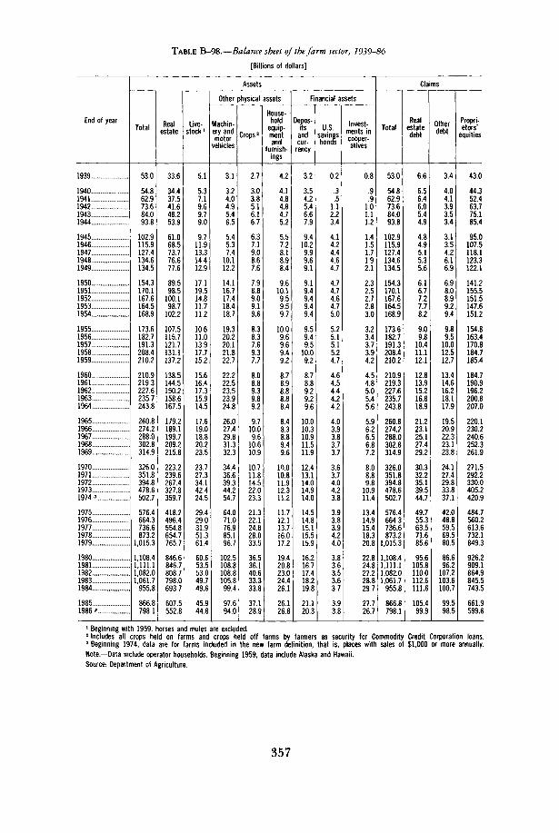
TABLE B-98.—Balance sheet of the farm sector, 1939-86

[Billions of dollars]

End of year

1939

1940194119421943 . .1944

1945 ..194619471948 .. .1949

19501951195219531954

1955195619571958. ..1959

1960 .1961196219631964

19651966196719681969

19701971197219731974 3

19751976. .197719781979

19801981198219831984

19851986 "

Assets

Total

53.0

54.862.973.684.093.8

102.9115.9127.4134.6134.5

154.3170.1167.6164.5168.9

173.6182.7191.3208.4210.2

210.9219.3227.6235.7243.8

260.8274.2288.0302.8314.9

326.0351.8394.8478.6502.7

576.4664.3736.6873.2

1,015.3

1,108.41,111.11,082.01,061.7

955.8

866.8798.1

Realestate

33.6

34.437.541.648.253.9

61.068.573.776.677.6

89.598.5

100.198.7

102.2

107.5115.7121.7131.1137.2

138.5144.5150.2158.6167.5

179.2189.1199.7209.2215.8

223.2239.6267.4327.8359.7

418.2496.4554.8654.7765.7

846.6846.7808.7798.0693.7

607.5552.8

Live-stock *

5.1

5.37.19.69.79.0

9.711.913.314.412.9

17.119.514.811.711.2

10.611.013.917.715.2

15.616.417.315.914.5

17.619.018.820.223.5

23.727.334.142.424.5

29.429.031.951.361.4

60.653.553.049.749.6

45.944.8

Other physical assets

Machin-ery andmotor

vehicles

3.1

3.24.04.95.46.5

5.45.37.4

10.112.2

14.116.717.418.418.7

19.320.220.121.822.7

22.222.523.523.924.8

26.027.429.831.332.3

34.436.639.344.254.7

64.071.076.985.196.7

102.5108.8108.8105.899.4

97.694.0

Crops2

2.7

3.03.85.16.16.7

6.37.19.08.67.6

7.98.89.09.19.6

8.38.37.69.37.7

8.08.89.39.89.2

9.710.09.6

10.610.9

10.711.814.522.023.3

21.322.124.828.033.5

36.536.140.633.333.8

37.128.9

House-hold

equip-mentand

furnish-ings

4.2

4.14.84.84.75.2

5.57.28.18.98.4

9.610.19.59.59.7

10.09.69.69.49.2

8.78.98.88.88.4

8.48.38.89.49.6

10.010.811.912.311.2

11.712.113.716.017.2

19.420.823.024.426.1

26.126.8

Financial assets

Depos-itsandcur-

rency

3.2

3.54.25.46.67.9

9.410.29.99.69.1

9.19.49.49.49.4

9.59.49.5

10.09.2

8.78.89.29.29.6

10.010.310.911.511.9

12.413.114.014.914.0

14.514.815.115.515.9

16.216.717.418.219.8

21.120.3

U.S.savingsbonds

0.2

.3

.51.12.23.4

4.14.24.44.64.7

4.74.74.64.75.0

5.25.15.15.24.7

4.64.54.44.24.2

4.03.93.83.73.7

3.63.74.04.23.8

3.93.83.94.24.0

3.83.63.53.63.7

3.93.8

Invest-ments incooper-atives

0.8

.9

.91.01.11.2

1.41.51.71.92.1

2.32.52.72.83.0

3.23.43.73.94.2

4.54.85.05.45.6

5.96.26.56.87.2

8.08.89.8

10.911.4

13.414.915.418.320.8

22.824.827.228.829.7

27.726.7

Claims

Total

53.0

54.862.973.684.093.8

102.9115.9127.4134.6134.5

154.3170.1167.6164.5168.9

173.6182.7191.3208.4210.2

210.9219.3227.6235.7243.8

260.8274.2288.0302.8314.9

326.0351.8394.8478.6502.7

576.4664.3736.6873.2

1,015.3

1,108.41,111.11,082.01,061.7

955.8

866.8798.1

Realestatedebt

6.6

6.56.46.05.44.9

4.84.95.15.35.6

6.16.77.27.78.2

9.09.8

10.411.112.1

12.813.915.216.818.9

21.223.125.127.429.2

30.332.235.139.544.7

49.755.363.571.685.6

95.6105.8110.0112.6111.6

105.499.9

Otherdebt

3.4

4.04.13.93.53.4

3.13.54.26.16.9

6.98.08.99.29.4

9.89.5

10.012.512.7

13.414.616.218.117.9

19.520.922.323.123.8

24.127.429.833.837.1

42.048.859.569.580.5

86.696.2

107.2103.6100.7

99.598.5

Propri-etors'

equities

43.0

44.352.463.775.185.4

95.0107.5118.1123.3122.1

141.2155.5151.5147.6151.2

154.8163.4170.8184.7185.4

184.7190.9196.2200.8207.0

220.1230.2240.6252.3261.9

271.5292.2330.0405.2420.9

484.7560.2613.6732.1849.3

926.2909.1864.9845.5743.5

661.9599.6

1 Beginning with 1959, horses and mules are excluded.2 Includes all crops held on farms and crops held off farms by farmers as security for Commodity Credit Corporation loans.3 Beginning 1974, data are for farms included in the new farm definition, that is, places with sales of $1,000 or more annually.

Note.—Data include operator households. Beginning 1959, data include Alaska and Hawaii.Source: Department of Agriculture.

357

INTERNATIONAL STATISTICS

TABLE B-99.—U.S. international transactions, 1946-86

[Millions of dollars; quarterly data seasonally adjusted, except as noted. Credits ( + ), debits (-)]

Year orquarter

1946194719481949

19501951195219531954

19551956195719581959

19601961196219631964

19651966196719681969

19701971197219731974

19751976197719781979

19801981198219831984

1985

1984:1III l lIV

1985:II IIllIV

1986:1IIIll ".

Merchandise * 2

Exports

11,76416,09713,26512,213

10,20314,24313,44912,41212,929

14,42417,55619,56216,41416,458

19,65020,10820,78122,27225,501

26,46129,31030,66633,62636,414

42,46943,31949,38171,41098,306

107,088114,745120,816142,054184,473

224,269237,085211,193201,820219,900

214,424

53,61454,59055,69156,005

5532453^87552,49852,727

53,66155,14955,318

Imports

-5,067-5,973-7,557-6,874

-9,081-11,176-10,838-10,975-10,353

-11,527-12,803-13,291-12,952-15,310

-14,758-14,537-16,260-17,048-18,700

-21,510-25,493-26,866-32,991-35,807

-39,866-45,579-55,797-70,499

-103,811

-98,185-124,228-151,907-176,001-212,009

-249,749-265,063-247,642-268,900-332,422

-338,863

-79,415-83,684-84,144-85,179

80369-84,242-84,173-90,079

-90,120-90,818-92,987

Net

6,69710,1245,7085,339

1,1223,0672,6111,4372,576

2,8974,7536,2713,4621,148

4,8925,5714,5215,2246,801

4,9513,8173,800

635607

2,603-2,260-6,416

911-5,505

8,903-9,483

-31,091-33,947-27,536

-25,480-27,978-36,444-67,080

-112,522

-124,439

-25,801-29,094-28,453-29,174

25Q45-30,367-31,675-37,352

-36,459-35,669-37,669

Investment income3

Receipts

7721,1021,9211,831

2,0682,6332,7512,7362,929

3,4063,8374,1803,7904,132

4,6164,9995,6186,1576,824

7,4377,5288,0209,368

10,912

11,74712,70714,76421,80827,587

25,35129,28632,17942,24564,132

72,50686,41183,54977,25186,221

89,991

22,86021,10421,39620,861

1872622^25324,50224,509

24,21622,63622,482

Payments

-212-245-437-476

-559-583-555-624-582

-676-735-796-825

-1,061

-1,237-1,245-1,324-1,561-1,784

-2,088-2,481-2,1 '47-3,378-4,869

-5,516-5,436-6,572-9,655

-12,084

-12,564-13,311-14,217-21,680-32,960

-42,120-52,329-54,883-52,410-67,469

-64,803

-15,446-17,208-17,991-16,823

16 507-16,804-16,240-15,254

-17,699-17,311-16,973

Net

560857

1,4841,355

1,5092,0502,1962,1122,347

2,7303,1023,3842,9653,071

3,3793,7544,2944,5965,040

5,3495,0475,2735,9906,043

6,2317,2718,192

12,15315,503

12,78715,97517,96220,56531,172

30,38634,08228,66624,84118,752

25,188

7,4143,8%3,4054,038

2 2195',4498,2629,255

6,5175,3255,509

Netmilitarytransac-

tions

-493-455-799-621

-576-1,270-2,054-2,423-2,460

-2,701-2,788-2,841-3,135-2,805

-2,752-2,596-2,449-2,304-2,133

-2,122-2,935-3,226-3,143-3,328

-3,354-2,893-3,420-2,070-1,653

-746559

1,528621

-1,778

-2,237-1,183

-274-369

-1,827

-2,917

-281-615-234-6%

-246-729-619

-1,322

-1,066-695-624

Nettraveland

transpor-tation

receipts

733946374230

-12029883

-238-269

-297-361-189-633-821

-964-978

-1,152-1,309-1,146

-1,280-1,331-1,750-1,548-1,763

-2,038-2,345-3,063-3,158-3,184

-2,812-2,558-3,565-3,573-2,935

-997144

-992-4,227-8,593

-11,128

-1,834-2,052-2,332-2,375

-2202-2i864-3,031-3,031

-2,701-2,395-2,415

Otherserv-ices,net3

310145175208

242254309307305

299447482486573

638732911

1,0371,161

1,4801,4961,7421,7591,964

2,3292,6492,9653,4064,231

4,8535,0275,6796,4596,214

7,7938,6998,8299,7119,881

10,603

2,6302,4712,4482,333

24422i5522,6092,999

2,6943,1003,0%

Balanceon goods

andservices * 4

7,80711,6176,9426,511

2,1774,3993,1451,1952,499

2,9285,1537,1073,1451,166

5,1916,4846,1277,2449,724

8,3786,0955,8383,6933,524

5,7732,423

-1,74211,2449,392

22,9849,521

-9,488-9,875

5,138

9,46613,764-214

-37,123-94,308

-102,694

-17,872-25,394-25,166-25,874

—22832-25i959-24,454-29,451

-31,015-30,334-32,103

Remit-tances,

pensions,and otherunilateral

transfers >

-2,922-2,625-4,525-5,638

-4,017-3,515-2,531-2,481-2,280

-2,498-2,423-2,345-2,361-2,448

-2,367-2,662-2,740-2,831-2,901

-2,948-3,064-3,255-3,082-3,125

-3,443-3,856-4,052-4,103

5 -7,431

-4,868-5,314-5,023-5,552-6,128

-7,593-7,425-8,917-9,481

-12,157

-14,983

-2,368-2,439-3,107-4,243

—3280-3',458-4,001-4,244

-3,023-4,079-4,177

Balanceon

currentac-

count14

4,8858,9922,417

873

-1,840884614

-1,286219

4302,7304,762

784-1,282

2,8243,8223,3874,4146,823

5,4313,0312,583

611399

2,331-1,433-5,795

7,1401,962

18,1164,207

-14,511-15,427

-991

1,8736,339

-9,131-46,604

-106,466

-117,677

-20,240-27,833-28,273-30,117

—26112-29]417-28,455-33,695

-34,038-34,413-36,280

1 Excludes military.2 Adjusted from Census data for differences in valuation, coverage, and timing.3 Fees and royalties from U.S. direct investments abroad or from foreign direct investments in the United States are excluded frominvestment income and included in other services, net.4 In concept, balance on goods and services is equal to net exports and imports in the national income and product accounts (andthe sum of balance on current account and allocations of special drawing rights is equal to net foreign investment in the accounts),although the series differ because of different handling of certain items (gold, capital gains and losses, etc.), revisions, etc.

See next page for continuation of table.

358

TABLE B-99.—U.S. international transactions, 1946-86—Continued

[Millions of dollars; quarterly data seasonally adjusted, except as noted]

Year orquarter

1946194719481949

19501951195219531954

1955 •1956195719581959

I9601961196219631964

19651966196719681969

19701971197219731974

19751976197719781979

19801981198219831984

1985

1984- 1||I I IIV

1985- 1III l lIV

1986:1I IIll "

U.S. assets abroad, net[increase/capital outflow (-)]

Total

-4,099-5,538-4,174

7270-9,560

-5,7167321

-9,75710977

-11,585

-9,337-12,475-14,497-22,874-34,745

-39,70351 269

-34,785-61,130-64,331

-86,118-111,031-121,273-50,022-23,639

32436

-3,5712017116,443

-16,338

510-2,793-5,867

-23,266

-12,898-25,550-29,082

U.S.officialreserveassets 6

623-3,315-1,736

-266

1,758-33

-4151,256

480

182-86911652,2921,035

2,145607

1,535378171

1,22557053

-870-1,179

2,4812,349

4158

1 467

-8492558-375

732-1,133

-8,1555175

-4,965-1,196-3,131

-3,858

657-566-799

-1,110

-233-356-1213 148

11516

280

OtherU.S.

Govern-ment

assets

-1,100910

-1,0851662

-1,680

-1,6051543

-2,423-2,274-2,200

1589-1,884

1 568-2,644

5 366

-3,4744 214

-3,6934660

-3,746

-5,162-5,097

6131-5,005

5523

-2,824

2 029-U86-1,388

-717

-807-1,055

-422540

250-209

-1,346

U.S.privateassets

-5,1445235

-4,6235986

-8,050

-5,3366347

-7,386-7,833-8,206

10229-12,940

12925-20,388

33643

-35,380-44,498-30,717

57 202-59,453

-72,802-100,758

110 177-43,821

14986

-25,754

885-18,220

18,630-14,512

530-1,382-5,32419 579

12533-25,357

28016

Foreign assets in the U.S., net[increase/capital inflow ( + )]

Total

2,2942,7051,9113,2173,643

7423,6617,3799,928

12,702

6,35922,97021,46118,38834,241

15,67036,51851,31964,03638,752

58,11283,32294,07885,496

102,767

127,106

22,25141,963

2,66835,885

14,24725,35835,66551,837

36,62047,52669,133

Foreignofficialassets

1,473765

1,2701,9861,660

134-6723,451-774

-1,301

6,90826,87910,4756,026

10,546

7,02717,69336,81633,678

-13,665

15,4974,9603,5935,9683,037

-1,324

2947-157-7656,906

-11,0668,4862,5771 322

2,46914,70415,839

Otherforeignassets

8211,939

6411,2311,983

6074,3333,928

10,70314,002

-550-3,90910,98612,36223,696

8,64318,82614,50330,35852,416

42,61578,36290,48679,52799,730

128,430

25,19842,120

3,43328,979

25,31316,87233,08853,158

34,15132,82253,294

Alloca-tions ofspecialdrawingrights(SlIRs)

867717710

l',139

1,1521,093

Statisticaldiscrepancy

Total(sum of

the itemswith signreversed)

-1,019989

-1,124360

-907

-457629

-205438

-1,516

219-9,779-1,879-2,654

1458

5,91710,544

-2,02312,52125,431

24,98220,27636,32511,13027,338

23,006

1,5606,0409,162

10,570

12,3756,852

-1,3435,125

10,31612,437

-3,771

Of which:Seasonaladjust-ment

discrep-ancy

'— "Z

940-962

-3,5613,577

1,094-1,174-3,687

3,771

1,216-1,505-3,993

5 Includes extraordinary U.S. Government transactions with India.6 Consists of gold, special drawing rights, convertible currencies, and the U.S. reserve position in the International Monetary Fund

Note.—Quarterly data for U.S. official reserve assets and foreign assets in the United States are not seasonally adjusted.Source: Department of Commerce, Bureau of Economic Analysis.

359

TABLE B-100.—U.S. merchandise exports and imports by principal end-use category, 1965-86

[Billions of dollars; quarterly data seasonally adjusted]

Year orquarter

1965 . ..1966196719681969

197019711972.1973. ...1974

19751976197719781979

19801981198219831984

1985

1984:1IIIllIV

1985:1IIIllIV

1986:1IIIll "...

Exports

Total

26529.330.733.636.4

42543.349.471.498.3

107.1114.7120.8142.1184.5

224.3237.1211.2201.8219.9

214.4

53.654.655.756.0

55.353.952.552.7

. 53.755.155.3

Agricul-tural

products

636.96.56.36.1

7.47.89.5

18.022.4

22.223.424.329.935.6

42.244.037.237.138.4

29.6

10.09.79.39.3

8.37.56.77.1

7.16.26.5

Nonagricultural products

Total

20222.424.227.330.3

35135.539.953.475.9

84.891496.5

112.2148.9

182.1193.1174.0164.7181.5

184.8

43.644.946.446.7

47.046.445.845.6

46.649.048.8

Indus-trial

suppliesand

mate-rials

768.28.59.6

10.4

12310.911.816.926.2

26.728.329.733.751.8

64963357.352.256.0

53.7

13.314.114.514.2

13.913.113.313.4

13.715.614.5

Capitalgoodsexcept

automo-tive

8.18.99.9

11.112.4

14.715.416.922.030.9

36.639.139.846.558.8

74.281673.768.974.1

75.6

17.818.218.819.3

19.219.118.718.6

19.019.320.3

Auto-motive

1.92.42.83.53.9

3.94.75.57.08.8

10.812.213.515.718.4

17.519.817.418.722.5

24.5

5.65.45.75.8

6.06.26.36.1

6.05.95.6

Other

262.93.03.23.7

434.55.67.6

10.0

10.711.713.516.219.8

25.428325.624.928.9

30.9

7.07.17.47.4

7.97.97.57.5

8.08.28.5

Imports

Total

21.525.526.933.035.8

39.945.655.870.5

103.8

98.2124.2151.9176.0212.0

2498265.1247.6268.9332.4

338.9

79.483.784.185.2

80.484.284.290.1

90.190.893.0

Petro-leumand

prod-ucts

2.02.12.12.42.6

293.64.78.4

26.6

27.034645.042.360.5

79377861.355.057.3

50.5

14.014.914.114.3

10.413.612.414.1

10.07.88.0

Nonpetroleum products

Total

19.523.424.830.633.2

36.941.951.162.177.2

71.289.7

106.9133.7151.5

170.51873186.4213.9275.1

288.3

65.468.770.170.8

70.070.671.876.0

80.183.085.0

Indus-trial

suppliesand

mate-rials

9.110.210.012.011.7

12313.616.019.227.4

23.629135.041.348.5

54.057450.054.766.6

62.9

16.217.116.616.7

15.915.815.615.6

17.517.716.6

Capitalgoodsexcept

automo-tive

152.22.52.83.4

404.35.98.39.8

10.212.314.019.725.0

31.236738.343.161.1

64.0

14.115.216.015.8

15.815.715.616.9

17.918.819.3

Auto-motive

091.82.44.05.1

577.69.0

10.712.4

12.116.819.425.026.4

27.930934.143.556.6

65.1

13.513.914.414.9

14.715.716.717.9

17.819.120.6

Other

809.29.9

11.813.0

15.016.520.223.927.5

25.331438.647.751.6

57.462363.972.690.9

96.3

21.722.623.223.4

23.523.423.925.5

26.927.428.4

Note.—Data are on an international transactions basis and exclude military shipments.Source: Department of Commerce, Bureau of Economic Analysis.

360

TABLE B-101.—U.S. merchandise exports and imports by area, 1977-86

[Millions of dollars]

Item

Exports

Industrial countries. .

CanadaJapanWestern Europe ...Australia, New

Zealand, and SouthAfrica

Other countries, exceptEastern Europe

OPEC2

Other3

Eastern Europe

Internationalorganizations andunallocated

Imports

Industrial countries

CanadaJapanWestern Europe.Australia, New

Zealand, and SouthAfrica

Other countries, exceptEastern Europe

OPEC2

Other3

Eastern Europe

Internationalorganizations andunallocated

1977

120,816

76970

2853310,56634094

3,777

40,951

12,87728074

2,895

151,907

79,447

29,8641856528,226

2792

70,679

3577834,901

1127

654

1978

142,054

87948

3122912,96039,546

4,213

50,213

14,84635367

3,893

176,001

99,344

33,7562454036608

4440

74,397

3328641,111

1508

752

1979

184,473

115930

3869017,62954177

5,434

62,630

14,55648074

5913

212 009

112,797

392272626041817

5493

96131

45 03951092

1896

1 185

1980

224,269

137 152

4162620,80667603

7,117

82,941

17,36865573

4,143

33

249,750

127,884

429013121647235

6532

119 135

5560263533

1444

1287

1981

237,085

141 900

4601621,79665108

8,980

90,657

21,09769560

4,440

88

265,063

144,322

482533759752864

5608

119 188

4993469254

1553

1982

211,198

127,254

3920320,69459,701

7,656

80,130

20,65159479

3,749

65

247,642

144,139

48,5233768352,900

5033

102 414

3151770897

1066

23

1983

201,820

128,353

4451221,78955448

6,604

70,426

15,25655170

2976

65

268 900

159,893

559824284455623

5443

107 593

2528282311

1413

1

1984

219,900

140,991

5303723,24156867

7,849

74,587

13,77160816

4,290

33

332 422

205,526

67,6306021072,054

5632

124 679

2685297,827

2217

1985

214,424

139,008

5387922,14556,015

6,967

71,966

11,40960557

3,258

192

338,863

219,881

71,1736565377,454

5601

117,135

2268094,455

1,847

1986 first3 quartersat annual

rate1

218,837

145,315

52,34426,66759,313

6,991

71,361

10,58360,778

2,161

365,233

243,368

69,94079,78887,933

5,707

119,806

19,168100,638

2,059

1 Preliminary; seasonally adjusted.2 Algeria, Ecuador, Gabon, Indonesia, Iran, Iraq, Kuwait, Libya, Nigeria, Qatar, Saudi Arabia, United Arab Emirates, and3 Latin American Republics, other Western Hemisphere, and other countries in Asia and Africa, less membersNote.—Data are on an international transactions basis and exclude military.Source: Department of Commerce, Bureau of Economic Analysis.

Venezuela,of OPEC.

361

TABLE B-102.—U.S. merchandise exports and imports by commodity groups, 1966-86

[Millions of dollars; monthly data for statistical month]

Year ormonth

196619671968196919701971197219731974

1974*....1975* ....1976*....1977* ....1978* ....1979* ....1980

198119821983198419851985:

JanFebMar....

fcJune...July....Aug....Sept...OctNov....Dec ....

1986:Jan....Feb....Mar...

fcJune..July...Aug...Sept..Oct....Nov...

Merchandise exports

Totaldomes-tic andforeign

exports1

Domestic exports

Total tzFood,bever-ages,and

tobacco

Crudemateri-als andfuels3

Manu-facturedgoods*

Merchandise imports

General imports5

Total2

Food,bever-ages,and

tobacco

Crudemateri-als andfuels3

Manu-facturedgoods4

F.a.s. value7 Customs value

29,49031,03034,06337,33242,65943,54949,19970,82397,998

98,092107,652115,223121,232143,681181,860220,630

233,677212,193200,486217,865213,146

18,67317,14320,33017,97318,33718,01216,72716,58417,03417,61817,72116,994

17,00617,73518,91317,96517,43119,07017,70717,60417,51819,33018,595

29,05430,64633,62636,78842,02542,91148,39969,73096,634

96,679106,161113,549119,024141,142178,633216,515

228,899207,076195,917212,034206,925

18,12416,64819,76517,49217,81617,43316,17216,10616,54317,12217,22716,479

16,50117,16418,34917,37616,69116,42715,91116,83116,86018,59417,895

5,1864,7104,5924,4465,0585,0766,569

12,93815,233

15,23316,79317,23415,96320,60424,58730,407

33,20626,97726,97927,31222,226

2,1611,9951,9731,9131,6031,6141,6041,7831,7091,8362,1281,907

1,7971,6891,7061,4751,3951,4381,6481,8141,6721,8661,863

4,4044,7264,8655,0066,6926,4417,091

10,73515,802

15,80215,19716,09518,57920,95728,22233,719

33,02233,51829,55531,48228,344

2,6712,5802,5622,4412,2612,1222,0332,2582,1152,2852,5592,459

2,4672,3672,3492,4362,2281,7761,7642,0351,9882,2872,339

19,21820,84423,81826,78529,34430,44333,74044,73163,523

63,52370,95177,24180,15194,473

116,587143,891

154,283139,716132,409143,142145,384

12,44511,21814,24512,22812,99212,75911,55611,23311,70012,10211,68811,221

11,39312,18213,32512,61512,27412,29811,62312,04212,25313,36712,755

25,61826,88933,22636,04339,95145,56355,58369,476

101,394

4,5904,7015,3655,3086,2306,4047,3799,235

10,701

5,7185,3676,0316,3916,5427,2688,838

13,44631,842

14,44615,75620,62423,01125,90730,41437,76745,00156,202

F.a.s. value 7

102,55998,503

123,477150,390174,757209,458244,871

10,7099,923

11,89114,22715,74317,73518,551

32,06432,59641,47453,55451,90171,39093,973

Customs value

260,982243,952258,048325,726345,276

28,83625,94128,72528,57229,30230,13627,00026,24731,34928,42930,01030,728

32,00528,89531,97228,76230,27231,76434,12129,47628,69530,01836,187

18,35017,81718,81921,62622,376

1,9321,8172,1281,8041,9191,9121,6411,7191,9031,5981,8652,138

2,2151,9082,1002,0182,3291,8862,1431,9311,9631,9352,328

92,87374,40468,03772,75864,981

5,3444,9064,3835,7725,7006,0545,0854,8515,5625,6565,6576,011

6,2344,7414,2843,1763,6594,1633,9633,4133,8743,5143,866

55,22351,08064,77576,554

100,317112,226125,122

142,475144,022163,449221,515246,778

20,44818,38521,30120,08020,72521,26819,28618,91622,88720,27121,55721,654

22,47721,28924,26122,22623,00123,97126,60923,10621,84923,53728,350

Total,c.i.f.

value6

28,74535,32038,24142,42948,34258,86273,573

108,392

110,875105,880132,498160,411186,045222,228256,984

273,352254,885269,878341,177361,626

30,24527,16930,10729,90730,71231,59628,31227,51232,86029,69531,37132,141

33,46530,22533,43530,03631,63833,24035,74530,92530,07831,38937,816

Merchandise trade balance

Exportsless

imports,customs

value

3,8724,141

8371,2892,708

-2,014-6,384

1,348-3,396

-27,305-31,759

57562-107,861-132,129

-10,1638798

-8,395-10,599-10,965-12,124-10,274-9,663

-14,315-10,811-12,290-13,734

14999-11,161-13,059-10,797-12,842

12694-16,414-11,871-11,177

10688-17,592

Exportsless

imports,f.a.s.

»••"••

44679,1498254

-29,158-31,076-27,599

24,241

Exportsless

imports,c.i.f.

2,283-1,257

-909230

-4,793-9,663

2,752-10,395

-12,7831,772

-17,274-39,179-42,364-40,368-36,354

-39,675-42,691-69,392

-123,312-148,480

-11,572-10,026-9,777

-11,935-12,375-13,584-11,585-10,927-15,826-12,077-13,651-15,146

-16,459-12,491-14,522-12,071-14,208-14,170-18,037-13,321-12,560-12,059-19,221

1 Department of Defense shipments of grant-aid military supplies and equipment under the Military Assistance Program are excludedthrough 1984 and included beginning 1985 from total exports.2 Total includes commodities and transactions not classified according to kind.3 Includes fats and oils.4 Includes machinery, transportation equipment, chemicals, metals, and other manufactures. Export data for these items include, ,military grant-aid shipments through 1977 and exclude them thereafter.5 Total arrivals of imported goods other than intransit shipments.6 C.i.f. (cost, insurance, and freight) import value at first port of entry into United States. Data for 1967-73 are estimates.7 F.a.s. (free alongside ship) value basis at U.S. port of exportation for exports and at foreign port of exportation for imports.

Note.— Data are as reported by the Bureau of the Census adjusted to include silver ore and bullion reported separately prior to 1969.Trade in gold is included beginning 1974. Export statistics cover all merchandise shipped from the U.S. customs area, except suppliesfor the U.S. Armed Forces. Exports include shipments under Agency for International Development and Food for Peace programs as wellas other private relief shipments.

Data beginning 1980 include trade of the U.S. Virgin Islands, except that for 1980 Virgin Islands exports are reflected only in thefigures for domestic and foreign exports combined, total domestic exports, and trade balance.

*Data for 1974-79 for domestic and foreign exports combined, total domestic exports, total general imports, and trade balanceinclude trade of the Virgin Islands.

Source: Department of Commerce (Bureau of the Census and International Trade Administration, Office of Trade Information andAnalysis, Trade Statistics Division).

362

TABLE B-103.—International investment position of the United States at year-end, 1978-85

[Billions of dollars]

Type of investment

Net international investment position of the United States...

U S assets abroad

U.S. official reserve assets

GoldSpecial drawing rightsReserve position in the International Monetary

Fund .Foreign currencies

U.S. Government assets, other than official reserveassets

U.S loans and other long-term assetsRepayable in dollarsOther

U.S. foreign currency holdings and U.S. short-term assets

U S private assets

Direct investment abroadForeign securities

BondsCorporate stocks... ..

U.S. claims on unaffiliated foreigners reportedby U S nonbanking concerns

U.S. claims reported by U.S. banks, not includedelsewhere

Foreign assets in the United States

Foreign official assets in the United States

U.S Government securitiesU.S. Teasury securitiesOther

Other U.S. Government liabilitiesU.S. liabilities reported by U.S. banks, not in-

cluded elsewhereOther foreign official assets

Other foreign assets in the United States

Direct investment in the United StatesU.S. Treasury securitiesU.S. securities other than U.S. Treasury securi-

tiesCorporate and other bondsCorporate stocks

U.S. liabilities to unaffiliated foreigners reportedby U.S. nonbanking concerns

U.S. liabilities reported by U.S. banks, not in-cluded elsewhere

1978

76.1

4478

18.7

1171.6

1.044

54.2

52349.824

19

3750

162753442111.2

281

1308

3717

173.1

12851240

45127

23385

1987

4258.9

53.611542 1

16.0

777

1979

94.5

510.6

19.0

1122.7

1.338

58.4

56554.124

19

4332

187956.842014.8

315

1570

4161

159.9

10661017

49127

30599

2563

54514.2

58.6103483

18.7

1103

1980

106.0

606.9

26.8

1122.6

2.9101

63.5

61859.622

17

5166

215462.743519.2

347

2039

5008

176.1

1182111.3

69134

304141

3248

83016.1

74195

646

30.4

121 1

1981

140.7

719.7

30.1

1124.1

5.198

68.5

67.064.72.3

15

6212

228363.545817.7

359

2935

5790

180.4

1251117.0

8113.0

26.7155

3986

108718.5

75.4107646

30.6

1654

1982

136.2

824.9

34.0

1115.3

7.3102

74.3

72.770.72.0

17

7166

207875.756719.0

286

4046

6887

189.1

1326124.9

7713.6

25.0179

4996

124725.8

93.6168768

27.5

2280

1983

88.5

874.1

33.7

11.15.0

11.363

79.3

77.675.7

1.9

17

761 1

207284.357726.6

35.1

434.5

7856

194.6

137.0129.7

7314.4

25.5177

5910

137.133.9

114.717.5973

26.9

2783

1984

4.4

898.2

34.9

11.15.6

11.567

84.6

82.780.81.8

20

7786

213090.062127.9

30.0

445.6

893.8

199.1

143.0135.5

7.514.8

26.115.2

694.7

164.658.3

128.632.7958

31.0

312.2

1985

-107.4

952.4

43.2

11.17.3

11.912.9

87.4

85.683.8

1.8

1.8

821.8

2327114.173440.7

28.2

446.7

1,059.8

202.3

143.7136.0

7.715.3

26.616.7

857.5

183.083.8

207.881.8

125.9

29.1

353.8

Source: Department of Commerce, Bureau of Economic Analysis.

363

TABLE B-104.—International reserves, selected years, 1952-86

[Millions of SDRs; end of period]

Area and country

All countries

Industrial countries

United StatesCanadaAustraliaJapanNew Zealand

AustriaBelgium . .DenmarkFinlandFrance

GermanyIcelandIrelandItalyNetherlands . . . . .

NorwaySpainSweden :SwitzerlandUnited Kingdom

Developing countries: TotalBy area:

AfricaAsiaEuropeMiddle EastWestern Hemisphere

Memo:Oil-exporting countriesNon-oil developing countries

1952

49,388

38,582

247141,944

9201101

183

1161 133

150132686

9608

318722953

164134504

1,6671956

10272

1,7863721

9661,1832616

1,6998573

1962

62,851

52,535

172202,5611,1682021

251

1,0811,753

256237

4049

6,95832

3594,0681,943

3041045

8022,9193,308

10,202

2,11026581 3481,8052282

2,0308172

1972

147,323

110,282

121125,5725,656

16916767

2,5053,564

787664

9224

21,90878

10385,6054407

1,2204,6181,4536,9615,201

36,083

3,9627,17164259,4369089

9,95626127

1982

360,854

211,918

299183,4286,053

22001577

5,5444,7572,1111,420

17,850

43,909133

239015,10710723

6,2727,4503,397

16,93011,904

141,071

7,64236,7127063

64,09425560

67,16373907

1983

393,979

232,234

308314,0168,838

24346744

5,0525,6993,5151,227

21,826

44,092144

253421,28411253

6,3737,5814,065

17,27511,496

150,274

7,30444,5348206

62,25427,977

67,20083,075

1984

438,927

252,033

335173,2467,869

278111,824

5,0705,8533,1272,854

24,227

44,282132

241223,54910961

9,59612,7094,135

18,52010,297

170,757

7,13552,7099702

59,63741,574

69,605101,152

1985

437,577

254,834

384122,9825,528

251731,454

5,0805,6114,9993,481

27,071

43,735189

268916,45811,354

12,71110,6865,487

19,31712,373

162,033

8,67247,0639,779

58,73037,788

69,32592,708

1986

Novem-ber

443,447

274,102

J39 5943,2145,790

35578^,041

5,1315,6854,1251,340

'30,386

45,954240

295918,81011,300

10,488113,415

5,88917,99715,822

137,601

7,33042,98910,26749,04727,969

53,55684,045

1 Data refer to October 1986.Note.—International reserves is comprised of monetary authorities' holdings of gold (at SDR 35 per ounce), special drawing rights

(SDRs), reserve positions in the International Monetary Fund, and foreign exchange. Data exclude U.S.S.R., other Eastern Europeancountries, and Cuba (after 1960).

U.S. dollars per SDR (end of period) are-. 1952 and 1962—1.00000; 1972—1.08571; 1979—1.31733; 1980—1.27541; 1982—1.10311; 1983-1.04695; 1984-.98021; 1985-1.09842; and November 1986-1.21030.

Source: International Monetary Fund, "International Financial Statistics."

364

TABLE B-105.—Exchange rates, 1967-86

[Cents per unit of foreign currency, except as noted]

Period

March 1973

196719681969

19701971197219731974

19751976197719781979

1980 .19811982 ..19831984 ..

19851986

1985: 1||IIIIV

1986- IIIIllIV

March 1973

196719681969

19701971197219731974

19751976197719781979

1980198119821983 ..1984

19851986

1985- 1IIIIIIV

1986: 1IIIllIV

Belgian franc

2.5378

2.01252.00261.9942

2.01392.05982.27162.57612.5713

2.72532.59212.79113.18093.4098

3.42472.70072.19821.96211.7348

1.69682.2464

1.53151.60831.73991.9074

2.08292.18302.32092.3989

Netherlandsguilder

34.834

27.75927.62627.592

27.65128.65031.15335.97737.267

39.63237.84640.75246.28449.843

50.36940.19137.47335.12031.245

30.37041.008

27.17428.68531.25334.367

37.77539.57042.56244.126

Canadiandollar

100.333

92.68992.80192.855

95.80299.021100.93799.977102.257

98.297101.41094.11287.72985.386

85.53083.40881.07781.13377.244

73.22671.959

73.87573.01373.52472.493

71.22772.23072.17572.205

Swedish krona

22.582

19.37319.34919.342

19.28219.59221.02222.97022.563

24.14122.95722.38322.13923.323

23.64719.86016.06313.04412.103

11.67214.041

10.78911.17911.92312.796

13.48713.89214.33714.448

French franc

22.191

20.32320.19119.302

18.08718.14819.82522.53620.805

23.35420.94220.34422.21823.504

23.69418.48915.29313.18311.474

11.22014.467

10.05010.61611.52912.686

13.88214.01114.75615.221

Swiss franc

31.084

23.10423.16923.186

23.19924.32526.19331.70033.688

38.74340.01341.71456.28360.121

59.69751.02549.37347.66042.676

41.05855.925

36.33238.56542.48146.856

50.61453.65259.33760.097

German mark

35.548

25.08425.04825.491

27.42428.76831.36437.75838.723

40.72939.73743.07949.86754.561

55.08944.36241.23639.23535.230

34.24746.266

30.72832.38035.16238.719

42.63344.57747.99049.864

United Kingdompound

247.24

275.04239.35239.01

239.59244.42250.08245.10234.03

222.16180.48174.49191.84212.24

232.58202.43174.80151.59133.56

129.56146.68

111.52125.56137.63143.53

144.05150.94148.77142.98

Italian lira

0.17604

.16022

.16042

.15940

.15945

.16174

.17132

.17192

.15372

.15328

.12044

.11328

.11782

.12035

.11694

.08842

.07411

.06605

.05708

.05255

.06730

.04949

.05074

.05285

.05713

.06258

.06496

.06966

.07199

Japanese yen

0.38190

.27613

.27735

.27903

.27921

.28779

.32995

.36915

.34302

.33705

.33741

.37342

.47981

.45834

.44311

.45432

.40284

.42128

.42139

.42248

.59709

.38837

.39874

.41977

.48302

.53380

.58918

.64186

.62352

Multilateral trade-weighted value ofthe U.S. dollar (March 1973 = 100)

Nominal

100.0

120.0122.1122.4

121.1117.8109.199.1101.4

98.5105.6103.392.488.1

87.4102.9116.6125.3138.3

143.2112.0

156.5149.1139.2128.2

119.5114.2108.3107.0

Real1

100.0

98.899.2

93.997.393.184.283.2

84.8100.8111.7117.3128.5

132.0103.4

144.1137.0128.5118.4

110.1104.599.998.9

1 Adjusted by changes in consumer prices.Source: Board of Governors of the Federal Reserve System.

365

TABLE B-106.—Industrial production and consumer prices, major industrial countries, 1962-86

Year or quarter

1962 ....1963196419651966196719681969197019711972197319741975197619771978197919801981 . .19821983 .. ..198419851986 "1985- 1

IIIllIV

1986- 1IIHIIV

19621963196419651966196719681969. ..197019711972 .. .197319741975197619771978197919801981198219831984198519861985:1

II . .IllIV

1986:1IIIIIIV

UnitedStates Canada Japan

EuropeanCommu-nity1

France WestGermany Italy United

Kingdom

Industrial production ( 1977= 100) 2

53.256.360.166.172.073.577.681.278.579.687.394.493.084.892.6100.0106.5110.7108.6111.0103.1109.2121.4123.81251123.1123.5124.0124.7125.0124.4125.0126.0

46.649.654.158.763.065.569.774.575.579.685.694.797.791.997.5100.0103.3109.7108.1108.699.0104.0112.6118.1

115.8117.6119.2120.1119.2118.2116.8

29.232.537.739.244.252.860.870.480.182.386.899.096.786.596.1

100.0106.4113.9119.2120.4120.9125.1138.9145.1

143.0146.1146.1144.9145.1145.3144.1

55.758.162.364.967.468.573.680.584.586.490.296.897.591.097.7100.0102.3107.4106.7104.2102.9104.0106.8110.3

108.6109.7110.3111.2110.8113.1112.5

505660616466687579848895989198100102107106106104105106107

106106109109106109110

56.658.263.366.967.565.571.580.685.887.590.896.796.490.598.7100.0102.7107.7108.0106.2103.1104.1107.6112.9

111.3112.3114.1115.0114.7115.7116.2

49.654.056.158.765.670.774.877.682.682.286.294.598.389.6100.0100.0101.9108.8114.4112.6108.5105.8109.4110.9

110.6111.1109.8110.1113.2114.9110.9

68.470.776.478.679.880.486.589.589.989.591.199.297.392.195.1100.0103.0106.999.896.498.2101.7103.0108.0

106.6108.9108.1108.2109.2108.7110.3

Consumer prices (1967=100)

90.691.792.994.597.2100.0104.2109.8116.3121.3125.3133.1147.7161.2170.5181.5195.4217.4246.8272.4289.1298.4311.1322.2328.4317.4321.2323.6326.5327.3326.5328.9330.8

87.789.290.993.196.5100.0104.0108.8112.4115.6121.2130.3144.5160.1172.1185.9202.5221.0243.5273.9303.5321.0335.0348.2362.8343.0346.8350.0353.2357.5360.4364.7368.4

76.782.585.891.696.3100.0105.3110.9119.3126.5132.3147.9184.0205.8224.9243.0252.3261.3282.3296.2304.1309.7316.5323.0

320.1322.9322.8326.2324.6325.6324.5

84.387.690.794.197.5100.0103.7107.9113.2120.2127.5138.2156.2176.7195.2214.3229.2250.0280.9312.1343.3373.0398.0423.3

415.2423.0425.3429.5433.4436.5438.2

85.489.592.594.897.4100.0104.5111.3117.1123.5131.1140.7160.0178.9196.1214.5233.9259.1294.2332.7373.1407.9439.5465.1

456.1464.4468.7471.4472.4475.8478.5

87.489.992.095.098.4100.0101.6103.5107.1112.7119.0127.2136.1144.2150.5156.0160.2166.9175.8186.9196.8203.3208.2212.8

211.8213.1212.6213.2213.3212.7211.7

79.285.190.194.296.4100.0101.4104.1109.2114.4121.0134.0159.7186.8218.1255.2286.2328.5398.0472.4549.4631.8698.8758.9

743.5760.4768.7786.1800.4809.9815.0

85.186.889.693.997.6100.0104.8110.3117.4128.5137.7150.2174.3216.5252.4292.4316.6359.0423.6473.9514.7538.3565.1599.5

582.9602.9604.5607.5611.7619.6620.3

1 Consists of Belgium-Luxembourg, Denmark, France, Greece, Ireland, Italy, Netherlands, United Kingdom, West Germany, Portugal, andSpain. Industrial production prior to July 1981 excludes data for Greece, which joined the EC in 1981. Data for Portugal and Spain,which became members on January 1,1986 are excluded prior to 1982.2 All data exclude construction. Quarterly data are seasonally adjusted.

Sources-. Department of Commerce (International Trade Administration, Office of Trade Information and Analysis, Trade StatisticsDivision) and Department of Labor (Bureau of Labor Statistics).

366

TABLE B-107.—Civilian unemployment rate, and hourly compensation, major industrial countries,

1960-86

[Quarterly data seasonally adjusted]

Year or quarter

1960196119621963196419651966..19671968196919701971197219731974197519761977197819791980198119821983198419851986

1985: IIII I IIV

1986: 1 ...III I I .IV

I9601961196219631964196519661967196819691970197119721973197419751976197719781979198019811982198319841985

UnitedStates Canada Japan France West

Germany Italy UnitedKingdom

Civilian unemployment rate (percent)1

5.56.75.55.75.24.53.83.83.63.54.95.95.64.95.68.57.77.16.15.87.17.69.79.67.57.27.0

7.37.27.27.17.17.16.96.9

6.56.75.55.24.43.63.43.84.54.45.76.26.25.55.36.97.18.18.37.47.57.5

11.011.911.310.59.6

11.110.610.210.19.79.69.79.4

1.71.51.31.31.21.21.41.31.21.11.21.31.41.31.41.92.02.02.32.12.02.22.42.72.82.6

2.62.62.72.92.72.82.9

1.61.41.31.21.31.41.71.82.42.22.52.72.82.72.94.24.55.05.46.06.47.58.38.59.9

10.4

10.510.410.410.110.210.510.7

1.1.6.6.5.4.3.3

1.31.1.6.5.6.7.7

1.63.43.43.53.43.02.94.15.97.47.87.9

7.97.97.97.87.87.67.5

3.73.32.82.42.73.53.83.43.53.53.23.33.83.73.13.43.94.14.14.44.34.85.45.95.96.0

5.95.86.06.36.36.56.1

2.22.02.73.32.52.12.33.33.23.13.13.94.23.23.14.65.96.46.35.47.1

10.511.411.911.711.3

11.411.311.311.311.511.711.6

Manufacturing hourly compensation ( 1977 = 100) 2

36.537.639.040.241.942.744.646.950.253.757.460.964.268.876.285.192.1

100.0108.2118.6132.4145.2157.5162.4168.2176.7

29.729.228.429.230.331.834.436.939.742.747.452.757.662.874.481.796.9

100.099.5

107.3118.7134.3143.8154.6149.3148.9

6.67.78.89.8

11.012.413.615.317.821.325.330.239.854.566.476.081.9

100.0137.0139.2143.2157.6146.9158.6163.3166.5

15.216.818.620.222.023.825.227.030.430.932.636.944.357.963.488.191.5

100.0123.9149.4172.6155.0151.1146.4138.9143.1

10.512.213.914.816.117.619.120.221.724.130.535.943.459.169.179.984.2

100.0124.8147.0160.7138.6134.8134.9126.9130.1

11.913.115.518.320.421.822.825.427.130.736.843.152.366.473.995.089.5

100.0119.1143.1165.3152.8154.8160.6150.6152.8

24.426.127.528.730.533.536.236.834.337.443.251.060.867.877.598.592.4

100.0128.0168.8224.7223.9213.0198.0187.1194.8

ivilian unemployment rates, approximating U.S. concepts. Quarterly data for France, West Germany, and United Kingdom should bed as less precise indicators of unemployment under U.S. concepts than the annual data. Beginning 1977, changes in the Italian

1 Civilian

survey resulted'in a large increase in persons enumerated as unemployed. However, many also "reported that they~had not activelysought work in the past 30 days. Such persons have been provisionally excluded for comparability with U.S. concepts; their inclusionwould about double the rates shown for Italy.2 Hourly compensation in manufacturing, U.S. dollar basis. Data relate to all employed persons (wage and salary earners and the self-employed) in the United States and Canada, and to all employees (wage and salary earners) in the other countries. For France andUnited Kingdom, compensation adjusted to include changes in employment taxes that are not compensation to employees, but are laborcosts to employers.

Source: Department of Labor, Bureau of Labor Statistics.

367

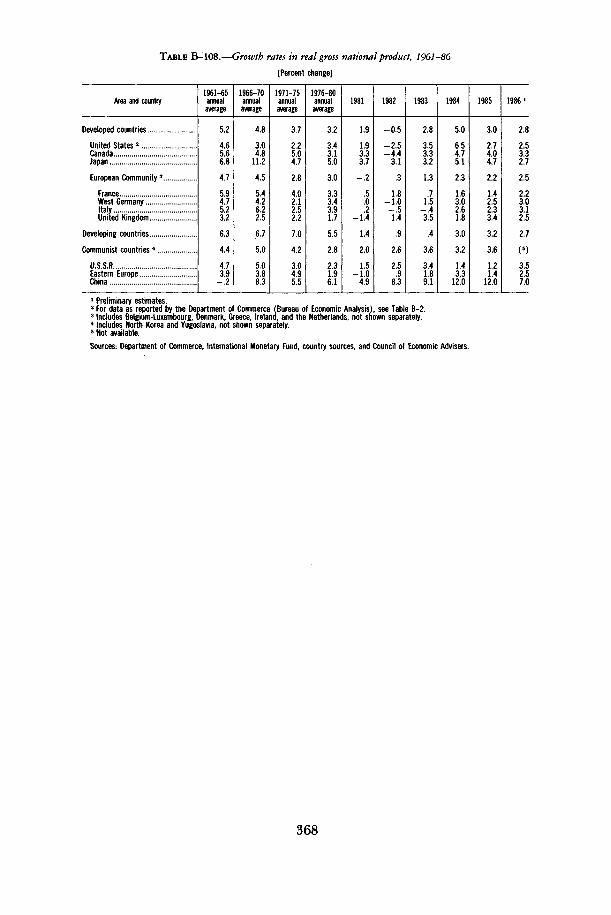
TABLE B-108.—Growth rates in real gross national product, 1961-86

[Percent change]

Area and country

Developed countries

United States 2

CanadaJapan

European Community 3

FranceWest GermanyItalyUnited Kingdom

Developing countries

Communist countries 4

U S S REastern EuropeChina

1961-65annualaverage

52

465.668

47

5.94.75232

63

44

4739

2

1966-70annualaverage

4 8

304.8

112

4 5

5.44.2622.5

67

50

503.883

1971-75annualaverage

37

225.04 7

28

4.0212522

70

42

304955

1976-80annualaverage

32

343150

30

3.3343917

55

28

231961

1981

19

193.337

2

.502

-14

14

20

15-10

49

1982

-05

-25-4.4

31

3

1.8-1.0

514

9

26

25.9

83

1983

28

353.332

13

.715

435

4

36

341.891

1984

50

654.751

23

1.6302618

30

32

1433

120

1985

30

274.047

22

1.4252334

32

36

121.4

120

1986 i

28

253.327

25

2.2303125

27

(5)

352570

1 Preliminary estimates.2 For data as reported by the Department of Commerce (Bureau of Economic Analysis), see Table B-2.3 Includes Belgium-Luxembourg, Denmark, Greece, Ireland, and the Netherlands, not shown separately.4 Includes North Korea and Yugoslavia, not shown separately.5 Not available.

Sources: Department of Commerce, International Monetary Fund, country sources, and Council of Economic Advisers.

368