Ecological patterns, distribution and population structure of Prionace glauca (Chondrichthyes:...

Ecological patterns, distribution and population structure of Prionace glauca(Chondrichthyes: Carcharhinidae) in the tropical-subtropical transition zoneof the north-eastern Pacific

Rodolfo Vögler a,*, Emilio Beier b, Sofía Ortega-García a,1, Heriberto Santana-Hernández c,J. Javier Valdez-Flores c

aDepartamento de Pesquerías y Biología Marina, Centro Interdisciplinario de Ciencias Marinas-Instituto Politécnico Nacional (CICIMAR-IPN),Av. Instituto Politécnico Nacional s/n, Col. Playa Palo de Santa Rita, Casilla 952, La Paz, B.C.S, MexicobCentro de Investigación Científica y de Educación Superior de Ensenada (CICESE), Unidad La Paz, Miraflores No. 334, CP 23050, La Paz, B.C.S, MexicocDirección General de Investigación Pesquera en el Pacífico Sur, Playa Ventana s/n, Manzanillo, Colima, Instituto Nacional de Pesca de México, Mexico

a r t i c l e i n f o

Article history:Received 8 September 2010Received in revised form14 September 2011Accepted 29 October 2011

Keywords:Blue sharkBy-catchSpatial-temporal distribution patternsLandscape ecologySubtropical convergenceNorth-eastern Pacific

a b s t r a c t

Regional ecological patterns, distribution and population structure of Prionace glauca were analyzedbased on samples collected on-board two long-line fleets operating in oceanic waters (1994e96/2000e02) and in coastal oceanic waters (2003e2009) of the eastern tropical Pacific off México. Generalizedadditive models were applied to catch per unit of effort data to evaluate the effect of spatial, temporaland environmental factors on the horizontal distribution of the life stages (juvenile, adult) and the sexesat the estimated depth of catch. The presence of breeding areas was explored. The population structurewas characterized by the presence of juveniles’ aggregations and pregnant females towards coastalwaters and the presence of adult males’ aggregations towards oceanic waters. The species exhibitedhorizontal segregation by sex-size and vertical segregation by sex. Distribution of the sex-size groups atoceanic waters was seasonally affected by the latitude; however, at coastal oceanic waters mainlyfemales were influenced by the longitude. Latitudinal changes on the horizontal distribution werecoupled to the seasonal forward and backward of water masses through the study area. Adult malesshowed positive relationship with high temperatures and high-salinities waters (17.0�e20.0 �C; 34.2e34.4) although they were also detected in low-salinities waters. The distribution of juvenile malesmainly occurred beyond low temperatures and low-salinities waters (14.0�e15.0 �C; 33.6e34.1), sug-gesting a wide tolerance of adult males to explore subartic and subtropical waters. At oceanic areas, adultfemales were aggregated towards latitudes <25.0�N, mainly associated to subtropical waters duringsummer. The distribution of juvenile females indicated its preference by lower temperatures and moresaline waters. Presence of pregnant females suggests that the eastern tropical Pacific off México repre-sents an ecological key region to the reproductive cycle of P. glauca.

� 2011 Elsevier Ltd. All rights reserved.

1. Introduction

At open ocean ecosystems, the dynamic changes on theoceanographic conditions are the cause of the mobility and widedistribution of big fish species with highly migratory habits. In thepast, the researchers found severe limitations to achieve a better

understanding of the biological and ecological characteristics ofmigratory sharks, as a consequence of their high mobility and widedistribution. However, the combination of tagging techniques withsatellite telemetry have increased the present pace of obtainingknowledge about the migration pathways, spatial dynamics,swimming depth and habitat preferences of Prionace glauca (Casey,1985; Kohler and Turner, 2008; Stevens et al., 2010), Carcharodoncarcharias (Bonfil et al., 2005; Boustany et al., 2002; 2008), Rin-chodon typus (Eckert and Stewart, 2001; Wilson et al., 2006),Cetorhinus maximus (Gore et al., 2008; Skomal et al., 2009), Lamnaditropis (Weng et al., 2005, 2008), Isurus oxyrinchus (Stevens et al.,2010), Alopias supercilliosus (Weng and Block, 2004; Stevens et al.,2010), and Alopias vulpinus (Stevens et al., 2010). However, these

* Corresponding author. CICIMAR-IPN, Av. Instituto Politécnico Nacional s/n, Col.Playa Palo de Santa Rita, CP 23096, La Paz, B.C.S, Mexico. Tel.: þ52 612 1234658;fax: þ52 612 1225322.

E-mail address: [email protected] (R. Vögler).1 Fellowship of Comisión de Operación y Fomento de Actividades Académicas

del IPN.

Contents lists available at SciVerse ScienceDirect

Marine Environmental Research

journal homepage: www.elsevier .com/locate/marenvrev

0141-1136/$ e see front matter � 2011 Elsevier Ltd. All rights reserved.doi:10.1016/j.marenvres.2011.10.009

Marine Environmental Research 73 (2012) 37e52

studies are generally based on only a few individuals, which isa central limitation when attempting to apply these results ata population level. Thus, the use of fishing fleets as samplingplatforms represents a complementary tool to understand thebiological and ecological population characteristics of these highlymigratory shark species.

Prionace glauca is a large oceanic-epipelagic shark, but it mayalso be found in coastal waters with a narrow continental shelf(Compagno, 2008). Of all of the cartilaginous fish, this shark hasthe widest geographic distribution (Kohler and Turner, 2008) andis cosmopolitan in areas located between tropic and temperateregions (Nakano and Stevens, 2008). Prionace glauca is the mostimportant by-catch species of the long-line and gillnet fisheriesaround the world. This pelagic shark is increasingly targeted byseveral fisheries for their fins or meat, particularly in nationswhere the fishing fleets operate in oceanic waters (Nakano andStevens, 2008). In the eastern tropical Pacific off México (ETPM),P. glauca numerically dominates the catches of the oceanic long-line commercial fleet and is the second most common targetspecies caught by the coastal long-line commercial fleet (Sosa-Nishizaki et al., 2002).

In temperate regions, the distribution and movements ofP. glauca are strongly influenced by seasonal variations in watertemperature coupled with their reproductive conditions and theavailability of their prey (Kohler and Turner, 2008). Using conven-tional tagging, Casey (1985) found changes in the spatial andseasonal distribution of P. glauca in the temperate region of thenorth-eastern Atlantic. He also reported the occurrence of spatialsegregation between groups based on sex and size. A theoreticalmodel by Nakano (1994) explains the macro-scale distribution ofthis species in the temperate region of the northern Pacific, andrelated results indicate a latitudinal segregation pattern, dependingon the sex and size of the individuals. According to Nakano (1994),mating occurs in early summer between 20.0 and 30.0�N, and sexsegregation takes place only among juveniles. This model sug-gested the distribution of the parturition area extended around theSubarctic Convergence zone (SAC, between 35.0 and 45.0�N). Thenursery areas of juvenile females andmales would be located northand south of the SAC, respectively. Adult males and females shouldbe distributed from the breeding areas towards the equator(Nakano, 1994). Recently, Montealegre-Quijano and Vooren (2010)emphasized that the Subtropical Convergence (STC) of the south-western Atlantic could be used by P. glauca as a nursery area forsmall juveniles of both sexes and also they noted that adult femaleswere more abundant at lower latitudes (<25�S). Lastly, Carvalhoet al. (2011) used spatial prediction maps for P. glauca Catch PerUnit Effort (CPUE) to model the presence of two areas of higherdensity of juveniles that were located south of 30�S in the south-western Atlantic, one area close to shore (possibly related toupwelling process at the shelf break off the south coast of Brazil,Argentina, and Uruguay) and another one offshore (possibly relatedto the frontal system of the STC). Nevertheless, at the present onlysome pieces has been added to the puzzle that conform the land-scape distribution patterns of P. glauca coupled with their pop-ulation structure at tropical and subtropical regions of the Worldoceans.

Based on the lack of knowledge about the population structureof P. glauca in the ETPM, the unquantified relationships betweenthe species and the oceanographic variability and the lack ofdescription about their spatial-temporal distribution patterns, theaims of this study were to: i) analyze their population structure,ii) evaluate the spatial-temporal distribution patterns of juvenilesand adults of both sexes, and iii) quantify the relationship betweenhydrographic variables and the distribution of P. glauca at estimateddepth of catch.

2. Materials and methods

2.1. Oceanographic conditions in the study area

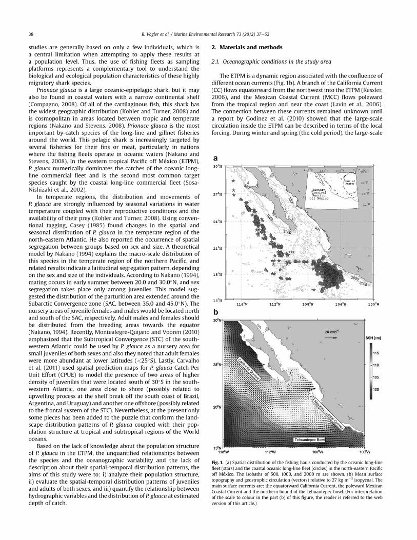
The ETPM is a dynamic region associated with the confluence ofdifferent ocean currents (Fig. 1b). A branch of the California Current(CC) flows equatorward from the northwest into the ETPM (Kessler,2006), and the Mexican Coastal Current (MCC) flows polewardfrom the tropical region and near the coast (Lavín et al., 2006).The connection between these currents remained unknown untila report by Godínez et al. (2010) showed that the large-scalecirculation inside the ETPM can be described in terms of the localforcing. During winter and spring (the cold period), the large-scale

Fig. 1. (a) Spatial distribution of the fishing hauls conducted by the oceanic long-linefleet (stars) and the coastal oceanic long-line fleet (circles) in the north-eastern Pacificoff México. The isobaths of 500, 1000, and 2000 m are shown. (b) Mean surfacetopography and geostrophic circulation (vectors) relative to 27 kg m�3 isopycnal. Themain surface currents are: the equatorward California Current, the poleward MexicanCoastal Current and the northern bound of the Tehuantepec bowl. (For interpretationof the scale to colour in the part (b) of this figure, the reader is referred to the webversion of this article.)

R. Vögler et al. / Marine Environmental Research 73 (2012) 37e5238

circulation is cyclonic, transporting subarctic waters towards theETPM. During summer and autumn (the warm period), the large-scale circulation is anticyclonic and brings tropical-subtropicalwaters towards the ETPM. This reversing circulation pattern isexplained in Godínez et al. (2010) as a long Rossby wave forced bythe local wind stress curl and a long Rossbywave radiating from thecontinental coast. The equatorward California Current, turns east-ernward near 17�N and recirculates poleward over the coast giventhe Mexican Coastal Current. There is a cyclonic circulationbetween the California Current and the Mexican Coastal Currentattached to the coast south of Cabo Corrientes. Mean circulation inthe ETPM is showed in Fig. 1b as inferred from the mean surfacetopography and geostrophic circulation (vectors) relative to27 kg m�3 isopycnal calculated from 1/4� WOD01 data (see Section2.2 for details).

Water mass properties inside the ETPM are poorly understood,but León-Chávez et al. (2010) recently showed that the surface layer(0.0e150.0 m) mainly consists of three water masses: CC Water(CCW, 12.0e21.0 �C, 33.8e34.5); Subtropical Subsurface Water(StSsW, 14.0e21.0 �C, 34.5e35.0), and Tropical Surface Water (TSW,25.0e30.0 �C, 33.8e34.5). Other kinds of water masses are theresult of mixing between the main water masses, in addition toatmospheric forcing (León-Chávez et al., 2010). CCW exhibitsa minimum subsurface salinity near a depth of 50 m.

The Baja California Frontal System (BCFS) is a dynamic regionwithin the ETPM, spreading between 0 and 300 km east of BajaCalifornia Sur, characterized by a persistent (>8 month/year) highconcentration of frontal features generated by the confluence of thecold southbound CC, and the warm northbound Davidson Current(i.e. the California Counter-Current) as it intersects the Baja Cal-ifornia Peninsula (BCP) (Etnoyer et al., 2004).

2.2. Hydrographic variables

Gridded high resolution (1/4�) of temperature and salinityclimatology (hereafter, Levitus database) at standard depths(WOD01, Boyer et al., 2005) was obtained from the NationalOceanographic Data Center web site (http://www.nodc.noaa.gov). Levitus is a historical database of worldwide scope andconsists of monthly mean hydrographic datasets at standarddepths (from 0.0 to 5500.0 m) that were calculated from in situmeasurements that were obtained using different platforms(vessels, buoys) and diverse instruments (Expendable Bathy-thermograph, Conductivity-Temperature-Depth profiler, andinverted thermometers).

2.3. Fleet characteristics

2.3.1. Oceanic long-line fishing fleetThe fishing operations of the oceanic long-line commercial fleet

were carried out in vessels that were 40.0e50.0 m in length andwith steel hulls. These vessels have autonomy of 40 days to navigatewithout refuelling. During the sampling period (1994e96/2000e02), a total of 907,300 hooks were deployed, and a total of703 fishing hauls (mean ¼ 117.2; standard deviation ¼ 59.7) wereperformed. The target species were all species of shark until 1998,after which the fishery changed to targeting Xiphias gladius. Thegear used was the drifting long-line and their characteristics are asfollow. The main line length varied between 25.2 and 75.6 km,depending on the number of hooks used in each haul (min ¼ 285;max ¼ 2270). The branch lines measured from 19.0 to 22.0 m inlength, and the flag lines measured from 11.0 to 12.0 m. The branchlines were positioned on the main line with a separation ofapproximately 50.0 m. The type of hooks used was “straight” withdifferent sizes (number 7, 8 or 9). The bait used was Scomber

japonicas, Mugil cephalus or Mugil Curema. The vessels hada hydraulic system to control the launch speed of the main lain andconsequently, it was possible to select the fishing depth. The esti-mated times of fishing operations were: launching of the long-linebetween 04:00 and 08:00, soaking of the long-line between 08:00and 14:00, and retrieving the long-line between 14:00 and 20:00.

2.3.2. Coastal oceanic long-line fishing fleetThe fishing operations of the coastal oceanic long-line commer-

cial fleet were carried out in vessels that were 11.0e14.0 m in lengthandwith fibreglass hulls. These vessels have autonomy of 8e10 daysto navigate without refuelling. During the sampling period(2003e2009), a total of 418,020 hooks were deployed, and a total of805 fishing hauls (mean ¼ 115.0; standard deviation ¼ 15.9) wereperformed. The target specieswere all species of shark. The gearusedwas the drifting long-line and their characteristics are as follow. Themain line length varied between 28.0 and 37.0 km, depending on thenumber of hooks used in each haul (min ¼ 96; max ¼ 860). Thebranch lines measured from 7.5 to 9.0 m in length, and the flag linesmeasured from6.0 to 8.0m. The branch lineswere positioned on themain line with a separation of approximately 50.0e70.0 m. The typeof hooks used was “straight” or “circular” with different sizes(number 8 or 9). The bait used was Euthynnus lineatus, Katsuwonuspelamis, or Auxis thazard. The estimated times of fishing operationswere: launching of the long-line between 04:00 and 08:00, soakingof the long-line between 08:00 and 15:00, and retrieving the long-line from 15:00 to 21:00.

2.4. On-board sampling

The biological data used in this researchwere collected on-boardtwo long-line commercial fleets, one of which operated in oceanicwaters (12 vessels, 1994e96/2000e02, 15�350e28�400N,102�580e117�050W) and another that operated in coastal oceanicwaters (37 vessels, 2003e2009, 15�820e20�070N, 102�990e107�000W). Samples were provided by observers from the SouthPacific General Fisheries Research Center (Dirección General deInvestigación Pesquera en el Pacífico Sur, Manzanillo, Colima) of theNational Fisheries Institute of México (Instituto Nacional de PescadeMéxico, INAPESCA). The following datawere collected during theoperation of retrieving the long-line: date, number of hooks used,initial and final latitude, and initial and final longitude. Dependingon weather conditions, the sharks caught per fishing haul (ora random sample per haul) were identified to the species level, theindividuals were sexed and were counted; finally their total bodylength (LT) was measured to the lowest cm, according to Compagno(1984). Pregnant females as well as their litter were examined andwere counted during several random fishing hauls.

2.5. Data analyses

2.5.1. Population structure of P. glaucaTo analyze the population structure of P. glauca, the number of

total specimens sampled in each fishing fleet was divided into foursex-size groups: juvenile males, juvenile females, adult males, andadult females. The separation between juveniles and adults wasdetermined a posteriori according to the LT at which 50% of thepopulation reached sexual maturity (LT50). In the ETPM, the LT50 ofP. glauca corresponds to 180.0 cm and 200.0 cm in males andfemales, respectively (Carrera-Fernández et al., 2010).

2.5.2. Size compositions and sexual ratioThe total specimens sampled were grouped into size classes

using the Sturges rule (Sturges, 1926). The Frequency of OccurrenceIndex (FO, %) of the size classes was annually calculated for each

R. Vögler et al. / Marine Environmental Research 73 (2012) 37e52 39

sex. The FO expressing the number of times that a given size classare represented in the annual sample as a percentage. To determinethe annual relationship between sexes, a Chi-square test (Zar, 1999)was applied under the following null hypothesis: the annual ratioof sharks sampled was similar between sexes.

2.5.3. Modelling the speciesehabitat relationshipsof P. glauca sex-size groups

Generalized Linear Models (GLM, McCullagh and Nelder, 1989)and Generalized Additive Models (GAM, Hastie and Tibshirani,1990) are two of the most sophisticate statistical modelling toolsused to represent the relation between pelagic fish catches (asresponse variable) and spatial-temporal factors, environmentalfactors and/or operational fishing characteristics (as predictorvariables). Here, the use of GAM was preferred because they candeal to complex, non-linear relations that often occurring betweenspecies and predictor variables, in a non-parametric way. Previousworks based on GAM (e.g. Bigelow et al., 1999; Walsh and Kleiber,2001; Carvalho et al., 2011) have explored the relationshipbetween predictor variables and catches of P. glauca.

Pearson analysis (Zar, 1999) was applied to measure thecorrelation between the selected predictor variables. This analysiswas performed previous to run the GAMs. The pairs of predictorvariables with high (r � 0.50) or very high (r � 0.70) correlationwere not used to build the GAMs. Pearson analysis and GAMswere conducted with the datasets of each long-line commercialfleet (oceanic and coastal-oceanic) separately. The responsevariable was the CPUE (number of sharks per 1000 hooks) of eachsex-size group of P. glauca per fishing haul. Datasets of CPUE werenot fitted to normal or log-normal distribution because therewere zero data points. It was assumed the Poisson distribution asthe underlying probability distribution of the response variableand the log link function was used. In GAMs, a link functiondescribing the total explained variance is modelled as the sum ofthe smooth functions of the covariates (Wood, 2006). Thepredictor variables included in the analyses were two spatialfactors (latitude, longitude), three temporal factors (month,season and year, those were considered as discrete variables), twohydrographic factors (salinity and temperature at depth of catch),two interactions between temporal-spatial factors (month-lati-tude, month-longitude) and one operational fishing characteristic(number of hooks per haul). Santana-Hernández et al. (1998)determined that the highest catches of P. glauca within watersof the ETPM were distributed between 57.3 and 108.7 m. Thus,three depth strata (50-m, 75-m and 100-m) were chosen asscenarios of possible depth of catch. The performance of GAMswas tested to evaluate their fit to each of three depth strata. Themodel with the highest total deviance was chosen. Three groupsof multivariate models were considered: (1) the full model (allthe single variables and interactions) and models constructedadding up one interaction at each step (the order was based onthe factor weight); (2) the basic models (includes a single vari-able); and (3) other models (following the single factor weightincluding the highest factors). The argument “scale” was fixedas �1, which forces the scale parameter of the Poisson to betreated as unknown, and smoothing parameters to be estimatedby Generalized Cross Validation score (GCV), rather than byUn-Biased Risk Estimator, which is the Poisson default: hencethe model is employing an over-dispersed Poisson structure(Wood, 2006). The argument “gamma” was fixed as 1.40, whichforces each model effective degrees of freedom (df) to count as1.40 df in the GCV score, then the model is forced to be a littlesmoother than they might otherwise be; this is an ad hoc way ofavoiding over-fitting (Kim and Gu, 2004). A forward stepwisetechnique was used to identify the appropriate set of predictor

variables to be included in the P. glauca CPUE-habitat models. TheGCV score was computed for every candidate predictor variablethat was entered in the models. The predictor with the lower GCVscore was tested as the next entry; the decision was predictedupon a forward entry F-test with a significance level of P < 0.05.Forward entry continued until additional predictors no longeryielded significant reductions in the GCV of multiple predictorGAMs. Adequacy of models fit was assessed in terms of thecoefficient of determination (R2). The computational tasks wereconducted using the software R 2.13.0 (R Development CoreTeam, 2011) and the mgcv library.

2.5.4. Hydrographic variability and distribution of P. glauca sex-sizegroups

Synoptic maps by season were constructed to explore the rela-tionship between the hydrography of the ETPM and the horizontaldistribution of P. glauca. The spatial distribution of catches,discriminated by sex-size groups, was superimposed to fields ofsalinity and temperature, considering the estimated depth of catchof each group. The estimated depth of catch was obtained fromGAMs. The CPUE was calculated for each sex-size group using thetime series of each fishing fleet separately. Physical data was ob-tained from Levitus database described before (see Section 2.2.).Seasons were defined as follow: winter: JanuaryeMarch; spring:AprileJune; summer: JulyeSeptember; and autumn: OctobereDe-cember. An aggregation area for each group was defined when theCPUE was � 11 to 20 sharks per 1000 hooks.

3. Results

3.1. Population structure of P. glauca

3.1.1. Size classesThirteen size classes were established for the total sample of

sharks caught by each long-line fleet (oceanic and coastal oceanic)with a range of 15.0 cm for each size class.

3.1.2. Size compositions and sexual ratio3.1.2.1. Oceanic waters of the eastern tropical Pacific off México. Thetotal catches (n ¼ 1587) were dominated by adults (n ¼ 925,58.29%) between 1994 and 1996. By contrast, juveniles (n ¼ 2552,63.94%) numerically dominated the total catches (n ¼ 3991)between 2000 and 2002. For males, the size class between 188.0and 202.0 cm LTwas the dominantmode duringmost of the studiedyears. For females, were observed year-to-year variations in the sizeclass mode (Fig. 2). The annual sex ratio was significantly differentfrom 1M:1F (c2 ¼ 140.23, P < 0.05) and it was dominated by males,in juveniles (Table 1) as well as adults (Table 2).

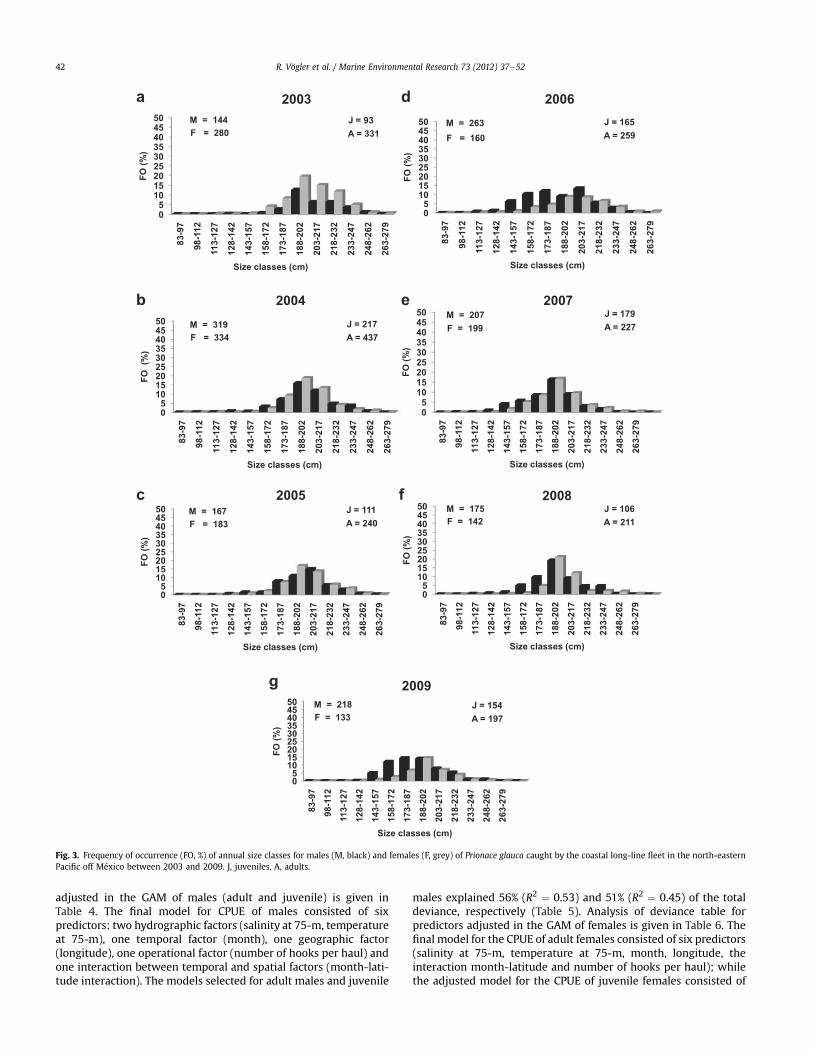
3.1.2.2. Coastal oceanic waters of the eastern tropical Pacific offMéxico. The total catches (n ¼ 2927) of the 7-year period weredominated by adults (n ¼ 1025, 64.98%); nevertheless, juvenileshad a sustainable increase between 2003 (21.93%) and 2009(43.87%). The size class between 188.0 and 202.0 cm LT was thedominant mode during all years (males) or during several years(females) (Fig. 3). The annual sex ratio was significantly differentfrom 1M:1F (c2 ¼ 58.18, P < 0.05). In juveniles, this ratio wasdominated by females (Table 1). In adults, the annual sex ratio wasdominated by males (Table 2).

3.2. Modelling the speciesehabitat relationships of P. glaucasex-size groups

Several pair of predictor variables had high (r� 0.50) or very high(r� 0.70) correlation coefficient values at oceanicwaters. In contrast,


the same pair of predictors showed low correlation coefficient values(r< 0.50) at coastal oceanicwaters (Table 3). The interaction betweentemporal and spatial factors described more efficiently the CPUEdistribution of P. glauca than the other predictors.

3.2.1. Oceanic waters of the eastern tropical Pacific off MéxicoThe GAM results for P. glauca at oceanic waters of ETPM reveal

that the distribution of all sex-size groups was better fits with the75.0-m depth stratum. Analysis of deviance table for predictors

Table 1Annual sex ratio of juveniles of Prionace glauca caught by two long-line fleets in thenorth-eastern Pacific off México. M, males. F, females. n, annual number of juveniles.

Juveniles

Oceanic long-line fleet Coastal oceanic long-line fleet

Year M:F n Year M:F n

1994 2.59:1 262 2003 0.50:1 931995 0.83:1 196 2004 0.29:1 2161996 1.08:1 204 2005 0.30:1 1122000 5.08:1 1022 2006 1.54:1 1652001 12.78:1 868 2007 0.49:1 1792002 25.48:1 662 2008 0.49:1 106

2009 1.08:1 154

Table 2Annual sex ratio of adults of Prionace glauca caught by two long-line fleets in thenorth-eastern Pacific off México. M, males. F, females. n, annual number of adults.

Adults

Oceanic long-line fleet Coastal oceanic long-line fleet

Year M:F n Year M:F n

1994 15.65:1 333 2003 3.04:1 3311995 8.72:1 243 2004 1.63:1 4371996 15.62:1 349 2005 1.40:1 2402000 4.33:1 703 2006 1.73:1 2592001 2.84:1 449 2007 1.87:1 2272002 5.67:1 287 2008 1.97:1 211

2009 2.34:1 197

0

5

10

15

20

25

30

35

40

45

50

83

-9

7

98

-11

2

11

3-1

27

12

8-1

42

14

3-1

57

15

8-1

72

17

3-1

87

18

8-2

02

20

3-2

17

21

8-2

32

23

3-2

47

24

8-2

62

26

3-2

79

FO

(%

)

Size classes (cm)

1996

0

5

10

15

20

25

30

35

40

45

50

83

-9

7

98

-11

2

11

3-1

27

12

8-1

42

14

3-1

57

15

8-1

72

17

3-1

87

18

8-2

02

20

3-2

17

21

8-2

32

23

3-2

47

24

8-2

62

26

3-2

79

FO

(%

)

Size classes (cm)

1995

0

5

10

15

20

25

30

35

40

45

50

83

-9

7

98

-11

2

11

3-1

27

12

8-1

42

14

3-1

57

15

8-1

72

17

3-1

87

18

8-2

02

20

3-2

17

21

8-2

32

23

3-2

47

24

8-2

62

26

3-2

79

FO

(%

)

Size classes (cm)

1994a d

eb

c f

0

5

10

15

20

25

30

35

40

45

50

83

-9

7

98

-11

2

11

3-1

27

12

8-1

42

14

3-1

57

15

8-1

72

17

3-1

87

18

8-2

02

20

3-2

17

21

8-2

32

23

3-2

47

24

8-2

62

26

3-2

79

FO

(%

)

Size classes (cm)

2002

0

5

10

15

20

25

30

35

40

45

50

83

-9

7

98

-11

2

11

3-1

27

12

8-1

42

14

3-1

57

15

8-1

72

17

3-1

87

18

8-2

02

20

3-2

17

21

8-2

32

23

3-2

47

24

8-2

62

26

3-2

79

FO

(%

)

Size classes (cm)

2001

0

5

10

15

20

25

30

35

40

45

50

83

-9

7

98

-11

2

11

3-1

27

12

8-1

42

14

3-1

57

15

8-1

72

17

3-1

87

18

8-2

02

20

3-2

17

21

8-2

32

23

3-2

47

24

8-2

62

26

3-2

79

FO

(%

)

Size classes (cm)

M = 1425

F = 300

M = 1137

F = 180

M = 881

F = 68

2000

M = 502

F = 93

M = 307

F = 132

M = 434

F = 119

J = 262

A = 333

J = 196

A = 243

J = 204

A = 349

J = 1022

A = 703

J = 868

A = 449

J = 662

A = 287

Fig. 2. Frequency of occurrence (FO, %) of annual size classes for males (M, black) and females (F, grey) of Prionace glauca caught by the oceanic long-line fleet in the north-easternPacific off México between 1994e96 and 2000e02. J, juveniles. A, adults.


adjusted in the GAM of males (adult and juvenile) is given inTable 4. The final model for CPUE of males consisted of sixpredictors: two hydrographic factors (salinity at 75-m, temperatureat 75-m), one temporal factor (month), one geographic factor(longitude), one operational factor (number of hooks per haul) andone interaction between temporal and spatial factors (month-lati-tude interaction). The models selected for adult males and juvenile

males explained 56% (R2 ¼ 0.53) and 51% (R2 ¼ 0.45) of the totaldeviance, respectively (Table 5). Analysis of deviance table forpredictors adjusted in the GAM of females is given in Table 6. Thefinal model for the CPUE of adult females consisted of six predictors(salinity at 75-m, temperature at 75-m, month, longitude, theinteraction month-latitude and number of hooks per haul); whilethe adjusted model for the CPUE of juvenile females consisted of

0

5

10

15

20

25

30

35

40

45

50

83

-9

7

98

-11

2

11

3-1

27

12

8-1

42

14

3-1

57

15

8-1

72

17

3-1

87

18

8-2

02

20

3-2

17

21

8-2

32

23

3-2

47

24

8-2

62

26

3-2

79

FO

(%

)

Size classes (cm)

2009

0

5

10

15

20

25

30

35

40

45

50

83

-9

7

98

-11

2

113

-1

27

12

8-1

42

14

3-1

57

15

8-1

72

17

3-1

87

18

8-2

02

20

3-2

17

21

8-2

32

23

3-2

47

24

8-2

62

26

3-2

79

FO

(%

)

Size classes (cm)

2008

0

5

10

15

20

25

30

35

40

45

50

83

-9

7

98

-11

2

11

3-1

27

12

8-1

42

14

3-1

57

15

8-1

72

17

3-1

87

18

8-2

02

20

3-2

17

21

8-2

32

23

3-2

47

24

8-2

62

26

3-2

79

FO

(%

)

Size classes (cm)

2007

0

5

10

15

20

25

30

35

40

45

50

83

-9

7

98

-11

2

11

3-1

27

12

8-1

42

14

3-1

57

15

8-1

72

17

3-1

87

18

8-2

02

20

3-2

17

21

8-2

32

23

3-2

47

24

8-2

62

26

3-2

79

FO

(%

)

Size classes (cm)

2006

0

5

10

15

20

25

30

35

40

45

50

83

-9

7

98

-11

2

11

3-1

27

12

8-1

42

14

3-1

57

15

8-1

72

17

3-1

87

18

8-2

02

20

3-2

17

21

8-2

32

23

3-2

47

24

8-2

62

26

3-2

79

FO

(%

)

Size classes (cm)

2005

0

5

10

15

20

25

30

35

40

45

50

83

-9

7

98

-11

2

11

3-1

27

12

8-1

42

14

3-1

57

15

8-1

72

17

3-1

87

18

8-2

02

20

3-2

17

21

8-2

32

23

3-2

47

24

8-2

62

26

3-2

79

FO

(%

)

Size classes (cm)

2004

0

5

10

15

20

25

30

35

40

45

50

83

-9

7

98

-11

2

11

3-1

27

12

8-1

42

14

3-1

57

15

8-1

72

17

3-1

87

18

8-2

02

20

3-2

17

21

8-2

32

23

3-2

47

24

8-2

62

26

3-2

79

FO

(%

)

Size classes (cm)

2003a d

eb

c f

g

M = 319

F = 334

M = 144

F = 280

M = 167

F = 183

M = 263

F = 160

M = 207

F = 199

M = 175

F = 142

M = 218

F = 133

J = 165

A = 259

J = 179

A = 227

J = 106

A = 211

J = 154

A = 197

J = 111

A = 240

J = 217

A = 437

J = 93

A = 331

Fig. 3. Frequency of occurrence (FO, %) of annual size classes for males (M, black) and females (F, grey) of Prionace glauca caught by the coastal long-line fleet in the north-easternPacific off México between 2003 and 2009. J, juveniles, A, adults.


five predictors (salinity at 75-m, month, latitude, the interactionmonth-longitude, and number of hooks per haul). The modelsselected for adult females and juvenile females explained 54%(R2 ¼ 0.43) and 47% (R2 ¼ 0.47) of the total deviance, respectively(Table 7).

The month-latitude interaction factor was the most influentialpredictor that affected the CPUE of three sex-size groups, althoughthe monthelongitude interaction was the most important factorthat affected the CPUE of juvenile females. The influence of latitudeon the CPUE of males (juvenile and adult) was positive duringwinter and spring (adults: January to May; juveniles: January toApril) between 17�N and 24�N. Slight negative effects of the lati-tude on the CPUE of males occurred mainly in late spring andsummer (June to October) between 17�N and 23�N. Strong negativeeffects of latitude on the distribution of adult females’ CPUE wereobserved during summer and autumn (July to November) at lati-tudes>25�N,while slight positive effects were also detected duringthe same period within a wide range of latitude (between 17�N and25�N). The CPUE distribution of juvenile females was negativelyaffected by the longitude mainly during spring (April to June),although slight positive effects occurred during early winter(January to February); both kind of effects were detected between110�W and 115�W.

Temperature at 75.0-m depth or salinity at 75.0-m depth werethe hydrographic factors with the highest contribution to thedeviance explained by the models of adult males and juvenilefemales, respectively. However, both factors had a similar deviancecontribution to the GAMs of juvenile males and adult females.Positive effects of the temperature at 75.0-m depth on the CPUE ofadult females and juvenile males were detected at two thermalranges (14.0e15.0 �C; 17.0e18.0 �C), while the CPUE of adult maleswere positively affected mainly at higher temperatures (between17.0� and 20.0 �C). The negative effects of temperature on the CPUEof the adults and juvenile males were generated between 16.0� and17.0 �C. For juvenile females, their partial response curve oftemperature at 75.0-m depth showed an erratic behaviour, wherenegative and positive effects being occurred between 14.0� and

20.0 �C. Salinity at 75.0-m depth influenced positively the CPUE ofadult females and juvenile males between 33.6 and 34.1, mean-while the positive influence on the CPUE of adult males weredetected at two salinity ranges (from 33.6 to 33.8, and from 34.2 to34.4). Strong negative effects of salinity on the CPUE of juvenilemales were detected at higher salinities values (between 34.5 and34.8), while in the case of adult males only slight negative effectswere detected at lower salinity values. Salinities >34.2 hadpromoted slight negative effects on CPUE of adult females. Finally,the CPUE of juvenile females were positively affected within twosalinity ranges (from 33.8 to 34.0, and from 34.5 to 34.8), whilethe negative effects occurred at salinities <33.8 and between 34.0and 34.2.

Month was a temporal factor that affected the CPUE of all sex-size groups, with different contribution to the deviance explainedby the GAM of each group.

Longitude was a spatial factor that affected the CPUE of adults(male and female) and juvenile males, with different deviancecontribution for the model of each group. Latitude had a marginalcontribution to the deviance explained by the model of juvenilefemales’ CPUE.

Number of hooks per haul showed different contribution to thedeviance explained by the model of the sex-size groups. For allcases, the partial response curve exhibited slightly positive orneutral effects between 1000 and 1500 hooks per haul.

3.2.2. Coastal oceanic waters of the eastern tropical Pacificoff México

The GAM results for P. glauca at coastal oceanic waters of ETPMare indicating differences on vertical distribution between sexes.The models for males showed a better fits with the 50.0-m depthstratum, while the females’ models were better adjusted with the100-m depth stratum. Analysis of deviance table for predictorvariables adjusted in the GAM of males of P. glauca is given inTable 8. The final model for the CPUE of adult males was adjustedusing four predictor variables: salinity at 50-m, longitude, theinteraction between month and latitude, and number of hooks per

Table 3Pearson correlation coefficient values for a set of predictor variables selected to build the generalized additive models of each sex-size group of Prionace glauca at oceanicwaters and coastal oceanic waters of the north-eastern Pacific off México. AM, adult males. JM, juvenile males. AF, adult females. JF, juvenile females.

Correlation Oceanic waters Coastal oceanic waters

AM JM AF JF AM JM AF JF

Salinity vs Longitude �0.93 �0.93 �0.93 �0.93 �0.37 �0.37 �0.37 �0.21Temperature vs Latitude �0.75 �0.75 �0.74 �0.75 �0.37 �0.38 �0.37 �0.32Year vs Longitude 0.62 0.62 0.62 0.62 �0.23 �0.23 �0.23 �0.23Latitude vs Longitude 0.60 0.60 0.60 0.59 0.38 0.38 0.38 0.38Salinity vs Latitude �0.58 �0.57 �0.57 �0.58 0.31 0.32 0.32 0.25Salinity vs Temperature 0.54 0.54 0.53 0.54 �0.54 �0.54 �0.54 �0.32Temperature vs Longitude �0.50 �0.50 �0.50 �0.50 �0.08 �0.08 �0.08 �0.11Temperature vs Season �0.17 �0.17 �0.16 �0.17 0.48 0.48 0.48 0.54

Table 4Analysis of deviance for predictor variables adjusted in the GAMs of males (adult and juvenile) of Prionace glauca at oceanic waters of the north-eastern Pacific off México. Thepercentage of deviance explained (% DE), Generalized Cross Validation score (GCV), degrees of freedom (df), the F- test (F) and its associated significance (P), are presented foreach term. *, P < 0.1, **, P < 0.01, ***, P < 0.001. T75-m, temperature at 75-m depth. S75-m, salinity at 75-m depth.

Predictor Adult males Juvenile males

% DE GCV df F P % DE GCV df F P

Month:Latitude 39.4 4.14 21.41 11.75 ***2.0 � e�16 31.3 2.88 23.25 9.63 ***2.0 � e�16

Month 22.0 4.43 8.35 20.52 ***2.0 � e�16 14.5 3.35 6.99 9.62 ***4.5 � e�12

Hooks 13.2 5.60 5.18 12.11 ***1.9 � e�12 15.8 3.32 8.79 11.10 ***2.0 � e�16

T75-m 12.4 5.61 5.53 13.64 ***1.0 � e�14 6.3 3.63 4.65 8.09 ***1.3 � e�7

Longitude 7.0 5.99 6.90 5.70 ***1.1 � e�6 10.9 3.49 7.05 9.01 ***2.7 � e�11

S75-m 4.8 6.10 5.64 4.65 ***1.0 � e�4 7.8 3.58 4.99 9.94 ***7.4 � e�10


haul. The final model for CPUE of juvenile males was integrated byfour predictor variables: salinity at 50-m, longitude, the interactionbetween month and latitude, and month. The models selected foradult males and juvenile males explained 52% (R2 ¼ 0.40) and 59%(R2 ¼ 0.57) of the total deviance, respectively (Table 9). Analysis ofdeviance table for predictor variables adjusted in the GAM offemales of P. glauca is given in Table 10. The final model for the CPUEof females (adult and juvenile) was adjusted using four predictorfactors: salinity at 100-m, temperature at 100-m, the interactionbetween month and longitude, and number of hooks per haul. Themodels selected for adult females and juvenile females explained42% (R2 ¼ 0.36) and 32% (R2 ¼ 0.23) of the total deviance, respec-tively (Table 11).

Month-latitude interaction factor was the predictor with thehighest contribution to the total deviance explained by GAMs ofmales (adult and juvenile). Strong negative effects of the latitude onthe distribution of males’ CPUE were detected during summer andautumn (July to November) between 15�N and 19�N, althoughslight positive effects were occurred during winter and early spring(January to April) at similar range of latitude (between 17�N and20�N). On the other hand, the predictor with the highest contri-bution to the total deviance explained by GAMs of females (adultand juvenile) was the monthelongitude interaction factor. Strongnegative effects on the CPUE of females (juveniles and adults)were detected during late summer and autumn (September toNovember) within a narrow range of longitude (between 103�W

and 105�W, towards the coast). Slight positive effects on the CPUEof juvenile females were detected at higher longitudes (between105�W and 107�W, towards the open ocean) mainly during latespring and summer (May to August), while in the case of adultfemales the positive longitudinal effects were detected in spring(May to June).

Salinity was the most influential hydrographic factor thataffected the CPUE of adult and juvenile at coastal oceanic waters,but the salinity effects were different according to the sex of sharks;suggesting a possible vertical segregation between male andfemale. Positive effects of salinity at 50.0-m on the distribution ofmales’ CPUE were detected mainly between 34.5 and 34.6 whilenegative effects being occurred at salinities <34.3 or at salinities>34.6. On the other hand, the positive effects of salinity at 100.0-mon the distribution of females’ CPUE were detected between 34.5and 34.6, although negative effects were observed at higher salin-ities (between 34.6 and 34.8). Temperature at 100.0-m hada marginal contribution to the deviance explained by the model offemales (adult and juvenile). The positive thermal effects weredetected between 14� and 15 �C, while their negative effects beingoccurred between 15� and 16 �C.

Longitudewas an important spatial factor for the adjusted GAMsof males, with similar contribution to the deviance explained forthe models of adults and juveniles. The CPUE of males was posi-tively influenced by this geographic predictor towards the openocean (between 105 and 107�W), while adult as well as juvenile

Table 6Analysis of deviance for predictor variables adjusted in the GAMs of females (adult and juvenile) of Prionace glauca at oceanic waters of the north-eastern Pacific off México. Thepercentage of deviance explained (% DE), Generalized Cross Validation score (GCV), degrees of freedom (df), the F- test (F) and its associated significance (P), are presented foreach term.*, P < 0.1, **, P < 0.01, ***, P < 0.001. T75-m, temperature at 75-m depth. S75-m, salinity at 75-m depth.

Predictor Adult females Juvenile females


Month: Latitude 34.6 0.96 27.34 9.16 ***2.0 � e�16 e e e e e

Month: Longitude e e e e e 35.0 1.31 27.80 4.91 ***9.2 � e�15

Hooks 21.6 1.07 8.92 11.30 ***2.0 � e�16 11.3 1.65 7.34 8.94 ***1.6 � e�11

Longitude 15.8 1.14 7.45 14.72 ***2.0 � e�16 e e e e e

Latitude e e e e e 1.9 1.79 2.60 3.24 *2.0 � e�1

S75-m 11.7 1.19 7.13 10.11 ***6.4 � e�13 5.2 1.76 7.84 3.71 ***2.3 � e�4

T75-m 10.9 1.21 7.37 3.97 ***1.4 � e�4 2.2 1.82 8.53 27.83 **1.0 � e�2

Month 10.5 1.22 7.58 6.61 ***2.13 � e�8 18.6 1.51 6.83 12.29 ***2.0 � e�15

Table 5Multiple predictors GAM fits for CPUE of males (adult and juvenile) of Prionaceglauca at oceanic waters of the north-eastern Pacific off México. The model retainedfor each group is highlighted in grey. The percentage of deviance explained (% DE),Generalized Cross Validation score (GCV) and the coefficient of determination (R2),are presented for each model. T75-m, temperature at 75-m depth. S75-m, salinity at75-m depth. LN, latitude north. LW, longitude west. :, indicates interaction betweenpredictors.

Model % DE GCV R2

Adult males1- Month 21.9 5.06 0.192-...þ T75-m 33.3 4.43 0.353-.......þ S75-m 38.6 4.09 0.404-.............þ Hooks 41.6 4.02 0.415-..............þ (Month: LN) 54.2 3.56 0.526- CPUE w Month þ T75-m þ S75-m þ Hooks þ

(Month: LN) þ LW55.6 3.51 0.53

Juvenile males1- Month 14.5 3.35 0.112-....þ T75-m 28.8 2.89 0.243-.......þ LW 32.7 2.76 0.284-..........þ (Month: LN) 42.5 2.69 0.375-..................þ S75-m 47.0 2.53 0.426- CPUE w Month þ T75-m þ LW þ

(Month: LN) þ S75-m þ Hooks51.3 2.43 0.45

Table 7Multiple predictors GAM fits for CPUE of females (adult and juvenile) of Prionaceglauca at oceanic waters of the north-eastern Pacific off México. The model retainedfor each group is highlighted in grey. The percentage of deviance explained (% DE),Generalized Cross Validation score (GCV) and the coefficient of determination (R2),are presented for each model. T75-m, temperature at 75-m depth. S75-m, salinity at75-m depth. LN, latitude north. LW, longitude west. :, indicates interaction betweenpredictors.

Model % DE GCV R2

Adult females1- Month 10.5 1.22 0.042-.....þ LW 28.2 1.01 0.183-......þ T75-m 31.7 0.98 0.234-...........þ S75-m 35.2 0.96 0.285-.............þ Hooks 43.4 0.85 0.326- CPUE w Month þ LW þ T75-m þ S75-m þ

Hooks þ (Month: LN)53.8 0.81 0.43

Juvenile females1- Month 18.6 1.51 0.132-...þ S75-m 26.2 1.40 0.213-.......þ Hooks 30.9 1.35 0.244-...........þ LN 33.7 1.32 0.275- CPUE w Month þ S75-m þ Hooks þ

LN þ (Mon: LW)46.7 1.18 0.47


were negatively affected towards the coast (between 103 and105�W).

Month was a temporal factor that affected only the CPUE ofjuvenile males. Number of hooks per haul exhibited similarcontribution to the deviance explained by the models of females(adult and juvenile) and adult males. For all cases, the partialresponse curve showed positive effects between 400 and 500hooks per haul, although negative effects were detected when thenumber was <300 or >600 hooks per haul.

3.3. Hydrographic variability and distribution of P. glauca sex-sizegroups

3.3.1. Oceanic waters of the eastern tropical Pacific off México3.3.1.1. Winter (1994e96/2000e02). The winter relationshipsbetween the hydrography of oceanic waters at 75.0-m depth and theCPUE of two life stages of males and females are shown in Fig.4. Thecore aggregation area ofmales (juvenile and adult)was distributed ina central oceanic zone (17.0e23.0�N; 109.0e114.0�W), which wasassociated with a mixing of water masses with intermediatetemperatures (15.0e18.0 �C) and intermediate salinities (34.1e34.5).Furthermore, other core aggregation area of juveniles and adults ofboth sexes was distributed in a central coastal zone (18.0e23.0�N;105.0e107.0�W), which was affected by waters with low tempera-tures (13.0e15.0 �C) and high salinities (34.5e34.7).

3.3.1.2. Summer (1994e96/2000e02). The summer relationshipsbetween the hydrography of oceanic waters at 75.0-m depth andthe CPUE of two life stages of males and females are shown in Fig. 5.Large core aggregation area of males (juvenile and adult) wasobserved over awide area located towards the northern zone of theETPM (24.0e28.0�N; 112.0e117.0�W). Small core aggregation areaof females (juvenile and adult) was distributed within the same

zone than males, although with smaller spatial coverage (between24.0 and 26.0�N and 113.0e115.0�W). All group aggregations wereassociated to waters with low temperatures (13.0e15.0 �C) and lowsalinities (33.5e34.0). Furthermore, core aggregations of the twolife stages of male (22.0e23.0�N; 112.0e113.0�W) and female(23.0e24.0�N; 111.0e112.0�W) were distributed within a centralzone of the ETPM. These aggregations were affected by waters withintermediate temperatures (14.0e15.0 �C) and intermediate salin-ities (34.0e34.3).

3.3.2. Coastal oceanic waters of the eastern tropical Pacific offMéxico3.3.2.1. Winter (2003e09). The winter relationships between thehydrography of coastal oceanic waters and the CPUE of two lifestages of males (at 50.0-m depth) and females (at 100.0-mdepth) are shown in Fig. 6. Large core aggregation of maleswas detected during this season and they were affected bywaters with high temperatures (17.0e25.0 �C) and high salinities(34.3e34.7). Small core aggregation of females were distributedat longitudes <106.0�W within an area which was affected bywaters with low temperatures (13.0e15.0 �C) and high salinities(34.5e34.7).

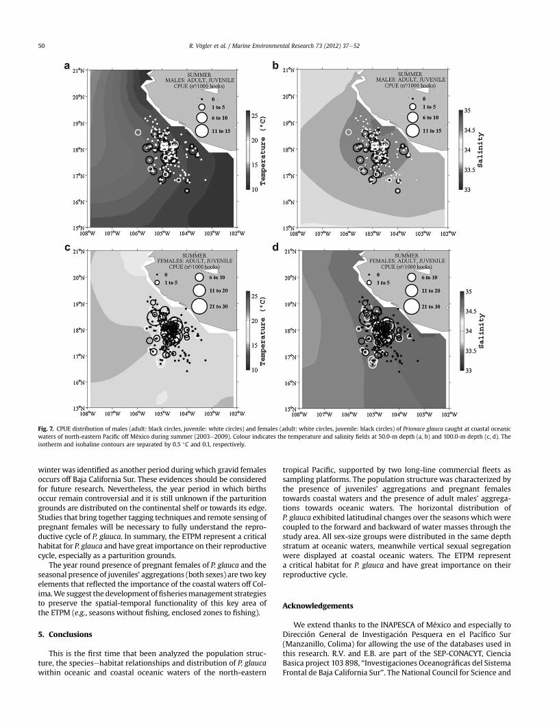
3.3.2.2. Summer (2003e09). The summer relationships betweenthe hydrography of coastal oceanic waters and the CPUE of two lifestages of males (at 50.0-m depth) and females (at 100.0-m depth)are shown in Fig. 7. Contrary to what was observed during thewinter, only a small core aggregation of males (mainly juveniles)was observed at the coastal oceanic zone. These aggregations wereaffected by waters with high temperatures (22.0e25.0 �C) and highsalinities (34.3e34.5). Large core aggregation of females (mainlyjuveniles) was detected during this season and they were affectedby waters with low temperatures (15.0e16.0 �C) and high salinities(34.5e34.6).

3.4. Pregnant females

Pregnant females with embryos at different stages of develop-ment were caught in coastal oceanic waters off Colima(16.0e20.0�N, 104.0e107.0�W, n ¼ 84, 2000e03) as well as off BajaCalifornia Peninsula (22.0e28.0�N, 111.0e116.0�W, n ¼ 254, 1998).A common characteristic of both zones was the narrow continentalshelf. Random sampling prevented the establishment of theparturition season, but we confirmed a year round presence ofpregnant females at waters off Colima (Fig. 8).

4. Discussion

Here, the speciesehabitat relationships and populationdynamics of P. glauca were analyzed through samples collectedduring 13 years and from a large area that covered 14� of latitudeand 15� of longitude, which included the tropical-subtropical

Table 8Analysis of deviance for predictor variables adjusted in the GAMs of males (adult and juvenile) of Prionace glauca at coastal oceanic waters of the north-eastern Pacific offMéxico. The percentage of deviance explained (% DE), Generalized Cross Validation score (GCV), degrees of freedom (df), the F- test (F) and its associated significance (P), arepresented for each term.*, P < 0.1, **, P < 0.01, ***, P < 0.001. S50-m, salinity at 50-m depth.

Predictor Adult males Juvenile males


Month: Latitude 32.6 5.97 27.52 9.23 ***2.0 � e�16 42.6 2.17 27.7 12.41 ***2.0 � e�16

Longitude 29.8 5.68 2.37 94.40 ***2.0 � e�16 27.2 2.63 5.94 30.88 ***2.0 � e�16

Month e e e e e 26.1 2.66 4.85 32.79 ***2.0 � e�16

Hooks 8.9 7.52 8.37 7.21 ***5.4 � e�10 e e e e e

S50-m 5.13 7.79 6.81 2.75 **6.9 � e�3 3.1 2.44 5.16 1.88 ***2.2 � e�13

Table 9Multiple predictors GAM fits for CPUE of males (adult and juvenile) of Prionaceglauca at coastal oceanic waters of the north-eastern Pacific off México. The modelretained for each group is highlighted in grey. The percentage of deviance explained(% DE), Generalized Cross Validation score (GCV) and the coefficient of determina-tion (R2), are presented for eachmodel. S50-m, salinity at 50-m depth. LW, longitudewest. LN, latitude north. :, indicates interaction between predictors.

Model % DE GCV R2

Adult males1- LW 29.8 5.68 0.222-...þ (Month: LN) 48.0 4.64 0.363-........þ S50-m 50.4 4.54 0.394- CPUE w LW þ (Month: LN) þ S50-m þ Hooks 51.9 4.47 0.40Juvenile males1- LW 27.2 2.63 0.172-..þ (Month: LN) 52.6 1.89 0.443-........þ S50-m 55.4 1.82 0.524- CPUE w LW þ (Month: LN) þ S50-m þ Month 59.0 1.73 0.57


transition zone of the north-eastern Pacific. The spatial andtemporal coverage varied between fishing trips. It is highlights thehigh relative weight of the effort (number of hooks per haul) asa predictor to explain the deviance of the models that wereadjusted to describe the CPUE of the life stages and the sexes ofP. glauca. These results indicate an implicit fishing bias on thedatasets. However, the sampling of individuals of both sexes atdifferent life stages and the presence of size classes over a widerange of LT denote a good representation of the population struc-ture within the catches of the two long-line fishing fleets. Thus, thedatabases obtained from fishing platforms were considered usefulto achieve the ecological and biological aims of this study.

The population structure of P. glauca in tropical regions hasnumerous gaps related mainly to the juvenile portion. Nakano(1994) suggested the distribution of a parturition area ofP. glauca within the North Pacific SAC (between 35.0 and 45.0�N).Nakano (1994) proposed that the nursery area occurs around thesubpolar convergence and it would be extending towards thenorth (juvenile females distributed until 55.0�N) and towards thesouth (juvenile males distributed until 30�N) of the parturitionarea. Recently, Carvalho et al. (2011) predicted the presence ofanother nursery area of P. glauca that would be extended withinthe STC of the south-western Atlantic (south of 30.0�S). Theseevidences are extending the possibilities of location of nurseryareas towards subtropical zones. In turn, Litvinov (2006) notedthe presence of juveniles’ aggregations of P. glauca (calling as“kindergartens”) distributed in subtropical coastal waters of theeastern Pacific and Atlantic. These aggregations were confirmedat both hemispheres. Additionally, aggregations of adult maleswith a similar size composition (calling as “male clubs”) weredetected towards oceanic waters and within the same areaswhere “kindergartens” were observed (Litvinov, 2006). Accordingto this author, the juveniles’ aggregations remained at the neriticzone and they showed segregation by sex, with a quasi-stationary

pattern: males were distributed offshore meanwhile femalesremained closer to the coast. The same kind of aggregations ofjuvenile and adult were detected at waters of the ETPM (between15.0�N and 23.0�N). The sexual segregation between juvenileswas observed during winter at longitudes <106.0�W, whilea weak signal of this pattern was detected during spring andautumn and finally during summer it was lost because the lowpresence of juveniles in coastal areas. Aggregations of adult maleswere found offshore all year round at longitudes �106.0�W,within a wide range of latitude (between18.0 and 23.0�N) whichwas included in the same region where the juveniles’ aggrega-tions were observed. Our results confirmed the hypothesis notedby Litvinov (2006) and allow us to indicate that the populationstructure of P. glauca within the Eastern Tropical Pacific is char-acterized by the presence of juveniles’ aggregations (both sexes)towards coastal waters and the presence of adult males’ aggre-gations towards oceanic waters. Both kinds of aggregations seemto have a spatial persistence that should be related to the distanceto the coast, while the temporal aggregation of juveniles could berelated to their seasonal residence within subtropical zones.When juveniles grow and reach the adult size they begin toexpand its distribution range and move away through migratoryroutes.

The horizontal distribution of P. glauca exhibited latitudinalchanges that were coupled to the forward and backward ofsubarctic waters (12.0e21.0 �C; 33.8e34.5) and also with theforward and backward of subtropical waters (14.0e21.0 �C,34.5e35.0) and tropical waters (25.0e30.0 �C, 33.8e34.5) throughthe ETPM. The great variability on the horizontal distributionoccurred in winter as well as in summer, while their distributionpatterns were weakened during transition periods (spring andautumn). The effects of latitude (Casey, 1985; Nakano, 1994;Kohler and Turner, 2008; Montealegre-Quijano and Vooren, 2010;Carvalho et al., 2011) and of longitude (Litvinov, 2006; Carvalhoet al., 2011) on the horizontal distribution of P. glauca (individ-uals or catches) were previously reported. In this study, latitudeas well as longitude represents the spatial indicators of thegeographical position where the catches were obtained and theirvariation was used to infer spatial changes in the horizontaldistribution of sexes and size classes of P. glauca over time. Lati-tude had positive effects on the distribution of males (juvenileand adult) at oceanic areas (between 17.0�N and 24.0�N) in winterand spring. Similar signal was detected at coastal oceanic areas(between 17.0�N and 20.0�N) mainly in winter, when there isa maximum influence of subarctic waters whose range spread upto w17.0�N. Conversely, the negative influence of the latitude onthe distribution of males were detected within oceanic areas(between 18.0�N and 23.0�N) and also within coastal oceanicareas (between 15.0�N and 19.0�N) in summer and autumn. Notethat the range of latitude between 15.0�N and 23.0�N was underthe influence of subtropical waters (high temperatures and highsalinities), especially in summer when its maximum influencespread to w23.0�N. The GAMs indicated the presence of adult

Table 10Analysis of deviance for predictor variables adjusted in the GAMs of females (adult and juvenile) of Prionace glauca at coastal oceanic waters of the north-eastern Pacific offMéxico. The percentage of deviance explained (% DE), Generalized Cross Validation score (GCV), degrees of freedom (df), the F- test (F) and its associated significance (P), arepresented for each term. *, P < 0.1, **, P < 0.01, ***, P < 0.001. S100-m, salinity at 100-m depth. T100-m, temperature at 100-m depth.

Predictor Adult females Juvenile females


Month: Longitude 28.4 3.21 22.04 6.46 ***2.0 � e�16 22.1 3.30 22.46 5.25 ***5.7 � e�14

Hooks 10.3 3.83 8.85 6.63 ***1.9 � e�9 8.9 3.68 8.54 6.54 ***4.7 � e�9

S100-m 7.2 3.96 8.15 7.24 ***7.5 � e�10 3.9 3.86 7.63 3.42 ***6.6 � e�4

T100-m 1.9 4.11 3.15 3.35 *1.2 � e�2 2.2 3.87 3.32 3.72 **5.9 � e�3

Table 11Multiple predictors GAM fits for CPUE of females (adult and juvenile) of Prionaceglauca at coastal oceanic waters of the north-eastern Pacific off México. The modelretained for each group is highlighted in grey. The percentage of deviance explained(% DE), Generalized Cross Validation score (GCV) and the coefficient of determina-tion (R2), are presented for each model. S100-m, salinity at 100-m depth. T100-m,temperature at 100-m depth. LW, longitude west. :, indicates interaction betweenpredictors.

Model % DE GCV R2

Adult females1- (Mon: LW) 28.4 3.21 0.192-......þ (Hooks) 37.4 2.91 0.273-.........þ S100-m 40.7 2.84 0.334- CPUEw (Mon: LW) þ Hooks þ S100-m þ T100-m 42.4 2.81 0.36Juvenile females1- (Mon: LW) 22.1 3.31 0.132-...........þ Hooks 28.3 3.12 0.193-........þ S100-m 31.0 3.09 0.224- CPUEw (Mon: LW) þ Hooks þ S100-m þ T100-m 32.5 3.07 0.23


males distributed in cold waters as well as in warm waters, whilejuvenile males were distributed mainly in cold waters, suggestingan unequal relationship between adults and juveniles respect totheir preferences of water masses. Adults’ distribution showedstrong positive relationship with high temperatures and high-salinities waters (17.0�e20.0 �C; 34.2e34.4), although they werealso detected in low-salinities waters (33.6e33.8). In the case ofjuvenile males, the strongest positive effects on their distributionoccurred beyond low temperatures and low-salinities waters(14.0�-15.0 �C; 33.6e34.1). These evidences are suggesting a widetolerance of adult males to explore subartic as well as subtropicalwaters, possibly as consequence of a large physiological capacityof adults to tolerate changes in temperature and salinity. Ithighlights that this knowledge is first reported for the species. Onthe other hand, the distribution of adult females suffered positiveeffects in latitudes <25.0�N during summer and autumn, wheretheir core of aggregation was associated with warmer waters(17.0e18.0 �C), although the negative effects occurred in latitudes>25.0�N during the same period. These results suggest that adultfemales are able to be distributed in subtropical waters. Probablythese incursions occur during the period in which the warmwaters are dominating the ETPM and could be linked, at leastpartially, to the last phase of their reproductive cycle (for further

details see the penultimate paragraph of Discussion). Thefollowing records match with the period of greatest abundance ofadult females. Hazin et al. (1994) indicated that the CPUE of malesof P. glauca in the south-western equatorial Atlantic tended todecline with an increase in the water temperature, whereas CPUEof females showed an inverse trend. Montealegre-Quijano andVooren (2010) also noted that adult females of P. glauca weremore abundant towards lower latitudes (<25.0�S) within warmerwaters of the south-western Atlantic in late summer. Finally, it isimportant to note that the positive longitude effects on thedistribution of juvenile females were detected in oceanic watersof the ETPM during the early winter, when its core aggregationarea was distributed at longitudes >110.0�W. Similar effectsoccurred in coastal-oceanic waters during spring and summer,when juvenile females were distributed in longitudes >105.0�Wand they were associated to waters with low temperatures andlow-salinities. According to Montealegre-Quijano and Vooren(2010), large juveniles of both sexes occurred in all months butwith peak abundance in late winter and spring in the southernportion of the sampling area at surface temperatures between16.0 and 18.0 �C. Our results partially coincide with those indi-cated by Montealegre-Quijano and Vooren (2010), pointing tospring as one of the periods of occurrence of juvenile females in

Fig. 4. CPUE distribution of males (adult: black circles, juvenile: white circles) and females (adult: white circles, juvenile: black circles) of Prionace glauca caught at oceanic waters ofnorth-eastern Pacific off México during winter (1994e96/2000e02). Colour indicates temperature (a, c) and salinity (b, d) fields at 75.0-m depth. The isotherm and isohalinecontours are separated by 0.5 �C and 0.1, respectively.


subtropical zones. However, methodological differences limit thecontrasting of results, since those authors used other variables(latitude and sea surface temperature) to describe the distribu-tion patterns of P. glauca.

The studies published to date have systematically explored therelationship between the distribution of P. glauca and the seasurface temperature (e.g., Vas, 1990; Nakano, 1994; Walsh andKleiber, 2001; Queiroz et al., 2005; Montealegre-Quijano andVooren, 2010; Carvalho et al., 2011). However, P. glauca is char-acterized by extensive vertical displacements. These movementswere tracked around Santa Catalina Island (Scariotta and Nelson,1977), in the north-western Atlantic (Carey and Scharold, 1990),in the vicinity of La Jolla submarine canyon, California (Klimleyet al., 2002) and off the eastern coast of Australia (Stevens et al.,2010). Our results suggested that the sex-size groups of P. glaucawere distributed within the stratum of 75-m depth at oceanicwaters of ETPM, and their optimum thermal range oscillatedbetween 14 and 20 �C, indicating that temperatures of distributionwere similar to which were reported for this species within otheroceanic ecosystems. The diving time estimated by Stevens et al.(2010) indicate that the sharks spend more than half of theirtime (52.0e78.0%) diving at depths between 50.0-m and 100.0-mand used more than half of their time (52.0e66.0%) diving inwater temperatures between 17.5 and 20.0 �C. Scariotta and

Nelson (1977) noted that the optimum thermal range of distri-bution was situated between 14.0 and 16.0 �C. In turn, duringa series of sharks’ dives tracked by Carey and Scharold (1990), theaverage water temperature estimated was 13.7 �C while surfacetemperature was 26.0 �C. These authors suggested that surfacetemperature bears little relationship to the temperatures actuallyexperienced by P. glauca; this factor may be important for func-tions such as reproduction, or distribution of prey, rather than actas a physiological limit for the species. According to previousevidences plus the results obtained here, we stress that thevertical displacements represent a strong limitation to relate thesea surface temperature with the spatial distribution of P. glauca; ifthis speciesehabitat relationship is explored it should be consid-ered only as a descriptive approximation. For future studies werecommend the use of the temperature at depth of diving (if useddata from sharks tagged) or use the temperature at the depth ofcapture (if used fishery data), only through these channels will bepossible to estimate the thermal preference of P. glauca corre-sponding to their depth distribution and be able to identify thephysiological limits of the species.

The horizontal distribution of P. glauca commonly shows spatialsegregation by sex; this behaviour has been broadly documented inthe Atlantic Ocean (Casey, 1985; Hazin et al., 1994; Henderson et al.,2001; Kohler and Turner, 2008), Pacific Ocean (Nakano, 1994), and

Fig. 5. CPUE distribution of males (adult: black circles, juvenile: white circles) and females (adult: white circles, juvenile: black circles) of Prionace glauca caught at oceanic waters ofnorth-eastern Pacific off México during summer (1994e96/2000e02). Colour indicates temperature (a, c) and salinity (b, d) fields at 75.0-m depth. The isotherm and isohalinecontours are separated by 0.5 �C and 0.1, respectively.


Indian Ocean (Gubanov and Grigor’yev, 1975). Nevertheless,vertical sexual segregation of P. glauca had been not quantifiedbefore, even though Hazin et al. (1994) suggested differences in thevertical distribution displayed by sexes in the first half of the year atthe equatorial Atlantic. Here, we found differences in verticaldistribution displayed bymale and female at coastal oceanic watersof the ETPM, with males located at shallower depth stratum thanfemales. Females dominated the portion of juvenile; meanwhilemales dominated the portion of adult within this area. Then, wesuggest that the vertical sexual segregation might be acting mainlybetween juvenile females and adult males at coastal areas. Furtherstudies will be necessary to add new quantitative evidences tosupport the existence of this sexual behaviour in P. glauca.

To date is unclear when and where the pregnant females ofP. glauca give birth. According to Pratt (1979), it is estimated thatparturition occurs duringearly spring at north-westernAtlantic but itis unknownwhere takes place this process. Nakano (1994) suggestedthat the parturition grounds of P. glauca are distributedwithin awideopen ocean region of the central north Pacific (between 20.0 and30.0�N and 140.0�E�145.0�W). According to the author, only thisareawould qualifyas a parturition ground.However, considering that

it is a species whose distribution range can cover an entire oceanbasin is at least unlikely that all pregnant females distributed in theNorth Pacific using only this area for their parturitions. Evidencecollected by Carrera-Fernández et al. (2010) support the ideamentioned above, since from samples taken from artisanal fishinglandings off thewestern coast of Baja California Sur they found gravidfemales (n ¼ 37, 2000e03) at different stages of pregnancy (initialandfinal stage, postpartum). Pregnant femaleswere primarily caughtin autumn (51% of the total, between November and December), andthe remainder femaleswere caught during late summer (September)and winter (January and February). Unfortunately, the position offishinghaulswasnot reportedbyCarrera-Fernández et al. (2010), andthen it was not possible to determine the distribution of the partu-rition grounds. The results of our research confirm the presence ofpregnant females within coastal waters off Baja California Peninsula(22.0e28.0�N, 111.0e116.0�W) and off Colima (16.0e20.0�N,104.0�e107.0�W). Furthermore, our results were consistent withCarrera-Fernández et al. (2010), who indicated that the largestcatches of pregnant females occurred during autumn, althoughdifferences arise related with the records during spring, which werereported in our study and previously by Pratt (1979). Note that the

Fig. 6. CPUE distribution of males (adult: black circles, juvenile: white circles) and females (adult: white circles, juvenile: black circles) of Prionace glauca caught at coastal oceanicwaters of north-eastern Pacific off México during winter (2003e2009). Colour indicates the temperature and salinity fields at 50.0-m depth (a, b) and 100.0-m depth (c, d). Theisotherm and isohaline contours are separated by 0.5 �C and 0.1, respectively.


winter was identified as another period during which gravid femalesoccurs off Baja California Sur. These evidences should be consideredfor future research. Nevertheless, the year period in which birthsoccur remain controversial and it is still unknown if the parturitiongrounds are distributed on the continental shelf or towards its edge.Studies that bring together tagging techniques and remote sensing ofpregnant females will be necessary to fully understand the repro-ductive cycle of P. glauca. In summary, the ETPM represent a criticalhabitat for P. glauca and have great importance on their reproductivecycle, especially as a parturition grounds.

The year round presence of pregnant females of P. glauca and theseasonal presence of juveniles’ aggregations (both sexes) are two keyelements that reflected the importance of the coastal waters off Col-ima.We suggest thedevelopmentoffisheriesmanagement strategiesto preserve the spatial-temporal functionality of this key area ofthe ETPM (e.g., seasons without fishing, enclosed zones to fishing).

5. Conclusions

This is the first time that been analyzed the population struc-ture, the speciesehabitat relationships and distribution of P. glaucawithin oceanic and coastal oceanic waters of the north-eastern

tropical Pacific, supported by two long-line commercial fleets assampling platforms. The population structure was characterized bythe presence of juveniles’ aggregations and pregnant femalestowards coastal waters and the presence of adult males’ aggrega-tions towards oceanic waters. The horizontal distribution ofP. glauca exhibited latitudinal changes over the seasons which werecoupled to the forward and backward of water masses through thestudy area. All sex-size groups were distributed in the same depthstratum at oceanic waters, meanwhile vertical sexual segregationwere displayed at coastal oceanic waters. The ETPM representa critical habitat for P. glauca and have great importance on theirreproductive cycle.

Acknowledgements

We extend thanks to the INAPESCA of México and especially toDirección General de Investigación Pesquera en el Pacífico Sur(Manzanillo, Colima) for allowing the use of the databases used inthis research. R.V. and E.B. are part of the SEP-CONACYT, CienciaBasica project 103 898, “Investigaciones Oceanográficas del SistemaFrontal de Baja California Sur”. The National Council for Science and

Fig. 7. CPUE distribution of males (adult: black circles, juvenile: white circles) and females (adult: white circles, juvenile: black circles) of Prionace glauca caught at coastal oceanicwaters of north-eastern Pacific off México during summer (2003e2009). Colour indicates the temperature and salinity fields at 50.0-m depth (a, b) and 100.0-m depth (c, d). Theisotherm and isohaline contours are separated by 0.5 �C and 0.1, respectively.


Technology (CONACYT) funded R.V. (269770/220070) througha scholarship to pursue graduate studies at CICIMAR-IPN. We thankthe National Oceanographic Data Center of the NOAA for the Lev-itus database.

References

Bigelow, K.A., Boggs, C.H., He, Xi, 1999. Environmental effects on swordfish and blueshark catch rates in the US North Pacific longline fishery. Fisheries Oceanog-raphy 8, 178e198.

Bonfil, R., Meyer, M., School, M.C., Johnson, R., O’Brien, S., Oosthuizen, H.,Swanson, S., Kotze, D., Paterson, M., 2005. Transoceanic migration, spatialdynamics, and population linkages of white sharks. Science 310, 100e103.

Boustany, A.M., Davis, S.F., Pyle, P., Anderson, S.D., Le Boeuf, B.J., Block, B.A., 2002.Expanded niche for white sharks. Nature 415, 35e36.

Boustany, A.M., Weng, K.C.M., Anderson, S.D., Pyle, P., Block, B.A., 2008. Case study:white shark movements in the North Pacific pelagic ecosystem. In: Camhi, M.D.,Pikitch, E.K., Babcock, E.A. (Eds.), Sharks of the Open Ocean: Biology, Fisheriesand Conservation. Blackwell Publishing, Oxford, pp. 82e86.

Boyer, T., Levitus, S., Garcia, H., Locarnini, R.A., Stephens, C., Antonov, J., 2005. Objectiveanalyses of annual, seasonal, andmonthly temperature and salinity for theWorldOcean on a 0.25� grid. International Journal of Climatology 25, 931e945.

Carey, F.G., Scharold, J.V., 1990. Movements of blue sharks (Prionace glauca) in depthand course. Marine Biology 106, 329e342.

Carrera-Fernández, M., Galván-Magaña, F., Ceballos-Vázquez, B.P., 2010. Repro-ductive biology of the blue shark Prionace glauca (Chondrichthyes: Carcharhi-nidae) off Baja California Sur, México. Aqua, International Journal of Ichthyology16, 101e110.

Carvalho, F.C., Murie, D.J., Hazin, F.H.V., Hazin, H.G., Leite-Mourato, B., Burgess, G.H.,2011. Spatial predictions of blue shark (Prionace glauca) catch rate and catchprobability of juveniles in the Southwest Atlantic. ICES Journal of MarineScience 68, 890e900.

Casey, J.G., 1985. Transatlantic migrations of the blue shark: a case history ofcooperative shark tagging. In: Stroud, R.H. (Ed.), Proceedings of the First Word

Angling Conference. Caped’Adge, France, 12e18 September 1984. InternationalFish Game Association, Dania Beach, Florida, pp. 253e267.

Compagno, L.J.V., 2008. Pelagic elasmobranch diversity. In: Camhi, M.D.,Pikitch, E.K., Babcock, E.A. (Eds.), Sharks of the Open Ocean: Biology, Fisheriesand Conservation. Blackwell Publishing, Oxford, pp. 14e23.

Compagno, L.J.V., 1984. FAO species catalogue 4. sharks of the world. an annotatedand illustrated catalogue of shark species known to date. Part 1. FAO FisheriesSynopsis 125, 4(2), pp. 521.

Eckert, S.A., Stewart, B.S., 2001. Telemetry and satellite tracking of whale sharks,Rhincodon typus, in the Sea of Cortez, México, and the north Pacific Ocean.Environmental Biology of Fishes 60, 299e308.

Etnoyer, P., Canny, D., Mate, B., Morgan, L., 2004. Persistent pelagic habitats in theBaja California to Bering Sea (B2B) ecoregion. Oceanography 17, 90e101.

Godínez, V.M., Beier, E., Lavín, M.F., Kurczyn, J.A., 2010. Circulation at the entrance ofthe Gulf of California from satellite altimeter and hydrographic observations.Journal Geophysical Research 115, C04007. doi:10.1029/2009JC005705.

Gore, M.A., Rowat, D., Hall, J., Gell, F.R., Ormond, R.F., 2008. Transatlantic migrationand deep mid-ocean diving by basking shark. Biology Letters 4, 395e398.

Gubanov, Y.P., Grigor’yev, V.N., 1975. Observation on the distribution and biology ofthe blue shark Prionace glauca (Carcharhinidae) of the Indian Ocean. Journal ofIchthyology 15, 37e43.

Hastie, T., Tibshirani, R.J., 1990. Generalized Additive Models. Monographs onStatistics and Applied Probability. Chapman and Hall, London, 335 pp.

Hazin, F., Boeckman, C.E., Leal, E.C., Lessa, R., Kihara, K., Otsuka, K., 1994. Distributionand relative abundance of the blue shark, Prionace glauca, in the southwesternequatorial Atlantic Ocean. Fishery Bulletin 92, 474e480.

Henderson, A.C., Flannery, K., Dunne, J., 2001. Observations on the biology andecology of the blue shark in the north-east Atlantic. Journal of Fish Biology 58,1347e1358.

Kessler, W., 2006. The circulation of the eastern tropical Pacific: a review. Progressin Oceanography 69, 181e217.

Kim, Y.J., Gu, C., 2004. Smooting spline gaussian regression: more scalablecomputation via efficient approximation. Journal of the Royal Statistical Society,Series B 66, 337e356.

Klimley, P.A., Beavers, S.C., Curtis, T.H., Jorgensen, S.J., 2002. Movements andswimming behavior of three species of sharks in La Jolla Canyon, California.Environmental Biology of Fishes 63, 117e135.

Fig. 8. Spatial (number by square) and temporal (number by month) distribution of pregnant females of Prionace glauca caught by the coastal oceanic long-line fleet (a, b) and bythe oceanic long-line fleet (c, d) in the north-eastern Pacific off México. The isobaths of 50, 100, 200, 500, 1000, 2000 and 3000 m are shown.


Kohler, N.E., Turner, P.A., 2008. Stock structure of the blue shark (Prionace glauca) inthe North Atlantic Ocean based on tagging data. In: Camhi, M.D., Pikitch, E.K.,Babcock, E.A. (Eds.), Sharks of the Open Ocean: Biology, Fisheries and Conser-vation. Blackwell Publishing, Oxford, pp. 339e350.

Lavín, M.F., Beier, E., Goméz-Valdés, J., Godínez, V.M., García, J., 2006. On thesummer poleward coastal current off SW México. Geophysical Research Letters33, L02601.

León-Chávez, C.A., Sánchez-Velasco, L., Beier, E., Lavín, M.F., Godínez, V.M., Farber-Lorda, J., 2010. Larval fish assemblages and circulation in the eastern tropicalPacific in autumn and winter. Journal of Plankton Research 32, 397e410.

Litvinov, F.F., 2006. On the role of dense aggregations of males and juveniles in thefunctional structure of the range of the blue shark Prionace glauca. Journal ofIchthyology 46, 643e655.

McCullagh, P., Nelder, J.A., 1989. Generalized Linear Models. Monographs onStatistics and Applied Probability. Chapman and Hall, London, 261 pp.

Montealegre-Quijano, S., Vooren, C.M., 2010. Distribution and abundance of the lifestages of the blue shark Prionace glauca in the Southwest Atlantic. FisheriesResearch 101, 168e179.

Nakano, H., 1994. Age, reproduction and migration of blue shark in the NorthPacific Ocean. Bulletin of the Natural Research Institute of Far Seas Fisheries31, pp. 141e256.

Nakano, H., Stevens, J., 2008. The biology and ecology of the blue shark Prionace glauca.In: Camhi, M.D., Pikitch, E.K., Babcock, E.A. (Eds.), Sharks of the Open Ocean:Biology, Fisheries and Conservation. Blackwell Publishing, Oxford, pp. 140e151.

Pratt, H.W., 1979. Reproduction in the blue shark, Prionace glauca. Fishery Bulletin77, 445e470.

Queiroz, N., Lima, F.P., Maia, A., Ribeiro, P.A., Correia, J.P., 2005. Movement of blueshark, Prionace glauca, in the north-east Atlantic based on mark-recapture data.Journal of the Marine Biological Association U.K. 85, 1107e1112.

R Development Core Team, 2011. R: A Language and Environment for StatisticalComputing. R Foundation for statistical computing, Vienna, Austria, ISBN 3-900051-07-0. http://www.R-project.org Cited Feb 2011.

Santana-Hernández, H., Macías-Zamora, R., Vázquez-Martínez, R., Valdez-Flores, J.J.,1998. Selectivity of the long-line system used by the Mexican fleet in theExclusive Economic Zone. Ciencias Marinas 24, 193e210.

Scariotta, T.C., Nelson, D.R., 1977. Diel behavior of the blue shark, Prionace glauca,near Santa Catalina Island, California. Fishery Bulletin 75, 519e528.

Skomal, G.B., Zeeman, S.I., Chisholm, J.H., Summers, E.L., Walsh, H.J.,McMahon, K.W., Thorrold, S.R., 2009. Transequatorial migrations by baskingsharks in the western Atlantic Ocean. Current Biology 19, 1e4.

Sosa-Nishizaki, O., Fulong-Estrada, E., Reyes- Gonzales, J.A., Perez-Jimenez, J.C.,2002. Blue shark (Prionace glauca) fishery in Baja California, México: anexample of artisanal and middle scale fisheries interaction. Science CouncilResearch Document NAFO 02/140.

Stevens, J.D., Bradford, R.W., West, G.J., 2010. Satellite tagging of blue sharks(Prionace glauca) and other pelagic sharks off eastern Australia: depth behav-iour, temperature experience and movements. Marine Biology 157, 575e591.

Sturges, H.A., 1926. The choice of a class interval. Journal of the American StatisticalAssociation 21, 65e66.

Vas, P., 1990. The abundance of the blue shark, Prionace glauca, in the westernEnglish Channel. Environmental Biology of Fishes 29, 209e225.

Walsh, W.A., Kleiber, P., 2001. Generalized additive model and regression treeanalysis of blue shark (Prionace glauca) catch rates by the Hawaii-basedcommercial long-line fishery. Fisheries Research 53, 115e131.

Weng, K.C., Block, B.A., 2004. Diel vertical migration of the bigeye thresher shark(Alopias superciliosus), a species possessing orbital retia mirabilia. FisheriesBulletin 102, 221e229.

Weng, K.C., Foley, D.G., Ganong, J.E., Perle, C., Shillinger, G.L., Block, B.A., 2008.Migration of an upper trophic level predator, the salmon shark Lamnaditropis, between distant ecoregions. Marine Ecology Progress Series 372,253e264.

Weng, K.C., Castilho, P.C., Morrissette, J.M., Landeira-Fernandez, A.M., Holts, D.B.,Schallert, R.J., Goldman, K.J., Block, B.A., 2005. Satellite tagging and cardiacphysiology reveal niche expansion in salmon sharks. Science 310, 104e106.

Wood, S.N., 2006. Generalized Additive Models: An Introduction with R. Chapmanand Hall/CRC, Boca Raton, Florida, pp. 221e270.

Wilson, S.G., Polovina, J.J., Stewart, B.S., Meekan, M.G., 2006. Movements of whalesharks (Rhincodon typus) tagged at Ningaloo Reef, western Australia. MarineBiology 148, 1157e1166.

Zar, J.H., 1999. Biostatistical Analysis, fourth ed. Prentice Hall, New Jersey, 663 pp.


Ecological patterns, distribution and population structure of Prionace glauca (Chondrichthyes:...

Documents

Transcript of Ecological patterns, distribution and population structure of Prionace glauca (Chondrichthyes:...