Ecological engineering with oysters for coastal resilience

Ecological engineering with oystersfor coastal resilience:

Habitat suitability, bioenergetics, and ecosystem services

Mohammed Shah Nawaz Chowdhury

3

Thesis committee

Promotors Prof. Emeritus Dr A.C. Smaal Professor of Aquaculture and Fisheries Wageningen University & Research

Prof. Dr Tom Ysebaert Researcher at Wageningen Marine ResearchWageningen University & ResearchRoyal Netherlands Institute for Sea Research (NIOZ), YersekeUniversity of Antwerp, Belgium

Co-promotor Prof. Dr M. Shahadat HossainInstitute of Marine Sciences, University of Chittagong, Bangladesh

Other members Prof. Dr Han Lindeboom, Wageningen University& ResearchProf. Dr Jaap van der Meer, Royal Netherlands Institute for Sea Research (NIOZ), Texeland VU AmsterdamProf. Dr Peter Herman, TU Delft and Deltares, DelftProf. Dr Loren D. Coen, Florida Atlantic University, USA

This research was conducted under the auspices of the Graduate School of Wageningen Institute of Animal Sciences (WIAS)

Ecological engineering with oystersfor coastal resilience:

Habitat suitability, bioenergetics, and ecosystem services

Thesissubmitted in fulfilment of the requirements for the degree of doctor

at Wageningen Universityby the authority of the Rector Magnificus

Prof. Dr A.P.J. Mol,in the presence of the

Thesis Committee appointed by the Academic Boardto be defended in publicon Monday 1 July 2019at 1:30 p.m. in the Aula

Mohammed Shah Nawaz Chowdhury

Mohammed Shah Nawaz ChowdhuryEcological engineering with oysters for coastal resilience: Habitat suitability, bioenergetics, and ecosystem services, 196 pages.

PhD thesis, Wageningen University, Wageningen, The Netherlands (2019) With references, with summary in English

ISBN 978-94-6343-393-8DOI: https://doi.org/10.18174/466205

For my Dad, Son (Nihan)and the people of Kutubdia Island, Bangladesh

Kutubdia Island: Swallowed by the SeaYou doubt climate change? Come to this island—but hurry, before it disappears.

By Nicholas KristofThe New York Times January 19, 2018

7

(e)

SummaryPage 159

BibliographyPage 165

AcknowledgementsPage 185

WIAS TSPPage 193

Contents

Affiliations1 Wageningen Marine Research – Wageningen University & Research2 Aquaculture and Fisheries Group - Wageningen University & Research3 Institute of Marine Sciences – University of Chittagong4 Department of Estuarine and Delta Systems - NIOZ (Royal Netherlands Institute for Sea Research)5 Utrecht University6 Antwerp University

Chapter 1Page 09

Chapter 2Page 25

Chapter 3Page 51

Chapter 4Page 73

Chapter 5Page 93

Chapter 6Page 115

Chapter 7Page 141

General introductionMohammed Shah Nawaz Chowdhury1,2,3,

A varified habitat suitability model for the intertidal rock oyster, Saccostrea cucullata

Mohammed Shah Nawaz Chowdhury1,2,3, Johannes W.M. Wijsman1, M. Shahadat Hossain3, Tom Ysebaert1,4,5,6, Aad C. Smaal1,2

DEB parameter estimation for Saccostrea cucullata (Born), an intertidal rock oyster in the Northern Bay of Bengal


Growth potential of rock oyster (Sacosstrea cucullata) exposed to dynamic environmental conditions simulated by a Dynamic Energy Budget model


Oyster breakwater reefs promote adjacent mudflat stability and salt marsh growth in a monsoon dominated subtropical coast

Mohammed Shah Nawaz Chowdhury1,2,3, Brenda Walles1, S.M. Sharifuzzaman3, M. Shahadat Hossain3, Tom Ysebaert1,4,5,6, Aad C. Smaal1,2

Do oyster breakwater reefs facilitate benthic and fish faunain a dynamic subtropical environment?

Mohammed Shah Nawaz Chowdhury1,2,3, M. Shahadat Hossain3, Tom Ysebaert1,4,5,6, Aad C. Smaal1,2

General discussionMohammed Shah Nawaz Chowdhury1,2,3,

Chapter 1

General introduction

4

1.1 Ecosystem-based coastal managementThe value of ecosystem-based coastal management has gained in interest over the last decades (e.g., Borsje et al., 2011; Capobianco and Stive, 2000; King and Lester, 1995; Swann, 2008; Temmerman et al., 2013). Its development was enhanced also by incorporating different ecosystem services along with coastal protection in order to deal with threats related to climate change, such as accelerating sea level rise and increased storm intensity (Borsje et al., 2011; Temmerman et al., 2013). This ecosystem-based approach tries to minimize the impacts of coastal protection infrastructure (e.g., bulkhead) on ecosystems, while also aiming to provide mecha-nisms that enhance ecosystem functioning and resilience (Borsje et al., 2011). Sever-al studies (reviewed in Morris et al., 2018) have shown different directions to use the potency of nature to mitigate coastal management problems (i.e. erosion and habitat degradation) in a sustainable way.

1.2 Coastal ecosystems and ecosystem engineersNatural coastal ecosystems and habitats, such as biogenic reefs, dunes, beaches and tidal wetlands have potential value in providing ecosystem services while also protecting the coastlines from erosion, waves and flooding. The benefit of these systems is also that they can adapt to changes through time in climate while having the capacity for self-repair (i.e. resilience) (Gittman et al., 2014). Certain key species comprising these coastal habitats are known to also be ecosystem engineers. Ecosystem engineering organisms can not only maintain and modify their abiotic and biotic environments, but they can also create habitat and resourc-es for other organisms (Jones et al., 1994). A number of ecosystem engineers viz., coral reefs (Lugo-Fernández et al., 1998), reef-forming bivalves (Dame and Patten, 1981; Lenihan, 1999; Piazza et al., 2005; Ruesink et al., 2005; van Leeuwen et al., 2010; Walles et al., 2015a), kelps and seagrasses (Bos et al., 2007; Bouma et al., 2005a; Jones et al., 1994), marshes (Bouma et al., 2010; Bouma et al., 2005b; Ysebaert et al., 2011) and mangroves (Danielsen et al., 2005; Mazda et al., 1997; Sanford, 2009) are known to play unique engineering roles in shallow estuarine and coastal areas. These organisms have been identified as important to trap and stabilize sediment in intertidal areas by changing the tidal flow dynamics, attenuating waves and regulating sediment movement (Bouma et al., 2005a; Commito and Boncavage, 1989; Duarte et al., 2013; Gutiérrez et al., 2003; Jones et al., 1994; Koch and Gust, 1999; Koch et al., 2009; Murray et al., 2002; Spalding et al., 2014). Additionally, sediment accumulation in association with coastal vegetation can elevate marshes relative to sea-level, thus helping to create new land through accretion, thus reduc-ing the likelihood of flooding (Shepard et al., 2011). Moreover, the effects of natural habitats in terms of coastal protection can be additive, as two or more habitats may lie in close proximity (Spalding et al., 2014), facilitating each other (van de Koppel et al., 2015). Wave height reduction by ecosystem engineers in coastal ecosystems is also important, as they can reduce hydraulic pressure on primary defence struc-tures used for flood control. However, the degree of wave attenuation depends on

11

Generalintroduction

Chapter 1

a variety of ecosystem characteristics and prevailing hydrodynamic conditions (Shepard et al., 2011). With respect to wave attenuation, some ecosystems for example, oyster reefs, salt marshes are comparable to those reported for low crest-ed breakwaters (Ferrario et al., 2014; Narayan et al., 2016). The main advantage of using coastal ecosystems for protection is their intrinsic ability to adapt in the face of climate change (Paice and Chambers, 2016).

1.3 Ecological engineeringMitsch (2012) defined ecological engineering as ‘the design of sustainable ecosys-tems that integrate human society with its natural environment for the benefit of both’. Ecological engineering (or eco-engineering) is the attempt to combine engineering principles with ecological processes thus reducing the environmental impacts of anthropogenic derived infrastructure (Chapman and Underwood, 2011). It has also been defined as ‘actions using and/or acting for nature’ (Rey et al., 2015). Ecological engineering incorporated into coastal defence infrastructure ranges from hard to soft approaches (Morris et al., 2018). Hard eco-engineering approaches use ecological principals that are integrated into the design of various defence structures in order to enhance diversity and ecological functions, while also maintaining defence services. These techniques are proposed in areas where one cannot manage shorelines using soft engineering techniques due to for instance insufficient space for creating or restoring natural habitats (Bouma et al., 2014). Densely populated areas or areas with economical or historical importance are such examples (see Fig. 1.1). This hard eco-engineering concept has been increasingly applied in many parts of the world (Chapman and Underwood, 2011). In contrast, soft eco-engineering is being advocated as the preferred approach from an ecological and ecosystem perspective (Daffron et al., 2015; May-er-Pinto et al., 2017), as it generally enhances climate change mitigation and adap-tation. The technique involves promoting natural ecosystems through restoration and habitat creation or enhancement. Soft-engineering can act as an alternative to, or can complement built structures (Moris et al., 2018; Nesshöver et al., 2017). Soft eco-engineering is comparable with the terminologies: ‘nature-based solutions’ (Nesshöver et al., 2017), ‘soft engineering’ (Chapman and Underwood, 2011), ‘nature-based features or infrastructure’ (Bridges et al., 2015), ‘green/blue infra-structure’ (Mayer-Pinto et al., 2017) ‘Building with Nature’ (de Vriend et al., 2014) and ‘living shorelines’ (Bilkovic et al., 2016) (see Box 1.1). An intermediate solution between hard and soft eco-engineering can be defined as ‘hybrid eco-engineering’ (Nesshöver et al., 2017; Sutton-Grier et al., 2015). In this approach, natural ecosys-tems are combined with built structures to provide maximal coastal protection benefits, while minimizing the weaknesses of both and harnessing the strength of the ecosystem and the physical structures (Sutton-Grier et al., 2015). For instance, biogenic reefs can be created in intertidal areas by placing artificial substrates, which can facilitate the environment for enhancing or creating other ecosystems (example: salt marshes and mangroves) which not only protect the shoreline but also enhance local biodiversity. Thus, hybrid engineering might create novel

12

Generalintroduction

Chapter 1

6

habitats or ecosystems, which can provide an alternative to traditional engineering approaches, particularly where soft engineering alone is not as effective (Morris et al., 2018).

Box 1.1 Non-exhaustive overview of various concepts related to ecological engineering.

13

Generalintroduction

Chapter 1

‘Nature-based solutions are actions inspired by, supported by or copied from nature; both using and enhancing existing solutions to challenges, as well as exploring more novel solutions, for example, mimicking how non-human organisms and communities cope with environmental extremes. Nature-based solutions use the features and complex system processes of nature’ (Nesshöver et al., 2017)

‘Soft engineering approaches include removal or re-arranging the armouring, replacing it with natural habitat or combining vegetation into the shoreline structures’ (Chapman and Underwood, 2011).

‘Natural features are created through the action of physical, geological, biological and chemical processes over time. Nature-based features, in contrast, are created by human design, engineering, and construction (in concert with natural processes) to provide specific services such as coastal risk reduction and other ecosystem services (e.g., habitat for fish and wildlife). Nature-based features are acted upon by processes operat-ing in nature, and as a result, generally must be maintained by human intervention in order to sustain the functions and services for which they were built’.

‘A strategically planned and managed, spatially interconnected network of multi-functional natural, semi-natural and man-made green and blue features including agricultural land, green corridors, urban parks, forest reserves, wetlands, rivers, coastal sand other aquatic ecosystems’ (European Commission, 2013a). Green infrastructure (land-based) can include, terrestrial protected areas, field margins in intensive agricultur-al land, ecoducts and tunnels for animals, parks and green roofs in cities. Blue infrastructure (water related) includes coastal areas, rivers, lakes, wetlands but also designed elements such as artificial channels, ponds, water reservoirs, retention basins and tanks as well as urban waste water networks (CEEWEB and ECNC, 2013; European Commission, 2013b; Haase, 2015; Naumann et al., 2010).

This is a philosophy to make use of the dynamics of the natural environ-ment and provide opportunities for natural processes when doing infrastructural works (de Vriend et al., 2014).

Living shorelines are created or enhanced shorelines that make the best use of nature’s ability to abate shoreline erosion while maintaining or improving habitat and water quality. Capitalizing on ability of different coastal habitats to stabilize shorelines, one or more of these habitats may be incorporated into living shoreline designs (Bilkovic et al., 2016).

Nature-basedsolutions

Concept Definitions

Soft engineering

Nature-based featuresor infrastructure

Green/blueinfrastructure

Building with Nature

Living shorelines

7

1.4 Oyster reefs for coastal protection and habitat facilitationIn their natural setting, shellfish reefs are often found in coastal waters and their three-dimensional structures can attenuate erosive wave energies, stabilize sediments and reduce marsh retreat, thereby making them an attractive eco-engi-neering approach (Dame and Patten, 1981; Meyer et al., 1997; NRC, 2007; Piazza et al., 2005). Oysters are often reffered as “ecosystem engineers” as they form struc-tures that influence the abiotic environment around them in ways that are also beneficial to other species (Jones et al., 1994). There is a positive feedback of oyster reefs on the settlement of new recruits which makes the reefs self-sustaining (Walles et al., 2016). They provide a variety of ecologically and economically valu-able goods and services (Coen et al., 1999; Grabowski et al., 2012; Lipton, 2004; Newell and Koch, 2004; Newell et al., 2005). Oyster reefs serve as natural coastal buffers, absorbing wave energy directed at shorelines and reducing erosion from boat wakes, wind waves, sea level rise, and storms (Piazza et al., 2005; Sutton-Grier

Fig. 1.1 Different ecological engineering approaches incorporated into coastal defences: (a) Traditional embankment with concrete tide pole to enhance biodiversity (Singapore); (b) Sea wall with water retaining feature to enhance biodiversity (Sydney); (c) oyster breakwater reefs to enhance marsh vegetation (Bangladesh); (d) Artificial substrates used in front of sea wall for oyster reef formation (Florida); (e) planted mangrove forest (Bangladesh); and (f) Natural salt marsh facilitat-ed by planted mangroves (Bangladesh). [Photographs: a, b, d were taken from different internet sources].

Hard eco-engineering

(a) (b)

(c) (d)

(e) (f)

Grey

Green

Hybrid eco-engineering

Soft eco-engineering

14

Generalintroduction

Chapter 1

8

et al., 2015; Van Leeuwen et al., 2010; Walles et al., 2015a). Given adequate recruit-ment and survival, oyster reefs could be self-sustaining elements for coastal protection (Meyer et al., 1997; Piazza et al., 2005; Troost et al., 2009) that enhance other habitats (Coen et al., 1999; Grabowski et al., 2005; Gregalis et al., 2009; Lenihan et al., 2001; Peterson et al., 2003; Scyphers et al., 2011; Tolley and Volety, 2005; Wells, 1961). More than fifty studies (reviewed in Morris et al., 2018) have been conducted throughout the world since 1995 that evaluate the different ecosystem services provided by oyster reefs including coastal defence. Several studies showed that created oyster reefs can reduce the coastal erosion rate in comparison to control sites with no reefs (La Peyre et al., 2014; La Peyre et al., 2013; Moody et al., 2013). Constructed oyster reefs were found to be effective to having higher impact on shoreline retreat at shorelines with higher exposures (La Peyre et al., 2015). This study evaluated the applicability of oyster breakwater reefs in reducing coastal erosion along a dynamically eroding coastline in a subtropical, monsoon-dominat-ed region in Bangladesh.

1.5 Erosion problems in BangladeshThe geomorphological configuration along the Bangladesh coast is highly dynam-ic and rapidly changing because of high rates of both land erosion and accretion (Ahmed et al., 2018; Brammer, 2014). The Bengal delta encompasses a large part of the coastal area and is the second largest delta in the world (Goodbred et al., 2003; Hori and Saito, 2007). It is driven by the hydrologic discharges from the Ganges-Brahmaputra-Meghna (GBM) river system (Allison and Kepple, 2001; Fergusson, 1863; Goodbred and Kuehl, 2000a, 2000b; Sarker et al., 2015; Williams, 1919). One trillion cubic meters of water and a billion tons of sediment are estimat-ed annually to be carried downstream by this river system (Ahmed et al., 2018) and these processes have been considered as the major driving forces in shaping the coastal areas of Bangladesh (Sarker et al., 2015). More than 44.8 million people (28% of the total population in Bangladesh) live near the coast (Ahmed, 2011). Though there is a net gain (7.9 km2 annual average) of land in the area (mostly in the central part) due to sediment transport through the GBM river system. Howev-er, morphological equilibrium between erosion and accretion rate is shifting in many areas of the coast. An area of 1,576 km2 has been lost from the coastline over a period from 1985–2015, and the rate of erosion has increased from 6.3 km2 yr-1 (1985–1995) to 11.4 km2 yr-1 (2005–2015) for the eastern coastal belt (Ahmed et al., 2018), which is the focus of this study. Particularly, the islands such as Kutubdia Island appear to be extremely dynamic (Rahman et al., 2017). Although there is a significant amount of land gained, there is also a considerable amount of land lost in the islands. These morphological changes are the result of the dynamic nature of the estuarine and offshore islands due to high river water discharges in mon-soon months, astronomical tides, storm surges and sea level rise (SLR) induced by climate change (Ali, 1999; Barua, 1997; Brammer, 2004; Brammer, 2014; Hossain, 2012; Masatomo, 2009; Mikhailov and Dotsenko, 2007; Parvin et al., 2008; Sham-suddoha and Chowdhury, 2007).

15

Generalintroduction

Chapter 1

1.6 Existing coastal protection measures in Bangladesh

Since 1960 around 4750 km of coastal embankments including 1479 km of sea facing embankments have been constructed along the 139 polders in order to protect the coastlines and offshore islands (BWDB, 2017). A recurring problem is that most of these embankments are earthen dikes and usually erode after some-time, particularly in monsoon periods (Hossain et al., 2008; Saari and Rahman, 2003). During these times, storm surges and accompanying waves, monsoon waves and heavy rains, and river currents are increased (Saari and Rahman, 2003).

The Coastal Embankment Rehabilitation Project (CERP) has directed efforts to improve planning and design methods in order to reduce losses using hard engineering structures (World Bank, 2005). Unfortunately, many of the hard protection systems emplaced have failed due to imperfect designs and related improper maintenance (Hossain and Sakai 2008; Hoque and Siddique, 1995; Hossain et al., 2008). A major concern in implementing hard engineering techniques for coastal protection is that erosive wave energies are reflected back, instead of being absorbed or dampened. As a consequence, adjacent shorelines are exposed to even greater wave energies causing higher rate of vertical erosion down the barrier, resulting in subsequent loss of intertidal habitats. Climate induced coastal erosion, coupled with anthropogenic impacts (i.e. poorly designed hard structures for coastal defence) and removal of vegetation (salt marsh and

Climate change

Storm surges Water currentSea level rise Causes

Loss morphological equilibrium

Increased wave pressure on dike

Reduced fisheries production Livelihood insecurity Biodiversity loss

Decrease intertidal surface

Coastal habitat loss Longer period of flooding

EffectsIncreased social tension

Core problemCoastline erosion

Fig. 1.2 Causes and consequences of coastal erosion in Bangladesh.

16

Generalintroduction

Chapter 1

mangroves) for economic development (coastal aquaculture, sea salt pens, etc.) is continuously posing even greater threats to ecological integrity. Losses of intertid-al habitats are also increasing the wave pressure on primary dikes as well as prolonging the flooding period. Simultaneously, all of these measuresare affecting coastal biodiversity and fisheries productivity, leading to major socio-economic impacts (Nandy et al., 2013; Rahman and Rahman, 2015; Samsuddoha and Chowd-hury, 2007). As a result, the dynamic nature of the coastline is affecting the liveli-hoods of the people living in that area, while placing people and property at great-er risks (Shamsuddoha and Chowdhury, 2007). Due to these increasing vulnerabil-ities, hundreds of thousands of people have been forced to migrate from these islands to the mainland (Islam et al., 2014b), thus increasing the social tensions-throughout the region (Fig. 1.2).

1.7 Coastal ecosystems in BangladeshDifferent coastal ecosystems (mangroves, salt marsh, seagrass, tidal flats, etc.) co-occur along the Bangladesh coastlines. Mangroves are found along the tidally dominated riverbanks, estuaries and the muddy coastlines in Bangladesh, and play an important ecological role maintaining coastal biodiversity in the region (Hossain, 2009). Apart from providing important coastal habitats for a variety of marine, estuarine and terrestrial organisms, mangrove forests form a bio-shield against tsunamis and tropical cyclones, while also stabilising coastlines thus reducing erosion (Brander et al., 2012; Danielsen et al., 2005; GoB, 2008). In general, the mangrove forests of Bangladesh are divided into three zones, namely the Sundarban (located in the southwest corner of Bangladesh), the Chakaria Sundar-ban (located in Cox’s Bazar district) and the planted coastal mangrove forests along various coasts and offshore islands. The Sundarban forest is the largest remaining tract (about 6,017 km2) of mangrove forest in the world. Of the total area, about 4038 km2 (67%) is forestland with more than 115 km2 marshland within a network of 450 rivers (DoF, 2010). It is a unique biome very rich in biodiversity. Over 115 plant species and 1136 animal species are found in the biome (Aziz and Paul, 2015). Over one million people directly or indirectly depend on the Sundar-ban forest for their livelihood with the forest contributing a significant amount to the Gross Domestic Product (GDP) of Bangladesh (Giri et al., 2008). The Sundar-bans was declared as a Reserve Forest in 1875. About 32,400 hectares of the Sund-arbans have been designated as wildlife sanctuaries, coming under as a UNESCO World Heritage Site in 1997. The Chakaria Sundarban in the Cox’s Bazar coast is viewed as one of the oldest mangrove forests in the subcontinent. Unfortunately, the entire Chakaria Sundarban (8510 ha) was deforested from 1926-1996 (Hossain et al., 2001). The factors responsible for such mass destruction of mangrove forest included the removal of forest wood, high grazing pressures by buffalos, fishing, cleaning for human settlements, salt production, and shrimp aquaculture. Shrimp farmers built dams in the mouth of tidal creeks, disrupting normal tidal inunda-tion, causing water stagnation. Damming changes the hydrology of the forest with not regenerating seedlings in stagnant water (Hossain et al., 2001). Upon realizing

17

Generalintroduction

Chapter 1

the importance of mangrove forests, the Bangladesh Department of Forest (DoF) has been carrying out replanting programmes since 1966 at various coastal locations. Now, an area of over 196,000 ha of mangrove forest is visible along the coastal belt of Cox’s Bazar, Chittagong, Barisal, Patuakhali, and numerous off-shore islands (Moheshkhali, Kutubdia, Sandwip, Nijhum Dwip, Bhola) (DoF, 2017).

Salt marshes are also a common habitat in muddy coastal areas throughout coastline, predominantly distributed along the low-energy coastline as well as in many estuaries. Five salt marsh species (Portersia coarctata, Imperata cylindrica, Erichloa procera, Myrostachya wightiana and Phragmites karka) are found along the Bangladesh coast (Abu Hena and Khan, 2009). They presently occupy an area of over 111,585 ha (Chowdhury et al., 2015). Seagrasses also occur in sheltered areas, where they grow extensively in soft substrates like sand and mud. They are found mainly in estuaries and coastal waters from the mid intertidal to shallow depths. Five species of seagrass (Halophila decipiens, Halophila beccarii, Halodule uninervis, Halodule pinifolia and Ruppia maritima) have been reported from Bangladesh (Abu Hena and Khan, 2009), mostly from south-eastern coast. Both salt marsh and seagrass habitats support substantial fisheries in Bangladesh either as nursery grounds or a refuge from predators (Billah et al., 2018). Besides these coastal ecosystems, tidal flats are found also along most of the 710 km long coastline. These flats have generally low slopes (<1:200) with tidal ranges of 2 - 6 m. They are inundated during high tides but are exposed at low tides (Islam, 2004). These areas are biologically significant, playing a crucial role in food and reproductive cycles of many marine and estuarine species.

1.8 Coastal eco-engineering in Bangladesh Soft eco-engineering techniques have been practiced in Bangladesh since 1966. These include the planting of mangroves as a coastal defence against cyclones and related storm surges (Saenger and Siddiqi, 1993). To date, an area of 196,000 ha has been planted (DoF, 2017). It has already proven to be a cost effective measure in dissipating wave energy and reducing hydraulic load on shorelines during storm surges (GoB, 2008). Salt marshes are also common in muddy coastal areas as with mangroves. Salt marsh vegetation attenuates waves and stabilizes intertidal flats. Their eco-engineering effects largely depends on marsh width, vegetation height and density (Shepard et al., 2011). Mangroves were planted in salt marsh areas in support of the growth of salt marshes. The aim is to trap new sediment and increase the eco-engineering effects of the two habitats. However, in many areas these two vegetation types have been degraded after storm surges and severe cyclones (e.g., Ayla, Nargis, Roanu). Additionally, the annual monsoonal climate found there is also impacting these ecosystems as the lower energy flats are becoming more dynamic due to changes in hydrodynamic conditions.

3

18

Generalintroduction

Chapter 1

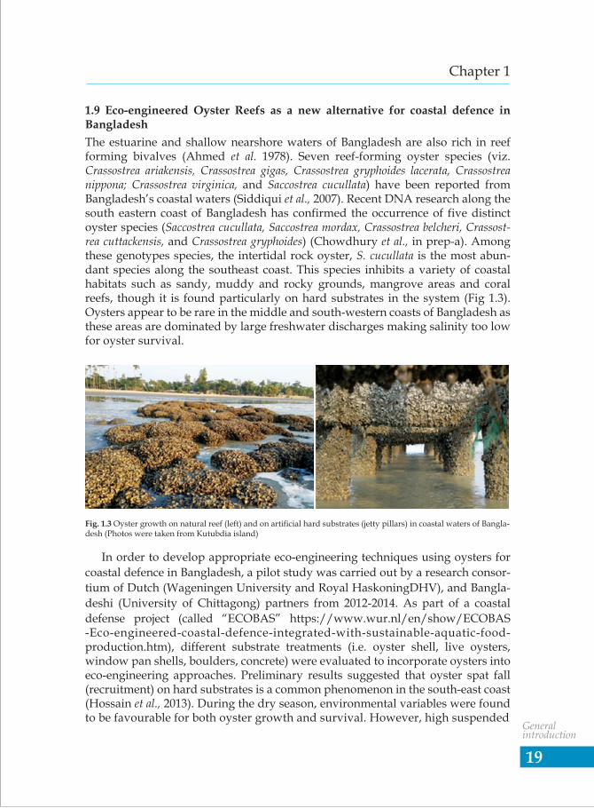
Fig. 1.3 Oyster growth on natural reef (left) and on artificial hard substrates (jetty pillars) in coastal waters of Bangla-desh (Photos were taken from Kutubdia island)

1.9 Eco-engineered Oyster Reefs as a new alternative for coastal defence in BangladeshThe estuarine and shallow nearshore waters of Bangladesh are also rich in reef forming bivalves (Ahmed et al. 1978). Seven reef-forming oyster species (viz. Crassostrea ariakensis, Crassostrea gigas, Crassostrea gryphoides lacerata, Crassostrea nippona; Crassostrea virginica, and Saccostrea cucullata) have been reported from Bangladesh’s coastal waters (Siddiqui et al., 2007). Recent DNA research along the south eastern coast of Bangladesh has confirmed the occurrence of five distinct oyster species (Saccostrea cucullata, Saccostrea mordax, Crassostrea belcheri, Crassost-rea cuttackensis, and Crassostrea gryphoides) (Chowdhury et al., in prep-a). Among these genotypes species, the intertidal rock oyster, S. cucullata is the most abun-dant species along the southeast coast. This species inhibits a variety of coastal habitats such as sandy, muddy and rocky grounds, mangrove areas and coral reefs, though it is found particularly on hard substrates in the system (Fig 1.3). Oysters appear to be rare in the middle and south-western coasts of Bangladesh as these areas are dominated by large freshwater discharges making salinity too low for oyster survival.

In order to develop appropriate eco-engineering techniques using oysters for coastal defence in Bangladesh, a pilot study was carried out by a research consor-tium of Dutch (Wageningen University and Royal HaskoningDHV), and Bangla-deshi (University of Chittagong) partners from 2012-2014. As part of a coastal defense project (called “ECOBAS” https://www.wur.nl/en/show/ECOBAS -Eco-engineered-coastal-defence-integrated-with-sustainable-aquatic-food- production.htm), different substrate treatments (i.e. oyster shell, live oysters, window pan shells, boulders, concrete) were evaluated to incorporate oysters into eco-engineering approaches. Preliminary results suggested that oyster spat fall (recruitment) on hard substrates is a common phenomenon in the south-east coast (Hossain et al., 2013). During the dry season, environmental variables were found to be favourable for both oyster growth and survival. However, high suspended 4

19

Generalintroduction

Chapter 1

sediment loads and low salinities from both river runoff and monsoon rainfall resulted oyster mortality in the wet season (June to September). Siltation of the artificial substrates was reported also to be a limiting factor for oyster growth, while high flow rates and tidal surge were considered to be significant threats damaging the reef structures. In these circumstances, more durable three dimen-sional substrates with high vertical relief were tested to create artificial oyster reefs along the Bangladesh coast. It was hoped that they could stand up to high energy periods, offering also maximum surface area for oyster spat settlement and growth (Hossain et al., 2013). In 2014, ECOBAS used high relief (80 cm) cylindrical concrete rings (80 cm in diameter) as test substrates. These structures were compa-rable to OysterBreaktm used in coastal Louisiana for similar goals (La Peyre et al., 2017). Concrete rings were found to be effective for spat settlement and were stable under high energy conditions (Tangelder et al., 2015). However, this approach raised a number of concerns regarding the applicability of the design concept, which were not addressed during ECOBAS trials. Particularly, the extent of morphological changes due to the reef interventions were not quantified well. Moreover, the effect of using concrete rings on the intertidal mudflat faunal community was not evaluated in ECOBAS. Thus, it is necessary to better under-stand the applicability of using artificial oyster reefs to enhance coastal resilience.

In order to achieve the required ecological benefits for shoreline protection, artificial oyster reefs need to be self-sustaining over time. Additionally, one requires multiple age classes to survive via larval recruitment for the reefs to be viable (Coen and Luckenbach, 2000). The dynamic nature of the coastal environ-ment strongly influences oyster populations (Hossain et al., 2013; Tangelder et al., 2015). Oysters can settle under a variety of hydrodynamic conditions. However, not all places where settlement can occur are favourable for oyster reef develop-ment. The factors that determine oyster survival and growth are still poorly understood for the Bangladesh coast. Further research is necessary to better understand habitat quality prior to constructing or enhancing oyster reef-popula-tions. In general, the placement of artificial substrates (e.g., concrete rings) to begin oyster reefs is known to have a positive impact on local coastal eco-mor-phology (La Peyre et al., 2017; Walles et al., 2015a). However, the efficacy in dynamic subtropical coasts has not been well examined. These issues will be addresses in this study. In this PhD study, ‘hybrid eco-engineering’ techniques will be utilized by integrating oysters with concrete hard structures into oyster breakwater reefs. Precast concrete structures similar to Reef Ballstm (see The Reef Ball Foundation, http://www.reefball.org/) used in over 59 countries, were placed on an intertidal mudflat adjacent to the study site at Kutubdia (21°50'27.71N, 91°51'56.27E). The same tidal exposure was used for two years allowing for the recruitment and growth of oysters thus developing extensive oyster populations (see Fig. 1.4) before starting the experiment. A total of 123 rings (each was 0.8 m in diameter, 0.8 m high, with walls 0.05 m thick with 4 number of holes in them) were used in this study. The unit (i.e. each ring) cost was ~ $50 including deployment.

20

Generalintroduction

Chapter 1

Fig. 1.4 Eco-engineered concrete units with recruited oysters. Note the oyster growth on deployed oyster reef units after just eight months (left), and 2 years (right) post-deployment at the offshore island of Kutubdia.

Fig. 1.5 Concept of hybrid eco-engineering with oyster breakwater reefs for this PhD study.

Earthen embankment

Mangrove

Consolidation Stabilization

Salt marsh

Breakwateroyster reef

Faunal biodiversity

Habitat facilitation

Tidal flat morpology

After two years, those rings with oysters were moved to the experiment site. A total of three replicated 20 m long breakwater reefs were placed again in the lower intertidal zone of the study site at Kutubdia. Each of the three reefs consisted of a total of 41 units of the eco-engineered concrete rings (with veneer of oysters) arranged in two rows touching to each other. This approach was aimed at positively impacting the leeward (=landward) side of the reefs, thus accumulating sediment via the alteration of wave energy in and around the breakwater reefs. The morphological changes were expected to also impact on nearby coastal habi-tats (i.e. salt marsh and mangroves) and macrobenthic communities, attracting a variety of transient nekton species (Fig. 1.5). Studying the impact of oyster break-water reefs on sediment dynamics, associated biota and key species should provide new insights into our understanding of the habitat value of oyster reefs for coastal resilience.

621

Generalintroduction

Chapter 1

1.10 Aims and ObjectivesThis study aims at analysing these critical factors that determine oyster (S. cuculla-ta) growth and development in a dynamic, monsoon-dominated coastal ecosystem in south-east Bangladesh. It will experimentally test the ecosystem engineering capacity of oysters to enhance coastal resilience. It is hypothesized that the appli-cation of oyster breakwater reefs is beneficial for mitigating the erosion of tidal flats, thereby promoting sediment accretion, while facilitating adjacent coastal habitats (Fig. 1.5). The main research questions addressed here in the study are as follows:

1. What are the environmental boundary conditions for oyster settlement and growth in a monsoon-dominated area along the Bangladesh coast?

2. How do the oysters physiologically respond to their local environment, which is typically characterized by high variability in environmental condi-tions (i.e. food, temperature, salinity, and suspended sediment loads)?

3. Do oyster breakwater reefs attenuate waves and associated energy, and by doing so, reduce sediment resuspension and erosion rates, thereby promot-ing mudflat ‘stability’ while enhancing salt marsh growth?

4. Do the soft-bottom macrobenthic faunal (infaunal and epifaunal) assem-blages, together with intertidal ‘resident’ and ‘transient’ (=mobile) species (e.g., finfish, shrimp, crabs and other macro-invertebrates) benefit from oyster breakwater reefs employed for coastal protection?

722

Generalintroduction

Chapter 1

1.11 Outline of the thesis

In this thesis, three main research topics are distinguished and described in five research chapters (i.e. Chapter 2-6, see Fig. 1.6).

Fig. 1.6 Flowchart illustrating the key content of each chapter related to research questions (C = Chapter; HSI = Habitat suitability index; GIS = Geographic Information System; DEB = Dynamic energy budget model; DEM = Digital elevation model; TPM = Total particulate matter; PIM = Particulate inorganic matter; Chl-a = Chlorophyll-a).

Eco-

engi

neer

ed b

reak

wat

er o

yste

r re

efs

for

Coas

tal R

esili

ence

Oysters are ecosystem engineers that modify, create and maintain the habitat; they are self-sustaining and act as coastal buffers, i.e. absorb wave energy, increase sedimentation, reduce erosion, enhance habitat for other species.

Aims and objectives of the research

C1

Applicability of oyster breakwater reefs

Poor site

Potential site

Ideal site

• Seven Environmental Parameters (Salinity, temperature, pH, DO, PIM, water �low, Chl-a)

• Dry vs wet season

HSI model GIS

• Physiological experiments

• Co-variation Growth DEB

parameters

Chl-a TPM

Temp.

DEB model

DEM models: Changes in coastal morphology

Sediment characteristics Erosion/Accretion

Changes in ecology: Macrobenthic community

Fish/shrimps/crabs/ other invertebrates

Shore and habitat Protection Habitat facilitation

Why oyster?

Where to grow?

How oysters respond to local

environment?

What to say?

How oyster breakwater reefs can contribute to

coastal resilience?

C2

C3 C4

C5 C6

C7

First, the question is where oysters can settle and grow out, so the focus is on boundary conditions in terms of habitat quality (Chapter 2). This information is then translated into a habitat suitability model (HSI) as a decision making tool, which can provide quantitative information about the oyster habitat suitability for a particular site along the Bangladesh coast. In Chapter 2, multiple environmental parameters are considered as the determining factors for oyster settlement and growth. For each parameter, the suitability function relative to physiological

823

Generalintroduction

Chapter 1

response measures was developed, which was used to further develop the HSI model. Mechanistic processes involved in model formulation are illustrated through a tree diagram and factors related to the seasonal influences for habitat suitability model development are also described. The HSI model not only describes the suitability of habitats but also provides geo-spatial information about the distribution and abundance of oysters, which were validated with field data.

Second, the seasonal dynamics of oyster performances were analysed using measurements of oyster physiological performance as a function of environmental conditions (Chapter 3 and 4). Chapter 3 provides physiological information of S. cucullata related to various ecological parameters, which were synthesized from a large number of eco-physiological experiments and the outcomes were used further to estimate DEB model parameters. The process involved to estimate the DEB model parameters is comprehensively described, which also complement the application of the energy budget theory for describing the bivalves’ (here, S. cucul-lata) life stages. Chapter 4 shows the DEB model runs for simulating growth, reproduction and maintenance of S. cucullata. The model is fitted to a dataset of field observations by changing the parameters of the functional response that describes the ratio between the food uptake rate and the maximum uptake rate as a function of temperature and food concentrations.

Thirdly, in Chapters 5 and 6, the application of oyster breakwater reefs was tested as they contribute to reducing coastal erosion as well as beneficiating the facilitation of other habitats (i.e. mudflats, salt marsh) and associated species (e.g., macro-invertebrates, finfish). A suitable site was chosen based on model outputs and observations. An eroding mudflat was used on Kutubdia Island. Here concrete rings with recruited oysters for 2 years were deployed as oyster breakwa-ter reefs in the lower intertidal zone of a mudflat. The oyster breakwater reefs were then tested to see whether they could reduce localized erosion by changes in local tidal flat morphology versus those areas without such reefs. Moreover, the effect of oyster breakwater reefs to the adjacent salt marsh habitat is also described. Chapter 6 focuses on the faunal changes related to the presence of the oyster breakwater reefs. Particularly, the changes in benthic macrofaunal assemblages, along with transient fishes and a wide group of mobile invertebrates were evaluat-ed in this chapter again by comparing them with communities observed at repli-cated control sites. These two chapters provide valuable information highlighting the habitat value of oyster breakwater reefs in protecting coast lines and facilitat-ing ecologically important habitats.

The final chapter contains a summary, where main outcomes of the thesis are discussed. This chapter provides insight regarding the applicability of oyster breakwater reefs in subtropical, dynamic environments and evaluates their ecological role for enhancing coastal resilience.

24

Generalintroduction

Chapter 1

Accepted for publication : PLOS ONE

Chapter 2

A verified habitat suitabilitymodel for the intertidal rockoyster, Saccostrea cucullata

Mohammed Shah Nawaz ChowdhuryJohannes W.M. Wijsman

M. Shahadat HossainTom YsebaertAad C. Smaal

3

AbstractThere is growing interest to restore oyster populations and develop oyster reefs for their role in ecosystem health and delivery of ecosystem services. Successful and sustainable oyster restoration efforts largely depend on the availability and selection of suitable sites that can support long-term growth and survival of oysters. Hence, in the present study a habitat suitability index (HSI) model was developed for the intertidal rock oyster (Saccostrea cucullata), with special atten-tion: (1) to the role of the monsoon in the suitability of oyster habitats, and (2) to identify potential suitable sites along the south-eastern Bangladesh coast. Seven habitat factors were used as input variables for the HSI model: (1) water tempera-ture; (2) salinity; (3) dissolved oxygen; (4) particulate inorganic matter (PIM); (5) pH; (6) Chlorophyll-a; and (7) water flow velocity. Seven field surveys were conducted at 80 locations to collect geo-spatial environmental data, which were then used to determine HSI scores using habitat suitability functions. The model results showed that the areas suitable (HSI >0.50) for oyster settlement and growth were characterized by relatively high salinities, Chlorophyll-a, dissolved oxygen and pH values. In contrast, freshwater dominated estuaries and nearby coastal areas with high suspended sediment were found less suitable (HSI <0.50) for oysters. HSI model results were validated with observed oyster distribution data. There was strong correlation between the HSI calculated by the model and observed oyster densities (r = 0.87; n = 53), shell height (r = 0.95; n = 53) and their condition index (r = 0.98; n = 53). The good correspondence with field data enhances the applicability of the HSI model as a quantitative tool for evaluating the quality of a site for oyster restoration and culture.

26

Habitatsuitability

model

Chapter 2

Habitatsuitabilitymodel

2.1 IntroductionReef-forming oysters are habitat-structuring species in coastal and estuarine areas providing essential ecosystem goods and services to human society (Beck et al., 2009; 2011; Coen et al., 2007). Both their reef structures and suspension-feeding behaviour exert large ecosystem influences (Newell, 2004). Conservation and restoration of reef-forming oyster is therefore important to maintain ecosystem health and provide multiple ecosystem services including: (1) shoreline stabiliza-tion (Piazza et al., 2005; Scyphers et al., 2011; Walles et al., 2015a; Ysebaert et al., 2012); (2) water quality regulation (Kellogg et al., 2013; Newell et al., 2002; Piehler and Smith, 2011); (3) ecosystem succession (La Peyre et al., 2017); and (4) fisheries production (Gregalis et al., 2009; Hossain et al., 2013; Peterson et al., 2003; Tolley and Volety, 2005). This implies also a sustainable management of these aquatic resources. To restore or create healthy oyster reefs, it is necessary to know the habi-tat requirements of the target species.

The intertidal rock oyster, Saccostrea cucullata is the dominant oyster species living along the south-eastern coast of Bangladesh, but the natural population is under great threat for habitat deterioration caused by recent developmental activi-ties (e.g., Matarbari power plant project, LNG import terminal in Maheshkhali Island). At the same time, oyster reef development is considered to enhance coast-al resilience in Bangladesh (Hossain et al., 2014). Successful and sustainable oyster reef development largely depends on the selection of suitable sites that support long-term growth and survival of oysters (Hargis and Haven, 1999; Pollack et al., 2012; Schulte et al., 2009). In fact, site selection for such approach is very challeng-ing for the coastal zone of Bangladesh. The area is very dynamic and influenced by the annual monsoonal climate. To enhance survival and growth, one requires an understanding of the complex interactions between oysters and their environment (Chowdhury et al., 2018). Based on these complex relationships, a model was developed to determine suitable locations for oyster reef creation.

In the present paper, we developed a habitat suitability index (HSI) model for S. cucullata in Bangladesh that can be a useful tool for coastal resource managers. A HSI model provides spatially explicit information on the relative potential of a given area to support a particular species of interest (Prosser and Brooks, 1998; Roloff and Kernohan, 1999; U. S. Fish and Wildlife Service, 1981). Over 150 HSI models for wildlife species were published prior to 1990 (Terrell and Carpenter, 1997), with many others developed since then. For oysters, the HSI efforts focus on their: (1) aquaculture (Brown and Hartwick, 1988; Cho et al., 2012); (2) fishery production (Cake, 1983; Soniat and Brody, 1988); and (3) restoration (Barnes et al., 2007; Pollack et al., 2012; Soniat et al., 2013; Starke et al., 2011; Swannack et al., 2014; Theuerkauf and Lipcius, 2016). To determine the reliability and utility of an HSI model, a four-step process is used consisting of development, calibration, verifica-tion, and validation (Brooks, 1997; Reiley et al., 2014; Theuerkauf and Lipcius, 2016; Tirpak et al., 2009).

27

Chapter 2

A comprehensive field monitoring program was initiated to quantify the forcing functions of the model covering all seasons along the entire south-east coast of Bangladesh. Then, based on experimental physiological data along with the data from literature, environmental factors were calibrated in order to develop the habitat suitability functions for each environmental parameter considered. Finally, model results were verified using an independent and spatially explicit population dataset. The aim of this study was to develop and test a spatially explicit HSI model for Saccostrea cucullata as a function of selected site characteris-tics that can be used to identify areas for oyster restoration and reef development.

2.2 Materials and Methods2.2.1 Study areaThe present study was located in the south-eastern coastal waters of Bangladesh covering about 1,050 km of coastline including tidal river banks, from the Big Feni River in the west to the mouth of the Naaf River in the east (see Fig. 2.1). The area consists of rivers, streams/tributaries, estuaries, channels, coastal waters and nearshore islands. No specific permissions were required for these locations/activities, as the field studies did not involve endangered or protected species. The northern part of the study area is a regular, unbroken stretch of coastline having intertidal mudflats and submerged sand banks. More to the south, a continuous sandy beach runs from Cox’s Bazar to the southern tip of the Teknaf peninsula. The coastal areas are characterised by a subtropical maritime climate. There are four seasonal weather patterns: (1) the dry winter season (December-February); (2) pre-monsoon (March-May); (3) monsoon (June-September); and (4) post-monsoon (October-November), which are principally governed by the southwest and northeast monsoon winds (Khatun et al., 2016; Mahmood, 1994). Among these four seasons, monsoon months are distinct from the non-monsoon months (see Table 2.1 as an example). About 80 - 90% of the annual rainfall is confined to the monsoon months, which makes the coastal environment very dynamic, with a lot of fluctuations in biotic and abiotic conditions (ESCAP, 1988; Mahtab, 1989; Pemetta, 1993). During the season winter, the climate is mild and dry, with minimum air temperatures from 7 - 13°C and maximum temperatures from 24 - 31°C. The winds are predominantly north-easterly at the beginning of the winter and north-westerly at the end. May is generally the hottest month with air temperatures potentially reaching 40°C (BMD, 2017). The heavy southwest monsoon rains begin in early June and continue into mid-October. During the monsoon period, floodwaters from extended rainfall pushes the freshwater to near the coast, while salinity variations in other seasons are relatively small (Mahmood, 1994). The annual average rainfall varies from 1,500 - 3,500 mm (BMD, 2017). Semi-diurnal tides are typical in these coastal waters, with a tidal range of approximately 3 - 6 m during the spring tide season (BIWTA, 2017). Coastal water temperatures have distinct bimodal seasonal cycles with two warm and two cool seasons per year. Daily average waterHabitat

suitabilitymodel

28

Chapter 2

6

temperature is lowest (26.9°C) during winter months (December-January) and highest (29.7°C) during early summer months (April-May) (Chowdhury et al., 2012). Though the air temperature drops in winter for a short period, it has minor effect on seawater temperatures as it is buffered by the Bay of Bengal with its strong water circulations.

2.2.2 Assimilation of data sets on environmental variablesThe most common variables utilised in HSI models for oysters are: temperature, salinity, pH, dissolved oxygen, water flow velocity, particulate inorganic matter (PIM), and chlorophyll-a (as a proxy of food for oysters, reviewed in Theuerkauf and Lipcius, 2016). For the present study, we collected environmental data from 80 sampling stations representing tributaries, river mouths, estuaries, channels and nearshore waters in south-eastern Bangladesh, covering about 1000 km of coastline (Fig. 2.1). To cover seasonal influences, a total of 7 surveys visiting all 80 locations were conducted during the 12 month investigation period (January 2016 to December 2016). During the non-monsoon period (October–May), sampling was carried out only in representative months (January, May and November) covering three of the four seasons (i.e. winter, pre-monsoon and post monsoon). During the monsoon period (June-September), monthly sampling was carried out to quantify the variability during monsoonal period. Therefore, to reduce the high environmental variation, two mean datasets (monsoon and rest of the seasons, here-after called non-monsoon) were created for model application.

Each survey was conducted during the full moon phase to cover the maximum tidal range and data were collected during flood and ebb tide periods to consider diurnal variations due to tides. Hand-held SCT (salinity, conductivity, tempera-ture) and dissolved oxygen sensors (YSI model 30 and 55 respectively; YSI Inc., USA) were used to record water temperature (°C), salinity (ppt), dissolved oxygen (mg l-1). Water pH was recorded using a hand held pH meter (Model HI98107, HANNA Instruments, Romania). Water flow velocity (m sec-1)was


29

Chapter 2

Major parameters Monsoon Non-monsoon Annual mean

Water Temperature (°C) 29.4 ± 0.2 28.1 ± 1.6 28.5 ± 1.4Water salinity (ppt) 16.2 ± 4.5 28 ± 3.5 24.1 ± 6.9DO (% saturation) 72.2 ± 4.9 77.1 ± 5.3 75.5 ± 5.4pH (-) 7.7 ± 0.0 8.0 ± 0.1 7.9 ± 0.1Chl-a (µg l-1) 2.6 ± 0.2 3.7 ± 0.7 3.3 ± 0.8PIM (mg l-1) 571 ± 84 240 ± 108 351 ± 190Water flow velocity (m sec-1) 0.6 ± 0.1 0.3 ± 0.1 0.4 ± 0.1Total rainfall (mm) * 2162 726 2888

Table 2.1 Example of distinct environmental variation (mean ± 1 standard deviation based on four observations during the monsoon period and three observations during the non-monsoon period) in monsoon and non-monsoon months (Location: Kutubdia channel;Year 2016). DO = Dissolved oxygen; Chl-a = Chlorophyll a; PIM = Particulate inorganic matter.

*Rainfall during 2016

7

Habitatsuitability

model

30

Chapter 2

Fig 2.1 Geographical map showing the 80 field sampling locations (red dots) in this study for oyster habitat suitability model development in the South-eastern coastal waters of Bangladesh.

N

8

measured by deploying a flowmeter (SKU 2030R; General Ocean Inc., USA) in mid flood and ebb tidal periods for 10 minutes. Concentration of total particulate matter (TPM, mg-l) was determined from water samples as weight of residue remaining on a filter (GF/C Whatman glass microfiber with 1.2 µm pore size) after drying at 60°C for 12 h. After ignition of TPM filter at 450°C for 5 h, particu-late inorganic matter (PIM) concentrations were determined from weight loss. The chlorophyll-a concentration (μg l-1) in water samples were determined by fluorescence meter (FluoroSensetm, Turner Designs, USA), calibrated by taking data from chlorophyll extraction into acetone following the procedure of Strick-land and Parsons (1972).

2.2.3 Model descriptionThe HSI model is composed of two life stage components: (1) the settling larval stage (at metamorphosis); and (2) the post-settlement life stages (spat and adult). Gametes, eggs and planktonic larval stages were excluded from the model as they have no habitat requirements beyond the water conditions which permits their parents to spawn. Fig. 2.2 illustrates how the HSI is related to the variables and life stages of the oyster. The cycle starts at the metamorphosis, where the eyed-pe-diveliger larval stage that needs to settle onto a hard substrate. Ambient salinity, and the presence of suitable substrates are considered as key components for successful spatfall while high water flows can limit the settlement of oysters in turbulent waters. Temperature, salinity, pH, dissolved oxygen, PIM, and Habitat

suitabilitymodel

31

Chapter 2

Environmental variable Research output Life Stages Habitat

V1 Salinity for spat settlement

V2Water �low velocity

V3 Temperature V4 Salinity for growth V5 pH V6 Dissolved oxygen V7PIM V8 Chlorophyll-a as proxy of food

Larval (at metamorphosis)

Spat/Adult

Estuarine/ Coastal

HSI

GIS Geo-

spatial HSI Maps

Validation by population

data

Fig 2.2 Tree diagram illustrating the relations between environmental variables, life stages, and habitat type used to setup the Habitat Suitability Index (HSI) for the rock oyster S. cucullata.

Chlorophyll-a were considered as important environmental variables for growth and survival of juveniles (=spat) and adult oysters. To calculate component indices for determining HSI, Suitability Index (SI) graphs were used that were obtained from existing literature (see Fig. 2.3 and Table 2.2) except for salinity. Suitability Index (SI) graph for salinity are derived from empirical data from present study. Laboratory experiments were conducted to determine the influ-ence of salinity (Fig. 2.3) on adult oyster respiration. Respiration rates were measured at 0, 5, 10, 15, 20, 25, 30, 35 ppt water salinities by keeping individual adult oysters (n = 12; size = 5 ± 0.2 cm) in closed chambers of 1 l capacity filled with water of 28 ± 0.5°C. Seawater was diluted by adding freshwater to get the desired salinity for the respiration experiments. Suitability scale was standardised from maximum respiration rates at observed salinity levels (i.e. maximum respi-ration rate = 1). Before running the respiration experiments, oysters were acclima-tize for 24 h at the desired salinity condition to avoid stress related to change in physiological response. Respiration rates were measured when the oysters were actively filtering, which can easily be observed with shells open. Hand-held dissolved oxygen sensors (YSI model 55; YSI Inc., USA) were used to record the oxygen consumption rates at time intervals of five minutes, to check for a devia-tion in the linear decline. Each experimental trial was continued for about 2 hrs. Attention was given to prevent low oxygen concentration (< 3 mg O2 l-1) during trial.

RR = -V*(pO2 ,end – pO2 ,start)/t, where RR = respiration rate in ml O2.h-1; V = volume of the chamber in l; pO2,start and pO2,end = oxygen concentration in ml l-1 at the start and at the end of the measurements; t = time difference in hour between start and end of the experiment.

SI is the Suitability Index for the environmental variables indicated in the Table 2.2. To obtain component index (CI) values for the two life stage components of the model, the SI values for appropriate variables were grouped and summarised by their geometric mean, as this is more sensitive to changes in individual variables than the arithmetic mean. It means that if an SI of 0 for any variable results in a CI of 0. Overall CI for settlement and post-settlement stages were estimated by using the following equations.

For the larval settlement:CI settlement-m = (SISs-m× SIV-m)1/2

CI settlement- nm = (SISs-nm× SIV-nm)1/2

CI settlement = (CI settlement-m + CI settlement-nm)/2

For the post-settlement:CI post-settlement-m = (SIT-m× SISg-m × SIpH-m × SIDO-m × SIPIM-m × SIChla-m)1/6

CI post-settlement- nm = (SIT-nm× SISg-nm × SIpH-nm × SIDO-nm × SIPIM-nm × SIChla-nm)1/6

CI post-settlement = (CI post-settlement-m)1/3× (CI post-settlement- nm)2/3Habitatsuitability

model

32

Chapter 2

In these equations, CI settlement is the component index for the larval settlement stage, which was considered for two seasonal component indices (i.e. CI settlement-m, CI settlement-nm) as the conditions for larval settlement can be different during the monsoon and non-monsoon periods. Thus, two different environmental mean data sets were used for the two periods (i.e. m = monsoon, nm = non-monsoon). During monsoon, a site may not be suitable for larval settlement, still it can have successful recruitment in the non-monsoon period. Therefore, arithmetic mean for seasonal larval CI is used instead of geometric mean, to consider the overall seasonal influences on the larval stage. Field observations indicated two seasonal settlement peaks in the investigated areas, thus equal weight coefficients were used for seasonal component indices (i.e. CI settlement-m and CI settlement-nm). CI post-settle-

ment is the component index for the post-settlement (i.e. spat/adult) stage. Mean environmental data for monsoon and non-monsoonal were used as well to calcu-late CI post-settlement, as these seasons differ from each other. Based on the length of the seasonal periods (Monsoon = 4 months = 0.33 yr.; Non-monsoon = 8 months = 0.66 yr.), different weight coefficients were used for the seasonal component indices (i.e., CI post-settlement-m and CI post-settlement-nm) in determining the component index for the post-settlement stage. In contrast to the component index for larval settlement, a multiplication function is used for the post-settlement phase because the habitat conditions need to be suitable throughout the entire year. After obtain-ing the mean environmental data, the suitability indices (SIs) were determined by using suitability graphs (Fig. 2.3) and the component indices (CIs) were then calculated using the appropriate life stage equations. From the component indices, the overall HSI was determined following below equations as suggested by Cake (1983):

2.2.4 Habitat suitability mapHabitat suitability indices were calculated for the 80 sampling locations along the south-east coast of Bangladesh using the measured environmental variables. To get a first estimate of the length of coastline that is suitable for oyster restoration, the HSI values of the 80 sampling locations were interpolated over the entire south-east coast-line using a nearest neighbour algorithm (ESRI, 2017). For each HSI class, the total length (km) of the coastline was calculated using ArcGIS (version 10.5).

Chapter 2

1) If the component index for the post-settlement stage (CI post-settlement) is the lowest component index (i.e. CI post-settlement< CI settlement), then HSI = CI post settlement

2) If the component index for the post-settlement stage (CI post settlement) is not the lowest component index (i.e. CI post-settlement> CI settlement), then HSI = (CI post-settlement × CI settlement)1/2

8


33

3

2.2.5 Oyster data for model validationTo verify the model results with field observations, an oyster population survey was conducted after the monsoon. Based on the availability of substrates (jetty pillars, sluice gates, bridge pillars, and boulders), 53 sites among the 80 sampling locations were available for this survey. At the remaining sampling locations no nearby suitable substrates were present and therefore those sites were omitted from the analysis. Popu-lation data for model verification can be affected due to long sampling period during survey time, particularly for large scale area of the study. To avoid it, three volun-tary teams simultaneously engaged at northern, middle and southern part of the study area and complete the filed survey within a week, covering only 2-3 stations in a day using speed boat. Oyster density, shell height and condition index (percentage of dry shell weight-dry flesh weight ratio) were determined by taking oyster samples at each site. For this, replicated (>5) quadrats (25 cm × 25 cm) were used for sampling oysters from substrates available in the intertidal areas, which were positioned randomly along a 15 m long transect line (parallel to coastline) above mean lowest low water level (MLLW, ~ 0.5 m), having similar emersion times for all locations. Quadrat areas without any oysters counted as zero. Quadrat areas with oysters were excavated without damaging the oysters. Living oysters were separated from dead shell remains. Living specimens were cleaned from epibionts and transported to the field laboratory, where individual shell height and fresh weight were measured. The soft tissue of each living oyster was separat-ed from their shells, drained on paper towel and weighted after drying at 60°C for 12h. Geospatial oyster density data for the 53 locations were plotted on the poten-tial HSI map where the size (area) of the circle represents the observed oyster density.

Chapter 2

Variables Variables description Data sources of suitability index (SI) Conditions

SS Salinity for settlement Cake, 1983 At eyed-pediveliger stage

V Water flow velocity Cho et al., 2012 -

T Temperature Chowdhury et al., 2018 Salinity: 28 ppt; pH: 7.9; Physiological relationship: Oxygen Filtered seawater; consumption rate vs temperature Starved oystersSG Salinity for growth This study Temperture: 28°C; pH: 7.9 Physiological relationship: Oxygen consumption rate vs salinity

pH pH Brown and Hartwick, 1988 -

DO Dissolved oxygen Cho et al., 2012; Brown and Hartwick, 1988 -

PIM Particulate Inorganic Chowdhury et al., 2018 Temperature: 28°C; Salinity: Matter 28ppt; pH: 7.9 Physiological relationship: Water clearance rate vs suspended solids

Chl-a Chlorophyll-a as proxy Brown and Hartwick, 1988; Cho et al., 2012 for food -

Table 2.2 Data sources used to generate suitability index graphs for oysters.

Habitatsuitability

model

34

2.2.6 Data analysisStatistical differences in mean environmental variables for the monsoon vs the non-monsoon seasons were verified, using a simple t-test. Moreover, multiple linear regression models were used in order to relate the response variables (i.e. oyster density, shell height, and condition index,) to a set of independent variables (i.e. temperature, salinity, pH, dissolved oxygen, PIM, Chlorophyll-a, water veloc-ity) recorded for the non-monsoon season. The non-monsoon season had more influence on settlement and growth, as oyster growth is almost stagnant during monsoon (Chowdhury et al., 2018). A forward stepwise procedure was followed by linear modelling to determine the environmental variable(s) that most influ-ence oyster density, condition index, and shell height during growth season (i.e. non-monsoon months). Obtained data ranges for independent variables were checked whether they showed linear relationship with the suitability function curves used for the HSI modeling. Variance inflation factors (VIF) were used to check how much amount multicollinearity (correlation between independent variables) existed in a given regression analysis. The models were:

Chapter 2

0.0

0.2

0.4

0.6

0.8

1.0

0.0

0.2

0.4

0.6

0.8

1.0

0 10 20 30 400.0

0.2

0.4

0.6

0.8

1.0

0 10 20 30 400 1 2 3 4 5

0.0

0.2

0.4

0.6

0.8

1.0

0 10 20 30 40 7 7.5 8 8.50.0

0.2

0.4

0.6

0.8

1.0

0 25 50 75 100

1

0.8

0.6

0.4

0.2

0

0 200 400 600

1

0.8

0.6

0.4

0.2

00 200 400 600

1

0.8

0.6

0.4

0.2

0

Salinity for spat settlement (ppt) Water flow velocity (m sec-1) Temperature (°C)

Salinity (ppt)

V1 V2 V3

V4 V5 V6

V7 V8

pH Dissolved oxygen saturation (%)

PIM (mg l-1) Chl-a (μg l-1)

Suita

bilit

ySu

itabi

lity

Suita

bilit

y

Fig 2.3 Relationships between environmental variables and associated habitat suitability values for the rock oyster S. cucullata. Top two graphs (V1, V2) were used for larval settlement, while the other graphs (V3-V8) were used for the post-settlement period in the model (see Table 2.2 for sources).

8


35

Where, y is the response variable indicating oyster density (d), shell height (h) and condition index (CIndex). T = temperature; S = salinity; pH = water pH; DO = dissolved oxygen; PIM = particulate inorganic matter; Chla= chlorophyll-a; V = water velocity. The parameter β0 is the y-intercept, which represents the theoreti-cal expected value of y when each x is zero. The other parameters (β1, β2, . . . , β7) in the multiple regression equation are partial slopes. βj (here, j= 1....7) representing the expected change in y for a given unit increase in xj while holding all other xs constant, and does not depend on the value of any other x. Other assumptions were: E (εi ) = 0 for all i, where ε is the residual terms of each model and i =1….7 assigned for seven environmental parameters ( i.e. T, S, pH, DO, PIM, Chla, and V) respectively; Var (εi )=δε

2 for all i; the εis were independent; and εi was normally distributed. Before statistical analysis, the normality of a response and indepen-dent variables were tested using the Kolmogorov-Smirnov test and homogeneity of variances using Levene’s test.All analyses were performed using IBM SPSS statistics software (Version 2015) using α = 0.05.

2.3 Results2.3.1 Environmental variablesEnvironmental conditions showed both spatial and seasonal variations over the study period (Fig 2.4). A strong seasonal effect was observed, with monsoon months (June – September) differing from non-monsoon period (October – May). Particularly, salinity, PIM, chlorophyll-a concentrations and water flow velocity during monsoon period showed significant (p <0.05) differences with the non-monsoon period. Spatially, a clear salinity gradient was observed for both seasonal periods showing an increasing trend from north to south. Feni, Mirsarai, and upper Chittagong coastal areas received strong influences from the nearby river systems and mean salinities ranged from 0.5 - 7.0 ppt with high mean partic-ulate inorganic matter concentration (360 - 707 mg l-1). Mean salinities and suspended concentration in the lower part of Chittagong coast, Kutubdia, Moheshkhali, Cox’s Bazar, and Teknaf ranged from 6.7 - 29.5 ppt and 66 - 433 mg l-1, respectively. Among these areas, a few sites like Sonadia (southern Maheshkha-li) and the Teknaf peninsula were strongly dominated by the Bay of Bengal, show-ing smaller variation even in monsoon months. Chlorophyll-a concentrations varied from 0.8 - 9.6 µgl-1 and was relatively high in the southern part of the study area compared to the freshwater dominated and turbid northern part of the study area. Mean water temperatures for all stations showed minimal variation (27 - 28.6°C) throughout the entire study period. Water pH levels ranged from 7.4 - 8.5 along the station sampled. pH was relatively high in non-monsoonal months and

Chapter 2

yd=β0+β1xT+β2xS+β3xpH+β4 xDO+β5xPIM+β6xChla+β7xV+εd

yh=β0+β1xT+β2xS+β3xpH+β4 xDO+β5xPIM+β6xChla+β7xV+εh

yCIndex=β0+β1xT+β2xS+β3xpH+β4xDO+β5xPIM+β6xChla+β7xV+εCIndex

Habitatsuitability

model

36

6

showed reduced values from north to south, probably influence of river discharge. Saturation level of dissolved oxygen varied from 49 - 91%. No signifi-cant differences (p = 0.70) in monsoon and non-monsoon season were observed for dissolved oxygen concentration, but a decreasing trend was observed from South to North which might be related to the organic loading from the rivers. Water flow velocity became stronger in monsoon periods and higher in exposed vs sheltered sites, ranging from 0.2 - 2.4 m sec-1. Environmental variables (salinity, water flow velocity, temperature, pH, dissolved oxygen, PIM, and chlorophyll-a) showed both spatial and seasonal (monsoon vs no-monsoon period) variations along the investigated sites. Sites are ordered from south to north (see Fig 2.1).

2.3.2 Model estimationBy considering the effect of the two seasons, 37 sites, occupying approximately 397 km of coastline were predicted as suitable (HSI score >0.50) for year round growth of oysters (Table 2.3). Most of these sites were located in the area of lower Chittagong (Banskhali, Chanua), Pekua, Kutubdia, Moheshkhali, Sonadia, Cox’s Bazar and Teknaf coastal waters (Fig. 2.5). Among those sites, 114 km of coastline along Sonadia, south-western Maheshkhali channel and southern tip of Teknaf peninsula were predicted as places with the highest HSI score (HSI score >0.7). In addition, 24 scattered sites in the southern part, representing a coastline of approx-imately 269 km, were less suitable for oysters (HSI score: 0.3 - 0.5). 19 sites repre-senting approximately 391 km of coastline showed least prospect (HSI score: 0.0 - 0.3) for oyster development. Most of these sites belong to the coastline between Sandwip-Feni to mouth Karnaphully River. Few sites in the inner parts of the Moheshkhali channel, Chokoria and Cox’s Bazar coast (Inani and Monkhali) were also not considered as potential sites for oyster development. A habitat suitability map is presented in Fig 2.5 based on HSI scores.

5

Chapter 2

8


37

HSI score # of site Length of the coast (km)

0.00-0.10 13 332

0.11-0.20 1 12

0.21-0.30 5 46

0.31-0.40 7 101

0.41-0.50 17 168

0.51-0.60 19 186

0.61-0.70 9 96

0.71-0.80 6 74

0.81-0.90 3 40

0.90-1.00 0 0

Table 2.3 Estimated length of the coast corresponding with HSI scores.

7

Chapter 2

30.0

30

29

28

27

26

25

85

1.20

1.00

0.80

0.60

0.40

0.20

0.00

75

65

55

45

12

9

6

3

0

Monsoon Non-monsoon

20.0

10.0

20.5 21 21.5

Latitude (°N) Latitude (°N)22 22.5 23

20.5 21 21.5

Latitude (°N)22 22.5 23

20.5 21 21.5

Latitude (°N)22 22.5 23

9

8

7

8.5

7.5

20.5 21 21.5 22 22.5 23

3

2

1

0

Salin

ity (‰

)Te

mpe

ratu

re (°

C)

DO

(Sat

urat

ion%

)C

hl-a

(ug

l-1)

PIM

(gl-1

)W

ater

flow

vel

ocity

(m s

ec-1

)

0.0

Monsoon Non-monsoon

Monsoon Non-monsoon

Monsoon Non-monsoon

20.5 21 21.5

Latitude (°N)22 22.5 23

Monsoon Non-monsoon

20.5 21 21.5

Latitude (°N)22 22.5

Monsoon Non-monsoon

20.5 21 21.5

Latitude (°N)22 22.5 23

Wat

er p

H

Monsoon Non-monsoon

Fig. 2.4 Environmental variables ( salinity, water flow velocity, temperature, pH, dissolved oxygen, PIM, andchlorophyll-a) showed both spatial and seasonal (monsoon vs no-monsoon period) variations along the investigtedsites. Sites are ordered from south to north (see Fig. 2.1).Habitat

suitabilitymodel

38

Chapter 2

Fig 2.5 Map summarizing the results of the HSI indicating the suitability of the investigated sites (coloured lines), and verification of the model results with observed oyster density (coloured circles). Data not measured are sites (n = 27) where no substrate was available and therefore omitted from the oyster population survey

8


39

N

2.3.3 Field validationThree population descriptors were used for the assessment: (1) oyster density; (2) shell height; and (3) condition index. These were then correlated with the HSI scores for model verification (Fig 2.6). HSI values showed a strong positive relationship with the mean oyster densities (r = 0.87). Oysters were not observed at sites which had an HSI score less than 0.27. The highest number of oysters (1064 - 1596 indiv. m-2 ) were observed at sites which showed highest HSI scores (> 0.70) (Fig. 2.5). Moreover, mean oyster size (shell height) varied among the sites and showed positive relationship (r = 0.95) with HSI values as well. Variation in shell height was higher for upper HSI values, suggesting that the oysters in high HSI sites have multiple age classes due to multiple recruitments years. The oysters grew bigger in size (>5 cm shell height) in those sites, where the HSI score exceed-ed 0.50. Regression results for HSI and condition index also showed a similar trend. Field data showed that the shell-body flesh weight ratio largely varied (4.0 - 10.9%) among sites. Condition index increased with the increasing HSI scores, showing good correlation (r = 0.98). Condition indices were found relatively high (>6%), when the HSI score exceeded 0.50. Condition index for lower HSI sites showed more variability, which might be due to larger seasonal variation at these sites. Conversely, sites with high HIS values showed less variability in soft tissues coinciding with smaller seasonal variation. All the population descriptors were also strongly correlated (r >0.90) with each other (Fig. 2.7), thus showing good agreement with HSI scores.

Chapter 2

Habitatsuitability

model

40

2.3.4 Influencing environmental factorsThe linear regression model results indicated that salinity, chlorophyll-a, pH, and dissolved oxygen are the main predictors of oyster occurrence and their condi-tions (Table 2.4, for more details see Table S2.2). Water temperature, PIM and water flow velocity were removed from the model during the stepwise procedure, as these factors failed to improve the model outputs. Salinity and Chlorophyll-a were found as common explanatory variables in the model that influenced oyster density, shell height and condition index. Oyster density and also shell height had high values in areas where the oxygen saturation level was relatively high. pH values also contributed to explain observed condition index of oysters. Scatter plots and correlation coefficients among all variables also gave the same results (Fig. 2.7). Collinearity statistics in the linear model showed that variance inflation factors (VIF) were less than 5. It rejected the hypothesis of a multicollinearity relationship among environmental factors, thus explanatory variables used in the linear models were independent.

Chapter 2

Fig. 2.6 Habitat suitability index (HSI) scores derived from seven environmental datasets correlated against: live oyster density (top left), shell height (top right), condition index (bottom) shown with standard deviation (n = 53). The 0.95 confidence bounds (grey coloured) were calculated with the bootstrap (quantile) method.

8


41

3

Chapter 2

0.7

0.7

0.8

0.6

0.6

0.6 0.6

0.6

0.80.8

0.7

0.7 0.7 0.7 0.7

0.8

0.9

0.9

0.9 0.9

1.0

0.5

0.5

0.5

0.4

0.4 0.4

-0.5

-0.4

-0.5

-0.6

-0.0

-0.0

-0.4 -0.3

-0.3 -0.0 -0.3 -0.0

-0.0

-0.0

-0.0

-0.3

-0.5

Temp

DO

pH

Salinity

PIM

Chla

Velocity

Cl

Size

Density

0.6

50

70

50 70

5

20

5 20

2

6

2 6

0

6

0 6

0 1

000

0 1000

26.5

26.5

7.8 8.4

7.8

8.4

100 500

100

500

0.2 0 4

04

1.2

0.2

1.2

Fig. 2.7 Scatter plots and correlation coefficients (correlations >0.7 are shown in bold) among the independent (Temperature, dissolved oxygen, pH, salinity, PIM, chlorophyll-a, water flow rate) and dependant variables (CI, shell length, oyster density)

Table 2.4 Summary of linear regression models that were used to correlate among the dependant variables (oyster density, condition index and shell height) with independent environmental variables (for more details including the beta values of each predictors, see Table S2.2).

a Predictors: Dissolved oxygen, Chl-a, Salinity; dependant variable: Oyster densityb Predictors: Salinity, pH, Chl-a; dependant variable: Condition indexc Predictors: Salinity, Chl-a, Dissolved oxygen; dependant variable: Average shell height

Change StatisticsModel R R Adjusted Std. Error of Square R Square the Estimate F df1 df2 Sig. F

yd 0.839a 0.704 0.686 276.01538 8.216 1 49 0.006yCI 0.926b 0.858 0.849 1.35382 6.250 1 49 0.016yh 0.925c 0.855 0.846 0.97826 5.428 1 49 0.024

Habitatsuitability

model

42

2.4 DiscussionSelection of relevant environmental variables for HSI model development is critical. It depends on the magnitude of the environmental factors related to habi-tat quality, as they vary in time (i.e. seasons) and space and the tolerance range of the oysters. In this study we developed an HSI model for the intertidal rock oyster, S. cucullata using seven environmental factors. Out of seven environmental factors, four factors viz., salinity, chlorophyll-a, dissolved oxygen and pH were found to be predictors of oyster density, condition index, and shell height. Water temperature, PIM concentrations and water flow velocity were not consider as predictors in the linear models used in this study. More than 70% of the variation in dependent descriptors (i.e. oyster density, condition index, and shell height) was explained by adding the variables: salinity, Chlorophyll-a, dissolved oxygen and pH (see Table S2.2).

A large number of sites (n = 42) investigated in this study showed a decrease in salinity (> 5ppt) during the monsoon period. Most of these sites were located in upper south-eastern coast of Bangladesh, where large number of newly settled oysters die during the monsoon period. HSI scores were correspondingly low in these low salinity areas (Table S2.1). Indeed, fluctuations in salinity regulate meta-bolic activities in oysters living in shallow marine and estuarine areas (Naik and Gowda, 2013). The reproductive capacities, spat settlement and growth of oysters are typically impaired by low salinities (Rao, 1951). Low salinities can also cause mass mortalities of tropical oysters during the monsoon season, if the exposure to low salinities last too long (Angell, 1986). In contrast, oysters flourished at sites of the investigated area where the salinity remained more than 10 ppt.

Chlorophyll-a concentrations varied both spatially and seasonally within the study area, and were lower during the monsoon period as compared to the non-monsoon period. Chlorophyll-a concentration increased with decreased suspended sediment load which might be due to better light penetration enhanc-ing primary productivity. Higher HSI scores were found at locations where chlorophyll-a concentrations were high. In a study by Sasikumar et al. (2007), oyster growth was positively correlated with Chlorophyll-a concentrations.

Dissolved oxygen levels appeared not to be critical in the investigated areas (all sites have values >50% saturation level). pH values were relatively high in the non-monsoon season as compared to the monsoon season. However, both param-eters showed an increasing trend towards the south, which might be the influence of strong water circulation from the Bay of Bengal (Chowdhury et al. 2012). Oyster densities and related condition indices were relatively high in the area, where oxygen saturation levels (>70%) and pH (>7.9) also were high. In the Indian coasts, dissolved oxygen and water pH showed positive correlation with oyster spat settling rate (Naik, 2012; Naik and Gowda, 2013). Physiological activities slowed down with decreasing pH (<7.75) (Mahadevan and Nayer, 1987).

Chapter 2

8


43

Water temperatures did not vary much along the coastline and did therefore not show any significant correlation with any dependent variables. PIM concen-tration (i.e. suspended sediment) in the study area varied between 21 and 1044 mg l-1 depending on the distance from river mouth. It showed a clear seasonal pattern at all sites with a large increase during the monsoon period, when 80 percent (~1850 mm) of the total rainfall occurs along with huge amounts of suspended sediments carried to the coast via rivers. Oysters can feed in turbid environments, but are less efficient and produce copious amount of pseudofaeces, which affects gill sorting (Urban and Krichman, 1992; Ward et al., 1998). However, geo-spatial field PIM data did not show any significant correlation with the population descriptors used for model validation. Field observations also confirmed that S. cucullata population can thrive under high turbid (<700 mg l-1) conditions, if other environmental variables are optimal. Water flow velocity also did not show a good correlation with any of the dependent descriptors as the oysters were present in both high and low energy coasts, where other environmental factors are favour-able. So, water temperature, PIM concentrations and water flow velocity can be neglected for determining the oyster habitat suitability in Bangladesh coast. In this regard, a sensitivity test was performed through simple model application, where these three factors were not included. It provided similar results (R2 = 0.96) in categorizing the site characteristics in terms of HSI scores.

Means of annual survey data are often used as input variables into HSI models (Cho et al., 2012; Pollack et al., 2012). It may not provide appropriate HSI scores to evaluate a site, if strong seasonal influences exist as in monsoon dominated areas (Roloff and Kernohan, 1999). Some habitat factors can be constant over time (like in our case water temperature), while other factors viz., salinity, pH, PIM, dissolved oxygen, Chlorophyll-a may show strong seasonal differences. The use of extreme values for dynamic environmental variables in a HSI model can predict presence or absence of target species. However this approach might underesti-mate habitat quality, if the extreme values are not lethal to target species. Annual means without a seasonal considerations and also extreme environmental variable values were applied to evaluate the consequences in our model outputs. These provided high and low number of suitable sites respectively, which did not reflect field situations. Extreme values (i.e. observed lower ranges) only need to use, when they reach at or near the lethal levels and limit the survival. Otherwise mean seasonal data should consider to determine the component index of each environ-mental factor. Moreover, tolerance ranges could vary with different life history stages. Though adult oysters can tolerate extreme low salinities for extended periods, small periods of low salinity have a pronounced effect on settlement rate (Hopkins, 1935). Spat settlement was generally unsuccessful during the monsoon period at many sites, but this phenomenon may not determine the quality of a habitat over the entire year. Spatfall after the monsoon is also important to main-tain the population in dynamic coast. Particularly, the oysters that survive the non-monsoon period can then also survive the next monsoon months as they grow

Chapter 2

Habitatsuitability

model

44

and tolerate low salinities. These seasonal and longer life stage considerations improved the model outputs with respect to previous unreported version of the model, and HSI scores showed strong correlations (r >0.87) with the oyster popu-lation descriptors (i.e. density, shell height and condition index). This study also assumed that all model inputs and functions were independent. However, one environmental factor can be influenced by others. For example, water pH can be regulated by salinity conditions as both the factors are influenced by the Bay of Bengal. This type of relationship should be considered to further improve the model.

Field verification is a critical part to determine the accuracy of HSI models, but is often lacking in oyster HSI models (Theuerkauf and Lipcius, 2016). Adult oyster density is commonly used to validate an HSI model; however, this may not explain the complete picture. Here we not only considered adult oyster density, but also size (i.e., shell height) variation and condition index from 53 sites. All these descriptors demonstrate strong positive relationships with the HSI scores. Mean oyster size (>5 cm) and condition index were to be high at those sites, where the HSI scores exceeded 0.50. In Bangladesh coastal waters, it usually takes more than a year to reach 5 cm size (shell height) (Chowdhury et al., 2018). It confirms that oysters survive longer than a single year and that oyster populations probably can become self-sustaining with multiple year (size) classes when HSI scores are greater than 0.50. Population data were collected from a single survey after the monsoon period; this may differ with other seasons, yet it confirmed that oyster survival occurred after the monsoon. Still, demographic information for various seasons may improve the validation. Incorporation of the HSI scores into a GIS interface provides a visual aids in the format of maps for coastal resource manag-ers and policy makers. An attempt was made to develop an HSI geospatial map for oysters, where validation data that reflect the population survey were used. We investigated about 1050 km of coastline using 80 representative sampling sites, and the strong spatial patterning in the map of HSI scores shows regions with good habitat suitability within the study area (see Fig. 2.5). This gives a spatially explicit visualization of potential oyster habitats along the south-east Bangladesh coast. A simple nearest neighbour algorithm was used as an interpolation technique in a GIS interface to categorize the length of coastline using HSI scores. This forms a good basis for site selections, thus can be further expanded upon by increasing the number of sampling sites and the extent of the temporal environ-mental samples.

The present study has attempted to include all the available information to identify suitable sites for oysters through HSI model development. Nevertheless, the approach could be refined further with additional information. Such as, the amount of substrate available is important as it would also both contribute to the HSI and also could affect oyster density. There are some areas that showed poten-tial for oyster development, but oysters were absent due to lack of substrate. Artificial hard substrate can be added there to test the model results. In this

5

Chapter 2

8


45

7

regard, bottom characteristics and wave energy conditions of coastal sites could be useful for determining the substrate types, which is inevitable for oyster reef formation. Yet, the verification of the model with field surveys shows a good fit for this oyster HSI model.

2.5 ConclusionThis study developed an HSI model for the intertidal rock oyster, Saccostrea cucul-lata and applied it to the entire south-eastern coast of Bangladesh. Salinity, Chloro-phyll-a, dissolved oxygen and pH were identified as driving factors that deter-mine the habitat quality of oyster populations along this region. The results clearly show that freshwater dominated low saline estuaries and nearby coastal areas with high suspended sediments are least suitable for oyster settlement and growth. In contrast, the bay dominated areas with relative high salinity, Chloro-phyll-a, dissolved oxygen and pH were found to be suitable for oyster settlement and growth. Seasons (i.e. monsoon and non-monsoon) and life stage (i.e. settle-ment and post settlement) considerations are found effective and suggested as integral part in habitat suitability model formulation for subtropical dynamic coastal systems. In this study, the HSI model results match the current distribu-tion of oysters throughout the investigated area. The good correspondence with the field data enhances the reliability of the presented HSI model as a quantitative tool for planning oyster restoration and managing oyster resources along the south-eastern coast of Bangladesh.

6

Chapter 2

Suplimentary informationTable S2.1 Measured environmental conditions and oyster population characteristics for each HSI score (divided into 9 HSI classes), based 80 sampling stations (see Fig. 2.1).

HSI #of site Water Temp DO pH Salinity PIM Chl-a Water flow Density CI Size (°C) (Saturation %) (-) (ppt) (mg l-1) (μg l-1) velocity (ind. m-2) (cm) (m sec-1)

0-0.10 13 27.5 27.0 55 56 7.67 7.96 0.5 4.1 506 370 1.82 3.48 0.59 0.41 0 0

0.11-0.20 1 26.6 26.1 58 63 7.7 7.66 0.1 5.3 239 250 2.5 4.85 0.57 0.41 0 0

0.21-0.30 5 27.6 27.1 61 63 7.76 8.06 1.5 7.1 748 498 2.14 4.08 1.17 0.81 0 0

0.31-0.40 7 27.8 27.3 58 60 7.75 8.05 1.4 15.3 680 459 1.98 3.74 0.79 0.55 125 4.0 0.82 3.25

0.41-0.50 17 27.9 27.4 64 66 7.83 8.11 2.9 23.8 362 233 2.82 4.83 0.83 0.61 263 4.5 0.79 4.93

0.51-0.60 19 28.0 27.5 69 71 7.87 8.15 8.9 26.5 435 271 2.83 5.09 1.13 0.79 772 6.5 0.8 8.59

0.61-0.70 9 28.3 27.8 74 76 7.95 8.22 11.3 27.2 241 181 3.97 6.85 1.21 0.84 920 7.3 0.77 9.01

0.71-0.80 6 28.5 28.0 76 78 8.06 8.34 3.2 29.4 211 128 6.06 8.67 0.94 0.72 1290 10.1 0.82 12.64

0.81-0.90 3 28.4 27.9 78 80 8.1 8.36 12.4 28.7 100 66 7.66 8.35 0.97 0.87 1476 10.9 0.86 12.82

M NM M NM M NM M NM M NM M NM M NM Min Max

Note: [Environmental variables are these averaged values over the number of sites per HSI class and over the representative months for monsoon and non-monsoon, while oyster population descriptors are averaged values over the number of sites per HSI class.].

Habitatsuitability

model

46

Chapter 2

a Predictors: (Constant), DOb Predictors: (Constant), DO, Chl-ac Predictors: (Constant), DO, Chl-a, Salinityd Dependent Variable: Oyster density

R Adjusted Std. Error ofModel R Square R Square the Estimate R Square Change F Change df1 df2 Sig. F Change

Change Statistics

1 .749a .561 .552 329.54381 .561 65.159 1 51 .0002 .809b .654 .641 295.26137 .094 13.531 1 50 .0013 .839c .704 .686 276.01538 .050 8.216 1 49 .006

Table S2.2 Summery of linear model results

Model, yd

8


47

Chapter 2


Change Statistics

1 .866a .750 .745 1.76219 .750 152.793 1 51 .0002 .917b .840 .834 1.42313 .090 28.196 1 50 .0003 .926c .858 .849 1.35382 .018 6.250 1 49 .016

a Predictors: (Constant), Salinityb Predictors: (Constant), Salinity, pHc Predictors: (Constant), Salinity, pH, Chl-ad Dependent Variable: Condition index

Habitatsuitability

model

48

Table S2.2 Summery of linear model results (continued)

Model, yCIndex

849

Chapter 2

a Predictors: (Constant), Salinityb Predictors: (Constant), Salinity, Chl-ac Predictors: (Constant), Salinity, Chl-a, DOd Dependent Variable: Average shell height


Change Statistics

1 .884a .782 .778 1.17646 .782 182.972 1 51 .0002 .916b .839 .833 1.02066 .057 17.759 1 50 .0003 .925c 855 .846 .97826 .016 5.428 1 49 .024

Model, yh


Table S2.2 Summery of linear model results (continued)

Chapter 3

DEB parameter estimation forSaccostrea cucullata (Born),

an intertidal rock oyster in theNorthern Bay of Bengal



Published in Journal of Sea Research 142 (2018): 180-190

3

AbstractDynamic Energy Budget (DEB) models describe the energy flow in organisms focusing on food assimilation and utilization for maintenance, growth and repro-duction. In this paper, specific DEB parameters were obtained for the intertidal rock oyster Saccostrea cucullata, which has culture potential and important ecologi-cal functions in estuarine and coastal ecosystems along the Bay of Bengal, Bangla-desh. Oyster samples were collected from natural oyster beds and used in a starva-tion experiment for 20 weeks in the laboratory. A sub-sample of starved oyster was used to record respiration rates and depletion of reserves was recorded by fortnightly measurements of flesh weight. Simultaneously, a group of oysters was used for physiological experiments and growth measurements, required for DEB parameter estimation. Consequently, Arrhenius temperature related parameters (i.e. TA, TL, TH, TAL, and TAH), shape coefficient (δM), volume specific maintenance rate ([ṗM]) and volume specific cost for structure ([EG]) were estimated using data from the respiration and starvation experiments. An iterative co-variation method was used to estimate the specific DEB parameters using the results of the physio-logical experiments, field observations and additional literature information. Estimated Arrhenius temperature was 5640 K, which applies between 297 and 305 K. Shape coefficient (δM= 0.159) was low, compared to other oyster species that characterized the morphology of the oyster. Volume specific maintenance rate ([ṗM]) was equivalent to 17.99 J cm-3 day-1, while 2377 J cm-3 was estimated as the volume specific cost for structure ([EG]). These efforts provide opportunities to apply the DEB model for better understanding the energetics of bivalves under sub-tropical conditions. It is concluded that the hydrometeorological aspects, i.e. a monsoon regime and high turbidity levels, are quite different from temperate regions and drives the physiological traits of shellfish organisms.

DEBparameterestimation

52

Chapter 3

4

3.1 Introduction The intertidal rock oyster, Saccostrea cucullata is the most dominant oyster species along the coast of Bay of Bengal, occurring as thick beds in the estuaries, creeks, backwaters, jetty pillars, sluice gates, ports and harbours (Ahmed et al., 1978; Ahmed, 1990; Awati and Rai, 1931; Rao, 1987). The presence of local stocks, high tidal amplitude, sufficient tidal current and high phytoplankton abundance offer a favourable environment for oyster growth around the south-east coastal waters of Bangladesh (Ahmed, 1990; Shahabuddin et al., 2010; Wahab and Amin, 2004). This species has culture potential due to its highly euryhaline nature, fast growth rate and abundant spat fall (Angel, 1986; Braley, 1984; Hossain et al., 2013; Kripa and Salih, 1996; Krishnakumari et al., 1990; Pagcatipunan, 1984; Sukumar and Joseph, 1988; Van Someron and Whitehead, 1961). Furthermore, a recent pilot study in Bangladesh showed that artificial reef structures placed on tidal flats have poten-tial for oyster settlement and reef development. These artificial reef structures develop into living oyster reefs, which can act as coastal ecosystem engineers to protect the shore from erosion and can deliver harvestable aquatic food from surplus oysters grown on the structures (Hossain et al., 2013; Tangelder et al., 2015). Thus, artificial oyster reefs have been suggested as one of the tools to mitigate shoreline erosion and enhance coastal resilience in Bangladesh (Hossain et al., 2014). But the success of such efforts, aiming at facilitating vegetation succes-sion or land reclamation, and aquatic food production, largely depends on local environmental aspects and hydro-meteorological dynamics.

Bangladesh coastal environment is dominated by the south-west monsoon climate, which makes the coast very dynamic with significant variations in envi-ronmental parameters. The average annual precipitation is 3740 mm and about 80% of the total rainfall occurs during the monsoon months i.e. June – September (BMD, 2017). During the monsoon period huge amounts of sediment (even >0.5g inorganic particulate matter per litre of water) are carried through river discharges and increase the suspended loads in the coastal waters. Though the species is abundant and apparently perform well under these varying conditions, their responses to such dynamic situations, particularly for Bangladesh coastal waters, are not described well. The aim of the study was to understand how the oysters react to local environmental conditions, which are characterized by high variation in suspended load and food availability.

Dynamic energy budget (DEB) theory (Kooijman, 2010, Nisbet et al., 2000) offers an opportunity to address this research question, which establishes links between organism’s physiology and the environment using metabolic dynamics of an individual organism through its entire life cycle (Kooijman, 2010; Sousa et al., 2008). As a powerful tool, a DEB model based on DEB theory can simulate growth, development, maintenance and reproduction of individual organisms in response to natural variability in biotic and abiotic conditions (Kooijman, 2010). In connec-tion to this, a DEB model discriminates organism’s responses to environmental variations and allows predicting its performance under different climatological DEB

parameterestimation

53

Chapter 3

regions (Jusup et al., 2017). However, application of the DEB models involves precise estimation of required parameters to evaluate physiological responses under varying conditions. For instance, DEB model parameters have been estimat-ed for hundreds of species including oysters in different geographical locations (Barillè et al., 2011; Bourles et al., 2009; Emmery et al., 2011; Freitas et al., 2009; Grangerè et al., 2009; Pouvreau et al., 2006; Ren and Schiel, 2008; Rico-Villa et al., 2009; Sarà et al., 2012, 2013; van der Meer, 2006; van der Veer et al., 2006). Despite all these efforts, we still lack DEB outcomes for the rock oyster, S. cucullata that is an ecologically and commercially important oyster species, widely distributed throughout the subtropical Indo-Pacific region. Therefore, laboratory experiments and field observations were conducted to demonstrate the large extent of DEB model applications for this oyster species. The objective is to estimate the DEB model parameters for S. cucullata under conditions as they appear in the coastal ecosystem of Bangladesh.

3.2 Materials and methods

3.2.1 The standard DEB modelWe used a standard DEB model with metabolic acceleration (i.e. abj-model) for the rock oyster by assuming their three life stages: embryo, juvenile and adult. Oysters neither feed nor reproduce at embryo stage, juvenile oysters feed after reaching maturity threshold for birth (EH

b) but do not reproduce, adult oysters feed and reproduce only when it reaches to maturity threshold for reproduction (EH

p). A simplified model scheme with the description of energy fluxes is presented in Fig. 3.1. This model has four state variables: structural volume (V, cm3), stored energy reserves (E, J), energy allocated to maturity (EH, J) and energy used for reproduc-tion (ER, J) (Kooijman, 2010). The dynamics of the state variables are specified by :

Reserved :

Structural volume : with specific volumetric growth rate,

Maturity :

Reproduction buffer :

ṗ denotes the energy fluxes, which are defined byAssimilation rate :Reserved mobilization rate :Somatic maintenance rate :

Maturity maintenance rate :Growth rate :

Energy flux to maturation/reproduction :DEB

parameterestimation

54

Chapter 3

dE= =0with if-dtb ;ṗA ṗ

Aṗ𝐶 , 𝐸 <H 𝐸H

𝑟dV V=dt 𝐸𝑟 =𝐸𝐿4

𝐿3

−p𝑀

Ƙ

+ 𝐸GƘ

[[

[[dE = ifdtp ,ṗR 𝐸 <H 𝐸H

H

dE = ifdtpṗR 𝐸 ≥H 𝐸H

R

f L2ṗ ṗA= { {Am

=ṗ L + { }LM p [[ pM T3 2

ṗ𝐶𝑣𝐿-𝑟)

min{ }p𝐸H, 𝐸HpJ kJ=

ƘpG

pM

pC= -

(1-Ƙ)pR

pJ

pC= -

6

The parameters Ƙ, and [EG] denote the fraction of reserve allocated to soma and volume specific cost for structure respectively. {p��T} and ��J denote surface area specific somatic maintenance rate and specific maturity maintenance rate coeffi-cient respectively. It is assumed that the oysters change their shape in the early juvenile period, leading up to a metamorphosis after which they reach the adult shape (metabolic acceleration, Kooijman, 2014; Lika et al., 2014; Zimmer et al., 2014). During this process, they develop from V1-morph to isomorph. This has effect on the surface-to-volume ratio. During the V1-morphic larval stage (i.e. after birth till metamorphosis), the surface area specific assimilation rate {p��Am } changes with length while the volume specific assimilation rate [p��M] is constant. For an isomorph, the surface area specific assimilation rate, {p��Am } = p��A/L2 is constant, while volume specific assimilation rate [p��M] = p��A/L3 decreases with length. Accel-eration ends with metamorphosis (Kooijman, 2014). The energy conductance v�� , which determines reserve mobilization, is defined as {p��Am }/[EM], where [EM] is the maximum reserve density. Hence, v� is also influenced during V1-morphic larval stage and increases with length. To consider these changes, a shape correction function (�(L)) was used and functions for p��C, p��A, and r� were modified as suggest-ed by Lika et al. (2014) and Zimmer et al. (2014).


55

Chapter 3

Food Reserve

Maturation

Reproduction

Structure

Assimilation

Growth

Somaticmaintenance

Maturitymaintenance

Mobilization

(1− Ƙ)

Ƙ

p��A p��C

p��G

p��M

p��R

p��J

Faeces

Fig. 3.1 A simplified scheme of the main metabolic processes as defined by the DEB theory (Kooijman, 2010). Boxes represent state variables and arrows energy fluxes (J d-1)

7

3.2.2 Lab and field experiments for estimating common parameters and generat-ing empirical data

After the spawning season (i.e. May-June), oyster specimen were collected from the intertidal oyster bed at Maheshkhali Island in the southeast coast of Bangla-desh (Fig. 3.2). Collected specimen were cleaned of epibionts and transported to the field laboratory of the Institute of Marine Sciences and Fisheries (IMSF), University of Chittagong at Kutubdia Island (Fig. 3.2). The laboratory has a recir-culation system for seawater with necessary facilities including water holding tanks. All the collected oysters were immediately kept in recirculation seawater tanks and acclimatized for one week before starting any experiment. A total of DEB

parameterestimation

56

Chapter 3

92°0'0"E91°30'0"E

22°0

'0"N

21°3

0'0"

N

0 10 205 Kilometers

±

KutubdiaIsland

MaheshkhaliIsland

Sangu River

Kutubdia channel

Maheshkhali channel

Cox's BazarBay of Bengal

BANGLADESH

Bay of Bengal

Fig. 3.2 Map showing the locations of Kutubdia and Maheshkhali Islands along Bangladesh coast from where oyster population data were collected to support the DEB model calibration.

N

8

500 oysters ranging from 20 to 150 mm shell length were placed into a 500 l tank containing filtered seawater. Among those specimen, 220 oysters of similar size (size: 50 ± 2 mm in length) were selected and kept in a separate tank for running starvation experiments and monitoring reserve utilization by animals. Tank water was recirculated through an aerated bio-filter system for controlling ammonia and keeping oxygen concentration at high level. Water temperature was kept at 28 ± 0.5°C in experiment tank as it is the mean annual temperature in the investigated site (see Table 3.1). Oysters were checked daily to observe and remove dead individuals from the tank. A total of 21 dead individuals were removed from the system during the starvation experiment, which was continued for 140 days. 19 individuals were sampled at 2 weeks interval and biometric data (i.e. length, volume and total wet weight) for each individual were recorded. Body flesh of each oyster was separated from the shells, drained on paper towel and stored in pre-weighed aluminium pans. Flesh samples were dried at 60°C for 72 h and weighed, ashed at 500 °C for 4 h and weighed again to obtain dry weight (DW) and ash-free dry weight (AFDW), respectively.

The remaining 280 oysters were kept in a separate tank by maintaining the similar water conditions as the starved tank. These oysters were used for different physiological studies within a month. Additionally, oysters (n = 30) in varying size were sampled monthly from the natural oyster bed located at Maheshkhali Island and sacrificed to monitor Gonado Somatic Index (GSI) by separating gonad mass from somatic mass under a microscope. Ash-free dry mass (AFDM) of somatic mass and gonad were determined to the nearest 0.01 mg. The Gonado Somatic Index (GSI) was expressed as the AFDM of the gonad divided by total tissue weight (AFDM).

3.2.2.1 Physiological experiments for univariate data setsPhysiological experiments were conducted to create six sets of univariate data (Data-01 to Data-06, see Table 3.2), required for the DEB parameter estimation (Saraiva et al., 2011a).

Food uptakeClearance rate was determined by measuring particle uptake (Smaal and Widdows, 1994) in 2 l flow through chambers at a temperature of 28 ± 0.5°C. We used 9 chambers in each trial with individual oysters that were acclimatized in filtered seawater for 1 month. Additionally, one chamber was kept empty (without oyster) as control. Each experiment lasted for 3 - 4 h with flow rate 3 l hr-1. Animals were exposed to different diets i.e. 50, 100, 200, 400, 600 mg total particulate matter (TPM) l-1 and ~ 6 µg Chl-a l-1. Samples were taken from the outflow of different chambers at 10 min interval. Only the data for actively filtering oysters were taken into account. The Clearance Rate was calculated as:CR = {(Cin-Cout)/Cout) * Q}

Where CR is clearance rate in l hr-1, C = concentration of TPM (mg l-1) or DEBparameterestimation

57

Chapter 3


58

Chapter 3

Chl-a (µg l-1), Cin = concentration of the inflowing water and Cout = outflow of exper-imental chamber. For Cin the concentration of the outflow of the control chamber was used. Q = flow rate in l h-1. Faeces and pseudofaeces produced by the individ-ual oysters were collected separately from each chamber at the end of each feeding trial using a micro-pipette. Each sample was then filtered through a GF/F filter and treated as described below for determining the particulate inorganic matter (PIM) and chlorophyll-a concentrations. The ingestion rate was determined as follows: IRChl-a = CR*CChl-a - PFChl-a and IRPIM= CR*CPIM - PFPIM

Where, IRChl-a = Algal ingestion rate (µg Chl-a hr-1); IRPIM= Inorganic matter ingestion rate (mg PIM hr-1); CChl-a = Chlorophyll-a concentration in water (µg Chl-a l-1); CPIM = Particulate inorganic matter concentration in water (mg l-1); PFChl-a = amount of Chl-a produced as pseudofaeces (µg Chl-a h-1); and PFPIM = amount of PIM produced as pseudofaeces (mg hr-1)

Water sample analysesTen ml water was sampled from each chamber and analysed with a turbidity meter (Model TU-2016, Lutron Electronic Enterprise Co. Ltd., Taiwan; sensitivity 0.01 NTU, which was calibrated with mg TPM l-1) to know the changes in particle concentrations. Moreover, 500 ml water was sampled from outflow of each control and oyster chamber, which was filtered onto ashed and pre-weighted 25mm diam-eter GF/F filters (0.7 µm pore, Whatman). The filters were dried in an oven at 105°C for 48 h, weighed for the TPM, and ashed in a muffle furnace at 500°C for 4 h to measure the ash fraction, which is PIM: particulate inorganic matter; this gives particulate organic matter (POM) = TPM-PIM content in the water samples. For the measurement of chlorophyll-a, a further 500 ml of seawater from each chamber was filtered through 25mm Whatman GF/F filters and the filters were stored in a dark box at -20°C for further analysis. Standard procedures using acetone extraction and fluorometric analysis (Strickland and Parson, 1968) was followed to measure the chlorophyll-a concentration in samples.

RespirationThe rate of oxygen consumption was measured by keeping individual oysters in closed chambers of 1000 ml capacity filled with sea water of 28 ± 0.5°C, containing POM: 0.45 mg l-1 and TPM: 50 mg l-1. Different sizes (50 - 91 mm) oysters were used to observe the oxygen demand in respect of length. Hand-held dissolved oxygen sensors (YSI model 55; YSI Inc., USA) were used to record the oxygen consump-tion rate at time intervals of five minute, to check for a linear decline.

RR = -V*( pO2,2 –pO2,1)/t, where RR = respiration rate in ml O2 h-1; V = volume of the chamber in l; pO2,1 and pO2,2 = oxygen concentration in ml l-1 at the start and at the end of the measurements; t = time difference in hour between start and end of the measurement. Each experimental trial was carried out for about 2 h. Attention was given to prevent low oxygen concentration (<2 ml O2 l-1)

during trial. The unit of the respiration rate (ml O2 l-1) was converted to mol O2 l-1

(1 mol of gas takes up 22.4 l of volume).

3.2.2.2 Growth experiments in the fieldTo observe the growth of oysters under field conditions, newly settled oysters (size ~10 mm; age: ~2 months) were collected by placing oyster shell as substrates near the wild bed located in Kutubdia island (Fig. 3.2). After taking the biographic data (length and total wet weight), oysters were placed in perforated plastic boxes (ten oysters in each box) to avoid predation and allowed them to grow in natural conditions for three years. Each oyster was labelled by adding plastic tag with a code for individual identification. A total of 72 oyster boxes were deployed with 720 oysters, and hanged at the jetty pillars in Kutubdia Island at the same exposure level (20% aerial exposure) where the wild oyster population grow. Randomly two boxes were sampled in each month to estimate oyster growth rate in terms of length. Hydro-meteorological aspect of the experimental site (Kutubdia channel) is presented in Table 3.1. Additionally, a population survey was also carried out to determine the length-weight relationship. A total of 382 oysters were collected from natural beds located in Maheshkhali Island by quadrate sampling to measure the length by digital callipers and sacrificed to measure the tissue wet weight.

3.2.3 DEB model parameter estimation3.2.3.1 Shape coefficient (δM)The shape coefficient converts structural length to structural volume (V1/3= δML) (van der Veer et al., 2006). According to the DEB theory, the total body mass consists of three components: Structural volume (V), Reserves (E) and Gonads (EH and ER). After a post spawned starvation period, Reserves and Gonads are mini-mal and it can be assumed that the body mass is mainly composed of structural volume. The shape coefficient is estimated by least square regression of wet flesh mass versus shell length using oysters after 120 days of starvation oysters (n = 280 at different size ranges from 10 to 150 mm). It is assumed that the specific density of wet structural volume was 1 g cm-3.

59

Chapter 3

a Rainfall during 2016; DO = Dissolved oxygen; Chl-a = Chlorophyll a; TPM = Total particulate matter.

Major parameters Monsoon Non-monsoon Annual mean

Water Temperature (°C) 29.4 ± 0.2 28.1 ± 1.6 28.5 ± 1.4Water salinity (ppt) 16.2 ± 4.5 28 ± 3.5 24.1 ± 6.9DO (% saturation) 72.2 ± 4.9 77.1 ± 5.3 75.5 ± 5.4pH (-) 7.7 ± 0.0 8.0 ± 0.1 7.9 ± 0.1Chl-a (μg l-1) 2.6 ± 0.2 3.7 ± 0.7 3.3 ± 0.8TPM (mg l-1) 571.4 ± 84.1 240.2 ± 107.7 350.6 ± 189.5Total rainfall (mm) a 2162 726 2888

Table 3.1 Environmental variation (mean ± standard deviation) in monsoon (i.e. June – September) and non-monsoon months (i.e. October – May) at Kutubdia Island (Year 2016).


3

3.2.3.2 Arrhenius TemperaturePhysiological rates of cold-blooded organisms increase with increasing tempera-ture. Each species has a specific temperature tolerance range for their metabolic performances. The effect of temperature on metabolic processes can be described by the Arrhenius concept of enzyme activation for DEB theory (Aguera et al., 2015). Arrhenius temperature (TA) provide information on the variation of meta-bolic rates with temperature, which can be calculated from observed values of metabolic rate, particularly oxygen consumption at different temperatures (Riis-gard and Seerup 2003; van der Veer et al., 2006). Measurements on oxygen consumption at different temperatures were conducted using 8 similar size oysters (50 ± 1 mm) as replicates in each run. Each oyster was kept in a separate chamber (capacity: 1 l) containing sea water and immersed in a temperature-con-trolled tank to keep temperature in replicated identical. The effect of temperature on oxygen consumption was measured over a temperature range from 16 to 35°C. In this study, TA was calculated by linear regression: ln (O2 consumption rate) = a + TA (1/T) (van der Veer et al., 2006). For the estimation of the thermal performance breadth, the quantitative formulation by Sharpe and de Michele (1977) was followed (see Kooijman, 2010). This formulation is based on the idea that the rate is controlled by an enzyme that has an inactive configuration at high and low temperatures, respectively, above and below the optimum temperature. This means that the reaction rate has to be multiplied by the enzyme fraction that is in its active state in relation to prevailing temperature (Freitas et al., 2007; van der Veer et al., 2006):

Four additional parameters are needed: TL and TH, which indicate to the lower and upper boundary of the tolerance range where 69% (= ln 2%) of the enzymes are active and TAL and TAH, which are the Arrhenius temperatures for the rate of decrease at both boundaries. In this study, the optimum temperature is defined as the temperature at which oxygen consumption is maximal (0.40 ml O2 hr-1 g-1 DFW). Besides, temperature performance breadth was estimated by observing the temperature range, at which oxygen consumption is >69% of the maximum observed (Freitas et al., 2007).

3.2.3.3 Volume specific maintenance cost [ṗM], and volume specific costs for growth [EG] Initial values for two parameters, ([ṗM] and [EG]) were estimated from the starva-tion experiment in this study, which was carried out for a period of 140 days. Maintenance is defined as the energy requirement for an individual to stay alive, which excludes investments in the production process of growth, reproduction and development (Kooijman, 2010). Therefore, the volume specific maintenance cost [ṗM] was estimated from the respiration rate of the experiment when reserves

60

Chapter 3

-1(1+ TALT L

TALT

exp { } - + TAHTH

TAHT

exp { } )-


4

were depleted (Ren and Schiel, 2008). The maintenance rate was expressed in energy unit by using the conversion (1 ml of O2 consumed is equivalent to 21 J) described in Tyndale-Biscoe (2005). Volume-specific costs for growth were estimated in an indirect way. According to the DEB theory, the volume-specific costs for growth and the volume specific energy content are similar (van der Veer et al., 2006). The reserves are continued to deplete in starvation experiments until any reserve left and somatic mass roughly equalled to the structural mass (Ren and Schiel, 2008). In combination with the shape coefficient and energy content, the volume specific energy content was estimated at zero reserve density which was adjusted with 40% of overhead cost for material synthesis, suggested by van der Veer et al. (2006) to determine volume specific cost for growth [EG].

3.2.4 Covariation method We applied the covariation method for further estimation of the DEB model parameters as described in Lika et al. (2011 a,b) and Marques et al. (2018), which has been implemented in MATLAB® 2015 using the functions of DEBtool_M avail able at “Add_my_pet” collection (https://www.bio.vu.nl/thb/deb/deb lab/debtool/DEBtool_M/manual/index.html). The covariation method links the parameters to experimental and field observations of different life stages and approximate the parameter to minimize the difference between observed and predicted values based on weighted least-squares criteria (Lika et al., 2011b). The initial values of the parameters (δM, TA, TL, TH, TAL, TAH, [ṗM] and [EG]) that have been approximated by the procedures described in section 3.2.2. The parameters with-out experimental estimation comprised a set of values of primary or compound parameters for a generalized animal called “pseudo-data” and their starting values yield from a large collection of estimated parameters from various data sets for closely related species as presented in Kooijman (2010) and in Cardoso et al. (2006), van der Veer et al. (2006). Estimates do not show large deviations from these values, since all organisms regulate metabolism using the same mechanisms and share metabolic properties (Kooijman, 2010; Lika et al., 2011a). According to Lika et al. (2011a), there are two types of observations that can be used in the covariation method: (i) zero variate data are single data points for a range of differ-ent physiological observations; (ii) uni-variate data consist of sets of observations of an organism as a function of independent (e.g., time, temperature) and/or dependent (e.g., mass, oxygen consumption) variables. A total of 9 uni-variate dataset (see Table 3.2) were considered in this study. Model functions and main assumptions used to estimate parameters are described in Saraiva et al., (2011a) and parameters description and their dimension can be found in Kooijman (2010). The goodness of fit of the covariation method was defined by a mean relative error(MRE):

61

Chapter 3

−YiiŶi

i=1n

Yβ

i( )

2∑

ii=1n β∑MRE= , and Goodness of Fit = 10(1-MRE)


Where n is the number of data points, βi the weight coefficient (in the present study, equal weight was given to all datasets, as most of those datasets were based on experimental observations especially designed for this study with confidences) and Yi and Ŷi are the observations and model prediction respectively. An overall error of 0 (goodness-of-fit mark of 10) represents a perfect fit and a high value represents high discrepancies between model and observations. A list of zero-vari-ate and uni-variate data used in the estimation of the DEB model parameters is represented in Table 3.2, alongside the references from which the data was sourced.

62

Chapter 3

Table 3.2 Lists both the zero variate and uni-variate data used in this study for estimating DEB model parameters.

Data type Symbol Description Values/specific Dimensions Reference conditions

Zero-variate ab Age at birth (28 °C) 0.8 D Kalyanasundaram and Ramamoorthi, 1987 ap Age at puberty (28 °C) 60 D This study am Life span (~ 28 °C) 9490 D Arkhipkin et al., 2017 Lb Length at birth 0.0085 cm Kalyanasundaram and Ramamoorthi, 1987 Lp Length at puberty 1 cm Nagabhushanan and Bidarkar, 1977 Li Ultimate length observed 20 cm Poutiers, 1998 GSI Gonado-somatic index 0.39 g g-1 This study

Generalized v�� Energy conductance 0.02 cm d-1 Kooijman (2010)animal К Allocation fraction 0.8 - Kooijman (2010)parametersa КG Growth efficiency 0.8 - Kooijman (2010)

Uni-variate Data 01 TPMb vs. pseudo Size = 5 cm; T = mg l-1 vs. mg This study production rate 28°C; S = 30 ‰; hr-1

Data 02 TPM vs. Size = 5 cm; T = mg l-1 vs. mg This study Ingestion rate 28°C; S = 30 ‰; hr-1

Data 03 TPM vs. algal Size = 5 cm; T = mg l-1 vs. μg This study ingestion rate 28°C; S = 30 ‰; Chl-a hr-1

Data 04 TPM vs. algae faeces Size = 5 cm; T = mg l-1 vs. μg This study production rate 28°C; S = 30 ‰; Chl-a hr-1

Data 05 Oxygen consumption Size = 5 cm; T = mol O2 d-1 vs. This study vs. shell length 28°C; S = 30 ‰; cm Data 06 Oxygen consumption Size = 5 cm; T = mol O2 d-1 vs. This study vs. ingestion rate 28°C; S = 30 ‰; Cmol d-1

Data 07 Shell length vs. time Field cm vs. d This study observation Data 08 Tissue wet weight vs. Field g vs. cm This study shell length observation Data 09 Growth vs. time Starvation cm d-1 vs. d This study (f=0); T = 28°C; S = 30 ‰; Size = 5 cm

a The values of the generalized animal parameter are at 20°C and they are used as pseudo-data;b TPM = Total particulate matter; size in terms of shell length (cm).


6

3.3.2 Food uptake and respirationPhysiological experiments with increasing TPM load from 50 mg l-1 to 600 mg l-1 indicated that the pseudofaeces production rate was almost stable (53.04 ± 3.19 mg hr-1) and the clearance rate declined from 1.63 (± 0.06) l hr-1 cm-2 to 0.04 (± 0.01) l hr-1cm-2. Ingestion rate remained stable at around 5.2 mg hr-1 reflecting the capacity of the gut. The rate of algal ingestion exponentially declined at increasing TPM load as the Chl-a fraction of TPM declined as well with increasing TPM load. It dropped from 0.50 (± 0.09) to 0.04 (± 0.02) µg Chl-a hr-1. Algal faeces production rates decreased from 0.17 (± 0.03) to 0.02 (± 0.01) µg Chl-a hr-1 at increasing TPM concentrations. Oxygen consumption rate was measured over a range of oyster size classes (n = 34; size: 50 - 91 mm) and showed an increase with increasing body size at constant food condition (TPM = 50 mg l-1; POM = 0.45 mg l-1). This is described by the allometric relationship: RR = 6E - 07 × Lw

3.1427 (R2 = 0.98), where RR = oxygen consumption rate (mol O2 d-1) and Lw = body length of oyster (cm).

3.3 Results

3.3.1 Changes in DFW during starvationThe dry flesh weight of starved oysters declined exponentially throughout the starvation experiment until day 115, after which little change was detected (Fig. 3.3). This implies that the storage of body reserves had been depleted during this period and somatic mass at day 115 consisted of only structural mass. Oyster started to die from 118 days and no oyster survived after 140 days. The total DFW had decreased by 64.27% during the course of experiment and the change in reserves were obtained by subtracting DFW at day 115 from DFW. The maximum ratio of structural mass to reserve was 1: 1.82, at day 0.

63

Chapter 3

Dry flesh weight (g)Reserve (g)Structural mass (g)

8.00

7.00

6.00

5.00

4.00

3.00

2.00

1.00

0.00

0 20 40 60 80 100 120 140

Dry

wei

ght (

g)

Time (days)Fig. 3.3 The changes in dry flesh weight and storage of reserve in the Saccostrea cucullata (size: 50 ± 5 mm in length, n = 19) during the starvation experiment.


7

Oxygen consumption rate showed a strong correlation (R2 = 0.99) with ingestion rate and followed relationship: O2 = 0.0009 × IR+3E-05, where O2 = oxygen consumption rate (mol O2 d-1) and IR = ingestion rate (mg POM hr-1).

3.3.3 Growth experimentsGrowth observations for three years showed that growth rate of the newly settled spat was quite fast in the initial phase; in year one they reached 36 (± 3.9) mm length by the end of year. The growth rates slowed down to 10 (± 1.7) and 7 (± 1.1) mm in second and third years respectively. The tissue wet weight (W, g) increased allometrically with body length (Lw, cm), which is described by W = 0.0209Lw

2.6737 (R2 = 0.87; n = 382).

3.3.4 Shape coefficient (δM), volume specific maintenance cost [ṗM] , and volume specific cost for growth [EG]Initial value of the post-metamorphic shape coefficient of 0.169 was calculated from the observed shell length and wet somatic mass weight relationship. Data taken during the starvation experiments show that the reserves were depleted after 115 days and the somatic mass was then roughly equal to the structural mass. The volume specific maintenance cost [ṗM] was estimated from the respiration rate of the experiments when there was no reserve left. In combination with the shape coefficient, the volume specific oxygen consumption rate was measured as 0.86 (± 0.11) ml O2 cm-3 day-1 at 28 (± 0.5) °C, which is equivalent to 17.99 J cm-3 day-1. The volume specific energy content was estimated to be 2082 (± 111) J cm-3 from the ash free dry weight of structural mass by using the conversion (23 KJ g-1 AFDFW) mentioned in van der Veer et al., 2006. In this regard, wet mass was used to substi-tute structural volume by assuming specific density of 1 g cm-3. According to van der Veer et al. (2006), the overhead cost for material synthesis was 40%, which would give about 2915 J cm-3 for the volume specific cost for growth [EG].

3.3.5 Arrhenius TemperatureThe change of oxygen consumption rate with temperature (16 - 35°C) is shown in Figs. 3.4. Oxygen consumption rate increased up to a temperature of 28°C (~301K) and then decrease beyond this temperature. The temperature tolerance range was wide and performance breadth (i.e. TL and TH) was between 297 to 305 K. The estimate of the Arrhenius temperature is 5640 (± 769) K. The Arrhenius tempera-tures of the rate of decrease at the lower (TAL) and upper (TAH) temperature bound-aries are 10710 (± 1303) K and 30060 (± 1840) K respectively.

64

Chapter 3


865

Chapter 3

A B

TL

Temperature (ºC)

Ln (O

2 co

ns. r

ate,

ml O

2 hr

-1g1

DFW

)

Rela

tive

O2

con

sum

ptio

n (-)

15

1

0.9

0.8

0.70.6

0.5

0.4

0.3

0.20.1

020 25 30

0.00332-0.8

-0.85

-0.9

-0.85

-1

-1.05

-1.1

-1.15

0.00333 0.00334 0.00335 0.00336

35 T-1(K-1)

TH

Fig. 3.4 (A) Temperature tolerance for Saccostrea cucullata. Relative rates (dots are mean values with SD) are scaled to the maximum rate (0.40 ml O2 hr-1 g-1 DFW). TL and TH indicate the lower and upper boundary of the temperature performance breadth, at which oxygen consumption is >69% of the maximum observed. (B) Arrhenius plot (ln rate versus 1/T) for the oxygen consumption data for S. cucullata.

Table 3.3 Model predictions by data type for zero variate data (Relative error, )

Zero-variate data Observation Prediction Er

ab 0.8 0.77 0.033ap 60 40.84 0.319am 9490 8302 0.125Lb 0.0085 0.0164 0.926Lp 1 1.22 0.222Li 20 17.05 0.148Wb

w 6.082 ×10-8 5.377×10-8 0.116Wp

w 0.021 0.022 0.065Wi

w 62.91 60.69 0.035GSI 0.39 0.383 0.019MRE 0.162Goodness-of-fit 8.38


−Yi Ŷiin

Yn

i( )∑

Er =

3.3.6 Parameter estimation through the covariation methodTable 3.3 shows observed and predicted zero-variate data for Saccostrea cucullata. Table 3.4 presents primary DEB parameters obtained for Saccostrea cucullata at a reference temperature of 20°C. Comparison of model prediction against observed (uni-variate) datasets for Saccostrea cucullata are shown in Figs. 3.5 - 3.9. Most compound parameters are derived using the zoom factor (z = 1.279 in this case), which controls the maximum length (Lm) via the specific assimilation {ṗAm}. The specific maximum assimilation rate follows from the relationship zLmref=�{�Am}/[�M] with Lmref=and was estimated at 26.71 J d-1cm-2 for Saccost-rea cucullata. Ƙ is the fixed allocation fraction spent on growth and somatic mainte-nance and was estimated at 0.86 for this species. 2377 J energy is estimated to synthesise a unit volume of structure (EG, J cm-3).

66

Chapter 3

Symbol Description Units Parameter estimatesPrimary parameters

Z Zoom factor relative to reference Lm = 1 cm - 1.279

[F�m] Maximum specific searching rate l d-1cm-2 24.0{p��Am} Surface-specific assimilation rate Jd-1cm-2 26.71ƘX Fraction of food energy fixed in reserve - 0.53ƘP Fraction of food energy fixed to faecesa - 0.30v� Energy conductance cm d-1 0.006Ƙ Allocation fraction to growth and somatic - 0.862 maintenanceƘR Fraction of reproduction energy fixed in reservea - 0.95

[ṗM] Volume specific somatic maintenancea Jd-1cm-3 17.99kJ Maturity maintenance rate d-1 0.002[EG] Volume specific cost for structure Jcm-3 2377Eb

H Maturation threshold for feeding (birth) J 6.69×10-6

EjH Maturation threshold for metamorphosis J 6.307×10-5

EpH Maturation threshold for reproduction (puberty) J 3.063

ha Weibull aging acceleration d-1 1.242×10-10

sG Gompertz stress coefficienta - 0.0001KY Half saturation coefficient for inorganic mattera mg l-1 100Tref Reference temperaturea K 293TA Arrhenius temperaturea K 5640TAH Arrhenius temperature for rate of decrease at K 3.006×104

upper boundarya

TAL Arrhenius temperature for rate of decrease at K 1.071×104

lower boundarya

TH Lower boundary of tolerance rangea K 305TL Upper boundary of tolerance rangea K 297δM Shape coefficient - 0.159�(L) Acceleration factor - 2.8652

Table 3.4 DEB parameters for Saccostrea cucullata at the reference temperature of T = 20°C

zLmref =Ƙ{ṗAm}/[ṗM] with Lmref = 1cm,


a Fixed parameter in covariation method

Estimated value for energy conductance v was 0.006 cm d-1 that controls the reserve metabolism. To perform the model simulation, some additional parame-ters defining the maturity level at birth (Eb

H= 6.69×10-6 J), metamorphosis (EjH=

6.31×10-5 J) and puberty (EpH= 3.06 J), and the Weibull aging acceleration (ha =

1.24×10-10 J) were estimated. These parameters control the transition stages in the life cycle and the life span of the organism respectively. Model simulation results from the parameters ƘX and ƘP indicated that 53% of the food energy can be fixed in reserve and 30% of the energy in the food can end up as faeces for this species, respectively.

67

Chapter 3

Fig. 3.5 Pseudofaeces production (Data 01, Er = 0.13) and ingestion rate (Data 02, Er = 0.20) at different TPM level (dots are observations and lines indicate model predictions)

0 100 200 300 400 500 600 700

0.7

0.6

0.5

0.4

0.3

0.2

0.1

00 100 200 300 400 500 600 700

0.25

0.2

0.15

0.1

0.05

0

Data 04: TPM vs. Alage faeces

Fig. 3.6 Algal ingestion (Data 03; Er = 0.20) and algal faeces production (Data 04; Er = 0.22) rate at different TPM level (dots are observations and lines indicate model predictions)

Data 03 : TPM vs. Alagal ingestion rate

TPM (mg l -1) TPM (mg l -1)

Inge

stio

n ra

te (m

µgC

hla

h-1)

0 100 200 300 400 500 600 700

100

80

60

40

20

0

Data 01: TPM vs. Pseudofaeces

0 100 200 300 400 500 600 700

8

7

6

5

4

3

Data 02: TPM vs. Ingestion rate

TPM (mg l -1) TPM (mg l -1)

Pseu

dofa

ces

prod

uctio

n (m

g h-1

)

Inge

stio

n ra

te (m

g h-1

)In

gest

ion

rate

(mµg

Chl

a h-1

)


3

68

Chapter 3

7

6

5

4

3

2

1

05 6 7 8

Shell length (cm)

Data 05: Shell length vs. Oxygen consumption

Oxy

gen

cons

umpt

lon

(mol

O2d

-1)

9 10

lngestion rate (C mol d-1)

Data 06: lngestion vs. Oxygen consumption

Oxy

gen

cons

umpt

lon

(mol

O2d

-1)

1.5

1.3

1.2.5

1.2

1.15

1.1

1.05

11.6 1.7 1.8 1.9 2 2.1

Data 07: Time vs. length

Time (day)0 200 400 600 800 1000 1200

6

5

4

3

2

1

0

Shel

l len

gth

(cm

)

Data 08: Shell length vs. Wet weightW

et w

eigh

t (g)

Shell length (cm)

25

20

15

10

5

02 4 6 8 10 12

Fig. 3.7 Oxygen consumption rate at different size group (size : 50 - 91 mm; n = 34; Er = 0.20) and ingestion rate (size : 50 mm; Er = 0.02) (dots are observations and lines indicate model predictions).

Fig. 3.8 Shell length over time (Data 07; Er = 0.04) and wet weight at various length (Data 08; Er = 0.31) by assuming 28ºC during simulation (dots are observations and lines indicate model predictions)

x10-4 x10-4

x10-4

Data 09: Growth rate during starvation

Time (day)

Gro

wth

rate

(cm

d -1

)

4

3.5

3

2.5

2

1.5

1

0.5

00 2 4 6 8 10 12 14

Fig. 3.9 Growth rate over time (Data 09; Er = 0.26) during starvation (dots are observations and line indicate model prediction)

x10-3


4

3.3.7 Completeness and goodness of fitIn Table 3.3 relative error by data type is presented, which helps to evaluate the quality of the data used to estimate the parameter set. Additionally, a complete-ness mark (ranked 1 to 10) and a goodness of fit based on mean relative error are assigned to parameter set as estimates of data reliability. Using the completeness scale provided in Lika et al. (2011a), we assigned a completeness mark of 3.8 to our data and calculated a goodness of fit mark of 8.38.

3.4 DiscussionParameterisation of a DEB model requires comprehensive datasets, which are not always available for many species. General characteristics of particular stages (birth, metamorphosis, puberty and adult) of the rock oyster Saccostrea cucullata and their physiological performances at varying environmental variables have not yet been described. This study synthesized the existing literature (see Table 3.2) together with field and laboratory observations for creating the zero and uni-vari-ate datasets necessary for DEB parameter estimation for this species. Early life stage data were obtained from the study conducted by Kalayanasundaram and Ramamoorthi (1987), which showed that larvae of Saccostrea cucullata start to take up food after reaching ‘D’ shape (length: 80-85 µm), which may take 20 - 25 h time after fertilization. Whereas, the whole larval period from straight-hinge stage to metamorphosis to spat takes nearly 28 days. Our microscopic gonadal observa-tions indicated that first gametogenesis starts at about 10 mm length, which takes only two months after settlement, while maximum 0.39 (g g-1) Gonado-Somatic Index was observed for adults. Nagabhushanam and Bidarkar (1977) investigated the reproductive biology of Saccostrea cucullata and reported that spermatocytes in males and eggs in females start to develop after the oyster reaching a size of 10 to 12 mm in length. To reach a 10 mm shell length size, it takes about two months along the Bangladesh coast. Whereas, the length at first maturity is 29 mm in males and 33 mm in females, which is reached after 4 to 5 months of settlement (Kripa and Salih, 1996). It means that this species becomes reproductively active at an early stage of their life cycle. Saccostrea cucullata can grow up to 20 cm (commonly to 12 cm) in length depending on the food availability and other environmental conditions (Pout-iers, 1998) and can live up to 26 years (example: in Ascension island, see Arkhipkin et al. 2017). To determine the somatic wet weight at birth, puberty and ultimate length, morphometric relationship was used, W=0.0209Lw

2.6737 (R2 = 0.87) which was based on the field data (n = 382) taken from Moheshkhali island; this place is known as most suitable ground for oyster growth in Bangladesh (Hossain et al., 2013). After model simulation, prediction of zero variate values were found closer to observed values except length at birth (Lb). It might be due to unknown pre-metamorphic shape coeffi-cient, which may differ from the post-metamorphic shape coefficient (0.159).

69

Chapter 3


In addition to these zero-variate datasets, several approaches were taken to collect the necessary datasets for univariates as well. Traditional starvation experiments were found effective to observe the change of body composition (e.g., Gaffney and Diehl, 1986; Ren and Schiel, 2008; Riley, 1976). According to the DEB theory (Kooijman, 2010), volume-specific cost for growth and maintenance can be estimated from starvation experiments designed for energetic models. Ren and Schiel (2008) successfully estimat-ed those parameters from similar experiments for Crassostrea gigas by monitoring changes in body flesh weight and respiration rate. Their study showed that dry flesh weight and oxygen consumption rate decreased by 63.4% and 44.0% respectively over the period of 170 days. We had similar observations in our starvation experiments for Saccostrea cucullata where dry flesh weight and oxygen consumption rate decreased by 64.47% and 50.84% respectively after 115 days of starvation periods. Ingestion rate and consequently pseudofaeces production depend on the clearance rate, which is greatly influenced by the TPM concentration in ambient water column. Both model predic-tions and laboratory observations confirm that an increase in TPM in the water column leads to a decrease in the ingestion rate (Figs. 3.5, 3.6). This is in agreement with Saraiva et al. (2011b) who made similar observations for another bivalve, Mytilus edulis. The existence of a TPM concentration threshold for pseudofaeces was not evaluated in this study as experiments were conducted in high TPM concentration (50 - 600 mgl-1). Half saturation coefficient for inorganic particulate matter was about 100 mg l-1, which was derived from the exponential decline of clearance rate in increasing TPM concentra-tion. Ren et al. (2000) and Gerdes (1983) suggested that oxygen consumption rate involves a complex interaction between gametogenesis (gonad development need additional energy) and tissue weight. As expected, oxygen consumption rate was found higher for large sized oysters than small ones (Fig. 3.7), but their rate is depend-ing on food ingestion rate (Fig. 3.7). Body length may not be a good descriptor to explain the oxygen consumption rate in terms of size, particularly for larger animals. Field observation indicated that edge of the bigger shells were eroded due to the hydro-dynamic nature of site. That’s why we observed some deviations in oxygen consump-tion from the model predictions for larger oyster size (see Fig. 3.7), which had higher somatic mass i.e. larger gill areas. Both model simulation and empirical observations indicated that oxygen demand goes up at increasing food ingestion rate as the animal needs oxygen to consume food. Our measurements of the temperature effect on respiration displayed a trend similar to Freitas et al. (2007), Ren et al. (2000) and van der Veer et al. (2006). According to these references, Arrhe-nius temperature for the various bivalve species differed between 5290 ± 1108 and 7051 ± 453 K, whereas the estimated of Arrhenius temperature for Saccostrea cucullata is 5640 (± 769) K. This species has a wide temperature tolerance range and a small thermal performance breadth (8°C). The optimal temperature for this species is 301 K, which is higher than the species C. gigas (293K) (van der Veer et al., 2006). More information on physiological responses at lower temperatures (<16°C) would improve the Arrhenius temperature estimation.

70

Chapter 3


6

DEB primary parameter estimates are presented in Table 3.5 for four oyster species: S. cucullata, C. gigas, C. virginica and O. edulis. Main differences between these four oyster species concern maximum surface area specific ingestion rate {ṗAm}, fraction of energy utilization rate on maintenance plus growth, Ƙ and matura-tion threshold parameters (Eb

H, EjH, Ep

H). These differences might be due to the variation in both genetics and environmental aspects. The coastal environmental conditions in Bangladesh differ from those in other ecosystems, which can affect the physiological rates of an organism. For example, suspended solid concentra-tion is high in Bangladesh coastal waters and oysters need to adapt to the prevail-ing environmental conditions for their survival, which would modify the physio-logical traits; this ability is also reported for other bivalves (Bayne et al., 1984; 1987). This causes high maintenance costs and explains the relatively high energy utilization rate on maintenance plus growth (Ƙ = 0.86) and low assimilation rate, ({ṗAm} = 26.71 J d-1cm-2) for adults. Volume specific cost for growth [EG] was estimat-ed high which indicates low growth rate and explains the reason of having smaller size during birth, metamorphosis and puberty (Lika et al., 2011a). It was also reflect-ed by the low value of maturation thresh old parameters (Eb

H, EjH, Ep

H), which controls the timing and size at different stages of the life cycle (Lika et al., 2011a). Energy conductance (v) was found low for adults that also suggested slow growth rate. Zoom factor was comparatively high as the model related it with the maximum length (20 cm) that was recorded from Ascension island (Poutiers, 1998). The value of zoom factor (z) can be revised for this region, if the maximum size for this species is known. Use of weight coefficient for different data is common practice to normalize the error in the estimation procedure (Lika et al., 2011a; Saraiva et al., 2011a). As most of the datasets designed for this study are derived from direct experimental observations with high confidence and model predictions were close to those observations with low relative errors (MRE = 0.16), the choice of specific weight coefficients for different data was avoided. Neverthe-less, this estimation can be further upgraded by taking more information on the eggs production and reproduction energy content, which will improve the Ƙ parameter estimation as well as the reproduction efficiency, ƘR.

71

Chapter 3

aValues before/after acceleration; symbol notation from Kooijman (2010) see text;b values published in this issue.

C. gigas 1.183 0.197 0.33 77.60/ 0.005/ 4.81 0.26 0.95 17.35 2374 1.79E-04 2.08E-0 1.78 0.36 373.5a 0.024a

C. virginica 1.871 0.247 0.80 11.27/ 0.021/ 3.91 0.66 0.95 3.95 2303 1.30E-03 7.77E-02 967.5 0.28 44.06a 0.237a

O. edulis 0.589 0.136 0.80 26.31/ 0.005/ 1.99 0.65 0.95 28.88 2374 4.65E-04 3.70E-03 525.6 0.21 52.37a 0.010a S. cucullatab 1.279 0.159 0.53 26.71/ 0.006/ 2.87 0.86 0.95 17.99 2377 6.69E-06 6.31E-05 3.06 0.16 76.53a 0.017a

Species z δM ƘX {ṗAm} Acceleration Ƙ ƘR [ṗM] [EG] EbH Ej

H EpH MRE

factorv


Table 3.5 DEB parameter estimations for oyster species (C. gigas , O. edulis and S. cucullata) at reference Tref = 20°C with the mean relative error (MRE) for datasets used; data obtained from the add_my_pet collection as indicated on the “predictions & data” pages (http://www.bio.vu.nl/thb/deb/deblab/add_my_pet/species_list.html)

7

3.5 ConclusionDEB parameters for the rock oyster S. cucullata were estimated using the co-varia-tion method, which permitted to estimate all parameter simultaneously. Initial values of five parameters (TA, TL, TH, TAL, and TAH) related to the Arrhenius tempera-ture and three primary DEB parameters (δM, [ṗM], [EG]) where estimated from experimental i.e. physiological and starvation measurements. Using an experimen-tal data as input to the covariation method for parameter estimation, improves parameter estimates and hence improves the applicability of the DEB model. The estimated DEB parameters for Saccostrea cucullata and their related univariate data will provide opportunities to apply the DEB model for understanding the energet-ics of bivalves under sub-tropical conditions.

72

Chapter 3


Published in Journal of Sea Research 147 (2019): 19-27

Chapter 4

Growth potential of rock oyster(Sacosstrea cucullata) exposed to dynamic

environmental conditions simulatedby a Dynamic Energy Budget model



3

AbstractA Dynamic Energy Budget (DEB) model for the intertidal rock oyster (Saccostrea cucullata) is presented and applied for three different sites (Sonadia, Kutubdia and Inani) located in the south-eastern coast of Bangladesh, covering a distinct environ-mental gradient. At the three sites, field observations of oyster growth, tempera-ture, total particulate matter (TPM) and food availability (Chlorophyll-a and Partic-ulate Organic Matter-POM) were carried out during a period from September 2014 to August 2017. DEB model simulations produced temporal, as well as spatial variation in oyster growth as a function of the prevailing environmental condi-tions. Growth rates of oysters were highest (shell increment: 3 cm yr-1) at Sonadia Island due to the high food concentrations. Growth rates were relatively low (shell increment: 1.94 cm yr-1) at Kutubdia and none of oysters survived in Inani during the monsoon period. At this site TPM concentrations were quite high (889 ± 101 mg l-1), but Chlorophyll-a was quite low (1.86 ± 0.16 µg l-1) during monsoon period. Temporal variation is largely monsoon driven. The period between November to May was the main growing season for oysters along the Bangladesh coast. In contrast, growth slowed down significantly during the monsoon months (June-September). DEB model simulations for S. cucullata showed good fit (Good-ness of fit score >8.54 out of 10 and low mean relative error, MRE <0.18) with observed growth data for all three locations throughout the seasons. Therefore, the model can be used to evaluate potential sites for oyster development either for aquaculture, restoration or coastal protection to enhance coastal resilience.

DEBmodel

validation

74

Chapter 4

4

4.1 IntroductionThe intertidal rock oyster, Saccostrea cucullata, together with other oyster species (e.g., Crassostrea gryphoides, C. belcheri, C. madrasensis), and mussels (e.g., Perna viridis, Mytilus edulis), dominate bivalve populations in the southeastern coast of Bangladesh. S. cucullata occurs abundantly as beds and reefs in estuaries, tidal creeks, and backwaters, and on jetty pillars, sluice gates, ports and harbors along the coast. The rock oyster population growth and survival vary from location to location depending on prevailing hydrodynamic and local conditions. In coastal and estuarine ecosystems, oysters are keystone species that often form the reef structures. They are also ecosystem engineers that create, maintain and modify the biotic and abiotic environment of the habitats in which they live (Jones et al., 1994). Oyster reefs can mitigate coastal erosion by attenuating waves and accumulating sediments (e.g., de Paiva et al., 2018; Walles et al., 2015; Ysebaert et al., 2012) while simultaneously providing essential habitat for numerous fish and resident inverte-brates (Coen et al., 1999; Grabowski et al., 2005; Peterson et al., 2003; Tolley and Volety, 2005). Oysters also serve as valuable commercial resource that sustains traditional fisheries in many parts of the world. In Bangladesh, exploitation of oysters does not usually occur due to the absence of commercial interventions, though S. cucullata has been considered as a cultivable oyster species in the Indo-Pacific region including neighboring India, Thailand, Malaysia and The Philippines due to its euryhaline nature and fast growth rate (Angell, 1986; Braley, 1984; Kripa and Salih, 1996; Mahadevan and Nayar, 1987; Wisely et al., 1979).

Spat fall of oysters commonly occurs during dry season along the entire south-eastern coast of Bangladesh including its offshore islands, but their survival and growth appear to be site specific and greatly influenced by local environmen-tal parameters such as temperature, salinity, seston concentration, and quality (Hossain et al., 2013). Bangladesh coastal environments are dominated by its monsoon climate. The sea surface temperature over the region show distinct seasonal cycles with two warm (April - May and October) and a relatively cold (December - January) season in a year, ranging from 22 to 31°C (Chowdhury et al., 2012; Murty et al., 1998). Variations in phytoplankton biomass, and productivity are significantly influenced by changes in macronutrients loadings due to flashy rainfall caused by the monsoonal climate of the northern Bay of Bengal (Gomes et al., 2000; Vinaychandran, 2009). There is also a great variation in salinity and total particulate matter (TPM). Fluctuations in biotic and abiotic conditions, predomi-nantly during early June to mid-October makes the coast along the Bay of Bengal highly dynamic (ESCAP, 1988; Holmgren, 1994; Mahtab, 1989; Pemetta, 1993). Such dynamism in environmental fluctuation complicates our understanding of where and when oyster performance can be maximised in the region.

This study utilizes the dynamic energy budget (DEB) theory (Kooijman, 2010; Nisbet et al., 2000), allowing one to establish links between the physiology of an organism and its environment by capturing the metabolic dynamics of an individu-al organism through its entire life cycle (Kooijman, 2010; Sousa et al., 2008). A DEB DEB

modelvalidation

75

Chapter 4

model based on DEB theory describes the processes of energy and food-uptake and their use for maintenance, development, growth and reproduction of individu-al organisms. This makes DEB models powerful tools for understanding the growth and development of individual organisms in response to natural variabili-ty in food supply and temperature. DEB theory is generic and increasingly popu-lar for use in studies on marine filter feeding organisms, including oysters (Alun-no-Bruscia et al., 2011, Barillé et al., 2011; Bacher and Gangnery, 2006; Pouvreau et al., 2006; Thomas et al., 2011). A recent study by Chowdhury et al. (2018) presented a DEB model of S. cucullata based on empirical ecophysiology and growth data under local environmental conditions. In this study, we aim to validate this DEB model by simulating S. cucullata growth under varying hydro-biological condi-tions. The model results are compared with independent field observations of the growth (length and weight) of S. cucullata at three different sites, covering the natural variability of food quality and temperature along the Bangladesh coast. This is the first model that address the energetic needs of S. cucullata. This informa-tion can be used to inform strategies for managing the performance of oysters in dynamic monsoon driven systems.

4.2 Materials and methods4.2.1 Study areaSaccostrea cucullata has a scattered distribution along the entire south-eastern coastline of Bangladesh. It extends from the mouth of the Shangu River to Badar Mokam, at the southern tip of the mainland (Fig. 4.1). A subtropical monsoonal climate prevails in this area. The climate is mild and dry from December to Febru-ary, with minimum air temperatures from about 10°C to 16.4°C, and maximum air temperatures reaching 38.5°C during summer. The heavy southwest monsoon rains begin in early June and continue to mid-October. The annual rainfall varies between 2320 and 5447 mm with about 80% of the total rainfall occurs during the monsoon months (i.e. June–September) (BMD, 2017). A semi-diurnal tide is typical in these coastal waters. The tidal range is approximately 3.5 m with a seasonal variations in Mean Tide Level of 50-80 cm (BIWTA, 2017). Three different sites: (i) Inani (a rocky shore site); (ii) Kutubdia (Boroghop Jetty site); and (iii) Sonadia (Gotibanga inner bridge site, and surrounding areas) were chosen to setup a moni-toring programme for major environmental parameters along with assessing oyster growth rates (Fig. 4.1). These three sites are distinct from each other in hydro-biological settings (see Table 4.1) due to differences in their coastal geo-mor-phological configurations. Specially, Inani coastal waters are strongly influenced by a number of seasonal and intermittent tributaries locally known as ‘Khal’ and ‘Chara’. Hydro-biological characteristics of Kutubdia coastal waters also showed seasonal variations driven by water discharges from upstream rivers through the Kutubdia channel. Whereas, coastal water in Sonadia is dominated mainly by the Bay of Bengal in the south.

DEBmodel

validation

76

Chapter 4

6

DEBmodelvalidation

77

Chapter 4

0 0.2 0.4 km

a

0.6 km0 0.3

b

BANGLADESH

Bay of Bengal

N

0 1.5 3 km

c

Fig. 4.1 Geographical map indicating the three study locations (a = Kutubdia Boroghop jetty site; b= Sonadia inner canals; c = Inani rocky shore site; red stars denote the place mark positions of two monitoring oyster baskets at each site)

7

4.2.2 Environmental variablesData on water temperature, total particulate matter (TPM), organic (POM) and particulate inorganic matter (PIM), and Chlorophyll-a concentrations were collect-ed at the three locations as these parameters are forcing functions for the DEB model application. The selected parameters were measured in each quarter of the lunar cycle at the Kutubdia station. For logistic reasons, data collection in the other two stations was done fortnightly during the full moon and the new moon phase. Measurements were done in the period September 2014 – August 2017, except at Inani site where monitoring started in September 2015.

Hand-held temperature sensor (YSI model 30 YSI Inc., USA) were used to record water temperature (°C), while TPM (mg l-l) concentration was determined from water samples (minimum 1 l with four replicates) as weight of residue remaining on the filter (GF/C Whatman glass microfibre with 1.2 µm pore size) after drying at 60°C for 12 h. After ignition of TPM filter at 450°C for 5 h, concentra-tion of PIM and POM were determined as weight of residue and combusted weight loss, respectively. Chl-a concentrations (μg l-1) in the water were deter-mined using a fluorescence meter (FluoroSense™, Turner Designs, USA) which was calibrated by taking data from chlorophyll extraction into acetone following the procedure found in Strickland and Parsons (1972).

4.2.3 Oyster growth data In order to assess the growth of oysters at the three sites, oyster spat were collected using shell substrate (Placuna placenta shells) at each location. Newly settled oysters were dislodged from the shell substrate and retained in plastic baskets. A total of 72 baskets were deployed at each site (see Fig. S4.1) at the same aerial exposure level (~20%) under low tide with 10 oysters (shell length: 0.5 ± 0.03 cm; weight: 0.02 ± 0.002 g) in each basket. Oysters were allowed to grow in ambient conditions for three years (September 2014 - August 2017), except at Inani site, where monitoring started later (September 2015). At this site, all oysters died within a year. Natural mortality rates were low (<10% per year) for the two otherDEB

modelvalidation

78

Chapter 4

Table 4.1 Seasonal mean (±1SD) values of major hydro-biological parameters based on four different seasonal observations (i.e. n = 4) at the three investigated sites (Chapter 2).

Parameters Inani Kutubdia Sonadia

Water temperature (°C) 27.03 ± 1.79 28.03 ± 1.80 28.28 ± 1.78

Water salinity (‰) 21.58 ± 13.69 23.45 ± 8.36 26.15 ± 6.58

pH 7.93 ± 0.09 8.12 ± 0.17 8.45 ± 0.12

Dissolved oxygen (saturation %) 68.74 ± 5.58 74.18 ± 6.03 81.57 ± 6.63

Total suspended solids 672.05 ± 189.71 330.57 ± 175.16 155.82 ± 89.85

Chl-a (μg l-1) 1.71 ± 0.84 3.65 ± 1.42 6.74 ± 1.7

8

sites. At each location, two baskets were randomly sampled per month to deter-mine the growth increment in terms of changing shell length, and wet tissue weight of live oysters. Shell length (cm) was measured with a caliper and wet flesh weights (g) were obtained from a digital weighing scale (accuracy: 0.001 - 100g) after separating the soft tissue of each live oyster from their shells, drained on paper towel.

4.2.4 The DEB model formulation We used a standard DEB model with the metabolic acceleration for the rock oyster (Saccostrea cucullata) as described by Chowdhury et al. (2018). Ascheme of the model is presented in Fig. 4.2 illustrating the energy flow assimilated through the ingesting of food and partitioned into four main state variables: (1) structural volume (V, cm3); (2) stored energy reserves (E, J); and gonad and/or stored energy reserves allocated to (3) maturity (EH,J); and (4) reproduction (ER,J) (Kooijman, 2010). Suspension-feeding oysters obtain their food from filtering the surrounding water by retaining suspended organic particles when water is transported through their gills (Winter, 1978). Using their labial palps, edible particles are DEB

modelvalidation

79

Chapter 4

Fig. 4.2 Schematic presentation of the DEB model for Saccostrea cucullata (adapted from Kooijman 2010).

E

Total Seston

Food (X)

Ingestion

Assimilation

(1-Ƙ)

Maintenance

Temperature

Temperature

Overheadsand faeces

jX

V

EH

ER

p��A

p��C

Ƙp��C

p��C

p��R

p��M p��j

selected and ingested, while inedible particles are excreted prior to ingestion in the form of pseudo-faeces. A fraction (assimilation efficiency, ae) of the ingested food is assimilated and then converted to energy, the rest is excreted as faeces. This assimilated energy is first stored in a reserve pool (E) from which it is allocated for either maintenance, growth, development and reproduction. A fixed fraction (Ƙ) of the energy flux from the reserves is then utilized for growth and somatic mainte-nance, with a priority for maintenance. The remaining energy fraction (1-Ƙ) is utilized for maturity (juveniles), reproduction (adults), ormaintenance towards reproduction.

In standard DEB models the ingestion rate (J�X, J d-1) is proportional to the maximum specific energy ingestion rate ({J�Xm}, J d-1 cm-2), the surface area of the structural body volume (V2/3, cm2) and relies on the functional response (f, dimen-sionless). Functional response describes the relationship between food uptake and food availability using a scaled hyperbolic function called Holling type II function-al response, where the inhibiting effects of inorganic particles on the filtration rate of bivalves are also incorporated (Kooijman, 2006; Ren, 2009; Troost et al., 2010). The value of f vary from 0 (no food uptake) to 1 (maximum food uptake at ad libitum food conditions).

X is the food concentration (see below), expressed in µg Chl-a l-1, XK is the half saturation constant (µg Chl-a l-1). Y is the particulate inorganic matter (PIM = TPM - POM) concentration expressed in mg l-1 and YK is the half saturation constant for particulate inorganic matter (mg l-1). In this study, both Chlorophyll-a and detritus are considered as food for filter-feeding bivalves, as suggested by Wijsman and Smaal (2011). POM is composed of a living fraction (mainly phytoplankton and bacteria) and a mixture of labile and refractory non-living part (detritus). The labile fraction of detritus and bacteria (on labile fraction) can be used by the oyster as a food source too. Composition of the edible fractions (i.e. the phytoplankton fraction plus labile detritus and their ratio with PIM) determine the quality of the seston as a food source. The relative contribution of POM to food (X) is described by a scaling factor α (µg Chl-a mg-1 POM) (see Troost et al., 2010, Wijsman and Smaal, 2011).

α may vary both spatially and temporally as depending on quality of POM and Chlorophyll-a. XK and α are the free-fitted parameters of the DEB model. YK was estimated at 100 mg l-1 based on a respiration rate as physiological response at varying TPM values (Chowdhury et al., 2018), that also corresponds to the results in Kooijman (2006).

DEBmodel

validation

80

Chapter 4

X = Chla + . POM

DEBmodelvalidation

81

Chapter 4

Only a fraction of the ingested food is assimilated and then added to the overall reserve pool, E. Note, DEB assumes that the assimilation efficiency of food is independent of the feeding rate. The assimilation rate (ṗA, J d-1) is calculated as:

where {ṗAm} is the maximum surface-area specific assimilation rate expressed in J d-1 cm-2, which depends on the oyster’s diet. The ratio {J�Xm}/{ṗAm} gives the conver-sion efficiency of ingested food into assimilated energy, which is known as the assimilation efficiency (ae).

The energy stored in reserves (E) can be utilized for catabolic processes (growth and maintenance). Reserve utilization rate (ṗC, J d-1) can be written as:

with specific volumetric growth rate,

Following the energy conversion law, dynamics of the reserve pool can be described as:

For an extended explanation of the above equations see Kooijman (2010). In summary, the energy conductance, v, which determines reserve mobilization, is defined as {ṗAm}/[EM], where [EM] is the maximum reserve density. The parameters {ṗAm}, and [EG] denote the maximum surface-area specific assimilation rate (J d-1 cm-2), and volume specific cost for structure (J cm-3), respectively. The DEB model states that the energy required for maintenance, ṗM is proportional to the structural

volume V (cm3), so , where, [ṗM] and {ṗT } denote the maintenance costs per unit of volume (J cm-3 d-1), and the surface area specific somatic mainte-nance rate (J cm-2 d-1), respectively. The dynamics of the structural body volume can be derived according to the kappa rule as:

and the growth rate (J d-1) of structural volume as:In case the energy required for maintenance (ṗM) is greater than the energy

available for growth and maintenance (Ƙ∙ṗC), the energy for maintenance can be compensated by the energy from the reproduction buffer (ER). When the energy in the reproduction buffer is depleted, maintenance can temporarily be borrowed from the structural volume.

DEB theory also states that the maturity maintenance costs do not increase after reaching the maturity level, where the development stops. Juveniles utilize all available energy for reproductive development until they reach the adult phase. Animals at adult phase invest energy for reproduction and maintenance. Since, it

f .V. 32ṗ ṗ

A= =ae. jX { {Am

ṗ𝐶𝑣𝐿-𝑟)

𝐸𝑟 =𝐸𝐿4

𝐿3

−p𝑀

Ƙ

+ 𝐸GƘ

[[

[[

dE= =0with if-dtb ;ṗA ṗ

Aṗ𝐶 , 𝐸 <H 𝐸H

𝑟dV V=dtƘp

GpM

pC= -

=ṗ V + { }VM p [[ p𝑀 T32

Overall, energy allocates first to maturation (EH, J) in juveniles, and then to the reproduction buffer ER(J) in adults:

where energy flux to maturation/reproduction is: Estimated shell length (L, cm) for the oyster was calculated from the structural volume using the shape coefficient (δM) based on relationship:

Length increases approximately exponentially with age during the early juvenile stage, while growth is assumed to be isomorphic for later stages (Kooi-jman, 2010). Metabolic acceleration is included in the model to accommodate the change of shape after the birth and until maturity as suggested by Lika et al. (2014), Kooijman (2014) and Zimmer et al. (2014). A shape correction function (M(L)) was used and functions for ṗC, ṗA, and r were modified (see Chowdhury et al., 2018). In the DEB model, it is assumed that physiological rates, such as ingestion and main-tenance, depend on the ambient temperature. Within a species–specific tolerance range (between upper and lower temperature boundaries), physiological rates increase exponentially with temperature (Kooijman, 2010; van der Veer et al., 2006). This relationship can be expressed as:

Where k�(T), is the value of the physiological rate at ambient temperature T (in K), k� 1 is the value of the physiological rate at a chosen reference temperature T1 (20 °C =293K in this study) and, TA is the Arrhenius temperature (in K) for all physio-logical rates of an animal. Outside the optimal temperature boundaries defined as TL (lower boundary), and TH (upper boundary), physiological rates decline at a faster rate (van der Veer et al., 2006). TAL and TAH are Arrhenius temperatures for the rate of decrease at lower (TL) and upper (TH) boundaries, respectively. The estimates related to the Arrhenius temperatures for S. cucullata were derived from Chowdhury et al. (2018).DEB

modelvalidation

3

82

Chapter 4

is assumed that the somatic and maturity maintenance rate coefficients are equal, the maturity maintenance ṗJ is then proportional to the structure V and [ṗM] until the juvenile reaches sexual maturity at volume Vp: where

1-ƘƘ( ( p𝑀 [[p

J = min (V,Vp)

dE = ifdtp ,ṗR 𝐸 <H 𝐸H

H

dE = ifdtpṗR 𝐸 ≥H 𝐸H

R

(1-Ƙ)pR

pJ

pC= -

𝐸G [[δM δM

L = V =

𝐸V31

31

( (

TAT1

TAT

k(T) = k exp { (1+} .- TALT L

TALT

exp { } - + TAHTH

TAHT

exp { } )-1

(�(L))

DEBmodelvalidation

83

Chapter 4

4.2.5 Model simulationThe model was run using R software (Version: 3.3.3) for the three study sites, using the model parameters from Chowdhury et al. (2018). The growth data that are presented in the present paper differ from the data that were used in the parame-ter estimation procedure. The present dataset was created based on field observa-tions for 2 - 3 years by launching independent growth experiments at three separate locations (see Section 4.2.3). The parameters used for the model simula-tions are summarized in Table 4.2. All parameters were kept the same for all model simulations, except for the parameters XK and α which are related to the functional response. The half-saturation coefficient (XK) and site-specific scaling factor α (contribution of POM to food, X) were free fitted for each location by minimizing the weighted squared residuals between the model and observations. In this regard, both the free fitted parameters were allowed to vary simultaneously for Sonadia site to set the standard. Then he fitted values were applied to the other sites and calibrated further to fit the model to the observations, while one parame-ter is fixed with varying another one. Site-specific environmental data (tempera-ture, Chl-a, POM and TPM) were used in the model as forcing variables. Environ-mental data from September 2014 to August 2017 were used as input on a monthly basis by averaging the weekly to biweekly measurements to get the seasonal curves. The simulation started at day 60 with a shell length of about 0.5 cm (see section 4.3.2). The initial energy values for the state variables, storage (E), and reproduction buffer (ER) were 2 J, and 0 J, respectively for physical length at start (0.5 cm). In the model simulation, some additional information is used: wet weight is converted to AFDW weight assuming a AFDW/WW ratio of 0.2. AFDW is converted to C-mol assuming that 1 C-mol biomass corresponds to 23 g AFDW. Then it is assumed that 1 C-mol biomass corresponds to 5×105 joule.

Finally, growth data from three locations were used to validate the DEB model. For all simulations, the Goodness of model Fit (GoF) was calculated from the models results (Ŷi), and the mean observed data (Yi) by estimating mean relative error (MRE):

Where n is the number of data points. An MRE of 0 (i.e. Goodness-of-Fit mark of 10) represents a perfect fit and a high MRE value represents high discrepancies between model and observations. It means that higher the value of GoF, the better the model fit. GoF were calculated for both length and weight estimations.

1 n Yi Ŷii=1n

Yi/ ( )− 2∑MRE= and Goodness of Fit = 10(1-MRE)

DEBmodel

validation

84

Chapter 4

Table 4.2 Parameters used in the DEB model for Saccostrea cucullata.

Symbol † Unit Description Value Reference

DEB parametersZ - Zoom factor relative to reference Lm=1cm 1.279 Chowdhury et al. 2018{F�m} l d-1cm-2 Maximum speci�ic searching rate 24.0 Chowdhury et al. 2018{p�Am} J d-1cm-2 Surface-speci�ic assimilation rate 26.71 Chowdhury et al. 2018Ƙx - Fraction of food energy �ixed in reserve 0.53 Chowdhury et al. 2018Ƙp - Fraction of food energy �ixed to faeces 0.30 Chowdhury et al. 2018v� cm d-1 Energy conductance 0.006 Chowdhury et al. 2018Ƙ - Allocation fraction to growth and somatic maintenance 0.862 Chowdhury et al. 2018ƘR - Fraction of reproduction energy �ixed in reserve 0.95 Chowdhury et al. 2018[ṗM] Jd-1cm-3 Volume speci�ic somatic maintenance 17.99 Chowdhury et al. 2018kJ d-1 Maturity maintenance rate 0.002 Chowdhury et al. 2018[EG] J cm-3 Volume speci�ic cost for structure 2377 Chowdhury et al. 2018Eb

H J Maturation threshold for feeding (birth) 6.69 ×10-6 Chowdhury et al. 2018Ej

H J Maturation threshold for metamorphosis 6.307 ×10-5 Chowdhury et al. 2018Ep

H J Maturation threshold for reproduction (puberty) 3.063 Chowdhury et al. 2018ha d-1 Weibull aging acceleration 1.242 ×10-10 Chowdhury et al. 2018sG - Gompertz stress coef�icient 0.0001 Kooijman, 2010Tref K Reference temperature 293 Chowdhury et al. 2018TA K Arrhenius temperature 5640 Chowdhury et al. 2018TAH K Arrhenius temperature for rate of decrease at upper 3.006×104 Chowdhury et al. 2018 boundaryTAL K Arrhenius temperature for rate of decrease at lower 1.071×104 Chowdhury et al. 2018 boundaryTH K Lower boundary of tolerance range 305 Chowdhury et al. 2018TL Upper boundary of tolerance range 297 Chowdhury et al. 2018δM Shape coef�icient 0.159 Chowdhury et al. 2018Additional parametersAe - Assimilation ef�iciency 0.65 Chowdhury et al. 2018KY mg l-1 Half saturation coef�icient for inorganic matter 100 Chowdhury et al. 2018XK_Sonadia μg Chl-a Half saturation coef�icient for food in Sonadia 2.45 This study l-1

XK_Kutubdia μg Chl-a Half saturation coef�icient for food in Kutubdia 2.45 This study l-1

XK_Inani μg Chl-a Half saturation coef�icient for food in Inani 3.0 This study l-1

αSonadia μg Chl-a Relative contribution of POM to food for Sonadia 0.10 This study mg POM-1

αKutubdia μg Chl-a Relative contribution of POM to food for Kutubdia 0.15 This study mg POM-1

αInani μg Chl-a Relative contribution of POM to food for Inani 0.10 This study mg POM-1

ThreshGSI - Gonad-somatic index triggering spawning 0.30 Chowdhury unpbl.Threshtemp °C Temperature threshold triggering spawning 25 Chowdhury unpbl.rS d-1 Relative spawning rate 0.20 Chowdhury unpbl

† The notation and symbols used in this study from Kooijman (2000). Quantities that are expressed per unit of structural volume have square brackets [], quantities per unit of surface area of the structural body volume have braces {}; and all rates have dots, indicating the dimension per unit of time

DEBmodelvalidation

685

Chapter 4

4.3 Results4.3.1 Environmental dataMonthly variations in water temperature, chlorophyll-a, POM and TPM are present-ed in Fig. 4.3. The water temperature at all three sites showed a decreasing trend during the winter months i.e. December and January, while the highest mean water temperatures were recorded from April-May at all sites. The temperature curves for Inani, Kutubdia and Sonadia are comparable. The largest temperature range was found at Inani (24.7 - 29.6°C), which might be influenced by a locally cold water discharge from the nearby mountain range through the canals and small rivers. Temperature variation was a bit lower at Sonadia (26 - 30.2°C). The water temperature at this site is more buffered by the Bay of Bengal.

The Chlorophyll-a concentrations fluctuated seasonally for all stations with two peaks in a year. Higher mean Chlorophyll-a concentrations were found during post-monsoon (October - November) and pre-monsoon (April - May) periods. Sonadia showed higher mean Chlorophyll-a concentration than the two other sites. TPM showed a clear seasonal pattern depending on the monsoonal rainfalls, which occurred during June - August. Inani site showed the highest TPM concentrations. At Sonadia, TPM concentrations were comparatively low with a high POM content (Fig. 4.3). High mean POM concentrations were observed during the monsoon months, and dropped in the winter season.

4.3.2 Oyster growthMean shell length (in cm) and wet weight (in g) of S. cucullata derived from the deployed growth experiments as a function of age over the period of three consecu-tive years (September, 2014 - August, 2017) plotted with days (see Figs. 4.4 - 4.6) for the three different sites, respectively. Since the exact date of birth for the oysters was not known, we estimated it by using the date when oyster spat were visually observed (August for Kutubdia and Sonadia; October for Inani) on deployed substrates. It was assumed that most oysters spawned after late June and settled after 1 month (i.e. August/October) of their larval phase and takes an additional month to reach 0.5 cm size in shell length, from the time we started to monitor growth. The growth rates showed large variability among the three sites. After reaching a size of about 2.5 cm in the first year, we observed 100% mortalities at Inani site during the monsoon months, when food concentrations were low and TPM levels were high (Fig. 4.3). Oysters at Sonadia survived and grew better than the oysters at Kutubdia as function of wet tissue weight. Growth rates (in terms of length increment) were also faster at Sonadia with oysters reaching about 3.5 cm shell length at the end of the first year. Growth mainly took place during pre-mon-soon and post-monsoon periods. During the monsoon period, growth almost stagnated at Kutubdia site. Oyster tissue wet weight showed variation, which was caused by seasonally and spatially fluctuating environmental conditions and repro-ductive events. Lower food levels in the water column and reproduction events led to a decrease in biomass (somatic mass), but not to a decrease in shell length.

DEBmodel

validation

786

Chapter 4

4.3.3 Model resultsIn general, the prediction for oyster growth by the DEB model provided a good agreement (GoF: 8.54 - 9.74) with the observations for all three sites. At Kutubdia (Fig. 4.5) and Inani (Fig. 4.6), a slight over estimation of the shell length was observed in the year 1, while at Sonadia (Fig. 4.4) there was good agreement between the model and observed data for change in shell length for the entire simulation period. Seasonal variation in wet tissue weight for Sonadia was also described well by the model (Fig. 4.4). Though the simulations of oyster wet weight for Inani and Kutubdia provided satisfactory results for non-monsoon months, it was over estimated during monsoon months, when the quality of the food might be lower due to the high TPM levels (Fig. 4.3). The model failed to predict the growth of oysters after the first six months at Inani due to low food quality and quantity in monsoon periods. So, there was no survival during the monsoon months which was confirmed by the field observations. The data showed relatively high values in wet tissue weight during non-monsoon months for both Kutubdia and Sonadia, which reduced in monsoon months. During the

Fig. 4.3 Monthly averaged with the error bars (standard deviation) of temperature (°C), Chlorophyl-a (Chl-a, μg l-1), particulate organic matter (POM, mg l-1), and total particulate matter (TPM, g l-1) concentrations in the Sonadia, Kutubdia and Inani coastal regions (Sep, 2014 –Aug, 2017).

9.0

8.0

7.0

6.0

5.0

4.0

3.0

2.0

1.0

0.0

Chl

-a (

μg l-1

)

S D M J S D M I S D M J

12

10

8

6

4

2

0

POM

(mg

l-1)


Sonadia Kutubdia Inani 1

0.8

0.6

0.4

0.2

0

TPM

(g l-

1 )


3231302928272625242322

Tem

pera

ture

(°C

)


SonadiaKutubdiaInani

DEBmodelvalidation

887

Chapter 4

monsoon period of each year, a decrease in somatic wet tissue mass was observed, indicating that reserves were utilized as an energy source, thus accounting for the energy needs for maintenance during low food periods. However, length and wet weight did not show the same pattern. Simulation results showed minimal length increase during monsoon months for Kutubdia. In contrast, simulation for Sonad-ia suggested that oysters could grow (in shell length) throughout the year includ-ing the monsoon period. Simulated oyster size (i.e. shell length) were similar to the observations, following the same pattern over time. The functional response, a proxy for the food availability, as predicted by the model for the entire study

Fig. 4.4 Model results (solid line) and averaged field observation (dots with SD bars) of shell length (cm, left panel) and wet weight (g, right panel) in Sonadia waters. Age is days since July 1st of the year of birth (2014). GoF for shell length and wet weight is 9.58 (MRE = 0.04) and 8.54 (MRE = 0.15), respectively.

Fig. 4.5 Model results (solid line) and averaged field observation (dots with SD bars) of shell length (cm, left panel) and wet weight (g, right panel) in Kutubdia waters. Age is days since July 1st of the year of birth (2014). GoF for shell length and wet weight is 0.9.5 (MRE = 0.05) and 8.54 (MRE = 0.18), respectively.

12

10

8

6

4

2

00 200 400 600 800

Age (days)1000 1200

Leng

th (c

m)

12

10

8

6

4

2

0

Age (days)0 200 400 600 800 1000 1200

Wet

wei

ght (

g)

87653210

0 200 400 600 800

Age (days)1000 1200

Leng

th (c

m)

3

2.5

2

1.5

1

0.5

0

0 200 400 600 800

Age (days)1000 1200

Wet

wei

ght (

g)

Fig. 4.6 Model results (solid line) and averaged field observation (dots with SD bars) of shell length (cm, left panel) and wet weight (g, right panel) in Inani waters. Age is days since September 1st of the year of birth (2015). GoF for shell length and wet weight is 9.74 (MRE = 0.03) and 9.26 (MRE =0.07), respectively.

0 100 200 300 400Age (days)

32.5

21.5

10.5

0

Leng

th (c

m)

0 100 200Age (days)

0.140.120.1

0.080.060.040.02

0

Wet

wei

ght (

g)

DEBmodel

validation

88

Chapter 4

duration is shown in Fig. 4.7. The functional response showed variability among sites with significant seasonal oscillations that determined the growth of oysters. The functional response showed a strong decrease in monsoon periods, particular-ly for Inani and Kutubdia. Sonadia showed higher values than the other two sites, while among the three sites Inani showed the lowest functional response values throughout the study period.

4.4 DiscussionSeveral Several studies have been conducted to simulate the growth of oysters (particularly Crassostrea gigas) using DEB theory (Alunno-Bruscia et al., 2011; Bacher and Gangnery, 2006; Barillé et al., 2011; Bourlès et al., 2009; Pouvreau et al., 2006; Ren and Schiel, 2008). Here, a DEB model was validated for the intertidal rock oyster, Saccostrea cucullata, for sites along the coast of Bangladesh, where the climate is quite dynamic and strongly influenced by north-west monsoon winds. A large variation in monthly mean hydro-biological parameters (e.g., TPM: 30 - 978 mg l-1, POM: 0.92 - 8.37 mg l-1, and Chl-a: 1.65 - 6.98 µg l-1) was observed at the three study sites. In contrast, temperature variation among the three sites was relatively low (25.2 - 30.4°C). These seasonal, as well as spatial differences in hydro-biological values provided a unique opportunity to validate the developed DEB model for S. cucullata. DEB parameters were used to simulate the model for S. cucullata, which was based on the parameters estimated by Chowdhury et al. (2018). The model was fitted to the dataset of field observations on oyster growth collected over a three-year period by changing the parameters (XK and α) for the functional response only. Data on oyster growth were independent from the data that were used in the parameter estimation (Chowdhury et al., 2018). Troost et al. (2010) and Rosland et al. (2009) reported that shell length is a better predictor for

Fig. 4.7 Oyster functional responses for three sites (Sonadia, Kutubdia, and Inani) along the south-eastern coast of Bangladesh (Sep, 2014 – Aug, 2017).

Func

tiona

l res

pons

e (f)

SonadiaKutubdiaInani

2014 2015 2016 20170.7

0.6

0.5

0.4

0.3

0.2

0.1

0S SN NJ J JM M S NJM

Month

M JJ M M

DEBmodelvalidation

89

Chapter 4

the DEB model than body weight. In this study, the DEB model for S. cucullata growth fitted well and showed a relatively good agreement between the modelled and observed lengths as well as body weight, except some observed small varia-tions during the monsoon months. The period between November to May was identified as the primary growing season for oysters along the Bangladesh coast at all sites. During this period, the availability of food is relatively high. However, growth performance slowed down during the monsoon months (June - Septem-ber) due to lower food and high suspended matter concentrations. Low oyster survival was observed at the Inani site (see Fig. S4.2), as during the monsoon period, salinities were quite low and turbidity was high due to high sediment loads from nearby river/canals, and strong wave action that resuspended sediment into the water column. At Inani site oysters can grow during the non-monsoon season but die during the monsoon period (see Fig. S4.2). In contrast, oysters at Sonadia continue to grow throughout the year. Non-monsoon-al months were more favorable for the growth of oysters at Kutubdia where during the monsoon months, growth rates were slowed down due to lower food and high suspended matter concentrations.

The best model fit was achieved by adjusting the half saturation coefficient, XK (2.45-3 µg Chl-a l-1) and the contribution of POM to food, α (0.10 - 0.15 µg Chl-a mg-1 of POM) parameters. The differences in the fitted values XK and α for three locations suggested that food quality varied among the sites. Lower value of XK (2.45 mg l-1) indicated that the quality of live algae (Chl-a) at Sonadia and Kutubdia was better than those at Inani waters (XK = 3 µg l-1). Results for Kutubdia further indicated that oysters can survive only in low Chlorophyll-a concentration environments, when food is supplemented by detritus (i.e. labile POM) as confirmed by the model simulation (i.e. α = 0.15). Detritus has been considered as a potential food source for bivalves, and often introduced in growth models (e.g., Bacher and Gangnery, 2006; Duarte et al., 2003; Grant and Bacher, 1998; Scholten and Smaal, 1998; Troost et al., 2010; Wijsman and Smaal, 2011). Detritus can be a significant fraction of a bivalve’s food supply, though this is site-specific depend-ing on the quality of POM (Troost et al., 2010). POM concentrations in the water column were high during the monsoon period. During monsoon season, strong wind generated waves and currents re-suspend detritus (including dead algae) into the water column predominantly in these muddy areas, where mangroves and salt marsh vegetation exists, adding detritus into the aquatic environment. Oysters from Kutubdia and Sonadia may benefit from high POM loads in the water column. In order to understand this process, a simple sensitivity analysis was run using model without considering POM as a food source for the S. cucullata (α = 0). It shows that the DEB model was unable to predict the oyster growth for either Inani or Kutubdia due to extremely low food concentrations and growth rate were underestimated for Sonadia. Hence, the model results confirmed that organically rich suspended detritus can supplement oyster growth.

DEBmodel

validation3

90

Chapter 4

In this study, shell length and meat tissue wet weight were considered as descriptors for simulating oyster growth. Estimated shell lengths from the model simulation were consistent with the observed lengths from field sites. However, the variation in the modelled wet tissue weights was less pronounced than in the observed data for the monsoon months when wet tissue weight was overestimat-ed during these periods. It was not possible to improve the model fit further by adjusting the parameters related to the functional response (half saturation coeffi-cient, XK and relative contribution of POM to food, α). Several factors may be responsible for these differences. The total tissue wet weight is the sum of the amount of reserves, structure and reproduction buffers in the organism. Model simulation results as well as field observations suggested that the amount of structural biomass was well predicted. Therefore, the main differences in weight between the predicted and observed values may be due to the differences in the reserves and/or the reproduction buffer.

Reserves can be depleted due to low food conditions and high metabolic costs. The ratio between Chl-a and PIM was relatively high during monsoon months, decreasing the functional responses of the organism (see Fig. 4.7). For instance, high inorganic particle load in the water column reduces oyster food acquisition and absorption (Chowdhury et al., 2018; Troost et al., 2010). Food quality can also be variable due to seasonal variation in phytoplankton assemblages, which are strongly influenced by the monsoonal water discharge into the estuaries and adjacent waters (Iqbal et al., 2017). Besides these factors, rapid changes in salinity may stress oysters, while increasing related maintenance cost. Such changes (3 – 32‰) are frequently observed at the studied areas, particularly at the beginning and end of the monsoon period. During the monsoon period, most of the south-east coast becomes an estuarine system, with low salinities due to the large input of freshwater from the upland river systems. S. cucullata is able to adapt to a wide range of salinities (from 9 - 27 ‰) (Pinto and Wignarajah, 1980), but their physiological performances may decline at these lower salinity regimes. In this study, high TPM was considered as proxy to low salinity. Salinity drops with the increase of riverine discharges driven primarily by monsoon related rainfall. It also carried suspended sediment and increased the TPM levels in coastal waters (Fig. S4.3). The effects of living in low, and highly variable salinity regimes should be considered in models describing bivalve growth, as the metabolic cost from osmoregulation is a major cost (74% – 87% of total costs) for bivalves at low salinity regimes (Maar et al., 2015).

In terms of the reproduction buffer, the model assumes that a threshold of gonado-somatic ratio and temperature is needed as a stimulating factor to promot spawning. The threshold values for gonado-somatic index (GSI) and temperature used in this study were based on field observations at Sonadia, which may be different for either Kutubdia or Inani. Differences in those values could lead to significant differences in the somatic weight of the organism. Despite the fact that these considerations need to be taken into account, the overall goodness of fit of

DEBmodelvalidation

91

Chapter 4

the present model was quite good, as indicated by a high GoF (scored > 8.54 out of 10).

In conclusion, the DEB model for S. cucullata satisfactorily demonstrated accura-cy for simulating growth in its natural environment along the Bay of Bengal. There-fore, the model can be used to evaluate potential sites for oyster culture develop-ment or restoration to enhance coastal resilience. This model can also inform oyster farmers or resource managers where and when to make use of high-growth conditions and protect stock from sub-optimal conditions.

DEBmodel

validation

92

Chapter 4

Fig. S4.1 Plastic box filled with oysters were hung under jetty pillars to monitor the growth of Saccostrea cucullata.

Fig. S4.2 Recruited Saccostrea cucullata died at Inani rocky areas during monsoon period.

Fig. S4.3 Seasonal variation in rainfall, TPM and salinity in Bangladesh coastal waters (Kutubdia island) (Source: Chapter 2)

1200

1000

800

600

400

200

0

TPMRainfallSalinity

Sep

Oct

Nov Dec Jan

Feb

Mar

Apr

May Jun Jul

Aug Se

pO

ctN

ov Dec Jan

Feb

Mar

Apr

May Jun Jul

Aug Se

p

TPM

(mg

l-1) R

ainf

all (

mm

mon

th-1

)

Salin

ity (‰

)

35

30

25

20

15

10

5

0

Supplementary materials

Accepted for publication : Scientific Reports

Chapter 5

Oyster breakwater reefs promote adjacentmudflat stability and salt marsh growth

in a monsoon dominatedsubtropical coast

Mohammed Shah Nawaz ChowdhuryBrenda Walles

S. M. SharifuzzamanM. Shahadat Hossain

Tom YsebaertAad C. Smaal

3

Abstract Oyster reefs have the potential as eco-engineers to improve coastal protection. A field experiment was undertaken to assess the benefit of oyster breakwater reefs to mitigate shoreline erosion in a monsoon-dominated subtropical system. Three breakwater reefs with recruited oysters were deployed on an eroding intertidal mudflat at Kutubdia Island, the southeast Bangladesh coast. Data were collected on wave dissipation by the reef structures, changes in shoreline profile, erosion-ac-cretion patterns, and lateral salt marsh movement and related growth. This was done over four seasons, including the rainy monsoon period. The observed wave height in the study area ranged 0.1 - 0.5 m. The reefs were able to dissipate wave energy and act as breakwaters for tidal water levels between 0.5 – 1.0 m. Waves were totally blocked by the vertical relief of the reefs at water levels <0.5 m. On the lee side of the reefs, there was accretion of 29 cm clayey sediments with erosion reduction of 54% as compared to control sites. The changes caused by the deployed reefs also facilitated seaward expansion of the salt marsh. This study showed that breakwater oyster reefs can reduce erosion, trap suspended sediment, and support seaward salt marsh expansion demonstrating the potential as a nature-based solution for protecting the subtropical coastlines.

94

Oyster Reefspromotemudflatstability

Chapter 5

4

5.1 IntroductionCoastal habitats play a critical role in coastal adaptation strategies as they can

reduce the vulnerability of coastal communities to natural hazards like flooding, eroding shorelines and sea level rise (e.g., Borsje et al., 2011; Spalding et al., 2014; Swann, 2008; Temmerman et al., 2013). These habitats include coral reefs (Lugo-Fernández et al., 1998), reef-forming bivalves (Hossain et al., 2013; Piazza et al., 2005; van Leeuwen et al., 2010; Walles et al., 2015a), dense vegetation of kelps and seagrasses(Bos et al., 2007; Bouma et al., 2005a), salt marsh vegetation (Bouma et al., 2010; Bouma et al., 2005b; Ysebaert et al., 2011) and mangroves (Danielsen et al., 2005; Hossain, 2013; Mazda et al., 1997; Sanford, 2009). They have the capacity to reduce flow and dampen wave energy through their physical structures and by doing so, they trap and stabilize sediments, allowing to keep pace with sea-level rise by natural accretion and growth (Bouma et al., 2005b; Duarte et al., 2013; Koch and Gust, 1999; Ridge et al., 2015; Rodriguez et al., 2014, Walles et al. 2015b). More-over, they offer additional ecosystem services including: (1) water quality regula-tion (e.g., Kellogg et al., 2013; Newell et al., 2002); (2) ecosystem succession(e.g., Baggett et al., 2014; La Peyre et al., 2017); and (3) fisheries production(e.g., Gregalis et al., 2009; Peterson et al., 2003; Tolley and Volety, 2005). The use/design of sustainable ecosystems that integrate human society with related natural habitats for the benefit of both is called ecological engineering (Mitsch, 2012; Mitsch and Jørgensen, 1989; 2003). It provides opportunities to combine engineering princi-ples with ecological processes to reduce environmental impacts of man-made infrastructure (Chapman and Underwood, 2011).

The coastline of Bangladesh has changed rapidly over the last few decades (Ahmed et al., 2018; Brammer, 2014). Until 2015, a total of 1,576 km2 area was lost due to shoreline erosion at an annual rate of 6.3 km2 in 1985 - 1995 and 11.4 km2 in 2005 - 2015, respectively (Ahmed et al., 2018). Coastal erosion is increasingly threatening coastal communities and their livelihoods (Shamsuddoha and Chow-dhury, 2007), forcing thousands of people to migrate to the mainland (Islam et al., 2014a). Erosion is the most severe in offshore (island) areas, such as in the islands of Kutubdia and Sandwip that are frequently impacted by storm surges, increas-ing astronomical tides and erosive waves associated with southwest monsoon winds (Ahmed et al., 2018).

Mangroves, salt marshes and oyster reefs, which form part of the biotic envi-ronment of the coastal ecosystems in Bangladesh have the ability to provide coast-al protection through trapping sediments and promoting accretion. Mangroves have proven to be cost effective in dissipating wave energy and reducing hydrau-lic load on embankments during storm surges (GoB, 2008). However, only 60 km out of a total of 957 km sea facing embankments are protected by a forest belt, which is gradually degrading due to ever increasing cyclones (Dasgupta et al., 2010). Moreover, mangroves were also being deforested due to unplanned aqua-culture pond and salt pan construction in many intertidal areas (Hossain et. al., 2001). The succession and growth of other vegetation types, such as salt marshes

95

Chapter 5


varies with season and is becoming less efficient in trapping sediments due to incoming erosive waves during high energy periods in the monsoon season (see Supplementary Fig. S5.1).

Oyster reefs form persistent, three-dimensional structures which can attenuate waves (La Peyre et al., 2017; Manis et al., 2015), trap sediment (Meyer et al., 1997; Piazza et al., 2005; Walles et al. 2015a; Ysebaert et al., 2012), and are resilient grow-ing with sea level rise (Rodriguez et al., 2014, Walles et al., 2015b). Moreover, it provides additional ecosystem services, such as habitat for fish and resident inver-tebrates (Coen et al., 1999; Grabowski et al., 2012; Gregalis et al., 2009; Peterson et al., 2003; Tolley and Volety, 2005), improve water quality and enhance primary production(Coen et al., 2007; Cressman et al., 2003; Kellogg et al., 2013). Oyster reefs also has opportunities for oyster aquaculture by increasing seed supply to oyster culture areas (Beck et al., 2011). However, the effectiveness of oyster reefs in coastal protection has not yet been tested in the context of monsoon-dominated subtropi-cal coasts, such as Bangladesh.

This experimental study investigated the scale of morphological changes after constructing replicated (three) oyster breakwater reefs on an eroding intertidal mudflat of the Kutubdia Island at southeast Bangladesh. We evaluated the hypothesis that wave attenuation by these oyster breakwaters could reduce sediment erosion, promote mudflat stability, and enhance lateral salt marsh expansion and growth. Oysters occur abundantly in the study area and the inter-tidal rock oyster, Saccostrea cucullata is the dominant species frequently found on all types of hard substrates, i.e. on oyster shells, boulders, sluice gates and jetties pilings.

5.2 Methods

5.2.1 Study Area A manipulative field experiment was carried out at Kutubdia island (Fig. 5.1),

located in the southeast coast of Bangladesh. Over the last 42 years (1972 – 2014) erosion rates have increased reaching up to 33.7 m yr-1 (Islam et al., 2014b). About 40 km of earthen embankments, including 4 km of concrete blocks, have been constructed since the 1990s to protect the island, although a large area still unpro-tected and exposed to tidal flooding and erosion. The earthen embankments often collapse and cannot prevent flooding during the monsoon period, and require maintenance every year with new alignments as there is a constant loss of the foreshore. The east part of the island, which is characterized by wide tidal mud-flats, is a suitable habitat for salt marsh and mangroves (Chowdhury et al., 2014). Currently, 290 ha area are vegetated by mangroves/salt marsh covers, which is only 4.2% of the total island area (Rahman et al., 2017). Oysters occur along the shoreline where substrates are available.


96

Chapter 5

6

A field experiment was carried out at the Boroghop jetty site at the eastern side of the island (Fig. 7). Here the mudflat slope is gentle (~1.4°). The southwest and northeast monsoon winds together with north-easterly winds in non-monsoon periods govern the prevailing four different seasonal weather patterns, i.e. winter (December - February), pre-monsoon (March - May), monsoon (June - September), and post-monsoon (October - November) periods in the coastal areas of Bangla-desh (Khatun et al., 2016; Mahmood et al., 1994). In the study area, the climatic conditions are mild and dry during winter, with air temperature ranging from 6.2 – 22.4°C. Winds are north-easterly at the beginning of winter but become north-westerly by the end. Air temperature is maximum (~38.5°C) during the pre-monsoon season. Heavy southwest monsoon rains begin in early June, continuing in to mid-October. During the monsoon season, floodwaters from rainfall lowers the salinity to estuarine conditions (10 – 15 ppt). Salinity levels in other seasons, including the post-monsoon season remain steady, >22 ppt. Annual average rainfall varies from 2,300 – 3,200 mm (BMD, 2017). Suspended sediment concentrations in the water are quite high, varying among seasons from 100 – 700 mg l-1 (Chowdhury et al., 2018). Tides along the coast are semi-diurnal, and the tidal range is approximately 4 m with a seasonal variation of mean tide level (MTL) 50 – 80 cm (BIWTA, 2017). Water current direction is from the north during peak flood tides and from the south during ebb tides. During the pre-monsoon and monsoon seasons strong longshore currents prevail (ECOBAS, 2014) with high and variable waves because of summer storms, reaching a height of 0.75 m or more depending on wind conditions. Average annual wind speed ranges from 0.8 – 2.2 m sec-1.

5.2.2 Constructed oyster breakwater reefs Oyster reefs were often constructed by using shell derived materials, forming either piles of loose shell or in bags or filling gabions with loose shell (La Peyre et al., 2017; Stocks et al., 2012; Walles et al., 2016). In a dynamic and high energy coast, like the study site, more robust reefs are needed with high vertical relief to avoid smothering by sediments and less physical damage to the deployed structure during the monsoon season (Hossain et al., 2013). Three oyster reefs were constructed on a tidal mudflat of Kutubdia Island using precast concrete rings. Each of concrete ring was 0.8 m in diameter, 0.8 m high, and 0.05 m thick with four holes in them (ECOBAS, 2014), a structure similar to reef balls (Harris, 2003). Each reef contained 41 concrete rings, each placed in two rows next to each other, result-ing in 20 m long reefs (Fig. 5.1). These reefs were deployed parallel to the coastline (~0.5 m above mean lower low water, MLLW) as wave-break structures to attenu-ate wave energy. About 50 – 70 cm of the rings were exposed to the air or water depending on the season and tidal phase, while rest of part (i.e. bottom side) were sunk in mud after deployment at the experimental site. Prior to the deployment of the reefs, ECOBAS project used the concrete rings on the intertidal mudflat adjacent to the experimental site (at the same tidal exposure) for two years to allow oyster larvae settlement and grow (ECOBAS, 2014). During the first year, settlement


97

Chapter 5

7

of oysters was low (<100 spat m-2), however, successful spat fall (>300 spat m-2) was observed in year two, when rings covered with high densities of oysters S. cucullata (~1200 individuals m-2; size class 5 – 47 mm shell height) and other marine organisms such as barnacles, sea anemones, gastropods and polychaetes. The overgrown rings were transported to the experimental site in March 2016 and termed as “oyster breakwater reefs”. A terminology OysterBreaktm was also used for a similar experimental setup in Vermilion Cove, Louisiana, USA (La Peyre et al., 2017). Top 50 cm of the reef substrates were covered with as thick as ~10 cm layer of live and dead oysters, while the dynamic bottom part (30 cm) was occu-pied by various benthic epifauna, mostly reef forming polychaetes, Sabellaria sp. (Fig. 5.2).

Fig 5.1 (A) Study area in the Kutubdia Island, Bangladesh; (B) Google earth satellite image (2017) showing the experimen-tal reef sites (RS = reef site; solid white rectangles), and control sites (CS = control site; dotted white rectangle) with ecological settings (mudflat, salt marsh, mangroves) of the area. Thick dotted white lines were transect lines for measur-ing monthly and seasonal changes of shore profiles; Black dots were sediment sampling stations; Black stars were wave gauges; White arrows were marsh retreat/seaward expansion monitoring points, measuring the distance between a benchmark stick at the reef edge and the salt marsh edge. Black square: quadrates for salt marsh density measurement; (C) Reef dimension. A 20 m long reefs was constructed by placing 41 concrete rings in two rows next to each other.


98

Chapter 5

5 cm

10cm

70 cm80 cm

80 cm

450

m

100 m

Salt

mar

sh

Land

war

d m

udfla

t

Man

grov

e

MLL

W

CS

R

S

CS

R

S

RS

2.5 m

20 m

10 m5 m

BA C

Base

line

Seaw

ard

mud

flat

BANGLADESH

Bay of Bengal

N

Image © DigitalGlobe© 2017 Google

8

Fig. 5.2 Abundance of: (a) oysters; and (b) reef forming polychaetes (Sabellaria sp.) with anemones in the upper (top 50 cm) and lower (bottom 30 cm) parts of the oyster breakwater reefs, respectively. Photographs were taken in October 2017, 20 months after deployment of the concrete rings.

5.2.3 Wave dissipationTo quantify wave dissipation by the reef structures, wave heights were measured 0.5 m seaward and 0.5 m landward of a given constructed reef (Fig. 5.1). Wave dissipation was determined as the difference in wave height seawards and land-wards of the reef. Wave heights were measured using a manual wave gauge which was composed of four connected sticks, equipped with a vertical ruler (cm), with a float (ping-pong ball) in between that could freely floats atop of the surface water. Vertical movements of the float (rising with the wave crests and falling with the troughs) were visually recorded monthly for 5 - 10 minutes at 25, 50, 75, 100 and 125 cm tidal heights for each of the three replicated reef sites. For logistic reasons, wave dissipation could only be determined for one reef site per tide. Prior to each final measurement, uncertainty in measuring wave heights were checked by setting multiple wave gauges (n = 3) parallel to each other at same depth and collecting wave height data for same waves. Any significant variation was not noted for each measurement (see Supplementary Fig. S5.2). Due to the large (seasonal) variation in the wave climate and measurement uncertainty, monthly data of all three reefs were first categorized according to wave heights and then only the wave heights of 10, 20, 30, 40 and 50 cm were evaluated for calculating the mean wave dissipation percentage. Ten observations for 10, 20, 30, 40 and 50 cm high waves were considered at five different tidal heights (i.e. 25, 50, 75, 100 and 125 cm), thus a total of 250 observations were made from seaward and land-ward wave gauges to determine the mean wave dissipation rate.


99

Chapter 5

a b

5.2.4 Changes in tidal flat morphologyShore elevation was measured (March 2016 to February 2017) along a transect crossing each of the three reefs (here after called reef sites, RS) and along two transects crossing two adjacent control sites (CS) (Fig. 5.1). Each transect started at a location 10 m seaward of the reefs on the mudflat and proceeded to the edge of the mangrove forest 90 – 100 m landward of the reefs, crossing the seaward mud-flat, landward mudflat, salt marsh and mangroves. Elevation measurements were taken at <1 m intervals to capture the major morphologic changes along the transects. Elevation measurements were made with a shore-based rotating laser (TOPCON RL-H4C, 600 rpm), tripod stand and a level sensor (LS-80L) with a scale (TOPCON Corporation, Japan). The laser had a range of 1000 m and an accuracy of ~1 mm per 20 m. Since the relative distance between the mudflat and the horizontal plane of the laser was measured, a correction using a reference point with a known elevation was needed. For this purpose, 24 benchmarks referenced to national datum (i.e. mean lower low water, MLLW) were placed in the field prior to the measurements. These benchmarks consisted of a pvc pipe, filled with concrete and fixed in 0.5 meter of concrete base to a depth of 1 m into the mud still it reached the sandy under layer ensuring they would remain in place. All bench-marks were marked at the same height in the horizontal plane. Tests over time showed that the benchmarks remained at the same vertical elevation. To observe the seasonal sediment dynamics, elevation surveys were conducted at the end of each season (May: pre-monsoon; September: monsoon; November: post-monsoon; and February: winter). Survey began in March 2016 with relative height changes assessed monthly and averaged for the three reef transects. The same being done for the two control sites.

Additionally, elevation was measured on a 1 m by 1 m grid, covering the entire study area (450 m×100 m = 45,000 m2), before (2015) and after (2016) the construc-tion of the reefs. These measurements were conducted in October at the end of the monsoon season after which the maximum erosion was observed. A digital eleva-tion model (DEM) was made in R software (version 3.3.0) using the packages grDevices and graphics. Based on the measured relative elevations, net sediment accretion or erosion could be calculated by subtracting the DEM for 2016 from 2015. To calculate net sediment accretion or erosion in terms of sediment volume (m3) for either the reef and control sites, five-cross sections, three crossing the middle of the reef area and two crossing the control area from baseline till the edge of the mangrove forest, were made from the DEMs of 2015 and 2016. In this regard, a 1 m wide grid pattern was used to calculate sediment accretion/erosion in terms of volume (m3) by multiplying the sediment height increase/decrease (in meters) and the area of corresponding grid (1 m2) in each crosssection. Cross sections for RS and CS were averaged for each year, with changes in sediment accretion/ero-sion (m3 sediment m-2 area) along the cross-sections measured by comparing the year 2016 with 2015.


100

Chapter 5

5.2.5 Sediment grain sizeTo investigate sediment granulometry changes, monthly sediment samples were taken 5 m seaward and 10 m landward of each reef and at the same height at the control sites (Fig. 5.1). Measurements were done before (September 2015 to Febru-ary 2016), and after reef construction (March 2016 to March 2017) using a core sampler (10 cm diameter). A total of 190 samples (2 samples × 5 sites × 19 months) were taken from the top 10 cm of sediment. Collected sediment samples were air dried and grounded to fine particles using a mortar and pestle. The materials were oven dried at 110°C until constant weight. The distribution of particle sizes >75 µm were determined mechanically (sieving following the ASTM standard test method D422-6, ASTM, 2000), while particle sizes <75 µm retained on the sieve (No. 200 mesh) were determined by a sedimentation process, using a soil hydrometer (ASTM 151H, USA). The soil was classified by plotting the particle-size fraction (sand: 0.05 – 2.0 mm, silt: 0.002 – 0.05 mm, and clay: <0.002 mm) in the USDA textural triangle system (Gerakis and Baer, 1999).

5.2.6 Lateral salt marsh movementReference points were set at the lee side of the reefs and at the same height at the control sites by placing benchmark sticks in the middle of the reef to measure later-al (i.e. seaward expansion or landward retreat) salt marsh movement (Fig. 5.1). To determine the salt marsh edge movement rate, the distance between the bench-mark sticks and the actual salt marsh edge was measured every month after the reefs were set in place (i.e. March 2016) and then compared with the two control sites. Salt marsh stem density (number of stems m-2) was counted monthly in a fixed quadrat (1 m2) 15 m from the leeside of the reefs, which was initially 2 – 3 m inside the salt marsh edge.

5.2.7 Statistical analysisThe statistical difference in net sediment accumulation or loss (m3), mean clay percentages, salt marsh stem density at reefs and at the control sites were verified, using a simple t-test. Before statistical analysis, the normality of response variables was tested using the Kolmogorov-Smirnov Test, and a homogeneity of variances using Levene’s Test. All analyses were performed using IBM SPSS statistics software (Version 2015) by setting statistical significance at p ≤0.05.

101

Chapter 5


3

5.3 Results

5.3.1 Wave dissipationThe reefs, being ~0.6 m in height after settling above the mud, dissipated wave energy, acting as wave breakwaters. Dissipation of wave energy depended on tidal height (water level) and wave height (Fig. 5.3). Wave heights varied per season, and small waves (<20 cm) were recorded in post-monsoon (Oct - Nov) and winter (Dec - Feb) seasons. The highest wave height (~50 cm) was observed in pre-monsoon period (Mar - May), when most of the tropical depressions appeared in the Bay of Bengal. Wave heights ranged from 20 – 40 cm during monsoon period depending on wind speeds. Waves were blocked (i.e. attenuation) 95 - 100% by the vertical relief of the reef at water levels <0.5 – 0.6 m. At water levels between 0.6 – 1.0 m, waves broke and dissipated depending on water level and wave height (Fig. 5.3). For water levels >1.0 m, the smaller waves were not dissipated by the reef structures, whereas the larger waves (40 – 50 cm) were still dissipated.

102

Chapter 5

Fig. 5.3 Percentage of wave height dissemination by the reefs, as measured at five water levels related to tidal height (25, 50, 75, 100 and 125 cm) at wave measurement points, classified in five different wave heights (WH). Lines show the linear regressions for each wave height. They indicate the reduction of wave height in relation to increase in tidal (water) levels.


Average % wave dessimination

WH = 10cmWH = 30cmWH = 50cm

WH = 20cmWH = 40cm

0 25 50 75 100

140

120

100

80

60

40

20

0

50cm

40cm

30cm

10cm

20cm

Wat

er le

vel r

elat

ed to

tida

l hei

ght (

cm)

4

103

Chapter 5

Fig 5.4 (a) Elevation profiles, based on seasonal measurements from March 2016 to February 2017, along three transects crossing the constructed reefs (right) and two transects crossing control sites (left) without any reefs, during the pre-monsoon, monsoon, post-monsoon and winter; (b) comparison in changing elevation at seaward mudflat (0 – 10 m), landward mudflat (10 – 25 m), salt marsh (25 – 80 m) and mangrove (>80 m) areas of reef and control sites by the end of pre-monsoon (May 2016), monsoon (September 2016), post-monsoon (November 2016) and winter (February 2017). Elevation changes were the difference between two consecutive seasons, whereas changes in post-monsoon were measured by the differences between the initial transect profile surveyed in March 2016 and the transect profile of May, 2016; Star on the bar showing significant difference in reef and control sites.

0

-50

-100

-150

-200

-250

0m 20m 40m 60m 80m 100Distance to landward form lowest low water mark (m)(a)

Seaw

ard

mud

flat

Land

war

d m

udfla

t

Seaw

ard

mud

flat

Land

war

d m

udfla

tSalt marsh Mangrove

Distance to landward form lowest low water mark (m)

Elev

atio

n (c

m)

Elev

atio

n (c

m)

(b)

2016-MarchPre-monsoon (May)Monsoon (Sep)Post-monsoon (Nov)Winter (Feb)

2016-MarchPre-monsoon (May)Monsoon (Sep)Post-monsoon (Nov)Winter (Feb)

0

-50

-100

-150

-200

-250

0m 20m 40m 60m 80m 100

Salt mars Mangrove

45

35

25

15

5

-5

-15

-25

-35

-45

45

35

25

15

5

-5

-15

-25

-35

-45

Elev

atio

n ch

ange

(cm

m-2 a

rea)

Elev

atio

n ch

ange

(cm

m-2 a

rea)

Pre-monsoon (Mar - May) Monsoon (Jun - Sep)

Reef

Control

Lowermudflat

Uppermudflat

Salt marsh Mangrove Lowermudflat

Uppermudflat

Salt marsh Mangrove

Lowermudflat

Uppermudflat

Salt marsh Mangrove Lowermudflat

Uppermudflat

Salt marsh Mangrove

Reef

Control

Reef

ControlReef

Control

Reef position

45

35

25

15

5

-5

-15

-25

-35

-45

Elev

atio

n ch

ange

(cm

m-2 a

rea)

45

35

25

15

5

-5

-15

-25

-35

-45

Elev

atio

n ch

ange

(cm

m-2 a

rea)

Post-monsoon (Oct - Nov) Winter (Dec - Feb)


Control site Reef site

5.3.2 Seasonal sediment dynamicsThe overall site showed complex sediment dynamics related to the four different seasons (Figs. 5.4a, 5.4b). Seasonal transect measurements at the control and reef sites indicated that during the pre-monsoon period (March-May) erosion occurs at both the vegetated (i.e. mangrove and salt marsh) areas and seaward mudflat areas. Whereas sedimentation occurred at the landward mudflat at significantly (p <0.001) higher rates in the reef sites than the control sites (Fig. 5.4b). Possibly sediment eroded from the supralittoral zone was captured in the upper mudflat area of the reef sites. Southwest monsoon winds became active from May causing maximum rainfall (2,162 mm) during the monsoon period (June-September) in 2016. The rain showers, coupled with higher waves generated by southwest mon-soon winds triggered greater erosion along the transect at the control sites (Fig. 5.4a). At the reef sites, erosion was observed also in the seaward and landward mudflat area during monsoon (Fig. 5.4a), but was significantly (p <0.001) less as compared to control mudflats areas (Fig. 5.4b). For both control and reef sites, the highest erosion rates occurred in the lower portion (seaward) of mudflat during the monsoon, though the erosion was still significantly (p <0.001) lower at reef sites. Sediment deposition occurred during the post-monsoon (i.e. November) predominantly in the vegetated areas at both control and reef sites (Fig. 5.4b). Sediment deposition was significantly (p <0.001) higher at the saltmarsh areas of reef sites than at the salt marsh areas of the control sites during this period. In the mudflat area (i.e. seaward and landward mudflat) no distinct changes were observed in the post-monsoon season and elevation remained identical at the end of the monsoon period (Fig. 5.4a). By the end of the winter (i.e. February 2017) sediment accumulation reached maximum levels along the transects at the both reef and control sites with elevation as higher as compared to March 2016. Sedimentation was maximum in the lower (seaward) portion of the mudflat for both the control and reef sites. Despite the presence of the reef structures, elevation along the transects for both control and reef sites appeared to be similar in Febru-ary 2017. These observation indicate that tidal flat morphology is in a dynamic equilibrium, with high erosion during the monsoon period, followed by deposi-tion during the dry winter.

5.3.3 Changes in tidal flat morphology due to the presence of the reefsBased on the seasonal sediment dynamics observed above, the difference map between October 2015 (before reef deployment) and October 2016 (after reef deployment, Fig. 5.5) describes the effect of reefs on the erosion and deposition patterns in monsoon season. The difference map (Fig. 5.5) shows that reefs locally had an impact on the tidal flat morphology. For example, in the low intertidal areas significant accretion (p = 0.03) occurred at up to 35 m landward of the reefs with a maximum accretion of 29 ± 1 cm (Fig. 5.6). Accretion was also observed at the low intertidal areas of control sites, but was only 12.5 ± 4.5 cm. Beyond 35 m landward of the reefs, sediment heights were similar at reef and control sites (Fig. 5.6).

104

Chapter 5


6

Average sediment accretion or losses along cross sections of the difference map indicated an average accumulation of 0.11 m3 sediment m-2 area that occurred over an area ranging from 5 – 35 m at the landward of the reef sites (Fig. 5.6), and this rate was 3x greater than those measured for the control sites (0.03 m3 sediment m-2 area). On the other hand, erosion occurred at distance class between 0 – 5 m and 35 – 100 m along the assessed cross-sections for both reefs and control sites (p = 0.32) over a 12 months period. Cumulative changes in terms of either the erosion or accretion rates along the whole transect (0 – 100 m) demonstrated that erosion on average are dominant at both reef and control sites, but at different rates. Mean net erosion rates are almost 2x higher over the entire transect at control sites (0.051 m3 sediment m-2) vs. at the reef sites (0.023 m3 sediment m-2).

Fig 5.5 Changes observed for mudflat elevation areas around the oyster breakwater reefs. (A) Showing the differences in elevation between October 2015 and October 2016; the position of reefs (RS, grey bars) and control sites (CS). (B) Zoom (40 m × 40 m) in view on RS1, RS2 and RS3 to observe the sediment accreted areas around the breakwater oyster reefs (grey bars).

105

Chapter 5


100

80

60

40

20

0

40

30

20

10

0

Dis

tanc

e to

land

war

d fr

om lo

wes

t low

wat

er m

ark

(m)

Elev

atio

n (c

m)

Elev

atio

n (c

m)

Dis

tanc

e to

land

war

d fr

om lo

wes

t low

wat

er m

ark

(m)

Baseline parallel to lowest water mark (m)

Baseline parallel to lowest water mark (m)

0 10 20 30 40

0 100 200 300 400

CS CSRS1

RS1 RS2 RS3

RS2 RS3

40

30

20

10

00 10 20 30 40

40

30

20

10

0

40

20

0

-20

-40

0 10 20 30 40

40

20

0

-20

-40

7

5.3.4 Sediment grain sizeSediment at the study site mainly consists of clay particles (>84%) (see Supplemen-tary Fig. S5.3). The % clay changed seasonally under the influence of the monsoon winds and waves. During the low energy periods (November - February), the sediment consisted of ~96% clays with the accumulation of finer sediments, whereas sediment contained less (~84%) clay during the monsoon months (June - October) when intensity of water turbulence, and surficial erosion rates were high due to heavy rainfall and flash-flooding events. Before reef deployment, all of sites showed similar characteristics in grain sizes (see Supplementary Fig. S5.4). After reef deployment, fine sediments were trapped by the breakwater reefs due to changes in local hydrodynamics resulting in a higher percentage (95 ± 3%) of clay at leeward of the reefs as compared to the control sites (90 ± 6%). This difference was more prominent (92% reef vs. 84% control) during the monsoon months, but it was not significantly different (p >0.05). The difference in clay percentage seaward of the reefs vs. the control sites was minimal (p = 0.32).

5.3.5 Lateral salt marsh movementLateral salt marsh movement (i.e. seaward expansion or landward retreat) showed a seasonal pattern (Fig. 5.7). During the monsoon (when erosion process dominat-ed on the mudflat) the salt marsh retreated, whereas at the end of the winter (when

106

Chapter 5

Fig. 5.6 (A) Mean elevation changes across the transect lines over one year period, and (B) net sediment accretion or erosion rates by distance classes along the reef (right) and control (left) sites.


2015

2016

REEF SITE

Reef position

Low

er m

udfla

t

Upp

er m

udfla

t Saltmarsh Mangrove

0 10 20 30 40 50 60 70 80 90 1000

-50

-100

-150

-200

-250

0 10 20 30 40 50 60 70 80 90 100

Elev

atio

n (c

m)


2015

2016

CONTROL SITE

Low

er m

udfla

t

Upp

er m

udfla

t Saltmarsh Mangrove

0.3

0.2

0.1

-0.1

-0.2

-0.3


Acc

retio

n or

ero

sion

(m3 se

di. m

-2 a

rea)

AccretionsErosion

A

B

8

sedimentation processes dominated on the tidal flat) seaward salt marsh expan-sion was observed. Retreatment rate of the salt marsh during the monsoon was significantly higher (p <0.05) at control sites as compared to the reef sites (Fig. 5.8). During the dry winter months a faster seaward expansion of the marsh was observed at the reef sites as compared to the control sites. Overall, a seaward salt marsh expansion of 1.37 ± 0.13 m was observed at the reef sites in one year post-construction of the oyster breakwater reefs, whereas the salt marsh seaward margin retreated 0.20 ± 0.01 m at the control sites.

Salt marsh stem density also declined during the monsoon, with highest rates of loss at the control sites (CS 54% vs. RS 42%). Salt marsh started to expand again in the post-monsoon season, while the stem density increased, reaching maximum during the winter months (see Supplementary Fig. S5.5). Salt marsh regeneration rates (increase in stem density m-2 area) were about 36% higher at reef sites than that of the control sites (see Supplementary Fig. S5.5).

5.4 DiscussionThe tidal flat investigated in this study showed complex seasonal sediment dynamics. Sediment deposition was common during winter (December - Febru-ary) period due to low energy incoming waves (ECOBAS, 2014). A dry (<60% humidity) and hot (~ 4ºC above the average) air from the north western India moves into the northern Bay of Bengal during the pre-monsoon (March-May) season causing a pre-monsoonal depression in the region (Akter, 2017). At that time the coast receives strong longshore currents and waves. As a result, deposited sediments begin to erode from intertidal flats. Sediment erosion reaches a maxi-mum rate during the monsoon (June - September) season, when southwest mon-soonal winds result in huge rains and much more turbulent waves (BMD, 2017). Subsequently, new sediments deposited in the late post-monsoon season (November),

107

Chapter 5

Fig. 5.7 Seasonal dynamics in the movement of salt marsh edge at control (CS) and reef (RS) sites.

Monsoon

Salt

mar

sh e

dge

mov

emen

t (m

)

Mar Apr May Jun Jul Aug Sep Oct Nov Dec Jan Feb Mar

CSRS

2

1

0

-1

-2

-3

-4


that continues throughout the dry winter season. The tidal flat seems unchanged at the end of the winter as compared to the previous winter period (Fig. 5.4a, see transect line March 2016 and February 2017), indicating that the sediments lost in the previous seasons were regained. As more sediment eroded at the control sites, sedimentation rates were maximum during the winter as more sediment was needed to compensate for the higher losses caused by the monsoon. With only a single year of data, it is difficult to say whether the tidal flat investigated is in a dynamic sediment equilibrium.

If we focus on the effect of the monsoon season alone, sites reach their highest erosion state, oyster breakwater reefs appear to be effective locally at reducing tidal flat erosion (Figs. 5.5 and 5.6). The deployed structures enhanced sediment deposition at the lee ward (landward) side of the reefs, increasing the bed level up to 29 cm. Interestingly, the control sites also showed some deposition (<12 cm) in landward mudflat portion (see Fig. 5.5) and the mechanism is unknown, but it could be a common topographic cycle at the site. Still the sedimentation rate is significantly higher in all reef sites than controls, confirming the morphological effect of the breakwater reefs. Furthermore, sediment composition changed post-deployment of the breakwater reefs. Notably, mean sediment grain sizes were more stable, even in monsoon months, with finer sediment (i.e. clay and less sand) as compared to the control sites (see supplementary Fig. S5.4). Changes in deposition and sediment grain characteristics are a result of probably the interac-tion between hydrodynamics (i.e. waves action), and the relative height of the

108

Chapter 5

Fig. 5.8 Photographs showing the difference in salt marsh growth at (a) reef and (b) control sites in December 2017, and (c) seaward salt marsh expansion (photograph was taken in February, 2019).


a

c

b


breakwater reefs. Wave dissipation was noted when the water level is less than a meter above the reefs. If the wave height was smaller than the relative water depth above the breakwater reefs, wave dissipation was minimal. Despite the impor-tance of reef structures to attenuate wave energy, almost no data on wave dissipa-tion can be found in literature. Our study shows for the same relative water level that larger waves are dissipated more by the reef than smaller waves. La Peyre et al. (2015) observed that reefs were more effective in reducing shoreline erosion in an exposed area compared to a sheltered area. The interaction of a reef with larger waves could explain for this difference. Waves and wave dissipation are the primary reasons for the observed local morphological changes. Our study clearly indicates that breakwater reefs can successfully reduce the wave heights (i.e. wave energy). It provided better stability in sediment movement from intertidal bed and reduces erosion, which was not the case for control site without reefs. A 50 cm vertical relief of breakwater reefs resulted in long-periods of reduced wave height, resulting in an area of influence over 30 m behind the reef favoring sediment accu-mulation. Moreover, this accumulated sediment, which normally erodes during the monsoon months, was successfully trapped behind (lees) the reefs, thus reduc-ing erosion and stabilizing the tidal flat locally. However, these effects might vary, depending on the intensity of monsoon. The net sediment budget at the end of monsoon (i.e. October) after 2016, but before 2015 also indicated at the reef site that the oyster breakwater reef could reduce the erosion rate by ~50% (i.e. 0.014 m3

sediment m-2 area) along the entire reef cross-sectional tidal flat area than the adjacent control areas (see Fig. 5.6). Though winter deposits resets the whole area, with no reef effect visible during winter, this situation only lasts for three months (December - February), while the rest of the year tidal flat showed positive effect on sediment state. Morphological changes in the intertidal mudflat due to reef placement might also depend on other factors. For example, in the Oosterschelde (SW Netherlands), Walles et al. (2015a) found that the leeward side of constructed oyster reefs was elevated due to sediment accumulation and the effect was correlated with the reef dimension (length). They suggested that longer extended reefs were more likely to generate larger impacts on tidal flat morphology. The experimental reef units used in this study were only 20 m in overall length result-ing in an impact on the mudflat morphology up to 30 m area at the landward side. Beyond this distance, erosion was unchanged for reef and control sites. This entire zone was severely affected continuously by wave actions particularly during the monsoon period. The effect of the reef could be enhanced by extending the length and height of the reefs depending on immersion time in the investigated site. Moreover, the extent of the impact also depends on tidal range, wave condition, bed slope and flow directions at the reef construction site(Walles et al. in prep). Studies(e.g., La Peyre et al., 2014; Meyer et al., 1997) along US coast have indicated that the effect of reefs in controlling shoreline erosion is quite variable over time, with their efficacy only viewed as significant during storm induced erosion. How-ever, this study showed that oyster breakwater reefs were equally effective in trapping sediment for all seasons including stormy periods (for instance, a tropical

109

Chapter 5


3

cyclone with wind speeds of 70 – 110 km h-1, named ‘Roanu’ that hit the study site on May 21, 2016).

Not only the waves, regular flow and current dynamics around oyster reefs have also been shown to be crucial in driving local sedimentation (e.g., Reiden-bach et al., 2013; Colden et al., 2016). As particulate-laden water moves over an oyster reef, eddies slow water flow to the point where deposition may occur, and the amount of deposition dependent upon suspended sediment concentration in ambient water and their particle size and flow speed. Suspended sediment concentration were higher in ebb than the flood tidal phase, but the tidal current was relatively stronger in ebb tide compared to flood tide, suggesting that sediment deposition rate varies with the tidal phase. Longshore flow and current velocity showed some variation in and around the reef areas. Depth-averaged mean current velocity was less strong in the landward side of the reef than the seaward side (Chowdhury, 2019). Whitman and Reidenbach (2012) conducted a study of flows along mudflats and found that flow velocity was reduced by a factor of 2 compared with flows over an adjacent oyster reefs. In this study, high sediment deposition behind the reefs suggest these low flow areas tended to trap fine sediments. However, drag exerted on current flow by an object like oyster reefs and its influence on sediment deposition and particle flux are a function of the length and orientation of that object in the direction of the flow (Vogel, 1996). Perpendicular reefs were found more effective than parallel or circular reefs at producing hydrodynamic conditions that maintain higher deposition rate (Reidenbach et al., 2013). In this study, the reefs were placed parallel to coast as breakwater for attenuating wave energy that also effective in trapping sediment. We did not see any possibility that the placement of the parallel breakwater reefs accelerates erosion in adjacent areas including the control sites.

In monsoon season, water flows were strong and erosion of other intertidal ecosystem like salt marshes occur. Short-distance interactions between the reef structures and adjacent saltmarshes could accelerate the process toward more local tidal flat stability (van de Koppel et al., 2015). As indicated above, reefs can influence the tidal flat morphology during the monsoon period, impacting nearby salt marsh vegetation in terms of increased plant survival and lateral marsh expan-sion (Figs. 5.7 and 5.8). At both the control and reef sites, seasonal dynamics in terms of the lateral salt marsh movement showed retreat during the monsoon followed by seaward expansion. Overall landward salt marsh retreat was signifi-cantly lower at the reef sites as compared to the control site during the monsoon season. By reducing the overall erosion rates at landward (= behind the reefs) area, the reefs have created a window of opportunity for salt marshes to withstand pressure of erosion during the monsoon season, facilitating its seawards expan-sion, 1.37 ± 0.13 m yr-1 vs. -0.20 ± 0.01 m yr-1 retreat in control site. Alteration of the physical conditions by the deployed reef structures protected the salt marsh during the monsoon season, resulting in the seaward expansion and fast regenera-tion of the marsh after the monsoon season. Previous studies have only recorded a

110

Chapter 5

Oyster Reefspromotemudflatstability4

reduction of marsh edge erosion after deployment of the oyster reefs(La Peyre et al., 2015; Meyer et. al., 1997; Scyphers et al., 2011). This is the first study from subtropical region showing seaward expansion of salt marshes after deployment of reef structures. Furthermore, a much larger area can be influenced and protect-ed using longer reef structures and increasing the vertical relief that, in turn, can elevate the intertidal bed and create other important shallow habitats, like man-groves(see Kamali et al., 2010; Kamali and Hashim, 2011). Breakwater structures have often found to play a successful role to rehabilitating mangrove forests in subtropical regions (Akbar et al., 2017). Therefore, oyster breakwater reefs not only have the potential for stabilizing the tidal flats but also useful for restoring or enhancing other ecologically important habitats such as salt marsh, offering favor-able conditions for many organisms to dwell and grow (so-called Window of Opportunity, Balke et al., 2011).

Apart from the investigated Kutubdia Island, breakwater reefs can also be implemented in other coastal areas of Bangladesh where natural habitat of oysters is present. Oyster settlement and growth, in general, are characterized by relative-ly high levels of salinity, Chlorophyll-a, dissolved oxygen and pH. Therefore, estuaries dominated by freshwater plume and coastal areas with high suspended sediments are less suitable for oysters (Chowdhury, 2019). For example, the central and southwestern coasts of Bangladesh may not be ideal for deploying artificial oyster reefs as these areas are prone to large amount of sediment-laden freshwater discharge through the Ganges-Brahmaputra-Meghna (GBM) river system. While ~397 km coastline and offshore islands of the southeastern coast, which receives much influence from the Bay of Bengal than other parts and blessed with plentiful oyster spat supply, are deemed suitable for year round growth of oysters (Chowd-hury, 2019). The development of oyster reefs is thus feasible in those areas to improve salt marsh and mangroves ecosystems for generating multiple ecosystem services and reducing the vulnerability of coastal islands from erosion.

5.5 ConclusionThe use of oyster breakwater reefs at lower intertidal zone can protect the tidal flat in front of primary embankments by changing the shoreline eco-morphology. The results of this study demonstrated that oyster breakwater reefs are particularly useful in reducing erosion at lower intertidal areas as the reefs successfully stabi-lized sediments in both high (monsoon) and low energy periods. Additionally, they enhanced the growth of adjacent salt marsh vegetation, which expanded their seaward edge thereby further stabilizing the adjacent unconsolidated sediments. This effect can be improved by widening the reef length and height. Moreover, the reef structures provide space for new oysters to grow and develop as biogenic habitat overtime leading to a self-sustained oyster reefs. Therefore, along the coast of Bangladesh, where larval supply of oysters are abundant, the eco-engineered breakwater structures hold promise for a more sustainable shoreline protection against erosion.

111

Chapter 5


112

Chapter 5

Supplementary Information

Fig. S5.1 Erosion in a salt marsh during the early monsoon period at Kutubdia.


6113

Chapter 5

Fig. S5.2 Uncertainties in wave height measurements vs water depth

76

71

66

61

56

51

46

41

36

31

26

21

16

11

6

1

0 25 50 75 100 125 150 175 200

0 10 20 30 40 50 60

Wave height (cm)

Water depth (cm)

Obs

erva

tion

(#)


7114

Chapter 5

100

90

80

70

60

50

40

30

20

10

00 10 20 30 40 50 60 70 80 90 100

% c

lay

% sand

claysiltyclay

siltyclay loam

clayloam

loamsilt loam

sandy clayloam

sandy loamloamysand sandsilt

sandyclay

100

90

80

70

60

50

40

30

20

10

00 10 20 30 40 50 60 70 80 90 100

% c

lay

% sand

claysiltyclay

siltyclay loam

clayloam

loamsilt loam

sandy clayloam

sandy loamloamysand sandsilt

sandyclay

100

95

90

85

80

75

Perc

enta

ge o

f cla

y

Before Impact After Impact


Monsoon

Apr May Jun Jul AugSep Oct Nov Dec Jan Feb Mar Sep Oct Nov Dec Jan Feb Mar

Pre-monsoon Monsoon Post-monsoon Winter Pre-monsoon Monsoon Post-monsoon Winter

Control site

700

600

500

400

300

200

100

0

Reef site

700

600

500

400

300

200

100

0

Fig. S5.3 Sediment texture of the control (right) and reef (left) sites (colored dots are indicating different months).

Fig. S5.4 Seasonal distribution of clay particles (average percentage and standard deviation) at the lee side (within 10 m) of the reefs and control site

Fig. S 5.4 Seasonal distribution of clay particles (average percentage and standard deviation) at the lee side (within 10 m) of the reefs and control site

Salt

mar

sh d

ensit

y (S

tem

m-2)

Chapter 6

Do oyster breakwater reefsfacilitate benthic and fish fauna

in a dynamic subtropical environment?

Mohammed Shah Nawaz ChowdhuryM. Shahadat Hossain

Tom YsebaertAad C. Smaal

Submitted to Ecological Engineering

AbstractOyster breakwater reefs used for coastal protection have shown to enhance local biodiversity. Particularly, macro-invertebrate and fish assemblages can benefit directly from reefs providing structurally complex habitats and indirectly through alteration of soft-sediment environment near the reef areas. To test this hypothesis, a manipulative field experiment was carried out on an eroding intertidal flat in the southeastern coast of Bangladesh by deploying replicate units of each 20 m long oyster breakwater reefs specially designed to protect adjacent shorelines. Transient fishes and resident intertidal macro-invertebrate communities were assessed monthly for a period of 18 months. On the intertidal flat, five transects were setup for faunal and environmental data collection, three crossing the break-water reefs and two along the control areas without reefs. Prior to the deployment of the reefs, both the macro-invertebrate and fish assemblage were not significant-ly different among the five transects, indicating a rather uniform distribution of species in all tidal flats. Data collected post-reef deployment revealed that oyster breakwater reefs supported a greater biomass as well as abundance of benthic macro-invertebrates on the landward mudflat behind the reefs than the mudflat of control sites. The community structure, and seasonal variation of the macroben-thic community were associated with the variations in the sediment accumulation, as influenced by the breakwater reefs. Additionally, higher abundance of transient finfish and mobile macro-invertebrates at the reef sites suggest that the faunal communities were attracted by the higher abundance of prey resources (i.e. polychaetes, small crustaceans, juvenile gastropods, and bivalves) as supported by the reefs. Thus, the reef areas served as shelter, nursery, and foraging grounds for different species. Though the ecological benefits of using oyster breakwater reefs only span adjacent to the reefs, this study confirms the importance of reef structure in facilitating local coastal biodiversity in a subtropical region.

116

Chapter 6

Oyster Reefsfacilitate

benthic &fish fauna

6.1 IntroductionTidal wetlands, as well as numerous intertidal habitats are productive ecosystems that deliver various ecosystem services (reviewed in Seitz et al., 2014). These habitats often are inhabited by keystone species or ecosystem engineers that can have a strong impact on their environment, and thus also on biodiversity. Oysters are a good example of such an ecosystem engineer and their importance as for ecosystem services is increasingly recognized (Coen and Humphries, 2017). Oyster reefs are being restored in different climatological latitudes to achieve a suite of different goals (Baggett et al., 2015; Morris et al., 2018; Gillies et al., 2018). Oyster reefs have the potential to attract and aggregate finfish (Coen et al., 1999; Gilby et al., 2018; Peterson et al., 2003; Scypers et al., 2011), enhance fish species diversity (Gregalis et al., 2009; Humphries and La Peyre, 2015; Luckenbach et al., 2005; zu Ermgassen et al., 2016), control shoreline erosion (de Paiva et al., 2018 ; La Peyre et al., 2015, Meyer et al., 1997; 2018; Piazza et al., 2005; Walles et al., 2015a), restore other coastal habitats (Meyer et al., 1997; Smith et al., 2009), conserve biodi-versity (Beck et al., 2011; Coen et al., 2007) and are used to test ecological concepts of restoration (Coen and Luckenbach, 2000; Gillies et al., 2018; Peterson and Lipcius, 2003). The deployment of artificial reef structure causes changes to the pre-existing environmental conditions in the reef surrounding area (Bohnsack and Sutherland, 1985; Bortone, 2006). The presence of artificial reefs on soft sediment bottoms alters the local water current regime, and sediment dynamics through biophysical interactions, which induces changes in bottom topography and sediment granu-lometry (Chapter 5). Additionally, these added structures may accelerate the deposition of organic material in the surrounding area, which may increase the sediment organic content (Davis et al., 1982; Fukunaga and Bailey-Brock, 2008). Changes in sediment characteristics and related organic content influence the composition of soft-bottom macrobenthic assemblages (Davis et al., 1982; Gray, 1974; Weston, 1990; Zalmon et al., 2014), which are then the prey for other larger resident macro-invertebrates, as well as for transient piscivorous fishes (Grabows-ki et al., 2005; Plunket and La Peyre, 2005). Several studies on artificial reefs have shown a change in the community structure (Perkol-Finkel et al., 2006; Santos et al., 2010, 2011, Zalmon et al., 2002), and revealed trophic interactions with associat-ed fishes (Belmaker et al., 2005; Fabi et al., 2006; Herrera et al., 2002). Other studies have reported also their effects on the abundance of both infauna and epifauna (Ambrose and Anderson 1990, Boaventura et al., 2006; Cheung et al., 2009; Fabi et al., 2002; Qinzeng et al., 2014; Wilding, 2006; Zalmon et al., 2014). In spite of these diverse marine and estuarine community findings, there is little known regarding those factors that facilitate the subtropical habitats for multiple species, when artificial reefs are deployed. Therefore, we designed a replicated manipulative experiment by deploying oyster breakwater reefs in the lower intertidal zone of Kutubdia Island (southeast Bangladesh). This area is a dynamic coastal environment with multiple adjacent

117

Chapter 6

Oyster Reefsfacilitatebenthic &fish fauna

Elevation (cm) change40 20 0 -2

0

-40

CS

RS

CS

RS

RS

Man

grov

e

Salt

mar

sh

Land

war

d m

udfla

tSe

awar

d m

udfla

t

Reef

line

2.5 m

20 m RS

2.5 m

20 m C

S

100

m

100 80 60 40

Meter

20 020

0 m

300

m40

0 m

habitats (i.e. mudflats, salt marsh mudflats, and mangrove) that are all being significantly affected by coastal erosion, particularly during the monsoon season (Islam et al., 2014a). This study aims to analyze the effects of these deployed oyster breakwater reefs on abundance and composition of macrobenthic soft-bottom (i.e. infauna and epifauna) assemblages together with wide group of transient and resident mobile fauna (finfish, decapods, and other macro-invertebrates), contrast-ing with adjacent control sites where reefs were not present. Seasonal influences were also evaluated to better understand whether the effects of reefs are seasonal-ly dependent. The hypotheses tested were: (1) do breakwater oyster reefs locally facilitate benthic macrofauna through the stabilization of fine sediments; and (2) do breakwater oyster reefs also facilitate resident and transient mobile fauna by enhancing food/prey resources, while also providing shelter for smaller animals.

118

Chapter 6

Fig. 6.1 A: Study area location, Kutubdia Island, Bangladesh. B: Zoomed in view of study sites (CS = control site, n = 2; RS = reef site; n = 3) showing the topographic changes after one year post-reef deployment (Elevation model was adapted from Chapter 5) and ecological settings (landward and seaward mudflat, salt marsh, mangrove) at site. Black dots across the transect lines indicate the sediment sampling points for analysis benthos and sediment characteristics. C: Gillnet (straight bold dotted line), liftnet (rectangular dotted line), crab traps (red triangles) and invertebrates sampling trays (orange rectangles) positions along the reef (RS) and control site (CS).


benthic &fish fauna

BANGLADESH

Bay of Bengal

N

A B C

6.2 Materials and methods6.2.1 Study area and construction of reefThe study was conducted at Kutubdia (21°50'27.71N, 91°51'56.27E), an offshore island in the southeast coast of Bangladesh, bordering the Bay of Bengal, and separated from the mainland (Pekua upozila) by a 3 km wide channel. This study focused on the intertidal zone near the Boroghop Jetty at the west bank of the Kutubdia Channel (Fig. 6.1). The intertidal zone was composed of muddy to sandy sediments. At higher elevations salt marshes (Spartina sp.) may be found with occasional patches of planted mangroves (Avecennia sp.). The tidal range varies from 0.5 m (during neap tides) to 4.5 m (during spring tides) (BIWTA, 2017). Air temperature varies from maximum 38.5°C to minimum 10°C. The annual mean rainfall is 3153 mm (BMD, 2017).

Five adjacent sub-sites were selected in the lower intertidal zone with similar environmental characteristics identified by extensive pre-construction survey (Fig. 6.1). To observe any potential differences in site characteristics, these five sub-sites were assessed from October 2015 to March 2016 prior to the deployment of oyster breakwater reefs. Among the five areas, three treatment plots were randomly selected for the deployment of breakwater reefs. The other two plots were consid-ered as control plots.

A total of 41 units of precast concrete rings, arranged in two rows next to each other, were deployed in March 2016 at each of the three treatment plots to create three 20 m long experimental footprints. Each ring was 0.8 m in diameter, 0.8 m high, 0.1 m thick, with several holes (ECOBAS, 2014), similar to concrete reef balls used worldwide (Harris, 2003). Prior to reef constriction, all of the new concrete rings were deployed on the intertidal mudflat adjacent to the experimental site, but at the same tidal exposure for two years, to allow oyster larval settlement, and subsequent growth on the structures. After two years, all the rings (41 × 3 = 123 units) were covered with high densities of the intertidal rock oyster, Saccostrea cucullata (~1200 individuals m-2) at various sizes (5 - 47 mm) and ages along with other marine organisms (barnacles, sea anemones, crabs, gastropods and polychaetes).

6.2.2 Sampling and data collection6.2.2.1 Benthic macrofaunal community and sediment characteristicsAt each of the sub-sites (n = 5), we selected ~100 m long transects running perpen-dicular to the shoreline from the lower intertidal zone (seaward of reefs) to the mangrove area (Fig. 6.1). At the reef sites, the transect crossed the middle of the reef structure. Each transect crossed four distinct habitats (the landward and seaward mudflats of reef, salt marsh, and mangrove, see Fig. 6.1, lower mudflat 0 - 10 m; landward mudflat: 10 - 25 m; salt marsh: 25 - 80 m; mangrove: 80 - 100 m). Along each transect, four sampling points were selected at fixed distances of 5 m, 15 m, 40 m, and 90 m encompassing all four habitat types. Prior to reef installation (i.e. September 2015 – February 2016), monthly samples were collected from each

119

Chapter 6


7

sampling location. A total of 30 sediment samples (6 months × 5 transect lines) were taken from each of the four habitat sites during this time. After then reefs were installed in March 2016, monthly sampling continued until February 2017 at all sampling locations. Two additional sampling locations were added on April, 2016 at distances of 20 m and 25 m as replicates for the landward (i.e. of reefs) mudflat habitat (Fig. 6.1). These locations were added, as we assumed more reef influence. After reef installation, a total of 60 samples (12 months × 5 transect lines) were taken from seaward mudflat, salt marsh and mangrove habitat areas, while a total of 170 samples (1 month × 5 transect lines × 1 point + 11 months × 5 transect lines × 3 points) were drawn from the landward mudflat areas.

The top 10 cm of sediment was collectectd at submergence (at mid-ebb tide) by box grab (16 cm x 16 cm). Each sediment sample was rinsed with freshwater over a 0.5 mm mesh sieve and the residual material preserved in 500 ml sample jars. Samples were narcotized in 10% ethanol in seawater for 30 min, and then fixed in a 4% buffered formaldehyde solution (i.e. 10 % Formalin solution). Macrofauna were sorted into six major taxonomic groups using a dissecting microscope. These were: (1) polychaetes; (2) oligochaetes; (3) bivalves; (4) gastropods; (5) crustaceans (decapods, shrimp, amphipods, isopods); and (6) all other soft-bodied fauna (i.e. echinoderms, anemones, sea slugs). Sorted organisms were then placed in vials and preserved in 70% buffered ethanol. Organisms were identified and enumerat-ed to at least the family level. Abundance was calculated as the number of individ-uals m-2 area. Ash free dry weight (ADFW) was considered as unit for expressing biomass. Before ignition, dry weights biomass for crustaceans, molluscs, echino-derms were determined separately as constant weight of residue remaining after drying at 60°C for 12h. Dried specimens were ignited at 450°C for 5 h and ash free dry weight (AFDW) biomass were determined as weight of combusted weight loss. Biomass (g AFDW) for annelids (i.e. polychaetes and oligochaetes) were estimated from the blotted wet weights using conversion factors (see Eleftheriou and Basford, 1989; Ricciardi and Bourget, 1998).

Sediment cores were taken from each sampling location (see Fig. 6.1B) using a simple core (10 cm in diameter) with two replicates to measure pH, grain size percent and organic matter content during each macrobenthic sampling event (See above). We used a soil pH meter (Model DM-I3, TAKEMURA Electric Works Ltd., Japan) to record the sediment pH. The percentages of sand, silt, and clay in sediments were determined by ASTM standard test methods (D422-63) (ASTM, 2000). Particle distributions larger than 75 µm were determined by mechanically operated sieving, while smaller ones less than 75 µm (retained on the No. 200 sieve) were determined by a sedimentation process, using an ASTM 151H hydrom-eter. The soil organic content quantified using ASTM D 2974 – Standard Test Meth-ods (ASTM, 1993). To record the relative vertical sediment change (i.e. loss or gain), a fixed bench mark pole was installed in each sediment sampling location in the five sub-sites during the month March, 2016. Relative vertical distance (cm) between benchmark level to sediment surface was measure four times at the end

120

Chapter 6


benthic &fish fauna

of each of season (i.e. post-monsoon: May; monsoon: September; post-monsoon: October; and winter: February).

6.2.2.2.Transient and resident mobile fauna (piscivorous and juvenile fishes, shrimp, crabs, and other macro-invertebrates)Transient and resident mobile faunas were sampled monthly at both control (n = 2) and reef sites (n = 3) by gill-net, push-net, crab traps, and invertebrate traps (trays filled with empty oyster shell). Monthly sampling began in September 2015 and continued until February 2017 to capture most seasonal trends. For each sample event, two experimental gill-nets (20 m long × 1m high; 20 mm mesh) were used to sample transient fishes. Nets were oriented with the dominant wind or current direction at each site, and parallel to the reef during each full moon phase (Fig. 6.1C). Nets were deployed after sunset and hung with bamboo poles before flood tide so that they were always open. Nets were retrieved at the end of mid-ebb tide. During net retrieval, fish were collected and placed on ice and then returned to the laboratory for identification, and enumeration (length and weight). Push nets (1.5 m mouth and 5 mm mesh size) were used to sample all decapods including shrimp. Push nets were hauled parallel to reef edges for an hour at full-flood and collected individuals were preserved as above. Five baited commer-cial crab traps (each 60 cm in length, 30 cm in diameter, 3 cm mesh) were set overnight at each site targeting decapod crabs, such as Scylla sp. Trapped organ-isms were collected, identified, photographed, and released after carapace width and body weight measurements. Catch per unit effort (CPUE) was measured for gill-net, push-net and crab trap samples.

To assess abundance of other mobile macro-invertebrates utilizing the reef site, three 0.25 m2 sampling trays were placed inside each reef as trap and compared with deployed units in control sites at the same exposure level (Fig. 6.1C). Trays had three holes with 60 mm diameter in the bottom covered by 1.5 mm mesh similar to Gregalis et al., (2009) allowing the tray to drain without losing organisms during retrieval. Each tray was filled with empty oyster shells to a height of ~10 cm. Trays were covered with 5 cm mesh net in the top and anchored using rebar to prevent movement or loss. These trays were sampled four times (i.e. May, Septem-ber, November, February) covering all four seasons (pre-monsoon, monsoon, post-monsoon and winter, respectively) after reefs installed. After two weeks from each deployment date, trays were retrieved and placed in a plastic tub to minimize escape. All the shell material was washed over a 0.5 mm mesh sieve, and all captured organisms placed in 80% ethanol, identified and enumerated (lowest practical taxonomic level). At each of the five sites, total abundance and biomass were calculated similarly to the benthic macrofauna sampling described earlier.

121

Chapter 6


6.2.3 Data analysisTotal abundance and biomass/CPUE from the different sampling methods (i.e. sediment grabs, gill-net, push-net, crab traps, and shell trays) were used to identi-fy any habitat and seasonal differences among means at treatment versus control sites. A Two-Way Analysis of Variance (ANOVA) was used to test, whether mean abundance and biomass, as well as the sediment characteristics (sediment pH, organic matter %, clay %, and sediment loss/gain) were different between reef and control sites. The treatment type (i.e. reef and control) and season pre-mon-soon (Mar - May), monsoon (Jun - Sep), post monsoon (Oct - Nov), and winter (Dec - Feb) was treated as fixed orthogonal factors for each habitat type (landward mudflat, seaward mudflat, salt marsh and mangrove habitats) that might be influenced by either the presence or absence of oyster breakwater reefs. Data for pre-installation period were used to characterize the area whether spatial differ-ence existed among sites prior to experiments. Data from the post installation period were used to analyse and compare between reef and control sites, to test for difference in treatment, and the interaction between season and each treatment. A posteriori Fisher’s LSD and Tukey's tests were also performed for pairwise comparison, when the differences were significant (particularly for seasons). Before ANOVA analysis, normality of response variables were tested using a Shapiro-Wilk Test and for homogeneity of variances using a Levene’s Test. When necessary, a loge(x+1) were used to reduce data heterogeneity (Underwood, 1998). A Non-Parametric Kruskal Wallis Test and Mann-Whitney U Test were used when data could not meet the normality assumptions.

Additionally, Analysis of Similarities (ANOSIM) were used to carry out habitat wise multivariate comparisons of macrobenthic faunal composition between reef and control sites. Bray–Curtis similarity distance was used for the ANOSIMs analysis. The species density log-transformed data were permuted 9999 times per analysis at a significance level of 0.05. The pattern of macrobenthic faunal associa-tion was compared among habitats (landward mudflat, seaward mudflat, salt marsh and mangroves), and seasons (winter, pre-monsoon, monsoon, and post monsoon) using a matrix of the transformed abundance data for the representa-tive species, and then an ordinated non-metric multidimensional scaling [nMDS]) using the Bray–Curtis similarity index (Clarke and Warwick, 2001). Moreover, normalized data of sediment characteristics (sediment pH, organic matter %, clay %, and sedimentation) were performed on nMDS ordination to visualize their similarity among the habitats and seasons. All these univariate and multivariate analyses were performed using SPSS v.23 and PAST v.3.18 (Hammer et al., 2001), respectively.

122

Chapter 6


benthic &fish fauna

6.3 Results6.3.1 Site characteristics before reef deploymentBefore reef deployment, the results of the One-Way ANOSIM on the benthic macrofauna community assemblages by season showed no significant differences between reef and control sites. The Two-Way ANOSIM results found a significant difference (R >0.63, p <0.0001) of macrobenthos assemblages among the seasons. However, no significant difference (R <0.02, p >0.43) on community assemblages were found between reef and control sites for each habitat type (mangrove, salt marsh, landward and seaward mudflat). Two-Way ANOVA results on mean macrofaunal abundance and biomass data by each habitat type showed no signifi-cant differences between reef and control sites. Additionally, all the sites showed similar characteristics in sediment pH (F1,24 = 1.55, p = 0.23), organic matter % (Mann-Whitney U Test: p = 0.07), clay % (Mann-Whitney U Test: p = 0.58) and sediment change (loss/gain) (Mann-Whitney U Test: p = 0.62) in the landward mudflat area. The statistical results were also similar (i.e. non-significant) for the other three habitats and it meant similar sediment characteristic in each habitat type of all sites (see Table S6.1). Furthermore, data from the sediment cores, gill-net, push net, and crab trap samples taken before reef deployment showed no significant differences in fish and benthic macro-faunal community assemblages, abundances and biomass/CPUE at reef and control sites (For all statistical results see Supplementary Tables S6.2 - 6.4). These findings confirmed that before reef deployment, selected sites were alike in faunal abundance, despite seasonal varia-tions.

6.3.2 Site characteristics after reef deployment6.3.2.1 Sediment characteristics Sediment characteristics in the landward mudflat area showed significant differ-ences with the control site after reef deployment. Sediment pH in the landward mudflat of reef sites was significantly higher (Mann-Whitney U Test: p <0.001) than the adjacent control sites, with difference greatest during the pre-monsoon and monsoon periods (Table 6.1). Two-Way ANOVA results for organic matter % in the landward mudflat also showed significant higher values (F1, 162 = 49.91, p <0.0001) at the reef sites. Organic matter % in sediment also showed significant seasonal differences (F3, 162 = 49.91, p <0.0001). However season did not show any interaction to treatments (F3, 162 = 1.648, p = 0.173). Sediment organic matter % were highest in winter and lowest in monsoon season at the landward mudflat. Addi-tionally, % of clay (fines) in landward mudflat were significantly higher in reef sites (Mann-Whitney U Test: p <0.001). A clear difference was observed in sediment change (loss or gain) pattern between reef and control sites at the landward mudflat (Table 6.1). The breakwater reefs provided stability at the landward mudflat by reducing sediment erosion in the monsoon period, when the waves are the greatest and sediment erosion was significantly (F1, 162 = 13.26, p <0.001) lower behind the reefs. Sediment characteristics (i.e. sediment pH, organic

123

Chapter 6


matter % and clay %) and sediment change (loss or gain) did not show any differ-ence between reef and control site for seaward mudflat, salt marsh and mangrove areas, suggesting that breakwater oyster reefs only affected sediment characteris-tics behind the reefs.

6.3.2.2 Benthic sediment macrofaunal community The macrobenthic core sampling yielded a total of 37 polychaete species, 2 oligochaete species, 3 bivalves species, 16 gastropod species, 12 crustaceans, and 7 other invertebrate species. Total individuals during the 24 months study period indicated that polychaetes and nemertean were the dominant taxonomic group, followed by molluscs (gastropods and bivalves). Gastropods and bivalves (with-out shell) were the main contributors to biomass (Fig. S6.1). Gastropods included of Natica spp. (62%), Pirenella spp. (19%), Nassaria spp. (8%), and Littoraria spp. (6%). Tellina sp. (84%) and Sanguinolaria sp. (14%) were recorded as most abundant bivalves during this investigation. The soft-bodied infaunal community was mostly shared by nemertean species (30%), Eunicidae (Lunbrineries spp., 24%, Diopatra spp., 19%) and Nereidae (Lycastis spp., 12%, Neries spp., 4%) families belonging to phylum polychaete. Amphipods (46%) was the major crustacean group and the group was also shared by juvenile mud crab (Scylla sp., 23%), ghost crabs (Ocypoda sp., 15%), alpheid shrimp (5%), and other decapods (9%).

After reef deployment, significant changes were observed in community composition at the protected side (i.e. landward mudflat) of the reefs in compari-son to the control sites. For example, polychaetes (Lumbrinereis spp., Lycastis spp., Dendronereis spp., Nereis spp.), gastropods (Natica spp., Pirenella spp., Nassaria spp.), bivalves (Tellina sp.), decapod crabs (Scylla olivacea, Ocypoda spp.), and few other decapod species were higher at the reef sites. These changes were limited to the landward mudflat (for all seasons, R >0.10, p <0.05) areas. During monsoon (R = 0.34, p = 0.0012), and post-monsoon (R = 0.4167, p = 0.0204) periods, the macrofau-nal community compositions were also different between salt marsh habitats in reef and adjacent control site, while in other seasons there were no differences. The community composition in the seaward mudflat and mangrove area were similar between the reef and adjacent control sites for all seasons (Table S6.3). Thus, these two habitats (i.e. seaward mudflat and mangrove) were not included in the further analysis.

Benthic macrofaunal abundances and biomasses in the landward mudflat increased significantly after reef deployment (abundance: F1,162= 24.9, p <0.0001; biomass; F1,162 = 36.87, p <0.0001). These differences were highest during dry winter season, when the differences in biomasses were also large. The abundances and biomasses of benthic macrofauna were low during monsoon, and post-monsoon periods (Fig. 6.2). Season had a significant effect on benthic macrofaunal abundanc-es (F3,162 = 22.43, p <0.0001) but there was no interaction relation with the treatment (F3,162= 1.016, p = 0.387). There was also a significant effect of season on total benthic macrofaunal biomass (F3,162 = 33.91, p <0.0001), and this showed interaction with

124

Chapter 6


benthic &fish fauna

the treatment (F3,162 = 3.95, p <0.0001).Abundances and biomass were higher in salt marsh habitat adjacent to the reefs

than in the salt marsh at the control sites. In salt marsh habitat, the highest macro-faunal abundances were recorded during winter period and the biomass was found high both in winter and monsoon due to greater abundance of arthropods. The variations in abundances (F3,52= 8.922, p <0.0001) and biomass (F3,52= 5.265, p = 0.003) for different seasons were significant in salt marsh. However, the effect of reef treatment does not depend on seasons as no interaction was observed for the salt marsh between season and treatment (abundance: F3,52= 1.414, p = 0.249; biomass: F3,52 = 0.419, p = 0.7399). Each of the two nMDS analysis (see Fig. 6.3) for landward mudflat and salt marsh habitats respectively explained at least 65% of observed variation in the data on macro-benthic community (landward mudflat:

125

Chapter 6


Parameter Habitat Pre-monsoon Monsoon Post-monsoon Winter

CS RS CS RS CS RS CS RS

Soil pH Mangrove 4.9±0.3a 4.8±0.3 4.2±0.1 4.1±0.1 4.7±0.4 4.7±.4 5.9±0.3 5.6±0.2

(-) Salt marsh 5.7±0.5 5.7±0.4 5.4±0.2 5.4±0.1 5.6±0.4 5.8±0.3 6.5±0.1 6.4±0.1

Landward 6.1±0.2 6.5±0.1 5.5±0.1 6.1±0.2 6.2±0.1 6.1±0.1 6.5±0.1 6.7±0.1

mudflat

Seaward 6.4±0.3 6.3±0.2 5.5±0.1 5.6±0.1 6.3±0.2 6.1±0.2 6.6±0.2 6.6±0.1

mudflat

Organic Mangrove 3.1±0.1 3.2±0.1 4.0±0.1 4.2±0.2 2.9±0.1 3.0±0.1 3.2±0.1 3.4±0.1

matter (%) Salt marsh 3.4±0.1 3.4±0.1 4.4±0.1 4.4±0.1 3.1±0.0 3.2±0.0 3.5±0.1 3.6±0.1

Landward 2.7±0.1 2.9±0.2 2.3±0.2 2.5±0.2 2.9±0.2 3.0±0.2 3.3±0.1 3.6±0.2

mudflat

Seaward 2.4±0.1 2.4±0.1 2.1±.01 2.1±0.1 2.6±0.1 2.6±0.1 3.0±0.1 2.9±.01

mudflat

Clay (%) Mangrove 86±1 87±1 81±2 81±2 83±1 84±1 91±3 91±2

Salt marsh 91±4 94±1 69±4 76±3 89±8 93±3 96±1 96±1

Landward 95±1 98±2 90±2 94±1 88±2 92±1 93±1 95±1

mudflat

Seaward 93±1 94±2 89±3 90±3 85±1 86±1 94±1 94±1

mudflat

Sediment Mangrove -3.5±1.3 -4.1±1.4 -4±0.5 -0.1±0.5 1.2±0.6 4.8±0.8 7.5±0.5 3.9±0.8

loss or gain Sal tmarsh -12.8±2 -10.7±4 3.8±1.1 5.6±3.5 5.6±0.3 7.2±1.0 9.2±1.6 -3.4±0.5

(cm) Landward 3.7±2.7 6.1±2.3 -29.5±10 -12.1±9 4.3±3.2 2.2±1.3 19±6.8 4.1±6.9

mudflat

Seaward -3.2±1.8 -3.8±2.4 -41.8±1.4 -31.9±1 -1.2±1.6 3±2.3 38.7±1 24.4±1.8

mudflat

amean ±1SD; CS: Control site; RS: Reef site.

Table 6.1 Comparison of sediment characteristics for different habitats during post-reef deployment

R2 = 0.69; salt marsh: R2 = 0.65). Two-dimensional representation was utilized for each nMDS analysis with a stress of 0.06 and 0.10, respectively. In both nMDS analyses, samples from the different seasons tended to group separately by keeping distance between reef (R) and control (C) sites (Fig. 6.3). It indicated that the macrobenthic communities were largely different between seasons. Among each season, it also showed differences between reef and control sites particular for the landward mudflat area. The samples representing reef and control sites were grouped separately indicating that macrobenthic community near reefs differ from those adjacent control area without reefs. These differences became smaller in winter and pre-monsoon periods for both habitats when sediment pH, organic matter %, clay % and sedimentation increased, influencing reef as well as control sites (Fig. 6.3).

6.3.2.3 Transient and resident fauna Transient fishes by gill-net samplingA total of 32 transient fish species belonging to a total of 16 families were collected in the gill net samples during the entire study period. After the reef deployment, both abundance and biomass were significantly higher at reef sites (abundance: F1,52 = 14.77, p <0.0001; CPUE: F1,52 = 24.89, p = 0.003) throughout the seasons (Fig. 6.4). Transient fishes were dominated by croaker (Sciaenidae: Johnius sp., Otolithoides pama, Panna microdon), mullet (Mugilidae: Mugil cephalus, Liza subvir-idis, Liza tade, Rhinomugil corsula), flatfishes (Cynoglossidae: Cynoglossus spp.) and threadfins (Polynemidae: Eleutheronema tetradactylum, Polynemus paradiseus), all showing the higher abundances on the reef sites (Fig. 6.4). Predatory fishes like the Conger eel (Muraenesocidae: Congresox talabonoides), eeltail catfish (Plotosidae: Plotosus canius), long whiskers catfish (Bagridae: Mystus gulio), bartail flathead (Platycephalidae: Platycephalus indicus) and sharpnose stingray (Dastatidae: Dasya-tis zugei) all were found at the reef sites primarily, and rarely observed in the control sites. Two-Way ANOVA results on interaction (F3,52 = 0.59, p = 0.644) between treatment and season indicated that the effect of reef treatment was not dependent on season, though transient finfish abundances were highest in pre-monsoon period, and lowest during winter season.

Juvenile fish, shrimps and other decapods by push-net samplingA total of 12 penaeid shrimp species, 5 palaemonid shrimp species, 3 alpheid shrimp species, 15 juvenile fish species and 7 carb species were identified from the push net samples taken from both the reef and control sites. After reef deploy-ment, total species abundance from push-nets sampling was greatly affected by the presence of the reefs. Significantly higher values in total abundance (F1,52 = 14.30, p <0.001) and CPUE (F1,52 = 16.97, p <0.0001) were observed at the reef sites. Penaeid (Metapenaeus tenuipes, Metapenaeus lysinassa, Parapenaeopsis coromandelica, Parapenaeopsis stylifera and Acetes sp.) and a few palaemonid shrimp (Exopalaemon stylifera, Macrobrachium sp.) were the dominant taxa in push net samples, with

126

Chapter 6


benthic &fish fauna

127

Chapter 6


Fig. 6.2 Seasonal mean variations in benthic macrofaunal abundance and their total biomass (±1 SD) in landward mudflat (A, B) and saltmarsh (C, D) habitats after deployment of the breakwater oyster reefs.

3500

3000

2500

2000

1500

1000

500

0Pre-monsoon

Control site

Abu

ndan

ce (i

ndi.m

-2)

Reef site

Monsoon Post-monsoon Dry winter

3

2.5

2

1.5

1

0.5

0Pre-monsoon

Control site

Biom

ass

(g A

FDW

m-2

)

Reef site


2500

2000

1500

1000

500

0Pre-monsoon

Control site

Abu

ndan

ce (i

ndi.m

-2)

Reef site


3

2.5

2

1.5

1

0.5

0Pre-monsoon

Control siteBi

omas

s (g

AFD

W m

-2)

Reef site


Fig. 6.3 Non-metric multidimensional scaling ordinates (A) upper mudflat, (B) salt marsh indicating similarities of community composition between reef and control sites across four different seasons (M = monsoon; PosM = post-monsoon; W = winter; PreM = pre-monsoon). All values calculated with Bray-Curtis similarity index on abundance data.

C_M C_M

0.25

0.20

0.15

0.10

0.05

-0.05

-0.10

-0.15

-0.20

-0.300 -0.225 -0.150 -0.075 0.075 0.150 0.225 0.300

Organic matterR_Wx

oo

oo

o

oo

o

x

xx

xxx

x x x

R_WR_W

R_PreMR_PreM R_PreMR_M

R_M

R_M

R_PosM

R_PosMR_PosM

C_W

C_W

C_PreM

C_PreM

C_PosMC_PosM

Sediment pH

Sediment gain

Clay

Coo

rdin

ate

2

Coordinate 1

C_M

-0.375 -0.300 -0.225 -0.150 -0.075

0.20

0.15

0.10

0.05

-0.05

-0.10

-0.15

-0.20

0.075 0.150 0.225

Organic matter

R_Wxo

o

oo

oC_Mo

oo

x x

xx

x

xx

x

xx xx

R_WR_W

R_PreMR_PreMR_PreM

R_MR_M

R_M

R_PosM

R_PosM

R_PosM

C_W

C_W

C_PreMC_PreM

C_PosMC_PosM

Sediment pH

Sediment gain

Clay

Coo

rdin

ate

2

Coordinate 1

A B

C D

128

Chapter 6

Fig. 6.5 Seasonal variation in pushnet catch rate in terms of abundance (A) and CPUE (B) (with ± 1SD) post reef deployment.

Abu

ndan

ce (i

ndi.h

ual -

1 )

Control site Reef site200180160140120100806040200

.CPU

E (g

hau

l -1)


250

200

150

100

50

0


benthic &fish fauna

Fig. 6.4 Seasonal mean variation in transient finfish abundances (A) and their CPUE (B) (with ± 1SD) in gill-net samples post-reef deployment. (C) is representing the total finfish numbers by family that were collected form reef and control sites.


30

25

20

15

10

5

0

Abu

ndan

ce (i

ndi.C

PUE

-1)


Control site

0 20 40 60

Total individuals

80

Harpodontidae

Sillaginidae

Gobioididae

Belonidae

Gobiidae

Muraenesocidae

Arridae

Dastatidae

Platycephalidae

Bagridae

Engraulidae

Plotosidae

Polynemidae

Cynoglossidae

Mugilidae

Sciaenidae

Reef site

1235

1000

750

500

250

0

CPU

E (g

hau

l -1)

A B

C

Pre-monsoon Monsoon Pre-monsoon Dry winter Pre-monsoon Monsoon Pre-monsoon Dry winter

Pre-monsoon Monsoon Pre-monsoon Dry winter Pre-monsoon Monsoon Pre-monsoon Dry winter

A B

higher abundances at the reef sites (Fig. 6.5). Crabs (Scylla olivacea, Matuta planipes, Ocypoda sp.) and juvenile fishes (Eleutheronema tetradactylum, Cynoglossus sp., Johnius sp.) were also higher at reef sites. In fact, the reef site had 3x higher crabs and juvenile fish biomass (Fig. S6.2) than the adjacent non-reef control site. Catch rates (CPUE) were higher in pre-monsoon and monsoon periods, and lower in the winter, though abundance were higher in the winter as catches were dominated by small sergestid shrimp (Acetes spp). Both the abundances and CPUE varied with season, but it did not show any effect to the treatment (F3,52 = 0.475, p = 0.701).

Portunid crabs by trap samplingBreakwater reefs had a positive effect on portunid crab (Scylla olivacea) abundance, as it provided space for foraging and shelter (personal observations). CPUE of the portunid crab increased at reef site after reef deployment (Fig. 6.6), being signifi-cantly different (CPUE in number: F1,52 = 59.93, p <0.0001; CPUE in biomass: F1,52 = 24.28, p <0.0001) from the adjacent control sites. The catch rate was higher in the post-monsoon than the other seasons, but season did not interact significantly (CPUE in number: F3,52 = 0.226, p = 0.877; CPUE in biomass: F3,52 = 0.211, p = 0.889) with the treatment.

Mobile invertebrates by shell traysShell trays attracted mobile organisms such as gastropods, bivalves, crabs, alphaeid shrimp, amphipods, isopods, brittle stars, sea anemones, and polychaetes at both reef and control sites. Their abundance and biomass were significantly higher at the reefs than adjacent non-reef control site (Abundance: F1,12 = 104.5, p <0.0001; biomass: F1,12= 136.8, p <0.0001) (Fig. 6.7). Crabs, alphaeid shrimp, amphipods, and polychaetes mean abundance at the reef site was twice that of the control sites (Fig. 6.7). Brittle stars and juvenile moray eel (Gymnothorax sp.) were common in every tray placed at reef sites throughout all seasons. Gastro-pods abundance was higher in post monsoon and showed higher densities at the reef site, while sea anemones were equally abundant in reef and control trays for the entire period.

129

Chapter 6


Fig. 6.6 Seasonal mean variations in crab trap CPUE in terms of individuals numbers (A) and biomass (B) (±1 SD) post-reef deployment

A B

CPU

E (#

of c

rab

trap

-1 d

ay-1)

Control site Reef site1.6

1.4

1.2

1

0.8

0.6

0.4

0.2

0Pre-monsoon Monsoon Post-monsoon Dry winter

CPU

E (g

trap

-1 d

ay-1)


400

350

300

250

200

150

100

50

0Pre-monsoon Monsoon Post-monsoon Dry winter

130

Chapter 6


benthic &fish fauna


200

150

100

50

0

Pre-monsoon Monsoon

Abu

ndan

ce (i

ndiv

idua

ls 0

.25m

-2)


90

80

70

60

50

40

30

20

10

0

Pre-monsoon Monsoon Post-monsoon Dry winter

Biom

ass

(g A

FDW

0.2

5m-2)

Post-monsoon Dry winter

Fig. 6.7 Seasonal variations in invertebrates mean abundance (A) and mean biomass (B) (±1SD) record-ed from shell trays post-reef deployment. (C ) represents the corresponding groups that were observed in reef and control sites in different season.

Reef GastropodsBivalvesCrabsShrimpsAlphaeus ShrimpsAmphipods and lsopodsSea anemonesBrittle starsFishesPolychaetes

Mean abundances (individual 0.25m-2)

Control

Reef

Control

Reef

Control

Reef

Control

0 50 100 150 200 250

Pre-

mon

soon

Mon

soon

Post

-m

onso

onD

ry w

inte

r

A

C

B

131

Chapter 6


Key: 1 – 6 = reef types (i.e. 1 = live oyster cluster; 2 = limestone marl base covered by an oyster shell veneer; 3 = breakwater oyster reef made by loose oyster shell; 4 = concrete oyster castles; 5 = artificial oyster reef made by concrete block with oysters on it. 6 = Breakwater oyster reef made by concrete rings with live oysters); +sign = increase in abundance; -sign = decrease in abundance; a = gillnet (5 cm); b = gillnet (10 cm); c = drop net (6.35 mm mesh); d = gill net (2 cm mesh); e = seine net, f = push net; g = lift net (6.4 mm mesh); h = quadrat excavation along with benthic core; i = invertebrates trays; j = crab trap; k = sediment core.

Transient fish Reef vs bare - +54 to 58%a +52%b +330%c - +38%d

mudflat +45 to 54%b -44%c

Juvenile fish Reef vs bare - +77%e - - +114%f

mudflatPenaeidae Reef vs bare +130%g - +31%e -67%c +78%c - +50% f

shrimp mudflatPalaemonidae Reef vs bare +100%g - +351%e +644c +683%c - +25%f

shrimp mudflatAlpheidae Reef vs bare +1,175%g - - +500%d +450%h +123%i

shrimp mudflatPortunid crab Reef vs bare - - - - - +57%j

mudflatOther crabs Reef vs bare +866%g - +297%e + 57%d +100%d +1777%h +121%i

(e. g., stone mudflatcarb, grapsidcrab, etc.) Reef vs bare - - - - - +184%f

mudflatBivalves Mudflats near - - - - - +80%k

reef vs control site Reef vs bare - - - - -36%h +60%i

mudflatGastropods Mudflats near - - - - - +87%k

reef vs control site Reef vs bare - - - - +4254%h +64%i

mudflatPolychaetes Mudflats near - - - - - +75%k

reef vs control site Reef vs bare - - - - +1900%h +99%i

mudflatOther Mudflats near - - - - - +651%k

invertebrates reef vs control(amphipods, siteisopods, brittlestars, etc.) Reef vs bare - - - - +1249%h +82%i

mudflat

Group Compared Changes occurred at reef site habitats Tolley and Gregalis Scypers Kingsley-Smith Quan This study6

Volety, 20051 et al., 20092 et al., 20113 et al., 20123,4 et al., 20135

Table 6.2 Faunal abundance differences in enhancement by the addition of breakwater reefs in comparison to unstructured adjacent control sites

6.4 DiscussionIn this study, oyster breakwater reefs, constructed in an eroding intertidal environ-ment that is influenced by a subtropical monsoonal climate, were found to signifi-cantly enhance the abundance and biomass of different biota including benthic macrofauna, fish and other mobile macro-invertebrates (Figs. 6.2 - 6.7). Other studies (Gregalis et al., 2009; Kingsley-Smith et al., 2012; Lejart and Hily, 2011; Rodney and Paynter, 2006; Scyphers et al. 2011; Tolley and Volety, 2005) also demonstrated that communities of macro-invertebrates and fishes can benefit from artificial reefs. Using multiple sampling gear (i.e. cores, gillnets, pushnets, and invertebrate traps) this study is one of the first from south Asia to demonstrate a positive effect of oyster reefs as breakwaters on a diverse biota including macro-infaunal and macro-epifaunal benthos, fish, shrimp, crabs, and other decapods. We also quantitatively determined changes in both their abundances and biomass post-breakwater reef deployment by comparing adjacent control sites with those on or near the breakwater reefs. We demonstrated that abundance of all faunal groups considered were higher in reef sites compared to control sites. Similar observations were also reported from other climatological regions (see Table 6.2). It takes 1 - 2 months after the reef deployment to observe the difference in Bangladesh coast, but these changes did not show any apparent trend overtime and varied with the seasons.

6.4.1 Soft-sediment macrobenthic community changes6.4.1.1 Reef vs control sitesWe demonstrated that oyster breakwater reefs support a diverse and unique benthic macro-faunal assemblage near the reef at the landward mudflat. Commu-nity composition, density, and benthic macro-invertebrates biomass were signifi-cantly different from the adjacent control sites. To test that habitat value for artificial oyster reefs, Quan et. al., (2013) used concrete substrates with oysters in East China Sea. They observed that artificial oyster reefs had significantly greater abundances, and biodiversity (resident benthic macro-invertebrates) relative to the adjacent vegetated and non-vegetated habitats. Here, we observed the influence of the deployed oyster break waters to be limited to an area just behind the reef structures (i.e. the landward mudflat and salt marsh) within 30 m of the reefs. Mean density and biomass of benthic macro-invertebrates counted in the landward mudflat and salt marsh, near the breakwater oyster reef were twice than the adjacent control without reefs. Macrobenthic communities in the seaward mudflat of the reef as well as in the landward mangrove habitat did not show any difference with the controls located in seaward mudflat and landward mangrove.

6.4.1.2 Sediment dynamicsThe investigated sites were morphologically dynamic. Sites started to receive high energy waves in the late pre-monsoon season causing erosion of surficial sediments. Here, we show that control sites with eroding sediments had lower

132

Chapter 6


benthic &fish fauna

infaunal macrobenthic densities, as well as related biomass, which lasted until the post-monsoon period (see Fig. 6.2). This seasonal trend was similar for both the landward mudflat and salt marsh habitats. Most of the accumulated winter sediments were washed away from the intertidal beds (see Table 6.2) because of high energy waves, along with the extremely high rainfall during the monsoon season, when 80% percent occurs (i.e. ~2.1m) occurs (BMD, 2017). About 29.5 (± 10.4) cm of sediments were washed away from the sampling stations at the landward section of the mudflat at the control site after the end of monsoon season. In contrast, the reefs were successful in keeping more than 50% of the prior accumulated sediments. Thus, reefs can reduce landward mudflat erosion. Morpho-dynamic studies conducted at the same sites in the study area showed that oyster breakwater reefs had a significant morphological effect within a distance up to 30 m at landward position, leading to stabilization of fine sediments up to 29 cm, as compared to the adjacent control sites (Chapter 5). This suggests that the landward mudflat area at reefs was relatively stable during the monsoon as compared to the control sites, which were subject to significantly more erosion (Fig. 6.1). Macrobenthos occurred in abundances, as well as biomass, at the more stable landward (i.e. protected) side of the breakwater reef. On the other hand, macrobenthos abundances were greatly affected by the unstable resuspended (eroding) sediments at the control sites, showing a much slower rate of recoloniza-tion. Larger scale disturbances (i.e. sediment erosion) that cause mortality are likely to result in very slow recovery rates, particularly in wave disturbed, soft sediment habitats (Thrush et al., 1996). Several studies addressed the negative effects of artificial reefs on macrobenthic communities, observing numbers decreas-ing soon after the deployment of the reef as a consequence of increase in bottom current and alteration of sediment characteristics near the reefs (Ambrose and Anderson, 1990; Fabi et al., 2002; Fukunaga and Bailey-Brock, 2008; Wilding, 2006). Most of these reefs were placed in coarse sedimentary environment at subtidal areas. This is in contrast to the reefs studied here, that were deployed in soft-sedi-ment intertidal areas and regulated flow at breakwaters, reducing erosion at the landward side of the reef by dissipating wave energy (Chapter 5). Thus, oyster breakwater reefs provide sediment stability to the landward mudflat, supporting higher abundance of benthic macro-invertebrates.

6.4.1.3. Seasonal dynamicsThe impact of reef deployment on associated benthic macrofaunal communities showed a clear seasonal cycle during the study with high abundances and biomass of benthic macrofauna observed during the dry winter season, when the adjacent intertidal mudflats accumulate sediment (20 – 50 cm) due to new sediment deposi-tion as a result of low hydrodynamic actions (Chapter 5). In the winter, sediment pH was relatively high (6.66 - 6.53) and mean sediment grain size was dominated by fine clay particles (94 - 95%), which were higher also in organic matter content (3.30 - 3.62%) than other seasons. Moreover, a thick phytobenthos mat (~0.5 mm) was observed superficially all over the mudflats on the landward (protected) side

133

Chapter 6


of the reefs (Fig. S6.3), which might explain the observed high % organics there. Oyster reefs can enhance the physical deposition of organic particles in direct and indirect ways: (1) biodeposition of faeces and pseudofaeces through the physiologi-cal activities of the oysters adding organic matter to the sediments; (2) the reef can trap organic matter by their structures and increase organic matter in the sediment, hence food availability for polychaetes (Hosack et al., 2006). The relation-ship of infauna with soft-bottom grain-size composition is typical (Snelgrove and Butman, 1994) and is usually associated with trophic guilds (Putro, 2009; Taurus-man, 2010). Polychaetes were the dominant infaunal component (by abundance) associated with the observed seasonal sediment changes. Polychaetes belong to the Eunicidae (e.g., Lumbrinereis spp.), Nereidae (e.g., Lycastis spp., Dendronereis spp., Nereis spp.) families and other deposit feeders (e.g., nemertean species) abundantly occurred in the winter period, when organic matter, pH, and sediment bed load were high. The input of organic matter and fine sediments near the break-water reefs favoured deposit feeders through increased food availability (Macdon-ald et al., 2012; Santos and Pires-Vanin, 2004; and Zalmon et al., 2014). Similar seasonal patterns were also observed for gastropods, bivalves and crabs. Horn snails (Pirenella spp.) were the most abundant gastropod species found near the reefs year round, feeding on sediment micro-phytobenthos (see Fig. S6.3). In contrast, other molluscs (i.e. gastropods and bivalves) used the reef area as a nursery ground as new recruits and juveniles, occurring only after the monsoon. Most of the crabs utilize the areas as foraging and breeding ground, particularly during the monsoon season. Crab abundances increased in the early post-mon-soon period due to recruitment of new juvenile crabs and these crabs were attract-ed by the reefs. Though benthic macrofaunal abundances and biomass varied with season, they showed clear differences between the reef and control sites for all seasons, particularly between the landward mudflat areas, suggesting that reef effect does not depend on season.

6.4.2 Resident and transient faunasMorphological changes induced by the physical structure of the breakwater reefs provided a unique habitat for benthic macro-invertebrates that, in turn, may also serve as prey for both resident and transient species (Baggett et al., 2014; Coen et al., 1999; Coen and Luckenbach 2000; Harding and Mann, 2001; Tolley and Volety, 2005). Moreover, the high-relief concrete ring structures used in this study offered large surface areas for both oysters and other sessile organisms to settle on to. Aggregation of those organisms on the reef substrate created more pronounced three-dimensional reef systems, which then enhanced also mobile invertebrates, including polychaetes and amphipods abundances as prey. Our invertebrate sampling trays placed inside the reefs showed abundant Brachyuran crabs (e.g., Heteropanope glabra, Myomenippe hardwickii,Pilumnopeus spp.), grapsid crabs (e.g., Episesarma spp.), snapping shrimp (Alpheus spp.), brittle stars, and juvenile morey eel (Gymnothorax sp.), which were not common in shell trays placed in non-struc-tured mudflats. Recruitment and survival of decapod crustaceans might largely be

134

Chapter 6


benthic &fish fauna

augmented by the structured reef habitats (Coen et al., 1999; ASMFC, 2007; Stunz et al., 2010). Both natural and artificial oyster reefs showed greater densities and species diversity of mobile crustaceans, which are generally positively correlated with habitat complexity (Humphries and La Peyre, 2015; Coen et al., 1999; Grabowski and Powers, 2004; Weimin et al. 2013). Exposed hard substrates covered by oyster recruitments can enhance local coastal biodiversity for a large number of mobile fish and invertebrates (Luckenbach et al., 2005; Powers et al., 2009; Wells, 1961), including rare species (Weimin et al., 2013). Another potential reason for their occurrence around the reef might be linked to their carnivorous and/or detritivorous feeding behavior (Gaudencio and Cabral, 2007; Santelli et al., 2013). Higher abundances of juvenile fish, penaeid, and palaemonid shrimps near the reef also indicated that reefs provide shelter for those species. Additionally, structured habitats serve as nursery grounds by enhancing juvenile fish and mobile crustacean survival and abundance (zu Ermgassen et al., 2016). Penaeid and palaemonid shrimps commonly use structured habitats. The catch rate of the shrimp increased during monsoon, when most of the shrimps come closer to the coast for breeding (Bailey-Brock and Moss 1992). During winter, pushnet catch was dominated by small sergestid marine shrimp (Acetes spp.), while juvenile fish (Mugil spp., Eleutheronema tetradactylum, Johnius spp.) were common in the catches during post-monsoon and winter. Higher densities of mud crab (Scylla olivacea) near reefs were likely due to the refuge value. Scylla spp. support an important commercial fishery throughout the southeast and southwest coast of Bangladesh (Molla et al., 2009). Reef-based crab fisheries can be developed and local communi-ties may consider it as alternative livelihood option by sustainable crab fishery management.

A wide group of transient fishes also benefited from the constructed oyster reefs. Nineteen and twelve finfish species were found to be enhanced by the addition of oyster reefs to previously unstructured habitat in the Gulf of Mexico and the South Atlantic and Mid-Atlantic USA, respectively (zu Ermgassenet et al., 2016). From the gill-net samples, we found a large group of transient fishes, which were more abundant (40% higher) near breakwater reefs than adjacent mudflat controls. Transient fishes use the artificial reefs for purposes such as shelter, nursery and breeding habitats (Bagget et al., 2014; Zalmon et al., 2014). In this study, adult croakers (Johnius sp., Otolithoides pama, Panna microdon), mullets (Mugil cephalus, Liza subviridis, Liza tade, Rhinomugil corsula), flat fishes (Cynoglossus sp.) and threadfins (Eleutheronema tetradactylum, Polynemus paradiseus) visited the places for breeding during monsoon as their juveniles were trapped in pushnets, while conger eel (Congresox talabonoides), eeltail catfish (Plotosus canius), long whiskers catfish (Mystus gulio), bartail flathead (Platycephalus indicus) and sharp-nose stingrays (Dasyatis zugei) were predatory in nature. Most of these predatory transient fishes occurred in non-monsoon periods, when the salinity is relatively high (20 - 30 ppt) (Chapter 2). Sessile and mobile benthic prey densities attract the transient fishes (Boaventura et al., 2006), which was higher in abundance near the

135

Chapter 6


investigated reef comparison to adjacent control sites. Utilization or reduction of benthic prey due to predation was not evaluated in this study. Predation pressure is less evident at sites where the predators are not resident species (Herrera et al., 2002), which is a characteristic of many species found in the present investigation. In general, our results illustrate significant species abundance and biomass differ-ences in enhancement by the addition of oyster breakwater reefs to previously unstructured habitat. These differences are likely the results of sediment accumula-tion, as influenced by the breakwater reefs.

6.5 ConclusionsThis study clearly showed that oyster breakwater reefs had a significant and positive effect on shifting mudflat communities. It showed higher abundances and biomass of fish and macro-invertebrates relative to the adjacent control sites. Seasonal variation was obvious, but didn’t overshadow the reef impact. Multivari-ate analyses also demonstrated that the reef sites held distinct faunal communities, which differed from the control sites. Changes in macrobenthic community compo-sition were associated with the variations in sediment deposition and characteris-tics, which were influenced directly by the breakwater reefs. The breakwater reefs help to stabilize fine sediments locally in lee side of the reefs, which was the key factor on observation of the higher rates of macrobenthic colonization. Higher abundance of transient fish and mobile macro-invertebrates in reef sites indicated that breakwater oyster reefs attract mobile species. Our study suggests that three dimensional oyster breakwater reefs provide shelter for mobile resident fauna, and extends the ecosystem services related to nursing, breeding and foraging for numerous transient species by augmenting different prey resources for them. Though the ecological impact of oyster breakwater reefs was limited to a local area surrounding the reefs, this study provided hands-on evidence of ecological benefits using these reef configurations in estuarine and coastal habitats.

136

Chapter 6


benthic &fish fauna

137

Chapter 6

Parameter Habitat Pre-monsoon Monsoon Post-monsoon Winter CS RS CS RS CS RS CS RSSoil pH Mangrove - - 4.3±0.1a 4.2±0.1 5.4±1.1 4.9±0.6 5.7±0.2 5.5±0.3(-) Salt marsh - - 5.4±0.2 5.2±0.2 6.4±0.1 6.3±0.2 6.6±0.1 6.5±0.1 Landward mudflat - - 5.3±0.1 5.2±0.1 6.2±0.2 6.4±0.2 6.7±0.2 6.7±0.1 Lower mudflat - - 5.5±0.0 5.2±0.1 6.3±0.1 6.6±0.1 6.9±0.1 6.8±0.2Organic Mangrove - - 3.8±0.1 4.0±0.1 2.8±0.1 3.0±0.1 3.3±0.1 3.5±0.1matter Salt marsh - - 4.2±0.1 4.3±0.0 2.9±0.1 3.2±0.0 3.6±0.1 3.6±0.1(%) Landward mudflat - - 2.2±0.1 2.2±0.0 2.8±0.1 2.7±0.1 3.1±0.2 2.9±0.1 Lower mudflat - - 2.1±0.0 2.2±0.1 2.7±0.1 2.6±0.1 3.0±0.1 2.9±0.1Clay (%) Mangrove - - 80.5±1.4 81.2±1.0 83.9±1.4 83.7±0.9 89.9±3.0 90.7±2.2 Salt marsh - - 70.3±1.5 71.4±0.3 83.4±8.2 89.6±7.3 96.5±0.9 96.8±0.8 Landward mudflat - - 84.9±0.1 85.9±0.6 89.6±1.9 90.1±1.0 94.1±1.0 94.7±1.3 Lower mudflat - - 79.0±0.0 78.4±1.1 84.5±0.8 85.2±0.5 93.6±0.9 93.5±1.2Sediment Mangrove - - -5.2±1.2 -4.9±2.1 2.0±1.1 1.8±0.5 6.3±1.4 5.9±1.7loss or Salt marsh - - 2.9±0.9 3.1±.04 5.2±0.7 4.9±1.2 8.8±1.5 8.4±2.1gain (cm) Landward mudflat - - -30.1±4.2 -32.9±2.6 4.2±1.1 4.6±0.8 17.9±4.2 16.6±5.7 Lower mudflat - - -38.1±4.4 -37.9±1.2 -2.2±0.6 -1.9±0.4 36.5±2.3 34.4±4.1amean ± 1SD; CS = Control site; RS = Reef site

Supplementary InformationTable S6.1 Comparison of sediment characteristics for different habitats during pre-reef deployment

Table S6.2 ANOSIM results for comparison of benthic macrofaunal composition among the habitat types between control and reef treated sites at different seasons (− = data missing; bold = significant difference).

Seaward - R = -0.1667 R = -0.1607 R = -0.1518 mudflat p = 0.8013 p = 0.8791 p = 0.9873 (n = 5) (n = 10) (n = 15) Landward - R = -0.08333 R = 0.1468 R = -0.1293 mudflat p = 0.6972 p = 0.8657 p = 0.942 (n = 5) (n = 10) (n = 15) Salt marsh - R = 0.1667 R = -0.04762 R = -0.0319 p = 0.4012 p = 0.5674 p = 0.5429 (n = 5) (n = 10) (n = 15) Mangroves - R = -0.08333 R = -0.1468 R = -0.006536 p = 0.7964 p = 0.8195 p = 0.4528 (n = 5) (n = 10) (n = 15) Seaward R =-0.07335 R = -0.06161 R = 0.1944 R = -0.1249 mudflat p = 0.7247 p = 0.7658 p = 0.1616 p = 0.9583 (n = 15) (n = 20) (n = 10) (n = 15)

Landward R = 0.1409 R = 0.1956 R = 0.3442 R = 0.1053 mudflat p = 0.0204 p = 0.0001 p = 0.0003 p = 0.0213 (n = 45) (n = 60) (n = 30) (n = 45) Salt marsh R = -0.01452 R = 0.3424 R = 0.4167 R = -0.04866 p = 0.4522 p = 0.0012 p = 0.0204 p = 0.6097 (n = 15) (n = 20) (n = 10) (n = 15) Mangroves R = -0.0167 R = -0.01485 R = -0.1627 R = 0.0886 p = 0.4856 p = 0.4916 p = 0.8584 p = 0.1576 (n = 15) (n = 20) (n = 10) (n = 15)

Habitat type Seasons Pre-monsoon Monsoon Post-monsoon Dry winter

Befo

re re

ef de

loym

ent

After

reef

depl

oym

ent


138

Chapter 6


benthic &fish fauna

Seaward R = -0.15972 R = 0.7446mudflat p = 0.8842 p = 0.0001

Landward R = -0.1052348 R = 0.671mudflat p = 0.64392 p = 0.0001 Salt marsh R = 0.029013 R = 0.71191 p = 0.4317 p = 0.0001 Mangroves R = -0.078898 R = 0.62905 p = 0.7596 p = 0.0001

Seaward R = -0.016357 R = 0.46038mudflat p = 0.5564 p = 0.0001

Landward R = 0.22288 R = 0.54963mudflat p = 0.0001 p = 0.0001

Salt marsh R = 0.17398 R = 0.5134 p = 0.0092 p = 0.0001

Mangroves R = -0.026413 R = 0.25418 p = 0.639 p = 0.0001

Table S6.3 Two-Way ANOSIM results comparing the benthic macrofaunal composition among habitat types between control and reef sites in different seasons.

Befo

re re

ef de

loym

ent

After

reef

depl

oym

ent

Table S6.4 Two-Way ANOVA results. Note: no significant difference in faunal abundance or biomass/CPUE was detected among the sites before reef deployment.

Group Habitats Abundance Biomass Treatment Seasons Interaction Treatment Seasons InteractionBenthic Mangrove F (1, 30) = F (2, 30)= F (2, 30) = F (1, 30) = F (2, 30) = F (2, 30) = macro 0.003; 0.30; 0.004; 1.47; 12.08; 0.418; invertebrates p = 0.96 p =0.74 p = 0.99 p = 0.24 p <0.001 p = 0.66 Saltmarsh F (1, 30) = F (2, 30)= F (2, 30)= F (2, 30) = F (1, 30) = F (2, 30) = 0.02; 51.88; 0.05; 0.41; 7.8; 1.04; p = 0.88 p <0.001 p = 0.95 p = 0.53 p = 0.002 p = 0.36 Landward F (1, 30)= F (2, 30)= F (2, 30)= F (1, 30)= F (2, 30) = F (2, 30)= mudflat 0.03; 14.06; 0.011; 0.006; 35.5; 0.018; p = 0.87 p <0.001 p = 0.99 p = 0.94 p <0.001 p = 0.98 Seaward F (1, 30)= F (2, 30) = F (2, 30) = F (1, 30) = F (2, 30) = F (2, 30) = mudflat 0.01; 10.15; 0.012; 0.16; 5.62; 0.028; p = 0.92 p <0.001 p = 0.99 p = 0.69 p <0.01 p = 0.97 Transient fish Landward F (1, 30) = F (2, 30) = F (2, 30) = F (1, 30) = F (2, 30) = F (2, 30) = mudflat 0.001; 5.11; 0.014; 0.03; 0.44; 0.013; p = 0.97 p =0.014 p = 0.87 p = 0.86 p =0.65 p = 0.99 Juvenile fish, Landward F (1, 30) = F (2, 30) = F (2, 30) = F (1, 30) = F (2, 30) = F (2, 30) =shrimps and mudflat 0.037; 8.03; 0.15; 0.09; 52.93; 0.04; other decapods p = 0.85 p =0.002 p = 0.86 p = 0.77 p <0.001 p = 0.96 Potunid crabs Landward F (1, 30) = F (2, 30) = F (2, 30) = F (1, 30) = F (2, 30) = F (2, 30) = mudflat 0.09; 13.52; 0.03; 0.13; 127.3; 0.037; p = 0.77 p <0.001 p = 0.97 p = 0.71 p <0.001 p = 0.96

Habitat type Treatment Season

139

Chapter 6


50000

45000

40000

35000

30000

25000

20000

15000

10000

5000

0

Tota

l com

posi

tion

(indi

vidu

als)

Others

Crustacea

Oligochates

Polychaetesand nemerteansBivalvia

Gastropods

Others

Crustacea

Oligochates

Polychaetesand nemerteansBivalvia

Gastropods

CS RS

60

50

40

30

20

10

0

Tota

l com

posi

tion

(gA

FDW

)

CS RS

2000

1800

1600

1400

1200

1000

800

600

400

200

0

Tota

l com

posi

tion

(indi

vidu

als)

Others

Molluscs

Crabs

Fishes

Alpheidae

Palaemonidae

Penaeidae

Others

Molluscs

Crabs

Fishes

Alpheidae

Palaemonidae

Penaeidae

CS RS

1200

1000

800

600

400

200

0

Tota

l bio

mas

s co

mpo

sitio

n (g

)

CS RS

Fig. S6.3 Algal mats in reef site (left) and microscopic image of these mats showing micro-phytobenthos and nematodes (right), which was utilized as food source by snails (e.g., Pirenella spp.) present abundantly at reef areas.

Fig. S6.1 Difference in macrobenthic composition (left: abundance; right: biomass) between reef and control site after reef deployment.

Fig. S6.2 Difference in push net catch composition (left: abundance; right: biomass) between reef and control sites after reef deployment.

Chapter 7

General discussion

143

Generaldiscussion

Chapter 7

Oysters are commonly said to be ecosystem engineers (reviewed in Bayne, 2017). Ecosystem engineers cause physical state changes in biotic or abiotic materials; in doing so, they modify, maintain and/or create habitats,while modulating available resources for other organisms (Grabowski and Peterson, 2007; Jones et al., 1994; 1997). Their effects often persist beyond the death of the engineer (Bayne, 2017). Due to their autogenic (i.e. reef structure), and allogenic (i.e. filter-feeding) properties, the soft sediment environment is changed by damping waves, trapping and increasing fine sediment, and associated organic matter. The interest-ing aspect about oyster reefs (but also other ecosystem engineers) is that they can spatially extend their local effects beyond the boundaries of their own reef structure (Walles et al., 2015a). Because of this, resources to other organisms, including commercial species (i.e. species of human interest because of produc-tion) are affected over longer distances (see e.g., van de Koppel et al., 2015 for review) and in general this leads to an increase in the local abundance and biomass of certain macroinvertebrates and fish species. In addition, oyster reefs have other interesting ecological properties: they are able to grow with sea level rise (Ridge et al., 2015; Rodriguez et al., 2014), while exerting influences on water quality through their filter feeding and denitrification through bio-deposition (Coen et al., 2007; Cressman et al., 2003; Grizzle et al., 2006).

In the past, oysters were only recognized as a food source for humans and oyster populations were fished down to nearly extinction (see Beck et al., 2011; Kirby, 2004).Today we increasingly recognize the above mentioned values of oysters, and nowadays we consider these keystone species and their ability to exert a large influence on the ecosystem functioning of our estuaries and nearshore. Restoring oyster reefs or creating conditions (i.e. placing substrate where oyster larvae are plentiful) for larval recruitment and growth in novel places is increasingly promoted today. Oyster restoration is usually done where they were once before. On the other hand, oysters can be developed at sites where we want oyster reefs to deliver one or more certain ecosystem service like shore-line protection or enhancing coastal biodiversity. Several techniques are proven successful in constructing oyster reefs at desired places, depending on the goal (see NRC, 2017). We call this examples of ecological engineering or nature-based solutions, as they aim to adaptan ecosystem in such a way that it is beneficial for both human well-being and nature. This can be for instance protecting an eroding shoreline against erosion. In this study, I particularly looked at the Bangladesh case, as here many societal problems (i.e. coastal erosion, climate change, a vulner-able coastal community) are present, at the same time oysters are present, but not yet recognized as a potential part of an ecosystem-based approach to manage the coast of Bangladesh in a more sustainable way. This PhD study utilized this concept of oysters as ecosystem engineers and studied the rock oyster, Saccostrea cucullata, in a subtropical, monsoon-dominated environment in Bangladesh. This particular environment imposed dynamic conditions on oysters to thrive and act as ecosystem engineers. I investigated the environmental conditions under which

144

Generaldiscussion

Chapter 7

S. cucullata can grow along the Bangladesh coast, and conducted an experiment by using oyster breakwater reefs to evaluate their effect on: (1) erosion control; and (2) associated biodiversity of benthic macroinvertebrates and fishes (Table 7.1).

Environmental boundary conditions for oyster performance and their physio-logical responses to local environmental conditions were investigated also in detail. In this regard, a habitat suitability model was developed to identify poten-tial sites for oyster reef development along the Bangladesh coast. It indicated that not all sites are suitable for oyster settlement and growth, depending on hydro-bio-logical variables. In an environment dominated by a monsoonal climate, especially seasonal influences appeared important in determining oyster survival and growth,

Table 7.1 Research questions and answers addressed in this thesis

Chapter Research questions Answers

Chapter 2

Chapter 3

Chapter 4

Chapter 5

Chapter 6

Is the entire southeastern coast favorable for oyster growth?If not, what are the main environmental factors that determine the habitat quality?

How do the oyster physiologicallyrespond to local hydrodynamic conditions?

No, it showed spatio-temporal variation depending on environmental variables.Salinity, Chlorophyll-a, pH, and dissolved oxygen were found to be key environmental variables determining habitat quality.

Oyster respond by regulating their physiological activities (i.e. filtration, ingestion, pseudofaeces production, respiration rate and changing their energy allocation strategies).The monsoon period was found as a hard time for oysters. In addition to the reduction in filtration rates, oysters also generate and release large quantities of pseudofaeces due to increase of suspended sediment concentrations in monsoon months. Food ingestion and assimilation rates also decrease during this stressful period and gonadal maturation almost stopped as they need to invest energy for maintenance related to survival.

Oyster growth was spatially varied with functional response i.e. food uptake rate depending on food quantity and quality (i.e. POM: IPM; Chl-a: IPM). During monsoon (i.e. Jun-Sep) oyster growth slowed down due to less food (Chl-a) and higher turbidity conditions.

Yes, it can reduce the erosion locally at the lee side of the reef, which helps to stabilize the leeward mudflatsCreated oyster reef act as breakwater and dissipate the wave energy that reduce the sediment erosion rate at lee side of the reef.Yes, it can reduce the retreat of salt marshes by stabilizing the tidal flat.Yes, they can facilitate habitats for a large number of resident and transient species.

It supports: (1) a high density of macro-benthos adjacent to reef areas by changing mudflat morphology; (2) numerous sessile macro-fauna (oysters, barnacles, sea anemones, etc.) by providing space i.e. surface of reef substrates; and (3) large number of mobile macro-inver-tebrates and fishes by providing prey resources, and increasing habitat complexity that attracts transient nektons.

How does oyster growth vary under different environmental conditions?

Do the oyster breakwater reefs reduce nearshore erosion?If yes, what are the bio-mechanical processes associated with these changes?

Do the eco-engineered breakwater oyster reefs as used here for coastal protection also have a significant ecological role facilitating intertidal habitats?

Do they also reduce the salt marsh retreat rate?

If yes, can we evaluate these?

145

Generaldiscussion

Chapter 7

which were critically evaluated by examining three different sites (i.e. poor, poten-tial, ideal) through dynamic energy budget model. It suggested that monsoon climate determines the lower boundaries for forcing environmental variables and put stress to oyster growth. Oysters were found to adapt in a monsoon environ ment by changing their physiological traits (e.g., reproductive behaviour, feeding on labial POM, using energy storage). These adaptive strategies were not 100% sufficient for survival at some sites, and oysters failed to maintain their popula-tions at those sites due to extreme monsoonal environmental variability. Based on the outcome of habitat suitability and DEB models, one potential site (Kutubdia Island) was chosen to placethe breakwater reefs to test experimentally the associat-ed ecosystem engineering effects. In this regard, an effort was made to create breakwater oyster reefs using ecological engineering techniques for the southeast coast of Bangladesh. The rock oyster, Saccostrea cucullata was incorporated with concrete structures by allowing multiple year oyster recruitment and grow on to the structures for two years. After reef formation, oyster breakwater reefs were re-deployed on an adjacent eroding tidal mudflat to study their ecosystem engineering effects on monsoon-dominated tidal flat eco-morphology. Three engineering cause and effect relationships were developed from the monitoring efforts (Fig. 7.1):

(1) Oysters were autogenically causing the formation of structure in the abiotic environment through multiple year accumulation, and subsequent growth on the deployedconcrete rings, with a survival rate of 30 - 40% during monsoon. Dead oysters also contributed to reef increment and provided a feedback to oysters by providing substrates for new larval settlement (Powel et al., 2006; Walles et al., 2015b). These autogenic structural changes were about 10 – 15 cm (i.e. reef increment by live and dead oysters during the investigating period) in all around the surface of substrates that were used for reef initiation. Live oysters in the reef also have allogenic effects that change the physical states surrounding the reef

Fig. 7.1 The cause and effect relationships obtained from the action of ecosystem engineer (oyster). Grey boxes indicated feedback to ecosystem engineer from different manifestations/changes/components.

Structural changeAbiotic change

Biotic change Ecosystemengineer: Oyster

Oys

ter r

ecru

itm

ent

Oys

ter g

row

th

Dea

th o

yste

r she

ll

Subs

trat

e fo

r new

oy

ster

Wave dissipation Sedimentation

Changes in sedimentcharacteristics

Attract mobilemacro-invertebratesand fishes Fa

cilit

ate

habi

tats

for

mac

robe

nthi

c

Resuspension of seston

Allogeneic

AutogenicFi

lter f

eedi

ngSediment burial Shelte

r for fi

sh

Shelter fo

r macro

-inverte

brates

Substrate fo

r sessi

le organism

Protection from predation

Enhance predatorsSymbiotic relationship

7146

Generaldiscussion

Chapter 7

structures. This allogenic property of the oyster is based on the fact that they are filter-feeders and transform living and non-living material (i.e. plankton, inorgan-ic particulate matter, seston) from one state (the water column) to another state (the benthic compartment) through biodeposition (see Dame, 1996).

(2) A new abiotic state was observed after deploying the oyster breakwater reefs, as compared to the abiotic state of the adjacent control site without reefs. Particularly, waves were attenuated by the reef structure, helping to reduce sediment erosion at the lee side of the reefs and provided a new sedimentary regime. The magnitude of such an effect was related with distance from the reef structure, and differed significantly among all seasons. Oysters also receive both negative and positive feedbacks from the newly created abiotic conditions. As sedimentation at the lee side (= behind the reef) increased, oysters grown on back reef edges were buried by sediment. Positive feedbacks can be the resuspension of organic particles due to bioturbation at reef edges, which increases the seston flux rate in the water column.

(3) Biotic states were also changed after reef deployment by two non-exclusive pathways: (a) structural changes due to living and non-living matters in the reef as it created both physical space and structural complexity, thus providing habitat for other species, particularly macroinvertebrates; and (b) abiotic changes to the surrounding soft-sediment environment (i.e. wave dampening, sedimentstability, sediment pH, organic matter %, and fine clay %) due to the reef presence, that favoured nearby saltmarsh to expand seaward and facilitated nearby mudflat habitat for a wide group of local macrobenthic communities. These biotic changes also attracted other macro-invertebrates and fishes. Oysters received both positive and negative feedback from biotic states changes. For example, grapsidae crabs took shelter in oyster beds, and re-suspended the organic matter, which was taken in as food by oysters during filtration. In another example, sea anemones settled on oysters and preyed on zooplankton, the abundant food in the reef system (microcosm observations). They also provided protection to oysters from preda-tors like oyster drills, starfish and hermit crabs. The observed diverse biota ofthe oyster reefs also attracted predators (e.g., stone crabs, mud crabs and moray eels), which feed on oysters. All these cause and effect relationships encompasses the framework proposed by Jones et al. (2010) for understanding the ecosystem engineering effect by oysters. It suggested that breakwater reefs using oysters can structurally grow and the structure has combined effects to biotic and abiotic states. The processes involved in those changing states support the concept of ecosystem engineers.

Saccostrea cucullata: A monsoon resilient OysterThe rock oyster, Saccostrea cucullata, is one of the dominating filter feeding bivalves along the southeast coast of Bangladesh. It is a tropical and sub-tropical species widely distributed in littoral areas in the Indo-Pacific Ocean (Poutiers, 1998). It appears to be a variable polymorphic form and the systematics of the genus Saccostrea

147

Generaldiscussion

Chapter 7

has been very confused in the past. However, oyster tissue samples were taken during this study from various locations for DNA analysis. It has confirmed that Saccostrea cucullata is the most dominant oyster species in Bangladesh. On the Bangladesh coast S. cucullata is a littoral species, occurring mainly intertidally in both estuarine and near shore ecosystems. It is rarely found to be subtidal. The oyster distribution follows a vertical zonation and settlement of the species invari-ably occurs midway between mean high tide and mean low tide levels over avari-able tide range of 3 - 4 m in depth. They grow on hard substrates, maintaining their populations up to 2 m above the mean low water (MLW) level with 70 - 80% immersion time. However, their abundance and growth patterns varied along the Bangladesh coast. The combined effect of spatial and temporal variation in environmental conditions determines its population characteristics along the Bangladesh coast. Strong seasonal influences were detected at study sites due to presence of multiple estuaries, those becoming more dynamic in monsoon months. About eighty % of the annual rainfall occurs during monsoon months, increasing the river discharges during this season, significantly influencing the habitat characteristics of the estuaries and nearby coastal areas. Sessile species that are filter feeders, like S. cucullata are facing more challenges to maintain their popu-lation in such dynamic monsoon conditions, where salinity, suspended sediment and food quality greatly vary with the season. Small changes in long-term means as well as short-term changes of these environmental variables can significantly affect population dynamics (i.e. recruitment, growth, mortality) (Powell et al., 2003).

Seven habitat variables (i.e. temperature, salinity, sediment suspended load, Chlorophyll-a, pH, dissolve oxygen, and water flow) were evaluated through HSI model development in determining the habitat quality where S. cucullata could survive and grow (Chapter 2). Among the evaluated variables, salinity, Chloro-phyll-a, suspended sediment concentration, and water flow showed strong season-al signals, varying betweenthe monsoon and non-monsoon seasons (Table 7.2). This seasonal variation also showed spatial gradients along the south-eastern coast, related to the distance from the mouth of river systems. For example, salini-ty was relatively low, and suspended sediment concentration was comparatively high along the upper (northern side) part of the coast as compared to the lower coast (southern side). Northern areas were more influenced by the constant river discharges from Meghna estuary (see Fig. 2.1 in Chapter 2). Out of seven environ-mental variables, four (i.e. salinity, Chlorophyll-a, pH, and dissolved oxygen) were found to have profound effects on both occurrence and distribution of oysters along the Bangladesh coast. Geo-spatial data on salinity, Chlorophyll-a, pH, and dissolved oxygen showed significant positive correlations with oyster abundance that were recorded during field monitoring campaigns. Alternatively, oysters were less abundant or absent where suspended sediment concentrations were high (Chapter 2). Though this spatial variation in environmental factors deter-mined the presence or absence of oysters, population density and local conditions

148

Generaldiscussion

Chapter 7

were governed by strong seasonal signals.

Oysters under monsoon conditionsThe monsoon was a stressful period for oysters in comparison to the non-monsoon period, but oysters were able to survive at many sites along the south-east coast of Bangladesh during the monsoon season. However, it affected their normal physio-logical activities, such as growth and reproduction. Salinities along the Bangla-desh coast arise from a combination of tidal effects, freshwater run-off and river discharges associated with the heavy rainfall during the monsoon season (80% to total annual rainfall) (Chapter 4). Diurnal variation in salinities due to tidal effectswas small (1- 3 ppt), while the seasonal variation could be over 20 ppt in many parts of the coast (Chapter 2). Thus, the salinity regime encountered by oysters can vary considerably over very short periods (e.g., tidal), but especially over longer (i.e. seasonal) time frames. Field observations indicated that oyster spawning occurs year-round except during the monsoon months because of low salinity in the water. S. cucullata showed two spawning peaks (October - Novem-ber and April-May), when the salinitieswere high (>20 ppt). Extended periods of low salinitiescan have pronounced effects on larval and adult growth rates. Larval growth was significantly slower under prolonged low saline conditions, thus extending the time required for development to settlement size. Oyster recruit-ment was rare in periods when salinities were below 10 ppt. Abbe (1988) and Davis (1958) also reported that oyster larval recruitment was related to periods of sustained salinity higher than 12 ppt. Hence, the frequency and spatial distribu-tion of low salinity periods may be a factor in determining the settlement patterns of oysters. Between 12 to 32 ppt physiological response (i.e. respiration) was found optimum for adult oysters. Self-sustaining populations typically occurred where salinities were as low as 1.5 to 5 ppt for four consecutive months (i.e. monsoon) annually, and stable oyster communities flourished at l0 to 32 ppt. Oysters from low-salinity areas tended to be small, with abundance and condition index low. Where salinities fluctuated from 12 to 32 ppt, population densities tended to be dense ( >900 ind. m-2) with mean oyster size larger than 5 cm in shell length (Chapter 2).

Environmental variables Monsoon Non-monsoon

Temperature (°C) 27.98 ± 0.53 27.47 ± 1.85

Salinity (‰) 5.80 ± 5.40 20.21 ± 9.94

Total suspended concentration (mg l-1) 418.79 ± 262.49 279.18 ± 180.18

Chlorophyll-a (µg l-1) 3.11 ± 1.91 5.19 ± 2.69

pH 7.84 ± 0.17 8.12 ± 0.18

Dissolved oxygen (saturation %) 65.98 ± 9.39 67.52 ± 10.99

Water flow rate (m sec-1) 0.93 ± 0.57 0.67 ± 0.46

Table 7.2 Mean environmental variables (±1SD) in monsoon and non-monsoon seasons in southeast coast of Bangladesh (number of sites = 80, covering an area from Feni River to the southern tip of Teknaf, see Fig. 2.1 in Chapter 2).

8149

Generaldiscussion

Chapter 7

Suspended sediment concentrations largely varied with the season, reaching maximum concentration during monsoon season in Bangladesh coast. Filtration rates of adult S. cucullata dropped to 50% at 0.1 g l-1 TPM concentrations (Chapter 3). A 91% reduction in filtration rate was recorded at 0.6 g l-1 concentration for S. cucullata. In addition to this reduction in filtration, oysters also generated and released large quantities of pseudofaeces. Food ingestion and assimilation rates also decrease with increasing suspended sediment concentrations (Chapter 3). In heavy suspended sediment concentrations, oysters closed their shell valves entire-ly. Field observations indicated that oyster abundances were generally high when the suspended sediment concentrationswere below 0.30 g l-1. Oysters were totally absent in those areas where the annual suspended sediment concentration exceed 0.70 g l-1. The condition indices were high, and oyster size was large at those areas where sediment concentrations varied between 0-0.20 g l-1 (Chapter 2).

Food availability was another important factor governing oyster growth (Bayne, 2017; Sasikumar et al., 2007). Chlorophyll-a concentrations varied both spatially and temporally in the southeastern coast depending on the macronutri-ent inputs (Chapter 2, 4). Though monsoon months demonstrated low levels of Chlorophyll-a concentrationsas compared to non-monsoon months, rainfall discharges caused by the monsoonal climate add macronutrients to the northern Bay of Bengal that are beneficial for phytoplankton growth (Gomes et al., 2000, Vinaychandran 2009). As a result, a peak in Chlorophyll-a concentration was observed after the ending of the monsoon season (i.e. October - November). Anoth-er peak in Chlorophyll-a was observed in March-April driven by summer tempera-tures and high salinities. November to May was found to be the main growing season for oysters along the southeast coast. During monsoon (June-September) oyster growth slowed down due to low food “quantity” as well as low food “quali-ty” (Chl-a and PIM ratio). Food quality can be deteriorated with the increased particulate inorganic material (i.e. suspended sediments) by functional response (i.e. food uptake rate) reduction in oysters (Chapter 4). During low food periods, oysters can feed on detritus (i.e. labile particulate organic matter, POM) (Bacher and Gangnery, 2006; Duarte et al., 2003; Grant and Bacher, 1998; Scholten and Smaal, 1998; Troost et al., 2010; Wijsman and Smaal, 2011). POM concentrations in the water column were high (5.40 ± 1.73 mg l-1) during the monsoon period, most likely due to the resuspension of detritus into the water column caused by strong waves and currents (Chapter 4). The DEB model outputs indicated that 10-15% of an oyster’s food can be attributed to detritus, playing an important role for the survival during monsoon season. Oysters also utilized their reserves during this period, causing their somatic weight loss in monsoon season with recovery duringthe non-monsoon seasons (Chapter 4). However, oyster survival in the monsoon season has some boundary conditions. If a site (e.g., Inani) showed characteristic extremely low food concentrations (Chlorophyll-a <1.5 µg l-1) in addition to low salinity (<1 ppt), and high suspended sediment concentrations (>800 mg l-1) for a period longer than 4 - 5 months, oysters could not survive, even after having good spatfall in the non-monsoon period (Chapter 2, 4).

3

150

Generaldiscussion

Chapter 7

In conclusion, the rock oyster, S. cucullata can be considered a highly resilient species occurring in this dynamic intertidal physical environment and surviving-during the monsoonal period with its varying salinity, turbidity and food condi-tions. During low food times, they can utilize the labile part of the POM as food that is available along the coastal ecosystem. During extreme climate conditions (i.e. monsoon) they are able to adapt to the ambient environment by modifying their physiological traits,whenthey reduce their energy utilization for reproduc-tion, and most of their assimilated energy normally spent for maintenance and growth. Moreover, this oyster species can survive up to four months without taking any additional food depending on the amount of storage energy in somatic tissues. Interestingly, this species becomes reproductively active at an early stage of its life cycle (~1 cm), probably due to high temperature in water and can breed throughout the year when salinity is optimal. All these attributes make this species a highly resilient one to deal with the dynamics of a monsoonal environment. In fact, Saccostrea cucllata showed that it can maintain substantial growth (1.94 - 3.00 cm yr-1) in these varying estuarine and coastal environments.

Table 7.3 Objectives of different oyster reef creation techniques that are applied in different geographical locations (Adapted from Stokes et al., 2012).

Alabama

U.S

.A.

Euro

peA

sia

Florida

Louisiana

Mississippi

Texas

Chesapeake

Mid-Atlantic †

Intertidal; Sub tidal; High-relief planted cultch;

† Includes Atlantic coasts of VA, NC, SC, GA, and FL

Contained cultch; Precast concrete;

Dutch waters

(Oosterschelde)

Northern Bay ofBengal (BD)

LocationsIncreaseoyster

production

Increasefisheries

production

Enhanceshorelineprotection

Improve water quality

151

Generaldiscussion

Chapter 7

Eco-engineering with oysters for coastal protectionOver the last few decades, various approaches have been developed to construct or restore oyster reefs in many coastal and estuarine environments around the world (Baggett et al., 2015; La Peyre et al., 2017; Stokes et al., 2012). What strategies might aid in selecting the right approach to insure the oyster reef development? Oysters need substrate to settle and grow. Oyster shell is considered as preferred substrate for oyster reef creation, but because of the decline of wild oyster fisheries worldwide and its often limited availability and supply, a variety of alternative substrates are being used as well (e.g., see Brumbaugh and Coen 2009; Coen and Humphries, 2017; George et al., 2015; Gillies et al., 2018). The substrate types can be grouped into three broad categories: (1) high-relief planted cultch, (2) contained cultch, and (3) precast concrete (Stokes et al., 2012). Oyster shells (fresh or fossil dredged or mined oyster shells) or crushed rock (limestone or granite) are often used as planted cultch by broadcasting material into intertidal or subtidal areas for enhancing the recruitment of juvenile oysters (Morris et al., 2018). As they are mainly aiming to recruit juvenile oysters in intertidal and subtidal areas, this technique is less efficient at attenuating waves, and protecting upland properties (specially for high energy coasts), if the loose shells expand and flatten out prior to the cementing together that may result from oyster settlement and survival (Scyphers et al., 2011). Contained cultch reefs is commonly used in intertidal zones by using various containers filled with cultch (See Fig. 7.2). Additionally, various precast concrete structures are used as reefs that are designed to mimic the attributes of natural three-dimensional oyster reef (See Fig. 7.2). The strategies chosen to create or enhance oyster reefs depend on local site characteristics, and the goal of a project (Table 7.3). By considering the hydrodynamic conditions (i.e. sedimentation rate and wave energy) of Bangladesh coast, high-relief concrete substrates were preferred for this study that mimics a natural oyster reef.

High-relief structures either with precast concerts (i.e. A-Jack, OysterBreak, Reef balls) or with contained clutches including mesh cages filled with oyster shell (i.e. ReefBlk) or mesh mats filled with limestone or shell (i.e. Gabion Mats) were reported as effective eco-engineering techniques to reduce erosion in US coasts (La Peyre et al., 2017). But their role or mechanism in changing morpho-dynamics that responsible for reducing erosion is not well described. This study indicated that oyster breakwater reefs placed in the lower intertidal acted as breakwaters damp-ing waves and trapping sediment at the landward side of the reefs, whereas adjacent unprotected shorelines showed significant erosion. These eco-engineer-ing effects of a breakwater reef are not limited to the boundaries of the reef structure, the magnitude of the impact reach the nearby salt marsh habitat, and enhance their growth and expand their footprints. The area of influence (i.e. the spatially extended effect of the ecosystem engineer) depended on the slope of the tidal flat (investigated site at Kutubdia Island, ~1.5°). The area of influence will be

Generaldiscussion

152

Chapter 7

less for a steeper slope. A similar effect of constructed oyster reefs in sediment accumulation at the landward side is also reported by Meyer et al. (1997). This study also showed that breakwater oyster reefs can block incoming waves up to point where water levels exceeded the reef height. While, water levels above the reef still showed some wave dissipation depending on the wave heights, dissipa-tion ratesdeclined with increasing water level. A similar mechanism was also observed by Walles et al. (2015a), who investigated tidal flat morphological chang-es surrounding natural non-native oyster reefs in Dutch coastal waters. They reported also large scale eco-engineering effects on tidal flat morphology, particu-larly at the leeward sideof the reefs depending on reef height and length. In fact,

Fig. 7.2 Different eco-engineered oyster reefs used for coastal protection: (1) high-relief planted cultch (1a. piles of oyster shells, Alabama, USA); (2) contained cultch (2a. shells on mesh bags, Alabama, USA; 2b. Shell in gabion boxes, Louisiana, USA; 2c. Oyster shell covered by gabion mesh, Oosterschelde, The Netherlands; 2d. Reefblk, Louisiana, USA; 2e. HESCO delta unit, Louisiana, USA; (3) Precast concretes (3a. Concrete pyramid having oyster shell on surface, Virginia, USA; 3b. Oyster castle or tower, Virginia, USA; 3c. Reef balls, Florida, USA; 3d & 3e. OysterBreak, Louisiana, USA; 3f. Breakwater oyster reefs (Kutubdia Island, Bangladesh). [Photos were taken from different internet sources such as TNC, BwN, CHE, etc.]

1a 2a 2b

2c 2d 2e

3a 3b 3c

3d 3e 3f

4Generaldiscussion

153

Chapter 7

the reef dimensions control the directional spreading and diffraction of incoming waves determining the depositional area behind the reefs. Directional spreading was important for small as well as large reefs, whereas diffraction was mainly an edge effect, and therefore only important for small reefs (Walles et al., 2015a). Therefore, long reefs with high vertical reliefs have the potential to reduce tidal flat erosion.

What do the oysters add to the concrete substrates that are deployed as settle-ment substrates? This can be illustrated by the structural changes observed during the two year study period. The oyster breakwater reefs were allowed to develop at an adjacent mudflat on Kutubdia Island. Before starting the experiments on eco-morphological effects of the reefs (Chapter 5), the concrete substrates (i.e. circular rings having wall of 5 cm) were kept in nearby intertidal areas for two years to allow oyster settlement and growth. Thickness of the rings was increased by up to ~10 cm due to oyster settlement and growth during this period. During this study settlement and growth continued resulting in an increased total thickness of the rings of up to ~15 cm (see Fig. 5.2 in Chapter 5). Mortality was a common phenomenon among settled oysters, but dead oyster shell also contrib-utes to the growth of the reef by providing additional substrate for new recruits to settle on. Hence, the substrates used for reef formation were structurally modified by the biological activities of the oysters. Of course one can question if the added thickness and roughness by the oysters contribute to a more sustainable and longer-lasting reef structure. Additional observations were made by adding some extra concrete rings in the same intertidal environment to evaluate their durability when oysters are not allowed to settle and grow. In that case, the surface of the rings were cleaned of settlement every month. Observations indicated that these concrete rings without oysters became weakened and started to decay 1.5 years after deployment due to wave actions. Thus, the biological cover with oysters increased durability of the concrete substrates despite high energy waves lashed during the monsoon period. The impact of the concrete structures without oysters might have similar effects reducing wave energy or enhancing sedimentation at the leeward side, but then durability will be for a relatively short period as structures collapsed and fell apart without oysters. Hence the veneer of live and dead oysters absorbed the incoming wave energy instead of being reflected back in case of the concrete alone, while also providing more long-term sustainability. So, habitat complexity cannot be achieved using concrete rings without the veneer of oysters, which are essential for making significant biotic changes in the reef system. Thus, concrete rings alone are not enough to make long-term biotic and abiotic changes in high energy coasts. Concrete substrates can be effective for reef formation, when shell substrate are limited but larval supply is sufficient.

3

154

Generaldiscussion

Chapter 7

Coastal habitat facilitation by oyster breakwater reefsMany studies to date have demonstrated that restored or constructed oyster reefs can locally enhance a variety of macroinvertebrate and fish species by providing three-dimensional complex habitats, and rich food resources (Gregalis et al., 2009; Grabowski et al., 2005; Quan et al., 2013; Rodney and Paynter, 2006; Tolley and Volety, 2005; zu Ermgassen et al., 2016). This study added information from a monsoon-dominated subtropical region, showing significant positive effects of using breakwater oyster reef that not only reduce coastal erosion, but also enhance biodiversity (i.e. transient fishes and resident intertidal macro-invertebrate).

Oyster reefs can significantly affect faunal communities in multiple ways. Firstly, the physical reef structure alters the surrounding physical environment leading to substantial changes in community abundance and biomass. For exam-ple, the presence of breakwater oyster reefs on soft-bottoms alter the surrounding wave and sediment dynamics, inducing changes in bottom topography and granu-lometry (Chapter 5). In addition, these reefs can retain suspended organic materi-al, leading to an increasedlocal organic content in sediments (Chapter 6). Sediment characteristics and organic matter % can determine the composition of soft-bottom macrobenthic assemblages (e.g., Carvalho et al., 2012; Cozzoli et al., 2013; Fitch and Crowe, 2012; Macdonald et al., 2012; Pacheco et al., 2012; Zalmon et al., 2014). In fact, organically-rich accumulated fine sediments can increase the growth of macrophyto-benthos, thus providing a rich food source for motile epibenthic macrofauna (Grabowski et al., 2005; Lehnert and Allen, 2002; Meyer and Townsend, 2000). Moreover, breakwater oyster reefs also provide mudflat stabili-ty by reducing seasonal erosion that ultimately increases the chances of benthic communities for colonizing and maintaining their communities in dynamic environment. As a result, abundances of soft-bodied infaunal and epifaunal communities were consistently higher at reef sites than control sites. This effect reached beyond the reef footprints and was profound in areas that were morpho-logically changed due to physical influence of the reefs, especially on the protected leewardside of the reefs (Chapter 6). Secondly, high vertical relief reefs improve fishery and habitat functioning (Nestlerode et al., 2007; O'Beirn et al., 2000; Peter-son et al., 2003; Soniat et al., 2004) by providing refuge for associated reef organ-isms (Grabowski, 2004; Grabowski et al., 2008; Hadley et al., 2010; Meyer, 1994; Soniat et al., 2004;). At beginning after reef deployment, numerous sessile organ-isms (oysters, barnacles, sea anemones) used the concrete surface to settle on and enhance habitat complexity and rugosity (see Fig. 7.3).Furthermore, a large number of motile macro-invertebrates (i.e. amphipods, decapods, gastropods, and echinoderms) used the reefs (Chapter 6). Abundant sessile and motile macrofauna in restored or natural reefs also attracted nekton, making transient use of the habitats (ASMFC, 2007; Coen and Luckenbach, 2000; Luckenbach et al., 2005, Meyer and Townsend, 2000; Harding and Mann, 2001).

155

Generaldiscussion

Chapter 7

Nekton utilization of oyster reefs often varies substantially among species or life stages (Coen and Luckenbach, 2000; Coen et al., 1999; Lehnert and Allen, 2002; Meyer and Townsend, 2000). Complex three-dimensional oyster reef habitats provide both substrata and refuges to juvenile fish and shrimp (Lehnert and Allen, 2002; Meyer and Townsend, 2000). This may explain the presence of a large number of Alpheid, Penaeid and Palaemonid shrimp on constructed breakwater oyster reef (Chapter 6). Chowdhury et al. (in prep-b) demonstrated the value of oyster reefs as refuges for blennies and alpheid shrimp within a microcosm experi-ment. In the presence of predators (eels, stone crabs), blennies and Alpheus preferred to shelter in oyster cavities (see Fig. 7.2). Some fish and gastropods make use of oyster reef habitats as sites for reproduction (Coen et al., 1999; Coen and Luckenbach, 2000; Lehnert and Allen, 2002). For example, field observations indicated that muricid gastropods often attach eggs to the underside of oyster shells during monsoon, while blennies layed eggs on the inside of recently dead oyster shells. In addition, abundant macro-invertebrates on oyster reefs also provide food for associated fish (Breitburg, 1999; Harding and Mann, 2001; Meyer and Townsend, 2000). Another function of oyster reefs is to provide nursery habitats for juvenile finfish (Breitburg, 1999; Breitburg et al., 1995; Coen et al., 1999). This could be the reason that higher abundances of juvenile croakers, mullets, threadfins and flat fishes were observed at the investigated reef sites (Chapter 6). Moreover, numerous predatory fishes often visit the breakwater oyster reefs to forage there, thus facilitating the transfer of energy from the benthos to higher trophic levels. During this study, conger eels (Congresox talabonoides), eeltail catfish (Plotosus canius), long whiskers catfish (Mystus gulio), bartail flatheads (Platycepha-lus indicus) and sharpnose stingrays (Dasyatis zugei) aggregated near the reef and found higher in numbers as compared withadjacent control sites (Chapter 6). Gut content analysis (pers. observ.) showed that these higher trophic level fishes mainly preyed on shrimp, polychaetes, and other small crustaceans at the constructed breakwater oyster reef. Thus, breakwater oyster reefs can provide foraging, refuge, as well as nursery habitats for resident and transient macrofauna. Interestingly, this study revealed that changes in tidal flats morphology due to the breakwater reefs also affected the adjacent salt marsh in a positive way. Tidal marshes are considered as highly productive nursery, feeding, and spawning grounds for commercially and ecologically important fish and invertebrate species (reviewed in Seitz et al., 2014). Breakwater oyster reef stimulated the natural regen-eration of salt marsh (36% higher density at reef sites versus control sites) and salt marshes expanded their footprints seaward in the presence of reefs probably stabilizing by the fine sediments at the landward of reefs. Macrobenthic communi-ties were also significantly more abundant in salt marsh areas adjacent to the break-water reefs as compared to the control salt marsh sites. Sediment characteristics at the salt marsh beds were significantly influenced by the reefs. So, breakwater oyster reefs can enhance the habitat quality for a variety of ecologically important species by improving the ecological functioning thus increasing the intrinsic value of the overall reef system in terms of ecosystem services.

Generaldiscussion

156

Chapter 7

Practical implications of oyster breakwater reefs for coastal resilienceThis study demonstrated that the oyster breakwater reefs can have multiple charac-teristics (Fig. 7.4). They can locally protect tidal flats against erosion, while promot-ing salt marsh growth at the landward of the reefs. Eco-engineered reefs also acted as breakwaters dissipating wave energy thus accelerating soft-sediment deposi-tion behind the reef structure, while increasing the sediment level. This type of morphological change may provide additional opportunities for mangrove plant-ing (Kamali et al., 2010; Kamali and Hashim, 2011). The study also showed that eco-engineered oyster reefs can support a high density of macrobenthos in reef areas, and sessile macroinvertebrates (e.g., oysters, barnacles, sea anemones, etc.) on the reef surface along with a large number of motile macroinvertebrates within the reef system attracting transient nektons. The eco-engineered oyster reefs clearly have the potential to improve local fishery production by providing high quality habitat and prey to a variety of commercially and ecologically important fishes, shrimps and crabs

Despite of having these new benefits and opportunities, oyster breakwater reefs also have some limitations. Oysters settle, survive and grow at limited places(i.e. hard substrates) in order to achieve long-term, persistent and self-sus-taining reefs. This depends on the habitat characteristics of the site in the first place. Not all sites are equally suitable for oyster settlement, survival and growth. Selection of the appropriate site for creating oyster reefs is crucial (Coen and Hum-phries, 2017). Therefore, we developed a HSI model to aid in identifying appropri-ate potential sites (Chapter 2). Sites can be further critically evaluated using a DEB model to better understand seasonal dynamics in predicting oyster growth and reproduction (see Chapter 4). Particularly, burial by sediment can cause significant loss of reef habitat (Powers et al., 2009; Rodriguez et al., 2014). This can be avoided by increasing reef substrate heights based on the characteristics of the site (Jordan-Cooley et al., 2011; Schulte et al., 2009). Additional constraints are the vulnerability of oysters for diseases and predation (Eggleston, 1990; Walles et al., 2015b). Oyster drills (Urosalpinx spp.), and stone crabs (Myomenippe spp.) were found as meso-predators at the investigated sites, but their effects on oyster popu-lation still need to be investigated.

Fig. 7.3 Photographs of oyster reef are showing the habitat complexity during submergence that benefits sea anemones (left) and blennies (Omobranchus punctatus) (right) in the maintenance of their populations.

4Generaldiscussion

157

Chapter 7

Furthermore, oyster breakwater reefs dissipate the wave energy thus stabiliz-ing the adjacent mudflat by accumulating sediments, and enhancing the growth of salt marsh. This influence depends on reef height and tidal flat slope. Integration of oyster reefs with other ecosystems can greatly benefit them all. Coexisting with other ecosystems (salt marsh and mangroves along with oyster breakwater reefs) in the intertidal zone can act as bio-shield, preventing erosion, and reducing the effect of cyclonic storm surge in the region. Moreover, it can reduce the hydrody-namic stressors on primary dike by increasing the shear strength of tidal flat and thus reduce the dike maintenance cost. Therefore, oysters provide a chance for Bangladesh to utilize them for the benefit of coastal inhabitants. Even better, they can enhance local aquatic food production by proving different ecosystem services (i.e. shelter and prey resources as food) thus benefiting shrimp, crab, and various fish. Furthermore, live oysters on the reef can enhance the larval supply in nearby coastal waters, which can be utilized for oyster culture development near the reef areas.

1

2

3

4

Primary Dike

Mangrove

ShrimpBivalves,

gastropods

CrabSalt marsh

Fish

Breakwateroyster reef

Accumulatedsediments

Eel Predatoryfish

Dissipated waves

Fig. 7.4 Characteristics of an eco-engineered oyster breakwater reefs system in a subtropical region. (1) Reefs dissipate incoming waves thus reduce hydrodynamic forces; (2) Surface of the reefs provides space for settlement and growth of sessile organisms thus increasing the habitat complexity, providing refuges for a large number of motile macro-invertebrates and attracting transient nekton species; (3) Reefs also reduce tidal flat erosion by trapping sediments at the lee side (= landward), while providing stability thus allowing for the growth and survival of salt marsh habitats. This also provides foraging grounds for many species by creating expanded or new niches for various macrobenthos species; (4) it may also create favourable conditions for planting mangrove seedlings, which can extend the ecosystem services in many folds.

3

158

Chapter 7

ConclusionTo our knowledge, the present study is the first ecological engineering initiative with oysters in south Asia. We reported eco-morphological benefits of breakwater oyster reefs under monsoon driven environmental conditions. The intertidal native rock oyster, S. cucullata can be ecologically engineered by providing hard substrates to settle on, that offer a kick-start for reef formation at places where they have been lost or are desirable for coastal protection. Reef formation and develop-ment is however strongly dependent on the local environmental conditions governing oyster recruitment, survival and growth dynamics. These conditions can be highly dynamic, for example during the monsoon season. S. cucullata showed the ability to adapt to these conditions by regulating their physiological activities. The study also showed that S. cucullata populations can be self-sustain-ing in many estuarine areas along the southeast coast of Bangladesh, coping with the monsoonal climate. This makes them suitable for the role as eco-engineers for coastal protection. The study also showed that artificial substrates can be used to develop self-sustaining oyster populations that contribute to overall coastal protec-tion. Moreover, the reefs affected the surrounding tidal flat morphology by altering sediment and flow dynamics from which intertidal communities (macroin-vertebrates, fish, and salt marsh) benefited. Therefore, coastal resilience can be enhanced in an eroding coast by applying breakwater oyster reefs, which not only protect the tidal flats against erosion, but also facilitate other habitats like salt marshes, and enhance a large variety of ecologically and economically important species and therefore can offer additional livelihood for local communities.

Generaldiscussion

Ecosystem based coastal management has gained strong interest over the last decades. Development was achieved by incorporating different ecosystems services into coastal protection that can deal with threats related to climate change, such as accelerating sea level rise and increased storminess. The ecosys-tem-based approach not only tries to minimize anthropogenic impacts of coastal protection infrastructures on ecosystems but also aims at offering possibilities to enhance ecosystem functioning and resilience. Natural coastal ecosystems, such as biogenic reefs, dunes, beaches and tidal wetlands have potential value in protect-ing the coast from erosion and waves, with the benefit that these systems have some ability to self-repair and adapt in changing climate. The use of sustainable ecosystems that integrate human society with its natural environment for the benefit of both is called ecological engineering. It attempts to combine engineering principles with ecological processes to reduce environmental impacts from built infrastructure. Certain key species inhabiting those coastal habitats are known as ecosystem engineers. A number of ecosystem engineers viz., coral reefs, reef forming bivalves, vegetation of kelps and seagrasses, marshes and mangroves are known to play engineering roles in shallow estuarine and coastal areas. These ecosystem engineers have been identified as potentially important to trap and stabilize sediment in intertidal areas by changing the tidal flow dynamics, attenu-ating waves and regulating sediment movement. Further, sediment accumulation in association with coastal vegetation can elevate the tidal flats relative to sea-lev-el, thus helping new land accretion and reducing the likelihood of flooding. More-over, the effects of natural habitats in terms of coastal protection can be additive, as two or more habitats may lie in close proximity and can facilitate each other, for example shellfish reefs and salt marsh

Reef forming bivalves that occur in coastal waters can attenuate erosive wave energies, stabilize sediments and reduce marsh retreat. Oysters are commonly said to be ecosystem engineers as they form structures that influence the environ-ment around them in ways that are beneficial to other species. There is a positive feedback of oyster reefs on the settlement of new recruits which makes the reefs self-sustaining. They provide a variety of ecologically and economically valuable goods and services. Oyster reefs serve as natural coastal buffers, absorbing wave energy directed at shorelines and reducing erosion from boat wakes, sea level rise, and storms. Given adequate recruitment and survival, oyster reefs could be self-sustaining elements of coastal protection that enhance other habitats. More than fifty studies were conducted throughout the world since 1995 to evaluate the different ecosystem services provided by oyster reefs including coastal defence. Several studies showed that created oyster reefs can reduce the coastal erosion rate in comparison to control sites with no reefs. This PhD study utilized this concept of oysters as ecosystem engineers and studied the rock oyster, Saccostrea cucullata, in a subtropical, monsoon dominated environment in Bangladesh. This particular environment imposes dynamic conditions for oysters to grow and act as ecosystem engineers. This study investigated the critical factors that determine oyster (S. cucullata) growth and development in a dynamic, monsoon dominated

160

Summary

coastal ecosystem of Bangladesh. This study performed experiments by using oyster breakwater reefs to evaluate their eco-engineering effect on (1) erosion control and (2) biodiversity of benthic macro-invertebrates and fishes. It was aimed that the application of oyster breakwater reefs can be beneficial to mitigate erosion of tidal flats, promote sediment accretion and facilitate habitats for increas-ing salt marsh growth and faunal abundance.

At first, the question was where oysters can settle and grow out, so the focus is on boundary conditions in terms of habitat quality (Chapter 2). To answer this, a habitat suitability index (HSI) model was developed to identify potential suitable sites around the south-eastern Bangladesh coast, where oysters can establish. Seven habitat factors were used as input variables for the HSI model: water temperature, salinity, dissolved oxygen, particulate inorganic matter (PIM), pH, Chlorophyll-a, and water flow velocity. Comprehensive field surveys were conducted at 80 locations to collect geo-spatial environmental data, which were used to determine HSI scores using habitat suitability functions. The model results clearly showed that sites from the mouth of Sangu River to the tip of Teknaf, including the offshore islands (Kutubdia and Maheshkhali), are found suitable (HSI >0.50) habitats for oysters, except a few areas near small river mouths which become dynamic with freshwater flashes during monsoon months. These areas showed relative high salinity, Chlorophyll-a, dissolved oxygen and pH. In contrast, freshwater dominated estuaries and nearby coastal areas (i.e. northern part of the study area covering Sandwip, Feni, Mirsarai, Chittagong) with high suspended sediment concentrations from river discharges were found less suitable (HSI <0.50) for oysters. Salinity, Chlorophyll-a, dissolved oxygen and pH were identified as driving factors that determine the habitat quality for oyster in Bangladesh coast. The HSI model results match the current distribution of oysters throughout the investigated area. The good correspondence with the field data enhances the reliability of the presented HSI model as an interactive and quantita-tive tool for planning and managing oyster resources along the south-eastern coast of Bangladesh.

Secondly, seasonal dynamics in oyster performances are analysed by measure-ments of the physiological performance of the oysters as a function of environmen-tal conditions (Chapter 3 and 4). Chapter 3 provides physiological information of S. cucullata related to different ecological parameters, which were synthesized from large number of eco-physiological experiments and the outcomes were further used to estimate the DEB model parameters. An iterative co-variation method was used to estimate the specific DEB parameters using the results of the physiological experiments, field observations and additional literature informa-tion. Estimated Arrhenius temperature was 5640 K, which applies between 297 and 305 K. Shape coefficient (δM = 0.159) was low, compared to other oyster species that characterized the morphology of the oyster. Volume specific maintenance rate ([PM ]) was equivalent to 17.99 J cm-3 day-1, while 2377 J cm-3 was estimated as the volume specific cost for structure ([EG]). It is concluded that the hydrometeorological

[p��M]

6161

Summary

aspects, i.e. a monsoon regime and high turbidity levels, are quite different from temperate regions and drives the physiological traits of shellfish organisms in Bangladesh coastal waters. The estimated DEB parameters for Saccostrea cucullata and their related univariate data provided opportunities (see Chapter 4) to simulate the oyster growth in a monsoon dominated hydrodynamic environment. Chapter 4 utilizes the dynamic energy budget (DEB) theory, which allows to estab-lish links between the physiology of an organism and its environment by captur-ing the metabolic dynamics of an individual organism through its entire life cycle. Developed DEB model was validated by simulating S. cucullata growth under varying hydro-biological conditions. The model results are compared with independent field observations on the growth (length and weight) of S. cucullata at three different sites (Sonadia, Kutubdia and Inani) located in the southeastern coast of Bangladesh, covering a distinct environmental gradient. The sites vary spatially and temporally in environmental conditions such as salinity, total partic-ulate matter (TPM) and Chlorophyll-a concentrations due to the monsoonal river discharges. At the three sites, field observations of oyster growth, temperature and food availability (Chlorophyll-a and Particulate Organic Matter-POM) have been carried out in the period between September 2014 - August 2017. DEB model simulations of oyster growth showed that good fit could be achieved by only changing the half saturation parameter (XK: 2.45 - 2.80 mg l-1) of the functional response describing the food uptake rate as a function of food concentration. The DEB model reproduced temporal as well as spatial variation in oyster growth as a function of the prevailing environmental conditions. Growth rates of oysters were highest (shell length: 3 cm yr-1) in Sonadia Island due to better food conditions. Whereas, the growth rates were relatively low (1.94 cm yr-1) in Kutubdia and none of oysters survived in Inani during the monsoon event due to high suspended load (889 ± 101 mg l-1) and low Chlorophyll-a (1.86 ± 0.16 µg l-1) conditions. Tempo-ral variation is largely monsoon driven: the period between November to May was the main growing season for oysters along the Bangladesh coast, while growth slowed down in the monsoon months (June-September). DEB model simulations for S. cucullata showed good fit (>8.54 score out of 10) with measured growth data under the different in situ conditions throughout the seasons. It means that the DEB model for S. cucullata demonstrated accuracy for simulating growth in its natural environment along the Bay of Bengal. Therefore, the model can be used to evaluate potential sites for oyster culture development or restoration to enhance coastal resilience.

Thirdly, in Chapters 5 and 6, it was tested if the application of oyster breakwa-ter reefs contribute to reducing coastal erosion in the context of monsoon dominat-ed sub-tropical coast and at the same time be beneficial in facilitating other habitats (i.e. mudflat, salt marsh) and species (macro-invertebrates, fishes). There-fore a suitable site was chosen based on model outputs and observations, namely an eroding mudflat on Kutubdia Island. Here, concrete rings with oysters overgrown for 2 years were placed as oyster breakwater reefs in the lower intertidal

7162

Summary

zone of the mudflat. The oyster breakwater reefs were tested to see whether it reduced sediment erosion, promoted mudflat stability and enhanced lateral salt marsh expansion and growth, in comparison with areas without such reefs. The results demonstrated that oyster breakwater reefs are particularly useful to reduce erosion at lower intertidal areas as the reefs successfully trapped sediments by dissipating waves. Oyster breakwater reefs modified the mudflat morphology up to 35 m distance at the lee side with accretion of 29 cm clayey sediments and erosion rate was two times lower during the monsoon period compared to control sites. By doing so, it enhanced the growth of new salt marsh vegetation and expanded their seaward edge effectively, thereby further stabilizing the unconsoli-dated sediments. This effect can be enhanced further by increasing the length of the reef and possibly also by planting mangrove at the lee side of reef. Moreover, the reef structures provide space for new oysters to grow and develop as biogenic habitat overtime leading to a self-sustained oyster breakwater reef. Therefore, along the coast of Bangladesh, where oyster larval supply is abundant, the eco-en-gineered breakwater structures have the potential to contribute to a more sustain-able shoreline protection against erosion.

Chapter 6 aims to analyze the effects of these breakwater reefs on abundance and composition of macrobenthic soft-bottom assemblages together with transient and resident mobile fauna (fish, shrimp, crabs, and other macro-inverte-brates) in comparison with nearby control sites without reefs present. Seasonal influences were also considered to understand whether the effects of reefs depend on seasons. This study clearly indicates that oyster breakwater reefs had a positive effect on mudflat fauna communities. It shows higher abundances and biomass of fish and macro-invertebrates relative to the adjacent control sites. Seasonal varia-tion was obvious, but didn’t overrule the reef impact. Multivariate analyses also demonstrated that the reef sites held distinct faunal communities, which differed from the control sites. Changes in macrobenthic community composition were associated with the variations in sediment load and characteristics, which were influenced by the breakwater reefs. Oyster breakwater reefs help to stabilize find sediments locally in lee side of the reefs, which is found as key reason to observe higher rates of macrobenthic colonization. Higher abundance of transient fish and mobile macro-invertebrates in reef sites indicated that breakwater oyster reefs attract mobile species as the reefs offer food and shelter. In fact, the study suggest-ed that three dimensional oyster breakwater reefs not only provide the shelter functions for mobile resident fauna, but also extend the ecosystem services related to nursing, breeding and foraging for numerous transient species by augmenting different prey resources for them. Though the ecological impact of oyster breakwa-ter reefs was limited to a local area surrounding the reefs, this study provided hands-on evidence of ecological benefits using these reef configurations in estua-rine and coastal habitats.

This PhD study demonstrates that the use of the oyster breakwater reefs has multiple benefits. It can locally protect tidal flats against erosion and promote salt marsh growth at the lee side of the reefs. These reefs act as breakwater and dissipate wave energy that accelerate the soft sediment deposition behind the structure and increase the bed level. This type of morphological changes may provide opportunities for mangrove planting. The study also showed that eco-en-gineered oyster reefs can support a high density of macro-benthos in reef areas, sessile macrofauna (oysters, barnacles, sea anemones etc.) on surface of reef substrates, large number of motile macro-invertebrates in reef system that attract transient nektons. The oyster breakwater reefs clearly has the potential to improve fishery production by providing high quality habitat and prey to a variety of commercially and ecologically important fishes, shrimps and crabs. Despite of having these benefits and opportunities, oyster breakwater reefs also have some limitations. Oysters need to settle, survive and grow at the designated place i.e. substrates in order to achieve long-term, persistent structures and self-sustainable reefs. This depends on the habitat characteristics of the site in the first place. Not all sites are equally suitable for oyster settlement survival and growth. Selection of the right site for creating oyster reefs is crucial. Therefore, we developed a HSI model that showed to be helpful in identifying potential sites (Chapter 2). The site can be further critically evaluated by a DEB model to understand seasonal dynam-ics in predicting oyster growth and reproduction (see Chapter 4). Particularly, burial by sediment can cause significant loss of reef habitat. It can be avoided by increasing the heights of reef substrates based on the characteristics of the site. Additional constraints are the vulnerability of oysters for diseases and predation. Oyster drills (Urosalpinx spp.) and stone crabs (Myomenippe sp.) were found as meso-predators in the investigated sites, but their effects on oyster population need to be investigated.

The intertidal rock oyster, S. cucullata can be ecologically engineered by provid-ing hard substrates to settle on, that offers a kick-start for reef formation at places where they were lost or are desirable for coastal protection. Reef formation and development is however strongly dependent on the local environmental condi-tions governing oyster recruitment, survival and growth dynamics. These condi-tions can be highly dynamic, for example during the monsoon season. S. cucullata shows abilities to adapt to these conditions by regulating their physiological activi-ties. The study shows that the S. cucullata populations are able to sustain in many estuarine areas along the southeast coast of Bangladesh as they can cope with the monsoonal climate. This makes them suitable for the role as eco-engineers for coastal protection. The study showed that artificial substrates can be used to devel-op self-sustaining oyster populations that contribute to coastal protection. Further-more, oyster breakwater reefs dissipate the wave energy that reduces the hydrody-namic pressure on the foreshore of the primary dike and thus reduce the dike maintenance cost. Integration of oyster reefs with other ecosystems can add more benefits. Even it can enhance the possibility of doing oyster culture by enhancing

164

Summary

larval supply in the area. Moreover, coexisting with other ecosystems viz., salt marsh and mangrove along with oyster breakwater reefs in the intertidal zone can act as bio-shield to prevent erosion and reduce the effect of cyclonic storm surges in the region. Therefore, oysters provide a great chance for Bangladesh to utilize them for the benefit of coastal people and environment.

165

Bibliography

Abbe G.R., 1988. Population structure of the American oyster, Crasostera virginica, on an oyster bar in central Chesapeake Bay: Changes associated with shell planting and increased recruitment. J. Shellfish Res. 7, 33-40.

Abu Hena, M.K., Khan, M.A.A., 2009. Coastal and estuarine Resources of Bangladesh: Management and Conservation Issues. Maejo Int. J. Sci. Technol. 3, 313–342.

Agüera, A., Collard, M., Jossart, Q., Moreau, C., Danis, B., 2015. Parameter Estimations of Dynamic Energy Budget (DEB) Model over the life history of a key Antarctic species: the Antarctic Sea Star Odontaster validus Koehler, 1906. PLoS One 10(10), e0140078.

Ahmed, A., 2011. Some of the major environmental problems relating to land use changes in the coastal areas of Bangladesh: a review. J. Geogr. Reg. Plan. 4 (1), 1–8.

Ahmed, A., Drake, F., Nawaz, R., Woulds, C., 2018. Where is the coast? Monitoring coastal land dynamics in Bangladesh: An integrated management approach using GIS and remote sensing techniques. Ocean Coast. Manage. 151, 10-24.

Ahmed, A.T.A., 1990. Identity and Abundance of Molluscan Fauna of the Bay of Bengal, Bangladesh Agricultural Research Council, Dhaka.

Ahmed, A.T.A., Islam, R., Sanaullah, M., 1978. A preliminary report on the molluscan fauna of the Bay of Bengal with notes on their ecology. J. Asia. Soc. Bang. (Sci.) 3, 59–82.

Akbar, A.A., Sartohadi, J., Djohan, T. S., Ritohardoyo, S., 2017. The role of breakwaters on the rehabilitation of coastal and mangrove forests in West Kalimantan, Indonesia. Ocean Coast. Manage 138, 50-59.

Akter, N., 2017. An Overview of Tropical Cyclone Formation over the Bay of Bengal. Bangladesh Maritime J. 1 (1), 99-111.

Ali, A., 1999. Climate change impacts and adaptation assessment in Bangladesh. Clim. Res. 12, 109–116.

Allison, M.A., Kepple, E.B., 2001. Modern sediment supply to the lower delta plain of the Ganges-Brahmaputra River in Bangladesh. Geo. Marine Lett. 21 (2), 66–74.

Alunno-Bruscia, M., Bourlès, Y., Maurer, D., Robert, S., Mazurié, J., Gangnery, A., Goulletquer, P., Pouvreau, S., 2011. A single bio-energetics growth and reproduction model for the oyster Crassostrea gigas in six Atlantic ecosystems. J. Sea Res. 66, 340–348.

Ambrose, R.F., Anderson, T.W., 1990. Influence of an artificial reef on the surrounding infaunal community. Mar. Biol. 107, 42–52.

Angell, C.L., 1986. The Biology and Culture of Tropical Oysters. ICLARM Studies and Reviews 13, 42p. Arkhipkin, A., Boucher, E., Gras, M., Brickle, P., 2017. Variability in age and growth of common rock

oyster Saccostrea cucullata (Bivalvia) in Ascension Island (central-East Atlantic). J. Mar. Biol. Assoc. U. K. 97(4), 735–742.

ASMFC. 2007. The importance of habitat created by shellfish and shell beds along the Atlantic coast of the U.S. Prepared by Coen LD, Grizzle R, with contributions by Lowery J, Paynter KT Jr. Atlantic States Marine Fisheries Commission, Washington, DC, p 1–116.

ASTM, 1993. Standard Test Methods for Moisture, Ash, and Organic Matter of Peat and Other Organic Soils, D 2974-87 ASTM: West Conshohocken, PA.

ASTM, 2000. Standard Test Method for Particle-Size Analysis of Soils, D422-63; ASTM: West Conshohocken, PA.

Awati, P.R., Rai, H.S., 1931. Ostrea cucullata (the Bombay oyster). Ind. Zool. Mem. 3, 1–107.Aziz, A., Paul, A.R., 2015. Bangladesh Sundarbans: Present Status of the Environment and Biota.

Diversity 7, 242-269.

3

166

Bibliography

Bacher, C., Gangnery, A., 2006. Use of dynamic energy budget and individual based models to simulate the dynamics of cultivated oyster populations. J. Sea Res. 56, 140–155.

Baggett, L.P., Powers, S.P., Brumbaugh, R., Coen, L.D., de Angelis, B., Greene, J., Hancock, B., Morlock, S., 2014. Oyster habitat restoration monitoring and assessment handbook. The Nature Conservancy, Arlington, Virginia. 96 pp

Baggett, L.P., Powers, S.P., Brumbaugh, R.D., Coen, L.D., de Angelis, B.M., Greene, J.K., Hancock, B.T., Morlock, S.M., 2015. Guidelines for evaluating performance of oyster habitat restoration. Restoration Ecol. 23(6), 737–745.

Bailey-Brock, J.H., Moss, S.M., 1992. Penaeid taxonomy, biology and zoogeography, p. 9-27. In: Fast, A.W., Lester, L.J. (Eds). Marine shrimp culture: principles and practices. Developments in aquaculture and fisheries science, volume 23. Elsevier Science Publisher B.V., the Netherlands.

Balke, T., Bouma, T.J., Horstman, E. M., Webb, E.L., Erftemeijer, P. L. A., Herman, P.M.J., 2011. Windows of opportunity: thresholds to mangrove seedling establishment on tidal flats. Mar. Ecol. Prog. Ser. 440, 1–9.

Barillè, L., Lerouxel, A., Dutertre, M., Haure, J., Barillè, A.L., Pouvreau, S., Alunno-Bruscia, M., 2011. Growth of the Pacific oyster (Crassostrea gigas) in a high-turbidity environment: comparison of model simulations based on scope for growth and dynamic energy budgets. J. Sea Res. 66, 392–402.

Barnes, T., Volety, A., Chartier, K., Mazzotti, F., 2007. Pearlstine L. A habitat suitability index model for the eastern oyster Crassostrea virginica, a tool for restoration of the Caloosahatchee Estuary, Florida. J. Shellfish Res. 26, 949–959.

Barua, D.K., 1997. The active delta of the Ganges-Brahmaputra Rivers: dynamics of its present formations. Mar. Geod. 20 (1), 1–12.

Bayne, B.L., 2017. Biology of Oyster. Saint Louis, Elsevier Science. Bayne, B.L., Hawkins, A.J.S., Navarro, E., 1987. Feeding and digestion by the mussel Mytilus edulis, L.

(Bivalvia, Mollusca) in mixtures of silt and algal cells at low concentration. J. Exp. Mar. Biol. Ecol. 111, 1–22.

Bayne, B.L., Klump, K.D.W., Clarke, K.R., 1984. Aspects of feeding, including estimates of gut residence time, in three Mytilus species (Bivalvia, Mollusca) at two contrasting sites in the Cape Peninsula, S. Africa. Oecologia 64, 26–33.

Beck, M.W., Brumbaugh, R.D., Airoldi, L., Caranza, A., Coen, L.D., Crawford, C., Defeo, O., Edgar, G.J., Hancock, B., Kay, M., Lenihan, H., Luckenbach, M,W,, Toropova, C.L., Zhang, G., 2009. Shellfish Reefs at Risk: A Global Analysis of Problems and Solutions. Virginia: The Nature Conservancy.

Beck, M.W., Brumbaugh, R.D., Airoldi, L., Carranza, A., Coen, L.D., Crawford, C., Defeo, O., Edgar, G.J., Hancock, B., Kay, M., Lenihan, H., Luckenbach, M.W., Toropova, C.L., Zhang, G., Guo, X., 2011. Oyster reefs at risk and recommendations for conservation, restoration and management. BioScience 61, 107-116.

Belmaker, J., Shashar, N., Ziv, Y., 2005. Effects of small-scale isolation and predation on fish diversity on experimental reefs. Mar. Ecol. Prog. Ser., 289, 273-283.

Bilkovic, D.M., Mitchell, M., Mason, P., Duhring, K., 2016. The role of living shorelines as estuarine habitat conservation strategies. Coast. Manage. 44, 161–174.

Billah, M.M., Zamal, H., Kamal, A.H.M., Hoque, A.T.M.R, Rahman, M.M., Hoque, M.M., Akhtar, A., Hoque, M.N., 2018. Salt marsh and seagrass beds on the south-eastern coast of Bangladesh: vegetation characteristics and adjacent fisheries diversity. Zool. Ecol., DOI:10.1080/21658005.2016.1225364

BIWTA (Bangladesh Inland Water Transport Authority), 2017. Bangladesh Tide Tables. Department of Hydrology, BIWTA, Dhaka.

BMD (Bangladesh Meteorological Department), 2017. Record Book of Meteorological Data, Kutubdia station

4

167

Bibliography

Boaventura, D., Moura, A., Leitão, F., Carvalho, C., Cúrdia, J., Pereira, P., Fonseca, L.C., Santos, M.N., Monteiro, C.C., 2006. Macrobenthic colonization of artificial reefs on the southern coast of Portugal (Ancão, Algarve). Hydrobiologia 555, 335–343.

Bohnsack, J., Sutherland, D., 1985. Artificial reef research: a review with recommendations for future priorities. Bull. Mar. Sci. 37(1), 11-39.

Borsje, B.W., van Wesenbeeck, B.K., Dekker, F., Paalvast, P., Bouma, T.J., van Katwijk, M.M., de Vries, M.B., 2011. How ecological engineering can serve in coastal protection. Ecol. Eng. 37, 113–122.

Bortone S.A., 2006. A perspective of artificial reef research: the past, present, and future. Bull. Mar. Sci. 78(1), 1-8.

Bos, A.R., Bouma, T.J., de Kort, G.L.J., van Katwijk, M.M., 2007. Ecosystem engineering by annual intertidal seagrass beds: sediment accretion and modification. Estuar. Coast. Shelf Sci. 74, 344–348.

Bouma, T. J., de Vries, M.B., Herman, P.M.J., 2010. Comparing ecosystem engineering efficiency of two plant species with contrasting growth strategies. Ecology 91, 2696–2704.

Bouma, T. J., van Belzen, J., Balke, T., Zhu, Z. C., Airoldi, L., Blight, A. J., Herman, P. M. J., 2014. Identifying knowledge gaps hampering application of intertidal habitats in coastal protection: Opportunities & steps to take. Coast. Eng. 87, 147–157.

Bouma, T.J., de Vries, M.B., Low, E., Kusters, L., Herman, P.M.J., Tánczos, I.C., Temmerman, S., Hesselink, A., Meire, P., Van Regenmortel, S., 2005b. Flow hydrodynamics on a mudflat and in salt marsh vegetation: identifying general relationships for habitat characterisations. Hydrobiologia 540, 259–274.

Bouma, T.J., de Vries, M.B., Low, E., Peralta, G., Tanczos, C., van de Koppel, J., Herman, P.M.J., 2005a. Trade-offs related to ecosystem engineering: a case study on stiffness of emerging macrophytes. Ecology 86, 2187–2199.

Bourlès, Y., Alunno-Bruscia, M., Pouvreau, S., Tollu, G., Leguay, D., Arnaud, C., Goulletquer, P., Kooijman, S.A.L.M., 2009. Modelling growth and reproduction of the Pacific oyster Crassostrea gigas: advances in the oyster-DEB model through application to a coastal pond. J. Sea Res. 62, 62–71

Braley, R.D., 1984. Mariculture potential of introduced oysters Saccostrea cucullata tuberculata and Crassostrea echinata, and a histological study of reproduction of C. echinata. Aust. J. Mar. Freshw. Res. 35, 129-141.

Brammer, H., 2004. Can Bangladesh Be Protected from Floods? First ed. University Press Limited (UPL), Dhaka, Bangladesh.

Brammer, H., 2014. Bangladesh's dynamic coastal regions and sea-level rise. Clim. Risk Manag. 1, 51–62.

Brander, L.M., Wagtendonk, A.J., Hussain, S.S., McVittie, A., Verburg, P.H., de Groot, R.S., van der Ploeg, S., 2012. Ecosystem service values for mangroves in Southeast Asia: A meta-analysis and value transfer application. Ecosystem Services 1, 62-69.

Breitburg, D.L., 1999. Are three-dimensional structure and healthy oyster populations the keys to an ecologically interesting and important fish community? In: Luckenbach, M.W., Mann, R., Wesson, J.A. (Eds.), Oyster Reef Habitat Restoration: A Synopsis and Synthesis of Approaches. Virginia Institute of Marine Science Press, Gloucester Pt., VA, pp. 239–250

Breitburg, D.L., Palmer, M.A., Loher, T., 1995. Larval distributions an oyster reef fish: response flow and structure. Mar. Ecol. Prog. Ser. 125, 45-60.

Bridges, T.S., Wagner, P.W., Burks-Copes, K. A., Bates, M.E., Collier, C. J., Gailani, J.Z., Wamsley, T.V., 2015. Use of natural and nature based features (NNBF) for coastal resilience. Vicksburg, MS, USA: The US Army Engineer Research and Development Center.

Brooks, R.P., 1997. Improving habitat suitability index models. Wildl. Soc. Bull. 25: 163–167. Brown, J., Hartwick, E., 1988. A habitat suitability index model for suspended tray culture of the Pacific

oyster, Crassostrea gigas Thunberg. Aquac. Res. 19, 109–126.

168

Bibliography

Brumbaugh, R.D., Coen, L.D., 2009. Contemporary approaches for small-scale oyster reef restoration to address substrate versus recruitment limitation: a review and comments relevant for the Olympia oyster, Ostrea lurida Carpenter 1864. J. Shellfish Res. 28,147–161.

BWDB (Bangladesh Water Development Board), 2017. Annual Report 2016-2017. Bangladesh Water Development Board, Ministry of Water Resources, Dhaka. 80pp.

Cake, E., 1983. Habitat suitability index models: Gulf of Mexico American Oyster. US Dept. Int. Fish Wildl. Serv. FWS/OBS -82/10.57.

Capobianco, M., Stive, M.J.F., 2000. Soft intervention technology as a tool for integrated coastal zone management. J. Coast. Conserv. 6, 33–40.

Cardoso, J.F.M.F., Witte, J.I.J., van der Veer, H.W., 2006. Intra- and interspecies comparison of energy flow in bivalve species in Dutch coastal waters by means of the dynamic energy budget (DEB) theory. J. Sea Res. 56, 182–197.

Carvalho, S., Cunha, M.R., Pereira, F., Pousão-Ferreira, P., Santos, M.N., Gaspar, M.B., 2012. The effect of depth and sediment type on the spatial distribution of shallow soft-bottom amphipods along the southern Portuguese coast. Helgol. Mar. Res. 66, 489–501.

CEEWEB, ECNC, 2013. Enriching our Society through Natural Solutions: Why and How to Make Green Infrastructure Projects a Sustainable Answer for Ecological, Social and Economic Problems? CEEWEB, Budapest.

Chapman, M.G., Underwood, A.J., 2011. Evaluation of ecological engineering of “armoured” shorelines to improve their value as habitat. J. Exp. Mar. Biol. Ecol. 400, 302–313.

Cheung, S-G., Wai, H-Y., Zhou, H., Shin, P.K.S., 2009. Structure of infaunal macrobenthos in the presence of artificial reefs in subtropical Hong Kong. Mar. Poll. Bull. 58, 928-946.

Cho, Y., Lee, W.C., Hong, S., Kim, H.C., Kim, J.B., 2012. GIS based suitable site selection using habitat suitability index for oyster farms in Geoje-Hansan Bay, Korea. Ocean Coast. Manage. 56, 10–16.

Chowdhury S.R., Hossain, M.S., Sharifuzzaman, S.M., 2014. Simple and inexpensive method for muddy shore profiling. Chin. J. Oceanol. Limnol. 32(6), 1383-1391.

Chowdhury, M.S.N., Hossain, M.S., Ysebaert, T., Smaal, A.C. In preparation (b). Resident invertebrates and fishes in monsoon dominated oyster reefs ecosystem.

Chowdhury, M.S.N., Reece, K.S., Coen, L.D., Ysebaert, T., Smaal, A.C., In preparation (a). Oyster genetic diversity in the Northern Bay of Bengal.

Chowdhury, M.S.N., Wijsman, J.W.M., Hossain, M.S., Ysebaert, T., Smaal, A.C., 2018. DEB parameter estimation for Saccostrea cucullata (Born), an intertidal rock oyster in the Northern Bay of Bengal. J. Sea Res. 141, 180–190.

Chowdhury, S.R., Hossain, M.S., Shamsuddoha, M., Khan, S.M.M.H., 2012. Coastal Fishers’ Livelihood in Peril: Sea Surface Temperature and Tropical Cyclones in Bangladesh. Dhaka: Foreign and Commonwealth Office through British High Commission and Centre for Participatory Research and Development (CPRD).

Chowdhury, S.R., Hossain, M.S., Shamsuddoha, M., Khan, S.M.M.H., 2012. Coastal fishers’ livelihood in peril: Sea surface temperature and tropical cyclones in Bangladesh. CPRD, Dhaka, Bangladesh

Chowdhury, S.R., Hossain, M.S., Sharifuzzaman, S.M., Sarker, S., 2015. Blue carbon in the coastal ecosystems of Bangladesh. IUCN Bangladesh country office.

Chowdhury. M.S.N. Ecological engineering with oysters for coastal resilience. PhD Thesis (Wageningen University, 2019)

Clarke, K.R., Warwick, R.M., 2001. Change in Marine Communities: An Approach to Statistical Analyses and Interpretation. PRIMER-E, Plymouth.

Coen, L.D., Brumbaugh, R.D., Bushek, D., Grizzle, R., Luckenbach, M.W., Posey, M.H., Powers, S.P., Tolley, S.G., 2007. Ecosystem services related to oyster restoration. Mar. Ecol. Prog. Ser. 341, 303–307.

6169

Bibliography

Coen, L.D., Grizzle, R., 2007. The importance of habitat created by molluscan shellfish to managed species along the Atlantic Coast of the United States. Atlantic States Marine Fisheries Commission Habitat Management Series no. 8, Washington DC. pp 1–108.

Coen, L.D., Humphries, A., 2017. Oyster-generated marine habitats: their services, enhancement, restoration, and monitoring. Pp. 275-295. In: Murphy, S., Allison, S. (Eds.), Routledge Handbook of Ecological and Environmental Restoration. Taylor & Francis Group, Routledge, Cambridge, U.K.

Coen, L.D., Luckenbach, M.W., 2000. Developing success criteria and goals for evaluating oyster reef restoration: ecological function or resource exploitation? Ecol. Eng. 15, 323-343.

Coen, L.D., Luckenbach, M.W., Breitburg, D.L., 1999. The role of oyster reefs as essential fish habitat: a review of current knowledge and some new perspectives. Am. Fish. Soc. Symp. 22, 438-454.

Colden, A.M., Fall, K.A., Cartwright, G.M., Friedrichs, C.T., 2016. Sediment suspension and deposition across restored oyster reefs of varying orientation to flow: implications for restoration. Estuar. Coasts 39, 1435−1448.

Cole, C.A., Smith, R.L., 1983. Habitat suitability indices for monitoring wildlife populations—an evaluation. Trans. North Am. Wildlife Nat. Resour. Conf. 48, 367–375.

Commito, J.A., Boncavage, E.M., 1989. Suspension-feeders and coexisting infauna: an enhancement counterexample. J. Exp. Mar. Biolo. Ecol. 125, 33–42.

Cozzoli, F., Bouma, T., Ysebaert, T., Herman, A.P.M.J., 2013. Application of non-linear quantile regression to macrozoobenthic species distribution modelling: comparing two contrasting basins. Mar. Ecol. Prog. Ser. 475, 119–133.

Cressman, K.A., Posey, M.H., Mallin, M.A., Leonard, L.A., Alphin, T.D., 2003. Effects of oyster reefs on water quality in a tidal creek estuary. J. Shellfish Res. 22, 753-762.

Dafforn, K.A., Glasby, T.M., Airoldi, L., Rivero, N.K., Mayer-Pinto, M., Johnston, E.L., 2015. Marine urbanization: An ecological framework for designing multifunctional artificial structures. Front. Ecol. Environ. 13, 82–90.

Dame, R., 1996. Ecology of marine bivalves: an ecosystem approach. CRC Marine Science Series, Boca Raton, FL.

Dame, R.F., Patten, B.C., 1981. Analysis of energy flows in an intertidal oyster reef. Mar. Ecol. Prog. Ser. 5, 115–124.

Danielsen, F., Sørensen, M.K., Olwig, M.F., Selvam, V., Parish, F., Burgess, N. D., Hiraishi, T., Karunagaran, V. M., Rasmussen, M. S., Hansen, L. B., Quarto, A., Suryadiputra, N., 2005. The Asian tsunami: a protective role for coastal vegetation. Science 310, 643.

Dasgupta, S., Huq, M., Khan, Z.H., Murshed, M., Ahmed, Z., Mukherjee, N., Khan, M.F., Pandey, K., 2010. Vulnerability of Bangladesh to Cyclones in a Changing Climate; Potential Damages and Adaptation Cost, The World Bank Development Research Group, WPS5250 http://documents.worldbank.org/curated/en/670111467998813052/pdf/WPS5280.pdf.

Davis, H., 1958. Survival and growth of clam and oyster larvae at different salinities. Biol. Bull. 114, 296-307.

Davis, N., Vanblaricom, G.R., Dayton, P.K., 1982. Man-made structures on marine sediments: effects on adjacent benthic communities. Mar. Biol. 70, 295–303.

de Paiva, J.N.S., Walles, B., Ysebaert, T., Bouma, T.J., 2018. Understanding the conditionality of ecosystem services: The effect of tidal flat morphology and oyster reef characteristics on sediment stabilization by oyster reefs. Ecol. Eng. 112, 89–95.

de Vriend, H., van Koningsveld, M., Aarninkhof, S., 2014. ‘Building with nature’: The new Dutch approach to coastal and river works. P. I. Civil Eng-Civ. En. 167, 18–24.

DoF (Department of Forest), 2010. Integrated Resources Management Plans for the Sundarbans; Forest Department, Ministry of Environment and Forests: Dhaka, Bangladesh, 2010; Volume I, pp. 1–281.

7170

Bibliography

DoF, 2017. Department of Forest: Annual Report 2017. Ministry of Forest and Environment, Dhaka. http://www.bforest.gov.bd/site/page/2490e1cc-927e-4272-bbbf-5c95446457fa/

Duarte, C.M., Losada, I.J., Hendriks, I.E., Mazarrasa, I., Marba, N., 2013. The role of coastal plant communities for climate change mitigation and adaptation. Nat. Clim. Change 3, 961–968.

Duarte, P., Meneses, R., Hawkins, A.J.S, Zhu, M., Fang, J., Grant, J., 2003. Mathematical modelling to assess the carrying capacity for multi-species culture within coastal waters. Ecol. Model. 168, 109–143.

ECOBAS, 2014. Ecological Engineering for Coastal Resilience: A basis for shoreline protection, food security and socioeconomic development. https://www.scribd.com/document/247940584/

Eggleston, D.B., 1990. Functional responses of blue crabs Callinectes sapidus (Rathbun) feeding on juvenile oysters Crassostrea virginica (Gmelin): effects of predator sex and size, and prey size. J. Exp. Mar. Biol. Ecol. 143, 73-90.

Eleftheriou, A., Basford, D.J., 1989. The macrobenthic infauna of the offshore northern North Sea. J. Mar. Biol. Assoc. UK 69, 123-143.

Emmery, A., Lefebvre, S., Alunno-Bruscia, M., Kooijman, S.A.L.M., 2011. Understanding the dynamics of 13C and 15N in soft tissues of the oyster Crassostrea gigas facing environmental fluctuations in the context of Dynamic Energy Budgets (DEB). J. Sea Res. 66, 361–371.

ESCAP, 1988. Coastal environmental management plan for Bangladesh. Vol. 2: Final Report. Economic and Social Commission for Asia and the Pacific, Bangkok, Thailand.

ESRI, 2017. Create Thiessen Polygons. Available from: http://pro.arcgis.com/en/pro-app/tool-reference/analysis/create-thiessen-polygons.htm#L_

(Accessed in November 23, 2017)European Commission, 2013a. Communication from the Commission to the European Parliament, the

Council, the Economic and Social Committee and the Committee of the Regions: Green Infrastructure (GI) — Enhancing Europe's Natural Capital, COM (2013) 249 Final. European Commission, Brussels.

European Commission, 2013b. Communication from the Commission to the European Parliaments, the Council, the Economic and Social Committee and the Committee of the Regions: Green Infrastructure (GI) — Enhancing Europe's Natural Capital {COM (2013) 249 Final}, Brussels.

Fabi, G., Luccarcini, F., Panfili, M., Solustri, C., Spagnolo, A., 2002. Effects of an artificial reef on the surrounding soft-bottomcommunity (central Adriatic Sea). ICES J. Mar. Sci. 59, 343–349.

Fabi, G., Manoukian, S., Spagnolo, A., 2006. Feeding behavior of three common fishes at an artificial reef in the northern Adriatic Sea. Bull. Mar. Sci. 78, 39–56.

Fergusson, J., 1863. On recent changes in the delta of the Ganges. Proc. Geol. Soc. Q. J. 19, 321–353.Ferrario, F., Beck, M. W., Storlazzi, C. D., Micheli, F., Shepard, C. C., Airoldi, L., 2014. The effectiveness

of coral reefs for coastal hazard risk reduction and adaptation. Nat. Commun. 5, 3794.Fitch, J.E., Crowe, T.P., 2012. Combined effects of inorganic nutrients and organic enrichment on

intertidal benthic macrofauna: an experimental approach. Mar. Ecol. Prog. Ser. 461, 59–70.Freitas, V., Campos, I., Fonds, M., van der Veer, H.W., 2007. Potential impact of temperature change on

epibenthic predators-bivalve prey interactions in temperate estuaries. J. Ther. Biol. 32, 328-340.Freitas, V., Cardoso, J.F.M.F., Santos, S., Campos, J., Drent, J., Witte, J.I.J., Kooijman, S.A.L.M., van der

Veer, H., 2009. Reconstruction of food conditions for Northeast Atlantic bivalve species based on Dynamic Energy Budget theory. J. Sea Res. 62, 75–82.

Fukunaga, A., Bailey-Brock, J.H., 2008. Benthic infaunal communities around two artificial reefs in Mamala Bay, Oahu, Hawaii. Marine Environmental Research 65(3), 250-263.

Gaffney, P.M., Diehl, W.J., 1986. Growth, condition and specific dynamic action in the mussel Mytilus edulis recovering from starvation. Mar. Biol. 93, 401–409.

8171

Bibliography

Gaudencio, M.J., Cabral, H.N., 2007. Trophic structure of macrobenthos in the Tagus estuary and adjacent coastal shelf. Hydrobiologia, 587, 241-251.

George, L.M., de Santiago, K., Palmer, T.A., Pollack, J.B., 2015. Oyster reef restoration: effect of alternative substrates on oyster recruitment and nekton habitat use. J. Coast. Conserv. 19, 13–22.

Gerakis, A., Baer, B., 1999. A computer program for soil textural classification. Soil Sci. Soc. Am. J. 63, 807-808.

Gerdes, D., 1983. The Pacific oyster Crassostrea gigas Part II. Oxygen consumption of larvae and adults. Aquaculture 31, 221–231.

Gilby, B.L., Olds, A.D., Peterson, C.H., Connolly, R.M., Voss, C.M., Bishop, M.J., Elliott, M., Grabowski, J.H., Ortodossi, N.L., Schlacher, T.A., 2018. Maximizing the benefits of oyster reef restoration for finfish and their fisheries. Fish and Fisheries 19, 931-947.

Gillies, C.L., McLeod, I.M., Alleway, H.K., Cook, P., Crawford, C., Creighton, C., Diggles, B., Ford, J., Hamer, P., Heller-Wagner, G., Lebrault, E., Le Port, A., Russell, K., Sheaves, M., Warnock, B., 2018. Australian shellfish ecosystems: past distribution, current status and future direction. PLoS ONE 13(2), e0190914.

Giri, C., Zhu, Z., Tieszen, L. L., Singh, A., Gillette, S., Kelmelis, J. A., 2008. Mangrove forest distributions and dynamics (1975-2005) of the tsunami-affected region of Asia. J. Biogeogr. 35(3), 519-528

Gittman, R. K., Popowich, A. M., Bruno, J. F., Peterson, C. H., 2014. Marshes with and without sills protect estuarine shorelines from erosion better than bulkheads during a Category 1 hurricane. Ocean Coast. Manage. 102, 94–102.

GoB (Government of the People’s Republic of Bangladesh), 2008. Cyclone Sidr in Bangladesh: Damage, loss and needs assessment for disaster recovery and reconstruction. A report prepared by the Government of Bangladesh and assisted by the international development community with financial support from the European Commission.

Gomes, H.R., Goes, J.I., Saino, T., 2000. Influence of physical processes and freshwater discharge on the seasonality of phytoplankton regime in the Bay of Bengal. Cont. Shelf. Res. 20, 313-330.

Goodbred, J., Kuehl, S.A., 2000a. The significance of large sediment supply, active tectonism, and eustasy on sequence development: late Quaternary Stratigraphy and evolution of the Ganges-Brahmaputra delta. Sediment. Geol. 133, 227–248.

Goodbred, J., Kuehl, S.A., 2000b. Enormous Ganges-Brahmaputra sediment discharge during strengthened early Holocene monsoon. Geology 28, 1083–1086.

Goodbred, J., Kuehl, S.A., Stecler, M.S., Sarker, M.H., 2003. Controls on facies distribution and stratigraphic preservation in the Ganges-Brahmaputra delta sequence. Sediment. Geol. 155, 301–316.

Grabowski, J. H., Brumbaugh, R.D., Conrad, R.F., Keeler, A.G., Opaluch, J.J., Peterson, C.H., Piehler, M.F., Powers, S.P., Smith, A.R., 2012. Economic valuation of ecosystem services provided by oyster reefs. BioScience 62, 900–909.

Grabowski, J., Powers, S., 2004. Habitat complexity mitigates trophic transfer on oyster reefs. Mar. Ecol. Prog. Ser. 277, 291–295.

Grabowski, J.H., 2004. Habitat complexity disrupts predator–prey interactions but not the trophic cascade on oyster reefs. Ecology 85, 995–1004.

Grabowski, J.H., Hughes, A.R., Kimbro, D.L., 2008. Habitat complexity influences cascading effects of multiple predators. Ecology 89, 3413–3422.

Grabowski, J.H., Hughes, A.R., Kimbro, D.L., Dolan, M.A., 2005. How habitat setting influences restored oyster reef communities. Ecology 86, 1926–1935.

Grabowski, J.H., Peterson, C.H., 2007. Restoring oyster reefs to recover ecosystem services. Ch. 15, Pp. 281-298. In: Cuddington, K., Byers, J.E., Wilson, W.G., Hastings, A., (Eds.). Ecosystem engineers: concepts, theory and applications, Elsevier/Academic Press, Burlington, MA.

172

Bibliography

Grangerè, K., Menesguen, A., Lefebvre, S., Bacher, C., Pouvreau, S., 2009. Modelling the influence of environmental factors on the physiological status of the Pacific oyster Crassostrea gigas in an estuarine embayment; the Baie des Vey (France). J. Sea Res. 62, 147–158.

Grant, G., Bacher, C., 1998. Comparative models of mussel bioenergetics and their validation at field culture sites. J. Exp. Mar. Biol. Ecol. 219, 21–44.

Gray, J.S., 1974. Animal-sediment relationships. Oceanogr. Mar. Biol. Annu. Rev. 12, 223–261. Gregalis, K.C., Johnson, M.W., Powers, S.P., 2009. Restored oyster reef location and design affect

responses of resident and transient fish, crab, and shellfish species in Mobile bay, Alabama. Transact. Am. Fish. Soc. 138, 314-327.

Grizzle, R.E., Greene, J.K., Luckenbach, M.W., Coen, L.D., 2006. A new in situ method for measuring seston uptake by suspensionfeeding bivalve molluscs. J. Shellfish Res. 25, 643–649.

Gutiérrez, J.L., Jones, C.G., Strayer, D.L., Iribarne. O.O., 2003. Mollusks as ecosystem engineers: the role of shell production in aquatic habitats. Oikos 101, 79–90.

Haase, D., 2015. Reflections about blue ecosystem services in cities. Sustainability Water Qual. Ecol. 5, 77–83.

Hadley, N.H., Hodges, M., Wilber, D.H., Coen, L.D., 2010. Evaluating intertidal oyster reef development in South Carolina using associated faunal indicators. Restor. Ecol. 18, 691–701.

Hammer, Ø., Harper, D.A.T., Ryan, P.D., 2001. Paleontological statistics software package for education and data analysis. Palaeontol. Electron. 4, 9.

Harding, J.M., Mann, R., 2001. Oyster reefs as fish habitat: opportunistic use of restored reefs by transient fishes. J. Shellfish Res. 20, 951–959.

Hargis, W.J.J., Haven, D.S., 1999. Chesapeake Bay oyster reefs, their importance, destruction and guidelines for restoring them. In: Luckenbach, M.W., Mann, R., Wesson, J.A. (eds.), Oyster Reef Habitat Restoration: A Synopsis and Synthesis of Approaches. Gloucester Point: Virginia Institute of Marine Science Press, pp. 329-358.

Harris, L.E., 2003. Artificial Reef Structures for Shoreline Stabilization and Habitat Enhancement. Proceedings of the 3rd International Surfing Reef Symposium, Raglan, New Zealand.

Herrera, R., Espino, F., Garrido, M., Haroun, R.J., 2002. Observations on fish colonization and predation on two artificial on two artificial reefs in the Canary Islands. ICES J. Mar. Sci. 59, 69–73.

Holmgren, S., 1994. An environmental assessment of the Bay of Bengal region. Bay of Bengal Programme, Report No. 67, Madras, India.

Hopkins, A.E., 1935. Attachment of larvae of the Olympia oyster, Ostrea lurida, to plane surfaces. Ecology 16, 82-87.

Hoque, M.M., Siddique, M.A.B., 1995. Flood control projects in Bangladesh: Reasons for failure and recommendations for improvements. Disasters 19(3), 260-263.

Hori, K., Saito, Y., 2007. Classification, architecture, and evolution of large-river deltas. In: Gupta, A. (Ed.), Large Rivers: Geomorphology and Management. John Wiley & Sons Ltd., UK, pp. 75–96.

Hosack, G.R., Dumbauld, B.R., Ruesink, J.L., Armstrong, D.A., 2006. Habitat associations of estuarine species: comparisons of intertidal mudflat, seagrass (Zostera marina), and oyster (Crassostrea gigas) habitats. Estuar. Coast. 29, 1 150-1 160.

Hossain M.S., 2009. Mangrove Ecosystem for Climate Change Resilience. Institute of Marine Sciences and Fisheries, University of Chittagong.

Hossain M.S., Shamsuddoha, M., Akhteruzzaman, M., 2004. Mollusc aquaculture for sustainable coastal livelihood, Support for University Fisheries Education and Research (SUFER) Project, DFID, University Grants Commission, Dhaka, Bangladesh.

Hossain, M.M., 2012. Storm Surges and Coastal Erosion in Bangladesh -State of the System, Climate Change Impacts and 'low Regret' Adaptation Measures. Unpublished Master Thesis. Leibniz University, Germany.

173

Bibliography

Hossain, M.S., 2013. Conserving Mangrove Ecosystem for Climate Change Adaptation in the Ganges Basin. In: Moksness, E., Dahl, E., Stottup, J. (eds.), Global challenges in integrated coastal zone Management, Wiley-Blackwell, pp 85-100.

Hossain, M.S., Chowdhury, S.R., Navera, U.K., Hossain, M.A.R., Imam, D.I., Sharifuzzaman, S.M., 2014. Opportunities and Strategies for Ocean and River Resources Management. Background paper for preparation of the 7th Five Year Plan. Planning Commission, Ministry of Planning, Bangladesh.

Hossain, M.S., Lin, C.K., Hussain, M.Z., 2001. Goodbye Chakaria Sunderban: The oldest mangrove forest. Wetl. Sci. Prac. 18(3), 19-22.

Hossain, M.S., Rothuis, A., Chowdhury, S.R., Smaal, A., Ysebaert, T., Sharifuzzaman, S.M., van Sluis, C., Hellegers, P., van Duijn, A., Dankers, P., Chowdhury, M.S.N., Sarker, S., 2013. Oyster aquaculture for coastal defense with food production in Bangladesh. Aquacult. Asia 18(1), 15-24.

Hossain, M.Z., Islam, M.Z., Sakai, T., 2008. An Investigation on failure of embankments in Bangladesh. 6th International conference on case histories in geotechnical engineering, Arlington, VA, August 11-16, 2008.

Hossain, M.Z., Sakai, T., 2008. Severity of flood embankments in Bangladesh and its remedial approach. Agri. Eng. Int. 10, 1-11.

Humphries, A.T., La Peyre, M.K., 2015. Oyster reef restoration supports increased nekton biomass and potential commercial fishery value, PeerJ 3, e1111.

Iqbal, M.M., Billah, M.M., Haider, M.N., Islam, M.S., Payel, H.R., Bhuiyan, M.K.A., Dawood, M.A.O., 2017. Seasonal distribution of phytoplankton community in a subtropical estuary of the south-eastern coast of Bangladesh. Zool. Ecol. 27 (3-4), 304-310.

Islam, M.A., Hossain, M.S., Hasan, T., Murshed, S., 2014a. Shoreline changes along the Kutubdia Island, south east Bangladesh using digital shoreline analysis system. Bangladesh J. Sci. Res. 27 (1), 99-108.

Islam, M.M., Sallu, S., Hubacek, K., Paavola, J., 2014b. Migrating to tackle climate variability and change? Insights from coastal fishing communities in Bangladesh. Clim. Change 124, 733–746.

Islam, M.R., 2004. Where Land Meet the Sea: A profile of the coastal zone of Bangladesh. The University Press Limited, Dhaka, 317pp.

Jones, C., Gutie´rrez, J., Byers, J., Crooks, J., Lambrinos, J., Talley, T., 2010. A framework for understanding physical ecosystem engineering by organisms. Oikos 119(12), 1862–1869.

Jones, C., Lawton, J., Shachak, M., 1997. Positive and negative effects of organisms as physical ecosystem engineers. Ecology 78(7), 1946–1957.

Jones, C.G., Lawton, J.H., Shachak, M., 1994. Organisms as ecosystem engineers. Oikos 69, 373–386.Jordan-Cooley, W.C., Lipcius, R.N., Shaw, L.B., Shen, J., Shi, J., 2011. Bistability in a differential

equation model of oyster reef height and sediment accumulation. J. Theor. Biol. 289, 1–11.Jusup, M., Sousa, T., Domingos, T, Labinac, V., Marn, N., Wang, Z., Klanjscek, T., 2017. Physics of

metabolic organization. Phys. Life Rev. 20, 1-39.Kalyanasundaram, M., Ramamoorthi, K., 1987. Larval development of the oyster Saccostrea cucullata

(Born). Mahasagar-Bulletin of the National Institute of Oceanography 20 (1), 53-58.Kamali, B., Hashim, R., 2011. Mangrove restoration without planting. Ecol. Eng. 37: 387–391.Kamali, B., Hashim, R., Akib, S., 2010. Efficiency of an integrated habitat stabilisation approach to

coastal erosion management. Int. J. Phys. Sci. 5, 1401–1405.Kellogg, M.L., Cornwell, J.C., Owens, M.S., Paynter, K.T., 2013. Denitrification and nutrient

assimilation on a restored oyster reef. Mar. Ecol. Prog. Ser. 480, 1-19.Khatun, M.A., Rashid, M.B., Hygen, H.O., 2016. Climate of Bangladesh. MET Report No. 08/2016.

Dhaka: Norwegian Meteorological Institute and Bangladesh Meteorological Department.

3

174

Bibliography

King, S.E., Lester, J.N., 1995. The value of salt-marsh as a sea protection. Mar. Poll. Bull. 30, 180–189.Kingsley-Smith, P., Joyce, R., Arnott, S., Roumillat, W., McDonough, C., Reichart, M., 2012. Habitat use

of intertidal Eastern oyster (Crassostrea virginica) reefs by nekton in South Carolina estuaries. J. Shellfish Res. 31(4), 1009–1021.

Kirby, M. X., 2004. Fishing down the coast: historical expansion and collapse of oyster fisheries along coastal margins. P. Natl. Acad. Sci. USA 101, 13096–13099.

Koch, E.W., Barbier, E.B., Silliman, B.R., Reed, D.J., Perillo, G.M.E., Hacker, S.D., Granek, E.F., Primavera, J.H., Muthiga, N., Polasky, S., Halpern, B.S., Kennedy, C.J., Kappel, C.V., Wolanski, E., 2009. Non-linearity in ecosystem services: temporal and spatial variability in coastal protection. Front. Ecol. Environ. 7, 29–37.

Koch, E.W., Gust, G., 1999. Water flow in tide- and wave-dominated beds of the seagrass Thalassia testudinum. Mar. Ecol. Prog. Ser. 184, 63–72.

Kooijman, S.A.L.M., 2006. Pseudo-faeces production in bivalves. J. Sea Res. 56, 103–106.Kooijman, S.A.L.M., 2010. Dynamic Energy Budget Theory for Metabolic Organisation, 3rd ed.

Cambridge University Press, Cambridge.Kooijman, S.A.L.M., 2014. Metabolic acceleration in animal ontogeny: an evolutionary perspective. J.

Sea Res. 94, 19–28. Kripa, V., Salih. K.Y.M., 1996. Growth and reproduction of the rock oyster Saccostrea cucullata (Born) in

Ashtamudi Lake, Kerala. The fourth Indian Fisheries Forum proceedings, 24-28 November, Kochi. 371-372.

Krishnakumari, L., Nair, V.R., Govindan. K., 1990. Some aspects on growth and condition index of Saccostrea cucullata (Born), Cerithium rubus (Desh) and Tellina angulata (Gmelin) from Bombay coast. J. Indi. Fish. Asso. 20, 21-29.

La Peyre, M.K., Humphries, A.T., Casas, S.M., La Peyre, J. F., 2014. Temporal variation in development of ecosystem services from oyster reef restoration. Ecol. Eng. 63, 34–44.

La Peyre, M.K., L. Schwarting, and S. Miller. 2013. Preliminary assessment of bioengineered fringing shoreline reefs in Grand Isle and Breton Sound, Louisiana: U.S. Geological Survey Open-File Report 2013–1040, 34 pp.

La Peyre, M.K., Miller, L.S., Miller, S., Melancon, E., 2017. Comparison of Oyster Populations, Shoreline Protection Service, and Site Characteristics at Seven Created Fringing Reefs in Louisiana: Key Parameters and Responses to Consider. In: Bilkovic, D.M., Mttchell, M.M., La Peyre, M.K., Toft, J.D. (eds.), Living Shorelines: The Science and Management of Nature-Based Coastal Protection. CRC Press (Taylor & Francis Group), pp. 363-381.

La Peyre, M.K., Serra, K., Joyner, T. A., Humphries, A., 2015. Assessing shoreline exposure and oyster habitat suitability maximizes potential success for sustainable shoreline protection using restored oyster reefs. PeerJ 3, e1317.

Lehnert, R.L., Allen, D.M., 2002. Nekton use of subtidal oyster shell habitat in a southeastern U.S. estuary. Estuaries 25, 1015-1024.

Lejart, M., Hily, C., 2011. Differential response of benthic macrofauna to the formation of novel oyster reefs (Crassostrea gigas, Thunberg) on soft and rocky substrate in the intertidal of the Bay of Brest, France. J. Sea Res. 65:84–93.

Lenihan, H.S., 1999. Physical-biological coupling on oyster reefs: how habitat structure influences individual performance. Ecol. Monograph. 69, 251–275.

Lenihan, H.S., Peterson, C.H., Byers, J.E., Grabowski, J.H., Thayer, G.W., Colby, D.R., 2001. Cascading of habitat degradation: Oyster reefs invaded by refugee fishes escaping stress. Ecol. Appl. 11, 764–782.

Lika, K., Kearney, M.R., Freitas, V., van der Veer, H.W., van der Meer, J., Wijsman, J.W.M., Pecquerie, L., Kooijman, S.A.L.M., 2011a. The “covariation method” for estimating the parameters of the standard Dynamic Energy Budget model I: philosophy and approach. J. Sea Res. 66, 270–277.

4

175

Bibliography

Lika, K., Kearney, M.R., Kooijman, S.A.L.M., 2011b. The “covariation method” for estimating the parameters of the standard Dynamic Energy Budget model II: Properties and preliminary patterns. J. Sea Res. 66, 278–288.

Lika, K., Kooijman, S.A.L.M., Papandroulakis, N., 2014. Metabolic acceleration in Mediterranean Perciformes. J. Sea Res. 94, 37–46.

Lipton, D., 2004. The value of improved water quality to Chesapeake Bay boaters. Marine Resource Economics 19, 265-270.

Luckenbach, M.W., Coen, L.D., Ross, P.G., Jr, Stephen J.A., 2005. Oyster reef habitat restoration: relationship between oyster abundance and community development based on two studies in Virginia and South Carolina. J. Coast. Res. (Special issue) 40, 64-78.

Lugo-Fernández, A., Roberts, H.H., Wiseman, J.W.J., 1998. Tide effects on wave attenuation and wave set-up on a Caribbean coral reef. Estuar. Coast. Shelf Sci. 47, 385–393.

Maar, M., Saurel, C., Landes, A., Dolmer, P., Petersen, J.K., 2015. Growth potential of blue mussels (M. edulis) exposed to different salinities evaluated by a Dynamic Energy Budget model. J Mar. Syst. 148, 48-55.

Macdonald, T.A., Burd, B.J., van Roodselaar, A., 2012. Size structure of marine softbottom macrobenthic communities across natural habitat gradients: bimplications for productivity and ecosystem function. PLoS ONE 7, e40071.

Mahadevan, S., Nayar, K.N., 1987. Ecology of oyster beds. CMFRI Bull. 38, 7-13.Mahmood, N., Chowdhury, N.J.U., Hossain, M.M., Haider, S.M.B., Chowdhury, S.R., 1994.

Bangladesh. In: Holmgren S, editor. An Environmental Assessment of Bay of Bengal Region. BOBP/REP/67, pp. 75–94.

Mahtab, F.U., 1989. Effect of climate change and sea-level rise on Bangladesh. Report to Expert Group on Climate Change and Sea-level Rise. Commonwealth Secretariat, London.

Manis, J.E., Garvis, S.K., Jachec, S.M., Walters, L.J., 2015. Wave attenuation experiments over living shorelines over time: a wave tank study to assess recreational boating pressures. J. Coast. Conserv. 19, 1–11.

Marques, G.M, Augustine, S., Lika, K., Pecquerie, L. Kooijman, S.A.L.M., 2018. The AmP project: comparing Species on the Basis of Dynamic Energy Budget Parameters. PLoS Comput. Biol. 14(5), e1006100.

Masatomo, U., 2009. Landforms and floods in the Ganges delta and coastal lowland of Bangladesh. Mar. Geod. 20 (1), 77–87.

Mayer-Pinto, M., Johnston, E., Bugnot, A., Glasby, T., Airoldi, L., Mitchell, A., Dafforn, K., 2017. Building ‘blue’: An eco-engineering framework for foreshore developments. J. Environ. Manage. 189, 109–114.

Mazda, Y., Magi, M., Kogo, M., Hong, P., 1997. Mangroves as a coastal protection from waves in the Tong King delta, Vietnam. Mangroves and Salt Marshes 1, 127–135.

Meyer, D.L., 1994. Habitat partitioning between the xanthid crabs Panopeus herbstii and Eurypanopeus depressus on intertidal oyster reefs (Crassostrea virginica) in south-eastern North Carolina. Estuaries 17, 674–679.

Meyer, D.L., Townsend, E.C., Thayer, G.W., 1997. Stabilization and erosion control value of oyster cultch for intertidal marsh. Restoration Ecol. 5, 93–99.

Meyer, D.L., Townsend, E.D., 2000. Faunal utilization of created intertidal Eastern oyster (Crassostrea virginica) reefs in the southeastern United States. Estuaries 23, 34-45.

Mikhailov, V.N., Dotsenko, M.A., 2007. Processes of delta formation in the mouth area of the Ganges and Brahmaputra rivers. Water Resour. 34 (4), 385–400.

Mitsch, W.J., 2012. What is ecological engineering? Ecol. Eng. 42, 5-12.

176

Bibliography

Mitsch, W.J., Jørgensen, S.E., 1989. Ecological Engineering: An Introduction to Ecotechnology. John Wiley & Sons, Inc., New York, 472 pp.

Mitsch, W.J., Jørgensen, S.E., 2003. Ecological engineering: A field whose time has come. Ecol. Eng. 20, 363–377.

Molla, M.A.G., Islam, M.R., Islam, S., Salam, M.A., 2009. Socio-economic status of crab collectors and fatteners in the southwest region of Bangladesh. J. Bangladesh Agril. Univ. 7(2), 411–419.

Moody, R. M., Cebrian, J., Kerner, S. M., Heck, K. L., Powers, S. P., Ferraro, C., 2013. Effects of shoreline erosion on salt-marsh floral zonation. Mari. Ecol. Prog. Ser. 488, 145–155.

Morris, J.P., Backeljau, T., Chapelle, G., 2018. Shells from aquaculture: a valuable biomaterial, not a nuisance waste product. Rev. Aquacult. DOI: 10.1111/raq.12225

Morris, R.L., Konlechner, T.M., Ghisalberti, M., Swearer, S.E., 2018. From grey to green: Efficacy of eco-engineering solutions for nature-based coastal defence. Glob. Change Biol. 24(5), 1827-1842.

Murray, J.M.H., Meadows, A., Measdows, P.S., 2002. Biogeomorphological implications of microscale interactions between sediment geotechnics and marine benthos: a review. Geomorphology 47, 15–30.

Murty, V.S.N., Subrahmanyam, B., Rao, L.V.G., Reddy, G.V., 1998. Seasonal variation of sea surface temperature in the Bay of Bengal during 1992 as derived from NOAA-AVHRR SST data. Intl. J Remote Sensing 19(12), 2361-2372.

Nagabhushanam, R., Bidarkar, D.S., 1977. Reproductive biology of Indian rock oyster Crassostrea cucullata. Indi. J. Fish. 24, 135-142.

Naik, G., 2012. Influence of environmental factors on the oyster beds of Mulky estuary, south west coast of India. Ph.D Thesis, Karnataka Veterinary, Animal and Fisheries Sciences University, Bidar.

Naik, G.M., Gowda, G., 2013. Influence of environmental factors on oyster: A review. Int. J. Adv. Sci. Tech. Res. 3(2), 341-353

Nandy, P., Ahammad, R., Alam, M., Islam, A., 2013. Coastal Ecosystem Based Adaptation: Bangladesh Experience. In: Shaw R, Mallick F, Islam A (eds.), Climate Change Adaptation Actions in Bangladesh. Japan: Springer. pp 277-303.

Narayan, S., Beck, M. W., Reguero, B. G., Losada, I. J., van Wesenbeeck, B., Pontee, N., Burks-Copes, K. A., 2016. The effectiveness. Costs and coastal protection benefits of natural and nature-based defences. PLoS ONE 11, e0154735.

National Research Council (NRC), 2007. Mitigating shore erosion along sheltered coasts. In: Council NR, editor. Washington, D.C.: National Academies Press. 174 p.

National Research Council (NRC), 2017. Effective monitoring to evaluate ecological restoration in the Gulf of Mexico. National Academies Press, Washington, DC.

Naumann, S., Davis, M., Kaphengst, T., Pieterse, M., Rayment, M., 2010. Design, implementation and cost elements of green infrastructure projects. Final Report to the European Commission, DG Environment, Contract: 577182.

Nesshöver, C., Assmuth, T., Irvine, K. N., Rusch, G. M., Waylen, K. A., Delbaere, B., Wittmer, H., 2017. The science, policy and practice of nature-based solutions: An interdisciplinary perspective. Sci. Total Environ. 579, 1215–1227.

Nestlerode, J.A., Luckenbach, M.W., O'Beirn, F.X., 2007. Settlement and Survival of the Oyster Crassostrea virginica on Created Oyster Reef Habitats in Chesapeake Bay. Restoration Ecol. 15, 273–283.

Newell, R.I.E., 2004. Ecosystem influences of natural and cultivated populations of suspension-feeding bivalve molluscs: A review. J. Shellfish Res. 23, 51-61.

Newell, R.I.E., Cornwell, J.C., Owens, M.S., 2002. Influence of simulated bivalve biodeposition and microphyto-benthos on sediment nitrogen dynamics: A laboratory study. Limnol. Oceanogr. 47, 1367-1379.

6177

Bibliography

Newell, R.I.E., Fisher, T.R., Holyoke, R.R., Cornwell, J.C., 2005. Influence of eastern oysters on nitrogen and phosphorus regeneration in Chesapeake Bay, USA. In R.F. Dame and S. Olenin, (editors). The Comparative Roles of Suspension Feeders in Ecosystems. Springer, Netherlands.

Newell, R.I.E., Koch, E.W., 2004. Modeling seagrass density and distribution in response to changes in turbidity stemming from bivalve filtration and seagrass sediment stabilization. Estuaries 27, 793–806.

Nisbet, R.M., Muller, E.B., Lika, K., Kooijman, S.A.L.M., 2000. From molecules to ecosystems through dynamic energy budget models. J. Anim. Ecol. 69, 913-926.

O’Beirn, F.X., Luckenbach, M.W., Nestlerode, J.A., Coates, G.M., 2000. Toward design criteria in constructed oyster reefs: oyster recruitment as a function of substrate type and tidal height. J. Shellfish Res. 19, 387–395.

Pacheco, A.S., Thiel, M., Oliva, M.E., Riascos, J.M., 2012. Effects of patch size and position above the substratum during early succession of subtidal soft-bottom communities. Helgol. Mar. Res. 66, 523–536.

Pagcatipunan, R., 1984. Technical Assistance on Oyster and Pearl Culture in Bangladesh. FAO/UNDP Fishery Advisory Services/Project Report (BGD 81/034).

Paice, R., Chambers, J., 2016. Climate change adaptation planning for protection of coastal ecosystems. Coast. Adapt Information Manual 10, National Climate Change Adaptation Research Facility, Gold Coast, Australia.

Parvin, G.A., Takahashi, F., Shaw, R., 2008. Coastal hazards and community-coping methods in Bangladesh. J. Coast. Conserv. 12 (4), 181–193.

Pemetta, J.C., 1993. Marine Protected Area needs in the South Asian seas region. Volume 1: Bangladesh. A marine conservation and development report. IUCN, Gland, Switzerland.

Perkol-Finkel, S., Shashar, N., Benayahu, Y., 2006. Can artificial reefs mimic natural reef communities? The roles of structural features and age. Mar. Environ. Res. 61, 121-135.

Peterson, C.H., Grabowski, J.H., Powers, S. P., 2003. Estimated enhancement of fish production resulting from restoring oyster reef habitat: quantitative valuation. Mar. Ecol. Prog. Ser. 264, 249–264.

Peterson, C.H., Lipcius, R.N., 2003. Conceptual progress towards predicting quantitative ecosystem benefits of ecological restoration? Mar. Ecol. Prog. Ser. 264, 297–307.

Piazza, B.P., Banks, P.D., La Peyre, M.K., 2005. The potential for created oyster shell reefs as a sustainable shoreline protection strategy in Louisiana. Restoration Ecol. 13, 499–506.

Piehler, M.F., Smith, A.R., 2011. Habitat-specific distinctions in estuarine denitrification affect both ecosystem function and services. Ecosphere 2, article 12 doi:10.1890/ES10-00082.1.

Pinto, L., Wignarajah, S., 1980. Some ecological aspects of the edible oyster Crassostrea cucullata (Born) occurring in association with mangroves in Nigombo Lagoon, Sri Lanka. Hydrobiologia 69, 11-19.

Plunket, J., La Peyre, M., 2005 Oyster beds as fish and macroinvertebrate habitat in Barataria Bay, Louisiana. Bull. Mar. Sci. 77(1), 155-164.

Pollack, J., Cleveland, A., Palmer, T., Reisinger, A., Montagna, P., 2012. A restoration suitability index model for the eastern oyster Crassostrea virginica in the Mission-Aransas Estuary, TX, USA. PLoS ONE 7, e40839.

Poutiers, J.M., 1998. Bivalves, In: Carpenter, K.E., Niem, V.H. (Eds), FAO species identification guide for fishery purposes. The living marine resources of the Western Central Pacific. Volume 1. Seaweeds, corals, bivalves and gastropods. Rome, FAO. pp. 1-686.

Pouvreau, S., Bourles, Y., Lefebvre, S., Gangnery, A., Alunno-Bruscia, M., 2006. Application of a dynamic energy budget model to the Pacific oyster, Crassostrea gigas, reared under various environmental conditions. J. Sea Res. 56, 156–167.

Powell, E. N., Kraeuter, J. N., Ashton-Alcox, K. A., 2006. How long does oyster shell last on an oyster reef? Estuar. Coast. Shelf S. 69, 531–542.

7178

Bibliography

Powell, E.N., Klinck, J.M., Hofmann, E.E., McManus, M.A., 2003. Influence of water allocation and freshwater inflow on oyster production: A hydrodynamic–oyster population model for Galves- ton Bay, Texas, USA. Environ. Manage. 31(1), 100–121.

Powers, S.P., Peterson, C.H., Grabowski, J.H., Lenihan, H.S., 2009. Success of constructed oyster reefs in no-harvest sanctuaries: implications for restoration. Mar. Ecol. Prog. Ser. 389, 159-170.

Prosser, D.J., Brooks, R.P., 1998. A verified Habitat Suitability Index for the Lousiana water thrush. J. Field Ornithol. 69, 288–298.

Putro, S.P., 2009. Response of trophic groups of macrobenthic fauna to environmental disturbance caused by fish farming. J. Coastal Develop. 12, 155–166.

Qinzeng, X.U., Libin, Z., Tao, Z., Yi, Z., Sudong, X., Hui, L., Hongsheng, Y., 2014. Effects of an artificial oyster shell reef on macrobenthic communities in Rongcheng Bay, East China. Chin. J. Oceanol. Limnol. 32, 99-110.

Quan, W., Lin, Z., Beijun, L., Chuanguang, A., 2013. Habitat values for artificial oyster (Crassostrea ariakensis) reefs compared with natural shallow-water habitats in Changjiang River estuary. Chin. J. Oceanol. Limnol. 31(5), 957-969.

Rahman, M.K., Schmidlin, T.W., Munro-Stasiuk, M.J., Curtis, A., 2017. Geospatial Analysis of Land Loss, Land Cover Change, and Landuse Patterns of Kutubdia Island, Bangladesh. Int. J. Appl. Geospat. Res. 8 (2), 45-60.

Rahman, S., Rahman, M.A., 2015. Climate extremes and challenges to infrastructure development in coastal cities in Bangladesh. Weather Clim. Extrem. 7, 96–108.

Rao, K.S., 1987. Taxonomy of Indian oysters. Bull. Cent. Mar. Fish. Res. Inst. 38, 1-6.Rao, K.V., 1951. Observations on the probable effects of salinity on the spawning, development and

setting of the Indian backwater oyster Ostrea madrasensis Preston. Proc. Indian Acad. Sci. 33, 231-256.

Reidenbach, M.A., Berg, P., Hume, A., Hansen, J.C.R. & Whitman, E.R., 2013. Hydrodynamics of intertidal oyster reefs: the influence of boundary layer flow processes on sediment and oxygen exchange. L&O:F&E 3, 225–239.

Reiley, B.M., Bednarz, J.C., Brown, J.D., 2014. A test of the Swainson’s warbler habitat suitability index model. Wildl. Soc. Bull. 38, 297–304.

Ren, J.F., Schiel, D.R., 2008. A dynamic energy budget model: parameterisation and application to the Pacific oyster Crassostrea gigas in New Zealand waters. J. Exp. Mar. Biol. Ecol. 361, 42–48.

Ren, J.S., 2009. Effect of food quality on energy uptake. J. Sea Res. 62, 72–74.Ren, J.S., Ross, A.H., Schiel, D.R., 2000. Functional description of feeding and energetics of the Pacific

oyster Crassostrea gigas in New Zealand. Mar. Ecol. Prog. Ser. 208, 119-130.Rey, F., Cécillon, L., Cordonnier, T., Jaunatre, R., Loucougaray, G., 2015. Integrating ecological

engineering and ecological intensification from management practices to ecosystem services into a generic framework: a review. Agron. Sustain. Dev. 35(4), 1335–1345.

Ricciardi, A., Bourget, E., 1998. Weight-to-weight conversion factors for marine benthic macroinvertebrates. Mar. Ecol. Prog. Ser. 163, 245-251.

Rico-Villa, B., Bernard, I., Robert, R., Pouvreau, S., 2009. A dynamic energy budget (DEB) growth model for Pacific oyster larvae, Crassostrea gigas. Aquaculture 305, 84–94.

Ridge, J.T., Rodriguez, A.B., Fodrie, F.J., Lindquist, N.L., Brodeur, M.C., Coleman, S.E., Grabowski, J.H., Theuerkauf, E.J., 2015. Maximizing oyster-reef growth supports green infrastructure with accelerating sea-level rise. Scientific Reports 5, 14785.

Riisgård, H.U., Seerup, D.F., 2003. Filtration rates in the soft clam Mya arenaria: effects of temperature and body size. Sarsia 88, 415–428.

Riley, R.T., 1976. Changes in the total protein, lipid, carbonhydrate and extracellular body fluid free amoni acids of the Pacific oyster, Crassostrea gigas, during starvation. Proc. Nat. Shellfish Ass. 65, 84–90.

8179

Bibliography

Rodney, W.S., Paynter, K.T., 2006. Comparisons of macrofaunal assemblages on restored and non-restored oyster reefs in mesohaline regions of Chesapeake Bay in Maryland. J. Exp. Mar. Biol. Ecol. 335, 39–51.

Rodriguez, A.B., Fodrie, F.J., Ridge, J.T., Lindquist, N. L., Theuerkauf, E.J., Coleman, S.E., Grabowski, J. H., Brodeur, M.C., Gittman, R. K., Keller, D.A., Kenworthy, M.D., 2014. Oyster reefs can outpace sea-level rise. Nat. Clim. Change 4, 493–497.

Roloff, G.J., Kernohan, B.J., 1999. Evaluating reliability of habitat suitability index models. Wildl. Soc. Bull. 27, 973–985.

Rosland, R., Strand, Ø., Alunno-Bruscia, M., Bacher, C., Strohmeier, T., 2009. Applying dynamic energy budget (DEB) theory to simulate growth and bio-energetics of blue mussels under low seston conditions. J. Sea Res. 62, 49–61.

Ruesink, J.L., Lenihan, H.S., Trimble, A.C., Heiman, K.W., Micheli, F., Byers, J.E., Kay, M.C., 2005. Introduction of non-native oysters: ecosystem effects and restoration implications. Annu. Rev. Ecol. Evol. Syst. 36, 643–689.

Saari, M., Rahman, S., 2003. Development of the Coastal Embankment System in Bangladesh. In: Goudas, C., Katsiaris, G., May, V., Karambas, T. (eds.), Soft Shore Protection. Coastal Systems and Continental Margins, vol 7. Springer, Dordrecht

Saenger, P., Siddiqi, N.A., 1993. Land from the sea: The mangrove afforestation program of Bangladesh. Ocean Coast. Manage. 20(1), 23-39.

Sanford, M.P., 2009. Valuating mangrove ecosystems as coastal protection in post-tsunami South Asia. Nat. Area. J. 29, 91–95.

Santelli, A., Punzo, E., Scarcella, G., Stafella, P., Spagnolo, A., Fabi, G., 2013. Decapod crustaceans associated with an artificial reef (Adriatic Sea). Medit. Mar. Sci. (special issue) 14(3), 64-75.

Santos, L.N., Brotto, D.S., Zalmon, I.R., 2010. Fish responses to increasing distance from artificial reefs on the Southeastern Brazilian Coast. J. Exp. Mar. Biol. Ecol. 386, 54–60.

Santos, L.N., Brotto, D.S., Zalmon, I.R., 2011. Assessing artificial reefs for fisheries management: a 10-year assessment off Northern coast of Rio de Janeiro. In: Bortone, S.A., Brandini, F.P., Fabi, G., Otake, S. (Eds.), Artificial Reefs in Fisheries Management. CRC Press, Taylor & Francis Group, pp. 125–140.

Santos, M.F.L., Pires-Vanin, A.M., 2004. Structure and dynamics of the macrobenthic communities of Ubatuba bay, southeastern Brazilian coast. Braz. J. Oceanogr. 52, 59–73.

Sarà, G., Palmeri, V., Montalto, V., Rinaldi, A., Widdows, J., 2013. Parameterisation of bivalve functional traits for mechanistic eco-physiological Dynamic Energy Budget (DEB) models. Mar. Ecol. Prog. Ser. 480, 99–117.

Sarà, G., Reid, G., Rinaldi, A., Palmeri, V., Troell, M., Kooijman, S.A.L.M., 2012. Growth and reproductive simulation of candidate shellfish species at fish cages in the southern Mediterranean: Dynamic Energy Budget (DEB) modelling for integrated multitrophic aquaculture. Aquaculture 324–325, 259–266.

Saraiva, S., van der Meer, J., Kooijman, S.A.L.M., Sousa, T., 2011a. DEB parameters estimation for Mytilus edulis. J. Sea Res. 66, 289–296.

Saraiva, S., van der Meer, J., Kooijman, S.A.L.M., Sousa, T., 2011b. Modelling feeding process in bivalves: A mechanistic approach. Ecol. Model. 222, 514-523.

Sarker, M.H., Akter, J., Rahman, M.M., 2015. Century-scale dynamics of the Bengal delta and future development. In: Proc. 4th International Conference on Water & Flood Management (ICWFM-2013), Dhaka, Bangladesh, 9–11 March, p. (on CDROM).

Sasikumar, G., Krishnakumar, P.K., Thomas, S., Sampathkumar, G., Nagaraja, D., Bhat, G.S., 2007. Influence of environmental factors on growth rate of Crassostrea madrasensis (Preston) in suspended culture. Asian Fish. Sci. 20, 247-255.

Scholten, H., Smaal, A.C., 1998. Responses of Mytilus edulis L. to varying food concentrations: testing EMMY, an ecophysiological model. J. Exp. Mar. Biol. Ecol. 219, 217–239.

180

Bibliography

Schulte, D.M., Burke, R.P., Lipcius, R.N., 2009. Unprecedented restoration of a native oyster metapopulation. Science 325, 1124–1128.

Scyphers, S.B., Powers, S.P., Heck, K.L., Byron, D., 2011. Oyster reefs as natural breakwaters mitigate shoreline loss and facilitate fisheries. PLoS ONE 6(8), e22396.

Seitz, R.D., Wennhage, H., Bergstro¨m, U., Lipcius, R. N., and Ysebaert, T. 2014. Ecological value of coastal habitats for commercially and ecologically important species. – ICES J. Mar. Sci. 71, 648–665.

Shahabuddin, A.M., Wahab, M.A., Miah, M.I., Salam, M.A., 2010. Abundance, Distribution and Culture Potentials of Three Commercially Important Mollusks Species along the Coast of Bay of Bengal. Res. J. Agri. Biol. Sci. 6(6), 754-762.

Shamsuddoha, M., Chowdhury, R.K., 2007. Climate Change Impact and Disaster Vulnerabilities in the Coastal Areas of Bangladesh, first ed. COAST Trust, Dhaka, Bangladesh.

Sharpe, P.J.H., de Michele, D.W., 1977. Reaction kinetics of poikilotherm development. J. Theor. Biol. 64, 649–670.

Shepard, C. C., Crain, C. M., Beck, M. W., 2011. The protective role of coastal marshes: A systematic review and meta-analysis. PLoS ONE 6(11), e27374.

Siddique, K.U., Islam, M.A., Kabir, S.M.H., Ahmad, M., Ahmed, A.T.A., Rahman, A.K.A., Haque, E.U., Ahmed, Z.U., Begum, Z.N.T., Hassan, M.A., Khondker, M., Rahman, M.M. (eds.), 2007. Encyclopedia of Flora and Fauna of Bangladesh, Vol.17 Molluscs. Asiatic Society of Bangladesh, Dhaka, 415pp.

Smaal, A.C., Widdows, J., 1994. Biomonitoring of Coastal Waters and Estuaries. Boca Raton, FL CRC Press, Inc.

Smith, K.A., North, E.W., Shi, F.Y., Chen, S.N., Hood, R.R., Koch, E.W., Newell, R.I.E., 2009. Modeling the effects of oyster reefs and breakwaters on seagrass growth. Estuar. Coast. 32, 748-757.

Snelgrove, P.V.R., Butman, C.A. 1994. Animal-Sediment Relationships Revisited: Cause versus Effect. Oceanogr. Mar. Biol. 32, 111-177.

Soniat, T.M., Brody, M.S., 1988. Field validation of a habitat suitability index model for the American oyster. Estuaries 11, 87–95.

Soniat, T.M., Conzelmann, C.P., Byrd, J.D., Roszell, D.P., Bridevaux, J.L., Suir, K.J., et al., 2013. Predicting the effects of proposed Mississippi River diversions on oyster habitat quality: application of an oyster habitat suitability index model. J. Shellfish Res. 32, 629-638.

Soniat, T.M., Finelli, C.M., Ruiz, J.T., 2004. Vertical structure and predator refuge mediate oyster reef development and community dynamics. J. Exp. Mar. Biol. Ecol. 310,163–182.

Sousa, T., Domingos, T., Kooijman, S.A.L.M., 2008. From empirical patterns to theory: a formal metabolic theory of life. Phil. Trans. R. Soc. B 363, 2453–2464.

Spalding, M.D., Ruffo, S., Lacambra, C., Meliane, I., Hale, L.Z., Shepard, C.C., Beck, M.W., 2014. The role of ecosystems in coastal protection: Adapting to climate change and coastal hazards. Ocean Coast. Manage. 90, 50–57.

Starke, A., Levinton, J., 2011. Doall M. Restoration of Crassostrea virginica (Gmelin) to the Hudson River, USA: a spatiotemporal modeling approach. J. Shellfish Res. 30, 671-684.

Stickland, J.D.H., Parsons, T.R., 1972. A practical handbook of seawater analysis, Second ed. Fisheries Research Board of Canada, Ottawa.

Stokes, S., Wunderink, S., Lowe, M., Gereffi, G., 2012. Restoring Gulf Oyster Reefs: Opportunities for innovation. Duke Center on Globalization, Governance and Competitiveness. 60p.

Strickland, J.D.H., Parson, T.R., 1968. A practical handbook of sea water analysis. Bull. Fish. Res. Brd. Can. 167, 311p.

Stunz, G.W., Minello, T.J., Rozas, L.P., 2010. Relative value of oyster reef as habitat for estuarine nekton in Galveston Bay, Texas. Mar. Ecol. Prog. Ser. 406, 147–159.

181

Bibliography

Sukumar, P., Joseph, M.H., 1988. Annual reproductive cycle of the rock oyster Saccostrea cucullata (von Born), in: Joseph, M.M. (Ed.), The first Indian Fisheries Forum, Proceedings. Asian Fisheries Society, Indian branch, Mangalore, pp.207-210.

Sutton-Grier, A.E., Wowk, K., Bamford, H., 2015. Future of our coasts: The potential for natural and hybrid infrastructure to enhance the resilience of our coastal communities, economies and ecosystems. Environ. Sci. Poli. 51, 137-148

Swann, L., 2008. The use of living shorelines to mitigate the effects of storm events on Dauphin Island, Alabama, USA. Am. Fish. Soc. Symp. 64, 47–57.

Swannack, T.M., Reif, M., Soniat, T.M., 2014. A robust, spatially explicit model for identifying oyster restoration sites: case studies on the Atlantic and Gulf coasts. J. Shellfish Res. 33, 395 408.

Tangelder, M., Ysebaert, T.J.W., Chowdhury, S.N., Reinhard, S., Doorn, F., Hossain, M.S., Smaal, A.C., 2015. Eco-engineered Coastal Defense Integrated with Sustainable Aquatic Food Production in Bangladesh (ECOBAS). Project Report number C048/15, In: IMARES, Wageningen University, the Netherlands.

Taurusman, A.A., 2010. Community structure of macrozoobenthic feeding guilds in responses to eutrophication in Jakarta Bay. Biodiversitas 11, 133–138.

Temmerman, S., Meire, P., Bouma, T.J., Herman, P.M.J., Ysebaert, T., de Vriend, H.J., 2013. Ecosystem-based coastal defence in the face of global change. Nature 504, 79–83.

Terrell, J.W., Carpenter, J., 1997. Selected habitat suitability index model evaluations. USGS/BRD/ITR-1997-0005. U.S. Geological Survey, Washington DC.

Theuerkauf, S.J., Lipcius, R.N., 2016. Quantitative Validation of a Habitat Suitability Index for Oyster Restoration. Front. Mar. Sci. 3, 1-9.

Thomas, Y., Garen, P., Pouvreau, S., 2011. Application of a bioenergetic growth model to larvae of the pearl oyster Pinctada margaritifera L. J. Sea Res. 66, 331–339.

Thrush, S.F., Whitlatch, R.B., Pridmore, R.D., Hewitt, J.E., Cummings, V.J., Wilkinson, M.R., 1996. Scale‐Dependent Recolonization: The Role of Sediment Stability in a Dynamic Sandflat Habitat. Ecology 77 (8), 2472-2487.

Tirpak, J.M., Jones-Farrand, D., Thompson, F.R., Twedt, D.J., Baxter, C.K., Fitzgerald, J.A., et al., 2009. Assessing eco regional-scale habitat suitability index models for priority land birds. J. Wildl. Manage. 73, 1307–1315.

Tolley, G., Volety A.K., 2005. The role of oysters in habitat use of oyster reefs by resident fishes and decapod crustaceans. J. Shellfish Res. 24, 1007-1012.

Troost, K., Gelderman, E., Kamermans, P., Smaal, A.C., and Wolff, W.J., 2009. Effects of an increasing filter feeder stock on larval abundance in the Oosterschelde estuary (SW Netherlands). J. Sea Res. 61, 153-164.

Troost, T.A., Wijsman, J.W.M., Saraiva, S., Freitas, V., 2010. Modeling shellfish growth with Dynamic Energy Budget models: an application for cockles and mussels in the Oosterschelde (SWNetherlands). Phil. Trans. R. Soc. B 365, 3567–3577.

Tyndale-Biscoe, H., 2005. Life of Marsupials. CSIRO Publishing, Collingwood, Vic.Underwood, A.J., 1998. Design, implementation and analysis of ecological and environmental

experiments: pitfalls in the maintenance of logical structures. In: Resetarits, W.J., Bernardo, J. (Eds.), Experimental Ecology: Issues and Perspectives. Oxford University Press, New York, pp. 325–349.

Urban, E.R., Kirchman, D.L., 1992. Effect of kaolinite clay on the feeding-activity of the Eastern oyster Crassostrea virginica (Gremlin). J. Exp. Mar. Biol. Ecol. 160, 47–60.

US Fish and Wildlife Service, 1981. Standards for the Development of Habitat Suitability Index Models. Technical Report 103ESM, USDI Fish and Wildlife Service, Division of Ecological Services, Washington DC.

3

182

Bibliography

van de Koppel, J., van der Heide, T., Altieri, A.H., Eriksson, B.K., Bauma, T.J., Olff, H. Silliman, B. R., 2015. Long-Distance Interactions Regulate the Structure and Resilience of Coastal Ecosystems. Annu. Rev. Mar. Sci. 7, 139–58.

van der Meer, J., 2006. An introduction to Dynamic Energy Budget (DEB) models with special emphasis on parameter estimation. J. Sea Res. 56, 85–102.

van der Veer, H.W., Cardoso, J.F.M.F., van der Meer, J., 2006. The estimation of DEB parameters for various North Atlantic bivalve species. J. Sea Res. 56, 107–124.

van Leeuwen, B., Augustijn, D.C.M., van Wesenbeeck, B.K., Hulscher, S.J.M.H., de Vries, M.B., 2010. Modeling the influence of a young mussel bed on fine sediment dynamics on an intertidal flat in the Wadden Sea. Ecol. Eng. 36, 145–153.

van Someren, V.D., Whitehead, P.J., 1961. An investigation of the biology and culture of an East African Oyster Crassostrea cucullata. Fishery publication No. 14, Colonial Office, London. 35pp.

Vinaychandran, P.N., 2009. Impact of physical processes on chlorophyll distribution in the Bay of Bengal. In: Wiggert, J.D., Hood, R.R., Naqvi, A.W.A., Brink, K.H., Smith, S.L. (Eds.), India Ocean biogeochemical processes and ecological variability, Geophysical Monograph Series 185, American Geophysical Union, p 71-86.

Vogel, S. 1996. Life in moving fluids, 2nd ed., Princeton University Press.Wahab, M.A., Amin, S.M.N., 2004. Assessment of abundance, distribution and standing crops of green

mussel (Perna viridis), clam (Meretrix meretrix) and oyster (Crassostrea sp.) and their harvest as a potential alternative livelihood option for poor individual and groups within coastal communities. Support for University Fisheries Education and Research (SUFER) Project, DFID, University Grants Commission, Dhaka, Bangladesh, 37pp.

Walles, B., de Paiva J.S., Van Prooijen, B., Ysebaert, T., Smaal, A., 2015a. The ecosystem engineer Crassostrea gigas affects tidal flat morphology beyond the boundary of their reef structures. Estuaries Coast. 38, 941–950.

Walles, B., Mann, R., Ysebaert, T., Troost, K., Herman, P.M.J., Smaal, A. C., 2015b. Demography of the ecosystem engineer Crassostrea gigas, related to vertical reef accretion and reef persistence. Estuar. Coast. Shelf Sci. 154, 224–233.

Walles, B., Troost, K., Ende, D., van den Nieuwhof, S., Smaal, A.C., Ysebaert, T., 2016. From artificial structures to self-sustaining oyster reefs. J. Sea Res. 108, 1-9.

Walles, B., van prooijen, B.C., Ysebaert, T. A tool to increase the effectiveness of oyster reef restoration efforts for shoreline protection (In preparation).

Ward, J.E., Levinton, J.S., Shumway, S.E., Cucci, T., 1998. Particle sorting in bivalves: in vivo determination of the pallial organs of selection. Mar. Biol. 131, 283–292.

Weimin, Q., Lin, Z., Beijun, L., Chuanguang, A. 2013. Habitat values for artificial oyster (Crassostrea ariakensis) reefs compared with natural shallow-water habitats in Changjiang River estuary. Chin. J. Oceanol. Limnol. 31 (5), 957-969.

Wells, H. W., 1961. The fauna of oyster beds, with special reference to the salinity factor. Ecol. Monogr. 31, 239–266.

Weston, D.P., 1990. Quantitative examination of macrobenthic community changes along an organic enrichment gradient. Mar. Ecol. Prog. Ser. 61, 233–244.

Whitman, E.R., Reidenbach, M.A., 2012. Benthic flow environments affect recruitment of Crasostrea virginica larvae to an intertidal oyster reef. Mar. Ecol. Prog. Ser. 463, 177−191.

Wijsman, J.W.M., Smaal, A.C., 2011. Growth of cockles (Cerastoderma edule) in the Oosterschelde described by a Dynamic Energy Budget model. J. Sea Res. 66, 372-380.

Wilding, T.A., 2006. The benthic impacts of the Loch Linnhe artificial reef. Hydrobiologia 555, 345-353.Williams, C.A., 1919. History of the Rivers in the Ganges Delta 1750-1918. Bengal Secretariat press, pp.

96 1919. Reprinted by East Pakistan Inland Water transport Authority, 1966.

4

183

Bibliography

Winter, J., 1978. A review on the knowledge of suspension-feeding in lamellibranchiate bivalves, with special reference to artificial aquaculture systems. Aquaculture 13, 1–33.

Wisely, B., Holliday, J.E., Reid, B.L., 1979. Experimental deep water culture of the Sydney rock oyster (Crossastrea commercialis = Saccostrea cucullata): I. Growth of vertical clumps of oyster (‘ren’). Aquaculture 16, 127-140.

World Bank, 2005. Bangladesh - Coastal Embankment Rehabilitation Project (English). Washington, DC: World Bank. http://documents.worldbank.org/curated/en/904761467996994427/Bangladesh-Coastal-Embankment-Rehabilitation-Project

Ysebaert, T., L.Yang, S., Zhang, L., He, Q., Bouma, T., Herman, P.J., 2011. Wave attenuation by two contrasting ecosystem engineering salt marsh macrophytes in the intertidal pioneer zone. Wetlands 31, 1043–1054.

Ysebaert, T., Walles, B., Doresch, C., Dijkstra, J., Troost, K., Volp, N., van Prooijen, B., De Vries, M., Herman, P., Hibma, A., 2012. Ecodynamic solutions for the protection of intertidal habitats: the use of oyster reefs. J. Shellfish Res. 31, 362–362.

Zalmon, I.R., de Sá, F.S., Neto, E.J.D., de Rezende, C.E., Mota , P.M., de Almeida, T.C.M., 2014. Impacts of artificial reef spatial configuration on infaunal community structure — Southeastern Brazil. J. Exp. Mar. Biol. Ecol. 454, 9–17.

Zalmon, I.R., Novelli, R., Gomes, M.P., Faria, V.V., 2002. Experimental results of an artificial reef program—Brazilian coast north of Rio de Janeiro. ICES J. Mar. Sci. 59, 83–87.

Zimmer, E,I., Ducrot, V., Jager, T., Koene, J., Lagadic, L., Kooijman, S.A.L.M., 2014. Metabolic acceleration in the pond snail Lymnaea stagnalis. J. Sea Res. 94, 84–91.

zu Ermgassen, P.S.E., Grabowski, J.H., Gair, J.R., Powers, S.P., 2016. Quantifying fish and mobileinvertebrate production from a threatened nursery habitat. J. Appl. Ecol. 53, 596–606.

6

Acknowledgement

185

The work presented in this thesis would not have been possible without the supports of many people from the Netherlands, United States and Bangladesh who were always there when I needed them the most. I take this opportunity to acknowledge them and extend my sincere gratitude for helping me to finish the PhD thesis successfully.

First and foremost I want to thank my principle promotor, Professor Emeritus Dr. Aad C. Smaal who made the biggest difference in my life. It has been an honor to be his last PhD student. I still remember, he came to pick me from the train station at day one, when I landed to the Netherlands for first time. Since then, he has been there, in front of my eyes for last four and a half years, motivating and inspiring every bit of me towards new possibilities in life. Not only in the research, I found him as my mentor to understand the philosophy of life. Professor Dr. Aad has been a living role model to me. He taught me the true meaning of science and how to tackle the challenges to become an interactive scientist with determination. His critical scientific views has inspired me to thrive for excellence. Not only in the Netherlands, we passed beautiful time together, when we travelled to South Carolina (USA), Bangladesh, Austria and Italy for attending and enjoying conferences, workshops and family holidays. He was also my first instructor, who taught me, how to ski from the tip of Alps and how to taste salted sardines and raw oysters with lime!

It was also an honor to work with Professor Dr. Tom Ysebaert as one of his PhD students. Professor Dr. Tom always came to rescue me with his intelligent ideas, thought provoking discussions and comprehensive understanding, when I was struggling to synthesize my research outcomes. I found him as an excellent supervisor for understanding the fundamentals in the field of Ecological Engineering. His research contributions inspired me to develop my research career in the track of ecosystem based approach that integrate human society with its natural environment for the benefit of both. I am also grateful to my co-promotor, Professor Dr. M. Shahadat Hossain for his valuable guidance during field investigations at Bangladesh end. Professor Dr. Shahadat was also my research supervisor during my Bachelor and Master studies. I have been working with him since 2003 as one of his research associates until (2013) I joined as faculty member at the Institute of Marine Science and Fisheries, University of Chittagong. In this long journey, Professor Dr. Shahadat was always beside me as my mentor to develop my research and academic career. I am thankful for his entire contributions in my life.

The scientists and staff members of the Wageningen Marine Research (WMR) group at Yerseke have contributed immensely to my personal and professional time at WMR. The group has been a source of friendships as well as good advice and collaboration. I am especially grateful to Dr. Brenda Walles, Dr. Henrice Jansen, Marijn Tangelder, Marnix Poelman, Dr. Karin Troost, Dr. Pauline Kamermans for their suggestions and technical discussions while writing the thesis. I can’t forget the moral support form Ad van Gool, who always gave constant

7

Acknowledgement

186

inspiration to work in pressure situations. I am thankful to Douwe van den Ende and Carola van Zweeden for their technical help to deal with the ArcGIS software. I would like to acknowledge Dr. Jeroen Wijsman who extended his all supports and acted as my unofficial daily supervisor to deal the modelling works that are presented in this thesis. His door was always open for me for any sort of discussion or technical help. We worked together to write and develop the MATLAB and R codes for Dynamic Energy Budget (DEB) model. He was my inspiration to learn about the DEB theory and apply this technique for modelling the bio-energetics of rock oyster, Saccostrea cucullata. Moreover, his technical thoughts regarding the habitat suitability model helped me a lot to improve and critically evaluate the developed model. Special thanks to Dr. Sofia Saraiva (Swedish Meteorological and Hydrological Institute) for answering all technical questions regarding DEB issues and providing valuable suggestions for fitting and estimating the DEB model parameters. I am indebted to Dr. Philine S. E. zuErmgassen and her husband Dr. Jonathan Gair in Cambridge who opened their homes to me during my study time at University of Cambridge. Dr. Ermgassen provided valuable suggestions about my experimental design, particularly for monitoring fish assemblages in reef systems. My special words of thanks should also go to David Judge who really helped a lot for attending the training on bioinformatics at School of Biological Science in the University of Cambridge. My sincere thanks to Marit Nederlof and her boyfriend for offering their house to stay during my course works at Wageningen. My thanks to Professor. Dr. Evert Jan Bakker and Dr. Marc Verdegem for their special arrangement to finish the courses, Advanced Statistics and Aquaculture system respectively. I would like to acknowledge the technical advice with thanks that I received from Professor Dr. JL van Leeuwen and Professor Dr. Jerry M. Wells during writing my thesis. Their suggestions really helped a lot to organize my PhD chapters.

In regards to the PhD proposal development, I am thankful to Professor Dr. Loren D. Coen (Florida Atlantic University, USA) and Professor Dr. Roger Mann (Virginia Institute of Marine Sciences, USA) for evaluating my PhD proposal. Their technical comments on my research protocols really helped to refine the experimental design. Particularly, Professor Dr. Loren gave valuable insights about the methodology with plenty of references to monitor the biotic changes after deployment of oyster reef, while Professor Dr. Mann reminded the critical points for evaluating the habitat variables that are often missed in habitat suitability models. I also would like to thank the former director of WIAS graduate school, Professor. Johan Verreth for giving the approval of my PhD proposal with valuable remarks. Professor Dr. Verreth liked the interaction with these two American professors and greatly inspired me to maintain this contact and suggested to look for technical collaboration about this PhD project. Later on, it brought the opportunity for me to collaborate with benthic ecology lab and molecular genetics lab at Virginia Institute of Marine Sciences (VIMS) for identifying invertebrates and solving the phylogenetic problem of Bangladesh

8187

Acknowledgement

oysters. I am grateful for the help provided by Dr. Lisa Kellogg (VIMS) and Jennifer Dreyer (Research Manager, Benthic Ecology Lab at VIMS) to identify the polychaetes. I am thankful to Professor Dr. Kimberly S. Reece and her molecular genetics lab at VIMS for accepting my oyster samples and confirming the oyster species through their laboratory investigation. Moreover, I have appreciated the support from Professor Dr. Mark W. Luckenbach for providing me the opportunity to visit different experimental sites with living shoreline initiatives at Chesapeake Bay (Virginia) operated by Centre for Coastal Resource Management. It was really a nice experience to see the various defended shorelines. I would like to thank Professor. Dr. Donna Bilkovic and her team (Karen Duhring, Pam Mason, Mitchell Molly) for sharing their successful research experiences on living shorelines as nature-based approaches for shoreline protection at Virginia coast. Discussion meeting with Professor Dr. Rochelle D. Seitz at VIMS was really exciting to know about her ongoing experiments on predator-prey interaction in oyster reef communities. Thankful to Professor Dr. Rochelle for her valuable suggestions about my experiments. I specially thank to Virginia Oyster Restoration Manager, Jackie Shannon for showing the oyster restoration activities conducted by Chesapeake Bay Foundation. It provided deep insights to understand the different techniques for restoring the oysters.

Once again, I would like to thank Professor Dr. Loren D. Coen for assisting me to make contact with Sanibel-Captive Conservation Foundation (SCCF) at Florida. I am greatful to SCCF for giving me the opportunity to see their oyster restoration techniques that they applied at Sanibel and Captiva and in the surrounding watershed. I am thankful to their Marine Laboratory Director, Dr. Eric Milbrandt and his research assistant Ashley Harner for taking me on board during their field monitoring program and explaining me the technical details about their activities. It really helped to understand the oyster reef ecology in Florida coast. I am also thankful to City of Sanibel Natural Resources Director, Mr. James Evans for inviting me and Professor Dr. Loren to visit their project sites where they applied different living shoreline techniques to protect the coast from erosion. These field experiences gave me new ideas regarding the successful mangrove plantation in eroding coast. They also used concrete rings as breakwater, which were integrated with mangrove plant.

My time at Kutubdia Island during field works was successful in large part due to the efforts from my lab students and supports from governmental officials, political leaders and local people. In this regards, former Director of IMSF, Professor Dr. M. Shahadat Hossain helped to communicate with the administrative head (i.e. District Commissioner) of Cox’z Bazar district, Mr. Ali Hossain by asking building facilities for base lab formation. I want to acknowledge the valuable supports of Cox’s Bazar DC office with thanks, who took immediate actions for necessary arrangements to establish research lab with dormitory and ensured security for me and my students. With the supports from Cox’s Bazar DC office, we utilized two apartments of Upazila Health Complex as

188

Acknowledgement

our base lab with dorm facilities. I am thankful to heads of Upazila Health Complex (Dr. Shahabuddin, Dr. Misbah Uddin Ahmed) for extending their hands and supporting our research by providing building facilities in Kutubdia Island. My sincere thanks to Upazila administrative heads i.e. Upazila Nirbahi Officer (Mr. Salehin Tanvir Gazi, Mr. Shohidul Hoque Opu, Mr. Sujan Chowdhury) who always ensured all governmental supports for conducting the research activities in remote Kutubdia Island. I really had a great time with these officers and enjoyed their friendship with lot of fun. A special word of gratefulness to Mr. Salehin Tanvir Gazi who has gone out of way to help me with several administrative matters. Especial thanks to Bangladesh Coast Guards (Kutubdia Contingent) for ensuring the security of our experimental setups at Kutubdia Channel. I also appreciate the support from Kutubdia Police station for assigning a sub-inspector (Mr. Divakar) to ensure lab security. It was also nice experience to work with the people of Coastal Forest Department. Particularly, Forest Range Officer at Kutubdia, Mr. Ashith Kumar Roy was really helpful and supported our research by providing necessary information and mangrove samplings used in the experiments, thanks to him. I also would like to thank Upazila Chairman, Mr. A.T.M. Nurul Bashar Chowdhury and local political leader Mr. Aurangazeb Matbor for their supports during the field works at Kutubdia Island. I express my heart-felt gratitude to honourable Member of Parliament (MP, Cox’s Bazar - 2), Mr. Asheq Ullah Rafiq for visiting my lab at Kutubdia and appreciating our research activities in his parliamentary constituency. To inform the local people about the outcomes of this PhD work, my lab organized a national seminar in 2017 by highlighting the importance of oysters in protecting the Kutubdia Island. To encourage me and my students, honourable Vice Chancellor of the University of Chittagong (CU), Professor Dr. Iftekhar Uddin Chowdhury visited my lab at Kutubdia and graced the seminar occasion as Chief guest. Professor Dr. Chowdhury made an important speech about the research outcomes to print and electronic media on behalf of my research team, which was broadcasted in TV channels and published in all daily newspapers. Mr. Rafiq MP was also present in the occasion as special guest and explained the importance of this research to local community. I am really grateful to CU Vice Chancellor and Mr. Rafiq MP for their encouragement and kind supports.

My acknowledgement will never be complete without the special mention of my lab students who really worked hard with me during field data collection for two years. More than fifty undergraduate students from Institute of Marine Sciences (IMSF, CU) put their valuable times in my lab to achieve the field experiences. They did their job quite brilliantly. I still remember their valuable efforts to organize the seminars and ocean literacy campaign for local people and school students, where my lab student joint their hands to explain the importance of oyster for coastal environment. Special thanks to all secondary school heads in Kutubdia Island for sending their students in our lab. About seven hundred students visited our lab and field sites, where they experienced different ecological

189

Acknowledgement

aspects of using oyster reefs. It was really a stimulating moments for us, when we saw their appreciation and excitement with this practical observations.

My heartfelt gratitude to my senior colleagues (Professor Sayedur Rahman Chowdhury, Professor Dr. S. M. Sharifuzzaman, Professor Dr. Sheik Aftab Uddin, Mr. Nesar Ahmed, Mr . Jewel Das) at my home institute and our IMSF Director, Mr. Zahedur Rahman Chowdhury for their moral support, technical advice and motivation by visiting my lab several times at Kutubdia, which drives me to give my best. My sincere thanks to field and laboratory assistant Mr. Joynal who was always there when I needed him. His laboratory and field experiences helped a lot to solve technical problems during experimental setups in Kutubdia. I am also thankful to my personal driver Mr. Rasel who was always standby to carry me, my students and necessary field instruments safely for conducting all sorts of field surveys in my investigated sites.

For this dissertation I would like to thank my defense committee members: Professor Dr. Han Lindeboom, Professor Dr. Jaap van der Meer, Professor Dr. Peter Herman, and Professor Dr. Loren D. Coen for their time, interest, and constructive comments. It really helped to improve the thesis a lot.

I would like to acknowledge Niels Wagenaar and Mike Hoeder for being my roommate at WMR lab at Yerseke (NL). I enjoyed their thoughts and encouragement during pressure situations for meeting the deadlines. I am grateful for time spent with Professor Smaal’s family in their houses at Zierikzee (Nentherlands) and Celleno (Italy). In addition to PhD, I got a complete family in the Netherlands. I will never forgot the hospitality and supports that I received from Dieuwke Maria Parlevliet (wife of Professor Dr. Aad) and their kids (Ate Amenta, Peter, and Judith). They always remind me about my family. They were always beside me at my good and bad times.

I gratefully acknowledge the funding sources that made my PhD work possible. I was funded by the Dutch Ministry of Foreign Affairs through Netherlands Fellowship Program for entire period of my PhD. My work was also partially supported by the AFI chair group and WIAS graduate school. I am also grateful to Dutch government for providing the house rental subsidy during my staying periods in the Netherlands.

Lastly, I would like to thank my family for showing confidence in me and giving me liberty to choose what I desired. I consider myself the luckiest in the world to have such a supportive family, standing behind me with their love and support. Thank you all.

Mohammed Shah Nawaz Chowdhury was born in the port city Chittagong, Bangladesh on January 11th, 1982. Before his PhD, Mr. Chowdhury obtained BSc (2005) and MSc (2007) in Marine Science from the Institute of Marine Sciences (IMS) at the University of Chittagong. He also attended summer school program at Arizona University, USA and worked at Prof. Dr. Donald Lightner’s lab on shellfish diseases. He had a 10 years research track in issues related to coastal resources management and was involved as associate researcher in various projects until 2013 operated by the Coastal and Ocean Research Group of Bangladesh (CORG) and IMS, University of Chittagong. During this period, he published 9 research articles as first author and 2 books as co-author in the field of coastal resource management.

In 2013-14, he received fellowship from Cornel University to conduct higher study on Marine Bio-acoustics at Friday Harbor Lab in Washington University, USA. He worked with the group of scientists from Woods Hole Oceanographic Institution, (USA), and actively participated research cruises in coastal areas of northern Pacific Ocean to learn the deep sea techniques using bio-acoustic tools.

In June 2014, he received a grant € 85,000 from the Dutch government (NUFFIC) through Netherlands Fellowship Program for investigating the eco-engineering techniques to solve the coastal erosion problem of Bangladesh in the format of PhD study at the Wageningen University (NL). This PhD study brought excellent opportunities for him to work with Dutch scientists who were investigating various aspects of ecological engineering under the research framework “Building with Nature”. It also provided practical opportunities for him to understand roles of various coastal ecosystems in shaping Dutch and Bengal deltas. Moreover, during his PhD period, he conducted various advance courses at Wageningen University and University of Cambridge and visited Virginia Institute of Marine Sciences (VIMS) and Sanibel-Captive Conservation Foundation (SCCF) at Florida for scientific discussions and building research networks. He successfully presented his research at international conferences in USA, EU and Asia, and published in peer-reviewed journals. Under the joint collaboration of Wageningen University and University of Chittagong, he established a base lab “ShoreLab” at erosion prone Kutubdia Island (SE BD) for monitoring eco-morphological processes, where more than 50 graduate and undergraduate students received hands on training to collect the various biotic and abiotic data related to coastal science.

At present, Mr. Chowdhury’s research interests span issues in the field of coastal oceanography. He is specifically interested in invertebrate ecology, marine habitat (coral reefs, seagrass, salt marsh, and mangroves) restoration, their functioning and associated ecosystem services. His current research aims to address the role of ecosystem engineers (shellfish reefs, seagrass, salt marsh, and mangroves) in changing coastal eco-morphology and how do these ecosystem engineers maintain their population in monsoon dominated dynamic coastal environment?

In March 2013, he joined in the permanent position of lecturer at his home Marine Institute, University of Chittagong and promoted to assistant professor in 2016. Mr. Chowdhury will continue his work at the Institute of Marine Sciences, University of Chittagong to serve his nation.

About the author

Ecological engineeringwith oysters forcoastal resilience:Habitat suitability, bioenergetics,and ecosystem services

6

WIAS Training and Supervision Plan (TSP)

193

Education and training ECTS

A. The basic package 3WIAS introduction course 0.3Course on philosophy of science and/or ethics 1.5Course on essential skills 1.2

B. Disciplinary Competences 29Writing PhD proposal 6.0Advance course: Bio-informatics: How to solve biological problem with R at Cambridge University, UK 0.6Advance course: Marine Bio-acoustical Oceanography at the University of Washington, USA 6.0Training program on living shoreline approaches in Chesapeak Bay coasts,Organized by Virginia Institute of Marine Science, USA 2.0Training program on oyster restorations in Gulf of Mexico, Oragnizedby Prof. Loren D. Coen, Harbour Branch Oceanographic Institution, Florida 1.0Training program on “Mangrove Biodiversity and Ecosystems” at theCentre of Advanced Study on Marine Biology, University of Annamalai, India through United Nations University Fellowship (Canada). 4.0Overseas training course on Marine Spatial Planning for Bangladesh, organized by the Ministry of Commerce, China 3.0Statistics course: Advanced Statistics 6.0

C. Professional Competences 3.6Project and Time Management course 1.5Organized national seminar on "Oysters for Coastal Resilience" at University of Chittagong; participants: 350 1.5WIAS Course The Final Touch: Write the General Introduction and Discussion 0.6

D. Societal Relevance 2.5Organizing Regional Seminar for local community "Oyster: The protector of Kutubdia Island"at Kutubdia island, BD, where the Phd experiment were conducted, Participants = 700 1.5“Nature helps to protect coast from erosion” Public talk in Grote Kerk at Haamstede,the Netherlands organized by the project Balancing Between Fresh and Salt water, the Bewaerschole 1

E. Presentation Skills 4Oyster Reefs: Oppurtunities for Coastal protection and Aquatic Food Production,Deltas in Times of Climate Change II Conference, Rotterdam, 24-26 September, 2014, Poster 1.0Shore facilitation with Oyster Reefs to Enhance Coastal habitats and Aquatic Food Production,NIOZ Young Scientist Day 2014, Yerseke, October 7, 2014, Oral 1.0Biological Modelling for Oyster Reef Growth Estimation, International Seminar onEcosystem based Coastal Defense in Bangladesh, Dhaka, Bangladesh, November 26, 2014, Oral 1.0Reef Structure with Oysters: A tool for Coastal habitat facilitaion, 16th International Conferenceon Shellfish restoration, Charleston, South Carolina, USA, December 10-13, 2014, Oral 1.0Reef Structure with Oysters: A tool for Coastal habitat facilitation, World Aquaculture 2015, Jeju,Korea May 26 - 30, 2015, Poster (1.0)Mini Symposium on "Oysters as Ecosystem Engineers", 1st June, 2015, AFI, Wageningen University (1.0)Oyster Dynamics: From Individual to Population Modelling, IMSF Seminar onWorld Ocean Day 2015, Chittagong University, Bangladesh, 8 June, 2015, Oral (1.0)Oysters for Coastal Resilience (Key Note), National Seminar on Oyster for Coastal Resilience,University of Chittagong, 9 February, 2017, Oral (1.0)Ecological engineering with oysters for coastal resilience, WIAS Science Day 2018,Wageningen University, February 5, 2018, Poster (1.0)Ocean Observing Systems: A new direction in oceanographic research for Bangladesh,Seventh WESTPACTechnical Workshop on SEAGOOS Ocean Forecasting System Development (SEAGOOS/OFS-VII), Beihai, China, 18 November 2018 (1.0)

F. Teaching competences 6Lecturing: Professional Training Course on Building with Nature atDhaka University of Engineering and Technology (DUET), Session: 2015 (1.0)Supervising practical and excursion: WUR Building with Nature course 2015 2.0Supervising thesis: 4 BSc thesis 4.0Supervising thesis: 5 MSc major (10.0)

Education and Training Total 48 (64)

One ECTS ceredit equals a study load of approximately 28 hours

The research described in this thesis was financially supported by The Dutch Organisation for Internationalisation in Education (NUFFIC, Grant Number: NFP-PhD.14/151).

Ecological engineering with oysters for coastal resilience

Documents

Transcript of Ecological engineering with oysters for coastal resilience