Economic Resilience and Recovery

in the U.S. Great Lakes Region:

A Socioeconomic and Transportation

Infrastructure Perspective

Sponsored by:

The U.S. Economic Development Administration

Final Project Report

January 28, 2022

2

Partners

Funded by the U.S. Economic Development Administration, 2019-2021

3

Final Technical Report

Lisa Lorena Losada-Rojas, PhD Candidate

Annie Cruz-Porter, PhD

Indraneel Kumar, PhD

Lionel J. Beaulieu, PhD

Konstantina Gkritza, PhD

User Guide What-If Tool?

Andrey Zhalnin, PhD

User Guide Data Dashboard

Benjamin St. Germain

Website

Tyler Wright

Graphics & Report Formatting

Ryan Maluchnik

Acknowledgments

We extend our thanks to a number of people who have provided guidance and support to this

project. They include Sarah Adsit for her assistance with Chapter 2 and Yue Ke, PhD for his

input on Chapter 4; Tamara Ogle and Daniel Walker, AICP for lending their expertise to the

focus group activities; Philip Watson, PhD, for sharing expert insights on economic resilience; Ty

Warner, AICP and his team at NIRPC, Susan Craig and her colleagues at SIRPC staff, along with

Purdue Extension representatives, for their input and collaboration during various facets of the

project; and the Chicago EDA Office team for investing in this important pilot project in Indiana.

4

Table of Contents 1. Introduction ...............................................................................................................................5

1.1 Project Background, Purpose, Goals and Objectives ...........................................................6

1.2 Regional Partners .................................................................................................................8

1.3 Organization of the Project and Major Steps ................................................................... 13

1.4 Organization of this Report ............................................................................................... 14

1.5 References ........................................................................................................................ 15

2. Overview of Economic Resilience Concept and Literature Review ................................. 26

2.1 What is Economic Resilience and What it isn’t? .............................................................. 26

2.2 Types of Economic Resilience and Measurement ............................................................ 27

2.3 Transportation Accessibility and Mobility ........................................................................ 41

2.4 Community Capitals Framework....................................................................................... 43

2.5 References ........................................................................................................................ 45

3. The Nature of “Disruption” on Regional Economies: Focus Group Discussions .......... 50

3.1 Focus group delivery ......................................................................................................... 50

3.2 Focus Group Data Interpretation ..................................................................................... 50

3.3 Coding and Themes .......................................................................................................... 52

3.4 Community Capitals .......................................................................................................... 52

3.5 Built Environment Capital ................................................................................................. 53

3.6 Infrastructure .................................................................................................................... 55

3.7 Financial Capital ................................................................................................................ 56

3.8 Human and Educational Capital ........................................................................................ 57

3.9 Social and Cultural Capital ................................................................................................ 58

3.10 Conclusions ..................................................................................................................... 58

4. Latent Variables, Structural Equation Model, and Tool .................................................... 60

4.1 What is Structural Equation Model (SEM)? ...................................................................... 60

4.2 SEM Set Up for this Project ............................................................................................... 61

4.3 Key Findings ...................................................................................................................... 67

4.4 Tool Development............................................................................................................. 67

4.5 References ........................................................................................................................ 69

5. Conclusions, Policy Implications, and Guidelines .............................................................. 71

5.1 Conclusions ....................................................................................................................... 71

5.2 Policy Implications ............................................................................................................ 75

5.3 Guidelines ......................................................................................................................... 81

5.4 References ........................................................................................................................ 82

6. Appendix .................................................................................................................................. 83

5

1 Introduction

The U.S. economy has observed recessions regularly since the 1850s, according to the records

maintained by the National Bureau of Economic Research (NBER). However, it was the Great

Depression, which occurred from August 1929 to March 19331, that was termed the “worst economic

downturn in the history of industrialized nations”2. The reasons included unemployment rates that

climbed to more than 25%3, the failure of more than half of the banks in the U.S., and the millions of

households that suffered from bankruptcy. Since the Great Depression, recessionary cycles have been

either frequent or sporadic over various decades. For example, 1950 to 1960 observed several

recessions followed by a period of calm during the economic boom between 1960 and 1970. Between

1970 and 1990, there was at least one economic recession in each decade. It was followed by the dot

com bubble in 2001, the housing bubble in 2008-2009, and the COVID-19 pandemic induced recession in

2020.4

The real-estate and housing bubble that occurred during the 2008-2009 recession came to be known as

the Great Recession5 because of the economy contracting continuously for 18 months. It is considered

as the worst downturn in the economy after World War II and during 2010, the high unemployment

rates established a record in the post-World War II period.6 A limited amount of research has focused on

the structural effects of the Great Recession of 2008-2009. However, scholars have found that despite

the growth in jobs openings post-2010, the unemployment rate did not experience a proportional

decline (Rothstein 2017). Rothstein (2017) noted that post-Great Recession unemployment rates

improved from 10 to 4.9 percent by 2017 but the decline was caused, in part, by the reduction in the

labor force participation rate and not an actual increase in employment. For example, the Employment-

to-population ratio (EPR) fell almost 5 percentage points between 2006 and 2009 and remained below

the pre-recession level even after a decade (Rothstein 2017). Worthy of note is that the U.S. EPR could

not recover to the pre-recession level even in 2019 before plummeting further in 2020 due to the

COVID-19 pandemic-induced recession (Figure 1.1). One advantage of the EPR is that it better at

detecting structural trends than the labor participation and unemployment rates. Moreover, it is easy

to track and interpret (Donovan 2015). The author used the Bureau of Labor Statistics (BLS) definition of

the EPR as the ratio of civilian employment divided by the civilian noninstitutional population (Donovan

2015).

The reasons for under-performance of the EPR included discouraged workers who left the labor market

voluntarily, major skills mismatch between the available labor force and jobs openings, and laid-off

workers who were not ready for the job market (Kalleberg and Wachter 2017). The Great Recession did

originate with the crash in housing markets and financial institutions, but unprecedented job losses

happened in manufacturing and construction industries (Gallagher, Hoang and Keil 2019). Scholars argue

1 https://www.nber.org/research/data/us-business-cycle-expansions-and-contractions 2 https://www.history.com/topics/great-depression/great-depression-history 3 https://www.cnbc.com/2020/05/19/unemployment-today-vs-the-great-depression-how-do-the-eras-compare.html 4 https://www.nber.org/research/business-cycle-dating 5 As per NBER, Great Recession started from the peak on December 2007 to the trough on June 2009. The economy contracted from peak to trough for continuous 18 months. https://www.nber.org/research/data/us-business-cycle-expansions-and-contractions 6 https://www.pewresearch.org/social-trends/2019/12/13/two-recessions-two-recoveries-2/

6

that these industry sectors have yet to recover from the loss of low-skilled jobs, which were ultimately

replaced by higher-skilled positions. Many of the displaced workers found themselves having to change

industries and/or occupations (Kalleberg and Wachter 2017). Another feature of the Great Recession

was that the impacts were disproportionate by gender, educational level, race, ethnicity, and household

wealth. Additionally, the effects of the Great Recession were different across geographical regions of the

U.S.

The primary purpose of our EDA project is to study and explore the regional economic resilience or

capacity of regions to absorb and recover from the economic shocks in the context of the Great

Recession of 2008-2009, along with the post-recovery period up to the year 2018. We do so by lending

technical assistance to and engaging with two regional planning organizations in Indiana for the

purposes of assessing how well each fared during the time periods of the post Great Recession (2008 to

2009).

Figure 1.1: Employment Population Ratio 1990 to 2020

Source: BLS and usafacts.org7

1.1 Project Background, Purpose, Goals and Objectives

This project was funded by the U.S. Economic Development Administration (EDA) under the local

technical assistance program. In light of the Great Recession (December 2007 to June 2009), and the

7 https://usafacts.org/data/topics/economy/jobs-and-income/jobs-and-wages/jobs-per-working-age-person/

0.644

0.631

0.608

0.568

0.5

0.52

0.54

0.56

0.58

0.6

0.62

0.64

0.66

0.68

1990

1991

1992

1993

1994

1995

1996

1997

1998

1999

2000

2001

2002

2003

2004

2005

2006

2007

2008

2009

2010

2011

2012

2013

2014

2015

2016

2017

2018

2019

2020

Emp

loym

ent

Pop

ula

tio

n R

atio

YEAR

7

resulting loss of nearly 8.8 million U.S. jobs and sluggish economic recovery during the post-recession

period, EDA introduced the need to incorporate economic resilience as one of the elements in the

Comprehensive Economic Development Strategies (CEDS) process. As such, our project looks into

building economic resilience and capacity for recovery of the regions with an emphasis on the regional

transportation and infrastructure elements including other socioeconomic factors. For this project,

economic resilience includes the following8:

• Ability to anticipate, withstand or absorb a shock

• Ability to recover or bounce back from a shock

• Ability to avoid the shock altogether

The capacity to absorb the recessionary shock is demonstrative of the “resilience capacity” of a region.

This is a characteristic that regions aspire to achieve and is typically a less common attribute of many

regions. The ability to recover from a shock shows the “rebound capacity” of the region, and regions

aspire to recover quickly from the economic shocks. The ability to avoid the shock completely shows the

“predictive and adaptive capacity” of the region. Such regions develop capacity for risk and vulnerability

assessment and agile strategy building techniques to reconfigure the regional economies. In a real

context, regions might have some level of “absorbing, rebounding, and adaptive” traits but only a

limited capacity to build economic resilience and steer away from economic shocks. Note that economic

recessions or shocks can occur in addition to the structural changes happening in the regional

economies. Nuess (2019) stated quoting Kuznets (1973) that structural transformation or structural

change is the long-term movement of production and labor from agriculture to manufacturing to

services experienced in many global and regional economies. Hence, recessionary shocks might cause

additional changes to the industrial and occupational compositions of the regions undergoing structural

shifts. However, regions usually employ performance measures such as unemployment rate, jobs

openings, etc., that are metrics suitable to capture only the short-term economic recovery, and not

suitable to capture the structural social and economic shifts.

The purpose of this project is to uncover the significant socioeconomic and physical infrastructure

factors that may influence and build the economic resilience capacity of regions and contribute to the

maintenance and expansion of robust regional economies. In particular, the key research questions we

examine as follows: (1) What is the definition of regional economic resilience? (2) What socioeconomic

and infrastructure variables are significant contributors to economic resilience? And, (3) What are the

major socioeconomic and physical concepts, or combinations of variables, that can advance the

economic resilience of a region?

The project employs the community capitals framework and the structural economic concepts to

explore regional economic resilience. The major steps undertaken for this project are described in a

latter section of this report. The deliverables include a final report on research findings and qualitative

and quantitative analyses focused on the two specific regions, online data dashboards for both the

regions, a tool to conduct “What-If?” types of analyses for both the regions, and a project website. The

grant actively involves two regional partners, Northwestern Indiana Regional Planning Commission

(NIRPC) and Southeastern Indiana Regional Planning Commission (SIRPC).

8 https://www.cedscentral.com/resilience.html

8

1.2 Regional Partners

The project commenced in partnership with two existing regions in Indiana that are members of the

Indiana Association of Regional Councils (IARC). They are Northwestern Indiana Regional Planning

Commission (NIRPC) and Southeastern Indiana Regional Planning Commission (SIRPC). NIRPC is a

regional council of governments and a metropolitan planning organization. It has been serving

northwest Indiana since 1966.9 SIRPC is a regional council of governments and community and economic

development agency for southeast Indiana. Both NIRPC and SIRPC were enabled by the State of Indiana

statutes to facilitate regional planning in their respective regions.

NIRPC is located to the northwest of Indiana and a gateway to the Greater Chicago Region. It serves

three counties in Indiana; Lake, Porter, and LaPorte . All counties in the NIRPC are metropolitan counties

based on the U.S. Census Bureau’s March 2020 definition10. Hence, NIRPC is primarily an urban region.

Lake, Porter, and LaPorte counties are part of the Chicago-Naperville, IL-IN-WI combined statistical area

(CSA).

SIRPC is located to the southeast of Indiana and is a gateway to the Greater Cincinnati Region. It

encompasses nine counties in Indiana, namely, Shelby, Decatur, Franklin, Jennings, Ripley, Dearborn,

Jefferson, Switzerland, and Ohio. Out of nine counties, four counties are metropolitan(Shelby, Dearborn,

Franklin, and Ohio counties). Decatur, Jefferson, and Jennings are micropolitan counties whereas the

remaining two counties, Ripley and Switzerland, are non-core counties. SIRPC is a mixed urban and rural

region. The SIRPC Region is part of the two CSAs. Dearborn, Franklin, and Ohio are metropolitan

counties and part of the Cincinnati-Wilmington-Maysville, OH-KY-IN CSA. Shelby, a metropolitan county,

and Decatur and Jennings, micropolitan counties are part of the Indianapolis-Carmel-Muncie, IN CSA.

Figures 1.2 and 1.3 show the NIRPC and SIRPC locations and the constituent counties.

1.2.1 Northwestern Indiana Regional Planning Commission (NIRPC)

• Employment Trends

According to the Bureau of Economic Analysis (BEA), NIRPC had 306,331 full-and-part time jobs in 1970,

grew to 336,506 jobs by 1980, and expanded further to 342,058 jobs in 1990. NIRPC added more than

32,000 jobs during the economic growth period in the 1990s resulting in 373,054 jobs as of the year

2000. Before the onset of the Great Recession (2008-2009), NIRPC reported a maximum of 384,032 jobs

in 2007. As per the BEA, NIRPC was able to recover the lost jobs and increase from the 2007 threshold to

a total of 385,345 jobs in 2018. Between the peak (384,032 jobs) in 2007 and trough (363,434 jobs) in

2010, NIRPC had lost 20,598 jobs. Since 2011, NIRPC experienced a year-to-year positive growth in jobs,

but the jobs recovery was slow and long-drawn, a trend observed in several U.S. Midwestern regions in

the post-Great Recession period. Figure 1.4 shows the long-term employment growth from 1970 to

2018 indexed to jobs in 1969. Porter County experienced the maximum growth compared to the 1969

jobs. Despite being the largest county in the region, Lake County observed decreasing as well as

9 https://nirpc.org/about-nirpc/history-of-nirpc/ 10 https://www.census.gov/geographies/reference-files/time-series/demo/metro-micro/delineation-files.html

9

increasing trends in the five-decade period. In the long-term employment trend, the NIRPC region

performed better than Lake and LaPorte counties, but worse than Indiana and Porter County.

As observed in other U.S. regions, the recovery rate in unemployment was faster in NIRPC and by 2017,

NIRPC had an unemployment rate of under 5% (refer to Figure 1.5). During the peak recession, LaPorte

County suffered from an unemployment rate of 12% in 2010, whereas, Lake and Porter counties had

unemployment rates of 10.8% and 9.5%, respectively. In 2018, the three counties faced unemployment

rates slightly higher than Indiana’s unemployment rate of 3.5%.

• A Look at Industry Shifts

During the 2001 recession, Manufacturing was the top industry sector providing almost 54,000 jobs in

the NIRPC Region (refer to Figure 1.6). For nearly two decades, manufacturing jobs experienced

continuous declines and by 2018, it was the third-largest industry providing nearly 42,000 jobs in the

region (refer to Figure 1.6). At the same time, health care and social assistance increased from fourth

rank (39,000 jobs) in 2001 to the top rank (51,600 jobs) in 2018. Health care and social assistance was

the only industry sector not affected during the 2008-2009 Great Recession. Accommodation and food

services remained the fifth largest industry sector from 2001 to 2018. It grew continuously over the two

decades, except for declines during the 2008 to 2010 period. The retail and government sectors

swapped their positions between 2001 and 2018 and suffered job losses during the Great Recession

period. In 2001, manufacturing provided 15.1% of the total jobs which declined to 11.3% in 2018. Retail

and government sector jobs followed suit declining from 12.5% to 11.7% and 13.2% to 10.9% in the 18-

year period. In comparison, health care and social assistance jobs grew from 11% in 2001 to 13.8% in

2018 whereas accommodation and food services expanded from 6.6% in 2001 to 8.3% in 2018. Note

that the industry sector data are obtained from Economic Modeling Specialists International (EMSI) and

includes Quarterly Census of Employment and Wages (QCEW), non-QCEW, self-employed, and extended

proprietor categories of job classes.

Without question, the manufacturing industry has undergone major structural shifts in the region. The

BEA data show that in 1970, manufacturing provided 41% employment in the NIRPC Region, which

declined to 32.5% in 1980, 20.7% in 1990, and 15.9% in 2000. The EMSI data included above show that

eventually, manufacturing declined to 11.3% jobs in 2018. In more than four decades, manufacturing

lost a percent share of jobs by nearly 30 percentage points. Despite these job losses, manufacturing

remains a competitive sector in the NIRPC Region. As per EMSI data, the Location Quotient (LQ) of

manufacturing was 1.47 in 2001 and it increased to 1.68 in 2018. This means that the share of jobs in

manufacturing in NIRPC was nearly 1.7 times more than the U.S. average in 2018. Note that the LQ of a

region can increase if overall the industry is declining in other parts of the U.S. In 2018, NIRPC had

utilities, manufacturing, retail trade, arts entertainment and recreation, health care and social assistance

sectors with higher than 1.2 LQ values, the threshold to delineate exporting or basic industries in the

region.

• Demographic Profile

NIRPC had a population of 738,709 persons in 1970, which increased to 751,413 persons by 1980. In

1990, the population declined to 711,592. However, since 2000 NIRPC’s population has continuously

increased from 741,468 persons in 2000 to 771,815 persons in 2010 to eventually 784,332 persons as

per the latest decennial census in 2020 (Refer to Table 1.1). From 2000 to 2010, NIRPC had a 4.1%

10

growth in the resident population. From 2010 to 2020, NIRPC observed a population growth of 1.6%. A

growing population is a strength for any region as residents demand and consume goods and services

and contribute to strengthening the regional economy.

From 2000 to 2019, NIRPC lost its share of teens (19 years or less) to the total population by four

percentage points and young adults and working-age groups (20 to 59 years) by more than three

percentage points. In comparison, the old age group (60 to 79 years) increased by more than six

percentage points and the oldest age group (80 years and above) by one percentage point. In 2019,

teens (19 years or less) made 1 in four persons or 25.1% whereas old (60 to 79 years) made nearly 1 in

five persons or 19.9%. The resident population is gradually growing older in place without adequate in-

migration of young age populations or new births outpacing deaths.

• Educational Attainment Among Adults

NIRPC has realized gains in educational attainment among its resident population 25 years of age or

older. In 2000, almost 56% of the adult population had either a terminal high school education or less.

By 2019, this share decreased to 47%. In comparison, NIRPC had a 17% of its population with bachelor’s

degrees or more in 2000 and this increased to 21.5% in 2019 (Refer to Table 1.1). An educated resident

workforce can help attract, retain, or grow industries requiring advanced skills and paying higher wages.

Note that due to proximity to Chicago, communities in NIRPC may have served as residential

communities for professionals working in the Greater Chicago Region. Despite a decrease from 2000 to

2019, almost half (47%) of the adult population has a high school or less, indicating that a

disproportionate share of the labor force in the region may be low skilled workers.

1.2.2 Southeastern Indiana Regional Planning Commission (SIRPC)

• Employment Trends

According to the BEA, SIRPC had 67,584 full- and part-time jobs in 1970, which grew to 80,008 jobs in

1980, and 94,030 jobs by 1990. SIRPC added more than 27,000 jobs during the economic growth period

in the 1990s to have 121,274 jobs in 2000. Before the onset of the Great Recession (2008-2009), SIRPC

had reported a maximum of 119,681 jobs in 2006. As per the BEA, SIRPC observed growth in jobs after

2010. It was able to recover the lost jobs and exceed the pre-recession job numbers with a total of

120,501 jobs in 2018. Between the peak (119,681 jobs) in 2006 and trough (112,608 jobs) in 2010, SIRPC

suffered a net loss of 7,073 jobs. Since 2011, SIRPC has experienced a year-to-year positive growth in

jobs, but the recovery has been a slower longer-drawn process, a trend observed in several Midwestern

U.S. regions after the Great Recession. Figure 1.7 shows the long-term employment growth from 1970

to 2018 indexed to jobs in 1969. Decatur County observed the maximum comparative growth compared

to its 1969 jobs. Despite being the smallest county in the region, Ohio County realized the highest

comparative growth in 1998, and since then jobs were in decline in that county. During recent years,

Switzerland and Jefferson Counties performed worse than SIRPC and Indiana. The remainder of the

seven counties performed better than both the SIRPC region and the state of Indiana.

Recovery in the unemployment rate was faster in the SIRPC region. By 2016, other than Franklin and

Jennings, the remainder of the seven counties had recovered from their unemployment rates of the pre-

recession trough in 2007. During the peak recession, Jennings County had the maximum unemployment

rate of 13.6% and Switzerland County had the minimum unemployment rate of 7.9% in 2009. In 2018,

11

six counties had unemployment rates slightly higher than Indiana’s unemployment rate of 3.5%. Decatur

and Shelby counties had unemployment rates lower than Indiana’s 3.5% whereas Jefferson County had

the same unemployment rate as the state in 2018.

• The Industry Make-Up of the Region

During 2001, Manufacturing was the top industry sector providing almost 24,500 jobs in the SIRPC

Region (refer to Figure 1.9). Between 2001 and towards the end of the Great-Recession in 2010, the

manufacturing sector had declined to nearly 16,800 jobs. The manufacturing industry has observed

continuous growth since 2010 but it was unable to achieve the pre-recession status (21,200 jobs in

2007) even in 2018. Manufacturing remained the predominant sector with 20,860 jobs in 2018. This was

followed by government (14,800 jobs), retail (11,800 jobs), health care and social assistance (9,400

jobs), and accommodation and food services (7,600 jobs). In the post-Great-Recession period,

government and retail sector jobs experienced a slow decline. In contrast, health care and social

assistance and accommodation and food services achieved a slow pace of growth. In 2001,

manufacturing provided 20.8% of the total jobs, declining to 17.8% by 2018. Job changes in the

government and retail sectors were very modest, from 12.3% to 12.6% and 10.7% to 10.1%,

respectively, over the 18-year period. In comparison, health care and social assistance jobs grew from

6.4% in 2001 to 8.1% in 2018 whereas accommodation and food services expanded from 5.8% in 2001 to

6.5% in 2018. Note that the industry sector data were obtained from Economic Modeling Specialists

International (EMSI) and includes Quarterly Census of Employment and Wages (QCEW), non-QCEW, self-

employed, and extended proprietor categories of job classes.

Like several other regions in Indiana, SIRPC underwent structural changes in its economy. In particular,

the manufacturing industry had major changes in the region. The BEA data show that in 1970,

manufacturing provided 27.3% employment in the SIRPC Region, which declined to 24.7% in 1980,

increased slightly to 25.5% in 1990, and declined further to 23.3% by 2000. The EMSI data included

above show that eventually, manufacturing declined to 17.8% jobs in 2018. Over the course of more

than four decades, manufacturing employment slipped by nearly 10 percentage points, but remains an

important component of the regional economy given that nearly one in five jobs in the region remains

associated with the manufacturing industry. Despite losses in jobs, manufacturing is a strong

competitive sector in the SIRPC Region. As per EMSI data, the LQ of manufacturing was 2.04 in 2001 and

it increased to 2.66 in 2018. This means that the share of jobs in manufacturing in SIRPC was almost

three times that of the U.S. average in 2018. In 2018, SIRPC had several sectors that had LQ values of 1.2

or more. These included industries such as agriculture forestry fishing and hunting, utilities, arts

entertainment and recreation, transportation and warehousing, and management of companies and

enterprises. Technically, these industry sectors have the capacity to export goods and services outside

the region.

As per the EMSI data, agriculture forestry fishing and hunting provided more than 7,000 (6.2% of total

jobs) jobs in 2001. This declined to 5,500 jobs, or 4.7% of the total jobs in 2018. Despite a decline in

agriculture jobs, the competitiveness metric of LQ is strong and changed slightly from 2.68 in 2001 to

2.60 in 2018. As explained previously, the EMSI data include covered jobs such as QCEW, other

12

categories of not-covered jobs, and self-employed and proprietors.11 In the case of SIRPC, manufacturing

and agriculture are the top two sectors with the highest LQ in 2018.

• Demographic Features

SIRPC had a population of 185,101 persons in 1970, which increased to 207,569 persons in 1980. In

1990, the population grew to 213,494 and further increased to 236,730 persons in 2000, 249,822

persons in 2010, and finally to 250,423 persons in the latest 2020 census (Refer to Table 1.1). Note that

from 2000 to 2010, SIRPC increased its resident population by 5.5%. However, from 2010 to 2020, SIRPC

observed a population growth of only 0.2% indicating a stagnant population.

From 2000 to 2019, the share of the SIRPC population under 20 years of age slipped by l nearly five

percentage points and young adults and working-age groups (20 to 59 years) fell by four percentage

points. In comparison, the age cohort 60 to 79 years increased by almost eight percentage points while

the oldest age group (80 years and above) expanded by a modest one percentage point. In 2019,

persons 19 years or less comprised 1 in four persons (or 24.9%) whereas older residents (60 to 79 years)

represented about 1 in five persons or 21.2% (Refer to Table 1.1). While the resident population is

gradually growing older, the overall population is stagnant indicating that the number of in-migrants and

new births are failing to keep pace with total population losses due to out-migration and deaths.

• Educational Attainment of Adults

SIRPC has realized some gains in educational attainment of adult populations 25 years or older. In 2000,

65% of the adult population had either a terminal high school education or less. By 2019, the share of

residents with this educational credential decreased to 54.5%. (Refer to Table 1.1). However, the fact

that more than half of the adult population possessed a high school or less could pose a major

challenge when it comes to growing and attracting higher-skilled jobs to the region. One positive note,

however, is that the adult population with bachelor’s degree or more increased from 12.7% in 2000 to

17.4% in 2019 (Refer to Table 1.1). Growing the region’s educated population could help close the skills

gap in the labor market.

At the onset of the project, NIRPC and SIRPC had counties that were either distressed by unemployment

or distressed by income. For example, the economic distress report for NIRPC from January 2017

showed that Lake County was distressed by unemployment and LaPorte County by income. In the case

of SIRPC, Decatur, Jefferson, Jennings, Ohio, Ripley, and Switzerland counties were distressed by income

(Refer to Table 1.1). Note that the distress metric is based on EDA criteria where the county is

determined to be distressed by unemployment if the average unemployment rate for the past 24

months exceeds the U.S. average by one percentage point. Similarly, a county is distressed by income if

the annual per capita personal income is 80% or less than the U.S. average. The economic distress data

retrieved in January 2020 showed no change in the status of counties in the case of NIRPC. For SIRPC,

Shelby County which was not distressed in 2017 moved to the distressed category based on income in

2020.

11 One reason that agriculture jobs are estimated higher by EMSI is due to proprietors and self-employed.

13

1.3 Organization of the Project and Major Steps

The economic resilience project included both qualitative and quantitative components. Both methods

were pursued in parallel so that the focus groups, literature review, and data collection processes could

inform and improve the methodology. Focus groups constituted a significant aspect of the qualitative

analysis component. The executive directors and planning staff from NIRPC and SIRPC, along with

Purdue University Extension Educators, helped identify and recruit focus group participants. Focus

groups were conducted on a face-to-face basis in two counties in NIRPC during the early phase of 2020.

However, with the onset of COVID-19 restrictions, all focus groups in SIRPC and the remaining one in

NIRPC had to be performed online. The purpose of the focus group was to tease out the experiences and

insights that residents had during the Great Recession of 2008 and 2009. The focus group was framed

around the Community Capitals Framework (CCF) and working groups were established based on

different community capitals. The details and findings of the focus groups are described in a separate

chapter. The protocols are available in Appendix A.

The literature review evolved around major areas of regional economic resilience that included

theoretical concepts, measurement of resilience, and a unique set of studies/projects that delved into

the building of resilience through the examination of real wages and earnings of the labor force,

innovation in the regional economies, and inter-industry relationships via the use of economic input-

output (IO) tables. The review helped identify the variables and indicators employed in previous

research projects, the mix of statistical methods employed, and constraints in assessing regional

economic resilience. A smaller part of the review explored transportation accessibility. The review

informed the collection of data, our statistical analysis, and to a modest extent, our focus group

protocol. Over the course of the project, the team engaged in discussions with a handful of economic

resilience researchers, such as a faculty member from the University of Idaho. See the separate chapter

that showcases our literature review.

The data collection process involved a variety of public and proprietary sources, including the U.S.

Census Bureau, Environmental Protection Agency, National Transportation Atlas Database, Harvard

Dataverse, Bureau of Economic Analysis, and the Economic Modeling Specialists International. The

majority of the data were from 2011 to 2018 and included counts, proportions, shares,

distances/lengths, etc., measured in different units. This project employed a Structural Equation Model

(SEM) to understand the interrelationships between community capitals and economic resilience, and

further the mix of variables and indicators associated with each of the community capitals. Economic

resilience and community capitals served as latent constructs or concepts, and hence could not be

measured or observed directly. At the same time, the socioeconomic space was multidimensional with

various events and processes affecting each other. The SEM enabled a quantitative understanding of the

multidimensional and multivariable relationships. Essentially, it provided an idea of how a specific

variable could influence economic resilience – either directly or indirectly. The details of SEM and data

are provided in a separate chapter.

The project team engaged with the NIRPC and SIRPC planners on a regular basis, informing them of the

milestones and sharing the results for their feedback. The outcomes of this project included a report,

tools, and a website as mentioned previously. Drafts of these deliverables were shared with NIRPC and

SIRPC representatives at various points during the project.

14

1.4 Organization of this Report

The report begins with the cover page, acknowledgements, table of contents, and an executive

summary. The main portion of the report is organized into five chapters. Chapter 1 is the introduction

and provides the background, goals and objectives, regional partners, their socioeconomic

characteristics, and a schematic of the steps. Chapter 2 includes the literature review of economic

resilience, methodologies for measuring economic resilience and their applications in NIRPC and SIRPC,

the role of transportation and accessibility, and concludes with describing the Community Capitals

Framework and the Grounded Theory. Chapter 3 provides details of the focus groups in the two regions

and the results and insights gleaned from these engagements. Chapter 4 presents the statistical data

analysis and the Structural Equation Model (SEM) that describes the direct and indirect relationships,

along with the tool development. Chapter 5 focuses on conclusions from the study including the policy

implications of the findings from qualitative and quantitative studies. References are included after each

chapter. Following the main chapters, the report contains user guides on how to use the “What-If?” tool

and the data dashboards, followed by a discussion of the results and conclusions. The report ends with

a collection of appendices that include the focus group instruments, a roster of community meetings,

project meetings with NIRPC and SIRPC, and detailed tables of statistical analysis results associated with

Chapter 4.

15

1.5 References Donovan, Sarah A. 2015. An Overview of the Employment-Population Ratio. Congressional Research

Service 7-5700.

Gallagher, Eamon, Bach Hoang, and Manfred Keil. 2019. Sectoral Shifts in the U.S. Economy During and

After the Great Recession. Lowe Institute of Political Economy. https://www.lowe-institute.org/wp-

content/uploads/2019/06/White-Paper-2-Final.pdf. Accessed on August 13, 2021.

Kalleberg, Arne L., and Till M. Von Wachter. 2017. The U.S. Labor Market During and After the Great

Recession: Continuities and Transformations. The Russell Safe Foundation Journal of the Social Sciences.

Vol. 3 (3), pp. 1-19.

Kuznets, Simon. 1973. Modern Economic Growth: Findings and Reflections. The American Economic

Review. Vol. 63, No. 3, pp. 247-258.

Nuess, Leif van. 2019. The Drivers of Structural Change. Journal of Economic Surveys. Vol. 33, No. 1, pp.

309-349.

Rothstein, Jesse. 2017. The Great Recession and its Aftermath: What Role for Structural Changes? The

Russell Safe Foundation Journal of the Social Sciences. Vol. 3 (3), pp. 22-49.

16

Table 1.1: Demographic and Economic Distress Variables for NIRPC and SIRPC

Variable NIRPC SIRPC

Population 2020 784,332 250,423

Population 2010 771,815 249,822

Population 2000 741,468 236,730

Population 1990 711,592 213,494 Population 1980 751,413 207,569

Population 1970 738,709 185,101

% Change 2010-2020 1.6% 0.2%

% Change 2000-2010 4.1% 5.5%

Age group 2019

19 years or less 25.1% 24.9%

20 to 59 years 50.8% 50%

60 to 79 years 19.9% 21%

80 years and older 4.2% 4.1%

Age group 2000

19 years or less 29.1% 29.6%

20 to 59 years 54.2% 54%

60 to 79 years 13.5% 13.3%

80 years and older 3.2% 3.1%

Educational attainment 2019

Bachelor’s degree or more 21.5% 17.4%

Associates degree 7.9% 7.7%

Some college 23.5% 20.4% High school 36.1% 42.5%

Less than high school 11% 12%

Educational attainment 2000

Bachelor’s degree or more 17.1% 12.7%

Associates degree 5.4% 5.2% Some college 21.6% 17.1%

High school 38% 44.1% Less than high school 17.8% 20.9%

Economic Distress 01-2020

Distress by income LaPorte County Decatur, Jefferson, Jennings,

Ohio, Ripley, Shelby and Switzerland counties

Distress by unemployment Lake County

Not distressed Porter County Dearborn and Franklin

counties

Economic Distress 01-2017

17

Variable NIRPC SIRPC

Distress by income LaPorte County Decatur, Jefferson, Jennings, Ohio, Ripley and Switzerland

counties Distress by unemployment Lake County

Not distressed Porter Dearborn, Franklin and

Shelby counties Source: Developed by authors using U.S. Census Bureau and StatsAmerica’s Measuring Distress Tool

18

Figure 1.2: Northwestern Indiana Regional Planning Commission Source: Mapped by PCRD using Esri and other data sources.

19

Figure 1.3: Southeastern Indiana Regional Planning Commission Source: Mapped by PCRD using Esri and other data sources.

20

Figure 1.4: NIRPC Long-Term Employment Growth Trend 1970-2018 Source: Prepared by PCRD using the BEA data.

Note: Employment is indexed to 1969 jobs. Gray bars are recession periods.

0.5

1

1.5

2

2.5

319

70

197

1

197

2

197

3

197

4

197

5

197

6

197

7

197

8

197

9

198

0

198

1

198

2

198

3

198

4

198

5

198

6

198

7

198

8

198

9

199

0

199

1

199

2

199

3

199

4

199

5

199

6

199

7

199

8

199

9

200

0

200

1

200

2

200

3

200

4

200

5

200

6

200

7

200

8

200

9

201

0

201

1

201

2

201

3

201

4

201

5

201

6

201

7

201

8

NIRPC Long Term Employment Growth Trend 1970-2018

Recession Indiana Lake, IN LaPorte, IN Porter, IN NIRPC

21

Figure 1.5: NIRPC Annual Average Unemployment Rate 2001 to 2018 Source: Prepared by PCRD using the BLS data.

Note: Gray bars are recession periods.

0

2

4

6

8

10

12

14

2001 2002 2003 2004 2005 2006 2007 2008 2009 2010 2011 2012 2013 2014 2015 2016 2017 2018

Per

cen

t (%

)

Recession Indiana Lake LaPorte Porter NIRPC

22

Figure 1.6: NIRPC Top Five Industry Sectors 2001 to 2018 Source: Prepared by PCRD using the EMSI 2020.1 data.

Note: Gray bars are recession periods. QCEW, non-QCEW, self-employed, and extended proprietors.

20,000

25,000

30,000

35,000

40,000

45,000

50,000

55,000

2001 2002 2003 2004 2005 2006 2007 2008 2009 2010 2011 2012 2013 2014 2015 2016 2017 2018

Recession Manufacturing Retail Health Care and Social Assistance Accommodation and Food Services Government

23

Figure 1.7: SIRPC Long-Term Employment Growth Trend 1970-2018 Source: Prepared by PCRD using the BEA data.

Note: Employment is indexed to 1969 jobs. Gray bars are recession periods.

0.5

1

1.5

2

2.5

319

70

197

1

197

2

197

3

197

4

197

5

197

6

197

7

197

8

197

9

198

0

198

1

198

2

198

3

198

4

198

5

198

6

198

7

198

8

198

9

199

0

199

1

199

2

199

3

199

4

199

5

199

6

199

7

199

8

199

9

200

0

200

1

200

2

200

3

200

4

200

5

200

6

200

7

200

8

200

9

201

0

201

1

201

2

201

3

201

4

201

5

201

6

201

7

201

8

SIRPC Long Term Employment Growth Trend 1970-2018

Recession Indiana Dearborn, IN Decatur, IN Franklin, IN Jefferson, IN

Jennings, IN Ohio, IN Ripley, IN Shelby, IN Switzerland, IN SIRPC

24

Figure 1.8: SIRPC Annual Average Unemployment Rate 2001 to 2018 Source: Prepared by PCRD using the BLS data.

Note: Gray bars are recession periods.

2

4

6

8

10

12

14

2001 2002 2003 2004 2005 2006 2007 2008 2009 2010 2011 2012 2013 2014 2015 2016 2017 2018

Perc

ent

(%)

Recession Dearborn Decatur Franklin Jefferson Jennings

Ohio Ripley Shelby Switzerland SIRPC Indiana

25

Figure 1.9: SIRPC Top Five Industry Sectors 2001 to 2018 Source: Prepared by PCRD using the EMSI 2021.2 data.

Note: Gray bars are recession periods. QCEW, non-QCEW, self-employed, and extended proprietors.

0

5,000

10,000

15,000

20,000

25,000

2001 2002 2003 2004 2005 2006 2007 2008 2009 2010 2011 2012 2013 2014 2015 2016 2017 2018

Recession Manufacturing Government Retail Trade Health Care and Social Assistance Accommodation and Food Services

26

2 Overview of Economic Resilience Concept and Literature Review

2.1 What is Economic Resilience and What it isn’t?

Studies on economic, business and disaster resilience have increased by leaps and bounds in the last few years as communities and regions have faced significant and frequent economic, natural, and man-made disruptions. These include economic crises such as the Great Recession (2008-2009), impacts of hurricanes such as Hurricane Maria on Puerto Rico and Hurricane Harvey on Houston, 2020 wildfires in California, and the COVID-19 pandemic. In 2012, a New York Times op-ed called for “resilience thinking” in planning and urged us to plan for developing “resilience” in our communities.12 The authors of the book, “Resilience: Why Things Bounce Back”, have suggested a need to move beyond “sustainability” by embracing “resilience” so that systems are better prepared for uncertain shocks and risks (Zolli and Healy 2012). Whereas the paradigm of resilience is broad, covering ecological, environmental, social, and national economies, our project focuses strictly on the resilience of economies. Furthermore, while scholars have explored resilience at different scales -- such as individual, family, community, and region -- our focus is on the economic resilience of a region that encompasses of several counties and communities. Martin (2012) has provided four dimensions of regional economic resilience:

• Resistance: Sensitivity of a regional economy and depth of a reaction to a recessionary shock13

• Recovery: Speed and magnitude or degree of recovery from a recessionary shock14

• Re-orientation: Adaptation and re-alignment of a regional economy in response to a recessionary shock15

• Renewal: Developing new growth paths and altered growth trends or resuming pre-recession growth paths as a result of a recessionary shock16

Recent scholarly discussions have mentioned “resistance and recovery” as processes for mitigation and “re-orientation and renewal” as part of adaptive resilience (Mayor and Ramos 2012). The authors conclude that economic resilience can enhanced by pursuing one or more of the dimensions mentioned above. Note that a region might have underpinnings in one or more of the dimensions. Conversations on economic resilience need to go beyond the discussions on sustainability and focus not only on “what” but also on “how” and “when”. In this context, the following sections attempt to summarize the limited literature available in this area. First, we explore regional economic resilience and its measurement by different researchers including the application of a few of those methods on the two regional partners, NIRPC and SIRPC. Second, we present a summary of transportation accessibility and community capitals framework, two important characteristics to strengthen the economic resilience of the regions. The review focuses on the literature published in the areas of regional economics, regional science, and transport and economic geography, including emerging areas such as network science and complex adaptive systems.

12 https://www.nytimes.com/2012/11/03/opinion/forget-sustainability-its-about-resilience.html 13 Four dimensions of regional economic resilience, p.12, Martin (2012). 14 Ibid. p.12. 15 Ibid. p.12. 16 Ibid. p.12.

27

2.2 Types of Economic Resilience and Measurement Regional economic resilience refers to the capacity of the regions to counter and cope, recover and rebound, and adapt and reconfigure from external economic shocks that are unexpected and unanticipated (Fingleton et al., 2012; Boschma, 2015; Martin et al., 2016). Scholars distinguish three types of regional resilience: Engineering, Ecological, and Evolutionary resilience. The engineering-resilience focuses on the single equilibrium concept assuming that the economy will return back to the steady-state (Fingleton et al., 2012; Holling, 1996). Ecological-resilience delves into the multi-equilibrium concept where the shock has caused significant changes in the growth path and returning to the steady-state is not feasible (Fingleton et al., 2012). Hence, the region might recover either the growth rate or the level (employment or output) or both to the pre-shock period or adapt to a completely different growth rate or level in the post-shock period (Fingleton et al., 2012; Martin, 2012). Ecological-resilience is measured by the level of shock or disturbance that the system can absorb and sustain before changing its steady state (Holling, 1996). The third type of resilience is known as adaptive resilience or evolutionary resilience (Boschma, 2015; Martin 2012). This resilience refers to the adaptation and evolution of the socio-economic systems and regional economies as complex adaptive systems (Boschma, 2015; Chacon-Hurtado et al. 2020). Martin (2012) describes adaptive resilience as the capacity to anticipate, sense, and prepare to counter the shock and minimize its effects. Boschma (2015) presents evolutionary perspective as the capacity of the region to adapt its socioeconomic structure and configure new growth paths. The evolutionary resilience incorporates synergies between industry structure, networks, and institutions, and hence provides a systems perspective to the regional resilience (Boschma, 2015).

Past studies have measured economic resilience either through the engineering-resilience or the ecological resilience lens (Modica and Reggiani, 2015; Chacon-Hurtado et al., 2020). For example, researchers have measured employment-decline or difference between peak employment level before the shock and the lowest employment level or trough after the shock. The employment-recovery in the same vein is measured as a difference between the lowest employment level at the trough and the peak employment level in the post-recession recovery period. Researchers found that counties entered and exited the Great Recession of 2008-2009 during different time-periods (Han and Goetz, 2015; Ringwood et al., 2018). They also found that counties had unique trajectories or slopes (pathways) between employment-decline and employment-recovery stages. Past studies have measured economic resilience, in general, as a ratio between economic-recovery (rebound) and economic-decline (drop).

2.2.1 Measuring Economic Resilience

Research on economic resilience surged after the Great Recession of 2008-2009 with pioneering studies and projects in Europe, the United States, and Australia. The geographical scope and scale for measuring resilience varied from metropolitan areas (Hill et al. 2011) to counties (Han and Goetz 2015, Kahsai et al. 2015, Ringwood et al. 2018, Han and Goetz 2019, Chacon-Hurtado et al. 2020) to small communities (Dinh et al. 2017). One recent study looked into the susceptibility of industry sectors to economic shocks at the country level (Klimek et al. 2019). This study analyzed economic input-output (IO) tables for 43 countries from 2000 to 2014 and found that in the case of retail, real estate, and public administration sectors, shocks were amplified, and in the case of manufacturing sector, the rebound was quicker (Klimek et al. 2019). The pathways to recovery might differ based on the particular industry sector impacted by the economic shock. For example, the 2001 U.S. recession was primarily the dotcom and finance industry bubble affected by the growth in telecommunications and information technology sectors during the late 1990s. The recession lasted from March to November 2001 and impacted the

28

manufacturing, wholesale, and transportation sectors with the U.S., shedding more than 1.3 million jobs in 2001 (Langdon et al., 2002). In comparison, the 2008-2009 Great Recession commenced from the real estate and housing market bubble and gradually spread to almost every industry sector. The recession lasted from December 2007 to June 2009 with the U.S. shedding nearly 8.8 million jobs (Goodman and Mance 2011). In both cases, the leading events were the collapse of the financial markets, loan and mortgage, and investment institutions.

While leading indicators of recessions are usually plummeting stock market values, a large number of studies have utilized employment level, a lagging indicator, to measure economic-decline during recession and economic-recovery in the post-recession period. Some exceptions include Klimek et al. (2019) and Han and Goetz (2019) who used economic IO tables to assess economic resilience based on the interindustry relationships. Similarly, a handful of studies explored resilience through other parameters. For example, Chapple and Lester (2010) used real earnings per worker to examine the resilience of labor markets; Lewin et al. (2018) employed personal income and income inequality to study the Great Recession; and Bristow and Healey (2018) used innovation to classify economic resilience of regions. A select group of studies are described below.

• Martin et al. (2016)

This research team developed the concept of resistance and recoverability by assuming a counterfactual or an expected value based on the national trend. Hence, the measure for resistance is a ratio of the difference between actual contraction versus contraction per the national trend divided by the absolute value of contraction per the national trend. The recoverability has a similar formula based on the growth. The positive value indicates that the region is more resistant while a negative value shows that the region is less resistant compared to the nation. Both the metrics in Equations 1 and 2 are centered around 0, where a region has the same resilience as the nation (Martin et al. 2016). If Resisr is positive, it means that the region has countered the national rate of decline. If Recovr is positive, it means that the region has recovered with a higher growth rate than the nation. Martin et al. (2016) presented a framework to classify regions based on robust resistance and recoverability versus weak resistance and recoverability. The authors further decompose the numerators in Equations 1 and 2 into industry mix and competitive effects of the shift-share analysis. If the regional economy has industry sectors that are resilient at the national level, the region will have the resilience to the economic shocks (Martin et al. 2016).

𝑅𝑒𝑠𝑖𝑠𝑟 =(∆𝐸𝑟

𝐶𝑜𝑛𝑡𝑟𝑎𝑐𝑡𝑖𝑜𝑛−∆𝐸𝑟𝐶𝑜𝑛𝑡𝑟𝑎𝑐𝑡𝑖𝑜𝑛𝑒𝑥𝑝𝑒𝑐𝑡𝑒𝑑

)

|∆𝐸𝑟𝐶𝑜𝑛𝑡𝑟𝑎𝑐𝑡𝑖𝑜𝑛𝑒𝑥𝑝𝑒𝑐𝑡𝑒𝑑

| 1

𝑅𝑒𝑐𝑜𝑣𝑟 =(∆𝐸𝑟

𝑅𝑒𝑐𝑜𝑣𝑒𝑟𝑦−∆𝐸𝑟

𝑅𝑒𝑐𝑜𝑣𝑒𝑟𝑦𝑒𝑥𝑝𝑒𝑐𝑡𝑒𝑑)

|∆𝐸𝑟𝑅𝑒𝑐𝑜𝑣𝑒𝑟𝑦𝑒𝑥𝑝𝑒𝑐𝑡𝑒𝑑

| 2

• Han and Goetz (2015), Han and Goetz (2019), Appalachian Regional Commission (2019), Ringwood et al. (2018)

Han and Goetz (2015) compiled monthly employment data for counties from 2000 to 2014 from the Quarterly Census of Employment and Wages (QCEW), Bureau of Labor Statistics (BLS). They estimated the pre-shock compound annual growth rate to determine the expected growth in absence of the recession after adjusting the data for seasonal variations. The estimates for drop or economic-decline and rebound or economic-recovery were developed. Economic resilience is the standardized value (Z-

29

score) of a ratio, where the ratio is the natural log of rebound versus drop. Equations 3 to 6 from Han and Goetz (2015) show the drop, rebound, ratio, and resilience, respectively.

𝐷𝑟𝑜𝑝 =�̂�𝑡2−𝑦𝑡2

�̂�𝑡2; Yt2 is the lowest employment value 3

𝑅𝑒𝑏𝑜𝑢𝑛𝑑 =𝑦𝑡3−𝑦𝑡2

𝑦𝑡2∗

1

𝑡3−𝑡2; Yt3 is the highest employment during recovery phase 4

𝑅𝑎𝑡𝑖𝑜 = 𝑙𝑛 [𝑅𝑒𝑏𝑜𝑢𝑛𝑑−𝑚𝑖𝑛(𝑅𝑒𝑏𝑜𝑢𝑛𝑑)+𝑠

𝐷𝑟𝑜𝑝−𝑚𝑖𝑛(𝐷𝑟𝑜𝑝)+𝑠]; S is a small number to ensure positive values 5

𝑅𝑒𝑠𝑖𝑙𝑖𝑒𝑛𝑐𝑒 =𝑟𝑎𝑡𝑖𝑜−𝑎𝑣𝑒(𝑟𝑎𝑡𝑖𝑜)

𝑠𝑡𝑑𝑒𝑣(𝑟𝑎𝑡𝑖𝑜); Z-score 6

The Appalachian Regional Commission (2019) followed a similar methodology with two major differences. First, the study period was extended from 2014 to March 2016. Second, the study introduced the concept of impulse or velocity to the peak, trough, and rebound based on Han and Goetz (2019). The research showed that in addition to the magnitude of the drop and rebound, the velocities of reaching the pre-recession peak, aftershock trough, and post-recession rebound also mattered. In other words, slow, moderate, or fast declines and slow, moderate, or fast recoveries are important parameters to assess regional economic resilience. Ringwood et al. (2018) built on previous researches and defined depth or magnitude of shock and duration after accounting for random variations. Pre-shock, post-shock, and actual employment trendlines constitute the dimensions of a county’s response to the economic shock (Ringwood et al. 2018). A county’s resilience is an area under the actual employment curve minus the area based on the pre-recession trendline after adjusting for random variations. A positive value means the county was resilient. Ringwood et al. (2018) presented recovery as a return to the pre-recession employment growth rate than the level.

• Chacon-Hurtado et al. (2020)

This research developed a metric, “Regional Economic Resilience”, based on the regional shift or competitive effect of the shift-share analysis. The dynamic shift-share analysis is used and the competitive effects are plotted on a timeline. Hence, the economic resilience of the region can be interpreted as the area under the curve of competitive effects after deducting the area of the national effects trendline. Equation 7 shows the Regional Economic Resilience metric as a sum of competitive effects 𝐶𝐸𝑟

𝑡 scaled by the average employment 𝐸𝑏 from 2004 to 2007. An advantage of using a competitive effect is that it measures the region’s capacity to counter the national trend. The scaling helped to reduce the effects of very large or small labor markets of counties in the Great Lakes Region.

𝑅𝐸𝑅𝑟 =∑ 𝐶𝐸𝑟

𝑡𝑚𝑡=1

𝐸𝑏⁄ 7

• Chapple and Lester (2010), Lewin et al. (2018)

These studies explored regional economic resilience from the perspective of the labor markets. Chapple and Lester (2010) studied persistence or change in income inequality by using the middle-income or 50:10 ratio. The ratio measures income differences between the median and the lowest 10th percentile population. The authors also studied the change in real average earnings per worker to assess economic resilience. Chapple and Lester (2010) defined a region as transformative if the level or change was below average in the previous decade and above average in the following decade. Further, the authors defined stagnant, faltering, and thriving regions based on the start and end states of the indicators (Figure 2.1). Lewin et al. (2018) argued that limited research has happened on the effects of income inequality on

30

the economic recession. The authors established the causal mechanism that hollowing out of the middle class can increase the propensity for a county to enter an economic recession. The hazard modeling results revealed that a 1% increase in the GINI Index increased the chance to enter a recession by 6.6%. Lewin et al. (2018) found that growth in the population 65 years and over, of those under 18 years of age, and of individuals employed in service-providing sectors, boosted the chances of entering into an economic recession. At the same time, an increase in diversity (Blacks and Hispanics), transfer income, per capita income relative to the U.S. average, etc., decreased the chances for entering into an economic recession. Lewin et al. (2018) described the context that hollowing out of the middle class can lower the resilience of the counties since the middle class spend and consume locally and drive the local demand, and is “educated, mobile, entrepreneurial and pay taxes (p.789)”.

Figure 2.1: Resilience Typology Source: Based on Chapple and Lester (2010)

• Bristow and Healy (2018), Shutters et al. (2015)

Bristow and Healy (2018) found that innovative regions in Europe were able to counter the recessionary shocks of 2007 to 2008 effectively and recovered from the recession within three years. In so doing, the authors made a compelling case for building and investing in the regional innovation capacity (RIC) of the regions. Innovation builds capacity and adaptability for regions, enabling them to change their growth paths after sustaining economic shocks and hence, add to the evolutionary economic resilience capacity of the regions (Bristow and Healy 2018). The study used a unique European Regional Innovation Scoreboard as the data source. The data included outputs from the well-known Community Innovation Survey (CIS) in Europe which captured the firm-level innovation activities. A higher proportion of innovation-leader regions were able to either resist the economic recession or recovered from the shock at a faster pace compared to regions that were either innovation-follower, moderate-innovator, or modest-innovator.

Shutters et al. (2015) explored economic resilience through the lens of the complex systems measured via interrelatedness in labor markets. In particular, the authors dealt with two competing points of view. First, a highly interconnected system can sustain a shock if one node fails because of the existing complementary linkages in the network. The other view is that a highly interconnected system will fail due to an economic shock because of the cascading effects spreading out through the network. The authors’ research on occupational labor markets in the U.S. metropolitan areas led to the conclusion that matured, specialized, and interconnected labor markets were vulnerable and less resilient (Shutters et al. 2015). The authors defined a conditional probability that two randomly selected occupations will be specialized (LQ>1)17 in Equation 8, where 𝑚, 𝑚′, 𝑎𝑛𝑑 𝑚′′ are randomly selected metropolitan areas.

17 LQ stands as Location Quotient which is a ratio of proportion of occupational employment to total employment in the region versus proportion of occupational employment to total employment in the nation. LQ>1 for an occupation indicates specialization in that particular occupation.

31

The authors further estimated link values by weighting the conditional probability between two occupations with average normalized employment followed by the tightness index for a metropolitan area as the sum of all link values. The metropolitan areas with many specialized pairs of occupations and higher tightness values did not fare well during the recession period. The average tightness value of the U.S. metropolitan areas decreased in 2009 and increased gradually in the post-recession period (Shutters et al., 2015). This shows that having pairs of specialized occupations might not help to counter the recession. Industrial diversification has been suggested as a strategy to counter the economic shocks, Shutters et al. (2015) show that occupational or skill diversification is equally important.

𝜉𝑖𝑗 = {[𝐿𝑄𝑖

(𝑚)> 1, 𝐿𝑄𝑗

(𝑚)> 1]

𝑃 [𝐿𝑄𝑖

(𝑚′)> 1] 𝑃 [𝐿𝑄𝑖

(𝑚′′)> 1]

⁄ } − 1 8

• Kahsai et al. (2015), Dinh et al. (2017)

Kahsai et al. (2015) developed a county-level economic resilience index comprised of six dimensions which included human capital, industrial diversity, income diversity, entrepreneurial activity, business dynamics, scale and proximity, and physical capital, respectively. Each dimension was comprised of more than one indicator. The authors standardized the data and created sub-indices by adding the standardized indicators. The county economic resilience index is the sum of weighted averages of the sub-indices assuming equal weightage for each of the six sub-indices. The authors classified counties in West Virginia into quartiles for 2000 and 2005.

Dinh et al. (2017) developed a community economic resilience index for statistical area level 1 (SA1) geographies in Australia for 2006 and 2011. The SA1 is the smallest geography with populations varying between 200 and 800 with an average of 400 individuals. The authors developed the index based on five community capital measures which included human, social, natural, physical, and financial capital. In addition, the authors added the community’s economic diversity and the level of accessibility by using the Accessibility and Remoteness Index developed for Australia. The authors first developed specific index by using the principal component analysis followed by the composite index, which is the mean of standardized values (0 to 100) of seven different indexes. Next, they developed fixed effects models for individual and composite resilience index by including time-invariant effects such as urban, rural, state, etc., and dummy variables for the years. In general, rural areas in Australia increased their resilience index between 2006 and 2011. The model between the composite resilience index in 2006 and median household income in 2011 revealed a positive relationship. Hence, enhanced resiliency in the past increased household incomes in the future. In contrast, economic shocks and recessions could plummet significant financial resources at different hierarchical levels. For example, Shutters et al. (2015) quoted that U.S. households lost nearly $16 trillion of wealth during the recession of 2008-2009 and highlighted the Panarchy Framework where shocks cascaded from nation to the households which belonged to the lowest order in the hierarchy.

• Hill et al. (2011), Foster (2012)

The authors researched economic resilience as part of the Building Resilient Regions Initiative funded by the MacArthur Foundation from 2006 to 2013. The article by Edward Hill and co-authors is part of the studies in Urban and Regional Policy and Its Effects: Building Resilient Regions, published by the Brookings Institution in 2012. Hill et al. (2011) defined a region as “shock-resistant” if no adverse impacts on employment and economic output resulted from the economic shock. Conversely, a region

32

is determined to be “resilient” if it recovers at least the prior growth-path if not the level within a certain period of the shock (Hill et al., 2011). In contrast, a region can be “non-resilient”, the most undesirable condition for a region. The authors defined economic shocks either as a national economic downturn, a national or local industry shock, or a combination of both, and studied the recovery of the metropolitan regions since 1970. They found that regions generally had recovered their pre-shock unemployment rates but not the employment levels. Note that a declining labor participation rate can explain declining unemployment rates, but it fails to capture the underemployed and discouraged workers in the labor market. The modeling results revealed that a region dependent on durable manufacturing, a smaller number of export industries, lower levels of formal schooling in residents, experiencing a national industry shock, without right-to-work laws or with unions, and higher income inequality is more susceptible to a downturn in employment, gross regional product, or both. The modeling results, based on select regions that experienced shocks, revealed that a higher share of employment in durable manufacturing and lower levels of educational attainment made the regions less resilient. They also found that diversity in export industries was more important than overall industrial diversity in explaining the shock-resistance of the regions.

The third type of model focused on the resiliency or capacity of the regions to rebound after economic shocks. The regions with right-to-work laws or flexible non-unionized labor markets had more resilience in both employment and gross regional product (Hill et al., 2011). A counterfactual finding was that higher-income inequality decreased employment resilience but increased gross regional product resilience, (Hill et al., 2011). A higher share of employment in health care and social assistance might help during recession making regions less susceptible, but also hinder faster recovery in the post-recession period (Hill et al., 2011). The authors also found unique characteristics by geography such as metropolitan areas in the West were more susceptible to employment downturns but more resilient in recovering after the downturn. The authors’ final model explored the duration of recovery or the length of time to recover after a downturn and found that regions with the higher number of research universities recovered faster in employment than in the gross regional product. Overall, the research revealed the importance of multi-pronged policies targeting state workforce laws, structural economic factors, and household plus individual-level characteristics.

As part of the Building Resilient Regions Initiative, Foster (2012) presented resilience as an “outcome” measured as the degree of recovery in the post-stress period or a “capacity” comprised of the socioeconomic conditions and attributes that enabled resiliency in the regions. The author developed a framework for regional performance as a function of resilience capacity, attributes of the stress, and non-capacity factors. This particular research proposed an index for metropolitan regions based on relative-resilience. Compared to absolute-resilience, which is based on identifying the threshold values for various indicators, relative-resilience incorporates simple ranking of regions, and hence more tractable in sparse data situations (Foster 2012). The author identified three main categories of resilience capacity index which included regional economic capacity, sociodemographic capacity, and community connection capacity. The regional economic capacity included variables for economic diversity, income, and income distribution; sociodemographic capacity was comprised of education, working age, ability, and poverty; and community connection capacity encompassed variables on familiarity, linguistic connection, and housing. The index values were developed by summing average z-scores of various capacity variables. Laredo, TX was identified as a metropolitan region with the lowest resilience capacity while Rochester, MN emerged as the region with the highest resilience capacity. Additional metropolitan areas with higher scores in resilience capacity were Ames, IA; Madison, WI; Minneapolis-St. Paul-Bloomington, MN-WI; and Burlington-South Burlington, VT which performed well in sociodemographic capacity. Foster (2012) found that college-towns fared well in sociodemographic capacity enhancing their resilience capacity scores. On the other spectrum include metropolitan areas

33

with dominant industries but non-diversified economies such as Dalton, GA; Las Cruces, NM; Visalia-Porterville, CA; and Laredo, TX. These areas had negative scores in all the three main categories of economic capacity, sociodemographic capacity, and community connection.

2.2.2 Application of Existing Frameworks on NIRPC and SIRPC Regions

The previous sections covered definitions of economic resilience, measurement framework, and

summaries of select research studies on economic resilience. This section presents the application of a

few previously published methods on the NIRPC and SIRPC regions, particularly at the county level.

• Framework by Han and Goetz (2015)

The researchers developed an index for economic resilience. Figure 2.2 shows the chart for resilience

index for NIRPC and SIRPC counties based on the framework developed by Han and Goetz (2015). The

resilience index is the standardized value of the log of the ratio of rebound to drop. If a county has

experienced a smaller drop from an economic shock, and a greater rebound after the economic shock, it

is more resilient. As per this framework, Decatur, Ohio, Ripley, and Dearborn counties in the SIRPC

region are more resilient with positive values for the Resilience Index. Within NIRPC, only Lake County

exhibited a positive resilience index. Note that Switzerland County in SIRPC peaked and then declined

continuously after the economic shock of the Great Recession. Hence, Switzerland County is not

included in the chart. This framework is applicable when a county has observed both, a drop and a

rebound. Henceforth, this framework is not applicable for some of the counties in Indiana. For example,

Hendricks County has grown continuously during the study period despite the Great Recession of 2008-

2009. Martin, Posey, Union, and Switzerland counties in Indiana declined continuously from their peak

values of jobs after the Great Recession. Han and Goetz (2015) based their research, data, and charts on

the QCEW, BLS up to 2014.

Figure 2.2: Resilience Index for NIRPC and SIRPC Counties Source: Chart developed by the authors based on data from Han and Goetz (2015)

Note: Data were updated on May, 2021 by Han and Goetz (2015)

-1.5 -1 -0.5 0 0.5 1 1.5 2

**La Porte, IN

**Porter, IN

Franklin, IN

Jennings, IN

Shelby, IN

Jefferson, IN

**Lake, IN

Dearborn, IN

Ripley, IN

Ohio, IN

Decatur, IN

Resilience Index

Resilient Not Resilient

34

The framework by Han and Goetz (2015) has two parts, drop and rebound. Hence, a county can occupy

a position in the cartesian plane bounded by the two axes of drop and rebound. If axes are drawn based

on U.S. average values for drop and rebound, a county can have a combination of drop (high or low)

and rebound (high or low) values. Figure 2.3 shows a county’s position based on the drop and rebound

planes, where axes are based on the U.S. averages of 0.19 for drop and 0.03 for the rebound. Decatur,

Ripley, and Dearborn counties in SIRPC occupy low drop and high rebound quadrant, which provides

higher resilience index values for the three counties (see Figure 2.3). Ohio County has the drop value

close to the U.S. average, and the highest rebound value amongst all SIRPC and NIRPC counties. Hence,

Ohio County has a higher value for the resilience index (see Figure 2.2 and 2.3). SIRPC counties are

spread in all four quadrants, which means that counties in the region adjusted to the economic shocks

from the Great Recession differently. In contrast, NIRPC counties of Lake, Porter, and La Porte are in the

same quadrant of low drop and low rebound. Whereas the low drop is a positive trait showing that

county economies have countered the Great Recession shocks, low rebound values indicate a lower rate

of recovery capacity in the post-recession period. Hence, NIRPC counties exhibit a lower value of

resilience index in Figure 2.2 except Lake County. The rebound value for Lake County is close to the U.S.

average, hence, giving a slightly positive resilience index for the county. Note that the formulas for the

drop, rebound, and resilience index account for the velocity of job changes and are standardized to

adjust for differences in the absolute number of jobs.

It is evident from Figure 2.3 that despite differences in populations and size, NIRPC counties exhibit

similar capacity and challenges for economic resilience. In comparison, SIRPC counties occupy all four

quadrants. SIRPC has three counties in low drop and high rebound quadrant, which is the strongest

quadrant for economic resilience. SIRPC has two counties in high drop and low rebound quadrant, which

is the weakest quadrant for economic resilience. In addition, SIRPC has two counties in low drop and low

rebound quadrant and one county in high drop and high rebound quadrant.

At the national level, Han and Goetz (2015) could not estimate the resilience index for 302 counties

because either they declined continuously, peaked and then declined continuously, or grew

continuously. There were 12 counties in the U.S. that grew continuously during the study period. The

counties included Hendricks County in Indiana; Dunn, Mountrail, Stark, and Williams counties in North

Dakota; Bell, Grimes, and McMullen counties in Texas; Prince George County in Virginia; Lincoln County

in South Dakota; Kings County in New York; and La Salle Parish in Louisiana. Houston County in Texas

exhibited the maximum resilience index value of 9.57, which was in part due to the minimum drop value

of -0.33 in the U.S. Clinton County in Iowa exhibited the minimum resilience value of -5.84. Similarly,

Mercer County in Missouri exhibited the maximum rebound value of 2.2.

35

Figure 2.3: Drop and Rebound Values for NIRPC and SIRPC Counties Source: Chart developed by the authors based on data from Han and Goetz (2015)

Note: Data were updated on May, 2021 by Han and Goetz (2015). Axes values are based on the U.S. averages for drop and rebound.

36

Figure 2.4: Resistance and Recoverability for NIRPC and SIRPC Counties Source: Chart developed by the authors based on Martin et al. (2016)

Note: Resistance and recoverability estimates are based on the U.S. average values.

37

• Framework by Martin et al. (2016)

The researchers developed the framework of resilience based on the characteristics of resistance,

recoverability, and the national trend counterfactuals. If the region has countered the national declining

trend and declined less than expected, it has demonstrated a higher resistance. Similarly, if the region

has exceeded the national growth rate during the post-recession period, it has demonstrated a higher

recoverability. Figure 2.4 lays out the NIRPC and SIRPC counties based on the research framework

developed by Martin et al. (2016), U.S. trends, and data from the Economic Modeling Specialists,

International (EMSI). Note that the EMSI jobs data are comprised of four classes of workers which

include QCEW, non-QCEW, self-employed, and extended proprietors estimate. The method by Martin et

al. (2016) has enabled us to locate counties in NIRPC and SIRPC either into moderate resilient, most

resilient, or the least resilient quadrants. The overall SIRPC and NIRPC regions are also allocated a

quadrant.

Switzerland, Ripley, Dearborn, Shelby, and Decatur counties in SIRPC fall into the moderate resilient

quadrant. Franklin, Ohio, Jennings, and Jefferson counties in SIRPC fall into the least resilient quadrant.

Overall, the SIRPC region places in the least resilient quadrant. In NIRPC, all three of its counties of--

Lake, La Porte, and Porter – as well as the region as a whole fall into the least resilient quadrant. As

regions, NIRPC and SIRPC are close in economic resilience capacity and fall within the least resilient

quadrant. This analysis uses EMSI data from 2007 to 2014.

• Framework by Chapple and Lester (2010)

The researchers developed the economic resilience framework based on average earnings and income

inequality, and introduced methodologies to determine the new equilibrium and path dependency for

regions. If a region has below average earnings in the starting period and remains below average in the

ending period, it is a stagnant region. Refer to Figure 2.1 in Chapter 2, which shows faltering, thriving,

and transformative regions based on Chapple and Lester (2010). Figure 2.5 shows NIRPC and SIRPC

counties in the transformative, stagnant, faltering, and thriving quadrants based on the real total

earnings per worker for the recession year of 2009 and the post-recession year of 2018. The data are

obtained from EMSI using the four classes of workers and version 2020.1. Lake County in NIRPC falls into

the thriving quadrant because it maintains its real average earnings above the state average values

during 2009 and 2018. Porter County in NIRPC falls into the transformative quadrant because it

increased its real average earnings from below the state average in 2009 to above the state average

value in 2018. Similarly, Decatur County in SIRPC falls into the transformative quadrant. A

transformative equilibrium state happens when a county moves its real earnings from below the state

average to above the state average during the study period. The remaining SIRPC and NIRPC counties

are in a stagnant state in terms of their real earnings per worker. Note that the new equilibrium is based

on the point estimates for real earnings per worker. The analysis highlights the importance of higher-

wage jobs in enhancing the economic resilience of the regions.

38

Figure 2.5: Real Total Earnings Per Worker ($ 2018)- New Equilibrium 2009 and 2018. Source: Chart developed by the authors based on Chapple and Lester (2010)

Note: The quadrants are based on Indiana average total earnings values

Figure 2.6:

Growth Rate of Real Total Earnings Per Worker ($2018)- Path Dependency 2001-2018 Source: Chart developed by the authors based on Chapple and Lester (2010)

Note: The quadrants are based on Indiana average growth rate of total earnings

39

The researchers defined path dependency based on the growth rates in real earnings over a longer

period. If a region had an above-average growth rate in the pre-recession period and retained the

above-average growth rate during the post-recession period, it was assigned into the thriving quadrant.

Similarly, a transformative region had a growth rate below the average in the pre-recession, and above

the average in the post-recession period. Stagnant regions remained below-average growth rates during

the pre-recession and the post-recession periods. Similarly, faltering regions had a higher than average

growth rate in the pre-recession but lower than an average growth rate in the post-recession period.

Figure 2.6 shows the path dependency for NIRPC and SIRPC counties based on real earnings growth

rates from 2001 to 2009 and 2009 to 2018 periods. NIRPC counties fall into thriving and transformative

quadrants if growth rates of real earnings over a longer period are considered. Similar to previous

analyses, SIRPC counties are distributed across all four quadrants.

Chapple and Lester (2010) also explored relationships between economic resilience and income

inequality. Are regions distressed with income inequality also less resilient? The researchers presented

changes in income inequality as a “path dependency” framework for economic resilience. A region could

decrease or increase its income inequality and become a transformative or a faltering region in terms of

the regional labor market.

Figures 2.7 and 2.8 show the 50:10 ratio of NIRPC and SIRPC counties from 2000, 2008-2012, to 2014-

2018 periods. The 50:10 is a ratio between middle versus the lowest 10th of the income distribution (The

Equality Trust 2021). The ratios for counties in Figures 2.7 and 2.8 are estimated by using the decennial

census 2000 and 5-year American Community Survey for 2008-2012 and 2014-2018 periods. The data

include the number of households by different income ranges, such as less than $10,000; $10,000 to

$14,999; etc. The estimation required developing cumulative percentages of households to identify

relevant income ranges for 10% and 50% of the households. Within NIRPC, the income inequality

increased in Lake County, increased and then decreased in Porter County, and increased and remained

stagnant in LaPorte County. Within SIRPC, income inequality increased in Dearborn, Decatur, Ohio, and

Ripley counties and decreased continuously for Jefferson County. For Franklin, Jennings, Shelby, and

Switzerland counties, the income inequality increased and then decreased. Refer to Figure 2.7 for

individual values of income inequality for NIRPC and SIRPC counties. In comparison, Figure 2.8 shows the

changes in the 50:10 ratio between 2000 and 2014-2018 for NIRPC and SIRPC counties. A negative value

shows an increase in income inequality, whereas a positive value shows a decrease in income inequality

over a longer period. SIRPC counties of Franklin, Jefferson, Shelby, and Switzerland observed a decrease

in their income inequality over a longer period of time.

40

Figure 2.7: 50:10 Ratio for 2000, 2008-2012, and 2014-2018 Periods Source: Chart developed by the authors based on Chapple and Lester (2010) and U.S. Census Bureau

Data.

Figure 2.8: Change in 50:10 Ratio from 2000 to 2014-2018

Source: Chart developed by the authors based on Chapple and Lester (2010) and U.S. Census Bureau

Data.

• Discussion

It is evident that based on different frameworks developed in the previous research studies, the

economic resilience of constituent counties within a region could be different. The variables such as

jobs, real earnings per worker, changes in real earnings, income inequality, and changes in income

inequality provide useful perspectives on new equilibrium and path dependency -- two important

paradigms of regional economic resilience. Regions might have a stronger position in one socioeconomic

41

variable and might be weaker in another. Such heterogeneity reveals that the planning for regional

economic resilience needs to have a holistic approach in assessing equilibrium and path dependency

conditions from different perspectives. The counties within NIRPC and SIRPC regions have similarities as

well as diversity, strengths as well as weaknesses, and interventions and strategies need to consider the

diverse constituent counties in both the regions. The analysis also reveals that economic resilience is a

dynamic concept, and hence should be analyzed using different frameworks, socioeconomic variables,

and both point- as well as period-estimates. Note that depending on the data sources for different

variables, some changes in county positions within the quadrants might be plausible. In the recent past,

only a few studies have explored the role of transportation accessibility in assessing the resilience

capacity of the regions (Östh et al., 2015; Chacon-Hurtado et al., 2020). In the next section, we review

the concepts of transportation accessibility and mobility and briefly present the findings from the recent

research. We commence by describing the differences between accessibility and mobility followed by

discussions on the relationship between transportation accessibility and economic resilience.

2.3 Transportation Accessibility and Mobility

Transportation accessibility represents the ability of individuals to access opportunities with ease. It links

two key concepts: the ability to travel (mobility) and the presence and distribution of desirable activities

such as employment, education, health care, retail, and recreation (opportunity). Accessibility is an

important metric of transportation system performance from a conceptual standpoint as it represents

the true purpose of transportation – participation in activities outside the home. Compared to mobility-

based metrics such as intersection delay and highway level of service, accessibility is much more difficult

to measure due to its complexity (Litman, 2011). However, there is currently an ‘accessibility shift’

underway in which accessibility is desired over mobility during the planning process (Jonathan C. Levine,

2019; J. Levine, 2020).

2.3.1 Benefits of Transportation Accessibility

Better accessibility can improve overall community quality of life, also known as livability. Ensuring that

community members have a wide range of transportation options, including transit and active modes, is

crucial to enhance accessibility (Rue et al., n.d.; Pfeiffer et al., 2020). This improvement in accessibility

and livability can in turn attract higher quality employees looking for a nice place to live. Access to

transit has also proven to be a valuable asset for a location, which is often reflected in increased values

in nearby properties (Appleyard et al., 2017; Robert Cervero & Day, 2008; Yang et al., 2020).

Transportation accessibility (or lack thereof) can often contribute to a community’s social equity issues,

especially when it comes to access to employment. An increasingly important concept in this area is

known as spatial mismatch. Spatial mismatch refers to the access gaps in locations that can exist

between jobs and residential areas – a ‘mismatch’ of land uses that can leave suitable employment

opportunities geographically far away from where potential employees live. Spatial mismatch creates an

accessibility problem that most heavily impacts lower income individuals who cannot afford to own a

car and may not be able to reach the areas where suitable employment is located. Spatial mismatch can

contribute to excess commute burden – individuals being forced to spend excessive amounts of time,

money, energy, or other resources in order to commute to work. Excess commute burden is also known

to most heavily impact lower income individuals, often due to spatial mismatch. These equity issues are

42

both caused by lack of accessibility stemming from land-use patterns and transportation network

density.

Accessibility also has the fundamental role of influencing travel behavior. When, where, why, and how

people travel is tied to their mobility and destination options. Ewing & Cervero (2010) discusses the

impact accessibility has on travel behavior. They note that quantity of private vehicle travel (measured

in vehicle miles traveled, VMT) is closely tied to indicators of accessibility to destinations. Walking

behavior is closely tied to several accessibility concepts including land use diversity and the number of

destinations within walking distance (a function of density). Transit use is closely related with nearness

to the stops and street network design with a lesser relationship with land use diversity. Most

surprisingly, the study finds that once other variables have been controlled for, population and job

density have minimal impact on travel behavior. It is clear that accessibility is a fundamental

determinant of travel behavior and that changes in travel behavior are likely only possible through

changes in accessibility.

2.3.2 Measures of Transportation Accessibility and Economic Resilience

(Páez et al., 2012) notes that measures of accessibility often consist of two basic components: cost of

travel (in time, money, energy, etc.) and the availability of a sufficient number of desirable

opportunities. These components can be combined to produce both location-based and person-based

indicators. Location-based indicators typically measure accessibility from (origin-based) or to

(destination-based) a specific land use from some other location. An example of a location-based

indicator is the number of supermarkets within a given distance from the town center. Person-based

indicators measure accessibility for an individual matching a specific profile (such as a fully employed

single parent) from (origin-based) or to (destination-based) a specific land use from some other location.

An example of a person-based indicator is the number of pharmacies within a typical trip distance of an

individual with profile (such distance varies for different individual profiles). The choice of location-

based or person-based indicator is often a question of data availability and required level of analytic

detail. Location-based indicators can be converted into a person-based indicator through consideration

of different profiles, modes available to different profiles, and any temporal constraints different groups

may have.

Páez et al. (2012) also raises the important issue of whether an accessibility indicator is positive or

normative. Positive indicators measure strict facts regarding travel behavior and accessibility (how far

people actually travel). Normative indicators apply a judgement or assumption about what travel

behavior ought to look like (what the ‘norm’ should be). For example, a normative analysis of transit

accessibility might be that those living within a five-minute walk of a stop have accessibility to the

system – relying on the assumptions that five minutes is a maximum walk time and that the only way

people access the stop is by walking. A positive analysis would try to determine the number of people

actually utilizing the stop and remove the assumptions regarding travel time and mode. Normative

indicators are not inherently limited and can be quite useful, but it is important to check that the

assumptions underlying them are reasonable.

Accessibility is an important component of community success from practically any viewpoint. Previous

works have shown accessibility to be an important component of regional economic resilience where

regions with better access to markets and labor tend to weather recession shocks better (Chacon-

43

Hurtado et al., 2020; Östh et al., 2015). Businesses need a workforce to create their produce and as per

Chacon-Hurtado et al. (2020) transportation systems can affect accessibility of both commuters as well

as the labor force. Chacon-Hurtado et al. (2020) found a positive relationship between transportation

accessibility and regional economic resilience. In addition to affecting movement of personnel,

enhanced accessibility can make it easy to obtain raw materials for industries and to bring their final

products to markets. Historically, business activity has centered on areas with the best accessibility –

first by water, then by rail, and later by freeways -- and hence, accessibility is still a fundamental

element of community economic success (R. Cervero, 2001).

Good accessibility has a more indirect impact on economic resilience as well. Higher levels of

accessibility have been shown to promote higher levels of industrial diversity. More diverse economies

are generally more resilient ones (Kreston & Wójcik, 2013). Good accessibility additionally facilitates the

development of healthier and more highly educated communities as people are better able to reach

quality health care and educational opportunities. Researchers have determined that active

transportation (walking and cycling) have positive impacts on community health outcomes (Mueller et

al., 2015; Frank et al., 2006).

The preceding discussion shows that accessibility is a result of interactions between various elements of

the community including transportation, land use, income group of the households, and preferences. It

has both, quantitative or measurable and qualitative or perceptional dimensions, and can affect

resilience of the regional economies by improving the access to the labor markets and transportation of

goods and supplies. Within the general equilibrium framework of regions, reducing transportation costs

for movement of labor and goods increases the production efficiencies of the industries and businesses.

The accrued positive effects can be observed through the lower cost of doing business, increased wages,

etc., which are positive traits to enhance the regional economic resilience.

The penultimate section of the literature review deals with the Community Capitals, a framework to

evaluate and facilitate community development. Every community has some form of community

capitals, and some communities are resilient enough to recover from an economic shock whereas others

delve into perpetual decline. Communities could recharge their socioeconomic conditions by applying

this framework. The final section of the literature review presents the Grounded Theory, which is the

qualitative method employed in this project.

2.4 Community Capitals Framework

2.4.1 What are Community Capitals?

The Community Capitals Framework (CCF) (Emery & Flora, 2006) provides a way to analyze both

community and economic development efforts from a systems perspective. The framework capitalizes

on the identification of assets within each capital, the investments related to each capital, interactions

between capitals and how these impact communities. Seven community capitals constitute the CCF

which include: natural, cultural, human, social, political, financial, and built capitals. These community

capitals, as defined by Emery and Flora (2006), present in the following paragraphs.

Natural capital refers to the environmental assets for a location such as the weather, geography, natural

resources, recreational amenities and attractiveness. According to Flora and Flora (2008), natural capital

shapes how cultural capital connects to place. Cultural capital remains rooted in the ways that people

44

experience the world and how they act within it. This capital influences who we listen to and what we

hear and how creativity, innovation and influence may emerge and are nurtured therein. Frequently,

cultural capital forms a privileged component of dominant groups.

Human capital encapsulates the talents, skills and knowledge of people to enhance or access resources.

Some of the prized assets include leadership that proactively shapes the future for a community or

group and acts in an inclusive manner. While leadership is a desirable characteristic, other key assets at

the community level include the workforce and local employers. Social capital, another crucial element,

precludes a community’s ability to leverage assets found in other categories and is often considered to

be the “glue” which allows actions to happen. Bonding social capital consists of close redundant ties that

build community cohesion such as within families or among colleagues. While bridging social capital

involves loose ties that span across organizations and communities (Granovetter, 1973 and 1985). Flora

and Flora (2008) found that entrepreneurial social capital is often related to community economic

development and includes networks, mobilization of resources and connections to power brokers.

Political capital often springs from social capital and is critical to the ability to find their voice and engage

in actions that ostensibly further their community (Flora, 1998; see Aigner et al., 2002) in the public

realm. Increased financial capital directly results from the funding resources available to invest in

capacity-building, the development of businesses, and support civic organizations which accumulate

wealth for future endeavors. Lastly, built capital, finally, includes the physical infrastructure supporting

all of the capital activities (Emery & Flora, 2006).

Previous research has explored the role of community capitals in regional economic resilience

(Ringwood, 2017). This project will make use of the CCF through quantitative and qualitative analysis to

explore regional economic resilience.

2.4.2 What is Grounded Theory?

Grounded Theory is a qualitative method of enquiry. it is one of the four popular research methods used

in social sciences along with ethnographies, case studies, and phenomenological studies (Kolb 2012).

Ethnographic studies are based on participant observations over a long-term and primarily used in

Anthropology18; Case studies are used in both, social sciences and engineering disciplines, and require

an in-depth focus on a single event or a phenomenon, organization, program, project, or a location to

gain a multi-faceted understanding of the subject (Crowe et al., 2011); and Phenomenology, which is

used mostly in psychology, learns from experiences of the people who have observed, participated or

were affected by the event19. What sets the Grounded Theory apart from the other three methods is the

emphasis on discovering a theory from the beginning of the research (Kolb 2012). It is comprised of a

collection of steps to formulate and verify theories of participant’s behavior (responses) from the

collected data. It was developed by sociologists Barney Glaser and Anslem Strauss and includes aspects

of both “rigorous” but “down-to-earth qualitative research” (Glaser and Strauss, 1967). Charmaz,

Thornberg and Keane (2018) explained Grounded Theory as a combination of inductive and abductive

18 Ethnography, https://www.emeraldgrouppublishing.com/how-to/observation/use-ethnographic-methods-participant-observation. 19 Phenomenology, https://guides.library.duq.edu/c.php?g=836228&p=5972144#:~:text=A%20phenomenological%20study%20explores%20what,before%20embarking%20on%20your%20research.

45

reasonings where “specific and/or incomplete observations can be used to provide general conclusions

and/or possibly best predictions”20. Margolis and Zunjarwad (2018) quoting Charmaz and Mitchell

(2001) explained the Grounded Theory as follows:

• Simultaneous data collection and analysis,

• Identifying emergent themes while doing data analysis,

• Identify social processes,

• Develop abstract theory inductively based on social processes, and

• Refine the abstract theoretical framework by causes, conditions, and consequences.

Grounded Theory uses the Constant Comparative Method where the researcher is continuously coding

and analyzing the data (interview responses, focus groups, etc.) to identify emergent themes with the

purpose to uncover the underlying theory (Kolb 2012). For example, emerging themes and findings

could be that urban versus rural residents experienced the Great Recession differently despite having

similar macro-economic shocks. Or the individual, household, and community level responses differ for

urban and rural areas for similar types of impacts or shocks. The Grounded Theory provides flexibility in

data collection and analysis (Zamani and Babaei 2021). It is being used in various disciplines such as care

giving and gerontology, social work, women and gender studies, cultural studies, education, business,

family studies, etc., and even in urban planning and design (Zamani and Babaei 2021). In this project, the

Grounded Theory will be used to analyze the data collected from the focus groups of residents in NIRPC

and SIRPC regions.

2.5 References

Aigner, S., Raymond, V., & Smidt, L. (2002). “Whole Community Organizing” for the

21St Century. Journal of the Community Development Society, 33:1, 86-106.

Appalachian Regional Commission. (2019). Strengthening economic resilience in Appalachia: Technical report. https://www.arc.gov/wp-content/uploads/2019/02/StrengtheningEconomicResilienceTechnicalReport-Feb2019-1.pdf. Accessed March 11, 2021.

Appleyard, B., Ferrell, C. E., & Taecker, M. (2017). Transit corridor livability: Realizing the potential of transportation and land use integration. Transportation Research Record, 2671, 20–30. https://doi.org/10.3141/2671-03.

Boschma, R. (2015). Towards an evolutionary perspective on regional resilience. Regional Studies, 49(5), 733-751.

Bristow, G., Healy, A. (2018). Innovation and regional economic resilience: An exploratory analysis. Annals of Regional Science, 60, 265-284.

Cervero, R. (2001). Efficient urbanisation: Economic performance and the shape of the metropolis. Urban Studies, 38(10), 1651–1671. https://doi.org/10.1080/00420980120084804

20 Abductive reasoning, https://research-methodology.net/research-methodology/research-approach/abductive-reasoning-abductive-approach/.

46

Cervero, Robert, & Day, J. (2008). Suburbanization and transit-oriented development in China. Transport Policy, 15(5), 315–323. https://doi.org/10.1016/j.tranpol.2008.12.011

Chacon-Hurtado, D., Kumar, I., Gkritza, K., Fricker, J., & Beaulieu, L. (2020). The role of transportation accessibility in regional economic resilience. Journal of Transport Geography, 84, 102695.

Chapple, K., Lester, T. (2010). The resilient regional labour market? The US case. Cambridge Journal of Regions, Economy and Society, 3, 85-104.

Charmaz, K., Thornberg, R. & Keane, E. (2018). Evolving Grounded Theory and Social Justice Enquiry. In N. K. Denzin & Y. S. Lincoln (Eds.), The Sage Handbook of Qualitative Research. SAGE, Washington DC: USA.

Charmaz, K., & Mitchell, R. (2001). Grounded Theory in Ethnography. In P. Atkinson, A. Coffey, S. Delamont, J. Lofland, & L. Lofland (Eds.), Handbook of Ethnography. SAGE, London: USA.

Crowe, S., Creswell, K., Robertson, A., Huby, G., Avery, A., & Sheikh, A. (2011). The case study approach. BMC Medical Research Methodology, 11:100. http://www.biomedcentral.com/1471-2288/11/100

Dinh, H., Freyens, B., Daly, A., & Vidyattama, Y. (2017). Measuring community economic resilience in Australia: Estimates of recent levels and trends. Social Indicators Research, 132, 1217-1236.

Emery, M., & Flora, C. (2006). Spiraling-Up: Mapping Community Transformation with

Community Capitals Framework. Community Development, 37:1, 19-35.

Ewing, R., & Cervero, R. (2010). Travel and the built environment. Journal of the American Planning Association, 76(3), 265–294. https://doi.org/10.1080/01944361003766766

Fingleton, B., Garretsen, H., & Martin, R. (2012). Recessionary shocks and regional employment: Evidence on the resilience of U.K. Regions. Regional Science, 52(1), 109-133.

Flora, J. (1998). Social capital and communities of place. Rural Sociology, 63:4, 281-506.

Flora, C. & Flora, J. (2008). Rural Communities, Legacy + Change (3rd Edition). Boulder, CO: Westview Press.

Foster, K. (2012). In search of regional resilience. In M. Weir, N. Pindus, H. Wial, & H. Wolman (Eds.), Urban and regional policy and its effects: Building resilient regions (pp. 24-59). Brookings Institution Press.

Frank, L. D., Sallis, J. F., Conway, T. L., Chapman, J. E., Saelens, B. E., & Bachman, W. (2006). Many pathways from land use to health: Associations between neighborhood walkability and active transportation, body mass index, and air quality. Journal of the American Planning Association, 72(1), 75–87. https://doi.org/10.1080/01944360608976725

Glaser, B. & Strauss, A. (1967). The Discovery of Grounded Theory: Strategies for Qualitative Research. Aldine Transaction, New Brunswick: USA.

47

Goodman, C., Mance, S. (2011). Employment loss and the 2007-2009 recession: An overview. Monthly Labor Review, Bureau of Labor Statistics.

Granovetter, M. (1973). The strength of weak ties. American Journal of Sociology, 78, 1360-

1380.

Granovetter, M. (1985). Economic action and social structure: The problem of

embeddedness. American Journal of Sociology, 91(3), 481–510.

Han, Y., Goetz, S. (2015). The economic resilience of U.S. counties during the Great Recession. The Review of Regional Studies, 45, 131-149.

Han, Y., Goetz., S. (2019). Predicting US county economic resilience from industry input-output accounts. Applied Economics, 51(19), 2019-2028.

Hill, E., St. Clair, T., Wial, H., Wolman, H., Atkins, P., Blumenthal, P., Ficenec, S., & Friedhoff, A. Economic shocks and regional economic resilience. In Building resilient regions, working paper 2011-03. Institute of Government Studies.

Holling, C., S. (1996). Engineering resilience versus ecological resilience. In P. C. Schulze (Ed.), Engineering within ecological constraints (pp. 31-44). The National Academies Press.

Kahsai, M., Yu, J., Middleton, M., Schaeffer, P., & Jackson, R. A framework for measuring county economic resilience: An application to West Virginia. Working paper number 2015-03. Regional Research Institute, West Virginia University.

Klimek, P., Poledna, S., & Thurner, S. (2019). Quantifying economic resilience from input-output susceptibility to improve predictions of economic growth and recovery. Nature Communications. https://doi.org/10.1038/s41467-019-09357-w

Kolb, S. M. (2012). Grounded theory and the Constant Comparative Method: Valid research strategies for educators. Journal of Emerging Trends in Educational Research and Policy Studies, 3 (1)L 83-86.

Kreston, N., & Wójcik, D. (2013). Resilience of US metropolitan areas to the 2008 financial crisis. A research agenda for regeneration economies: Reading city-regions, July, 107–125. https://doi.org/10.4337/9781785360299.00012

Langdon, D., McMenamin, T., & Krolik, T. (2002). U.S. labor market in 2001: Economy enters a recession. Monthly Labor Review, Bureau of Labor Statistics.

Lewin, P., Watson, P., & Brown, A. (2018). Surviving the Great Recession: The influence of income inequality in US urban counties. Regional Studies, 52(6), 781-792.

Levine, J. (2020). A century of evolution of the accessibility concept. Transportation Research Part D: Transport and Environment, 83(March), 102309. https://doi.org/10.1016/j.trd.2020.102309

Levine, J., Jonathan C., & Merlin, L.A. (2019). From mobility to accessibility : transforming urban transportation and land-use planning. Cornell University Press, Ithaca, New York.

48

Litman, T. (2011). Measuring Transportation: Traffic, Mobility and Accessibility. In Victoria Transport Policy Institute. https://doi.org/0162-8178.

Margolis, E. & Zunjarwad, R. (2018). Visual Research. In N. K. Denzin & Y. S. Lincoln (Eds.), The Sage Handbook of Qualitative Research. SAGE, Washington DC: USA.

Mayor, M., & Ramos, R. (2020). Regions and Economic Resilience: New Perspectives. Sustainability, 12, 4693, 1-4.

Martin, R. (2012). Regional economic resilience, hysteresis and recessionary shocks. Journal of Economic Geography, 12(1), 1-32.

Martin, R., Sunley, P., Gardiner, B., & Tyler, P. (2016). How regions react to recessions: Resilience and the role of economic structure. Regional Studies, 50(4), 561-585.

Modica, M., Reggiani, A. (2015). Spatial economic resilience: Overview and perspectives. Networks and Spatial Economics, 15, 211-233.

Mueller, N., Rojas-Rueda, D., Cole-Hunter, T., de Nazelle, A., Dons, E., Gerike, R., Götschi, T., Int Panis, L., Kahlmeier, S., & Nieuwenhuijsen, M. (2015). Health impact assessment of active transportation: A systematic review. Preventive Medicine, 76, 103–114. https://doi.org/10.1016/j.ypmed.2015.04.010

Östh, J., Reggiani, A., & Galiazzo, G. (2015). Spatial economic resilience and accessibility: A joint perspective. Computers, Environment and Urban Systems, 49, 148–159. https://doi.org/10.1016/j.compenvurbsys.2014.07.007

Páez, A., Scott, D. M., & Morency, C. (2012). Measuring accessibility: Positive and normative implementations of various accessibility indicators. Journal of Transport Geography, 25, 141–153. https://doi.org/10.1016/j.jtrangeo.2012.03.016

Pfeiffer, D., Ehlenz, M. M., Andrade, R., Cloutier, S., & Larson, K. L. (2020). Do Neighborhood Walkability, Transit, and Parks Relate to Residents’ Life Satisfaction? Insights from Phoenix. Journal of the American Planning Association, 86(2), 171–187. https://doi.org/10.1080/01944363.2020.1715824

Ringwood, L., Watson, P., & Lewin, P. (2018). A quantitative method for measuring regional economic resilience to the Great Recession. Growth and Change, 1-22.

Ringwood, L. (2017). Economic Resilience and Community Capitals: A Study in the Estimation and Dynamics of U.S. County Economic Resilience to the Great Recession. Master’s thesis, University of Idaho, USA.

Rue, H., Mcnally, L., Rooney, K., Raulerson, M., Lim-Yap, J., Mann, J., & Burden, D. (n.d.). Livability in Transportation Guidebook: Planning Approaches that Promote Livability. http://www.wsdot.wa.gov/NR/rdonlyres/035FF785-7D8E-4DB0-8D9B-08C0ED2AD936/0/Livability_in_Transportation_Guide.pdf.

49

Shutters, S., Muneepeerakul, R., & Lobo, J. (2015). Quantifying urban economic resilience through labour force interdependence. Palgrave Communications. DOI: 10.1057/palcomms.2015.10.

The Equality Trust. 2021. https://www.equalitytrust.org.uk/how-economic-inequality-defined. Accessed on June 07, 2021.

Yang, L., Chau, K. W., Szeto, W. Y., Cui, X., & Wang, X. (2020). Accessibility to transit, by transit, and property prices: Spatially varying relationships. Transportation Research Part D: Transport and Environment, 85(June), 102387. https://doi.org/10.1016/j.trd.2020.102387

Zamani, B. & Babaei, E. (2021). A critical review of Grounded Theory research in urban planning and design. Planning Practice & Research, 36:1, 77-90. https://doi.org/10.1080/02697459.2020.1830240

Zolli, A. and A. M. Healy. (2012). Resilience: Why Things Bounce Back. Free Press, New York, NY 10020.

50

3 The nature of “disruption” on regional economies: focus group

discussions

The Economic Resiliency and Transportation project focused on two main data components:

quantitative and qualitative. The team set the project so that the qualitative focus group results

informed the search for the quantitative variables that were ultimately selected for the dashboard

model. Additionally, the focus groups were divided into two primary groups their narratives differed

based on primary home or work geographic locations. Each section outlined in the focus group is divided

by both urban and rural as well as each of the community capital subgroups.

The protocol questions during the focus groups were developed to solicit responses based on the

perceptions and experiences of decision makers during the Great Recession of 2007-2009. The

community capitals were used as a central theme to probe experiences. The group discussions

concentrated on the ways that participants perceived the negative impacts of the recession in relation

to each of the community capitals. The participants’ responses to the community capitals during Great

Recession, as well as the perception (despite prompting) of what constitutes a capital, were recorded

during the sessions. The following chapter outlines the focus group methodology (protocol in Appendix

A), focus group data interpretation and the main themes which emerged.

3.1 Focus group delivery

The three urban focus groups spanned over two time periods and employed two delivery methods in

northwest Indiana. Two focus groups were conducted in person on February 21, 2020, one at the

Purdue Northwest (PNW) campus and the second at the LaPorte County Purdue Extension office. Twelve

participants took part in the PNW event, while the LaPorte County focus group had seven individuals

taking part in the session. All participants were regional decision-makers and represented local

nonprofits, banking, educational, religious and governmental institutions.

February 21, 2020 Lake county: 8-11 am - PNW

February 21, 2020 LaPorte County – 1:30 – 4:30 Porter County Extension and NIRPC Conference room

November 20, 2020 Porter County – 9am-11am – virtual focus group session

Both the NIRPC and SIRPC focus groups spanned over two time periods in 2020. The first group of focus

groups were conducted in person and used a protocol and flip charts. The second group, later in 2020

(for SIRPC and one for NIRPC), was implemented via an online focus group session using Google

Jamboard. The Jamboard method was used in place of flip charts to generate discussion for all of the

counties based in southeast Indiana and Porter County in northwest Indiana. Thirty-two decision makers

across three focus groups participated in SIRPC’s focus groups.

Dearborn, Ohio and Franklin Counties: November 18, 2020 from 8:30 – 11:00 am

Ripley, Decatur and Shelby Counties: November 24, 2020 from 8:30 – 11:00 am

Jennings, Switzerland and Jefferson Counties: December 2, 2020 from 1:30 – 4:00 pm

3.2 Focus Group Data Interpretation

51

The focus group notes, recordings and flip charts were utilized to create a narrative of what was said

and communicated during the sessions. The researcher used the grounded theory (GT) method of

decoding and uncovering the central themes found in focus groups. This is an extremely useful approach

it allowed the team to focus on how economic shocks impacted a region both individually and

community-wide. Anecdotes about individual perspectives were discussed in the context of the

overarching economic recessionary situation. The perceived and observed economic changes were

documented which reflect what occurred in two Indiana regions. GT methodologies is one of the best

approaches for gaining insight into the complexities and intricacies of a situation. GT is a methodological

approach best suited for the inductive study of phenomena with little theoretical understanding. In this

case, there are few theoretical underpinnings about how institutions could support economic resiliency.

Focus group participation remains a strong qualitative, participatory research component to gain an in-

depth understanding of social issues. For this project, data was collected from decision makers from two

regional locations (northwestern and southeastern Indiana), rather than a statistically representative

sample of the population. This geographic focus provided qualitative data on perceptions of economic

resiliency from a multitude of geographic classifications: urban, small town and rural built environments

and populations.

Achieving myriad perspectives from a range of regional decision-makers living and working within a

variety of geographic areas in Indiana became an important project goal. This approach was adopted in

order to expand the scope, definition and usability of economic resiliency tools developed out of the

focus groups.

The link between people’s perceptions and their socio-cultural situation, in this case economic

resiliency, is critical to decision-making. Most regional decision-makers derive at least part of their

notions and interpretations from their immediate experiences (Berkes, 2004).

Figure 3.1: Flow Chart of Focus Group Methodology

Data Collection Analysis

Protocol Development (in person and

online environments)

Pre-session and Meeting

Facilitation

Objectives

Participants

Suitable location

Coding and

themes emerge

Research Design

Next step: Data Dashboard Development

52

The flow chart above provides an illustration of the methodological process utilized in the qualitative

research piece and how they came together to develop the data dashboard tool. The research team,

illustrated by the Research Design images, began by working by identifying the study’s objectives. The

team then collaborated to identify potential regions in which to focus the study.

The next step, as visualized by the interlinking circles in the middle of the Figure 3.1, found the team

working with both NIRPC and SIRPC, meeting with the regions regularly to establish the best locations

and timings for the focus groups. A protocol was also developed at this stage for in-person focus groups.

But with the onset of the Covid-19 pandemic, the focus groups in the SIRPC region had to be delayed. A

new, virtual protocol was crafted and launched in November/December 2020 for the continuation of the

focus groups. The last step, involved transcribing the focus groups, using GT and outlining the primary

themes. All of these steps led to the formation of the resiliency dashboard tool.

3.3 Coding and Themes

Four main themes emerged as focus group participants discussed the Great Recession. On an individual

basis, people were concerned for their work prospects for the future and feared that they would not be

able to meet their financial obligations. At the nonprofit level, organizations were concerned by the

growing needs within their communities and whether they would be able to continue to serve the

community adequately. This included being able to provide food and shelter for people who come to

them for help. As the crises endured, the number of individuals seeking help from nonprofits only

continued to rise while supporting resources dwindled. At the local government level, civil servants and

elected officials sought ways to cut services to the community as tax revenues. State and federal air cuts

were necessitated by declining revenues to sales, property and income taxes. Public infrastructure

financing for projects such as bridge and highway repairs fell across the US. Lastly, the business

community suffered because there was concern over who could afford to purchase products and

services that they offered.

Financial uncertainty permeated across all levels of society. Some words and phrases that participants

used to signify the situation include: constant uncertainty; dread and change; constant cycle; crises,

inflexibility; contingency; cycle; out of control; and bad to worse.

3.4 Community Capitals

The focus groups generated discussions around 5 community capitals: Built Environment, Transportation &

Infrastructure, Social & Political, Educational & Human, and Financial. It is important to note that the

CCF framework has been used as an analytical tool in the past such as to determine the effectiveness of

investments in addressing social conditions (Emery and Flora: 2008). Additionally, the CCF, in

conjunction with its spiraling up theory posits that by strategically increasing the capacity within each

category, a community may build a stronger, more vibrant regional economy.

53

Figure 3.2 depicts all seven CCF’s and how the outcomes related to each bolster a regional

economy. Olsen, David P. 2006. Factors Contributing to the Growth of a Small Town. Ph.D. dissertation, Department of Rural Sociology,

South Dakota University, Brookings, SD. Adapted from Cornelia Flora’s presentation slides (2005)

3.5 Built Environment Capital

3.5.1 Urban

The loss of homes (both rental and owner occupied, foreclosures and loss of property value were the

main themes discussed and voted on during the focus groups in the Northern Indiana region.

Participants mentioned the visibility of the foreclosures on their psyche and the impact that had – the

fear which it instilled. The property values entered a deflationary period which both followed and

caused a period of jobs losses: both in terms of losing jobs across multiple industrial sectors which then

caused the housing industry to fold. This perception deviates from the reality in that it the housing

market crash was fueled by the subprime lending market. Levitin and Wachter (2012) posited that there

was an excess of mispriced mortgage finance, thus increasing risk as over-supply occurred (which began

in 2004). The crash has also been attributed to government policies encouraging affordability, irrational

consumer expectations, and an inelastic supply of housing. Whatever the cause, participants noticed an

endless cycle of job losses followed by more and more “for sale” signs and a glut over available homes

on the market. One participant lost all of their rental homes as a result of the housing market crash. His

tenants lost their income and this forced him to declare bankruptcy.

Home foreclosures in the region increased threefold from nearly 4,000/year to 12,000/year. Newbie and

inexperienced homeowners and house flippers were blamed for some of the housing market crash. The

market crash clearly had repercussions beyond housing – participants suggested that it also brought

about a downturn in the retail sector as several participants voted that empty storefronts blighted the

54

retail landscape. At the time of the focus groups in 2020, as well, the availability of affordable housing

remained a continuing problem for the region.

Figure 3.3: Ripple effects of urban recessionary cycle

3.5.2 Rural

The rural impacts within this category differed significantly from the urban themes. While economic

stability is sought by regional decision makers, recommended measures are balanced with emerging

vulnerabilities and a marked desire for the rural character and lifestyle to remain as a hallmark of these

communities. Some of the policy recommendations may be supported (by amplifying the need for

support at the community level) and organized by regional governmental organized. Other

recommendations may be supported by simply elevating the pressures faced by women/families in the

workforce with local Chambers of Commerce and private banking institutions such as highlighting the

need for day care (and maybe lending resources) to would be local entrepreneurs interested in

developing child care facilities. The overall goal of the proposed economic resiliency pathway is to: 1)

generate needed core service stability during a time of turmoil; 2) ensure that the workforce is able to

perform their jobs without having to manage their family’s acute needs simultaneously.

Rural communities noticed a marked decline in their downtown stores and small businesses. A shortage

of supermarkets and grocery stores was also noted during the focus groups. The Great Recession had an

overall negative impact on the retail environment in rural Indiana – downtown stores along with

supermarkets both closed leaving residents having to shop further away for essentials and creating

downtown blight. At the same time, large retail investments also shuttered in some of the larger towns

such as Greensburg. During the Great Recession period, retail investment by possible stores was lost.

Household income declined

Mortgage affordabilty

declined/Red lining

Bankrupcty increases

Residential migration stalled due to lack of credit or money to

move

Rental and Owner occupied housing

prices dropped

55

Participants also cited the rise of online shopping as being challenging on local retailers – a loss of

connection was cited. Some areas continue to be underserved by supermarket and grocery locations in

rural southeast Indiana. This was the main theme that emerged from the rural focus groups.

A second, and critical point in terms of housing also effected the region. Independent contractors in the

trade professions: electricians, carpenters and plumbers were not able to sustain themselves. Many

retrained into other occupations in order to earn a living. The impacts of this are keenly observed today

by the lack of new homes being built throughout the region. The deflationary property values caused

people to invest less in their homes – fueling the existing workforce shortage in this area. As opposed to

the urban focus groups, this perception matches the reality in that it the housing market crash was

fueled by the subprime lending market. Levitin and Wachter (2012) posited that there was an excess of

mispriced mortgage finance, thus increasing risk as over-supply occurred (which began in 2004). The

market crash clearly had repercussions beyond housing – participants suggested that bank lending

locally caused tighter lending practices which in turn influenced a higher unemployment rate along with

small business closures. As a result, loss of skilled workforce, the area continues to be negatively

impacted by the lack of construction workers in order to generate its own housing developments. The

cycle of continuous impacts in rural areas is illustrated in Figure 3.3 above.

3.6 Infrastructure

This category naturally forms as part of the built environment capital. However, given the special

attention this project is giving to infrastructure resiliency, it was discussed separately in order to tease

out a deeper set of issues.

Figure 3.4: Ripple effects of rural recessionary cycle

3.6.1 Urban

Household income declined

Local new construction ceased

Real estate market declines

Downtown retail and small businesses

close

Local job losses (manufacturing,

retail, tourism and trades)

56

The most voted area of discussion for participants was a lack of broadband or dial up services at the

time of the Great Recession. In fact, the participants felt that internet speeds were poor despite a highly

urbanized population along with a growing agricultural industry in parts of the region.

There was much discussion on the INDOT Major Moves investment in transportation infrastructure

which occurred through 2012. The participants felt that the timeliness of this project helped set up the

NIRPC region for success by investing in transportation projects while the economy was contracting. The

perception of participants was that this helped aid regional recovery during a critical period.

During the same time period, however, many participants commented on how the rerouting of Cline

Avenue through the region contributed to a disconnection between northwest Indiana and the great

Chicagoland region. As a result, many stated that the job market was inaccessible to them due to

increased commuting times to potential jobs.

3.6.2 Rural

The most voted on area of discussion for participants was poor port accessibility to the wider roadway

network, a lack of broadband or dial up services at the time of the Great Recession, and the widespread

need for public water, sanitary sewer and infrastructure investments.

The participants cited a general lack of funding to keep up crucial infrastructure improvements prior to

the Community Crossing grants – and while this has helped, it still does not meet the need in regard to

public local water and sewer services. Two other funds were noted as being lost: the “motor vehicle

highway fund” and “local roads and streets”. These two funding sources are likely not coming back and

are forcing county-level and small-town governments to rethink how they continue to fund critical

maintenance costs.

Decatur County noted substantial losses in missed development opportunities that would have

strengthened the tax base, thereby leading to increase infrastructure resiliency. The Great Recession

impacted investments in telecommunications and broadband upgrades. It was cited that the region is at

least 4-5 years behind similar locations in their broadband installation.

3.7 Financial Capital

When discussing financial risks, a variety of viewpoints were expressed by participants. Not only did a

housing market crash occur, but the stock market also collapsed. This negatively affected the workforce,

particularly those who hoped to retire within a couple of years.

3.7.1 Urban

Local tax revenues were deeply impacted by a fall in housing values at the local level which impacted the

quality of life for residents. Participants also noticed that schools lacked resources for routine

maintenance and upgrades because of a dip in tax revenue at the local level. LaPorte County

participants mentioned that several of their schools consolidated as local finances sought to balance

budgets. Some participants felt that the quality of education for local school children suffered as a result

and that the resulting job losses would be difficult for the community to absorb.

3.7.2 Rural

57

The process of working with local lending institutions was lengthy as towns had to set up as surrogate

homeowners to keep up the appearance of foreclosed and abandoned homes with general property

maintenance (Rising Sun and Dillboro). This caused a drain on the local financial resources for the small

towns that also lost significant tax revenues. Building conditions declined across the region and local

governments had to step in to help.

The ability to secure financing for small businesses became difficult during the Great Recession. Several

mechanisms were ultimately established, but not in time to stem local job losses. A revolving loan fund

was established leveraging the state’s Office of Community and Rural Affairs (OCRA) funds, local banks

and USDA rural enterprise grants in order to build a sizable enough fund.

Lastly, the consolidation of local lending institutions from small town banks to larger conglomerates was

noted as occurring during the Great Recession. This changed local lending patterns and the access to

financial capital and ultimately levels of local reinvestment.

3.8 Human and Educational Capital

3.8.1 Urban

The Great Recession played a significant role in what the regional decision-making participants called

“economic diversification” and how this was key to resiliency. They stated that the lack of diversity at

the regional level contributed to an inability to absorb job losses or the ability to find compatible

occupations. This means that the workforce could not easily convert their skills to another industry

within the region.

The issue of maintenance not only impacted local schools, but also contributed to the “deterioration of

neighborhoods.” In general, participants noted that sidewalks and road potholes remained unfixed for

months and years which contributed to a less pleasing community aesthetic.

These lack of resources at the community level also laid bare a disturbing trend: an increase in

substance abuse among the working age population. Several participants noticed a general decline in

mental health among those living in the region and saw an increase in substance abuse problems among

both the unemployed and underemployed.

3.8.2 Rural

One major impetus to stemming out-migration was a concerted effort to step up re-education and

workforce training offerings in the region. The East Area Health Education center was established to

serve 14 counties in southeast Indiana to find, train and keep healthcare professionals in rural areas.

Despite this effort, however, few doctors exist in some of the counties and a key hospital closure

occurred in Dearborn County (it tried to re-establish but was ultimately sold to the St Elizabeth

network). Both of these facts compounded a legacy issue of substance abuse and lack of mental health

assistance which is not an uncommon occurrence during an economic downturn.

Despite this, substance abuse continues even with the increase in mental health facilities that could help

tackle this problem. Similar to their urban counterpart, the participants in this region cited a lack of

resources for therapy at the community level. They also noticed a disturbing trend starting to take hold

at this time: an increase in substance abuse among the working age population. Additionally, several

58

participants noticed a general decline in mental health in the population which coincided with an

increase in substance abuse problems among both the unemployed and underemployed.

3.9 Social and Cultural Capital

Social capital became an interesting topic for discussion as many of the participants represented local

and regional nonprofits directly serving the communities.

3.9.1 Urban

As the Great Recession took hold of the economy, funding for Federal, state and local grant programs

dried up leaving nonprofits to compete for a less. Nonprofits had to become more targeted in their

outreach programs at the same time as they had their budgets slashed. In response, they had to focus

on critical and immediate areas of need while putting off serving crises areas in their infancy. As a result,

many local nonprofits had to consolidate with larger entities such as The United Way in order to keep

some of their programming alive. At the same time, the “at need” and “at risk” populations grew given

the presence of fewer nonprofit entities or resources to serve their needs. For example, participants

cited the growth in working age adults who abused drugs during this period. There were few to no local

or regional resources available to help people be resilient during a climate of job, housing, and

educational opportunity losses. At the same time, participants noted that race relations appeared more

strained across the region.

3.9.2 Rural

Nonprofits in rural southeastern Indiana faced cuts and with little money in its reserves. Endowments,

who also fund county-wide, needs were also severely cut. At a time when human need increased

dramatically for increased social services, funding and programs were cut across all areas. Increase drug

use, for example, was cited as not only negatively impacting the local workforce but also as a drain on

local police. In addition, the drug use generated a huge swathe of mental health issues across the family

spectrum. Once the economy began to grow again, and recover, it was also difficult for local employees

who could pass drug tests and safely operate machinery. The workforce situation was compounded by

an overall lack of training and experience for people to secure jobs or interviews. Participants felt that

schools emerged stronger after the recession primarily because they were forced to consolidate and

pool institutional and civic resources.

3.10 Conclusions

The focus groups provided a narrative of the Great Recession’s regional impacts – how the negative

changes rippled and were varied based on whether the community was urban or rural in typology. The

disruption experienced to the regional economies could be characterized as jarring as the economy

corrected itself over a number of years. The economic corrections were unforeseen at the regional level.

This left community businesses, nonprofits, institutions scrambling over a several year period to stabilize

and find a workable normalcy.

The results of these focus groups paved the way for the team to test a number of variables for fit against

the resiliency dashboard. In some instances, the data was not available and proxies were sought such as

the case with the number of religious jobs in a county or a region versus nonprofit positions. The stories

59

which emerged from the focus groups allowed the team to make determinations on the data variables

which ultimately drove the formation of the economic resiliency dashboard.

60

4 Latent Variables, Structural Equation Model, and Tool

4.1 What is Structural Equation Model (SEM)?

Structural equation model (SEM) integrates several multivariate techniques into one modeling

framework: Measurement theory, factor analysis, path analysis, regression, and simultaneous

regressions. Multivariate techniques attempt to model a real problem where the outcome is affected by

more than a single factor. For example, the decision to increase resilience in a region may consider

employment opportunities, financial status, and infrastructure levels, among others. Multivariate

techniques allow researchers to understand relationships between variables in an overarching way and

quantify the relationship between variables. SEM is useful for research questions involving complex and

multi-faceted constructs measured within some error margins (Kline, 2005). As a multivariate technique,

it can help specify a ‘system’ of relationships in addition to uncovering indirect as well as direct effects of

a variable on other variables, and vice versa. Most socioeconomic concepts are neither directly observable

nor measurable; hence we use SEM to define hypothetical or ‘latent’ constructs (Iacobucci, 2009). The

latent construct can be understood as index variables or concepts that are based on the variables that can

be measured.

SEM usually comprises three main steps: model specification, numerical estimation of the measurement

model, and structural model estimation. Model specification refers to identifying variables and stating a

model by determining which parameters are related. This process is carried out by establishing

hypotheses from previous findings in the literature and drawing the hypothesized diagram model. A

measurement model is carried out for each individual latent through confirmatory factor analysis (CFA).

This enables us to determine whether the observed variables are good indicators of their respective latent

construct or concept. Finally, the structural model represents the relationships between latent variables

only, and it must be inferred from the measured variables (Carvalho & Chima, 2014). The advantages of

SEM compared to other multivariate methods lie in its capability of simultaneously estimating

relationships among a set of observed variables as mediated by other variables and the ability to account

for measurement errors in the modeling process. Additionally, SEM can disentangle the direct, indirect,

and total effects of a variable on another variable, even in complex models, to streamline the results.

SEM was used in this project to investigate the complex relationships among the different community

capital(s) identified in Sections 2 and 3 of this report. The Community Capitals Framework (CCF; Flora and

Flora 1998) capitalizes on identifying assets within each capital, the investments related to each capital,

interactions between capitals, and how these impact communities. Seven community capitals constitute

the CCF: natural, cultural, human, social, political, financial, and built capitals. The relationships between

community capitals have been identified as non-linear, and different interrelations have been uncovered

in previous research (Ringwood, 2017). For example, social capital can influence political capital, but it

could also be affected by financial capital. Specifically, the community capitals offer an approach for

analyzing the effect of economic development on various socioeconomic outcomes and vice versa (Hunter

et al., 2020).

61

4.2 SEM Set Up for this Project

Various observed variables were analyzed and tested for each latent variable constructed to create an

SEM representing economic resilience for the NIRPC and SIRPC regions. After the focus groups and

literature review processes, five community capitals or themes were identified as important in this

project: Human Capital (HC), Financial Capital (FC), Social and Political Capital (S&PC), Labor

Characteristics (LC), and Built Environment and Infrastructure (BE&I). The Capitals were reduced to five

as a product of the discussion of the focus group and the results of the confirmatory analysis done to

choose the adequate variables to represent each of them. For instance, Social and Political Capital were

group together, as well as the Infrastructure and the Built Environment capital. For each capital, at least

eight variables were tested initially as part of the measurement model. These capitals aimed to

represent the dependent variable, the Employment population ratio (Out_EPR). The availability of the

data and residents’ inputs during the focus groups helped identify these variables. We used data from

multiple years to examine the latent variables and found high correlations across years; thus, it was

decided that using latent variables comprised of the average of these variables was more robust to

secular trends than single-year indicators (Poulsen et al., 2019). Hence, variables considered in this

project were the averages of multiple years of data when possible. The study area was defined as the

employment (or population) that could be reached within a 180-min drive from the county population

centroid. This threshold considers a round trip for same-day deliveries and measures access to markets

for domestic supply chains (Alstadt et al., 2012; Chacon-Hurtado et al., 2020). The final study area is

comprised of 258 counties from Indiana, Illinois, Kentucky, Michigan, Ohio, and Wisconsin, as presented

in Figure 4.1.

Figure 4.1: Counties Considered in the SEM model

62

Many observed variables did not fulfill the normality (normal distribution) assumptions. Hence, those

variables were transformed using logarithmic transformation to meet assumptions. Additionally,

multicollinearity was checked between the variables and was a factor of consideration in variable

inclusion within the measurement model. Higher multicollinearity, where variables can be highly

correlated with each other, can be problematic and make the estimation biased. All variables initially

included in the analysis can be found in Appendix B. Once the assumptions of normality and

multicollinearity were met, exploratory factor analysis was conducted to identify which observed

variables could better represent each latent variable (community capital). Table 4.1 presents the final

variables considered in this analysis and how they fit into the community capitals.

Table 4.1: Description of Major Variables

Latent Observed Variables Description Expected Direction

Dependent Variable

Out_EPR Average employment-population ratio 2011-2018

Human Capital (HC)

STEM Percentage of population with STEM occupations - average between 2011 and 2018

Positive

DISA Percentage of population with disabilities average between 2012 and 2018

Negative

EDHS Percentage of population with high school education and more - average between 2011 and 2018

Positive

EDBH Percentage of population with bachelor education and more - average between 2011 and 2018

Positive

Financial Capital (FC)

HHMOR Average housing units without a mortgage between 2011 and 2018

Positive

TRpctPI Transfer receipts as a percent of total personal income

Positive

ENT Employment diversification measured as entropy

Positive

Labor Characteristics

(LC)

FEMP The average percentage of female labor participation rate 2011 to 2018

Positive

MOVE Percent population that moved within the same county and moved from a different county

Positive

63

Latent Observed Variables Description Expected Direction

but the same state in the last year.

LRELJ Logarithm of religious jobs per 10K population

Positive

Social and Political Capital

(S&PC)

ETH Ethnicity index Positive

POLC Political competition in 2016 Positive

PVOTEC Change of vote between 2012 and 2016

Positive

FAMHH Family households as a percent of total households

Negative

Built Environment and Infrastructure (BE&I)

WALK Population weighted national walkability index

Positive

LROADSQR Logarithm of roads in the county (miles)

Positive

LEST Logarithm of average total utility establishments between 2011 and 2018

Positive

LBRIDGESQR Logarithm of bridge density Positive

PNIA Percent no internet access Negative

LDIR1 Logarithm of distance to rail class I from county centroid

Negative

The exploratory factor analysis was also evaluated using different measures of goodness of fit (GoF). A

Cronbach alpha higher than 0.5 indicates adequate internal consistency across the measurement

variables considered for each latent. Sample size over significant chi-square (the smaller than 5, the

better) aims to overcome the test’s high sensitivity due to sample size and have an accurate measure of

GoF. Reliability is defined as “the degree to which the scores are free from random measurement error”

and free from random sampling error (Kline, 2005). Reliability is calculated as the average proportion of

variance in the items that go into the latent variable (Kline, 2005). Root Mean Square Error of

Approximation (RMSEA) (the smaller than 0.08, the better) assesses how far a hypothesized model is

from a perfect model. Comparative Fit Index (CFI) and Tucker-Lewis Index (TLI) are incremental fit

indices that compare the fit of a hypothesized model with that of a baseline model (Xia & Yang, 2019).

For CFI and TLI, the closer to one, the better. The cutoff values considered were recommended by Hu &

Bentler (1999). Additionally, the sign of the effect of each observed variable on the latent variable was

considered. Table B4.2 in the Appendix B presents the most common GoF statistics for this analysis.

64

Once the exploratory factor analysis was completed, the structural equation model was estimated.

Figure 4.2 discloses the different associations and the relationships between latent and measurement

variables in the model.

In Table 4.1 and Figure 4.2, the average Employment-population ratio from 2011 to 2018 is used as the

dependent variable. This macroeconomic statistic measures the civilian labor force currently employed

against the county’s total population. Researchers have explored the economic resilience of the regions

using labor market variables (Chapple & Lester, 2010; Lewin et al., 2018). Whereas jobs, unemployment

rate, and the regional gross domestic values have been used to study the recovery of regions from

recessions and usually reported in the media, the employment-population ratio variable is more robust

in capturing the growth in jobs in comparison to the changes in the population base. Note that a

recessionary shock can not only impact jobs but also the population because of outmigration of the

resident labor force. For example, Hill et al. (2012) and Foster (2012) stated that many areas had

recovered their unemployment rates after the Great Recession much earlier despite poor labor market

performances. Hence, we selected a ratio-based labor market-related outcome variable for this project.

Individual community capital, measurement variables (Figure B4.2), and data sources are presented

below:

Human Capital (HC): Human Capital (HC) is represented by four measured variables presented in Table

4.1. The STEM (science, technology engineering, and mathematics) variable captures the average

percentage of the jobs within the 91 STEM occupations between 2011 and 2018. STEM occupations are

based on six-digit standard occupational classification categories, the most detailed occupation

classification provided by the Bureau of Labor Statistics. This variable is expected to influence HC

positively. A higher value of STEM variable indicates proportionately more jobs that require a bachelor’s

education or higher and specialized training. The STEM occupations include higher paid jobs and are part

of the creative class identified by Richard Florida (Florida, 2002). Florida has proposed that human

capital and the creative class are essential for urban and regional development (Florida, 2003). On the

other hand, the population with disabilities averaged between 2012 and 2018 is expected to impact HC

negatively as the disabled population may require special care and accommodations. Both the

percentage of the population with high school education and higher- averaged between 2011 and 2018

and the average rate of the population with bachelor education and higher between 2011 and 2018 are

significant and expected to influence the HC positively. The four variables that affect the HC were

collected from the American Community Survey (ACS) (US Census Bureau, 2019) and Economic

Modeling Specialists, International (EMSI).

65

Figure 4.2: SEM associations for Economic Resilience

Financial Capital (FC): Financial Capital (FC) is represented by the three measurement variables: average percentage of housing units, transfer receipts, and employment diversification. The average percentage of housing units without a mortgage was measured between 2011 and 2018 and indicates the proportion of owner-occupied housing units that have the mortgages paid and are mortgage-free. This variable was collected from the ACS, U.S. Census Bureau. The percentage transfer receipts variable was also significant to represent FC, as well as the employment diversification measured as entropy. The former variable was collected from the Bureau of Economic Analysis (BEA), and the latter was collected from the EMSI. These three variables were expected to influence FC positively. BEA defines transfer receipts as the income received from government social benefits and net transfer receipts from businesses, including net insurance settlements, donations, fines, fees, certain penalty taxes, and excise taxes paid by non-profit institutions serving households (BEA, 2018). Here, the variable measures average percent transfer receipts of total personal income from 2011 to 2018. The employment diversification or entropy index is based on Equation 1, where Si represents the share of employment in the ith industry in the economy. N is the number of industry sectors. A log value is estimated for the reciprocal of the share of the individual industry sector and multiplied by the same share. The entropy value is the sum of values for all industry sectors. A value closer to 0 indicates that jobs are concentrated in fewer industries, and more negative values indicate more diverse economies.

𝐸𝑛𝑡𝑟𝑜𝑝𝑦 = ∑ 𝑆𝑖𝑙𝑛 (1

𝑠𝑖)𝑁

𝑖 1

Labor Characteristics (LC): Labor Characteristics (LC) is represented by three measurement variables. During the focus group discussions, gender-based challenges in retaining employment or obtaining new employment, out-migration of talent out of the region, and the critical role of religious and non-profit institutions as support organizations were shared by the participants. The average percentage of female labor participation rate from 2011 to 2018 collected from the ACS met the criteria to explain LC and is

66

expected to influence this latent variable positively. The percentage of population that moved within the same county or moved from a different county but within the same state in the previous year is collected from the Census, and it is expected to influence LC positively. The geographic mobility within the same state averaged from 2011 to 2018 shows in-migration happening within the same state. In addition, the logarithm of average religious jobs per 10,000 population from 2011 to 2018 is expected to impact the LC positively. The data for this variable is obtained from the EMSI. Social and Political Capital (S&PC): Social and Political Capital (S&PC) is comprised of the following four measurement variables. The ethnic diversity index is based on Alesina et al. (1999) and measures population distribution in eight different races based on ACS data. Higher values of the ethnicity diversity index are reflective of more racial and ethnic diversity in the community and is expected to influence S&PC positively. The average index value from 2011 to 2018 is used. The political competition variable represents the ratio of votes between two major political parties in the 2016 presidential election in the US. The closer the value is to 1, the more equal the representation of both major political parties in the region. The data for 2016 is obtained from the Harvard University Dataverse and it is expected to impact the S&PC positively. The change of vote measures the difference between percentage of voter participation in the 2016 presidential elections and the percentage of voter participation in 2012 presidential elections. A higher value represents more engagement in the democratic process and enfranchisement; this variable is expected to impact S&PC positively. These data were also collected from the Harvard University Dataverse. The ACS-based family household variable indicates the proportion of families against total households and is expected to influence the S&PC positively. Built Environment and Infrastructure (BE&I)): Built Environment and Infrastructure (BE&I) is represented by six measurement variables. The population-weighted national walkability index from the Environmental Protection Agency’s Smart Location Database is expected to influence the BE&I latent positively. The walkability data are developed for 2015 at the census block group level. The walkability index values are aggregated for the county level by using the population as weights. The higher values indicate more walkable communities. The walkability index is based on three urban form characteristics: design, distance, and diversity (Watson et al., 2020). The logarithms of roads (road miles) and bridge (number of bridges) per unit area are two variables that are expected to influence BE&I positively. Both the variables were collected from the National Transportation Atlas Database (NTAD) (Bureau of Transportation Statistics, 2015). Distance to Class I railroad is estimated using the data from NTAD (Bureau of Transportation Statistics, 2015). The lower value for this variable indicates closer distance to the Class I railroad, which is considered a positive trait for the county. Class I railroads are major freight carriers in Northern America. Hence, this variable has a negative direction with respect to the BE&I latent construct as smaller distances to Class I railroad are preferable for economic development. The remaining two variables include the percent of households without access to the internet in 2017 and average number of utility establishments between 2011 and 2018. The former data is obtained from the ACS, U.S. Census Bureau, and the latter from EMSI. The percentage of homes without internet access is expected to influence BE&I negatively as lower values are better for socioeconomic development. The utility establishments include business establishments engaged in electric power generation, transmission, and distribution; natural gas distribution; and water, sewerage, and other systems. This indicator is expected to affect the BE&I positively as large values indicate variety of utilities present in the region.

67

4.3 Key Findings

From the 258 counties that encompass this project's sample, we found that resilience (measured as the employment-population ratio) is directly affected by Labor Characteristics and Built Environment and Infrastructure (BE&I) capitals. Resilience is indirectly influenced by Human Capital, Social Capital, and Labor Characteristics through BE&I Capital. Social Capital also affects Human Capital directly. Further, Labor Characteristics Index indirectly affects Resilience. Built Environment and Infrastructure measurement variables have a higher impact on the employment-population ratio than any other variables. For example, walkability and road density measurement variables have direct effects on this latent variable (Table B4.3). In addition, Human Capital and Labor Characteristics variables do not affect the employment-population ratio directly but affect BE&I variables, which is translated as an indirect effect to the Resilience outcome variable.

From the observed linkages between measured and outcome variables, we present a few key findings and their implications. If road density (road miles per square mile area) increases by 1 square mile, the Infrastructure & Built Environment latent increases by 0.802. If the walkability index increases by one unit, the Built Environment and Infrastructure index increases by 0.919. Note that the BE&I is positively impacted by both roads and highway as well as walkability infrastructure. Since BE&I affects the resilience measure directly, the results indicate that multimodal transportation systems can enhance the economic resilience of the region. Educational attainment affects the Human Capital positively which in turn influences the resilience indirectly, but positively. For example, if a bachelor’s degree increases by 1%, Human Capital latent increases by 0.987. If disability rates in the county increase by 1%, the Human Capital decreases by -0.407. These results are intuitive in that more educated, healthy, and less disabled population are better for Human Capital. In Financial Capital, the rise of transfer receipt by 1%, increases the latent by 0.798. If the entropy of employment diversification increases by 1, Financial Capital latent increases by 0.438. The findings in Labor Characteristics highlights important linkages between gender-based labor participation rate and economic resilience of the region. For example, if female workforce rises by 1%, Labor Characteristics latent increases by 0.778. It is mentioned previously that Labor Characteristics influences resilience in a positive manner via the BE&I Capital. The challenges of female workforce participation came to light during the Great Recession (2008-2009). Similarly, another effect of the Great Recession was population outmigration. This study finds that if percent population that moved within the same county, or moved from a different county but remained in the same state in the last year, rises by 1%, the Labor Characteristics latent increases by 0.346. In other words, in-migration affects the resilience of a region positively. Additional numerical coefficients and findings are included in Table B4.3 in Appendix B.

4.4 Tool Development

The results and associations presented in Table B4.3 were used as weights to describe the influence that one observed variable or a latent concept has on economic resilience. Given those associations, we can create “what-if” scenarios. For example, we could assess the ripple effects on the regional economy if NIRPC improved the female labor participation rate by one percentage point. In this case, Labor Characteristics Index improves by 0.791, and the Economic Resilience index improves by (0.791*0.36) or 0.28 units. In addition, there are impacts on the BE&I Capital.

To visually show how changes in an area’s economic resilience can result from shifts in various attributes, we used Tableau to create a dynamic and easy-to-use online tool. The tool is conceived to permit analysis and scenario development at the regional level, specifically for NIRPC and SIRPC. It is

68

necessary to highlight that the final value of the Employment-Population ratio is an index (unitless), and it serves as a reference to compare NIRCP or SIRPC regions with the 258 counties included in the analysis. As presented in Figure 4.3, we have provided a reference point for each index. For instance, the Built Environment and Infrastructure index’s indicators are set in the average value of each of the variables for the region. For example, the average value of the percentage of no internet access is 17%, which is listed close to the variable name in parenthesis. Given this average value and all the other average values of the variables included to form this index, the index value in average is 9.30. If we kept all other variables at the average value, the Resilience Index would be 3.98. If we were to decrease the percentage of internet access to 10%, this index value would increase to 9.37, and in turn, the Resilience Index would become 4.00 (ceteris paribus). Changing only this variable could mean an increase of 0.5% in the overall Resilience Index.

Figure 4.3: Infrastructure and Built Environment Index - Tool Example

Using the tool, we can also quantify the impact of adopting a policy that will change two variables in the model, even if they are related to a different index. For instance, if we consider increasing by 4% the

69

percentage of STEM-educated population and by 10% the female labor participation rate, the Economic Resilience Index increases from 3.98 to 4.01, which is again an increase of 0.75%. Hence, the tool developed allows to change multiple variables and assess the impact of those on the Economic Resilience of a region.

4.5 References

Alesina, A., Baqir, R., & Easterly, W. (1999). Public Goods and Ethnic Divisions*. The Quarterly Journal of

Economics, 114(4), 1243–1284. https://doi.org/10.1162/003355399556269

Alstadt, B., Weisbrod, G., & Cutler, D. (2012). Relationship of Transportation Access and Connectivity to

Local Economic Outcomes: Statistical Analysis. Transportation Research Record: Journal of the

Transportation Research Board, 2297(1), 154–162. https://doi.org/10.3141/2297-19

BEA. (2018). Current transfer receipts. https://www.bea.gov/help/glossary/current-transfer-receipts

Bureau of Transportation Statistics. (2015). National Transportation Atlas Database. United States

Department of Transportation. https://www.bts.gov/geospatial/national-transportation-atlas-database

Carvalho, J., & Chima, F. O. (2014). Applications of Structural Equation Modeling in Social Sciences

Research. American International Journal of Contemporary Research, 4(1), 6.

Chacon-Hurtado, D., Losada-Rojas, L. L., Yu, D., Gkritza, K., & Fricker, J. D. (2020). A Proposed Framework

for the Incorporation of Economic Resilience into Transportation Decision Making. Journal of

Management in Engineering, 36(6), 04020084. https://doi.org/10.1061/(ASCE)ME.1943-5479.0000834

Chapple, K., & Lester, T. W. (2010). The resilient regional labour market? The US case. Cambridge Journal

of Regions, Economy and Society, 3(1), 85–104. https://doi.org/10.1093/cjres/rsp031

Florida, R. (2002). The Rise of the Creative Class (Updated edition). Basic Books.

Florida, R. (2003). Cities and the Creative Class. City and Community, 17.

Foster, K. A. (2012). In search of regional resilience. In Urban and regional policy and its effects: Building

resilient regions (pp. 24–59). Brookings Institution Press.

Hill, E., Clair, T. S., Wial, H., Wolman, H., Atkins, P., Blumenthal, P., Ficenec, S., & Friedhoff, A. (2012).

Economic shocks and regional economic resilience. Urban and Regional Policy and Its Effects: Building

Resilient Regions, 193–274.

Hu, L., & Bentler, P. M. (1999). Cutoff criteria for fit indexes in covariance structure analysis:

Conventional criteria versus new alternatives. Structural Equation Modeling: A Multidisciplinary Journal,

6(1), 1–55. https://doi.org/10.1080/10705519909540118

Hunter, L. M., Talbot, C. B., Connor, D. S., Counterman, M., Uhl, J. H., Gutmann, M. P., & Leyk, S. (2020).

Change in U.S. Small Town Community Capitals, 1980–2010. Population Research and Policy Review,

39(5), 913–940. https://doi.org/10.1007/s11113-020-09609-4

70

Iacobucci, D. (2009). Everything you always wanted to know about SEM (structural equations modeling)

but were afraid to ask. Journal of Consumer Psychology, 19(4), 673–680.

https://doi.org/10.1016/j.jcps.2009.09.002

Kline, R. B. (2005). Principles and practice of structural equation modeling, 2nd ed. Guilford Press.

Lewin, P. A., Watson, P., & Brown, A. (2018). Surviving the Great Recession: The influence of income

inequality in US urban counties. Regional Studies, 52(6), 781–792.

https://doi.org/10.1080/00343404.2017.1305492

Poulsen, M. N., Glass, T. A., Pollak, J., Bandeen-Roche, K., Hirsch, A. G., Bailey-Davis, L., & Schwartz, B. S.

(2019). Associations of multidimensional socioeconomic and built environment factors with body mass

index trajectories among youth in geographically heterogeneous communities. Preventive Medicine

Reports, 15, 100939. https://doi.org/10.1016/j.pmedr.2019.100939

Ringwood, L. (2017). Economic Resilience and Community Capitals: A Study in the Estimation and

Dynamics of U.S. County Economic Resilience to the Great Recession [Master]. University of Idaho.

U.S. Census Bureau. (2019). 2018 American Community Survey 5 Year Estimates.

https://data.census.gov/cedsci/table?t=Commuting&tid=ACSST5Y2018.S0801&hidePreview=true

Watson, K. B., Whitfield, G. P., Thomas, J. V., Berrigan, D., Fulton, J. E., & Carlson, S. A. (2020).

Associations between the National Walkability Index and walking among US Adults—National Health

Interview Survey, 2015. Preventive Medicine, 137, 106122.

https://doi.org/10.1016/j.ypmed.2020.106122

Xia, Y., & Yang, Y. (2019). RMSEA, CFI, and TLI in structural equation modeling with ordered categorical

data: The story they tell depends on the estimation methods. Behavior Research Methods, 51(1), 409–

428. https://doi.org/10.3758/s13428-018-1055-2

71

5 Conclusions, Policy Implications, and Guidelines

5.1 Conclusions

The research findings presented in the previous chapters were guided and informed by the community

capitals framework (CCF). Both the qualitative component as represented by the series of focus group

sessions, as well as the quantitative component reflected in the Structural Equation Model (SEM), were

interpreted with a lens on the CCF. The CCF includes an array of capitals, such as political and social

capital, where improvements are much desired but would require resources beyond the capacity of

SIRPC and NIRPC, the two regions serving as the pilot sites for this project. This chapter will focus on the

mix of community capitals that SIRPC and NIRPC could influence by focusing on a set of programs and

projects that could enhance the economic resiliency of these regions.

5.1.1 Inferences from Qualitative and Quantitative Analyses

The focus groups revealed that sustained, incremental change from the onset of economic turbulence is

the only way to buffer communities. This begins with a recognition of the social vulnerabilities that

become visible as the result of an economic downturn. In order to survive the initial short term and have

resiliency during both the response and recovery stages of an economic crisis, well-coordinated

partnerships and collective action among myriad organizations -- including: educational institutions

(such as adult education, colleges, early childhood providers), nonprofits, community foundations, the

business community and government institutions -- are required in order to forge a resilient future.

Turning into the quantitative analysis, the SEM results showed that the variables used to assess the

impacts of CCF factors on regional economic resilience have different influences. As shown in Table 5.1

and Figure 5.1, the Built Environment and Infrastructure Capital is the one that has the highest impact

on the economic resilience index compared to other capitals. From the variables that constitute this

factor, the population-weighted national walkability index is the one that prompts the most significant

improvement in the economic resilience index. Changes in either the built environment and

infrastructure variables and especially in the walkability index have the most significant impact on the

measure of economic resilience among all variables considered in this research study.

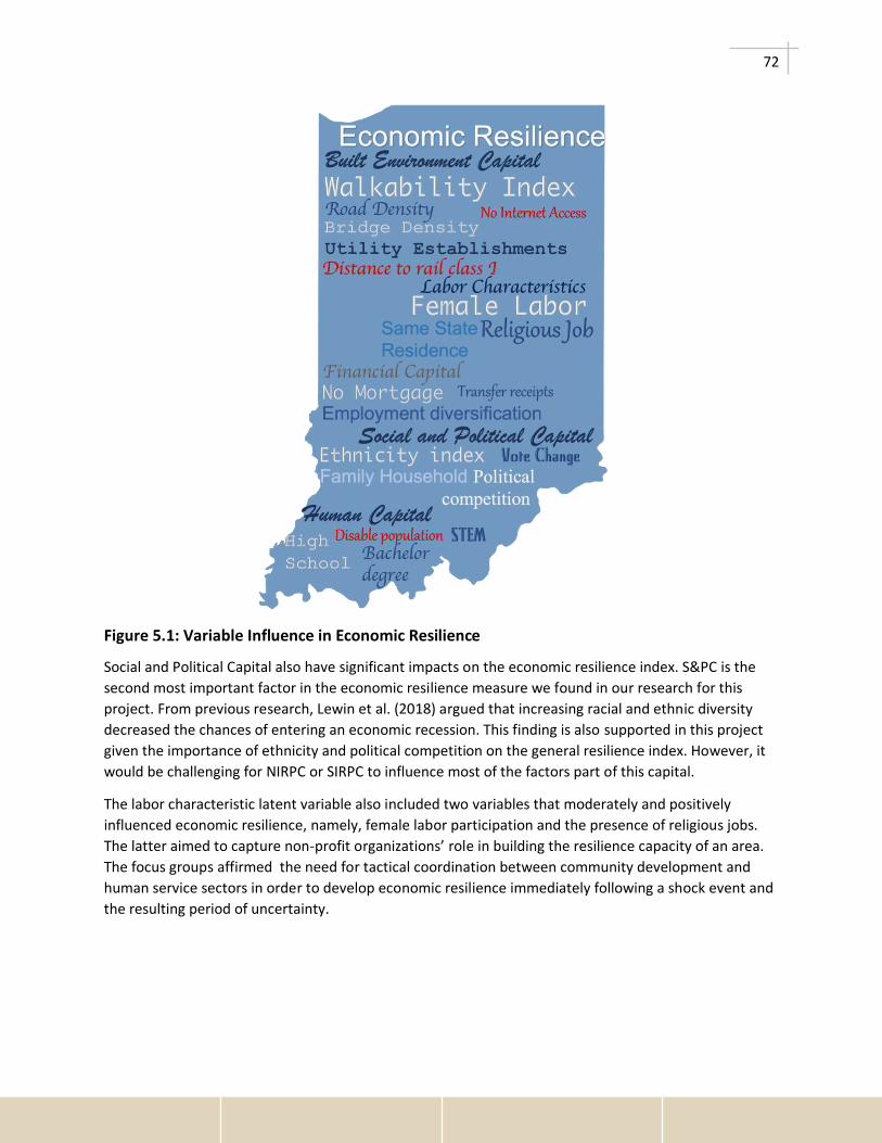
72

Figure 5.1: Variable Influence in Economic Resilience

Social and Political Capital also have significant impacts on the economic resilience index. S&PC is the

second most important factor in the economic resilience measure we found in our research for this

project. From previous research, Lewin et al. (2018) argued that increasing racial and ethnic diversity

decreased the chances of entering an economic recession. This finding is also supported in this project

given the importance of ethnicity and political competition on the general resilience index. However, it

would be challenging for NIRPC or SIRPC to influence most of the factors part of this capital.

The labor characteristic latent variable also included two variables that moderately and positively

influenced economic resilience, namely, female labor participation and the presence of religious jobs.

The latter aimed to capture non-profit organizations’ role in building the resilience capacity of an area.

The focus groups affirmed the need for tactical coordination between community development and

human service sectors in order to develop economic resilience immediately following a shock event and

the resulting period of uncertainty.

73

Table 5.1: Impact of CCF factor and other variables on Economic Resilience

Description Impact on

Resilience

Human Capital (HC) +

Percentage of population with STEM occupations - average between 2011 and

2018 +

Percentage of population with disabilities average between 2012 and 2018 -

Percentage of population with high school education and more - average

between 2011 and 2018 +

Percentage of population with bachelor education and more - average between

2011 and 2018 +

Financial Capital (FC) IA

Average housing units without a mortgage between 2011 and 2018 +

Transfer receipts as a percent of total personal income +

Employment diversification measured as entropy +

Labor Characteristics (LC) +

The average percentage of female labor participation rate 2011 to 2018 ++

Percent population that moved within the same county and moved from a

different county but the same state in the last year. +

Logarithm of religious jobs per 10K population ++

Social and Political Capital (S&PC) ++

Ethnicity index +

Political competition in 2016 ++

Change of vote between 2012 and 2016 +

Family households as a percent of total households -

Built Environment and Infrastructure (BE&I) +++

Population weighted national walkability index +++

Logarithm of roads in the county (miles) +

Logarithm of average total utility establishments between 2011 and 2018 +

Logarithm of bridge density +

74

Description Impact on

Resilience

Percent no internet access -

Logarithm of distance to rail class I from county centroid -

How to interpret the table:

+/- means the item improves/reduces test score by up to 0.9 points; + + / - - means the item improves/reduces score 1-2.5 points; + + + / - - -

means the item improves/reduces score by 2.5 or more points. IA means the item has no significant direct impact on the score but through other

latent variables such as S&PC and HC.

Most other community capitals highlighted in Table 5.1 had positive, but less substantial impact on the

economic resilience index. Three variables were found to influence the index negatively: the percentage

of population disabilities from Human Capital, family households from Social and Political Capital, and

percent no internet access and distance to rail class I, both from Built Environment and Infrastructure

Capital. Financial Capital was found to influence the economic resilience index indirectly. As explained in

Chapter 4, the influence is embedded in the Human Capital and Labor Characteristics factors’ in the case

of Financial Capital. Labor Characteristics seem to play a critical role in the general index from those

two. Factors such as female labor participation and religious jobs per 10 K population should improve

the Labor Characteristics.

Additionally, we compared the index results with the level of rurality of the different counties in the

study area to determine whether urban areas are more likely to have higher resilience levels. The index

of relative rurality (IRR) was chosen due to its continuous, threshold-free, and unit-free features, making

it a good alternative against the traditional discrete classifications (Waldorf & Kim, 2018). As shown in

Figure 5.2, the more rural the place (higher IRR), the lower its resiliency index. This is in line with

previous research. This pattern was also confirmed from NIRPC (in grey) and SIPRC counties (in orange).

Note that the research has focused on the recovery period of 2010 to 2018 after the Great Recession of

2008-2009. Figure 5.2 reveals that rural areas were comparatively disadvantaged during the post-

recession recovery. It is known that the recovery after the Great Recession was slower and longer drawn

with marginal increases in indicators such as labor participation rate and employment population ratio.

This suggest that rural areas will need more support and assistance to advance their economic

resiliency.

75

Figure 5.2: Resilience Index compared to IRR. NIRPC Counties (1. Lake, 2. Porter, and 3. LaPorte) and SIRPC Counties (4. Dearborn, 5. Shelby, 6. Jefferson, 7. Jennings, 8. Decatur, 9. Ripley, 10. Franklin, 11. Switzerland and, 12. Ohio)

5.2 Policy Implications

There are a host of strategies that could help NIRPC and SIRPC strengthen the factors that were found to

impact the economic resilience index. As discussed in the previous section, built environment and

infrastructure variables, specifically the walkability index, were important from the focus group results

and the quantitative analysis. Policies that enhance the walkable environment around the study area

could increase accessibility, reflected in the region's likelihood of being resilient. Investments in

infrastructure that allow non-motorized modes (i.e., walking, biking) to be present in the communities

remain particularly important to resiliency. NIRPC and SIRPC could use the “What-If?” Tool (created as

part of this project) to evaluate how changes in the built environment and infrastructure features of

their regions could guide their transportation planning and implementation activities.

On a similar note, female labor participation highly influenced the resilience index. For that reason,

programs that expand the opportunity for females to be an active part of the labor force, such as better

access to childcare serving children 0-13-year olds, should be promoted. In addition, employers could be

encouraged to offer more family friendly policies dedicated to childcare and eldercare. Some programs

could also help increase the resilience index by focusing on the less impactful variables found from the

quantitative analysis, which in combination with other variables, could help improve the index. For

instance, educational programs that encourage the importance of science and technology among

different groups could increase the percentage of STEM jobs in the area, increasing the resilience index.

The comparison with the rurality index inferred that rural counties might need a higher commitment to

improving their resilience levels compared to urban areas.

5.2.1 Urban policy evolution and the creation of new pathways for resiliency

The research pointed to the need to have a wide-range of shorter and longer-term strategies for

communities and regions in the face of an economic shock. Most participants felt that the most critical

Cook, IL

1

23

45 6

7

89

10

1112

Robertson, KY

y = -12.564x + 8.1623R² = 0.763

-1.000

0.000

1.000

2.000

3.000

4.000

5.000

6.000

7.000

8.000

9.000

0 0.1 0.2 0.3 0.4 0.5 0.6 0.7

Res

ilien

ce In

dex

IRR2010

76

issues needed to be addressed within the first month to three-year timeframe. In order to survive on a

short-term basis, the focus groups pointed to the need to increase partnerships across education,

nonprofits, community foundations, the business community and government institutions working

together to address more immediate needs. The steps toward a more resilient region in the short term,

as they presented in the focus groups, are presented in the following text and illustrated in Figure 5.3.

Prior to implementing any of the aforementioned steps, it is strongly suggested that the region identify

any vulnerable populations and/or groups that exist and who would immediately feel the negative

impacts of an event, effects that could cause ripples in the local economy. This may include people with

disabilities, non-English speakers, the elderly, minorities, migrant workers, and people who live in

poverty. The region should also determine where pockets of vulnerabilities are spatially located. This

will enable the policy recommendations and resource provisions to be more targeted during a response

and recovery phase.

Another recommendation is for the region to convene with local governments in their jurisdiction to

undertake an honest appraisal of how well the local government can operate following a major shock.

This could include whether the local governmental institutions can continue to function given any

anticipated financial constraints that are predicted to occur as a result of a shock. Several questions

regions should could pose is whether these jurisdictions have the resources and support necessary to

continue with normal operations, and, if not, how can the two organizations work together to bring

more resources to address the issue?

Depending on the nature of the economic shock, access to utilities such as clean water, sanitation

sewer, electricity and broadband may be severely impacted following an event. If these services are

impacted at all, the region should help lead localized efforts to address these locations, particularly if

outages occur in multiple places. Furthermore, as a longer-term approach, resiliency strategy would

seek to evaluate the vulnerabilities associated with the utility infrastructure and plan to bring resources

to address these weaknesses. Ideally this tactic would consider infrastructure interdependencies,

capability/capacity gaps and the consequences of their disruption to the health of the regional

economy.

Mental health issues surface during an economic shock and continue beyond its duration and even after

an economic recovery. Stakeholders reported how mental health issues cropped up because of job

layoffs, lack of employment, underemployment, drug addiction (which may or may not be connected

with job situation), homelessness and a general lack of resources which contribute to self-care. In this

instance, regional entities should convene local nonprofits to determine resource needs, at-risk

populations, service gaps and potential solutions to address the situation before it becomes chronic.

Other steps that can be taken to limit the economic damage following a shock could consist of the

following stages: (1) Ensure that prior to a shock, the regional economy has a diverse industrial and

occupational base to drive growth; and (2) The nonprofit sector, which serves the region, should be

assessed for strengths and gaps in offerings. For example, during the Great Recession, many nonprofits

folded or became part of larger organizations because of few funding opportunities. This ultimately led

to few services and resources to help vulnerable populations to be unable to ultimately meet the

population needs. Organizational and community-wide helplessness set in as a result.

77

The Figures found on the following pages provide a pathway for both urban and rural local governments

in which to focus their stabilizing efforts during economic periods of uncertainty. The Figures also

provide a timeline for short and medium-term resiliency strategies. While they remain steps toward

resiliency, it is of utmost importance that each phase is strengthened and maintained during the entire

economic recovery process. For example, this means that once a region is able to move onto step 4 that

each previous step remains in place and is sustained. In other words, each phase builds on the previous

step or steps as way to actively recover and build resilience.

Figure 5.3: Urban active recovery strategies 0 to 4 years after economic shock

The timeline shown in Figure 5.3 indicates the order of support an urban region needs following an

economic shock for an urban area. For instance, urban decision makers expressed the need for

communities to bolster the social safety net immediately. Although the Figure indicates that this is a first

step, it is crucial as it sets the foundation for recovery and must be maintained for the entirety of the

recovery period. The main challenge outlined during the focus groups was the absolute need for

organizations to collaborate and strategize on a tremendous number of projects to stem economic falls

in a short period of time. The window in which to actually support economic activity after a shock

appears to be a very tight timeframe and requires a committed heavy lift with some prioritization of

workload.

The fiscal health of local government institutions needs to remain sound in order to survive the

protracted economic turbulence a shock brings. Sometimes institutions face funding issues when its tax

base declines (with falling property values and business closures) – these should be outlined and the

region be prepared to offer collaborative support during those potentially difficult times.

78

The next two steps addressing regional resiliency, are closely intertwined: economic diversity and

workforce compatibilities. Manufacturing industries, along with transportation and trade professionals

faced significant declines in demand during the Great Recession. This triggered a protracted period of

instability and uncertainty in urban regions for manufacturing industries, transportation and trade

professionals all of whom are in extremely short supply over a decade later. This shortage prevented

economic gains during the recovery period.

Lastly, urban residents, as a result of workforce instability face homelessness and mental health

challenges. Urban/metro regions should coordinate efforts to address household instability because the

consequences reverberate over generations once poverty occurs to a household – or a slip from middle

to lower middle class occurs. Once this is widespread, it is difficult to escape the cycle of deprivation and

poverty and rebound as an intact household.

Figure 5.4: Urban medium to long- term resiliency strategies Years 5 to 15+ years after economic shock

All of the medium- and long-term steps outlined in Figure 5.4 mirror the short-term resiliency steps for

the most part. However, it focuses on taking a balanced approach to address gaps in the social and built

environmental capitals. One way that regions may build up resiliency is to partner, collaborate and

support nonprofit efforts very closely over the long term. This theme was particularly acute in the urban

focus groups. There appeared an overall lack of awareness on behalf of regional and urban decision

makers on how to work closely with nonprofits – bridging and leveraging governmental and nonprofit

institutions. Rural regions appear to be more socially supportive and aware of the challenges which

exist, although, again, a lack of true collaborations remain. Further research should be conducted on

what form and funding exists for government & nonprofit regional partnerships for the future.

5.2.2 Rural policy evolution and the creation of new pathways for resiliency

79

The research pointed out the need to have a wide-ranging and immediate path in the face of an

economic shock. Most of the participants felt that the most critical issues needed to be handled within

the first month to three-year timeframe. In order to survive the short term, the focus groups pointed to

the need to increase partnerships across education, nonprofits, community foundations, the business

community and government institutions to work together (Figure 5.5).

Figure 5.5: Rural recovery strategies Years 1 to 3 after economic shock

The first three years after an economic shock is the most crucial period in which to implement changes

in order to avoid institutional collapse. It is also recognized as the most stressful to people because the

ravages of the economic issues become visible and plentiful to witness. The policy guidance outlined

above provides broad steps that regional and local governmental organizations can implement which

will allow to endure the short and long-term consequences of an economic downturn.

The proposed strategies seek to mitigate the impacts of an economic downturn which threaten the

fiscal health of institutions and stymie their ability to help vulnerable populations. While not outlined in

Figure 5.5, economic resiliency begins with industrial and occupational diversification and planning for

that at the regional level is feasible through its Comprehensive Economic Development Strategy (CEDS).

In addition, the health of public utilities such as water, sewer, and electrical providers should be

assessed along with privately operated broadband services.

Mental health issues begin to crop up shortly after an economic shock – the population feels helpless

and constantly buffeted by change. This takes a toll on mental health particularly among people who

may face homelessness or joblessness. Mental health, nonprofits and their services should be prepared

to expand immediately after a downturn or a shock event.

80

Lastly, in order poise the rural region to remain steadfast in light of changing events and a shifting

economic landscape, it was found that Main Street and small business retention programs should be

implemented, bolstered and supported. Their needs could be easily determined with a quick survey

assessing skills, equipment, workforce and other measures for short term relief of stresses. Younger

populations may not have experienced economic downturns in their adult lives prior to this time, and

those who work in the trade professions are particularly vulnerable to seeking employment

opportunities outside of a region during this time. If the region wants to retain this workforce which is

vital to rebuilding and sustained growth following an economic shock, additional workforce training or

upskilling and/or short-term retention programs should be implemented. Measures which stem outside

talent migration for skilled professionals may serve to ensure the region is poised for recovery and

growth post economic recession.

Figure 5.6: Rural medium to long- term resiliency strategies Years 5 to 15+ years after

economic shock

Following the first three years, the second period identified through the focus groups concerned the 4 to

20-year timeline (Figure 5.6). This represents a critical period in which recovery and growth should be

planned for and prioritized. However, this period should be recognized as a time when households

which have endured the economic challenges remain vulnerable to lingering burn out. This concern

extends to community business owners. It is also the time to plan for future economic shocks and

positioning regional economies to withstand the changes that may be encountered at that time. Thus,

this guidance provides general steps which will help regional and local governmental organizations

supplement their CEDS policy development over the long term. It is recommended that the CEDS

document make note of how the regional economy may position itself as resilient in the future, beyond

the typical five-year time horizon.

81

The proposed strategies seek to mitigate the medium and long-term impacts of an economic downturn.

First of all, regional communities should coordinate efforts and pool resources to seek funding at the

state and federal level in order to overcome any institutional or population challenges. Secondly, while

many regional entities have established workforce development networks to address rural healthcare

occupation gaps, it is suggested that their scope is broadened to address some of the mental and

physical health impacts facing community populations. For example, substance abuse and mental health

treatment centers could be identified and a judgement made concerning whether it meets the needs of

the region.

Infrastructure improvements such as street and highway, sanitation sewer services and other utility

maintenance should be prioritized. Funding opportunities should address population growth and decline

in terms of suitability and sustainability to ensure future fiscal health. Population decline remains a

serious issue for many rural populations. In these cases, civic engagement programs should address

talent pool retention and welcoming of newcomers to the area. Rural focus group participants

emphasized that a social safety net is best supported by nonprofit institutions. These are the groups

who should also lead the way in bringing a community-wide recognition to newcomer populations such

as (and, for instance) migrant workers and remote workers.

5.3 Guidelines

The policy directions discussed previously are specific suggestions and recommendations for urban and

rural communities because they have unique assets, strengths, and challenges. Both NIRPC and SIRPC

have urban and rural components although in different proportions. Some regional planning

organizations might have more urban areas and some will be more rural. It is evident from the research

that urban and rural areas experience impacts from a recessionary shock in different sequences. The

recovery period and the trajectory are also different. Hence, when regions work on their Comprehensive

Economic Development Strategies (CEDS), it will be important that the unique characteristics and

challenges of urban and rural areas be recognized and addressed in their resiliency plans. Some areas

where NIRPC and SIRPC can work to strengthen the economic resilience of their regions include Built

Environment and Infrastructure Capital. For other areas, such as Social and Political Capital and Labor

Characteristics, partnerships with non-profits, community support organizations, grass-root workers,

etc., are vital. Similarly, partnerships with private institutions such as community banks are suggested

for Financial Capital, while educational institutions and workforce development organizations are

suggested for Human Capital. The research uncovered multifaceted linkages of economic resilience to

community capitals. Hence, planning and program development will require a multi-pronged approach.

Considering that temporal scale (immediate, short-term, medium, and long-term) of impacts can vary

for households, communities, and regions, planning for economic resilience may consider developing a

bundle of programs and initiatives for different constituents and for different time periods.

82

5.4 References

Lewin, P., Watson, P., & Brown, A. (2018). Surviving the Great Recession: The influence of income

inequality in US urban counties. Regional Studies, 52(6), 781-792.

Waldorf, B., Kim, A. (2018). The Index of Relative Rurality (IRR) : US County Data for 2000 and 2010.

Purdue University Research Repository. doi:10.4231/R7959FS8.

83

6 Appendix

Appendix A. Focus Group Question Protocol

Focus Group Question Protocol

Projected Audience: Regional decision makers

Required tools: large sheet of paper at least 8 feet in length for focus group notes. Have 1 packet of

surveys and for each participant (no names or identifying features will be used when collecting this

information). Include 20 pens with supplies to complete surveys. Room will be set up prior to

participants’ arrivals.

Introduction: Explain who we are, what the project is, why and where we are conducting focus groups.

Hand out IRB consent forms for signatures and project information.

The first 2 questions will be put into handouts for the participants to complete before the breakout

session found at Questions #4, the Community Capitals Exercise. The pre-focus group survey is found

attached.

1. Hand out quick survey questions to each participant as they arrive. Ask participants to write

their home location in 2008, their work location in 2008, and any employment or home

locations since 2008. (10 minutes)

2. What were the occupations of the focus group participants before, during and after Great

Recession? Did they change? What was the type of company or business that they worked in?

Example: wait staff, retail, car sales etc.

3. In which industries did they see as most impacted by the Great Recession in their area?

i. Each participant will circle to indicate their perception of the top 5 industries

which suffered in the region. (15 min)

i. Investigate key, regional industries ahead of time and provide a list of

employers and sectors to participants from which to choose. Replicate this short

activity for top occupation groups as well. Each participant will circle to indicate

their perception of the top 5 industries which suffered in the region. (15 min)

4. Adopt and breakdown an abbreviated version of the Community Capitals (Emery & Flora, 2006)

framework and have people discuss how aspects of the Great Recession negatively impacted the

regions (Use rotating flip charts to record and place people into groups of 3 randomly selected

individuals and place recording devices at each station. Do not call this “community capitals”

to participants as it is just a conceptual framework). Each flipchart will explain the topic

category at the top of each sheet (in case multiple sheets are used per focus group). Ask

participants to first list the places that were negatively impacted during the recession in their

84

county and/or community under each topic. Ask participants to be specific – which roads were

affected? Which parks went downhill? Which banks did not offer support to small businesses in

trouble during the recession? (30 min)

a. Built environment – public spaces such as parks & libraries, housing, factories/tech

parks, schools, offices, stores and malls

a. Infrastructure- roads, bridges, airports, sidewalks and broadband

a. Financial – community development banks, reliable financial capital institutions, banks,

credit unions, loan funds, venture capital funds and microenterprise loan funds.

a. Social & Cultural – local nonprofit organizations, local churches, regional nonprofits,

other civically-engaged groups, senior centers, services for disabled residents,

organizations that support homeless, immigrants, or specific demographics such as

children, Latinx, African Americans, etc. museums, libraries, parks, playhouses, theatres,

art studios, colleges/universities, community or adult sports teams, community arts

institutions, cultural districts

a. Human – Investments in education, on-the-job training, skills and health status which

increase their productivity and earning levels

Each flip chart will contain a definition of the category. Participants will be given a short list of questions

with each chart which will help them to discuss the category.

5. Part 2 of Community Capitals: Review the lists generated in Part 1 and use stickers to vote on

the top 3 from each category which is of crucial importance to the recovery of a stressed

economy. Each participant casts 3 votes on each chart to indicate community capitals they

consider to be most important to the resistance and/or recovery of a regional downturn. Each

topic will be placed on a notecard. The top 3 from each category will be on a notecard to set up

for the next exercise. (10 min + 5 min voting)

Hand out a sheet with the region’s top 10 industries and occupational groups. Each participant will vote

to indicate their choices. These will be collected by the convener prior to the Community Capitals

Timeline brainstorm.

6. In which industries did they see as most impacted by the Great Recession in their area?

ii. Each participant will circle to indicate their perception of the top 5 industries

which suffered in the region. (15 min)

ii. Investigate key, regional industries ahead of time and provide a list of

employers and sectors to participants from which to choose. Replicate this short

activity for top occupation groups as well. Each participant will circle to indicate

their perception of the top 5 industries which suffered in the region. (15 min)

While #6 is in progress, #7 is set up by conveners.

7. Community Capitals Timeline for Recovery long sheet with a 1 – 20 year time horizon

represented (short 1-5), medium (6-12) and long term (12+) time spans will be delineated. The

participants will come together to rank the temporal features of the capitals cited crucial to a

85

recovering economy. If one government agencies should prioritize, what timeline and sequence

of activities should be dealt with in the short, medium and long term? (15 min)

8. Several cities have developed, or are in the process of developing, resiliency plans with an

emphasis on equity and inclusion. Who are the most vulnerable groups of people in your area?

And, how should REGIONAL planning address social vulnerabilities? What capacity should it

serve in during planning and recovery efforts? (15 min)

General Discussion Questions located with their corresponding each community capital stations:

1. Built environment - is located at the Built Environment flipchart only

a. What did you see in your town or neighborhood that was negatively impacted during the

recession in this category? Did malls and retail shops begin to close down? What about local

supermarkets and chain stores? Was there a problem with empty buildings and/or foreclosures

such as with housing? If so, where in your town/neighborhood?

b. Did you see similar negative impacts in other areas of the region (Lake, Porter and Laporte

counties).

c. Did any parts of the built environment improve in these 3 counties during the Great Recession

that surprised you? If so, what and where?

2. Infrastructure - is located at the Infrastructure flipchart only

a. What did you see in your town or neighborhood that was negatively impacted during the

recession in this category? Were bridges and roads in the region well salted during the winter?

How were your Internet speeds? Were potholes dealt with? Did traffic increase or decrease

during this period? What about the performance of utilities (water supply, wastewater, etc.)?

b. Did you see similar negative impacts in other areas of the region (Lake, Porter and Laporte

counties).

c. Did any aspects of Infrastructure improve in these 3 counties during the Great Recession that

surprised you? If so, what and where?

3. Financial - is located at the Financial flipchart only.

a. What did you see in your town or neighborhood that was negatively impacted during the

recession in this category? Were home improvement loans difficult to get? What about

refinancing options? Were banks badly impacted by local foreclosures? Did you notice local

lending to small businesses decreased during this period? Were small businesses closing their

doors? If so, where?

b. Did you see similar negative impacts in other areas of the region (Lake, Porter and Laporte

counties).

86

c. Did access to any Financial institutions in these 3 counties during the Great Recession that

surprised you? If so, what and where?

4. Social & Cultural - is located at the Social and Cultural flipchart only.

a. What did you see in your town or neighborhood that was negatively impacted during the

recession in this category? Did local nonprofits close? How did local churches respond to the

challenge? Did plans for additional centers for seniors, or disabled close? Did food banks provide

more meals and establish new outlets?

b. Did you see similar negative impacts in other areas of the region (Lake, Porter and Laporte

counties).

c. Did any aspects of Social and Cultural amenities improve in these 3 counties during the Great

Recession that surprised you? If so, what and where?

5. Human & Educational Resources - is located at the Human and Educational Resources flipchart only.

d. What did you see in your town or neighborhood that was negatively impacted during the

recession in this category? Were lots of people out of work from a specific industry? Did any

hospitals, doctor practices or health clinics close? Did you see a major decline in agriculture

production and agribusiness? Did employers stop offering or funding additional training for their

employees?

e. Did you see similar negative impacts in other areas of the region (Lake, Porter and Laporte

counties).

f. Did any aspects in this category improve in these 3 counties during the Great Recession that

surprised you? If so, what and where?

Appendix B. Quantitative Analysis

Table B4.1: Descriptive Statistics of crucial variables

Latent Observed Description Mean Std. Dev Min Max Model

Sign

Out_EPR Average Employment Population Ratio 2011-2018

0.480 0.122 0.232 0.938

HC STEM

Percentage of population with STEM occupations - average between 2011 and 2018

0.029 0.016 0.010 0.176 Positive

87

Latent Observed Description Mean Std. Dev Min Max Model

Sign

HC DISA

Percentage of population with disabilities average between 2012 and 2018

0.144 0.034 0.068 0.237 Negative

HC EDHS

Percentage of population with high school education and more - average between 2011 and 2018

0.866 0.045 0.628 0.962 Positive

HC EDBH

Percentage of population with bachelor education and more - average between 2011 and 2018

0.189 0.084 0.090 0.560 Positive

FC HHMOR

Average housing units without a mortgage between 2011 and 2018

0.252 0.057 0.126 0.412 Positive

FC TRpctPI Transfer receipts as a percent of total personal income

0.230 0.059 0.073 0.386 Positive

FC ENT Employment Diversification measured as Entropy

-0.262 0.122 -1.052 0.053 Positive

LC FEMP

The average percentage of female labor participation rate 2011 to 2018

0.708 0.052 0.513 0.815 Positive

LC MOVE

Percent population that moved within the same county and moved from a different county but the same state in the last year.

0.116 0.030 0.067 0.254 Positive

LC LRELJ The logarithm of Religious jobs per 10K population

4.005 0.493 0.000 4.982 Positive

S&PC ETH Ethnicity Index 0.145 0.113 0.021 0.607 Positive

S&PC POLC Political Competition in 2016

0.485 0.376 0.150 3.556 Positive

S&PC PVOTEC Change of vote between 2012 and 2016

-0.071 0.106 -0.578 0.155 Positive

88

Latent Observed Description Mean Std. Dev Min Max Model

Sign

S&PC FAMHH Family households as a percent of total households

0.675 0.045 0.515 0.817 Negative

BE&I WALK Population Weighted National Walkability Index

6.170 1.631 2.544 13.247 Positive

BE&I LROADSQR The logarithm of Roads in the county (miles)

7.388 0.554 5.503 9.920 Positive

BE&I LEST

The logarithm of Average Total Utility Establishments between 2011 and 2018

1.087 0.878 -0.981 4.353 Positive

BE&I LBRIDGESQR The logarithm of Bridge density

-0.817 0.475 -2.603 0.844 Positive

BE&I PNIA percent no internet access

23.334 7.248 5.876 51.599 Negative

BE&I LDIR1 Distance to rail class I from county centroid

20.577 13.785 0.044 76.417 Negative

Cutoff criteria for acceptance are also shown in Table 4.2.

Table B4.2: Goodness of fit and results for factor analysis

Latent HC FC LM S&PC BE&I Cut of criteria

Source

Cronbach Alpha

0.668 0.527 0.616 0.516 0.720 >0.5 (Hu & Bentler, 1999).

Reliability 0.879 0.749 0.760 0.887 0.885 closer to 1 (Hu & Bentler, 1999).

Chi-square 2.289 9.549 7.814 3.184 17.781

df 1.000 2.000 2.000 2.000 7.000

Chi-square/df 2.289 4.770 3.907 1.892 2.540 <5 (Hu & Bentler, 1999).

RMSEA 0.071 0.072 0.036 0.048 0.054 0.080 (Hu & Bentler, 1999).

CFI 0.995 0.846 0.939 0.996 0.984 >0.9 (Hu & Bentler, 1999).

TLI 0.972 0.839 0.817 0.989 0.965 >0.9 (Hu & Bentler, 1999).

89

Table B4.3: SEM Results

Path Path Coefficient z-value p-value

Infrastructure and Built Environment (I&BE)

WALK ← I&BE 0.919 5.76 0.000

LROADSQR ← I&BE 0.802 16.58 0.000

LEST ← I&BE 0.684 17.38 0.000

LBRIDGESQR ← I&BE 0.601 12.13 0.000

PNIA ← I&BE -1.004 -13.67 0.000

LDIR1 ← I&BE -0.383 -4.32 0.000

Human Capital (HC)

STEM ← HC 0.599 12.18 0.000

EDHS ← HC 0.662 11.93 0.000

EDBH ← HC 0.987 15.71 0.000

DISA ← HC -0.407 -7.88 0.000

Social and Political Capital (S&PC)

ETH ← S&PC 0.848 6.26 0.000

POLC ← S&PC 0.927 10.18 0.000

PVOTEC ← S&PC -0.223 -5.11 0.000

FAMHH ← S&PC -0.385 -6.32 0.000

Labor Characteristics (LC)

FEMP ← LC 0.778 5.12 0.000

MOVE ← LC 0.346 3.42 0.001

LRELJ ← LC 0.434 4.46 0.000

Financial Capital (FC)

HHMOR ← FC 0.659 6.43 0.000

TRpctPI ← FC 0.789 8.91 0.000

ENT ← FC 0.438 6.85 0.000

Employment-Population Ratio (Out_EPR)

Out_EPR ← LC 0.377 4.64 0.000

Out_EPR ← I&BE 0.313 4.93 0.000

Structural Model

I&E ← SC 1.217 7.15 0.000

I&E ← HC -0.465 -2.85 0.006

I&E ← LC 0.466 8.46 0.000

HC ← SC 0.709 18.55 0.000

90

Figure B4.1: Measurement Variable Infrastructure and Built Environment

Figure B4.2: Measurement Variable Human Capital

Figure B4.3: Measurement Variables Social and Political Capital

91

Figure B4.4: Measurement Variables Financial Capital

Figure B4.5: Measurement Variables Labor Characteristics