Eastern Europe's forest cover dynamics from 1985 to 2012 quantified from the full Landsat archive

Remote Sensing of Environment xxx (2014) xxx–xxx

RSE-09256; No of Pages 16

Contents lists available at ScienceDirect

Remote Sensing of Environment

j ourna l homepage: www.e lsev ie r .com/ locate / rse

Eastern Europe's forest cover dynamics from 1985 to 2012 quantifiedfrom the full Landsat archive

P.V. Potapov a,⁎, S.A. Turubanova a, A. Tyukavina a, A.M. Krylov a, J.L. McCarty b, V.C. Radeloff c, M.C. Hansen a

a Department of Geographical Sciences, University of Maryland, College Park, MD 20742, USAb Michigan Tech Research Institute, Ann Arbor, MI 48105, USAc SILVIS Lab, Department of Forest and Wildlife Ecology, University of Wisconsin-Madison, Madison, WI 53706, USA

⁎ Corresponding author.E-mail address: [email protected] (P.V. Potapov).

http://dx.doi.org/10.1016/j.rse.2014.11.0270034-4257/© 2014 Elsevier Inc. All rights reserved.

Please cite this article as: Potapov, P.V., et al.,Remote Sensing of Environment (2014), http:

a b s t r a c t
a r t i c l e i n f o
Article history:Received 1 July 2014Received in revised form 14 November 2014Accepted 25 November 2014Available online xxxx

Keywords:LandsatEastern EuropeForestForest cover dynamicsWildfiresTimber harvesting

In the former “Eastern Bloc” countries, there have been dramatic changes in forest disturbance and forest recoveryrates since the collapse of the Soviet Union, due to the transition to open-market economies, and the recent eco-nomic crisis. Unfortunately though, Eastern European countries collected their forest statistics inconsistently, andtheir boundaries have changed, making it difficult to analyze forest dynamics over time. Our goal here was to con-sistently quantify forest cover change across Eastern Europe since the 1980s based on the Landsat image archive.We developed an algorithm to simultaneously process data from different Landsat platforms and sensors (TMand ETM+) to map annual forest cover loss and decadal forest cover gain. We processed 59,539 Landsat imagesfor 527 footprints across Eastern Europe and European Russia. Our results were highly accurate, with gross forestloss producer's and user's accuracy of N88% and N89%, respectively, and gross forest gain producer's and user'saccuracy ofN75% and N91%, basedon a sample of probability-based validationpoints.We found substantial changesin the forest cover of Eastern Europe. Net forest cover increased from 1985 to 2012 by 4.7% across the region, butdecreased in Estonia and Latvia. Average annual gross forest cover loss was 0.41% of total forest cover area,with a statistically significant increase from 1985 to 2012. Timber harvesting was the main cause of forest loss,accompanied by some insect defoliation and forest conversion, while only 7.4% of the total forest cover losswas due to large-scale wildfires and windstorms. Overall, the countries of Eastern Europe experienced constantlevels or declines in forest loss after the collapse of socialism in the late 1980s, but a pronounced increase in loss inthe early 2000s. By the late 2000s, however, the global economic crisis coincided with reduced timber harvestingin most countries, except Poland, Czech Republic, Slovakia, and the Baltic states. Most forest disturbance did notresult in a permanent forest loss during our study period. Indeed, forest generally recovered fast and only 12% ofthe areas of forest loss prior to 1995 had not yet recovered by 2012. Our results allow national and sub-nationallevel analysis and are available on-line (http://glad.geog.umd.edu/europe/) to serve as a baseline for further anal-yses of forest dynamics and its drivers.

© 2014 Elsevier Inc. All rights reserved.

1. Introduction

European forests co-evolved with humans since the beginning ofthe Holocene, and their current distribution, structure, and dynamicsrepresent a long history of clearing, alteration, andmanagement (Fuchs,Herold, Verburg, & Clevers, 2013; Johann, 2004; Kalyakin et al., 2004;Kaplan, Krumhardt, & Zimmermann, 2009, 2012). Shaped by human ac-tivities, forests were a main sector of the economy providing food(e.g., hunting, livestock grazing, and plant products), timber products(e.g., lumber for construction and naval fleets, and pulp for paper),fuel (e.g., firewood, and charcoal), and other important resources(e.g., potash, and tar). The importance of forest resources, which can bequickly exhausted by unrestricted use, provided the impetus for forest

Eastern Europe's forest cover//dx.doi.org/10.1016/j.rse.201

mapping, inventory, and management. Forest mapping techniqueswere developed concomitantly with land tenure systems, and the firstforest maps were already produced in the 14th century (Morse, 2007).In North and Central Europe, exhaustion of timber resources for navalship building, lumber, and charcoal used for iron production, were themain factors why forest inventories were established in the 19th century(Eliasson, 2002; Tomppo, Gschwantner, Lawrence, & McRoberts, 2010).Forest inventories and management expanded into Eastern Europe andEuropean Russia in the 19th and 20th centuries. In the 20th century,national forest inventory and monitoring incorporated various instru-mental measurement methods, statistical sampling, and, later, remotesensing technology. As a result, the forests of Europe are among themost well-monitored ecosystems of the world.

Despite the wealth of forest inventory data, this information isunfortunately not readily available, nor well suited for region-wideanalyses. One problem is that forest definitions and inventory methods

dynamics from 1985 to 2012 quantified from the full Landsat archive,4.11.027

http://glad.geog.umd.edu/europe/

http://dx.doi.org/10.1016/j.rse.2014.11.027

mailto:[email protected]


http://www.sciencedirect.com/science/journal/00344257

www.elsevier.com/locate/rse


https://www.researchgate.net/publication/233773078_Skog_Makt_och_Manniskor_En_Miljohistoria_om_Svensk_Skog_1800-1875?el=1_x_8&enrichId=rgreq-c1b9b021-9606-4d80-94d3-3a3b965386a6&enrichSource=Y292ZXJQYWdlOzI3MDUwNzY5ODtBUzoxODMwNDg4MjYwMDc1NTJAMTQyMDY1MzY0OTE5NA==

2 P.V. Potapov et al. / Remote Sensing of Environment xxx (2014) xxx–xxx

vary among countries and have changed over time, making cross-national and multi-temporal comparisons complicated or even impossi-ble (Seebach, Strobl, San Miguel-Ayanz, Gallego, & Bastrup-Birk, 2011).The lack of accessibility to national forest data poses another complica-tion because many countries in Eastern Europe treat forest maps andprecise forest statistics as either commercially sensitive or even a matterof national security, and thus prohibit its distribution beyond govern-mental agencies. Even where forest inventory information is in principleavailable, it is often hard to obtain from national (or sometimes regional)agencies where it is stored in a variety of formats.

Remote sensing (RS) data can provide an alternative data source toquantify forest cover and change independent of official governmentaldata sources. Information derived from satellite imagery, however, isnot equivalent to inventory data collected by forest managers. Opticalremote sensing data is suitable for mapping land-cover (tree canopycover, dominant tree species composition) while national forest inven-tory data focuses on land-use (e.g., forest land). This means that whiletree canopy cover change can be readily observed with remote sensingdata, it is not directly comparable to harvested timber volumes reportedby the national forest statistics. As a result, remote sensing data are rare-ly used as a primary source for national forest inventories, and statisticalreports due to differences between land-use and land-cover forest def-initions (Tomppo et al., 2010). The recent expansion in remote sensing-based forest monitoring products, however, highlights that these datacould be valuable for many applications. First, remote sensing-basedproducts can cover vast areas consistently, avoiding discontinuitiesdue to administrative and national boundaries (Hansen et al., 2013;Kuemmerle, Radeloff, Perzanowski, & Hostert, 2006; Pekkarinen,Reithmaier, & Strobl, 2009; Potapov, Turubanova, & Hansen, 2011).Second, long-term records of satellite observations now available inimage archives allow forest change quantification over several decades(Baumann et al., 2012; Griffiths, Muller, Kuemmerle, & Hostert, 2013;Margono et al., 2012; Potapov et al., 2012).

Spatial and temporal consistency is an inherent property of remotesensing-based forest cover and change products, alleviating the needfor harmonization procedures commonly applied to regional andnational forestry inventory data (Seebach et al., 2011; Tomppo et al.,2010). Simple biophysical criteria such as forest cover (defined usingcertain tree canopy cover thresholds without attribution to specific landcover categories and land use) make remote sensing-based productsmore suitable to assess carbon change than national forest inventoriesthat are based on land use definitions (DeFries et al., 2002; Harris et al.,2012; Tyukavina et al., 2013). At the same time, remote sensing-basedforest cover change analysis requires less effort and time than groundsurveys, and can be performed in areas of limited ground access. This iswhy remote sensing-based products are widely used for multi-nationalforest assessments and change estimations, and their results serveas a baseline for carbon modeling and socio-economic analyses aswell as for studies of landscape dynamics and biodiversity patterns(Burgess, Hansen, Olken, Potapov, & Sieber, 2012; Griffiths et al., 2012;Hansen et al., 2013; Harris et al., 2012; Kuemmerle, Hostert, Radeloff,Perzanowski, & Kruhlov, 2007; Tyukavina et al., 2013; Wendland et al.,2011).

While there have been prior assessments of forests in Europe withremote sensing (e.g., Gallaun et al., 2010; Pekkarinen et al., 2009;Schuck et al., 2003), none of them analyzed the full Landsat record forall of Eastern Europe. The lack of a comprehensive analysis of forestdynamics in Eastern Europe is unfortunate, because the region haswitnessed numerous changes in forest cover since the collapse of social-ism. Several remote sensing-based forest cover change projects havedocumented some of these changes (Baumann et al., 2012; EuropeanEnvironment Agency, 2007; Griffiths et al., 2013; Kuemmerle et al.,2009; Pekkarinen et al., 2009; Potapov et al., 2011). However, prior pro-jects have several limitations precluding their use for analyses of forestsdynamics across Eastern Europe: (i) none of these products cover theentire region; (ii) the methodologies used in different studies are not

Please cite this article as: Potapov, P.V., et al., Eastern Europe's forest coverRemote Sensing of Environment (2014), http://dx.doi.org/10.1016/j.rse.201

compatible; (iii) validation results are inconsistent and hard to compare;and (iv) with few exceptions (Potapov et al., 2011), products are notreadily available.

Our research goal here was to fill these gaps and to produce a forestcover change product for all of Eastern Europe for nearly three decadesusing a consistent set of remote sensing data, methodology, and defini-tions. Our first objective was to develop a methodology that wouldallow multi-sensor data integration and seamless forest cover andchangemapping. The methodology that we developed was then imple-mented to map forest cover change in Eastern Europe from 1985 to2012. Our second objective was to provide consistent and rigorous vali-dation of the reported forest cover change. Lastly, our third objectivewasthe unrestricted sharing of the resulting product for further analyses(http://glad.geog.umd.edu/europe/). While we provide here an over-view of the results and discuss potential forest change factors, the in-depth analysis of social and economic drivers of the observed forestchanges was outside the scope of this project.

2. Data and methods

2.1. Study area

Our study area included the Eastern European countries that formedthe “Eastern Bloc” until the end of the 1980s, except the former GermanDemocratic Republic (aka East Germany, now part of Germany), andAlbania (which disassociated from the Eastern Bloc in 1961). Thestudy area included several former USSR republics (Estonia, Latvia,Lithuania, Belarus, and Ukraine) and the European part of Russia(Fig. 3A). The 2012 national and administrative boundaries of the coun-tries were obtained from the Global Administrative Areas Dataset(GADM v2.0, http://www.gadm.org/). Because of the large variabilityin the hierarchy of administrative units as well as their size among thecountries in our study area, we performed the sub-national analysisfor administrative units only for the largest countries (Russia, Ukraine,Belarus, and Poland). For Romania and Bulgaria,we used the Eurostat ter-ritorial units for statistics (NUTS level 2, GISCO — Eurostat, EuropeanCommission; http://epp.eurostat.ec.europa.eu/) and the other countrieswere analyzed at the national level. To simplify area estimation, all datawas processed in the Albers Equal Area projection with a spatial resolu-tion of 30m per pixel. The total study area encompassed 600million ha,or 6.7 billion pixels.

2.2. Landsat imagery process

We analyzed Landsat Thematic Mapper and Enhanced ThematicMapper Plus (TM/ETM+) imagery from the U.S. Geological Survey(USGS) Earth Resources Observation and Science (EROS) Data Centerdata archive. All imagery available in theUSGS archives as off November2013 were used for our project. In total, we processed 59,539 Landsatimages, including 3436 from Landsat 4 TM, 26,400 from Landsat 5 TM,and 29,703 from Landsat 7 ETM+. The selected imagery dataset includedall Level 1 Terrain corrected (L1T) growing season images from 1984until the end of 2012 for the 527 Worldwide Reference System 2(WRS-2) Path/Row scenes in our study area. We defined start and endof the growing season using Moderate Resolution Imaging Spectro-radiometer (MODIS)-based 16-day Normalized Difference VegetationIndex (NDVI) profiles derived within MODIS-based forest cover maskfor each Landsat footprint (Potapov et al., 2011). Consistent with ourearlier research (Potapov et al., 2011), the growing season was definedas the sum of all 16-day intervals having an NDVI equal to or above 90%of the maximum annual NDVI.

All reflective bands (excluding ETM+ panchromatic band) of eachLandsat image were converted to Top of Atmosphere (TOA) reflectanceand the thermal band (high gain thermal band for ETM+)was convertedto brightness temperature (Chander, Markham, & Helder, 2009). We didnot conduct an atmospheric correction. A set of Quality Assessment (QA)



http://www.gadm.org/

http://epp.eurostat.ec.europa.eu/


https://www.researchgate.net/publication/222065888_Regional-scale_boreal_forest_cover_and_change_mapping_using_Landsat_data_composites_for_European_Russia?el=1_x_8&enrichId=rgreq-c1b9b021-9606-4d80-94d3-3a3b965386a6&enrichSource=Y292ZXJQYWdlOzI3MDUwNzY5ODtBUzoxODMwNDg4MjYwMDc1NTJAMTQyMDY1MzY0OTE5NA==



https://www.researchgate.net/publication/226377861_Comparisons_of_National_Forest_Inventories?el=1_x_8&enrichId=rgreq-c1b9b021-9606-4d80-94d3-3a3b965386a6&enrichSource=Y292ZXJQYWdlOzI3MDUwNzY5ODtBUzoxODMwNDg4MjYwMDc1NTJAMTQyMDY1MzY0OTE5NA==

https://www.researchgate.net/publication/258529161_High-Resolution_Global_Maps_of_21st-Century_Forest_Cover_Change?el=1_x_8&enrichId=rgreq-c1b9b021-9606-4d80-94d3-3a3b965386a6&enrichSource=Y292ZXJQYWdlOzI3MDUwNzY5ODtBUzoxODMwNDg4MjYwMDc1NTJAMTQyMDY1MzY0OTE5NA==

Fig. 1. Landsat time series and multi-temporal metric sets.

Table 1Multi-temporal metrics derived from Landsat time-series.

Metrics extracted from observations ordered by dateComputed independently for each Landsat spectral band (3, 4, 5, and 7), NDVI andNDWIFirst and last cloud-free observationMedian and mean of three earliest and latest observationsSlope of linear regression between reflectance value and observation dateDifference between maximal value and preceding/following minimal valuesDifference between minimal value and preceding/following maximal valuesLargest reflectance drop or gain between consecutive observations

Metrics extracted from observations ranked by band (index) valueComputed independently for each Landsat spectral band (3, 4, 5, and 7), NDVI andNDWIReflectance (index) value corresponding to selected rank (minimum, 10%, 25%,50%, 75%, and 90% percentiles, maximum)“Symmetrical” averages for all values between selected ranks(minimum–maximum, 10%–90%, 25%–75%)“Asymmetrical” average for all values between selected ranks (minimum–10%,10%–25%, 25%–50%, 50%–75%, 75%–90%, 90%–maximum)

Metrics extracted from observations ranked by corresponding NDVI, NDWI, or brightnesstemperature

Computed for each Landsat spectral band (3, 4, 5, and 7)Reflectance value corresponding to selected rank (minimum, 10%, 25%, 50%, 75%,and 90% percentiles, maximum)“Asymmetrical” average for all values between selected ranks (minimum–10%,10%–25%, 25%–50%, 50%–75%, 75%–90%, 90%–maximum)

3P.V. Potapov et al. / Remote Sensing of Environment xxx (2014) xxx–xxx

models were applied to each image yielding land, water, and snow/icecover classes and probability of cloud, shadow, and haze contaminationat per-pixel level. We developed the QA algorithm in our earlier work(Potapov et al., 2011), and improved it using additional input data. EachQA model consisted of a set of seven bagged classification trees(Breiman, 1996; Breiman, Friedman, Olshen, & Stone, 1984) derivedfrom 193 training images distributed throughout the study area. Weconducted a supervised classification for each training image to mapland/water classes and cloud/shadow contaminated pixels. Based on ini-tial results, we parameterized a separate set of QA models for TM andETM+ sensors, and for scenes having a complete Shuttle Radar Topogra-phy Mission (SRTM) elevation data coverage (one of the inputs for themodel; downloaded from CGIAR-CSI: http://srtm.csi.cgiar.org) andscenes outside SRTM coverage, where Global Multi-resolution TerrainElevation Data 2010 (GMTED; Danielson & Gesch, 2011) were used. Atotal of 75 TM images (40 with SRTM and 35 with GMTED) and 118ETM+ images (45 and 73 with SRTM and GMTED, respectively) wereused to build four generic sets of QA models. Source data for the QAmodels included all image spectral bands, a cloud-free 2000–2012median reflectance composite for the red, NIR and SWIR bands (Hansenet al., 2013), and Digital Elevation Model (DEM)-based variables. TheDEM-based variables included elevation, slope, aspect with respect to ac-tual sun position, and illumination (Richter, 2010). Our shadowdetectionmodel used distance to detected clouds calculated using acquisition sunazimuth. After we implemented the QA mask, each pixel was classifiedas either clear-sky land, water, ice, or cloud/shadow contaminated. Toexclude pixels affected by light scattering from neighboring clouds, atwo-pixel area around clouds was also mapped as a separate QA state.

After the QA screening, we applied a normalization and a surfaceanisotropy correction using global Top of Canopy (TOC) reflectancefrom MODIS as reference. The relative normalization to the commonreflectance target (MODIS data) was applied to ensure consistency be-tween sensors in time and space. We used the MOD44C (collection5) standard product, which consists of 16-day composites of reflectiveand thermal bands after atmospheric correction (Vermote, Saleous, &Justice, 2002; Carroll et al., 2010) from 2000 to 2010 to compile a globalseamless cloud-free TOC reflectance dataset for red, NIR, and two SWIRMODIS bands (Potapov et al., 2012). For each Landsat image, we createda Pseudo-Invariant Objects Mask (PIOM) automatically. First, weexcluded all detected cloud/shadow contaminated pixels and waterfrom PIOM. Second, we excluded pixels with N5% difference in reflec-tance betweenMODIS TOC and Landsat TOA.We computed the spectralreflectance difference for Landsat red, NIR and SWIR (bands 5 and7) and corresponding MODIS bands for all pixels within the PIOM, andmodeled the reflectance bias as a function of the Landsat scan angle(Hansen et al., 2008; Potapov et al., 2012).Whenwe applied the derivedmodel to every pixel in the Landsat images, it resulted in normalized,anisotropy-adjusted reflectance values. Shortwave Landsat spectralbands (blue and green) were not normalized and not used for furtherprocessing. Surface brightness temperature was used without normali-zation. We also computed the NDVI and Normalized Difference WaterIndex (NDWI; Gao, 1996) for every image as additional data layers.

2.3. Landsat time series and multi-temporal metrics

The Landsat imagery process resulted in a time-series of cloud- andshadow-free normalized reflectance observations. From this time-series, we derived a suite of multi-temporal metric sets for each 30-mpixel, each metric set for a specific purpose (Fig. 1). Multi-temporalmetrics are useful transformations of image time-series for both coarseresolution (DeFries, Hansen, & Townshend, 1995; Hansen, Townshend,DeFries, & Carroll, 2005; Reed et al., 1994) and medium resolution data(Broich et al., 2011; Hansen et al., 2013; Potapov et al., 2012), and facil-itate land cover and land cover change mapping and characterizationboth the state of biophysical variables such as biomass and height(Pflugmacher, Cohen, & Kennedy, 2012) and the change in biomass


over time (Pflugmacher, Cohen, Kennedy, & Yang, 2014). For gross for-est cover loss mapping, we derived two “long interval”metric sets: onefor 1985–2000, and a second for 2000–2012, identical to the recentlypublished global forest loss product (Hansen et al., 2013). These metricsets had a 1-year overlap to insure that change around year 2000 wascorrectly detected. To map tree canopy cover and ultimately forestcover gain, we derived a 3-year “short interval” metric set for circayear 1985 (1984–1986), 2000 (1999–2001), and 2011 (2009–2012).In addition, a set of annualmetricswere produced to compliment longerinterval datasets and to assign the date of gross forest cover loss events.

The “long interval” metric sets (1985–2000 and 2000–2012) wereconstructed from all cloud-free observations between the last availableobservation before the start of the first year (1985 or 2000) and the lastavailable observation of the last year (2000 or 2012). The mean startand end dates of the observations that we included were 26 April1985 and 5 August 2000 for the 1985–2000 interval, 13 October 1999and 8 August 2012 for the 2000–2012 interval. The average number ofcloud-free observations used to calculate metrics was 30 per pixel forthe 1985–2000 interval and 70 for the 2000–2012 interval.

To calculate themulti-temporal metrics, we implemented twomainapproaches: one based on time-sequential reflectance change, andanother based on reflectance ranking (Table 1). For the first approach,we analyzed the spectral reflectance time-series and corresponding ob-servation dates. For the second approach, we ranked the spectral bandreflectance from low to high (each band was processed individually),or ranked observations by the corresponding NDVI, NDWI, and bright-ness temperature ranks. In addition to metrics based on individual


http://srtm.csi.cgiar.org



https://www.researchgate.net/publication/223637457_NDWI_-_A_Normalized_Difference_Water_Index_for_Remote_Sensing_of_Vegetation_Liquid_Water_From_Space?el=1_x_8&enrichId=rgreq-c1b9b021-9606-4d80-94d3-3a3b965386a6&enrichSource=Y292ZXJQYWdlOzI3MDUwNzY5ODtBUzoxODMwNDg4MjYwMDc1NTJAMTQyMDY1MzY0OTE5NA==


observations, we used annual median reflectance values to calculatefirst and last yearmetrics and the slope of linear regression of the annualmedian reflectance as a function of the year of observation.

The 3-year metric centered on years 1985, 2000, and 2011 includedonly observations for the center year plus one year before and after. If nocloud-free observations were available during these years, then we ex-panded the search interval to ±2 years of the target date. The 3-yearmetric sets were based only on reflectance ranking (selected percentiles,“symmetrical” and “asymmetrical” averages). The annual metric set wasbased only on observations within a single calendar year (if no observa-tions were found, metric value was defaulted to “no data”), and includedminimal, maximal, and median spectral band reflectance, NDVI, andNDWI values within the year.

2.4. Forest cover change mapping

We defined gross forest cover loss (“forest loss” hereafter) as anydisturbance event, be it a natural disturbance or a human disturbancesuch as logging, resulting in complete or nearly complete tree removalin a given 30-m Landsat pixel. Based on this definition,we treated forestlosswithin natural, managed forests and tree plantations the sameway.Classifications were implemented at per-Landsat pixel level, with aminimum mapping unit equivalent to 0.09 ha. We mapped forest lossas a single dynamic class using a supervised bagged classification treealgorithm (Breiman, 1996; Breiman et al., 1984). To balance betweenmodel stability and computation timewe employed seven classificationtrees in the bagged tree model. Training areas for 1985–2000 werecollected using visual interpretation of the first and last dates, andmax-imum reflectance composites. We added training data iteratively untilwe achieved the desired quality of the outputmap. In total, the manuallyselected training polygons of forest loss and forest persistence included21 million pixels. For each classification iteration, we sampled randomly20% of source training data seven times to build seven bagged classi-fication trees. Training data served as the dependent variable and the1985–2000 time intervalmetrics as the independent variable in the treemodel.We applied our classification trees to the entire study area yield-ing a forest loss map. For 2000–2012, a forest loss map was alreadyavailable as part of a global forest change assessment (Hansen et al.,2013). However, the global classification model was a conservative es-timate of forest loss, and thus had higher forest loss omission ratesthan our 1985–2000 model. To improve product accuracy and consis-tency across the entire time series,we performed a new regional changeclassification for 2000–2012 using results of the global changemappingas training data. Seven bagged classification trees were created using0.1% sampling of no-change areas and 0.5% sampling of change areasfrom the global product as dependent variable and 2000–2012 metricsas independent variables (3.5 million training pixels per tree model intotal).

While forest cover loss usually results in a clear and immediatechange in spectral reflectance, gain of forest cover is a gradual processwith subtle annual change of spectral properties.We define gross forestcover gain (“forest gain” hereafter) as areas where tree canopy coverreached a certain threshold by the end of our study period. Instead ofmapping forest gain using a single classification model, as we didwhen mapping forest loss, we decided to use a post-classification com-parison of the tree canopy cover maps for circa 1985, 2000, and 2011,which were produced using 3-year metric sets. The use of annual treecanopy cover maps was not viable due to the data gaps and low treecanopy cover model stability in “data poor” years and regions. We cre-ated a bagged regression tree model using circa-2000 (1999–2001)metric set and tree canopy cover training data from the global year2000 product (Hansen et al., 2013). The global product, however,overestimated tree canopy cover within peat bog areas in the northernpart of our study area. To address this problem, we manually addedtraining sites where the initial tree canopy cover results were incorrect.A set of seven bagged regression trees were created incorporating 0.1%


random sample from global tree canopy cover product and manuallycreated training as dependent variables (3.5 million training pixels pertree). The same regression tree model was implemented for all threedates to insure consistent tree canopy cover mapping. To map areasthat changed in land cover from non-forest to forest during analyzedtime interval, we had to define “forest cover” using a tree canopycover threshold. A simple comparison of aggregated areas under canopycover classes with official forest area for each country (FAO, 2010) andeach Russian region (ROSLESINFORG, 2003) did not result in a singleconsistent threshold. Instead, we used a previously published Landsat-derived forest cover map for European Russia (Potapov et al., 2011).The threshold of N=49% tree canopy cover resulted in the same forestarea as in the previously published map, and we used this threshold todefine persistent forest cover and to map forest gain from 1985 to2012. Forest loss pixels were classified as “no forest gain”, “forest coverestablished by year 2000”, and “forest cover established by year 2012”.Mapping forest gain within areas that had no forest cover in 1985 wasbased on a post-classification comparison of tree canopy cover for 1985,2000, and 2012. Initial results based on a simple comparison showedthat sub-pixel image misregistration caused some false forest gainalong edges of forests. To remove these false changes, we increasedthe minimum mapping unit for forest gain from a single Landsat pixel(0.09 ha) to 0.45 ha, and removed all forest gain areas below thisthreshold.

2.5. Forest cover change date attribution

We assigned the date for each forest loss event based on the time se-ries of two annual products: minimum annual NDVI (within growingseason) and annual tree canopy cover. The first product was part ofthe annual multi-temporal metric set, and annual tree canopy coverwas mapped using a separate bagged regression tree model. We usedstable forest areas in the circa year 2000 tree canopy cover product toselect 0.1% of the study area as training data, and annual metrics fromyears where sufficient cloud-free data coverage existed (1986–1989,1994, and every second year after 2000) as independent variables tocreate the generalized treemodel. The resulting treemodel was appliedannually. At the pixel level, only pixels with at least one cloud-free ob-servation within the year were processed, otherwise the pixel wasmarked as “no data” for the given year. We then analyzed both treecanopy cover and theminimum annual NDVI time series for each forestloss pixel, and applied a set of heuristics to assign forest loss date withhigh, medium or low certainty level. If a pixel had a tree canopy coverabove 49% for at least two successive years, and then tree canopycover dropped below 20% and did not increase for at least one year,then loss event date was assigned with the high certainty. More than52% of all forest loss pixels had this high level of certainty. However, ifno high certainty sequence was found, then the year with the highesttree canopy cover drop was assigned as the loss date with a mediumlevel of certainty. If the tree canopy cover trend analysis did not produceany results (1.4% of all loss pixels), then we used the date of the highestNDVI drop instead, and assigned a low detection certainty. For pixelswhere the loss date was assigned with low certainty, especially in thecase of mixed-pixels on the boundary of loss areas, the loss date maybe assigned incorrectly. Tofix these problems, we applied a 90-m radiusmoving window filter for pixels where the loss date was detected withlow ormedium certainty, and assigned it as themajority of the loss datefor pixels in the neighborhood. This filtering process had the effect ofimproving date assignments for edge or mixed pixels that were labeleddifferently to adjacent pure change pixels. Themajorityfilter altered theloss date for less than 10% of all forest loss pixels. In relatively rare cases,a second loss event was assigned for a pixel. This occurred when a pixelwas mapped as forest loss during both time periods, 1985–2000 and2000–2012. However, a second loss date was assigned only if bothfirst and second date were assigned with the highest certainty.





Because the annual tree canopy cover products had temporal gapsdue to clouds and inconsistent data acquisition, the date of forest lossdetection was not always preceded by a year with cloud-free data. Toaccount for this effect, we recorded the number of years between aloss event and the preceding cloud-free observation for each changepixel andused it to allocate change area over time (see Section 3 below).

To analyze the annual trends of forest loss we performed a linearregression model fit of the annual forest loss time-series. The slope oflinear regression between y= annual loss versus x=year was derivedusing linear least squares method. The p-value of the slope per regres-sion model was used to measure significance of the forest loss trendwithin countries and regions.

For forest cover gain, it is not meaningful to assign a specific year asthe year when the gain occurred, especially in boreal and temperateforests where tree canopy cover and tree height gradually increase astrees grow on previously open land. Instead, we assigned dates onlyfor 2000 or 2012, i.e., the years where we mapped tree canopy coverusing the 3-yearmetrics. This resulted in two nominal periods for quan-tification of forest gain, 1985–2000 and 2000–2012.

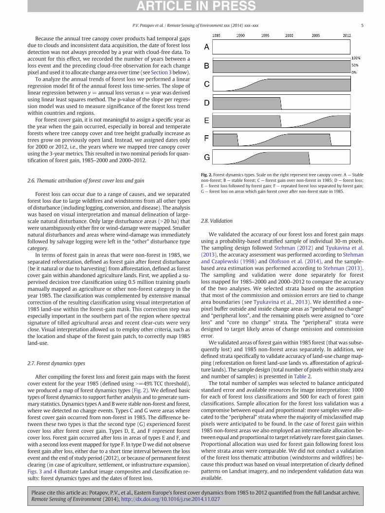
Fig. 2. Forest dynamics types. Scale on the right represent tree canopy cover. A — Stablenon-forest; B — stable forest; C — forest gain over non-forest in 1985; D — forest loss;E — forest loss followed by forest gain; F — repeated forest loss separated by forest gain;G — forest loss on areas which gain forest cover after non-forest state in 1985.

2.6. Thematic attribution of forest cover loss and gain

Forest loss can occur due to a range of causes, and we separatedforest loss due to large wildfires and windstorms from all other typesof disturbance (including logging, conversion, and disease). The analysiswas based on visual interpretation and manual delineation of large-scale natural disturbance. Only large disturbance areas (N20 ha) thatwere unambiguously either fire or wind-damageweremapped. Smallernatural disturbances and areas where wind-damage was immediatelyfollowed by salvage logging were left in the “other” disturbance typecategory.

In terms of forest gain in areas that were non-forest in 1985, weseparated reforestation, defined as forest gain after forest disturbance(be it natural or due to harvesting) from afforestation, defined as forestcover gain within abandoned agriculture lands. First, we applied a su-pervised decision tree classification using 0.5 million training pixelsmanually mapped as agriculture or other non-forest category in theyear 1985. The classification was complemented by extensive manualcorrection of the resulting classification using visual interpretation of1985 land-use within the forest-gain mask. This correction step wasespecially important in the southern part of the region where spectralsignature of tilled agricultural areas and recent clear-cuts were veryclose. Visual interpretation allowed us to employ other criteria, such asthe location and shape of the forest gain patch, to correctly map 1985land-use.

2.7. Forest dynamics types

After compiling the forest loss and forest gain maps with the forestcover extent for the year 1985 (defined using N=49% TCC threshold),we produced a map of forest dynamics types (Fig. 2). We defined basictypes of forest dynamics to support further analysis and to generate sum-mary statistics. Dynamics types A andBwere stable non-forest and forest,where we detected no change events. Types C and G were areas whereforest cover gain occurred from non-forest in 1985. The difference be-tween these two types is that the second type (G) experienced forestcover loss after forest cover gain. Types D, E, and F represent forestcover loss. Forest gain occurred after loss in areas of types E and F, andwith a second loss eventmapped for type F. In type Dwe did not observeforest gain after loss, either due to a short time interval between the lossevent and the end of study period (2012), or because of permanent forestclearing (in case of agriculture, settlement, or infrastructure expansion).Figs. 3 and 4 illustrate Landsat image composites and classification re-sults: forest dynamics types and the dates of forest loss.


2.8. Validation

We validated the accuracy of our forest loss and forest gain mapsusing a probability-based stratified sample of individual 30-m pixels.The sampling design followed Stehman (2012) and Tyukavina et al.(2013), the accuracy assessment was performed according to Stehmanand Czaplewski (1998) and Olofsson et al. (2014), and the sample-based area estimation was performed according to Stehman (2013).The sampling and validation were done separately for forestloss mapped for 1985–2000 and 2000–2012 to compare the accuracyof the two analyses. We selected strata based on the assumptionthat most of the commission and omission errors are tied to changearea boundaries (see Tyukavina et al., 2013). We identified a one-pixel buffer outside and inside change areas as “peripheral no change”and “peripheral loss”, and the remaining pixels were assigned to “coreloss” and “core no change” strata. The “peripheral” strata weredesigned to target likely areas of change omission and commissionerror.

We validated areas of forest gainwithin 1985 forest (thatwas subse-quently lost) and 1985 non-forest areas separately. In addition, wedefined strata specifically to validate accuracy of land-use change map-ping (reforestation on forest land-use lands vs. afforestation of agricul-ture lands). The sample design (total number of pixelswithin study areaand number of samples) is presented in Table 2.

The total number of samples was selected to balance anticipatedstandard error and available resources for image interpretation: 1000for each of forest loss classifications and 500 for each of forest gainclassifications. Sample allocation for the forest loss validation was acompromise between equal and proportional: more samples were allo-cated to the “peripheral” strata where themajority of misclassifiedmappixels were anticipated to be found. In the case of forest gain within1985 non-forest areas we also employed an intermediate allocation be-tweenequal and proportional to target relatively rare forest gain classes.Proportional allocation was used for forest gain following forest losswhere strata areas were comparable. We did not conduct a validationof the forest loss thematic attribution (windstorms and wildfires) be-cause this product was based on visual interpretation of clearly definedpatterns on Landsat imagery, and no independent validation data wasavailable.



Fig. 3. A. Circa year 1985 Landsat image composite for the entire region of analysis (SWIR-NIR-red RGB band combination). Areas outside region of analysis shown in white. B. A colorcomposite of stable forest cover in green (1), gross forest cover loss in red (2), and gross forest cover gain in blue (3). Magenta (4) represent areas with forest cover loss followed by forestgain. For visualization purposes, we resampled the dataset to a 300-m pixel grid, and calculated the percentage of the pixel area with forest cover and forest change values. For the visu-alization, each layer scaled independently to highlight geographic pattern of forest dynamics. (For interpretation of the references to color in this figure legend, the reader is referred to theweb version of this article.)


The only reference data available to collect information for our vali-dation sample for 1985 to 2012 were Landsat imagery. High spatial res-olution imagery data over the study period are largely non-existent, andonly available since 2000. We decided against using different sources ofreference data for the 1985–2000 and the 2000–2012 accuracy assess-ment, because this would make the validation results incompatible. Tocreate a consistent sample validation dataset, we complied annualLandsat composites. All available annual median composites, togetherwith selected annual metrics and products, were visually examinedfor every validation sample (Fig. 5). Our Landsat-based per-pixel visualchange detection method is similar to the TimeSync application devel-oped by Cohen, Yang, and Kennedy (2010) to assess the accuracy ofLandsat-derived forest change products. Sample pixelswere interpretedby a regional forest mapping specialist (S.T.), and ambiguous sampleswere cross-validated by a second observer (A.T. or P.P.). Validationresults were used to report model accuracy measures and associatedconfidence intervals following Olofsson et al. (2014). Sample-basedclass areas were computed from error matrices using a stratified esti-mator (Stehman, 2013).

We also conducted a limited field verification of our forest gain mapfocusing on abandoned agriculture areas in several regions of EuropeanRussia (Kirov, Nizhny Novgorod and Vladimir) during the summers of2012 and 2013. We selected these regions because they had extensive


forest gain on former agriculture lands. Conducting field work through-out our entire study area was unfortunately beyond the scope of ourproject. In total, we collected 75 field points within different stages ofabandonment and afforestation. Point samples were randomly selectedwithin abandoned areas. For each point we visually assessed tree canopycover andmeasured tree canopy height using a clinometer. For 58 pointswe alsomeasured the age of the oldest trees foundwithin the abandonedarea with an increment borer.

3. Results

The forest cover for year 1985 (sum of dynamics types B, D, E, F, seeFig. 2 for explanation)was 216million ha (Table 3). By 2012, forest areaincreased by 10 million ha (4.7%) and reached 226 million ha (sum oftypes B, C, E). In total, there were 24 million ha of forest loss (includingareas that experienced forest gain after loss), which was substantiallylower than the 34 million ha of forest gain. Forest loss of 1985 forests(sum of types D, E, F) represented 11% of the 1985 forest area, or 0.41%of forest loss/year. The majority (58%) of the forest loss areas werereforested by 2012. Indeed, by 2012, more than 15% of the total forestarea consisted of young forests originating within the previous 27 years.Forest gain on 1985 non-forest lands represented 5.8% of the 1985 non-forest land area (excluding permanent water). Forest dynamics types



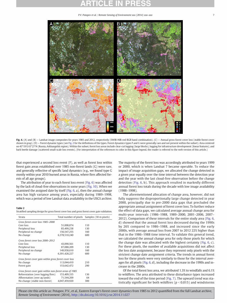
Fig. 4. (A) and (B) — Landsat image composites for years 1985 and 2012, respectively (SWIR-NIR-red RGB band combination). (C) — Annual gross forest cover loss (stable forest covershown in gray). (D)— Forest dynamic types (see Fig. 2 for the definitions of the types. Forest dynamics types F and Gwere generally rare and not presentwithin the subset). Area centeredon 43°19′E 63°27′N (Russia, Arkhangelsk region).Within the subset, forest loss areas include clear-cut logging (large blocks), logging for infrastructure development (linear features), andbark beetle damage (scattered small-scale loss events). (For interpretation of the references to color in this figure legend, the reader is referred to the web version of this article.)


that experienced a second loss event (F), as well as forest loss withinforest gain areas established over 1985 non-forest lands (G) were rare,and generally reflective of specific land dynamics (e.g., we found type Gmostly within year 2010 burned areas in Russia, where fires affected for-ests of all age groups).

The attribution of year to each forest loss event (Fig. 6) was affectedby the lack of cloud-free observations in some years (Fig. 10). Whenweexamined the assigned date by itself (Fig. 6, a), then the annual changearea has high variance among years, especially during 1989–1998,whichwas a period of low Landsat data availability in the USGS archive.

Table 2Stratified sampling design for gross forest cover loss and gross forest cover gain validation.

Strata Total number of pixels Samples (30 m pixels)

Gross forest cover loss 1985–2000Core loss 51,008,874 110Peripheral loss 85,499,238 130Peripheral no change 156,547,255 160No change 6,378,510,240 600

Gross forest cover loss 2000–2012Core loss 43,090,561 110Peripheral loss 87,088,209 130Peripheral no change 149,958,610 160No change 6,391,428,227 600

Gross forest cover gain within gross forest cover lossNo change 113,044,410 210Forest gain 153,642,472 290

Gross forest cover gain within non-forest areas of 1985Reforestation (over logging/fires) 153,409,335 136Afforestation (over ag lands) 71,544,209 64No change (stable non-forest) 4,047,459,920 300


The majority of the forest loss was accordingly attributed to years 1999or 2000, which is when Landsat 7 became operable. To reduce theimpact of image acquisition gaps, we allocated the change detected ina given year equally over the time interval between the detection yearand the year with the last cloud-free observation before the changedetection (Fig. 6, b). This approach resulted in markedly differentannual forest loss totals during the decade with low image availability(1988–1998).

The aforementioned allocation of change area, however, did notfully suppress the disproportionally large change detected in year2000, principally due to pre-2000 data gaps that precluded theappropriate annual assignment of forest cover loss. To further reducethe effect of data gaps, we calculated average annual change area formulti-year intervals (1986–1988, 1989–2000, 2001–2006, 2007–2012). Comparison of these intervals for the entire study area (Fig. 6,d) showed that the annual forest loss decreased during the 1990sby 26% compared to 1986–1988, and increased since the early2000s, with average annual loss from 2007 to 2012 22% higher thanthat in the 1986–1988 time interval. To validate this general trend,we calculated the annual change area for only those pixels for whichthe change date was allocated with the highest certainty (Fig. 6, c).For these pixels, the number of available acquisitions did not affectthe loss date assignment, because they represent only pixels with thestrictest change date assignment criteria. The trends in annual forestloss for these pixels were very similarly to those for the interval aver-ages for all pixels (Fig. 6, d), including the decrease in the 1990s and in-crease in the 2000s.

Of the total forest loss area, we attributed 1.3% to windfalls and 6.1%to wildfires. The area attributed to these disturbance types increasedtoward the end of the time period (Fig. 7). The upward trend was sta-tistically significant for both wildfires (p b 0.015) and windstorms



Fig. 5.Validation data used for validation pixel interpretation. Upper part— available Landsat image composites (band combination SWIR-NIR-red). Cloud or shadow contaminated pixelswere removed. The sample pixel is outlined in red (location 24.4101 E, 55.1556 N). The graph at the bottom shows annual profiles of SWIR band reflectance (red line), tree canopy cover(green line) and minimumNDVI (white line) for this sample pixel. In this example, forest loss occurred in 2007 without subsequent forest gain. Visualization images were automaticallyprepared for all validation pixels using GDAL and R software packages. (For interpretation of the references to color in this figure legend, the reader is referred to the web version of thisarticle.)


(p b 0.001). Forest loss due to wildfire was often detected with a one-year lag though due to cloud and smoke contamination during the fireyear, which reduced image availability, and also because fires some-times occurred after the last cloud-free Landsat acquisition for the fireyear. During an extreme fire year, large proportions of the total forestloss may be due to fire. For example, in 2011, 29% of all forest loss wasdue to wildfires. In comparison, windstorm damage did not contributemore than 7% of total forest loss even during extreme years.

While forest loss was widespread, forest generally recovered fast(Fig. 8). More than 60% of the total area where forest loss occurredprior to 2007 had a tree canopy cover above 49% by 2012, and thisrate was more than 85% for pre-1988 loss areas. The highest rate of for-est recovery occurred in European Russia (where forest loss rates were

Table 3Area of forest dynamics types 1985–2012.

Forest dynamics type 1985forestcover

2012forestcover

Area, ha ∗1000

No data 0.5A Non-forest (stable) N N 364,272B Forest (stable) Y Y 192,056C Forest gain on 1985 non-forest N Y 20,111D Forest loss Y N 9974E Forest loss followed by forest gain Y Y 13,828F Forest loss followed by forest gain, and another

forest loss (two loss events)Y N 64

G Forest gain on over 1985 non-forest followed byforest loss

N N 135

The “no data” areas represent several small Croatian islands that are outside the Landsatprocessing area.


highest in the 1980s) and the lowest in Macedonia, potentially due todry climate conditions slowing tree regrowth.

The total forest gain on areas that were not forests in 1985 was over20 million ha. Of this area, 68% (or 13.6 million ha) was due to forestland-use dynamics (reforestation after pre-1985 forest loss), and 32%(or 6.4 million ha) due to forest growth on former agricultural land.The reforestation of forest disturbance happened largely before 2000(72% were reforested by this date), while afforestation of former agri-cultural lands occurred largely between 2000 and 2012 (53% of thetotal afforestation area).

The trends of forest cover change and forest loss area at the nationallevel for the 20 countries in our study area were highly variable andillustrated the diversity of forest land change dynamics in EasternEurope (Table 4). Forest cover area increased in all countries exceptEstonia, Latvia, and Macedonia. Annual forest loss trends varied substan-tially among countries, and among epochs: 1986–1988 (socialism),1989–2000 (transition and post-socialism), 2001–2006 (before economiccrisis), and 2007–2012 (during and after economic crisis). These differ-ences are discussed below in Section 4.3.

Across Eastern Europe, there were pronounced regional hotspots offorest loss rates (Fig. 9A), and changes in annual forest cover loss area(Fig. 9B), as well as of net forest cover area change (Fig. 9C), and forestgain on former agricultural areas (Fig. 9D). Differences in these metricswere pronounced among counties, and there was substantial variabilityamong administrative regions within Russia, Ukraine, and Poland.

3.1. Validation results

Our sample-based estimated accuracy assessment (Table 5) showedreliable classification model performance for both forest loss and forestgain classifications. The expert-driven model (forest loss 1985–2000)



Fig. 6.Annual gross forest cover loss area (ha ∗ 1000). (a) Areabydate of changedetection; (b) area of changedistributed over years between detection and the last cloud-free observation;(c) average annual change area for intervals 1986–1988, 1989–2000, 2001–2006, 2007–2012; (d) area of change allocated with the highest certainty distributed over years between de-tection and the last cloud-free observation.


delivered balanced omission and commission errors, which was theobjective of our iterative classification approach. The forest loss 2000–2012 model based on existing training resulted in a higher omissionrate, and hence a 6.96% difference between map-based and sample-based area estimate. The high accuracy of forest gain after forest losscan be explained by relative simplicity of the change event and smalltotal area of both classes (limited by forest loss). The forest gain detec-tion within 1985 non-forest areas had the lowest accuracy of all of ourresults. The comparison of sample-based and map-based estimatesshowed that the post-classification approach that we employed forthe change detection failed to map 21% of the forest gain area.

The accuracy of the attribution of forest gain to either precedingforest loss or agricultural land-use was assessed only for those pixelsthat were correctly mapped as afforestation (182 samples). In total,83.52% of those samples were allocated to the correct classes. Themajority of expert-interpreted forestry land-use samples were mappedcorrectly (94.44%), while a substantial percent of agriculture land-usepixels (32.43%) were falsely attributed as forestry land-use. Thus,

Fig. 7. Annual area (in ha ∗ 1000) of gross forest cov


the area of afforestation on former agricultural lands was possiblyunderestimated.

Our validation of the forest loss date allocationwas based on a sampleof 887 forest loss pixels from forest loss 1985–2000, forest loss 2000–2012, and forest gain after forest loss sample sets, where we could inter-pret the reference date unambiguously. It should be noted that analystcan interpret the date of change event only from available Landsat acqui-sitions, and so this date may not represent the actual forest loss date butthe date of the first clear Landsat image after the change event. For eachsample, the date assigned by the automatic model was compared todate assigned by visual interpretation of annual image composites. Thedatewas correctly determined for 76.4% of samples; and 89.9% of sampleshad a date difference of ±1 year. On average, the allocation modelassigned the date of forest loss of 0.26 years later compared to actualchange event date. Pixels for which the date was assigned with thehighest certainty had the lowest average difference compared to theactual change event (0.17 years later). The highest difference in date(almost 3 years on average) occurred in the case of samples with the

er loss attributed to windstorms and wildfires.



Fig. 8. Percent forest gainwithin forest loss areas as a function of the year of the forest loss.


lowest certainty of the date allocation (i.e., where NDVI time-series wasused instead of tree canopy cover annual data).

Field verification results (Table 6) confirmed that our tree canopycover threshold resulted in an accurate forest gain detection. Themajorityof plots withmore than 50% tree canopy cover in the field were correctlymapped as forest gain. For broadleaf and pine tree forests growing onabandoned lands in the central part of European Russia this thresholdcorresponded to a median tree height above 6 m and an age older than12 years. Our field-based results, however, are only valid for regrowthon abandoned agriculture areas in the hemiboreal forest zone.

4. Discussion

4.1. Data availability

The USGS Landsat program is the oldest provider of operationalmedium-resolution satellite data. The data record of Landsat TM/ETM+/OLI instruments spans over last 30 years, and the free dataaccess and redistribution policy made it the best data source for theanalysis of long time-series of land cover change. The main problem ofthe existing archive, however, is an inconsistent data acquisition record.

Table 4Forest cover change and annual gross forest cover loss in each country.

Country Forest cover,(thousand ha)

Net forest cover change (%

1985 2012

Belarus 7771 8253 6.2Bosnia and Herzegovina 2299 2570 11.8Bulgaria 3508 3902 11.2Croatia 1954 2229 14.1Czech Republic 2689 2801 4.2Estonia 2409 2361 −2.0Hungary 1411 1791 26.9Kosovo 335 349 4.0Latvia 3292 3164 −3.9Lithuania 2008 2083 3.7Macedonia 694 689 −0.7Moldova 241 310 28.9Montenegro 561 569 1.5Poland 8470 9235 9.0Romania 6978 7270 4.2Russia (European Russia only) 156,996 163,289 4.0Serbia 2246 2493 11.0Slovakia 2176 2221 2.1Slovenia 1214 1233 1.6Ukraine 8671 9182 5.9


A dramatic decline in acquisitions occurred after the commercializationof the Landsat 5 satellite in 1984, with a considerable amount of datacollected by international ground receiving stations.While data from in-ternational ground receiving stations are currently being transferred tothe USGS EROS archive, the degree to which they may fill the existingdata gap over Eastern Europe was unclear when we conducted ourstudy. Another factor reducing data availability are problems withLandsat 4 and 5 imagery calibration precluding the conversion to terraincorrected L1T data. Together, these limitations cause low image avail-ability before 1986 and between 1989 and 1998 (Fig. 10). This is unfor-tunate, because the number of growing season images per footprintdetermines the amount of cloud-free data available within the studyarea. A nearly 100% annual cloud-free coverage is available only duringyears for which there are seven or more images per footprint. However,such a high number of acquisitions cannot be obtained by a single sensorfor the entire region. The growing season length (as defined usingMODIS data, see Section 2.2) is highly variable across the study area,but only 80 days in tundra regions, 110 days in the temperate part ofthe study area, and 160 days in the south. A single Landsat sensor withan observation frequency once per 16 days will acquire only 5 imagesin the tundra region, and less than 7 in the temperate zone. A constella-tion of two sensors (e.g., Landsat 5 and 7) actively acquiring data (as wasthe case in 2006, 2007, and 2009–2011) collects enough observationsfor nearly complete cloud-free coverage sufficient for annual forestchange mapping and correct change date allocation. Similarly, theacquisition frequency from both Landsat 7 and 8 platforms in 2013(Fig. 10) provides data coverage sufficient for annual monitoring untilthe decommissioning of Landsat 7.

4.2. Classification model performance

The approach that we present here, including the per-image calibra-tion, per-pixel quality assessments, and time-sequential metric analyseshave been developed and tested before in both regional (Hansen et al.,2008; Potapov et al., 2011, 2012) and global analyses (Hansen et al.,2013). However, the work presented here extends these prior ap-proaches, and introduces a number of improvements. First, all reflectanceand brightness temperature data were scaled to a 16-bit dynamic range,preserving radiometric resolution of the source data and enabling futureLandsat 8 data incorporation. Second, the new QAmodels included addi-tional input metrics such as illumination, distance to clouds, and medianreflectance cloud-free reference image composite. Third, we used

of 1985 forest) Annual forest loss (thousand ha)

1986–1988 1989–2000 2001–2006 2007–2012

30.6 37.7 48.0 44.12.6 3.8 3.4 2.29.8 6.7 12.1 9.93.3 3.7 5.6 4.9

13.7 10.6 17.1 27.17.2 11.2 22.1 26.37.3 7.7 13.6 11.51.8 1.1 1.6 1.49.9 20.3 39.7 46.78.7 11.3 16.9 20.62.3 1.8 3.1 3.70.4 0.2 0.5 0.41.7 1.1 1.3 1.1

26.1 31.6 57.5 71.116.1 16.8 28.7 29.7

704.4 536.6 600.5 687.23.6 2.7 4.2 3.84.2 6.1 10.9 18.10.8 1.1 1.9 2.4

28.1 32.8 58.8 61.3



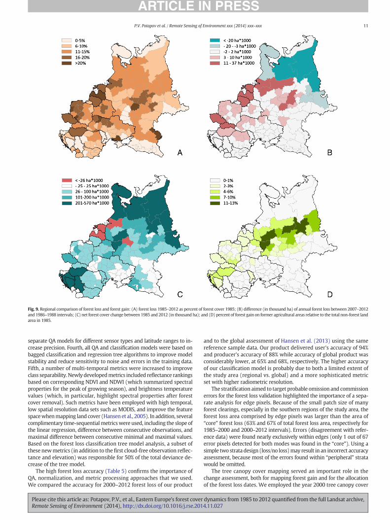
Fig. 9. Regional comparison of forest loss and forest gain: (A) forest loss 1985–2012 as percent of forest cover 1985; (B) difference (in thousand ha) of annual forest loss between 2007–2012and 1986–1988 intervals; (C) net forest cover change between 1985 and 2012 (in thousand ha); and (D) percent of forest gain on former agricultural areas relative to the total non-forest landarea in 1985.


separate QA models for different sensor types and latitude ranges to in-crease precision. Fourth, all QA and classification models were based onbagged classification and regression tree algorithms to improve modelstability and reduce sensitivity to noise and errors in the training data.Fifth, a number of multi-temporal metrics were increased to improveclass separability. Newly developedmetrics included reflectance rankingsbased on corresponding NDVI and NDWI (which summarized spectralproperties for the peak of growing season), and brightness temperaturevalues (which, in particular, highlight spectral properties after forestcover removal). Such metrics have been employed with high temporal,low spatial resolution data sets such as MODIS, and improve the featurespacewhenmapping land cover (Hansen et al., 2005). In addition, severalcomplimentary time-sequentialmetricswere used, including the slope ofthe linear regression, difference between consecutive observations, andmaximal difference between consecutive minimal and maximal values.Based on the forest loss classification tree model analysis, a subset ofthese newmetrics (in addition to the first cloud-free observation reflec-tance and elevation) was responsible for 50% of the total deviance de-crease of the tree model.

The high forest loss accuracy (Table 5) confirms the importance ofQA, normalization, and metric processing approaches that we used.We compared the accuracy for 2000–2012 forest loss of our product


and to the global assessment of Hansen et al. (2013) using the samereference sample data. Our product delivered user's accuracy of 94%and producer's accuracy of 88% while accuracy of global product wasconsiderably lower, at 65% and 68%, respectively. The higher accuracyof our classification model is probably due to both a limited extent ofthe study area (regional vs. global) and a more sophisticated metricset with higher radiometric resolution.

The stratification aimed to target probable omission and commissionerrors for the forest loss validation highlighted the importance of a sepa-rate analysis for edge pixels. Because of the small patch size of manyforest clearings, especially in the southern regions of the study area, theforest loss area comprised by edge pixels was larger than the area of“core” forest loss (63% and 67% of total forest loss area, respectively for1985–2000 and 2000–2012 intervals). Errors (disagreement with refer-ence data) were found nearly exclusively within edges (only 1 out of 67error pixels detected for both modes was found in the “core”). Using asimple two strata design (loss/no loss)may result in an incorrect accuracyassessment, because most of the errors found within “peripheral” stratawould be omitted.

The tree canopy cover mapping served an important role in thechange assessment, both for mapping forest gain and for the allocationof the forest loss dates. We employed the year 2000 tree canopy cover



Table 5Forest loss and forest gain map accuracy measures (including 95% confidence intervalboundaries).

Forest loss 1985–2000

Forest loss user's accuracy 89.9 ± 3.8Forest loss producer's accuracy 90.0 ± 23.0Map overall accuracy 99.6 ± 0.3Difference between sample-based and map-based forest loss area,% of map-based estimate

−0.083 ± 0.005%

Forest loss 2000–2012Forest loss user's accuracy 94.3 ± 2.9Forest loss producer's accuracy 88.2 ± 22.0Map overall accuracy 99.6 ± 0.4Difference between sample-based andmap-based forest loss area,% of map-based estimate

+6.96 ± 0.38%

Forest gain after forest lossForest gain user's accuracy 98.3 ± 1.5Forest gain producer's accuracy 96.9 ± 1.9Map overall accuracy 97.2 ± 1.5Difference between sample-based andmap-based forest gain area,% of map-based estimate

+1.43 ± 0.04%

Forest gain on 1985 non-forestForest gain user's accuracy 91.0 ± 4.0Forest gain producer's accuracy 75.2 ± 16.3Map overall accuracy 98.0 ± 1.4Difference between sample-based andmap-based forest gain area,% of map-based estimate

+21.00 ± 4.58%


map produced by Hansen et al. (2013) as training data due to projectlimitations that precluded collecting direct training from high spatialresolution data. The resulting tree canopy cover map was used forchange detection and stratification of forest cover and non-forestareas, but its accuracy is unknown.We suggest that this is not a problembecause our primary goal was not to map exact values of tree canopycover per pixel, but rather to produce a consistent time-series of treecanopy cover for change analysis. Forest gain was mapped using post-classification comparison of tree canopy cover layers, and forest lossdate was attributed based on the annual tree canopy cover time-series. High accuracy of these final products, proved by our validationresults, confirms the viability of our approach, and the validity of theinput data that we used. Some problems remained, however. First, apost-classification method is sensitive to image misregistration espe-cially when there are mixed pixels along forest boundaries. We solvedthis problem by increasing the minimum mapping unit, which, inturn, increased forest gain omission error. Second, our annual treecanopy covermodel was sensitive to time of the year for available annualobservations, which caused model instability in years with low imageavailability. Our annual forest loss allocation algorithm employed a

Table 6Field-based validation results for forest loss over abandoned agricultural areas.

Tree canopy characteristics Total samples Percent detected as forest gain

Height, mb5 26 05–6 22 147–9 19 84N9 8 100

Tree canopy cover, %b10 19 011–30 13 831–50 17 18N50 26 92

Oldest tree age, yearb6 4 06–12 33 12N12 21 81


specific set of rules to control for “spikes” in the tree canopy covertime-series.

Setting the correct tree canopy cover threshold to map the “forestcover” class is another challenge.We defined forest cover class thresholdas N=49% tree canopy cover, based on a comparison with a previouslypublished Landsat-based forest map for European Russia (Potapov et al.,2011). This threshold was used for both forest gain and “stable” forestmapping. Comparing the area of forest cover derived using this thresholdfor circa 2000 tree canopy cover with national forest area for year 2000(FAO, 2010) we found that our results overestimated the area reportedby FAO by only 4.07%. At the individual country level, countries withlarge areas of natural forests in relatively flat terrain (Poland, Estonia,Latvia, Lithuania, Slovenia) FAO reported forest areas within 10% withour forest cover estimate. However, our results overestimated forestarea by 14% in countries with extensive tree plantations, and mountainareas (Romania, Bulgaria, Croatia). The same was true for the Europeanregions of Russia when we compared our forest area with official forestcover statistics for the year 2003 (ROSLESINFORG, 2003). Our year 2000product overestimated forest area by 4.04%, with most of the large for-ested regions having an official forest area estimate within 10% of ourestimate. The largest difference was found in the southernmost forest-steppe and northernmost forest–tundra administrative regions, whereforest cover is generally sparse. We concluded that while a forestcover map based on a consistent threshold across Eastern Europe isslightly different fromnational forest cover estimates, it provides a con-sistent measurement of established tree cover without differentiatingland-use types and distinguishing trees in natural forests, plantations,andmature orchards. The forest loss productwas created independentlyof tree canopy cover. However, our forest loss training data were consis-tent with our forest cover definition. Comparison of forest loss areasafter 2002 with tree canopy cover 2000 showed that more than 98% ofthe forest loss areas had tree canopy cover of N=49% before the changeevent. Field verification, although limited, also confirmed our choice ofthe tree canopy cover threshold for the forest gain mapping. Based onthese comparisons we concluded that our forest cover and forest coverloss and gain definitions were consistent between our products, andthe resulting area statistics are close to national forest cover standards.

4.3. National and sub-national dynamics of forest cover

Timber harvesting is the main driver of forest cover dynamics inEastern Europe (Schelhaas, Nabuurs, & Schuck, 2003). The extent oflarge natural disturbanceswas relatively low inour study, and comprisedless than 10% of the total forest loss area. It should be noted though thatwe did notmap small-scale, scattered disturbance, such as treemortalitydue to insect infestation, as well as salvage logging, as large natural dis-turbance class. However, we assume that their relative extent is small.Analyzing annual forest loss (excluding large-scale fires and wind dam-age) per country revealed interesting parallels in forest disturbancetrends (Fig. 11). Most of the countries had a small increase or declinein forest loss after the breakdown of the Soviet system in the late1980s. However, some Central and Northern European countries morequickly transitioned to market economies, and did not decrease timberharvesting (Poland, Slovakia, Estonia, Latvia, Lithuania). Other countriesexperienced a pronounced decline in timber harvesting due to the eco-nomic crisis (Russia, Bulgaria, Romania) and armed conflicts (formerYugoslavia countries) in the 1990s. During the first half of the 2000s,timber harvesting increased in all countries (except Bosnia andHerzegovina). However, the global economic crisis of the late 2000sslowed down wood production in most countries, with exceptions ofCentral Europe and Baltic states. In many countries forest loss waslower in 2012 compared to pre-2007.

The total annual forest loss trend and the net forest cover areachange within the study area was largely driven by its largest region —

European Russia. Russia comprised 72% of the total forest area withinthe study area andwas responsible for 69% of the forest loss area. Forest



Fig. 10. Left scale: L1T image availability per sensor/year over selected 527 WRS-2 Path/Row scenes. Right scale: percent of the study area covered with annual cloud-free observations.


loss dynamicwithin the Russian part of the study area dependedmainlyon two factors: timber harvesting rates and natural disturbance events.Timber harvesting experienced dramatic changes during the transitionfrom the Soviet planned economy to more open markets. After thebreakdown of the Soviet Union, timber production decreased by 29%compared to 1990 (ROSSTAT, 2008). Since 2000 timber harvestingincreased slightly, but still remained lower than in the late 1980s. Thisrecent historical logging dynamic aligns well with our forest loss arearesults at the national level (Fig. 11G). Forest loss trends other thanthose attributed to large-scale natural disturbance in European Russiadid not exhibit a statistically significant increase from 2000 to 2012.

The regional variation of forest loss and forest gain within EuropeanRussia was quite pronounced (Fig. 9). Forest loss rates (measuredas percent loss of forest area) was highest in Western (especially in

Fig. 11. Average annual gross forest cover loss (excluding wind and fire damage) as per-cent of year 1985 forest cover; (A) Baltic countries (Estonia, Latvia, Lithuania);(B) Central European countries (Poland, Czech Republic, Slovakia); (C) Hungary;(D) Ukraine; (E) Belarus; (F) Black sea countries (Bulgaria, Romania, Moldova);(G) European part of Russia; (H) former Yugoslavian countries (Bosnia, Croatia, Kosovo,Macedonia, Montenegro, Serbia, Slovenia).


Leningrad) and Central regions, where it increased from the late1980s to 2012. Logging and windfalls were responsible for the forestloss increase in the West, while wildfires of 2002 and 2010 affectedCentral regions. Forest loss rates in the Northern and Northeastern partwere lower, and decreased even further by 2012. As a result, most ofthe territory experienced net forest cover gain, except the regions withthe highest population density around Moscow and Saint Petersburgwhere extensive clearing for infrastructure and settlements occurred.Central andNorthern European Russiawere the hotspots for the decreaseof agricultural area after the breakdown of the planned economy(Alcantara, Kuemmerle, Prishchepov, & Radeloff, 2012; Prishchepov,Radeloff, Dubinin, & Alcantara, 2012). Agricultural land abandonmentand subsequent afforestation was mostly located in the southern taigaand hemiboreal forest belt, where poor soils and cold climate limit theprofitability of row crop production. Cropland area within the Russianpart of the study area decreased by 34% from 1990 to 2007, resulting in28million ha of abandoned land (ROSSTAT, 2008). According to our re-sults, only a small fraction of these abandoned croplands (4 million ha,or 14% of total abandoned area) converted to forests, mostly due tonatural succession with seed sources from nearby forests. Other areasare likely in the process of forest and shrub encroachment, but thetree canopy cover on these lands did not meet our forest cover criteria(N=49%) by year 2012. Of the total forest gain area on former agricul-tural lands within the study area, 64% was located in European Russia.

Baltic countries represent hotspot of intensive forest use within theregion. These countries are characterized by the highest disturbancerates, estimated as percent forest loss of 1985 forest cover (24% inLatvia, 22% in Lithuania, and 18% in Estonia). Most of these disturbanceswere due to timber harvesting. Wildfire and windstorms played a rela-tively small role in these countries. Forest loss within these countriesdid not decline during the economic transition period, and in fact expe-rienced the highest rates of increase compared to the late 1980s (theforest loss area increase was significant with p b 0.1e−6 for Estonia,p b 0.1e−7 for Latvia, and p b 0.001 for Lithuania). As a result, Estoniaand Latvia experienced a net forest cover decline, by 2% and 4%, respec-tively. Several factors may be responsible for the intensive logging andnet forest cover decline: land restitution and market opening, trade lib-eralization after joining the EuropeanUnion, short distance to paper andtimber mills in Scandinavia and Poland, removal of Soviet forest




protection restrictions, and the maturing of pine plantations establishedimmediately after World War II in areas of degraded and burned forests(Brukas, Linkevicius, & Cinga, 2009; Lazdinis, Carver, Carlsson, Tõnisson,& Vilkriste, 2004). Analysis of the relative importance of these factorswill require a separate socio-economic research. The forest gain rateswere also high in these countries, and young tree stands (establishedafter 1985) comprised more than 20% of total forest cover area inEstonia and Latvia.

Overall, forest loss rates were high in Central European countries(Czech Republic, Slovakia, and Western regions of Poland). The forestloss area increased throughout the study period in Slovakia andPoland, and in Czech Republic it increased after a brief decrease in the1990s. For all of these countries, the forest loss increase trendwas statis-tically significant (p b 0.001). Interestingly, the Central European coun-tries did not experience a decrease in timber harvesting during theeconomic crisis. We consider the growth of the Polish timber industrya main factor for the forest loss increase in the Central and Baltic coun-tries. From 1985 to 2012 fiberboard production in Poland increased by afactor of 4 and paper and paperboard production doubled (FAOSTAT,http://faostat.fao.org/). As of 2012, Poland had the second largest timberprocessing industry in Eastern Europe (after Russia). Polish timberprocessing uses wood from domestic sources and from neighboringEuropean countries. Windstorms, scattered bark beetle damage, andconsequent salvage logging in mountain conifer forests contributed toforest loss in Slovakia and in Czech Republic (Seidl, Schelhaas, & Lexer,2011). Despite high forest loss rates, forest gain dominated in thesecountries though resulting in net forest cover gain compared to thelate 1980s.

In Hungary, forest loss increased from the late 1980s to the beginningof the 2000s, but then decreased by 25% after 2007. Hungary had thehighest net increase of forest cover area (by 27%), partly due to extensiveconversion of cropland to tree plantations (Griffiths et al., 2013). Becauseof the rapid expansion of plantations, the country had the highest per-centage of young forest, i.e., forests established between 1985 and 2012(36% of the total forest cover area) of any country in the study area.

Ukraine, Belarus, Romania, Bulgaria, and Moldova had moderaterates of forest loss, except for the Northern and Carpathians regions ofUkraine where forest logging intensity was high. Forest loss droppedin Belarus and the Black Sea countries after 2007, but remained stablein Ukraine despite the economic crisis. Our analysis showed relativelylow rates of afforestation on former agriculture lands in these countries,with the exception of substantial forest gain on former cropland areas inNorthern Belarus and around the Chernobyl Exclusion Zone in Ukraine.In Belarus, the stability of agricultural land is partly due to governmentalsubsidies and regulations (World Bank, 2009). All these countries expe-rienced small net forest cover area increase.

Former Yugoslavian countries were characterized by relatively lowforest loss rates. Slovenia and Macedonia had only a small increase ofannual forest loss area since the 1990s. Fore loss rates in all other coun-tries dropped after 2007, and inBosnia andHerzegovina after 2000.Wild-fire plays an important role in forest loss in Macedonia, Montenegro,Croatia, and Bosnia, especially during extreme fire years of 2000 and2007 (European Commission, 2011; Nikolov, 2006). According to ourdata,wildfires comprised 8–15% of the total forest losswithin these coun-tries. Extensive forest gain, including forest regrowth on abandoned crop-lands and pastures, caused net forest cover to increase by more than 10%relative to 1985's forest cover in Bosnia, Croatia, and Serbia. Due to theeconomic crisis and population displacement after armed conflicts inthe 1990s, entire settlements and all surrounding cropland areas wereabandoned in Croatia and Bosnia, and there was widespread tree en-croachment in these locations (Witmer, 2008). Because of their low forestdisturbance rates, Slovenia andMontenegro had the largest proportion ofmature forest stands (established before 1985) of total forest cover com-pared to other countries within the study area.

While the fraction of large-scale natural disturbance (windstorms andwildfires) was low, the extent and frequency of these disturbance events


did increase in the 2000s compared to 1985–1999. Large-scale naturaldisturbances played an increasingly important role in European Russiacompared to other countries.Wildfirewas responsible for 8.1% of the for-est loss area in European Russia, compared to 1.8% outside of this region,andwindstormswere responsible for 1.6% in European Russia, comparedto 0.7% outside. The role of natural disturbance increased throughout theanalyzed time interval. The percentage of wildfire changed from 1.5% in1986–1988 to 11.3% in 2007–2012 (annual trend statistically significantwith p b 0.01).Windstormswere responsible for less than 1% of the forestloss until 2006, but up to 3.6% in 2007–2012 (trend statistically significantwith p b 0.001). Both types of natural disturbance aremore commondur-ing extreme weather conditions. The drought and windstorm frequencyincreased after 2000, whichmay be related to the overall temperature in-crease and global climate warming (Schelhaas et al., 2003; Seidl et al.,2011; Groisman & Soja, 2009), but past forest management, especiallythe planting of spruce monocultures that are more susceptible to wind-throw may have also exacerbated the effects of these storms. Extensivewindstorms affected the Czech Republic in the 1990s (JizeraMountains);Slovakia in 2004 (Tatra Mountains); and European Russia in 2009 (Kirovand Komi regions) and in 2010 (Leningrad, Novgorod, Yaroslavl, Vologdaregions) (Krylov, Malahova, & Vladimirova, 2012). Mediterranean forestsin the former Yugoslavia experienced fires predominantly during the1990s. In European Russia extreme fire events occurred in 1997 and1999 (West and Northwestern regions), 2000 (Northern regions), 2002,and 2010 (Central regions). The forest loss area caused by EuropeanRussia fires did affect the total fire-related annual forest loss trendwithin the study area (Fig. 7). However, we stress that we mapped onlylarge-scale wind and fire damage. Smaller-scale burned areas, windfalls,and forest dieback due to insect infestation were not mapped. Mappingsmall-scale scattered disturbance type is a complicated task and shouldbe addressed in future research.

While most of the forest disturbance within the study area quicklyrecovered, certain portions of forest loss had no signs of tree covergain (Fig. 8). For example, of the forest loss area that occurred between1985 and 1995 almost 12% did not recover by 2005. There are two likelycauses for this. Some of these areas may represent permanent land-cover conversion where forests were replaced by either settlements orinfrastructure. Other areas, especially in the northern boreal forests orin dry climate, may represent slow forest regeneration.

5. Conclusion

Our analysis proved the feasibility of a Landsat-based, long-term (27years) forest cover change assessment for a large region. Despite datalimitations, especially the incomplete Landsat archive for the 1990s,our proposed approach for the mapping of gross forest cover loss andgain events was successful and enabled the estimation of net forestcover change. Our validation, which was performed using probability-based sampling and specifically focused on classification errors withinedge pixels, showed high quality of the developed map products. Re-sults can easily be aggregated from 30-m pixels to various nationaland sub-national units to perform regional forest cover and changeanalyses.

Our results at the national scale confirmed the forest cover increasereported by FAO (2010). However, regional analysis showed substantialvariation of forest cover change, especially within large countries. Areaswith net forest cover loss, especially Estonia, Latvia, Saint PetersburgandMoscow regions of Russia, are of concern as theymay represent ex-amples of unsustainable forest use. The effect of recent socio-economicchanges, including the collapse of the planned economies, armedconflicts in Balkan countries, changes in agriculture policy after EUexpansion, and the economic crisis of late 2000s, clearly manifestedthemselves in our forest change data. The role of large-scale natural dis-turbance and their increase in the recent decade was also notable. Ourresults provide a baseline for further socio-economic research to selectdominant factors regulating forest cover changes at national and sub-


http://faostat.fao.org/



national level. Providing our results as independent, consistent datasource for unrestricted use (http://glad.geog.umd.edu/europe/) enablessuch analyses.

The constellation of multiple Landsat satellites (L5/L7 inmid-2000s)allowed for nearly-complete annual cloud-free data coverage in someyears. While the existing constellation of L7/L8 is sufficient for such anal-yses, single sensor constellations, e.g., a sole L8 after the decommissioningof L7, will not be sufficient for annual data collection in our study areagiven the short growing season and frequent cloud cover. Other solutionssuch as the integration of L8 with the future Sentinel missions, and thelaunch of a follow-on Landsat 9 sensor, are needed to fill this loomingdata gap.

Acknowledgements

The project was supported by NASA Land-Cover/Land-Use ChangeProgram research grants NNX13AC66G and NNX12AG74G. We greatlyappreciate help in fieldwork from our colleagues E. Boren, M. Doktorova,M. Dubinin, A. Manisha, and A. Purekhovsky; and valuable comments byDr. L. Laestadius and two anonymous reviewers.

References

Alcantara, C., Kuemmerle, T., Prishchepov, A.V., & Radeloff, V.C. (2012). Mappingabandoned agriculture with multi-temporal MODIS satellite data. Remote Sensing ofEnvironment, 124, 334–347.

Baumann, M., Ozdogan, M., Kuemmerle, T., Wendland, K.J., Esipova, E., & Radeloff, V.C.(2012). Using the Landsat record to detect forest-cover changes during and afterthe collapse of the Soviet Union in the temperate zone of European Russia. RemoteSensing of Environment, 124, 174–184.

Breiman, L. (1996). Bagging predictors. Machine Learning, 24, 123–140.Breiman, L., Friedman, J.H., Olshen, R.A., & Stone, C.J. (1984). Classification and regression

trees. Monterey, California: Wadsworth and Brooks/Cole.Broich, M., Hansen, M.C., Potapov, P., Adusei, B., Lindquist, E., & Stehman, S.V. (2011).

Time-series analysis of multi-resolution optical imagery for quantifying forest coverloss in Sumatra and Kalimantan, Indonesia. International Journal of Applied EarthObservation and Geoinformation, 13(2), 277–291.

Brukas, V., Linkevicius, E., & Cinga, G. (2009). Policy drivers behind forest utilisation inLithuania in 1986–2007. Baltic Forestry, 15(1), 86–96.

Burgess, R., Hansen, M., Olken, B.A., Potapov, P., & Sieber, S. (2012). The political economyof deforestation in the tropics. Quarterly Journal of Economics, 127(4), 1707–1754.

Carroll, M., Townshend, J.R.G., Hansen, M.C., DiMiceli, C., Sohlberg, R., & Wurster, K. (2010).Vegetative cover conversion and vegetation continuous fields. In B. Ramachandran, C.Justice, & M. Abrams (Eds.), Land remote sensing and global environmental change:NASA's EOS and the science of ASTER and MODIS. New York: Springer.

Chander, G., Markham, B.L., & Helder, D.L. (2009). Summary of current radiometriccalibration coefficients for Landsat MSS, TM, ETM+, and EO-1 ALI sensors. RemoteSensing of Environment, 113, 893–903.

Cohen,W.B., Yang, Z., & Kennedy, R. (2010). Detecting trends in forest disturbance and re-covery using yearly Landsat time series: 2. TimeSync — Tools for calibration and val-idation. Remote Sensing of Environment, 114, 2911–2924.

Danielson, J.J., & Gesch, D.B. (2011). Global multi-resolution terrain elevation data 2010(GMTED2010): U.S. Geological Survey. Open-File Report 2011-1073.

DeFries, R., Hansen, M., & Townshend, J. (1995). Global discrimination of land cover typesfrom metrics derived from AVHRR Pathfinder data. Remote Sensing of Environment,54, 209–222.

DeFries, R.S., Houghton, R.A., Hansen, M.C., Field, C.B., Skole, D., & Townshend, J. (2002).Carbon emissions from tropical deforestation and regrowth based on satellite obser-vations for the 1980s and 1990s. Proceedings of the National Academy of Sciences,99(22), 14256–14261.

Eliasson, P. (2002). Skog, makt och människor. En miljöhistoria om svensk skog 1800–1875[Forest, power and people. An environmental history of Swedish forest 1800–1875].Stockholm: KSLA (453 pp. [in Swedish]).

European Commission (2011). Forest fires in Europe 2010 (EUR 24910 EN). Luxembourg:Publication Office of the European Union.

European Environment Agency (2007). CORINE Landcover 2006 technical guidelines.Luxembourg: Office for Official Publications of the European Communities (DOI 10.2800/12134).

FAO [Food and agriculture organization of the United Nations] (2010). Global forestresources assessment 2010. Rome: UNFAO.

Fuchs, R., Herold, M., Verburg, P.H., & Clevers, J.G.P.W. (2013). A high-resolution and har-monized model approach for reconstructing and analyzing historic land changes inEurope. Biogeosciences, 10, 1543–1559.

Gallaun, H., Zanchi, G., Nabuurs, G. -J., Hengeveld, G., Schardt, M., & Verkerk, P.J. (2010).EU-wide maps of growing stock and above-ground biomass in forests based onremote sensing and field measurements. Forest Ecology and Management, 260(3),252–261.

Gao, B. (1996). NDWI — A normalized difference water index for remote sensing ofvegetation liquid water from space. Remote Sensing of Environment, 58(3), 257–266.


Griffiths, P., Kuemmerle, T., Kennedy, R.E., Abrudan, I.A., Knorn, J., & Hostert, P. (2012).Using annual time-series of Landsat images to assess the effects of forest restitutionin post-socialist Romania. Remote Sensing of Environment, 118, 199–214.

Griffiths, P., Muller, D., Kuemmerle, T., & Hostert, P. (2013). Agricultural land change in theCarpathian ecoregion after the breakdown of socialism and expansion of the EuropeanUnion. Environmental Research Letters, 8, 045024.

Groisman, P.Y., & Soja, A. (2009). Ongoing climatic change in Northern Eurasia: Justifica-tion for expedient research. Environmental Research Letters, 4, http://dx.doi.org/10.1088/1748-9326/4/4/045002.

Hansen, M.C., Potapov, P.V., Moore, R., Hancher, M., Turubanova, S.A., Tyukavina, A., et al.(2013). High-resolution global maps of 21st-century forest cover change. Science,342(6160), 850–853.

Hansen, M.C., Roy, D.P., Lindquist, E., Adusei, B., Justice, C.O., & Altstatt, A. (2008). A meth-od for integrating MODIS and Landsat data for systematic monitoring of forest coverand change and preliminary results for Central Africa. Remote Sensing of Environment,112, 2495–2513.

Hansen, M.C., Townshend, J.R.G., DeFries, R.S., & Carroll, M. (2005). Estimation of tree coverusingMODIS data at global, continental and regional/local scales. International Journal ofRemote Sensing, 26, 4359–4380.

Harris, N.L., Brown, S., Hagen, S.C., Saatchi, S.S., Petrova, S., Salas, W., et al. (2012). Baselinemap of carbon emissions from deforestation in tropical regions. Science, 336(6088),1573–1576.

Johann, E. (2004). Forest history in Europe. In D. Werner (Ed.), Biological resources andmigration (pp. 73–82). Berlin: Springer.

Kalyakin, V.N., Smirnova, O.V., Bobrovskii, M.V., Turubanova, S.A., Potapov, P.V., &Yaroshenko, A.Y. (2004). History of the Eastern European forest cover. In O.V.Smirnova (Ed.), Forests of Eastern Europe (pp. 51–153). Moscow, Russia: Nauka ([inRussian]).

Kaplan, J.O., Krumhardt, K.M., & Zimmermann, N. (2009). The prehistoric and preindustrialdeforestation of Europe. Quaternary Science Reviews, 28, 3016–3034.

Kaplan, J.O., Krumhardt, K.M., & Zimmermann, N.E. (2012). The effects of land use and cli-mate change on the carbon cycle of Europe over the past 500 years. Global ChangeBiology, 18, 902–914.

Krylov, A.M., Malahova, E.G., & Vladimirova, N.A. (2012). Identification and assessment offorest areas damaged by windfalls in 2009–2010 by means of remote sensing.Izvestija Sankt-Peterburgskoj lesotehnicheskoj akademii. 200. (pp. 197–207) ([inRussian]).

Kuemmerle, T., Chaskovskyy, O., Knorn, J., Radeloff, V.C., Kruhlov, I., Keeton, W.S., et al.(2009). Forest cover change and illegal logging in the Ukrainian Carpathians in thetransition period from 1988 to 2007. Remote Sensing of Environment, 113(6),1194–1207.

Kuemmerle, T., Hostert, P., Radeloff, V.C., Perzanowski, K., & Kruhlov, I. (2007).Postsocialist forest disturbance in the Carpathian border region of Poland, Slovakia,and Ukraine. Ecological Applications, 17, 1279–1295.

Kuemmerle, T., Radeloff, V.C., Perzanowski, K., & Hostert, P. (2006). Cross-border compar-ison of land cover and landscape pattern in Eastern Europe using a hybrid classifica-tion technique. Remote Sensing of Environment, 103, 449–464.

Lazdinis, M., Carver, A., Carlsson, L., Tõnisson, K., & Vilkriste, L. (2004). Forest policy networksin changing political systems: Case study of the Baltic states. Journal of Baltic Studies,35(4), 402–419, http://dx.doi.org/10.1080/01629770400000181.

Margono, B.A., Turubanova, S., Zhuravleva, I., Potapov, P., Tyukavina, A., Baccini, A., et al.(2012). Mapping and monitoring deforestation and forest degradation in Sumatra(Indonesia) using Landsat time series datasets from 1990 to 2010. EnvironmentalResearch Letters, 7(3), http://dx.doi.org/10.1088/1748-9326/7/3/034010.

Morse, V. (2007). The role of maps in later medieval society: Twelfth to fourteenth century.In D. Woodward (Ed.), Cartography in the European renaissance. In: Vol. 3 of the historyof cartography (pp. 25–52). Chicago: University of Chicago Press.

Nikolov, N. (2006). Global forest resources assessment 2005 — Thematic report on forestfires in the Balkan Region. FAO Fire Management Working Paper #11. Rome: FAO.

Olofsson, P., Foody, G.M., Herold, M., Stehman, S.V., Woodcock, C.E., & Wulder, M.A. (2014).Good practices for estimating area and assessing accuracy of land change. RemoteSensing of Environment, 148, 42–57.

Pekkarinen, A., Reithmaier, L., & Strobl, P. (2009). Pan-European forest/non-forestmapping with Landsat ETM+ and CORINE Land Cover 2000 data. ISPRS Journalof Photogrammetry and Remote Sensing, 64, 171–183.

Pflugmacher, D., Cohen, W.B., & Kennedy, R.E. (2012). Using Landsat-derived disturbancehistory (1972–2010) to predict current forest structure. Remote Sensing ofEnvironment, 122, 146–165.

Pflugmacher, D., Cohen,W.B., Kennedy, R.E., & Yang, Z. (2014). Using Landsat-derived dis-turbance and recovery history and lidar to map forest biomass dynamics. RemoteSensing of Environment, 151, 124–137.

Potapov, P., Turubanova, S., & Hansen, M.C. (2011). Regional-scale boreal forest cover andchange mapping using Landsat data composites for European Russia. Remote Sensingof Environment, 115, 548–561.

Potapov, P.V., Turubanova, S.A., Hansen, M.C., Adusei, B., Broich, M., Altstatt, A.,et al. (2012). Quantifying forest cover loss in Democratic Republic of theCongo, 2000–2010, with Landsat ETM+ data. Remote Sensing of Environment,122, 106–116.

Prishchepov, A.V., Radeloff, V.C., Dubinin, M., & Alcantara, C. (2012). The effect of LandsatETM/ETM + image acquisition dates on the detection of agricultural land abandon-ment in Eastern Europe. Remote Sensing of Environment, 126, 195–209.

Reed, B.C., Brown, J.F., VanderZee, D., Loveland, T.R., Merchant, J.W., & Ohlen, D.O. (1994).Measuring phenological variability from satellite imagery. Journal of VegetationScience, 5, 703–714.

Richter, R. (2010). Atmospheric/topographic correction for satellite imagery — ATCOR2/3user guide. DLR — German Aerospace Center.



http://refhub.elsevier.com/S0034-4257(14)00481-7/rf0005

























































http://dx.doi.org/10.1088/1748-9326/4/4/045002

http://dx.doi.org/10.1088/1748-9326/4/4/045002



































http://dx.doi.org/10.1080/01629770400000181

http://dx.doi.org/10.1088/1748-9326/7/3/034010


































ROSLESINFORG (2003). Forest fund of Russia (data of state forest account). Moscow:VNIILM ([in Russian]).

ROSSTAT [Russian Federal State Statistics Service] (2008). Regions of Russia: Social andeconomic indicators. Russia: Moscow ([in Russian]).

Schelhaas, M.J., Nabuurs, G.J., & Schuck, A. (2003). Natural disturbances in the Europeanforests in the 19th and 20th centuries. Global Change Biology, 9(11), 1620–1633.

Schuck, A., Päivinen, R., Häme, T., Van Brusselen, J., Kennedy, P., & Folving, S. (2003).Compilation of a European forest map from Portugal to the Ural mountains basedon earth observation data and forest statistics. Forest Policy and Economics, 5(2),187–202.

Seebach, L., Strobl, P., San Miguel-Ayanz, J., Gallego, J., & Bastrup-Birk, A. (2011). Compar-ative analysis of harmonized forest area estimates for European countries. Forestry,84, 285–299.

Seidl, R., Schelhaas, M.J., & Lexer, M.J. (2011). Unraveling the drivers of intensifying forestdisturbance regimes in Europe. Global Change Biology, 17(9), 2842–2852.

Stehman, S.V. (2012). Impact of sample size allocation when using stratified random sam-pling to estimate accuracy and area of land-cover change. Remote Sensing Letters, 3,111–120.

Stehman, S.V. (2013). Estimating area from an accuracy assessment error matrix. RemoteSensing of Environment, 132, 202–211.


Stehman, S.V., & Czaplewski, R.L. (1998). Design and analysis of thematic map accu-racy assessment: Fundamental principles. Remote Sensing of Environment, 64,331–344.

Tomppo, E., Gschwantner, Th., Lawrence, M., & McRoberts, R.E. (2010). National forestinventories. New York: Springer (DOI 10.1007/978-90-481-3233-1).

Tyukavina, A., Stehman, S.V., Potapov, P.V., Turubanova, S.A., Baccini, A., Goetz, S.J., et al.(2013). National-scale estimation of gross forest aboveground carbon loss: A casestudy of the Democratic Republic of the Congo. Environmental Research Letters, 8(4),http://dx.doi.org/10.1088/1748-9326/8/4/044039.

Vermote, E.F., Saleous, N.Z., & Justice, C.O. (2002). Atmospheric correction of MODIS data inthe visible to middle infrared: first results. Remote Sensing of Environment, 83, 97–111.

Wendland, K.J., Lewis, D.J., Alix-Garcia, J., Ozdogan, M., Baumann, M., & Radeloff, V.C. (2011).Regional- and district-level drivers of timber harvesting in European Russia after thecollapse of the Soviet Union. Global Environmental Change, 21(4), 1290–1300.

Witmer, F.D.W. (2008). Detecting war-induced abandoned agricultural land in northeastBosnia using multispectral, multitemporal Landsat TM imagery. International Journalof Remote Sensing, 29, 3805–3831.

World Bank (2009). Belarus: agricultural productivity and competitiveness. Impact ofstate support and market intervention. Report No. 48335-BY ([http://siteresources.worldbank.org/INTBELARUS/Resources/PDF_DOC.pdf]).


























http://dx.doi.org/10.1088/1748-9326/8/4/044039








http://siteresources.worldbank.org/INTBELARUS/Resources/PDF_DOC.pdf

http://siteresources.worldbank.org/INTBELARUS/Resources/PDF_DOC.pdf


Eastern Europe's forest cover dynamics from 1985 to 2012 quantified from the full Landsat archive

Documents

Transcript of Eastern Europe's forest cover dynamics from 1985 to 2012 quantified from the full Landsat archive