e, i & pi: A Mathematical Drama in Three Acts
399
ALTERNATIVE MATHEMATICS e, i & p A Mathematical Drama in Three Acts by Martin Mosse 2013 BRAINWAVES Last updated June 2017
-
Upload
independent -
Category
Documents
-
view
1 -
download
0
Transcript of e, i & pi: A Mathematical Drama in Three Acts

ALTERNATIVE MATHEMATICS
e, i & π
A Mathematical Drama in Three Acts
by
Martin Mosse
2013
BRAINWAVES
Last updated June 2017

ii
© 2013, 2015, 2016, 2017 M. B. Mosse
The author asserts his moral and intellectual rights over this work in the UK and worldwide. All rights to this book/PDF document, including creator rights, and material contained herein are reserved in entirety by the author Martin Mosse. The book in its entirety or materials contained within it may not be republished or sold in part or full without the prior written permission of the author. The book has been designed to be an academic and learning aid, and as such, it can be referenced for study purposes citing the copyright owner, title of book and featuring the website address/link where it is hosted.
The text of this volume, and the software utilities referred to it inside, may be downloaded free of charge from the Books section of the BRAINWAVES website www.brainwaves.org.uk subject to the above constraints.
To Barbara, the Queen of 'killer' Su Doku,
whose mental arithmetic far surpasses my own.
ACKNOWLEDGEMENTS
I am indebted for my mathematical education to The Wick and Parkfield School, Haywards Heath (Col. D.H.W. Sanders, OBE, RM), Sherborne School (Col. J.H. Randolph and M. Higginbottom), and The Open University.
I am indebted to the following for reading and commenting on various parts of my script:
Peter Van Peborgh and Alison Van Peborgh, John Birchenough, Sue Sims and David Sims, Dr Nigel Coote, Richenda Simeon, Dr Watcyn Wynn. and above all Nick Salkilld, who nobly ploughed through two extensive versions of my text and made a
succession of valuable comments and criticisms.
I am further indebted to The British Council for helping to publicise an early version of the work; to John Cozens of Recalldate Ltd for much IT advice and support; and to my wife Barbara for her constant encouragement during the long and not always easy process of producing it. M.B.M.

Contents
iii
CONTENTS
Figures vii Plate viii Tables viii Conventions, Notation and Abbreviations ix Introduction x Cast in Order of Appearance xii Baseline Flowchart xiv Continuity, Parallels and Contrasts xv Act 1: Basics 1
Scene 1: Preliminaries 1
A1.1.1: Prologue: Pascal's Triangle 1 A1.1.2: The Number Line 4 A1.1.3: Euclid and his Axioms 8 A1.1.4: The Axioms of Arithmetic and Algebra 10 A1.1.5: Exponents 14 A1.1.6: Arithmetic Progressions 17 A1.1.7: Geometric Progressions 19 A1.1.8: Coordinate Geometry 22 A1.1.9: Simultaneous Linear Equations 24 A1.1.10: Functions 27
Scene 2: π, Angles and Triangles 31
A1.2.1: π 31 A1.2.2: Angles 36 A1.2.3: Euclidean Triangles 38 A1.2.4: Pythagoras' Theorem 41 A1.2.5: Irrational Numbers 45
Scene 3: Trigonometry 47 A1.3.1: Trigonometrical Ratios 47 A1.3.2: Pythagorean Identities 54 A1.3.3: Sample Trigonometrical Values 56 A1.3.4: Cosine and Sine Rules 58
Scene 4: Special Binomial Theorem 61
A1.4.1: Factorials 61 A1.4.2: Permutations and Combinations 63 A1.4.3: Special Binomial Theorem 66 A1.4.4: Binomial Probability 72
Scene 5: i 74
A1.5.1: Quadratic Equations 74 A1.5.2: The Imaginary Number i 77 A1.5.3: Cubic Equations - Cardano's Formula 80 A1.5.4: Complex Numbers 87 A1.5.5: de Moivre's Theorem 92 A1.5.6: de Moivre's Theorem Proved by Induction 95 A1.5.7: Trigonometrical Identities 97 A1.5.8: Complex Roots 103 A1.5.9: Cubic Equations - Viète's Method 107 A1.5.10: Quartic Equations 110

Contents
iv
Scene 6: e 113
A1.6.1: Logarithms 113 A1.6.2: e 117 A1.6.3: What Kind of Number is e? 121 A1.6.4: The Exponential Function ex 123
Interlude 1: Integer Sequences 127
I1.1: Additive Sequences 127
I1.1.1: The Fibonacci Sequence 127 I1.1.2: The Golden Ratio 132 I1.1.3: The Lucas and Golden Sequences 138
I1.2: Intermediate Binomial Theorem 140
I1.2.1: Polynomial Reciprocals 140 I1.2.2: Polynomial Division 144 I1.2.3: Intermediate Binomial Theorem 148 I1.2.4: Pascal's Triangle - Recapitulation 152 I1.2.5: Harmonic Progressions 156 I1.2.6: The Harmonic Triangle 159
I1.3: The Sequence of Prime Numbers 162
Act 2: The Calculus 169
Scene 1: Differentiation, Theory 169 A2.1.1: Differentiation 169 A2.1.2: Leibniz' Notation 173 A2.1.3: The Three Step Rule for Finding Derivatives 175 A2.1.4: Rules for Differentiation 177 A2.1.5: Derivatives of Inverse Functions 180 A2.1.6: Stationary Points and Points of Inflection 181
Scene 2: Integration, Theory 184 A2.2.1: Quadrature 184 A2.2.2: Quadrature of Powers of x 188 A2.2.3: Integration 195 A2.2.4: Rules for Integration 202
Scene 3: Differentiation, Practice 204 A2.3.1: Derivatives of Trigonometrical Functions 204 A2.3.2: Derivatives of Inverse Trigonometrical Functions 208 A2.3.3: Derivatives of Exponentials and Logarithms 212
Scene 4: Integration, Practice 216 A2.4.1: Standard Integrals 216 A2.4.2: Integration Techniques 219 A2.4.3: Integration by Parts 226 A2.4.4: 't' Substitution 230

Contents
v
Scene 5: Euler's Identities (Preview) 232
A2.5.1: Euler's Identities (Preview) 232
Interlude 2: π Revisited 235
I2.1: Calculating π 235 I2.2: Offshoots of π and the Harmonic Series 245
Act 3: Power Series 247
Scene 1: Power Series Introduced 247
A3.1.1: Geometric Progressions (Reprise) 247 A3.1.2: Power Series Defined 250 A3.1.3: Convergence of Power Series 252 A3.1.4: Manipulating Power Series 254
Scene 2: General Binomial Theorem 256
A3.2.1: Binomial Coefficients Revisited 256 A3.2.2: Properties of the Binomial Coefficients 258 A3.2.3: General Binomial Theorem 262
Scene 3: Reversion of Series 266
A3.3.1: Reversion of Series 266 A3.3.2: Trigonometrical Power Series by Reversion 268 A3.3.3: Mercator's Series for Logarithms 271 A3.3.4: Exponential Series by Reversion 275
Scene 4: Taylor and Maclaurin Series 277
A3.4.1: Taylor and Maclaurin Series 277 A3.4.2: Maclaurin Series for the Cosine and Sine Functions 280 A3.4.3: Maclaurin Series for the Exponential Function 284 A3.4.4: Newton-Raphson Iteration 286
Scene 5: Euler's Identities 289
A3.5.1: Exponential Series by the General Binomial Theorem 289 A3.5.2: Euler's Identities (Reprise) 292 A3.5.3: Climax 295
Epilogues 299
E1: Hyperbolic Functions 299 E1.1: Hyperbolic Functions 299 E1.2: Inverses of the Hyperbolic Functions 304
E2: Logarithms of Negative and Complex Numbers 307 E3: The Γ Function 309
Sideshows 313
S1: Limits 313 S2: Binomial Theorem Spreadsheet 318 S3: Conics 323 S4: Continued Fractions 327 S5: Continued Radicals 333 S6: Circular and Hyperbolic Identities 336

Contents
vi
S7: Standard Derivatives and Integrals 339 S8: Important Series 345 S9: Chronology 349
Glossary 351
G1: General 351 G2: Numbers and Quantities 355 G3: Algebra 357 G4: Geometry and Graphs 359 G5: Sequences and Series 361
Bibliography of Modern Works 363
B1: Popular Instructive 363 B2: Recreational 365 B3: Serious Reference 366 B4: Historical, Biographical 367
Index of Mathematicians 369 Index of Topics 372
Figures
vii
FIGURES
Section Figure Title A1.1.3 1 Euclid's Fifth Axiom 9 A1.1.3 2 Euclid's Fifth Axiom Re-expressed as the Parallel Postulate 9 A1.1.3 3 A Consequence of Euclid's Fifth Axiom 9 A1.1.3 4 The Angles of a Triangle Add up to Two Right Angles 9 A1.1.8 1 Linear Equations 22 A1.1.9 1 Intersecting Straight Lines 25 A1.1.10 1 Quadratic and Cubic Functions 28 A1.2.1 1 Area of a Circle 31 A1.2.1 2 Regular Hexagon Enclosed in a Circle 33 A1.2.1 3 Circle Enclosed in a Square 33 A1.2.2 1 The Angle as a Ratio 36 A1.2.2 2 Angles Forming a Straight Line 37 A1.2.3 1 Similar Triangles 38 A1.2.3 2 Area of a Triangle 40 A1.2.4 1 Pythagoras' Theorem 41 A1.2.4 2 Pythagoras' Theorem: Proof by Rearrangement 42 A1.3.1 1 Angle, Cosine, Sine and Tangent as Ratios 47 A1.3.1 2 Triangular Measure 48 A1.3.1 3 Polar Coordinates 48 A1.3.1 4 Major Trigonometrical Functions 49 A1.3.1 5 Minor Trigonometrical Functions 51 A1.3.1 6 Inverses of Major Trigonometrical Functions 52 A1.3.1 7 Inverses of Minor Trigonometrical Functions 52 A1.3.2 1 Pythagoras' Theorem: Proof by Trigonometry 54 A1.3.3 1 Isosceles Right-angled Triangle 56 A1.3.3 2 Equilateral Triangle 56 A1.3.4 1 Cosine Rule 58 A1.3.4 2 Sine Rule 59 A1.4.3 1 Binomial Expansion of (a + x)
n 67 A1.5.2 1 Quadratic with Two Real Roots 77 A1.5.2 2 Quadratic with Two Equal Real Roots 77 A1.5.2 3 Quadratic with No Real Roots 77 A1.5.3 1 Reduced Cubic f(y) = y^3 - 72y - 280 83 A1.5.3 2 Reduced Cubic f(y) = y^3 - 12y - 16 84 A1.5.3 3 Reduced Cubic f(y) = y^3 - 15y - 4 85 A1.5.4 1 Vector Addition and Subtraction 87 A1.5.4 2 Argand Diagram (The Complex or Gaussian Plane) 89 A1.5.5 1 cis
n 30°, n = 0 to 11 93
A1.5.7 1 Rotated Point 97 A1.5.7 2 Tan (θ/2) 99 A1.5.8 1 Cube Roots of 4 + 4i 104 A1.6.4 1 Exponential and Natural Logarithmic Functions 124 I1.1.2 1 Nested Regular Pentagons and Pentagrams 133 I1.1.2 2 Golden Triangles and Golden Gnomons 133 I1.1.2 3 The Golden Rectangle and Quasi-Logarithmic Spiral 134 I1.2.4 1 Sierpinski Triangle Created from Pascal's Triangle 154 I1.2.4 2 Sierpinski Triangle Generated From 'Chaos Game' Random Input 154 I1.2.5 1 Hn - ln n → γ 157 I1.3 1 The Prime Number Theorem 165 A2.1.1 1 Gradients of Tangents and Chord 169 A2.1.6 1 Stationary Points and Point of Inflection 181 A2.1.6 2 Curves and Tangents 183 A2.2.1 1 Quadrature 185 A2.2.1 2 Area of Trapezium 185 A2.2.1 3 Trapezium Rule 186

Figures
viii
A2.2.1 4 Parabolic Fit for Simpson's Rule 186 A2.2.2 1 Area Under Line y = 1 188 A2.2.2 2 Area Under Line y = x 189 A2.2.2 3 Area Under a Generalised Parabola y = x
n (n >= 2) 189
A2.2.2 4 Area Under a Generalised Hyperbola y = 1/xm (m >= 2) 192
A2.2.2 5 Area Under Hyperbola y = 1/x 192 A2.2.2 6 Area Under Hyperbola y = 1/x 193 A2.2.3 1 Area Function I 195 A2.2.3 2 Quadrature by Vertical Strips 197 A2.2.3 3 Differences and Sums 197 A2.3.2 1 Principal Values of Inverses of Trigonometrical Functions (1) 208 A2.3.2 1 Principal Values of Inverses of Trigonometrical Functions (2) 209 I2.1 1 Viète's Method for Calculating π 235 I2.1 2 Wallis's Method for Calculating π 237 A3.1.3 1 Radius of Convergence 252 A3.2.3 1 Convergence of (1 + x/a)
r 263 A3.3.3 1 Hyperbola y = 1/x 271 A3.3.3 2 Hyperbola y = 1/(1 + x) 271 A3.3.3 3 z = (x - 1)/(x + 1) 273 A3.4.1 1 Taylor Series, First Expression 278 A3.4.1 2 Taylor Series, Second Expression 279 A3.4.4 1 Newton-Raphson Iteration 287 A3.5.3 1 e^(iπ) = -1 295 E1.1 1 Hyperbolic Functions (1) 299 E1.1 2 Hyperbolic Functions (2) 301 E3 1 The Γ Function 310 S1 1 Rectangular Hyperbola y = 1/x 316 S3 1 Conic Sections 323 S3 2 Conics in Standard Form 324 G4 1 Graph of a Linear Equation 359 G4 2 Medieval View of the Trigonometrical Functions 360
PLATE A2.2.1 1 Polar Planimeter 184
TABLES I1.1.1 1 Pascal's Triangle and the Fibonacci Sequence 129 I2.1 1 Convergence of Formulae for π 244 S2 1 Special Binomial Theorem Spreadsheet Example 321 S2 2 General Binomial Theorem Spreadsheet Example 322

Conventions, Notation and Abbreviations
ix
CONVENTIONS, NOTATION AND ABBREVIATIONS Conventions and Symbols Common in Mathematics The following conventions and symbols are common in mathematics. The list is not meant to be exhaustive, many of the more obvious ones having been omitted.
= equals ≡ is identically equal to, in all cases (identity, (q.v. G1)) := is assigned the value > is greater than < is less than ≥ or >= is greater than or equal to ≤ or <= is less than or equal to ≠ or <> is not equal to ^ to the power (exponent) of (see A1.1.5)
the positive square root of |x| the modulus (absolute or positive value) of x ∠ angle ! Factorial (see A1.4.1) LHS The left hand side (of an equation) RHS The right hand side (of an equation)
r
n The binomial coefficient nCr
N The set of all natural (counting) numbers Z The set of all integers Q The set of all rational numbers R The set of all real numbers ∞ Infinity (q.v. G2) Σ The sum of (see A1.4.3) Π The product of d The derivative of, with respect to x (see A2.1.1) dx ∫ The integral of (see A2.2.3) SCF Simple continued fraction (see Sideshow S4) γ Euler's constant (see I1.2.5) Γ The gamma function (see Epilogue E3)
Conventions Adopted in This Book The following conventions are used in this book.
Underlined italics (q.v. G<n>) For more information see Glossary section <n>. (B<n>) See item in Bibliography section <n> (sometimes
accompanied by year of publication). Bold type is often used to denote early references to technical terms, which may also be
found in the Index of Topics.

Introduction
x
INTRODUCTION Philosophy This is a book about WHAT IS. You and I are here today and gone tomorrow. The truths of mathematics are eternal. They have always been true everywhere in the universe, and will continue always to be true. Such is the view of mathematics held by Plato and many philosophers and mathematicians after him. There is an alternative doctrine, called formalism, that the truths of mathematics are but constructs of the human mind, derived from prior sets of axioms which we are free to choose. This would place man at the centre of the mathematical universe just as Ptolemaic astronomy placed him at the centre of the physical universe. It is this writer's belief that the three constants e, i and π which form the subject matter of this book provide a powerful vindication of Plato. We do not choose the values of e and π. They are not dependent on any particular axiom sets. They are forced upon us by the nature of mathematics, indeed the nature of reality. Not only would mathematics be totally impossible without them, or with any different values; so also would be any physical description of the universe. Much the same is true of i, the square root of minus one. Mathematics and the physical sciences would be extremely limited without it. These three quantities therefore bridge the gap between the conceptual and the material. I hope the reader will find them worth studying. Intention This book is intended for anyone who wants to learn, or refresh their understanding of, some of the basic elements of mathematics and how they relate to each other. It differs from conventional texts primarily in terms of the sequence in which its material is presented, and in the connecting threads between topics. Where possible, it seeks to present mathematics in the order in which mankind discovered it, giving passing references to the discoverers of particular branches as it does so, and showing how one discovery led to the next. As a result, at whatever point a student leaves the course, he or she ought to have acquired a body of knowledge which has a definite beginning and progresses intelligibly towards a definite end. In particular, we celebrate in this book the Swiss mathematician Leonhard Euler (pronounced "oiler") (1707-1783), surely the greatest mathematician of the eighteenth century and unquestionably one of the greatest of all time. As Laplace said of him, 'He is the master of us all.' Euler's celebrated unification of trigonometry, complex numbers, and exponentials, described in his Introductio in Analysin Infinitorum (1744, published 1748), takes us to the climax of this book. In it he brings together the three most fundamental constants around which this book is based: e : central to logarithms, exponentials and the calculus, i : central to complex numbers, and π : central to trigonometry (and much else). From this follows what is probably the most beautiful and astonishing equation in all mathematics eiπ + 1 = 0 or, re-expressed, eiπ = -1 This book attempts to chart the path which leads to that climax. It presents its material as a logical progression from the initial key concepts towards its goal. This progression is depicted in the Baseline Flowchart. Consequently, in terms of content, the book does not claim to be modern. With some carefully considered exceptions, almost all of it was known by the middle of the eighteenth century. A conscious decision has been taken to make minimal use of the abstract algebra of set theory. Groups, which were unknown to Euler, have been omitted altogether in the belief that they add little

Introduction
xi
which is of value at this stage and are best left until they become essential. Structure The book is structured as a drama in which e, i, and π are the protagonists. It has a Prologue, a cast list, three Acts of five or more Scenes each, two Interludes, a Climax at the end of Act 3, three Epilogues and nine Sideshows. The Acts are
Act 1: Basics Act 2: The Calculus, and Act 3: Power Series
Much play is made of the links between the Acts, as described under 'Continuity, Parallels and Contrasts' below. The three Epilogues, added for completeness after Act 3, describe summarily other, related or logically subsequent, work of Euler and his contemporaries. The Sideshows present summaries and other information placed there in parallel with the course to help you as you go through it. Sideshow 9 at the end presents a chronology of mathematical history. In the Glossary are explained some of the concepts that are not fully defined in the text. The reader may consult it at any time. References to it are given where I have thought it most helpful. A deliberate aim has been to make the concepts involved as rapidly assimilable as possible, so that the relations between topics may be grasped before in-depth study begins. So it has been divided into 'bite-sized' sections of only a few pages each. Each section carries a brief header summarising its contents so as to enable readers to 'surf' over topics that are not of immediate interest. Guidance is sometimes given where a section may be omitted on first reading without serious loss. Additional Support Supplied on disk are some utility programs which enable readers to explore experimentally some of the ground covered for themselves. In particular a spreadsheet program enables readers to explore vividly the three variants of the binomial theorem. I have included also a Bibliography of favourite modern books to which reference is made in the text, and others which may prove of interest. Prerequisites The course assumes familiarity, however rusty, with some of the fundamental ideas implicit in GCSE standard mathematics, such as basic algebraic manipulation, but supplies reminders where these are likely to be helpful. Anyone unsure of their grasp at this level would do well to familiarise themselves with Graham and Sargent, Countdown to Mathematics, Volume 1 (see Bibliography) before starting this book. Most of the subject matter is of approximately 'A' level standard, some parts being easier, some towards the end perhaps a little more difficult. Scope In keeping with the book's primary intended readership - 'A' level students and their teachers - I have supplied simplified treatments of various topics which ultimately require the full rigour of analysis. In such cases I have tried to supply conceptual justification in place of rigorous proof as seems most instructive.

Cast in Order of Appearance
xii
CAST IN ORDER OF APPEARANCE
(To be read in conjunction with the Baseline Flowchart) In the Prologue we meet Pascal's triangle, the start of the longest thread of continuity running through the book. Act 1 then opens with some of the nuts and bolts of mathematics, the fundamental concepts - different types of number, rules for combining them, arithmetic and geometric progressions, graphs, simultaneous linear equations and functions - which are elsewhere presupposed. We then introduce our protagonist π, which was known in some form to the great civilisations of the world since the beginnings of time. From π we learn about the radian - the natural unit of angle, leading us into Euclidean triangles and Pythagoras' theorem. We move on to trigonometry and the ratios of cosine, sine, tangent, and their concomitants and inverses. Here we establish three Pythagorean identities for later use. We prove also the cosine and sine rules. Introducing factorials, we now explore the binomial coefficients in their simplest form and the special binomial theorem. Along the way we discover three totally different ways of arriving at Pascal's triangle. Our assault on quadratic equations leads us to introduce our second great player i, the 'imaginary' square root of minus one, without which some quadratics are insoluble. We follow the medieval Italian mathematicians as they set about unravelling cubic equations, and later quartic equations, with the aid of i. i in turn leads us on to complex numbers. With Wessel's equation we establish de Moivre's theorem and a large number of trigonometrical identities. We use de Moivre's theorem also to illustrate the method of proof by mathematical induction. and to show how to obtain the complex roots of any number, real or imaginary. There follows an account of logarithms and their inverses, exponentials, where we encounter our third protagonist, e, the base of natural logarithms, and the exponential function e
x. So ends Act 1.
In Interlude 1 we meet some important integer sequences - the additive (Fibonacci, Lucas and golden) sequences - which divert us in the direction of the golden ratio φ. Consideration of rational functions introduces us to the intermediate binomial theorem. We look also at harmonic progressions, Euler's constant γ and the harmonic triangle. The Interlude ends with a look at the disorderly sequence of prime numbers. In Act 2 we lay down the basis of differentiation (the differential calculus), founding it upon the special binomial theorem. Looking at quadrature, we see how the application of geometric progressions led to an understanding of integration (the integral calculus). As we learn from the fundamental theorem of the calculus, this is the inverse of differentiation. We show in detail how both trigonometrical and exponential/logarithmic functions may be both differentiated and integrated, making particular use of the Pythagorean identities. In Interlude 2 we trace the history of attempts to calculate π, and indicate how an understanding of the nature of π helped to solve the three great classical problems bequeathed to us by the Greeks. We meet the ζ function. ` Act 3 begins with a discussion of power series and when they converge (the ratio test for convergence of power series), and how to manipulate them when they do. This leads into the general binomial theorem. There follow three quite different ways of generating the series for both the parallel trigonometrical and exponential functions. This brings us to Euler's identities, from which our target eiπ = -1

Cast in Order of Appearance
xiii
follows as the coup de théâtre. Along the way we take a detailed look at the properties of the binomial coefficients, and discover the Newton-Raphson iteration method which follows from the Taylor expansion. In the Epilogues we touch on some other of Euler's innovations. In Epilogue E1 we meet, differentiate and integrate the hyperbolic functions and their inverses. In Epilogue E2 we show how he generated the logarithms of negative and complex numbers. Epilogue E3 introduces the Γ (gamma) function for the factorials of real numbers. The Sideshows include treatments of limits, conic sections, continued fractions and continued radicals (with a bow to Ramanujan). The Glossary is intended to support the whole drama as a cast list of minor players and is frequently referred to throughout. Enjoy the show!

Baseline Flowchart
xiv
┌───────────────────────┐ ┌────────────┐ ┌───────────┐ ┌───────────┐ │ A1.4 P1 │ │ A1.1.6,7 │ │ A1.2 │ │ A1.5 │ │Factorials Pascal's │ │Arithmetic/ │ │ π │ │ Quadratic │ │ │ Triangle │ │ geometric │ │ │ │ │ equations │ │Permutations/ │ │ │progressions│ │ Angles │ │ │ │ │combinations │ │ └──┬───────┬─┘ │ │ │ │ i │ │ └────────────┤ │ │ │ │ Triangles │ │ │ │ │ Special │ │ ┌─┴────┐ │ │ │ │ Cubic │ │ Binomial │ │ │ S1 │ │Pythagoras'│ │ and │ │ Theorem │ │ │Limits│ │ theorem │ │ quartic │ │ │ │ │ └─┬───┬┘ └─────┬─────┘ │ equations │ │ Binomial │ ┌──┴───────┴─┐ │ ┌──────┴─────┐ │ │ │ │ probability│ │ A1.6 │ │ │ A1.3 ├──────┐ │ │ └──────────────────┬────┘ │ Logarithms │ │ │Trigonometry│ │ Complex │ │ │ │ │ │ └──────╥─────┘ │ numbers │ ┌─────────┐ │ │ e, ex │ │ ║ │ │ │ │ I1.1 │ │ └──────╥─────┘ ├────────╫──────┐ │de Moivre's│ │Additive │ ├──────────┐ ║ │ ║ │ │ theorem │ │sequences│ │ ┌─┴───╨───────┴────────╨─────┐│ │ │ │ └─────────┘ │ │A2.1,3 Differential Calculus││ │Trigonom- │ │ └─────╥───────┬────────╥─────┘│ │ etrical │ ┌───────┐ ┌──────┴─────┐ ║ │ ║ │ │identities │ │ I1.3 │ │ I1.2 │ ┌─────╨───────┴────────╨─────┐│ │ │ │ │ Prime │ │Intermediate│ │ A2.2,4 Integral Calculus ││ │ Complex │ │numbers│ │ Binomial │ └─────╥───────┬────────╥─────┘│ │ roots │ └───────┘ │ Theorem │ ║ │ ║ │ └─────────┬─┘ └──────┬─────┘ e ║ ┌─────┴──────┐ ║ π │ │ │ ║ │ A3.1 │ ║ ┌────┴─────────┐ │ ┌───────────┐ │ ┌───────────║─┤Power series│ ║ │ I2 │ │ │ S2 │ │ │ ║ │ │ │ ║ │Calculating π │ │ │ Binomial │ │ │ ║ │Convergence │ ║ │ │ │ │ │ theorem ├──────┤ │ ║ └─────┬──────┘ ║ │Offshoots of π│ │ │spreadsheet│ │ │ ║ │ ║ └──────────────┘ │ └───────────┘ │ │ ┌╨───────┴────────╨┐ │ │ │ │ A3.3 Reversion │ │ │ │ │ of series │ │ ┌────┴──┴─┐ └╥───────┬────────╥┘ │ ┌──────┐ │ A3.2 │ ║ │ ║ │ │ S3 │ │ General │ ┌╨───────┴────────╨┐ │ │Conics│ │ Binomial│ │ A3.4 Taylor/ │ │ └──────┘ │ Theorem │ │ Maclaurin series │ │ ┌─────────┐ └────┬────┘ └╥───────┬────────╥┘ i │ │ S4 │ ├──────────────║────┐ │ ┌───║──────────────────┘ │Continued│ │ ┌─╨────┴──┴────┴───╨─┐ │fractions│ │ │ A3.5 │ └─────────┘ │ │ Euler's Identities │ ┌─────────┐ │ │ │ │ │ S5 │ │ │ eiπ = -1 │ │Continued│ │ └─────────┬──────────┘ │radicals │ │ ├─────────────────────┐ └─────────┘ │ │ ┌──────┴─────┐ │ │ │ E2 │ ┌───────┴───────┐ ┌───────────┴─────────────┐│Logs of neg/│ │ E3 Γ function │ │ E1 Hyperbolic functions ││complex nos │ └───────────────┘ └─────────────────────────┘└────────────┘
BASELINE FLOWCHART

Continuity, Parallels and Contrasts
xv
CONTINUITY, PARALLELS AND CONTRASTS One feature which we try to highlight, and which the reader should look out for, is the way concepts which are relatively simple when we first meet them develop in depth and complexity later on. This gives us another snapshot of our drama. From Integer to Real and Beyond Perhaps the best example of this is the way our concept of number grows from positive integers (the counting numbers), through negative ones, rational (fractions), irrational, and real numbers to complex, algebraic and transcendental numbers. So for instance we move from integer exponents to logarithms (A1.6.1). Geometric progressions (A1.1.7) and the sequences of integers, such as the Fibonacci, Lucas and prime number sequences (Interlude 1), prepare us for our detailed coverage of power series of real numbers in Act 3. From Finite to Infinite Again, various topics arrive as finite expressions in Act 1, to be rediscovered later on as infinite series. π, for instance, which gives rise to the trigonometrical functions sine, cosine and tangent, enters first through approximating ratios in Act 1; it reappears as the subject of numerous infinite series in Interlude 2. Correspondingly the trigonometrical functions themselves appear first as ratios in Act 1 and then as infinite power series in Act 3. e similarly arrives in Act 1 as the base of natural logarithms, and with it the exponential function e
x.
However, not until Act 3 do we learn how to compute the values of this function from its representation as an infinite power series. Parallel to our growth in understanding of infinite sequences and series is the concept of the limit, which we first meet with geometric progressions in A1.1.7. This frequently recurring concept, which supplies the basis of the calculus, is documented in Sideshow 1 which runs in parallel with the main text. The Binomial Theorems The three variants of the binomial theorem illustrate both of the above forms of development. In the special variant (Act 1 Scene 4), the exponent is a nonnegative integer and the resulting coefficients are a finite set of integers, taken from a row in Pascal's triangle. In the intermediate variant (Interlude 1.2), the exponent is a negative integer and the coefficients are an infinite set of integers, taken from a column of Pascal's triangle. In the all-embracing general variant (Act 3 Scene 2), both exponent and coefficients may be any real number, and the coefficients typically form an infinite series. Binomial Coefficients
In parallel with this we can follow the development of the binomial coefficients
w
r which are
≥
≥
0 integer
0 integerfor the special and intermediate binomial theorems, A1.4 and I1.2,
≥ 0integer
real for the general binomial theorem, A3.2

Continuity, Parallels and Contrasts
xvi
real
real for the Γ function, Epilogue 3.
The Γ function itself, which has real arguments, echoes the factorials of A1.4.1 whose arguments are solely integers. Trigonometrical, Exponential/logarithmic and Hyperbolic Functions Another sustained parallel is seen between the trigonometrical (circular) and exponential/logarithmic functions, which are introduced in Scenes A1.3 and A1.6 respectively, differentiated in A2.3.1 and A2.3.3 respectively, and integrated in A2.4. In Act 3 the parallel continues as we find the power series for the cosine and sine functions on the one hand, and the exponential function on the other, by three different routes: by reversion of series (A3.3), by Taylor/Maclaurin expansion (A3.4), and by the general binomial theorem (A3.5). This parallelism finds its consummation in Euler's identities. It is emphasised by the use of double vertical bars on the Baseline Flowchart. Parallel in turn to the trigonometrical functions in their various aspects are the hyperbolic functions, which are described in Epilogue E1. Other Threads Other threads may be discerned. That which runs from Pascal's triangle through the special binomial theorem gives us the differential calculus (A2.1.1). Geometric progressions give us the basis of quadrature which underlies the integral calculus (A2.2.2). The interplay between arithmetic and geometric progressions gives us logarithms. It is this tapestry which supplies the subplots of our drama.

A1.1.1: Prologue: Pascal's Triangle
1
ACT 1: BASICS
ACT 1 SCENE 1: PRELIMINARIES
A1.1.1: PROLOGUE: PASCAL'S TRIANGLE
OR, THE RAMIFICATIONS OF SHEEP
******************************************************************************************************************** IN WHICH we discover Pascal's triangle, by counting sheep. ******************************************************************************************************************** As everyone knows, all mathematics begins with SHEEP. Our story opens with a young, untaught shepherd who is asked if he can count his flock. "Why yes", he replies, "There's one there, one there, one there", and so on. "No doubt", answers his friend, "but how many are there?" Our poor shepherd is dumbfounded. He'd never thought of asking that. So off he goes to the village school to learn to count. Triumphantly he returns and starts again. "One sheep, two sheep, three sheep...", and so he goes on. Finally he goes off to the pub that night and finds that the same technique works for beermugs: "One beermug, two beermugs, three beermugs...." At which point he has a flash of illumination : it doesn't matter what you are counting - sheep, beermugs, young ladies - the rules are just the same. So you don't have to say what it is you are counting. Next day he has another attempt on his sheep. Starting "One, two three...", he soon finds himself saying "one hundred and nineteen thousand seven hundred and sixty three" (it was quite a big flock), "one hundred and nineteen thousand seven hundred and sixty four", and so forth. Which leads him back to the schoolroom in search of further tuition. This gained, he returns to the fold in possession of decimal notation (the written numerals 0 to 9). Now he can count properly : "1, 2, 3, ..., 119763, 119764, ...". (For it is indeed true that the major advances in mathematics have often been accompanied by an improvement in notation.) In need of further refreshment after this exercise he returns to the pub where he sees a snooker table laid out, with the fifteen red balls forming a succession of growing triangles, thus: o o o o o o o o o o o o o o o He notes that the numbers in each row - 1, 2, 3, 4, 5 - are the initial natural or counting numbers he has been using to count his sheep. He also notices that if he starts at the top and adds in each row, one at a time, he arrives at another sequence:
1 = 1 1 + 2 = 3 1 + 2 + 3 = 6 1 + 2 + 3 + 4 = 10 1 + 2 + 3 + 4 + 5 = 15
This sequence, formed of the sums of the counting numbers, is called the triangular numbers, because they represent the total number of balls in each successive triangle. Pleased with his success, he begins to create a succession of triangular pyramids - triangles extended into three dimensions - by balancing on each of the triangles depicted above the set of balls that comprised the next smaller such pyramid, starting from 1. These triangular pyramids supply a further sequence

A1.1.1: Prologue: Pascal's Triangle
2
1 = 1 1 + 3 = 4 1 + 3 + 6 = 10 1 + 3 + 6 + 10 = 20 1 + 3 + 6 + 10 + 15 = 35
So he has the beginnings of a table: Units Counting Triangular Triangular Numbers numbers pyramid numbers o 1 1 1 1 o o 1 2 3 4 o o o 1 3 6 10 o o o o 1 4 10 20 o o o o o 1 5 15 35 He then begins to examine his creation and realises that he can in principle go on extending his table indefinitely by adding new sequences, both rows and columns. Each new row or column begins with a 1. Thereafter the next new term in that row or column is the sum of the term above it and the term immediately to its left. Soon his table begins to look like this:
1 1 1 1 1 1 1 1 1 2 3 4 5 6 7 1 3 6 10 15 21 1 4 10 20 35 1 5 15 35 1 6 21 1 7 1
With another rush of insight he now rolls his creation over on to its side, so that diagonals become rows, thereby disclosing a remarkable feature of symmetry: each row reads the same from right to left as it does from left to right.
1 1 1 1 2 1 1 3 3 1 1 4 6 4 1 1 5 10 10 5 1 1 6 15 20 15 6 1 1 7 21 35 35 21 7 1
In this form each term apart from the ones is the sum of the two terms immediately above it. The fascinating construction which they comprise has been known to many civilisations. It was known to the Sufi mathematician and poet Omar Khayyam (eleventh century A.D.), and is called in the West Pascal's triangle after the great French mathematician Blaise Pascal who investigated it in detail in his Traité du Triangle Arithmétique of 1654. Although we have only given the first eight rows, it can in fact be extended indefinitely. The sequences of units, counting numbers, triangular numbers and triangular pyramid numbers through which our hero made his discovery are also known respectively as arithmetic sequences of the 0th, 1st, 2nd and 3rd order. The numbers in the entire table so formed are collectively known as the figurate numbers (q.v. G2).

A1.1.1: Prologue: Pascal's Triangle
3
Pascal's triangle is the source of much mathematical magic, as we shall see. But in the meantime, we need to look at a few preliminaries.

A1.1.2: The Number Line
4
A1.1.2: THE NUMBER LINE ******************************************************************************************************************** IN WHICH we meet different kinds of numbers which go to make up the real number system. ******************************************************************************************************************** Numbers are to a large extent the raw material of mathematics. Let us begin by considering how our concept of number has typically grown from earliest days. Integers We can think of different types of number as existing on a straight line drawn across the page. The natural or counting numbers would look like this:
° ° ° ° ° ° ° ° ° ° 1 2 3 4 5 6 7 8 9 10...
where the line of dots above is equally spaced and disconnected. The row starts at 1. The three dots after the 10 mean that it goes on for ever. They are the numbers we first encounter when we go to school. They are also historically the first numbers which different peoples recognise in their first experience of arithmetic. These were the numbers our shepherd used in the Prologue to count his sheep. They are the numbers from which Pascal's triangle is composed. They are also called the positive integers, the word integer meaning a whole number. The family or set of natural numbers is often denoted by N.. When we add two natural numbers as, m + n, the result is always another natural number. Moving on, we begin to subtract, as m - n. Provided m is bigger than n (m > n) this is straightforward: as with addition, the result is always another natural number. If on the other hand, m equals n (m = n), we need to enlist the number zero to record the answer. Our number line now becomes
° ° ° ° ° ° ° ° ° ° ° 0 1 2 3 4 5 6 7 8 9 10...
rather like a ruler. These are sometimes called the nonnegative integers. It was the Hindu mathematicians of the late ninth century who first used a symbol for zero, making possible the type of positional number system we use today in which the value of a digit depends upon its position (so the 3 in 30 denotes ten times the value of 3 on its own; in 300, a hundred times). (We may contrast the Roman numeral system, where there was no zero, and the successive powers of 10 were denoted by different letters: I, X, C, M. Position was irregular, and the number of letters used could go up or down as the value represented increased. So XVIII, XIX, XX, XXI represented 18, 19, 20, 21.) However, if m is less than n (m < n), the result is negative, that is, less than 0. So in order to express the subtraction result m - n, we need to extend our number line backwards so as to include the negative integers. Our number line now looks like
° ° ° ° ° ° ° ° ° ° ° ...-5 -4 -3 -2 -1 0 1 2 3 4 5... extending indefinitely in both directions. Negative numbers often proved a stumbling block for early mathematicians, as though they were somehow not as 'real' as positive numbers. (After all, you can't

A1.1.2: The Number Line
5
see -3 sheep!) Even the Greeks were unhappy with them, although the Chinese may have been using them around 300 BC.. However, once the rules for dealing with them become familiar, such as those in section A1.1.4, we cope with them perfectly well. They serve a purpose and make some operations possible, like subtraction, that were not always possible before. We can summarise this by writing
If m > n, m - n > 0 If m = n, m - n = 0 If m < n, m - n < 0
We note that our number line is so far not continuous like a piece of string. It is more like a row of stones, each separated by gaps from its neighbours. If you pick up one of them, the others will not come with it. We often denote integers by one of the letters i, j, k, l, m, or n. The set of integers is often denoted by Z. Rational Numbers (Fractions) If we now begin to multiply and divide integers, something very similar happens. Like addition, multiplication does not of itself require us to extend our range of numbers. That is, any two integers, whether positive or negative, when multiplied together produce another integer. We often use the symbol × or just a plain dot to denote multiplication. However, the symbol can often be omitted altogether. But like subtraction, division may take us beyond the types of number encountered so far. Sometimes, as 4 ÷ 2, (or 4 / 2, as we often write it nowadays) the result (or, quotient) is an integer. In other cases, as 2 / 4, this is not so: the quotient (here ½) does not appear on the number line we drew above.
So again, we need another type of number, called fractions. Common fractions are written as nm
or m/n, and their value is found by dividing the numerator m by the denominator n. If their absolute value is less than 1 (i.e. |m|<|n|) they are called proper fractions ((e.g. 1/3, 4/9); otherwise (|m| ≥|n|) they are called improper fractions (e.g. 3/2, 7/4). We give the name rational numbers to numbers that can be expressed in this way, that is, as the ratio of one integer to another. These include integers as well as fractions, since integers can also be expressed as ratios (e.g. 2 = 4/2, 3 = 3/1). And of course, rational numbers can be negative as well as positive. We could illustrate a segment of the number line by marking in some of the rational numbers, like this:
° ° ° ° ° ° ° 2 4
12 212 4
32 3 413 2
13
Fractions can also be expressed as decimal fractions (or just, decimals): a row of digits following a decimal point. Sometimes these can be represented by a limited number of decimal places, as 1/2 = 0.5, 1/4 = 0.25, 12/5 = 2.4. Such non-recurring decimals are thus said to terminate. They can easily be converted back to common fractions by dividing the digits by increasing powers of 10. So
10037
1007
10337.0 =+=
Other decimal fractions do not terminate but recur, such as 1/3 = 0.33333333..., repeating the 3 for ever. They are called recurring decimals. They do not always begin repeating at the first decimal place. So 5/6 = 0.83333333....

A1.1.2: The Number Line
6
Sometimes it is not just one digit which repeats, but a whole cycling sequence. For instance 1/7 = 0.142857 142857 142857... These can also be written with a dot above the first and last digits of the recurring pattern. So ,6.0...666666.03/2 &== ,128574.0...428571428571.07/3 &&== 1285746.0...4285716428571.014/9 &&== These can be converted back to ordinary fractions by dividing the digit pattern which recurs by the same number of 9s. So
,32
966.0 ==&
73
999999428571128574.0 ==&&
We shall give a simple explanation of this when we come to discuss geometric progressions, section A1.1.7. So both terminating and recurring decimals can be expressed as the ratios of two integers, which justifies their description as rational. Decimals are often easier to work with than common fractions. We could redraw more neatly the number line segment given most recently as
° ° ° ° ° ° ° 2 2.25 2.5 2.75 3 3.25 3.5 The set of rational numbers is often denoted by Q. Irrational Numbers There is an unlimited (infinite) number of rational numbers between any two endpoints. Nevertheless they still do not form a continuous line. A number line composed only of rational numbers might look like a trail of sand rather than a line of stones; if you were to try to pick it up it would still fall apart. It only becomes a continuous thread when we include the irrational numbers. These are the set of numbers which, like 2 , cannot be expressed as the quotient (ratio) of any two integers. Their decimal expansion continues without limit and without regular recurring sequences. We shall meet different types of these later on in our drama (see particularly A1.2.5). Real Numbers Lastly, the rational numbers (including integers), combined with the irrational numbers, together make up the real numbers, which are all we need to do simple arithmetic. One way of saying this is that at whatever point we cut a number line, we shall have arrived at a real number. This is not always true for rational numbers or integers. One section of our continuous number line might now look like this:
^ ^ ^ ^ 3 3.14159... 3.333... 3.5
Real numbers can be denoted by any letter of the alphabet. The set of real numbers is often denoted by R. Summary: Types of Real Number We can summarise the different types of real number encountered so far. If we use braces {} to

A1.1.2: The Number Line
7
denote a set (or collection or class) of objects, we can write
{real numbers} = {rational numbers} ∪ {irrational numbers} where the ∪ symbol means "united with". So also
{rational numbers} = {integers} ∪ {fractions} {integers} = {negative integers} ∪ {nonnegative integers} {negative integers} = {..., -3, -2, -1} {nonnegative integers} = {0} ∪ {positive integers} {positive integers} = {natural or counting numbers} = {1, 2, 3,...)
We have seen in this section how advances in mathematics have led us to recognise different types of number. With addition came the integers. With subtraction we met zero and negative numbers. Division then gave us fractions. We shall see in section A1.2.5 how Pythagoras' theorem first brought irrational numbers to light. In Act 1 Scene 5 quadratic equations will introduce us to imaginary and complex numbers. This process of progressive extension calls to mind the dictum of Leopold Kronecker (1823-1891): "God made the integers; all the rest is the work of man." It may not be strictly true but it is worth pondering. We shall often find in our drama that concepts which are introduced by reference to the integers are later extended to include other types of numbers as well. Examples of this are exponents, factorials, and the binomial coefficients.

A1.1.3: Euclid and his Axioms
8
A1.1.3: EUCLID AND HIS AXIOMS ******************************************************************************************************************** IN WHICH we meet the axiomatic method first exemplified by Euclid. ******************************************************************************************************************** Euclid and his Axioms The Elements of Euclid of Alexandria, written around 300 BC, has been described as "perhaps the most influential mathematics book of all time". The account of geometry which it contains held sway for some 2000 years. Early in Book I he lays down five 'common notions' and five 'postulates', which latter today we call axioms (q.v. G1), as a basis for the theorems (q.v. G1) he proves meticulously from them. I list them here for illustration and not because they are to be learned. Euclid's common notions were:
(1) Things that are equal to the same thing are equal to one another. (So if a = b and b = c, then a = c.) (2) If equals are added to equals, the wholes are equal. (So if a = b and c = d, then a + c = b + d.) (3) If equals are subtracted from equals, the remainders are equal. (So if a = b and c = d, then a - c = b - d.) (4) Things that coincide with one another are equal to one another. (5) The whole is greater than the part.
And his postulates (using the modern convention that a 'line' extends indefinitely, whereas a 'line segment' has two end points):
(1) A line segment can be drawn between any two points. (2) A line segment can be extended indefinitely in any direction. (3) It is possible to describe a circle with any centre and radius. (4) All right angles are equal. (5) (See Figure 1) If a straight line N falls on two straight lines L and M, and if the interior
angles (a and b) on one side of N add up to less than two right angles, then the lines L and M will meet on that side of N.
Upon these last five axioms is based the whole of Euclidean geometry. The best known and perhaps most important element of this massive edifice is Pythagoras' theorem, for which we shall provide proofs in sections A1.2.4 and A1.3.2 which are rather simpler than the classical proof offered by Euclid. Euclid excelled also in number theory (q.v. G1); we shall meet his famous proof that there is an infinity of prime numbers in Interlude I1.3. This procedure of laying down a set of axioms and proving theorems from them - drawing conclusions from premises - is still central to mathematics today. As a result Euclid is often thought of the first recognisably modern mathematician. Euclid's Fifth Axiom [This may be omitted on first reading.] Euclid's fifth axiom can be re-expressed as the parallel postulate, according to which there is one and only one line through a given point x which is parallel to a given line (Figure 2). A consequence of this is that if a line N crosses two parallel lines L and M, the alternate angles are equal. So in Figure 3, a = a' and b = b'. From this in turn we can show as in Figure 4 that the sum of the interior angles of a triangle is two right angles (180°). However, whereas the first four postulates are considered self-evident, the fifth turns out to be in a class of its own. Today it is no longer considered absolute, and indeed other, non-Euclidean,

A1.1.3: Euclid and his Axioms
9
geometries (q.v. G4) have been constructed which incorporate alternatives. That not all axioms are necessary truths was to have a considerable impact on our understanding of the nature of mathematics.

A1.1.4: The Axioms of Arithmetic and Algebra
10
A1.1.4: THE AXIOMS OF ARITHMETIC AND ALGEBRA ******************************************************************************************************************** IN WHICH we note the rules governing the operations of addition, subtraction, multiplication and division. ******************************************************************************************************************** We saw in section A1.1.3 how Euclid based his geometry upon a set of axioms (rules), most of which appear to be self-evident. Similarly, when doing simple arithmetic or algebra - adding, subtracting, multiplying and dividing - we habitually follow a set of rules which may seem self-evident, but which it is instructive to identify and label. This helps to clarify what we are doing, while at the same time setting the scene for branches of mathematics where we decide to do something different. For instance, we shall find that Wessel's equation, which we shall meet in A1.5.4 (1), finds its springboard in the concept of multiplicative identity that we introduce here. Rules for Addition and Subtraction (Add1) The commutative law for addition. Under addition, the two terms involved can be swapped
around without it making any difference, since
a + b = b + a (1)
By contrast, subtraction is not commutative, since
a - b ≠ b - a (we recall that ≠ means "does not equal".) (Add2) The associative law for addition. When we group terms in brackets to show in what order
additions must be carried out, this does not affect the result. So
(a + b) + c = a + (b + c) (2)
where the intermediate calculations are different, but the result is the same. Hence a + b + c has only one answer no matter in what order the sums are done.
By contrast, subtraction is not associative:
(a - b) - c ≠ a - (b - c)
(Add3) The additive identity 0. If you add 0 to anything, the result is unchanged:
a + 0 = a (3)
From (Add1) this gives
0 + a = a (4)
Similarly under subtraction,
a - 0 = a (5)
As such 0 has the unique property that for all a,
a - a = 0 (6)
(Add4) The additive inverse of a number a is the number which when added to a gives the additive identity, 0. We write it as -a. So
a + (-a) = 0 (7)

A1.1.4: The Axioms of Arithmetic and Algebra
11
from which by (Add1),
(-a) + a = 0 (8)
It is found by subtracting a from 0. So for all a,
0 - a = -a (9)
Note here that the minus symbol "-" has two roles. It can be a unitary operator, serving to indicate a position to the left of zero on the number line, or a binary operator, involving two terms, one of which it subtracts from the other.
From the definition of the additive inverse it follows that
b + a - a = b + 0 = b (10) Because adding and subtracting the same term leaves the result unchanged, we say that addition and subtraction are inverse operations (q.v. G3).
(Add5) The cancellation law for addition:
If a + b = a + c then b = c (11) Rules for Multiplication and Division (Mul1) The commutative law for multiplication. Like addition, multiplication is commutative:
a × b = b × a (12) And like subtraction (Add1), division is not commutative, since
a / b usually ≠ b / a
(Mul2) The associative law for multiplication. As with additions, the order in which multiplications are carried out does not affect the answer:
a × (b × c) = (a × b) × c (13)
where the intermediate calculations are different, but the result is the same. Hence a × b × c has only one answer no matter in what order the multiplications are done.
And like subtraction (under Add2 above), division is not associative:
a / (b / c) ≠ (a / b) / c. (Mul3) The multiplicative identity 1. The number 1 serves under multiplication and division as the
multiplicative identity, just as 0 does for addition and subtraction, since multiplying or dividing by it makes no difference:
a × 1 = a (14)
From (Mul1) this gives 1 × a = a (15)
Similarly under division a / 1 = a (16)

A1.1.4: The Axioms of Arithmetic and Algebra
12
As such, 1 has also the unique property that for all a except zero,
a / a = 1 (17) While it is always possible to multiply two numbers, no real number can supply the result of a division by zero. So
a / 0
is not a permissible operation within the real numbers. There is an exception to this when a is itself zero, in which case the answer 0/0 is indeterminate and depends on the context. The impossibility of dividing by zero becomes an important issue when we come to define differentiation (A2.1).
(Mul4) The multiplicative inverse of a number a is the number which when multiplied by a gives the
multiplicative identity, 1. Thus
a × a-1
= 1 (a ≠ 0) (18) From (Mul1) this gives
a
-1 × a = 1 (a ≠ 0) (19)
a
-1 is the same as 1/a, the reciprocal of a.
Note that the symbol "/" has two roles. It can denote a ratio or fraction a/b, or alternatively indicate the operation of division of a by b whereby the value of the ratio or fraction is computed.
From the definition of the multiplicative inverse it follows that
b × a / a = b × 1 = b (a ≠ 0) (20) Because multiplying and dividing by the same term leaves the result unchanged, we say that multiplication and division are inverse operations.
(Mul5) The cancellation law for multiplication:
If a × b = a × c then b = c (a ≠ 0) (21)
Rule for Combining Addition and Multiplication (Dis1): The distributive law:
a × (b + c) = a × b + a × c (22) From this follows one very important consequence: -1 × (-1 + 1) = -1 × 0 = 0 By (Dis1), -1 × (-1) + (-1 × 1) = 0 -1 × (-1) - 1 = 0 This can only be true if -1 × (-1) = 1

A1.1.4: The Axioms of Arithmetic and Algebra
13
Hence the product of two negative terms is always positive. Summary
(Add1): a + b = b + a (Add2): (a + b) + c = a + (b + c) (Add3): a + 0 = a (Add4): a + (-a) = 0 (Add5): If a + b = a + c then b = c (Mul1): a × b = b × a (Mul2): a × (b × c) = (a × b) × c (Mul3): a × 1 = a (Mul4): a × a
-1 = 1 (a ≠ 0)
(Mul5): If a × b = a × c then b = c (a ≠ 0) (Dis1): a × (b + c) = a × b + a × c

A1.1.5: Exponents
14
A1.1.5: EXPONENTS ******************************************************************************************************************** IN WHICH we familiarise ourselves with the operation of exponents. ******************************************************************************************************************** Definition An exponent or index is a symbol indicating repeated multiplication of a number or variable by itself. The product of such a multiplication is called a power of the original number or variable. For instance 4 × 4 = 16 can be written as 4
2 = 16
where the exponent 2 denotes that two fours have been multiplied by each other. The resulting value of 16 is called the second power (or square) of 4, just as 64 is the third power (or cube, 4
3) of 4.
Exponents are part of the grammar of mathematics, functioning as a form of mathematical shorthand. They are often indicated by the symbol ^. So 5^10 is another way of writing 5
10. While it may seem
that not much is gained when the numbers are small, as in the examples above, they become more useful with large numbers. For example, 10
100 is a very compact way of writing 1 followed by 100
zeros. (This number is sometimes called a googol, while googol10 is called a googolplex. It is very big.) In this section, a, b, p and q denote real numbers; m and n denote integers. Where indicated, lessons learned from integer exponents are extended to apply to all real numbers. Note that the extension to real exponents requires a significant logical leap; however the precise justification for doing this lies beyond the scope of this book. Integer Exponents First, from the definition above, for all a, a
1 = a (Exp1)
Exponents are best understood from the way two powers of a number can be multiplied together. The rule is that when we multiply two powers of the same number together, we add their exponents. For instance (3 × 3 × 3) × (3 × 3) = 27 × 9 = 243 can be written more succinctly as 3
3× 3
2 = 3
3+2 = 3
5
So generally, for all p and q, a
p × a
q = a
p+q (Exp2)
Conversely, when we divide one power of a number by another, we subtract exponents. For instance

A1.1.5: Exponents
15
33
333×
××
can be expressed as 3
3-2 = 3
1 = 3
This principle can again be generalised for all p and q: a
p / a
q = a
p-q (Exp3)
By putting p = q we deduce that for all a, a
0 = 1 (Exp4)
Negative Exponents This leads us into negative exponents, which are interpreted as reciprocals: a
-p = a
0-p = a
0 / a
p = 1/a
p (Exp5)
Next, from (3 × 3 × 3) × (3 × 3 × 3) = 27 × 27 = 729, we have (3
3)2 = 3
3 × 3
3 = 3
3+3 = 3
6
giving us the general rule (a
p)q = a
pq (Exp6)
Lastly, (3 × 4)
2 = (3 × 4) × (3 × 4) = 3 × 3 × 4 × 4 = 3
2 × 4
2
giving, for any a and b, (ab)
p = a
pb
p (Exp7)
Rational Exponents We now enquire what meaning can be given to rational (or, fractional) exponents, such as a
1/n. We
know from (Exp2) that if we multiply together n values of a1/n
, we have a
1/n × a
1/n × a
1/n × ...× a
1/n = a
1/n + 1/n + 1/n...+ 1/n
= a
n(1/n) = a
1 = a
a
1/n is the nth root of a, and can also be written n a When n = 2, 2 a (or, simply a ) is termed the
square root of a, while if n = 3, we have in 3 a the cube root of a. So
64 = 8 since 8
2 = 64, and 3 27 = 3 since 3
3 = 27.

A1.1.5: Exponents
16
Generally, a
1/n = n a (Exp8)
a
m/n is now explained by invoking (Exp6) and (Exp8). If b = a
m/n, we have
b = (am)1/n
= n ma Then b is the nth root of a
m, that is,
b
n = a
m, or
am/n
= n ma (Exp9) Lastly, n ba / = (a × 1/b)
1/n = a
1/n (1/b)
1/n
n
n
ba
1
1
=
n
nn
bba a/ = (Exp10)
Summary
(Exp1): a1 = a
(Exp2): a
p+q = a
p × a
q
(Exp3): a
p-q = a
p / a
q
(Exp4): a
0 = 1
(Exp5): a
-p = 1/a
p
(Exp6): (a
p)q = a
pq
(Exp7): (ab)
p = a
pb
p
(Exp8): a
1/n = n a
(Exp9): am/n
= n ma
(Exp10): n
nn
bba a/ =
In this section we have concentrated upon exponents which are either integers or fractions, while noticing that the basic laws so discovered can be extended to real numbers as well. We shall see in section A1.6.1 how this extension forms the basis of logarithms.
A1.1.6: Arithmetic Progressions
17
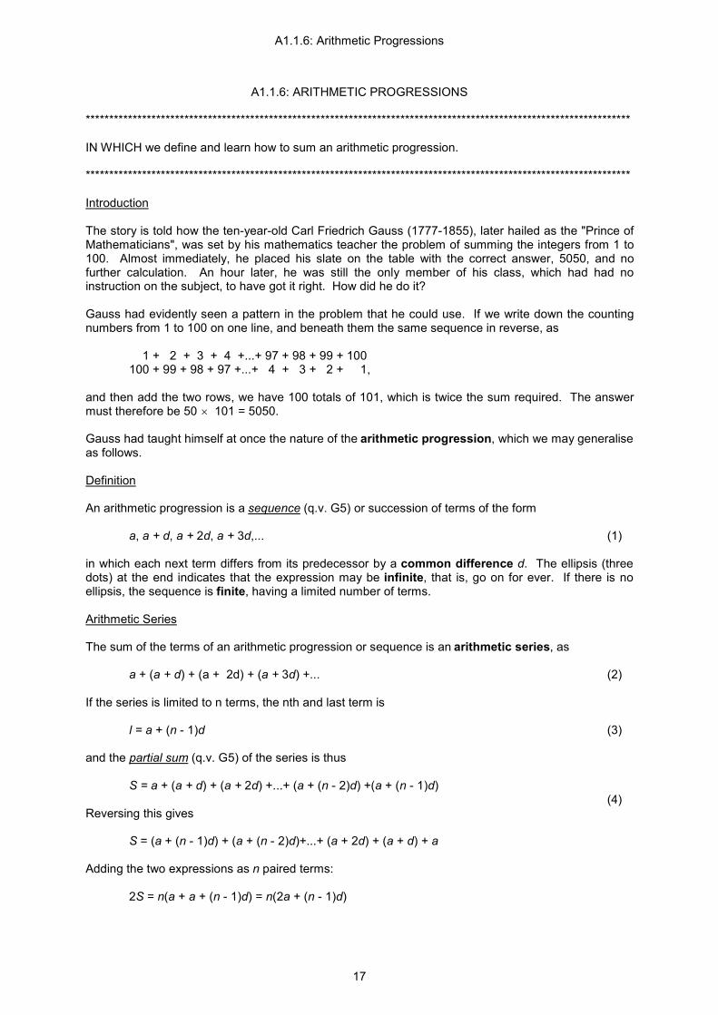
A1.1.6: ARITHMETIC PROGRESSIONS ******************************************************************************************************************** IN WHICH we define and learn how to sum an arithmetic progression. ******************************************************************************************************************** Introduction The story is told how the ten-year-old Carl Friedrich Gauss (1777-1855), later hailed as the "Prince of Mathematicians", was set by his mathematics teacher the problem of summing the integers from 1 to 100. Almost immediately, he placed his slate on the table with the correct answer, 5050, and no further calculation. An hour later, he was still the only member of his class, which had had no instruction on the subject, to have got it right. How did he do it? Gauss had evidently seen a pattern in the problem that he could use. If we write down the counting numbers from 1 to 100 on one line, and beneath them the same sequence in reverse, as
1 + 2 + 3 + 4 +...+ 97 + 98 + 99 + 100 100 + 99 + 98 + 97 +...+ 4 + 3 + 2 + 1,
and then add the two rows, we have 100 totals of 101, which is twice the sum required. The answer must therefore be 50 × 101 = 5050. Gauss had taught himself at once the nature of the arithmetic progression, which we may generalise as follows. Definition An arithmetic progression is a sequence (q.v. G5) or succession of terms of the form a, a + d, a + 2d, a + 3d,... (1) in which each next term differs from its predecessor by a common difference d. The ellipsis (three dots) at the end indicates that the expression may be infinite, that is, go on for ever. If there is no ellipsis, the sequence is finite, having a limited number of terms. Arithmetic Series The sum of the terms of an arithmetic progression or sequence is an arithmetic series, as a + (a + d) + (a + 2d) + (a + 3d) +... (2) If the series is limited to n terms, the nth and last term is l = a + (n - 1)d (3) and the partial sum (q.v. G5) of the series is thus S = a + (a + d) + (a + 2d) +...+ (a + (n - 2)d) +(a + (n - 1)d) (4) Reversing this gives S = (a + (n - 1)d) + (a + (n - 2)d)+...+ (a + 2d) + (a + d) + a Adding the two expressions as n paired terms: 2S = n(a + a + (n - 1)d) = n(2a + (n - 1)d)

A1.1.6: Arithmetic Progressions
18
Hence S = ½n(2a + (n - 1)d) (5) or alternatively S = n(a + ½(n - 1)d) (6) or again, from (5), S = ½n(a + l) (7) Triangular Numbers We have already seen in the Prologue that the triangular numbers 1, 3, 6, 10... are the sums of the counting numbers. Writing T
1 = 1
T2 = 1 + 2
T3 = 1 + 2 + 3 etc
we have the arithmetic series T
n = 1 + 2 +...+ n
= ½n(1 + n) (8) as Gauss presumably divined. Later on, in 1796, he was to prove that every positive integer was the sum of at most three triangular numbers. Arithmetic Mean The arithmetic mean of n quantities whose sum is S is S/n. If three consecutive terms of an arithmetic progression are a, a + d, and a + 2d, then their arithmetic mean is {a + (a + d) + (a + 2d)}/3 = (3a + 3d)/3 = a + d which is the middle term. Series The arithmetic series (2) above is the first and one of the simplest series which we shall encounter. We will find that series play a large and important role in our drama. Characteristic features of series are described in G5. We shall meet another important type of series in the next section.

A1.1.7: Geometric Progressions
19
A1.1.7: GEOMETRIC PROGRESSIONS ******************************************************************************************************************** IN WHICH we meet geometric progressions and series, learning how to sum them when this is possible. ******************************************************************************************************************** Definitions Geometric progressions (or sequences, (q.v. G5)) and series are comparable to the arithmetic progressions and series which we met in section A1.1.6, with the difference that successive terms grow not by a common difference but by a common ratio. So a geometric progression takes the form c, ct, ct
2, ct
3, ct
4, ..., ...
in which the terms are successively multiplied by the constant ratio t. If t is negative the terms will be alternately positive and negative. A geometric series then takes the form of the sum S = c + ct + ct
2 + ct
3 + ct
4 +... (1)
Like their arithmetic counterparts, geometric progressions and series can be finite or infinite. Partial Sum The sum of the first n terms of a geometric series, called the nth partial sum (q.v. G5), is given by S
n = c + ct + ct
2 + ct
3 + ct
4 +...+ ct
n-1 (2)
Then tS
n = ct + ct
2 + ct
3 + ct
4 +...+ ct
n-1 + ct
n
Subtracting, S
n - tS
n = S
n (1 - t) = c - ct
n = c (1 - t
n)
,1
1t
tcSn
n −−
= 1≠n (3)
(If t = 1, we can see from (2) that S
n = nc.)
Infinite Sum Is it possible to sum an infinite geometric series, or is the sum S always infinite? This is the same as asking, does the series converge (q.v. G5)? Let us consider what happens to S
n as n increases.
If |t| > 1, then as n increases the terms in equation (1) get ever greater in magnitude and the series does not converge. Equally, if t = 1, S is unlimited. But if |t| < 1, that is, -1 < t < 1, t
n in equation (3)
comes ever closer to zero as n increases. That is to say, tn has a limit (Sideshow S1) of zero. In
notation:

A1.1.7: Geometric Progressions
20
,0lim =∞→
n
nt |t| < 1 (4)
Hence in equation (3), as n approaches infinity, S
n has a limit which is given by
,1
01limt
cSS nn −−
==∞→
|t|<1
,1 t
cS−
= |t| < 1 (5)
We shall discuss this topic of convergence in greater detail, with some examples, in section A3.1.1. The special case when c = 1 is then found by combining (1) and (5),
...,11
1 432 +++++=−
= ttttt
S |t| < 1 (6)
Examples The recurring decimal fraction (see A1.1.2) A = 0.141414... = 0.14 (1 + 0.01 + 0.01
2 + 0.01
3 ...)
gives
c = 0.14, t = 0.01. Since |t| < 1, from equation (5) the sum of its terms
99.014.0
01.0114.0
=−
=A
This result generalises:
If decimal fraction digits abcd...m recur, as in
A = 0.abcd...m abcd...m abcd...m..., . . often written as mbcda && ....0 ,
then A may be expressed as the proper fraction
9...9999...mabcdA =
So 0.428571428571..., or 128574.0 && , 73
999999428571
==
unexplained in our treatment of rational numbers in section A1.1.2. The method can be extended to the case where the early decimal digits do not recur:
0.83333..., or 38.0 & , = )3.08(10/1̀ &+ = 1/10 (8 + 3/9) = 1/10 (8 + 1/3) = 1/10 (25/3) = 25/30 = 5/6

A1.1.7: Geometric Progressions
21
Alternative Derivation from Long Division By long division we can evaluate 1/(1 + x) as 1 - x + x
2 - x
3 + x
4 +...
1 + x) 1 1 + x - x - x - x
2
x2
x2 + x
3
- x3
- x3 - x
4
x4...
Thus
...,11
1 432 −+−+−=+
xxxxx
|x| < 1 (7)
The validity of this may be tested by multiplying out. Changing the sign of x then confirms result (6):
...,11
1 432 +++++=−
xxxxx
|x| < 1 (8)
We shall meet these two very important results (7) and (8) on various occasions in the future. Geometric Mean The geometric mean of n quantities is the nth root of their product. Thus the geometric mean of a,b,c,d, and e is 5 abcde . If three consecutive terms of a geometric progression are a, at, and at
2, then their geometric mean is
attaatata ==×× 3 333 2 which is the middle term. Notes (1) The limit is one of the most important concepts in the whole of mathematics. We may think of a limit as the value which some infinite expression may approach as we calculate it more and more accurately. The paradox that an infinite number of terms, when combined, can converge to a finite value, defeated mathematicians until Newton. Limits are explained in more detail in Sideshow S1, which like the Glossary runs in parallel to the main acts. Later on we will find that they are central to the calculus in Act 2, and to series in Act 3. We shall revisit geometric progressions in A3.1.1, discussing convergence in greater detail and giving other important examples of converging geometric series. (2) The relationship between arithmetic and geometric progressions is also of immense importance in mathematics. In particular, as we shall see in section A1.6.1, it gives birth to logarithms. Indeed, as we shall see in A3.3.3, equations (7) and (8) lead directly to Mercator's series for calculating logarithms.

A1.1.8: Coordinate Geometry
22
A1.1.8: COORDINATE GEOMETRY ******************************************************************************************************************** IN WHICH we meet the Cartesian coordinate system and see how it can be used to illustrate a linear equation. ******************************************************************************************************************** The Cartesian Coordinate System Two Frenchmen, Pierre de Fermat (1601-65) and the philosopher René Descartes (1596-1650) share the credit for the concepts of analytic or coordinate geometry by which we plot graphs today. At the heart of these lies the marrying of algebra and arithmetic with geometry, whereby equations can be represented by corresponding graphs and vice versa. Arithmetic and geometry had been sharply divided since Euclid some 2000 years previously. So this development ranks as one of the most important single advances in the entire history of mathematics. Figure 1 illustrates the conventions for doing this in two dimensions (a plane) as we do today. A pair of axes is drawn which meet at right angles at the origin, which is normally identified as O. The horizontal axis is negative to the left of O, zero at O, and positive to the right of O. The vertical axis, is negative below O, zero at O and positive above O. Most commonly the horizontal axis represents the variable x, and the vertical axis the variable y. All points on the plane can now be identified uniquely in relation to these two axes, by means of their Cartesian (from Descartes) coordinates, which indicate how far they are displaced from O in the two directions. These two values are written separated by a comma within a pair of brackets. So in Figure 1 point P has the coordinates (2,-3) because it lies 2 units to the right of O in the x direction and 3 units below O in the y direction. The general coordinates (x,y) can then be used to represent any unspecified point in terms of its position with regard to the two respective axes. The x values are also sometimes termed abscissas, and the y values ordinates. The two axes divide the plane into four quadrants, which are numbered anticlockwise from the top right and shown on Figure 1 as Q1 to Q4.

A1.1.8: Coordinate Geometry
23
Linear Equations Any equation which relates y to x can now be represented by a line or curve drawn through all the points for which the relation holds good. For instance in Figure 1 the straight line p passes through all points for which y = 2x + 3 (1) This may be verified by inserting values into the equation and confirming that the line passes through the corresponding points. For instance equation (1) is true when x is 1 and y is 5; or when x is 0 and y is 3; so both points (1,5) and (0,3) lie on p. More generally, all straight lines have equations which can be written in the form y = mx + c (2) Linear equations, as they are known, have order or degree 1 because the highest power of any variable is 1. m here is called the gradient or slope. It shows how steeply the line is rising, that is, the number of units y increases for each unit gain in x. For a straight line this value is constant. In Figure 1, when on line p x rises from 0 to 1 (one unit), y rises from 3 to 5 (two units). So the gradient is 2, which is the value of m in equation (1). (We shall study this in more depth when we come to the differential calculus in section A2.1.1). c here is called the y intercept: this is the value of y where the line cuts the y axis (i.e. when x = 0). In Figure 1 the y intercept of line p is 3, the value of c in equation (1). If the line is known to pass through two points (x
0,y
0) and (x
1,y
1) then the slope m can be given by
m = 01
01
xxyy
−−
(3)
Replacing (x
1,y
1) by the general point (x,y) gives another, equivalent way of writing its equation as
mxxyy
=−−
0
0 (4)
y - y
0 = m(x - x
0) (5)
or y = mx - mx
0 + y
0 (6)
where the y intercept is - mx
0 + y
0, corresponding to c in (2).
Parallel lines have the same gradient but different y intercepts. So in Figure 1 the line q, which is parallel to p, has the equation y = 2x - 1 since its y intercept is -1. We are now equipped to draw the graph of any linear equation, and conversely to find the equation of any straight line.
A1.1.9: Simultaneous Linear Equations
24
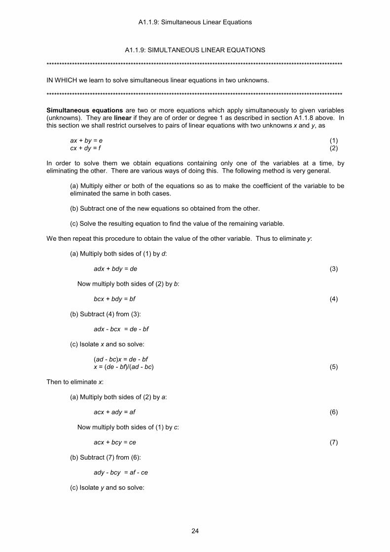
A1.1.9: SIMULTANEOUS LINEAR EQUATIONS ******************************************************************************************************************** IN WHICH we learn to solve simultaneous linear equations in two unknowns. ******************************************************************************************************************** Simultaneous equations are two or more equations which apply simultaneously to given variables (unknowns). They are linear if they are of order or degree 1 as described in section A1.1.8 above. In this section we shall restrict ourselves to pairs of linear equations with two unknowns x and y, as ax + by = e (1) cx + dy = f (2) In order to solve them we obtain equations containing only one of the variables at a time, by eliminating the other. There are various ways of doing this. The following method is very general.
(a) Multiply either or both of the equations so as to make the coefficient of the variable to be eliminated the same in both cases. (b) Subtract one of the new equations so obtained from the other. (c) Solve the resulting equation to find the value of the remaining variable.
We then repeat this procedure to obtain the value of the other variable. Thus to eliminate y:
(a) Multiply both sides of (1) by d: adx + bdy = de (3) Now multiply both sides of (2) by b: bcx + bdy = bf (4) (b) Subtract (4) from (3): adx - bcx = de - bf (c) Isolate x and so solve: (ad - bc)x = de - bf x = (de - bf)/(ad - bc) (5)
Then to eliminate x: (a) Multiply both sides of (2) by a: acx + ady = af (6) Now multiply both sides of (1) by c: acx + bcy = ce (7) (b) Subtract (7) from (6): ady - bcy = af - ce (c) Isolate y and so solve:

A1.1.9: Simultaneous Linear Equations
25
(ad - bc)y = af - ce y = (af - ce)/(ad - bc) (8)
So the solution to the pair of simultaneous equations (1) and (2) is the pair of values x and y given by equations (5) and (8). On a graph this solution is typically indicated as the single point where the straight lines representing equations (1) and (2) intersect. Since equations (5) and (8) provide a general solution, we do not have to work through steps (a) to (c) each time but can apply the formulae directly. Example
Consider the equations illustrated in Figure 1, 2x - 3y = 5 (9) 3x + 2y = 14 (10) From equations (5) and (8) these have the solution x = (2×5 + 3×14)/(2×2 + 3×3) = 52/13 = 4 y = (2×14 - 3×5)/(2×2 + 3×3) = 13/13 = 1 So on Figure 1 the two lines intersect at the point (4,1). We can confirm our solution by inserting these values in the original equations: 2×4 - 3×1 = 5 3×4 + 2×1 = 14 Special Cases Note that equations (1) and (2) have a unique solution only if the quantity ad - bc, known as the

A1.1.9: Simultaneous Linear Equations
26
determinant, does not equal zero, since division by zero is inadmissible. There are two ways in which this can happen, which are readily understood in graphical terms:
(1) The two lines are parallel, i.e. never intersect, in which case there is no solution. E.g.: -2x + y = -1 (11) -2x + y = 3 (12) where ad - bc = -2 + 2 = 0. There are no values of x and y for which these two equations can simultaneously be true. Their graphs are the two parallel lines depicted in A1.1.8 Figure 1.
(2) Alternatively, the two lines coincide, in which case there is an infinite number of solutions. E.g.: 3x + 4y = 10 (13) 6x + 8y = 20 (14) where ad - bc = 24 - 24 = 0. Equation (14) is merely equation (13) with all terms multiplied by 2. So any point (x,y) which satisfies one of these equations will necessarily satisfy the other.

A1.1.10: Functions
27
A1.1.10: FUNCTIONS ******************************************************************************************************************** IN WHICH we meet the fundamental concept of a function. ******************************************************************************************************************** Definition A function is a rule for obtaining the value of one variable, said to be dependent, from the value of one or more others, which are called independent. We commonly express such a relationship where y is a function f of x by writing
y = f(x) This is read, "y equals f of x" or just "y equals f x". x, in brackets, is here called the argument. The function is one of the most important concepts in mathematics, and we can trace its origins back to Galileo (1564-1642), and perhaps even beyond him to Oresme (c.1361). Our modern understanding of it, including the f(x) notation itself, we owe very largely to Euler (1748). In section A1.1.8 we encountered expressions such as y = 2x + 3 (1) Here y is a linear function of x (since its graph is a straight line, A1.1.8 Figure 1), whose rule we can express as
f(x) = 2x + 3 (2) On a graph, the independent variable is conventionally drawn horizontally and the dependent variable vertically. Functions are commonly denoted by the letters f,g,h,u and v. The two notations y and f(x) used in (1) and (2) above are often interchangeable. (For present purposes we shall ignore cases where there is more than one independent variable.) Domain and Codomain The domain of a function y = f(x) is the set of x values for which rule f applies. Its codomain is the set of y values which can potentially be generated by the x values in the domain. In Figure 1 curve (a), the function y = x
2 is valid for all real x values, its domain. But the y values, its
codomain, are all positive. So here -∞ < x < ∞ , y > 0 In Figure 1 curve (b), the function y = x
3 is valid for all real x (its domain) and y (codomain). So here
-∞ < x < ∞ , -∞ < y < ∞ Even Functions Any function for which always f(-x) = f(x) (3) is said to be an even function. Its graph will be symmetrical about the vertical (y) axis. For example

A1.1.10: Functions
28
y = x
2
is an even function since (-x)
2 = x
2 for all x. Its graph, a parabola, is the curve Figure 1 (a). (We learn
more about parabolas in Sideshow S3.)
-3 -2 -1 0 1 2 3
x
-3
-2
-1
1
2
3y Figure 1
Quadratic and cubic functions
(a) y = x^2
(b) y = x^3
Odd Functions Any function for which always f(-x) = -f(x) (4) is said to be an odd function. Its graph will be unchanged if rotated through 180° about the origin. For example y = x
3
is an odd function since (-x)
3 = -x
3 for all x. Its graph is the curve Figure 1 (b).
Zeros of a Function We say that a function has a zero, or its equation has a solution or root, at the point when f(x) = 0. That is, when the graph of the function crosses the x axis. In the case of equation (1) this occurs when x = -1.5 (see A1.1.8 Figure 1). Polynomial Functions Among the simplest and most commonly occurring functions are polynomials , which take the form f(x) = a
nx
n +...+ a
3x
3 + a
2x
2 + a
1x + a
0 (5)
A1.1.10: Functions
29
where the highest index n is called the degree or order of the polynomial. The constants a
n,..., a
3, a
2,
a1, a
0 are called coefficients.
If n = 1, the graph is linear as described in section A1.1.8. If n > 1, the graph is non-linear (curved). For instance if n = 2, the polynomial is called quadratic, and its graph will be a parabola similar to Figure 1 (a), such as A1.5.2 Figures 1 to 3. If n = 3, it is called cubic, and its graph will resemble Figure 1 (b) or a distortion (stretching) of it such as A1.5.3 Figures 1 to 3. We shall learn how to solve quadratic and cubic equations in Act 1 Scene 5. Inverse of a Function Often it is possible to re-express a function y = f(x) so that x is given uniquely as a function of y, as x = f-1
(y). In the case of equation (2), this would be x = f
-1(y) = (y - 3)/2 (6)
f-1
is then called the inverse or inverse function of f. Inverse functions behave in much the same way as the inverse operations of A1.1.4 (Add4) and (Mul4). So if we carry out function f on x, and then f
-1 on the result, we end up with our starting value
x: f
-1(f(x)) = x (7)
E.g. if f and f
-1 are defined as in equations (2) and (6) then
f
-1(f(x)) = f
-1(2x + 3) = ((2x + 3) - 3)/2 = x
The same holds if we do f
-1 first and then f:
f(f
-1(x)) = x (8)
E.g. using the same function, f(f
-1(x)) = f((x - 3)/2) = 2(x - 3)/2 + 3 = x
Not all functions have inverses. For a function to have an inverse there must be one and only one value of x which generates each value of y. An example is y = x
3.
However, in some cases there is more than one value of x which can generate a given y. So if we want an inverse function for f we restrict its domain so that f
-1(y) is unique. We then say that the
principal values of f lie in this restricted domain. For example, if y = f(x) = x
2, both x = 2 and x = -2 both give f(x) = 4. So in order to obtain an inverse
function x = f-1
(y) = y which gives a unique value of x, we restrict the domain of f to positive values
of x only. So we say the principal value of 4 is 2 even though -2 is also a root. In practice the convention is adopted whereby n is understood to mean 'the positive square root of n'.

A1.1.10: Functions
30
Other examples of inverse functions that we shall meet are cos and arccos (i.e. cos
-1, A1.3.1)
sin and arcsin (i.e. sin-1
, A1.3.1) tan and arctan (i.e. tan
-1, A1.3.1)
exp and ln (the natural logarithm, A1.6.4).

A1.2.1: π
31
ACT 1 SCENE 2: π, ANGLES, AND TRIANGLES
A1.2.1: π ******************************************************************************************************************** IN WHICH we first encounter π and various approximations to it. ******************************************************************************************************************** Circumference of a Circle Let us begin with a practical experiment. Collect a number of circular objects - cake tins, cans, jars, bottles, dustbins - and measure the circumference (distance round them) with a flexible tape measure, writing down the value C of each. Then in each case measure the diameter d (distance across the centre). Next, with a calculator divide the circumference of each object by its diameter and note the resulting ratio, C/d. You should find that the answer in each case comes to somewhere between 3 and 3.2. And although in the experiment you may get answers that are not entirely accurate, and not all quite the same, for all true circles the ratio
circumference C diameter d
has a unique, constant value in this region which we call π. So we can say that for any circle with diameter d, its circumference will be this value, π, times d. And since the diameter is twice the length of a radius, we can write
C = πd = 2πr (1) where r, the radius, is half the diameter. If your calculator has a π button it will give a value for π close to 3.1415926535. But no numerical expression of π is ever going to be exact, because the expansion of π into decimal places goes on for ever without repeating itself. So we stick with the familiar abbreviation "π". Area of a Circle
Suppose we now want to know how big is such a circle in terms not of its circumference but of its
π
π π

A1.2.1: π
32
area. Is there another simple formula to tell us this, which again is the same for all circles? There is. Figure 1a shows a circle whose radius is r divided into eight equal sectors by drawing four diameters. In Figure 1b these sectors have been rearranged by putting them alongside each other, with the angles pointing alternately downwards and upwards. The length of the curved edge from P to Q is half the circumference, and so πr. The length of the straight lines is r. The total area of the shape is the same as that of the original circle. In Figure 1c the sectors have been halved and rearranged again. As before, the curved edge RS has length πr, the straight lines have length r and the area is unchanged. But the shape, in spite of its 'wobbly' edges, is beginning to look like a rectangle. (You can try this for yourself by cutting up a circle drawn on thin card and sticking down the pieces side by side.) If we continued this process indefinitely, the top and bottom edges would come to look ever straighter, so that the resemblance to a rectangle would be even more marked. This 'rectangle' would have length πr and height r. Its area would therefore be A = πr times r, or πr
2. Since this is the same as the
area of the original circle, we deduce that the area of the circle must be
A = πr2 (2)
Such a formula seems to have been known to the Greek geometer Hippocrates around 450 BC. So we have for a circle of diameter d and radius r (it doesn't matter what the units are, metres, furlongs, cricket pitches or whatever): Circumference of circle : C = πd = 2πr units Area of circle : A = πr² square units History of π Hence there is one formula for calculating the circumference of any circle in terms of a special constant (q.v. G3), π, and another for the area of any circle in terms of that same constant. And although we might have guessed that two such formulae existed for all circles, it was by no means obvious that the constants involved were actually the same, as we have just found. For the discovery that these two constants are one and the same, we have to thank the mighty Archimedes (c.287-212 BC), undoubtedly the greatest of the Greek mathematicians. Curiously however it was not a Greek but the English mathematician William Jones who in 1706 chose to name this constant by the Greek letter by which we now know it - "π". This usage became standard on being espoused in 1736 by the Swiss genius Euler. Today we know its value to trillions of decimal places. Blatner (B1), a delightful compendium of π lore, gives the first million. Civilisations have of course handled π for almost as long as we have records. For instance in the Old Testament (1 Kings 7:23) we read "And he made a molten sea, ten cubits from the one brim to the other: it was round all about...and a line of thirty cubits did compass it round about". The circumference is three times the diameter, so we have here an ascription to π, albeit perhaps unconscious, of the value 3. Other societies have used other values as follows:
Egyptians c.2000 BC : (16/9)2 (about 3.160).
Babylonians c.1800 BC : 25/8 (3.125). Archimedes (c.287-212 BC): Between 3 10/71 (about 3.1408) and 3 1/7 (about 3.1429) Hindus c.AD 650 : 10 (about 3.162). Tsu Ch'ung-chih (Chinese) c.AD 470 : 355/113 (3.1415929...)
Not bad without a pocket calculator. There is an impressive list of such historical values in Hogben (B1) pp.261-2; and an even more

A1.2.1: π
33
impressive one in Rouse Ball & Coxeter (B2), pp.350-58. Estimating π As beginners, we often use the ratio 22/7 (3 1/7, about 3.1429) for pen and paper calculations. But today many calculators are equipped with a π button as above, which is accurate enough for most purposes. How do we calculate the value of π mathematically other than by measuring cake tins or cutting out cardboard circles? One way to begin is to use the two formulae given above to establish a range bracket - that is, two endpoints within which π must lie. We begin by comparing two lengths, using the formula for the circumference of a circle.
Figure 2 shows a regular hexagon (q.v. G4) of side t = 1 inside a circle of radius r = 1. The outer perimeter (edge) of the hexagon must clearly be 6t = 6. From above, the circle has a circumference of 2πr, which is in this case 2π. Clearly the six (curved) arcs T must each be longer than the six (straight) sides t of the hexagon to which they correspond. So the total circumference of the circle must be longer than the outer perimeter of the hexagon. This gives 2π > 6 or π > 3 (3) This is the lower endpoint of our range bracket for π. To obtain our upper endpoint we compare two areas, using the formula given above for the area of a circle, as follows.
In Figure 3 we have drawn a circle of radius r = 1 inside a square of side 2. The area of the square is clearly 4 square units. From above, the area of the circle is πr
2 = π square units. So
π < 4 (4)

A1.2.1: π
34
This is the upper endpoint of our range bracket. So π lies between 3 and 4, which we write as 3 < π < 4. Geometrical Approximations One ancient method for computing π geometrically is to sandwich a circle between two regular polygons (q.v. G4), one slightly bigger than the circle, the other slightly smaller. We then make the sandwich thinner and thinner by using polygons with more and more sides, which approximate more and more closely to the circle. If we can calculate the perimeters of the polygons we can work out the circumference of the circle which lies between them (and hence π) to any precision that we like. By using polygons with 96 sides, Archimedes arrived at the values attributed to him above. (For his method see Beckmann (B1), 64-7.) Limits We have in this section twice touched again on the concept of a limit, which we met in A1.1.7 and which is explained in greater detail in Sideshow S1. We may think of it as a finite value arrived at from (in principle) an infinite number of terms.
(1) In the first case, we found the area of our circle more and more accurately by cutting it into ever more pieces and rearranging them into something that looked increasingly like a rectangle. In theory we could have gone on improving the likeness for ever, although in practice this would soon have become too fiddly! (2) Secondly, Archimedes' method for estimating π would be increasingly accurate as polygons with ever more sides were used, the only difficulty being the practical one of computation.
We shall see that limits are central to the calculus in Act 2, and to series in Interlude I2 and Act 3. These will make possible respectively
(1) A more rigorous demonstration, by integration, of the formula for the area of a circle (section A2.2.2). (2) The modern calculation of π by computer from formulae for infinite series (q.v. G5) (Interlude I2.1 and see below).
* * * * *
We have now met π, the first of the three principal actors in our drama and a primary witness in the debate we opened in section A1.1.1 on the nature of mathematics. From its early history we can observe a difference between those who have assigned to it an arbitrary value such as (16/9)
2 or 10
which served as adequate for practical purposes, and those who like Archimedes realised that π was a quantity in its own right which could in principle be computed to any required degree of accuracy, even supplying a method for doing so. π stands as a challenge to those who maintain that all mathematics is merely a human creation, no more than the proving of theorems from axioms. For the value of π is independent of mankind. No human being chose its actual value and no human being can change it. It does not alter with time and it is independent of space. As we began to see in A1.1.3, we can change the axioms of geometry and so develop different geometries. As we do so we can study which properties change and which are invariant. However, whatever changes we make to the axioms of arithmetic or algebra (see A1.1.4) or geometry, π is an invariant. Indeed not one of all the axiom sets currently employed by mathematicians, if altered, would result in a different value of π. Circles will still be circles everywhere in the universe. This suggests that π is more fundamental to mathematics than are those axioms. Axioms may come and go, but π

A1.2.1: π
35
is, always was, and shall be forever, everywhere, the same. It is a thought worth pondering, for it strikes at the heart of formalism, and indeed at the determined efforts of the early twentieth century to reduce the whole of mathematics to sets of axioms, a project which ultimately foundered in 1931 against Gödel's undecidability theorems (q.v. G1). π has innumerable properties, and proving these from one or more axiomatic sets is very much the business of mathematics. But these proofs would be meaningless if its value were not a mathematical given. Postscript: π Redefined It has subsequently become apparent to me that the geometrical definition of π in terms of circles as given above is both inadequate and erroneous. This tells us only about some of its properties – what it does – not what it actually is. π is a number and so the first thing we need to know about it is its value – its place on the number line, which cannot be computed directly from the circular definition. Hence the best definition comes from the limit of the infinite series ...
71
51
311
4+−+−=
π (5)
known as Leibniz’ series, whose derivation we shall give as I2.1 (17). This is optimally simple, requiring nothing more complex than the basic operations of arithmetic and a lot of patience to compute. A child could understand and attempt to compute it. The circular properties may then be derived from this later on with the aid of the calculus.
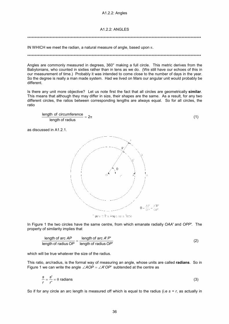
A1.2.2: Angles
36
A1.2.2: ANGLES ******************************************************************************************************************** IN WHICH we meet the radian, a natural measure of angle, based upon π. ******************************************************************************************************************** Angles are commonly measured in degrees, 360° making a full circle. This metric derives from the Babylonians, who counted in sixties rather than in tens as we do. (We still have our echoes of this in our measurement of time.) Probably it was intended to come close to the number of days in the year. So the degree is really a man made system. Had we lived on Mars our angular unit would probably be different. Is there any unit more objective? Let us note first the fact that all circles are geometrically similar. This means that although they may differ in size, their shapes are the same. As a result, for any two different circles, the ratios between corresponding lengths are always equal. So for all circles, the ratio
π= 2radius of length
ncecircumfereoflength (1)
as discussed in A1.2.1.
In Figure 1 the two circles have the same centre, from which emanate radially OAA' and OPP'. The property of similarity implies that
' radius of length
''arc of length radius of length
arc of lengthOPPA
OPAP
= (2)
which will be true whatever the size of the radius. This ratio, arc/radius, is the formal way of measuring an angle, whose units are called radians. So in Figure 1 we can write the angle ''OPAAOP ∠=∠ subtended at the centre as
θ==''
rs
rs radians (3)
So if for any circle an arc length is measured off which is equal to the radius (i.e s = r, as actually in
θ
θ

A1.2.2: Angles
37
Figure 1), the angle at the centre will be 1 radian. How big is this? From equation (1), a full circle contains 2π radians. In degree terms this gives us 2π radians = 360° 1 radian = 360° / (2π) which is about 57.3°. So also π radians = 180° π/2 radians = 90°, a right angle. π/3 radians = 60° π/4 radians = 45° π/6 radians = 30° It turns out that the radian is a very natural unit. All kinds of formulae and expressions fall into place if we use it rather than degrees. For instance, we can rearrange (3) to give us the length of a circular arc from the radius and the angle at the centre, as s = rθ (4) Further, as a ratio of two lengths, it is dimensionless. Hence the word "radians" is commonly omitted. This will become important later on, when it becomes apparent that much that is true of angles can in fact be predicated of all real numbers. The values of angles are often denoted by Greek letters such as π, θ, φ. Right angles are often indicated on a diagram by a little square box as in Figure 2(b). By a basic theorem of Euclid's,
if two straight lines meet at a point, the two adjacent angles formed at that juncture add up to two right angles (π radians).
This may also be put by saying that
a straight line is the sum of two right angles. (Figures 2a and 2b) (5)

A1.2.3: Euclidean Triangles
38
A1.2.3: EUCLIDEAN TRIANGLES ******************************************************************************************************************** IN WHICH we learn some of the properties of Euclidean triangles. ******************************************************************************************************************** Terminology The triangles we meet in this drama are Euclidean triangles - that is, such as feature in Euclidean geometry (q.v. G4). They are defined as plane (flat) figures bounded by three straight lines, which are said to meet at three vertices or angles. As noted already in section A1.1.3, their internal angles add up to two right angles (180°, that is, π radians as we saw in A1.2.2). Euclidean triangles come in different shapes and sizes. They can be
equilateral : all sides equal, and all angles equal; the angles must therefore be equal to π/3 radians (60°); or
isosceles : two sides equal, the angles opposite these two sides being always equal; or scalene : all sides of different length, and all angles different.
Similarly they can be
acute-angled : all angles less than a right angle; or right-angled : one angle equal to a right angle; or obtuse-angled : one angle greater than a right angle.
The long side opposite the right angle of a right-angled triangle is called the hypoteneuse (Greek "stretched under").
Notation By convention the internal angles may be denoted by single capital letters where this is unambiguous, or more precisely by the three capital letters which spell out the two sides containing the angle. So in the triangle ABC in Figure 1, the angle A may also be designated ∠ BAC or ∠ CAB.

A1.2.3: Euclidean Triangles
39
Conversely, sides of triangles may be identified either by the two capital letters used to pinpoint their ends, or else by small letters corresponding to the angles they are opposite. So in Figure 1 the side BC or CB, opposite angle A, is also denoted a. Here as so often we follow a convention originating from Euler.
Similar Triangles In A1.2.2 we met the concept of similarity as it applies to circles. Even though they may be of different sizes, their shapes are all the same: the ratios of corresponding pairs of arcs of different circles are always equal. Two figures bounded by straight lines - as polygons (q.v. G4) - are said to be similar if
(a) their corresponding angles are equal, and (b) the ratio between corresponding sides is the same in all cases.
As before, this expresses the fact that their shapes are the same, even if they are of different sizes or of opposite handedness (as through reflection in a mirror). In Figure 1 the triangles ABC and PQR are similar, with angles A = P, B = Q, C = R. So from property (b),
rc
qb
pa
== (2)
From this it follows that between similar triangles corresponding ratios of sides are preserved:
qp
ba ,
= ,rq
cb
= pr
ac
= (3)
Triangles are the only polygons for which equality of angles alone guarantees similarity (i.e. property (a) implies property (b)). For instance any rectangle shares with a square the property that all its angles are right angles, but its corresponding sides may have very different proportions: its shape is different. This concept of similarity is the basis on which we draw maps or plans, in which context ratios such as a/p in equation (2) are called the scale. And as we shall see in A1.3.1, similar triangles are the foundation of trigonometry. Congruent Triangles Two triangles are congruent if they are similar, and in addition corresponding sides are equal. Area The area of a triangle can be deduced from Figure 2, where the height h of triangle ABC is given by the perpendicular (q.v. G4) BF from B to the base AC. The rectangle ACDE is twice the size of ABC and has an area bh equal to the product of its sides. So the triangle's area is half of this. That is, Area of a triangle = ½ × (length of base) × height usually written as ½ b h (4) The same is true for any triangle whichever side is chosen as the "base". It follows that congruent triangles have equal areas.

A1.2.3: Euclidean Triangles
40

A1.2.4: Pythagoras' Theorem
41
A1.2.4: PYTHAGORAS' THEOREM ******************************************************************************************************************** IN WHICH we prove Pythagoras' theorem and meet some extensions. Notable Source for Pythagorean triads: Courant and Robbins (B1), 40-1. ******************************************************************************************************************** Pythagoras' theorem, as it is called today, was not original to that worthy sixth century Greek, but was known to the Babylonians over 1000 years earlier. What does it say?
In Figure 1 the triangle ABC has a right angle at C. On each side a, b and c, squares have been drawn whose areas are respectively a
2, b
2 and c
2. Pythagoras' theorem tells us that
"The square on the hypoteneuse of a right-angled triangle is equal to the sum of the squares on the two adjacent sides."
That is, c
2 = a
2 + b
2 (1)
There are several hundred published proofs of this, more than for any other theorem in mathematics. At the age of 17 the Hungarian prodigy Paul Erdős knew thirty-seven. It is possible that Pythagoras was the first to prove it, but doubtful whether he originated the particular rather complex proof of it that appears in Euclid and is rehearsed in the older school texts. That offered here is rather more simple. In Figure 2a the four shaded right-angled triangles each have shorter sides of length a and b, and a hypoteneuse of length c. The unshaded squares marked A and B have areas a
2 and b
2 respectively.
In Figure 2b the triangles have been rearranged without overlapping, and the remaining unshaded square marked C has area c
2. Since the outer square is unchanged, the total unshaded area within it
must also be unchanged. So

A1.2.4: Pythagoras' Theorem
42
c
2 = a
2 + b
2
We shall offer another proof in A1.3.2 after acquiring a little trigonometry. Extension (1): Pythagorean Triads Pythagorean triads are sets of three integers a, b, c for which relationship (1) holds good. We can generate such triads from pairs of positive integers p and q as follows. Writing x = a/c, y = b/c, we have x
2 + y
2 = 1 (2)
y2 = 1 - x
2 = (1 + x)(1 - x)
Let y/(1 + x) = (1 - x)/y = t Then x = 1 - ty y = t + xt x = 1 - t
2 - xt
2
22 1)1( ttx −=+
2
2
11
ttx
+
−= (3)
+
−++=
+
−+=
2
22
2
2
111
111
tttt
ttty
21
2tty
+= (4)
Writing t = q/p (p > q)

A1.2.4: Pythagoras' Theorem
43
and substituting in (3) and (4) for x, y and t:
,22
22
qpqp
ca
+
−=
222
qppq
cb
+=
Then for some rational constant of proportionality r, a = (p
2 - q
2)r
b = (2pq)r c = (p
2 + q
2)r
We recall the two identities (q.v. G1),
(x + y)
2 ≡ x
2 + 2xy + y
2 (5)
(x - y)2 ≡ x
2 - 2xy + y
2 (6)
Then, from identity (5) we have c
2 = (p
4 + 2p
2q
2 + q
4)r
2
and from identity (6), a
2 + b
2 = (p
4 - 2p
2q
2 + q
4)r
2 + (4p
2q
2)r
2
= (p4 + 2p
2q
2 + q
4)r
2
= c2
Since this result is independent of r we shall simplify by setting r = 1. This gives a = p
2 - q
2 (7)
b = 2pq (8) c = p
2 + q
2 (9)
where c
2 = a
2 + b
2
So for any positive integers p and q, the triads a, b, and c formed from equations (7) to (9) always conform to Pythagoras' theorem. By choosing different values for p and q we can build up a table of such triads, as p q │ a b c
──────────────┼─────────────────── 2 1 │ 3 4 5 3 1 │ 8 6 10 3 2 │ 5 12 13 4 1 │ 15 8 17 4 2 │ 12 16 20 4 3 │ 7 24 25 5 3 │ 16 30 34 In fact any such p and q with p > q, where p and q have no common factor and are not both odd, generate all the primitive triads a, b and c (i.e. those with no common factors).

A1.2.4: Pythagoras' Theorem
44
Pythagorean triads appear to be represented on the Old Babylonian cuneiform tablet Plimpton 322 dating from c.1900 - 1600 BC. We shall meet again the 't' substitution adopted in (3) and (4) above as an aid to integration in A2.4.4, where at equation (4) we will further identify t. Extension (2): Fermat's Last Theorem The question arises, are there any other integer values of a, b, c and n (n > 2) for which the same relationship c
n = a
n + b
n
holds good? The great French number theorist Pierre de Fermat (1601 - 1665) managed to prove that there were no such values a, b and c for n = 4. Later he claimed in a tantalising note written in the margin of a textbook that he had found a "truly marvellous" proof that the equation had no solutions for n > 2, which the margin was too narrow to contain. His proof was never found. And although some later mathematicians found proofs for a few specific values of n (e.g. Euler, 1753 for n=3), Fermat's Last Theorem, as it became known, that a
n + b
n = c
n has no integer solutions for n > 2,
remained unproven by the world's greatest mathematicians until finally proved by the Cambridge Professor Andrew Wiles in 1994. The verification of this - too long to include here - is left as an exercise for the reader...! The history of this theorem and of its final conquest by Professor Wiles is given in Simon Singh's fascinating and most readable book Fermat's Last Theorem (B4).

A1.2.5: Irrational Numbers
45
A1.2.5: IRRATIONAL NUMBERS ******************************************************************************************************************** IN WHICH we explore the irrational numbers disclosed by Pythagoras' theorem. ******************************************************************************************************************** It was quite possibly Pythagoras himself who first discovered irrational numbers (recall section A1.1.2) as a consequence of the theorem which bears his name. He - or perhaps a member of his school - deduced from it that the diagonal of a square is not commensurable with its side; that is, the quotient of the diagonal divided by the side cannot be expressed as the ratio of two integers. If the side of the square is 1 unit and the diagonal x, then from Pythagoras' theorem we have
x2 = 1
2 + 1
2 = 2,
x = 2 What Pythagoras realised was that 2 / 1 cannot be expressed as a ratio of two integers. His proof, known to Aristotle, has come down to us from Euclid. It is an excellent example of a reductio ad absurdum, under which we prove something to be true by demonstrating that its contrary leads to a contradiction. Today we would write it like this:
Assume that there is a rational number x = m/n, where m and n are integers with no common factor. Then
m
2/n
2 = 2, m
2 = 2n
2.
The square of an odd number is odd, so m must be even. Write m = 2k. Then
(2k)
2 = 2m
2, m
2 = 2k
2.
Hence n also is even. Since m and n are both even, they have a common factor of 2, which contradicts our statement that they have no common factors. So, arguing from our original assumption that x exists, we have obtained a contradiction. Hence the assumption is false; no such x exists, in which case 2 must be irrational.
After Pythagoras, Theodorus of Cyrene (born c.460 BC), who was Plato's tutor, proved individually that 3 , 5 and the square roots of all the non-square numbers up to 17 were irrational. In fact the above proof can be modified to show that this is true for all non-squares. As noted in section A1.1.2, it is characteristic of irrationals that their decimal expansion never terminates or repeats itself. So, 2 is given by 1.4142135623730950488.... Uncalculated irrational roots, either on their own, or combined with rational numbers - as 2 or 3 /2 - are known as surds. Well known is the golden ratio φ = ½ (1 + 5 ) which we shall explore in Interlude I1.1.2. However, there are many irrational numbers which cannot be expressed as roots. These include the transcendental numbers (q.v. G2), such as π and e, which cannot be the solution of polynomial equations (q.v. G3). What is significant for us is the way an advance in mathematics - here Pythagoras' theorem - has led to the recognition of a new type of number. Just as in section A1.1.2,

A1.2.5: Irrational Numbers
46
addition first came with the integers, subtraction gave us zero and negative numbers, division gave us rational numbers,
so Pythagoras' theorem has led us to the irrationals. It is a pattern which will repeat itself when we come to investigate quadratic equations (Act 1 Scene 5), which will lead us to the imaginary number i and the associated complex numbers.

A1.3.1: Trigonometrical Ratios
47
ACT 1 SCENE 3: TRIGONOMETRY
A1.3.1: TRIGONOMETRICAL RATIOS ******************************************************************************************************************** IN WHICH we encounter trigonometry, the study of angular relationships. ******************************************************************************************************************** We have in previous sections looked at angles and triangles. We now begin to ask, given the angles of a triangle, what can be known about the relative sizes of its sides - that is, about the ratios which exist between them? This is the subject matter of trigonometry, which was discovered by one Greek astronomer, Hipparchus of Nicaea (born c.190 BC), and extended by another one, Ptolemy of Alexandria (c.AD 150). For angles, with time, constitute the two principal measurable data of astronomy. In A1.2.2 Figure 1 and equation (2), using the concept of similarity as it applies to circles, we defined ∠ AOP as the ratio θ = arc AP / radius OP Since all circles are similar, we concluded that this ratio was independent of the size of the circle - that is, of the radius OP.
In Figure 1 of this section, we now drop PM perpendicular to OA and define three more ratios:
OM/OP, which we call the cosine of θ, written "cos θ", PM/OP, which we call the sine of θ, or "sin θ", and PM/OM, which we call the tangent of θ, or "tan θ" (this is the second sense of tangent (q.v.
G4) given in the Glossary). In A1.2.3 (3) we saw that between similar triangles, corresponding ratios of sides are equal. So in any triangles which are similar to OPM, regardless of size, the ratios corresponding to OM/OP, PM/OP and PM/OM will be identical. That is, the cosines, sines and tangents of angles are independent of the size of the (usually right-angled) triangles we may use to measure them. This is the basis of trigonometry. Let us look at these ratios more closely.
θ
θ
θ
θ
θ

A1.3.1: Trigonometrical Ratios
48
Major Trigonometrical Functions
In Figure 2, the triangle ABC has a right angle at C. The side c is therefore its hypoteneuse. We wish to investigate the ratios associated with the (acute) angle A, whose size we shall write as θ. From our definitions,
,cos θ=cb ,sin θ=
ca θ= tan
ba
we have already tan θ = sin θ / cos θ (1) We can write also b = c cos θ a = c sin θ a = b tan θ Since angle B is π/2 - θ, we have immediately cos θ = sin (π/2 - θ) (2) sin θ = cos (π/2 - θ) (3) Thus cosine, sine and tangent are functions (A1.1.10) which supply the values of their associated ratios for any input angle. They are in fact termed the major trigonometrical functions (we shall meet the minor ones below). We saw in A1.2.2 that as ratios of two lengths, angles are dimensionless. It is clear from the above that the same is true of cosine, sine and tangent; it is in fact true of all the trigonometrical functions. Polar Coordinates and Periodicity However, these functions, and the relationships between them, are not confined to acute angles. Figure 3 extends our original definition of cosine and sine in relation to a circle, by superimposing on it the x and y axes of Cartesian geometry (A1.1.8). If we draw a circle of radius r centred on the origin, any point (x,y) on its circumference has the polar coordinates x = r cos θ (horizontal component) (4) y = r sin θ (vertical component) (5)
θ θ
θ
θ

A1.3.1: Trigonometrical Ratios
49
where θ by convention starts at 3 o'clock and rotates anticlockwise, like the beam on a radar screen. Polar coordinates were introduced into analytic geometry by Jakob Bernoulli (1654-1705). The circle is divided into four cycling quadrants, as θ between π and π/2 ( 0° to 90°) : 1st quadrant Q1 θ between π/2 and π ( 90° to 180°) : 2nd quadrant Q2 θ between πand 3π/2 (180° to 270°) : 3rd quadrant Q3 θ between 3π/2 and 2π (270° to 360°) : 4th quadrant Q4 From their graphs depicted in Figure 4 it will be apparent that: cos θ is positive in Q1 and Q4, being negative in Q2 and Q3. sin θ is positive in Q1 and Q2, being negative in Q3 and Q4. tan θ is positive in Q1 and Q3, being negative in Q2 and Q4. Cosine and sine have values which always lie between -1 and 1. The tangent function veers off towards ∞ or -∞ whenever θ approaches π/2 or 3π/2, or any other odd multiple of π/2. This is because cos θ, the denominator in equation (1), is zero at these angles, and division by zero is considered infinite or undefined (A1.1.4 (Mul4)). Further, cosine is an even function (section A1.1.10). So: cos (-θ) = cos θ (6) Conversely, sine and tangent are seen to be odd functions (section A1.1.10). So: sin (-θ) = - sin θ (7) tan (-θ) = - tan θ (8)
0 30 60 90 120 150 180 210 240 270 300 330 360
x degrees
-4
-3
-2
-1
1
2
3
4y Figure 4
Major trigonometrical functions
cosine, sine and tangent
y = cos x
y = sin x
y = tan x

A1.3.1: Trigonometrical Ratios
50
Further, there is no limit to the number of times that our radius, like the radar beam to which we compared it above, can sweep round the circle in either direction. So the trigonometrical functions can have as arguments any real number, and not just those between 0 and 2π. Their values will then repeat themselves periodically (cyclically) at intervals of 2π, that is, once per complete revolution. So in Figure 4, cos (θ - 2nπ) = cos θ = cos (θ + 2nπ), (9) sin (θ - 2nπ) = sin θ = sin (θ + 2nπ), n = 1,2,3... (10) However, the tangent curve repeats itself at intervals of π, that is, twice in every complete revolution. So in Figure 4, tan (θ - nπ) = tan θ = tan (θ + nπ), n = 1,2,3... This fact, that the trigonometrical functions can take any real argument, will enable us in due course to dispense altogether with the geometrical interpretation through which we first encountered them, treating them as pure abstracts instead. When we begin to do so we shall replace the Greek letters θ and φ etc, denoting angles, by letters such as x and y which we customarily use to denote algebraic quantities. Minor Trigonometrical Functions Referring again to Figure 2:
bc is termed the secant of θ, written "sec θ".
ac is termed the cosecant of θ, written "csc θ" or "cosec θ".
ab is termed the cotangent of θ, written "cot θ".
As before, these definitions may be extended to cover any angles, as sec θ = 1 / cos θ (even function), (11) csc θ = 1 / sin θ (odd function), (12) cot θ = 1 / tan θ = csc θ / sec θ (odd function), (13) which are valid for all θ. Their graphs are illustrated in Figure 5.

A1.3.1: Trigonometrical Ratios
51
0 30 60 90 120 150 180 210 240 270 300 330 360
x degrees
-4
-3
-2
-1
1
2
3
4y Figure 5
Minor trigonometrical functions secant, cosecant and cotangent
y = sec x
y = csc x
y = cot x
Inverses of Trigonometrical Functions Because of their close connection with the circle, the six trigonometrical functions defined above are also known as circular functions, to distinguish them from the comparable hyperbolic functions we shall meet in Epilogue E1. They have as their respective inverse functions (section A1.1.10) arccosine, denoted arccos x or alternatively cos
-1 x
arcsine, arcsin x sin-1
x arctangent, arctan x tan
-1 x
arcsecant, arcsec x sec-1
x arccosecant, arccsc x csc
-1 x
arccotangent, arccot x cot-1
x which respectively mean "the angle whose cosine sine tangent secant cosecant cotangent is x" which are depicted in Figures 6 and 7. [Note that this index of
-1 is a special case indicating the inverse function. Ordinarily we use other
indices in the same place to indicate powers, e.g. cos
2 θ = (cos θ)
2

A1.3.1: Trigonometrical Ratios
52
sin2 θ = (sin θ)
2
and so forth. The distinction is usually clear from the context.]
-4 -3 -2 -1 0 1 2 3 4
x
30
60
90
120
150
180
210
240
270
300
330
360y degrees Figure 6
Inverses of major trigonometrical functions arccosine, arcsine and arctangent
y = arccos x
y = arcsin x
y = arctan x
-4 -3 -2 -1 0 1 2 3 4
x
30
60
90
120
150
180
210
240
270
300
330
360y degrees Figure 7
Inverses of minor trigonometrical functions arcsecant, arccosecant and cotangent
y = arcsec x
y = arccsc x
y = arccot x

A1.3.1: Trigonometrical Ratios
53
However, there is a risk of ambiguity, since, given the periodic (cyclical) nature of the trigonometrical functions noted above, there is an unlimited number of angles whose cosine or sine etc is a particular value, as the radius r in Figure 3 goes on sweeping round the circle. So the convention is usually adopted that each of the inverse functions should return only one principal value (A1.1.10) θ for each x. Principal values are defined as lying within the following ranges:
arccosine, arcsecant, arccotangent: [0, π] arcsine, arctangent, arccosecant: [-π/2, π/2].
as illustrated in section A2.3.2 Figures 1 and 2 respectively. These are the values which will be returned by a pocket calculator. However, if we need an answer within the full range of the four quadrants, we will have to adjust this for particular cases. In particular, in the case of arctan, if our calculator returns tan
-1 y/x as θ, how we understand this will depend on whether x is positive or
negative:
If x > 0, we require a value in Q1 or Q4; θ is correct. If x < 0, we require an answer in Q2 or Q3; this is given by θ + π.

A1.3.2: Pythagorean Identities
54
A1.3.2: PYTHAGOREAN IDENTITIES ******************************************************************************************************************** IN WHICH we use elementary trigonometry to reprove Pythagoras' theorem and establish from it three important identities. ******************************************************************************************************************** Pythagoras' Theorem Reproved We now offer a second proof of Pythagoras' theorem made possible by our acquisition of trigonometry in section A1.3.1.
In Figure 1, triangle ABC has a right angle at C, with CH perpendicular to AB. Then AB = AH + HB = AC cos θ + BC cos φ
ABBCBC
ABACAC ×+×=
Hence AB
2 = AC
2 + BC
2
Pythagorean Identities Equations A1.3.1 (4) and (5) give us the polar coordinates x = r cos θ y = r sin θ for all points (x,y) on the circumference of a circle of radius r. The horizontal component cos θ, the vertical component sin θ, and the radius together always form a right angled triangle. So from Pythagoras' theorem we have for all θ (r cos θ)
2 + (r sin θ)
2 ≡ r
2, or
r
2 cos
2 θ + r
2 sin
2 θ ≡ r
2
Dividing through by r
2 to give a radius of 1:
cos
2 θ + sin
2 θ ≡ 1 (1)
θ φ

A1.3.2: Pythagorean Identities
55
These three equations are true for all values of r and θ and therefore constitute identities (q.v. G1) - that is, they are true for all values of r and θ - which is why we have used the triple bar sign "≡" to express them. Equation (1) in particular is a most important result. From it flow immediately two more. First, if we divide (1) by cos
2 θ we have
,cos
1cossin1
22
2
θ≡
θ
θ+ or
1 + tan
2 θ ≡ sec
2 θ (2)
Second, dividing (1) by sin
2 θ gives
,sin
11sincos
22
2
θ≡+
θ
θ or
cot
2 θ + 1 ≡ csc
2 θ (3)
Summary
cos2 θ + sin
2 θ ≡ 1 (1)
sec2 θ - tan
2 θ ≡ 1 (2)
csc2 θ - cot
2 θ ≡ 1 (3)

A1.3.3: Sample Trigonometrical Values
56
A1.3.3: SAMPLE TRIGONOMETRICAL VALUES ******************************************************************************************************************** IN WHICH we obtain values of the trigonometrical functions of certain selected angles. ******************************************************************************************************************** How do we obtain values for the sine, cosine and tangent of different angles? Whilst the full answer cannot be given until we meet the power series (q.v. G5) in Act 3, for certain particular values answers are supplied by elementary Euclidean geometry.
For instance in Figure 1 we have ABC as an isosceles (two sides equal) right-angled triangle with AC = BC = 1 unit. We know therefore from Euclid that the angles at A and B (that is, ∠ BAC and ∠ ABC) must be the same, and equal to π/4 (45°). Also from Pythagoras' theorem AB = 2 units. So looking at A we have cos π/4 = AC/AB = 1/ 2 sin π/4 = BC/AB = 1/ 2 tan π/4 = BC/AC = 1 Now look at Figure 2 which shows an equilateral (all sides equal) triangle ABD bisected by BC, which is perpendicular to AD. The sides of ABD are of length 2, so AC must be 1. Applying Pythagoras' theorem to triangle ABC gives AC as 3 . Looking first at ∠ BAC, which (from Euclid) is π/3 (60°): cos π/3 = AC/AB = 1/2 sin π/3 = BC/AB = 3 /2
tan π/3 = BC/AC = 3 Now looking at ABC, which is half BAC, ie π/6 (30°): cos π/6 = BC/AB = 3 /2 sin π/6 = AC/AB = 1/2 tan π/6 = AC/BC = 1/ 3
π/4 π/3
π/6
√2 √3

A1.3.3: Sample Trigonometrical Values
57
What happens to any of these triangles if the angle under examination is allowed to vary? For instance in Figure 1 suppose the point B slides down BC until it rests on C. We are scarcely left with a triangle at all, but we can think of it as one with angle A = 0, BC = 0 and AB = AC. From this we can deduce about the new angle A ( ∠ BAC) that sin 0 = BC/AB = 0 cos 0 = AC/AB = 1 tan 0 = BC/AC = 0 What happens on the other hand if the point A slides along AC until it effectively rests on C? Again we scarcely have a triangle, but we can think of it as one in which ∠ BAC has become a right angle, AC has become zero, and sides AB and BC are equal, meeting at point B which is now an infinite distance away. Then again considering the new angle BAC: cos π/2 = AC/AB = 0 sin π/2 = BC/AB = 1 tan π/2 = BC/AC = ∞ This gives us the beginnings of a table for the first quadrant: radians degrees │ cosine sine tangent ──────────────────────┼─────────────────────────────────── │ 0 0 │ 1 0 0 π/6 30 │ 3 /2 ½ 1/ 3 π/4 45 │ 1/ 2 1/ 2 1 π/3 60 │ 1/2 3 /2 3 π/2 90 │ 0 1 ∞ To three decimal places these become radians degrees │ cosine sine tangent ──────────────────────┼─────────────────────────────────── │ 0 0 │ 1.000 0.000 0.000 π/6 30 │ 0.866 0.500 0.577 π/4 45 │ 0.707 0.707 1.000 π/3 60 │ 0.500 0.866 1.732 π/2 90 │ 0.000 1.000 ∞ Equivalents to all of these may be found in all the other three quadrants. Other values may be found by interpolation, using the trigonometrical identities described in section A1.5.7. However, it is not until we meet the power series (q.v G5) of Act 3 that we are able to compute the values of the trigonometrical functions for all real arguments.
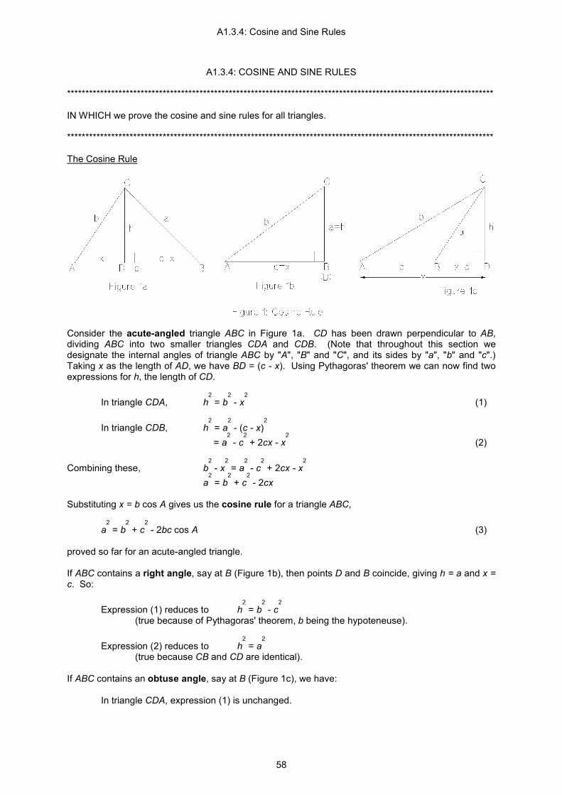
A1.3.4: Cosine and Sine Rules
58
A1.3.4: COSINE AND SINE RULES ******************************************************************************************************************** IN WHICH we prove the cosine and sine rules for all triangles. ******************************************************************************************************************** The Cosine Rule
Consider the acute-angled triangle ABC in Figure 1a. CD has been drawn perpendicular to AB, dividing ABC into two smaller triangles CDA and CDB. (Note that throughout this section we designate the internal angles of triangle ABC by "A", "B" and "C", and its sides by "a", "b" and "c".) Taking x as the length of AD, we have BD = (c - x). Using Pythagoras' theorem we can now find two expressions for h, the length of CD. In triangle CDA, h
2 = b
2 - x
2 (1)
In triangle CDB, h
2 = a
2 - (c - x)
2
= a2 - c
2 + 2cx - x
2 (2)
Combining these, b
2 - x
2 = a
2 - c
2 + 2cx - x
2
a2 = b
2 + c
2 - 2cx
Substituting x = b cos A gives us the cosine rule for a triangle ABC, a
2 = b
2 + c
2 - 2bc cos A (3)
proved so far for an acute-angled triangle. If ABC contains a right angle, say at B (Figure 1b), then points D and B coincide, giving h = a and x = c. So:
Expression (1) reduces to h2 = b
2 - c
2
(true because of Pythagoras' theorem, b being the hypoteneuse). Expression (2) reduces to h
2 = a
2
(true because CB and CD are identical). If ABC contains an obtuse angle, say at B (Figure 1c), we have: In triangle CDA, expression (1) is unchanged.

A1.3.4: Cosine and Sine Rules
59
In triangle CDB, h2 = a
2 - (x - c)
2
= a2 - x
2 + 2cx - c
2
which is equivalent to expression (2). Since as we saw in section A1.2.3 all triangles are either acute-angled, right-angled or obtuse-angled, results (1) and (2) hold for all possible triangles ABC. Hence the cosine rule (3) which follows from them is true for all triangles. Rearranging the lettering cyclically gives us the three forms a
2 = b
2 + c
2 - 2bc cos A
b2 = c
2 + a
2 - 2ac cos B
c2 = a
2 + b
2 - 2ab cos C
If the angle in question is a right angle the formula reduces to Pythagoras' theorem since cos π/2 = 0. The cosine rule was first derived by the great Persian mathematician Jamshid al-Kashi (c.1380-1429). The Sine Rule
Consider now the acute-angled triangle ABC in Figure 2a. As before, CD has been drawn perpendicular to AB. We can now find two expressions for h, the length of CD. In triangle CDA, sin A = h/b, h = b sin A In triangle CBD, sin B = h/a h = a sin B So b sin A = a sin B,
B
bA
asinsin
= (4)
If we draw another perpendicular AE of length l from point A to BC (Figure 2b), we have similarly: In triangle AEC, l = b sin C In triangle AEB, l = c sin B Hence
C
cB
bsinsin
= (5)
Results (4) and (5) together give us the sine rule for a triangle ABC:

A1.3.4: Cosine and Sine Rules
60
C
cB
bA
asinsinsin
== (6)
proved so far for an acute-angled triangle. If instead ABC contains a right angle, say at B (Figure 2b), we have a = b sin A and c = b sin C Since sin B = sin π/2 = 1, we can multiply by it to give a sin B = b sin A and c sin B = b sin C from which results (4) and (5) follow. Finally if ABC contains an obtuse angle, say at B, we draw perpendiculars CD and AE as before, but this time to the extensions of AD and CB respectively (Figure 2c). By theorem (5) in section A1.2.2, ∠ CBD = ∠ ABE = π - B. In triangle CDA, h = b sin A In triangle CDB, h = a sin (π - B) = a sin B (see the sine graph in section A1.3.1 Figure 4) from which result (4) follows. Similarly In triangle EAC, l = b sin C In triangle EAB, l = c sin (π - B) = c sin B from which result (5) follows. As before with the cosine rule, we have now exhausted all possible types of triangle. Hence expressions (4) and (5) hold for all triangles ABC and so the sine rule (6) which follows from them is true for all triangles.

A1.4.1: Factorials
61
ACT 1 SCENE 4: SPECIAL BINOMIAL THEOREM
A1.4.1: FACTORIALS ******************************************************************************************************************** IN WHICH we discover the factorials of nonnegative integers. ******************************************************************************************************************** We define the mathematical symbol for factorials, "!", as follows:
n!, where n is a positive integer, means "n times all the other integers smaller than n down to 1". That is,
n! = n × (n-1) × (n-2) ×...× 1 (1)
So for instance
1! = 1 = 1 2! = 2 × 1 = 2 3! = 3 × 2 × 1 = 6 4! = 4 × 3 × 2 × 1 = 24
So that n! can be specified for all nonnegative integers, we define for completeness the convention
0! = 1 (2) whose primary justification is that it works out very well in practice. Then
"3!" is read as "factorial three" or "three factorial". It will be seen that each factorial n! can be defined recursively, that is, in terms of its predecessor, (n-1)!:
n! = n × (n-1)! Further, we can multiply and divide factorials by each other, as:
5! 3! = 5 × 4 × 3 × 2 × 1 × 3 × 2 × 1 = 720, while, more interestingly,
2045123
12345!3!5
=×=××
××××=
The notation n! was first introduced in an algebra text of 1808 by a little known mathematician called Christian Kramp. We observe that the factorials of even small integers grow rapidly into large numbers. Continuing the sequence given above we have:
5! = 120 6! = 720 7! = 5040 8! = 40320 9! = 362888 10! = 3628800

A1.4.1: Factorials
62
Like the exponents of section A1.1.5, the factorial, besides being a convenient form of shorthand, is one of the essential building blocks of mathematics. This is not least because it is our basis for calculating the binomial coefficients we are about to consider. For most of this drama the above definition in terms of integers will suffice. However, in Epilogue E3 we shall extend the concept to all real numbers (the Γ function), and give Stirling's formula for approximating the factorials of large integers.

A1.4.2: Permutations and Combinations
63
A1.4.2: PERMUTATIONS AND COMBINATIONS ******************************************************************************************************************** IN WHICH we learn in how many ways we can choose and arrange k different objects out of a set of n. ******************************************************************************************************************** There are many situations when we may wish to estimate the likelihood or probability that one particular outcome may happen out of a number of different possibilities. It turns out that the mathematics of calculating such things reappears in many different guises. Let us proceed by question and answer. Q1: In how many different ways can we order (arrange) a set of n different objects?
A1: Let us start with an example. If there are n=3 different objects A, B and C, possible arrangements are
1st choice (from 3): A B C / \ / \ / \ 2nd choice (from 2): B C A C A B | | | | | | 3rd choice (from 1): C B C A B A
giving the permutations ABC, ACB, BAC, BCA, CAB, CBA, that is, 3 × 2 × 1 = 6 in all. Permutations are simply arrangements. Generalising, if we have n different objects, we can choose
the first in n ways, the second in n-1 ways, the third in n-2 ways,
and so on until the nth object, which we can choose in only 1 way. So in all there are n × (n-1) × (n-2) ×...× 1 different ways of arranging the objects, which we learned in the last section to write neatly as n! ways. Q2: In how many different ways can we choose k objects out of n when the order matters? A2: This case begins the same way as answer A1, but instead of arranging all n objects, we stop after choosing the first k. Suppose that there are n=8 objects, and we want to know how many different ways there are of arranging k=3 of them. We can choose
the first in 8 ways, the second in 7 ways, and the third and last in 6 ways.
So we have 8 × 7 × 6 = 336 different permutations. Is there a neat way of expressing this, using factorials as before? There is. We can write the answer as
!5!8
1234513345678678 =
×××××××××××
=××
where we have written 5! because 5 = 8 - 3 (= n - k). By cancelling out the last five terms of 8! we have effectively selected the first three.

A1.4.2: Permutations and Combinations
64
We can generalise this. The number of permutations of k terms selected out of n is written as
nP
k = n(n-1)(n-2)...(n-k+1) (1)
)1)(2)(3)...((
)1)(2)(3)...()(1)...(2)(1(kn
knknnnn−
−+−−−=
So nP
k
)!(!kn
n−
= (2)
In our example we found 8P
3 336
)!38(!8
=−
=
We can now see Q1 as a special case in which k=n, giving
nP
n !
)!(! nnn
n=
−= (3)
since from A1.4.1 (2) we have 0! = 1. Q3: In how many different ways can we choose k objects out of n when the order does not matter? A3: We describe cases like this, when the order does not matter, as combinations. So in answer A1 above, the single combination, A, B and C, gives rise to the six permutations - different arrangements - that we listed there. To answer Q3 we divide the number of possible permutations of k from n, which we found in answer A2 to be
nP
k, by the number of different orders in which the chosen k objects can be arranged - which
from answer A1 we know to be k!. We then write the result as nC
k. This gives
nC
k
!kPk
n= (4)
nC
k is the number of combinations - choices - of k objects that can be made from a total of n, no
distinction being made between different arrangements. We can compute it from equation (1) as
nC
k
!)1)...(2)(1(
kknnnn +−−−
= (5)
or from (2) as
nC
k
)!(!!
knkn−
= (6)
Equations (5) and (6) are equivalent definitions of
nC
k, and are valid for 0 ≤ k ≤ n. Otherwise the
definition is adopted, If k < 0 or k > n,
nC
k = 0 (7)
This factorial expression was known in India in AD 850 and in the West in 1321.

A1.4.2: Permutations and Combinations
65
Symmetrical Property We can rewrite (6) as
nC
m
)!(!!
mnmn−
Substituting m = n-k gives
nC
n-k
!)!(!
kknn
−=
yielding the symmetrical property
nC
n-k =
nC
k, 0 ≤ k ≤ n (8)
Values of
nC
k
We deduce from relations (5), (6) and (7):
0C
0 1
11
== (from (2), recalling that 0! = 1)
1C
0 ,
111×
= 1C
1 =
1C
0 = 1 (from (7))
2C
0 1
212
=×
= , 2C
1 2
112
=×
= , 2C
2 =
2C
0 = 1
3C
0 1
616
=×
= , 3C
1 3
216
=×
= = 3C
2,
3C
3 =
3C
0 = 1
4C
0 1
24124
=×
= , 4C
1 4
6124
=×
= , 4C
2 6
2224
=×
= ,
4C
3 =
4C
1 = 4,
4C
4 =
4C
0 = 1
Let us now draw up a table of n, k, and the values calculated:
k: 0 1 2 3 4 ───┼──────────────────────────────────────── │
n: 0 │ 1 1 │ 1 1 2 │ 1 2 1 3 │ 1 3 3 1 4 │ 1 4 6 4 1
As if by magic, we have begun to recreate the figurate numbers that we met in the Prologue! (In this format it is sometimes called the Chinese triangle.) So the number of combinations of
nC
k of k
objects taken from n turns out to be in all cases an element of Pascal's triangle. This identification was first made by Cardano in 1570. The significance of it will become clear as we move on.

A1.4.3: Special Binomial Theorem
66
A1.4.3: SPECIAL BINOMIAL THEOREM ******************************************************************************************************************** IN WHICH we meet the simple or special binomial theorem, discovering a third manifestation of Pascal's triangle. ******************************************************************************************************************** Binomial Expansion Let us now examine what happens as we expand by successive multiplication the expression (a + x)
n,
called binomial expansion on account of the two quantities within the brackets. In each case we wish to determine particularly the binomial coefficients, in order, of the various terms in a and x. When n = 0, (a + x)
n = (a + x)
0 = 1. (1)
There is just one coefficient, 1. When n = 1, (a + x)
n = (a + x)
1 = a + x. (2)
There are two coefficients, 1 and 1. For n = 2, we multiply (a + x)(a + x) as: a + x a + x a
2 + ax
ax + x2
a2 + 2ax + x
2 = (a + x)
2 (3)
There are three coefficients, 1, 2, and 1. For n = 3, we multiply (a + x)
2(a + x) as:
a
2 + 2ax + x
2
a + x a
3 + 2a
2x + ax
2
a2x + 2ax
2 + x
3
a3 + 3a
2x + 3ax
2 + x
3 = (a + x)
3 (4)
There are four coefficients, 1, 3, 3, and 1. When n = 4, we multiply (a + x)
3(a + x) as:
a
3 + 3a
2x + 3ax
2 + x
3
a + x_ a
4 + 3a
3x + 3a
2x
2 + ax
3
a3x + 3a
2x
2 + 3ax
3 + x
4
a4 + 4a
3x + 6a
2x
2 + 4ax
3 + x
4 = (a + x)
4 (5)
There are five coefficients, 1, 4, 6, 4, and 1. These expansions into powers of x are called polynomials in x (q.v. G3).

A1.4.3: Special Binomial Theorem
67
What we have been doing is to obtain the expansion (a + x)n for each new n by multiplying the
expansion of (a + x)n-1
first by a, then by x, and adding like terms. This process is illustrated in Figure 1.
Picking out the coefficients, we have for successive values of n,
n = 0, 1 n = 1, 1 1 n = 2, 1 2 1 n = 3, 1 3 3 1 n = 4, 1 4 6 4 1
which we recognise as Pascal's triangle. In this context we identify the kth term in the nth row as the
binomial coefficient
kn
, where both n and k are counted from 0 upwards.
So for instance
32
= 3;
43
= 6;
n1
and
nn
are always 1.
The process of adding like terms in Figure 1 by which we accomplished this expansion enables us to generalise: each term is the sum of the two immediately above it:
kn
=
−−
11
kn
+
−kn 1
(6)
For instance putting n = 4 and k = 3, we have
23
+
33
= 3 + 1 = 4 =
34
We first noticed this property in the Prologue. Equation (6) is the fundamental and defining property of Pascal's triangle. It enables us to continue the table we began in A1.4.2:

A1.4.3: Special Binomial Theorem
68
k: 0 1 2 3 4 5 6 7 8 ───┼───────────────────────────────────── │
n: 0 │ 1 1 │ 1 1 2 │ 1 2 1 3 │ 1 3 3 1 4 │ 1 4 6 4 1 5 │ 1 5 10 10 5 1 6 │ 1 6 15 20 15 6 1 7 │ 1 7 21 35 35 21 7 1 8 │ 1 8 28 56 70 56 28 8 1
and so forth. (More rows are given in Interlude I1.1.1 Figure 1.) The Magic of Pascal's Triangle And so we have now found a third way of generating Pascal's triangle. In the Prologue we used additive relations involving arithmetic sequences such as the units, counting numbers, triangular numbers, triangular pyramid numbers and so forth. In A1.4.2 (6) we recreated it from the factorial expression by which we computed the number of combinations of k objects taken from n as
nC
k
)!(!!
knkn−
= (7)
Now we have found by multiplication that the same Pascal's triangle supplies the coefficients of the binomial expansion of (a + x)
n. This is magic indeed! So we have the exceedingly important identity
nC
k
≡
kn
, integers 0 ≤ k ≤ n (8)
Both expressions designate the elements of Pascal's triangle. However, whereas in order to obtain values of the triangle for n and k from equation (6) we would have to compute all previous rows, equation (7) enables us to calculate them directly from their factorials. This is not just a computational convenience. It also enables us to explore the manifold properties of Pascal's triangle much more widely. In particular we can rewrite A1.4.2 equations (5), (6) and (8) respectively as, for all integers 0 ≤ k ≤ n,
kn
= !
)1)...(2)(1(k
knnnn +−−− (9)
kn
= )!(!
!knk
n−
(10)
and
− kn
n =
nn
(11)
So we have

A1.4.3: Special Binomial Theorem
69
0n
= 1,
1n
= n, ,!2
)1(2
−=
nnn ,
!3)2)(1(
3−−
=
nnnn…,
,!2
)1(2
−=
−
nnnn
− 1n
n = n,
nn
= 1 (12)
Terms for k outside this range are all zero since from A1.4.2 (7),
for k < 0 and k > n,
kn
(n) = 0 (13)
Proof of Identity (8) Identity (8) can be proved by demonstrating that relation (6) holds if we replace each term by its factorial equivalent given in equation (7). That is,
)!1(!
)!1()!()!1(
)!1()!(!
!knk
nknk
nknk
n−−
−+
−−−
=−
After cancellation of like terms this reduces to
k
knkn −
+≡ 1
which is a correct identity for 0 < k ≤ n as required; the case for k=0 is true by definition. Identity (8) follows. Identity (8) also supplies the power of the binomial theorem which we can now define. (Special) Binomial Theorem The (special) binomial theorem gives us a simple way of writing down the expansion of (a + x)
n
without every time having to multiply it out (as we did at the start of this section). It states that for integers 0 ≤ k ≤ n,
(a + x)n =
0n
an +
1n
an-1
x +
2n
an-2
x2 +
3n
an-3
x3 +...
+
kn
an-k
xk +...+
− 2n
na
2x
n-2 +
− 1n
nax
n-1 +
nn
xn (14)
where
kn
are the elements of Pascal's triangle. So for instance by putting n = 4, equation (14) yields
equation (5) above. Since on account of identity (8) we can compute these as shown in relations (12), we can rewrite the theorem as
...!3
)2)(1(!2
)1()( 33221 +−−
+−
++=+ −−− xannnxannxnaaxa nnnnn
nnnkkn xnaxxannxaknk
n++
−++
−+ −−− 122
!2)1(...
)!(!! (15)

A1.4.3: Special Binomial Theorem
70
We note that
(1) There are n+1 terms in each expansion, from k=0 to k=n. (2) As we move from left to right, the powers of a decrease by one with each term, and the
powers of x increase by one. So the sum of the powers (n-k) + k is always the row number n.
(3) The (k + 1)th term is the term in a
n-kx
k.
(4) The special case a = x = 1 gives
(1 + 1)n =
0n
+
1n
+
2n
+
nn
= 2n (16)
That is, the sum of each row n of Pascal's triangle is 2
n.
(5) In consequence, the sum of all previous rows before row n is 2
0 + 2
1 + 2
2 + 2
3 +...+ 2
n-1 = 2
n - 1 (17)
Σ Notation We can write this form of the binomial theorem more concisely as
kknn
k
n xakn
xa −
=∑
=+
0
)( (18)
where Σ is a symbol meaning "the sum of...", and so ∑=
n
k 0
or, more fully, ∑=
=
nk
k 0
means
"the sum of...for all values of k starting when k equals 0 and finishing when k equals n, going up in steps of 1".
Hence ∑=
n
kkn
0
an-k
xk means
"the sum of all terms "
kn
an-k
xk" where k varies from 0 to n in steps of 1".
It can be seen that Σ is a very powerful and convenient form of abbreviation. It is particularly useful when the number of terms to be summed is infinite. Proof of the Special Binomial Theorem When we multiply out (a + x)
n = (a + x)(a + x)(a + x)...(a + x)
we obtain a sequence of individual terms of the form a
n-rx
r, by choosing the x from r of the brackets
and the a from the remaining n-r brackets. So the number of ways of getting an-r
xr is the number of
ways of choosing r brackets from n, that is, nC
r, which from identity (8) is
rn
.

A1.4.3: Special Binomial Theorem
71
Binomial Theorem Spreadsheet The reader may generate individual rows of Pascal's triangle using the binomial theorem spreadsheet described in Sideshow S2, in which the exponent n is denoted "r". If integer values of n ≥ 0 are
entered under "r" at the top, the values of row n of the triangle will appear in the column headed "
kr
",
corresponding to the values of k in the left hand column. Subsequent columns show how the expansion of (a + x)
n is computed term by term.
Binomial Coefficient Notation
The notation
kn
was introduced in this form by Andreas von Ettingshausen in 1826 but was very
similar to that of Euler, to whom we owe so much of our present notation, including, to a large extent, the symbols e, i and π themselves (Boyer and Merzbach (B4) pp.493-5).
But we must be careful not to confuse
kn
with
kn , which is a fraction.
Terminology This form of the binomial theorem applies when the exponent n is restricted to the nonnegative integers, in which case the expansion has a finite number of coefficients taken from a row of Pascal's triangle. However, the same name, binomial theorem, is also conventionally used when the exponent is not so restricted, but may be any real number, including negative or fractional. In this case the expansion is called a binomial series, and may have an infinite number of terms, whose coefficients do not always derive from Pascal's triangle. To resolve this ambiguity we refer in this drama to the restricted case, described in this section, as the special binomial theorem, and to the unrestricted case, described in Act 3 Scene 2, as the general binomial theorem. (Relativity addicts will recall how Einstein's special theory of relativity led to his more comprehensive general theory.) Between the two lies the case where n is a negative integer, when the expansion is an infinite series of terms whose coefficients are drawn from a column of Pascal's triangle. We propose to call this the intermediate binomial theorem, and shall discuss it in Interlude I1.2.1. To summarise: Theorem Exponent Expansion Special Integer n ≥ 0 Row of Pascal's triangle (finite polynomial) Intermediate Integer n < 0 Column of Pascal's triangle (infinite series) General (a) Any integer As above (b) Non-integer Infinite series, not in Pascal's triangle In its special form this theorem was known to the Persian al-Kashi in Samarkand by 1427 at the latest. In Europe it was essentially given for the first time by Cardano in 1570. The general form was discovered by Newton in 1664/5 en route to his discovery of the calculus. In fact the special binomial theorem plays an important part in the differential calculus, as we shall see in A2.1.1. We shall further revisit Pascal's triangle in Interlude I1.2.4. In A3.2.2 we shall detail more of the properties of the binomial coefficients.

A1.4.4: Binomial Probability
72
A1.4.4: BINOMIAL PROBABILITY ******************************************************************************************************************** IN WHICH we learn how to compute probabilities using the special binomial theorem. ******************************************************************************************************************** The quantities a and x in the binomial expansion (A1.4.3 (18))
(a + x)n = ∑
=
n
kkn
0
an-k
xk, integer n ≥ 0 (1)
can of course be replaced by others in order to obtain binomial expansions of similar expressions. For instance the expansion of (2b + 3c)
3 is obtained from the expression for (a + x)
3 by substituting 2b for
a and 3c for x, giving (2b + 3c)
3 = (2b)
3 + 3(2b)
2(3c) + 3(2b)(3c)
2 + (3c)
3
= 8b
3 + 36b
2c + 54bc
2 + 27c
3
When a + x = 1, the theorem has applications in the realm of probability. Notationally a is commonly replaced by p here and x by q, where p is the probability of something happening on a single attempt q is the probability of it not happening on a single attempt = 1 - p n is the number of attempts
(p + q)n = ∑
=
n
kkn
0
pn-k
qk (2)
In this case the sum of all possible outcomes is (p + q)
n = 1
n = 1.
The typical term
kn
pn-k
qk
represents the probability of p happening n-k times and q (or, not p) happening k times, in n attempts. Let us look at the probability of throwing various numbers of sixes when we toss a fair die four times. If
p is the probability of throwing a six in one toss, = 1/6 q is the probability of not throwing a six, = 1-p = 5/6 n = 4 tosses
Then by the special binomial theorem we can expand (2) above as
(1/6 + 5/6)4 = ∑
=
4
0
4
kk
(4) (1/6)4-k
(5/6)k

A1.4.4: Binomial Probability
73
where from row 4 of Pascal's triangle the binomial coefficients for n=4 are 1 4 6 4 1 So (1/6 + 5/6)
4 = (1/6)
4 + 4(1/6)
3(5/6) + 6(1/6)
2(5/6)
2 + 4(1/6)(5/6)
3 + (5/6)
4
= 0.000772 + 0.015432 + 0.115741 + 0.385802 + 0.482253 to six decimal places, the sum being 1. (This may be confirmed using the binomial theorem spreadsheet described in Sideshow S2.) The computed terms represent in order the probability of obtaining in four throws
4 sixes : 0.000772 (k = 0, n-k = 4) 3 sixes : 0.015432 (k = 1, n-k = 3) 2 sixes : 0.115741 (k = 2, n-k = 2) 1 six : 0.385802 (k = 3, n-k = 1) 0 sixes : 0.482253 (k = 4, n-k = 0)
So the term of the expansion in which the exponent of p is n-k tells us the probability of p happening n-k times in n attempts (and not-p happening all the other k times).
However, if we only need a single term, we do not need to compute the entire expansion. For instance, suppose
p is the probability of a fair die showing a 1 or a 2 in a single throw, (= 1/6 + 1/6 = 1/3) q is the probability of its showing a 3, 4, 5 or 6 (= 2/3)
To compute the probability of showing a 1 or a 2 exactly four times in n=6 throws we need to compute the term for which the exponent n-k of p is 4, giving us the exponent k of q as 6-4 = 2. This term is
kn
pn-k
qk =
26
p4 q
2
where from Pascal's triangle
26
= 15. The required calculation is therefore
15 (1/3)4 (2/3)
2
729415 ×
= ≈ 0.082305

A1.5.1: Quadratic Equations
74
ACT 1 SCENE 5: i
A1.5.1: QUADRATIC EQUATIONS ******************************************************************************************************************** IN WHICH we learn two methods of solving quadratic equations. ******************************************************************************************************************** A quadratic equation is a polynomial equation (q.v. G3) of order 2, that is, whose highest power is 2. Its typical form is ax
2 + bx + c = 0
Its graph is a parabola of which examples may be found in the figures for section A1.5.2; the parabola is one of the conic sections (Sideshow S3). Because it is of order 2, it has a maximum of 2 solutions or roots. The roots are the values of x for which the polynomial expression (q.v. G3) ax
2 + bx + c takes on the value zero.
These may be found in two principal ways as follows. Method 1: Factorising the quadratic expression Given a quadratic equation ax
2 + bx + c = 0
(1) Remove factors which are common to a, b, and c. (2) Look for two numbers α and β such that
αβ = ac, α + β = b (3) Write down the pairs (a, α), (a, β) (4) Divide each pair by its highest common factor to get (r, s) and (t, u) (5) The factors are (rx + s) and (tx + u). So (rx + s)(tx + u) = 0 which is true when either factor is zero. This tells us that either rx + s = 0 and so x = - s/r or tx + u = 0 and so x = - u/t
These two values of x are the required roots.
This method depends on your being able to find α and β, which is not always easy, or even always possible. So more often we use Method 2.

A1.5.1: Quadratic Equations
75
Method 2: The Quadratic Formula The quadratic formula is based on the method of completing the square which was known to the Babylonians. It is derived as follows: Given a quadratic equation ax
2 + bx + c = 0 (1)
(1) Divide through by a: x
2 + (b/a)x = - c/a (2)
This must be possible since by definition a ≠ 0. (2) We now create a perfect square on the left hand side (LHS) by the addition of a suitable third (constant) term. We use as our model the perfect square
(x + y)2 ≡ x
2 + 2xy + y
2
in which the third term (y
2) on the right hand side (RHS) can be generated from the second
term (2xy) by taking its coefficient (2y), dividing by two (to get y), and squaring the result. Thus required constant term = (half the coefficient of x)
2
Similarly, the LHS of equation (2) will become a perfect square if we add to it (b/2a)
2. Doing
the same to the RHS as well gives
ac
ab
abx
abx −
=
++22
2
22 (3)
Simplifying,
ac
ab
abx −
=
+22
22
2
2
44
aacb −
=
This technique is known as completing the square. (3) Taking the square root of both sides, and remembering that a square root may be positive or negative (we write ± the root to indicate this):
x + ab2
= a
acb2
42 −±
x = a
acbb2
42 −±− (4)
which is the required formula for solving quadratic equations such as (1). The two roots are

A1.5.1: Quadratic Equations
76
a
acbb2
42 −+− and a
acbb2
42 −−−
Alternatively, a less known but equivalent formula, which is sometimes used to minimise computational errors, is the following:
x = acbb
c
4
22 −±−
(5)
The reader may like to amuse him/herself by demonstrating that these two formulae are in fact equivalent. Sum and Product of the Roots If the two roots are x
1, x
2 then from the definition of root,
(x - x
1) = 0 and (x - x
2) = 0
So (x - x
1)(x - x
2) = 0
x
2 - (x
1 + x
2)x + x
1x
2 = 0
Multiplying by a ax
2 - a(x
1 + x
2)x + ax
1x
2 = 0
and comparing coefficients with the original equation
ax
2 + bx + c = 0
gives x
1 + x
2 = -b/a (sum of the roots) (6)
x
1x
2 = c/a (product of the roots) (7)
This method can be usefully extended to polynomials of higher orders.

A1.5.2: The Imaginary Number i
77
A1.5.2: THE IMAGINARY NUMBER i ******************************************************************************************************************** IN WHICH we meet i, the square root of minus one and basis of complex numbers. ******************************************************************************************************************** Formulae (4) and (5) in section A1.5.1 for solving quadratic equations work very well if the expression b
2 - 4ac within the square root - known as the discriminant - is positive. The quadratic will then have
two perfectly normal, real, solutions, one using + acb 42 − , and the other - acb 42 − .
This corresponds to the parabola cutting the x axis in two distinct places (Figure 1) which represent its real roots. Even if the discriminant is zero, we get one real root, or rather, two equal real roots (the x axis is a tangent (q.v. G4, sense 1) to the curve, Figure 2). But what if it is negative?
This means that the x axis does not cut the curve at all (Figure 3), and there are no real roots. So to solve such an equation we have to make an invention. What we do is to invent a special, 'imaginary' number i such that
i2 = -1
The need for a number with this property was first recognised by the Renaissance Italian mathematicians Cardano and after him Bombelli (1572) in their grapplings not with quadratic equations but with cubics, which we shall examine in A1.5.3. (As Nahin (B1), p.25, explains, the early mathematicians, when faced with equations such as x
2 + 1 = 0,
did not see a need for a number such as 1− . They merely dismissed such equations as impossible.) This number was designated "i" by Euler in 1737, and is now universally known as this except by physicists, who call it "j" (i being reserved for current in electronics). For centuries this invention baffled mathematicians so much (as negative and irrational numbers had before it) that they called it "imaginary" - and the name has stuck. Let us play with it. By successive multiplication,
i2 = -1
i3 = -1 × i = -i

A1.5.2: The Imaginary Number i
78
i4 = -i × i = 1
i5 = 1 × i = i
and so on forever, cyclically. Further,
4i2 = -4 . So 4− = 24i = 2i.
Generally, 2q− is qi.
So if our discriminant is negative, our quadratic still has two roots, but they contain a term which is "imaginary" - it involves i. They are found by applying the quadratic formula, finding the discriminant, and taking its square root in terms of i as just explained. Here is an example:
We want to solve x
2 - 2x + 5 = 0
that is to say the coefficients are a = 1 b = -2 c = 5
Applying formula (4) from section A1.5.1 we have
x = 12
51442×
××−±
The discriminant is 4 - 4 × 1 × 5 = -16 . This has its square root equal to 4i, so
242 ix ±
=
2
42 i+= or
242 i−
= 1 + 2i or 1 - 2i which can be checked by putting x equal to each of these values and demonstrating that our original equation holds good.
* * * * * We have now met the imaginary number i, the second of our great protagonists. So yet again, an advance in our mathematical understanding has introduced us to a new type of number. We recall from A1.1.2 how
Addition first came with the integers, Subtraction gave us zero and negative numbers, Division gave us rational numbers,
while in A1.2.5 Pythagoras' theorem led us to the irrationals. Now quadratic equations have brought us to i and the complex numbers which like 1 + 2i and 1 - 2i in the above example combine a real number with a a multiple of i. These are the subject of section A1.5.4. In fact the term "imaginary" is a misnomer. Imaginary numbers are no more unreal than negative ones, and they are arrived at for very similar reasons: they do a mathematical job which needs doing. In fact they do very much more than enable us to solve quadratic or cubic equations in mathematics;

A1.5.2: The Imaginary Number i
79
they are also indispensable in physics. Arguably it is the name "real number" which is truly misleading.

A1.5.3: Cubic Equations - Cardano's Formula
80
A1.5.3: CUBIC EQUATIONS - CARDANO'S FORMULA ******************************************************************************************************************** IN WHICH we learn how to solve cubic equations. Notable source: Nahin (B1), chapter 1. ******************************************************************************************************************** Historical Introduction Paradoxically, it was not through quadratic equations that i was first discovered. i was first explored and understood by the Renaissance Italian mathematicians Scipione del Ferro (1465-1526), Niccolo Tartaglia (1500-77), Girolamo Cardano (1501-76) and Rafael Bombelli (1526-72), in their endeavours to solve the general cubic. The General and Reduced Cubic A cubic equation is a polynomial equation (q.v. G3) of order 3, that is, whose highest power is 3. Its typical form is x
3 + ax
2 + bx + c = 0 (1)
(If the coefficient of x
3 is not initially 1, equation (1) is obtained by dividing throughout by that
coefficient beforehand.) In order to solve it we first remove the quadratic (x
2) term by writing
x = y - a/3 (2) to get the depressed or reduced cubic y
3 + 3py + 2q = 0 (3)
where 3p = -a
2/3 + b
2q = 2(a/3)3 - ab/3 + c
We then solve equation (3) for y, using the method first discovered by del Ferro, rediscovered by Tartaglia and finally published by Cardano in his book Ars Magna in 1545. The First Root in y: "Cardano's Formula" Del Ferro's insight was to write y as the sum y = u + v (4) Equation (3) then becomes (u + v)
3 + 3p(u + v) + 2q = 0
u3 + 3u
2v + 3uv
2 + v
3 + 3p(u + v) + 2q = 0
u3 + v
3 + 3(uv + p)(u + v) + 2q = 0 (5)

A1.5.3: Cubic Equations - Cardano's Formula
81
Equation (5) may then be understood as the simultaneous equations uv + p = 0 (6) u
3 + v
3 + 2q = 0 (7)
in terms of which (3) can be re-expressed as y
3 - 3uvy - u
3 - v
3 = 0 (8)
From (6), v = -p/u Substituting in (7),
023
33 =+− q
upu
u
6 + 2qu
3 - p
3 = 0, (9)
a quadratic equation in u
3 which we solve with the quadratic formula A1.5.1 (4) to give
=3u2
442 32 pqq +±−
Taking the positive root,
323 pqqu −+−= (10)
3 32 pqqu −+−= (11) Since from (7), v
3 = -2q - u
3,
=3v 32 pqq −−− (12)
3 32 pqqv −−−= (13) So from (4) we have the first root y
1 = u + v
= 3 32 pqq −+− + 3 32 pqq −−− (14) now called Cardano's formula. It may sometimes be more conveniently expressed as
=1y 3 32 pqq −+− - 3 32 pqq −+ (15) Second and Third Roots in y However, we know from the fundamental theorem of algebra (q.v. G3) that there are two more roots,

A1.5.3: Cubic Equations - Cardano's Formula
82
which we shall call y2 and y
3. To obtain them we now factorise the reduced cubic (8) as
(y - y
1)(y - y
2)(y - y
3) = y
3 - 3uvy - u
3 - v
3 = 0
where we already have y
1 = u + v. Long division of the central expression by (y - u - v) gives us the
quadratic y
2 + (u + v)y + u
2 - uv + v
2 = 0
to which the quadratic formula gives the solutions
2
)(3)(2
vuivuy −++−= (16)
2
)(3)(3
vuivuy −−+−= (17)
Roots in x The roots of the original equation (1) in x are obtained by reversing the transformation (2). Thus x
1 = y
1 + a/3 (18)
and so on for x
2 and x
3.
Nature of the Roots y
1 is always real. The nature of y
2 and y
3 depends on the discriminant q
2 + p
3 in equations (10) and
(12):
If q2 + p
3 > 0, u and v are real, y
2 and y
3 are complex conjugates (that is, their real parts are
the same, but their imaginary parts have opposite signs). If q
2 + p
3 = 0, u and v are real, y
2 and y
3 are real and equal.
If q2 + p
3 < 0, u and v are complex, y
2 and y
3 are real and different. This is the 'irreducible
case' (see below).
The same relations are true of the roots in x. 'Irreducible' Case When q
2 + p
3 < 0, its square root is complex, and so Cardano's formula (15) requires us to take the
cube root of a complex number, a problem which remains even after manipulation. Hence Cardano called this case 'irreducible'. However, Bombelli showed in his Algebra of 1572 that the solution given by Cardano's formula is correct, albeit difficult to evaluate. All three roots in such a case are real. Example 3 below is such a case. Example 1 We wish to solve 3x
3 + 18x
2 - 180x - 1248 = 0 (19)
Divide by 3 to obtain unit coefficient of x
3:

A1.5.3: Cubic Equations - Cardano's Formula
83
x
3 + 6x
2 - 60x - 416 = 0 (20)
from which a = 6. Following equation (2) we substitute x = y - 2 (21) which reduces (20) to y
3 - 72y - 280 = 0 (22)
Comparison with equation (3) gives p = -24, q = -140 p
3 = -13824, q
2 = 19600
q
2 + p
3 = 5776
Since this > 0, we have one real and two imaginary roots. This is borne out by Figure 1.
-15 -10 -5 0 5 10 15
y
-600
-500
-400
-300
-200
-100
100
200
300
400f(y) Figure 1
Reduced cubic f(y) = y^3 - 72y - 280 q^3 + p^2 > 0: 1 real root 2 complex roots
From (11),
6216761405776140 333 ==+=+=u From (13)
464761405776140 333 ==−=−=v Hence from (14)

A1.5.3: Cubic Equations - Cardano's Formula
84
y
1 = u + v = 10
and from (16) and (17)
352
)46(3)46(2 iiy +−=
−++−=
352
)46(3)46(3 iiy −−=
−−+−=
Reversing substitution (21), x
1 = y
1 - 2 = 8
x2 = y
2 - 2 = -7 + i 3
x3 = y
3 - 2 = -7 - i 3
Example 2 We wish to solve the reduced cubic y
3 - 12y - 16 = 0 (see Figure 2)
-5 -4 -3 -2 -1 0 1 2 3 4 5
y
-100
-80
-60
-40
-20
20
40
60f(y) Figure 2
Reduced cubic f(y) = y^3 - 12y - 16 q^2 + p^3 = 0: 3 real roots (2 equal)
Comparison with equation (3) gives p = -4, q = -8 p
3 = -64, q
2 = 64
q2 + p
3 = 0

A1.5.3: Cubic Equations - Cardano's Formula
85
We have three real roots, two of which are equal. This is borne out by Figure 2. From equations (11) and (13), u = v = 3 8 = 2 Hence from (14), (16) and (17), y
1 = u + v = 4,
y2 = y
3 = -(u + v)/2 + 0i = -2
Example 3 We wish to solve the reduced cubic y
3 - 15y - 4 = 0
Comparison with equation (3) gives p = -5, q = -2 The discriminant q
2 + p
3 = 4 - 125 = -121 < 0. This is therefore Cardano's 'irreducible' case, which will
have three real roots as illustrated in Figure 3.
-6 -4 -2 0 2 4 6
y
-150
-100
-50
50
100
150f(y) Figure 3
Reduced cubic f(y) = y^3 - 15y - 4'Irreducible' case: q^2 + p^3 < 0, 3 different real roots
Equations (11) and (13) yield
33 1121212 iu +=−+= (23)
33 1121212 iv −=−−= (24)

A1.5.3: Cubic Equations - Cardano's Formula
86
which involve taking the cube root of a complex number, something Cardano was unable to do. We shall show how this can be done in Example 3 of A1.5.8. How such an 'irreducible' case could be solved without recourse to complex numbers at all was later discovered by Viète, as we shall see in section A1.5.9.

A1.5.4: Complex Numbers
87
A1.5.4: COMPLEX NUMBERS ******************************************************************************************************************** IN WHICH we explore the geometry and algebra of complex numbers. Notable source for Wessel's equation: Nahin (B1), pp.48-53. ******************************************************************************************************************** Two-dimensional Numbers Bombelli's explanation of the algebraic significance of i nevertheless left its geometrical significance unexplained. Wallis attempted this in 1685 with no lasting success, but he did bequeath a valuable concept in the addition and subtraction of directed line segments or vectors (q.v. G4).
Vectors can be added and subtracted as in Figure 1 by placing them so that each begins where its predecessor ends. The sum is then the net resulting line segment running from the start of the first to the end of the last. The difference is obtained similarly, but reversing the direction of the vector to be subtracted. This thread then lay dormant until in 1797 the Norwegian Caspar Wessel, by showing how to multiply vectors, finally established the geometrical significance of i. Unfortunately his paper made no impact at the time, and so credit for what follows has usually been attributed to others such as the Swiss Argand and the German Gauss. The story is well told in Nahin's (B1) third chapter. So far in our drama we have explored what we may call 'one-dimensional' numbers - that is, numbers which can be found on the number line of section A1.1.2. In Wessel's understanding complex numbers are two-dimensional numbers whose depiction requires not a line but a plane. He postulated that, as vectors, besides their representation in the form a + bi (a and b both being real) which we met in section A1.5.2, complex numbers have also a polar form which define them in terms of their length and direction. We can write these as <r,θ>, where r and θ are initially understood as in Figure 3 of section A1.3.1, where r is necessarily positive. On this interpretation the horizontal (x) axis is identified with the number line; the vertical axis has yet to be identified. r is the length of the vector and θ is the angle it makes with the positive direction of the x axis. This is the background against which Wessel explained vector multiplication. We saw how under rule (Mul3) of multiplication expressed in A1.1.4, any real number equals itself times the multiplicative identity, the unit 1. So 3 × 1 = 3 -2 × 1 = -2

A1.5.4: Complex Numbers
88
Extending this principle, Wessel postulated in effect that there is a unit vector <1,0> which operates as a multiplicative identity in the same way. Any vector times this will equal itself. Then we could write <r, θ> × <1,0> = <r, θ> Wessel deduced correctly that vector multiplication constitutes
multiplication of the two (always positive) lengths (in this case r × 1 = r) addition of the two angles (in this case θ + 0 = θ)
Thus in general if <r', φ> is another vector we have Wessel's equation <r, θ> × <r', φ> = <rr', θ + φ> (1) where
rr' is the length of the resultant vector, and θ + φ indicates a rotation to a new position at an angle of θ + φ with the x axis.
This extremely important result is the basis of de Moivre's theorem which we shall prove in sections A1.5.5 and A1.5.6. Now let us suppose that there is a vector <w, α> which represents 1− , which we have called i. It will thus have the property
i2 = -1 = <w, α> × <w, α> = <w
2,2α>
However, -1 is the point (-1,0) = <1, π>. So w = 1 and α = π /2. That is to say that i is the vector of length 1 which points directly up the vertical axis. i = 1− = <1, π/2> (2) Multiplication by i thus constitutes an anticlockwise rotation through a right angle.
This enables us to identify the vertical axis as denoting the imaginary dimension of complex numbers, since it is an anticlockwise rotation of the horizontal axis which denotes their real dimension. We now have a geometrical explanation of the Cartesian form of complex numbers a + bi that we met above. a denotes the real component, measured along the horizontal axis. bi denotes a value b units along the horizontal axis multiplied by i, that is, rotated through a right angle. bi is thus the imaginary component, measured b units up the vertical axis. One significant property of two-dimensional numbers is that unlike one-dimensional numbers on a number line, they cannot be arranged into a unique order in terms of their magnitude. Cartesian and Polar Coordinates We have now defined the complex or Gaussian plane, as illustrated on an Argand diagram such as Figure 2, where the point P, denoting the complex number z = a + bi, can be identified in two different ways. On the one hand it has Cartesian coordinates (a,b). Here the real component, a, of z is often written Re z and the imaginary component, bi, as Im z. Complex numbers in their Cartesian form may be manipulated according to the ordinary rules of algebra, subject to i
2 = -1.
They can be added or subtracted by treating their respective real and imaginary components

A1.5.4: Complex Numbers
89
separately. So if
z' = c + di, z + z' = (a + bi) + (c + di) = (a + c) + (b + d)i (3) They may be multiplied as zz' = (a + bi)(c + di) = ac + adi + bci - bd = (ac - bd) + (ad + bc)i (4)
On the other hand, z can also be represented in polar coordinates <r, θ>, where
r is the length (OP in Figure 2), known as the modulus, often denoted |z|, a real number, θ is the angle made by OP with the positive direction of the real axis and working
anticlockwise, known as the argument or amplitude and often written as arg z.
So from Figure 2 we have
a = r cos θ (5) b = r sin θ (6)
We can therefore rewrite a + bi as
a + bi = r cos θ + ir sin θ = r (cos θ + i sin θ) (7)
giving
z = <r, θ> = r (cos θ + i sin θ) (8) Values of Modulus and Argument From Pythagoras' theorem we know that |z|
2 = r
2 = a
2 + b
2, (9)
|z| = r = 22 ba + (10) Dividing (6) by (5) gives (compare A1.3.1 (1))
θ θ
θ θ

A1.5.4: Complex Numbers
90
tan θ = b/a (11) So we can use the arctan function to determine arg z, remembering to add π to the result when a < 0 as explained at the end of A1.3.1. We note that if b = 0, then θ = 0 or a multiple of π, so tan θ = 0. Such a number a + 0i has no imaginary component and so is real. On an Argand diagram it will lie on the real axis. Complex Conjugates Each complex number z of the form a + bi has a complex conjugate of the form z = a - bi (also shown on Figure 2). These pairs of complex conjugates often appear together. For instance when quadratic or cubic equations have pairs of complex numbers as their roots, the pairs are always conjugates of each other. (See the example in A1.5.2.) The modulus and argument of z are respectively
||)(|| 2222 zbabaz =+=−+= (12) arg z = tan
-1 (-b/a)
= -tan-1
(b/a) (since tangent is an odd function, A1.3.1 (8)) = -θ = -arg z (13) Adding two conjugates: zbiabiazz Re2)()( =−++=+ (14) Subtracting two conjugates: zbiabiazz Im2)()( =−−+=− (15) Multiplying two conjugates: ))(( biabiazz −+=
= a2 + b
2, a real number (16)
= r2
= |z|2 (from (9) above) (17)
Or from (1) above, in polar coordinates >>=<θ−θ=< 0,, 2rrrzz (18) where the zero argument confirms that the result is a real number since it lies on the horizontal axis. Dividing both sides of (16) by (a
2 + b
2) gives
122
=+ bazz
so the reciprocal of z is

A1.5.4: Complex Numbers
91
2222
1babia
baz
z +
−=
+= (19)
If r = 1 this reduces to 1/z = z (20) Result (16) also enables us to divide complex numbers:
22
)()())(())((
' dciadbcbdac
dicdicdicbia
dicbia
zz
+
−++=
−+−+
=++
= (21)
Cis Notation A convenient alternative expression of the polar form is the abbreviation,
cis θ = cos θ + i sin θ (22) cis θ is a function defining a complex number <1, θ> whose modulus is always 1. It is valid for all arguments θ. On an Argand diagram the values of cis all lie on the circumference of a circle centred on the origin with radius 1 (the unit circle). Hence from (2), i = cis π/2 (23) From (8)
z = r cis θ (24) If
z' = <r', φ> = r' cis φ, we can re-express equation (1) as
zz' = rr' cis (θ + φ) (25)
Putting r = r' = 1 gives the identity
cis θ cis φ ≡ cis (θ + φ) (26)
This is the form of Wessel's equation which we shall use to derive the compound angle formulae and de Moivre's theorem in the following sections. The complex conjugate of cis θ is
cos θ - i sin θ = cos (-θ) + i sin (-θ) = cis (-θ).
However, from (26) above,
cis θ cis (-θ) = cis (θ - θ) = cos 0 - i sin 0 = 1 - 0 = 1
Hence, confirming (20),
cis (-θ) = 1 / cis θ (27)

A1.5.5: De Moivre's Theorem
92
A1.5.5: DE MOIVRE'S THEOREM ******************************************************************************************************************** IN WHICH we prove de Moivre's theorem, first for integer exponents, and then for rational ones. ******************************************************************************************************************** Statement de Moivre's theorem is the identity
(cos θ + i sin θ)n ≡ cos nθ + i sin nθ (1)
which has the corollary
(cos θ - i sin θ)
n ≡ cos nθ - i sin nθ (2)
It is commonly attributed to the Huguenot mathematician Abraham de Moivre, an exile in England, around 1707. However, de Moivre himself indicated that Newton was using an equivalent of it as early as 1676 to obtain cubic roots. In it complex numbers were introduced into trigonometry for the first time. We shall write it as
cisn θ ≡ cis nθ (3)
using the cis notation introduced in section A1.5.4. Proof for Integer Exponents (a) When the index or exponent n is a positive integer de Moivre's theorem follows directly from Wessel's equation for vector multiplication which we gave at A1.5.4 (26) in the form
cis θ cis φ ≡ cis (θ + φ) (4) Putting φ = θ gives
(cis θ)2 = cis 2θ
(cis θ)3 = (cis θ)
2 cis θ = cis (2θ + θ) = cis 3θ
Hence by extrapolation
cisn θ ≡ cis nθ for positive integer n.
(b) If n is a negative integer we write n = -m where m is a positive integer. Then
θ=θ=θ
mn
cis1ciscis m-
θ
=mcis
1 (from (3) above, just proved for positive indexes)
However, from A1.5.4 (27), 1 / cis θ = cis (-θ). So
θ≡θ−=θ
=θ nmm
n cis)(ciscis
1cis for negative integer n.
(c) For zero n, cis
0 θ = 1, as we would expect for any number with exponent 0. But 1 = <1,0> = cis 0.

A1.5.5: De Moivre's Theorem
93
Hence the theorem is true for all integers. de Moivre's theorem is sometimes expressed as
(r cis θ)n ≡ r
n cis nθ (5)
Extension to Rational Exponents In section A1.1.5 we showed how the concept of exponents can be extended from integers to rational numbers. de Moivre's theorem can be similarly extended by writing the exponent as m/n, where m and n are both integers. In this form it becomes
θ≡θnmnm ciscis / (6)
From equation (3), since m and n are both integers,
θ=θ=
θ mn
mnm cisciscis (7)
(We recall from (Exp9) of section A1.1.5, am/n
= n ma . So if b = am/n
, bn = a
m, i.e. b
is the nth root of
am.)
So θnmcis is an nth root of cis
m θ, i.e. θ
nmcis is a value of cis
m/n θ, thus satisfying equation (6). This
gives us de Moivre's theorem for all rational exponents. Graphical Illustration
As we saw in section A1.5.4, multiplication by a complex number <1, θ> may be represented on an Argand diagram by an anticlockwise rotation through θ about the origin. Figure 1 illustrates the values of cis
n θ on an Argand diagram for integral n = 0 to 11. Putting θ = π/6 =
30°, de Moivre's theorem gives us values for cisn 30° = cis (n × 30°) which, since the cis function
always has a modulus of 1, become in polar notation <1,nθ>:

A1.5.5: De Moivre's Theorem
94
n │ cis
n 30°
──────┼─────────── │ 0 │ <1, 0°> 1 │ <1, 30°> 2 │ <1, 60°>
and so on until
12 │ <1, 360°> = <1, 0°> So repeated multiplications by cis θ causes our starting point to rotate by equal jumps around the unit circle. If θ is a rational fraction 1/k of 2π (as here, 30° = 360°/12), then cis
n θ can take on one of just k
different possible values, after which it repeats cyclically. We shall reverse this procedure in A1.5.8 to show how de Moivre's theorem can be used to generate nth roots in more detail.

A1.5.6: De Moivre's Theorem Proved by Induction
95
A1.5.6: DE MOIVRE'S THEOREM PROVED BY INDUCTION ******************************************************************************************************************** IN WHICH we introduce the principle of mathematical induction and use it to provide an alternative proof of de Moivre's theorem for positive integer exponents. ******************************************************************************************************************** The principle of mathematical induction is a method of proof which operates in two stages, like the process of climbing a ladder. First we have to show that we are standing on the ladder (usually, the bottom rung). Then, we show that, once on any rung, we can always climb up to the next. If we can show both of these, we have demonstrated that we can go on climbing forever. In mathematical terms:
Let P be a statement or theorem involving an integer n, which may be potentially true or false depending on the value of n. For a particular n we denote it P(n). Then
(I) If there is at least one integer m for which P(m) is true, and
(II) If for any integer k, the statement that P(k) is true always implies that P(k+1) is
also true,
then P(n) is true for all n ≥ m.
Let us apply this to de Moivre's theorem, stated as A1.5.5 (3), cis
n θ ≡ cis nθ (1)
where cis θ was defined in section A1.5.4 (22) as cos θ + i sin θ. This is our statement P(n), which we wish to prove for all integers n ≥ 1. We reason as follows. (I) Putting m = 1 gives
cis1 θ ≡ cis θ,
that is, P(1) is true. We are on the ladder.
(II) P(k) and P(k+1) are the statements
P(k): cisk θ = cis kθ, and
P(k+1): cisk+1
θ = cis ((k+1) θ) (2) We shall refer to the two components of P(k+1) in (2) as the left hand side (LHS) and right hand side (RHS).
Assume that P(k) is true. We want to show that P(k+1) follows from it, that is to say, LHS = RHS. Let us consider the LHS, applying the usual law of exponentiation:
LHS = cis
k+1 θ
= cis
k θ cis θ
From P(k) which we have assumed, we can replace the first term:
LHS = cis kθ cis θ

A1.5.6: De Moivre's Theorem Proved by Induction
96
However, we know from Wessel's equation, given at A1.5.4 (26) as for any θ and φ,
cis θ cis φ ≡ cis (θ + φ) Putting φ = kθ gives
LHS = cis kθ cis θ ≡ cis (kθ + θ) = cis ((k+1) θ) = RHS
Hence P(k+1) is true if P(k) is true, which gives us (II). Once on any rung, we can always climb to the next.
Hence (I) and (II) are both true, in which case by the principle of mathematical induction de Moivre's theorem is true for all integers n ≥ 1. The extensions to n < 1 and rational numbers generally then follow as in A1.5.5.
* * * * *
Now that we have proved de Moivre's theorem in two different ways it is worth reflecting a little on the nature of mathematical proof. Once a theorem has been proved on earth, would we need to travel to the moon to see if it is true there also? Or to Mars? Will we have to wait another hundred years to see if it will still be valid then? Somehow we need very little convincing that the answer is in each case no. Whilst our physical understanding of the universe, as expressed in mathematics, may change, we have no difficulty in believing that anything that is mathematically proven today has always been true and will always be true independently of time and place. This gives us pause for thought as we consider the debate between Platonism and formalism which we opened in the Introduction.

A1.5.7: Trigonometrical Identities
97
A1.5.7: TRIGONOMETRICAL IDENTITIES ******************************************************************************************************************** IN WHICH we use Wessel's equation and de Moivre's theorem to establish a variety of trigonometrical identities. Notable source: Nahin (B1) 55-61. ******************************************************************************************************************** Addition Formulae
At A1.5.4 (26) we gave Wessel's equation for vector multiplication as the rotation
cis θ cis φ ≡ cis (θ + φ)
The situation is depicted in Figure 1 where OP, denoting cis φ, has been rotated by angle θ to obtain the resultant OP' = cis (θ + φ). Expanding,
cis (θ + φ) = cos (θ + φ) + i sin (θ + φ)
= (cos θ + i sin θ) × (cos φ + i sin φ) = cos θ cos φ + i cos θ sin φ + i sin θ cos φ - sin θ sin φ = cos θ cos φ - sin θ sin φ + i (sin θ cos φ + cos θ sin φ)
Equating like components gives us the compound angle formulae,
cos (θ + φ) ≡ cos θ cos φ - sin θ sin φ (1) sin (θ + φ) ≡ sin θ cos φ + cos θ sin φ (2)
Since these are true for all θ and φ, we have used the triple bar symbol "≡" to mark them out as identities (q.v. G1). They are a valuable item in the mathematician's toolkit, having been used historically in the generation of trigonometrical tables.
θ
θ
θ
θ
θ φ θ
φ φ
φ
φ
φ
φ
φ
φ

A1.5.7: Trigonometrical Identities
98
Difference Formulae From identities (1) and (2) can be generated a whole family of others. For instance, writing -φ for φ and correspondingly cos φ for cos (-φ) - sin θ for sin (-φ) (from A1.3.1 equations (6) and (7) respectively) gives cos (θ - φ) ≡ cos θ cos φ + sin θ sin φ (3) sin (θ - φ) ≡ sin θ cos φ - cos θ sin φ (4) Product Formulae Variously adding and subtracting identities (1) to (4) gives
cos θ cos φ ≡ ½ {cos (θ + φ) + cos (θ - φ)} (5) sin θ sin φ ≡ ½ {cos (θ - φ) - cos (θ + φ)} (6) cos θ sin φ ≡ ½ {sin (θ + φ) - sin (θ - φ)} (7) sin θ cos φ ≡ ½ {sin (θ + φ) + sin (θ - φ)} (8)
Double and Half Angle Formulae Setting φ = θ, we have from (1) and (2) the double angle formulae cos 2θ ≡ cos
2 θ - sin
2 θ (9)
sin 2θ ≡ 2 sin θ cos θ (10) Identities such as these are to be found in the Almagest ('The Greatest') of Ptolemy of Alexandria, written in the second century AD, but they have never been so neatly derived as has been made possible by Wessel's geometry of complex numbers. We can now combine (9) with the Pythagorean identity from A1.3.2 (1) cos
2 θ + sin
2 θ ≡ 1 (11)
in two different ways to get cos 2θ ≡ cos
2 θ - (1 - cos
2 θ)
cos 2θ ≡ 2 cos2 θ - 1 (12)
and cos 2θ ≡ 1 - 2 sin
2 θ (13)
from which respectively cos
2 θ ≡ ½ (1 + cos 2θ) (14)
sin2 θ ≡ ½ (1 - cos 2θ) (15)
and so the half angle formulae

A1.5.7: Trigonometrical Identities
99
cos (θ/2) ≡ ±
θ−θ+
θ+Q4orQ3inis2fiQ2orQ1inis2if
½cos ½ (16)
sin (θ/2) ≡ ±
θ−θ+
θQ3orQ2inis2fiQ4orQ1inis2if
½cos- ½ (17)
tan (θ/2) ≡ ±
θ−θ+
θ+θ−
Q4orQ2inis2fiQ3orQ1inis2if
½cos ½ ½cos ½ (18)
Other expressions for tan (θ/2) can be derived from Figure 2:
( ) ( ) ( )( )2cos2
2cos2sin2
2
22tan
2 θ
θθ====θ
cb
cb
cb
ca
cbca
ba (19)
Substituting from (10)
tan (θ/2) ≡ )2(cos2
sin2 θ
θ (20)
and from (14),
tan (θ/2) ≡ θ+
θcos1
sin (21)
However, from (11) sin
2 θ ≡ 1 - cos
2 θ ≡ (1 + cos θ)(1 - cos θ),
sin θ ≡ 1 - cos θ 1 + cos θ sin θ so
tan (θ/2) ≡ θ
θ−sincos1
(22)
Dividing out the RHS, tan (θ/2) ≡ csc θ - cot θ (23) Similarly, inverting (21),
θ
θ

A1.5.7: Trigonometrical Identities
100
cot (θ/2) ≡ θ
θ+sincos1
(24)
and by dividing out, cot (θ/2) ≡ csc θ + cot θ (25) Tangent and Arctangent Formulae From the definition of tangent in A1.3.1 (1), tan (θ + φ) ≡ sin (θ + φ) / cos (θ + φ) Substituting from (1) and (2)
φθ−φθφθ+φθ
≡φ+θsinsincoscossincoscossin)(tan
Dividing top and bottom throughout by (cos θ cos φ) gives
φθ−φ+θ
≡φ+θtantan1tantan)(tan (26)
Substituting -φ for φ, -tan φ for tan (-φ) (from A1.3.1 (8)),
φθ+
φ−θ≡φ−θ
tantan1tantan)(tan (27)
Setting φ = θ in (26) gives
θ−
θ≡θ
2tan1tan22tan (28)
Further, if we write x = tan θ, y = tan φ from which θ = tan
-1 x, φ = tan
-1 y, (29)
we have from (26)
xyyx
−+
=φ+θ1
)(tan
xyyx
−+
=φ+θ −
1tan 1
and so from (29)
xyyxyx
−+
≡+ −−−
1tantantan 111 (30)
This expression is invalid when xy = 1 which gives a division by zero on the RHS. This corresponds to (θ + φ) equalling an odd multiple of π/2, whose tangent is infinite (cf. section A1.3.1).

A1.5.7: Trigonometrical Identities
101
As we shall see in Interlude I2.1, identity (30) has been used to generate a variety of infinite series for computing π.
Cotangent Formulae Similar reasoning from
)(sin)(cos
)(tan1)(cot
φ+θφ+θ
≡φ+θ
≡φ+θ
gives
θ+φ
−φθ≡φ+θ
cotcot1cotcot)(cot (31)
θ−φ
+φθ≡φ−θ
cotcot1cotcot)(cot (32)
θθ
≡θcot2
cot2cot2
(33)
Multiple Angle Formulae Writing φ/n for θ in de Moivre's equation A1.5.5 (1) gives (cos (φ/n) + i sin (φ/n))
n ≡ cos φ + i sin φ (34)
This can be used to generate an unlimited number of trigonometrical identities. For instance putting n = 3, (cos (φ/3) + i sin (φ/3))
3 ≡ cos φ + i sin φ (35)
Expanding the LHS by the special binomial theorem, (cos (φ/3) + i sin (φ/3))
3 ≡
cos
3 (φ/3) + 3 i cos
2 (φ/3) sin (φ/3) - 3 cos (φ/3) sin
2 (φ/3) - i sin
3 (φ/3)
= cos
3 (φ/3) - 3 cos (φ/3) sin
2 (φ/3) + i (3 cos
2 (φ/3) sin (φ/3) - sin
3 (φ/3)) (36)
Equating the real components on the RHS of equations (35) and (36), and writing φ = 3θ, cos 3θ ≡ cos
3 θ - 3 cos θ sin
2 θ
= cos2 θ cos θ - 3 cos θ sin
2 θ
= cos θ (cos2 θ - 3 sin
2 θ)
However, since from (11), cos
2 θ + sin
2 θ ≡ 1
cos 3θ ≡ cos θ (cos
2 θ + 3 cos
2 θ - 3)
= cos θ (4 cos2 θ - 3)
cos 3θ ≡ 4 cos
3 θ - 3 cos θ (37)
A1.5.7: Trigonometrical Identities
102
θ+θ≡θ 3coscoscos 41
433 (38)
This is the identity Viète used to crack the 'irreducible' form of cubic equation, as we shall see in A1.5.9. Similarly, equating the imaginary components on the RHS of equations (35) and (36) yields sin 3θ ≡ 3 sin θ - 4 sin
3 θ (39)
θ−θ≡θ 3sinsinsin 4
14
33 (40)
* * * * * Besides the applications already mentioned, many of the identities in this section will prove valuable in the practice of integration (see A2.4.2).

A1.5.8: Complex Roots
103
A1.5.8: COMPLEX ROOTS ******************************************************************************************************************** IN WHICH we use de Moivre's theorem to obtain multiple roots of complex numbers. ******************************************************************************************************************** From A1.5.5 (6) we have as an expression of de Moivre's theorem
θ≡θnmcisnm /cis
Putting m = 1 demonstrates that cis θ/n is an nth root of cis θ. Similarly r
1/n cis θ/n is an nth root of the vector r cis θ.
However, just as there are two square roots of any number, so there are n nth roots. (This is a consequence of the fundamental theorem of algebra (q.v. G3)). All of them will have the same modulus r
1/n, but they will differ in their arguments. Since from A1.3.1 (9) and (10),
cos θ = cos (θ + 2π) = cos (θ + 4π) = cos (θ + 2kπ), k = 0,1,2... sin θ = sin (θ + 2π) = sin (θ + 4π) = sin (θ + 2kπ), k = 0,1,2... and by definition A1.5.4 (22) cis θ = cos θ + i sin θ, we have cis θ = cis (θ + 2π) = cis (θ + 4π) = cis (θ + 2kπ), k = 0,1,2... So the n roots of r cis θ will be the first n vectors in the sequence
r1/n
cis θ/n r1/n
cis (θ + 2π)/n r1/n
cis (θ + 4π)/n,...
that is, r1/n
cis (θ + 2kπ)/n, 0 ≤ k ≤ n-1 On an Argand diagram these will be equally spaced around the circumference of a circle of radius r
1/n,
similar to A1.5.5 Figure 1. Each of them, when multiplied by itself n times, will give r cis θ. However, when k = n, the vector whose argument is (θ + 2nπ)/n will coincide with the first one, whose argument is θ/n. So there will be no further roots. Example 1 Find the five fifth roots of 1.
1 is the complex number cis 0 or <1,0>. The roots have modulus 1
1/5 = 1 and arguments 0, 2π/5, 4π/5, 6π/5 and 8π/5.
So they are 1, cis (2π/5), cis (4π/5), cis (6π/5) and cis (8π/5), or in degrees, 1, cis 72°, cis 144°, cis 216°, and cis 288°.

A1.5.8: Complex Roots
104
From the definition of cis θ their respective real and imaginary parts are approximately
1 0i 0.3090 0.9510i -0.8090 0.5878i -0.8090 -0.5878i 0.3090 -0.9510i
Note how the complex roots come in pairs of conjugates.
Example 2 Find the three cube roots of 4 + 4i. Let us express this as r cis θ.
From A1.5.4 (10) we have r = 3244 22 =+ . So the roots have modulus ( 32 )
1/3 = 6 32
≈ 1.782 (by calculator), which we shall adopt. From A1.5.4 (11) θ = tan
-1 4/4 = π/4 = 45°.
So the roots have arguments (π/4)/3, (π/4 + 2π)/3 and (π/4 + 4π)/3 = π/12, 3π/4 and 17π/12 = 15°, 135° and 255° Hence the roots are approximately 1.782 cis 15° 1.782 cis 135° 1.782 cis 255° From the definition of cis θ their real and imaginary parts are approximately 1.721 + 0.461i -1.260 + 1.260i -0.461 - 1.721i

A1.5.8: Complex Roots
105
These solutions are depicted in the Gaussian plane in Figure 1. Example 3 In section A1.5.3 Example 3 and Figure 3, while discussing Cardano's formula, we left uncalculated the roots of the 'irreducible' equation y
3 - 15y - 4 = 0, having shown in equations (23) and (24) there
that u = 3 112 i+ v = 3 112 i− We are now able to calculate these two complex cube roots. Working to three decimal places, we have first, u = <r
1/3, θ/3>
v = <r1/3
,-θ/3> (cf. A1.5.4 (13)) where r
2 = 2
2 + 11
2 = 125, r = 125 = 11.180,
r1/3
= 2.236 and θ = tan
-1 (11/2) = 79.695°,
θ/3 = 26.565° Hence u = <2.236, 26.565°> v = <2.236, -26.565°> or in Cartesian coordinates u = 2.236 cos 26.565° + 2.236i sin 26.565° = 2 + i v = 2.236 cos -26.565° + 2.236i sin -26.565° = 2 - i So from A1.5.3 equations (14), (16), (17) y
1 = u + v = 4
2
)(3)(2
vuivuy −++−= = -2 - 3 = -3.732
2
)(3)(3
vuivuy −−+−= = -2 + 3 = -0.268
This is the paradox of the 'irreducible' cubic resolved by Bombelli in 1572: that it has three real solutions even though the route to them takes us through complex numbers. The explanation is that u and v are pairs of conjugates whose imaginary parts cancel on addition (for y
1), or multiply out (for y
2
and y3).

A1.5.8: Complex Roots
106
We shall show in section A1.5.9 how the same roots can be arrived at using Viète's method without recourse to complex numbers at all.

A1.5.9: Cubic Equations - Viète's Method
107
A1.5.9: CUBIC EQUATIONS - VIÈTE'S METHOD ******************************************************************************************************************** IN WHICH we learn Viète's method of solving 'irreducible' cubic equations. Notable source: Nahin (B1), pp.22-24. ******************************************************************************************************************** When we looked at Cardano's formula for solving cubic equations (A1.5.3 (14)), we noted the paradox that the 'irreducible' case in which all three roots were real nevertheless involved the computation of complex components to find them. It was the Frenchman Francoise Viète (1540-1603) who found how the primary real root y
1 could be calculated without involving complex numbers.
Viète's solution was published posthumously in 1615, and was in essence as follows. We wish to solve for y the reduced cubic equation A1.5.3 (3) y
3 + 3py + 2q = 0 (1)
or y
3 = - 3py - 2q (2)
We recall from A1.5.3 that the 'irreducible' case is characterised by the discriminant q
2 + p
3 < 0. Since
q2 is necessarily positive, p must be negative.
Viète wrote equation (2) as y
3 = 3a
2y + 2a
2b (3)
where pa −= , (4) b = q/p (5) and the identification p = -a
2 ensures that p is negative as required.
Viète then used the identity we proved as A1.5.7 (38), θ+θ≡θ 3coscoscos 4
14
33 Putting cos θ = y/2a, (6) gives
θ+= 3cos41
243
8 3
3
ay
ay
y
3 = 3a
2y + 2a
3 cos 3θ (7)
which is identical with equation (3) if

A1.5.9: Cubic Equations - Viète's Method
108
2a3 cos 3θ = 2a
2b,
or
ab1cos
31 −=θ (8)
Since
pp
qab−
=/ (9)
we can write (8) as
θ = φ/3 (10) where
pp
q−
=φcos (11)
Then from (6), y = 2a cos θ (12) Since from (4), a = p , the first solution is y
1 = 2 p− cos θ (13)
or in full
−−= −
ppqpy 1
1 cos31cos2 (14)
where the arccos function's principal values lie in the first two quadrants. If q is positive, φ (and so θ) lies in Q1, if negative, in Q2. The other two solutions are found from values of φ which satisfy equation (11) in other quadrants. From A1.3.1 (9), cos (φ - 2π) = cos φ = cos (φ + 2π) (15) Hence we can write y
2 = 2 p− cos (φ + 2π)/3 (16)
y3 = 2 p− cos (φ - 2π)/3 (17)
Check on Roots For y
1 to be real, )/( ppq − must be a valid cosine, i.e.
1≤− ppq

A1.5.9: Cubic Equations - Viète's Method
109
Squaring both sides,
13
2≤
− pq
here since p is negative, the denominator -p
3 is positive. So
q
2 ≤ -p
3
from which the discriminant q
2 + p
3 ≤ 0
which includes the 'irreducible' case. Hence Viète's method solves this case without recourse to complex numbers. Example Consider the 'irreducible' equation to which we applied Cardano's formula in A1.5.3 Example 3 and Figure 3, and A1.5.8 Example 3. y
3 - 15y - 4 = 0
Writing y
3 + 3py + 2q = 0
we have p = -5, q = -2 The discriminant q
2 + p
3 = 4 - 125 = -121 < 0
confirming that this is an irreducible case; hence Viète's method is applicable. Then from (11) and (10),
φ = 178885.0cos55
2cos 11 −− =
−
− (18)
This gives as principal value, φ = 79.695°, from which to three decimal places θ = 26.565°. Consequently from (13) y
1 = 2 5 cos θ = 4
From (15), alternative solutions for θ in (18) are (79.695 + 360)° and (79.695 - 360)°, giving respectively y
2 = 2 5 cos (439.695/3)° = -3.732 = -2 - 3
y3 = 2 5 cos (-280.305/3)° = -0.268 = -2 + 3
which confirm the result given in A1.5.8 Example 3.

A1.5.10: Quartic Equations
110
A1.5.10: QUARTIC EQUATIONS ******************************************************************************************************************** IN WHICH we learn to solve fourth order polynomial equations. This section may be omitted on first reading. ******************************************************************************************************************** Not long after the solution of the cubic, the rule for solving the general quartic equation (fourth order polynomial) was obtained by Ludovico Ferrari (1522-1565), a pupil of Cardano. His algorithm may be found in Boyer and Merzbach (B4), pp.320-1. Below is essentially Euler's solution. Consider the general quartic Ax
4 + Bx
3 + Cx
2 + Dx + E = 0 (1)
Normalise by dividing by A:
0234 =++++AEx
ADx
aCx
ABx (2)
and rewrite as x
4 + bx
3 + cx
2 + dx + e = 0 (3)
Now substitute x = y - b/4 in order to eliminate the cubic term: (y - b/4)
4 + b(y - b/4)
3 + c(y - b/4)
2 + d(y - b/4) + e = 0 (4)
which boils down to the depressed quartic
0416256
3288
3 2432
24 =
+−+
−+
+−+
+
−+ ebdcbbydbcbycby (5)
in which the cubic term has vanished. Rewrite this as y
4 + c'y
2 + d'y + e' = 0 (6)
where by equating coefficients with (5):
cbc +−
=83'
2
dbcbd +−=28
'3
ebdcbbe +−+−
=416256
3'24
We now factorise (6) as the product of two quadratics: 0 = (y
2 + py + q)(y
2 + ry + s)
= y4 + (p + r)y
3 + (q + r + s)y
2 + (ps + qr)y + qs
where, equating coefficients with (6),

A1.5.10: Quartic Equations
111
0 = p + r c' = q + s + pr d' = ps - qr e' = qs Eliminate r: c' + p
2 = s + q
d'/p = s - q e' = sq Now eliminate s and q: (c' + p
2)2 - (d'/p)
2 = (s + q)
2 - (s - q)
2
= 4sq = 4e' (7) Write z = p
2 and rearrange to obtain the resolvent cubic in z:
(c' + z)
2 - d'
2/z = 4e'
z3 + 2c'z
2 + (c'
2 - 4e')z - d'
2 = 0 (8)
We now solve this for z using the methods detailed in the previous sections to get the three roots z
1,
z2, z
3. We take the (complex) square roots of these, choosing the signs so that
dzzz −=321 (it does not matter which of the three is adjusted). Then the roots of the quartic equations (4), (5) and (6) in y are )z½( 3211 zzy ++=
)z½( 3212 zzy −−=
)z½( 3213 zzy −+=
)z½( 3214 zzy +−= From which the roots of (1), (2) and (3) in x are x
1 = y
1 - b/4
x2 = y
2 - b/4
x3 = y
3 - b/4
x4 = y
4 - b/4
The following table shows the relationship between the discriminant ∆ (see A1.5.3) of the resolvent cubic equation (8), the roots of the resolvent cubic, and the roots of the original quartic equation (1).

A1.5.10: Quartic Equations
112
∆ Resolvent cubic Original quartic < 0 1 real root 2 real roots 1 pair complex conjugates 1 pair complex conjugates = 0 3 real roots 4 real roots (at least two equal) > 0 3 different real roots 2 pairs complex conjugates Polynomials of Higher Degrees The successful solution of quartic equations naturally led to a search for a formula for solving the general quintic equation (fifth order polynomial) - but in vain. Liebeck (B3), p.50 writes:
"There was good reason for this. There is no such formula. Nor is there a formula for equations of degree greater than 5. This amazing fact was first established in the early 19th century by the Danish mathematician Abel (who died at age 26), after which the Frenchman Galois (who died at age 21) built an entirely new theory of equations, linking them to the recent subject of group theory, which not only explained the non-existence of formulae, but laid the foundations of a whole edifice of algebra and number theory known as Galois theory, a major area of modern-day research."
So it is that the impossibility of solving by formula the general quintic provided a gateway into the modern world of abstract algebra, groups and symmetries. The story of this is told by Mario Livio, in his book The Equation That Couldn't Be Solved (B4). However, Livio goes on (pp.194-7) to explain how the general quintic was eventually cracked, not by a formula but using elliptic functions, first by Hermite and Kronecker (both in 1858), and subsequently using group theory by the geometer Felix Klein (1884).
A1.6.1: Logarithms
113
ACT 1 SCENE 6: e
A1.6.1: LOGARITHMS ******************************************************************************************************************** IN WHICH we discover the principle of logarithms. ******************************************************************************************************************** The Fundamental Relation Logarithms are an extension of the concept of exponents which we met in section A1.1.5, with which the reader is advised to ensure that he or she is familiar. Although in that section we were principally concerned with integer and rational (fractional) exponents, logarithms enable us to handle real number exponents as well. We shall find that the same laws (Exp1) to (Exp10) that we met there continue to apply. Consider the following sequences: A: 0 1 2 3 4 5 6 7 ... B: 1 10 100 1000 10000 100000 1000000 10000000 ... It will be seen that the terms in row B are severally 10 raised to the corresponding powers above them in row A. Thus 10
4 = 10000, and 10000 in row B lies below 4 in row A.
The terms in row A grow by a common added increment (one) in arithmetic progression (section A1.1.6); those in row B by a common multiplying factor (in this case ten) in geometric progression (section A1.1.7). By the law of exponents (Exp2), 10
(p+q) = 10
p × 10
q
So if we want to multiply two terms 10
p and 10
q in row B, all we have to do is to add p to q and then
see which term in row B lies underneath (p+q) in row A. This method of doing a multiplication by adding two terms instead is the principle of logarithms. So Euler in 1744 defined:
If xay = , then x is the logarithm to the base a of y, written x = log
a y. (1)
This gives us two equivalent expressions for a
x:
(1) ya x =
(2) yx aaa log= Hence yaa xya ==log (2) Note: a
x here is called an exponential function because its variable part, x, is located in the index or
exponent. This is the defining quality of an exponential function. So taking logarithms and exponentiation - raising a quantity to a given index - are inverse operations, since doing one after the other to y returns us to our starting value. This remains true whichever we

A1.6.1: Logarithms
114
do first. We note that the value of the logarithm is not restricted to integers as in the table of exponents above. So somewhere between 3 and 4 is a number which is log
10 6000 (actually around 3.778).
Also, although "common" logarithms use the base a = 10, other bases are possible. We shall explore the most significant of these in the next section. Common logarithms are sometimes written without the 10 being specified, as log x. They are frequently used in sound and radar engineering. Logarithmic Principle The basic logarithmic principle is then demonstrated like this. If 1
1xay = , so 11 log yx a= and
22
xay = , so 22 log yx a= then by the law (Exp2) of exponents 2121
21xxxx aaayy +=×=×
Hence by the definition of a logarithm (1), 2121 )(log xxyya +=× whence in turn 2121 loglog)(log yyyy aaa +=× , (3) which is the basic logarithmic principle: a multiplication has been replaced by a sum. The corresponding relation 2121 loglog)/(log yyyy aaa −= (4) follows similarly from (Exp3). Special Cases (a) Exponential. From (Exp4), we have a
0 = 1. It is worth confirming that this holds in the special case
when a = 0. Does 00 = 1?
We can test it on any calculator which offers a general exponential function (marked, perhaps, '' xy ). If we take values for a increasingly close to 0, we will find something like:
a aa
0.1 0.794328235 0.01 0.954992586 0.001 0.993116048 0.0001 0.999079390 0.00001 0.999884877 0.000001 0.999986185 0.0000001 0.999998388
So as a approaches 0, aa gets closer and closer to the limiting value of 1. This illustrates the concept
of a limit, which we describe in Sideshow S1. In notation, we have the limit

A1.6.1: Logarithms
115
1lim0
=→
a
aa (5)
from which we may legitimately conclude that 0
0 = 1.
(b) Logarithmic. If y = a
x and a = y then x = 1 for all a. So
1log =aa (6) Also since a
0 = 1 for all a,
log
a 1 = 0 for all a. (7)
Logarithms of Powers and Roots Logarithms of numbers raised to an integer power are found as follows: log
a b
n = log
a (b × b × b × ...) (n times)
= loga b + log
a b + log
a b + ... (n times)
= n loga b (8)
So also log
a n b = log
a b
1/n = (log
a b)/n (9)
These can be generalised for real numbers c: log
a b
c = c log
a b (10)
whence log
a b
1/c = (log
a b)/c (11)
Conversely, for any base a, bcc aab log= (12) cbc aab /)(log/1 = (13) Changing Bases Bases may be changed as follows. Suppose x is the logarithm of z to the base a, and we want its logarithm y to the base b. We have x = log
a z
y = logb z
By definition (1), z = b
y. So
x = log
a z = log
a b
y
= y log
a b (from (9))
A1.6.1: Logarithms
116
So log
a z = y log
a b,
bz
zya
ab log
loglog == (14)
This gives us a chain rule for changing bases: log
a z = log
a b × log
b z (15)
Also if z = a then since from (6) log
a a = 1,
1 = log
a b × log
b a
log
a b = 1 / log
b a (16)
Notes (1) Any positive real (non-complex) number has a real logarithm to a given base; all other numbers have only complex logarithms (see Epilogue E2). (2) A graphical illustration of logarithmic and exponential functions will be found at A1.6.2 Figure 1.

A1.6.2: e
117
A1.6.2: e
******************************************************************************************************************** IN WHICH we meet our third protagonist, e, the natural base of logarithms. Notable source: Maor (B1) ******************************************************************************************************************** Compound Interest Historically it is probable that attention was first drawn to e through considerations of compound interest, perhaps during the trading explosion of the early seventeenth century. If we invest a principal sum £P at an annual compound interest rate r (expressed as a decimal, as 0.05 for 5%), our balance after t years will be, in pounds, S = P (1 + r)
t (1)
This formula is the basis of practically all financial calculations, whether of bank accounts, mortgages, loans or annuities. If however interest is computed n times per year, it will be added at the faster rate of r/n per period. So after t years our balance in pounds will be S = P (1 + r/n)
nt (2)
In the unrealistic case where r = 1 (representing 100% interest per annum), an initial investment of P = £1 will after t = 1 year be worth S = (1 + 1/n)
n (3)
Let us explore this on a calculator:
n (1 + 1/n)n
50 2.69... 100 2.704... 500 2.7155... 1000 2.7169... 5000 2.71801... 10000 2.71804... 50000 2.718254... 100000 2.718268... 500000 2.7182791... 1000000 2.7182804...
Clearly, as n increases, S comes ever closer to 2.71828.... However, convergence is very slow. And the significance of this mysterious number will not have been immediately obvious. The Natural Base of Logarithms
Around the same time, in 1614, Napier was inventing his logarithms. And it is from logarithms, which we met in section A1.6.1, that e comes to the notice of the mathematician. Logarithms can have any positive real number as base. Ten is commonly used, since we normally operate in base 10 arithmetic; that is, using 10 digits, conveniently equal to the number of the fingers on our hands. So the decibel scale used in radar and sound engineering operates with base 10 logarithms. But mathematically this is somewhat arbitrary. It seems sensible to ask, Is there a 'natural' base for logarithms, just as there is a 'natural' unit of angle, the radian? e provides the answer to this question.

A1.6.2: e
118
Let us consider what happens to the function f(x) = log
10 (1 + x) for small values of x. From our
calculator log10
function we can draw up the following table:
x log10
(1 + x) (log10
(1 + x))/x 1 0.30102... 0.30102... 0.1 0.041392... 0.41392... 0.01 0.0043213... 0.43213... 0.001 0.00043407... 0.43407... 0.0001 0.000043427... 0.43427... 0.00001 0.0000043429... 0.43429... 0.000001 0.00000043429... 0.43429...
It appears that as x gets ever smaller, (log
10 (1 + x))/x approaches a limit, which we shall call k:
( ) 43429.0/)1(loglim 100
≈=+→
kxxx
(4)
where xkx
x+=
→110lim
0 (5)
Thus when x = 0 we have 10
0 = 1 as expected from section A1.1.5 (Exp4).
This suggests that a 'natural' base of logarithms, which we may call e, would be one where the apparently arbitrary constant k disappears, giving xe x
x+=
→1lim
0 (6)
so that e
x = 10
kx or
e = 10
k (7)
We now need a way of computing e without begging the question by using logarithms, whether in tables or on a calculator. We can do this by approximating the diminishing real number x by 1/n, where n is an increasingly large integer. Equation (6) then becomes ne n
n/11lim 1 +≈
∞→
Since x is arbitrarily small, and n arbitrarily large, we can rewrite this as ne n
n/11lim 1 +=
∞→ (8)
Taking nth powers of both sides gives us the formal definition of e as the limit n
nne )/11(lim +=
∞→ (9)
We now expand (1 + 1/n)
n according to the special binomial theorem.
n
n
nnnnn
nnn
nnn
++
−−+
−+
+=+11
!3)2)(1(1
!2)1(11)/11(
32
L (10)

A1.6.2: e
119
or on simplification,
( )n
n
nnnnn
++−−
++
++=+1
!3)/21)(/11(
!2)/11(
!111/11 K
As n becomes very large, the terms 1/n, 2/n etc and (1/n)
n all have limits of 0. So
...!3
1!2
1!111)/11(lim ++++=+
∞→
n
nn (11)
Hence
...!3
1!2
1!111 ++++=e (12)
= ∑∞
=0!
1
nn
(13)
That the limit (11) does actually converge to a single value as we have assumed can be proved in the branch of mathematics called analysis (q.v. G1), which however lies beyond the scope of this drama. Instead we will content ourselves with the following demonstration. We can compute by pocket calculator the first partial sums (q.v. G5) as
1 + 1/1 = 2 1 + 1/1 + 1/2 = 2.5 1 + 1/1 + 1/2 + 1/6 = 2.666... 1 + 1/1 + 1/2 + 1/6 + 1/24 = 2.708333... 1 + 1/1 + 1/2 + 1/6 + 1/24 + 1/120 = 2.716666... 1 + 1/1 + 1/2 + 1/6 + 1/24 + 1/120 + 1/720 = 2.7180555... 1 + 1/1 + 1/2 + 1/6 + 1/24 + 1/120 + 1/720 + 1/5040 = 2.718253968...
It would appear that the limiting sum e is the same as S computed as from equation (3) above. However, in this case convergence is very much faster, because the incremental terms on the LHS decrease rapidly on account of the rapid growth of the factorial n!. This series was first discovered by Newton in 1665. Its early digits are given by e = 2.71828 18284 59045 23536 02874... Checking from (7), this value corresponds well with 10
0.43429, where 0.43429 is the approximate value
for k deduced in (4) above. The connection between the limit of equation (9) and the problem of continuous compound interest was first made by Jakob Bernoulli (1654-1705) who from the binomial expansion showed that the limit must be between 2 and 3. Natural or Napierian Logarithms We can now compute from (7) above, k = log
10 e = 0.43429 44819....
while from section A1.6.1 equation (16) we have log
e 10 = 1/log
10 e = 1/k = 2.3025 85092... (14)

A1.6.2: e
120
From the chain rule for changing bases (section A1.6.1 equation (15)), log
e x = log
e 10 × log
10 x = (log
10 x)/k (15)
We have now found what we were looking for. Logarithms to the base e are called natural or Napierian logarithms, after John Napier who invented logarithms around 1614, although they are not in fact precisely what Napier invented, whose base was 1/e. Natural logarithms are often written "ln" or sometimes "logn", as well as "log
e". We shall use ln
wherever we are not concerned to emphasise the base.
* * * * * The third and last of our great protagonists, e occurs in an enormous variety of contexts, and particularly as we shall see, in the calculus. Like π, it is one of the most important constants in mathematics. We shall examine it more closely in section A1.6.3. Further Reading Besides Maor (B1) already cited, there is also an entertaining introduction to e in Martin Gardner (B2, 1977), Chapter 3, pp.34-42, 'The Transcendental Number e', which opens with the following clerihew by J.A. Lindon:
"The conduct of e Is abhorrent to me. He is (not to enlarge on his disgrace) More than a little base."
On p.40 Gardner gives some mnemonics supplied by some of his readers for remembering the early digits of e:
"I'm forming a mnemonic to remember a function in analysis." (Maxey Brooke of Sweeney, Texas.) "In showing a painting to probably a critical or venomous lady, anger dominates. O take guard, or she raves and shouts!" (Edward Conklin of New Haven, Connecticut.) "He repeats: I shouldn't be tippling, I shouldn't be toppling here!" (A.R. Krall, of Cockeysville, Maryland, exploiting the repeated 1828.)

A1.6.3: What Kind of a Number is e?
121
A1.6.3: WHAT KIND OF NUMBER IS e? ******************************************************************************************************************** IN WHICH we discuss the nature of e. Notable source for the proof of irrationality of e: Courant and Robbins (B1) pp.298-99. See also Maor (B1) pp.202-3. ******************************************************************************************************************** Irrationality of e "e" was first given its name by Euler, who in 1737 proved it to be irrational and calculated its value to 23 places. The following reductio ad absurdum (q.v. G1) proves that e is irrational. This is done in much the same way as the classical proof that 2 is irrational, which we reproduced in A1.2.5. First we assume that the number in question is a rational fraction. Then we prove that this assumption leads to a contradiction. So let us assume that e = p/q, the ratio of two integers p and q. We already know that 2 < e < 3, so e cannot be an integer; consequently the denominator q must be at least 2. We now multiply both sides of equation A1.6.2 (12)
...!3
1!2
1!111 ++++=e
by q! = 1 × 2 × 3 × ... × q. On the LHS this gives e × q! = p/q × 1 × 2 × 3 ×...× q = p × 1 × 2 × 3 ×...× (q - 1) and on the RHS
[ ] ...)2)(1(
11
11)1(......54...43!! +++
++
+++−++×××+×××++qqq
qqqqqqq
where the 1 before the closing square bracket comes from the 1/q! term in the series for e. The LHS is obviously an integer, as is the bracketed expression on the RHS. However, the remaining terms are not integers because each denominator is at least 3. Nor can their sum be an integer. For since q ≥ 2, we have
21
11
31...
31
31
31...
5431
431
31...
)2)(1(1
11
3132
=−
×=+++<+××
+×
+≤+++
++ qqq
where we have used the formula A1.1.7 (5) for the sum of an infinite geometric progression to obtain the final value. Thus we have an integer on the LHS and a fraction on the RHS, which is clearly a contradiction. Hence our original assumption must be wrong, and e must be irrational.

A1.6.3: What Kind of a Number is e?
122
Continued Fractions Euler also supplied the following three continued fractions (see Sideshow S4):
...611
11
14
11
11
12
11
12
++
++
++
++
+=e (1)
...655
44
33
22
11
12
++
++
++
+=e (2)
...911
11
15
11
11
11
11
++
++
++
++=e (3)
= 1.64872127... Transcendence of e e was proved to be transcendental (q.v. G2) by the Frenchman Charles Hermite (1822-1901) in 1873. In so doing, he paved the way for Lindemann's (1852-1939) proof in 1882 that π is also transcendental. We shall summarise this in Interlude I2.2. Following his proof, Hermite gave the following rational approximations for e and e
2:
,2144458291
≈e 21444
1584522 ≈e

A1.6.4: The Exponential Function ex
123
A1.6.4 THE EXPONENTIAL FUNCTION ex
******************************************************************************************************************** IN WHICH we take early notice of the exponential function e
x.
******************************************************************************************************************** We saw in section A1.6.1 that taking logarithms and exponentiation are inverse operations. We can now begin to explore the exponential function
y = ex
corresponding to the natural logarithm
x = loge y
In A1.6.2 (9) we defined the base n
nne )/11(lim +=
∞→ (1)
whose expansion we obtained from the special binomial theorem as
...!3
1!2
1!111 ++++=e
= 2.71828 18284 59045 23536 02874... We could attempt to evaluate e
x from (1) by taking the xth power of both sides
( )x
n
n
x ne
+=
∞→/11lim (2)
Interpreting this as nx
n
x ne )/11(lim +=∞→
(3)
we could try to expand (1 + 1/n)
nx according to the binomial theorem. However, the special binomial
theorem of A1.4.3 is not applicable since the exponent nx is real and not necessarily integral. Instead we note that e
x is commonly defined as
n
n
x nxe )/1(lim +=∞→
(4)
from which (1) follows. Even now the special binomial theorem does not avail us as it did with e at A1.6.2 (10), since we will still need to prove that the limit exists for all x, i.e. that the resulting infinite series will always converge. For this we need more powerful tools, such as Newton's general binomial theorem and an understanding of convergence (q.v.G5), which we develop in Act 3. We shall in fact find three different and independent ways of generating the required series, which gives us some indication of the very great importance to mathematics of the exponential function (recall the variety of independent approaches which led to Pascal's triangle, A1.4.3). Note that, whereas any function whose variable lies in the index, as a
x, may be described as an
exponential function (see A1.6.1), the description "the exponential function" is reserved for ex. e
x may

A1.6.4: The Exponential Function ex
124
also be written "e^x", "exp x" or "exp (x)". Graphical Representation
-4 -3 -2 -1 0 1 2 3 4 5 6
x
-4
-3
-2
-1
1
2
3
4
5
6y Figure 1
Exponential and natural logarithmic functions
y = e^x
y = e^-x
y = ln x
Figure 1 shows the graphs of the three functions
y = ex,
y = e-x, and
y = ln x Note:
(1) The curves of y = ex and its inverse y = ln x are reflections of each other about the leading
diagonal y = x, which would pass through the origin at an angle of 45°. Such a reflection is typical behaviour for inverse functions (A1.1.10). (2) y = e
x and y = e
-x both pass through the point (0,1). This is characteristic of all exponential
curves: as we recall, a0 = 1 for all a.
(3) Correspondingly, y = ln x passes through the mirror image point (1,0). Logarithms for all bases a have log
a 1 = 0 (equation (7) in section A1.6.1).
(4) y = e
x and y = e
-x both have the x axis as an asymptote (q.v. G4).
(5) Correspondingly, y = ln x has the y axis as an asymptote indicating that ln 0 would be infinite and negative. (6) y = e
x and y = e
-x are both always positive.

A1.6.4: The Exponential Function ex
125
(7) There are no real values of ln x for negative x.
The curtain falls on Act 1.


I1.1.1: The Fibonacci Sequence
127
INTERLUDE 1: INTEGER SEQUENCES
I1.1: ADDITIVE SEQUENCES
I1.1.1: THE FIBONACCI SEQUENCE ******************************************************************************************************************** IN WHICH we encounter the Fibonacci sequence and a few of its properties and offshoots. Notable source: Knuth (B3), 1.2.8. ******************************************************************************************************************** The Fibonacci Sequence In the Prologue we encountered Pascal's triangle, which we have discovered to be the source of much mathematical magic. This section introduces another, related, powerhouse of magic, the Fibonacci sequence. This is commonly denoted F
n, where n is the position number of each term. So for
n = 0, 1, 2, 3, 4, 5, 6, 7, 8, 9, 10, 11, 12, 13, 14,...
we have correspondingly F
n = 0, 1, 1, 2, 3, 5, 8, 13, 21, 34, 55, 89, 144, 233, 377,...
(although the initial term F
0 = 0 is often omitted).
This infinite Fibonacci sequence was discovered by Leonardo of Pisa whose book, Liber Abaci (Book of the Abacus), in 1202 first brought the Hindu-Arabic positional number system (our familiar arabic numerals, complete with zero) to Western Europe, demonstrating its superiority over Roman numerals. The sequence is called after his pen name Filius Bonaccii (son of the Bonacci family, or "son of good nature"). It was given its name by the Frenchman Édouard Lucas (1842-1891), one of the first to investigate it in any depth. In his book Fibonacci related it to a recreational problem about the multiplication of rabbits:
"How many pairs of rabbits can be produced from a single pair in one year if it is assumed that every month each pair begets a new pair which from the second month on becomes productive?"
Suppose we represent an adult pair by R and a baby pair by r. We start with a single adult pair R. Then every month R by reproducing becomes Rr, and r by maturing becomes R. This gives for each month n: n │ R r Total ───┼────────────────────────────────────────────────────────────
1 │ R 1 0 1 2 │ Rr 1 1 2 3 │ Rr R 2 1 3 4 │ Rr R Rr 3 2 5 5 │ Rr R Rr Rr R 5 3 8 6 │ Rr R Rr Rr R Rr R Rr 8 5 13
We notice that the three columns for R, r and the Total all form Fibonacci sequences, albeit offset by different starting points.

I1.1.1: The Fibonacci Sequence
128
If the months begin at n=1, the number of adult pairs is Fn. The number of baby pairs then is F
n-1. The
total
Fn+1
= Fn-1
+ Fn, (1)
which is the defining characteristic of the Fibonacci sequence as a recurrence relation in which each term is generated from the previous two. Since the relation is one of addition, it is also called an additive sequence. Let us look a little closer. Suppose we write
a
n = the number of adult pairs R at month n
bn = the number of baby pairs r at month n
Then at month n the number of adult pairs
an = a
n-1 + b
n-1 (previous adult pairs + matured baby pairs)
But the number of baby pairs at month n-1
bn-1
= an-2
(adult pairs at n-2)
So a
n = a
n-1 + a
n-2
Properties and Manifestations Like Pascal's triangle, the Fibonacci sequence has an astonishing number of remarkable mathematical properties. For instance, if we find by long division the reciprocal of the polynomial (1 - x - x
2), the result is a power series (q.v. G5) whose coefficients are the Fibonacci sequence:
1/(1 - x - x
2) = 1 + x + 2x
2 + 3x
3 + 5x
4 + 8x
5 + 13x
6 +... (2)
The polynomial long division looks like this: 1 + x + 2x
2 + 3x
3 + 5x
4 + 8x
5 + 13x
6 +...
1 - x - x2)1
1 - x - x2
x + x2
x - x2 - x
3
2x2 + x
3
2x2 - 2x
3 - 2x
4
3x3 + 2x
4
3x3 - 3x
4 - 3x
5
5x4 + 3x
5
5x4 - 5x
5 - 5x
6
8x5 + 5x
6
8x5 - 8x
6 - 8x
7
13x6 + 8x
7...
Here the expression 1/(1 - x - x
2) is called a generating function of the Fibonacci sequence. We
shall be making much use of polynomial long division in this Interlude and the reader will do well to ensure that he/she understands how it is done.

I1.1.1: The Fibonacci Sequence
129
Relations between terms include
Fn+1
2 = F
nF
n+2 + (-1)
n (3)
F
n
2 + F
n+1
2 = F
2n+1 (4)
Again, any natural number is the sum of a set of distinct Fibonacci numbers. The sequence occurs often in nature, for instance in the position of leaves and flowers in plant life (the subject known as phyllotaxis), as noted by Kepler in 1611; and in the numbers of ancestors of a male honeybee in different generations. Relation to Pascal's Triangle
The Fibonacci sequence has a very striking relationship with the binomial coefficients in Pascal's triangle, as was first noted by Lucas and is illustrated in Table 1. The totals of each positive (upward sloping) diagonal are, in order, the Fibonacci numbers. E.g.
165133
24
15
06
137 +++=
+
+
+
==F

I1.1.1: The Fibonacci Sequence
130
635563610156
47
38
29
110
011
14412 +++++=
+
+
+
+
+
==F
In general
,...2
21
101
−++
−+
−+
=+ k
knnnnFn nk ≤≤0 (5)
which may be summarised as ∑≤≤
−
nkk
kn
0
. (6)
(We recall from A1.4.3 (13) that if the upper term of a binomial coefficient, in this case n-k, exceeds the lower, k, then the coefficient is defined as zero. This why the summation terminates when this point is reached.) Remarkable as is this relationship with Pascal's triangle, we should perhaps be not too surprised by it. Both structures are formed recursively by deriving each new term as the sum of two previous terms (A1.4.3 (6)). Relation to Pythagorean Triads If we call any four consecutive Fibonacci numbers a, b, c and d, then ad, 2bc and b
2 + c
2 form a
Pythagorean triad (see Extension (1) in section A1.2.4). For instance: a b c d │ ad 2bc b
2 + c
2
────────────────────────┼──────────────────────────────── │ 1 1 2 3 │ 3 4 5 1 2 3 5 │ 5 12 13 2 3 5 8 │ 16 30 34 3 5 8 13 │ 39 80 89 5 8 13 21 │ 105 208 233 8 13 21 34 │ 272 546 610 Note that the final column consists of Fibonacci numbers. Applications The manifold diverse applications of the Fibonacci sequence include
A test for the efficiency of Euclid's algorithm (q.v. G1) for finding the greatest common divisor of two integers (G. Lamé. 1844).
A proof that the 39-digit Mersenne number 2127
-1 is prime (Lucas, 1876 - see Wells (B1), p.144-6; Mersenne numbers are defined in Interlude I1.3).
However, many of the important properties of the Fibonacci sequence are bound up with the golden ratio φ which is the subject of I1.1.2. Further Reading The best formal account I know of the Fibonacci sequence and the golden ratio is to be found in D.E. Knuth (B3), section 1.2.8. The reader may also enjoy Martin Gardner (B2, 1966), Chapter 8, and (B2, 1981), Chapter 13, which gives a good list of Fibonacci properties. The journal, The Fibonacci Quarterly, is devoted to the Fibonacci sequence and related topics, and has become a well-recognised journal in number theory.

I1.1.1: The Fibonacci Sequence
131
The Wikipedia entry http://en.wikipedia.org.wiki/Fibonacci_number is particularly good.

I1.1.2: The Golden Ratio
132
I1.1.2: THE GOLDEN RATIO ******************************************************************************************************************** IN WHICH we meet the golden ratio φ and some of its numerical and geometrical properties. Notable sources: Livio (B1); Huntley (B1). ******************************************************************************************************************** From Fibonacci to φ If we start at n=1 and calculate the ratios F
n+1/F
n of successive terms in the Fibonacci sequence,
1/1 = 1, 2/1 = 2, 3/2 = 1.5, 5/3 = 1.66... 8/5 = 1.6, 13/8 = 1.625, 21/13 = 1.615..., 34/21 = 1.619... we find that they converge increasingly to a limit whose value is an irrational number around 1.618. This quantity, known today as the golden ratio, was known to Euclid as the "extreme and mean ratio", to the Renaissance as the "divine proportion", and to the nineteenth century as the "golden section". Around 1909 the American mathematician Mark Barr designated it φ after Pheidias, the Athenian sculptor associated with the Parthenon in which the ratio has been (probably wrongly) detected. Geometrically, it has long been considered the ratio most pleasing to the human eye. We can find the value of the golden ratio by examining the limit to which the ratios of successive values of the Fibonacci sequence converge:
1
lim−∞→
=φn
nn F
F (1)
and from the immediately previous terms
2
1lim−
−
∞→=φ
n
nn F
F (2)
From the defining characteristic I1.1.1 (1) of the Fibonacci sequence, which we can rewrite as
Fn = F
n-1 + F
n-2, (3)
equation (1) gives us
1
21lim−
+−
∞→
+=φ
n
nnn F
FF
Dividing top and bottom halves by F
n-2:
2
1
2
1
2
1
2
2
2
1 1limlim
−
−
−
−
∞→
−
−
−
−
−
−
∞→
+=
+=φ
n
n
n
n
n
n
n
n
n
n
n
n
FF
FF
FF
FF
FF

I1.1.2: The Golden Ratio
133
Substituting from (2), as n approaches ∞, we have
φ+φ
=φ1
or
φ
+=φ11 (4)
This yields the defining quadratic equation φ
2 - φ - 1 = 0 (5)
We can solve this with the quadratic formula (section A1.5.1 (4)) to get the two solutions
2
411',2
411 +−=φ
++=φ (6),(7)
or φ = ½ (1 + 5 ) = 1.6180339887…
φ' = ½ (1 - 5 ) = -0.6180339887... In fact, any additive sequence which conforms to equation (3) will exhibit property (2): the ratio of successive terms will converge to φ. We shall see another example of this in the Lucas sequence described in I1.1.3. Numerical Properties of φ We note at once that
(1) φ and φ' have the same fractional part. (2) φφ' = -1. (3) φ - 1 = 1/φ. φ is exactly 1 more than its inverse. (4) φ and φ', as surds, are irrational numbers. As the solutions to (quadratic) polynomial equations (q.v. G3), they are algebraic numbers (q.v. G2), not transcendental numbers (q.v. G2) like e and π.
Geometrical Properties of φ
φ
φ
φ2
1
1/φ

I1.1.2: The Golden Ratio
134
The golden ratio was probably first known to the Pythagoreans on account of its geometrical properties. It was explored by the fourth century BC mathematician Eudoxus, whose results feature in Euclid's Elements. It may have been the Pythagoreans who were first aware of its irrationality. It is easily constructed, as in Figure 1, from the regular pentagram (q.v. G4) ACEBD formed from the diagonals of a regular pentagon (q.v. G4) ABCDE. Then if AC and CE meet at F,
AD/AF = AF/FD = φ (8) The succession of nested regular pentagrams and pentagons getting smaller and smaller could continue indefinitely. In Figure 2 the isosceles golden triangle ACD has been extracted from Figure 1. A series of nested triangles CDF, DFG, FGH and so on has been drawn, all similar to ACD and therefore golden in their own right. This is done by bisecting the base angles as at C, giving CF = CD = AF, DG = DF = CG, FH = FG = DH. The isosceles triangles AFC, CGD and DHF are also similar to each other and are called golden gnomons. (A gnomon is a portion of a figure which has been added to another figure so that the whole is of the same shape as the smaller figure.) As with Figure 1, this succession of 'whirling' triangles could carry on indefinitely. Each of them displays the ratio φ characterised by equation (6).
The golden rectangle, with sides in the golden ratio φ:1, is depicted in Figure 3. If a square based on the shorter side is subtracted from the rectangle, the result is another golden rectangle. This process can also be carried on indefinitely. Within the rectangle may be inscribed a logarithmic spiral (that is, one characterised by the polar coordinates r = a
θ), approximated to in Figure 3 by a sequence of
quarter circles. The spiral tends towards the point where the corresponding diagonals of all mother-daughter pairs of golden rectangles meet, as shown in Figure 3. This point, called the pole, has also fancifully been termed the "Eye of God". The same spiral will be traced out by connecting the vertices of the nested 'whirling' golden triangles in Figure 2. The logarithmic spiral which is thus closely linked to φ is often found in nature. It has the unique property that it does not alter its shape as its size increases, which is precisely the property required
φ3
φ
φ
φ4
φ2 φ5

I1.1.2: The Golden Ratio
135
by many natural growth phenomena. So we find it in the shell of the chambered nautilus, in rams' horns and elephants' tusks, sunflowers, seashells, whirlpools, hurricanes and giant spiral galaxies. From φ to Fibonacci We first arrived at the value of φ from the Fibonacci sequence. We can also reverse the process. De Moivre in 1730 proved that the nth term F
n in the Fibonacci sequence is given by
5
''' nnnn
nF φ−φ=
φ−φφ−φ
= (9)
(nevertheless known as Binet's formula) as may be verified by calculator. Since |φ'| is less than 1, φ'n becomes negligible as n increases, and indeed for all terms
5
n
nF φ= rounded to the nearest integer (10)
Continued Fractions Starting with equation (4),
φ
+=φ11
we can substitute for φ as often as we like to give the continued fractions (Sideshow S4)
φ+
++
+=
φ+
++=
φ+
+=φ
11
11
11
11
11
11
1111
11 (11)
This can be written as
...1111
11
11
11
++
++
+=φ (12)
or in the notation for continued fractions (Sideshow S4), φ = [1; 1, 1, 1,...] (13) We can now obtain successive approximations to φ by interrupting the continued fractions at successive stages. Starting from the simplest case, and working to five decimal places, 00000.11 =≈φ Then
00000.212
111 ==+≈φ

I1.1.2: The Golden Ratio
136
50000.123
1111 ==+
+≈φ
66667.135
1111
11 ==
++
+≈φ
60000.158
1111
11
11 ==
++
++≈φ
So the successive convergents 1, 2/1, 3/2, 5/3, 8/5,... are equal to the ratios between successive Fibonacci numbers, as may be confirmed by program CONFRA.BAS described in Sideshow S4. Continued Radical Comparable to the continued fraction above is the continued radical
...1111 ++++=φ (14) which follows from equation (4) as can be seen in Sideshow S5. Relation to π: φ and Trigonometry Consider the equation sin 2θ = cos 3θ (15) Since from A1.3.1 (3), sin θ = cos (π/2 - θ), 3θ = π/2 - 2θ 5θ = π/2 θ = π/10 = 18° Moreover, since sin 2θ = 2 sin θ cos θ (A1.5.7 (10)) cos 3θ = 4 cos
3 θ - 3 cos θ (A1.5.7 (37))
equation (15) can be rewritten as 2 sin θ cos θ - 4 cos
3 θ + 3 cos θ = 0
cos θ (2 sin θ - 4 cos2 θ + 3) = 0
2 sin θ - 4 cos2 θ + 3 = 0
2 sin θ - 4 (1 - sin2 θ) + 3 = 0 (from A1.3.2 (1))
4 sin2 θ + 2 sin θ - 1 = 0
Applying the quadratic formula A1.5.1 (4) to this gives
2 sin θ = 2/)5(-12
411+=
+±− or 2/)5(1+−
sin θ = -φ'/2 or -φ/2

I1.1.2: The Golden Ratio
137
which has solutions θ = π/10 (18°) or -3π/10 (-54°), both of which satisfy equation (15). Taking the first of these, from A1.5.7 (13) cos 2θ = 1 - 2 sin
2 θ
we have cos 36° = 1 - 2 sin
2 18° = 1 - 2 (-φ'/2)
2 = φ/2
Further manipulation yields the table:
θ │ (2 sin θ)2 (2 cos θ)
2
──────────────────┼─────────────────────────────── │ π/20 9° │ 22 +φ− 22 +φ+ π/10 18° │ φ' + 1 φ + 2
3π/20 27° │ 2'2 +φ− 2'2 +φ+ π/5 36° │ φ' + 2 φ + 1 π/4 45° │ φ' + φ φ' + φ 3π/10 54° │ φ + 1 φ' + 2 7π/20 63° │ 2'2 +φ+ 2'2 +φ− 2π/5 72° │ φ + 2 φ' + 1 9π/20 81° │ 22 +φ+ 22 +φ−
Summary The magic of φ can be summarised as
φ = ½ (1 + 5 ) = φ
+=−∞→
11lim1n
nn F
F
=
...1111
11
11
11
++
++
+
= ...1111 ++++ Further Reading Livio (B1) is devoted to the golden ratio, its history and properties. Huntley (B1) is a delightful exploration of beauty in mathematics which takes the various manifestations of the golden ratio as its subject matter. There are also websites devoted to such topics, such as www.goldennumber.net .

I1.1.3: The Lucas and Golden Sequences
138
I1.1.3: THE LUCAS AND GOLDEN SEQUENCES ******************************************************************************************************************** IN WHICH we meet the Lucas sequence and the golden sequence. ******************************************************************************************************************** The Lucas Sequence Édouard Lucas (1842-1891), one of the first to investigate the Fibonacci sequence in any depth, and who actually gave it its name, discovered the related Lucas sequence
n : 0, 1, 2, 3, 4, 5, 6, 7, 8, 9, 10, 11,... L
n : 2, 1, 3, 4, 7, 11, 18, 29, 47, 76, 123, 199,...
(where the initial value L
0 = 2 is often omitted), which has many Fibonacci-like properties, e.g.
L
2n = L
n
2 - 2(-1)
n (1)
Ln
2 = L
n-1L
n+1 + 5(-1)
n (2)
with the same limit to the ratio of consecutive terms,
φ=−∞→ 1
limn
nn L
L (3)
Individual terms L
n may be found as the nearest integer to φ
n.
Another property which it shares with the Fibonacci sequence enables us to calculate the next number in either sequence following a given element A. It will be given by the value of
2
)51(1 ++ A (4)
rounded down to the nearest integer. (For the Lucas sequence this formula applies after L
2.)
Generating Function Just as we saw at I1.1.1 (2) that the Fibonacci sequence could be generated by the long division of 1/(1 - x - x
2) = 1 + x + 2x
2 + 3x
3 + 5x
4 + 8x
5 + 13x
6 +...,
so with a slight modification we can generate the Lucas sequence by the long division of (1 + 2x)/(1 - x - x
2) = 1 + 3x + 4x
2 + 7x
3 + 11x
4 + 18x
5 +... (5)

I1.1.3: The Lucas and Golden Sequences
139
1 + 3x + 4x2 + 7x
3 + 11x
4 + 18x
5 + 29x
6 +...
1 - x - x2)1 + 2x
1 - x - x2
3x + x2
3x - 3x2 - 3x
3
4x2 + 3x
3
4x2 - 4x
3 - 4x
4
7x3 + 4x
4
7x3 - 7x
4 - 7x
5
11x4 + 7x
5
11x4 - 11x
5 - 11x
6
18x5 + 11x
6...
The Golden Sequence Equation I1.1.2 (4), rewritten as 1 + φ = φ
2
enables us to generate the only possible sequences which are both additive, (each term is the sum of its two predecessors), and a geometric progression (A1.1.7; each term is its predecessor multiplied by a constant factor). The first is the golden sequence 1/φ, 1, φ, φ + 1, 2φ + 1, 3φ + 2, 5φ + 3, 8φ + 5,... ≡ 1/φ, 1, φ, φ
2, φ
3, φ
4, φ
5, φ
6,...
Typically, φ
n + φ
n+1 = φ
n (1 + φ) = φ
n. φ
2 = φ
n+2
Since φ', which is negative, possesses the same property (I1.1.2 (4)), there is a corresponding sequence in φ', whose terms are alternately positive and negative.

I1.2.1: Polynomial Reciprocals
140
I1.2 : THE INTERMEDIATE BINOMIAL THEOREM
I1.2.1 POLYNOMIAL RECIPROCALS ******************************************************************************************************************** IN WHICH we consider how polynomial reciprocals can be used to generate a variety of integer sequences. ******************************************************************************************************************** Rational Functions Rational functions, or polynomial fractions, are the quotients of polynomials, e.g.
,1x
y = ,1
12x
y+
= 53
1224 ++
+=
xxxy
The first two of these are the reciprocals of polynomials, since the numerator is 1. They are special cases of the more general type illustrated by the third. In this section we look at the power series (q.v. G5) which are generated when the implied division is carried out. Polynomial Reciprocals In A1.1.7 (7) we found by long division the reciprocal of the polynomial 1 + x:
( ) ...,111
1 4321 −+−+−=+=+
− xxxxxx
|x| < 1 (1)
The RHS is a power series which in this case is a geometric progression. Changing the sign of x gave A1.1.7 (8),
( ) ...,111
1 4321 +++++=−=−
− xxxxxx
|x| < 1 (2)
Similarly we can evaluate (1 - x)
-2. Writing
(1 - x)
-2 = 1/(1 - x)
2
we can expand the RHS according to the special binomial theorem (A1.4.3 (15)) as 1/(1 - x)
2 = 1/(1 - 2x + x
2)
which becomes by long division 1 + 2x + 3x
2 + 4x
3 + 5x
4 +...
1 - 2x + x2)1
1 - 2x + x2
2x - x2
2x - 4x2 + 2x
3
3x2 - 2x
3
3x2 - 6x
3 + 3x
4
4x3 - 3x
4
4x3 - 8x
4 + 4x
5
5x4 - 10x
5...

I1.2.1: Polynomial Reciprocals
141
giving (1 - x)
-2 = 1 + 2x + 3x
2 + 4x
3 + 5x
4 +.. . (3)
The validity of this may be tested by multiplying out. Similarly (1 - x)
-3 = 1/(1 - x)
3 = (1 - 3x + 3x
2 + x
3)-1
= 1 + 3x + 6x
2 + 10x
3 + 15x
4 +... (4)
(1 - x)
-4 = 1/(1 - x)
4 = (1 - 4x + 6x
2 - 4x
3 + x
4)-1
= 1 + 4x + 10x
2 + 20x
3 + 35x
4 +... (5)
1/(1 - x - x
2) = 1 + x + 2x
2 + 3x
3 + 5x
4 + 8x
5 + 13x
6 +... (I1.1.1 (2)) (6)
The expression on the LHS - in this instance the reciprocal of a polynomial - is called the generating function of the series on the right. Arithmetic and Additive Sequences Let us for the purposes of this section write the two sequences of coefficients in shorthand as (a
0, a
1[, a
2...]) → b
0, b
1, b
2, b
3, b
4,...
where the symbol → is read, "generates". So for instance (1, -2, 3) → 1, 2, 1, -4, -11,... signifies that (1 - 2x + 3x
2)-1
generates 1 + 2x + x2 - 4x
3 - 11x
4...
Then we have arithmetic sequences such as (1, -1) → 1, 1, 1, 1, 1,... (7)
the units, column k=0 in Pascal's triangle, an arithmetic sequence of order 0 ((1) above)
(1, -2, 1) → 1, 2, 3, 4, 5,... (8)
the counting numbers, column k=1 in Pascal's triangle, an arithmetic sequence of order 1 ((3) above)
(1, -3, 3, -1) → 1, 3, 6, 10, 15,... (9)
the triangular numbers, column k=2 in Pascal's triangle, an arithmetic sequence of order 2 ((4) above, cf. Prologue)
(1, -4, 6, -4, 1) → 1, 4, 10, 20, 35,... (10)
the triangular pyramid numbers, column k=3 in Pascal's triangle, an arithmetic sequence of order 3 ((5) above, cf. Prologue)
We also have the fundamental additive sequence (1, -1, -1) → 1, 1, 2, 3, 5, 8,... (11)

I1.2.1: Polynomial Reciprocals
142
the Fibonacci sequence - the sums of diagonals of Pascal's triangle ((6) above; cf. I1.1.1 Table 1)
Program RECIP.EXE Reciprocal relationships of this kind can be explored using program RECIP.EXE on the accompanying disk. It was built under the Microsoft QuickBASIC compiler v. 4.50. Program RECIP computes the n coefficients b
0 to b
n-1 of the series on the RHS of
.........
1 11
22102
210++++→
++++−
−n
nmm
xbxbxbbxcxcxcc
The input dialogue runs like this: Prompt Enter Order of polynomial? Order m of the generating polynomial Power 0? Coefficient c
0 of units
Power 1? Coefficient c1 of x
... Power <m>? Coefficient c
m of highest power x
m
No of terms in series (max 35)? No n of series b terms to be computed There are five b coefficients to a line; the last line will be padded with zeros at the end if n is not divisible by five. Control:
After printing the computed series, the program prompts for a new generating polynomial. If an entry is not recognised, the diagnostic "Redo from start" is issued indicating a reprompt for the current entry. Execution is terminated by typing ctrl-C at any point.
Geometric Sequences Some examples of coefficients of geometric sequences follow. (1, -2) → 1, 2, 4, 8, 16, 32,... (powers of 2) (12)
(These also form the sums of rows in Pascal's triangle, A1.4.3 (16).)
(1, -3) → 1, 3, 9, 27, 81, 243,... (powers of 3) (13) Hence generally (1, -q) → 1, q, q
2, q
3, q
4, q
5,... (14)
(compare (1 - x)
-1, (1) above). Also
(2, -1) → 1/2, 1/4, 1/8, 1/16,... (powers of 1/2) (15) (3, -1) → 1/3, 1/9, 1/27, 1/81,... (powers of 1/3) (16) from which

I1.2.1: Polynomial Reciprocals
143
(p, -1) → 1/p, 1/p
2, 1/p
3, 1/p
4, 1/p
5,... (17)
and generally (p, -q) → 1/p, q/p
2, q
2/p
3, q
3/p
4, q
4/p
5,... (18)
Of particular importance will be (1, 0, 1) → 1, 0, -1, 0, 1, 0, -1,... (19) from which we have
...11
1 6422
+−+−=+
tttt
(20)
which later becomes the basis for Gregory's series for tan
-1 x (I2.1 (16)).
Permutations Permutations enable us to manipulate some of these results for special effects. Thus writing -x for x in the polynomial causes odd powers of x in the resultant series to go negative: compare (2) above with (1, 1) → 1, -1, 1, -1, 1,... (21) Again, (1, -1, -1, 1) → 1, 1, 2, 2, 3, 3, 4, 4,... (22) duplicating the counting numbers given by (1, -2, 1) ((7) above). Also (1, -3, 1) → 1, 3, 8, 21, 55, 144,... (23) terms F
2n in the Fibonacci sequence.
Insertion of a zero term in the polynomial can result in alternate zeros in the series: (1, 0, -2) → 1, 0, 2, 0, 4, 0, 8, 0,... (24) The reader can discover other patterns of his/her own. What patterns arise for instance from (1, -1, -1, -1), (1, -1, -1, -1, -1) and so forth? How do successive terms relate to each other, and what general formulae describe the sequences in each case? Note Because this procedure finds the b terms by dividing by the units term c
0, we shall describe this term
here as the critical divisor. Program RECIP will therefore fail when the critical divisor c
0 is zero. In such cases we divide through
by x and compensate afterwards. The coefficients so found are unaffected. E.g.
...)168421(121
1121 432
2+++++=
−=
−xxxx
xxxxx
(compare (12) above).

I1.2.2: Polynomial Long Division
144
I1.2.2: POLYNOMIAL LONG DIVISION ******************************************************************************************************************** IN WHICH we look further at the ways of dividing one polynomial by another. This section may be omitted on first reading. ******************************************************************************************************************** Program POLYDIV.EXE The technique employed in section I1.2.1 can be extended to cover cases where the dividend (expression which is to be divided) is itself a full polynomial rather than just the number 1. For instance as we showed at I1.1.3 (5), the Lucas sequence can be generated as the coefficients of the quotient of
21
21xxx
−−
+ = 1 + 3x + 4x2 + 7x
3 + 11x
4 + 18x
5 +... (1)
Program POLYDIV.EXE, also supplied on the disk, is an extension of program RECIP described in I1.2.1, for calculating such coefficients in a very similar way. The essential difference is that the coefficients of the dividend have to be entered in each case. Program POLYDIV was built under the Microsoft QuickBASIC compiler v. 4.50. It computes the n coefficients b
0 to b
n-1 of the quotient on the RHS of
............ 1
12
2102210
210 +++++→
++++
++++ −−
nnm
m
lla xbxbxbbxcxcxccxaxaxaa
The input dialogue runs like this: Prompt Enter Order of dividend? Order l of the dividend Coefficients of dividend, lowest powers first: Power 0? Coefficient a
0 of units of dividend
Power 1? Coefficient a1 of x of dividend
... Power <l>? Coefficient a
l of x
l of dividend
Order of divisor? Order m of the divisor Coefficients of divisor, lowest powers first: Power 0? Coefficient c
0 of units of divisor
Power 1? Coefficient c1 of x of divisor
... Power <m>? Coefficient c
m of x
m of divisor
No of terms in series (max 35)? No n of series b terms to be computed The initial outputs are the coefficients of the quotient series b
0 to b
n-1, starting with the lowest powers,
as described under program RECIP. (There are five of these to a line; the last line will be padded with

I1.2.2: Polynomial Long Division
145
zeros at the end if n is not divisible by five.) The output series is thus b
0 + b
1x + b
2x
2 + b
3x
3 +...+ b
n-1x
n-1
The user is then offered the choice of evaluating this series for a succession of values of x, or of terminating this run and starting again with a new polynomial division. Type 0 to evaluate; 1 for new series? 0 or 1 as required. If 0 is entered, the program outputs for the initial terms (k = 0 to maximum k = 10) and the last three computed terms, the value of k, the corresponding term, and the sum of the series so far. The last prompt for a 0 or 1 is then repeated as often as desired so that the series may be re-evaluated. This feature may be used to see whether and when the series converges. For instance entering l = 1 a
0 = 1
a1 = 2
m = 2 c
0 = 1
c1 = -1
c2 = -1
n = 12 will cause the coefficients 1, 3, 4, 7, 11, 18, 29, 47, 76, 123, 199, 322 to be output, which we recognise as the Lucas sequence (compare (1) above). The resulting power series 1 + 3x + 4x
2 + 7x
3 +...
may then be repeatedly evaluated for different values of x as desired. It should be found to converge when x = 0.5. As in the note appended to I1.2.1, the critical divisor (in this case c
0) may not equal zero.
Control:
If an entry is not recognised, the diagnostic "Redo from start" is issued indicating a reprompt for the current entry. Execution is terminated by typing ctrl-C at any point.
Alternative Method: Division by the Highest Power In A1.1.7 (7) we found by long division the relationship
...,11
1 432 −+−+−=+
xxxxx
(2)
noting that this was valid only for the range |x| < 1.

I1.2.2: Polynomial Long Division
146
It is worth asking, is there a series for this quotient which is valid for |x| > 1? Although not commonly found in the textbooks, there is in fact such a series. We can rewrite the long division sum so that the critical divisor is the highest x power of the divisor, rather than by the units term as before: x
-1 - x
-2 + x
-3 - x
-4 + x
-5 -...
x + 1)1 1 + x
-1
- x-1
- x
-1 - x
-2
x-2
x
-2 + x
-3
- x-3
- x
-3 - x
-4
x-4
x
-4 + x
-5
- x-5
... The validity of this may be demonstrated by multiplying out. So we have also
...1
1 54321 −+−+−=+
−−−−− xxxxxx
(3)
How do we explain the difference between (2) and (3)? It lies in the range of validity. Consider the following alternative derivation. Let x = y
-1. Then we can rewrite (2) as
...11
1 43211
−+−+−=−
−−−−−
yyyyy
|y-1| < 1, i.e. |y| > 1
Dividing both sides by y,
...1
1 4321 +−+−=+
−− yyyyy
|y| > 1
This in form is identical to (3). Hence expression (3) must be valid in the range |x| > 1:
...1
1 54321 −+−+−=+
−−−−− xxxxxx
|x| > 1 (4)
We have also
...1
1 54321 +++++=−
−−−−− xxxxxx
|x| > 1 (5)
Expressions (2) and (4), though different, are therefore both expansions of (1 + x)
-1. The difference is
that
(2) is computed by long division in which the critical divisor is 1. It is valid for |x| < 1. For this we can use program POLYDIV.EXE (4) is computed by long division in which the critical divisor is the highest power of x. It is valid for |x| > 1. For this we can use program POLYDIV2.EXE, to which we now turn.

I1.2.2: Polynomial Long Division
147
Program POLYDIV2.EXE Program POLYDIV2.EXE is a derivative of program POLYDIV, also also to be found on the accompanying disk, such that the critical divisor is the highest power of x, whose coefficient is c
m.
It was created under Microsoft QuickBASIC v.4.5. It computes the n coefficients b
n-1 to b
0 of decreasing powers of x in the quotient on the RHS of
.........
... 10
121
01
1
01
1 ++++=+++
+++ −−−−−
−−−
−
−− nlml
nml
nmm
mm
ll
ll xbxbxb
cxcxcaxaxa
The input coefficients are therefore entered in descending order of powers, as follows: Prompt Enter Order of dividend? Order l of the dividend Coefficients of dividend, highest powers first: Power <l>? Coefficient a
l of units of dividend
Power <l-1>? Coefficient al-1
of x of dividend ... Power <0>? Coefficient a
0 of units of dividend
Order of divisor? Order m of the divisor Coefficients of divisor, highest powers first: Power <m>? Coefficient c
m of x
m of divisor
Power <m-1>? Coefficient cm-1
of xm-1
of divisor ... Power 0? Coefficient c
0 of units of divisor
No of terms in series (max 35)? No n of series b terms to be computed The first output indicates the power (l-m) of x in the first term. Thereafter the outputs are the first n coefficients of the quotient series in descending order of powers, starting from b
n-1 down to b
0.
(There are five of these to a line; the last line will be padded with zeros at the end if n is not divisible by five.) The output series is thus b
n-1x
l-m + b
n-2x
l-m-1 +...+ b
0x
l-n-1
The user is then offered the choice of evaluating this series for a succession of values of x, or of terminating this run and starting again with a new polynomial division. Type 0 to evaluate; 1 for new series? 0 or 1 as required. If 0 is entered, the program outputs for the initial terms (k = 0 to maximum k = 10) and the last three computed terms, the value of k, the corresponding term, and the sum of the series so far.

I1.2.2: Polynomial Long Division
148
The last prompt for a 0 or 1 is then repeated as often as desired so that the series may be re-evaluated. This feature may be used to see whether and when the series converges. For instance entering l = 1 a
1 = 2
a0 = -1
m = 2 c
2 = 1
c1 = -1
c0 = -1
n = 12 will cause the coefficients 2, 1, 3, 4, 7, 11, 18, 29, 47, 76, 123, 199 to be output, which again we recognise as the Lucas sequence. In this example the power of the first term is output as 1 - 2 = -1. Thereafter, successive terms decrease by a power of x each time. Hence in this case we have
=−−
−
112
2 xxx 2x
-1 + x
-2 + 3x
-3 + 4x
-4 + 7x
-5 +...
This power series may then be repeatedly evaluated for different values of x as desired. It should be found to converge when x = 2. Control:
If an entry is not recognised, the diagnostic "Redo from start" is issued indicating a reprompt for the current entry. Execution is terminated by typing ctrl-C at any point.

I1.2.3: The Intermediate Binomial Theorem
149
I1.2.3: THE INTERMEDIATE BINOMIAL THEOREM ******************************************************************************************************************** IN WHICH we show how expanding negative integer powers of (1 - x) leads us to the intermediate binomial theorem. ******************************************************************************************************************** Reciprocals of (1 - x)
-m
In I1.2.1 results (2), (3) and (4) respectively we found ( ) ...,11 4321 +++++=− − xxxxx |x| < 1 (1)
(1 - x)-2
= 1 + 2x + 3x2 + 4x
3 + 5x
4 +... (2)
(1 - x)-3
= 1/(1 - 3x + 3x2 - x
3)
= 1 + 3x + 6x2 + 10x
3 + 15x
4 +... (3)
From expansions (1), (2) and (3) a pattern begins to emerge:
The coefficients resulting from the expansion of (1 - x)-m
(m > 0) are the values of column k = m-1 in Pascal's triangle.
The Intermediate Binomial Theorem Generalising,
...,1
312
11
111
)1( 432 +
−
++
−+
+
−+
+
−
+
−−
=− − xm
xmm
xmm
xmm
mm
x m m>0 (4)
Replacing - x by + x causes the odd powers to become negative:
...,1
312
11
111
)1( 432 −
−
++
−+
−
−+
+
−
−
−−
=+ − xm
xmm
xmm
xmm
mm
x m m>0 (5)
This gives us what we have called the intermediate binomial theorem (A1.4.3). Writing n = -m,
33221
12
11
111
)( xann
xann
xann
ann
xa nnnnn −−−
−−+−
−
−−+−
+
−−
−−
−−−−
=+
+ ...,13 44 −
−−+− − xa
nn n n<0 (6)
which, putting k = -n-1, abbreviates to
,)1()(0
jjn
j
jn xak
jkxa −
∞
=∑
+−=+ n<0 ((7)
where
+k
jk represents the (positive) binomial coefficients in column k = -n-1 in Pascal's triangle
and therefore always integers.

I1.2.3: The Intermediate Binomial Theorem
150
From A1.4.3 (10) the binomial coefficient
!!)!(
)!(!)!(
jkjk
kjkkjk
kjk +
=−+
+=
+ (8)
For instance if n = -3, k = 2,
when j = 0, 1!0!2
!2!!)!(
==+
jkjk
when j = 1, 3!1!2!3
!!)!(
==+
jkjk
when j = 2, 6!2!2
!4!!)!(
==+
jkjk
when j = 3, 10!3!2
!5!!)!(
==+
jkjk
when j = 4, 15!4!2
!6!!)!(
==+
jkjk
thus confirming the coefficients reported in (3) above. I have chosen the name intermediate binomial theorem in order to indicate verbally its midway position between the special variant of that theorem, in which a finite set of coefficients is selected from a row of Pascal's triangle, and the general binomial theorem (A3.2.3), in which the coefficients are potentially infinite in number and are not necessarily integral at all. Reference to the binomial theorem spreadsheet (Sideshow S2) (in which the exponent n is written as
the real number r) will show that the column
kr
gives the values of the signed coefficients
+−
kjkj)1( in equation (7) which are alternately positive and negative. So equation (7) can be
rewritten
,)(0
kkn
k
n xakn
xa −∞
=∑
=+ integer n<0 (9)
How
kn
can be computed for negative n will be explained in greater detail in A3.2.1 when we begin
to propound the general binomial theorem. In the meantime we note the similarity with the special binomial theorem, which we wrote as A1.4.3 (18),
,)(0
kknn
k
n xakn
xa −
=∑
=+ integer n ≥ 0

I1.2.3: The Intermediate Binomial Theorem
151
Resumé Under the special binomial theorem, (a + x)
n (integer n ≥ 0) expands into a (finite) polynomial whose
coefficients are row n of Pascal's triangle:
nnnnnn
,...,3
,2
,1
,0
Under the intermediate binomial theorem, (a + x)
n (n < 0) expands into an infinite power series whose
coefficients are column k = |n|-1 in Pascal's triangle:
,...4
,3
,2
,1
,
+
+
+
+
kk
kk
kk
kk
kk
where
kk
is always 1.
Thus equipped we can now expand (a + x)
n for all integers n. When the exponent is nonintegral will
be the subject of the general binomial theorem (Act 3 Scene 2). We will save until then issues of convergence (q.v. G5).
I1.2.4: Pascal's Triangle - Recapitulation
152
I1.2.4: PASCAL'S TRIANGLE - RECAPITULATION ******************************************************************************************************************** IN WHICH we summarise the properties of Pascal's triangle. Notable reference: The best general historical treatment is Edwards (B4). ******************************************************************************************************************** We now gather together some of the features of Pascal's triangle which support its claim to be the single most important structure in arithmetic; and indeed one of the most important structures in mathematics generally, which is why we gave it pride of place in our Prologue. History Pascal's triangle appears to have been discovered independently by several ancient societies. The triangular and pyramidal numbers were known in ancient Greece. It would seem that the Chinese mathematician Chia Hsien used it c.AD 1050 to extract square and cubic roots. At about the same time the binomial coefficients were known to the Hindus. The Persian Sufi poet Omar Khayyam (c.1048 - c.1131) also apparently knew of it, since he claimed to be able to extract third, fourth and fifth roots. We have a Chinese representation of it in a work of Chu Shi-Chieh dating to 1303. In Europe it was already well known when Blaise Pascal (1623-62) gave it a full treatment in his Traité du Triangle Arithmétique in 1654, one of the first works on probability theory. Generation
As we saw in A1.4.3, the terms
kn
in Pascal's triangle can be generated by at least three distinct
processes:
(1) By addition of arithmetic sequences - the figurate numbers - as we saw in the Prologue: Each term is then the sum of the two above it:
−+
−−
=
kn
kn
kn 1
11
(2) By factorials, which compute the number of combinations of k objects that can be made out of a total of n (A1.4.3 (8), (7)):
)!(!
!knk
nCkn
rn
−=≡
(3) By multiplication, when n copies of (a + x) are multiplied together to obtain the coefficients of the resulting binomial expansion. This property gives rise to what we called the special binomial theorem (A1.4.3 (14)).
Embodied Sequences In addition to the sequences of (n+1) binomial coefficients which constitute each row n, we have also found the following infinite sequences associated with Pascal's triangle. (The reader may like to refer back to the table in I1.1.1 Table 1.)
(1) The units, column k=0, generated by the expansion of (1 - x)-1
(I1.2.1 (2)). This is, trivially, both the simplest arithmetic and geometric progressions.
(2) The counting numbers, column k=1, generated by (1 - x)
-2 (I1.2.1 (3)). This is the most
fundamental non-trivial arithmetic progression.

I1.2.4: Pascal's Triangle - Recapitulation
153
(3) The triangular numbers, 1, 3, 6, 10, 15,..., column k=2, (Prologue), generated by (1 - x)
-3
(I1.2.1 (4)). (4) The triangular pyramid numbers, 1, 4, 10, 20, 35,..., column k=3, (Prologue), generated by (1 - x)
-4 (I1.2.1 (5)).
(5) The powers of 2, which are the row sums (A1.4.3 (16)). This is arguably the most fundamental non-trivial geometric progression. (6) The Fibonacci numbers, 1, 1, 2, 3, 5, 8,..., which are the sums of diagonals (I1.1.1 (6)).
Relation to the Prime Numbers Further, as we shall see in I1.3, prime numbers in Pascal's triangle have a unique property identified in a theorem of Leibniz: if row number n is prime, all the terms of that row except the ones at each end are divisible by n. Relation to the Binary System (q.v. G2) A theorem of the French mathematician Édouard Lucas is used by computer designers today in comparing two binary strings (sequences of bits, that is, of 0s and 1s). Suppose the first string is the binary representation of k and the second that of n. Then Lucas's theorem tells us that if, whenever a bit is on (set to 1) in the string k, the corresponding bit is also on in
the string n, then the binomial coefficient
kn
is always odd.
For instance, let k = 1 = "001" in binary and n = 5 = "101" in binary. Then the only bit in k set to 1 is
matched by a 1 in n, and
15
= 5 which is odd.
If k rises to 2 = "010", then its only 1 bit is not matched in "101", and
25
= 10, which is even.
If k = 0, then all its bits are 0, and every binomial coefficient is 1 which is odd, for all n. This too is consistent. The Sierpinski Triangle Suppose we take Pascal's triangle and replace all odd terms by a * and all even terms by a blank. The result, the top of which is illustrated in Figure 1, increasingly resembles a Sierpinski triangle (or gasket or sieve; discovered by the Polish mathematician Waclaw Sierpinski in 1916). This was first brought to general notice by Stephen Wolfram in 1982. A remarkable property of the Sierpinski triangle, with its beauty, its multiple symmetries and high degree of order, is that it can be generated from a random input. So the chaos game runs as follows:
(1) Identify the three apexes of an equilateral triangle on a sheet of paper. (2) Select at random a single point on the sheet. This is the first 'point of interest'. (3) Choose at random one apex of the triangle. (4) Choose the next 'point of interest' by moving halfway from the present one towards the
chosen apex. Mark this point on the page. (5) Repeat steps (3) and (4) as often as desired.
Once the 'point of interest' lies within the triangle it can never leave. After about 500 points the Sierpinski triangle begins to become visible. That shown in Figure 2 took 12,288 points. The astonishing way in which such a high degree of order can be generated from such a random process

I1.2.4: Pascal's Triangle - Recapitulation
154
is for me one of the most magical phenomena in the whole of mathematics.
Figure 2:Sierpinski trianglegenerated from 'chaosgame' random input,12,288 points
The nested pattern, of infinite depth, is characteristic of fractals. Similar nested patterns of great beauty can be generated by applying a modification of this technique to other regular polygons (q.v.

I1.2.4: Pascal's Triangle - Recapitulation
155
G4), and indeed to many irregular convex polygons. Other Applications As already noted, Pascal's triangle forms the basis of the special binomial theorem; also of the intermediate binomial theorem which we investigated in I1.2.3. We shall find in A2.1.1 that the special binomial theorem itself provides the essential foundation for the differential calculus, of which Pascal's triangle is therefore the grandfather. It was also by interpolation within Pascal's triangle that Wallis came upon his infinite product for π/4 that we shall give as I2.1 (8), which in turn led Newton to the general binomial theorem that we know as A3.2.3 (5) and (6). Looking beyond the curtains of this drama, we find that Pascal's triangle presents us with perhaps the neatest way of computing the Bernoulli numbers. This sequence, denoted B
0, B
1, B
2,..., was
originally introduced by Jakob Bernoulli (1654-1705) as a means of summing the powers of integers. The method is to expand B
n = (B + 1)
n and subsequently downgrade the exponents of B to subscripts.
We then use each such equation to find Br-1
in terms of Br-2
, Br-3
,...,B0 where B
0 is taken to be 1 and
n≥2. So B
2 = B
2 + 2B
1 + B
0, B
1 = -1/2
B3 = B
3 + 3B
2 + 3B
1 + B
0, B
2 = 1/6
B4 = B
4 + 4B
3 + 6B
2 + 4B
1 + B
0, B
3 = 0
B5 = B
5 + 5B
4 + 10B
3 + 10B
2 + 5B
1 + B
0, B
4 = -1/30
B6 = B
6 + 6B
5 + 15B
4 + 20B
3 + 15B
2 + 6B
1 + B
0, B
5 = 0
and so forth. We shall present a different method of summing the powers of integers when we discuss the properties of the binomial coefficients in A3.2.2.

I1.2.5: Harmonic Progressions
156
I1.2.5: HARMONIC PROGRESSIONS ******************************************************************************************************************** IN WHICH we meet harmonic progressions and, derived from these, Euler's constant, γ. This section may be omitted on first reading. ******************************************************************************************************************** Definitions A harmonic progression or sequence is a sequence a
1, a
2, a
3, a
4,...
in which the reciprocals 1/a
1, 1/a
2, 1/a
3, 1/a
4... of the terms form an arithmetic progression (see
A1.1.6), as
1/a, 1/(a + d), 1/(a + 2d), 1/(a + 3d),... (1) The most common example is 1/1, 1/2, 1/3, 1/4,... often thought of as simply, "the harmonic sequence". A harmonic series is a series whose terms form a harmonic sequence. The most important is the infinite series
∑∞
=∞ =++++=
1
1...41
31
21
11
rr
H (2)
commonly called "the harmonic series", which was first investigated by Pythagoras (6th century BC) in connection with musical tones. The nth partial sum (q.v. G5) of the harmonic series is written
∑=
=++++=n
rn rn
H1
11...41
31
21
11 (3)
The harmonic mean H of a set of n quantities b
1, b
2, b
3,..., b
n is given by
+++=
nbbbbnH1...11111
321 (4)
(Compare the arithmetic and geometric means defined in A1.1.6 and A1.1.7). Proof that the Harmonic Series Diverges That the harmonic series diverges is not at all obvious at first sight but was first shown by Nicholas Oresme (1323-82), as follows. We write the sum in bracketed groups, the number of whose elements doubles each time. From the smallest term in each group, we can see that the sum of each group always ≥ ½.

I1.2.5: Harmonic Progressions
157
...161
151
141
131
121
111
101
91
81
71
61
51
41
31
21
11
+
++++++++
++++
+++=∞H
> ...161
161
161
161
161
161
161
161
81
81
81
81
41
41
211 +
++++++++
++++
+++
...168
84
42
211 +++++=
= ...21
21
21
211 +++++
which of course is infinite. However, ∞H diverges exceedingly slowly. Euler's Constant, γ
0 10 20 30 40 50 60 70 80 90 100
n0
1
2
3
4
5
6Figure 1:Hn - ln n
where Hn = harmonic series 1/1 + 1/2 +...+ 1/n = Euler's constant = 0.577215...
Hn
ln n
Euler showed first that the nth partial sum H
n tends to ln n. He then considered the difference
between the two as n increases: 1/1 - ln 1 = 1 1/1 + 1/2 - ln 2 = 0.80685... 1/1 + 1/2 + 1/3 - ln 3 = 0.73472... 1/1 + 1/2 + 1/3 + 1/4 - ln 4 = 0.69703... 1/1 + 1/2 + 1/3 + 1/4 + 1/5 - ln 5 = 0.67389... 1/1 + 1/2 + 1/3 + 1/4 + 1/5 + 1/6 - ln 6 = 0.65824... discovering that the limit nHnn
lnlim −∞→
→ γ
γ

I1.2.5: Harmonic Progressions
158
is a constant, now known as Euler's constant, or the Euler-Mascheroni constant, which he labelled γ (gamma). Thus
∑=
∞→−=γ
n
rn
nr
1
ln1lim (5)
This is illustrated in Figure 1 where the vertical difference between the graph of H
n and ln n
approaches γ as n increases. γ is another of the important constants of mathematics, like e, π and φ, and plays a significant role in number theory (q.v. G1); see the fascinating and comprehensive account in Havil (B1), whose second chapter contains a valuable discussion of the harmonic series. Euler in 1781 calculated γ's first 16 decimal places, 0.5772156649015328. The great English mathematician G. H. Hardy famously offered to surrender his Savilian Chair of Geometry at Oxford to anyone who could prove γ to be irrational or otherwise. To this day, it is still not known whether γ is rational, irrational or transcendental.

I1.2.6: The Harmonic Triangle
159
I1.2.6: THE HARMONIC TRIANGLE ******************************************************************************************************************** IN WHICH we meet Leibniz's triangle and the harmonic triangle. Notable source: Edwards (B4) pp.104-7. This section may be omitted on first reading. ******************************************************************************************************************** Leibniz' Triangle Some time after 1665 Leibniz was prompted by Huygens to find the sum of the infinite series given by the inverses of the triangular numbers, 1/1 + 1/3 + 1/6 + 1/10 + 1/15... (1) Leibniz found a general method by drawing up a triangle of the inverses of Pascal's triangle, as follows: 1/1 1/1 1/1 1/1 1/1 1/1 1/1 1/2 1/3 1/4 1/5 1/6 1/1 1/3 1/6 1/10 1/15 1/1 1/4 1/10 1/15 1/1 1/5 1/15 1/1 1/6 1/1 This is known as Leibniz's triangle (henceforth LT), in which the terms in sum (1) are found in column 3. From this triangle he developed the harmonic triangle (HT) by eliminating the first column and then dividing each kth remaining column by k: k: 1 2 3 4 5 6 ───────────────────────────────────────────────────────────────── 1/1 1/2 1/3 1/4 1/5 1/6 1/2 1/6 1/12 1/20 1/30 1/3 1/12 1/30 1/60 1/4 1/20 1/60 1/5 1/30 1/6 This harmonic triangle has the property that each number is the difference between the one immediately above and the one above and to the right (starting with the harmonic series as the first row). Thus in row 4, 1/20 = 1/12 - 1/30 Comparing row 2 HT with row 1 HT we have 1/2 = 1/1 - 1/2 1/6 = 1/2 - 1/3 1/12 = 1/3 - 1/4 1/20 = 1/4 - 1/5 1/30 = 1/5 - 1/6... So as Leibniz concluded, the sum of all terms in row 2 HT is Σ (row 2 HT) = (1/1 - 1/2) + (1/2 - 1/3) + (1/3 - 1/4) + (1/4 - 1/5) + (1/5 - 1/6) + ...

I1.2.6: The Harmonic Triangle
160
As the number of terms extends towards infinity we have the limit Σ (row 2 HT) = 1/1 = 1 But the terms 1/2, 1/6, 1/12, 1/20, 1/30... in row 2 HT are respectively half the terms 1/1, 1/3, 1/6, 1/10, 1/15... in column 3 LT. That is, Σ (row 2 HT) = 1/2 Σ (column 3 LT), from which the desired sum 1/1 + 1/3 + 1/6 + 1/10 + 1/15... = 2 (2) Generally, each term of HT is the sum of all the terms in the succeeding row starting with the term immediately below and proceeding to the right. So Σ (row 3 HT) = 1/2 = 1/3 Σ (column 4 LT) 1/1 + 1/4 +1/10 + 1/15 +…= 3/2 (3) Σ (row 4 HT) = 1/3 = 1/4 Σ (column 5 LT) 1/1 + 1/5 + 1/15 +... = 4/3 (4) and so on. For ease of identification we can represent HT as a grid as we did with Pascal's triangle in A1.4.3:
k: 1 2 3 4 5 6 ──┼──────────────────────────────────────────────────────────────────
n: 1 │ 1/1 2 │ 1/2 1/2 3 │ 1/3 1/6 1/3 4 │ 1/4 1/12 1/12 1/4 5 │ 1/5 1/20 1/30 1/20 1/5 6 │ 1/6 1/30 1/60 1/60 1/30 1/6 If we denote the kth term in row n as L
n,k, we have
L
n,1 = 1/n (5)
Ln,k
= Ln+1,k
+ Ln+1,k+1
(6) from which L
n+1,k+1 = L
n,k - L
n+1,k (7)
Ln,k
= Ln-1,k-1
- Ln,k-1
(8) In terms of the binomial coefficients:
=
kn
kL kn
1, (9)
−−
=
11
1
kn
n (10)

I1.2.6: The Harmonic Triangle
161
For example
301
35
3
13,5 =
=L
301
24
5
13,5 =
=L

I1.3: The Sequence of Prime Numbers
162
I1.3: THE SEQUENCE OF PRIME NUMBERS ******************************************************************************************************************** IN WHICH we discover the irregular sequence of prime numbers, the "atoms of arithmetic". ******************************************************************************************************************** Hitherto we have been examining patterns, sequences and expressions which exhibit forms of regularity. So there are all manner of regularities associated with Pascal's triangle, and again in the Fibonacci sequence, and it was the great number of such regularities which led us to speak of their "magic". We now turn to the prime numbers, whose principal characteristic is the irregularity with which they occur. Yet these too have a "magic" of their own, which makes them a continued source of fascination. The advent of computers has made possible levels of exploration previously undreamed of, so that they have become one of the major topics of research by mathematicians today. A prime number or prime is an integer greater than 1 which is divisible only by 1 and itself. So the sequence of primes runs
2, 3, 5, 7, 11, 13, 17, 19, 23, 29,..., 101,..., 1093,... By contrast, composite numbers can be written as a product of factors other than 1 and themselves, as 42 = 6 × 7. There are many theorems about primes, which for the most part lie within the branch of mathematics known as number theory (q.v. G1). Many of these are very easy to state and understand. Most of them however are also exceedingly difficult to prove. Euclid One of the earliest researchers into prime numbers was the Greek Euclid (c.300 B.C.). He proved for instance that
If a prime number divides a product then it must divide at least one of the factors. No other numbers bigger than 1 have this property.
E.g. 30 is the product 5 × 6. The prime number 3 divides 30 and also divides one of its factors, 6. By contrast, 12 is the product 3 × 4. The number 6, which is not prime, divides 12 but not either of its factors 3 or 4.
Euclid knew also the fundamental theorem of arithmetic:
Every natural number bigger than 1 is either prime or may be expressed as a product of primes in only one way.
So for instance 20 = 2 × 2 × 5. No other product of primes can ever make 20 (the order does not matter here so 2 × 5 × 2 is not considered as different).
This theorem, formally proved by Gauss in 1801, lies at the heart of modern research into primes. It is because of it that 1 is today no longer classified as a prime. For if it were, there would be more than one way of factorising products. So we could have
20 = 2 × 2 × 5 20 = 1 × 2 × 2 × 5 20 = 1 × 1 × 2 × 2 × 5
and so on, breaching the fundamental theorem.
I1.3: The Sequence of Prime Numbers
163
But most significant is Euclid's proof of the infinity of primes, i.e. that there is no highest prime number. It follows from the fundamental theorem just given:
Suppose that p1, p
2, p
3,...,p
n is any finite list of primes. Then let N = p
1 × p
2 × p
3 ×...× p
n + 1.
N cannot be divisible by any of the primes p
1 to p
n, since a remainder of 1 is left whenever we
try to divide by one of them. But N is bigger than 1 and so - by the fundamental theorem of arithmetic - must be either
(a) prime itself, or (b) divisible by a prime not in the original list.
Examples are:
(a) 2 × 3 × 5 × 7 × 11 = 2310. 2310 + 1 = 2311, which is prime. (b) 2 × 3 × 5 × 7 × 11 × 13 = 30030. 30030 + 1 = 30031 = 59 × 509, which are both prime but not in the original list.
So the set of all primes cannot be contained in any finite list; it must therefore be infinite.
For two millennia this was the most significant theorem about primes. The Sieve of Eratosthenes Some of the earliest tables of primes were produced using the sieve of Eratosthenes of Cyrene, who was the librarian at Alexandria (c.230 B.C.). From a list of the natural numbers from 1 in increasing order, one first strikes out every second number following the number 2, every third number (in the original list) following 3, every fifth number following 5 and so on. The remaining numbers are then all primes. Adaptations of this method are still in use in computers today. For a set of numbers from 1 to n it is necessary to sieve by prime numbers only up to the largest integer less than or equal to n . Relation to Pascal's Triangle A theorem of Leibniz (1666) states that for each row of Pascal's triangle in which the row number, n, is prime, all the terms apart from the 1s at each end are divisible by n. This only happens when n is prime. For example consider rows 7 and 8:
1 7 21 35 35 21 7 1 1 8 28 56 70 56 28 8 1
Here 7, which is prime, is a factor all the terms 7, 21 and 35 (excluding 1) in row 7. But 8, which is not prime, is not a factor of all the terms 8, 28, 56, and 70 (excluding 1) in row 8. Relation to the Fibonacci Sequence With the exception of 3, every Fibonacci number F
n that is prime has subscript n which is also prime.
For instance the thirteenth Fibonacci number F13
is the prime number 233, and 13 is prime. However, this does not work in reverse. For example, 19 is prime but F
19 = 4181 is not prime, having
factors 113 × 37.
I1.3: The Sequence of Prime Numbers
164
Just how many Fibonacci primes there are is not known. Computer exploration continues to reveal more and more of them. By 2001, F
81839 was shown to be a prime with 17103 digits. Whether or not
there is an infinite number of Fibonacci primes remains one of the greatest unsolved mysteries relating to the Fibonacci sequence. Relation to e: The Prime Number Theorem We commented above on the irregularity with which they occur as a distinguishing mark of the primes. The interval between one prime and the next cannot be predicted by any formula or pattern - unlike, say the Fibonacci sequence where patterns abound. However, there are various ways of estimating approximately how many primes there are up to any given number N we may care to choose. This quantity is often written as π(N), the prime counting function, where π is not the familiar constant 3.14159... as elsewhere in this book, but recalls the first letter of the word 'prime'. The first approximation to π(N) was suggested by Gauss, whose notation it is, at the age of 15 in 1792, by investigating a table of the occurrences of primes such as this: N π(N) N/π(N)
───────────────────────────── 10 4 2.5 100 25 4.0 1,000 168 6.0 10,000 1,229 8.1 100,000 9,592 10.4 1,000,000 78,498 12.7
10,000,000 664,579 15.0 100,000,000 5,761,455 17.4
1,000,000,000 50,847,534 19.7 10,000,000,000 455,052,511 22.0
The final column consists of the terms of the first column divided by those of the second. It may be thought of as, the average number of natural numbers we need to count before we reach a prime. What Gauss noticed was that, for the larger values of N, this value N/π(N) increases by approximately 2.3 each time N grows by a factor of 10. We recall from section A1.6.1 that this behaviour, in which multiplication by a constant factor converts to addition by a constant sum, is what characterises logarithms. Gauss knew also that 2.3 is very close to ln 10, the natural logarithm (to the base e) of 10 - (see A1.6.2 (14)). So he conjectured that there was a connection between logarithms and the function π(N), expressing it as the following approximation. For any natural number N > 1,
π(N) ≈ N/ln N This became known as the prime number conjecture. We can tabulate the values of N/ln N to the nearest whole number as follows:
N π(N) N/ln N (N/ln N)/π(N)% ────────────────────────────────────────────────────────── 10 4 4 108.57 100 25 22 86.86 1,000 168 145 86.17 10,000 1,229 1,086 88.34 100,000 9,592 8,686 90.55 1,000,000 78,498 72,382 92.21 10,000,000 664,579 620,421 93.36 100,000,000 5,761,455 5,428,681 94.22 1,000,000,000 50,847,534 48,254,942 94.90 10,000,000,000 455,052,511 434,294,482 95.44

I1.3: The Sequence of Prime Numbers
165
In general the accuracy, expressed as (unrounded) N/ln N as a percentage of π(N), improves as N increases.
0 50 100 150 200 250 300 350 400 450 500 550 600
N0
20
40
60
80
100
120
Numb
er o
f Pr
imes
Figure 1The prime number theorem
(1) Actual
(2) N/ln N
In Figure 1, the stepped graph (1), actual π(N), rises with each new prime, while the smooth curve (2) below it shows Gauss' function N/ln N. In this early region, as in the table just above, Gauss' value lies noticeably below π(N). However, the two ultimately converge as N increases, as was proved in 1896 independently by Hadamard and Vallée-Poussin, since when it has been known as the prime number theorem. A less complex proof was found in 1949 by A. Selberg and P. Erdős. It is commonly held to be the next most important theorem about primes after Euclid's demonstration that there are an infinity of them. Gauss himself, and others such as Riemann and Spencer-Brown after him, made subsequent improvements to his original approximate formula. Generating Functions There are a small number of ingenious formulae which always produce primes, such as
=
nnf 33064.1)(
where the square brackets mean, 'the integer part of'. This gives f(1) = 2, f(2) 11, f(3) = 1361, all primes. However, the size of the answers increases very rapidly, as f(4) has 10 digits and f(5) has 29. So it is of little practical value. There are also polynomials which for a time produce a high proportion of primes. Best known of these is Euler's polynomial 41)( 2 ++= nnnf
π(N)

I1.3: The Sequence of Prime Numbers
166
which produces primes for all of 0 < n < 39, fails at 40 and has progressively reduced success thereafter. Other Properties, Conjectures and Theorems Gaps between primes may be of any length.
For any n, n! + 1 may be prime, but
n! + 2, n! + 3, n! + 4,..., n! + n divide by 2, 3, 4, ..., n respectively.
This gives a sequence of n-1 non-primes between n! + 1 and (n! + n + 1).
Twin primes are pairs of primes separated by 2.
E.g. 3 and 5, 5 and 7, 11 and 13, 17 and 19.
After 3, all primes take the form 6n+1 or 6n+5 since integers of the form 6n are divisible by 6 6n+2, 6n+4 are divisible by 2 6n+3 are divisible by 3. Since integers of the form 6n+5 can also be written in the form 6n-1, twin primes after 3 and 5 can all be written as 6n±1. In 2003 the largest known twin primes were 1,807,318,575 × 2
98,305 ±1, which has 29,603 digits. The
unproven twin primes conjecture states that there is an infinite number of twin primes. Fermat numbers 122 +=
n
nF are not all prime as Fermat (1601-65) believed. (Note that Fn in this
context is not the same as Fn in Interlude I1.1 and above in this section which denoted Fibonacci
numbers.) The first six Fermat numbers are
n: 0 1 2 3 4 5 F
n: 3 5 17 257 65,537 4,294,967,297
F
0 to F
4 are prime, but F
5 was factorised by Euler in 1732 as 641 × 6,700,417. Prime Fermat numbers
are known as Fermat primes. No others are known.
At 18 (in 1796), Gauss proved that it is possible to create a regular polygon (q.v. G4) of n sides using only the classical Greek tools of straight edge and compass if and only if n is either
a Fermat prime, or a product of different Fermat primes, or a power of 2 multiplied by such a product.
Perfect numbers are numbers which equal the sum of their proper divisors (all factors including 1 but not the number itself). So 6 = 1 + 2 + 3 28 = 1 + 2 + 4 + 7 + 14 All those that are known conform to a rule essentially devised by Euclid:
Add up the first n powers of 2. The total is 2
0 + 2
1 + 2
2 + ... + 2
n-1 = 2
n - 1

I1.3: The Sequence of Prime Numbers
167
Whenever this total 2
n - 1 is prime, multiply by the last term in the addition, 2
n-1. The product,
(2n - 1) × 2
n-1 will be a perfect number.
For example
1 + 2 = 3. 3 is prime so 3 × 2 = 6 is perfect. 1 + 2 + 4 = 7. 7 is prime so 7 × 4 = 28 is perfect. 1 + 2 + 4 + 8 = 15 which is not prime. 15 × 8 = 120 is not perfect. 1 + 2 + 4 + 8 + 16 = 31 which is prime so 31 × 16 = 496 is perfect.
In 1747 Euler proved that all even perfect numbers are of this form. It is not known if there are any odd perfect numbers. If there are, they will be extremely large (greater than 10
300).
Mersenne numbers M
n = 2
n - 1 (natural n) may be prime if n is prime, in which case it is called a
Mersenne prime. (If n is composite, 2n - 1 is always composite.) There is thus one Mersenne prime
corresponding to each perfect number of the form described above. They were first recognised by the friar Mersenne (1588-1648), who proposed the following list as the only such primes with n ≤ 257:
E.g. n = 2, 3, 5, 7, 13, 19, 31, 67, 127, 257. But 2
11 - 1 = 2047 = 23 × 89.
In fact he was wrong about n = 67 and 257, and omitted n = 61, 89 and 107. That M
127 is prime was first verified by Lucas in 1876. (An account of his proof is supplied in Wells
(B1), pp.144-6.) But M257
remained unresolved until exposed as composite by an early computer, SWAC, in 1952. Since then increasingly powerful computer power has revealed numerous others: in 2008 the highest known Mersenne prime, found by the Great Internet Mersenne Prime Search (GIMPS) which began in 1996, was 2
43,112,609 - 1, which has almost 13 million digits.
It is believed but not proven that the number of Mersenne primes is infinite. Goldbach's conjecture (proposed in a letter to Euler in 1742) states that
Every even number greater than 2 is the sum of two primes.
Thus 4 = 2 + 2, 6 = 3 + 3, 8 = 5 + 3, etc. This problem has proved extraordinarily resistant to a solution, the source of the difficulty being that primes are defined in terms of multiplication, while the problem involves addition. In 2003 it was still unproven but known to be true up till at least 10
14.
Applications The great English number theorist G.H. Hardy (1877-1947) boasted that none of his work had any practical application whatever. This is no longer true. Since the discovery of public key cryptography in the 1970s, many coding algorithms such as RSA are founded upon prime number theory, and in particular the difficulty of factorising very large numbers even with the most powerful of modern computers. On this fact depends much of the security of the internet as used by banks and other businesses. Further Reading Clawson (B1) contains some excellent chapters on primes. Wells (B1) is an intriguing alphabetical compendium of the prime number world. More advanced, but in excellent narrative form, is du Sautoy (B4).

I1.3: The Sequence of Prime Numbers
168
The use made of prime numbers in modern cryptography is fascinatingly explained in Flannery (B4).
* * * * * The prime numbers constitute another witness in our debate on the nature of mathematics (see Introduction). Like the value of the constant π (section A1.2.1), it would appear that the primeness of prime numbers is a mathematical given, and not a result of some humanly-selected choice of axioms. As G.H. Hardy put it when arguing for the Platonic view of mathematics in a famous passage,
"Pure mathematics...seems to me a rock on which all idealism founders: 317 is a prime, not because we think so, or because our minds are shaped in one way or another, but because it is so, because mathematical reality is built that way." (Hardy (B4), p.130).
This commonsense view of the absoluteness of prime numbers is well exploited in Carl Sagan's science fiction novel (later a film) Contact. In this story signals from extraterrestrials are recognised as coming from intelligent beings because they are framed in repeated 'drumbeats' comprising the first prime numbers up to 907. That no one finds this manifestly absurd supports the view that primeness is an absolute quality which could be recognised by any adequate intelligence anywhere in the universe, and is in no sense merely a human invention. The curtain rises for Act 2.

A2.1.1: Differentiation
169
ACT 2: THE CALCULUS
ACT 2 SCENE 1: DIFFERENTIATION, THEORY
A2.1.1: DIFFERENTIATION
******************************************************************************************************************** IN WHICH, from a geometrical beginning, we use the special binomial theorem to provide a model for the differential calculus. ******************************************************************************************************************** Origins The differential calculus arose from considerations of speed: we are given a rule for finding where an object is at any one time, and we want to find out how fast it is moving. Its key concept is the rate at which something changes, typically how much it does so in a given time; for instance, how many metres per second or miles per hour. However, by extension, it can be applied to anything which moves, or has a shape, or changes in any way (not only in time), including fields as wide apart as engineering, astronomy, and economics. On the traditional account it was discovered more or less independently by the English genius Sir Isaac Newton (1642-1727) and the German Gottfried Leibniz (1646-1716) towards the end of the seventeenth century. Their respective followers spent the next 100 years or so disputing priority. In fact it now appears that a version of the calculus was first discovered in the fourteenth century by the Indian mathematician Madhava. Gradients First let us note the distinction between the two senses of the word tangent (q.v. G4).
Consider the graph of function y = f(x) in Figure 1. We wish to know the rate of change of y with respect to x at the general point P (x,y); that is, the amount that y increases at that point for a unit increase in x. Is there a function 'f , corresponding to f, which will tell us this? ( 'f is read "f primed" or "f dashed".)
φ
φ
θ
θ δ δ
δ δ
δ
δ
δ

A2.1.1: Differentiation
170
The required rate of change at P is given by the slope or gradient (q.v. G4) of the tangent (sense (1), geometric) PT which touches the curve y = f(x) there, making an angle φ with the horizontal (x) direction. So at P, 'f (x) = tan φ (1) where tan φ is the tangent (sense (2), trigonometrical) of angle φ. Let us consider another general point Q also on the curve, whose coordinates are (x + δx, y + δy), where δy and δx are the small distances in the y and x directions respectively between P and Q. (Note: the δ symbols here do not exist on their own: they just indicate smallness in the appropriate direction.) PQ is therefore a chord (q.v. G4) of the curve of f(x). Since P and Q both lie on the curve, we have
y = f(x) (point P) y + δy = f(x + δx) (point Q)
The gradient of PQ is given (while δx is non-zero) by
x
xfxxfxy
δ−δ+
=δδ
=θ)()(tan (2)
xy
δδ measures the average change in y per unit change in x, i.e. the average rate of change in y with
respect to x in the interval δx. If Q moves down the curve, δx will decrease towards zero, the chord PQ will come ever closer to the
tangent PT, and θ will approach φ. If then xy
δδ approaches a limit, we can write
tan φ = ,limtanlim00 x
yxx δ
δ=θ
→δ→δ
Substituting from (1) and (2),
x
xfxxfxfx δ
−δ+=
→δ
)()(lim)('0
(3)
We have now found an expression for our gradient function 'f in terms of the original function f. 'f is the derivative or differential of f and the process which obtains it is called differentiation. The name derivative and the notation 'f (x) were introduced by the French mathematician Joseph Louis Lagrange (c.1780). In algebraic terms, and putting a = δx, we write
a
xfaxfxfa
)()(lim)('0
−+=
→ (4)
This raises the significant problem of apparently requiring a division by zero. So we seek to cancel out the lower a from the right hand expression before taking the limit. In simple cases, for instance where f(x) is a power of x, this may done by expanding f(x + a) according to the special binomial theorem (A1.4.3 (14)), as in the following example.

A2.1.1: Differentiation
171
Example: f(x) = x3
Suppose the curve is that of the function f(x) = x
3. From equation (3), we will need to evaluate the
expression f(x + a) - f(x), where f(x + a) = (x + a)
3
f(x) = x3
So
a
xaxxfa
33
0
)(lim)(' −+=
→
However, we know from the special binomial theorem that (x + a)
3 = x
3 + 3ax
2 + 3a
2x + a
3
This gives
a
axaaxa
xaxaaxxxfaa
322
0
33223
0
33lim)33(lim)(' ++=
−+++=
→→
We now cancel out the lower a: )33(lim)(' 22
0aaxxxf
a++=
→
As a approaches zero, all the terms with a in them become negligible and so can be eliminated. This is the process of obtaining the limit, which gives us the derivative 'f (x) = 3x
2
Generalisation : f(x) = x
n
It will be seen that this value of 3x
2 in the above example owes its origin to the second term 3ax
2 in the
binomial expansion of (x + a)3.
This way of using the special binomial theorem can be generalised for all integral powers of x, i.e. f(x) = x
n. Such cases involve the following steps:
Obtain f(x + a) by expanding (x + a)
n according to the special binomial theorem:
f(x + a) = (x + a)
n
= ...!3
)2)(1(!2
)1( 33221 +−−
+−
++ −−− nnnn xannnxannnaxx
Subtract f(x) = x
n = first term in the expansion:
f(x + a) - f(x) = ...!3
)2)(1(!2
)1( 33221 +−−
+−
+ −−− nnn xannnxannnax
Divide by a and then cancel:
...!3
)2)(1(!2
)1()()( 3221 +−−
+−
+=−+ −−− nnn xannnaxnnnx
axfaxf

A2.1.1: Differentiation
172
Find the limit by setting 0→a . This removes all but the one term descended from the second term nax
n-1 in the binomial expansion:
10
)()(lim)(' −
→=
−+= n
anx
axfaxfxf
So for f(x) = xn,
11expansion binomial in term second)(' −
−
=== nn
nxa
naxa
xf (5)
It can be shown that this result extends to all rational values of n. On this model we shall construct a more general procedure for obtaining derivatives in section A2.1.3. Avoidance of Division by Zero The critical problem in differentiation is how to avoid a division by zero (the lower a term in expression (4) above) which may invalidate the limit we are trying to obtain. In some cases, as with f(x) = x
n
treated above, the a term simply cancels out. In other cases, we may need to establish in advance the value of some other, valid, limit which includes the a term, which we can substitute into the limit we are trying to obtain. We shall find examples of this when establishing the derivatives of cos x and sin x in A2.3.1, and of e
x in A2.3.3.
Notes (1) The foundations of the calculus - the treatment of limits, and when they do or don't exist - are very complex. They are made rigorous in the branch of mathematics known as analysis, which lies beyond the scope of this book. However, for our purposes, the required limit will exist (can be meaningfully evaluated) when f(x) is a continuous (smooth) function at the point x in question. This requires that
)()( xfxxf −δ+ should tend to zero as 0→δx . (2) Although we have introduced differentiation in geometrical terms through graphs, the algebraic process we have described has many applications where geometrical interpretations may not be helpful. (3) The process of differentiation may be repeated indefinitely. Successive derivatives of f are denoted .,...,,''','',' )()4( nfffff (4) Note the following relationships between f, the curve direction and 'f , as x increases:
f curve 'f ────────────────────────────────────── decreases slopes downwards < 0 is static is horizontal = 0 increases slopes upwards > 0
We will explore this behaviour later on. (5) From its origins we note that differentiation is essentially about infinitesimal differences. We will contrast this with integration later on.

A2.1.2: Leibniz' Notation
173
A2.1.2: LEIBNIZ' NOTATION ******************************************************************************************************************** IN WHICH we learn Leibniz' powerful notation for expressing derivatives. ******************************************************************************************************************** There is an older alternative to the function notation for expressing derivatives (f, 'f etc) that we have used above, which was proposed by the German philosopher Leibniz (1646-1716). Leibniz, as mentioned, shares with Newton the credit for having discovered the calculus. In A2.1.1 (4), we defined the derivative of the function y = f(x) as the limit (where it exists),
a
xfaxfxfa
)()(lim)('0
−+=
→
which was arrived at by considering the limit of the geometrical ratio
x
xfxxfxy
δ−δ+
=δδ )()(
as δx approached zero. δy and δx were small changes in y and x. Leibniz' notation replaces " 'f (x)" by "dy/dx". This is termed "the derivative of y with respect to x". In Leibniz' notation therefore, once we have obtained an expression for δy/δx as above, we can in principle convert this into the limit
xy
dxdy
x δδ
=→δ 0
lim
So, writing as before a = δx for convenience,
a
afaxfdxdy
a
)()(lim0
−+=
→
So if y = f(x), its derivative dy/dx will be the same as 'f (x) in the function notation given earlier. The upper term indicates the dependent variable, the lower one the independent. It is important to realise that, unlike δy and δx, the terms dy and dx on their own do not have values. They are symbols which follow certain rules very much like the ordinary rules of algebra (multiplication, division, cancellation and so forth), and which then help us to understand what is going on. The two notations both have their strengths and weaknesses. For instance, for expressing repeated differentiation with respect to a single variable, the function notation )()4( ,...,,''','',' nfffff is briefer and less cumbersome than Leibniz' equivalent
n
n
dxyd
dxyd
dxyd
dxyd
dxdy ,...,,,,
4
4
3
3
2
2
On the other hand, Leibniz' notation carries more information. "dy/dx" specifies clearly what is being differentiated with respect to what. This is particularly valuable when variables other than x and y are involved. So for instance in physics if s is a measure of distance travelled by a body in a particular direction and t a measure of time, ds/dt supplies the rate of change of distance with respect of time, which is velocity.

A2.1.2: Leibniz' Notation
174
The symbol "d/dx" may itself be applied to specified functions in order to indicate their derivative with respect to x. So we may write,
dxxd )( 2
or ( ) xxdxd 22 =
The power of Leibniz' more formal notation will become even plainer when we come to consider integration (the inverse of differentiation) later on.

A2.1.3: The Three Step Rule for Finding Derivatives
175
A2.1.3: THE THREE STEP RULE FOR FINDING DERIVATIVES ******************************************************************************************************************** IN WHICH we learn a general algorithm (q.v. G1) for finding derivatives. ******************************************************************************************************************** We now extend the principle of differentiation found in section A2.1.1 to general cases without using a geometrical interpretation. To differentiate a function f(x):
Step 1: Write the formula for f(x + a) - f(x)
Step 2: Divide this by a to get
a
xfaxf )()( −+ (1)
and then where possible cancel out the lower a so as to avoid division by zero in step 3.
Step 3: Take the limit of (1) as a tends to zero:
a
xfaxfxfa
)()(lim)('0
−+=
→ (2)
The first two steps are usually quite mechanical; it is the third that often requires ingenuity and algebraic manipulation. Note: If the lower a term cannot be cancelled out in step 2, in order to avoid dividing by zero we may need to replace part of expression (2) by another limit involving 0→a which is independently known to be valid. We shall see examples of this in A2.3.1 and A2.3.3. Example 1: Differentiate f(x) = 3x
2.
Step 1: f(x + a) - f(x) = 3(x + a)
2 - 3x
2
= 3x2 + 6ax + 3a
2 - 3x
2
= 6ax + 3a2
Step 2: Divide by a and cancel:
axa
aaxa
xfaxf 3636)()( 2+=
+=
−+
Step 3: Take the limit as 0→a : )36(lim)('
0axxf
a+=
→
= 6x
xxdxd 6)3( 2 = (3)
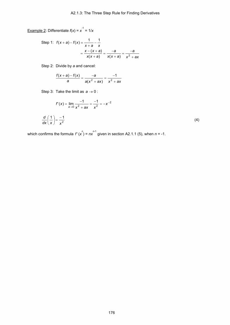
A2.1.3: The Three Step Rule for Finding Derivatives
176
Example 2: Differentiate f(x) = x-1
= 1/x
Step 1: xax
xfaxf 11)()( −+
=−+
axx
aaxx
aaxxaxx
+
−=
+−
=+
+−=
2)()()(
Step 2: Divide by a and cancel:
axxaxxa
aa
xfaxf+
−=
+
−=
−+22
1)(
)()(
Step 3: Take the limit as 0→a :
2220
11lim)(' −
→−=
−=
+
−= x
xaxxxf
a
211
xxdxd −
=
(4)
which confirms the formula 'f (x
n) = nx
n-1 given in section A2.1.1 (5), when n = -1.

A2.1.4: Rules for Differentiation
177
A2.1.4: RULES FOR DIFFERENTIATION ******************************************************************************************************************** IN WHICH we learn how to differentiate functions which are combined in different ways. ******************************************************************************************************************** Leibniz went on to define a series of rules of differentiation, which may be established from the basic principle given as A2.1.1 (4). In what follows, u and v are by convention functions of x, while k is any real constant. The Constant Multiple Rule
If y = ku, dxduk
dxdy
= (1)
The constant multiple rule enables us to extend the conclusion we drew in A2.1.1 (5),
If f(x) = x
n then 'f (x) = nx
n-1,
by introducing a constant multiplier:
If f(x) = kx
n, 'f (x) = knx
n-1,
This enables us to differentiate any one term of a polynomial (q.v. G3).
The Sum Rule
If y = u ± v, dxdv
dxdu
dxdy
±= (2)
The sum rule then enables us to differentiate entire polynomials by adding the derivatives of each term. So the derivative of
x
3 + 3x
2 + 3x + 1
is
3x
2 + 6x + 3.
(Note that we have one term less than we started with. This is because the derivative of any constant term, here 1, is zero).
The Chain Rule
This applies when y is a function of a function of x, e.g.:
If ( ),)(xufy = dxdu
dudy
dxdy
×= (3)
Note the effective "cancellation" here of the two du terms, which is a powerful feature of Leibniz' notation not shared by that of Newton.

A2.1.4: Rules for Differentiation
178
Example: If y = (x
3)2
Let y = u
2, and u = x
3
Then ,2ududy
= 23xdxdu
=
By the chain rule,
dxdu
dudy
dxdy
×=
= 2u × 3x
2 = 2x
3 × 3x
2
= 6x
5
Check: y = x
6 whose derivative is 6x
5.
The chain rule may be used to obtain any derivative where x is replaced by a function of x. It may also be used when the chain contains more links, as when
y = f(u(v(x))),
dxdv
dvdu
dudy
dxdy
××=
The Product Rule
If y = uv, dxduv
dxdvu
dxdy
+= (4)
Example:
If y = x3 × 4x,
Let u(x) = x
3 and v(x) = 4x
Then ,3 ,2xdxdu
= 4=dxdv
By the product rule
dxduv
dxdvu
dxdy
+=
23 344 xxx ×+×= = 4x
3 + 12x
3
= 16x3
Check: y=4x4 whose derivative is 16x3.

A2.1.4: Rules for Differentiation
179
The Quotient Rule
If y = u/v, 2v
dxdvu
dxduv
dxdy
−= (5)
Example:
If y = x
3/x
4,
Let u(x) = x
3, v(x) = x
4
Then 23xdxdu
= , 34xdxdv
=
By the quotient rule,
2v
dxdvu
dxduv
dxdy
−=
8
3324 43x
xxxx ×−×=
8
66 43x
xx −=
21
x−
Check: y = 1/x whose derivative was found in section A2.1.3 example 2 to be -1/x
2.

A2.1.5: Derivatives of Inverse Functions
180
A2.1.5: DERIVATIVES OF INVERSE FUNCTIONS ******************************************************************************************************************** IN WHICH we use both modern and Leibniz' notations to express the derivatives of inverse functions. ******************************************************************************************************************** If a function y = f(x) has a derivative )(' xf , and
a corresponding inverse function (A1.1.10) )(1 yfx −= , then the derivative ))'(( 1 yf − of the inverse function is the reciprocal of ).(' xf So
)('
1))'(( 1
xfyf =− or
dxdydy
dx 1=
For example, if our function f(x) is y = x
2
differentiating gives )(' xf :
xdxdy 2=
The inverse function )(1 yf − 2/1yyx == (choosing the principal, positive, value as in A1.1.10) has a derivative ))'(( 1 yf − , that is
dxdyxy
ydydx 1
21
2121
2/12/1 ==== −
which illustrates again the power and economy of the Leibnizian notation.

A2.1.6: Stationary Points and Points of Inflection
181
A2.1.6: STATIONARY POINTS AND POINTS OF INFLECTION ******************************************************************************************************************** IN WHICH we learn to use the technique of differentiation to identify stationary points and points of inflection on a curve. ******************************************************************************************************************** Stationary Points
A stationary point on a curve of function f(x) occurs where the tangent to the graph is temporarily horizontal, i.e. the first derivative 'f (x) = 0. Figure 1 shows stationary points at B, C and D. Stationary points can be of two kinds: turning points and points of inflection. Turning Points Turning points are stationary points where a curve approaches its horizontal tangent, touches it and then retreats from it without crossing. When this happens 'f changes sign, passing through zero. Turning points can be either maxima or minima. We recall from section A2.1.1 note (4) that when the curve of a function f
is decreasing, 'f < 0 is horizontal, 'f = 0 is increasing, 'f > 0.
At a local maximum the curve of f first rises, becomes horizontal and then falls. 'f is therefore first positive, then zero, then negative, i.e. 'f is consistently decreasing, so ''f is negative. In Figure 1 point C is a local maximum. At a local minimum the curve of f first falls, becomes horizontal and then rises, so that 'f is first negative, then zero, then positive, i.e. 'f is consistently increasing, so ''f is positive. In Figure 1 point D is a local minimum. We say 'local' maximum or minimum because the curve may in principle have respectively higher or lower values in a different region not under consideration. Where this is known not to be the case we can describe the turning point as an absolute maximum or minimum. In Figure 1 point B is an absolute minimum.

A2.1.6: Stationary Points and Points of Inflection
182
Points of Inflection A point of inflection is one where the curve crosses from one side of its tangent to the other as in Figure 1 at point E. When this happens the sense of rotation of the curve changes from clockwise to anticlockwise, or vice versa. At such a point the second derivative ''f (x) changes sign, passing through zero as it does. Points of inflection may be stationary (having 'f = 0), but do not have to be. Point E in Figure 1 is not. It is also possible for ''f to reach zero without changing sign and without the tangent being crossed. Hence this condition on its own does not guarantee a point of inflection. Finding Stationary Points and Points of Inflection We can identify stationary points of any kind by differentiating f, setting the derivative 'f equal to zero, and then solving this new equation to obtain the value of x and so f(x). This is an extremely powerful technique. Let us try an example. Consider the cubic equation f(x) = x
3 - 72x - 280 (1)
Differentiating, 'f (x) = 3x
2 - 72 (2)
''f (x) = 6x (3)
'f (x) = 0 when 3x
2 = 72,
9.424 ±≈±=x Inserting these values in turn in (1) and (3): f(4.9) = 515.2, ''f (4.9) = 29.4 Hence there is a stationary point close to (4.9,-515.2), where ''f is positive. This is therefore a local minimum. Next, f(-4.9) = -44.8, ''f (-4.9) = -29.4 So there is also a stationary point close to (-4.9,-44.8), where ''f is negative. This is therefore a local maximum. Finally, ''f (x) = 0 when 6x = 0 x = 0 f(0) = -280 'f (0) = -72 We therefore expect to find a non-stationary point of inflection at (0,-280). To check this let us evaluate ''f (x) just before and just after this point. From (3), ''f (-0.01) = -0.06 ''f (0.01) = 0.06

A2.1.6: Stationary Points and Points of Inflection
183
''f has indeed changed sign, thus confirming that (0,-280) is a genuine point of inflection. These results are all confirmed by A1.5.3 Figure 1, which depicts the curve in question (although for reasons explained in the text the dependent variable is shown as y). Notes (1) The various possibilities discussed in this section are illustrated in Figure 2.
(2) The technique of locating the maxima and minima of a function by identifying points of zero derivative was pioneered by Fermat c.1629.

A2.2.1: Quadrature
184
ACT 2 SCENE 2: INTEGRATION, THEORY
A2.2.1: QUADRATURE ******************************************************************************************************************** IN WHICH we learn how to calculate approximately the area under a curve using the trapezium rule and Simpson's rule. ******************************************************************************************************************** Concept The integral calculus is designed to solve problems whose type is the reverse of those treated by the differential calculus. In section A2.1.1 we introduced the latter as a means of determining, for instance, how fast an object is moving, given a rule for its position. By contrast, the integral calculus answers typically questions such as, how far does an object travel in a given time, given some indication of its speed? In the first case, the rate of change is the solution; in the second, it is the datum. As we shall discover in section A2.2.3, this problem is equivalent to calculating the area under a curve - the area on a graph between a section of the curve and the horizontal axis. For instance in Figure 1, we are talking about the area enclosed between the four points P, Q, R and S. This problem of finding the area of a closed planar shape is known as quadrature, or squaring. There are two distinct approaches.
(1) Practical, whether or not we know the equation of the curve. We can use any of three methods, all of which offer approximate solutions.
(1a) We can draw the curve on squared paper and count the number of squares in the area of interest. This may well be inaccurate whenever the edge of the curve does not coincide with the edge of a square.
(1b) Numerically: We divide the figure into a number of vertical strips whose heights we can measure or calculate - the y values on Figure 1 - and then compute an approximate answer from these according to some rule. When done by computer this is often called numerical integration.
(1c) Mechanically: We can use an analogue scientific device called a planimeter, illustrated in Plate 1, which has a moving arm whose tip we trace over the curve, and a dial which registers the enclosed area as we do so.
Source: Wikipedia
Plate 1. Polar Planimeter
(2) Analytical, when we do know the equation of the curve. In this case we may be able to use the integral calculus - or just, integration - to find the definite integral, which - if it can be

A2.2.1: Quadrature
185
done - will be the exact answer. We will learn how to do this in section A2.2.3. In this section we shall consider two rules for quadrature of the type described in (1b) above.
Consider Figure 1. We wish to calculate the area PQRS under the curve y = f(x), that is, bounded above by the curve itself, below by the x axis, and on the left and right by the ordinates y
0 and y
n. So
we divide this area into n strips of equal width (or, interval) h, and known heights (the y ordinates f(x))), and then to sum the areas of these strips according to the preferred rule. The result is an easily computed approximate measure, which we shall denote I. Trapezium Rule In the simplest case each strip is treated as a trapezium (q.v. G4), and I is computed as the sum of the areas of each of these.
We can find the area of a single trapezium from Figure 2, where the trapezium ABCD has parallel sides AB of length a and CD of length b, which are h units apart. The inner rectangle ABGH then has area ah square units, and the outer rectangle EFCD has area bh square units. The area of the trapezium is the mean of the areas of these two rectangles. So Area of trapezium ABCD = (ah + bh) / 2 = ½ h (a + b) (1) Hence in Figure 3 the six successive trapezia have areas

A2.2.1: Quadrature
186
½ h (y0 + y
1),
½ h (y1 + y
2),
½ h (y2 + y
3),
½ h (y3 + y
4),
½ h (y4 + y
5) and
½ h (y5 + y
6)
The sum of these is ( )65432102
1 )(2 yyyyyyyh ++++++
Generalising, if there are n strips as in our original Figure 1, the trapezium rule gives us ( ),)...(2 1232102
1−− +++++++≈ nnn yyyyyyyhI or
++≈ ∑
−
=
1
102
1 2n
iin yyyhI (2)
that is, I ≈ half interval × (first ordinate + last ordinate + twice all the other ordinates) Simpson's Rule

A2.2.1: Quadrature
187
Simpson's rule is named after Thomas Simpson (1710-1761), although it had in fact been published in a different form by James Gregory in 1668. In its simple form, illustrated in Figure 4, it approximates the area under f(x) between x=a and x=b by fitting a parabola (the dotted curve) to the ordinates at a and b, and the mid-point ½(a + b). This gives the area of the parabola under the two strips as exactly ( )( ))()(4)()( 2
16
1 bfbafafab +++− (3) Repeated Simpson's Rule The repeated Simpson's rule gives a more accurate value than the trapezium rule by taking the strips in Figure 1 in pairs and fitting a parabola as just described to the top of the three ordinates defining each pair. Rewriting expression (3) then gives the area under each pair as approximately )4( 213
1++ ++ mmm yyyh (4)
where
h = ½(b - a), the width of a single strip, and m is the index of the initial ordinate of the pair.
Suppose there are an even number n strips divided into pairs whose initial ordinates are y
0, y
2,... y
n-2.
Then the total area is given by the sum of the areas under each pair:
I ≈ 1/3 h {(y0 + 4y
1 + y
2) + (y
2 + 4y
3 + y
4) +...+ (y
n-2 + 4y
n-1 + y
n)}
= 1/3 h {y
0 + 4y
1 + 2y
2 + 4y
3 +...+ 2y
n-2 + 4y
n-1 + y
n}
= 1/3 h {y
0 + y
n + 4(y
1 + y
3 +...+ y
n-1) + 2(y
2 +...+ y
n-2)} (5)
that is
I ≈ 1/3 interval × {first + last ordinates + 4 × (sum of odd ordinates) + 2 × (sum of even ordinates)} Because this formula is based upon pairs of strips, it can be used only when the number of strips n is even, i.e. the number of ordinates is odd. Comment As noted above, quadrature formulae such as the trapezium rule and Simpson's rule are in general only approximations: they are practical tools easily adapted for computation, but mathematically not very interesting. They are precise in only a very few cases. Their value to us is as stepping stones towards the more precise and mathematically far more important method of calculating areas (and much else) known as integration, to which we now turn.

A2.2.2: Quadrature of Powers of x
188
A2.2.2: QUADRATURE OF POWERS OF X ******************************************************************************************************************** IN WHICH we learn how powers of x came to be integrated. Notable source: Maor (B1), chapter 7. ******************************************************************************************************************** Introduction In section A2.2.1 we looked at ways of estimating the approximate area under a curve between two bounds. We now consider how to obtain an exact value analytically, that is, by a formula derived from the known function f(x). We begin by looking at the family of curves for which y = f(x) = x
n, where n
covers the full range of integers. We wish to compute, for each value of n, the area I between the curve and the x axis, whose lower bound is the abscissa x = a and whose upper one is x = b. Then in each case we shall try to find a function A(x), specific to the value of n, from which this area can be computed in terms of A(a) and A(b). Ultimately we want to find a general expression for A in terms of n, if one exists. Note: we shall confine ourselves at this stage to the first quadrant, x ≥ 0, y ≥ 0. In general the results found can be extrapolated to the other quadrants as required, although some adjustment of signs may be necessary. Let us first look at the area under y = x
n for n = 0 and 1 using simple geometry.
Case n = 0
y = x
0. The graph of this is the horizontal line y = 1. From Figure 1, the required area is the shaded
rectangle of size I = (b - a) × 1 = b - a So for n = 0, I = A(b) - A(a), where A(x) = x (1)

A2.2.2: Quadrature of Powers of x
189
Case n = 1
y = x
1. Its graph is the straight line y = x. From Figure 2, the required area is the shaded trapezium
whose width is (b - a) and whose exact size we know from equation A2.2.1 (1) to be I = ½ (b - a)(b + a)
= 22
22 ab−
So for n = 1, I = A(b) - A(a), where A(x) = x
2/2 (2)
Case 2 ≤ n ≤ 9: Cavalieri

A2.2.2: Quadrature of Powers of x
190
In 1635 the Italian Bonaventura Cavalieri, a disciple of Galileo, published an expression for calculating areas he had arrived at, by a method known as indivisibles. If in Figure 3 the curve depicted is that of y = x
n, then the area under the curve (i.e., between the curve and the horizontal axis) from x = 0 to x
= a is A(a) where
1
)(1
+=
+
nxxA
n (3)
He had proved this geometrically for positive values of n up to n = 9, but was unable to generalise this any further. From it, in these cases the area between x = a and a further bound x = b will be I = A(b) - A(a) Case (n ≥ 2): Fermat (Generalised Parabolas) Around 1640, the French mathematician Pierre de Fermat, like Descartes a pioneer of the new analytic tool of Cartesian graphs which linked algebra to coordinate geometry (section A1.1.8), found a more broadly applicable and more powerful proof of equation (3) as follows. First, he approximated the area under the curve of y = x
n, where n ≥ 2 (a generalised parabola - an
actual parabola has n = 2) by a series of rectangles whose bases form a geometric progression. So in Figure 3 we imagine the interval from x = 0 to x = a is divided into an infinite number of subintervals at the points ending at K, L, M, and N, where ON = a. Then working backwards from N, from the definition of a geometric progression we have OM = at, OL = at
2, OK = at
3 and so forth where t < 1 is the common ratio. The ordinates at these points are
respectively (at)n, (at
2)n, (at
3)n and so forth. The widths of the rectangles are then successively,
a - at = a(1 - t), at - at
2 = at(1 - t)
at2 - at
3 = at
2(1 - t)
and so on. Their corresponding areas are a
n.a(1 - t), (at)
n.at(1 - t), (at
2)n.at
2(1 - t), ...
For a given t the total area of these rectangles is the sum: A
t = a
n+1 (1 - t) + (at)
n+1 (1 - t) + (at
2)n+1
(1 - t) +... = a
n+1 (1 - t) B
t,
where B
t is another infinite geometrical progression,
B
t = 1 + t
n+1 + (t
n+1)2 + (t
n+1)3 +...
whose common ratio is t
n+1. Since t < 1, t
n+1 < 1. So we can evaluate B
t using the standard formula
given at A1.1.7 (5), giving
11
1+−
=nt
tB

A2.2.2: Quadrature of Powers of x
191
So
1
1
1)1(
+
+
−
−=
n
n
tt
taA
Clearly, the closer t is to 1, the narrower will be the rectangles and so the better the fit. However, simply substituting t = 1 gives the indeterminate quantity 0/0. So Fermat factorised the denominator as 1 - t
n+1 = (1 - t)(1 + t + t
2 + t
3 + ...t
n),
enabling him to cancel the two factors (1 - t). This gives
n
n
ttttt
aA...1 32
1
++++=
+
If now t tends to 1, the area A(a) under the curve is given by the limit
1
lim)(1
1 +==
+
→ naAaA
n
tt
which is Cavalieri's formula (3) above. It also incorporates results (1) and (2) obtained above for n = 0 and 1. Fermat has applied it to the whole family of curves for which n is a positive integer. So for all integer n ≥ 0, I = A(b) - A(a), where
1
)(1
+=
+
nxxA
n (as (3) above)
The reader may wish to verify that when n = 2, this result gives the same area as Simpson's rule in equation A2.2.1 (3). Fermat's success in finding the area of a parabola analytically was the first major advance in this field since Archimedes. We have already noted in A1.2.1 the latter's method for estimating the area of a circle. Archimedes went on to compute the area of a parabola using the method of exhaustion which had been pioneered by Eudoxus (c.370 BC). This entailed filling it 'exhaustively' with a succession of triangles whose areas decrease in a geometric progression. He then added the areas of the individual triangles, using the formula for the sum of a geometric progression as in A1.1.7 (5). However, Archimedes failed in his attempts to apply this method to the remaining conics (Sideshow S3), the ellipse and hyperbola. Case n ≤-2: Fermat (Generalised Hyperbolas) y = x
-m. Fermat went on to show that the same formula works for the generalised hyperbolas which
represent y = xn when n is a negative integer ≤ -2 (so, y = x
-m = 1/x
m for positive m = -n). In these
cases formula (3) gives the numerical value of the area from x = a (where a > 0) to infinity as illustrated in Figure 4. This is the only case where x = a denotes the lower bound of the area being measured by A(a), which is therefore drawn to the right of a instead of the left. This has the result that the value returned by A(x) in this quadrant is negative. For instance
3/1)3(:1112
)(,2112
−=−
=−
=+−
==−+−
Ax
xxxAn
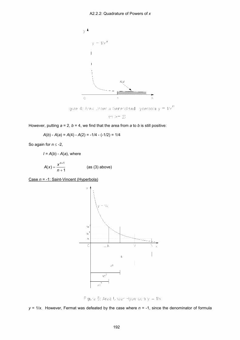
A2.2.2: Quadrature of Powers of x
192
However, putting a = 2, b = 4, we find that the area from a to b is still positive: A(b) - A(a) = A(4) - A(2) = -1/4 - (-1/2) = 1/4 So again for n ≤ -2, I = A(b) - A(a), where
1
)(1
+=
+
nxxA
n (as (3) above)
Case n = -1: Saint-Vincent (Hyperbola)
y = 1/x. However, Fermat was defeated by the case where n = -1, since the denominator of formula

A2.2.2: Quadrature of Powers of x
193
(3) becomes zero. This became one of the outstanding mathematical problems of the seventeenth century. Then in 1647 Grégoire de Saint-Vincent (1584-1667), a Belgian Jesuit, pointed out (see Figure 5) that the rectangles fitted to this curve, whose bases are in geometrical progression as before, all have equal areas. Starting at N, their heights are 1/at, 1/at
2, 1/at
3, while their widths are as
before, a - at = a(1 - t), at - at
2 = at(1 - t)
at2 - at
3 = at
2(1 - t)
So their areas are successively,
,...)1(,)1(,)1(3
2
2 attat
attat
atta −−−
each of which equals (1 - t)/t. So as the abscissa - the distance from O - grows by a common factor t, geometrically, the area grows by a common increment (1 - t)/t, arithmetically. This remains true in the limiting case as t -> 1 and we move from rectangles to a smooth hyperbolic curve. From this, a student of his concluded that the relationship between the two is logarithmic (compare A1.6.1). So if A(p) is defined as the area under y = 1/x from x = 1 to x = p, then in Figure 6, A(pq) = A(p) + A(q)
This suggests that for some base s we have aaA slog)( = However, not any base will do, since the area has a unique value. In fact, the area is only measured correctly if the base is e, the natural base of logarithms. So the conclusion from Saint-Vincent's work is that the area under the hyperbola y = 1/x from x = 1 to x = a is A(a) = ln a (4) So for case n = -1,

A2.2.2: Quadrature of Powers of x
194
I = A(b) - A(a), where A(x) = ln x, (x > 0) (5) Note that for 0 < x < 1, ln x returns a negative value; I however, as defined, remains positive. We shall look at this result in greater detail in section A2.2.3. Historically this is significant as one of the first times when use was made of the logarithmic function; previously logarithms were regarded mainly as a computational device. It was now possible to define a logarithm as the area under the curve of y = 1/x. How this could be computed was later devised by Mercator in 1668, as we shall see at A3.3.3 (9). Summary For all integers n the area under the curve y = x
n from x = a to x = b is
I = A(b) - A(a) (6) where
1
)(1
+=
+
nxxA
n (n )1≠ , (7)
and A(x) = ln x (n = -1; x > 0) (8) We shall extend this last result to cover negative values of x in A2.2.3 (14) and (15).
* * * * * We have now provided the foundation on which stands the whole theory of integration, deriving it in turn from the geometric progression.

A2.2.3: Integration
195
A2.2.3: INTEGRATION ******************************************************************************************************************** IN WHICH we discover integration, proved by the fundamental theorem of the calculus to be the inverse of differentiation. ******************************************************************************************************************** The Definite Integral
The definite integral of a continuous function between a lower bound a and an upper bound b may be thought of as the area between the curve of that function and an axis - usually the x axis - between those bounds (see Figure 1). If the function is f(x) and the area in question is I, then we write
∫=b
adxxfI )( (1)
The RHS is read, "the definite integral of f(x) with respect to x from x=a to x=b". The process of evaluating it is called "integration". dx is Leibniz' formal notation (section A2.1.2) used to show in respect of which variable the integration is being carried out (there can be more than one), and to indicate how integrals may legitimately be manipulated. This corresponds closely to its use in differentiation. It has no numerical value. Example from Powers of x In A2.2.2 we found that for all functions y = f(x) = x
n - that is, integer powers n of x - and between the
bounds a and b, the area under the curve could be given by I = A(b) - A(a) (A2.2.2 (6)) (2) where A(x) is an area function specific to f(x). In particular, from Cavalieri and Fermat,
1
)(1
+=
+
nxxA
n (n )1≠ , (A2.2.2 (7)) (3)
and from the work of Saint-Vincent, A(x) = ln x (n = -1; x > 0) (A2.2.2 (8)) (4)

A2.2.3: Integration
196
What is remarkable about this is that in both of these cases (3) and (4), the derivative of A is the same as our original f(x), that is, x
n:
)(xfdxdA
=
Thus
1,1
1−≠=
+
+
nxnx
dxd n
n (A2.1.1 (5)), (5)
and
0,1,1)(ln >−=== xnxx
xdxd n (proved easily at A2.3.3 (6)) (6)
So while function A supplies the area under function f, function f supplies the tangents to function A. Fundamental Theorem of the Calculus This suggests that there is an inverse relationship between the problem of finding areas, carried out by integration, and that of finding tangents, carried out by differentiation. This reciprocity is the great discovery made from their different starting points by Newton and Leibniz in the 1680s, which lies at the heart of the calculus. It is formally known as the fundamental theorem of the calculus. Furthermore, it applies generally and is not limited to powers of x as above. We may express it by saying that if A(x) is a function giving the area under the graph of any function f(x), then the rate of change, or derivative, of A at every point x is equal to f(x). So A and f stand in the relationship
A' = f or in Leibniz' notation )(xfdxdA
= (7)
The converse of this is that
)()()( aAbAdxxfb
a−=∫ (compare equations (1) and (2))
That is, the area under the graph of f between a and b, measured geometrically, is equal to the value computed analytically from function A. A is said to be a primitive (or antiderivative) of f. Different functions f will have different primitives A. So this theorem converts the problem of evaluating integrals by measuring areas (quadrature) into the (analytic) problem of finding primitives. The expression A(b) - A(a) occurs so often in integration that it is commonly written as [ ]baxA )( or just
[ ]baA which is read as "A evaluated from a to b". Summation of Infinitesimals Leibniz envisaged the area I as the sum of a large number, m, of very thin rectangular vertical strips, each xδ units wide, whose heights are that of the curve f(x
k) at the successive mid-points x
k (see
Figure 2 where m has been drawn as 5). Each strip will have an area xxf k δ×)( . He then approximated,

A2.2.3: Integration
197
∑=
δ×≈m
kk xxfI
1
)(
As xδ approaches zero, each vertical strip may be thought of as a notional 'line' of infinitesimal thickness. At the limit,
∫=δ×= ∑=
→δ
b
a
m
kkx
dxxfxxfI )()(lim1
0 (9)
which is the definite integral in equation (1).
The extended S symbol, like the Σ symbol before it, emphasises that what we are dealing with here is

A2.2.3: Integration
198
essentially a summation process, just as earlier we noted that differentiation is essentially a process related to differences. Figure 3 illustrates this relationship. Derivation A simple derivation of the fundamental theorem runs as follows. In Figure 1, let I(b) be the area under the graph of function y = f(x) from a constant lower limit x = a to a variable upper limit x = b. I(b) corresponds to A(b) - A(a) in the foregoing argument. We wish to show that dI/db = f(b). Moving from the point b to b + δb, I grows from I(b) to I(b + δb). Since for small δb, the growth δI in I(b) is approximately a rectangle of height f(b) and width δb, we have bbfI δ≈δ )( ` This approximation will be increasingly accurate as δb decreases towards zero. We now use the three step rule of A2.1.3 to obtain dI/db.
Step (1): δI = I(b + δb) - I(b) bbf δ≈ )( Step (2): Divide by δb: )(/ bfbI ≈δδ Step (3): Take the limit as δb -> 0:
)(lim0
bfbI
dbdI
b=
δδ
=→δ
which is the fundamental theorem. Indefinite Integral The fundamental theorem can be expressed more generally by removing the bounds a and b, as ∫ += CxAdxxf )()( or simply ∫ += CAf (10)
where A'(x) = f(x). Here ∫ dxxf )( is called the indefinite integral of f(x) with respect to x. Whereas the definite integral is the value of an area which may be calculated, the indefinite integral is a function. It is found by asking, "What function A if differentiated gives us the function f?" C is an arbitrary constant of integration explained below. Indefinite Integrals of Powers of x Applying the fundamental theorem expressed in equation (10) to equation (3) above, we have
∫ ++
=+
,1
1C
nxdxx
nn 1−≠n (11)
Putting n = 0 gives
∫ ∫ +== ,1
10 Cxdxdxx (12)

A2.2.3: Integration
199
However, if n = -1, the denominator n+1 of result (9) becomes infinite. So in this case we resort to equation (4) instead:
∫ += ,ln1 Cxdxx
x > 0 (13)
But ln x is defined only for x > 0, whereas y = 1/x has real (negative) values for x < 0. So in this region we write
∫ +−= ,)ln(1 Cxdxx
x < 0 (14)
We can combine results (13) and (14) by writing
∫ += ,||ln1 Cxdxx
x ≠ 0 (15)
where |x| is the modulus or positive value of x. The indefinite integral, once found, can be used to obtain the definite integral between two bounds. So for instance Saint-Vincent's result which we first met as A2.2.2 (5) and (8), can now be derived from (15) as the definite integral
∫ =−=−=a
aaadxx1
ln0ln1lnln1 (16)
Constant of Integration The solution to A(x) = ∫ dxxf )( is not one but an infinite family of curves. For instance A(x) = 4x
2 + 2
A(x) = 4x2 + 5
A(x) = 4x2 + 16
all on being differentiated give f(x) = 8x. This is because the constant term has a zero derivative and so does not appear in f(x). But if we are integrating, we must allow for the possibility of a constant term appearing in the integral. The first such constant term is usually denoted C. So if M is a constant,
∫ += CMxdxM (17)
Integrating this again,
DCxMxdxCMx ++=+∫ 22
1 (18)
where D is a second constant of integration. Each time the new constant of integration would appear on a graph as the y intercept. The constant of integration does not feature in definite integrals, since in the expression A(b) - A(a) it cancels out. In physical terms it can often be found as a condition of the system being investigated. Where it is known the integral is often called a particular integral; otherwise it may be called a general integral. It is often omitted where it is immaterial.

A2.2.3: Integration
200
Basic Indefinite Integrals Since from the fundamental theorem, integration and differentiation are inverse operations (q.v. G3), if we differentiate a function and then integrate the result, we end up with our original function. This is the defining principle of inverse operations. Formally, if y = f(x),
∫ ∫ +== Cydydxdxdy (19)
This suggests how we can arrive at some of the most basic indefinite integrals, by reversing a differentiation. For instance if y = x
n,
1−= nnxdxdy (21)
Integrating reverses this:
∫ ∫ +== − Cxdxnxdxdxdy nn 1 (22)
Geometric Example: Area of Circle We wish to compute the area of a circle of radius R given that the circumference of a circle of radius r is rπ2 . We shall apply Leibniz' technique of the summation of infinitesimals. Suppose that the circle is made up of a large number of concentric rings each of very small thickness
rδ . Then each ring will have an area approximately equal to its circumference times its width, that is, rr δπ .2 where r is the local radius of each ring, within the range
0 ≤ r ≤ R
The whole circle will have an area approaching the sum of the areas of these rings. As 0→δr , the number of rings ∞→ . The area of the circle then equals the limit
[ ] 220
2
002 RRrdrrA R
Rπ=−π=π=π= ∫ (23)
So the area of a circle of radius R is 2Rπ . Thus we have a more formal proof of this formula than was offered in section A1.2.1. Notes (1) Sometimes the dx term is omitted, when x is the only variable in the problem. However, when f(x) depends on more than one variable, the dx term indicates which particular variable is being integrated, the others being held constant. In addition the dx term is useful when a change of the variable of integration is being made to simplify a problem. We shall see some examples of this later on. (2) Not all functions can be integrated; and some functions can only be integrated over a part of their range. Again, as with differentiation, so with integration, the foundations are very complex and we have of necessity simplified. However, here also they can be made good in the branch of mathematics called analysis (q.v. G1), which lies beyond the scope of our drama.

A2.2.3: Integration
201
(3) If part of the curve between x=a and x=b lies below the x axis, i.e. f(x) is negative, ∫b
adxxf )( will
subtract the area computed for this section from the integral. If both the areas above and below the x axis are required, they must be computed separately. (4) The situation where b < a corresponds to a negative value of xδ in equation (9), giving in turn a negative area I, and so negating the value of the integral. So
∫ ∫−=b
a
a
b
dxxfdxxf )()( (24)
* * * * *
The calculus, and the fundamental theorem in particular, pose a mighty challenge to formalism. For they were deduced from no axioms. Indeed, the formal justification for them - in particular, the theory of limits - was not complete until analysis was perfected by Cauchy and others a century and a half later. Formalism, the theory that mathematics is the process of deducing theorems from axioms, is therefore in conflict with history. It is not what the greatest mathematicians have always done. Further, the fact that the calculus was in essence discovered by not one but two men - Newton and Leibniz - more or less independently, as is now generally conceded, poses a second problem for formalism. For while we could all understand if the same conclusions were deduced by two different people from the same axiom set, how without the benefit of such a set could they have arrived at such similar conclusions unless those conclusions possessed in themselves some absolute validity? How could two people discover the same thing unless that thing in some sense actually existed; or, in other words, the same truth unless that truth were not universal, so universal in fact that it forms the basis of vast tracts of physical science? In reality, for Newton at least, the calculus was not a logical deduction at all. Like the general binomial theorem which he discovered en route, it was the product of inductive reasoning from a mass of mathematical data which had been accumulating for most of the century. Their attraction lay not in their proof - he proved neither - but in their explanatory power, the amount of known results which could be subsumed under them. In a very similar way his theory of gravitation brought together into one equation the three laws of Kepler, which could be deduced from it and not the other way round. As ever, doctrinaire formalism dies hard. We should be wary of any account of mathematics according to which Newton and Leibniz were not mathematicians.

A2.2.4: Rules for Integration
202
A2.2.4: RULES FOR INTEGRATION ******************************************************************************************************************** IN WHICH we learn how to integrate functions which are combined in different ways. ******************************************************************************************************************** Leibniz developed a set of rules for integration comparable to those for differentiation which we met in section A2.1.4. As before, u and v are functions of x, while k is any constant. The Constant Multiple Rule The integral of a constant times a function is the constant times the integral of the function:
∫ ∫= ukku (1)
For instance
∫ ∫ +=+== CxCxdxxdxx 4433 3)(34312
The Sum Rule The integral of the sum (or difference) of two functions is the sum (or difference) of their integrals:
∫ ∫ ∫±=± vuvu (2)
For instance
∫ ∫∫ ++=+=+ Cxxdxxdxxdxxx 34
2323
433
as may be verified by differentiating. With these two rules we can integrate any polynomial. For instance
∫ ∫∫∫ ++=++ dxdxxdxxdxxx 5253751021 22
)5()5()7( 322
13 CxCxCx +++++=
where C
1, C
2, C
3 are arbitrary constants of integration which can be added to give a single term C,
giving the final answer as
Cxxxdxxx +++=++∫ 55751021 232
Integration of f '(x)/f(x)
The quotient rule for differentiation has the following as its nearest equivalent: When the numerator of a fraction = the derivative of the denominator, the integral is the natural logarithm of the modulus of the denominator.
∫ += Cxfdxxfxf |)(|ln)()(' , 0)( ≠xf (3)
For the proof we shall require result (15) from section A2.2.3 above, that

A2.2.4: Rules for Integration
203
∫ += ,||ln1 Cxdxx
x ≠ 0
Then let y = any function f(x). Then
∫ ∫∫ +=== Cydyy
dxy
dxdy
dxxfxf ||ln1)()(' , 0≠y
So generally,
∫ += Cxfdxxfxf |)(|ln)()(' , 0)( ≠xf
* * * * *
The chain rule for differentiation has no general equivalent under integration. The product rule for differentiation has a counterpart in the technique known as integration by parts which we shall meet in section A2.4.3.

A2.3.1: Derivatives of Trigonometrical Functions
204
ACT 2 SCENE 3: DIFFERENTIATION, PRACTICE
A2.3.1: DERIVATIVES OF TRIGONOMETRICAL FUNCTIONS ******************************************************************************************************************** IN WHICH we differentiate the major and minor trigonometrical functions. ******************************************************************************************************************** Derivatives of Cosine and Sine It may be verified on a calculator that if a is measured in radians, then for very small a, the ratios ( aa /)1(cos − and aa /)(sin both approach limits. If you draw up tables in the same way as we did
for aa in section A1.6.1 and for (1 + 1/n)
n in section A1.6.2, you should find that
01)(coslim0
=−
→ aa
a (1)
and similarly
1sinlim0
=→ a
aa
(2)
which can be also derived by manipulation from (1). We note that both these expressions imply the computation of 0/0, whose value is generally indeterminate and depends on context (see under A1.1.4 (17)). In this case the values assigned can in fact be determined geometrically. We offer these two limits without their proof as a basis for differentiating the cosine and sine functions using the three step rule of A2.1.3. Derivative of cosine Applying the three step rule to f(x) = cos x:
Step 1: xaxxfaxf cos)cos()()( −+=−+ Step 2: Divide by a
a
xaxa
xfaxf cos)cos()()( −+=
−+
where from section A1.5.7 (1)
axaxax sinsincoscos)cos( −=+
axaxax
axfaxf cossinsincoscos)()( −−
=−+
a
axaax sinsin1coscos −
−
Step 3: Take the limit
axfaxfxf
a
)()(lim)('0
−+=
→

A2.3.1: Derivatives of Trigonometrical Functions
205
−−
=→ a
axaax
a
sinsin1)(coscoslim0
Since we cannot avoid division by zero by cancelling out the lower a, we adopt the alternative procedure of substituting the previously noted limits (1) and (2):
xxxxf sin1sin0cos)(' −=×−×=
xxdxd sin)(cos −= (3)
Derivative of sine Applying the three step rule to f(x) = sin x:
Step 1: xaxxfaxf sin)sin()()( −+=−+ Step 2: Divide by a
a
xaxa
xfaxf sin)sin()()( −+=
−+
where from section A1.5.7 (2) axaxax sincoscossin)sin( +=+
axaxax
axfaxf sinsincoscossin)()( −+
=−+
a
axaax sincos1)(cossin +
−=
Step 3: Take the limit
axfaxfxf
a
)()(lim)('0
−+=
→
+−
=→ a
axaax
a
sincos1)(cossinlim0
As above, since the lower a does not cancel, we avoid division by zero by substituting from limits (1) and (2): xxxxf cos1cos0sin)(' =×+×=
xxdxd cos)(sin = (4)
In A3.4.2 we shall show how results (3) and (4) enable us to obtain power series (q.v. G5) for the cosine and sine functions. These in turn will justify the limits (1) and (2) that we have employed above. Derivatives of Tangent, Cotangent, Secant, and Cosecant We now show how the derivatives of the tangent function, and of the minor trigonometrical functions secant, cosecant, and cotangent may be obtained by applying the quotient and chain rules from section A2.1.4 to the results for cosine and sine just obtained.

A2.3.1: Derivatives of Trigonometrical Functions
206
Derivative of tangent
Let xxxy
cossintan ==
,sin xu = xv cos=
,cos xdxdu
= xdxdv sin−=
Then by the quotient rule A2.1.4 (5),
2v
dxdvu
dxduv
dxdy
−=
x
xxxx2cos
)sin(sincoscos −−×=
xxx
xx 222
22sec
cos1
cossincos
==+
=
xxdxd 2sec)(tan = (5)
The remainder of this section may be omitted on first reading. Derivative of cotangent
Let xx
xxy
sincos
tan1cot ===
,cos xu −== xv sin= Then similar application of the quotient rule gives
xxdx
dy 22
cscsin
1−=
−=
xxdxd 2csc)(cot −= (6)
Derivative of secant
Let x
xycos
1sec ==
,cos xu = uy /1= By the chain rule, A2.1.4 (3),
( )xx
xxxx
udxdu
dudy
dxdy
cossin
cos1
cossinsin1
22==−
−=×=

A2.3.1: Derivatives of Trigonometrical Functions
207
xxxdxd tansec)(sec = (7)
Derivative of cosecant
Let x
xysin
1csc ==
,sin xu = uy /1= Then similar application of the chain rule gives
xx
xxx
dxdy
sin1
sincos
sincos
2−
=−
=
xxxdxd csccot)(csc −= (8)

A2.3.2: Derivatives of Inverse Trigonometrical Functions
208
A2.3.2: DERIVATIVES OF INVERSE TRIGONOMETRICAL FUNCTIONS ******************************************************************************************************************** IN WHICH we differentiate the inverses of the major and minor trigonometrical functions. This section may be omitted on first reading. ******************************************************************************************************************** Derivatives of Inverse Trigonometrical Functions We now obtain the derivatives of the inverse trigonometrical functions arccos, arcsin, arctangent, arccotangent, arcsecant, and arccosecant. These inverse functions, being periodic (cyclical), have multiple angular values for each argument. For instance arcsin 0.5 may be not just π/6 (30°) and 5π/6 (150°), but also π/6 ± 2nπ and 5π/6 ± 2nπ for any integer n. It is conventional, therefore, when treating them to confine our attention to a range of uniquely defined principal values in each case as described in A1.3.1, and as depicted in Figures 1 and 2 below.
-4 -3 -2 -1 0 1 2 3 4
x
30
60
90
120
150
180y degrees Figure 1
Principal values of inverses of trigonometrical functions
(1) Arccosine, arccotangent and arcsecant
y = arccos x
y = arccot x
y = arcsec x
We shall exploit the relationship between the derivative of a function and that of its inverse, found in section A2.1.5:
dxdydy
dx 1= (1)
We use also the Pythagorean identities, A1.3.2 (1) to (3):
cos2 y + sin
2 y ≡ 1 (2)

A2.3.2: Derivatives of Inverse Trigonometrical Functions
209
sec2 y - tan
2 y ≡ 1 (3)
csc2 y - cot
2 y ≡ 1 (4)
-4 -3 -2 -1 0 1 2 3 4
x
-90
-60
-30
30
60
90y degrees Figure 2
Principal values of inverses of trigonometrical functions
(2) Arcsine, arctangent and arccosecant
y = arcsin x
y = arctan x
y = arccsc x
Derivative of arccosine and arcsine Let y = cos
-1 x. x takes the range -1 ≤ x ≤ 1, or |x| ≤ 1. y is limited to the principal values 0 ≤ y ≤ π.
Then
x = cos y, ydydx sin−= (A2.3.1 (3))
y
dydxdx
dysin
11 −==
Since from identity (2)
sin2 y ≡ 1 - cos
2 y,
22 1cos1sin xyy −±=−±=
However, within the permitted range for y, sin y ≥ 0. So choosing the positive root,
11,1
1)(cos2
1 <<−−
−==− x
xdxdyx
dxd (5)
That this is uniformly negative in the specified range is confirmed by Figure 1. For y = sin
-1 x, the principal values of y are -π/2 ≤ y ≤ π/2. Then the derivative of sin
-1 x is found
similarly to be

A2.3.2: Derivatives of Inverse Trigonometrical Functions
210
11,1
1)(sin2
1 <<−−
=− xx
xdxd (6)
That this is uniformly positive in the specified range is confirmed by Figure 2. Derivative of arctangent and arccotangent Let y = tan
-1 x. x may take any real value. y is limited to the principal values -π/2 < y < π/2. Then
x = tan y, ydydx 2sec= (A2.3.1 (5))
ydydxdx
dy2sec
11==
Since from identity (3)
sec2 y ≡ 1 + tan
2 y,
221
11
tan11)(tan
xydxdyx
dxd
+=
+==− (7)
That this is uniformly positive in the specified range is confirmed by Figure 2. This result, arrived at geometrically rather than through the calculus, became the basis for Gregory's series for tan
-1 x (I2.1 (16)).
For y = cot
-1 x, the x range is unchanged. y is limited to the principal values π < y < π. Then using
identity (4) the derivative of cot-1
x is found similarly to be
2
1
11)(cotx
xdxd
+
−=− (8)
That this is uniformly negative in the specified range is confirmed by Figure 1. Derivative of arcsecant and arccosecant Let y = sec
-1 x. The graph consists in two disjoint curves in which |x| may take any real value > 1. y is
limited to the principal values such that:
When x < -1, π/2 < y < π, x > 1, 0 < y < π/2 Then
x = sec y, yydydx tansec= (A2.3.1 (7))
yydydxdx
dytansec
11==

A2.3.2: Derivatives of Inverse Trigonometrical Functions
211
From identity (3)
11sectan 22 −±=−±≡ xyy
As to which sign to use, note that sec y and tan y are both positive for 0 < y < π/2, and both negative for π/2 < y < π. So dy/dx is always positive in the region 0 < y < π.
1||
1)(sec2
1
−==−
xxdxdyx
dxd , |x| > 1 (9)
That this is uniformly positive in the specified range is confirmed by Figure 1. For y = csc
-1 x, the x range is unchanged. y is limited to the principal values such that:
When x < -1, -π/2 < y < 0, x > 1, 0 < y < π/2
Using identity (4), the derivative of csc
-1 x is similarly found to be
1||
1)(csc2
1
−
−=−
xxx
dxd , |x| > 1 (10)
That this is uniformly negative in the specified range is confirmed by Figure 2.

A2.3.3: Derivatives of Exponentials and Logarithms
212
A2.3.3: DERIVATIVES OF EXPONENTIALS AND LOGARITHMS ******************************************************************************************************************** IN WHICH we differentiate the exponential and logarithmic functions. ******************************************************************************************************************** Derivative of e
x
We adopt a similar procedure to that with which we began section A2.3.1. In A1.6.2 (6) we gave as the defining characteristic of e the limit xe x
x+=
→1lim
0
From this we have
11lim0
=−
→ aea
a (1)
which may be verified by drawing up a table of values using a calculator. It should be found that, even though implying the indeterminate division 0/0, the limit is genuine. Applying the three step rule to f(x) = e
x:
Step 1: xax eexfaxf −=−+ +)()( Step 2: Divide by a:
a
eea
xfaxf ax 1)()( −
=−+
Step 3: Take the limit:
a
eexfa
a
x 1lim)('0
−=
→
Since the lower a does not cancel, we avoid division by zero by substituting from limit (1): xx eexf =×= 1)('
xx eedxd
=)( for all x. (2)
That is, the derivative of e
x is e
x for all x. This exceedingly important result may be confirmed by
inspection of Figure 1 of section A1.6.4. E.g.
When x = 0, ex = 1 and 1)( =xe
dxd
The exponential function is the only function in mathematics which equals its own derivative. This is why e is so important in the calculus. Indeed, that it is the only function with this property is even sometimes used as a definition of e. In A3.4.3 we shall show how this property can be used to generate a power series (q.v. G5) for the exponential function. This in turn will justify the limit (1) that

A2.3.3: Derivatives of Exponentials and Logarithms
213
we have employed above. On account of this property e
x typifies any organic process where the rate of growth of an object is
proportional to its size. Many physical and chemical processes behave similarly. The rate at which many chemical reactions take place is proportional to the quantity of reacting substances present. The amount of heat a body gives off to the surrounding medium is proportional to its temperature. The instantaneous rate at which a radioactive substance diminishes through emanation is proportional to its mass. Each of these may be modelled by a variant of the exponential function y = e
x.
Derivative of e
ax
We use the chain rule in section A2.1.4 (3) in order to differentiate e
ax where a is any real number.
If axey = ,
Let axu = , adxdu
=
Then uey = , uedudy
=
By the chain rule,
aedxdu
dudy
dxdy u ×=×=
axax aee
dxd
=)( for all x (3)
Putting a = -1 gives
xx eedxd −− −=)( (4)
Exponentials of the form y = e
at feature commonly in physics and nature wherever growth is being
represented as a function of time t. Exponentials with a negative index, as y = e
-at, are often used to indicate the decay of a property (e.g.
radioactivity) as a function of time t. Derivative of a
x
If xay = axx ea ln= (from section A1.6.1 result (12)), From result (3) above,
xax aaae
dxdy
×== lnln ln
aaadxd xx ln)( = for all x. (5)

A2.3.3: Derivatives of Exponentials and Logarithms
214
Derivative of ln x
If xy ln= then yex = and yedydx
=
From the rule for derivatives of inverse functions in section A2.1.5,
xedx
dyy
11=
= . x > 0
x
xdxd 1)(ln = , x > 0 (6)
We have already met this very important result as A2.2.3 (6). It is the converse of A2.2.3 (13).
Derivative of ln (1 + x) It follows that
xx
dxd
+=+
11)1( , x > -1 (7)
another important result, which we shall meet again as A3.3.3 (16). Derivative of ln (ax + b) Generalising, if y = ln (ax + b):
Let ,baxu += ,adxdu
= uy ln=
From result (6),
ududy 1
=
By the chain rule for differentiation in section A2.1.4 (3),
audx
dududy
dxdy 1
=×=
baxabax
dxd
+=+ ))(ln( , x > b/a (8)
Derivative of log
a x
If y = log
a x,
then from result (14) of section A1.6.1:
y = ln x / ln a
By the constant multiple rule for differentiation A2.1.4 (1),

A2.3.3: Derivatives of Exponentials and Logarithms
215
xax
dxd
adxdy 1
ln1)(ln
ln1
==
axx
dxd
a ln1)(log = (9)

A2.4.1: Standard Integrals
216
ACT 2 SCENE 4: INTEGRATION, PRACTICE
A2.4.1: STANDARD INTEGRALS ******************************************************************************************************************** IN WHICH we demonstrate a number of standard indefinite integrals. ******************************************************************************************************************** Unlike differentiation where a few simple principles suffice, integration requires a wide variety of techniques, and even with them there is no guarantee of success in particular cases. In this section we offer a sample of standard integrals; in the next two sections some basic techniques. For more detailed coverage the reader is referred to the more specialised texts, such as Abbott (B1) or Lang (B3). Integrals of Algebraic Functions Integral of (ax + b)
n
From section A2.2.3, result (11),
∫ ++
=+
,1
1C
nxdxx
nn 1−≠n
So generally, for real a, b:
Cna
baxdxbaxn
n ++
+=+∫
+
)1()()(
1 1−≠n (1)
as may be verified by differentiating. Integral of 1/(ax + b) This is the special case of (1) when n = -1. From section A2.2.3, result (15),
∫ += ,||ln1 Cxdxx
x ≠0
So generally
∫ ++=+
,||ln11 Cbaxa
dxbax
x ≠ -b/a (2)
as may be verified by differentiating (see A2.3.3 (8)). Integrals of Exponential Functions Integral of e
x
Since from section A2.3.3 (2),
xx eedxd
=)( for all x

A2.4.1: Standard Integrals
217
∫ += Cedxe xx (3)
So generally,
∫ += Ca
edxeax
ax (4)
as may be verified by differentiating. Integral of a
x
From section A1.6.1 result (12), axx ea ln= From the result (4) on e
ax,
∫ ∫ +== Ca
edxedxaax
axx
ln
lnln
∫ += Ca
adxax
x
ln (5)
Standard Trigonometrical Integrals Integral of cosine
Since from A2.3.1 (4),
,cos)(sin xxdxd
=
∫ += Cxdxx sincos (6)
So generally
Cbaxa
dxbax ++=+∫ )sin(1)cos( (7)
Integral of sine Similarly, since from A2.3.1 (3),
,sin)(cos xxdxd
=
∫ +−= Cxdxx cossin (8)
So generally
∫ ++−
=+ Cbaxa
dxbax )cos(1)sin( (9)

A2.4.1: Standard Integrals
218
Integral of tangent
∫ ∫ −−== dxxdx
xxdxx
cossin
cossintan
where the fraction has the form )(/)(' xfxf . Hence from rule (3) in section A2.2.4,
CxCxdxx +=+−=∫ |sec|ln|cos|lntan (10)
So generally
∫ ++=+ Cbaxa
dxbax |)sec(|ln1)tan( (11)
Integral of cotangent
dxxxdxx∫ ∫=
sincoscot
where the fraction has the form )(/)(' xfxf . Hence as before
∫ += Cxdxx |sin|lncot (12)
So generally
∫ ++=+ Cbaxa
dxbax )sin(|ln1)cot( (12)
Additional Trigonometrical Integrals The following integrals follow from the derivatives in section A2.3.1. From A2.3.1 (5),
∫ += Cxdx tansec 2 (14)
From A2.3.1 (6),
Cxdx∫ +−= cotcsc2 (15)
From A2.3.1 (7),
∫ += Cxdxxx sectansec (16)
From A2.3.1 (8),
∫ +−= Cxdxxx csccotcsc (17)

A2.4.2: Integration Techniques
219
A2.4.2: INTEGRATION TECHNIQUES ******************************************************************************************************************** IN WHICH we learn some basic techniques for carrying out further integrals. ******************************************************************************************************************** General This section and the next suggest various simplifying techniques which may be employed when direct integration is not possible. In the absence of all-embracing rules we proceed more than usually by examples. Rational Functions Some rational functions (see I1.2.1) may be split into their component fractions. E.g.
∫ ∫ ∫ ∫∫ ++=
++=
++ dxxdxdx
xdxxdx
xxxdx
xxx
333
24 131313
Cx
xx+−+=
2
2
21||ln3
2
Products of Functions There is no direct rule for integrating the products of two functions. Sometimes the factors may be multiplied out. E.g.
∫∫ ∫ ∫∫ −+=−+=−+ dxdxxdxxdxxxdxxx 232232)12)(2( 22
Cxxx +−+= 223
32 23
Other cases may be amenable to the device of integration by parts which is the subject of section A2.4.3. Substitution by Pythagorean Identities The Pythagorean identities from section A1.3.2
cos2 θ + sin
2 θ ≡ 1 (1)
sec2 θ - tan
2 θ ≡ 1 (2)
csc2 θ - cot
2 θ ≡ 1 (3)
may be readily employed. So directly from (2), coupled with A2.4.1 (14):
Cxxdxxdxx +−=−=∫ ∫ tan1sectan 22 (4)
And from (3) coupled with A2.4.1 (15):
Cxxdxdxx ++−=−=∫∫ )(cot1csccot 22 (5)

A2.4.2: Integration Techniques
220
Substitution by Trigonometrical Identities Some of the identities found in section A1.5.7 may be used or adapted to advantage. For instance the compound angle formulae from A1.5.7 (5) to (8),
cos θ cos φ ≡ ½ {cos (θ + φ) + cos (θ - φ)} (6) sin θ sin φ ≡ ½ {cos (θ - φ) - cos (θ + φ)} (7) cos θ sin φ ≡ ½ {sin (θ + φ) - sin (θ - φ)} (8) sin θ cos φ ≡ ½ {sin (θ + φ) + sin (θ - φ)} (9)
may be used to convert between the products of sines and cosines and sums of them. From (8) follows also the double angle formula sin 2θ ≡ 2 sin θ cos θ (A1.5.7 (10)) (10) Again, from
cos2 θ ≡ ½ (1 + cos 2θ) (A1.5.7 (14)) (11)
sin2 θ ≡ ½ (1 - cos 2θ) (A1.5.7 (15)) (12)
we can obtain
Cxxdxxdxx ++=+=∫∫ )2sin()2cos1(cos 21
21
212 (13)
Cxxdxxdxx +−=−=∫∫ )2sin()2cos1(sin 21
21
212 (14)
Higher powers may also be reduced by standard formulae to first order. E.g. θ+θ≡θ 3coscoscos 4
14
33 (A1.5.7 (38)) (15)
θ−θ≡θ 3sinsinsin 41
433 (A1.5.7 (40)) (16)
are directly integrable. Change of Variable In addition to substitutions from identities as described above, it is also open to us to change the variable whose function we are trying to integrate. Here again we benefit from the versatility of Leibniz' notation. Suppose we wish to integrate
∫= dxxfI )( (17)
If we write ),(θ= gx
we can differentiate to get ,θd
dx from which we can write
θθ
= dddxdx

A2.4.2: Integration Techniques
221
So in (17) we can replace f(x) by ))(( θgf and dx by ,θθ
dddx giving
∫ θθ
θ= dddxgfI ))(( (18)
On evaluation we then reverse the substitution to give the answer in terms of x.
* * * * * In the examples that follow a and b are positive real numbers. The examples may be omitted on first reading. Example 1
dxxba∫ − 222 , |x| ≤ a/b
The form of this suggests using identity (1), written as θ≡θ− 22 cossin1
Write θ= sinbax . Then
θ= sinabx , xab1sin−=θ
From A2.3.1 (4)
,cos θ=θ b
addx θθ= d
badx cos
θθ−=− ∫∫ dbaxbadxxba cos222222
θθθ−= ∫ dbaa cossin1 2
∫ θθ= db
a 22
cos
which from result (13) above
Cb
a+θ+θ= ))2sin(( 2
12
12
and from identity (10) above
Cb
a+θθ+θ= )cossin(
2
2

A2.4.2: Integration Techniques
222
Caaab
+θ×θ+θ= )cossin(21 2
Substituting back xab1sin−=θ ,
bxa =θsin
2222sin1cos xbaaa −=θ−=θ
,sin21 22212222 Cxbabx
abxa
bdxxba +
−+=− −∫ |x| ≤ a/b (19)
Note: Substituting initially θ= cosbax would have given
,cos2
1 22212222 Cxbabxabxa
bdxxba +
−−−
=− −∫ |x| ≤ a/b (20)
Putting a = b = 1 in (19) gives
∫ +−+=− − Cxxxdxx 212 1sin1 |x| ≤ 1 (21)
or in (20)
∫ +−−=− − Cxxxdxx 212 1cos1 |x| ≤ 1 (22)
Example 2
∫ − 222 xba
dx |x| < a/b
The form of this suggests using identity (1) again, written as θ≡θ− 22 cossin1
Substitute θ= sinbax as before. Then as before
θ= sinabx , xab1sin−=θ
,cos θ=θ b
addx θθ= d
badx cos
θ=−=θ−=− cossin1sin 2222222 aaaaxba
∫∫∫ +θ
=θ
=θ
θθ=
−C
bbd
a
dba
xba
dxcos
cos
222

A2.4.2: Integration Techniques
223
Cxab
bxba
dx+=
−
−∫ 1
222sin1 |x| < a/b (23)
Note: Substituting θ= cosbax would have given
Cxab
bxba
dx+
−=
−
−∫ 1
222cos1 |x| < a/b (24)
Putting a = b = 1 in (23) gives
Cxx
dx+=
−
−∫ 1
2sin
1 |x| < 1 (25)
or in (24)
Cxx
dx+−=
−
−∫ 1
2cos
1 |x| < 1 (26)
Example 3
∫ + 222 xbadx
The form of this suggests using identity (2), written as θ≡θ+ 22 sectan1
Substitute θ= tanbax . Then
θ= tanabx , xab1tan−=θ
From A2.3.1 (5)
,sec 2 θ=θ b
addx θθ= d
badx 2sec
θ=θ+=θ+=+ 2222222222 sec)tan1(tan aaaaxba
Cab
daba
xbadx
+θ=θθ
θ=
+ ∫∫ 1sec
sec
22
2
222
Cxab
abxbadx
+=+
−∫ 1222
tan1 for all x (27)

A2.4.2: Integration Techniques
224
Note: Substituting θ= cotbax would have given
Cxab
abxbadx
+−
=+
−∫ 1222
cot1 for all x (28)
Putting a = b = 1 in (27) gives
Cxx
dx+=
+−∫ 1
2tan
1 for all x (29)
(cf. A2.3.2 (7)) or in (28)
Cxx
dx+−=
+−∫ 1
2cot
1 for all x (30)
(cf. A2.3.2 (8)).
Example 4
∫ − 222 axbx
dx |x| > a/b
The form of this suggests using identity (2), written as θ≡−θ 22 tan1sec
Substitute θ= secbax . Then
,sec θ= abx xab1sec −=θ
From A2.3.1 (7)
,tansec θθ=θ b
addx θθθ= d
badx tansec
θ=−=−=− tan1secsec 2222222 aaaaaxb
Cab
dab
daba
axbx
dx+θ=θ=θ
θθ
θθ=
− ∫∫∫ 11tansec
tansec
2222
,sec1 1
222Cx
ab
abaxbx
dx+=
−
−∫ |x| > a/b (31)
Note: Substituting θ= cscbax would have given

A2.4.2: Integration Techniques
225
,csc1 1
222Cx
ab
abaxbx
dx+
−=
−
−∫ |x| > a/b (32)
Putting a = b = 1 gives
,sec1
1
2Cx
xx
dx+=
−
−∫ |x| > 1 (33)
or
,csc1
1
2Cx
xx
dx+−=
−
−∫ |x| > 1 (34)
* * * * *
We pass now to what is probably the most powerful and most commonly used technique of integration of all.

A2.4.3: Integration by Parts
226
A2.4.3: INTEGRATION BY PARTS ******************************************************************************************************************** IN WHICH we learn the powerful mathematical trick of integration by parts. ******************************************************************************************************************** Description Integration by parts is the counterpart of the product rule for differentiation that we met as A2.1.4 rule (4):
If y = uv, dxduv
dxdvu
dxdy
+=
where u and v are functions of x. Integrating with respect to x and applying the sum rule for integration (A2.2.4 rule (2)):
∫ ∫ ∫+= dxdxduvdx
dudyudx
dxdy
Since from A2.2.3 (19)
∫ ∫ +== Cydydxdxdy
we have by cancellation of the dx terms
∫ ∫+== duvdvuuvy (1)
which is known as the rule for integration by parts. It is used to obtain the integral of u dv when the integral of v du is known to be easier. u and v are chosen accordingly.
In its simpler form, if ,1,)( ==dxdvxxv it reduces to
∫ ∫−= duxuxdxu (2)
Example 1
∫ dxxx cos
Let ,xu = dxdu =
,cos dxxdv = ∫ == xdxxv sincos (A2.4.1 (6))
Substituting in the formula (1) for integration by parts,
∫ ∫+== duvdvuuvy

A2.4.3: Integration by Parts
227
∫ ∫−= dxxxxdxxx sinsincos
So instead of finding the original integral, we now have to find the simpler one, of sin x, which we know to be -cos x.
∫ ++= Cxxxdxxx cossincos (3)
If we had reversed the substitution of u and v, the new integral to be found would have been more difficult than the original. Example 2
∫ ,ln dxx x > 0
Let ,ln xu = ,
1xdx
du= (A2.3.3 (6)),
xdxdu =
Substituting in formula (2),
∫ ∫−×=x
dxxxxdxx )(lnln
∫ +−= Cxxxdxx lnln , x > 0 (4)
By extension,
∫ +−++=+ ,)ln()(1)ln( Cxbaxbaxa
dxbax x > -b/a (5)
from which, putting a = b = 1,
∫ +−++=+ ,)1ln()1()1ln( Cxxxdxx x > -1 (6)
Also
)ln(loglnloglog xxxedxxedxx aaa −==∫ ∫ , x > 0
,ln
lna
xxx −= x > 0 (7)
Example 3
∫ dxxeax
Let ,2xu = dxdu =
,dxedv ax= ∫ == axax ea
dxev 1 (A2.4.1 (4))
Substituting in formula (1),

A2.4.3: Integration by Parts
228
∫∫ −= dxea
ea
xdxxe axaxax 11
Ceaa
ea
x axax +−=111
Ca
xea
dxxe axax +
−=∫ 11 (8)
Example 4
∫ dxxx sin2
Let ,2xu = dxxdu 2=
,dxedv ax= ∫ −== xdxxv cossin
Substituting in formula (1),
∫∫ +−= dxxxxxdxxx cos2cossin 22
However, since from Example 1 equation (3)
∫ ++= Cxxxdxxx cossincos
Cxxxxxdxxx +++−=∫ )cossin(2cossin 22 (9)
Example 5
∫ − dxx1cos
Let ,cos 1 xu −= 21 x
dxdu−
−= (A2.3.2 (5))
Substituting in formula (2),
∫∫ −
−−= −−
2
11
1coscos
x
dxxxxdxx
In the last term the numerator -x is a numerical multiple of the derivative of (1 - x
2) in the denominator.
Hence
2
21
1x
x
dxx−=
−
−∫
(verify by differentiating)
Cxxxdxx +−−= −−∫ 211 1coscos |x| < 1 (10)
Similarly

A2.4.3: Integration by Parts
229
Cxxxdxx +−+= −−∫ 211 1sinsin |x| < 1 (11)
Cxxxdxx ++−=∫ −− )1ln(tantan 22
111 (12)
Cxxxdxx +++=∫ −− )1ln(cotcot 22
111 (13)
∫ =− dxx1sec
π<<π
+−++
π<<
+−+−
−
−
−
−
x
Cxxxx
x
Cxxxx
1
21
1
21
sec2
,)1ln(sec
2sec0
,)1ln(sec
|x| > 1 (14)
∫ =− dxx1csc
<<π−
+−+−
π<<
+−++
−
−
−
−
0csc2
,)1ln(csc
2csc0
,)1ln(csc
1
21
1
21
Cxxxx
x
Cxxxx
|x| > 1 (15)

A2.4.4: 't' Substitution
230
A2.4.4: 't' SUBSTITUTION ******************************************************************************************************************** IN WHICH we extend 't' substitution in order to integrate θcsc and θsec . ******************************************************************************************************************** We recall how in A1.2.4 we explored the relationship x
2 + y
2 = 1 (1)
by making the 't' substitutions
2
2
11
ttx
+
−= (A1.2.4 (3)) (2)
and
21
2tty
+= (A1.2.4 (4)) (3)
On that occasion x, y and t were all rational numbers. However, this is not a necessary restriction, and these relationships are equally valid if x, y and t are real. In this case, as we have since learnt, (A1.3.2), equation (1) represents a unit circle; hence equations (2) and (3) can be understood as the polar coordinates θ= cosx θ= siny Then since
t
t
tt
tt
tt
=
+
+=
+
−+
+=θ+
θ
2
2
2
2
2
12
12
111
12
cos1sin
we have from A1.5.7 (21) 2/tan θ=t (4) Then from A2.3.1 result (5),
2/sec 22
1 θ=θd
dt
So using the Pythagorean identity A1.3.2 (2),
222 1
22/tan1
22/sec
2tdt
d+
=θ+
=θ
=θ
Then, first
∫ ∫∫∫∫ =+
+=
θ+=
θθ
=θθt
dtdttt
tdtdtd
ttdd
2
22
12
21
21
sincsc
Ct += ||ln (A2.2.3 (15))

A2.4.4: 't' Substitution
231
∫ +θ=θ C|2/tan|lncsc (5)
C+θ−θ= |cotcsc|ln (A1.5.7 (23)) (6) Second, since ),2/csc(sec θ+π≡θ
∫ ∫ θθ+π=θθ dd )2/csc(sec
From (5),
( )∫ θθ+π=θθ dd 2/4/tan|lnsec (7)
|)2/cot()2/csc(|ln θ+π−θ+π= +C (A1.5.7 (23) again) C+θ+θ= |tansec|ln (8)

A2.5.1: Euler's Identities (Preview)
232
ACT 2 SCENE 5: EULER'S IDENTITIES (PREVIEW)
A2.5.1: EULER'S IDENTITIES (PREVIEW) ******************************************************************************************************************** IN WHICH we find our first proof of Euler's identities and, by repute, the most beautiful equation in the whole of mathematics. Notable source: Nahin (B1), pp.66-7. ******************************************************************************************************************** We recall Wessel's definition of complex multiplication which we gave as A1.5.4 (26),
cis θ cis φ ≡ cis (θ + φ) (1) where from A1.5.4 (22)
cis θ = cos θ + i sin θ (2) From this we derived de Moivre's theorem A1.5.5 (3),
cisn θ ≡ cis nθ (3)
Suppose we now rewrite these by replacing cis with the function symbol f, giving
)())((
)()()()(
θ≡θ
φ+θ≡φθ
nff
ffffn
and ask what function have we encountered which exhibits these two properties. One answer will be θ=θ aef )( (4) where a is a constant, since by the laws of exponentiation )(. φ+θφθ = aaa eee (A1.1.5 (Exp2)) θθ = anna ee )( (A1.1.5 (Exp6)) So we can write θ=θ+θ=θ=θ aeif sincoscis)( We can identify the constant a by differentiating cis θ and θae and equating the results. We will need to recall that i behaves in all respects like any other constant, subject to i
2 = -1.
From A2.3.1 (3) and (4) we have
θ+θ−=θ+θθ
=θθ
cossin)sin(cos)cis( iidd
dd (5)
and from (A2.3.3 (3))
θθ =θ
aa aeedd )( (6)

A2.5.1: Euler's Identities (Preview)
233
But in (5),
θ=θ+θ=θ+θ− aieiii )sin(coscossin Equating the two derivatives θθ = aa ieae from which
a = i
So from (4) our function f(θ) is θie , from which follows
θ+θ≡θ sincos ie i (7) and its twin (substituting -θ for θ),
θ−θ≡θ− sincos ie i (8) which are known as Euler's identities. Adding (7) and (8) leads to
2
cosθ−θ +
≡θii ee (9)
whilst subtracting (8) from (7) gives
2
sinθ−θ −
≡θii ee (10)
a union of trigonometry, complex numbers and exponentials which amounts to one of the greatest mathematical achievements of all time. In their full glory they appeared in Euler's Introductio in Analysin Infinitorum, written in 1744 but not published until 1748, although in essence they had been anticipated by Cotes and de Moivre. However, as we found with e
x in section A1.6.4, we lack at this stage the ability to compute the values
of the functions concerned. This will be supplied by the power series (q.v. G5) which are the subject of Act 3. Nevertheless even at this stage they present us with the first glimpse of our target. Writing θ = π in equation (7) we have
θ+π=π sincos ie i = -1 + i × 0 givng what has been judged the most beautiful equation in all mathematics, 1−=πie (11) or 01 =+πie (12) We have now found one route to our summit. We shall offer an appreciation of this when we have rescaled it in A3.5.3. For the present let us note the words of Hardy (B4) p.85, who writes on beauty generally in mathematics:
A2.5.1: Euler's Identities (Preview)
234
"The mathematician's patterns, like the painter's or the poet's, must be beautiful; the ideas, like the colours or the words, must fit together in a harmonious way. Beauty is the first test: there is no permanent place in the world for ugly mathematics."
The curtain falls on Act 2.

I2.1: Calculating π
235
INTERLUDE 2: π REVISITED
I2.1: CALCULATING π ******************************************************************************************************************** IN WHICH we explore various infinite expressions for calculating π. Notable source: Beckmann (B1). See also David Blatner's fascinating little book (B1), an excellent source of π lore and trivia, some of which appear here and in the next section. The entry for π in Wells (B3) also contains a very readable short history. ******************************************************************************************************************** " 'Tis a favourite project of mine, A new value of π to assign. I would fix it at 3, For it's simpler you see Than 3 point 1 4 1 5 9."
- Harvey L. Carter, Professor of History at Colorado College, quoted in W. S. Baring-Gould, The Lure of the Limerick (Panther, 1970).
In section A1.2.1 we described early, geometrical, attempts by such as Archimedes to calculate π using a finite number of terms. We discover here how π has subsequently been evaluated by products and sums of series with an infinite number of terms. No numerical expression of π is ever going to be exact, because as proved by Lambert in 1767, π is irrational. Hence its decimal expansion goes on for ever without repeating itself. However, the later digits are of purely mathematical, not scientific interest. The American astronomer and mathematician Simon Newcomb once remarked, 'Ten decimal places are sufficient to give the circumference of the earth to the fraction of an inch, and thirty decimals would give the circumference of the whole visible universe to a quantity imperceptible with the most powerful telescope.' The early terms computed by spreadsheet from the various formulae for π discussed in this section are listed for comparison in Table 1. Viète The first known theoretically precise expression for π was discovered by the French mathematician Viète in 1593 - who also cracked the 'irreducible' form of cubic equation as described in A1.7.9. Like Archimedes, he worked from an analysis of polygons, but compared areas instead of perimeters. Today we can obtain his result, a little more simply than he did, as follows.
π

I2.1: Calculating π
236
In Figure 1, the triangle AOB is a segment of a regular n-sided polygon inscribed in the circle, subtending an angle 2β at the centre O. The radius CO bisects this angle, so that AOC and COB are segments of a regular 2n-sided polygon inscribed in the same circle. Then the area of the regular n-sided polygon is A(n) = n × the area of triangle AOB = n.½. 2r sin β .r cos β = nr
2 sin β cos β (1)
= ½nr2 sin 2β (see A1.5.7 (10)) (2)
Hence the area of the regular 2n-sided polygon is A(2n) = nr
2 sin β (3)
So from (1) and (3), A(n) / A(2n) = cos β Doubling the number of sides again gives
( ) )2/cos(cos)2(
)2()2()4(
)(2 ββ==nA
nAnAnA
nAnA
Continuing to double the sides k times gives
( ) )2/cos()...2/cos(cos)2()2(...
)2()2(
)2()2()( 1
2k
k
k
k nAnA
nAnA
nAnA
nAnA
βββ==+
(4)
If k tends to infinity, the area of the polygon tends to that of the circle, giving the limit 2)2(lim rnA k
kπ=
∞→ (5)
Substituting (2) and (5) in (4) and rearranging gives
)...2/cos()2/cos()2/cos(cos
2sin32
21
ββββ
β=π
n
Viète chose the original polygon to be a square, giving n = 4, β = π/4, cos β = sin β = 2
1 . He also replaced the cosine factors recursively, using the identity A1.5.7 (16), cos (θ/2) ≡ ± θ ½cos ½ + and assuming the positive root to give
...
2321 ×××
=πTTT
where
,21
1 =T 121
21
−+= nn TT Hence Viète's product formula,

I2.1: Calculating π
237
...
2
21
21
21
21
21
21
21
21
21 +++++
=π (6)
which although correct requires a very large amount of computation to achieve even a few digits of π, on account of the awkward square roots. Viète himself gave π correct to 9 decimal places. What is significant about this is that it is the first time an infinite process was explicitly written as a mathematical formula. However, π computation did not really become prominent until the seventeenth century, when the European mathematical community was groping its way towards the calculus. Wallis
In 1655 John Wallis sought to evaluate π by calculating the area of a quarter of the unit circle x
2 + y
2 = 1,
or 2
1)1( 2xy += (7)
between x = 0 and x = 1 (Figure 2). Since the general binomial theorem and the integral calculus were still unknown, he set about exploring expressions of the type mkxy )1( −= generally, finally coming up with Wallis's product formula,
...76
56
54
34
32
4×××××=
π (8)
This he achieved by a speculative, but ultimately successful, interpolation of intermediate values in Pascal's triangle. (The details are given in Edwards (B4) pp.87-95). This was the first infinite expression for π in history whose evaluation involved only algebraic operations, there being no square roots to calculate as in the methods of Archimedes and Viète. However, as can be seen from Table 1, its convergence is painfully slow. It was subsequently manipulated, somehow, by Lord Brouncker, (1620?-1684), the first president of
π
π

I2.1: Calculating π
238
the Royal Society, into the elegant continued fraction (Sideshow S4)
...272
52
32
114
2
2
2
2
++
+
+
+=π
(9)
Newton In 1664-6 Isaac Newton, having before him the work of Wallis on equation (7), made it a springboard towards his discovery of the general binomial theorem (our Act 3 Scene 2) through interpolation in infinite series, in which Pascal's triangle yet again featured (see Edwards (B4) pp.97-103). This led him in to a series expansion comparable to sin
-1 x, from which he computed the value for π to 16
decimal places. Today we would rework the same ground more simply as follows. We start with A2.4.2 (25),
Cxx
dx+=
−
−∫ 1
2sin
1 |x| < 1
Anticipating Newton's general binomial theorem (A3.2.3 (6)), we expand
( )∫ ∫ +××××
+××
++=−−
dxxxxdxx ...642531
4231
2111 6422 2
1
Integrating each term individually:
...7642
531542
3132
1sin753
1 +××××
+××
++=− xxxxx (10)
(where the constant of integration C has vanished since we require sin
-1 0 = 0).
Substituting x = ½, sin
-1 ½ = π/6 gives
...27
1642531
251
4231
231
21
21
6 753+
×××××
+
×××
+
×+=
π (11)
which may be re-expressed as
...141210864
53110864
3164
113
222222+
×××××××
+×××
×+
×+=
π (12)
Gregory and Leibniz In 1671, James Gregory, who came close to understanding the calculus before Newton, starting from the known result that the area under the curve y = 1/(1 + t
2) from t = 0 to t = x is arctan x, or as we
would now put it,
∫ −=+
x
xt
dt
0
12
tan1
(see A2.3.2 (7), A2.4.2 (29)), (13)

I2.1: Calculating π
239
expanded the fraction by long division as
...11
1 6422
+−+−=+
tttt
see I1.2.1 (20)) (14)
Integrating term by term as we did at (10) above (he would have known Cavalieri's formula of c.1635 (section A2.2.2 (3)),
...7531
753
02
+−+−=+∫ xxxx
tdt
x
, |x| ≤ 1 (15)
from which follows Gregory's series of 1671,
...753
tan753
1 +−+−=− xxxxx , |x| ≤ 1 (16)
Putting x = 1 yields
...71
51
311
4+−+−=
π = 0.785398163… (45°) (17)
which Leibniz gave in 1674 as the area of a quarter circle of unit radius. This result, with its striking connection between π and the odd integers, is still called Leibniz' series, although Gregory had reached it three years earlier and it was known to the Indian mathematician Madhava three centuries before that. By showing that the sum of an infinite number of terms could be a finite number, Newton and Gregory effectively became the ancestors of the modern concept of a limit (Sideshow S1). As can be seen from Table 1, Leibniz' series (17) converges only slightly faster than Wallis' product (8), and is therefore of more mathematical interest than practical value; while Newton's formula outstrips them both. Sharp Gregory's series can however be used to generate formulae which converge faster if values of x are chosen which are closer to zero. For instance, if we choose 3/1=x , which we know from section A1.3.3 to be the tangent of π/6, we get
...7
)3/1(5
)3/1(3
)3/1(3/1)3/1(tan6
7531 +−+−==
π −
+−+−= ...189
1451
911
31 (18)
which is sometimes called Sharp's formula after the astronomer Abraham Sharp (1651-1742) who in 1699 used it to compute 71 decimal places of π. However, from Table 1, convergence is still slower than for Newton's formula. Addition of Arctangents Other effective formulae for computing π can be obtained using the addition formula for arctangents that we proved as A1.5.7 (30):
,1
tantantan 111
xyyxyx
−+
≡+ −−− 1≠xy (19)

I2.1: Calculating π
240
For instance substituting x = 1/2 and y = 1/3 we have
1tan.1
tantantan 1
31
21
31
21
13
112
11 −−−− =−
+=+
and since we already know that tan
-1 (1) = π/4, we have
4/tantan 3
112
11 π=+ −− (20) where the LHS may be evaluated using Gregory's series (16) for tan
-1 given above. The sums of the
first twenty term pairs are listed under 'Anon' in Table 1. This formula and others like it can also be arrived at very neatly by means of complex numbers. Consider the vector product (2 + i)(3 + i) = 5 + 5i From A1.5.4 (11) we have the argument (angle) of the first factor as 2
11tan−=θ , and of the second
as 311tan−=φ . That of the product is .4/1tantan 1
551 π== −−
Recalling Wessel's equation for vector multiplication, which we gave as A1.5.4 (1), <r, θ> × <r', φ> = <rr', θ + φ> we have as the argument of the product 3
112
11 tantan −− +=φ+θ 4/tantan 3
112
11 π=+ −− Machin In 1706, John Machin (1680-1752) professor of Astronomy in London, adapted the technique embodied in equation (20) to produce a formula which is rapidly convergent and easy to calculate. Taking tan β = 1/5, the double angle formula A1.5.7 (28) gives
125
1tan1tan22tan
2515
2
2=
−=
β−
β≡β
and
119120
2tan12tan24tan
144119
65
2==
β−
β≡β
This differs by 1/119 from 1, whose arctangent is π/4 (see A1.3.3). We now recall identity A1.5.7 (27), tan (θ - φ) ≡ tan θ - tan φ 1 + tan θ tan φ Writing θ = 4β, φ = π/4, we have

I2.1: Calculating π
241
( )239
14tan1
14tan4/4tan119
)120119(119
)119120(==
β+−β
=π−β+
−
tan
-1 (1/239) = 4β - π/4
π/4 = 4 tan-1 (1/5) - tan
-1 (1/239) (21)
Machin's formula is particularly useful since tan
-1 (1/5) is easy to calculate using Gregory's series,
and tan-1
(1/239) converges quickly. Euler and Afterwards Euler's Introductio of 1748 produced a variety of series for π and π
2. He also found an expression for
the arctangent function which converges more quickly than any other:
+××××
+××
++=− ...753642
5342
321tan 321 yyy
xyx (22)
where y = x
2 / (1 + x
2)
Using this, in c.1755 he adapted Machin's strategy by writing π/4 = 5 tan
-1 (1/7) + 2 tan
-1 (3/79) (23)
from which he calculated π to 20 decimal places in one hour! One motive for such digit-hunting was to discover any repetition which would demonstrate that π was rational. However, even after Lambert's 1767 proof that π is irrational, the fascination for digit-hunting continued unabated. In 1794 Legendre proved that π
2 is irrational, dashing hopes that π might be the
square root of a rational number. In 1844 the calculating prodigy Johann Dase obtained 205 digits of π (200 of them correct) in two months from the formula (not his own), π/4 = tan
-1 (1/2) + tan
-1 (1/5) + tan
-1 (1/8) (24)
The double arctangent formula has become a triple. Using Machin's formula (21) above, William Shanks by 1873 calculated 707 decimal places of π, although he was discovered by Ferguson in 1945 to be incorrect beyond the 527th place. To carry out this check Ferguson evaluated on a desk calculator a formula given by Loney in 1893, π/4 = 3 tan
-1 (1/4) + tan
-1 (1/20) + tan
-1 (1/1985) (25)
In 1896 Störmer obtained another triple arctangent formula, π/4 = 6 tan
-1 (1/8) + 2 tan
-1 (1/57) + tan
-1 (1/239) (26)
which in 1961, early in the computer age, was used by Shanks (Daniel, no relative of William above) and Wrench to obtain 100265 decimal places. Since then computers have been used to calculate π with ever increasing precision. In 1997 51.5 billion digits were computed by Kanada and Takahashi, taking just over 29 hours on a Hitachi SR2201

I2.1: Calculating π
242
computer. These massively long sequences are used for testing computers, for statistical analysis and for the generation of quasi-random numbers. Computation by Algorithm Wells (B3), p.36 reports that modern computation of π is based on Gauss's study of the arithmetic-geometric mean of two numbers. Instead of using an infinite product or series, such methods follow an algorithm (set of instructions) around a repeated loop which can roughly double the number of correct digits on each circuit. The following is an example: A := 1 B := 21 C := 1/4 X := 1
┌> π := (A + B)2/4C (approximate answer) (27)
│ Y := A (store last A) │ A := A + B (arithmetic mean; │ 2 stabilises at 0.84721308479) │ B := BY (geometric mean;
│ stabilises at 0.84721308479) │ C := C - X(A - Y)
2 (stabilises at 0.22847329052)
│ X := 2X (power of 2) └< Restart loop
where the symbol ":=" means, "is set equal to". Ramanujan Around the time of World War I the brilliant Indian mathematician and number theorist Ramanujan was coming up with an astonishing sequence of formulae involving π, of which the following is perhaps the most famous:
∑∞
=
+=
π0
44 396)!()26391103()!4(
9801221
n
nnnn (28)
When n = 0, this expression has one term and is accurate to six decimal places. Thereafter its accuracy grows by about eight digits with each new value of n. Another is
∫∞
π=
+0
3
2
2
81)(ln dx
xx (29)
More Recent The following equation by Simon Plouffe, Peter Borwein and Jonathan Borwein allows you to compute individual hexadecimal (base 16) digits of π independently of any others :
n
nnnn
+
−+
−+
−+
=π ∑∞
161
681
581
482
184
0
(30)
However, to convert this into a decimal (base 10) value for π you need to know all the preceding hexadecimal digits. (Blatner (B1), p.119) Formulae of this kind are currently used for computing

I2.1: Calculating π
243
today's trillions of digits of π. Mnemonics To assist in remembering the first few decimal digits of π we offer the following mnemonics, whose word lengths give the successive digits: "May I have a large container of coffee ?" 3. 1 4 1 5 9 2 6 Also "See I have a rhyme assisting 3. 1 4 1 5 9 my feeble brain 2 6 5 its tasks oft-times resisting" 3 5 8 9 and "How I need a drink, alcoholic of course, after all those 3. 1 4 1 5 9 2 6 5 3 5 formulas involving tangent functions !" 8 9 7 9 A marathon self-descriptive narrative mnemonic of some 380 words long by Michael Keith is to be found in Blatner (B1), p.120.
* * * * * The history of π mirrors in many ways that of mathematics itself. We have seen contributions towards its calculation from geometry, algebra, trigonometry, the general binomial theorem, the (integral) calculus and complex numbers; from limits, the finite and the infinite. One after another, the masters have honed and added to the toolkit they have received from their predecessors, bequeathing more powerful weaponry to their successors. We shall look at some by-products in the next section. Another point of view illustrates the growing usefulness to us of series. In this section we have seen how infinite series can enable us to compute the single value of π, just as in A1.6.2 (12) an infinite series gave us the single value of e. In Act 3 we will be exploring how different series enable us to calculate, not just single values, but entire functions from their arguments (as for instance sin x or e
x).
Postscript: A More Fundamental Constant (1) As was observed in the Postscript to Section A1.2.1, equation (17) above gives us the definition of π in its simplest terms, such that a child could understand it. It is thus superior to the traditional definition of π as the ratio of the circumference of a circle to its diameter, which merely states one of its properties, but does not directly supply its value. (2) However it will be seen how many of the formulae given above for computing π actually supply π/4, needing to be multiplied by 4 to obtain π itself. This suggests that the most fundamental form of the universal constant that we are seeking is not π at all but the actual limit of these series, given by
4/...5660897448309617853981633.0...71
51
311 π==+−+−=ψ (31)
It is as a multiple of this elegant and simple series that π gains its power and significance in mathematics, and not in its own right.
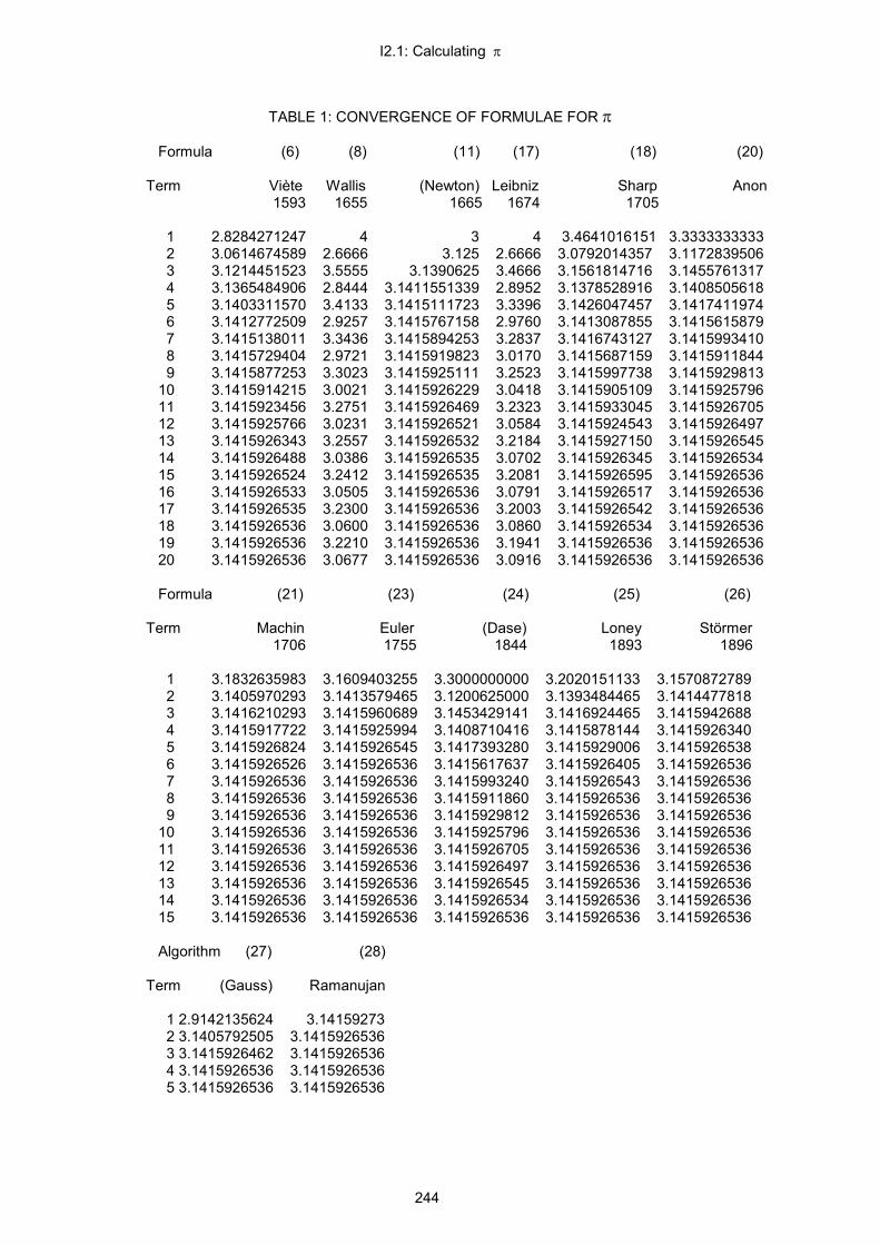
I2.1: Calculating π
244
TABLE 1: CONVERGENCE OF FORMULAE FOR π
Formula (6) (8) (11) (17) (18) (20) Term Viète Wallis (Newton) Leibniz Sharp Anon
1593 1655 1665 1674 1705
1 2.8284271247 4 3 4 3.4641016151 3.3333333333 2 3.0614674589 2.6666 3.125 2.6666 3.0792014357 3.1172839506 3 3.1214451523 3.5555 3.1390625 3.4666 3.1561814716 3.1455761317 4 3.1365484906 2.8444 3.1411551339 2.8952 3.1378528916 3.1408505618 5 3.1403311570 3.4133 3.1415111723 3.3396 3.1426047457 3.1417411974 6 3.1412772509 2.9257 3.1415767158 2.9760 3.1413087855 3.1415615879 7 3.1415138011 3.3436 3.1415894253 3.2837 3.1416743127 3.1415993410 8 3.1415729404 2.9721 3.1415919823 3.0170 3.1415687159 3.1415911844 9 3.1415877253 3.3023 3.1415925111 3.2523 3.1415997738 3.1415929813 10 3.1415914215 3.0021 3.1415926229 3.0418 3.1415905109 3.1415925796 11 3.1415923456 3.2751 3.1415926469 3.2323 3.1415933045 3.1415926705 12 3.1415925766 3.0231 3.1415926521 3.0584 3.1415924543 3.1415926497 13 3.1415926343 3.2557 3.1415926532 3.2184 3.1415927150 3.1415926545 14 3.1415926488 3.0386 3.1415926535 3.0702 3.1415926345 3.1415926534 15 3.1415926524 3.2412 3.1415926535 3.2081 3.1415926595 3.1415926536 16 3.1415926533 3.0505 3.1415926536 3.0791 3.1415926517 3.1415926536 17 3.1415926535 3.2300 3.1415926536 3.2003 3.1415926542 3.1415926536 18 3.1415926536 3.0600 3.1415926536 3.0860 3.1415926534 3.1415926536 19 3.1415926536 3.2210 3.1415926536 3.1941 3.1415926536 3.1415926536 20 3.1415926536 3.0677 3.1415926536 3.0916 3.1415926536 3.1415926536
Formula (21) (23) (24) (25) (26)
Term Machin Euler (Dase) Loney Störmer
1706 1755 1844 1893 1896
1 3.1832635983 3.1609403255 3.3000000000 3.2020151133 3.1570872789 2 3.1405970293 3.1413579465 3.1200625000 3.1393484465 3.1414477818 3 3.1416210293 3.1415960689 3.1453429141 3.1416924465 3.1415942688 4 3.1415917722 3.1415925994 3.1408710416 3.1415878144 3.1415926340 5 3.1415926824 3.1415926545 3.1417393280 3.1415929006 3.1415926538 6 3.1415926526 3.1415926536 3.1415617637 3.1415926405 3.1415926536 7 3.1415926536 3.1415926536 3.1415993240 3.1415926543 3.1415926536 8 3.1415926536 3.1415926536 3.1415911860 3.1415926536 3.1415926536 9 3.1415926536 3.1415926536 3.1415929812 3.1415926536 3.1415926536 10 3.1415926536 3.1415926536 3.1415925796 3.1415926536 3.1415926536 11 3.1415926536 3.1415926536 3.1415926705 3.1415926536 3.1415926536 12 3.1415926536 3.1415926536 3.1415926497 3.1415926536 3.1415926536 13 3.1415926536 3.1415926536 3.1415926545 3.1415926536 3.1415926536 14 3.1415926536 3.1415926536 3.1415926534 3.1415926536 3.1415926536 15 3.1415926536 3.1415926536 3.1415926536 3.1415926536 3.1415926536
Algorithm (27) (28)
Term (Gauss) Ramanujan
1 2.9142135624 3.14159273 2 3.1405792505 3.1415926536 3 3.1415926462 3.1415926536 4 3.1415926536 3.1415926536 5 3.1415926536 3.1415926536

I2.2: Offshoots of π and the Harmonic Series
245
I2.2: OFFSHOOTS OF π AND THE HARMONIC SERIES ******************************************************************************************************************** IN WHICH we explore various directions opened up for us by π and the harmonic series. ******************************************************************************************************************** What Kind of Number is π? In 1767 Lambert (1728-77) proved by means of continued fractions (Sideshow S4) that π is irrational. His argument was made more rigorous by Legendre in 1794. In 1775 Euler first suggested that π might also be transcendental - that is, it could not be the root of any algebraic equation (q.v. G3). However, it was not known until Liouville (1809-92) proved it in 1840 that such numbers even existed. Then in 1873 Hermite proved the transcendence of e. In 1882 von Lindemann, building upon this, proved that π is transcendental from the theorem 1−=πie which this book seeks to establish (see A2.5.1 (11) and A3.5.3 (1)). His proof showed that if x is the root of a rational integral algebraic equation, then e
x cannot be
rational. Hence, if iπ were the root of such an equation, πie could not be rational. But πie is equal to -1, and therefore is rational. Hence iπ cannot be the root of such an algebraic equation, and therefore neither can π. Three Classical Problems By doing so, Lindemann dealt the death blow to one of the three great classical problems bequeathed to us by the Greeks. These were
(1) "Squaring the circle": Draw a square of the same area as a given circle. (2) "Trisecting the angle": Draw an angle one third of the size of one already given. (3) "Doubling the cube" (the "Delian problem"): Find the edge of cube which has twice the volume of a given cube.
In their traditional form each of these problems had to be solved under the constraint, possibly deriving from Plato, of using a finite number of steps with a compass and straight-edge only. Without this condition
Archimedes solved the first, using a proof by reductio ad absurdum (q.v. G1) Hippias of Elis (c.420 BC) solved the second, using a curve called the trisectrix, and Menaechmus (c.350 BC), a researcher into conic sections or conics (Sideshow S3) solved the
third. A fascinating historical account of these three problems is to be found in Chapter XII, "Three Classical Geometrical Problems", in Rouse Ball & Coxeter (B2) pp.338-59. The arrival of Descartes' analytic geometry in 1637 made it possible to tackle such questions analytically. It turns out that the only constructions possible with the required instruments correspond to first- and second-order algebraic equations. Von Lindemann proved that π is not only not the root of first- and second-order algebraic equations, but it is not the root of any algebraic equation of any order. It follows that squaring the circle by compass and straight-edge alone is impossible; the other two problems were also shown in the nineteenth century to be insoluble under that constraint. The Danish mathematician G. Mohr proved in 1672 that any geometric construction that is possible with straight edge and compass can be achieved with compass alone; but his work was lost until 1928, and the credit for this is therefore usually given to the Italian geometer Mascheroni, who reproved it in 1797.

I2.2: Offshoots of π and the Harmonic Series
246
Zeta Function We should perhaps mention here Euler's triumph in solving the 'Basel problem' of his day (1735) by proving the convergence
6
...41
31
21
11 2
2222π
=++++ (1)
Although not originally a device for computing π, it provided a stepping stone from the harmonic series
∑∞
=∞ =++++=
1
1...41
31
21
11
rr
H (I1.2.5 (2))
which does not converge, to the ζ (zeta) function
∑∞
=
−=++++=ζ1
...41
31
21
11)(
k
sssss
ks (2)
which converges for all real s > 1. (ζ(1) is of course the harmonic series ∞H ) Euler's astonishing proof (1737) that
,1
1)(1
∏∑ −
∞
=
−
−==ζ
primeps
k
s
pks s > 1 (3)
known as Euler's product, one of his most brilliant and surprising discoveries, is now foundational to our understanding of prime numbers. (The capital pi indicates the product taken over all prime
numbers p of the expression sp −−1
1 .) It gains much of its power from having an infinite sum on one
side of the equation and an infinite product on the other. Euler himself computed the first fourteen values of the ζ function for even values of s, continuing
,90
)4(4π
=ζ 945
)6(6π
=ζ ,…
It is surely awesome - magical - that any single constant so seemingly arbitrary as π should be the end product of so many different formulae and the subject of so many diverse theorems in so many disparate branches of mathematics. How can this be? It is a question well worth pondering. The ζ function is central to the present day investigation of prime numbers, being the subject matter of the Riemann hypothesis, in which the argument s is made complex. This is the most famous, and probably the most significant, of the unsolved mathematical problems of our day. The story is told in du Sautoy (B4) and in greater depth by Havil (B1), who supplies Euler's 1735 proof of (1) on p.39.

A3.1.1: Geometric Progressions (Reprise)
247
ACT 3: POWER SERIES
ACT 3 SCENE 1: POWER SERIES INTRODUCED
A3.1.1: GEOMETRIC PROGRESSIONS (REPRISE) ******************************************************************************************************************** IN WHICH we explore the convergence and divergence of geometric series, invoking the help of the spreadsheet. ******************************************************************************************************************** Introduction to Act 3 Hitherto in our drama, we have spent much time looking at how certain elementary functions, such as trigonometrical, logarithmic and exponential functions, arise, and how they relate to each other (Act 1), as well as how to differentiate and integrate them (Act 2). Except in certain special cases, such as in A1.3.3, we have said very little about how to calculate their values to any great precision. This is a question we tackle in Act 3, where we find in various different ways power series (q.v. G5) for these functions which enable us to evaluate them for a given range of arguments. This process mirrors our treatment of π. In Act 1 Scene 2 we introduced this constant and began to indicate its fundamental importance and some of the relations in which it appears. But not until Interlude I2.1 did we discuss the many formulae by which its single value can be calculated. We now build on what we have already learned about the simple form of power series called geometric series (A1.1.7) in order to familiarise ourselves with the concept of convergence (q.v. G5) and the properties of power series generally (A3.1). We shall also extend our understanding of the binomial theorem by introducing the general version (A3.2) from which many such power series may be generated. Along the way we shall consider two other methods - reversion (A3.3) and Maclaurin series (A3.4) - by which the same power series have historically been arrived at. Finally we draw the threads together to show the unity of these various functions as proclaimed by Euler's identities (A3.5). Recapitulation: When |t| < 1 In section A1.1.7 we met the geometric progression or sequence c, ct, ct
2, ct
3, ct
4, ...,
and its sum, the geometric series S = c + ct + ct
2 + ct
3 + ct
4 +... (1)
We saw also that the nth partial sum (q.v. G5)
,1
1t
tcSn
n −−
= 1≠n (A1.1.7 (3)) (2)
and found that if |t| < 1, as n gets ever larger,
,0lim =∞→
n
nt |t| < 1 (A1.1.7 (4)) (3)
So in this case S
n converges to the limit
,1
01limt
cSS nn −−
==∞→
|t| < 1

A3.1.1: Geometric Progressions (Reprise)
248
,1 t
cS−
= |t| < 1 (A1.1.7 (5)) (4)
Since c and t are both constants, we have a genuine limit within the stated range for t. Two examples of convergence follow, after which we consider cases where the constraint |t| < 1 is not met. Example (1) Putting c = 1, t = ½ gives the series
...21...
321
161
81
41
211
1
+
+++++++−n
Since |t| < 1, from equation (4) its limiting sum is
( ) ( ) 21
1
21
021
1
121 =
−== ∑∑
∞
=
∞
=
−
n
n
n
n (5)
Example (2) Putting c = 1, t = -½ gives the series
...21...
321
161
81
41
211
1
+
−++−+−+−−n
Since |t| < 1, from equation (4) its limiting sum is
( ) ( )32
11
21
021
1
121 =
+=−=− ∑∑
∞
=
∞
=
−
n
n
n
n (6)
When |t| = 1 If t = 1, from equation (1), S = c + c + c +..., i.e. S is infinite and divergent.
If t = -1, from equation (1), S = c - c + c - c...
= c and 0 alternately. Divergent series that do this are said to oscillate.
When |t| > 1 If t > 1, S in equation (1) keeps on growing in magnitude by terms which themselves are increasing
without limit, and so diverges. For instance if t = 2,
S = c + 2c + 4c + 8c + 16c +...
If t < -1, S in equation (1) keeps on growing in magnitude, but the terms keep changing sign. For instance if t = -2,
S = c - 2c + 4c - 8c + 16c - 32c +...+ c(-2)n-1
+...
and the partial sums become successively S
n = c, -c, 3c, -5c, 11c, -21c,...
i.e. they oscillate and diverge.

A3.1.1: Geometric Progressions (Reprise)
249
In all these cases, where |t| ≥ 1, we find that the series diverges. So |t| < 1 is the only case which converges, since only here does limit (3) hold. We offer some examples below.
Spreadsheet Much of this can be verified using the binomial theorem spreadsheet detailed in Sideshow S2. This enables us to compute the terms and partial sums of (a + x)
r for various a, x and r which can be
entered at the top. Setting a = 1 and the exponent r to -1 enables us to examine the behaviour of
x+11 for various values of x, where x = -t in equation (4). We restrict ourselves to c = 1 since this
does not feature in the spreadsheet. Ignoring the first five columns which do not concern us here, we will find the individual sequence terms in the column headed "term k", and the partial sums S
n in that
headed "sum terms". Convergence is indicated if this final column ever becomes constant. Let us start with cases where c = 1 and |t| < 1. By entering suitable values of x = -t into the
spreadsheet such that -1 < x < 1 we can see how x+1
1 behaves. For instance:
t = 0.5 (x = -0.5).
Result: the spreadsheet converges to S = 2 as expected in Example (1). t = -0.5 (x = 0.5).
Result: the spreadsheet converges to S = 0.666666... = 2/3 as expected in Example (2).
These two results confirm that S converges when |t| < 1. Other values of |x| < 1 may be entered into the spreadsheet as desired. Let us now try values of |t| ≥ 1 as discussed above, setting c = 1 in equation (4) as before.
t > 1 (x < 1). Put x = -2. Result: S
n = 1, 3, 7, 15, 31,..., increasing without limit as expected.
t = 1. Put x = -1.
Result: Sn = 1, 2, 3, 4, 5,..., increasing by c = 1 as expected.
t = -1. Put x = 1.
Result: Sn = 1, 0, 1, 0, 1,..., oscillating as expected.
t < -1 (x > 1). Put x = 2.
Result: Sn = 1, -1, 3, -5, 11, -21,..., oscillating and diverging as expected.
Our spreadsheet therefore confirms that S diverges when |t| ≥ 1. Other values may be entered as desired.
* * * * * We have now met in the geometric series a simple form of power series which are the subject of this act, and the concepts of convergence and divergence which are integral to it.

A3.1.2: Power Series Defined
250
A3.1.2: POWER SERIES DEFINED
******************************************************************************************************************** IN WHICH we find a general definition of a power series. ******************************************************************************************************************** A power series is an infinite expression of the form a
0 + a
1 (x - a) + a
2 (x - a)
2 + a
3 (x - a)
3 +...+a
n (x - a)
n +... (1)
where a
0, a
1, a
2, a
3, ..., a
n,... are coefficients (constants)
x is a variable a (plain) is a value of x at which the series is known to be valid. [Note: we follow traditional notation as in most books. The reader should not confuse "a" plain with "a" subscripted, as "a
0", "a
1": the two are distinct.]
Such series are called "power series" as their terms involve increasing powers of the variable concerned. An example of a power series is 1 + 2 (x - 3) + 3 (x - 3)
2 + 4 (x - 3)
3 +...
If a = 0 series (1) reduces to a
0 + a
1x + a
2x
2 + a
3x
3 +...+ a
nx
n +... (2)
For example 1 + 2x + 3x
2 + 4x
3 +...
In either form a power series may often (when it converges) be treated as an indefinitely extended polynomial. Form (1) may be written more concisely as
( )∑∞
=
−0n
nn axa
and form (2) as
∑∞
=0n
nn xa
where ∑∞
=0n
means "the sum of all terms involving n when n varies from zero to infinity in steps of 1".
The infinity in question here is a countable infinity (q.v. G2) because the steps towards it can be counted (mapped on to the counting numbers).

A3.1.2: Power Series Defined
251
The geometric series that we met in sections A1.1.7 and A3.1.1 are a special case of power series (form (2)) in which all the a
n terms are the same.

A3.1.3: Convergence of Power Series
252
A3.1.3: CONVERGENCE OF POWER SERIES ******************************************************************************************************************** IN WHICH we show how to apply the ratio test for power series in order to determine whether or not a given power series converges. Notable source: Open University M203 Unit AB3 Power Series (1987), pp.21-2. ******************************************************************************************************************** Crucial to our treatment of any infinite series is the issue of whether or not it converges, and for what values of the variable it does so. If it converges, we are able to manipulate it (section A3.1.4) in ways that would not be valid otherwise. For power series we use the ratio test for convergence of power series described below. We first establish whether or not there exists a radius of convergence, that is a range of values of x within which convergence is possible. Radius of Convergence Theorem The radius of convergence theorem runs as follows.
For a given power series ( )∑∞
=
−0n
nn axa , one of three possibilities must occur:
(a) The series converges only when x = a. (b) The series converges for all x.
(c) There is a number R > 0, called the radius of convergence of the series, such that the series converges if x > a - R and x < a + R, that is, if |x - a| < R, and the series diverges if x < a - R or x > a + R that is, if |x - a| > R. (Recall that | | means "the absolute or positive value of".)
(See Figure 1. The theorem does not specify for the cases when x = a - R or x = a + R, where each series must be considered separately.)
Ratio Test for Convergence of Power Series We can tell which of the above three possibilities applies by the ratio test for convergence of power series, as follows.

A3.1.3: Convergence of Power Series
253
If we look at the successive coefficients an, a
n+1 and so forth, as n grows ever larger )( ∞→n , we can
determine what happens to the absolute ratio n
n
aa 1+ . If this ratio tends to a limiting value L, then three
things can happen, corresponding to (a), (b) and (c) above: (a) If L is ∞, the series converges only for x = a, (R = 0). (b) If L = 0, the series converges for all x (R = ∞). (c) If L > 0, the series has radius of convergence R = 1/L.
If the ratio n
n
aa 1+ does not tend to a limit, the ratio test gives no criterion for determining whether or not
there is convergence. Example Consider the power series
...54321
5432−+−+−
xxxxx
which as we shall see at A3.3.3 (9) is Mercator's series for ln (1 + x).
This has a = 0 and the sequence of absolute coefficient ratios n
n
aa 1+
,...1
,...,54,
43,
32,
21,...,...,,,,
11
1
415
1
314
1
213
1
112
1
+=+
nn
n
n
for which the limit as ∞→n is L = 1 (case (c) above), giving radius of convergence R = 1. So the series converges for |x| < 1 at least, but the end points x = ±1 need to be tested individually. If x = 1 the series gives
ln (1 + 1) = 1 - 1/2 + 1/3 - 1/4 + 1/5 -... (1)
which eventually converges to 0.69314718..., the correct value for ln 2. If x = -1 it gives
ln (1 - 1) = -1 - 1/1 - 1/2 - 1/3 - 1/4 -1/5 -… (2)
that is, the negative of the harmonic series H∞, which latter was proved by Oresme in the fourteenth century to diverge (see the proof in I1.2.5). This confirms that ln 0 is infinite and negative, as we found in A1.6.4 (see Figure 1 there).
Hence the series ln (1 + x) = ...54321
5432−+−+−
xxxxx converges for -1 < x ≤ 1.

A3.1.4: Manipulating Power Series
254
A3.1.4: MANIPULATING POWER SERIES ******************************************************************************************************************** IN WHICH we learn how to manipulate convergent power series in order to obtain new ones. ******************************************************************************************************************** Let us first define by way of illustration three typical convergent power series f, g and h on which we are going to operate:
∑∞
=
−=0
)()(n
nn axaxf
= a0 + a
1(x - a) + ... + a
n(x - a)
n + ... for |x - a| < R
f
∑∞
=
−=0
)()(n
nn axbxg
= b0 + b
1(x - a) + ... + b
n(x - a)
n + ... for |x - a| < R
g
∑∞
=
=0
)(n
nn xcxh
= c0 + c
1x + c
2x
2 + ... + c
nx
n + for |x| < R
h
where R
f , R
g and R
h are the respective radii of convergence as described in section A3.1.3.
The following rules, offered without proof, show how the series can be manipulated so as to obtain further power series which also converge. Constant Multiple Rule for Power Series Convergent power series may be multiplied throughout by a constant by multiplying each coefficient by that constant.
∑∞
=
−=0
))(()(n
nn axkaxkf for |x - a| < R
f (1)
Sum Rule for Power Series Convergent power series can be added by adding the matching coefficients term by term.
∑∞
=
−+=+0
))(())((n
nnn axbaxgf for |x - a| < r,
where r = minimum of Rf , R
g. (2)
Product Rule for Power Series Convergent power series in x may be multiplied together by multiplying coefficients and adding the resulting new coefficients for each power of x.
...)(...)()( 10 +−++−+= n
n axdaxddxfg where

A3.1.4: Manipulating Power Series
255
d0 = a
0b
0
d1 = a
0b
1 + a
1b
0
... d
n = a
0b
n + a
1b
n-1 + ... a
n-1b
1 + a
nb
0
for |x - a| < r, where r = minimum of R
f , R
g. (3)
Differentiation Rule for Power Series (at 0) Convergent power series may be differentiated by differentiating each term individually.
∑∞
=
−=1
1)('n
nn xncxh for |x| < R
h (4)
Integration Rule for Power Series (at 0) Convergent power series may be integrated by integrating each term individually.
∫ ∫∞
=
+ ++
=0
1
1)(
n
nn Cxnc
dxxh for |x| < Rh (5)
where the value of C, the constant of integration, can be found by putting x = 0 .
In all these respects convergent power series may be treated naively as mere polynomials. No such assumption may be made in the case of non-convergent power series, whose behaviour may be undefined. Conversely, the above rules continue to hold in principle if any of f, g, or h is replaced by a polynomial, since a polynomial may be considered to be a series with only a finite number of non-zero coefficients, the rest being zero.

A3.2.1: Binomial Coefficients Revisited
256
ACT 3 SCENE 2: GENERAL BINOMIAL THEOREM
A3.2.1: BINOMIAL COEFFICIENTS REVISITED ******************************************************************************************************************** IN WHICH we learn how the binomial coefficients can be extended into an infinite sequence. ******************************************************************************************************************** Historical Note In 1664 or 1665 Newton, whilst still at Cambridge, embarked upon a mathematical and scientific voyage of discovery that was to make him one of the greatest scientists of all time. One of the first tasks he set himself was to generalise the (special) binomial theorem, which had been known since the Middle Ages, so as to accommodate exponents that were other than positive integers. His starting point was Wallis's interpolation of Pascal's triangle which had led him to his product formula for π/4 (I2.1 (8)). Newton's solution was what in this book we term the general binomial theorem, in which the exponent can take any real value (as now understood; Newton himself reasoned with only rational and negative indices). The tale is told in detail by Edwards (B4), pp.95-103). Central to this is the identification of the binomial coefficients which apply under the new circumstances. This led to a whole new approach to infinite series, which were already appearing on the horizon. We have already noted echoes of this when describing Newton's calculation of π/6 in I2.1 (11). The general binomial theorem proved to be a stepping stone on Newton's route towards discovering the calculus in 1665-6, at his home in Woolsthorpe, Lincolnshire whither he had fled from Cambridge in order to avoid the plague. However, in our drama, with the benefit of hindsight, we have found it convenient to reverse the order: we need the calculus in order to give any useful treatment of series, and to illustrate the full significance of the contribution later made by Euler. Like Euler, Newton was a great unifier, and therein lay much of his greatness. This is apparent not only in the general binomial theorem but also in his law of gravitation which combined into one the three laws of Kepler. This he published in his Principia Mathematica of 1687, called by Boyer and Merzbach (B4, p.444) 'the most admired scientific treatise of all times.' Binomial Coefficients Consider the sequence of products k product (0) 1 (1) r (2) r(r-1) (3) r(r-1)(r-2) ... (r) r(r-1)(r-2) ... (r-k+1) (r+1) r(r-1)(r-2) ... (r-k)(r-k+1) (r+2) r(r-1)(r-2) ... (r-k-1)(r-k)(r-k+1) and so forth where k is any nonnegative integer (integer ≥ 0). Each product ends with the new factor (r-k+1). If ever the factor (r-k+1) becomes zero, then the product also becomes zero. Further, since each product is a factor of all subsequent products, all subsequent products become zero also. This can only happen if r = k - 1 is a nonnegative integer, in which case all products having k ≥ (r+1) vanish, and the sequence terminates when k = r. This is what happened with the binomial coefficients which featured in the special binomial theorem in

A3.2.1: Binomial Coefficients Revisited
257
Act 1 Scene 4. Here r was a nonnegative integer, as we indicated by denoting it n. The sequence of binomial coefficients in A1.4.3 (9)
!
)1)...(2)(1(k
knnnnkn +−−−
=
(1)
had exactly n+1 non-zero terms, the last of which had k = n, giving ,1=
kn
with 0=
kn
thereafter as
k > n. However, if the exponent r is not a nonnegative integer while k continues to remain one - for instance if r is negative or not an integer at all - (r-k+1) can never equal zero. Hence there is no threshold beyond which all the coefficients are zero, so terminating the expansion. Then the sequence
!
)1)...(2)(1(k
krrrrkr +−−−
=
(2)
has a genuinely infinite number of terms. Hence equation (2) is valid for all real numbers, equation (1) being a special case when the number of terms is finite. The reader can explore this for him/herself by running the binomial theorem spreadsheet detailed in Sideshow S2, and seeing what are effects of entering different values of r. When, and only when, r is
supplied as 0 or a positive integer, there comes a value of k (= r+1) when the column "
kr
" becomes
0 and stays 0 ever afterwards, at which point the final column "sum terms" remains constant. For negative or fractional values of r, this never happens.
In section A3.2.2 we look at the properties of the binomial coefficients
kr
for real r, before showing in
A3.2.3 how we use them to generate the general binomial theorem.
We note in passing that, by a further extension,
wr
can be computed with the Γ (gamma) function
where r and w can both be any real numbers. This is described in Epilogue 3.

A3.2.2: Properties of the Binomial Coefficients
258
A3.2.2: PROPERTIES OF THE BINOMIAL COEFFICIENTS ******************************************************************************************************************** IN WHICH we explore the properties of the binomial coefficients for real exponents. Notable source: Knuth (B3), pp.51-73. The reader is also referred to the binomial theorem spreadsheet (Sideshow S2) for experimental verification. ******************************************************************************************************************** Definition: (Compare A1.4.3 (9).) For all real numbers r and integers k,
,1)1)...(1(
)1)...(2)(1(
1∏
≤≤
−+=
−+−−−
=
kjj
jrkk
krrrrkr
integer k > 0 (1)
,10
=
r (2)
,0=
kr
integer k < 0 (3)
For particular cases,
,1
rr
=
2)1(
2−
=
rrr (4),(5)
Factorials For completeness we recall the factorial expression for computing binomial coefficients given in section A1.4.3 (10),
kn
= )!(!
!knk
n−
, integer 0 ≤ k ≤ n (6)
Symmetry Likewise from section A1.4.3 (11):
,
=
− k
nkn
n integer k, n, 0 ≤ k ≤ n (7)
When k < 0 or k > n, 0=
kn
(nonnegative integer n, A1.4.3 (13)).
Moving in and out of Brackets From definition (1) we have
−−
=
11
kr
kr
kr
integer k ≠ 0 (8)
This formula is very useful for combining a binomial coefficient with other parts of an expression. Hence also
A3.2.2: Properties of the Binomial Coefficients
259
−−
=
11
kr
rkr
k , integer k (9)
For instance, for r = 6, k = 2,
305615
615226
2 =×=
=×=
Also
−−
=
1111
kr
kkr
r (10)
when no division by zero has been performed.
Applying equations (7), (8) and (7) again gives
−−
=
−−
−−
=
−
=
kr
krr
krr
krr
krr
kr 1
11
, integer k ≠ r (11)
which can be shown to be valid in spite of the jump from integer n to real r.
Addition Formula By extension from Pascal's triangle (A1.4.3 (6)),
kr
=
−−
11
kr
+
−kr 1
(12)
This is often useful in obtaining proofs by induction on r, when r is an integer. Summation Formulae From equation (11) we can derive the useful summation
,11
...1
10
0
++=
+++
++
=
+∑≤≤
nnr
nrrr
kkr
nk
integer n ≥ 0 (13)
as follows:
Put 'r = r + n + 1
and define
=
++=
nr
nnr
nF'1
)(
Then from addition formula (12)
−+
−−
=
=
nr
nr
nr
nF1'
11''
)(
++−=
nnr
nF )1(
This recursive expression gives

A3.2.2: Properties of the Binomial Coefficients
260
,1
)(0∑
≤≤
+=
++=
nkk
krn
nrnF integer n ≥ 0 (13)
which is equation (12).
A second valuable summation
∑≤≤
+
+=
++
+
+
=
nkmn
mn
mmmmk
011
...210
, integer m ≥ 0, integer n ≥ 0 (14)
can be proved by induction on n. Sums of Powers and Polynomials Putting m = 1 in equation (14) gives
!2
)1(2
1...210
1...
12
11
10 nnn
nn +
=
+=++++=
++
+
+
(15)
the sum of an arithmetic progression from 0 to n (A1.1.6 (8)). Similarly, in order to sum the squares 1
2 + 2
2 + 3
2 +...+ n
2, we note that
k2 = k(k-1) + k =
+
12
2kk
Then from equation (14),
∑ ∑≤≤ ≤≤
++
+=
+
=
nk nk
nnkkk
0 0
2
21
31
212
2
So in polynomial notation,
12 + 2
2 + 3
2 +... + n
2
6)12)(1(
!2)1(
!3)1()1(2 ++
=+
+−+
=nnnnnnnn (16)
This formula was known to, and proved by, Fibonacci. The sum
13 + 2
3 + 3
3 +...+ n
3 = ( )2
2
...3212
)1( nnn++++=
+ (17)
can be obtained in a similar way. Indeed any polynomial
a0 + a
1k + a
2k
2 +...+ a
mk
m
can be expressed using equation (14) as
+
+
+
mk
bk
bk
bk
b m...210 210

A3.2.2: Properties of the Binomial Coefficients
261
for suitably chosen coefficients b0, b
1, b
2,...b
m.
Negating the Upper Index The basic identity
( )
−+−=
−k
krk
r k 11 , integer k (18)
follows from the definition (equations (1) to (3)) when each term of the numerator is negated. From this can be shown that
( ) ( ) ( ) ,1
11...10
1
−−=
−++
−
=−
∑≤
nr
nrrr
kr nnk
nk
integer n ≥ 0 (19)
Simplifying Products Products of binomial coefficients can usually be handled by moving in and out of factorials as in equation (6). For instance
−
−
=
km
krkr
km
mr
, integer m, integer k (20)
Equation (8) is a special case of this, when k=1.
Sums of Products These formulae show how to sum over a product of two binomial coefficients, considering various places where a running variable k might appear. The most important is
+=
−
∑ nsr
kns
kr
k
, integer n (21)
But note also
,
++
=
+
∑ nrsr
kns
kr
k
integer n, integer n ≥ 0 (22)
( ) ( )∑
−
−=−
+
k
rk
rns
nks
kr
,11 integer n, integer n ≥ 0 (23)
( ) ( )∑≤≤
−−−−
−=−
−
−
rk
tk
mtrstr
tks
mkr
0
,11 integer t ≥ 0, integer r ≥ 0, integer m ≥ 0 (24)
General Binomial Theorem The most powerful application of the binomial coefficients is the general binomial theorem which is the subject of the next section.

A3.2.3: General Binomial Theorem
262
A3.2.3: GENERAL BINOMIAL THEOREM ******************************************************************************************************************** IN WHICH we explore the general binomial theorem, from which derive a variety of important power series. ******************************************************************************************************************** Derivation In section A1.4.3 (18) we established the special binomial theorem as
kknn
k
n xakn
xa −
=∑
=+
0
)( (1)
where k and n are nonnegative integers and the binomial coefficient
kn
= !
)1)...(2)(1(k
knnnn +−−− (A1.4.3 (9)) (2)
As we saw then, there are in this case (that is, 0 ≤ k ≤ n) n + 1 non-zero coefficients which form row n of Pascal's triangle. However, as explained in section A3.2.1, for k > n, expression (2) yields zero ever afterwards, so that we can re-express equation (1) as
kkn
k
n xakn
xa −∞
=∑
=+
0
)( (3)
We saw also in section A3.2.1 that
kn
is a special case of
kr
, where r is any real number. So
,!
)1)...(2)(1(k
krrrrkr +−−−
=
(4)
When r is negative or nonintegral, this gives an infinite sequence of non-zero coefficients. Combining (3) and (4) we have now the general binomial theorem, as follows:
kkr
k
r xakr
xa −∞
=∑
=+
0
)( (5)
where r is any real number. This expands as
( ) ...!3
)2)(1(!2
)1(!1
33221 +−−
+−
++=+ −−− xarrrxarrxaraxa rrrrr (6)
If r is negative or nonintegral this is an infinite power series which does not always converge. However, if we write (a + x)
r as a
r (1 + x/a)
r, it converges when
r < 0: -1 < x/a < 1, that is, |x/a| < 1 (7) r > 0: -1 ≤ x/a ≤ 1, that is, |x/a| ≤ 1 (8)
(When r = 0, (a + x)
r = 1 for all a and x.) Figure 1 is a map of x/a against r which indicates where
convergence is achieved:

A3.2.3: General Binomial Theorem
263
on all unbroken lines, both horizontal and vertical, and on the shaded area where |x/a| < 1 (conditions (7) and (8))
If a = 1 the theorem becomes
k
k
r xkr
x ∑∞
=
=+
0
)1( (9)
...321
1 32 +
+
+
+= x
rx
rx
r (10)
...!3
)2)(1(!2
)1(!1
1 32 +−−
+−
++= xrrrxrrxr (11)
which converges at least where |x| < 1. The general binomial theorem was independently rediscovered by Gregory in 1670. It can be formally proved from the rules about power series given in section A3.1.4, and in particular, A3.1.4 (4), the differentiation rule for power series. Newton himself offered no formal proof. It was in proving it early

A3.2.3: General Binomial Theorem
264
in his career that Gauss, the "Prince of Mathematicians", initiated the rigorous modern understanding of analysis (q.v. G1), which centres on the correct use of infinite processes. Example (1): Negative r (The Intermediate Binomial Theorem)
Putting r = -1 we can expand x+1
1 as
...!3
)3()2(1!2
)2(1!111)1( 21 +
−×−×−+
−×−+
−+=+ − xx
= 1 - x + x
2 - x
3 +..., |x| < 1 (12)
That is, it reduces to the familiar geometric series of A1.1.7 (7). (Note that if we put x=1 here the series becomes (1 + 1)
-1 = 1 - 1 + 1 - 1 + 1 - 1 +...
whose sum oscillates between 1 and 0. Yet 2
-1 = ½, which illustrates the dangers of drawing
conclusions from non-convergent series.)
Similarly, writing - x for + x gives an expansion of x−1
1 which reduces to the familiar A1.1.7 (8),
(1 - x)
-1 = 1 + x + x
2 + x
3 +..., |x| < 1 (13)
Generally, if r is a negative integer, the coefficients of (1 - x)
r, themselves all integers, are given by
column k = |r| - 1 in Pascal's triangle. So column k = 2 gives the coefficients of (1 - x)
-3 = 1 + 3x + 6x
2 + 10x
3 +... (14)
This is the intermediate binomial theorem that we met in I1.2.3. Like the special variant, it is a subset of the general theorem. If + x replaces - x then the signs alternate. So (1 + x)
-2 = 1 - 2x + 3x
2 - 4x
3 +... (15)
Example (2): Nonintegral r If r = ½ we can take square roots by
( ) ...!3
1.23.
21.
21
!21.
21.
21
!11.
2111 322
1+
−−+
−++=+ xxxx
...642
3142
1211 32 −
×××
+×
−+= xxx (16)
for all |x| < 1. E.g. Putting x = 0.3 gives 3.1 = 1 + 0.15 - 0.01125 + 0.0016875 -... = 1.1404375 -...
(correct answer 1.140175...). Other roots (cubic, fourth etc) may be obtained similarly.

A3.2.3: General Binomial Theorem
265
In such a case the binomial coefficients may be any real number. Where |x| > 1, other techniques may be used, such as Newton-Raphson iteration (section A3.4.4).
* * * * * The binomial theorems form the centre piece of our drama. Both the special and the intermediate forms of the theorem are, algebraically, special cases of the general form, but their properties are sufficiently distinct to warrant treating them separately. The relationships between them are summarised in the following table of the properties of the expansion (1 + x)
r, in terms of their exponents r, the number and nature of the binomial coefficients
generated and their relationship with Pascal's triangle, as well as the range of convergence.
r Theorem Coefficients Converge Integer ≥ 0 Special Integer Finite Row of P's T All x
Integer < 0 Intermediate Integer Infinite Col of P's T |x| <1 Real General Real Infinite - |x| <1
The reader may find it instructive to explore the three variants for him/herself using the Binomial Theorem Spreadsheet program described in Sideshow S2. This has been devised to illustrate the relationship between the three theorems, and to show when convergence is achieved and when not. We shall find that some of the major functions we met in Act 1 - in particular the trigonometrical and exponential functions - which were expressed there as ratios or formulae, can now by expanding them under the general binomial theorem be expressed as convergent power series. This enables us to compute and manipulate them very effectively. However, historically, these series were arrived at by a variety of different routes. We shall find it instructive to see how different techniques led to the same series as mathematical technology improved. So we shall see how they were arrived at by reversion (Scene A3.3), by Taylor and Maclaurin series (Scene A3.4), and by the general binomial theorem (Scene A3.5).

A3.3.1 Reversion of Series
266
ACT 3 SCENE 3: REVERSION OF SERIES
A3.3.1: REVERSION OF SERIES ******************************************************************************************************************** IN WHICH we learn how to derive a power series representing the inverse function x = f-1(y) from that for a given function y = f(x). Notable source: Abramowitz and Stegun (B3), 3.6.25. ******************************************************************************************************************** This form of series manipulation was devised by Newton c.1669 and communicated by him to Leibniz in 1676. Given a converging power series y = ax + bx
2 + cx
3 + dx
4 + ex
5 + fx
6 + gx
7 +... (1)
we want to find another power series, if one exists, for its inverse function x = Ay + By
2 + Cy
3 + Dy
4 + Ey
5 + Fy
6 + Gy
7 +... (2)
Then, working to as many terms as we choose, we replace the x values in (1) by the RHS of (2) to obtain an identity in y: y ≡ a (Ay + By
2 + Cy
3 +...)
+ b (Ay + By2 + Cy
3 +...)
2
+ c (Ay + By2 + Cy
3 +...)
3 +... (3)
We now expand the brackets and collate the coefficients of each power of y in separate equations, which we solve in succession to obtain A, B, C,... in terms of a, b, c,.... This gives: For y: aA = 1 (4) y
2: a
3B = - b (5)
y
3: a
5C = 2b
2 - ac (6)
y
4: a
7D = 5abc - a
2d - 5b
3 (7)
y
5: a
9E = 6a
2bd + 3a
2c
2 + 14b
4 - a
3e - 21ab
2c (8)
y
6: a
11F = 7a
3be + 7a
3cd + 84ab
3c - a
4f - 28a
2bc
2 - 42b
5 - 28a
2b
2d (9)
y
7: a
13G = 8a
4bf + 8a
4ce + 4a
4d
2 + 120a
2b
3d + 180a
2b
2c
2
+ 132b6 - a
5g - 36a
3b
2e - 72a
3bcd - 12a
3c
3 - 330ab
4c (10)
etc This gives us the first seven terms of our series, which should be adequate for most computational purposes. With them, we should be able to identify the general term. We shall see how Newton used reversion to obtain a series expansion for sin x from sin
-1 x in section A3.3.2; and one for e
x from
Mercator's logarithmic series in A3.3.4. The historical importance of reversion is that it supplied an early, albeit clumsy, technique for deriving such series. It is in fact little more than an algebraic trick for deriving one series from another, which

A3.3.1 Reversion of Series
267
tells us very little of mathematical interest about the series themselves. These limitations are largely due to the fact that it took no account of the calculus, then in its infancy. As we shall see in A3.4.2, it was later supplanted by the much neater and more powerful procedure deriving from Taylor's series in 1715, which is based upon successive differentiation. In consequence of which power series of this kind became known as Taylor or Maclaurin series.

A3.3.2: Trigonometrical Power Series by Reversion
268
A3.3.2: TRIGONOMETRICAL POWER SERIES BY REVERSION ******************************************************************************************************************** IN WHICH we show how the trigonometric power series expansions were arrived at by Newton, Gregory and Leibniz. Notable source: Spiegel, Lipshutz and Liu (B3), chapter 22. ******************************************************************************************************************** Sine and Cosine Series (Newton) We have already seen how in 1665-6 Newton arrived with the aid of his freshly discovered general binomial theorem at the series I2.1 (10)
...7642
531542
3132
1sin753
1 +××××
+××
++=− xxxxx |x| < 1 (1)
From this cos
-1 x = π/2 - sin
-1 x, |x| < 1 (cf.A1.3.1 (2)) (2)
He then deduced the Maclaurin series for sin x from equation (1) in the first known use of the process of reversion that we described in section A3.3.1, as follows. Let y = sin
-1 x, x = sin y
Then adopting the coefficients from (1) above, a = 1, b = 0, c = 1/6, d = 0, e = 3/40, f = 0, g = 5/112,... for insertion in A3.3.1 (1), we have A3.3.1 (2), x = Ay + By
2 + Cy
3 + Dy
4 + Ey
5 + Fy
6 + Gy
7 +..., (3)
where from equations A3.3.1 (4) to (10)..., A = 1 B = 0
!31
61 −
=−
=C
D = 0
!5
1120
1403
363
==−=E
F = 0
!71
50401
181
1125
101
21612
1125
403.
68 −
=−
=−−=−−=G
Equation (3) now becomes

A3.3.2: Trigonometrical Power Series by Reversion
269
...!7!5!3
sin753
+−+−==yyyyyx
which we write, changing the variable from y to x, as
...!7!5!3
sin753
+−+−=xxxxx (4)
The Pythagorean identity A1.3.2 (1) cos
2 x + sin
2 x ≡ 1
then gives
...!6!4!2
1cos642
+−+−=xxxx (5)
These are the Maclaurin series expansions for sin x and cos x. We shall show in section A3.4.2 that they converge for all x. They were known to Gregory, Newton and Leibniz around 1670. Inverse of Tangent, and Tangent (Gregory) The Maclaurin series for tan
-1 x has already been given as Interlude I2.1 (16) as Gregory's series,
dating to 1671,
...753
tan753
1 +−+−=− xxxxx , |x| ≤ 1 (6)
However, this is only valid if |x| ≤ 1. If |x| > 1 we use
...,5
13
112
tan53
1 +−+−π
±=−
xxxx (7)
writing +2π if x ≥ 1 and -
2π if x ≤ -1.
The Maclaurin series expansion for tan x, deducible from (7) by reversion, was given by Gregory in 1671 as
...315
1715
23
tan753
++++=xxxxx , |x| < π/2 (8)
which converges unless x is an odd multiple of π/2 when tan x is undefined (+∞ or -∞). This can be obtained by reversion of equation (7) for tan
-1 x, or as the quotient sin x / cos x. (The latter can be
explored using program POLYDIV described in I1.2.2. Note however that this program works in decimal notation rather than fractions or factorials.) Secant, Cosecant and Cotangent (Gregory) The reciprocals of the series for cosine, sine and tangent give respectively those for secant, cosecant and cotangent:
...72061
245
21cos/1sec
642++++==
xxxxx , |x| < π/2 (9)

A3.3.2: Trigonometrical Power Series by Reversion
270
(another result of Gregory (1671)),
...,1512031
3607
61sin/1csc
53++++==
xxxx
xx 0 < |x| < π (10)
...9452
4531tan/1cot
53−−−−==
xxxx
xx 0 < |x| < π (11)
These can be explored using program RECIP described in I1.2.1 above. However, like POLYDIV, this program works in decimal notation rather than fractions or factorials. Inverses of Secant, Cosecant and Cotangent Finally the inverse functions for secant, cosecant and cotangent can be obtained by similar manipulation: sec
-1 x = cos
-1(1/x) = π/2 - csc
-1 x, |x| > 1 (12)
where
...,54231
3211)/1(sincsc
5311 +
××
×+
×+== −−
xxxxx |x| > 1 (13)
cot
-1 x = tan
-1 (1/x) = π/2 - tan
-1 x
=
>−+−+π
<
+−+−−
π
)15(1||...,5
13
11
)14(1||,...7532
53
753
xxxx
p
xxxxx
where p = 0 if x > 1, p = 1 if x < -1.
* * * * * Note that we have made a transition from thinking about the trigonometrical functions as geometrical properties of angles, as in Act 1 Scene 3 onwards, to their more abstract and algebraic representations as series. This transition we have indicated by denoting their arguments as typically x rather than θ. Possession of the trigonometric series enables us to calculate the function values for all real arguments, rather than just those which are geometrically convenient as in A1.3.3. The rather cumbersome method of deriving series (4) and (5) for the sine and cosine series by reversion was later supplanted by the much neater procedure made possible by the publication of Taylor's series in 1715, as we shall see in A3.4.2. In A3.5.2 we shall see a third method, based on Newton's general binomial theorem, propounded by Euler in 1744.

A3.3.3: Mercator's Series for Logarithms
271
A3.3.3: MERCATOR'S SERIES FOR LOGARITHMS ******************************************************************************************************************** IN WHICH we find Mercator's series for natural logarithms. ******************************************************************************************************************** Mercator's Series for Natural Logarithms
Figures 1 and 2 show respectively the hyperbolas representing the functions y = 1/x and y = 1/(1 + x), in the region x > 0, y > 0. It will be seen that the curve in Figure 2 is simply that in Figure 1 shifted one unit to the left. The two corresponding shaded areas are equal, each starting from the same point on the curve and resting on a base a-1 units wide in the x direction. So we can equate the definite integrals
∫ ∫−
=+
1
0 1
11
1a a
dxx
dxx
(1)
where from A2.2.3 (16) we have Saint-Vincent's result
∫ =a
adxx
1
ln1 (2)
So, replacing a-1 by a in (1), we have
∫ +=+
a
adxx
0
)1ln(1
1 (3)
From A1.1.7 (7) we have the geometric series
...,11
1 432 −+−+−=+
xxxxx
|x| < 1 (4)
Therefore, integrating term by term according to A2.2.3 (11),

A3.3.3: Mercator's Series for Logarithms
272
,...54321
1 5432Cxxxxxdx
x+−+−+−=
+∫ |x| < 1
Taking the definite integral
0...54321
1 5432
0
−−+−+−=+∫ aaaaadx
x
a
|a| < 1 (5)
Equating (3) and (5), and re-expressing in terms of x,
...,5432
)1ln(5432
−+−+−=+xxxxxx 0 < x ≤ 1 (6)
Writing -x for x in (4) gives the geometric series A1.1.7 (8),
...,11
1 432 +++++=−
xxxxx
(7)
from which similarly
...,5432
)1ln(5432
−−−−−−=−xxxxxx 0 < x < 1 (8)
Results (6) and (8) combine to give
...,5432
)1ln(5432
−+−+−=+xxxxxx -1 < x ≤ 1 (9)
This important result was first published in 1668 by Nicolaus Mercator (c.1620-1687, not the mapmaker Gerhardus Mercator of 1512-94) and is known as Mercator's series, although it had been previously discovered but not published by Newton. The range of convergence -1 < x ≤ 1 was found in the example to section A3.1.3. Similarly
...,5432
)1ln(5432
−−−−−−=−xxxxxx -1 ≤ x < 1 (10)
Equations (9) and (10) are used for calculating natural logarithms. So x = 1 in equation (9) gives
ln 2 = 1 - 1/2 + 1/3 - 1/4 + 1/5 -... = 0.69314718... (11) as we saw at A3.1.3 (1). Logarithms of Larger Magnitudes Equation (9) is not very practical as a means of computing logarithms as it is slow to converge and is valid only for 0 < 1 + x ≤ 2. However, suppose we transform x as
zzx
−+
=11 (12)
whose inverse is
11
+−
=xxz (13)

A3.3.3: Mercator's Series for Logarithms
273
Then any positive x always has a corresponding z between -1 and +1, as can be seen from Figure 3.
-10 -8 -6 -4 -2 0 2 4 6 8 10
x
-4
-3
-2
-1
1
2
3
4z Figure 3
z = (x - 1)/(x + 1)
x >= 0 maps on to -1 <= z < 1
Exploiting the logarithmic principle A1.6.1 (4), we have from equations (9) and (10), ln x = ln (1 + z) - ln (1 - z)
...5432
5432−+−+−=
zzzzz
...5432
5432−−−−−−
zzzzz
+++= ...
532
53 zzz (14)
Not only does this converge much faster, but it enables us to calculate the logarithm of any positive number x. Equation (14) can then be written
,...11
51
11
31
112ln
53
+
+−
+
+−
++−
=xx
xx
xxx x > 0 (15)
For example, x = 3 gives z = 2/4 = ½. Then
( ) ( )
+++= ...
5323ln
52
132
1
21
Seven terms of this equation give ln 3 = 1.09861, which is accurate to six digits.

A3.3.3: Mercator's Series for Logarithms
274
Logarithms for Other Bases Conversion to a different base, e.g. 10 as for common logarithms, is done as described in section A1.6.1 (14) and (15). Derivative of ln (1 + x) From (3) above we have
,1
1))1(ln(x
xdxd
+=+ x > -1 (16)
which confirms result A2.3.3 (7). If |x| < 1, from (4) this may be expressed as
...,1))1(ln( 432 −+−+−=+ xxxxxdxd (17)

A3.3.4: Exponential Series by Reversion
275
A3.3.4: EXPONENTIAL SERIES BY REVERSION ******************************************************************************************************************** IN WHICH we obtain a power series for the exponential function by reversion from Mercator's series for logarithms. ******************************************************************************************************************** We recall Mercator's series of 1668 (A3.3.3 (9))
...,5432
)1ln(5432
−+−+−=+xxxxxx -1 < x ≤ 1 (1)
Newton appears to have found an inverse for this function by the process of reversion described in A3.3.1. Let y = ln(1 + x) (2) Then adopting the coefficients from (1) above, a = 1, b = -1/2, c = 1/3, d = -1/4, e = 1/5,..., for insertion in A3.3.1 (1), we have A3.3.1 (2), x = Ay + By
2 + Cy
3 + Dy
4 + Ey
5 + Fy
6 + Gy
7 +..., (3)
where from equations A3.3.1 (4) to (8)..., A = 1
!2
121
==B
!3
161
31
21.
21.2 ==−
−−=C
!4
1241
2415620
21.
21.
21.5
41
31.
21.5 ==
++−=
−−−−
−−
−=D
!5
1120
147
51
87
31
43
31.
21.
21.21
51
21.
21.
21.
21.14
31.
31.3
41.
21..6 ==−−++=
−−−−
−−−−++
−−=E
...!5!4!3!2
5432+++++=
yyyyyx
Taking exponents of both sides of (2), e
y = 1 + x
...!5!4!3!2!1
15432
++++++=yyyyye y
which is the exponential function in y. Rewriting in x, we have

A3.3.4: Exponential Series by Reversion
276
...!5!4!3!2!1
15432
++++++=xxxxxe x (4)
∑∞
=
=0
!n
n
nx (5)
Putting x = 1 gives us the series for e that we reached at A1.6.2 (12):
...718281828.2...!3
1!2
1!111 =++++=e (6)
Similarly
...!5!4!3!2!1
15432
+−+−+−=− xxxxxe x (7)
Putting x = 1 gives us an expansion for 1/e:
1...0.36787941...!3
1!2
1!1111 =+−+−=−e (8)
Exponential Function for Other Bases From A1.6.1 (12), axx ea ln= So
...!3
)ln(!2
)ln(!1
ln132
++++=axaxaxa x (9)
* * * * *
We shall see in A3.4.3 an alternative derivation for expansion (4) derived from the Taylor series, and another one in A3.5.1 used by Euler, from the general binomial theorem.

A3.4.1: Taylor and Maclaurin Series
277
ACT 3 SCENE 4: TAYLOR AND MACLAURIN SERIES
A3.4.1: TAYLOR AND MACLAURIN SERIES ******************************************************************************************************************** IN WHICH we learn about the Taylor and Maclaurin power series expansions of differentiable functions. ******************************************************************************************************************** Brook Taylor in 1715 proposed that any function to which the calculus applies can be written in the form of a power series, and that the successive coefficients of the series are closely related to the successive derivatives of the function. Because it employed the relatively new techniques of the calculus, Taylor's series offered a neater and more powerful way of obtaining the coefficients of such power series than that of reversion, which was the subject of Act 3 Scene 3. Suppose we have a function f(x) set equal to the infinite sum
∑∞
=
−0
)(n
nn axa (1)
which is known to converge in the region surrounding (x = a) (this is normally true but may not be in special cases). a
n is a set of coefficients, one for each power of (x - a). We can expand the series and
write f(x) = a
0 + a
1(x - a) + a
2(x - a)
2 + a
3(x - a)
3 + ... (2)
Since the series is known to converge we can apply the types of manipulation - and in particular differentiation - described in section A3.1.4. Let us start by putting x = a so that all the bracketed terms become equal to zero. This leaves f(a) = a
0 If we now differentiate (2) we have )(' xf = a
1 + 2a
2(x - a) + 3a
3(x - a)
2 + 4a
4(x - a)
3 + ...
Again setting x = a gives us )(' af = a
1
Continuing to differentiate and set x = a gives us successively
)(" af = 2a2 = 2! a
2 or
!2)(''
2afa =
)("' af = 2 . 3a3 = 3! a
3 or
!3)('''
3afa =
which gives us a pattern: the general formula for the coefficients a
0, a
1 etc is
!
)()(
nafa
n
n = (3)

A3.4.1: Taylor and Maclaurin Series
278
So we can substitute this expression for a
n in (1) above to get
∑∞
=
−=0
)()(
!)()(
n
nn
axn
afxf (4)
We can do the same thing in (2), replacing the a
n terms where they occur by their equivalents in the
form of (3), for instance replacing a3 by
!3)(''' af . This gives
...)('''!3
)()(''!2
)()('!1
)()(32
+−
+−
+−
+= afaxafaxafaxafxf (5)
which is simply the expansion of (4) just as (2) is the expansion of (1). The RHS of (5) is called the Taylor series for f about the point a, or the expansion of f into a power series about a. That is, it tells us how to compute the value of f(x) when x is in the region of a. The relationships between the first two terms are illustrated in Figure 1.
Writing x in place of a and h in place of (x - a) gives us an alternative expression for Taylor's series:
∑∞
=
=+0
)( )(!
)(n
nn
xfnhhxf
...)('''!3
)(''!2
)('!1
)(32
++++= xfhxfhxfhxf (6)
The relationships between the first two terms are illustrated in Figure 2.
α
α

A3.4.1: Taylor and Maclaurin Series
279
If a = 0 then (4) becomes
∑∞
=
=0
)(
!)0()(
n
nn
xn
fxf (7)
which is known as the Maclaurin series for f and expands as
...)0('''!3
)0(''!2
)0('!1
)0()(32
++++= fxfxfxfxf (8)
It owes its name to Colin Maclaurin, who wrote of it in his Treatise of Fluxions in 1742, although it was published by Stirling some twelve years previously. The Taylor series was known to Gregory some forty years before Taylor published it; it was also known in essence to Jean Bernoulli. However, it should be understood that the fact that a function can be infinitely differentiated does not in itself guarantee the existence of a valid converging series. This requires further verification.
α
α
A3.4.2: Maclaurin Series for the Cosine and Sine Functions
280
A3.4.2: MACLAURIN SERIES FOR THE COSINE AND SINE FUNCTIONS ******************************************************************************************************************** IN WHICH we find a second derivation for the Maclaurin series for the cosine and sine functions and demonstrate their convergence. ******************************************************************************************************************** Maclaurin Series for Cosine In A3.4.1 (8) we gave the Maclaurin series for an infinitely differentiable function as
...)0('''!3
)0(''!2
)0('!1
)0()(32
++++= fxfxfxfxf (1)
We know from A2.3.1 (3) and (4) that the derivatives of cos x and sin x are -sin x and cos x respectively. So we have for the cosine function: )(xf = cos x, )0(f = 1 )(' xf = -sin x, )0('f = 0 )('' xf = -cos x, )0(''f = -1 )(''' xf = sin x, )0('''f = 0
)()4( xf = cos x, )0()4(f = 1 These values repeat cyclically. Substituting them in (1) gives the Maclaurin series for the cosine of x as
...!8!6!4!2
1cos8642
−+−+−=xxxxx (2)
which we first found by manipulation of sin x in A3.3.2 (5). Maclaurin Series for Sine Similarly the Maclaurin series for the sine of x is determined by )(xf = sin x, )0(f = 0 )(' xf = cos x, )0('f = 1 )('' xf = -sin x, )0(''f = 0 )(''' xf = -cos x, )0('''f = -1 )()4( xf = sin x, )0()4(f = 0 Substituting in (1) gives the Maclaurin series for the sine of x as
...!7!5!3
sin753
+−+−=xxxxx (3)
which we first found by the more cumbersome process of reversion in A3.3.2 (4). Convergence of Cosine and Sine Series We demonstrate the convergence of the cosine and sine series in two steps:
(1) Show that the series in question can be written as a power series, i.e. in the form

A3.4.2: Maclaurin Series for the Cosine and Sine Functions
281
∑∞
=
−0
)(n
nn axa
where n increases from 0 to ∞ in steps of 1.
(2) Apply the ratio test for convergence of power series that we met in A3.1.3.
Convergence of Cosine Series Step (1): In the case of the cosine series (2) above, the exponent increases in steps of 2 rather than 1. The required ratio test is therefore not immediately applicable. However, if we substitute y = x
2
series (2) becomes
...!8!6!4!2
1cos432
−+−+−=yyyyx
which is of the form
∑∞
=
−0
)(n
nn aya
with a set equal to 0. The ratio test for power series may now legitimately be applied. Step (2): From A3.1.3, we examine the successive values taken by the absolute ratio of coefficients
n
n
aa 1+ as n increases. The coefficients are:
,...!6
1,!4
1,!2
1,!0
14310 −==−== aaaa
So 21
121
)!2(!0
0
1 =×
=−
=aa
121
123412
!4)!2(
1
2 =×××
×=
−=
aa
301
1234561234
)!6(!4
2
3 =×××××
×××=
−=
aa
So the sequence n
n
aa 1+ takes values 1/2, 1/12, 1/30 ... which ultimately approaches zero as n
increases towards ∞. Hence by the ratio test for power series, case (b),
the Maclaurin series for cos x converges for all x. Convergence of Sine Series Steps (1) & (2): Let us rewrite series (3) as

A3.4.2: Maclaurin Series for the Cosine and Sine Functions
282
+−+−= ...
!7!5!31sin
642 xxxxx
The same argument which proved from the ratio test for power series that the series for cos x converges for all x can be applied to the series in brackets (again putting y = x
2) which therefore
converges for all x. The term x which lies outside the brackets is, trivially, a power series. The series for sin x is therefore the product of
a trivially convergent power series in x, and a power series which converges for all y.
From the product rule for power series given as section A3.1.4 (3) it follows that
the Maclaurin series for sin x converges for all x. Differentiation Since both series, for cosine and sine, converge for all x, we conclude from A3.1.4 rule (4) that they may be legitimately differentiated term by term like a polynomial. We can now confirm that differentiating series (2) term by term gives
...!7!5!3!1
0)(cos753
−+−+−=xxxxx
dxd
...!7!5!3
753−+−+−=
xxxx (4)
which we recognise from series (3) as -sin x, in accordance with A2.3.1 result (3). Similarly, differentiating series (3) term by term gives
...!6!4!2
1)(sin642
+−+−=xxxx
dxd (5)
which we recognise from series (2) as cos x, in accordance with A2.3.1 result (4). Limits for Small Values We can now retrospectively justify the two limits which we used in section A2.3.1 equations (1) and (2) as a basis for differentiating the cosine and sine functions. Rearranging (2) above we have
...!8!6!4!2
1)(cos 753−+−+−=
− aaaaaa
01)(coslim0
=−
→ aa
a (6)
which is A2.3.1 (1). Rearranging (3) above we have

A3.4.2: Maclaurin Series for the Cosine and Sine Functions
283
...!7!5!3
sin 753+−+−=
aa
aa
aa
aa
aa
....!7!5!3
1642
+−+−=aaa
1sinlim0
=→ a
aa
(7)
which is A2.3.1 (2).
* * * * * The method of obtaining the cosine and sine series from their derivatives is very much more concise than using reversion as in A3.3.2. We shall find a third derivation, based by Euler on the general binomial theorem, in A3.5.2.

A3.4.3: Maclaurin Series for the Exponential Function
284
A3.4.3: MACLAURIN SERIES FOR THE EXPONENTIAL FUNCTION ******************************************************************************************************************** IN WHICH we find a second derivation for the Maclaurin series for the exponential function and demonstrate its convergence. ******************************************************************************************************************** In A3.4.1 (8) we gave the Maclaurin series for an infinitely differentiable function as
...)0('''!3
)0(''!2
)0('!1
)0()(32
++++= fxfxfxfxf (1)
We know from A2.3.3 (2) that the derivative of the exponential function e
x is e
x. So we have
)(xf = e
x, )0(f = 1
)(' xf = ex, )0('f = 1
)('' xf = ex, )0(''f = 1
)(''' xf = ex, )0('''f = 1 etc
Substituting in (1) gives us the Maclaurin series for the exponential function as
...!5!4!3!2!1
15432
++++++=xxxxxe x (2)
∑∞
=
=0
!n
n
nx (3)
which is the Maclaurin series expansion for e
x that we first found by reversion in A3.3.4 (4) and (5).
Convergence of Exponential Series Expansion (2) is a power series whose coefficients are 1, 1/1!, 1/2!, 1/3!,... Applying the ratio test for convergence of power series (section A3.1.3), the absolute ratio of the (m+1)th to the mth coefficient is
,...41,
31,
21,11 =+
m
m
aa
which reaches the limiting value of 0 as ∞→m . Hence by the ratio test, case (b), the exponential function converges for all x. Differentiation We can therefore apply the differentiation rule for power series A3.1.4 (4), and so take its derivative as if for a finite polynomial:
++++++= ...
!5!4!3!2!11)(
5432 xxxxxdxde
dxd x

A3.4.3: Maclaurin Series for the Exponential Function
285
...!4!3!2!1
10432
++++++=xxxx (4)
which we recognise as e
x as expected.
Limit for Small Values Note that expansion (2) confirms that e matches our original specification for a natural base of logarithms in A1.6.2 (6), that xe x
x+=
→1lim
0
From this came the limit
11lim0
=−
→ aea
a (5)
that we used as a basis for differentiating e
x in A2.3.3.
* * * * *
This method of obtaining the exponential series from their derivatives is very much more concise than using reversion as in A3.3.4. We shall find a third derivation, based the general binomial theorem and used by Euler, in A3.5.1.

A3.4.4: Newton-Raphson Iteration
286
A3.4.4: NEWTON-RAPHSON ITERATION ******************************************************************************************************************** IN WHICH we apply the Taylor series expansion to obtain an iterative formula for calculating numerical roots. ******************************************************************************************************************** Newton-Raphson iteration is a method of obtaining successively closer approximations to the root of an equation f(x) = 0. It offers second order - or, "quadratic" - convergence (doubling the accuracy with each iteration) provided 'f (root) exists and is not zero, and that the initial approximation is "sufficiently close" - a concept which can be made good, but not here. The method is to use the first two terms of the Taylor expansion given in equation (5) of section A3.4.1 as a shorthand for the whole series.
)('!1
)()( afaxafxf −+≈ (1)
and since 1! = 1, )(')()()( afaxafxf −+≈ (2) Given a current approximate root a, its function value f(a) and derivative f'(a), we want to find a better approximation x such that 0)( ≈xf . So writing f(x) = 0 we have from equation (2) 0)(')()( =−+ afaxaf )('/)( afafax −=− )('/)( afafax −= x is then our new approximation. This process can be repeated iteratively until the required precision is reached. It is therefore common to use notation which expresses each successive approximation in terms of its predecessor. So for a we write initially x
0, and for x initially x
1. Then
)(')(
0
001 xf
xfxx −= (3)
and the successive approximations become x
0, x
1, x
2 etc.
The same expression can also be reached geometrically. Consider Figure 1. As before we start with an approximate root x
0. f(x
0) is its function value so that (x
0,f(x
0)) lies on the curve. The gradient of the
curve at this point is )(' 0xf (= tan α). x1 is the next approximation we are looking for, as near as
possible to where the curve cuts the x axis (f(x1) ¸ 0). This gives us
)(')0(
tan 010
0 xfxx
xf=
−−
=α
)(')(
0
010 xf
xfxx =−

A3.4.4: Newton-Raphson Iteration
287
)(')(
0
001 xf
xfxx −=
Figure 1 also indicates where the next approximation x
2 is to be found.
Generalising,
)(')(
1n
nnn xf
xfxx −=+ (4)
This procedure is also called Newton's method, or Newton-Raphson iteration, after Sir Isaac Newton who discovered it. Who Raphson was, and what part he played, seems to be one of the greater unsolved problems of mathematics. Example Find the square root of 15625, accurate to 3 decimal places.
Let f(x) = x2 - 15625
Then 'f (x) = 2x
The required square root is the value of x for which f(x) = 0. Since 15625 lies between 10000 (= 100
2) and 40000 (= 200
2), we choose our first estimate x
0 as 100.
Then we obtain more accurate estimates x1, x
2 etc by repeatedly applying equation (4).
Where applicable we record 5 decimal places. First estimate:
x0 = 100
f(x0) = 10000 - 15625 = -5625
)(' 0xf = 200 Second estimate:
)('/)( 0001 xfxfxx −=
α
α

A3.4.4: Newton-Raphson Iteration
288
= 100 - (-5625/200) = 128.12500 )( 1xf = 16146.01563 - 15625 = 791.01563 )(' 1xf = 256.25000
Third estimate:
)('/)( 1112 xfxfxx −= = 128.12500 - (791.01563/256.25000) = 125.03811
)( 2xf = 15634.52888 - 15625 = 9.52888 )(' 2xf = 250.07622
Fourth estimate:
)('/)( 2223 xfxfxx −= = 125.03811 - (9.52888/250.07622) = 125.00001
)( 3xf = 15625.00145 - 15625 = 0.00145 )(' 3xf = 250.00001
Fifth estimate:
)(')( 3334 xfxfxx −= = 125.00000
Hence to 3 decimal places x = x
3 = x
4 = 125.000.
Convergence to the required level of accuracy has been reached. (125 is in fact the precise answer.)
* * * * * Newton-Raphson iteration is still in use today when speed and accuracy are required, for instance in the computation of trillions of digits of π.

A3.5.1: Exponential Series by the General Binomial Theorem
289
ACT 3 SCENE 5: EULER'S IDENTITIES
A3.5.1: EXPONENTIAL SERIES BY THE GENERAL BINOMIAL THEOREM
******************************************************************************************************************** IN WHICH we derive the exponential series from the general binomial theorem and extend it for complex arguments. ******************************************************************************************************************** e
x by the General Binomial Theorem
In A1.6.4 we noted, first, the limit A1.6.4 (3) nx
n
x ne )/11(lim +=∞→
(1)
which we obtained from A1.6.4 (1) n
nne )/11(lim +=
∞→
and, second, the limit A1.6.4 (4) n
n
x nxe )/1(lim +=∞→
(2)
which as stated there is commonly used as a definition of the exponential function e
x, but which we
were unable to justify at the time. Our problem was that we were unable to expand either (1) or (2) because the only (special) version of the binomial theorem available to us was invalid for infinite or real exponents. However, Newton's extension of the binomial theorem to all real exponents, which we have dubbed the general binomial theorem, our A3.2.3 (9), will have enabled him - and later, Euler - to expand both (1) and (2) into power series. Thus from (1) we have
nx
nn)/11(lim +
∞→
+
−−+
−++=
∞→...1.
!3)2)(1(1.
!2)1(1.
!11lim
32 nnxnxnx
nnxnx
nnx
n
+−−
+−
++=∞→
...!3
)/2)(/1(!2
)/1(1lim nxnxxnxxxn
As n tends to infinity the terms 1/n, 2/n etc vanish. So the terms in brackets all reduce to x, giving
nx
nn)/11(lim +
∞→...
!3!2!11
32++++=
xxx (3)
Meanwhile from (2),
+
−−+
−++=+
∞→∞→....
!3)2)(1(.
!2)1(.
!11lim)/1(lim
3
3
2
2
nxnnn
nxnn
nxnnx
n
n
n
+−−
+−
++=∞→
...!3
)/21)(/11(!2
)/11(!1
1lim 32 xnnxnxn
As n tends to infinity the terms 1/n, 2/n etc vanish. So the terms in brackets all reduce to 1, giving

A3.5.1: Exponential Series by the General Binomial Theorem
290
n
nnx )/1(lim +
∞→...
!3!2!11
32++++=
xxx (4)
Thus both nx
nn)/11(lim +
∞→ and n
nnx )/1(lim +
∞→
expand to the same power series
...!3!2!1
132
++++xxx
which in A3.4.3 we showed to converge for all x. This provides a justification for the definition of e
x
given in (2) above. So we have our third derivation of the Maclaurin series for the exponential function
...!3!2!1
132
++++=xxxe x (5)
which we were not able to achieve in A1.6.4 by means of the special binomial theorem on its own. Putting x = 1 gives us the series for e that we reached at A1.6.2 (12):
...!3
1!2
1!111 ++++=e = 2.718281828... (6)
Exponential Function with Complex Argument, e
ix
Euler in his Introductio of 1748 took the argument a stage further as we shall see in section A3.5.2. With characteristic boldness, he replaced the real exponent x in (5) by the complex ix. Expanding as before, with the qualification that i
2 = -1, then gives the Maclaurin series
...!5)(
!4)(
!3)(
!2)(
!11
5432−+++++=
ixixixixixe ix
...!5!4!3!2!1
15432
−++−−+=ixxixxix (7)
∑∞
=
=0
!)(
n
n
nix (8)
Formal justification came later, and it can be shown that the argument for convergence (A3.4.3) is unaffected. Derivative of e
ix
With similar caution we can extrapolate
−++−−+= ...
!5!4!3!2!11)(
5432 ixxixxixdxde
dxd ix
= ...!5
5!4
4!3
3!2
2!1
0432
−++−−+ixxixxi

A3.5.1: Exponential Series by the General Binomial Theorem
291
= ...!4!3!2!1
432−++−−
ixxixxi
= ieix
ixix iee
dxd
=)( (9)
* * * * *
We have now generated the exponential series (5) by three different routes, based on three different properties of this function.
In A3.3.4 we obtained it by reversion of Mercator's series for logarithms A3.3.3 (9). This relied on the fact that the exponential and logarithmic functions are inverses. In A3.4.3 we obtained the Maclaurin series by successive differentiation, based on the property that e
x is its own derivative.
In this section we used the general binomial theorem to expand limit (2) which defines e
x, and
which, arguably, is mathematically the most informative. This proliferation of approaches gives an indication of the enormous importance of the exponential series within mathematics (compare Pascal's triangle I1.2.4).

A3.5.2: Euler's Identities (Reprise)
292
A3.5.2: EULER'S IDENTITIES (REPRISE) ******************************************************************************************************************** IN WHICH we learn how Euler's identities were proved by the master himself, thus unifying the elementary functions. Notable source: Fauvel and Gray (B3) 14.A2, 449-51. ******************************************************************************************************************** Foundation: De Moivre's Theorem We now see how in his Introductio in Analysin Infinitorum, written in 1744, Euler achieved his grand unification of the elementary functions of trigonometry, complex numbers and exponentials. In this section we shall follow his argument closely on account of its genius and intrinsic historical interest even though in places it involves steps which contemporary rigour would reject. Euler began with de Moivre's theorem, which we proved as A1.5.5 (1):
(cos θ + i sin θ)
n ≡ cos nθ + i sin nθ (1)
and its corollary A1.5.5 (2),
(cos θ - i sin θ)
n ≡ cos nθ - i sin nθ (2)
Adding equations (1) and (2) gave him nn iin )sin(cos)sin(coscos2 θ−θ+θ+θ≡θ (3) while subtracting (2) from (1) gave nn iini )sin(cos)sin(cossin2 θ−θ−θ+θ≡θ (4) With a breathtaking and less than rigorous daring, Euler then supposed θ to be infinitesimally small and n infinitely great in such a way that the product nθ is finite and equal to a real number, x. Thus x = nθ (5) Also, since θ was infinitesimally small, he allowed himself to write cos θ = 1 (6) sin θ = θ = x/n (7) where we would write limits as A2.3.1 (1) and (2) respectively. Cosine and Sine as Power Series He then developed his argument in two directions. First, he gave an original derivation of the already known power series expansions for cosine and sine, as follows. Taking the two bracketed expressions in equation (3), he expanded each according to the general binomial theorem, so as to give two infinite series, which he added. Pairing matching terms, he found =θncos2 θ+θ nn coscos θθ−θθ+ −− sincossincos 11 nn inin

A3.5.2: Euler's Identities (Reprise)
293
θθ−
−θθ−
− −− 2222 sincos!2
)1(sincos!2
)1( nn nnnn
...sincos!3
)2)(1(sincos!3
)2)(1( 3333 +θθ−−
+θθ−−
− −− nn nnninnni
Since the imaginary terms cancel and the real ones repeat, he simplified and divided by 2 to get
...sincos!4
)3)(2)(1(sincos!2
)1(coscos 4422 −θθ−−−
+θθ−
−θ=θ −− nnn nnnnnnn (8)
Then substituting from (6) and (7), he obtained
....1.
!6)5)(4)(3)(2)(1(
.1.!4
)3)(2)(1(.1.!2
)1(1cos
6
42
+θ−−−−−
−
θ−−−
+θ−
−=θ
nnnnnn
nnnnnnn
And since n is 'infinitely great':
...!6!4!2
1cos664422
+θ
−θ
+θ
−=θnnnn
Substituting again from (5) yields the Maclaurin series for cosine A3.3.2 (5),
...!6!4!2
1cos642
+−+−=xxxx (9)
The Maclaurin series for sine A3.3.2 (4) follows similarly from equation (4):
...!7!5!3
sin753
+−+−=xxxxx (10)
As already stated, Euler was not the first to discover these series, which were previously known to Newton, Gregory and Leibniz around 1670. What was original to him was his melding of them into a single unity, as follows. Cosine and Sine as Exponential Functions In his second thrust, he demonstrated that cosine and sine could also be expressed as exponentials, as we anticipated in A2.5.1. Dazzlingly and outrageously, he rewrote (3) and (4) using substitutions (6) and (7) again to get
( ) ( )
211
cosn
nxn
nx ii
x−++
=
( ) ( )
iii
xn
nxn
nx
211
sin−−+
=
Substituting from his earlier conclusion that (1 + x/n)
n = e
x
(where we would write the limit given at A3.5.1 (2)), he deduced that

A3.5.2: Euler's Identities (Reprise)
294
2
cosixix eex
−+≡ (11)
ieex
ixix
2sin
−−≡ (12)
which we have already met as A2.5.1 (9) and (10). The Two Strands Reunited From these follow e
ix ≡ cos x + i sin x (13)
e-ix
≡ cos x - i sin x (14) which we recognise as Euler's identities, having arrived at them by a shorter route as A2.5.1 (7) and (8). Thus he completed the second part of his treatment of cosine and sine. And even if today such cavalier lack of rigour would cause him to fall foul of the mathematical health and safety police, one can nevertheless but gasp at his brilliance. And rigour, when it arrived long afterwards, justified him. At any rate, confirmation of equations (13) and (14) may be obtained by recalling from A3.5.1 (7) the Maclaurin series posited for the exponential function of a complex argument
...!7!6!5!4!3!2!1
1765432
+−−++−−+=ixxixxixxixe ix (15)
+−+−+
+−+−= ...
!7!5!3!1...
!6!4!21
753642 xxxxixxx (16)
The real and imaginary parts of this are respectively the Maclaurin series for cos x (equation (9)) and sin x (equation (10)) Equations (13) and (14) follow. As we commented in A2.5.1, this constitutes a union of trigonometry, complex numbers, and exponentials which amounts to one of the greatest mathematical achievements of all time, although equation (13) itself had been anticipated by Cotes and de Moivre.

A3.5.3: Climax
295
A3.5.3 CLIMAX ******************************************************************************************************************** IN WHICH we present the equation e
iπ = -1 and other consequences of Euler's unification.
******************************************************************************************************************** If we supply x = π in A3.5.2 (13): π+π=π sincos ie i = -1 + i × 0 we have what is often held to be the most beautiful equation in all mathematics: 1−=πie (1) or, equivalently, 01 =+πie (2)
-4 -3 -2 -1 0 1 2 3 4
Real
-4
-3
-2
-1
1
2
3
4
Imag
inar
y Figure 1e^(i ) = -1
We can illustrate this visually. Setting x = π in equation A3.5.2 (15)
...!7!6!5!4!3!2!1
1765432
+−−++−−+=ixxixxixxixe ix
gives the expansion
π

A3.5.3: Climax
296
...!7!6!5!4!3!2!1
1765432
+π
−π
−π
+π
+π
−π
−π
+=π iiiie i (3)
Figure 1 shows how this series rapidly converges on the point (-1,0) in the complex plane as the successive terms are included, thus visually confirming equation (3). The great American physicist Richard Feynman in April 1933, a month before his fifteenth birthday, wrote above equation (2) in his notebook, "THE MOST REMARKABLE FORMULA IN MATH." Boyer and Merzbach (B4) p.494 write of it:
"The three symbols e, π, and i, for which Euler was in large measure responsible, can be combined with the two most important integers, 0 and 1, in the celebrated equality 01 =+πie , which contains the five most significant numbers (as well as the most important relation and the most important operation) in all of mathematics."
Other Consequences Supplying instead x = π/2 in A3.5.2 (15) gives iiie i =+=π+π=π 02/sin2/cos2/ (4) from which, as Euler wrote in 1746,
( ) ...20787957.02/.2/ === ππ iiiii eei (5) So an imaginary number to an imaginary power can be real! The American Benjamin Pierce (1809-80) spoke of this "mysterious result", commenting to his students at Harvard,
"Gentlemen, that is surely true, it is absolutely paradoxical; we cannot understand it, and we don't know what it means, but we have proved it and therefore, we know it must be the truth."
From equation (1) von Lindemann in 1882 demonstrated that π was transcendental (q.v. G2). We have summarised his proof in Interlude I2.2. πe was proved to be transcendental in 1929 and 22 in 1930. We know that at least one of (π + e) and (πe) is transcendental, but not which. But we do not know whether π
e, ππ or e
e are transcendental.
* * * * *
We conclude the question that we opened in A1.1.1 on the nature of mathematical truth with a comment reported by Rouse Ball and Coxeter (B2), p.348:
"I recollect a distinguished professor explaining how different would be the ordinary life of a race of beings for whom the fundamental processes of arithmetic, algebra and geometry were different from those which seem to us so evident; but, he added, it is impossible to conceive of a universe in which e and π should not exist."
I think that a part of what the professor meant is contained in Euler's unification of so many fundamental mathematical concepts which we have observed in this section. There is not a particle or wave pulse anywhere in the universe whose behaviour does not exemplify the mathematical properties that surround e, i and π; and without either particles or waves no universe can be imagined. No more need be said about e or π to establish that at least some of the entities of mathematics have absolute, objective existence, independent of mankind or of any humanly selected axiom set, indeed of time and space - spacetime - altogether. Plato wins. De Morgan relates how at the Russian court, at the request of the Tsaritsa, the devout Euler once

A3.5.3: Climax
297
naughtily accosted the materialist but flippant Frenchman Diderot with the grave pronouncement,
," xnba n
=+ donc Dieu existe. Répondez!"
The story is probably apocryphal and most uncharacteristic of Euler, who, had he said instead
" 1−=πie ", would I think have presented a far stronger case. The curtain falls on Act 3.


E1.1: Hyperbolic Functions
299
EPILOGUES
EPILOGUE E1: HYPERBOLIC FUNCTIONS
E1.1: HYPERBOLIC FUNCTIONS ******************************************************************************************************************** IN WHICH we meet the hyperbolic functions cosh, sinh, tanh, coth, sech and csch, their derivatives and integrals. ******************************************************************************************************************** Definitions of the Hyperbolic Functions Euler in developing the synthesis described in A3.5.2 above also noted in passing the family of hyperbolic functions, but did very little with them. They were instead first investigated in depth by the Italian Jesuit Riccati (1707-75) in 1757, who first noticed the close parallels between them and the familiar trigonometric or circular functions that we met in Act 1 Scene 3. They bear a similar relation to the hyperbola (Sideshow S3) to that borne by the circular functions to the circle. They have applications in engineering, physics, chemistry, biology and the social sciences. Beginning with the hyperbolic cosine and sine, we define
,2
coshxx eex
−+≡
2sinh
xx eex−−
≡ (1),(2)
(compare the definitions of trigonometric cosine and sine in A3.5.2 (11) and (12)). Their names are respectively pronounced "cosh" and "shine". They are illustrated in Figure 1. The curve of cosh x is called a catenary, and is the curve of a uniform flexible chain which hangs freely with its ends fixed.
-4 -3 -2 -1 0 1 2 3 4
x
-4
-3
-2
-1
1
2
3
4y Figure 1
Hyperbolic functions
(1) Cosh x, sinh x and tanh x
y = cosh x
y = sinh x
y = tanh x

E1.1: Hyperbolic Functions
300
Conversely, cosh x + sinh x ≡ e
x, (3)
cosh x - sinh x ≡ e-x (4)
By adding and subtracting the series for e
x and e
-x given in A3.3.4 (4) and (7), we have respectively
...!6!4!2
1cosh642
++++≡xxxx (5)
...!7!5!3
sinh753
++++≡xxxxx (6)
From them is derived the hyperbolic tangent function
xx
xx
eeee
xxx
−
−
+
−≡≡
coshsinhtanh (7),(8)
Dividing throughout by e
-x gives
1
2111tanh
22
2
+−≡
+
−≡
xx
x
eeex (9),(10)
Tanh is usually pronounced "than". Like the circular cosine and sine functions, cosh and sinh are respectively even and odd functions, since ( ) ( ) xeeeex xxxx cosh)cosh( 2
1)(2
1 ≡+≡+≡− −−−−
( ) ( ) xeeeex xxxx sinh)sinh( 21)(
21 ≡−≡−≡− −−−−−
while from (7) it follows that, like tangent, tanh is also odd: tanh (-x) = -tanh x These three functions are illustrated in Figure 1. From these come the hyperbolic cotangent, secant and cosecant functions coth x ≡ 1 / tanh x ≡ csch x / sech x (odd) (11) sech x ≡ 1 / cosh x, (even) (12) csch x ≡ 1 / sinh x (odd) (13) pronounced respectively "coth", shec" and "coshec". In exponential terms they are given by
,cothxx
xx
eeeex
−
−
−
+≡ (14)
,2sechxx ee
x−+
≡ xx ee
x−−
=2hcsc (15),(16)
They are illustrated in Figure 2.

E1.1: Hyperbolic Functions
301
-4 -3 -2 -1 0 1 2 3 4
x
-4
-3
-2
-1
1
2
3
4y Figure 2
Hyperbolic functions
(2) Coth x, sech x and csch x
y = coth x
y = sech x
y = csch x
Relation to Circular Functions The hyperbolic functions are closely related to the circular functions, as may be seen from the following example. Parallel to the Pythagorean identity A1.3.2 (1) cos
2 θ + sin
2 θ ≡ 1
which defines a unit circle, we have
cosh2 x - sinh
2 x ( ) ( ) 1
422
22
222222
=+−−++
=
−−
+≡
−−−− xxxxxxxx eeeeeeee
cosh2 x - sinh
2 x ≡ 1, (17)
which recalls the rectangular hyperbola (Sideshow S3). In fact the hyperbolic functions are related to the circular functions by cosh x ≡ cos ix, sinh x ≡ -i sin ix, (18),(19) tanh x ≡ -i tan ix, coth x ≡ i cot ix, (20),(21) sech x ≡ sec ix, csch x ≡ i csc ix (22),(23) All of the identities involving the circular functions given in Act 1 have their hyperbolic analogues. These can be conveniently obtained by substituting cosh x for cos x, -i sinh x for sin x, -i tanh x for tan x, i coth x for cot x, sech x for sec x, i csch x for csc x, which will give a change of sign whenever i
2 appears.

E1.1: Hyperbolic Functions
302
So from the remaining Pythagorean identities in A1.3.2 (2) and (3), sec
2 x - tan
2 x ≡ 1 yields
sech2 x + tanh
2 x ≡ 1, and (24)
csc
2 x - cot
2 x ≡ 1 yields
coth2 x − csch
2 x ≡ 1 (25)
Further, corresponding to the trigonometrical identities A1.5.7 (1) to (4) and (26),(27), we have cosh (x ± y) ≡ cosh x cosh y ± sinh x sinh y (26) sinh (x ± y) ≡ sinh x cosh y ± cosh x sinh y (27)
tanh (x ± y) yxyx
tanhtanh1tanhtanh
±±
≡ (28)
from which cosh 2x ≡ cosh
2 x + sinh
2 x (29)
≡ 2 cosh2 x - 1 (30)
≡ 1 + 2 sinh2 x (31)
sinh 2x ≡ 2 sinh x cosh x (32)
tanh 2x ≡ xx
2tanh1tanh2
+
+ (33)
Derivatives of Hyperbolic Functions The derivatives of cosh x and sinh x follow directly from their definitions. Since from A2.3.3 (2) and (4),
,)( xx eedxd
= ,)( xx eedxd −− −=
if ,2
coshxx eexy
−+==
xeedxdy xx
sinh2
=−
=−
xxdxd sinh)(cosh = . (34)
Similarly,
if ,2
sinhxx eexy
−−==
xeedxdy xx
cosh2
=+
=−
xxdxd cosh)(sinh = . (35)
The derivatives of tanh x, coth x, sech x, and csch x may be similarly obtained from the definitions (8) and (14) to (16) above. This gives
=)(tanh xdxd sech2 x (36)

E1.1: Hyperbolic Functions
303
=)(coth xdxd csch x2 (37)
dxd (sech x) = -sech x tanh x (38)
dxd (csch x) = -csch x coth x (39)
Integrals of Hyperbolic Functions Since from the above the derivative of cosh x is sinh x, and vice versa, we have at once
,sinhcosh Cxdxx +=∫ ∫ += Cxdxx coshsinh (40),(41)
Next,
=∫ dxxtanh ∫ =dxxx
coshsinh ∫ dx
x
xdxd
cosh
)(cosh
= ln cosh x + C (42)
Similarly,
∫ += Cxdxx |sinh|lncoth (43)
Finally,
Cedxx x += −∫ 1tan2hsec or Cx +− sinhtan 1 (44)
Cxdx +=∫ |2tanh|lnxhcsc (45)

E1.2: Inverses of Hyperbolic Functions
304
E1.2: INVERSES OF HYPERBOLIC FUNCTIONS ******************************************************************************************************************** IN WHICH we meet the inverses of the hyperbolic functions, together with their derivatives and integrals. This section may be omitted on first reading. ******************************************************************************************************************** Inverses of Hyperbolic Functions The hyperbolic functions have inverses which continue the parallelism with the trigonometric or circular functions. Thus the inverse of
sinh x is arcsinh x or alternatively sinh-1
x cosh x arccosh x cosh
-1 x
tanh x arctanh x tanh-1
x coth x arccoth x coth
-1 x
sech x arcsech x sech-1
x csch x arccsch x csch
-1 x
These are called respectively "the inverse hyperbolic sine of x" etc. Inverse Hyperbolic Sine Let y = sinh
-1 x. Then x = sinh y. From the definition of sinh in E1.1 (2),
x = ½(ey - e
-y) from which 021
=−− xe
ey
y
Multiplying throughout by ey:
( ) ( ) 0122
=−− yy exe
which we solve for ey by the quadratic formula A1.5.1 (4) to give
12
442 22
+±=++
= xxxxe y
The plus sign must be chosen, since e
y > 0 always.
Taking natural logarithms of both sides:
++= 1ln 2xxy
++=− 1lnsinh 21 xxx for all x (1)
Other Inverse Hyperbolic Functions The other inverse hyperbolic functions are found similarly:
(1) Express the hyperbolic function in terms of exponentials. (2) Solve for the exponential by the quadratic formula. (3) Make the correct choice of the plus or minus sign in the quadratic formula.

E1.2: Inverses of Hyperbolic Functions
305
(4) Take logarithms of both sides. From which
,1lncosh 21
−+=− xxx x ≥ 1 (2)
( ))1)(1(lntanh 211 xxx −+=− , -1 < x < 1 (3)
( ),)1)(1(ln1tanhcoth 2111 −+== −− xxxx |x| > 1 (4)
,111ln1coshhsec 211
−+== −− xxxx 0 < x ≤ 1 (5)
,111ln1sinhhcsc 211
++== −− xxxx x ≠ 1 (6)
Derivatives of Inverse Hyperbolic Functions Derivative of Inverse Hyperbolic Sine The derivative of sinh
-1 x follows directly from its definition.
Let
++== − 1lnsinh 21 xxxy ((1) above),
12 ++= xxu , uy ln=
1
1
11
2
2
2 +
++=
++=
x
xx
x
xdxdu
1
112 ++
==xxudu
dy
By the chain rule for differentiation (A2.1.4 (3)),
1
1
1
12
2
2 +
++
++==
x
xx
xxdxdu
dudy
dxdy
( )1
1sinh2
1
+=−
xx
dxd for all x (7)
Derivatives of Other Inverse Hyperbolic Functions Similar procedures supply the remaining derivatives:
( )
><−
>>+
−
±=
−
−−
1,0coshif
1,0coshif,
1
1cosh1
1
2
1
xx
xx
xx
dxd (8)
- if cosh-1
x < 0, x > 1
( ) ,1
1tanh2
1
xx
dxd
−=− -1 < x < 1 (9)
( ) ,1
1coth2
1
xx
dxd
−
−=− |x| > 1 (10)
( )
<<<+
<<>−
−
±=
−
−−
10,0hsec
10,0hsec,
1
1hsec1
1
2
1
xxif
xxif
xxx
dxd (11)

E1.2: Inverses of Hyperbolic Functions
306
( ) ,1||
1hcsc2
1
xxx
dxd
+
−=− x ≠ 0 (12)
Integrals of Inverse Hyperbolic Functions For completeness we conclude:
∫ ++−= −− ,1sinhsinh 211 Cxxxdxx all x (13)
∫
<+−+
>+−−=
−−
−−−
0cosh,1cosh
0cosh,1coshcosh
121
1211
xCxxx
xCxxxdxx (14)
( ) ,1lntanhtanh 22
111 Cxxxdxx +++=∫ −− |x| < 1 (15)
( ) Cxxxdxx +−+= −−∫ 1lncothcoth 22
111 |x| > 1 (16)
∫
<+−
>++=
−−
−−−
0hsec,sinsec
0hsec,sinsechsec
11
111
xCxxx
xCxxxdxx (17)
∫
<+−
>++=
−
−−
0,sinhhcsc
0,sinhhcschcsc
1
11
xCxxx
xCxxxdxx (18)

E2: Logarithms of Negative and Complex Numbers
307
EPILOGUE E2: LOGARITHMS OF NEGATIVE AND COMPLEX NUMBERS ******************************************************************************************************************** IN WHICH we use Euler's identities to find an infinite number of logarithms of any given negative or complex number. This epilogue may be omitted on first reading. ******************************************************************************************************************** Euler's identity A3.5.2 (13)
eix ≡ cos x + i sin x (1)
has many consequences. We have already noted A3.5.3 (1) 1−=πie (2) from which by taking logarithms of both sides it follows immediately that )1ln(−=πi (3) where we find that the logarithm of a negative number - not previously possible - is complex. If x = π/2, equation (1) gives us A3.5.3 (4), ,102sin2cos2/ +=π+π=π ie i
2/π= iei (4) Taking logarithms of both sides 2ln π= ii , or (5) ( ) ii /ln2=π (6) Generalisation Euler in 1746 generalised these results by obtaining ln (a + ib) as follows.
Write a + ib = r (cos x + i sin x), where a, b, r and x are real. So ln (a + ib) = ln (r (cos x + i sin x)) = ln r + ln (cos x + i sin x) But by Euler's identity (1) above cos x + i sin x ≡ e
ix
So ln (cos x + i sin x) = ix Hence

E2: Logarithms of Negative and Complex Numbers
308
ln (a + ib) = ln (r × ix) = ln r + ix (8)
We now recall the argument of A1.5.8 in the context of complex roots, where we supplemented the initial nth root of r cis θ given in terms of θ by n-1 further roots in which we replaced x by (θ + 2π), (θ + 4π),...( θ + 2(n-1) π), since the cosines and sines of these angles were the same as those of θ. In that context the total number of roots was limited to n, after which cyclical repetition occurred. In the present case there is no such risk of repetition. So as Euler realised, any number (complex or real) has infinitely many logarithms, of the form
ln r + ix, ln r + i(x + 2π), ln r + i(x + 4π), etc.
Hence we can write ln (a + ib) = ln r + i(x + 2kπ), k = 0, 1, 2,… (9)

E3: The Γ Function
309
EPILOGUE E3: THE Γ FUNCTION ******************************************************************************************************************** IN WHICH we discover the Γ (gamma) function by exploring the factorials of real numbers. Notable source: Knuth (B3), 46-9. ******************************************************************************************************************** Stirling's Formula: Nonnegative Integers In section A1.4.1 (1) and ((2) we defined the factorials of nonnegative integers n as
n! = n × (n-1) × (n-2) ×...× 1, 0! = 1
We saw also that n! rises very steeply when n is still comparatively small. The question arose, therefore, in the pre-computer age, Is there a convenient way of computing, or even estimating, the factorials of large integers - say, 1000! - where manual computation would be prohibitive? In 1730 James Stirling published in his Methodus Differentialis the formula which now bears his name: nennn )/(2! π≈ (1) which gives an astonishingly good approximation. So for instance for
n = 8, 8! = 40320; Stirling's formula: 8! ≈ 39902 (error ≈ -1.036%)
n = 10, 10! = 3628800; Stirling's formula: 10! ≈ 3598696 (error ≈ -0.830%)
In general the relative error in the value given by Stirling's formula is approximately 1/(12n). So the accuracy improves as n increases. Γ Function: Real Numbers The question then arises, can we find a comparable formula for the "factorials" of numbers which are not nonnegative integers? Is it not reasonable to assume that between 4! (= 24) and 5! (=120) there is a unique number which answers to 4.5! ? Stirling began to set about this by observing that
...)2)(1(!3
1!2
1!111)1(
!21
!111
!1111! +−−
−+−+−
+−+
−+= nnnnnnn
which however only converges when n is a nonnegative integer. The solution was found by Euler in 1729 to be
x
kk
kxxxkx
))...(2)(1(!lim!
+++=
∞→ (2)
which holds for all real numbers x except the negative integers -1, -2, -3..., which reduce the denominator to zero giving an infinite limit. Let us now rewrite x! in the notation of Legendre, who postulated what we now call the Γ (gamma) function, which behaves very similarly to the factorials with which we are familiar, but operates on (x + 1) in place of x. So:
x! = Γ (x + 1) (3)

E3: The Γ Function
310
For instance
5! = Γ (6) = 5 × 4 × 3 × 2 × 1 4! = Γ (5) = 4 × 3 × 2 × 1 5 × 4! = 5 × 4 × 3 × 2 × 1 = 5 × Γ (5) = Γ (6)
Generalising, by writing x in place of 5,
x (x - 1)! = x! = x Γ(x) = Γ (x + 1) (4) Γ (x) = x!/x (5)
Then from (1) above
,))...(2)(1(
!lim)( x
kk
kxxxxkx
+++=Γ
∞→ x ≠ 0, -1, -2, -3,… (6)
A graph of this is given in Figure 1.
-5 -4 -3 -2 -1 0 1 2 3 4 5
x
-5
-4
-3
-2
-1
1
2
3
4
5Figure 1: The Function
Γ (x) turns out to be
∫ −−=Γx
tx dtetx0
1 ,)( x > 0 (7)
with values for negative x found by recurrence. From (4) above,
Γ (x) = Γ (x + 1) / x, x < 0 (8) Special values are
Γ Γ(x)

E3: The Γ Function
311
...72245.1)21( =π=Γ
...88622.021)23( =π=Γ while 4.5! = Γ (5.5) = 52.34..., located as expected above between 24 and 120. Binomial Coefficients for All Real Arguments Our interest in the Γ function is that it enables us to generalise still further the binomial coefficients. We recall that for the special binomial theorem we defined the binomial coefficients at A1.4.3 (9) and (10) as
kn
= )!(!
!!
)1)...(2)(1(knk
nk
knnnn−
=+−−−
where both n and k were nonnegative integers, 0 ≤ k ≤ n. Then for the general binomial theorem we extended this in A3.2.1 (2) to
!
)1)...(2)(1(k
krrrrkr +−−−
=
where r was any real number but k was still a nonnegative integer. This worked in spite of the fact that we had then no definition of r! for non-integral r. This is supplied above by the Γ function. So we can now generalise still further, at the same time replacing k with any real number w. Then
)1()1(
)1()!(!
!+−Γ+Γ
+Γ=
−=
wxw
xwrw
rwr
(9)


S1: Limits
313
SIDESHOWS
SIDESHOW S1: LIMITS ******************************************************************************************************************** IN WHICH we summarise our understanding of limits as they appear in this drama. ******************************************************************************************************************** Concept A limit is a unique value to which a mathematical expression approaches ever closer as a certain condition is met. Origination: Example (1) The need for such a concept first arose from the four paradoxes of Zeno of Elea (born c.490 BC), which seemed to prove the impossibility of motion. The most famous of these concerns the race between Achilles and the tortoise, purporting to show that the faster of two runners can never overtake the slower, if the latter has any start at all. Suppose that Achilles can run ten times faster than the tortoise, who is given 100 metres start.
When Achilles has run 100m, the tortoise has crawled 10m. When Achilles has run a further 10m, the tortoise has crawled another 1m. When Achilles has run another 1m, the tortoise has crawled a further 0.1m, and so on.
Provided the race is no longer than
100 + 10 + 1 + 0.1 + 0.01 + 0.001 +... metres, Achilles never overtakes the tortoise. We recognise this figure as the finite value 111.111..., or 111 1/9 metres, which today we call a limit or limiting value. Example (2) As another example, consider the line PQ below of length 2 units: P P
1 P
2 P
3 Q
PQ is bisected at P
1, giving PP
1 = 1
P1Q is bisected at P
2, giving P
1P
2 = 1/2, PP
2 = 1 + 1/2.
P2Q is bisected at P
3, giving P
2P
3 = 1/4, PP
3 = 1 + 1/2 + 1/4
and so on until at the nth bisection
PPn = 1 + 1/2 + 1/4 + 1/8 +...+ 1/2
n-1
We note here that the remaining segment P
nQ can be made as close to zero - and so PP
n as close to
2 - as may be desired, by repeating the bisection process. So the series 1 + 1/2 + 1/4 + 1/8 +... has a limiting value of 2. This result, that

S1: Limits
314
( )∑∞
=
=0
221n
n (1)
we demonstrate as A3.1.1 example (1). Among the first to recognise that the sum of an infinite number of terms could itself be finite were Newton in 1665, and Gregory in 1671, in their evaluations of fractions of π (Interlude I2.1 and see below).
Formal Definition The limit is formally defined in the branch of mathematics known as analysis (q.v. G1). It is commonly written as lf
c=lim (2)
where f is an expression (a function or sequence/series) c is the condition to be met l is the limiting value Where a limit exists, the expression f is said to converge; if it diverges, there is no limit. It is a defining property of limits generally that if you choose any small value ε, you can always find a value of f whose distance from l is less than ε, remaining so ever afterwards. So in Example (2) if we choose ε = 0.05, we find that 1 + 1/2 + 1/4 + 1/8 + 1/16 + 1/32 = 1.96875 whose distance from the limit 2 is less than 0.05. This remains the case however many more terms are added. The condition c usually requires a certain variable to approach zero or infinity. If the variable is n, say, this would be written 0→n or ∞→n So we could rewrite the limit in Example (2) as 221...8141211lim =++++
∞→
n
n
which conveys the same information as result (1) above. Sometimes, where it is unambiguous, the condition may be omitted. So we could also write 1 + 1/2 + 1/4 + 1/8 +... = 2 Limits of Geometric Series Examples (1) and (2) are both illustrations of geometric series, which we meet in A1.1.7, where we find that the series A1.1.7 (1) S = c + ct + ct
2 + ct
3 + ct
4 +...
has a limit

S1: Limits
315
,1 t
cS−
= (A1.1.7 (5))
if and only if |t| < 1. This is treated in more detail in section A3.1.1. Mathematical Constants as Limits In A1.6.2 (4) we open our search for e by identifying a limit k ≈ 0.43429 which turns out to be log
10 e.
We then define e as ...718281828.2)/11(lim =+=
∞→
n
nne (A1.6.2 (9))
In Interlude I1.1.2 (1) we see the golden ratio φ expressible as the limit of successive terms in the (integer) Fibonacci sequence:
...6180339887.1lim1
==φ−∞→ n
nn F
F
In the Interlude I2.1 we find numerous series which converge to fractions of π, such as Leibniz' series (I2.1 (17)),
...71
51
311
4+−+−=
π
Function Values as Limits Limits can be used to supply the values of functions in critical places. For instance, in section A1.6.1 (5) we find that 1lim
0=
→
a
aa
Again, at A1.6.4 (4) we define the exponential function as n
n
x nxe )/1(lim +=∞→
Limits on Graphs On a graph, the limits of functions often appear as asymptotes (q.v. G4). See for instance the graph of f(x) = 1/x (i.e. xy = 1) which is the rectangular hyperbola (Sideshow S3) illustrated here as Figure 1. In the first quadrant this function approaches the limit of zero from above as x tends to infinity. This is written +
∞→= 0)(lim xf
x

S1: Limits
316
-8 -6 -4 -2 0 2 4 6 8
x
-8
-6
-4
-2
2
4
6
8y Figure 1
Rectangular hyperbola y = 1/x
In the same quadrant f(x) approaches infinity as x approaches zero from above: ∞=
+→)(lim
0xf
x
It has also corresponding limits in the third quadrant:
−
∞→= 0)(lim xf
x (f(x) approaches 0 from below)
−∞=
−→)(lim
0xf
x (x approaches 0 from below)
Limits in the Calculus Limits are central to the calculus (q.v. G1). In Act 2, both derivatives and definite integrals are defined by taking the limit as an arbitrarily small quantity δx reduces to zero. So the derivative of function f(x) is given by
x
xfxxfxfx δ
−δ+=
→δ
)()(lim)('0
(A2.1.1 (3))
and the definite integral of f(x) between a and b is given by
∫ ∑=
→δδ×=
b
a
m
kkx
xxfdxxf1
0)(lim)( (A2.2.3 (9))
where there are m vertical strips between a and b in the x direction each δx units wide. The rigorous justification for this use of limits as a basis of the calculus is supplied by analysis.

S1: Limits
317
We have used some limits as a basis for differentiation, as:
01)(coslim0
=−
→ aa
a (A2.3.1 (1))
1sinlim0
=→ a
aa
(A2.3.1 (2))
which are later verified from the respective Maclaurin series in A3.3.1. Similarly
11lim0
=−
→ aea
a (A2.3.3 (1))
which follows directly from the defining property of e given at A1.6.2 (6). Limits of Power Series In Act 3 we meet the limits of power series (q.v. G5), of which the geometric series discussed above are a special case. In A3.1.3 we see how to apply the ratio test for convergence of power series in order to tell whether or not a given power series converges to a limit.

S2: Binomial Theorem Spreadsheet
318
SIDESHOW S2: BINOMIAL THEOREM SPREADSHEET ******************************************************************************************************************** IN WHICH we describe an interactive computer model of the special, intermediate and general binomial theorems. ******************************************************************************************************************** Spreadsheet BINOM.XLS, generated under Microsoft Excel v. 5, illustrates the binomial series expansion of
kkrM
k
r xakr
xa −
=∑
=+
0
)( (cf. A3.2.3 (5))
where M is set arbitrarily high and the binomial coefficient
,!
)1)...(2)(1(k
krrrrkr +−−−
=
(A3.2.3 (4))
kkr
kr 1
1+−
−
=
It is valid for
(1) The special binomial theorem (r a nonnegative integer), in which case the series is finite, composed of the r+1 terms of Pascal's triangle row r. Values for k > M are ignored.
(2) The intermediate binomial theorem (r a negative integer), in which case the series is infinite, comprising column |r|-1 of Pascal's triangle. (3) The general binomial theorem (r real) in which case the series may be infinite. We expect it to converge when
r < 0: -1 < x/a < 1, that is, |x/a| < 1 (A3.2.3 (7)) r > 0: -1 ≤ x/a ≤ 1, that is, |x/a| ≤ 1 (A3.2.3 (8))
The spreadsheet is intended for use in exploring, in particular,
(a) the relations between the special, intermediate and general binomial theorems; (b) The behaviour of the binomial coefficients; and
(c) the convergence of series under the intermediate and general binomial theorems.
It is intended that the instructions which follow should make it possible to reproduce the spreadsheet from scratch on any other system, checking the results against those in Tables 1 and 2. Cell Notation Cells are denoted by terms beginning with capitals between A and G, followed by a digit or algebraic expression, e.g.
A7 : Column A row 7 Bm : Column B row m B(m-1) : Column B row (m-1)
where the row index m is used as a constant offset against k, such that
m = k + 7

S2: Binomial Theorem Spreadsheet
319
Hence the data for term index k always appear in row k+7. Structure Input data are:
A2 := a B2 := x C2 := r
These are the only alterable input cells. From them is computed cell E2 = x/a. There follows a seven column table of computed values. Each row computes a single term in the expansion of the series, corresponding to the current value of k, which increases in steps of 1 down the table, starting with k=0. The number of rows may be increased by the user if desired. The seven columns A to G represent:
Column Title Content Am k Index k Bm r - k + 1 r - k + 1
Cm
kr
Binomial coefficient
Dm a^(r - k) ar - k
Em x^k x
k
Fm term k Expansion term Cm×Dm×Em =
kr
ar - k
xk
Gm sum terms Sum of series, terms 0 to k iirk
i
xair −
=∑
=
0
So cell Gm gives the sum of the series of terms so far computed, that is, up till the current value of k (= m-7). Hence it is column G which, if it approaches constant value, will indicate convergence. If r is zero or a positive integer, then for k > r, all binomial coefficients (column C) are zero. Therefore all further terms computed from them (column F) are also zero. So the overall sum of terms (column G) is henceforth constant. This is why, under the special binomial theorem, the number of terms is finite: even if we computed any more, they would all come to zero. That is to say, the series halts at the value reached at k = r. Alternatively, if r is negative or nonintegral, this does not happen, and so there are an infinite number of terms whose sum converges under the conditions given above. First row k = 0, m = 7 The table is initialised as follows.
Cell Content Evaluation ──────────────────────────────────────── A7 0 = k = 0 B7 C2-A7+1 = r-k+1 = r+1
C7 1 =
kr
= 1
D7 A2^(C2-A7) = ar-k
= ar

S2: Binomial Theorem Spreadsheet
320
E7 1 = xk = 1
F7 C7×D7×E7 = kkr xakr −
= a
r
G7 F7 = ar
Subsequent Rows 1+→ kk , m = k + 7 Subsequent rows continue as follows:
Cell Content Evaluation ──────────────────────────────────────────────────── Am A(m-1)+1 = k Bm A2-Am+1 = r - k + 1
Cm C(m-1) ×Bm/Am kkr
kr 1
1+−
−
= =
kr
Dm A2^(C2-Am) = ar - k
Em B2^Am = x
k
Fm Cm×Dm×Em kkr xakr −
=
Gm G(m-1)+Fm ∑=
−
=
k
i
iir xair
0
Examples Table 1 shows how the spreadsheet illustrates the special binomial theorem expansion (2 + 4)
6 = 46656
Table 2 shows how the spreadsheet illustrates the general binomial theorem expansion (1 - 0.51)
0.5 = 49.0 = 0.7
Other Uses Other uses of the spreadsheet include: (1) Generating the first lines of Pascal's triangle (compare Figure 1 of Interlude I1.1). (2) Verifying Figure 1 of section A3.2.3, and in particular the boundaries where convergence begins and ends. Establishing what happens at these boundaries, and at the unique point r = -1, x/a = 1. (3) Observing the difference when r changes from positive to negative.

S2: Binomial Theorem Spreadsheet
321
TABLE 1
SPECIAL BINOMIAL THEOREM SPREADSHEET EXAMPLE m │ A B C D E F G ───┼───────────────────────────────────────────────────────────────────── │ 1 │ a x r x/a 2 │ 2 4 6 2 3 │ 4 │ k r-k+1 (r) a^(r - k) x^k term k sum terms 5 │ (k) 6 │ 7 │ 0 7 1 64 1 64 64 8 │ 1 6 6 32 4 768 832 9 │ 2 5 15 16 16 3840 4672 10 │ 3 4 20 8 64 10240 14912 11 │ 4 3 15 4 256 15360 30272 12 │ 5 2 6 2 1024 12288 42560 13 │ 6 1 1 1 4096 4096 46656 14 │ 7 0 0 0.5 16384 0 46656 15 │ 8 -1 0 0.25 65536 0 46656 16 │ 9 -2 0 0.125 262144 0 46656 17 │ 10 -3 0 0.0625 1048576 0 46656 18 │ 11 -4 0 0.03125 4194304 0 46656 19 │ 12 -5 0 0.015625 16777216 0 46656 20 │ 13 -6 0 0.0078125 67108864 0 46656 21 │ 14 -7 0 0.00390625 268435456 0 46656 22 │ 15 -8 0 0.001953125 1073741824 0 46656 23 │ 16 -9 0 0.000976563 4294967296 0 46656 24 │ 17 -10 0 0.000488281 17179869184 0 46656 25 │ 18 -11 0 0.000244141 68719476736 0 46656 26 │ 19 -12 0 0.00012207 2.74878E+11 0 46656 27 │ 20 -13 0 6.10352E-05 1.09951E+12 0 46656 28 │ 21 -14 0 3.05176E-05 4.39805E+12 0 46656 29 │ 22 -15 0 1.52588E-05 1.75922E+13 0 46656 30 │ 23 -16 0 7.62939E-06 7.03687E+13 0 46656 31 │ 24 -17 0 3.8147E-06 2.81475E+14 0 46656 32 │ 25 -18 0 1.90735E-06 1.1259E+15 0 46656 33 │ 26 -19 0 9.53674E-07 4.5036E+15 0 46656 34 │ 27 -20 0 4.76837E-07 1.80144E+16 0 46656 35 │ 28 -21 0 2.38419E-07 7.20576E+16 0 46656 36 │ 29 -22 0 1.19209E-07 2.8823E+17 0 46656 37 │ 30 -23 0 5.96046E-08 1.15292E+18 0 46656 38 │ 31 -24 0 2.98023E-08 4.61169E+18 0 46656 39 │ 32 -25 0 1.49012E-08 1.84467E+19 0 46656 40 │ 33 -26 0 7.45058E-09 7.3787E+19 0 46656 41 │ 34 -27 0 3.72529E-09 2.95148E+20 0 46656 42 │ 35 -28 0 1.86265E-09 1.18059E+21 0 46656 43 │ 36 -29 0 9.31323E-10 4.72237E+21 0 46656 44 │ 37 -30 0 4.65661E-10 1.88895E+22 0 46656 45 │ 38 -31 0 2.32831E-10 7.55579E+22 0 46656 46 │ 39 -32 0 1.16415E-10 3.02231E+23 0 46656 47 │ 40 -33 0 5.82077E-11 1.20893E+24 0 46656 48 │ 41 -34 0 2.91038E-11 4.8357E+24 0 46656

S2: Binomial Theorem Spreadsheet
322
TABLE 2
GENERAL BINOMIAL THEOREM SPREADSHEET EXAMPLE m │ A B C D E F G ───┼───────────────────────────────────────────────────────────────────── │ 1 │ a x r x/a 2 │ 1 -0.51 0.5 -0.51 3 │ 4 │ k r-k+1 (r) a^(r - k) x^k term k sum terms 5 │ (k) 6 │ 7 │ 0 1.5 1 1 1 1 1 8 │ 1 0.5 0.5 1 -0.51 -0.255 0.745 9 │ 2 -0.5 -0.125 1 0.2601 -0.032512 0.7124875 10 │ 3 -1.5 0.0625 1 -0.132651 -0.008290 0.7041968 11 │ 4 -2.5 -0.039063 1 0.06765201 -0.002642 0.7015541 12 │ 5 -3.5 0.0273438 1 -0.03450253 -0.000943 0.7006107 13 │ 6 -4.5 -0.020508 1 0.017596288 -0.000360 0.7002498 14 │ 7 -5.5 0.0161133 1 -0.00897411 -0.000144 0.7001052 15 │ 8 -6.5 -0.013092 1 0.004576794 -5.99E-05 0.7000453 16 │ 9 -7.5 0.01091 1 -0.00233417 -2.54E-05 0.7000198 17 │ 10 -8.5 -0.009274 1 0.001190424 -1.10E-05 0.7000088 18 │ 11 -9.5 0.008009 1 -0.00060712 -4.86E-06 0.7000039 19 │ 12 -10.5 -0.007008 1 0.000309629 -2.16E-06 0.7000018 20 │ 13 -11.5 0.0061992 1 -0.00015791 -9.78E-07 0.7000008 21 │ 14 -12.5 -0.005535 1 8.05346E-05 -4.45E-07 0.7000000 22 │ 15 -13.5 0.0049815 1 -4.1073E-05 -2.04E-07 0.7000001 23 │ 16 -14.5 -0.004515 1 2.0947E-05 -9.45E-08 0.7000000 24 │ 17 -15.5 0.0041162 1 -1.0683E-05 -4.39E-08 0.7000000 25 │ 18 -16.5 -0.003773 1 5.44833E-06 -2.05E-08 0.7000000 26 │ 19 -17.5 0.0034753 1 -2.7786E-06 -9.65E-09 0.7000000 27 │ 20 -18.5 -0.003215 1 1.41711E-06 -4.55E-09 0.7000000 28 │ 21 -19.5 0.002985 1 -7.2273E-07 -2.15E-09 0.7000000 29 │ 22 -20.5 -0.002781 1 3.6859E-07 -1.02E-09 0.7000000 30 │ 23 -21.5 0.0026001 1 -1.8798E-07 -4.88E-10 0.7000000 31 │ 24 -22.5 -0.002438 1 9.58703E-08 -2.33E-10 0.7000000 32 │ 25 -23.5 0.0022913 1 -4.8894E-08 -1.12E-10 0.7000000 33 │ 26 -24.5 -0.002159 1 2.49359E-08 -5.E-11 0.7000000 34 │ 27 -25.5 0.0020392 1 -1.2717E-08 -2.59E-11 0.7 35 │ 28 -26.5 -0.00193 1 6.48582E-09 -1.25E-11 0.7 36 │ 29 -27.5 0.0018301 1 -3.3078E-09 -6.05E-12 0.7 37 │ 30 -28.5 -0.001739 1 1.68696E-09 -2.93E-12 0.7 38 │ 31 -29.5 0.0016545 1 -8.6035E-10 -1.42E-12 0.7 39 │ 32 -30.5 -0.001577 1 4.38779E-10 -6.91E-13 0.7 40 │ 33 -31.5 0.0015053 1 -2.2378E-10 -3.36E-13 0.7 41 │ 34 -32.5 -0.001439 1 1.14126E-10 -1.6E-13 0.7 42 │ 35 -33.5 0.0013772 1 -5.8204E-11 -8.0E-14 0.7 43 │ 36 -34.5 -0.00132 1 2.96843E-11 -3.91E-14 0.7 44 │ 37 -35.5 0.0012663 1 -1.5139E-11 -1.91E-14 0.7 45 │ 38 -36.5 -0.001216 1 7.72088E-12 -9.39E-15 0.7 46 │ 39 -37.5 0.0011695 1 -3.9376E-12 -4.60E-15 0.7 47 │ 40 -38.5 -0.001126 1 2.0082E-12 -2.26E-15 0.7 48 │ 41 -39.5 0.0010845 1 -1.0242E-12 -1.11E-15 0.7

S3: Conics
323
SIDESHOW S3: CONICS ******************************************************************************************************************** IN WHICH we find a summary of conic sections. Notable source: Whitehead (B1), Chapter 10 (93-106) ******************************************************************************************************************** In Three Dimensions Conic sections were first investigated by the Greeks in the interim between their investigation of figures bounded by straight lines and circles (brought together by Euclid c.300 BC) and the discovery of trigonometry by Ptolemy of Alexandria (c.150 BC). The subject was pioneered by Menaechmus (c.375-325 BC), who was a pupil of Plato and tutor to Alexander the Great. It was given a comprehensive treatment by Apollonius of Perga c.225 BC. Conic sections are the family of plane curves comprising
the ellipse, the circle (a special case of the ellipse), the parabola (see section A1.6.1, and the figures in section A1.6.2), and the hyperbola.
They owe their original name conic sections to the discovery by which they were first classified. They are the figures formed when a circular (double) cone is cut by a plane tilted at various angles as shown in Figure 1.
If the plane intersects only one portion of the cone and the curve is closed, the figure is an ellipse (Figure 1a). If in addition the plane is parallel to the base of the cone, it is a circle (a special case of an ellipse, Figure 1b). If the plane intersects only one portion of the cone, and the curve is open, it is a parabola (Figure 1c).

S3: Conics
324
If the plane intersects both portions of the cone, the figure is a hyperbola (Figure 1d). There are also degenerate conics - a single point, a straight line or a pair of intersecting straight lines - when the plane passes through the vertex. The names ellipse, parabola and hyperbola were first assigned by Apollonius. In Two Dimensions
The three principal conics are drawn in two dimensions in standard form in Figure 2. It will be seen that the ellipse (Figure 2a) and the hyperbola (Figure 2b) are both marked with two foci, points F and F', which are of great importance; the parabola (Figure 2b) has one focus, at F. Similarly the ellipse and the hyperbola both have vertices at A and A'; the line through these is called the major axis. The parabola has one vertex at A.

S3: Conics
325
Apollonius proved that if M is the foot of a perpendicular from P to the major axis, then for both ellipse and hyperbola, the ratio PM
2/(AM.MA') is a constant, while correspondingly for a parabola the ratio
PM2/AM is a constant.
He knew also that for any point P on an ellipse, the sum '' AAPFFP =+ (constant); and that for any point P on a hyperbola, the difference '' AAFPPF =− when P is on one branch, and that ''' PFPF − = AA' when 'P is on the other branch. However, the parabola has no such feature. Conics in Standard Form It was not until c.AD 320 that the Alexandrian Pappus found the property which unifies the conics as plane curves. This enables us to define a conic as the locus of a point P which is restricted to move so that it satisfies the condition
ePdPF
= (a constant) (1)
where F is a fixed point (the focus), d is a fixed line called the directrix and the constant e (not to be confused with e = 2.71828... the subject of our drama) is called the eccentricity. Pd is the perpendicular distance from P to the directrix. In Figure 2 we see that the ellipse and hyperbola both have directrices d and d' corresponding to F and 'F . Definition (1) holds for both of these pairs. The parabola has a single directrix corresponding to F. We can now express the salient features of conics in standard form in the following table. Type eccentricity focus directrix equation in standard form Circle "e = 0" none none x
2 + y
2 = a
2 (2)
Ellipse: 0 < e < 1 (ae,0) x = a/e 12
2
2
2=+
by
ax (3)
where )1( 222 eab −= (4)
Parabola: e = 1 (a,0) x = -a y2 = 4ax (5)
Hyperbola: e > 1
−=−=
eaxaeeaxae
)0,()0,(
12
2
2
2=−
by
ax (6)
where )1( 222 −= eab (7) Since all parabolas have the same value for e (= 1), all parabolas are similar, differing only in size. Ellipses and hyperbolas on the other hand may have many different shapes depending on their eccentricity. The equation of the circle is found from that for the ellipse by allowing e to approach 0, giving a = b. They may also be expressed parametrically, that is, in terms of a parameter t: circle: x = a cos t, y = a sin t (8) ellipse: x = a cos t, y = b sin t (9) parabola: x = at
2, y = 2at (10)
hyperbola: x = a sec t, y = b tan t (11)

S3: Conics
326
Conics in General Form Conics are second degree equations - that is, their highest power is 2 - whose general form is Ax
2 + 2Hxy + By
2 + 2Gx + 2Fy + C = 0 (12)
In general H
2 - AB < 0 gives an ellipse,
H2 - AB = 0 gives a parabola,
H2 - AB > 0 gives a hyperbola.
Hyperbola Asymptotes A hyperbola has two asymptotes - straight lines to which it approaches ever more closely without actually touching. In standard form these are the lines y = bx/a and y = -bx/a. If a = b, the asymptotes are mutually perpendicular, the lines y = x and y = -x. In this case the hyperbola is said to be a rectangular hyperbola. If the coordinate axes are rotated through 45°, the equation of the rectangular hyperbola becomes xy = c
2, where 2ac = . An example is the curve of xy = 1, which is illustrated in Figure 1 of Sideshow
S1, where the asymptotes are the x and y axes.

S4: Continued Fractions
327
SIDESHOW S4: CONTINUED FRACTIONS ******************************************************************************************************************** IN WHICH we learn how various constants and elementary functions may be expressed as continued fractions. Principal source: Clawson (B1), pp.134-40, 225. See also Maor (B1), pp.157-8. ******************************************************************************************************************** Simple Continued Fractions Every real number x > 0 may be expressed as the sum of an integer [x] and a fractional part (x):
x = [x] + (x)
If (x) = 0, x is an integer. Otherwise, (x) > 0 and we can write (x) = 1/y where y > 1 and similarly y = [y] + (y),
giving
)(][
1][yy
xx+
+=
If (y) > 0, we can write y = 1/z where z > 1 and z = [z] + (z), giving
)(][1][
1][
zzy
xx
++
+=
Repetition of this process gives the simple continued fraction (SCF) representation of x as
...1
11
32
1
0
++
++=
aa
aax (1)
where a
0 = [x], a
1 = [y], a
2 = [z] etc. This is written more simply as [a
0; a
1, a
2, a
3,...].
Euler proved that if x is rational the process terminates after a finite number of steps, e.g.
21
23
32
355
3
111
1111
111
11111
++
+=+
+=+
+=+=
= [1; 1, 1, 2] whereas if x is irrational the process does not terminate. For instance in Interlude I1.1.2, starting from the quadratic equation I1.1.2 (5) φ
2 - φ - 1 = 0,
one of whose solutions is the golden ratio ),51(2
1 +=φ we took this as I1.1.2 (4)

S4: Continued Fractions
328
φ
+=φ11
Then by repeatedly substituting for φ we found the simplest of all infinite continued fractions I1.1.2 (12)
...1111
11
11
11
++
++
+=φ
or more briefly, I1.1.2 (13), φ = [1; 1, 1, 1,...] (2) Irrational numbers of this kind involving square roots (surds) whose terms are periodic or endlessly repeated may have the repeated block indicated by a bar, as ]1;1[=φ (3)
,...]4,1,1,1,4,1,1,1,4,1,1,1;2[7 =
]4,1,1,1;2[= (4) Convergents Truncating the continued fraction of an irrational number P at the integer a
n produces a rational
number
pn/q
n = [a
0; a
1, a
2,...,a
n], (5)
called the nth convergent to P. p
n/q
n is closer to P than any other rational number h/k with
denominator k < qn.
For example, as we showed in I1.1.2, the successive convergents of equation (2) above are 1, 1/2, 3/2, 5/3, 8/5... which are in fact the ratios between successive Fibonacci numbers. General Case More generally, consider the infinite continued fraction
...3
32
21
10
++
++=
ab
a
ba
baf (6)
which may be written as
...3
3
2
2
1
10 +++
+=ab
ab
ab
af (7)
The nth convergent is
,...2
2
1
10
n
n
n
nn a
bab
ab
aAB
f++
+== (8)

S4: Continued Fractions
329
f is convergent if n
nn A
B∞→
lim exists, which is always true if all bi = 1 and all a
i are integers.
Square roots Continued fractions for particular square roots can be generated as follows. From the quadratic equation x
2 = ax + b (9)
we have by the quadratic formula A1.5.1 (4)
2
42 baax ++= (10)
Also
...++++
+=+=ab
ab
ab
aba
xbax (11)
By selecting suitable a and b we can obtain continued fractions for any required square roots. For instance if a = 2, b = 1, we have from equation (10) 21+=x and from equation (11)
...21
21
21
212
+++++=x
from which
]2;1[...21
21
21
2112 =
+++++= (12)
Note how much simpler is this form of representation of 2 than, say, decimal expansion. Other examples are:
a b a2 + 4b
242 ba + From which:
──────────────────────────────────────────────────────────────
2 2 12 3 ...21
11
21
1113
+++++= (13)
2 4 20 5 ...22
12
22
1215
+++++= (14)
2 6 28 7 ...23
13
23
1317
+++++= (15)
4 1 20 5 ...41
41
41
4125
+++++= (16)

S4: Continued Fractions
330
4 3 28 7 ...43
43
43
4327
+++++= (17)
π and e So far we have considered only continued fractions of algebraic numbers (q.v. G2). Transcendental numbers (q.v. G2) may also be expressed in this way. For instance the SCF for π begins
π = [3; 7, 15, 1, 292, 1, 1, 1, 2, 1, 3, 1, 14, 2, 1, 1, 2, 2, 2,...] (18)
Note how the early convergents supply us with commonly used approximations for π:
;722]7,3[ =
113355]1,15,7,3[ = (19),(20)
π and e lend themselves to all kinds of patterns. For instance we noted in Interlude I2.1 that Brouncker turned Wallis's product for π/4 (I2.1 (8)) into the continued fraction (I2.1 (9))
...272
52
32
114
2
2
2
2
++
+
+
+=π
(21)
which is actually equivalent to Leibniz' series (1675) (I2.1 (17))
...71
51
311
4+−+−=
π
Euler gave us A1.6.3 (1), e = [2; 1, 2, 1, 1, 4, 1, 1, 6, 1, 1, 8,...] (22) and A1.6.3 (2),
...65
54
43
32
21
112
+++++++=e (23)
which even this far converges to 2.718263.... It is in fact common for continued fractions to converge more rapidly than power series expansions. Compare, from the series expansion for e at n = 10000,
(1 + 1/10000)10000
= 2.7181.... However, when the fraction is periodic, convergence is often slow. Also from Euler came A1.6.3 (3): ,...]1,1,13,1,1,9,1,1,5,1,1,1;1[=e (24) = 1.64872127... From Ramanujan we have,

S4: Continued Fractions
331
...55
44
33
22
11
11
+++++=
−e (25)
Functions The following continued fractions for functions are believed to be due to Euler:
...,69
64
44
321)1ln(
++++++=+
xxxxxxx -1 < x (26)
(compare A3.3.3 (9)); also
...,2523211
1−+−+−+−
=xxxxxxe x all x (27)
...,7252321
1−+−+−+−
+=xxxxxxx all x (28)
(compare A3.3.4 (4). There are also continued fractions for trigonometrical functions, as
...,7531
tan222
−−−−=
xxxxx π±π≠ nx 2 (29)
(compare A3.3.2 (8)), and
...,9
1679
54
31tan
22221
+++++=− xxxxxx (30)
(compare Gregory's series I2.1 (16)). And for hyperbolic functions, as:
...7531
tanh222
++++=
xxxxx (31)
...79
54
31tanh
2221
−−−−=− xxxxx (32)
Program CONFRA We can explore continued fractions of both the simple and general kind using program CONFRA.EXE on the accompanying disk. It was built under the Microsoft QuickBASIC compiler v. 4.50. The dialogue is as follows. Prompt Enter Units term a0? Units term a
0
Simple case (all b = 1) (Y/N)? "Y" for SCF, else "N" For the simple (SCF) case then Next a (0 to end)? Next a term

S4: Continued Fractions
332
Otherwise Next b, a (0,0 to end)? Next b and a terms, separated by a comma The fraction is reduced to its simplest components, which are output together with its current computed value. The program then reprompts for the next term(s). Control:
If a or b is input zero, the program ceases to compute the current continued fraction and prompts for a new one. If an entry is not recognised, the diagnostic "Redo from start" is issued indicating a reprompt for the current entry. Execution is terminated by typing ctrl-C at any point.
Examples (1) To compute φ according to equation (2), enter a
0 = 1, followed by "Y" to indicate an SCF, and a
succession of a values = 1 until the required precision is achieved. (2) To compute e according to equation (23), enter a
0 = 2, followed by "N" to indicate a general
continued fraction, followed by b and a values 1,1 1,2 2,3 3,4 4,5 5,6... until the required precision is reached.
S5: Continued Radicals
333
SIDESHOW S5: CONTINUED RADICALS ******************************************************************************************************************** IN WHICH we learn some of the properties of continued radicals. Principal source: Clawson (B1), pp.140-4, 204-5, 227-9. ******************************************************************************************************************** Continued radicals are cousins of the continued fractions of Sideshow S4. They take the form of radicals nested within other radicals, typically as
...44332211 babababa ++++ (1)
where the ellipsis at the end implies that the expression goes on for ever. In certain cases they converge to a limit L. In their simplest form all b terms are one, and all the a terms have the same value, n. Thus
...++++= nnnnL (2) Squaring both sides,
...2 ++++= nnnnL
...2 +++=− nnnnL where the right hand side is now our original L. So L
2 - n = L (3)
Arranging this as n = L
2 - L
enables us to find a value of n which will generate a given limit L. So L = 2 gives n = 4 - 2 = 2, as
...22222 ++++= (4) Conversely, we can use the quadratic formula A1.5.1 (4) to solve for L: L
2 - L - n = 0, (5)
giving
2
411 nL +±= (6)
For instance n = 20 gives
2
8011 +±=L

S5: Continued Radicals
334
where the positive root gives L = 5. So
5...20202020 =++++ Putting n = 1 gives L
2 - L - 1 = 0
which we recognise as the familiar equation I1.1.2 (5) defining the golden ratio φ. Hence
...1111 ++++=φ (7) which we cited without proof at I1.1.2 (14). Thus φ is the limit of the simplest possible continued radical. Program CONRAD We can explore these and other continued radicals using program CONRAD.EXE supplied on the accompanying disk. It was built under the Microsoft QuickBASIC compiler v. 4.50. The dialogue is as follows. Prompt Enter Repeated entries (Y/N)? "Y" if all subsequent a and b terms equal respectively a
1 and
b1; else "N".
If "Y" has been entered, then Max no of terms (<= 100)? The number of values MAXN to be computed (maximum
100). Then in either case a1, b1? First pair of constants a
1, b
1, separated by a comma.
If "Y" was entered, MAXN values of the radical are output. Otherwise, if "N" was entered, then repeat Next a, b (0,0 to end)? Subsequent pair of constants a
n, b
n, separated by a comma
causing the next value to be output. Control:
If a and b are input zero, the program ceases to compute the current continued radical and prompts for a new one. If an entry is not recognised, the diagnostic "Redo from start" is issued indicating a reprompt for the current entry. Execution is terminated by typing ctrl-C at any point.
Examples (1) To compute φ we answer "Y" to the first question, since all a and b values will be 1. In this case a precision of some 15 correct decimal places will be reached when MAXN = around 29 values have

S5: Continued Radicals
335
been computed. (2) To evaluate
...4321 ++++ we answer "N" to the first question, and supply a
1 = 1, b
1 = 1. Thereafter we enter a and b values as
2,1 3,1 4,1 etc until sufficient precision has been reached, at which point 0,0 terminates the run and returns to the beginning. Footnote We owe to Ramanujan the generalisation
...)()()()( 22 nxannxaxanaxanx ++++++++=++ (8) Here the first term has the progression ax, a(x + n), a(x + 2n), a(x + 3n), a(x + 4n)..., the second term is the constant (n + a)
2, while the third term progresses as
x, (x + n), (x + 2n), (x + 3n), (x + 4n)... E.g. Putting x = 2, n = 1, a = 0 gives
...4131213 +++= (9) as may be verified using program CONRAD. T. Vijayaraghavan discovered that the continued radical
,...4321 aaaa +++
where a
n ≥ 0, has a limit if and only if the limit of (ln a
n)/2
n exists.

S6: Circular and Hyperbolic Identities
336
SIDESHOW S6: CIRCULAR AND HYPERBOLIC IDENTITIES ******************************************************************************************************************** IN WHICH we summarise the circular (trigonometrical) and hyperbolic identities, and where to find them. Notable source: Spiegel, Lipshutz and Liu (B3) chapters 12 and 14. ********************************************************************************************************************
Circular (Trigonometrical) Identities Equation Pythagorean
cos2 x + sin
2 x ≡ 1 A1.3.2 (1)
sec2 x - tan
2 x ≡ 1 A1.3.2 (2)
csc2 x - cot
2 x ≡ 1 A1.3.2 (3)
Compound Angle cos (x + y) ≡ cos x cos y - sin x sin y A1.5.7 (1) sin (x + y) ≡ sin x cos y + cos x sin y A1.5.7 (2) cos (x - y) ≡ cos x cos y + sin x sin y A1.5.7 (3) sin (x - y) ≡ sin x cos y - cos x sin y A1.5.7 (4)
cos x cos y ≡ ½ {cos (x + y) + cos (x - y)} A1.5.7 (5) sin x sin y ≡ ½ {cos (x - y) - cos (x + y)} A1.5.7 (6) cos x sin y ≡ ½ {sin (x + y) - sin (x - y)} A1.5.7 (7) sin x cos y ≡ ½ {sin (x + y) + sin (x - y)} A1.5.7 (8)
Double Angle cos 2x ≡ cos
2 x - sin
2 x A1.5.7 (9)
sin 2x ≡ 2 sin x cos x A1.5.7 (10) cos 2x ≡ 2 cos
2 x - 1 A1.5.7 (12)
cos 2x ≡ 1 - 2 sin2 x A1.5.7 (13)
cos
2 x ≡ ½ (1 + cos 2x) A1.5.7 (14)
sin2 x ≡ ½ (1 - cos 2x) A1.5.7 (15)
Half Angle
cos (x/2) ≡ ±−+
+Q4orQ3inis2fiQ2orQ1inis2if
½cos ½xx
x A1.5.7 (16)
sin (x/2) ≡ ±
−+
Q3orQ2inis2fiQ4orQ1inis2if
½cos- ½xx
x A1.5.7 (17)
tan (x/2) ≡ ±−+
+−
Q4orQ2inis2fiQ3orQ1inis2if
½cos ½ ½cos ½
xx
xx A1.5.7 (18)
S6: Circular and Hyperbolic Identities
337
tan (x/2) ≡ )2(cos2
sin2 x
x A1.5.7 (20)
tan (x/2) ≡ x
xcos1
sin+
A1.5.7 (21)
tan (x/2) ≡ x
xsincos1−
A1.5.7 (22)
tan (x/2) ≡ csc x - cot x A1.5.7 (23)
cot (x/2) ≡ x
xsincos1+
A1.5.7 (24)
cot (x/2) ≡ csc x + cot x A1.5.7 (25) Tangent, Arctangent and Cotangent
yxyxyx
tantan1tantan)(tan
−+
≡+ A1.5.7 (26)
yxyxyx
tantan1tantan)(tan
+−
≡− A1.5.7 (27)
x
xx2tan1
tan22tan−
≡ A1.5.7 (28)
xyyxyx
−+
≡+ −−−
1tantantan 111 A1.5.7 (30)
xy
yxyxcotcot
1cotcot)(cot+
−≡+ A1.5.7 (31)
xy
yxyxcotcot
1cotcot)(cot−
+≡− A1.5.7 (32)
xxx
cot2cot2cot
2≡ A1.5.7 (33)
Multiple Angle cos 3x ≡ 4 cos
3 x - 3 cos x A1.5.7 (37)
xxx 3coscoscos 4
14
33 +≡ A1.5.7 (38) sin 3x ≡ 3 sin x - 4 sin
3 x A1.5.7 (39)
xxx 3sinsinsin 4
14
33 −≡ A1.5.7 (40) Euler's cos x ≡ (e
ix + e
-ix)/2 A2.5.1 (9), A3.5.3 (11)
sin x ≡ (eix - e
-ix)/2i A2.5.1 (10), A3.5.2 (12)

S6: Circular and Hyperbolic Identities
338
Hyperbolic Identities
Equation Definitions cosh x ≡ (e
x + e
-x)/2 E1.1 (1)
sinh x ≡ (ex - e
-x)/2 E1.1(2)
tanh x ≡ sinh x/cosh x E1.1 (7) ≡ )/()( xxxx eeee −− +− E1.1 (8)
≡ (e2x
- 1)/(e2x
+ 1) E1.1 (9) ≡ 1 - 2/(e
2x + 1) E1.1 (10)
Pythagorean cosh
2 x - sinh
2 x ≡ 1 E1.1 (17)
sech2 x + tanh
2 x ≡ 1 E1.1 (24)
coth2 x - csch
2 x ≡ 1 E1.1 (25)
Compound cosh (x ± y) ≡ cosh x cosh y ± sinh x sinh y E1.1 (26) sinh (x ± y) ≡ sinh x cosh y ± cosh x sinh y E1.1 (27)
tanh (x ± y) yxyx
tanhtanh1tanhtanh
±±
≡ E1.1 (28)
cosh 2x ≡ cosh
2 x + sinh
2 x E1.1 (29)
≡ 2 cosh2 x - 1 E1.1 (30)
≡ 1 + 2 sinh2 x E1.1 (31)
sinh 2x ≡ 2 sinh x cosh x E1.1 (32)
tanh 2x ≡ xx
2tanh1tanh2
+
+ E1.1 (33)

S7: Standard Derivatives and Integrals
339
SIDESHOW S7: STANDARD DERIVATIVES AND INTEGRALS ******************************************************************************************************************** IN WHICH we present a basic set of derivatives and integrals and where to find them. Notable sources: Spiegel, Lipshutz and Liu (B3), chapters 15 and 17. Abramowitz and Stegun (B3), chapter 4. ******************************************************************************************************************** Note: The constant of integration C has been omitted throughout for convenience.
General Note: u and v are functions of x.
dxdy ← Equation ← y → ∫ dxy Equation
─────────────────────────────────────────────────────────────────────────
nxn-1
A2.1.1 (5) xn
1
1
+
+
nx n
)1( ≠n A2.2.2 (7)
na(ax + b)n-1
(ax + b)n
)1()( 1
++ +
nabax n
A2.4.1 (1)
-x
-2 A2.1.3 (4) x
-1 ln |x| A2.2.2 (8)
-a/(ax + b)
2 (ax + b)
-1 1/a (ln |ax + b|) A2.4.1 (2)
dxduk A2.1.4 (1) ku ∫ dxuk A2.2.4 (1)
(constant multiple rule) (constant multiple rule)
dxdv
dxdu
± A2.1.4 (2) u ± v ∫∫ ± dxvdxu A2.2.4 (2)
(sum rule) (sum rule)
dxdv
dvdu A2.1.4 (3) u(v(x)) No general equivalent
(chain rule)
dxdvu
dxduv + A2.1.4 (4) uv Integrate by parts:
(product rule) ∫ ∫−= duvuvdvu A2.4.3 (1)
dxdu u ∫ ∫−= duxuxdxu A2.4.3 (2)
2vdxdvu
dxduv
− A2.1.4 (5)
vu No general equivalent
(quotient rule)

S7: Standard Derivatives and Integrals
340
dxdy ← Equation ← y → ∫ dxy Equation
─────────────────────────────────────────────────────────────────────────
(Use quotient rule) )()('
xfxf ln |f(x)| A2.2.4 (3)
Exponential and Logarithmic
dxdy <- Equation <- y -> ∫ dxy Equation
───────────────────────────────────────────────────────────────────────── e
x A2.3.3 (2) e
x e
x A2.4.1 (3)
aeax
A2.3.3 (3) eax
a
eax A2.4.1 (4)
-e-x A2.3.3 (4) e-x -e-x
ax ln a A2.3.3 ((5) a
x
aa x
ln A2.4.1 (5)
x1 A2.3.3 (6) ln x x ln x - x
x > 0 A2.4.3 (4)
x+11 A2.3.3 (7) ln (1 + x) (1 + x) ln (1 + x) - x,
x > -1 A2.4.3 (6)
baxa+
A2.3.3 (8) ln (ax + b) xbaxa
bax−+
+ )ln( ,
x > -b/a A2.4.3 (5)
ax ln1 A2.3.3 (9) log
a x ,
lnln
axxx −
=
x > 0 A2.4.3 (7)

S7: Standard Derivatives and Integrals
341
Circular (Trigonometrical)
dxdy ← Equation ← y → ∫ dxy Equation
───────────────────────────────────────────────────────────────────────── -sin x A2.3.1 (3) cos x sin x A2.4.1 (6) cos x A2.3.1 (4) sin x -cos x A2.4.1 (8) sec
2 x A2.3.1 (5) tan x -ln |cos x|
= ln |sec x| A2.4.1 (10) -csc
2 x A2.3.1 (6) cot x ln |sin x| A2.4.1 (12)
sec x tan x A2.3.1 (7) sec x ln |tan π/4 + x/2| A2.4.4 (7) = ln |sec x + tan x| A2.4.4 (8) -csc x cot x A2.3.1 (8) csc x ln |tan x/2| A2.4.4 (5) = ln |sec x - cot x| A2.4.4 (6)
-a sin (ax + b) cos (ax + b) )sin(1 baxa
+ A2.4.1 (7)
a cos (ax + b) sin (ax + b) )cos(1 baxa
+− A2.4.1 (9)
a sec2 (ax + b) tan (ax + b) |)sec(|ln1 bax
a+ A2.4.1 (11)
-a csc2 (ax + b) cot (ax + b) |)sin(|ln1 bax
a+ A2.4.1 (13)
-sin 2x cos2 x ½ (x + ½ sin 2x) A2.4.2 (13)
sin 2x sin2 x ½ (x - ½ sin 2x) A2.4.2 (14)
2 tan x sec2 x tan
2 x tan x - x A2.4.2 (4)
-2 cot x csc2 x cot
2 x -cot x - x A2.4.2 (5)
2 tan x sec2 x sec
2 x tan x A2.4.1 (14)
-2 cot x csc2 x csc
2 x -cot x A2.4.1 (15)
Inverse Circular
dxdy ← Equation ← y → ∫ dxy Equation
─────────────────────────────────────────────────────────────────────────
21
1
x−
− A2.3.2 (5) cos-1
x 21 1cos xxx −−− A2.4.3 (10)
|x| < 1
21
1
x− A2.3.2 (6) sin
-1 x 21 1sin xxx −+− A2.4.3 (11)
|x| < 1
211x+
A2.3.2 (7) tan-1
x x tan-1
x - ½ ln (1 + x2) A2.4.3 (12)
211x+
− A2.3.2 (8) cot-1
x x cot-1
x + ½ ln (1 + x2) A2.4.3 (13)
1||
12 −xx
A2.3.2 (9) sec-1
x
π<<π
−++
π<<
−+−
−
−
−
−
x
xxxx
x
xxxx
1
21
1
21
sec2
),1ln(sec
2sec0
),1ln(sec
A2.4.3 (14)
|x| > 1

S7: Standard Derivatives and Integrals
342
dxdy ← Equation ← y → ∫ dxy Equation
─────────────────────────────────────────────────────────────────────────
1||
12 −
−
xx A2.3.2 (10) csc
-1 x
<<π−
−+−
π<<
−++
−
−
−
−
0csc2
),1ln(csc
2csc0
),1ln(csc
1
21
1
21
xxxx
x
xxxx
A2.4.3 (15)
|x| > 1
Hyperbolic
dxdy ← Equation ← y → ∫ dxy Equation
───────────────────────────────────────────────────────────────────────── sinh x E1.1 (34) cosh x sinh x E1.1 (40) cosh x E1.1 (35) sinh x cosh x E1.1 (41) sech
2 x E1.1 (36) tanh x ln cosh x E1.1 (42)
-csch2 x E1.1 (37) coth x ln |sinh x| E1.1 (43)
-sech x tanh x E1.1 (38) sech x tan-1
(ex) E1.1 (44)
= tan-1
sinh x -csch x coth x E1.1 (39) csch x ln |tanh x/2| E1.1 (45)
Inverse Hyperbolic
dxdy ← Equation ← y → ∫ dxy Equation
─────────────────────────────────────────────────────────────────────────
1
12 +x
E1.2 (7) sinh-1
x 1sinh 21 +−− xxx E1.2 (13)
><−
>>+
−
±− 1,0coshif
1,0coshif
1
11
-1
2 xx
xx
x cosh
-1 x
<−+
>−−−−
−−
0cosh,1cosh
0cosh,1cosh121
121
xxxx
xxxx
E1.2 (8) E1.2 (14)
21
1
x− E1.2 (9) tanh
-1 x x tanh
-1 x + ½ ln (1 - x
2) E1.2 (15)
|x| < 1
21
1
x−
− E1.2 (10) coth-1
x x coth-1
x + ½ ln (x2 - 1) E1.2 (16)
|x| > 1
<<<+
<<>−
−−
−
10,0hsecif
10,0hsecif
1
11
1
2 xx
xx
xx
m sech-1 x
<−
>+−−−
−−−
0hsec,sinhsec
0hsec,sinhsec111
111
xxxx
xxxx
E1.2 (11) E1.2 (17)
)0(,1||
12
≠+
− xxx
E1.2 (12) csch-1
x
<−
>+−
−
0,sinhhcsc
0,sinhhcsc1
1
xxxx
xxxx E1.2 (18)

S7: Standard Derivatives and Integrals
343
Miscellaneous Inverse Circular Integrals Note: a and b are positive real numbers.
y → ∫ dxy Equation
─────────────────────────────────────────────────────────────────────────
222 xba −
−−−
−+
−
−
)20(2.4.2cos2
1
)19(2.4.2sin2b1
22212
22212
Axbabxabxa
b
Axbabxabxa
|x| ≤a/b
222
1
xba −
− −
−
)24(2.4.2cos1
)23(2.4.2sin1
1
1
Aabx
b
Aabx
b
|x|<a/b
2221
xba +
− −
−
)28(2.4.2cot1
)27(2.4.2tan1
1
1
Aabx
ab
Aabx
ab
222
1
axbx −
− −
−
)32(2.4.2csc1
)31(2.4.2sec1
1
1
Aabx
ab
Aabx
ab
|x| > a/b

S7: Standard Derivatives and Integrals
344
Miscellaneous Inverse Hyperbolic Integrals These do not appear in the main text. Note: a and b are positive real numbers.
y → ∫ dxy
─────────────────────────────────────────────────────────────────────────
222
1
axb +
++=− 2221 ln1sinh1 axbbx
babx
b
222
1
axb − ,ln1cosh1 2221 axbbx
babx
b−+=− |x| > a/b
2221
xba −
bxabxa
ababx
ab −+
=− ln2
1tanh1 1
2221
axb −
abxabx
ababx
ab +−
=− − ln
21coth1 1
222
1
xbax −
bxxbaa
ababx
ab
2221 ln1hsec1 −+−
=− − , |x| < a/b
222
1
xbax +
bxxbaa
ababx
ab
2221 ln1hcsc1 ++−
=− −
222 axb +
abx
baaxbbx 1
2222 sinh
22−−+
++−+= 222
2222 ln
22axbbx
baaxbbx
222 axb −
abx
baaxbbx 1
2222 cosh
22−−− , |x| > a/b
−+−−= 222
2222 ln
22axbbx
baaxbbx , |x| > a/b

S8: Important Series
345
SIDESHOW S8: IMPORTANT SERIES ******************************************************************************************************************** IN WHICH we classify some of the more important series which appear in our drama. The reader is referred to Glossary G5 for more information about series in general. ******************************************************************************************************************** Offshoots from Geometric Series The geometric series (A1.1.7 (1)) c + ct + ct
2 + ct
3 + ct
4 +...
converges to a limit t
c−1
when |t| < 1 (A1.1.7 (5))
In particular, with c = 1, we have the series obtainable by long division
...11
1 432 −+−+−=+
ttttt
, |t| < 1 (A1.1.1 (7))
...11
1 432 +++++=−
ttttt
, |t| < 1 (A1.1.1 (8))
and correspondingly
...1
1 54321 −+−+−=+
−−−−− xxxxxx
, |x| >1 (I1.2.2 (4))
...1
1 54321 +++++=−
−−−−− xxxxxx
, |x| >1 (I1.2.2 (5))
These are versatile springboards. As we see in A2.2.2, it is A1.1.1 (8) which provides us with the basis for the quadrature of powers of x which lies at the root of integration. In addition A1.1.1 (7) leads to Gregory's series
...753
tan753
1 +−+−=− xxxxx , |x| ≤ 1 (I2.1 (16))
Substituting x = 1 gives Leibniz' series
...71
51
311
4+−+−=
π (I2.1 (17))
one of the earliest, and slowest converging, series yielding π.

S8: Important Series
346
Offshoots from the Harmonic Series The Harmonic Series and Gamma The harmonic series
∑∞
=∞ =++++=
1
1...41
31
21
11
rr
H (I1.2.5 (2))
does not converge. Nor does the subset of this which is the harmonic series of primes 1/1 + 1/3 + 1/5 + 1/7 + 1/11 +... However, if we negate alternate terms we have A3.3.3 (11),
1/1 - 1/2 + 1/3 - 1/4 + 1/5 -... = ln 2 = 0.69314718...
Pursuing the connection with logarithms, if from the partial sum H
n of n terms of the harmonic series
we subtract ln n, thus 1/1 + 1/2 + 1/3 + 1/4 + 1/5 + 1/6 +... + 1/n - ln n, then the limit nHnn
lnlim −∞→
is Euler's constant γ (gamma) = 0.5772156649015328... (I1.2.5 (5)) The Zeta Function On another tack, we find the limit
6
...41
31
21
11 2
2222π
=++++ (I2.2 (1))
as first proved by Euler in 1735, thereby solving the 'Basel problem'. In so doing Euler opened up the study of the ζ (zeta) function
∑∞
=
−=++++=ζ1
...41
31
21
11)(
k
sssss
ks (I2.2 (2))
which converges for all real s > 1. (ζ(1) is of course the harmonic series ∞H cited above.) Maclaurin Series for Transcendental Functions Trigonometrical Functions
...!6!4!2
1cos642
+−+−=xxxx , all x (A3.3.2 (5))
...!7!5!3
sin753
+−+−=xxxxx , all x (A3.3.2 (4))

S8: Important Series
347
...315
1715
23
tan753
++++=xxxxx , |x| < π/2 (A3.3.2 (8))
...72061
245
21sec
642++++=
xxxx , |x| < π/2 (A3.3.2 (9))
...,1512031
3607
61csc
53++++=
xxxx
x 0 < |x| < π (A3.3.2 (10))
...9452
4531cot
53−−−−=
xxxx
x 0 < |x| < π (A3.3.2 (11))
Inverse Trigonometrical Functions
...7642
531542
3132
1sin753
1 +××××
+××
++=− xxxxx |x| < 1 (A3.3.2 (1))
cos
-1 x = π/2 - sin
-1 x |x| < 1 (A3.3.2 (2))
...753
tan753
1 +−+−=− xxxxx |x| ≤ 1 (A3.3.2 (6))
(Gregory's series noted above)
...,5
13
112
tan53
1 +−+−π
±=−
xxxx |x| > 1 (A3.3.2 (7))
writing +2π if x ≥ 1 and -
2π if x ≤ -1.
sec
-1 x = cos
-1(1/x) = π/2 - csc
-1 x, |x| > 1 (A3.3.2 (12))
where
...,54231
3211)/1(sincsc
5311 +
××
×+
×+== −−
xxxxx |x| > 1 (A3.3.2 (13))
cot
-1 x = tan
-1 (1/x) = π/2 - tan
-1 x
=
>−+−+π
<
+−+−−
π
))15(2.3.3A(1||...,5
13
11
))14(2.3.3A(1||,...7532
53
753
xxxx
p
xxxxx
where p = 0 if x > 1, p = 1 if x < -1. Logarithmic and Exponential Functions Mercator's series:
...,5432
)1ln(5432
−+−+−=+xxxxxx -1 < x ≤ 1 (A3.3.3 (9))

S8: Important Series
348
The exponential series:
...!5!4!3!2!1
15432
++++++=xxxxxe x (A3.3.3 (4))
Putting x = 1 gives
...718281828.2...!3
1!2
1!111 =++++=e (A3.3.4 (6))
Similarly
...!5!4!3!2!1
15432
+−+−+−=− xxxxxe x (A3.3.4 (7))
from which
1...0.36787941...!3
1!2
1!1111 =+−+−=−e (A3.3.4 (8))
Writing ix for x gives Euler's expansion
...!7!6!5!4!3!2!1
1765432
+−−++−−+=ixxixxixxixe ix (A3.5.2 (15))
which is the sum of (the series for cos x) and i × (the series for sin x) (respectively A3.3.2 (5) and (4) given above).
Hyperbolic Functions
...!6!4!2
1cosh642
++++≡xxxx (E1.1 (5))
...!7!5!3
sinh753
++++≡xxxxx (E1.1 (6))

S9: Chronology
349
SIDESHOW S9: CHRONOLOGY ******************************************************************************************************************** IN WHICH we present a chronology of the history of mathematics as it concerns us. Notable source: Boyer and Merzbach (B4). ******************************************************************************************************************** BC c.2000 Egyptians. c.1800 Babylonians: scale of 60; Pythagorean triads; completing the square. c.585 Thales of Miletus: Beginning of deductive geometry. c.540 Pythagoras: Geometry. Arithmetic. Irrational numbers. c.450 Zeno of Elea: Paradoxes of motion. c.380 Plato: Ruler and compass constructions. c.370 Eudoxus: Method of exhaustion. c.350 Menaechmus: Conic sections. c.300 Euclid of Alexandria, Elements: Systematisation of deductive geometry (proof).
Number theory. c.300 Chinese using negative numbers. c.230 Sieve of Eratosthenes. c.225 Apollonius of Perga: Conic sections. c.225 Archimedes of Syracuse: π computed from polygons. c.140 Hipparchus of Nicaea: Chords (sines) table. AD c.150 Ptolemy, Almagest: Trigonometry. c.250 Diophantus, Arithmetica: Theory of integers. c.320 Pappus of Alexandria, Mathematical Collections; Conics. c.830 al Khwarizmi: Algebra. 876 Indians using zero. c.1100 Omar Khayyam: Pascal's triangle. Cubic roots. 1202 Fibonacci, Liber Abaci: Hindu-Arabic positional notation. Fibonacci sequence. c.1361 Oresme: Harmonic series diverges. 1427 al-Kashi: Special binomial theorem 1527 Apian: Pascal's triangle. 1545 Tartaglia, Cardano, Ferrari: Cubic and quartic equations. 1570 Cardano: Special binomial theorem. 1572 Bombelli posits 1− . 1593 Viète: Theory of equations. Series for π. c.1600 Cataldi: Continued fractions. 1614 Napier: Logarithms. 1629 Fermat: Number theory. Analytic geometry. 1635 Cavalieri: Geometric basis of integration ('indivisibles'). 1637 Descartes, Discours de la Méthode: Analytic geometry. 1640 Pascal, Essay pour les Coniques: Conics. 1647 Saint-Vincent: Area under hyperbola. 1654 Pascal:, Traité du Triangle Arithmétique: Pascal's triangle. 1655 Wallis' product formula for π. 1664-6 Newton: General binomial theorem. Infinite series. Series for π and e. The calculus. 1668 Gregory's series for tan
-1 x. Limits. Simpson's rule.
Mercator's series for ln (1 + x). 1669 Newton: Reversion of series. c.1670 Power series for cosine and sine. 1671 Gregory: Leibniz' series for π /4.

S9: Chronology
350
1676 de Moivre's theorem in use by Newton. 1684 Leibniz: First paper on the calculus. 1685 Wallis: Vectors. 1687 Newton, Principia Mathematica: Theory of gravitation. 1699 Sharp's formula for π. 1706 π named by William Jones. Machin's formula for π. 1715 Taylor series. 1730 Stirling's formula for factorials. 1737 Euler: e irrational. 1742 Goldbach's conjecture. 1748 Euler, Introductio in Analysin Infinitorum (written 1744). Calculus; series; complex
variables; notation; Euler's identities; (hyperbolic functions). 1757 Riccati on hyperbolic functions. 1767 Lambert: π irrational. 1781 Euler's constant (γ). 1792 Gauss: Prime number theorem posited. 1794 Legendre: π
2 irrational.
1797 Wessel: Equation for multiplication of vectors. 1801 Gauss: Disquisitiones Mathematicae. 1820s Cauchy: Calculus made rigorous. 1824 Abel: Quintic unsolvable. 1825 Bolyai, Lobatchevsky: Non-Euclidean geometries.
1826 von Ettingshausen:
kr
notation for binomial coefficients.
1830 Galois: Groups. 1844 Lamé: Test for efficiency of Euclid's algorithm. 1844 Dase: 200 correct digits for π. 1854 Riemann's geometry. 1858 Cayley: Matrices. 1873 Hermite: e transcendental. 1873 Shanks: 526 correct digits for π. 1876 Lucas: 2
127-1 is prime.
1880 Cantor: Infinite sets. 1882 von Lindemann: π transcendental. 1896 Hadamard and de la Vallée-Poussin: Prime number theorem proved. 1900 Hilbert's twenty-three problems. 1910-3 Russell and Whitehead, Principia Mathematica. 1917 Hardy and Ramanujan on number theory. 1931 Gödel's undecidability theorems. 1936 Turing: Universal computer defined. 1976 Appel and Haken: Four colour theorem verified by computer. 1994 Wiles: Fermat's Last Theorem proved.

G1: General
351
GLOSSARY The definitions supplied below are not intended to be comprehensive but are included to supplement those given in the text. Items not found here may therefore be traced through the Index of Topics. Frequent use has been made of Borowski and Borwein (B1) and of Nelson (B1), to both of which the reader is referred for further information.
G1: GENERAL Algorithm: A set of rules or procedure for solving a problem. Its name derives from the Arab
mathematician al-Khwarizmi (c 830 AD), whose book Kitab al jabr w'al-muqabala ("Rules of restoration and reduction") also gives us our word "algebra".
The most well known early example is Euclid's algorithm (q.v. below) for finding the greatest common divisor of two positive integers. Another example, an algorithm for taking derivatives, is given in section A2.1.3. An algorithm for computing π is given at Interlude I2.1 (27). The Newton-Raphson algorithm for the iterative solution of equations is explained in A3.4.4.
Analysis: The branch of mathematics which refines the concept of limits (Sideshow S1) so as to supply a rigorous foundation to the calculus (q.v. below) and to the treatment of infinite series (q.v. G5). It owes its present form in particular to the work of Cauchy in the 1820s.
Axiom: A statement assumed to be true without proof, used as a premise from which other statements
are derived. Axioms may be assumed as self-evident; or they may be selected for mathematical convenience from a set of possible alternatives.
The earliest known is the set of five axioms (A1.1.3) upon which Euclid of Alexandria built what we now call Euclidean geometry (q.v. G4). Hilbert's belief that the whole of mathematics could be founded on a single set of axioms was dealt a mortal blow in 1931 by Gödel's incompleteness or undecidability theorems (q.v. below).
Calculus: Comprises the differential calculus (Scene A2.1), concerned with rates of change, and its inverse the integral calculus (Scene A2.2), rooted in the calculation of areas and volumes. The fundamental theorem of the calculus (A2.2.3) which relates the two was developed in the late seventeenth century independently by the Englishman Newton and the German Leibniz. Both depend upon the theory of limits (Sideshow S1).
Cardinal number: See set. Equation: A statement that two expressions are equal. Euclid's algorithm: Finds the greatest common divisor of two positive integers m and n, that is, the
largest positive integer which divides both m and n without a remainder:
Step 1: [Find remainder] Divide m by n and let r be the remainder. (This will give 0 ≤ r < n.)
Step 2: [Is it zero?] If r = 0, terminate; n is the answer.
Step 3: [Interchange] Set m = n, n = r, and go back to Step 1.
Expression: Any mathematical form expressed symbolically, e.g. in an equation. Fallacy: A chain of reasoning containing a flaw. For instance:

G1: General
352
-1 = -1 (1)
1
111
−=
− (2)
1
111
−=
− (3)
1
111
−=
− (4)
1111 ×=−×− (5) -1 = 1 (6)
Here line (3) is correct (both sides = 1− ). The flaw lies on the RHS, in moving from line (3) to line (4), where LHS has kept its value, but the new RHS has changed signs:
,11
1−=
− but 1
11
11
11
11
11
−−=−−
=−
−
−=
−=
−
Northrop (B1) is an abundant source of good fallacies.
Gödel's incompleteness or undecidability theorems (1931) showed that
(1) Any formal axiomatic system containing arithmetic contains propositions which can be neither proved or disproved, and (2) No such system can be proved to be internally consistent without recourse to other axioms outside the system. They rendered impossible Hilbert's programme for founding the whole of mathematics on a single body of axioms. Gödel's conclusions about incompleteness were strengthened by Turing's revolutionary 1936 paper in uncomputability which first defined the programmable computer or 'Turing machine'.
Hypothesis (conjecture): A statement which may be true, but for which a proof (or disproof) has not
been found. Goldbach's Conjecture (Interlude I1.3) is an example. Once proved, a hypothesis becomes a theorem.
Identity: Equation which is true for all values of the variables, often distinguished for emphasis by
replacing the equals sign "=" by " ≡". E.g. for all x and y, (x + y)
2 ≡ x
2 + 2xy + y
2
(x - y)2 ≡ x
2 - 2xy + y
2
(These two follow from the special binomial theorem.)
(x + y)(x - y) ≡ x
2 - y
2
Also for complex numbers
(x + iy)2 ≡ x
2 + 2xy - y
2
(x - iy)2 ≡ x
2 - 2xy - y
2
(x + iy)(x - iy) ≡ x2 + y
2
Other examples are given in sections A1.3.2, A1.5.5, A1.5.7, A3.5.2 and E1.1. Induction: See proof.

G1: General
353
Lemma: A theorem required as a 'stepping stone' in a proof, which is established before the main proof is begun.
Mathematics: W. W. Sawyer (B1, 1955), p.12, defines mathematics as "the classification and study of
all possible patterns". Number theory: the study of the arithmetical properties of the integers, held by Gauss to be the
"queen of mathematics". It thus includes the sequence of prime numbers (Interlude I1.3) as well as the additive Fibonacci and Lucas sequences (Interlude I1.1). The theorems of number theory are characteristically easy to state but exceedingly difficult to prove. Indeed, it has been said that any problems in mathematics which have been unproved for at least a century are likely to belong to number theory.
Proof: A chain of reasoning from premises to a conclusion. Two common types are
Induction: The principle of mathematical induction is defined and illustrated in section A1.5.6. Its earliest known application was by the French Jew Levi ben Gerson, who in 1321 employed it to prove the rules for the number of arrangements and combinations (A.1.4.2). It was also used by Pascal in his 1654 paper on Pascal's triangle.
Reductio ad absurdum: Proof of a theorem by showing that to assume its contrary leads to a
contradiction. For a famous early example see the proof in A1.2.5 that 2 is irrational. See also the proof in A1.6.3 that e is irrational.
Reductio ad absurdum: See proof. Set or Class: A collection of any kind of objects, which are called its members or elements. The
statement "a is an element of set A" can be written as Aa ∈ , and a set containing elements a, b, and c may be denoted by {a,b,c}. A set with no elements is called the empty or null set, and may be denoted Φ .
Sets are often defined by a condition of membership, e.g. the set {x: x is a sheep} is the set of all sheep. The number of elements in a set is called its cardinal number or cardinality. The union of two sets A and B comprises all the elements of A and all those of B, and is denoted BA ∪ , sometimes read 'A cup B'. The intersection of two sets A and B comprises all the elements which belong to both A and B and is denoted BA ∩ , sometimes read 'A cap B'. So if A = {1, 2, 3} and B = {1, 4, 9}, BA ∪ = {1,2,3,4,9} BA ∩ = {1}
Set theory, developed initially by Cantor in 1874, has since then become very important in the
foundations of mathematics. However, the assumption that any condition could be used to define a set led to Russell's paradox, with which Bertrand Russell in 1902 famously torpedoed Frege's second volume of The Fundamental Laws of Arithmetic just as it was being printed. We may paraphrase it thus:
(1) Some sets are not members of themselves: e.g. the set of all sheep is not a sheep. (2) Some sets are members of themselves: eg.. the set of all concepts is a concept. So (3) Consider the set of all sets that are not members of themselves. Is it a member of itself? If it is, then it is not, and if it is not, then it is!

G1: General
354
However, Russell's own attempt, with A.N. Whitehead (Principia Mathematica, 1910-1913), to found the whole of mathematics upon a set of purely logical assumptions was later invalidated by Gödel's incompleteness theorems (q.v. above) in 1931.
Theorem: A statement derived (proved) from premises (e.g. axioms or lemmas) or from previously
proved theorems rather than assumed.

G2: Numbers and Quantities
355
G2: NUMBERS AND QUANTITIES Algebraic numbers: Real numbers which may be the solutions to polynomial or algebraic equations
(q.v. G3) with integer coefficients. They include all rational numbers and many irrational numbers including surds like the golden ratio φ (section I1.1.2). There is a countable infinity (q.v. below) of algebraic numbers. Contrast: transcendental numbers (q.v. below)
Argument (1) The quantity upon which a function operates, enclosed in brackets, as x in f(x).
(2) Amplitude, of a complex number see A1.5.4. Binary system: Base 2 arithmetic, in which the only numerals are the bits (binary digits) 0 and 1. Bit
values increase by a factor of 2 as they move leftward. Thus decimal 1 is given by binary 1, decimal 2 by 10, decimal 3 by 11, 4 by 100 and so on. Since the bits 0 and 1 can be easily represented by the on/off status of a current, the binary system is the basis of all today's digital computers. Its earliest serious exponent was Gottfried Leibniz.
Composite number: A number that has factors other than itself and 1. Countable infinity: See infinity. Figurate numbers: The numbers that occur in a certain family of progressions in which the lth number
of the kth progression is the sum of the first l numbers in the previous, or (k - 1)th, progression, the first such progression being the sequence of integers 1, 2, 3, 4,....
Infinity: May be thought of as a number so great that many of the ordinary rules of mathematics like
addition and subtraction break down. This is sometimes expressed by saying that any result which is so big as to be infinite (literally "unbounded"), such as tan π/2 or division by zero, is "undefined". We denote it by the symbol ∞, first used by John Wallis in 1655.
Nevertheless it is possible to reason about infinity, and we can determine more than one kind. (There is an excellent account in Northrop (B1), chapter 7.)
Countable infinity: Each element of such a set may be mapped (matched) by a rule to
correspond one-to-one with an element of the set of integers (q.v. below). So for instance
{..., -6, -4, -2, 0, 2, 4, 6, ...}
may by dividing by 2 be mapped exactly on to the integers
{..., -3, -2, -1, 0, 1, 2, 3, ...}
and so in this sense may be "counted". We cannot say that one such is greater or smaller than another, both being accorded the cardinal number (q.v. G1) ℵ0 ("aleph-null"). Examples of countably infinite sets are the natural numbers and the algebraic numbers (q.v. above) which include rational numbers). The mapping of countable infinities on to each other was first observed by Galileo (1564-1642) who pointed out that we can map the positive integers on to the positive square integers.
Uncountable infinities: Cannot be mapped to the integers. There is an infinite number of
uncountable infinities. The best known is the set of real numbers R, whose cardinality (size) is denoted c. This is also the cardinality of the real numbers in any section of the number line, as between 1 and 2. The next larger infinity after 0ℵ is denoted 1ℵ . Whether this is the same as c (the continuum hypothesis) has been shown to be undecidable within the standard axioms of set theory.
The theory of countable and uncountable infinite or transfinite sets was first promulgated by Cantor in 1874, following Dedekind. According to it, if n is any finite natural number and

G2: Numbers and Quantities
356
10 ,ℵℵ and c are as just described,
00 ℵ=+ℵ n
000 ℵ=ℵ+ℵ
00. ℵ=ℵn
00 ℵ=ℵ n
110 ℵ=ℵ+ℵ
110 ℵ=ℵ×ℵ
c=ℵ02 Integers: The set of positive and negative whole numbers …-3, -2, -1, 0, 1, 2, 3,… Modulus: The absolute value or magnitude of a quantity, always positive, often written within vertical
bars. So |-3| = |3| = 3.
For the modulus of a complex number see A1.5.4. Numbers: There are many different types of number, as initially described in A1.1.2. Numbers are
most commonly defined axiomatically in terms of sets (q.v. G1). However, they may have properties in their own right which are not wholly dependent upon axioms, but which may be the subject of empirical - e.g. computer - investigation. (See for instance the Great Internet Mersenne Prime Search referred to in Interlude I1.3.) Abundant examples of the properties of numbers are to be found in Wells (B3, 1997).
Prime number (prime): An integer greater than 1 which is divisible only by 1 and itself. See Interlude
I1.3. Product: The result of a multiplication. Quotient: The result of a division. Transcendental numbers: These cannot be the solutions to polynomial equations (q.v. G3), eg e, π.
They are always irrational. There is an uncountable infinity (q.v.) of transcendental numbers. Contrast: algebraic numbers (q.v. above).
Uncountable infinity: See infinity. Zero (1): A symbol to indicate a space in a positional number system - that is, a notation in which the
symbol values are determined by their relative positions. The decimal-based Indian positional system, ancestor of ours today, is first recorded with a zero symbol in AD 876.
On division, according to the axioms defined in A1.1.4,
0/x (x ≠ 0) = 0 x/0 (x ≠ 0): undefined, or designated infinity (q.v. above). 0/0 is indeterminate, i.e. needs to be decided in each individual case. Not least, the differential calculus (section A2.1.1) arose from the problem of computing δy/δx when δx decreases towards zero. Some examples are given in A2.3.1 and A2.3.3.
(2): A zero of a function f(x) is a root (q.v. G3, sense (2)) of the equation f(x) = 0.

G3: Algebra
357
G3: ALGEBRA Coefficient: A constant used to multiply a variable. See examples under polynomial expression and
power series (q.v. G5). Constant: A quantity whose value may be known or unknown, but which does not change. Constants
which are real numbers (q.v. G2) are often denoted by the letters a, b, c. Some constants which are particularly important are denoted by symbols of their own, as e, π, φ and Euler's constant γ (I1.2.5).
Fundamental theorem of algebra: A polynomial equation has as many roots (q.v. below, sense (2))
(real or complex) as its order. One consequence of the theorem is that we do not need to specify other kinds of numbers in order to solve, say, higher order polynomials: real and complex numbers are all we need. The German mathematician Gauss, celebrated as the "Prince of Mathematicians", produced four proofs of this theorem in the course of his lifetime (1777-1855).
Inverse operations: Like the inverse functions of A1.1.10, these come in pairs which are the opposite
of each other. If you carry out one of such a pair, followed by the other, you end up with your initial quantity unaltered. Examples are
addition and subtraction (A1.1.4) multiplication and division (A1.1.4) taking logarithms and exponentiation (A1.6.1). differentiation and integration (by the fundamental theorem of the calculus, A2.2.3)
Polynomial (or algebraic) equation: a polynomial expression (q.v. below) set equal to zero, e.g.
4x
3 - 3x
2 + 5 = 0
Polynomial equations of order four or less can have their roots (q.v. below, sense (2)) fully defined in terms of their coefficients combined only by the operations ×, ÷, +, - and . This was shown in the sixteenth century for cubics (order 3) and quartics (order 4). But this is not the case for higher order polynomial equations, as was proved in 1824 by the Norwegian Abel for quintics (order 5), and by the Frenchman Galois (c.1830) for higher order polynomials generally. Any number which can be the root of a polynomial equation is called an algebraic number (q.v. G2).
Polynomial expression (or just, polynomial): An expression in integer powers of a variable with a finite number of terms (elements), of the form: a
0 + a
1x + a
2x
2 + a
3x
3 + ... + a
nx
n
where a
0, a
1, a
2, a
3, ... a
n are the coefficients (rational numbers, normally integers, which can
be zero or negative) and x, x2, x
3, ... x
n are powers of x. The degree or order of a polynomial
is the value of its highest power. See A1.1.10.
Radical: Root (1) (q.v. below). Root: (1) (or, radical): Root of a number. If p is the nth root of q then q = p
n and n qp = . See
A1.1.5, argument leading to (Exp8).
(2) The roots of an equation are the values of the variable for which the equation is true. For instance the roots of

G3: Algebra
358
x2 - 5x + 6 = 0
are x = 2 and x = 3. On an x-y graph, the real roots (if any) of an equation in x are the values of x at which the graph crosses the x axis.
Transcendental function: A function that is not algebraic, for example the trigonometric, logarithmic, exponential and hyperbolic functions.
Variable: A quantity whose value is unknown or may change. Variables which are real numbers are
often denoted by the letters x, y, z.

G4: Geometry and Graphs
359
G4: GEOMETRY AND GRAPHS Asymptote: An asymptote for the graph of f(x) is a straight line to which the curve gets ever closer but
never crosses, as x or f(x) (or both) become infinite. An asymptote may often be a graphical representation of a limit - see Sideshow S1, where in Figure 1 both the x and y axes are asymptotes to the rectangular hyperbola (Sideshow S3) xy = 1.
Chord: A straight line segment joining any two points on a curve or surface. Euclidean geometry: Geometry based on the definitions and axioms (q.v. G1) set out in Elements of
Euclid of Alexandria (c.300 BC) (see A1.1.3). In particular, by Euclid's fifth postulate, the sum of the internal angles of a triangle is two right angles.
Hexagon: Polygon with six sides. Non-Euclidean geometry: Geometry in which Euclid's fifth postulate does not hold, i.e. the sum of the
internal angles of a triangle may be more or less than two right angles. Such geometries were developed in the nineteenth century by, in particular, Janos Bolyai and Nicolai Ivanovitch Lobachevsky. One such applies, for instance, on the surface of a sphere, where the sum of the angles of a triangle exceeds two right angles. Further developed by Riemann in the nineteenth century, it forms the basis of Einstein's General Theory of Relativity, and provides a better model of space than Euclid's.
Pentagon: Polygon with five sides. Pentagram: Five-pointed star. Perpendicular: Two straight lines are said to be perpendicular when they meet at right angles. Polygon: An enclosed, straight-sided plane figure. Quadrilateral: Polygon with four sides. Regular polygon: Polygon whose sides are all equal and whose angles are all equal, such as an
equilateral triangle or a square.
Slope or gradient of a straight line in a Cartesian coordinate system: the tangent (sense (2), q.v.
below) of the angle that the line makes with the (horizontal) x axis. On Figure 1 the gradient of
δ
δ
δ δ
θ
θ θ
θ

G4: Geometry and Graphs
360
PQ (projected until it meets the x axis) is shown as tan θ. If the x and y scales are equal, then it may be calculated as the quotient
values)( horizontal indifference
values)(verticalindifferencexx
yyδ
δ
between P and Q. So the gradient of PQ is
tan θ = δy/δx
(compare A1.1.8 on the equations of straight lines). Finding gradients is the central problem of the differential calculus.
Tangent: (1) (Geometric) The tangent to a curve at a given point is a straight line which touches the
curve at that point (from the Latin tango, I touch), without crossing or intersecting it. The tangent to a circle is always perpendicular (q.v. above) to the radius at the point where it touches. (2) (Trigonometrical) The tangent of an angle is a function abbreviated "tan", defined in section A1.3.1. For any angle it has a numerical value which may in principle be calculated although periodically its value is infinite.
The connection between the two senses is to be found in the medieval understanding of trigonometry which is illustrated in Figure 2. If the radius OP is assigned the value of 1, the tangent line PQ has a length equal to the function value tan θ.
Trapezium: Quadrilateral with two sides parallel. Vector: An entity that has both magnitude and direction.
θ
θ
θ θ

G5: Sequences and Series
361
G5: SEQUENCES AND SERIES Converge: An infinite series converges to a limit (Sideshow S1) if as the number of terms n
increases, the nth partial sum (q.v. below) approaches ever closer to a single value l which is the limit. This may be expressed by lSnn
=∞→
lim
Diverge: An infinite series whose sum is infinite or oscillates is said to diverge. Partial sum: The nth partial sum of a series is the sum of its first n terms, as S
n = a
0 + a
1 + a
2 + ...+ a
n-1
Power series: An infinite series involving successive powers of a variable, as a
0 + a
1 (x - a) + a
2 (x - a)
2 + a
3 (x - a)
3 +...
+ an (x - a)
n +...
or more simply if a = 0
a
0 + a
1x + a
2x
2 + a
3x
3 +...+ a
nx
n +...
As with polynomials. the terms a
0, a
1, a
2, a
3, ...a
n, ... are constants called the coefficients.
Power series behave like polynomials (and so can be taken at face value) when they converge (q.v. above). Some power series converge always (i.e. for all values of the variable), like those for e
x, sin x and cos x. Others converge for only some values of the
variable (e.g. tan x; the binomial series for (1 + x)1/2
, which converges for |x| < 1, A3.2.3 (16)).
Others do not converge at all (see section A3.1.3).
Progression: A sequence of numbers in which there is a constant relation between two consecutive terms, e.g.
arithmetic progression (A1.1.6 (1)): a, a + d, a + 2d, a + 3d, ... geometric progression (A1.1.7 (1)) c, ct, ct
2, ct
3, ct
4,...
harmonic progression (I1.2.5 (1)) 1/a, 1/(a + d), 1/(a + 2d), 1/(a + 3d),...
Sequence: A succession of terms
a0, a
1, a
2, a
3,...
A finite sequence has a limited number of terms. An infinite sequence has no last term.
Series: The sum of a sequence. The sum of a finite sequence, written as

G5: Sequences and Series
362
∑=
=+++++N
nnN aaaaaa
13210 ...
is called a finite series. The sum of an infinite sequence, written as
∑∞
=
=++++++1
3210 ......n
nn aaaaaa
is called an infinite series.

B1: Popular Instructive
363
BIBLIOGRAPHY OF MODERN WORKS
This bibliography lists some of the author's personal favourites. No guarantee is given that anyone else will like them as much; or that all of them will be in print. Those that are not can probably be obtained on the second hand market. Where two dates are given, it is the second to which references in the text refer.
B1: POPULAR INSTRUCTIVE
Abbott, P., Teach Yourself Calculus, revised by Hugh Neill (London: Hodder & Stoughton, 1997). Comprehensive, in very clear steps.
Beckmann, Petr, A History of π (New York: St Martin's Press, 1971). Illuminating while he sticks to his declared subject.
Blatner, David, The Joy of π (London: Penguin, 1997).
A concentrated and most enjoyable source of information about π.
Clawson, Calvin C., Mathematical Mysteries: The beauty and magic of numbers (New York: Basic, 1996. A very readable account of number theory.
Courant, Richard and Herbert Robbins, What is Mathematics? An Elementary Approach to Ideas and
Methods, Second Edition (revised by Ian Stewart) (Oxford: Oxford University Press, 1996). Excellent coverage. Recommended by Einstein as 'Easily understandable.'
Crilly, Tony, 50 Mathematical Ideas You Really Need to Know (London: Quercus).
Very broad coverage, most entertaining and very well presented.
Critchlow, Keith, Islamic Patterns: An Analytical and Cosmological Approach (Rochester, Vermont: Inner Traditions, 1999). Beautifully illustrated account of the geometric patterns of Islamic art and their significance, including also a fascinating chapter on magic squares.
Gowers, Timothy, Mathematics: A Very Short Introduction (Oxford: Oxford University Press, 2002). Summarises dominant concepts in a variety of major fields.
Graham, Lynne and David Sargent, Countdown to Mathematics, 2 Volumes produced for the Open
University (Wokingham: Addison-Wesley, 1981). Excellent general introduction designed for self-teaching. Volume 1 is strongly recommended as a preliminary to this book. Volume 2 offers a first rate accompaniment to our Act 1, well illustrated and with a good range of exercises throughout.
Havil, Julian, Gamma: Exploring Euler's Constant (Princeton: Princeton University Press, 2003).
Brilliant historical approach; but not for beginners! Hogben, Lancelot, Mathematics for the Million, Third Edition (London: George Allen & Unwin, 1951).
Mathematics in its social and historical context. Huntley, H.E., The Divine Proportion: A Study in Mathematical Beauty (New York: Dover, 1970).
A delight, centring on the aesthetics of the golden ratio and the Fibonacci numbers. Kaplan, Robert and Ellen Kaplan, The Art of the Infinite: Our Lost Language of Numbers (London:
Allen Lane (Penguin), 2003). Readable introduction to number theory and much else.

B1: Popular Instructive
364
Kasner, Edward and James Newman, Mathematics and the Imagination (London: G. Bell and Sons, 1949). Pure delight.
Lines, Malcolm E., A Number for Your Thoughts: Facts and Speculations about Numbers from Euclid
to the Latest Computers (Bristol: Adam Hilger, 1986). Very lucid and entertaining.
Livio, Mario, The Golden Ratio: The Story of Phi, The World's Most Astonishing Number (New York:
Broadway 2002). Strong on history. Goes out of its way not to over-romanticise.
Maor, Eli, e: The Story of a Number (Princeton: Princeton University Press, 1994). The definitive work.
Nahin, Paul J., An Imaginary Tale: The Story of 1− (Princeton: Princeton University Press, 1998). Strong in both history and mathematical content.
Northrop, Eugene P., Riddles in Mathematics: A Book of Paradoxes (Harmondsworth: Pelican, revised
1961). Excellent source of fallacies.
Polya, G., How to Solve It: A New Aspect of Mathematical Method, Second Edition (New York:
Doubleday Anchor, 1957). On heuristics, a classic study of the methods and rules of discovery and invention.
Samson, Ilan, Demathtifying: Demystifying Mathematics (Chesham: QED Books, 2004).
Tries to take out the mystique from misunderstood school mathematics. Sawyer, W.W., Mathematician's Delight (Harmondsworth: Pelican, 1943).
Attempts to overcome the fear of mathematics by presenting the subject as an attractive mental exercise. One of the best teaching books this writer has ever read.
Sawyer, W.W., Prelude to Mathematics (Harmondsworth: Pelican, 1955).
An account of some of the more stimulating and surprising branches of mathematics introduced by an analysis of the mathematical mind, and the aims of the mathematician.
Wells, David : Prime Numbers: The Most Mysterious Figures in Math (Hoboken, New Jersey: Wiley,
2005) Comprehensive, readable, and fascinating with numerous leads elsewhere in its excellent bibliography.
Whitehead, A.N., An Introduction to Mathematics (Oxford: Oxford University Press, 1958).
Short, broad coverage of general concepts.

B2: Recreational
365
B2: RECREATIONAL Martin Gardner's series, republished from his world-renowned columns in Scientific American and
enormous fun. All appeared first in the USA and were then reprinted in the UK (Harmondsworth: Pelican). They include: (1) Mathematical Puzzles and Diversions (1959, Pelican 1965) (2) More Mathematical Puzzles and Diversions (1961, Pelican 1966) (3) Further Mathematical Diversions (1969, Pelican 1977) (4) Mathematical Carnival (1975, Pelican 1978) (5) Mathematical Circus (1979, Pelican 1981)
Pickover, Clifford A., A Passion for Mathematics: Numbers, Puzzles, Madness, Religion and the Quest
for Reality (Hoboken, NJ: Wiley, 2005). Fascinating miscellany of mathematical lore, history, trivia, formulae, puzzles and philosophy.
Rouse Ball, W.W. & H.S.M. Coxeter: Mathematical Recreations & Essays, Twelfth Edition (Toronto:
University of Toronto Press, 1974). Often quoted, a classic.
Stewart, Ian, Professor Stewart's Cabinet of Mathematical Curiosities (London: Profile, 2008).
Entertaining as well as instructive. Very dippable.

B3: Serious Reference
366
B3: SERIOUS REFERENCE Abramowitz, Milton and Irene A. Stegun, Handbook of Mathematical Functions - With Formulas,
Graphs and Mathematical Tables, ninth printing (New York: Dover, 1970). The ultimate reference work for professionals. The present writer is still hoping he will one day come to understand it.
Borowski, E.J. and J.M. Borwein, Dictionary of Mathematics (London: Collins, 1989).
Clear and well illustrated. Fauvel, John and Jeremy Gray, The History of Mathematics: A Reader (Basingstoke: Macmillan and
Milton Keynes: Open University, 1987). Source texts from the great mathematicians of history.
Gow, Margaret M., A Course in Pure Mathematics (London: English Universities Press, 1960).
Formal and thorough. Knuth, D.E., Fundamental Algorithms, Second Edition (Reading, Massachusetts: Addison-Wesley,
1973), which forms Volume 1 of his series, The Art of Computer Programming. Solid. Contains excellent treatment of the binomial coefficients and powerful ways of manipulating them. Also the best treatment of the Fibonacci numbers known to me.
Lang, Serge, A First Course in Calculus, Third Edition (Reading, Mass.: Addison-Wesley, 1973).
Solid groundwork. Liebeck, Martin, A Concise Introduction to Pure Mathematics, Second Edition (Boca Raton, FL:
Chapman and Hall/CRC, 2006). The ideal sequel to this book.
Nelson, David (ed.), The Penguin Dictionary of Mathematics, Second Edition (London: Penguin,
1998). Very useful reference work on both mathematics and mathematicians.
Spiegel, Murray R., Seymour Lipshutz, and John Liu (Schaum's Outline Series) Mathematical
Handbook of Formulas and Tables, Third Edition (New York: McGraw-Hill, 2008). Invaluable compendium of almost all the formulae you will ever need (and quite a few you won't).
The Universal Encyclopedia of Mathematics (London: George Allen & Unwin, 1964).
A mine of information, comprehensive and very lucidly expressed. Wells, David, The Penguin Dictionary of Curious and Interesting Numbers, Revised Edition (London:
Penguin, 1997). Curious and interesting. Eminently dippable.

B4: Historical, Biographical
367
B4: HISTORICAL, BIOGRAPHICAL Al-Khalili, Jim: Pathfinders: The Golden Age of Arabic Science (London: Allen Lane, 2010).
Deeply researched account of those brilliant Arabic-speaking and Islamic scientists and mathematicians who flourished during what we call the ‘Dark Ages’, bridging the gap between the Greeks and the Renaissance.
Bell, E.T., Men of Mathematics (New York: Simon and Schuster, 1937). Biographies of 29 of the greatest mathematicians of history and what they achieved.
Boyer, Carl B. and Uta C. Merzbach, A History of Mathematics, Second Edition (New York: Wiley, 1989). Very comprehensive and detailed.
Davis, Philip J. and Reuben Hersh, The Mathematical Experience (USA: Birkhäuser, 1980);
republished (Harmondsworth: Pelican, 1983). A penetrating and enthralling grapple with the philosophy of mathematics, and particularly with the central issue of whether mathematics is discovered or invented.
Edwards, A.W.F., Pascal's Arithmetical Triangle: The Story of a Mathematical Idea (Baltimore: Johns
Hopkins University Press, 2002). Meticulously researched history of Pascal's triangle and its offshoots.
Flannery, Sarah with David Flannery, In Code: A Mathematical Journey (London: Profile, 2000).
An Irish teenager almost revolutionises cryptography. A most engaging introduction to number theory.
Hardy, G.H., A Mathematician's Apology (1940). Reprinted with a foreward by C.P. Snow (1967)
(Cambridge: Cambridge University Press, 1992). A classic self-description of the pure mathematician and his works.
Hoffman, P., The Man Who Loved Only Numbers (London: Fourth Estate, 1998).
Biography of Paul Erdős, one of the best known and best loved number theorists of the twentieth century.
Kline, Morris, Mathematics for the Nonmathematician (New York: Dover, 1967). A survey of the basic concepts of mathematics and the historical, cultural and scientific philosophical environments which gave rise to them, and to which they gave rise.
Livio, Mario, The Equation That Couldn't Be Solved: How Mathematical Genius Discovered the
Language of Symmetry (New York: Simon & Schuster, 2005). How attempts to solve the general quintic led to the development of group theory.
Rouse Ball, W.W., A Short Account of the History of Mathematics, Fourth Edition (1908; Mineola, NY:
Dover). Standard work.
du Sautoy, Marcus, The Music of the Primes: Why an Unsolved Problem in Mathematics Matters (London: Fourth Estate, 2003). On the Riemann Hypothesis, its history and significance. Illustrates compellingly how front line mathematicians think today.
Singh, Simon, Fermat's Last Theorem (London: Fourth Estate, 1997).
Fascinating and most readable account of this historic theorem and how it was finally proved by Cambridge Professor Andrew Wiles in 1994.
Smith, D.E., History of Mathematics, 2 volumes (New York, Dover, 1958).
Comprehensive and readable.


Index of Mathematicians
369
INDEX OF MATHEMATICIANS Many of the dates are taken from Nelson (B3) or from Boyer and Merzbach (B4). Abel, Niels Henrik (1802-29), 112, 350, 357 al Khwarizmi (c.830), 349, 351 Apian (c.1527), 349 Apollonius of Perga (c.260-c.190 BC), 323-5, 349 Appel, Kenneth I. (b.1932), 350 Archimedes of Syracuse (c.287-212 BC), 32, 34, 191, 235, 237, 245, 349 Argand, Jean Robert (1768-1822), 87 Aristotle (384-322 BC), 45 Babylonians, 32, 36, 41, 43, 75, 349 Barr, Mark (fl. 1909), 132 ben Gerson, Levi (c.1321), 353 Bernoulli, Jakob (1654-1705), 49, 119, 155 Bernoulli, Jean (1667-1748), 279 Bolyai, Janos (1802-60), 350, 359 Bombelli, Rafael (1526-72), 77, 80, 82, 87, 105, 349 Borwein, Jonathan (b. 1951), 242 Borwein, Peter (b. 1953), 242 Brouncker, William (1620?-1684), 237-8, 330 Cantor, Georg (1845-1919), 350, 353, 355 Cardano, Girolamo (Cardan) (1501-76), 65, 71, 77, 80, 82, 86, 110, 349 Cataldi, Pierre (1548-1626), 349 Cauchy, Augustin-Louis, Baron (1789-1857), 201, 350, 351 Cavalieri, Bonaventura Francesco (1598-1647), 189-90, 195, 349 Cayley, Arthur (1821-95), 350 Chia Hsien (fl. c.1050), 152 Chinese, 5, 349 Chu Shi-Chieh (fl. c.1303), 152 Cotes, Roger (1682-1716), 233, 294 Dase, Johann Martin Zacharias (1824-61), 241, 244, 350 Dedekind, J.W. Richard (1831-1916), 355 de Moivre, Abraham (1667-1754), 92, 135, 233, 294, 349 Descartes, René (1596-1650), 22, 190, 245, 349 Diophantus of Alexandria (c.250), 349 Egyptians, 32, 349 Einstein, Albert (1879-1955), 359 Eratosthenes of Cyrene (c.275-194 BC), 163, 349 Erdős, Paul (1913-96), 41, 165, 367 Ettingshausen, Andreas von (fl. 1826), 71, 350 Euclid of Alexandria (fl. c.300 BC), 8, 10, 22, 37, 45, 134, 162, 165, 166, 323, 349, 351, 359 Eudoxus of Cnidus (c.400-c.350), 134, 191, 349 Euler, Leonhard (1707-83), x, xi, 27, 32, 39, 71, 77, 110, 113, 121-2, 157-8, 233, 241, 244, 245, 246,
256, 270, 276, 283, 285, 289, A3.5.2, 296-7, 299, 307-8, 309, 327, 330-1, 350 Ferguson, D.F. (fl. 1945), 241 Fermat, Pierre de (1601-65), 22, 44, 166, 183, 190-2, 195, 349 Ferrari, Ludovico (1522-65), 110, 349 Ferro, Scipione del (1465-1526), 80 Feynman, Richard (1918-88), 296 Fibonacci, see Leonardo of Pisa Frege, Friedrich Ludvig Gottlob (1848-1925), 353

Index of Mathematicians
370
Galileo, Galilei (1564-1642), 27, 190, 355 Galois, Évariste (1811-32), 112, 350, 357 Gauss, Carl Friedrich (1777-1855), 17-8, 87, 162, 164-5, 242, 244, 264, 350, 353, 357 Gödel, Kurt (1906-78), 350, 352 Goldbach, Christian (1690-1764), 167, 350 Greeks, xii, 5, 152, 245, 323 Gregory, James (1638-75), 187, 238-9, 263, 269-70, 279, 293, 314, 349 Hadamard, Jacques (1865-1963), 165, 350 Haken, Wolfgang (b.1928), 350 Hardy, Geoffrey Harold (1877-1947), 158, 167, 168, 233, 350 Hermite, Charles (1822-1901), 112, 122, 245, 350 Hilbert, David (1862-1943), 350, 351, 352 Hindus/Indians, 4, 32, 239, 349 Hipparchus of Nicaea (c.190-c.126), 47, 349 Hippias of Elis (b. c.460 BC), 245 Hippocrates (fl. 450 BC), 32 Huygens, Christiaan (1629-95), 159 Indians, see Hindus Italians, xii Jones, William (1675-1749), 32, 350 Kanada, Yasumasa (fl. 1997), 241 al-Kashi, Jamshid (1380-1429), 59, 71, 349 Kramp, Christian (fl. c.1808), 61 Kepler, Johannes (1571-1630), 129, 201, 256 Klein, Felix (1849-1925), 112 Kronecker, Leopold (1823-91), 7, 112 Lagrange, Joseph Louis (1736-1813), 170 Lambert, Johann Heinrich (1728-77), 235, 241, 245, 350 Lamé, Gabriel (1795-1870), 130, 350 Laplace, Pierre-Simon, Marquis de (1749-1827), x Legendre, Adrien Marie (1752-1833), 241, 245, 309, 350 Leibniz, Gottfried Wilhelm (1646-1716), 159, 163, 169, 173, 177, 196, 201, 202, 239, 244, 266, 269,
293, 350, 351, 355 Leonardo of Pisa (Fibonacci, c.1175-c.1250), 127, 260, 349 Lindemann, Carl Louis Ferdinand von (1852-1939) 122, 245, 296, 350 Liouville, Joseph (1809-92), 245 Lobatchevsky, Nicolai Ivanovitch (1793-1856), 350, 359 Loney, Sidney Luxton (1860-1939), 241, 244 Lucas, Édouard (1842-91), 127, 129, 130, 138, 153, 167, 350 Machin, John (1680-1752), 240, 244, 350 Maclaurin, Colin (1698-1746), 279 Madhava (fl. c.1350), 169, 239 Mascheroni, L. (1750-1800), 245 Menaechmus (c.375-325 BC), 245, 323, 349 Mercator, Nicolaus (1619-87), 272, 349 Mersenne, Marin (1588-1648), 167 Mohr, Georg (1640-97), 245 Napier, John (1550-1617), 117, 120, 349 Newcomb, Simon (1835-1909), 235 Newton, Sir Isaac (1642-1727), 71, 92, 119, 155, 169, 173, 177, 196, 201, 238-9, 244, 256, 263, 266,
268-9, 272, 275, 287, 289, 293, 314, 349, 350, 351

Index of Mathematicians
371
Omar Khayyam (c.1048-c.1131), 2, 152, 349 Oresme, Nicholas (1323-82), 27, 156, 253, 349 Pappus of Alexandria (c.AD 320), 325, 349 Pascal, Blaise (1623-62), 2, 152, 349 Pierce, Benjamin (1809-80), 296 Plato of Athens (c.428-348), x, 45, 296, 323, 349 Plouffe, Simon (b.1956), 242 Ptolemy of Alexandria (c.AD 100-70), 47, 98, 323, 349 Pythagoras of Samos (fl. c.540 BC), 41, 45, 156, 349 Pythagoreans, 134 Ramanujan, Srinivasa Aaiyangar (1887-1920), xiii, 242, 244, 330, 335, 350 Riccati, Vincenzo (1707-75), 299, 350 Riemann, G.F. Bernhard (1826-66), 165, 350, 359 Russell, Bertrand Arthur William (1872-1970), 350, 353-4 Saint-Vincent, Grégoire de (1584-1687), 192-3, 195, 349 Selberg, Atle (1917-2007), 165 Shanks, Daniel (1917-96), 241 Shanks, William (1812-82), 241, 350 Sharp, Abraham (1651-1742), 239, 244, 350 Sierpinski, Waclaw (1882-1969), 153 Simpson, Thomas (1710-61), 187, 349 Spencer-Brown, George (b.1923), 165 Stirling, James (1692-1770), 279, 309, 350 Störmer, F.C.M. (1874-1957), 241, 244 Takahashi, Daisuke (fl. 1997), 241 Tartaglia, Niccolo (c.1500-1577), 80, 349 Taylor, Brook (1685-1731), 277, 279, 350 Thales of Miletus (c.625-547 BC), 349 Theodorus of Cyrene (b. c.460 BC), 45 Tsu Ch'ung-chih (430-501), 32 Turing, Alan (1912-54), 350, 352 Vallée-Poussin, Charles-Jean de la (1866-1962), 165, 350 Viète, François (Vieta) (1540-1603), 86, 102, 107, 235-7, 244, 349 Vijayaraghavan, Tirukkannapuram (1902-55), 335 Wallis, John (1616-1703), 155, 237 244, 256, 349, 350, 355 Wessel, Caspar (1745-1818), 87-8, 98, 350 Whitehead, Alfred North (1861-1947), 350, 354 Wiles, Andrew (b. 1953), 44, 350 Wolfram, Stephen (b. 1959), 153 Wrench, John (1911-2009), 241 Zeno of Elea (b. c.490 BC), 313, 349

Index of Topics
372
INDEX OF TOPICS abscissa, 22 Achilles and the tortoise, 313 additive sequence, see sequence, additive algebra, 349, 351, G3 algebraic equations, see polynomial equations functions, integrals of, 216, S7 derivatives of, S7 numbers, see numbers, algebraic algorithm, 175, 242, 351 amplitude, see argument (2) analysis, 119, 172, 200-1, 264, 314, 316, 351 analytic (coordinate) geometry, 22, 245, 349 angles, A1.2.2 arc-, see inverse hyperbolic functions, inverse trIgonometrical functions arcsin series, 238 arctangent, 90,
continued fraction, 331 formulae, 100, 239-41, S6 series, 239, 269; see Gregory's series
area under a curve, A2.2.1 Argand diagram 88-91 argument (1) of a function, 27, 103, 355 (2) of a complex number (amplitude), 89, 103, 355 arithmetic progression, see progression, arithmetic arithmetic sequence, see sequence, arithmetic associative law, for addition, 10 for multiplcation, 11 asymptote, 124, 315, 326, 359 axis, 22, 324 axioms, 34, 351 of Euclid, A1.1.3, 359 of arithmetic and algebra, A1.1.4 base, 113,
changing, 115-6, 120, 274, 276 Basel problem, 246, 346 Bernoulli numbers, 155 binary system, 153, 355 Binet's formula, 135 binomial coefficients, xii, xiii, xv, 7, 62, A1.4.3, 149-50, 155, A3.2.1, A3.2.2, 311, 350 expansion, A1.4.3 probability, A1.4.4 series, 71 binomial theorem, A1.4.3 general, xii, xv, xvi, 71, 150-1, 155, 256, 261, A3.2.3, 276, 318, 349 intermediate, xii, xv, 71, I1.2.3, 155, 264, 318 special, xii, xv, xvi, A1.4.3, 101, 119, 140, 150-1, 152, 155, 170-2, 256, 318, 349 spreadsheet BINOM.XLS, 71, 73, 150, 249, 257, 258, 265, S2 calculus, xv, 21, A2, 256, 316, S7, 350, 351 differential, xii, xvi, 155, A2.1, 351 integral, xii xvi, 102, A2.2, 351 cancellation law, for addition, 11 for multiplication, 12 Cardano's formula, 81-2, 105, 107 cardinal number (cardinality), 353, 355

Index of Topics
373
Cartesian coordinates, see coordinates, Cartesian catenary, 299 Cavalieri's formula, 189-90, 194, 195, 239, 349 chain rule, for changing bases, see base, changing
for differentiation, 177-8, 206-7, 213-4, 339 chaos game, 153 chord, 170, 359 Chinese triangle, 65 circle, 323, 325 area, 31-2, 200
circumference, 31-2, 36, 200 unit, 91, 230, 237, 301
circular functions, see trigonometrical functions cis notation, 91, 92, 232 codomain, 27 coefficient, 357 combinations, 64-5 commutative law, for addition, 10 for multiplication, 11 completing the square, 75, 349 complex conjugates, 82, 90, 104, 105
numbers, see numbers, complex (Gaussian) plane, 88-9, 105 roots, xii, A1.5.8
compound angle formulae, 91, 97-8, 220, 336 compound interest, A1.6.2 CONFRA.EXE, 331-2 congruent triangles, 39 conics (conic sections), xiii, 191, 245, S3, 349 degenerate, 324 conjecture, see hypothesis conjugates, see complex conjugates CONRAD.EXE, 334-5 constant, 32, 357
of integration, 198-9, 255 constant multiple rule, for differentiation, 177, 214, 339 for integration, 202, 339 for power series, 254 continued fractions, xiii, 122, 135-7, 238, 245, S4, 349 simple, 327, 331-2 continued radicals, xiii, 136-7, S5 continuum hypothesis, 355 convergence, 19, A3.1.1, A3.1.3, 262-3, 314, 361 convergent, nth, of a continued fraction, 136, 328 coordinates, Cartesian, 22, 88, 359 polar, 48, 54, 89 cosecant, 50 derivative, 207 integral, A2.4.4 series for, 270, 347 cosh, 299-300 derivative, 302 integral, 303 inverse, 305-6 series, 300, 348 cosine, xii, xv, 47 derivative, 204-5, 282 exponential function, 233, 293 integral, 217 rule, xii, 58-9

Index of Topics
374
series by general binomial theorem, 292-3 by reversion, 268-9, 349 by Maclaurin expansion, 280, 346 cotangent, 50 derivative, 206 formulae, 101, S6 integral, 218 series for, 270, 347 coth, 300 derivative, 303 integral, 303, 305-6 critical divisor, 143, 146 cryptography, 167 csch, 300 derivative, 303 integral, 303 inverse, 305-6 cube, 14
root, 15 cubic equations, see equations, cubic decimal fractions, see numbers, decimal decimal point, 5 degree (order) of equations, 23, 29, 357 de Moivre's theorem, xii, 88, 91, A1.5.5, A1.5.6, 101, 103, 232, 292, 350 denominator, 5 dependent variable, see variable, dependent derivative (differential), 170, S7 determinant, 26 diameter, 31 differential calculus, see calculus, differential differentiation, see calculus, differential rules for, A2.1.3, A2.1.4
rule for power series, 255, 263, 277, 282, 284 dimensions (real, imaginary, 88 directed line segments, see vectors directrix, 325 discriminant,
of a quadratic, 77 of a cubic, 82, 111-2
distributive law, 12 divergence, A3.1.1, 314, 361 domain, 27 double angle formulae, 98, 220, 336 doubling the cube, 245 e, x, xii, xv, A1.6.2, A1.6.3, 123, 193, 245, 276, 290, 315, 330-1, 348, 349, 350 eccentricity, 325 ellipse, 191, S3 equations, 351 cubic, xii, 28-9, A1.5.3, A1.5.9, 349, 357 'irreducible', 82, 85, 102, 105, 107-9, 235 reduced (depressed), 80, 82, 84, 85, 107 linear, 23, 24, 29 quadratic, xii, 7, 28-9, A1.5.1 quartic, xii, A1.5.10, 349, 357 quintic, 112, 357 simultaneous, xii, A1.1.9, 81 Eratosthenes, sieve of, 163, 349 Euclidean geometry, A1.1.3, 38, 56, 351, 359

Index of Topics
375
triangle, see triangle, Euclidean Euclid's algorithm, 130, 351 axioms, see axioms of Euclid proof of the infinity of primes, 163, 165 Euler's constant (Euler-Mascheroni constant, γ), xii, 157-8, 346, 350 formula for π/4, 241 identities, xii, xvi, A2.5.1, 294, 307, 337, 350 product, 246 exhaustion, method of, 191, 349 exponent, (index) 7, A1.1.5, 62 integer, xv exponential function, a
x, 113, 123, 213, 217, 340
ex, xii, xv, xvi, A1.6.4, 315
derivative, 212-3, 284-5, 302, 340 integral, 216, 340 series by general binomial theorem, A3.5.1 by reversion, A3.3.4 by Maclaurin expansion, A3.4.3, 348 expression,351 factorial, xii, xvi, 7, A1.4.1, A1.4.2, 68, 152, 258, 309 fallacy, 351-2 Fermat numbers, 166, primes, 166 Fermat's Last Theorem, 44, 350 Fibonacci sequence, see sequence, Fibonacci, figurate numbers, see numbers, figurate formalism, x, 35, 96, 201 four colour theorem, 350 fractals, 154 fractions, see numbers, fractions function, xii, A1.1.10, 48 as continued fractions, 331 elementary, 247 even, 27-8, 49 inverse, 29-30, 124 derivative of, A2.1.5, 214, 341 integral of, 228-9, 341, 343 linear, 27 odd, 28, 49 polynomial, 28 fundamental theorem of algebra, 81, 103, 357
of arithmetic, 162 of the calculus, xii, 196, 198, 351
γ, see Euler's constant Γ function, xiii, xvi, 62, 257, E3 Gaussian plane, see complex plane generating function, 128, 141 geometry, analytic (coordinate), A1.1.8 geometric progression, see progression, geometric gnomon, 134 Gödel's incompleteness/undecidability theorems, 35, 351-4, 350 Goldbach's conjecture, 167, 350, 352 golden gnomon, 133-4 golden ratio (φ), xii, 45, 130, I1.1.2, 315, 327-8, 334
rectangle, 134 sequence, see sequence, golden triangle, 133-4
googol, 14

Index of Topics
376
googolplex, 14 gradient (slope), 23, 170, 359-60 function, 170 graphs, xii, 22-3 Gregory's series (for tan-1 x), 143, 210, 239-41, 269, 314, 345, 347, 349 group theory, x, A1.5.9 half angle formulae, 98-100, 336-7 harmonic progression (sequence), see progression, harmonic
series, see series, harmonic triangle, xii, I1.2.6
hexagon, 33, 359 hyperbola, S3 generalised, 192-4 rectangular, 192-4, 271, 301, 315-6, 326, 359 hyperbolic functions, xiii, xvi, 51, E1.1, 342, 348, 350 inverses, xiii, E1.2, 342, 344 hypoteneuse, 38, 48 hypothesis (conjecture), 352 i, x, xii, 46, A1.5.2, A3.5.3, 349 identities, 55, S6, 352 Euler's, see Euler's identities Pythagorean, xii, A1.3.2, 98, A2.3.2, 219, 221-4, 230, 249, 301, 336 trigonometrical, xii, 57, A1.5.7, 220, 302, 336-7 hyperbolic, 301-2, 338 identity, additive, 10 multiplicative, 10, 11, 87 imaginary numbers, see numbers, imaginary independent variable, see variable, independent index, see exponent indivisibles, 190 induction, principle of mathematical, xii, A1.5.6, 353 infinity, 355
countable, 250, 355 uncountable, 355, 356
inflection, point of, A2.1.6 integer, see numbers, integer integral calculus, see calculus, integral
definite, 184, 195 general, 199 indefinite, 198, 200, S7 particular, 199 integration, see calculus, integral by parts, 203, A2.4.3, 339 constant of, see constant of integration numerical, 184 rules for, A2.2.4 for power series, 255 techniques, A2.4.2 inverse, additive, 10 function, see function, inverse multiplicative, 12 operations, 11-2, 113, 200, 357 inverse hyperbolic functions, E1.2 derivatives, 305-6, 344 integrals, 306, 344
trigonometrical functions, 51-3 derivatives, A2.3.2, 341, 343 integrals, A2.4.3, 341, 343

Index of Topics
377
series for, 238-9, 269-70, 347 'irreducible' cubic, see equations, cubic, irreducible Leibniz' notation, A2.1.2, 177, 180, 195-6, 220, 350 series (for π/4), 35, 239, 315, 330, 345, 349 triangle, 159 lemma, 353 limit, xiii, xv, 19-21, 34, 114-5, 118, 132, 170, 204, 212, 239, 282-3, 285, 289-90, S1, 329, 351, 361 linear equations, see equations, linear logarithmic function, xii, xvi, 194 derivative, 214, 340 integral, 227, 340 spiral, 134 logarithms, xii, xv, xvi, 16, 21, A1.6.1, 164, 349 natural (Napierian), xii, xv, 120, 193 of negative and complex numbers, xiii, E2 series for, see Mercator's series Lucas sequence, see sequence, Lucas Machin's formula (for π/4), 240-1 Maclaurin series, 267, A3.4.1, 284, 317 for cosine, see cosine for exponential function, see exponential function for sine, see sine mathematics, 353 matrices, 350 maximum, absolute/local, 181 mean, arithmetic, 18 arithmetic-geometric, 242 geometric, 21 harmonic, 156 Mercator's series for logarithms, 21, 253, 266, A3.3.3, 275, 291, 347, 349 Mersenne numbers, 130, 167
primes, 167 minimum, absolute/local, 181 modulus of a quantity, 356 of a complex number, 89, 103, 356 multiple angle formulae, 101-2, 337 N, ix, 5 Napierian (natural) logarithms, see logarithms, natural Newton's formula (for π/6), 238-9, 314 Newton-Raphson iteration, xiii, 265, A3.4.4, 351 non-Euclidean geometry, 8-9, 350, 359 notation, 1, 27, 32, 61, 71, 91, 164, 170, 309, 350, 355 see Leibniz' notation number line, A1.1.2, 11, 87 numbers, xv, G2, 356 algebraic, xv, 133, 330, 355, 357 complex, xii, xv, 7, 46, 78, A1.5.4 composite, 162, 355 counting, see natural cube, 14 decimal fractions, 5 non-recurring (terminating), 5 recurring, 5, 20 Fermat, see Fermat numbers Fibonacci, see sequence, Fibonacci figurate, 2, 65, 152, 355 fractions (rational numbers), ix, xv, 5, 7, 93

Index of Topics
378
proper, 5 improper, 5 imaginary, 7, A1.5.2 integer, ix, 4, 7, 349, 355-6 negative, 4, 7 nonnegative, 4, 7, 61, 71, 257, 258, 262, 309 positive, see natural (counting) irrational, 6, 7, A1.2.5 Mersenne, see Mersenne numbers natural (counting), ix, xv, 1-2, 4, 7, 61, 92, 129, 141, 152 negative, xv, 92, 349 perfect, 166-7 prime, xii, xv, 153, I1.3, 356 rational, see fractions real, ix, xv, 6-7 recurring, decimal, 5-6, 20 square, A1.1.5 transcendental, xv, 45, 133, 245, 296, 330, 356 triangular, 1-2, 18, 141, 152, 153 pyramid, 1-2, 141, 152, 153 number theory, 8, 130, 158, 162, 349, 350, 353 numerator, 5 numerical integration, see integration, numerical operator unitary/binary, 11 order of equations, see degree of equations ordinate, 22 origin, 22 oscillate, 248-9, 264 π, x, xii, xv, A1.2.1, I2.1, I2.2, 247, 288, A3.5.3, 330, 349, 350 φ, see golden ratio ψ (psi, = π/4), 243 parabola, 74, 77, S3 generalised, 191-2 parallel lines, 23 parallel postulate (of Euclid), 8 Parthenon, 132 partial sum, 17, 19, 119, 156-7, 361 Pascal's triangle, xii, xv, 2-3, 65, 67-9, 71, 73, 127-30, 141-2, 149, I1.2.4, 159-60, 162, 163, 237, 256,
259, 262, 264-5, 291, 320, 349 pentagon, 133-4, 359 pentagram, 133-4, 359 perfect numbers, see numbers, perfect permutations, 63-4 perpendicular, 39, 359 plane, 22 planimeter, 184 Platonism, A1.1.1, 96 Plimpton 322, 43 polar coordinates, see coordinates POLYDIV.EXE, 144-5 POLYDIV2.EXE, 146-8 polygon, 39, 359 regular, 154, 166, 359 polynomial (algebraic) equations, 45, 74, 80, 133, 245, 357 cubic, 29, 80 linear, 29 non-linear, 29 quadratic, 29, A1.5.1

Index of Topics
379
quartic, A1.5.10 quintic, 112 polynomial (expression), 28-9, 66, 74, 357 polynomial fractions, see rational functions polynomial function, 28-9 polynomial long division 21, 128, 138-9, I1.2.2, 146 polynomial reciprocals, I1.2.1 positional number system, 4, 127, 349, 356 power, 14 power series, xii, xv, 56-7, I1.2.1, 233, A3, 247, 250, 317, 361 prime counting function, 164-5 prime number theorem, 164-5, 350 prime numbers, see numbers, prime primitive (antiderivative), 196 principal values, 29, 53, A2.3.2 probability, 63
see binomial probability product, 356 product rule, for differentiation, 178, 203, 226, 339 for power series, 254-5, 282 progression (sequence), 361
arithmetic, xii, xvi, 2, A1.1.6, 113, 141, 152, 156, 361 geometric, xii, xv, xvi, A1.1.7, 113, 139, 140, 142-3, 153, 193-4, 247, 361 harmonic, xii, I1.2.5, 361
proof, 353 see induction, principle of mathematical, reductio ad absurdum proper divisors, 166 Ptolemaic astronomy, x Pythagoras' theorem, xii, 7, 8, 45-6, 54, 56, 89 Pythagorean triads, 42-4, 130, 349 identities, see identities, Pythagorean Q, ix, 6 quadrants Q1-Q4, 22 quadratic equations, see equations, quadratic formula, 75-6, 81-2, 133, 136 quadrature, xii, xvi, A2.2.1 of powers of x, A2.2.2 quadrilateral, 359 quartic equations, see equations, quartic quintic equations, see equations, quintic quotient, 5, 356 quotient rule, for differentiation, 178-9, 206, 339 R, ix, 6, 355 radian, xii, 36-7 radical, see root (1) radius of convergence theorem, 252 range bracket, 33 rate of change, 169-70, 173, 184, 213, 351 ratio test for the convergence of power series, xii, A3.1.3, 281-2, 284, 317 rational functions (polynomial fractions), xii, 140 integrals, 219 real dimension, 88 RECIP.EXE, 142-3, 144 reciprocal, 15 recurrence relation, 128 recurring decimal, see numbers, recurring, decimal recursion, 61

Index of Topics
380
reductio ad absurdum, 45, 121, 245, 353 reversion of series, xvi, A3.3.1, 265, A3.3.2, 275, 349 Riemann hypothesis, 246 Roman numeral system, 4 root (1) of a number (radical), 15, 357; see also complex roots (2) of an equation, 28, 74, 357-8 Russell's paradox, 353 Saint-Vincent's integral, 192-4, 195, 199, 271, 349 secant, 50 derivative, 206-7 integral, A2.4.4 series for, 269, 347 sech, 300 derivative, 303 integral, 303,
inverse, 305-6 sequence, 361 additive, xii, 128, 139, 141 arithmetic, see progression, arithmetic Fibonacci, xii, xv, I1.1.1, 132, 135, 138, 141, 163, 328
finite, 361 geometric, see progression, geometric golden, xii, 139 infinite, 361 integer, xii, xv Lucas, xii, xv, I1.1.3, 144-5, 168 prime number, see numbers, prime
series, 21, 350, 361-2 arithmetic, 17-8 binomial, see binomial series convergence, see converge
finite, 362 geometric, 19, A3.1.1, 251, 264, 314-5, 345 harmonic, 156-7, 246, 253, 346, 349 infinite, xv, 34, A3.2.1, 351, 362 Maclaurin, see Maclaurin series oscillating, A3.1.1 power, see power series Taylor see Taylor expansion/series
set (class), 6-7, 353, 350, 356 set theory, 353-4 Sharp's formula (for π/6), 239 Sierpinski triangle (/gasket/sieve), 153-4 similarity, 36, 39, 47, 325 Simpson's rule, 186-7, 349 repeated, 187 simultaneous equations, see equations, simultaneous sine, xii, xv, 47 derivative, 205, 282 exponential function, 233, 293-4 integral, 217-8 rule, xii, 59-60 series by general binomial theorem, 292-3 by reversion, 268-9, 349 by Maclaurin expansion, 280, 346 sinh, 299-300 derivative, 302 integral, 303 inverse, 304-6
Index of Topics
381
series, 300, 348 slope, see gradient square, 14
root, 15, 29 squaring the circle, 245 stationary point, A2.1.6 Stirling's formula, 62, 309, 350 straight-edge and compass construction, 245-6, 349 sum rule, for differentiation, 177, 339 for integration, 202, 226, 339 for power series, 254 sums of powers and polynomials, 260 surds, 45, 133, 328 't' substitution 44, A2.4.4 tangent, (1) to a curve, 77, 169-70, 360
(2) of an angle, xii, xv, 47, 169-70, 360 continued fraction, 331
derivative, 206 formulae, 100, 337 integral, 218 series for, 269, 347 tanh, 300 continued fraction, 331 derivative, 302 integral, 303 inverse, 305-6, 331 Taylor expansion/series, xiii, xvi, 265, 267, 276, A3.4.1, 286, 350 theorem, 8, 354 three step rule for differentiation, A2.1.3, 198, 204-5, 212 transcendental numbers, see numbers, transcendental function, 358 trapezium, area, 185, 360
rule, 185-6 triangle, Euclidean, xii, A1.2.3 acute-angled, 38, 58, 59 area of, 39-40 congruent, see congruence of triangles equilateral, 38, 56, 359 isosceles, 38, 56 obtuse-angled, 38, 58, 60 right-angled, 38, 56, 58, 60 scalene, 38 similar, see similarity triangular numbers, see numbers, triangular triangular pyramid numbers, see numbers, triangular pyramid trigonometrical (circular) functions, xii, xv, xvi, A1.3.1, 299,, 346, 349 derivatives, A2.3.1, 341 integrals, 217-8, A2.4.2, A2.4.4, 341 inverses, see inverse trigonometrical functions major, 48 minor, 49 trigonometrical identities, see identities, trigonometrical trigonometry, xii, A1.3 trisecting the angle, 245 trisectrix, 245 Turing machine, 350, 352 turning point, A2.1.6 twin primes conjecture, 166

Index of Topics
382
unit circle, see circle, unit vector, see vector, unit
units, 2, 141, 152 variable, 358 dependent, 27 independent, 27 vector (directed line segment), 87, 350, 360 addition/subtraction, 87 multiplication, 88 unit, 88 vertex, 38, 324 Viète's product formula (for π), 235-7 method for solving 'irreducible' cubic, 106, A1.5.9, 886, 102, 235 Wallis' product formula (for π/4) 237, 239, 330, 349 Wessel's equation, xii, 88, 91, 96, 97, 232, 240, 350 y intercept, 23 Z, ix, 5 ζ (zeta) function, xii, 246, 346 zero (1) number, 4, 92, 127, 349, 356 (2) of a function, 28, 356

383
This is a book for
the interested intelligent non-mathematician,
the young aspiring mathematician who wants to get a firmer grasp on his or her subject,
the older mathematician or mathematics teacher in search of a fresh perspective on the shape
of their subject -
perhaps, even you!
The Author
Martin Mosse was born in 1950 and has a double first class honours M.A. in Classics from New
College, Oxford, and a B.Sc. in Mathematics from the Open University. He has spent most of his
working life in mathematical modelling and operational research. In 2005 he gained a Ph.D. in New
Testament history from the University of Wales, Lampeter, and his thesis, The Three Gospels: New
Testament History Introduced by the Synoptic Problem, was published in 2007 by Paternoster. Since
1998 he has been researching and writing as a one man think tank called BRAINWAVES, the fruits of
which are now available online at www.brainwaves.org.uk .