2013/59

■

Dynamic protection of innovations through patents and trade secrets

Paul Belleflamme and Francis Bloch

Center for Operations Research and Econometrics

Voie du Roman Pays, 34

B-1348 Louvain-la-Neuve Belgium

http://www.uclouvain.be/core

D I S C U S S I O N P A P E R

CORE DISCUSSION PAPER 2013/59

Dynamic protection of innovations through patents and trade secrets

Paul BELLEFLAMME 1 and Francis BLOCH2

November 2013

Abstract

This paper analyzes the optimal protection strategy for an innovator of a complex innovation who faces the risk of imitation by a competitor. We suppose that the innovation can be continuously fragmented into sub-innovations. We characterize the optimal mix of patent and trade secrets when the innovator faces a strict novelty requirement and can only patent a fraction of the innovation once. We also study the optimal dynamic patenting policy in a soft novelty regime, when the innovator can successively patent different fragments of the process. We compare a regime with prior user rights, when the innovator can use the secret part of the process, even when it is patented by an imitator with a regime without prior user rights. Keywords: patents, trade secrets, dynamic protection of innovation, intellectual property rights.

JEL Classification: O31, O34

1 Université catholique de Louvain, CORE and Louvain School of Management, B-1348 Louvain-la-Neuve, Belgium. E-mail: paul.belleflamme@uclouvain.be. Also affiliated with CESifo. 2 Department of Economics, Université Paris I and Paris School of Economics, F-75647 Paris, France. E-mail: francis.bloch@univ-paris1.fr. Also affiliated with CORE.

We are grateful to Emeric Henry and Francisco Ruiz-Aliseda for discussions. The research was started when Paul Belleflamme visited the Department of Economics at Ecole Polytechnique.

1 Introduction

Many product and process innovations can be considered as “complex” in-sofar as they can be fragmented into a set of sub-innovations. Examplesof complex innovations are multi-stage production processes (where eachstage can be patented independently), production processes requiring theuse of di↵erent complementary components (where each component can bepatented individually), or processes combining the use of a specific ingredientwith a production method (where both the characteristics of the ingredientand the production method can be patented).

Although the possibility exists to patent each sub-innovation, innovatorsmay decide to keep some or all of them secret. Examples abound in the foodindustry where recipes, lists of ingredients or formula are kept secret, whilecooking, manufacturing or packaging processes are patented.1 Combinationsof patents and trade secrets are also documented in other industries. Arora(1997) describes how firms in the organic chemical industry resorted to bothpatenting and secrecy to protect their innovations. Jorda (2007) gives theexamples of the artificial manufacture of diamonds for industrial use (GEpatented much of the technology for making these diamonds but “also keptdistinct inventions and developments secret”), and of Premarin, a hormone-therapy drug (Wyeth owned patents on the manufacturing process but alsoheld a number of related trade secrets). Perng Pan and Mion (2010) describethe strategy of Coskata, a producer of biofuel, that “has several pendingpatent applications on the bioreactor segment of the process”, while “[t]heidentity of the micro-organism fed into the bioreactor is protected by tradesecret”; it is further explained that “this does not rule out the possibilityof a patent on the biological component”. Another indication that complex

1Kentucky Fried Chicken holds secret the recipe of 11 herbs and spices that go into

its fried chicken, and owns, e.g., a patent on “Device and method for frying and grilling”

(EP 1648235 A1). Similarly, McDonald keeps secret the Big Mac special sauce, and

has patented “Method and apparatus for making a sandwich” (WO 2006068865 A3) and

“Device and method for cooking food on a grill” (WO 2007044330 A3). It is well known

that Coca-Cola’s syrup formula is a trade secret, but the company also owns patents

on “Co↵ee cola beverage composition” (EP 1736063 B1) and on “Beverage preservatives”

(EP 2037765 A1). Finally, the overall formula to obtain the Ferrero’s Nutella paste is kept

secret but packages for food or devices responsible for creating specific food are patented;

e.g., Ferrero holds patents on “A container with several compartments” (EP 1424289 B1)

and “Improved solid honey composition and process of manufacture” (WO 2009100497

A1).

2

innovations are quite common is that the average number of US patents perinnovation is larger than 5 (Leveque and Meniere, 2007).

Objective. As illustrated by these examples, inventors of complex innova-tions face a rich set of strategies when it comes to protect their intellectualproperty. They may indeed choose between patenting and secrecy for eachfragment of their innovation, which theoretically opens up a large numberof combinations.2 However, the patent regime that is in force may restrictthese possibilities. For instance, a strict utility requirement may prohibitthe patenting of fragments of innovations, or a strict novelty requirementmay prevent inventors from patenting long held trade secrets.3

The objective of this paper is to provide a systematic study of the pro-tection of complex innovations. From a positive point of view, we want toanalyze the innovator’s choice of patent/secrecy mix under various patentregimes. From a normative point of view, our aim is to conduct a welfarecomparison of these various patent regimes. To this end, we build the fol-lowing model. The starting point is the discovery of a complex innovationby an inventor. As this innovation can be fragmented into sub-innovations,the inventor has to choose which fragments to patent and which fragmentsto keep secret. For simplicity, we consider that the innovation fragmentsare interchangeable and symmetric, so that the inventor’s decision amountsto choose the (continuous) fraction of the innovation that is protected. Weassume that the innovator faces a single imitator. That is, there is only firmthat has a su�cient absorptive capacity to appropriate the innovation and,

2In accordance with empirical surveys (see, e.g., Levin et al., 1987, or Cohen et al.,

2000), we take patents and secrecy as the two main instruments of, respectively, formal

and informal protection of intellectual property (IP). As reported by Hall et al. (2012),

other forms of formal IP are copyright, trademarks and designs, while alternative informal

appropriation mechanisms are lead time and complexity.3A first requirement for patentability is that the invention be of practical use. A

second requirement is that the invention show an element of novelty; that is, it must

show some new characteristic that is not known in what is called the “prior art”, i.e.,

the body of existing knowledge in the technical field of the claimed invention (see, e.g.,

www.wipo.int/patentscope/en/patents/). According to Quinn (2012), a claimed inven-

tion can fail the utility requirement if the applicant fails “to disclose enough information

about the invention to make its utility immediately apparent to those familiar with the

technological field of the invention.” As far as novelty is concerned, whether and/or when

trade secrets are considered as prior art varies across countries and through time (see the

discussion in Section 4).

3

thereby, compete with the inventor.4 In particular, the imitator is able, withsome probability, to discover or circumvent any part of the innovation thathas been kept secret; the imitator is also able to exploit any patented partof the innovation as soon as the patent expires.

We consider and compare four di↵erent regimes of patent protection.First, the binary patent regime corresponds to a strict utility requirement,which leads the patent o�ce to reject patent applications that only concerna fragment of the innovation; as a result, the innovator is left with a binarydecision: seek patent protection for the entire innovation or for nothing. Thesecond regime, called the single patent regime, relaxes the utility requirementby allowing patents on fragments, but imposes a strict novelty requirement,insofar as the innovator cannot introduce more than a single patent for theinnovation, which covers either a part or the full innovation; the patento�ce would reject any attempt to patent another fragment of the sameinnovation as the second fragment would not be deemed as novel enoughwith respect to the first one. Under these two regimes, the innovator facesa static optimization problem as his decision is to choose, once and for all,which parts of the complex innovation to patent and to keep secret.

When the novelty requirement is softer, the innovator’s maximizationproblem becomes dynamic as it is now possible to patent at a later dateparts of the innovation that were previously kept secret. As we discuss itin Section 4, the new Patent Reform Act in the U.S. (known as the Leahy-

Smith American Invents Act) implements such a softening of the noveltyrequirement. It is then a so-called sequential patent regime that prevails,where the innovator chooses both the fraction of the innovation to patent inthe first place, and the time at which a second patent is introduced.5 Twodi↵erent sequential patent regimes are considered according to whether theinnovator is granted prior user rights or not, i.e., whether or not the inno-vator is allowed to continue using parts of the innovation that are patentedby the imitator.

One feature that proves crucial for the analysis of the four patent regimes4According to Cohen and Levinthal (1990), the absorptive capacity is defined as a

firm’s ability to recognize the value of new information, assimilate it, and apply it to

commercial ends.5In our baseline model, we simplify the analysis by assuming that the innovator can

only introduce two successive patents and that the second patent must cover the remainder

of the innovation. We relax these assumptions in Section 6.

4

is the sensitivity of the innovator’s profit to the fraction of the innovationthat the imitator has access to. Quite naturally, we assume that the inno-vator’s profit decreases in this fraction (as the more of the innovation theimitator can exploit, the stronger the competition he exerts). What reallymatters is whether the innovator’s profit function is concave or convex inthe fraction that the imitator can exploit. Intuitively, the innovator’s profitfunction is concave if the benefit that the competitor obtains from the frac-tion he has access to is convex (i.e., the imitator must learn a large fragmentof the innovation in order to exploit it); conversely, the function is convexif the imitator benefits even from learning small fractions of the innovation,and the marginal benefit of learning a larger part of the innovative processis decreasing.

Results. The main results of our analysis are the following. First, in thestatic optimization problem (corresponding to a strict novelty requirement),we show that the innovator’s optimal conduct may involve mixing patentingand secrecy; for this to happen, the innovator’s profit function must be con-cave (i.e., the competitor needs to attain a critical share of the innovationto be able to exploit it); the optimal mix contains then more patents whenthe innovation is easier to reverse engineer, when the patent length is longerand when the discount rate is higher. Otherwise, when the profit function isconvex (meaning that the competitor benefits from small increments in theinnovation), the innovator optimally makes a binary choice between patent-ing the entire innovation (if secrets are relatively easy to leak) or keeping itentirely secret (otherwise). Hence, if the innovator’s profit function is con-vex in the fraction of the innovation that the imitator can exploit, softeningthe utility requirement by allowing patents on fragments of innovations hasno e↵ect whatsoever.

Second, when the novelty requirement is softer, the innovator dynami-cally chooses which fraction of the innovation to patent and when to patentthe remaining fraction. Under prior user rights, strategies are again quitesimple when the innovator’s profit is convex in the imitator’s fraction: theoptimal dynamic patenting strategy is identical to the static strategy, mean-ing that the innovator never introduces a second patent. However, if theprofit function is concave, the innovator may exploit the additional degreeof freedom of the soft novelty regime and optimally choose to patent se-

5

quentially two fragments of the innovation. This situation happens whenthe probability of reverse engineering the innovation is intermediate. Wenote that the region of parameters for which the innovator chooses to frag-ment the innovation is larger in the dynamic patenting regime than in thestatic regime; intuitively, when the innovator is allowed to file a secondpatent on the innovation, he has an incentive to decrease the share of theinnovation which is patented the first time. Finally, we show that the mainqualitative results of the analysis remain unchanged if we endogenize theimitation e↵ort, or if we allow a second patent that does not necessarilycover the remaining secret part of the innovation.

When the inventor does not hold prior user rights, the characterizationof the optimal dynamic patenting strategy becomes more challenging. Inthat case, the innovator is no longer allowed to use the part of the inno-vation patented by the imitator; this clearly reduces the innovator’s profit(as he is forced by the imitator to downgrade his product or resort to a lesse�cient production process). In this case, it is no longer possible to ascer-tain the concavity or convexity of the innovator’s present discounted flow ofprofits in the fraction that he initially chooses to patent. The reason is thefollowing: in the absence of prior user rights, a change in this fraction notonly a↵ects the fraction of the innovation that the imitator can exploit, butalso the fraction of the innovation that the inventor can still exploit if theimitator patents the secret part. As a result, we cannot fully characterizethe dynamic patenting strategy. A specific example of a process innovationsuggests, however, that the innovator may choose to patent the entire inno-vation even when successful reverse engineering is relatively unlikely; this isbecause the absence of prior user rights raises the cost of losing one’s tradesecrets.

Finally, we compare the four regimes of patent protection from the pointof view of the three stakeholders: the innovator, the imitator and consumers.The analysis is done in the context of two illustrating examples (the innova-tion may either reduce production costs or result in a quality upgrade). Notsurprisingly, in the two examples, the innovator’s profits increase as regimesbecome more flexible; that is, the dynamic regime with prior user rightsdominates the single patent regime, which dominates the binary regime. Asfor the other stakeholders, their preferences depend on the type of innova-tion. In the case of a process innovation that reduces the cost of production,

6

the welfare of the imitator and of consumers are aligned and in completeconflict with the profit of the innovator: they all favor regimes with lessflexibility, putting the binary regime on top. In contrast, in the case of aproduct innovation that enhances quality, the imitator and the consumersmay also prefer the more flexible regimes. In fact, they both rank the staticfragmentation regime above the binary regime, preferring to let the inven-tor segment the innovation in di↵erent pieces; the competitor also alwaysprefers the dynamic regime to the static regime, whereas consumers preferthe dynamic regime except for intermediate values of the ease with whichthe imitator can discover what is kept secret. The analysis of this secondexample thus shows that the conflict in welfare between innovator, imitatorand consumers does not necessarily arise and that there exist circumstanceswhere all three types of agents prefer more flexible intellectual propertyrights regimes.

Regarding the e↵ects of granting prior user rights, we observe (in thecase of the cost-reducing innovation) that the imitator clearly gains whenthe innovator cannot hold prior user rights. However, consumers lose as thisimplies that, after the competitor discovers the trade secret, the innovatoris not able to exploit the cost reducing innovation, yielding lower quantitiesin equilibrium.

Related literature. While there exists a large empirical literature on thechoice between patenting and secrecy at the firm level,6 the theoretical liter-ature remains rather scarce. Only a few studies consider secrecy as a viableoption to patenting, and most of them regard these two modes of protec-tion as mutually exclusive: the choice is between patenting or keeping secretthe whole innovation, which corresponds to what we call the “binary patentregime”. While this problem is relevant for “discrete” product industrieswhere a single patent is enough to protect an invention, it does not suit“complex” product industries as the ones described above.

The only two exceptions that we are aware of are Ottoz and Cugno (2008)and (2011), where the possibility of mixing patents and secrets for complexinnovations is explicitly considered. The starting point of Ottoz and Cugno

6Early studies carried out in the 1990s conclude that firms prefer secrecy over patenting

to protect their innovations; yet, patents have grown more popular over the last two

decades for a number of reasons (see Hussinger, 2006, Hall et al., 2012, and the references

therein).

7

(2008) is the same as ours: an innovator has discovered all the fragmentsof a complex innovation and uses them directly; his problem is to choosethe optimal mix between patents and secrets. The authors study solely thestatic optimization problem (what we call the “single patent regime”) butthey use a di↵erent framework than ours. The main di↵erence comes fromassuming that, to enter the market, an imitator must not only get accessto the secret but also circumvent the patent. The e↵ect of competition isthen binary: the innovator is either kicked out of the market (if the imitatormanages to enter) or remains a monopoly (otherwise). In contrast, we allowfor a much larger set of competitive configurations as the imitator may enterby exploiting only a part of the innovation, while the innovator stays on themarket (but faces a lower profit). Another important di↵erence in Ottozand Cugno’s model is that by choosing to patent a larger fraction of theinnovation (and thus to disclose more information), the innovator decreasesthe probability that trade secrets leak out (since there is less knowledge thatmust leak) but increases the probability that an imitator invents around thepatented part (since more knowledge has been disclosed). These oppositee↵ects (which are absent in our analysis) drive Ottoz and Cugno’s mainresult, namely that the innovator’s optimum may be to patent some fractionof the innovation while keeping the remainder secret. This paper thereforereaches a conclusion similar to ours but through a di↵erent route.

Ottoz and Cugno (2011) takes a more normative point of view by tryingto determine the socially optimal scope of trade secret protection when itcan be combined with patent protection for the same innovation. In partic-ular, they find conditions under which a broad scope of trade secret law maybe socially beneficial. A broader protection of trade secrets has the twofoldadvantage of increasing the incentives to innovate and of decreasing the in-centives to duplicate parts of existing innovations that are kept secret; moreinnovation and lower duplication costs may then, under certain conditions,compensate for higher R&D costs and reduced competition.

The papers that regard patents and secrets as mutually exclusive havemainly focused on the optimal patent design when secret is an option (e.g.,Friedman et al., 1991; Gallini, 1992; Takalo, 1998) and on the strategic dis-closure of secrets (e.g., Horstman, MacDonald, and Slivinski, 1985; Antonand Yao, 2004). The first line of research is more relevant for our work.In particular, the following two papers present similarities with our frame-

8

work and bring useful insights. First, Denicolo and Franzoni (2004) studythe relative merits of secrecy and patents from an innovator’s and from so-ciety’s point of view; like us, they also compare di↵erent regimes regardingprior user rights. In contrast with our setting, their model incorporates aninnovation stage (the innovator invests in R&D while the imitator investsin duplication e↵orts); they also consider patent length as a policy vari-able that a↵ects the relative attractiveness of patents and secrets for theinnovator (whereas in our model, it is the probability of leakage that playsthis role as we keep patent length fixed). Their main conclusion is that ifthe patent life is set optimally and if the initial innovator relied on secrecy,a succesful imitator should be allowed to patent and no prior user rightsshould be granted to the innovator. Second, Kultti, Takalo and Toikka(2007) consider a situation in which several firms innovate independentlyand can choose between patenting and secrecy. They show that innovatorsmay prefer patenting to secrecy even when patents o↵er a lower protectionthan secrets; this is because innovators are concerned by the threat thattheir secret could be discovered and patented by another firm. The sameintuition applies in our dynamic setting, in particular in the absence of prioruser rights.

Finally, two other strands of the economic literature on patents bearsome connections with our study. First, a number of papers, starting withScotchmer and Green (1990), consider situations where follow-up innova-tions are built on several complementary basic innovations. In this context,the choice between patenting and secrecy does not a↵ect the product mar-ket (as in our setting) but the research industry. For instance, Schneider(2008) studies a patent race model where firms choose between patentingand secrecy; he shows that an innovator relies on secrecy when he has ahigher speed of discovery of a subsequent invention than his competitor.More recently, Kwon (2012a) considers a patent portfolio race where firmscompete for complementary patents; he shows that there exists an equilib-rium where firms patent some innovations and keep other innovations secret.Kwon (2012b) makes a similar point in the case of a patent race for a sin-gle innovation; here, firms may randomize between secrecy and patenting.The second strand of literature is concerned with complementary pieces ofknowledge that are owned not by the same innovator (as in this paper) butby di↵erent firms. Although secrecy is most often not considerd as an alter-

9

native form of protection in these papers, they provide useful insights aboutissues of great relevance that are not addressed here, such as patent thickets,strategic patenting and licensing (e.g., Shapiro, 2001), or patent pooling andstandard-setting (e.g., Lerner and Tirole, 2004).

The rest of the paper is organized as follows. In Section 2, we describeour baseline model. In Section 3, we analyze the static optimization problemwhere the innovator choses which fraction of the innovation to patent undera strict novelty requirement. In Section 4, we study the innovator’s dynamicpatenting strategy under the sequential patent regimes with and withoutprior user rights. In Section 5, we perform welfare comparisons of the fourpatent regimes by using two specific examples. Finally, we test the robustnessof our results by extending the model in two directions in Section 6 and weo↵er some concluding remarks in Section 7.

2 The model

2.1 Imitation and protection strategies

We consider the protection strategy of an inventor who has discovered a com-plex innovation. As illustrated in the introduction, the complex innovationcan be fragmented into sub-innovations, and each fragment can be patentedin its own rights. We normalize the entire innovation to 1, and denote by� 2 [0, 1] the (continuous) fraction of the innovation that is protected.

The innovator faces a single imitator, which is the only firm that has thecapacity to compete with the inventor. We let (�1, �2) denote the fractionsof the innovation that the innovator and imitator have access to respectively.Any couple (�1, �2) results in profits for the innovator and imitator denotedby P (�1, �2) and Q(�1, �2) respectively. Throughout the paper, we assumethat P (·, ·) is increasing in �1 and decreasing in �2, and Q(·, ·) is increasing in�2. It will be of particular interest to check whether P is concave or convexin �2. Intuitively, P is concave in �2 if the benefit that the competitorobtains from �2 is convex, i.e., the imitator must learn a large fragment ofthe innovation in order to exploit it. Conversely, P is convex in �2 if theimitator benefits even from learning small fractions of the innovation, andthe marginal benefit of learning a larger part of the innovative process isdecreasing.

If a fraction of the innovation is covered by a patent, the patenting firm

10

has exclusive access to this fragment during the lifetime of the patent, andthe fragment becomes accessible to both firms after the expiry of the patent.7

Fractions that are not covered by a patent are trade secrets, which may bediscovered by the imitator according to a Poisson process with exogenousparameter � > 0. The parameter � measures the ease with which theimitator can discover or circumvent the part of the process covered by tradesecret. The length of the patent is denoted T and both firms discount thefuture at the same rate r > 0.

2.2 Examples

The innovation fragments (�1, �2) can be interpreted in di↵erent ways. Wegive below two examples of interpretation.

2.2.1 Cost reducing innovations

Suppose that the innovation is a process innovation, which results in a re-duction in the firm’s marginal costs. By exploiting only a fragment � of theinnovation, each firm obtains a reduction in marginal cost that is increasingin �, so that

C 0(q) = 1� f(�),

with f 0(�) > 0. If f(·) is concave, the marginal e↵ect of the innovationon cost reduction is decreasing; if f(·) is convex, the marginal e↵ect is in-creasing. Suppose in addition, that the innovator and imitator are Cournotcompetitors on a market with linear demand p = 2� 1

9 (q1 + q2). The profitsof the two firms are easily computed as

P (�1, �2) = (1 + 2f(�1)� f(�2))2,

Q(�1, �2) = (1� f(�1) + 2f(�2))2.

We also compute

@2P

@�22

= �2f 00(�2)[1 + 2f(�1)� f(�2)] + 2f 0(�2)2.

7For simplicity, we assume that patents are ironclad, meaning that it is impossible to

enter the market with an imitating product before the expiration of the patents. Assuming

that patents are “probabilistic” (i.e., have a chance of being litigated and declared invalid,

as argued by Lemley and Shapiro, 2005) would complicate the analysis without o↵ering

additional insights.

11

Hence, whenever f(�) is concave, P is convex in �2. In order for P tobe concave in �2, we require the function f(�) to be highly convex – i.e.,firms only benefit from the innovation when a large fragment is obtained.In particular, we note that when f(�) = �2 and �1 > �2,

@2P

@�22

= �4� 8�21 + 6�2

2 < 0,

so that the profit of the innovator is concave in �2.

2.2.2 Quality upgrades

We assume in this example that innovation results in quality upgrades, sothat �1 and �2 measure the quality of the products sold. We consider amodel of vertical di↵erentiation, where each firm faces two markets: a captive

market of size on which it is a monopolist, and a competitive market

on which it competes with the other firm. On both markets, consumershave a utility function Ui = ✓is � p, where s denotes the quality of theproduct bought at price p, and ✓i is a measure of sensitivity to quality,which is distributed uniformly over [0, 1]. With this specification, the marketis not covered and consumers with low sensitivity to quality do not buy theproduct. Let (�1, �2) denote the qualities of the two firms with �1 � �2.On the captive market, each firm sets the monopoly price mi = �i/2 andobtains a profit ⇧i = �i/4. On the competitive market, the low qualityfirm sells to consumers in the interval [ p2

�2, p1�p2

�1��2] whereas the high quality

firm sells to consumers in the interval [ p1�p2�1��2

, 1]. At equilibrium, prices aregiven by

p⇤1 =2(�1 � �2)�1

4�1 � �2, p⇤2 =

(�1 � �2)�2

4�1 � �2,

and profits are

P (�1, �2) =�1

4+

4�1(�1 � �2)(4�1 � �2)2

,

Q(�1, �2) =�2

4+

�1�2(�1 � �2)(4�1 � �2)2

.

We verify that P is increasing in �1 and, for su�ciently high, Q is increas-ing in �2. In addition, we observe that P is always decreasing and concavein �2 whereas Q is increasing in �1.

12

2.3 Regimes of innovation protection

We consider and compare four di↵erent regimes of patent protection. First,the binary regime is the regime that has been considered in the literatureheretofore, where the innovator is either granted protection for the entireinnovation or for nothing. This regimes corresponds to a strict utility re-

quirement where the patent o�ce rejects patent applications that only con-cern a fragment of the innovation (a step in the production process, or thecharacteristics of one component, which are deemed useless if they are notpooled with other innovations). Second, the single patent regime describes asituation where the innovator can only introduce one patent for the process– protecting either the full innovation or a fragment of the innovation. Anyattempt to introduce another patent on the same process is rejected by thepatent o�ce as it does not satisfy the strict novelty requirement. Finally,the sequential patent regime corresponds to a setting where the innovatorcan sequentially patent di↵erent fragments of the innovation. This assumesthat the novelty requirement is soft, in that the patent o�ce employs a weakprior art test and accepts to consider patents over processes that have al-ready been used before. For tractability reasons, we assume for now thatthe innovator can only introduce two successive patents and that the secondpatent must cover the remainder of the innovation. In the sequential patentregime, we distinguish between a situation with prior user rights, where theinnovator can continue to use parts of the processes that are patented bythe imitator, and a situation without prior user rights, where the innovatoris prevented from using parts of the processes that are later patented by theimitator.

We divide the analysis into two parts. We first focus on a static opti-

mization problem where the innovator chooses which parts of the process topatent and to keep secret – this corresponds to the strict novelty requirementand covers both the binary and the single patent regimes. We then analyzethe dynamic optimization process of the innovator choosing both the frac-tion of the innovation and the time at which a second patent is introduced– this corresponds to the soft novelty requirement and covers the sequentialpatent regimes with and without prior user rights. We summarize the fourpatent regimes in Figure 1.

13

Figure 1: The four regimes of patent protection

3 Static optimization: The optimal mix of patent

and secret

In this section, it is assumed that the patent o�ce applies a strict noveltyrequirement, implying that only one patent can be introduced for a particu-lar complex innovation. In this context, we contrast two static optimizationproblems according to whether the patent can only cover the entire innova-tion, or whether it can cover any part of it.

3.1 Binary choice

We assume here that the innovator faces a binary choice between patentingthe entire innovation or keeping it as a trade secret. By patenting, theinnovator obtains the deterministic profit

V P = 1rP (1, 0)� e�rT

r (P (1, 0)� P (1, 1)) ,

whereas by keeping the innovation secret, he obtains an expected profit

V T = 1rP (1, 1) + 1

r+� (P (1, 0)� P (1, 1)) .

The innovator prefers patenting over secret if the probability of discoveryexceeds a threshold �0:

V P > V T () 1�e�rT

r > 1r+� , � > re�rT

1�e�rT ⌘ �0,

where �0 is the rate of discovery that equates the discounting-adjusted du-rations of the patent and of the secret (as defined, e.g., by Denicolo andFranzoni, 2004).

14

3.2 Single patent fragmentation

We now suppose that the innovator can choose the fragment � 2 [0, 1] of theinnovation which is patented. Because the innovation can only be patentedonce, even if the imitator discovers the secret she will not be authorized topatent it. Hence, the inventor will always have access to the full innovation,�1 = 1. On the other hand, the imitator has access to �2 = 0 during thepatent life if she does not discover the secret, to �2 = 1�� during the patentlife after the secret is discovered, to �2 = � after the expiry of the patent ifthe trade secret is not discovered and �2 = 1 after the expiry of the patentand when the trade secret is discovered. Summarizing, the expected profitof the innovator is given by:

V (�) =Z T

0

⇣

P (1, 0) e��t + P (1, 1� �)⇣

1� e��t⌘⌘

e�rtdt

+Z 1

T

⇣

P (1, �) e��t + P (1, 1)⇣

1� e��t⌘⌘

e�rtdt

= 1�e�(r+�)T

r+� P (1, 0) +⇣

1�e�rT

r � 1�e�(r+�)T

r+�

⌘

P (1, 1� �)

+ e�(r+�)T

r+� P (1, �) +⇣

e�rT

r � e�(r+�)T

r+�

⌘

P (1, 1) .

Increasing the share of the innovation that is patented (�) has two op-posite e↵ects. On the one hand, it increases the per-period value for theinnovator when the patent is in force and the secret is discovered; on theother hand, it decreases the value when the patent has expired and the secretis not discovered:

dV

d�=⇣

1�e�rT

r � 1�e�(r+�)T

r+�

⌘

| {z }

+

(�P2 (1, 1� �))| {z }

+

+ e�(r+�)T

r+�| {z }

+

P2 (1, �)| {z }

�

. (1)

If the function P is convex in �2, the expected profit V is convex in �

and the optimal solution is either to patent the full innovation (if � > �0) orto keep the entire innovation as a trade secret (if � < �0). If the function P

is concave in �2, the expected profit V is concave in � and, for intermediatevalues of �, the optimal mix of patent and trade secret results in an interiorvalue �⇤ 2 (0, 1). Define

K ⌘1�e�rT

r � 1�e�(r+�)T

r+�

e�(r+�)T

r+�

= 1 +(�� �0)

(r + �0) e�(r+�)T,

15

Notice that K = 1 for � = �0, K < 1 if � < �0 and K > 1 if � > �0. AsP is concave in �, P2(1,0)

P2(1,1) < 1. Define implicitly the two values � < �0 < �

which are respectively solutions to:

P2(1, 0)P2(1, 1)

= K andP2(1, 0)P2(1, 1)

=1K

.

We are now ready to characterize the optimal fragmentation of the innova-tion (see the proof in Appendix 8.1).

Proposition 1 If the profit of the innovator is convex in �2, the innovator

either patents the entire innovation (if � > �0) or keeps the entire innovation

as a trade secret (if � < �0). If the profit of the innovator is concave in �2,

the innovator patents the entire innovation if � > � and keeps the entire

innovation secret if � < �. If � < � < �, the innovator optimally patents a

fragment �⇤ 2 [0, 1] of the innovation where �⇤ solves:

P2(1, �⇤)P2(1, 1� �⇤)

= K. (2)

The optimal patented share �⇤ is increasing in �, T and r.

Proposition 1 clearly distinguishes between situations where the functionP is convex (the competitor benefits from small increments in the innova-tion) and situations where the function P is concave (the competitor needsto attain a critical share of the innovation to be able to exploit it). In thefirst case, the innovator optimally makes a binary choice between patentingthe entire innovation or keeping it entirely secret. In the second case, theinnovator chooses to protect the innovation by a mix of patent and secret,where the mix contains more patents when the innovation is easier to re-verse engineer, when the patent length is longer and when the discount rateis higher.

We illustrate Proposition 1 by computing the optimal fragmentation ofthe innovation in the two examples discussed in the previous section, for apatent life T = 20 and a discount rate r = 0.05, which result in a value�0 ⇠ 0.0291.

Example 1 (continued) In the model of cost reducing innovation, whenthe cost function is a quadratic function of �, c(�) = 1 � �2, the optimalfragmentation �⇤ is given below for di↵erent values of �.

16

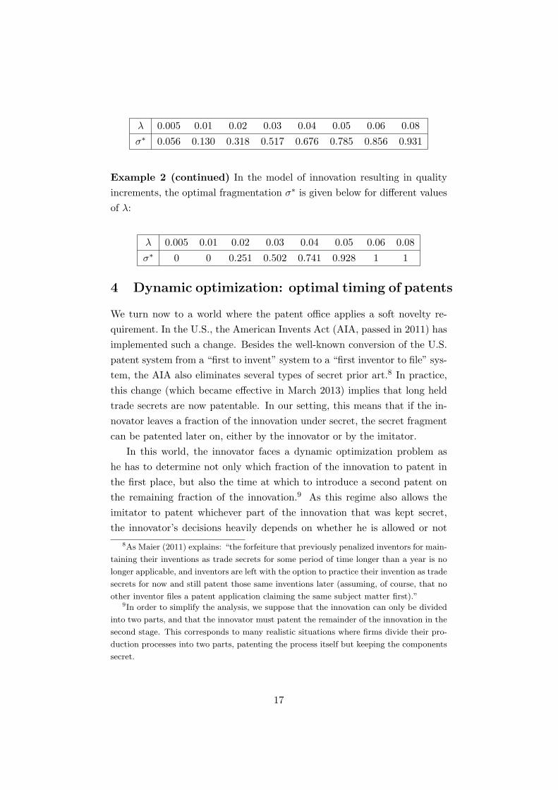
� 0.005 0.01 0.02 0.03 0.04 0.05 0.06 0.08�⇤ 0.056 0.130 0.318 0.517 0.676 0.785 0.856 0.931

Example 2 (continued) In the model of innovation resulting in qualityincrements, the optimal fragmentation �⇤ is given below for di↵erent valuesof �:

� 0.005 0.01 0.02 0.03 0.04 0.05 0.06 0.08�⇤ 0 0 0.251 0.502 0.741 0.928 1 1

4 Dynamic optimization: optimal timing of patents

We turn now to a world where the patent o�ce applies a soft novelty re-quirement. In the U.S., the American Invents Act (AIA, passed in 2011) hasimplemented such a change. Besides the well-known conversion of the U.S.patent system from a “first to invent” system to a “first inventor to file” sys-tem, the AIA also eliminates several types of secret prior art.8 In practice,this change (which became e↵ective in March 2013) implies that long heldtrade secrets are now patentable. In our setting, this means that if the in-novator leaves a fraction of the innovation under secret, the secret fragmentcan be patented later on, either by the innovator or by the imitator.

In this world, the innovator faces a dynamic optimization problem ashe has to determine not only which fraction of the innovation to patent inthe first place, but also the time at which to introduce a second patent onthe remaining fraction of the innovation.9 As this regime also allows theimitator to patent whichever part of the innovation that was kept secret,the innovator’s decisions heavily depends on whether he is allowed or not

8As Maier (2011) explains: “the forfeiture that previously penalized inventors for main-

taining their inventions as trade secrets for some period of time longer than a year is no

longer applicable, and inventors are left with the option to practice their invention as trade

secrets for now and still patent those same inventions later (assuming, of course, that no

other inventor files a patent application claiming the same subject matter first).”9In order to simplify the analysis, we suppose that the innovation can only be divided

into two parts, and that the innovator must patent the remainder of the innovation in the

second stage. This corresponds to many realistic situations where firms divide their pro-

duction processes into two parts, patenting the process itself but keeping the components

secret.

17

to continue exploiting any part of the innovation that the imitator has suc-ceeded in patenting, i.e., whether he can invoke prior user rights or not. Weanalyze the two sequential patent regimes in turn.10

4.1 Dynamic optimization with prior user rights

We suppose here that the initial innovator is granted prior user rights, sothat he may exploit the entire innovation irrespective of the fact that thecompetitor discovers his secret. The innovator now selects two control vari-ables: the fraction of the innovation which is covered by the first patent, �,and the time ⌘ at which the secret part of the innovation is patented if thecompetitor has not discovered it.

If the imitator discovers the secret before ⌘, he gains access to the secretpart of the innovation during the time of the first patent and to the entireinnovation after the expiry of the first patent. The expected payo↵ to theinventor is thus P (1, 0) until the discovery of the secret, P (1, 1��) during thelife of the patent after the secret has been discovered, and P (1, 1) after theexpiry of the patent. If on the other hand, the imitator has not discoveredthe secret before ⌘, she will stop making e↵orts to invent around the patentafter ⌘, and the inventor’s profit is given by P (1, 0) during the first patent,P (1, �) after the expiry of the first patent and before the expiry of thesecond, and P (1, 1) after the expiry of the second patent.

We distinguish between the case where the innovator patents the secretbefore the expiry of the first patent (⌘ < T ) and after the expiry of the firstpatent (⌘ > T ). In the first case, the expected value of the innovator as a

10The AIA has also modified provisions regarding prior user rights. As explained by

Kappos and Stanek Rea (2012, p. 1): “The AIA also expands the “prior user rights”

defense to infringement and broadens the classes of patents that are eligible for the new

limited prior user rights defense. (...) U.S. law already provided a prior user rights

defense that was limited to patents directed to methods of conducting business. The AIA,

by contrast, extends the prior user rights defense to patents covering all technologies, not

just business methods.” According to the Tegernsee Experts Group (2012, p. 2), “[p]rior

user rights are provided for by the di↵erent national legislations (...) [which] have common

ground, but also have di↵erences in the conditions under which they may be acquired.”

18

function of � and ⌘ is given by

V (�, ⌘) =Z ⌘

0

�

re��⌧

�

(1� e�r⌧ )P (1, 0) + (e�r⌧ � e�rT )P (1, 1� �)

+e�rT P (1, 1)

d⌧

+1re��⌘

n

(1� e�rT )P (1, 0) + (e�rT � e�r(T+⌘))P (1, �)

+e�r(T+⌘)P (1, 1)o

.

In the second case, the expected value is given by

V (�, ⌘) =Z T

0

�

re��⌧

�

(1� er⌧ ) P (1, 0) +�

e�r⌧ � e�rT�

P (1, 1� �)

+e�rT P (1, 1)

d⌧

+Z ⌘

T

�

re��⌧

��

1� e�rT�

P (1, 0) +�

e�rT � e�r⌧�

P (1, �)

+e�r⌧P (1, 1)

d⌧

+1re��⌘

n

�

1� e�rT�

P (1, 0) +⇣

e�rT � e�r(T+⌘)⌘

P (1, �)

+e�r(T+⌘)P (1, 1)o

.

4.1.1 Optimal timing of patents

We first consider, for a fixed �, the optimal choice of the time of the secondpatent, ⌘. By increasing ⌘, the innovator increases the length of the patentprotection of the innovation, but also increases the time during which thetrade secret is not protected, making it more likely that the imitator discov-ers the unpatented part of the innovation. As we will see, this trade-o↵ mayresult in the innovator choosing a finite time ⌘⇤ at which the secret part of

the innovation is patented.

The trade-o↵ crucially depends on two measures: the loss in utility dueto the fact that the second patent expires,

�P 1 = P (1, �)� P (1, 1),

and the loss in utility due to the fact that the innovator discovers the secret,

�P 2 = P (1, 0)� P (1, 1� �).

Notice that, if P is concave in �2, �P 1 > �P 2 whereas if P is convex in �2,�P 1 < �P 2. In order to derive the optimal timing of the second patent ⌘⇤,

19

we compute the derivative of the expected value V (�, ⌘) with respect to ⌘,both for ⌘ < T and for ⌘ > T . For ⌘ < T ,

@V

@⌘= e��⌘

h

e�r(T+⌘)�P 1

��

r

⇣

�

e�r⌘ � e�rT�

�P 2 +⇣

e�rT � e�r(T+⌘)⌘

�P 1⌘

�

.

For ⌘ > T ,@V

@⌘= e�(�+r)⌘�0 + r(�0 � �)�P 1.

Building on the computation of these derivatives, the following proposi-tion (whose proof can be found in Appendix 8.2) summarizes the optimalchoice of ⌘ as a function of the parameters.

Proposition 2 Given �, the optimal timing of the second patent is given

as follows. (1) If �P 2 > �P 1,

• ⌘⇤ = 0 for �0�P 1 ��P 2 � �0(1� e��T )(�P 2 ��P 1),

• ⌘⇤ =1 otherwise.

(2) If �P 1 > �P 2,

• ⌘⇤ = 0 for �0�P 1

�P 2 �,

• 0 < ⌘⇤ < T for �0 � �0�P 1

�P 2 ,

• ⌘⇤ =1 for � �0.

Proposition 2 characterizes the optimal delay between the two patentsfor a fixed value of �. As in the static case, the concavity of the profit ofthe innovator in �2 plays a crucial role in determining the optimal delay. IfP is convex, the innovator either immediately patents the entire innovation,or chooses never to file a second patent. If P is concave, for intermediatevalues of the probability of discovery, the innovator chooses to file a secondpatent before the expiry of the first patent. We note that one situation neverarises: it is never optimal for the inventor to file a second patent in finitetime but after the expiry of the first patent.

The first order condition for optimal timing of the second patent, when�P 1 > �P 2 and �0 � �0

�P 1

�P 2 is given by:

e�r⌘ =�P 1 ��P 2

r��P 1 � r

�0�P 2 + �P 1 ��P 2

. (3)

20

4.1.2 Optimal innovation fragmentation

We now consider the optimal choice of the share of the innovation coveredby the first patent, �. If ⌘ = 0, the innovator immediately patents the fullinnovation. If ⌘ = 1, his optimal choice is similar to that of Section 3.2.As shown by Proposition 2, the case ⌘ > T is irrelevant. When 0 < ⌘ T ,the derivative of V with respect to � can be computed as

@V

@�= �

"

1� e�rT

r� 1� e�(�+r)⌘

� + r� e��⌘

r(e�r⌘ � e�rT )

#

P2(1, 1� �)

+e�(�⌘+rT )

r(1� e�r⌘)P2(1, �).

Hence, when P is convex in �2, the optimal choice is either �⇤ = 0 or �⇤ = 1,and when P is concave, the solution is either �⇤ = 0 or �⇤ = 1 or the interiorsolution satisfying

P2(1, �⇤)P2(1� �⇤)

=1�e�rT

r � 1�e�(�+r)⌘

�+r � e��⌘

r (e�r⌘ � e�rT )e�(�⌘+rT )

r (1� e�r⌘). (4)

4.1.3 Optimal dynamic patenting strategy

We now piece together the analysis of the optimal timing and the optimalfragmentation to characterize the optimal dynamic patenting strategy ofthe innovator. Suppose first that P is convex in �. Then �P 2 > �P 1 andeither ⌘⇤ = 0 (and the innovator immediately patents the full innovation)or ⌘⇤ =1 (and the innovator optimally chooses, as in Section 3.2, either topatent the full innovation if � � �0 or to keep the entire innovation secretif � �0).

Consider next the more interesting case where P is concave in �2. If� �0, ⌘⇤ = 1 for all values of �, and the optimal choice is the same �⇤

as in Section 3.2, with �⇤ = 0 for � � and �⇤ 2 (0, 12) for �0 > � > �. If

� � �0, according to Proposition 2, the regime of repatenting depends onthe value of �. This requires an understanding of the e↵ect of changes in �

on the values of �P 2 and �P 1. Let

H(�) ⌘ P (1, �)� P (1, 1)P (1, 0)� P (1, 1� �)

=�P 1

�P 2.

We show in Appendix 8.3 that H(�) is increasing from H(0) = 1 to H(1) =P2(1,1)P2(1,0) and that �0H(1) > �. For any �0 < � < �0H(1), we can thus

21

compute � such that �P 1

�P 2 ��0

if and only if � �. We claim that at theoptimum, the innovator must choose � 2 (�, 1]. The argument is based onrevealed preference. If the innovator chooses � 2 (�, 1], by Proposition 2,the optimal timing choice is ⌘⇤ > 0, so that the utility of the innovator mustbe greater than the utility obtained when ⌘⇤ = 0, and the second patent isfiled immediately. If the innovator chooses � 2 [0, �], by Proposition 2, thesecond patent is immediately filed, resulting in a profit which, as we argued,must be strictly lower than the profit obtained by choosing � > � followedby ⌘⇤ > 0. We summarize this discussion in the following proposition.

Proposition 3 If the function P is convex in �2, the optimal dynamic

patenting strategy is identical to the static strategy, and the innovator chooses

�⇤ = 0, ⌘⇤ =1 if � < �0 and �⇤ = 1 if � > �0. If the function P is concavein �2,

• If � < �0, the optimal dynamic patenting strategy is identical to the

static strategy and the innovator chooses �⇤ 2 (0, 1), ⌘⇤ = 1, where

�⇤ solves Equation (2).

• If �0 < � < �0H(1), the optimal dynamic patenting strategy is to select

�⇤ 2 (0, 1), ⌘⇤ 2 (0, T ) which are solutions to Equations (3) and (4).

• If � > �0H(1), the optimal dynamic patenting strategy is identical to

the static strategy and the innovator chooses �⇤ = 1.

Proposition 3 identifies situations where the innovator optimally choosesto patent sequentially two fragments of the innovation, and the dynamicpatenting strategy di↵ers from the static choice of the optimal mix of patentand secrets. These situations arise when the function P is concave in �2 andthe probability of reverse engineering the innovation is intermediate. Wealso note that, because �0H(1) > �, the region of parameters for whichthe innovator chooses to fragment the innovation is larger in the dynamicpatenting regime than in the static regime. The following computationscharacterize the optimal interior values of ⌘ and � in the two examplesdiscussed in Section 2.2 for values of � greater than �0.

Example 1 (continued) In the model of cost reducing innovation, whenthe cost function is a quadratic function of �, c(�) = 1 � �2, the optimalfragmentation �⇤ and timing ⌘⇤ are given below for di↵erent values of �.

22

� 0.03 0.04 0.05 0.06 0.08�⇤ 0.513 0.626 0.700 0.752 0.816⌘⇤ 19.40 14.78 12.10 10.33 8.04

Example 2 (continued) In the model of innovation resulting in qualityincrements, the optimal fragmentation �⇤ is given below for di↵erent valuesof �:

� 0.03 0.04 0.05 0.06 0.08�⇤ 0.517 0.683 0.823 0.958 1⌘⇤ 19.77 18.37 18.33 19.41 -

The numerical computations first show, quite naturally, that the size ofthe first fragment is lower in the dynamic setting than in the static setting(sse the two tables in Section 3.2). As the innovator will file a second patenton the innovation, he has an incentive to decrease the share of the innovationthat is patented the first time. Computations in Example 1 suggest thatthe share of the innovation and the delay between the second patent playcomplementary roles in the strategy of the innovator. As the threat ofimitation increases, the innovator simultaneously increases the share of theinnovation covered by the first patent and reduces the delay before filingthe second patent. However, Example 2 shows that this phenomenon isnot general. In the example of quality upgrades, as the threat of imitationincreases, the share of the innovation covered by the patent increases butthe delay before the second patent (which remains very large and close tothe patent length T = 20) is not always decreasing.

4.2 Dynamic optimization without prior user rights

If the innovator does not possess prior user rights, he may become unableto exploit the part of the innovation patented by the imitator. The com-petitor can force the initial inventor to downgrade his product or resort to aless e�cient production process, resulting in a payo↵ of P (�, 1 � �) duringthe lifetime of the first patent and P (�, 1) between the expiry of the firstpatent held by the innovator and the expiry of the second patent held by

23

the imitator. The expected profit of the inventor when ⌘ < T is now givenby

V (⌘,�) =Z ⌘

0

�

re��⌧

��

1� e�r⌧�

P (1, 0) +�

e�r⌧ � e�rT�

P (�, 1� �)

+⇣

e�rT � e�r(T+⌧)⌘

P (�, 1) + e�r(T+⌧)P (1, 1)o

d⌧

+1re��⌘

n

�

1� e�rT�

P (1, 0) +⇣

e�rT � e�r(T+⌘)⌘

P (1, �)

+e�r(T+⌘)P (1, 1)o

.

and when ⌘ > T by

V (⌘,�) =Z T

0

�

re��⌧

n

(1� er⌧ )P (1, 0) +�

e�r⌧ � e�rT�

P (�, 1� �)

+⇣

e�rT � e�r(T+⌧)⌘

P (�, 1) + e�r(T+⌧)P (1, 1)o

d⌧

+Z ⌘

T

�

re��⌧

��

1� e�rT�

P (1, 0) +�

e�rT � e�r⌧�

P (1, �)

+⇣

e�r⌧ � e�r(T+⌧)⌘

P (�, 1) + e�r(T+⌧)P (1, 1)o

d⌧

+1re��⌘

n

�

1� e�rT�

P (1, 0) +⇣

e�rT � e�r(T+⌘)⌘

P (1, �)

+e�r(T+⌘)P (1, 1)o

.

4.2.1 Optimal timing of patents

In order to define the optimal timing of patents, we define a new term,

�P 3 = P (1, �)� P (�, 1),

which measures the loss experienced by the innovator when the imitatordiscovers and patents the trade secret after the expiry of the first patent.Notice that �P 3 � �P 1. We also compute the loss to the innovator whenthe imitator discovers the secret as

�P 4 = P (1, 0)� P (�, 1� �).

Equipped with this notation, we compute the derivative of the firm’sprofit with respect to ⌘. For ⌘ < T ,

@V

@⌘= e��⌘

h

e�r(T+⌘)�P 1

��r

⇣

�

e�r⌘ � e�rT�

�P 4 +⇣

e�rT � e�r(T+⌘)⌘

�P 3⌘i

.

24

For ⌘ > T ,@V

@⌘=

e�(�+r)⌘

�0 + r

�

�0�P 1 � ��P 3�

.

Following the same steps as in Subsection 4.1.1, we characterize the optimaltiming of patents for a fixed � in the next proposition (whose proof can befound in Appendix 8.4).

Proposition 4 Given �, the optimal timing of the second patent is given

as follows. (1) If �P 4 > �P 3,

• ⌘⇤ = 0 for �0�P 1 ��P 4 � �0(1� e��T )(�P 4 ��P 3),

• ⌘⇤ =1 otherwise

(2) If �P 3 > �P 4,

• ⌘⇤ = 0 for �0�P 1 ��P 4,

• 0 < ⌘⇤ < T for ��P 4 �0�P 1 ��P 3,

• ⌘⇤ =1 for �0�P 1 ��P 3.

4.2.2 Optimal dynamic patenting strategy

The characterization of the optimal dynamic patenting strategy when theinventor does not hold prior user rights di↵ers from the characterizationof the optimal dynamic patenting strategy with prior user rights in twoimportant respects. First, the comparison between �P 3 and �P 4 does notresult from the concavity or convexity of the profit function P . If P isconvex, and in addition, the marginal e↵ect of an increase in �1 is higherfor lower values of �2 (P12 < 0), we obtain

�P 4 ��P 3 = P (1, 0)� P (�, 1� �)� P (1, �) + P (�, 1),

= [P (1, 0)� P (1, �)]� [P (�, 1� �)� P (�, 1)]

� [P (�, 0)� P (�,�)]� [P (�, 1� �)� P (�, 1)]

� 0.

It is harder to find conditions under which �P 4 < �P 3, as this wouldrequire both that P is concave and that P12 > 0, and the latter condition isunlikely to be satisfied in regular applications. The second di�culty stems

25

from the lack of concavity/convexity of the function V with respect to thefragmentation parameter �. When the innovation is only patented once(⌘ =1), a simple computation shows that11

@V

@�=

⇣

1�e�rT

r � 1�e�(�+r)T

�+r

⌘

(P1(�, 1� �)� P2(�, 1� �))

+ e�(�+r)T

�+r P2(1, �) + �r(�+r)(1� e�rT )P1(�, 1).

A change in � a↵ects both the fraction of the innovation that the imitatorcan exploit (through the derivative P2) and the fraction of the innovationthat the inventor can still exploit if the imitator patents the secret part(through the derivative P1). Simple intuition suggests that if P is concavein �2, it should be convex in �1 and vice versa. But this implies thatthe function V is unlikely to be concave or convex in �, so that we cannotcharacterize the optimal fragmentation share �⇤ through a simple first ordercondition.

We now consider the two examples of Section 2.2. In Example 2, thesign of �P 4��P 3 is not constant over �, and we omit the characterizationof the optimal patenting policy. In Example 1, we observe that the sign of�P 4 ��P 3 is constant, allowing us to compute the optimal policy.

Example 1 (continued) In the model of cost reducing innovation, whenthe cost function is a quadratic function of �, c(�) = 1 � �2, we have�P 2 = 9 � �2(� + 2)2 > 9 � 3�2(�2 + 2) = �P 3 for all �. Hence, theinnovator only patents once and the fragment patented is given below fordi↵erent values of �.

� 0.005 0.01 0.02 0.03 0.04 0.05 0.06 0.08�⇤ 0 0 1 1 1 1 1 1

It is interesting to observe that, given that P12 < 0, even when P isconcave in �2, the function V turns out to be convex in �, so that theinnovator will never choose to fragment the innovation. The absence of prioruser rights, by making it more costly for the innovator to lose his trade secret,increases the incentive to patent to the point where the innovator choosesto patent the entire process, even when � < �0.

11A similar result holds for interior values of ⌘.

26

Figure 2: Process innovation: Innovator’s profit

5 Welfare Comparisons

In this section, we compare the four regimes of patent protection from thepoint of view of the three stakeholders: the innovator, the imitator and con-sumers. The analysis is done in the context of the two illustrating examplesof the paper.

5.1 Cournot model with process innovation

In addition to the profits of the innovator and imitator, P and Q, we computeconsumer surplus as

S(�1, �2) = 12(1 + f(�1) + f(�2))2.

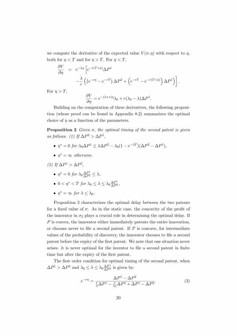
Figures 2, 3 and 4 compare, for di↵erent values of �, the welfare of theinnovator, imitator and consumers under the four regimes for f(�) = �2.

For the innovator, not surprisingly, as regimes become more flexible, prof-its increase. Hence, the dynamic regime with prior user rights dominatesthe static regime, which dominates the binary regime. We also observe thatthe dynamic regime without prior user rights results in a profit which ishigher than the binary regime but lower than any other patent protectionregime. Interestingly, in the Cournot model, the welfare of the imitator andof consumers are aligned and in complete conflict with the profit of the in-novator. The competitor and consumers favor regimes with less flexibility,preferring the binary regime to the static regime, and to the dynamic regimewith prior user rights. Comparing the dynamic regimes with and without

27

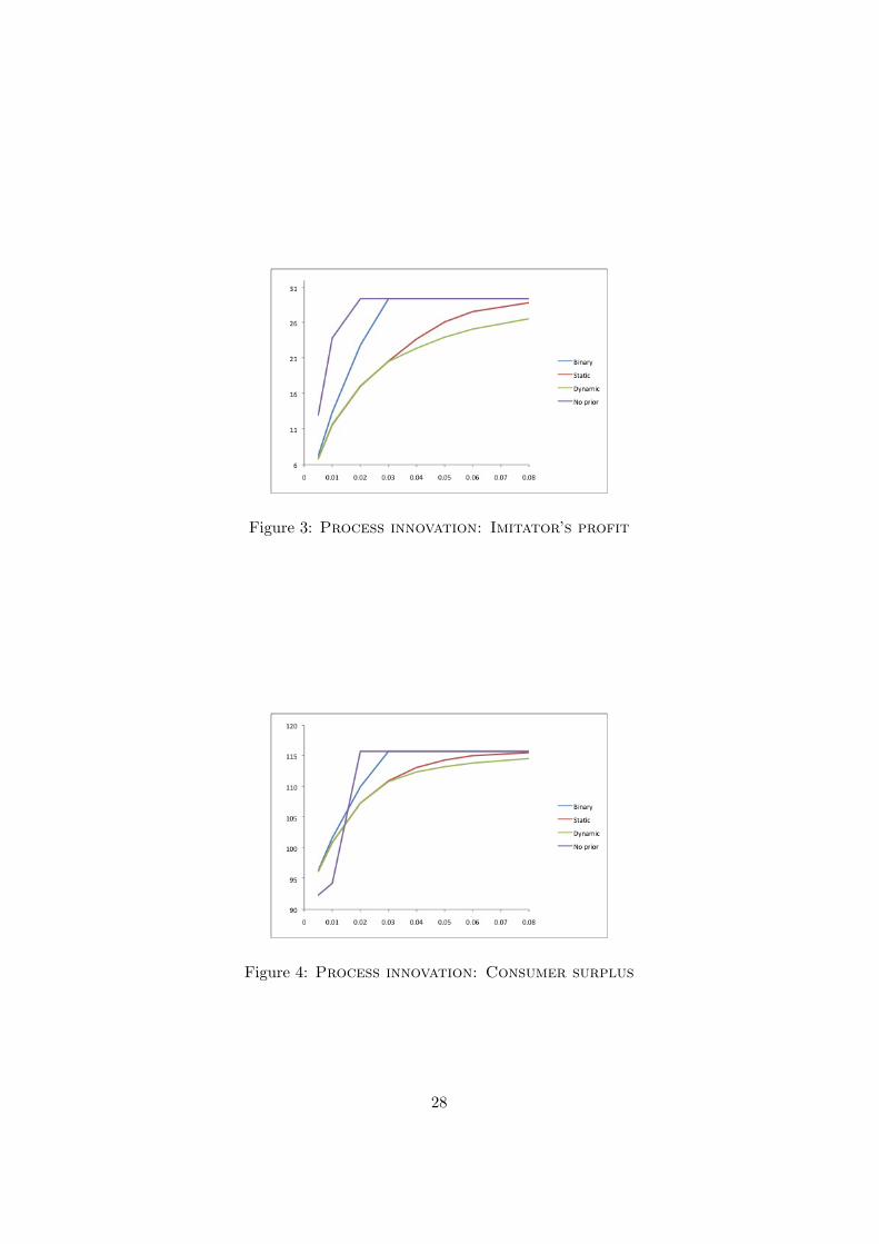
Figure 3: Process innovation: Imitator’s profit

Figure 4: Process innovation: Consumer surplus

28

prior user rights, we observe that, clearly, the imitator gains when the inno-vator cannot hold prior user rights. However, consumers lose as this impliesthat, after the competitor discovers the trade secret for low values of �, theinnovator is not able to exploit the cost reducing innovation, yielding lowerquantities in equilibrium.12

On balance, the comparison between the four regimes indicates a conflictin the welfare of the innovator, imitator and consumers. If however, theintellectual property regime puts more weight on the inventor in order togive him incentives to innovate, our analysis suggests that higher flexibilityshould always be favored.

5.2 Vertical di↵erentiation model with quality increments

In the vertical di↵erentiation model, we compute the surplus of consumerswhen �1 > �2 as

S(�1, �2) =

8(�1 + �2) +

�21(4�1 + 5�2)2(4�1 � �2)2

.

Figures 5, 6 and 7 illustrate the welfare of the innovator, imitator andconsumers for di↵erent values of � when = 3 for three regimes of patentprotection.13

As expected, the innovator always prefers regimes with more flexibility.But in the vertical di↵erentiation model, contrary to the Cournot model,the imitator and the consumers also may prefer the more flexible regimes.In fact, they both rank the static fragmentation regime above the binaryregime, preferring to let the inventor segment the innovation in di↵erentpieces. The competitor also prefers the dynamic regime to the static regimefor all values of � whereas consumers prefer the dynamic regime except for� close to �0. The analysis of the model of vertical di↵erentiation withquality increments thus shows that the conflict in welfare between innova-tor, imitator and consumers does not necessarily arise and that there exist

circumstances where all three types of agents prefer more flexible intellectual

property rights regimes.12Our analysis suggests thus an additional advantage of prior user rights, which was not

stressed in the literature considering patents and secrets as mutually exclusive protection

mechanisms (as in Denicolo and Franzoni, 2004, or Shapiro, 2006).13Recall that the optimal behavior of the innovator is not well defined in the dynamic

patent protection regimes without prior user rights.

29

Figure 5: Quality increments: Innovator’s profit

Figure 6: Quality increments: Imitator’s profit

Figure 7: Quality increments: Consumer surplus

30

6 Robustness and extensions

In this section, we test the robustness of our results by extending our frame-work in two directions: first, we endogenize the imitation e↵ort and second,we modify the sequential patent regime by allowing a second patent thatdoes not necessarily cover the remaining secret part of the innovation.

6.1 Endogenous imitation e↵ort

We analyze briefly the endogenous choice of the imitator, who selects theimitation rate � at a cost C(�). In the dynamic model with prior user rightsand ⌘ < T , the derivative of the present discounted value of the imitatorwith respect to � is given by:

@W (�, �, ⌘)@�

= (Q(1, 1� �)�Q(1, 0)){⌘�e��⌘

� + r(e�r⌘ � e�rT )

+r

(� + r)2(1� e�⌘(�+r) � ⌘(� + r)e��⌘�rT )}

+ (Q(1, 1)�Q(1, �))⌘e�(�+r)⌘(1� e�rT )

> 0.

Notice that, as the fraction of the innovation that is patented, �, in-creases, Q(1, 1 � �) � Q(1, 0) and Q(1, 1) � Q(1, �) decrease, so that theoptimal value of � goes down. Hence, when the competitor chooses herimitation e↵orts endogenously, higher values of � result in lower values of�. By comparison with the baseline model with exogenous imitation e↵orts,we remark that the inventor has an incentive to increase the fragment of

the innovation that is patented in order to reduce the imitation e↵orts of his

competitor. However, the thrust of the analysis, including the existence ofparameter regions for which the inventor chooses interior values of � and ⌘,remains unchanged.

6.2 Continuous fragmentation of the innovation

We examine now a variant of the model where the inventor may choose, inthe second patent, only to patent a fraction ⇢ < 1�� of the secret.14 When

14Notice that the imitator never has an incentive to patent less than 1 � � since the

secret is already known and exploited by the initial inventor.

31

⌘ < T , the present discounted value of the inventor is given by:

V (�, ⌘) =Z ⌘

0

�

re��⌧

�

(1� e�r⌧ )P (1, 0) + (e�r⌧ � e�rT )P (1, 1� �)

+e�rT P (1, 1)

d⌧

+Z T

⌘

�

re��⌧

�

(1� er⌧ )P (1, 0) + (e�r⌧ � e�rT )P (1, 1� � � ⇢)

+(e�rT � e�r(T+⌘))P (1, 1� ⇢) + e�r(T+⌘)P (1, 1)o

d⌧

+Z T+⌘

T

�

re��⌧

�

(1� e�rT )P (1, 0) + (e�rT � e�r⌧ )P (1, �)

+(e�r⌧ � e�r(T+⌘))P (1, 1� ⇢) + e�r(T+⌘)P (1, 1)o

d⌧

+Z 1

⌘

�

ren

��⌧ (1� e�rT )P (1, 0) + (e�rT � e�r(T+⌘))P (1, �)

+(e�r(T+⌘) � e�r⌧ )P (1, � + ⇢) + e�r⌧P (1, 1)o

d⌧.

While the computations of the optimal values of ⌘, � and ⇢ are clearlymore complicated than in the baseline model, we can use the same steps asin Section 4.1.3 to show that, when P is convex in �2, the optimal strategyis a binary strategy whereas when P is concave in �2, the optimal strategymay involve an interior choice of ⌘, ⇢ and � for some parameter values. Themain qualitative results of the analysis remain unchanged.

7 Conclusion

We have provided a unified model to study the protection of complex innova-tions, i.e., innovations that can be fragmented into several sub-innovations,each of them being patentable separately. The model allows us to analyzethe innovator’s choice of patent/secret mix under various patent regimes,which di↵er according to the strength of the utility and the novelty require-ments. We are also able to perform some welfare comparisons of these patentregimes. Our main result is to find conditions under which the innovatoroptimally chooses to mix patents and secrets (in a static framework cor-responding to a strict novelty requirement), or to patent sequentially twofragments of the innovation (in a dynamic framework corresponding to asofter novelty requirement). We also find examples where the other stake-holders (namely a potential imitator and the consumers) may agree with theinnovator’s conduct, suggesting that more flexible patent regimes could be

32

welfare-enhancing. It is important to stress that a pre-condition for theseresults to apply is that the innovator’s profit function be concave in thefraction of the innovation that the imitator can exploit. This occurs whenthe imitator must learn a large fragment of the innovation in order to beable to exploit it usefully. In contrast, if convexity prevails, the innovatorwill optimally choose an all-or-nothing strategy that consists in patentingthe whole innovation or in keeping it altogether secret.

Our framework could be extended in a number of directions that we leavefor further research. First, we have assumed in our model that there is noinformation leakage in the patenting process. In actual situations, patentsmay convey information about the innovation, so that it becomes easier fora competitor to circumvent the innovation. This e↵ect would diminish thebenefit of a patent, and reduce the part of a complex innovation which isprotected by a patent. Alternatively, more complex models of informationleakage and reverse engineering could be employed to analyze more preciselythe optimal fragmentation of an innovation. A second direction in which theanalysis could be extended is to analyze the incentive to engage in R & Dbefore the innovation is discovered. In a symmetric model among two com-peting firms, we could study how di↵erent regimes of patent protection a↵ectthe incentives to invest in R & D and how they shape the dynamics of thepatent race. Finally, we have assumed that the initial competitor does notlicense his innovation to his competitor. The introduction of licensing agree-ments would enrich the comparison of di↵erent regimes of patent protectionin an interesting way.

8 Appendix

8.1 Proof of Proposition 1

If P is concave, and � < �0 < �, the optimal fraction �⇤ is interior andgiven by the solution to the first order condition:

G(�) ⌘ P2(1, �)P2(1, 1� �)

= K.

Because P is concave in �2, G is increasing in �. To show that �⇤ is increasingin �, T and r, it su�ces to show that K is increasing in �, T and r. First,

dK

d�=

1r + �0

e(r+�)T (1� �0 + �) > 0.

33

where the last inequality is due to the fact that �0 1 as the functionf(r) = re�rT

1�e�rT is smaller than 1 for any r 2 <+. Note also that

dK

dT= �eT (r+�) (r + �)

1� e�Tr

r> 0,

anddK

dr= �e(r+�)T e�rT + rT � 1

r2> 0,

where the last inequality is due to the fact that the function g(r) = 1�e�rT

rT

is smaller than 1 for any r 2 <+.

8.2 Proof of Proposition 2

In order to compute the sign of @V@⌘ for ⌘ < T , we consider the term

A(⌘) = e�r(T+⌘)�P 1 � �

r

⇣

�

e�r⌘ � e�rT�

�P 2 +⇣

e�rT � e�r(T+⌘)⌘

�P 1⌘

.

Deriving A with respect to ⌘ and using the definition of �0,

A0(⌘) =re�r⌘

�0 + r

��P 2 � �0�P 1 +��0

r(�P 2 ��P 1)

�

.

Notice that the sign of A0(⌘) is independent of ⌘. Hence, either A(✓) isincreasing over [0, T ] or it is decreasing over [0, T ]. We also compute

A(0) =1� e�rT

r(�0�P 1 � ��P 2),

A(T ) = e�rT 1� e�rT

r(�0 � �)�P 1.

Now suppose that �P 2 > �P 1. If A(0) � 0, then A(T ) � 0 and V

is increasing over the entire interval [0, T ]. In addition, as �0 > �, V isincreasing over [T,1), so the optimal solution is ⌘⇤ =1. If A(0) 0, thenA0(⌘) > 0. If �0 < �, A(T ) < 0, so V is decreasing over [0, T ]. In addition,V is decreasing over [T,1) so the optimal solution is ⌘⇤ = 0. Finally, if�0 � � but �0�P 1 ��P 2, as A0(⌘) > 0, the function V is convex in [0, T ]and attains its maximum at the boundaries, either at 0 or at T . In addition,the function V is increasing over [T,1), so the optimal solution is either⌘⇤ = 0 or ⌘⇤ = 1. Computing the value of V at ⌘ = 0 and ⌘ = 1, weobtain the condition in the proposition.

Next suppose that �P 2 < �P 1. Then A(0) > A(T ). If �0 > �, A(T ) >

0, so the function V is increasing over [0, T ] and over [0,1) and the optimal

34

solution is ⌘⇤ = 1. If �0�P 1 < ��P 2, A0(⌘) < 0 and A(0) < 0, so thefunction V is decreasing over [0, T ] and as � > �0, it is also decreasingover [T,1). Hence the optimal solution is ⌘⇤ = 0. Finally, if � > �0 but�0�P 1 > ��P 2, the function V is increasing at 0, and decreasing over[T,1). This implies that there exists an interior maximum ⌘⇤ 2 (0, T ).

8.3 Properties of the function H(�)

We first show that H is increasing. We compute

H 0 (�) =P2 (1, �) �P 2 � P2 (1, 1� �) �P 1

(P (1, 0)� P (1, 1� �))2.

Hence, H 0 (�) > 0 if and only if

P (1, �)� P (1, 1)P (1, 0)� P (1, 1� �)

>P2 (1, �)

P2 (1, 1� �).

By concavity of P in �2,

P (1, �)� P (1, 1)P (1, 0)� P (1, 1� �)

> 1.

If � � 12 , by concavity of P in �2,

1 >P2 (1, �)

P2 (1, 1� �),

and the inequality is true. Suppose now that � 12 . Then,

(V2 (1, �)� V2 (1, 1� �)) (V (1, 0)� V (1, 1� �))

+V2 (1, 1� �) (V (1, 0)� V (1, 1� �))

�V2 (1, 1� �) (V (1, �)� V (1, 1))

= (V2 (1, �)� V2 (1, 1� �))| {z }

+

(V (1, 0)� V (1, 1� �))| {z }

+

+V2 (1, 1� �)| {z }

�

[(V (1, 0)� V (1, 1� �))� (V (1, �)� V (1, 1))]| {z }

�

which is positive, implying again that H 0 (�) > 0.Clearly, H(0) = 1. We compute H(1) using L’Hospital rule:

H (1) =V2 (1, 1)V2 (1, 0)

.

35

Recall that � is defined implicitly by the equation:

V2 (1, 0)V2 (1, 1)

= K�1�

��

, H (1) = K�

��

, with K (�) = 1 +(�� �0)

(r + �0) e�(r+�)T.

We show that �0H (1) > �. As K (�) is an increasing function of �, this isequivalent to showing that K (�0H (1)) > K

�

��

, or

1 +�0 (H (1)� 1)

(r + �0) e�(r+�0H(1))T> H (1), �0

r + �0= e�rT > e�(r+�0H(1))T ,

which is always satisfied.

8.4 Proof of Proposition 4

We consider the term

B(⌘) = e�r(T+⌘)�P 1 � �

r

⇣

�

e�r⌘ � e�rT�

�P 4 +⇣

e�rT � e�r(T+⌘)⌘

�P 3⌘

.

Deriving B with respect to ⌘ and using the definition of �0,

B0(⌘) =re�r⌘

�0 + r

��P 4 � �0�P 1 +��0

r(�P 4 ��P 3)

�

.

Notice that the sign of B0(⌘) is independent of ⌘. Hence, either B(✓) isincreasing over [0, T ] or it is decreasing over [0, T ]. We also compute

B(0) =1� e�rT

r(�0�P 1 � ��P 4),

B(T ) = e�rT 1� e�rT

r(�0�P 1 � ��P 3).

Now suppose that �P 4 > �P 3. Then, if B(0) > 0, then B(T ) > 0and V is increasing over the entire interval [0, T ]. In addition, as B(T ) > 0,�0�P 1���P 3 > 0 and V is increasing over [T,1), so the optimal solution is⌘⇤ =1. If B(0) 0, then B0(⌘) > 0. If �0�P 1 < ��P 3, B(T ) < 0, so V isdecreasing over [0, T ]. In addition, V is decreasing over [T,1) so the optimalsolution is ⌘⇤ = 0. Finally, if �0�P 1 � ��P 3 but �0�P 1 ��P 4, asB0(⌘) > 0, the function V is convex in [0, T ] and attains its maximum at theboundaries, either at 0 or at T . in addition, the function V is increasing over[T,1), so the optimal solution is either ⌘⇤ = 0 or ⌘⇤ = 1. Computing thevalue of V at ⌘ = 0 and ⌘ =1, we obtain the condition in the proposition.

Next suppose that �P 4 < �P 3. Then B(0) > B(T ). If �0�P 1 >

��P 3, B(T ) > 0, so the function V is increasing over [0, T ] and over [0,1)

36

and the optimal solution is ⌘⇤ = 1. If �0�P 1 < ��P 4, B0(⌘) < 0 andB(0) < 0, so the function V is decreasing over [0, T ] and as B(T ) < 0,�0�P 1 < ��P 3,and V is also decreasing over [T,1). Hence the optimalsolution is ⌘⇤ = 0. Finally, if � > �0 but ��P 4 < �0�P 1 < ��P 3, thefunction V is increasing at 0, and decreasing over [T,1). This implies thatthere exists an interior maximum ⌘⇤ 2 (0, T ).

References

[1] Anton, J. J., and Yao, D. A. (2004). Little Patents and Big Secrets:Managing Intellectual Property. RAND Journal of Economics 35, 1-22.

[2] Arora, A. (1997). Patents, Licensing, and Market Structure in theChemical Industry. Research Policy 26, 391-403.

[3] Cohen, W. M., and Levinthal; D. A. (1989). Absorptive Capacity: ANew Perspective on Learning and Innovation. Administrative ScienceQuarterly 35, 128-152.

[4] Cohen, W. M., Nelson, R. R., and Walsh, J. (2000). Protecting TheirIntellectual Assets: Appropriability Conditions and Why U.S. Manu-facturing Firms Patent (or Not). NBER Working Paper 7552.

[5] Denicolo, V. and Franzoni, L.A. (2004). Patents, Secrets, and the First-Inventor Defense. Journal of Economics and Management Strategy 13,517-538.

[6] Friedman, D.D., Landes, W.M. and Posner, R.A. (1991). Some Eco-nomics of Trade Secret Law. Journal of Economic Perspectives 5, 61-72.

[7] Gallini, N. (1992). Patent Length and Breadth with Costly Imitation.RAND Journal of Economics 23, 52–63.

[8] Hall, B. H., Helmers, Ch., Rogers, M., and Sena, V. (2012). The ChoiceBetween Formal and Informal Intellectual Property: A Literature Re-view. NBER Working Paper 17983.

[9] Horstmann, I., MacDonald, G. M., and Slivinski, A. (1985). Patentsas Information Transfer Mechanisms: To Patent or (Maybe) Not toPatent. Journal of Political Economy 93, 837–58.

37

[10] Hussinger, K. (2006). Is Silence Golden? Patents versus Secrecy at theFirm Level. Economics of Innovation and New Technology 15, 735-752.

[11] Jorda, K.F. (2007). Trade Secrets and Trade-Secret Licensing. In Krat-tiger, A., Mahoney, R.T., Nelsen, L. et al. (Eds). Intellectual PropertyManagement in Health and Agricultural Innovation: A Handbook ofBest Practices, Chapter 11.5. Oxford: MIHR & PIPRA.

[12] Kappos, D.J., and Stanek Rea, T. (2012). Report on the Prior UserRights Defense. The United States Patent and Trademark O�ce.Available at http://www.aiarulemaking.com/rulemaking-topics/group-1/documents/PriorUserRightsReporttoCongress.pdf

[13] Kultti, K., Takalo, T., and Toikka, J. (2007). Secrecy versus Patenting.RAND Journal of Economics 38, 22-42.

[14] Kwon, I. (2012a). Patent Thicket, Secrecy, and Licensing. The KoreanEconomic Review 28, 27-49.

[15] Kwon, I. (2012b). Patent Races with Secrecy. The Journal of IndustrialEconomics 60, 499-516.

[16] Lemley, M. A., and Shapiro, C. (2005). Probabilistic Patents. Journalof Economic Perspectives 19, 75-98.

[17] Lerner, J., and Tirole, J. (2004). E�cient Patent Pools. American Eco-nomic Review 94, 691–711.

[18] Leveque, F, and Meniere, Y. (2007). Patents and Innovation: Friendsor Foes. Berkeley Center for Law and Technology Working Paper 28.

[19] Levin, R. C., Klevorick, A. K., Nelson, R. R. and Winter, S. G. (1987).Appropriating the Returns from Industrial Research and Development.Brookings Papers on Economic Activity 3: 783-831.

[20] Maier, R.L. (2011). The Big Secret of the America Invents Act. Intel-lectual Property Today, December.

[21] Ottoz, E. and Cugno, F. (2008). Patent-Secret Mix in Complex ProductFirms. American Law and Economics Review 10, 142-158.

38

[22] Ottoz, E. and Cugno, F. (2011). Choosing the Scope of Trade SecretLaw when Secrets Complement Patents. International Review of Lawand Economics 31, 219–227.

[23] Perng Pan, S. and Mion, S. (2010). Hybrid Use of Trade Secret andPatent Protection in Green Technology. Bloomberg Law Reports 3 (4).

[24] Quinn, G. (2012). Patentability Overview: When can an Invention bePatented? IPWatchdog, www.ipwatchdog.com (last consulted on Au-gust 20, 2013).

[25] Schneider, C. (2008). Fences and Competition in Patent Races. Inter-national Journal of Industrial Organization 26, 1348–1364.

[26] Scotchmer, S., and Green, J. (1990). Novelty and Disclosure in PatentLaw. RAND Journal of Economics 21, 131–146.

[27] Shapiro, C. (2001). Navigating the Patent Thicket: Cross-Licenses,Patent-Pools, and Standard-Setting. In Ja↵e, A., Lerner, J., and Stern,S. (eds.), Innovation Policy and the Economy. Vol. 1. Cambridge, MA:MIT Press.

[28] Shapiro, C. (2006). Prior User Rights. American Economic Review 96,92-96.

[29] Takalo, T. (1998). Innovation and Imitation under Imperfect PatentProtection. Journal of Economics 67, 229–241.

[30] Tegernsee Experts Group (2012). Report on Prior User Rights. Mu-nich: European Patent O�ce (available at http://www.epo.org/news-issues/news/2012/20121108a.html).

39

Recent titles CORE Discussion Papers

2013/19 Pascal MOSSAY and Pierre M. PICARD. Spatial segregation and urban structure. 2013/20 Philippe DE DONDER and Marie-Louise LEROUX. Behavioral biases and long term care

insurance: a political economy approach. 2013/21 Dominik DORSCH, Hubertus Th. JONGEN, Jan.-J. RÜCKMANN and Vladimir SHIKHMAN.

On implicit functions in nonsmooth analysis. 2013/22 Christian M. HAFNER and Oliver LINTON. An almost closed form estimator for the

EGARCH model. 2013/23 Johanna M. GOERTZ and François MANIQUET. Large elections with multiple alternatives: a

Condorcet Jury Theorem and inefficient equilibria. 2013/24 Axel GAUTIER and Jean-Christophe POUDOU. Reforming the postal universal service. 2013/25 Fabian Y.R.P. BOCART and Christian M. HAFNER. Fair re-valuation of wine as an

investment. 2013/26 Yu. NESTEROV. Universal gradient methods for convex optimization problems. 2013/27 Gérard CORNUEJOLS, Laurence WOLSEY and Sercan YILDIZ. Sufficiency of cut-generating

functions. 2013/28 Manuel FORSTER, Michel GRABISCH and Agnieszka RUSINOWSKA. Anonymous social

influence. 2013/29 Kent WANG, Shin-Huei WANG and Zheyao PAN. Can federal reserve policy deviation

explain response patterns of financial markets over time? 2013/30 Nguyen Thang DAO and Julio DAVILA. Can geography lock a society in stagnation? 2013/31 Ana MAULEON, Jose SEMPERE-MONERRIS and Vincent VANNETELBOSCH.

Contractually stable alliances. 2013/32 Jean-François CAULIER, Ana MAULEON and Vincent VANNETELBOSCH. Allocation rules

for coalitional network games. 2013/33 Georg KIRCHSTEIGER, Marco MANTOVANI, Ana MAULEON and Vincent

VANNETELBOSCH. Limited farsightedness in network formation. 2013/34 Ana MAULEON and Vincent VANNETELBOSCH. Relative concerns and delays in

bargaining with private information. 2013/35 Kristof BOSMANS, Koen DECANCQ and Erwin OOGHE. What do normative indices of

multidimensional inequality really measure? 2013/36 Alain PHOLO BALA, Dominique PEETERS and Isabelle THOMAS. Spatial issues on a

hedonic estimation of rents in Brussels. 2013/37 Lionel ARTIGE, Antoine DEDRY and Pierre PESTIEAU. Social security and economic

integration. 2013/38 Nicolas BOUCKAERT and Erik SCHOKKAERT. Differing types of medical prevention appeal

to different individuals. 2013/39 Pierre M. PICARD. Trade, economic geography and the choice of product quality. 2013/40 Tanja B. MLINAR and Philippe CHEVALIER. Pooling in manufacturing: do opposites attract? 2013/41 Chiara CANTA and Marie-Louise LEROUX. Public and private hospitals, congestion, and

redistribution. 2013/42 Mathieu LEFEBVRE, Pierre PESTIEAU and Gregory PONTHIERE. FGT poverty measures

and the mortality paradox: Theory and evidence. 2013/43 Nada BELHADJ, Jean J. GABSZEWICZ and Ornella TAROLA. Social awareness and duopoly

competition. 2013/44 Volker BRITZ, P. Jean-Jacques HERINGS and Arkadi PREDTETCHINSKI. On the

convergence to the Nash bargaining solution for action-dependent bargaining protocols. 2013/45 Pasquale AVELLA, Maurizio BOCCIA and Laurence WOLSEY. Single item reformulations

for a vendor managed inventory routing problem: computational experience with benchmark instances.

2013/46 Alejandro LAMAS, Tanja MLINAR, Liang LU and Philippe CHEVALIER. Revenue management for operations with urgent orders.

Recent titles CORE Discussion Papers - continued

2013/47 Helmuth CREMER, Firouz GAHVARI and Pierre PESTIEAU. Uncertain altruism and the

provision of long term care. 2013/48 Claire DUJARDIN, Vincent LORANT and Isabelle THOMAS. Self-assessed health of elderly

people in Brussels: does the built environment matter? 2013/49 Marc FLEURBAEY, Marie-Louise LEROUX, Pierre PESTIEAU and Grégory PONTHIERE.

Fair retirement under risky lifetime. 2013/50 Manuel FÖRSTER, Ana MAULEON and Vincent VANNETELBOSCH. Trust and

manipulation in social networks. 2013/51 Anthony PAPAVASILIOU, Yi HE and Alva SVOBODA. Self-commitment of combined cycle

units under electricity price uncertainty. 2013/52 Ana MAULEON, Elena MOLIS, Vincent VANNETELBOSCH and Wouter VERGOTE.

Dominance invariant one-to-one matching problems. 2013/53 Jean GABSZEWICZ and Skerdilajda ZANAJ. (Un)stable vertical collusive agreements. 2013/54 François MANIQUET and Massimo MORELLI. Approval quorums dominate participation

quorums. 2013/55 Mélanie LEFÈVRE and Joe THARAKAN. Intermediaries, transport costs and interlinked

transactions. 2013/56 Gautier M. KRINGS, Jean-François CARPANTIER and Jean-Charles DELVENNE. Trade

integration and the trade imbalances in the European Union: a network perspective. 2013/57 Philip USHCHEV, Igor SLOEV and Jacques-François THISSE. Do we go shopping downtown

or in the 'burbs'? Why not both? 2013/58 Mathieu PARENTI. Large and small firms in a global market: David vs. Goliath. 2013/59 Paul BELLEFLAMME and Francis BLOCH. Dynamic protection of innovations through

patents and trade secrets.

Books V. GINSBURGH and S. WEBER (2011), How many languages make sense? The economics of linguistic

diversity. Princeton University Press. I. THOMAS, D. VANNESTE and X. QUERRIAU (2011), Atlas de Belgique – Tome 4 Habitat. Academia

Press. W. GAERTNER and E. SCHOKKAERT (2012), Empirical social choice. Cambridge University Press. L. BAUWENS, Ch. HAFNER and S. LAURENT (2012), Handbook of volatility models and their

applications. Wiley. J-C. PRAGER and J. THISSE (2012), Economic geography and the unequal development of regions.

Routledge. M. FLEURBAEY and F. MANIQUET (2012), Equality of opportunity: the economics of responsibility.

World Scientific. J. HINDRIKS (2012), Gestion publique. De Boeck. M. FUJITA and J.F. THISSE (2013), Economics of agglomeration: cities, industrial location, and

globalization. (2nd edition). Cambridge University Press. J. HINDRIKS and G.D. MYLES (2013). Intermediate public economics. (2nd edition). MIT Press. J. HINDRIKS, G.D. MYLES and N. HASHIMZADE (2013). Solutions manual to accompany intermediate

public economics. (2nd edition). MIT Press.

CORE Lecture Series R. AMIR (2002), Supermodularity and complementarity in economics. R. WEISMANTEL (2006), Lectures on mixed nonlinear programming. A. SHAPIRO (2010), Stochastic programming: modeling and theory.