Mech. Sci., 4, 185–197, 2013www.mech-sci.net/4/185/2013/doi:10.5194/ms-4-185-2013© Author(s) 2013. CC Attribution 3.0 License.

Mechanical Sciences

Open Access

Dynamic modelling of a 3-CPU parallelrobot via screw theory

L. Carbonari, M. Battistelli, M. Callegari, and M.-C. Palpacelli

Universita Politecnica delle Marche, Via Brecce Bianche, 60131, Ancona, Italy

Correspondence to:L. Carbonari (l.carbonari@univpm.it)

Received: 15 November 2012 – Revised: 15 March 2013 – Accepted: 5 April 2013 – Published: 24 April 2013

Abstract. The article describes the dynamic modelling of I.Ca.Ro., a novel Cartesian parallel robot recentlydesigned and prototyped by the robotics research group of the Polytechnic University of Marche. By means ofscrew theory and virtual work principle, a computationally efficient model has been built, with the final aim ofrealising advanced model based controllers. Then a dynamic analysis has been performed in order to point outpossible model simplifications that could lead to a more efficient run time implementation.

1 Introduction

Many approaches are available for the dynamic modellingof multi-body mechanical systems (Kovecses et al., 2003;Moon, 2008; Papastavridis, 2012) and in the last years, manymost of them have been investigated by robotics researchersto achieve efficient models of robots dynamics. Indeed, theefficiency in computation of inverse dynamics of robotic ma-nipulators has a fundamental importance if such tools are in-volved in the implementation of model based control algo-rithms whose effectiveness is strongly affected by the compu-tational efficiency of the mathematical model (Lin and Song,1990; Wang et al., 2007). Thus, it is interesting to investi-gate the possibility to build simplified dynamics models, es-pecially for parallel kinematic machines that are character-ized by an inherent toughness due to the closed kinematicstructure. Such peculiarity often complicates the computa-tion of the dynamic model and sometimes prevents the use ofmodel based controls. This inherent complexity is the mainreason why only few dynamic models of parallel robots arepresently available in scientific literature in symbolic form(Dasgupta and Mruthyunjaya, 1998; Tsai, 2000; Caccavaleet al., 2003).

The traditional Newton-Euler formulation, which has beenwidely used in the past (Do and Yang, 1988; Dasguptaand Mruthyunjaya, 1998) and is still used for specific tasksby some researchers (Kunquan and Rui, 2011; Khalil andIbrahim, 2007), hardly adapts to the particular case of par-allel kinematics machines.

As a matter of fact, all mechanical principles have beenused to carry on dynamic analysis of robotic systems, suchas the generalized momentum approach (Lopes, 2009), theHamilton’s principle (Miller , 2004), the Lagrange formula-tion (Wronka and Dunnigan, 2011; Di Gregorio and Parenti-Castelli, 2004) and the virtual work principle (Zhang andSong, 1993).

This last method was proposed in1993 by Zhang andSong, who used it for the inverse dynamic modelling ofopen-loop manipulators; laterWang and Gosselinin 1998expanded the approach to the study of closed kinematics me-chanical chains and it is still much used for the modellingof PKMs (Daun et al., 2010). Due to its computational effi-ciency, such approach is often used when the dynamic mod-elling aims at the realization of model-based control algo-rithms. In fact, even if all methods lead to equivalent dynamicequations, these equations present different levels of com-plexity and associated computational loads; minimizing thenumber of operations involved in the computation of the ma-nipulator dynamics model has been the main goal of recentlyproposed techniques (Abdellatif and Heimann, 2009; Yanget al., 2012): since by the use of the virtual work principleconstraint forces and moments do not need to be computed,this approach leads to faster computational algorithms, whichis a very important advantage for the purpose of robot con-trol. Furthermore, the vector approach specific of the virtualwork principle is particularly feasible for computer imple-mentation.

Published by Copernicus Publications.

186 L. Carbonari et al.: Dynamic modelling of a 3-CPU PKM

In order to formulate the dynamic model of a mechanicalsystem, the knowledge of its position kinematics is strictlynecessary. As a matter of fact, the solution of the forwardkinematics problem (FKP) of a parallel platform represents achallenging issue that not necessarily yields to a closed formsolution, especially when the robot end-effector is allowed toperform motions of rotation.

As argued by authors in past works (Carbonari, 2012; Car-bonari and Callegari, 2012) the 3-CPU parallel architecturecan provide the end-effector with different kinds of mobility,depending on the mutual configuration of the joints that com-pose the leg’s kinematic chain. Carbonari et al. (2013) alsodemonstrated that a reconfiguration of the universal joint al-lows to modify the kinematic behaviour of a 3-CPU parallelrobot, switching from a pure rotational to a pure translationalkinematic behaviour.

This paper focuses on the dynamic modelling of a puretranslational 3-CPU architecture, called I.Ca.Ro. byCalle-gari and Palpacelli(2008), aimed at the realization of a non-linear model based control scheme. The main object of thepresent work is to produce a numerically efficient dynamicmodel of the machine, suitable to be used for the realizationof a control algorithm. To this aim, the differential kinemat-ics of the manipulator has been tackled taking advantage of ascrew based approach (Gallardo et al., 2003). For the seek ofcompleteness, the position kinematics is also presented herein order to improve the reader’s understanding of the prob-lem.

2 Robot kinematics

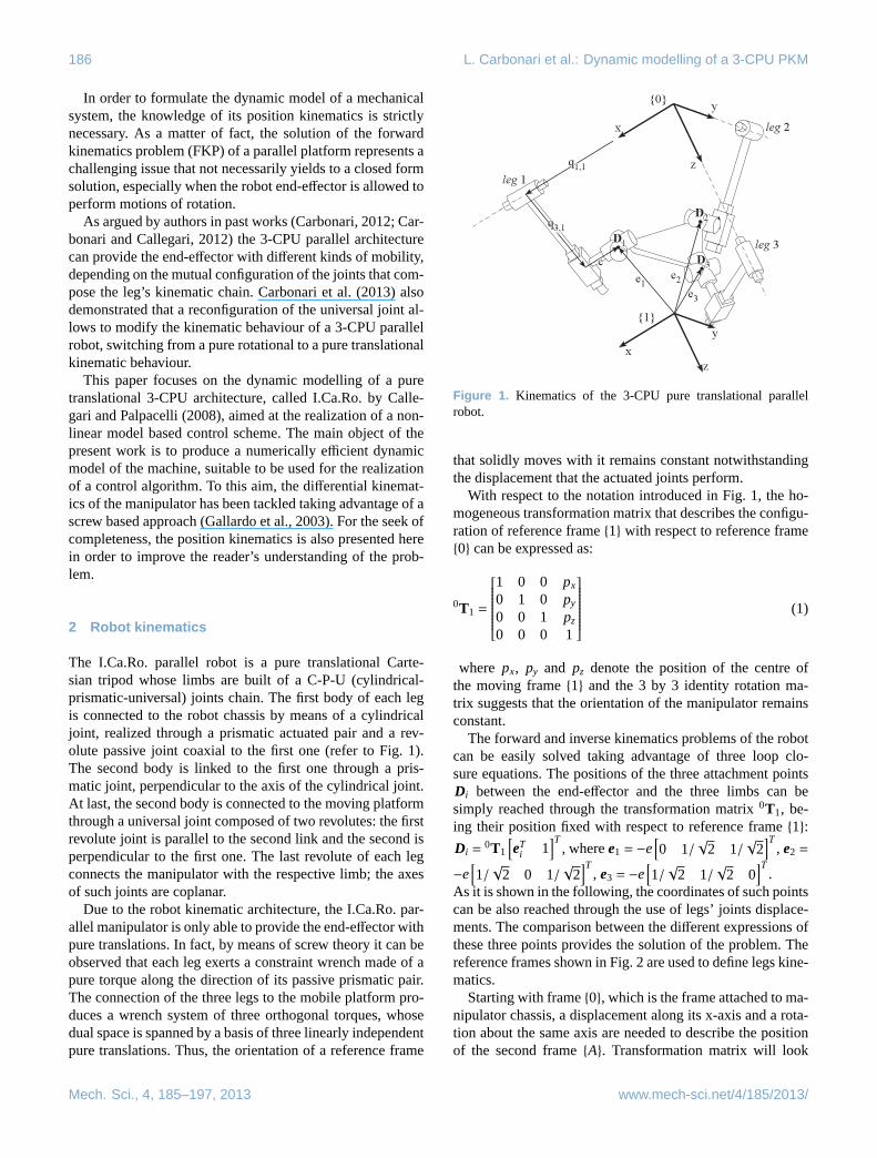
The I.Ca.Ro. parallel robot is a pure translational Carte-sian tripod whose limbs are built of a C-P-U (cylindrical-prismatic-universal) joints chain. The first body of each legis connected to the robot chassis by means of a cylindricaljoint, realized through a prismatic actuated pair and a rev-olute passive joint coaxial to the first one (refer to Fig.1).The second body is linked to the first one through a pris-matic joint, perpendicular to the axis of the cylindrical joint.At last, the second body is connected to the moving platformthrough a universal joint composed of two revolutes: the firstrevolute joint is parallel to the second link and the second isperpendicular to the first one. The last revolute of each legconnects the manipulator with the respective limb; the axesof such joints are coplanar.

Due to the robot kinematic architecture, the I.Ca.Ro. par-allel manipulator is only able to provide the end-effector withpure translations. In fact, by means of screw theory it can beobserved that each leg exerts a constraint wrench made of apure torque along the direction of its passive prismatic pair.The connection of the three legs to the mobile platform pro-duces a wrench system of three orthogonal torques, whosedual space is spanned by a basis of three linearly independentpure translations. Thus, the orientation of a reference frame

Figure 1. Kinematics of the 3-CPU pure translational parallelrobot.

that solidly moves with it remains constant notwithstandingthe displacement that the actuated joints perform.

With respect to the notation introduced in Fig.1, the ho-mogeneous transformation matrix that describes the configu-ration of reference frame{1} with respect to reference frame{0} can be expressed as:

0T1 =

1 0 0 px

0 1 0 py

0 0 1 pz

0 0 0 1

(1)

where px, py and pz denote the position of the centre ofthe moving frame{1} and the 3 by 3 identity rotation ma-trix suggests that the orientation of the manipulator remainsconstant.

The forward and inverse kinematics problems of the robotcan be easily solved taking advantage of three loop clo-sure equations. The positions of the three attachment pointsDi between the end-effector and the three limbs can besimply reached through the transformation matrix0T1, be-ing their position fixed with respect to reference frame{1}:

Di =0T1

[eT

i 1]T

, wheree1 = −e[0 1/

√2 1/

√2]T

, e2 =

−e[1/√

2 0 1/√

2]T

, e3 = −e[1/√

2 1/√

2 0]T

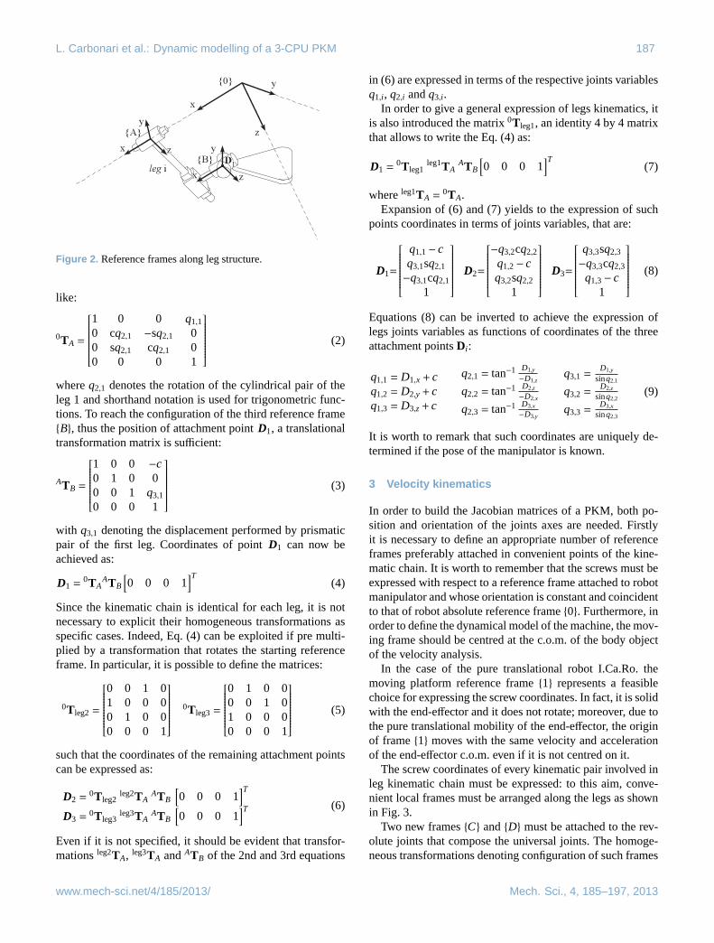
.As it is shown in the following, the coordinates of such pointscan be also reached through the use of legs’ joints displace-ments. The comparison between the different expressions ofthese three points provides the solution of the problem. Thereference frames shown in Fig.2 are used to define legs kine-matics.

Starting with frame{0}, which is the frame attached to ma-nipulator chassis, a displacement along its x-axis and a rota-tion about the same axis are needed to describe the positionof the second frame{A}. Transformation matrix will look

Mech. Sci., 4, 185–197, 2013 www.mech-sci.net/4/185/2013/

L. Carbonari et al.: Dynamic modelling of a 3-CPU PKM 187

Figure 2. Reference frames along leg structure.

like:

0TA =

1 0 0 q1,1

0 cq2,1 −sq2,1 00 sq2,1 cq2,1 00 0 0 1

(2)

whereq2,1 denotes the rotation of the cylindrical pair of theleg 1 and shorthand notation is used for trigonometric func-tions. To reach the configuration of the third reference frame{B}, thus the position of attachment pointD1, a translationaltransformation matrix is sufficient:

ATB =

1 0 0 −c0 1 0 00 0 1 q3,1

0 0 0 1

(3)

with q3,1 denoting the displacement performed by prismaticpair of the first leg. Coordinates of pointD1 can now beachieved as:

D1 =0TA

ATB

[0 0 0 1

]T(4)

Since the kinematic chain is identical for each leg, it is notnecessary to explicit their homogeneous transformations asspecific cases. Indeed, Eq. (4) can be exploited if pre multi-plied by a transformation that rotates the starting referenceframe. In particular, it is possible to define the matrices:

0T leg2=

0 0 1 01 0 0 00 1 0 00 0 0 1

0T leg3=

0 1 0 00 0 1 01 0 0 00 0 0 1

(5)

such that the coordinates of the remaining attachment pointscan be expressed as:

D2 =0T leg2

leg2TAATB

[0 0 0 1

]TD3 =

0T leg3leg3TA

ATB

[0 0 0 1

]T (6)

Even if it is not specified, it should be evident that transfor-mationsleg2TA, leg3TA andATB of the 2nd and 3rd equations

in (6) are expressed in terms of the respective joints variablesq1,i , q2,i andq3,i .

In order to give a general expression of legs kinematics, itis also introduced the matrix0T leg1, an identity 4 by 4 matrixthat allows to write the Eq. (4) as:

D1 =0T leg1

leg1TAATB

[0 0 0 1

]T(7)

whereleg1TA =0TA.

Expansion of (6) and (7) yields to the expression of suchpoints coordinates in terms of joints variables, that are:

D1=

q1,1− cq3,1sq2,1

−q3,1cq2,1

1

D2=

−q3,2cq2,2

q1,2− cq3,2sq2,2

1

D3=

q3,3sq2,3

−q3,3cq2,3

q1,3− c1

(8)

Equations (8) can be inverted to achieve the expression oflegs joints variables as functions of coordinates of the threeattachment pointsDi :

q1,1 = D1,x+ cq1,2 = D2,y+ cq1,3 = D3,z+ c

q2,1 = tan−1 D1,y

−D1,z

q2,2 = tan−1 D2,z

−D2,x

q2,3 = tan−1 D3,x

−D3,y

q3,1 =D1,y

sinq2,1

q3,2 =D2,z

sinq2,2

q3,3 =D3,x

sinq2,3

(9)

It is worth to remark that such coordinates are uniquely de-termined if the pose of the manipulator is known.

3 Velocity kinematics

In order to build the Jacobian matrices of a PKM, both po-sition and orientation of the joints axes are needed. Firstlyit is necessary to define an appropriate number of referenceframes preferably attached in convenient points of the kine-matic chain. It is worth to remember that the screws must beexpressed with respect to a reference frame attached to robotmanipulator and whose orientation is constant and coincidentto that of robot absolute reference frame{0}. Furthermore, inorder to define the dynamical model of the machine, the mov-ing frame should be centred at the c.o.m. of the body objectof the velocity analysis.

In the case of the pure translational robot I.Ca.Ro. themoving platform reference frame{1} represents a feasiblechoice for expressing the screw coordinates. In fact, it is solidwith the end-effector and it does not rotate; moreover, due tothe pure translational mobility of the end-effector, the originof frame{1} moves with the same velocity and accelerationof the end-effector c.o.m. even if it is not centred on it.

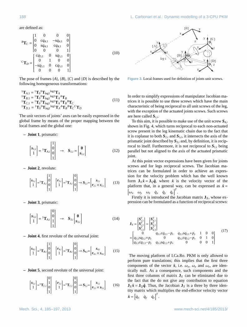
The screw coordinates of every kinematic pair involved inleg kinematic chain must be expressed: to this aim, conve-nient local frames must be arranged along the legs as shownin Fig. 3.

Two new frames{C} and{D} must be attached to the rev-olute joints that compose the universal joints. The homoge-neous transformations denoting configuration of such frames

www.mech-sci.net/4/185/2013/ Mech. Sci., 4, 185–197, 2013

188 L. Carbonari et al.: Dynamic modelling of a 3-CPU PKM

are defined as:

BTC =

1 0 0 00 cq4,1 −sq4,1 00 sq4,1 cq4,1 00 0 0 1

CTD =

cq5,1 0 sq5,1 0

0 1 0 0−sq5,1 0 cq5,1 0

0 0 0 1

(10)

The pose of frames{A}, {B}, {C} and{D} is described by thefollowing homogeneous transformations:

1TA,1 =1T0

0T leg1leg1TA

1TB,1 =1T0

0T leg1leg1TA

ATB1TC,1 =

1T00T leg1

leg1TAATB

BTC1TD,1 =

1T00T leg1

leg1TAATB

BTCCTD

(11)

The unit vectors of joints’ axes can be easily expressed in theglobal frame by means of the proper mapping between thelocal frames and the global one:

– Joint 1, prismatic:

[s1,i

1

]= 1TA,i

1001

→ S1,i =

[0

s1,i

](12)

– Joint 2, revolute:

[s2,i

1

]=1TA,i

1001

[r2,i

1

]=1TA,i

0001

→ S2,i=

[s2,i

r2,i × s2,i

](13)

– Joint 3, prismatic:

[s3,i

1

]= 1TA,i

0011

→ S3,i

[0

s3,i

](14)

– Joint 4, first revolute of the universal joint:

[s4,i

1

]=1TB,i

1001

[r4,i

1

]=1TB,i

0001

→ S4,i=

[s4,i

r4,i × s4,i

](15)

– Joint 5, second revolute of the universal joint:

[s5,i

1

]=1TC,i

0101

[r5,i

1

]=1TC,i

0001

→ S5,i=

[s5,i

r5,i × s5,i

](16)

Figure 3. Local frames used for definition of joints unit screws.

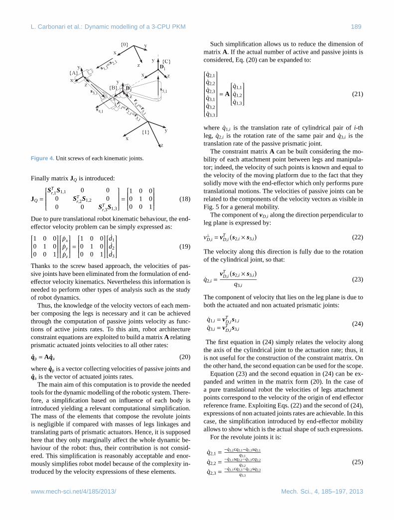
In order to simplify expressions of manipulator Jacobian ma-trices it is possible to use three screws which have the maincharacteristic of being reciprocal to all unit screws of the leg,with the exception of the actuated joints screws. Such screwsare here calledSr,i .

To this aim, it is possible to make use of the unit screwS4,i

shown in Fig.4, which turns reciprocal to each non-actuatedscrew present in the leg kinematic chain due to the fact thatit is coplanar to bothS2,i andS5,i , it intersects the axis of theprismatic joint described byS3,i and, by definition, it is recip-rocal to itself. Furthermore, it is not reciprocal toS1,i beingparallel but not aligned to the axis of the actuated prismaticjoint.

At this point vector expressions have been given for jointsscrews and for legs reciprocal screws. The Jacobian ma-trices can be formulated in order to achieve an expres-sion for the velocity problem which has the well knownform JX x = JQq, where x is the velocity vector of theplatform that, in a general way, can be expressed asx =[ωx ωy ωz qx qy qz

]T.

Firstly it is introduced the Jacobian matrixJX, whose ex-pression can be formulated as a function of reciprocal screws:

JX =

ST

r,1

STr,2

STr,3

=ST

4,1

ST4,2

ST4,3

=

0 q3,1cq2,1−pz q3,1sq2,1+py 1 0 0q3,2sq2,2+pz 0 q3,2cq2,2−px 0 1 0q3,3cq2,3−py q3,3sq2,3+px 0 0 0 1

(17)

The moving platform of I.Ca.Ro. PKM is only allowed toperform pure translations; this implies that the first threecomponents of the vectorx, i.e. ωx, ωy andωz, are iden-tically null. As a consequence, such components and thefirst three columns of matrixJX can be eliminated due tothe fact that the do not give any contribution to equationJX x = JQq. Thus, the JacobianJX is a three by three iden-tity matrix which multiplies the end-effector velocity vector

x =[qx qy qz

]T.

Mech. Sci., 4, 185–197, 2013 www.mech-sci.net/4/185/2013/

L. Carbonari et al.: Dynamic modelling of a 3-CPU PKM 189

Figure 4. Unit screws of each kinematic joints.

Finally matrixJQ is introduced:

JQ =

ST

r,1S1,1 0 00 ST

r,2S1,2 00 0 ST

r,3S1,3

=1 0 00 1 00 0 1

(18)

Due to pure translational robot kinematic behaviour, the end-effector velocity problem can be simply expressed as:1 0 00 1 00 0 1

pxpy

pz

=1 0 00 1 00 0 1

d1

d2

d3

(19)

Thanks to the screw based approach, the velocities of pas-sive joints have been eliminated from the formulation of end-effector velocity kinematics. Nevertheless this information isneeded to perform other types of analysis such as the studyof robot dynamics.

Thus, the knowledge of the velocity vectors of each mem-ber composing the legs is necessary and it can be achievedthrough the computation of passive joints velocity as func-tions of active joints rates. To this aim, robot architectureconstraint equations are exploited to build a matrixA relatingprismatic actuated joints velocities to all other rates:

qp = A qa (20)

whereqp is a vector collecting velocities of passive joints andqa is the vector of actuated joints rates.

The main aim of this computation is to provide the neededtools for the dynamic modelling of the robotic system. There-fore, a simplification based on influence of each body isintroduced yielding a relevant computational simplification.The mass of the elements that compose the revolute jointsis negligible if compared with masses of legs linkages andtranslating parts of prismatic actuators. Hence, it is supposedhere that they only marginally affect the whole dynamic be-haviour of the robot: thus, their contribution is not consid-ered. This simplification is reasonably acceptable and enor-mously simplifies robot model because of the complexity in-troduced by the velocity expressions of these elements.

Such simplification allows us to reduce the dimension ofmatrix A. If the actual number of active and passive joints isconsidered, Eq. (20) can be expanded to:

q2,1

q2,2

q2,3

q3,1

q3,2

q3,3

= A

q1,1

q1,2

q1,3

(21)

where q1,i is the translation rate of cylindrical pair ofi-thleg, q2,i is the rotation rate of the same pair and ˙q3,i is thetranslation rate of the passive prismatic joint.

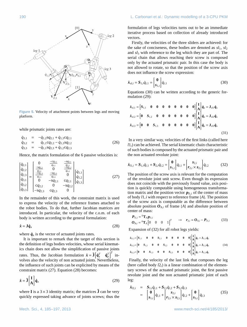
The constraint matrixA can be built considering the mo-bility of each attachment point between legs and manipula-tor; indeed, the velocity of such points is known and equal tothe velocity of the moving platform due to the fact that theysolidly move with the end-effector which only performs puretranslational motions. The velocities of passive joints can berelated to the components of the velocity vectors as visible inFig. 5 for a general mobility.

The component ofvD,i along the direction perpendicular toleg plane is expressed by:

v⊥D,i = vTD,i(s2,i × s3,i

)(22)

The velocity along this direction is fully due to the rotationof the cylindrical joint, so that:

q2,i =vT

D,i

(s2,i × s3,i

)q3,i

(23)

The component of velocity that lies on the leg plane is due toboth the actuated and non actuated prismatic joints:

q1,i = vTD,i s1,i

q3,i = vTD,i s3,i

(24)

The first equation in (24) simply relates the velocity alongthe axis of the cylindrical joint to the actuation rate; thus, itis not useful for the construction of the constraint matrix. Onthe other hand, the second equation can be used for the scope.

Equation (23) and the second equation in (24) can be ex-panded and written in the matrix form (20). In the case ofa pure translational robot the velocities of legs attachmentpoints correspond to the velocity of the origin of end effectorreference frame. Exploiting Eqs. (22) and the second of (24),expressions of non actuated joints rates are achievable. In thiscase, the simplification introduced by end-effector mobilityallows to show which is the actual shape of such expressions.

For the revolute joints it is:

q2,1 =−q1,2cq2,1−q1,3sq2,1

q3,1

q2,2 =−q1,1sq2,2−q1,3cq2,2

q3,2

q2,3 =−q1,1cq2,3−q1,2sq2,3

q3,3

(25)

www.mech-sci.net/4/185/2013/ Mech. Sci., 4, 185–197, 2013

190 L. Carbonari et al.: Dynamic modelling of a 3-CPU PKM

Figure 5. Velocity of attachment points between legs and movingplatform.

while prismatic joints rates are:

q3,1 = −q1,2sq2,1+ q1,3cq2,1

q3,2 = q1,1cq2,2− q1,3sq2,2

q3,3 = −q1,1sq2,3+ q1,2cq2,3

(26)

Hence, the matrix formulation of the 6 passive velocities is:

q2,1

q2,2

q2,3

q3,1

q3,2

q3,3

=

0 −cq2,1

q3,1

−sq2,1

q3,1−sq2,2

q3,20 −cq2,2

q3,2−cq2,3

q3,3

−sq2,3

q3,30

0 −sq2,1 cq2,1

cq2,2 0 −sq2,2

−sq2,3 cq2,3 0

q1,1

q1,2

q1,3

(27)

In the remainder of this work, the constraint matrix is usedto express the velocity of the reference frames attached tothe robot bodies. To do that, further Jacobian matrices areintroduced. In particular, the velocity of the c.o.m. of eachbody is written according to the general formulation:

x = Jqa (28)

whereqa is the vector of actuated joints rates.It is important to remark that the target of this section is

the definition of legs bodies velocities, whose serial kinemat-ics chain does not allow the simplification of passive joints

rates. Thus, the Jacobian formulationx = J[qT

a qTp

]Tin-

volves also the velocity of non actuated joints. Nevertheless,the influence of such joints can be explicited by means of theconstraint matrix (27). Equation (28) becomes:

x = J[IA

]qa (29)

whereI is a 3×3 identity matrix; the matricesJ can be veryquickly expressed taking advance of joints screws; thus the

formulation of legs velocities turns out to be an immediateiterative process based on collection of already introducedvectors.

Firstly, the velocities of the three sliders are achieved: forthe sake of conciseness, these bodies are denoted assl1, sl2andsl3 with reference to the leg which they are part of. Theserial chain that allows reaching their screw is composedonly by the actuated prismatic pair. In this case the body isnot allowed to rotate, so that the position of the screw axisdoes not influence the screw expression:

xsl,i = S1,i qi,1 =

[0

s1,i

]qi,1 (30)

Equations (30) can be written according to the generic for-mulation (29):

xsl,1 =[S1,1 0 0 0 0 0 0 0 0

] [ IA

]qa = Jsl1qa

xsl,2 =[0 S1,2 0 0 0 0 0 0 0

] [ IA

]qa = Jsl2qa

xsl,3 =[0 0 S1,3 0 0 0 0 0 0

] [ IA

]qa = Jsl3qa

(31)

In a very similar way, velocities of the first links (called herel1i) can be achieved. The serial kinematic chain characteristicof such bodies is composed by the actuated prismatic pair andthe non actuated revolute joint:

xl1,i = S1,i qi,1+S2,i qi,2 =

[0

s1,i

]qi,1+

[s2,i

r2,i × s2,i

]qi,2 (32)

The position of the screw axis is relevant for the computationof the revolute joint unit screw. Even though its expressiondoes not coincide with the previously found value, axis posi-tion is quickly computable using homogeneous transforma-tion matrix and the position vectorpl1,i of the center of massof bodyl1, i with respect to reference frame{A}. The positionof the screw axis is computable as the difference betweenabsolute positionOA,i of frame{A} and absolute position ofcenter of mass:

Pl1,i =0TA pl1,i

OA,i =0TA

[0 0 0 1

]T → r2,i =OA,i − Pl1,i (33)

Expansion of (32) for all robot legs yields:

xl1,1=[S1,1 0 0 S2,1 0 0 0 0 0

] [ IA

]qa = Jl1,1qa

xl1,2=[0 S1,2 0 0 S2,2 0 0 0 0

] [ IA

]qa = Jl1,2qa

xl1,3=[0 0 S1,3 0 0 S2,3 0 0 0

] [ IA

]qa = Jl1,3qa

(34)

Finally, the velocity of the last link that composes the leg(here called bodyl2i) is a linear combination of the elemen-tary screws of the actuated prismatic joint, the first passiverevolute joint and the non actuated prismatic joint of eachleg:

xl2,i = S1,i qi,1+S2,i qi,2+S3,i qi,3

=

[0

s1,i

]qi,1+

[s2,i

r2,i × s2,i

]qi,2+

[0

s3,i

]qi,3

(35)

Mech. Sci., 4, 185–197, 2013 www.mech-sci.net/4/185/2013/

L. Carbonari et al.: Dynamic modelling of a 3-CPU PKM 191

The positionr2,i of the screw axis is once again different fromthe previously exposed case. Nevertheless, its expression isachievable by the definition of a position vectorpl2,i of thecenter of mass of bodiesl2i with respect to their attachedframe {B}. The distance from this point to the axis of therevolute joint is given by:

pl2,i =0TBpl2,i

OB,i =0TB

[0 0 0 1

]T → r2,i =OB,i − pl2,i (36)

As done in previous case, the Jacobian formulation can beplainly reached also for velocities of bodiesl2i :

xl2,1 =[S1,1 0 0 S2,1 0 0 S3,1 0 0

] [ IA

]qa = Jl2,1qa

xl2,2 =[0 S1,2 0 0 S2,2 0 0 S3,2 0

] [ IA

]qa = Jl2,2qa

xl2,3 =[0 0 S1,3 0 0 S2,3 0 0 S3,3

] [ IA

]qa = Jl2,3qa

(37)

4 Acceleration kinematics

The dynamic modelling of a mechanical system requires acomplete knowledge of machine kinematics. Therefore, ac-celeration of each body must be studied.

Manipulator velocity kinematics has been formulatedthrough the well known Jacobian formulationqa = Jx, whereJ = J−1

Q JX is in this case a 3 by 3 identity matrix. Direct dif-ferentiation of such expression yields:

qa = Jx+ Jx (38)

whereJX is the derivative of the jacobian matrix, which isa constant matrix. Thus, in the case of a pure translationalmachine, the derivation ofJX yields JX = 0.

The acceleration kinematics of other robot members is eas-ily achievable by direct differentiation of the velocity kine-matics previously defined:

X j,i = J j,i qa+ J j,i qa (39)

wereJ j,i is the time derivative of the respective Jacobian ma-trix. Expansion of (39) yields to very a long formulation that,for sake of conciseness, is not shown here.

5 Virtual work principle

The virtual work principle approach for dynamic modellingrequires the definition of the 6 dimensional vectorF j,i , whosecomponents collect resultants of both active and inertialforces and torques acting on thej-th body of i-th leg, com-puted with respect to the center of mass of the member:

F j,i =

[n j,i

F j,i

]=

−0I j,iω j,i −ω j,i ×(0I j,iω j,i

)mj,i

(g− v j,i

) (40)

In a similar way, it is introduced the vectorFEE that collectsforces and torques acting on robot’s end-effector and com-puted with respect to manipulator centre of mass:

FEE =

[nEE

FEE

]=

[−0IEEωEE−ωEE×

(0IEEωEE

)mEE(g− vEE)

](41)

Virtual works principle allows writing:

δqTaτ+ δx

T FEE+∑i, j

δxTj,i F j,i = 0 (42)

where vectorδqa represents the virtual displacements of ac-tuated joints,τ is the vector of actuation torques andδx isthe virtual displacement of rotation/displacement of respec-tive body.

The differential kinematics of the manipulator, whose for-mulation has been introduced in previous sections, is use-fully exploited to relate actuated joints displacements to otherbodies twists. Indeed, end-effector differential kinematics ex-pression allows writing:

δqa = JXδx (43)

In a similar way, the twist of other robot members can beexpressed through the respective Jacobian matrices:

δx j,i = J j,iδqa (44)

When Eq. (43) is invertible, i.e. when determinant of the Ja-cobian matrix is not null, the differential of end effector twistcan be expressed in terms of actuated joints translations, be-ing δx = J−1

X δqa. Dynamics Eq. (42) becomes:

δqTaτA+ δqT

a J−TX FEE+ δqT

a

∑i, j

JTj,i F j,i = 0 (45)

For non null virtual displacementsδqa, such term can be col-lected and eliminated, yielding:

τ+ J−TX FEE+

∑i, j

JTj,i F j,i = 0 (46)

Equation (46) can be collected in the canonical form:

τ+M (qa) qa+V (qa, qa)+G(qa) = 0 (47)

As known, each component of this equation includes dif-ferent contributions to the dynamics of the manipulator:M (qa) qa called laterτM is a contribution due to inertial ef-fects of bodies masses,V (qa, qa), hereby calledτV, is due toCoriolis and centripetal accelerations and, at last,G(qa) arethe forces deriving from gravitational action on robot mem-bers, called hereτG.

www.mech-sci.net/4/185/2013/ Mech. Sci., 4, 185–197, 2013

192 L. Carbonari et al.: Dynamic modelling of a 3-CPU PKM

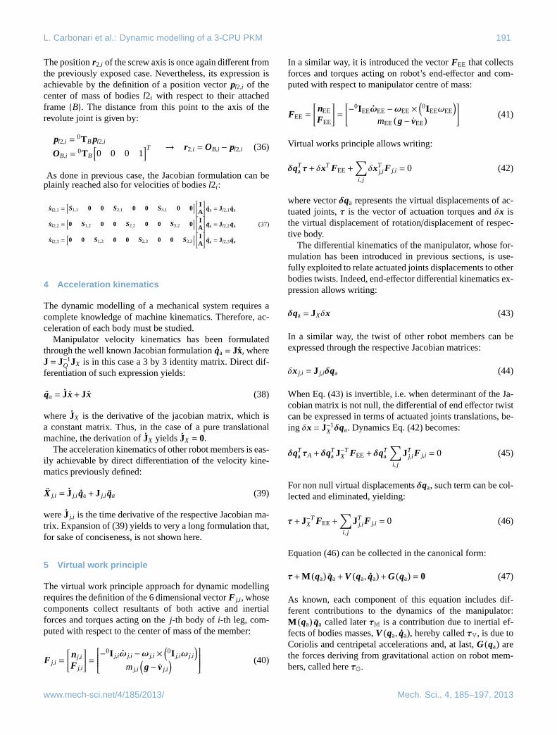
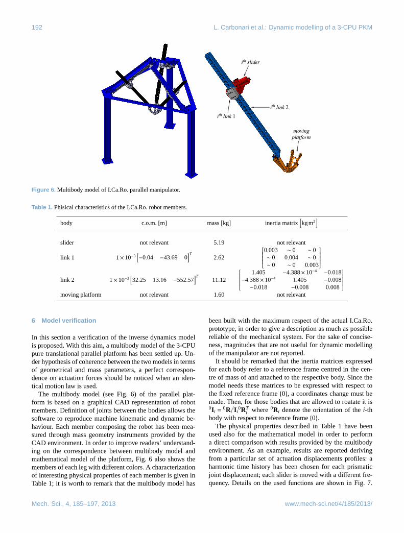
Figure 6. Multibody model of I.Ca.Ro. parallel manipulator.

Table 1. Phisical characteristics of the I.Ca.Ro. robot members.

body c.o.m.[m] mass[kg]

inertia matrix[kgm2

]slider not relevant 5.19 not relevant

link 1 1×10−3[−0.04 −43.69 0

]T2.62

0.003 ∼ 0 ∼ 0∼ 0 0.004 ∼ 0∼ 0 ∼ 0 0.003

link 2 1×10−3

[32.25 13.16 −552.57

]T11.12

1.405 −4.388×10−4 −0.018−4.388×10−4 1.405 −0.008−0.018 −0.008 0.008

moving platform not relevant 1.60 not relevant

6 Model verification

In this section a verification of the inverse dynamics modelis proposed. With this aim, a multibody model of the 3-CPUpure translational parallel platform has been settled up. Un-der hypothesis of coherence between the two models in termsof geometrical and mass parameters, a perfect correspon-dence on actuation forces should be noticed when an iden-tical motion law is used.

The multibody model (see Fig.6) of the parallel plat-form is based on a graphical CAD representation of robotmembers. Definition of joints between the bodies allows thesoftware to reproduce machine kinematic and dynamic be-haviour. Each member composing the robot has been mea-sured through mass geometry instruments provided by theCAD environment. In order to improve readers’ understand-ing on the correspondence between multibody model andmathematical model of the platform, Fig.6 also shows themembers of each leg with different colors. A characterizationof interesting physical properties of each member is given inTable1; it is worth to remark that the multibody model has

been built with the maximum respect of the actual I.Ca.Ro.prototype, in order to give a description as much as possiblereliable of the mechanical system. For the sake of concise-ness, magnitudes that are not useful for dynamic modellingof the manipulator are not reported.

It should be remarked that the inertia matrices expressedfor each body refer to a reference frame centred in the cen-tre of mass of and attached to the respective body. Since themodel needs these matrices to be expressed with respect tothe fixed reference frame{0}, a coordinates change must bemade. Then, for those bodies that are allowed to roatate it is0I i =

0Rii I i

0RTi where0Ri denote the orientation of thei-th

body with respect to reference frame{0}.The physical properties described in Table1 have been

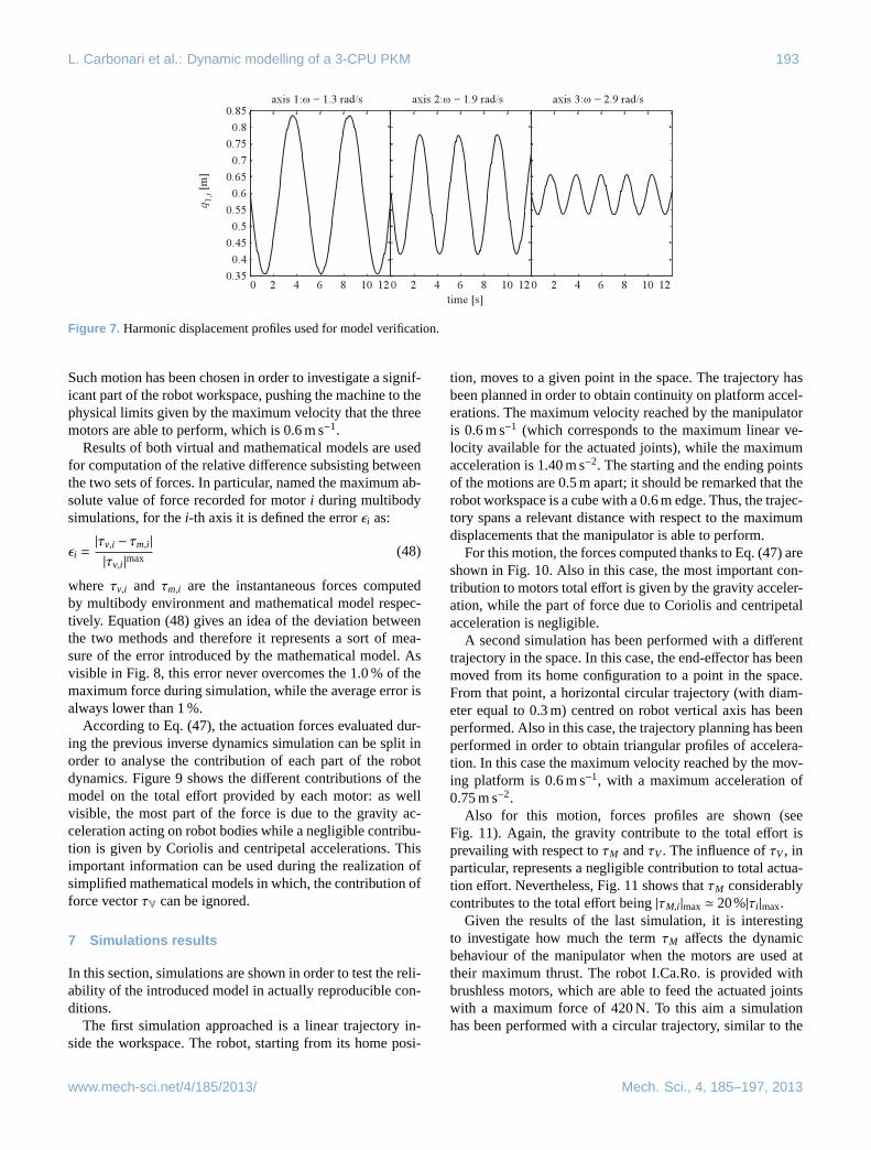
used also for the mathematical model in order to performa direct comparison with results provided by the multibodyenvironment. As an example, results are reported derivingfrom a particular set of actuation displacements profiles: aharmonic time history has been chosen for each prismaticjoint displacement; each slider is moved with a different fre-quency. Details on the used functions are shown in Fig.7.

Mech. Sci., 4, 185–197, 2013 www.mech-sci.net/4/185/2013/

L. Carbonari et al.: Dynamic modelling of a 3-CPU PKM 193

Figure 7. Harmonic displacement profiles used for model verification.

Such motion has been chosen in order to investigate a signif-icant part of the robot workspace, pushing the machine to thephysical limits given by the maximum velocity that the threemotors are able to perform, which is 0.6 m s−1.

Results of both virtual and mathematical models are usedfor computation of the relative difference subsisting betweenthe two sets of forces. In particular, named the maximum ab-solute value of force recorded for motori during multibodysimulations, for thei-th axis it is defined the errorεi as:

εi =|τv,i − τm,i |

|τv,i |max(48)

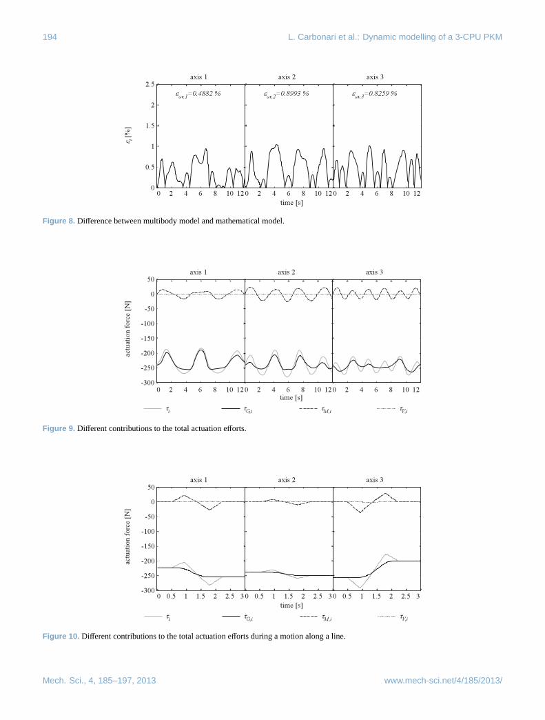
where τv,i and τm,i are the instantaneous forces computedby multibody environment and mathematical model respec-tively. Equation (48) gives an idea of the deviation betweenthe two methods and therefore it represents a sort of mea-sure of the error introduced by the mathematical model. Asvisible in Fig.8, this error never overcomes the 1.0 % of themaximum force during simulation, while the average error isalways lower than 1 %.

According to Eq. (47), the actuation forces evaluated dur-ing the previous inverse dynamics simulation can be split inorder to analyse the contribution of each part of the robotdynamics. Figure9 shows the different contributions of themodel on the total effort provided by each motor: as wellvisible, the most part of the force is due to the gravity ac-celeration acting on robot bodies while a negligible contribu-tion is given by Coriolis and centripetal accelerations. Thisimportant information can be used during the realization ofsimplified mathematical models in which, the contribution offorce vectorτV can be ignored.

7 Simulations results

In this section, simulations are shown in order to test the reli-ability of the introduced model in actually reproducible con-ditions.

The first simulation approached is a linear trajectory in-side the workspace. The robot, starting from its home posi-

tion, moves to a given point in the space. The trajectory hasbeen planned in order to obtain continuity on platform accel-erations. The maximum velocity reached by the manipulatoris 0.6 m s−1 (which corresponds to the maximum linear ve-locity available for the actuated joints), while the maximumacceleration is 1.40 m s−2. The starting and the ending pointsof the motions are 0.5 m apart; it should be remarked that therobot workspace is a cube with a 0.6 m edge. Thus, the trajec-tory spans a relevant distance with respect to the maximumdisplacements that the manipulator is able to perform.

For this motion, the forces computed thanks to Eq. (47) areshown in Fig.10. Also in this case, the most important con-tribution to motors total effort is given by the gravity acceler-ation, while the part of force due to Coriolis and centripetalacceleration is negligible.

A second simulation has been performed with a differenttrajectory in the space. In this case, the end-effector has beenmoved from its home configuration to a point in the space.From that point, a horizontal circular trajectory (with diam-eter equal to 0.3 m) centred on robot vertical axis has beenperformed. Also in this case, the trajectory planning has beenperformed in order to obtain triangular profiles of accelera-tion. In this case the maximum velocity reached by the mov-ing platform is 0.6 m s−1, with a maximum acceleration of0.75 m s−2.

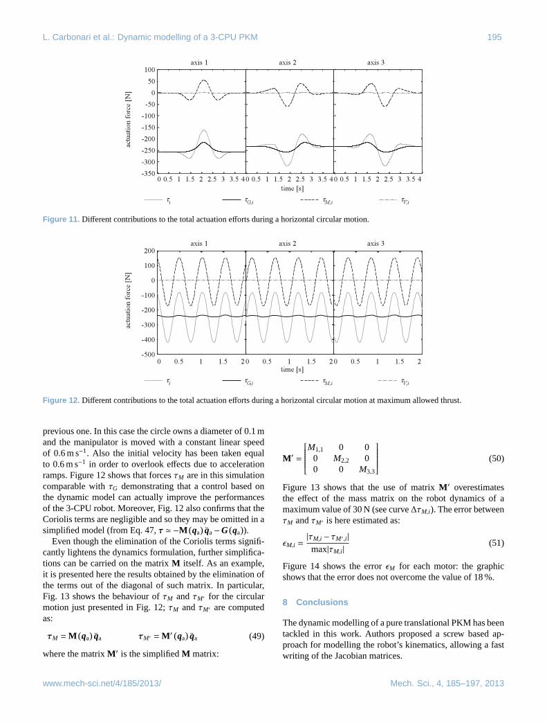
Also for this motion, forces profiles are shown (seeFig. 11). Again, the gravity contribute to the total effort isprevailing with respect toτM andτV. The influence ofτV, inparticular, represents a negligible contribution to total actua-tion effort. Nevertheless, Fig.11shows thatτM considerablycontributes to the total effort being|τM,i |max' 20%|τi |max.

Given the results of the last simulation, it is interestingto investigate how much the termτM affects the dynamicbehaviour of the manipulator when the motors are used attheir maximum thrust. The robot I.Ca.Ro. is provided withbrushless motors, which are able to feed the actuated jointswith a maximum force of 420 N. To this aim a simulationhas been performed with a circular trajectory, similar to the

www.mech-sci.net/4/185/2013/ Mech. Sci., 4, 185–197, 2013

194 L. Carbonari et al.: Dynamic modelling of a 3-CPU PKM

Figure 8. Difference between multibody model and mathematical model.

Figure 9. Different contributions to the total actuation efforts.

Figure 10. Different contributions to the total actuation efforts during a motion along a line.

Mech. Sci., 4, 185–197, 2013 www.mech-sci.net/4/185/2013/

L. Carbonari et al.: Dynamic modelling of a 3-CPU PKM 195

Figure 11. Different contributions to the total actuation efforts during a horizontal circular motion.

Figure 12. Different contributions to the total actuation efforts during a horizontal circular motion at maximum allowed thrust.

previous one. In this case the circle owns a diameter of 0.1 mand the manipulator is moved with a constant linear speedof 0.6 m s−1. Also the initial velocity has been taken equalto 0.6 m s−1 in order to overlook effects due to accelerationramps. Figure12 shows that forcesτM are in this simulationcomparable withτG demonstrating that a control based onthe dynamic model can actually improve the performancesof the 3-CPU robot. Moreover, Fig.12also confirms that theCoriolis terms are negligible and so they may be omitted in asimplified model (from Eq.47, τ ' −M (qa) qa−G(qa)).

Even though the elimination of the Coriolis terms signifi-cantly lightens the dynamics formulation, further simplifica-tions can be carried on the matrixM itself. As an example,it is presented here the results obtained by the elimination ofthe terms out of the diagonal of such matrix. In particular,Fig. 13 shows the behaviour ofτM andτM′ for the circularmotion just presented in Fig.12; τM andτM′ are computedas:

τM =M (qa) qa τM′ =M ′ (qa) qa (49)

where the matrixM ′ is the simplifiedM matrix:

M ′ =

M1,1 0 00 M2,2 00 0 M3,3

(50)

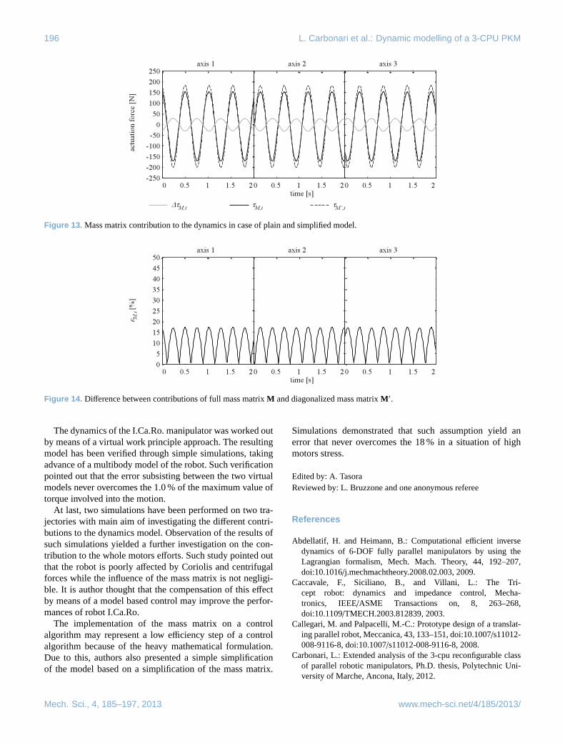
Figure 13 shows that the use of matrixM ′ overestimatesthe effect of the mass matrix on the robot dynamics of amaximum value of 30 N (see curve∆τM,i). The error betweenτM andτM′ is here estimated as:

εM,i =|τM,i − τM′,i |

max|τM,i |(51)

Figure 14 shows the errorεM for each motor: the graphicshows that the error does not overcome the value of 18 %.

8 Conclusions

The dynamic modelling of a pure translational PKM has beentackled in this work. Authors proposed a screw based ap-proach for modelling the robot’s kinematics, allowing a fastwriting of the Jacobian matrices.

www.mech-sci.net/4/185/2013/ Mech. Sci., 4, 185–197, 2013

196 L. Carbonari et al.: Dynamic modelling of a 3-CPU PKM

Figure 13. Mass matrix contribution to the dynamics in case of plain and simplified model.

Figure 14. Difference between contributions of full mass matrixM and diagonalized mass matrixM ′.

The dynamics of the I.Ca.Ro. manipulator was worked outby means of a virtual work principle approach. The resultingmodel has been verified through simple simulations, takingadvance of a multibody model of the robot. Such verificationpointed out that the error subsisting between the two virtualmodels never overcomes the 1.0 % of the maximum value oftorque involved into the motion.

At last, two simulations have been performed on two tra-jectories with main aim of investigating the different contri-butions to the dynamics model. Observation of the results ofsuch simulations yielded a further investigation on the con-tribution to the whole motors efforts. Such study pointed outthat the robot is poorly affected by Coriolis and centrifugalforces while the influence of the mass matrix is not negligi-ble. It is author thought that the compensation of this effectby means of a model based control may improve the perfor-mances of robot I.Ca.Ro.

The implementation of the mass matrix on a controlalgorithm may represent a low efficiency step of a controlalgorithm because of the heavy mathematical formulation.Due to this, authors also presented a simple simplificationof the model based on a simplification of the mass matrix.

Simulations demonstrated that such assumption yield anerror that never overcomes the 18 % in a situation of highmotors stress.

Edited by: A. TasoraReviewed by: L. Bruzzone and one anonymous referee

References

Abdellatif, H. and Heimann, B.: Computational efficient inversedynamics of 6-DOF fully parallel manipulators by using theLagrangian formalism, Mech. Mach. Theory, 44, 192–207,doi:10.1016/j.mechmachtheory.2008.02.003, 2009.

Caccavale, F., Siciliano, B., and Villani, L.: The Tri-cept robot: dynamics and impedance control, Mecha-tronics, IEEE/ASME Transactions on, 8, 263–268,doi:10.1109/TMECH.2003.812839, 2003.

Callegari, M. and Palpacelli, M.-C.: Prototype design of a translat-ing parallel robot, Meccanica, 43, 133–151,doi:10.1007/s11012-008-9116-8, doi:10.1007/s11012-008-9116-8, 2008.

Carbonari, L.: Extended analysis of the 3-cpu reconfigurable classof parallel robotic manipulators, Ph.D. thesis, Polytechnic Uni-versity of Marche, Ancona, Italy, 2012.

Mech. Sci., 4, 185–197, 2013 www.mech-sci.net/4/185/2013/

L. Carbonari et al.: Dynamic modelling of a 3-CPU PKM 197

Carbonari, L. and Callegari, M.: The kinematotropic 3-CPU parallelrobot: analysis of mobility and reconfigurability aspects, in: Lat-est Advances in Robot Kinematics, edited by: Lenarcic, J. andHusty, M., Springer, 2012.

Carbonari, L., Callegari, M., Palmieri, G., and Palpacelli, M.: Anew class of reconfigurable parallel kinematics machines, Mech.Mach. Theory, in review, 2013.

Dasgupta, B. and Mruthyunjaya, T.: A Newton-Euler formulationfor the inverse dynamics of the Stewart platform manipula-tor, Mech. Mach. Theory, 33, 1135–1152,doi:10.1016/S0094-114X(97)00118-3, 1998.

Daun, Q., Daun, B., and Daun, X.: Dynamics modelling and hy-brid control of the 6-UPS platform, in: 2010 International Con-ference on Mechatronics and Automation (ICMA), 434 –439,doi:10.1109/ICMA.2010.5589105, 2010.

Di Gregorio, R. and Parenti-Castelli, V.: Dynamics of aClass of Parallel Wrists, J. Mech. Design, 126, 436–441,doi:10.1115/1.1737382, 2004.

Do, W. Q. D. and Yang, D. C. H.: Inverse dynamic analysis andsimulation of a platform type of robot, J. Robotic Syst., 5, 209–227,doi:10.1002/rob.4620050304, 1988.

Gallardo, J., Rico, J., Frisoli, A., Checcacci, D., and Bergamasco,M.: Dynamics of parallel manipulators by means of screw the-ory, Mech. Mach. Theory, 38, 1113–1131,doi:10.1016/S0094-114X(03)00054-5, 2003.

Khalil, W. and Ibrahim, O.: General Solution for the Dynamic Mod-eling of Parallel Robots, J. Intell. Robotics Syst., 49, 19–37,doi:10.1007/s10846-007-9137-x, 2007.

Kovecses, J., Piedboeuf, J. C., and Lange, C.: Dynamicsmodeling and simulation of constrained robotic systems,Mechatronics, IEEE/ASME Transactions on, 8, 165–177,doi:10.1109/TMECH.2003.812827, 2003.

Kunquan, L. and Rui, W.: Closed-form Dynamic Equations of the6-RSS Parallel Mechanism through the Newton-Euler Approach,in: 2011 Third International Conference on Measuring Tech-nology and Mechatronics Automation (ICMTMA), 1, 712–715,doi:10.1109/ICMTMA.2011.180, 2011.

Lin, Y.-J. and Song, S.-M.: A comparative study of inverse dynam-ics of manipulators with closed-chain geometry, J. Robotic Syst.,7, 507–534,doi:10.1002/rob.4620070402, 1990.

Lopes, A. M.: Dynamic modeling of a Stewart platform using thegeneralized momentum approach, Commun. Nonlinear Sci., 14,3389–3401,doi:10.1016/j.cnsns.2009.01.001, 2009.

Miller, K.: Optimal Design and Modeling of Spatial Par-allel Manipulators, Int. J. Robot. Res., 23, 127–140,doi:10.1177/0278364904041322, 2004.

Moon, F.: Applied Dynamics: With Applications to Multibody andMechatronic Systems, John Wiley & Sons, 2008.

Papastavridis, J.: Analytical Mechanics: A Comprehensive Trea-tise on the Dynamics of Constrained Systems, World Scientific,2012.

Tsai, L.-W.: Solving the Inverse Dynamics of a Stewart-Gough Ma-nipulator by the Principle of Virtual Work, J. Mech. Design, 122,3–9,doi:10.1115/1.533540, 2000.

Wang, J. and Gosselin, C. M.: A New Approach for the DynamicAnalysis of Parallel Manipulators, Multibody Syst. Dyn., 2, 317–334,doi:10.1023/A:1009740326195, 1998.

Wang, J., Wu, J., Wang, L., and Li, T.: Simplified strategy ofthe dynamic model of a 6-UPS parallel kinematic machinefor real-time control, Mech. Mach. Theory, 42, 1119–1140,doi:10.1016/j.mechmachtheory.2006.09.004, 2007.

Wronka, C. and Dunnigan, M.: Derivation and analysis of a dy-namic model of a robotic manipulator on a moving base, Robot.Auton. Syst., 59, 758–769,doi:10.1016/j.robot.2011.05.010,2011.

Yang, C., Han, J., Zheng, S., and Ogbobe Peter, O.: Dynamicmodeling and computational efficiency analysis for a spatial 6-DOF parallel motion system, Nonlinear Dynam., 67, 1007–1022,doi:10.1007/s11071-011-0043-1, 2012.

Zhang, C.-D. and Song, S.-M.: An efficient method for inverse dy-namics of manipulators based on the virtual work principle, J.Robotic Syst., 10, 605–627,doi:10.1002/rob.4620100505, 1993.

www.mech-sci.net/4/185/2013/ Mech. Sci., 4, 185–197, 2013