Dynamic AGE model for water economics in the Netherlands (DEAN-WEMPA)

Dynamic AGE model for water economics in

the Netherlands (DEAN-WEMPA)

First results

Rob Dellink (Wageningen University)

Vincent Linderhof (Institute for Environmental Studies)

WEMPA working paper-04

November 2006 (latest version)

This report is part of the project ‘Water Economic Modelling for Policy Analysis’

(www.ivm.falw.vu.nl/watereconomics), funded by ‘Leven met Water’ under ICES-KIS

III and co-funded by the Directorate-General Water of the Ministry of Transport, Public

Works and Water Management and the Ministry of Agriculture, Nature and Food Qual-

ity.

The following institutes participate in the project ‘Water Economic Modelling for Policy

Analysis’:

IVM LEI

Institute for Environmental Studies Landbouw-Economisch Instituut

Vrije Universiteit Burgemeester Patijnlaan 19

De Boelelaan 1087 2585 BE Den Haag

1081 HV Amsterdam The Netherlands

The Netherlands

Tel. +31-20-5989 555 Tel. +31-70-3358330

Fax. +31-20-5989 553 Fax. +31-70-3615624

E-mail: [email protected] E-mail: [email protected]

Delft Hydraulics RIZA

Rotterdamseweg 185 Zuiderwagenplein 2

2629 HD Delft 8224 AD Lelystad

The Netherlands The Netherlands

Tel. +31-15-2858585 Tel. +31-320-298411

Fax. +31-15-2858582 Fax. +31-320-249218


CBS WUR

Statistics Netherlands Environmental Economics and Natural

Resources Group, Wageningen University

Prinses Beatrixlaan 428 Hollandseweg 1

2273 XZ Voorburg 6706 KN Wageningen

The Netherlands The Netherlands

Tel. +31-70-3373800 Tel. +31 317 482009


Cover and logo design: Ontwerpbureau Lood, Delden, the Netherlands

Copyright © 2006, Institute for Environmental Studies.

All rights reserved. No part of this publication may be reproduced, stored in a retrieval

system or transmitted in any form or by any means, electronic, mechanical, photocopy-

ing, recording or otherwise without the prior written permission of the copyright holder.

Dynamic water economic model for the Netherlands iii

Contents

Summary iv

1. Introduction 1

2. Model description 2

2.1 General description of the DEAN model 2

2.2 Pollution and abatement 3

2.3 Adaptations of the model for WEMPA 4

3. Data and scenarios 5

3.1 Calibration of the base year 5

3.2 Calibration of the abatement cost curve for Eutrophication 7

3.3 Calibration of the abatement cost curve for Dispersion to Water 8

3.4 Calibration of the parameters 9

4. Results 10

5. Concluding remarks 16

References 17

Appendix: Results 19

Water Economic Modelling for Policy Analysis iv

Summary

This report presents the first preliminary results of using a dynamic Applied General

Equilibrium (AGE) model for the Netherlands to study water issues. We simulate the

economic consequences for different emission reduction scenarios ranging from 10 to 50

percent emission reduction compared to the benchmark situation. As marginal abatement

costs for small amounts of reduction are relatively cheap, the first 10% of emission re-

ductions can almost completely be achieved through the implementation of technical

measures. The macroeconomic results suggest that these adjustments in the economy are

virtually costless. Though production levels of the Agricultural and Industrial sectors de-

creases, this is compensated by increases in the Abatement sector. As the stringency of

the policy target increases, the impacts become visible at the macro-economic level:

GDP and NNI levels are decreasing, and the welfare loss, measured via the Equivalent

Variation, equals almost 1.5 percent when 50 percent emission reduction is imposed.

Dynamic water economic model for the Netherlands 1

1. Introduction

The aim of the WEMPA project is to develop an integrated and operational water and

economy model that will enable us to determine the economic effects of measures to im-

prove the water quality and subsequently the ecological quality of rivers, regional and

local waters. An important requisite of this model is that it must be shaped in such a way

that it is suitable for applying cost effectiveness analysis of implementing measures

within the EU Water Framework Directive (WFD) in the Netherlands. The existing

models used to assess cost-effectiveness of measures are usually not integrated and are

either pure hydrologic models or economic models. With this integrated model, we will

be able to analyse the economic effects of implementing measures in a particular eco-

nomic sector, and the impacts on other economic sectors as well. Eventually, the inte-

grated water and economy model should be able to select the most efficient combination

of measures to fulfil the goals of WFD.

For the Netherlands, there is no comprehensive hydro-economic model to calculate the

economic consequences of the Water framework directive (WFD) (see Reinhard and

Linderhof, 2006). In fact, there is no economic model that explicitly includes physical

water flows. Linderhof et al. (2006) have made a first attempt to estimate the economic

consequences of the implementation of the WFD using a static AGE model that includes

water related emissions for the different economic sectors. The disadvantage of the static

AGE model is that it focuses on comparative static analyses (short run) and ignores the

long-run impacts which are particularly interesting in the case of analyzing the impact of

the implementation of the WFD in 2015. Therefore, we adopt the DEAN model as de-

scribed in Dellink (2005) and Dellink and Van Ierland (2005) to study the economic im-

pacts of the implementation of the WFD. This report presents the first preliminary results

of using a dynamic Applied General Equilibrium (AGE) model for the Netherlands to

study water issues. The model, DEAN-WEMPA, is an adaptation of the DEAN model

and it incorporates similar elements as the static AGE model of Linderhof et al. (2006).

The water quality requirements of the WFD are yet unknown, which makes it impossible

to calculate the exact consequences of the implementation of the WFD. Furthermore, the

dynamic AGE model requires standards for emissions for the environmental themes

rather than water quality standards, and the water quality requirements have to be trans-

lated into emission standards for water related substances. Therefore, we simulate the

economic consequences for different emission reduction scenarios ranging from 10 to 50

percent emission reduction compared to the benchmark situation (see Van der

Veeren, 2005, for a discussion of the appropriate emission reduction scenarios). Given

the assumed autonomous emission reduction over time in the DEAN-WEMPA model,

the 50 percent emission reduction compared to the benchmark is equivalent to a 50 per-

cent emission reduction in 2015 compared to 2000. Other assumptions might change the

results.

Section 2 describes the general features of the DEAN model, and the way it is adapted to

study water economics. Section 3 deals with the calibration of the model, and Section 4

presents the results of the first, preliminary calculations. Section 5 concludes.

https://www.researchgate.net/publication/24128273_Pollution_abatement_in_the_Netherlands_a_dynamic_applied_general_equilibrium_assessment?el=1_x_8&enrichId=rgreq-f4f79d24-9a87-4068-a471-684bb46fe3f3&enrichSource=Y292ZXJQYWdlOzQwMDk2NjI5O0FTOjEwNDY3Njg4ODQxNjI1OEAxNDAxOTY4MzIzMzE0

Water Economic Modelling for Policy Analysis 2

2. Model description

2.1 General description of the DEAN model1

DEAN2 is a forward-looking neo-classical growth model. This model type has the ad-

vantage that the specification is fully dynamic: the agents take not only the current state

of the economy, but also future situations into account when making decisions that affect

current and future welfare. This intertemporal aspect lacks in recursive-dynamic models.

Moreover, the transition path from the original balanced growth path to a new growth

path is more flexible and realistic in a model with an endogenous savings rate (Barro and

Sala-i-Martin, 1995). A full set of model equations is given in Dellink (2005); the main

features of the model will be discussed briefly below.

Consumption of different goods and environmental services are combined in a nested

CES utility function. Each level of consumption requires some combination of pollution

permits and abatement, as will be explained in more detail below. Non-unitary income

elasticities are specified using the Linear Expenditure System approach.

The private households have income from the sale of their endowments of capital goods

and labour, reduced with lumpsum transfers to the government. The government has

three sources of income: sale of the pollution permits, the lumpsum transfer from the

private households and tax revenues. The lumpsum transfers are endogenously adjusted

to ensure budget balance for the government.

Effective labour supply grows with an exogenous rate as a combination of demographic

developments and increases in labour productivity. Capital formation is based on an ex-

ogenous interest rate and endogenous capital stock. To account for capital stocks after

the model’s time horizon, a transversality condition is included.

Producer behaviour is specified through a nested CES production function for domestic

supply and through a zero-profit condition.

World market prices are exogenously given (in foreign currency), and the international

market is big enough to satisfy demand for imports and absorb supply of exports at these

international prices. Under these conditions, all international trade links with other coun-

tries can be aggregated into one additional sector in the model, ‘Rest of the World’

(RoW). The demand by this sector represents exports and the supply is imports; the

budget deficit is exogenously given and the endogenous exchange rate ensures that equi-

librium is attained. The reactions on the markets to changes in domestic prices are speci-

fied by the Armington approach by assuming that domestic and foreign goods are imper-

fect substitutes. The market balance conditions for produced goods, domestic demand,

the capital and labour market close the model.

1 This section is based on Dellink (2005) and Dellink and Van Ierland (2005).

2 Acronym for “Dynamic applied general Equilibrium model with pollution and Abatement for

the Netherlands”.



2.2 Pollution and abatement

Production and consumption processes lead to pollution (emissions). Allowances to emit

polluting substances to the environment are linked to production output and consump-

tion. The government sets the environmental policy targets exogenously by issuing a re-

stricted number of pollution permits3 and redistributing the proceeds to the private

households in a lumpsum manner. In this way, a market for pollution permits is created,

where prices are determined endogenously by equating demand and supply. Polluters

have the choice between paying for their pollution permits or increasing their expendi-

tures on pollution abatement. This choice is endogenous in the model, and the polluters

will always choose the cheaper of the two. A third possibility for producers and consum-

ers is to reduce their production and consumption of pollution intensive goods, respec-

tively. This becomes a sensible option when both the marginal abatement cost and the

price of the permits are higher than the value added foregone in reducing production or

utility foregone in reducing consumption. In the benchmark projection, the government

distributes exactly the number of permits that allows the producers and consumers to

maintain their original behaviour.

A key feature of the model is that the expenditures on abatement are explicitly specified

to capture as much information as possible about the technical measures underlying the

abatement options. The supply of ‘abatement goods’ is modelled through a separate pro-

ducer whose production inputs represent the cost components of the underlying technical

measures. For each environmental theme, abatement cost curves are constructed, using

detailed technical data (cf. Dellink, 2005). This procedure involves making an inventory

of all known options available to reduce pollution, including end-of-pipe measures and

process-integrated measures. A constant elasticity of substitution governs how much ad-

ditional abatement effort is needed to reduce pollution by one additional unit. The esti-

mated CES-elasticity describes the environmental theme-specific possibilities to substi-

tute between pollution and abatement goods (the Pollution – Abatement Substitution or

PAS curve) and reflects marginal abatement costs (cf. Dellink et al., 2004).

The existing technical potential to reduce pollution through abatement activities, i.e.

without economic restructuring, provides an absolute upper bound on technical abate-

ment in the model. This is a clear difference with the traditional quadratic abatement cost

curves, where no true upper bound on abatement activities exists. The empirical impor-

tance of an absolute limit on environmental technology has been emphasised by Hueting

(1996).

Autonomous pollution efficiency improvements result in a relative decoupling of eco-

nomic growth and pollution. The development of abatement possibilities and abatement

costs over time are captured via specific parameters that govern the changes in technical

potential for pollution reduction over time, and efficiency improvements in the abate-

ment sector. In the current specification of the model, these developments in the abate-

ment possibilities and costs, i.e. innovation of new abatement measures, are driven by

3 Practical considerations may lead to a different choice of policy instrument in reality. Nonethe-

less, the approach taken here can serve as a reference point for evaluating other policy in-

struments.



exogenous parameters. Nonetheless, the model does contain endogenous diffusion of ex-

isting abatement technology.

2.3 Adaptations of the model for WEMPA

In order to investigate the economic consequences of the implementation of the WFD

properly, DEAN-WEMPA differs in a number of aspects from DEAN. First, the time ho-

rizon of DEAN-WEMPA has been truncated to 2020, as the actual implementation of the

WFD is due in 2015. Secondly, DEAN considers time periods of 5 years; given the

much shorter model horizon in the DEAN-WEMPA model, this level of aggregation is

unnecessary. Therefore, annual results are calculated for the period 1990 – 2019.

Thirdly, DEAN considers several environmental themes that are not directly relevant

here. These are removed from the analysis, as they might interfere with the analysis of

the water-related policies. Fourthly, DEAN does not consider the environmental theme

‘Dispersion of toxic substances to Water’. The information on this environmental theme,

as available in WEMPA, has been incorporated into the model.

Together, these changes ensure that a suitable tool is used for the analysis of the eco-

nomic impacts of the water related policies discussed above.


3. Data and scenarios

3.1 Calibration of the base year

The base year data are taken from historical data for the Netherlands, as reported in Del-

link et al. (2001)4. The Netherlands is chosen because of the wide availability of data.

More recent data that is available for economic activity and emissions is used to calibrate

the model parameters. On the production side, 27 producers of private goods are identi-

fied; this allows for a moderate degree of detail on the side of economic and environ-

mental diversity. A more disaggregated set-up was not feasible due to environmental

data limitations. There are two consumer groups: private households and the govern-

ment.

Table 1. Sectoral economic data for The Netherlands, 1990

(in million Euro at 1990 prices).

Sector number & description1

SBI-code

(1993)2

Production 1990

mln Euro (share)

Consumption 1990

mln Euro (share)

1 Agriculture and fisheries 01 – 05 17154 (4.5%) 1362 (1.0%)

2 Extraction of oil and natural gas 11 8061 (2.1%) 122 (0.1%)

3 Other mining and quarrying 10, 14 430 (0.1%) 65 (0.0%)

4 Food and food products industry 15, 16 28588 (7.5%) 14390 (10.8%)

5 Textiles, clothing and leather industry 17 – 19 3355 (0.9%) 5593 (4.2%)

6 Paper and –board industry 21 3075 (0.8%) 361 (0.3%)

7 Printing industry 22 7453 (1.9%) 2420 (1.8%)

8 Oil refineries 23 8176 (2.1%) 866 (0.7%)

9 Chemical industry 24 15537 (4.1%) 2135 (1.6%)

10 Rubber and plastics industry 25 3711 (1.0%) 799 (0.6%)

11 Basic metals industry 27 4044 (1.1%) 476 (0.4%)

12 Metal products industry 28 8231 (2.1%) 116 (0.1%)

13 Machine industry 29 – 31 7225 (1.9%) 1324 (1.0%)

14 Electromechanical industry 32, 33 9587 (2.5%) 1196 (0.9%)

15 Transport equipment industry 34, 35 7633 (2.0%) 3824 (2.9%)

16 Other industries 20, 26, 36, 37 9585 (2.5%) 3058 (2.3%)

17 Energy distribution 40 8120 (2.1%) 2281 (1.7%)

18 Water distribution 41 874 (0.2%) 447 (0.3%)

19 Construction 45 28359 (7.4%) 2460 (1.9%)

20 Trade and related services 50 – 55 54178 (14.1%) 5080 (3.8%)

21 Transport by land 60 8760 (2.3%) 2452 (1.8%)

22 Transport by water 61 2904 (0.8%) 139 (0.1%)

23 Transport by air 62 3276 (0.9%) 401 (0.3%)

24 Transport services 63 5448 (1.4%) 1527 (1.1%)

25 Commercial services 64 – 74 60460 (15.8%) 21074 (15.9%)

26 Non-commercial services 75 – 95 68191 (17.8%) 58876 (44.3%)

27 Other goods and services 99 922 (0.2%) 0 (0.0%) 1 Goods are represented by their production sector.

2 See Statistics Netherlands (1996) for an explanation and official description of the sectors.

4 Statistics Netherlands have adjusted some numbers since then, and hence the numbers used here

may differ from Dellink et al. (2001).


Some characteristics of production in The Netherlands in 1990 are given in Table 1. To-

tal production value is given both in absolute amounts and as share of total production

value in the economy. The column for total consumption shows absolute and relative

consumption levels for private households and government together. The largest sectors

in terms of production value, value added and consumption are Non-commercial services

(23% of total value added) and Commercial services (22% of total value added).

Emissions of euthrophying substances are concentrated to a large extent in the Agricul-

tural sector. As shown in Table 2, this sector accounts for more than two-thirds of all

emissions. In addition, the Agricultural sector emits hardly any toxic substances. The

Chemical industry is responsible for more than one-third of the dispersion of toxic sub-

stances to water, see Section 3.3 for the definition of the individual substances of this

theme. Also, private households emit 25% of the total toxic substances dispersed to wa-

ter.

Table 2: Sectoral emissions for Eutrophication and Dispersion to Water for The

Netherlands, 1990.

Eutrophication Dispersion to Water

Sector number & description mln P-equivalents (%) mln P-equivalents (%)

1 Agriculture and fisheries 131.30 (68.3) 0.94 (0.5)

2 Extraction of oil and natural gas 0.08 (0.0) 0.00 (0.0)

3 Other mining and quarrying 0.02 (0.0) 0.00 (0.0)

4 Food and food products industry 5.75 (3.0) 23.04 (11.7)

5 Textiles, clothing and leather industry 0.25 (0.1) 1.30 (0.7)

6 Paper and –board industry 1.79 (0.9) 0.83 (0.4)

7 Printing industry 0.04 (0.0) 2.03 (1.0)

8 Oil refineries 0.63 (0.3) 1.12 (0.6)

9 Chemical industry 17.30 (9.0) 76.08 (38.7)

10 Rubber and plastics industry 0.02 (0.0) 0.67 (0.3)

11 Basic metals industry 0.54 (0.3) 8.05 (4.1)

12 Metal products industry 0.37 (0.2) 6.89 (3.5)

13 Machine industry 0.08 (0.0) 1.89 (1.0)

14 Electromechanical industry 0.15 (0.1) 6.30 (3.2)

15 Transport equipment industry 0.06 (0.0) 4.90 (2.5)

16 Other industries 0.90 (0.5) 3.92 (2.0)

17 Energy distribution 2.36 (1.2) 0.02 (0.0)

18 Water distribution 0.00 (0.0) 0.00 (0.0)

19 Construction 0.58 (0.3) 0.24 (0.1)

20 Trade and related services 0.69 (0.4) 0.71 (0.4)

21 Transport by land 2.46 (1.3) 0.43 (0.2)

22 Transport by water 3.33 (1.7) 5.31 (2.7)

23 Transport by air 0.92 (0.5) 0.02 (0.0)

24 Transport services 0.13 (0.1) 0.04 (0.0)

25 Commercial services 0.87 (0.5) 0.59 (0.3)

26 Non-commercial services 0.81 (0.4) 2.01 (1.0)

27 Other goods and services 0.15 (0.1) 0.20 (0.1)

Private households 20.69 (10.8) 49.24 (25.0)

Total 192.26 (100) 196.76 (100)

One technical problem that has to be dealt with is the fact that waste handling facilities

(part of the Non-commercial services) prevent substantial eutrophying emissions, mainly


due to household organic waste and manure that is incinerated or dumped. In the original

data, this is represented as negative emissions. These negative emissions are larger than

the positive eutrophying emissions in the other parts of the Non-commercial services,

and consequently the total sector Non-commercial services would have a negative emis-

sion coefficient for eutrophication. This can lead to technical problems in the model if a

system of pollution permits is introduced; therefore these eutrophication ‘sinks’ are re-

attributed to the sectors in which these emissions have originated, such as the agricul-

tural sector and the households.

3.2 Calibration of the abatement cost curve for Eutrophication

The substances that cause Eutrophication are phosphorus (P) and nitrogen (N). They

mainly stem from agricultural use of fertiliser and manure, but emissions of NH3 and

NOx contribute as well. The substances can be aggregated into P-equivalents by dividing

nitrogen emissions by 10, reflecting the lower environmental impact of N emissions. The

measures to reduce Eutrophication amount to a number of 142 options, many of which

also contribute to abatement of acidifying emissions. The curve, together with the CES

approximation, is given in Figure 1.

0

500

1000

1500

2000

2500

3000

3500

4000

0 20 40 60 80 100 120 140

mln P-equivalents

mln

Eu

ro .

Total

abatement

costs

PAS

approxi-

mation

Figure 1: Total annual costs of reducing eutrophying emissions for 1990

Reduction of Eutrophication concentrates in the sectors agriculture, industry and sewer-

age, resulting in a maximum reduction of emissions of just over 120 million P-

equivalents, around 62 percent of total emissions. The most important measure consists

of elimination of excess manure, which reduces over 65 million P equivalents at a yearly

cost of about 240 million Euro. Due to lack of data this measure could not be subdivided

into its components, which include also dephosphating and denitrifying of wastewater

from industry and households. Further steps in reduction relate to additional measures in

sewerage and water purification, and one of the measures at the very end of the curve is


relocation of farms: a reduction of 0.14 million P equivalents at the fabulous cost of

more than 100 million Euro yearly.

3.3 Calibration of the abatement cost curve for Dispersion to Water

Figure 2. Total annal costs of reducing dispersion of toxic substances to water for

1990

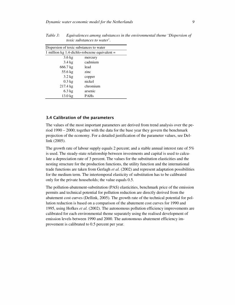
The environmental theme ‘dispersion of toxic substances to water’ consists of 8 heavy

metals (mercury, cadmium, lead, zinc, copper, nickel, chromium, and arsenic) and the to-

tal of 9 Polycyclic Aromatic Hydrocarbons (PAHs). The substances can be aggregated to

‘(aquatic eco)toxicity equivalents’ using the Aquatic Eco-Toxicity Potentials (AETPs) as

shown in Table 3. Van der Woerd et al. (2000) provide 127 independent options to re-

duce dispersion of toxic substances to water for 1995. With additional assumptions as

described in Hofkes et al. (2002), we construct the abatement cost curve for 1990. The

reduction potential is kept constant and proportionally with the level of emissions. The

abatement costs are corrected for the changes in the consumer price index between 1990

and 1995. Figure 2 shows the total amount of abatement costs and emission reduction

potential for ‘dispersion of toxic substances to water’. Based on the information of indi-

vidual measures, we approximate the cost abatement curve in a CES structure that will

be used in the model calculations.

The three main contributors to the dispersion of toxic substances to water are the chemi-

cal industry (38%), households (25.2%), and the textiles, clothing and leather industry

(11.7%).

0

2000

4000

6000

8000

10000

12000

14000

16000

0 20 40 60 80 100 120 140

Billion AETP equivalents

mln

Eu

ro Total

abatement

costs

PAS

approxim

ation


Table 3: Equivalences among substances in the environmental theme ‘Dispersion of

toxic substances to water’.

Dispersion of toxic substances to water

1 million kg 1.4-dichlo-robezene equivalent =

3.6 kg mercury

3.4 kg cadmium

666.7 kg lead

55.6 kg zinc

3.2 kg copper

0.3 kg nickel

217.4 kg chromium

6.3 kg arsenic

13.0 kg PAHs

3.4 Calibration of the parameters

The values of the most important parameters are derived from trend analysis over the pe-

riod 1990 – 2000; together with the data for the base year they govern the benchmark

projection of the economy. For a detailed justification of the parameter values, see Del-

link (2005).

The growth rate of labour supply equals 2 percent; and a stable annual interest rate of 5%

is used. The steady-state relationship between investments and capital is used to calcu-

late a depreciation rate of 3 percent. The values for the substitution elasticities and the

nesting structure for the production functions, the utility function and the international

trade functions are taken from Gerlagh et al. (2002) and represent adaptation possibilities

for the medium term. The intertemporal elasticity of substitution has to be calibrated

only for the private households; the value equals 0.5.

The pollution-abatement-substitution (PAS) elasticities, benchmark price of the emission

permits and technical potential for pollution reduction are directly derived from the

abatement cost curves (Dellink, 2005). The growth rate of the technical potential for pol-

lution reduction is based on a comparison of the abatement cost curves for 1990 and

1995, using Hofkes et al. (2002). The autonomous pollution efficiency improvements are

calibrated for each environmental theme separately using the realised development of

emission levels between 1990 and 2000. The autonomous abatement efficiency im-

provement is calibrated to 0.5 percent per year.


4. Results

The main results of the environmental policy where the emissions for Eutrophication and

Dispersion are reduced by 10 percent simultaneously are represented in Table 3. As

marginal abatement costs for small amounts of reduction are relatively cheap, the emis-

sion reductions can almost completely be achieved through the implementation of tech-

nical measures. The macroeconomic results suggest that these adjustments in the econ-

omy are virtually costless. Though production levels of the Agricultural and Industrial

sectors decreases, this is compensated by increases in the Abatement sector.

The prices of emission permits for Eutrophication and Dispersion to Water both increase

over time. Though the required percentage reduction in emissions remains constant from

2005 onwards, the permit price increases over time reflecting the autonomous efficiency

improvements in the benchmark, that induce compensating price increases; this effect

carries over from the benchmark to the counterfactual simulations.

Table 3: Main results for a required 10% reduction in emissions.

2000 2005 2010 2015

Macroeconomic results (%-change in volumes compared to benchmark projection)

Equivalent variation -0.1

GDP 0.0 0.0 0.0 0.0

NNI 0.0 0.0 0.0 0.0

Total private consumption 0.0 0.0 0.0 -0.1

Total production 0.0 -0.1 -0.1 -0.1

Capital investment 0.0 -0.1 -0.1 0.0

Sectoral results (%-change in volumes compared to benchmark projection)

Private consumption Agriculture 0.0 0.0 0.0 0.0

Private consumption Industry 0.0 -0.1 0.0 -0.1

Private consumption Services 0.0 0.0 0.0 0.0

Sectoral production Agriculture 0.0 -0.4 -0.4 -0.4

Sectoral production Industry 0.0 -0.4 -0.4 -0.4

Sectoral production Services 0.0 0.1 0.1 0.1

Sectoral production Abatement services 0.0 40.9 40.8 40.8

Environmental results (%-change in volumes compared to benchmark projection)

Emissions Eutrophication 0.0 -10.0 -10.0 -10.0

Emissions Dispersion to Water 0.0 -10.0 -10.0 -10.0

Prices of main variables (constant 1990 prices)

Wage rate index (benchmark index = 1) 1.0 1.0 1.0 1.0

Exchange rate index (benchmark index = 1) 1.0 1.0 1.0 1.0

Price of abatement services (bm. index = 1) 1.0 0.9 0.9 0.9

Price Eutrophication permits (Euro / P-eq.) 1.0 1.9 2.4 2.8

Price Dispersion permits (Euro / kilogram) 4.7 9.2 11.2 13.3


Table 4 gives the main results for the more stringent policy where emission reductions of

50 percent are required. Similar tables for 20, 30 and 40 percent reductions are given in

the Appendix. As the costs of the policy increases, the impacts become visible at the

macro-economic level: GDP and NNI levels are decreasing, and the welfare loss, meas-

ured via the Equivalent Variation, equals almost 1.5 percent. Though the emission reduc-

tions are only five times the previous scenario, the welfare loss is almost 15 times as

large (due to the non-linearities in the model).

Table 4. Main results for a required 50% reduction in emissions.

2000 2005 2010 2015



GDP 0.1 -0.5 -0.6 -0.7

NNI 0.0 -0.5 -0.6 -0.7

Total private consumption -0.2 -0.6 -0.9 -1.2


Capital investment 0.6 -0.9 -0.7 -0.4


Private consumption Agriculture -0.2 -0.1 -0.4 -0.7

Private consumption Industry -0.2 -1.1 0.0 -1.6

Private consumption Services -0.2 -0.1 -0.4 -0.7














Production levels of Agriculture and the industrial sectors decreases by several percent-

ages, and is not possible to maintain the benchmark consumption levels in the later

years. Aggregate production and consumption levels are also negative.

In the short run, consumers anticipate on the environmental policy by changing their sav-

ings/consumption decision. Households increase consumption in the short run at the ex-

pense of savings, as this has a positive effect on welfare, while accepting a lower growth

rate of the economy (as the lower savings translate into lower investments and conse-

quently into a lower growth rate of capital) and thus lower consumption levels in the

long run. This reduction in the growth rate of the economy is one part of the optimal mix

of reactions to the stringent environmental policy, together with expenditures on abate-


ment and a restructuring of the economy (mainly from agriculture and industry to ser-

vices). As consumers optimise their intertemporal utility function, this mix is the cost-

effective response to the new policy.

Figure 2 shows the development of the percentage change in GDP over time. Before the

environmental policy is introduced, there are some opportunities to increase production

levels and GDP, but the change in GDP becomes negative when the policy is imple-

mented. This shows that there is no “free lunch” and increased environmental quality

comes at an economic costs; this holds especially at the more stringent levels of policy,

as the economic costs of the policy increases more than proportionately with the strin-

gency of the policy. This is natural: first, the cheapest options to reduce emissions are

implemented, and further reductions will have to be realised through more costly ad-

justments. The costs of economic adjustments also increase more than proportionately

with stringency, as consumers prefer to stay as close as possible to the original consump-

tion bundle.

-0.8%

-0.7%

-0.6%

-0.5%

-0.4%

-0.3%

-0.2%

-0.1%

0.0%

0.1%

0.2%

19

90

19

92

19

94

19

96

19

98

20

00

20

02

20

04

20

06

20

08

20

10

20

12

20

14

20

16

20

18

%-c

han

ge c

om

pare

d t

o b

en

ch

mark

.

10pct-red 20pct-red 30pct-red 40pct-red 50pct-red

Figure 2. Percentage change in GDP – development over time

From Figure 3 the differences in impact of the environmental policy on production levels

are clearly visible. As expected, magnitued are larger when environmental policies are

more strict. This also means that the sectors that can benefit from the new policy, includ-

ing not only the Abatement sector (cf. Tables 3 and 4), but also Transport by Air and

Transport services, are best served by a stringent policy. This illustrates that the eco-

nomic impacts of environmental policy can best be regarded as a reallocation of avail-

able resources, rather than as a shrink of the economy. Thus, the sectoral impacts are

much larger than the macroeconomic results suggest.


-50% -40% -30% -20% -10% 0% 10% 20% 30% 40% 50%

Agriculture

Oil & gas extraction

Other mining

Food & -products industry

Textiles & related industry

Paper & -board industry

Printing industry

Oil refineries

Chemical industry

Rubber & plastics industry

Basic metals industry

Metal products industry

Machine industry

Electromechanical industry

Transport eq. industry

Other industries

Energy distribution

Water distribution

Construction

Trade & related services

Transport by land

Transport by water

Transport by air

Transport services

Commercial services

Non-commercial services

Other goods & services

%-change compared to benchmark

10pct-red

20pct-red

30pct-red

40pct-red

50pct-red

Figure 3. Percentage change in sectoral production levels in 2010

Figure 4 shows how the permit price for Dispersion to Water increases when the envi-

ronmental policy is implemented. These results confirm the discussion above.


0

20

40

60

80

100

120

140

160

19

90

19

92

19

94

19

96

19

98

20

00

20

02

20

04

20

06

20

08

20

10

20

12

20

14

20

16

20

18

%-c

han

ge c

om

pare

d t

o b

en

ch

mark

.

10pct-red 20pct-red 30pct-red 40pct-red 50pct-red

Figure 4. Permit price of Dispersion to Water – development over time

Finally, a preliminary assessment of the impact of the economic changes on emissions of

individual water pollutants has been carried out. By assuming a constant emission inten-

sity per unit of production, the changes in economic activity can be translated into

changes in emissions for these individual pollutants. It is assumed that no action is un-

dertaken to deliberately reduce these emissions; they are rather the by-product of the en-

vironmental policies on Eutrophication and Dispersion. It should be stressed that this

crude way of modelling the individual pollutants is far from perfect, as interactions with

the two main themes is not taken into account, other than the links with the economic ac-

tivity. Therefore, a more refined approach is advocated for further study. Nonetheless,

the approach used here gives insight into the interlinklages between the changes in eco-

nomic activity invoked by the water policy and the emissions of a wide range of pollut-

ants. The results are given in Table 5.


Table 5: Impact of the policies on individual pollutants.

10%

reduction

20%

reduction

30%

reduction

40%

reduction

50%

reduction

Eutro -10% -20% -30% -40% -50%

Dispers -10% -20% -30% -40% -50%

mercury -2% -5% -9% -14% -22%

cadmium -3% -6% -12% -19% -31%

lead 0% -1% -2% -4% -6%

zinc -1% -2% -3% -5% -9%

copper 0% -1% -2% -3% -5%

nickel -1% -4% -7% -11% -18%

chromium -2% -4% -8% -14% -22%

arsenic -1% -2% -5% -9% -15%

anthraceen 0% -1% -2% -4% -8%

benzoanthraceen 0% -1% -3% -6% -12%

benzopyreen 0% -1% -3% -6% -13%

benzoperyleen 0% -1% -3% -6% -12%

benzofluorantheen 0% -1% -3% -6% -13%

chryseen 0% -1% -3% -6% -12%

fenanthreen 0% -1% -1% -3% -6%

fluorantheen 0% -1% -3% -5% -11%

indenopyreen 0% -1% -3% -6% -13%

naftaleen 0% -1% -2% -5% -11%

While it is clear that the emissions of the two themes subject to the policy decrease more

than the emissions of the individual pollutants, the reductions induced for the individual

pollutants are substantial, at least for the more stringent policy levels. Especially the

emissions of mercury, cadmium and chromium are reduced a lot. This illustrates that the

emissions for these pollutants are closely linked to the same economic activities as the

emissions of the theme-equivalents.


5. Concluding remarks

At low levels of environmental policy, say a 10 percent reduction in eutrophying emis-

sions and toxic substances dispersed to water, there are good opportunities for the eco-

nomic agents to adjust to the new circumstances. Relatively cheap technical measures

are implemented to reduce emissions, and the macroeconomic impacts of the policy re-

main very limited. At more stringent levels of policy the alternatives to adjust disappear.

Then, an optimal mix arises from the trade-off between the implementation of technical

measures, a restructuring of the economy and a temporary slowdown of economic

growth (i.e. increasing short-term consumption at the expense of savings). Note that the

DEAN-WEMPA is applied to long-term or mid-term analysis, so that annual economic

fluctuations are ignored.

If we compare the results of DEAN-WEMPA and the static AGE model in Linderhof et

al. (2006), the decline in Net National Income seems to be much lower in the dynamic

model than in the static model. As the dynamic model predicts a 0.7 percent loss in NNI

compared to the benchmark in 2015, the static model predicts a 10 percent loss in NNI.

Obviously, the dynamic aspects of autonomous emission efficiency and developments in

the abatement costs curves are ignored in the static model results. Similar differences be-

tween the dynamic and static model in the evaluation of a wide range of environmental

problems are found in Dellink (2005), who analyses the differences in detail.

There are some obvious areas for improvement of our analysis. First, the base year 1990

on which the current model is calibrated is rather old. More recent economic and envi-

ronmental data are available and can be used. In particular, the DEAN-WEMPA model

will be calibrated for the year 2000 which is also the reference year of the Water Frame-

work Directive. Secondly, the balanced growth path assumed in the model is relatively

simple, and disregards structural changes in preferences and the structure of the econ-

omy. Most service (sub-)sectors in the economy showed an more than proportional

growth rate since 1990, while the reverse is the case of the agricultural sector, for in-

stance. Thirdly, the model represents a national economy, where the environmental is-

sues at stake are largely regional. Though it is possible to softlink these national results

with more detailed models at the scale of individual river basins, such as the Substance

Flow model for surface water quality in the Netherlands, a more direct link would im-

prove the analysis. Fourthly, the representation of water quality in the model is highly

stylised and deserves a more disaggregated approach. A first step is to consider individ-

ual substances instead of environmental themes, although we might run into problems

with the data availability of the Pollution-Abatement curves. Finally, the abatement cost

functions used can be specified for individual sectors when the appropriate data are

available. Note that it might be infeasible to extent the model in all directions simultane-

ously.


References

Dellink, R.B. (2005). Modelling the costs of environmental policy: a dynamic applied general

equilibrium assessment. Cheltenham: Edward Elgar.

Dellink, R.B., R. Gerlagh, M.W. Hofkes and L. Brander (2001). Calibration of an applied gen-

eral equilibrium model for the Netherlands in 1990. IVM report W-01/17. Institute for Envi-

ronmental Studies, Vrije Universiteit, Amsterdam.

Dellink, R.B. and E.C. van Ierland (2005). Pollution abatement in the Netherlands: a dynamic

applied general equilibrium assessment. Journal of Policy Modelling 28, 207-221.

Gerlagh, R., R.B. Dellink, M.W. Hofkes and H. Verbruggen (2002). A measure of Sustainable

National Income for the Netherlands. Ecological Economics 41, 157-174.

Hofkes, M.W., R. Gerlagh, W. Lise and H. Verbruggen (2002). Sustainable National Income: a

trend analysis for the Netherlands for 1990 – 1995. IVM report R-02/02. Institute for Envi-

ronmental Studies, Vrije Universiteit, Amsterdam..

Linderhof, V., R. Brouwer, & M. Hofkes (2006). An applied general equilibrium approach to the

estimation of the direct and indirect costs of water quality improvements in the WFD. Unpub-

lished paper. Institute for Environmental Studies, Vrije Universiteit, Amsterdam.

Reinhard, S. and V. Linderhof (2006). Inventory of economic models. Water Economic Model-

ling for Policy Analysis report-03. Institute for Environmental Studies, Vrije Universiteit,

Amsterdam. 49 pp.

Van de Veeren, R. (2005). Development of policy scenarios and measures. Water Economic

Modelling for Policy Analysis report-04. Institute for Environmental Studies, Vrije Universi-

teit, Amsterdam. 31 pp.

Van der Woerd, F., E. Ruijgrok & R. Dellink (2000). Kosteneffectiviteit van verspreiding naar

water. IVM report E-00/01. Institute for Environmental Studies, Vrije Universiteit, Amster-

dam..


Appendix: Results


2000 2005 2010 2015



GDP 0.0 -0.1 -0.1 -0.1

NNI 0.0 -0.1 -0.1 -0.1

Total private consumption 0.0 -0.1 -0.1 -0.2




Private consumption Agriculture 0.0 0.0 0.0 -0.1


Private consumption Services 0.0 0.0 0.0 -0.1
















2000 2005 2010 2015



GDP 0.0 -0.2 -0.2 -0.2

NNI 0.0 -0.1 -0.2 -0.2

Total private consumption 0.0 -0.2 -0.3 -0.3




Private consumption Agriculture 0.0 0.0 -0.1 -0.2


Private consumption Services 0.0 0.0 -0.1 -0.2
















2000 2005 2010 2015



GDP 0.0 -0.3 -0.4 -0.4

NNI 0.0 -0.3 -0.3 -0.4

Total private consumption -0.1 -0.3 -0.5 -0.6




Private consumption Agriculture -0.1 0.0 -0.2 -0.3

Private consumption Industry -0.1 -0.6 0.0 -0.9

Private consumption Services -0.1 0.0 -0.2 -0.3















Publications of the project ‘Water Economic Modelling for Policy Analysis’

(See also www.ivm.falw.vu.nl/watereconomics):

WEMPA report

Report Auteurs Titel

WEMPA Report-01 Roy Brouwer Toekomstige beleidsvragen en hun implicaties voor de ontwik-

keling van een integraal water-en-economie model (in Dutch)

WEMPA Report-02 Paul Baan

Aline te Linde

Inventory of water system models

WEMPA Report-03 Stijn Reinhard

Vincent Linderhof

Inventory of economic models

WEMPA Report-04 Rob van der Veeren Development of policy scenarios and measures

WEMPA Report-05 Gideon Kruseman

Roy Brouwer

Vincent Linderhof

Stijn Reinhard

Paul Baan

Integrated river basin modelling: basic concepts and character-

istics

WEMPA report

Working paper Athors Title

WEMPA working paper-01 Paul Baan Households and recreation: use and value of water

WEMPA working paper-02 Paul Baan Emissiereductie RWZI's en Huishoudens (in Dutch)

WEMPA working paper-03 Sjoerd Schenau Data availability for the WEMPA project

WEMPA working paper-04 Rob Dellink

Vincent Linderhof

Dynamic AGE model for water economics in the Nether-

lands (DEAN-WEMPA): first results

Dynamic AGE model for water economics in the Netherlands (DEAN-WEMPA)

Documents

Transcript of Dynamic AGE model for water economics in the Netherlands (DEAN-WEMPA)