University of Wollongong University of Wollongong

Research Online Research Online

University of Wollongong Thesis Collection 2017+ University of Wollongong Thesis Collections

2021

Domestic Multi-channel Sound Detection and Classification for the Domestic Multi-channel Sound Detection and Classification for the

Monitoring of Dementia Residents’ Safety and Well-being using Neural Monitoring of Dementia Residents’ Safety and Well-being using Neural

Networks Networks

Abigail Copiaco

Follow this and additional works at: https://ro.uow.edu.au/theses1

University of Wollongong University of Wollongong

Copyright Warning Copyright Warning

You may print or download ONE copy of this document for the purpose of your own research or study. The University

does not authorise you to copy, communicate or otherwise make available electronically to any other person any

copyright material contained on this site.

You are reminded of the following: This work is copyright. Apart from any use permitted under the Copyright Act

1968, no part of this work may be reproduced by any process, nor may any other exclusive right be exercised,

without the permission of the author. Copyright owners are entitled to take legal action against persons who infringe

their copyright. A reproduction of material that is protected by copyright may be a copyright infringement. A court

may impose penalties and award damages in relation to offences and infringements relating to copyright material.

Higher penalties may apply, and higher damages may be awarded, for offences and infringements involving the

conversion of material into digital or electronic form.

Unless otherwise indicated, the views expressed in this thesis are those of the author and do not necessarily Unless otherwise indicated, the views expressed in this thesis are those of the author and do not necessarily

represent the views of the University of Wollongong. represent the views of the University of Wollongong.

Research Online is the open access institutional repository for the University of Wollongong. For further information contact the UOW Library: research-pubs@uow.edu.au

Domestic Multi-channel Sound Detection and Classification for

the Monitoring of Dementia Residents’ Safety and Well-being

using Neural Networks

Abigail Copiaco

Supervisor:

Prof. Christian Ritz

Co-supervisors:

Dr. Nidhal Abdulaziz and Dr. Stefano Fasciani

This thesis is presented as part of the requirement for the conferral of the degree:

Doctor of Philosophy (PhD)

University of Wollongong

School of Electrical, Computer, and Telecommunications Engineering

Faculty of Informatics

August 2021

i

Abstract

Recent studies conducted by the World Health Organization reveal that approximately 50 million

people are affected by dementia. Such individuals require special care that translates to high social

costs. In the last decade, we assisted to the introduction of dementia assistive technologies that aimed

at improving the quality of life of residents, as well as facilitating the work of caregivers. Merging

the significance of both the alleviation in coping with dementia with the perceptible popularity of

assistive technology and smart home devices, the main focus of this work is to further improve home

organization and management of individuals living with dementia and their caregivers through the

use of technology and artificial intelligence. In particular, we aim at developing an effective but

non-invasive environment monitoring solution.

This thesis proposes a novel strategy to detect, classify, and estimate the location of household-

related acoustic scenes and events, enabling a less intrusive monitoring system for the assistance

and supervision of dementia residents. The proposed approach is based on classification of multi-

channel acoustical data acquired from omnidirectional microphone arrays (nodes), which consists

of four linearly arranged microphones, placed on four corner locations across each room. The

development of a customized synthetic database that reflects real-life recordings relevant to

dementia healthcare is also explored, in order to improve and assess the overall robustness of the

system. A combination of spectro-temporal acoustic features extracted from the raw digitized-

acoustic data will be used for detection and classification purposes. Alongside this, spectral-based

phase information is utilized in order to estimate the sound node location.

In particular, this work will explore and conduct a detailed study on the performance of different

types and topologies of Convolutional Neural Networks, developing an accurate and compact neural

network with a series architecture, that is suitable for devices with limited computational resources.

Considering that other state-of-the-art compact networks present complex directed acyclic graphs,

a series architecture proposes an advantage in customizability. The effectiveness of the Neural

Network classification techniques is measured through a set of quantitative performance parameters

that will also account for dementia-specific issues. Top performing classifiers and data from

multiple microphone arrays will then be subject to fine-tuning methods in order to maximize the

recognition accuracy, and overall efficiency of the designed system. The optimum methodology

developed has improved the performance of the AlexNet network while decreasing its network size

by over 95%. Finally, the implementation of the detection and classification algorithm includes an

easy-to-use interface enabling caregivers to customize the system for individual resident needs,

which is developed based on a design thinking research approach.

ii

Acknowledgments

I would like to thank my supervisors: Prof. Christian Ritz, Dr. Nidhal Abdulaziz, and Dr. Stefano

Fasciani, for their continuous support and guidance throughout the course of my PhD studies. It was

truly an honor to work with you. Thank you for always believing in me.

My sincerest gratitude is also given to my family. Thank you for being the source of my strength,

motivation, and encouragement. Yours were the silent applause every time I was able to accomplish

something. Further, your valuable gentle tap on my shoulders every time I feel discouraged did

wonders for me. To my best friend, thank you for always being there for me, for cheering me up

during difficult times, and for lending me your research server every time I need to do tedious

training tasks for my PhD. None of these would have been possible without your valuable support,

and I will forever be grateful.

Similarly, appreciation is also intended to the University of Wollongong in Australia, for the

International Postgraduate Tuition Awards (IPTA) granted to me. I am truly honored, and at the

same time humbled, for the opportunity to be associated with a novel project under a prestigious

university. I am also thankful for the University of Wollongong in Dubai for the support.

Above all, I would like to bring back all the glory and thanks to God. For I know that I was not able

to complete this thesis through my own strength and wisdom, but by His grace and blessings.

© Copyright by Abigail Copiaco, 2021

All Rights Reserved

iii

Certification I, Abigail Copiaco, declare that this thesis submitted in fulfilment of the requirements for the

conferral of the degree PhD by Research, from the University of Wollongong, is wholly my own

work unless otherwise referenced or acknowledged. This document has not been submitted for

qualifications at any other academic institution.

Abigail Copiaco

20th August 2021

iv

Thesis Publications

Journal Articles:

[1] A. Copiaco, C. Ritz, N. Abdulaziz, and S. Fasciani, A Study of Features and Deep Neural

Network Architectures and Hyper-parameters for Domestic Audio Classification, Applied

Sciences 2021, 11, 4880. https://doi.org/10.3390/app11114880

Conference Proceedings:

[1] A. Copiaco, C. Ritz, S. Fasciani, and N. Abdulaziz, “Development of a Synthetic Database

for Compact Neural Network Classification of Acoustic Scenes in Dementia Care

Environments”, APSIPA, accepted for publication, 2021.

[2] A. Copiaco, C. Ritz, S. Fasciani, and N. Abdulaziz, “Identifying Sound Source Node

Location using Neural Networks trained with Phasograms”, 20th IEEE International

Symposium on Signal Processing and Information Technology (ISSPIT) 2020, Louisville,

Kentucky, USA, Dec. 9-11, 2020, pp. 1-7.

[3] A. Copiaco, C. Ritz, S. Fasciani, and N. Abdulaziz, “An Application for Dementia Patients

Monitoring with an Integrated Environmental Sound Levels Assessment Tool”, 3rd

International Conference on Signal Processing and Information Security (ICSPIS), Dubai,

United Arab Emirates (UAE), Nov. 25-26, 2020, pp. 1-4.

[4] A. Copiaco, C. Ritz, N. Abdulaziz, and S. Fasciani, “Identifying Optimal Features for

Multi-channel Acoustic Scene Classification”, 2nd International Conference on Signal

Processing and Information Security (ICSPIS), Dubai, United Arab Emirates (UAE), 2019,

pp. 1-4.

[5] A. Copiaco, C. Ritz, S. Fasciani, and N. Abdulaziz, “Scalogram Neural Network

Activations with Machine Learning for Domestic Multi-channel Audio Classification”,

19th IEEE International Symposium on Signal Processing and Information Technology

(ISSPIT), Ajman, United Arab Emirates, 2019, pp. 1-6

Technical Reports and Pre-prints:

[1] A. Copiaco, C. Ritz, S. Fasciani, and N. Abdulaziz, “DASEE: A Synthetic Database of

Domestic Acoustic Scenes and Events in Dementia Patients’ Environment”,

arXiv:2104.13423v2 [eess.AS], Apr. 2021.

[2] A. Copiaco, C. Ritz, S. Fasciani, and N. Abdulaziz, “Sound Event Detection and

Classification using CWT Scalograms and Deep Learning”, Detection and Classification

of Acoustic Scenes and Events (DCASE) 2020, Task 4 Challenge, Technical Report, 2020.

[3] A. Copiaco, C. Ritz, S. Fasciani, and N. Abdulaziz, “Detecting and Classifying Separated

Sound Events using Wavelet-based Scalograms and Deep Learning”, Detection and

Classification of Acoustic Scenes and Events (DCASE) 2020, Task 4 Challenge, Technical

Report, 2020.

v

Awards and Distinctions

1. Best Paper Award, for paper entitled “An Application for Dementia Patients Monitoring

with an Integrated Environmental Sound Levels Assessment Tool”, presented at the 3rd

International Conference on Signal Processing and Information Security (ICSPIS) 2020.

2. Best Paper Award, for paper entitled “Identifying Optimal Features for Multi-channel

Acoustic Scene Classification”, presented at the 2nd International Conference on Signal

Processing and Information Security (ICSPIS) 2019.

3. Artificial Intelligence Practitioner – Instructor Certificate, issued by IBM on April 2021

Related Certificates:

- Enterprise Design Thinking, Team Essentials for AI Certificate, March 2021

- Artificial Intelligence Analyst, Explorer Award, July 2020

- Artificial Intelligence Analyst, Mastery Award, August 2020

4. Enterprise Design Thinking Practitioner – Instructor Certificate, issued by IBM on

February 2021

Related Certificates:

- Enterprise Design Thinking, Practitioner Badge, January 2021

- Enterprise Design Thinking, Co-creator Badge, January 2021

vi

List of Names or Abbreviations

AARP

ANN

The American Association of Retired Persons

Artificial Neural Networks

ASN

AT

CNN

CSV

CWT

DAG

DASEE

DCASE

DCT

DCNN

DEMAND

DFT

DNN

DOA

DWT

eLU

ESPRIT

FIR

FFT

Acoustic Sensor Network

Assistive Technology

Convolutional Neural Network

Comma Separated Value

Continuous Wavelet Transform

Directed Acyclic Graph

Domestic Acoustic Sounds and Events in the Environment database

Detection and Classification of Acoustic Scenes and Events

Discrete Cosine Transform

Deep Convolutional Neural Network

Diverse Environments Multi-channel Acoustic Noise Database

Discrete Fourier Transform

Deep Neural Network

Direction of Arrival

Discrete Wavelet Transform

Exponential Linear Unit

Estimation of Signal Parameters via Rotational Invariance Techniques

Finite Impulse Response

Fast Fourier Transform

GLCM

GMM

Gray-level Co-occurrence Matrix

Gaussian Mixture Model

GRNN

GUI

k-NN

LMS

LPCC

LSTM

LUFS

MCI

MFCC

MMSE

MUSIC

NATSEM

Gated Recurrent Neural Network

Graphical User Interface

k-nearest Neighbor

Least Mean Square

Linear Predictive Cepstral Coefficients

Long-short Term Memory Recurrent Neural Network

Loudness Units relative to Full Scale

Mild Cognitive Impairment

Mel Frequency Cepstral Coefficients

Minimum Mean Squared Error

Multiple Signal Classification

The National Centre for Social and Economic Modelling

PNCC

RASTA-PLP

ReLU

Power Normalized Cepstral Coefficients

Relative Spectral Perceptual Linear Prediction

Rectified Linear Unit

vii

RIR

RLS

RNN

SGDM

SINS

SNR

SPCC

STFT

SVM

TinyEARS

WHO

VDT

ZCR

Room Impulse Response

Recursive Least Squares

Recurrent Neural Network

Stochastic Gradient Descent with Momentum

Sound INterfacting through the Swarm database

Signal-to-Noise Ratio

Subspace Projection Cepstral Coefficients

Short Time Fourier Transform

Support Vector Machines

Tiny Energy Accounting and Reporting System

World Health Organization

Virtual Dementia Tour

Zero Crossing Rate

viii

Table of Contents

Abstract ......................................................................................................................................... i

Acknowledgments ....................................................................................................................... ii

Certification ................................................................................................................................ iii

Thesis Publications ..................................................................................................................... iv

Awards and Distinctions .............................................................................................................. v

List of Names or Abbreviations ................................................................................................ vi

Table of Contents ...................................................................................................................... viii

List of Tables, Figures and Illustrations ................................................................................ xiii

........................................................................................................................................ 1

Introduction .................................................................................................................................... 1

1.1 Overview ................................................................................................................................. 1

1.2 Dementia ................................................................................................................................. 2

1.2.1 Signs and Symptoms ............................................................................................................................. 3

1.2.2 Influence of Age and Gender ................................................................................................................ 3

1.2.3 Statistical Evidence ............................................................................................................................... 4

1.3 Assistive Technology ............................................................................................................... 4

1.3.1 Continual Influence of Smart Home Devices ...................................................................................... 5

1.3.2 Ethical Concerns and Considerations .................................................................................................. 6

1.4 Existing Assistive Technology Related to Dementia ............................................................... 6

1.4.1 Summary of the Limitations of Existing AT Devices for Dementia Care............................................ 8

1.4.2 Recommendations and Compliance to Ethical Requirements ............................................................. 9

1.4.3 Identification of Domestic Hazards for Dementia Monitoring Systems .............................................. 9

1.4.4 Users of the Monitoring System .......................................................................................................... 10

1.5 Objectives and Contributions ................................................................................................. 11

1.5.1 Objectives ............................................................................................................................................ 11

1.5.2 Contributions....................................................................................................................................... 12

1.6 Thesis Scope .......................................................................................................................... 12

1.7 Thesis Structure ..................................................................................................................... 13

1.7.1 Publications ......................................................................................................................................... 13

1.7.2 Thesis Structure and Research Output Alignment ............................................................................ 13

...................................................................................................................................... 15

Review of Approaches to Classifying and Localizing Sound Sources ........................................ 15

2.1 Introduction ............................................................................................................................ 15

2.1.1 System Framework .............................................................................................................................. 15

2.2 Acoustic Data ......................................................................................................................... 16

2.2.1 Single-channel Audio Classification .................................................................................................. 16

2.2.2 Multi-channel Audio Classification ................................................................................................... 17

2.2.3 Factors affecting Real-life Audio Recordings .................................................................................... 17

2.3 Feature Engineering for Audio Signal Classification ............................................................ 18

ix

2.3.1 Temporal Features .............................................................................................................................. 19

2.3.2 Spectral Features ................................................................................................................................ 19

2.3.3 Spectro-temporal Features .................................................................................................................. 20

2.3.4 Cepstral Features ................................................................................................................................ 22

2.3.5 Comparison and Verdict ..................................................................................................................... 23

2.4 Multi-level Classification Techniques ................................................................................... 25

2.4.1 Neural Networks ................................................................................................................................. 26

2.4.2 Convolutional Neural Network ........................................................................................................... 27

2.4.3 Deep Neural Network .......................................................................................................................... 28

2.4.4 Recurrent Neural Networks ................................................................................................................ 28

2.4.4.1 Long-short Term Memory Recurrent Neural Network .............................................................. 29

2.4.4.2 Gated Recurrent Neural Networks ............................................................................................. 30

2.4.5 Pre-trained Neural Network Models .................................................................................................. 30

2.5 Review of Audio Classification Systems ............................................................................... 31

2.5.1 Liabilities and Challenges: Audio Classification ............................................................................... 32

2.6 Review of Sound Source Localization Systems..................................................................... 34

2.6.1 Liabilities and Challenges: Sound Source Node Location Estimation .............................................. 36

2.7 Proposed System Design Specifications and Requisites ........................................................ 37

...................................................................................................................................... 41

Data Acquisition and Pre-processing ........................................................................................... 41

3.1 Introduction ............................................................................................................................ 41

3.2 Existing Databases ................................................................................................................. 41

3.3 Pre-processing ........................................................................................................................ 42

3.4 Noise Reduction Techniques ................................................................................................. 43

3.4.1 Beamforming....................................................................................................................................... 43

3.5 Data Augmentation Techniques ............................................................................................. 45

3.5.1 Mixing and Shuffling .......................................................................................................................... 45

3.6 Segmentation and Pre-processing Technique for Proposed System ...................................... 46

3.6.1 Pre-processing for Sound Classification ............................................................................................ 47

3.6.2 Pre-processing for Source Node Estimation ...................................................................................... 48

3.7 Development of the DASEE Synthetic Database .................................................................. 49

3.7.1 Data Curation...................................................................................................................................... 49

3.7.2 Experimental Setup ............................................................................................................................. 51

3.7.3 Room Impulse Response Generation .................................................................................................. 52

3.7.4 Dataset synthesis and refinement ....................................................................................................... 56

3.7.5 Background Noise Integration and Dataset Summary ...................................................................... 56

3.7.6 Curating an Unbiased Dataset ............................................................................................................ 59

3.8 Chapter Summary .................................................................................................................. 61

...................................................................................................................................... 62

Features for Audio Classification and Source Location Estimation ............................................ 62

4.1 Introduction ............................................................................................................................ 62

4.2 Feature Extraction for Audio Classification .......................................................................... 62

x

4.2.1.1 Cepstral, Spectral, and Spectro-temporal Feature Extraction ................................................... 63

4.2.1.2 Network Layer Activation Extraction ......................................................................................... 64

4.2.1.3 General Feature Performance Study and Results ...................................................................... 66

4.2.2 Fast Scalogram Features for Audio Classification ............................................................................ 68

4.2.2.1 FFT-based Continuous Wavelet Transform ................................................................................ 69

4.2.2.2 Selection of the Mother Wavelet ............................................................................................... 70

4.2.3 Scalogram Representation .................................................................................................................. 72

4.2.4 Results of CWTFT Features for Audio Classification ....................................................................... 73

4.2.4.1 Comparison against State-of-the-Art Features: Balanced and Imbalanced Data ..................... 73

4.2.4.2 Consideration of Signal Time Alignment .................................................................................... 76

4.2.4.3 Per-channel Scalogram with Channel Voting Technique ........................................................... 78

4.2.4.4 Cross-fold Validation .................................................................................................................. 80

4.2.4.5 Wavelet Normalization ............................................................................................................... 81

4.2.5 Classification Performance Observations .......................................................................................... 83

4.3 Feature Extraction Methodology for Node Location Estimation ........................................... 84

4.3.1 STFT-based Phasograms for Sound Source Node Location Estimation .......................................... 84

4.3.1.1 Node Locations Setup ................................................................................................................. 85

4.3.1.2 Phasogram Feature Calculation .................................................................................................. 85

4.3.1.3 Neural Network Integration ....................................................................................................... 87

4.3.2 Results and Detailed Study ................................................................................................................. 88

4.3.2.1 Comparison of STFT and CWTFT-based Phasograms ................................................................. 88

4.3.2.2 Countering the Effects of Spatial Aliasing .................................................................................. 89

4.3.2.3 Comparison against a Magnitude-based Approach ................................................................... 90

4.3.2.4 Results when using the DASEE Synthetic Database ................................................................... 91

4.4 Chapter Summary .................................................................................................................. 94

...................................................................................................................................... 95

Neural Networks Architectural and Hyper-parameter Study ....................................................... 95

5.1 Introduction ............................................................................................................................ 95

5.2 Comparison of Pre-trained Models ........................................................................................ 95

5.3 Development of MAlexNet-40 .............................................................................................. 96

5.3.1 Exploring Activation Functions for CNN Models ............................................................................. 96

5.3.2 Modifications on Weight Factors, Parameters, and the Number of Convolutional Layers .............. 98

5.3.3 Results and Detailed Study ............................................................................................................... 101

5.3.3.1 Exploring Variations of the Activation Function and the Number of Layers ........................... 101

5.3.3.2 Fully-connected Layer Output Parameter Modification .......................................................... 102

5.3.3.3 The Combination of Layer and Output Parameter Modification ............................................. 104

5.3.3.4 Exploring Normalization Layers ................................................................................................ 107

5.3.3.5 Convolutional Layer Learning and Regularization Parameter Modification ........................... 109

5.3.3.6 Examining System Response to Various Optimization Algorithms ......................................... 110

5.3.4 Discussion and Findings................................................................................................................... 112

5.4 MAlexNet-40 as a Compact Neural Network Model .......................................................... 115

5.4.1 Direct Comparison against Compact Neural Network Models ........................................................ 115

xi

5.4.2 Response to Compact Neural Network Configuration Inspirations ................................................ 116

5.4.3 Discussions and Findings ................................................................................................................. 120

5.5 Examining the Robustness of MAlexNet-40 ....................................................................... 121

5.5.1 Cross-fold Validation ........................................................................................................................ 121

5.5.1.1 Full dataset comparison ........................................................................................................... 121

5.5.1.2 Balanced dataset comparison .................................................................................................. 122

5.5.2 Verification using the SINS Database .............................................................................................. 123

5.5.3 Signal Time Alignment for Compact Networks ................................................................................ 124

5.5.4 Factors that affect training speed ..................................................................................................... 125

5.6 Chapter Summary ................................................................................................................ 127

.................................................................................................................................... 128

Integrated System Design .......................................................................................................... 128

6.1 Introduction .......................................................................................................................... 128

6.2 Design Thinking Approach for Graphical User Interface Development ............................. 129

6.2.1 Identifying the Persona ..................................................................................................................... 129

6.2.1.1 User Information ....................................................................................................................... 129

6.2.1.2 Challenges of Dementia Care ................................................................................................... 130

6.2.1.3 Concerns on Monitoring Systems ............................................................................................. 132

6.2.2 Identifying the Hill: Understanding the Challenges ........................................................................ 133

6.2.3 The Loop: Designing the Graphical User Interface ........................................................................ 134

6.2.3.1 Proposal and Reflection ............................................................................................................ 134

6.2.4 The Solution: Final Caregiver Software Application Functionalities............................................. 136

6.3 Integrated Domestic Multi-Channel Audio Classifier ......................................................... 138

6.3.1 Two-step Neural Network for Identifying Disruptive Sounds.......................................................... 138

6.3.1.1 Detailed Results ........................................................................................................................ 140

6.3.2 Node Voting Methodologies .............................................................................................................. 141

6.3.2.1 Histogram-based Counts Technique ......................................................................................... 141

6.3.2.2 Weighted Energy-based Technique .......................................................................................... 144

6.3.2.3 Comparison of the Node Voting Algorithms ............................................................................ 145

6.4 Graphical User Interface ...................................................................................................... 146

6.4.1 User Interface Overview ................................................................................................................... 147

6.4.2 Integrated Sound Levels Assessment Tool ....................................................................................... 149

6.5 Chapter Summary ................................................................................................................ 150

.................................................................................................................................... 151

Conclusions and Future Work.................................................................................................... 151

7.1 Summary of Research Contributions ................................................................................... 151

7.2 Societal Relevance ............................................................................................................... 152

7.3 Future Work and Research Directions ................................................................................. 153

7.3.1 Directions for Research .................................................................................................................... 153

7.3.2 Interface Improvement...................................................................................................................... 154

References ................................................................................................................................. 156

Appendices ................................................................................................................................ 173

xii

Appendix 1 ................................................................................................................................. 173

1. Room Impulse Response Generation Code........................................................................ 173

2. Code for Sound Convolution with the Room Impulse Response....................................... 175

3. Code for adding background noises ................................................................................... 176

xiii

List of Tables, Figures and Illustrations

List of Tables:

Table 1.1. Main subtypes of dementia and their symptoms [10] ............................................................... 3

Table 1.2: United Nations Conventions on the Rights of Persons with Disabilities – related article

summary [32, 28] ....................................................................................................................................... 6

Table 1.3. Limitations of Existing Assistive Technology Devices ............................................................ 8

Table 1.4. Common Household Hazards for Dementia Residents ........................................................... 10

Table 2.1. General Comparison Summary between Audio Classification Features ................................. 24

Table 2.2. Machine Learning versus Deep Learning Techniques [107] ................................................... 25

Table 2.3. General Comparison Summary between Pre-trained CNN Models ........................................ 31

Table 2.4. List of notable works in the field of multi-channel audio classification ................................. 33

Table 2.5. List of notable works in the field of multi-channel sound source estimation .......................... 36

Table 3.1. Summary of beamforming techniques .................................................................................... 44

Table 3.2. Summary of the SINS Database [163] .................................................................................... 47

Table 3.3 Dry Sample Sources and Licensing Summary ......................................................................... 50

Table 3.4. Room Dimensions and Source/Receiver Locations for Multi-channel Recordings ................ 52

Table 3.5. Average room reflectance for varying wall reflectance and obstruction percentages [189] ... 55

Table 3.6. Wall Reflectance Coefficients Used ....................................................................................... 55

Table 3.7. Room Dimensions and Source/Receiver Locations for Background Noises .......................... 57

Table 3.8. Summary of the Unbiased Sound Classification Dataset ........................................................ 60

Table 3.9. Summary of the Unbiased Source Node Estimation Dataset .................................................. 61

Table 4.1. Preliminary Results Summary for Individual Features ........................................................... 67

Table 4.2. Preliminary Results Summary for Combinational Features .................................................... 67

Table 4.3. Per-level Methods Comparison Summary (% in terms of Weighted F1-score) ...................... 68

Table 4.4. Mother Wavelet and Parameter Variation, Results Summary ................................................. 72

Table 4.5. Per-level comparison: imbalanced and balanced data between different types of features ..... 74

Table 4.6. Comparison of time-aligned versus non-time-aligned feature sets: AlexNet .......................... 78

Table 4.7. Scalogram Representations of Recordings from Individual Channels, samples from sound

classes (Top to Bottom): Alarm, Cat, and Kitchen .................................................................................. 79

Table 4.8. Crossfold Validation: Second Set Detailed Results ................................................................ 81

Table 4.9. Commonly Misclassified Sounds Summary ........................................................................... 83

Table 4.10. Sensor Nodes 1-8 Coordinates, Rectangular and Polar Form ............................................... 85

Table 4.11. Results Comparison of STFT-derived versus CWT-derived Phasograms ............................ 88

Table 4.12. Consideration of Cut off Frequencies ................................................................................... 89

Table 4.13. Closest Node Prediction, Proposed Phasograms Method ...................................................... 91

Table 4.14. Closest Node Prediction, Integrated LUFS Method .............................................................. 91

Table 4.15. Detailed Per-level Results of Sound Source Node Location Estimation on the Synthesized

Dataset...................................................................................................................................................... 93

Table 5.1. Comparison of CNN Activation Functions [231] ................................................................... 97

Table 5.2. Layer Information of the AlexNet Pre-trained Network ......................................................... 99

Table 5.3. Performance Measures of Different Networks using Variations of the F1-score .................. 101

Table 5.4. Successive Activation Function Combination Summary ...................................................... 102

Table 5.5. Parameter Modification Results ............................................................................................ 103

Table 5.6. Results for the combination of layer and parameter modification ........................................ 106

Table 5.7. Results Summary for the Further Variations of Convolutions .............................................. 106

Table 5.8. Normalization Layer Experiments Summary ........................................................................ 108

Table 5.9. Learning and Regularization Hyperparameter Study ............................................................ 109

Table 5.10. Layer Information of the MAlexNet-40 .............................................................................. 113

Table 5.11. Per-class Performance when using MAlexNet-40 .............................................................. 114

Table 5.12. Detailed Comparison with other Compact Neural Networks .............................................. 116

Table 5.13. Variations in Group Convolutional Network to fit the New Architecture .......................... 117

Table 5.14. Network Performance Response to the Fire ReLU Activation Layer ................................. 118

Table 5.15. Network Performance Response to the Addition and Batch Normalization Layers ........... 119

Table 5.16. Network Architecture Variations Summary ........................................................................ 120

Table 5.17. Per-level comparison between (R) DASEE Set 1 and (L) DASEE Set 2, using MAlexNet-40

............................................................................................................................................................... 121

Table 5.18. Per-level comparison between (R) DASEE Set 1 and (L) DASEE Set 2 balanced datasets,

xiv

using MAlexNet-40 ................................................................................................................................ 122

Table 5.19. Per-level comparison between AlexNet, and MAlexNet-40, using the SINS Database ..... 123

Table 5.20. Comparison of time-aligned versus non-time-aligned feature sets: MAlexNet-40 ............. 125

Table 6.1. Most Common Challenges of Dementia Care [253] ............................................................. 131

Table 6.2. Concerns on Lifestyle Monitoring Systems [255]................................................................. 132

Table 6.3. Graphical User Interface Alignment with Dementia Carers’ Needs ..................................... 137

Table 6.4. Assessment of Types of Sounds ............................................................................................ 139

Table 6.5. Summary of the Dataset Division ......................................................................................... 139

Table 6.6. Detailed Results for Two-step Neural Network .................................................................... 141

Table 6.7. Detailed Results for Two-step Neural Network, applying the Histogram-based Node Voting

Technique ............................................................................................................................................... 142

Table 6.8. Detailed Results for applying the Histogram-based Node Voting Technique on the full dataset

............................................................................................................................................................... 143

Table 6.9. Recommended Sound Levels (dBA) in Different Facility Areas [179, 258] ........................ 150

List of Figures:

Figure 1.1. Percentage of Different forms of Dementia [4] 2

Figure 1.2. Percentage of Ontarians with Dementia, by Age and Gender, for a sample size of 90000 [15].

................................................................................................................................................................... 4

Figure 1.3. Population of Smart Home Device Users in the United States, vision until 2023 [25]............ 5

Figure 1.4. Publication and Research Output Correspondence to Contribution Chapters........................ 13

Figure 2.1. General Overall System Framework ...................................................................................... 15

Figure 2.2. Feature Engineering ............................................................................................................... 18

Figure 2.3. Three Layers of the Neural Network ..................................................................................... 26

Figure 2.4. Convolutional Neural Network Architecture ......................................................................... 27

Figure 2.5. Recurrent Neural Networks Architecture [122] ..................................................................... 29

Figure 2.6.Gated Recurrent Unit Reset and Update Gate [122] ............................................................... 30

Figure 3.1. Audio Mixtures in Multi-channel Acoustics [166] ................................................................ 42

Figure 3.2. Multi-channel Wiener Filter (MWF) Technique.................................................................... 43

Figure 3.3. Node Location Setup for SINS database Recordings [163], .................................................. 46

Figure 3.4. Sound Segmentation with Overlap Technique ....................................................................... 47

Figure 3.5. Speech Enhancement with an Adaptive Wiener filter [177] .................................................. 48

Figure 3.6. One-bedroom apartment in Hebrew SeniorLife Facility [187], with node placements across

the four corners of each room .................................................................................................................. 51

Figure 3.7. Microphone Array Geometry for a single node: Four linearly spaced microphones ............. 51

Figure 3.8. Node Positions in a General Room Layout ............................................................................ 54

Figure 3.9. Dataset Synthesis and Refinement Process ............................................................................ 56

Figure 3.10. Training and Testing Data Curation Process ....................................................................... 59

Figure 4.1. PNCC computation dataflow (top) and MFCC computation dataflow (bottom) .................. 63

Figure 4.2. Per-channel Feature Extraction ............................................................................................. 64

Figure 4.3. Combination Layout of Deep and Machine Learning Technique .......................................... 65

Figure 4.4. Visualization of Constituent Wavelets ................................................................................... 69

Figure 4.5. CWTFT Scalograms with 0 to 1 Normalization: (a) Clean Signal, (b) – (d) Noisy Signals

with 15, 20, and 25 dB Levels .................................................................................................................. 72

Figure 4.6. Confusion Matrices for the top performing algorithm – CWTFT Scalograms for: (a)

Imbalanced dataset using the full synthetic database; (b) Balanced dataset with 1565 files for training,

and 260 files for testing ............................................................................................................................ 75

Figure 4.7. Average execution time for inference (in seconds) ............................................................... 76

Figure 4.8. Scalogram Images: Top – (L to R) Time-aligned Alarm, Non-time-aligned Alarm, Time-

aligned Scream, Non-time-aligned Scream; Bottom – (L to R) Time-aligned Speech, Non-time-aligned

Speech, Time-aligned Shaver, Non-time-aligned Shaver. ....................................................................... 77

Figure 4.9. Confusion Matrices (L) Time-aligned and (R) Non Time-aligned Features: AlexNet ......... 77

Figure 4.10. Comparison of Voting Algorithms for Per-channel Feature Methodology ......................... 80

Figure 4.11. Cross-fold Validation: Comparison of the two versions of DASEE dataset, AlexNet ....... 81

Figure 4.12. Normalization Technique Comparison for a Sample of the class ‘Alarm’ (L to R) –

Recordings from Nodes 1, 2, 3, and 4; Top: 0 to 1 Rescaling; Bottom: minimum to maximum rescaling

................................................................................................................................................................. 82

Figure 4.13. Performance Comparison between Normalization Methods using AlexNet ...................... 82

Figure 4.14. Confusion Matrices for the Balanced DASEE Dataset: (L) Set 1; (R) Set 2 ...................... 83

xv

Figure 4.15. Overall Optimal Proposed Methodology and its integration with Sound Scene

Classification ............................................................................................................................................ 88

Figure 4.16. Confusion matrices for sound source location estimation, where the x and y axis represent

the node numbers at every specific location (a) Bathroom, (b) Bedroom, (c) Living room, (d) Kitchen,

(e) Dressing room, and (d) Half bath ....................................................................................................... 92

Figure 5.1. Comparison of Pre-trained Models using a balanced version of the SINS Database............. 96

Figure 5.2. Representations of (Top to Bottom, Left to Right), (a) ReLU, (b) Leaky ReLU, (c) Clipped

ReLU, and (d) eLU Activation functions ................................................................................................. 98

Figure 5.3. AlexNet Layer Structure: this is a 25-layer series architecture imported via Matlab Deep

Network Designer. The CNN model accepts 227x227 image inputs, and is trained to classify between

1000 image classes via ImageNet. ......................................................................................................... 100

Figure 5.4. Accuracy and Training Losses Graph for 10 epochs, Traditional AlexNet Network .......... 104

Figure 5.5. Accuracy and Training Losses Graph for 10 epochs, Lower Parameter AlexNet Network. 104

Figure 5.6. Comparison of the Different Normalization Layers in terms of the Activation [239] ......... 107

Figure 5.7. Confusion Matrices for MAlexNet-40 trainings using (a) RMSProp Optimizer, and (b) Adam

Optimizer ............................................................................................................................................... 111

Figure 5.8. Fire ReLU Configuration, visualized through MATLAB Deep Network Designer ............ 117

Figure 5.9. Confusion Matrices for Fire ReLU Experiments (a) Fire ReLU with Bias Learn Rate of 1, (b)

Fire ReLU with Bias Learn Rate of 2 .................................................................................................... 118

Figure 5.10. Cross-fold Validation: Comparison of the two versions of DASEE dataset ..................... 123

Figure 5.11. Confusion Matrices for (L) Time-aligned and (R) Non Time-aligned Features: MAlexNet-

40 ........................................................................................................................................................... 124

Figure 5.12. Direct Proportionality of Training time with Number of Layers ...................................... 126

Figure 6.1. Sub-networks Concept ......................................................................................................... 138

Figure 6.2. Confusion Matrices for (a) First step classifier, (b) Urgent sound categories, and (c) Possible

Disruptive sound categories ................................................................................................................... 140

Figure 6.3. Confusion Matrices for (a) First step classifier, (b) Urgent sound categories, and (c) Possible

Disruptive sound categories, applying the Histogram-based Node Voting Technique .......................... 142

Figure 6.4. Confusion Matrix for applying the Histogram-based Node Voting Technique on the full

dataset .................................................................................................................................................... 143

Figure 6.5. Confusion Matrices for applying the Weighted-based Node Voting Technique on the full

dataset, (a) Method 1 – 91.39% Weighted F1, (b) Method 2 – 91.72% Weighted F1. .......................... 144

Figure 6.6. Confusion Matrices for applying the Weighted-based Node Voting Technique on the two-

level classifier, (L) Method 1, (R) Method 2. (Top to bottom) 3-level classifier, Possible disruptive

categories, Urgent categories ................................................................................................................. 145

Figure 6.7. Comparison of Node Voting Algorithms ............................................................................. 146

Figure 6.8. Overall View of the Graphical User Interface ..................................................................... 147

Figure 6.9. Tab Options of the Graphical User Interface (a) Top: Patient Wellness Tab, (b) Bottom:

Sound Levels Assessment Tool Tab ...................................................................................................... 148

1

Introduction

1.1 Overview

Current research advances covering the field of dementia suggests the apparent continual increase in the

population of dementia residents worldwide. Given the significance of dementia care, various works

aiming towards ameliorating the discomfort encountered by the residents and their families currently exist.

The expeditious progress made in technology comprises of different systems that facilitates the expansion

of medical assistive technology. Recent inventions include programmable companion robots, monitoring

systems that incorporate the utilization of multiple sensors, and virtual dementia simulation. These

innovative advances aid in supporting dementia residents adjust according to the severity progress of their

cognitive decline. Furthermore, such developments do not only add a new dimension in the field of

medical assistive technology, but also contribute to providing training support for potential caregivers.

Therefore, applications within this field are considerably beneficial to both the research industry and the

community. These applications will further be detailed in the succeeding sections.

However, despite the favourable outcome of the technologies initiated under dementia care, there are areas

subject to challenges and further development. A specific interest is given to ethical considerations and

codes that must be followed with designing medical care related devices. Due to the progressive cognitive

decline experienced by dementia residents, obtaining their full consent to expose themselves to medical

assistive devices, and ensuring that such devices do not limit their freedom and human rights, constitutes

several challenges. In addition to this, dementia residents can experience different side effects and

reactions to these devices. Their responses to assistive technologies may vary according to their level of

cognitive impairment, as well as the type of dementia that they are diagnosed with. Hence, it is crucial to

consider the adjustability of the system according to the needs of the resident when developing a system

for dementia care.

Thus, this work proposes the development of an innovative approach to identify various household

acoustic scenes, which enables a less intrusive multi-channel acoustic-based monitoring system for the

guidance and support of dementia residents. This thesis presents the overall procedure, inclusive of the

various phases of feature extraction, classification, and design.

The subsequent sections of this chapter aim to motivate the purpose of the work. Hence, the apparent

significance of dementia care to the community, along with the differing exclusive symptoms that arise

with each type of dementia, are discussed. Furthermore, it also provides information with regards to the

currently available assistive technology designed to aid dementia residents, and the considerations that

must be taken into account when designing a system for medical assistance purposes. Finally, the scope

and objectives of this research are distinctly identified in order to exhibit the notable contribution presented

in the work.

2

1.2 Dementia

Dementia is a term given to a progressive neurodegenerative brain disorder characterized by its negative

effects on the resident’s cognitive abilities [1, 2, 3]. It consists of various types, each related to different

parts of the human brain. For example, Fronto-temporal dementia and Vascular dementia are associated

with the frontal lobe and vascular pathologies, respectively [4]. However, Alzheimer’s disease is widely

acknowledged as the most common type of dementia, and is commonly concerned with the hippocampus

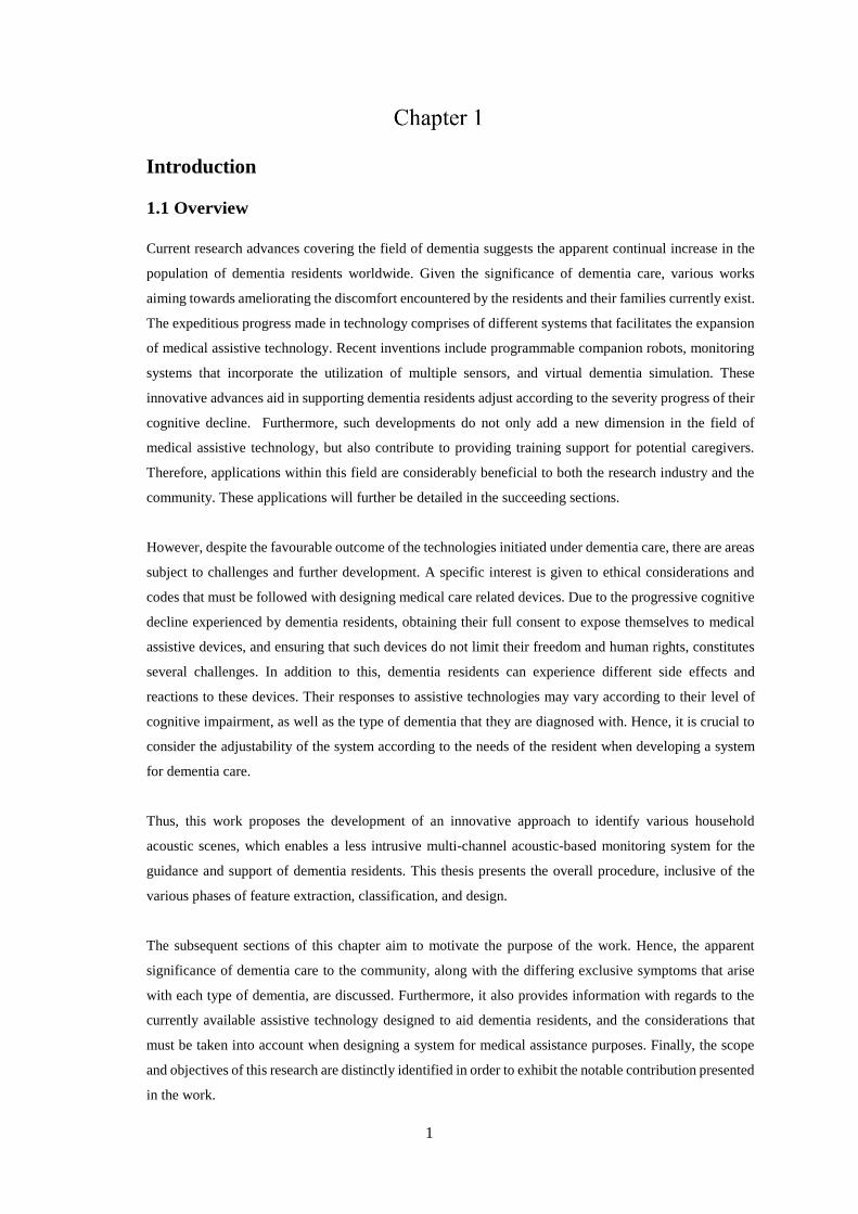
[1, 2, 3]. As per Figure 1.1, Alzheimer’s disease accounts to about 70% of dementia cases, followed by

Vascular dementia at 20% [4].

Figure 1.1. Percentage of Different forms of Dementia [4]

Despite affecting different areas of the brain, various types of dementia are similar in terms of their

cognitive impairment effects. Dementia tends to worsen throughout the course of time; with extreme cases

involving the inability to recognize relatives, and a substantial need of assistance with occurring tasks [5,

6]. According to a study conducted by P.K. Beville, M.S., a geriatrics specialist and the founder of Second

Wind Dreams, the difficulty experienced by dementia residents throughout their daily activities directly

relate to their senses, particularly in terms of visual and hearing impairments [7]. In order to help

individuals in gaining further understanding regarding dementia, P.K. Beville, M.S. had designed the

Virtual Dementia Tour (VDT), a patented and scientifically proven dementia simulation experience where

trained facilitators guide several individuals wearing sensory devices that modify their senses, allowing

them to perform daily activities [7]. As per the confirmation of the subjects to VDT, dementia residents

endure flecked and blurred vision. In addition to this, disrupted hearing prohibits them from hearing

audibly and concentrating on daily activities [7].

In the succeeding sub-sections, detailed signs and symptoms experienced by dementia residents are

discussed, along with the connection of factors such as age and gender in the progression of such ailment.

Finally, statistical evidence surrounding the importance and impact of dementia to the society is provided.

70

20

8

2

0

10

20

30

40

50

60

70

80

Alzheimer's Vascular Lewy Bodies Other Forms

Pe

rce

nta

ge

Type of Dementia

3

1.2.1 Signs and Symptoms

An early diagnosis of dementia has been deemed essential in the improvement of services provided for the

better management of the disorder, as supported by various national strategies implemented all over

Europe [8, 9]. Early intervention not only relieves the caregivers, but also allows the resident more time

to adjust and cope with the disorder. With dementia being progressive, a clinical diagnosis can be acquired

once a cognitive deficit is observed in the resident’s behaviour, which may interfere in his or her daily life

[10]. According to Hort, et al., a Mild Cognitive Impairment (MCI) is often developed prior to dementia

[11]. This can be distinguished when there are complaints and impartial deterioration in any cognitive

domains, despite the conservation of the ability to perform daily activities. MCI can be detected on

residents before 65 years of age [12].

The diagnosis of dementia refers to a category of syndromes that are all indicated by cognitive impairment.

Hence, it can be further narrowed down into subtypes. As discussed previously, various forms of dementia

exist, with Alzheimer’s disease being the most common type. A mixture of two or more subtypes of

dementia can also be diagnosed in one person, to which it is called mixed dementias [13, 14]. Table 1.1

details the signs and symptoms that are common to the main subtypes of dementia.

Table 1.1. Main subtypes of dementia and their symptoms [10]

Name Symptoms

Alzheimer’s Disease Cognitive dysfunction (memory loss, difficulty in language), Behavioral symptoms

(depression, hallucinations), difficulty with daily tasks and activities

Vascular Dementia Stroke, vascular problems (hypertension), decreased mobility and stability

Dementia with Lewy

Bodies

Tremor, frequent visual hallucinations and misapprehensions, slowness in

movement, rigidity

Fronto-temporal

Dementia

Decline in language skills (primary progressive aphasia), changes in behaviour,

decline in social awareness, mood disturbances. Fronto-temporal dementia

represents a considerable percentage of residents under 65 years old.

As implied in Table 1.1, certain symptoms can be observed stronger in a specific form of dementia

compared to others. Hence, this suggests that dementia residents require various types and levels of care

according to the category that they were diagnosed in, as well as the level of cognitive decline severity

unique to their case.

1.2.2 Influence of Age and Gender

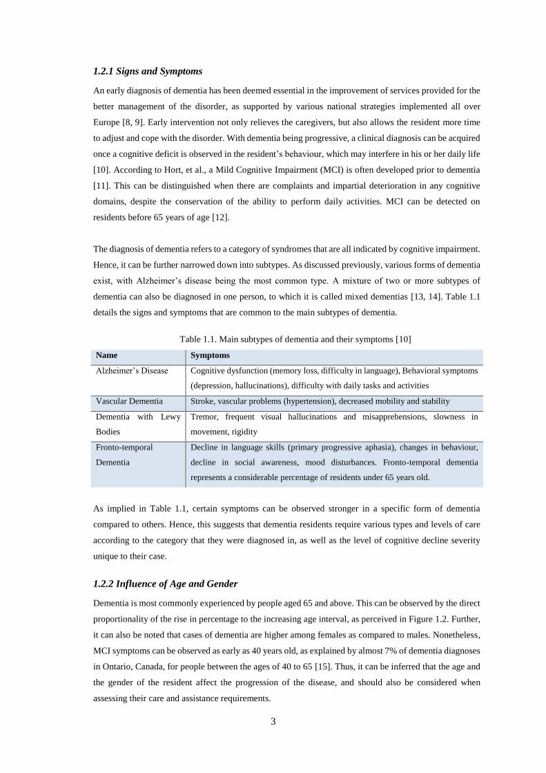
Dementia is most commonly experienced by people aged 65 and above. This can be observed by the direct

proportionality of the rise in percentage to the increasing age interval, as perceived in Figure 1.2. Further,

it can also be noted that cases of dementia are higher among females as compared to males. Nonetheless,

MCI symptoms can be observed as early as 40 years old, as explained by almost 7% of dementia diagnoses

in Ontario, Canada, for people between the ages of 40 to 65 [15]. Thus, it can be inferred that the age and

the gender of the resident affect the progression of the disease, and should also be considered when

assessing their care and assistance requirements.

4

Figure 1.2. Percentage of Ontarians with Dementia, by Age and Gender, for a sample size of 90000 [15].

1.2.3 Statistical Evidence

The growing population of dementia residents over the years account for the significance of a sufficient,

continuous progress achieved within this field. According to the Dementia Prevalence Data commissioned

by The National Centre for Social and Economic Modelling (NATSEM) at the University of Canberra,

there is an estimated number of 436,366 Australian people living with dementia [16]. This number is

expected to rise to almost 590,000 by 2028, and about a million by 2058 [16]. Worldwide, dementia

residents formulate about 47 million of the population in 2015. This number is expected to increase to

131.5 million by 2050 [17].

In addition to a considerable percentage of the world’s population being affected by dementia, the

Australian Bureau of Statistics had also declared dementia to be the principal cause of disability in

Australians aged 65 years old and above, and the second leading cause of death, imparting to about 5.4%

of deaths in males, and 10.6% in females [18]. Aside from its significant effect on the population, dementia

also has a considerable effect on the economy. In the year 2018, dementia is estimated to cost more than

$15 billion in Australia alone. This number is expected to increase to more than $36.8 billion by 2056 [19].

As the numbers mentioned in the statistics above are expected to increase, novel inventions and research

contributions that aim at alleviating the distress experienced by dementia residents, their families, and their

caregivers, are crucial to the society.

1.3 Assistive Technology

According to Section 508 of the Federal Rehabilitation Act, Assistive Technology (AT), is defined as any

product system or equipment utilized and aimed at maintaining and improving the functional abilities of

people with disabilities or impairments [20]. Recurrently, AT is described as products that help differently-

abled people regain their independence in performing daily activities, and can range from basic aids, such

6.50%

12.10%

39.70%41.70%

0.00%

5.00%

10.00%

15.00%

20.00%

25.00%

30.00%

35.00%

40.00%

45.00%

40 - 65 66 - 74 75 - 84 85+Age Group

35.70%

64.30%

0.00%

10.00%

20.00%

30.00%

40.00%

50.00%

60.00%

70.00%

Male FemaleGender

5

as foldable walkers, through electronic devices such as monitoring systems [21, 22].

The involvement of technology in dementia care imparts various advantages. Not only does it improve the

lives of the people living with dementia, but it also ameliorates the amount of effort that caregivers must

impart in the process. In the case of this thesis, high-technology AT developed towards aiding dementia

residents and their caregivers are considered. These devices are described and evaluated in Section 1.4.

The following sub-sections detail the current prevalence of assistive technology, and factors to consider

when developing an efficient system that aims to provide support for dementia care.

1.3.1 Continual Influence of Smart Home Devices

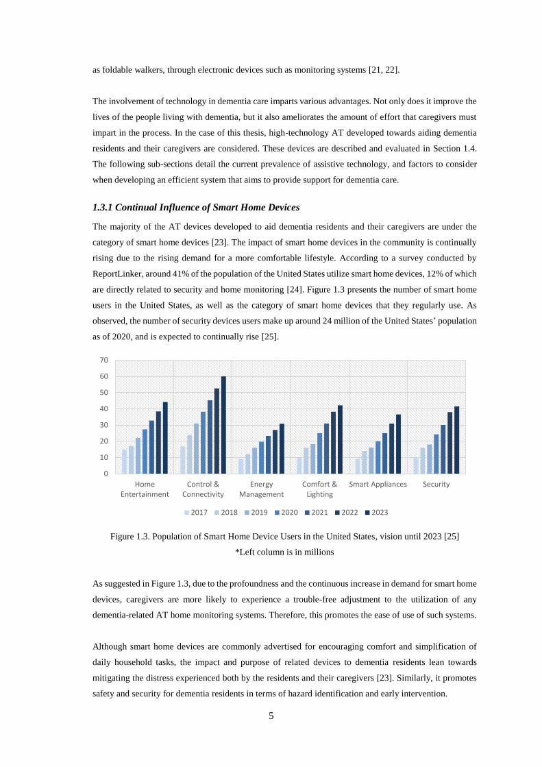
The majority of the AT devices developed to aid dementia residents and their caregivers are under the

category of smart home devices [23]. The impact of smart home devices in the community is continually

rising due to the rising demand for a more comfortable lifestyle. According to a survey conducted by

ReportLinker, around 41% of the population of the United States utilize smart home devices, 12% of which

are directly related to security and home monitoring [24]. Figure 1.3 presents the number of smart home

users in the United States, as well as the category of smart home devices that they regularly use. As

observed, the number of security devices users make up around 24 million of the United States’ population

as of 2020, and is expected to continually rise [25].

Figure 1.3. Population of Smart Home Device Users in the United States, vision until 2023 [25]

*Left column is in millions

As suggested in Figure 1.3, due to the profoundness and the continuous increase in demand for smart home

devices, caregivers are more likely to experience a trouble-free adjustment to the utilization of any

dementia-related AT home monitoring systems. Therefore, this promotes the ease of use of such systems.

Although smart home devices are commonly advertised for encouraging comfort and simplification of

daily household tasks, the impact and purpose of related devices to dementia residents lean towards

mitigating the distress experienced both by the residents and their caregivers [23]. Similarly, it promotes

safety and security for dementia residents in terms of hazard identification and early intervention.

0

10

20

30

40

50

60

70

HomeEntertainment

Control &Connectivity

EnergyManagement

Comfort &Lighting

Smart Appliances Security

2017 2018 2019 2020 2021 2022 2023

6

1.3.2 Ethical Concerns and Considerations

Assistive technology related to dementia play a vital part with alleviating the discomfort corresponding to

dementia care. Nonetheless, as of the year 2017, the World Health Organization (WHO) estimated that

only one in ten users of AT devices were provided access to the data received and transmitted to and from

their AT systems [26]. Due to the limitations caused by the cognitive impairments of dementia residents,

they may not be fully aware whether such systems would be compliant to their rights [27, 28]. The most

common ethical issues concerning AT in dementia care are invasion of privacy and limitations of freedom

[29]. The former is usually concerned with household monitoring systems and location tracking devices,

especially those that are based on visual technology [30, 31]. The latter, on the other hand, customarily

pertains to lock systems controlled by caregivers, as well as robotic companions, which are argued to limit

social interaction and freedom in dementia residents [29]. Therefore, any forms of AT must be attested in

accordance to the specifications of the United Nations Conventions on the Rights of Persons with

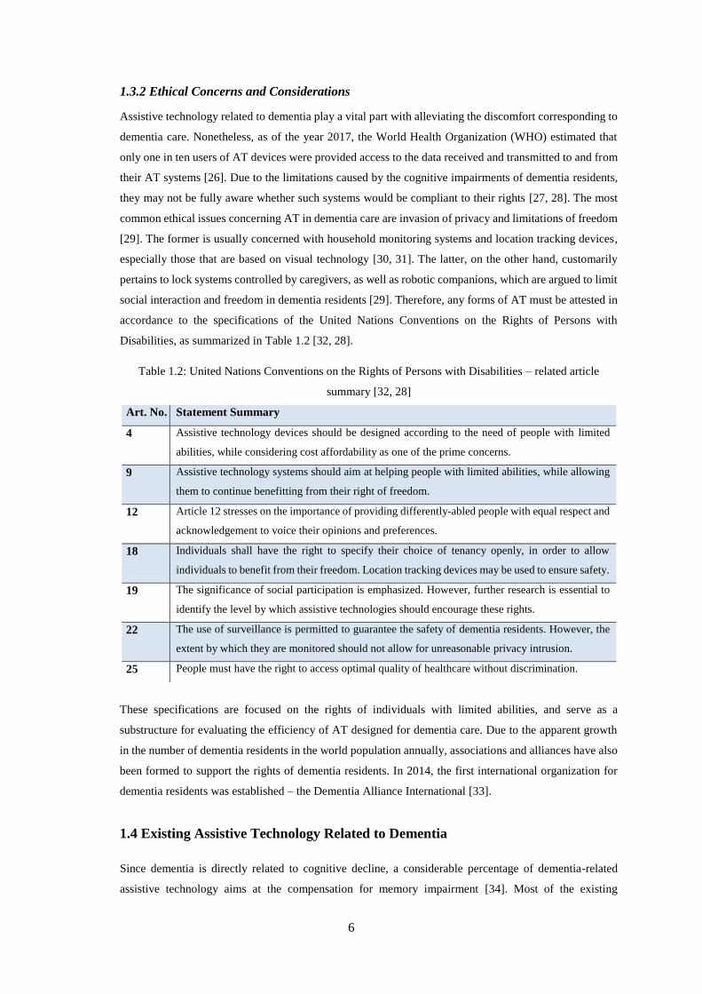
Disabilities, as summarized in Table 1.2 [32, 28].

Table 1.2: United Nations Conventions on the Rights of Persons with Disabilities – related article

summary [32, 28]

Art. No. Statement Summary

4 Assistive technology devices should be designed according to the need of people with limited

abilities, while considering cost affordability as one of the prime concerns.

9 Assistive technology systems should aim at helping people with limited abilities, while allowing

them to continue benefitting from their right of freedom.

12 Article 12 stresses on the importance of providing differently-abled people with equal respect and

acknowledgement to voice their opinions and preferences.

18 Individuals shall have the right to specify their choice of tenancy openly, in order to allow

individuals to benefit from their freedom. Location tracking devices may be used to ensure safety.

19 The significance of social participation is emphasized. However, further research is essential to

identify the level by which assistive technologies should encourage these rights.

22 The use of surveillance is permitted to guarantee the safety of dementia residents. However, the

extent by which they are monitored should not allow for unreasonable privacy intrusion.

25 People must have the right to access optimal quality of healthcare without discrimination.

These specifications are focused on the rights of individuals with limited abilities, and serve as a

substructure for evaluating the efficiency of AT designed for dementia care. Due to the apparent growth

in the number of dementia residents in the world population annually, associations and alliances have also

been formed to support the rights of dementia residents. In 2014, the first international organization for

dementia residents was established – the Dementia Alliance International [33].

1.4 Existing Assistive Technology Related to Dementia

Since dementia is directly related to cognitive decline, a considerable percentage of dementia-related

assistive technology aims at the compensation for memory impairment [34]. Most of the existing

7

technologies aims at providing reminders to dementia residents regarding their medication, extending

assistance in finding misplaced items, and handling phone calls and messages [34]. Such technology is

found to be effective in terms of helping residents in the early stages of dementia, as well as those who are

suffering from MCI [35]. Nonetheless, the current progress of AT in the field of memory impairment

compensation may be inadequate for attending to more severe cases of cognitive decline, as these devices

often require user interference and cooperation [34]. Hence, residents that are subject to moderate and

severe cases of dementia may not benefit abundantly from the assistance that these devices offer. Higher

levels of cognitive deficits often require more than prompting with regards to completing activities [34].

Another circumstance encountered by people with dementia is behavioural and emotional changes [36,

37]. In Section 1.2, it has been discussed that mood disturbances and social unawareness are symptoms of

Fronto-temporal dementia. In order to address this issue, several ATs aimed at facilitating entertainment

and relaxation for dementia residents were developed [38, 23]. Several examples include simplified remote

control systems and customized playlists for listening to music [38]. Robot companions also belong to this

field. Utilization of robots in dementia support aid in reducing the loneliness and mood swings experienced

by the residents [29, 23]. However, it can be argued that the minimization of human contact due to the use

of robots limits social interaction, and hence is also subject to ethical issues [29, 39].

Finally, one of the most common issues faced by dementia residents is the threat to their safety [40].

Progressively, due to their cognitive impairments, residents tend to become more dependent for support

and assistance. In turn, this increases the risks of obtaining injuries or accidents while performing everyday

tasks. The majority of dementia residents spend most of their time at home or in a nursing centre after

being diagnosed, mostly inactive due to the risks on their safety [41]. According to the 2018 Alzheimer’s

disease Facts and Figures, more than 50% of people living in elderly nursing homes are diagnosed with

dementia [42]. Hence, various AT devices focused on the improvement of the safety of dementia residents

are related to monitoring systems and smart home devices.

A large percentage of AT devices under the safety category are alarm devices, which alert caregivers of

any hazardous activities being performed by dementia residents. Several examples include sensor-based

systems such as temperature control systems, and heat detectors [43, 44, 45, 46]. Such devices are powered

by various sensors installed throughout the household, such as the daily activities monitoring system

proposed by Debes, et al. [47]. However, many of these systems, such as the Vigil Dementia System [46],

use audible or visible alarm systems in order to alert the caregiver. Although such products aid in

preventing potential injury around the household, it may pose challenges for reliability. This can be due to

the amount of time provided to the caregivers to make a response subsequent to receiving an alert.

Furthermore, audible alarms may be deemed disruptive for dementia residents, considering the hearing

impairments that they regularly experience [7]. Finally, the majority of these devices focus on only one

household hazard, such as water level monitoring, or temperature control. Hence, installing several alert

systems throughout the room in order to cater to all possible hazards translates to high costs and

complications in maintenance.

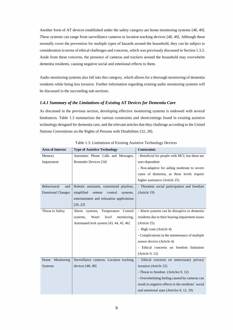
8

Another form of AT devices established under the safety category are home monitoring systems [48, 49].

These systems can range from surveillance cameras to location tracking devices [48, 49]. Although these

normally cover the prevention for multiple types of hazards around the household, they can be subject to

consideration in terms of ethical challenges and concerns, which was previously discussed in Section 1.3.2.

Aside from these concerns, the presence of cameras and trackers around the household may overwhelm

dementia residents, causing negative social and emotional effects to them.

Audio monitoring systems also fall into this category, which allows for a thorough monitoring of dementia

residents while being less invasive. Further information regarding existing audio monitoring systems will

be discussed in the succeeding sub-sections.

1.4.1 Summary of the Limitations of Existing AT Devices for Dementia Care

As discussed in the previous section, developing effective monitoring systems is endowed with several

hindrances. Table 1.3 summarizes the various constraints and shortcomings found in existing assistive

technology designed for dementia care, and the relevant articles that they challenge according to the United

Nations Conventions on the Rights of Persons with Disabilities [32, 28].

Table 1.3. Limitations of Existing Assistive Technology Devices

Area of Interest Type of Assistive Technology Constraints

Memory

Impairment

Automatic Phone Calls and Messages,

Reminder Devices [34]

- Beneficial for people with MCI, but these are

user-dependent

- Non-adaptive for aiding moderate to severe

cases of dementia, as these levels require

higher assistance (Article 25)

Behavioural and

Emotional Changes

Robotic assistants, customized playlists,

simplified remote control systems,

entertainment and relaxation applications

[29, 23]

- Threatens social participation and freedom

(Article 19)

Threat to Safety Alarm systems, Temperature Control

systems, Water level monitoring,

Automated lock system [43, 44, 45, 46]

- Alarm systems can be disruptive to dementia

residents due to their hearing impairment issues

(Article 25)

- High costs (Article 4)

- Complications in the maintenance of multiple

sensor devices (Article 4)

- Ethical concerns on freedom limitation

(Article 9, 12)

Home Monitoring

Systems

Surveillance cameras, Location tracking

devices [48, 49]

- Ethical concerns on unnecessary privacy

invasion (Article 22)

- Threat to freedom (Articles 9, 12)

- Overwhelming feeling caused by cameras can

result in negative effects to the residents’ social

and emotional state (Articles 9, 12, 19)

9

1.4.2 Recommendations and Compliance to Ethical Requirements

Considering the drawbacks mentioned in Table 1.3, we aim to develop a system that is adaptable according

to the needs of the dementia residents at every stage of cognitive decline.

Common to the needs of both residents that are early into experiencing dementia, and those that are in

higher cognitive decline levels, instigating an audio-based monitoring system eliminates the constraints of

intrusion through visual means, which makes the system less overwhelming and less intrusive to dementia

residents. This complies to Article 22, as per Table 1.2. In addition to this, audio-based surveillance is

compliant to Articles 9, 12, and 18, specifying that dementia residents are still allowed to choose their own

tenancy, make their own choices, and enjoy their freedom. The installation of audio-based home

monitoring systems can also be less overwhelming to residents, considering the fact that they are not

visually observed nor tracked.

Similarly, both residents experiencing mild and severe cases of dementia will be able to benefit in the form

of an adjustable severity index identified through the resident profile, which can be set according to the

degree of activity by which the caregiver should be notified. Since residents with mild cognitive decline

level require less assistance, the severity index can be set lower according to their dementia level diagnosis.

This will prevent unnecessary intrusions and will allow the residents to enjoy the maximum amount of

freedom without putting their safety at risk.

Likewise, audio-monitoring systems can be beneficial to residents experiencing hearing impairments, a

symptom that is identified to be directly linked to dementia, especially in more severe cases [7]. Such

systems can be programmed to alert the caregivers when a certain environment is beyond the tolerable

range for the resident, according to the level of hearing impairment that the resident is subject to, which

will be identified via hearing tests.

However, it is crucial that the permission and opinions of the resident should be considered prior to the

installation of microphone arrays, in order to avoid any other ethical issues from arising. It is important to

note that although the audio-based monitoring system devised in this work focuses on recording household

acoustic scenes and events, bits of speech and crosstalk may be involved in the recordings. Although this

may raise privacy issues, crosstalk and speech are to be filtered out in recordings prior to classification.

Furthermore, as opposed to devices that require user interaction, and those that use sensors around the

house, the concept of an audio-based monitoring system allows a continuous overall observation on the

residents’ wellbeing without being costly, which complies with Article 4.

1.4.3 Identification of Domestic Hazards for Dementia Monitoring Systems

The main objective of developing an assistive technology aimed at dementia care is to improve the quality

of healthcare for its residents. Nonetheless, instigating monitoring systems that alert caregivers when

dementia residents require any form of assistance, are required to efficiently classify hazardous domestic

activities from those that are not dangerous. This is necessary not only to ensure and promote safety, but

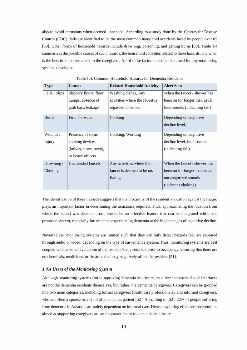
10

also to avoid intrusions when deemed unneeded. According to a study done by the Centres for Disease

Control (CDC), falls are identified to be the most common household accidents faced by people over 65

[50]. Other forms of household hazards include drowning, poisoning, and getting burns [50]. Table 1.4

summarizes the possible causes of such hazards, the household activities related to these hazards, and when

is the best time to send alerts to the caregivers. All of these factors must be examined for any monitoring

systems developed.

Table 1.4. Common Household Hazards for Dementia Residents

Type Causes Related Household Activity Alert Sent

Falls / Slips Slippery floors, floor

humps, absence of

grab bars, leakage

Washing dishes, Any

activities where the faucet is

regarded to be on.

When the faucet / shower has

been on for longer than usual,

loud sounds (indicating fall)

Burns Fire, hot water Cooking Depending on cognitive

decline level.

Wounds /

Injury

Presence of some

cooking devices

(knives, stove, oven),

or heavy objects

Cooking, Working Depending on cognitive

decline level, loud sounds

(indicating fall)

Drowning /

Choking

Unattended faucets Any activities where the

faucet is deemed to be on,

Eating

When the faucet / shower has

been on for longer than usual,

uncategorized sounds

(indicates choking)

The identification of these hazards suggests that the proximity of the resident’s location against the hazard

plays an important factor in determining the assistance required. Thus, approximating the location from

which the sound was detected from, would be an effective feature that can be integrated within the

proposed system, especially for residents experiencing dementia at the higher stages of cognitive decline.

Nevertheless, monitoring systems are limited such that they can only detect hazards that are captured

through audio or video, depending on the type of surveillance system. Thus, monitoring systems are best

coupled with personal evaluation of the resident’s environment prior to occupancy, ensuring that there are

no chemicals, medicines, or firearms that may negatively affect the resident [51].

1.4.4 Users of the Monitoring System

Although monitoring systems aim at improving dementia healthcare, the direct end-users of such interfaces

are not the dementia residents themselves, but rather, the dementia caregivers. Caregivers can be grouped

into two main categories, including formal caregivers (healthcare professionals), and informal caregivers,

who are often a spouse or a child of a dementia patient [52]. According to [52], 22% of people suffering

from dementia in Australia are solely dependent on informal care. Hence, exploring effective interventions

aimed at supporting caregivers are an important factor to dementia healthcare.

11

Caring for someone affected by dementia can cause heightened rates of stress, anxiety, and depression;

which can ultimately lead to health problems on the side of the carer [52]. A survey conducted by the

American Association of Retired Persons (AARP) also reported that caregivers of dementia residents tend

to spend more time in caregiving compared to those taking care of non-dementia residents [245].

Several support forms for carers include education and training, social support groups, and psychosocial

therapies [52]. Similarly, various health-care related assistive technology, such as those discussed in the

previous sub-sections, can also help alleviate caregiving-related stress. In this work, we look at the

development of an audio-based monitoring system that can act as a support to dementia caregivers. The

objectives and research contributions of this work are summarized in Section 1.5, while detailed

information regarding the interface of the monitoring system, as well as the research-based design thinking

approach used to finalize its design, are provided in Chapter 6.

1.5 Objectives and Contributions

Given the reasons and motivations discussed in the previous sections, a multi-channel audio classification

and location estimation system is proposed in this work. This was selected in order to help caregivers assist

and support dementia residents in their daily activities while being less invasive, and without the

unnecessary infringement to their freedom.

1.5.1 Objectives

Upon the completion of this project, the following objectives will be achieved:

- Identify a combination of relevant spectral and spatial acoustic features extracted from multi-channel

household acoustics, that would account for both sporadic (sound events) and continuous (acoustic

scenes) sounds;

- Improve the accuracy of current multi-channel audio classification methods through the detailed

revision of prevalent effective solutions;

- Conduct a study on the performance of several efficient feature classification methods in the specific

application of household acoustics;

- Utilize the performance analysis of proficient feature classification methodologies, for the purpose of

identifying the best techniques to combine for maximum accuracy;

- Conduct a thorough study on neural network architecture and hyper parameter modification, and a

detailed comparison against other pre-trained neural network models

- Integrate sound source estimation in order to provide a more reliable dementia resident monitoring

system, especially for more severe dementia cases;

12

1.5.2 Contributions

Accordingly, the following contributions are achieved:

- Design and validate an effective methodology for the classification of multi-channel domestic acoustic

scenes and events;

- Design and develop an effective methodology for the estimation of sound source location;

- Design, develop, and validate a novel and accurate customizable compact neural network architecture

that is compact and suitable for resource-limited devices utilization

- Develop a synthetic acoustic dataset of representative domestic audio recordings covering sounds that

are often experienced in a dementia resident’s environment.

- Design a Graphical User Interface (GUI) that allows the caregivers to pre-define severity indexes on

each activity through a customizable user profile, indicating the degree by which they should be

notified.

1.6 Thesis Scope

Through the objectives mentioned in Section 1.5, it can be deduced that from a societal perspective, the

scope of this research leans towards improving dementia resident care by developing a less intrusive

monitoring system. This system is designed to aid the potential prevention of possible household accidents

through domestic acoustic scene and event monitoring. In the research perspective, the identification of an

effective solution for multi-channel classification of household acoustics is the main goal, both in terms of

feature extraction and the development of a compact neural network model. Effectiveness is measured

both in terms of accuracy and resource requirements, such that the system will be compatible for devices

with resource-limited platforms. In addition to this, the development of an efficient sound source

estimation methodology according to the requirements of this work is also looked at. Furthermore, it also

aims to alleviate the current progress done in the field of home technology in terms of the overall speed,

accuracy, and reliability of the implementation. Efficacy of the proposed methodology is evaluated through

relevant quantitative performance measures. Finally, the creation of a synthetic database for dementia care

environments is also intended. This will be useful in order to avoid ethical considerations that would arise

if creating and sharing of recordings were made in a real environment. Hence, this allows for new systems

to be developed and refined, that might later be tested in real environments following appropriate ethical

procedures.

It is also important to mention that in the exploration of various detection and classification methods, only

those that are real-time or nearly real-time capable are to be considered. However, in the proof-of-concept

prototype, implementation within real-time constraints will not be the primary focus, as accuracy will have

a higher priority than computational efficiency.

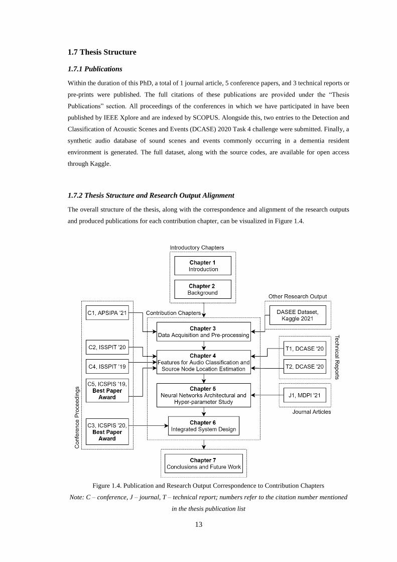
13

1.7 Thesis Structure

1.7.1 Publications

Within the duration of this PhD, a total of 1 journal article, 5 conference papers, and 3 technical reports or

pre-prints were published. The full citations of these publications are provided under the “Thesis

Publications” section. All proceedings of the conferences in which we have participated in have been

published by IEEE Xplore and are indexed by SCOPUS. Alongside this, two entries to the Detection and

Classification of Acoustic Scenes and Events (DCASE) 2020 Task 4 challenge were submitted. Finally, a

synthetic audio database of sound scenes and events commonly occurring in a dementia resident

environment is generated. The full dataset, along with the source codes, are available for open access

through Kaggle.

1.7.2 Thesis Structure and Research Output Alignment

The overall structure of the thesis, along with the correspondence and alignment of the research outputs

and produced publications for each contribution chapter, can be visualized in Figure 1.4.

Figure 1.4. Publication and Research Output Correspondence to Contribution Chapters

Note: C – conference, J – journal, T – technical report; numbers refer to the citation number mentioned

in the thesis publication list

14

As seen in Figure 1.4, the first chapter of this thesis aims to introduce the concept of dementia, the signs

and symptoms of its development, and its statistical evidence. Prominence is then centralized on the

significance of this research, with regards to the attenuation of the management of the disorder while being

less invasive to the dementia residents. Finally, the scope and objectives of this research are discussed in

detail.

The second chapter then reviews relevant research work. This chapter explores various methodologies and

existing studies done for the application of assistive technology to ameliorate dementia care. This includes

exploring different pre-processing, low-level feature extraction, and multi-channel household acoustic

scene classification methods derived from various research papers, journal and conference entries, and

reliable books. These existing works are then assessed in terms of their advantages and disadvantages with

regards to our application. Finally, the research gaps identified from the literature review are described,

and an overview of the proposed methodology is provided. Furthermore, the chapter gives reasons and

justifications on the selection of the techniques utilized, and its relevance to the research.

Chapters 3 to 6 then subsequently details the research contribution to the chosen field, starting from data

acquisition and the generation of a synthetic database relevant to dementia healthcare, audio classification

and sound source estimation, the development of an accurate, compact neural network, and the integrated

user interface in line with design thinking specifications. Information regarding the implementation

process of the research, as well as the results attained, are detailed within these chapters. Finally, the last

chapter of this thesis summarises the research outcomes, and explores future work and potential

improvements relevant to the topic.

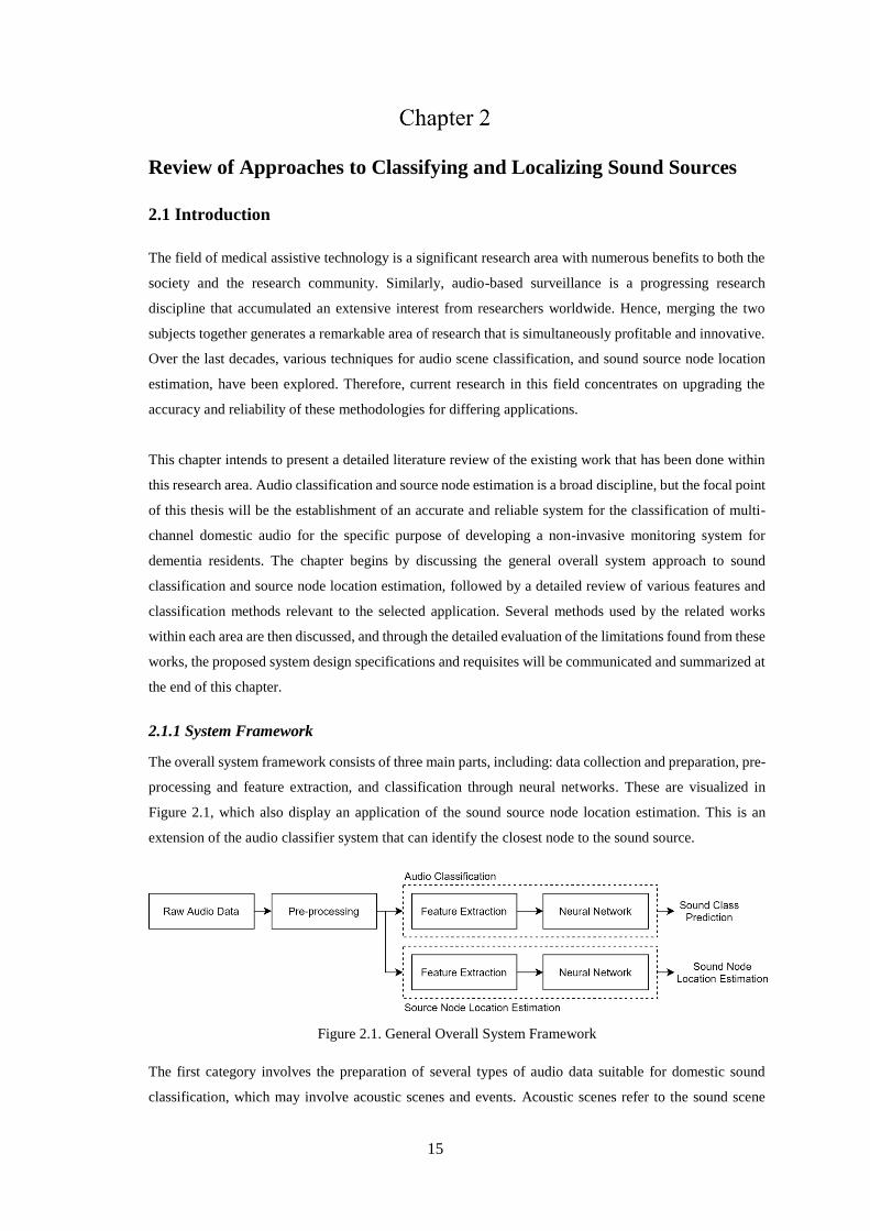
15

Review of Approaches to Classifying and Localizing Sound Sources

2.1 Introduction

The field of medical assistive technology is a significant research area with numerous benefits to both the

society and the research community. Similarly, audio-based surveillance is a progressing research

discipline that accumulated an extensive interest from researchers worldwide. Hence, merging the two

subjects together generates a remarkable area of research that is simultaneously profitable and innovative.

Over the last decades, various techniques for audio scene classification, and sound source node location

estimation, have been explored. Therefore, current research in this field concentrates on upgrading the

accuracy and reliability of these methodologies for differing applications.

This chapter intends to present a detailed literature review of the existing work that has been done within

this research area. Audio classification and source node estimation is a broad discipline, but the focal point

of this thesis will be the establishment of an accurate and reliable system for the classification of multi-

channel domestic audio for the specific purpose of developing a non-invasive monitoring system for

dementia residents. The chapter begins by discussing the general overall system approach to sound

classification and source node location estimation, followed by a detailed review of various features and

classification methods relevant to the selected application. Several methods used by the related works

within each area are then discussed, and through the detailed evaluation of the limitations found from these

works, the proposed system design specifications and requisites will be communicated and summarized at

the end of this chapter.

2.1.1 System Framework

The overall system framework consists of three main parts, including: data collection and preparation, pre-

processing and feature extraction, and classification through neural networks. These are visualized in

Figure 2.1, which also display an application of the sound source node location estimation. This is an

extension of the audio classifier system that can identify the closest node to the sound source.

Figure 2.1. General Overall System Framework

The first category involves the preparation of several types of audio data suitable for domestic sound

classification, which may involve acoustic scenes and events. Acoustic scenes refer to the sound scene

16

recording of a certain activity over time, while sound events refer to more specific sound classes happening

at short periods of time within a duration [53]. Subsequently, pre-processing and feature extraction involve

the conversion of audio data into useful features that can be mapped into an image for classification.

Finally, the last step is to generate the final prediction, which involves the utilization of neural networks.

The rest of the sections of this literature review will be presented in accordance to the order of these

processes.

2.2 Acoustic Data

Preparation of data is a crucial step in the development of a classification and node location estimation

system. Aside from gathering suitable data, this involve ensuring the uniformity of the sampling

frequencies used, length of duration, as well as the type of acoustic sensor network (ASN) from which the

samples are derived from. An ASN comprises of a network of sound sensors distributed across a room.

Relevant information such as the type of microphones, number of microphones for each microphone array

(node), and the distance between them are factors to consider for an ASN, and are also factors that

determine whether the recordings will be single or multi-channel. The following sub-sections examine and

compare existing works that utilize data from different forms of ASNs.

2.2.1 Single-channel Audio Classification

Audio-based monitoring systems appear to be less common in the field of surveillance as opposed to video

cameras [54, 55, 56]. Further, majority of these works utilize mono-channel data, which are derived from

ASN nodes that consists of a single microphone per node. Several works had earlier focused on identifying

indoor sounds [57, 58]. Other works also utilize audio classification for differing applications, such as

speech recognition smart home systems and culture heritage preservation [59, 60]. Almaadeed, et al. had

also proposed the use of audio event classification for road surveillance applications through the

combination of time, frequency, and time-frequency domain features for classification [61]. Nonetheless,

existing works within the domestic audio classification field remains limited.

In line with the application of the work presented in this thesis, Vafeiadis, et al. had proposed an effective

audio-based recognition system for smart homes [62]. However, the scope of this work leans solely in

sound events observed around the kitchen. Hence, the methodology proposed must undergo further testing

and verification in order to be deemed reliable for overall household acoustic classification. Similarly, the

system Tiny Energy Accounting and Reporting System (TinyEARS), had also implemented the

classification of mono-channel household acoustics [63]. However, it is purposed towards reporting the

individual power consumption of domestic appliances, which was successfully achieved within a 10%

error margin [63].

Hence, although the following works assessed may be beneficial, they generally classify only single

channel sound events as opposed to acoustic scenes. Sound events focus on specific sounds that are

identifiable, such as footsteps and coughing [53]. Acoustic scenes, on the other hand, allow the

investigation of the situation of the scene of the recording as a whole [53]. For the selected application in

17

this work, it is crucial to consider both sound events and acoustic scenes in order to acquire a more versatile

system that can aid in the monitoring of dementia residents. However, due to the distinct differences

between the occurrence of acoustic scenes and events, this may lead to challenges in terms of system

accuracy. Thus, it is important to ensure minimal loss of important information and maximization of

important data.

2.2.2 Multi-channel Audio Classification

Due to the overlapping sounds and the mixture of acoustic scenes and events present in real-life recordings,

classification through mono-channel audio may pose challenges in terms of accuracy and reliability [64].

Single channel audio have the tendency to disregard the additional cues that may be embedded in the

recordings [65], hence, utilizing multi-channel ASNs will be beneficial. This composes of a sensor array

consisting of multiple microphone sensors for each node at the specific network setup. Although the basic

steps of aural classification is common between single channel and multi-channel audio [62, 66, 67], the

utilization of multi-channel was proven to be up to 10% more accurate, allowing it to recognize 15.6%

more sound events as opposed to using single-channel audio [64].

Existing multi-channel audio classification systems are also used along different applications, and within

the context of gender recognition of a speaker, and distinguishing crosstalk from speech [68, 69]. Similarly,

as opposed to solely inspecting acoustic event recognition, the consideration of the acoustic scene

environment observed within the household presents challenges in terms of achieving adequate accuracy

due to various factors such as background noises and reflections, especially when dealing with smaller

datasets [64, 65]. Hence, investigating the maintenance of the robustness of the methodology used in such

acoustic conditions must be addressed. In addition to this, developing a reliable audio monitoring system

presents challenges in terms of the accuracy of hazard identification. An audial basis for hazard detection

may have a higher possibility for false identification; hence, improvement in terms of accuracy and

reliability will be beneficial to the current research progress done within this field.

2.2.3 Factors affecting Real-life Audio Recordings

According to Emmanouilidou and Gamper [70], the substantial variation of recording equipment, noise

conditions, and the environment are one of the major challenges faced when performing audio event

detection and classification. Hence, it is important to ensure decent audio quality when selecting data, and

to consider the variation between different datasets in the development process of the overall methodology.

Audio quality refers to the evaluation of the intelligibility of the output of recording devices. Aside from

the method of recording, type of microphones used, and the ASN structure, there are several other factors

that may influence the quality of audio recordings. Natural aspects such as background noises, overlapping

sounds, and reverberant conditions exist within real-life audio recordings, and may negatively influence

the process of classification. Previous studies show that the presence of background noise may decline

classification system performance, and this may depend on the class type [71]. Further, several works also

identified deterioration in sound event detection when faced with recordings with overlapping sounds [72].

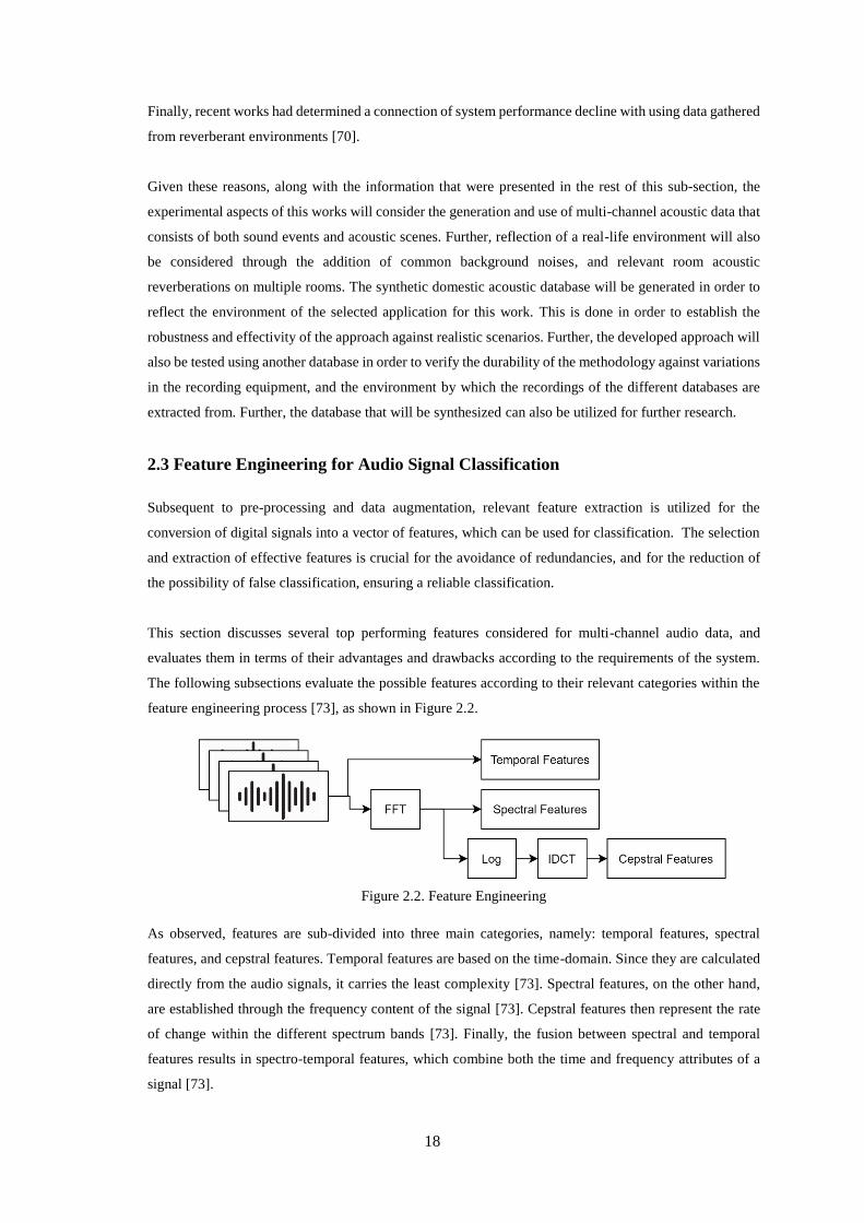
18

Finally, recent works had determined a connection of system performance decline with using data gathered

from reverberant environments [70].

Given these reasons, along with the information that were presented in the rest of this sub-section, the

experimental aspects of this works will consider the generation and use of multi-channel acoustic data that

consists of both sound events and acoustic scenes. Further, reflection of a real-life environment will also

be considered through the addition of common background noises, and relevant room acoustic

reverberations on multiple rooms. The synthetic domestic acoustic database will be generated in order to

reflect the environment of the selected application for this work. This is done in order to establish the

robustness and effectivity of the approach against realistic scenarios. Further, the developed approach will

also be tested using another database in order to verify the durability of the methodology against variations

in the recording equipment, and the environment by which the recordings of the different databases are

extracted from. Further, the database that will be synthesized can also be utilized for further research.

2.3 Feature Engineering for Audio Signal Classification

Subsequent to pre-processing and data augmentation, relevant feature extraction is utilized for the

conversion of digital signals into a vector of features, which can be used for classification. The selection

and extraction of effective features is crucial for the avoidance of redundancies, and for the reduction of

the possibility of false classification, ensuring a reliable classification.

This section discusses several top performing features considered for multi-channel audio data, and

evaluates them in terms of their advantages and drawbacks according to the requirements of the system.

The following subsections evaluate the possible features according to their relevant categories within the

feature engineering process [73], as shown in Figure 2.2.

Figure 2.2. Feature Engineering

As observed, features are sub-divided into three main categories, namely: temporal features, spectral

features, and cepstral features. Temporal features are based on the time-domain. Since they are calculated

directly from the audio signals, it carries the least complexity [73]. Spectral features, on the other hand,

are established through the frequency content of the signal [73]. Cepstral features then represent the rate

of change within the different spectrum bands [73]. Finally, the fusion between spectral and temporal

features results in spectro-temporal features, which combine both the time and frequency attributes of a

signal [73].

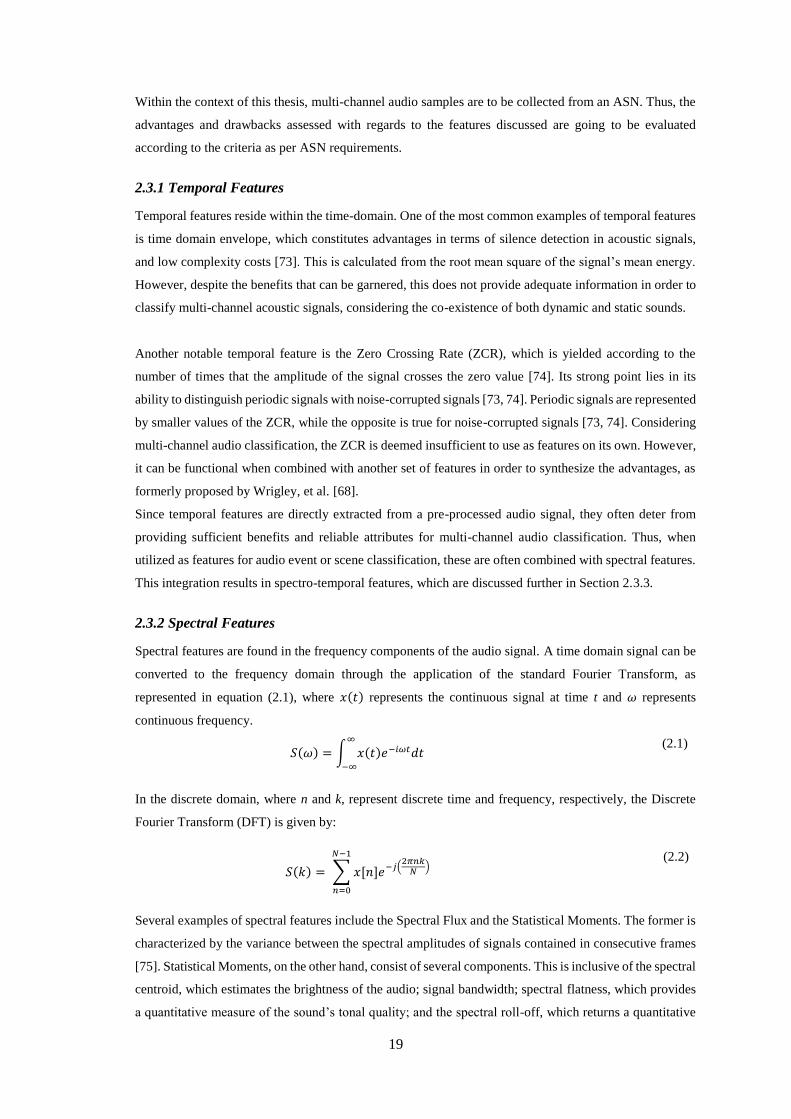
19

Within the context of this thesis, multi-channel audio samples are to be collected from an ASN. Thus, the

advantages and drawbacks assessed with regards to the features discussed are going to be evaluated

according to the criteria as per ASN requirements.

2.3.1 Temporal Features

Temporal features reside within the time-domain. One of the most common examples of temporal features

is time domain envelope, which constitutes advantages in terms of silence detection in acoustic signals,

and low complexity costs [73]. This is calculated from the root mean square of the signal’s mean energy.

However, despite the benefits that can be garnered, this does not provide adequate information in order to

classify multi-channel acoustic signals, considering the co-existence of both dynamic and static sounds.

Another notable temporal feature is the Zero Crossing Rate (ZCR), which is yielded according to the

number of times that the amplitude of the signal crosses the zero value [74]. Its strong point lies in its

ability to distinguish periodic signals with noise-corrupted signals [73, 74]. Periodic signals are represented

by smaller values of the ZCR, while the opposite is true for noise-corrupted signals [73, 74]. Considering

multi-channel audio classification, the ZCR is deemed insufficient to use as features on its own. However,

it can be functional when combined with another set of features in order to synthesize the advantages, as

formerly proposed by Wrigley, et al. [68].

Since temporal features are directly extracted from a pre-processed audio signal, they often deter from

providing sufficient benefits and reliable attributes for multi-channel audio classification. Thus, when

utilized as features for audio event or scene classification, these are often combined with spectral features.

This integration results in spectro-temporal features, which are discussed further in Section 2.3.3.

2.3.2 Spectral Features

Spectral features are found in the frequency components of the audio signal. A time domain signal can be

converted to the frequency domain through the application of the standard Fourier Transform, as

represented in equation (2.1), where 𝑥(𝑡) represents the continuous signal at time t and 𝜔 represents

continuous frequency.

𝑆(𝜔) = ∫ 𝑥(𝑡)𝑒−𝑖𝜔𝑡𝑑𝑡∞

−∞

(2.1)

In the discrete domain, where n and k, represent discrete time and frequency, respectively, the Discrete

Fourier Transform (DFT) is given by:

𝑆(𝑘) = ∑ 𝑥[𝑛]𝑒−𝑗(2𝜋𝑛𝑘

𝑁)

𝑁−1

𝑛=0

(2.2)

Several examples of spectral features include the Spectral Flux and the Statistical Moments. The former is

characterized by the variance between the spectral amplitudes of signals contained in consecutive frames

[75]. Statistical Moments, on the other hand, consist of several components. This is inclusive of the spectral

centroid, which estimates the brightness of the audio; signal bandwidth; spectral flatness, which provides

a quantitative measure of the sound’s tonal quality; and the spectral roll-off, which returns a quantitative

20

approximation of the cumulative value when the frequency response magnitude attains a certain threshold

of the total magnitude [76, 75].

Although spectral features consist of several advantages, the information that will be yielded is not deemed

sufficient for the characterization of multi-channel audio scene acoustics. Generally, spectral features are

solely intended for the representation of particular aspects in a signal. Often times, they are combined with

other features in order to produce a considerable representation of the signal magnitude [73]. However,

since different audio scenes require various requirements in terms of temporal and frequency resolutions

[77], the combination of several spectral features does not necessarily improve the accuracy of the

classifier. A study by Chu, S. et al had shown that integrating numerous spectral features for sound scene

classification is regarded unnecessary, increasing the complexity as opposed to the accuracy, as the system

tends to locate an optimal subset from the vast selection of spectral features [78].

Notwithstanding the reliability of previously mentioned spectral features, the log-mel energy features are

deemed beneficial for multi-channel acoustic scene classification, and were utilized in notable related

works mentioned in this research [79, 80]. Log-mel energy features had also been a well-received choice

of features for DCASE challenge entries, as per the review of Mesaros, A. et al [81], due to the two-

dimensional matrix output that it yields, which is a suitable input for the CNN classifier. It is also known

for its agreeable compatibility when combined with the Mel Frequency Cepstral Coefficients (MFCC)

[80]. Log-mel features are extracted through the application of a Short Time Fourier Transform (STFT)

over windows of audio with Hamming windowing [82]. A mel-scale filter bank is then implemented after

taking the square of the absolute value per bin, which are then normalized and processed in order to fit the

requirements of the system [82].

2.3.3 Spectro-temporal Features

Spectro-temporal features stems from the fusion of temporal, time-based features, and spectral, frequency-

based features. Although not widely explored in the field of multi-channel audio classification, several

works had devised algorithms that integrate the use of both temporal and spectral features. Oletic, et al.

used a spectro-temporal based feature extraction method in order to fabricate a low-power audio pattern

wake-up system [83]. However, although tested for a multi-channel environment, its performance

alongside classification methods is yet to be examined.

Several works had also applied spectro-temporal features for acoustic event detection [84, 85]. Cotton, et

al. proposed the use of a non-negative matrix factorization algorithm in order to detect a set of patches

containing relevant spectral and temporal information that best describes the data [85]. The results

achieved in their experiment suggest that their features provide more robustness in noisy environments as

opposed to MFCC as sole features. Schroder, et al., on the other hand, devises a spectro-temporal feature

algorithm through two-dimensional Gabor functions for robust classification [84].

Nevertheless, these algorithms were tested on acoustic events as opposed to acoustic scenes. As mentioned

21

in Section 2.2, household acoustic scenes pose higher accuracy challenges due to more complex cases of

environmental factors such as background noises and reflections. Similarly, the applicability of these

algorithms to multi-channel audio scenes remains controversial; aside from not being widely utilized,

comparison against other sets of top performing feature combinations for the same application were not

apparent.

The two-dimensional representation of the frequency components of an audio signal is called a

spectrogram, which often results from the application of the Short-time Fourier Transform (STFT) to

constantly compare the input signal with a sinusoidal analysing function [86]. This extends equation (2.1)

by multiplying the complex exponential 𝑥(𝑡) with a localizing window function, represented by 𝑤(𝑡), as

shown in equation (2.3).

𝑆(𝜏, 𝜔) = ∫ 𝑥(𝑡)𝑤(𝑡 − 𝜏)𝑒−𝑗(𝜔𝑡)𝑑𝑡∞

−∞

(2.3)

Subsequent to this, the STFT coefficients are calculated. Such coefficients result from the product between

the STFT of the audio signal, and the analysing function, which is a sinusoidal component. The research

described in this thesis involves digital audio signals. Hence, the STFT is implemented as a Discrete

Fourier Transform (DFT).Although this representation is known to work well with neural networks [87],

the signal processing techniques used in order to display the representation can cause inconsistency within

the structure of the spectrogram [86]. Further, majority of the works concerning the spectrogram solely

makes use of the magnitude component representation of the audio signal, omitting the information found

in the phase [88]. For the approaches described in this thesis, the DFT is implemented using the Fast

Fourier Transform (FFT), and as was shown in Figure 2.2.

However, one of the most notable works in the field of spectro-temporal features are scalogram features,

which are computed through Continuous Wavelet Transform (CWT) [89]. Such method also considers

both the time and frequency components of a signal. The time components represent the motion of the

signal, and the frequency components symbolize the pixel positions in an image [89]. Taking a computer

vision approach, the velocity vectors are first calculated through multi-scale wavelets, which are localized

in time [90]. The main difference between a wavelet transform against a Fourier transform is that it uses

wavelets as an analysing function instead of a sinusoid, as used by the latter. The CWT of a continuous

signal is defined by equation (2.4) [90].

𝐶𝑊𝑇𝑐(𝑠, 𝑡) = ∫ 𝑥(𝑢)1

√𝑠𝜓∗ (

𝑢 − 𝑡

𝑠) 𝑑𝑢

∞

−∞

(2.4)

where 𝜓∗ refers to the complex conjugate of the mother wavelet, provided that it satisfies the condition as

per equation (2.5); t refers to the time domain, and u signifies the signal segment. Finally, s refers to the

scale, which is a function of the frequency [90].

∫ 𝜓(𝑡)𝑑𝑡 = 0∞

−∞

(2.5)

22

Separation of the audio channels is then performed via the low-dimensional models that reverberated from

the firmness of the harmonic template models [89]. Such process is beneficial for multi-channel audio

classification due to its ability to separate mixed audio sources, which allows a thorough analysis for

individual audio channels. The scalogram is a visual representation of the absolute value of the CWT

coefficients, represented by the following formula [91]:

𝐸(𝑠, 𝑡) = |𝐶𝑊𝑇𝑐(𝑠, 𝑡)|2 (2.6)

Nonetheless, despite its advantages, computation of CWT coefficients are often subject to high elapsed

time [92]. Wavelets are computed through comparing and inverting the DFT of the signal against the DFT

of the wavelet, which can be computationally extensive. Thus, integration of other techniques in order to

improve the time requirements must also be examined.

2.3.4 Cepstral Features

Cepstral features are coefficients that result from the cepstrum, a depiction of acoustic signals that is

commonly utilized in homomorphic signal processing, and is often characterized by the conversion of

signals combined through convolution, into the sums of their specific cepstra [93]. Cepstral coefficients

were found to be one of the most commonly utilized features in multi-channel acoustic scenes and events.

The Mel-frequency Cepstral Coefficients (MFCC), were the most widely apparent, and is based on a filter

that models the behaviour of the Human Auditory system [93], a characteristic which makes it

advantageous in terms of sound identification. The MFCCs can be acquired through taking the log of the

mel spectrum, that is obtained through the multiplying the power spectrum of the STFT of an audio sample

with Mel Filter Banks. Following this, the Discrete Cosine Transform (DCT) of the log spectrum are

obtained, with the MFCCs being the result of the DCT’s amplitudes [94].

Calculation of the MFCC coefficient starts by dividing the time-aligned four-channel averaged audio

signal 𝑦𝑎𝑣𝑔(𝑡) into multiple segments. Windowing is then applied to each of these segments prior to being

subject to the DFT, resulting in the short-term power spectrum P(f) [95]. The power spectrum P(f) is then

warped along the frequency axis f, and into the mel-frequency axis M, resulting in a warped power

spectrum P(M). The warped power spectrum is then discretely convolved with a triangular bandpass filter

with K filters, resulting in 𝜃(𝑀𝑘). The MFCC coefficients are calculated according to equation (2.7) [95].

𝑀𝐹𝐶𝐶(𝑑) = ∑ 𝑋𝑘 cos [𝑑(𝑘 − 0.5)𝜋

𝐾] , 𝑑 = 1 … 𝐷

𝐾

𝑘=1

(2.7)

where 𝑋𝑘 = ln(𝜃(𝑀𝑘)), and D << K due to the compression ability of the MFCC [95]. Nonetheless, these

were also found to be prone to loss of substantial information and are assailable to low resolution [96, 97,

98]. Similarly, its performance can be affected by the shape and spacing of the filters, and the warping of

the power spectrum [95]. Nevertheless, it comprises for several advantages due to its simple computation,

and flexibility with regards to integration with several other features [95].

23

Another branch of cepstral coefficients is the Linear Predictive Cepstral Coefficients (LPCC). Similar to

MFCC, it follows a cepstral technique [99]. However, since it utilizes LPC parameters to describe

frequency and energy spectrums, pattern recognition is characterized according to the result of the

increasing logarithm [99]. In turn, this poses as a disadvantage due to the rapid changes happening in the

frequency spectrum for multi-channel audio. Thus, it can be inferred that this method is more suitable for

short-time audio samples.

The Power Normalized Cepstral Coefficients (PNCC) uses power-law nonlinearity, as opposed to the log

nonlinearity utilized in the MFCC and LPCC [100]. This algorithm allows the subtraction of the

background power from the ratio of the arithmetic and geometric mean power, which in turn, enhances the

quality of the signal [100]. Nonetheless, PNCC still provides a slightly greater computation complexity as

opposed to MFCC.

The Subspace Projection Cepstral Coefficients (SPCC) allows the preservation of the different sound

components within an acoustic scene. Multi-channel acoustic scenes are subject to several sound

components. Since audio will be directed from different directions, non-stationary components, quasi-

stationary components, and stationary components tend to coexist between each ASN recording [101].

Thus, non-stationary sounds have the tendency to get scattered throughout the acoustic feature. SPCC uses

target event analysis in order to initiate a subspace bank, simultaneously performing noise reduction and

the generation of discriminant characters that were formulated through the subspace banks [102].

Another branch of cepstral coefficients, which can be extended to spectral as well, is the Relative Spectral

Perceptual Linear Prediction model (RASTA-PLP) [103]. PLP analysis involves the use of the Bark scale,

as opposed to the Mel-filter bank during PLP analysis. The mathematical relationship between the Bark

scale, given by Ω(𝜔), and the linear frequency scale, as represented by 𝜔, is provided in equation (2.8)

[104].

Ω(𝜔) = 6 ln {𝜔

1200𝜋+ [(

𝜔

1200𝜋)

2

+ 1]0.5

} (2.8)

Furthermore, the RASTA-PLP model is based on the three concepts of psychophysics, including: the

critical band spectral resolution, the equal loudness curve, and the intensity loudness power law, in order

to derive an estimate of the auditory spectrum. While the estimation of the equal loudness curve ensures

the compatibility to the sensitivity of human hearing, the intensity loudness power law approximates the

relationship of the perceived loudness by taking the cubic root of the sound intensity, as per PLP analysis

[104]. However, this is extended for RASTA-PLP such that a band pass filter is concatenated at every sub-

band, improving the robustness of the feature and smoothening the noise variations in the process [103].

2.3.5 Comparison and Verdict

In this section, we assess the advantages and disadvantages of the features discussed, and examine their

suitability according to the selected application. This information is summarized in Table 2.1.

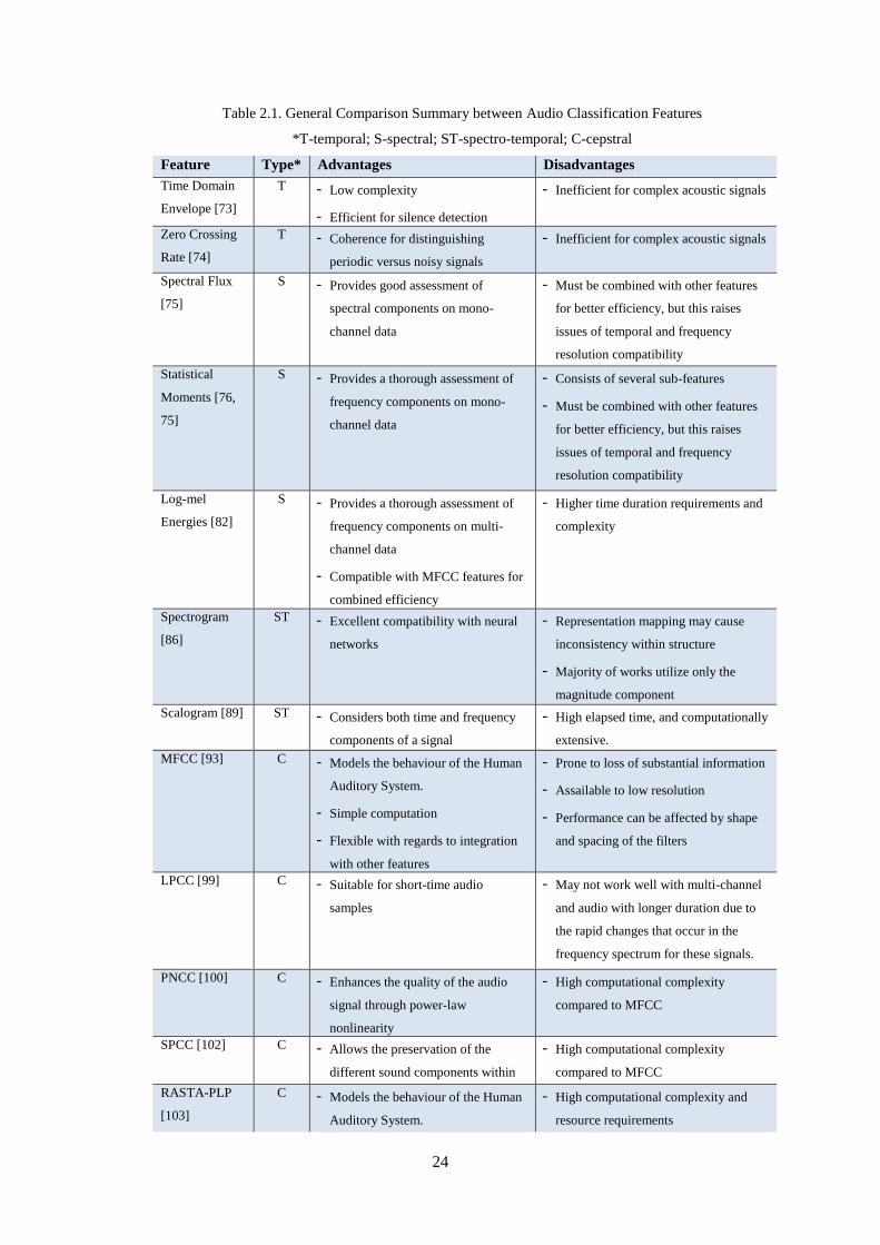
24

Table 2.1. General Comparison Summary between Audio Classification Features

*T-temporal; S-spectral; ST-spectro-temporal; C-cepstral

Feature Type* Advantages Disadvantages

Time Domain

Envelope [73]

T - Low complexity

- Efficient for silence detection

- Inefficient for complex acoustic signals

Zero Crossing

Rate [74]

T - Coherence for distinguishing

periodic versus noisy signals

- Inefficient for complex acoustic signals

Spectral Flux

[75]

S - Provides good assessment of

spectral components on mono-

channel data

- Must be combined with other features

for better efficiency, but this raises

issues of temporal and frequency

resolution compatibility

Statistical

Moments [76,

75]

S - Provides a thorough assessment of

frequency components on mono-

channel data

- Consists of several sub-features

- Must be combined with other features

for better efficiency, but this raises

issues of temporal and frequency

resolution compatibility

Log-mel

Energies [82]

S - Provides a thorough assessment of

frequency components on multi-

channel data

- Compatible with MFCC features for

combined efficiency

- Higher time duration requirements and

complexity

Spectrogram

[86]

ST - Excellent compatibility with neural

networks

- Representation mapping may cause

inconsistency within structure

- Majority of works utilize only the

magnitude component

Scalogram [89] ST - Considers both time and frequency

components of a signal

- High elapsed time, and computationally

extensive.

MFCC [93] C - Models the behaviour of the Human

Auditory System.

- Simple computation

- Flexible with regards to integration

with other features

- Prone to loss of substantial information

- Assailable to low resolution

- Performance can be affected by shape

and spacing of the filters

LPCC [99] C - Suitable for short-time audio

samples

- May not work well with multi-channel

and audio with longer duration due to

the rapid changes that occur in the

frequency spectrum for these signals.

PNCC [100] C - Enhances the quality of the audio

signal through power-law

nonlinearity

- High computational complexity

compared to MFCC

SPCC [102] C - Allows the preservation of the

different sound components within

an acoustic scene

- High computational complexity

compared to MFCC

RASTA-PLP

[103]

C - Models the behaviour of the Human

Auditory System.

- High computational complexity and

resource requirements

25

As inferred by Table 2.1, since temporal features are directly extracted from the audio signal, they often

deter from providing reliable descriptors for multi-channel audio classification, especially those that

contain background noises and mixtures of sound events and scenes. This is because temporal features do

not contain information about the frequency. Hence, in this work, only suitable cepstral and spectral

features are examined. Along with this, spectro-temporal features are also looked at, which is a

combination of temporal and spectral features.

Suitability to the selected application is decided based on the compatibility to multi-channel audio signals

that may consist of acoustic scenes and sound events, and with discrepancies such as background noise

and reverberation. Further, compatibility to neural networks, and efficiency in terms of time and duration

requirements are also looked at. Hence, in this work, we conduct a thorough investigation and comparison

of several features inclusive of: MFCC, PNCC, Log-mel Energies, RASTA-PLP, Spectrograms, and

Scalograms. Accordingly, we also examine several combinational strategies across these features. The

results for these experiments are discussed and reported in Chapter 4.

2.4 Multi-level Classification Techniques

To implement both audio classification and source node location estimation, the use of machine learning

is necessary to extract the final predictions. Machine learning techniques branch out to statistical-based

classification methods, such as Support Vector Machines (SVM), Clustering, Naïve Bayes Classifier,

Linear Regression, and Decision Trees [105]; as well as deep learning techniques, involving neural

networks, which are patterned over the behaviour of the human brain when it comes to identifying patterns

[106]. Appropriate selection of a classifier may depend on a number of factors, as summarized in Table

2.2 [107].

Table 2.2. Machine Learning versus Deep Learning Techniques [107]

Factor Machine Learning Deep Learning

Training Data Requires less data Requires larger datasets for training

Time Requirements Less training elapsed time Higher training elapsed time

Resource Requirements Trains on CPU Trains on GPU

Tuning Capability Limited tuning options Flexible based on requirements

Type of Output Numerical Form Any Form

Depending on the requirements of the selected application in this work, as well as the availability of the

resources, there are two main aspects to consider when selecting the optimum classification model: (1)

level of accuracy, (2) level of flexibility and robustness.

Accuracy is an important factor in monitoring applications in order to minimize the risks of false positive

and false negative alerts, which may be disruptive to both the dementia residents and the caregivers.

Further, the accuracy directly contributes to the reliability of the overall monitoring system. Identifying

the residents’ urgent need for assistance is a crucial matter that is essential to effective dementia care.

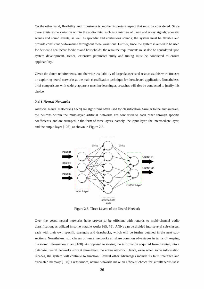
26

On the other hand, flexibility and robustness is another important aspect that must be considered. Since

there exists some variation within the audio data, such as a mixture of clean and noisy signals, acoustic

scenes and sound events, as well as sporadic and continuous sounds; the system must be flexible and

provide consistent performance throughout these variations. Further, since the system is aimed to be used

for dementia healthcare facilities and households, the resource requirements must also be considered upon

system development. Hence, extensive parameter study and tuning must be conducted to ensure

applicability.

Given the above requirements, and the wide availability of large datasets and resources, this work focuses

on exploring neural networks as the main classification technique for the selected application. Nonetheless,

brief comparisons with widely-apparent machine learning approaches will also be conducted to justify this

choice.

2.4.1 Neural Networks

Artificial Neural Networks (ANN) are algorithms often used for classification. Similar to the human brain,

the neurons within the multi-layer artificial networks are connected to each other through specific

coefficients, and are arranged in the form of three layers, namely: the input layer, the intermediate layer,

and the output layer [108], as shown in Figure 2.3.

Figure 2.3. Three Layers of the Neural Network

Over the years, neural networks have proven to be efficient with regards to multi-channel audio

classification, as utilized in some notable works [65, 79]. ANNs can be divided into several sub-classes,

each with their own specific strengths and drawbacks, which will be further detailed in the next sub-

sections. Nonetheless, sub classes of neural networks all share common advantages in terms of keeping

the stored information intact [108]. As opposed to storing the information acquired from training into a

database, neural networks store it throughout the entire network. Hence, even when some information

recedes, the system will continue to function. Several other advantages include its fault tolerance and

circulated memory [108]. Furthermore, neural networks make an efficient choice for simultaneous tasks

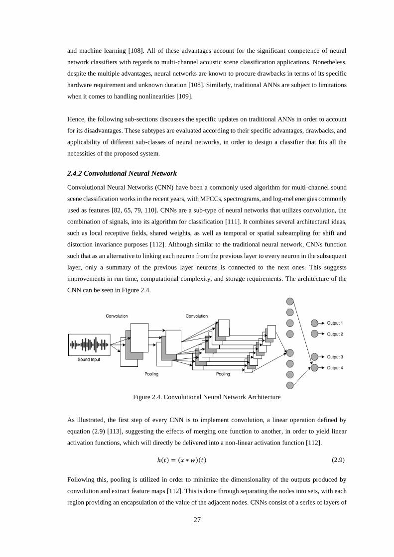
27

and machine learning [108]. All of these advantages account for the significant competence of neural

network classifiers with regards to multi-channel acoustic scene classification applications. Nonetheless,

despite the multiple advantages, neural networks are known to procure drawbacks in terms of its specific

hardware requirement and unknown duration [108]. Similarly, traditional ANNs are subject to limitations

when it comes to handling nonlinearities [109].

Hence, the following sub-sections discusses the specific updates on traditional ANNs in order to account

for its disadvantages. These subtypes are evaluated according to their specific advantages, drawbacks, and

applicability of different sub-classes of neural networks, in order to design a classifier that fits all the

necessities of the proposed system.

2.4.2 Convolutional Neural Network

Convolutional Neural Networks (CNN) have been a commonly used algorithm for multi-channel sound

scene classification works in the recent years, with MFCCs, spectrograms, and log-mel energies commonly

used as features [82, 65, 79, 110]. CNNs are a sub-type of neural networks that utilizes convolution, the

combination of signals, into its algorithm for classification [111]. It combines several architectural ideas,

such as local receptive fields, shared weights, as well as temporal or spatial subsampling for shift and

distortion invariance purposes [112]. Although similar to the traditional neural network, CNNs function

such that as an alternative to linking each neuron from the previous layer to every neuron in the subsequent

layer, only a summary of the previous layer neurons is connected to the next ones. This suggests

improvements in run time, computational complexity, and storage requirements. The architecture of the

CNN can be seen in Figure 2.4.

Figure 2.4. Convolutional Neural Network Architecture

As illustrated, the first step of every CNN is to implement convolution, a linear operation defined by

equation (2.9) [113], suggesting the effects of merging one function to another, in order to yield linear

activation functions, which will directly be delivered into a non-linear activation function [112].

ℎ(𝑡) = (𝑥 ∗ 𝑤)(𝑡) (2.9)

Following this, pooling is utilized in order to minimize the dimensionality of the outputs produced by

convolution and extract feature maps [112]. This is done through separating the nodes into sets, with each

region providing an encapsulation of the value of the adjacent nodes. CNNs consist of a series of layers of

28

convolution that produces feature maps, with a fully connected layer towards the output, where each

neuron retains a relationship with every neuron from the previous layer [112].

The traditional CNN is computationally efficient as it reduces the number of parameters needed in order

to train the classifier [114]. Similarly, it provides adequate accuracy for majority of applications, especially

with datasets garnering a spatial relationship. Nonetheless, deeper neural networks architectures tend to

yield better performance. This is due to the fact that the pooling technique solely captures the translational

invariance, which leaves out more complicated invariances, therefore affecting the accuracy [114].

However, several improvements to account to the limitations of the traditional CNN were proposed

throughout the years. Le, et al. had proposed the tiled convolutional networks, which uses a tiled approach

in allowing the system to capture complex invariances while minimizing the number of required

parameters [114]. This is done through forcing the first layer to share common weights, and considering

small regions of the input at a time [114]. Chong, D. et al. had also discovered multi-channel CNNs, which

utilizes a stack of 1D convolutional layers as opposed to the usual 2D convolution [115]. This update had

garnered advantages in the form of improved accuracy, real-time classification performance, and efficient

execution even for smaller data sizes [115].

2.4.3 Deep Neural Network

Deep Neural Network (DNN) expands the traditional neural networks architecture through providing

additional intermediate layers to the architecture, in order to cater to non-linear and more complicated

features [113, 116]. DNNs are also called feed-forward networks or multilayer perceptrons. Such feed-

forward networks also introduced the concept of hidden layers, for which we are required to select the

activation function for computation [113]. In this case, the input flows through several hidden layers within

the intermediate layer prior to classification, which makes it efficient for achieving high accuracies,

especially in multi-channel applications [113]. Nevertheless, due to the numerous hidden layers and its

requirement for a large dataset, training a DNN would require a much longer time, which therefore results

in a cost-benefit trade off [117].

In the field of acoustic scene classification, due to its high complexity and training time required, it is often

utilized with the CNN in order to merge their advantages. This results in Deep Convolutional Neural

Networks (DCNN), as per the works of Weiping, et al. [118] and Duppada and Hiray [119].

2.4.4 Recurrent Neural Networks

Recurrent Neural Networks (RNN) is a subtype of artificial neural networks that allow for recurrent

connections through non-linear dynamics [120], and are proficient with modelling data for sequence

identification and prediction [121]. Generally, RNNs are structured in the form of high dimensional hidden

states that formulates an input sequence into an output sequence at the prevalent time, in order to identify

the next sequence [122]. The architecture of an RNN includes feedback loops, identified as recurrent cycles

per sequence [122], which delivers impermanent memory. These can be foreseen in Figure 2.5.

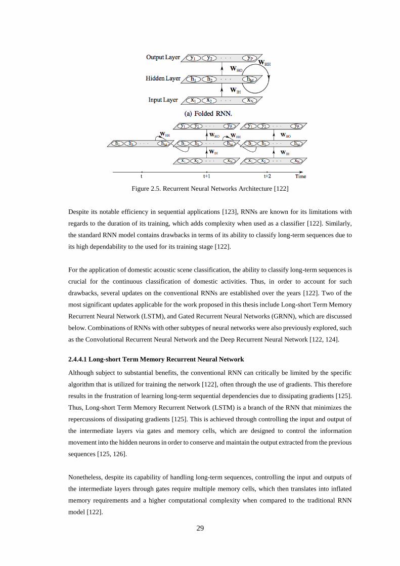
29

Figure 2.5. Recurrent Neural Networks Architecture [122]

Despite its notable efficiency in sequential applications [123], RNNs are known for its limitations with

regards to the duration of its training, which adds complexity when used as a classifier [122]. Similarly,

the standard RNN model contains drawbacks in terms of its ability to classify long-term sequences due to

its high dependability to the used for its training stage [122].

For the application of domestic acoustic scene classification, the ability to classify long-term sequences is

crucial for the continuous classification of domestic activities. Thus, in order to account for such

drawbacks, several updates on the conventional RNNs are established over the years [122]. Two of the

most significant updates applicable for the work proposed in this thesis include Long-short Term Memory

Recurrent Neural Network (LSTM), and Gated Recurrent Neural Networks (GRNN), which are discussed

below. Combinations of RNNs with other subtypes of neural networks were also previously explored, such

as the Convolutional Recurrent Neural Network and the Deep Recurrent Neural Network [122, 124].

2.4.4.1 Long-short Term Memory Recurrent Neural Network

Although subject to substantial benefits, the conventional RNN can critically be limited by the specific

algorithm that is utilized for training the network [122], often through the use of gradients. This therefore

results in the frustration of learning long-term sequential dependencies due to dissipating gradients [125].

Thus, Long-short Term Memory Recurrent Network (LSTM) is a branch of the RNN that minimizes the

repercussions of dissipating gradients [125]. This is achieved through controlling the input and output of

the intermediate layers via gates and memory cells, which are designed to control the information

movement into the hidden neurons in order to conserve and maintain the output extracted from the previous

sequences [125, 126].

Nonetheless, despite its capability of handling long-term sequences, controlling the input and outputs of

the intermediate layers through gates require multiple memory cells, which then translates into inflated

memory requirements and a higher computational complexity when compared to the traditional RNN

model [122].

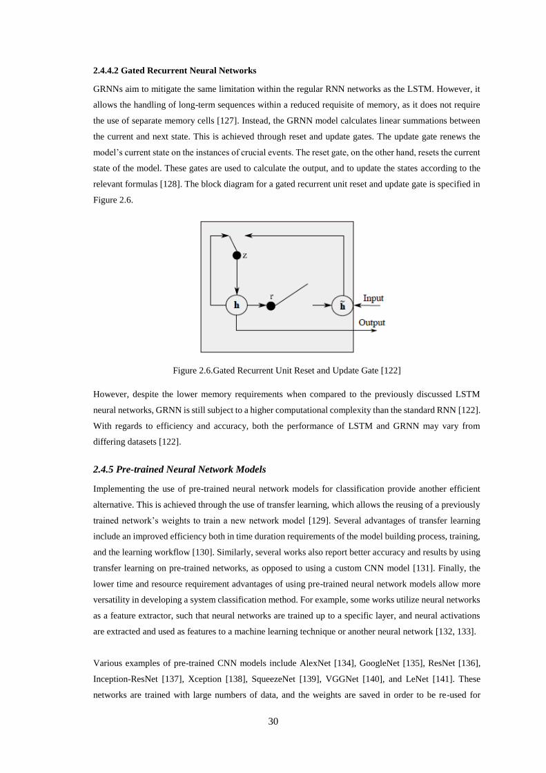
30

2.4.4.2 Gated Recurrent Neural Networks

GRNNs aim to mitigate the same limitation within the regular RNN networks as the LSTM. However, it

allows the handling of long-term sequences within a reduced requisite of memory, as it does not require

the use of separate memory cells [127]. Instead, the GRNN model calculates linear summations between

the current and next state. This is achieved through reset and update gates. The update gate renews the

model’s current state on the instances of crucial events. The reset gate, on the other hand, resets the current

state of the model. These gates are used to calculate the output, and to update the states according to the

relevant formulas [128]. The block diagram for a gated recurrent unit reset and update gate is specified in

Figure 2.6.

Figure 2.6.Gated Recurrent Unit Reset and Update Gate [122]

However, despite the lower memory requirements when compared to the previously discussed LSTM

neural networks, GRNN is still subject to a higher computational complexity than the standard RNN [122].

With regards to efficiency and accuracy, both the performance of LSTM and GRNN may vary from

differing datasets [122].

2.4.5 Pre-trained Neural Network Models

Implementing the use of pre-trained neural network models for classification provide another efficient

alternative. This is achieved through the use of transfer learning, which allows the reusing of a previously

trained network’s weights to train a new network model [129]. Several advantages of transfer learning

include an improved efficiency both in time duration requirements of the model building process, training,

and the learning workflow [130]. Similarly, several works also report better accuracy and results by using

transfer learning on pre-trained networks, as opposed to using a custom CNN model [131]. Finally, the

lower time and resource requirement advantages of using pre-trained neural network models allow more

versatility in developing a system classification method. For example, some works utilize neural networks

as a feature extractor, such that neural networks are trained up to a specific layer, and neural activations

are extracted and used as features to a machine learning technique or another neural network [132, 133].

Various examples of pre-trained CNN models include AlexNet [134], GoogleNet [135], ResNet [136],

Inception-ResNet [137], Xception [138], SqueezeNet [139], VGGNet [140], and LeNet [141]. These

networks are trained with large numbers of data, and the weights are saved in order to be re-used for

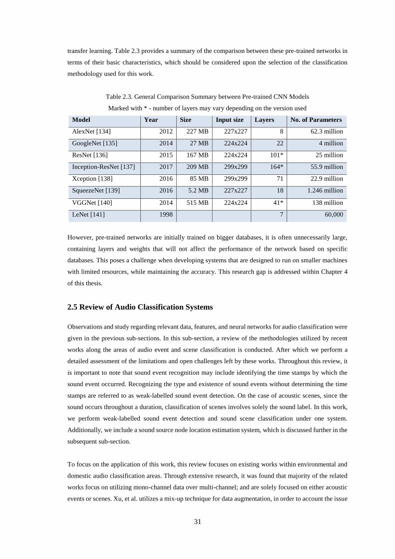
31

transfer learning. Table 2.3 provides a summary of the comparison between these pre-trained networks in

terms of their basic characteristics, which should be considered upon the selection of the classification

methodology used for this work.

Table 2.3. General Comparison Summary between Pre-trained CNN Models

Marked with * - number of layers may vary depending on the version used

Model Year Size Input size Layers No. of Parameters

AlexNet [134] 2012 227 MB 227x227 8 62.3 million

GoogleNet [135] 2014 27 MB 224x224 22 4 million

ResNet [136] 2015 167 MB 224x224 101* 25 million

Inception-ResNet [137] 2017 209 MB 299x299 164* 55.9 million

Xception [138] 2016 85 MB 299x299 71 22.9 million

SqueezeNet [139] 2016 5.2 MB 227x227 18 1.246 million

VGGNet [140] 2014 515 MB 224x224 41* 138 million

LeNet [141] 1998 7 60,000

However, pre-trained networks are initially trained on bigger databases, it is often unnecessarily large,

containing layers and weights that will not affect the performance of the network based on specific

databases. This poses a challenge when developing systems that are designed to run on smaller machines

with limited resources, while maintaining the accuracy. This research gap is addressed within Chapter 4

of this thesis.

2.5 Review of Audio Classification Systems

Observations and study regarding relevant data, features, and neural networks for audio classification were

given in the previous sub-sections. In this sub-section, a review of the methodologies utilized by recent

works along the areas of audio event and scene classification is conducted. After which we perform a

detailed assessment of the limitations and open challenges left by these works. Throughout this review, it

is important to note that sound event recognition may include identifying the time stamps by which the

sound event occurred. Recognizing the type and existence of sound events without determining the time

stamps are referred to as weak-labelled sound event detection. On the case of acoustic scenes, since the

sound occurs throughout a duration, classification of scenes involves solely the sound label. In this work,

we perform weak-labelled sound event detection and sound scene classification under one system.

Additionally, we include a sound source node location estimation system, which is discussed further in the

subsequent sub-section.

To focus on the application of this work, this review focuses on existing works within environmental and

domestic audio classification areas. Through extensive research, it was found that majority of the related

works focus on utilizing mono-channel data over multi-channel; and are solely focused on either acoustic

events or scenes. Xu, et al. utilizes a mix-up technique for data augmentation, in order to account the issue

32

of over-fitting concerning smaller datasets [65]. However, the methodology utilized in this work tend to

gravitate towards a baseline model proposed for multichannel classification. Utilizing the Mel-filter bank

features with the CNN classifier, it was able to achieve an accuracy range of 72.1-73.2%. Thus, this can

be subject to further improvement and investigation. Additionally, it employs environmental samples that

are mostly related to outdoor acoustic scenes, following the TUT Acoustic Scenes 2017 database [142].

Zheng, et al. had resorted to multi-spectrograms gathered from the Short-time Fourier Transform (STFT),

and the MFCC, to be extracted as features through CNN [77]. SVM is then used in order to classify the

acoustic scenes. Although this work had achieved 88.65% accuracy using the DCASE 2017 component

set, this is solely subject to environmental acoustics [77]; hence, accuracies may vary for domestic acoustic

scenes. Similarly, challenges arise from the utilization of spectrograms in audio processing, considering

that sounds do not occur as static objects [143]. Generally, it is important to separate simultaneous sounds

in spectrograms due to the differences between the properties of images and audio [143].

More similar works to the one proposed in this research include the top two performing systems submitted

to the DCASE 2018 Challenge Task 5 [144]. Being based on multi-channel acoustic scene classification,

these works had achieved the respective average F1‐scores of 89.8% and 89.95% on microphone arrays

available in the development set, and an 88.4% F1‐score on unknown microphone arrays [79, 80]. Aside

from the differing application and objectives, the methodologies used for these works differ from what is

proposed in this work. Nonetheless, these works presented a competent baseline to compare the proposed

methodology. Inou, et al. [79] proposes the utilization of log‐mel energies as features to the CNN, along

with data augmentation through shuffling and mixing. Tanabe, et al. [80] used a front-end and back-end

module approach. The front-end employ pre-processing methods without machine learning, while the

back-end performs feature extraction and classification. Features are drawn through the combination of

log‐mel energies and MFCC acoustic features, with spatial features for classification through a pre‐trained

VGG‐16 DCNN model [80]. Though the contribution is notable, VGG-16 is a pre-trained classifier model

provided by the DCASE 2018 Task 5 challenge. Thus, the reliability of the methodology proposed when

applied to different datasets can be challenged. Nevertheless, despite the current progress achieved within

the field of multichannel acoustic scene classification, it remains a broad topic with several areas that

necessitates further investigation, which will be described in detail in the following section.

2.5.1 Liabilities and Challenges: Audio Classification

To assess the open challenges and areas of improvement left by the existing works mentioned, a

comparison of the related works in terms of their application, feature methodologies, research

contributions, and liabilities is tabulated below. Nevertheless, it is important to note that Table 2.4 focuses

on works that concern multi-channel audio classification, in order to provide an equitable alignment with

the work presented in this thesis. Also note that accuracy results acquired from the works were not included

in the table comparison, as not all accuracies of these works were measured in the same datasets.

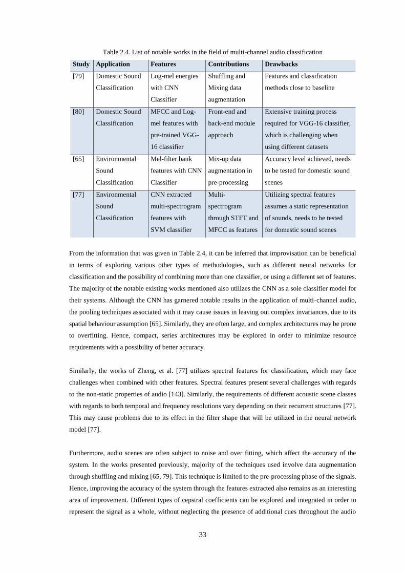
33

Table 2.4. List of notable works in the field of multi-channel audio classification

Study Application Features Contributions Drawbacks

[79] Domestic Sound

Classification

Log-mel energies

with CNN

Classifier

Shuffling and

Mixing data

augmentation

Features and classification

methods close to baseline

[80] Domestic Sound

Classification

MFCC and Log-

mel features with

pre-trained VGG-

16 classifier

Front-end and

back-end module

approach

Extensive training process

required for VGG-16 classifier,

which is challenging when

using different datasets

[65] Environmental

Sound

Classification

Mel-filter bank

features with CNN

Classifier

Mix-up data

augmentation in

pre-processing

Accuracy level achieved, needs

to be tested for domestic sound

scenes

[77] Environmental

Sound

Classification

CNN extracted

multi-spectrogram

features with

SVM classifier

Multi-

spectrogram

through STFT and

MFCC as features

Utilizing spectral features

assumes a static representation

of sounds, needs to be tested

for domestic sound scenes

From the information that was given in Table 2.4, it can be inferred that improvisation can be beneficial

in terms of exploring various other types of methodologies, such as different neural networks for

classification and the possibility of combining more than one classifier, or using a different set of features.

The majority of the notable existing works mentioned also utilizes the CNN as a sole classifier model for

their systems. Although the CNN has garnered notable results in the application of multi-channel audio,

the pooling techniques associated with it may cause issues in leaving out complex invariances, due to its

spatial behaviour assumption [65]. Similarly, they are often large, and complex architectures may be prone

to overfitting. Hence, compact, series architectures may be explored in order to minimize resource

requirements with a possibility of better accuracy.

Similarly, the works of Zheng, et al. [77] utilizes spectral features for classification, which may face

challenges when combined with other features. Spectral features present several challenges with regards

to the non-static properties of audio [143]. Similarly, the requirements of different acoustic scene classes

with regards to both temporal and frequency resolutions vary depending on their recurrent structures [77].

This may cause problems due to its effect in the filter shape that will be utilized in the neural network

model [77].

Furthermore, audio scenes are often subject to noise and over fitting, which affect the accuracy of the

system. In the works presented previously, majority of the techniques used involve data augmentation

through shuffling and mixing [65, 79]. This technique is limited to the pre-processing phase of the signals.

Hence, improving the accuracy of the system through the features extracted also remains as an interesting

area of improvement. Different types of cepstral coefficients can be explored and integrated in order to

represent the signal as a whole, without neglecting the presence of additional cues throughout the audio

34

scene. Similarly, very few existing works were able to test the systems developed for several datasets

involving domestic acoustic scenes. Thus, testing on several other datasets will be of great advantage for

increasing the reliability.

Finally, yielding contributions with regards to the adjustability of the system for a notable application are

of great interest. The outstanding works in the research area of multichannel acoustic scene classification,

as mentioned in Table 2.3, were not directly related to a specific application. Thus, connecting the work

into a specific application, as well as introducing adjustability and novel system manoeuvring would allow

for the expansion of research developments that aid in the distress experienced by the population.

2.6 Review of Sound Source Localization Systems

Estimating the location of the sound source comes with a variety of advantages, particularly within the

field of audio monitoring systems. The identification of the sound source location dramatically improves

the monitoring capabilities of such systems, especially when hazards are involved, and immediate action

is required. Hence, in this work, we investigate the concept of source node location estimation. This

technique identifies the closest node to the sound source within an ASN. The main purpose of integrating

sound source estimation into the monitoring system is to identify the room and estimate location from

which the hazardous sound occurs in. Integrating this functionality with the audio classification system

not only improves the overall system accuracy, but also acts as a verification step towards identifying the

urgency of assistance requirement.

In previous works, one of the most common approaches for approximating the Direction of Arrival (DOA)

are microphone pairing methods, where the DOA is measured through the time differences of sound arrival

between two microphones (TDOA) [145]. Nonetheless, the overall efficiency and performance of this

method decreases due to noise and multipath propagation, which are commonly experienced with

overlapping sounds [146]. In order to counter such disadvantages, several works proposed the utilization

of more than two microphones in order to extract a more accurate prediction [147, 148]. However, usage

of multiple microphones does not guarantee a robust system, as factors such as the number of overlapping

noise, as well as the type of microphones used, can also influence the performance of the system.

Working towards a more robust system, several researchers also introduced the use of eigen-

decomposition-based methods, such as the Narrowband Multiple Signal Classification (MUSIC) estimator

[149], the Root Multiple Signal Classification (Root-MUSIC) estimator [150], and the Estimation of Signal

Parameters via Rotational Invariance Techniques (ESPRIT) [151]. The MUSIC estimator decomposes the

sensor covariance matrix between orthogonal signals and noise subspaces, where higher eigenvector

values correspond to the former, while lower values correspond to the latter [149]. Overall, it provides a

high-resolution DOA algorithm that utilizes the covariance matrix of the sensor data array, which is known

to perform well in signal sources with smaller separation distances [149]. The Root-MUSIC algorithm, on

the other hand, approximates the DOA through the peaks within the spectrum polynomial [150]. Similar

35

to the MUSIC algorithm, this also exhibits good performance in closely spaced signal sources.

Nonetheless, it is also based on the assumption that every sensor is perfectly spaced within the array [150].

The ESPRIT algorithm differs from both methods such that it does not require the utilization of a scan

vector in order to go over every possible direction of the sound source [151]. Rather, DOA estimation is

achieved through the roots of independent equations that are closest to the unit circle [151]. Nevertheless,

although such methods return high resolution DOA approximation results, coherent signal conditions

remain a struggle. Further, they tend to be computationally complex [146]. Computational efficiency is

one of the factors that must be considered when deciding the DOA algorithm to use depending on the

system requirements.

Taking these factors into consideration, Klein and Vo then proposed a DOA estimation approach for multi-

channel audio data through the cross-correlation method [146]. In this algorithm, the TDOA is

approximated via the cross-correlation coefficient matrix determinant of the microphone array signals

[146]. This method is particularly beneficial because of the lower computational complexity, flexibility,

as well as its low sensitivity to noise and reverberant environments [146]. Nonetheless, application of this

technique still operates based on the prior knowledge of the exact number of active sources within the

system, which may not be beneficial for the scope of this work.

Recently, Adavanne, et al. proposed the use of DNNs for DOA estimation [152]. This technique trains a

custom neural network consisting of convolutional and recurrent neural networks for DOA estimation,

based on spectrogram magnitude and phase information, and has been proven to perform better when

compared to the MUSIC method [152]. Nonetheless, it has been observed that as the number of sources

increase, the accuracy of the estimation depletes, having an average accuracy of 42.7% for anechoic

recordings with two overlapping sound events, which even decreases dramatically with three events [152].

Chakarabarty and Habets then focused on improving the computational costs of CNN-based DOA

estimations through the addition of the systematic dilation on the networks trained [153]. Nonetheless,

drawbacks concerning the inconsistent performance of the neural network against increasing number of

overlapping sounds still remains an issue.

More recent works released by the DCASE 2021 Task 3 challenge involves sound event localization with

directional interference [154]. Nonetheless, the majority of the top performing methodologies utilizes

Ambisonic audio format with IPD-based audio features that require extensive prior knowledge about the

recording devices [155]. Although Ambisonics allow for better localization, it requires the use of a decoder

for playbacks, and a B-format microphone array that is less common than a ULA. Further, these also face

difficulty in terms of compatibility with various platforms, as well as recording static stereo sounds [156].

For these reasons, they are generally less flexible than microphone arrays.

Several other submissions that utilize microphone arrays did not exceed the performance of the baseline

system, and are subject to neural network models with very high model parameter requirement [157, 158],

which may not be suitable for systems with limited computational capabilities.

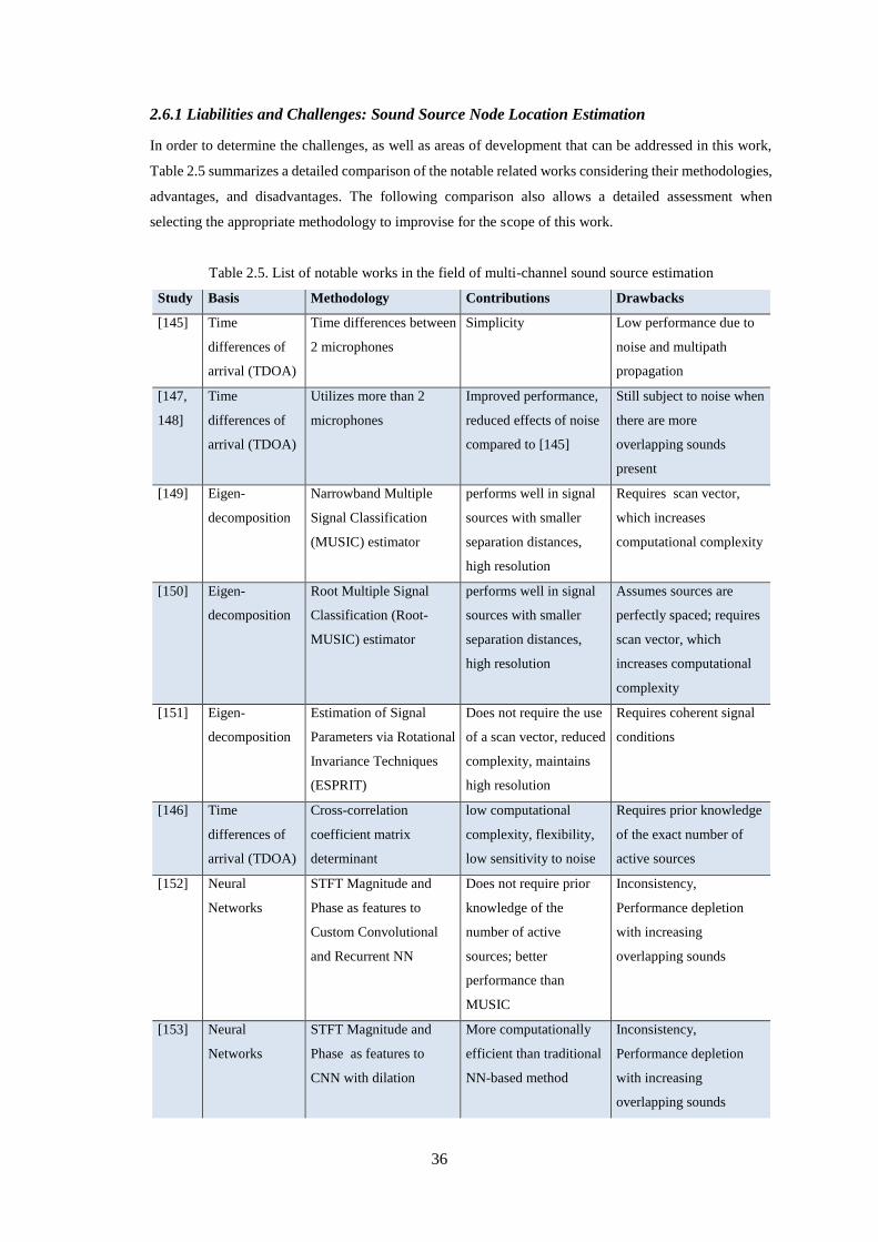
36

2.6.1 Liabilities and Challenges: Sound Source Node Location Estimation

In order to determine the challenges, as well as areas of development that can be addressed in this work,

Table 2.5 summarizes a detailed comparison of the notable related works considering their methodologies,

advantages, and disadvantages. The following comparison also allows a detailed assessment when

selecting the appropriate methodology to improvise for the scope of this work.

Table 2.5. List of notable works in the field of multi-channel sound source estimation

Study Basis Methodology Contributions Drawbacks

[145] Time

differences of

arrival (TDOA)

Time differences between

2 microphones

Simplicity Low performance due to

noise and multipath

propagation

[147,

148]

Time

differences of

arrival (TDOA)

Utilizes more than 2

microphones

Improved performance,

reduced effects of noise

compared to [145]

Still subject to noise when

there are more

overlapping sounds

present

[149] Eigen-

decomposition

Narrowband Multiple

Signal Classification

(MUSIC) estimator

performs well in signal

sources with smaller

separation distances,

high resolution

Requires scan vector,

which increases

computational complexity

[150] Eigen-

decomposition

Root Multiple Signal

Classification (Root-

MUSIC) estimator

performs well in signal

sources with smaller

separation distances,

high resolution

Assumes sources are

perfectly spaced; requires

scan vector, which

increases computational

complexity

[151] Eigen-

decomposition

Estimation of Signal

Parameters via Rotational

Invariance Techniques

(ESPRIT)

Does not require the use

of a scan vector, reduced

complexity, maintains

high resolution

Requires coherent signal

conditions

[146] Time

differences of

arrival (TDOA)

Cross-correlation

coefficient matrix

determinant

low computational

complexity, flexibility,

low sensitivity to noise

Requires prior knowledge

of the exact number of

active sources

[152] Neural

Networks

STFT Magnitude and

Phase as features to

Custom Convolutional

and Recurrent NN

Does not require prior

knowledge of the

number of active

sources; better

performance than

MUSIC

Inconsistency,

Performance depletion

with increasing

overlapping sounds

[153] Neural

Networks

STFT Magnitude and

Phase as features to

CNN with dilation

More computationally

efficient than traditional

NN-based method

Inconsistency,

Performance depletion

with increasing

overlapping sounds

37

Since the main functionality of the proposed work is an efficient home monitoring system, the exact

number of active sources is not known prior to extracting the DOA information. Further, considering that

the main purpose of integrating sound source estimation into the monitoring system is to identify the

resident’s location relative to the identified hazardous sound’s location, the exact coordinates of the sound

source is deemed unnecessary. Rather, an estimation of the room location of the sound source would

provide sufficient information for this purpose. Furthermore, by reason that the source estimator would be

integrated into a multi-channel sound classification system, lower time and resource requirements is

preferred.

Taking these into account, approximating DOA through neural networks provides the best advantages.

Given that it does not require prior knowledge of the number of active sound sources within the

surroundings, it provides benefits necessary for multi-channel audio recordings.

Nonetheless, this work aims to improve and counter drawbacks identified from previous works. In order

to increase computational efficiency and decrease the time and resource requirements, we aim to

implement the use of transfer learning in place of training a custom-built neural network classifier. Further,

in attempts to reduce the negative effects of multiple overlapping sound sources in the DOA estimation

results, this work aims to maximize the information found within the STFT phase differences in between

microphones, eliminating the use of the magnitude information, which mostly contains information

regarding the overlapping sound sources.

2.7 Proposed System Design Specifications and Requisites

Considering the limitations and open challenges for both sound scene classification and source node

estimation that were identified in this chapter, as well as the justifications, health, and ethical

considerations described in Chapter 1, a set of system development specifications and requisites to adhere

to have been articulated in the following points. These will further be expanded and discussed in the

following chapters of this work.

Proposed Methodology:

1. Generation of a synthetic domestic acoustic database comprising of sound events and scenes

(Chapter 3).

2. A well-researched approach to gathering relevant spectral and spatial features aiming at a better

accuracy and a shorter inference execution time (Chapter 4).

3. Segmentation of recorded audio signals prior to classification (Chapter 4).

4. Precise source node estimation for approximating the source node of the identified hazard that can

be integrated with both the sound classification component of the system design (Chapter 4).

5. Novel, compact, and reliable audio scene classification technique that is (Chapter 5)

38

As per the points above, the generation of a synthetic dataset that is carefully curated to reflect a typical

real-world dementia care environment will allow the exploration of effects such as background noise and

room reverberation, with regards to the chosen application. Further, this permits the testing of the system’s

robustness and effectiveness against multiple datasets with varying recording setups. Finally, it also opens

possibilities for future research. Details about the generation of this dataset will be presented in Chapter 3.

Once the dataset is generated, features for audio classification will be extracted through the use of optimal

spectro-temporal features stipulated according to their advantages, as per the second point. Segmentation

will also be considered in order to identify sound events happening within the entire duration per

classification. Further, the development of a phase-based audio location estimation system that is

compatible with the audio classification system is explored. This will not only provide approximate

information about the location of the sounds without the requirement of extensive prior knowledge about

the recordings, but will also improve the classification performance and reliability. Both features with

regards to the classification and location estimation aspects of the system will be expounded in Chapter 4.

The optimum features identified and developed in Chapter 4 will then be subject to neural network methods

for classification, as explored in Chapter 5. This chapter will detail the design and development of a

compact neural network model aimed at maintaining a high accuracy at much lower computational and

resource requirements. This is developed through a detailed study of various neural networks approaches

and architectures as specified by their benefits, and is designed to work towards achieving higher precision,

while being compatible with devices with limited computing capabilities at the same time.

Finally, these system functionalities will be integrated into an easy-to-use interface, which is designed

following a design thinking, user-centered approach. Details regarding the specifications and

characteristics of this interface are provided in Chapter 6.

2.7.1 Performance Evaluation Methods

To evaluate the performance of the proposed system, its response to the following aspects are investigated:

1. Per-class and overall comparison of different cepstral, temporal, and spectro-temporal features in

order to identify the best performing features. These will then be classified through the comparison of

various pre-trained neural network and machine learning models

2. Investigation of the effects of feature combination

3. Increasing the sample set, and cross-fold validation

Observing these aspects will help identify the top performing features and model classifier for the selected

application, which will help build the foundation for the design and development of a novel approach.

Further, in order to strengthen the performance investigation claims made in this research, cross-fold

validation will be performed, while choosing a different set of training and testing samples for each time.

This allows the extension of the system performance reliability, while maintaining a balanced dataset

throughout the implementation phase. Similarly, performing cross validation allows the verification of the

figurative results garnered within the scope of this work.

39

Aside from the standard accuracy, evaluation of the performances of different techniques will also be

compared and measured in terms of their F1-scores. This is defined to be a measure that takes into

consideration both the recall and the precision, which are derived from the ratios of True Positives (TP),

True Negatives (TN), False Positives (FP), and False Negatives (FN). The F1-score is given by equation

(2.10), where recall and precision are defined by equations (2.11) and (2.12) [159]. The parameters used

in the calculation of the F1-score can be extracted from confusion matrices.

𝐹1𝑠𝑐𝑜𝑟𝑒 = 2 ∗ 𝑅𝑒𝑐𝑎𝑙𝑙 ∗ 𝑃𝑟𝑒𝑐𝑖𝑠𝑖𝑜𝑛

𝑅𝑒𝑐𝑎𝑙𝑙 + 𝑃𝑟𝑒𝑐𝑖𝑠𝑖𝑜𝑛

(2.10)

𝑅𝑒𝑐𝑎𝑙𝑙 = 𝑇𝑃

𝑇𝑃 + 𝐹𝑁

(2.11)

𝑃𝑟𝑒𝑐𝑖𝑠𝑖𝑜𝑛 = 𝑇𝑃

𝑇𝑃 + 𝐹𝑃

(2.12)

The performance of each technique will be observed on an increasing sample set on different experiment

stages, starting with 3042 10-second audio files, with 338 files per category, increasing until the entire

database is used. The SINS database recordings, as well as the synthetic database generated as per Chapter

3, both compose of unequal numbers of audio files per category. To account for the data imbalance, the

following techniques are used:

1. Balancing the Dataset

This will particularly be used for the initial development and experiments conducted for this work. In

this technique, the dataset will be equalized across all levels in order to preserve a balanced dataset.

This is done in order to avoid biasing in favour of specific categories with more samples. It is achieved

by reducing the number of data per level to match the minimum number of data amongst the

categories. Selection of the data will be done randomly throughout the experiments.

2. Using Weight-sensitive Performance Metrics

Provided that the F1-score serves as the main performance metric used for the experiments conducted,

it is crucial to ensure that these metrics are unbiased, especially for multi-classification purposes.

When taking the average F1-score for an unbalanced dataset, the number of data per level may affect

and skew the results for the mean F1-score in favour of the classes with the most number of data.

Therefore, three different ways of calculating the mean F1-score will be considered [160]:

- Weighted F1-score: calculates the F1 score independently for each of the classes. However,

when taking the average F1-score value, it first adds up all of the F1-scores by multiplying them

to weights that are dependent on the number of true labels of each class. It is then divided by the

total number of data, as per equation (2.13).

𝐹1𝑤𝑒𝑖𝑔ℎ𝑡𝑒𝑑 =𝐹1𝑐𝑙𝑎𝑠𝑠1 ∗ 𝑊1 + 𝐹1𝑐𝑙𝑎𝑠𝑠2 ∗ 𝑊2 + ⋯ + 𝐹1𝑐𝑙𝑎𝑠𝑠𝑁 ∗ 𝑊𝑁

∑ 𝑊𝑁1

(2.13)

40

- Micro F1-score: utilizes the total number of TP, FN, and FP throughout the multi-classification.

It then directly calculates for the F1-score, without favouring any specific classes. Alternative to

using the total TP, FN, and FP, the micro-averaged F1-score can also be computed by calculating

the micro-averaged precision and recall over the entire database, prior to applying equation (2.10).

However, since the micro F1-score is calculated with respect to the total numbers instead of the

numbers for each class, the following case is observed with it:

𝐹1𝑚𝑖𝑐𝑟𝑜 = 𝑃𝑟𝑒𝑐𝑖𝑠𝑖𝑜𝑛𝑚𝑖𝑐𝑟𝑜 = 𝑅𝑒𝑐𝑎𝑙𝑙𝑚𝑖𝑐𝑟𝑜 = 𝐴𝑐𝑐𝑢𝑟𝑎𝑐𝑦 (2.14)

- Macro F1-score: this technique refers to the traditional method of averaging F1-scores. It

calculates the average F1-score by simply adding them, and dividing them by the number of

classes. This type of F1-score is separated per level, but does not use weights for the aggregation.

𝐹1𝑚𝑎𝑐𝑟𝑜 =𝐹1𝑐𝑙𝑎𝑠𝑠1 + 𝐹1𝑐𝑙𝑎𝑠𝑠2 + ⋯ + 𝐹1𝑐𝑙𝑎𝑠𝑠𝑁

𝑁

(2.15)

Aside from the accuracy and F1-score, other important measures used to assess the performance of the

system developed include the execution time and resource requirements. Since the system will be utilized

for monitoring purposes, and will mostly be used in mobile phone applications, compatibility with devices

with limited computing capabilities is necessary. Hence, it is important to ensure that the system will not

have advanced system requirements.

It is also important to note that the results presented for the development stage of the research solutions

(Chapters 4 and 5) take every prediction on each of the four nodes individually per recording, and present

the average results across four nodes. Nonetheless, different voting techniques will also be considered in

the integrated methodology, as communicated in Chapter 6; in order to decide one prediction for each

recording, considering the predictions made by the four nodes.

In terms of dataset distribution, 80% of the sample set will be used for training, while the remaining 20%

will be utilized for testing for the case of the Sound INterfacting through the Swarm (SINS) database,

which is utilized in the early implementation stages of this work. For the late stages of the implementation

phase, where the exclusively generated synthetic database is used, a carefully curated training and testing

sets are utilized, as detailed in Chapter 3.

The subsequent chapters detail the results following the discussed performance evaluation approach.

Furthermore, the top performing method has been translated into a MATLAB application through the App

Designer, with its functionalities also extended to resident wellness tracking, sound levels assessment tool,

and continuous single channel classification (more information about the application can be accessed in

Chapter 5).

41

Data Acquisition and Pre-processing

3.1 Introduction

The initial step of developing reliable technology requires the extraction of a valid dataset that supports

the requirements of the proposed system. Data acquisition for multi-channel household acoustic sounds

can be achieved through the use of recording various types of samples with a set of evenly spaced

microphone arrays using an adequate sampling frequency. Following this, subsequent steps must be done

in order to pre-process the raw data, and prepare it for feature extraction. Fundamentally, various existing

databases and pre-processing techniques for relevant data, including their advantages and disadvantages,

will be assessed within this chapter. Finally, this chapter thoroughly discusses the data curation of the

realistic synthetic database developed for this work, which will be used to assess the performance of the

proposed algorithms against existing methodologies at the later stages.

3.2 Existing Databases

Pre-processing is a critical course of action for raw data that have been experimentally extracted, and as

well as data extricated from a database. This is done in order to avoid overfitting, and minimize noise

throughout the sound signals [65]. Various existing pre-processing techniques will be discussed in the next

section. Several environmental sound databases currently exist, such as the NOISEX-92 [161], and the

AURORA-2 corpus [162]. However, the majority of these are limited to single to double channel

audiometry, and are only accessible with a certain fee.

Since the line of this work is with regards to multi-channel acoustics, an example of a profitable database

for this line of work is the Sound INterfacting through the Swarm (SINS) database, which comprises of

domestic activity acoustics [163]. This database had been formulated through an ASN with 13 nodes of 4

microphones each, and had been developed as a part of the DCASE Challenge, from which this research

idea’s application had also been based and formulated for [144]. The SINS database also offers a set of

acoustic data inclusive of SVM-trained Mel Frequency Cepstral Coefficient (MFCC) features [163].

The TUT database is a similar database that has been initiated as a part of the DCASE 2013 challenge

[164]. It consists of 15 different scenes involving human activities and home surveillance. Recordings

were taken at a 44.1 kHz sampling rate with a 24-bit resolution, and was subject to a two-level annotation,

and a privacy screening with post-processing [164]. Similar to the SINS database, it also offers acoustic

data in the form of the MFCC features. However, these are trained with a Gaussian Mixture Model (GMM)

based classifier as opposed to SVM, and are more focused towards environmental scenes as opposed to

domestic acoustic scenes.

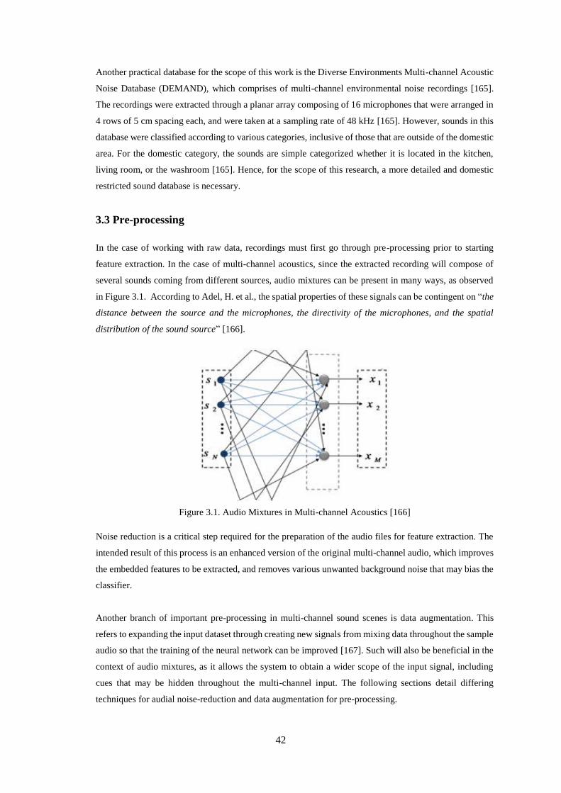
42

Another practical database for the scope of this work is the Diverse Environments Multi-channel Acoustic

Noise Database (DEMAND), which comprises of multi-channel environmental noise recordings [165].

The recordings were extracted through a planar array composing of 16 microphones that were arranged in

4 rows of 5 cm spacing each, and were taken at a sampling rate of 48 kHz [165]. However, sounds in this

database were classified according to various categories, inclusive of those that are outside of the domestic

area. For the domestic category, the sounds are simple categorized whether it is located in the kitchen,

living room, or the washroom [165]. Hence, for the scope of this research, a more detailed and domestic

restricted sound database is necessary.

3.3 Pre-processing

In the case of working with raw data, recordings must first go through pre-processing prior to starting

feature extraction. In the case of multi-channel acoustics, since the extracted recording will compose of

several sounds coming from different sources, audio mixtures can be present in many ways, as observed

in Figure 3.1. According to Adel, H. et al., the spatial properties of these signals can be contingent on “the

distance between the source and the microphones, the directivity of the microphones, and the spatial

distribution of the sound source” [166].

Figure 3.1. Audio Mixtures in Multi-channel Acoustics [166]

Noise reduction is a critical step required for the preparation of the audio files for feature extraction. The

intended result of this process is an enhanced version of the original multi-channel audio, which improves

the embedded features to be extracted, and removes various unwanted background noise that may bias the

classifier.

Another branch of important pre-processing in multi-channel sound scenes is data augmentation. This

refers to expanding the input dataset through creating new signals from mixing data throughout the sample

audio so that the training of the neural network can be improved [167]. Such will also be beneficial in the

context of audio mixtures, as it allows the system to obtain a wider scope of the input signal, including

cues that may be hidden throughout the multi-channel input. The following sections detail differing

techniques for audial noise-reduction and data augmentation for pre-processing.

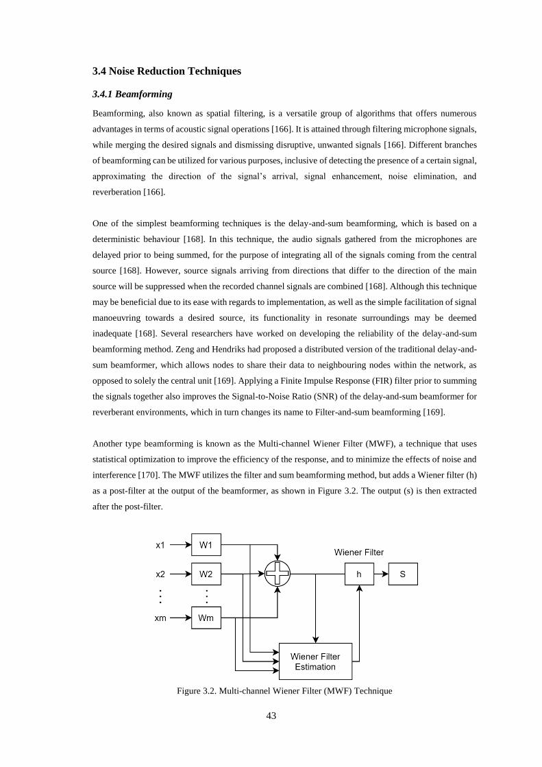
43

3.4 Noise Reduction Techniques

3.4.1 Beamforming

Beamforming, also known as spatial filtering, is a versatile group of algorithms that offers numerous

advantages in terms of acoustic signal operations [166]. It is attained through filtering microphone signals,

while merging the desired signals and dismissing disruptive, unwanted signals [166]. Different branches

of beamforming can be utilized for various purposes, inclusive of detecting the presence of a certain signal,

approximating the direction of the signal’s arrival, signal enhancement, noise elimination, and

reverberation [166].

One of the simplest beamforming techniques is the delay-and-sum beamforming, which is based on a

deterministic behaviour [168]. In this technique, the audio signals gathered from the microphones are

delayed prior to being summed, for the purpose of integrating all of the signals coming from the central

source [168]. However, source signals arriving from directions that differ to the direction of the main

source will be suppressed when the recorded channel signals are combined [168]. Although this technique

may be beneficial due to its ease with regards to implementation, as well as the simple facilitation of signal

manoeuvring towards a desired source, its functionality in resonate surroundings may be deemed

inadequate [168]. Several researchers have worked on developing the reliability of the delay-and-sum

beamforming method. Zeng and Hendriks had proposed a distributed version of the traditional delay-and-

sum beamformer, which allows nodes to share their data to neighbouring nodes within the network, as

opposed to solely the central unit [169]. Applying a Finite Impulse Response (FIR) filter prior to summing

the signals together also improves the Signal-to-Noise Ratio (SNR) of the delay-and-sum beamformer for

reverberant environments, which in turn changes its name to Filter-and-sum beamforming [169].

Another type beamforming is known as the Multi-channel Wiener Filter (MWF), a technique that uses

statistical optimization to improve the efficiency of the response, and to minimize the effects of noise and

interference [170]. The MWF utilizes the filter and sum beamforming method, but adds a Wiener filter (h)

as a post-filter at the output of the beamformer, as shown in Figure 3.2. The output (s) is then extracted

after the post-filter.

Figure 3.2. Multi-channel Wiener Filter (MWF) Technique

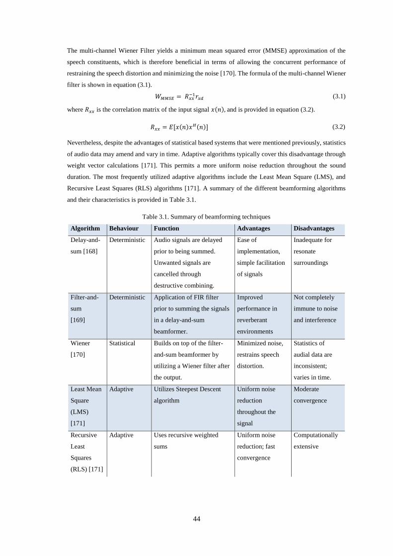
44

The multi-channel Wiener Filter yields a minimum mean squared error (MMSE) approximation of the

speech constituents, which is therefore beneficial in terms of allowing the concurrent performance of

restraining the speech distortion and minimizing the noise [170]. The formula of the multi-channel Wiener

filter is shown in equation (3.1).

𝑊𝑀𝑀𝑆𝐸 = 𝑅𝑥𝑥−1𝑟𝑥𝑑 (3.1)

where 𝑅𝑥𝑥 is the correlation matrix of the input signal 𝑥(𝑛), and is provided in equation (3.2).

𝑅𝑥𝑥 = 𝐸[𝑥(𝑛)𝑥𝐻(𝑛)] (3.2)

Nevertheless, despite the advantages of statistical based systems that were mentioned previously, statistics

of audio data may amend and vary in time. Adaptive algorithms typically cover this disadvantage through

weight vector calculations [171]. This permits a more uniform noise reduction throughout the sound

duration. The most frequently utilized adaptive algorithms include the Least Mean Square (LMS), and

Recursive Least Squares (RLS) algorithms [171]. A summary of the different beamforming algorithms

and their characteristics is provided in Table 3.1.

Table 3.1. Summary of beamforming techniques

Algorithm Behaviour Function Advantages Disadvantages

Delay-and-

sum [168]

Deterministic Audio signals are delayed

prior to being summed.

Unwanted signals are

cancelled through

destructive combining.

Ease of

implementation,

simple facilitation

of signals

Inadequate for

resonate

surroundings

Filter-and-

sum

[169]

Deterministic Application of FIR filter

prior to summing the signals

in a delay-and-sum

beamformer.

Improved

performance in

reverberant

environments

Not completely

immune to noise

and interference

Wiener

[170]

Statistical Builds on top of the filter-

and-sum beamformer by

utilizing a Wiener filter after

the output.

Minimized noise,

restrains speech

distortion.

Statistics of

audial data are

inconsistent;

varies in time.

Least Mean

Square

(LMS)

[171]

Adaptive Utilizes Steepest Descent

algorithm

Uniform noise

reduction

throughout the

signal

Moderate

convergence

Recursive

Least

Squares

(RLS) [171]

Adaptive Uses recursive weighted

sums

Uniform noise

reduction; fast

convergence

Computationally

extensive

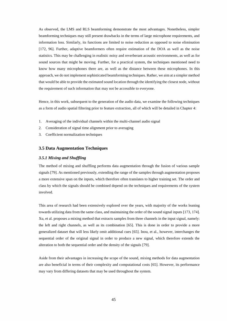
45

As observed, the LMS and RLS beamforming demonstrate the most advantages. Nonetheless, simpler

beamforming techniques may still present drawbacks in the terms of large microphone requirements, and

information loss. Similarly, its functions are limited to noise reduction as opposed to noise elimination

[172, 96]. Further, adaptive beamformers often require estimation of the DOA as well as the noise

statistics. This may be challenging in realistic noisy and reverberant acoustic environments, as well as for

sound sources that might be moving. Further, for a practical system, the techniques mentioned need to

know how many microphones there are, as well as the distance between these microphones. In this

approach, we do not implement sophisticated beamforming techniques. Rather, we aim at a simpler method

that would be able to provide the estimated sound location through the identifying the closest node, without

the requirement of such information that may not be accessible to everyone.

Hence, in this work, subsequent to the generation of the audio data, we examine the following techniques

as a form of audio spatial filtering prior to feature extraction, all of which will be detailed in Chapter 4:

1. Averaging of the individual channels within the multi-channel audio signal

2. Consideration of signal time alignment prior to averaging

3. Coefficient normalization techniques

3.5 Data Augmentation Techniques

3.5.1 Mixing and Shuffling

The method of mixing and shuffling performs data augmentation through the fusion of various sample

signals [79]. As mentioned previously, extending the range of the samples through augmentation proposes

a more extensive span on the inputs, which therefore often translates to higher training set. The order and

class by which the signals should be combined depend on the techniques and requirements of the system

involved.

This area of research had been extensively explored over the years, with majority of the works leaning

towards utilizing data from the same class, and maintaining the order of the sound signal inputs [173, 174].

Xu, et al. proposes a mixing method that extracts samples from three channels in the input signal, namely:

the left and right channels, as well as its combination [65]. This is done in order to provide a more

generalized dataset that will less likely omit additional cues [65]. Inou, et al., however, interchanges the

sequential order of the original signal in order to produce a new signal, which therefore extends the

alteration to both the sequential order and the density of the signals [79].

Aside from their advantages in increasing the scope of the sound, mixing methods for data augmentation

are also beneficial in terms of their complexity and computational costs [65]. However, its performance

may vary from differing datasets that may be used throughout the system.

46

3.6 Segmentation and Pre-processing Technique for Proposed System

Making the suitable choice for a pre-processing technique for our proposed system is highly dependent on

the application that the classifier is being used for, as well as the quality of the recordings, and the type of

microphones used for the dataset. For the initial stages of this work, the implementation phase was

accommodated through readily available domestic acoustic dataset provided by the Sound Interfacing

through the Swarm (SINS) database [163].

This composes of 10-second audio files that have been developed to aid researchers participating in the

DCASE 2018 Task 5-challenge, with the aim of detecting and classifying common household tasks [144].

Each sample in the dataset represents four individual channels, as the recordings were made through an

ASN consisting of 13 nodes with 4 microphones each [163]. However, audio data available in the database

were taken from the first four nodes of the 13-node setup, as per Figure 3.3. Sampling is done at 16 kHz

frequency with a bit depth of 12 [163].

Figure 3.3. Node Location Setup for SINS database Recordings [163],

with an example of a Dishwashing sound source

This database allows a 9-level sound classification consisting of the following categories: Absence,

Cooking, Eating, Dishwashing, Watching TV, Vacuuming, Movement, Social Activities, and Other

Activities. Similarly, it permits a 4-level source node estimation, as both the SINS development and

evaluation datasets consist of recordings from Nodes 1-4. A summary of the SINS dataset is seen in Table

3.2.

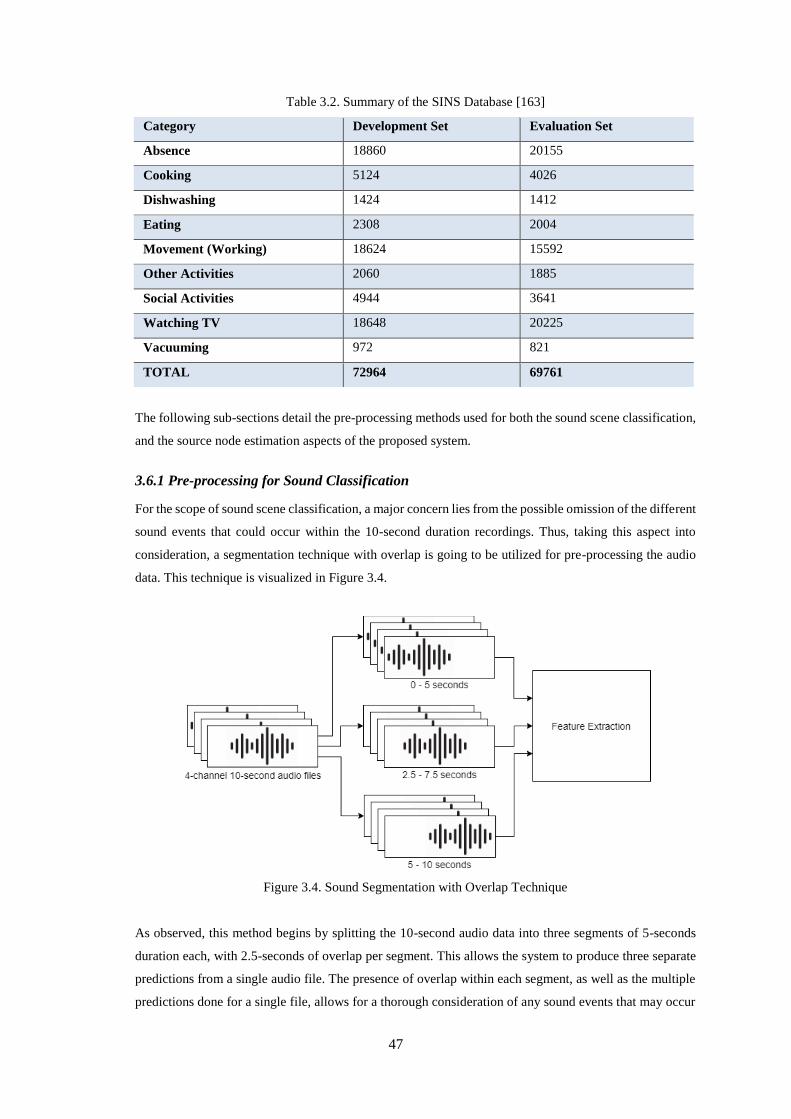
47

Table 3.2. Summary of the SINS Database [163]

Category Development Set Evaluation Set

Absence 18860 20155

Cooking 5124 4026

Dishwashing 1424 1412

Eating 2308 2004

Movement (Working) 18624 15592

Other Activities 2060 1885

Social Activities 4944 3641

Watching TV 18648 20225

Vacuuming 972 821

TOTAL 72964 69761

The following sub-sections detail the pre-processing methods used for both the sound scene classification,

and the source node estimation aspects of the proposed system.

3.6.1 Pre-processing for Sound Classification

For the scope of sound scene classification, a major concern lies from the possible omission of the different

sound events that could occur within the 10-second duration recordings. Thus, taking this aspect into

consideration, a segmentation technique with overlap is going to be utilized for pre-processing the audio

data. This technique is visualized in Figure 3.4.

Figure 3.4. Sound Segmentation with Overlap Technique

As observed, this method begins by splitting the 10-second audio data into three segments of 5-seconds

duration each, with 2.5-seconds of overlap per segment. This allows the system to produce three separate

predictions from a single audio file. The presence of overlap within each segment, as well as the multiple

predictions done for a single file, allows for a thorough consideration of any sound events that may occur

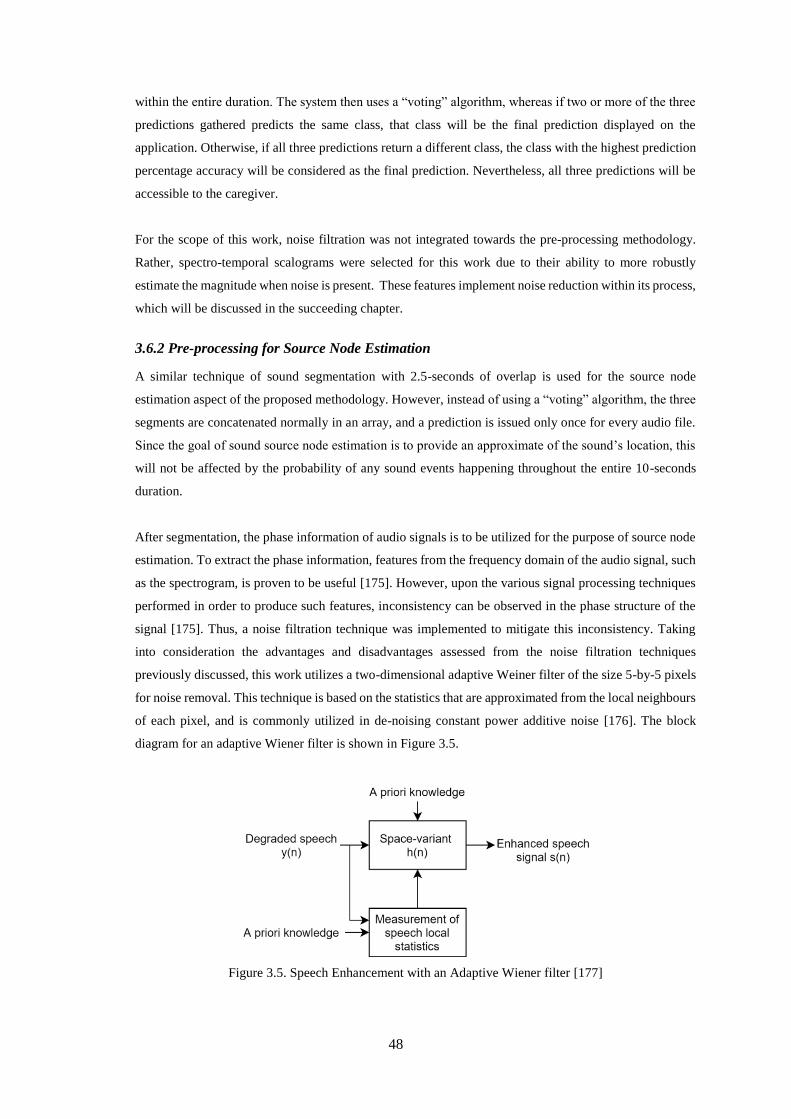
48

within the entire duration. The system then uses a “voting” algorithm, whereas if two or more of the three

predictions gathered predicts the same class, that class will be the final prediction displayed on the

application. Otherwise, if all three predictions return a different class, the class with the highest prediction

percentage accuracy will be considered as the final prediction. Nevertheless, all three predictions will be

accessible to the caregiver.

For the scope of this work, noise filtration was not integrated towards the pre-processing methodology.

Rather, spectro-temporal scalograms were selected for this work due to their ability to more robustly

estimate the magnitude when noise is present. These features implement noise reduction within its process,

which will be discussed in the succeeding chapter.

3.6.2 Pre-processing for Source Node Estimation

A similar technique of sound segmentation with 2.5-seconds of overlap is used for the source node

estimation aspect of the proposed methodology. However, instead of using a “voting” algorithm, the three

segments are concatenated normally in an array, and a prediction is issued only once for every audio file.

Since the goal of sound source node estimation is to provide an approximate of the sound’s location, this

will not be affected by the probability of any sound events happening throughout the entire 10-seconds

duration.

After segmentation, the phase information of audio signals is to be utilized for the purpose of source node

estimation. To extract the phase information, features from the frequency domain of the audio signal, such

as the spectrogram, is proven to be useful [175]. However, upon the various signal processing techniques

performed in order to produce such features, inconsistency can be observed in the phase structure of the

signal [175]. Thus, a noise filtration technique was implemented to mitigate this inconsistency. Taking

into consideration the advantages and disadvantages assessed from the noise filtration techniques

previously discussed, this work utilizes a two-dimensional adaptive Weiner filter of the size 5-by-5 pixels

for noise removal. This technique is based on the statistics that are approximated from the local neighbours

of each pixel, and is commonly utilized in de-noising constant power additive noise [176]. The block

diagram for an adaptive Wiener filter is shown in Figure 3.5.

Figure 3.5. Speech Enhancement with an Adaptive Wiener filter [177]

49

As observed, the adaptive Wiener filter bases the enhanced speech signal (with an improved SNR) on the

local statistics of the original speech signal [177]. The pixel-wise adaptive property also contradicts the

inconsistency found in the statistics of audial data experienced when the statistical Weiner filter is used

[177].

3.7 Development of the DASEE Synthetic Database

Although the SINS database is sufficient to conduct an initial experiment, and to test the effectiveness of

the proposed system in terms of sound classification, there are several limitations to this, especially when

conducting an in-depth analysis of the system performance. Firstly, the data provided publicly are extracted

solely from the first four receiver nodes of the 13-node setup [163]. Each node consists of a linear array

four microphones with individual channel sampling. The four nodes are also located only along the living

room and kitchen areas, which extensively limits the scope of the area. Further, it also poses a challenge

on covering sound categories that are deemed dangerous to the residents. Similarly, the exact locations of

the sound sources are not provided in the database.

Synthesizing a new database allows including data that address these issues and include additional

disruptive sounds commonly faced in a dementia resident’s environment. Further, it also allows to recreate

scenarios that could occur in real-world settings, including noisy environments, and various source-to-

receiver distances. Furthermore, this will also provide the exact locations of the sound sources, which will

be useful for sound location estimation purposes. This section details important information regarding the

process undertaken for synthesizing a database, which we call the Domestic Acoustic Sounds and Events

in the Environment of dementia residents (DASEE) dataset.

3.7.1 Data Curation

The developed database promotes domestic acoustic events and scenes likely to happen in a realistic

dementia resident care facility. Monitoring disruptive noises for dementia residents can be challenging,

even for healthcare professionals, as sound levels acceptable to staff may be distressing for dementia

residents. This is due to the fact that dementia may worsen the effects of sensory changes, as the

progressive nature of this ailment may alter how the resident perceives external stimuli, such as acoustic

noise pollution [178]. A summary of possible negative impacts caused by disruptive noise levels to

dementia residents is provided as follows:

- As hearing is linked to balance, aural disruption could lead to greater risks of falls, either through loss

of balance [179], or through an increase in disorientation as a result of people trying to orientate

themselves in an overstimulating environment [178].

- It has been proven that dementia residents respond on a more sensory level, rather than intellectually.

For example, they note the body language or tone of voice, rather than what people actually say [180].

Since people with dementia have a reduced ability to understand their sensory environment, when

combined with age-related deterioration in hearing, it can be overwhelming.

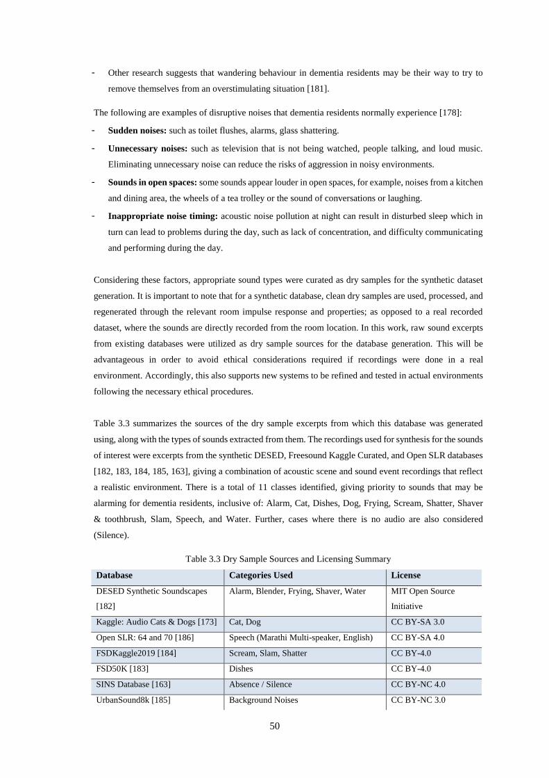
50

- Other research suggests that wandering behaviour in dementia residents may be their way to try to

remove themselves from an overstimulating situation [181].

The following are examples of disruptive noises that dementia residents normally experience [178]:

- Sudden noises: such as toilet flushes, alarms, glass shattering.

- Unnecessary noises: such as television that is not being watched, people talking, and loud music.

Eliminating unnecessary noise can reduce the risks of aggression in noisy environments.

- Sounds in open spaces: some sounds appear louder in open spaces, for example, noises from a kitchen

and dining area, the wheels of a tea trolley or the sound of conversations or laughing.

- Inappropriate noise timing: acoustic noise pollution at night can result in disturbed sleep which in

turn can lead to problems during the day, such as lack of concentration, and difficulty communicating

and performing during the day.

Considering these factors, appropriate sound types were curated as dry samples for the synthetic dataset

generation. It is important to note that for a synthetic database, clean dry samples are used, processed, and

regenerated through the relevant room impulse response and properties; as opposed to a real recorded

dataset, where the sounds are directly recorded from the room location. In this work, raw sound excerpts

from existing databases were utilized as dry sample sources for the database generation. This will be

advantageous in order to avoid ethical considerations required if recordings were done in a real

environment. Accordingly, this also supports new systems to be refined and tested in actual environments

following the necessary ethical procedures.

Table 3.3 summarizes the sources of the dry sample excerpts from which this database was generated

using, along with the types of sounds extracted from them. The recordings used for synthesis for the sounds

of interest were excerpts from the synthetic DESED, Freesound Kaggle Curated, and Open SLR databases

[182, 183, 184, 185, 163], giving a combination of acoustic scene and sound event recordings that reflect

a realistic environment. There is a total of 11 classes identified, giving priority to sounds that may be

alarming for dementia residents, inclusive of: Alarm, Cat, Dishes, Dog, Frying, Scream, Shatter, Shaver

& toothbrush, Slam, Speech, and Water. Further, cases where there is no audio are also considered

(Silence).

Table 3.3 Dry Sample Sources and Licensing Summary

Database Categories Used License

DESED Synthetic Soundscapes

[182]

Alarm, Blender, Frying, Shaver, Water MIT Open Source

Initiative

Kaggle: Audio Cats & Dogs [173] Cat, Dog CC BY-SA 3.0

Open SLR: 64 and 70 [186] Speech (Marathi Multi-speaker, English) CC BY-SA 4.0

FSDKaggle2019 [184] Scream, Slam, Shatter CC BY-4.0

FSD50K [183] Dishes CC BY-4.0

SINS Database [163] Absence / Silence CC BY-NC 4.0

UrbanSound8k [185] Background Noises CC BY-NC 3.0

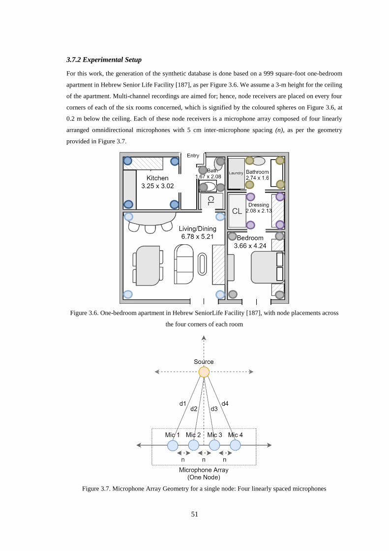
51

3.7.2 Experimental Setup

For this work, the generation of the synthetic database is done based on a 999 square-foot one-bedroom

apartment in Hebrew Senior Life Facility [187], as per Figure 3.6. We assume a 3-m height for the ceiling

of the apartment. Multi-channel recordings are aimed for; hence, node receivers are placed on every four

corners of each of the six rooms concerned, which is signified by the coloured spheres on Figure 3.6, at

0.2 m below the ceiling. Each of these node receivers is a microphone array composed of four linearly

arranged omnidirectional microphones with 5 cm inter-microphone spacing (n), as per the geometry

provided in Figure 3.7.

Figure 3.6. One-bedroom apartment in Hebrew SeniorLife Facility [187], with node placements across

the four corners of each room

Figure 3.7. Microphone Array Geometry for a single node: Four linearly spaced microphones

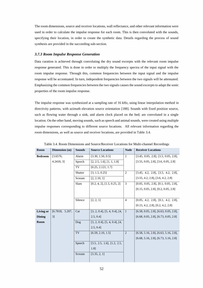
52

The room dimensions, source and receiver locations, wall reflectance, and other relevant information were

used in order to calculate the impulse response for each room. This is then convoluted with the sounds,

specifying their location, in order to create the synthetic data. Details regarding the process of sound

synthesis are provided in the succeeding sub-section.

3.7.3 Room Impulse Response Generation

Data curation is achieved through convoluting the dry sound excerpts with the relevant room impulse

response generated. This is done in order to multiply the frequency spectra of the input signal with the

room impulse response. Through this, common frequencies between the input signal and the impulse

response will be accentuated. In turn, independent frequencies between the two signals will be attenuated.

Emphasizing the common frequencies between the two signals causes the sound excerpts to adapt the sonic

properties of the room impulse response.

The impulse response was synthesized at a sampling rate of 16 kHz, using linear interpolation method in

directivity patterns, with azimuth elevation source orientation [188]. Sounds with fixed position source,

such as flowing water through a sink, and alarm clock placed on the bed; are convoluted in a single

location. On the other hand, moving sounds, such as speech and animal sounds, were created using multiple

impulse responses corresponding to different source locations. All relevant information regarding the

room dimensions, as well as source and receiver locations, are provided in Table 3.4.

Table 3.4. Room Dimensions and Source/Receiver Locations for Multi-channel Recordings

Room Dimension (m) Sounds Source Locations Node Receiver Locations

Bedroom [3.6576,

4.2418, 3]

Alarm [3.30, 1.50, 0.5] 1 [3.45, 0.05, 2.8], [3.5, 0.05, 2.8],

[3.55, 0.05, 2.8], [3.6, 0.05, 2.8] Speech [2, 2.5, 1.6], [1, 1, 1.8]

TV [0.25, 2.121, 1.7]

Shatter [3, 1.5, 0.25] 2 [3.45, 4.2, 2.8], [3.5, 4.2, 2.8],

[3.55, 4.2, 2.8], [3.6, 4.2, 2.8] Scream [2, 2.10, 1]

Slam [0.2, 4, 2], [1.5, 0.25, 2] 3 [0.05, 0.05, 2.8], [0.1, 0.05, 2.8],

[0.15, 0.05, 2.8], [0.2, 0.05, 2.8]

Silence [2, 2, 1] 4 [0.05, 4.2, 2.8], [0.1, 4.2, 2.8],

[0.15, 4.2, 2.8], [0.2, 4.2, 2.8]

Living or

Dining

Room

[6.7818, 5.207,

3]

Cat [3, 2, 0.4], [5, 4, 0.4], [4,

2.5, 0.4]

1 [6.58, 0.05, 2.8], [6.63, 0.05, 2.8],

[6.68, 0.05, 2.8], [6.73, 0.05, 2.8]

Dog [3, 2, 0.4], [5, 4, 0.4], [4,

2.5, 0.4]

TV [6.59, 2.10, 1.5] 2 [6.58, 5.16, 2.8], [6.63, 5.16, 2.8],

[6.68, 5.16, 2.8], [6.73, 5.16, 2.8]

Speech [3.5, 2.5, 1.6], [1.2, 2.5,

1.8]

Scream [3.35, 2, 1]

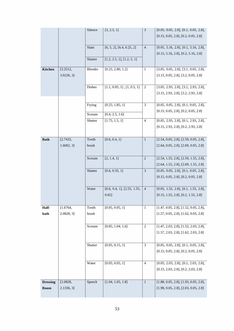
53

Silence [3, 2.5, 1] 3 [0.05, 0.05, 2.8], [0.1, 0.05, 2.8],

[0.15, 0.05, 2.8], [0.2, 0.05, 2.8]

Slam [6, 5, 2], [6.4, 0.25, 2] 4 [0.05, 5.16, 2.8], [0.1, 5.16, 2.8],

[0.15, 5.16, 2.8], [0.2, 5.16, 2.8]

Shatter [1.2, 2.5, 1], [1.2, 5, 1]

Kitchen [3.2512,

3.0226, 3]

Blender [0.25, 2.80, 1.2] 1 [3.05, 0.05, 2.8], [3.1, 0.05, 2.8],

[3.15, 0.05, 2.8], [3.2, 0.05, 2.8]

Dishes [1.1, 0.05, 1] , [1, 0.5, 1] 2 [3.05, 2.93, 2.8], [3.1, 2.93, 2.8],

[3.15, 2.93, 2.8], [3.2, 2.93, 2.8]

Frying [0.25, 1.85, 1] 3 [0.05, 0.05, 2.8], [0.1, 0.05, 2.8],

[0.15, 0.05, 2.8], [0.2, 0.05, 2.8] Scream [0.4, 2.5, 1.6]

Shatter [1.75, 1.5, 1] 4 [0.05, 2.93, 2.8], [0.1, 2.93, 2.8],

[0.15, 2.93, 2.8], [0.2, 2.93, 2.8]

Bath [2.7432,

1.6002, 3]

Tooth

brush

[0.6, 0.4, 1] 1 [2.54, 0.05, 2.8], [2.59, 0.05, 2.8],

[2.64, 0.05, 2.8], [2.69, 0.05, 2.8]

Scream [2, 1.4, 1] 2 [2.54, 1.55, 2.8], [2.59, 1.55, 2.8],

[2.64, 1.55, 2.8], [2.69, 1.55, 2.8]

Shatter [0.6, 0.35, 1] 3 [0.05, 0.05, 2.8], [0.1, 0.05, 2.8],

[0.15, 0.05, 2.8], [0.2, 0.05, 2.8]

Water [0.6, 0.4, 1], [2.55, 1.55,

0.65]

4 [0.05, 1.55, 2.8], [0.1, 1.55, 2.8],

[0.15, 1.55, 2.8], [0.2, 1.55, 2.8]

Half-

bath

[1.6764,

2.0828, 3]

Tooth

brush

[0.05, 0.05, 1] 1 [1.47, 0.05, 2.8], [1.52, 0.05, 2.8],

[1.57, 0.05, 2.8], [1.62, 0.05, 2.8]

Scream [0.85, 1.04, 1.6] 2 [1.47, 2.03, 2.8], [1.52, 2.03, 2.8],

[1.57, 2.03, 2.8], [1.62, 2.03, 2.8]

Shatter [0.05, 0.15, 1] 3 [0.05, 0.05, 2.8], [0.1, 0.05, 2.8],

[0.15, 0.05, 2.8], [0.2, 0.05, 2.8]

Water [0.05, 0.05, 1]

4 [0.05, 2.03, 2.8], [0.1, 2.03, 2.8],

[0.15, 2.03, 2.8], [0.2, 2.03, 2.8]

Dressing

Room

[2.0828,

2.1336, 3]

Speech [1.04, 1.05, 1.8] 1 [1.88, 0.05, 2.8], [1.93, 0.05, 2.8],

[1.98, 0.05, 2.8], [2.03, 0.05, 2.8]

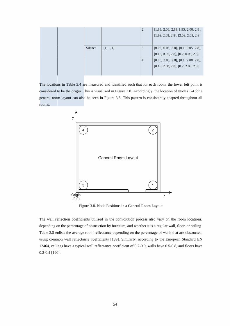
54

2 [1.88, 2.08, 2.8],[1.93, 2.08, 2.8],

[1.98, 2.08, 2.8], [2.03, 2.08, 2.8]

Silence [1, 1, 1] 3 [0.05, 0.05, 2.8], [0.1, 0.05, 2.8],

[0.15, 0.05, 2.8], [0.2, 0.05, 2.8]

4 [0.05, 2.08, 2.8], [0.1, 2.08, 2.8],

[0.15, 2.08, 2.8], [0.2, 2.08, 2.8]

The locations in Table 3.4 are measured and identified such that for each room, the lower left point is

considered to be the origin. This is visualized in Figure 3.8. Accordingly, the location of Nodes 1-4 for a

general room layout can also be seen in Figure 3.8. This pattern is consistently adapted throughout all

rooms.

Figure 3.8. Node Positions in a General Room Layout

The wall reflection coefficients utilized in the convolution process also vary on the room locations,

depending on the percentage of obstruction by furniture, and whether it is a regular wall, floor, or ceiling.

Table 3.5 enlists the average room reflectance depending on the percentage of walls that are obstructed,

using common wall reflectance coefficients [189]. Similarly, according to the European Standard EN

12464, ceilings have a typical wall reflectance coefficient of 0.7-0.9, walls have 0.5-0.8, and floors have

0.2-0.4 [190].

55

Table 3.5. Average room reflectance for varying wall reflectance and obstruction percentages [189]

Walls Obstructed Wall Reflectance

0.2 0.3 0.4 0.5 0.6 0.7 0.8

20 0.475 0.505 0.535 0.565 0.596 0.626 0.656

30 0.488 0.515 0.541 0.569 0.594 0.620 0.647

40 0.502 0.524 0.547 0.570 0.592 0.615 0.638

50 0.515 0.534 0.553 0.572 0.591 0.610 0.628

60 0.529 0.544 0.559 0.574 0.589 0.604 0.619

70 0.542 0.553 0.565 0.576 0.587 0.599 0.610

80 0.555 0.563 0.571 0.578 0.586 0.593 0.601

According to these guidelines, taking into consideration the wall type and obstruction percentages, the

wall reflectance coefficients utilized in the setup for the generation of the room impulse response are seen

in Table 3.6. The same wall reflectance coefficient was used for the four sides of the walls, and different

coefficients were used for the ceiling, and the floor, as per the European Standard EN [190].

Table 3.6. Wall Reflectance Coefficients Used

Room Reflectance Obstruction Reflectance Utilized

Bedroom Walls – 0.5

Ceiling – 0.7

Floor – 0.2

Walls – 30, 50, 70, 30

Ceiling – 0

Floor – 30

Walls – 0.568, 0.572, 0.576, 0.568

Ceiling – 0.7

Floor - 0.488

Living or Dining Walls – 0.5

Ceiling – 0.7

Floor – 0.2

Walls – 30, 50, 50, 20

Ceiling – 0

Floor – 30

Walls – 0.568, 0.572, 0.572, 0.568

Ceiling – 0.7

Floor – 0.488

Kitchen Walls – 0.6

Ceiling – 0.8

Floor – 0.3

Walls – 30, 30, 30, 30

Ceiling – 0

Floor – 20

Walls – 0.594, 0.594, 0.594, 0.594

Ceiling – 0.8

Floor – 0.515

Bath Walls – 0.7

Ceiling – 0.8

Floor – 0.4

Walls – 20, 30, 0, 0

Ceiling – 0

Floor – 30

Walls – 0.626, 0.62, 0.7, 0.7

Ceiling – 0.8

Floor – 0.541

Half-bath Walls – 0.7

Ceiling – 0.8

Floor – 0.4

Walls – 20, 20, 0, 0

Ceiling – 0

Floor – 30

Walls – 0.626, 0.626, 0.7, 0.7

Ceiling – 0.8

Floor – 0.541

Dressing Room Walls – 0.5

Ceiling – 0.7

Floor – 0.2

Walls – 80, 80, 20, 20

Ceiling – 0

Floor - 30

Walls – 0.578, 0.578, 0.565, 0.565

Ceiling – 0.7

Floor – 0.488

Based on the provided information, the room impulse responses are calculated following the image method

for simulating rectangular room acoustics [191]. Aside from the sound source and the nodes locations, the

room dimensions and wall obstruction and reflectance coefficients are also necessary components to be

considered during the room reverberation study. The calculated room impulse response results from a

series of image pulses received at various time delays, compiled into a histogram. The width of every bin

within the histogram is equivalent to the sampling period, which is identified through the maximum

frequency to be represented [191].

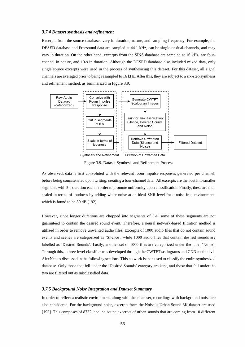
56

3.7.4 Dataset synthesis and refinement

Excerpts from the source databases vary in duration, nature, and sampling frequency. For example, the

DESED database and Freesound data are sampled at 44.1 kHz, can be single or dual channels, and may

vary in duration. On the other hand, excerpts from the SINS database are sampled at 16 kHz, are four-

channel in nature, and 10-s in duration. Although the DESED database also included mixed data, only

single source excerpts were used in the process of synthesizing this dataset. For this dataset, all signal

channels are averaged prior to being resampled to 16 kHz. After this, they are subject to a six-step synthesis

and refinement method, as summarized in Figure 3.9.

Figure 3.9. Dataset Synthesis and Refinement Process

As observed, data is first convoluted with the relevant room impulse responses generated per channel,

before being concatenated upon writing, creating a four-channel data. All excerpts are then cut into smaller

segments with 5-s duration each in order to promote uniformity upon classification. Finally, these are then

scaled in terms of loudness by adding white noise at an ideal SNR level for a noise-free environment,

which is found to be 80 dB [192].

However, since longer durations are chopped into segments of 5-s, some of these segments are not

guaranteed to contain the desired sound event. Therefore, a neural network-based filtration method is

utilized in order to remove unwanted audio files. Excerpts of 1000 audio files that do not contain sound

events and scenes are categorized as ‘Silence’, while 1000 audio files that contain desired sounds are

labelled as ‘Desired Sounds’. Lastly, another set of 1000 files are categorized under the label ‘Noise’.

Through this, a three-level classifier was developed through the CWTFT scalograms and CNN method via

AlexNet, as discussed in the following sections. This network is then used to classify the entire synthesized

database. Only those that fell under the ‘Desired Sounds’ category are kept, and those that fall under the

two are filtered out as misclassified data.

3.7.5 Background Noise Integration and Dataset Summary

In order to reflect a realistic environment, along with the clean set, recordings with background noise are

also considered. For the background noise, excerpts from the Noiseus Urban Sound 8K dataset are used

[193]. This composes of 8732 labelled sound excerpts of urban sounds that are coming from 10 different

57

classes, including: Air conditioner, car horn, children playing, dog barking, drilling, engine idling, gun

shot, jackhammer, siren, and street music. For this experiment, data from the noise sounds that are more

relevant for a dementia resident’s environment is utilized. This include: air conditioner, children playing,

and street music. Aside from this, white noise is also added as background noise for some of the files.

To add the background noise to the sound, the noise files are also resampled from 44 kHz to 16 kHz, and

cut in durations of 5 seconds, in order to match the synthetically generated clean dataset. Accordingly,

they are also convoluted with the relevant room impulse responses before being added to the clean data.

The relevant information regarding the background noise locations within each room is presented in Table

3.7. Background noise are added at different Signal-to-Noise (SNR) levels: 15 dB, 20 dB, and 25 dB,

respectively.

Table 3.7. Room Dimensions and Source/Receiver Locations for Background Noises

Room Dimensions (m) Background

Noise

Source

Locations

Nodes Receiver Locations

Bedroom [3.6576, 4.2418,

3]

AC [3.1, 3.8, 2] 1 [3.45, 0.05, 2.8], [3.5, 0.05,

2.8], [3.55, 0.05, 2.8], [3.6,

0.05, 2.8]

Children [1.75, 0.05,

1.25]

2 [3.45, 4.2, 2.8], [3.5, 4.2,

2.8], [3.55, 4.2, 2.8], [3.6,

4.2, 2.8]

Street Music [1.75, 0.05,

1.25]

3 [0.05, 0.05, 2.8], [0.1, 0.05,

2.8], [0.15, 0.05, 2.8], [0.2,

0.05, 2.8]

4 [0.05, 4.2, 2.8], [0.1, 4.2,

2.8], [0.15, 4.2, 2.8], [0.2,

4.2, 2.8]

Living or

Dining

Room

[6.7818, 5.207,

3]

AC [6.1, 0.45, 2] 1 [6.58, 0.05, 2.8], [6.63,

0.05, 2.8], [6.68, 0.05, 2.8],

[6.73, 0.05, 2.8]

Children [4.5, 0.05, 1.25] 2 [6.58, 5.16, 2.8], [6.63,

5.16, 2.8], [6.68, 5.16, 2.8],

[6.73, 5.16, 2.8]

Street Music [4.5, 0.05, 1.25] 3 [0.05, 0.05, 2.8], [0.1, 0.05,

2.8], [0.15, 0.05, 2.8], [0.2,

0.05, 2.8]

4 [0.05, 5.16, 2.8], [0.1, 5.16,

2.8], [0.15, 5.16, 2.8], [0.2,

5.16, 2.8]

Kitchen [3.2512, 3.0226,

3]

AC [0.45, 0.45, 2] 1 [3.05, 0.05, 2.8], [3.1, 0.05,

2.8], [3.15, 0.05, 2.8], [3.2,

0.05, 2.8]

Children [3.1, 1.5, 1.25] 2 [3.05, 2.93, 2.8], [3.1, 2.93,

2.8], [3.15, 2.93, 2.8], [3.2,

2.93, 2.8]

58

Street Music [3.1, 1.5, 1.25] 3 [0.05, 0.05, 2.8], [0.1, 0.05,

2.8], [0.15, 0.05, 2.8], [0.2,

0.05, 2.8]

4 [0.05, 2.93, 2.8], [0.1, 2.93,

2.8], [0.15, 2.93, 2.8], [0.2,

2.93, 2.8]

Bath [2.7432, 1.6002,

3]

AC [1.25, 0.05, 2] 1 [2.54, 0.05, 2.8], [2.59,

0.05, 2.8], [2.64, 0.05, 2.8],

[2.69, 0.05, 2.8]

Children [1.3, 0.05, 1.5] 2 [2.54, 1.55, 2.8], [2.59,

1.55, 2.8], [2.64, 1.55, 2.8],

[2.69, 1.55, 2.8]

Street Music

[1.3, 0.05, 1.5] 3 [0.05, 0.05, 2.8], [0.1, 0.05,

2.8], [0.15, 0.05, 2.8], [0.2,

0.05, 2.8]

4 [0.05, 1.55, 2.8], [0.1, 1.55,

2.8], [0.15, 1.55, 2.8], [0.2,

1.55, 2.8]

Half-bath [1.6764, 2.0828,

3]

AC [0.05, 1.8, 2] 1 [1.47, 0.05, 2.8], [1.52,

0.05, 2.8], [1.57, 0.05, 2.8],

[1.62, 0.05, 2.8]

Children [0.05, 1.7, 1.5] 2 [1.47, 2.03, 2.8], [1.52,

2.03, 2.8], [1.57, 2.03, 2.8],

[1.62, 2.03, 2.8]

Street Music [0.05, 1.7, 1.5] 3 [0.05, 0.05, 2.8], [0.1, 0.05,

2.8], [0.15, 0.05, 2.8], [0.2,

0.05, 2.8]

4 [0.05, 2.03, 2.8], [0.1, 2.03,

2.8], [0.15, 2.03, 2.8], [0.2,

2.03, 2.8]

Dressing

Room

[2.0828, 2.1336,

3]

AC [1.45, 1.45, 2] 1 [1.88, 0.05, 2.8], [1.93,

0.05, 2.8], [1.98, 0.05, 2.8],

[2.03, 0.05, 2.8]

2 [1.88, 2.08, 2.8],[1.93,

2.08, 2.8], [1.98, 2.08, 2.8],

[2.03, 2.08, 2.8]

Children [1, 0.05, 1.5]

3 [0.05, 0.05, 2.8], [0.1, 0.05,

2.8], [0.15, 0.05, 2.8], [0.2,

0.05, 2.8]

4 [0.05, 2.08, 2.8], [0.1, 2.08,

2.8], [0.15, 2.08, 2.8], [0.2,

2.08, 2.8]

Street Music [1, 0.05, 1.5]

59

3.7.6 Curating an Unbiased Dataset

The data generated must be curated into verified training and testing sets, ensuring that several instances

of the testing data do not exist within the training data. This is done in order to overcome the risks of

biasing and overfitting the network, which occurs when the network performs exceedingly well solely for

the particular dataset. This often occurs when the statistical model consists of abundant parameters that

are more than what can be accounted by the data [194].

Although splitting the data randomly between the training and the testing set can help overcome this

potential, it may still be risky due to the several instances of each sound that occur in the dataset, as per

Figure 3.10. The dataset developed contains recordings from the four different nodes across each room.

Further, there are 4 instances of these from the addition of the noises for the same sound at 3 different SNR

levels. Hence, the curation of the data into training and testing sets follow the algorithm specified in Figure

3.10.

Figure 3.10. Training and Testing Data Curation Process

Hence, as per Figure 3.10, the training and testing sets were constructed in such a way that it avoids the

chances of overfitting. Basically, each node is assigned with one of each specific noise levels, while the

fourth node is assigned with the clean signal. This ensures that even when the same sound is being recorded

by the four nodes present, it reduces the chances of biasing through the addition of different types of noise

at different SNR levels. Further, this is also designed to reflect real life recordings, where the sound from

different microphones may differ based on their distance to the source, and other sounds present in their

surroundings.

Overall, this data is curated such that the testing data consists of one noise level for each node. Any

instances of the data contained in the test set is then removed from the training data. The testing set content

is summarized as, for a specific sound being recorded at four nodes:

60

Node 1: Clean Signal with 15 dB Noise

Node 2: Clean Signal with 20 dB Noise

Node 3: Clean Signal with 25 dB Noise

Node 4: Clean Signal

Following this curation process, the summary of the dataset generated can be seen in Table 3.8. Two sets

of training and testing data are generated for cross-validation purposes. From these two sets, the first set

was generated such that raw sound segments that are shorter than 5-seconds in duration are repeated until

5-seconds is completed. On the other hand, the second set is constructed such that raw sound segments

with a duration of less than 5-seconds are appended with ‘silence’ until the 5-second duration is completed.

This way, system performance can be trained and assessed both in repetitive sound cases, as well as single

instances of sound within a specific duration.

It is important to note that all instances of any recording that exists in the test set has been removed from

the training set. For this reason, some of the data in various folders became too small. Hence, the categories

“Dishes” and “Frying” have been combined into one folder called “Kitchen Activities”. Despite the

changes made, this gets rid of potential biasing and overfitting, which will be helpful for the robustness of

our training results. Furthermore, this also helps get a fairer comparison between different networks,

provided that they all use the same training and testing set, instead of a randomized 80-20 split.

Table 3.8. Summary of the Unbiased Sound Classification Dataset

Category Train (Set 1) Test (Set 1) Train (Set 2) Test (Set 2)

Absence / Silence 11286 876 11286 876

Alarm 2765 260 2192 192

Cat 11724 1080 3264 192

Dog 6673 792 1584 192

Kitchen_Activities 12291 1062 7136 524

Scream 4308 376 784 192

Shatter 2877 370 896 192

Shaver_toothbrush 11231 1077 3664 192

Slam 1565 268 880 192

Speech 30113 2374 13810 2374

Water 6796 829 2208 192

TOTAL 101629 9364 47686 5310

As observed, audio classes used in the generation of this database focus on sound events and scenes that

often occur, or require an urgent response, in dementia residents’ environment. Further, this has also been

generated through the room impulse responses of the HebrewLife Senior Facility [187], in order to reflect

a realistic resident environment. This is because assistance monitoring systems are real-world applications

of deep-learning audio classifiers, such as the work presented in this thesis. Nonetheless, this can also be

extended to other application domains.

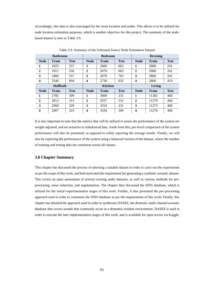
61

Accordingly, this data is also rearranged by the room location and nodes. This allows it to be utilized for

node location estimation purposes, which is another objective for this project. The summary of the node-

based dataset is seen in Table 3.9.

Table 3.9. Summary of the Unbiased Source Node Estimation Dataset

Bathroom Bedroom Dressing

Node Train Test Node Train Test Node Train Test

1 1923 557 1 2660 663 1 2868 241

2 1911 556 2 2670 663 2 2868 241

3 2484 557 3 2678 763 3 2868 241

4 2346 894 4 2730 635 4 2868 419

Halfbath Kitchen Living

Node Train Test Node Train Test Node Train Test

1 2785 309 1 3000 231 1 11282 468

2 2813 313 2 2937 231 2 11279 468

3 2960 329 3 3554 231 3 11273 468

4 2907 323 4 3556 369 4 11276 468

It is also important to note that the metrics that will be utilized to assess the performance of the system are

weight-adjusted, and are sensitive to imbalanced data. Aside from this, per-level comparison of the system

performance will also be presented, as opposed to solely reporting the average results. Finally, we will

also be exploring the performance of the system using a balanced version of the dataset, where the number

of training and testing data are consistent across all classes.

3.8 Chapter Summary

This chapter has discussed the process of selecting a suitable dataset in order to carry out the experiments

as per the scope of this work, and had motivated the requirement for generating a synthetic acoustic dataset.

This covers an open assessment of several existing audio datasets, as well as various methods for pre-

processing, noise reduction, and segmentation. The chapter then discussed the SINS database, which is

utilized for the initial experimentation stages of this work. Further, it also presented the pre-processing

approach used in order to customize the SINS database as per the requirements of this work. Finally, this

chapter has detailed the approach used in order to synthesize DASEE, the domestic multi-channel acoustic

database that covers sounds that commonly occur in a dementia resident environment. DASEE is used in

order to execute the later implementation stages of this work, and is available for open access via Kaggle.

62

Features for Audio Classification and Source Location Estimation

4.1 Introduction

In relation to the general flowchart of a sound classification and source node location system displayed in

Figure 2.1, this chapter is split into two main sections, whichassess the feature extraction techniques, and

the performance evaluation of the different features considered for the two main components: audio

classification (Section 4.2) and source node location estimation (Section 4.3). Audio classification is

typically achieved by extracting discriminative features that represent the underlying common

characteristics of audio signals belonging to the same class. Subsequently, source node location estimation

is attained through relevant features related to the phase and location characteristics of the sound sources.

Similar to the DCASE challenge [144], it is assumed that the audio signals are recorded by microphone

arrays placed at different locations (nodes) within a room. The recorded audio signals can then be

represented as:

𝑦𝑚(𝑡) = ∑ ℎ𝑚,𝑖(𝑡) ∗ 𝑠𝑖(𝑡)

𝐾

𝑖=1

+ 𝑣𝑚(𝑡)

(4.1)

where, 𝑦𝑚(𝑡) is the signal recorded at time t by microphone 𝑚 in the array at each node, 𝑠𝑖(𝑡) is the 𝑖𝑡ℎ

sound source signal (where K is the total number of sounds), ℎ𝑚,𝑖(𝑡) is the Room Impulse Response (RIR)

from source 𝑖 to microphone 𝑚 and 𝑣𝑚(𝑡) is additive background noise at microphone 𝑚. The audio

recordings used in this work are four-channel, and are time-aligned prior to extracting features.

The best performing features in terms of accuracy and time duration performances are implemented for

the domestic acoustic classification and location estimation components of the GUI that we later introduce

in this thesis, which also includes pre-processing stages for the synthetic database generation described in

the previous chapter. Comparison of the performance of our proposed system against state-of-the-art

approaches are also presented. Finally, the chapter is concluded through evaluating the proposed method

using the synthetic database generated.

4.2 Feature Extraction for Audio Classification

4.2.1 Optimal Feature Selection for Audio Classification

This sub-section begins by explaining the methodology used for the various feature extraction techniques

used and compares the performance of different techniques when used in a classification system. It then

reports the relevant results gathered, which strengthens the reasons for selecting scalograms as the main

features for the sound scene classification system.

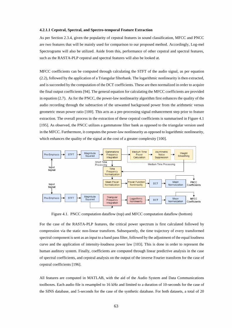
63

4.2.1.1 Cepstral, Spectral, and Spectro-temporal Feature Extraction

As per Section 2.3.4, given the popularity of cepstral features in sound classification, MFCC and PNCC

are two features that will be mainly used for comparison to our proposed method. Accordingly, Log-mel

Spectrograms will also be utilized. Aside from this, performance of other cepstral and spectral features,

such as the RASTA-PLP cepstral and spectral features will also be looked at.

MFCC coefficients can be computed through calculating the STFT of the audio signal, as per equation

(2.2), followed by the application of a Triangular filterbank. The logarithmic nonlinearity is then extracted,

and is succeeded by the computation of the DCT coefficients. These are then normalized in order to acquire

the final output coefficients [94]. The general equation for calculating the MFCC coefficients are provided

in equation (2.7). As for the PNCC, the power-law nonlinearity algorithm first enhances the quality of the

audio recording through the subtraction of the unwanted background power from the arithmetic versus

geometric mean power ratio [100]. This acts as a pre-processing signal enhancement step prior to feature

extraction. The overall process in the extraction of these cepstral coefficients is summarised in Figure 4.1

[195]. As observed, the PNCC utilizes a gammatone filter bank as opposed to the triangular version used

in the MFCC. Furthermore, it computes the power-law nonlinearity as opposed to logarithmic nonlinearity,

which enhances the quality of the signal at the cost of a greater complexity [100].

Figure 4.1. PNCC computation dataflow (top) and MFCC computation dataflow (bottom)

For the case of the RASTA-PLP features, the critical power spectrum is first calculated followed by

compression via the static non-linear transform. Subsequently, the time trajectory of every transformed

spectral component is sent as an input to a band pass filter, followed by the adjustment of the equal loudness

curve and the application of intensity-loudness power law [103]. This is done in order to represent the

human auditory system. Finally, coefficients are computed through linear predictive analysis in the case

of spectral coefficients, and cepstral analysis on the output of the inverse Fourier transform for the case of

cepstral coefficients [196].

All features are computed in MATLAB, with the aid of the Audio System and Data Communications

toolboxes. Each audio file is resampled to 16 kHz and limited to a duration of 10-seconds for the case of

the SINS database, and 5-seconds for the case of the synthetic database. For both datasets, a total of 20

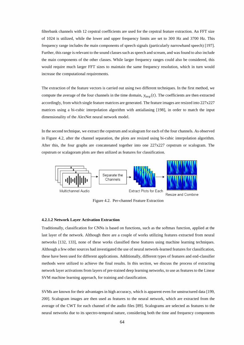
64

filterbank channels with 12 cepstral coefficients are used for the cepstral feature extraction. An FFT size

of 1024 is utilized, while the lower and upper frequency limits are set to 300 Hz and 3700 Hz. This

frequency range includes the main components of speech signals (particularly narrowband speech) [197].

Further, this range is relevant to the sound classes such as speech and scream, and was found to also include

the main components of the other classes. While larger frequency ranges could also be considered, this

would require much larger FFT sizes to maintain the same frequency resolution, which in turn would

increase the computational requirements.

The extraction of the feature vectors is carried out using two different techniques. In the first method, we

compute the average of the four channels in the time domain, 𝑦𝑎𝑣𝑔(𝑡). The coefficients are then extracted

accordingly, from which single feature matrices are generated. The feature images are resized into 227x227

matrices using a bi-cubic interpolation algorithm with antialiasing [198], in order to match the input

dimensionality of the AlexNet neural network model.

In the second technique, we extract the cepstrum and scalogram for each of the four channels. As observed

in Figure 4.2, after the channel separation, the plots are resized using bi-cubic interpolation algorithm.

After this, the four graphs are concatenated together into one 227x227 cepstrum or scalogram. The

cepstrum or scalagoram plots are then utilized as features for classification.

Figure 4.2. Per-channel Feature Extraction

4.2.1.2 Network Layer Activation Extraction

Traditionally, classification for CNNs is based on functions, such as the softmax function, applied at the

last layer of the network. Although there are a couple of works utilizing features extracted from neural

networks [132, 133], none of these works classified these features using machine learning techniques.

Although a few other sources had investigated the use of neural network-learned features for classification,

these have been used for different applications. Additionally, different types of features and end-classifier

methods were utilized to achieve the final results. In this section, we discuss the process of extracting

network layer activations from layers of pre-trained deep learning networks, to use as features to the Linear

SVM machine learning approach, for training and classification.

SVMs are known for their advantages in high accuracy, which is apparent even for unstructured data [199,

200]. Scalogram images are then used as features to the neural network, which are extracted from the

average of the CWT for each channel of the audio files [89]. Scalograms are selected as features to the

neural networks due to its spectro-temporal nature, considering both the time and frequency components

65

of the signal [89], which is advantageous for mapping the time-varying properties of continuous signals,

such as audio signals, with minimal loss of information. Other subsets of possible audial features are either

cepstral-based, spectral-based, or temporal-based, which either considers time or frequency components

individually [89]. For the context of domestic acoustic scenes, an excellent time and frequency localization

is necessary in order to take into account any sound events that may happen during its continuous duration.

The overall technique for this approach utilizes CWT coefficients as features to the DCNN portion of the

proposed methodology. Such coefficients are extricated through MATLAB’s Audio System and Data

Communications toolboxes. The wavelet computation involves an analytic Morse wavelet with a gamma

constant of 3, and a time- bandwidth product of 60. Accordingly, a total of 144 coefficient scales are

calculated for each channel of the audio signals.

The coefficients scales calculation is performed on the average of the four audio channels. Scalograms are

then extracted, and are resized into the relevant image size requirement of the pre-trained model through

bi-cubic interpolation. In order to combine the advantages of deep learning and machine learning for

classification, activations extracted from pre-trained neural networks are coupled with multi-class linear

SVM for the scope of this work. The gist of the overall process can be seen in Figure 4.3. Subsequent to

the extraction and concatenation of the scalograms for all channels of the audio files, these are sent into a

pre-trained model in order to re-train the model according to the specific application. Several types of pre-

trained models are investigated according to their performance, inclusive of the ResNet [136], Xception

[138], InceptionResNet [137], GoogleNet [135], and AlexNet [134] models.

Figure 4.3. Combination Layout of Deep and Machine Learning Technique

After training up to a specified fully-connected layer, the network layer activations are extracted via

MATLAB Parallel computing toolbox and a CUDA enabled NVIDIA GPU. Having been extracted from

neural network training, these activations provide more discriminative representations of time-frequency

signal components when compared to their scalogram counterparts. These network layer activations are

utilized as features to train the SVM. It is important to note that scalogram images that were used as

features to the model cannot be fed directly to the SVM, unless another feature extraction algorithm is

used, such as the Bag of Visual Words. This is because wavelets return large dimensional arrays of

complex parameters, consisting of 144 coefficient scales by 16000 (specified by the sampling rate)matrix

size per label, which cannot be accommodated in arrays to train the SVM with. Extracting network layer

activations, however, returns a 1-by-n size of features per label, where “n” is the number of activations

66

extracted from the model. The Multi-class Linear SVM is then trained through K(K-1)/2 SVM models,

which utilizes a one-versus-one coding design, where K represents the number of categories involved.

Results of the multi-class linear SVM reflects the prediction of the system.

4.2.1.3 General Feature Performance Study and Results

Domestic multi-channel acoustic scenes consist of several concatenated samples of spatial audio.

However, since data is collected continuously in order to monitor the household activities of dementia

residents, the ability to classify sequential data and those with background noises must also be considered.

This sub-section discusses the results gathered for a detailed comparison against existing methods, through

the SINS database.

For feature comparison, low-level acoustic feature vectors in the form of cepstral, spectral, and spectro-

temporal features, along with their combinations, are investigated. This includes the MFCC [94], PNCC

[100], Log-mel energies [82], Spectrograms [87] and regular Scalograms [89]. Alongside this, different

types of mother wavelets, such as Paul, Dog, and Morlet, are also examined for CWT Scalograms. Further,

pre-processing and post-processing techniques such as noise filtration, data splitting and overlapping,

time-alignment, and cross-fold validation were also looked at. Finally, the extraction of network

activations from different pre-trained neural network models integrated to a multi-class linear SVM was

also evaluated, for the purpose of enhancing the time-frequency feature components of the signal. Feature

extraction and trainings are achieved through MATLAB, with the aid of the MATLAB Audio and Data

Communications Toolboxes.

A general summary of the preliminary results associated with these studies can be observed in Table 4.1

and 4.2. Table 4.1 summarizes results observing the system performance of individual state-of-the-art

features examined, while Table 4.2 details results of feature combination, using differing pre-trained

network as classifiers. The first column signifies the features involved, while the second column indicates

the feature representation used for the relevant classifier mentioned in the third column. Finally, the last

column indicates the weighted average F1-scores depending on the dataset size. As previously mentioned,

it is important to note that the evaluation of the techniques tabulated is conducted on a continually

increasing sample set of the SINS database [163], with the final two columns being the full development

and evaluation databases, respectively. All datasets are split at 80-20 ratio in favour of the training set.

Further, all results treat recordings from each of the four nodes separately, and report an average

performance based on the predictions on each node per recording.

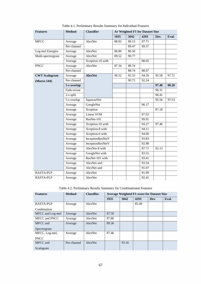
67

Table 4.1. Preliminary Results Summary for Individual Features

Features Method Classifier Av Weighted F1 for Dataset Size

1935 3042 4293 Dev. Eval.

MFCC Average AlexNet 88.92 89.15 87.71

Per-channel 89.47 89.37

Log-mel Energies Average AlexNet 86.80 86.50

Multi-spectrogram Average AlexNet 89.52 90.77

Average Xception-10 with

SVM

88.05

PNCC Average AlexNet 87.34 88.74

Per-channel 88.74 88.97

CWT Scalogram

(Morse-144)

Average AlexNet 90.52 92.33 94.59 95.58 97.71

Per-channel 90.72 92.24

5-s overlap 97.40 98.20

Fade-in/out 96.31

2-s split 96.41

5-s overlap SqueezeNet 95.56 97.53

Average GoogleNet 90.17

Average Xception 87.18

Average Linear SVM 87.63

Average ResNet-101 89.91

Average Xception-10 with

SVM

94.27 97.46

Average Xception-8 with

SVM

94.11

Average Xception-6 with

SVM

94.00

Average InceptionResNetV

2 Layer 303 with

SVM

93.83

Average InceptionResNetV

2 Layer 134 with

SVM

92.98

Average AlexNet-8 with

SVM

87.71 92.13

Average GoogleNet with

SVM

83.55

Average ResNet-101 with

SVM

93.41

Average AlexNet and

Xception-10 with

SVM

93.54

Average AlexNet and

GoogleNet

91.07

RASTA-PLP

Cepstral

Average AlexNet 81.99

RASTA-PLP

Spectral

Average AlexNet 82.41

Table 4.2. Preliminary Results Summary for Combinational Features

Features Method Classifier Average Weighted F1-score for Dataset Size

1935 3042 4293 Dev. Eval.

RASTA-PLP

Combination

Average AlexNet 85.49

MFCC and Log-mel Average AlexNet 87.50

MFCC and PNCC Average AlexNet 87.80

MFCC and

Spectrogram

Average AlexNet 89.36

MFCC, Log-mel,

PNCC

Average AlexNet 87.46

MFCC and

Scalogram

Per-channel AlexNet 93.16

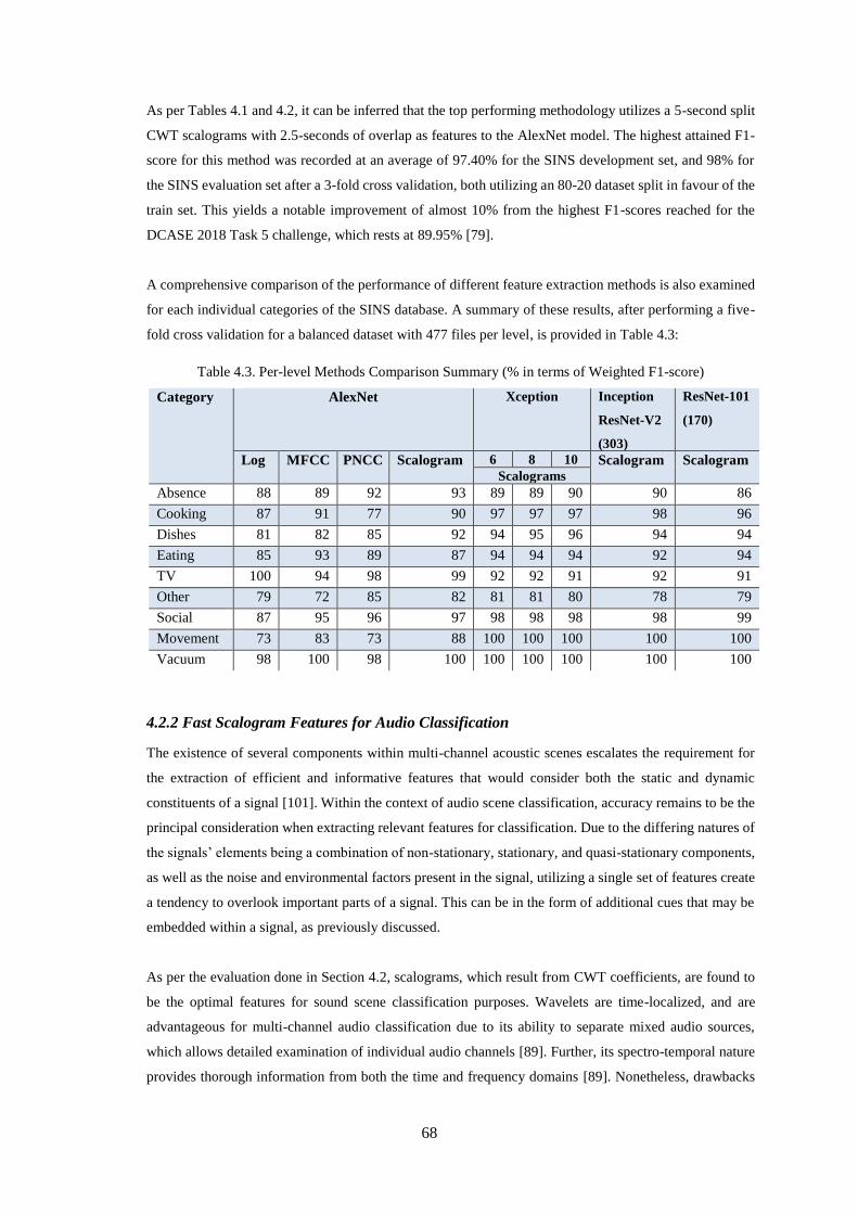
68

As per Tables 4.1 and 4.2, it can be inferred that the top performing methodology utilizes a 5-second split

CWT scalograms with 2.5-seconds of overlap as features to the AlexNet model. The highest attained F1-

score for this method was recorded at an average of 97.40% for the SINS development set, and 98% for

the SINS evaluation set after a 3-fold cross validation, both utilizing an 80-20 dataset split in favour of the

train set. This yields a notable improvement of almost 10% from the highest F1-scores reached for the

DCASE 2018 Task 5 challenge, which rests at 89.95% [79].

A comprehensive comparison of the performance of different feature extraction methods is also examined

for each individual categories of the SINS database. A summary of these results, after performing a five-

fold cross validation for a balanced dataset with 477 files per level, is provided in Table 4.3:

Table 4.3. Per-level Methods Comparison Summary (% in terms of Weighted F1-score)

Category AlexNet Xception Inception

ResNet-V2

(303)

ResNet-101

(170)

Log MFCC PNCC Scalogram 6 8 10 Scalogram Scalogram Scalograms

Absence 88 89 92 93 89 89 90 90 86

Cooking 87 91 77 90 97 97 97 98 96

Dishes 81 82 85 92 94 95 96 94 94

Eating 85 93 89 87 94 94 94 92 94

TV 100 94 98 99 92 92 91 92 91

Other 79 72 85 82 81 81 80 78 79

Social 87 95 96 97 98 98 98 98 99

Movement 73 83 73 88 100 100 100 100 100

Vacuum 98 100 98 100 100 100 100 100 100

4.2.2 Fast Scalogram Features for Audio Classification

The existence of several components within multi-channel acoustic scenes escalates the requirement for

the extraction of efficient and informative features that would consider both the static and dynamic

constituents of a signal [101]. Within the context of audio scene classification, accuracy remains to be the

principal consideration when extracting relevant features for classification. Due to the differing natures of

the signals’ elements being a combination of non-stationary, stationary, and quasi-stationary components,

as well as the noise and environmental factors present in the signal, utilizing a single set of features create

a tendency to overlook important parts of a signal. This can be in the form of additional cues that may be

embedded within a signal, as previously discussed.

As per the evaluation done in Section 4.2, scalograms, which result from CWT coefficients, are found to

be the optimal features for sound scene classification purposes. Wavelets are time-localized, and are

advantageous for multi-channel audio classification due to its ability to separate mixed audio sources,

which allows detailed examination of individual audio channels [89]. Further, its spectro-temporal nature

provides thorough information from both the time and frequency domains [89]. Nonetheless, drawbacks

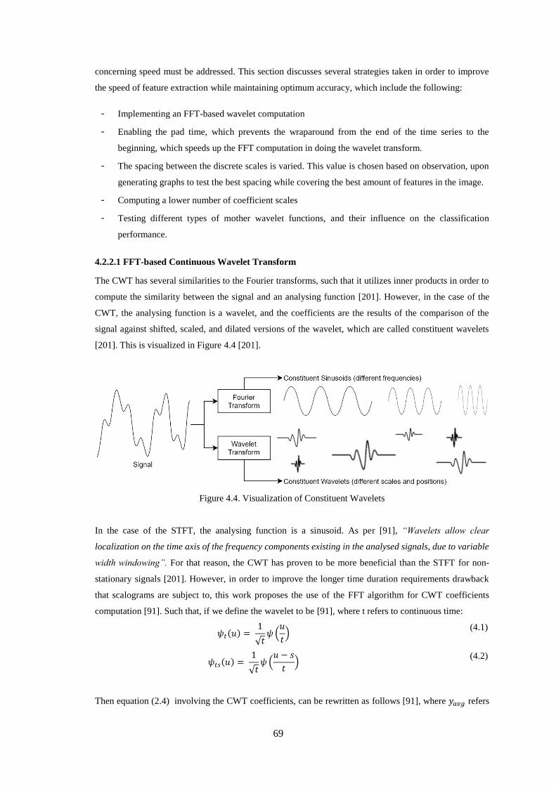
69

concerning speed must be addressed. This section discusses several strategies taken in order to improve

the speed of feature extraction while maintaining optimum accuracy, which include the following:

- Implementing an FFT-based wavelet computation

- Enabling the pad time, which prevents the wraparound from the end of the time series to the

beginning, which speeds up the FFT computation in doing the wavelet transform.

- The spacing between the discrete scales is varied. This value is chosen based on observation, upon

generating graphs to test the best spacing while covering the best amount of features in the image.

- Computing a lower number of coefficient scales

- Testing different types of mother wavelet functions, and their influence on the classification

performance.

4.2.2.1 FFT-based Continuous Wavelet Transform

The CWT has several similarities to the Fourier transforms, such that it utilizes inner products in order to

compute the similarity between the signal and an analysing function [201]. However, in the case of the

CWT, the analysing function is a wavelet, and the coefficients are the results of the comparison of the

signal against shifted, scaled, and dilated versions of the wavelet, which are called constituent wavelets

[201]. This is visualized in Figure 4.4 [201].

Figure 4.4. Visualization of Constituent Wavelets

In the case of the STFT, the analysing function is a sinusoid. As per [91], “Wavelets allow clear

localization on the time axis of the frequency components existing in the analysed signals, due to variable

width windowing”. For that reason, the CWT has proven to be more beneficial than the STFT for non-

stationary signals [201]. However, in order to improve the longer time duration requirements drawback

that scalograms are subject to, this work proposes the use of the FFT algorithm for CWT coefficients

computation [91]. Such that, if we define the wavelet to be [91], where t refers to continuous time:

𝜓𝑡(𝑢) = 1

√𝑡𝜓 (

𝑢

𝑡)

(4.1)

𝜓𝑡𝑠(𝑢) = 1

√𝑡𝜓 (

𝑢 − 𝑠

𝑡)

(4.2)

Then equation (2.4) involving the CWT coefficients, can be rewritten as follows [91], where 𝑦𝑎𝑣𝑔 refers

70

to the average of the four-channels of the audio signal:

𝐶𝑊𝑇𝑐(𝑠, 𝑡) = ∫ 𝑦𝑎𝑣𝑔(𝑢)𝜓𝑡∗(𝑠 − 𝑢)𝑑𝑢

∞

−∞

(4.3)

This shows that CWT coefficients can be expressed by the convolution of wavelets and signals. Thus, this

can be written in the Fourier transform form domain, resulting in equation (4.4) [91]:

𝐶𝑊𝑇𝑐(𝑠, 𝑡) = 1

2𝜋∫ 𝑦𝑎𝑣𝑔(𝜔)𝜓𝑠,𝑡

∗ (𝜔)𝑑𝜔∞

−∞

(4.4)

where 𝜓𝑠,𝑡∗ (𝜔) specifies the Fourier transform of the mother wavelet at scale t:

𝜓𝑠,𝑡∗(𝜔) = √𝑡𝜓∗(𝑡𝜔)𝑒𝑗𝜔𝑠 (4.5)

Further, 𝑦𝑎𝑣𝑔(𝜔) then denotes the Fourier transform of the analysed signal 𝑦𝑎𝑣𝑔(𝑡):

𝑦𝑎𝑣𝑔(𝜔) = ∫ 𝑦𝑎𝑣𝑔(𝑡)𝑒𝑗𝜔𝑡𝑑𝑡∞

−∞

(4.6)

Hence, the discrete versions of the convolutions can be represented as per equation (4.7), where n is in

discrete time domain:

𝑊(𝑠) = ∑ 𝑦𝑎𝑣𝑔(𝑛)𝜓∗(𝑠 − 𝑛)𝑁−1

𝑛=0

(4.7)

From the sum in equation (4.7), we can observe that CWT coefficients can be derived from the repetitive

computation of the convolution of the signal, along with the wavelets, at every value of the scale per

location [91]. This work follows this process in order to extract the DFT of the CWT coefficients at a faster

rate compared to the traditional method.

In summary, CWT coefficients are calculated through obtaining both the DFT of the signal, as per equation

(4.7), and the analysing function, as per equation (4.5), via the FFT. The product of these are then derived

and integrated, as per equation (4.4), in order to extract the wavelet coefficients. Accordingly, the discrete

version of the integration can be represented as a summation, which is observed in equation (4.7).

4.2.2.2 Selection of the Mother Wavelet

One of the most important factors in ensuring the optimal performance of the CWT is to select the wavelet

according to the desired system requirements. There are various types of wavelets that fall under two major

categories: Analytic and Non-analytic wavelets.

Analytic wavelets are complex-valued coefficients defined by their one-sided spectra characteristic, where

negative values are represented by zero [202]. Non-analytic wavelets, on the other hand, represents the

negative components as well. For the purpose of this work, analytic wavelets are preferred. Since the end

output is a scalogram representation, which plots the absolute value of the complex coefficients, only the

positive components are deemed useful. Some of the most important considerations that must be taken

into account when choosing a wavelet include: orthogonality, vanishing moments, and regularity [202].

An orthogonal wavelet preserves energy, while the vanishing moments is directly proportional to the

number of oscillations the wavelet has. Finally, regularity is a measure of wave smoothness, which allows

efficient detection of signal discontinuities and breakdown points [202].

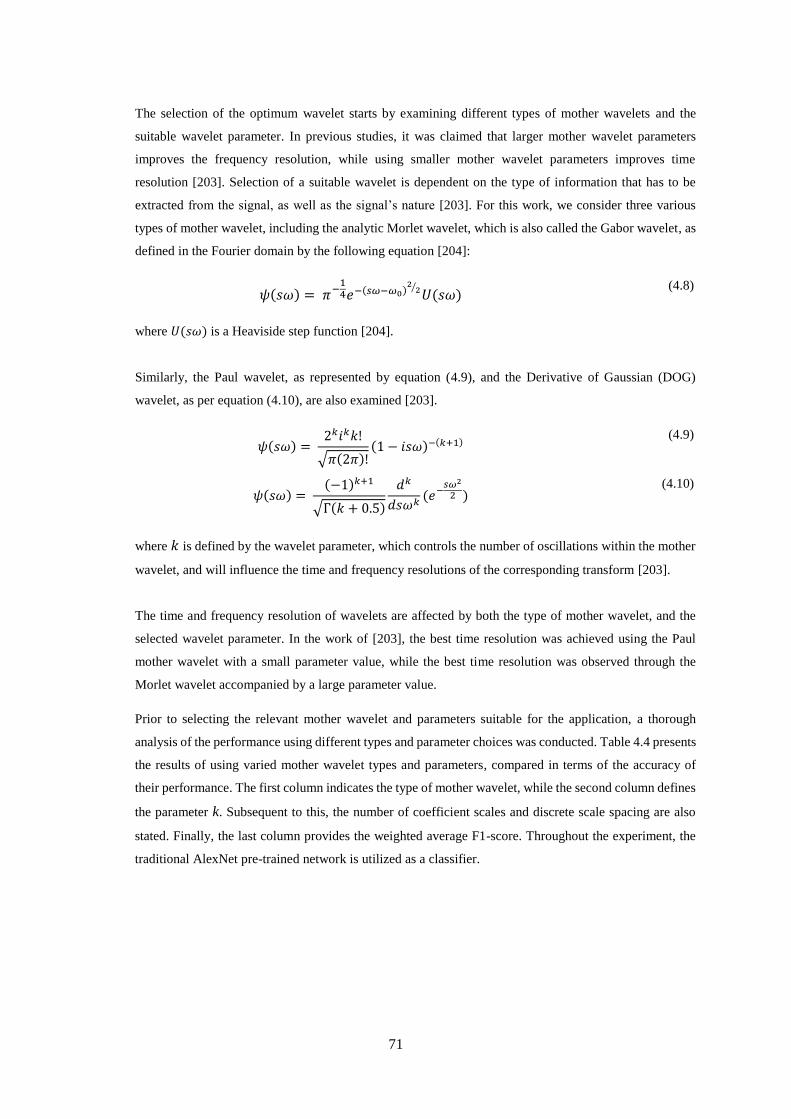
71

The selection of the optimum wavelet starts by examining different types of mother wavelets and the

suitable wavelet parameter. In previous studies, it was claimed that larger mother wavelet parameters

improves the frequency resolution, while using smaller mother wavelet parameters improves time

resolution [203]. Selection of a suitable wavelet is dependent on the type of information that has to be

extracted from the signal, as well as the signal’s nature [203]. For this work, we consider three various

types of mother wavelet, including the analytic Morlet wavelet, which is also called the Gabor wavelet, as

defined in the Fourier domain by the following equation [204]:

𝜓(𝑠𝜔) = 𝜋−14𝑒−(𝑠𝜔−𝜔0)

22⁄𝑈(𝑠𝜔)

(4.8)

where 𝑈(𝑠𝜔) is a Heaviside step function [204].

Similarly, the Paul wavelet, as represented by equation (4.9), and the Derivative of Gaussian (DOG)

wavelet, as per equation (4.10), are also examined [203].

𝜓(𝑠𝜔) = 2𝑘𝑖𝑘𝑘!

√𝜋(2𝜋)!(1 − 𝑖𝑠𝜔)−(𝑘+1)

(4.9)

𝜓(𝑠𝜔) = (−1)𝑘+1

√Γ(𝑘 + 0.5)

𝑑𝑘

𝑑𝑠𝜔𝑘(𝑒−

𝑠𝜔2

2 ) (4.10)

where 𝑘 is defined by the wavelet parameter, which controls the number of oscillations within the mother

wavelet, and will influence the time and frequency resolutions of the corresponding transform [203].

The time and frequency resolution of wavelets are affected by both the type of mother wavelet, and the

selected wavelet parameter. In the work of [203], the best time resolution was achieved using the Paul

mother wavelet with a small parameter value, while the best time resolution was observed through the

Morlet wavelet accompanied by a large parameter value.

Prior to selecting the relevant mother wavelet and parameters suitable for the application, a thorough

analysis of the performance using different types and parameter choices was conducted. Table 4.4 presents

the results of using varied mother wavelet types and parameters, compared in terms of the accuracy of

their performance. The first column indicates the type of mother wavelet, while the second column defines

the parameter k. Subsequent to this, the number of coefficient scales and discrete scale spacing are also

stated. Finally, the last column provides the weighted average F1-score. Throughout the experiment, the

traditional AlexNet pre-trained network is utilized as a classifier.

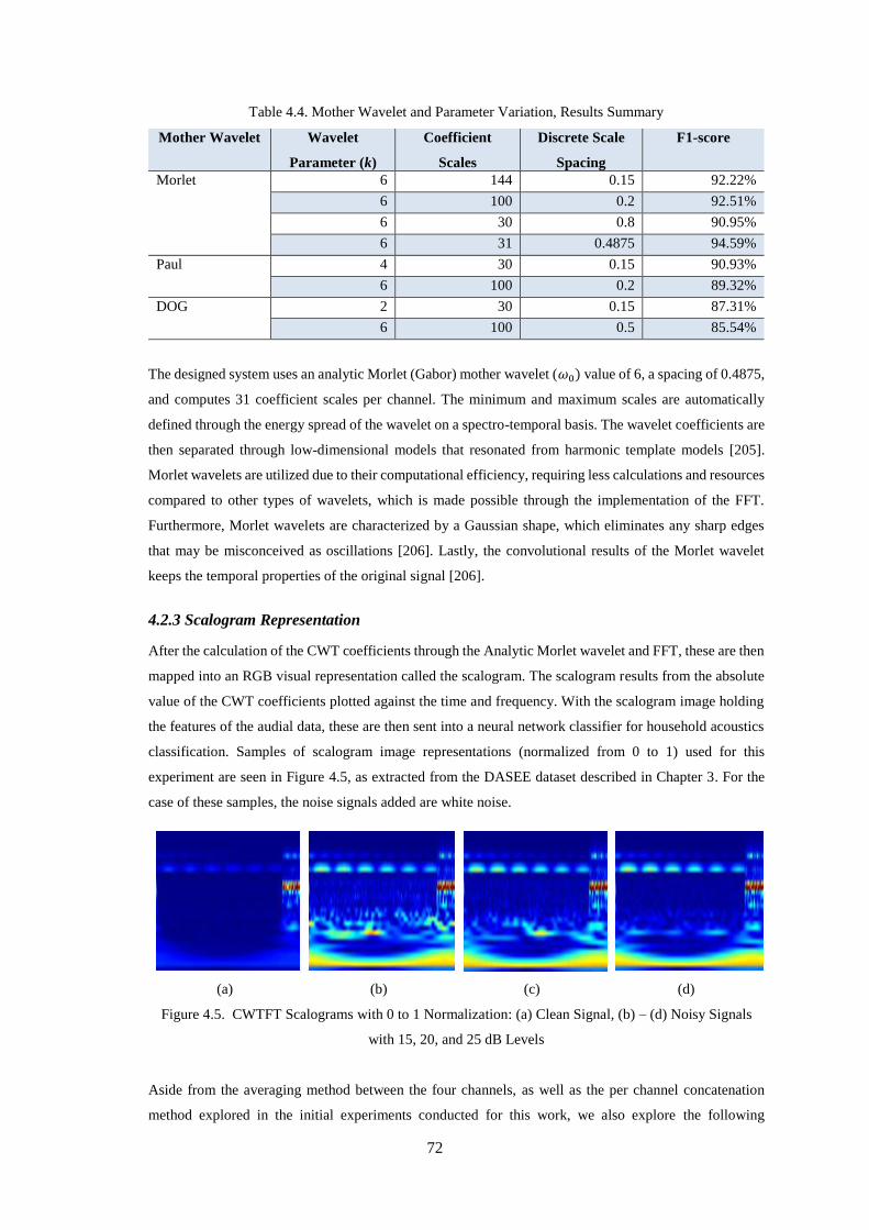
72

Table 4.4. Mother Wavelet and Parameter Variation, Results Summary

Mother Wavelet Wavelet

Parameter (k)

Coefficient

Scales

Discrete Scale

Spacing

F1-score

Morlet 6 144 0.15 92.22%

6 100 0.2 92.51%

6 30 0.8 90.95%

6 31 0.4875 94.59%

Paul 4 30 0.15 90.93%

6 100 0.2 89.32%

DOG 2 30 0.15 87.31%

6 100 0.5 85.54%

The designed system uses an analytic Morlet (Gabor) mother wavelet (𝜔0) value of 6, a spacing of 0.4875,

and computes 31 coefficient scales per channel. The minimum and maximum scales are automatically

defined through the energy spread of the wavelet on a spectro-temporal basis. The wavelet coefficients are

then separated through low-dimensional models that resonated from harmonic template models [205].

Morlet wavelets are utilized due to their computational efficiency, requiring less calculations and resources

compared to other types of wavelets, which is made possible through the implementation of the FFT.

Furthermore, Morlet wavelets are characterized by a Gaussian shape, which eliminates any sharp edges

that may be misconceived as oscillations [206]. Lastly, the convolutional results of the Morlet wavelet

keeps the temporal properties of the original signal [206].

4.2.3 Scalogram Representation

After the calculation of the CWT coefficients through the Analytic Morlet wavelet and FFT, these are then

mapped into an RGB visual representation called the scalogram. The scalogram results from the absolute

value of the CWT coefficients plotted against the time and frequency. With the scalogram image holding

the features of the audial data, these are then sent into a neural network classifier for household acoustics

classification. Samples of scalogram image representations (normalized from 0 to 1) used for this

experiment are seen in Figure 4.5, as extracted from the DASEE dataset described in Chapter 3. For the

case of these samples, the noise signals added are white noise.

(a) (b) (c) (d)

Figure 4.5. CWTFT Scalograms with 0 to 1 Normalization: (a) Clean Signal, (b) – (d) Noisy Signals

with 15, 20, and 25 dB Levels

Aside from the averaging method between the four channels, as well as the per channel concatenation

method explored in the initial experiments conducted for this work, we also explore the following

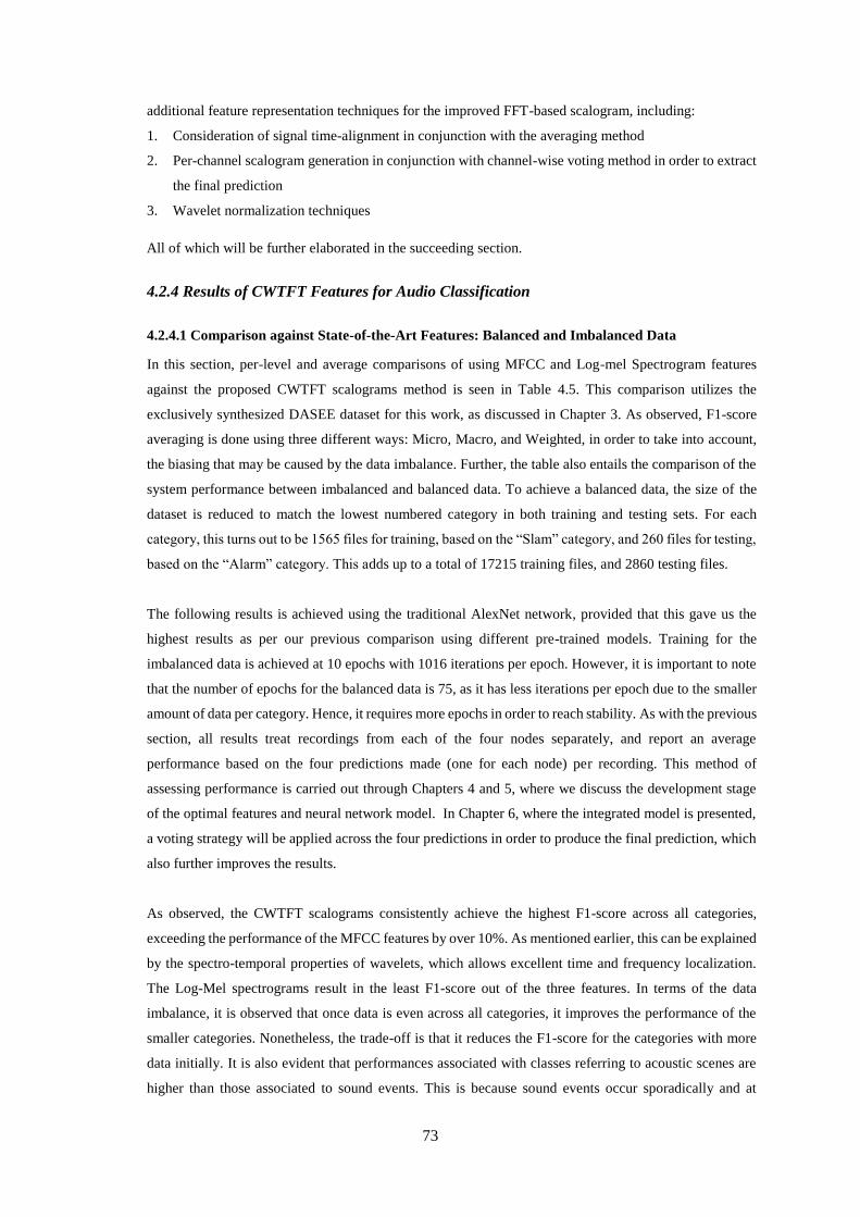
73

additional feature representation techniques for the improved FFT-based scalogram, including:

1. Consideration of signal time-alignment in conjunction with the averaging method

2. Per-channel scalogram generation in conjunction with channel-wise voting method in order to extract

the final prediction

3. Wavelet normalization techniques

All of which will be further elaborated in the succeeding section.

4.2.4 Results of CWTFT Features for Audio Classification

4.2.4.1 Comparison against State-of-the-Art Features: Balanced and Imbalanced Data

In this section, per-level and average comparisons of using MFCC and Log-mel Spectrogram features

against the proposed CWTFT scalograms method is seen in Table 4.5. This comparison utilizes the

exclusively synthesized DASEE dataset for this work, as discussed in Chapter 3. As observed, F1-score

averaging is done using three different ways: Micro, Macro, and Weighted, in order to take into account,

the biasing that may be caused by the data imbalance. Further, the table also entails the comparison of the

system performance between imbalanced and balanced data. To achieve a balanced data, the size of the

dataset is reduced to match the lowest numbered category in both training and testing sets. For each

category, this turns out to be 1565 files for training, based on the “Slam” category, and 260 files for testing,

based on the “Alarm” category. This adds up to a total of 17215 training files, and 2860 testing files.

The following results is achieved using the traditional AlexNet network, provided that this gave us the

highest results as per our previous comparison using different pre-trained models. Training for the

imbalanced data is achieved at 10 epochs with 1016 iterations per epoch. However, it is important to note

that the number of epochs for the balanced data is 75, as it has less iterations per epoch due to the smaller

amount of data per category. Hence, it requires more epochs in order to reach stability. As with the previous

section, all results treat recordings from each of the four nodes separately, and report an average

performance based on the four predictions made (one for each node) per recording. This method of

assessing performance is carried out through Chapters 4 and 5, where we discuss the development stage

of the optimal features and neural network model. In Chapter 6, where the integrated model is presented,

a voting strategy will be applied across the four predictions in order to produce the final prediction, which

also further improves the results.

As observed, the CWTFT scalograms consistently achieve the highest F1-score across all categories,

exceeding the performance of the MFCC features by over 10%. As mentioned earlier, this can be explained

by the spectro-temporal properties of wavelets, which allows excellent time and frequency localization.

The Log-Mel spectrograms result in the least F1-score out of the three features. In terms of the data

imbalance, it is observed that once data is even across all categories, it improves the performance of the

smaller categories. Nonetheless, the trade-off is that it reduces the F1-score for the categories with more

data initially. It is also evident that performances associated with classes referring to acoustic scenes are

higher than those associated to sound events. This is because sound events occur sporadically and at

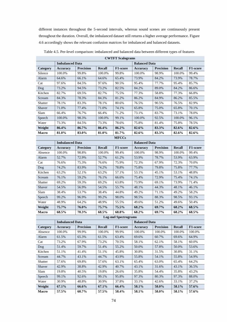
74

different instances throughout the 5-second intervals, whereas sound scenes are continuously present

throughout the duration. Overall, the imbalanced dataset still returns a higher average performance. Figure

4.6 accordingly shows the relevant confusion matrices for imbalanced and balanced datasets.

Table 4.5. Per-level comparison: imbalanced and balanced data between different types of features

CWTFT Scalograms

Imbalanced Data Balanced Data

Category Accuracy Precision Recall F1-score Accuracy Precision Recall F1-score

Silence 100.0% 99.8% 100.0% 99.8% 100.0% 98.9% 100.0% 99.4%

Alarm 64.6% 66.1% 64.6% 65.4% 73.9% 84.2% 73.9% 78.7%

Cat 97.6% 84.5% 97.6% 90.5% 95.4% 77.7% 95.4% 85.7%

Dog 73.2% 94.5% 73.2% 82.5% 84.2% 89.0% 84.2% 86.6%

Kitchen 82.7% 69.5% 82.7% 75.5% 77.3% 58.8% 77.3% 66.8%

Scream 84.3% 78.3% 84.3% 81.2% 86.2% 84.9% 86.2% 85.5%

Shatter 78.1% 83.3% 78.1% 80.6% 76.5% 90.5% 76.5% 82.9%

Shaver 71.0% 77.4% 71.0% 74.1% 65.8% 75.0% 65.8% 70.1%

Slam 66.4% 76.7% 66.4% 71.2% 73.1% 83.7% 73.1% 78.0%

Speech 100.0% 98.3% 100.0% 99.1% 100.0% 92.5% 100.0% 96.1%

Water 73.3% 84.5% 73.3% 78.6% 75.8% 81.4% 75.8% 78.5%

Weight 86.4% 86.7% 86.4% 86.2% 82.6% 83.3% 82.6% 82.6%

Macro 81.0% 83.0% 81.0% 81.7% 82.6% 83.3% 82.6% 82.6%

MFCCs

Imbalanced Data Balanced Data

Category Accuracy Precision Recall F1-score Accuracy Precision Recall F1-score

Absence 100.0% 98.8% 100.0% 99.4% 100.0% 98.9% 100.0% 99.4%

Alarm 52.7% 72.9% 52.7% 61.2% 53.9% 78.7% 53.9% 63.9%

Cat 76.6% 75.3% 76.6% 75.9% 72.3% 67.9% 72.3% 70.0%

Dog 74.2% 83.9% 74.2% 78.8% 75.8% 79.8% 75.8% 77.7%

Kitchen 63.2% 52.1% 63.2% 57.1% 53.1% 45.1% 53.1% 48.8%

Scream 76.1% 59.2% 76.1% 66.6% 75.4% 72.9% 75.4% 74.1%

Shatter 69.2% 59.3% 69.2% 63.8% 73.9% 69.1% 73.9% 71.4%

Shaver 54.5% 56.9% 54.5% 55.7% 48.1% 44.3% 48.1% 46.1%

Slam 38.4% 53.7% 38.4% 44.8% 49.2% 71.1% 49.2% 58.2%

Speech 99.2% 96.9% 99.2% 98.0% 98.5% 88.3% 98.5% 93.1%

Water 48.9% 64.2% 48.9% 55.5% 49.6% 51.2% 49.6% 50.4%

Weight 75.7% 76.0% 75.7% 75.5% 68.2% 69.7% 68.2% 68.5%

Macro 68.5% 70.3% 68.5% 68.8% 68.2% 69.7% 68.2% 68.5%

Log-mel Spectrograms

Imbalanced Data Balanced Data

Category Accuracy Precision Recall F1-score Accuracy Precision Recall F1-score

Absence 100.0% 99.9% 100.0% 99.9% 100.0% 100.0% 100.0% 100.0%

Alarm 61.5% 65.3% 61.5% 63.4% 69.6% 60.7% 69.6% 64.9%

Cat 73.2% 67.9% 73.2% 70.5% 58.1% 62.1% 58.1% 60.0%

Dog 51.4% 59.7% 51.4% 55.2% 50.0% 57.8% 50.0% 53.6%

Kitchen 51.1% 41.4% 51.1% 45.8% 30.8% 31.5% 30.8% 31.1%

Scream 44.7% 43.1% 44.7% 43.9% 55.8% 54.1% 55.8% 54.9%

Shatter 57.6% 69.8% 57.6% 63.1% 65.4% 63.0% 65.4% 64.2%

Shaver 42.9% 38.8% 42.9% 40.7% 43.1% 31.6% 43.1% 36.5%

Slam 19.8% 40.5% 19.8% 26.6% 35.8% 54.4% 35.8% 43.2%

Speech 99.1% 92.6% 99.1% 95.8% 97.3% 80.3% 97.3% 88.0%

Water 30.9% 48.8% 30.9% 37.8% 33.1% 42.6% 33.1% 37.2%

Weight 67.1% 66.6% 67.1% 66.4% 58.1% 58.0% 58.1% 57.6%

Macro 57.5% 60.7% 57.5% 58.4% 58.1% 58.0% 58.1% 57.6%

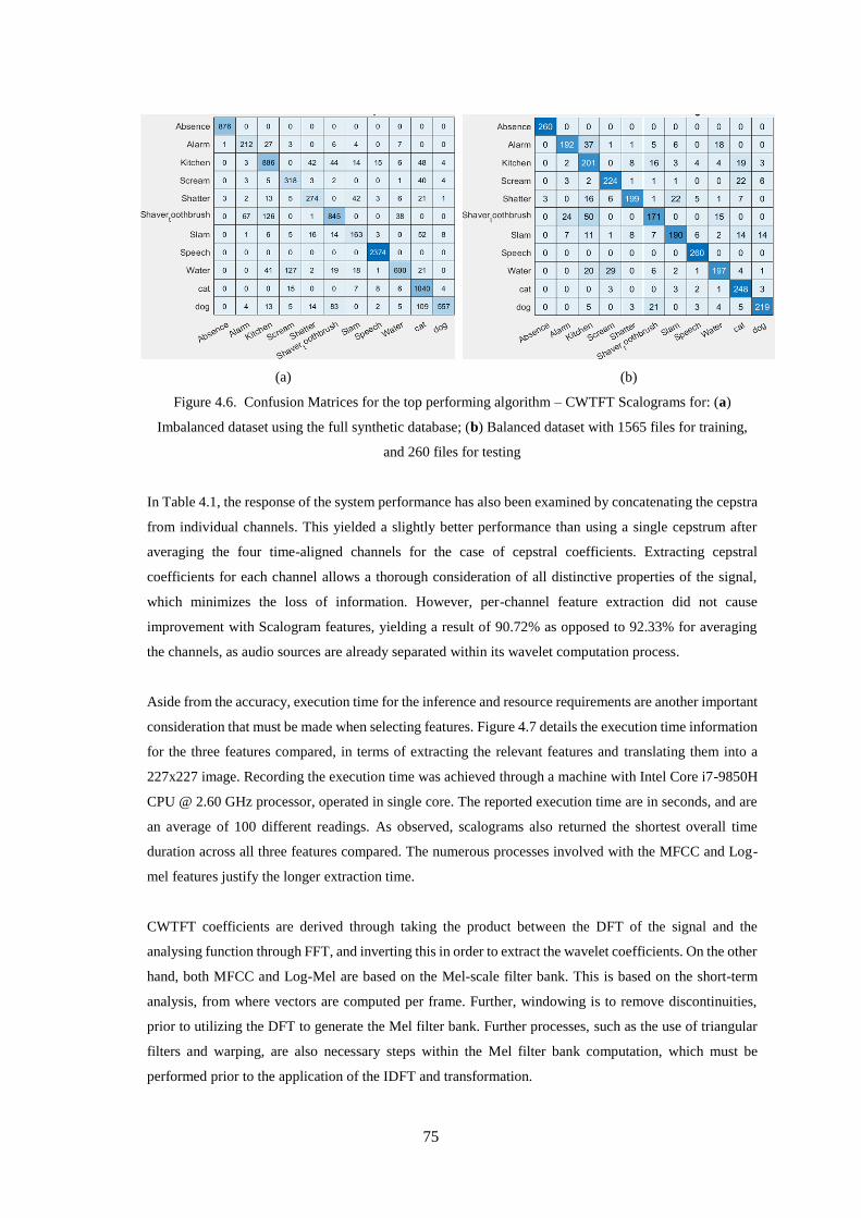
75

(a) (b)

Figure 4.6. Confusion Matrices for the top performing algorithm – CWTFT Scalograms for: (a)

Imbalanced dataset using the full synthetic database; (b) Balanced dataset with 1565 files for training,

and 260 files for testing

In Table 4.1, the response of the system performance has also been examined by concatenating the cepstra

from individual channels. This yielded a slightly better performance than using a single cepstrum after

averaging the four time-aligned channels for the case of cepstral coefficients. Extracting cepstral

coefficients for each channel allows a thorough consideration of all distinctive properties of the signal,

which minimizes the loss of information. However, per-channel feature extraction did not cause

improvement with Scalogram features, yielding a result of 90.72% as opposed to 92.33% for averaging

the channels, as audio sources are already separated within its wavelet computation process.

Aside from the accuracy, execution time for the inference and resource requirements are another important

consideration that must be made when selecting features. Figure 4.7 details the execution time information

for the three features compared, in terms of extracting the relevant features and translating them into a

227x227 image. Recording the execution time was achieved through a machine with Intel Core i7-9850H

CPU @ 2.60 GHz processor, operated in single core. The reported execution time are in seconds, and are

an average of 100 different readings. As observed, scalograms also returned the shortest overall time

duration across all three features compared. The numerous processes involved with the MFCC and Log-

mel features justify the longer extraction time.

CWTFT coefficients are derived through taking the product between the DFT of the signal and the

analysing function through FFT, and inverting this in order to extract the wavelet coefficients. On the other

hand, both MFCC and Log-Mel are based on the Mel-scale filter bank. This is based on the short-term

analysis, from where vectors are computed per frame. Further, windowing is to remove discontinuities,

prior to utilizing the DFT to generate the Mel filter bank. Further processes, such as the use of triangular

filters and warping, are also necessary steps within the Mel filter bank computation, which must be

performed prior to the application of the IDFT and transformation.

76

Figure 4.7. Average execution time for inference (in seconds)

It is important to note that in terms of memory usage, there are negligible differences between the three

features compared. This is because the features are being resized and translated into a 227x227 image

through bi-cubic interpolation, in order to fit the classifier. Nonetheless, each image translation occupies

between 4-12 KB of memory, depending on the sound class.

4.2.4.2 Consideration of Signal Time Alignment

Throughout this work, it is apparent that the optimum feature extraction methodology is formed through

averaging the four channels of the multi-channel audio signal as a pre-processing step. Considering that

there is a 5 cm inter-microphone spacing that exists within the four microphones in each node, it is apparent

that a presence of a delay will be observed upon receiving the audio signals. Signal time alignment may

be beneficial due to the possible loss of information within the averaging process when signals are not

time aligned. In this section, we consider the effects of time-aligning the signals prior to averaging, and

will do a direct comparison between this and the current top performing methodology, which does not

include time alignment.

Time alignment is achieved through a correlation-based method. The correlation is defined to be the

integral of a signal x, and a time-shifted version of another signal y, from 0 to the period, divided by the

period [207]. The auto-correlation function, which is defined to be the cross-correlation of a signal with

itself, proves that periodic signals align themselves through natural periodicity, where peaks occur at

particular time-shift intervals [207]. For non-periodic signals, the signal only aligns with itself when no

time shift exists. When the time shift is non-zero, the noise within the signal forces the value towards zero.

Figure 4.8 displays time-aligned scalogram images versus non-time-aligned ones, compared in four

different classes, inclusive of: Alarm, Scream, Speech, and Shaver or Toothbrush.

1.0076

1.064

0.1981

0 0.2 0.4 0.6 0.8 1 1.2

MFCC

Log-mel

CWT Scalograms

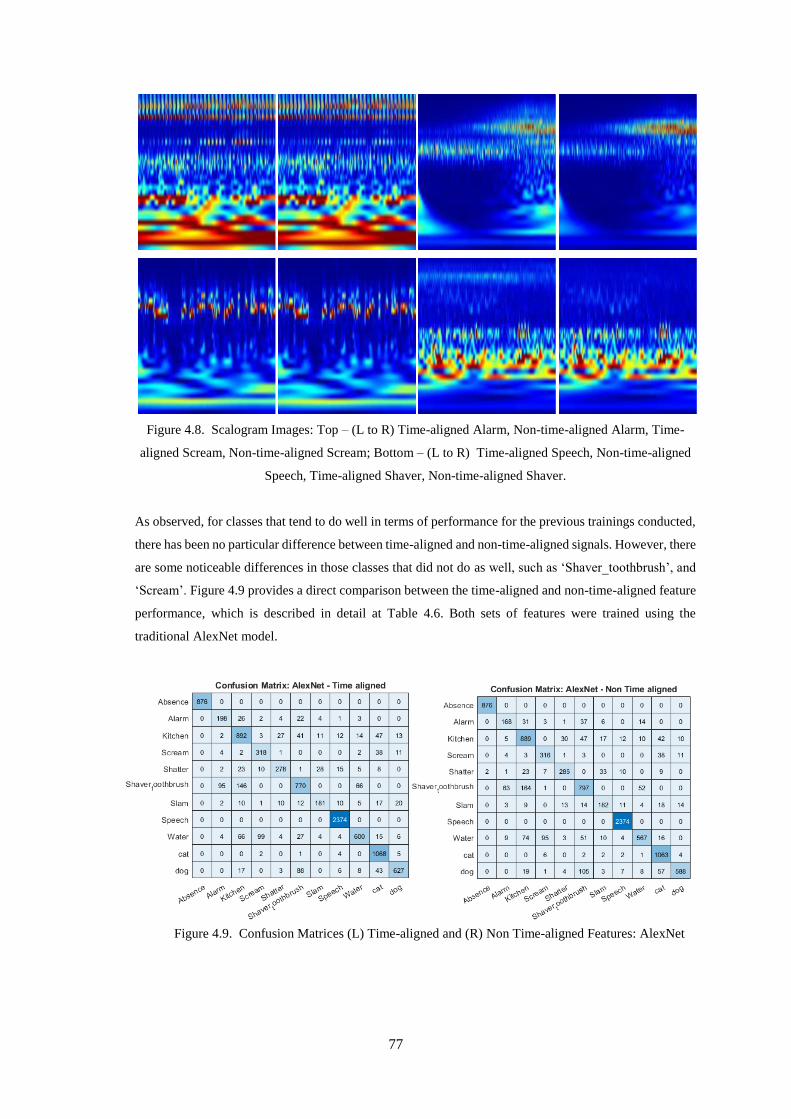
77

Figure 4.8. Scalogram Images: Top – (L to R) Time-aligned Alarm, Non-time-aligned Alarm, Time-

aligned Scream, Non-time-aligned Scream; Bottom – (L to R) Time-aligned Speech, Non-time-aligned

Speech, Time-aligned Shaver, Non-time-aligned Shaver.

As observed, for classes that tend to do well in terms of performance for the previous trainings conducted,

there has been no particular difference between time-aligned and non-time-aligned signals. However, there

are some noticeable differences in those classes that did not do as well, such as ‘Shaver_toothbrush’, and

‘Scream’. Figure 4.9 provides a direct comparison between the time-aligned and non-time-aligned feature

performance, which is described in detail at Table 4.6. Both sets of features were trained using the

traditional AlexNet model.

Figure 4.9. Confusion Matrices (L) Time-aligned and (R) Non Time-aligned Features: AlexNet

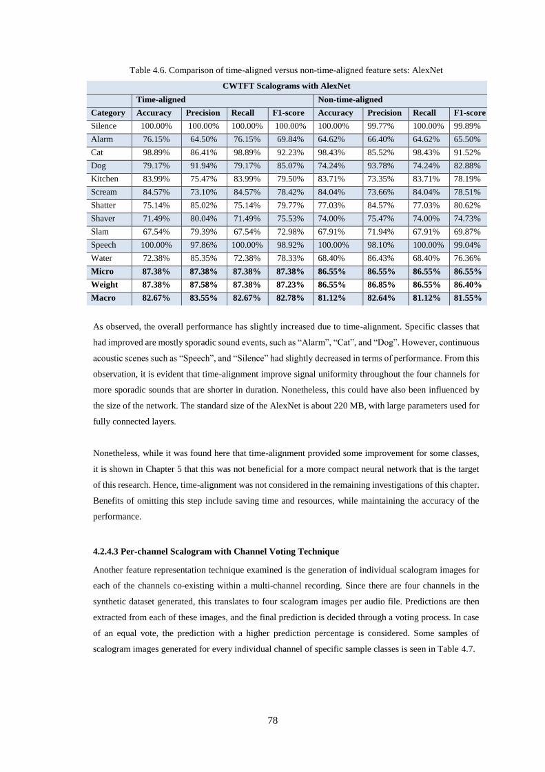
78

Table 4.6. Comparison of time-aligned versus non-time-aligned feature sets: AlexNet

CWTFT Scalograms with AlexNet

Time-aligned Non-time-aligned

Category Accuracy Precision Recall F1-score Accuracy Precision Recall F1-score

Silence 100.00% 100.00% 100.00% 100.00% 100.00% 99.77% 100.00% 99.89%

Alarm 76.15% 64.50% 76.15% 69.84% 64.62% 66.40% 64.62% 65.50%

Cat 98.89% 86.41% 98.89% 92.23% 98.43% 85.52% 98.43% 91.52%

Dog 79.17% 91.94% 79.17% 85.07% 74.24% 93.78% 74.24% 82.88%

Kitchen 83.99% 75.47% 83.99% 79.50% 83.71% 73.35% 83.71% 78.19%

Scream 84.57% 73.10% 84.57% 78.42% 84.04% 73.66% 84.04% 78.51%

Shatter 75.14% 85.02% 75.14% 79.77% 77.03% 84.57% 77.03% 80.62%

Shaver 71.49% 80.04% 71.49% 75.53% 74.00% 75.47% 74.00% 74.73%

Slam 67.54% 79.39% 67.54% 72.98% 67.91% 71.94% 67.91% 69.87%

Speech 100.00% 97.86% 100.00% 98.92% 100.00% 98.10% 100.00% 99.04%

Water 72.38% 85.35% 72.38% 78.33% 68.40% 86.43% 68.40% 76.36%

Micro 87.38% 87.38% 87.38% 87.38% 86.55% 86.55% 86.55% 86.55%

Weight 87.38% 87.58% 87.38% 87.23% 86.55% 86.85% 86.55% 86.40%

Macro 82.67% 83.55% 82.67% 82.78% 81.12% 82.64% 81.12% 81.55%

As observed, the overall performance has slightly increased due to time-alignment. Specific classes that

had improved are mostly sporadic sound events, such as “Alarm”, “Cat”, and “Dog”. However, continuous

acoustic scenes such as “Speech”, and “Silence” had slightly decreased in terms of performance. From this

observation, it is evident that time-alignment improve signal uniformity throughout the four channels for

more sporadic sounds that are shorter in duration. Nonetheless, this could have also been influenced by

the size of the network. The standard size of the AlexNet is about 220 MB, with large parameters used for

fully connected layers.

Nonetheless, while it was found here that time-alignment provided some improvement for some classes,

it is shown in Chapter 5 that this was not beneficial for a more compact neural network that is the target

of this research. Hence, time-alignment was not considered in the remaining investigations of this chapter.

Benefits of omitting this step include saving time and resources, while maintaining the accuracy of the

performance.

4.2.4.3 Per-channel Scalogram with Channel Voting Technique

Another feature representation technique examined is the generation of individual scalogram images for

each of the channels co-existing within a multi-channel recording. Since there are four channels in the

synthetic dataset generated, this translates to four scalogram images per audio file. Predictions are then

extracted from each of these images, and the final prediction is decided through a voting process. In case

of an equal vote, the prediction with a higher prediction percentage is considered. Some samples of

scalogram images generated for every individual channel of specific sample classes is seen in Table 4.7.

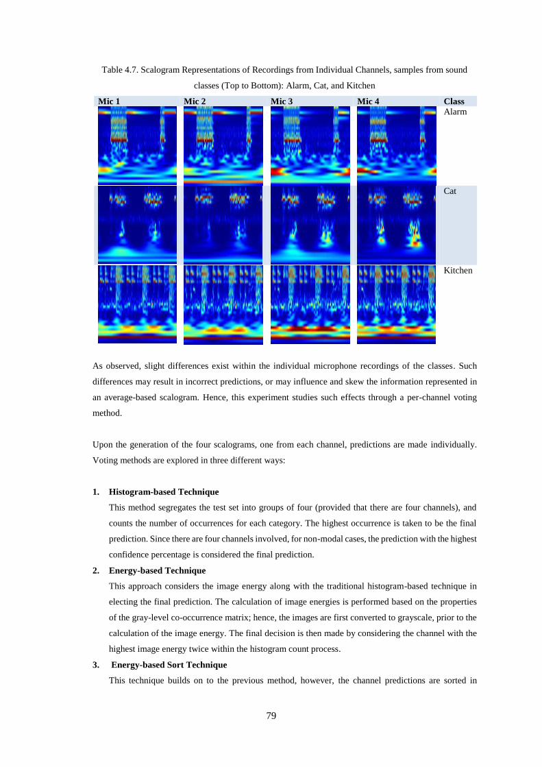
79

Table 4.7. Scalogram Representations of Recordings from Individual Channels, samples from sound

classes (Top to Bottom): Alarm, Cat, and Kitchen

Mic 1 Mic 2 Mic 3 Mic 4 Class

Alarm

Cat

Kitchen

As observed, slight differences exist within the individual microphone recordings of the classes. Such

differences may result in incorrect predictions, or may influence and skew the information represented in

an average-based scalogram. Hence, this experiment studies such effects through a per-channel voting

method.

Upon the generation of the four scalograms, one from each channel, predictions are made individually.

Voting methods are explored in three different ways:

1. Histogram-based Technique

This method segregates the test set into groups of four (provided that there are four channels), and

counts the number of occurrences for each category. The highest occurrence is taken to be the final

prediction. Since there are four channels involved, for non-modal cases, the prediction with the highest

confidence percentage is considered the final prediction.

2. Energy-based Technique

This approach considers the image energy along with the traditional histogram-based technique in

electing the final prediction. The calculation of image energies is performed based on the properties

of the gray-level co-occurrence matrix; hence, the images are first converted to grayscale, prior to the

calculation of the image energy. The final decision is then made by considering the channel with the

highest image energy twice within the histogram count process.

3. Energy-based Sort Technique

This technique builds on to the previous method, however, the channel predictions are sorted in

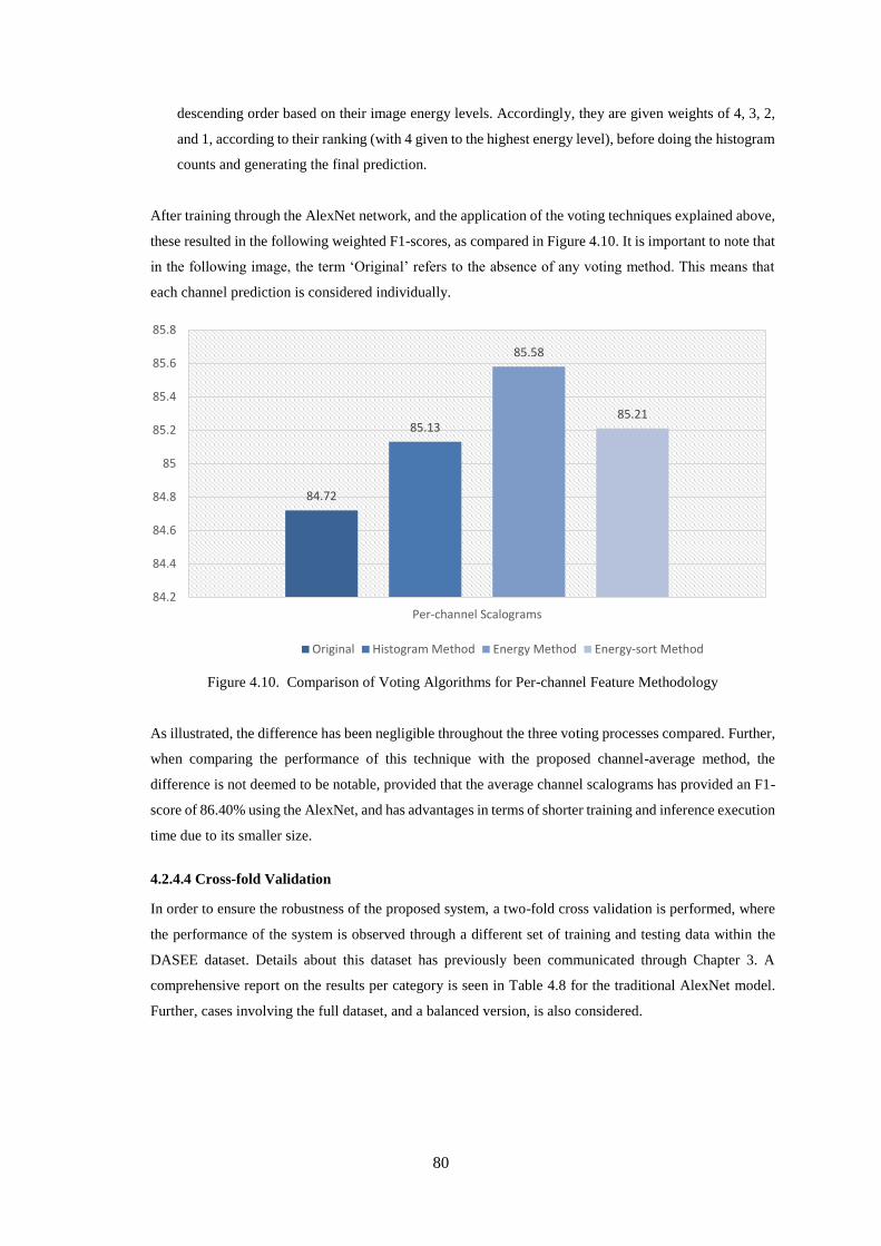
80

descending order based on their image energy levels. Accordingly, they are given weights of 4, 3, 2,

and 1, according to their ranking (with 4 given to the highest energy level), before doing the histogram

counts and generating the final prediction.

After training through the AlexNet network, and the application of the voting techniques explained above,

these resulted in the following weighted F1-scores, as compared in Figure 4.10. It is important to note that

in the following image, the term ‘Original’ refers to the absence of any voting method. This means that

each channel prediction is considered individually.

Figure 4.10. Comparison of Voting Algorithms for Per-channel Feature Methodology

As illustrated, the difference has been negligible throughout the three voting processes compared. Further,

when comparing the performance of this technique with the proposed channel-average method, the

difference is not deemed to be notable, provided that the average channel scalograms has provided an F1-

score of 86.40% using the AlexNet, and has advantages in terms of shorter training and inference execution

time due to its smaller size.

4.2.4.4 Cross-fold Validation

In order to ensure the robustness of the proposed system, a two-fold cross validation is performed, where

the performance of the system is observed through a different set of training and testing data within the

DASEE dataset. Details about this dataset has previously been communicated through Chapter 3. A

comprehensive report on the results per category is seen in Table 4.8 for the traditional AlexNet model.

Further, cases involving the full dataset, and a balanced version, is also considered.

84.72

85.13

85.58

85.21

84.2

84.4

84.6

84.8

85

85.2

85.4

85.6

85.8

Per-channel Scalograms

Original Histogram Method Energy Method Energy-sort Method

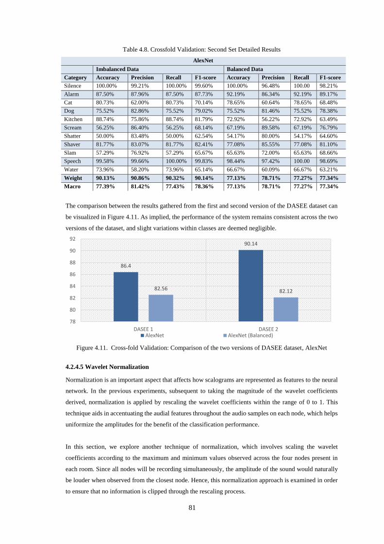
81

Table 4.8. Crossfold Validation: Second Set Detailed Results

AlexNet

Imbalanced Data Balanced Data

Category Accuracy Precision Recall F1-score Accuracy Precision Recall F1-score

Silence 100.00% 99.21% 100.00% 99.60% 100.00% 96.48% 100.00

%

98.21%

Alarm 87.50% 87.96% 87.50% 87.73% 92.19% 86.34% 92.19% 89.17%

Cat 80.73% 62.00% 80.73% 70.14% 78.65% 60.64% 78.65% 68.48%

Dog 75.52% 82.86% 75.52% 79.02% 75.52% 81.46% 75.52% 78.38%

Kitchen 88.74% 75.86% 88.74% 81.79% 72.92% 56.22% 72.92% 63.49%

Scream 56.25% 86.40% 56.25% 68.14% 67.19% 89.58% 67.19% 76.79%

Shatter 50.00% 83.48% 50.00% 62.54% 54.17% 80.00% 54.17% 64.60%

Shaver 81.77% 83.07% 81.77% 82.41% 77.08% 85.55% 77.08% 81.10%

Slam 57.29% 76.92% 57.29% 65.67% 65.63% 72.00% 65.63% 68.66%

Speech 99.58% 99.66% 100.00% 99.83% 98.44% 97.42% 100.00

%

98.69%

Water 73.96% 58.20% 73.96% 65.14% 66.67% 60.09% 66.67% 63.21%

Weight 90.13% 90.86% 90.32% 90.14% 77.13% 78.71% 77.27% 77.34%

Macro 77.39% 81.42% 77.43% 78.36% 77.13% 78.71% 77.27% 77.34%

The comparison between the results gathered from the first and second version of the DASEE dataset can

be visualized in Figure 4.11. As implied, the performance of the system remains consistent across the two

versions of the dataset, and slight variations within classes are deemed negligible.

Figure 4.11. Cross-fold Validation: Comparison of the two versions of DASEE dataset, AlexNet

4.2.4.5 Wavelet Normalization

Normalization is an important aspect that affects how scalograms are represented as features to the neural

network. In the previous experiments, subsequent to taking the magnitude of the wavelet coefficients

derived, normalization is applied by rescaling the wavelet coefficients within the range of 0 to 1. This

technique aids in accentuating the audial features throughout the audio samples on each node, which helps

uniformize the amplitudes for the benefit of the classification performance.

In this section, we explore another technique of normalization, which involves scaling the wavelet

coefficients according to the maximum and minimum values observed across the four nodes present in

each room. Since all nodes will be recording simultaneously, the amplitude of the sound would naturally

be louder when observed from the closest node. Hence, this normalization approach is examined in order

to ensure that no information is clipped through the rescaling process.

86.4

90.14

82.56 82.12

78

80

82

84

86

88

90

92

DASEE 1 DASEE 2AlexNet AlexNet (Balanced)

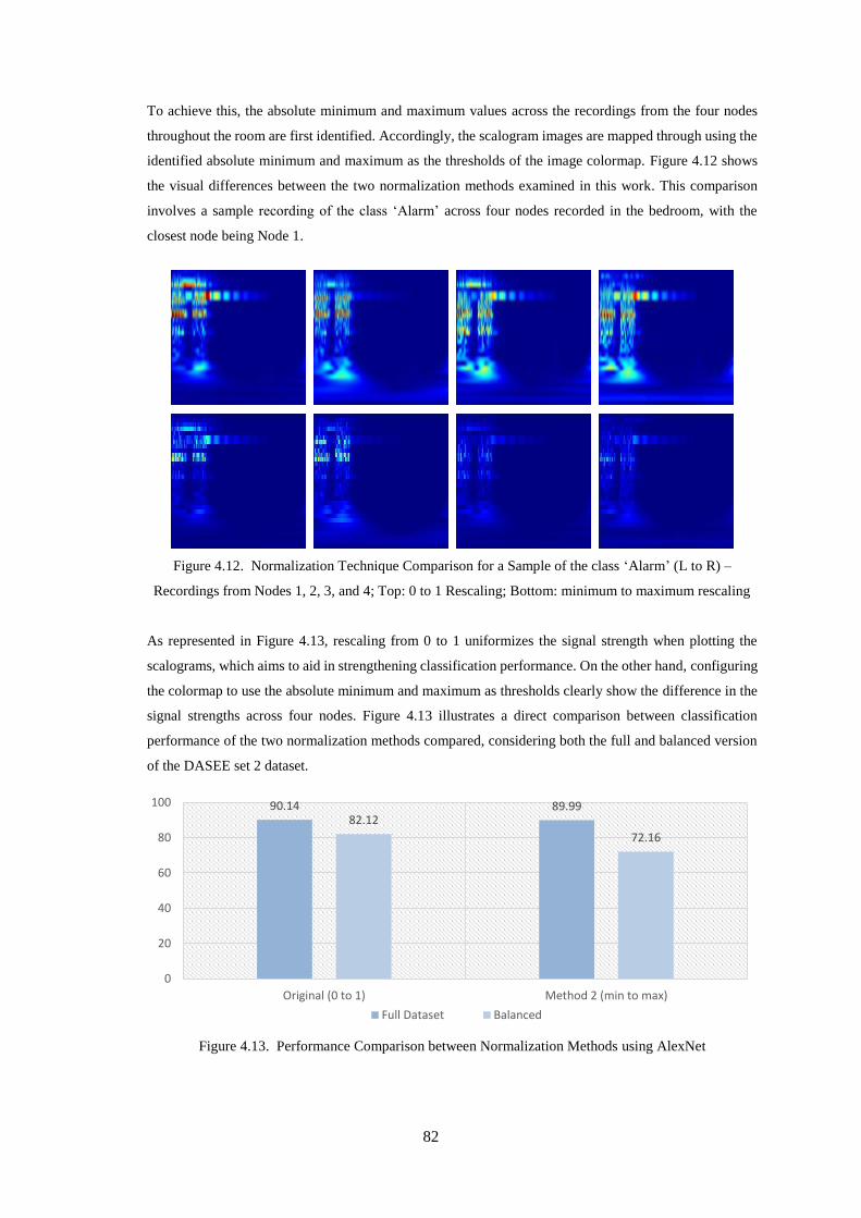
82

To achieve this, the absolute minimum and maximum values across the recordings from the four nodes

throughout the room are first identified. Accordingly, the scalogram images are mapped through using the

identified absolute minimum and maximum as the thresholds of the image colormap. Figure 4.12 shows

the visual differences between the two normalization methods examined in this work. This comparison

involves a sample recording of the class ‘Alarm’ across four nodes recorded in the bedroom, with the

closest node being Node 1.

Figure 4.12. Normalization Technique Comparison for a Sample of the class ‘Alarm’ (L to R) –

Recordings from Nodes 1, 2, 3, and 4; Top: 0 to 1 Rescaling; Bottom: minimum to maximum rescaling

As represented in Figure 4.13, rescaling from 0 to 1 uniformizes the signal strength when plotting the

scalograms, which aims to aid in strengthening classification performance. On the other hand, configuring

the colormap to use the absolute minimum and maximum as thresholds clearly show the difference in the

signal strengths across four nodes. Figure 4.13 illustrates a direct comparison between classification

performance of the two normalization methods compared, considering both the full and balanced version

of the DASEE set 2 dataset.

Figure 4.13. Performance Comparison between Normalization Methods using AlexNet

90.14 89.9982.12

72.16

0

20

40

60

80

100

Original (0 to 1) Method 2 (min to max)

Full Dataset Balanced

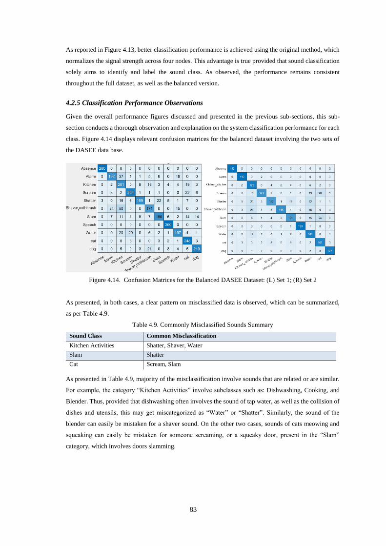
83

As reported in Figure 4.13, better classification performance is achieved using the original method, which

normalizes the signal strength across four nodes. This advantage is true provided that sound classification

solely aims to identify and label the sound class. As observed, the performance remains consistent

throughout the full dataset, as well as the balanced version.

4.2.5 Classification Performance Observations

Given the overall performance figures discussed and presented in the previous sub-sections, this sub-

section conducts a thorough observation and explanation on the system classification performance for each

class. Figure 4.14 displays relevant confusion matrices for the balanced dataset involving the two sets of

the DASEE data base.

Figure 4.14. Confusion Matrices for the Balanced DASEE Dataset: (L) Set 1; (R) Set 2

As presented, in both cases, a clear pattern on misclassified data is observed, which can be summarized,

as per Table 4.9.

Table 4.9. Commonly Misclassified Sounds Summary

Sound Class Common Misclassification

Kitchen Activities Shatter, Shaver, Water

Slam Shatter

Cat Scream, Slam

As presented in Table 4.9, majority of the misclassification involve sounds that are related or are similar.

For example, the category “Kitchen Activities” involve subclasses such as: Dishwashing, Cooking, and

Blender. Thus, provided that dishwashing often involves the sound of tap water, as well as the collision of

dishes and utensils, this may get miscategorized as “Water” or “Shatter”. Similarly, the sound of the

blender can easily be mistaken for a shaver sound. On the other two cases, sounds of cats meowing and

squeaking can easily be mistaken for someone screaming, or a squeaky door, present in the “Slam”

category, which involves doors slamming.

84

4.3 Feature Extraction Methodology for Node Location Estimation

As for the source node location estimation functionality, unlike the majority of works examined

implementing the DOA, extracting the exact coordinates of the sound location is unnecessary for this work.

Considering the purpose of this feature, the main objective in selecting a methodology for sound source

node estimation, is one that could provide a fairly accurate estimation of the sound location, whilst still

keeping complexity, time, and resource requirements into consideration. Further, the overall efficiency by

which this method can be integrated into the system is crucial.

In this section, we propose a neural network-based system that can easily be integrated with the sound

scene classification system in order to provide an estimated location of the sound source. For home

monitoring applications, the exact coordinates of the DOA are not relevant. Rather, the best approximate

of the sound location is determined by identifying where the sound recording is most prominent. Taking

into consideration the location of the sound source can also vastly improve the robustness of an audio

monitoring system for two main reasons. First, selecting the closest microphone array (node) to the source

results in quality improvement for classifying audio, particularly in the presence of background noise and

reverberation, as opposed to classifying the signals received at all nodes [208]. Secondly, estimating the

sound location would be useful for developing a sound map of the environment, which is beneficial for

understanding where and when sound might become distressing for dementia residents [209].

While Section 4.2 focuses on sound classification, this section emphasizes on estimating the location of

the sound through the corresponding closest node. Estimating sound source location is typically based on

estimating the DOA through processing the signals from the microphone array, with recent algorithms

considering neural network-based approaches, as discussed in Chapter 2. While many algorithms are based

on considering features derived from the magnitude spectrum, these features are susceptible to background

noise and other sounds. Here, we instead propose a neural network-based method, which is based on

features derived from the relationship of the phase information of the signals extracted from each

microphone. Phase-based features are first extracted prior to being sent to a neural network to provide the

node from which the recording has originated from. This approach is beneficial, as it eliminates the risks

of biasing that may be caused by noise and unwanted audio signals occurring simultaneously, which are

common factors that can negatively affect a magnitude-based approach at adverse SNR levels [210] .

4.3.1 STFT-based Phasograms for Sound Source Node Location Estimation

Succeeding the relevant pre-processing methodology for Sound Source Node Estimation, features are

extracted in the form of the phase components of the STFT coefficients, called the phase spectrogram. For

the scope of this work, these visual representations will be called phasograms. As mentioned in previous

studies, the magnitude component resulting from the STFT coefficients is what makes up the spectrogram.

However, the phase difference between signals gathered from microphones is related to the DOA [155],

and can therefore be useful for audio location estimation.

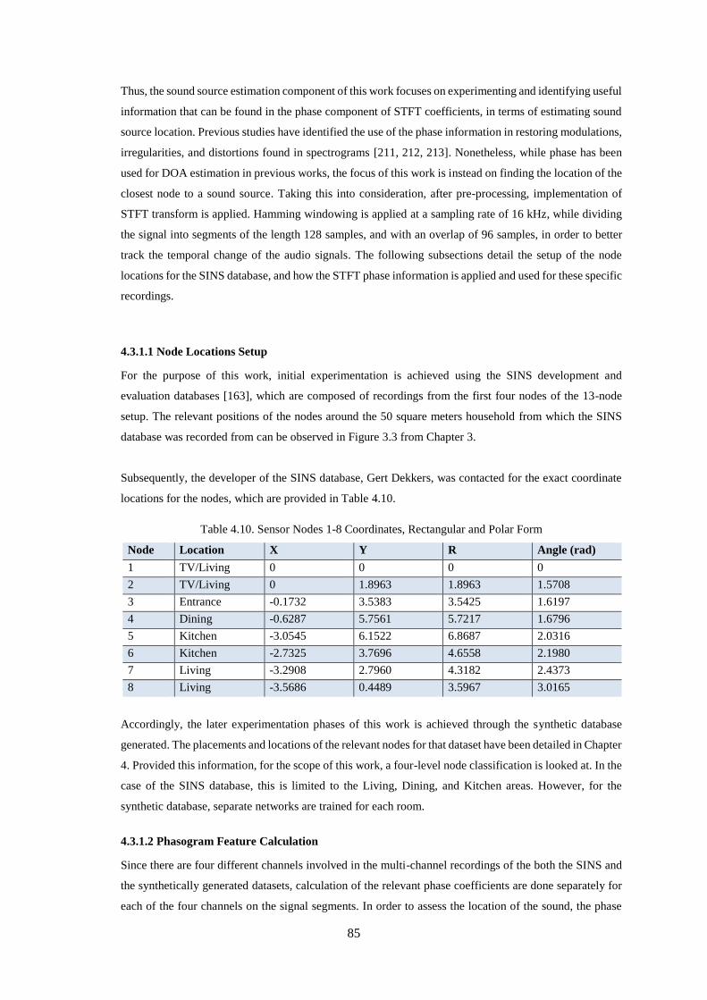
85

Thus, the sound source estimation component of this work focuses on experimenting and identifying useful

information that can be found in the phase component of STFT coefficients, in terms of estimating sound

source location. Previous studies have identified the use of the phase information in restoring modulations,

irregularities, and distortions found in spectrograms [211, 212, 213]. Nonetheless, while phase has been

used for DOA estimation in previous works, the focus of this work is instead on finding the location of the

closest node to a sound source. Taking this into consideration, after pre-processing, implementation of

STFT transform is applied. Hamming windowing is applied at a sampling rate of 16 kHz, while dividing

the signal into segments of the length 128 samples, and with an overlap of 96 samples, in order to better

track the temporal change of the audio signals. The following subsections detail the setup of the node

locations for the SINS database, and how the STFT phase information is applied and used for these specific

recordings.

4.3.1.1 Node Locations Setup

For the purpose of this work, initial experimentation is achieved using the SINS development and

evaluation databases [163], which are composed of recordings from the first four nodes of the 13-node

setup. The relevant positions of the nodes around the 50 square meters household from which the SINS

database was recorded from can be observed in Figure 3.3 from Chapter 3.

Subsequently, the developer of the SINS database, Gert Dekkers, was contacted for the exact coordinate

locations for the nodes, which are provided in Table 4.10.

Table 4.10. Sensor Nodes 1-8 Coordinates, Rectangular and Polar Form

Node Location X Y R Angle (rad)

1 TV/Living 0 0 0 0

2 TV/Living 0 1.8963 1.8963 1.5708

3 Entrance -0.1732 3.5383 3.5425 1.6197

4 Dining -0.6287 5.7561 5.7217 1.6796

5 Kitchen -3.0545 6.1522 6.8687 2.0316

6 Kitchen -2.7325 3.7696 4.6558 2.1980

7 Living -3.2908 2.7960 4.3182 2.4373

8 Living -3.5686 0.4489 3.5967 3.0165

Accordingly, the later experimentation phases of this work is achieved through the synthetic database

generated. The placements and locations of the relevant nodes for that dataset have been detailed in Chapter

4. Provided this information, for the scope of this work, a four-level node classification is looked at. In the

case of the SINS database, this is limited to the Living, Dining, and Kitchen areas. However, for the

synthetic database, separate networks are trained for each room.

4.3.1.2 Phasogram Feature Calculation

Since there are four different channels involved in the multi-channel recordings of the both the SINS and

the synthetically generated datasets, calculation of the relevant phase coefficients are done separately for

each of the four channels on the signal segments. In order to assess the location of the sound, the phase

86

differences between microphones should be taken into account. The STFT coefficients can be represented

as time and frequency components within each segment, which is defined as 𝑆𝑚,𝑙(𝑛, 𝜔), as per equation

(4.11), where, for microphone 𝑚 and segment l, 𝑛 denotes the samples and 𝜔 denotes the frequency [214].

𝑆𝑚,𝑙( 𝑛, 𝜔) = 𝐴𝑚,𝑙(𝑛, 𝜔)𝑒𝑗𝜗𝑚,𝑙(𝑛,𝜔) (4.11)

where 𝐴𝑚,𝑙(𝑛, 𝜔) represents the amplitude and 𝜗𝑚,𝑙(𝑛, 𝜔) represents the phase for segment l of

microphone channel signal m. For the 5-s segments, this results in 2497 STFTs of length 129 samples.

Considering an array with N channels, the phases derived for all time-frequency values in each segment

of channel m can be formed into a 2D plot showing the phase against time and frequency and represented

as a matrix Θ(𝑚, 𝑙) of size 129 by 2497 for channel m and segment l. Two experiments were considered

for the purpose of this work. The linear microphone array geometry for a single node was previously

illustrated in Fig. 3.7 from Chapter 3, which maintains a 5 cm inter-microphone distance.

For the first experiment examined (Experiment A), the average of the differences between the phase

spectra Θ(𝑚, 𝑙) of adjacent microphones are taken as features. A general representation of this is given by

equation (4.12), where n is the current channel, and N is the number of channels. Accordingly, l is the

number of segments. Since the average difference is taken for equation (4.12), this returns 129 by 2497

coefficients per segment, which, when combining all three segments, results in the matrix Θ̂ of size 387

by 2497.

Θ̂ = {∑ Θ(𝑛, 1) − Θ(𝑛 + 1,1)𝑁−1

𝑛=0

𝑁 − 1; … ;

∑ Θ(𝑛, 𝑙) − Θ(𝑛 + 1, 𝑙)𝑁−1𝑛=0

𝑁 − 1}

(4.12)

For the second experiment (Experiment B), the phase differences between the first microphone and the

other 3 microphones are concatenated and mapped into a feature set, as seen in equation (4.13), where the

parameters denote the same factors as equation (4.12). The phase information for this will be denoted by

Θ𝑛1 , and is formed by finding the differences between the two-dimensional phase spectra of the first

microphone and each other microphone in the node per segment, such that 2 ≤ 𝑛 ≤ 𝑁.

Θ𝑛1 = { Θ(1, 1) − Θ(𝑛, 1); … ; Θ(1, 𝑙) − Θ(𝑛, 𝑙)} (4.13)

Provided that equation (4.13) does not consider the average of the phase differences as equation (4.12)

does, this feature set returned is larger. Hence, for this work, we consider only the feature set for the first

segment, which corresponds to the first 5-seconds of the audio file. Doing this will not only maintain

consistency in terms of feature size, but will also allow the investigation of whether the first 5-seconds

contains enough information to accurately estimate the location of the sound.

For both experiments, the coefficients extracted are mapped into an image against time and frequency,

prior to being concatenated into a single image, which we generally call phasograms. Specifically, we call

them adjacent phasograms for the case of equation (4.12), and difference phasograms for equation (4.13).

This will then be resized into 227x227, as per the neural network size requirement, using bi-cubic

interpolation. After this, the image will be sent into a neural network classifier for node estimation.

87

It can also be observed from the linear microphone array geometry that once the sound source hits the

microphones at certain angles, this introduces a delay between the microphone recordings, which can be

represented by a phase difference. The differences between the microphone distances can be very small,

which can result to spatial aliasing. To avoid spatial aliasing, the distance between the microphones must

conform to the spatial sampling theorem, which means that they must be spaced a minimum of half the

wavelength of the maximum audio frequency [215]. The effects of spatial aliasing and consideration of

the cut-off frequencies are also considered upon the experimental stage of this work.

4.3.1.3 Neural Network Integration

Since there are four different channels involved in the multi-channel recordings of the both the SINS and

the synthetically generated datasets, calculation of the relevant phase coefficients are done separately for

each of the four channels on the signal segments. In order to assess the location of the sound, the phase

differences between microphones should be taken into account.

In order to estimate the nearest node to the sound, transfer learning through an optimal neural network,

which is further detailed in Chapter 5, is used for the purpose of saving training time, while still achieving

good accuracy and compatibility to mobile devices with limited computational resources. The network is

trained to predict data in four classes for each of the rooms concerned, corresponding to the nodes of the

dataset room setup, from which the audio data are extracted from. This is done in order to identify the

nodes from which the recordings arrive from. After this, an approximate angular direction of the sound is

calculated as per equation (4.14) [216] per node.

𝜃(𝑖, 𝑓𝑖) = arcsin (𝑐. 𝜗(𝑖, 𝑓𝑖)

2𝜋𝑓𝑖𝑑)

(4.14)

where i refers to the i-point index of the concatenated inter-phase differences, as derived from equations

(4.12) or (4.13), 𝑓𝑖 refers to the frequency at that index, c refers to the speed of sound in the air, and d is

the inter-microphone distance within each node.

Referring to Figure 3.3 in Chapter 3, with the example of a dishwashing sound source, since the node

coordinates are known, the vertex at which these four angles meet can provide an approximate coordinate

location of the sound source. The shortest Euclidean distance between the nodes and the estimated

coordinate is then used to determine the closest node to the sound.

The overall methodology proposed in this work, along with how it can be integrated within an audio-based

monitoring system through combination with a sound scene classifier to determine the audio class, is

represented by Figure 4.15. In summary, audio class prediction and estimation of the sound source location

can be achieved simultaneously through two networks working in parallel. Further, the common pre-/post-

processing techniques provide compatibility between the systems, saving resource and time requirements.

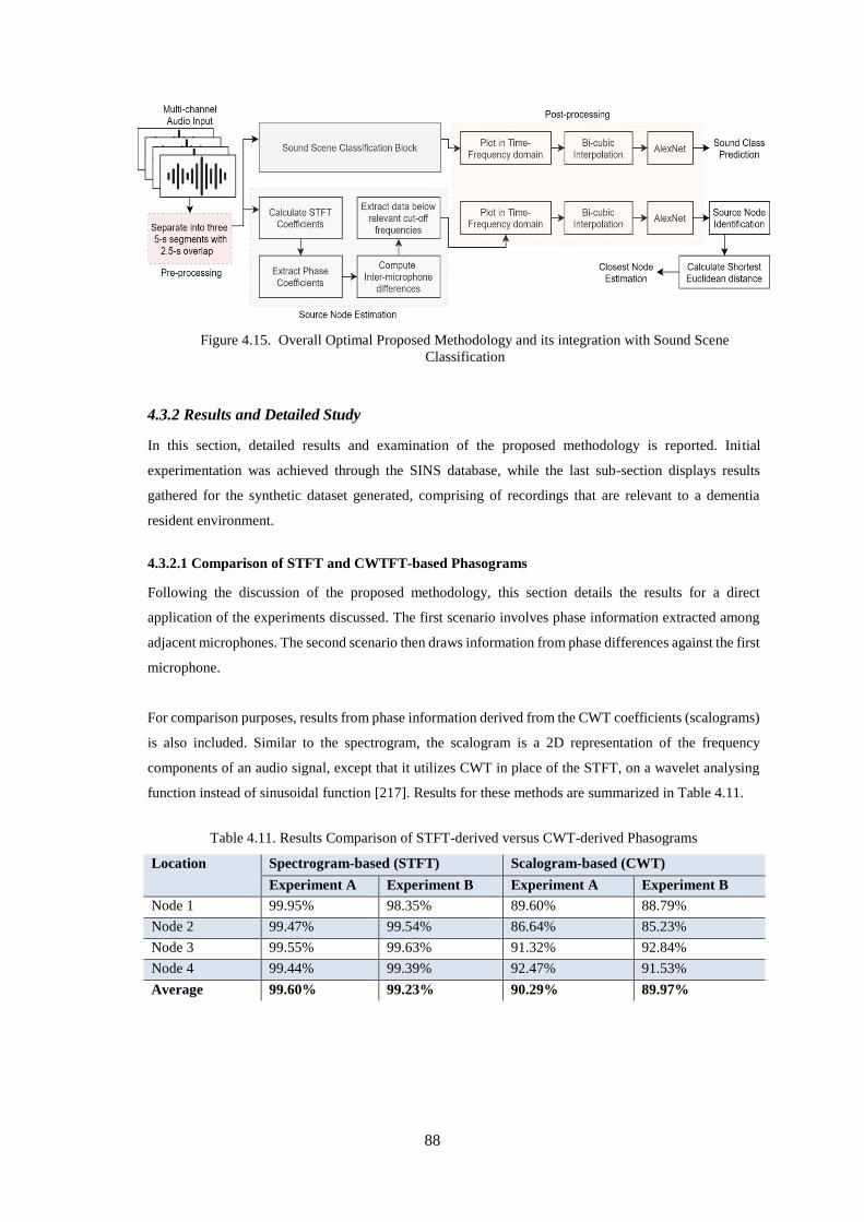
88

Figure 4.15. Overall Optimal Proposed Methodology and its integration with Sound Scene

Classification

4.3.2 Results and Detailed Study

In this section, detailed results and examination of the proposed methodology is reported. Initial

experimentation was achieved through the SINS database, while the last sub-section displays results

gathered for the synthetic dataset generated, comprising of recordings that are relevant to a dementia

resident environment.

4.3.2.1 Comparison of STFT and CWTFT-based Phasograms

Following the discussion of the proposed methodology, this section details the results for a direct

application of the experiments discussed. The first scenario involves phase information extracted among

adjacent microphones. The second scenario then draws information from phase differences against the first

microphone.

For comparison purposes, results from phase information derived from the CWT coefficients (scalograms)

is also included. Similar to the spectrogram, the scalogram is a 2D representation of the frequency

components of an audio signal, except that it utilizes CWT in place of the STFT, on a wavelet analysing

function instead of sinusoidal function [217]. Results for these methods are summarized in Table 4.11.

Table 4.11. Results Comparison of STFT-derived versus CWT-derived Phasograms

Location Spectrogram-based (STFT) Scalogram-based (CWT)

Experiment A Experiment B Experiment A Experiment B

Node 1 99.95% 98.35% 89.60% 88.79%

Node 2 99.47% 99.54% 86.64% 85.23%

Node 3 99.55% 99.63% 91.32% 92.84%

Node 4 99.44% 99.39% 92.47% 91.53%

Average 99.60% 99.23% 90.29% 89.97%

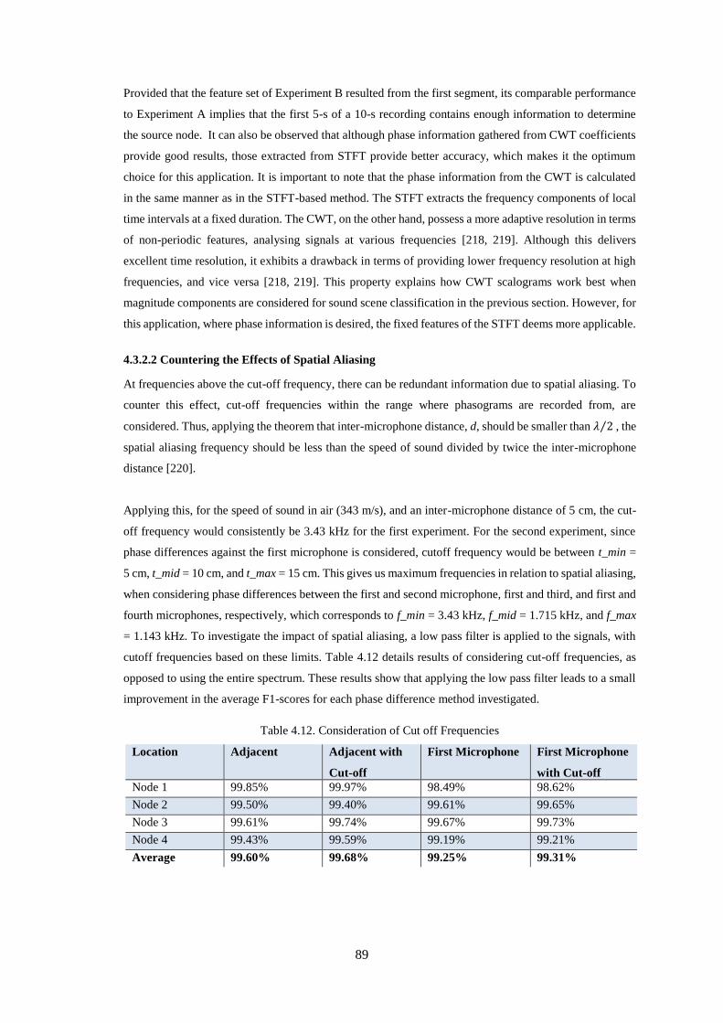
89

Provided that the feature set of Experiment B resulted from the first segment, its comparable performance

to Experiment A implies that the first 5-s of a 10-s recording contains enough information to determine

the source node. It can also be observed that although phase information gathered from CWT coefficients

provide good results, those extracted from STFT provide better accuracy, which makes it the optimum

choice for this application. It is important to note that the phase information from the CWT is calculated

in the same manner as in the STFT-based method. The STFT extracts the frequency components of local

time intervals at a fixed duration. The CWT, on the other hand, possess a more adaptive resolution in terms

of non-periodic features, analysing signals at various frequencies [218, 219]. Although this delivers

excellent time resolution, it exhibits a drawback in terms of providing lower frequency resolution at high

frequencies, and vice versa [218, 219]. This property explains how CWT scalograms work best when

magnitude components are considered for sound scene classification in the previous section. However, for

this application, where phase information is desired, the fixed features of the STFT deems more applicable.

4.3.2.2 Countering the Effects of Spatial Aliasing

At frequencies above the cut-off frequency, there can be redundant information due to spatial aliasing. To

counter this effect, cut-off frequencies within the range where phasograms are recorded from, are

considered. Thus, applying the theorem that inter-microphone distance, d, should be smaller than 𝜆 2⁄ , the

spatial aliasing frequency should be less than the speed of sound divided by twice the inter-microphone

distance [220].

Applying this, for the speed of sound in air (343 m/s), and an inter-microphone distance of 5 cm, the cut-

off frequency would consistently be 3.43 kHz for the first experiment. For the second experiment, since

phase differences against the first microphone is considered, cutoff frequency would be between t_min =

5 cm, t_mid = 10 cm, and t_max = 15 cm. This gives us maximum frequencies in relation to spatial aliasing,

when considering phase differences between the first and second microphone, first and third, and first and

fourth microphones, respectively, which corresponds to f_min = 3.43 kHz, f_mid = 1.715 kHz, and f_max

= 1.143 kHz. To investigate the impact of spatial aliasing, a low pass filter is applied to the signals, with

cutoff frequencies based on these limits. Table 4.12 details results of considering cut-off frequencies, as

opposed to using the entire spectrum. These results show that applying the low pass filter leads to a small

improvement in the average F1-scores for each phase difference method investigated.

Table 4.12. Consideration of Cut off Frequencies

Location Adjacent Adjacent with

Cut-off

First Microphone First Microphone

with Cut-off

Node 1 99.85% 99.97% 98.49% 98.62%

Node 2 99.50% 99.40% 99.61% 99.65%

Node 3 99.61% 99.74% 99.67% 99.73%

Node 4 99.43% 99.59% 99.19% 99.21%

Average 99.60% 99.68% 99.25% 99.31%

90

Using the same dataset, we applied a similar set of features proposed by [216] to our application, which

involves the closest node estimation, instead of DOA approximation. Similar to their approach, we also

extracted phase information through the difference of two microphones instead of four. This returned a

mean F1-score of 98.10% across all four nodes. This was also evaluated against node estimation, as per

our work, instead of the DOA. Since our proposed approach resulted in an F1-score of 99.68%, this exhibits

a good improvement.

4.3.2.3 Comparison against a Magnitude-based Approach

Since the nodes are placed throughout the room, and recordings are extracted from each of them, some

might argue that loudness can be used to estimate sound location. Thus, we compare the performance of

detecting locations via our proposed way, as opposed to using loudness as a measure. For this experiment,

loudness is measured through the integrated Loudness Units relative to Full Scale (LUFS), which upper

limit is 0 dBFS [221]. The algorithm computes loudness by breaking down the audio signal into 0.4-second

segments with 75% overlap. This is used to provide a standard measure, as loudness can depend on one’s

perception. Thus, the use of the LUFS would help promote consistency.

Comparison is achieved through a series of eight ‘Dishwashing’ and ‘TV’ recordings of 10-seconds each,

recorded at the same time from Nodes 1 to 4, where we try to identify the location of the sound and

corresponding closest node. These two sound classes are selected due to their fixed position nature, which

will provide more robustness to the magnitude-based versus phase-based assessment. Tables 4.13 and 4.14

summarizes the results of the comparison of our proposed method (Table 4.13) against LUFS readings

(Table 4.14). The prediction for the LUFS method is identified from the loudest reading, while the closest

node is determined based on the results of phasograms, where we identify the closest node through the

shortest Euclidean distance between the node and the estimated sound source coordinates. This coordinate

is identified from the vertex of the angular estimates for each node. For this, the inter-microphone phase

differences method used is through the differences between adjacent microphones.

As observed in the following tables, predictions made through the LUFS readings are not as accurate as

that of phasograms. Observing the data gathered, it is apparent that ‘Dishwashing’ sounds, is observable

in Node 4 (dining and kitchen area), while ‘TV’ sounds are observable between Nodes 1-2 (living room).

Although a slightly similar pattern can be observed with the LUFS readings, it is inaccurate to associate

TV readings with Node 3 (3 out of 8 cases in Table 4.14), and estimating the first two Dishwashing sounds

to go from Node 2 to 4 within 10-s. It is proposed that this is due to factors such as noise, and overlapping

sounds which are not of interest, that can negatively affect the loudness of a signal. Since phasograms are

based on the phase differences and inter-microphone distance, such factors do not affect its accuracy.

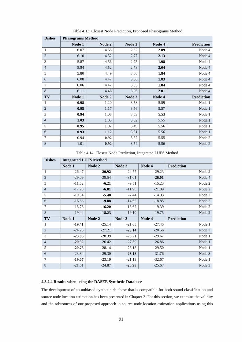
91

Table 4.13. Closest Node Prediction, Proposed Phasograms Method

Dishes Phasograms Method

Node 1 Node 2 Node 3 Node 4 Prediction

1 6.07 4.55 2.82 2.09 Node 4

2 6.10 4.52 2.77 2.13 Node 4

3 5.87 4.56 2.75 1.98 Node 4

4 5.84 4.52 2.78 2.04 Node 4

5 5.80 4.49 3.08 1.84 Node 4

6 6.08 4.47 3.06 1.83 Node 4

7 6.06 4.47 3.05 1.84 Node 4

8 6.11 4.46 3.06 2.01 Node 4

TV Node 1 Node 2 Node 3 Node 4 Prediction

1 0.98 1.20 3.58 5.59 Node 1

2 0.95 1.17 3.56 5.57 Node 1

3 0.94 1.08 3.53 5.53 Node 1

4 1.03 1.05 3.52 5.55 Node 1

5 0.95 1.07 3.49 5.56 Node 1

6 0.93 1.12 3.51 5.56 Node 1

7 0.94 0.92 3.52 5.55 Node 2

8 1.01 0.92 3.54 5.56 Node 2

Table 4.14. Closest Node Prediction, Integrated LUFS Method

Dishes Integrated LUFS Method

Node 1 Node 2 Node 3 Node 4 Prediction

1 -26.47 -20.92 -24.77 -29.23 Node 2

2 -29.09 -28.54 -31.01 -26.01 Node 4

3 -11.52 -6.21 -9.51 -15.23 Node 2

4 -17.28 -6.81 -11.90 -21.09 Node 2

5 -10.54 -5.48 -7.44 -14.93 Node 2

6 -16.63 -9.88 -14.62 -18.85 Node 2

7 -18.76 -16.20 -18.62 -19.39 Node 2

8 -19.44 -18.23 -19.10 -19.75 Node 2

TV Node 1 Node 2 Node 3 Node 4 Prediction

1 -19.41 -25.14 -21.63 -27.45 Node 1

2 -24.25 -27.21 -23.14 -28.56 Node 3

3 -23.86 -28.39 -25.21 -29.67 Node 1

4 -20.92 -26.42 -27.59 -26.86 Node 1

5 -20.73 -28.14 -26.18 -29.50 Node 1

6 -23.84 -29.30 -23.18 -31.76 Node 3

7 -19.07 -23.19 -21.13 -32.67 Node 1

8 -21.61 -24.87 -20.98 -25.67 Node 3

4.3.2.4 Results when using the DASEE Synthetic Database

The development of an unbiased synthetic database that is compatible for both sound classification and

source node location estimation has been presented in Chapter 3. For this section, we examine the validity

and the robustness of our proposed approach in source node location estimation applications using this

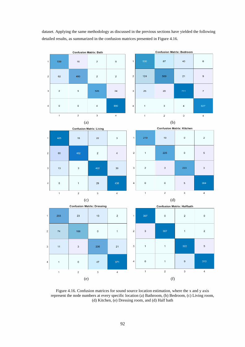
92

dataset. Applying the same methodology as discussed in the previous sections have yielded the following

detailed results, as summarized in the confusion matrices presented in Figure 4.16.

(a) (b)

(c) (d)

(e) (f)

Figure 4.16. Confusion matrices for sound source location estimation, where the x and y axis

represent the node numbers at every specific location (a) Bathroom, (b) Bedroom, (c) Living room,

(d) Kitchen, (e) Dressing room, and (d) Half bath

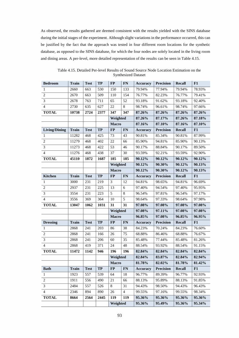
93

As observed, the results gathered are deemed consistent with the results yielded with the SINS database

during the initial stages of the experiment. Although slight variations in the performance occurred, this can

be justified by the fact that the approach was tested in four different room locations for the synthetic

database, as opposed to the SINS database, for which the four nodes are solely located in the living room

and dining areas. A per-level, more detailed representation of the results can be seen in Table 4.15.

Table 4.15. Detailed Per-level Results of Sound Source Node Location Estimation on the

Synthesized Dataset

Bedroom Train Test TP FP FN Accuracy Precision Recall F1

1 2660 663 530 150 133 79.94% 77.94% 79.94% 78.93%

2 2670 663 509 110 154 76.77% 82.23% 76.77% 79.41%

3 2678 763 711 65 52 93.18% 91.62% 93.18% 92.40%

4 2730 635 627 22 8 98.74% 96.61% 98.74% 97.66%

TOTAL 10738 2724 2377 347 347 87.26% 87.26% 87.26% 87.26%

Weighted 87.26% 87.17% 87.26% 87.18%

Macro 87.16% 87.10% 87.16% 87.10%

Living/Dining Train Test TP FP FN Accuracy Precision Recall F1

1 11282 468 425 73 43 90.81% 85.34% 90.81% 87.99%

2 11279 468 402 22 66 85.90% 94.81% 85.90% 90.13%

3 11273 468 422 53 46 90.17% 88.84% 90.17% 89.50%

4 11276 468 438 37 30 93.59% 92.21% 93.59% 92.90%

TOTAL 45110 1872 1687 185 185 90.12% 90.12% 90.12% 90.12%

Weighted 90.12% 90.30% 90.12% 90.13%

Macro 90.12% 90.30% 90.12% 90.13%

Kitchen Train Test TP FP FN Accuracy Precision Recall F1

1 3000 231 219 3 12 94.81% 98.65% 94.81% 96.69%

2 2937 231 225 13 6 97.40% 94.54% 97.40% 95.95%

3 3554 231 223 5 8 96.54% 97.81% 96.54% 97.17%

4 3556 369 364 10 5 98.64% 97.33% 98.64% 97.98%

TOTAL 13047 1062 1031 31 31 97.08% 97.08% 97.08% 97.08%

Weighted 97.08% 97.11% 97.08% 97.08%

Macro 96.85% 97.08% 96.85% 96.95%

Dressing Train Test TP FP FN Accuracy Precision Recall F1

1 2868 241 203 86 38 84.23% 70.24% 84.23% 76.60%

2 2868 241 166 26 75 68.88% 86.46% 68.88% 76.67%

3 2868 241 206 60 35 85.48% 77.44% 85.48% 81.26%

4 2868 419 371 24 48 88.54% 93.92% 88.54% 91.15%

TOTAL 11472 1142 946 196 196 82.84% 82.84% 82.84% 82.84%

Weighted 82.84% 83.87% 82.84% 82.94%

Macro 81.78% 82.02% 81.78% 81.42%

Bath Train Test TP FP FN Accuracy Precision Recall F1

1 1923 557 539 64 18 96.77% 89.39% 96.77% 92.93%

2 1911 556 490 21 66 88.13% 95.89% 88.13% 91.85%

3 2484 557 526 8 31 94.43% 98.50% 94.43% 96.43%

4 2346 894 890 26 4 99.55% 97.16% 99.55% 98.34%

TOTAL 8664 2564 2445 119 119 95.36% 95.36% 95.36% 95.36%

Weighted 95.36% 95.49% 95.36% 95.34%

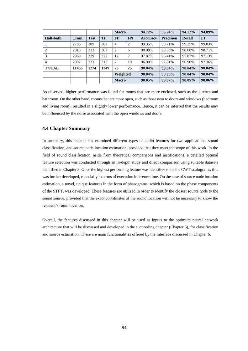
94

Macro 94.72% 95.24% 94.72% 94.89%

Half-bath Train Test TP FP FN Accuracy Precision Recall F1

1 2785 309 307 4 2 99.35% 98.71% 99.35% 99.03%

2 2813 313 307 2 6 98.08% 99.35% 98.08% 98.71%

3 2960 329 322 12 7 97.87% 96.41% 97.87% 97.13%

4 2907 323 313 7 10 96.90% 97.81% 96.90% 97.36%

TOTAL 11465 1274 1249 25 25 98.04% 98.04% 98.04% 98.04%

Weighted 98.04% 98.05% 98.04% 98.04%

Macro 98.05% 98.07% 98.05% 98.06%

As observed, higher performance was found for rooms that are more enclosed, such as the kitchen and

bathroom. On the other hand, rooms that are more open, such as those near to doors and windows (bedroom

and living room), resulted in a slightly lower performance. Hence, it can be inferred that the results may

be influenced by the noise associated with the open windows and doors.

4.4 Chapter Summary

In summary, this chapter has examined different types of audio features for two applications: sound

classification, and source node location estimation, provided that they meet the scope of this work. In the

field of sound classification, aside from theoretical comparisons and justifications, a detailed optimal

feature selection was conducted through an in-depth study and direct comparison using suitable datasets

identified in Chapter 3. Once the highest performing feature was identified to be the CWT scalograms, this

was further developed, especially in terms of execution inference time. On the case of source node location

estimation, a novel, unique features in the form of phasograms, which is based on the phase components

of the STFT, was developed. These features are utilized in order to identify the closest source node to the

sound source, provided that the exact coordinates of the sound location will not be necessary to know the

resident’s room location.

Overall, the features discussed in this chapter will be used as inputs to the optimum neural network

architecture that will be discussed and developed in the succeeding chapter (Chapter 5), for classification

and source estimation. These are main functionalities offered by the interface discussed in Chapter 6.

95

Neural Networks Architectural and Hyper-parameter Study

5.1 Introduction

Chapter 4 has focused on evaluating the performance of scalograms as input features for various pre-

trained neural networks. In this chapter, the performance of several neural network models is first

evaluated for classification purposes, in accordance to their benefits and limitations as per our application.

Once the optimum-performing model is identified, the architecture of the neural network and their hyper-

parameters are further investigated towards the development of an optimal, compact version of this neural

network model whilst maintaining high accuracy.

As discussed in Chapter 2, where the different sub-types of neural networks are detailed, CNNs have been

widely popular for its advantages with regards to its low computational complexity, as well as its efficiency

when used with data of spatial behaviour [222]. Therefore, in this chapter, the experimentation starts with

the comparison of different pre-trained network models for transfer learning, and the identification of the

optimum pre-trained model. Modifications of the hyper-parameters are then made on the best performing

network, and the response is observed in three ways:

1. Effects of changing the network activation function

2. Effects of fine-tuning the weight and bias factors, and parameter variation

3. Effects of modifications in the network architecture

The study of these effects is aimed towards the development of a modified, compact version of the AlexNet

model that maintains the model’s accuracy for the specific application, while reducing the network size by

over 90%, allowing compatibility with devices and applications with limited resources. Further, we also

aim to maintain the overall network customizability without inviting higher risks of overfitting. It is

important to note that the compact neural network development is not a step towards an actual deployment

in any specific resource-limited system. Rather, we explore and experiment the extent to which the system

can be scaled down while maintaining high performance. Throughout the experiments conducted in this

chapter, the CWTFT scalograms are utilized as features, provided that this has been identified to be the

optimum set of features for this application as per Chapter 4. The first set of the DASEE database is then

utilized, with the second set being used for cross-fold validation of the final network.

5.2 Comparison of Pre-trained Models

Prior to making modifications and fine tuning, testing the performance of different pre-trained networks

on the optimum features identified is necessary in order to find the best fit network for our application. In

Figure 5.1, the performance of different types of pre-trained models, along with the SVM classifier, is

compared specifically for the CWFT scalogram features. Although the performance of these models have

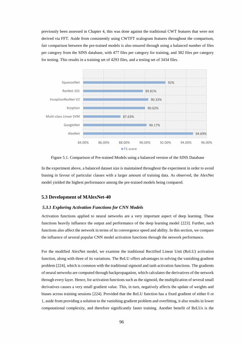
96

previously been assessed in Chapter 4, this was done against the traditional CWT features that were not

derived via FFT. Aside from consistently using CWTFT scalogram features throughout the comparison,

fair comparison between the pre-trained models is also ensured through using a balanced number of files

per category from the SINS database, with 477 files per category for training, and 382 files per category

for testing. This results in a training set of 4293 files, and a testing set of 3434 files.

Figure 5.1. Comparison of Pre-trained Models using a balanced version of the SINS Database

In the experiment above, a balanced dataset size is maintained throughout the experiment in order to avoid

biasing in favour of particular classes with a larger amount of training data. As observed, the AlexNet

model yielded the highest performance among the pre-trained models being compared.

5.3 Development of MAlexNet-40

5.3.1 Exploring Activation Functions for CNN Models

Activation functions applied to neural networks are a very important aspect of deep learning. These

functions heavily influence the output and performance of the deep learning model [223]. Further, such

functions also affect the network in terms of its convergence speed and ability. In this section, we compare

the influence of several popular CNN model activation functions through the network performance.

For the modified AlexNet model, we examine the traditional Rectified Linear Unit (ReLU) activation

function, along with three of its variations. The ReLU offers advantages in solving the vanishing gradient

problem [224], which is common with the traditional sigmoid and tanh activation functions. The gradients

of neural networks are computed through backpropagation, which calculates the derivatives of the network

through every layer. Hence, for activation functions such as the sigmoid, the multiplication of several small

derivatives causes a very small gradient value. This, in turn, negatively affects the update of weights and

biases across training sessions [224]. Provided that the ReLU function has a fixed gradient of either 0 or

1, aside from providing a solution to the vanishing gradient problem and overfitting, it also results in lower

computational complexity, and therefore significantly faster training. Another benefit of ReLUs is the

94.69%

90.17%

87.63%

90.02%

90.33%

89.81%

92%

84.00% 86.00% 88.00% 90.00% 92.00% 94.00% 96.00%

AlexNet

GoogleNet

Multi-class Linear SVM

Xception

InceptionResNet-V2

ResNet-101

SqueezeNet

F1-score

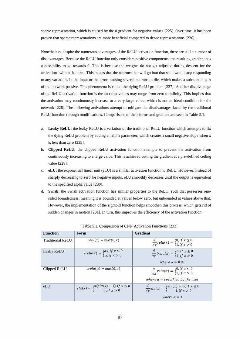
97

sparse representation, which is caused by the 0 gradient for negative values [225]. Over time, it has been

proven that sparse representations are more beneficial compared to dense representations [226].

Nonetheless, despite the numerous advantages of the ReLU activation function, there are still a number of

disadvantages. Because the ReLU function only considers positive components, the resulting gradient has

a possibility to go towards 0. This is because the weights do not get adjusted during descent for the

activations within that area. This means that the neurons that will go into that state would stop responding

to any variations in the input or the error, causing several neurons to die, which makes a substantial part

of the network passive. This phenomena is called the dying ReLU problem [227]. Another disadvantage

of the ReLU activation function is the fact that values may range from zero to infinity. This implies that

the activation may continuously increase to a very large value, which is not an ideal condition for the

network [228]. The following activations attempt to mitigate the disadvantages faced by the traditional

ReLU function through modifications. Comparisons of their forms and gradient are seen in Table 5.1.

a. Leaky ReLU: the leaky ReLU is a variation of the traditional ReLU function which attempts to fix

the dying ReLU problem by adding an alpha parameter, which creates a small negative slope when x

is less than zero [229].

b. Clipped ReLU: the clipped ReLU activation function attempts to prevent the activation from

continuously increasing to a large value. This is achieved cutting the gradient at a pre-defined ceiling

value [228].

c. eLU: the exponential linear unit (eLU) is a similar activation function to ReLU. However, instead of

sharply decreasing to zero for negative inputs, eLU smoothly decreases until the output is equivalent

to the specified alpha value [230].

d. Swish: the Swish activation function has similar properties to the ReLU, such that possesses one-

sided boundedness, meaning it is bounded at values below zero, but unbounded at values above that.

However, the implementation of the sigmoid function helps smoothen this process, which gets rid of

sudden changes in motion [231]. In turn, this improves the efficiency of the activation function.

Table 5.1. Comparison of CNN Activation Functions [232]

Function Form Gradient

Traditional ReLU 𝑟𝑒𝑙𝑢(𝑥) = max(0, 𝑥) 𝑑

𝑑𝑥𝑟𝑒𝑙𝑢(𝑥) = {

0, 𝑖𝑓 𝑥 ≤ 01, 𝑖𝑓 𝑥 > 0

Leaky ReLU 𝑙𝑟𝑒𝑙𝑢(𝑥) = {𝛼𝑥, 𝑖𝑓 𝑥 ≤ 0𝑥, 𝑖𝑓 𝑥 > 0

𝑑

𝑑𝑥𝑙𝑟𝑒𝑙𝑢(𝑥) = {

𝛼, 𝑖𝑓 𝑥 ≤ 01, 𝑖𝑓 𝑥 > 0

𝑤ℎ𝑒𝑟𝑒 𝛼 = 0.01

Clipped ReLU 𝑐𝑟𝑒𝑙𝑢(𝛼) = max(0, 𝛼) 𝑑

𝑑𝑥𝑟𝑒𝑙𝑢(𝛼) = {

0, 𝑖𝑓 𝛼 ≤ 01, 𝑖𝑓 𝛼 > 0

𝑤ℎ𝑒𝑟𝑒 𝛼 = 𝑠𝑝𝑒𝑐𝑖𝑓𝑖𝑒𝑑 𝑏𝑦 𝑡ℎ𝑒 𝑢𝑠𝑒𝑟

eLU 𝑒𝑙𝑢(𝑥) = {

𝛼(𝑒𝑙𝑢(𝑥) − 1), 𝑖𝑓 𝑥 ≤ 0𝑥, 𝑖𝑓 𝑥 > 0

𝑑

𝑑𝑥𝑒𝑙𝑢(𝑥) = {

𝑒𝑙𝑢(𝑥) + 𝛼, 𝑖𝑓 𝑥 ≤ 01, 𝑖𝑓 𝑥 > 0

𝑤ℎ𝑒𝑟𝑒 𝛼 = 1

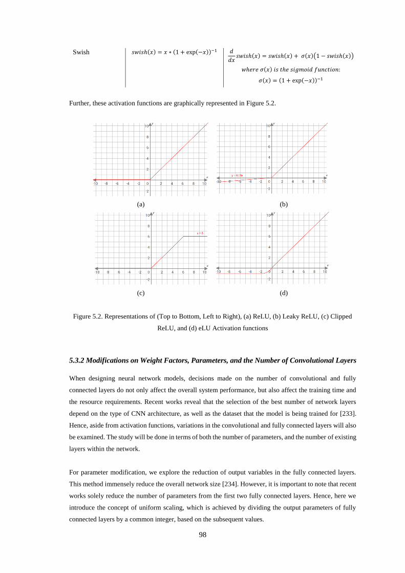
98

Swish 𝑠𝑤𝑖𝑠ℎ(𝑥) = 𝑥 ∗ (1 + exp(−𝑥))−1 𝑑

𝑑𝑥𝑠𝑤𝑖𝑠ℎ(𝑥) = 𝑠𝑤𝑖𝑠ℎ(𝑥) + 𝜎(𝑥)(1 − 𝑠𝑤𝑖𝑠ℎ(𝑥))

𝑤ℎ𝑒𝑟𝑒 𝜎(𝑥) 𝑖𝑠 𝑡ℎ𝑒 𝑠𝑖𝑔𝑚𝑜𝑖𝑑 𝑓𝑢𝑛𝑐𝑡𝑖𝑜𝑛:

𝜎(𝑥) = (1 + exp(−𝑥))−1

Further, these activation functions are graphically represented in Figure 5.2.

(a) (b)

(c) (d)

Figure 5.2. Representations of (Top to Bottom, Left to Right), (a) ReLU, (b) Leaky ReLU, (c) Clipped

ReLU, and (d) eLU Activation functions

5.3.2 Modifications on Weight Factors, Parameters, and the Number of Convolutional Layers

When designing neural network models, decisions made on the number of convolutional and fully

connected layers do not only affect the overall system performance, but also affect the training time and

the resource requirements. Recent works reveal that the selection of the best number of network layers

depend on the type of CNN architecture, as well as the dataset that the model is being trained for [233].

Hence, aside from activation functions, variations in the convolutional and fully connected layers will also

be examined. The study will be done in terms of both the number of parameters, and the number of existing

layers within the network.

For parameter modification, we explore the reduction of output variables in the fully connected layers.

This method immensely reduce the overall network size [234]. However, it is important to note that recent

works solely reduce the number of parameters from the first two fully connected layers. Hence, here we

introduce the concept of uniform scaling, which is achieved by dividing the output parameters of fully

connected layers by a common integer, based on the subsequent values.

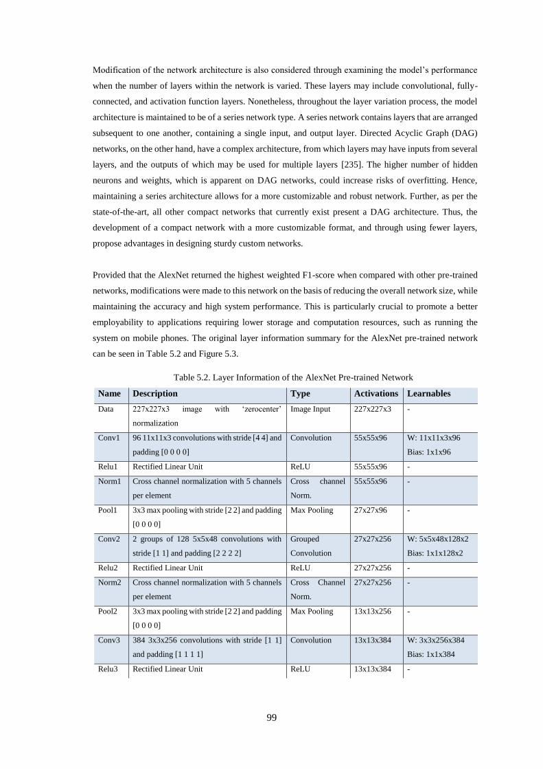
99

Modification of the network architecture is also considered through examining the model’s performance

when the number of layers within the network is varied. These layers may include convolutional, fully-

connected, and activation function layers. Nonetheless, throughout the layer variation process, the model

architecture is maintained to be of a series network type. A series network contains layers that are arranged

subsequent to one another, containing a single input, and output layer. Directed Acyclic Graph (DAG)

networks, on the other hand, have a complex architecture, from which layers may have inputs from several

layers, and the outputs of which may be used for multiple layers [235]. The higher number of hidden

neurons and weights, which is apparent on DAG networks, could increase risks of overfitting. Hence,

maintaining a series architecture allows for a more customizable and robust network. Further, as per the

state-of-the-art, all other compact networks that currently exist present a DAG architecture. Thus, the

development of a compact network with a more customizable format, and through using fewer layers,

propose advantages in designing sturdy custom networks.

Provided that the AlexNet returned the highest weighted F1-score when compared with other pre-trained

networks, modifications were made to this network on the basis of reducing the overall network size, while

maintaining the accuracy and high system performance. This is particularly crucial to promote a better

employability to applications requiring lower storage and computation resources, such as running the

system on mobile phones. The original layer information summary for the AlexNet pre-trained network

can be seen in Table 5.2 and Figure 5.3.

Table 5.2. Layer Information of the AlexNet Pre-trained Network

Name Description Type Activations Learnables

Data 227x227x3 image with ‘zerocenter’

normalization

Image Input 227x227x3 -

Conv1 96 11x11x3 convolutions with stride [4 4] and

padding [0 0 0 0]

Convolution 55x55x96 W: 11x11x3x96

Bias: 1x1x96

Relu1 Rectified Linear Unit ReLU 55x55x96 -

Norm1 Cross channel normalization with 5 channels

per element

Cross channel

Norm.

55x55x96 -

Pool1 3x3 max pooling with stride [2 2] and padding

[0 0 0 0]

Max Pooling 27x27x96 -

Conv2 2 groups of 128 5x5x48 convolutions with

stride [1 1] and padding [2 2 2 2]

Grouped

Convolution

27x27x256 W: 5x5x48x128x2

Bias: 1x1x128x2

Relu2 Rectified Linear Unit ReLU 27x27x256 -

Norm2 Cross channel normalization with 5 channels

per element

Cross Channel

Norm.

27x27x256 -

Pool2 3x3 max pooling with stride [2 2] and padding

[0 0 0 0]

Max Pooling 13x13x256 -

Conv3 384 3x3x256 convolutions with stride [1 1]

and padding [1 1 1 1]

Convolution 13x13x384 W: 3x3x256x384

Bias: 1x1x384

Relu3 Rectified Linear Unit ReLU 13x13x384 -

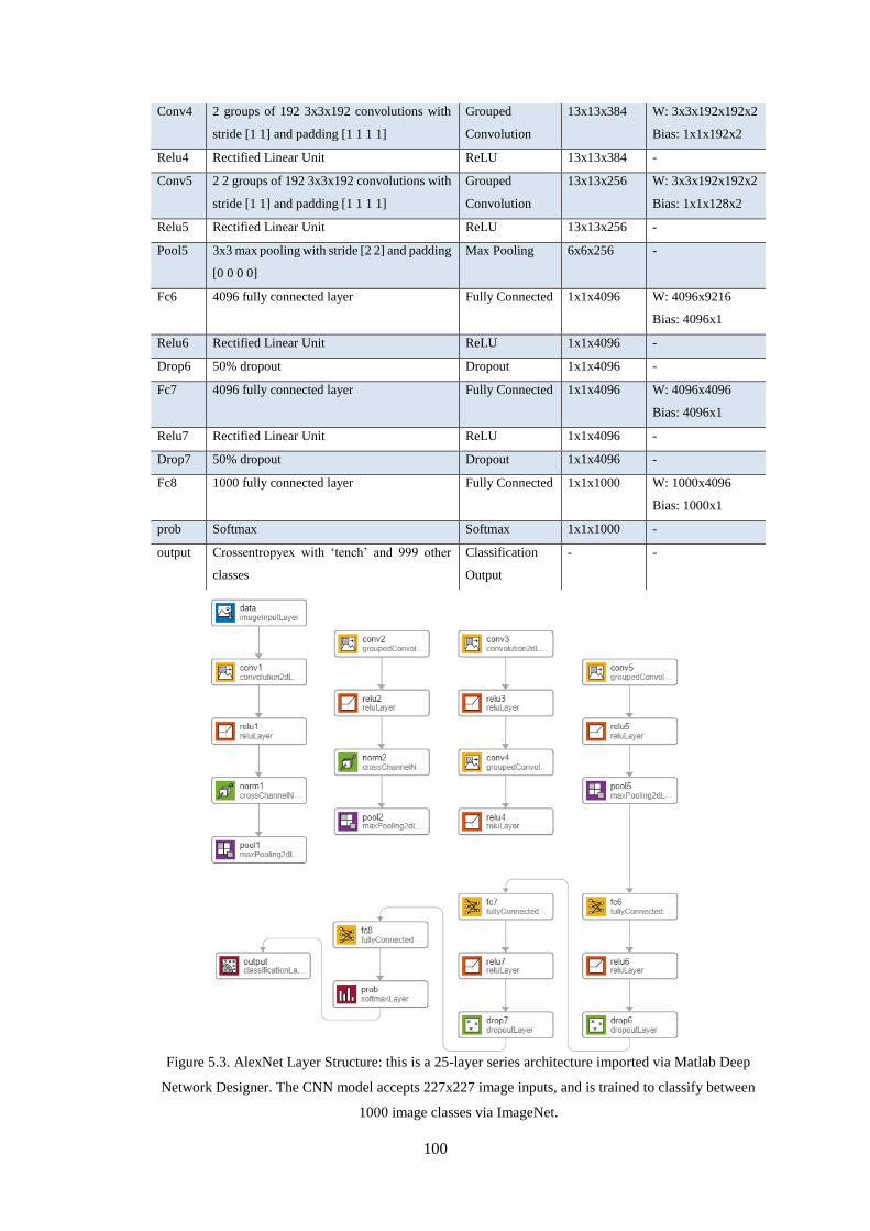
100

Conv4 2 groups of 192 3x3x192 convolutions with

stride [1 1] and padding [1 1 1 1]

Grouped

Convolution

13x13x384 W: 3x3x192x192x2

Bias: 1x1x192x2

Relu4 Rectified Linear Unit ReLU 13x13x384 -

Conv5 2 2 groups of 192 3x3x192 convolutions with

stride [1 1] and padding [1 1 1 1]

Grouped

Convolution

13x13x256 W: 3x3x192x192x2

Bias: 1x1x128x2

Relu5 Rectified Linear Unit ReLU 13x13x256 -

Pool5 3x3 max pooling with stride [2 2] and padding

[0 0 0 0]

Max Pooling 6x6x256 -

Fc6 4096 fully connected layer Fully Connected 1x1x4096 W: 4096x9216

Bias: 4096x1

Relu6 Rectified Linear Unit ReLU 1x1x4096 -

Drop6 50% dropout Dropout 1x1x4096 -

Fc7 4096 fully connected layer Fully Connected 1x1x4096 W: 4096x4096

Bias: 4096x1

Relu7 Rectified Linear Unit ReLU 1x1x4096 -

Drop7 50% dropout Dropout 1x1x4096 -

Fc8 1000 fully connected layer Fully Connected 1x1x1000 W: 1000x4096

Bias: 1000x1

prob Softmax Softmax 1x1x1000 -

output Crossentropyex with ‘tench’ and 999 other

classes

Classification

Output

- -

Figure 5.3. AlexNet Layer Structure: this is a 25-layer series architecture imported via Matlab Deep

Network Designer. The CNN model accepts 227x227 image inputs, and is trained to classify between

1000 image classes via ImageNet.

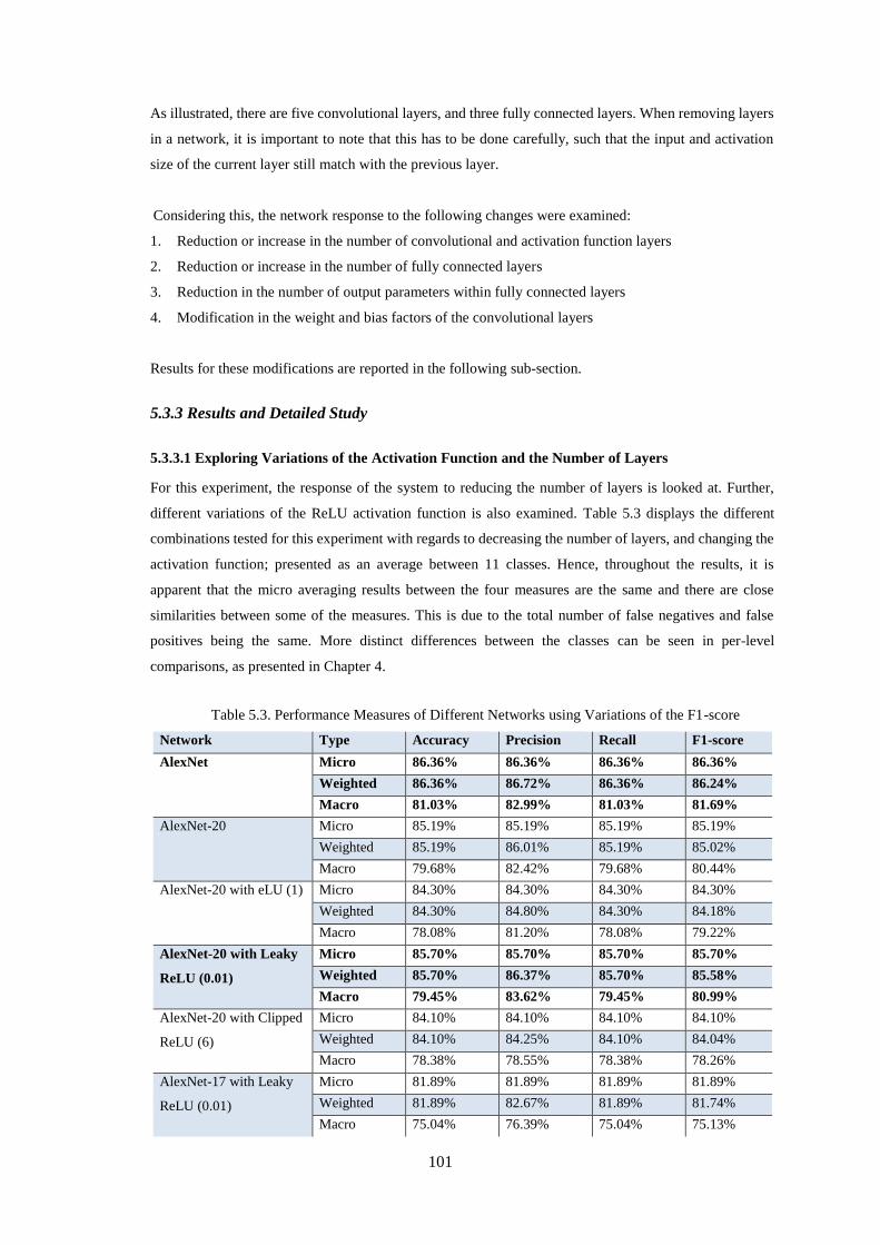
101

As illustrated, there are five convolutional layers, and three fully connected layers. When removing layers

in a network, it is important to note that this has to be done carefully, such that the input and activation

size of the current layer still match with the previous layer.

Considering this, the network response to the following changes were examined:

1. Reduction or increase in the number of convolutional and activation function layers

2. Reduction or increase in the number of fully connected layers

3. Reduction in the number of output parameters within fully connected layers

4. Modification in the weight and bias factors of the convolutional layers

Results for these modifications are reported in the following sub-section.

5.3.3 Results and Detailed Study

5.3.3.1 Exploring Variations of the Activation Function and the Number of Layers

For this experiment, the response of the system to reducing the number of layers is looked at. Further,

different variations of the ReLU activation function is also examined. Table 5.3 displays the different

combinations tested for this experiment with regards to decreasing the number of layers, and changing the

activation function; presented as an average between 11 classes. Hence, throughout the results, it is

apparent that the micro averaging results between the four measures are the same and there are close

similarities between some of the measures. This is due to the total number of false negatives and false

positives being the same. More distinct differences between the classes can be seen in per-level

comparisons, as presented in Chapter 4.

Table 5.3. Performance Measures of Different Networks using Variations of the F1-score

Network Type Accuracy Precision Recall F1-score

AlexNet Micro 86.36% 86.36% 86.36% 86.36%

Weighted 86.36% 86.72% 86.36% 86.24%

Macro 81.03% 82.99% 81.03% 81.69%

AlexNet-20 Micro 85.19% 85.19% 85.19% 85.19%

Weighted 85.19% 86.01% 85.19% 85.02%

Macro 79.68% 82.42% 79.68% 80.44%

AlexNet-20 with eLU (1) Micro 84.30% 84.30% 84.30% 84.30%

Weighted 84.30% 84.80% 84.30% 84.18%

Macro 78.08% 81.20% 78.08% 79.22%

AlexNet-20 with Leaky

ReLU (0.01)

Micro 85.70% 85.70% 85.70% 85.70%

Weighted 85.70% 86.37% 85.70% 85.58%

Macro 79.45% 83.62% 79.45% 80.99%

AlexNet-20 with Clipped

ReLU (6)

Micro 84.10% 84.10% 84.10% 84.10%

Weighted 84.10% 84.25% 84.10% 84.04%

Macro 78.38% 78.55% 78.38% 78.26%

AlexNet-17 with Leaky

ReLU (0.01)

Micro 81.89% 81.89% 81.89% 81.89%

Weighted 81.89% 82.67% 81.89% 81.74%

Macro 75.04% 76.39% 75.04% 75.13%

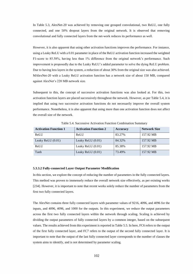
102

In Table 5.3, AlexNet-20 was achieved by removing one grouped convolutional, two ReLU, one fully

connected, and one 50% dropout layers from the original network. It is observed that removing

convolutional and fully connected layers from the net-work reduces its performance as well.

However, it is also apparent that using other activation functions improves the performance. For instance,

using a Leaky ReLU with a 0.01 parameter in place of the ReLU activation function increased the weighted

F1-score to 85.58%, having less than 1% difference from the original network’s performance. Such

improvement is proposedly due to the Leaky ReLU’s added parameter to solve the dying ReLU problem.

Due to having less layers in the system, a reduction of about 30% from the original size was also achieved.

MAlexNet-20 with a Leaky ReLU activation function has a network size of about 150 MB, compared

against AlexNet’s 220 MB network size.

Subsequent to this, the concept of successive activation functions was also looked at. For this, two

activation function layers are placed successively throughout the network. However, as per Table 5.4, it is

implied that using two successive activation functions do not necessarily improve the overall system

performance. Nonetheless, it is also apparent that using more than one activation function does not affect

the overall size of the network.

Table 5.4. Successive Activation Function Combination Summary

Activation Function 1 Activation Function 2 Accuracy Network Size

ReLU ReLU 83.27% 157.92 MB

Leaky ReLU (0.01) Leaky ReLU (0.01) 84.32% 157.92 MB

ReLU Leaky ReLU (0.01) 85.38% 157.92 MB

Tanh Leaky ReLU (0.01) 73.49% 157.92 MB

5.3.3.2 Fully-connected Layer Output Parameter Modification

In this section, we explore the concept of reducing the number of parameters in the fully connected layers.

This method was proven to immensely reduce the overall network size effectively, as per existing works

[234]. However, it is important to note that recent works solely reduce the number of parameters from the

first two fully connected layers.

The AlexNet contains three fully connected layers with parameter values of 9216, 4096, and 4096 for the

inputs, and 4096, 4096, and 1000 for the outputs. In this experiment, we reduce the output parameters

across the first two fully connected layers within the network through scaling. Scaling is achieved by

dividing the output parameters of fully connected layers by a common integer, based on the subsequent

values. The results achieved from this experiment is reported in Table 5.5. In here, FC6 refers to the output

of the first fully connected layer, and FC7 refers to the output of the second fully connected layer. It is

important to note that the output of the last fully connected layer corresponds to the number of classes the

system aims to identify, and is not determined by parameter scaling.

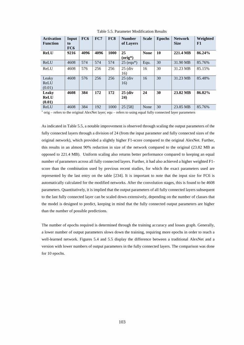
103

Table 5.5. Parameter Modification Results

Activation

Function

Input

to

FC6

FC6 FC7 FC8 Number

of Layers

Scale Epochs Network

Size

Weighted

F1

ReLU 9216 4096 4096 1000 25

(orig*)

None 10 221.4 MB 86.24%

ReLU 4608 574 574 574 25 (equ*) Equ. 30 31.90 MB 85.76%

ReLU 4608 576 256 256 25 (div

16)

16 30 31.23 MB 85.15%

Leaky

ReLU

(0.01)

4608 576 256 256 25 (div

16)

16 30 31.23 MB 85.48%

Leaky

ReLU

(0.01)

4608 384 172 172 25 (div

24)

24 30 23.82 MB 86.82%

ReLU 4608 384 192 1000 25 [58] None 30 23.85 MB 85.76% * orig – refers to the original AlexNet layer; equ – refers to using equal fully connected layer parameters

As indicated in Table 5.5, a notable improvement is observed through scaling the output parameters of the

fully connected layers through a division of 24 (from the input parameter and fully connected sizes of the

original network), which provided a slightly higher F1-score compared to the original AlexNet. Further,

this results in an almost 90% reduction in size of the network compared to the original (23.82 MB as

opposed to 221.4 MB). Uniform scaling also returns better performance compared to keeping an equal

number of parameters across all fully connected layers. Further, it had also achieved a higher weighted F1-

score than the combination used by previous recent studies, for which the exact parameters used are

represented by the last entry on the table [234]. It is important to note that the input size for FC6 is

automatically calculated for the modified networks. After the convolution stages, this is found to be 4608

parameters. Quantitatively, it is implied that the output parameters of all fully connected layers subsequent

to the last fully connected layer can be scaled down extensively, depending on the number of classes that

the model is designed to predict, keeping in mind that the fully connected output parameters are higher

than the number of possible predictions.

The number of epochs required is determined through the training accuracy and losses graph. Generally,

a lower number of output parameters slows down the training, requiring more epochs in order to reach a

well-learned network. Figures 5.4 and 5.5 display the difference between a traditional AlexNet and a

version with lower numbers of output parameters in the fully connected layers. The comparison was done

for 10 epochs.

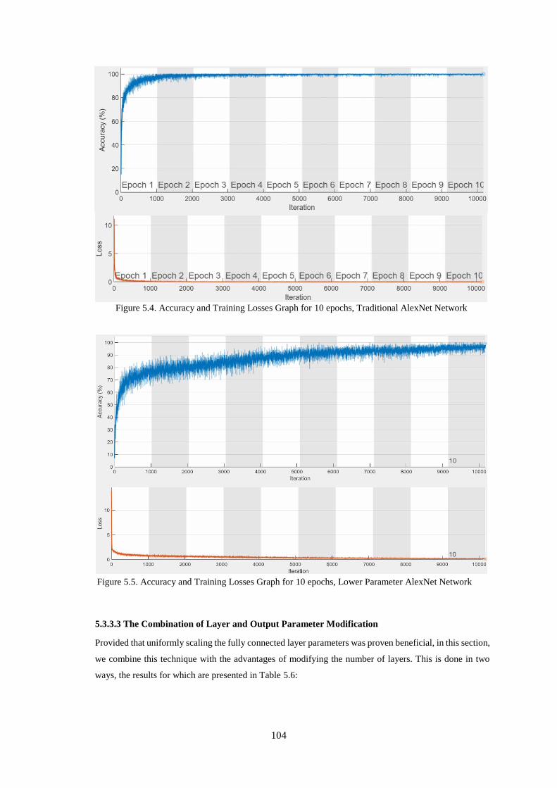
104

Figure 5.4. Accuracy and Training Losses Graph for 10 epochs, Traditional AlexNet Network

Figure 5.5. Accuracy and Training Losses Graph for 10 epochs, Lower Parameter AlexNet Network

5.3.3.3 The Combination of Layer and Output Parameter Modification

Provided that uniformly scaling the fully connected layer parameters was proven beneficial, in this section,

we combine this technique with the advantages of modifying the number of layers. This is done in two

ways, the results for which are presented in Table 5.6:

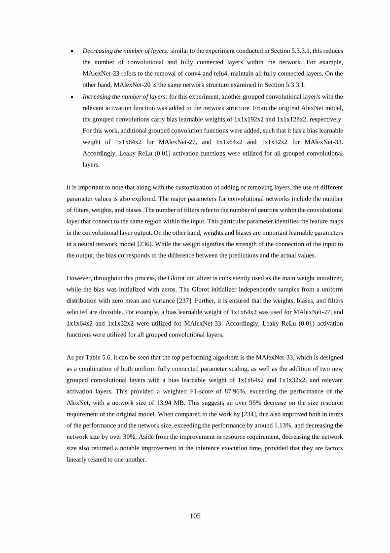
105

Decreasing the number of layers: similar to the experiment conducted in Section 5.3.3.1, this reduces

the number of convolutional and fully connected layers within the network. For example,

MAlexNet-23 refers to the removal of conv4 and relu4, maintain all fully connected layers. On the

other hand, MAlexNet-20 is the same network structure examined in Section 5.3.3.1.

Increasing the number of layers: for this experiment, another grouped convolutional layer/s with the

relevant activation function was added to the network structure. From the original AlexNet model,

the grouped convolutions carry bias learnable weights of 1x1x192x2 and 1x1x128x2, respectively.

For this work, additional grouped convolution functions were added, such that it has a bias learnable

weight of 1x1x64x2 for MAlexNet-27, and 1x1x64x2 and 1x1x32x2 for MAlexNet-33.

Accordingly, Leaky ReLu (0.01) activation functions were utilized for all grouped convolutional

layers.

It is important to note that along with the customization of adding or removing layers, the use of different

parameter values is also explored. The major parameters for convolutional networks include the number

of filters, weights, and biases. The number of filters refer to the number of neurons within the convolutional

layer that connect to the same region within the input. This particular parameter identifies the feature maps

in the convolutional layer output. On the other hand, weights and biases are important learnable parameters

in a neural network model [236]. While the weight signifies the strength of the connection of the input to

the output, the bias corresponds to the difference between the predictions and the actual values.

However, throughout this process, the Glorot initializer is consistently used as the main weight initializer,

while the bias was initialized with zeros. The Glorot initializer independently samples from a uniform

distribution with zero mean and variance [237]. Further, it is ensured that the weights, biases, and filters

selected are divisible. For example, a bias learnable weight of 1x1x64x2 was used for MAlexNet-27, and

1x1x64x2 and 1x1x32x2 were utilized for MAlexNet-33. Accordingly, Leaky ReLu (0.01) activation

functions were utilized for all grouped convolutional layers.

As per Table 5.6, it can be seen that the top performing algorithm is the MAlexNet-33, which is designed

as a combination of both uniform fully connected parameter scaling, as well as the addition of two new

grouped convolutional layers with a bias learnable weight of 1x1x64x2 and 1x1x32x2, and relevant

activation layers. This provided a weighted F1-score of 87.96%, exceeding the performance of the

AlexNet, with a network size of 13.94 MB. This suggests an over 95% decrease on the size resource

requirement of the original model. When compared to the work by [234], this also improved both in terms

of the performance and the network size, exceeding the performance by around 1.13%, and decreasing the

network size by over 30%. Aside from the improvement in resource requirement, decreasing the network

size also returned a notable improvement in the inference execution time, provided that they are factors

linearly related to one another.

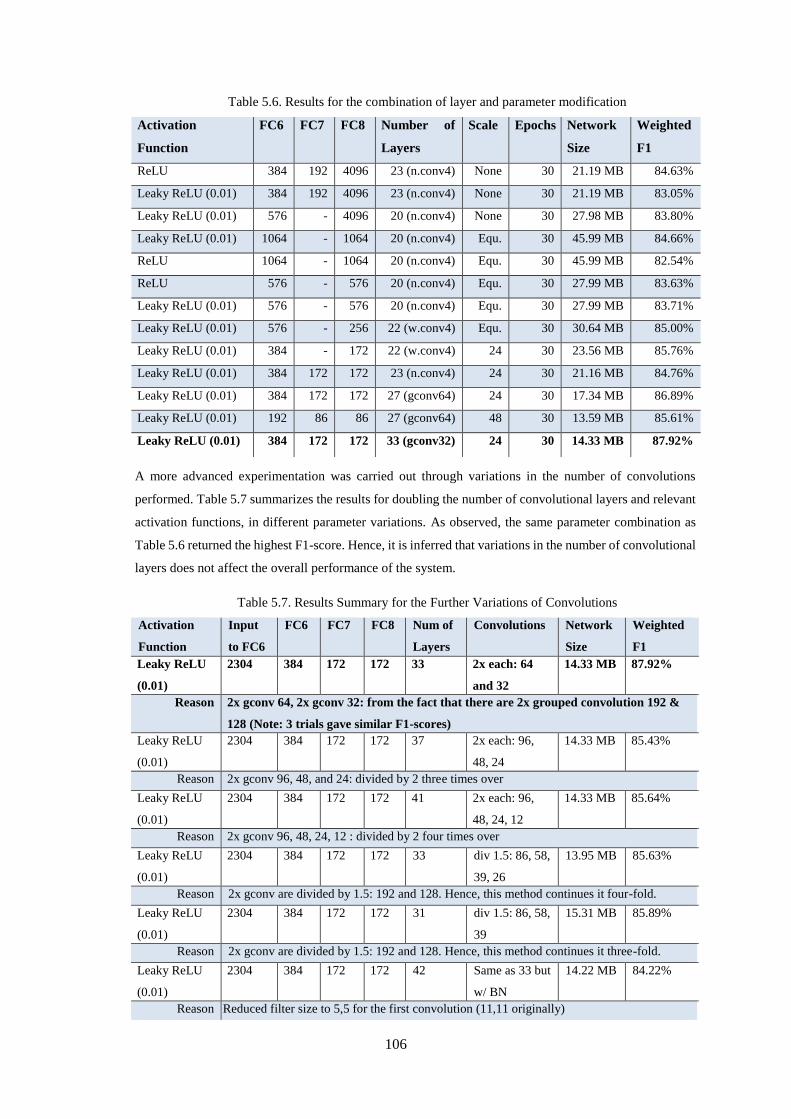
106

Table 5.6. Results for the combination of layer and parameter modification

Activation

Function

FC6 FC7 FC8 Number of

Layers

Scale Epochs Network

Size

Weighted

F1

ReLU 384 192 4096 23 (n.conv4) None 30 21.19 MB 84.63%

Leaky ReLU (0.01) 384 192 4096 23 (n.conv4) None 30 21.19 MB 83.05%

Leaky ReLU (0.01) 576 - 4096 20 (n.conv4) None 30 27.98 MB 83.80%

Leaky ReLU (0.01) 1064 - 1064 20 (n.conv4) Equ. 30 45.99 MB 84.66%

ReLU 1064 - 1064 20 (n.conv4) Equ. 30 45.99 MB 82.54%

ReLU 576 - 576 20 (n.conv4) Equ. 30 27.99 MB 83.63%

Leaky ReLU (0.01) 576 - 576 20 (n.conv4) Equ. 30 27.99 MB 83.71%

Leaky ReLU (0.01) 576 - 256 22 (w.conv4) Equ. 30 30.64 MB 85.00%

Leaky ReLU (0.01) 384 - 172 22 (w.conv4) 24 30 23.56 MB 85.76%

Leaky ReLU (0.01) 384 172 172 23 (n.conv4) 24 30 21.16 MB 84.76%

Leaky ReLU (0.01) 384 172 172 27 (gconv64) 24 30 17.34 MB 86.89%

Leaky ReLU (0.01) 192 86 86 27 (gconv64) 48 30 13.59 MB 85.61%

Leaky ReLU (0.01) 384 172 172 33 (gconv32) 24 30 14.33 MB 87.92%

A more advanced experimentation was carried out through variations in the number of convolutions

performed. Table 5.7 summarizes the results for doubling the number of convolutional layers and relevant

activation functions, in different parameter variations. As observed, the same parameter combination as

Table 5.6 returned the highest F1-score. Hence, it is inferred that variations in the number of convolutional

layers does not affect the overall performance of the system.

Table 5.7. Results Summary for the Further Variations of Convolutions

Activation

Function

Input

to FC6

FC6 FC7 FC8 Num of

Layers

Convolutions Network

Size

Weighted

F1

Leaky ReLU

(0.01)

2304 384 172 172 33 2x each: 64

and 32

14.33 MB 87.92%

Reason 2x gconv 64, 2x gconv 32: from the fact that there are 2x grouped convolution 192 &

128 (Note: 3 trials gave similar F1-scores)

Leaky ReLU

(0.01)

2304 384 172 172 37 2x each: 96,

48, 24

14.33 MB 85.43%

Reason 2x gconv 96, 48, and 24: divided by 2 three times over

Leaky ReLU

(0.01)

2304 384 172 172 41 2x each: 96,

48, 24, 12

14.33 MB 85.64%

Reason 2x gconv 96, 48, 24, 12 : divided by 2 four times over

Leaky ReLU

(0.01)

2304 384 172 172 33 div 1.5: 86, 58,

39, 26

13.95 MB 85.63%

Reason 2x gconv are divided by 1.5: 192 and 128. Hence, this method continues it four-fold.

Leaky ReLU

(0.01)

2304 384 172 172 31 div 1.5: 86, 58,

39

15.31 MB 85.89%

Reason 2x gconv are divided by 1.5: 192 and 128. Hence, this method continues it three-fold.

Leaky ReLU

(0.01)

2304 384 172 172 42 Same as 33 but

w/ BN

14.22 MB 84.22%

Reason Reduced filter size to 5,5 for the first convolution (11,11 originally)

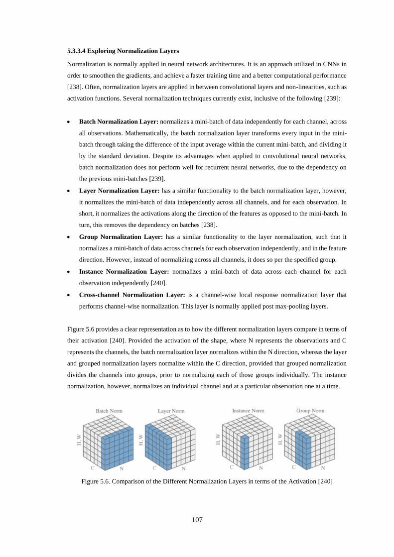
107

5.3.3.4 Exploring Normalization Layers

Normalization is normally applied in neural network architectures. It is an approach utilized in CNNs in

order to smoothen the gradients, and achieve a faster training time and a better computational performance

[238]. Often, normalization layers are applied in between convolutional layers and non-linearities, such as

activation functions. Several normalization techniques currently exist, inclusive of the following [239]:

Batch Normalization Layer: normalizes a mini-batch of data independently for each channel, across

all observations. Mathematically, the batch normalization layer transforms every input in the mini-

batch through taking the difference of the input average within the current mini-batch, and dividing it

by the standard deviation. Despite its advantages when applied to convolutional neural networks,

batch normalization does not perform well for recurrent neural networks, due to the dependency on

the previous mini-batches [239].

Layer Normalization Layer: has a similar functionality to the batch normalization layer, however,

it normalizes the mini-batch of data independently across all channels, and for each observation. In

short, it normalizes the activations along the direction of the features as opposed to the mini-batch. In

turn, this removes the dependency on batches [238].

Group Normalization Layer: has a similar functionality to the layer normalization, such that it

normalizes a mini-batch of data across channels for each observation independently, and in the feature

direction. However, instead of normalizing across all channels, it does so per the specified group.

Instance Normalization Layer: normalizes a mini-batch of data across each channel for each

observation independently [240].

Cross-channel Normalization Layer: is a channel-wise local response normalization layer that

performs channel-wise normalization. This layer is normally applied post max-pooling layers.

Figure 5.6 provides a clear representation as to how the different normalization layers compare in terms of

their activation [240]. Provided the activation of the shape, where N represents the observations and C

represents the channels, the batch normalization layer normalizes within the N direction, whereas the layer

and grouped normalization layers normalize within the C direction, provided that grouped normalization

divides the channels into groups, prior to normalizing each of those groups individually. The instance

normalization, however, normalizes an individual channel and at a particular observation one at a time.

Figure 5.6. Comparison of the Different Normalization Layers in terms of the Activation [240]

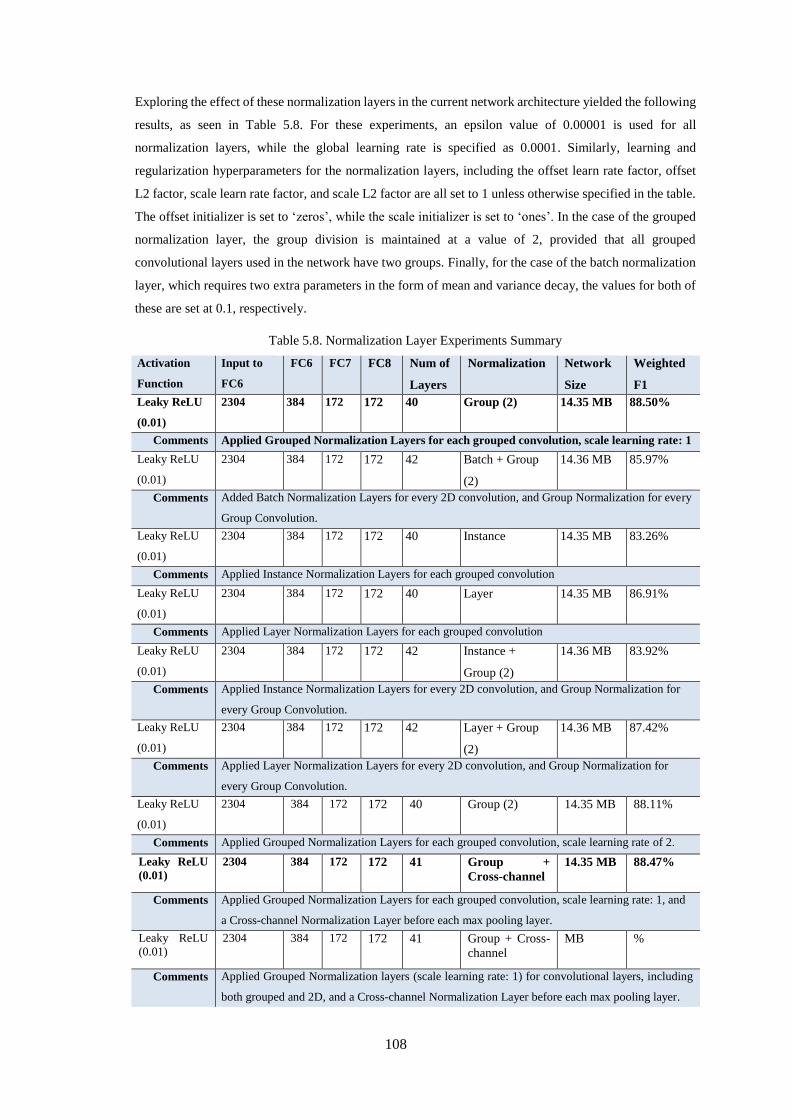
108

Exploring the effect of these normalization layers in the current network architecture yielded the following

results, as seen in Table 5.8. For these experiments, an epsilon value of 0.00001 is used for all

normalization layers, while the global learning rate is specified as 0.0001. Similarly, learning and

regularization hyperparameters for the normalization layers, including the offset learn rate factor, offset

L2 factor, scale learn rate factor, and scale L2 factor are all set to 1 unless otherwise specified in the table.

The offset initializer is set to ‘zeros’, while the scale initializer is set to ‘ones’. In the case of the grouped

normalization layer, the group division is maintained at a value of 2, provided that all grouped

convolutional layers used in the network have two groups. Finally, for the case of the batch normalization

layer, which requires two extra parameters in the form of mean and variance decay, the values for both of

these are set at 0.1, respectively.

Table 5.8. Normalization Layer Experiments Summary

Activation

Function

Input to

FC6

FC6 FC7 FC8 Num of

Layers

Normalization Network

Size

Weighted

F1

Leaky ReLU

(0.01)

2304 384 172 172 40 Group (2) 14.35 MB 88.50%

Comments Applied Grouped Normalization Layers for each grouped convolution, scale learning rate: 1

Leaky ReLU

(0.01)

2304 384 172 172 42 Batch + Group

(2)

14.36 MB 85.97%

Comments Added Batch Normalization Layers for every 2D convolution, and Group Normalization for every

Group Convolution.

Leaky ReLU

(0.01)

2304 384 172 172 40 Instance 14.35 MB 83.26%

Comments Applied Instance Normalization Layers for each grouped convolution

Leaky ReLU

(0.01)

2304 384 172 172 40 Layer 14.35 MB 86.91%

Comments Applied Layer Normalization Layers for each grouped convolution

Leaky ReLU

(0.01)

2304 384 172 172 42 Instance +

Group (2)

14.36 MB 83.92%

Comments Applied Instance Normalization Layers for every 2D convolution, and Group Normalization for

every Group Convolution.

Leaky ReLU

(0.01)

2304 384 172 172 42 Layer + Group

(2)

14.36 MB 87.42%

Comments Applied Layer Normalization Layers for every 2D convolution, and Group Normalization for

every Group Convolution.

Leaky ReLU

(0.01)

2304 384 172 172 40 Group (2) 14.35 MB 88.11%

Comments Applied Grouped Normalization Layers for each grouped convolution, scale learning rate of 2.

Leaky ReLU

(0.01)

2304 384 172 172 41 Group +

Cross-channel

14.35 MB 88.47%

Comments Applied Grouped Normalization Layers for each grouped convolution, scale learning rate: 1, and

a Cross-channel Normalization Layer before each max pooling layer.

Leaky ReLU

(0.01)

2304 384 172 172 41 Group + Cross-

channel

MB %

Comments Applied Grouped Normalization layers (scale learning rate: 1) for convolutional layers, including

both grouped and 2D, and a Cross-channel Normalization Layer before each max pooling layer.

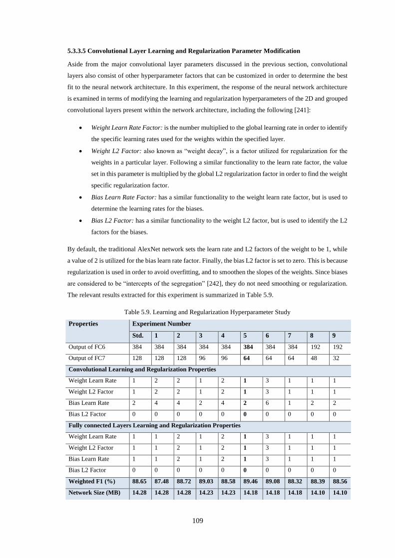
109

5.3.3.5 Convolutional Layer Learning and Regularization Parameter Modification

Aside from the major convolutional layer parameters discussed in the previous section, convolutional

layers also consist of other hyperparameter factors that can be customized in order to determine the best

fit to the neural network architecture. In this experiment, the response of the neural network architecture

is examined in terms of modifying the learning and regularization hyperparameters of the 2D and grouped

convolutional layers present within the network architecture, including the following [241]:

Weight Learn Rate Factor: is the number multiplied to the global learning rate in order to identify

the specific learning rates used for the weights within the specified layer.

Weight L2 Factor: also known as “weight decay”, is a factor utilized for regularization for the

weights in a particular layer. Following a similar functionality to the learn rate factor, the value

set in this parameter is multiplied by the global L2 regularization factor in order to find the weight

specific regularization factor.

Bias Learn Rate Factor: has a similar functionality to the weight learn rate factor, but is used to

determine the learning rates for the biases.

Bias L2 Factor: has a similar functionality to the weight L2 factor, but is used to identify the L2

factors for the biases.

By default, the traditional AlexNet network sets the learn rate and L2 factors of the weight to be 1, while

a value of 2 is utilized for the bias learn rate factor. Finally, the bias L2 factor is set to zero. This is because

regularization is used in order to avoid overfitting, and to smoothen the slopes of the weights. Since biases

are considered to be “intercepts of the segregation” [242], they do not need smoothing or regularization.

The relevant results extracted for this experiment is summarized in Table 5.9.

Table 5.9. Learning and Regularization Hyperparameter Study

Properties Experiment Number

Std. 1 2 3 4 5 6 7 8 9

Output of FC6 384 384 384 384 384 384 384 384 192 192

Output of FC7 128 128 128 96 96 64 64 64 48 32

Convolutional Learning and Regularization Properties

Weight Learn Rate 1 2 2 1 2 1 3 1 1 1

Weight L2 Factor 1 2 2 1 2 1 3 1 1 1

Bias Learn Rate 2 4 4 2 4 2 6 1 2 2

Bias L2 Factor 0 0 0 0 0 0 0 0 0 0

Fully connected Layers Learning and Regularization Properties

Weight Learn Rate 1 1 2 1 2 1 3 1 1 1

Weight L2 Factor 1 1 2 1 2 1 3 1 1 1

Bias Learn Rate 1 1 2 1 2 1 3 1 1 1

Bias L2 Factor 0 0 0 0 0 0 0 0 0 0

Weighted F1 (%) 88.65 87.48 88.72 89.03 88.58 89.46 89.08 88.32 88.39 88.56

Network Size (MB) 14.28 14.28 14.28 14.23 14.23 14.18 14.18 14.18 14.10 14.10

110

From Table 5.9, it is important to note that the activation function used for all experiments is the Leaky

ReLU, with 0.01 parameter. Further, a global learning rate of 0.0001 is specified for the trainings.

5.3.3.6 Examining System Response to Various Optimization Algorithms

Training neural network models involve multiple iterations of minimizing losses and learning the

parameters that converge to the desired function, which is achieved through an optimization algorithm

[243]. During the training process, the model yields an output for every iteration, prior to calculating the

difference between the yielded and desired output, aiming to minimize this difference as much as possible.

The gradient is defined to be the derivative of a function that contains multiple variables [244]. Given that

it expresses the slope of the function, it allows the approximation of the effects of taking a step from a

point from any direction [244]. Since the gradient is based on the rate of change of the loss function, the

idea is to be keep reducing the loss after each iteration. There are various types of optimization algorithms

available. However, for this experiment, the response to three specific optimization algorithms is examined

for the current optimum neural network model. The optimization algorithms examined in this work include

the following [243]:

Stochastic Gradient Descent with Momentum (SGDM) Optimizer [245]: The SGDM

optimizer calculates the gradient on one individual data element at a certain time. The

incorporation of the momentum aids in accelerating the SGD in the correct direction, which

dampens the oscillations accordingly and speeds up convergence. This also overcomes

disadvantages concerning noise in weight updates, provided its denoising capabilities [246]. The

calculation of the gradient is represented by equation (5.1), such that [246]:

𝑉(𝑡) = 𝛾 ∗ 𝑉(𝑡 − 1) + 𝛼 ∗𝑑(𝐸(𝜃))

𝑑𝜃

(5.1)

where 𝛾 represents the momentum, 𝛼 signifies the learning rate, 𝐸(𝜃) is the loss function, 𝑡

represents the time step, and the weights of the neural network are updated by 𝜃 = 𝜃 − 𝑉(𝑡).

RMSProp Optimizer [247]: the RMSProp is an optimization algorithm that computes adaptive

gradients, and accumulates these into an exponentially decaying weighted average. The running

average 𝐸[𝑔2]𝑡 is represented in equation (5.2), such that the global learning rate 𝜂 is divided by

the exponentially decaying average of the squared gradients for the weight update, as per equation

(5.3) [246].

𝐸[𝑔2]𝑡 = 𝛾 ∗ 𝐸[𝑔2]𝑡−1 + (1 − 𝛾)𝑔𝑡2 (5.2)

𝜃𝑡+1 = 𝜃𝑡 −𝜂

√𝐸[𝑔2]𝑡 + 𝜖𝑔𝑡

(5.3)

Adaptive Moments Optimizer [248]: — the adaptive moments optimizer, also called the “Adam

Optimizer”, and is a fusion of the SGDM and the RMSProp optimizers. This fusion is achieved

such that it accumulates an exponentially decaying weighted average, similar to RMSProp.

However, in addition to this, it also retains the exponentially decaying averages of the past

gradients, such as that of SGDM [246]. A bias correction mechanism is used for this particular

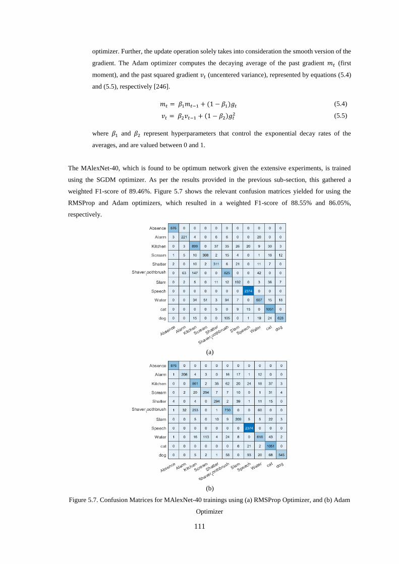
111

optimizer. Further, the update operation solely takes into consideration the smooth version of the

gradient. The Adam optimizer computes the decaying average of the past gradient 𝑚𝑡 (first

moment), and the past squared gradient 𝑣𝑡 (uncentered variance), represented by equations (5.4)

and (5.5), respectively [246].

𝑚𝑡 = 𝛽1𝑚𝑡−1 + (1 − 𝛽1)𝑔𝑡 (5.4)

𝑣𝑡 = 𝛽2𝑣𝑡−1 + (1 − 𝛽2)𝑔𝑡2 (5.5)

where 𝛽1 and 𝛽2 represent hyperparameters that control the exponential decay rates of the

averages, and are valued between 0 and 1.

The MAlexNet-40, which is found to be optimum network given the extensive experiments, is trained

using the SGDM optimizer. As per the results provided in the previous sub-section, this gathered a

weighted F1-score of 89.46%. Figure 5.7 shows the relevant confusion matrices yielded for using the

RMSProp and Adam optimizers, which resulted in a weighted F1-score of 88.55% and 86.05%,

respectively.

(a)

(b)

Figure 5.7. Confusion Matrices for MAlexNet-40 trainings using (a) RMSProp Optimizer, and (b) Adam

Optimizer

112

As observed, the SGDM optimizer produced the best performance for the MAlexNet-40 network

architecture, provided that it is a simpler, Series Network format. For more complicated architectures, such

as the DAG, the Adam optimizer is found to have a good performance [243]. As per the discussion above,

every optimization algorithm possesses relevant advantages, and suitability can be examined depending

on the neural network architecture.

5.3.4 Discussion and Findings

For the network developed, there are three main discoveries made throughout the extensive neural network

study. These can be summarized as follows:

Hypothesis 5.1: The Leaky ReLU activation function returned higher performance for multi-level

classification as opposed to the traditional ReLU in majority of the cases.

Verification of Hypothesis 5.1: This is true on a case-by-case scenario. This can be explained by the

presence of the dying ReLU problem in feature sets, which is ameliorated through the small parameter

added through the Leaky ReLU. However, it is important to note that the presence of the dying ReLU

problem could depend on several factors, including the nature of the data being trained. In cases where

this does not occur, re-placing the activation function to a Leaky ReLU may not return any advantages.

Hypothesis 5.2: Decreasing the number of fully connected and convolutional layers throughout the

network also slightly decreases the performance.

Verification of Hypothesis 5.2: Generally, convolutional layers represent high level features within the

network. Accordingly, fully connected layers flattens and combines these features. Hence, reducing the

number of these layers negatively affect the performance of the network.

Hypothesis 5.3: Decreasing parameters, weight factors, and biases within the fully connected and

convolutional layers help decrease the size of the network more, compared to when these layers are

removed completely.

Verification of Hypothesis 5.3: Both convolutional and fully connected layers contribute to the high and

low-level features from which the network learns, and are therefore essential. However, since pre-trained

models are originally trained on very large data, large parameters, weight, and bias factors are often not

necessary when using transfer learning applied to a much smaller dataset. This explains the maintenance

of the system performance despite decreasing the parameters for these layers accordingly. Based on our

experiments, scaling the parameters uniformly across fully connected layers returns the best performance.

The overall layer information for the top performing MAlexNet-40 is seen in Table 5.10. Subsequently,

the detailed per-level results are presented in Table 5.11.

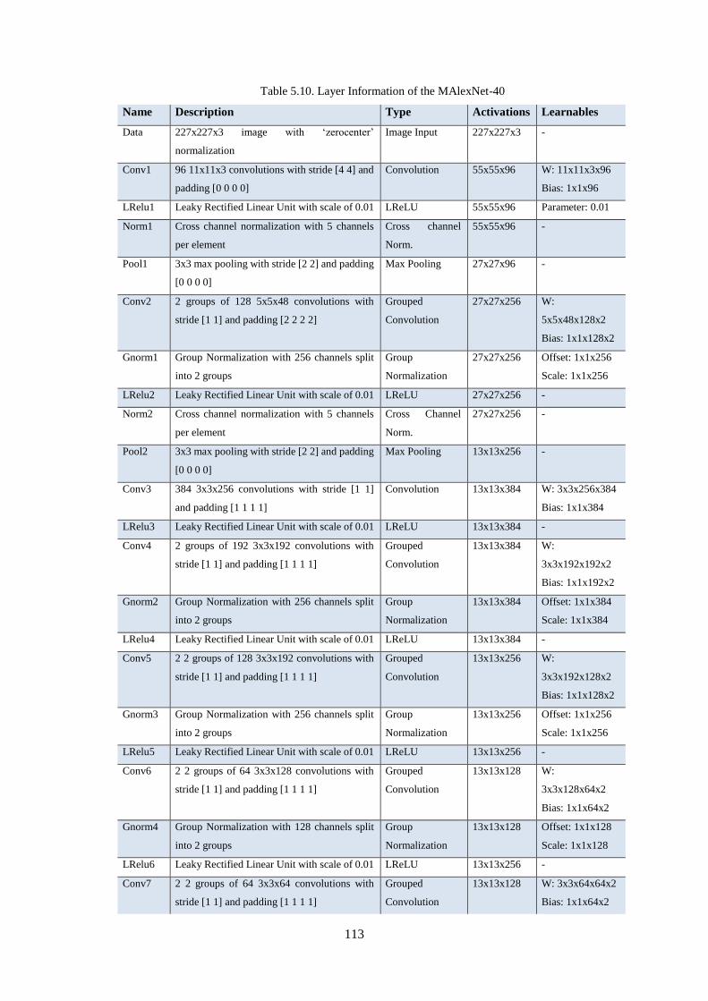
113

Table 5.10. Layer Information of the MAlexNet-40

Name Description Type Activations Learnables

Data 227x227x3 image with ‘zerocenter’

normalization

Image Input 227x227x3 -

Conv1 96 11x11x3 convolutions with stride [4 4] and

padding [0 0 0 0]

Convolution 55x55x96 W: 11x11x3x96

Bias: 1x1x96

LRelu1 Leaky Rectified Linear Unit with scale of 0.01 LReLU 55x55x96 Parameter: 0.01

Norm1 Cross channel normalization with 5 channels

per element

Cross channel

Norm.

55x55x96 -

Pool1 3x3 max pooling with stride [2 2] and padding

[0 0 0 0]

Max Pooling 27x27x96 -

Conv2 2 groups of 128 5x5x48 convolutions with

stride [1 1] and padding [2 2 2 2]

Grouped

Convolution

27x27x256 W:

5x5x48x128x2

Bias: 1x1x128x2

Gnorm1 Group Normalization with 256 channels split

into 2 groups

Group

Normalization

27x27x256 Offset: 1x1x256

Scale: 1x1x256

LRelu2 Leaky Rectified Linear Unit with scale of 0.01 LReLU 27x27x256 -

Norm2 Cross channel normalization with 5 channels

per element

Cross Channel

Norm.

27x27x256 -

Pool2 3x3 max pooling with stride [2 2] and padding

[0 0 0 0]

Max Pooling 13x13x256 -

Conv3 384 3x3x256 convolutions with stride [1 1]

and padding [1 1 1 1]

Convolution 13x13x384 W: 3x3x256x384

Bias: 1x1x384

LRelu3 Leaky Rectified Linear Unit with scale of 0.01 LReLU 13x13x384 -

Conv4 2 groups of 192 3x3x192 convolutions with

stride [1 1] and padding [1 1 1 1]

Grouped

Convolution

13x13x384 W:

3x3x192x192x2

Bias: 1x1x192x2

Gnorm2 Group Normalization with 256 channels split

into 2 groups

Group

Normalization

13x13x384 Offset: 1x1x384

Scale: 1x1x384

LRelu4 Leaky Rectified Linear Unit with scale of 0.01 LReLU 13x13x384 -

Conv5 2 2 groups of 128 3x3x192 convolutions with

stride [1 1] and padding [1 1 1 1]

Grouped

Convolution

13x13x256 W:

3x3x192x128x2

Bias: 1x1x128x2

Gnorm3 Group Normalization with 256 channels split

into 2 groups

Group

Normalization

13x13x256 Offset: 1x1x256

Scale: 1x1x256

LRelu5 Leaky Rectified Linear Unit with scale of 0.01 LReLU 13x13x256 -

Conv6 2 2 groups of 64 3x3x128 convolutions with

stride [1 1] and padding [1 1 1 1]

Grouped

Convolution

13x13x128 W:

3x3x128x64x2

Bias: 1x1x64x2

Gnorm4 Group Normalization with 128 channels split

into 2 groups

Group

Normalization

13x13x128 Offset: 1x1x128

Scale: 1x1x128

LRelu6 Leaky Rectified Linear Unit with scale of 0.01 LReLU 13x13x256 -

Conv7 2 2 groups of 64 3x3x64 convolutions with

stride [1 1] and padding [1 1 1 1]

Grouped

Convolution

13x13x128 W: 3x3x64x64x2

Bias: 1x1x64x2

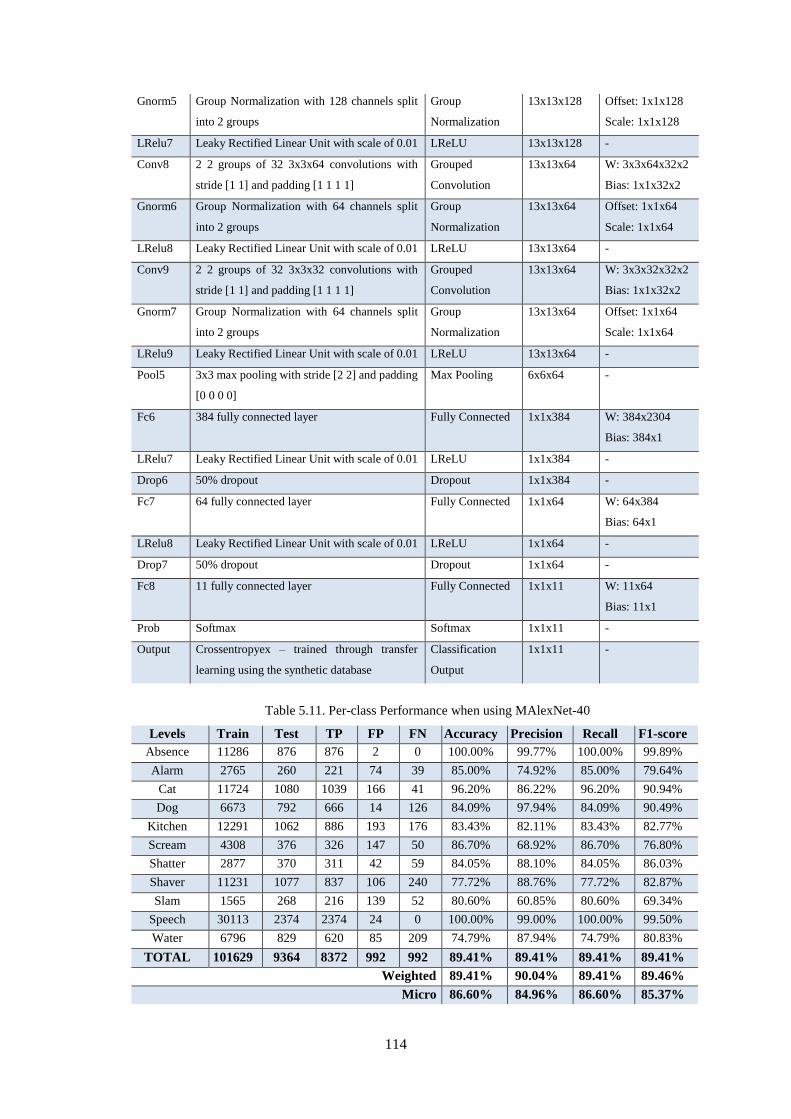
114

Gnorm5 Group Normalization with 128 channels split

into 2 groups

Group

Normalization

13x13x128 Offset: 1x1x128

Scale: 1x1x128

LRelu7 Leaky Rectified Linear Unit with scale of 0.01 LReLU 13x13x128 -

Conv8 2 2 groups of 32 3x3x64 convolutions with

stride [1 1] and padding [1 1 1 1]

Grouped

Convolution

13x13x64 W: 3x3x64x32x2

Bias: 1x1x32x2

Gnorm6 Group Normalization with 64 channels split

into 2 groups

Group

Normalization

13x13x64 Offset: 1x1x64

Scale: 1x1x64

LRelu8 Leaky Rectified Linear Unit with scale of 0.01 LReLU 13x13x64 -

Conv9 2 2 groups of 32 3x3x32 convolutions with

stride [1 1] and padding [1 1 1 1]

Grouped

Convolution

13x13x64 W: 3x3x32x32x2

Bias: 1x1x32x2

Gnorm7 Group Normalization with 64 channels split

into 2 groups

Group

Normalization

13x13x64 Offset: 1x1x64

Scale: 1x1x64

LRelu9 Leaky Rectified Linear Unit with scale of 0.01 LReLU 13x13x64 -

Pool5 3x3 max pooling with stride [2 2] and padding

[0 0 0 0]

Max Pooling 6x6x64 -

Fc6 384 fully connected layer Fully Connected 1x1x384 W: 384x2304

Bias: 384x1

LRelu7 Leaky Rectified Linear Unit with scale of 0.01 LReLU 1x1x384 -

Drop6 50% dropout Dropout 1x1x384 -

Fc7 64 fully connected layer Fully Connected 1x1x64 W: 64x384

Bias: 64x1

LRelu8 Leaky Rectified Linear Unit with scale of 0.01 LReLU 1x1x64 -

Drop7 50% dropout Dropout 1x1x64 -

Fc8 11 fully connected layer Fully Connected 1x1x11 W: 11x64

Bias: 11x1

Prob Softmax Softmax 1x1x11 -

Output Crossentropyex – trained through transfer

learning using the synthetic database

Classification

Output

1x1x11 -

Table 5.11. Per-class Performance when using MAlexNet-40

Levels Train Test TP FP FN Accuracy Precision Recall F1-score

Absence 11286 876 876 2 0 100.00% 99.77% 100.00% 99.89%

Alarm 2765 260 221 74 39 85.00% 74.92% 85.00% 79.64%

Cat 11724 1080 1039 166 41 96.20% 86.22% 96.20% 90.94%

Dog 6673 792 666 14 126 84.09% 97.94% 84.09% 90.49%

Kitchen 12291 1062 886 193 176 83.43% 82.11% 83.43% 82.77%

Scream 4308 376 326 147 50 86.70% 68.92% 86.70% 76.80%

Shatter 2877 370 311 42 59 84.05% 88.10% 84.05% 86.03%

Shaver 11231 1077 837 106 240 77.72% 88.76% 77.72% 82.87%

Slam 1565 268 216 139 52 80.60% 60.85% 80.60% 69.34%

Speech 30113 2374 2374 24 0 100.00% 99.00% 100.00% 99.50%

Water 6796 829 620 85 209 74.79% 87.94% 74.79% 80.83%

TOTAL 101629 9364 8372 992 992 89.41% 89.41% 89.41% 89.41%

Weighted 89.41% 90.04% 89.41% 89.46%

Micro 86.60% 84.96% 86.60% 85.37%

115

It is also important to note that the experimentation conducted in this chapter specifically explores the

modification and fine-tuning of a pre-trained model to accommodate an 8-12 level classification with an

imbalanced number of files per category. This has then been verified for both the SINS database, and the

DASEE dataset developed for this work. Hence, it is able to prove that the size of a model can drastically

be reduced without affecting the accuracy; suggesting the existence of unnecessary hidden layers and large

network parameters when utilizing transfer learning.

Nonetheless, it should be noted that MAlexNet-40 is not considered to be a pre-trained network, given that

it is trained and tuned for a smaller dataset. Pre-trained models are usually trained on large datasets in

order to accommodate transfer learning, where models trained for higher levels of classification are re-

used for classification problems involving fewer labels. However, since the network has been designed to

be highly customizable in terms of hyperparameter tuning with minimal risks of overfitting through its

series architecture, it can easily be tuned depending on the number of dataset classes.

5.4 MAlexNet-40 as a Compact Neural Network Model

Accuracy, execution inference time requirements, and memory size are some of the key priorities

considered whilst developing the optimum neural network architecture for our selected application. After

identifying the optimum network model through extensive experiments conducted in the previous section,

the performance of our proposed method, the MAlexNet-40, against other state-of-the-art compact neural

network models, inclusive of the: SqueezeNet [139], MobileNet-v2 [249], NasNet Mobile [250], and

ShuffleNet [251], is examined. A direct comparison is first conducted, followed by a thorough assessment

of the system response to the unique properties of each compact network. Finally, we detail the difference

and unique characteristics of the MAlexNet-40 in comparison to other compact network architectures.

It should be highlighted that the comparisons conducted within this section is specific to the selected

application of this work. While the other compact neural network models mentioned in this section are

DAG pre-trained network models, given that they are originally trained on a large dataset, MAlexNet-40

is specifically tuned to fit the classification requirements of this application, and is series in architecture.

The main aim of MAlexNet-40 is to maintain the accuracy and architecture of the highest performing pre-

trained model, while achieving the benefits of a compact network at the same time.

5.4.1 Direct Comparison against Compact Neural Network Models

A summary of the comparison is seen in Table 5.12, in terms of the total number of layers, depth, type,

network size in MB, the activation function used, the weighted F1-score, the training time for 30 epochs,

the network loading time, and the execution inference time average. The network loading time is an

average of 5 trials, while the execution time is measured on 100 trials. It is important to note that, while

MAlexNet-40 is a series network, all other compact networks are DAG networks. A series network

contains layers that are arranged subsequent to one another, containing a single input, and output layer.

DAGs, on the other hand, have a complex architecture, from which layers may have inputs from several

layers, and the outputs of which may be used for multiple layers [235].

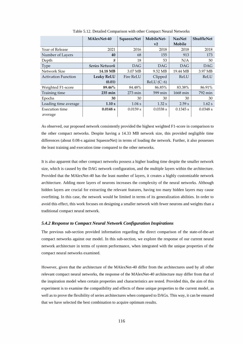
116

Table 5.12. Detailed Comparison with other Compact Neural Networks

MAlexNet-40 SqueezeNet MobileNet-

v2

NasNet

Mobile

ShuffleNet

Year of Release 2021 2016 2018 2018 2018

Number of Layers 40 68 155 913 173

Depth 8 18 53 N/A 50

Type Series Network DAG DAG DAG DAG

Network Size 14.18 MB 3.07 MB 9.52 MB 19.44 MB 3.97 MB

Activation Function Leaky ReLU

(0.01)

Fire ReLU Clipped

ReLU (C: 6)

ReLU ReLU

Weighted F1-score 89.46% 84.48% 86.85% 83.38% 86.91%

Training time 235 min 273 min 599 min 1668 min 792 min

Epochs 30 30 30 30 30

Loading time average 1.10 s 1.04 s 1.32 s 2.59 s 1.62 s

Execution time

average

0.0148 s 0.0159 s 0.0338 s 0.1345 s 0.0348 s

As observed, our proposed network consistently provided the highest weighted F1-score in comparison to

the other compact networks. Despite having a 14.33 MB network size, this provided negligible time

differences (about 0.08-s against SqueezeNet) in terms of loading the network. Further, it also possesses

the least training and execution time compared to the other networks.

It is also apparent that other compact networks possess a higher loading time despite the smaller network

size, which is caused by the DAG network configuration, and the multiple layers within the architecture.

Provided that the MAlexNet-40 has the least number of layers, it creates a highly customizable network

architecture. Adding more layers of neurons increases the complexity of the neural networks. Although

hidden layers are crucial for extracting the relevant features, having too many hidden layers may cause

overfitting. In this case, the network would be limited in terms of its generalization abilities. In order to

avoid this effect, this work focuses on designing a smaller network with fewer neurons and weights than a

traditional compact neural network.

5.4.2 Response to Compact Neural Network Configuration Inspirations

The previous sub-section provided information regarding the direct comparison of the state-of-the-art

compact networks against our model. In this sub-section, we explore the response of our current neural

network architecture in terms of system performance, when integrated with the unique properties of the

compact neural networks examined.

However, given that the architecture of the MAlexNet-40 differ from the architectures used by all other

relevant compact neural networks, the response of the MAlexNet-40 architecture may differ from that of

the inspiration model when certain properties and characteristics are tested. Provided this, the aim of this

experiment is to examine the compatibility and effects of these unique properties to the current model, as

well as to prove the flexibility of series architectures when compared to DAGs. This way, it can be ensured

that we have selected the best combination to acquire optimum results.

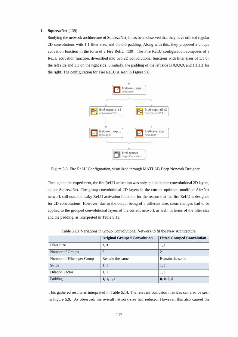
117

1. SqueezeNet [139]

Studying the network architecture of SqueezeNet, it has been observed that they have utilized regular

2D convolutions with 1,1 filter size, and 0,0,0,0 padding. Along with this, they proposed a unique

activation function in the form of a Fire ReLU [139]. The Fire ReLU configuration composes of a

ReLU activation function, diversified into two 2D convolutional functions with filter sizes of 1,1 on

the left side and 3,3 on the right side. Similarly, the padding of the left side is 0,0,0,0, and 1,1,1,1 for

the right. The configuration for Fire ReLU is seen in Figure 5.8.

Figure 5.8. Fire ReLU Configuration, visualized through MATLAB Deep Network Designer

Throughout the experiment, the fire ReLU activation was only applied to the convolutional 2D layers,

as per SqueezeNet. The group convolutional 2D layers in the current optimum modified AlexNet

network still uses the leaky ReLU activation function, for the reason that the fire ReLU is designed

for 2D convolutions. However, due to the output being of a different size, some changes had to be

applied to the grouped convolutional layers of the current network as well, in terms of the filter size

and the padding, as interpreted in Table 5.13.

Table 5.13. Variations in Group Convolutional Network to fit the New Architecture

Original Grouped Convolution Fitted Grouped Convolution

Filter Size 3, 3 1, 1

Number of Groups 2 2

Number of Filters per Group Remain the same Remain the same

Stride 1, 1 1, 1

Dilation Factor 1, 1 1, 1

Padding 1, 1, 1, 1 0, 0, 0, 0

This gathered results as interpreted in Table 5.14. The relevant confusion matrices can also be seen

in Figure 5.9. As observed, the overall network size had reduced. However, this also caused the

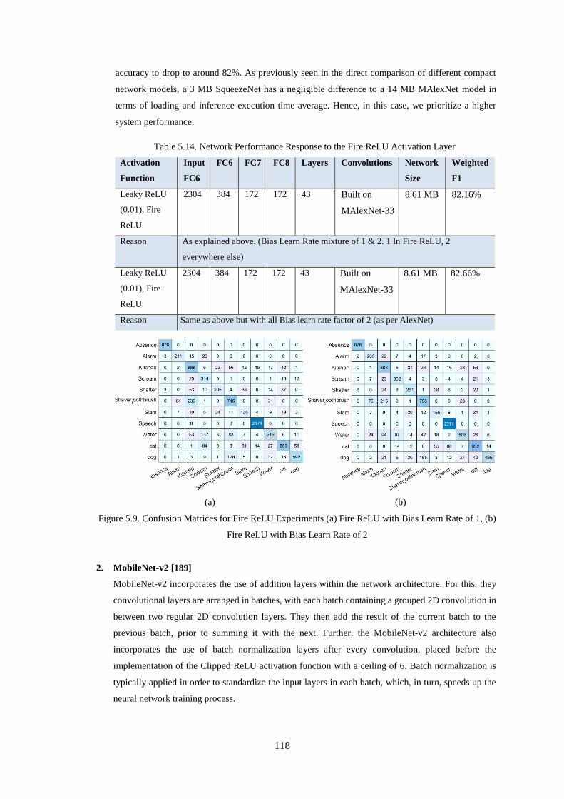
118

accuracy to drop to around 82%. As previously seen in the direct comparison of different compact

network models, a 3 MB SqueezeNet has a negligible difference to a 14 MB MAlexNet model in

terms of loading and inference execution time average. Hence, in this case, we prioritize a higher

system performance.

Table 5.14. Network Performance Response to the Fire ReLU Activation Layer

Activation

Function

Input

FC6

FC6 FC7 FC8 Layers Convolutions Network

Size

Weighted

F1

Leaky ReLU

(0.01), Fire

ReLU

2304 384 172 172 43 Built on

MAlexNet-33

8.61 MB 82.16%

Reason As explained above. (Bias Learn Rate mixture of 1 & 2. 1 In Fire ReLU, 2

everywhere else)

Leaky ReLU

(0.01), Fire

ReLU

2304 384 172 172 43 Built on

MAlexNet-33

8.61 MB 82.66%

Reason Same as above but with all Bias learn rate factor of 2 (as per AlexNet)

(a) (b)

Figure 5.9. Confusion Matrices for Fire ReLU Experiments (a) Fire ReLU with Bias Learn Rate of 1, (b)

Fire ReLU with Bias Learn Rate of 2

2. MobileNet-v2 [189]

MobileNet-v2 incorporates the use of addition layers within the network architecture. For this, they

convolutional layers are arranged in batches, with each batch containing a grouped 2D convolution in

between two regular 2D convolution layers. They then add the result of the current batch to the

previous batch, prior to summing it with the next. Further, the MobileNet-v2 architecture also

incorporates the use of batch normalization layers after every convolution, placed before the

implementation of the Clipped ReLU activation function with a ceiling of 6. Batch normalization is

typically applied in order to standardize the input layers in each batch, which, in turn, speeds up the

neural network training process.

119

Considering these observations, the following experiments are investigated with response to our

proposed network:

1. Adding a batch normalization layer every after convolutional layer

2. Implementing the addition layer: For this, the result of two grouped convolutional layers with the

same number of filters are added together. In this experiment, the addition layer incorporation

was only done in the grouped convolutions, and not for the 2D convolutional layers. Further, it is

important to note that the incorporation of addition layers involve taking two inputs in one layer.

In turn, the network type is converted to a directed graph network layout.

These experiments have yielded results as shown in Table 5.15. As observed, incorporating addition

layers did not improve the overall system performance. Further, implementing batch normalization

layers also decreases the performance of the system.

Table 5.15. Network Performance Response to the Addition and Batch Normalization Layers

Activation

Function

Input

to

FC6

FC6 FC7 FC8 Num of

Layers

Convolutions Network

Size

Weighted

F1

Leaky ReLU

(0.01)

2304 384 172 172 46 26 with

addition

15.45 MB 81.94%

Reason 2x gconv 96, 48, 24, 12, inputs are added through an “addition layer”

Leaky ReLU

(0.01)

2304 384 172 172 46 MAlexNet-37

w/ BN

14.57 MB 85.63%

Leaky ReLU

(0.01)

2304 384 172 172 42 MAlexNet-33

w/ BN

14.38 MB 87.59%

3. ShuffleNet [251]

The ShuffleNet network architecture contains similarities to MobileNet-v2, such that they incorporate

the use of addition layers throughout the network. However, they add a channel shuffling layer along

with a batch normalization layer for every after activation function, such that the activation function

is placed in between the batch normalization, and the shuffling layer. Similarly, they use ReLU instead

of a Clipped ReLU as their activation function. Taking this into consideration, experimentation on the

response of the MAlexNet-40 are done in three ways:

1. Adding a shuffling layer after every leaky ReLU activation function

2. Adding both a shuffling layer and batch normalization layer every after activation function.

3. Using an addition layer between a 2D convolution, and a group of grouped convolutions. The

number of filters are reduced on the 2D convolution side in order to match the input size to the

addition layer.

Accordingly, the results for these are summarized in Table 5.16, as follows:

120

Table 5.16. Network Architecture Variations Summary Activation

Function

Input

to

FC6

FC6 FC7 FC8 Num.

Layers

Comments Network

Size

F1-score

Leaky

ReLU

(0.01)

2304 384 172 172 44 Channel Shuffling Layer

after each activation

function

14.36 MB 86.92%

Leaky

ReLU

(0.01)

2304 384 172 172 55 As above, but with batch

normalization layer before

each activation function

14.26 MB 85.81%

Leaky

ReLU

(0.01)

2304 384 172 172 42 As above, but only covers

activation functions used by

convolutions (not for the

fully connected layers)

14.36 MB 85.27%

Leaky

ReLU

(0.01)

2304 384 172 172 30 Using an addition layer for

conv on one side, a group of

grouped conv on the other

side. Reduced number of

filters to match. (DAG)

6.13 MB 78.89%

As observed, channel shuffling and implementation of a directed graph architecture through the

incorporation of addition layers did not improve system performance. A directed graph may be

considered as a DAG architecture if the edges delineate partial ordering on the nodes [252]. Partial

ordering is a strong type of bias that defines the acyclic dependency of the computation [252]. This

is a crucial information that occurs upon carefully studying complex architectures and their

performances. Provided this, modifying DAG network architecture is a highly complicated process.

As per the findings in the experiments conducted, the MAlexNet-40 remains to be the optimum network,

providing the benefits of a high accuracy, at a compact size that is suitable for devices with limited

computational resources. In addition to this, the MAlexNet-40 also provides a highly customizable

architecture through its Series Network layout.

5.4.3 Discussions and Findings

As per the experiments conducted, our findings and hypotheses can be summarized as follows:

Hypothesis 5.4: Aside from the network size, the neural network layer arrangement is another factor that

considerably affects neural network training and loading time.

Verification of Hypothesis 5.4: Based on our findings, it is apparent that DAG networks, which is

composed of more complicated network layer architecture, consumes more time in terms of both loading

and executing the trained model despite having a smaller digital storage size.

Hypothesis 5.5: A Series Network layer arrangement provides an excellent baseline for a highly

customizable, compact model.

Verification of Hypothesis 5.5: Aside from the requirement of partial ordering, due to layer relationships

that exist within DAG network architectures, layers are normally treated in groups. Hence, modifying the

architecture based on adding or removing layers will involve large chunks of layers and numbers of

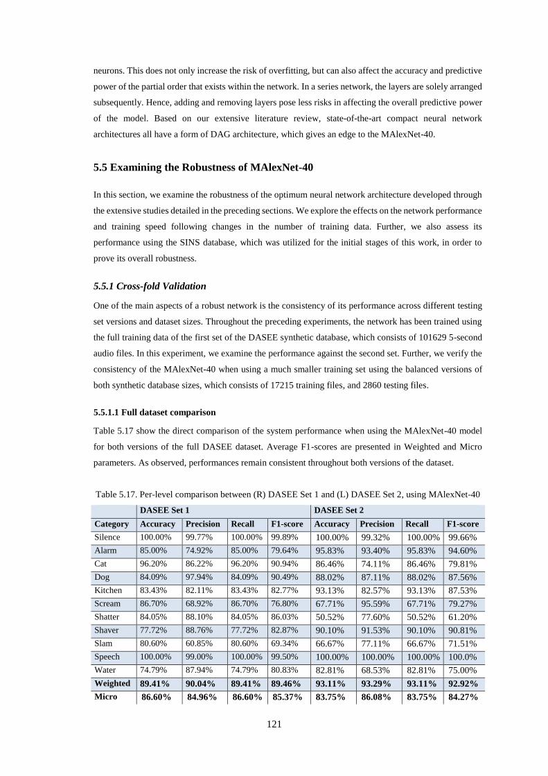
121

neurons. This does not only increase the risk of overfitting, but can also affect the accuracy and predictive

power of the partial order that exists within the network. In a series network, the layers are solely arranged

subsequently. Hence, adding and removing layers pose less risks in affecting the overall predictive power

of the model. Based on our extensive literature review, state-of-the-art compact neural network

architectures all have a form of DAG architecture, which gives an edge to the MAlexNet-40.

5.5 Examining the Robustness of MAlexNet-40

In this section, we examine the robustness of the optimum neural network architecture developed through

the extensive studies detailed in the preceding sections. We explore the effects on the network performance

and training speed following changes in the number of training data. Further, we also assess its

performance using the SINS database, which was utilized for the initial stages of this work, in order to

prove its overall robustness.

5.5.1 Cross-fold Validation

One of the main aspects of a robust network is the consistency of its performance across different testing

set versions and dataset sizes. Throughout the preceding experiments, the network has been trained using

the full training data of the first set of the DASEE synthetic database, which consists of 101629 5-second

audio files. In this experiment, we examine the performance against the second set. Further, we verify the

consistency of the MAlexNet-40 when using a much smaller training set using the balanced versions of

both synthetic database sizes, which consists of 17215 training files, and 2860 testing files.

5.5.1.1 Full dataset comparison

Table 5.17 show the direct comparison of the system performance when using the MAlexNet-40 model

for both versions of the full DASEE dataset. Average F1-scores are presented in Weighted and Micro

parameters. As observed, performances remain consistent throughout both versions of the dataset.

Table 5.17. Per-level comparison between (R) DASEE Set 1 and (L) DASEE Set 2, using MAlexNet-40

DASEE Set 1 DASEE Set 2

Category Accuracy Precision Recall F1-score Accuracy Precision Recall F1-score

Silence 100.00% 99.77% 100.00% 99.89% 100.00% 99.32% 100.00% 99.66%

Alarm 85.00% 74.92% 85.00% 79.64% 95.83% 93.40% 95.83% 94.60%

Cat 96.20% 86.22% 96.20% 90.94% 86.46% 74.11% 86.46% 79.81%

Dog 84.09% 97.94% 84.09% 90.49% 88.02% 87.11% 88.02% 87.56%

Kitchen 83.43% 82.11% 83.43% 82.77% 93.13% 82.57% 93.13% 87.53%

Scream 86.70% 68.92% 86.70% 76.80% 67.71% 95.59% 67.71% 79.27%

Shatter 84.05% 88.10% 84.05% 86.03% 50.52% 77.60% 50.52% 61.20%

Shaver 77.72% 88.76% 77.72% 82.87% 90.10% 91.53% 90.10% 90.81%

Slam 80.60% 60.85% 80.60% 69.34% 66.67% 77.11% 66.67% 71.51%

Speech 100.00% 99.00% 100.00% 99.50% 100.00% 100.00% 100.00% 100.0%

Water 74.79% 87.94% 74.79% 80.83% 82.81% 68.53% 82.81% 75.00%

Weighted 89.41% 90.04% 89.41% 89.46% 93.11% 93.29% 93.11% 92.92%

Micro 86.60% 84.96% 86.60% 85.37% 83.75% 86.08% 83.75% 84.27%

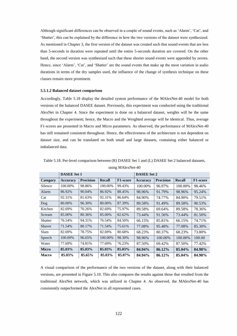
122

Although significant differences can be observed in a couple of sound events, such as ‘Alarm’, ‘Cat’, and

‘Shatter’, this can be explained by the difference in how the two versions of the dataset were synthesized.

As mentioned in Chapter 3, the first version of the dataset was created such that sound events that are less

than 5-seconds in duration were repeated until the entire 5-seconds duration are covered. On the other

hand, the second version was synthesized such that these shorter sound events were appended by zeroes.

Hence, since ‘Alarm’, ‘Cat’, and ‘Shatter’ are the sound events that make up the most variation in audio

durations in terms of the dry samples used, the influence of the change of synthesis technique on these

classes remain more prominent.

5.5.1.2 Balanced dataset comparison

Accordingly, Table 5.18 display the detailed system performance of the MAlexNet-40 model for both

versions of the balanced DASEE dataset. Previously, this experiment was conducted using the traditional

AlexNet in Chapter 4. Since the experiment is done on a balanced dataset, weights will be the same

throughout the experiment; hence, the Macro and the Weighted average will be identical. Thus, average

F1-scores are presented in Macro and Micro parameters. As observed, the performance of MAlexNet-40

has still remained consistent throughout. Hence, the effectiveness of the architecture is not dependent on

dataset size, and can be translated on both small and large datasets, containing either balanced or

imbalanced data.

Table 5.18. Per-level comparison between (R) DASEE Set 1 and (L) DASEE Set 2 balanced datasets,

using MAlexNet-40

DASEE Set 1 DASEE Set 2

Category Accuracy Precision Recall F1-score Accuracy Precision Recall F1-score

Silence 100.00% 98.86% 100.00% 99.43% 100.00% 96.97% 100.00% 98.46%

Alarm 86.92% 90.04% 86.92% 88.45% 98.96% 91.79% 98.96% 95.24%

Cat 92.31% 81.63% 92.31% 86.64% 84.90% 74.77% 84.90% 79.51%

Dog 80.00% 96.30% 80.00% 87.39% 89.58% 91.49% 89.58% 90.53%

Kitchen 82.69% 70.26% 82.69% 75.97% 89.58% 69.64% 89.58% 78.36%

Scream 85.00% 80.36% 85.00% 82.62% 73.44% 91.56% 73.44% 81.50%

Shatter 76.54% 94.31% 76.54% 84.50% 66.15% 85.81% 66.15% 74.71%

Shaver 71.54% 80.17% 71.54% 75.61% 77.08% 95.48% 77.08% 85.30%

Slam 82.69% 78.75% 82.69% 80.68% 68.23% 80.37% 68.23% 73.80%

Speech 100.00% 96.65% 100.00% 98.30% 98.96% 100.00% 100.00% 100.00

% Water 77.69% 74.81% 77.69% 76.23% 87.50% 69.42% 87.50% 77.42%

Micro 85.03% 85.03% 85.03% 85.03% 84.94% 86.12% 85.04% 84.98%

Macro 85.03% 85.65% 85.03% 85.07% 84.94% 86.12% 85.04% 84.98%

A visual comparison of the performance of the two versions of the dataset, along with their balanced

versions, are presented in Figure 5.10. This also compares the results against those that resulted from the

traditional AlexNet network, which was utilized in Chapter 4. As observed, the MAlexNet-40 has

consistently outperformed the AlexNet in all represented cases.

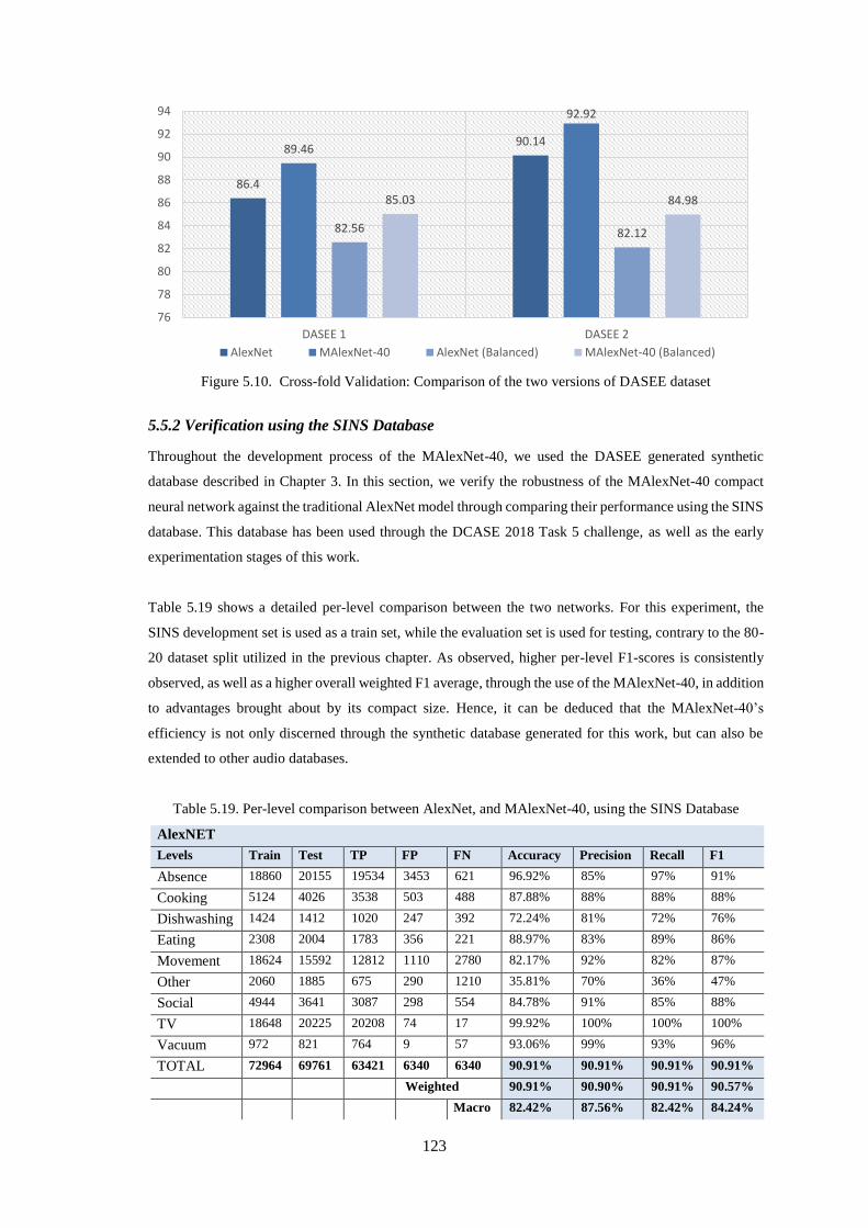
123

Figure 5.10. Cross-fold Validation: Comparison of the two versions of DASEE dataset

5.5.2 Verification using the SINS Database

Throughout the development process of the MAlexNet-40, we used the DASEE generated synthetic

database described in Chapter 3. In this section, we verify the robustness of the MAlexNet-40 compact

neural network against the traditional AlexNet model through comparing their performance using the SINS

database. This database has been used through the DCASE 2018 Task 5 challenge, as well as the early

experimentation stages of this work.

Table 5.19 shows a detailed per-level comparison between the two networks. For this experiment, the

SINS development set is used as a train set, while the evaluation set is used for testing, contrary to the 80-

20 dataset split utilized in the previous chapter. As observed, higher per-level F1-scores is consistently

observed, as well as a higher overall weighted F1 average, through the use of the MAlexNet-40, in addition

to advantages brought about by its compact size. Hence, it can be deduced that the MAlexNet-40’s

efficiency is not only discerned through the synthetic database generated for this work, but can also be

extended to other audio databases.

Table 5.19. Per-level comparison between AlexNet, and MAlexNet-40, using the SINS Database

AlexNET

Levels Train Test TP FP FN Accuracy Precision Recall F1

Absence 18860 20155 19534 3453 621 96.92% 85% 97% 91%

Cooking 5124 4026 3538 503 488 87.88% 88% 88% 88%

Dishwashing 1424 1412 1020 247 392 72.24% 81% 72% 76%

Eating 2308 2004 1783 356 221 88.97% 83% 89% 86%

Movement 18624 15592 12812 1110 2780 82.17% 92% 82% 87%

Other 2060 1885 675 290 1210 35.81% 70% 36% 47%

Social 4944 3641 3087 298 554 84.78% 91% 85% 88%

TV 18648 20225 20208 74 17 99.92% 100% 100% 100%

Vacuum 972 821 764 9 57 93.06% 99% 93% 96%

TOTAL 72964 69761 63421 6340 6340 90.91% 90.91% 90.91% 90.91%

Weighted 90.91% 90.90% 90.91% 90.57%

Macro 82.42% 87.56% 82.42% 84.24%

86.4

90.1489.46

92.92

82.56 82.12

85.03 84.98

76

78

80

82

84

86

88

90

92

94

DASEE 1 DASEE 2

AlexNet MAlexNet-40 AlexNet (Balanced) MAlexNet-40 (Balanced)

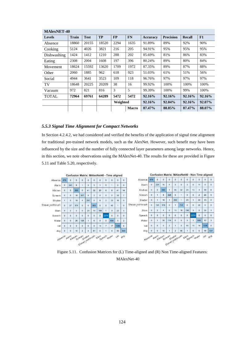
124

MAlexNET-40

Levels Train Test TP FP FN Accuracy Precision Recall F1

Absence 18860 20155 18520 2294 1635 91.89% 89% 92% 90%

Cooking 5124 4026 3821 216 205 94.91% 95% 95% 95%

Dishwashing 1424 1412 1210 288 202 85.69% 81% 86% 83%

Eating 2308 2004 1608 197 396 80.24% 89% 80% 84%

Movement 18624 15592 13620 1709 1972 87.35% 89% 87% 88%

Other 2060 1885 962 618 923 51.03% 61% 51% 56%

Social 4944 3641 3523 109 118 96.76% 97% 97% 97%

TV 18648 20225 20209 38 16 99.92% 100% 100% 100%

Vacuum 972 821 816 3 5 99.39% 100% 99% 100%

TOTAL 72964 69761 64289 5472 5472 92.16% 92.16% 92.16% 92.16%

Weighted 92.16% 92.04% 92.16% 92.07%

Macro 87.47% 88.85% 87.47% 88.07%

5.5.3 Signal Time Alignment for Compact Networks

In Section 4.2.4.2, we had considered and verified the benefits of the application of signal time alignment

for traditional pre-trained network models, such as the AlexNet. However, such benefit may have been

influenced by the size and the number of fully connected layer parameters among large networks. Hence,

in this section, we note observations using the MAlexNet-40. The results for these are provided in Figure

5.11 and Table 5.20, respectively.

Figure 5.11. Confusion Matrices for (L) Time-aligned and (R) Non Time-aligned Features:

MAlexNet-40

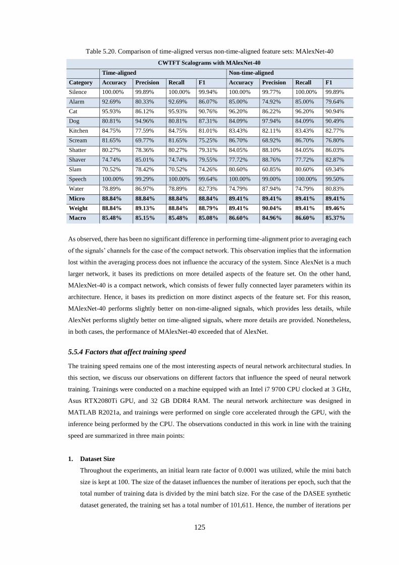
125

Table 5.20. Comparison of time-aligned versus non-time-aligned feature sets: MAlexNet-40

CWTFT Scalograms with MAlexNet-40

Time-aligned Non-time-aligned

Category Accuracy Precision Recall F1 Accuracy Precision Recall F1

Silence 100.00% 99.89% 100.00% 99.94% 100.00% 99.77% 100.00% 99.89%

Alarm 92.69% 80.33% 92.69% 86.07% 85.00% 74.92% 85.00% 79.64%

Cat 95.93% 86.12% 95.93% 90.76% 96.20% 86.22% 96.20% 90.94%

Dog 80.81% 94.96% 80.81% 87.31% 84.09% 97.94% 84.09% 90.49%

Kitchen 84.75% 77.59% 84.75% 81.01% 83.43% 82.11% 83.43% 82.77%

Scream 81.65% 69.77% 81.65% 75.25% 86.70% 68.92% 86.70% 76.80%

Shatter 80.27% 78.36% 80.27% 79.31% 84.05% 88.10% 84.05% 86.03%

Shaver 74.74% 85.01% 74.74% 79.55% 77.72% 88.76% 77.72% 82.87%

Slam 70.52% 78.42% 70.52% 74.26% 80.60% 60.85% 80.60% 69.34%

Speech 100.00% 99.29% 100.00% 99.64% 100.00% 99.00% 100.00% 99.50%

Water 78.89% 86.97% 78.89% 82.73% 74.79% 87.94% 74.79% 80.83%

Micro 88.84% 88.84% 88.84% 88.84% 89.41% 89.41% 89.41% 89.41%

Weight 88.84% 89.13% 88.84% 88.79% 89.41% 90.04% 89.41% 89.46%

Macro 85.48% 85.15% 85.48% 85.08% 86.60% 84.96% 86.60% 85.37%

As observed, there has been no significant difference in performing time-alignment prior to averaging each

of the signals’ channels for the case of the compact network. This observation implies that the information

lost within the averaging process does not influence the accuracy of the system. Since AlexNet is a much

larger network, it bases its predictions on more detailed aspects of the feature set. On the other hand,

MAlexNet-40 is a compact network, which consists of fewer fully connected layer parameters within its

architecture. Hence, it bases its prediction on more distinct aspects of the feature set. For this reason,

MAlexNet-40 performs slightly better on non-time-aligned signals, which provides less details, while

AlexNet performs slightly better on time-aligned signals, where more details are provided. Nonetheless,

in both cases, the performance of MAlexNet-40 exceeded that of AlexNet.

5.5.4 Factors that affect training speed

The training speed remains one of the most interesting aspects of neural network architectural studies. In

this section, we discuss our observations on different factors that influence the speed of neural network

training. Trainings were conducted on a machine equipped with an Intel i7 9700 CPU clocked at 3 GHz,

Asus RTX2080Ti GPU, and 32 GB DDR4 RAM. The neural network architecture was designed in

MATLAB R2021a, and trainings were performed on single core accelerated through the GPU, with the

inference being performed by the CPU. The observations conducted in this work in line with the training

speed are summarized in three main points:

1. Dataset Size

Throughout the experiments, an initial learn rate factor of 0.0001 was utilized, while the mini batch

size is kept at 100. The size of the dataset influences the number of iterations per epoch, such that the

total number of training data is divided by the mini batch size. For the case of the DASEE synthetic

dataset generated, the training set has a total number of 101,611. Hence, the number of iterations per

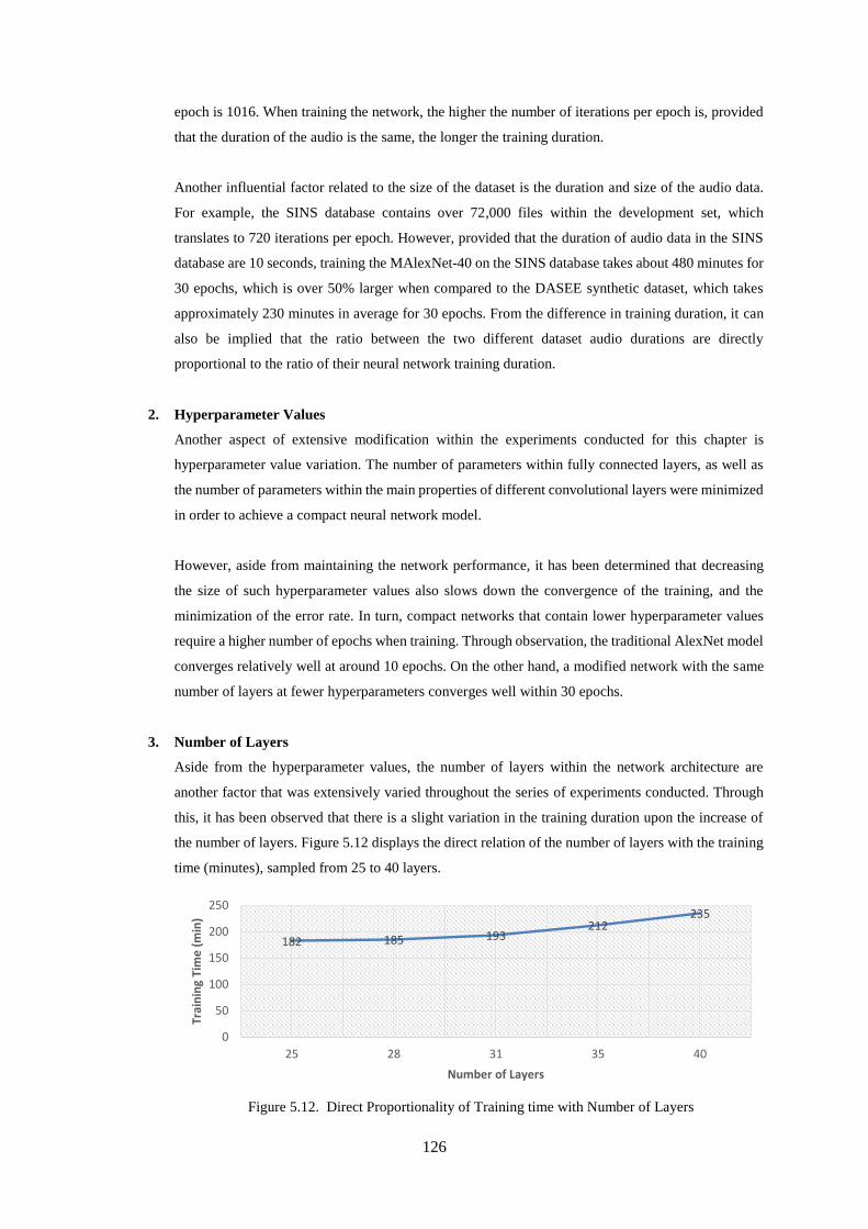
126

epoch is 1016. When training the network, the higher the number of iterations per epoch is, provided

that the duration of the audio is the same, the longer the training duration.

Another influential factor related to the size of the dataset is the duration and size of the audio data.

For example, the SINS database contains over 72,000 files within the development set, which

translates to 720 iterations per epoch. However, provided that the duration of audio data in the SINS

database are 10 seconds, training the MAlexNet-40 on the SINS database takes about 480 minutes for

30 epochs, which is over 50% larger when compared to the DASEE synthetic dataset, which takes

approximately 230 minutes in average for 30 epochs. From the difference in training duration, it can

also be implied that the ratio between the two different dataset audio durations are directly

proportional to the ratio of their neural network training duration.

2. Hyperparameter Values

Another aspect of extensive modification within the experiments conducted for this chapter is

hyperparameter value variation. The number of parameters within fully connected layers, as well as

the number of parameters within the main properties of different convolutional layers were minimized

in order to achieve a compact neural network model.

However, aside from maintaining the network performance, it has been determined that decreasing

the size of such hyperparameter values also slows down the convergence of the training, and the

minimization of the error rate. In turn, compact networks that contain lower hyperparameter values

require a higher number of epochs when training. Through observation, the traditional AlexNet model

converges relatively well at around 10 epochs. On the other hand, a modified network with the same

number of layers at fewer hyperparameters converges well within 30 epochs.

3. Number of Layers

Aside from the hyperparameter values, the number of layers within the network architecture are

another factor that was extensively varied throughout the series of experiments conducted. Through

this, it has been observed that there is a slight variation in the training duration upon the increase of

the number of layers. Figure 5.12 displays the direct relation of the number of layers with the training

time (minutes), sampled from 25 to 40 layers.

Figure 5.12. Direct Proportionality of Training time with Number of Layers

182 185 193212

235

0

50

100

150

200

250

25 28 31 35 40

Trai

nin

g Ti

me

(m

in)

Number of Layers

127

Nonetheless, despite the larger training time, it has also been deduced that having more layers also

causes a much faster network convergence. For the MAlexNet-40, convergence is reached at the tenth

epoch, similar to the traditional AlexNet model, at almost 95% less than the size and much lower

hyperparameter values. The faster convergence of this compact network would in turn require less

training time, given that it does not need many epochs in order to reach convergence.

5.6 Chapter Summary

This chapter has explored the making of MAlexNet-40, a mobile and highly accurate network architecture

developed for the applications of this work. Different types of neural networks for multi-level classification

are first studied and compared, prior to instigating a thorough initial experiment comparing the

performance of the state-of-the-art pre-trained networks. From this, it was found that the AlexNet pre-

trained network resulted in the highest F1-score. The AlexNet is then developed and modified within three

main objectives: exceed the network accuracy, decrease the network size in order to fit mobile applications,

and maintain a highly customizable network architecture. The neural network’s responses to various

hyperparameter modifications and architectural studies has been documented in this chapter. All three

objectives has been met through incorporating group normalization, swapping the traditional ReLU

activation function with a Leaky ReLU activation function with a scale of 0.01, incorporate additional

grouped convolutional layers, and implement scaling and modifications in relevant hyperparameters. The

resulting neural network architecture provided a weighted F1-score of 89.46% at a size of 14.18 MB using

our synthetic database, while maintaining a customizable series network architecture. This is a large

improvement compared to the traditional AlexNet, which yielded a weighted average F1-score of 86.24%

at a network size of 222.71 MB.

128

Integrated System Design

6.1 Introduction

This chapter presents the integrated model, incorporating both the identified optimal audio classification

and source node location estimation features developed in Chapter 4, with the compact neural network

model designed in Chapter 5, into a software application with an easy-to-use GUI. This interface is

intended for dementia caregivers and/or healthcare professionals, allowing the monitoring of the resident’s

activity and need for assistance through domestic sound classification and location estimation of the sound

source. Other useful functionalities for dementia care, such as the sound levels assessment tool, are also

included.

In order to promote and ensure the usefulness of the GUI to the dedicated users, a design thinking research

approach is utilized. This process revolves around the development of a user-inclined system through

continuous research regarding the requirements of the end-user, as well as continuously brainstorming on

how to align these requirements with the product functionalities. Hence, this chapter begins by applying a

design thinking approach to the development of an easy-to-use interface design, prior to explaining the

features and functionalities of the application developed. It then describes a proposed two-step neural

network-based audio classifier based on the approaches described in earlier chapters but using sub-

networks that re designed to improve the accuracy in detecting sounds that indicate a dementia resident

may require urgent assistance. Overall, this chapter combines the technological and research aspects of

our works into an application with a GUI, coupled with additional features that will be beneficial for

dementia healthcare. Another factor that adds a unique factor to this work is the ability to personalize the

system according to specific requirements. This is considered through an easy-to-use interface that allows

regular updates on the patient profile, based on the current cognitive decline level and observed

preferences. The key features of the caregiver software application include the following:

1. User friendly operability.

2. Adaptability and flexibility of the system according to the severity indices that is set as per the

resident’s customizable profile, which indicates the degree by which the caregiver should be

notified.

3. Severity indexes identified according to the diagnosis of the resident’s level of cognitive decline, in

order to avoid unnecessary intrusion.

4. Automated alerts sent to the caregiver when the noise level of the resident’s environment is beyond

the tolerable range. This range is defined according to the resident’s hearing condition diagnosis.

5. visualization of weekly summary of domestic activity pattern, which aims to familiarize the

caregivers towards the amount of assistance and the type of care that each resident requires.

6. Compact system design featuring computationally-efficient pre-processing, feature extraction, and

inference of the trained model.

129

Overall, the application discussed in this chapter is a demonstrator of a monitoring system interface

intended for dementia care, that is designed based on research through the design thinking approach.

6.2 Design Thinking Approach for Graphical User Interface Development

Design thinking is defined to be an iterative approach used to understand and redefine challenges in order

to produce solutions targeted towards the end user [253]. This process circulates around understanding and

developing empathy for the users by which the product is being developed for through continuous research

and brainstorming. In this section, we detail the process undertaken in order to ensure alignment of the

developed application based on the requirements, experiences, and challenges faced by dementia

caregivers. The aim of this section is to highlight the necessity of healthcare monitoring applications, and

to create value to its users using the concept of design thinking.

This section begins by describing the end-user, and discussing the difficulties and challenges that they

experience as dementia caregivers. It then identifies functionalities that align with ameliorating the

experience of dementia carers, promoting usability, accessibility, and reliability of the user interface as per

the requirement of the designated users. Finally, we discuss the advantages and disadvantages of the

developed application.

6.2.1 Identifying the Persona

Throughout this process, we consider dementia caregivers as the main persona, for which this application

is being developed for. This sub-section details specific user information about dementia caregivers, as

well as the most common challenges that they face through analyzing recently conducted research surveys.

6.2.1.1 User Information

The survey conducted by the American Association of Retired Persons (AARP) research is utilized to

gather relevant information regarding dementia caregivers [254]. This survey used a sample size of 1112

caregivers aged 18 and older, 711 of which are attending to dementia residents [254].

The important user information that must be considered for the application design include the following:

age group, education, employment status, and marital status, provided that these are factors that can

contribute to challenges in terms of lack of personal time and high demands for care [254]. Hence, there

are two main aspects that we aim to address with the development of our application: the relevance with

the age and technical knowledge of the selected users, and the requirement of the product based on the

challenges that they face.

The survey infers that 92% of the survey participants are under the age of 65, with the highest group being

at the age range of 18 – 34 years old, making up 35% of the responses [254]. With the surge of technology

over the last few years, it is apparent that majority of the world’s population are sufficiently familiar with

the use of mobile applications. Although mobile application usage decreases with age, for the year 2021

it is estimated that individuals between the ages of 18 – 34 spend over 100 hours on mobile applications

130

each month [255]. Further, the survey also states that 100% of the survey participants have attained a form

of secondary or tertiary education prior to caregiving [254]. Hence, it can be deduced that our selected

users are knowledgeable and experienced in using simple technological devices and mobile applications.

One of the major challenges of dementia care is the demand of time and care. Caring for dementia residents

may require extensive hours of assistance, and can potentially be demanding in terms of time and effort.

According to the research survey, 71% of the participants are employed alongside caring for the dementia

resident [254]. Hence, this causes challenges in balancing time between caretaking and their day jobs.

Further, 55% of them are married, and have other personal matters to attend to [254]. According to the

same survey, 60% of the participants believe that caretaking caused them to spend less time with their

other family members, and 70% claimed that this caused them to spend less time with friends [254].

From this research, detailed information regarding the users are cleared out. The users for which the

application will be intended for are under the age of 65, and are mostly within the age group of 18 – 34

years old. This generation composes of individuals that are proficient in the use of basic applications and

mobile technology. Further, it is also extrapolated that the main reasons for the challenges they face in

terms of time and demands for care is the difficulty of balancing between their personal life (friends,

family, and jobs) and caretaking.

6.2.1.2 Challenges of Dementia Care

Experiences of dementia patient caregivers may differ from that of carers of patients without dementia. A

survey conducted by the AARP research group reported that caregivers of dementia patients tend to spend

more time in caregiving when compared to those taking care of non-dementia patients, spending 13.7 hours

per week compared to 11.7 hours per week spent by the latter [254]. In turn, this results in lack of sleep,

depression and anxiety, and less time to spend socially for the caregivers.

The most common challenges faced by carers of dementia residents are divided into four categories,

including emotional challenges, demands for care, memory issues, and limitations in time [254]. The

results are detailed in Table 6.1, where each challenge are coded and numbered, in order to easily be

referred back to when solutions are discussed. The preceding letter to the codes refers to the sub-group by

which the challenge belongs, which are specified by the letters “A”-“D”. The following survey results are

collected from 711 dementia carers, when asked about the most challenging aspect of dementia care [254].

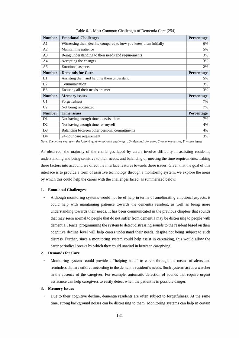
131

Table 6.1. Most Common Challenges of Dementia Care [254]

Number Emotional Challenges Percentage

A1 Witnessing them decline compared to how you knew them initially 6%

A2 Maintaining patience 5%

A3 Being understanding to their needs and requirements 3%

A4 Accepting the changes 3%

A5 Emotional aspects 2%

Number Demands for Care Percentage

B1 Assisting them and helping them understand 5%

B2 Communication 3%

B3 Ensuring all their needs are met 3%

Number Memory issues Percentage

C1 Forgetfulness 7%

C2 Not being recognized 7%

Number Time issues Percentage

D1 Not having enough time to assist them 7%

D2 Not having enough time for myself 4%

D3 Balancing between other personal commitments 4%

D4 24-hour care requirement 3%

Note: The letters represent the following: A –emotional challenges; B - demands for care; C –memory issues; D – time issues

As observed, the majority of the challenges faced by carers involve difficulty in assisting residents,

understanding and being sensitive to their needs, and balancing or meeting the time requirements. Taking

these factors into account, we direct the interface features towards these issues. Given that the goal of this

interface is to provide a form of assistive technology through a monitoring system, we explore the areas

by which this could help the carers with the challenges faced, as summarized below:

1. Emotional Challenges

- Although monitoring systems would not be of help in terms of ameliorating emotional aspects, it

could help with maintaining patience towards the dementia resident, as well as being more

understanding towards their needs. It has been communicated in the previous chapters that sounds

that may seem normal to people that do not suffer from dementia may be distressing to people with

dementia. Hence, programming the system to detect distressing sounds to the resident based on their

cognitive decline level will help carers understand their needs, despite not being subject to such

distress. Further, since a monitoring system could help assist in caretaking, this would allow the

carer periodical breaks by which they could unwind in between caregiving.

2. Demands for Care

- Monitoring systems could provide a “helping hand” to carers through the means of alerts and

reminders that are tailored according to the dementia resident’s needs. Such systems act as a watcher

in the absence of the caregiver. For example, automatic detection of sounds that require urgent

assistance can help caregivers to easily detect when the patient is in possible danger.

3. Memory Issues

- Due to their cognitive decline, dementia residents are often subject to forgetfulness. At the same

time, strong background noises can be distressing to them. Monitoring systems can help in certain

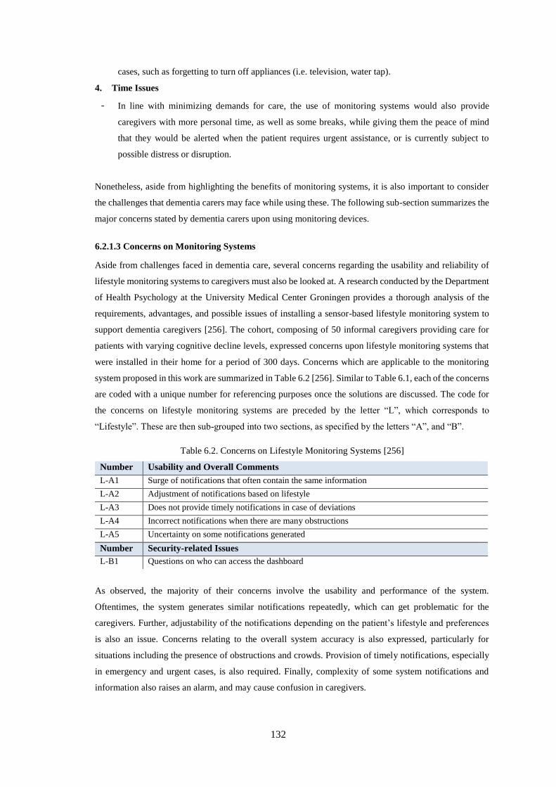
132

cases, such as forgetting to turn off appliances (i.e. television, water tap).

4. Time Issues

- In line with minimizing demands for care, the use of monitoring systems would also provide

caregivers with more personal time, as well as some breaks, while giving them the peace of mind

that they would be alerted when the patient requires urgent assistance, or is currently subject to

possible distress or disruption.

Nonetheless, aside from highlighting the benefits of monitoring systems, it is also important to consider

the challenges that dementia carers may face while using these. The following sub-section summarizes the

major concerns stated by dementia carers upon using monitoring devices.

6.2.1.3 Concerns on Monitoring Systems

Aside from challenges faced in dementia care, several concerns regarding the usability and reliability of

lifestyle monitoring systems to caregivers must also be looked at. A research conducted by the Department

of Health Psychology at the University Medical Center Groningen provides a thorough analysis of the

requirements, advantages, and possible issues of installing a sensor-based lifestyle monitoring system to

support dementia caregivers [256]. The cohort, composing of 50 informal caregivers providing care for

patients with varying cognitive decline levels, expressed concerns upon lifestyle monitoring systems that

were installed in their home for a period of 300 days. Concerns which are applicable to the monitoring

system proposed in this work are summarized in Table 6.2 [256]. Similar to Table 6.1, each of the concerns

are coded with a unique number for referencing purposes once the solutions are discussed. The code for

the concerns on lifestyle monitoring systems are preceded by the letter “L”, which corresponds to

“Lifestyle”. These are then sub-grouped into two sections, as specified by the letters “A”, and “B”.

Table 6.2. Concerns on Lifestyle Monitoring Systems [256]

Number Usability and Overall Comments

L-A1 Surge of notifications that often contain the same information

L-A2 Adjustment of notifications based on lifestyle

L-A3 Does not provide timely notifications in case of deviations

L-A4 Incorrect notifications when there are many obstructions

L-A5 Uncertainty on some notifications generated

Number Security-related Issues

L-B1 Questions on who can access the dashboard

As observed, the majority of their concerns involve the usability and performance of the system.

Oftentimes, the system generates similar notifications repeatedly, which can get problematic for the

caregivers. Further, adjustability of the notifications depending on the patient’s lifestyle and preferences

is also an issue. Concerns relating to the overall system accuracy is also expressed, particularly for

situations including the presence of obstructions and crowds. Provision of timely notifications, especially

in emergency and urgent cases, is also required. Finally, complexity of some system notifications and

information also raises an alarm, and may cause confusion in caregivers.

133

In terms of security, queries regarding the accessibility of the system dashboard to those who are not

directly involved with the patient are raised. As per the findings of the research done by [256], the sense

of safety and reassurance that the system proves more significant than these issues. Further, provided that

the lifestyle monitoring system involved in their work is sensor-based, it has been observed that the

absence of cameras and visual components lessened implications concerning intrusion [256], and did not

make the patients feel violated.

6.2.2 Identifying the Hill: Understanding the Challenges

According to the IBM Enterprise Design Thinking Trainer Course, “Hills are statements of intent written

as user enablements” [253]. This refers to the user-centred goal of the design process composed of ‘Who’,

which refers to the persona, ‘What’, which identify the persona’s goal, and ‘Wow’, which is what sets the

solution apart from its competitors [253]. Defining the hill enables the identification of the end-user’s main

needs; which, in design thinking terms, are called “pain points”. In turn, this allows the development of

the application focusing on the user outcome and requirement.

As per the challenges and concerns discussed in relation to Section 6.2.1, we can define our ‘hill’ to be:

“Dementia caregivers should be able to remotely monitor the dementia residents’ need for assistance

while minimizing intrusions, and without the requirement of being present 24/7, allowing time for

themselves.”, where the dementia resident caregivers are defined as the ‘Who’, the virtual monitoring

being the ‘What’, and the minimization of the system’s invasiveness while allowing more personal time

for the caregivers as the ‘Wow’. Upon the definition of the ‘hill’, throughout the design process, the scope

of the user interface should focus on the following caregiver benefits:

- Providing a better overview of the resident’s daily activities

Objective: to help carers understand the resident’s action and behavioural pattern. In turn, this would

help dementia caregivers to understand patients better. Similarly, monitoring their daily activities

would also help in the early detection of further cognitive decline and sudden behavioural changes.

- Customizes care requirement as per the resident’s level of cognitive decline and preferences

Objective: customization depending on preference and level of cognitive decline helps to improve

the anticipation of when, and whether care and assistance is required. In turn, this provides caregivers

of a form of peace of mind on times when they cannot be present with the resident, and when

occasional forms of monitoring is required. Further, maintaining up-to-date profiles also encourages

regular communication with the healthcare practitioner.

- Saving time and promoting a balanced lifestyle

Objective: Improved anticipation of assistance requirement allows caregivers to balance their time

and lifestyle better. Providing a form of monitoring to the resident in the caregiver’s absence also

brings a measure of peace to the caregivers, which would help them cope with stress. Accordingly,

spending some time during the day apart will also be beneficial to the resident, such that it promotes

independence and satisfies their need for solitude.

134

Through these definitions, it is important to note that the system is not meant to aid the resident as a

caregiver substitute. Rather, it assists caregivers in terms of managing their caregiving tasks.

6.2.3 The Loop: Designing the Graphical User Interface

The design thinking approach helps organizations in delivering outcomes that align as per the requirements

of the designated users. Successful outcomes are defined by meeting the objectives of the business, any

technical limitations, and the needs of the target market [253]. Design thinking influences developers to

build products based on insights and empathy for the users. Provided the ‘hill’ identified in the previous

subsection, this section focuses on the ‘loop’, which involve the continuous process of observing,

reflecting, and making [253]. Within this process, personal challenges faced by the persona is observed

and reflected upon, in order to form abstract ideas that focus on addressing these issues.

6.2.3.1 Proposal and Reflection

Given the information retrieved regarding the persona, as well as the challenges that they face in

caregiving, we now focus on forming and assessing abstract ideas. This sub-section provides a summary

of the ‘restless reinvention’ process, beginning with initial abstract ideas that were formed, a short

description of each, assessment and reflection of the pros and cons, as well as the proposed solution to

counteract the identified disadvantages. For the final proposed solution, a combination of the reinvented

ideas will be combined into the interface.

Idea 1: Audio Classification System

Description: the microphone nodes placed around each room classifies audio data, and notifies the

caregiver regarding any activity that requires urgent attention, or may cause possible irritation to the

residents.

Advantages:

- Allows monitoring the dementia residents with minimal invasiveness, and without making them

feel intimidated through visual objects such as cameras.

- Benefits caregivers with the ability to do other things in parallel to caretaking, while putting their

minds at ease that the resident is looked after. This promotes better life balance.

- Understanding and being aware of what is happening to the resident in the absence of the

caregiver, which brings benefits of reassurance.

Disadvantages:

- Unnecessary overflow of mobile notifications, especially during times where the caregiver is

present in the room with the resident.;

- Requirement for high data storage for all the audio recordings.

- Very high accuracy required for high urgency activities.

Reinvented Idea: The user will have the option to specify and control when the system should record,

and when it should stop. This way, the system will only record during the times where the caregiver is

situated in another area, or is pre-occupied with other tasks. In terms of the accuracy, a two-step neural

network will be developed in order to improve accuracy for urgent situations. The first step classifies

135

between urgent, possible disruptive, and silence sounds; while the second step specifies the sound class.

More information regarding this network will be discussed in the subsequent section.

Idea 2: Sound Source Location System

Description: the approximate room location of the audio sources (domestic activities) will be identified

and presented to the caregiver along with the sound class for monitoring purposes.

Advantages:

- Locating the audio source will allow the caregiver to easily access the location of the sound

sources, especially when assistance is required. This makes a more personal and secure

monitoring process.

- Including the estimation of the sound location will improve the accuracy of the classification.

Disadvantages:

- Presenting the audio source angles and elevation information to the caregivers is deemed

unnecessary, provided that they only have to know the estimated location of the sound source

relative to the room location, in order to assist the resident and tend to their need.

- Derivation of the sound source angles and elevation can be a computationally extensive process.

Reinvented Idea: Instead of presenting the exact sound source locations, an estimated location is provided

through the closest microphone node to the sound source within the specific room location. Additionally,

this can be easily integrated into the sound classification system, provided that both processes are based

on sound images and neural networks. In turn, this also mitigates the overall system computational

requirements.

Idea 3: Integrated Patient Profile

Description: the system allows a degree of personalization to the interface, which is based on specific

information about the dementia resident. This allows caregivers to set a severity index on each activity,

indicating the degree by which they should be notified. Further, it also contains a built-in reminder system

that displays the date and time of the resident’s next doctor’s appointment. Such functionality can also be

extended to provide medical records specific to the resident.

Advantages:

- Customizes the notifications received by the caregiver based on every individual’s requirement,

level of cognitive decline, and preferences.

- Helps keep track of the resident’s medical records and appointments. Although it can be argued

that normal smartphone reminder systems can work effectively, having healthcare-related

reminders within a healthcare monitoring application may help with overall organization.

Disadvantages:

- It may be a tedious task for the caregiver to set severity indexes on every possible activity

detectable by the system.

- This may affect the visual management of the application, making it look more complicated than

it actually is due to the presence of multiple severity index bars.

136

Reinvented Idea: Instead of setting a severity index on every activity, the system stores ID-based patient

profiles, which contain the current cognitive decline level as prescribed by the healthcare practitioner, as

well as individual preferences. Hence, instead of individually setting indexes at start up, the caregiver

solely has to load the specific resident’s profile, which displays the last date of update along with the

profile content. Further, the application provides the option to update this profile if required. In terms of

visual organization, the reminder system can be implemented such that the overall layout of the application

will be organized in header tabs. In this case, one tab will be dedicated to the resident’s wellness, where

the profile update and the reminder system will be placed. Another tab will be dedicated to household

monitoring, which is composed of the integrated model following the first two ideas discussed.

Idea 4: Sound level assessment tool

Description: Provided that dementia residents perceive external stimuli differently compared to those

without dementia, this system can be used to identify if the overall sound level of the facility or household

is suitable for the resident. Similarly, this may also be used in providing ratings for age care facilities.

Advantages:

- Can be used to assess suitability of the overall sound levels based on professional

recommendations considering the resident’s cognitive decline level.

- Can be used as an additional benchmark to determine assistance requirement.

Disadvantages:

- Since sound level assessment is recommended to be done periodically, it is a process that

caregivers may commonly fail to remember.

- Assessment will be highly dependent on the number of audio samples available for the selected

time of the day and area of assessment; hence, regular updates on the data will be crucial.

Reinvented Idea: Periodical reminders will be sent to the caregivers when the resident’s environment is

due for sound level assessment. In order to comply with application visual management standards, the

sound levels assessment tool will be placed in a separate tab.

As observed, through a round of playbacks, and the assessment of benefits and limitations, we have

devised reinvented ideas that will be utilized for the final solution.

6.2.4 The Solution: Final Caregiver Software Application Functionalities

As per the extensive reflection discussed in Section 6.2.3, Table 6.3 lists down aspects and characteristics

of the caregiver software application, and relates this to the challenges that they address, according to those

previously identified in Sections 6.2.1 and 6.2.2. As specified by the third column, the challenges

addressed are coded based on their categories, as per Tables 6.1 and 6.2.

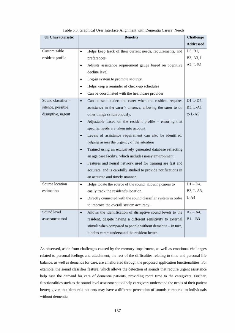
137

Table 6.3. Graphical User Interface Alignment with Dementia Carers’ Needs

UI Characteristic Benefits Challenge

Addressed

Customizable

resident profile

Helps keep track of their current needs, requirements, and

preferences

Adjusts assistance requirement gauge based on cognitive

decline level

Log-in system to promote security.

Helps keep a reminder of check-up schedules

Can be coordinated with the healthcare provider

D3, B1,

B3, A3, L-

A2, L-B1

Sound classifier –

silence, possible

disruptive, urgent

Can be set to alert the carer when the resident requires

assistance in the carer’s absence, allowing the carer to do

other things synchronously.

Adjustable based on the resident profile – ensuring that

specific needs are taken into account

Levels of assistance requirement can also be identified,

helping assess the urgency of the situation

Trained using an exclusively generated database reflecting

an age care facility, which includes noisy environment.

Features and neural network used for training are fast and

accurate, and is carefully studied to provide notifications in

an accurate and timely manner.

D1 to D4,

B3, L-A1

to L-A5

Source location

estimation

Helps locate the source of the sound, allowing carers to

easily track the resident’s location.

Directly connected with the sound classifier system in order

to improve the overall system accuracy.

D1 – D4,

B3, L-A3,

L-A4

Sound level

assessment tool

Allows the identification of disruptive sound levels to the

resident, despite having a different sensitivity to external

stimuli when compared to people without dementia – in turn,

it helps carers understand the resident better.

A2 – A4,

B1 – B3

As observed, aside from challenges caused by the memory impairment, as well as emotional challenges

related to personal feelings and attachment, the rest of the difficulties relating to time and personal life

balance, as well as demands for care, are ameliorated through the proposed application functionalities. For

example, the sound classifier feature, which allows the detection of sounds that require urgent assistance

help ease the demand for care of dementia patients, providing more time to the caregivers. Further,

functionalities such as the sound level assessment tool help caregivers understand the needs of their patient

better; given that dementia patients may have a different perception of sounds compared to individuals

without dementia.

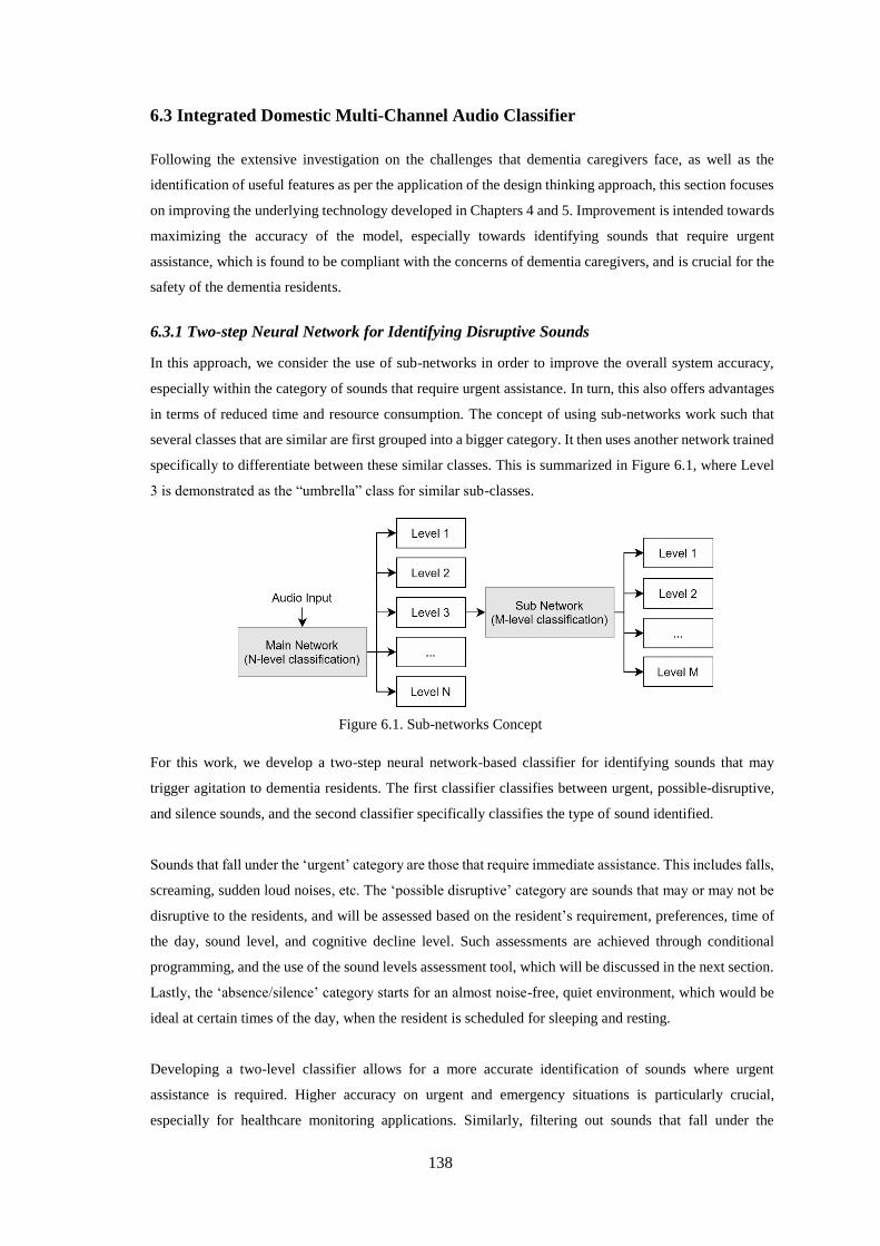
138

6.3 Integrated Domestic Multi-Channel Audio Classifier

Following the extensive investigation on the challenges that dementia caregivers face, as well as the

identification of useful features as per the application of the design thinking approach, this section focuses

on improving the underlying technology developed in Chapters 4 and 5. Improvement is intended towards

maximizing the accuracy of the model, especially towards identifying sounds that require urgent

assistance, which is found to be compliant with the concerns of dementia caregivers, and is crucial for the

safety of the dementia residents.

6.3.1 Two-step Neural Network for Identifying Disruptive Sounds

In this approach, we consider the use of sub-networks in order to improve the overall system accuracy,

especially within the category of sounds that require urgent assistance. In turn, this also offers advantages

in terms of reduced time and resource consumption. The concept of using sub-networks work such that

several classes that are similar are first grouped into a bigger category. It then uses another network trained

specifically to differentiate between these similar classes. This is summarized in Figure 6.1, where Level

3 is demonstrated as the “umbrella” class for similar sub-classes.

Figure 6.1. Sub-networks Concept

For this work, we develop a two-step neural network-based classifier for identifying sounds that may

trigger agitation to dementia residents. The first classifier classifies between urgent, possible-disruptive,

and silence sounds, and the second classifier specifically classifies the type of sound identified.

Sounds that fall under the ‘urgent’ category are those that require immediate assistance. This includes falls,

screaming, sudden loud noises, etc. The ‘possible disruptive’ category are sounds that may or may not be

disruptive to the residents, and will be assessed based on the resident’s requirement, preferences, time of

the day, sound level, and cognitive decline level. Such assessments are achieved through conditional

programming, and the use of the sound levels assessment tool, which will be discussed in the next section.

Lastly, the ‘absence/silence’ category starts for an almost noise-free, quiet environment, which would be

ideal at certain times of the day, when the resident is scheduled for sleeping and resting.

Developing a two-level classifier allows for a more accurate identification of sounds where urgent

assistance is required. Higher accuracy on urgent and emergency situations is particularly crucial,

especially for healthcare monitoring applications. Similarly, filtering out sounds that fall under the

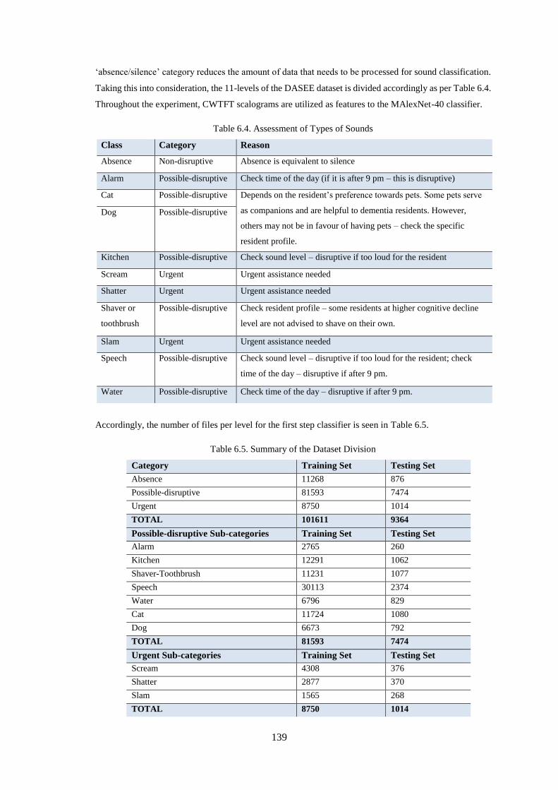
139

‘absence/silence’ category reduces the amount of data that needs to be processed for sound classification.

Taking this into consideration, the 11-levels of the DASEE dataset is divided accordingly as per Table 6.4.

Throughout the experiment, CWTFT scalograms are utilized as features to the MAlexNet-40 classifier.

Table 6.4. Assessment of Types of Sounds

Class Category Reason

Absence Non-disruptive Absence is equivalent to silence

Alarm Possible-disruptive Check time of the day (if it is after 9 pm – this is disruptive)

Cat Possible-disruptive Depends on the resident’s preference towards pets. Some pets serve

as companions and are helpful to dementia residents. However,

others may not be in favour of having pets – check the specific

resident profile.

Dog Possible-disruptive

Kitchen Possible-disruptive Check sound level – disruptive if too loud for the resident

Scream Urgent Urgent assistance needed

Shatter Urgent Urgent assistance needed

Shaver or

toothbrush

Possible-disruptive Check resident profile – some residents at higher cognitive decline

level are not advised to shave on their own.

Slam Urgent Urgent assistance needed

Speech Possible-disruptive Check sound level – disruptive if too loud for the resident; check

time of the day – disruptive if after 9 pm.

Water Possible-disruptive Check time of the day – disruptive if after 9 pm.

Accordingly, the number of files per level for the first step classifier is seen in Table 6.5.

Table 6.5. Summary of the Dataset Division

Category Training Set Testing Set

Absence 11268 876

Possible-disruptive 81593 7474

Urgent 8750 1014

TOTAL 101611 9364

Possible-disruptive Sub-categories Training Set Testing Set

Alarm 2765 260

Kitchen 12291 1062

Shaver-Toothbrush 11231 1077

Speech 30113 2374

Water 6796 829

Cat 11724 1080

Dog 6673 792

TOTAL 81593 7474

Urgent Sub-categories Training Set Testing Set

Scream 4308 376

Shatter 2877 370

Slam 1565 268

TOTAL 8750 1014

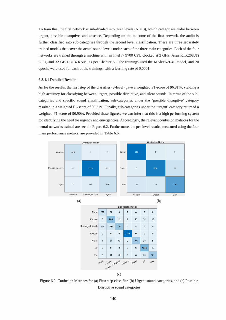
140

To train this, the first network is sub-divided into three levels (N = 3), which categorizes audio between

urgent, possible disruptive, and absence. Depending on the outcome of the first network, the audio is

further classified into sub-categories through the second level classification. These are three separately

trained models that cover the actual sound levels under each of the three main categories. Each of the four

networks are trained through a machine with an Intel i7 9700 CPU clocked at 3 GHz, Asus RTX2080Ti

GPU, and 32 GB DDR4 RAM, as per Chapter 5. The trainings used the MAlexNet-40 model, and 20

epochs were used for each of the trainings, with a learning rate of 0.0001.

6.3.1.1 Detailed Results

As for the results, the first step of the classifier (3-level) gave a weighted F1-score of 96.31%, yielding a

high accuracy for classifying between urgent, possible disruptive, and silent sounds. In terms of the sub-

categories and specific sound classification, sub-categories under the ‘possible disruptive’ category

resulted in a weighted F1-score of 89.31%. Finally, sub-categories under the ‘urgent’ category returned a

weighted F1-score of 90.90%. Provided these figures, we can infer that this is a high performing system

for identifying the need for urgency and emergencies. Accordingly, the relevant confusion matrices for the

neural networks trained are seen in Figure 6.2. Furthermore, the per-level results, measured using the four

main performance metrics, are provided in Table 6.6.

(a) (b)

(c)

Figure 6.2. Confusion Matrices for (a) First step classifier, (b) Urgent sound categories, and (c) Possible

Disruptive sound categories

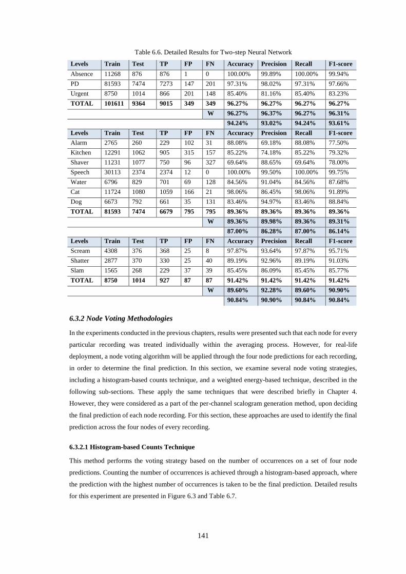
141

Table 6.6. Detailed Results for Two-step Neural Network

Levels Train Test TP FP FN Accuracy Precision Recall F1-score

Absence 11268 876 876 1 0 100.00% 99.89% 100.00% 99.94%

PD 81593 7474 7273 147 201 97.31% 98.02% 97.31% 97.66%

Urgent 8750 1014 866 201 148 85.40% 81.16% 85.40% 83.23%

TOTAL 101611 9364 9015 349 349 96.27% 96.27% 96.27% 96.27%

W 96.27% 96.37% 96.27% 96.31%

94.24% 93.02% 94.24% 93.61%

Levels Train Test TP FP FN Accuracy Precision Recall F1-score

Alarm 2765 260 229 102 31 88.08% 69.18% 88.08% 77.50%

Kitchen 12291 1062 905 315 157 85.22% 74.18% 85.22% 79.32%

Shaver 11231 1077 750 96 327 69.64% 88.65% 69.64% 78.00%

Speech 30113 2374 2374 12 0 100.00% 99.50% 100.00% 99.75%

Water 6796 829 701 69 128 84.56% 91.04% 84.56% 87.68%

Cat 11724 1080 1059 166 21 98.06% 86.45% 98.06% 91.89%

Dog 6673 792 661 35 131 83.46% 94.97% 83.46% 88.84%

TOTAL 81593 7474 6679 795 795 89.36% 89.36% 89.36% 89.36%

W 89.36% 89.98% 89.36% 89.31%

87.00% 86.28% 87.00% 86.14%

Levels Train Test TP FP FN Accuracy Precision Recall F1-score

Scream 4308 376 368 25 8 97.87% 93.64% 97.87% 95.71%

Shatter 2877 370 330 25 40 89.19% 92.96% 89.19% 91.03%

Slam 1565 268 229 37 39 85.45% 86.09% 85.45% 85.77%

TOTAL 8750 1014 927 87 87 91.42% 91.42% 91.42% 91.42%

W 89.60% 92.28% 89.60% 90.90%

90.84% 90.90% 90.84% 90.84%

6.3.2 Node Voting Methodologies

In the experiments conducted in the previous chapters, results were presented such that each node for every

particular recording was treated individually within the averaging process. However, for real-life

deployment, a node voting algorithm will be applied through the four node predictions for each recording,

in order to determine the final prediction. In this section, we examine several node voting strategies,

including a histogram-based counts technique, and a weighted energy-based technique, described in the

following sub-sections. These apply the same techniques that were described briefly in Chapter 4.

However, they were considered as a part of the per-channel scalogram generation method, upon deciding

the final prediction of each node recording. For this section, these approaches are used to identify the final

prediction across the four nodes of every recording.

6.3.2.1 Histogram-based Counts Technique

This method performs the voting strategy based on the number of occurrences on a set of four node

predictions. Counting the number of occurrences is achieved through a histogram-based approach, where

the prediction with the highest number of occurrences is taken to be the final prediction. Detailed results

for this experiment are presented in Figure 6.3 and Table 6.7.

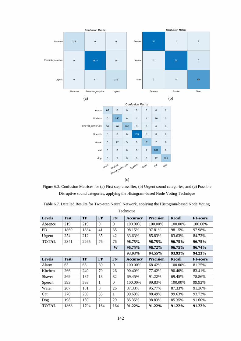
142

(a) (b)

(c)

Figure 6.3. Confusion Matrices for (a) First step classifier, (b) Urgent sound categories, and (c) Possible

Disruptive sound categories, applying the Histogram-based Node Voting Technique

Table 6.7. Detailed Results for Two-step Neural Network, applying the Histogram-based Node Voting

Technique

Levels Test TP FP FN Accuracy Precision Recall F1-score

Absence 219 219 0 0 100.00% 100.00% 100.00% 100.00%

PD 1869 1834 41 35 98.15% 97.81% 98.15% 97.98%

Urgent 254 212 35 42 83.63% 85.83% 83.63% 84.72%

TOTAL 2341 2265 76 76 96.75% 96.75% 96.75% 96.75%

W 96.75% 96.72% 96.75% 96.74%

93.93% 94.55% 93.93% 94.23%

Levels Test TP FP FN Accuracy Precision Recall F1-score

Alarm 65 65 30 0 100.00% 68.42% 100.00% 81.25%

Kitchen 266 240 70 26 90.40% 77.42% 90.40% 83.41%

Shaver 269 187 18 82 69.45% 91.22% 69.45% 78.86%

Speech 593 593 1 0 100.00% 99.83% 100.00% 99.92%

Water 207 181 8 26 87.33% 95.77% 87.33% 91.36%

Cat 270 269 35 1 99.63% 88.49% 99.63% 93.73%

Dog 198 169 2 29 85.35% 98.83% 85.35% 91.60%

TOTAL 1868 1704 164 164 91.22% 91.22% 91.22% 91.22%

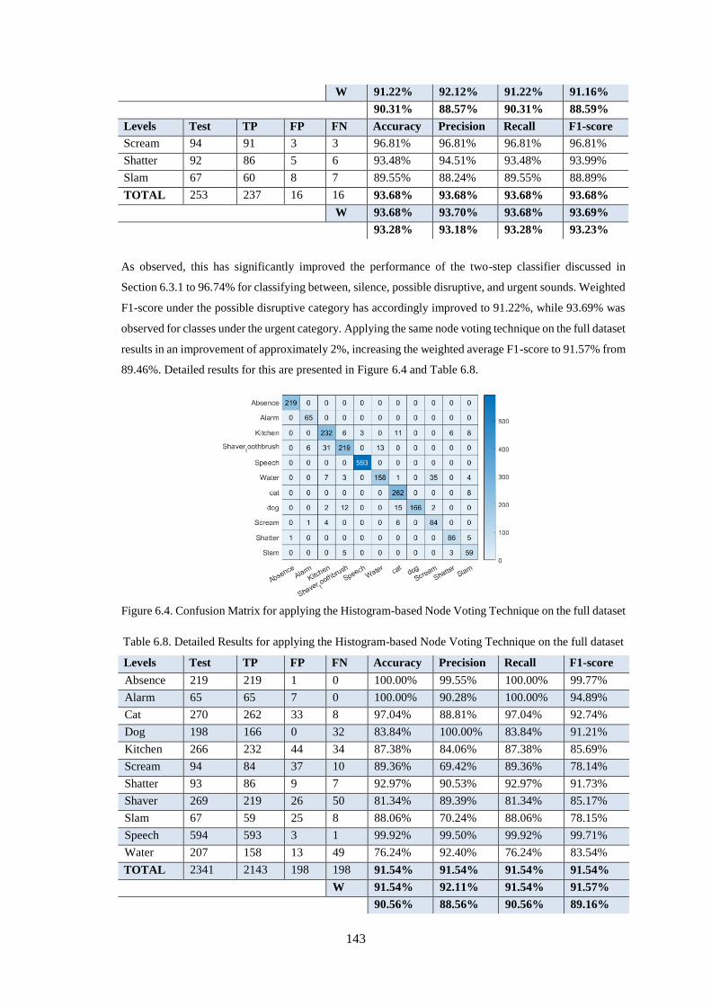
143

W 91.22% 92.12% 91.22% 91.16%

90.31% 88.57% 90.31% 88.59%

Levels Test TP FP FN Accuracy Precision Recall F1-score

Scream 94 91 3 3 96.81% 96.81% 96.81% 96.81%

Shatter 92 86 5 6 93.48% 94.51% 93.48% 93.99%

Slam 67 60 8 7 89.55% 88.24% 89.55% 88.89%

TOTAL 253 237 16 16 93.68% 93.68% 93.68% 93.68%

W 93.68% 93.70% 93.68% 93.69%

93.28% 93.18% 93.28% 93.23%

As observed, this has significantly improved the performance of the two-step classifier discussed in

Section 6.3.1 to 96.74% for classifying between, silence, possible disruptive, and urgent sounds. Weighted

F1-score under the possible disruptive category has accordingly improved to 91.22%, while 93.69% was

observed for classes under the urgent category. Applying the same node voting technique on the full dataset

results in an improvement of approximately 2%, increasing the weighted average F1-score to 91.57% from

89.46%. Detailed results for this are presented in Figure 6.4 and Table 6.8.

Figure 6.4. Confusion Matrix for applying the Histogram-based Node Voting Technique on the full dataset

Table 6.8. Detailed Results for applying the Histogram-based Node Voting Technique on the full dataset

Levels Test TP FP FN Accuracy Precision Recall F1-score

Absence 219 219 1 0 100.00% 99.55% 100.00% 99.77%

Alarm 65 65 7 0 100.00% 90.28% 100.00% 94.89%

Cat 270 262 33 8 97.04% 88.81% 97.04% 92.74%

Dog 198 166 0 32 83.84% 100.00% 83.84% 91.21%

Kitchen 266 232 44 34 87.38% 84.06% 87.38% 85.69%

Scream 94 84 37 10 89.36% 69.42% 89.36% 78.14%

Shatter 93 86 9 7 92.97% 90.53% 92.97% 91.73%

Shaver 269 219 26 50 81.34% 89.39% 81.34% 85.17%

Slam 67 59 25 8 88.06% 70.24% 88.06% 78.15%

Speech 594 593 3 1 99.92% 99.50% 99.92% 99.71%

Water 207 158 13 49 76.24% 92.40% 76.24% 83.54%

TOTAL 2341 2143 198 198 91.54% 91.54% 91.54% 91.54%

W 91.54% 92.11% 91.54% 91.57%

90.56% 88.56% 90.56% 89.16%

144

6.3.2.2 Weighted Energy-based Technique

In this experiment, we applied node voting through considering a weighted energy-based technique.

Calculating the energies of the audio data mapped into images can provide useful information, such as the

loudness and audio energy. For this case, the image energies are calculated based on the properties of

Gray-level Co-occurrence Matrix (GLCM); hence, the images are converted to grayscale first. The GLCM

algorithm calculates the number of occurrence of pairs of pixels with specific values that has a spatial

relationship within an image. It then creates a matrix, from which the statistical measures of energy are

extracted from [257]. Subsequent to this, weighting is considered in two different, independent scenarios:

1. For the first method, the node with the highest energy is counted twice within the counting process,

provided that the image energy is directly proportional to the audio energy.

2. For the second method, the node images are sorted in descending order, based on their energy levels.

Accordingly, we give them weights of 4, 3, 2, and 1 (starting with the highest energy level), before

doing the histogram counts.

In both methods, the tallies are achieved through a histogram-based approach, as discussed in the previous

subsection. The following confusion matrices shown in Figure 6.5 detail the findings when applying

counting methods 1 and 2 to the full dataset.

(a) (b)

Figure 6.5. Confusion Matrices for applying the Weighted-based Node Voting Technique on the full

dataset, (a) Method 1 – 91.39% Weighted F1, (b) Method 2 – 91.72% Weighted F1.

Accordingly, these methods have been applied to the two-level classifier, for which the results are reported

in Figure 6.6:

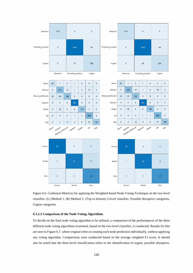
145

Figure 6.6. Confusion Matrices for applying the Weighted-based Node Voting Technique on the two-level

classifier, (L) Method 1, (R) Method 2. (Top to bottom) 3-level classifier, Possible disruptive categories,

Urgent categories

6.3.2.3 Comparison of the Node Voting Algorithms

To decide on the final node voting algorithm to be utilized, a comparison of the performances of the three

different node voting algorithms examined, based on the two-level classifier, is conducted. Results for this

are seen in Figure 6.7, where original refers to treating each node prediction individually, without applying

any voting algorithm. Comparisons were conducted based on the average weighted F1-score. It should

also be noted that the three-level classification refers to the identification of urgent, possible disruptive,

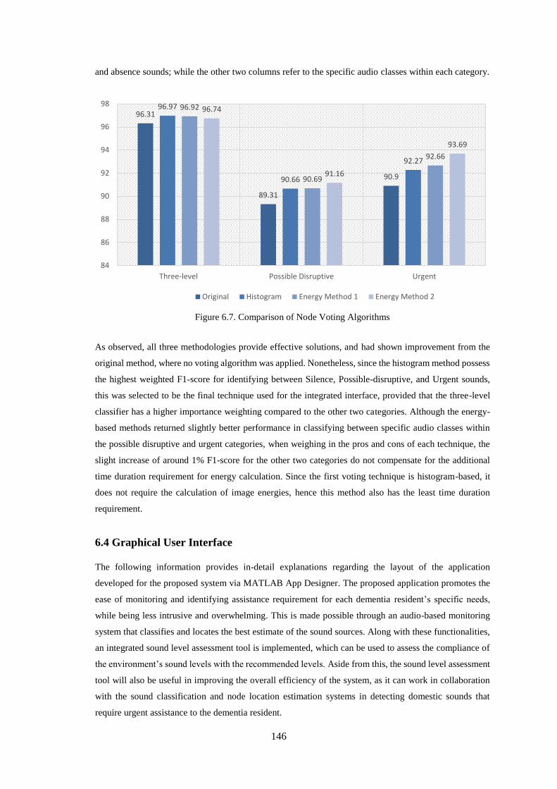
146

and absence sounds; while the other two columns refer to the specific audio classes within each category.

Figure 6.7. Comparison of Node Voting Algorithms

As observed, all three methodologies provide effective solutions, and had shown improvement from the

original method, where no voting algorithm was applied. Nonetheless, since the histogram method possess

the highest weighted F1-score for identifying between Silence, Possible-disruptive, and Urgent sounds,

this was selected to be the final technique used for the integrated interface, provided that the three-level

classifier has a higher importance weighting compared to the other two categories. Although the energy-

based methods returned slightly better performance in classifying between specific audio classes within

the possible disruptive and urgent categories, when weighing in the pros and cons of each technique, the

slight increase of around 1% F1-score for the other two categories do not compensate for the additional

time duration requirement for energy calculation. Since the first voting technique is histogram-based, it

does not require the calculation of image energies, hence this method also has the least time duration

requirement.

6.4 Graphical User Interface

The following information provides in-detail explanations regarding the layout of the application

developed for the proposed system via MATLAB App Designer. The proposed application promotes the

ease of monitoring and identifying assistance requirement for each dementia resident’s specific needs,

while being less intrusive and overwhelming. This is made possible through an audio-based monitoring

system that classifies and locates the best estimate of the sound sources. Along with these functionalities,

an integrated sound level assessment tool is implemented, which can be used to assess the compliance of

the environment’s sound levels with the recommended levels. Aside from this, the sound level assessment

tool will also be useful in improving the overall efficiency of the system, as it can work in collaboration

with the sound classification and node location estimation systems in detecting domestic sounds that

require urgent assistance to the dementia resident.

96.31

89.31

90.9

96.97

90.66

92.27

96.92

90.69

92.66

96.74

91.16

93.69

84

86

88

90

92

94

96

98

Three-level Possible Disruptive Urgent

Original Histogram Energy Method 1 Energy Method 2

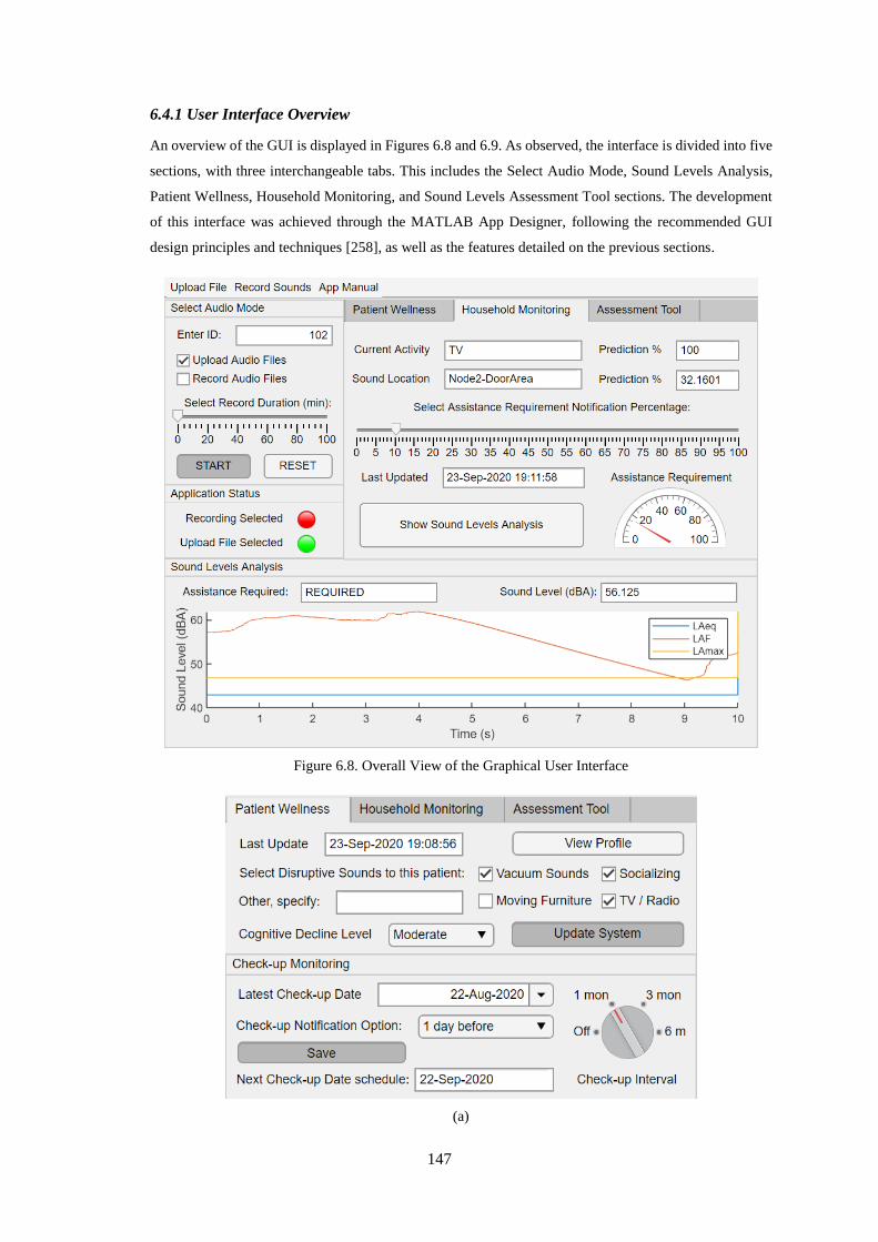
147

6.4.1 User Interface Overview

An overview of the GUI is displayed in Figures 6.8 and 6.9. As observed, the interface is divided into five

sections, with three interchangeable tabs. This includes the Select Audio Mode, Sound Levels Analysis,

Patient Wellness, Household Monitoring, and Sound Levels Assessment Tool sections. The development

of this interface was achieved through the MATLAB App Designer, following the recommended GUI

design principles and techniques [258], as well as the features detailed on the previous sections.

Figure 6.8. Overall View of the Graphical User Interface

(a)

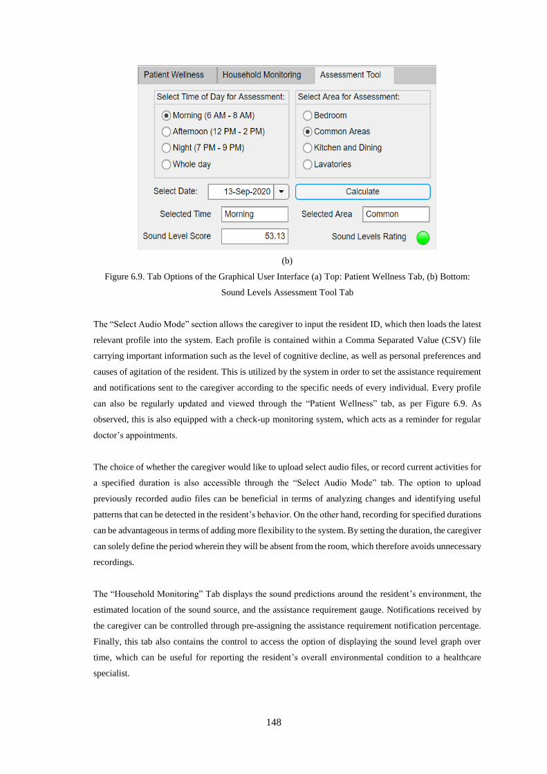
148

(b)

Figure 6.9. Tab Options of the Graphical User Interface (a) Top: Patient Wellness Tab, (b) Bottom:

Sound Levels Assessment Tool Tab

The “Select Audio Mode” section allows the caregiver to input the resident ID, which then loads the latest

relevant profile into the system. Each profile is contained within a Comma Separated Value (CSV) file

carrying important information such as the level of cognitive decline, as well as personal preferences and

causes of agitation of the resident. This is utilized by the system in order to set the assistance requirement

and notifications sent to the caregiver according to the specific needs of every individual. Every profile

can also be regularly updated and viewed through the “Patient Wellness” tab, as per Figure 6.9. As

observed, this is also equipped with a check-up monitoring system, which acts as a reminder for regular

doctor’s appointments.

The choice of whether the caregiver would like to upload select audio files, or record current activities for

a specified duration is also accessible through the “Select Audio Mode” tab. The option to upload

previously recorded audio files can be beneficial in terms of analyzing changes and identifying useful

patterns that can be detected in the resident’s behavior. On the other hand, recording for specified durations

can be advantageous in terms of adding more flexibility to the system. By setting the duration, the caregiver

can solely define the period wherein they will be absent from the room, which therefore avoids unnecessary

recordings.

The “Household Monitoring” Tab displays the sound predictions around the resident’s environment, the

estimated location of the sound source, and the assistance requirement gauge. Notifications received by

the caregiver can be controlled through pre-assigning the assistance requirement notification percentage.

Finally, this tab also contains the control to access the option of displaying the sound level graph over

time, which can be useful for reporting the resident’s overall environmental condition to a healthcare

specialist.

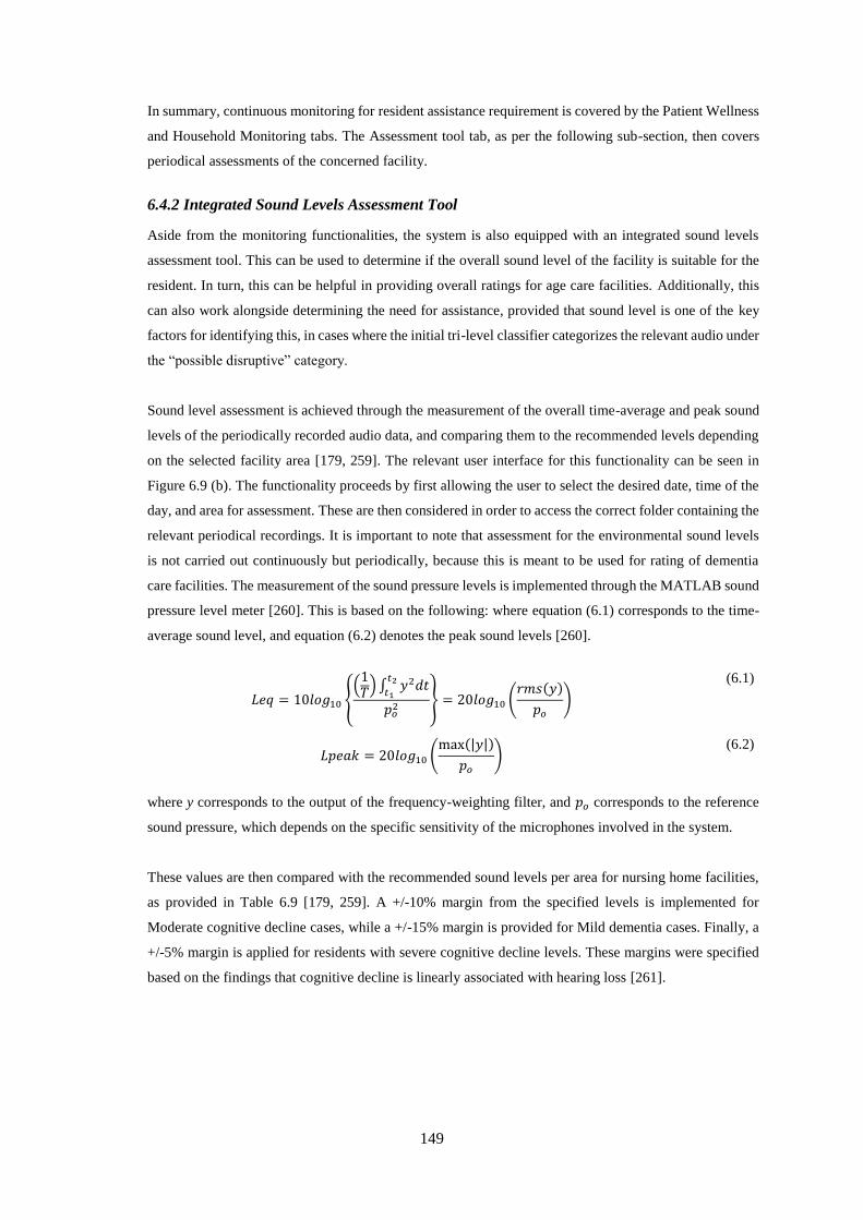
149

In summary, continuous monitoring for resident assistance requirement is covered by the Patient Wellness

and Household Monitoring tabs. The Assessment tool tab, as per the following sub-section, then covers

periodical assessments of the concerned facility.

6.4.2 Integrated Sound Levels Assessment Tool

Aside from the monitoring functionalities, the system is also equipped with an integrated sound levels

assessment tool. This can be used to determine if the overall sound level of the facility is suitable for the

resident. In turn, this can be helpful in providing overall ratings for age care facilities. Additionally, this

can also work alongside determining the need for assistance, provided that sound level is one of the key

factors for identifying this, in cases where the initial tri-level classifier categorizes the relevant audio under

the “possible disruptive” category.

Sound level assessment is achieved through the measurement of the overall time-average and peak sound

levels of the periodically recorded audio data, and comparing them to the recommended levels depending

on the selected facility area [179, 259]. The relevant user interface for this functionality can be seen in

Figure 6.9 (b). The functionality proceeds by first allowing the user to select the desired date, time of the

day, and area for assessment. These are then considered in order to access the correct folder containing the

relevant periodical recordings. It is important to note that assessment for the environmental sound levels

is not carried out continuously but periodically, because this is meant to be used for rating of dementia

care facilities. The measurement of the sound pressure levels is implemented through the MATLAB sound

pressure level meter [260]. This is based on the following: where equation (6.1) corresponds to the time-

average sound level, and equation (6.2) denotes the peak sound levels [260].

𝐿𝑒𝑞 = 10𝑙𝑜𝑔10 {(

1𝑇

) ∫ 𝑦2𝑑𝑡𝑡2

𝑡1

𝑝𝑜2

} = 20𝑙𝑜𝑔10 (𝑟𝑚𝑠(𝑦)

𝑝𝑜

)

(6.1)

𝐿𝑝𝑒𝑎𝑘 = 20𝑙𝑜𝑔10 (max(|𝑦|)

𝑝𝑜

) (6.2)

where y corresponds to the output of the frequency-weighting filter, and 𝑝𝑜 corresponds to the reference

sound pressure, which depends on the specific sensitivity of the microphones involved in the system.

These values are then compared with the recommended sound levels per area for nursing home facilities,

as provided in Table 6.9 [179, 259]. A +/-10% margin from the specified levels is implemented for

Moderate cognitive decline cases, while a +/-15% margin is provided for Mild dementia cases. Finally, a

+/-5% margin is applied for residents with severe cognitive decline levels. These margins were specified

based on the findings that cognitive decline is linearly associated with hearing loss [261].

150

Table 6.9. Recommended Sound Levels (dBA) in Different Facility Areas [179, 259]

Facility Area Comments Sound Level

Sleeping Areas (Bedrooms) Day time

Night Time

35 dBA

30 dBA

Hospital ward rooms - 30 dBA

Common Area (Living room, Leisure areas) Low tolerance

Medium tolerance

High tolerance

55 dBA

50 dBA

40 dBA

Toilets Minimized 45 dBA

Kitchen and Service Areas Minimized 45 dBA

Staff work areas - 40 dBA

Corridor / Lobbies - 40 dBA

Ceremonies and Entertainment Events Limit to 5 times/year 70 dBA

Public addresses - 85 dBA

6.5 Chapter Summary

This chapter has discussed the design thinking research approach undertaken for the development of a

dementia caregiver software application, used for the integration of the technical functionalities developed

in this work. This approach focuses on outcomes in benefit to the persona, which are the dementia

caregivers. The design process is carried out through empathizing with the users, identifying and

understanding their challenges, and forming abstract ideas based on these. Design refinement is then

carried out through the assessment of advantages and disadvantages for each of the ideas concerned,

creating reinvented ideas. As per the scope of this thesis, the purpose of developing this application is

solely to provide a usable platform to integrate and improve the underlying technology implemented in the

previous chapters.

There is a total of four main functionalities integrated within the application, including: a sound levels

assessment tool, a customizable profile that adjusts notifications based on user preferences and cognitive

decline level, and the sound classification and source node location estimation systems. The last two

functionalities are implemented using CWTFT scalograms for sound classification, and STFT-based

phasograms for source node location estimation, as features to the MAlexNet-40 classifier; all of which

are identified and developed within this work.

151

Conclusions and Future Work

This thesis has presented a customizable, accurate, and compact series neural network model developed

through extensive studies of hyperparameter and architecture modification. Aimed at a non-invasive

dementia resident monitoring application, two major functionalities are selected for the purpose of this

work: sound classification, and source node location estimation. Considering these, optimal features to the

developed neural network are selected and proposed in the form of FFT-based scalograms for sound

classification, and STFT-based phasograms for source node location estimation, both of which are

contemporary in their specific fields, and has well exceeded the performance of more widely used features.

Robustness and efficiency of the approach were verified through both the SINS database, and the DASEE

database, a synthetic acoustic dataset developed for this work. Optimal results are integrated into an easy-

to-use GUI which has originated through the application of a design thinking research approach. The

concluding chapter begins by summarizing the contributions made in this thesis, and confer about its

impact on a wider spectrum. We then discuss possible future directions of this research, as well as areas

of improvement within both the research and societal perspectives.

7.1 Summary of Research Contributions

In summary, this thesis has presented the following research contributions:

A realistic synthetic acoustic dataset of domestic audio recordings covering sound events and

scenes that are often experienced and observed in a dementia resident’s environment, based on

the room environment of the Hebrew Senior Life Facility [187]. Synthesis of the database

involves the convolution of the relevant room impulse responses generated through the image

method, with the audio signals and background noises. The database is released publicly in order

to be utilized for future research. (Chapter 3)

A detailed study on proficient features for audio classification, and the identification of the

Morlet-6 CWTFT scalogram features as an optimum method for sound classification, despite the

limited information surrounding this. Results from experiments evaluating the sound

classification performance were provided to support that these features exceeded that of the state-

of-the-art and widely used methods such as the MFCC and Log-mel spectrograms. (Chapter 4)

A novel method of providing estimated locations of sound sources by identifying the closest

microphone node in which they are originating from. This methodology focuses on multi-channel

recordings, which involves an image translation of the phase-based information gathered from

individual microphones within a node, as features to a neural network classifier, in combination

with the shortest angular Euclidean distance. In turn, this provided a fast and accurate approach

to determining sound location, which is also highly compatible with the neural network-based

classification system. (Chapter 4)

A highly customizable compact series neural network model with high accuracy, which makes it

152

suitable for devices with lower computational resource availability. The method was proven to

achieve better performance than various pre-trained network models with more complicated,

DAG architectures. Further, customization of the network architecture provides less risks in

affecting the overall network predictive power, and the lower number of layers and depth reduces

potential overfitting. The proposed model has also improved the system accuracy achieved

through the highest performing pre-trained model AlexNet, while decreasing the model size by

almost 95%. In turn, this greatly improved both resource and time requirements, as well as the

overall execution inference time. (Chapter 5)

A software application prototype intended for the use of dementia caregivers, that would aid in

dementia healthcare monitoring. The development of the application is compliant to the design

thinking research approach, focusing on dementia caregivers as the persona. The overall design

and proposal of the functionalities consider the challenges faced by dementia caregivers within

the concept of caregiving, and operating lifestyle monitoring systems. In turn, this promotes a

user-centred outcome. (Chapter 6)

7.2 Societal Relevance

The societal relevance refers to the effects of the conducted work beyond academic research [262]. This

is commonly associated to the benefits of this work on different areas of the society, particularly to the

healthcare and the economy. The societal relevance associated with this work can be summarized as

follows:

In line with time management and balancing challenges faced by dementia caregivers highlighted

in Chapter 6, the application prototype offers an improved organization and lifestyle management

for dementia caregivers. The application allows caregivers to perform other tasks in parallel to

caregiving, through customizable alerts and notifications depending on the resident’s cognitive

decline level and preferences. In turn, this also provides them with an added level of reassurance

on times where they are not in the same room as the resident.

The audio-based nature of the developed monitoring approach addresses major issues of intrusion

that is commonly associated with visual monitoring systems for individuals with dementia. This

is because the use of microphones was proven to be less intimidating and invasive to residents

as opposed to cameras.

The design thinking research-based design focused on addressing common challenges faced by

dementia caregivers, both within the field of caretaking, and the overall usability of lifestyle

monitoring systems. Thus, the system provides improvement and contribution in terms of ease

of use and adjustability of lifestyle monitoring systems.

Aside from focusing on caregivers specializing on dementia residents, the utilization advantages

and functionalities provided by the proposed system application can also be extended to assisting

individuals with special needs, and can also be generalized to caregiving.

153

7.3 Future Work and Research Directions

7.3.1 Directions for Research

The solutions presented in this work, which are proposed and developed through extensive

experimentation and studies, have invigorated further challenges and probable directions to overcome

identified limitations within the field of audio classification and neural networks. The extensive range of

administration for which these solutions can be appertained for, encourages exploration in the applicability

of the proposed solutions for other applications. Furthermore, the synthetic acoustic database developed

for this work also extends the ground for the future of audio classification research, and audio-based

lifestyle monitoring systems. For future work, this database can also be further improved through the

incorporation of real recordings from a dementia care facility. Within the scope of this work, there have

been limitations in terms of access to relevant dementia care facilities, as well as gathering the necessary

ethical approvals for these recordings due to the restrictions placed in response to the COVID-19

pandemic.

Within the field of audio classification, improvement can be explored in terms of feature development,

particularly in the field of sound source location estimation. In the context of this application, yielding the

exact coordinates of the source location was not necessary, provided that the caregivers solely require an

estimate of the location of the sound source in relation to the resident’s current location. However, for

more complex and research-oriented applications, the exact locations of the sound sources may be

beneficial. An example of this can be the development of interactive robots, audio surveillance systems,

bio-diversity monitoring, and virtual reality. For such applications, the image translated phase-based

features proposed in this work provide a baseline towards developing compatible sound source location

systems that can be integrated in conjunction with a sound classification model.

As for sound classification features, an extensive study and comparison between the FFT-based Morlet

Scalograms and current state-of-the-art methodologies are conducted, yielding high performing features

and a large improvement in speed and resource requirements. Nonetheless, these features may also be

improved and extended through the consideration of accurate timestamps. In this work, the generation of

timestamps were not required, provided that one of the concerns of dementia caregivers in lifestyle

monitoring systems are the overflow of unnecessary and complex information that may be difficult to

interpret without extensive training. Hence, we focus on a simplistic, accurate approach by taking general

predictions and sending out notifications when assistance is urgently or possibly needed, depending on

important factors such as: patient-specific requirements and preferences, recently assessed cognitive

decline level, time of the day, and sound level.

In terms of neural network architecture model development, the proposed model had improved the

performance of the AlexNet pre-trained neural network for the specific application, while decreasing its

overall size by almost 95%. The overall system achieved a weighted F1-score of 89.46% using the

154

synthetic database generated, which exceeded the performance of all the networks examined, both within

the compact network category, as well as non-compressed pre-trained network models. Within the design

and development process, we also managed to maintain the series network architecture of the AlexNet

model, allowing for a highly customizable neural network architecture that serves as a good foundation

for further extension with minimal risks of overfitting and loss of predictive power. Depending on further

studies and relevant predictive power calculations, this can also be extended and converted into a DAG

network. Aside from measuring its performance in terms of classification capabilities, it will also be

interesting to see how compact networks such as the MAlexNet-40 performs as a feature extractor through

neural network activations, as per Section 4.2.1.2. Finally, utilization of open-source hyperparameter

optimization frameworks, such as Optuna [263], can also be considered. Although the use of such

frameworks may be limited in terms of getting the optimum neural network structure, provided that it

could only identify optimal hyperparameter values, this can be a useful way of starting to explore DAG

architectures. Currently, the model rests at 14.18 MB, with a loading time of 1.1-s and an inference

execution time of 0.0148-s, which makes it compatible for mobile applications and devices with limited

resource allocations.

Aside from specific research areas, it would also be worth exploring the implementation of the proposed

system through Python-based environments for future work. Python is known to be one of the most widely-

used languages for deep and machine learning, and it offers advantages as an open-source platform, which

offers more flexibility in terms of program deployment.

In summary, the solutions and contributions presented in this thesis are versatile, and are applicable for

extension to many other applications. Further, this thesis provides a good foundation and baseline models

to encourage further research both within the fields of sound classification and sound source location

features, and neural network model architectures.

7.3.2 Interface Improvement

The GUI proposed for this work was carefully designed and implemented through the concept of design

thinking research, which focuses on the user outcome. During the design process, priority was intended

towards the main challenges experienced by dementia caregivers, as well as their difficulties and concerns

towards lifestyle monitoring systems. The functionalities covered by the interface are proposed in order to

mitigate challenges concerning time management and maintaining a balanced lifestyle, while keeping the

resident’s wellness as the top priority.

Several aspects of the interface create suitable grounds for improvement. In terms of the functionalities,

the sound levels assessment tool may be improved to provide better accuracy and versatility. The research

topic surrounding sound levels assessment and measurement is another vast research field, of which are

not covered within the scope of this thesis. However, the concept of sound levels assessment tool was

integrated in the application as a functionality, provided that we had identified a requirement for it for the

overall benefit of the user. Nonetheless, a baseline model was utilized for this work through the MATLAB

155

sound levels pressure meter. Thus, improvising the integrated sound levels assessment tool would be an

interesting direction of interface improvement.

As for the overall system and design improvement, further testing can be conducted through performing a

study survey on the response towards the user-directed improvements made for this interface. Due to the

study limitations caused by the COVID-19 pandemic restrictions, opportunities to interact with the end-

users have been limited. However, conducting such study would be beneficial for the further development

of the end-user interface. Through this, the concept of restless reinvention can continue, and the application

may be tweaked and improved depending on user feedback collected through various user-centered design

methods. Nonetheless, since the main focus of this thesis is the development of the underlying technology

used for the interface, performing iterative feedback methods to reach the optimal user-centered design is

not within the scope of this thesis. However, the design thinking method applied in this work provides an

excellent foundation towards the user-centered design research field.

156

References

[1] Alzheimer's Association, “2016 Alzheimer's Disease Facts and Figures,” 2016.

[2] I. Korolev, “Alzheimer's Disease: A Clinical and Basic Science Review,” Medical Student Research Journal, vol. 4,

pp. 24-33, September 2014.

[3] Alzheimer's Association, “Basics of Alzheimer's Disease,” 2011.

[4] H. Ayyoub, “Team Assessment and Planning of Care: Vascular Dementia,” Middle East Journal of Age and Ageing,

vol. 12, no. 2, 2015.

[5] Alzheimer's Association, 2016. [Online]. Available: www.alz.org/10-signs-symptoms-alzheimers-dementia.asp.

[6] M. A. a. S. Ramakrishnan, “Detection of Alzheimer disease in MR Images using structure tensor,” in 2014 36th

Annual International Conference of the IEEE Engineering in Medicine and Biology Society, Chicago, IL, 2014.

[7] Second Wind Dreams, Featured on ABC News, 2010, 1997-2017. [Online]. Available:

https://www.secondwind.org/virtual-dementia-tourreg.html. [Accessed 23 Februrary 2019].

[8] Scotland's National Dementia Strategy, 2010. [Online]. Available:

http://www.scotland.gov.uk/Publications/2019/09/10151751/17.

[9] Health, D.O., “A Vistion for Change: Report of the expert group on mental health policy,” 2006.

[10] T. Foley and G. Swanwick, Dementia: Diagnosis and Management in General Practice, Q. i. P. Committee, Ed., ICGP,

2014.

[11] J. Hort, J. O'Brien, G. Gainotti, T. Pirttila, B. Popescu, I. Rektorova, S. Sorbi and P. Scheitens, “EFNS Guidelines for

the Diagnosis and Management of Alzheimer's Disease,” European Journal of Neurology, 2010.

[12] M. Rossor, N. Fox and e. al., “The Diagnosis of Young On-set Dementia,” Lancet Neurology, vol. 9, no. 8, pp. 793-

806, August 2010.

[13] K. Jellinger, “The enigma of mixed dementia,” Elsevier, vol. 3, no. 1, pp. 40-53, January 2007.

[14] N. Custodio, R. Montesinos, D. Lira, E. Herrera-Perez, Y. Bardales and L. Valeriano-Lorenzo, “Mixed Dementia: A

review of the evidence,” Dementia Neuropsychology; Scielo, vol. 11, no. 4, pp. 364-370, December 2017.

[15] Ministry of Health and Long-term care, “Developing Ontario's Dementia Strategy: A Discussion Paper,” Ontario,

2016.

[16] Dementia Australia, “Dementia Prevalence Data 2018-2058,” Canberra, 2018.

[17] M. Wortmann, February 2019. [Online]. Available: https://www.openaccessgovernment.org/dementia-become-

trillion-dollar-disease-2018/26160/.

[18] Australian Bureau of Statistics, “Causes of Death, Australia, 2016,” 2017.

[19] The NAtional Centre for Social and Economic Modelling NATSEM, “Economic Cost of Dementia in Australia: 2016-

2056,” 2016.

[20] J. O'Keeffe, J. Maier and M. Freiman, “Assistive Technology for People with Dementia and Their Caregivers at Home:

What Might Help,” Washington, DC, 2020.

[21] L. Garcon, C. Khasnabis, L. Walker, Y. Nakatani, J. Lapitan, J. Borg and e. al., “Medical and assistive health

technology: meeting the needs of aging populations,” in Gerontologist, 2016.

[22] K. Marasinghe, J. Lapitan and A. Ross, “Assistive Technologies for ageing populations in six low-income and middle-

income countries: A systematic review,” BMJ Innovations, vol. 1, no. 4, pp. 182-195, October 2015.

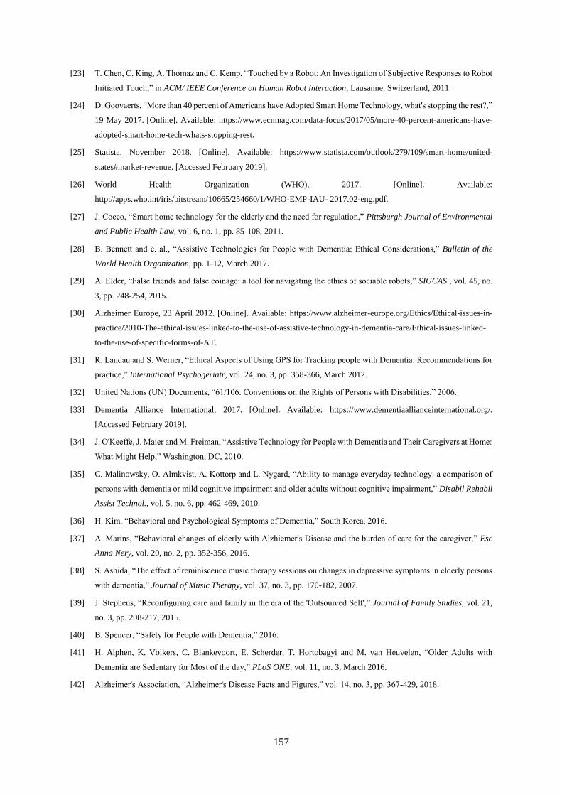
157

[23] T. Chen, C. King, A. Thomaz and C. Kemp, “Touched by a Robot: An Investigation of Subjective Responses to Robot

Initiated Touch,” in ACM/ IEEE Conference on Human Robot Interaction, Lausanne, Switzerland, 2011.

[24] D. Goovaerts, “More than 40 percent of Americans have Adopted Smart Home Technology, what's stopping the rest?,”

19 May 2017. [Online]. Available: https://www.ecnmag.com/data-focus/2017/05/more-40-percent-americans-have-

adopted-smart-home-tech-whats-stopping-rest.

[25] Statista, November 2018. [Online]. Available: https://www.statista.com/outlook/279/109/smart-home/united-

states#market-revenue. [Accessed February 2019].

[26] World Health Organization (WHO), 2017. [Online]. Available:

http://apps.who.int/iris/bitstream/10665/254660/1/WHO-EMP-IAU- 2017.02-eng.pdf.

[27] J. Cocco, “Smart home technology for the elderly and the need for regulation,” Pittsburgh Journal of Environmental

and Public Health Law, vol. 6, no. 1, pp. 85-108, 2011.

[28] B. Bennett and e. al., “Assistive Technologies for People with Dementia: Ethical Considerations,” Bulletin of the

World Health Organization, pp. 1-12, March 2017.

[29] A. Elder, “False friends and false coinage: a tool for navigating the ethics of sociable robots,” SIGCAS , vol. 45, no.

3, pp. 248-254, 2015.

[30] Alzheimer Europe, 23 April 2012. [Online]. Available: https://www.alzheimer-europe.org/Ethics/Ethical-issues-in-

practice/2010-The-ethical-issues-linked-to-the-use-of-assistive-technology-in-dementia-care/Ethical-issues-linked-

to-the-use-of-specific-forms-of-AT.

[31] R. Landau and S. Werner, “Ethical Aspects of Using GPS for Tracking people with Dementia: Recommendations for

practice,” International Psychogeriatr, vol. 24, no. 3, pp. 358-366, March 2012.

[32] United Nations (UN) Documents, “61/106. Conventions on the Rights of Persons with Disabilities,” 2006.

[33] Dementia Alliance International, 2017. [Online]. Available: https://www.dementiaallianceinternational.org/.

[Accessed February 2019].

[34] J. O'Keeffe, J. Maier and M. Freiman, “Assistive Technology for People with Dementia and Their Caregivers at Home:

What Might Help,” Washington, DC, 2010.

[35] C. Malinowsky, O. Almkvist, A. Kottorp and L. Nygard, “Ability to manage everyday technology: a comparison of

persons with dementia or mild cognitive impairment and older adults without cognitive impairment,” Disabil Rehabil

Assist Technol., vol. 5, no. 6, pp. 462-469, 2010.

[36] H. Kim, “Behavioral and Psychological Symptoms of Dementia,” South Korea, 2016.

[37] A. Marins, “Behavioral changes of elderly with Alzhiemer's Disease and the burden of care for the caregiver,” Esc

Anna Nery, vol. 20, no. 2, pp. 352-356, 2016.

[38] S. Ashida, “The effect of reminiscence music therapy sessions on changes in depressive symptoms in elderly persons

with dementia,” Journal of Music Therapy, vol. 37, no. 3, pp. 170-182, 2007.

[39] J. Stephens, “Reconfiguring care and family in the era of the 'Outsourced Self',” Journal of Family Studies, vol. 21,

no. 3, pp. 208-217, 2015.

[40] B. Spencer, “Safety for People with Dementia,” 2016.

[41] H. Alphen, K. Volkers, C. Blankevoort, E. Scherder, T. Hortobagyi and M. van Heuvelen, “Older Adults with

Dementia are Sedentary for Most of the day,” PLoS ONE, vol. 11, no. 3, March 2016.

[42] Alzheimer's Association, “Alzheimer's Disease Facts and Figures,” vol. 14, no. 3, pp. 367-429, 2018.

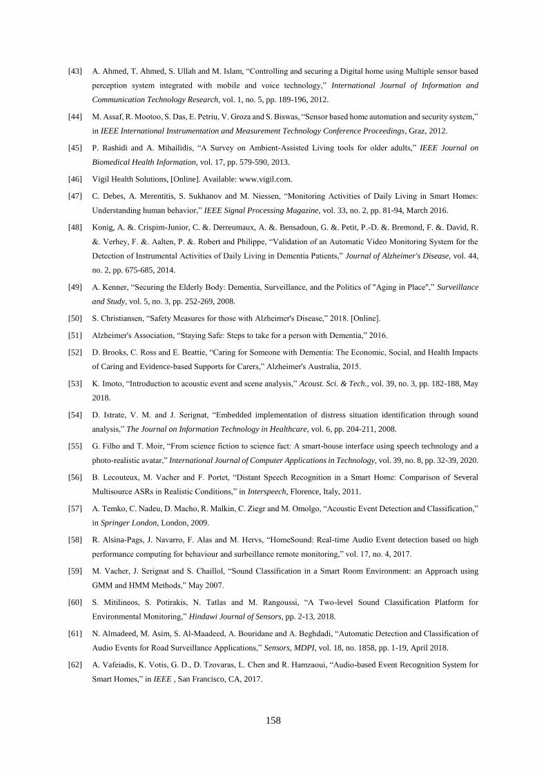
158

[43] A. Ahmed, T. Ahmed, S. Ullah and M. Islam, “Controlling and securing a Digital home using Multiple sensor based

perception system integrated with mobile and voice technology,” International Journal of Information and

Communication Technology Research, vol. 1, no. 5, pp. 189-196, 2012.

[44] M. Assaf, R. Mootoo, S. Das, E. Petriu, V. Groza and S. Biswas, “Sensor based home automation and security system,”

in IEEE International Instrumentation and Measurement Technology Conference Proceedings, Graz, 2012.

[45] P. Rashidi and A. Mihailidis, “A Survey on Ambient-Assisted Living tools for older adults,” IEEE Journal on

Biomedical Health Information, vol. 17, pp. 579-590, 2013.

[46] Vigil Health Solutions, [Online]. Available: www.vigil.com.

[47] C. Debes, A. Merentitis, S. Sukhanov and M. Niessen, “Monitoring Activities of Daily Living in Smart Homes:

Understanding human behavior,” IEEE Signal Processing Magazine, vol. 33, no. 2, pp. 81-94, March 2016.

[48] Konig, A. &. Crispim-Junior, C. &. Derreumaux, A. &. Bensadoun, G. &. Petit, P.-D. &. Bremond, F. &. David, R.

&. Verhey, F. &. Aalten, P. &. Robert and Philippe, “Validation of an Automatic Video Monitoring System for the

Detection of Instrumental Activities of Daily Living in Dementia Patients,” Journal of Alzheimer's Disease, vol. 44,

no. 2, pp. 675-685, 2014.

[49] A. Kenner, “Securing the Elderly Body: Dementia, Surveillance, and the Politics of "Aging in Place",” Surveillance

and Study, vol. 5, no. 3, pp. 252-269, 2008.

[50] S. Christiansen, “Safety Measures for those with Alzheimer's Disease,” 2018. [Online].

[51] Alzheimer's Association, “Staying Safe: Steps to take for a person with Dementia,” 2016.

[52] D. Brooks, C. Ross and E. Beattie, “Caring for Someone with Dementia: The Economic, Social, and Health Impacts

of Caring and Evidence-based Supports for Carers,” Alzheimer's Australia, 2015.

[53] K. Imoto, “Introduction to acoustic event and scene analysis,” Acoust. Sci. & Tech., vol. 39, no. 3, pp. 182-188, May

2018.

[54] D. Istrate, V. M. and J. Serignat, “Embedded implementation of distress situation identification through sound

analysis,” The Journal on Information Technology in Healthcare, vol. 6, pp. 204-211, 2008.

[55] G. Filho and T. Moir, “From science fiction to science fact: A smart-house interface using speech technology and a

photo-realistic avatar,” International Journal of Computer Applications in Technology, vol. 39, no. 8, pp. 32-39, 2020.

[56] B. Lecouteux, M. Vacher and F. Portet, “Distant Speech Recognition in a Smart Home: Comparison of Several

Multisource ASRs in Realistic Conditions,” in Interspeech, Florence, Italy, 2011.

[57] A. Temko, C. Nadeu, D. Macho, R. Malkin, C. Ziegr and M. Omolgo, “Acoustic Event Detection and Classification,”

in Springer London, London, 2009.

[58] R. Alsina-Pags, J. Navarro, F. Alas and M. Hervs, “HomeSound: Real-time Audio Event detection based on high

performance computing for behaviour and surbeillance remote monitoring,” vol. 17, no. 4, 2017.

[59] M. Vacher, J. Serignat and S. Chaillol, “Sound Classification in a Smart Room Environment: an Approach using

GMM and HMM Methods,” May 2007.

[60] S. Mitilineos, S. Potirakis, N. Tatlas and M. Rangoussi, “A Two-level Sound Classification Platform for

Environmental Monitoring,” Hindawi Journal of Sensors, pp. 2-13, 2018.

[61] N. Almadeed, M. Asim, S. Al-Maadeed, A. Bouridane and A. Beghdadi, “Automatic Detection and Classification of

Audio Events for Road Surveillance Applications,” Sensors, MDPI, vol. 18, no. 1858, pp. 1-19, April 2018.

[62] A. Vafeiadis, K. Votis, G. D., D. Tzovaras, L. Chen and R. Hamzaoui, “Audio-based Event Recognition System for

Smart Homes,” in IEEE , San Francisco, CA, 2017.

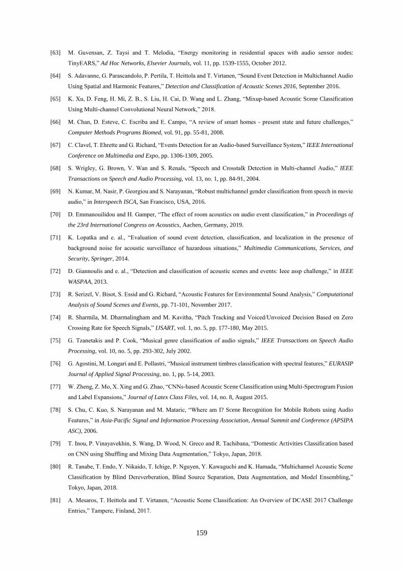
159

[63] M. Guvensan, Z. Taysi and T. Melodia, “Energy monitoring in residential spaces with audio sensor nodes:

TinyEARS,” Ad Hoc Networks, Elsevier Journals, vol. 11, pp. 1539-1555, October 2012.

[64] S. Adavanne, G. Parascandolo, P. Pertila, T. Heittola and T. Virtanen, “Sound Event Detection in Multichannel Audio

Using Spatial and Harmonic Features,” Detection and Classification of Acoustic Scenes 2016, September 2016.

[65] K. Xu, D. Feng, H. Mi, Z. B., S. Liu, H. Cai, D. Wang and L. Zhang, “Mixup-based Acoustic Scene Classification

Using Multi-channel Convolutional Neural Network,” 2018.

[66] M. Chan, D. Esteve, C. Escriba and E. Campo, “A review of smart homes - present state and future challenges,”

Computer Methods Programs Biomed, vol. 91, pp. 55-81, 2008.

[67] C. Clavel, T. Ehrette and G. Richard, “Events Detection for an Audio-based Surveillance System,” IEEE International

Conference on Multimedia and Expo, pp. 1306-1309, 2005.

[68] S. Wrigley, G. Brown, V. Wan and S. Renals, “Speech and Crosstalk Detection in Multi-channel Audio,” IEEE

Transactions on Speech and Audio Processing, vol. 13, no. 1, pp. 84-91, 2004.

[69] N. Kumar, M. Nasir, P. Georgiou and S. Narayanan, “Robust multichannel gender classification from speech in movie

audio,” in Interspeech ISCA, San Francisco, USA, 2016.

[70] D. Emmanouilidou and H. Gamper, “The effect of room acoustics on audio event classification,” in Proceedings of

the 23rd International Congress on Acoustics, Aachen, Germany, 2019.

[71] K. Lopatka and e. al., “Evaluation of sound event detection, classification, and localization in the presence of

background noise for acoustic surveillance of hazardous situations,” Multimedia Communications, Services, and

Security, Springer, 2014.

[72] D. Giannoulis and e. al., “Detection and classification of acoustic scenes and events: Ieee assp challenge,” in IEEE

WASPAA, 2013.

[73] R. Serizel, V. Bisot, S. Essid and G. Richard, “Acoustic Features for Environmental Sound Analysis,” Computational

Analysis of Sound Scenes and Events, pp. 71-101, November 2017.

[74] R. Sharmila, M. Dharmalingham and M. Kavitha, “Pitch Tracking and Voiced/Unvoiced Decision Based on Zero

Crossing Rate for Speech Signals,” IJSART, vol. 1, no. 5, pp. 177-180, May 2015.

[75] G. Tzanetakis and P. Cook, “Musical genre classification of audio signals,” IEEE Transactions on Speech Audio

Processing, vol. 10, no. 5, pp. 293-302, July 2002.

[76] G. Agostini, M. Longari and E. Pollastri, “Musical instrument timbres classification with spectral features,” EURASIP

Journal of Applied Signal Processing, no. 1, pp. 5-14, 2003.

[77] W. Zheng, Z. Mo, X. Xing and G. Zhao, “CNNs-based Acoustic Scene Classification using Multi-Spectrogram Fusion

and Label Expansions,” Journal of Latex Class Files, vol. 14, no. 8, August 2015.

[78] S. Chu, C. Kuo, S. Narayanan and M. Mataric, “Where am I? Scene Recognition for Mobile Robots using Audio

Features,” in Asia-Pacific Signal and Information Processing Association, Annual Summit and Conference (APSIPA

ASC), 2006.

[79] T. Inou, P. Vinayavekhin, S. Wang, D. Wood, N. Greco and R. Tachibana, “Domestic Activities Classification based

on CNN using Shuffling and Mixing Data Augmentation,” Tokyo, Japan, 2018.

[80] R. Tanabe, T. Endo, Y. Nikaido, T. Ichige, P. Nguyen, Y. Kawaguchi and K. Hamada, “Multichannel Acoustic Scene

Classification by Blind Dereverberation, Blind Source Separation, Data Augmentation, and Model Ensembling,”

Tokyo, Japan, 2018.

[81] A. Mesaros, T. Heittola and T. Virtanen, “Acoustic Scene Classification: An Overview of DCASE 2017 Challenge

Entries,” Tampere, Finland, 2017.

160

[82] M. Valenti, S. Squartini, A. Diment, G. Parascandolo and T. Virtanen, “A Convolutional Neural Network Approach

for Acoustic Scene Classification,” Budapest, Hungray, 2016.

[83] D. Oletic, V. Bilas, M. Magno, N. Felber and L. Benini, “Low-power multichannel spectro-temporal feature extraction

circuit for audio pattern wake-up,” in Design, Automation & Test in Europe Conference and Exhibition (DATE),

Dresden, 2016.

[84] J. Schroder, S. Goetze and J. Anemuller, “Spectro-temporal Gabor Filterbank Features for Acoustic Event Detection,”

IEEE/ACM Transactions on Audio, Speech, and Language Processing, vol. 23, no. 12, pp. 2198-2208, December

2015.

[85] C. Cotton and D. Ellis, “Spectral vs. Spectro-temporal Features for Acoustic Event Detection,” IEEE Workshop on

Applications of Signal Processing to Audio and Acoustics, pp. 69-72, October 2011.

[86] D. Xingjian, Z. Mengyao, S. Xuan, Z. Xinpeng, Z. Wen and C. Jingdong, “End-to-End Model for Speech

Enhancement by Consistent Spectrogram Masking,” in arXiv, 2019.

[87] W. Choi, M. Kim, J. Chung, D. Lee and S. Jung, “Investigating Deep Neural Transformations for Spectrogram-based

Musical Source Separation,” in arXiv, 2019.

[88] T. Gerkmann, M. Krawezyk-Becker and J. Roux, “Phase processing for single-channel speech enhancement: History

and recent advances,” in IEEE Signal Processing Mag., vol. 32, no. 2, pp. 55-66, 2015.

[89] S. Mallat and S. Shamma, “Audio Source Separation with Time-Frequency Velocities,” ScatBSS - Supported by ERC

Invariant Class 320959.

[90] E. Sejdic, I. Djurovic and L. Stankovic, “Quantitative Performance Analysis of Scalogram as Instantaneous Frequency

Estimator,” IEEE Transactions on Signal Processing, vol. 56, no. 8, pp. 3837 - 3845, 2008.

[91] D. Komorowski and S. Pietraszek, “The Use of Continuous Wavelet Transform Based on the Fast Fourier Transform

in the Analysis of Multi-channel Electrogastrography Recordings,” J. Med. Sys., vol. 40, no. 10, pp. 1-15, 2016.

[92] Y. Zhou, W. Hu, X. Liu, Q. Zhou, H. Yu and Q. Pu, “Coherency feature extraction based on DFT-based continuous

wavelet transform,” in IEEE PES Asia-Pacific Power and Energy Engineering Conference (APPEEC), Brisbane,

2015.

[93] G. Peeters, “A large set of audio features for sound description (similarity and classification) in the CUIDADO

project,” in IRCAM, Analysis and Synthesis Team, Paris, France, 2004.

[94] M. Sahidullah and G. Saha, “Design, analysis, and experimental evaluation of block based transformation in MFCC

computation for speaker recognition,” Speech Communication, vol. 54, no. 4, pp. 543-565, 2012.

[95] F. Zheng, G. Zhang and Z. Song, “Comparison of Different Implementations of MFCC,” J. Computer Science and

Technology, vol. 16, no. 6, pp. 582-589, 2001.

[96] H. Camargo, R. Burdisso, P. Ravetta and A. Smith, “A Comparison of Beamforming Processing Techniques for Low

Frequency Noise Source Identification in Mining Equipment,” in ASME International Mechanical Engineering

Congress and Exposition, 2009.

[97] J. Pohjalainen, “Methods of automatic audio content classification,” 2007.

[98] S. Ravindran, C. Demirogulu and D. and Anderson, “Speech Recognition using filter-bank features,” in The 37th

Asilomar Conference on Signals, Systems, and Computers, Pacific Grove, CA, USA, 2003.

[99] P. Chaudhary and K. Vagadia, “A Review Article on Speaker Recognition with Feature Extraction,” International

Journal of Emerging Technology and Advanced Engineering, vol. 5, no. 2, pp. 94-97, February 2015.

[100] C. Kim and R. Stern, “Feature Extraction for Robust Speech Recognition using a Power-Law Nonlinearity and Power-

bias Subtraction,” in Interspeech 2009, Brighton, Brighton, UK, 2009.

161

[101] S. Park, S. Mun, Y. Lee, D. Han and H. Ko, “Analysis Acoustic Features for Acoustic Scene Classification and Score

fusion of multi-classification systems applied to DCASE 2016 challenge,” 2018.

[102] S. Park, Y. Lee, D. Han and H. Ko, “Subspace Projection Cepstral Coefficients for Noise Robust Acoustic Event

Recognition,” in IEEE International Conference on Acoustics, Speech, and Signal Processing (ICASSP), 2017.

[103] P. Yuan, M. Lin, K. Xiangli, L. Zhengqing and W. and Lei, “A Study on Echo Feature Extraction based on the

Modified Relative Spectra (RASTA) and Perception Linear Prediction (PLP) Auditory Model,” in IEEE International

Conference on Intelligent Computing and Intelligent Systems, 2010.

[104] V. Kepuska and H. Elharati, “Robust Speech Recognition System Using Conventional and Hybrid Features of MFCC,

LPCC, PLP, RASTA-PLP and Hidden Markov Model Classifier in Noisy Conditions,” Journal of Computer and

Communications, vol. 3, no. 6, 2015.

[105] J. Kumari, K. Ramalakshmi, R. Venkatesan, A. Felsit and S. and Selvanayaki, “A Comparison of Machine Learning

Techniques for the Prediction of the Student's Academic Performance,” Emerging Trends in Computing and Expert

Technology, pp. 1052-1062, 2020.

[106] J. Jesan, “Human Brain and Neural Network Behavior: A Comparison,” in Ubiquity, New York, ACM Digital Library,

2003, p. 2.

[107] V. Advani, “What is the Difference Between Machine Learning and Deep Learning,” My Great Learning, 2021.

[Online]. Available: https://www.mygreatlearning.com/blog/deep-learning-vs-machine-learning/. [Accessed 23 June

2021].

[108] M. Mijwel, “Artificial Neural Networks Advantages and Disadvantages,” Researchgate, 2018.

[109] G. Hinton, S. Osindero and Y. Teh, “A fast learning algorithm for deep belief nets,” Neural computation, vol. 18, no.

7, pp. 1527-1554, 2006.

[110] Y. Han and K. Lee, “Convolutional Neural network with multiple-width frequency-delta data augmentation for

acoustic scene classification,” 2016.

[111] H. Phan, L. Hertel, M. K. P. Maass, R. Mazur and A. Mertins, “Improved Audio Scene Classification based on Label-

tree Embeddings and Convolutional Neural Networks,” IEEE Transactions on Audio, Speech, and Language

Processing, pp. 1278-1290, 2017.

[112] A. Dang, T. Vu and J. Wang, “Acoustic Scene Classification using Convolutional Neural Network and Multi-scale

Multi-Feature Extraction,” IEEE International Conference on Consumer Electronics, 2018.

[113] H. Mohsen, E. El-Dahshan, E. El-Horbaty and A. Salem, “Classification using deep learning neural networks for brain

tumors,” Future Computing and Informatics Journal, vol. 3, no. 1, pp. 68-71.

[114] Q. Le, J. Ngiam, Z. Chen, D. Chia, P. Koh and A. Ng, “Tiled convolutional neural networks,” 2010.

[115] D. Chong, Y. Zou and W. Wang, “Multi-channel Convolutional Neural Network with Multi-Level Feature Fusion for

Environmental Sound Classification,” in 25th International Conference, MMM 2019, Thessaloniki, Greece, 2019.

[116] R. Patiyal and P. Rajan, “Acoustic Scene Classification using Deep Learning,” in Detection and Classification of

Acoustic Scenes and Events 2016, Budapest, Hungray, 2016.

[117] D. Camilleri and T. Prescott, “Analysing the limitations of deep learning for developmental robotics,” in 6th

International Conference, Living Machines: Biomimetic and Biohybrid Systems, Stanford, CA, USA, 2017.

[118] Z. Weiping, Y. Jiantao, X. Xiaotao, L. Xiangtao and P. Shaohu, “Acoustic Scene Classification using Deep

Convolutional Neural Network and Multiple Spectrograms Fusion,” in Detection and Classification of Acoustic

Scenes and Events 2017, Munich, Germany, 2017.

162

[119] V. Duppada and S. Hiray, “Ensemble of Deep Neural Networks for Acoustic Scene Classification,” in Detection and

Classification of Acoustic Scenes and Events 2017, Munich, Germany, 2017.

[120] I. Sutskever, J. Martens and G. Hinton, “Generating text with recurrent neural networks,” in 28th International

Conference on Machine Learning (ICML-11), 2011.

[121] Y. Bengio, P. Simard and P. Frasconi, “Learning long-term dependencies with gradient descent is difficult,” IEEE

Transactions on Neural Networks, vol. 5, no. 2, pp. 157-166, 1994.

[122] H. Salehinejad, S. Sankar, J. Barfett, E. Colak and S. Valaee, “Recent Advances in Recurrent Neural Networks,” pp.

1-14, February 2018.

[123] A. Azzouni and G. Pujolle, “A Long Short-term Memory Recurrent Neural Network Framework for Network Traffic

Matrix Prediction,” LIP6/UPMC, June 2017.

[124] H. Phan, P. Koch, F. Katzberg, M. Maass, R. Mazur and A. Mertins, “Audio Scene Classification with Deep Recurrent

Neural Networks,” in Interspeech 2017, 2017.

[125] S. Hochreiter and J. Schmidhuber, “Long short-term memory,” Neural computation, vol. 9, no. 8, pp. 1735-1780,

1997.

[126] Q. Le, N. Jaitly and G. Hinton, “A simple way to initialize recurrent networks of rectified linear units,” 2015.

[127] J. Chung, C. Gulcehre, K. Cho and Y. Bengio, “Empirical evaluation of gated recurrent neural networks on sequence

modeling,” arXiv preprint, 2014.

[128] J. Chung, C. Gulcehre, K. Cho and Y. Bengio, “Gated Feedback Recurrent Neural Networks,” in International

Conference on Machine Learning, Lille, France, 2015.

[129] S. Krishna and H. Kalluri, “Deep Learning and Transfer Learning Approaches for Image Classification,” International

Journal of Recent Technology and Engineering (IJRTE), vol. 7, no. 5S4, pp. 427-432, 2019.

[130] B. Curry, “An Introduction to Transfer Learning in Machine Learning,” Medium, KCAIL, 2018.

[131] M. Zabir, N. Fazira, Z. Ibrahim and N. Sabri, “Evaluation of Pre-Trained Convolutional Neural Network Models for

Object Recognition,” International Journal of Engineering & Technology, vol. 7, no. 3.15, pp. 95-98, 2018.

[132] Z. Ren and e. al., “Deep scalogram representations for acoustic scene classification,” IEEE/CAA Journal of

Automatica Sinica, vol. 5, no. 3, pp. 662-669, 2018.

[133] Y. Pandeya, D. Kim and J. Lee, “Domestic cat sound classification using learned features from deep neural nets,” in

MDPI Applied Sciences, 2018.

[134] A. Krizhevsky, I. Sutskever and G. Hinton, “ImageNet classification with deep convolutional neural networks,” in

NIPS Proceedings, 2012.

[135] C. Szegedy and e. al., “Going deeper with convolutions,” in IEEE Conference on Computer Vision and Pattern

Recognition, 2015.

[136] K. He and e. al., “Deep residual learning for image recognition,” Technichal Report, 2015.

[137] C. Szegedy, S. Ioffe, V. Vanhoucke and A. Alemi, “Inception-v4, Inception-ResNet and the Impact of Residual

Connections on Learning,” in Proceedings of the Thirty-First AAAI Conference on Artificial Intelligence (AAAI-17),

CA, 2017.

[138] F. Chollet, “Xception: Deep Learning with Depthwise Separable Convolutions,” Technical Report, 2017.

[139] F. Iandola, S. Han, M. Moskewicz, K. Ashraf, W. Dally and K. Keutzer, “SqueezeNet: AlexNet-Level Accuracy with

50x Fewer Parameters and <0.5MB model size,” in ICLR 2017, 2017.

163

[140] K. Simonyan and A. Zisserman, “Very Deep Convolutional Networks for Large-scale Image Recognition,” in ICLR,

2015.

[141] Y. LeCun, L. Bottou, Y. Bengio and P. Haffner, “Gradient-based Learning Applied to Document Recognition,” in

Proceedings of the IEEE, 1998.

[142] A. Mesaros, T. Heittola and T. Virtanen, “TUT database for acoustic scene classification and sound event detection,”

in 24th European Signal Processing Conference 2016 (EUSIPCO 2016), Budapest, Hungray, 2016.

[143] D. Rothmann, 26 March 2018. [Online]. Available: https://towardsdatascience.com/whats-wrong-with-spectrograms-

and-cnns-for-audio-processing-311377d7ccd. [Accessed 24 February 2019].

[144] G. Dekkers, L. Vuegen, T. van Waterschoot, B. Vanrumste and P. Karsmakers, “DCASE 2018 Challenge - Task 5:

Monitoring of domestic activities based on multi-channel acoustics,” Tokyo, Japan, 2018.

[145] Y. Huang and e. al., “Real-time passive source localization: a practical linearcorrection least-squares approach,” IEEE

Transactions on Speech and Audio Processing, vol. 9, no. 8, 2001.

[146] U. Klein and T. Quoc Vo, “Direction-of-arrival estimation using a microphone array with the multichannel cross-

correlation method,” in 2012 IEEE International Symposium on Signal Processing and Information Technology

(ISSPIT), Ho Chi Minh City, 2012.

[147] J. Chen, J. Benesty and Y. Huang, “Robust time delay estimation exploiting redundancy among multiple

microphones,” IEEE Speech Audio Processing, vol. 11, no. 6, pp. 549-557, 2003.

[148] J. Benesty, J. Chen and Y. Huang, “Direction-of-arrival and time-deifference-of-arrival estimation,” in Microphone

Array Signal Processing, Berlin and Heidelberg, Springer-Verlag, 2008, pp. 181-215.

[149] Mathworks, “Documentation: phased.MUSICEstimator,” MATLAB, 2019.

[150] H. Hwang, Z. Aliyazicioglu, M. Grice and A. Yakovlev, “Direction of Arrival Estimation using a Root-MUSIC

Algorithm,” in International Multi-conference of Engineers and Computer Scientists, Hong Kong, 2008.

[151] H. Hwang, A. Zekeriya and A. Lok, “Simulation study and sensitivity analysis on DOA estimation using ESPRIT

algorithm,” Engineering Letters, vol. 18, no. 2, 2010.

[152] S. Adavanne, A. Politis and T. Virtanen, “Direction of arrival estimation for multiple sound sources using

convolutional recurrent neural network,” in EUSIPCO, 2018.

[153] S. Chakrabarty and E. Habets, “Multi-scale aggregation of phase information for reducing computational cost of CNN

based DOA estimation,” arXiv, Cornell University, 2018.

[154] DCASE, “Task 3: Sound Event Localization and Detection with Directional Interference,” DCASE, 2021.

[155] K. Shimada and e. al., “Ensemble of ACCDOA- and EINV2-based Systems with D3NETS and impulse response

simulation for sound event localization and detection,” DCASE, Sony Group Corporation, 2021.

[156] M. Rieger, “Ambisonics für Virtual Reality und 360° Schallfeld,” VRTONUNG, 2021. [Online]. Available:

https://www.vrtonung.de/en/ambisonics/. [Accessed 25 July 2021].

[157] J. Naranjo-Alcazar, S. Perez-Castanos, M. Cobos, F. Ferri and P. Zuccarello, “Sound Event Localization and Detection

using Squeeze-excitation Residual CNNs,” DCASE 2021, 2021.

[158] Z. Pu, J. Bai and J. Chen, “DCASE 2021 Task 3: SELD System based on Resnet and Random Segment

Augmentation,” DCASE 2021, 2021.

[159] S. Phung, A. Bouzerdoum and G. Nguyen, “Learning pattern classification tasks with imbalanced data sets,” P. Yin.

(Eds.), Pattern Recognition, pp. 193-208, 2009.

[160] B. Shmueli, “Multi-Class Metrics Made Simple, Part II: the F1-score,” Towards Data Science, 2019.

164

[161] A. Varga and H. Steeneken, “Assessment for automatic speech recognition: II. NOISEX-92: A database and an

experiment to study the effect of additive noise on speech recognition systems,” Speech Communication, vol. 12, no.

3, pp. 247-251, July 1993.

[162] G. Hirsch, “Applying the Advanced ETSI frontend to the Aurora-2 task,” 2006.

[163] G. Dekkers, S. Lauwereins, B. Thoen, M. Adhana, H. Brouckxon, T. van Waterschoot, B. Vanrumste, M. Verhelst

and P. Karsmakers, “The SINS database for detection of daily activities in a home environment using an acoustic

sensor network,” 2017.

[164] A. Mesaros, T. Heittola and T. Virtanen, “TUT database for acoustic scene classification and sound event detection,”

in 24th European Signal Processing Conference (EUSIPCO), Budapest, 2016.

[165] J. Thiemann, N. Ito and E. Vincent, “DEMAND: a collection of multi-channel recordings of acoustic noise in diverse

environments,” 2013.

[166] H. Adel, M. Souad, A. Alqeeli and A. Hamid, “Beamforming Techniques for Multichannel Audio Signal Separation,”

International Journal of Digital Content Technology and its Applications, vol. 6, no. 20, pp. 659 - 667, December

2012.

[167] Y. Fujita and R. Takashima, “Data Augmentation using Multi-Input Multi-Output Source Separation for Network-

based Acoustic Modeling,” in INTERSPEECH , 2016.

[168] S. Joiner, J. Guillory, A. Bratton and R. Hwong, “Investigation of Delay and Sum Beamforming Using a Two-

Dimensional Array,” Connexions, Rice University, Houston, Texas, 2006.

[169] Y. Zeng and R. Hendriks, “Distributed Delay and Sum Beamformer for Speech Enhancement via Randomized

Gossip,” in IEEE/ACM Transactions on Audio, Speech, and Language Processing, 2014.

[170] N. Modhave, Y. Karuna and S. Tonde, “Design of matrix wiener filter for noise cancellation of speech signals in

hearing aids,” in International Conference on Green Engineering and Technologies (IC-GET), 2016.

[171] G. Yadav and B. Krisha, “Study of Different Adaptive Filter Algorithms for Noise Cancellation in Real-Time

Environment,” International Journal of Computer Applications, vol. 96, no. 10, pp. 20-25, 2014.

[172] C. Ritcher and K. Kulewski, “Automated Method of Noise Removal from Multichannel Audio,” in Technical

Disclosure Commons, 2016.

[173] N. Takahashi, M. Gygli, B. Pfister and L. Van Gool, “Deep convolutional neural networks and data augmentation for

acoustic event recognition,” in INTERSPEECH 2016, 2016.

[174] H. Zhang, M. Cisse, Y. Dauphin and D. Lopez-Paz, “Mixup: Beyond empirical risk minimization,” in ICLR, 2018.

[175] P. Magron, R. Badeau and B. David, “Phase reconstruction of spectrograms with linear unwrapping: application to

audio signal restoration,” in EUSIPCO, Nice, France, 2015.

[176] J. Lim, Two-dimensional Signal and Image Processing, Englewood Cliffs, NJ: Prentice Hall, 1990.

[177] M. Desouky, A. Abbas, E. El-Rabaie and W. Al-Nuaimy, “Speech Enhancement with an adaptive Wiener filter,”

International Journal of Speech Technology, vol. 17, pp. 53-64, 2014.

[178] Social Care Institute for Excellence, “Dementia-friendly Environments: Noise Levels,” May 2015. [Online].

Available: https://www.scie.org.uk/dementia/supporting-people-with-dementia/dementia-friendly-

environments/noise.asp#:~:text=Of%20all%20the%20senses%2C%20hearing,such%20as%20noise%20and%20ligh

t. [Accessed 18 February 2021].

[179] M. Hayne and R. Fleming, “Acoustic design guidelines for dementia care facilities,” in Proceedings on 43rd

International Congress on Noise Control Engineering: Internoise, Melbourne, Australia, 2014.

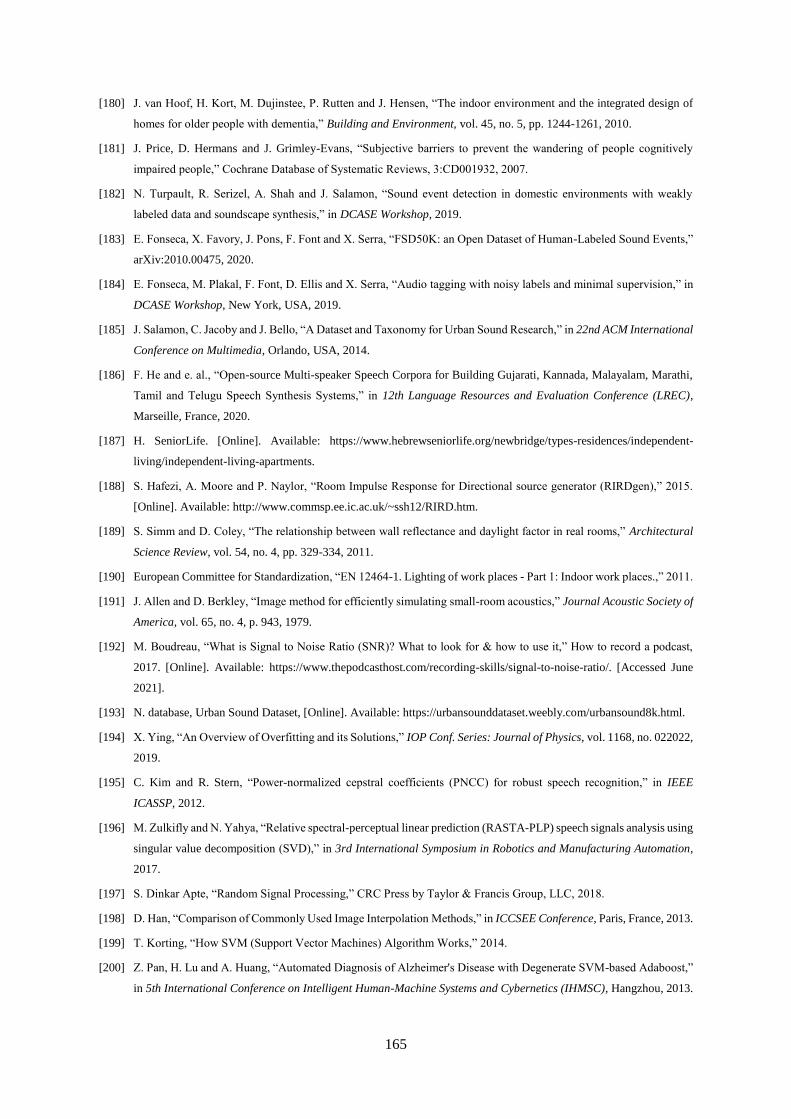
165

[180] J. van Hoof, H. Kort, M. Dujinstee, P. Rutten and J. Hensen, “The indoor environment and the integrated design of

homes for older people with dementia,” Building and Environment, vol. 45, no. 5, pp. 1244-1261, 2010.

[181] J. Price, D. Hermans and J. Grimley-Evans, “Subjective barriers to prevent the wandering of people cognitively

impaired people,” Cochrane Database of Systematic Reviews, 3:CD001932, 2007.

[182] N. Turpault, R. Serizel, A. Shah and J. Salamon, “Sound event detection in domestic environments with weakly

labeled data and soundscape synthesis,” in DCASE Workshop, 2019.

[183] E. Fonseca, X. Favory, J. Pons, F. Font and X. Serra, “FSD50K: an Open Dataset of Human-Labeled Sound Events,”

arXiv:2010.00475, 2020.

[184] E. Fonseca, M. Plakal, F. Font, D. Ellis and X. Serra, “Audio tagging with noisy labels and minimal supervision,” in

DCASE Workshop, New York, USA, 2019.

[185] J. Salamon, C. Jacoby and J. Bello, “A Dataset and Taxonomy for Urban Sound Research,” in 22nd ACM International

Conference on Multimedia, Orlando, USA, 2014.

[186] F. He and e. al., “Open-source Multi-speaker Speech Corpora for Building Gujarati, Kannada, Malayalam, Marathi,

Tamil and Telugu Speech Synthesis Systems,” in 12th Language Resources and Evaluation Conference (LREC),

Marseille, France, 2020.

[187] H. SeniorLife. [Online]. Available: https://www.hebrewseniorlife.org/newbridge/types-residences/independent-

living/independent-living-apartments.

[188] S. Hafezi, A. Moore and P. Naylor, “Room Impulse Response for Directional source generator (RIRDgen),” 2015.

[Online]. Available: http://www.commsp.ee.ic.ac.uk/~ssh12/RIRD.htm.

[189] S. Simm and D. Coley, “The relationship between wall reflectance and daylight factor in real rooms,” Architectural

Science Review, vol. 54, no. 4, pp. 329-334, 2011.

[190] European Committee for Standardization, “EN 12464-1. Lighting of work places - Part 1: Indoor work places.,” 2011.

[191] J. Allen and D. Berkley, “Image method for efficiently simulating small-room acoustics,” Journal Acoustic Society of

America, vol. 65, no. 4, p. 943, 1979.

[192] M. Boudreau, “What is Signal to Noise Ratio (SNR)? What to look for & how to use it,” How to record a podcast,

2017. [Online]. Available: https://www.thepodcasthost.com/recording-skills/signal-to-noise-ratio/. [Accessed June

2021].

[193] N. database, Urban Sound Dataset, [Online]. Available: https://urbansounddataset.weebly.com/urbansound8k.html.

[194] X. Ying, “An Overview of Overfitting and its Solutions,” IOP Conf. Series: Journal of Physics, vol. 1168, no. 022022,

2019.

[195] C. Kim and R. Stern, “Power-normalized cepstral coefficients (PNCC) for robust speech recognition,” in IEEE

ICASSP, 2012.

[196] M. Zulkifly and N. Yahya, “Relative spectral-perceptual linear prediction (RASTA-PLP) speech signals analysis using

singular value decomposition (SVD),” in 3rd International Symposium in Robotics and Manufacturing Automation,

2017.

[197] S. Dinkar Apte, “Random Signal Processing,” CRC Press by Taylor & Francis Group, LLC, 2018.

[198] D. Han, “Comparison of Commonly Used Image Interpolation Methods,” in ICCSEE Conference, Paris, France, 2013.

[199] T. Korting, “How SVM (Support Vector Machines) Algorithm Works,” 2014.

[200] Z. Pan, H. Lu and A. Huang, “Automated Diagnosis of Alzheimer's Disease with Degenerate SVM-based Adaboost,”

in 5th International Conference on Intelligent Human-Machine Systems and Cybernetics (IHMSC), Hangzhou, 2013.

166

[201] MATLAB Documentation, “Continuous Wavelet Transform and Scale-Based Analysis,” 2019.

[202] Mathworks, “Documentation: Choose a Wavelet,” 2019.

[203] I. De Moortel, S. Munday and A. Hood, “Wavelet Analysis: The Effect of Varying Wavelet Parameters,” Solar

Physics, vol. 222, pp. 203-228, 2004.

[204] Mathworks, “Help Center Documentation: cwtft,” 2011.

[205] G. Wolf, S. Mallat and S. Shamma, “Audio Source Separation with Time-Frequency Velocities,” in Proceedings of

IEEE MLSP, Reims, France, 2014.

[206] M. Cohen, “A better way to define and describe Morlet wavelets for time-frequency analysis,” Biorxiv, Donders

Institute for Neuroscience, n.d.

[207] M. Rhudy, “Time Alignment Techniques for Experimental Sensor Data,” International Journal of Computer Science

and Engineering Survey, vol. 5, no. 2, pp. 1-14, 2014.

[208] S. Paulose, E. Sebastian and B. Paul, “Acoustic Source Localization,” International Journal of Advanced Research in

Electrical, Electronics, and Instrumentation Engineering, vol. 2, no. 2, pp. 933-939, 2013.

[209] X. Bian, G. Abowd and J. Rehg, “Using Sound Source Localization to Monitor and Infer Activities in the Home,”

Georgia Institute of Technology, Atlanta, 2004.

[210] C. Lorenzi, S. Gatehouse and C. Level, “Sound localization in noise in normal-hearing listeners,” J Acoust Soc Am.,

vol. 105, no. 6, pp. 3454-3463, 1999.

[211] G. Athanasopoulos, T. Dekens and W. Verhelst, “Acoustic localization enhanced with phase information from

modified STFT magnitude,” in 18th International Conference on Digital Signal Processing (DSP), 2013.

[212] P. Magron, R. Badeau and B. David, “Phase Reconstruction of Spectrograms with linear Unwrapping: Application to

Audio Signal Restoration,” in 23rd European Signal Processing Conference (EUSIPCO 2015), Nice, France, 2015.

[213] F. Leonard, “Phase spectrogram and frequency spectrogram as new diagnostic tools,” Mechanical Systems and Signal

PRocessing, vol. 21, no. 1, pp. 125-137, 2007.

[214] S. Chakrabarty and E. Habets, “Multi-Speaker DOA Estimation using Deep Convolutional Networks trained with

Noise Signals,” IEEE Journal of Sel. Top. in Sig. Proc., vol. 13, no. 1, pp. 8-21, 2019.

[215] J. Dmochowski, J. Benesty and S. Affes, “On Spatial Aliasing in Microphone Arrays,” IEEE Transactions on Signal

Processing, vol. 57, no. 4, pp. 1383-1395, 2009.

[216] J. Pak and J. Shin, “Sound Localization Based on Phase Difference Enhancement Using Deep Neural Networks,”

IEEE / ACM Transactions on Audio, Speech, and Language Processing, vol. 27, no. 8, pp. 1335-1345, 2019.

[217] Mathworks, “MATLAB Documentation: Continuous Wavelet Transform and Scale-based Analysis,” 2019.

[218] Y. Zhang, Z. Guo, W. Wang, S. He, T. Lee and M. Loew, “Comparison of the Wavelet and Short-time Fourier

Transforms for Doppler Spectral Analysis,” Med Eng Phys., vol. 25, no. 7, pp. 547-557, 2003.

[219] V. Gerla, E. Saifutdinova, M. Macas, A. Mladek and L. Lhotska, “Comparison of short-time Fourier transform and

continuous wavelet transform for frequency analysis of sleep EEG,” Clinical Neurophysiology, Elsevier Journals,

vol. 129, no. 4, 2018.

[220] Vocal Technologies, “Spatial Sampling and Aliasing with Microphone Array,” Vocal, 2018. [Online]. Available:

https://www.vocal.com/echo-cancellation/spatial-sampling-and-aliasing-with-microphone-array/. [Accessed 01 07

2020].

[221] European Broadcasting Union, “Loudness Normalisation and Permitted Maximum Level of Audio Signals,” EBU-R-

128, 2014.

167

[222] T. Hirvonin, “Classification of Spatial Audio Location and Content Using Convolutional Neural Networks,” in Audio

Engineering Society 138th Convention, Warsaw, Poland, 2015.

[223] Y. Wang, Y. Li, Y. Song and X. Rong, “The Influence of the Activation Function in a Convolution Neural Network

Model of Facial Expression Recognition,” Applied Sciences, MDPI, vol. 10, no. 1897, 2020.

[224] M. Weir, “A method for self-determination of adaptive learning rates in back propagation,” Neural Networks, vol. 4,

pp. 371-379, 1991.

[225] S. Shi and X. Chu, “Speeding up Convolutional Neural Networks By Exploiting the Sparsity of Rectifier Units,”

arXiv, 2017.

[226] W. Hu, M. Wang, B. Liu, F. Ji, H. Chen, D. Zhao, J. Ma and R. Yan, “Transformation of Dense and Sparse Text

Representations,” arXiv, 2019.

[227] L. Lu, Y. Shin, Y. Su and G. Karniadakis, “Dying ReLU and Initialization: Theory and Numerical Examples,”

Commun. Comput. Physics, vol. 28, no. 5, pp. 1671-1706, 2020.

[228] C. Doshi, “Why Relu? Tips for using Relu. Comparison between Relu, Leaky Relu, and Relu-6,” Medium, 2019.

[229] A. Maas, A. Hanuun and A. Ng, “Rectifier nonlinearities improve neural network acoustic models,” in Proceedings

of ICML, 2013.

[230] C. Djork-Arne, T. Unterthiner and S. Hochre-iter, “Fast and accurate deep network learning by exponential linear

units (ELUs),” arXiv preprint, 2015.

[231] P. Ramachandran, B. Zoph and Q. Le, “Swish: A Self-gated Activation Function,” arXiv, 16 October 2017.

[232] D. Pedamonti, “Comparison of non-linear activation functions for deep neural networks on MNIST classification

task,” arXiv publication, 2018.

[233] S. Basha, S. Dubey, V. Pulabaigari and S. Mukherjee, “Impact of Fully Connected Layers on Performance of

Convolutional Neural Networks for Image Classification,” arXiv: preprint submitted to Neurocomputing, 2019.

[234] V. Romanuke, “An Efficient Technique for Size Reduction of Convolutional Neural Networks after Transfer Learning

for Scene Recognition Tasks,” Applied Computer Systems, vol. 23, no. 2, pp. 141-149, 2018.

[235] Mathworks, “DAG Network, Matlab Documentation,” 2017. [Online]. Available:

https://www.mathworks.com/help/deeplearning/ref/dagnetwork.html. [Accessed March 2021].

[236] A. Zayegh and N. A. Bassam, “Neural Network Principles and Applications,” in Digital Systems,

DOI:10.5772/intechopen.80416, 2018.

[237] X. Glorot and Y. Bengio, “Understanding the Difficulty of Training Deep Feedforward Neural Networks,” in In

Proceedings of the Thirteenth International Conference on Artificial Intelligence and Statistics, Sardinia, Italy, 2010.

[238] J. Xu, X. Sun, Z. Zhang, G. Zhao and J. Lin, “Understanding and Improving Layer Normalization,” in 33rd

Conference on Neural Information Processing Systems (NeurIPS 2019), Vancouver, Canada, 2019.

[239] N. Vijayrania, “Different Normalization Layers in Deep Learning,” Towards Data Science, 10 December 2020.

[Online]. Available: https://towardsdatascience.com/different-normalization-layers-in-deep-learning-1a7214ff71d6.

[Accessed 2 April 2020].

[240] S. Qiao, H. Wang, C. Liu, W. Shen and A. Yuille, “Micro-Batch Training with Batch-Channel Normalization and

Weight Standardization,” Journal of Latex Class Files, vol. 14, no. 8, pp. 1-15, 2015.

[241] Mathworks, “MATLAB Documentation: convolution2DLayer,” Mathworks, 2016. [Online]. Available:

https://www.mathworks.com/help/deeplearning/ref/nnet.cnn.layer.convolution2dlayer.html;jsessionid=c7f49d801e8

a242e369f28459e95. [Accessed 7 April 2021].

168

[242] S. Jadon, “Why we don’t use Bias in Regularization?,” Medium, 2 February 2018. [Online]. Available:

https://medium.com/@shrutijadon10104776/why-we-dont-use-bias-in-regularization-5a86905dfcd6. [Accessed 7

April 2021].

[243] R. Zaheer and H. Shaziya, “A Study of the Optimization Algorithms in Deep Learning,” in International Conference

on Inventive Systems and Control (ICISC 2019), 2019.

[244] M. Kochenderfer and T. Wheeler, Algorithms for Optimization, The MIT Press, 2019, p. 29.

[245] S. Ruder, “An overview of gradient descent optimization algorithms,” Sebastian Ruder, 19 January 2016. [Online].

Available: https://ruder.io/optimizing-gradient-descent/index.html#momentum. [Accessed 11 April 2021].

[246] N. Chauhan, “Optimization Algorithms in Neural Networks,” KDNuggets, 2020.

[247] M. Mukkamala and M. Hein, “Variants of RMSProp and Adagrad with Logarithmic Regret Bounds,” in Proceedings

of ICML, 2017.

[248] D. Kingma and J. Ba, “Adam: A Method for Stochastic Optimization,” in 3rd International Conference for Learning

Representations, San Diego, 2015.

[249] M. Sandler, A. Howard, M. Zhu, A. Zhmoginov and L. Chen, “MobileNetV2: Inverted Residuals and Linear

Bottlenecks,” in 2018 IEEE/CVF Conference on Computer Vision and Pattern Recognition (CVPR), 2018.

[250] B. Zoph, V. Vasudevan, J. Shlens and Q. Le, “Learning Transferable Architectures for Scalable Image Recognition,”

arXiv, 2018.

[251] X. Zhang, X. Zhou, M. Lin and J. Sun, “ShuffleNet: An Extremely Efficient Convolutional Neural Network for Mobile

Devices,” in 2018 IEEE/CVF Conference on Computer Vision and Pattern Recognition (CVPR), 2018.

[252] V. Thost and J. Chen, “Directed Acyclic Graph Neural Networks,” in ICLR, 2021.

[253] IBM, Train-the-Trainer Course: Enterprise Design Thinking Practicioner, United States of America: IBM, 2021.

[254] A. Research, “Caring for People with Dementia: Caregivers' Experiences,” AARP Research, 2018.

[255] H. Shah, “The State of Mobile App Usage,” Simform, 5 January 2021. [Online]. Available:

https://www.simform.com/the-state-of-mobile-app-usage/. [Accessed 16 April 2021].

[256] E. Zwierenberg, H. Nap, D. Lukkien, L. Cornelisse, E. Finnema, A. Dijkstra, M. Hagedoorn and R. Sanderman, “A

lifestly monitoring system to support (in)formal caregivers of people with dementia: Analysis of users need, benefits,

and concerns,” Gerontechnology, vol. 17, no. 4, pp. 194-205, 2018.

[257] A. Suresh and K. Shunmuganathan, “Image Texture Classification using Gray Level Co-Occurrence Matrix Based

Statistical Features,” European Journal of Scientific Research, vol. 75, no. 4, pp. 591-597, 2012.

[258] W. Galitz, The essential guide to user interface design: an introduction to GUI design principles and techniques, John

Wiley & Sons, 2007.

[259] World Health Organization, “Comnoise-4,” WHO, 2020.

[260] Mathworks, “splMeter,” Mathworks Documentation, 2018.

[261] F. Lin and e. al., “Hearing Loss and Cognitive Decline among Older Adults,” JAMA International Med., vol. 173, no.

4, 2013.

[262] K. Holmberg, S. Bowman, T. Bowman, F. Didegah and T. Kortelainen, “What Is Societal Impact and Where Do

Altmetrics Fit into the Equation?,” Journal of Altmetrics, vol. 2, no. 1, p. 6, 2019.

[263] Creative Tim, “Optuna,” Optuna, 2017. [Online]. Available: https://optuna.org/. [Accessed 2021].

[264] S. Bhuiya, F. Islam and M. Matin, “Analysis of Direction of Arrival Techniques Using Uniform Linear Array,”

International Journal of Computer Theory and Engineering, vol. 4, 2012.

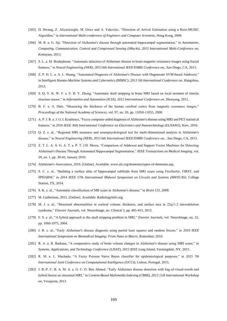
169

[265] H. Hwang, Z. Aliyazicioglu, M. Grice and A. Yakovlev, “Direction of Arrival Estimation using a Root-MUSIC

Algorithm,” in International Multi-conference of Engineers and Computer Scientists, Hong Kong, 2008.

[266] M. R. a. G. Jiji, “Detection of Alzheimer's disease through automated hippocampal segmentation,” in Automation,

Computing, Communication, Control and Compressed Sensing (iMac4s), 2013 International Multi-Conference on,

Kottayam, 2013.

[267] S. L. a. M. Boukadoum, “Automatic detection of Alzheimer disease in brain magnetic resonance images using fractal

features,” in Neural Engineering (NER), 2013 6th Internaional IEEE/EMBS Conference on,, San Diego, CA, 2013.

[268] Z. P. H. L. a. A. L. Huang, “Automated Diagnosis of Alzheimer's Disease with Degenerate SVM-based Adaboost,”

in Intelligent Human-Machine Systems and Cybernetics (IHMSC), 2013 5th International Conference on, Hangzhou,

2013.

[269] S. Q. Y. K. W. F. a. E. H. Y. Zhong, “Automatic skull stripping in brain MRI based on local moment of intertia

structure tensor,” in Information and Automation (ICIA), 2012 International Conference on, Shenyang, 2012.

[270] B. F. a. A. Dale, “Measuring the thickness of the human cerebral cortex from magnetic resonance images,”

Proceedings of the National Academy of Sciences, vol. 97, no. 20, pp. 11050-11055, 2000.

[271] A. P. J. R. a. J. G. I. Krashenyi, “Fuzzy computer-aided diagnosis of Alzheimer's disease using MRI and PET statistical

features,” in 2016 IEEE 36th International Conference on Electronics and Nanotechnology (ELNANO), Kiev, 2016.

[272] Q. Z. e. al., “Regional MRI measures and neuropsychological test for multi-dimensional analysis in Alzheimer's

disease,” in Neural Engineering (NER), 2013 6th International IEEE/EMBS Conference on, , San Diego, CA, 2013.

[273] Z. T. L. A. A. G. A. T. a. P. T. J.H. Morra, “Comparison of Adaboost and Support Vector Machines for Detecting

Alzheimer's Disease Through Automated Hippocampal Segmentation,” IEEE Transactions on Medical Imaging, vol.

29, no. 1, pp. 30-43, January 2010.

[274] Alzheimer's Association, 2016. [Online]. Available: www.alz.org/dementia/types-of-dementia.asp.

[275] S. C. e. al., “Building a surface atlas of hippocampal subfields from MRI scans using FreeSurfer, FIRST, and

SPHARM,” in 2014 IEEE 57th International Midwest Symposium on Circuits and Systems (MWSCAS), College

Station, TX, 2014.

[276] S. K. e. al., “Automatic classification of MR scans in Alzheimer's disease,” in Brain 131, 2008.

[277] M. Guiberteau, 2015. [Online]. Available: RadiologyInfo.org.

[278] M. J. e. al., “Structural abnormalities in cortical volume, thickness, and surface area in 22q11.2 microdeletion

syndrome,” Elsevier Journals, vol. NeuroImage, no. Clinical 3, pp. 405-415, 2013.

[279] F. S. e. al., “A hybrid approach to the skull stripping problem in MRI,” Elsevier Journals, vol. NeuroImage, no. 22,

pp. 1060-1075, 2004.

[280] J. R. e. al., “Early Alzheimer's disease diagnosis using partial least squares and random forests,” in 2010 IEEE

International Symposium on Biomedical Imaging: From Nano to Macro, Rotterdam, 2010.

[281] R. A. a. B. Barkana, “A comparative study of brain volume changes in Alzheimer's disease using MRI scans,” in

Systems, Applications, and Technology Conference (LISAT), 2015 IEEE Long Island, Farmingdale, NY, 2015.

[282] R. M. a. L. Machado, “A Fuzzy Poisson Naive Bayes classifier for epidemiological purposes,” in 2015 7th

International Joint Conference on Computational Intelligence (IJCCI), Lisbon, Portugal, 2015.

[283] J. B.-P. C. B. A. M. A. a. G. C. O. Ben Ahmed, “Early Alzheimer disease detection with bag-of-visual-words and

hybrid fusion on structural MRI,” in Content-Based Multimedia Indexing (CBMI), 2013 11th International Workshop

on, Veszprem, 2013.

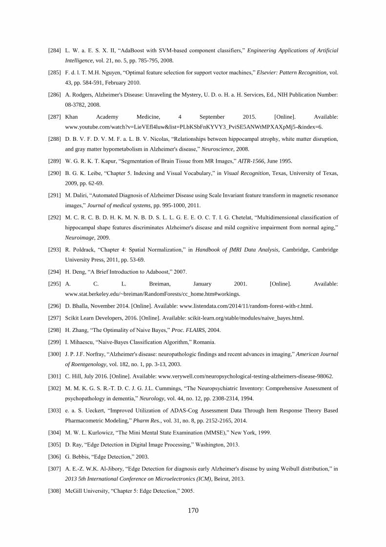
170

[284] L. W. a. E. S. X. II, “AdaBoost with SVM-based component classifiers,” Engineering Applications of Artificial

Intelligence, vol. 21, no. 5, pp. 785-795, 2008.

[285] F. d. l. T. M.H. Nguyen, “Optimal feature selection for support vector machines,” Elsevier: Pattern Recognition, vol.

43, pp. 584-591, February 2010.

[286] A. Rodgers, Alzheimer's Disease: Unraveling the Mystery, U. D. o. H. a. H. Services, Ed., NIH Publication Number:

08-3782, 2008.

[287] Khan Academy Medicine, 4 September 2015. [Online]. Available:

www.youtube.com/watch?v=LieVEfl4luw&list=PLbKSbFnKYVY3_PviSE5ANWtMPXAXpMj5-&index=6.

[288] D. B. V. F. D. V. M. F. a. L. B. V. Nicolas, “Relationships between hippocampal atrophy, white matter disruption,

and gray matter hypometabolism in Alzheimer's disease,” Neuroscience, 2008.

[289] W. G. R. K. T. Kapur, “Segmentation of Brain Tissue from MR Images,” AITR-1566, June 1995.

[290] B. G. K. Leibe, “Chapter 5. Indexing and Visual Vocabulary,” in Visual Recognition, Texas, University of Texas,

2009, pp. 62-69.

[291] M. Daliri, “Automated Diagnosis of Alzheimer Disease using Scale Invariant feature transform in magnetic resonance

images,” Journal of medical systems, pp. 995-1000, 2011.

[292] M. C. R. C. B. D. H. K. M. N. B. D. S. L. L. G. E. E. O. C. T. I. G. Chetelat, “Multidimensional classification of

hippocampal shape features discriminates Alzheimer's disease and mild cognitive impairment from normal aging,”

Neuroimage, 2009.

[293] R. Poldrack, “Chapter 4: Spatial Normalization,” in Handbook of fMRI Data Analysis, Cambridge, Cambridge

University Press, 2011, pp. 53-69.

[294] H. Deng, “A Brief Introduction to Adaboost,” 2007.

[295] A. C. L. Breiman, January 2001. [Online]. Available:

www.stat.berkeley.edu/~breiman/RandomForests/cc_home.htm#workings.

[296] D. Bhalla, November 2014. [Online]. Available: www.listendata.com/2014/11/random-forest-with-r.html.

[297] Scikit Learn Developers, 2016. [Online]. Available: scikit-learn.org/stable/modules/naive_bayes.html.

[298] H. Zhang, “The Optimality of Naive Bayes,” Proc. FLAIRS, 2004.

[299] I. Mihaescu, “Naive-Bayes Classification Algorithm,” Romania.

[300] J. P. J.F. Norfray, “Alzheimer's disease: neuropathologic findings and recent advances in imaging,” American Journal

of Roentgenology, vol. 182, no. 1, pp. 3-13, 2003.

[301] C. Hill, July 2016. [Online]. Available: www.verywell.com/neuropsychological-testing-alzheimers-disease-98062.

[302] M. M. K. G. S. R.-T. D. C. J. G. J.L. Cummings, “The Neuropsychiatric Inventory: Comprehensive Assessment of

psychopathology in dementia,” Neurology, vol. 44, no. 12, pp. 2308-2314, 1994.

[303] e. a. S. Ueckert, “Improved Utilization of ADAS-Cog Assessment Data Through Item Response Theory Based

Pharmacometric Modeling,” Pharm Res., vol. 31, no. 8, pp. 2152-2165, 2014.

[304] M. W. L. Kurlowicz, “The Mini Mental State Examination (MMSE),” New York, 1999.

[305] D. Ray, “Edge Detection in Digital Image Processing,” Washington, 2013.

[306] G. Bebbis, “Edge Detection,” 2003.

[307] A. E.-Z. W.K. Al-Jibory, “Edge Detection for diagnosis early Alzheimer's disease by using Weibull distribution,” in

2013 5th International Conference on Microelectronics (ICM), Beirut, 2013.

[308] McGill University, “Chapter 5: Edge Detection,” 2005.

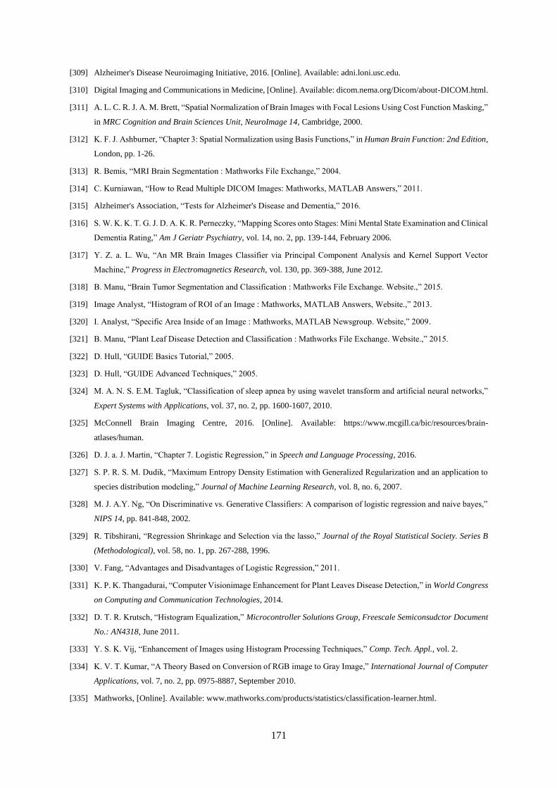
171

[309] Alzheimer's Disease Neuroimaging Initiative, 2016. [Online]. Available: adni.loni.usc.edu.

[310] Digital Imaging and Communications in Medicine, [Online]. Available: dicom.nema.org/Dicom/about-DICOM.html.

[311] A. L. C. R. J. A. M. Brett, “Spatial Normalization of Brain Images with Focal Lesions Using Cost Function Masking,”

in MRC Cognition and Brain Sciences Unit, NeuroImage 14, Cambridge, 2000.

[312] K. F. J. Ashburner, “Chapter 3: Spatial Normalization using Basis Functions,” in Human Brain Function: 2nd Edition,

London, pp. 1-26.

[313] R. Bemis, “MRI Brain Segmentation : Mathworks File Exchange,” 2004.

[314] C. Kurniawan, “How to Read Multiple DICOM Images: Mathworks, MATLAB Answers,” 2011.

[315] Alzheimer's Association, “Tests for Alzheimer's Disease and Dementia,” 2016.

[316] S. W. K. K. T. G. J. D. A. K. R. Perneczky, “Mapping Scores onto Stages: Mini Mental State Examination and Clinical

Dementia Rating,” Am J Geriatr Psychiatry, vol. 14, no. 2, pp. 139-144, February 2006.

[317] Y. Z. a. L. Wu, “An MR Brain Images Classifier via Principal Component Analysis and Kernel Support Vector

Machine,” Progress in Electromagnetics Research, vol. 130, pp. 369-388, June 2012.

[318] B. Manu, “Brain Tumor Segmentation and Classification : Mathworks File Exchange. Website.,” 2015.

[319] Image Analyst, “Histogram of ROI of an Image : Mathworks, MATLAB Answers, Website.,” 2013.

[320] I. Analyst, “Specific Area Inside of an Image : Mathworks, MATLAB Newsgroup. Website,” 2009.

[321] B. Manu, “Plant Leaf Disease Detection and Classification : Mathworks File Exchange. Website.,” 2015.

[322] D. Hull, “GUIDE Basics Tutorial,” 2005.

[323] D. Hull, “GUIDE Advanced Techniques,” 2005.

[324] M. A. N. S. E.M. Tagluk, “Classification of sleep apnea by using wavelet transform and artificial neural networks,”

Expert Systems with Applications, vol. 37, no. 2, pp. 1600-1607, 2010.

[325] McConnell Brain Imaging Centre, 2016. [Online]. Available: https://www.mcgill.ca/bic/resources/brain-

atlases/human.

[326] D. J. a. J. Martin, “Chapter 7. Logistic Regression,” in Speech and Language Processing, 2016.

[327] S. P. R. S. M. Dudik, “Maximum Entropy Density Estimation with Generalized Regularization and an application to

species distribution modeling,” Journal of Machine Learning Research, vol. 8, no. 6, 2007.

[328] M. J. A.Y. Ng, “On Discriminative vs. Generative Classifiers: A comparison of logistic regression and naive bayes,”

NIPS 14, pp. 841-848, 2002.

[329] R. Tibshirani, “Regression Shrinkage and Selection via the lasso,” Journal of the Royal Statistical Society. Series B

(Methodological), vol. 58, no. 1, pp. 267-288, 1996.

[330] V. Fang, “Advantages and Disadvantages of Logistic Regression,” 2011.

[331] K. P. K. Thangadurai, “Computer Visionimage Enhancement for Plant Leaves Disease Detection,” in World Congress

on Computing and Communication Technologies, 2014.

[332] D. T. R. Krutsch, “Histogram Equalization,” Microcontroller Solutions Group, Freescale Semiconsudctor Document

No.: AN4318, June 2011.

[333] Y. S. K. Vij, “Enhancement of Images using Histogram Processing Techniques,” Comp. Tech. Appl., vol. 2.

[334] K. V. T. Kumar, “A Theory Based on Conversion of RGB image to Gray Image,” International Journal of Computer

Applications, vol. 7, no. 2, pp. 0975-8887, September 2010.

[335] Mathworks, [Online]. Available: www.mathworks.com/products/statistics/classification-learner.html.

172

[336] Mathworks, “Train SVM Classifiers using a Gaussian Kernel,” 2017.

[337] A. Maurya, “Intuition behind Gaussian Kernel in the SVM,” 2016.

[338] S. David, “Handwritten Number Classification using Logistic Regression,” 2015.

[339] Mathworks, “Documentation: svmclassify,” 2013.

[340] Mathworks, “Create Apps with Graphical User Interfaces in MATLAB”.

[341] Government of Dubai, Health Facility Guidelines: Planning, Design, Construction, and Commissioning, 2012.

[342] V. Tiwari, “MFCC and its applications in speaker recognition,” International Journal of Emerging Technologies, vol.

1, no. 1, pp. 19-22, 2010.

[343] A. Graves, A. Mohamed and G. Hinton, “Speech recognition with deep recurrent neural networks,” in IEEE

International Conference on Acoustics, Speech, and Signal processing, 2013.

[344] R. Pascanu, C. Gulcehre, K. Cho and Y. Bengio, “How to construct Deep Recurrent Neural Networks,” 2013.

[345] M. Liang and X. Hu, “Recurrent convolutional neural network for object recognition,” in IEEE Conference on

Computer Vision and Pattern Recognition, 2015.

[346] P. Pinheiro and R. Collobert, “Recurrent Convolutional Neural Networks for Scene Labeling,” in International

Conference on Machine Learning, 2014.

[347] X. Zhang, J. Yu, G. Feng and D. Xu, “Blind Direction of Arrival Estimation of Coherent Sources using Multi-

invariance Property,” Progress In Electromagnetics Research, PIER, vol. 88, pp. 181-195, 2008.

[348] D. Stewart, H. Wang, J. Shen and P. Miller, “Investigations into the robustness of audio-visual gender classification

to background noise and illumination effects,” in Digital Image Computing: Techniques and Applications, IEEE

Computer Society, 2009.

[349] IBM, Enterprise Design Thinking Course, 2021.

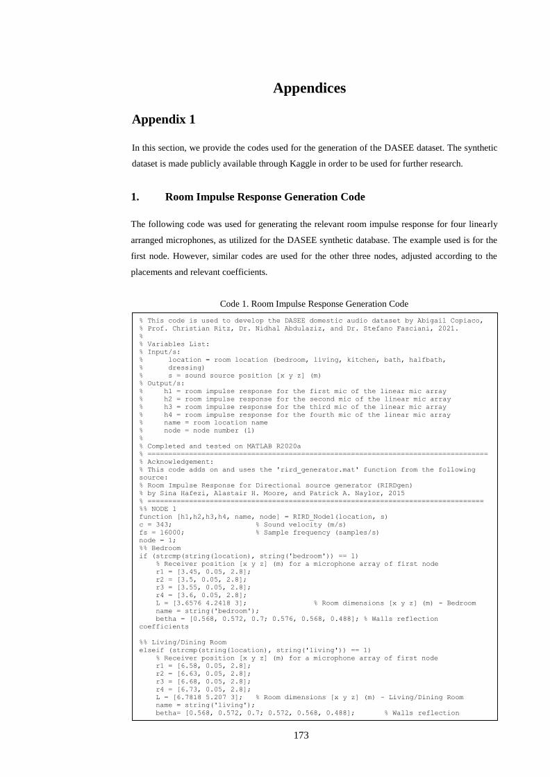
173

Appendices

Appendix 1

In this section, we provide the codes used for the generation of the DASEE dataset. The synthetic

dataset is made publicly available through Kaggle in order to be used for further research.

1. Room Impulse Response Generation Code

The following code was used for generating the relevant room impulse response for four linearly

arranged microphones, as utilized for the DASEE synthetic database. The example used is for the

first node. However, similar codes are used for the other three nodes, adjusted according to the

placements and relevant coefficients.

Code 1. Room Impulse Response Generation Code

% This code is used to develop the DASEE domestic audio dataset by Abigail Copiaco,

% Prof. Christian Ritz, Dr. Nidhal Abdulaziz, and Dr. Stefano Fasciani, 2021.

%

% Variables List:

% Input/s:

% location = room location (bedroom, living, kitchen, bath, halfbath,

% dressing)

% s = sound source position [x y z] (m)

% Output/s:

% h1 = room impulse response for the first mic of the linear mic array

% h2 = room impulse response for the second mic of the linear mic array

% h3 = room impulse response for the third mic of the linear mic array

% h4 = room impulse response for the fourth mic of the linear mic array

% name = room location name

% node = node number (1)

%

% Completed and tested on MATLAB R2020a

% ==================================================================================

% Acknowledgement:

% This code adds on and uses the 'rird_generator.mat' function from the following

source:

% Room Impulse Response for Directional source generator (RIRDgen)

% by Sina Hafezi, Alastair H. Moore, and Patrick A. Naylor, 2015

% =================================================================================

%% NODE 1

function [h1,h2,h3,h4, name, node] = RIRD_Node1(location, s)

c = 343; % Sound velocity (m/s)

fs = 16000; % Sample frequency (samples/s)

node = 1;

%% Bedroom

if (strcmp(string(location), string('bedroom')) == 1)

% Receiver position [x y z] (m) for a microphone array of first node

r1 = [3.45, 0.05, 2.8];

r2 = [3.5, 0.05, 2.8];

r3 = [3.55, 0.05, 2.8];

r4 = [3.6, 0.05, 2.8];

L = [3.6576 4.2418 3]; % Room dimensions [x y z] (m) - Bedroom

name = string('bedroom');

betha = [0.568, 0.572, 0.7; 0.576, 0.568, 0.488]; % Walls reflection

coefficients

%% Living/Dining Room

elseif (strcmp(string(location), string('living')) == 1)

% Receiver position [x y z] (m) for a microphone array of first node

r1 = [6.58, 0.05, 2.8];

r2 = [6.63, 0.05, 2.8];

r3 = [6.68, 0.05, 2.8];

r4 = [6.73, 0.05, 2.8];

L = [6.7818 5.207 3]; % Room dimensions [x y z] (m) - Living/Dining Room

name = string('living');

betha= [0.568, 0.572, 0.7; 0.572, 0.568, 0.488]; % Walls reflection

Receiver position [x y z] (m) for a microphone array of first node

r1 = [2.54, 0.05, 2.8];

r2 = [2.59, 0.05, 2.8];

r3 = [2.64, 0.05, 2.8];

r4 = [2.69, 0.05, 2.8];

L = [2.7432 1.6 3]; % Room dimensions [x y z] (m) - Bathroom

name = string('bath');

betha = [0.626, 0.62, 0.8; 0.7, 0.7, 0.541];

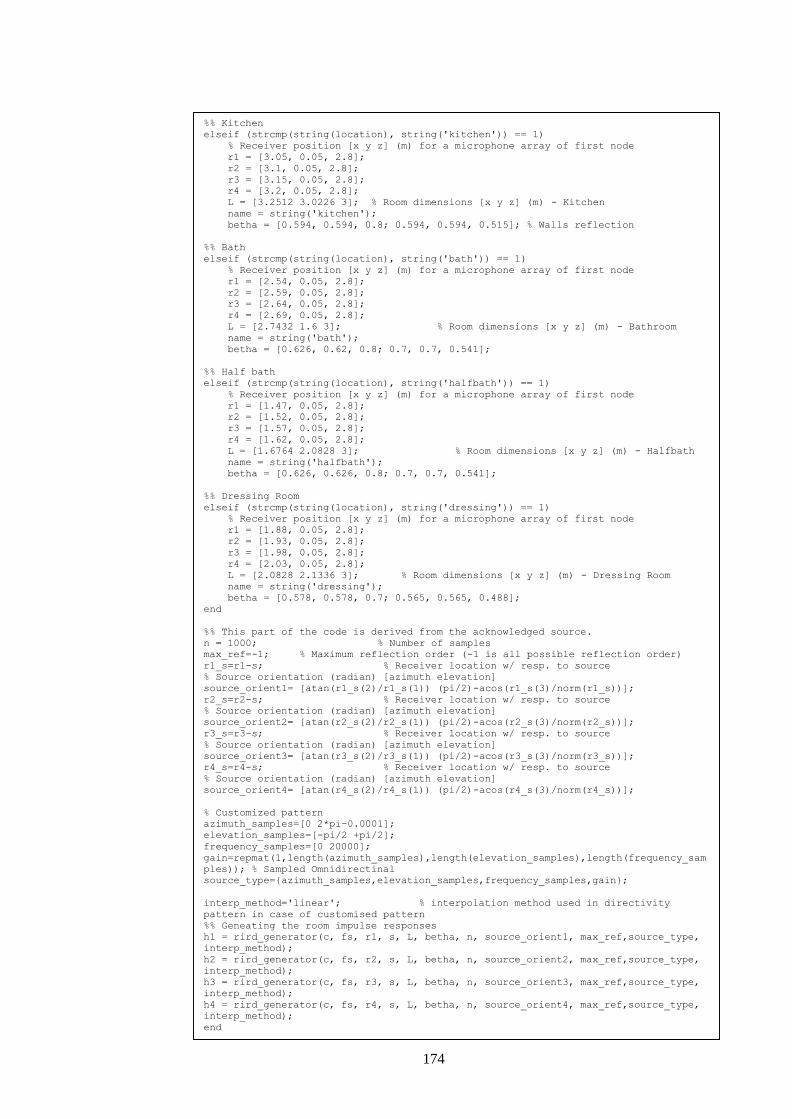
174

%% Kitchen

elseif (strcmp(string(location), string('kitchen')) == 1)

% Receiver position [x y z] (m) for a microphone array of first node

r1 = [3.05, 0.05, 2.8];

r2 = [3.1, 0.05, 2.8];

r3 = [3.15, 0.05, 2.8];

r4 = [3.2, 0.05, 2.8];

L = [3.2512 3.0226 3]; % Room dimensions [x y z] (m) - Kitchen

name = string('kitchen');

betha = [0.594, 0.594, 0.8; 0.594, 0.594, 0.515]; % Walls reflection

%% Bath

elseif (strcmp(string(location), string('bath')) == 1)

% Receiver position [x y z] (m) for a microphone array of first node

r1 = [2.54, 0.05, 2.8];

r2 = [2.59, 0.05, 2.8];

r3 = [2.64, 0.05, 2.8];

r4 = [2.69, 0.05, 2.8];

L = [2.7432 1.6 3]; % Room dimensions [x y z] (m) - Bathroom

name = string('bath');

betha = [0.626, 0.62, 0.8; 0.7, 0.7, 0.541];

%% Half bath

elseif (strcmp(string(location), string('halfbath')) == 1)

% Receiver position [x y z] (m) for a microphone array of first node

r1 = [1.47, 0.05, 2.8];

r2 = [1.52, 0.05, 2.8];

r3 = [1.57, 0.05, 2.8];

r4 = [1.62, 0.05, 2.8];

L = [1.6764 2.0828 3]; % Room dimensions [x y z] (m) - Halfbath

name = string('halfbath');

betha = [0.626, 0.626, 0.8; 0.7, 0.7, 0.541];

%% Dressing Room

elseif (strcmp(string(location), string('dressing')) == 1)

% Receiver position [x y z] (m) for a microphone array of first node

r1 = [1.88, 0.05, 2.8];

r2 = [1.93, 0.05, 2.8];

r3 = [1.98, 0.05, 2.8];

r4 = [2.03, 0.05, 2.8];

L = [2.0828 2.1336 3]; % Room dimensions [x y z] (m) - Dressing Room

name = string('dressing');

betha = [0.578, 0.578, 0.7; 0.565, 0.565, 0.488];

end

%% This part of the code is derived from the acknowledged source.

n = 1000; % Number of samples

max_ref=-1; % Maximum reflection order (-1 is all possible reflection order)

r1_s=r1-s; % Receiver location w/ resp. to source

% Source orientation (radian) [azimuth elevation]

source_orient1= [atan(r1_s(2)/r1_s(1)) (pi/2)-acos(r1_s(3)/norm(r1_s))];

r2_s=r2-s; % Receiver location w/ resp. to source

% Source orientation (radian) [azimuth elevation]

source_orient2= [atan(r2_s(2)/r2_s(1)) (pi/2)-acos(r2_s(3)/norm(r2_s))];

r3_s=r3-s; % Receiver location w/ resp. to source

% Source orientation (radian) [azimuth elevation]

source_orient3= [atan(r3_s(2)/r3_s(1)) (pi/2)-acos(r3_s(3)/norm(r3_s))];

r4_s=r4-s; % Receiver location w/ resp. to source

% Source orientation (radian) [azimuth elevation]

source_orient4= [atan(r4_s(2)/r4_s(1)) (pi/2)-acos(r4_s(3)/norm(r4_s))];

% Customized pattern

azimuth_samples=[0 2*pi-0.0001];

elevation_samples=[-pi/2 +pi/2];

frequency_samples=[0 20000];

gain=repmat(1,length(azimuth_samples),length(elevation_samples),length(frequency_sam

ples)); % Sampled Omnidirectinal

source_type={azimuth_samples,elevation_samples,frequency_samples,gain};

interp_method='linear'; % interpolation method used in directivity

pattern in case of customised pattern

%% Geneating the room impulse responses

h1 = rird_generator(c, fs, r1, s, L, betha, n, source_orient1, max_ref,source_type,

interp_method);

h2 = rird_generator(c, fs, r2, s, L, betha, n, source_orient2, max_ref,source_type,

interp_method);

h3 = rird_generator(c, fs, r3, s, L, betha, n, source_orient3, max_ref,source_type,

interp_method);

h4 = rird_generator(c, fs, r4, s, L, betha, n, source_orient4, max_ref,source_type,

interp_method);

end

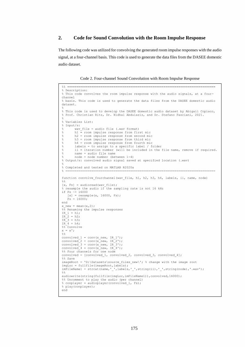
175

2. Code for Sound Convolution with the Room Impulse Response

The following code was utilized for convolving the generated room impulse responses with the audio

signal, at a four-channel basis. This code is used to generate the data files from the DASEE domestic

audio dataset.

Code 2. Four-channel Sound Convolution with Room Impulse Response

%% ================================================================================

% Description:

% This code convolves the room impulse response with the audio signals, at a four-

channel

% basis. This code is used to generate the data files from the DASEE domestic audio

dataset.

%

% This code is used to develop the DASEE domestic audio dataset by Abigail Copiaco,

% Prof. Christian Ritz, Dr. Nidhal Abdulaziz, and Dr. Stefano Fasciani, 2021.

%

% Variables List:

% Input/s:

% wav_file = audio file (.wav format)

% h1 = room impulse response from first mic

% h2 = room impulse response from second mic

% h3 = room impulse response from third mic

% h4 = room impulse response from fourth mic

% labels = to assign to a specific label / folder

% ii = iteration number (will be included in the file name, remove if required.

% name = audio file name

% node = node number (between 1-4)

% Output/s: convolved audio signal saved at specified location (.wav)

%

% Completed and tested on MATLAB R2020a

% =================================================================================

function convolve_fourchannel(wav_file, h1, h2, h3, h4, labels, ii, name, node)

%%

[x, Fs] = audioread(wav_file);

% resample the audio if the sampling rate is not 16 kHz

if Fs ~= 16000

[x] = resample(x, 16000, Fs);

Fs = 16000;

end

x_new = mean(x,2);

%% Renaming the impulse responses

IR_1 = h1;

IR_2 = h2;

IR_3 = h3;

IR_4 = h4;

%% Convolve

x = x';

%%

convolved_1 = conv(x_new, IR_1');

convolved_2 = conv(x_new, IR_2');

convolved_3 = conv(x_new, IR_3');

convolved_4 = conv(x_new, IR_4');

%% Four channels for one node

convolved = [convolved_1, convolved_2, convolved_3, convolved_4];

%% Save

imageRoot = 'D:\Datasets\source_files_new\'; % change with the image root

imgLoc = fullfile(imageRoot,labels);

imFileName1 = strcat(name,'_',labels,'_',string(ii),'_',string(node),'.wav');

%%

audiowrite(string(fullfile(imgLoc,imFileName1)),convolved,16000);

%% Uncomment to play the audio (per channel)

% conplayer = audioplayer(convolved_1, Fs);

% play(conplayer);

end

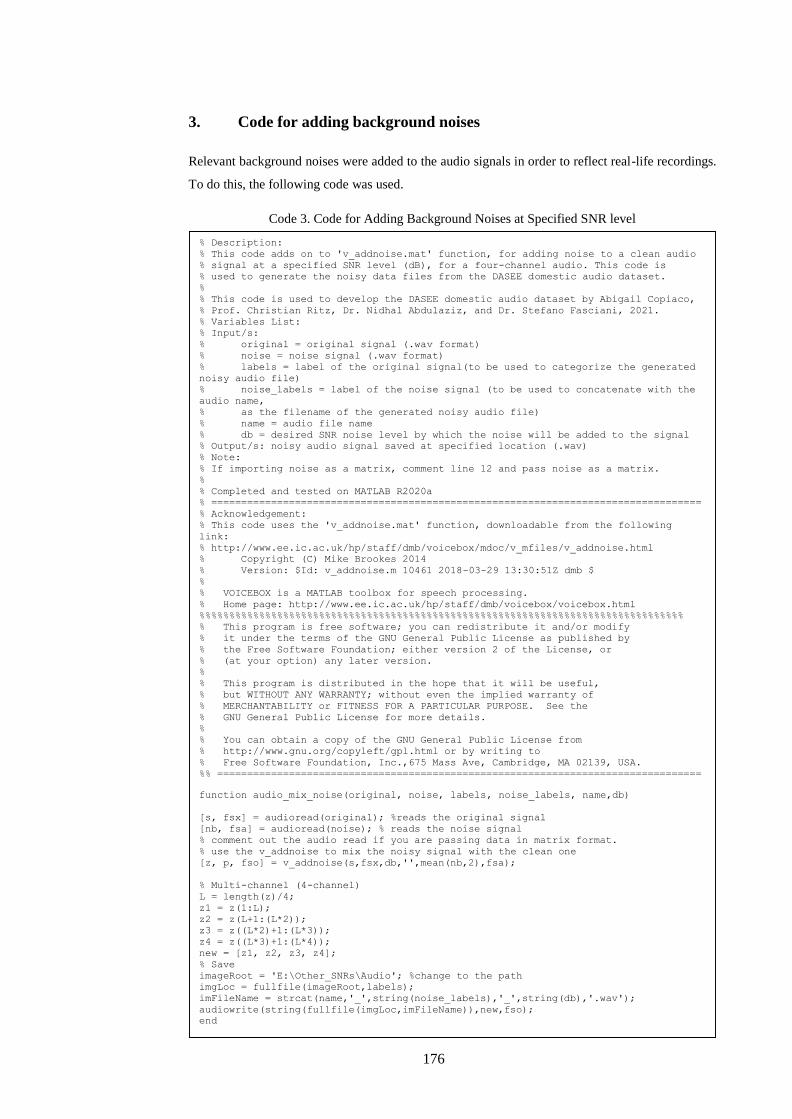
176

3. Code for adding background noises

Relevant background noises were added to the audio signals in order to reflect real-life recordings.

To do this, the following code was used.

Code 3. Code for Adding Background Noises at Specified SNR level

% Description:

% This code adds on to 'v_addnoise.mat' function, for adding noise to a clean audio

% signal at a specified SNR level (dB), for a four-channel audio. This code is

% used to generate the noisy data files from the DASEE domestic audio dataset.

%

% This code is used to develop the DASEE domestic audio dataset by Abigail Copiaco,

% Prof. Christian Ritz, Dr. Nidhal Abdulaziz, and Dr. Stefano Fasciani, 2021.

% Variables List:

% Input/s:

% original = original signal (.wav format)

% noise = noise signal (.wav format)

% labels = label of the original signal(to be used to categorize the generated

noisy audio file)

% noise_labels = label of the noise signal (to be used to concatenate with the

audio name,

% as the filename of the generated noisy audio file)

% name = audio file name

% db = desired SNR noise level by which the noise will be added to the signal

% Output/s: noisy audio signal saved at specified location (.wav)

% Note:

% If importing noise as a matrix, comment line 12 and pass noise as a matrix.

%

% Completed and tested on MATLAB R2020a

% ==================================================================================

% Acknowledgement:

% This code uses the 'v_addnoise.mat' function, downloadable from the following

link:

% http://www.ee.ic.ac.uk/hp/staff/dmb/voicebox/mdoc/v_mfiles/v_addnoise.html

% Copyright (C) Mike Brookes 2014

% Version: $Id: v_addnoise.m 10461 2018-03-29 13:30:51Z dmb $

%

% VOICEBOX is a MATLAB toolbox for speech processing.

% Home page: http://www.ee.ic.ac.uk/hp/staff/dmb/voicebox/voicebox.html

%%%%%%%%%%%%%%%%%%%%%%%%%%%%%%%%%%%%%%%%%%%%%%%%%%%%%%%%%%%%%%%%%%%%%%%%%%%%%%%%%

% This program is free software; you can redistribute it and/or modify

% it under the terms of the GNU General Public License as published by

% the Free Software Foundation; either version 2 of the License, or

% (at your option) any later version.

%

% This program is distributed in the hope that it will be useful,

% but WITHOUT ANY WARRANTY; without even the implied warranty of

% MERCHANTABILITY or FITNESS FOR A PARTICULAR PURPOSE. See the

% GNU General Public License for more details.

%

% You can obtain a copy of the GNU General Public License from

% http://www.gnu.org/copyleft/gpl.html or by writing to

% Free Software Foundation, Inc.,675 Mass Ave, Cambridge, MA 02139, USA.

%% =================================================================================

function audio_mix_noise(original, noise, labels, noise_labels, name,db)

[s, fsx] = audioread(original); %reads the original signal

[nb, fsa] = audioread(noise); % reads the noise signal

% comment out the audio read if you are passing data in matrix format.

% use the v_addnoise to mix the noisy signal with the clean one

[z, p, fso] = v_addnoise(s,fsx,db,'',mean(nb,2),fsa);

% Multi-channel (4-channel)

L = length(z)/4;

z1 = z(1:L);

z2 = z(L+1:(L*2));

z3 = z((L*2)+1:(L*3));

z4 = z((L*3)+1:(L*4));

new = [z1, z2, z3, z4];

% Save

imageRoot = 'E:\Other_SNRs\Audio'; %change to the path

imgLoc = fullfile(imageRoot,labels);

imFileName = strcat(name,'_',string(noise_labels),'_',string(db),'.wav');

audiowrite(string(fullfile(imgLoc,imFileName)),new,fso);

end

177