Does the dispersion of unit labor cost dynamics in the EMU imply long-run divergence

Department Economics and Politics

Does the Dispersion of Unit Labor Cost Dynamics in the EMU Imply Long-run Divergence? Results from a

Comparison with the United States of America and Germany

Sebastian Dullien

Ulrich Fritsche

DEP Discussion Papers

Macroeconomics and Finance Series

2/2007

Hamburg, 2007

Does the Dispersion of Unit Labor Cost Dynamics in

the EMU Imply Long-run Divergence? Results from a

Comparison with the United States of America and

Germany§

Sebastian Dullien∗ Ulrich Fritsche∗∗

January 18, 2007

.

Abstract

Using unit labor cost (ULC) data from Euro area countries as well asUS States and German Lander we investigate inflation convergence us-ing different approaches, namely panel unit root tests, cointegrationtests and error-correction models. All in all we cannot reject conver-gence of ULC growth in EMU, however, country-specific deviationsfrom the rest of the currency union are more pronounced in Europeand more persistent. This holds before and after the introduction ofthe common currency.

Keywords: Unit labor costs, inflation, EMU, convergence, panel unitroot tests, convergence clubs

JEL classification: E31, O47, C32

§We are grateful to Christian Dreger, Gustav Horn, Oliver Holtemoller, Vladimir Kuzin,Camille Logeay, Christian Proano Acosta, Rudolf Zwiener and participants of seminars inBoitzenburg and at the Institute for Macroeconomic and Business Cycle Research (IMK)at Hans Bockler Foundation Dusseldorf for helpful comments. All remaining errors areours.

∗Financial Times Deutschland, Friedrichstr. 60, D-10117 Berlin, Germany, e-mail:[email protected]

∗∗University Hamburg, Faculty Economics and Social Sciences, Department Economicsand Politics, Von-Melle-Park 9, D-20146 Hamburg, and German Institute for EconomicResearch (DIW Berlin), Germany, e-mail: [email protected]. The viewsexpressed in this Discussion Paper are those of the authors and do not necessarily representthose of the institutions the authors are affiliated with.

I

mailto:[email protected]

mailto:[email protected]

DEP Discussion Paper. Macroeconomics and Finance Series. 2/20071 Introduction S. Dullien and U. Fritsche

“(I)n most countries [of the Euro area], domestic factors dominate external factors ingenerating inflation differentials. In particular, we have witnessed a sustained divergenceof wage developments across the euro area, and narrower differences in labor productivity

growth. As a result, differentials in the growth of unit labor costs have been persistent.”Jean-Claude Trichet

1 Introduction

Several years after the introduction of a common monetary policy for a largegroup of European countries, there is widespread concern about the risk ofcurrency union countries drifting apart from each other (Gros, 2006). An im-portant argument is the lasting divergence in inflation rates (Alvarez et al.,2006, Angeloni et al., 2006, Cecchetti and Debelle, 2006, European Central Bank,2005).

It is argued (Angeloni and Ehrmann, 2004, Benigno and Lopez-Salido,2002, Michaelis and Minich, 2004, Campolmi and Faia, 2006), that the ob-servation of a relatively large – or even increasing – dispersion across EMUinflation dynamics might be due to labour market or other structural rigidi-ties which reduce the speed of the adjustment process. Fritsche et al. (2005)stress an inappropriate macroeconomic policy mix which in turn lowers dis-cipline on the wage-setting process. Furthermore, it has been argued thatthe observable divergence in inflation and in economic performance are con-nected (Lane, 2006) and might lead to dangerous imbalances in EMU if theyamplify each other. These arguments are in line with the research results ofthe ECB Inflation Persistence Network and announcements of ECB officials –see European Central Bank (2005), Trichet (2006), Gonzalez-Paramo (2005),and Issing (2005) – which all confirm that the most important source of in-flation differentials across EMU can be found in internal factors, namely asustained differential in wage growth and narrower differences in productivitygrowth.

This paper tries to add to this debate by analysing in how far unit labourcost trends (thus combined wage and productivity trends) continue to divergein the euro area. This divergence is measured against two benchmarks: First,it is examined in how far unit labour cost developments has been convergingover the past decades before the introduction of the euro when flexible ex-change rates were able to correct misalignments. Second, it is scrutinized inhow far the degree of convergence or divergence in the euro-area is unusualcompared to other currency unions, especially the United States of Americaand the Federal Republic of Germany.

1

http://www.bis.org/review/r060406b.pdf

DEP Discussion Paper. Macroeconomics and Finance Series. 2/20071 Introduction S. Dullien and U. Fritsche

Methodologically, this paper draws from the vast body of convergenceanalysis from modern growth theory building on Barro and Sala-i-Martin(1991) and Barro and Sala-i-Martin (1992), applying the concept of conver-gence not to GDP, but to unit labour cost data. According to Barro and Sala-i-Martin(1991), β-convergence is present if different cross-sectional time series show amean reverting behavior to a common level. In principle, there are differentroutes in tackling the problem of measuring β-convergence in growth theoryframeworks, which can be applied to the problem of inflation or unit laborcost growth convergence. One line of research aims to estimate the averagegrowth rate as a function of the deviation from equilibrium at a given startingpoint (Beck et al., 2006). A second line of research analyzes common trendsbetween inflation (or – in our case – ULC growth rates) in levels within acointegration framework as e.g in Mentz and Sebastian (2003). A third lineof research is based on the analysis of the stationarity properties of inflationdifferentials (Beck et al., 2006, Busetti et al., 2006).

To get a deeper understanding of the sources of inflation divergence, weadd to existing literature on inflation persistence in the following way:

• We apply several approaches developed for convergence analysis ingrowth models (and recently applied to inflation differentials) to in-vestigate the differentials in unit labor cost dynamics and to comparethe results.

• We furthermore compare the results the EMU countries with the evi-dence for the federal states and census regions of the United States ofAmerica as well as the German Lander. The possibility to compare theresults with those of established currency areas might help to answerthe question if there is something very special or are there even desta-bilizing forces at work within the EMU area – which is a controversialissue.

• We use bivariate co-integration tests and error-correction models totest for convergence and to analyze the dynamic interactions betweendifferent countries/regions and the rest of the respective currency area.We add to literature by an explizit analysis of cointegration vectorsand adjustment speeds and we also test for structural stability usingrecursive estimations.

On the one hand, our findings can be interpreted in such a way, that wecannot statistically reject the hypothesis of inflation respective unit labourcost growth convergence in EMU. There is evidence for stationarity with

2

DEP Discussion Paper. Macroeconomics and Finance Series. 2/20072 Theoretical Background S. Dullien and U. Fritsche

respect to unit labour cost growth differentials and evidence for co-integrationbetween the rates in individual countries and the rest of EMU.1

However, this finding does on the other hand not imply that the dispersionin ULC growth – after a fall in the second half of the 90s, cross-sectiondispersion of ULC growth rates has increased after 2000 and remains highuntil the end of the sample – is not harmful. There is a high degree ofscepticism justified, especially regarding the structural stability at the endof the sample. Furthermore, there are remarkable differences to Germanyand the United States. The variance of the respective national equilibriumdeviations from an area-wide average in Europe – as implied by the estimatedco-integration vectors – are remarkably larger than the respective regionaldeviations in Germany and the United States – and the adjustment towardsequilibrium seems to occur much slower in the Euro area compared to othercurrency regions. Given that the scope for national policy is eliminated formonetary policy and highly restricted for fiscal policy, a significantly sloweradjustment within the Euro area is indeed a matter of serious concern.

The paper is organized as follows: Section 2 explains the theoretical back-ground. Section 3 explains the data sources and results of unit root tests,section 4 gives a brief overview of the empirical approaches considered hereand presents results. Section 5 concludes.

2 Theoretical Background

Before starting to measure unit labour cost convergence in the euro-area, it isuseful to establish what kind of divergence could theoretically be expected ina currency union and what economic conclusions could be drawn from its ab-sence. According to Barro and Sala-i-Martin (1991) and Barro and Sala-i-Martin(1992), β-convergence implies that time series are mean reverting. In theframework of growth theory, this would imply that countries that are fur-ther away from their steady-state grow faster than those already in steadystate. However, even in the standard neoclassical growth theory (Solow,1956) without explicit mentioning of human capital, this does not necessar-ily imply convergence towards a common level of per-capita-income. Onlyif the parameters of steady-state per-capita-income (in the Solow-modell es-

1Stationarity of inflation or unit labour cost growth differentials around a certain con-stant does of course imply that the unit labour cost levels diverge with a linear trend.However, there is evidence, that these (deterministic) differences in ULC growth ratesbecame smaller over the last decades for almost all countries.

3

DEP Discussion Paper. Macroeconomics and Finance Series. 2/20072 Theoretical Background S. Dullien and U. Fritsche

pecially the savings rate) were identical across countries, per-capita-incomeswould converge to a common level.

For unit labour costs this would imply that even β-convergence does notmean that production costs per unit necessarily converge to a common EMUlevel (convergence toward which would be measured by the concept of σ-convergence). There are good theoretical reasons why even across EMU,unit labour cost levels might continue to differ: First, the single countrieshave different tax structures with different emphasis on payroll or indirecttaxation. Second, the countries have different sectors of specialisation whichmight result in different degrees of elasticity of demand in the world mar-ket and thus different profit rates (which in turn might be shared betweenemployers and employees). Only if countries were completely identical intheir economic structures, a common level of unit labour costs could be ex-pected. Thus, an absence of σ-convergence would be not necessarily reasonof concern.

These considerations have another important theoretical implication: Eveninflation differentials (measured as differentials both in the rate of change inconsumer prices or the rate of change in unit labour costs) that persist overseveral years are compatible with β-convergence. If countries have enteredEMU with a nominal exchange rate that implies unit labour costs signifi-cantly away from their steady-state, unit labour cost inflation in these coun-tries can be expected to be significantly higher or lower than in countriesclose to their steady state.2 If a country had – for example – entered EMU in1999 with a real exchange rate undervaluation of 10 percent, it could have arate of inflation 1.5 percentage points higher than the rest of EMU for sevenyears (that is until 2006) until equilibrium is reached again.

However, a possible absence of β-convergence would bode ill for EMU. Ifeconomies would not converge back to there equilibrium, asymmetric shocksto single countries would permanently alter their competitive positions andthus their output and employment. If there were even increasing divergencefrom the equilibrium, regional (that is single-country) economic problemsmight grow worse over time, resulting in grave imbalances elsewhere in theeconomy. Costs above the long-term-equilibrium would probably result inlower employment and lower investment in equipment and software whichmight – as we know from New Growth Theory – lead to lower long-termgrowth. Moreover, a permanent divergence could be expected to also lead toincreasing current-account imbalances which might lead to explosive external

2This is an argument which has repeatedly been made by the ECB, albeit in lesstechnical terms. See European Central Bank (2003) and European Central Bank (2005).

4

DEP Discussion Paper. Macroeconomics and Finance Series. 2/20073 Data S. Dullien and U. Fritsche

debt developments in single countries.3

The following analysis will thus try to discern whether there is evidencefor β-convergence in the euro-zone and for which countries – if any – β-convergence needs to be rejected.

3 Data

3.1 Sources

The data under investigation are nominal unit labor costs, defined as theratio of a nominal compensation of employees numbers to the respective realgross domestic - or gross state - product numbers. All data are annual data– however the available time span differs a lot. The longest available dataset covers the EMU countries. The data (1960 to 2007 as we included thecommissions forecast as two extra data points) are directly available fromthe AMECO data base of the EU commission. 4

For Germany, the numbers were calculated using the data from the web-site of the Lander’s network for economic statistics (Arbeitskreis VGR der

Lander).5 Unit labor costs have been computed by dividing the (nominal)compensation for employees by the real gross regional product for each of the11 Lander. The SNA classification was changed quite recently in Germanyand the backward calculated numbers cover the time span from 1970 to 2004only. As the data for the old federal republic is only available until 1990, andfrom 1991 only data for all of Germany is provided, the pan-German unitlabor cost index is calculated from the old Lander data until 1990 and frompan-German data from 1991 onwards.

For the United States, the necessary data on gross state products and to-tal compensation of employees has been taken from the Bureau of EconomicAnalysis’ database on regional and state GSP. 6 The change from the SICindustrial classification to the NAICS classification in 1997 has created how-ever a slight problem: As data on employees’ compensations has not been

3Of course, external finance in a currency union is less of a concern than in a floatingexchange rate environment. However, even if there would be no problem financing thedeficit, it might still lead to a situation in which interest rate payments alone lead to anincrease in the net external debt of a country, making a sharp correction of the tradebalance necessary to reach long-term-sustainability again.

4Please follow the link.5Please follow the link.6Please follow the link.

5

http://ec.europa.eu/economy_finance/indicators/annual_macro_economic_database/ameco_en.htm

http://www.vgrdl.de

http://www.bea.gov/bea/regional/gsp.htm

DEP Discussion Paper. Macroeconomics and Finance Series. 2/20073 Data S. Dullien and U. Fritsche

published for the first years after the statistical change and have only beenresumed in 2001, the time series can only be constructed from 1977 to 1997.For the US, the data are available on two levels of aggregation, one for thesingle states and one for the census regions. We used both datasets.

To conduct the analysis of bivariate error-correction models as explainedin section 4.2 it was necessary to calculate ULC series for the respectivecurrency area excluding one single region or country. We relied on realGDP/GSP numbers from the above-mentioned sources, to calculate the nec-essary weights. All data were transformed in log-levels before conductingunit root tests.

3.2 Determining the order of integration

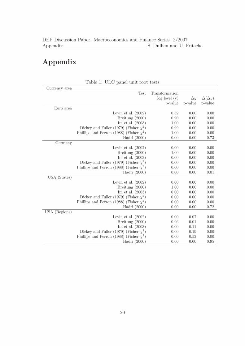
Before starting with our convergence investigation, we conducted an analysisof the stationarity properties of the time series under investigation. Weconsidered the following tests:7

• Tests based on a common unit root process: here the methods ofLevin et al. (2002) and Breitung (2000) were considered.

• Tests based on individual unit roots: here an augmented Dickey and Fuller(1979) test and an Phillips and Perron (1988) test in panel versions asproposed by Maddala and Wu (1999) and Choi (2001) were considered.

• All the tests mentioned before are based on the null of a unit root.However we furthermore considered the test described by Hadri (2000),which is based on the null of no unit root.

Table 1 summarize the results.

Insert table 1 about here.

Considering the contradictory results when comparing the tests with op-posing null hypotheses, the overall evidence can be interpreted as in favour ofa level of integration higher than 1 for nominal unit labor costs. This is notsurprising, since several studies found I(2) properties for nominal variables

7The panel unit root tests were performed using EViews 5.1 and the respective stan-dard settings with regard to lag length (BIC) and bandwidth selection (Newey-West usingBartlett kernel).

6

DEP Discussion Paper. Macroeconomics and Finance Series. 2/20074 Empirical Analysis S. Dullien and U. Fritsche

(Juselius, 1999). This calls for an I(2) analysis of ULC level convergence –which we leave for a further paper. For the further conduct of this study, wedecided to analyze the convergence issue in terms of ULC growth rates – avariable which is at highest I(1). The reasoning is twofold: on the one handthere is a direct link to the discussion about appropriateness of a uniqueEMU wide inflation rate as the target of monetary policy of the ECB withinthe Euro area and on the other hand this makes our results comparablewith existing studies dealing with inflation differentials in currency unions(Mentz and Sebastian, 2003, Beck et al., 2006, Busetti et al., 2006).

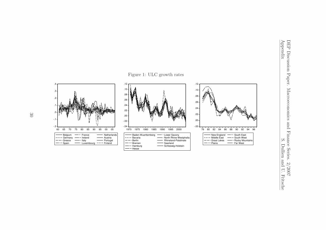
The data used for further investigations are presented in figure 1.8

Insert figure 1 about here.

The figures indicate that the variance in ULC growth rates was muchmore pronounced in Europe over the sample period than in Germany or theUnited States – most likely a result of nominal exchange rate fluctuation inthe pre-EMU times. There is a remarkable decline in the dispersion in theperiod before joining the EMU, however still, the dispersion remains highercompared to that observed in the other currency areas.

4 Empirical Analysis

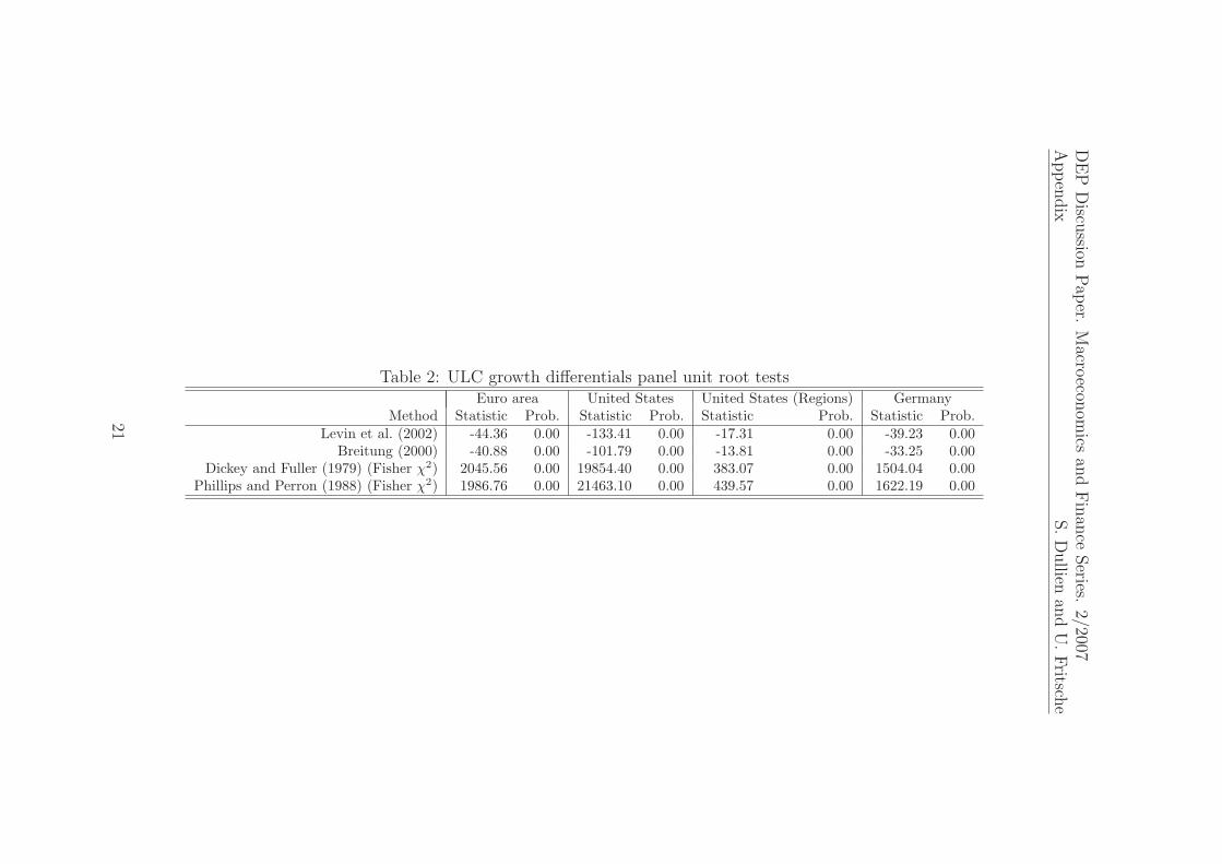
4.1 Panel unit root tests on ULC growth rate differ-

entials

For each currency union with N separate nations or regions, we can calculate(N−1)N

2series of different ULC growth differentials. As Bernard and Durlauf

(1996) or Busetti et al. (2006) discuss, the hypothesis of absolute convergenceimplies stationarity of the panel of inflation differentials with a mean of zero,whereas relative convergence is in line with (panel) stationarity around a(individual) constant different from zero. We therefore apply panel unit roottests on the respective panels of ULC growth differentials. According to ourstated hypothesis, we tested for absolute convergence by using respectiveunit root tests which allow to test without a constant. Two type of tests arecalculated: under the assumption of a common unit root process suggestedby Levin et al. (2002) as well as by Breitung (2000), and under the assump-tion of individual unit root processes proposed by Maddala and Wu (1999)

8Mind the different scaling when comparing the data.

7


employing a Fisher-type procedure of combining p-values.9 The results arepresented in table 2


The overall result can be summarized very briefly: in all panels, the nullhypothesis of a unit root in ULC growth rate differentials has to be rejectedif we test without a constant. The hypotheses of convergence is not rejectedso far.

4.2 Cointegration and error correction

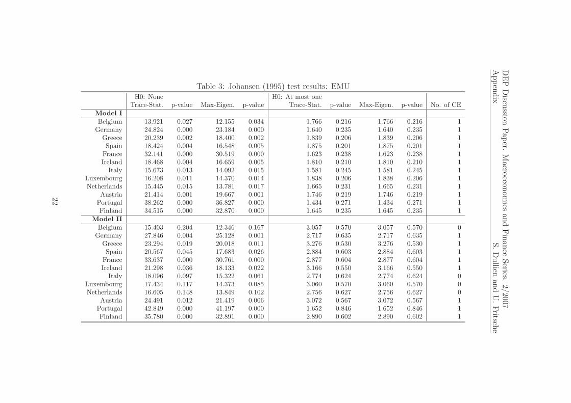
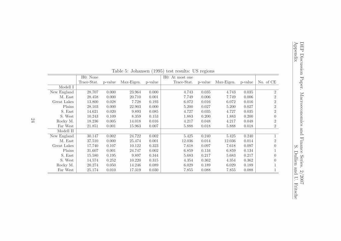
In the next section, we investigate, if a stable stationary relation between theregional or national ULC growth rate on the one hand and the average ofthe currency union (excluding the region/nation under investigation) on theother hand exist and how fast an equilibrium correction – if ever – takes place.The cointegration property is tested in different settings. We consideredthe following tests: the multivariate VAR-based Johansen (1995) test, theseminal Engle and Granger (1987) type regression based test, and we alsotested for cointegration within a bivariate error correction model – usingthe critical values as in Banerjee et al. (1998). The error correction modelresults furthermore help to assess if the respective regional/national ULCgrowth rates adjust to the currency area average or vice versa or both.

4.2.1 Multivariate cointegration test using a VAR framework

The Johansen (1995) test is based on a vectorautoregression (VAR) of theseries under investigation:

yt = A1yt−1 + . . . + Apyt−p + Bxt + εt (1)

where yt is a k-dimensional vector of I(1) variables and xt is a vector ofdeterministic variables. The error correction form of (1) is given by:

∆yt = Πyt−1 +

p−1∑

i=l

Γi∆yt−i . . . + Apyt−p + Bxt + εt (2)

9We used the Newey-West bandwidth selection using a Bartlett kernel and the SIC lagselection criterion as both suggested by the standard settings in EViews 5.1.

8


where Π =p

∑

t=1

At − I and Γt = −p

∑

j=t+l

Aj.

Under the existence of cointegration, Π has reduced reduced rank τ < k

and there exist τ × k matrices α and β such that Π = αβ⊤ .

The test procedure proposed by Johansen (1995) identifies the rank τ

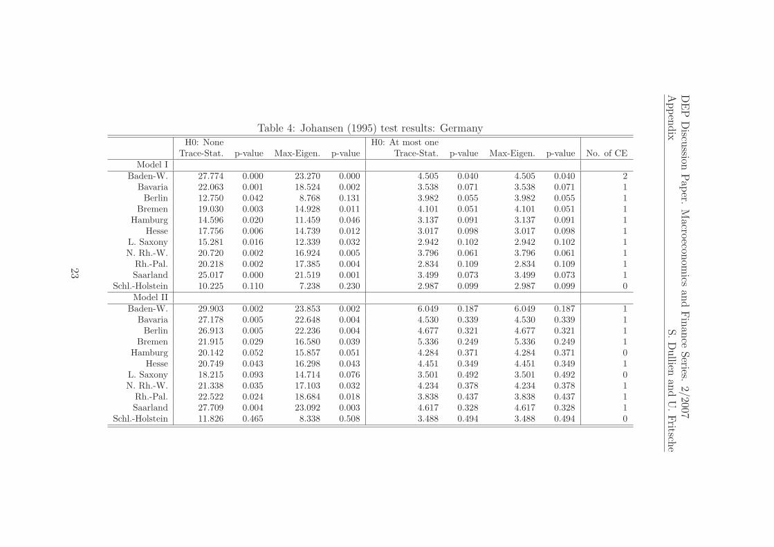
with regard to the specification of deterministic terms in the VAR. The ranktest is not independent from the model assumed. We tested the followingmodels – as described in Johansen (1995), pp. 80-84.:10

• Model 1: The level data have no deterministic trends and the cointe-grating equations (CE) do not have intercepts

• Model 2: The level data have no deterministic trends and the CE haveintercepts.

We interpret the models to be a representation of absolute and relativeconvergence – here: convergence of one single country/region towards theaverage of all other countries/regions.

The results for the Euro area, Germany, and the US census regions canbe seen in tables 3, 4, and 5.

Insert tables 3, 4, and 5 about here.

We report the test statististics for both tests – trace and maximum eigen-value – and the respective p-values according to MacKinnon et al. (1999).The header contain the hypothesized number of cointegration equations (CE).The column ”No. of CE” indicates the number of implied cointegration rela-tionships under a strict interpretation of the findings assuming a p-value of0.05 for the rejection.

All in all, there is strong evidence for most countries and regions to becointegrated with the rest of the currency area under the models of absoluteand relative convergence for the EMU countries and Germany. The evidenceis shaky, when using US census regions, where the test indicates stationarytime series under absolute convergence (full rank of Π) – a result at oddswith the unit root test results. However, when looking at the data under thehypothesis of relative convergence, only half of the regions show cointegrationproperties with the rest of the US. This finding for the US is confirmed,

10We used the procedure as implemented in EViews 5.1.

9


when using data for US states.11 When interpreting these results, we haveto keep in mind that the power of these types of tests for our limited dataset is relatively low. We turn to slightly less sophisticated methods butnevertheless powerful methods to evaluate the cointegration properties andthe structural stability over time more deeply.

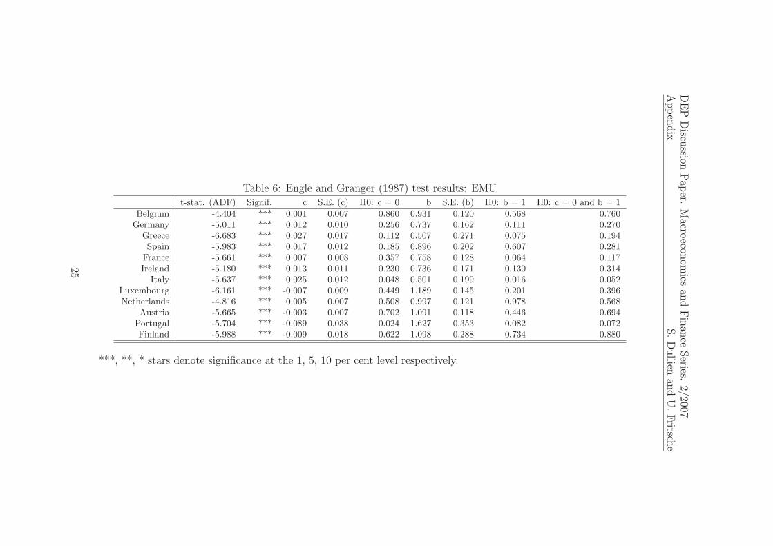
4.2.2 Static cointegration test

The Johansen (1995) procedure gave evidence for cointegration under abso-lute and relative convergence assumptions for the EMU countries, however,given the limitations of our data set, we decided to use a less sophisticatedmethod to confirm the findings and to explore the nature and the structuralstability of the relationship in detail. To this end, we made use of the seminalapproach of Engle and Granger (1987) to estimate the long-run relationshipin a two-step procedure.

First, we estimate the long-run relationship for each entity n as:

yt = c + bxt + εt (3)

where yt stands for the individual time series and xt for the currency areaaverage, corrected for the effect of yt.

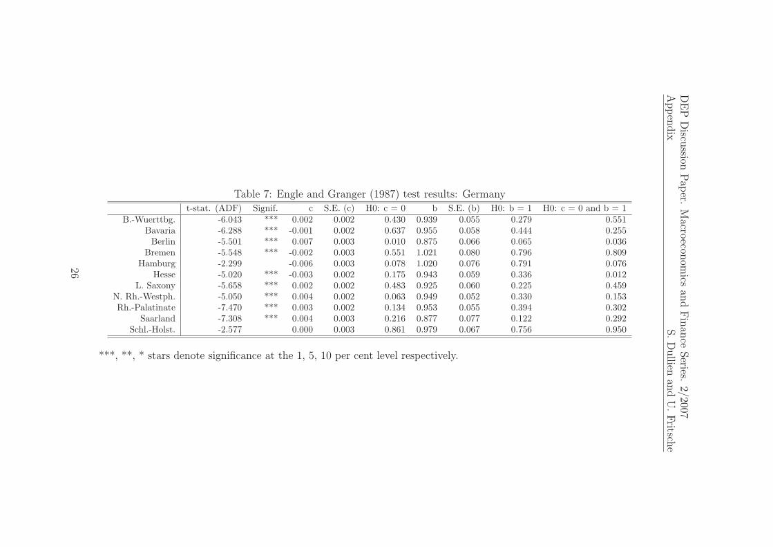
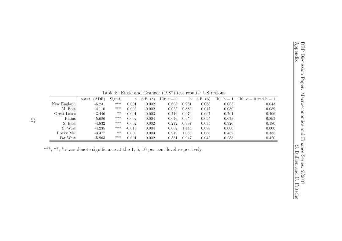
In those cases, where a linear trend was significant, we added the lineartrend as an additional regressor.12 In a second step, we tested for a unit rootin εt. Tables 6, 7, and 8 summarize the results.13

Insert tables 6, 7, and 8 about here.

The test statistic of the augmented Dickey and Fuller (1979) test, takinginto account the (approximate) critical values of MacKinnon (1991), is eval-uated in the first two columns. There is widespread evidence for equilibriumcorrection in all currency areas – with the exceptions of some northern Lander

11Results are not reported here but available from the authors on request.12This was the case for Portugal when analyzing EMU and Louisiana, when analyzing

the United States.13Given the fact, that the residuals are found to be correlated in some cases, we further-

more estimated the long-run relationships using seemingly unrelated regressions. Sinceresults remain qualitatively unchanged, we only report the equation-by-equation OLS re-sults. SUR results are available from the authors on request.

10


in Germany (Hamburg and Schleswig-Holstein). The result also holds for al-most all US states – with the notable exception of the capital district as wellas Wyoming.14

Assuming long-run convergence, the cointegration vector should be ofthe form β = (1,−1)⊤. This is due to the fact that in the long-run all unitlabor cost grwoth rates should be similar under convergence – allowing fora constant in the special case of relative convergence (Bernard and Durlauf,1996). The results indicate that the estimated coefficients for Germany andthe US are very close to this in most cases. Formal test results for thehypothesis ”b = 1” can be found in the respective column. The resultsindicate, that the hypothesis cannot be rejected for most German Lander

(with the possible exception of Berlin) and also holds for most of the USstates. Using the Census region perspective, we can reject the hypothesis forthe Middle East and the South West region.

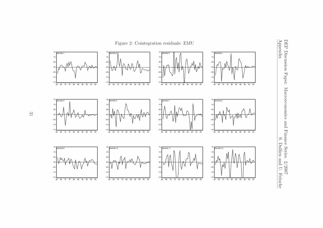
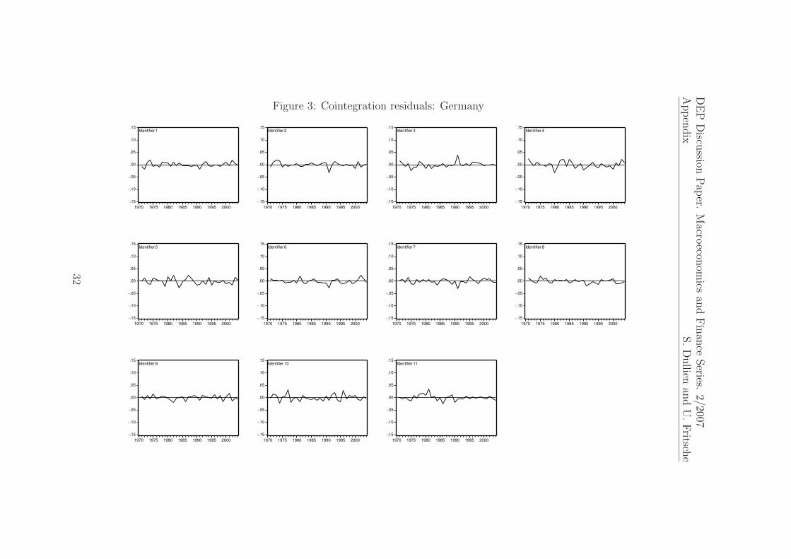
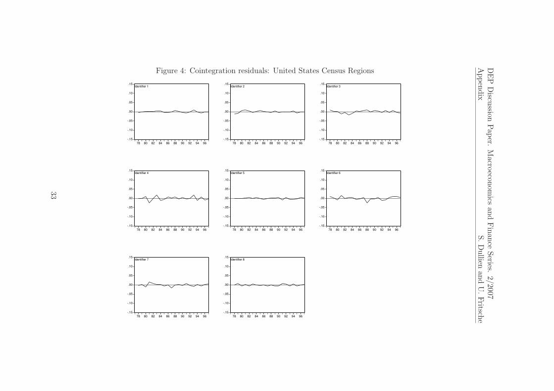
When looking at the residuals εt – which under the existence of cointegra-tion can be interpreted as an estimate of equilibrium deviations – as plottedin figures 2, 3, and 4 with harmonized scaling, one can see, that the devi-ations for the EMU countries are noticeably more pronounced and possiblymore persistent than equivalent measures for German Lander and the USstates or regions.15

Insert figures 2, 3, and 4 about here.

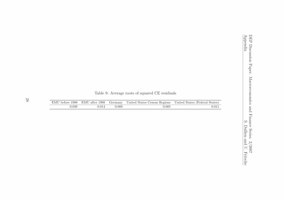
To get a simple quantitative measure to compare the respective diver-gences as implied by the deviations from the estimated long-run relation-ships, we calculated unweighted average roots of squared residuals εt for allcurrency areas.16


The results in table 9 indicate, that the divergence in the Euro area – asmeasured by the deviation from long-run equilibrium – decreased by morethan 60 percent compared to the pre-EMU period but is still remarkablyhigher than the respective dispersion in Germany and in the United States.

14Detailed results for US states are available from the authors on request.15Again, results for the US states were omitted to keep the paper at a reasonable length,

however are available from the authors on request.

16Defined as s = 1

N

N∑

n=1

1

T

T∑

t=1

√

(εnt)2, where N is the number of entities in a currency

area and T the number of observations.

11


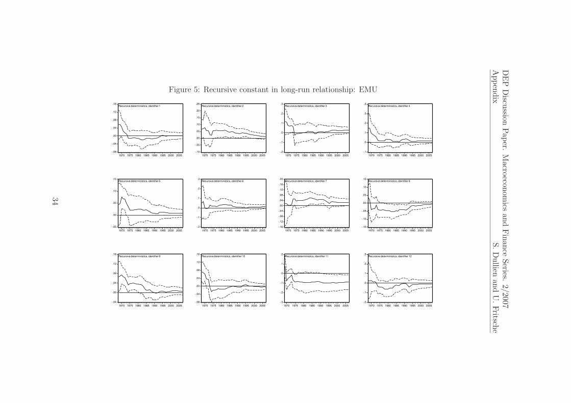
There is one further aspect, which points into the direction of more con-vergence within the Euro area – at least for most countries. When analyzingthe behaviour of the deterministic elements in the long-run relationship overtime by using recursive estimates, we can clearly see a tendency towardsabsolute convergence for the Euro area. In almost all cases, the estimatesfor the deterministic coefficient declined over time and became statisticallyinsignificant for most counries. However, when looking carefully at figure5, we can also see, that some ULC growth rates of some countries remainon a stationary – but small – distance to respective measure for the cur-rency union. This is true for Portugal and Greece (even slightly increasingcoefficient) but also for Italy to some extent. This result is in line with thet-tests reported in the fifth column of table 6. Comparing the results withthose for Germany and the United States reveals, that the deterministic co-efficients – which indicate a stationary deviation of individual ULC growthrates from the rest of the currency area – are much smaller. Switching toa moving window estimate leads to smaller differences, yet, the coefficientsremain higher.


Translated into the context of β-convergence between the regions, thiswould mean that the hypothesis of convergence towards a long-run unitlabour cost equilibrium level cannot be supported for Portugal, Greece and(some extent) Italy. Instead, the permanently higher level of ULC growthrates in these countries would mean a continous divergence in ULC lev-els, casting doubts on these economies’ abilities to function smoothly withinEMU.

4.2.3 Bivariate error-correction models

In the next step, we kept the long-run relationships as estimated in sec-tion 4.2.2, formulated error-correction models and analyzed the adjustmentprocess. Using the same notation for y and x as in section 4.2.2, we canformulate:

∆yt = a0 − γy (yt−1 − bxt−1) +nx∑

j=0

axj∆xt−j +

ny∑

j=1

ayj∆yt−j + uyt

∆xt = b0 + γx (yt−1 − bxt−1) +kx

∑

j=1

bxj∆xt−j +

ky∑

j=0

byj∆yt−j + uxt

(4)

12


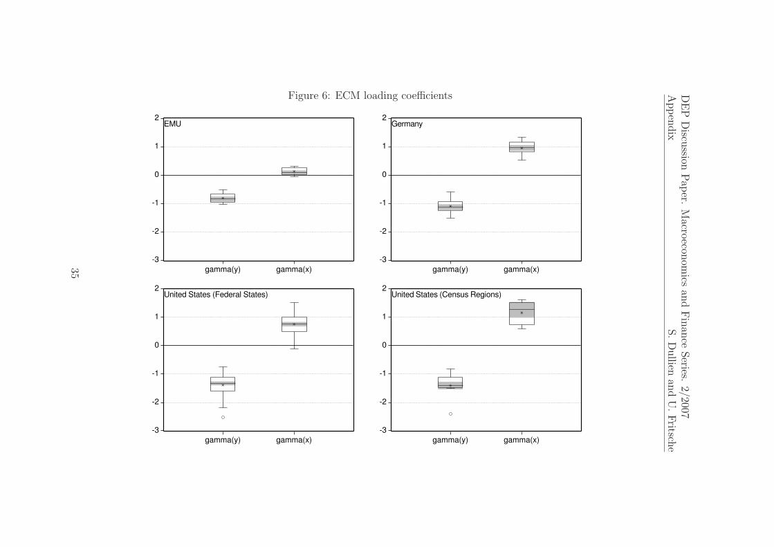
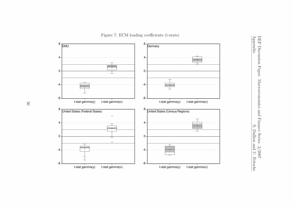
We are especially interested in the behaviour of the loading coefficientsγy and γx – which matches the elements of the vector α in the Johansen(1995) test procedure. A high γ is equivalent to fast adjustment, whereasestimates of γ which are not significantly different from zero indicate weakexogeneity of the endogenous variable of the respective equation with respectto the other variable in the system. To keep the presentation at a reasonablelength, we opted for a graphical presentation of the distribution of results –namely box plots of the γ-coefficients and the respective t-values – for eachanalyzed currency area. The summarized results for point estimates can befound in figures 6 and 7. We did not test formally for cointegration in theECM framework because these results are already reported in sections 4.2.1and 4.2.2. In figure 7, we added informal significance lines at ±2.

Insert figures 6 and 6 about here.

There are differences between the countries, which can be summarized asfollows. Adjustment speed and persistence differs among the currency areas.All in all, the γy-coefficients are on average found to be highly significant butdifferent in values. There is relatively fast adjustment in the United States –irrespective if we look at States or Census Regions –, slightly slower adjust-ment within Germany and the relatively slowest adjustment among EMUcountries. Regarding weak exogeneity of the currency area average with re-gard to the individual country/region (insignificance of λx), there is evidencefor a one-sided adjustment in the EMU. Countries on average adjust towardsthe average not vice versa. There is – on average – a tendency for countriesto deviate quite persistently from the rest of the area. There are two ex-ceptions for the EMU area, which show a significant γx-coefficient: Germanyand the Netherlands. For the pre-EMU-time this mirrors Germany’s role asan anchor for the European Monetary system: National Central Banks hadto keep their rate of inflation close to that of Germany in order to preventspeculative attacks in the EMS. For the time since the beginning of EMU,this result supports the hypothesis of Hancke (2002) that there might be animplicit coordination of wage increases around the German wage contracts.The case for weak exogeneity is less clear for Germany and the United States.Here we have – on average – feedback relationships. The result might be dueto the use of annual data but surely a sign of fast(er) adjustment.

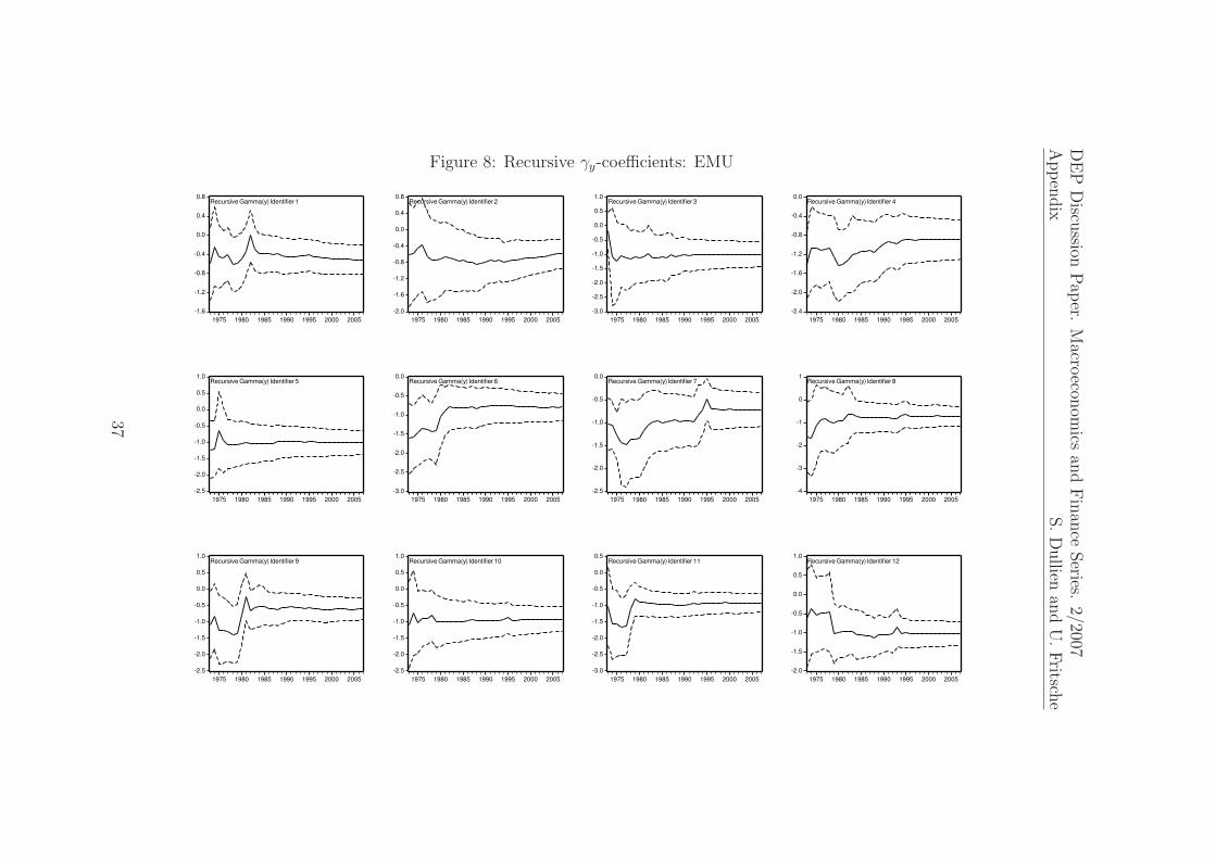
Finally, for the Euro area, we tested for the structural stability of γy overtime using recursive estimates of the γy-coefficients. The results are shownin 8.


13

DEP Discussion Paper. Macroeconomics and Finance Series. 2/20075 Conclusion S. Dullien and U. Fritsche

There is no evidence, that a structural break occured around the in-troduction of the Euro. However, when looking at the graphs carefully, adecrease in the recursively estimated loading coefficient is visible for Ger-many – indicating a somewhat slower adjustment since the middle of 1990s.This is in line with the equilibrium deviations as shown in figure 2 andcan be confirmed, once the equilibrium deviations are cumulated over time.There is a clear tendency for a persistent long-lasting equilibrium deviationfor Germany since the mid-1990s – which is a reason of concern. To testin detail for a structural break in the long-run relationship between Ger-many and the rest of the EMU, we applied a formal test on the stability ofthe cointegration relationship (recursive eigenvalue and τ -stat.) as describedin Lutkepohl and Kratzig, eds (2004, pp. 138ff.). However, no statisticallysignificant structural break can be detected so far.

5 Conclusion

In conclusion, one can say that for most countries, the tests applied forconvergence do not reject the hypothesis of β-convergence of unit labourcosts to long-run-equilibrium levels in EMU. This is in line with the evidencefor longer existing and well-functioning currency areas – United States ofAmerica and (West) Germany here – and can be interpreted as good newsinsofar, as no ever-lasting deviations of inflations rates due to cost-push areto be expected from the behaviour of the time series in the past.

Careful inspection reveals several less optimistic points: There is evidenceof relative convergence instead of absolute convergence for some countries.For Portugal, Greece and to a lesser extent Italy, the cointegration test hintsat a permanently higher rate of unit labour cost increases than in the otherEMU countries which poses a problem for competitiveness within the cur-rency union. This result is qualitatively confirmed by recursive estimates ofthe deterministic component in static cointegration estimates.

Furthermore, deviations from the long-run-equilibrium seem to be muchmore pronounced in the Euro area than between the United States and theGerman Lander. The analysis of adjustment speeds in the bivariate error cor-rection models reveals shows remarkable differences across currency unions.Given that fiscal policy within the EU can only react slowly and labour isclearly less mobile, this indeed should be a matter of concern. If divergencespersist for a prolonged periods, they might cause misallocations and evenlong-term detrimental effects to growth.

14


First, as an above-average rate of domestic inflation makes finance cheaperwhile investment in the tradable sector becomes less attractive with the lossof competitiveness, it might lead to excessive investment in the housing sec-tor. Not only might an excessive amount of capital be allocated to this sectorwhich contributes relatively little to long-term productivity growth. In ad-dition, there is the danger that workers are lured into construction jobs whomight later be very hard to retrain once a building boom ends, thus shiftingthe Beveridge curve outwards and increasing structural unemployment.

Second, persistent deviations in the price trend might lead to a strongovervaluation of one country in monetary union. Whereas undervaluationleads to increasing exports and income, import prices raise and via a deteri-oration in the trade balance, adjustment occurs in the long run. Adjustmentprocesses might however be asymmetric with regard to speed and intensity,due to hysteresis phenonenom: Once trapped in a situation of overvalua-tion, profits might suffer and investment contract, leading to a longer periodof sub-trend economic growth until the real appreciation is corrected again.These boom-and-bust-periods might not only bring about negative welfareeffects17, but might also lower the potential output of a single country: As weknow from labour market economics, there are good arguments for hysteresisin the labour market, meaning that unemployment is at least to a certainextent path dependent. This does not necessarily imply an insider/outsiderset-up as it has been assumed by Blanchard and Summers (1986), but canalso be constructed by new-growth-theory considerations of human capitalaccumulation. Saint-Paul (1997) describes the detrimental effects of longerstints of unemployment on potential output with the words ”unlearning bynot doing”: If a person is unemployed for an extended period, she would missout learning new technologies and might even lose some basic skills necessaryfor productive employment.

Finally, political economy arguments hint that prolonged boom-and-bustcycles as a result from divergences might actually endanger the politicalstability of the euro-area: A country which finds itself at the beginning ofthe bust leg of a business cycle amplified by the structure of EMU might findthe idea of leaving monetary union increasingly attractive. Leaving the unionwould allow the country to depreciate sharply and forego the adjustment costsof relative wage deflation. If the country’s politicians have a sufficiently highpersonal discount rate, the short-term benefits of leaving EMU might actuallybe perceived larger than the long-run costs of the forgone membership in the

17This might be true even though Lucas (2003) argues that direct welfare effects fromeconomic fluctuations are rather small. See Yellen and Akerlof (2006) for counterargu-ments.

15


monetary union such as lower long-term interest rates. This might in theend lead to single countries pulling out of EMU.

All of these negative effects of divergences can be expected to start kick-ing in as soon as a region’s real exchange rate and inflation trend is farenough away from equilibrium. However, they will only be sizable if a singlecountry’s real exchange rate has deviated significantly from its equilibriumvalue. We tried to asses the size by comparing equilibrium deviations fromerror-correction models with the evidence for other currency areas. Whencomparing the Euro area evidence with that of the United States or Ger-many, it comes clear, that the danger of divergence seems to be much morepronounced for the Euro area than elsewhere. This argument should be amatter of even more concern when taking into consideration the limited scopefor countercyclical national fiscal policy under the stability and growth pactand the evidence for procyclical effects of a common monetary policy on anational level (Fritsche et al., 2005).

16

DEP Discussion Paper. Macroeconomics and Finance Series. 2/2007References S. Dullien and U. Fritsche

References

Alvarez, L., E. Dhyne, M. Hoeberichts, C. Kwapil, H. Le Bihan,

P. Lunnemann, F. Martins, R. Sabbatini, H. Stahl, Ph. Vermeulen, and

J. Vilmunen, “Sticky prices in the euro area: a summary of new micro evidence,”Discussion Paper Series 1: Economic Studies 02/2006, Deutsche Bundesbank 2006.

Angeloni, I. and M. Ehrmann, “Euro area inflation differentials,” Working PaperSeries 388, European Central Bank 2004.

, L. Aucremanne, M. Ehrmann, J. Gali, A. Levin, and F. Smets, “New evidenceon inflation persistence and price stickiness in the Euro area: Implications for macromodelling,” Journal of the European Economic Association, 2006, 4, 562–574.

Banerjee, A., J.J. Dolado, and R. Mestre, “Error-Correction Mechanism Tests forCointegration in a Single-Equation Framework,” Journal of Time Series Analysis, 1998,19, 267–283.

Barro, R. and X. Sala-i-Martin, “Convergence across states and regions,” BrookingsPapers on Economic Activity, 1991, 1991 (1), 107–182.

and , “Convergence,” The Journal of Political Economy, April 1992, 100 (2), 223–251.

Beck, G., K. Hubrich, and M. Marcellino, “Regional Inflation Dynamics within andacross Euro Area Countries and a Comparison with the US,” Technical Report 2006.

Benigno, P. and David Lopez-Salido, “Inflation persistence and optimal monetarypolicy in the Euro area,” Working Paper Series 178, European Central Bank 2002.

Bernard, A. B. and S. N. Durlauf, “Interpreting tests of the convergence hypothesis,”Journal of Econometrics, 1996, 71, 161–173.

Blanchard, O. and L. H. Summers, “Hysteresis and the European UnemploymentProblem,” NBER Macroeconomics Annual, 1986, 1, 15–78.

Breitung, J., “The Local Power of Some Unit Root Tests for Panel Data,” in B. Balt-agi, ed., Nonstationary Panels, Panel Cointegration, and Dynamic Panels, Vol. 15 ofAdvances in Econometrics, Amsterdam: JAI Press, 2000, pp. 161–178.

Busetti, F., L. Forni, A. Harvey, and F. Venditti, “Inflation convergence and diver-gence within the European Monetary Union,” ECB Working Paper Series 574, EuropeanCentral Bank 2006.

Campolmi, A. and E. Faia, “Cyclical inflation divergence and different labor marketinstitutions in the EMU.,” Working Paper Series 619, European Central Bank 2006.

Cecchetti, S. G. and G. Debelle, “Has the inflation process changed?,” EconomicPolicy, 2006, 46, 313–351.

Choi, I., “Unit Root Tests for Panel Data,” Journal of International Money and Finance,2001, 20, 249–272.

17


Dickey, D.A. and W.A. Fuller, “Distribution of the Estimators for AutoregressiveTime Series with a Unit Root,” Journal of the American Statistical Association, 1979,74, 427–431.

Engle, R. and C. W. Granger, “Co-integration and Error Correction: Representation,Estimation, and Testing,” Econometrica, 1987, 55, 251–276.

European Central Bank, “Inflation Differentials in the Euro Area: Potential Causesand Policy Implications,” Technical Report, European Central Bank 2003.

, “Monetary policy and inflation differentials in a heterogenous currency area,” MonthlyBulletin, 2005, 05/2005, 61–77.

Fritsche, U., C. Logeay, K. Lommatzsch, K. Rietzler, S. Stephan, R. Zwiener,

C. Kiziltepe, and Ch. Proano Acosta, “Auswirkungen von landerspezifischenDifferenzen in der Lohn-, Preisniveau und Produktivitatsentwicklung auf Wachstumund Beschaftigung in den Landern des Euroraums,” Politikberatung kompakt 08/2005,Deutsches Institut fur Wirtschaftsforschung (DIW Berlin) 2005.

Gonzalez-Paramo, J. M., “Regional divergence in the euro area,” 2005. Speech by JoseManuel Gonzalez-Paramo, Member of the Executive Board of the ECB, InternationalConference on “The Role of Government in Regional Economic Development”, REDE(Research in Economics, Energy and the Environment), Universidade de Vigo, Baiona,19 September 2005.

Gros, D., “Will EMU survive 2010?,” Technical Report, Centre for European PolicyStudies 2006.

Hadri, K., “Testing for Stationarity in Heterogeneous Panel Data,” Econometric Journal,2000, 3, 148–161.

Hancke, Bob, “The Political Economy of Wage-Setting in the Eurozone,” in PhilippePochet, ed., Wage Policy in the Eurozone, Brussels: PIE-Peter Lang, 2002, pp. 131–148.

Im, K.S., M.H. Pesaran, and Y. Shin, “Testing for unit roots in heterogenous panels,”Journal of Econometrics, 2003, 115, 53–74.

Issing, O., “One size fits all! A single monetary policy for the euro area,” 2005. Speechby Otmar Issing, Member of the Executive Board of the ECB International ResearchForum, Frankfurt am Main, 20 May 2005.

Johansen, S., Likelihood-based Inference in Cointegrated Vector Autoregressive Models,Oxford: Oxford University Press, 1995.

Juselius, K., “Price convergence in the long run and the medium run. An I(2) analysisof six price indices,” in R. Engle and H White, eds., Cointegration, Causality, andForecasting: Festschrift in Honour of Clive W.J. Granger, Oxford University Press,1999, chapter 13.

Lane, Ph., “The real effects of EMU,” Discussion Paper Series 5536, CEPR 2006.

18


Levin, A., C.-F. Lin, and C.-S. Chu, “Unit root tests in panel data: Asymptotic andfinite sample properties,” Journal of Econometrics, 2002, 108, 1–24.

Lucas, R. E., “Macroeconomic Priorities,” American Economic Review, 2003, 93 (3),1–14.

Lutkepohl, H. and M. Kratzig, eds, Applied Time Series Econometrics, Cambridge:Cambridge University Press, 2004.

MacKinnon, J. G., “Critical Values for Cointegration Tests,” in R.F. Engle andC.W.J. Granger, eds., Long-Run Economic Relationships, Oxford University Press 1991,pp. 267–276.

, A. A. Haug, and L. Michelis, “Numerical Distribution Functions of LikelihoodRatio Tests For Cointegration,” Journal of Applied Econometrics, 1999, 14, 563–577.

Maddala, G. S. and S. Wu, “A Comparative Study of Unit Root Tests with PanelData and A New Simple Test,” Oxford Bulletin of Economics and Statistics, 1999, 61,631–52.

Mentz, M. and S. P. Sebastian, “Inflation convergence after the introduction of theEuro,” CFS Working Paper 2003/30, Center for Financial Sudies an der Johann Wolf-gang Goethe-Universitat 2003.

Michaelis, J. and H. Minich, “Inflationsdifferenzen im Euroraum - eine Bestandsauf-nahme,” Volkswirtschaftliche Diskussionsbeitrge 62/04, Universitat Kassel 2004.

Phillips, P.C.B. and P. Perron, “Testing for a Unit Root in Time Series Regression,”Biometrika, 1988, 75, 335–346.

Saint-Paul, G., “Business Cycles and Long-Run Growth,” Oxford Review of EconomicPolicy, 1997, 13 (3), 145–153.

Solow, R. M., “A Contribution to the Theory of Economic Growth,” Quarterly Journalof Economics, 1956, 70, 65–94.

Trichet, J. C., “Economic integration in the euro area,” BIS Review, 2006, 27, 1–7.Speech by Mr Jean-Claude Trichet, President of the European Central Bank, at the15th European Regional Conference of the Board of Governors, Tel Aviv University,Paris, 31 March 2006.

Yellen, J. L. and G. A. Akerlof, “Stabilization Policy: A Reconsideration,” EconomicInqiry, 2006, 44 (1), 1–22.

19

DEP Discussion Paper. Macroeconomics and Finance Series. 2/2007Appendix S. Dullien and U. Fritsche

Appendix

Table 1: ULC panel unit root testsCurrency area

Test Transformationlog level (y) ∆y ∆(∆y)

p-value p-value p-valueEuro area

Levin et al. (2002) 0.32 0.00 0.00Breitung (2000) 0.90 0.00 0.00Im et al. (2003) 1.00 0.00 0.00

Dickey and Fuller (1979) (Fisher χ2) 0.99 0.00 0.00Phillips and Perron (1988) (Fisher χ2) 1.00 0.00 0.00

Hadri (2000) 0.00 0.00 0.73Germany



Hadri (2000) 0.00 0.00 0.01USA (States)



Hadri (2000) 0.00 0.00 0.72USA (Regions)



Hadri (2000) 0.00 0.00 0.95

20

DE

PD

iscussion

Pap

er.M

acroecon

omics

and

Fin

ance

Series.

2/2007A

ppen

dix

S.D

ullien

and

U.Fritsch

e

Table 2: ULC growth differentials panel unit root testsEuro area United States United States (Regions) Germany

Method Statistic Prob. Statistic Prob. Statistic Prob. Statistic Prob.Levin et al. (2002) -44.36 0.00 -133.41 0.00 -17.31 0.00 -39.23 0.00

Breitung (2000) -40.88 0.00 -101.79 0.00 -13.81 0.00 -33.25 0.00Dickey and Fuller (1979) (Fisher χ2) 2045.56 0.00 19854.40 0.00 383.07 0.00 1504.04 0.00

Phillips and Perron (1988) (Fisher χ2) 1986.76 0.00 21463.10 0.00 439.57 0.00 1622.19 0.00

21

DE

PD

iscussion

Pap

er.M

acroecon

omics

and

Fin

ance

Series.

2/2007A

ppen

dix

S.D

ullien

and

U.Fritsch

e

Table 3: Johansen (1995) test results: EMUH0: None H0: At most one

Trace-Stat. p-value Max-Eigen. p-value Trace-Stat. p-value Max-Eigen. p-value No. of CEModel I

Belgium 13.921 0.027 12.155 0.034 1.766 0.216 1.766 0.216 1Germany 24.824 0.000 23.184 0.000 1.640 0.235 1.640 0.235 1

Greece 20.239 0.002 18.400 0.002 1.839 0.206 1.839 0.206 1Spain 18.424 0.004 16.548 0.005 1.875 0.201 1.875 0.201 1

France 32.141 0.000 30.519 0.000 1.623 0.238 1.623 0.238 1Ireland 18.468 0.004 16.659 0.005 1.810 0.210 1.810 0.210 1

Italy 15.673 0.013 14.092 0.015 1.581 0.245 1.581 0.245 1Luxembourg 16.208 0.011 14.370 0.014 1.838 0.206 1.838 0.206 1Netherlands 15.445 0.015 13.781 0.017 1.665 0.231 1.665 0.231 1

Austria 21.414 0.001 19.667 0.001 1.746 0.219 1.746 0.219 1Portugal 38.262 0.000 36.827 0.000 1.434 0.271 1.434 0.271 1Finland 34.515 0.000 32.870 0.000 1.645 0.235 1.645 0.235 1

Model II

Belgium 15.403 0.204 12.346 0.167 3.057 0.570 3.057 0.570 0Germany 27.846 0.004 25.128 0.001 2.717 0.635 2.717 0.635 1

Greece 23.294 0.019 20.018 0.011 3.276 0.530 3.276 0.530 1Spain 20.567 0.045 17.683 0.026 2.884 0.603 2.884 0.603 1

France 33.637 0.000 30.761 0.000 2.877 0.604 2.877 0.604 1Ireland 21.298 0.036 18.133 0.022 3.166 0.550 3.166 0.550 1

Italy 18.096 0.097 15.322 0.061 2.774 0.624 2.774 0.624 0Luxembourg 17.434 0.117 14.373 0.085 3.060 0.570 3.060 0.570 0Netherlands 16.605 0.148 13.849 0.102 2.756 0.627 2.756 0.627 0

Austria 24.491 0.012 21.419 0.006 3.072 0.567 3.072 0.567 1Portugal 42.849 0.000 41.197 0.000 1.652 0.846 1.652 0.846 1Finland 35.780 0.000 32.891 0.000 2.890 0.602 2.890 0.602 1

22

DE

PD

iscussion

Pap

er.M

acroecon

omics

and

Fin

ance

Series.

2/2007A

ppen

dix

S.D

ullien

and

U.Fritsch

e

Table 4: Johansen (1995) test results: GermanyH0: None H0: At most one

Trace-Stat. p-value Max-Eigen. p-value Trace-Stat. p-value Max-Eigen. p-value No. of CEModel I

Baden-W. 27.774 0.000 23.270 0.000 4.505 0.040 4.505 0.040 2Bavaria 22.063 0.001 18.524 0.002 3.538 0.071 3.538 0.071 1

Berlin 12.750 0.042 8.768 0.131 3.982 0.055 3.982 0.055 1Bremen 19.030 0.003 14.928 0.011 4.101 0.051 4.101 0.051 1

Hamburg 14.596 0.020 11.459 0.046 3.137 0.091 3.137 0.091 1Hesse 17.756 0.006 14.739 0.012 3.017 0.098 3.017 0.098 1

L. Saxony 15.281 0.016 12.339 0.032 2.942 0.102 2.942 0.102 1N. Rh.-W. 20.720 0.002 16.924 0.005 3.796 0.061 3.796 0.061 1

Rh.-Pal. 20.218 0.002 17.385 0.004 2.834 0.109 2.834 0.109 1Saarland 25.017 0.000 21.519 0.001 3.499 0.073 3.499 0.073 1

Schl.-Holstein 10.225 0.110 7.238 0.230 2.987 0.099 2.987 0.099 0Model II

Baden-W. 29.903 0.002 23.853 0.002 6.049 0.187 6.049 0.187 1Bavaria 27.178 0.005 22.648 0.004 4.530 0.339 4.530 0.339 1

Berlin 26.913 0.005 22.236 0.004 4.677 0.321 4.677 0.321 1Bremen 21.915 0.029 16.580 0.039 5.336 0.249 5.336 0.249 1

Hamburg 20.142 0.052 15.857 0.051 4.284 0.371 4.284 0.371 0Hesse 20.749 0.043 16.298 0.043 4.451 0.349 4.451 0.349 1

L. Saxony 18.215 0.093 14.714 0.076 3.501 0.492 3.501 0.492 0N. Rh.-W. 21.338 0.035 17.103 0.032 4.234 0.378 4.234 0.378 1

Rh.-Pal. 22.522 0.024 18.684 0.018 3.838 0.437 3.838 0.437 1Saarland 27.709 0.004 23.092 0.003 4.617 0.328 4.617 0.328 1

Schl.-Holstein 11.826 0.465 8.338 0.508 3.488 0.494 3.488 0.494 0

23

DE

PD

iscussion

Pap

er.M

acroecon

omics

and

Fin

ance

Series.

2/2007A

ppen

dix

S.D

ullien

and

U.Fritsch

e

Table 5: Johansen (1995) test results: US regionsH0: None H0: At most one

Trace-Stat. p-value Max-Eigen. p-value Trace-Stat. p-value Max-Eigen. p-value No. of CEModell I

New England 28.707 0.000 23.964 0.000 4.743 0.035 4.743 0.035 2M. East 28.458 0.000 20.710 0.001 7.749 0.006 7.749 0.006 2

Great Lakes 13.800 0.028 7.728 0.193 6.072 0.016 6.072 0.016 2Plains 28.103 0.000 22.903 0.000 5.200 0.027 5.200 0.027 2

S. East 14.621 0.020 9.893 0.085 4.727 0.035 4.727 0.035 2S. West 10.243 0.109 8.359 0.153 1.883 0.200 1.883 0.200 0

Rocky M. 18.236 0.005 14.018 0.016 4.217 0.048 4.217 0.048 2Far West 21.851 0.001 15.963 0.007 5.888 0.018 5.888 0.018 2Modell II

New England 30.147 0.002 24.722 0.002 5.425 0.240 5.425 0.240 1M. East 37.510 0.000 25.474 0.001 12.036 0.014 12.036 0.014 2

Great Lakes 17.740 0.107 10.122 0.323 7.618 0.097 7.618 0.097 0Plains 31.607 0.001 24.747 0.002 6.859 0.134 6.859 0.134 1

S. East 15.580 0.195 9.897 0.344 5.683 0.217 5.683 0.217 0S. West 14.574 0.252 10.220 0.315 4.354 0.362 4.354 0.362 0

Rocky M. 20.274 0.050 14.246 0.089 6.029 0.189 6.029 0.189 1Far West 25.174 0.010 17.319 0.030 7.855 0.088 7.855 0.088 1

24

DE

PD

iscussion

Pap

er.M

acroecon

omics

and

Fin

ance

Series.

2/2007A

ppen

dix

S.D

ullien

and

U.Fritsch

e

Table 6: Engle and Granger (1987) test results: EMUt-stat. (ADF) Signif. c S.E. (c) H0: c = 0 b S.E. (b) H0: b = 1 H0: c = 0 and b = 1

Belgium -4.404 *** 0.001 0.007 0.860 0.931 0.120 0.568 0.760Germany -5.011 *** 0.012 0.010 0.256 0.737 0.162 0.111 0.270

Greece -6.683 *** 0.027 0.017 0.112 0.507 0.271 0.075 0.194Spain -5.983 *** 0.017 0.012 0.185 0.896 0.202 0.607 0.281

France -5.661 *** 0.007 0.008 0.357 0.758 0.128 0.064 0.117Ireland -5.180 *** 0.013 0.011 0.230 0.736 0.171 0.130 0.314

Italy -5.637 *** 0.025 0.012 0.048 0.501 0.199 0.016 0.052Luxembourg -6.161 *** -0.007 0.009 0.449 1.189 0.145 0.201 0.396Netherlands -4.816 *** 0.005 0.007 0.508 0.997 0.121 0.978 0.568

Austria -5.665 *** -0.003 0.007 0.702 1.091 0.118 0.446 0.694Portugal -5.704 *** -0.089 0.038 0.024 1.627 0.353 0.082 0.072Finland -5.988 *** -0.009 0.018 0.622 1.098 0.288 0.734 0.880

***, **, * stars denote significance at the 1, 5, 10 per cent level respectively.

25

DE

PD

iscussion

Pap

er.M

acroecon

omics

and

Fin

ance

Series.

2/2007A

ppen

dix

S.D

ullien

and

U.Fritsch

e

Table 7: Engle and Granger (1987) test results: Germanyt-stat. (ADF) Signif. c S.E. (c) H0: c = 0 b S.E. (b) H0: b = 1 H0: c = 0 and b = 1

B.-Wuerttbg. -6.043 *** 0.002 0.002 0.430 0.939 0.055 0.279 0.551Bavaria -6.288 *** -0.001 0.002 0.637 0.955 0.058 0.444 0.255

Berlin -5.501 *** 0.007 0.003 0.010 0.875 0.066 0.065 0.036Bremen -5.548 *** -0.002 0.003 0.551 1.021 0.080 0.796 0.809

Hamburg -2.299 -0.006 0.003 0.078 1.020 0.076 0.791 0.076Hesse -5.020 *** -0.003 0.002 0.175 0.943 0.059 0.336 0.012

L. Saxony -5.658 *** 0.002 0.002 0.483 0.925 0.060 0.225 0.459N. Rh.-Westph. -5.050 *** 0.004 0.002 0.063 0.949 0.052 0.330 0.153Rh.-Palatinate -7.470 *** 0.003 0.002 0.134 0.953 0.055 0.394 0.302

Saarland -7.308 *** 0.004 0.003 0.216 0.877 0.077 0.122 0.292Schl.-Holst. -2.577 0.000 0.003 0.861 0.979 0.067 0.756 0.950


26

DE

PD

iscussion

Pap

er.M

acroecon

omics

and

Fin

ance

Series.

2/2007A

ppen

dix

S.D

ullien

and

U.Fritsch

e

Table 8: Engle and Granger (1987) test results: US regionst-stat. (ADF) Signif. c S.E. (c) H0: c = 0 b S.E. (b) H0: b = 1 H0: c = 0 and b = 1

New England -5.231 *** 0.001 0.002 0.663 0.931 0.038 0.083 0.043M. East -4.110 *** 0.005 0.002 0.055 0.889 0.047 0.030 0.089

Great Lakes -3.446 ** -0.001 0.003 0.716 0.979 0.067 0.761 0.496Plains -5.686 *** 0.002 0.004 0.646 0.959 0.095 0.673 0.895

S. East -4.832 *** 0.002 0.002 0.272 0.997 0.035 0.926 0.180S. West -4.235 *** -0.015 0.004 0.002 1.444 0.088 0.000 0.000

Rocky Ms. -3.477 ** 0.000 0.003 0.949 1.050 0.066 0.452 0.335Far West -5.963 *** 0.001 0.002 0.531 0.947 0.045 0.253 0.420


27

DE

PD

iscussion

Pap

er.M

acroecon

omics

and

Fin

ance

Series.

2/2007A

ppen

dix

S.D

ullien

and

U.Fritsch

e

Table 9: Average roots of squared CE residuals

EMU before 1998 EMU after 1998 Germany United States Census Regions United States (Federal States)0.038 0.014 0.008 0.005 0.011

28

DEP Discussion Paper. Macroeconomics and Finance Series. 2/2007Appendix S. Dullien and U. Fritsche

Table 10: Country/region identifiers (figures)

Identifier EMU Germany US Census Regions US Federal States1 Belgium Baden-Wuerttembg. New England Alabama2 Germany Bavaria Middle East Alaska3 Greece Berlin Great Lakes Arizona4 Spain Bremen Plains Arkansas5 France Hamburg South East California6 Ireland Hesse South West Colorado7 Italy Lower Saxony Rocky Montains Connecticut8 Luxembourg North Rh.-Westphalia Far West Delaware9 Netherlands Rh.-Palatinate District of Columbia

10 Austria Saarland Florida11 Portugal Schleswig-Holstein Georgia12 Finland Hawaii13 Idaho14 Illinois15 Indiana16 Iowa17 Kansas18 Kentucky19 Louisiana20 Maine21 Maryland22 Massachusetts23 Michigan24 Minnesota25 Mississippi26 Missouri27 Montana28 Nebraska29 Nevada30 New Hampshire31 New Jersey32 New Mexico33 New York34 North Carolina35 North Dakota36 Ohio37 Oklahoma38 Oregon39 Pennsylvania40 Rhode Island41 South Carolina42 South Dakota43 Tennessee44 Texas45 Utah46 Vermont47 Virginia48 Washington49 West Virginia50 Wisconsin51 Wyoming

29

DE

PD

iscussion

Pap

er.M

acroecon

omics

and

Fin

ance

Series.

2/2007A

ppen

dix

S.D

ullien

and

U.Fritsch

e

Figure 1: ULC growth rates

-.2

-.1

.0

.1

.2

.3

.4

60 65 70 75 80 85 90 95 00 05

BelgiumGermanyGreeceSpain

FranceIrelandItalyLuxembourg

NetherlandsAustriaPortugalFinland

-.04

-.02

.00

.02

.04

.06

.08

.10

.12

1970 1975 1980 1985 1990 1995 2000

Baden-WuerttembergBavariaBerlinBremenHamburgHesse

Lower SaxonyNorth Rhine-WestphaliaRhineland-PalatinateSaarlandSchleswig-Holstein

-.02

.00

.02

.04

.06

.08

.10

.12

78 80 82 84 86 88 90 92 94 96

New EnglandMiddle EastGreat LakesPlains

South EastSouth WestRocky MountainsFar West

30

DE

PD

iscussion

Pap

er.M

acroecon

omics

and

Fin

ance

Series.

2/2007A

ppen

dix

S.D

ullien

and

U.Fritsch

eFigure 2: Cointegration residuals: EMU

-.15

-.10

-.05

.00

.05

.10

.15

60 65 70 75 80 85 90 95 00 05

Identifier 1

-.15

-.10

-.05

.00

.05

.10

.15

60 65 70 75 80 85 90 95 00 05

Identifier 2

-.15

-.10

-.05

.00

.05

.10

.15

60 65 70 75 80 85 90 95 00 05

Identifier 3

-.15

-.10

-.05

.00

.05

.10

.15

60 65 70 75 80 85 90 95 00 05

Identifier 4

-.15

-.10

-.05

.00

.05

.10

.15

60 65 70 75 80 85 90 95 00 05

Identifier 5

-.15

-.10

-.05

.00

.05

.10

.15

60 65 70 75 80 85 90 95 00 05

Identifier 6

-.15

-.10

-.05

.00

.05

.10

.15

60 65 70 75 80 85 90 95 00 05

Identifier 7

-.15

-.10

-.05

.00

.05

.10

.15

60 65 70 75 80 85 90 95 00 05

Identifier 8

-.15

-.10

-.05

.00

.05

.10

.15

60 65 70 75 80 85 90 95 00 05

Identifier 9

-.15

-.10

-.05

.00

.05

.10

.15

60 65 70 75 80 85 90 95 00 05

Identifier 10

-.15

-.10

-.05

.00

.05

.10

.15

60 65 70 75 80 85 90 95 00 05

Identifier 11

-.15

-.10

-.05

.00

.05

.10

.15

60 65 70 75 80 85 90 95 00 05

Identifier 12

31

DE

PD

iscussion

Pap

er.M

acroecon

omics

and

Fin

ance

Series.

2/2007A

ppen

dix

S.D

ullien

and

U.Fritsch

eFigure 3: Cointegration residuals: Germany

-.15

-.10

-.05

.00

.05

.10

.15

1970 1975 1980 1985 1990 1995 2000

Identifier 1

-.15

-.10

-.05

.00

.05

.10

.15

1970 1975 1980 1985 1990 1995 2000

Identifier 2

-.15

-.10

-.05

.00

.05

.10

.15

1970 1975 1980 1985 1990 1995 2000

Identifier 3

-.15

-.10

-.05

.00

.05

.10

.15

1970 1975 1980 1985 1990 1995 2000

Identifier 4

-.15

-.10

-.05

.00

.05

.10

.15

1970 1975 1980 1985 1990 1995 2000

Identifier 5

-.15

-.10

-.05

.00

.05

.10

.15

1970 1975 1980 1985 1990 1995 2000

Identifier 6

-.15

-.10

-.05

.00

.05

.10

.15

1970 1975 1980 1985 1990 1995 2000

Identifier 7

-.15

-.10

-.05

.00

.05

.10

.15

1970 1975 1980 1985 1990 1995 2000

Identifier 8

-.15

-.10

-.05

.00

.05

.10

.15

1970 1975 1980 1985 1990 1995 2000

Identifier 9

-.15

-.10

-.05

.00

.05

.10

.15

1970 1975 1980 1985 1990 1995 2000

Identifier 10

-.15

-.10

-.05

.00

.05

.10

.15

1970 1975 1980 1985 1990 1995 2000

Identifier 11

32

DE

PD

iscussion

Pap

er.M

acroecon

omics

and

Fin

ance

Series.

2/2007A

ppen

dix

S.D

ullien

and

U.Fritsch

eFigure 4: Cointegration residuals: United States Census Regions

-.15

-.10

-.05

.00

.05

.10

.15

78 80 82 84 86 88 90 92 94 96

Identifier 1

-.15

-.10

-.05

.00

.05

.10

.15

78 80 82 84 86 88 90 92 94 96

Identifier 2

-.15

-.10

-.05

.00

.05

.10

.15

78 80 82 84 86 88 90 92 94 96

Identifier 3

-.15

-.10

-.05

.00

.05

.10

.15

78 80 82 84 86 88 90 92 94 96

Identifier 4

-.15

-.10

-.05

.00

.05

.10

.15

78 80 82 84 86 88 90 92 94 96

Identifier 5

-.15

-.10

-.05

.00

.05

.10

.15

78 80 82 84 86 88 90 92 94 96

Identifier 6

-.15

-.10

-.05

.00

.05

.10

.15

78 80 82 84 86 88 90 92 94 96

Identifier 7

-.15

-.10

-.05

.00

.05

.10

.15

78 80 82 84 86 88 90 92 94 96

Identifier 8

33

DE

PD

iscussion

Pap

er.M

acroecon

omics

and

Fin

ance

Series.

2/2007A

ppen

dix

S.D

ullien

and

U.Fritsch

e

Figure 5: Recursive constant in long-run relationship: EMU

-.08

-.04

.00

.04

.08

.12

.16

1970 1975 1980 1985 1990 1995 2000 2005

Recursive deterministics, identifier 1

-.10

-.05

.00

.05

.10

.15

.20

.25

1970 1975 1980 1985 1990 1995 2000 2005


-.2

-.1

.0

.1

.2

.3

1970 1975 1980 1985 1990 1995 2000 2005


-.1

.0

.1

.2

.3

.4

1970 1975 1980 1985 1990 1995 2000 2005


-.05

.00

.05

.10

.15

1970 1975 1980 1985 1990 1995 2000 2005


-.2

-.1

.0

.1

.2

.3

1970 1975 1980 1985 1990 1995 2000 2005


-.16

-.12

-.08

-.04

.00

.04

.08

.12

.16

.20

1970 1975 1980 1985 1990 1995 2000 2005


-.15

-.10

-.05

.00

.05

.10

.15

1970 1975 1980 1985 1990 1995 2000 2005


-.04

.00

.04

.08

.12

.16

1970 1975 1980 1985 1990 1995 2000 2005


-.08

-.04

.00

.04

.08

.12

.16

1970 1975 1980 1985 1990 1995 2000 2005


-.3

-.2

-.1

.0

.1

.2

1970 1975 1980 1985 1990 1995 2000 2005


-.2

-.1

.0

.1

.2

.3

1970 1975 1980 1985 1990 1995 2000 2005


34

DE

PD

iscussion

Pap

er.M

acroecon

omics

and

Fin

ance

Series.

2/2007A

ppen

dix

S.D

ullien

and

U.Fritsch

eFigure 6: ECM loading coefficients

-3

-2

-1

0

1

2

gamma(y) gamma(x)

EMU

-3

-2

-1

0

1

2

gamma(y) gamma(x)

Germany

-3

-2

-1

0

1

2

gamma(y) gamma(x)

United States (Federal States)

-3

-2

-1

0

1

2

gamma(y) gamma(x)

United States (Census Regions)

35

DE

PD

iscussion

Pap

er.M

acroecon

omics

and

Fin

ance

Series.

2/2007A

ppen

dix

S.D

ullien

and

U.Fritsch

eFigure 7: ECM loading coefficients (t-stats)

-8

-4

0

4

8

t-stat gamma(y) t-stat gamma(x)

EMU

-8

-4

0

4

8


Germany

-8

-4

0

4

8


United States (Federal States)

-8

-4

0

4

8


United States (Census Regions)

36

DE

PD

iscussion

Pap

er.M

acroecon

omics

and

Fin

ance

Series.

2/2007A

ppen

dix

S.D

ullien

and

U.Fritsch

eFigure 8: Recursive γy-coefficients: EMU

-1.6

-1.2

-0.8

-0.4

0.0

0.4

0.8

1975 1980 1985 1990 1995 2000 2005

Recursive Gamma(y) Identifier 1

-2.0

-1.6

-1.2

-0.8

-0.4

0.0

0.4

0.8

1975 1980 1985 1990 1995 2000 2005


-3.0

-2.5

-2.0

-1.5

-1.0

-0.5

0.0

0.5

1.0

1975 1980 1985 1990 1995 2000 2005


-2.4

-2.0

-1.6

-1.2

-0.8

-0.4

0.0

1975 1980 1985 1990 1995 2000 2005


-2.5

-2.0

-1.5

-1.0

-0.5

0.0

0.5

1.0

1975 1980 1985 1990 1995 2000 2005


-3.0

-2.5

-2.0

-1.5

-1.0

-0.5

0.0

1975 1980 1985 1990 1995 2000 2005


-2.5

-2.0

-1.5

-1.0

-0.5

0.0

1975 1980 1985 1990 1995 2000 2005


-4

-3

-2

-1

0

1

1975 1980 1985 1990 1995 2000 2005


-2.5

-2.0

-1.5

-1.0

-0.5

0.0

0.5

1.0

1975 1980 1985 1990 1995 2000 2005


-2.5

-2.0

-1.5

-1.0

-0.5

0.0

0.5

1.0

1975 1980 1985 1990 1995 2000 2005


-3.0

-2.5

-2.0

-1.5

-1.0

-0.5

0.0

0.5

1975 1980 1985 1990 1995 2000 2005


-2.0

-1.5

-1.0

-0.5

0.0

0.5

1.0

1975 1980 1985 1990 1995 2000 2005


37

Does the dispersion of unit labor cost dynamics in the EMU imply long-run divergence

Documents

Transcript of Does the dispersion of unit labor cost dynamics in the EMU imply long-run divergence