Union CollegeUnion | Digital Works

Honors Theses Student Work

6-2015

Does Participation in High School Sports InfluenceYour Income?Marisa LiebermanUnion College - Schenectady, NY

Follow this and additional works at: https://digitalworks.union.edu/theses

Part of the Income Distribution Commons, and the Sports Studies Commons

This Open Access is brought to you for free and open access by the Student Work at Union | Digital Works. It has been accepted for inclusion in HonorsTheses by an authorized administrator of Union | Digital Works. For more information, please contact digitalworks@union.edu.

Recommended CitationLieberman, Marisa, "Does Participation in High School Sports Influence Your Income?" (2015). Honors Theses. 350.https://digitalworks.union.edu/theses/350

Does Participation in High School Sports Influence Your Income?

by

Marisa Lieberman

* * * * * * * *

Submitted in partial fulfillment of the requirements for

Honors in the Department of Economics

UNION COLLEGE June, 2015

  ii  

Abstract

LIEBERMAN, MARISA Does Participation in High School Sports Influence Your Income? Department of Economics, June 2015.

ADVISOR: Stephen J. Schmidt

My thesis uses data from the National Education Longitudinal Study of 1988

(NELS-88) to examine the relationship between participation in high school athletics and

income. NELS-88 follows students from 8th grade through age 25 and asks them

questions about family, school, and personal preferences. I use this information to

determine if participation in high school sports affects a person’s wage when he or she

enters the labor force. Students gain valuable skills from playing on a sports team that

help them achieve great things later in life, such as higher paying jobs. However, students

who join sports teams may already have the skills that they are potentially gaining by

playing on an athletic team. Therefore, I need to use instrumental variables such as family

income and school size to correct for endogeneity.

I use both ordinary least squares and two-stage least squares as estimation

techniques in this paper. I run each regression both controlling for fulltime employment

and with the unrestricted sample. I separate participating in a varsity high school sports

team into two different variables: individual sports and team sports. Additionally, I look

at how a person’s gender, race, post-secondary degree type, industry, and state also affect

an individual’s income. I find that participating in either an individual sport or a team

sport positively affects income. However, when controlling for endogeneity, only

individual sports positively affect income.

  iii  

Table of Contents Chapter 1: Introduction 1 Chapter 2: Literature Review 4

Ordinary Least Squares 4

Two-Stage Least Squares 7

Logistic Regression 12

Fixed Effects 13 Chapter 3: Model 15

Ordinary Least Squares 15

Human Capital, Screening, and Networking Models 16

Two-Stage Least Squares 17 Chapter 4: Data 20

Exogenous Variables 20 Instruments 22

Chapter 5: Regressions and Interpretations 24

Ordinary Least Squares 24 Two-Stage Least Squares 25

Chapter 6: Conclusion 28 Appendix 31 References 38

  1  

Introduction

In high school, students are given the opportunity to become involved in various

organizations such as athletic teams, academic clubs, and performance groups. These

activities generally provide students with leadership, teamwork, and time management

skills. Once these skills are gained, they typically stay with an individual for life.

Therefore, extracurricular activities have the potential to set people up for success in the

labor market. For example, these activities can increase a student’s likelihood to graduate

from high school, to attend college, or to even earn more money in the labor market.

In this paper, I examine the relationship between participation in high school

athletics and income at age 25. I would like to see if participation in high school sports

affects a person’s wage when he or she enters the labor force. The model shows that

students gain valuable human capital skills from playing on a sports team that help them

achieve great things later in life, such as higher paying jobs. However, students who join

sports teams may already have the skills that they are potentially gaining by playing on

an athletic team. Therefore, there are other factors that need to be used as instruments to

account for this endogeneity, such as family income and school size. Additionally, I look

at how a person’s gender, race, post-secondary degree type, and state also affect an

individual’s income. I also study how people who work specifically in the finance

industry are affected by participating in high school sports.

This paper uses data from the National Education Longitudinal Study of 1988

(NELS-88). The study follows students from 8th grade through age 25 and asks them

questions about family, school, and personal preferences. I separate participating in a

varsity high school sports team into two different variables. The first is playing on an

  2  

individual sports team, which includes sports such as cross-country, gymnastics, golf,

track, tennis, and wrestling. The second is playing on a team sport, which includes sports

such as the following: football, baseball, soccer, basketball, and hockey.

There are three models that can explain the correlation between participation in

extracurricular activities and wages. The first is the human capital model, which argues

that people are more productive because of certain skills that they have acquired. This

means that playing a sport develops human capital skills such as teamwork and

leadership, which helps people in the job market. The second is the screening model,

which uses participation in various activities and educational attainment as characteristic

indicators for employers. Thus, when an individual joins a sports team, it lets employers

know that he or she works well with a team and that he or she has discipline. It signals

the presence of skills; however, it does not develop them. Finally, the networking model

states that participation in athletics could positively affect wages because of a team

connection. Being on a sports team brings a person into a whole new network of people

that can help with job searches in the labor force.

This paper is different than many other economic papers on this topic because I

am specifically looking at how participation in athletics affects wages. Other economists

have looked at how participation in athletics has affected educational outcomes or test

scores. However, the ones who have only looked at wages did not narrow down the

activity to just athletics. There have been several studies that look at the relationship

between all types of extracurricular activities and income. However, my research limits

the activities to only athletics and more specifically individual and team sports.

  3  

I use multiple regressions to test the relationship between high school athletic

participation and income. Through my regressions, I intend to show that high school

sports provide students with an advantage in the labor force. Whether it is because of the

human capital model, the screening model, the networking model, or another reason, I

want to find if there is a correlation between playing a high school sport and income. I

use both ordinary least squares and two-stage least squares as estimation techniques in

this paper. I run each regression both controlling for fulltime employment and with the

unrestricted sample. I want to find out if there is significance in participating in high

school sports. It is often regarded as an important part of a high school career, so I

discover whether this has any relevance later in life.

I’m going to show to you that playing a sport in high school positively affects

income when assuming that participating in athletics is causal towards income. Both

individual sports and team sports are significant in this situation. However, I will

illustrate that the results vary when controlling for endogeneity. In this case, only

participation in individual sports has a positive effect on income at age 25. Playing a team

sport is not statistically significant with regards to income.

  4  

Literature Review

Several economists have studied how participation in extracurricular activities in

high school has affected various school and workforce outcomes. Additionally,

economists have looked at the effect of athletics separately and in combination with

clubs. Furthermore, the relevant literature includes how these activities not only affect

labor force wages, but also educational attainment and test scores. These economists have

found that participation in extracurricular activities, for the most part, positively affects

important aspects of people’s lives such as income and educational attainment. The

majority of these economists have used data from nationally representative surveys such

as NELS-88. This is important to note because I will be doing the same thing.

Economists who are knowledgeable on this topic have analyzed their data using several

different methods. I will highlight four of them: ordinary least squares (OLS),

instrumental variables (IV), logistic regression, and fixed effects.

Ordinary Least Squares

Primarily, most economists use OLS as an estimation for their research. Broh

(2002), Dhuey and Lipscomb (2008), and Costa (2010) solely use OLS to analyze their

data. Broh (2002) studies the relationship between participation in extracurricular

activities and academic achievement in high school. The author seeks to determine

whether there are actually any benefits to the highly emphasized extracurricular

programs. There are three models that Broh uses to try and explain how after school

activities can positively impact students: developmental model, leading-crowd

hypothesis, social capital model. The developmental model suggests that sports can teach

students skills that enhance academic learning. Self-discipline, respect for authority,

  5  

teamwork, and several other lessons can be taught through athletic activities. Therefore,

these activities are setting students up for academic success. The leading-crowd

hypothesis believes that sports participation grants students with a higher social status,

which encourages academic achievement. Research shows that “the leading crowd” is a

group of high achievers. When students play sports, their social status increases, which

puts them closer or in “the leading crowd”. Thus, these students are then friends with

academically driven people, which influence them to do also do well in school. The

social capital model proposes that students receive benefits from participating in

extracurriculars through the interactions of their parents at these events. For example, if

parents converse and exchange educational resources at sporting events then the students

benefit. Therefore, potentially all of the participating students can profit if their parents

are present. Broh uses these three models to explain the different ways that

extracurricular activities can affect academic achievement; however, these are not the

only models that can explain the correlation. They are simply the three that Broh has

chosen to focus on.

Broh uses the data from NELS-88 for her study because it has a large range of

information on extracurricular activities. However, she only uses the records from the

1990 and 1992 follow-ups because this is when students are in high school. Broh

concluded that interscholastic sports have an extremely positive effect on grades and test

scores; however, vocational clubs and cheerleading have a negative effect. Plus, the

author found that some clubs, like student council, have almost no academic benefits.

Broh’s results provide an encouraging outlook for my analysis; plus, she illustrates an

  6  

appropriate use of several distinct models in her paper. However, Broh does not follow

the students to the point of wage determination.

Dhuey and Lipscomb (2008) study whether a student’s age affects his or her

likelihood of becoming a leader in high school. The article emphasizes the importance of

extracurricular activities and the valuable skills that can be gained from them. They also

discuss research that shows that leaders of clubs and sports teams earn higher wages and

are more likely to become managers in their job. Thus, the authors explore which type of

student is most likely to become these leaders. Dhuey and Lipscomb narrow their

analysis to looking at a student’s age. Each state has a different cut off date for when a

child can enter a certain grade; therefore, there are varying ages across the country. They

use three national surveys to determine if a student’s age is correlated to becoming a

leader. The data comes from Project Talent (1960), the National Longitudinal Study of

the High School Class of 1972, and High School and Beyond. Using ordinary least

squares, the authors found that the older students in a grade are more likely to be leaders

in high school than the younger ones. Thus, holding a leadership role is not solely based

on genetics or family background because it also associated with rules of school districts.

Leaders often make more money than those who have not held a leadership position;

therefore, people who earn higher wages were hypothetically the oldest students in their

grade. Dhuey and Lipscomb provide a unique, yet insightful analysis by focusing on

leadership roles in extracurricular activities instead of just participation.

Costa (2010) wants to see how policies that eliminate high school extracurriculars

affect students’ academic life. Research has shown that extracurricular activities can

provide students with useful skills that are necessary for today’s job market. However,

  7  

there is also concern that participation in these activities takes away valuable time from

studying. Therefore, students face a trade-off between spending time on academics and

participating in an after-school activity. Costa questions whether there are real benefits to

extracurricular activities because of this trade-off. The author uses the removal of these

programs to determine their importance. Costa uses a sample of 1,875 white males from

NELS-88 to analyze the significance of extracurricular activities in high school. He uses

ordinary least squares to empirically test whether there is merit to removing

extracurricular programs. The results revealed that eliminating these programs negatively

affected graduation rates, future earnings, and test scores. Costa’s results illustrate the

importance of extracurricular activities and demonstrate the need to evaluate their

benefits.

Two-Stage Least Squares

In addition to OLS, some economists use IV as an additional estimation for their

research. Instrumental variables allow for a better estimation than OLS when the

explanatory variables are correlated with the error terms. It is a desirable technique

because it permits the qualification curve to shift without shifting the skill development

curve. It allows for a more comprehensive analysis than just OLS. However, it is often

difficult to select an appropriate instrument. Barron, Ewing, and Waddell (2000), Gius

(2011), Eide and Ronan (2001), and Kuhn and Weinberger (2005) use IV as well as OLS

to analyze their data.

Barron, Ewing, and Waddell (2000) examine how participation in high school

athletics affects earnings in the labor force. The authors suggest that athletic participation

is an indicator for employers when selecting students for positions. Their research shows

  8  

that putting involvement in a team sport on a resume displays certain skills like teamwork

and self-discipline. Therefore, there is a greater chance of getting hired because the

quality of the individual is indicated to the employer from the resume. The data for this

study was taken from the National Longitudinal Survey of Youth and the National

Longitudinal Study of the High School Class of 1972. Primarily, the authors use ordinary

least squares to analyze the data. However, after they initially examine the data with

OLS, Barron, Ewing, and Waddell try instrumental variables as an estimation approach.

They first conclude that students who participate in athletics have a higher educational

attainment and earn higher incomes than those who do not participate.

Then the authors use IV because they believe that there may be a correlation

between athletic participation and the error term. This is under the assumption that high

school rank and test scores do not fully capture a student’s ability. The part that they

don’t capture is correlated with athletics because people with those scores are better able

to join athletic teams. Thus, the authors employ several instruments to try and combat this

correlation. They use many instruments including size of school, faculty-to-student ratio,

and individual height and weight. The authors picked these instruments because they

affect the opportunity that a student has to play on a sports team. Using IV, Barron,

Ewing, and Waddell concluded that participation in an athletics team strongly increases

educational attainment. However, they do not find a connection between athletic

participation and higher wages. The authors admit that this conclusion is dependent on

the strength of the instruments. This paper is the most relevant to my analysis and it

demonstrates that my results may not be conclusive due to the variance of instrumental

variables.

  9  

Gius (2011) analyzes the effects of participation in high school athletics and in the

National Honor Society (NHS) on future earnings. While there has been quite a lot of

research on how participation in high school athletics affects labor force wages, Gius

distinguishes his study by also including involvement in the NHS. Membership in the

honor society is based on academic excellence, leadership, and service. Therefore, the

students who are members of the NHS are not only scholars, but they have also

demonstrated that they are leaders in their community. Gius uses data from the National

Longitudinal Survey of Youth (NLSY) in 1980, 1990, and 2000.

He uses two different empirical methods to test the correlation between

participation in athletics, the NHS, and future wages. Primarily, Gius uses ordinary least

squares regression. However, to determine whether the variables are endogenous or not,

Gius uses two-stage least squares regression. The variables that are used in the first

regression may not be able to fully capture the aptitude of the students. Students who

already have the skills that they can gain from playing sports may be more likely to elect

to play sports. Thus, the students may not be benefiting as much as the ordinary least

squares equation suggests. Hence, both equations are necessary. Gius concluded that

students who participated in high school sports earn more in the labor force than those

who did not play sports. The OLS and IV regressions for the year 2000 did not produce

similar results. Using the OLS estimator, the sports variable was insignificant. However,

when he used the IV estimator, Gius concluded that there was a positive relationship

between athletic participation and higher earnings. This means that endogeneity needed

to be controlled and that IV estimation is more comprehensive. IV estimation is used

because the author believes that participation in both athletics and the NHS are

  10  

endogenous. In such a case, OLS is biased and inconsistent; therefore, IV is used because

it is consistent. He also found that involvement in the National Honor Society did not

have any impact on future earnings. Gius’ study is one of the most relevant pieces of

literature to my study in terms of background knowledge and in terms of structure. While

it is interesting to see the results for the National Honor Society, the fact that he looks at

the effect of athletic participation on wages using both OLS and IV is the most significant

part of his paper.

Eide and Ronan (2001) study whether athletic participation has an effect on

educational attainment. They believe that participation in sports can provide individuals

with valuable human capital skills like self-discipline and teamwork; however, there is

also the potential for the participation to be detrimental to the individual. It could take

time away from more productive activities like studying. Eide and Ronan use data from

the High School and Beyond data set, which is a nationally representative survey. The

participants were interviewed as sophomores in 1980 and then again in 1982, 1984, 1986,

and 1992.

They use two different empirical methods to determine the correlation between

sports participation and educational attainment. First, the authors use ordinary least

squares to analyze how sports involvement affects the educational attainment of the

interviewees. However, to account for endogeneity, Eide and Ronan use an instrumental

variable regression where height at age 16 is the instrument. Height is a good instrument

to use because it is correlated with being on an athletics team and is uncorrelated with

graduating from an educational institution. Research has shown that taller people make

better athletes. This is a fact that most people are aware of; however, not all tall people

  11  

are good athletes and not all short people are bad athletes. Taller people are just more

likely to be a better athlete than a shorter person. This is why height is correlated to sports

participation. Furthermore, height has no bearing on the likelihood of graduating.

This method is used to account for possible endogeneity. Eide and Ronan found that

participation in varsity sports increased the likelihood of college graduation for white

males with the OLS estimator. However, with the IV estimator, varsity sports decreased

the likelihood of college graduation for white males. This could mean that the IV

estimation was more thorough or that the instrument was not strong enough. This analysis

offers an example of using height as an instrument for athletic participation, which is an

extremely useful resource for my own study.

Kuhn and Weinberger (2005) analyzed the effect high school leadership positions

have on future earnings. Their study focuses solely on leadership positions in

extracurricular activities instead of just participation. The authors chose to only look at

the data from white males for their analysis. Therefore, they want to see if holding a

leadership position in high school affects the wages that white males earn when they

enter the labor force. Kuhn and Weinberger concentrate on leadership positions because

their research shows that society is putting an emphasis on their importance. There are

three nationally representative data sets used for this study: Project TALENT (1960), the

National Education Longitudinal Survey of 1972 (NELS-72), and High School and

Beyond. The authors first use an OLS regression to estimate the correlation between

holding a leadership position in high school and high wages. However, to make sure that

they capture students’ full ability, Kuhn and Weinberger use test scores as an instrument.

  12  

Kuhn and Weinberger determined that students who held leadership positions in

high school receive higher wages in the labor force. They came to this conclusion while

holding cognitive skills and family background constant. Kuhn and Weinberger provide a

unique, yet insightful analysis by focusing on leadership roles in extracurricular activities

instead of just participation. Additionally, their use of instrumental variables when trying

to determine the effect on future wages was informative because they used a different

instrument than authors who conducted similar studies. Kuhn and Weinberger used tenth

grade math tests scores as an instrument for twelfth grade math test scores to correct for

measurement error. When the authors used the instrumental approach, the coefficient on

the variable doubled.

Logistic Regression

McNeal, Jr. (1995) studies how extracurricular activities affect the dropout rate of

high school students. The author defines extracurricular activities to include athletics,

fine arts, academic, and vocational clubs. He wants to know whether participation in any

of these activities reduces, increases, or has no effect on the high school drop out rate.

After thoughtful research, McNeal explains he has found that integrating oneself into

school life decreases the likelihood of leaving. Therefore, the more activities an

individual is involved in, the less likely it is that he or she will drop out of school. The

data for this study comes form the High School and Beyond national survey. The author

uses a logistic regression to determine his results because dropping out of high school is a

dichotomous dependent variable. Thus, the typical estimation techniques will not work,

so McNeal employs a logistic regression which uses log of odds of dropping out. McNeal

found that participation in athletics and the fine arts significantly reduce the rate of

  13  

dropping out of high school. On the other hand, participation in academic clubs has no

effect on high school dropouts. If participation in an activity decreases the drop out rate,

then it should also have the potential to influence future earnings. Therefore, there are

benefits to participating in extracurricular activities and this study indicates that my

results should be positive.

Fixed Effects

Lipscomb (2007) analyzes whether participation in extracurriculars delivers a

return to student learning. The author defines extracurricular activities as being both

clubs and sports. He wants to see how participation in these activities affects secondary

school test scores and Bachelor’s degree attainment expectations. In addition to sports,

the author believes that it is important to include clubs. He admits that most of the

existing literature omits these activities when analyzing the effects on wages and

educational attainment. Lipscomb uses the National Education Longitudinal Study of

1988 (NELS-88) to find a result. He utilizes the data from 1988, 1990, and 1992 where

he eliminates any individuals who do not have club, sport, and test-score information in

all three years. The author employs a fixed effects model to estimate a result without

time-constant factors. Lipscomb points out that his study is different than others who

have come before him because he used a fixed effects approach instead of instrumental

variables. Lipscomb uses panel data where he needs to control for heterogeneity; thus, he

uses a fixed effects model. Lipscomb concludes that participating in extracurricular

activities increases test scores by 1 to 2 percent. Additionally, he found that there was a

positive effect on Bachelor’s degree attainment expectations. Therefore, both clubs and

  14  

athletics are beneficial to students. This literature demonstrates another estimation

method for a topic that is similar to mine.

  15  

Model

In this chapter, I describe the econometric and theoretical models that I employ in

this paper. In the first section I discuss the ordinary least squares econometric model.

This is under the assumption that playing high school sports is causal towards income.

Then in the second section I review the theoretical models that help explain a positive

relationship between athletics and income, if it is causal. Finally, in the third section of

this chapter I address the causality issue by controlling for endogeneity. I cannot just

assume that the relationship goes one way, so I use a two-stage least squares econometric

model to fix this.

Ordinary Least Squares

An individual’s income can also be a measure of personal productivity. This

includes various skills that have been acquired during different life experiences, such as

high school athletic participation. Education, like Jacob Mincer said, is an extremely

important factor in determining an individual’s wage. The amount of schooling a person

receives does affect income because education is a form of training. Thus, the more

someone is trained, the more productive he or she is. A person’s occupation also

influences income because different professions make different amounts of money. I am

interested in looking at the financial industry, which pays relatively well compared to

other fields. Location is also a crucial factor in determining income because some places

are more expensive to live than others. Therefore, it may be the location that causes the

variance in incomes. Participating in high school sports is another factor that affects

personal productivity or income. It is a form of training, which can cause higher incomes.

As a person’s skills rise, his or her personal productivity should also rise. Mincer (1959)

  16  

said, “Differences in training result in differences in levels of earnings among

occupations”. Sports participation develops leadership and teamwork skills; thus, it is an

important factor to include in the equation. Finally, race and gender are two other

variables that influence income. Thus, the equation I will estimate using Ordinary Least

Squares is the following:

Log (Income) = Y1 = β0 + β1 Team Sport + β2 Individual Sport + β3 Gender + β4 Race + β5 PSE Type + β6 State + β7 Finance Industry + ε Human Capital, Screening, and Networking Models

There are three models that can explain the correlation between participation in

extracurricular activities and wages. The first is the human capital model, which argues

that people are more productive because of certain skills that they have acquired. For

example, students develop skills through participation in athletics such as teamwork,

discipline, and leadership. Thus, athletics increases students’ human capital because the

skills make them more desirable to employers. Once these skills are gained, they

typically stay with an individual for life. Therefore, extracurricular activities have the

potential to set people up for success in the labor market.

However, the students who choose to play sports may already have the human

capital skills that they could gain through participating in this activity. In other words, if

there is a positive correlation between participation in high school athletics and high

wages it may not be because of the skills gained from being on a sports team. Rather, it

could be because the people who play high school sports already have the skills and are

choosing to be a part of an athletics team. Furthermore, students may be more likely to

choose to play on a sports team because they already have these skills. It is difficult to

determine whether or not sports participation has an actual effect on earnings because of

  17  

this ambiguity. Participation in athletics could be developing human capital skills or

already having these skills is why students are making the team. However, it is important

to note that Jacob Mincer wrote specifically about how variations in training can affect a

person’s wage. High school athletics is a form of training; thus, there is merit in this

study despite the endogeneity.

The second is the screening model, which uses participation in various activities

and educational attainment as characteristic indicators for employers. For example, being

on a high school athletics team demonstrates responsibility and determination, even

though it doesn’t develop them; therefore, employers might be more inclined to hire

someone who they know has those qualities. If there are two candidates with similar

applications, but one of the candidates played a sport all four years of high school and the

other candidate didn’t, then the employer might lean towards hiring the athlete. The

employer can be more certain of the work ethic of an athlete compared to a non-athlete.

Finally, I will use the networking model in my thesis to show that participation in

athletics could positively affect wages because of a team connection. Employers

constantly search for applicants, and connections make it easier to be found by the search.

If a student is a member of an athletics team then he or she is automatically enrolled in an

alumni network. This network could potentially help the student get a job just because the

individual was on a certain sports team. This means that the student could spend less time

looking for a job and more time earning money.

Two- Stage Least Squares

Participation in athletics could be developing important life skills like leadership

and teamwork or already having these skills could be why students are making the team.

  18  

In order to be confident that participating in a sports team affects future earnings, I need

to use instrumental variables for my estimation. Participating in athletics is included in

the income equation; however, there are factors that determine participation in athletics

that also need to be taken into consideration. Thus, I will estimate a separate equation for

the variables that affect athletic participation, but are clearly excludable from the income

equation.

Students choose to participate in athletics because they enjoy it. If it gives a

student happiness then he or she will decide to spend his or her free time doing said

activity. However, if a student does not enjoy playing a sport then he or she will opt not

to do so. There are factors that contribute to a student’s participation in athletics: size of

high school, educational attainment of parents, family income, type of high school,

location, race, and gender. For example, if a student attends a smaller high school, it is

more likely that he or she will make the team. In a larger school, there is more

competition, so an average student may not make the team. The educational attainment of

a student’s parents also influences his or her likelihood to participate in sports. Students

with higher educated parents are more likely to join a sports team. Similarly, students

who live in a household with a higher family income are more likely to participate in

sports. There are various costs involved with high school athletics, so students who come

from lower income households cannot afford to participate. The type of high school also

impacts students’ decision to participate in sports. Some high schools are very

competitive, like private boarding schools, and others are more relaxed about their

programs, like religious schools.

  19  

There are some parts of the country where it is highly celebrated to be part of an

athletic team. It is more integrated with the culture; therefore, more students participate.

Thus, location affects a student’s decision to join a sports team. Finally, race and gender

are two other variables that influence participation in high school athletics. Thus, the

equation I will estimate using Two-Stage Least Squares is the following:

Log (Income) = Y1 = β0 + β1 Team Sport + β2 Individual Sport + β3 Gender + β4 Race + β5 PSE Type + β6 State + β7 Finance Industry + ε Participation in Athletics = Y2 = γ0 + γ1 Log (Income) + γ2 Size of High School + γ3 Family Income + γ4 Educational Attainment of Mother + γ5 Educational Attainment of Father + γ6 Type of High School + γ7 Urbanicity + γ8 Region of the USA

  20  

Data

The data for this paper comes from the National Education Longitudinal Study of

1988 (NELS-88). NELS-88 tracks the same students from age 13 all the way through age

25. The participants were interviewed in the 8th grade, 10th grade, 12th grade, sophomore

year of college, and four years after graduating college. Thus, this data ranges from the

years 1988 to 2000. These students come from all across the United States and represent

almost every racial and socio-economic background. The data set contains diverse

information about students’ home, school, and job experiences. Participating students,

parents, and school administrators all filled out NELS-88 questionnaires; however, this

paper mainly uses the information from the 12,144 student respondents. In the first

section of this chapter I describe the data for the exogenous variables. Then in the second

section I explain the data for the instruments. Descriptive statistics for both the

exogenous variables and the instruments can be found in Table 1.

Exogenous Variables

The dependent variable (INCOME99) is the income of the respondents during the

fourth follow up in 1999. The respondents were 25 years old at the time and four years

out of college. Most respondents were working; however, some were unemployed or still

in school pursuing advanced degrees. The incomes range from $0 to $500,000 with an

average income of $24,942. Additionally, there are eight independent variables in this

regression. Participation in high school sports has two separate variables in the income

equation. The first is participation in a varsity team sport as a 12th grader

(INDIVSPORT2) and the second is participation in a varsity individual sport as a 12th

grader (TEAMSPORT). Originally, these variables also included participation in non-

  21  

varsity sports; however, they were restricted and transformed into dummy variables for

the income equation. An individual sports team includes sports such as cross-country,

gymnastics, golf, track, tennis, and wrestling. A team sport includes sports such as the

following: football, baseball, soccer, basketball, and hockey. Interestingly, 25% of

respondents played a team sport and 17% of respondents played an individual sport.

The race variable (F1RACE) is broken into five categories: Asian Pacific

Islander, Hispanic, Black, White, and American Indian. This is made into five dummy

variables, one of which is dropped. The gender variable (FEMALE) is a dummy variable

where 0 is for male and 1 is for female. I limited the industry code variable (INDCODE1)

to only include jobs from the financial industry because I am interested to see specifically

if these positions are affected. The information for this variable comes from the fourth

follow-up in 2000 when the respondents are 25 years old. This was also created as a

dummy variable by dropping the first one. The type of post-secondary education that a

respondent has received (PSETYPE) is another variable included in this equation. The

different types are the following: none, certificate or license, associate’s degree,

bachelor’s degree, master’s degree, and PHD. The first category was dropped to make

this a dummy variable in the equation. The respondents provided this information during

the fourth interview. The final variable in the income equation is the state that the

respondent lived in during the final follow-up in 2000 (F4STATE). All fifty states of the

United States are options, plus Guam, Puerto Rico, and American Military bases.

Additionally, there is an option to select foreign country, which means that a respondent

moved abroad during his or her time participating in the survey. The first state was

omitted to make this a dummy variable.

  22  

In estimating the equation, I used two different observation pools. The first was

an unrestricted sample and the second only included people who work full time. I wanted

to see if this made a difference in the result. I thought it might be difficult to see the

effects of high school athletic participation on a group of individuals that included

unemployed, part-time, and fulltime workers. Any respondent who did not answer a

question was given an NA for their response. The restricted sample for the ordinary least

squares regression was 5,651 observations.

Instruments

I also employed seven instrumental variables to allow for possible endogeneity of

athletics. I used the following instruments: total school enrollment, father’s educational

attainment, mother’s educational attainment, family income, school classification,

urbanicity, and region of the United States. The entire school enrollment

(F2TOTALENROLL) is an essential independent variable in this equation because if a

school is large, then it is more likely that a student will make the team. There are seven

categories of school enrollment totals from the second follow-up: 200, 500, 700, 900,

1100, 1400, 1800, 2250, and 2750 students. These are the median enrollment totals from

the initial ranges displayed on the questionnaire. This is made into a set of seven

dummies, one of which is dropped. Parental educational attainment also affects sports

participation because students with lower educated parents are less likely to play on an

athletic team. The educational attainment of a respondent’s father and mother are

represented by (F2DADSCHOOL) and (F2MOMSCHOOL), respectively. The following

were the response choices with the first dropped to make a dummy variable: did not

  23  

finish high school, high school diploma or equivalent, junior college, some college but no

degree, college graduate, master’s, and MD or PHD.

Respondents were asked the amount of income their families earned in 1991. This

information was collected in ranges, but for this family income variable

(FAMINCOME91) the ranges were reduced to just the median amount. They are: $0,

$500, $2000, $4000, $6000, $8750, $12500, $17500, $22500, $30000, $42500, $62500,

$87500, $150000, $275000. The type of high school a student goes to also affects

participation in athletics because some schools emphasize sports more than others.

Respondents used the following categories to classify their school: public, Catholic,

private/other religious, private/not religious, private/not ascertained. This variable

(G12CLASSIFICATION) was made into a dummy variable for this equation by dropping

the first choice. The type of environment a school is located in influences a student’s

decision to participate in athletics. The urbanicity variable (G12URBAN) has three

categories: urban, suburban, and rural. The first one was removed to make a dummy

variable. The region of the Unites States where the high school is located (G12REGION)

is another location variable. Some parts of the country more heavily emphasize sports

than others. The country is broken into four parts: Northeast, Midwest, South, and West.

The first category is dropped to create a dummy variable.

  24  

Regressions and Interpretations

In the first section of this chapter, I explain how I used ordinary least squares to

test whether participation in high school athletics causes higher wages in the labor force.

Initially, I thought the results from this regression would indicate that participating in

high school sports develops human capital skills, which then causes higher wages. If I

assume that playing on an athletic team is causal, then my original hypothesis is correct.

However, to account for endogeneity, I cannot assume participation in high school sports

is causal. Thus, in the second section of this chapter, I describe how I used two-stage

least squares to estimate a more complete regression.

Ordinary Least Squares

First I regress the natural log of income on participation in athletics, race, gender,

industry type, post-secondary degree type, and current state. I used ordinary least squares

to run this regression two different ways. Primarily, I did not control the sample to

respondents who were working fulltime. This provided a sample of 6,895 respondents.

Playing an individual sport or a team sport significantly affected income. Playing an

individual sport has a positive coefficient of 0.0556 and playing a team sport a coefficient

of 0.1090. These results are displayed in Table 2.

I then restricted the sample to only include respondents who indicated that they

were working fulltime. By limiting the sample, I lost 1,244 respondents to achieve a total

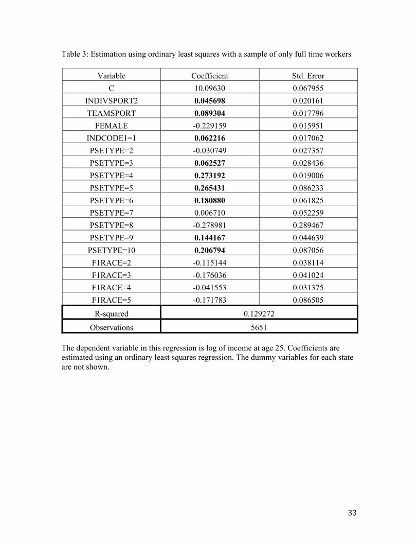
sample of 5,651 respondents. When controlling for fulltime employment, participating in

an athletic team also affects income. Playing an individual sport has a positive coefficient

of 0.0456 and playing a team sport has a positive coefficient of 0.0893. These results are

statistically significant because the t-statistics are greater than 2. People who played

  25  

individual sports have 4.5 % higher incomes than those who did not participate.

Similarly, people who played team sports in high school have 8.9% higher incomes than

those who did not participate. This produces incomes that are greater by a few thousand

dollars. Working in the financial industry also has a positive impact on income with a

coefficient of 0.0622. Additionally, there was a positive correlation between people who

had an associate’s degree, bachelor’s degree, a license and an associate’s degree, a

license and a bachelor’s degree, master’s degree, or a PHD and their income. The

complete list of these results can be found in Table 3. Ultimately, both of these

regressions produce significant results indicating that participating in high school sports

positively affects income. However, this is only true if we assume that the situation is

causal. We cannot just assume that participating in high school athletics is causal towards

income because there are other factors to consider, such as school size.

Two-Stage Least Squares

Therefore, to account for endogeneity I used two-stage least squares to estimate a

regression that tells a more complete story. I selected several instruments to use in the

equation that affect participation in high school athletics, but not income. I used the

following instruments: total school enrollment, father’s educational attainment, mother’s

educational attainment, family income, school classification, urbanicity, and region of the

United States. Primarily, I looked at a two-stage least squares regression without limiting

the sample to respondents who were employed fulltime. Plus, I also kept participation in

individual sports and participation in team sports as two separate variables. I found that

this yielded insignificant results. Thus, according to this estimation, playing on an

individual sport or on a team sport in high school does not affect income. Table 4

  26  

displays these results. However, when I ran the same regression, but controlled for

fulltime employment, I found significant results. Playing on an individual sport positively

affected the natural log of income with a coefficient of 0.3715. Thus, people who played

individual sports have 37 % higher incomes than those who did not participate. It is

important to note that the truth is probably lower than this, but using the instruments

available, this is the result. This could be because in individual sports, an individual’s

performance is directly correlated to the outcome. However, with team sports, an

individual’s performance is only a small part of the final outcome. Plus, individual sports

are more expensive, so only students who come from higher income homes can

participate in them. Interestingly, playing on a team sport was insignificant in this

particular regression. The complete list of results for this equation is displayed in Table 5.

It is important to note that the coefficient on team sports is close to 0 with a standard

error of 0.105, so we can’t tell that it is different from 0.

After finding these results, I created another two-stage least squares regression

where I introduced a new variable that combined playing an individual sport and playing

a team sport. This variable (DIDSPORT) is a dummy variable that has a value of 1 if a

respondent played an individual sport or if a respondent played a team sport, but a value

of 0 if a respondent did not play either. I introduced this new variable to see if

simplifying the athletics variable produced significant results. Without controlling for

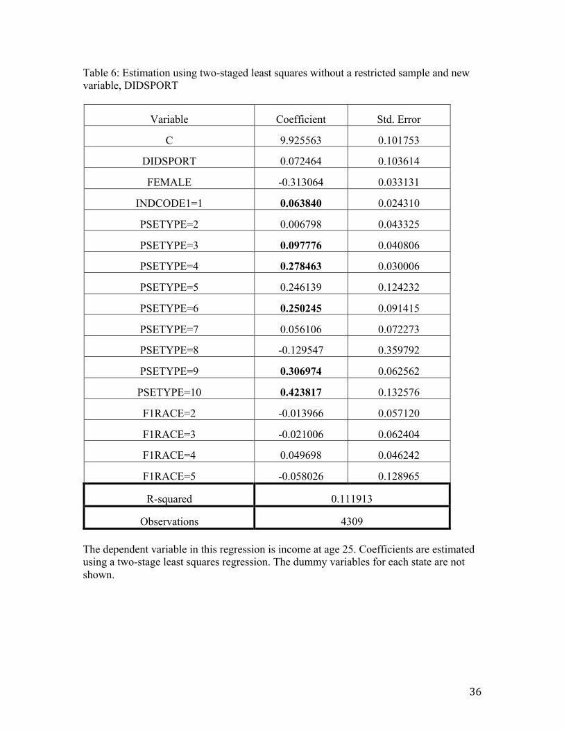
fulltime employment, playing on either type of athletic team was insignificant. Table 6

shows the detailed results from this equation. However, when the sample was restricted

to only include people working a fulltime job, there was a significant positive coefficient

on the new variable. Table 7 displays the following results. Playing either an individual

  27  

sport or a team sport in high school positively increased income by 0.1935. Thus,

participating in a varsity athletics team in high school affected income by 19%. Also

having a job in the financial industry positively affects income with a coefficient of

0.0755. Finally, there is a positive correlation between people who had an associate’s

degree, bachelor’s degree, a license and a bachelor’s degree, master’s degree, or a PHD

and their income.

Unfortunately, I was limited to the variables that were already in NELS-88. Thus,

there were other instruments that I would have liked to use if they were available to me.

Height is the perfect example of an instrument that would have strengthened my

argument, but was not available in the NELS-88 data. Several other economists who have

conducted similar studies have used height as an instrument because taller people are

more likely to play a sport. These types of variables would have made my analysis more

comprehensive.

When I did not restrict the sample to only include fulltime employees, my results

were not significant. However, when the sample was restricted, playing on an individual

sport positively affected the natural log of income and playing on either an individual

sport or on a team sport positively affected the natural log of income. Therefore, limiting

the population is an important element to my successful results.

  28  

Conclusion

Using data from the National Education Longitudinal Study of 1988, I have

examined how a person’s participation in high school athletics positively affects his or

her wage in the labor force. I specify the difference between a causal and non-causal

relationship with high school sports and income. Thus, I use two types of estimation

techniques: ordinary least squares and two-stage least squares.

When assuming that playing a sport is causal towards income, I used ordinary

least squares to regress the natural log of income on participation in high school athletics,

gender, race, post-secondary degree type, job industry type, and current state. I also

restrict the regression to only include fulltime workers. High school athletics is a broad

term and in order to be more specific, I separate it into two variables: individual sports

and team sports. I find that participation in both high school individual sports and team

sports significantly affects income.

However, when I control for endogeneity, the results are slightly different. We

can’t assume that playing a sport is causal because the relationship can go both ways. A

student can join an athletic team and earn the benefits associated, such as valuable human

capital skills. Nonetheless, a student could join an athletic because he or she already has

these skills. Thus, it is unclear whether participation in the sports team is the real cause

for higher wages. Therefore, I employ several instruments to control for endogeneity by

using two-stage least squares. Size of high school, educational attainment of parents,

family income, type of high school, and location in the United States are the instruments

for this regression. I also restrict the sample to fulltime employees. My results show that

  29  

playing a team sport does not significantly affect income; however, playing an individual

sport significantly increases income with a coefficient of 0.3715.

Through my regressions I have shown that there is a correlation between high

school sports and income. While my results are significant, I do not have a definitive

reason as to why they are significant. Earlier in my paper, I described three models that

are potential reasons for the positive relationship between high school athletics and

income: human capital model, screening model, and the networking model. My results

lead me to think that students are mostly likely collecting human capital skills while

playing on a sports team in high school, which help them out later in life. People are

more productive because of these skills that they have acquired. The screening model is

another explanation for the correlation between high school sports and income. When an

individual joins a sports team, it lets employers know that he or she works well with a

team and that he or she has discipline. Finally, the networking model explains that being

on a sports team brings a person into a whole new network of people that can help in the

labor force. However, hypothetically, all three of these models could happen all at once.

The data for this paper is from the years of 1988-2000; therefore, it is slightly

outdated. I would love to see this study repeated with more current data. The Education

Longitudinal Study of 2002 is currently being processed, which is the most recent study

of this nature. The study started in 2002 when respondents were sophomores in high

school and ended in 2012 when respondents were four years out of college. Not only are

there differences in the education system nowadays, but also preferences towards sports

may have changed. Additionally, there were instruments that weren’t available in NELS-

  30  

88, such as height and weight. If these were included in the next study then it would

make the results more accurate.

  31  

Appendix Table 1: Descriptive Statistics Dependent Variable:

Variable Mean Maximum

Minimum Std. Dev.

Observations

INCOME99 24942.35 500000 0 20190.49 11147 Independent Variables:

Instruments:

Variable Mean Maximum

Minimum Std. Dev.

Observations

F2DADSCHOOL 3.232913 7 1 1.869951 10154 F2TOTALENROLL 4.705166 9 1 2.440443 9931 F2MOMSCHOOL 2.999526 7 1 1.671863 10549 FAMINCOME91 48189.47 275000 0 47065.3 10194 G12CLASSIFICATION 1.230176 5 1 0.698135 11678 G12REGION 2.549632 4 1 1.015781 11686 G12URBAN 2.030217 3 1 0.773033 11682

Variable Mean Maximum

Minimum Std. Dev.

Observations

TEAMSPORT 0.2514 1 0 0.433836 12144 INDIVSPORT2 0.166914 1 0 0.372914 12144 FEMALE 0.524936 1 0 0.499399 12051 F1RACE 3.443667 5 1 0.977092 12009 INDCODE1 0.286927 1 0 0.452349 10250 PSETYPE 2.952612 10 1 2.108252 9496 F4STATE 26.39138 63 1 15.11921 12134

  32  

Table 2: Estimation using ordinary least squares without a restricted sample

Variable Coefficient Std. Error C 9.935296 0.079077

INDIVSPORT2 0.055694 0.023759 TEAMSPORT 0.109015 0.020890

FEMALE -0.318438 0.018442 INDCODE1=1 0.056755 0.019753 PSETYPE=2 0.002208 0.031512 PSETYPE=3 0.080160 0.032888 PSETYPE=4 0.278814 0.021976 PSETYPE=5 0.334383 0.099843 PSETYPE=6 0.260797 0.073202 PSETYPE=7 0.059863 0.060558 PSETYPE=8 -0.163506 0.370096 PSETYPE=9 0.252190 0.052445 PSETYPE=10 0.301805 0.105412 F1RACE=2 -0.063198 0.043180 F1RACE=3 -0.075684 0.046845 F1RACE=4 0.024035 0.035391 F1RACE=5 -0.225808 0.098169

R-squared 0.108915

Observations 6895 The dependent variable in this regression is log of income at age 25. Coefficients are estimated using an ordinary least squares regression. The dummy variables for each state are not shown.

  33  

Table 3: Estimation using ordinary least squares with a sample of only full time workers

Variable Coefficient Std. Error C 10.09630 0.067955

INDIVSPORT2 0.045698 0.020161 TEAMSPORT 0.089304 0.017796

FEMALE -0.229159 0.015951 INDCODE1=1 0.062216 0.017062 PSETYPE=2 -0.030749 0.027357 PSETYPE=3 0.062527 0.028436 PSETYPE=4 0.273192 0.019006 PSETYPE=5 0.265431 0.086233 PSETYPE=6 0.180880 0.061825 PSETYPE=7 0.006710 0.052259 PSETYPE=8 -0.278981 0.289467 PSETYPE=9 0.144167 0.044639 PSETYPE=10 0.206794 0.087056 F1RACE=2 -0.115144 0.038114 F1RACE=3 -0.176036 0.041024 F1RACE=4 -0.041553 0.031375 F1RACE=5 -0.171783 0.086505

R-squared 0.129272

Observations 5651 The dependent variable in this regression is log of income at age 25. Coefficients are estimated using an ordinary least squares regression. The dummy variables for each state are not shown.

  34  

Table 4: Estimation using two-staged least squares without a restricted sample

Variable Coefficient Std. Error

C 9.906035 0.101936

INDIVSPORT2 0.326611 0.205693

TEAMSPORT -0.069159 0.120202

FEMALE -0.299356 0.034992

INDCODE1=1 0.064946 0.024649

PSETYPE=2 0.005735 0.043353

PSETYPE=3 0.091747 0.041537

PSETYPE=4 0.260223 0.032614

PSETYPE=5 0.225402 0.126337

PSETYPE=6 0.215310 0.095699

PSETYPE=7 0.062579 0.072792

PSETYPE=8 -0.089047 0.366098

PSETYPE=9 0.280001 0.065493

PSETYPE=10 0.345487 0.144666

F1RACE=2 0.006664 0.059946

F1RACE=3 -0.009868 0.064485

F1RACE=4 0.067542 0.048571

F1RACE=5 -0.047358 0.130803

R-squared 0.088150

Observations 4309 The dependent variable in this regression is log of income at age 25. Coefficients are estimated using a two-stage least squares regression. The dummy variables for each state are not shown.

  35  

Table 5: Estimation using two-staged least squares with a sample of only full time workers

Variable Coefficient Std. Error

C 10.04055 0.085013

INDIVSPORT2 0.371512 0.172182

TEAMSPORT 0.000554 0.105683

FEMALE -0.193509 0.029157

INDCODE1=1 0.075764 0.021153

PSETYPE=2 -0.006424 0.037466

PSETYPE=3 0.083317 0.035970

PSETYPE=4 0.240154 0.027758

PSETYPE=5 0.099460 0.109209

PSETYPE=6 0.138006 0.081356

PSETYPE=7 0.017334 0.062197

PSETYPE=8 -0.236127 0.287150

PSETYPE=9 0.131660 0.058172

PSETYPE=10 0.187482 0.121394

F1RACE=2 -0.072527 0.054003

F1RACE=3 -0.142972 0.057231

F1RACE=4 -0.039044 0.043585

F1RACE=5 -0.192663 0.110269

R-squared 0.092607

Observations 3571 The dependent variable in this regression is income at age 25. Coefficients are estimated using a two-stage least squares regression. The dummy variables for each state are not shown.

  36  

Table 6: Estimation using two-staged least squares without a restricted sample and new variable, DIDSPORT

Variable Coefficient Std. Error

C 9.925563 0.101753

DIDSPORT 0.072464 0.103614

FEMALE -0.313064 0.033131

INDCODE1=1 0.063840 0.024310

PSETYPE=2 0.006798 0.043325

PSETYPE=3 0.097776 0.040806

PSETYPE=4 0.278463 0.030006

PSETYPE=5 0.246139 0.124232

PSETYPE=6 0.250245 0.091415

PSETYPE=7 0.056106 0.072273

PSETYPE=8 -0.129547 0.359792

PSETYPE=9 0.306974 0.062562

PSETYPE=10 0.423817 0.132576

F1RACE=2 -0.013966 0.057120

F1RACE=3 -0.021006 0.062404

F1RACE=4 0.049698 0.046242

F1RACE=5 -0.058026 0.128965

R-squared 0.111913

Observations 4309 The dependent variable in this regression is income at age 25. Coefficients are estimated using a two-stage least squares regression. The dummy variables for each state are not shown.

  37  

Table 7: Estimation using two-staged least squares with a sample of only full time workers and a new variable, DIDSPORT

Variable Coefficient Std. Error

C 10.02675 0.085639

DIDSPORT 0.193579 0.089071

FEMALE -0.197999 0.028503

INDCODE1=1 0.075556 0.020666

PSETYPE=2 0.005405 0.037100

PSETYPE=3 0.093402 0.034844

PSETYPE=4 0.254323 0.025394

PSETYPE=5 0.126563 0.106295

PSETYPE=6 0.169032 0.077177

PSETYPE=7 0.008292 0.061127

PSETYPE=8 -0.281160 0.279252

PSETYPE=9 0.160168 0.053474

PSETYPE=10 0.260337 0.108447

F1RACE=2 -0.095171 0.050454

F1RACE=3 -0.146309 0.055376

F1RACE=4 -0.054589 0.041812

F1RACE=5 -0.206521 0.107897

R-squared 0.133437

Observations 3571 The dependent variable in this regression is income at age 25. Coefficients are estimated using a two-stage least squares regression. The dummy variables for each state are not shown.

  38  

Bibliography

Barron, John M., Bradley T. Ewing, and Glen R. Waddell. 2000. "The Effects of High School Athletic Participation on Education and Labor Market Outcomes." Review of Economics and Statistics 82 (3): 409-421.

Broh, Beckett A. 2002. "Linking Extracurricular Programming to Academic Achievement: Who Benefits and Why?" Sociology of Education 75 (1): 69-95.

Costa, Cristiano M. 2010. "Extracurricular Activities and Wage Differentials." University of Pennsylvania.

Dhuey, Elizabeth and Stephen Lipscomb. 2008. "What Makes a Leader? Relative Age and High School Leadership." Economics of Education Review 27 (2): 173-183.

Eide, Eric R. and Nick Ronan. 2001. "Is Participation in High School Athletics an Investment Or a Consumption Good? Evidence from High School and Beyond." Economics of Education Review 20 (5): 431-442.

Gius, Mark P. 2011. "The Effects of Participation in High School Athletics and the National Honor Society on Future Earnings." Review of Applied Economics 7 (1-2): 69-80.

Kuhn, Peter and Catherine Weinberger. 2005. "Leadership Skills and Wages." Journal of Labor Economics 23 (3): 395-436.

Lipscomb, Stephen. 2007. "Secondary School Extracurricular Involvement and Academic Achievement: A Fixed Effects Approach." Economics of Education Review 26 (4): 463-472.

McNeal, Ralph B., Jr. 1995. "Extracurricular Activities and High School Dropouts." Sociology of Education 68 (1): 62-80.

Mincer, Jacob. 1958. "Investment in Human Capital and Personal Income Distribution." Journal of Political Economy 66 (4): 281-302.