Does City Structure Affect Job Search and Welfare?

Journal of Urban Economics 51, 515–541 (2002)

doi:10.1006/juec.2001.2256, available online at http://www.idealibrary.com on

Does City Structure Affect Job Search and Welfare?1

Etienne Wasmer

ECARES, Universite Libre de Bruxelles and Universite de Metz, CP 114,39 Avenue F.D. Roosevelt, B-1050 Bruxelles, Belgium

E-mail: [email protected]

and

Yves Zenou

University of Southampton and GAINS, Department of Economics,Southampton SO17 1BJ, United Kingdom

E-mail: [email protected]

Received January 11, 2001; revised September 10, 2001; published online February 2, 2002

We develop a model in which workers’ search efficiency is negatively affected byaccess to jobs. Workers’ location in a city is endogenous and reflects a trade-off betweencommuting costs and the surplus associated with search. Different configurations emergein equilibrium; notably, the unemployed workers may reside far away (segregated city)or close to jobs (integrated city). We prove that there exists a unique and stable marketequilibrium in which both land and labor markets are solved for simultaneously. We findthat, despite inefficient search in the segregated city equilibrium, the welfare differencebetween the two equilibria is not so large due to differences in commuting costs. Wealso show how a social planner can manipulate wages by subsidizing/taxing the transportcosts and can accordingly restore the efficiency. © 2002 Elsevier Science (USA)

Key Words: job matching; urban land use; transportation policies.

1. INTRODUCTION

The urban economics literature has often focused on the existence of areas ofhigh poverty and high criminality, namely the ghettos. The geographic positionof these areas within cities coincides in general with high unemployment and,more precisely, with the absence of jobs in the areas surrounding the ghettos.The labor market is thus a very important channel of the transmission andpersistence of poverty across city tracts. In the United States, there has been an

1 The authors thank two anonymous referees and particularly the Editor, Jan Brueckner, for veryhelpful comments. Part of this work was written while both authors were visiting the Institute forthe Study of Labor (IZA), Bonn, whose hospitality is gratefully acknowledged.

515

0094-1190/02 $35.00© 2002 Elsevier Science (USA)

All rights reserved.

516 wasmer and zenou

important empirical debate revolving around this issue. The spatial mismatchhypothesis, first developed by Kain [16], stipulates that the increasing distancebetween residential location and workplace is very harmful to black workersand, with labor discrimination, constitutes one of the main explanation of theiradverse labor market outcomes.Since the study of Kain, dozens of empirical studies have been carried out try-

ing to test this hypothesis (surveyed by Holzer [9], Kain [17], and Ihlanfeldt andSjoquist [13]). The usual approach is to relate a measure of labor-market out-comes, based on either individual or aggregate data, to another measure of jobaccess, typically some index that captures the distance from residences to centersof employment. The weight of the evidence suggests that bad job access indeedworsens labor-market outcomes, confirming the spatial mismatch hypothesis.The economic mechanism behind this hypothesis is, however, unclear. Sometend to argue that black workers refuse to take jobs involving excessively longcommuting trips (Zax and Kain [32]). Others think that firms do not recruitworkers who live too far away from them because their productivity is lowerthan those residing closer (see, e.g., Zenou [34]). In the present paper, we pro-pose an alternative approach to explain the spatial mismatch hypothesis: wedevelop a model based on job search in which distance to jobs is harmfulbecause it negatively affects workers’ search efficiency. It is indeed our con-tention that search activities are less intense for those living further away fromjobs because the quality of information decreases with the distance to jobs. Onthe contrary, individuals who reside close to jobs have good access to infor-mation about these jobs and are in general more successful in their job searchactivities.This view is consistent with empirical studies. Indeed, Barron and Gilley [1]

and Chirinko [4] have shown that there are diminishing returns to search whenpeople live far away from jobs whereas Van Ommeren et al. [28] have found thatpeople who expect to receive more job offers will generally not have to accept along commute. Rogers [22] have also demonstrated that access to employmentis a significant variable in explaining the probability of leaving unemployment.Finally, Seater [24] have shown that workers searching further away from theirresidences are less productive in their search activities than those who searchcloser to where they live.Our first task is thus to analyze the interaction between job search and the

location of workers vis-a-vis the job centers, in a framework where two urbanconfigurations can emerge: a “segregated city” equilibrium in which the unem-ployed workers reside far away from jobs and an “integrated city” equilibriumin which the unemployed workers are close to jobs. The predominance of oneequilibrium over the other strongly depends on the differential in commutingcosts between the employed and the unemployed, and on the expected returnof being more efficient in search. We show that there exists, for each urban

city structure and job search 517

configuration, a unique market equilibrium in which the land and the labor mar-ket are solved for simultaneously.We then discuss welfare issues. We show that, despite higher inefficiency of

the search process in the segregated city, the resulting welfare loss is smallcompared to the other equilibrium, because of higher commuting costs paidby the employed in the integrated city. We also find that, in both equilibria,the market outcome is in general not efficient because of search externalities.In addition, due to the spatial structure of the model, the social planner hasone more set of tools to restore the constrained efficiency, namely through thedesign of transportation policies. Indeed, the social planner can raise wagesby subsidizing the commuting costs of the unemployed and reduce them bysubsidizing the commuting costs of the employed workers. As a matter of fact,the standard non-spatial Hosios–Pissarides condition of efficiency of the searchmatching equilibrium is affected by commuting costs. Interestingly, the policyrecommendation does not depend on the urban configuration, but the magnitudeof the impact of the policy parameter does. Indeed, in the segregated city, theimpact of policy is much larger, by a factor of 10 to 15. Stated differently, suchtransportation policies may have very little impact in an integrated city, andmuch more in a segregated city.Our model is related to other theoretical studies that combine search and

urban models. The first papers that dealt with these issues (Jayet [14, 15], Seater[24], and Simpson [25]) had a shallow modelling of the urban space. In partic-ular, these papers did not explicitly model the intra-urban equilibrium in whichthe location of unemployed and employed workers is endogenously determinedand influences the labor market equilibrium. More recently, a more explicit mod-elling of the urban space has been incorporated in search-matching models. Ina companion paper (Wasmer and Zenou [30]), we focus on the labor marketequilibrium and more precisely on how search theory is affected by the intro-duction of a spatial dimension. We deal in particular with endogenous searcheffort. Coulson et al. [5] and Sato [23] focus on inter-urban equilibria and thuson wage and unemployment differences between different cities. Wheeler [31]investigates the link between urban agglomeration and the firm–worker matchingprocess. Smith and Zenou [26] deal with endogenous search effort. Our presentpaper is quite different from these approaches since we develop an intra-urbansearch model and we focus on the impact of city structure (where do workersof different employment status reside?) on the labor market outcomes. In par-ticular, contrary to all the papers mentioned above, we evaluate the impact ofdifferent urban equilibria on the search-matching equilibrium.The remainder of the paper is as follows. The next section presents the basic

model. Section 3 focuses on the two urban equilibrium configurations whereasthe existence and uniqueness of the market equilibrium (solving for both theland and labor markets) is carried out in Section 4. Section 5 is devoted to thewelfare analysis. Finally, Section 6 concludes.


2. THE MODEL AND GENERAL NOTATIONS

There is a continuum of firms and workers that are all (ex ante) identical.For simplicity, we normalize the size of the population to 1. This implies thatthe unemployment rate in the economy is equal to the unemployment level andwill be denoted by u.A firm is a unit of production that can either be filled by a worker whose

production is y units of output or be unfilled and thus unproductive. In order tofind a worker, a firm posts a vacancy. We denote by v the number of vacancies inthe economy. A vacancy can be filled according to a random Poisson process.Similarly, workers searching for a job will find one according to a randomPoisson process. In aggregate, these processes imply that there is a number ofcontacts per unit of time between the two sides of the market that are determinedby the standard matching function2

x�su, v�,

where s is the average search efficiency of the unemployed workers (a worker ihas an efficiency of search equal to si). Since this term represents the aggregatesearch frictions, it is also an index of aggregate information about economicopportunities. How si depends on the location of workers is specified below.We simply assume here that x�.� is increasing both in its arguments, concave,and homogeneous of degree 1 (or equivalently has constant return to scale).In this context, the probability for a vacancy to be filled per unit of time isx�su, v�/v. By constant return to scale, it can be rewritten as x�1/θ, 1� ≡ q�θ�where θ = v/su is a measure of labor market tightness in efficiency units andq�θ� is a Poisson intensity. By using the properties of x�.�, it is easily verifiedthat q ′�θ� ≤ 0: the greater the labor market tightness, the lower the probabilityfor a firm of filling a vacancy. Observe that we assume that firms have no impacton their own search efficiency and consider s, u, and v as given. Similarly, fora worker i with efficiency si , the probability of obtaining a job per unit of timeis x�su,v�

u· sis≡ θq�θ�si ≡ p�si�, where p�si� is defined as the intensity of the

exit rate from unemployment for this worker.In contrast to the standard model of job matching, where space is absent

(Mortensen and Pissarides [18], Pissarides [20]), we make here the importantassumption that s strongly depends on the location of the unemployed workersin the city: the closer the location to the workplace, the greater the efficiencyand the more likely is a contact (s = s�d�, where d is the distance between

2This matching function is written under the assumption that the city is monocentric; i.e., all firmsare located in one fixed location. See the next section for the description of the spatial structure ofthe city.


residence and workplace, with s ′�d� < 0).3 In other words, the probability tofind a job now negatively depends on d and is defined by p�d� = θq�θ�s�d�.Think for example of firms that place help-wanted signs in their windows orthat place ads in local newspapers. Then, obviously, workers living further awayfrom these firms have less information on these jobs than those residing closer.For example, Ihlanfeldt [12] has shown that, in Atlanta, inner-city residents wereless able to identify the location of suburban employment centers than surbur-banites and thus had less information on those jobs. In addition, Turner [27]demonstrated that, in Detroit, suburban firms using local recruitment methods(such as local newspapers or help-wanted signs in their windows) had few inner-city applicants whereas those using general formal methods (such as city news-papers) had much more inner-city applicants. Finally, Holzer and Reaser [10]have found that, in four major metropolitan areas (Atlanta, Boston, Detroit, andLos Angeles), inner-city workers apply less frequently for jobs in the suburbsthan in central cities because of higher costs of applying and/or lower informa-tion flows.Once the match is made, the wage is determined by the standard generalized

Nash bargaining solution. In each period, there is also a probability δ that thematch is destroyed. In order to determine the (general) equilibrium, we will pro-ceed as follows. We first determine the partial urban equilibrium configurations.Then, depending on the location of workers and thus on the aggregate searchefficiency s, we determine the partial labor market equilibria. Hereafter, thelabor (respectively urban) equilibrium will refer to the partial equilibrium. Thegeneral equilibrium will be denoted a “market equilibrium.” Thus, by denot-ing by R�d� the land market price at a distance d from the city-center, by w

the wage earned by workers, and by u the unemployment rate, we have thefollowing definition.

Definition 1. A market equilibrium consists of a land rent function, wage,labor market tightness, and unemployment level �R�d�, w, θ, u� such that theurban land use equilibrium and the labor market equilibrium are solved forsimultaneously.

Thus, a market equilibrium requires solving simultaneously two problems:

(i) a location and rental price outcome (referred to as an urban land useequilibrium)

(ii) a (steady state) matching equilibrium with determines w, θ , and u

(referred to as a labor market equilibrium)

We will give below more precise definitions of these two markets.

3This relation s ′�d� < 0 can be derived endogenously by showing that workers living furtheraway from jobs put less effort in search than those residing closer. See Wasmer and Zenou [29].


3. EQUILIBRIUM URBAN CONFIGURATIONS

The city is monocentric (i.e., all firms are assumed to be exogenously locatedin the central business district (CBD hereafter)), is linear, is closed, and hasabsentee landlords.4 There is a continuum of workers uniformly distributedalong the linear city who endogenously decide their optimal residence betweenthe CBD and the city fringe. The utility function of workers is defined such thatthey are risk neutral, live infinitely, and discount the future at a rate r . Work-ers all consume the same amount of land (normalized to 1) and the density ofresidential land parcels is taken to be unity so that there are exactly d units ofhousing within a distance d of the CBD.Employed workers go to the CBD to work and to shop while unemployed

workers go to the CBD to be interviewed and to shop. Let us denote by ted andtud the transportation cost at a distance d from the CBD for respectively workingand unemployed specific activities (interviews, registration), with te > tu > 0.For instance, if the unemployed commute once a week to the CBD and theemployed commute five times a week, te/tu could be considered as a con-stant, equal to 5. All workers bear land rent costs at the market price R�d�and receive a wage w when employed and unemployment benefits b if unem-ployed. We denote by U and W the discounted expected lifetime utilities (or netintertemporal incomes since workers are risk neutral) of the unemployed andthe employed, respectively. We assume that location changes are costless. Withthe Poisson probabilities defined above, infinite lived workers have the intertem-poral utility functions (given by the Bellman equations determined at the steadystate)

rU�d� = b − tud − R�d� + p�d�[(

maxd ′

W �d ′�)− U�d�

](1)

rW �d� = w − ted − R�d� + δ

[(maxd ′

U�d ′�)−W �d�

], (2)

where r is the exogenous discount rate. Let us comment on (1). When a workeris unemployed today, he/she resides in d and his/her net income is b − tud −R�d�. Then, he/she can obtain a job with a probability p�d� and if so, he/sherelocates optimally in d ′ and obtains an increase in income of W �d ′� − U�d�.The interpretation of (2) is similar.

Since there are no relocation costs, the urban equilibrium is such that all theunemployed enjoy the same level of utility rU = r�U as well as the employedrW = r �W . Indeed, any utility differential within the city would lead to the relo-cation of some workers up to the point where all differences in utility disappear.

4All these assumptions are very standard in urban economics (see, e.g., Brueckner [3] or Fujita[7]). In particular, the extension to a circular symmetric city is straightforward since any ray throughthe center looks like any other ray. So examining a single ray is almost the same as looking at thewhole city.


We now have to determine the optimal location of all workers in the city. Thestandard way of doing it is to use the concept of bid rents (Fujita [7]) which aredefined as the maximum land rent at a distance d that each type of worker isready to pay in order to reach its respective equilibrium utility level. Therefore,the bid rents of the unemployed and employed are respectively equal to

�u�d, �U, �W � = b − tud + p�d��W − �r + p�d��U (3)

�e�d, �U, �W � = w − ted + δ�U − �r + δ��W. (4)

We have now to determine the location of the unemployed and of the employedworkers in the city. For that, we need to calculate the bid rent slopes for eachtype of worker since a steeper bid rent corresponds to an equilibrium locationcloser to the CBD. They are respectively given by

∂�u�d, �U, �W �∂d

= −tu + p′�d��W − �U� < 0 (5)

∂�e�d, �U, �W �∂d

= −te < 0, (6)

where p′�d� = θq�θ�s ′�d� < 0. These slopes (in absolute values) can be inter-preted as the marginal cost that a worker is ready to pay in order to be marginallycloser to the CBD.5 For the unemployed, this marginal cost is the sum of themarginal commuting cost, tu, and the marginal probability of finding a job,p′�d�, times the (intertemporal) surplus of being employed, �W − �U . On theother hand, the employed workers bear only marginal the commuting cost tesince the probability of losing a job δ is exogenous and does not depend onthe location of workers. If df denotes the city fringe, we have the followingdefinition.

Definition 2. The urban land rent function R�d� is the upper envelope ofall workers’ bid rents and of the agricultural land rent RA; i.e.,

R�d� = max��u�d, �U, �W �, �e�d, �U, �W �, RA at each d ∈ �0, df �.With this general definition, a large number of urban equilibria can

arise. However, for analytical simplicity, we here focus on linear bid rentslopes, in which case only two urban equilibria can emerge. In the first one(Equilibrium 1), the unemployed reside in the vicinity of the CBD and theemployed at the outskirts of the city. We call such a city the “integrated city”because the unemployed have a good access to jobs. By contrast, in the other

5The set of parameters for which the slope of the two bid rents is equal is of zero measure.Accordingly, we exclude this possibility and thus mixed configurations where both employed andunemployed workers are located in the same place. We thus only consider perfectly separatedconfigurations where only one type of worker locates within the same segment.


one (Equilibrium 2), the unemployed locate at the outskirts of the city andthe employed close to the city-center. This city is called the “segregated city”because the unemployed have a bad access to jobs.In order to have linear bid rents, we assume that s�d� = s0 − ad, with s0 > 0

and a > 0. To guarantee that search efficiency is always positive, we imposethat s�d� > 0 for all d ≤ 1. This linear formulation implies that p′′�d� = 0 andthus

∂2�u�d, �U, �W �∂d2 = ∂2�e�d, �U, �W �

∂d2 = 0.

Thus, according to (5) and (6), the resulting urban equilibrium is determinedby a trade-off between the difference in commuting costs, te − tu, and themarginal probability of getting a job. This is due to the fact that both theemployed and the unemployed want to be as close as possible to the CBDbecause the former want to save on commuting costs and the latter desire toincrease their probability of getting a job.The important condition for having one equilibrium or the other is given by an

inequality comparing the slopes of the bid rents of employed and unemployedworkers. Equilibrium 1 occurs if and only if:6

Condition 1 (Integrated City).

te − tu < aθ1q�θ1��W1 − �U1�. (7)

Equation (7) means that the differential in commuting costs per unit of dis-tance between the employed and the unemployed is lower than the marginalexpected return of search for the unemployed if he/she moves closer to the cen-ter by one unit of distance. Indeed, since a = � ∂s

∂d�, aθ1q�θ1� is the marginal

increase in the probability of obtaining a job for an unemployed worker. Thus if(7) holds, the unemployed occupy the core of the city and the employed the out-skirts of the city. In the other equilibrium (Equilibrium 2), we have the oppositeinequality:

Condition 2 (Segregated City).

te − tu > aθ2q�θ2��W2 − �U2� (8)

and the employed bid away the unemployed.Observe that anything that may improve the return to search for unem-

ployed workers �θq�θ� and �W − �U� can help to switch from Equilibrium 2to Equilibrium 1. Observe also that when the employed have lower commutingcosts than the unemployed, the only possible equilibrium is integrated since theunemployed have stronger incentives to reside closer to the CBD.

6All variables determined at the equilibrium k�= 1, 2� are indexed by k. At each urbanequilibrium k corresponds a labor market equilibrium k.


FIG. 1. Urban equilibrium 1 (the integrated city).

By using Definition 2 and the two conditions, (7) and (8), we are now able todefine the two urban equilibria. If we denote the distance of the border betweenthe unemployed and the employed by dk (k = 1, 2), we have the followingdefinition:

Definition 3. The urban land use equilibrium k = 1, 2 consists of intertem-poral utility functions of being unemployed and employed, a border between theemployed and the unemployed, and a city fringe ��Uk, �Wk, dk, df � such that

d1 = u1 or d2 = 1− u2 (9)

df = 1 (10)

�e�dk, �Uk, �Wk� = �u�dk, �Uk, �Wk� (11)

�e�df , �Uk, �Wk� = RA or �u�df , �Uk, �Wk� = RA. (12)

These two equilibria are illustrated in Figs. 1 and 2. By using (3), (4), and(9) and replacing them in (11) and (12), we obtain

�Wk − �Uk =wk − b − �te − tu�dk

r + δ + p�dk�k = 1, 2, (13)

where wk, uk, θk will be determined at the labor market equilibrium k. Theaverage search intensity in equilibrium k is equal to

sk = s0 − adk k = 1, 2, (14)

where dk is the average location of the unemployed in equilibrium k. It is easyto verify that d1 = u1/2 and d2 = 1− u2/2.


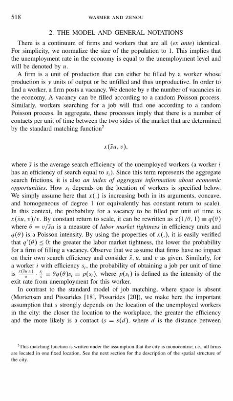
FIG. 2. Urban equilibrium 2 (the segregated city).

Since d1 < d2 (this is always true because u1 + u2 < 2), the averagesearch efficiency in urban equilibrium 1 is higher than in urban equilibrium2; i.e., s1 > s2. This result is quite intuitive. Indeed, in the integrated city, theunemployed reside closer to the CBD than in the segregated city and thus theirprobability of finding a job is higher.

4. THE MARKET EQUILIBRIUM

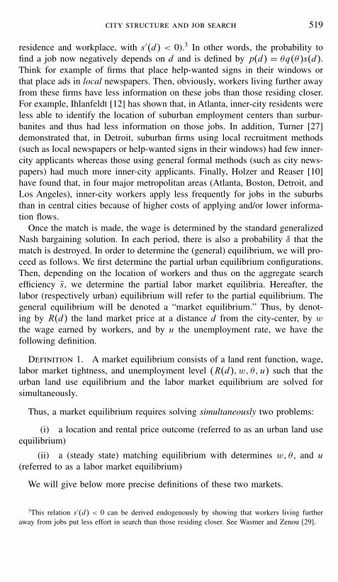
4.1. Free-Entry Condition and Labor Demand

Let us denote respectively by Jk and Vk the intertemporal profit of a job andof a vacancy in equilibrium k = 1, 2. If γ is the search cost for the firm perunit of time and y is the product of the match, then Jk and Vk can be written as

rJk = y − wk + δ�Vk − Jk� (15)

rVk = −γ + q�θk��Jk − Vk�. (16)

Following Pissarides [20], we assume that firms post vacancies up to a pointwhere

Vk = 0 (17)

which is a free entry condition. From (16) and using (17), the value of a job isnow equal to

Jk =γ

q�θk�. (18)


FIG. 3. Labor demand and endogenous wage setting.

Finally, plugging (18) into (15), we obtain the following decreasing relationbetween labor market tightness and wages in equilibrium:

γ

q�θk�= y − wk

r + δk = 1, 2. (19)

In words, the value of a job is equal to the expected search cost, i.e. the costper unit of time multiplied by the average duration of search for the firm.Equation (19) defines in the space �θk, wk� a curve (see Fig. 3) representing

the supply of vacancies. This curve is in fact a labor demand curve LD since itdetermines the number of vacancies posted per period as a function of wages.This curve is independent of the type of urban equilibrium since, independentlyof workers’ location, firms post vacancies up to Vk = 0. We show in LemmaA.17 that it is downward sloping in the plane (θk, wk�.4.2. Wage Determination

The usual assumption about wage determination is that, at each period, thetotal intertemporal surplus is shared through a generalized Nash-bargaining pro-cess between the firm and the worker.8 The total surplus is the sum of thesurplus of the workers, �Wk − �Uk , and the surplus of the firms Jk − Vk . At eachperiod, the wage is determined by

wk = argmax��Wk − �Uk�β�Jk − Vk�1−β k = 1, 2, (20)

7All lemmas are stated and proved in the Appendix.8All negotiations take place between two agents: the worker and the firm. In particular, no agent

is allowed to make offers simultaneously to more than one other agent.


where k denotes the urban equilibrium and 0 ≤ β ≤ 1 is the bargaining power ofworkers. Observe that �Uk is the value of continued search in equilibrium k, i.e.,the value of workers’ outside option whereas Vk equals the employers’ value ofholding the job vacant in equilibrium k, i.e., the value of firms’ outside option.Observe also that �Uk , the threat point (or the outside option) of the worker inthe urban equilibrium k, does not depend on the current location of the worker,who will relocate if there is a transition in his/her employment status. Using (2)and (15), the first-order maximization condition derived from (20) satisfies

�1− β��Wk − �Uk� = β�Jk − Vk� k = 1, 2. (21)

Now, observing that Vk = 0 (free-entry condition) and p�dk� ≡ θkq�θk�s�dk�,and using (13) and (18), we can write (21) as

�1− β��wk − b − �te − tu�dk� = �r + δ�β γ

q�θk�+ θks�dk�βγ k = 1, 2.

Finally, since by (19) γ �r + δ�/q�θk� = y −wk , we obtain, in urban equilibriumk = 1, 2, the wage

wk = �1− β��b + �te − tu�dk� + β�y + s�dk�θkγ �, (22)

where dk is defined by (9).Let us first interpret the wage equation (22) for city 1, with a focus on

how wages depend on unemployment u1.9 The first part of the RHS of (22),

�1 − β��b + �te − tu�u1�, is what firms must pay to induce workers to acceptthe job offer: firms must exactly compensate the transportation cost difference(between the employed and the unemployed) of the unemployed worker who isthe furthest away from the CBD, i.e., located at d1 = u1 (remember that hereunemployment is also a distance). Therefore, when u1 increases, this marginalunemployed worker is further away from the CBD and wages must compen-sate the transportation cost difference. This is referred to as the “compensationeffect.”10 The second part of the RHS of (22), β�y + s�u1�θ1γ �, implies thatdistance (u1) has the opposite effect. When u1 rises, the marginal unemployed(i.e., the one located in d1 = u1) is further away from the city-center and thushis/her outside option (i.e., the value of continued search) decreases, leading toa reduction in the wage. This is referred to as the “outside option effect.” Thefirst effect is a pure spatial cost since �te − tu�u1 represents the space cost dif-ferential between employed and unemployed workers paying the same bid rentwhereas the second effect is a mixed labor-spatial cost one. The interpretationof Eq. (22) for city 2 is similar, except that one needs to replace d1 = u1 byd2 = 1− u2.

9For empirical evidence of links between local wages and unemployment, see Blanchflower andOswald [2].

10Using an efficiency wage model, Zenou and Smith [33] found a similar effect.


In search-matching models, the wage-setting curve (a relation between wagesand the state of the labor market, here θk , k = 1, 2) replaces the traditionallabor-supply curve. Equations (22) are the two wage-setting curves (WS1 andWS2) and are both positively sloped in the plan (θk, wk). Lemma A.2 statesthat the curve WS1 is steeper than WS2 but the intercept of WS1 is lower (seeFig. 3). The reason WS1 is steeper than WS2 is the following. The slope ofthese curves represents the ability of workers to exert wage pressures when thelabor market is tighter. Thus, for a given labor market tightness, a more efficientlabor market, i.e., s�d1� > s�d2�, leads to a higher wage pressure per unit of θ ,thus a steeper WS1 curve. The latter inequality on search efficiencies is true forreasonable values of the unemployment rates (a sufficient condition being thatboth u’s are less than a half) and implies that the marginal worker is closer andthus more efficient in his/her search in Equilibrium 1. The intercept is, however,higher in Equilibrium 2 since when θ = 0, the outside option effect vanishesand only the compensation effect remains. Since the same marginal worker isfurther away in Equilibrium 2, he/she must have a higher compensation forhis/her transportation costs.As in the standard labor economics approach, for each equilibrium k, the

equilibrium value of wk and θk will be determined by the intersection betweenthe wage-setting curve (22) and the labor demand curve (19), defined above.In fact, two situations may arise: either the labor demand curve cuts the wagesetting curve before the intersection point (w, θ ) (see Fig. 3 for an illustrationof this case) or after it.11 The value of θ , determined in Lemma A.2, is givenby

θ = 1− β

β

�te − tu�aγ

. (23)

In fact, it turns out that θ also defines a critical value that determines whichurban equilibrium prevails. Indeed, it is easy to see that, at the labor mar-ket equilibrium, urban equilibrium 1 prevails if and only if θ∗1 > θ and urbanequilibrium 2 prevails if and only if θ∗2 < θ .12 Using this result, the followingproposition is straightforward to establish.

Proposition 1. When θ∗1 < θ∗2 :

• if θ∗1 < θ∗2 < θ , urban equilibrium 2 exists and is unique;

11Because it is too peculiar, we exclude the case when the labor demand curve intersects the twowage setting curves at exactly (w, θ ).

12This result is derived as follows. Using (17) and (18) in (21), we obtain

�Wk − �Uk =β

1− β

γ

q�θk�.

Now plugging this value in (7) (respectively (8)) gives the result.


• if θ < θ∗1 < θ∗2 , urban equilibrium 1 exists and is unique;

• if θ∗1 < θ < θ∗2 , there is no urban equilibrium.

When θ∗2 < θ∗1 :

• if θ∗2 < θ∗1 < θ , urban equilibrium 2 exists and is unique;

• if θ < θ∗2 < θ∗1 , urban equilibrium 1 exists and is unique;

• if θ∗2 < θ < θ∗1 , both urban equilibria exist.

Therefore, when the labor demand curve cuts the wage setting curve before(w, θ ), we have θ∗2 < θ∗1 < θ , and then according to Proposition 1, there isonly one unique urban equilibrium, which is Equilibrium 2. When the labordemand curve cuts the wage setting curve after (w, θ ), we have θ < θ∗1 < θ∗2 ,and, according to Proposition 1, only Equilibrium 1 exists and is unique. Onecan thus see that several of the above possibilities, including multiple equilibriaand no equilibrium, are not possible.

4.3. Steady-State Labor Market Equilibrium

In order to derive the market equilibrium, we have first to define a labormarket equilibrium for each urban equilibrium k = 1, 2. We have the followingdefinition:

Definition 4. A (steady-state) labor market equilibrium consists of alabor market tightness, wage, and unemployment level �θk, wk, uk� such that,given the matching technology, all agents (workers and firms) maximize theirrespective objective function; i.e. this triple is determined by a free-entry con-dition for firms, a wage-setting mechanism, and a steady-state condition onunemployment.

Since each job is destroyed according to a Poisson process with arrival rateδ, in equilibrium k = 1, 2, the number of workers who enter unemploymentis δ�1 − uk� and the number who leave unemployment is θkq�θk�skuk . Theevolution of unemployment is thus given by the difference between these twoflows,

uk = δ�1− uk� − θkq�θk�skuk, k = 1, 2, (24)

where, in equilibrium k, uk is the variation of unemployment with respect totime. In steady state, the rate of unemployment is constant and therefore thesetwo flows are equal (flows out of unemployment equal flows into unemploy-ment). We thus have:13

uk =δ

δ + θkq�θk�sk, k = 1, 2. (25)

13It is easy to see that, when the matching technology exhibits constant returns, Eq. (24) has aunique stable steady-state solution for every vacancy rate. This solution is given by (25).


In the search-matching literature, the above equation defines in the �u, v� spacea downward sloping curve referred to as the Beveridge curve. In our model, thiscurve would be further away from the origin in Equilibrium 2. See Wasmer andZenou [29] for a formal exposition of these results.

4.4. Market Equilibrium: Existence and Uniqueness

We have three equations, (19), (22), and (25), and three unknowns, wk, θk ,and uk (k = 1, 2). By combining (19) and (22), the market solution that definesthe equilibrium θk is given by

y − b = γ

q�θk�[δ + r + θkq�θk�s�dk�β

1− β

]+ dk�te − tu� (26)

and the equilibrium value of wk is determined by plugging this θk in (22).For each equilibrium k = 1, 2, Eq. (26) defines a first relation between thelabor market tightness θk and the unemployment rate uk , since s�dk� dependson unemployment. Equation (25) defines a second relation between these twovariables. These two equations are central to the following result:14

Proposition 2. There exists a unique and stable market equilibrium�R∗�d�, w∗

k , θ∗k , u

∗k�, k = 1, 2, and only the two following cases are possible:

• If θ < θ∗1 < θ∗2 , urban equilibrium 1 prevails.

• If θ∗2 < θ∗1 < θ , urban equilibrium 2 prevails.

Proof. See the Appendix.

Observe that multiple urban equilibria can never happen (i.e., having both asegregated and an integrated city) because, according to Proposition 1, the con-dition for multiple equilibria is θ∗2 < θ < θ∗1 and it can never be verified sincethe intersection of the labor demand curve with the wage setting curve neversatisfies this condition. This is because θ , defined initially as the intersectionpoint between the two wage-setting curves (see Fig. 3), is also the critical valuethat determines which urban equilibrium prevails.A stimulating insight of the model is as follows. Suppose that aggregate

macroeconomic conditions are summarized by the productivity parameter y.Then, by totally differentiating (26), it is easy to see that y and θ are positivelylinked. Given that θ is independent of y according to Eq. (23), this impliesthat, using conditions (7) and (8), the higher y, the higher θ and thus the morelikely an integrated city is to be the equilibrium outcome. As a result, in periodsof booms, an integrated city is likely to emerge as an equilibrium outcome ofour model. Conversely, in periods of slumps (or similarly, when the job match-ing rate is low due to lower s0 for instance), segregated cities are more likely

14A variable with a star as a superscript refers to the market equilibrium.


to occur. This prediction of the model is consistent with the higher attentionpaid to segregation and ghetto issues in the last decades. It is also consistentwith the empirical observations (e.g., Zax and Kain [32]) that adverse shocksof the mid 1970s have lead to the relocation of firms outside the CBDs andthus to an increasing distance between residences and jobs for the unemployed(black) workers. Moreover, a shift from an integrated city to a segregated citydue to such a change in aggregate conditions will have a dramatic effect onunemployment (but, as will become clear in the next section, not necessarily onwelfare). Indeed, because of a lower average search efficiency, for a given levelof vacancy, the unemployment rate will be higher.

5. WELFARE ANALYSIS

Let us now proceed to the welfare analysis. The first issue we address is therespective efficiency of the two types of land market configurations. Since thereare no multiple equilibria in the land market, we cannot Pareto-rank the equilib-ria and it is difficult to compare them. Nevertheless, we are able to investigatewhat happens to the welfare difference in the range of parameters around thefrontier separating the two types of land market equilibria. We show in fact thatthe welfare difference between the two cities is very marginal so that a socialplanner does not necessarily want to impose the integrated city. We then focuson the efficiency and the welfare analysis of each equilibrium. We show thateach equilibrium is in general not efficient and that a social planner can restorethe efficiency using transportation policies.

5.1. Comparison of the Two Cities

We first investigate the welfare of the city and study how it varies in eachurban configuration. In the context of our matching model, the welfare is givenby the sum of the utilities of the employed and the unemployed, the productionof the firms net of search costs, and the land rents received by the (absentee)landlords. The wage w as well as the land rent R�d�, being pure transfers, arethus excluded in the social welfare function. The latter is therefore given by

'k =∫ +∞

0e−rt

{ ∫employed

�y − tez�dz+∫unemployed

�b − tuz�dz− γ θkskuk

}dt,

(27)

where z is used for distance.To see how this quantity varies and if it can be compared across cities,

let us proceed to a simple numerical resolution of the model. We use thefollowing Cobb–Douglas function for the matching function: x�skuk, vk� =�skuk�0.5v0.5k . This implies that q�θk� = θ−0.5

k , p�dk� = θ0.5k and, whatever theprevailing urban equilibrium, the elasticity of the matching rate �defined asη�θk� = −q ′�θk�θk/q�θk�� is equal to 0.5. The values of the parameters (inyearly terms) are the following: the output y is normalized to unity, as is the


scale parameter of the matching function. The relative bargaining power ofworkers is equal to η�θ�; i.e., β = η�θ� = 0.5. Unemployment benefits have avalue of 0.2 and the costs of maintaining a vacancy γ are equal to 0.3 per unitof time. Commuting costs te are equal to 0.4 for the employed, and tu = 0.1for the unemployed. The discount rate r = 0.05, whereas the job destructionrate δ = 0.1, which means that jobs last on average 10 years. Finally, s0 isnormalized to 1, implying that 0 ≤ a ≤ 1.In order to single out the spatial effects from the non-spatial ones, we have

decomposed the total unemployment rate given by (25) by using a Taylor first-order expansion for small a/s0, i.e.,

u∗k =δ

δ + θkq�θk��s0 − a�1− uk/2��,

in two parts. The first one is the part of unemployment that is independent ofspatial frictions, i.e., when a = 0 so that s = s0. This unemployment rate isthus given by

u0 =δ

δ + θ0q�θ0�s0(where θ0 is the labor market tightness when a = 0) and corresponds to thestandard non-spatial unemployment rate in Pissarides [20]. The second one isthe part of unemployment that is only due to additional spatial frictions, denotedby usk , and is defined by

usk = u∗k − u0.

We have the following results:

a City u∗k�%� u0�%� us

k�%� usk/u

∗k θk dk sk Welfare

1 1 6.86 6.64 0.22 0.03 1.98 0.069 0.966 0.7150.75 1 6.85 6.69 0.16 0.02 1.95 0.069 0.974 0.7140.6 1 6.85 6.72 0.13 0.02 1.93 0.069 0.979 0.7140.55 1 6.85 6.73 0.12 0.02 1.92 0.069 0.981 0.7140.525 1 6.85 6.73 0.15 0.02 1.92 0.069 0.982 0.7140.522+ 1 6.85 6.73 0.12 0.02 1.92 0.069 0.982 0.7140.522− 2 12.4 6.73 5.65 0.46 1.92 0.876 0.511 0.7120.52 2 12.4 6.74 5.63 0.45 1.91 0.876 0.512 0.7120.5 2 12.1 6.82 5.31 0.44 1.86 0.879 0.530 0.7130.25 2 10.0 7.81 2.20 0.22 1.39 0.900 0.763 0.7270.1 2 9.15 8.35 0.80 0.09 1.20 0.909 0.905 0.732

In this table, we have chosen to vary a key parameter a, the loss of informa-tion per unit of distance (remember that workers’ search intensity is defined bys�dk� = s0 − adk). This parameter a varies from a very large value 1 (wherecity 1 is the prevailing equilibrium) to a very small value 0.1 (where city 2 isthe prevailing equilibrium). The cutoff point is equal to a = 0.522. The sign


“−” indicates the “limit to the left,” whereas the sign “+” indicates the “limitto the right.”The first interesting result of this table is that, when we switch from an inte-

grated city (Equilibrium 1) to a segregated city (Equilibrium 2), for values veryclose to the cutoff point a = 0.522, the unemployment rate u∗k nearly doubles(from 6.85% to 12.4%). However, it is clear that this result is due to the spa-tial part of unemployment usk since the non-spatial one u0 is not at all affected.Indeed, when we switch from Equilibrium 1, where the unemployed are closeto jobs and are very efficient in their job search (s = 0.982), to Equilibrium 2,where the unemployed reside far away from jobs and are on average not veryactive in their search activity (s = 0.511), the spatial part of unemploymentchanges values from 0.12 to 5.65. Another way to see this is to consider col-umn 6 (usk/u

∗k): the part of unemployment due to space varies from 2% to 46%.

So the main effect from switching from one equilibrium to another is that searchfrictions are amplified by space and consequently unemployment rates sharplyincrease. So here the spatial access to jobs is crucial to understanding the forma-tion of unemployment. This result is in accordance with the findings of Cutlerand Glaeser [6] who find that residential segregation is very harmful to (black)workers. They show that (black) workers living in segregated areas experienceworse labor market outcomes than those residing in less segregated areas.The last column of the table shows the value of the welfare 'k when a

varies. The result is very striking: even though unemployment rates are higherin Equilibrium 1 than in Equilibrium 2, this does not imply that the generalwelfare of the economy is higher in the first equilibrium. Indeed, even thoughthe unemployed are better off in Equilibrium 1 (lower unemployment spellsand lower commuting costs), the employed can in fact be worse off becauseof much higher commuting costs in Equilibrium 1. In the above table, it isinteresting to see that at the vicinity of a = 0.522, switching from Equilibrium 1to Equilibrium 2 does not involve much change in the welfare level (from 0.714to 0.712).

5.2. Welfare and Policy Implications within Each City

The shape of the city thus has little impact on welfare, since in the segregatedcity, what is lost from lower search efficiency is gained through lower commut-ing costs. We now investigate the issue of the optimality of the decentralizedequilibrium within each land market equilibrium.In the standard search-matching literature (Mortensen and Pissarides [18],

Pissarides [20]), market failures are caused by search externalities. Indeed,the job-acquisition rate is positively related to vk and negatively related to ukwhereas the job-filling rate has exactly the opposite sign. For example, nega-tive search externalities arise because of the congestion that firms and workersimpose on each other during their search process. Therefore, two types of exter-nalities must be considered: negative intra-group externalities (more searching


workers reduces the job-acquisition rate) and positive inter group externalities(more searching firms increases the job-acquisition rate). For a class of relatedsearch-matching models, Hosios [11] and Pissarides [20] have established thatthese two externalities just offset one another in the sense that search equilibriumis socially efficient if and only if the matching function is homogenous of degreeone and the worker’s share of surplus β is equal to η�θ�, the elasticity ofthe matching function with respect to unemployment (this is referred to as theHosios–Pissarides condition). Of course, there is no reason for β to be equal toη�θ� since these two variables are not related at all and, therefore, the search-matching equilibrium is in general inefficient. However, when β is larger thanη�θ�, there is too much unemployment, creating congestion in the matchingprocess for the unemployed. When β is lower, there is too little unemployment,creating congestion for firms.In our present model, we have exactly the same externalities (intra- and inter-

group externalities). The spatial dimension does not entail any inefficiency sothat it is easily verified that, for each equilibrium k = 1, 2, the Hosios–Pissaridescondition still holds; i.e., β = η�θk�.15However, because of the spatial dimension of our model, the government

has more instruments than in the spaceless matching model (Pissarides [20,Chap. 9]). Let us thus be more specific about the structure of transport cost.Let us introduce a difference between the transportation cost faced by agents (teand tu) and the (exogenous) marginal cost of transportation of respectively theemployed and the unemployed (ce and cu). Denote by σ the subvention rate ofthese costs. We thus have

te = �1− σ �ce and tu = �1− σ �cu.We assume that ce > cu (recall that te > tu). Note that taxation of the transportcost would imply a negative σ , which we do not rule out at this stage. Weassume that, in each case, there is a lump-sum transfer to the workers, negativeif σ > 0 and positive otherwise.We would first like to compare the model with no subsidy with the one with

subsidy, treating σ as exogenous and not as a policy parameter that can beadjusted to achieve efficiency. This will allow us to analyze the discrepancybetween the two outcomes. By solving the same problem as in Hosios [11] andPissarides [20], we obtain the following result:

Proposition 3. In Equilibrium k = 1, 2, we have the spatial Hosios–Pissarides condition that ensures that the private and the social outcomes

15To see this, observe that, as in Hosios [11] and Pissarides [20, Chap. 8], the social plannersolves the following problem: he/she chooses θk and uk that maximize (27) under the constraint(24). Then, by comparing the solution of this problem and the market solution (26), it is easy toverify that the private and social solutions coincide if and only if β = η�θk�.


coincide,

β = η�θk� +/k, (28)

where

/k = �1− β��1− η�θk��q�θk�/γ

δ + r + θkq�θk�s�dk�σ �ce − cu�dk � 0. (29)

Proof. See the Appendix.

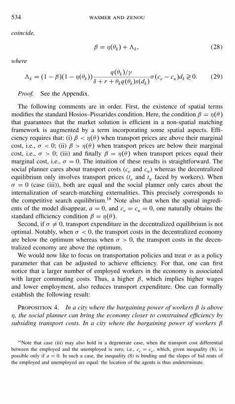
The following comments are in order. First, the existence of spatial termsmodifies the standard Hosios–Pissarides condition. Here, the condition β = η�θ�that guarantees that the market solution is efficient in a non-spatial matchingframework is augmented by a term incorporating some spatial aspects. Effi-ciency requires that: (i) β < η�θ� when transport prices are above their marginalcost, i.e., σ < 0; (ii) β > η�θ� when transport prices are below their marginalcost, i.e., σ > 0; (iii) and finally β = η�θ� when transport prices equal theirmarginal cost, i.e., σ = 0. The intuition of these results is straightforward. Thesocial planner cares about transport costs (ce and cu) whereas the decentralizedequilibrium only involves transport prices (te and tu faced by workers). Whenσ = 0 (case (iii)), both are equal and the social planner only cares about theinternalization of search-matching externalities. This precisely corresponds tothe competitive search equilibrium.16 Note also that when the spatial ingredi-ents of the model disappear, a = 0, and ce = cu = 0, one naturally obtains thestandard efficiency condition β = η�θ�.Second, if σ �= 0, transport expenditure in the decentralized equilibrium is not

optimal. Notably, when σ < 0, the transport costs in the decentralized economyare below the optimum whereas when σ > 0, the transport costs in the decen-tralized economy are above the optimum.We would now like to focus on transportation policies and treat σ as a policy

parameter that can be adjusted to achieve efficiency. For that, one can firstnotice that a larger number of employed workers in the economy is associatedwith larger commuting costs. Thus, a higher β, which implies higher wagesand lower employment, also reduces transport expenditure. One can formallyestablish the following result:

Proposition 4. In a city where the bargaining power of workers β is aboveη, the social planner can bring the economy closer to constrained efficiency bysubsiding transport costs. In a city where the bargaining power of workers β

16Note that case (iii) may also hold in a degenerate case, when the transport cost differentialbetween the employed and the unemployed is zero, i.e., ce = cu, which, given inequality (8), ispossible only if a = 0. In such a case, the inequality (8) is binding and the slopes of bid rents ofthe employed and unemployed are equal: the location of the agents is thus undeterminate.


is below η, the social planner can bring the economy closer from constrainedefficiency by taxing transport costs.

From this proposition, it is easy to see that, in the segregated city(Equilibrium 2), the policy influence of σ is much more important thanin the integrated city (Equilibrium 2). This deserves some more comments: thetype of the city has no impact on the sign of /k; it has, however, an impact onits magnitude. Notably, given that /k is proportional to dk , a policy interven-tion through σ will have much more impact in land market equilibrium 2 thanin land market equilibrium 1. Indeed, ceteris paribus,17 a change in σ wouldbe 1− u2/u1 more powerful in configuration 2, i.e., an order of magnitude of10 to 15 for a rate of unemployment between 6 and 10%. The reason is simplythat all the emphasis is put on the marginal worker located at the border dk .For the other workers, the rents’ differential adjusts so that their utility is thesame as the one reached by the marginal worker located in dk . The impact ofσ is thus much larger when the marginal worker has a longer commute. Theinterpretation is easy to figure out: to make an unemployed worker to accepta job, the firm has to partly compensate for transportation costs. In city 1 (theintegrated city), the unemployed are so close to jobs so that the compensa-tion is very small. In city 2 (the segregated city), we have exactly the oppositeresult: high distance to jobs implies that the compensation is very large. It fol-lows that any change in σ has a huge impact on wages and on the welfarecondition.18

Finally, it is easy to see that if the policymaker can subsidize and tax theemployed and the unemployed workers differently, then he/she would subsidizethe employed and tax the unemployed when β is larger than η, and tax theemployed and subsidize the unemployed when β is lower than η.19

To summarize, adding a spatial dimension in the standard matching modeldoes not change the efficiency results (i.e., the Hosios–Pissarides condition)but allows the government to implement transportation policies that can restoresocial efficiency.

17Of course, there are also second order effects of a change in σ on the equilibrium values ofθk . Throughout this discussion, we ignore them for clarity reasons.

18Observe that the policy recommendation on transport costs of the employed do not considertheir effect on search intensity since we have not made the search effort of workers endogenous, orvery indirectly, through location choices.

19In such a case, it is trivial to show that

/k = �1− β��1− η�θk��q�θk�/γ

δ + r + θkq�θk�s�dk��σece − σucu�dk,

where σe and σu are the “net” subsidy to transport costs of the employed and the unemployedworkers, respectively.


6. CONCLUDING COMMENTS

We would like to discuss some implications of our model for real-world cities.In fact, our two urban equilibria roughly correspond to the two typical types ofcities that one observes in the United States (see in particular Glaeser et al. [8]).The first ones, “new or edge cities,”20 are cities where most jobs are created inthe suburbs and where most unemployed (especially blacks) reside close to thecity center. The second ones, “old cities,”21 are cities where most jobs are stillcreated in the city center and where most unemployed (especially blacks) liveclose to jobs. Our integrated-city equilibrium (Equilibrium 1) corresponds to anold city since the unemployed reside close to jobs whereas our segregated-cityequilibrium (Equilibrium 2) corresponds to an edge city since the unemployedare far away from jobs. The distinction between the two types of cities maythus be quite crucial. In particular, our model predicts that the unemployedliving in cities in which they are poorly connected to jobs (“new cities”) shouldexperience worse labor-market outcomes than those residing in cities in whichthey have better spatial connections to jobs (“old cities”). However, our modelalso suggests that welfare differences between the two cities are not that largebecause of higher commuting costs of the employed.Our policy results suggested that transportation policies should differ from

one city to another. This is in accordance with Pugh [21] who categorizes dif-ferent metropolitan areas according to the severity of the mismatch between thelocation of jobs and residence. In particular, she advocates different transporta-tion policies depending on the degree of this mismatch. For instance, Atlanta (a“new city”) has been shown to present spatial features that are strongly consis-tent with the assumptions underlying the spatial mismatch hypothesis: a major-ity black central city, high rates of segregation, and high rates of entry-leveljob decentralization. By contrast, Chicago (an “old city”) has less spatial mis-match because of job opportunities within city limits. We have here a validationof Pugh’s insight. Indeed, as explained above, the marginal impact of trans-portation policies on efficiency crucially depends on which urban equilibriumprevails; it is much higher if it concerns a marginal worker located further awayfrom the center.To conclude, we call for a better modelling of the labor market structure

in urban equilibria. We believe that several other dimensions of the macroeco-nomic search literature could be investigated. In particular, incorporating labordiscrimination and/or endogenous job destruction through quits or technologi-cal shocks into our framework could lead to very interesting and policy relevantresults.

20New cities, like, e.g., Atlanta, Houston, Los Angeles, or Phoenix, are MSAs that did not rankin terms of population among the 12 largest MSAs in 1900, but do rank among them in 1990.

21“Old cities,” like, e.g., Boston, Chicago, New York, or Philadelphia, are MSAs which werealready among the 12 most populated agglomerations in 1900 and are still among them in 1990.


APPENDIX

Lemma A.1 (Labor demand). In the plane (θk, wk), the labor demand curve(19) is downward sloping. It cuts the axes at wk�θk = 0� = y and θk�wk = 0� =θ > 0 where θ is defined by the following equation: q�θ� = �r + δ�γ /y.

Proof. By differentiating (19) at constant uk , we obtain

∂wk

∂θk= �r + δ�γ q ′�θk�

q�θk�2< 0.

Then by using (19), we easily obtain

wk�θk = 0� = yk and θk�wk = 0� = θ > 0.

Lemma A.2 (Wage setting curves). Assume that both u1 and u2 are lessthan a half. Then, in the plane (θk, wk), k = 1, 2, the line defined for eachk by (22) is upward sloping. The line for k = 1 is steeper than for k = 2but the intercept in case k = 1 is lower than for k = 2. The intersection pointbetween these two lines is equal to

w = �1− β�[b + 1

a�te − tu�s0

]+ βy (30)

θ = 1− β

β

�te − tu�aγ

. (31)

Proof. Along (22) for k = 1, we have ∂w1/∂θ1 = β�s0 − au1�γ .22 Along(22), for k = 2, we have ∂w2/∂θ2 = β�s0 − a�1 − u2��γ . Then we have∂w1/∂θ1 > ∂w2/∂θ2 ⇔ u1 + u2 < 1. This is the realistic assumption statedin the lemma. The intercepts of (22) are calculated as

w1�θ1 = 0� = �1− β��b + �te − tu�u1� + βy

< w2�θ2 = 0� = �1− β��b + �te − tu��1− u2�� + βy

⇔ u1 + u2 < 1.

To find the intersection point, one has to solve (22)k=1 = (22)k=2.

22When we differentiate the wage wk with respect to θk , we hold uk fixed.


Proof of Proposition 2

Existence and Uniqueness

The proof is in two steps. First (i) we show that θ determines the uniquenessof the land market equilibrium. Then (ii) we show that, for a given land marketequilibrium, there is a unique equilibrium labor market �θ∗k , u∗k�. The combina-tion of the two elements shows the uniqueness of the market equilibrium.

(i) This follows immediately from Proposition 1 and the discussion justafter it.

(ii) We have two equations, (26) and (25), and two unknowns, θk anduk . Let us first study (26) in the plan (uk, θk). By differentiating Eq. (26), it iseasy to see that the relation between θk and uk is positive if and only if θk > θ

in Equilibrium 1 and θk < θ in Equilibrium 2. These inequalities are alwaysverified in each respective equilibrium (see above) so that ∂uk/∂θk > 0, ∀ k =1, 2. Moreover, it is easy to verify that the intercept of the curve correspondingto (26) is a finite positive value as long as y − b − �te − tu�dk�u = 0� > 0,which is the usual viability condition.

Let us now differentiate (25). We obtain

∂uk

∂θk= − �1− η�θk��θkq�θk�skuk

δ + θkq�θk��sk − aukξk�,

where η�θk� is the elasticity of q�θk� with respect to θk in equilibrium k = 1, 2and ξ1 = 1 (Equilibrium 1) and ξ2 = −1 (Equilibrium 2). In Equilibrium 2, thedenominator is clearly positive (since it reduces to δ + θ2q�θ2��s2 + au2� > 0),whereas in Equilibrium 1, a sufficient condition for a positive denominator iss0 − 3au/2 > 0. Since by construction, s�d� > 0 for all d ≤ 1, a sufficientcondition is 3u/2 < 1 or u < 2/3. Thus, except for parameters leading toan implausible large value of unemployment rate, ∂uk/∂θk < 0, ∀ k = 1, 2.Furthermore, since limθk→∞ θkq�θk� = +∞ and limθk→0 θkq�θk� = 0, it is easyto show that

limθk→∞

uk = 0 and limθk→0

uk = 1.

We have thus shown that the curve corresponding to (26) is upward slop-ing whereas the curve corresponding to (25) is downward sloping. Therefore,since the intercept of the curve corresponding to (26) has a finite positive valuewhereas the intercept of the curve corresponding to (25) has an infinite value,the market equilibrium exists and is unique.

Stability

We use the same argument as in Pissarides [19, Chap. 3, p. 47]; see graph3.2 for instance.


Proof of Proposition 3

The welfare function 'k is now given by

'k =∫ +∞

0e−rt

{ ∫employed

�y − cez�dz

+∫unemployed

�b − cuz�dz− γ θkskuk

}dt. (32)

The social planner chooses θk and uk that maximize (32) under the constraint(24). In this problem, the control variable is θk and the state variable is uk . Letλ be the co-state variable. The Hamiltonian is thus given by

H = e−rt��1− u1��y − cedk� + uk�b − cudk� − γ θkskuk +λk�δ�1− uk� − θkq�θk�sk uk�.

The Euler conditions are ∂H/∂θk = 0 and ∂H/∂uk = −λk . They are thus givenby

γ e−rt + λq�θk��1− η�θk�� = 0 (33)

{y − b − �ce − cu�dk +

∂dk

∂uk�uktu + �1− uk�te� + γ θk

[sk +

∂sk

∂ukuk

]}e−rt

+ λ

{δ + θkq�θk�

[sk +

∂sk

∂ukuk

]}= λk, (34)

where η�θk� = −q ′�θk�θk/q�θk�. Let us focus on the steady state equilibriumin which θk = 0. By differentiating (33), we easily obtain that λk = −rλk .

23 Byplugging this value and the value of λk from (33) in (34), and by observing thatsk + �∂sk/∂uk�uk = s�dk�, we obtain

y − b = γ

q�θk�[δ + r + θkq�θk�s�dk�η�θk�

1− η�θk�]+ �ce − cu�dk. (35)

In order to see if the private and social solutions coincide, we compare (26) and(35). It is easy to verify that the two solutions coincide if and only if

γ

q�θk�[δ + r + θkq�θk�s�dk�β

1− β

]+ �te − tu�dk

= γ

q�θk�[δ + r + θkq�θk�s�dk�η�θk�

1− η�θk�]+ �ce − cu�dk (36)

which leads to (28).

23The transversality condition is given by

limt→+∞

λk uk = 0

and is obviously verified.


REFERENCES

1. J. M. Barron and O. Gilley, Job search and vacancy contacts: Note, American Economic Review,71, 747–752 (1981).

2. D. G. Blanchflower and A. J. Oswald, “The Wage Curve,” MIT Press, Cambridge, MA(1994).

3. J. K. Brueckner, The structure of urban equilibria: A unified treatment of the Muth-Mills model,in “Handbook of Regional and Urban Economics” (E.S. Mills, Ed.), pp. 821–845, Elsevier,Amsterdam (1987).

4. R. Chirinko, An empirical investigation of the returns to search, American Economic Review,72, 498–501 (1982).

5. E. Coulson, D. Laing, and P. Wang, Spatial mismatch in search equilibrium, Journal of LaborEconomics, 19, 949–972 (2001).

6. D. M. Cutler and E. L. Glaeser, Are ghettos good or bad?, Quarterly Journal of Economics,112, 827–872 (1997).

7. M. Fujita, “Urban Economic Theory,” Cambridge Univ. Press, Cambridge, UK: (1989).8. E. L. Glaeser, M. Kahn, and J. Rappaport, “Why Do the Poor Live in Cities?,” NBER Working

Paper Ser. 7636 (2000).9. H. Holzer, The spatial mismatch hypothesis: What has the evidence shown?, Urban Studies,

28, 105–122 (1991).10. H. Holzer and J. Reaser, Black applicants, black employees, and urban labor market policy,

Journal of Urban Economics, 48, 365–387 (2000).11. A. Hosios, On the efficiency of matching and related models of search and unemployment,

Review of Economic Studies, 57, 279–298 (1990).12. K. R. Ihlanfeldt, Information on the spatial distribution of job opportunities within Metropolitan

Areas, Journal of Urban Economics, 41, 218–242 (1997).13. K. R. Ihlanfeldt and D. L. Sjoquist, The spatial mismatch hypothesis: A review of recent studies

and their implications for welfare reform, Housing Policy Debate, 9, 849–892 (1998).14. H. Jayet, Spatial search processes and spatial interaction: 1. Sequential search, intervening

opportunities, and spatial search equilibrium, Environment and Planning A, 22, 583–599(1990).

15. H. Jayet, Spatial search processes and spatial interaction: 2. Polarization, concentration, andspatial search equilibrium, Environment and Planning A, 22, 719–732 (1990).

16. J. F. Kain, Housing segregation, negro employment, and Metropolitan decentralization, Quar-terly Journal of Economics, 82, 175–197 (1968).

17. J. F. Kain, The spatial mismatch hypothesis: Three decades later, Housing Policy Debate, 3,371–460 (1992).

18. D. T. Mortensen and C. A. Pissarides, New developments in models of search in the labormarket, in “Handbook of Labor Economics” (D. Card and O. Ashenfelter, Eds.), Chap. 39,pp. 2567–2627, Elsevier, Amsterdam (1999).

19. C. A. Pissarides, “Equilibrium Unemployment Theory,” Oxford Univ. Press, Oxford (1990).20. C. A. Pissarides, “Equilibrium Unemployment Theory,” 2nd ed., MIT Press, Cambridge, MA

(2000).21. M. Pugh, “Barriers to Work: The Spatial Divide between Jobs and Welfare Recipients in

Metropolitan Areas,” The Brookings Institution, Washington, DC (1998).22. C. L. Rogers, Job search and unemployment duration: Implications for the spatial mismatch

hypothesis, Journal of Urban Economics, 42, 109–132 (1997).23. Y. Sato, Search theory and the wage curve, Economics Letters, 66, 93–98 (2000).24. J. Seater, Job search and vacancy contacts, American Economic Review, 69, 411–419 (1979).25. W. Simpson, “Urban Structure and the Labor Market. Worker Mobility, Commuting, and Under-

employment in Cities,” Clarendon, Oxford (1992).


26. T. E. Smith and Y. Zenou, “Spatial Mismatch, Search Effort and Workers’ Location,” unpub-lished manuscript, University of Southampton (2001).

27. S. Turner, Barriers to a better break: Employers discrimination and spatial mismatch inMetropolitan Detroit, Journal of Urban Affairs, 19, 123–141 (1997).

28. J. Van Ommeren, P. Rietveld, and P. Nijkamp, Commuting: in search of jobs and residences,Journal of Urban Economics, 42, 402–421 (1997).

29. E. Wasmer and Y. Zenou, “Equilibrium Urban Unemployment,” CEP Discussion Paper 368,London School of Economics (1997).

30. E. Wasmer and Y. Zenou, “Search, Space, and Efficiency,” IZA Discussion Paper Ser. 181,Bonn (2000).

31. C. H. Wheeler, Search, sorting, and urban agglomeration, Journal of Labor Economics, 19,879–899 (2001).

32. J. Zax and J. F. Kain, Moving to the suburbs: do relocating companies leave their black employ-ees behind?, Journal of Labor Economics, 14, 472–493 (1996).

33. Y. Zenou and T. E. Smith, Efficiency wages, involuntary unemployment and urban spatialstructure, Regional Science and Urban Economics, 25, 821–845 (1995).

34. Y. Zenou, “How Do Firms Redline Workers?,” unpublished manuscript, University ofSouthampton (2000).

Does City Structure Affect Job Search and Welfare?

Documents

Transcript of Does City Structure Affect Job Search and Welfare?