
Staggered wage setting with real wage relativities: Variations on a theme of Taylor
Upload
independentCategory
view
4download
0
School of Economics and Political Science,
Department of Economics
University of St. Gallen
Do Long-term Unemployed Workers
Benefit from Targeted Wage Subsidies
Benjamin Schünemann, Michael Lechner, Conny Wunsch
July 2011 Discussion Paper no. 2011-26

Editor: Martina Flockerzi
University of St. Gallen
School of Economics and Political Science
Department of Economics
Varnbüelstrasse 19
CH-9000 St. Gallen
Phone +41 71 224 23 25
Fax +41 71 224 31 35
Email [email protected]
Publisher:
Electronic Publication:
School of Economics and Political Science
Department of Economics
University of St. Gallen
Varnbüelstrasse 19
CH-9000 St. Gallen
Phone +41 71 224 23 25
Fax +41 71 224 31 35
http://www.seps.unisg.ch

Do Long-term Unemployed Workers Benefit
from Targeted Wage Subsidies1
Benjamin Schünemann, Michael Lechner, Conny Wunsch 2
Author’s address: Benjamin Schünemann
University of St.Gallen
Swiss Institute for Empirical Economic Research (SEW-HSG)
Varnbüelstrasse 14
CH-9000 St.Gallen Email [email protected]
Michael Lechner
University of St.Gallen
Swiss Institute for Empirical Economic Research (SEW-HSG)
Varnbüelstrasse 14
CH-9000 St.Gallen
Email [email protected]
Conny Wunsch
University of St.Gallen
Swiss Institute for Empirical Economic Research (SEW-HSG)
Varnbüelstrasse 14
CH-9000 St.Gallen
Email [email protected]
1 This project received financial support from the Institut für Arbeitsmarkt und Berufsforschung, IAB,
Nuremberg (contract 8104). We would like to thank Patrycja Scioch (IAB), and Darjusch Tafreschi (SEW, St.
Gallen) for their help in the early stages of data preparation. Comments are welcome. 2 Michael Lechner is a Research Associate of ZEW, Mannheim, and a Research Fellow of CEPR and PSI,
London, CES-Ifo, Munich, IZA, Bonn, and IAB, Nuremberg. Conny Wunsch is associated with CES-Ifo,
Munich, and IZA, Bonn.

Abstract
Wage subsidies are often suggested as a particularly effective policy to improve labor market
chances of economically disadvantaged groups. We empirically evaluate an employer-side
wage subsidy scheme targeted at the long-term unemployed in Germany. Based on program
regulations and a large data set we estimate the impact of program existence locally at the
eligibility threshold using an RDD framework in differences. The results suggest no significant
effect of the subsidy on exit rates out of unemployment or employment stability.
Employment rates up to three years after eligibility show no significant improvement. In
conclusion, our findings are in contrast to previous empirical results justifying such policies.
Keywords
Wage subsidy, Long-term unemployment, Regression discontinuity.
JEL Classification
J08, J23.
Introduction
I. Introduction
For many years wage subsidies have been and still are advocated as an effective tool within the measures of Active Labor Market Policy (ALMP) to reduce unemployment. This policy instrument became particularly popular in many OECD countries in the late 1980ʹs and 1990ʹs when the subsidies were designed to influence employment of specific target groups with potential disadvantages in the labor market (welfare recipients, youths, veterans etc.). The favorable view on its effects can easily be derived from a simple labor supply and demand framework ‐ lower labor costs (employer‐side subsidy) or higher take home earnings (employee‐side subsidy) should increase employment.1 Nevertheless, the actual impact depends largely on demand and supply elasticities making the assessment of the effectiveness of such a policy foremost an empirical issue according to Katz (1998). Furthermore, he argues that in markets with transaction costs or imperfect information the subsidy scheme should differ if policy makers intend to influence the search behavior of individuals (employee‐side subsidy) or the recruitment decision of firms (employer‐side subsidy).2 Thus, the large empirical literature on wage subsidies consists of studies examining the effect of employee‐side payments implemented mainly as tax credits for individual workers3 and analyses of the employer‐side subsidies. Subsidy programs targeting the long‐term unemployed are particularly prevalent in European countries, especially in Germany, due to persistently high long‐term unemployment rates from the late 1990ʹs up to today.
In this study we empirically evaluate an employer‐side wage subsidy targeted at individuals with at least 12 months of unemployment (the long‐term unemployed) in Germany in the years 2000‐2002. We investigate the effect of program eligibility on labor market outcomes. Using eligibility instead of actual take‐up allows to assess whether or not the existence of the program helps to improve labor market chances for the long‐term unemployed. In particular, we analyze whether being eligible to subsidy receipt increases transition rates from unemployment to employment and induces persistent employment for the target group. We exploit the eligibility
1 Theoretical contributions supporting the positive implications on the wage subsidy effects date back to the work by Kaldor (1936). More recent articles are e.g. Phelps (1994) or Snower (1994).
2 In his survey on the development of wage subsidy programs in the US Katz (1998) describes in more detail that e.g. in markets with wage rigidities or minimum wages employee‐side subsidies are more effective in increasing income while payments to employers rather result in more employment.
3 Prominent examples of the evaluation of such financial incentives are e.g. Meyer (1995, 1996). Liebman and Eissa (1996) or Eissa and Hoynes (2004) investigate the impact of the Earned Income Tax Credit in the US on labor supply. The Working Families Tax Credit in the UK is analyzed e.g. in Blundell and Hoynes (2001) or Duncan, Shepard, Brewer and Suárez (2006). Card and Hyslop (2005) assess the effectiveness of a wage subsidy experiment in Canada.
2
Introduction
threshold of the program to account for selection bias and use individuals close to eligibility as control group. Given the exceptionally rich and large administrative data we can estimate the effect locally at the threshold using a regression discontinuity design (RDD). Potential differences in unobserved motivation or search effort and the presence of other programs are likely to have differential impacts on labor market outcomes for eligibles and non‐eligibles contaminating the basic RDD estimates. Thus, in order to remove any of such time constant unobserved effects we use the RDD in differences instead of levels i.e. we estimate the difference of the local eligibility ‐ non‐eligibility comparison for time periods with and without the subsidy program.
Empirical studies such as Boockmann, Zwick, Ammermüller, and Maier (2007) or Huttunen, Pirttilä, and Uusitalo (2010) assess the effectiveness of employer‐side wage subsidies analyzing as well the impact of subsidy eligibility. They consider the integration supplement (Eingliederungszuschuss, EGZ) in Germany and a low‐wage subsidy in Finland, respectively. They exploit regulation changes to estimate the effects using a Difference‐in‐Differences (DiD) method.5 Both programs are however, targeted at the elderly6 and their analyses do not consider long‐term employment outcomes to assess the effect on job stability. Hamersma (2008) evaluates the effect of eligibility on employment rates for two US tax credit programs using quarterly data. The control group consists of ʺalmost eligibleʺ individuals which is similar to our approach. However, the target group of US welfare recipients is not comparable to the long‐term unemployed we consider and our much larger data with exact spell durations allows to obtain estimates much closer to the eligibility threshold.
Other studies on employer‐side wage subsidies mainly during the 1990s7 evaluate programs from the US and the UK that target the youth unemployed aged between 18‐24.8 Their findings point to mainly positive employment effects but none of these provides conclusions about the effects on the much broader group of long‐term unemployed. More recent evaluations such as Carling and Richardson (2004), Sianesi (2008), Jaenichen and Stephan (2007), Bernhard, Gartner, and Stephan (2008) or Neubäumer (2010) investigate the effect of actual participation in the subsidy program instead of eligibility. From a policy perspective this is a very different parameter as participation is a combined effect of receiving the subsidy and being
3
5 Huttunen et al. (2010) even apply a difference‐in‐difference‐in‐differences method to identify the effect given their specific program regulations.
6 In case of the EGZ the unemployed have to be 50‐55 or older and the Finish subsidy scheme requires workers to be older than 54 to be eligible.
7 Previous attempts to analyze wage subsidies are e.g. Perloff and Wachter (1979) or Burtless (1985). Those are less relevant for our evaluation as they investigate a general tax credit for firms for employment increases of more than 2 percent and a wage voucher which leads to negative employment effects for welfare recipients due to stigmatization, respectively.
8 Lorenz (1988), Hollenbeck and Willke (1991) and Katz (1998) are examples of the evaluation of the Targeted Jobs Tax Credit (TJTC) that exists from 1978 to 1994 in the US. Bell, Blundell, and van Reenen (1999) and van Reenen (2004) investigate the New Deal reforms starting in 1998 in the UK.
Do Long-term Unemployed Workers Benefit from Targeted Wage Subsidies?
employed. Finding an adequate comparison group to obtain the isolated effect of the subsidy in this context is rather difficult. Using unemployed individuals or training program participants as controls, as in the abovementioned studies, for a program that requires employment for participants, largely overestimates the effects. The estimates mainly capture the effect of gaining a job instead of just the incremental effect of receiving the subsidy. Thus, the 20‐35 and 40 percentage points increase in employment rates due to the subsidy suggested in Sianesi (2008) and Bernhard et al. (2008), respectively, occurs almost by construction.
In contrast to these large positive and significant effects obtained using participation as treatment, we find no impact of the existence of the subsidy program on employment outcomes. Subsidy availability does not improve the chances of long‐term unemployed to exit unemployment and their employment stability does not increase either. In conclusion, the results based on the eligibility approach do not support the justification of employer‐side wage subsidies obtained from related empirical studies.
The next section provides an overview of the economic environment in the years under consideration and describes the institutional settings in more detail. In Section III we give an overview of the data and define the sample before we explain the identification strategy and the estimation procedure in section IV. Section V contains the results of our analysis and section VI concludes.
II. Institutional Details and Economic Background
A. Active Labor Market Policies for the Long‐term Unemployed
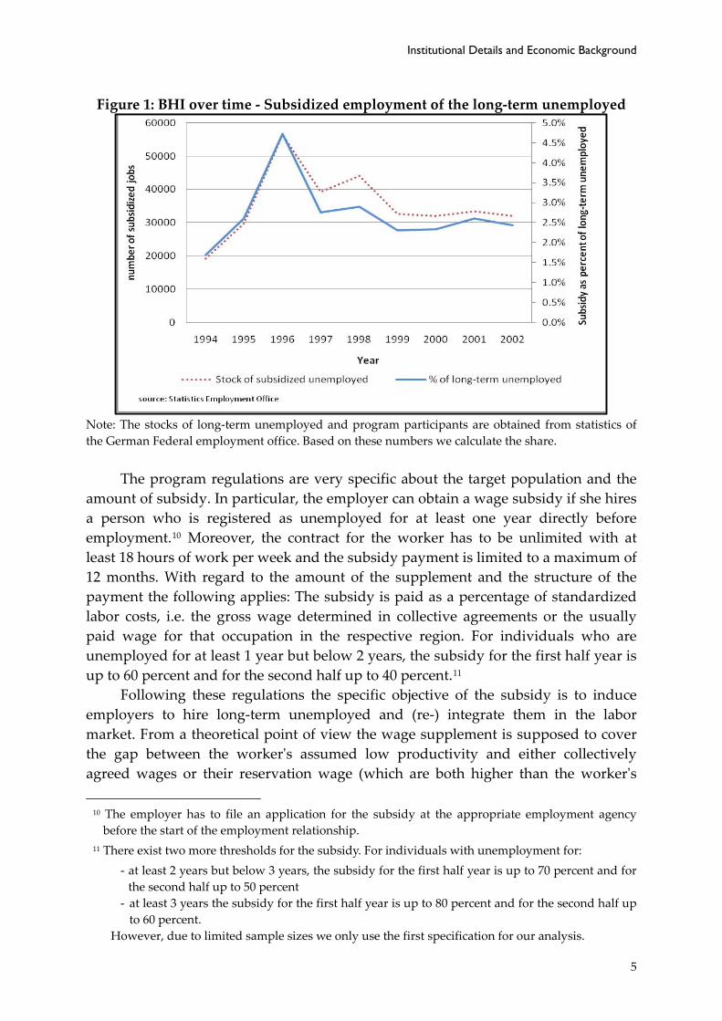
The wage subsidy program Our empirical analysis is based on a wage subsidy program (Beschäftigungshilfen für Langzeitarbeitslose, BHI) for long‐term unemployed individuals. It existed in Germany from 1989 until the end of 2002.9 During that time the number of subsidized employees increased significantly until 1996 about 4.5 percent of the long‐term unemployed participated in the program (Figure 1). Afterwards the number of participants declined from almost 60000 cases per year to around 30000 (about 2.5 percent of the long‐term unemployed) in 1997 remaining at that level until the program was phased out in 2003. Due to data limitations we focus on the years 2000 to 2002 for investigating program effects.
9 Initially the program started in 1989 and was prolonged several times ‐ in 1996 until the end of 1998 and in 1998 until the end of 2002. In 2003 there are no new entries but only previously accepted cases.
4
Institutional Details and Economic Background
Figure 1: BHI over time ‐ Subsidized employment of the long‐term unemployed
Note: The stocks of long‐term unemployed and program participants are obtained from statistics of the German Federal employment office. Based on these numbers we calculate the share.
The program regulations are very specific about the target population and the amount of subsidy. In particular, the employer can obtain a wage subsidy if she hires a person who is registered as unemployed for at least one year directly before employment.10 Moreover, the contract for the worker has to be unlimited with at least 18 hours of work per week and the subsidy payment is limited to a maximum of 12 months. With regard to the amount of the supplement and the structure of the payment the following applies: The subsidy is paid as a percentage of standardized labor costs, i.e. the gross wage determined in collective agreements or the usually paid wage for that occupation in the respective region. For individuals who are unemployed for at least 1 year but below 2 years, the subsidy for the first half year is up to 60 percent and for the second half up to 40 percent.11
Following these regulations the specific objective of the subsidy is to induce employers to hire long‐term unemployed and (re‐) integrate them in the labor market. From a theoretical point of view the wage supplement is supposed to cover the gap between the workerʹs assumed low productivity and either collectively agreed wages or their reservation wage (which are both higher than the workerʹs 10 The employer has to file an application for the subsidy at the appropriate employment agency before the start of the employment relationship.
11 There exist two more thresholds for the subsidy. For individuals with unemployment for: ‐ at least 2 years but below 3 years, the subsidy for the first half year is up to 70 percent and for the second half up to 50 percent ‐ at least 3 years the subsidy for the first half year is up to 80 percent and for the second half up to 60 percent.
However, due to limited sample sizes we only use the first specification for our analysis.
5
Do Long-term Unemployed Workers Benefit from Targeted Wage Subsidies?
productivity). During the subsidized period and on‐the‐job training workerʹs productivity is expected to increase such that unsubsidized wage payments are justified and stable employment is established. In general, those programs might not work accordingly or influence employment through other channels than expected. On the one hand, this refers to potential substitution or replacement effects triggered by the subsidy.12 Firms may change their recruitment behavior systematically substituting similar ineligible workers for the subsidized long‐term unemployed. It is also imaginable that they lay off workers in order to hire eligible individuals to reduce wage costs. Our data do not allow assessing these issues, i.e. the net effects of the subsidy. Finding positive effects at least for the target group would, however, be the first step in the program assessment. On the other hand, employers could try to claim the subsidy by firing and rehiring the worker or employ each program participant just for the subsidy period and hire a ʹnewʹ long‐term unemployed afterwards. The former issue is negligible considering that the time between layoff and rehiring would have to be one year. The latter can be excluded given that the program requires a post‐subsidy employment period of the length of the subsidized period.13 A final concern that we address in the present analysis refers to firms exploiting the program by hiring eligible individuals they would employ even without the subsidy.
Given the relatively generous payments the take‐up rate depicted in Figure 1 might seem too low and might raise doubts about the public information policy and the actual implementation. In that respect it is worth noting that the final subsidy receipt is not a legal entitlement. It is, at least partly, subject to the caseworkers discretion and simultaneously depends on the public employment officeʹs budget. This is distributed according to the regional prevalence of long‐term unemployment. Moreover, employers might just be ignorant about the program or still reluctant to employ long‐term unemployed workers. The relatively low take‐up rate and the abovementioned reasons, do not limit the potential to analyze the subsidyʹs effectiveness per se, though. The annual costs of the program in 2002 are about 290 million euro, i.e. about 10 percent of total spending for direct measures to integrate unemployed into regular employment (and about 1.3 percent of total spending of 22.4 billion on all ALMP measures in 2002).
12 Katz (1998) and Bell et al. (1999) describe these general concerns about the wage subsidy. 13 The employer has to pay back the subsidy or parts of it when laying off the program participant too early after subsidy payment ends. This does not apply if the layoff is due to inappropriate worker behavior or is justified with bad economic conditions for that specific firm.
6
Institutional Details and Economic Background
Other Active Labor Market Policies Many of the labor market programs14 in Germany are available also for the long‐term unemployed without any restrictions compared to short‐term unemployed. Thus, the labor supply decisions should not differ by unemployment duration because of different government sponsored programs and different eligibility criteria. Nevertheless, there are two programs, other than the BHI that might be relevant for potentially distinct incentives of the long‐term unemployed compared to short‐term unemployed. The so‐called job creation scheme (Arbeitsbeschaffungsmassnahmen, ABM)15 is available for individuals with at least 12 months of unemployment or if they are registered at the employment office for at least 6 months within the last 12 months before assignment to one ABM employer. This implies that 6 months of unemployment should suffice to be eligible. Thus, it does not influence incentives locally around 12 months of unemployment in the years 2000 and 2001. In 2002 the rules are relaxed even more allowing basically all unemployed to receive ABM. Another subsidy program prevalent in our evaluation period is the integration supplement (Eingliederungszuschuss, EGZ). It is designed to support various groups of hard‐to‐place individuals such as disabled, workers who need specific initial skill adaption training, elderly or the long‐term unemployed. Consequently, this program might impact the incentives around the 12‐month unemployment threshold differently, potentially contaminating a pure RDD approach. However, with regard to our identification strategy applied later on, it is worth noting that the regulations concerning the long‐term unemployed did not change in the years 2000‐2002.
B. The Unemployment Insurance System
Employer‐side wage subsidies are expected to influence labor demand. Nevertheless, for evaluating their effects individual employment decisions reflecting the supply side of the labor market need to be considered as well. One important policy in Germany affecting incentives and determining labor market behavior is the unemployment insurance system. It is necessary to understand how our later eligible and control groups are influenced by this system, especially if they encounter different impacts.
In the entire time period under consideration (2000‐2006) the unemployment insurance system provides benefits for all employees for a minimum of six months if they are employed for at least 12 months during three years before filing the claim.
14 Active labor market policy in Germany consists broadly of employment programs, training measures and job seeker assistance. In general, everyone who is registered unemployed and receives unemployment benefits (or unemployment assistance) is eligible for any of the programs (compare e.g. Wunsch and Lechner (2008) for an overview of ALMP in Germany).
15 The ABM program is a subsidy scheme paying between 30 to 100 percent of the salaries to selected ABM providers hiring an ABM eligible worker. Providers of the job creation scheme need to be approved by the German federal employment agency (Bundesagentur für Arbeit, BA) and need not be in competition with the market, i.e. they provide non‐market jobs.
7
Do Long-term Unemployed Workers Benefit from Targeted Wage Subsidies?
To receive benefits unemployed need to register with the public employment office. With an increasing contribution period, i.e. with a longer spell of insured employment, the duration of entitlement increases up to a maximum of 32 months of benefit payments if the person worked for 64 months and is older than 57. Crucial for our empirical strategy are individuals with 24 months of insured employment since they are entitled to 12 months unemployment benefits (UB) without any age restriction. The replacement rate for unemployed with at least one dependent child is 67 percent of their previous average net earnings from employment subject to social insurance. Without children it is 60 percent.
C. General Trends in the German Labor Market
The overall economic environment is a crucial factor influencing the employment chances of the (long‐term) unemployed and the effectiveness of the subsidy program, besides individual preferences and characteristics. Table 1 provides an overview of the economic development over our period of investigation (2000‐2006) based on three broad indicators. At the start of our sampling period real GDP growth is 3.2 percent in 2000, which is relatively high. However, at the end of 2000 the economy began to slow down and with September 11, 2001, and the world economic downturn a period of stagnation started. Growth rates dropped to 1.2 percent in 2001 and even ‐0.2 in 2003. In 2004 with the slow recovery of the world economy also Germanyʹs growth rates increased again to 1.2 percent in 2004 and 0.8 percent in 2005. The unemployment rate declined from 10.5 percent in 1999 to 9.4 in 2001 showing its lagged character with regard to the economyʹs growth rate. From 2002 onwards unemployment increased up to 11.7 percent in 2005 before it declines to 10.8 percent in 2006. Despite the relatively high growth rates in 2000 and 2006, the economic development was quite stable on a low level during the period under consideration. The unemployment rates are quite high and relatively stable for the years 2000 to 2002, which further supports our RDD in differences identification strategy (see section IV).
Table 1: GDP and unemployment rates for Germany 1999‐2006 1999 2000 2001 2002 2003 2004 2005 2006real GDP growth a) 2.0 3.2 1.2 0.0 ‐0.2 1.2 0.8 3.2 unemployment rates b) 10.5 9.6 9.4 9.8 10.5 10.5 11.7 10.8Note: All numbers are in percent. a) GDP at constant 2000 prices. b) Registered unemployment as percentage of civilian labor force. Source: Statistics Employment Office, Statistisches Bundesamt
The incidence of long‐term unemployment became increasingly persistent in
the mid to late 1990s. During the short economic recovery at the end of the 1990s and in 2000 the long‐term unemployment rates in Germany dropped slightly by about 4 percentage points to about 48 percent in 2002 according to Figure 2. However, after the economic downturn in 2001 to 2003 the rate increased again to an even higher
8
Data and Sample Definition
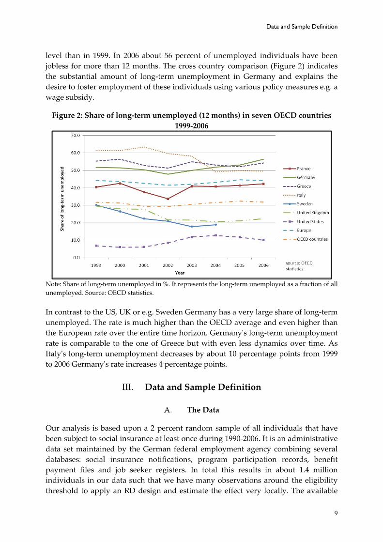
level than in 1999. In 2006 about 56 percent of unemployed individuals have been jobless for more than 12 months. The cross country comparison (Figure 2) indicates the substantial amount of long‐term unemployment in Germany and explains the desire to foster employment of these individuals using various policy measures e.g. a wage subsidy.
Figure 2: Share of long‐term unemployed (12 months) in seven OECD countries 1999‐2006
Note: Share of long‐term unemployed in %. It represents the long‐term unemployed as a fraction of all unemployed. Source: OECD statistics.
In contrast to the US, UK or e.g. Sweden Germany has a very large share of long‐term unemployed. The rate is much higher than the OECD average and even higher than the European rate over the entire time horizon. Germanyʹs long‐term unemployment rate is comparable to the one of Greece but with even less dynamics over time. As Italyʹs long‐term unemployment decreases by about 10 percentage points from 1999 to 2006 Germanyʹs rate increases 4 percentage points.
III. Data and Sample Definition
A. The Data
Our analysis is based upon a 2 percent random sample of all individuals that have been subject to social insurance at least once during 1990‐2006. It is an administrative data set maintained by the German federal employment agency combining several databases: social insurance notifications, program participation records, benefit payment files and job seeker registers. In total this results in about 1.4 million individuals in our data such that we have many observations around the eligibility threshold to apply an RD design and estimate the effect very locally. The available
9
Do Long-term Unemployed Workers Benefit from Targeted Wage Subsidies?
spell information allows the exact calculation of the duration of different labor market states such as employment and unemployment spells as well as program participation periods. An advantage in justifying our identification based on a control group close to the eligibility threshold is the availability of many socio‐demographic characteristics and the possibility to compute employment histories for at least 10 years for the individuals. Additionally, we can match regional economic data to each individual. With regard to the higher number of subsidy recipients in the mid 1990ʹs (compare Figure 1 in section II.A) it would be preferable to use that period for our investigation. However, given our differencing approach we use data from a period close before subsidy program termination avoiding that unobserved effects from other programs influencing our comparison groups change over time.
B. The Evaluation Sample
Given the general database described above we select all individuals entering unemployment16 between April 2000 and December 2002. We start in April 2000 and not earlier due to missing information and potential underreporting of job‐seeker spells in the first months of 2000. Our evaluation sample ends in December 2002 such that we could obtain at least 3 years of outcome for all individuals after eligibility (remember that individuals are eligible for the subsidy only after 1 year in unemployment). Note, that individuals becoming unemployed in 2002 can become eligible only at the beginning of 2003, when the subsidy program does not exist anymore. We use this part of our sample for the time difference in the effects at the eligibility threshold as eligibles from 2002 cannot actually receive the subsidy. In order to obtain a homogeneous sample that describes a rather typical unemployed we impose further conditions. We exclude individuals who participated in a program or who were unemployed for at least 2 weeks during 1 year before entry to ensure that the entry is not just a short interruption of a previous unemployment spell. Furthermore, we only consider unemployed with an UB claim and at least 6 months of employment during the last year before entry. The latter condition ensures that any person with 12 months unemployment duration is eligible for the subsidy.17 More details on further restrictions we impose on the sample with regard to our eligible and control groups and to obtain credible identification will be given in the next part.
16 We select individuals that enter from unsubsidized employment or general non‐unemployment e.g. out of labor force.
17 To calculate the unemployment duration that determines eligibility the rules of the subsidy program allow short disruptions of the unemployment spell within 5 years prior to eligibility e.g. 6 months of employment. To avoid complex structures of unemployment‐employment spells resulting in unreasonable cases in our sample we require at least 6 months of employment before entry.
10

Evaluation Problem and Empirical Strategy
IV. Evaluation Problem and Empirical Strategy
A. The empirical evaluation problem
The empirical question we intend to answer is motivated by the policy objective of the subsidy program: Does the existence of temporary employer‐side wage subsidies targeted at the long‐term unemployed improve their employment chances and induce stable employment after the subsidy period ends? In that sense we investigate the impact of program existence compared to the counterfactual situation of non‐existence of the wage subsidy.
Establishing a convincing causal relationship between the subsidy and employment outcomes is, however, rather complicated and driven by two main difficulties. Firstly, it crucially depends on treatment definition and the related choice of a control group that needs to approximate the counterfactual situation for the treated appropriately. Using actual program participation as treatment describes the impact of the subsidy as the combined effect of gaining the job and gaining the subsidy since all participants are necessarily employed. The underlying policy question based on this definition is not obvious and finding a good comparison group is an intricate task. A general group of non‐participants (individuals remaining unemployed) does not reflect the counterfactual situation adequately resulting in largely overestimated employment effects attributed to the subsidy.18 Defining subsidy eligibility as treatment, instead, allows considering the impact of the subsidy without the effect of gaining the job. In particular, this treatment definition facilitates the investigation of the tradeoff ʺexistence of the subsidyʺ versus ʺnon‐existence of the subsidyʺ which should be the most relevant one from a policy perspective. The second difficulty, as in most non‐experimental program evaluation studies, arises since selection into program is not random. In contrast to other ALMP measures such as training programs or jobseeker assistance, the assignment process for the wage subsidy involves three parties: the caseworker, the unemployed, and the employer. Since all of them have an influence also on outcomes one would ideally like to control for these variables and thus eliminate the likely selection bias. Our data, however, does not provide sufficient relevant information on program assignment. For instance, it is not known who initiated the process ‐ did the caseworker and/or the unemployed contact the firm or did the firm and the unemployed agree and contact the caseworker afterwards. Furthermore, the extent of discretion of the caseworker or the particular rules the caseworker based her decision on is not observable. In conclusion, we will focus on an identification strategy, explained in more detail in the next section, that does rely only partly on observable 18 If interest is in actual program participation (as usually done in many ALMP evaluation studies) credible identification requires solving the so‐called double selection problem described in papers such as Lee (2009) or Lechner and Melly (2010) i.e. selection into program and selection into employment. Neglecting this issue would result in biased estimates. This problem remains even if the control group is chosen as unemployed workers who find employment without the subsidy.
11
Do Long-term Unemployed Workers Benefit from Targeted Wage Subsidies?
characteristics to control for selection bias and helps to obtain a credible control group.
B. Identification Strategy
In order to identify the effect of eligibility appropriately and avoid the aforementioned problems we use an RD design initially introduced by Thistlethwaite and Campbell (1960). In particular, we apply RDD in differences instead of levels to account for discontinuities in potential outcomes around the eligibility threshold due to unobservable factors and the existence of other programs. This approach is similar to a local version of the DiD method outlined e.g. in Angrist and Krueger (1999). As abovementioned we define treatment as ʺbeing eligible for the subsidyʺ, i.e. being unemployed for at least 12 months and our outcomes are exit rates out of unemployment and employment stability. The implementation is as follows.
Based on program regulations we use unemployment duration as an observable pre‐intervention variable that changes the eligibility probability in a deterministic way discontinuously at the 12‐month threshold. In our case this refers to a sharp RDD as the probability of eligibility jumps from 0 to 1.19 Comparing individuals close to the threshold allows arguing that treatment assignment (i.e. staying unemployed for at least 12 months) is as if random. Becoming eligible is not related to any non‐ignorable (i.e. influencing potential outcomes) characteristic other than the forcing variable, unemployment duration, and thus, we claim to account for the unobservable assignment process. Eventually, this implies that the unemployed with a duration of less than 12 months and close to the threshold describe the counterfactual situation of non‐existence of the wage subsidy program (control group). The group of eligibles in particular comprises all individuals with at least 12 months unemployment, whereas the control group consists of all unemployed with at least 11 months unemployment duration. The above reasoning relies crucially on the assumption of local continuity in potential outcomes. If it holds, i.e. if the mean potential outcome is a continuous function of unemployment duration, at the threshold we can obtain the counterfactual outcome for the eligibles using the observed outcome of the control group. Remaining unobserved factors that might invalidate this assumption are related to labor market programs existent and unchanged between 2000 and 2002, and available for unemployed just above the threshold such as the integration supplement EGZ (see section II.A). It may also include different unobserved motivation or (search) effort of the unemployed or caseworker just below and above the threshold, or the mere difference in unemployment duration. To account for these factors and their potentially differential impact on eligible and control group we apply the initial RDD approach
19 For a more detailed overview of this method and its assumptions compare Hahn, Todd and van der Klaauw (2001), Imbens and Lemieux (2008), or van der Klaauw (2008). We use the definitions and assumptions according to these articles.
12
Evaluation Problem and Empirical Strategy
in an additional period when the subsidy program is not present anymore. We do that for entries into unemployment in 2002 as they cannot receive the subsidy once they become eligible at the beginning of 2003. Conditional on the validity of the common trend assumption20 estimating the eligibility‐control comparison in this time period and subtracting it from the initial estimates will remove the remaining bias in the average effect of subsidy availability. In particular, the assumption requires that the aforementioned unobserved factors have the same impact on the expected (potential) outcomes over time, i.e. they are independent of becoming eligible. Combining these two methods leads to what can be called an RDD in differences. Our parameter of interest, the average effect of subsidy existences on the eligibles at the threshold for the time period 2000‐2001, can be obtained if both assumptions hold. Local continuity allows controlling for program selection bias in the subsidy period (2000‐2001) and the common trend permits removing additional bias from time constant unobserved effects that are different for subsidy eligibles and controls. In other words, the identification requires local continuity in differences to approximate the unobserved counterfactual outcome for the eligibles.21
For the described assumption to hold, there should not be any observable or unobservable factor that influence the labor supply decision (to exit unemployment or employment stability) differently at the threshold unless their effects are constant over time. One factor questioning the assumption could be an early retirement program existent in Germany allowing older workers to retire at age 60 if they are unemployed for one year. We exclude elderly unemployed (older than 59) from our sample such that a difference in outcomes would not be due to that program.22 Another difficulty arises due to the unemployment insurance system. Individuals with exactly 12 months UB claim might exit just after benefit exhaustion, which is easily understandable from an incentive point of view ‐ higher search effort once benefit payments end. We account for this effect by excluding from our entire sample all individuals with exactly 12 months claim (measured at the beginning of the unemployment spell). Based on this modified sample we investigate observable characteristics available in our data that are prone to influence program eligibility (i.e. staying in unemployment) as well as exit rates and future employment duration. Figure 3 depicts the differences in means between 2000‐2001 and 2002 by unemployment duration for some selected characteristics.23 Note that unemployment duration on the abscissa refers to a minimum criterion: e.g. 6 months unemployment duration includes all individuals jobless for at least 6 months. A jump in the mean 20 This assumption is extensively explained in various contributions to the literature such as e.g. Angrist and Pischke, 2009, Blundell and Costa Dias, 2009, and Imbens and Wooldridge, 2009.
21 A formal representation of the assumption as well as the identification of the effect is presented in the Appendix.
22 The changing regulations for that program in 2003 additionally require the exclusion of elderly unemployed.
23 The separate means for 2000‐2001 and 2002 are shown in Figure A. 1 in the Appendix to get an idea about their magnitude.
13

Do Long-term Unemployed Workers Benefit from Targeted Wage Subsidies?
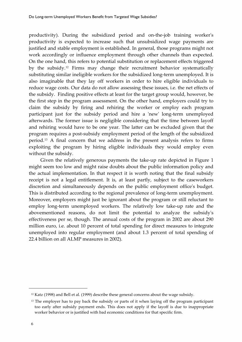
differences of these confounders at the cut‐off point would indicate selectivity of eligibles and control that is different over time. Estimated outcome differences could then just be related to the respective individual characteristics instead of the subsidy program. As an example consider the time difference in the share of unemployed with no vocational training. This difference is never significantly different from zero and it seems to be continuous in unemployment duration especially at the threshold.24 All other covariates in Figure 3 follow a similar pattern. In fact, computing the time difference of other available observable characteristics just below and above the threshold results in similar conclusions (see Table A. 1 in the Appendix). Even though the table shows some significant differences in means over time, those differences are similar above and below the threshold. Accordingly, the local continuity in differences does not rely on additional conditioning on observable characteristics and potential outcomes are likely to be locally continuous in differences as well.
Figure 3: Differences in means between 2000‐2001 and 2002 by unemployment duration for some select s ed characteristic
Note: The graphs are obtained using samples defined by unemployment duration, i.e. we select individuals with at least e.g. 9 months of unemployment separately for entries in 2000‐2001 (T=1) and 2002 (T=0). For each of these sample we difference the means of the covariates over time.
-.04
-.02
0.0
2.0
4di
ffere
nce
in m
eans
6 9 12 15 18unemployment duration
no vocational training vocational traininguniversity degree 10y history fraction employed
y p y
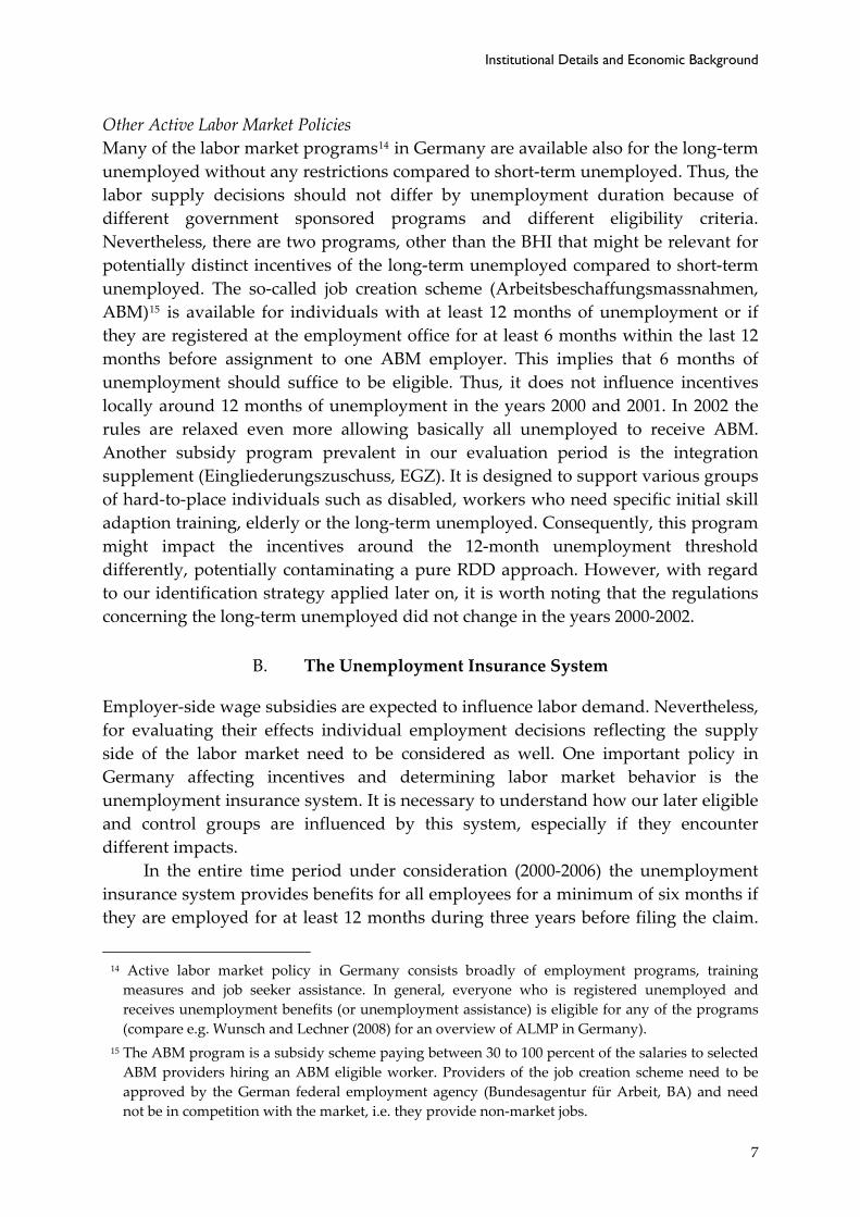
Additional concerns with the RDD part of our identification strategy might be manipulation of the threshold (getting the subsidy before 12 months of unemployment) or anticipation effects (ʹwaiting in unemploymentʹ until eligibility is achieved). The regulations of the program do not leave much room for manipulation and our data shows that about 93 percent of actual participants comply with the rules i.e. they receive the subsidy earliest after 12 months in unemployment (see
24 We do not depict the confidence bands here for the sake of clarity but all of them include zero over the entire range of unemployment duration in the graph.
14
Evaluation Problem and Empirical Strategy
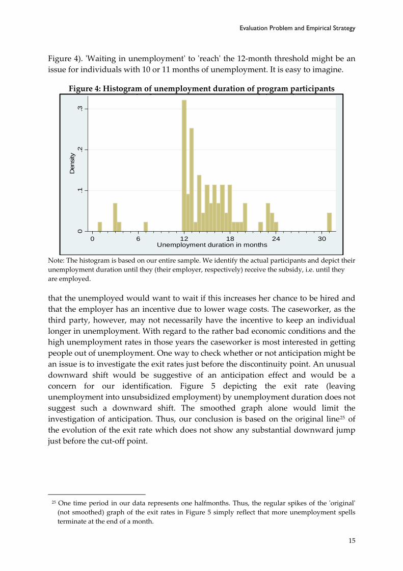
Figure 4). ʹWaiting in unemploymentʹ to ʹreachʹ the 12‐month threshold might be an issue for individuals with 10 or 11 months of unemployment. It is easy to imagine.
Figure 4: Histogram employment duration of p m participants
of un rogra
Note: The histogram is based on our entire sample. We identify the actual participants and depict their unemployment duration until they (their employer, respectively) receive the subsidy, i.e. until they are employed.
0.1
.2.3
Den
sity
0 6 12 18 24 30Unemployment duration in months
p y y p p
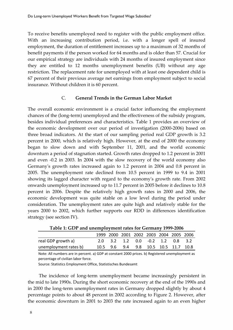
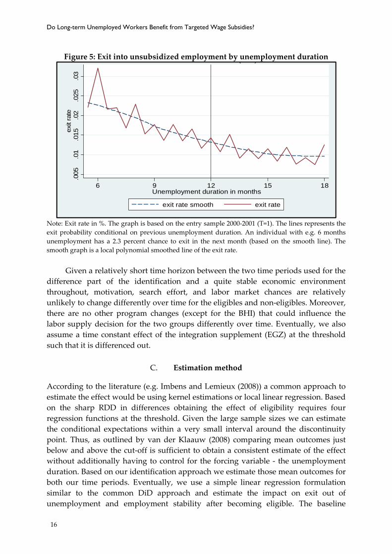
that the unemployed would want to wait if this increases her chance to be hired and that the employer has an incentive due to lower wage costs. The caseworker, as the third party, however, may not necessarily have the incentive to keep an individual longer in unemployment. With regard to the rather bad economic conditions and the high unemployment rates in those years the caseworker is most interested in getting people out of unemployment. One way to check whether or not anticipation might be an issue is to investigate the exit rates just before the discontinuity point. An unusual downward shift would be suggestive of an anticipation effect and would be a concern for our identification. Figure 5 depicting the exit rate (leaving unemployment into unsubsidized employment) by unemployment duration does not suggest such a downward shift. The smoothed graph alone would limit the investigation of anticipation. Thus, our conclusion is based on the original line25 of the evolution of the exit rate which does not show any substantial downward jump just before the cut‐off point.
25 One time period in our data represents one halfmonths. Thus, the regular spikes of the ʹoriginalʹ (not smoothed) graph of the exit rates in Figure 5 simply reflect that more unemployment spells terminate at the end of a month.
15
Do Long-term Unemployed Workers Benefit from Targeted Wage Subsidies?
Figure 5: Exit into unsubsidized employment by yment duration unemplo
Note: Exit rate in %. The graph is based on the entry sample 2000‐2001 (T=1). The lines represents the exit probability conditional on previous unemployment duration. An individual with e.g. 6 months unemployment has a 2.3 percent chance to exit in the next month (based on the smooth line). The smooth graph is a local polynomial smoothed line of the exit rate.
.005
.01
.015
.02
.025
.03
exit
rate
6 9 12 15 18Unemployment duration in months
exit rate smooth exit rate
( )
Given a relatively short time horizon between the two time periods used for the
difference part of the identification and a quite stable economic environment throughout, motivation, search effort, and labor market chances are relatively unlikely to change differently over time for the eligibles and non‐eligibles. Moreover, there are no other program changes (except for the BHI) that could influence the labor supply decision for the two groups differently over time. Eventually, we also assume a time constant effect of the integration supplement (EGZ) at the threshold such that it is differenced out.
C. Estimation method
According to the literature (e.g. Imbens and Lemieux (2008)) a common approach to estimate the effect would be using kernel estimations or local linear regression. Based on the sharp RDD in differences obtaining the effect of eligibility requires four regression functions at the threshold. Given the large sample sizes we can estimate the conditional expectations within a very small interval around the discontinuity point. Thus, as outlined by van der Klaauw (2008) comparing mean outcomes just below and above the cut‐off is sufficient to obtain a consistent estimate of the effect without additionally having to control for the forcing variable ‐ the unemployment duration. Based on our identification approach we estimate those mean outcomes for both our time periods. Eventually, we use a simple linear regression formulation similar to the common DiD approach and estimate the impact on exit out of unemployment and employment stability after becoming eligible. The baseline
16
Results
estimation equation includes a time dummy capturing any outcome difference due to the two entry‐time periods and a group dummy that captures the effect of being long‐term unemployed. In addition, to obtain the effect of interest, i.e. the impact of subsidy existence for the long‐term unemployed entering unemployment from 2000‐2001 we include the interaction term between group and time dummy. Finally, the constant represents the mean outcome for individuals with at least 11 months of unemployment entering in 2002.
As discussed in the previous section we do not need to control for any observable characteristics in the baseline estimations as they do not seem to be the source for potentially biased estimates. Accordingly we avoid problems that might arises due to functional form assumptions or issues of effect heterogeneity when including covariates in a linear way. Since our main outcomes are defined as binary variables (1=exit into employment, 0 otherwise) a probit specification of the model might be more appropriate. However, this would not yield different results as the model is fully saturated locally around the threshold.
V. Results
A. Outcome definition and the average effects of eligibility
As previously mentioned and according to the program objective we measure the impact of the wage subsidy using exit rates out of unemployment as well as employment stability over time. In particular, we consider as the first outcome the probability to leave unemployment (exit rate). This outcome is measured in two ways: (1) exit into unsubsidized employment (1 if exit, 0 otherwise) and (2) exit into regular employment (includes subsidized employment). Thus, we estimate the average effect by the mean differences in exit rates of individuals with at least 11 months unemployment duration and the ones with at least 12 months of unemployment duration.26 We use a symmetric window of one month around the identification threshold. The second outcome, employment stability, is measured by employment rates (unsubsidized employment) over a time horizon of 3 years after becoming eligible for the subsidy.
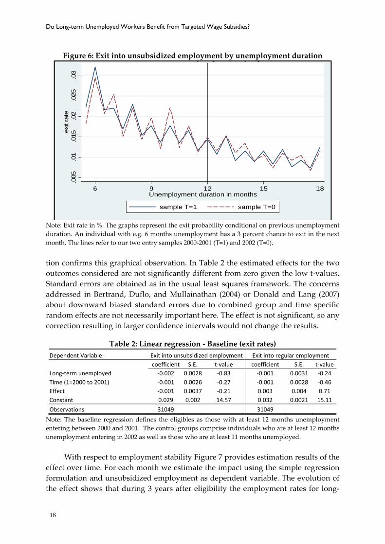
Figure 6 shows graphically the evolution of exit rates out of unemployment for the 4 comparison groups defined by the threshold and the two time periods. The differences of the exit rates at the threshold are very similar for T=1 and T=0 indicating a small impact of the subsidy if any. Using the linear regression formula‐
26 The outcome represents the probability to exit in a certain month conditional on having been unemployed until then. It is calculated using a survivor function approach (see Jenkins (2004)) as number of individuals leaving unemployment in a specific month as a share of all that are unemployed until then. E.g. how many individuals leave unemployment between 11 and 12 months, and between 12 and 13 months are the outcomes just below and above the threshold.
17
Do Long-term Unemployed Workers Benefit from Targeted Wage Subsidies?
Figure 6: Exit into unsubsidized emplo y unemployment duration yment b
Note: Exit rate in %. The graphs represent the exit probability conditional on previous unemployment duration. An individual with e.g. 6 months unemployment has a 3 percent chance to exit in the next month. The lines refer to our two entry samples 2000‐2001 (T=1) and 2002 (T=0).
.005
.01
.015
.02
.025
.0ex
it ra
te3
6 9 12 15 18Unemployment duration in months
sample T=1 sample T=0
p y p y
tion confirms this graphical observation. In Table 2 the estimated effects for the two outcomes considered are not significantly different from zero given the low t‐values. Standard errors are obtained as in the usual least squares framework. The concerns addressed in Bertrand, Duflo, and Mullainathan (2004) or Donald and Lang (2007) about downward biased standard errors due to combined group and time specific random effects are not necessarily important here. The effect is not significant, so any correction resulting in larger confidence intervals would not change the results.
Table 2: Linear regression ‐ Baseline (exit rates) Dependent Variable: Exit into unsubsidized employment Exit into regular employment
coefficient S.E. t‐value coefficient S.E. t‐valueLong‐term unemployed ‐0.002 0.0028 ‐0.83 ‐0.001 0.0031 ‐0.24 Time (1=2000 to 2001) ‐0.001 0.0026 ‐0.27 ‐0.001 0.0028 ‐0.46 Effect ‐0.001 0.0037 ‐0.21 0.003 0.004 0.71 Constant 0.029 0.002 14.57 0.032 0.0021 15.11
Observations 31049 31049
Note: The baseline regression defines the eligibles as those with at least 12 months unemployment entering between 2000 and 2001. The control groups comprise individuals who are at least 12 months unemployment entering in 2002 as well as those who are at least 11 months unemployed.
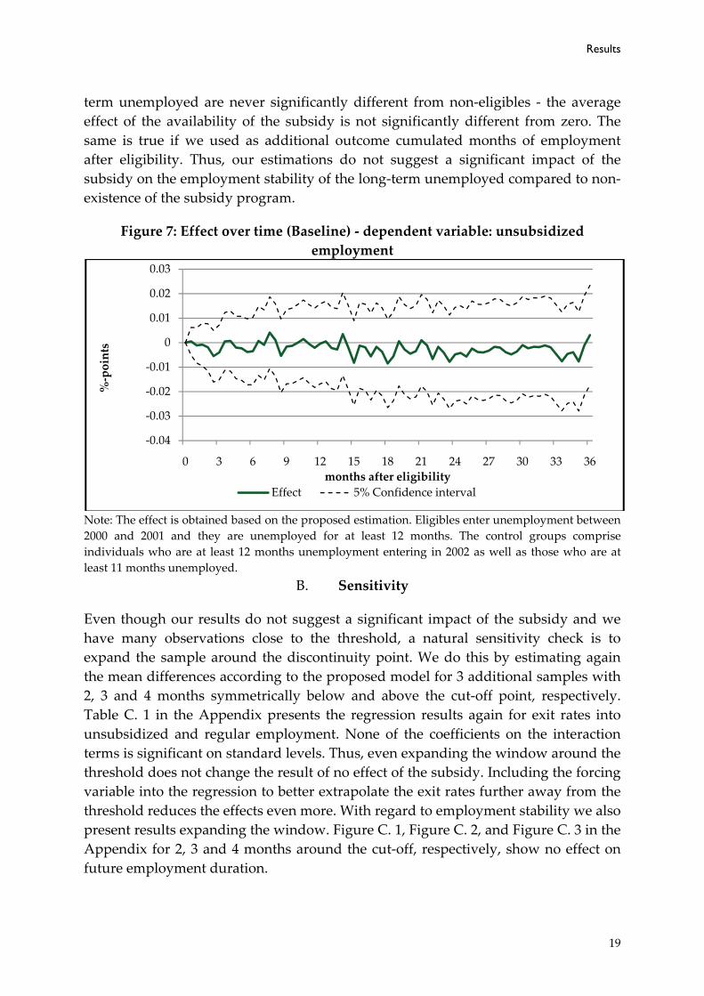
With respect to employment stability Figure 7 provides estimation results of the
effect over time. For each month we estimate the impact using the simple regression formulation and unsubsidized employment as dependent variable. The evolution of the effect shows that during 3 years after eligibility the employment rates for long‐
18
Results
term unemployed are never significantly different from non‐eligibles ‐ the average effect of the availability of the subsidy is not significantly different from zero. The same is true if we used as additional outcome cumulated months of employment after eligibility. Thus, our estimations do not suggest a significant impact of the subsidy on the employment stability of the long‐term unemployed compared to non‐existence of the subsidy program.
Figure 7: Effect over time (Baseline) ‐ dependent variable: unsubsidized employment
Note: The effect is obtained based on the proposed estimation. Eligibles enter unemployment between 2000 and 2001 and they are unemployed for at least 12 months. The control groups comprise individuals who are at least 12 months unemployment entering in 2002 as well as those who are at least 11 months unemployed.
‐0.04
‐0.03
‐0.02
‐0.01
0
0.01
0.02
0.03
0 3 6 9 12 15 18 21 24 27 30 33 36
%‐points
months after eligibilityEffect 5% Confidence interval
B. Sensitivity
Even though our results do not suggest a significant impact of the subsidy and we have many observations close to the threshold, a natural sensitivity check is to expand the sample around the discontinuity point. We do this by estimating again the mean differences according to the proposed model for 3 additional samples with 2, 3 and 4 months symmetrically below and above the cut‐off point, respectively. Table C. 1 in the Appendix presents the regression results again for exit rates into unsubsidized and regular employment. None of the coefficients on the interaction terms is significant on standard levels. Thus, even expanding the window around the threshold does not change the result of no effect of the subsidy. Including the forcing variable into the regression to better extrapolate the exit rates further away from the threshold reduces the effects even more. With regard to employment stability we also present results expanding the window. Figure C. 1, Figure C. 2, and Figure C. 3 in the Appendix for 2, 3 and 4 months around the cut‐off, respectively, show no effect on future employment duration.
19
Do Long-term Unemployed Workers Benefit from Targeted Wage Subsidies?
20
VI. Conclusion
In this study, we investigate an employer‐side wage subsidy targeted at the long‐term unemployed in Germany. The programʹs objective is to increase exit rates from unemployment to employment and to induce stable employment relationships for the economically disadvantaged target group. Using a large administrative data we assess the effectiveness of the program by estimating the impact of subsidy eligibility on employment outcomes.
We exploit the eligibility criterion of the program in conjunction with an RDD approach to investigate whether or not the availability of the subsidy is beneficial for the target group. Individuals just below the 12‐month unemployment threshold are used as control group reflecting the hypothetical situation of non‐existence of the government support. Given our large sample sizes around the cut‐off point we can estimate the effect locally and obtain new results on subsidy effectiveness. We do not find any significant impact on employment outcomes. The possibility for firms to reduce wage cost by hiring preferably the long‐term unemployed does not affect their exit rates out of unemployment. Furthermore, we find no substantial improvement on employment stability for those individuals due to the subsidy program.
Our findings are in contrast to the previous empirical literature on employer‐side wage subsidies. These studies mainly suggest rather large positive effects of actual program participation which have been used as the main empirical justification of such policies. However, these studies are unable to separate the effect of finding employment from the incremental effect of the wage subsidy. By focusing on eligibility rather than actual receipt of the subsidy we avoid this problem and obtain results that are not supportive for those ALMP.
In order to better understand how employer‐side wage subsidies work it would be helpful to know the actual assignment process in more detail. If for instance, the reasons of the caseworker to allocate individuals to the program or of firms to hire long‐term unemployed with the subsidy were observable, one could systematically correct for selection bias by a selection‐on‐observable strategy. Nevertheless, even in this case disentangling employment and subsidy effect remains the major challenge.
References
Angrist, J. D., and A. B. Krueger (1999): “Empirical strategies in labor economics,” Handbook of Labor Economics, 3, 1277–1366.
Angrist, J. D., and J.‐S. Pischke (2009): Mostly Harmless Econometrics: An Empiricist’s Companion. New York: Princeton University Press.
Bell, B., R. Blundell, and J. Van Reenen (1999): “Getting the Unemployed back to Work: The Role of Targeted Wage Subsidies,” International Tax and Public Finance, 6, 339–360.
References
Bernhard, S., H. Gartner, and G. Stephan (2008): “Wage subsidies for needy job‐seekers and their effect on individual labour market outcomes after the German reforms,” IAB Discussion Paper.
Bertrand, M., E. Duflo, and S. Mullainathan (2004): “How much should we trust differences‐in‐differences estimates?” Quarterly Journal of Economics, 249–275.
Blundell, R., and M. Costa Dias (2009): “Alternative Approaches to Evaluation in Empirical Microeconomics,” The Journal of Human Resources, 44.
Blundell, R., and H. W. Hoynes (2001): “Has ʺIn‐Workʺ Benefit Reform Helped the Labour Market?,” NBER Working Paper Series.
Boockmann, B., T. Zwick, A. Ammermüller, and M. Maier (2007): “Do hiring subsidies reduce unemployment among the elderly? Evidence from two natural experiments,” ZEW Working paper.
Burtless, G. (1985): “Are Targeted Wage Subsidies armful? Evidence from a Wage Voucher Experiment,” Industrial and Labor Relations Review, 39, 05–114.
H 1
Card, D., and D. R. Hyslop (2005): “Estimating the e cts of a time‐limited earnings subsidy for welfare‐leavers,” Econometrica, 73, 1723–1770.
ffe
Carling, K., and K. Richardson (2004): “The relative efficiency of labor market programs: Swedish experience from the 1990s,” Labour Economics, 11, 335 – 354.
Donald, S. G., and K. Lang (2007): “Inference with Difference‐in‐Differences and other Panel Data,” The Review of Economics and Statistics, 89, 221–233.
Duncan, A., A. Shephard, M. Brewer, and M. J. Suárez (2006): “Did working families’ tax credit work? The impact of in‐work support on labour supply in Great Britain,” Labour Economics, 13, 699–720.
Eissa, N., and H. W. Hoynes (2004): “Taxes and the labor market participation of married couple the earned income tax credit,” Journal of Public Economics, 88, 1931–1958.
s:
Hahn, J., P. Todd, and W. va Der Klaauw (2001): “Identification and estimation of treatment effects with a regression‐disconti uity design,” Econometrica, 69, 201–209.
nn
Hamersma, S. (2008): “The effects of an employer subsidy on employment outcomes: A study of the work opportunity and welfare‐to‐work tax credits,” Journal of Policy Analysis and Management, 27, 498–520.
Hollenbeck, K. M., and R. J. Willke (1991): “The Employment and Earnings Impacts of the Targeted Jobs Tax Credit,” W.E. Upjohn Institute for Employment Research.
Huttunen, K., J. Pirttilä, and R. Uusitalo (2010): “The Employment Effects of Low‐Wage Subsidies,” IZA Discussion Paper, (4931).
Imbens, G. W., and T. Lemieux (2008): “Regression discontinuity designs: A guide to practice,” Journal of Econometrics, 142, 615–635.
Imbens, G. W., and J. M. Wooldridge (2009): “Recent Developments in the Econometrics of Program Evaluation,” Journal of Economic Literature , 5–86. , 47
Jaenichen, U., and G. Stephan (2007): “The Effectiveness of Targeted Wage Subsidies for Hard‐to‐place Workers,” IAB Discussion Paper.
Jenkins, S. P. (2004): “Survival Analysis,” Unpublished Manuscript, Institute for Social and Economic Research, University of Essex.
Kaldor, N. (1936): “Wage Subsidies as a Remedy for Unemployment,” The Journal of Political Economy, 44, 721–742.
Katz, L. F. (1998): Wage Subsidies for the Disadvantaged, The Russell age Foundation. SLechner, M., and B. Melly (2010): “Partial Identification of wage effects of training programs,” Working Paper.
Lee, D. S. (2009): “Training, Wages, and Sample Selection: Estimating Sharp Bounds on Treatment Effects,” The Review of Economic Studies, 1071–1102.
Liebman, J. B., and N. Eissa (1996): “Labor Supply Response to the Earned Income Tax Credit,” The Quarterly Journal of Economics, 111, 605–637.
Lorenz, E. C. (1988): “The Targeted Jobs Tax Credit in Maryland and Missouri: 1982‐1987.,” National Commission for Employment Policy.
21
Do Long-term Unemployed Workers Benefit from Targeted Wage Subsidies?
22
Meyer, B. D. (1995): “Lessons from the U.S. Unemployment Insurance Experiments,” Journal of Economic Literature, 33, 91–131.
______(1996): “What Have We Learned from the Illinois Reemployment Bonus Experiment?,” Journal of Labor Economics, 14, 26–51.
Neubäumer, R. (2010): “Can Training Programs or Rather Wage Subsidies Bring the Unemployed Back to Work? A Theoretical and Empirical Investigation for Germany,” IZA Discussion Paper, (4864).
Perloff, J. M., and M. L. Wachter (1979): “The new jobs tax credit: An evaluation of the 1977‐78 wage subsidy program,” American Economic Review, 69, 173–179.
Phelps, E. S. (1994): Low‐Wag Employment Subsidies versus the Welfare State,” The American Economic Review, 8 54–58.
“ e4,
Sianesi, B. (2008): “Differential effects of active labour market programs for the unemployed,” Labour Economics, 15, 370 – 399.
Snower, D. J. (1994): “Converting Unemployment Benefits into Employment Subsidies,” The American Economic Review, 84(2), 65–70.
Thistlethwaite, D. L., and D. T. Campbell (1960): “Regression‐Discontinuity Analysis: An Alternative to the Ex Post Facto Experiment,” The Journal of Educational Psychology, 51, 309–317.
van der Klaauw, W. (2008): “Regression Discontinuity Analysis: A Survey of Recent Developments in Economics,” Labour, 22, 219–245.
Van Reenen, J. (2004): Active labour market policies and the British New Deal for the young nemployed in context. Universtiy of Chicago Press for NBER.
u
Wunsch, C., and M. Lechner (2008): “What Did All the Money Do? On the General Ineffectiveness of Recent West German Labour Market Programmes,” Kyklos, 61, 134–174.
Appendix A: Data supporting the identification strategy
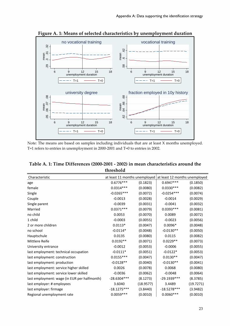
Given our identification strategy explained in detail in section IV.B this part provides some more information on our data that supports the identifying assumptions. Figure A. 1 depicts the sample means of four different variables by unemployment duration. For instance, for the group of individuals who are unemployed for at least 6 months entering in 2002 we observe that 30 percent have no vocational training (solid line in the top left panel). This share remains almost constant for all unemployment duration samples and especially does not depict a discontinuity at 12 months. For individuals entering between 2000 and 2001 the share is constantly about 31 percent. The difference between the solid and the dashed lines are provided in Figure 3 in part IV.B. Table A. 1 provides time differences in means of selected characteristics that are prone to influence the decision to stay in unemployment to become subsidy eligible as well as the average employment outcomes. It shows for instance that the share of women in the group of individuals who are at least 11 months unemployed entering in 2000‐2001 is about 3 percentage points higher compared to the group entering in 2002. This difference is at face value very close to the one of individuals with at least 12 months of unemployment (second column). Since this is true for basically all variables in the table our assumption of local continuity in differences can be supported on the basis of these observable characteristics.
Appendix A: Data supporting the identification strategy
Figure A. 1: Means of selected characteristics by unemployment duration
Note: The means are based on samples including individuals that are at least X months unemployed. T=1 refers to entries in unemployment in 2000‐2001 and T=0 to entries in 2002.
.29
.3.3
1.3
2m
ean
6 9 12 15 18unemployment duration
T=1 T=0
no vocational training
.58
.6.6
2m
ean
6 9 12 15 18unemployment duration
T=1 T=0
vocational training.0
5.0
6.0
7.0
8m
ean
6 9 12 15 18unemployment duration
T=1 T=0
university degree
.62
.64
.66
.68
mea
n6 9 12 15 18
unemployment duration
T=1 T=0
fraction employed in 10y history
Table A. 1: Time Differences (2000‐2001 ‐ 2002) in mean characteristics around the threshold
Characteristic at least 11 months unemployed at least 12 months unemployedage 0.6776*** (0.1823) 0.6947*** (0.1850) female 0.0314*** (0.0080) 0.0330*** (0.0082) Single ‐0.0265*** (0.0072) ‐0.0254*** (0.0074) Couple ‐0.0013 (0.0028) ‐0.0014 (0.0029) Single parent ‐0.0039 (0.0031) ‐0.0041 (0.0032) Married 0.0371*** (0.0079) 0.0393*** (0.0081) no child 0.0053 (0.0070) 0.0089 (0.0072) 1 child ‐0.0003 (0.0055) ‐0.0023 (0.0056) 2 or more children 0.0113* (0.0047) 0.0096* (0.0048) no school ‐0.0114* (0.0048) ‐0.0130** (0.0050) Hauptschule 0.0135 (0.0080) 0.0115 (0.0082) Mittlere Reife 0.0192** (0.0071) 0.0229** (0.0073) University entrance ‐0.0012 (0.0053) ‐0.0006 (0.0055) last employment: technical occupation ‐0.0111* (0.0051) ‐0.0122* (0.0053) last employment: construction 0.0155*** (0.0047) 0.0130** (0.0047) last employment: production ‐0.0128** (0.0040) ‐0.0130** (0.0041) last employment: service higher skilled 0.0026 (0.0078) 0.0068 (0.0080) last employment: service lower skilled ‐0.0036 (0.0062) ‐0.0048 (0.0064) last employment: wage (in EUR per halfmonth) ‐28.6304*** (8.1273) ‐29.1939*** (8.3785) last employer: # employees 3.6040 (18.9577) 3.4489 (19.7271) last employer: firmage ‐18.1275*** (3.8440) ‐18.5278*** (3.9482) Regional unemployment rate 0.0059*** (0.0010) 0.0060*** (0.0010)
23

Do Long-term Unemployed Workers Benefit from Targeted Wage Subsidies?
Table A.1: continued at least 11 months unemployed at least 12 months unemployedRegional LTU rate 0.0293*** (0.0016) 0.0298*** (0.0016) UB claim in days 111.4850*** (4.1229) 116.5093*** (4.2537) Unemployment benefits (in EUR per halfmonth) ‐0.2877 (2.5515) ‐0.6559 (2.6221)
Observations 15933 15116
Note: Standard errors in parentheses. *** 1 percent significance level, ** 5 percent significance level, * 10 percent significance level.
Appendix B: Identifying assumption and formal derivation of the effect
For the formal representation we use the rather common notation in the literature defining D as the treatment status in terms of a binary random variable with realizations { }0,1d∈ . According to the RDD approach D=1 represents subsidy
eligibility based on the following deterministic relation: { }1D x x= ≥ , where x is the 12‐month unemployment threshold. The time period is similarly defined as T=t with
{ }0,1t∈ . T=1 refers to individuals entering unemployment from 2000 to 2001, T=0 indicates 2002. The potential outcomes for individual, i, are denoted with and X represents the forcing variable, unemployment duration. Then the effect of interest can be defined as
diY
27: 1 0[ | ,ATET i iE Y Y X x Tθ 1]= − = =
Formally, local continuity in differences states:
0 0
0 0
[ | , 1] [ | , 0]
[ | , 1] [ | , 0i i
i i
E Y x T E Y x T
E Y x T E Y x T
+ +
− −
= − =
= = − ]=
where x + and x − refer to the outcomes just above and just below the threshold, respectively. Except for 0[ | , 1]iE Y x T+ = , representing the mean potential non‐eligibility outcome above the discontinuity point in T=1, all other quantities are observable, according to the following notation:
0 0[ | , ] lim [ | , , 0] lim [ | , , 0i i ix x x xE Y x T t E Y X x T t D E Y X x T t D−
↑ ↑= = = = = = = = = ] .
The potential non‐eligibility outcome above the threshold (i.e. the counterfactual outcome for the eligibles) is observable in T=0. In this time period the counterfactual for the long‐term unemployed corresponds to the observed mean as the program does not exist: 0 0[ | , 0] lim [ | , 0, 1] lim [ | , 0, 1i i ix x x x
E Y x T E Y X x T D E Y X x T D+
↓ ↓= = = = = = = = = ]
.
27 ATET is an abbreviation for the average treatment effect on the treated.
24
Appendix C: Sensitivity Results
Thus, according to our notation the effect of the presence of the subsidy is identified as follows: 28
[ | , 1] [ | , 1] [ | , 0] [ | , 0]ATET i i i iE Y x T E Y x T E Y x T E Y x Tθ − + −= = − = + = − =
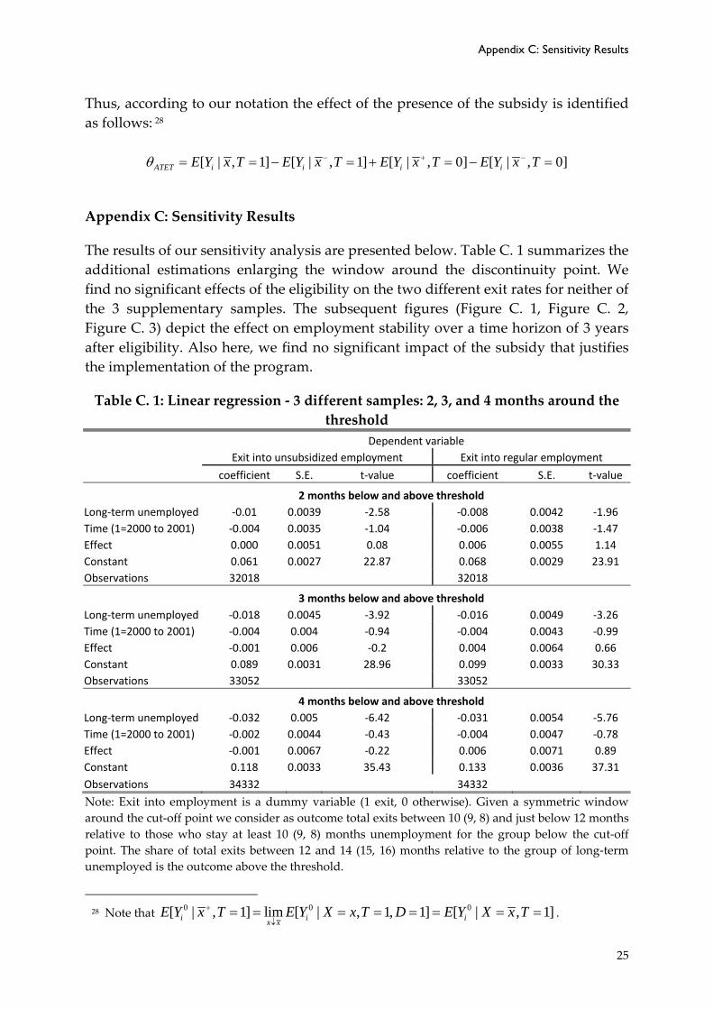
Appendix C: Sensitivity Results
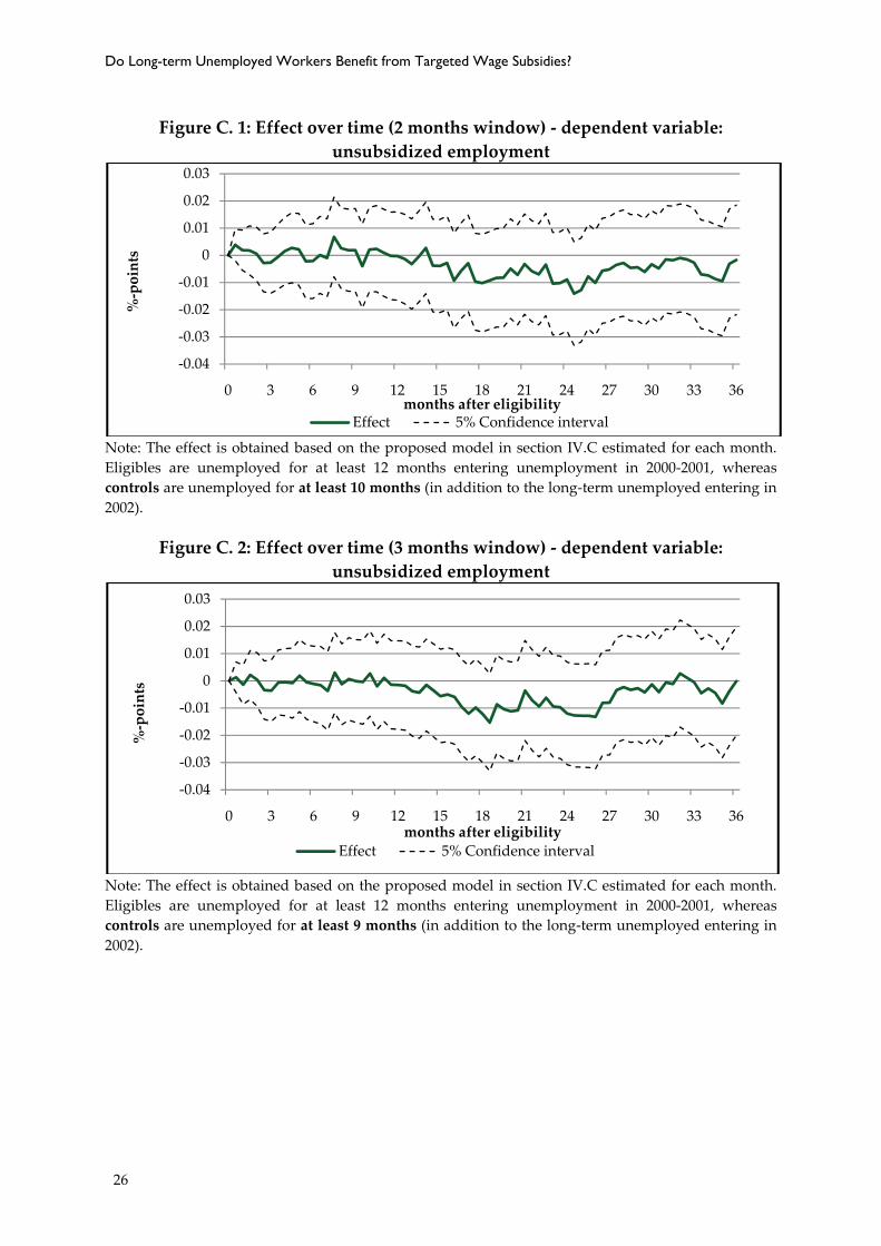
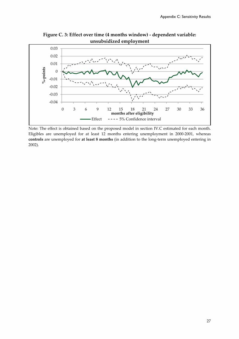
The results of our sensitivity analysis are presented below. Table C. 1 summarizes the additional estimations enlarging the window around the discontinuity point. We find no significant effects of the eligibility on the two different exit rates for neither of the 3 supplementary samples. The subsequent figures (Figure C. 1, Figure C. 2, Figure C. 3) depict the effect on employment stability over a time horizon of 3 years after eligibility. Also here, we find no significant impact of the subsidy that justifies the implementation of the program.
Table C. 1: Linear regression ‐ 3 different samples: 2, 3, and 4 months around the threshold
Dependent variable Exit into unsubsidized employment Exit into regular employment
coefficient S.E. t‐value coefficient S.E. t‐value
2 months below and above thresholdLong‐term unemployed ‐0.01 0.0039 ‐2.58 ‐0.008 0.0042 ‐1.96 Time (1=2000 to 2001) ‐0.004 0.0035 ‐1.04 ‐0.006 0.0038 ‐1.47 Effect 0.000 0.0051 0.08 0.006 0.0055 1.14 Constant 0.061 0.0027 22.87 0.068 0.0029 23.91 Observations 32018 32018
3 months below and above thresholdLong‐term unemployed ‐0.018 0.0045 ‐3.92 ‐0.016 0.0049 ‐3.26 Time (1=2000 to 2001) ‐0.004 0.004 ‐0.94 ‐0.004 0.0043 ‐0.99 Effect ‐0.001 0.006 ‐0.2 0.004 0.0064 0.66 Constant 0.089 0.0031 28.96 0.099 0.0033 30.33 Observations 33052 33052
4 months below and above thresholdLong‐term unemployed ‐0.032 0.005 ‐6.42 ‐0.031 0.0054 ‐5.76 Time (1=2000 to 2001) ‐0.002 0.0044 ‐0.43 ‐0.004 0.0047 ‐0.78 Effect ‐0.001 0.0067 ‐0.22 0.006 0.0071 0.89 Constant 0.118 0.0033 35.43 0.133 0.0036 37.31 Observations 34332 34332
Note: Exit into employment is a dummy variable (1 exit, 0 otherwise). Given a symmetric window around the cut‐off point we consider as outcome total exits between 10 (9, 8) and just below 12 months relative to those who stay at least 10 (9, 8) months unemployment for the group below the cut‐off point. The share of total exits between 12 and 14 (15, 16) months relative to the group of long‐term unemployed is the outcome above the threshold.
28 Note that 0 0 0[ | , 1] lim [ | , 1, 1] [ | , 1i i ix x
E Y x T E Y X x T D E Y X x T+
↓= = = = = = = = ] .
25
Do Long-term Unemployed Workers Benefit from Targeted Wage Subsidies?
Figure C. 1: Effect over time (2 months window) ‐ dependent variable: unsubsidized employment
Note: The effect is obtained based on the proposed model in section IV.C estimated for each month. Eligibles are unemployed for at least 12 months entering unemployment in 2000‐2001, whereas controls are unemployed for at least 10 months (in addition to the long‐term unemployed entering in 2002).
‐0.04
‐0.03
‐0.02
‐0.01
0
0.01
0.02
0 3 6 9 12 15 18 21 24 27 30 33 36
%‐points
months after eligibility
0.03
Effect 5% Confidence interval
Figure C. 2: Effect over time (3 months window) ‐ dependent variable: unsubsidized employment
Note: The effect is obtained based on the proposed model in section IV.C estimated for each month. Eligibles are unemployed for at least 12 months entering unemployment in 2000‐2001, whereas controls are unemployed for at least 9 months (in addition to the long‐term unemployed entering in 2002).
‐0.04
‐0.03
‐0.02
‐0.01
0
0.01
0.02
0.03
0 3 6 9 12 15 18 21 24 27 30 33 36
%‐points
months after eligibilityEffect 5% Confidence interval
26
Appendix C: Sensitivity Results
27
Figure C. 3: Effect over time (4 months window) ‐ dependent variable: unsubsidized employment
Note: The effect is obtained based on the proposed model in section IV.C estimated for each month. Eligibles are unemployed for at least 12 months entering unemployment in 2000‐2001, whereas controls are unemployed for at least 8 months (in addition to the long‐term unemployed entering in 2002).
‐0.04
‐0.03
‐0.02
‐0.01
0
0.01
0.02
0.03
0 3 6 9 12 15 18 21 24 27 30 33 36
%‐points
months after eligibilityEffect 5% Confidence interval
Copyright © 2022 FDOKUMEN