Distant shocks, migration, and housing supply in India*

Arnab Dutta1, Sahil Gandhi2, and Richard K. Green1

1University of Southern California2University of Manchester

January 7, 2022

Abstract

Housing supply elasticity estimates for cities in large and rapidly urbanizing countries likeIndia can tell us whether their urban housing markets’ supply keeps pace with the rising de-mand. The case of India is particularly interesting in this regard because of its variety ofhousing typologies. We estimate the supply elasticity of (1) durable or formal houses madeof concrete, bricks, and metal, (2) non-durable or informal houses made of thatch, mud, plas-tic, etc. and typically found in slums, and (3) vacant residential housing units in urban Indiabetween 2001 and 2011. We use two migration-inducing exogenous events — negative rain-fall shocks and a highway upgrade program — occurring in distant states as demand shiftersfor local urban housing markets. We apply the Rosen-Roback spatial equilibrium frameworkto show that the negative rainfall shocks and the highway upgrade program in distant statesincreased inter-state migration in India. This increase led to urban population growth, andtherefore, higher demand for housing in local urban markets. Our findings are three-fold.First, we estimate that the decadal supply elasticity of durable housing in urban India is 1.62.Second, we find that the supply elasticity of non-durable housing is −0.49. A negative supplyelasticity value for non-durable houses is consistent with the existence of urban gentrificationthrough the demolition and upgradation of slums. And finally, we estimate the elasticity ofvacant residential housing units’ supply to be 2.62. We posit that a relatively higher vacanthousing supply elasticity reflects speculative building by developers in Indian cities during the2000s.

JEL Classification: J61, R23, R31Keywords: Housing supply, migration, India

*The authors would like to thank Richard Arnott, Marlon Boarnet, Gene Burinsky, Matthew E. Kahn, RajatKochhar, Rakesh Mohan, Somik V. Lall, Rodney Ramcharan, Jorge De La Roca, Ruozi Song, and Vaidehi Tandelfor their suggestions. The authors benefited from comments provided by participants at the annual Association of Col-legiate Schools of Planning (ACSP) conference 2021 and in seminars organized by the USC Price School of PublicPolicy and the Center for Social and Economic Progress.

1

1 Introduction

Indian cities were home to 377 million people or roughly 10.4% of the global urban population

in 2011 (Census of India, 2011; Desa et al., 2014). Data from the Census of India indicates that

India’s urban population grew by roughly 91 million or 32% between 2001 and 2011. Although

prior academic literature indicates that internal migration to Indian cities has been historically low

(Bhavnani and Lacina, 2017; Kone et al., 2018; Munshi and Rosenzweig, 2016), this seems to

be changing as the number of internal migrants living in urban India went up by 71% between

the 1990s and the 2000s (see figure 1).1 Therefore, India is urbanizing, and its urbanization is

increasingly accompanied by migration to urban areas. Empirical evidence from other countries

like the United States suggests that urbanization and migration are likely to contribute to a surge

in housing demand in cities (Molloy et al., 2011). But is the market supply of housing in urban

Indian enough to meet the rising demand?

Figure 2 indicates that the number of houses grew faster than the urban population in India

during the 2000s. The total number of residential housing units in urban India grew by 50% from

52 million in 2001 to 78 million in 2011. As with any developing country, a large share of India’s

housing stock consists of informal houses. In the absence of data on informal houses, we identify

proxies for formal and informal houses based on the type of material used to construct the roofs and

walls of houses. We use durable houses made of concrete, bricks, metal, and stone as a proxy for

formal houses and non-durable houses made of thatch, mud, unburnt bricks, plastic, etc. as a proxy

for informal houses.2 Non-durable houses are typically found in slums.3 Figure 2 indicates that

about 15% of the housing stock in urban India in 2011 consisted of non-durable houses. However,

the growth in residential housing by type was uneven. While the number of durable residential

units grew by 61% between 2001 and 2011, the number of non-durable units increased by 9%

1Recent studies have found that the Information Technology (IT) boom of the late 1990s and the early 2000s partlyexplains this growth in the internal movement of Indians (Ghose, 2019).

2Our definition of durable and non-durable housing is based on the Census of India’s definition of permanent andtemporary houses, respectively.

3Hereon, we use the terms informal housing, slums, and non-durable houses interchangeably.

2

Figure 1: Decadal growth in migration to Indian cities by last residence

Source: Author’s calculations based on the Census of India.Note: Figure presents the percentage growth rate in migration to urban areas between 1991-2000 and 2001-2010 bymigrants’ last residence (same or different state). All bars are labeled by the corresponding values being represented.

during the same time.4 The number of vacant houses also grew by about 83% suggesting that there

was a lot of speculative building in Indian cities during the 2000s (Gandhi et al., 2021a). The

question is whether the increase in residential housing in urban India between 2001 and 2011 was

at par with the increase in prices. In other words, what was the housing supply elasticity in urban

India during the 2000s?

In this paper, we estimate the supply elasticity of durable, non-durable, and vacant residential

housing units in urban India between 2001 and 2011.5 We use two migration-inducing exogenous

4Note that, as a result of the uneven growth, the share of non-durable housing units in the overall housing stock fellfrom 21% in 2001 to 15% in 2011.

5We employ first difference regressions throughout the paper to explain the changes in our outcome variables as afunction of changes in covariates between 2001 and 2011. See section 5 for details.

3

Figure 2: Housing units by type in urban India

Source: Author’s calculations based on the Census of India.Note: Figure presents the number of housing units (in millions) by type. Durable units’ roofs and walls made ofgalvanized iron, metal, asbestos sheets, burnt bricks, stone, and concrete. Non-durable units’ roofs or walls made ofgrass, thatch, bamboo, plastic, polythene, mud, unburnt brick, and wood. All vacant houses are durable units. All barsare labeled by the corresponding values being represented.

events — negative rainfall shocks and a highway upgrade program — occurring in distant states

as demand shifters for local urban housing markets. We apply the Rosen-Roback spatial equi-

librium framework (Roback, 1982; Rosen, 1979) to show that both the negative rainfall shocks

and the highway upgrade program in distant states increased inter-state migration in India during

the 2000s. The increased inter-state migration led to changes in urban population, and therefore,

higher demand for housing in local urban markets.

We illustrate the spatial equilibrium mechanism in figure 3 with the example of two Indian

states — Maharashtra and Bihar. Let’s say that we want to estimate the housing supply elasticity

in urban areas of Maharashtra. We define Maharashtra as the local state. Now, consider the

4

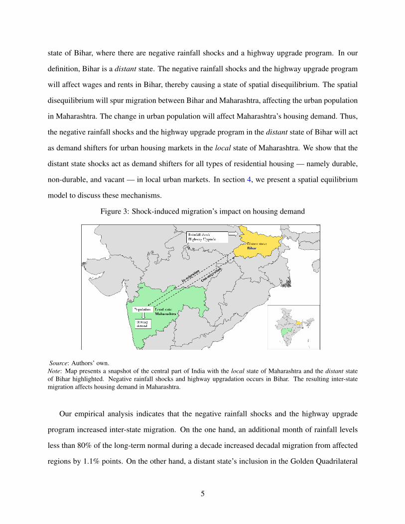
state of Bihar, where there are negative rainfall shocks and a highway upgrade program. In our

definition, Bihar is a distant state. The negative rainfall shocks and the highway upgrade program

will affect wages and rents in Bihar, thereby causing a state of spatial disequilibrium. The spatial

disequilibrium will spur migration between Bihar and Maharashtra, affecting the urban population

in Maharashtra. The change in urban population will affect Maharashtra’s housing demand. Thus,

the negative rainfall shocks and the highway upgrade program in the distant state of Bihar will act

as demand shifters for urban housing markets in the local state of Maharashtra. We show that the

distant state shocks act as demand shifters for all types of residential housing — namely durable,

non-durable, and vacant — in local urban markets. In section 4, we present a spatial equilibrium

model to discuss these mechanisms.

Figure 3: Shock-induced migration’s impact on housing demand

Source: Authors’ own.Note: Map presents a snapshot of the central part of India with the local state of Maharashtra and the distant stateof Bihar highlighted. Negative rainfall shocks and highway upgradation occurs in Bihar. The resulting inter-statemigration affects housing demand in Maharashtra.

Our empirical analysis indicates that the negative rainfall shocks and the highway upgrade

program increased inter-state migration. On the one hand, an additional month of rainfall levels

less than 80% of the long-term normal during a decade increased decadal migration from affected

regions by 1.1% points. On the other hand, a distant state’s inclusion in the Golden Quadrilateral

5

(GQ) highway upgrade program increased migration both to and from such states.6 This increased

inter-state mobility led to urbanization in the local state which in turn increased the demand for

housing in local urban housing markets. The demand for durable housing units increased relatively

more than the demand for non-durable units in response to the distant shock-induced urbanization.

We show that both the negative rainfall shocks and the GQ highway upgrade program are strong

instruments for the number of durable, non-durable, and vacant houses in local urban markets.

Our housing supply elasticity estimates can be summarized in three points. First, we estimate

that the decadal supply elasticity of durable housing in urban India is 1.62. This estimate is very

close to the supply elasticity of 1.75 obtained by Saiz (2010) for the average metropolitan area

in the United States. Second, we find that the supply elasticity of non-durable housing is −0.49.

The negative supply elasticity of non-durable housing is counterintuitive, suggesting that as non-

durable housing rents increase, the supply of non-durable residential housing units decreases. This

is consistent with urban gentrification that occurs in two ways in Indian cities. First, a simultaneous

increase in rents paid by slum dwellers and land values around slums attract real estate developers.

Slums are cleared to construct durable residential and commercial real estate space (Bhan, 2009).

And second, slums are upgraded through various government and non-government programs that

convert non-durable units to durable ones (Rains and Krishna, 2020; Rains et al., 2019). Finally,

we estimate the elasticity of vacant residential housing units’ supply in urban India to be 2.62,

which is larger than the elasticity of durable housing units’ supply. We posit that developers were

engaged in speculative building with the expectation of higher demand as market rents went up

during the 2000s (Gandhi et al., 2021a).

Our contributions to the literature are three-fold. First, we exploit the Rosen-Roback frame-

work to construct novel housing demand shifters. It is hard to find instruments that satisfy all the

exclusion restrictions. Prior research has used migration shocks such as international immigration

(Saiz, 2010) and imputed migration based on historic flows (Paciorek, 2013) as housing demand

6The Golden Quadrilateral (GQ) or the National Highways Development Project Phase I (NHDP I) was introducedas a highway upgrade program by the Central government of India in 2000, and it came into effect in 2001. Its primarygoal was to upgrade preexisting highways connecting the four largest metropolitan areas of India — Delhi, Mumbai,Kolkata, and Chennai — from two lanes to four lanes. See section 5.4 for details.

6

shifters. Some papers have also used labor demand shocks in the form of shift-share instruments as

housing demand shifters (Baum-Snow and Han, 2019; Paciorek, 2013; Saiz, 2010). The problem

with using such migration shocks as housing demand shifters is that the migration decisions are

endogenous to potential migrant destinations’ housing market outcomes such as prices and rents

(Zabel, 2012). The strength of our instruments is three-fold. First, we use migration-inducing

shocks as demand shifters instead of migration itself. Second, by separating the regions where

shocks occur and the regions where we estimate the housing supply elasticities, we reduce the

pathways through which omitted variable bias can occur as a result of correlation between the

shocks and the unobservables affecting the housing supply. The spatial equilibrium framework

provides the theoretical basis for identifying the indirect impact of such distant events on local

housing market outcomes, with migration being the channel of the impact. This idea is resonated

in Boustan (2010) who studied the impact of the Black migration during the post-war period on

suburbanization in US cities. And finally, we use rainfall shocks that are plausibly exogenous even

in the region of direct impact. We argue that if a shock is somewhat exogenous in a region of direct

impact, its validity as an instrument is strengthened for another region where its impact is indirect.

We discuss the exclusion restrictions for our instruments in detail in section 5.4.

The second contribution in this paper is providing a policy-relevant housing supply elasticity

estimate for a large and urbanizing country like India. Prior academic literature has predomi-

nantly focused on developed countries like the United States (Baum-Snow and Han, 2019; Green

et al., 2005; Saiz, 2010).7 Many studies have underscored the role of regulations (Diamond, 2017;

Glaeser et al., 2005; Quigley and Raphael, 2005) and natural land constraints like hilly terrains

(Saiz, 2010) in reducing the supply elasticity of housing in metropolitan areas of the United States.

Similar regulatory constraints also exist in developing countries like India. The land and hous-

ing markets in Indian cities are heavily regulated with floor-area-ratio (FAR) restrictions, urban

land ceiling constraints, and stringent rent control laws.8 Studies have indicated that these regu-

7Some studies have estimated housing supply elasticities in other countries such as Australia (McLaughlin, 2012),China (Wang et al., 2012), Italy (Accetturo et al., 2021), and United Kingdom (Malpezzi and Maclennan, 2001).

8The Urban Land (Ceiling and Regulation) Act of 1976 required firms and individuals to sell vacant land beyond aspecific size to the government at low prices (Sridhar, 2010).

7

lations impose significant building costs on developers (Bertaud and Brueckner, 2005; Brueckner

and Sridhar, 2012; Gandhi et al., 2021b). Therefore, durable housing supply elasticity estimates

almost surely reflect land-use policy decisions.

Last but not least, we estimate the supply elasticity of non-durable or informal housing, which

is both an academic contribution and a policy-relevant parameter for a developing country like

India. Informal housing has been studied in the literature because it’s existence is associated with

poverty (Marx et al., 2013) and institutional frictions such as lack of property rights (Brueckner

and Selod, 2009) and formal housing regulations (Henderson et al., 2021). Niu et al. (2021) un-

derscored the important role played by informal housing markets in reducing urbanization costs

in Chinese cities by providing low-income migrants with cheaper housing. Informal housing in

urban India accounts for 15% of the housing stock and fills the supply gap left by the formal hous-

ing market. Hence, an informal housing supply elasticity estimate is important for understanding

the housing markets in Indian cities. To the best of our knowledge, this is the first paper that pro-

vides an informal housing supply elasticity estimate in a developing country. The closest attempt

at estimating an informal housing supply elasticity has been made by Niu et al. (2021) in Chinese

cities. However, they calculate a proxy for informal housing elasticity using the share of village

areas on the edges of cities in the total urban built-up area. By contrast, we use direct observations

on informal housing to obtain our elasticity figures.

The rest of the paper is organized as follows. In section 2 we describe the data used for analysis

and present some stylized facts about housing and migration in India in section 3. Section 4

provides a theoretical discussion of the Rosen-Roback spatial equilibrium setting applied in this

paper to explain the mechanisms through which distant state shocks act as demand shifters in local

housing markets. Section 5 presents the empirical implementation. We present the results and

robustness checks in section 6 and provide concluding remarks in section 7.

8

2 Data

For our analysis, we gather data from the National Sample Survey Organization (NSS), the Cen-

sus of India, and the India Meteorological Department (IMD). We construct datasets at the state

and district levels.9 We use the state-level datasets to study inter-state migration and analyze the

impact of distant state-level shocks on local district-level outcomes. We estimate our elasticity

figures using the district-level datasets. We construct a wide form panel for both datasets based

on variable values from the Census years 2001 and 2011, which we then use to construct first-

differenced variables for the actual analysis. In this section, we provide a brief description of the

datasets used in the analysis. Summary statistics of all variables are presented in table 1.

2.1 State-level data

The Census provides decennial data on aggregated in-migration figures for a given region. The

data provides details on the time of movement of migrants (i.e., less than a year ago, 1-4 years ago,

and 5-9 years ago), the distance migrants traveled from their last place of residence (inter-district,

inter-state, etc.), the sector of origin (rural or urban), and their current place of residence (urban

or rural). We use this information to construct decadal inter-state migration variables based on the

number of individuals who moved into urban areas of a state from both rural and urban areas of

another state in the decade leading up to the Census years – 2001 and 2011. The Census datasets

also provide the urban population and the urban surface area for a given state.

We obtain data on the mean monthly per capita consumption from the NSS and calculate real

values based on the Consumer Price Index data provided by the Labor Bureau of India. We get our

data on the National Highways Development Project Phase I, also known as the Golden Quadri-

lateral (GQ) highway upgrade program, from Ghani et al. (2016). In figure 4, we indicate the 14

states and union territories in India that were recipients of the GQ program. And finally, we gather

rainfall shock data from the Open Government Data (OGD) portal of the central government of

9A district is an administrative unit in India similar to that of a county in the United States.

9

Table 1: Summary Statistics

Panel (a): State-level variables

2001 2011

Variable Mean Std. dev. Mean Std. dev.

No. of months absolute rainfall <80% last decade 58 12 64 11

No. of inter-state urban migrants moved last decade ('000) 319 543 452 691

Urban population (millions) 8 11 11 14

Mean monthly per capita real consumption (INR) 890 274 1001 374

Urban surface area (sq. miles) 873 1,119 2,321 2,719

N 35 35 35 35

Panel (b): District-level variables

2001 2011

Variable Mean Std. dev. Mean Std. dev.

Urban population ('000) 1,181 1,777 1,515 2,184

No. of non-durable residential houses ('000) 46 42 46 39

No. of durable residential houses ('000) 180 311 284 446

No. of vacant residential houses ('000) 28 56 44 81

Mean real rent for non-durable residential houses (INR) 302 223 311 233

Mean real rent for durable residential houses (INR) 628 276 751 332

Mean real rent for all residential houses (INR) 570 246 684 307

Mean monthly per capita real consumption (INR) 1,051 247 1,110 338

Urban surface area (sq. miles) 104 126 134 142

Median no. of rooms per house 2 0 2 0

N 144 144 144 144

Data sources: National Sample Survey Organization, Census of India, and Labor Bureau of India.Note: Table presents summary statistics of variables used in the analysis. Panel (a) presents state-level variables and panel (b) presents district-levelvariables. All values rounded off to the nearest integer. State-level migration and the number of district-level residential housing units given inthousands. State-level urban population given in millions. Urban surface area values are given in square miles. Rents and consumption values areinflation-adjusted to 2001 INR values using the Consumer Price Index (CPI) data from the Labor Bureau of India. In PPP terms, $1 = 10 INR in2001. For exchange rates see: https://data.oecd.org/conversion/purchasing-power-parities-ppp.htm

India.10 This dataset is sourced from the IMD. It reports the percentage deviation of rainfall from

the long-term average on a monthly basis between 1901 and 2015. We use this data to construct

rainfall shock variables at the state level. 11

2.2 District-level data

We obtain data on the number of various types of residential housing units – non-durable, durable,

vacant – at the district level from the Census of India. In addition, we get data on urban population

10Please visit the link: https://data.gov.in/11The original data provides rainfall departure percentages for each of the 36 meteorological subdivisions in India.

Meteorological subdivisions are roughly analogous to the state boundaries of India, with a few exceptions. Largerstates consist of more than one subdivision, while some smaller states are clustered into one subdivision. We mapthese meteorological subdivisions to state boundaries and recalculate the rainfall departure values at the state level.

10

Figure 4: Map of Golden Quadrilateral recipient states in India

Data Source: Ghani et al. (2016).Note: Figure presents a map of India with the 35 states and union territories demarcated. Light-colored states were not recipients of the NationalHighways Development Project Phase I or the Golden Quadrilateral (GQ) highway upgrade project. Dark-colored states were part of the GQprogram.

and urban surface area from the Census. We also gather data on district-level mean per capita

consumption and the mean housing rents for the various types of housing units in our analysis

from the NSS. These rent and consumption values are inflation-adjusted to 2001 values based on

the Consumer Price Index data provided by the Labor Bureau of India.

Although there were 640 districts in India in 2011, our final district-level data consists of 144

districts. The number of districts reduces in two ways. First, we recreate the actual administrative

district boundaries to obtain time-consistent hypothetical boundaries because district boundaries

are realigned in India very frequently.12 And second, we have data on mean non-durable housing

12While in 2001 there were 593 districts in India, in 2011 that number went up to 640. We create 479 hypotheticaldistricts with time-consistent boundaries by combining all contiguous districts affected by boundary changes and

11

rent values for fewer districts. We estimate the housing supply elasticity of durable units using a

larger sample of 339 districts and present the results in table A.3.

3 Stylized facts

Housing markets in India have been understudied in the academic literature. There are very few

quantitative papers on the subject aside from a couple of demand-side and affordability studies

(Tiwari and Parikh, 1998; Tiwari et al., 1999) and some papers looking at new housing construction

and rent control laws (Dutta et al., 2021; Gandhi et al., 2021a,b). Hence, the relationship between

internal migration and housing in India is not well understood. In this section, we provide some

key stylized facts about the relationship between internal migration and urban housing markets.

We argue that the growth in inter-state migration in India between the 1990s and the 2000s caused

a shift in the demand for housing in India’s urban housing markets.

Internal migration in India grew by 71% between 2001 and 2011 (see figure 1). But historically,

India has had very low levels of internal mobility. A large body of literature is dedicated to studying

the low rates of internal migration in India (Bhavnani and Lacina, 2017; Kone et al., 2018; Munshi

and Rosenzweig, 2016). One recent study suggests that more Indians are moving internally as a

result of the IT boom of the late 1990s and the early 2000s (Ghose, 2019).

Even though migration in India grew substantially between the 1990s and the 2000s, figure 5

shows that the urban population’s share of internal migrants living in Indian cities increased very

little during this time. Inter-state migrants as a share of India’s urban population remained flat at

4% between 2001 and 2011. Hence, the question is whether the increase in migration between

2001 and 2011 was enough to cause a shift in the demand for housing in urban India.

We argue that despite the low levels, the increase in inter-state migration in India during the

decade of 2001-2011 constituted a housing demand shock in urban areas of India. First, inter-state

migration grew by 42% between 2001 and 2011, which is higher than the growth of 32% in India’s

urban population (see figure 1). And second, there exists a significant and positive relationship

leaving districts unaffected by boundary realignment unchanged.

12

Figure 5: Share of decadal migrants in urban population of India

Source: Author’s calculations based on the Census of India.Note: Figure presents the share of inter-city and rural-urban migrants that moved during 1991-2000 and 2001-2010 bymigrants’ last residence (same or different state) in India’s urban population. All bars are labeled by the correspondingvalues being represented.

between the number of in-migrants and the number of durable and non-durable housing units in

urban areas of India, seen in figure 6b and figure 6a. In section 6, we discuss several regression re-

sults that indicate the strength of inter-state migration-inducing shocks in explaining local housing

demand.

One issue is that prior literature suggests that a major share of migrants in India move into slums

and not formal housing (Mitra, 2010; Srivastava, 2011). Hence, migration shocks would more

likely capture non-durable rather than durable housing demand shifts. However, while it might

be true that a large number of poor Indians move seasonally for one to six months to supplement

farm incomes with urban informal earnings during lean agricultural seasons before moving back

13

Figure 6: Housing and migration in urban India

(a) Urban non-durable units and in-migrants

(b) Urban durable units and in-migrants

Source: Author’s calculations based on Census of India.Note: Figure in panel (a) presents a scatter plot of the log of state-level urban non-durable housing units and the logof inter-state migrants living in urban areas. The regression lines have slopes of 0.72 and 0.67 respectively for 2001and 2011, significant at the 99% level. Figure in panel (b) presents a scatter plot of the log of state-level urban durablehousing units and the log of inter-state migrants living in urban areas. The regression lines have slopes of 0.80 and0.71 respectively for 2001 and 2011, significant at the 99% level.

14

to their homes (Imbert and Papp, 2015, 2020; Rosenzweig and Udry, 2014), many affluent Indians

also migrate and do so permanently rather than seasonally. For instance, the National Sample

Survey Organization (NSS) data on employment and migration indicates that while about 12% of

households had a seasonal migrant, about 27% of households had a former member that moved out

permanently for employment or education. Moreover, the NSS data also indicates that educated

households with higher consumption were more likely to have a permanent migrant and less likely

to have a seasonal migrant member. Therefore, it is likely that individuals who move permanently

across regions choose formal housing over slums.

4 Theoretical framework

We use the Rosen-Roback spatial equilibrium framework (Roback, 1982; Rosen, 1979) to analyze

the effect of distant region shocks on inter-regional mobility and local housing demand. A shock

that affects rents and incomes in a distant region induces spatial disequilibrium, spurring inter-

regional mobility. Such mobility affects local housing demand if net inward mobility to the local

region is non-zero. Therefore, distant region shocks that affect rents and incomes in the distant

region act as demand shifters and can be used to estimate the local housing supply elasticity. In

this section, we provide an analytical discussion of these effects.

4.1 Spatial equilibrium

Consider an economy with a local region i where we are interested in estimating the housing

supply elasticity and a distant region j that has exogenous shocks to its economy. The number of

individuals occupying regions i and j are ni and n j respectively. We assume that each individual

is equivalent to a household in either region.13 In both locations, individuals earn w and derive

utility from housing services h, a numeraire good c, and location-specific amenities a. Individuals

can only transact h and c in the market. Amenities a are exogenously given in a location at any

13As long as the number of households and the total population at i is monotonically related, relaxing the assumptionthat each individual in the economy is equivalent to a household does not alter the model mechanisms.

15

given point in time. The market-clearing rent for housing services is r. The user-cost model relates

r to the market-clearing house price p through the equation r = p(K + T +D+E). Here, K is

the cost of capital, T is the property tax rate, D is the rate of depreciation, and E is the rate of

expected appreciation (Poterba, 1984). The fact that market-clearing rent for housing services is

an appropriate measure of market-clearing price for housing as a composite commodity is well

established in the literature (Brueckner et al., 1987; Mills, 1967).

The representative individual’s utility maximization problem at i can be written as follows:

maxhi,ci

Ui(hi,ci)+ai s.t. hiri + ci = wi (1)

Here, U(.) is a strictly quasiconcave utility function such that equation (1) results in an interior

solution. The resulting demand for housing services at i is hdi (ri,wi). Hence, the aggregate demand

for housing services at i can be written as follows:

HDi = nihd

i (ri,wi) where hdi (ri,wi)> 0 (2)

The implied indirect utility obtained by the representative individual at i is Vi(ri,wi,ai). At

equilibrium, the values of r and w adjust such that, given the location-specific amenities in every

region, the indirect utility is equal across both regions i and j. The spatial equilibrium is charac-

terized as follows:

Vi(ri,wi,ai) =Vj(r j,w j,a j) = V (3)

At this equilibrium, there are no gains to mobility between i and j.

16

4.2 Spatial disequilibrium, mobility, and local housing demand

Now consider a shock z j at the distant region j that does not affect amenities a j but changes rent

r j or income w j, or both, thus changing the utility Vj of individuals at j.14 The shock z could

be a negative shock like a drought or a positive shock like a highway upgrade program. Because

z j affects rent r j and income w j, it follows that Vj(r j(z j),w j(z j),a j) is an implicit function of z j.

Hence, in response to z j, we have a state of spatial disequilibrium as follows:

Vj =Vj(z j) =Vj(r j(z j),w j(z j),a j) = V =Vi (4)

Since there are gains to mobility because of the difference in Vi and Vj, the shock z j will induce

mobility between j and i until r and w adjust in both i and j, so that Vj = Vi = V . In other words,

a shock affecting rents and incomes at a distant region j induces movement between the distant

and the local regions so that rents and incomes change in both locations until spatial equilibrium is

restored and there are no gains to moving. This proposition is consistent with past literature on the

effects of regional labor and housing market shocks on inter-regional mobility in the United States

(Molloy et al., 2011; Saks and Wozniak, 2011).

We characterize mobility m between regions i and j as the vector (m ji,mi j). m ji represents

the number of individuals moving from j to i and mi j denotes the number of individuals moving

from i to j. In other words, m ji represents in-migration from the distant region j to the local

region i and mi j represents out-migration from local region i to the distant region j. This idea

is consistent with the bi-directional movement of individuals across regions observed in the data.

Spatial equilibrium implies that the net movement between two regions in equilibrium should be

equal to zero. A disequilibrium induced by a shock will cause net migration into the region where

utility is higher.

14The impact of z on mobility m between i and j will be determined by the implicit function m(V (r(z),w(z),a(z))).Hence, assuming that a remains exogenous to z does not alter the main mechanisms. Note however, that while mobilitywill respond to r(z), w(z), and a(z), and r and w will in turn change in response to such mobility changes, a will not.In other words, a(z) changes only in response to z.

17

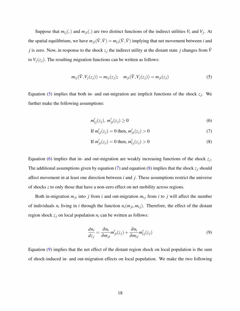
Suppose that mi j(.) and m ji(.) are two distinct functions of the indirect utilities Vi and Vj. At

the spatial equilibrium, we have m ji(V ,V ) = mi j(V ,V ) implying that net movement between i and

j is zero. Now, in response to the shock z j the indirect utility at the distant state j changes from V

to Vj(z j). The resulting migration functions can be written as follows:

mi j(V ,Vj(z j)) = mi j(z j); m ji(V ,Vj(z j)) = m ji(z j) (5)

Equation (5) implies that both in- and out-migration are implicit functions of the shock z j. We

further make the following assumptions:

m′i j(z j), m′

ji(z j)≥ 0 (6)

If m′i j(z j) = 0 then, m′

ji(z j)> 0 (7)

If m′ji(z j) = 0 then, m′

i j(z j)> 0 (8)

Equation (6) implies that in- and out-migration are weakly increasing functions of the shock z j.

The additional assumptions given by equation (7) and equation (8) implies that the shock z j should

affect movement in at least one direction between i and j. These assumptions restrict the universe

of shocks z to only those that have a non-zero effect on net mobility across regions.

Both in-migration m ji into j from i and out-migration mi j from i to j will affect the number

of individuals ni living in i through the function ni(m ji,mi j). Therefore, the effect of the distant

region shock z j on local population ni can be written as follows:

dni

dz j=

∂ni

∂m jim′

ji(z j)+∂ni

∂mi jm′

i j(z j) (9)

Equation (9) implies that the net effect of the distant region shock on local population is the sum

of shock-induced in- and out-migration effects on local population. We make the two following

18

assumptions on the effect of in- and out-migration on population at i:

∂ni

∂m ji(z j)≥ 0 and

∂ni

∂mi j(z j)≤ 0 (10)

Equation (10) implies that the number of individuals ni at i weakly increases in response to in-

migration and weakly decreases in response to out-migration. The weak inequality follows from

the fact that the natural rate of growth component in population changes is a major factor and can

act as a countering force to both in- and out-migration effects on the local population. Since we

do not explicitly model the natural rate of growth component in dni, we allow for the possibility of

population changes to be independent of migration.

Proposition 1 Under the assumptions given by equations (6) to (8) and equation (10), dHDi

dz j⋚ 0 if

and only if∣∣∣ ∂ni

∂m jim′

ji(z j)∣∣∣⋚ ∣∣∣ ∂ni

∂mi jm′

i j(z j)∣∣∣

Proposition 1 indicates that the aggregate demand for local housing services Hdi responds to

migration-inducing shocks at the distant region j. The direction of change in aggregate demand

for housing services at i depends on the relative magnitude of the in-migration and out-migration

effects on the local population resulting from the shock z j. To see this, let us first write the effect

of the shock z j on the aggregate demand for local housing services Hdi , as follows:

dHDi

dz j=

∂HDi

∂ni

dni

dz jhd

i (ri,wi) =∂HD

i∂ni

(∂ni

∂m jim′

ji(z j)+∂ni

∂mi jm′

i j(z j)

)hd

i (ri,wi) (11)

The last expression in equation (11) is derived by substituting equation (9) after differentiating the

aggregate demand HDi given by equation (2) with respect to z j.

The fact that dHDi

dz j⋚ 0 implies

∣∣∣ ∂ni∂m ji

m′ji(z j)

∣∣∣⋚ ∣∣∣ ∂ni∂mi j

m′i j(z j)

∣∣∣ directly follows from equation (11)

and the inequality ∂HDi

∂ni> 0 derived from equation (2). Now, to see the if condition, note first

that ∂ni∂m ji

, m′ji(z j) and m′

i j(z j) are all weakly positive and ∂ni∂mi j

is weakly negative. Hence, we

have ∂ni∂m ji

m′ji(z j)≥ 0 and ∂ni

∂mi jm′

i j(z j)≤ 0. If∣∣∣ ∂ni

∂m jim′

ji(z j)∣∣∣= ∣∣∣ ∂ni

∂mi jm′

i j(z j)∣∣∣, then dHD

idz j

= 0 trivially

follows from equation (11). Now, if∣∣∣ ∂ni

∂m jim′

ji(z j)∣∣∣ = ∣∣∣ ∂ni

∂mi jm′

i j(z j)∣∣∣, then there are three possibilities.

19

First, we can have ∂ni∂m ji

m′ji(z j)> 0 and ∂ni

∂mi jm′

i j(z j) = 0, in which case equation (11) implies dHDi

dz j>

0. The second possibility is where ∂ni∂m ji

m′ji(z j) = 0 and ∂ni

∂mi jm′

i j(z j) < 0, in which case dHDi

dz j< 0

follows from equation (11). And finally, we can have ∂ni∂m ji

m′ji(z j)> 0 and ∂ni

∂mi jm′

i j(z j)< 0, in which

case we have dHDi

dz j> 0 if

∣∣∣ ∂ni∂m ji

m′ji(z j)

∣∣∣> ∣∣∣ ∂ni∂mi j

m′i j(z j)

∣∣∣.Proposition 1 implies that a distant region shock affecting inter-regional migration acts as a

demand shifter in local housing markets. The driving mechanisms behind the distant region shock

effect on local housing demand can be described as follows. First, a shock at a distant point affects

rents and incomes in that region. This, in turn, changes the indirect utility in the distant region,

thereby inducing a state of spatial disequilibrium in the economy. The resulting difference in

utilities across the two regions implies gains to mobility. Individuals move across regions. This

movement causes a change in the local population and households, thus affecting local housing

demand.

It is important to note here, that, distant state shocks such as highway upgrades can lead to

increased trading of commodities across states which can in turn affect commodity prices and

thereby cause a second channel of impact on housing demand. This is particularly true if both the

distant and the local states were recipients of the highway upgrade program. However, it is unlikely

that the highway upgrade would have had a long-term impact on consumers’ budget constraints

since non-housing commodity prices are affected by other factors such as international prices. We

test whether the Golden Quadrilateral (GQ) highway upgrade in India had any impact on recipi-

ent states’ commodity prices by regressing price changes of baskets of non-housing commodities

consumed by urban households in a state on the state’s GQ recipient status. We find that a state’s

inclusion in the GQ program had no impact on its commodity prices in urban areas. The results

from this regression are given in table A.1. Hence, we ignore the trade channel of impact of distant

states’ inclusion in the GQ program on local housing demand.

20

4.3 Local housing supply

Now, let us consider the total housing stock HSi in the region i supplied through a competitive

market. HSi is a function of ri. At the market equilibrium, we have HS

i = HDi (ri,wi,ni). In other

words, the market equilibrium implies that the housing supply equals the aggregate quantity of

housing services demanded within a region. Let us assume that the supply function is log-linear.

Then, the reduced form for the inverse supply function at i can be written as follows:15

log(ri) =1ηi

log(HSi ) (12)

where the housing supply elasticity at i is ηi. Since housing supply is never perfectly elastic, ηi is

a finite real number greater than zero.16

Estimating ηi in equation (12) presents a classic endogeneity problem since we only observe

market equilibrium values of ri and HSi . Hence, we need exogenous demand shifters to trace the

slope 1/ηi of the inverse supply curve. Proposition 1 shows that exogenous shocks z j incident

upon a distant region can act as a demand shifter at i if the shock z j induces net non-zero mobility

between i and j. We can write the reduced form effect of z j on the aggregate demand for housing

services as follows:

log(HDi ) = β z j (13)

Proposition 1 implies that β could be either negative or positive, and its sign depends on the

relative magnitude of the in- and out-migration effects of the shock z j. The predicted log(HDi )

obtained after estimating the parameter β is an exogenous demand shock which can be substituted

in equation (12) to estimate ηi. However, if the shock-induced migration affects construction

wages, then β might include supply-side factors as well, a concern we address in the empirical

15Throughout the paper, the log function is used to denote the natural log of its argument.16See Green et al. (2005) for a discussion on imperfect housing supply elasticities and the various reasons for why

that is the case in the context of a monocentric city model.

21

section. We posit that z j is a demand shifter for all kinds of residential houses — non-durable,

durable, and vacant. However, since these housing categories represent different markets, their

slopes will be different. In other words, the coefficient β will be different for the three different

types of residential housing used in our analysis.

5 Empirical implementation

The theoretical framework discussed in section 4 explains that distant region shocks affect local

population, and hence, local housing demand. The driving channel of effect is the migration flow

of individuals across regions. In this section, we first discuss the empirical framework for esti-

mating the effect of a distant state shock on inter-state mobility and the resulting effects on local

urban population growth. Next, we provide the estimating equations to analyze the effect of the

distant state shock-induced urbanization on demand for local urban housing. These two estimation

exercises are meant to test whether Proposition 1 holds true and provide empirical evidence for the

mechanisms through which the distant state shocks act as demand shifters in the local urban hous-

ing market. Finally, we provide the housing supply estimation model using the distant state shocks

as local urban housing demand shifters. Following Saiz (2010), we use first difference regressions

to explain changes in outcomes as a function of changes in independent variables between 2001

and 2011. We discuss the validity of the distant region shocks as instruments at the end of this

section.

5.1 Distant shocks, inter-state migration, and urbanization

Let us consider two regions i and j. Region i consists of urban areas of a local state and region

j is made up of both rural and urban areas of a distant state. The terms local and distant here are

consistent with the previous sections. Following section 4.2, let us denote migration flows between

i and j as mk where k = { ji, i j}. m ji represents the number of individuals moving from j to i and

mi j denotes the number of individuals moving from i to j. Our goal is to isolate the impact of

22

migration flows m ji and mi j on local urbanization ∆ log(ni) between 2001 and 2011.17 To do so,

we would ideally like to estimate the following first difference equation using data on i− j pairs of

Indian states between 2001 and 2011:

∆ log(ni) = λ∆ log(m ji)+π∆ log(mi j)+ τ∆xi +υi j (14)

where xi consists of the log of state-level mean per capita consumption, urban surface area, and

urban surface area squared at i.18 The error term is given by υi j. ∆ represents changes in the

variables between 2001 and 2011. The identification of the coefficients given by λ and π is from

the variation in the inter-state flows of migration between different i− j state pairs.

However, the inter-state migration flows are clearly endogenous to local urbanization. Hence,

we require instruments for mk. We propose using distant shocks occurring at state j as instruments.

Let us denote exogenous events happening at j with the vector z j = {s j,g j}. Here, s j represents

the change in the number of months in the previous decade with rainfall levels less than 80%

of the long-term normal at j between 2001 and 2011; and g j is a dummy variable equal to one

if state j was a recipient of the National Highways Development Project Phase I or the Golden

Quadrilateral (GQ) highway upgrade program. We estimate the impact of s j and g j on migration

flows mk between i and j using the following first-stage equation:

∆ log(mk) = µs j +σg j +ψ∆xi +ϕk (15)

where xi is as defined for equation (14). The error term is given by ϕk. The identification of the

parameter α is the same as in equation (14).

We discuss the exclusion restrictions for the instruments in section 5.4. However, we address

two additional identification issues here before moving on to the next section. First, by including

consumption at i as a covariate in equations (14) and (15), we control for labor market equilibrium

17We use the term urbanization to mean both an increase and a decrease in urban population at local region i.18We use state-level mean monthly per capita consumption as a proxy for income.

23

changes induced by urbanization at i that is caused by changes in migration flows between j and

i. While we model the effect of changing population on demand for housing at local region i in

section 4.2, we do not say anything about the labor market effects of mobility at i. If the labor

supply at i changes in response to the shock-induced mobility, we should expect the labor market

equilibrium at i to reflect that. The resulting change in incomes will also affect housing demand at

i. Therefore, we include consumption at i as a proxy for income to capture this general equilibrium

effect on housing demand through the labor market equilibrium changes resulting from shock-

induced migration. We include consumption at i as a covariate for all regressions in our empirical

analysis.

And second, we include the urban surface area of i as a covariate in equations (14) and (15).

This is because several settlements in India are reclassified and declassified as Census towns each

Census year, which changes the urban area across Census years.19 Since we have aggregated data

for the urban area in a region, controlling for the urban area allows us to mitigate any effect on

migration and urbanization that can be attributed to the change in the urban area itself. We also

control for urban area squared to account for the non-linear relationship between the urban area

and the outcome variables.

5.2 Urbanization and housing demand

In the previous section 5.1, we discussed the estimating equations for analyzing the effect of exoge-

nous migration on local urbanization. In this section, we provide the empirical model to estimate

the effect of exogenous urbanization on urban housing demand. Following our use of notations

from the earlier sections, let’s denote changes in the number of housing units as ∆ log(Hi) and

urbanization as ∆ log(ni) in the local region i. We use district-level data to estimate the impact of

19Census towns are areas without an urban administrative body, but with urban-like features with at least 5,000people, a population density of at least 400 persons per sq. km. and with at least 75% of the male workforce employedin non-agricultural activities.

24

∆ log(ni) on ∆ log(Hi), with the following equation:

∆ log(Hi) = θ∆ log(ni)+κ∆yi +ϑi (16)

where i represents urban areas of a district, yi consists of the median number of rooms at i in

addition to the log of district-level mean per capita consumption, urban surface area, and urban

surface area squared.20 The error term is given by ϑi. As before, ∆ denotes changes in variables

between 2001 and 2011. In other words, we want to estimate the impact of urbanization on housing

demand during the 2000s.

Equation (16) is endogenous because of omitted variable bias since there are unobservables that

affect urbanization and housing demand. As in section 5.1, we use rainfall shocks s j and highway

upgrade g j that occur in a distant region j as instruments for local urbanization at i. We use data

on i− j district-state pairs to estimate the following first-stage equation:

∆ log(ni) = γs j +δg j +φ∆yi +νi j (17)

where all symbols are as defined before and the error term is given by νi j. We identify equa-

tions (16) and (17) the way as in equations (14) and (15).

The identification of equation (17) is also predicated on the fact that the distant region shocks

would cause migration flows between the distant region and the local region, which would in turn

cause urbanization the local region i. We establish this in our earlier empirical analysis of the

impact of shock-driven migration on urbanization. Next, we use the analysis in this section and in

section 5.1 to construct an empirical strategy to estimate the supply elasticity of housing in urban

India.20The type of housing can potentially determine the median number of rooms in a house inducing a reverse causal

effect of housing on median rooms. We address this endogeneity concern by running regressions without the mediannumber of rooms and find that the results are largely similar (see table A.2).

25

5.3 Demand shifters and housing supply elasticity estimation

In this section, we propose an empirical framework to estimate the inverse supply elasticity of

urban housing at the local region i. As defined in section 5.2, i consists of urban areas in a district

of the local state, and j represents a distant state. Let’s say that developers’ supply response to

housing market rent changes ∆ log(ri) at i is given by ∆ log(HSi ). Ideally, we would like to estimate

the following inverse supply equation:

∆ log(ri) = η∆ log(HSi ) (18)

where η is the inverse supply elasticity.

However, we do not observe ∆ log(HSi ). Instead, we know the market equilibrium quantities of

the number of housing units ∆ log(Hi). So, in reality we can only estimate the following equation:

∆ log(ri) = η∆ log(Hi)+ω∆xi + εi (19)

where xi consists of the log of district-level mean per capita consumption, urban surface area, and

urban surface area squared. The error term is given by εi. Estimating the slope η of the inverse

supply curve from equation (19) presents a classic endogeneity problem. Hence, the question is

how do we find a consistent estimate of η .

To address the endogeneity problem in equation (19), we need demand shifters. Proposition 1

in section 4 shows that shocks at a distant state j, that affect rent and income at j, act as de-

mand shifters for housing in district i. Our empirical framework discussed in sections 5.1 and 5.2

will provide the evidence for the channels through which we expect distant state shocks to act as

demand shifters for local urban markets.

We use the same instrument z j = {s j,g j} as defined in section 5.1 as demand shifters to con-

sistently estimate equation (19). To this end, we estimate the following first stage equation using

26

data on i− j district-state pairs in India between 2001 and 2011:

∆ log(Hi) = αs j +βg j +ρ∆xi + εi j (20)

where all symbols are as defined before and εi j is the error term. We estimate three sets of equa-

tions, one each for non-durable, durable, and vacant housing units.

There are two things to note here. First, contrary to the existing literature on housing supply

estimation, we do not control for construction cost in equations (19) and (20). This is because we

do not have any data on the construction cost at the district level in India.21 Second, a possible

concern may arise owing to the various rent control laws present in Indian states that prohibit

landlords from increasing rents (Harari, 2020). However, this is unlikely to be a cause for concern

since our analysis uses a first difference estimation framework, and new rent control laws were

not enacted in India after 2001. Amendments to the preexisting rent control laws did not have

provisions that could affect rents paid by tenants (Gandhi et al., 2021a). Hence, the first differences

would mostly absorb the rent control law effects.

5.4 Discussion on instruments

The empirical models given by the previous sections 5.1 to 5.3 are meant to test the hypothesis

that distant state shocks act as local housing demand shifters by inducing migration across regions.

Equations (14) to (17) will be used to estimate the effect of distant shock-induced in- and out-

migration on local urbanization and housing demand. Since there are two endogenous independent

variables in the migration analysis, we require two instruments to identify equations (14) and (15).

We propose negative rainfall shocks and a national highway upgrade program occurring at a distant

state as instruments for in- and out-migration, local urbanization, and changes in the number of

housing units in local urban markets. Below, we discuss the validity of these two instruments.

21The Construction Industry Development Council (CIDC) database provides monthly construction cost indexesfor the largest cities in India since 2007. This data is not applicable in this paper because the period of our analysisintersects with this data partly. Besides, we conduct a district-level analysis instead of at the city level.

27

Negative rainfall shocks act as negative income shocks in most parts of India due to largely

rainfall-dependent agricultural practices. Hence, rainfall levels less than 80% of the long-term nor-

mal induce drought-like conditions in several regions and are unfavorable for agricultural output.

There is a body of literature examining this relationship between rainfall shocks and agricultural

output and its subsequent impact on migration (Jayachandran, 2006; Morten, 2019; Rosenzweig

and Udry, 2014). Rainfall shocks have been used as an instrument to study civil conflict and dowry

deaths in India (Sarsons, 2015; Sekhri and Storeygard, 2014). Bhavnani and Lacina (2017) con-

structed an instrument from negative rainfall shocks to estimate the effect of inter-state migration

flows on fiscal federalism in India. Consistent with their use of a rainfall shock instrument and

the definition used by the IMD to designate regions as rainfall deficient, we measure the rainfall

shock variable as the number of months when absolute rainfall was less than 80% of the long-term

normal.22

The validity of rainfall shocks at a distant region as instruments can be argued on two fronts.

First, a negative rainfall shock in a distant state is a strong predictor of inter-state migration, local

urbanization, and local housing demand as seen in the first-stage regression results given in tables 2

to 4. The diagnostic test statistics confirm the strength of the instruments.

Second, the exogeneity assumption implies that a negative rainfall shock occurring in one state

should be sufficiently unexpected and uncorrelated with unobserved factors that affect local ur-

banization and demand for housing in local urban markets. This can be violated if there is a

spatial correlation in rainfall shocks occurring in neighboring states. To rule out this possibility,

we conduct robustness checks by running the regressions given in equations (14) and (15) using

shocks that occur in non-contiguous states as instruments. These robustness results, discussed in

section 6.4, are roughly unchanged from the models using rainfall shocks in all other states as the

instrument.

Another potential concern is that the rainfall shocks could spill over into neighboring states

as income shocks. However, any such spillover effects of income shocks can only be driven by

22The complete list of all weather event definitions used by the IMD can be downloaded from the following weblink:https://www.imdpune.gov.in/Weather/Reports/glossary.pdf

28

the migration of individuals and firms from one state to the other. Since negative rainfall shocks

predominantly affect agricultural incomes, we would not expect firms to move in response to such

income shocks, especially given the high sunk cost of setting up businesses in India. Therefore,

we can argue that negative rainfall shocks meet the exclusion restrictions for an instrument.

The National Highways Development Project Phase I (NHDP I) or the Golden Quadrilateral

(GQ) highway project was introduced as a highway upgrade program by the Central government

of India in 2000, and it came into effect in 2001. The project was undertaken to primarily upgrade

preexisting national highways connecting India’s four largest metropolitan cities– Delhi, Mumbai,

Kolkata, and Chennai– from two lanes to four lanes. These highways ran through 14 states and

union territories (see figure 4). The Golden Quadrilateral project has been documented as a positive

economic shock since it affected firm relocation along the highway in the states through which it

passed (Abeberese and Chen, 2021; Ghani et al., 2016).

Inclusion of a state in the GQ program is the second distant state shock in our empirical frame-

work. We expect two countervailing effects of the highway upgrade program in a state. First,

due to firm relocation along the highways, we would expect to see a growth in employment in the

program states. And second, the firm and employment growth will also lead to a positive income

shock in program states. These two effects would have a subsequent impact on the mobility of in-

dividuals between states. Based on conventional models of mobility, the employment effect would

induce movement to the states that were part of the GQ. However, the income effect itself consists

of two additional opposing forces. First, higher incomes at the present state of location would re-

duce outward mobility as predicted by the Harris-Todaro models of rural-urban migration (Harris

and Todaro, 1970; Todaro, 1969). And second, higher incomes would also spur movement out of

the state of location because higher incomes insure individuals against risky migration outcomes

(Morten, 2019; Munshi and Rosenzweig, 2016). The net income effect on mobility hinges on the

relative strength of these two factors.

We argue that a distant state’s inclusion in the GQ program is a valid instrument for inter-state

migration, local urbanization, and demand for housing in local urban markets. First, a distant

29

state’s inclusion in the GQ program is a significant predictor of inter-state migration, local urban-

ization, and local demand for housing as seen in the first-stage regressions in tables 2 to 4.

Second, to satisfy the exogeneity assumption, the inclusion of one state in the GQ program

should be exogenous to unobservables that affect inter-state migration, local urbanization, and

local demand for housing. This can be violated if the inclusion of one state in the GQ program

is correlated with the inclusion of another state in the program. This is unlikely to be the case

since these highways were constructed on trade routes built during ancient and colonial times. For

instance, the National Highway II (NH2) was constructed on portions of the Grand Trunk Road

that was first built by the emperor Chandragupta Maurya during the 3rd century BCE and later

redeveloped under the rule of emperor Sher Shah Suri, the Mughals, and the British Raj (Elisseeff,

2000; Thapar, 2015).

Another concern is that neighboring states have a higher probability of being on ancient trade

routes, thereby indicating a correlation between contiguous states’ inclusion in the GQ program.

In our first difference framework, such time constant state border effects would be eliminated.

The GQ upgrade program across contiguous states might also potentially affect housing sup-

ply if better contiguous-state road networks lead to higher trading, and thus, reduced prices of

construction material. Robustness checks with distant non-contiguous states’ inclusion in the GQ

program as the instrument yield similar results as discussed in section 6.4.23

Third, the only channel other than the migration of individuals through which the GQ program

in one state can affect local urbanization and local demand for housing in another state is through

the simultaneous relocation of firms. However, it is unlikely that the relocation of firms producing

non-housing goods would affect local urbanization and local demand for housing that is indepen-

dent of individual migration. If real estate firms or developers relocate across state boundaries in

response to the GQ program, then the housing supply would also be affected by the GQ program in

a different state, thus violating the exogeneity assumption. But, given the heterogeneity in property

23Even though we expect construction material to be traded across neighboring states, it’s unlikely that trading ofconstruction material happens across non-contiguous states since substances such as cement are heavy and difficult totransport.

30

rights and laws across Indian states due to individual state governments’ jurisdiction over land and

real estate, it is unlikely that developers from one state would relocate to another in response to

the GQ program.24 Hence, a distant state’s inclusion in the GQ program is a valid instrument for

inter-state migration, local urbanization, and demand for housing in local urban markets.

6 Results

The previous sections 4 and 5 lay down the theoretical and the empirical framework to analyze the

effect of distant region shocks on local urban housing demand due to mobility in spatial disequilib-

rium. This allows for the estimation of local urban housing supply elasticity using the distant state

shocks as demand shifters. In this section, we first estimate the effect of the distant state shocks

on inter-state mobility. Next, we estimate the effect of exogenous shock induced-mobility on lo-

cal urbanization. Then, we estimate the effect of exogenous urbanization on local urban housing

demand. We use the same distant state exogenous shocks as housing demand shifters to estimate

the local urban housing supply elasticities. Additional identification concerns are addressed with

robustness checks. We end this section with a discussion on state-level durable and vacant housing

supply elasticities.

6.1 Effect of inter-state migration on local urbanization

We estimate the impact of distant state shocks on inter-state migration. We then use the distant

state shocks as instruments for migration and estimate migration’s impact on local urbanization in

India. We use state-level data for Census years 2001 and 2011 for our estimation. Consistent with

our use of notations in previous sections, we denote urban areas of a local state with index i and

the distant state with index j.

We use two exogenous shocks that occur in the distant state j. The first shock is measured as

24In some cases, states might directly prohibit non-residential individuals from property ownership or constructionof houses. For instance, Karnakata and Sikkim allow individuals to own land and construct houses only upon providingstate domicile certificates.

31

the decadal change in the number of months when absolute rainfall was less than 80% of the long-

term normal at j. The second shock is the inclusion of state j in the Golden Quadrilateral (GQ)

highway upgrade program. We estimate the regression coefficients in equations (14) and (15) and

present the results in table 2.

Table 2: Distant shock-induced migration and local urbanization

2SLS

First-stage Second-stage︷ ︸︸ ︷ ︷ ︸︸ ︷∆ = 2011–2001 Dependent variable

∆ log migration 0-9 yrs. j to i ∆ log migration 0-9 yrs. i to j ∆ log urban population at i

(1) (2) (3)

∆ log migration 0-9 yrs. j to i 0.999***

(0.232)

∆ log migration 0-9 yrs. i to j -0.365

(0.372)

∆ #months rainfall < 80% last decade at j 0.011*** -0.002

(0.003) (0.003)

GQ highway dummy at j 0.269*** 0.211***

(0.043) (0.046)

∆ log consumption at i -0.275* -0.069 0.451***

(0.159) (0.232) (0.166)

∆ urban surface area at i 0.030 0.221*** 0.147*

(0.028) (0.035) (0.081)

∆ urban surface area squared at i 0.007*** -0.015*** -0.018**

(0.002) (0.003) (0.007)

F-stat on excluded instruments 29.9*** 10.4***

Anderson–Rubin Wald χ2(2) 254***

N 1,028 1,028 1,028

Adj. R-sq 0.179 0.122

Source: Authors’ calculations.Note: Table presents results from two-stage least squares regression of the log difference of urban population in state i on endogenous variables– log differences of in- and out-migration in the previous decade between state i and other states j. State i is the local region and state j is thedistant region. There are 1,028 i− j state pairs consisting of the 35 states and union territories in India. The log differences are calculated as firstdifferences of log values between the years 2001 and 2011. The log differences of in- and out-migration are instrumented by the decadal change inthe number of months when rainfall was less than 80% of the long-term normal in state j, and a dummy variable equal to one if state j was recipientof the Golden Quadrilateral highway upgrade program. The first-stage regression coefficients are given in columns (1) and (2) and the second-stageresults are given in column (3). Other variables in the regressions include log difference in state-level mean per capita consumption at i, and changesin the urban surface area and the urban surface area squared at i. Diagnostics reported are the F-test of excluded instruments’ joint significance andthe Anderson-Rubin Wald chi-square test of significance of endogenous regressors. Urban surface area unit is in 1000 sq. miles. Robust standarderrors in parentheses. * p < 0.10, ** p < 0.05, *** p < 0.01.

We observe a number of things in table 2. First, while the rainfall shock at j had a positive

impact on migration from j to i, it did not affect migration from i to j. One additional month

of absolute rainfall less than 80% of the long-term normal at j increased migration from j to i

by 1.1%. This is consistent with the literature that negative rainfall shocks spur outward mobility

32

from affected regions in India spur (Bhavnani and Lacina, 2017; Rosenzweig and Udry, 2014).

Second, the highway upgrade at j had a positive and significant impact on migration from both

j to i and i to j. A distant state’s inclusion into the GQ program increased migration from j to i by

27% and migration from i to j by 21%. This is consistent with the idea that the labor demand shock

from firm relocation along the highway would have increased movement toward states included in

the GQ program (Bartik, 1993), and the higher insurance due to the income effect resulting from

the labor demand shock would have spurred movement outward from those states (Morten, 2019).

And finally, we see in the second-stage results that an increase in migration from j to i caused i

to urbanize roughly at the same rate but migration from i to j had no impact on the urban population

at i suggesting that the net impact of the distant shock-induced migration was to cause an increase

in urban population at i.

6.2 Effect of local urbanization on local demand for housing

In this section, we first estimate the effect of distant state shocks on local urbanization. Then we

use the distant state shocks as instruments for local urbanization to estimate urbanization’s impact

on local housing demand. As in previous sections, we use the index i to denote the local region or

urban areas of a district and j to represent the distant region or states other than the one in which

district i is located. We estimate the coefficients in equations (16) and (17) with first difference

models using data on i− j district-state pairs in India between 2001 and 2011. The results are

presented in table 3.

33

Table 3: Distant shock-induced local urbanization and housing demand

2SLS

First-stage Second-stage︷ ︸︸ ︷ ︷ ︸︸ ︷∆ = 2011–2001 Dependent variable

∆ log urban population at i ∆ log non-durable units at i ∆ log durable units at i ∆ log vacant units at i

(1) (2) (3) (4)

∆ log urban population at i 0.237*** 1.85*** 2.42***

(0.024) (0.026) (0.035)

∆ #months rainfall < 80% at j 0.011***

(0.000)

GQ highway dummy at j 0.124***

(0.005)

∆ log consumption at i 0.009 -0.210*** 0.040** -0.205***

(0.013) (0.013) (0.018) (0.020)

∆ urban surface area at i 5.12*** 0.502** -1.46*** -2.89***

(0.202) (0.205) (0.225) (0.318)

∆ urban surface area squared at i -5.51*** -1.38*** 1.13*** 1.13**

(0.417) (0.324) (0.309) (0.464)

∆ median no. rooms per unit at i -0.007 -0.142*** 0.035*** -0.030***

(0.008) (0.007) (0.007) (0.011)

F-stat on excluded instruments 983***

Anderson–Rubin Wald χ2(2) 78.4*** 3281*** 2500***

Sargan-Hansen J-stat p-value 0.728 0.424 0.973

N 4,896 4,896 4,896 4,896

Adj. R-sq 0.603

Source: Authors’ calculations.Note: Table presents results from two-stage least squares regressions of the log differences of three types of residential housing units in district i – non-durable, durable, and vacant – on the endogenousvariable – log difference of urban population in district i. The log differences are calculated as first differences of log values between the years 2001 and 2011. District i is the local region and is paired withdistant states indexed j. There are 4,896 i− j district-state pairs consisting of 144 districts and 35 states and union territories in India. The log difference of urban population in district i is instrumentedby the decadal change in the number of months when rainfall was less than 80% of the long-term normal in a distant state j, and a dummy variable equal to one if state j was recipient of the GoldenQuadrilateral highway upgrade program. The first-stage regression coefficients are given in column (1) and the second-stage results are given in columns (2)-(4). Other variables in the regressions includelog difference in district-level mean per capita consumption at i, changes in the urban surface area and the urban surface area squared at i, and the median number of rooms in a residential housing unitin district i. Diagnostics reported are the F-test of excluded instruments’ joint significance, the Anderson-Rubin Wald chi-square test of significance of endogenous regressors, and the Sargan-HansenJ-statistic for overidentification tests. Urban surface area unit is in 1000 sq. miles. Robust standard errors in parentheses. * p < 0.10, ** p < 0.05, *** p < 0.01.

34

In the first-stage regressions, we find that both the rainfall shock and the highway upgrade

program at the distant state j led to urbanization at i. An additional month of rainfall level less

than 80% of the long-term normal at state j led to an increase in urban population by 1.1% at i.

The inclusion of state j in the GQ program increased the urban population by 12% at i. This is

consistent with findings in table 2 that the shocks had a positive effect on migration from j to i and

not on migration from i to j and that such in-migration led to urbanization at i.

In the second-stage regression results, we see that the distant state shock-induced urbanization

had a positive impact on the number of urban non-durable, durable, and vacant housing units. A

1% increase in urban population led to a 0.24% increase in demand for non-durable houses, 1.8%

increase in demand for durable houses, and 2.4% increase in vacant houses in urban India. A

higher impact of urbanization on durable housing units compared to non-durable ones is consistent

with the fact that individuals living in non-durable houses consume lower floor area than those

living in durable houses.25 The significant increase in vacant houses in response to urbanization

in India was in part due to developers engaging in speculative building with the expectation that

future demand would be higher in response to migrant in-flows (Gandhi et al., 2021a).

6.3 Housing supply elasticity estimates

In sections 6.1 and 6.2, we discussed empirical estimates for the effect of distant state shocks

on mobility, urbanization, and demand for housing in local urban markets. These results helped

explain the mechanisms through which negative rainfall shocks and the Golden Quadrilateral (GQ)

highway upgrade program status of distant states can affect local urban housing demand. We build

on this framework to estimate the supply elasticity of local urban housing using distant state rainfall

shocks and the distant state’s GQ highway upgrade program inclusion status as demand shifters.

25Data from the National Sample Survey Organization housing conditions survey conducted in 2012 indicates thatwhile the average per capita floor area consumption among durable housing occupants was 77 square feet, floor areaper person was 52 square feet among those living in non-durable housing in urban India.

35

Table 4: Housing demand shifters and inverse supply elasticity estimation

2SLS

First-stage Second-stage︷ ︸︸ ︷ ︷ ︸︸ ︷∆ = 2011–2001 Dependent variable

∆ log non-durable units at i ∆ log durable units at i ∆ log vacant units at i ∆ log non-durable rent at i ∆ log durable rent at i ∆ log overall rent at i

(1) (2) (3) (4) (5) (6)

∆ log non-durable units at i -2.06***

(0.564)

∆ log durable units at i 0.617***

(0.037)

∆ log vacant units at i 0.381***

(0.026)

∆ #months rainfall < 80% at j 0.002*** 0.021*** 0.027***

(0.000) (0.001) (0.001)

GQ highway dummy at j 0.027*** 0.226*** 0.300***

(0.007) (0.007) (0.011)

∆ log consumption at i -0.195*** 0.054*** -0.181*** -0.515*** 0.453*** 0.397***

(0.015) (0.018) (0.026) (0.127) (0.041) (0.035)

∆ urban surface area at i 1.88*** 7.96*** 9.53*** 6.67*** -2.18*** -0.011

(0.167) (0.322) (0.399) (1.408) (0.504) (0.424)

∆ urban surface area squared at i -2.98*** -9.01*** -12.3*** -5.82*** 2.81*** 1.62**

(0.368) (0.673) (0.812) (2.126) (0.759) (0.699)

F-stat on excluded instruments 27.4*** 1699*** 1246***

Anderson–Rubin Wald χ2(2) 17.5*** 293*** 235***

Sargan-Hansen J-stat p-value 0.938 0.798 0.622

N 4,896 4,896 4,896 4,896 4,896 4,896

Adj. R-sq 0.075 0.659 0.557

Source: Authors’ calculations.Note: Table presents results from two-stage least squares regressions of the log differences of average housing rents paid on the endogenous variables – log differences of the market clearing quantitiesof housing units in district i. Regressions are run for three types of residential housing – non-durable, durable, and vacant. The log differences are calculated as first differences of log values between theyears 2001 and 2011. District i is the local region and is paired with distant states indexed j. There are 4,896 i− j district-state pairs consisting of 144 districts and 35 states and union territories in India.The log differences of housing units in district i are instrumented by the decadal change in the number of months when rainfall was less than 80% of the long-term normal in a distant state j, and a dummyvariable equal to one if state j was recipient of the Golden Quadrilateral highway upgrade program. The first-stage regression coefficients are given in columns (1)-(3) and the second-stage results are givenin columns (4)-(6). Other variables in the regressions include log difference in district-level mean per capita consumption at i, and changes in the urban surface area and the urban surface area squared ati. Diagnostics reported are the F-test of excluded instruments’ joint significance, the Anderson-Rubin Wald chi-square test of significance of endogenous regressors, and the Sargan-Hansen J-statistic foroveridentification tests. Urban surface area unit is in 1000 sq. miles. Robust standard errors in parentheses. * p < 0.10, ** p < 0.05, *** p < 0.01.

36

We estimate three supply elasticity figures, one each for the three different types of urban

housing units in our analysis — non-durable, durable, and vacant. As in section 6.2, we use i to

denote the local region or urban areas of a district, and j to represent the distant region or states

other than the one in which district i is located. We estimate the coefficients in equations (19)

and (20) with first difference models using data on i− j district-state pairs in India between 2001

and 2011. The results are presented in table 4.

In the first-stage regressions, we see that both the rainfall shocks and the GQ highway upgrade

program at a distant state j had a strong positive effect on all three types of houses in district i.

An additional month with rainfall levels less than 80% of the long-term average at j increased

the demand for non-durable houses by 0.2%, durable houses by 2.1%, and vacant houses by 2.7%

at i. The inclusion of state j in the GQ program led to a 2.7% higher demand for non-durable

houses, 23% higher demand for durable houses, and 30% higher vacant houses in district i. These

effects are consistent with results from tables 2 and 3 which show that the distant shocks increased

inter-state migration and urbanization, therefore led to higher housing demand in the local region.

These results empirically confirm proposition 1.

The second-stage results essentially provide the inverse supply elasticity estimates for urban

India. First, we find that the inverse supply elasticity of housing of non-durable houses is −2.06

implying a decadal non-durable housing supply elasticity of −0.49. A negative value for housing

supply elasticity is contrary to theory and empirical estimates of housing supply elasticities seen

elsewhere in the literature. The negative elasticity of supply for non-durable houses indicates that

a process of urban gentrification is underway in Indian cities. Gentrification occurs in two ways.

On the one hand, a simultaneous increase in rents paid by slum dwellers and land values around

slums attract real estate developers. Slums are cleared for the construction of durable residential

and commercial real estate space (Bhan, 2009). On the other hand, slums are upgraded through

various government and non-government programs that convert non-durable units to durable ones

(Rains and Krishna, 2020; Rains et al., 2019).

Second, the inverse supply elasticity of durable houses is 0.62 implying a decadal elasticity of

37

supply of durable housing of 1.62.26 This estimate is very close to the housing supply elasticity

estimate of 1.75 for the average metropolitan area in the United States provided by Saiz (2010). In

fact, our estimate is also within the estimated range of 1-3 for national housing supply elasticities

proposed in the literature for the United States (Gyourko et al., 2008). This indicates that, housing

markets in Indian cities during the 2000s responded at a pace similar to that in the United States

during 1970-2000.

Third, the decadal supply elasticity of vacant housing units is 2.62, which is substantially

higher than that of durable housing units. This is perhaps due to the fact that developers were

engaged in speculative building during the 2000s. Gandhi et al. (2021a) argues that a large number

of buyers were investing in home purchases during the 2000s to sell them at a later stage when

prices would increase. Developers responded to such speculative demand-driven higher market

prices by building more units. Hence, as prices went up, the number of vacant houses in markets

with speculative buyers increased.

6.4 Robustness checks

In sections 6.1 to 6.2, we discussed the effects of distant shock-induced inter-state migration on

local urbanization and the resulting change in the local demand for housing. We used the distant

state shocks as instruments. In section 6.3, we used the same shocks as demand shifters to estimate

the supply elasticities of housing in local urban markets. In this section, we address two major

identification concerns in our previous empirical estimation.

The first threat to the identification strategy is that the negative rainfall shocks and the Golden

Quadrilateral (GQ) highway upgrade program at the distant state might have induced local labor

supply effects in the construction industry, thereby affecting local construction wages. Hence, the

distant state shocks would also have a local housing supply effect through changes in construction

cost. This is particularly relevant in the Indian context since a large number of Indians migrate

26The regression sample used in table 4 is restricted to the 144 districts for which we have rent data for all types ofhousing. Using the full sample of 339 districts for which we have durable rents, we estimate that the supply elasticityfor durable units is 1.36, and the vacant housing supply elasticity is 1.78. We present these results in table A.3.

38

for construction work. However, such migrant workers are more likely to move seasonally for one

to six months before moving back to their homes. The National Sample Survey on migration and

employment conducted in 2007-08 indicates that 36% of seasonal inter-state migrants move for

construction work compared to only 1.5% of long-term inter-state migrants. Hence, if we elimi-

nate short-run migrants from our analysis, we alleviate the endogeneity concern arising from the

housing supply effects of distant state shocks. We address this by redefining the migration vari-

ables in equation (14) to exclude short-run migrants who moved less than a year before the Census

enumeration. The redefined migration variables m ji and mi j represent the number of individuals

who moved during the previous 1-9 years. We present the results from these regressions in table 2.

As seen in table 2, the distant state’s inclusion in the GQ highway upgrade program had a

positive significant effect on both long-term migration from j to i and from i to j, albeit with a

smaller magnitude of effect. A distant state’s inclusion in the GQ program increased long-term

migration from j to i by 22% and from i to j by 19%. However, contrary to table 2, here we

see that the negative rainfall shock at j does not affect long-term outward mobility. Instead, the

rainfall shocks in the distant state reduce long-term movement towards such regions. Even though

different in magnitudes, these results still indicate that the distant state shocks impacted long-term

migration, thereby affecting urbanization in the local state. Similar to table 2, here we see that

1% increase in long-term migration from j to i increased urbanization by 1.44% but out-migration

from i had no impact on urbanization. The higher impact of long-term in-migration on urbanization

is also consistent with long-term movers settling down and starting families of their own at their

destinations.

The second identification issue is the spatial correlation of the shocks across state boundaries.

Bhavnani and Lacina (2017) discusses the problem of spatial correlation of rainfall events across

state boundaries and resolves the issue by controlling for rainfall at both the origin and destination

of migrants. The GQ upgrade program across contiguous states might have also potentially affected

housing supply if better contiguous-state road networks led to higher trading across neighboring

states and, thus, reduced construction material prices. To alleviate these endogeneity concerns,

39

Table 5: Distant shock-induced long-term migration and local urbanization

2SLS

First-stage Second-stage︷ ︸︸ ︷ ︷ ︸︸ ︷∆ = 2011–2001 Dependent variable

∆ log migration 1-9 yrs. j to i ∆ log migration 1-9 yrs. i to j ∆ log urban population at i

(1) (2) (3)

∆ log migration 1-9 yrs. j to i 1.44***

(0.390)

∆ log migration 1-9 yrs. i to j -0.630

(0.472)

∆ #months rainfall < 80% last decade at j 0.005 -0.007**

(0.003) (0.003)

GQ highway dummy at j 0.217*** 0.189***

(0.041) (0.045)

∆ log consumption at i -0.198 -0.297 0.265

(0.148) (0.220) (0.272)

∆ urban surface area at i -0.002 0.206*** 0.235**

(0.028) (0.035) (0.104)

∆ urban surface area squared at i 0.009*** -0.014*** -0.028***

(0.002) (0.003) (0.010)

F-stat on excluded instruments 16.5*** 10.6***

Anderson–Rubin Wald χ2(2) 251***

N 1,013 1,013 1,013

Adj. R-sq 0.126 0.083

Source: Authors’ calculations.Note: Table presents results from two-stage least squares regression of the log difference of urban population in state i on endogenous variables– log differences of in- and out-migration in the previous 1-9 years between state i and other states j. State i is the local region and state j is thedistant region. There are 1,013 i− j state pairs consisting of the 35 states and union territories in India. The log differences are calculated as firstdifferences of log values between the years 2001 and 2011. The log differences of in- and out-migration are instrumented by the decadal change inthe number of months when rainfall was less than 80% of the long-term normal in state j, and a dummy variable equal to one if state j was recipientof the Golden Quadrilateral highway upgrade program. The first-stage regression coefficients are given in columns (1) and (2) and the second-stageresults are given in column (3). Other variables in the regressions include log difference in state-level mean per capita consumption at i, and changesin the urban surface area and the urban surface area squared at i. Diagnostics reported are the F-test of excluded instruments’ joint significance andthe Anderson-Rubin Wald chi-square test of significance of endogenous regressors. Urban surface area unit is in 1000 sq. miles. Robust standarderrors in parentheses. * p < 0.10, ** p < 0.05, *** p < 0.01.

we run regressions using equations (14) and (15), but restricting the universe of shocks z j to in-

clude only those that occurred in non-contiguous distant states. We present the results from these

regressions in table 6.

The coefficient estimates in table 6 are very similar in magnitude to those seen in table 2. Every

additional month of rainfall levels below 80% of long-term normal in distant non-contiguous states

increased migration from such states by 1%. A distant non-contiguous state’s inclusion in the GQ

program increased migration from such states by 29% and to such states by 22%. Just as in table 2,

in-migration led to a positive significant impact on urbanization, whereas out-migration had no

40

Table 6: Distant non-contiguous states’ shock-induced migration and local urbanization

2SLS

First-stage Second-stage︷ ︸︸ ︷ ︷ ︸︸ ︷∆ = 2011–2001 Dependent variable

∆ log migration 0-9 yrs. j to i ∆ log migration 0-9 yrs. i to j ∆ log urban population at i

(1) (2) (3)

∆ log migration 0-9 yrs. j to i 1.03***

(0.261)

∆ log migration 0-9 yrs. i to j -0.428

(0.424)

∆ #months rainfall < 80% last decade at j 0.010*** -0.003

(0.004) (0.003)

GQ highway dummy at j 0.288*** 0.216***

(0.047) (0.051)

∆ log consumption at i -0.276 -0.048 0.473**

(0.168) (0.246) (0.189)

∆ urban surface area at i 0.025 0.230*** 0.174*

(0.031) (0.039) (0.096)

∆ urban surface area squared at i 0.008*** -0.016*** -0.021**

(0.003) (0.003) (0.009)

F-stat on excluded instruments 26.2*** 9.01***

Anderson–Rubin Wald χ2(2) 241***

N 908 908 908

Adj. R-sq 0.163 0.108

Source: Authors’ calculations.Note: Table presents results from two-stage least squares regression of the log difference of urban population in state i on endogenous variables –log differences of in- and out-migration in the previous decade between state i and other non-contiguous states j. State i is the local region and statej is the distant region and it represents every other state that is non-contiguous to state i. There are 908 non-contiguous i− j state pairs consistingof the 35 states and union territories in India. The log differences are calculated as first differences of log values between the years 2001 and 2011.The log differences of in- and out-migration are instrumented by the decadal change in the number of months when rainfall was less than 80% ofthe long-term normal in state j, and a dummy variable equal to one if state j was recipient of the Golden Quadrilateral highway upgrade program.The first-stage regression coefficients are given in columns (1) and (2) and the second-stage results are given in column (3). Other variables inthe regressions include log difference in state-level mean per capita consumption at i, and changes in the urban surface area and the urban surfacearea squared at i. Diagnostics reported are the F-test of excluded instruments’ joint significance and the Anderson-Rubin Wald chi-square test ofsignificance of endogenous regressors. Urban surface area unit is in 1000 sq. miles. Robust standard errors in parentheses. * p < 0.10, ** p < 0.05,*** p < 0.01.

impact.

While these results are similar in magnitude to those seen in table 2, one contentious issue is

that the instruments for migration from i to j do not pass the F-test criterion for strong IVs. This

indicates that the instruments are weak for out-migration from i to j, and the estimates presented

in table 6 could be biased. This is not an unexpected finding, given that the strength of non-

contiguous states’ shocks in explaining migration could be significantly weaker than when we

consider shocks that occur in contiguous states as well. However, the F-stat in column (2) of

41

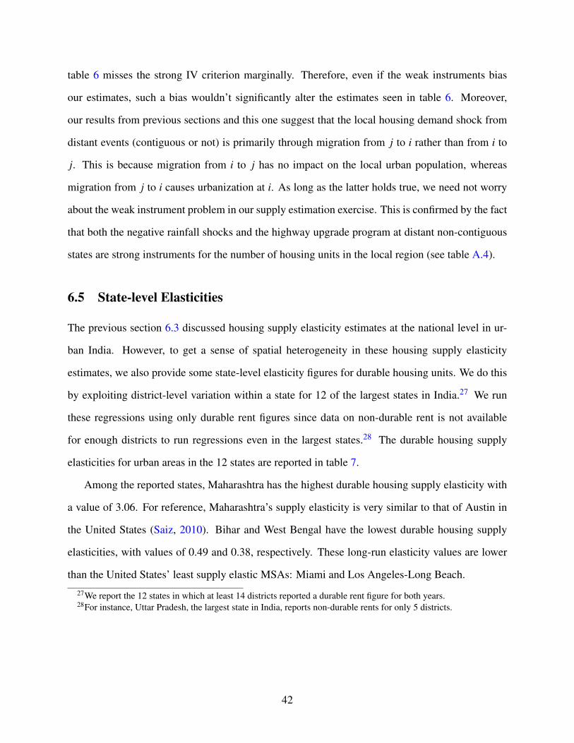
table 6 misses the strong IV criterion marginally. Therefore, even if the weak instruments bias

our estimates, such a bias wouldn’t significantly alter the estimates seen in table 6. Moreover,

our results from previous sections and this one suggest that the local housing demand shock from

distant events (contiguous or not) is primarily through migration from j to i rather than from i to

j. This is because migration from i to j has no impact on the local urban population, whereas

migration from j to i causes urbanization at i. As long as the latter holds true, we need not worry

about the weak instrument problem in our supply estimation exercise. This is confirmed by the fact

that both the negative rainfall shocks and the highway upgrade program at distant non-contiguous

states are strong instruments for the number of housing units in the local region (see table A.4).

6.5 State-level Elasticities

The previous section 6.3 discussed housing supply elasticity estimates at the national level in ur-

ban India. However, to get a sense of spatial heterogeneity in these housing supply elasticity

estimates, we also provide some state-level elasticity figures for durable housing units. We do this

by exploiting district-level variation within a state for 12 of the largest states in India.27 We run

these regressions using only durable rent figures since data on non-durable rent is not available

for enough districts to run regressions even in the largest states.28 The durable housing supply

elasticities for urban areas in the 12 states are reported in table 7.

Among the reported states, Maharashtra has the highest durable housing supply elasticity with

a value of 3.06. For reference, Maharashtra’s supply elasticity is very similar to that of Austin in

the United States (Saiz, 2010). Bihar and West Bengal have the lowest durable housing supply

elasticities, with values of 0.49 and 0.38, respectively. These long-run elasticity values are lower

than the United States’ least supply elastic MSAs: Miami and Los Angeles-Long Beach.

27We report the 12 states in which at least 14 districts reported a durable rent figure for both years.28For instance, Uttar Pradesh, the largest state in India, reports non-durable rents for only 5 districts.

42

Table 7: State-level Elasticity of Housing Supply

State Urban population (mil.) Durable elasticity Comparable US MSAs (Saiz, 2010)

Maharashtra 51 3.06 Austin, TX

Odisha 7 2.05 Mobile, AL

Tamil Nadu 35 1.92 Fresno, CA

Andhra Pradesh 28 1.63 Phoenix, AZ

Gujarat 26 1.31 Las Vegas, NV

Madhya Pradesh 20 1.25 Detroit, MI

Uttar Pradesh 44 1.17 Newark, NJ

Rajasthan 17 1.06 Jacksonville, FL

Karnataka 24 0.75 New York, NY

Haryana 9 0.54 Miami, FL

Bihar 12 0.49

West Bengal 29 0.38

Source: Authors’ calculations.Note: All reported states have observations on durable housing rents and quantities for at least 14 districts. States arranged in decreasing orderof elasticity values. All elasticity values rounded off to two decimal places. Last column shows MSAs in the United States that have comparablehousing supply elasticities. There are no metropolitan areas in the United States with elasticity figures comparable to Bihar and West Bengal. Miamiis the least supply elastic MSA in the United States with an elasticity value of 0.6.

7 Conclusion

According to the United Nations, developing countries in Africa and South Asia are set to ex-

perience the next wave of urbanization (United-Nations, 2018). India will be one of the largest

contributors to this growth. But, academic literature on housing in India is sparse. We fill this gap

by estimating the supply elasticity of housing in urban India. We apply the Rosen-Roback spa-

tial equilibrium framework to estimate the effect of distant state shock-induced migration on local

urbanization and housing demand in local urban markets. We use a distant state’s rainfall shocks

and a highway upgrade program implementation status as demand shifters to estimate the supply

elasticity of local urban housing markets.

We begin by presenting some stylized facts on housing and migration in India. Next, we discuss

the underlying theoretical framework, followed by a discussion of the empirical implementation

of the model mechanisms. Then we discuss the empirical results and robustness checks. We find

43

that both the negative rainfall shocks and the highway upgrade implementation at the distant state

induce inter-state migration, thereby inducing local urbanization and the demand for local urban

housing. We estimate national-level housing supply elasticity figures for urban India’s durable,

non-durable, and vacant residential housing units.

While national-level housing supply elasticity estimates do not paint an accurate picture of

metropolitan-level elasticities and the underlying heterogeneity across metropolitan areas of dif-

ferent sizes and regulations, it is a relevant parametric estimate in the context of a large, urbanizing

country. Further research with metropolitan-level price and new construction data would be re-

quired to provide granular estimates.

44

References

Abeberese, A. B. and Chen, M. (2021) Intranational trade costs, product scope and productivity:

Evidence from India’s Golden Quadrilateral project, Journal of Development Economics, p.

102791.

Accetturo, A., Lamorgese, A., Mocetti, S. and Pellegrino, D. (2021) Housing supply elasticity and

growth: Evidence from Italian cities, Journal of Economic Geography, 21, 367–396.

Bartik, T. J. (1993) Who benefits from local job growth: migrants or the original residents?, Re-

gional studies, 27, 297–311.

Baum-Snow, N. and Han, L. (2019) The microgeography of housing supply, Work in progress,

University of Toronto.

Bertaud, A. and Brueckner, J. K. (2005) Analyzing building-height restrictions: predicted impacts

and welfare costs, Regional Science and Urban Economics, 35, 109–125.

Bhan, G. (2009) “This is no longer the city I once knew”. Evictions, the urban poor and the right

to the city in millennial Delhi, Environment and Urbanization, 21, 127–142.

Bhavnani, R. R. and Lacina, B. (2017) Fiscal federalism at work? Central responses to internal

migration in India, World Development, 93, 236–248.

Boustan, L. P. (2010) Was postwar suburbanization “white flight”? Evidence from the black mi-

gration, The Quarterly Journal of Economics, 125, 417–443.

Brueckner, J. K. and Selod, H. (2009) A theory of urban squatting and land-tenure formalization

in developing countries, American Economic Journal: Economic Policy, 1, 28–51.

Brueckner, J. K. and Sridhar, K. S. (2012) Measuring welfare gains from relaxation of land-use

restrictions: The case of India’s building-height limits, Regional Science and Urban Economics,

42, 1061–1067.

45

Brueckner, J. K. et al. (1987) The structure of urban equilibria: A unified treatment of the Muth-

Mills model, Handbook of Regional and Urban Economics, 2, 821–845.

Census of India, P. (2011) Census of India 2011 Provisional Population Totals, Office of the Reg-

istrar General and Census Commissioner New Delhi.

Desa, U. et al. (2014) World urbanization prospects, the 2011 revision, Population Division, De-

partment of Economic and Social Affairs, United Nations Secretariat.

Diamond, R. (2017) Housing supply elasticity and rent extraction by state and local governments,

American Economic Journal: Economic Policy, 9, 74–111.

Dutta, A., Green, R. K., Panchapagesan, V. and Venkataraman, M. (2021) Are move-in ready

properties more expensive?, Available at SSRN 3851745.

Elisseeff, V. (2000) The silk roads: Highways of culture and commerce, Berghahn Books.

Gandhi, S., Green, R. K. and Patranabis, S. (2021a) India’s housing vacancy paradox: How rent

control and weak contract enforcement produce unoccupied units and a housing shortage at the

same time, CSEP Working Paper.

Gandhi, S., Tandel, V., Tabarrok, A. and Ravi, S. (2021b) Too slow for the urban march: Litigations

and the real estate market in Mumbai, India, Journal of Urban Economics, 123, 103330.

Ghani, E., Goswami, A. G. and Kerr, W. R. (2016) Highway to success: The impact of the Golden

Quadrilateral project for the location and performance of Indian manufacturing, The Economic

Journal, 126, 317–357.

Ghose, D. (2019) Trade, Internal Migration, and Human Capital: Who Gains from India’s IT

Boom?

Glaeser, E. L., Gyourko, J. and Saks, R. (2005) Why is Manhattan so expensive? Regulation and

the rise in housing prices, The Journal of Law and Economics, 48, 331–369.

46

Green, R. K., Malpezzi, S. and Mayo, S. K. (2005) Metropolitan-specific estimates of the price

elasticity of supply of housing, and their sources, American Economic Review, 95, 334–339.

Gyourko, J., Saiz, A. and Summers, A. (2008) A new measure of the local regulatory environment

for housing markets: The Wharton Residential Land Use Regulatory Index, Urban Studies, 45,

693–729.

Harari, M. (2020) Cities in bad shape: Urban geometry in India, American Economic Review, 110,

2377–2421.

Harris, J. R. and Todaro, M. P. (1970) Migration, unemployment and development: a two-sector

analysis, The American Economic Review, 60, 126–142.

Henderson, J. V., Regan, T. and Venables, A. J. (2021) Building the city: from slums to a modern

metropolis, The Review of Economic Studies, 88, 1157–1192.

Imbert, C. and Papp, J. (2015) Labor market effects of social programs: Evidence from india’s

employment guarantee, American Economic Journal: Applied Economics, 7, 233–63.

Imbert, C. and Papp, J. (2020) Short-term migration, rural public works, and urban labor markets:

Evidence from India, Journal of the European Economic Association, 18, 927–963.

India Meteorological Department, P. (1901-2017) India Meteorological Department Rainfall

Datasets, http://www.imd.gov.in.

Jayachandran, S. (2006) Selling labor low: Wage responses to productivity shocks in developing

countries, Journal of Political Economy, 114, 538–575.

Kone, Z. L., Liu, M. Y., Mattoo, A., Ozden, C. and Sharma, S. (2018) Internal borders and migra-

tion in India, Journal of Economic Geography, 18, 729–759.

Labor Bureau of India, D. (2001-2012) Consumer Price Index Series,

http://www.labourbureau.gov.in/.

47

Malpezzi, S. and Maclennan, D. (2001) The long-run price elasticity of supply of new residential

construction in the United States and the United Kingdom, Journal of Housing Economics, 10,

278–306.

Marx, B., Stoker, T. and Suri, T. (2013) The economics of slums in the developing world, Journal

of Economic perspectives, 27, 187–210.

McLaughlin, R. B. (2012) New housing supply elasticity in Australia: a comparison of dwelling

types, The Annals of Regional Science, 48, 595–618.

Mills, E. S. (1967) An aggregative model of resource allocation in a metropolitan area, The Amer-

ican Economic Review, 57, 197–210.

Mitra, A. (2010) Migration, livelihood and well-being: Evidence from indian city slums, Urban

Studies, 47, 1371–1390.

Molloy, R., Smith, C. L. and Wozniak, A. (2011) Internal migration in the United States, Journal

of Economic Perspectives, 25, 173–96.

Morten, M. (2019) Temporary migration and endogenous risk sharing in village India, Journal of

Political Economy, 127, 1–46.

Munshi, K. and Rosenzweig, M. (2016) Networks and misallocation: Insurance, migration, and

the rural-urban wage gap, American Economic Review, 106, 46–98.

National Sample Survey Organization, I. (1999-2012) Indian National Sample Surveys, Rounds

55, 58, 66, and 69, http://mospi.nic.in.

Niu, D., Sun, W. and Zheng, S. (2021) The role of informal housing in lowering China’s urbaniza-

tion costs, Regional Science and Urban Economics, p. 103638.

Paciorek, A. (2013) Supply constraints and housing market dynamics, Journal of Urban Eco-

nomics, 77, 11–26.

48

Poterba, J. M. (1984) Tax subsidies to owner-occupied housing: an asset-market approach, The

Quarterly Journal of Economics, 99, 729–752.

Quigley, J. M. and Raphael, S. (2005) Regulation and the high cost of housing in California,

American Economic Review, 95, 323–328.

Rains, E. and Krishna, A. (2020) Precarious gains: Social mobility and volatility in urban slums,

World Development, 132, 105001.

Rains, E., Krishna, A. and Wibbels, E. (2019) Combining satellite and survey data to study indian

slums: Evidence on the range of conditions and implications for urban policy, Environment and

Urbanization, 31, 267–292.

Roback, J. (1982) Wages, rents, and the quality of life, Journal of Political Economy, 90, 1257–

1278.

Rosen, S. (1979) Wage-based indexes of urban quality of life, Current Issues in Urban Economics,

pp. 74–104.

Rosenzweig, M. R. and Udry, C. (2014) Rainfall forecasts, weather, and wages over the agricultural

production cycle, American Economic Review, 104, 278–83.

Saiz, A. (2010) The geographic determinants of housing supply, The Quarterly Journal of Eco-

nomics, 125, 1253–1296.

Saks, R. E. and Wozniak, A. (2011) Labor reallocation over the business cycle: New evidence

from internal migration, Journal of Labor Economics, 29, 697–739.

Sarsons, H. (2015) Rainfall and conflict: A cautionary tale, Journal of Development Economics,

115, 62–72.

Sekhri, S. and Storeygard, A. (2014) Dowry deaths: Response to weather variability in India,

Journal of Development economics, 111, 212–223.

49

Sridhar, K. S. (2010) Impact of land use regulations: Evidence from India’s cities, Urban Studies,

47, 1541–1569.

Srivastava, R. (2011) Internal migration in india, Human Development in India.

Thapar, R. (2015) The Penguin history of early India: from the origins to AD 1300, Penguin UK.

Tiwari, P. and Parikh, J. (1998) Affordability, housing demand and housing policy in urban India,

Urban Studies, 35, 2111–2129.

Tiwari, P., Parikh, K. and Parikh, J. (1999) Effective housing demand in Mumbai (Bombay)

metropolitan region, Urban Studies, 36, 1783–1809.

Todaro, M. P. (1969) A model of labor migration and urban unemployment in less developed

countries, The American Economic Review, 59, 138–148.

United-Nations (2018) World Urbanization Prospects: The 2018 Revision.

Wang, S., Chan, S. H. and Xu, B. (2012) The estimation and determinants of the price elasticity of

housing supply: Evidence from China, Journal of Real Estate Research, 34, 311–344.

Zabel, J. E. (2012) Migration, housing market, and labor market responses to employment shocks,

Journal of Urban Economics, 72, 267–284.

50

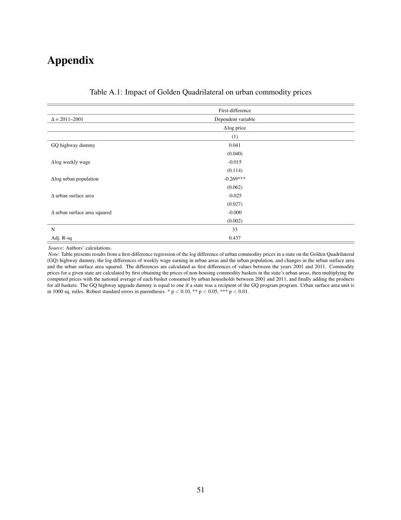
Appendix

Table A.1: Impact of Golden Quadrilateral on urban commodity prices

First-difference

∆ = 2011–2001 Dependent variable

∆ log price

(1)

GQ highway dummy 0.041

(0.040)

∆ log weekly wage -0.015

(0.114)

∆ log urban population -0.269***

(0.062)

∆ urban surface area -0.025

(0.027)

∆ urban surface area squared -0.000

(0.002)

N 33

Adj. R-sq 0.437

Source: Authors’ calculations.Note: Table presents results from a first-difference regression of the log difference of urban commodity prices in a state on the Golden Quadrilateral(GQ) highway dummy, the log differences of weekly wage earning in urban areas and the urban population, and changes in the urban surface areaand the urban surface area squared. The differences are calculated as first differences of values between the years 2001 and 2011. Commodityprices for a given state are calculated by first obtaining the prices of non-housing commodity baskets in the state’s urban areas, then multiplying thecomputed prices with the national average of each basket consumed by urban households between 2001 and 2011, and finally adding the productsfor all baskets. The GQ highway upgrade dummy is equal to one if a state was a recipient of the GQ program program. Urban surface area unit isin 1000 sq. miles. Robust standard errors in parentheses. * p < 0.10, ** p < 0.05, *** p < 0.01.

51

Table A.2: Distant shock-induced local urbanization and housing demand without median rooms as a control

2SLS

First-stage Second-stage︷ ︸︸ ︷ ︷ ︸︸ ︷∆ = 2011–2001 Dependent variable

∆ log urban population at i ∆ log non-durable units at i ∆ log durable units at i ∆ log vacant units at i

(1) (2) (3) (4)

∆ log urban population at i 0.205*** 1.86*** 2.41***

(0.025) (0.026) (0.034)

∆ #months rainfall < 80% at j 0.011***

(0.000)

GQ highway dummy at j 0.124***

(0.005)

∆ log consumption at i 0.009 -0.197*** 0.037** -0.203***

(0.013) (0.014) (0.018) (0.020)

∆ urban surface area at i 5.12*** 0.824*** -1.54*** -2.82***

(0.202) (0.220) (0.226) (0.316)

∆ urban surface area squared at i -5.53*** -1.84*** 1.24*** 1.03**

(0.418) (0.348) (0.310) (0.463)

F-stat on excluded instruments 1018***

Anderson–Rubin Wald χ2(2) 54.8*** 3402*** 2495***

Sargan-Hansen J-stat p-value 0.708 0.420 0.968

N 4,896 4,896 4,896 4,896

Adj. R-sq 0.603

Source: Authors’ calculations.Note: Table presents results from two-stage least squares regressions of the log differences of three types of residential housing units in district i – non-durable, durable, and vacant – on the endogenousvariable – log difference of urban population in district i. The log differences are calculated as first differences of log values between the years 2001 and 2011. District i is the local region and is paired withdistant states indexed j. There are 4,896 i− j district-state pairs consisting of 144 districts and 35 states and union territories in India. The log difference of urban population in district i is instrumentedby the decadal change in the number of months when rainfall was less than 80% of the long-term normal in a distant state j, and a dummy variable equal to one if state j was recipient of the GoldenQuadrilateral highway upgrade program. The first-stage regression coefficients are given in column (1) and the second-stage results are given in columns (2)-(4). Other variables in the regressions includelog difference in district-level mean per capita consumption at i, and changes in the urban surface area and the urban surface area squared at i. Diagnostics reported are the F-test of excluded instruments’joint significance, the Anderson-Rubin Wald chi-square test of significance of endogenous regressors, and the Sargan-Hansen J-statistic for overidentification tests. Urban surface area unit is in 1000 sq.miles. Robust standard errors in parentheses. * p < 0.10, ** p < 0.05, *** p < 0.01.

52

Table A.3: Housing supply elasticity estimation with full sample data on durable rents

2SLS

First-stage Second-stage︷ ︸︸ ︷ ︷ ︸︸ ︷∆ = 2011–2001 Dependent variable

∆ log durable units at i ∆ log vacant units at i ∆ log durable rent at i ∆ log overall rent at i

(1) (2) (3) (4)

∆ log durable units at i 0.738***

(0.029)

∆ log vacant units at i 0.561***

(0.022)

∆ #months rainfall < 80% at j 0.020*** 0.025***

(0.000) (0.001)

GQ highway dummy at j 0.214*** 0.284***

(0.004) (0.006)

∆ log consumption at i 0.044*** 0.006 0.175*** 0.128***

(0.010) (0.013) (0.024) (0.023)

∆ urban surface area at i 9.42*** 11.4*** -6.88*** -5.65***

(0.217) (0.277) (0.485) (0.443)

∆ urban surface area squared at i -10.9*** -15.0*** 8.02*** 7.95***

(0.500) (0.622) (0.767) (0.736)

F-stat on excluded instruments 3696*** 3271***

Anderson–Rubin Wald χ2(2) 677*** 712***

Sargan-Hansen J-stat p-value 0.799 0.657

N 11,526 11,526 11,526 11,526

Adj. R-sq 0.673 0.611

Source: Authors’ calculations.Note: Table presents results from two-stage least squares regressions of the log differences of average housing rents paid on the endogenous variables – log differences of the market clearing quantitiesof housing units in district i. Regressions are run for two types of residential housing – durable and vacant. The log differences are calculated as first differences of log values between the years 2001and 2011. District i is the local region and is paired with distant states indexed j. There are 11,526 i− j district-state pairs consisting of 339 districts and 35 states and union territories in India. The logdifferences of housing units in district i are instrumented by the decadal change in the number of months when rainfall was less than 80% of the long-term normal in a distant state j, and a dummy variableequal to one if state j was recipient of the Golden Quadrilateral highway upgrade program. The first-stage regression coefficients are given in columns (1)-(3) and the second-stage results are given incolumns (4)-(6). Other variables in the regressions include log difference in district-level mean per capita consumption at i, and changes in the urban surface area and the urban surface area squared ati. Diagnostics reported are the F-test of excluded instruments’ joint significance, the Anderson-Rubin Wald chi-square test of significance of endogenous regressors, and the Sargan-Hansen J-statistic foroveridentification tests. Urban surface area unit is in 1000 sq. miles. Robust standard errors in parentheses. * p < 0.10, ** p < 0.05, *** p < 0.01.

53

Table A.4: Housing supply elasticity estimation with non-contiguous state shocks

2SLS

First-stage Second-stage︷ ︸︸ ︷ ︷ ︸︸ ︷∆ = 2011–2001 Dependent variable

∆ log non-durable units at i ∆ log durable units at i ∆ log vacant units at i ∆ log non-durable rent at i ∆ log durable rent at i ∆ log overall rent at i

(1) (2) (3) (4) (5) (6)

∆ log non-durable units at i -2.03***

(0.609)

∆ log durable units at i 0.601***

(0.039)

∆ log vacant units at i 0.377***

(0.027)

∆ #months rainfall < 80% at j 0.001*** 0.022*** 0.027***

(0.001) (0.001) (0.001)

GQ highway dummy at j 0.035*** 0.219*** 0.309***

(0.008) (0.008) (0.012)

∆ log consumption at i -0.192*** 0.055*** -0.196*** -0.474*** 0.439*** 0.399***

(0.016) (0.019) (0.029) (0.135) (0.045) (0.038)

∆ urban surface area at i 1.94*** 7.98*** 9.60*** 6.67*** -2.14*** -0.091

(0.181) (0.347) (0.429) (1.532) (0.532) (0.450)

∆ urban surface area squared at i -3.09*** -9.17*** -12.5*** -5.91** 2.82*** 1.67**

(0.397) (0.720) (0.870) (2.327) (0.807) (0.742)

F-stat on excluded instruments 21.7*** 1491*** 1072***

Anderson–Rubin Wald χ2(2) 14.9*** 254*** 212***

Sargan-Hansen J-stat p-value 0.514 0.400 0.022

N 4,224 4,224 4,224 4,224 4,224 4,224

Adj. R-sq 0.072 0.661 0.554

Source: Authors’ calculations.Note: Table presents results from two-stage least squares regressions of the log differences of average housing rents paid on the endogenous variables – log differences of the market clearing quantitiesof housing units in district i. Regressions are run for three types of residential housing – non-durable, durable, and vacant. The log differences are calculated as first differences of log values between theyears 2001 and 2011. District i is the local region and is paired with distant non-contiguous states j that are outside the state in which district is located. There are 4,224 non-contiguous i− j district-statepairs consisting of 144 districts and 35 states and union territories in India. The log differences of housing units in district i are instrumented by the decadal change in the number of months when rainfallwas less than 80% of the long-term normal in a distant state j, and a dummy variable equal to one if state j was recipient of the Golden Quadrilateral highway upgrade program. The first-stage regressioncoefficients are given in columns (1)-(3) and the second-stage results are given in columns (4)-(6). Other variables in the regressions include log difference in district-level mean per capita consumption ati, and changes in the urban surface area and the urban surface area squared at i. Diagnostics reported are the F-test of excluded instruments’ joint significance, the Anderson-Rubin Wald chi-square test ofsignificance of endogenous regressors, and the Sargan-Hansen J-statistic for overidentification tests. Urban surface area unit is in 1000 sq. miles. Robust standard errors in parentheses. * p < 0.10, ** p <0.05, *** p < 0.01.

54