This content has been downloaded from IOPscience. Please scroll down to see the full text.

Download details:

IP Address: 218.18.30.123

This content was downloaded on 11/10/2013 at 03:35

Please note that terms and conditions apply.

Dissipative ground-state preparation of a spin chain by a structured environment

View the table of contents for this issue, or go to the journal homepage for more

2013 New J. Phys. 15 073027

(http://iopscience.iop.org/1367-2630/15/7/073027)

Home Search Collections Journals About Contact us My IOPscience

Dissipative ground-state preparation of a spin chainby a structured environment

Cecilia Cormick1,2,3, Alejandro Bermudez1,2, Susana F Huelga1,2

and Martin B Plenio1,2

1 Institute for Theoretical Physics, Universitat Ulm, D-89069 Ulm, Germany2 Center for Integrated Quantum Science and Technology, Universitat Ulm,D-89069 Ulm, GermanyE-mail: cecilia.cormick@uni-ulm.de

New Journal of Physics 15 (2013) 073027 (30pp)Received 16 April 2013Published 15 July 2013Online at http://www.njp.org/doi:10.1088/1367-2630/15/7/073027

Abstract. We propose a dissipative method to prepare the ground state of theisotropic XY spin Hamiltonian in a transverse field. Our model consists of a spinchain with nearest-neighbor interactions and an additional collective couplingof the spins to a damped harmonic oscillator. The latter provides an effectiveenvironment with a Lorentzian spectral density and can be used to drive thechain asymptotically toward its multipartite-entangled ground state at a rate thatdepends on the degree of non-Markovianity of the evolution. We also present adetailed proposal for the experimental implementation with a chain of trappedions. The protocol does not require individual addressing, concatenated pulses,or multi-particle jump operators, and is capable of generating the desired targetstate in small ion chains with very high fidelities.

3 Author to whom any correspondence should be addressed.

Content from this work may be used under the terms of the Creative Commons Attribution 3.0 licence.Any further distribution of this work must maintain attribution to the author(s) and the title of the work, journal

citation and DOI.

New Journal of Physics 15 (2013) 0730271367-2630/13/073027+30$33.00 © IOP Publishing Ltd and Deutsche Physikalische Gesellschaft

2

Contents

1. Introduction 22. Steady-state entanglement of a spin chain 4

2.1. Spin chain with controllable decoherence . . . . . . . . . . . . . . . . . . . . 42.2. Cooling or heating to an entangled steady state . . . . . . . . . . . . . . . . . 52.3. Preparation of the ground state of the isotropic XY chain in a transverse field . 13

3. Realization with crystals of trapped ions 173.1. Trapped-ion crystal as a spin-boson chain . . . . . . . . . . . . . . . . . . . . 173.2. Engineering the isotropic XY spin model . . . . . . . . . . . . . . . . . . . . 203.3. Controlling the spin-boson coupling . . . . . . . . . . . . . . . . . . . . . . . 213.4. Effective damping of the bosonic mode . . . . . . . . . . . . . . . . . . . . . 223.5. Numerical analysis of the trapped-ion dissipative protocol . . . . . . . . . . . . 24

4. Conclusions and outlook 27Acknowledgments 28References 28

1. Introduction

The general goal of quantum information processing is to manipulate the information codedin a particular quantum system, while simultaneously trying to isolate it from undesiredperturbations due to the external environment. For instance, in the fields of quantumcomputation [1] and quantum simulation [2], the processing stage usually relies on a designedunitary evolution which, preserving the coherence of the system, provides a quantum statethat contains the outcome of the computation, or the properties of the quantum phase ofmatter under study. Therefore, the experimental progress in these fields has been typicallyassociated to technological developments that minimize experimental imperfections andmaximize environmental isolation [1, 2].

However, the coupling of a system to its surrounding environment is not necessarily adisadvantage. In fact, the dissipation of a quantum system, if judiciously exploited, can act asa resource for quantum information processing. This interesting change of paradigm startedwith the recognition that dissipation can assist the generation of entanglement between distantatoms, either in free space [3], or trapped inside cavities [4, 5]. By measuring the presenceof a photon spontaneously emitted by the atoms [3, 5], or its absence [4], it is possible toproject an initially uncorrelated atomic state into a maximally entangled one, as has beenrecently experimentally demonstrated [6]. These schemes can be improved further by tailoringthe atom–cavity interaction [7] or by modifying the measurement techniques [8], and can also begeneralized to provide a route toward universal quantum computation [9]. Since the dissipationdoes not always render the desired result in these approaches, the measurement is required toselect only the successful outcomes. Therefore, the combination of dissipation and measurementcan be considered as a probabilistic resource for quantum information.

Another promising approach is to assess whether, by designing the system–environmentcoupling in a particular way, the dissipation could provide the desired quantum state withcertainty. This quantum reservoir engineering finds its roots in the theory of laser coolingof atoms [10] and, more related to this work, of trapped ions [11]. Laser-cooling schemes

New Journal of Physics 15 (2013) 073027 (http://www.njp.org/)

3

try to design the system–environment coupling such that the dissipation yields a stationarystate with reduced kinetic energy. These ideas can be taken a step further in order to non-probabilistically produce stationary states that display non-classical aspects, or a certain amountof entanglement [12]. For instance, by mimicking superradiance phenomena [13], certainengineered decay channels yield partial entanglement in the stationary mixed state [14].However, it would be highly desirable to devise dissipative protocols that provide maximallyentangled pure states asymptotically, the so-called dark states, showing fidelities comparable tothose obtained by more standard unitary schemes [1].

This approach has been recently pursued by different groups which have shown that,provided that one can engineer a dissipation that acts quasi-locally on different parts of thesystem, it is possible to design dissipative protocols to produce a number of paradigmaticdark states [15], or to perform universal dissipative quantum computation [16]. For instance,by engineering a particular dissipation that acts on pairs of adjacent atoms in an opticallattice, the system can be driven dissipatively into a superfluid phase [17]. In addition,as initially proposed for Rydberg atoms [18] and first realized in experiments of trappedions [19], by concatenating multi-qubit gates with a controlled dissipation of ancillary qubits,a variety of multipartite entangled states (i.e. Bell, Greenberger–Horne–Zeilinger and Dickestates) have been dissipatively generated with reasonably high fidelities. Let us note that thisstroboscopic time-evolution corresponds to a Markovian master equation in the limit of manygates and dissipation steps, where the dissipative jump operators correspond to multi-qubitjump operators. From a fundamental point of view, it is of interest to address whether similardissipative protocols can also work in an (i) analogue and (ii) global fashion (i.e. using always-on couplings without individual addressing). Additionally, from a more pragmatic point of view,such global analogue schemes would not be limited by the accumulation of the errors in eachstep of the stroboscopic protocols. However, finding particular schemes to provide multi-qubitjump operators in an analogue manner seems to be a tremendous task from both a theoreticaland experimental point of view. Therefore, we impose a further constraint, the jump operatorsshould be composed of (iii) single-qubit operators.

In this paper, we develop an instance of a global analogue dissipative protocol thatgenerates multipartite entangled states corresponding to ground states of a quantum spin chain.The underlying idea is to engineer jump operators that are a particular sum of single-spinoperators, in analogy to the models of collective spontaneous emission [13]. We show that,if the dissipation of the spins is mediated by a common harmonic mode, the spin chainsees a structured Markovian environment. By structured environment we refer to a spectraldensity exhibiting a sharp peak at a certain frequency (so called Breit–Wigner resonance),corresponding to a weakly damped harmonic oscillator. This structure will allow us to designjump operators in such a way that the stationary state of the system corresponds to the groundstate of the quantum spin chain. In particular, we consider an isotropic XY spin chain, whichdescribes a critical phase of matter.

We explain in detail how to implement this protocol with trapped ions, relying ontools that have already been achieved experimentally. These tools are the so-called state-dependent forces [20–24], and sympathetic resolved-sideband cooling developed for quantumcomputation [25, 26]. We test the scheme for realistic parameters, and show that the fidelitiesthat can be achieved are comparable to the unitary protocols that produce multipartite entangledstates [27]. Our procedure performs well for small chains of trapped ions, which is actually theregime in most of the current experiments.

New Journal of Physics 15 (2013) 073027 (http://www.njp.org/)

4

a

J J

gigi

Δa

κ

E

S

κ

κ

b

qn

2J

−2J

Δn

L−n

L+n

n

Figure 1. Damped spin-boson chain: (a) schematic representation of a spinchain with an isotropic XY Hamiltonian subjected to an additional transversefield whose intensity depends on the position coordinate of a damped harmonicoscillator. This oscillator mediates the dissipation of the spin chain, whicheffectively sees a structured environment. (b) The effect of the oscillator on thespin chain is described by jump operators L+

n and L−

n going respectively up anddown the spectrum of spin-chain excitations with quasimomentum qn and energyεn (the model parameters are defined in the text).

This paper is organized as follows. In section 2, we describe the dissipative protocol. Westart by introducing the model under consideration in section 2.1, and then move onto an analyticdiscussion, supported by numerical results, of how to engineer a structured environment thatallows us to prepare multipartite entangled states dissipatively (section 2.2). In section 2.3 weexplain how the method can be used to cool the system to the many-body ground state of thequantum spin chain. In section 3 we show how crystals of trapped atomic ions are ideally suitedfor an experimental implementation of our ideas. Section 3.1 describes the trapped-ion setup, atwo-species Coulomb crystal. In sections 3.2–3.4 we introduce the trapped-ion toolbox requiredto implement the dissipative protocol. Section 3.5 contains a numerical analysis of the trapped-ion dissipative protocol. Finally, we present our conclusions and an outlook in section 4.

2. Steady-state entanglement of a spin chain

2.1. Spin chain with controllable decoherence

Let us start by introducing the model under consideration: an interacting spin- 12 chain coupled to

a damped bosonic mode (see figure 1(a)). This model, which shall be referred to as the dampedspin-boson chain (DSBC) in the rest of the paper, is a many-body generalization of a systemconsidered recently for the dissipative generation of two-qubit entanglement [28]. The DSBC isdescribed by the following master equation (h = 1):

dρ

dt= LDSBC(ρ)= −i[Hb + Hs + Hsb, ρ] + Db(ρ), (1)

New Journal of Physics 15 (2013) 073027 (http://www.njp.org/)

5

where ρ is the total density matrix and LDSBC is the dissipative Liouvillian. We consider a finitechain of N spins evolving under the isotropic XY Hamiltonian [29]

Hs =

N−1∑i=1

Jσ +i σ

−

i+1 + H.c., (2)

where J > 0 is an antiferromagnetic interaction strength, and we introduced the raising andlowering operators σ +

i = |↑i〉〈↓i | = (σ−

i )†. The bosonic Hamiltonian consists of a single mode

Hb =1aa†a, (3)

where a† and a are respectively the creation and annihilation operators (the oscillator frequency1a can actually correspond to a detuning 1a ≶ 0, as will become clear from the experimentalimplementation). The spins and the boson are coupled through

Hsb =

N∑i=1

giσzi (a + a†). (4)

In the above expression, we have introduced the site-dependent coupling strength gi and thePauli matrices σ z

i = |↑i〉〈↑i | − | ↓i〉〈↓i |. Finally, we also consider weak damping of the bosonicmode via a Lindblad-type dissipator:

Db(ρ)= κ(aρa†− a†aρ)+ H.c., (5)

where κ > 0 is the damping rate. We note that all these individual ingredients can be realizedwith the state-of-the-art technology of trapped-ion crystals, as described in section 3. Theobjective of this work is to understand the interplay of these dynamics, such that the LiouvillianLDSBC generates stationary entanglement between the initially uncorrelated spins. So far, wecan already appreciate two of the properties of the protocol outlined in the introduction: (i)it is analogue, since the couplings (2)–(5) are considered to be switched on during the wholeprotocol. (ii) It is global, since the couplings (2)–(5) address all the spins of the chain.

Let us note that the spin-chain Hamiltonian (2) alone could already generate entangledstates unitarily at given instants of time. Nonetheless, these correlations have a transient nature,whereas the interest of this work is the onset of stationary correlations. Therefore, we explorethe interplay of this Hamiltonian part with the irreversible dynamics introduced by the dampedboson through the spin-boson coupling (4).

In figure 1(a), we represent schematically the DSBC. The spin chain is considered tobe our system S , whereas the bosonic mode, together with the Markovian reservoir whereit dissipates, provide an effective structured environment E for the spin chain. At first sight,the dephasing-like spin-boson coupling (4) seems to introduce a source of decoherence inthe spin chain, thus hindering rather than assisting the generation of stationary entanglement.In the following section, we will show that this naıve intuition is not always valid, and explainthe subtle mechanism that allows for generation of stationary entanglement in a particularregime of the system parameters.

2.2. Cooling or heating to an entangled steady state

We consider an initial state of the system ρ(0)= |ψ0〉〈ψ0| ⊗ ρb(0), where ρb(0) is an arbitrarystate of the harmonic mode, and the uncorrelated spin state |ψ0〉 = |↑1↓2↓3 . . . ↓N 〉 has asingle spin excitation at the left edge of the chain. In this section, we discuss how the systemLiouvillian LDSBC acts on this state, allowing for the onset of stationary entanglement.

New Journal of Physics 15 (2013) 073027 (http://www.njp.org/)

6

2.2.1. Spin-chain spectrum. As a consequence of the XY Hamiltonian (2), the initiallylocalized spin excitation is exchanged between different neighbors. In fact, the spin chaincorresponds exactly to a tight-binding model where the excitation hops along the sites of theunderlying chain according to

Hs,1 = Ps HsPs =

N−1∑i=1

J |i〉〈i + 1| + H.c. (6)

In this expression, Hs,1 results from the projection of the XY Hamiltonian onto the single-excitation subspace Hs → Ps HsPs, where Ps is the projector onto an N -dimensional subspacespanned by the states |i〉, such that i labels the position of the spin excitation in the chain. Thistight-binding model gives rise to the following band structure (see figure 1(b)):

εn = 2J cos(qn), qn =πn

N + 1, n = 1, . . . , N , (7)

where each energy is associated to a ‘spin-wave excitation’

|qn〉 = NN∑

i=1

sin(qni)|i〉, N =

(2

N + 1

) 12. (8)

The goal of this section is to find the conditions to generate dissipatively one of these multipartiteentangled states Tra{eLDSBCt

|ψ0〉〈ψ0| ⊗ ρb(0)} → |qn〉〈qn|.

2.2.2. Spin-wave ladder. We consider a spatial modulation of the spin-boson couplingstrength (4) in the form gi = g cos(qgi), where qg = π/(N + 1). In the single-excitationsubspace, the spin-boson coupling becomes

Hsb,1 = Ps HsbPs =

N−1∑n=1

g(L+n + L−

n )(a + a†), (9)

where the ladder operators L+n = |qn〉〈qn+1| = (L−

n )† are responsible for ascending or descending

along the ladder of spin-wave excitations (see figure 1(b)). Accordingly, the spin-bosoncoupling (9) connects different spin-wave excitations, while simultaneously creating orannihilating bosonic quanta. Moreover, since the harmonic mode dissipates irreversibly into aMarkovian environment (5), the ladder operators L±

n introduce irreversible dynamics in the spinchain. In terms of these ladder operators, the single-excitation spin-chain Hamiltonian (6) reads

Hs,1 =

N−1∑n=1

εn L+n L−

n , (10)

where for simplicity we reset the zero of energy at the bottom of the band. We show below howto generate mesoscopic entangled states, by controlling the relative strengths of the dissipativeprocesses that take the system up and down the spin-wave ladder.

2.2.3. Irreversible dynamics in the spin chain. Since we are interested in the stationaryproperties of the DSBC, we consider long times t � κ−1, such that the bosonic mode has enoughtime to relax under the action of the damping. Besides, for |g| � κ , this relaxation is much fasterthan the process of energy exchange between the boson and the spins. In this limit, the boson

New Journal of Physics 15 (2013) 073027 (http://www.njp.org/)

7

thermalizes individually, and the spin chain evolves on a much slower timescale under such abosonic background.

To obtain the effect of the boson background on the slower spin dynamics [30], we must‘integrate out’ the bosonic degrees of freedom from the spin-boson coupling (4). We start witha state of the form ρ(t)= ρss

b ⊗ ρs(t), where ρssb is the vacuum of the harmonic mode, and

fulfills Dbρssb = 0. We then expand the state at a later time t + δt , with κδt � 1, in powers of the

coupling constant g between the spin system and the oscillator, keeping up to second order ing. Tracing over the mode, we obtain

ρs(t + δt)' ρs(t)+∫ t+δt

tdt ′

∫ t ′

tdt ′′ Trb{Lsb(t

′) eDb(t ′−t ′′)Lsb(t′′)ρss

b ⊗ ρs(t)}, (11)

where the ‘hat’ indicates that we work in interaction picture with respect to Hs,1 + Hb, and wherewe have introduced Lsb(•)= −i[Hsb,1, •]. Using the explicit form of Db and Lsb, after somealgebra and one integral in t ′′ we find

ρs(t + δt)' ρs(t)+|g|

2

κ

∫ t+δt

tdt ′[ J (2)coll(t

′)ρs(t) J(1)coll(t

′)− J (1)coll(t′) J (2)coll(t

′)ρs(t)+ H.c.]. (12)

Here, we introduced the collective jump operators

J (1)coll =

N−1∑n=1

(L+n + L−

n ), J (2)coll =

N−1∑n=1

(ξ+n L+

n + ξ−

n L−

n ), (13)

with ξ±

n = κ/[κ + i(1a ±1n)], being 1n = εn − εn+1 > 0 the energy difference between twoneighboring spin-wave excitations in the spin-wave ladder (see figure 1(b)).

The integrand in equation (12) contains some terms that oscillate rapidly in time. We nowperform the remaining integral, assuming that the time interval δt is short compared to the timescale given by κ/g2, but long enough such that δt |1n −1n′| � 1 ∀1n 6=1n′ . This conditionrestricts the values of g for which this treatment is valid. To perform the integral, we groupthe frequencies 1n in such a way that within each group the frequencies are equal, and thedifference between the frequencies in different groups is finite (we note that this is not possiblein the limit of infinite sizes, where the energies become a continuum). It is worth noticingthat the presence of degenerate frequencies is typical in this model and makes the groupingnecessary. If one keeps only the dominant terms, which are the terms in the integrand that areconstant in time, back in Schrodinger picture one finds the following master equation governingthe coarse-grained evolution over the time scales of interest:

dρs

dt= Ls(ρs)= −i[Heff, ρs] + Ds(ρs), (14)

with

Heff = Hs,1 + 2π∑1

[1a −1

2κJa(1)J

+1 J −

1 +1a +1

2κJa(−1)J

−

1 J +1

], (15)

and where

Dsρs = 2π∑1

[Ja(1)(J−

1 ρs J +1 −

12{J +

1 J −

1 , ρs})+ Ja(−1)(J +1ρs J −

1 −12{J −

1 J +1, ρs})]. (16)

In the expressions above, the sum over 1 runs over the different transition frequencies in thesystem, { , } denotes an anticommutator, and the Lindblad operators are defined as

J +1 =

∑n/1n=1

L+n = J −

1

†, (17)

New Journal of Physics 15 (2013) 073027 (http://www.njp.org/)

8

where the sum is over all the values of n such that1n =1. The action of the different Lindbladoperators is weighted by the spectral density of the effective environment:

Ja(ω)=κ

π

|g|2

[κ2 + (ω−1a)2]. (18)

According to these expressions, the spins are subjected to a Lorentzian reservoir centered at theboson detuning 1a with a width given by the boson damping rate κ . Therefore, the dissipationon the spins is not equal at all frequencies, but stronger at frequencies matching that of thebosonic mode (i.e. they do not see a totally flat environment, but a structured one [31]).

As announced previously, the ladder operators L±

n are responsible for introducing theirreversible dynamics in the spin chain. In particular, they determine the collective jumpoperators (17), where the adjective collective emphasizes that they act over all the spins inthe chain. However, we remark that these jump operators are a sum of single-spin operators, asopposed to the multi-spin nature of some other engineered dissipation protocols consideredrecently [15, 16, 18, 19]. With this discussion, we show the third property of the protocoloutlined in the introduction: jump operators are composed of sums of (iii) single-qubit operators.This draws an analogy to the models of collective spontaneous emission [13], but we willshow that the special dissipation mediated by the boson mode allows us to use them to preparedissipatively the ground state of the spin chain.

2.2.4. Stationary entanglement. We are searching for the steady state ρsss of equation (14),

Ls(ρsss )= 0, with three properties: being pure, displaying multipartite entanglement and

being unique. A pure steady state ρsss = |9ss〉〈9ss| necessarily belongs to a Hamiltonian

eigenspace [15], which in our case is given by the spin-wave excitations |9ss〉 ∈ {|qn〉, n =

1, . . . , N }. Additionally, the steady state should also belong to the kernel of the dissipator,Ds(|9ss〉〈9ss|)= 0. By inspection of the jump operators, we identify two regimes where this canhappen, which depend on the boson detuning with respect to the spin-wave energy difference

κ � +1a ≈1n ⇒ |1a −1n| � |1a +1n|, rn → 0, (19)

κ � −1a ≈1n ⇒ |1a +1n| � |1a −1n|, rn → ∞. (20)

For the regime of positive detunings, we can then approximate the evolution using that Ja(−1n)

is negligibly small for all n, while all the Ja(1n) are non-negligible. In that case the non-unitarypart of the evolution is

Dsρs ' 2π∑1

Ja(1)(J−

1 ρs J +1 −

12{J +

1 J −

1 , ρs}), (21)

taking the system to the lowest state in the manifold of spin waves (the Hamiltonian part does notinduce transitions between spin waves). Thus, the unique pure steady state corresponds to thelowest spin wave |9ss〉 = |qN 〉. Conversely, for negative detunings, the steady state correspondsto the highest spin-wave |9ss〉 = |q1〉. Following [15], it can be shown that in these limits theparticular form of the Lindblad operators does not allow for mixed steady states. We thus getthe desired result: a unique pure state displaying stationary multipartite entanglement.

In figure 2, we represent schematically the two regimes of interest. When conditions (19)are fulfilled, for κ �1a ≈1n, the dissipative processes that go down the spin-wave ladderdominate since |ξ+

n | � |ξ−

n |. Effectively, the dissipation induced by the damped bosonic mode‘cools’ the spin state to the lowest-energy spin wave, Trb{eLDSBCt

|ψ0〉〈ψ0| ⊗ ρb(0)} → |qN 〉〈qN |

New Journal of Physics 15 (2013) 073027 (http://www.njp.org/)

9

κ κ

L−n

{Δa > 0

a b

qn

2J

−2J

L+n

qn

2J

−2J

L−n

|Ψss = |qN

|Ψss = |q1|ξ+n | |ξ−n |

|ξ−n | |ξ+n |

Ja(ω)

ω

L+n

{

Ja(ω)

ω

L−n

{L+n

{

Δa < 0

c d

ΔN2

Δ1−Δ1−ΔN2ΔN

2Δ1−Δ1−ΔN

2

nn

Figure 2. Tailoring the dissipative jump operators: (a), (c) in the regime ofpositive oscillator detuning 1a ≈1n, the jump operators that descend theladder govern the dissipative dynamics (i.e. rn � 1). This can be understood interms of the effective Lorentzian spectral density Ja of the environment seenby the spin chain, which overlaps minimally with the processes that climbup the ladder. (b), (d) In the regime of negative oscillator detuning 1a ≈ −1n,the jump operators that climb up the ladder dominate the dissipative dynamics(i.e. rn � 1), since in this case the spectral density of the environment seen bythe spin chain overlaps minimally with the processes that descend the ladder.

(see figure 2(a)). The bath spectral density peaks at the frequencies corresponding to thedissipative processes descending the spin-wave ladder (see figure 2(c)) and therefore, the bathabsorbs very efficiently the energy dissipated by the spin chain during its relaxation to thespin wave |9ss〉 = |qN 〉. Conversely, when the system parameters fulfill conditions (20), fornegative detunings κ � −1a ≈1n, it is the dissipative processes that climb up the ladder whichdominate, |ξ−

n | � |ξ+n |. In this limit, the bosonic mode drives the spin state to the highest-energy

spin wave, Trb{eLDSBCt|ψ0〉〈ψ0| ⊗ ρb(0)} → |q1〉〈q1| (see figure 2(b)). The bath spectral density

is maximal for the ascending dissipative processes (see figure 2(d)), and the bath provides therequired energy to climb up the spin-wave ladder. We may thus conclude that in both regimes,the structured reservoir singles out a unique spin wave as the steady state of the chain, assistingthe generation of stationary multipartite entanglement.

In the light of these results, we can also understand the regime κ � J . In this limit, thereservoir spectral density (18) becomes essentially flat, and both up/down processes contributeequally ξ+

n ≈ ξ−

n ≈ 1. It is straightforward to see that if Ja(ω) is constant, the dissipator in

New Journal of Physics 15 (2013) 073027 (http://www.njp.org/)

10

equation (16) satisfies Ds(I)= 0, and the totally mixed state ρsss ∝ I becomes a steady state.

This regime corresponds to the naıve argument of section 2.1, following which one expectsthat the dephasing-like term (4) can only decohere the spin chain. It is now clear that there areother regimes, (19) and (20), where we can profit from a structured environment to assist thegeneration of stationary entanglement.

We now comment on the time required to reach the aforementioned steady states. Inthe regime where the effective Liouvillian (14) was derived, it is given by tf ∼ (|g|

2/κ)−1,where |g| � κ � J . For a particular experimental setup, where the spin couplings cannotreach arbitrarily large values, this preparation time may turn out to be too long for practicalpurposes. We emphasize, however, that the same dissipative preparation of entangled statescan be obtained in a non-Markovian regime where |g| ∼ κ � J , or κ � |g| � J . Since simplemaster equations cannot be derived analytically for this regime, we shall explore it numerically.

2.2.5. Dissipative preparation of W -like states. Let us note that although the spin-waveexcitations (8) are genuinely multipartite entangled, the weights for the excitation of each ofthe spins in the system are different. A small modification of the scheme also allows for thedissipative generation of N -partite W -like states, where the W -state is defined as

|W 〉 =1

√N(|↑↓↓ · · · ↓〉 + |↓↑↓ · · · ↓〉 + · · · |↓↓↓ · · · ↑〉). (22)

Let us leave for a moment the constraint to consider purely global couplings, and assume thatit is possible to add external transverse fields that act locally at the two edges of the chain

Hs = J

(N−1∑i=1

(σ +i σ

−

i+1 + H.c.)− 12σ

z1 −

12σ

zN

). (23)

In the subspace with one spin excitation, the ground state of this Hamiltonian is of the form

|qN 〉 =1

√N

N∑i=1

(−1)i |i〉, (24)

which is locally equivalent to the above N -partite W -state (we note that the actual W -statecan be obtained if the spin–spin coupling is ferromagnetic instead of antiferromagnetic). Asopposed to the ground state of the spin system considered so far, the W -state has the propertythat it is fully symmetric under particle interchanges. In the state |qN 〉, the excitation is equallydistributed over all the sites, and each of the particles is equally entangled with the rest. Thisstate can be prepared with the same method described before, at the price of introducingindividual addressability in the trapped-ion proposal of section 3.

2.2.6. Numerical analysis of the protocol. In this section, we analyze numerically the validityof our previous analytical derivations by integrating directly the master equation of the dampedspin-boson chain (1). We obtain the fidelity with the desired stationary entangled state

F|9target〉 = |〈9target|Trb{eLDSBCt

|ψ0〉〈ψ0| ⊗ ρb(0)}|9target〉|, (25)

where |ψ0〉 = |↑1↓2↓3 . . . ↓N 〉, we consider that the boson mode is initially in the vacuum stateρb(0)= |0〉〈0|, and |9target〉 is the particular entangled state that the protocol targets. We test therobustness of this fidelity against a non-optimal choice of the system parameters (19) and (20),a limited protocol time tf, and an increasing particle number N .

New Journal of Physics 15 (2013) 073027 (http://www.njp.org/)

11

Figure 3. Approach to the asymptotic state: time evolution of the error ε =

1 − F , where F is the fidelity with the inhomogeneous spin-wave excitation|q3〉 = (|↑↓↓〉 −

√2|↓↑↓〉 + |↓↓↑〉)/2 for a chain of three spins. The curves

correspond to the resonant case 1=√

2J , while the other parameters are g =

0.01, κ = 0.1 (red), g = 0.075, κ = 0.0075 (blue) and g = κ = 0.06 (green). Forthese numerical calculations, the oscillator was truncated to three levels, withtrace preserved to order 10−12.

In figure 3, we consider the time evolution of the fidelity for the preparation of the lowest-energy spin-wave excitation of an N = 3 spin chain

|q3〉 =1

2|↑↓↓〉 −

1√

2|↓↑↓〉 +

1

2|↓↓↑〉. (26)

For these calculations, we set the oscillator detuning 1a to the value 1?a =

√2J which is

resonant with the spin–wave transitions, and vary the ratio between the spin-boson couplingstrength g and the damping rate κ . The plot indicates that, for similar values of the final fidelity,the convergence is much faster when g and κ are of the same order. This implies that for practicalpurposes it is most convenient to work in the deeply non-Markovian regime. The optimal ratiog/κ , however, depends in general on the number of spins and the value of 1a.

It is important to note that the resonance condition can be relaxed to some extent.In figure 4 we analyze the fidelity as a function of the detuning 1a and of the couplingg, setting κ = g. From our previous analysis, we expect the fidelity to be maximal when1a =1?

a, and when g, κ approach zero to fulfill the requirement g, κ � J . This behavior istotally captured by the numerical results in figure 4(a), displaying the asymptotic fidelity. Themaximum fidelity, highlighted with a white dot, is indeed found in this limit and is equalto 1 within the numerical errors. We remark that, even when the above conditions are onlypartially fulfilled, the dynamics can provide the desired state with fidelities well above 90%.Therefore, we can claim that our dissipative protocol is considerably robust against parameterimperfections.

Nevertheless, the time required to approach the desired target state might be prohibitivelylong. Therefore, we also characterize the fidelity for a fixed protocol duration. In figure 4(b),we show the value of the fidelity at a finite fixed time tf = 103/J . As can be seen in this figure,

New Journal of Physics 15 (2013) 073027 (http://www.njp.org/)

12

Figure 4. Stationary tripartite entangled state: (a) contour plot of the asymptoticfidelity F∞ for generating the inhomogeneous spin-wave excitations |q3〉 =

(|↑↓↓〉 −√

2|↓↑↓〉 + |↓↓↑〉)/2, as a function of the bosonic detuning 1a

(horizontal axis), and the spin-boson coupling g = κ (vertical axis), for a chainof N = 3 sites (the optimal condition (19) is met for 1a =

√2J , and g � J ).

(b) The same as in (a) but setting a finite time tf = 103/J . (c) Contour plot ofthe asymptotic fidelity F∞ for generating the W -like states |q3〉 = (|↑↓↓〉 −

|↓↑↓〉 + |↓↓↑〉)/√

3, as a function of the bosonic detuning 1a (horizontal axis),and the spin-boson coupling g = κ (vertical axis), for a chain of N = 3 sites (theoptimal condition (19) is met for1a = J , and g � J ). (d) The same as in (c) butsetting a finite time tf = 103/J . For these numerical calculations, the oscillatorwas truncated to three levels, the trace is preserved to 10−6 and the maximumfidelity is equal to 1 within this error. In each plot, the highest fidelity is indicatedby a white dot.

the optimal choice for the oscillator detuning is still 1?a =

√2J , while the optimal value for

g = κ has moved away from zero. In fact, the best choice now results from the interplaybetween the condition g, κ �1a, J , and the required convergence speed. We emphasizethat it is still possible to find parameters such that the achieved fidelities remain very high,F ?

tf= 0.9999.We now address the dissipative generation of W -like states by adding boundary transverse

fields (23). For the N = 3 spin chain under consideration, the target state is

|q3〉 =1

√3(|↑↓↓〉 − |↓↑↓〉 + |↓↓↑〉). (27)

New Journal of Physics 15 (2013) 073027 (http://www.njp.org/)

13

In figures 4(c) and (d), we show the asymptotic and finite-time fidelities for the dissipativegeneration of such a tripartite entangled state with homogeneously distributed excitations. Weobserve high fidelities comparable to the inhomogeneous spin-wave state (8), and moreover, ananalogous robustness with respect to a non-optimal choice of the system parameters. Let us notethat, for N = 3, there are two different transitions in the spectrum of these W -type spin-waves:one is resonant at a frequency of 12 = J , and the remaining one occurs at 11 = 2J . Therefore,it is impossible to set an oscillator detuning at resonance with both transitions simultaneously,and thus the conditions (19) are not completely fulfilled. This explains the fact that the W -typefidelities achieved for finite times are lower than those corresponding to the inhomogeneousspin waves in figure 4(b), where the two transitions have the same frequency 11 =12 =

√2J .

In this section, we have analyzed numerically the validity of the scheme for the generationof the simplest case of multipartite entanglement, namely tripartite entangled states. A questionthat should be carefully addressed is whether the same scheme can be used to generate N -partiteentangled states, and how large can the attained fidelities be as N is increased. This is the topicof the following section.

2.2.7. Mesoscopic spin chains. We start by assessing the fulfillment of the necessaryconditions (19) and (20), which rely on the energetic difference between the dissipativeprocesses that climb up/down the spin-wave ladder, as the number of spins N is increased.For very large spin chains N → ∞, the energy differences between neighboring spin waves|1n|. 2π J/N → 0. This implies that the energetic argument selecting only processes goingup or down the ladder can no longer hold. Indeed, limN→∞rn = limN→∞|ξ+

n |/|ξ−

n | = 1, sothat the protocol ceases to be operative in the thermodynamic limit of infinitely long chains.However, for mesoscopic spin chains, the ratio rn can be controlled to an acceptable degree. Infigure 5(a), we show that for positive detunings and N ∼ 10, rn ≈ 0.1 for the most of the spin-wave excitations, whereas slightly higher values are attained for the extremal spin excitations(where |1n| ∝ J/N 2). For ratios rn on this order, we expect that the dissipative preparation ofentangled states still works with acceptable fidelities.

To be more specific, we note that the presence of different transition frequencies 1n isgeneric for N > 4, which represents an obstacle for the efficiency of the procedure. As thenumber of spins is increased, the convergence also becomes slower because of the larger numberof steps down/up the ladder toward the target state, and the lower transition frequencies whichrequire a decrease in g and κ . In figure 5(b), we show numerical results for the dependence ofthe protocol error εtf achieved for a finite time tf = 103/J as a function of the number of sitesand optimizing the values of g, κ and1a. We observe that the errors obtained for the dissipativestate preparation of the inhomogeneous spin wave |qN 〉 are below 10% for chains of up to tensites. In comparison, the creation of the W -like states is worse, and such high fidelities can onlybe achieved for short chains of up to five sites.

2.3. Preparation of the ground state of the isotropic XY chain in a transverse field

So far, our analysis has been restricted to an N -dimensional subspace of the spin chain, sincethe initial spin state |ψ0〉 = |↑1↓2↓3 . . . ↓N 〉 contains a single excitation, and the number of spinexcitations is preserved by the complete DSBC Liouvillian (1). In the following we explore thefull 2N -dimensional Hilbert space of the spin chain.

New Journal of Physics 15 (2013) 073027 (http://www.njp.org/)

14

Figure 5. The dissipative protocol in mesoscopic chains: (a) ratio rn = |ξ+n |/|ξ−

n |

of the relative strength of the dissipative processes climbing up and goingdown the ladder as a function of quasimomentum index n for different numberof spins N . The values rn > 1 correspond to negative oscillator detunings1a = −1N/2 < 0 which select the processes up the ladder, whereas rn < 1corresponds to positive oscillator detunings1a =1N/2 > 0 selecting the coolingprocesses down the ladder. (b) Error εtf = 1 − Ftf for the dissipative generationof the target state in a finite time tf = 103/J as a function of the numberof spins N in the chain. The blue circles represent the errors correspondingto the inhomogeneous spin waves |qN 〉 ∝ sin(qN )|↑↓↓ · · · ↓〉 + sin(2qN )|↓↑↓

· · · ↓〉 + · · · + sin(NqN )|↓↓↓ · · · ↑〉. The red diamonds represent the error for theW -like states |qN 〉 ∝ |↑↓↓ · · · ↓〉 − |↓↑↓ · · · ↓〉 + · · · + (−1)N+1

|↓↓↓ · · · ↑〉. Forthe numerical calculation, the Hilbert space of the oscillator was truncated tofour levels.

2.3.1. Jordan–Wigner jump operators. In order to treat the full Hilbert space of the spins, wefermionize the spin chain via the so-called Jordan–Wigner transformation [32], namely

σ zi = 2c†

i ci − 1, σ +i = c†

i eiπ∑

j<i c†j c j = (σ−

i )†, (28)

New Journal of Physics 15 (2013) 073027 (http://www.njp.org/)

15

where c†i , ci are fermionic creation-annihilation operators. The spin-chain (2) and spin-boson (4)

Hamiltonians can be expressed in terms of the Jordan–Wigner fermions as follows:

Hs =

N−1∑i=1

Jc†i ci+1 + H.c., Hsb =

n∑i=1

2gi c†i ci (a + a†), (29)

where we recall that the spin-boson couplings are gi = g cos(qgi)with qg = π/(N + 1). The nextstep is to express these Hamiltonian terms in the spin-wave basis introduced in equation (8),which leads to the following expressions:

Hs =

N∑n=1

εnc†qn

cqn, Hsb =

N−1∑n=1

gc†qn

cqn+1(a + a†)+ H.c., (30)

where the fermionic operators in momentum space are cqn = N∑

i sin(qni)ci . In combinationwith the dissipative part given by equation (5), the spin-boson system is analogous to a dampedsingle-mode Holstein model, a dissipative version of the familiar Holstein model describingelectron–phonon interactions [33].

We can obtain the same formal expressions as in the single-excitation problem by rewritingthe ladder operators in second-quantized form

L+n = |qn〉〈qn+1| = (L−

n )†

→ L+f,n = c†

qncqn+1

= (L−

f,n)†. (31)

Accordingly, in the regime where the boson degrees of freedom can be integrated out, we obtaina purely fermionic master equation which coincides with equations (14)–(16), but with thecollective jump operators (17) now expressed in terms of the Jordan–Wigner ladder operators

J +f,1 =

∑n/1n=1

L+f,n = J −†

f,1. (32)

As a result, the dissipative dynamics restricted to the single-excitation sector can be generalizeddirectly to the full Hilbert space with arbitrary numbers of spin excitations.

2.3.2. Effective ground-state cooling. Let us now consider an initial state with an arbitrarynumber of spin excitations ns 6 N distributed along the chain

|ψ0〉 = |↑1↑2 · · · ↑ns↓ns+1↓ns+2 · · · ↓N 〉. (33)

We would like to determine the steady-state of the spin-boson system if the conditions (19) arefulfilled. In this limit, the Lindblad operators are only of the form

J −

f,1 =

∑n/1n=1

c†qn+1

cqn. (34)

Such a jump operator has the effect of lowering the energy of the fermionic quasiparticles. Dueto the Pauli exclusion principle, the initial ns excitations cannot all occupy the lowest energylevel, with quasimomentum qN . Instead, the stationary state must be of the following form:

ρsss = |Gs〉〈Gs|, |Gs〉 = c†

qN−ns+1. . . c†

qN−1c†

qN|vac〉. (35)

This is precisely the ground state of the original isotropic XY model (2), if supplemented witha homogeneous transverse field Hs → H(J, µ)= Hs − (µ/2)

∑i σ

zi . In this Hamiltonian, the

transverse field plays the role of an effective chemical potential µ=12(εN−(ns−1) + εN−ns), which

is determined by the initial number of spin excitations. Due to the to the dissipative process,

New Journal of Physics 15 (2013) 073027 (http://www.njp.org/)

16

Figure 6. Cooling to the ground state of the spin chain: (a) schematicrepresentation of the dissipative processes that cool each of the ns spinexcitations to the lowest non-occupied state. The stationary state correspondsto the ground state of the isotropic XY Hamiltonian, with the particular fillingdetermined by an additional transverse field acting as a chemical potential. (b)The same as in (a) but selecting the processes that climb up the ladder. Thestationary state would correspond to the zero-temperature state of the same XYmodel in a transverse field, but with reversed coupling strengths.

the excitations are distributed in the lowest available single-particle states (see figure 6(a)). Thismeans, for each number of spins up in the initial state prepared, there is a value of the transversefield µ such that the asymptotic state corresponds to the ground state of H(J, µ). Conversely, agiven choice of J, µ determines the number of spins that should be up in the initial state so thatthe dissipative dynamics take the system into the desired ground state.

We could also explore the steady state when the conditions (20) are fulfilled. In this limit,the only Lindblad operators are of the form:

J +f,1 =

∑n/1n=1

c†qn

cqn+1, (36)

and pump all the excitations to the highest-energy available single-particle states

ρsss = |Gs〉〈Gs|, |Gs〉 = c†

qns· · · c†

q2c†

q1|vac〉, (37)

corresponding to the ground-state of the XY Hamiltonian H(−J,−µ) with a ferromagneticspin–spin coupling, and an inverted chemical potential (see figure 6(b)).

2.3.3. Numerical results. Let us now confirm the validity of the above argument by numericalanalysis for small spin chains with different numbers of initial excitations. In figure 7, wedisplay the error in producing the ground-state (35) taking a fixed protocol time of tf = 103/J .The highest errors occur when the number of excitations is 1 or N − 1, since the transitionfrequencies are lowest at these points (this is the worst case, with the errors plotted in figure 7by means of red squares). With yellow squares, we represent the lowest attained errors. Notethat the average errors of the protocol (blue circles, averaged over all the possible excitationnumbers) are as low as 10−2 for chains up to N = 6 spins, which would thus allow us to preparedissipatively the ground state of the spin model with fidelities of 99%.

Let us close this section by noting that, in the general case with an arbitrary number ofspin excitations, a different choice for the site-dependence of the coupling coefficients gi may

New Journal of Physics 15 (2013) 073027 (http://www.njp.org/)

17

Figure 7. Scaling of the ground-state-cooling protocol: error εtf in producing thedesired ground-state |Gs〉 after a fixed time tf = 103/J and for a number of spinsranging from N = 2 to N = 6. For each number of sites, we plot in blue circlesthe average over the different possible numbers of excitations (ns ∈ [1, N − 1]),and with yellow and red squares the best and worst cases, respectively. For thenumerical calculation, the Hilbert space of the oscillator was truncated to threelevels.

allow for jump operators that go down/up the spin ladder in larger steps, and therefore favora faster convergence to the asymptotic state (this appears to be specially well suited for chainsaround the half-filling condition). However, for up to N = 6 spins, we have not found any sizableadvantage, and the highest fidelities were always achieved for transitions between neighboringspin waves n → n ± 1.

3. Realization with crystals of trapped ions

3.1. Trapped-ion crystal as a spin-boson chain

Let us describe a specific platform where the DSBC model (1) can be realized. We consider asystem of N + N ′ ions confined in a linear radio-frequency trap [34], and arranged forminga one-dimensional chain (see figure 8(a)). The vibrational degrees of freedom around theequilibrium positions can be expressed in terms of the so-called normal modes [35], namely

Hp =

∑α,n

ωnαb†nαbnα, (38)

where α ∈ {x, y, z} refers to the trap axis, n ∈ {1, . . . , N + N ′} labels the different modes

with frequencies ωnα, and bnα, b†nα, are bosonic operators that annihilate/create phonons in

a particular mode. In a linear chain of ions with equal mass, the phonon branches have thestructure shown in figure 8(b), such that the different modes spread around the trap frequencieslying in the range ωx/2π,≈ 1–10, ωy/2π,≈ 1–10 and ωz/2π ≈ 0.1–1 MHz. A property of thelongitudinal branch that will be used in this work is the existence of an energy gap between thelowest-energy mode (i.e. the center-of-mass mode) and the following one.

As shown in figure 8(a), N ions of the chain correspond to a particular atomic specieswith hyperfine structure, whereas the remaining N ′ ions, that will be used for cooling, do not

New Journal of Physics 15 (2013) 073027 (http://www.njp.org/)

18

Figure 8. Trapped-ion implementation: (a) mixed Coulomb crystal in a linearradio-frequency trap. We consider two different types of ions with masses m, m,either of a different species m 6= m or a different isotope m ≈ m. The crucialproperty is that each type has a very different transition frequency ω0 6= ω0.Colored arrows represent the combination of beams in a different configuration(i.e. R = Raman, tw = traveling wave, sw = standing wave) leading to thedesired laser–ion interaction. Let us note that the standing-wave state-dependentforces can also be replaced by traveling waves without compromising severelythe fidelities of the dissipative scheme. (b) Scheme of the different phononbranches for a two-isotope Coulomb crystal. The vibrational frequencies ωnα

span around the trap frequency of each axis ωα. We note that the energygap between the longitudinal center-of-mass mode and its neighboring modeis equal to (

√3 − 1)ωz for the case of ions with equal masses. (c) Atomic

3-scheme for the N ions with hyperfine structure. A couple of laser beamswith Rabi frequencies �Lα,1, �Lα,2 connect the two hyperfine states {|↑〉, | ↓〉}

to an auxiliary excited state |aux〉. When ωLα ≈ ω0, the lasers drive a two-photonRaman transition, and a pair of Raman beams of this type lead to the state-dependent forces in equation (43). When ωLα ≈ ωnz � ω0, the lasers lead to adifferential ac-Stark shift, such that the contribution from the crossed beamsleads to the state-dependent force in equation (49). (d) Atomic scheme for the(N + 1)th ion. A driving of the transition with Rabi frequency �Lα is red-detunedfrom the atomic transition ωLα = ω0 + 1Lα , such that 1Lα < 0, leading to aneffective damping of the modes.

New Journal of Physics 15 (2013) 073027 (http://www.njp.org/)

19

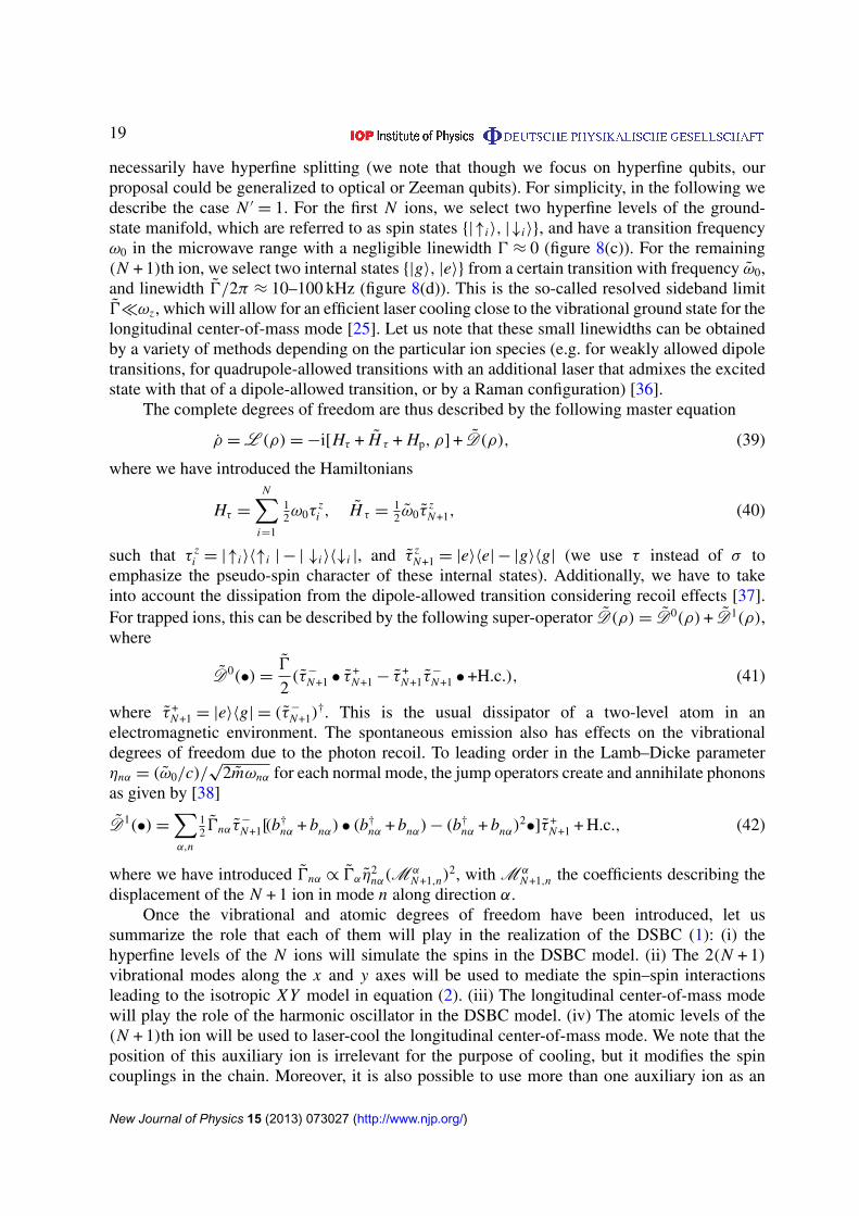
necessarily have hyperfine splitting (we note that though we focus on hyperfine qubits, ourproposal could be generalized to optical or Zeeman qubits). For simplicity, in the following wedescribe the case N ′

= 1. For the first N ions, we select two hyperfine levels of the ground-state manifold, which are referred to as spin states {|↑i〉, |↓i〉}, and have a transition frequencyω0 in the microwave range with a negligible linewidth 0 ≈ 0 (figure 8(c)). For the remaining(N + 1)th ion, we select two internal states {|g〉, |e〉} from a certain transition with frequency ω0,and linewidth 0/2π ≈ 10–100 kHz (figure 8(d)). This is the so-called resolved sideband limit0�ωz, which will allow for an efficient laser cooling close to the vibrational ground state for thelongitudinal center-of-mass mode [25]. Let us note that these small linewidths can be obtainedby a variety of methods depending on the particular ion species (e.g. for weakly allowed dipoletransitions, for quadrupole-allowed transitions with an additional laser that admixes the excitedstate with that of a dipole-allowed transition, or by a Raman configuration) [36].

The complete degrees of freedom are thus described by the following master equation

ρ = L (ρ)= −i[Hτ + H τ + Hp, ρ] + D(ρ), (39)

where we have introduced the Hamiltonians

Hτ =

N∑i=1

12ω0τ

zi , H τ =

12 ω0τ

zN+1, (40)

such that τ zi = |↑i〉〈↑i | − | ↓i〉〈↓i |, and τ z

N+1 = |e〉〈e| − |g〉〈g| (we use τ instead of σ toemphasize the pseudo-spin character of these internal states). Additionally, we have to takeinto account the dissipation from the dipole-allowed transition considering recoil effects [37].For trapped ions, this can be described by the following super-operator D(ρ)= D0(ρ)+ D1(ρ),where

D0(•)=0

2(τ−

N+1 • τ +N+1 − τ +

N+1τ−

N+1 • +H.c.), (41)

where τ +N+1 = |e〉〈g| = (τ−

N+1)†. This is the usual dissipator of a two-level atom in an

electromagnetic environment. The spontaneous emission also has effects on the vibrationaldegrees of freedom due to the photon recoil. To leading order in the Lamb–Dicke parameterηnα = (ω0/c)/

√2mωnα for each normal mode, the jump operators create and annihilate phonons

as given by [38]

D1(•)=

∑α,n

12 0nα τ

−

N+1[(b†nα + bnα) • (b

†nα + bnα)− (b

†nα + bnα)

2•]τ +

N+1 + H.c., (42)

where we have introduced 0nα ∝ 0αη2nα(M

αN+1,n)

2, with M αN+1,n the coefficients describing the

displacement of the N + 1 ion in mode n along direction α.Once the vibrational and atomic degrees of freedom have been introduced, let us

summarize the role that each of them will play in the realization of the DSBC (1): (i) thehyperfine levels of the N ions will simulate the spins in the DSBC model. (ii) The 2(N + 1)vibrational modes along the x and y axes will be used to mediate the spin–spin interactionsleading to the isotropic XY model in equation (2). (iii) The longitudinal center-of-mass modewill play the role of the harmonic oscillator in the DSBC model. (iv) The atomic levels of the(N + 1)th ion will be used to laser-cool the longitudinal center-of-mass mode. We note that theposition of this auxiliary ion is irrelevant for the purpose of cooling, but it modifies the spincouplings in the chain. Moreover, it is also possible to use more than one auxiliary ion as an

New Journal of Physics 15 (2013) 073027 (http://www.njp.org/)

20

additional knob to control the damping rate. In the following sections, we will detail the differentelements required for the ion-trap implementation of the DSBC. We emphasize that all of themcan be realized with state-of-the-art technology.

3.2. Engineering the isotropic XY spin model

We start by addressing how to implement the isotropic XY model (2) in the ion chain bymeans of a variation of the Mølmer–Sørensen gate [39]. The idea is to use the so-called spin-dependent forces, a tool that has already been implemented in several laboratories for differentpurposes [20–24]. By combining a pair of Raman laser beams (see figure 8(c)), each of whichis tuned to the red/blue first vibrational sideband of the hyperfine transition [40], it is possibleto obtain the following state-dependent force

H Lα=

∑in

F αinτ

φαi bnαeiϕαe−iδnα t + H.c.,

(43)F α

in = i 12ηnα�LαM

αin,

where the ‘hat’ indicates the interaction picture with respect to H0 = Hσ + H σ + Hp. In the aboveexpression, we have assumed that the effective wavevector of the Raman beams kLα = kLα,1 −

kLα,2 points along the α = {x, y} axis of the trap (see figure 8(a)). Additionally, we assume thatthe strength of both Raman beams is equal, such that they share a common Rabi frequency |�Lα |,and have opposite detunings, such that we can define a common δnα = ωLα − (ω0 −ωnα). Wehave introduced the laser Lamb–Dicke parameter ηnα = eα · kLα/

√2mωnα�1. The constraints

on these parameters are |�Lα | � ωα to neglect other terms in addition to such a state-dependentforce. Finally, we have defined the sum and difference of the Raman beam phases

φα = φLα,1 +φLα,2, ϕα = φLα,1 −φLα,2, (44)

and the Pauli spin operator τ φαi = e−iφα |↑i〉〈↓i | + e+iφα |↓i〉〈↑i |.In order to obtain the desired isotropic XY model, we apply two orthogonal state-dependent

forces with the following phases and directions

α = x, φx = 0, α = y, φy =π

2 . (45)

Altogether, the Hamiltonian of the ion chain in the interaction picture becomes

H L=

∑in

F xinτ

xi bnxeiϕx e−iδnx t +

∑in

F yinτ

yi bnyeiϕy e−iδny t + H.c.. (46)

Performing a Magnus expansion [41], the evolution turns out to be given by the unitaryoperator U (t)= exp{�eff(t)}, where �eff(t) displays the following form to second order

�eff(t)= −i∫ t

0dt ′ H L(t

′)−1

2

∫ t

0dt ′

∫ t ′

0dt ′′[H L(t

′), H L(t′′)]. (47)

We want to derive an effective Hamiltonian from this expression �eff(t)≈ −it H tis (where the

superscript ‘ti’ stands for the trapped-ions realization). The first-order contribution leads to acouple of orthogonal state-dependent displacements, which can only be neglected in the limit|F α

in|�δnα [42]. In addition, from the non-commutativity of the σ x and σ y forces, we get aresidual spin–phonon coupling in the second-order term of the Magnus expansion. In order toneglect it, we have to impose a further constraint, namely |F x

in(Fy

im)∗| � |δnx − δmy|, which can

New Journal of Physics 15 (2013) 073027 (http://www.njp.org/)

21

be fulfilled if the trap frequencies along the x, y axes are sufficiently different ωx 6= ωy . Underthese constraints, an interacting quantum spin chain is obtained

H tis =

∑i, j

J xi jτ

xi τ

xj + J y

i jτy

i τyj , J αi j = −

∑n

1

δnαF α

in(Fαjn)

∗. (48)

Therefore, by adjusting the strengths of the Raman beams, and their detunings, it is possibleto find a regime where J x

i j = J yi j , and the above spin Hamiltonian corresponds to the desired

isotropic XY model since τ xi τ

xj + τ y

i τyj = 2(τ +

i τ−

j + τ−

i τ+j ). Let us remark that the resulting XY

model has the peculiarity of displaying long-range couplings. In fact, when ωx , ωy � ωz, andthe Raman lasers are far-detuned from the whole vibrational branch, it can be shown that thesecouplings decay with a dipolar law. The trapped-ion Hamiltonian (48) becomes a realizationof the XY interaction (2) in the DSBC model (1) after the identifications τ±

i ↔ σ±

i , andJ x

i j = J yi j ↔ J . For typical nearest-neighbor distances of z0 ≈ 1–10µm, the spin–spin couplings

attain strengths in the J αi i+1/2π ≈ 1–10 kHz. Let us note that modifications of the scheme ofstate-dependent forces have been proposed to yield other quantum spin models [42, 43], someof which have also been realized experimentally [23].

3.3. Controlling the spin-boson coupling

Let us now address how to implement the spin-boson coupling (4) in the ion chain. The ideais again to use a 3-beam configuration (see figure 8(c)), but in a different regime. Rather thantuning the two-photon frequencies ωLα to the vibrational sidebands of the hyperfine transition,we impose that ωLα ≈ ωnz � ω0. Moreover, we consider that the laser beams form a standingwave along the trap z-axis (see figure 8(a)). Under these constraints, the laser–ion interactionleads to a crossed-beam differential ac-Stark shift, which can be interpreted as another state-dependent force in the τ z basis

HLz =

∑in

F zinτ

zi bnze

−iδnz t + H.c.,

(49)F z

in =12ηnz�LzM

zin sin(ϕz − kLz · r0

i ),

where the ‘hat’ refers to the interaction picture with respect to H0 = Hτ + Hτ + Hp. Here, theparameters are defined in analogy to those in equation (43), with three important differences:(i) �Lz is not the two-photon Rabi frequency of the hyperfine transition, but rather a differentialac-Stark shift coming from processes where a photon is exchanged between the pair of laserbeams in the 3 configuration. (ii) The detunings are changed to δnz = ωLz −ωnz. (iii) Since theion chain lies along the z axis, there is an additional site-dependent phase when shining thelasers such that kLz · r0

i 6= 0. When adjusting the difference of the laser phases to be ϕ = π/2,then we obtain F z

in =12ηnz�LzM

zin cos(kLz · r0

i ). Let us highlight that the standing-wave natureof this spin-dependent force is not essential for the dissipative protocol. However, it makes theconnection with the DSBC studied in section 2 more transparent. We will show in section 3.5that essentially the same fidelities can be achieved for a traveling-wave configuration, which hasalso been experimentally demonstrated [40].

We now exploit the particular properties of the longitudinal phonon branch (seefigure 8(b)). More precisely, we use the presence of a gap between the axial center-of-mass mode and the rest of the modes along the same direction. For the case of equal ions,|ωnz −ω1z|>(

√3 − 1)ωz, while for different ion species or isotopes, the exact value of the gap

New Journal of Physics 15 (2013) 073027 (http://www.njp.org/)

22

will depend on the mass ratio and the position of the cooling ions. We assume that ωLz is red-detuned with respect to the axial center-of-mass mode ωLz = ω1z − δ1z, such that δ1z � ω1z.Since the next vibrational modes are separated by a large energy gap, the laser coupling to theremaining phonon branch is highly off-resonant and can be thus neglected. Accordingly, thisstate-dependent force gives

H Lz =

∑i

F zi1τ

zi b1ze

−iδ1z t + H.c. (50)

We can finally move to a different picture where the above Hamiltonian becomes time-independent HLz = H ti

b + H tisb, where

H tib =

∑i

δ1zb†1zb1z,

(51)H ti

sb =

∑i

F zi1τ

zi (b1z + b†

1z).

Therefore, it is clear that the center-of-mass mode plays the role of the harmonic oscillator{b1z, b†

1z} ↔ {a, a†} in the DSBC, with the laser detuning corresponding to the oscillator

detuning δ1z ↔1a in the DSBC model (3). In addition, the strength of the state-dependentforce determines the spin-boson coupling F z

in ↔ gi in the DSBC model (4).Let us now comment on realistic values for the trapped-ion parameters. Since the

laser detuning should only fulfill δ1z/2π � ω1z/2π = ωz/2π ≈ 1–10 MHz, it will be easyto reach the required condition of δ1z/2π ∼ J αi i+1/2π ≈ 1–10 kHz. On the other hand, weknow from the previous section that g � J is necessary to have an accurate pumping to thedesired entangled state. Nevertheless, g should not be too small that the total preparationtime becomes prohibitively long. A suitable choice could be g ≈ 0.1–0.5 kHz. Since F z

i1 =

η1z�Lz cos(kLz · r0i )/

√N + 1, it will suffice to set the Rabi frequency in the �Lz≈1–5

√N kHz.

Finally, we should adjust the laser wavevector such that kLz · r0i ≈ π i/(N + 1).

3.4. Effective damping of the bosonic mode

Once the implementation of the XY model (2) and the spin-boson coupling (4) has beendescribed, let us turn into the last required ingredient: an effective damping of the bosonicmode (5). As discussed previously, the idea is to exploit the atomic levels of the (N + 1)thion to laser-cool the longitudinal center-of-mass mode. Since the resonance frequencies arevery different, ω0 6= ω0, the cooling lasers do not affect the spin dynamics of the other N ions.However, since the vibrational modes are collective, it is possible to sympathetically cool thevibrations of the crystal by only acting on the (N + 1)th ion. This sympathetic laser cooling [44]has been already realized experimentally in small crystals for quantum computation [25, 26].

Our starting point is the master equation (39) with the dissipation superoperators (41)and (42). To control the effective damping, we introduce a laser beam red detuned fromthe atomic transition ωLz

≈ ω0 + 1Lz, such that 1Lz

<0 (see figure 8(d)). Let us note thatthe particular laser-beam configuration will depend on the particular ion species, and thescheme to attain the resolved-sideband limit [36]. We consider that the laser is in a traveling-wave configuration, such that its wavevector is aligned parallel to the trap axis kLz ‖ ez (seefigure 8(a)). After expanding in series of the Lamb–Dicke parameter ηnz = ez · kLz

/√

2mωnz�1,

New Journal of Physics 15 (2013) 073027 (http://www.njp.org/)

23

the laser–ion interaction leads to two different terms, the so-called carrier term

H 0Lz

=12�Lz

eikLz·r0

N+1 τ +N+1e−iωLz

t + H.c., (52)

and the red and blue sideband terms

H 1Lz

=

∑n

F zN+1,n(bnz + b†

nz)τ+N+1e−iωLz t + H.c., (53)

where we introduced F zN+1,n = i 1

2 ηnz�LzM z

N+1,neikLz·r0

N+1 , and the corresponding Rabi frequency�Lz

. By controlling appropriately these sideband terms, and their interplay with the atomicspontaneous emission, it is possible to tailor the damping of the longitudinal modes.

Let us rearrange the full Liouvillian (39) as a sum of two terms L = L0 + L1, where

L0(•)= −i[Hs + H s + Hb + H 0Lz, •] + D0(•),

(54)L1(•)= −i[H 1

Lz, •] + D1(•)

which is justified for small Lamb–Dicke parameters. To obtain the effective damping of thelongitudinal center-of-mass mode, we use a similar formalism as in [30]. In this case, the fastesttimescale in the problem is given by the decay rate 0 of the atomic states of the (N + 1)th ion.Therefore, we must ‘integrate out’ these atomic degrees of freedom, which can be accomplishedby projecting the density matrix of the full system into Pρ(t)= ρss

N+1 ⊗ ρN (t), where ρssN+1

fulfills D0(ρssN+1)= 0, and ρN (t) is the reduced density matrix for the N spins and the chain

vibrational modes. For this we use the expression

dρN

dt=

∫∞

0dτTrN+1{PL1(t)e

L0τL1(t − τ)Pρ(t)}, (55)

where the ‘hats’ refer to the interaction picture with respect to H0 = Hτ + H τ + Hp. After somealgebra, one gets the effective damping of the longitudinal modes

ρN = −i[Hs + Hb, ρN ] + Db(ρN ), (56)

where we have introduced the bosonic dissipator

Db(•)=∑

n

κ−

n (bnz • b†nz− b†

nzbnz•)+ κ+n (b

†nz • bnz− bnzb

†nz•)+ H.c., (57)

together with the effective rates for laser cooling and heating

κ∓

n = Dn + Sn(±ωnz). (58)

Here, the so-called diffusion coefficient accounting for the recoil heating is Dn =

0nz〈τ+N+1τ

−

N+1〉ss, and the spectral functions of the sideband terms are

Sn(ω)=

∫∞

0dτ 〈(Fn(τ )Fn(0)〉sse

iωτ , Fn = F zN+1,nτ

+i + H.c., (59)

which can be obtained by means of the quantum regression theorem. The formalism and coolingrates coincide with those of a single trapped ion [38], with the difference that in the diffusioncoefficient Dn and forces Fn one must consider the normal vibrational modes at the position ofthe cooled ion.

The idea is to work in the resolved sideband regime 0�ωz, and set the laser-coolingparameters to optimize the cooling of the longitudinal center-of-mass mode κ−

1 � κ+1 . In this

New Journal of Physics 15 (2013) 073027 (http://www.njp.org/)

24

regime, the cooling dominates in (57), and we are left with the desired damping of the bosonicmode

D tib (•)= κ−

1 (b1z • b†1z− b†

1zb1z•)+ κ+1 (b

†1z • b1z− b1zb

†1z•)+ H.c. (60)

Once more, after the identifications {b1z, b†1z} ↔ {a, a†

}, and κ−

1 ↔ κ , we obtain an analogousDSBC damping (5).

Let us finally comment on the required cooling rates. Ideally, we should achieve the regimeκ ≈ g ≈ 0.1–0.5 kHz. Since such cooling is not particularly fast, it is possible to find the rightdetuning 1Lz

<0 such that κ−

1 ≈ 0.1–0.5 kHz. Besides, since we are in the resolved sidebandlimit, the heating can be made much smaller, κ+

1 � κ−

1 . The stationary state of a harmonicoscillator under the action of D ti

b in equation (60) is a thermal state with mean number of quantan1z = κ+

1 /(κ−

1 − κ+1 ). In the limit κ+

1 /κ−

1 = ζ � 1, such that the cooling is the dominant effectand the heating only presents a small correction, the equilibrium state of the center-of-massmode is close to the vacuum state.

3.5. Numerical analysis of the trapped-ion dissipative protocol

In this last section, we will explore numerically how the dissipative protocol describedin the part 2 of this paper can be implemented with the trapped-ion DSCB model inequations (48), (51) and (60), namely

dρ

dt= L ti

DSBC(ρ)= −i[H tib + H ti

s + H tisb, ρ] + D ti

b (ρ). (61)

Therefore, the results discussed below correspond to the actual spin–spin couplings J αi j in an iontrap, which are not nearest-neighbors couplings, but display a dipolar decay with the cube of thedistance. Furthermore, we have taken into account that in harmonic ion traps, the interparticledistance is not constant over the chain. More importantly, we have considered the effects of thealways-present heating term in the trapped-ion effective damping (60).

In figure 9(a), we show the optimal fidelity for the dissipative generation of the idealground state at different fillings (35), by integrating numerically the dipolar and inhomogeneoustrapped-ion DSBC model (61) as a function of the ratio between heating and cooling rate ζ . Westudy a chain of N + 2 = 6 ions, in which N = 4 have a hyperfine structure and play the role ofthe spins in the XY chain, while the two peripheral ions are assumed to be used for sympatheticcooling (this choice of auxiliary cooling ions at the ends of the chain makes the interparticlespacing slightly more homogeneous for the ‘system’ ions). As can be seen in the figure, whenζ → 0, the fidelities with the target ground state approach 100%, which allows us to concludethat the differences due to the inhomogeneity of the chain and the dipolar range of interactionswith respect to the ideal homogeneous and nearest-neighbor DSBC (1) do not compromise thefidelities severely.

The situation is different as finite heating rates ζ > 0 are considered. In figure 9(a), weobserve that the fidelity with the target ground state decays essentially linear with ζ . In theworst case considered, where ζ = 0.2 leads to a mean phonon number of n1z ' 0.25, thefidelities obtained are reduced to roughly Ftf ≈ 0.8. We note that resolved sideband coolingof single vibrational modes has been experimentally achieved reaching n1z below 0.1 for singletrapped ions [36]. Sympathetic cooling of crystals up to N = 4 ions has also been achieved [26],reaching values as low as n1z ≈ 0.06 with pulsed techniques. We note that our scheme does not

New Journal of Physics 15 (2013) 073027 (http://www.njp.org/)

25

Figure 9. Heating in the trapped-ion dissipative protocol: (a) fidelity with thedesired target state for a fixed time tf = 103/J and as a function of the ratioζ = κ+

1 /κ−

1 between the sympathetic heating and cooling rates in a chain of sixions in which the central four represent sites of the isotropic XY spin chain. Theblue dots correspond to the case of ns = {1, 3} initial spin excitations, and theorange squares to the case of ns = 2 excitations. The oscillator was truncated tofive levels. (b) Same as in (a), but considering a shorter time tf = 102/J , anda traveling-wave configuration of the spin-boson coupling in equation (51). Theachieved fidelities for this experimentally simpler configuration are similar to theones in (a).

demand such an accurate ground-state cooling (see figure 9(a)), and we expect that the requiredmean phonon numbers n1z ≈ 0.1 can also be achieved in a continuous cooling scheme.

Another source of experimental imperfections is given by slow drifts of the trap frequencieswhich will modify the detuning δ1z in different experimental runs, such that the conditions (19)will not be perfectly fulfilled. Nonetheless, in figure 4 we have shown that the dissipativecharacter of the protocol endows it with a natural robustness with respect to non-optimal choicesof the parameters. Therefore, one can expect large fidelities even in the presence of slow drifts ofthe trap frequency within the kHz-range. In any case, to alleviate imperfections caused by bothmagnetic-field dephasing and trap frequency drifts, we have considered a faster protocol wherethe required time is tf ∼ 102/J ≈ 1–10 ms. In figure 9(b), we show that the achieved fidelities inthis case are still above 0.8 (for heating/cooling ratios below 0.2). Moreover, in this figure we

New Journal of Physics 15 (2013) 073027 (http://www.njp.org/)

26

Figure 10. Anisotropy in the trapped-ion dissipative protocol: (a) fidelity withthe desired target state for a fixed time tf = 102/J and as a function of theanisotropy ratio (J x

− J y)/(J x + J y) for a chain of six ions in which the centralfour ions represent sites of the slightly anisotropic XY spin chain. The bluedots correspond to the case of ns = {1, 3} initial spin excitations, and the orangesquares to the case of ns = 2 excitations. The oscillator was truncated to fivelevels.

have also considered substituting the standing-wave force in equation (51) by a traveling-waveconfiguration, which is experimentally less demanding.

The need of the τ z state-dependent force (49) forbids the use of magnetic-field insensitivestates (i.e. clock states). Therefore, the hyperfine spins will be subject to fluctuations inducedby non-shielded external magnetic fields, typically leading to dephasing in a timescale ofT2 ≈ 1–10 ms. These timescales are comparable to the protocol times tf ∼ 102/J ≈ 1–10 ms,where we have taken J/2π ∼ 1–10 kHz. Nevertheless, these magnetic-field fluctuations actglobally for standard radio-frequency traps Hn =

121ω0(t)

∑i τ

zi , where 1ω0(t) is a fluctuation

of the resonance frequency due to the Zeeman shift (note that this might not be the case formicro-fabricated surface traps, where fluctuating magnetic-field gradients can also arise). Sincethe dynamics of the DSBC (61) conserves the number of spin excitations, this magnetic-fieldnoise only introduces a global fluctuating phase, and thus does not decohere the state of thesystem. Therefore, as far as the induced spin dynamics occurs within any subspace with aconserved number of excitations, the dissipative protocol is robust to global magnetic-fieldnoise.

It is, however, important to stabilize the intensity of the state-dependent forces to the sweetspot where J x

i j = J yi j , and make sure that |F α

i j | � δnα to neglect any term that does not conservethe number of excitations. The effect of off-resonant terms in the scheme leading to the XTinteractions, that could give rise to non-conservation of the number of spin excitations, shouldbe much smaller than in stroboscopic proposals [19] since our protocol does not require fastgates [45]. In figure 10, we show the achieved fidelities for anisotropies in J x

i j/J yi j 6= 1. The

results have been obtained numerically for the same regime as in figure 9(b), and indicate that ifJ x

i j , J yi j differ by one part in 103, the fidelities are not severely reduced. The results in figure 10

also show a marked difference in the robustness depending on the number of spin excitations

New Journal of Physics 15 (2013) 073027 (http://www.njp.org/)

27

in the initial state. This behavior, at first surprising, can be understood by looking at thesmall undesired Hamiltonian terms responsible for the anisotropy in an interaction picture withrespect to the ideal isotropic Hamiltonian. The anisotropy term creates or destroys fermionicquasiparticles in pairs, and rotates with a frequency that is the sum of the energies of the twoquasiparticles. For the case with only one spin up, it is possible to create from the ideal targetstate pairs of fermions with energy adding up to zero, so that these error terms do not rotate.In the case with two spin excitations, on the contrary, the lower half of the fermionic spectrumis filled, so that any Hamiltonian term creating or destroying a pair of fermions from the idealtarget state oscillates in time, and therefore its effect is strongly suppressed.

4. Conclusions and outlook

We have presented a method to dissipatively generate multipartite-entangled statescorresponding to the ground states of small spin chains with isotropic XY Hamiltonianin a transverse field. The protocol for dissipative state preparation is interesting from afundamental point of view, as it illustrates how local and even purely Markovian noise canassist entanglement production. Indeed, the jump operators required are sums of terms acting onindividual sites, in contrast with the few-body (quasi-local) nature of the operators in [15, 17].When the noise deviates from exact Markovianity, the required time for achieving the steadystate is reduced, which illustrates the value of non-Markovian effects for practical purposes. Wewould like to emphasize that the general idea underlying the procedure presented in this work isnot specific to the model considered, and might be generalized to other spin Hamiltonians. Asan example, we introduced a variation that can be used to generate states locally equivalent toW -states. It would also be interesting to modify our dissipative protocol to prepare the groundstate of a gapped spin model. For longer ion chains, the combination of more state-dependentforces (4) with different wavevectors could improve the scalability of the protocol.

We have also explained in detail how to implement this method in small chains oftrapped ions. In our proposal, two internal levels of the ions embody the spin system and acollective motional mode represents the damped oscillator. The preparation procedure requiresthe implementation of spin–spin interactions using the so-called Mølmer–Sørensen scheme, theaction of a state-dependent force, and sympathetic cooling, all ingredients within the capabilitiesof present ion-trap technology. Numerical simulations including different sources of errorsindicate that the protocol can produce the target states with fidelities comparable to the morestandard coherent protocols [27]. The method presented is indeed robust against a number ofexperimental imperfections, and the implementation is simplified since only global addressingof the ions is required.

Our results, however, may find a realization in different experimental setups. For instance,the application of our ideas to arrays of superconducting qubits in stripline resonators seemsfeasible. Moreover, since this model can also be understood as a quadratic fermonic modelwith an additional chemical potential fixing the number of particles, the results may also beinteresting for fermionic atoms in optical lattices.

The realization of this kind of dissipative system paves the way for the implementation ofmore complex scenarios to study the interplay of coherent and incoherent dynamics giving riseto noise-induced criticality [16, 46]. Indeed, recent work in the area of non-equilibrium quantumphase transitions [47] has shown a number of fascinating results that could be demonstrated insystems of trapped ions using tools similar to the ones in our protocol.

New Journal of Physics 15 (2013) 073027 (http://www.njp.org/)

28

Acknowledgments

We thank A Rivas for fruitful comments on the paper. This work was supported by PICC andby the Alexander von Humboldt Foundation. AB thanks FIS2009-10061, and QUITEMAD.

References

[1] Ladd T D, Jelezko F, Laflamme R, Nakamura Y, Monroe C and O‘Brien J L 2010 Nature 464 45[2] Trabesinger A 2012 Nature Phys. 8 263 (see entire Nature Phys. Insight – Quantum Simulation)[3] Cabrillo C, Cirac J I, Garcia-Fernandez P and Zoller P 1999 Phys. Rev. A 59 1025[4] Plenio M B, Huelga S F, Beige A and Knight P L 1999 Phys. Rev. A 59 2468[5] Bose S, Knight P L, Plenio M B and Vedral V 1999 Phys. Rev. Lett. 83 5158[6] Slodicka L, Hetet G, Rock N, Schindler P, Hennrich M and Blatt R 2013 Phys. Rev. Lett. 110 083603[7] Browne D E, Plenio M B and Huelga S F 2003 Phys. Rev. Lett. 91 067901

Duan L-M and Kimble H J 2003 Phys. Rev. Lett. 90 253601[8] Sørensen A S and Mølmer K 2003 Phys. Rev. Lett. 91 097905[9] Beige A, Braun D, Tregenna B and Knight P L 2000 Phys. Rev. Lett. 85 1762

Pachos J and Walther H 2002 Phys. Rev. Lett. 89 187903Beige A, Braun D, Bose S, Huelga S F, Knight P L, Plenio M B and Vedral V 2000 J. Mod. Opt. 47 2583–98

[10] See Metcalf H J and van der Straten P 1999 Laser Cooling and Trapping (New York: Springer) and referencestherein

[11] Stenholm S 1986 Rev. Mod. Phys. 58 699[12] Poyatos J F, Cirac J I and Zoller P 1996 Phys. Rev. Lett. 77 4728

Plenio M B and Huelga S F 2002 Phys. Rev. Lett. 88 197901[13] Dicke R H 1954 Phys. Rev. 93 99

Lemberg R H 1970 Phys. Rev. A 2 889[14] Gonzalez-Tudela A, Martin-Cano D, Moreno E, Martin-Moreno L, Tejedor C and Garcia-Vidal F J 2011

Phys. Rev. Lett. 106 020501Bermudez A, Schaetz T and Plenio M B 2013 Phys. Rev. Lett. 110 110502Kastoryano M J, Reiter F and Sørensen A S 2011 Phys. Rev. Lett. 106 090502

[15] Kraus B, Buchler H P, Diehl S, Kantian A, Micheli A and Zoller P 2008 Phys. Rev. A 78 042307[16] Verstraete F, Wolf M M and Cirac J I 2009 Nature Phys. 5 633[17] Diehl S, Micheli A, Kantian A, Kraus B, Buchler H P and Zoller P 2008 Nature Phys. 4 878[18] Weimer H, Muller M, Lesanovsky I, Zoller P and Buchler H P 2010 Nature Phys. 6 382[19] Barreiro J T, Muller M, Schindler P, Nigg D, Monz T, Chwalla M, Hennrich M, Roos C F, Zoller P and

Blatt R 2011 Nature 470 486Schindler P, Muller M, Nigg D, Barreiro J T, Martinez E A, Hennrich M, Monz T, Diehl S, Zoller P and

Blatt R 2013 Nature Phys. 9 361[20] Monroe C, Meekhof D M, King B E and Wineland D J 1996 Science 272 1131

Haljan P C, Brickman K-A, Deslauriers L, Lee P J and Monroe C 2005 Phys. Rev. Lett. 94 153602McDonnell M J, Home J P, Lucas D M, Imreh G, Keitch B C, Szwer D J, Thomas N R, Webster S C,

Stacey D N and Steane A M 2007 Phys. Rev. Lett. 98 063603Poschinger U, Walther A, Singer K and Schmidt-Kaler F 2010 Phys. Rev. Lett. 105 263602

[21] Sackett C A et al 2000 Nature 404 256Leibfried D et al 2003 Nature 422 412Benhelm J, Kirchmair G, Roos C and Blatt R 2008 Nature Phys. 4 463Noguchi A, Haze S, Toyoda K and Urabe S 2011 Phys. Rev. Lett. 108 060503

[22] Ospelkaus C, Warring U, Colombe Y, Brown K R, Amini J M, Leibfried D and Wineland D J 2011 Nature476 181

New Journal of Physics 15 (2013) 073027 (http://www.njp.org/)

29

Khromova A, Piltz Ch, Scharfenberger B, Gloger T F, Johanning M, Varon A F and Wunderlich Ch 2012Phys. Rev. Lett. 108 220502

[23] Friedenauer A, Schmitz H, Glueckert J T, Porras D and Schaetz T 2008 Nature Phys. 4 757Kim K, Chang M-S, Korenblit S, Islam R, Edwards E E, Freericks J K, Lin G-D, Duan L-M and Monroe C

2010 Nature 465 590Islam R et al 2011 Nature Commun. 2 377Lanyon B P et al 2011 Science 334 57Britton J W, Sawyer B C, Keith A C, Wang C-C J, Freericks J K, Uys H, Biercuk M J and Bollinger J J 2012

Nature 484 489[24] Schmitz H, Matjeschk R, Schneider Ch, Glueckert J, Enderlein M, Huber T and Schaetz T 2009 Phys. Rev.

Lett. 103 090504Zahringer F, Kirchmair G, Gerritsma R, Solano E, Blatt R and Roos C F 2010 Phys. Rev. Lett. 104 100503

[25] Rohde H, Gulde S T, Roos C F, Barton P A, Leibfried D, Eschner J, Schmidt-Kaler F and Blatt R 2001J. Opt. B: Quantum Semiclass. Opt. 3 S3

Barrett M D et al 2003 Phys. Rev. A 68 042302[26] Home J P, McDonnell M J, Szwer D J, Keitch B C, Lucas D M, Stacey D N and Steane A M 2009

Phys. Rev. A 79 050305Home J P, Hanneke D, Jost J D, Amini J M, Leibfried D and Wineland D J 2009 Science 325 1227

[27] Blatt R and Wineland D 2008 Nature 453 1008[28] Huelga S F, Rivas A and Plenio M B 2012 Phys. Rev. Lett. 108 160402[29] Lieb E H, Schultz T and Mattis D J 1961 Ann. Phys. 16 407[30] Chaturvedi S and Shibata F 1979 Z. Phys. B 35 297[31] Imamoglu A 1994 Phys. Rev. A 50 3650

Garraway B M 1997 Phys. Rev. A 55 2290Chin A W, Rivas A, Huelga S F and Plenio M B 2010 J. Math. Phys. 51 092109

[32] Jordan P and Wigner E 1928 Z. Phys. 47 631[33] Holstein T 1959 Ann. Phys. 8 325

Holstein T 1959 Ann. Phys. 8 343[34] See Wineland D J, Monroe C, Itano W M, Leibfried D, King B E and Meekhof D M 1998 J. Res. Natl Inst.

Stand. Technol. 103 259 and references therein[35] James D F V 1998 Appl. Phys. B 66 181[36] Leibfried D, Blatt R, Monroe C and Wineland D 2003 Rev. Mod. Phys. 75 281[37] Dalibard J and Cohen-Tannoudji C 1985 J. Phys. B: At. Mol. Phys. 18 166

Castin Y, Wallis H and Dalibard J 1989 J. Opt. Soc. Am. B 6 2046[38] Cirac J I, Blatt R, Zoller P and Phillips W D 1992 Phys. Rev. A 46 2668[39] Sørensen A and Mølmer K 1999 Phys. Rev. Lett. 82 1971[40] See Brickman Soderberg K-A and Monroe C 2010 Rep. Prog. Phys. 73 036401 and references therein[41] Magnus W 1954 Commun. Pure Appl. Math. 7 649

Blanes S, Casas F, Oteo J A and Ros J 2010 Eur. J. Phys. 31 907[42] Porras D and Cirac J I 2004 Phys. Rev. Lett. 92 207901[43] Pons M, Ahufinger V, Wunderlich Ch, Sanpera A, Braungardt S, Sen A, Sen U and Lewenstein M 2007 Phys.

Rev. Lett. 98 023003Bermudez A, Porras D and Martin-Delgado M A 2009 Phys. Rev. A 79 060303Hauke P, Cucchietti F M, Muller-Hermes A, Banuls M C, Cirac J I and Lewenstein M 2010 New J. Phys.

12 113037Ivanov P A and Schmidt-Kaler F 2011 New J. Phys. 13 125008Bermudez A, Almeida J, Schmidt-Kaler F, Retzker A and Plenio M B 2011 Phys. Rev. Lett. 107 207209Schmied R, Wesenberg J H and Leibfried D 2011 New J. Phys. 13 115011Lin G-D, Monroe C and Duan L-M 2011 Phys. Rev. Lett. 106 230402

New Journal of Physics 15 (2013) 073027 (http://www.njp.org/)

30

Bermudez A, Almeida J, Ott K, Kaufmann H, Ulm S, Poschinger U, Schmidt-Kaler F, Retzker A and PlenioM B 2012 New J. Phys. 14 093042

[44] Kielpinski D, King B E, Myatt C J, Sackett C A, Turchette Q A, Itano W M, Monroe C, Wineland D J andZurek W H 2000 Phys. Rev. A 61 032310

Morigi G and Walther H 2001 Eur. Phys. J. D 13 261[45] Kirchmair G, Benhelm J, Zahringer F, Gerritsma R, Roos C F and Blatt R 2009 New. J. Phys. 11 023002[46] Schon G and Zaikin A D 1990 Phys. Rep. 198 237

Capriotti L, Cuccoli A, Fubini A, Tognetti V and Vaia R 2005 Phys. Rev. Lett. 94 157001Cazalilla M A, Sols F and Guinea F 2006 Phys. Rev. Lett. 97 076401Eisert J and Prosen T 2012 arXiv:1012.5013

[47] Morrison S and Parkins A S 2008 Phys. Rev. Lett. 100 040403Prosen T and Ilievski E 2011 Phys. Rev. Lett. 107 060403Bhaseen M J, Mayoh J, Simons B D and Keeling J 2012 Phys. Rev. A 85 013817Bastidas V M, Emary C, Schaller G and Brandes T 2012 Phys. Rev. A 86 063627

New Journal of Physics 15 (2013) 073027 (http://www.njp.org/)