Dissipation of Turbulent Kinetic Energy Inferred from Seagliders: An Applicationto the Eastern Nordic Seas Overflows

NICHOLAS BEAIRD

School of Oceanography, University of Washington, Seattle, Washington

ILKER FER

Geophysical Institute, University of Bergen, Bergen, Norway

PETER RHINES AND CHARLES ERIKSEN

School of Oceanography, University of Washington, Seattle, Washington

(Manuscript received 31 May 2012, in final form 16 August 2012)

ABSTRACT

Turbulent mixing is an important process controlling the descent rate, water massmodification, and volume

transport augmentation due to entrainment in the dense overflows across the Greenland–Scotland Ridge.

These overflows, along with entrained Atlantic waters, form a major portion of the North Atlantic Deep

Water, which pervades the abyssal ocean. Three years of Seaglider observations of the overflows across the

eastern Greenland–Scotland Ridge are leveraged to map the distribution of dissipation of turbulent kinetic

energy on the Iceland–Faroe Ridge. A method has been applied using the finescale vertical velocity and

density measurements from the glider to infer dissipation. The method, termed the large-eddy method

(LEM), is compared with a microstructure survey of the Faroe Bank Channel (FBC). The LEM reproduces

the patterns of dissipation observed in the microstructure survey, which vary over several orders of magni-

tude. Agreement between the inferred LEM and more direct microstructure measurements is within a factor

of 2.Application to the 9432 dives that encountered overflowwaters on the Iceland–FaroeRidge reveals three

regions of enhanced dissipation: one downstream of the primary FBC sill, another downstream of the sec-

ondary FBC sill, and a final region in a narrow jet of overflow along the Iceland shelf break.

1. Introduction

The Faroe Bank Channel (FBC) and its smaller

neighboring overflow across the Iceland–Faroe Ridge

(IFR) account for one-third of total Nordic Seas outflow

into the North Atlantic (Hansen and Østerhus 2000).

Considerable effort has been focused on the region in

general and on the FBC in particular. Along with en-

trained Atlantic waters, which double the initial overflow

volume transport, these overflowsmake up a large part of

the North Atlantic Deep Water (NADW). NADW has

global extent in the deep ocean and its circulation forms

the lower limb of the Atlantic meridional overturning

circulation. The location and intensity of turbulent

mixing and entrainment in these overflows has an im-

portant impact on ventilation of the deep ocean and

the oceanic meridional heat transport. Entrainment of

overlaying waters is particularly interesting in this re-

gion where wintertime mixed layers can sometimes

reach the depth of the overflow plume interface.

A comprehensive review of North Atlantic–Nordic

Seas exchanges is given by Hansen and Østerhus (2000)

and of the FBC overflow by Hansen and Østerhus

(2007). At the sill thresholds, approximately 3 Sv (Sv[106 m3 s21) of Nordic origin waters form energetic

bottom-intensified gravity currents flowing into the

Iceland Basin. Of the total 3 Sv, 1.9 Sv exits through

the FBC, and the remainder crosses the IFR. The Faroe

Bank Channel overflow is swift [O(1 m s21)] and uni-

directional, with a bottom mixed layer of cold (;08C)water capped by a thick [O(100 m)] interfacial layer

below the ambient Atlantic waters. Dissipation levels

Corresponding author address: Nicholas Beaird, University of

Washington, 1492 NE Boat St., Seattle, WA 98195.

E-mail: nlbeaird@uw.edu

2268 JOURNAL OF PHYS ICAL OCEANOGRAPHY VOLUME 42

DOI: 10.1175/JPO-D-12-094.1

� 2012 American Meteorological Society

as high as 1025 W kg21 illustrate the energetic turbu-

lence at work in the overflow (Fer et al. 2010). The FBC

overflow exhibits considerable mesoscale variability,

which plays a role in the mixing and descent of the

plume (Darelius et al. 2011; Seim and Fer 2011). After

exiting the FBC, the overflow plume makes an inertial

turn to the right and flows along isobaths on the At-

lantic flank of the IFR, driven by a balance of pressure

gradient, Coriolis, and frictional forces. As it flows

downstream, the plume descends slightly due to the

frictional relaxation of the geostrophic constraint. The

FBC plume is joined along this path by overflow from

the IFR, which is more spatially intermittent but has

very similar source waters.

By the time these waters have traveled downstream to

form Northeast Atlantic Deep Water (NEADW) their

volume flux will have doubled to 6 Sv and their tem-

perature and salinity properties will be significantly di-

luted by entrainment of overlying Atlantic waters.

These overflows occur in physically small regions (the

FBC sill is;10 kmwide), exhibit complex submesoscale

flow features, and depend intimately on very small scale

mixing processes. Despite the small scales of the over-

flows, their influence is felt on basin, planetary, and cli-

matic scales. It is critical, but notoriously difficult, to

represent overflows in numerical models (Legg et al.

2009). The intensity of mixing and entrainment in the

overflow plumes affects their eventual volume flux, de-

scent rate, end-member properties and detrainment

depth. In addition to the obvious effect on plume prop-

erties, recent studies of the Mediterranean Outflow also

suggest that the upper ocean responds directly to the

potential vorticity forcing from the descent and entrain-

ment of overflows (Kida et al. 2008).

Several indirect mixing estimates (mainly based on

heat budgets) have been made in the FBC (Saunders

1990; Duncan et al. 2003; Mauritzen et al. 2005), while

more recently the first direct microstructure turbulence

measurements have beenmade by Fer et al. (2010), all of

which indicate intense mixing in the FBC plume down-

stream of the sill. These studies are important to facili-

tate understanding of mixing in the overflows; however,

in each case the shipboard surveys only lasted a short

time. The well-documented variability of the FBC over-

flow (Geyer et al. 2006; Darelius et al. 2011) and the

myriad locations of IFR overflow suggest that more

complete time series and higher spatial resolution of

mixing estimates are desirable.

In this paper a three year dataset of Seaglider obser-

vations in the FBC and on the IFR is used to obtain

a more complete spatial picture of the mixing and en-

trainment in these overflows. These data extend 300 km

farther downstream than the majority of the FBC overflow

studies mentioned above and offer the first look at tur-

bulence in the IFR overflows. The analysis presented

here hinges on the development of a method to obtain

estimates of dissipation of turbulent kinetic energy («)

from the Seaglider. The method is developed and then

validated by comparison between a Seaglider deploy-

ment and a contemporaneous microstructure survey

(Fer et al. 2010).

2. Measurements

The data presented in this study come from two sour-

ces: one shipboard and one Seaglider survey. Ancillary

data include approximately 2-month-long measurements

from a moored instrument located at the center of the

shipboard and Seaglider surveys. The glider data were

collected over three years between November 2006 and

November 2009. Deployments were made every three

months, with 23 successful missions producing roughly

17 400 profiles of temperature, salinity, dissolved oxygen,

fluorescence, optical backscatter, and vertical velocity in

the Iceland–Faroes region.

The Seaglider is a small, autonomous, buoyancy-driven

vehicle that profiles to a maximum depth of 1000 m in

a sawtooth pattern (Eriksen et al. 2001). The gliders

deployed in this survey were equipped with unpumped

custom Sea-Bird Electronics conductivity (SBE 4) and

temperature (SBE 3) sensors, a Wetlabs BB2FVMG

optical puck with florescence and two wavelengths of

backscatter, and a Sea-Bird Electronics oxygen sensor

(SBE 43). During the Faroes mission, the gliders sam-

pled water column properties at 20-s intervals. With

typical vehicle descent/ascent rates of 6–10 cm s21, the

vertical resolution of the profiles was approximately 1.2–

2 m. The vertical to horizontal glide ratio of 1:3 gives

horizontal resolution of 3.6–6 m between consecutive

samples, while dive and climb profile separations vary

with depth owing to the slant-vertical path of the in-

strument. Adjacent glider surfacings are typically 3 to

6 km apart. An acoustic altimeter mounted forward on

the Seaglider is used to detect and avoid the seafloor. To

fully sample the overflow plume, these gliders were

programed to begin their dive-to-climb transition 10 m

above the acoustically ranged bottom.

The distribution of the Seaglider data in the FBC and

downstream on the IFR is shown in Fig. 1. Each point in

the figure represents one dive/climb profile pair and

color indicates the bottom temperature, or the temper-

ature at the deepest observation made by the instru-

ment. Typically Seagliders were deployed in the FBC

where they remained for several days as the pilot trim-

med flight control parameters. Trimmed vehicles were

subsequently flown northwestward along isobaths of the

DECEMBER 2012 BEA IRD ET AL . 2269

IFR. After reaching the Iceland shelf break the gliders

were piloted back to the FBC or, on occasion, across the

IFR into the Norwegian Basin.

The shipboard survey was made from the R.V.H�akon

Mosby during the period 29 May–8 June 2008 (Fer et al.

2010). During the cruise, 90 profiles were collected using

a vertical microstructure profiler (VMP2000, Rockland

Scientific Instruments, VMP hereafter). The VMP had a

depth rating of 2000 m and was equipped with pumped-

SBE conductivity–temperature–depth (CTD) sensors,

a pair of airfoil shear probes used for measuring the

dissipation rate of turbulent kinetic energy («), and fast

response temperature and conductivity sensors. The

turbulence and slow sensors sampled at 512 and 64 Hz,

respectively, at a nominal profiling speed of 0.6 m s21.

Stations were taken on six cross sections along the path

of the overflow plume starting from the sill crest to about

120 km downstream of the sill, a downstream section, as

well as two repeat stations of approximately 12-h dura-

tion (Fig. 2). The downcast of theVMP typically reached

10–50-m height above bottom (HAB). The profiles of

« were obtained from the shear probes of the VMP as

1-m vertical averages by integrating the vertical wave-

number spectrum of shear and assuming isotropy. The

lowest detection level (noise level) in « measurements

based on shear probe data in the quiescent portions of

the water column was 10210 W kg21. Details on the

sampling and data processing can be found in Fer et al.

(2010) and Seim and Fer (2011).

Additionally, we make use of vertical velocity and

temperature measurements acquired by temperature

loggers and a downward looking acoustic Doppler cur-

rent profiler (ADCP, RDI 300-kHz Workhorse Senti-

nel), moored at 618419N, 98119W at the 804-m isobath,

between 14 May and 18 July 2008. The mooring is lo-

cated about 60 km downstream of the FBC sill, referred

to as B2 inDarelius et al. (2011) and CM in Seim and Fer

(2011). We refer to the mooring as B2, consistent with

Darelius et al. (2011). The ADCP installed in a spherical

buoy at 200 m HAB ensemble averaged 50 profiles ev-

ery 5 min with 2-m vertical depth bins, returning high

quality data with negligible tilt from vertical (1.6 6 0.78roll and 21.4 6 0.78 pitch). Temperature time series

were recorded by a number of temperature (SBE39 and

RBR TR-1050) and CTD (SBE37 MicroCAT) sensors

mounted on the mooring at 20, 101, 148, 140–200 (10-m

intervals), 201 and 210 m HAB. Vertical displacements

of the instruments due to horizontal currents were cal-

culated following Dewey (1999), and temperature re-

cords were linearly interpolated onto a vertical grid using

the inferred instrument depths (Darelius et al. 2011). The

time series of the HAB of the 38C isotherm is used to

highlight the low-frequency variability associated with

the FBC overflow. A more complete description of the

moored instruments, data processing, and discussion on

mesoscale variability and plume dynamics can be found

in Darelius et al. (2011) and Seim and Fer (2011).

A comparison will be made between the dissipation

measurements from the VMP and the estimates from

a concurrent Seaglider deployment. Seagliders are des-

ignated by the letters ‘‘sg’’ followed by a serial number.

Around the time of the VMP survey in June 2008,

Seaglider 5 (sg005) was deployed in the Faroe Bank

Channel. The data from sg005 will be compared with the

VMP survey to determine calibration coefficients for the

Seaglider « estimate.

FIG. 1. Location of all Seaglider dives on the Iceland–Faroe

Ridge from November 2006 through November 2009. Each dot

indicates the location of one dive/climb pair. Color is proportional

to the bottom temperature (8C) with color scale indicated at bot-

tom left.

FIG. 2. Location of 57 VMP casts from the 2008 cruise (blue

circles), the sg005 June 2008 dives in the FBC (magenta circles),

and mooring B2 (green triangle).

2270 JOURNAL OF PHYS ICAL OCEANOGRAPHY VOLUME 42

3. Methods

a. Vertical velocities from Seaglider

The Seaglider can furnish an estimate of vertical water

velocity w by taking advantage of an accurate vehicle

flight model and its on board pressure sensor. The val-

idity of the flight model assumptions is critical, but in

principal the w estimate is straightforward: the vehicle

vertical speed through a quiescent ocean, wmodel, is

calculated by a flight model using the measured pitch

and buoyancy, while the absolute vertical speed is cal-

culated from the time rate of change of pressure on-

board the glider, wmeas. Removing the relative vehicle

speed from the absolute gives the ambient water vertical

velocity: w 5 wmeas 2 wmodel. Detailed descriptions of

the flight model and the process of determining w may

be found in Frajka-Williams et al. (2011) and Eriksen

et al. (2001). We will reproduce the basics of the calcu-

lation here.

Assuming steady flight, the force balance on the

Seaglider is between the lift (L) from the wings, the drag

(D) on the body, and the glider’s excess buoyancy (B):

L5Ph2aa52B cosu , (1)

D5Ph2(bq2(1/4) 1 ca2)5B sinu , (2)

B5 g[2M1 rV(t, p,T)] , (3)

where h is the hull length, a the attack angle, u the glide-

slope angle; a, b, c are the lift, drag, and induced drag

coefficients respectively; g is gravitational acceleration,

M the vehicle mass,V(t, p, T) the total vehicle volume as

a function of time (t, a result of controlled pumps/bleeds

of hydraulic oil between reservoirs interior and exterior

to the pressure hull), pressure (p), and temperature (T),

and P is the dynamic pressure. The glide-slope angle (u)

is the angle between the horizontal and the trajectory

of flight, while the attack angle (a) is the angle between

the chord line of the glider wings and the direction of the

incident fluid. The distinction is critical because the

glider can only measure its pitch angle (f) from the in-

clinometer, but lift and drag are functions of the attack

angle, while the glide-slope angle describes the ratio of

vertical to horizontal motion through the water. The

glide-slope and attack angles are related to the mea-

sured pitch angle by f 5 a 1 u. The dynamic pressure

term contains the velocity information,P 5 r(U21W2)/2,

where U and W are the horizontal and vertical glider

speeds and r is the water density. The functional forms

of lift and drag in Eqs. (1) and (2) are based on hydro-

dynamic testing of the vehicle shape (Hubbard 1980).

The flight model is sensitive to the values of the flight

parameters a, b, and c and the total vehicle volume

V(t, p, T), all of which must be independently deter-

mined for each Seaglider. The flight equations (1) and

(2) are solved iteratively for P and a. Finally, the mod-

eled vertical vehicle speed is calculated from the dynamic

pressure and glide angle as

wstdy5

ffiffiffiffiffiffi2Pr

ssinu . (4)

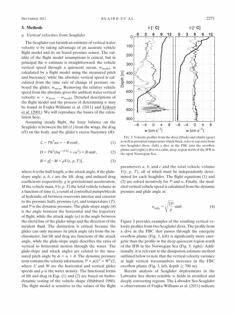
Figure 3 provides examples of the resulting vertical ve-

locity profiles from two Seaglider dives. The profile from

a dive in the FBC that passes through the energetic

overflow plume (Fig. 3, left) is significantly more ener-

getic than the profile in the deep quiescent region north

of the IFR in the Norwegian Sea (Fig. 3, right). Addi-

tionally, it is relevant to the dissipation estimate method

outlined below to note that the vertical velocity variance

at high vertical wavenumbers increases in the FBC

overflow plume (Fig. 3, left, depth T 700 m).

Recent analysis of Seaglider deployments in the

Labrador Sea shows sensible w fields in stratified and

deeply convecting regions. The Labrador Sea Seaglider

w observations of Frajka-Williams et al. (2011) indicate

FIG. 3. Velocity profiles from the dives (black) and climbs (gray)

as well as potential temperature (thick black, refer to top axis) from

two Seaglider dives: (left) a dive in the FBC into the overflow

plume and (right) a dive in a calm, deep, region north of the IFR in

the open Norwegian Sea.

DECEMBER 2012 BEA IRD ET AL . 2271

that the root-mean-square w roughly scales with the

amplitude of the surface forcing, for low stratification

WKB scaling holds, and the vertical wavenumber and

amplitude of w profiles increase within the surface mixed

layers associated with deep convection. A similar deter-

mination of w has been carried out on Slocum gliders in

the Mediterranean Sea (Merckelbach et al. 2010), again

illustrating the possibility of using gliders to observe

oceanic vertical velocities.

Spectra were used to assess noise in the Seaglider

vertical velocity measurement. Profiles were taken

from a constant stratification portion of the water

column (400–900 m) in the open, quiescent, Norwe-

gian Basin. The spectra were integrated from where

the slope flattened (1/240Hz) to the Nyquist frequency

(1/40Hz) to find noise variance. Six different gliders in

the region suggest similar Seaglider w error estimates

of 60.2 cm s21. It should be noted that this value is

considered the precision of the w measurement, not

the accuracy. It is possible that a full depth offset, or

low-frequency systematic error exists due to improp-

erly known values of the Seaglider vehicle volume or

compressibility. However, as will be mentioned below,

a high-pass filter is used in this analysis to look at ve-

locity fluctuations, making offsets and low frequency

errors irrelevant. Therefore we adopt an error esti-

mate of 0.2 cm s21, consistent with the application

outlined below.

b. Large-eddy method

Themethod of estimating dissipation employed in this

analysis is based on a simple scaling of the turbulent

kinetic energy (TKE) equation (Taylor 1935). We refer

to this scaling as the ‘‘large-eddy method’’ (LEM). The

method relies on the hypothesis (Kolmogoroff 1941)

that a steady turbulent energy cascade exists, which

allows measurements of the relatively large energy-

containing scales to be used to infer the energy loss at

viscous scales (Moum 1996). Energy is introduced to the

turbulent flow by instabilities in the large-scale mean. In

a steady state, this energy must be passed to smaller and

smaller scales until it can be dissipated by viscosity.

Described by the Kolmogoroff scale, h 5 (n3/«)1/4, the

dissipation scale for ocean turbulence can be on the

order of millimeters. This level of spatial resolution is

well beyond the sampling capacity of the standard Sea-

glider. Assuming no leakage of energy (by, for example,

nondissipative linear internal waves), the cascade of

TKE may be described by the energy of the largest

eddies in the turbulent flow and their overturning time

scale (Tennekes and Lumley 1972). We let q9 be a ve-

locity scale of the largest eddies, and l be their length

scale. The eddy time scale may be written as t; l/q9 anddissipation « scales as

«;(q9)2

t;

(q9)3

l. (5)

A physical interpretation of Eq. (5) is that the kinetic

energy (q9)2 of a turbulent eddy is dissipated in the time

it takes to overturn once t ; l/q9.This scaling has been investigated by many authors

including Moum (1996), Peters et al. (1995), and

Gargett (1999). These authors find that the scaling

holds in a variety of oceanic regimes, including regions

of low average dissipation containing sporadic ener-

getic events (Peters et al. 1995). For stratified flow,

a modification may be obtained by using the Ozmidov

length LOz 5 «1/2N23/2 for l in Eq. (5). The Ozmidov

length is a measure of the maximum vertical overturn

displacement that may occur for a given turbulent

energy level and stratification (Thorpe 2005). Re-

arranging Eq. (5), using l 5 LOz and introducing a

proportionality constant c«, leads to an expression for

the estimate (e) of dissipation of TKE that is explicitly

independent of l:

e5 c«N(q9)2 . (6)

Use of the Ozmidov scaling in Eq. (6) is equivalent to

assuming that the overturning time scale of the largest

eddies is 1/N. D’Asaro and Lien (2000a) investigate

the scaling in Eq. (6) in their discussion of the wave–

turbulence transition, finding that it should hold in

sufficiently high energy environments. The high energy

regime where Eq. (6) holds is defined in D’Asaro and

Lien (2000b) as the ‘‘stratified turbulence’’ regime

where the internal wave bandwidth of the vertical

wavenumber shear spectra becomes small. The shear

spectra in Fig. 14 of Seim et al. (2010) indicate the FBC

is energetic enough to be considered part of the strat-

ified turbulence regime.

Equation (6) is, of course, still implicitly dependent on

a length scale, the length scale over which the velocity

fluctuations are calculated. The appearance of the

buoyancy frequency N in Eq. (6) may also prove prob-

lematic for well-mixed layers; however, we still find it

advantageous to have an ‘‘l-less’’ estimate of «. Fol-

lowing Gargett (1999) we will use the vertical velocity w

to define the velocity scale q9. D’Asaro and Lien (2000a)

note that, for stratified flows with a large internal wave

component, kinetic energy is anisotropic and concen-

trated in the horizontal motions of the waves. Vertical

kinetic energy, however, is nearly equipartitioned be-

tween waves and turbulence, making vertical kinetic

2272 JOURNAL OF PHYS ICAL OCEANOGRAPHY VOLUME 42

energy a more appropriate choice to study turbulence

(D’Asaro and Lien 2000a). Unlike the ADCP mea-

surements in Gargett (1999), who must use the velocity

profile to define both q9 and l in Eq. (5), we have parallel

density measurements that we use to define the buoy-

ancy frequency used in Eq. (6). We determine c« by

a comparison of bulk dissipation properties of the FBC

as observed from sg005 and the 2008 microstructure

survey.

c. Choosing the scales

To proceed with the estimate of dissipation the ve-

locity and length scales must be determined. We are

interested in the kinetic energy and length scales of the

largest turbulent motions in the flow field that lead to

dissipation. Therefore, the influence of nondissipative

motions such as linear internal waves must be sup-

pressed. A strict scale separation between the internal

wave regime and the turbulent regime does not exist in

the ocean, and separating turbulent and internal wave

motions has been a long standing problem. However,

low vertical wavenumber motions that are clearly re-

lated to internal waves or tidal frequency motions may

be removed from the Seaglider w record.

In the first step toward obtaining the velocity scale q9,a high-pass filter is run over the fullw(z) profile to obtain

a profile of high frequency velocity fluctuations whp(z).

The filter removes energy associated with low wave-

number motions that are clearly not related to turbulent

overturns and has the added benefit of reducing errors

associated with any improperly determined flight pa-

rameters. As Frajka-Williams et al. (2011) point out,

adjustments to the flight model parameters tend to in-

fluence low frequency characteristics of the w(z) profile,

for example the full depth offsets or large scale di-

vergence. Using whp(z) removes these low frequency

error signals. As noted previously, it is not guaranteed

that the filter removes all internal wavemotions.Wewill

rely on the agreement between the LEM and VMP dis-

sipation estimates to determine whether nondissipative

motions have been satisfactorily removed.

A fourth-order Butterworth high-pass filter with

a lower cutoff wavelength lc of 30 m is used. For cutoff

lengths shorter than 100 m, the method does not appear

to be sensitive to the exact choice of lc. A larger lcproduces higher values of the dissipation estimate pro-

file, which in turn requires a smaller value of c« to match

the VMP data, but no change in profile shape is evident

until lc exceeds about 100 m. It is possible that in the

FBC the energetic internal wave field leads to this in-

sensitivity. The internal wave field is greatly enhanced

relative to the Garrett–Munk spectrum (Fer et al. 2010).

The internal waves may be highly nonlinear in the FBC,

leading to significant breaking and dissipation. Thus, if

much of the internal wave energy is dissipated locally, a

larger lc that includes some internal wave energy does

not reduce the agreement of the LEM with the VMP

dissipation estimates. With this possibility in mind, the

smallest lc possible has been chosen to allow application

of the LEM to regimes other than the FBC. A value of

lc 5 30 m corresponds to about 300 s of glider flight or

about 15 sample intervals. Finally, the velocity scale q9 iscalculated as the rms value of the whp(z) profile over

a moving 10-m window. The window ensures that q9 isa representative velocity scale over several eddy length

scales, which we take to be on the order of the Ozmidov

scale. For comparison, the implied Ozmidov scale (cal-

culated from the Seaglider LEM measurements) in the

FBC is approximately lognormally distributed and has

a maximum likelihood estimate (standard deviation) of

0.77 (2.4) m. The corresponding values from the VMP

survey are 0.51 (3.13) m.

Several choices of length scale have been explored. The

first, Thorpe displacements (d9), are calculated as the ver-

tical distance between the depths of a given isopycnal in an

observed profile and in the profile resorted into its statically

stable equivalent. TheThorpe scaleLTh is then obtained by

taking the root-mean-square of d9 over the vertical extent

of an individual overturn event. The Thorpe scale has the

advantage of being a direct measurement of overturning

scales and of being unaffected by internal wave motions.

However, the Seaglider vertical sampling resolution of

1.2–2 m is coarse relative to typical LTh values, particu-

larly in regions of strong stratification. Additionally, the

slant profiling pattern of the Seaglider could produce

spurious LTh in strong horizontal gradient regions near

Kelvin–Helmholtz instabilities or steep internal waves

(Smyth and Thorpe 2012). Furthermore, it is possible to

infer dissipation directly from Thorpe displacements, in

some cases, using the relation «Th5 0:64L2Th N

3 (Dillon

1982) and therefore adding a dependence on w may in-

troduce undue complication. The full analysis described

below was also carried out using Thorpe displacements in

Eq. (5), and the results were not qualitatively different

from those presented. However, as mentioned above, the

length scale chosen for the LEM presented here is LOz.

TheOzmidov length scalewas chosen for several reasons.

First, the definition of LOz as the largest scale at which

overturns may occur for a particular turbulent energy level

and stratification is consistent with the physical interpre-

tation of the LEM. Additionally, the revised formulation

[Eq. (6)] leads to a continuous dissipation profile, unlike the

Thorpe displacements which give undefined values of e

where LTh 5 0 or is below the vertical resolution of the

observations, which is the case for much of the record. Fi-

nally, previous studies have shown the scaling in Eq. (5)

DECEMBER 2012 BEA IRD ET AL . 2273

with l 5 LOz to have better agreement with dissipation-

scale estimates than Eq. (5) with l 5 LTh (Moum 1996).

Equation (6) is employed throughout the following analysis.

4. Method validation

VMP and Seaglider comparison survey

A procedure for calculating q9(z), and hence e, has

been outlined above. To complete the estimate of dis-

sipation, the proportionality constant c«was determined

by calibration with the 2008 VMP survey. Of the 90

VMP casts collected, 57 are close to the Seaglider survey

region and have been used for the comparison. These

are shown in blue in Fig. 2. From the full three month

deployment, 108 dives of sg005 were selected for com-

parison and are plotted in magenta in Fig. 2. The Sea-

glider was launched 21 h after the VMP survey was

completed, making a direct calibration of the large-eddy

method impossible. Instead, survey-averaged profiles

and probability distribution functions of dissipation

were used. When calculating survey-averaged profiles

from both the Seaglider and the VMP, only casts that

encounter the overflow plume have been considered. It

will be shown below that both VMP and Seaglider sur-

veys adequately sampled themesoscale variability of the

overflow.

As a consistency check on the Seaglider vertical ve-

locities in the FBC, the distribution of w observations

from sg005 was compared with the downward looking

ADCP on mooring B2 (Fig. 4). ADCP vertical velocity

was collected from each of the useable 2-m vertical

depth bins, which are 6 to 66 m below the instrument—

nominally between 610 and 676 m—but, due to current-

induced knockdown, the ensonified region varies between

594 m and 690 m. Typically the ADCP measured the

interfacial layer between the plume and the ambient

Atlantic above. The Seaglider vertical velocities were

taken from 42 dives located within 10 km of the moor-

ing. The distribution of Seaglider observed w from

depths between 600 and 700 m is plotted in the bottom

panel of Fig. 4. The distributions ofADCP and Seaglider

derived w overlap and have similar means and standard

deviations: mean (std dev.) for the glider is 20.29 (2.9)

cm s21 and for the ADCP is 20.73 (2.5) cm s21. A

quantile–quantile plot in the upper panel of Fig. 4 plots

the empirical distribution of the ADCP velocities

against that of the Seaglider. The linear relationship

indicates the similarity of the two distributions and in-

creases our confidence in the Seaglider wmeasurement.

1) SURVEY-AVERAGED PROFILES

The height-above-bottom of the 38C isotherm, a good

indication of the maximum stratification in the interface

between the overflow plume and the overlaying Atlantic

water, is plotted against yearday of 2008 in Fig. 5. The

strong mesoscale variability of the overflow with a pe-

riod of about 3.5 days is readily apparent. This overflow

variability has been documented by other authors and

has significant dynamical consequences for the plume

(Geyer et al. 2006; Darelius et al. 2011). The oscillation

must be taken into consideration when comparing the

Seaglider andVMP surveys. Thick and thin vertical lines

at the bottom of Fig. 5 indicate the times of VMP casts

and Seaglider dives. The gap around yearday 157 shows

the 21-h delay between the end of the VMP cruise and

the beginning of the sg005 mission. Evidently both VMP

and sg005 sample all phases of the mesoscale variability,

as can be seen from the temporal coverage of the two

surveys. Average profiles will be unbiased with respect

to the phasing of the oscillation. We may reasonably

expect the average profiles to be comparable between

the two instruments and representative of the mean

conditions of the overflow plume.

In light of the presence of the mesoscale oscillation,

the survey-averaged profiles of the VMP and sg005

presented in Fig. 6 have been calculated with three dif-

ferent vertical coordinates: the shallowest 200 m was

computed with respect to the surface; the bulk of the

FIG. 4. (top) The empirical distributions of vertical velocity w

from the ADCP (x axis) vs that of sg005 (y axis) in a quantile–

quantile plot. (bottom) Histograms of vertical velocity from the

ADCP on mooring B2 (gray) and from 42 dives made by sg005

(black) within 10 km of B2. Velocities are measured between 600

and 700 m by the glider and between 594 and 690 m by the ADCP.

2274 JOURNAL OF PHYS ICAL OCEANOGRAPHY VOLUME 42

water column was calculated with respect to vertical

distance from the 38C isotherm; and the bottom 150 m

were averaged with respect to height above the bottom.

A linear least squares fit between the Seaglider LEM

and the VMP survey-averaged profiles produced

a proportionality constant c« 5 0.37, resulting in the

survey-averaged profile in Fig. 6c. This value is broadly

consistent with previous studies using Eq. (6), for

example c« 5 0.3 2 0.6 in D’Asaro and Lien (2000b)

and c« 5 0.73 6 0.06 in Moum (1996). The noise level,

that is, the lowest detection limit, of the LEM was found

by substituting the velocity noise w 5 0.002 m s21

(section 3a) into Eq. (6), giving

enoise 5 (1:43 1026)N . (7)

FIG. 5. Time series of the height-above-bottom (HAB) of the 38C isotherm from the B2

mooring (black). Short vertical lines indicate the times when the VMP casts (black) or sg005

dives (gray) took place. Colored dots are plotted at the HAB of the 38C isotherm as seen by the

Seaglider, and their color indicates the distance (km) between sg005 and mooring B2.

FIG. 6. Survey-averaged profiles of (a) potential density anomaly su, (b) buoyancy frequency

N, (c) dissipation of TKE «, and (d) ratio of VMP to sg005 dissipation estimates. VMP profiles

are plotted in gray; Seaglider (sg005) profiles in black. Profiles are averaged with respect to (top)

depth, (middle) distance from the 38C isotherm, and (bottom) height above bottom in 15-m bins.

Average noise level (i.e., lowest detection level) for theLEM [Eq. (7)] is plotted as a dashed black

line in (c). Light gray lines in (d) show factor of 2 bounds on the estimate ratio.

DECEMBER 2012 BEA IRD ET AL . 2275

For typical FBC buoyancy frequencies ranging between

1 and 4 cph, Eq. (7) gives enoise between 2.5 3 1029 and

1 3 1028 W kg21. The survey-averaged profile of enoiseis plotted as a dashed line in Fig. 6c.

Figure 6a shows the typical vertical density structure

of the FBC region. Near the surface, a seasonal pyc-

nocline overlies a thick, modestly-stratified, layer of

Atlantic water (27.4 ( su ( 27.6 kg m23). The At-

lantic layer then lies above a high stratification inter-

face (27.6 ( su ( 27.9 kg m23) capping the relatively

well mixed overflow plume (su T 27.9 kg m23). Dis-

sipation of TKE (Fig. 6c) varies over 2.5 orders of

magnitude throughout the water column. Dissipation is

elevated near the surface, falls to a minimum in the

Atlantic water above the interface, and gradually in-

creases with depth until the overflow plume layer is

reached, remaining high to the bottom. The Seaglider

dissipation estimate falls to near its noise level in the

Atlantic waters around 250 m above the 38 isotherm.

The Seaglider LEM and the VMP dissipation estimates

covary over the full water column (Fig. 6c). Because

of the large number of observations that go into the

average profiles, 95% confidence intervals are very

tight. A more reasonable indication of the agreement

between the Seaglider LEM and the VMP is found by

looking at the ratio of the survey-averaged profiles

(Fig. 6d). The vertical mean (std dev) of «VMP/eLEMreferenced to the 38 isotherm (Fig. 6d, center row) is

1.01 (0.53). Faint gray lines in Fig. 6d show that the

Seaglider LEM agrees with the VMP to within a factor

of 2. A two sample Kolmogoroff–Smirnoff test of the

survey-averaged profiles in Fig. 6c shows no significant

differences in the distributions of the Seaglider LEM

and the VMP dissipation.

In Fig. 7 the same ratio of survey-averaged dissipation

profiles is plotted for all Seagliders that entered the FBC

region. In this case only the average with respect to the

38 isotherm is computed and the vertical limits are re-

duced because some gliders did not encounter thick

overflow layers. Some of these gliders spent only a few

dives in the plume and are not as well suited for com-

parison with the VMP survey as sg005 (in the sense of not

sufficiently sampling the mesoscale variability); however,

the profile is displayed to show that theLEM is applicable

to other Seagliders. We conclude that the Seaglider LEM

accurately measures dissipation of TKE in the FBC to

within a factor of 2.

Outside the FBC, on the less energetic IFR, micro-

structure measurements are not available for compari-

son with the Seaglider; therefore, we cannot rule out the

possibility that the error is larger than the factor of 2

found in the channel. In order for the large eddy scaling

[Eqs. (5) and (6)] to hold, the assumptions of a cascade

of energy through fully developed turbulence must be

valid. This is certainly the case in the FBC, but may not

be entirely valid on the IFR, necessitating caution when

interpreting results from the ridge. There are, however,

examples of energy cascades observed in lower energy

environments (Lueck et al. 1997) and indications that

Eq. (5) holds in regions of low -average dissipation con-

taining individual energetic events (Peters et al. 1995).

2) PROBABILITY DISTRIBUTION FUNCTIONS IN

LAYERS

In a second method of comparison between the VMP

and Seaglider, dissipation estimates from the FBC re-

gion have been sorted into three layers: Atlantic (AL),

interfacial (IL), and overflow layer (OL). The OL is the

quasi-homogeneous layer of the bottom-attached over-

flow plume, defined as the cold (,38C) layer above the

bottom where the temperature gradient is less than

0.0048C m21. The AL is the ambient warm water, ex-

cluding the upper 50 m influenced by surface forcing.

FIG. 7. Ratio of Seaglider LEM survey-averaged profiles to the

VMP average profile for all 13 gliders in the FBC region. Each gray

symbol represents a different Seaglider deployment. Averages are

made with respect to distance from the 38C isotherm. Black line

shows the mean of all profiles; light gray lines show factor of 2

bounds on the estimate ratio. Glider deployments are represented

by the following symbols: sg012 Sep 2007 (plus), sg104 Sep 2007

(open circle), sg014 Sep 2008 (asterisk), sg005 Sep 2009 (filled circle),

sg103Feb 2009 (multiplication symbol), sg101 Jun 2007 (open square),

sg005 Jun 2008 (open diamond), sg016 Jun 2008 (open triangle), sg016

Jun 2009 (open upside-down triangle), sg016 Nov 2007 (open left-

pointing triangle), sg102 Nov 2007 (open right-pointing triangle),

sg103 Nov 2007 (filled star), and sg101 Nov 2008 (six-pointed star).

2276 JOURNAL OF PHYS ICAL OCEANOGRAPHY VOLUME 42

The base of the AL is identified as the deepest point

where the temperature is greater than 7.78C and the

temperature gradient is less than 0.018C m21. The IL is

the strongly stratified layer between the top of the OL

and the bottom of the AL, where the bulk of the en-

trainment occurs. Typical thicknesses of these three

layers in the FBC are approximately 70 m, 100 m, and

more than 600 m for the OL, IL, and AL respectively.

The three layers have been chosen because they rep-

resent regions where mixing is driven by different

mechanisms: turbulence due to internal wave breaking

in the ambient (AL), shear instabilities and entrain-

ment (IL), and shear and boundary layer processes

(OL).

Probability distribution functions (PDFs) of the Sea-

glider (colored lines) and the VMP (gray patch) in each

layer are plotted in Fig. 8. The column on the left shows

the distributions of the VMP and sg005, on which the

calibration of c« is based. The right column adds the

distributions of all Seagliders that made dives in the FBC

region over the full three years of field work. Colored

circles and gray squares show the maximum likelihood

estimate (mle) for each Seaglider and VMP layer dis-

tribution. Horizontal bars plotted over the VMP mle

squares show½ and 2 times the mle. The Seaglider LEM

distributions cover the range of the VMP distributions

fairly well, with the best agreement in the OL and the

worst in the IL. The stratification-dependent noise

level of the LEM results in fewer measurements of low

dissipation, causing disagreement between the VMP

and Seaglider PDFs at low magnitude in the IL and

to a lesser extent in AL. The dissipation estimates in

the FBC are nearly lognormally distributed. Agree-

ment at high values is most important for lognormally

distributed variables. Agreement is better for the high-

magnitude tail of the layer PDFs than for the low side.

As in Fig. 7, the right column of Fig. 8 indicates that the

LEM is applicable to the other Seagliders deployed in

the FBC.

5. Results and discussion

a. Seaglider-inferred dissipation section

During its June 2008 deployment, sg005 spent a con-

siderable amount of time targeting mooring B2, after

which it traveled out of the FBC and completed a section

normal to the IFR. Deployment-length sections of tem-

perature and inferred dissipation rate plotted against

profile number are presented in Fig. 9. Most of the first

400 profiles were in the FBC and constitute the subset

used for comparison with the VMP. While trying to

maintain its position near mooring B2, occasionally

the glider was advected onto the Faroe Plateau (profiles

280–360) where strong anticyclonic flow was a persistent

hazard to navigation. Those dives on the Faroe Plateau

were not included in the intercalibration described in

the preceding sections. Figure 9 shows high values of

dissipation in the overflow plume (102721026 W kg21),

and much lower levels in the Atlantic layer above.

Dissipation is elevated in the near surface layers

throughout the deployment. Once the glider exited the

FBC, around profile 400, dissipation decreased in the

deep overflow layer. However, the Seaglider continued

to observe slightly elevated dissipation above the ridge

topography in a layer of diluted overflow water (profiles

450–600) and in the Iceland–Faroe Front (600–700). In

the quiescent deep waters north of the IFR the sections

show very little measurable dissipation.

The literature of the FBC overflow contains many

claims that all of the important plume water mass

FIG. 8. PDFs of « from the VMP (gray patch) and e from the

Seaglider (colors) separated into the (top) Atlantic layer (AL),

(middle) interfacial layer (IL), and (bottom) overflow layer (OL):

(left) plot of the VMP and sg005 Jun 2008 deployment and (right) all

Seagliders, from the three years of field work, that entered the FBC

region along with the VMP. Colored dots plotted in each box show

the maximum likelihood estimate (mle) of each distribution. The

VMPmle is plotted just above the Seaglider values, with a horizontal

line indication a factor of 2 range about the mle.

DECEMBER 2012 BEA IRD ET AL . 2277

transformation happens immediately downstream of

the FBC. It is clear from Fig. 9 (and Fig. 11, later) that

the FBC terminus is an extremely active turbulent re-

gion. However, Fig. 9 also indicates that turbulence is

elevated in the more diluted overflow layer on the IFR

(profiles 450–600), which suggests that entrainment is

still taking place downstream of the FBC.

b. Mixing ‘‘hot spots’’

As mentioned above, previous studies have, justifi-

ably, focused on the Faroe Bank Channel outflow where

direct mixing estimates are now available on discrete

ship tracks (Fer et al. 2010). An application of the LEM

to the three years of Seaglider data allows us to de-

scribe the spatial distribution of mixing of the overflows

along the IFR. Individual profiles of dissipation have

been integrated over the thickness of the plume (50 m

above the depth of the 27.65 isopycnal, Hp, to the

bottom, HAB 5 0) to produce the map of plume-

integrated dissipation (r0ÐHp

0 «dz) shown in Fig. 10.

The integrals are multiplied by a reference density,

r0 5 1027.4 kg m23, to give units of watts per square

meter. The field of plume-integrated dissipation reveals

several interesting regions of enhanced mixing on the

IFR, including the regions downstream of the primary

and secondary sills of the FBC, and in a relatively

undiluted IFR overflow plume adjacent to the Iceland

shelf.

FIG. 9. (top) Depth vs profile number section of dissipation, log10(e) [W kg21], from the

entire sg005 deployment for which where each dive and climb is counted as a profile, and

(bottom) corresponding temperature section (8C). Inset map shows the dive locations in red;

the FBC dives may be seen in more detail in Fig. 2.

FIG. 10. Vertically integrated dissipation rates over the plume

thickness, r0ÐHp

0 « dz (mW m22), from all Seaglider data.

2278 JOURNAL OF PHYS ICAL OCEANOGRAPHY VOLUME 42

1) DOWNSTREAM OF PRIMARY AND SECONDARY

FBC SILLS

The FBC region stands out as an energetic area where

plume-integrated dissipation reaches a maximum of

330 mW m22, two orders of magnitude above most of

the IFR. The Faroe Bank Channel contains both a pri-

mary and secondary sill separated by a shallow basin

approximately 50 km long and 900 m deep. The primary

sill, which is the narrowest and shallowest part of the

channel, is 840 m deep and coincides with a horizontal

constriction to about 10 km. The secondary sill, marking

the terminus of the FBC, is wider and slightly deeper at

;850 m. Beyond the secondary sill the channel opens

onto the Atlantic flank of the IFR. Downstream of both

the primary and secondary sills plume-integrated dissi-

pation jumps significantly in two distinct energetic re-

gions (Fig. 11).

The energetic region downstream of the secondary sill

corresponds well to the regions of enhanced mixing

identified in discrete sections by Mauritzen et al. (2005)

(100 km downstream of primary sill), Girton et al.

(2006) (20–90 km) and Fer et al. (2010) (;80 km). The

largest overflow velocities are often found in this region,

where Fer et al. (2010) observed a maximum speed of

135 cm s21.Analysis of the Seaglider dataset (N.L.Beaird

et al. 2012, unpublished manuscript) shows that down-

stream of the secondary sill the FBC overflow plume

widens and thins considerably, while doubling its decent

rate. This transition occurs as the plume evolves from

a channelized gravity current to a dense flow on a slope.

Numerical models produce plume widening in this re-

gion (Riemenschneider and Legg 2007; Seim et al. 2010),

which is interpreted by Pratt et al. (2007) as a transverse

hydraulic jump. Observations also suggest hydraulic

control downstream of the secondary sill region (Girton

et al. 2006) where Froude numbers become critical

(Mauritzen et al. 2005; Fer et al. 2010; Seim et al. 2010).

Additionally, these previous studies, as well as the

Seaglider data, indicate that the FBC plume bifurcates

into a shallow and a deep branch at a topographic bump

located at 61.98N, 10.128W.

All of these observations are consistent with the large

region of enhanced turbulent dissipation centered

around 61.758N, 9.58W shown in Fig. 11, referred to as

‘‘Mixing Zone 2’’ (MZ2). Plume-integrated dissipation

is elevated (up to 330 mW m22) from west of the sec-

ondary sill at about 98W to the topographic feature at

10.128W. The mean plume-integrated dissipation over

the whole area is 19 mW m22. The Seaglider is depth-

limited to 1000 m, so from Fig. 11 it is unclear how far

downstream the high dissipation extends in the deepbranch

of the overflow. However, the extent of the elevated

dissipation region can be seen on the shallow side of the

plume. It appears that the highest dissipation in the

shallow branch has relaxed to IFR mean values by

100 km downstream of the primary sill (;628N, 9.58W).

The high spatial resolution of the Seaglider surveys

resolves two different zones of enhanced mixing: the

previously discussed region beyond the secondary sill

(MZ2) and a region immediately downstream from the

primary sill (Mixing Zone 1, or MZ1) (Fig. 11). Coarser

section spacing in previous studies of the FBC has not

resolved the separation between these two regions.MZ1

and a relatively quiescent region separating it fromMZ2

are contained in the basin between the sills. MZ1 has

a maximum plume-integrated dissipation of 195 mW m22,

and the mean is 21 mW m22, slightly higher than in

MZ2. Girton et al. (2006) use three different methods to

locate the section of hydraulic control in the FBC,

finding general agreement that the critical section lies

between 20 and 90 km downstream of the primary sill.

The most confident estimate was found to be 50 km

downstream at the secondary sill. That there are two

distinct regions of enhanced dissipation in Fig. 11 seems

consistent with the spread in the estimates of the loca-

tion of hydraulic control, perhaps suggesting time vari-

ability of the control section location.

2) WESTERN VALLEY JET

A previously undocumented area of enhanced tur-

bulent dissipation is located adjacent to the Iceland shelf

at the northwestern end of the IFR (Fig. 10). A slight

depression in the ridge crest where the IFR intersects

the Iceland shelf, sometimes referred to as the Western

Valley (WV), has long been thought to provide a path-

way for a portion of the dense overflow across the IFR.

Current meter records in the region indicate long-term

near bottom velocities are steady and directed along the

Iceland shelf with mean speeds of 50 cm s21 (Perkins

et al. 1998). It is unclear from the Perkins et al. study if

FIG. 11. Vertically integrated dissipation rates over the plume

thickness, r0ÐHp

0 « dz (mW m22), in the FBC. MZ1 and MZ2 in-

dicate the general region of the two enhanced mixing locations

described in the text.

DECEMBER 2012 BEA IRD ET AL . 2279

the steady near bottom velocities imply a steady over-

flow transport because contemporaneous temperature

records are not published with the current meter data.

Many (31) Seaglider transects where made in the re-

gion, often observing the WV overflow in a 10 km wide

jet with 50–70 cm s21 absolute geostrophic velocities.

Figure 12 shows one such crossing of the WV overflow

jet by sg016 in late July 2008. The maximum absolute

geostrophic velocity in the overflow during that crossing

was 57 cm s21. The temperature section shows the

narrow jet of cold water balanced against the Iceland

shelf break. The accompanying dissipation section re-

veals elevated turbulence in the jet. The set of Seaglider

transects intersecting the Iceland shelf indicates that the

overflow transport in the WV is much more variable

than the current meter records of Perkins et al. would

suggest. Observed dense water (su $ 27.8 kg m23)

overflow transports calculated from absolute geo-

strophic velocities range between 0.07 and 2.13 Sv in six

transects made over a 12 day period in June/July 2009

(N. L. Beaird et al. 2012, unpublished manuscript). An

episodic overflow event of similar duration appears in

the observations of Perkins et al. (1994).

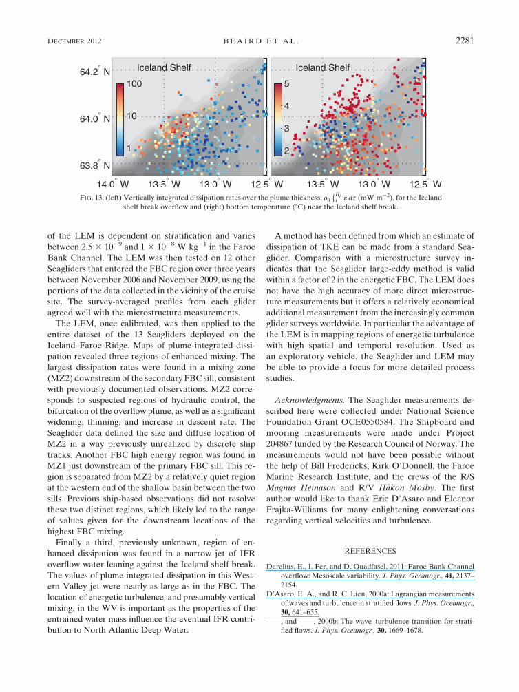
Figure 13 shows that the narrowWV overflow region,

delineated by the low bottom temperatures in the right

panel, is also a region of high dissipation. Maximum

plume-integrated dissipation reaches 250 mW m22,

with a mean value 13 mW m22 in the WV overflow jet.

A clear advantage of the Seaglider LEM is the identifi-

cation of regions such as this one, which was observed

during the course of a survey designed to map the hy-

drography of overflows on the IFR. Dedicated micro-

structure surveys in the region have never been carried

out, so it is only through this ancillary inferred Seaglider

measurement that the energetic region was discovered.

While the Atlantic water above the overflow in the WV

is much the same as that overlying the FBC, there are

gradients in Atlantic water properties across the ridge.

Additionally, very fresh coastal water from Iceland is

occasionally advected off the shelf into the surface wa-

ters of theWV.Mixing between the overflowwaters and

different ambient waters influences the downstream

properties of the overflow (Price and Baringer 1994),

potentially resulting in distinct contributions to North

Atlantic Deep Water from the WV and FBC overflows.

Therefore, mapping the regions of energetic turbulence

and the ambient properties by Seagliders provides in-

sight into dense water production by these overflows.

6. Summary

Levels of turbulent dissipation have been mapped in

one of the two major source regions of North Atlantic

Deep Water. Mixing and entrainment in these small

overflow regions are of great importance to the global

abyssal circulation and the climate system. A scaling has

been investigated that infers dissipation of turbulent

kinetic energy from finescale vertical velocity observed

by an autonomous vehicle.

The large-eddy method (LEM) defined here assumes

that most of the kinetic energy in a turbulent eddy is

dissipated in the time it takes to overturn once. The

scaling requires a length scale and a velocity scale of

these eddies. The length scale is taken to be the Ozmidov

length scale, which is the largest size of an overturn

in stratified flow. The velocity scale is estimated from

the vertical velocity fluctuations, after removing the low

wavenumber and internal-wave-induced contribution

by a suitably chosen high-pass filter, as the root-mean-

square over several eddy lengths. The dissipation esti-

mate depends on a proportionality constant, which is

determined by calibrating the results from a dedicated

Seaglider, collocated with a cruise, against dissipation

measurements from a shipboard microstructure survey.

A comparison between the Seaglider-inferred dissipa-

tion and the microstructure measurements indicate that

the LEM reproduces the direct measurements within

a factor of 2. Survey-averaged profiles of dissipation rate

covary over several orders of magnitude. The noise level

FIG. 12. (top) Section of dissipation, log(e) (W kg21), from sg016

crossing the Western Valley 24–25 July 2008. Depth vs profile

number where each dive and climb is counted as a profile. (bottom)

Corresponding temperature section (8C).

2280 JOURNAL OF PHYS ICAL OCEANOGRAPHY VOLUME 42

of the LEM is dependent on stratification and varies

between 2.5 3 1029 and 1 3 1028 W kg21 in the Faroe

Bank Channel. The LEM was then tested on 12 other

Seagliders that entered the FBC region over three years

between November 2006 and November 2009, using the

portions of the data collected in the vicinity of the cruise

site. The survey-averaged profiles from each glider

agreed well with the microstructure measurements.

The LEM, once calibrated, was then applied to the

entire dataset of the 13 Seagliders deployed on the

Iceland–Faroe Ridge. Maps of plume-integrated dissi-

pation revealed three regions of enhanced mixing. The

largest dissipation rates were found in a mixing zone

(MZ2) downstream of the secondary FBC sill, consistent

with previously documented observations. MZ2 corre-

sponds to suspected regions of hydraulic control, the

bifurcation of the overflow plume, as well as a significant

widening, thinning, and increase in descent rate. The

Seaglider data defined the size and diffuse location of

MZ2 in a way previously unrealized by discrete ship

tracks. Another FBC high energy region was found in

MZ1 just downstream of the primary FBC sill. This re-

gion is separated from MZ2 by a relatively quiet region

at the western end of the shallow basin between the two

sills. Previous ship-based observations did not resolve

these two distinct regions, which likely led to the range

of values given for the downstream locations of the

highest FBC mixing.

Finally a third, previously unknown, region of en-

hanced dissipation was found in a narrow jet of IFR

overflow water leaning against the Iceland shelf break.

The values of plume-integrated dissipation in this West-

ern Valley jet were nearly as large as in the FBC. The

location of energetic turbulence, and presumably vertical

mixing, in the WV is important as the properties of the

entrained water mass influence the eventual IFR contri-

bution to North Atlantic Deep Water.

A method has been defined from which an estimate of

dissipation of TKE can be made from a standard Sea-

glider. Comparison with a microstructure survey in-

dicates that the Seaglider large-eddy method is valid

within a factor of 2 in the energetic FBC. The LEM does

not have the high accuracy of more direct microstruc-

ture measurements but it offers a relatively economical

additional measurement from the increasingly common

glider surveys worldwide. In particular the advantage of

the LEM is in mapping regions of energetic turbulence

with high spatial and temporal resolution. Used as

an exploratory vehicle, the Seaglider and LEM may

be able to provide a focus for more detailed process

studies.

Acknowledgments. The Seaglider measurements de-

scribed here were collected under National Science

Foundation Grant OCE0550584. The Shipboard and

mooring measurements were made under Project

204867 funded by the Research Council of Norway. The

measurements would not have been possible without

the help of Bill Fredericks, Kirk O’Donnell, the Faroe

Marine Research Institute, and the crews of the R/S

Magnus Heinason and R/V H�akon Mosby. The first

author would like to thank Eric D’Asaro and Eleanor

Frajka-Williams for many enlightening conversations

regarding vertical velocities and turbulence.

REFERENCES

Darelius, E., I. Fer, and D. Quadfasel, 2011: Faroe Bank Channel

overflow: Mesoscale variability. J. Phys. Oceanogr., 41, 2137–2154.

D’Asaro, E. A., and R. C. Lien, 2000a: Lagrangian measurements

of waves and turbulence in stratified flows. J. Phys. Oceanogr.,

30, 641–655.

——, and ——, 2000b: The wave–turbulence transition for strati-

fied flows. J. Phys. Oceanogr., 30, 1669–1678.

FIG. 13. (left) Vertically integrated dissipation rates over the plume thickness, r0ÐHp

0 « dz (mW m22), for the Iceland

shelf break overflow and (right) bottom temperature (8C) near the Iceland shelf break.

DECEMBER 2012 BEA IRD ET AL . 2281

Dewey,R., 1999:Mooring design and dynamics—AMatlab package

for designing and analyzing oceanographic moorings. Mar.

Models, 1, 103–157.

Dillon, T. M., 1982: Vertical overturns: A comparison of Thorpe

and Ozmidov length scales. J. Geophys. Res., 87, 9601–9613.

Duncan, L.M., H. L. Bryden, and S.A. Cunningham, 2003: Friction

andmixing in the FaroeBankChannel outflow.Oceanol. Acta,

26, 473–486.Eriksen, C. C., T. J. Osse, R. D. Light, T. Wen, T.W. Lehman, P. L.

Sabin, J. W. Ballard, and A. M. Chiodi, 2001: Seaglider:

A long-range autonomous underwater vehicle for oceano-

graphic research. IEEE J. Oceanic Eng., 26, 424–436.Fer, I., G. Voet, K. S. Seim, B. Rudels, and K. Latarius, 2010: In-

tense mixing of the Faroe Bank Channel overflow. Geophys.

Res. Lett., 37, L02604, doi:10.1029/2009GL041924.

Frajka-Williams, E., C. Eriksen, P. Rhines, and R. Harcourt, 2011:

Determining vertical water velocities from Seaglider. J. Atmos.

Oceanic Technol., 28, 1641–1656.

Gargett, A., 1999: Velcro measurement of turbulent kinetic en-

ergy dissipation rate «. J. Atmos. Oceanic Technol., 16, 1973–

1993.

Geyer, F., S. Østerhus, B. Hansen, and D. Quadfasel, 2006: Ob-

servations of highly regular oscillations in the overflow plume

downstream of the Faroe Bank Channel. J. Geophys. Res.,

111, C12020, doi:10.1029/2006JC003693.

Girton, J. B., L. J. Pratt, D. A. Sutherland, and J. F. Price, 2006: Is

the Faroe Bank Channel overflow hydraulically controlled?

J. Phys. Oceanogr., 36, 2340–2349.

Hansen, B., and S. Østerhus, 2000: North Atlantic–Nordic Seas

exchanges. Prog. Oceanogr., 45, 109–208.——, and ——, 2007: Faroe Bank Channel overflow 1995–2005.

Prog. Oceanogr., 75, 817–856.

Hubbard, R. M., 1980: Hydrodynamics technology for an Ad-

vanced Expendable Mobil Target (AEMT). APL-UW Tech.

Rep. 8013, 34 pp.

Kida, S., J. Price, and J. Yang, 2008: The upper-oceanic response to

overflows: A mechanism for the Azores Current. J. Phys.

Oceanogr., 38, 880–895.

Kolmogoroff, A., 1941: The local structure of turbulence in in-

compressible viscous fluid for very large Reynolds numbers.

Dokl. Akad. Nauk SSSR, 30, 299–303.Legg, S., and Coauthors, 2009: Improving oceanic overflow rep-

resentation in climate models: The gravity current en-

trainment climate process team. Bull. Amer. Meteor. Soc., 90,

657–670.

Lueck, R. G., D. Huang, D. Newman, and J. Box, 1997: Turbulence

measurement with a moored instrument. J. Atmos. Oceanic

Technol., 14, 143–161.

Mauritzen, C., J. Price, T. Sanford, and D. Torres, 2005: Circulation

andmixing in theFaroeseChannels.Deep-SeaRes., 52, 883–913.

Merckelbach, L., D. Smeed, and G. Griffiths, 2010: Vertical water

velocities from underwater gliders. J. Atmos. Oceanic Tech-

nol., 27, 547–563.Moum, J. N., 1996: Energy-containing scales of turbulence in the

ocean thermocline. J. Geophys. Res., 101, 14 095–14 109.

Perkins, H., T. S. Hopkins, S. A. Malmberg, P. M. Poulain, and

A. Warn-Varnas, 1998: Oceanographic conditions east of

Iceland. J. Geophys. Res., 103, 21 531–21 542.

——, T. J. Sherwin, and T. Hopkins, 1994: Amplification of tidal

currents by overflow on the Iceland–Faroe Ridge. J. Phys.

Oceanogr., 24, 721–735.

Peters, H., M. C. Gregg, and T. B. Sanford, 1995: Detail and scaling

of turbulent overturns in the Pacific Equatorial Undercurrent.

J. Geophys. Res., 100, 18 349–18 368.

Pratt, L. J., U. Riemenschneider, and K. R. Helfrich, 2007:

A transverse hydraulic jump in a model of the Faroe Bank

Channel outflow. Ocean Modell., 19, 1–9.

Price, J. F., and M. O. Baringer, 1994: Overflows and deep water

production by marginal seas. Prog. Oceanogr., 33, 161–200.

Riemenschneider, U., and S. Legg, 2007: Regional simulations of

the Faroe Bank Channel overflow in a level model. Ocean

Modell., 17, 93–122.

Saunders, P. M., 1990: Cold outflow from the Faroe Bank Channel.

J. Phys. Oceanogr., 20, 29–43.

Seim, K. S., and I. Fer, 2011: Mixing in the stratified interface of

the Faroe Bank Channel overflow: The role of transverse cir-

culation and internal waves. J. Geophys. Res., 116, C07022,

doi:10.1029/2010JC006805.

——, ——, and J. Berntsen, 2010: Regional simulations of the

Faroe Bank Channel overflow using a s-coordinate ocean

model. Ocean Modell., 35, 31–44.

Smyth, W., and S. A. Thorpe, 2012: Glider measurements of

overturning in a Kelvin–Helmholtz billow train. J. Mar. Res.,

70, 119–140.

Taylor, G. I., 1935: Statistical theory of turbulence. Proc. Roy. Soc.

London, A151, 421–454.Tennekes,H., and J. L. Lumley, 1972:AFirst Course in Turbulence.

The MIT Press, 300 pp.

Thorpe, S. A., 2005: The Turbulent Ocean. Cambridge University

Press, 439 pp.

2282 JOURNAL OF PHYS ICAL OCEANOGRAPHY VOLUME 42