
dissertation.pdf - Aditya Grover
237
LEARNING TO REPRESENT AND REASON UNDER LIMITED SUPERVISION A DISSERTATION SUBMITTED TO THE DEPARTMENT OF COMPUTER SCIENCE AND THE COMMITTEE ON GRADUATE STUDIES OF STANFORD UNIVERSITY IN PARTIAL FULFILLMENT OF THE REQUIREMENTS FOR THE DEGREE OF DOCTOR OF PHILOSOPHY Aditya Grover August 2020
-
Upload
khangminh22 -
Category
Documents
-
view
0 -
download
0
Transcript of dissertation.pdf - Aditya Grover

LEARNING TO REPRESENT AND REASONUNDER LIMITED SUPERVISION
A DISSERTATIONSUBMITTED TO THE DEPARTMENT OF COMPUTER SCIENCE
AND THE COMMITTEE ON GRADUATE STUDIESOF STANFORD UNIVERSITY
IN PARTIAL FULFILLMENT OF THE REQUIREMENTSFOR THE DEGREE OF
DOCTOR OF PHILOSOPHY
Aditya GroverAugust 2020

http://creativecommons.org/licenses/by-nc/3.0/us/
This dissertation is online at: http://purl.stanford.edu/jv138zg1058
© 2020 by Aditya Grover. All Rights Reserved.
Re-distributed by Stanford University under license with the author.
This work is licensed under a Creative Commons Attribution-Noncommercial 3.0 United States License.
ii

I certify that I have read this dissertation and that, in my opinion, it is fully adequatein scope and quality as a dissertation for the degree of Doctor of Philosophy.
Stefano Ermon, Primary Adviser
I certify that I have read this dissertation and that, in my opinion, it is fully adequatein scope and quality as a dissertation for the degree of Doctor of Philosophy.
Moses Charikar
I certify that I have read this dissertation and that, in my opinion, it is fully adequatein scope and quality as a dissertation for the degree of Doctor of Philosophy.
Jure Leskovec
I certify that I have read this dissertation and that, in my opinion, it is fully adequatein scope and quality as a dissertation for the degree of Doctor of Philosophy.
Eric Horvitz
Approved for the Stanford University Committee on Graduate Studies.
Stacey F. Bent, Vice Provost for Graduate Education
This signature page was generated electronically upon submission of this dissertation in electronic format. An original signed hard copy of the signature page is on file inUniversity Archives.
iii

Abstract
Natural agents, such as humans, excel at building representations of the world andusing them to effectively draw inferences andmake decisions. Critically, the develop-ment of such advanced reasoning capabilities can occur even with limited supervision.In stark contrast, the major successes of machine learning (ML)-based artificialagents are primarily in tasks that have access to large labelled datasets or simulators,such as object recognition and game playing. This dissertation focuses on probabilis-tic modeling frameworks that shrink this gap between natural and artificial agentsand thus enable effective reasoning in supervision constrained scenarios.
This dissertation comprises of three parts. First, we formally lay the foundationsfor learning probabilistic generative models. The goal here is to simulate any availabledata, thus providing a natural learning objective even in settings with limited su-pervision. We discuss various trade-offs involved in learning and inference in highdimensions using these models, including the specific choice of learning objective,optimization procedure, and parametric model family. Building on these insights,we develop new algorithms to boost the performance of state-of-the-art models andmitigate their biases when trained on large uncurated and unlabelled datasets.
Second, we extend thesemodels to learn feature representations for relational data.Learning these representations is unsupervised, and we demonstrate their utility forclassification and sequential decision making. Third and last, we present two real-world applications of these models for accelerating scientific discovery in: (a) learningdata dependent priors for compressed sensing, and (b) design of experimentsfor optimizing charging in electric batteries. Together, these contributions enableML systems to overcome the critical supervision bottleneck for high-dimensionalinference and decision making problems in the real world.
iv

Acknowledgments
First and foremost, I would like to thank my PhD advisor, Stefano Ermon. As one ofStefano’s first students, I have been fortunate to cherish a long list of experienceswith him. My rollercoaster PhD, involving diverse research projects and teachinga new course to hundreds of students among many other endeavors, would nothave been possible without Stefano’s inspiring work ethics, patient advising, andtrademark clarity in thought. In all these years, it amazes me how every researchmeeting I have with Stefano ends on a personal note of optimism and intellectualsatisfaction. Thank you for sharing your magic with me, I will treasure it forever.
My experience at Stanfordwould be incompletewithout the company I enjoyed inErmon group. Neal instantaneously became a lifelong trusted friend (and personalgym trainer); Jonathan and Tri exemplify humility (and solving convex optimizationproblems); Shengjia, Tony, and Yang never fail to bring a smile (and write greatpapers for every deadline); Kristy and Rui double up as my creative alter egos (andMixer buddies). Some who left early on continue to be great friends: Jon, Michael,Russell, Tudor, Vlad, and the newer ones continue to make the group as vibrant asever: Andy, Burak, Chris, Kuno, Lantao, Ria. Outside of Ermon group, I will alsodearly miss hanging out with the many friends at StatsML Group, InfoLab, StanfordData Science Institute, and Stanford AI Lab.
I have also had the privilege of standing on the shoulders of amazing mentorsand collaborators over the years: Ankit Anand, Mausam, and Parag Singla trickedme into the joys of research when I was an undergraduate at IIT Delhi; ChristopherRé, Greg Valiant, Jure Leskovec, Moses Charikar, Noah Goodman, Percy Liang,and Stephen Boyd were generous with their insightful feedback and time during
v

rotations and oral exams at Stanford; Alekh Agarwal, Ashish Kapoor, Ben Poole,Dustin Tran, Eric Horvitz, Harri Edwards, Ken Tran, Kevin Murphy, Maruan Al-Shedivat, and Yura Burda broadened my research perspectives in fun summerinternships at Google, Microsoft, and OpenAI. I have also enjoyed mentoring juniorstudents who helped me pursue new directions in research: Aaron Zweig, ChrisChute, Eric Wang, Manik Dhar, and Todor Markov. A shoutout to Will Chueh andPeter Attia, my co-leads on the 4 year long battery project—Will’s investment in myresearch and career success coupled with Peter’s positivity, perseverance, and hardwork makes for a dream collaboration. I am also deeply thankful to all my othercollaborators, administrators, and funding agencies for keeping the show running.
It is rightly said that friends are the family you choose. Thanks to my friendsfrom Indiawho have stayed in touch even after I moved to US. And Iwould be remissin not acknowledging friends from Stanford who I have interacted with regularly inthe last five years: Jayesh for his excellent taste in spices and Netflix shows and beingthe most helpful roommate I could have hoped for, Hima & Pracheer for being myno-filter friends on any topic of conversation from academia to Bollywood, Danielfor all the laughs, vents, and immigrant walks at Bytes and Coupa, and Aditi, Anmol& Vivek for allowing me to be myself without judgement. Thanks to many otherfriends and extended family who have been an integral part of this journey; I couldnot overstate their importance in lifting me during the lows, cheering for my highs,and being a part of memories that will last a lifetime.
Finally, I would like to thank my brother, Abhinav, for being my best friendsince childhood and my sister-in-law, Vaishali, for being a pillar of support to ourfamily. Last and definitely the most, I will forever be indebted to my parents, Manila& Vimal, for their unconditional love and unfaltering care for my happiness andwell-being. This one is for you.
vi

To my parents, Manila and Vimal Grover.
vii

Contents
Abstract iv
Acknowledgments v
1 Introduction 11.1 Approach . . . . . . . . . . . . . . . . . . . . . . . . . . . . . . . . . . . 2
1.1.1 Foundations of Probabilistic Generative Modeling . . . . . . . 31.1.2 Relational Representation and Reasoning . . . . . . . . . . . . 41.1.3 Applications in Science and Society . . . . . . . . . . . . . . . 5
1.2 Related Research . . . . . . . . . . . . . . . . . . . . . . . . . . . . . . 61.3 Dissertation Overview . . . . . . . . . . . . . . . . . . . . . . . . . . . 7
I Foundations of Probabilistic Generative Modeling 9
2 Background 102.1 Problem Setup . . . . . . . . . . . . . . . . . . . . . . . . . . . . . . . . 102.2 Learning & Inference . . . . . . . . . . . . . . . . . . . . . . . . . . . . 122.3 Deep Generative Models . . . . . . . . . . . . . . . . . . . . . . . . . . 13
2.3.1 Energy-based Models . . . . . . . . . . . . . . . . . . . . . . . 142.3.2 Autoregressive Models . . . . . . . . . . . . . . . . . . . . . . . 152.3.3 Variational Autoencoders . . . . . . . . . . . . . . . . . . . . . 162.3.4 Normalizing Flows . . . . . . . . . . . . . . . . . . . . . . . . . 182.3.5 Generative Adversarial Networks . . . . . . . . . . . . . . . . 20
viii

3 Trade-offs in Learning & Inference 223.1 Introduction . . . . . . . . . . . . . . . . . . . . . . . . . . . . . . . . . 223.2 Flow Generative Adversarial Networks . . . . . . . . . . . . . . . . . 243.3 Empirical Evaluation . . . . . . . . . . . . . . . . . . . . . . . . . . . . 25
3.3.1 Log-likelihoods vs. sample quality . . . . . . . . . . . . . . . . 263.3.2 Comparison with Gaussian mixture models . . . . . . . . . . 283.3.3 Hybrid learning of Flow-GANs . . . . . . . . . . . . . . . . . . 30
3.4 Explaining log-likelihood trends . . . . . . . . . . . . . . . . . . . . . 313.5 Discussion & Related Work . . . . . . . . . . . . . . . . . . . . . . . . 323.6 Conclusion . . . . . . . . . . . . . . . . . . . . . . . . . . . . . . . . . . 33
4 Model Bias in Generative Models 354.1 Introduction . . . . . . . . . . . . . . . . . . . . . . . . . . . . . . . . . 354.2 Preliminaries . . . . . . . . . . . . . . . . . . . . . . . . . . . . . . . . . 374.3 Likelihood-Free Importance Weighting . . . . . . . . . . . . . . . . . . 384.4 Boosted Energy-Based Model . . . . . . . . . . . . . . . . . . . . . . . 434.5 Empirical Evaluation . . . . . . . . . . . . . . . . . . . . . . . . . . . . 46
4.5.1 Goodness-of-fit testing . . . . . . . . . . . . . . . . . . . . . . . 464.5.2 Data augmentation for multi-class classification . . . . . . . . 474.5.3 Model-based off-policy policy evaluation . . . . . . . . . . . . 49
4.6 Discussion & Related Work . . . . . . . . . . . . . . . . . . . . . . . . 534.7 Conclusion . . . . . . . . . . . . . . . . . . . . . . . . . . . . . . . . . . 54
5 Dataset Bias in Generative Models 555.1 Introduction . . . . . . . . . . . . . . . . . . . . . . . . . . . . . . . . . 555.2 Preliminaries . . . . . . . . . . . . . . . . . . . . . . . . . . . . . . . . . 575.3 Learning with Multiple Data Sources . . . . . . . . . . . . . . . . . . . 585.4 Empirical Evaluation . . . . . . . . . . . . . . . . . . . . . . . . . . . . 63
5.4.1 Density ratio estimation . . . . . . . . . . . . . . . . . . . . . . 665.4.2 Dataset bias mitigation . . . . . . . . . . . . . . . . . . . . . . . 66
5.5 Discussion & Related Work . . . . . . . . . . . . . . . . . . . . . . . . 695.6 Conclusion . . . . . . . . . . . . . . . . . . . . . . . . . . . . . . . . . . 73
ix

II Relational Representation & Reasoning 74
6 Representation & Reasoning in Graphs 756.1 Introduction . . . . . . . . . . . . . . . . . . . . . . . . . . . . . . . . . 756.2 Preliminaries . . . . . . . . . . . . . . . . . . . . . . . . . . . . . . . . . 76
6.2.1 Weisfeiler-Lehman algorithm . . . . . . . . . . . . . . . . . . . 776.2.2 Graph neural networks . . . . . . . . . . . . . . . . . . . . . . . 78
6.3 Graphite: Generative Modeling for Graphs . . . . . . . . . . . . . . . 796.4 Empirical Evaluation . . . . . . . . . . . . . . . . . . . . . . . . . . . . 82
6.4.1 Reconstruction & density estimation . . . . . . . . . . . . . . . 836.4.2 Link prediction . . . . . . . . . . . . . . . . . . . . . . . . . . . 846.4.3 Semi-supervised node classification . . . . . . . . . . . . . . . 87
6.5 Discussion & Related Work . . . . . . . . . . . . . . . . . . . . . . . . 876.6 Conclusion . . . . . . . . . . . . . . . . . . . . . . . . . . . . . . . . . . 88
7 Representation & Reasoning in Multiagent Systems 897.1 Introduction . . . . . . . . . . . . . . . . . . . . . . . . . . . . . . . . . 897.2 Preliminaries . . . . . . . . . . . . . . . . . . . . . . . . . . . . . . . . . 907.3 Learning Policy Representations . . . . . . . . . . . . . . . . . . . . . 92
7.3.1 Generative representation learning via imitation . . . . . . . . 927.3.2 Contrastive representation learning via triplet loss . . . . . . . 937.3.3 Hybrid generative-contrastive representations . . . . . . . . . 95
7.4 Generalization in Multiagent Systems . . . . . . . . . . . . . . . . . . 957.4.1 Generalization across agents & interactions . . . . . . . . . . . 957.4.2 Generalization across tasks . . . . . . . . . . . . . . . . . . . . 97
7.5 Empirical Evaluation . . . . . . . . . . . . . . . . . . . . . . . . . . . . 987.5.1 The RoboSumo environment . . . . . . . . . . . . . . . . . . . . 997.5.2 The ParticleWorld environment . . . . . . . . . . . . . . . . . 104
7.6 Discussion & Related Work . . . . . . . . . . . . . . . . . . . . . . . . 1077.7 Conclusion . . . . . . . . . . . . . . . . . . . . . . . . . . . . . . . . . . 108
x

III Applications in Science & Society 109
8 Compressed Sensing via Generative Models 1108.1 Introduction . . . . . . . . . . . . . . . . . . . . . . . . . . . . . . . . . 1108.2 Preliminaries . . . . . . . . . . . . . . . . . . . . . . . . . . . . . . . . . 1118.3 Uncertainty Autoencoders . . . . . . . . . . . . . . . . . . . . . . . . . 113
8.3.1 Implicit generative modeling . . . . . . . . . . . . . . . . . . . 1158.3.2 Comparison with Principal Component Analysis . . . . . . . 116
8.4 Empirical Evaluation . . . . . . . . . . . . . . . . . . . . . . . . . . . . 1188.4.1 Statistical compressed sensing . . . . . . . . . . . . . . . . . . 1188.4.2 Transfer compressed sensing . . . . . . . . . . . . . . . . . . . 1228.4.3 Dimensionality reduction . . . . . . . . . . . . . . . . . . . . . 122
8.5 Discussion & Related Work . . . . . . . . . . . . . . . . . . . . . . . . 1258.6 Conclusion . . . . . . . . . . . . . . . . . . . . . . . . . . . . . . . . . . 128
9 Multi-Fidelity Optimal Experimental Design: A Case Study in BatteryFast Charging 1299.1 Introduction . . . . . . . . . . . . . . . . . . . . . . . . . . . . . . . . . 1299.2 Preliminaries . . . . . . . . . . . . . . . . . . . . . . . . . . . . . . . . . 1319.3 Closed-Loop Optimization With Early Prediction . . . . . . . . . . . . 1339.4 Empirical Evaluation . . . . . . . . . . . . . . . . . . . . . . . . . . . . 1369.5 Discussion & Related Work . . . . . . . . . . . . . . . . . . . . . . . . 1429.6 Conclusion . . . . . . . . . . . . . . . . . . . . . . . . . . . . . . . . . . 144
10 Conclusions 14510.1 Summary of Contributions . . . . . . . . . . . . . . . . . . . . . . . . . 14510.2 Future Work . . . . . . . . . . . . . . . . . . . . . . . . . . . . . . . . . 147
A Additional Proofs 149
B Additional Experimental Details & Results 153
C Code & Data 175
xi

List of Tables
3.1 Best MODE scores and test negative log-likelihood estimates for Flow-GANmodels on MNIST. 26
3.2 Best Inception scores and test negative log-likelihood estimates for Flow-GANmodels on CIFAR-10. 26
4.1 Goodness-of-fit evaluation on CIFAR-10 dataset for PixelCNN++ and SNGAN.Standard errors computed over 10 runs. Higher IS is better. Lower FID andKID scores are better. 46
4.2 Classification accuracy on the Omniglot dataset. Standard errors computedover 5 runs. 47
4.3 Off-policy policy evaluation on MuJoCo tasks. Standard error is over 10 MonteCarlo estimateswhere each estimate contains 100 randomly sampled trajectories.
51
5.1 Comparison between the cross-entropy loss of the Bayes classifier and learneddensity ratio classifier. 66
6.1 Mean reconstruction errors and negative log-likelihood estimates (in nats) forautoencoders and variational autoencoders respectively on test instances fromsix different generative families. Lower is better. 83
6.2 Citation network statistics 846.3 Area Under the ROC Curve (AUC) for link prediction (* denotes dataset with
features). Higher is better. 85
xii
6.4 Average Precision (AP) scores for link prediction (* denotes dataset with fea-tures). Higher is better. 85
6.5 Classification accuracies (* denotes dataset with features). Baseline numbersfrom [KW17]. 86
7.1 Intra-inter clustering ratios (IICR) and accuracies for outcome prediction (Acc)for weak (W) and strong (S) generalization on RoboSumo. 101
7.2 Intra-inter clustering ratios (IICR) for weak (W) and strong (S) generalizationon ParticleWorld. Lower is better. 105
7.3 Average train and test rewards for speaker policies on ParticleWorld. 105
8.1 PCA vs. UAE. Average test classification accuracy for the MNIST dataset. 124
B.1 Bias-variance analysis for PixelCNN++ and SNGAN when T = 10, 000. Stan-dard errors over the absolute values of bias and variance evaluations are com-puted over the 2048 activation statistics. Lower absolute values of bias, lowervariance, and lower MSE is better. 156
B.2 Bias-variance analysis for PixelCNN++ and SNGAN when T = 5, 000. Stan-dard errors over the absolute values of bias and variance evaluations are com-puted over the 2048 activation statistics. Lower absolute values of bias, lowervariance, and lower MSE is better. 157
B.3 Statistics for the environments. 160B.4 Off-policy policy evaluation on MuJoCo tasks. Standard error is over 10 Monte
Carlo estimateswhere each estimate contains 100 randomly sampled trajectories.Here, we perform stepwise LFIW over transition triplets. 161
B.5 ResNet-18 architecture adapted for attribute classifier. 164
xiii

B.6 Architecture for the generator and discriminator. Notation: ch refers to thechannel width multiplier, which is 64 for 64× 64 CelebA images. ResBlock uprefers to aGenerator Residual Block inwhich the input is passed through a ReLUactivation followed by two 3× 3 convolutional layers with a ReLU activation inbetween. ResBlock down refers to a Discriminator Residual Block in which theinput is passed through two 3× 3 convolution layers with a ReLU activationin between, and then downsampled. Upsampling is performed via nearestneighbor interpolation, whereas downsampling is performed via mean pooling.‘‘ResBlock up/down n→ m’’ indicates a ResBlock with n input channels andm output channels. 165
B.7 AUC scores for link prediction with Monte Carlo subsampling during training.Higher is better. 168
B.8 Frobenius norms of the encoding matrices for MNIST and Omniglot. 173
xiv
List of Figures
2.1 Learning a generative model. The true data distribution is a mixture of 2Gaussians (blue). We only observe a training dataset of samples from thisdistribution (shown as ×). The model familyM is unimodal Gaussian dis-tributions and the parameters θ correspond to the mean and variance. Welearn the best fit parameters θ∗ (green) by minimizing the Kullback-Leibler(KL) divergence between pdata and pθ . Post learning, we can use the generativemodel p∗θ to generate more data via sampling (shown as ). 11
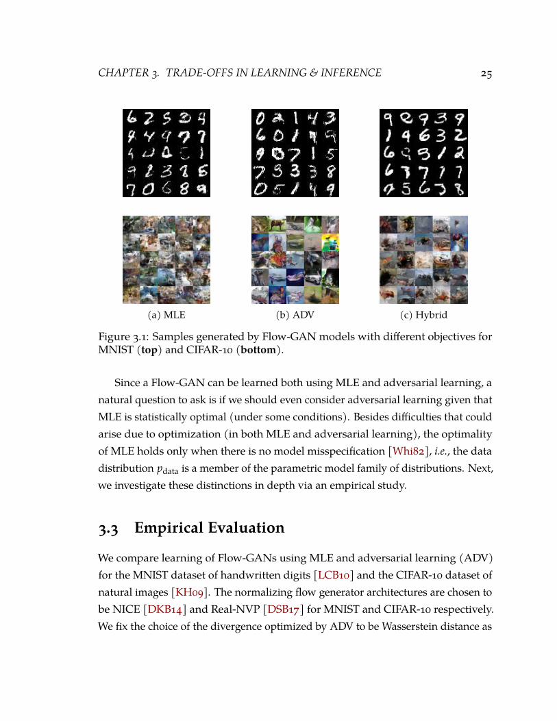
3.1 Samples generated by Flow-GAN models with different objectives for MNIST(top) and CIFAR-10 (bottom). 25
3.2 Learning curves for negative log-likelihood (NLL) evaluation on MNIST (top,in nats) and CIFAR (bottom, in bits/dim). Lower NLLs are better. 27
3.3 Gaussian Mixture Models outperform adversarially learned models for anybandwidth in the green shaded region on both held-out log-likelihoods andsampling metrics. 29
3.4 Singular value analysis for the Jacobian of the generator functions. The Jacobianis evaluated at 64 random noise vectors sampled from the prior. The x-axis ofthe figure shows the singular value magnitudes (on a log scale) and for eachsingular value s, we show the corresponding cumulative distribution function(CDF) value on the y-axis which signifies the fraction of singular values lessthan s. 31
xv
4.1 Importance Weight Estimation using Probabilistic Classifiers. (a) A univariateGaussian (blue) is fit to samples from a mixture of two Gaussians (red). (b-d)Estimated class probabilities (with 95% confidence intervals based on 1000
bootstraps) for varying number of points n, where n is the number of trainingdata points used for training the generative model andmultilayer perceptron.42
4.2 Qualitative evaluation of importance weighting for data augmentation. (a-f)Within each figure, top row shows held-out data samples from a specific classin Omniglot. Bottom row shows generated samples from the same class rankedin decreasing order of importance weights. 48
4.3 Estimation error δ(v) = v(πe)− vH(πe) for different values of H (min 0, max100). Shaded area denotes standard error over 10 random seeds. 52
5.1 Samples from a baseline BigGAN that reflect the gender bias underlying thetrue data distribution in CelebA. All faces above the orange line (67%) areclassified as female, while the rest are labeled as male (33%). 56
5.2 Distribution of importance weights for different latent subgroups. On average,The underrepresented subgroups are upweighted while the overrepresentedsubgroups are downweighted. 65
5.3 Single-Attribute Dataset Bias Mitigation for bias=0.9. Standard error in (b)and (c) over 10 independent evaluation sets of 10,000 samples each drawnfrom the models. Lower fairness discrepancy and FID is better. We find thaton average, imp-weight outperforms the equi-weight baseline by 49.3% andthe conditional baseline by 25.0% across all reference dataset sizes for biasmitigation. 67
5.4 Single Attribute Dataset Bias Mitigation for bias=0.8. Standard error in (b)and (c) over 10 independent evaluation sets of 10,000 samples each drawnfrom the models. Lower fairness discrepancy and FID is better. We find thaton average, imp-weight outperforms the equi-weight baseline by 23.9% andthe conditional baseline by 12.2% across all reference dataset sizes for biasmitigation. 68
xvi

5.5 Mult-Attribute Dataset Bias Mitigation. Standard error in (b) and (c) over 10independent evaluation sets of 10,000 samples each drawn from the models.Lower fairness discrepancy and FID is better. We find that on average, imp-weight outperforms the equi-weight baseline by 32.5% and the conditionalbaseline by 4.4% across all reference dataset sizes for bias mitigation. 70
6.1 Latent variable model for Graphite. Observed evidence variables in gray. 796.2 t-SNE embeddings of the latent feature vectors for the Cora dataset. Colors
denote labels. 86
7.1 Agent-Interaction Graph. An example of a graph used for evaluating gener-alization in a multiagent system with 5 train agents (A, B, E, F, G) and 2 testagents (C, D). 96
7.2 Illustrations for the environments used in our experiments: (a) competitive;and (b) cooperative. 98
7.3 Illustration of the proposed model for optimizing a policy πψ that conditionson an embedding of the opponent policy πA. At time t, the pre-trained rep-resentation function fφ computes the opponent embedding based on a pastinteraction et−1. We optimize πψ tomaximize the expected rewards in its currentinteractions et with the opponent. 99
7.4 Embeddings learned using Emb-Hyb for 10 test interaction episodes of 5 agentsprojected on the first three principal components for RoboSumo and ParticleWorld.Color denotes agent policy. 100
7.5 Average win rates of the newly trained agents against 5 training agent and 5 test-ing agents. (a) Top: Baseline comparison with policies that make use of Emb-Im,Emb-Id, and Emb-Hyb (all computed online). (b) Bottom: Comparison of differ-ent baseline embeddings used at evaluation time (all embedding-conditionedpolicies use Emb-Hyb). At each iteration, win rates were computed based on50 1-on-1 games. Each agent was trained 3 times, each time from a differentrandom initialization. Shaded regions correspond to 95% CI. 101
xvii

7.6 Win, loss, and draw rates plotted for the first agent in each pair. Each pair ofagents was evaluated after each training iteration on 50 1-on-1 games; curvesare based on 5 evaluation runs. Shaded regions correspond to 95% CI. 102
7.7 Win rates for agents specified in each row at computed at iteration 1000. 102
8.1 Dimensionality reduction using PCA vs. UAE. Projections of the data (blackpoints) on the UAE direction (green line) maximize the likelihood of decodingunlike the PCA projection axis (magenta line) which collapses many points ina narrow region. 117
8.2 (a-b) Test `2 reconstruction error (per image) for compressed sensing. (c-d)Reconstructions for m = 25. First: Original. Second: LASSO. Third: CS-VAE.Last: UAE. 25 projections of the data are sufficient for UAE to reconstruct theoriginal image with high accuracy. 120
8.3 (a) Test `2 reconstruction error (per image) for compressed sensing on CelebA.(b) Reconstructions for m = 50 on the CelebA dataset. First: Target. Second:LASSO-DCT. Third: LASSO-Wavelet. Fourth: DCGAN. Last: UAE. 121
8.4 (a-b) Test `2 reconstruction error (per image) for transfer compressed sensing.(c-d) Reconstructions for m = 25. Top: Target. Second: CS-VAE. Third: UAE-SD. Last: UAE-SE. 123
9.1 Schematic of our closed-loop optimization (CLO) system. First, batteries aretested. The cycling data from the first 100 cycles, specifically electrochemicalmeasurements such as voltage and capacity, are used as input for early outcomeprediction of cycle life. These cycle life predictions are subsequently sent to aBayesian optimization (BO) algorithm, which recommends the next protocolsto test by balancing the competing demands of exploration (testing protocolswith high uncertainty in estimated cycle life) and exploitation (testing protocolswith high estimated cycle life). This process iterates until the testing budget isexhausted. 133
xviii

9.2 Structure of our 10-minute, six-step fast-charging protocols. (a) Current vs.SOC for an example charging protocol, 7.0C–4.8C–5.2C–3.45C (bold lines).Each charging protocol is defined by five constant current (“CC”) steps followedby one constant voltage (“CV”) step. The last two steps (CC5 and CV1) areidentical for all charging protocols. We optimize over the first four constant-current steps, denoted CC1, CC2, CC3, and CC4. Each of these steps comprisesa 20% SOC window, such that CC1 ranges from 0–20% SOC, CC2 ranges from20–40% SOC, etc. CC4 is constrained by specifying that all protocols charge inthe same total time (10 minutes) from 0% to 80% SOC. Thus, our parameterspace consists of unique combinations of the three free parameters CC1, CC2,and CC3. For each step, we specify a range of acceptable values; the upperlimit is monotonically decreasing with increasing SOC to avoid the upper cutoffpotential (3.6 V for all steps). (b) CC4 (color) as a function of CC1, CC2, andCC3 (x, y, and z axes, respectively). Each point represents a unique chargingprotocol. 135
9.3 Early cycle life predictions per round. The tested charging protocols and theresulting predictions are plotted for rounds 1–4. Each point represents a charg-ing protocol, defined by CC1, CC2, and CC3 (x, y, and z axes, respectively).The color represents cycle life predictions from the early outcome predictionmodel. The charging protocols in the first round of testing are randomly se-lected. As BO shifts from exploration to exploitation, the charging protocolsselected for testing by the closed loop in subsequent rounds are primarily inthe high-performing region. 137
9.4 Evolution of the parameter space per round. The color represents cycle life asestimated by BO. The initial cycle life estimates are equivalent for all protocols;as more predictions are generated, BO updates its cycle life estimates. 137
9.5 (a) Distribution of the number of repetitions for each charging protocol. Only46 of 224 protocols (21%) are tested multiple times. (b) Current vs. SOCfor the top three fast-charging protocols as estimated by CLO. CC1–CC4 aredisplayed in the legend. All three protocols have relatively uniform charging(i.e., CC1≈CC2≈CC3≈CC4). 138
xix
9.6 Discharge capacity vs. cycle number for all batteries in the validation experi-ment. See Figure 9.7 for the color scheme legend. 139
9.7 (a) Comparison of early-predicted cycle lives from validation to closed-loopestimates, averaged on a protocol basis. Each 10-minute charging protocol istested with five batteries. Error bars represent the 95% confidence intervals. (b)Observed vs. early-predicted cycle life for the validation experiment. While ourearly predictor appears biased, likely due to calendar aging effects, the trendis correctly captured (Pearson correlation coefficient r = 0.86). (c) Final cyclelives from validation, sorted by CLO ranking. The length of each bar and theannotations represents the mean final cycle life from validation per protocol.Error bars represent the 95% confidence intervals. 140
B.1 Calibration of classifiers for density ratio estimation. 158B.2 Environments in OPE experiments. 161B.3 Estimation error δ(v) = v(πe)− vH(πe) for different values of H (minimum
0, maximum 100). Shaded area denotes standard error over different randomseeds; each seed uses 100 sampled trajectories. Here, we perform stepwiseLFIW over transition triplets. 162
B.4 Results from the Shapes3D dataset. After restricting the possible floor colors tored or blue and using a biased dataset of bias=0.9, we find that the samplesobtained after importance reweighting (b) are considerably more balancedthan those without reweighting (a), as desired. 166
B.5 AUC score ofVGAEandGraphitewith subsampled edges on theCora dataset.168B.6 (a) An example clique agent interaction graph with 10 agents. (b) An example
bipartite agent interaction graph with 5 speakers and 5 listeners. 172
xx

1 Introduction
Imagination is the living power and prime agent of all human perception.– Samuel Taylor Coleridge
The ability to effectively combine data and computation to make inferences anddecisions is a long-standing goal of artificial intelligence (AI). In the last few decades,there has been an explosion in the scale of datasets and computational resourcesavailable within several disciplines ranging from natural to social sciences [RD15].Yet, there exists a fundamental gap in the capabilities of current AI systems and thoserequired for complex reasoning in science and engineering. Most of the successfuldata-driven deployments of AI in the real world are restricted to applications of ma-chine learning (ML) where we have access to large labelled datasets or environmentsimulators, such as object recognition [He+16] and game playing [Sil+17]. Thisis hardly a practical assumption for many scientific domains, such as the physicaland biological sciences, where the collection of labels can be prohibitively expensiveincurring costs due to time, money, privacy, and safety [Zho18].
At the same time, there is compelling evidence from natural agents in the realworld, such as humans, suggesting that complex reasoning tasks such as probabilis-tic inference and long-horizon planning do not require copious amounts of labelledsupervision [Bar89; BK96; Gop10]. Real world data modalities, including the onesthat arise in scientific applications, are typically high-dimensional, e.g., images,video, graphs. And even with limited access to supervision, natural agents can learnto reason over such data by learning meaningful spatiotemporal representations. For ex-ample, instead of monitoring individual pixels in the frames of a video, we can learn
1

CHAPTER 1. INTRODUCTION 2
to represent physical objects by clustering similarly colored pixels in close proximityand reasoning about their dynamics over successive frames collectively. How dowe endow artificial agents with similar representation and reasoning capabilities inhigh dimensions given only limited access to labelled supervision?
1.1 Approach
This dissertation explores the above question in detail from the lens of probabilisticgenerative modeling. To motivate the generative modeling paradigm, consider theImagenet dataset of natural images [Den+09]. What is the process by which anyimage in the dataset was created? Intuitively, one can think of multiple factors atplay during image creation. Some of these factors are specific to imaging technology,such as lighting, camera resolution, and location; whereas other factors concernexogenous physical and biological phenomena, such as the shapes, colors, and sizesof plants, animals, and inanimate objects. While a complete characterization of thefactors of variation during image creation seems to be an arduous task for large anddiverse datasets, it can offer us useful insights about the structure of the world.
The goal of a probabilistic generative model is to automate the above task bylearning to generate a given dataset. As we noted in the thought experiment above,one can hope that a model that succeeds at this task would learn to extract insight-ful structure in large datasets. As such this goal is not tied to the availability (orunavailability) of labelled supervision and hence its use does not preclude anyof the traditional learning paradigms such as supervised or reinforcement learn-ing. For example, Naive Bayes is a standard generative classifier that models thejoint distribution between inputs and labels and makes predictions using Bayesrule [NJ02]. Above and beyond the aforementioned learning paradigms, the focusof this dissertation will be on using generative models for learning representationsand reasoning for various kinds of supervision constrained settings, such as unsu-pervised and transfer learning. To this end, we organize the dissertation aroundthree key organizational themes, which we discuss next.

CHAPTER 1. INTRODUCTION 3
1.1.1 Foundations of Probabilistic Generative Modeling
A generative model induces a probability distribution and generating data from themodel is equivalent to sampling from this induced distribution. During learning,we are given a dataset and our goal is to optimize for the model distribution thatis as close as possible to the underlying (unknown) data distribution from whichthe dataset was obtained. In high dimensions however, the curse of dimensionalitykicks in as the dataset covers only a small region of the true support of a potentiallycomplex data distribution. Hence, a practical algorithm for learning a generativemodel for high-dimensional data involves numerous design choices and trade-offstherein. For example, howdowe formalize a learning objective for closeness betweenthe model and data distributions? How do we optimize and regularize such anobjective to enable generalization beyond the training dataset?
The status quo in generative modeling is a large set of sufficiently distinct frame-works derived from different algorithmic design choices (see Chapter 2 for a briefreview and [Goo16; KW19; Pap+19] for broad surveys). Yet, till date, there is nodominant framework even when we restrict ourselves to a minimal set of basicevaluation criteria. The contributions in this dissertation contribute to this growingliterature in two fundamental ways. First, we quantify the trade-offs in learningand inference for existing generative models. In particular, we show for the firsttime quantitatively that existing models which optimize for sample generation pro-gressively assign poorer likelihoods to the observed data during training even in theabsence of overfitting [GDE18]. As a remedy, we provide alternate regularizationschemes for learning to excel at both sampling and likelihood estimation.
Second, we develop ‘‘plug-in” model-agnostic algorithms for increasing theexpressiveness of generative models. We provide two such techniques: (a) anunsupervised boosting algorithm to sequentially increase model capacity [GE18;Gro+19a], (b) a bias mitigation algorithm that fuses multiple unlabelled datasources (potentially uncurated) for sample-efficient learning and avoids the perilsof dataset bias accompanying such a fusion [Cho+20]. Together, these contributionsimprove the performance of state-of-the-art models on data generation [Gro+19a;

CHAPTER 1. INTRODUCTION 4
Cho+20] as well as a diverse set of downstream use cases such as domain adapta-tion [Gro+20], data augmentation [Gro+19a], and model-based off-policy policyevaluation [Gro+19a].
1.1.2 Relational Representation and Reasoning
Reasoning with relational data is key to understanding how objects interact witheach other and give rise to complex phenomena in the everyday world. Well-known applications include knowledge base completion [Wan+17a], programsynthesis [Bro+18], visual question-answering [Ant+15], and social network anal-ysis [WF+94]. Although access to relational datasets has increased significantlyin the last few decades, canonical representations, such as adjacency matrices forgraphs, are discrete and combinatorial. Moreover, obtaining labeled supervisionfor predictive tasks over nodes and edges can be expensive in large graphs. Hence,integrating these datasets directly into modern ML systems that rely on continuousgradient-based optimization techniques, make strong independence and identicallydistributed (i.i.d.) assumptions, or require excessive supervision is challenging.
A successful remedy for these challenges is to design unsupervised algorithms tolearn continuous representations for the nodes in graphs. We improve upon classicapproaches such as spectral decomposition by proposing new frameworks basedon generative modeling and contrastive learning. For the latter, the goal is to learnrepresentations that can distinguish similar nodes from dissimilar ones. We extendpreviously proposed objectives in vision and language, such as skipgram [Mik+13]and triplet losses [HA15], to establish notions of similarity for graph-structureddata. Notably, our frameworks [GL16; GZE19] are carefully designed to scale tolarge graphs both during learning and inference, with downstream use cases innode classification and link prediction. Furthermore, we successfully extend theseideas to even interactive graphs specified as a multiagent system [Woo09]. Here, weare interested in modeling the behavior of an agent (nodes) based on its interactions(edges) with other agents. We show that the behaviors encoded in our learnedrepresentations inform effective counter or complementary strategies for competitive
CHAPTER 1. INTRODUCTION 5
and cooperative reinforcement learning respectively [Gro+18c; Gro+18d].
1.1.3 Applications in Science and Society
In 2015, the United Nations adopted 17 Sustainable Development Goals as a ”blueprintto achieve a better and more sustainable future for all”. Science and engineering hasa dominant role to play in succeeding at these goals, which range from eradicatingpoverty and hunger to providing quality healthcare and clean energy [Gom+19].However, scientific discovery and technology development can be very expensive,as it crucially relies on experimental evidence for validating hypothesis and runningexperiments incurs costs due to time, money, resources, and safety.
Probabilistic models can play a key role in alleviating experimental costs by re-thinking conventional paradigms for data acquisition. Broadly, there are two distinctavenues for improvement: what data to acquire and how to acquire it. The formerconcerns with optimal experimental design, where we are interested in finding anexperimental configuration that maximizes an objective of interest. In a Nature casestudy, we ground this problem in a novel setup aimed to optimize charging proto-cols that maximize the battery life of electric vehicles [Att+20]. The search spacefor charging protocols is massive, and every single experiment is time-consumingand has safety risks. Traditional approaches, such as Bayesian optimization andmulti-armed bandits, use different strategies for balancing exploration and textit-exploitation in order to reduce the total number of experiments [Sha+15]. This isnot always enough, as the running costs of even a single experiment can often beprohibitive (in the order of months to years for battery charging).
To cut such costs, we use low-fidelity signals that are noisy but easy-to-obtain forexploration-exploitation [HKV19]. Specifically, we train a probabilistic model ofbattery lifetimes (learned on offline data) to predict the outcomes of experiments(battery life) based on data collected during the experiment run (e.g., voltage,capacity etc.). If the outcome of an experiment is predicted to be suboptimal withhigh confidence, we terminate it and allocate resources for future experiments muchfaster. In our real-world deployment, we observe a ∼15x reduction in testing times
CHAPTER 1. INTRODUCTION 6
over baselines using this approach. Further, we discover novel charging protocolsthat outperform prior art and suggest new modes of battery degradation [Att+20].
Besides expensive labels, the curse of dimensionality also bottlenecks data ac-quisition for many real world applications. For instance, high resolution MRI scansin hospitals are important for accurate diagnosis but they can be very slow to obtainpixel-by-pixel. Instead, compressed sensing partially alleviates this difficulty byacquiring a compressed representation of the data using a small number of randomprojections [Don06; CT05; CRT06]. If the data is sparse in some suitable basis(e.g., images in the wavelet basis), then we can provably recover the data exactlyusing approximately a logarithmic number of measurements. In the real world, wehowever routinely have access to pre-existing datasets for many target domains. Toexploit this statistical resource, we learn an acquisition (encoding) and recovery(decoding) strategy via a novel autoencoder-based generative model [GE19]. Ourproposed generative approach improves recovery of high-dimensional images by∼30% for the same number of measurements as baseline approaches.
1.2 Related Research
Broadly, this dissertation builds upon a rich body of prior work in probabilisticmethods for modeling and learning from data. This prominently includes thewide literature on graphical models [KF09], where the focus is on representingprobability distributions over high-dimensional data compactly using a (sparse)graph data structure. A generative model can also be thought of as a probabilisticgraphical model and both terminologies are routinely used for models that expressjoint distributions over high-dimensional data. However, the graph structure is oflimited relevance here as most modern generative models, such as autoregressivemodels [Uri+16], correspond to a dense graphical model that provides expressivepower and yet are amenable to efficient learning via the use of functional parameter-izations such as deep neural networks. Moreover, the inference queries of interestin downstream applications of generative models are typically more specialized(e.g., sampling, density estimation) than the broad scope considered for graphical
CHAPTER 1. INTRODUCTION 7
models. Nevertheless, many of the algorithms we discuss in this dissertation tracetheir roots to learning and inference in probabilistic graphical models.
Another line of related research concerns dimensionality reduction techniqueswhich aim to find low dimensional structure in high-dimensional data. A classicexample is Principal Component Analysis (PCA) which computes linear projectionsof the data that maximize the variance in the data [Pea01]. Several other linearand non-linear dimensionality techniques draw their inspiration from manifoldlearning, metric learning, and information theory and are frequently used for featureextraction in machine learning. These prominently include autoencoders [BCV13]and their variants, such as denoising autoencoders [Vin+08] and variational autoen-coders [KW18], which employ deep neural networks for dimensionality reductionand have close connections with generative modeling.
Finally, this dissertation benefits and contributes to the prior literature on stochas-tic optimization. Stochastic optimization is the workhorse of modern ML on largedatasets. Perhaps the most successful instantiation concerns the optimization ofdeep neural networks using gradient-based optimization methods [LBH15]. Wewill routinely use such parameterizations and optimization methods for developingprobabilistic modeling frameworks that can scale to large datasets. Further, we willalso extensively employ and extend stochastic optimization methods that accountfor randomness due to unobserved (latent) variables [Moh+19].
1.3 Dissertation Overview
This dissertation is organized into 3 thematic parts.Part 1 investigates the statistical and computational foundations of probabilisticgenerative modeling.
• In Chapter 2, we provide the necessary background to setup the problem andreview some key prior works.
• In Chapter 3, we discuss trade-offs in two central learning paradigms of gen-erative modeling: maximum likelihood estimation and adversarial learning.
CHAPTER 1. INTRODUCTION 8
This chapter is based on [GDE18].
• In Chapter 4, we present a model-agnostic algorithm to boost the performanceof any existing generative model. This chapter is based on [Gro+19a] andbuilds on our earlier work in [GE18].
• In Chapter 5, we present anothermodel-agnostic algorithm to address the issueof latent dataset bias in fusing multiple unlabelled data sources for traininggenerative models. This chapter is based on [Cho+20].
Part 2 extends the use of probabilistic generative models for representing and rea-soning over relational domains, where the data points violate the independent andidentically distributed (i.i.d.) assumption.
• In Chapter 6, we present a latent variable generative model for learning rep-resentations of nodes in graphs. This chapter is based on [GZE19] and alsodiscusses our earlier work in contrastive graph representation learning [GL16].
• In Chapter 7, we present an algorithm combining generative and contrastiveobjectives for learning representations of agent policies in a multiagent system.This chapter is based on [Gro+18c] and [Gro+18d].
Part 3 discusses the use of probabilistic methods for real world applications inscientific discovery and sustainable development.
• In Chapter 8, we present a generative modeling framework for learning acqui-sition and recovery procedures in statistical compressed sensing. This chapteris based on [GE19].
• In Chapter 9, we present an optimal experimental design approach suitable fordomains with large design spaces and time intensive experimentation. As acase-study, we use it to optimize charging protocols for electric batteries. Thischapter is based on [Att+20] and builds on our earlier work in [Gro+18b].
We summarize the major contributions in this dissertation and exciting open direc-tions for future research in Chapter 10.

Part I
Foundations of ProbabilisticGenerative Modeling
9

2 Background
We begin by providing some background on probabilistic generative modeling.Generative models are a framework for learning and sampling from probabilitydistributions. The focus in this thesis will be on distributions defined over high-dimensional objects, which includes images, videos, and graphs among other datamodalities. We first formally setup learning in generative models as an optimizationproblem. Thereafter, we elucidate the challenges in learning due to the curse ofdimensionality. Finally, we characterize and contrast major families of generativemodels in use today that seek to overcome these challenges.
Notation. Unless explicitly stated otherwise, we assume that probability distribu-tions admit absolutely continuous densities on a suitable reference measure. Weuse uppercase notation X, Y, Z to denote random variables and lowercase notationx, y, z to denote specific values. We use boldface for multivariate random variablesX, Y, Z and their vector values x, y, z.
2.1 Problem Setup
We start with the standard assumption in probabilistic machine learning that anyobserved data point x ∈ Rd is sampled from some fixed data distribution pdata. Here,d is the data dimensionality and typically in the order of hundreds to thousands forthe data modalities of interest, e.g., number of pixels in high-resolution images. Wedo not know pdata analytically; we only have access to a datasetDtrain of training data
10

CHAPTER 2. BACKGROUND 11
Figure 2.1: Learning a generative model. The true data distribution is a mixtureof 2 Gaussians (blue). We only observe a training dataset of samples from thisdistribution (shown as×). The model familyM is unimodal Gaussian distributionsand the parameters θ correspond to the mean and variance. We learn the best fitparameters θ∗ (green) byminimizing the Kullback-Leibler (KL) divergence betweenpdata and pθ. Post learning, we can use the generative model p∗θ to generate moredata via sampling (shown as ).
points drawn independently from pdata.1 We will use pdata to denote the empiricaldata distribution which assigns uniform probability mass to all points in Dtrain andzero outside.
The goal of generative modeling is to learn the data distribution pdata givenaccess to Dtrain. In order to do so, we parameterize a family of modelsM (i.e., thehypothesis class). Each member ofM is specified by a set of real-valued parametersθ that induce a probability distribution pθ. During learning, we search for theparameters θ∗ that best minimize some notion of discrepancy (e.g., a probabilisticdivergence) between the data distribution pdata and the model distribution pθ.
θ∗ = arg minθ∈M
dis(pdata, pθ) (2.1)
Figure 2.1 shows an illustrative example for learning a toy 1D data distribution. In1Wherever necessary, we will also assume access to held-out datasets Dvalid for model selection
during validation and Dtest for reporting testing results.

CHAPTER 2. BACKGROUND 12
practice, since we only have sample access to pdata via Dtrain, we effectively evaluateand minimize the discrepancy between pdata and pθ following the principal ofempirical risk minimization [Vap99]. To prevent overfitting the model to Dtrain,we can further regularize the optimization problem using any of the standardapproaches in machine learning, such as minimizing the norm of the weights orearly stopping based on validation error.
2.2 Learning & Inference
In this section, we dig deep deeper into some concrete learning objectives for genera-tive modeling and some fundamental inference tasks of interest using these models.For a gentle introduction, we begin our discussion with maximum likelihood es-timation which is the foundation for many classical and contemporary learningframeworks for generative modeling. We will also discuss likelihood-free objectivesin later sections, notably in the context of generative adversarial networks.
Learning. The Maximum Likelihood Estimation (MLE) principle optimizes forthe model parameters that minimize the Kullback-Leibler (KL) divergence betweenthe data distribution and the model distribution:
DKL(pdata, pθ) = Epdata [log pdata(x)]−Epdata [log pθ(x)] (2.2)
Note that the first term corresponds to the entropy of the data distribution whichis constant w.r.t. θ and hence, it can be ignored. Consequently, the MLE objectivesimplifies to minimizing the expected negative log-likelihood assigned by the modelto the training dataset:
minθ∈M−Epdata [log pθ(x)] := LMLE(θ). (2.3)
In practice, since we do not have access to pdata, we can approximate pdata via theempirical data distribution pdata.
CHAPTER 2. BACKGROUND 13
Inference. There are two key fundamental inference tasks with a generative model.
1. Sampling: generating samples from the model distribution x ∼ pθ.
2. Density estimation: evaluating the probability assigned by a model pθ(x) to agiven data point x.
A few models additionally include latent variables Z in addition to the observedvariables X. For these models, we will also consider another task of inferring thelatent variables for a given data point x.
2.3 Deep Generative Models
The earliest generative models were restricted to simple model families, such asmixtures of finite Gaussians or Bernoullis to model continuous and discrete datarespectively. These models suffer from the curse of dimensionality and have limitedsuccess when applied to high-dimensional data modalities such as images, videos,and graphs. As the data dimensionality increases, the target data distribution pdata
can be very complex (high number of modes). This requires a very large number ofmixture components to fit high-dimensional data distributions and consequently,optimization can be a challenge for such largemixturemodels. Moreover, the samplecomplexity for learning large models is prohibitively high as pdata will generallyhave a support much larger than the empirical data distribution pdata. It is critical tochoose model families and optimization algorithms which reflect inductive biasesthat can generalize beyond Dtrain.
In recent years, we have seen ample evidence in favor of deep neural networksas general-purpose non-linear function approximations across a variety of tasksand modalities involving high-dimensional data [LBH15]. They can be optimizedeffectively on large datasets with stochastic gradient-based optimizationmethods. Inthis section, we will see how deep networks can also enable probabilistic generativemodeling of high-dimensional data. In order to do so, we instantiate and contrast5 major frameworks of generative modeling in use today: energy-based models,

CHAPTER 2. BACKGROUND 14
autoregressive models, variational autoencoders, normalizing flows, generativeadversarial networks.
2.3.1 Energy-based Models
An energy-based model is a parameterized instantiation of the Boltzmann distri-bution. That is, the probability density of any data point x ∈ Rd is given via theBoltzmann distribution:
pθ(x) ∝ exp (−Eθ(x)) , (2.4)
where the partition functionZθ =∫
exp(−Eθ(x))dx. The real-valued function Eθ(x)
denotes the scalar energy of a data point x with parameters θ and is low for pointswith high probability under pθ. The origins of such a distributional form trace tostatistical physics, where this distribution is used to model the preference of systemsto be in states with lower energy [LeC+06]. EBMs can include latent variables Z andefficiently learned by restricting the connectivity between the latent and observedvariables in a framework called Restricted Boltzmann Machines (RBM). For brevity,we focus on learning and inference in the default EBM formulation in Eq. (2.4) andrefer the reader to [Hin12] for extending these methods to RBMs.
The energy function for an EBM can be parameterized by a deep neural networkand the learning objective for the model parameters is derived via MLE. For an EBM,we can substitute the Boltzmann distribution in Eq. (2.4) in Eq. (2.3):
LEBM(θ) = Epdata [log Eθ(x)]− logZθ. (2.5)
The partition function Z(θ) is intractable to compute for high-dimensional spaces.The gradients of the loss function are given as:
∇θLEBM(θ) = Epdata [∇θEθ(x)]−Epθ[∇θEθ(x)] . (2.6)
Intuitively, the first term in the gradient decreases the energy at data points

CHAPTER 2. BACKGROUND 15
drawn from the training dataset (also called positive examples) and the second termincreases the energy at samples drawn from the model pθ (negative examples).
Estimating the expectation in the second term requires us to draw samples fromthe model. This can be done via Markov Chain Monte Carlo (MCMC) methods,which perform sampling by running a carefully designed Markov chain. In practice,these methods can however be slow to converge (‘‘mix”) in the absence of goodproposal distributions for transitioning across states in the chain. A number ofmethods have been developed to overcome the slow mixing time for learning andsampling from EBMs, notably contrastive divergence which runs chains for only afew steps to give biased, but fast estimates [Hin02] and Langevin dynamics whichexploits the gradient information in the chain transitions [DM19].
2.3.2 Autoregressive Models
One of the key challenges with energy-based models is that they are unnormalizedand hence sampling and density estimation using these models is intractable. Now,we look at a class of self-normalized models called autoregressive models. Inan autoregressive model (ARM), the joint distribution over d random variablesx = (x1, x2, . . . , xd) can be factorized using the chain rule as:
pθ(x) =d
∏i=1
pθ(xi|x1, x2, . . . , xi−1) =d
∏i=1
pθ(xi|x<i). (2.7)
If the conditionals pθ(xi|x<i) are arbitrarily expressive to represent any unidi-mensional probability distribution, then the overall model pθ(x) can also representany data distribution over x. The argument follows directly from the chain ruleapplied to the data distribution itself. In practice, we first pick an ordering for theindices (e.g., raster scan for images) and parameterize these conditionals via deepneural networks. The model parameters are learned by maximizing the likelihood

CHAPTER 2. BACKGROUND 16
over the training dataset. Substituting Eq. (2.7) in Eq. (2.3), we get:
LARM(θ) =d
∑i=1
Epdata [log pθ(xi|x<i)] . (2.8)
To sample from these models, we follow ancestral sampling where every dimen-sion is sampled one at a time in sequence.
x1 ∼ pθ(X1)
x2 ∼ pθ(X2|X1 = x1)
...
xn ∼ pθ(Xn|X<i = x<i)
ARMs represent one of the state-of-the-art models in use today. A key avenuefor ongoing research in this field concerns the design of expressive parameteri-zations for the conditionals. Past work has explored the use of MLPs [Uri+16;Ger+15], RNNs [SMH11; OKK16], CNNs [Van+16; Oor+16; Sal+17], and trans-formers [Vas+17; RMC15] and demonstrated success on a wide variety of datamodalities including images, audio, and text.
2.3.3 Variational Autoencoders
One of the key goals of unsupervised learning is to learn useful representations of thedata. An effective way to achieve this goal is via latent variable generative models. Inaddition to the set of observed variables X ∈ Rd, a latent variable generative modeladditionally consists of a set of latent or unobserved random variables Z ∈ Rk. Theuse of latent variables provides more flexibility for modeling complex distributionsand can uncover hidden structure in the data. From a probabilistic standpoint, alatent variable model expresses a joint distribution pθ over X and Z. We will discussthree key characterizations of this distribution that define major latent variablegenerative modeling frameworks: variational autoencoders, normalizing flows, andgenerative adversarial networks.

CHAPTER 2. BACKGROUND 17
As before, we are interested in the maximizing the log-likelihood of the observeddata. Since we also have latent variables as part of our model, evaluating the log-likelihood involves marginalizing out these latent variables. Consider the marginallog-likelihood of a latent variable model for a data point x:
log pθ(x) = log∫
pθ(x, z)dz. (2.9)
Evaluating the integrand for a single (x, z) configuration is generally tractable via thechain rule as long as we choose a tractable prior pθ(z) and conditional distributionpθ(x|z). However, computing the integral in the above expression is intractable andneeds to be estimated approximately. The key idea in variational approximations isto consider a simple (i.e., easy to sample and evaluate) distribution to approximatethe posterior distribution pθ(z|x). Denoting the variational approximation as aparameterized distribution qφ(z|x) with parameters φ, we get an evidence lowerbound (ELBO) on the marginal likelihood as:
log pθ(x) ≥ Eqφ(z|x)
[log
pθ(x, z)qφ(z|x)
]:= ELBO(θ, φ). (2.10)
The proof is based on Jensen’s inequality (see [KW18] for a derivation). Thegap equals the KL divergence between qφ(z|x) and pθ(z|x) and the approximationis tight when these two distributions match.
The learning objective for a variational autoencoder (VAE) is to maximize theELBO w.r.t. both the model parameters θ and the variational parameters φ [KW18;RMW14]. In practice, we can implement this framework similar to an autoen-coder [BCV13]. The encoding phase of an autoencoder which maps the data pointsto a latent space—in a VAE, this corresponds the mapping that parameterizes thevariational posterior distribution qφ(z|x). The decoding phase of an autoencodertries to reconstruct the data point using the latents—in a VAE, this corresponds themapping that parameterizes the generative model pθ(x, z). More intuitively, we can

CHAPTER 2. BACKGROUND 18
factorize the ELBO in Eq. (2.10) as a sum of two distinct terms:
ELBO(θ, φ) = Eqφ(z|x) [log pθ(x|z)]− DKL(qφ(z|x), pθ(z)
). (2.11)
The first term corresponds to the accuracy of a VAE in reconstructing the inputto the encoder at the output of the decoder. The second term regularizes the ap-proximate posterior distribution to be close to the prior distribution over the latentsas measured by KL divergence. Post-learning, we can sample from the generativemodel pθ(x, z) (decoder) via ancestral sampling:
z ∼ pθ(Z), (2.12)
x ∼ pθ(X|Z = z).
As intended, we can evaluate latent representations z for any data point x us-ing the encoder qφ(z|x). Finally, we conclude this section with a note on practicalimplementation of VAEs. In the initial VAE implementation proposed in [KW18],the prior distribution is fixed to be an isotropic Gaussian and both the encodingand decoding conditionals are specified as multivariate Gaussians with diagonalcovariance. Furthermore, it proposed the use of reparameterization for computinglow-variance Monte Carlo gradient estimators of the ELBO. In the last few years,many extensions have been proposed to the different components of a VAE (expres-sive parameterizations, alternate loss functions, improved stochastic optimization);it is beyond the scope of this chapter to cover the vast literature and we refer theinterested reader to recent surveys for more details [KW19; Moh+19].
2.3.4 Normalizing Flows
Unlike autoregressive models, variational autoencoders contain latent variables forflexible modeling and representation learning. However, the price we pay in suchmodels is that the marginal log-likelihood of the observed data is intractable andneeds to be approximated using variational methods. In this section, we will discussnormalizing flows, which is a class of latent variable models that can provide exact

CHAPTER 2. BACKGROUND 19
likelihoods with additional modeling assumptions.As with VAEs, a normalizing flow (NF) consists of a set of latent variables
Z ∈ Rk and a set of observed variables X ∈ Rd. The key distinguishing feature ofan NF is that the mapping between any latent vector z and observed vector x isinvertible [DKB14; ML16]. This requirement also constraints the dimensionalityof the latent space to equal the data dimensionality (i.e., k = d) and the decodingdistribution pθ(x|z) to be deterministic and one-to-one. Let Gθ : Rd → Rd be theparameterized invertible mapping from Z to X. Letting z = G−1
θ (x), we can expressthe marginal likelihood of x using the change-of-variables formula as:
pθ(x) = p(z)
∣∣∣∣∣det∂G−1
θ
∂X
∣∣∣∣∣X=x
(2.13)
where p is a fixed prior density over Z (e.g., an isotropic Gaussian) and the secondterm on the RHS corresponds to the absolute value of the determinant of the Jacobianof G−1
θ evaluated at x. Geometrically, it signifies the local change in volume whentranslating across the two sample spaces.
For evaluating likelihoods via the change-of-variables formula, we require effi-cient and tractable evaluation of (1) the prior density p(z), (2) the inverse transfor-mation G−1
θ , and (3) the determinant of the Jacobian of G−1θ . Evaluating the Jacobian
of a transformation defined over a high-dimensional space can be computationallyexpensive. To enable efficient evaluation, standard normalizing flows exploit thefollowing observations from linear algebra:
1. Composition of invertible transformations is invertible. This allows the designof an expressive flow of transformations with modular invertible components.
2. The determinant of a product of matrices is the product of their determinants.So as long as the determinants of each individual transformations are easy toevaluate, same holds for the overall flow.
3. If the Jacobian of any invertible transformation is an upper or lower triangularmatrix, then the determinant can be easily evaluated as the product of itsdiagonal entries.

CHAPTER 2. BACKGROUND 20
For example, consider a coupling transformation [DSB17]. Let i ∈ {1, 2, ...d− 1}be any random integer. Then a coupling transformation between z to x is given as:
x≤i = z≤i,
x>i = µθ(x<=i) + σθ(x≤i)� z>i
where µθ : Ri → Rd−i and σθ : Ri → Rd−i+ are parameterized neural networks
that perform a shift and scale operation respectively on the last (d− i) indices of z.Note that this transformation is indeed invertible. The Jacobian is a lower triangularmatrix and the determinant equals the product of the scales output by σθ(·).
To draw a sample from this model, we perform ancestral sampling, i.e., we firstsample a latent vector z ∼ p(z) and obtain the data sample as x = Gθ(z). Thisrequires the ability to efficiently: (1) sample from the prior density and (2) evaluatethe forward transformation Gθ . Many transformations parameterized by deep neuralnetworks that satisfy one or more of these criteria have been proposed in the recentliterature on normalizing flows, e.g., NICE [DKB14] and Real-NVP [DSB17]. Werefer the interested reader to [Pap+19] for an extensive survey on recent progressin the design of such invertible transformations.
2.3.5 Generative Adversarial Networks
So far, we have considered generative models that are trained to maximize thelikelihood of the training data exactly (autoregressive models, normalizing flows)or approximately (energy-based models, variational autoencoders). Crucially, aswe saw in Section 2.2, MLE minimizes the KL divergence between the data andmodel distributions. This can be a limitation because the KL divergence has beenshown to not converge for even relatively simple sequence of distributions unlikeother alternatives (see Example 1 in [ACB17]).
A large family of probabilistic divergences and distances can be conveniently

CHAPTER 2. BACKGROUND 21
expressed as a difference in expectations w.r.t. pdata and pθ:
maxφ∈F
Epθ
[hφ(x)
]−Epdata
[h′φ(x)
](2.14)
where F denotes a set of parameters, hφ and h′φ are appropriate real-valued func-tions parameterized by φ. Specific choices of F , hφ and h′φ recover a variety off -divergences such as Jenson-Shannon divergence as well as integral probabilitymetrics such as the Wasserstein distance [NCT16; MNG17b]. Importantly, a MonteCarlo estimate of Eq. (2.14) can be obtained using only samples from the model.Combining Eq. (2.1) with Eq. (2.14), we obtain the following minimax objective:
minθ∈M
maxφ∈F
Epθ
[hφ(x)
]−Epdata
[h′φ(x)
]. (2.15)
As a result, any differentiable model that allows tractable sampling can be learnedadversarially by optimizing minimax objectives of the form given in Eq. (2.15).
A generative adversarial network (GAN) is one such latent variable modelingframework for adversarial learning. It consists of two differential mappings: (a)a generator Gθ : Rk → Rd that maps a latent vector z ∈ Rk to an observed datapoint x ∈ Rd, (b) a critic function Cφ : Rd → R that maps X to a scalar score. Toobtain samples from the generator, we first sample a latent vector from a fixed priordistribution z ∼ p(z) (e.g., isotropic Gaussian) and then obtain the data sample viaa forward pass through the generator as x = Gθ(z). Using these two mappings, wecan we can instantiate Eq. (2.14) to optimize a suitable divergence or distance. Forexample, we get the original GAN objective proposed by [Goo+14] when the criticminimizes the binary cross-entropy loss:
minθ∈M
maxφ∈F
Ep[log(1− Cφ(Gθ(z))
)]+ Epdata
[log Cφ(x)
]. (2.16)
The generator and the critic parameters are both learned via alternating gradient up-dates. We refer the interested reader to [WSW19] for a recent survey on algorithmicadvancements in GANs and their applications in artificial intelligence.
3 Trade-offs in Learning & Inference
3.1 Introduction
Highly expressive parametric models have enjoyed great success in supervised learn-ing, where learning objectives and evaluation metrics are typically well-specifiedand easy to compute. On the other hand, the learning objective for a generativemodel trained in an unsupervised setting is less clear. At a fundamental level, theidea is to learn a generative model that minimizes some notion of discrepancy withrespect to the data distribution. As we showed in the last chapter, there are two keysfamilies of learning objectives depending on the target inference task being densityestimation or sampling. Models that can estimate densities typically minimize theKL divergence between the data distribution and the model, or equivalently per-forms maximum likelihood estimation (MLE) on the observed data. In contrast, theobjective of adversarial learning is to generate data indistinguishable from the ob-served data. Adversarially learned models such as generative adversarial networks(GAN; [Goo+14]) can sidestep specifying an explicit density for any data point andbelong to the class of implicit generative models [DG84; ML16].
The lack of characterization of an explicit density in GANs hinders a quantitativecomparison of their generalization performance. The typical evaluation criteria forsuch models is based on ad-hoc sample quality metrics [Sal+16; Che+17a] which donot address this issue since it is possible to generate good samples by memorizingthe training data, or missing important modes of the distribution, or both [TOB16].
22

CHAPTER 3. TRADE-OFFS IN LEARNING & INFERENCE 23
Further, density estimates of GANs based on approximate inference techniquessuch as annealed importance sampling (AIS; [Nea01; Wu+17]) and non-parametricmethods such as kernel density estimation (KDE; [Par62; Goo+14]) are slow tocompute and potentially misleading in high dimensions [GDE18]. Moreover, severalapplications of deep generative models rely on density estimates; e.g., the design ofexploration strategies in challenging reinforcement learning environments [Ost+17]and out-of-distribution detection [CJA18]. A handle on density estimates of GANscan enable their application to many such tasks.
We propose Flow-GANs, the first family of generative adversarial networks withexact likelihoods. The key modeling assumption in a Flow-GAN is the use of aninvertible latent variable generator. By using an invertible generator, we can tractablyevaluate exact likelihoods in a Flow-GAN using the change-of-variables formula.Further, we can perform exact posterior inference over the latent variables, anotherdesirable inference property that does not hold for a typical GAN. Using a Flow-GAN, we perform a principled quantitative comparison of MLE and adversariallearning on two benchmark high-dimensional image datasets: MNIST andCIFAR-10.While adversarial learning outperforms MLE on sample quality metrics as expectedbased on prior empirical studies, the log-likelihood estimates of adversarial learningare orders of magnitude worse than those of MLE. The difference is so stark that asimple Gaussian mixture model baseline outperforms adversarially learned modelson both sample quality and held-out likelihoods.
Next, we attempt to resolve the dichotomy between sample quality and likeli-hoods by optimizing a hybrid objective that augments the adversarial training withthe MLE objective. While this objective achieves the intended effect of smoothlytrading-off the two goals in the case of CIFAR-10, it has a regularizing effect onMNIST where it outperforms MLE and adversarial learning on both likelihoodsand sample quality metrics. Finally, we quantitatively analyze the reasons for thepoor likelihoods of adversarial learning. We attribute this phenomena to an ill-conditioned Jacobian matrix for the generative model that suggests a mode collapse,rather than memorization of the training dataset. The proposed hybrid objectivesuccessfully overcomes this issue.

CHAPTER 3. TRADE-OFFS IN LEARNING & INFERENCE 24
3.2 Flow Generative Adversarial Networks
As discussed above, generative adversarial networks can tractably generate high-quality samples but have intractable or ill-defined likelihoods. Techniques such asAIS and KDE get around this by assuming a Gaussian observation model pθ(x|z)for the generator.1 This assumption alone is not sufficient for quantitative evaluationsince the marginal likelihood of the observed data, pθ(x) =
∫pθ(x, z)dz in this case
would be intractable as it requires integrating over all the latent factors of variation.This would then require approximate inference (e.g., Monte Carlo or variationalmethods) which in itself is a computational challenge for high-dimensional distribu-tions. To circumvent these issues, we propose flow generative adversarial networks(Flow-GAN).
A Flow-GAN consists of a pair of generator-discriminator networks with thegenerator specified as a normalizing flow model. As discussed in Chapter 2, thisimplies that the generator transformation Gθ : Rd → Rd mapping the latent space Z
to the observed space X is invertible with the likelihood given in Eq. (2.13) [DKB14].We restate the equation here for clarity. Letting z = G−1
θ (x), we can express thelikelihood of x as:
pθ(x) = p(z)
∣∣∣∣∣det∂G−1
θ
∂X
∣∣∣∣∣X=x
(3.1)
In a Flow-GAN, the likelihood is well-defined, computationally tractable, and canbe evaluated exactly for standard invertible transformations [DKB14; DSB17]. Hence,a Flow-GAN can be trained via maximum likelihood estimation using Eq. (2.3) inwhich case the discriminator is redundant. Additionally, we can perform ancestralsampling just like a regular GAN whereby we sample a random vector z ∼ p(z)
and transform it to a model generated sample via Gθ . This makes it possible to learna Flow-GAN using an adversarial learning objective, such as the GAN objective inEq. (2.16).
1The true observation model for a GAN is a Dirac delta distribution, i.e., pθ(x|z) is infinite whenx = Gθ(z) and zero otherwise.
CHAPTER 3. TRADE-OFFS IN LEARNING & INFERENCE 25
(a) MLE (b) ADV (c) Hybrid
Figure 3.1: Samples generated by Flow-GAN models with different objectives forMNIST (top) and CIFAR-10 (bottom).
Since a Flow-GAN can be learned both using MLE and adversarial learning, anatural question to ask is if we should even consider adversarial learning given thatMLE is statistically optimal (under some conditions). Besides difficulties that couldarise due to optimization (in both MLE and adversarial learning), the optimalityof MLE holds only when there is no model misspecification [Whi82], i.e., the datadistribution pdata is a member of the parametric model family of distributions. Next,we investigate these distinctions in depth via an empirical study.
3.3 Empirical Evaluation
We compare learning of Flow-GANs using MLE and adversarial learning (ADV)for the MNIST dataset of handwritten digits [LCB10] and the CIFAR-10 dataset ofnatural images [KH09]. The normalizing flow generator architectures are chosen tobe NICE [DKB14] and Real-NVP [DSB17] for MNIST and CIFAR-10 respectively.We fix the choice of the divergence optimized by ADV to be Wasserstein distance as

CHAPTER 3. TRADE-OFFS IN LEARNING & INFERENCE 26
Table 3.1: Best MODE scores and test negative log-likelihood estimates for Flow-GAN models on MNIST.
Objective MODE Score Test NLL (in nats)MLE 7.42 −3334.56ADV 9.24 −1604.09Hybrid (λ = 0.1) 9.37 −3342.95
Table 3.2: Best Inception scores and test negative log-likelihood estimates for Flow-GAN models on CIFAR-10.
Objective Inception Score Test NLL (in bits/dim)MLE 2.92 3.54ADV 5.76 8.53Hybrid (λ = 1) 3.90 4.21
proposed in WGAN [ACB17] with the Lipschitz constraint over the critic imposedby penalizing the norm of the gradient with respect to the input [Gul+17]. Thediscriminator chosen corresponds to the DCGAN architecture [RMC15]. The abovechoices are among the current state-of-the-art in maximum likelihood estimationand adversarial learning and greatly stabilize GAN training [ACB17].
3.3.1 Log-likelihoods vs. sample quality
The learning curves for log-likelihoods attained by Flow-GANs learned using MLEand ADV are shown in Figure 3.2 for MNIST (top row) and CIFAR-10 (bottom row)respectively. Following standard convention, we report the negative log-likelihoods(NLL) in nats for MNIST and bits/dimension for CIFAR-10.
MLE. In Figure 3.2a, we see that normalizing flow models attain low validationNLLs (blue curves) after few gradient updates as expected because it is explicitlyoptimizing for the MLE objective in Eq. (2.3).
ADV. Surprisingly, ADV models show a consistent increase in validation NLLs astraining progresses (for the CIFAR-10, the estimates are reported on a log scale!)in Figure 3.2b. Based on the learning curves, we can disregard overfitting as an

CHAPTER 3. TRADE-OFFS IN LEARNING & INFERENCE 27
0.0 0.5 1.01e5
generator iterations
3
2
1
0
1e3NL
L (in
nat
s)
0.0 0.5 1.01e5
generator iterations
3
2
1
0
1e3NL
L (in
nat
s)
train nllval nll
0.00 0.25 0.50 0.75 1.001e5
generator iterations
0.0
0.2
0.4
0.6
0.8
1.0
1e5
NLL
(in n
ats)
0
5
10
15
20
wgan
loss
0.00 0.25 0.50 0.75 1.001e5
generator iterations
0.0
0.2
0.4
0.6
0.8
1.0
1e5
NLL
(in n
ats)
train nllval nllwgan loss
0 1 21e5
generator iterations
4
6
8
10
NLL
(in b
its p
er d
im)
0 1 21e5
generator iterations
4
6
8
10
NLL
(in b
its p
er d
im) train nll
val nll
(a) MLE
0 1 21e5
generator iterations
103
104
105
106
NLL
(in b
its p
er d
im)
0
100
200
300
400
wgan
loss
0 1 21e5
generator iterations
103
104
105
106
NLL
(in b
its p
er d
im)
train nllval nllwgan loss
(b) ADV
Figure 3.2: Learning curves for negative log-likelihood (NLL) evaluation on MNIST(top, in nats) and CIFAR (bottom, in bits/dim). Lower NLLs are better.

CHAPTER 3. TRADE-OFFS IN LEARNING & INFERENCE 28
explanation since the increase in NLLs is observed even on the training data. Thetraining and validation NLLs closely track each other suggesting that ADV modelsare not simply memorizing the training data. Comparing the right vs. left panelsin Figure 3.2, we see that the log-likelihoods attained by ADV are 100 and 100,000times worse than those attained by MLE after sufficient training. Finally, we notethat the WGAN loss (green curves) does not correlate well with NLL estimates.While the WGAN loss stabilizes after few iterations of training the generator, theNLLs continue to increase. This is in contrast to prior work which has shown theloss to be strongly correlated with sample quality metrics [ACB17].
Sample quality metrics. Next, we use MODE scores [Che+17a] and Inceptionscores [Sal+16] for evaluating sample quality of the MNIST and CIFAR-10 modelsrespectively. The samples corresponding to the best MODE and Inception scoresare shown in Figure 3.1. ADV models significantly outperform MLE with respectto the final MODE/Inception scores achieved in line with expectations and listedin Table 3.1 and Table 3.2. Visual inspection of samples confirms the observationsmade on the based of the sample quality metrics.
3.3.2 Comparison with Gaussian mixture models
How good are the log-likelihoods attained by ADV? The above experiments suggestthat ADV can produce excellent samples but assigns low likelihoods to the observeddata. However, a direct comparison of ADV with the log-likelihoods of MLE isunfair since the latter is explicitly optimizing for the desired objective. To highlightthat generating good samples at the expense of low likelihoods is not a challenginggoal, we propose a simple baseline to compare with the adversarially learned Flow-GAN model that achieves the highest MODE/Inception score. Specifically, we use aGaussian Mixture Model consisting of m isotropic Gaussians with equal weightscentered at each of the m training points as the baseline Gaussian Mixture Model(GMM). The bandwidth hyperparameter σ is the same for each of the mixturecomponents and optimized for the lowest validation NLL via a line search in (0, 1].
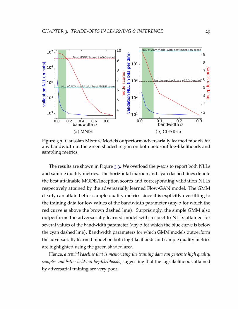
CHAPTER 3. TRADE-OFFS IN LEARNING & INFERENCE 29
0.0 0.2 0.4 0.6 0.8bandwidth
103
104
105
106
107
valid
atio
n NL
L (in
nat
s)
4
5
6
7
8
9
10
mod
e sc
ores
0.0 0.2 0.4 0.6 0.8bandwidth
103
104
105
106
107
valid
atio
n NL
L (in
nat
s)
NLL of ADV model with best MODE score
Best MODE Score of ADV model
(a) MNIST
0.0 0.1 0.2 0.3bandwidth
101
102
103
104
valid
atio
n NL
L (in
bits
per
dim
)
2
3
4
5
6
7
8
9
ince
ptio
n sc
ores
0.0 0.1 0.2 0.3bandwidth
101
102
103
104
valid
atio
n NL
L (in
bits
per
dim
) NLL of ADV model with best inception score
Best Inception Score of ADV model
(b) CIFAR-10
Figure 3.3: Gaussian Mixture Models outperform adversarially learned models forany bandwidth in the green shaded region on both held-out log-likelihoods andsampling metrics.
The results are shown in Figure 3.3. We overload the y-axis to report both NLLsand sample quality metrics. The horizontal maroon and cyan dashed lines denotethe best attainable MODE/Inception scores and corresponding validation NLLsrespectively attained by the adversarially learned Flow-GAN model. The GMMclearly can attain better sample quality metrics since it is explicitly overfitting tothe training data for low values of the bandwidth parameter (any σ for which thered curve is above the brown dashed line). Surprisingly, the simple GMM alsooutperforms the adversarially learned model with respect to NLLs attained forseveral values of the bandwidth parameter (any σ for which the blue curve is belowthe cyan dashed line). Bandwidth parameters for which GMM models outperformthe adversarially learned model on both log-likelihoods and sample quality metricsare highlighted using the green shaded area.
Hence, a trivial baseline that is memorizing the training data can generate high qualitysamples and better held-out log-likelihoods, suggesting that the log-likelihoods attainedby adversarial training are very poor.

CHAPTER 3. TRADE-OFFS IN LEARNING & INFERENCE 30
3.3.3 Hybrid learning of Flow-GANs
So far, we observed that adversarially learning Flow-GANs models attain poorheld-out log-likelihoods. This makes it challenging to use such models for densityestimation. On the other hand, Flow-GANs learned usingMLE are ‘‘mode covering”but do not generate high quality samples. With a Flow-GAN, it is possible to trade-off the two goals by combining the learning objectives corresponding to both theseinductive principles. Without loss of generality, let V(Gθ, Dφ) denote the minimaxobjective of any GAN model (such as WGAN). The hybrid objective of a Flow-GANcan be expressed as:
minθ
maxφ
V(Gθ, Dφ)− λEx∼Pdata [log pθ(x)] (3.2)
where λ ≥ 0 is a hyperparameter for the algorithm. By varying λ, we can interpolatebetween plain adversarial training (λ = 0) and MLE (very high λ).
We summarize the results from MLE, ADV, and Hybrid for log-likelihood eval-uation and sample quality in Table 3.1 and Table 3.2 for MNIST and CIFAR-10respectively. The tables report the test log-likelihoods corresponding to the bestvalidated MLE and ADV models as well as the highest MODE/Inception scoresobserved during training. The samples obtained by models corresponding to thebest MODE/Inception scores for each learning objective are shown in Figure 3.1 forMNIST and CIFAR-10.
While the results on CIFAR-10 are along expected lines, the hybrid objectiveinterestingly outperforms MLE and ADV on both test log-likelihoods and samplequality metrics in the case of MNIST. One potential explanation for this is becausethe ADV objective can regularize MLE to generalize to the test set and in turn, theMLE objective can stabilize the optimization of the ADV objective. Hence, the hybridobjective in Eq. (3.2) can smoothly balance the two objectives using the tunablehyperparameter λ, and in some cases such as MNIST, the performance on both taskscould improve as a result of the hybrid objective.

CHAPTER 3. TRADE-OFFS IN LEARNING & INFERENCE 31
10 45 10 37 10 29 10 21 10 13 10 5
magnitude of singular value, s
0.0
0.2
0.4
0.6
0.8
1.0
P(S<
s)
Hybrid (NICE)MLE (NICE)ADV (NICE, WD)ADV (DCGAN-784,WD)ADV (DCGAN-784,JSD)
(a) MNIST
10 6 10 4 10 2 100
magnitude of singular value, s
0.0
0.2
0.4
0.6
0.8
1.0
P(S<
s)
Hybrid (real-nvp)MLE (real-nvp)ADV (real-nvp, WD)ADV (DCGAN-3072,WD)ADV (DCGAN-3072,JSD)
(b) CIFAR-10
Figure 3.4: Singular value analysis for the Jacobian of the generator functions. TheJacobian is evaluated at 64 random noise vectors sampled from the prior. The x-axisof the figure shows the singular value magnitudes (on a log scale) and for eachsingular value s, we show the corresponding cumulative distribution function (CDF)value on the y-axis which signifies the fraction of singular values less than s.
3.4 Explaining log-likelihood trends
We perform a singular value analysis to explain the variation in log-likelihoodsattained by various Flow-GAN learning objectives. Specifically, we investigate thedistribution of the magnitudes of singular values for the Jacobian matrix of severalgenerator functions, Gθ for MNIST in Figure 3.4 evaluated at 64 noise vectors, z
randomly sampled from the prior density p(z). Note that the Jacobian function hereis computed for the forward mapping, while the one used for likelihood evaluationin Eq. (2.13) corresponds to the inverse mapping.
The Jacobian is a good first-order approximation of the generator function locally.In Figure 3.4, we observe that the singular value distribution for the Jacobian of aninvertible generator learned using MLE (orange curves) is concentrated in a narrowrange and hence, the Jacobian matrix is well-conditioned and easy to invert. In thecase of invertible generators learned using ADV with Wasserstein distance (greencurves) however, the spread of singular values is very wide and hence, the Jacobianmatrix is ill-conditioned.

CHAPTER 3. TRADE-OFFS IN LEARNING & INFERENCE 32
As further numerical evidence, the average log determinant of the Jacobianmatri-ces for MLE, ADV, and Hybrid models trained on MNIST are −4170.34, −15588.34,and −5184.40 respectively which translates to the trend ADV<Hybrid<MLE. Sim-ilar trend holds for CIFAR-10 with corresponding values −12818.84, −21848.09,and −14729.51. These trends indicate that the ADV models are trying to squisha sphere of unit volume centered at a latent vector to a very small volume in theobserved data space. Tiny perturbations of training and held-out data points canhence manifest as poor log-likelihoods. This suggests that ADV prefers to learn adistribution over a smaller support than the true support of the data distribution inspite of not being limited in the representational capacity to cover the entire space,since the dimensions of z (i.e., k) and x (i.e., d) match for invertible generators.
The Hybrid learning objective (blue curves), however, is able to correct for theconditioning of the Jacobian and the distribution of singular value magnitudesmatches closely to that of MLE. This observation extends beyond invertible Flow-GAN generators to other commonly used architectures and adversarial learningobjectives. We considered standard DCGAN generator architectures with k = d
varying the divergence minimized comparing Wasserstein distance (red curves)and Jenson-Shannon divergence (purple curves). The relative shift in distributionof singular value magnitudes to lower values is apparent even in this case.
3.5 Discussion & Related Work
Any model which allows for log-likelihood evaluation and efficient sampling can betrained using MLE as well as adversarial training. This line of reasoning has beenexplored to some extent in prior work that combine the objectives of prescribedlatent variable models such as VAEs (maximizing an evidence lower bound onthe data) with adversarial learning [Lar+15; MNG17a]. However, the benefits ofsuch procedures does not come for ‘‘free’’ since we still need to resort to someform of approximate inference to get a handle on the log-likelihoods. This couldbe expensive, for instance combining a VAE with a GAN introduces an additionalinference network increasing the overall model complexity.
CHAPTER 3. TRADE-OFFS IN LEARNING & INFERENCE 33
Our approach sidesteps the additional complexity due to approximate inferenceby considering a normalizing flow model. The trade-off made by a normalizingflow model in this case is that the generator function needs to be invertible whileother generative models such as VAEs have no such requirement. On the positiveside, we can tractably evaluate exact log-likelihoods assigned by the model for anydata point. Parallel and independent of this work, concurrent work also considersadversarial learning of Real-NVP [Dan+17].
The low dimensional support of the distributions learned by adversarial learningoften manifests as lack of sample diversity and is referred to as mode collapse.In prior work, mode collapse is detected based on visual inspection or heuristictechniques [Goo16; AZ17]. Techniques for avoiding mode collapse explicitly focuson stabilizing GAN training such as [Met+16; ACB17; Che+17a; MNG17b; BSM17;Bel+17] rather than quantitative methods based on likelihoods.
3.6 Conclusion
As an attempt to more quantitatively evaluate generative models, we introducedFlow-GAN. It is a generative adversarial network which allows for tractable likeli-hood evaluation, exactly like in a flow model. Since it can be trained both adversari-ally (like a GAN) and in terms of MLE (like a flow model), we can quantitativelyevaluate the trade-offs involved. We observe that adversarial learning assigns verylow-likelihoods to both training and validation data while generating superior qual-ity samples. To put this observation in perspective, we demonstrate how a naiveGaussian mixture model can outperform adversarially learned models on bothlog-likelihood estimates and sample quality metrics.
Inspecting the distribution of singular value magnitudes for the Jacobian of thegenerator function provide insights into the contrast between maximum likelihoodestimation and adversarial learning. The latter have a tendency to learn distributionsof low support, which can lead to low likelihoods. To correct for this behavior, weconsider a hybrid objective function which involves loss terms corresponding toboth MLE and adversarial learning. On MNIST, the hybrid Flow-GAN objective

CHAPTER 3. TRADE-OFFS IN LEARNING & INFERENCE 34
outperforms both vanilla MLE and adversarial learning, both in terms of samplequality and validation log-likelihoods. On CIFAR-10, the hybrid objective outper-forms MLE in terms of visual sample quality, and is only slightly worse in terms ofvalidation log-likelihood.
Recent Progress. Follow-up work by [Ode+18] builds on the singular value anal-ysis in this chapter to show that controlling for the conditioning of the Jacobianof the generator during training can both stabilize training and improve samplequality. In [Gro+20], we further extend the use of Flow-GANs to domain translation.Here, the goal is to translate data across domains e.g., converting satellite imagery tocorresponding ground maps using a forward model and vice versa using a reversemodel. Beyond the virtues of hybrid MLE and adversarial training, Flow-GANshave an additional advantage here in ensuring that the mapping across domainsis exactly cycle-consistent [Zhu+17] i.e., a data point translated from one domainto another using the forward translation model gives back the original data pointwhen translated back using the reverse translation model.

4 Model Bias in Generative Models
4.1 Introduction
In the last chapter, we explored trade-offs in learning objectives for generative mod-eling. Once learned, these models are used to draw inferences and to plan futureactions. For example, in data augmentation, samples from a learned model are usedto enrich a dataset for supervised learning [ASE17]. Inmodel-based off-policy policyevaluation (henceforth MBOPE), a learned dynamics model is used to simulate andevaluate a target policy without real-world deployment [Man+07], which is espe-cially valuable for risk-sensitive applications [Tho15]. In spite of the recent successesof deep generative models, there are glaring imperfections even in state-of-the-artmodels: e.g., imagemodels have noticeable artifacts in background textures [McD18]and language models can fail to generate diverse and coherent dialogue [Li+15].Moreover, existing theoretical results show that learning distributions in an unbiasedmanner is either impossible or has prohibitive sample complexity [Ros56; ARZ18].Consequently, the models used in practice are inherently biased,1 and can lead tomisleading downstream inferences. This chapter will focus on the characterizationand mitigation of such bias in generative models.
In order to address this issue, we start from the observation that many typicaluses of generative models involve computing expectations under the model. Forinstance, inMBOPE, we seek to find the expected return of a policy under a trajectory
1We call a generative model biased if it produces biased statistics relative to the data distribution.
35
CHAPTER 4. MODEL BIAS IN GENERATIVE MODELS 36
distribution defined by this policy and a learned dynamics model. A classical recipefor correcting the bias in expectations, when samples from a different distributionthan the ground truth are available, is to importance weight the samples accordingto the likelihood ratio [HT52]. If the importance weights were exact, the resultingestimates are unbiased. But in practice, the likelihood ratio is unknown and needsto be estimated since the true data distribution is unknown and even the modellikelihood is typically intractable or ill-defined for many deep generativemodels, e.g.,variational autoencoders [KW18] and generative adversarial networks [Goo+14].
Our proposed solution to estimate the importance weights is to train a calibrated,probabilistic classifier to distinguish samples from the data distribution and thegenerative model. As shown in prior work, the output of such classifiers can beused to extract density ratios [SSK12]. Appealingly, this estimation procedure islikelihood-free since it only requires samples from the two distributions. Together,the generative model and the importance weighting function (specified via a binaryclassifier) induce a new energy function. While exact density estimation and sam-pling from this induced energy-based model is intractable, we can derive a particlebased approximation which permits efficient sampling via resampling based meth-ods. We derive conditions on the quality of the weighting function such that theinduced model provably improves the fit to the the data distribution.
Empirically, we evaluate our bias reduction framework on three main sets ofexperiments. First, we consider goodness-of-fit metrics for evaluating sample qualitymetrics of a likelihood-based and a likelihood-free state-of-the-art model on theCIFAR-10 dataset. All these metrics are defined as Monte Carlo estimates from thegenerated samples. By importance weighting samples, we observe a bias reductionof 23.35% and 13.48% averaged across commonly used sample quality metrics onPixelCNN++ [Sal+17] and SNGAN [Miy+18] models respectively.
Second, we demonstrate the utility of our approach on the task of data aug-mentation for multi-class classification on the Omniglot dataset [LST15]. We showthat, while naively extending the model with samples from a data augmentation, agenerative adversarial network [ASE17] is not very effective for multi-class classifi-cation, we can improve classification accuracy from 66.03% to 68.18% by importance

CHAPTER 4. MODEL BIAS IN GENERATIVE MODELS 37
weighting the contributions of each augmented data point.Finally, weperformMBOPE [PSS00] for standardMuJoCo environments [TET12]
with continuous high-dimensional state and action spaces. A typical MBOPE ap-proach is to first estimate a generative model of the dynamics using off-policy dataand then evaluate the policy via Monte Carlo [Man+07; TB16]. Here, we observethat correcting the bias of the estimated dynamics model via our proposed approachreduces root mean squared error (RMSE) for MBOPE by 50.25% on average.
4.2 Preliminaries
We are interested in use cases where the goal is to evaluate or optimize expectationsof functions under some distribution p (either equal or close to the data distributionpdata). Assuming access to samples from p as well some generative model pθ, oneextreme is to evaluate the sample average using the samples from p alone. However,this ignores the availability of pθ, through which we have a virtually unlimitedaccess of generated samples ignoring computational constraints and hence, couldimprove the accuracy of our estimates when pθ is close to p. We begin by presentinga direct motivating use case of data augmentation using generative models fortraining classifiers which generalize better.
Example use case. Sufficient labeled training data for learning classification andregression system is often expensive to obtain or susceptible to noise. Data augmenta-tion seeks to overcome this shortcoming by artificially injecting new data points intothe training set. These new data points are derived from an existing labeled dataset,either by manual transformations (e.g., rotations, flips for images), or alternatively,learned via a generative model [Rat+17; ASE17].
Consider a supervised learning task over a labeled dataset Dcl. In additionto the feature spaces x ∈ Rd, this includes a label space y ∈ Y . The dataset Dcl
consists of feature and label pairs (x, y), each of which is assumed to be sampledindependently from a data distribution pdata(x, y). Further, let Y ⊆ Rk. In order tolearn a classifier fψ : X → Rk with parameters ψ, we minimize the expectation of a

CHAPTER 4. MODEL BIAS IN GENERATIVE MODELS 38
loss ` : Y ×Rk → R over the dataset Dcl:
Epdata(x,y)[`(y, fψ(x))] ≈1|Dcl| ∑
(x,y)∼Dcl
`(y, fψ(x)). (4.1)
e.g., ` could be the cross-entropy loss. A generative model for the task of data aug-mentation learns a joint distribution pθ(x, y). Several algorithmic variants exist forlearning the model’s joint distribution and we defer the specifics to the experimentssection. Once the generative model is learned, it can be used to optimize the ex-pected classification loss in Eq. (4.1) under a mixture distribution of empirical datadistributions and generative model distributions given as:
pmix(x, y) = mpdata(x, y) + (1−m)pθ(x, y) (4.2)
for a suitable choice of the mixture weights m ∈ [0, 1]. Notice that, while the even-tual task here is optimization, reliably evaluating the expected loss of a candidateparameter ψ is an important ingredient. We focus on this basic question first inadvance of leveraging the solution for data augmentation. Further, even if evaluatingthe expectation once is easy, optimization requires us to do repeated evaluation (fordifferent values of ψ) which is significantly more challenging. Also observe thatthe distribution p under which we seek expectations is same as pdata here, and werely on the generalization of pθ to generate transformations of an instance in thedataset which are not explicitly present, but plausibly observed in other, similarinstances [Zha+18].
4.3 Likelihood-Free Importance Weighting
Whenever the distribution p, under which we seek expectations, differs from pθ,model-based estimates exhibit bias. In this section, we start out by formalizing biasfor Monte Carlo expectations and subsequently propose a bias reduction strategy

CHAPTER 4. MODEL BIAS IN GENERATIVE MODELS 39
based on likelihood-free importance weighting (LFIW). We are interested in evalu-ating expectations of a class of functions of interest f ∈ F w.r.t. the distribution p.For any given f : X → R, we have Ep[ f (x)] =
∫p(x) f (x)dx.
Given access to samples from a generative model pθ, if we knew the densitiesfor both p and pθ, then a classical scheme to evaluate expectations under p usingsamples from pθ is to use importance sampling [HT52]. We reweight each samplefrom pθ according to its likelihood ratio under p and pθ and compute a weightedaverage of the function f over these samples.
Ep[ f (x)] = Epθ
[p(x)pθ(x)
f (x)]≈ 1
T
T
∑i=1
w(xi) f (xi) (4.3)
where w(xi) := p(xi)pθ(xi)
is the importance weight for xi ∼ pθ. The validity of thisprocedure is subject to the use of a proposal pθ such that for all x ∈ Rd wherepθ(x) = 0, we also have f (x)p(x) = 0.2
To apply this technique to reduce the bias of a generative sampler pθ w.r.t. p,we require knowledge of the importance weights w(x) for any x ∼ pθ. However,we typically only have a sampling access to p via finite datasets. For instance, inthe data augmentation example above, where p = pdata, the unknown distributionused to learn pθ. Hence we need a scheme to learn the weights w(x), using samplesfrom p and pθ, which is the problem we tackle next.In order to do this, we considera binary classification problem over Rd × {0, 1} and the joint distribution over datapoints and their binary labels is denoted as q(x, y). Let γ = q(y=0)
q(y=1) > 0 denote anyfixed odds ratio. To specify the joint q(x, y), we additionally need the conditionalq(x|y) which we define as follows:
q(x|y) =
pθ(x) if y = 0
p(x) otherwise.(4.4)
Since we only assume sample access to p and pθ(x), our strategy would be to2A stronger sufficient, but not necessary condition that is independent of f , states that the proposal
pθ is valid if it has a support larger than p, i.e., for all x ∈ Rd, pθ(x) = 0 implies p(x) = 0.

CHAPTER 4. MODEL BIAS IN GENERATIVE MODELS 40
estimate the conditional above via learning a probabilistic binary classifier. To trainthe classifier, we only require datasets of samples from pθ(x) and p(x) and estimateγ to be the ratio of the size of two datasets. Let cφ : Rd → [0, 1] denote the probabilityassigned by the classifier with parameters φ to a sample x belonging to the positiveclass y = 1. As shown in prior work [SSK12; GE18], if cφ is Bayes optimal, then theimportance weights can be obtained via this classifier as:
wφ(x) =p(x)pθ(x)
= γcφ(x)
1− cφ(x). (4.5)
In practice, we do not have access to a Bayes optimal classifier and hence, theestimated importance weights will not be exact. Consequently, we can hope toreduce the bias as opposed to eliminating it entirely. Hence, our default LFIWestimator is given as:
Ep[ f (x)] ≈ 1T
T
∑i=1
wφ(xi) f (xi) (4.6)
where wφ(xi) = γcφ(xi)
1−cφ(xi)is the importance weight for xi ∼ pθ estimated via cφ(x).
Practical considerations. Besides imperfections in the classifier, the quality of agenerative model also dictates the efficacy of importance weighting. For example,images generated by deep generative models often possess distinct artifacts whichcan be exploited by the classifier to give highly-confident predictions [ODO16;Ode19]. This could lead to very small importance weights for some generatedimages, and consequently greater relative variance in the importance weights acrossthe Monte Carlo batch. Below, we present some practical variants of LFIW estimatorto offset this challenge.1. Self-normalization: The self-normalized LFIW estimator forMonte Carlo evaluationnormalizes the importance weights across a sampled batch:
Ep[ f (x)] ≈T
∑i=1
wφ(xi)
∑Tj=1 wφ(xj)
f (xi) where xi ∼ pθ. (4.7)

CHAPTER 4. MODEL BIAS IN GENERATIVE MODELS 41
2. Flattening: The flattened LFIWestimator interpolates between uniform importanceweights and the default LFIW weights via a power scaling parameter α ≥ 0:
Ep[ f (x)] ≈ 1T
T
∑i=1
wφ(xi)α f (xi) where xi ∼ pθ. (4.8)
For α = 0, there is no bias correction, and α = 1 returns the default estimator inEq. (4.6). For intermediate values of α, we can trade-off bias reduction with anyundesirable variance introduced.3. Clipping: The clipped LFIW estimator specifies a lower bound β ≥ 0 on theimportance weights:
Ep[ f (x)] ≈ 1T
T
∑i=1
max(wφ(xi), β) f (xi) where xi ∼ pθ. (4.9)
When β = 0, we recover the default LFIW estimator in Eq. (4.6). Finally, we notethat these estimators are not exclusive and can be combined e.g., flattened or clippedweights can be normalized.
Confidence intervals. Bootstrap is a widely-used tool in statistics for derivingconfidence intervals by fitting ensembles of models on resampled data points. If thedataset is finite e.g., Dtrain, then the bootstrapped dataset is obtained via randomsampling with replacement and confidence intervals are estimated via the empiricalbootstrap. For a parametric model generating the dataset e.g., pθ , a fresh bootstrappeddataset is resampled from the model and confidence intervals are estimated via theparametric bootstrap. See [ET94] for a detailed review.
Since we have real and generated data coming from a finite dataset and para-metric model respectively, we propose a combination of empirical and parametricbootstraps to derive confidence intervals around the estimated importance weights.In particular, we can estimate the confidence intervals by retraining the classifieron a fresh sample of points from pθ and a resampling of the training dataset Dtrain
(with replacement). Repeating this process over multiple runs and then taking asuitable quantile gives us the corresponding confidence intervals.

CHAPTER 4. MODEL BIAS IN GENERATIVE MODELS 42
(a) Setup (b) n = 50
(c) n = 100 (d) n = 1000
Figure 4.1: Importance Weight Estimation using Probabilistic Classifiers. (a) Aunivariate Gaussian (blue) is fit to samples from a mixture of two Gaussians (red).(b-d) Estimated class probabilities (with 95% confidence intervals based on 1000bootstraps) for varying number of points n, where n is the number of training datapoints used for training the generative model and multilayer perceptron.
Synthetic experiment. We visually illustrate our importance weighting approachin a toy experiment (Figure 4.1a). We are given a finite set of samples drawnfrom a mixture of two Gaussians (red). The model family is a unimodal Gaussian,illustrating mismatch due to a parametric model. The mean and variance of themodel are estimated by the empirical means and variances of the observed data.Using estimated model parameters, we then draw samples from the model (blue).

CHAPTER 4. MODEL BIAS IN GENERATIVE MODELS 43
In Figure 4.1b, we show the probability assigned by a binary classifier to a pointto be from true data distribution. Here, the classifier is a single hidden-layer multi-layer perceptron. The classifier is not Bayes optimal, which can be seen by the gapsbetween the optimal probabilities curve (black) and the estimated class probabilitycurve (green). However, as we increase the number of real and generated examplesn in Figures 4.1c, 4.1d, the classifier approaches optimality. Furthermore, even itsuncertainty shrinks with increasing data, as expected. In summary, this experimentdemonstrates how a binary classifier can mitigate this bias due to a mismatchedgenerative model.
4.4 Boosted Energy-Based Model
In the previous section, we described a procedure to augment any base generativemodel pθ with an importance weighting estimator wφ for debiased Monte Carloevaluation. Here, we will use this augmentation to induce an energy-based modelwith density pθ,φ given as:
pθ,φ(x) ∝ pθ(x)wφ(x) (4.10)
where the partition function is expressed as Zθ,φ =∫
pθ(x)wφ(x)dx = Epθ[wφ(x)].
On the default measure for pθ(x), the energy function Eθ,φ(x) = − log pθ(x) −log wφ(x). Alternatively, we can change the measure to be pθ(x) itself in whichcase the energy function is Eφ(x) = − log wφ(x) Another useful interpretation isto think of this procedure as a variant of the product of experts or multiplicativeboosting formulation [Hin99; GE18] where the ‘‘first expert” corresponding to thebase density pθ(x) and boosting is done via the ‘‘second expert” corresponding tothe importance weighting estimator wφ.
Density Estimation. Exact density estimation requires a handle on the densityof the base model pθ (typically intractable for models such as VAEs and GANs)and estimates of the partition function. Exactly computing the partition function is

CHAPTER 4. MODEL BIAS IN GENERATIVE MODELS 44
Algorithm 4.1 SIR for Boosted Energy-Based Model pθ,φ
Input: Generative Model pθ, Importance Weight Estimator wφ, budget T1: Sample x1, x2, . . . , xT independently from pθ
2: Estimate importance weights wφ(x1), wφ(x2), . . . , wφ(xT)
3: Compute Zθ,φ ← ∑Tt=1 wφ(xt)
4: Sample j ∼ Categorical(
wφ(x1)
Zθ,φ, wφ(x2)
Zθ,φ, . . . , wφ(xT)
Zθ,φ
)5: return xj
intractable. If pθ permits fast sampling and importance weights are estimated viaLFIW (requiring only a forward pass through the classifier network), we can obtainunbiased estimates via a Monte Carlo average, i.e., Zθ,φ ≈ 1
T ∑Ti=1 wφ(xi) where
xi ∼ pθ. To reduce the variance, a potentially large number of samples are required.Since samples are obtained independently, the terms in the Monte Carlo averagecan be evaluated in parallel.
Sampling. While exact sampling from pθ,φ is intractable, we can instead per-form sample from a particle-based approximation to pθ,φ via sampling-importance-resampling [LC98; DGA00] (SIR). We define the SIR approximation to pθ,φ via thefollowing density:
pSIRθ,φ (x; T) := Ex2,x3,...,xT∼pθ
[wφ(x)
wφ(x) + ∑Ti=2 wφ(xi)
pθ(x)
](4.11)
where T > 0 denotes the number of independent samples (or ‘‘particles”). For anyfinite T, sampling from pSIR
θ,φ is tractable, as summarized in Algorithm 4.1. Moreover,any expectation w.r.t. the SIR approximation to the induced distribution can beevaluated in closed-form using the self-normalized LFIW estimator (Eq. (4.7)). Inthe limit of T → ∞, we recover the induced distribution pθ,φ:
limT→∞
pSIRθ,φ (x; T) = pθ,φ(x) ∀x (4.12)
Next, we analyze conditions under which the resampled density pθ,φ provably
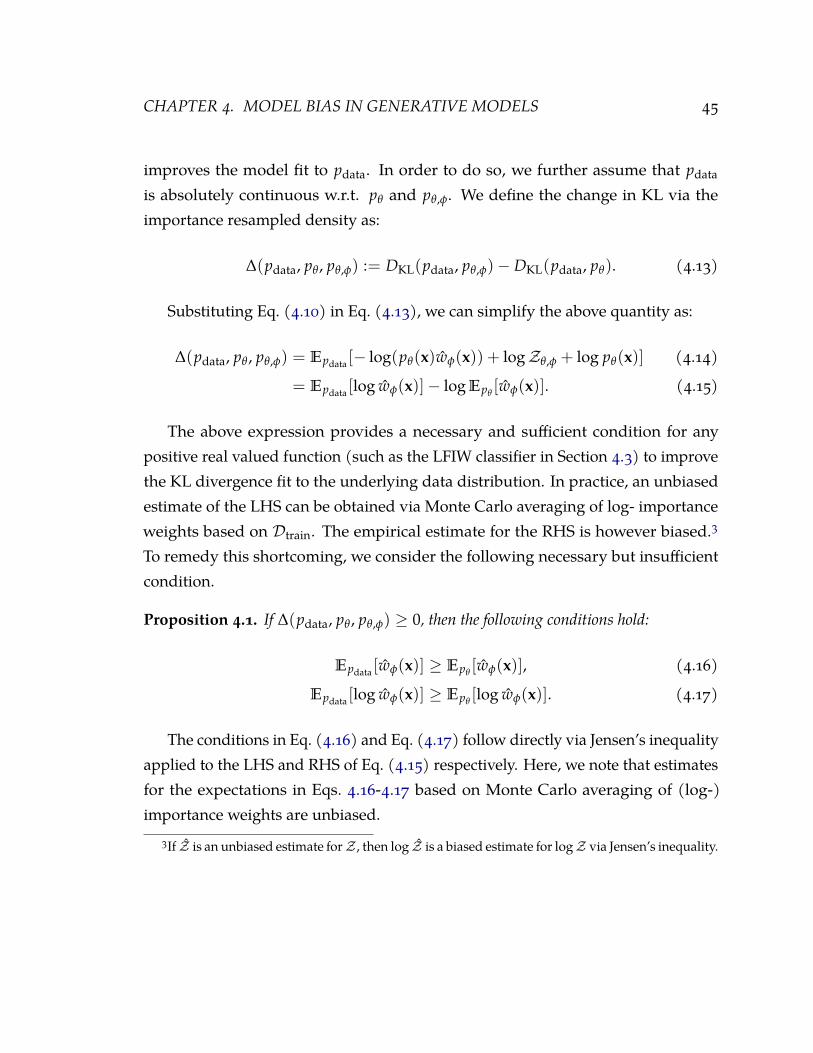
CHAPTER 4. MODEL BIAS IN GENERATIVE MODELS 45
improves the model fit to pdata. In order to do so, we further assume that pdata
is absolutely continuous w.r.t. pθ and pθ,φ. We define the change in KL via theimportance resampled density as:
∆(pdata, pθ, pθ,φ) := DKL(pdata, pθ,φ)− DKL(pdata, pθ). (4.13)
Substituting Eq. (4.10) in Eq. (4.13), we can simplify the above quantity as:
∆(pdata, pθ, pθ,φ) = Epdata [− log(pθ(x)wφ(x)) + logZθ,φ + log pθ(x)] (4.14)
= Epdata [log wφ(x)]− log Epθ[wφ(x)]. (4.15)
The above expression provides a necessary and sufficient condition for anypositive real valued function (such as the LFIW classifier in Section 4.3) to improvethe KL divergence fit to the underlying data distribution. In practice, an unbiasedestimate of the LHS can be obtained via Monte Carlo averaging of log- importanceweights based on Dtrain. The empirical estimate for the RHS is however biased.3
To remedy this shortcoming, we consider the following necessary but insufficientcondition.
Proposition 4.1. If ∆(pdata, pθ, pθ,φ) ≥ 0, then the following conditions hold:
Epdata [wφ(x)] ≥ Epθ[wφ(x)], (4.16)
Epdata [log wφ(x)] ≥ Epθ[log wφ(x)]. (4.17)
The conditions in Eq. (4.16) and Eq. (4.17) follow directly via Jensen’s inequalityapplied to the LHS and RHS of Eq. (4.15) respectively. Here, we note that estimatesfor the expectations in Eqs. 4.16-4.17 based on Monte Carlo averaging of (log-)importance weights are unbiased.
3If Z is an unbiased estimate forZ , then log Z is a biased estimate for logZ via Jensen’s inequality.

CHAPTER 4. MODEL BIAS IN GENERATIVE MODELS 46
Table 4.1: Goodness-of-fit evaluation on CIFAR-10 dataset for PixelCNN++ andSNGAN. Standard errors computed over 10 runs. Higher IS is better. Lower FIDand KID scores are better.
Model Evaluation IS (↑) FID (↓) KID (↓)
- Reference 11.09 ± 0.1263 5.20 ± 0.0533 0.008 ± 0.0004
PixelCNN++ Default (no debiasing) 5.16 ± 0.0117 58.70 ± 0.0506 0.196 ± 0.0001LFIW 6.68 ± 0.0773 55.83 ± 0.9695 0.126 ± 0.0009
SNGAN Default (no debiasing) 8.33 ± 0.0280 20.40 ± 0.0747 0.094 ± 0.0002LFIW 8.57 ± 0.0325 17.29 ± 0.0698 0.073 ±0.0004
4.5 Empirical Evaluation
In all our experiments, the binary classifier for estimating the importance weightswas a calibrated deep neural network trained to minimize the cross-entropy loss.The self-normalized LFIW in Eq. (4.7) worked best.
4.5.1 Goodness-of-fit testing
In the first set of experiments, we highlight the benefits of importance weighting fora debiased evaluation of three popularly used sample quality metrics viz. Incep-tion Scores (IS) [Sal+16], Frechet Inception Distance (FID) [Heu+17], and KernelInception Distance (KID) [Biń+18]. All these scores can be formally expressed asempirical expectations with respect to the model. For all these metrics, we can simu-late the population level unbiased case as a ‘‘reference score” wherein we artificiallyset both the real and generated sets of samples used for evaluation as finite, disjointsets derived from pdata.
We evaluate the three metrics for two state-of-the-art models trained on theCIFAR-10 dataset: (a) an autoregressive model PixelCNN++ learned via maximumlikelihood estimation [Sal+17] and (b) a latent variable model SNGAN learned viaadversarial training [Miy+18]. For evaluating each metric, we draw 10,000 samplesfrom the model. In Table 4.1, we report the metrics with and without the LFIW biascorrection. The consistent debiased evaluation of these metrics via self-normalized

CHAPTER 4. MODEL BIAS IN GENERATIVE MODELS 47
Table 4.2: Classification accuracy on the Omniglot dataset. Standard errors com-puted over 5 runs.
Dataset Accuracy
Dcl 0.6603 ± 0.0012Dg 0.4431 ± 0.0054Dg w/ LFIW 0.4481 ± 0.0056Dcl + Dg 0.6600 ± 0.0040Dg w/ LFIW 0.6818 ± 0.0022
LFIW suggest that the SIR approximation to the importance resampled distribution(Eq. (4.11)) is a better fit to pdata.
4.5.2 Data augmentation for multi-class classification
We consider data augmentation using a generative model for multi-class classifi-cation. The dataset we consider is the Omniglot dataset of handwritten charac-ters [LST15] for which we use a pretrained Data Augmentation Generative Adver-sarial Network (DAGAN) [ASE17]. The dataset is particularly relevant becauseit contains 1600+ classes but only 20 examples from each class and hence, couldpotentially benefit from augmented data.
Once the model has been trained, it can be used for data augmentation in manyways. In particular, we consider ablation baselines that use various combinationsof the real training data Dcl and generated data Dg for training a downstreamclassifier. When the generated data Dg is used, we can either use the data directlywith uniform weighting for all training points, or choose to importance weight(LFIW) the contributions of the individual training points to the overall loss. Theresults are shown in Table 4.2. While generated data (Dg) alone cannot be used toobtain competitive performance relative to the real data (Dcl) on this task as expected,the bias it introduces for evaluation and subsequent optimization overshadows eventhe naive data augmentation (Dcl + Dg). In contrast, we can obtain significantimprovements by importance weighting the generated points (Dcl + Dg w/ LFIW).
Qualitatively, we can observe the effect of importance weighting in Figure 4.2.

CHAPTER 4. MODEL BIAS IN GENERATIVE MODELS 48
(a) (b)
(c) (d)
(e) (f)
Figure 4.2: Qualitative evaluation of importance weighting for data augmentation.(a-f) Within each figure, top row shows held-out data samples from a specific classin Omniglot. Bottom row shows generated samples from the same class ranked indecreasing order of importance weights.
Here, we show true and generated samples for 6 randomly choosen classes (a-f)in the Omniglot dataset. The generated samples are ranked in decreasing orderof the importance weights. There is no way to formally test the validity of suchrankings and this criteria can also prefer points which have high density underpdata but are unlikely under pθ since we are looking at ratios. Visual inspectionsuggests that the classifier is able to appropriately downweight poorer samples, asshown in Figure 4.2 (a, b, c, d - bottom right). There are also failure modes, suchas the lowest ranked generated images in Figure 4.2 (e, f - bottom right) where theclassifier weights reasonable generated samples poorly relative to others. This couldbe due to particular artifacts such as a tiny disconnected blurry speck in Figure 4.2

CHAPTER 4. MODEL BIAS IN GENERATIVE MODELS 49
(e - bottom right) which could be more revealing to a classifier distinguishing realand generated data.
4.5.3 Model-based off-policy policy evaluation
So far, we have seen use cases where the generative model was trained on data fromthe same distribution we wish to use for Monte Carlo evaluation. We can extendour debiasing framework to more involved settings when the generative model is abuilding block for specifying the full data generation process, e.g., trajectory datagenerated via a dynamics model along with an agent policy.
In particular, we consider the setting of off-policy policy evaluation (OPE),where the goal is to evaluate policies using experiences collected from a differentpolicy. Formally, let (S ,A, r, P, η, T) denote an (undiscounted) Markov decisionprocess with state space S , action space A, reward function r, transition P, initialstate distribution η and horizon T. Assume πe : S ×A → [0, 1] is a known policythat we wish to evaluate. The probability of generating a certain trajectory τ =
{s0, a0, s1, a1, ..., sT, aT} of length T with policy πe and transition P is given as:
p?(τ) = η(s0)T−1
∏t=0
πe(at|st)P(st+1|st, at). (4.18)
The return on a trajectory R(τ) is the sum of the rewards across the state, actionpairs in τ: R(τ) = ∑T
t=1 r(st, at), where we assume a known reward function r.We are interested in the value of a policy defined as v(πe) = Ep∗ [R(τ)]. Evalu-
ating πe requires the (unknown) transition dynamics P. The dynamics model isa conditional generative model of the next states st+1 conditioned on the previousstate-action pair (st, at). If we have access to historical logged data Dτ of trajectoriesτ = {s0, a0, s1, a1, . . . , } from some behavioral policy πb : S ×A → [0, 1], then wecan use this off-policy data to train a dynamics model pθ(st+1|st, at). The policy πe
can then be evaluated under this learned dynamics model as v(πe) = Ep[R(τ)],where p uses pθ instead of the true dynamics in Eq. (4.18).

CHAPTER 4. MODEL BIAS IN GENERATIVE MODELS 50
However, the trajectories sampled with pθ could significantly deviate from sam-ples from P due to compounding errors [RB10]. In order to correct for this bias,we can use likelihood-free importance weighting on entire trajectories of data. Thebinary classifier c(st, at, st+1) for estimating the importance weights in this casedistinguishes between triples of true and generated transitions. For any true triple(st, at, st+1) extracted from the off-policy data, the corresponding generated triple(st, at, st+1) only differs in the final transition state, i.e., st+1 ∼ pθ(st+1|st, at). Sucha classifier allows us to obtain the importance weights w(st, at, st+1) for every pre-dicted state transition (st, at, st+1). The importance weights for the trajectory τ canbe derived from the importance weights of these individual transitions as:
p?(τ)p(τ)
=∏T−1
t=0 P(st+1|st, at)
∏T−1t=0 pθ(st+1|st, at)
=T−1
∏t=0
P(st+1|st, at)
pθ(st+1|st, at)≈
T−1
∏t=0
w(st, at, st+1). (4.19)
Our final LFIW estimator is given as:
v(πe) = Ep
[T−1
∏t=0
w(st, at, st+1) · R(τ)]
. (4.20)
In Appendix B.2.5, we also consider a stepwise LFIW estimator for MBOPE whichapplies importance weighting at the level of every decision as opposed to entiretrajectories.
Setup. Weconsider three continuous control tasks in theMuJoCo simulator [TET12]from OpenAI gym [Bro+16] (in increasing number of state dimensions): Swim-mer, HalfCheetah and HumanoidStandup. High dimensional state spaces makes itchallenging to learning a reliable dynamics model in these environments. We trainbehavioral and evaluation policies using Proximal Policy Optimization [Sch+17a]with different hyperparameters for the two policies.
The dataset collected via trajectories from the behavior policy is used to traina ensemble neural network dynamics model. We the use the trained dynamicsmodel to evaluate v(πe) and its LFIW version v(πe), and compare them with theground truth returns v(πe). Each estimation is averaged over a set of 100 trajectories
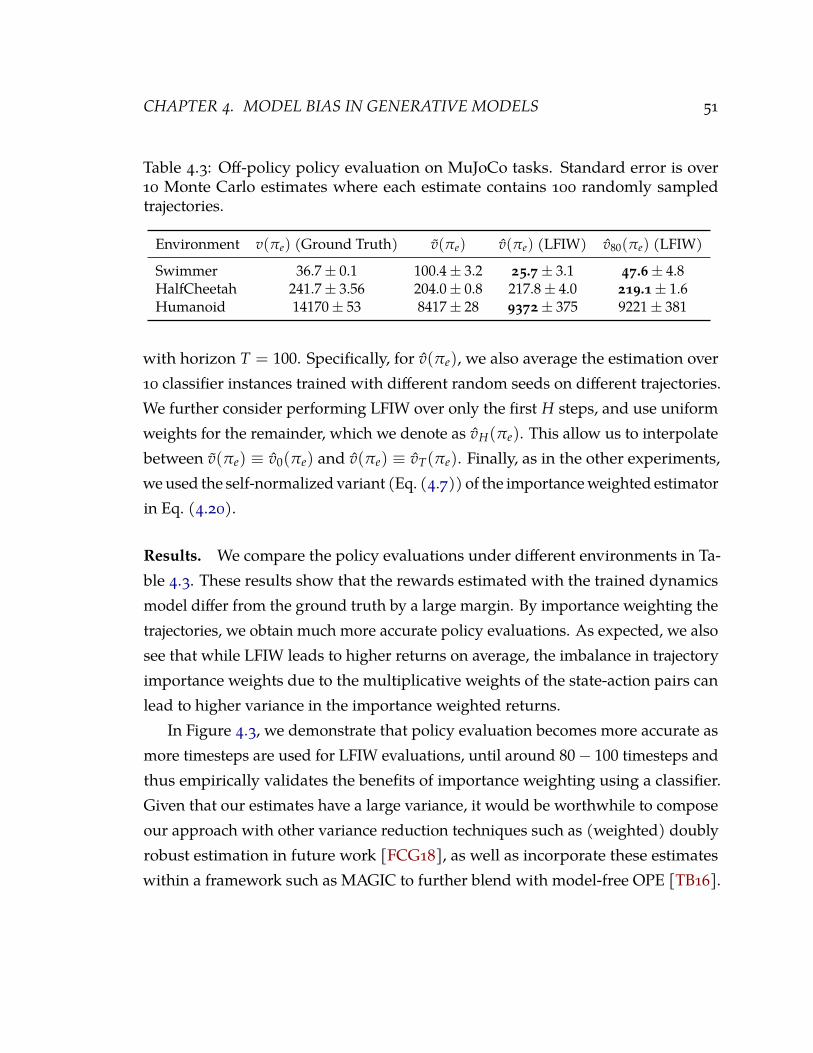
CHAPTER 4. MODEL BIAS IN GENERATIVE MODELS 51
Table 4.3: Off-policy policy evaluation on MuJoCo tasks. Standard error is over10 Monte Carlo estimates where each estimate contains 100 randomly sampledtrajectories.
Environment v(πe) (Ground Truth) v(πe) v(πe) (LFIW) v80(πe) (LFIW)
Swimmer 36.7± 0.1 100.4± 3.2 25.7± 3.1 47.6± 4.8HalfCheetah 241.7± 3.56 204.0± 0.8 217.8± 4.0 219.1± 1.6Humanoid 14170± 53 8417± 28 9372± 375 9221± 381
with horizon T = 100. Specifically, for v(πe), we also average the estimation over10 classifier instances trained with different random seeds on different trajectories.We further consider performing LFIW over only the first H steps, and use uniformweights for the remainder, which we denote as vH(πe). This allow us to interpolatebetween v(πe) ≡ v0(πe) and v(πe) ≡ vT(πe). Finally, as in the other experiments,weused the self-normalized variant (Eq. (4.7)) of the importanceweighted estimatorin Eq. (4.20).
Results. We compare the policy evaluations under different environments in Ta-ble 4.3. These results show that the rewards estimated with the trained dynamicsmodel differ from the ground truth by a large margin. By importance weighting thetrajectories, we obtain much more accurate policy evaluations. As expected, we alsosee that while LFIW leads to higher returns on average, the imbalance in trajectoryimportance weights due to the multiplicative weights of the state-action pairs canlead to higher variance in the importance weighted returns.
In Figure 4.3, we demonstrate that policy evaluation becomes more accurate asmore timesteps are used for LFIW evaluations, until around 80− 100 timesteps andthus empirically validates the benefits of importance weighting using a classifier.Given that our estimates have a large variance, it would be worthwhile to composeour approach with other variance reduction techniques such as (weighted) doublyrobust estimation in future work [FCG18], as well as incorporate these estimateswithin a framework such as MAGIC to further blend with model-free OPE [TB16].

CHAPTER 4. MODEL BIAS IN GENERATIVE MODELS 52
0 20 40 60 80 100H
20
40
60
|(v
)|
Swimmer
0 20 40 60 80 100H
20
30
|(v
)|
HalfCheetah
0 20 40 60 80 100H
4500
5000
5500
|(v
)|
HumanoidStandup
Figure 4.3: Estimation error δ(v) = v(πe)− vH(πe) for different values of H (min 0,max 100). Shaded area denotes standard error over 10 random seeds.
Overall. Across all our experiments, we observe that importance weighting thegenerated samples leads to uniformly better results, whether in terms of evaluatingthe quality of samples, or their utility in downstream tasks. Since the technique is ablack-box wrapper around any generative model, we expect this to benefit a diverseset of tasks in follow-up works.
However, there is also some caution to be exercised with these techniques asevident from the results of Table 4.1. Note that in this table, the confidence intervals(computed using the reported standard errors) around the model scores after

CHAPTER 4. MODEL BIAS IN GENERATIVE MODELS 53
importance weighting still do not contain the reference scores obtained from the truemodel. This would not have been the case if our debiased estimator was completelyunbiased and this observation reiterates our earlier claim that LFIW is reducing bias,as opposed to completely eliminating it. Indeed, when such a mismatch is observed,it is a good diagnostic to either learn more powerful classifiers to better approximatethe Bayes optimum, or find additional data from pdata in case the generative modelfails the full support assumption.
4.6 Discussion & Related Work
Density ratios enjoy widespread use across machine learning e.g., for handlingcovariate shifts and class imbalance [SSK12; BL18]. In generative modeling, esti-mating these ratios via binary classifiers is frequently used for defining learningobjectives and two sample tests [ML16; Ros+17; Gre+07; Bow+15; LO16; Dan+17;Ros+17; Im+18; GRM19]. In particular, such classifiers have been used to definelearning frameworks such as generative adversarial networks [Goo+14; NCT16],likelihood-free Approximate Bayesian Computation (ABC) [GH12] and earlierwork in unsupervised-as-supervised learning [FHT01] and noise contrastive es-timation [GH12] among others. These works are explicitly interested in learningthe parameters of a generative model. In contrast, we use the binary classifier forestimating importance weights to correct for the model bias of any fixed generativemodel and in doing so, we include the classifier as part of the induced generativemodel. In another line of work, [Die+18] and [Cho+20] used importance weightingto reweigh data points based on differences in training and test data distributionsi.e., dataset bias. We will discuss this setting in the following chapter.
Recent concurrent works use MCMC and rejection sampling to explicitly trans-form or reject the generated samples [Tur+18; Aza+18; Tao+18]. These methodsrequire extra computation beyond training a classifier, in rejecting the samples orrunning Markov chains to convergence, unlike the proposed importance weightingstrategy. For many model-based Monte Carlo evaluation usecases (e.g., data aug-mentation, MBOPE), this extra computation is unnecessary. If samples or density

CHAPTER 4. MODEL BIAS IN GENERATIVE MODELS 54
estimates are explicitly needed from the induced resampled distribution, we pre-sented a particle-based approximation to the induced density where the number ofparticles is a tunable knob allowing for trading statistical accuracy with computa-tional efficiency. Finally, we note resampling based techniques have been extensivelystudied in the context of improving variational approximations for latent variablegenerative models [BGS15; SKW15; Nae+17; Gro+18a].
4.7 Conclusion
We identified bias with respect to a target data distribution as a fundamental chal-lenge restricting the use of generative models as proposal distributions for MonteCarlo evaluation. We proposed a bias correction framework based on importanceweighting. The importance weights are estimated in a likelihood-free fashion viaa binary classifier. Empirically, we find the bias correction to be useful across avariety of tasks including goodness-of-fit sample quality tests, data augmentation,and off-policy policy evaluation.
We also characterized the induced energy-based generative model along withan approximate sampling procedure based on sequential-importance-resamplingand the theoretical conditions under which it improves the base generative model.In a recent follow-up work, [AZG20] extend this framework to update both thebase generative model and energy function during learning and observe improvedperformance on density estimation and sampling using the induced energy-basedmodel. In summary, these works show that such approaches sequentially increasesmodel capacity to fix themodel bias of a base generativemodel. The source of this biaswas the mismatch in the base generative model family and the true data distribution,or simply challenges in optimization. The next chapter will focus on another pieceof the puzzle: bias that can occur due to unlabelled and uncurated datasets.

5 Dataset Bias in Generative Models
5.1 Introduction
Increasingly, we are able to train generative models on large unannotated datasetsand deploy them in the real world. Examples of such production level systemsinclude Transformer-based models such as BERT and GPT-3 for natural languagegeneration [Vas+17; Dev+18; Rad+19; Bro+20], Wavenet for text-to-speech syn-thesis [Oor+17], and a large number of creative applications such Coconet usedfor designing the ‘‘first AI-powered” Google [Hua+17]. As these generative ap-plications become more prevalent, it becomes increasingly important to considerquestions with regards to the potential discriminatory nature of such systems andways to mitigate it [Pod+14]. For example, some natural language generation sys-tems trained on internet-scale datasets have been shown to produce generationsthat are biased towards certain demographics [She+19].
A variety of socio-technical factors contribute to the discriminatory nature ofML systems [BHN18]. A major factor is the existence of biases in the training dataitself [TE+11; Tom+17]. Since data is the fuel of machine learning, any existing biasin the dataset can be propagated to the learned model [BS16]. This is a particularlypressing concern for generative models which can easily amplify the bias by gen-erating more of the biased data at test time. Further, learning a generative modelis fundamentally an unsupervised learning problem and hence, the bias factorsof interest are typically latent. For example, while learning a generative model of
55

CHAPTER 5. DATASET BIAS IN GENERATIVE MODELS 56
human faces, we often do not have access to attributes such as gender, race, and age.Any existing bias in the dataset with respect to these attributes are easily picked bydeep generative models. See Figure 5.1 for an illustration.
Figure 5.1: Samples from a baseline BigGAN that reflect the gender bias underlyingthe true data distribution in CelebA. All faces above the orange line (67%) areclassified as female, while the rest are labeled as male (33%).
We present a model-agnostic bias mitigation approach dor learning fair genera-tive models even in the presence of dataset bias. In our setup, we assume we haveaccess to multiple unlabelled (potentially biased) datasets in addition to a particulartarget (reference) dataset. The unlabelled datasets are relatively cheap to obtain formany domains in the big data era but our goal is to ultimately generate samplesthat are close in distribution to a particular target (reference) dataset. We notethat while there may not be concept of a reference dataset devoid of bias, carefullydesigned representative data collection practices may be more accurately reflectedin some data sources [Geb+18] and can be considered as reference datasets. As aconcrete example of such a reference dataset, organizations such as the World Bankand certain biotech firms [23m16; Hon16] typically have quality checks to ensurerepresentativeness in their collected datasets. We note two key features of our setupthat are well allied with real-world scenarios: (a) we do not require the biased orreference datasets need to be labeled w.r.t. the latent bias attributes and (b) the sizeof the curated reference dataset can be much smaller than the biased dataset.
Using a reference dataset to augment a biased dataset, our goal is to learn agenerative model that best approximates the reference data distribution. Simplyusing the reference dataset alone for learning is an option, but this may not sufficesince this dataset can be too small to learn an expressive model that accurately

CHAPTER 5. DATASET BIAS IN GENERATIVE MODELS 57
captures the underlying reference data distribution. Our approach to learning afair generative model that is robust to biases in the larger training set is based onimportance reweighting. In particular, we learn a generative model which reweighsthe data points in the biased dataset based on the ratio of densities assigned by thebiased data distribution as compared to the reference data distribution. Since we donot have access to explicit densities assigned by either of the two distributions, weestimate the weights by using a probabilistic classifier [SSK12; ML16].
We test our bias mitigation approach on learning generative adversarial networkson the CelebA dataset [Liu+15]. The dataset consists of attributes such as genderand hair color, which we use for designing biased and reference data splits andsubsequent evaluation. Empirically, we demonstrate the efficacy of our approachwhich reduces bias w.r.t. latent factors by an average of up to 34.6% over baselines forcomparable image generation using generative adversarial networks in this dataset.
5.2 Preliminaries
Our bias mitigation framework is agnostic to the choice of generative modelingframework. For generality, we consider expectation-based learning objectives, where`(·) is a per-example loss that depends on both examples x drawn from a dataset Dand the model parameters θ:
Epdata [`(x, θ)] ≈ 1T
T
∑i=1
`(xi, θ) := L(θ;D) (5.1)
The above expression encompasses all the objectives discussed in Chapter 2. Forexample, if `(·) denotes the negative log-likelihood assigned to the point x as perpθ, then we recover the MLE training objective.
Dataset Bias. The standard assumption for learning a generative model is thatwe have access to a sufficiently large dataset Dref of training examples, where eachx ∈ Dref is assumed to be sampled independently from a reference distributionpdata = pref. In practice however, collecting large datasets that are i.i.d. w.r.t. pref

CHAPTER 5. DATASET BIAS IN GENERATIVE MODELS 58
is difficult due to a variety of socio-technical factors. The sample complexity forlearning probability distributions can be doubly-exponential in the dimension inmany cases [ARZ18], surpassing the size of the largest available datasets.
We can partially offset this difficulty by considering data from alternate sourcesrelated to the target distribution, e.g., images scraped from the Internet. However,these additional data points are not expected to be i.i.d. w.r.t. pref. We character-ize this phenomena as dataset bias, where we assume the availability of a datasetDbias, such that the examples x ∈ Dbias are sampled independently from a biased(unknown) distribution pbias that is different from pref, but shares the same support.
5.3 Learning with Multiple Data Sources
We assume a learning setting where we are given access to a data source Dbias inaddition to a dataset of training examples Dref. Our goal is to capitalize on bothdata sourcesDbias andDref for learning a model pθ that best approximates the targetdistribution pref. We begin by discussing two baseline approaches for learning withmultiple data sources and the trade-offs involved.
Baseline 1. One could completely ignore Dbias and consider learning pθ based onDref alone. Since we only consider proper losses w.r.t. pref, global optimization ofthe objective in Eq. (5.1) in a well-specified model family will recover the referencedata distribution as |Dref| → ∞. However, since Dref is finite in practice, this issample inefficient and the sample quality will be poor.
Baseline 2. On the other extreme, we can consider learning pθ based on the fulldataset consisting of both Dref and Dbias. This procedure will be data efficient andcould lead to high sample quality, but it comes at the cost of fairness since thelearned distribution will be heavily biased w.r.t. pref.
Both baselines fall short in achieving the twin goals of data efficiency (challengefor Baseline 1) without introducing dataset bias (challenge for Baseline 2). Next,we consider two approaches that seek to satisfy these aforementioned desiderata.
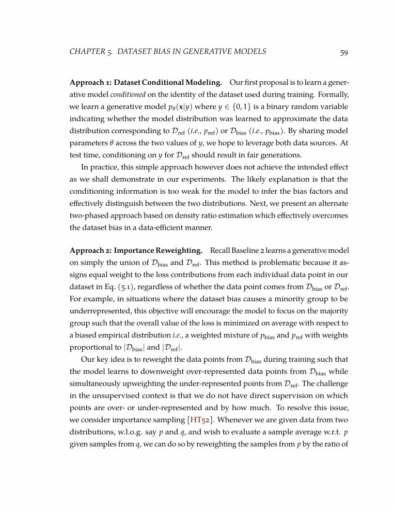
CHAPTER 5. DATASET BIAS IN GENERATIVE MODELS 59
Approach 1: Dataset ConditionalModeling. Our first proposal is to learn a gener-ative model conditioned on the identity of the dataset used during training. Formally,we learn a generative model pθ(x|y) where y ∈ {0, 1} is a binary random variableindicating whether the model distribution was learned to approximate the datadistribution corresponding to Dref (i.e., pref) or Dbias (i.e., pbias). By sharing modelparameters θ across the two values of y, we hope to leverage both data sources. Attest time, conditioning on y for Dref should result in fair generations.
In practice, this simple approach however does not achieve the intended effectas we shall demonstrate in our experiments. The likely explanation is that theconditioning information is too weak for the model to infer the bias factors andeffectively distinguish between the two distributions. Next, we present an alternatetwo-phased approach based on density ratio estimation which effectively overcomesthe dataset bias in a data-efficient manner.
Approach 2: ImportanceReweighting. Recall Baseline 2 learns a generativemodelon simply the union of Dbias and Dref. This method is problematic because it as-signs equal weight to the loss contributions from each individual data point in ourdataset in Eq. (5.1), regardless of whether the data point comes from Dbias or Dref.For example, in situations where the dataset bias causes a minority group to beunderrepresented, this objective will encourage the model to focus on the majoritygroup such that the overall value of the loss is minimized on average with respect toa biased empirical distribution i.e., a weighted mixture of pbias and pref with weightsproportional to |Dbias| and |Dref|.
Our key idea is to reweight the data points from Dbias during training such thatthe model learns to downweight over-represented data points from Dbias whilesimultaneously upweighting the under-represented points fromDref. The challengein the unsupervised context is that we do not have direct supervision on whichpoints are over- or under-represented and by how much. To resolve this issue,we consider importance sampling [HT52]. Whenever we are given data from twodistributions, w.l.o.g. say p and q, and wish to evaluate a sample average w.r.t. p
given samples from q, we can do so by reweighting the samples from p by the ratio of

CHAPTER 5. DATASET BIAS IN GENERATIVE MODELS 60
densities assigned to the sampled points by p and q. In our setting, the distributionsof interest are pbias and pref respectively. Hence, an importance weighted objectivefor learning from Dbias is:
Epref [`(x, θ)] = Epbias
[pref(x)pbias(x)
`(x, θ)
](5.2)
≈ 1T
T
∑i=1
w(xi)`(xi, θ) := L(θ,Dbias) (5.3)
where w(xi) := pref(x)pbias(x)
is defined to be the importance weight for xi ∼ pbias.To estimate the importance weights, we use a binary classifier as described
below [SSK12]. Consider a binary classification problem with classes Y ∈ {0, 1}with training data generated as follows. First, we fix a prior probability for p(Y = 1).Then, we repeatedly sample y ∼ p(Y). If y = 1, we independently sample a datapoint x ∼ pref, else we sample x ∼ pbias. Then, as shown in [FHT01], the ratio ofdensities pref and pbias assigned to an arbitrary point x can be recovered via a Bayesoptimal (probabilistic) classifier c∗ : X → [0, 1]:
w(x) =pref(x)pbias(x)
= γc∗(Y = 1|x)
1− c∗(Y = 1|x) (5.4)
where c(Y = 1|x) is the probability assigned by the classifier to the point x belongingto class Y = 1. Here, γ = p(Y=0)
p(Y=1) is the ratio of marginals of the labels for two classes.In practice, we do not have direct access to either pbias or pref and hence, our
training data consists of points sampled from the empirical data distributions defineduniformly over Dref and Dbias. Further, we may not be able to learn a Bayes optimalclassifier and denote the importance weights estimated by the learned classifier c
for a point x as w(x).Our overall procedure is summarized in Algorithm 5.1. We use deep neural
networks for parameterizing the binary classifier and the generative model. Given abiased and reference dataset alongwith the network architectures and other standardhyperparameters (e.g., learning rate, optimizer etc.), we first learn a probabilisticbinary classifier (Line 2). The learned classifier can provide importance weights for

CHAPTER 5. DATASET BIAS IN GENERATIVE MODELS 61
Algorithm 5.1 Mitigating Dataset Bias in Generative ModelsInputs: Datasets Dbias and DrefClassifier and Generative Model Architectures & HyperparametersOutput: Generative Model Parameters θ
1: . Phase 1: Estimate importance weights2: Learn binary classifier c for distinguishing (Dbias, Y = 0) vs. (Dref, Y = 1)3: Estimate importance weight w(x)← c(Y=1|x)
c(Y=0|x) for all x ∈ Dbias (using Eq. (5.4))4: Set importance weight w(x)← 1 for all x ∈ Dref
nothing5: . Phase 2: Minibatch gradient descent on θ based on weighted loss6: Initialize model parameters θ at random7: Set full dataset D ← Dbias ∪Dref8: while training9: Sample a batch of points B from D at random
10: Set loss L(θ;D)← 1|B| ∑xi∈B w(xi)`(xi, θ)
11: Estimate gradients ∇θL(θ;D) and update parameters θ based on optimizerupdate rule
12: end whilenothing
13: return θ
the data points from Dbias via estimates of the density ratios (Line 3). For the datapoints fromDref, we do not need to perform any reweighting and set the importanceweights to 1 (Line 4). Using the combined dataset Dbias ∪Dref, we then learn thegenerative model pθ where the minibatch loss for every gradient update weightsthe contributions from each data point (Lines 6-12).
For a practical implementation, it is best to account for some diagnostics and bestpractices while executing Algorithm 5.1. For density ratio estimation, we test that theclassifier is calibrated on a held out set. This is a necessary (but insufficient) checkfor the estimated density ratios to be meaningful. If the classifier is miscalibrated, wecan apply standard recalibration techniques such as Platt scaling before estimatingthe importance weights. Furthermore, while optimizing the model using a weightedobjective, there can be an increased variance across the loss contributions from eachexample in a minibatch due to importance weighting. We did not observe this in our

CHAPTER 5. DATASET BIAS IN GENERATIVE MODELS 62
experiments, but techniques such as normalization of weights within a batch canpotentially help control the unintended variance introduced within a batch [SSK12].
The performance of Algorithm 5.1 critically depends on the quality of estimateddensity ratios, which in turn is dictated by the training of the binary classifier. Wedefine the expected negative cross-entropy (NCE) objective for a classifier c as:
NCE(c) :=1
γ + 1Epref(x)[log c(Y = 1|x)] + γ
γ + 1Epbias(x)[log c(Y = 0|x)]. (5.5)
In the following result, we characterize the NCE loss for the Bayes optimalclassifier.
Theorem 5.1. Let Z denote a set of unobserved bias variables. Suppose there exist two jointdistributions pbias(x, z) and pref(x, z) over x ∈ X and z ∈ Z . Let pbias(x) and pbias(z)
denote the marginals over x and z for the joint pbias(x, z) and similar notation for the jointpref(x, z):
pbias(x|z = k) = pref(x|z = k) ∀k (5.6)
and pbias(x|z = k), pbias(x|z = k′) have disjoint supports for k 6= k′. Then, the negativecross-entropy of the Bayes optimal classifier c∗ is given as:
NCE(c∗) =1
γ + 1Epref(z)
[log
1γb(z) + 1
]+
γ
γ + 1Epbias(z)
[log
γb(z)γb(z) + 1
]. (5.7)
where b(z) = pbias(z)/pref(z).
Proof. See Appendix A.1.
For example, as we shall see in our experiments in the following section, the in-puts x can correspond to face images, whereas the unobserved z represents sensitivebias factors for a subgroup such as gender or ethnicity. The proportion of examplesx belonging a subgroup can differ across the biased and reference datasets with therelative proportions given by b(z). Note that the above result only requires knowingthese relative proportions and not the true z for each x. The practical implication is
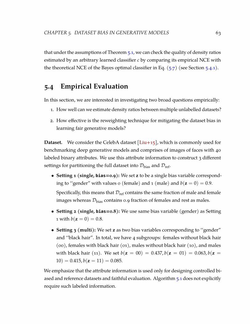
CHAPTER 5. DATASET BIAS IN GENERATIVE MODELS 63
that under the assumptions of Theorem 5.1, we can check the quality of density ratiosestimated by an arbitrary learned classifier c by comparing its empirical NCE withthe theoretical NCE of the Bayes optimal classifier in Eq. (5.7) (see Section 5.4.1).
5.4 Empirical Evaluation
In this section, we are interested in investigating two broad questions empirically:
1. Howwell canwe estimate density ratios betweenmultiple unlabelled datasets?
2. How effective is the reweighting technique for mitigating the dataset bias inlearning fair generative models?
Dataset. We consider the CelebA dataset [Liu+15], which is commonly used forbenchmarking deep generative models and comprises of images of faces with 40labeled binary attributes. We use this attribute information to construct 3 differentsettings for partitioning the full dataset into Dbias and Dref.
• Setting 1 (single, bias=0.9): We set z to be a single bias variable correspond-ing to ‘‘gender” with values 0 (female) and 1 (male) and b(z = 0) = 0.9.
Specifically, this means thatDref contains the same fraction of male and femaleimages whereas Dbias contains 0.9 fraction of females and rest as males.
• Setting 2 (single, bias=0.8): We use same bias variable (gender) as Setting1 with b(z = 0) = 0.8.
• Setting 3 (multi): We set z as two bias variables corresponding to ‘‘gender”and ‘‘black hair”. In total, we have 4 subgroups: females without black hair(00), females with black hair (01), males without black hair (10), and maleswith black hair (11). We set b(z = 00) = 0.437, b(z = 01) = 0.063, b(z =
10) = 0.415, b(z = 11) = 0.085.
We emphasize that the attribute information is used only for designing controlled bi-ased and reference datasets and faithful evaluation. Algorithm 5.1 does not explicitlyrequire such labeled information.

CHAPTER 5. DATASET BIAS IN GENERATIVE MODELS 64
Evaluation metrics. We are interested in evaluating metrics that relate to bothsample quality and fairness w.r.t. the latent bias attributes.
1. Sample quality: Standardmetrics such as Frechet InceptionDistance (FID) [Heu+17]can be used here. Note that we are interested in measuring these metrics w.r.t.the reference data distribution pref even if the model has been trained to useboth Dref and Dbias.
2. Fairness: Alternatively, we can evaluate bias of generative models specificallyin the context of some sensitive latent variables, say u ∈ Rk. For example, u
may correspond to the gender and hair color of an individual depicted viaan image x. If we have access to a highly accurate predictor p(u|x) for thedistribution of the sensitive attributes u conditioned on the observed x, wecan evaluate the extent of bias mitigation via the discrepancies in the expectedmarginal likelihoods of u as per pref and pθ.
Formally, we define the fairness discrepancy f for a generative model pθ w.r.t.pref and sensitive attributes u:
f (pref, pθ) = |Epref [p(u|x)]−Epθ[p(u|x)]|2. (5.8)
In practice, the expectations in Eq. (5.8) can be computed via Monte Carloaveraging. Lower is the discrepancy in the above two expectations, the betteris mitigation in dataset bias w.r.t. the sensitive attributes u.
Models. We train two classifiers for our experiments: (1) the attribute (e.g., gender)classifier which we use to assess the level of bias present in our final samples; and (2)the density ratio classifier. For both models, we use a variant of ResNet18 [He+16]on the standard train and validation splits of CelebA. For the generative model, weused a BigGAN model [BDS18] trained to minimize the hinge loss objective [LY17;TRB17].

CHAPTER 5. DATASET BIAS IN GENERATIVE MODELS 65
(a) single, bias=0.9
(b) single, bias=0.8
(c) multi
Figure 5.2: Distribution of importance weights for different latent subgroups. On av-erage, The underrepresented subgroups are upweighted while the overrepresentedsubgroups are downweighted.

CHAPTER 5. DATASET BIAS IN GENERATIVE MODELS 66
Model Bayes optimal Empirical
single, bias=0.9 0.591 0.605single, bias=0.8 0.642 0.650multi 0.619 0.654
Table 5.1: Comparison between the cross-entropy loss of the Bayes classifier andlearned density ratio classifier.
5.4.1 Density ratio estimation
For each of the three experiments settings, we can evaluate the quality of the esti-mated density ratios by comparing empirical estimates of the cross-entropy loss ofthe density ratio classifier with the cross-entropy loss of the Bayes optimal classifierderived in Eq. (5.7). We show the results in Table 5.1 for perc=1.0 where we findthat the two losses are very close, suggesting that we obtain high-quality densityratio estimates that we can use for subsequently training fair generative models.
In Figure 5.2, we show the distribution of our importance weights for the variouslatent subgroups. We find that across all the considered settings, the underrepre-sented subgroups (e.g., males in Figure 5.2a, 5.2b, females with black hair in 5.2c)are upweighted on average (mean density ratio estimate > 1), while the overrepre-sented subgroups are downweighted on average (mean density ratio estimate <
1). Also, as expected, the density ratio estimates are closer to 1 when the bias is low(see Figure 5.2a v.s. 5.2b).
5.4.2 Dataset bias mitigation
We compare our importance weighted approach against three baselines: (1) equi-weight: a BigGAN trained on the full dataset Dref ∪Dbias that weighs every pointequally; (2) reference-only: a BigGAN trained on the reference dataset Dref; and(3) conditional: a conditional BigGAN where the conditioning label indicateswhether a data point x is from Dref(y = 1) or Dbias(y = 0). In all our experiments,the reference-only variant which only uses the reference dataset Dref for learninghowever failed to give any recognizable samples. For a clean presentation of the

CHAPTER 5. DATASET BIAS IN GENERATIVE MODELS 67
(a) Samples generated via importance reweighting with subgroups separated by theorange line. For the 100 samples above, the classifier concludes 52 females and 48males.
(b) Fairness Discrepancy
(c) FID
Figure 5.3: Single-Attribute Dataset Bias Mitigation for bias=0.9. Standard error in(b) and (c) over 10 independent evaluation sets of 10,000 samples each drawn fromthe models. Lower fairness discrepancy and FID is better. We find that on average,imp-weight outperforms the equi-weight baseline by 49.3% and the conditionalbaseline by 25.0% across all reference dataset sizes for bias mitigation.

CHAPTER 5. DATASET BIAS IN GENERATIVE MODELS 68
(a) Samples generated via importance reweighting with subgroups separated by theorange line. For the 100 samples above, the classifier concludes 52 females and 48males.
(b) Fairness Discrepancy
0.1 0.25 0.5 1.0Ratio of unbiased to biased dataset sizes
05
10152025303540
FID
imp-weightequi-weightconditional
(c) FID
Figure 5.4: Single Attribute Dataset Bias Mitigation for bias=0.8. Standard error in(b) and (c) over 10 independent evaluation sets of 10,000 samples each drawn fromthe models. Lower fairness discrepancy and FID is better. We find that on average,imp-weight outperforms the equi-weight baseline by 23.9% and the conditionalbaseline by 12.2% across all reference dataset sizes for bias mitigation.
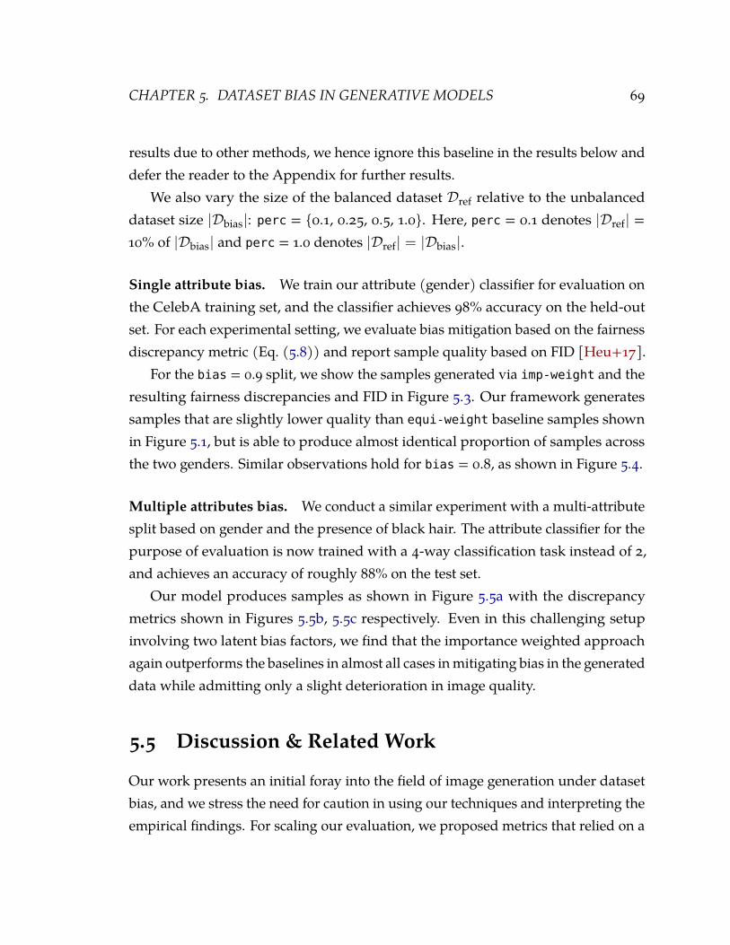
CHAPTER 5. DATASET BIAS IN GENERATIVE MODELS 69
results due to other methods, we hence ignore this baseline in the results below anddefer the reader to the Appendix for further results.
We also vary the size of the balanced dataset Dref relative to the unbalanceddataset size |Dbias|: perc = {0.1, 0.25, 0.5, 1.0}. Here, perc = 0.1 denotes |Dref| =10% of |Dbias| and perc = 1.0 denotes |Dref| = |Dbias|.
Single attribute bias. We train our attribute (gender) classifier for evaluation onthe CelebA training set, and the classifier achieves 98% accuracy on the held-outset. For each experimental setting, we evaluate bias mitigation based on the fairnessdiscrepancy metric (Eq. (5.8)) and report sample quality based on FID [Heu+17].
For the bias = 0.9 split, we show the samples generated via imp-weight and theresulting fairness discrepancies and FID in Figure 5.3. Our framework generatessamples that are slightly lower quality than equi-weight baseline samples shownin Figure 5.1, but is able to produce almost identical proportion of samples acrossthe two genders. Similar observations hold for bias = 0.8, as shown in Figure 5.4.
Multiple attributes bias. We conduct a similar experiment with a multi-attributesplit based on gender and the presence of black hair. The attribute classifier for thepurpose of evaluation is now trained with a 4-way classification task instead of 2,and achieves an accuracy of roughly 88% on the test set.
Our model produces samples as shown in Figure 5.5a with the discrepancymetrics shown in Figures 5.5b, 5.5c respectively. Even in this challenging setupinvolving two latent bias factors, we find that the importance weighted approachagain outperforms the baselines in almost all cases inmitigating bias in the generateddata while admitting only a slight deterioration in image quality.
5.5 Discussion & Related Work
Our work presents an initial foray into the field of image generation under datasetbias, and we stress the need for caution in using our techniques and interpreting theempirical findings. For scaling our evaluation, we proposed metrics that relied on a
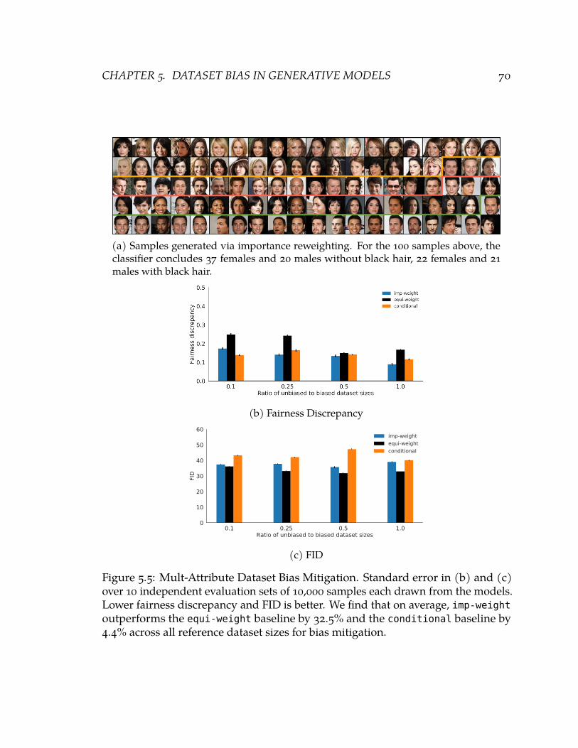
CHAPTER 5. DATASET BIAS IN GENERATIVE MODELS 70
(a) Samples generated via importance reweighting. For the 100 samples above, theclassifier concludes 37 females and 20 males without black hair, 22 females and 21males with black hair.
(b) Fairness Discrepancy
0.1 0.25 0.5 1.0Ratio of unbiased to biased dataset sizes
0
10
20
30
40
50
60
FID
imp-weightequi-weightconditional
(c) FID
Figure 5.5: Mult-Attribute Dataset Bias Mitigation. Standard error in (b) and (c)over 10 independent evaluation sets of 10,000 samples each drawn from the models.Lower fairness discrepancy and FID is better. We find that on average, imp-weightoutperforms the equi-weight baseline by 32.5% and the conditional baseline by4.4% across all reference dataset sizes for bias mitigation.

CHAPTER 5. DATASET BIAS IN GENERATIVE MODELS 71
pretrained attribute classifier for inferring the bias in the generated data samples.The classifiers we considered are highly accurate on all subgroups, but can haveblind spots when evaluated on generated data. For future work, we would like toinvestigate human evaluations to mitigate such issues during evaluation [Grg+18].
As another case in point, our work calls for rethinking sample quality metricsfor generative models in the presence of dataset bias [Mit+19]. On one hand, ourapproach increases the diversity of generated samples in the sense that the differentsubgroups are more balanced; at the same time, however, variation across otherimage features decreases because the newly generated underrepresented samples arelearned from a smaller dataset of underrepresented subgroups. Moreover, standardmetrics such as FID even when evaluated with respect to a reference dataset, couldexhibit a relative preference for models trained on larger datasets with little or nobias correction to avoid even slight compromises on perceptual sample quality. Next,we discuss some key lines of related work for the current chapter.
Fairness & generative modeling. There is a rich body of work in fair ML, whichfocus on different notions of fairness (e.g.demographic parity, equality of oddsand opportunity) and study methods by which models can perform tasks suchas classification in a non-discriminatory way [BHN18; Dwo+12; Hei+18; Pin+18].Our focus is in the context of fair generative modeling. The vast majority of relatedwork in this area is centered around fair and/or privacy preserving representationlearning, which exploit tools from adversarial learning and information theoryamong others [Zem+13; ES15; Lou+16; Beu+17; Son+19; Ade+19]. A unifyingprinciple among these methods is such that a discriminator is trained to performpoorly in predicting an outcome based on a protected attribute. [RAM17] considerstransfer learning of race and gender identities as a form of weak supervision forpredicting other attributes on datasets of faces. While the end goal for the aboveworks is classification, our focus is on data generation in the presence of dataset biasand we do not require explicit supervision for the protected attributes.
The most relevant prior works in data generation are FairGAN [Xu+18] andFairnessGAN [Sat+19]. The goal of both methods is to generate fair data points and

CHAPTER 5. DATASET BIAS IN GENERATIVE MODELS 72
their labels as a preprocessing step. This allows for learning a useful downstreamclassifier and obscures information about protected attributes. These works arenot directly comparable to our setting as we do not assume explicit supervisionregarding the protected attributes during training, and our goal is fair generationgiven unlabelled biased datasets where the bias factors are latent. Another relevantwork is DB-VAE [Ami+19], which uses a VAE to learn the latent structure of sensitiveattributes and employs importance weighting based on this structure to mitigatebias in downstream classifiers. Contrary to our work, these importance weights areused to directly sample (rare) data points with higher frequencies for training aclassifier, as opposed to fair data generation.
Importance reweighting. Reweighting data points is a common algorithmic tech-nique for problems such as dataset bias and class imbalance [BL18]. It has oftenbeen used in the context of fair classification [CKP09], for example, [KC12] detailsreweighting as a way to remove discrimination without relabeling instances. Forreinforcement learning, [DTB17] used an importance sampling approach for select-ing fair policies. There is also a body of work on fair clustering [Chi+17; Bac+19;BCN19; SSS18] which ensure that the clustering assignments are balanced withrespect to some sensitive attribute.
Density ratio estimation using classifiers. The use of classifiers for estimatingdensity ratios has a rich history of prior works across ML [SSK12]. For deep genera-tive modeling, density ratios estimated by classifiers have been used for expandingthe class of various learning objectives [NCT16; ML16; GE18], evaluation metricsbased on two-sample tests [Gre+07; Bow+15; LO16; Dan+17; Ros+17; Im+18;GRM19], or improved Monte Carlo inference via these models [Gro+19a; Aza+18;Tur+18; Tao+18]. Closest related is the proposal of [Die+18] to use importancereweighting for learning generative models where training and test distributionsdiffer, but explicit importance weights are provided for at least a subset of the train-ing examples. In contrast, we consider a more realistic setting where we estimatethe importance weights using a small reference dataset.

CHAPTER 5. DATASET BIAS IN GENERATIVE MODELS 73
5.6 Conclusion
We considered the task of data generation given access to a (potentially small) refer-ence dataset and large biased dataset(s). For data-efficient learning, we proposedan importance weighted objective that corrects bias by reweighting the biased datapoints. These weights are estimated by a binary classifier. Empirically, we showedthat our technique outperforms baselines by up to 34.6% on average in reducingdataset bias on CelebAwithout incurring any significant reduction in sample quality.
Finally, it is worth emphasizing the need to be mindful of the decisions made ateach stage in the development and deployment of ML systems [Abe+20]. Factorssuch as the dataset used for training [Geb+18; She+19; JG20] or algorithmic deci-sions such as the loss function or evaluation metric [HPS16; BG18; Kim+18; Liu+18a;Has+18], among others, may have undesirable consequences. These effects can befurther amplified by the very nature of the goal of generative models.

Part II
Relational Representation &Reasoning
74

6 Representation & Reasoning in Graphs
6.1 Introduction
Graphs are a fundamental abstraction for modeling relational data. Many importantanalysis over graphs can be cast as predictions over nodes and edges. In a typicalnode classification task, we are interested in predicting the most probable labels ofnodes in a graph [BCM11]. For example, in a social network, we might be interestedin predicting interests of users, or in a protein-protein interaction network we mightbe interested in predicting functional labels of proteins [Rad+13; Yan+11]. Similarly,in link prediction, we wish to predict whether a pair of nodes in a graph shouldhave an edge connecting them [LK07]. Link prediction is useful in a wide variety ofdomains; for instance, in genomics, it helps us discover novel interactions betweengenes, and in social networks, it can identify real-world friends [BL11; Vaz+03].
For the above prediction problems, we require feature representations for thenodes and edges that can be fed as input to a supervised machine learning algo-rithm. Hand-engineering features based on expert knowledge, e.g., structural graphfeatures include node degrees, centrality measures, etc. is tedious and suboptimal.
The goal in this chapter is discuss algorithms to automatically learn feature rep-resentations for nodes in a graph using unsupervised methods [BCV13]. Classicapproaches include linear and non-linear dimensionality reduction such as Princi-pal Component Analysis, isoMap and other approaches based on matrix factoriza-tion [BN02; RS00; TDL00; Yan+06]. Besides computational limitations of matrix
75

CHAPTER 6. REPRESENTATION & REASONING IN GRAPHS 76
factorization approaches, the learning objective for these techniques is often notaligned with downstream predictive tasks of interest and hence these approachesare suboptimal.
Here, we present Graphite, a latent variable generative model for graph represen-tational learning based on variational autoencoding [KW18]. The encoding phasemaps each node in an input graph to a latent representation and the decoding phasemaps the latent representations to a graph. Our model uses graph neural networksfor inference (encoding) and generation (decoding). These networks can be seen asa parameterized extension to the Weisfeiler-Lehman test for graph isomorphismand use message passing techniques to efficiently map nodes to feature representa-tions. While the encoding is straightforward and can use any existing graph neuralnetwork, the decoding of these latent features to reconstruct the original graph isdone using a multi-layer iterative procedure. The procedure starts with an initialreconstruction based on the inferred latent features, and iteratively refines the re-constructed graph via a message passing operation. We benchmark the benefitsof Graphite over previous approaches on the tasks of node classification and linkprediction on real-world graph datasets.
6.2 Preliminaries
Consider a weighted undirected graph G = (V, E)where V and E denote index setsof nodes and edges respectively. Additionally, we denote the (optional) feature ma-trix associated with the graph as X ∈ Rn×m for an m-dimensional signal associatedwith each node, e.g., these could refer to the user attributes in a social network. Werepresent the graph structure using a symmetric adjacency matrix A ∈ Rn×n wheren = |V| and the entries Aij denote the weight of the edge between node i and j.

CHAPTER 6. REPRESENTATION & REASONING IN GRAPHS 77
6.2.1 Weisfeiler-Lehman algorithm
The Weisfeiler-Lehman (WL) algorithm [WL68; Dou11] is a heuristic test of graphisomorphism between any two graphs G and G′. The algorithm proceeds in iter-ations. Before the first iteration, we label every node in G and G′ with a scalarisomorphism invariant initialization (e.g., node degrees). That is, if G and G′ are as-sumed to be isomorphic, then an isomorphism invariant initialization is one wherethe matching nodes establishing the isomorphism in G and G′ have the same labels(a.k.a. messages). Let H(0) = [h(l)1 , h(l)2 , · · · , h(l)n ]T denote the vector of initializationsfor the nodes in the graph at iteration l ∈N∪ 0. At every iteration l > 0, we performa relabelling of nodes in G and G′ based on a message passing update rule:
H(l) ← hash(
AH(l−1))
(6.1)
where A denotes the adjacency matrix of the corresponding graph and hash : Rn →Rn is any suitable hash function e.g., a non-linear activation. Hence, the messagefor every node is computed as a hashed sum of the messages from the neighboringnodes (since Aij 6= 0 only if i and j are neighbors). We repeat the process for aspecified number of iterations, or until convergence. If the label sets for the nodes inG and G′ are equal (which can be checked using sorting in O(n log n) time), thenthe algorithm declares the two graphs G and G′ to be isomorphic.
The ‘‘k-dim”WL algorithm extends the 1-dim algorithm above by simultaneouslypassing messages of length k (each initialized with some isomorphism invariantscheme). A positive test for isomorphism requires equality in all k dimensions fornodes in G and G′ after the termination of message passing. This algorithmic test isa heuristic which guarantees no false negatives but can give false positives whereintwo non-isomorphic graphs can be falsely declared isomorphic. Empirically, the testhas been shown to fail on some regular graphs but gives excellent performance onreal-world graphs [She+11].

CHAPTER 6. REPRESENTATION & REASONING IN GRAPHS 78
6.2.2 Graph neural networks
Intuitively, the WL algorithm encodes the structure of the graph in the form ofmessages at every node. Graph neural networks (GNN) build on this observationand parameterize an unfolding of the iterative message passing procedure whichwe describe next.
A GNN consists of many layers, indexed by l ∈ N with each layer associatedwith an activation ηl and a dimensionality dl. In addition to the input graph A,every layer l ∈ N of the GNN takes as input the activations from the previouslayer H(l−1) ∈ Rn×dl−1 , a family of linear transformations Fl : Rn×n → Rn×n, and amatrix of learnable weight parameters Wl ∈ Rdl−1×dl and optional bias parametersBl ∈ Rn×dl . Recursively, the layer wise propagation rule in a GNN is given by:
H(l) ← ηl
(Bl + ∑
f∈Fl
f (A)H(l−1)Wl
)(6.2)
with the base cases H(0) = X and d0 = m. Here, m is the feature dimensionality. Ifthere are no explicit node features, we set H(0) = In (identity) and d0 = n. Severalvariants of graph neural networks have been proposed in prior work. For instance,graph convolutional networks (GCN) [KW17] instantiate graph neural networkswith a permutation equivariant propagation rule:
H(l) ← ηl
(Bl + AH(l−1)Wl
)(6.3)
where A = D−1/2AD−1/2 is the symmetric diagonalization of A given the diagonaldegree matrix D (i.e., Dii = ∑(i,j)∈E Aij), and same base cases as before. Comparingthe above with the WL update rule in Eq. (6.1), we can see that the activations forevery layer in a GCN are computed via parameterized, scaled activations (messages)of the previous layer being propagated over the graph, with the hash functionimplicitly specified using an activation function ηl.
Our framework is agnostic to instantiations of message passing rule of a graph
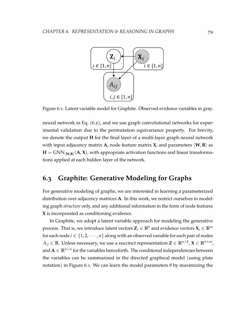
CHAPTER 6. REPRESENTATION & REASONING IN GRAPHS 79
Figure 6.1: Latent variable model for Graphite. Observed evidence variables in gray.
neural network in Eq. (6.2), and we use graph convolutional networks for exper-imental validation due to the permutation equivariance property. For brevity,we denote the output H for the final layer of a multi-layer graph neural networkwith input adjacency matrix A, node feature matrix X, and parameters 〈W, B〉 asH = GNN〈W,B〉(A, X), with appropriate activation functions and linear transforma-tions applied at each hidden layer of the network.
6.3 Graphite: Generative Modeling for Graphs
For generative modeling of graphs, we are interested in learning a parameterizeddistribution over adjacency matrices A. In this work, we restrict ourselves to model-ing graph structure only, and any additional information in the form of node featuresX is incorporated as conditioning evidence.
In Graphite, we adopt a latent variable approach for modeling the generativeprocess. That is, we introduce latent vectors Zi ∈ Rk and evidence vectors Xi ∈ Rm
for each node i ∈ {1, 2, · · · , n} alongwith an observed variable for each pair of nodesAij ∈ R. Unless necessary, we use a succinct representation Z ∈ Rn×k, X ∈ Rn×m,and A ∈ Rn×n for the variables henceforth. The conditional independencies betweenthe variables can be summarized in the directed graphical model (using platenotation) in Figure 6.1. We can learn the model parameters θ by maximizing the

CHAPTER 6. REPRESENTATION & REASONING IN GRAPHS 80
marginal likelihood of the observed adjacency matrix conditioned on X:
maxθ
log pθ(A|X) = log∫
Zpθ(A, Z|X)dZ (6.4)
Here, p(Z|X) is a fixed prior distribution over the latent features of every nodee.g., isotropic Gaussian. If we have multiple graphs in our dataset, we maximizethe expected log-likelihoods over all the corresponding adjacency matrices. We canobtain a tractable, stochastic evidence lower bound (ELBO) to the above objectiveby introducing a variational posterior qφ(Z|A, X) with parameters φ:
log pθ(A|X) ≥ Eqφ(Z|A,X)
[log
pθ(A, Z|X)qφ(Z|A, X)
](6.5)
The lower bound is tight when the variational posterior qφ(Z|A, X) matchesthe true posterior pθ(Z|A, X) and hence maximizing the above objective optimizesfor the parameters that define the best approximation to the true posterior withinthe variational family [BKM17]. We now discuss parameterizations for specifyingqφ(Z|A, X) (i.e., encoder) and pθ(A|Z, X) (i.e., decoder).
Encoding using forward message passing. Typically we use the mean field ap-proximation for defining the variational family and hence:
qφ(Z|A, X) ≈n
∏i=1
qφi(Zi|A, X) (6.6)
Additionally, we would like to make distributional assumptions on each variationalmarginal density qφi(Zi|A, X) such that it is reparameterizable and easy-to-sample,such that the gradients w.r.t. φi have low variance [KW18]. In Graphite, we assumeisotropic Gaussian variational marginals with diagonal covariance. The parametersfor the variational marginals qφi(Z|A, X) are specified using a graph neural network:
µ, σ = GNNφ(A, X) (6.7)

CHAPTER 6. REPRESENTATION & REASONING IN GRAPHS 81
where µ and σ denote the vector of means and standard deviations for the varia-tional marginals {qφi(Zi|A, X)}n
i=1 and φ = {φi}ni=1 are the full set of variational
parameters.
Decoding using reverse message passing. For specifying the observation modelpθ(A|Z, X), we cannot directly use a graph neural network since we do not have aninput graph for message passing. To sidestep this issue, we propose an iterativetwo-step approach that alternates between defining an intermediate graph and thengradually refining this graph through message passing. Formally, given a latentmatrix Z and an input feature matrix X, we iterate over the following sequence ofoperations:
A =ZZT
‖Z‖2 + 11T, (6.8)
Z∗ = GNNθ(A, [Z|X]) (6.9)
where the second argument to the GNN is a concatenation of Z and X. The firststep constructs an intermediate weighted graph A ∈ Rn×n by applying an innerproduct of Z with itself and adding an additional constant of 1 to ensure entriesare non-negative. And the second step performs a pass through a parameterizedgraph neural network. We can repeat the above sequence to gradually refine thefeature matrix Z∗. The final distribution over graph parameters is obtained using aninner product step on Z∗ ∈ Rn×k∗ akin to Eq. (6.8), where k∗ ∈N is determined viathe network architecture. For efficient sampling, we assume the observation modelfactorizes:
pθ(A|Z, X) =n
∏i=1
n
∏j=1
p(i,j)θ (Aij|Z∗). (6.10)
The distribution over the individual edges can be expressed as a Bernoulli or Gaus-sian distribution for unweighted and real-valued edges respectively. For example,the edge probabilities for an unweighted graph are given as sigmoid(Z∗Z∗
T).

CHAPTER 6. REPRESENTATION & REASONING IN GRAPHS 82
Scalable learning & inference in Graphite For representation learning of largegraphs, we require the encoding and decoding steps in Graphite to be computation-ally efficient. This can be challenging as the decoding step involves inner productsof potentially dense matrices Z, which is by default an O(n2k) operation. Here, k isthe dimension of the per-node latent vectors Zi used to define A.
For any intermediate decoding step as in Eq. (6.8), we propose to offset thisexpensive computation by using the associativity property of matrix multiplicationsfor the message passing step in Eq. (6.9). For notational brevity, consider thesimplified graph propagation rule for a GNN:
H(l) ← ηl
(AH(l−1)
)where A is defined in Eq. (6.8).
Instead of directly taking an inner product of Z with itself, we note that thesubsequent operation involves another matrix multiplication and hence, we canperform right multiplication instead. If dl and dl−1 denote the size of the layers H(l)
and H(l−1) respectively, then the time complexity of propagation based on rightmultiplication is given by O(nkdl−1 + ndl−1dl).
The above trick sidesteps the quadratic n2 complexity for decoding in the inter-mediate layers without any loss in statistical accuracy. The final layer however stillinvolves an inner product with respect to Z∗ corresponding to potentially densematrices. However, since the edges are generated independently, we can approxi-mate the loss objective by performing a Monte Carlo evaluation of the reconstructedadjacency matrix parameters in Eq. (6.10). By adaptively choosing the numberof entries for Monte Carlo approximation, we can trade-off statistical accuracy forcomputational budget.
6.4 Empirical Evaluation
We evaluate Graphite on tasks involving entire graphs, nodes, and edges. We con-sider two variants of our proposed framework: theGraphite-VAE, which corresponds

CHAPTER 6. REPRESENTATION & REASONING IN GRAPHS 83
Table 6.1: Mean reconstruction errors and negative log-likelihood estimates (in nats)for autoencoders and variational autoencoders respectively on test instances fromsix different generative families. Lower is better.
Erdos-Renyi Ego Regular Geometric Power Law Barabasi-Albert
GAE 221.79 ± 7.58 197.3 ± 1.99 198.5 ± 4.78 514.26 ± 41.58 519.44 ± 36.30 236.29 ± 15.13Graphite-AE 195.56 ± 1.49 182.79 ± 1.45 191.41 ± 1.99 181.14 ± 4.48 201.22 ± 2.42 192.38 ± 1.61
VGAE 273.82 ± 0.07 273.76 ± 0.06 275.29 ± 0.08 274.09 ± 0.06 278.86 ± 0.12 274.4 ± 0.08Graphite-VAE 270.22 ± 0.15 270.70 ± 0.32 266.54 ± 0.12 269.71 ± 0.08 263.92 ± 0.14 268.73 ± 0.09
to a directed latent variable model as described in Section 6.3 andGraphite-AE, whichcorresponds to an autoencoder trained to minimize the error in reconstructing aninput adjacency matrix. For unweighted graphs (i.e., A ∈ {0, 1}n×n), the reconstruc-tion terms in the objectives for both Graphite-VAE and Graphite-AE minimize thenegative cross entropy between the input and reconstructed adjacency matrices. Forweighted graphs, we use the mean squared error.
6.4.1 Reconstruction & density estimation
In the first set of tasks, we evaluate learning in Graphite based on held-out recon-struction losses and log-likelihoods estimated by the learned Graphite-VAE andGraphite-AE models respectively on a collection of graphs with varying sizes. Indirect contrast to modalities such as images, graphs cannot be straightforwardly re-duced to a fixed number of vertices for input to a graph convolutional network. Onesimplifying modification taken by [Boj+18] is to consider only the largest connectedcomponent for evaluating and optimizing the objective, which we appeal to as well.Thus by setting the dimensions of Z∗ to a maximum number of vertices, Graphitecan be used for inference tasks over entire graphs with potentially smaller sizes byconsidering only the largest connected component.
We create datasets from six graph families with fixed, known generative pro-cesses: the Erdos-Renyi, ego-nets, random regular graphs, random geometricgraphs, random Power Law Tree and Barabasi-Albert. For each family, 300 graph in-stances were sampled with each instance having 10− 20 nodes and evenly split intotrain/validation/test instances. As a benchmark comparison, we compare against
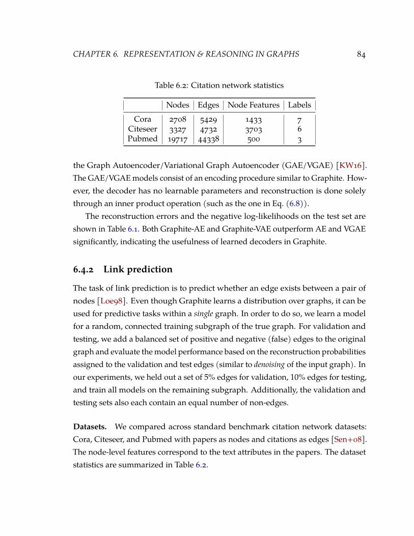
CHAPTER 6. REPRESENTATION & REASONING IN GRAPHS 84
Table 6.2: Citation network statistics
Nodes Edges Node Features Labels
Cora 2708 5429 1433 7Citeseer 3327 4732 3703 6Pubmed 19717 44338 500 3
the Graph Autoencoder/Variational Graph Autoencoder (GAE/VGAE) [KW16].The GAE/VGAEmodels consist of an encoding procedure similar to Graphite. How-ever, the decoder has no learnable parameters and reconstruction is done solelythrough an inner product operation (such as the one in Eq. (6.8)).
The reconstruction errors and the negative log-likelihoods on the test set areshown in Table 6.1. Both Graphite-AE and Graphite-VAE outperform AE and VGAEsignificantly, indicating the usefulness of learned decoders in Graphite.
6.4.2 Link prediction
The task of link prediction is to predict whether an edge exists between a pair ofnodes [Loe98]. Even though Graphite learns a distribution over graphs, it can beused for predictive tasks within a single graph. In order to do so, we learn a modelfor a random, connected training subgraph of the true graph. For validation andtesting, we add a balanced set of positive and negative (false) edges to the originalgraph and evaluate themodel performance based on the reconstruction probabilitiesassigned to the validation and test edges (similar to denoising of the input graph). Inour experiments, we held out a set of 5% edges for validation, 10% edges for testing,and train all models on the remaining subgraph. Additionally, the validation andtesting sets also each contain an equal number of non-edges.
Datasets. We compared across standard benchmark citation network datasets:Cora, Citeseer, and Pubmed with papers as nodes and citations as edges [Sen+08].The node-level features correspond to the text attributes in the papers. The datasetstatistics are summarized in Table 6.2.

CHAPTER 6. REPRESENTATION & REASONING IN GRAPHS 85
Table 6.3: Area Under the ROC Curve (AUC) for link prediction (* denotes datasetwith features). Higher is better.
Cora Citeseer Pubmed Cora* Citeseer* Pubmed*
SC 89.9 ± 0.20 91.5 ± 0.17 94.9 ± 0.04 - - -DeepWalk 85.0 ± 0.17 88.6 ± 0.15 91.5 ± 0.04 - - -node2vec 85.6 ± 0.15 89.4 ± 0.14 91.9 ± 0.04 - - -
GAE 90.2 ± 0.16 92.0 ± 0.14 92.5 ± 0.06 93.9 ± 0.11 94.9 ± 0.13 96.8 ± 0.04VGAE 90.1 ± 0.15 92.0 ± 0.17 92.3 ± 0.06 94.1 ± 0.11 96.7 ± 0.08 95.5 ± 0.13
Graphite-AE 91.0 ± 0.15 92.6 ± 0.16 94.5 ± 0.05 94.2 ± 0.13 96.2 ± 0.10 97.8 ± 0.03Graphite-VAE 91.5 ± 0.15 93.5 ± 0.13 94.6 ± 0.04 94.7 ± 0.11 97.3 ± 0.06 97.4 ± 0.04
Table 6.4: Average Precision (AP) scores for link prediction (* denotes dataset withfeatures). Higher is better.
Cora Citeseer Pubmed Cora* Citeseer* Pubmed*
SC 92.8 ± 0.12 94.4 ± 0.11 96.0 ± 0.03 - - -DeepWalk 86.6 ± 0.17 90.3 ± 0.12 91.9 ± 0.05 - - -node2vec 87.5 ± 0.14 91.3 ± 0.13 92.3 ± 0.05 - - -
GAE 92.4 ± 0.12 94.0 ± 0.12 94.3 ± 0.5 94.3 ± 0.12 94.8 ± 0.15 96.8 ± 0.04VGAE 92.3 ± 0.12 94.2 ± 0.12 94.2 ± 0.04 94.6 ± 0.11 97.0 ± 0.08 95.5 ± 0.12
Graphite-AE 92.8 ± 0.13 94.1 ± 0.14 95.7 ± 0.06 94.5 ± 0.14 96.1 ± 0.12 97.7 ± 0.03Graphite-VAE 93.2 ± 0.13 95.0 ± 0.10 96.0 ± 0.03 94.9 ± 0.13 97.4 ± 0.06 97.4 ± 0.04
Baselines and evaluation metrics. We evaluate performance based on the AreaUnder the ROC Curve (AUC) and Average Precision (AP) metrics. We consider thefollowing baselines: Spectral Clustering (SC) [TL11], DeepWalk [PAS14], node2vec [GL16],and GAE/VGAE [KW16]. SC, DeepWalk, and node2vec do not provide the abilityto incorporate node features while learning embeddings, and hence we evaluatethem only on the featureless datasets.
Results. The AUC and AP results (along with standard errors) are shown inTable 6.3 and Table 6.4 respectively averaged over 50 random train/validation/testsplits. On both metrics, Graphite-VAE gives the best performance overall. Graphite-AE also gives good results, generally outperforming its closest competitor GAE.

CHAPTER 6. REPRESENTATION & REASONING IN GRAPHS 86
(a) Graphite-AE (b) Graphite-VAE
Figure 6.2: t-SNE embeddings of the latent feature vectors for the Cora dataset.Colors denote labels.
Table 6.5: Classification accuracies (* denotes dataset with features). Baselinenumbers from [KW17].
Cora* Citeseer* Pubmed*
SemiEmb 59.0 59.6 71.1DeepWalk 67.2 43.2 65.3
ICA 75.1 69.1 73.9Planetoid 75.7 64.7 77.2
GCN 81.5 70.3 79.0
Graphite 82.1 ± 0.06 71.0 ± 0.07 79.3 ± 0.03
Qualitative evaluation. We visualize the embeddings learned by Graphite andgiven by a 2D t-SNE projection [MH08] of the latent feature vectors (given as rowsfor Z with λ = 0.5) on the Cora dataset in Figure 6.2. Even without any access tolabel information for the nodes during training, the name models are able to clusterthe nodes (papers) as per their labels (paper categories).

CHAPTER 6. REPRESENTATION & REASONING IN GRAPHS 87
6.4.3 Semi-supervised node classification
Given labels for a subset of nodes in an underlying graph, the goal of this task is topredict the labels for the remaining nodes. We consider a transductive setting, wherewe have access to the test nodes (without their labels) during training.
Closest approach to Graphite for this task is a supervised graph convolutionalnetwork (GCN) trained end-to-end. We consider an extension of this baseline,wherein we augment the GCN objective with the Graphite objective and a hyperpa-rameter to control the relative importance of the two terms in the combined objective.The parameters φ for the encoder are shared across these two objectives, with anadditional GCN layer for mapping the encoder output to softmax probabilities overthe requisite number of classes. All parameters are learned jointly.
Results. The classification accuracy of the semi-supervised models is given inTable 6.5. We find that Graphite-hybrid outperforms the competing models on alldatasets and in particular the GCN approach which is the closest baseline.
6.5 Discussion & Related Work
Probabilistic modeling of graphs. The earliest probabilistic models of graphs pro-posed to generate graphs by creating an edge between any pair of nodes with aconstant probability [ER59]. Several alternatives have been proposed since; e.g.,the small-world model generates graphs that exhibit local clustering [WS98], theBarabasi-Albert models preferential attachment wherein high-degree nodes arelikely to form edges with newly added nodes [BA99], the stochastic block model isbased on inter and intra community linkages [HLL83] etc. We direct the interestedreader to prominent surveys on this topic [New03; Mit04; CF06].
Representation learning on graphs. For representation learning on graphs, thereare broadly three kinds of approaches: matrix factorization, random walk basedapproaches, and graph neural networks. We refer the reader to [HYL17b] for a

CHAPTER 6. REPRESENTATION & REASONING IN GRAPHS 88
recent survey on these three kinds of approaches and focus on the latter below.Graph neural networks, a collective term for networks that operate over graphs
using message passing, have shown success on several downstream applications,e.g., [Duv+15; Li+16; Kea+16; KW17; HYL17a] and the references therein. [Gil+17]provides a comprehensive characterization of these networks in the message passingsetup. We used Graph Convolution Networks, partly to provide a direct comparisonwith GAE/VGAE and leave the exploration of other GNN variants for future work.
Latent variable models for graphs. Several deep generative models for graphshave beenpreviously proposed. Amongst adversarial generation approaches, [Wan+18]and [Boj+18] model local graph neighborhoods and random walks on graphs re-spectively. [Li+18] and [You+18] model graphs as sequences and generate graphsvia autoregressive procedures. Adversarial and autoregressive approaches are suc-cessful at generating graphs, but do not directly allow for inferring latent variablesvia encoders. Latent variable generative models have also been proposed for gen-erating small molecular graphs [JBJ18; Sam+18; SK18]. These methods involve anexpensive decoding procedure that limits scaling to large graphs. Finally, closestto our framework is the GAE/VGAE approach [KW16] discussed in Section 6.4.[Pan+18] extends this approach with an adversarial regularization framework butretain the inner product decoder. Our work proposes a novel multi-step decodingmechanism based on graph refinement.
6.6 Conclusion
We proposed Graphite, a scalable deep generative model for graphs based on varia-tional autoencoding. The encoders and decoders in Graphite are parameterized bygraph neural networks that propagate information locally on a graph. Our proposeddecoder performs a multi-layer iterative decoding comprising of alternate innerproduct operations and message passing on the intermediate graph. Empirically,we observed superior performance of Graphite over other competing approachesfor density estimation, node classification, and link prediction.

7 Representation & Reasoning in Multia-gent Systems
7.1 Introduction
In the last chapter, we discussed representation learning and reasoning for staticgraph networks. Relational data can appear in many other interactive contextsbeyond static graph networks. An intelligent agent rarely acts in isolation in thereal world and typically seeks to achieve its goals through interaction with otheragents. Such interactions give rise to rich, complex behaviors formalized as per-agent policies in a multiagent system [Fer99; Woo09]. Depending on the underlyingmotivations of the agents, interactions could be directed towards achieving a sharedgoal in a collaborative setting, opposing another agent in a competitive setting, or bea mixture of these in a setting where agents collaborate in teams to compete againstother teams. Learning useful representations of the policies of agents based on theirinteractions is an important step towards characterization of the agent behavior andmore generally reasoning in multiagent systems.
In this chapter, we propose a representation learning framework for agent poli-cies, given access to only a few episodes of interaction. Our framework builds ontwomajor lines of advancements in representation learning: (a) generative methods,whichwe formalize as learning representations that can aid imitation in amultiagentsetup; and (b) contrastive methods, which we formalize as learning representations
89

CHAPTER 7. REPRESENTATION&REASONING INMULTIAGENT SYSTEMS 90
that can aid in distinguishing multiple agents using triplet losses.For the embeddings to be useful, the representation function should generalize to
both unseen interactions and unseen agents for novel downstream tasks. Generaliza-tion is well-understood in the context of supervised learning where a good modelis expected to attain similar train and test performance. For multiagent systems,we consider a notion of generalization based on agent-interaction graphs. An agent-interaction graph provides an abstraction for distinguishing the agents (nodes) andinteractions (edges) observed during training, validation, and testing.
Our framework is agnostic to the nature of interactions inmultiagent systems, andhence broadly applicable to competitive and cooperative environments. In particular,we consider two multiagent environments: (i) a competitive continuous control en-vironment, RoboSumo [Al-+18], and (ii) a cooperative communication environment,ParticleWorld where agents collaborate to achieve a common goal [MA18]. Weshow empirically that the representations learned by our framework are effectivefor various tasks, including policy optimization. In particular, we demonstrate theuse of these representations as privileged information for better training of agentpolicies. In RoboSumo, we train agent policies that can condition on the opponent’srepresentation and achieve superior win rates much more quickly as comparedto an equally expressive baseline policy with the same number of parameters. InParticleWorld, we train speakers that can communicate more effectively with amuch wider range of listeners given knowledge of their representations.
7.2 Preliminaries
Markov games. We use the classical framework of Markov games [Lit94] to repre-sent multiagent systems. AMarkov game extends the general formulation of partiallyobservable Markov decision processes (POMDP) to the multiagent setting. In aMarkov game, we are given a set of n agents on a state space S with action spacesA1,A2, · · · ,An and observation spaces O1,O2, · · · ,On respectively. At every timestep t, an agent i receives an observation o(t)
i ∈ Oi and executes an action a(t)i ∈ Ai
based on a stochastic policy π(i) : Oi ×Ai → [0, 1]. Based on the executed action,

CHAPTER 7. REPRESENTATION& REASONING INMULTIAGENT SYSTEMS 91
the agent receives a reward r(t)i : S ×Ai → R and the next observation o(t+1)i . The
state dynamics are determined by a transition function T : S ×A1× · · · ×An → S .The agent policies are trained to maximize their own expected reward ri = ∑H
t=1 r(t)i
over a time horizon H.
ExtendedMarkov games. We are interested in interactions that involve not all butonly a subset of agents. For this purpose, we generalize Markov games as follows.First, we augment the action space of each agent with a NO-OP (i.e., no action). Then,we introduce a problem parameter, 2 ≤ k ≤ n, with the following semantics. Duringevery rollout of the Markov game, all but k agents deterministically execute theNO-OP operator while the k agents execute actions as per the policies defined on theoriginal observation and action spaces. Accordingly, we assume that each agentreceives rewards only in the interaction episode it participates in. Informally, theextension allows for multiagent systems where all agents do not necessarily have toparticipate simultaneously in an interaction. For instance, this allows to considerone-vs-one multiagent game tournaments where only two players participate in anygiven match.
Consider a multiagent system specified as an extendedMarkov game. We denotethe set of agent policies as P = {π(i)}n
i=1 and interaction episodes as E = {EMj}mj=1
where Mj ⊆ {1, 2, · · · , n}, |Mj| = k is the set of k agents participating in episodeEMj . For the rest of the chapter, we assume k = 2 to simplify presentation andconsequently, denote the set of interaction episodes between agents i and j as Eij. Asingle episode eij ∈ Eij consists of a sequence of observations and actions for somefinite time horizon.
Imitation learning. Our approach to learning policy representations relies onbehavioral cloning [Pom91]—a type of imitation learning where we train a mappingfrom observations to actions using a standard supervised regression loss. Otheralgorithms also exist for imitation learning that typically require additional super-vision, e.g., generative adversarial imitation learning [HE16] requires knowledgeof the transition dynamics. In either case, our framework is largely agnostic to the

CHAPTER 7. REPRESENTATION& REASONING INMULTIAGENT SYSTEMS 92
choice of the imitation algorithm, and we restrict our presentation to behavioralcloning, leaving other imitation learning paradigms to future work.
7.3 Learning Policy Representations
Our goal is to learn a parameterized function that maps episode(s) from an agentpolicy π(i) to a real-valued vector embedding. That is, we optimize for the param-eters φ for a function fφ : E → Rd where E denotes the space of episodes and d
is the dimension of the representation embedding. Here, we have assumed theagent policies are black-boxes, i.e., we can only access them based on interactionepisodes with other agents in a Markov game. Hence, for every agent i, we wishto learn policies using all the available episode data Ei = ∪jE
(i)ij . Here, E(i)
ij refersthe episode data for interactions between agent i and j, but consisting of only theobservation and action pairs of agent i. For a multiagent system, we propose thefollowing auxiliary tasks for learning a good representation of an agent’s policy:
1. Generative representations. The representation should be useful for simulatingthe agent’s policy.
2. Contrastive representations. The representation should be able to distinguishthe agent’s policy from the policies of other agents.
7.3.1 Generative representation learning via imitation
Imitation learning does not require direct access to the reward signal, making it anattractive task for unsupervised representation learning. Formally, we are interestedin learning a policy π
(i)θ : S ×A → [0, 1] for an agent i given access to observation
and action pairs from interaction episode(s) involving the agent. For behavioralcloning, we maximize the following (negative) cross-entropy objective w.r.t. θ:
Ee∼Ei
∑〈o,a〉∼e
[log π
(i)θ (a|o)
]

CHAPTER 7. REPRESENTATION& REASONING INMULTIAGENT SYSTEMS 93
where the expectation is over interaction episodes of agent i.Learning individual policies for every agent can be computationally expensive
and statistically prohibitive for large-scale multiagent systems with dozens of agents,especially when the number of interaction episodes per agent is small. Moreover, itprecludes generalization across the behaviors of such agents. On the other hand,learning a single policy for all agents increases sample efficiency but comes at thecost of reduced modeling flexibility in simulating diverse agent behaviors. Weoffset this dichotomy by learning a single conditional policy network. To do so,we use the embedding output by the representation function fφ : E → Rd tocondition the policy network. Formally, the policy network is denoted by πθ : S ×A×Rd → [0, 1] and maps the agent observation and embedding to a distributionover the agent’s actions. The parameters φ and θ for the embedding function andthe conditional policy network respectively are learned jointly by maximizing thefollowing objective:
1n
n
∑i=1
Ee1∼Ei,e2∼Ei\e1
∑〈o,a〉∼e1
log πθ(a|o, fφ(e2))
(7.1)
For every agent, the objective function samples two distinct episodes e1 and e2. Theobservation and action pairs from e2 are used to learn an embedding fφ(e2) thatconditions the policy network trained on observation and action pairs from e1. Theconditional policy network shares statistical strength through a common set ofparameters for the policy network and the representation function across all agents.
7.3.2 Contrastive representation learning via triplet loss
An intuitive requirement for any representation function learned for a multiagentsystem is that the embeddings should reflect characteristics of an agent’s behaviorthat distinguish it from other agents. To do so in an unsupervised manner, wepropose a contrastive objective for agent identification based on the triplet loss directlyin the space of embeddings.
For every agent i, we use the representation function fφ to compute three sets
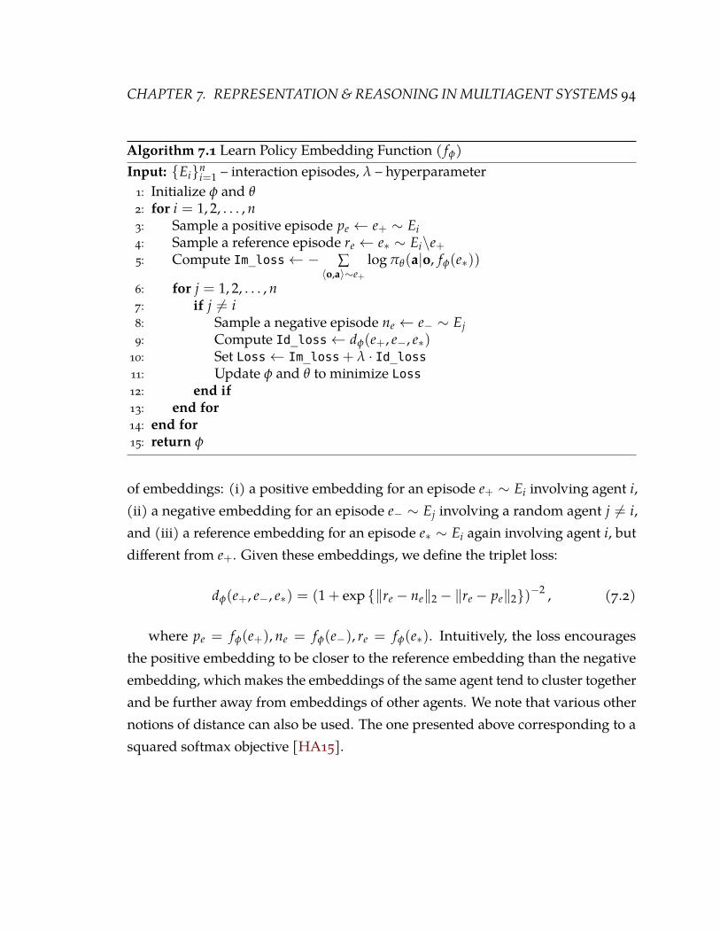
CHAPTER 7. REPRESENTATION&REASONING INMULTIAGENT SYSTEMS 94
Algorithm 7.1 Learn Policy Embedding Function ( fφ)Input: {Ei}n
i=1 – interaction episodes, λ – hyperparameter1: Initialize φ and θ2: for i = 1, 2, . . . , n3: Sample a positive episode pe ← e+ ∼ Ei4: Sample a reference episode re ← e∗ ∼ Ei\e+5: Compute Im_loss← − ∑
〈o,a〉∼e+log πθ(a|o, fφ(e∗))
6: for j = 1, 2, . . . , n7: if j 6= i8: Sample a negative episode ne ← e− ∼ Ej9: Compute Id_loss← dφ(e+, e−, e∗)
10: Set Loss← Im_loss+ λ · Id_loss11: Update φ and θ to minimize Loss12: end if13: end for14: end for15: return φ
of embeddings: (i) a positive embedding for an episode e+ ∼ Ei involving agent i,(ii) a negative embedding for an episode e− ∼ Ej involving a random agent j 6= i,and (iii) a reference embedding for an episode e∗ ∼ Ei again involving agent i, butdifferent from e+. Given these embeddings, we define the triplet loss:
dφ(e+, e−, e∗) = (1 + exp {‖re − ne‖2 − ‖re − pe‖2})−2 , (7.2)
where pe = fφ(e+), ne = fφ(e−), re = fφ(e∗). Intuitively, the loss encouragesthe positive embedding to be closer to the reference embedding than the negativeembedding, which makes the embeddings of the same agent tend to cluster togetherand be further away from embeddings of other agents. We note that various othernotions of distance can also be used. The one presented above corresponding to asquared softmax objective [HA15].
CHAPTER 7. REPRESENTATION& REASONING INMULTIAGENT SYSTEMS 95
7.3.3 Hybrid generative-contrastive representations
Conditional imitation learning encourages fφ to learn representations that cansimulate the entire policy of the agents and agent identification using a tripletloss incentivizes representations that can distinguish between agent policies. Bothobjectives are complementary, and we combine Eq. (7.1) and Eq. (7.2) to get thefinal objective used for representation learning:
1n
n
∑i=1
Ee+∼Ei,e∗∼Ei\e+
∑〈o,a〉∼e+
log πθ(a|o, fφ(e∗))︸ ︷︷ ︸imitation
−λ ∑j 6=i
Ee−∼Ej
[dφ(e+, e−, e∗)
]︸ ︷︷ ︸
agent identification
, (7.3)
where λ > 0 is a tunable hyperparameter that controls the relative weights of thecontrastive and generative terms. The pseudocode for the proposed algorithm isgiven in Algorithm 7.1. In experiments, we parameterize the conditional policyπθ and the embedding function fφ using deep neural networks and use stochasticgradient-based methods for optimization.
7.4 Generalization in Multiagent Systems
Generalization is well-understood for supervised learning—models that showssimilar train and test performance exhibit good generalization. To measure thequality of the learned representations for a multiagent system (MAS), we introducea graphical formalism for reasoning about agents and their interactions.
7.4.1 Generalization across agents & interactions
In many scenarios, we are interested in generalization of the policy representationfunction fφ across novel agents and interactions in a multiagent system. For in-stance, we would like fφ to output useful embeddings for a downstream task, evenwhen evaluated with respect to unseen agents and interactions. This notion of

CHAPTER 7. REPRESENTATION& REASONING INMULTIAGENT SYSTEMS 96
F
E
A
G B
C
D
Figure 7.1: Agent-Interaction Graph. An example of a graph used for evaluatinggeneralization in a multiagent system with 5 train agents (A, B, E, F, G) and 2 testagents (C, D).
generalization is best understood using agent-interaction graphs [Gro+18d].The agent-interaction graph describes interactions between a set of agent policies P
and a set of interaction episodes I through a graph G = (P, I).1 An example graphis shown in Figure 7.1. The graph represents a multiagent system consisting ofinteractions between pairs of agents, and we will especially focus on the interactionsinvolvingAlice, Bob, Charlie, andDavis. The interactions could be competitive (e.g.,a match between two agents) or cooperative (e.g., two agents communicating for anavigation task).
We learn the representation function fφ on a subset of the interactions, denoted bythe solid black edges in Figure 7.1. At test time, fφ is evaluated on some downstreamtask of interest. The agents and interactions observed at test time can be differentfrom those used for training. In particular, we consider the following cases:
Weak generalization. Here, we are interested in the generalization performance ofthe representation function on an unseen interaction between existing agents, all ofwhich are observed during training. This corresponds to the red edge representingthe interaction between Alice and Bob in Figure 7.1. From the context of an agent-interaction graph, the test graph adds only edges to the train graph.
Strong generalization. Generalization can also be evaluated with respect to un-seen agents (and their interactions). This corresponds to the addition of agents
1If we have more than two participating agents per interaction episode, we could represent theinteractions using a hypergraph.

CHAPTER 7. REPRESENTATION& REASONING INMULTIAGENT SYSTEMS 97
Charlie and Davis in Figure 7.1. Akin to a few shot learning setting, we observea few of their interactions with existing agents Alice and Bob (green edges) andgeneralization is evaluated on unseen interactions involvingCharlie andDavis (blueedges). The test graph adds both nodes and edges to the train graph.
For brevity, we skip discussion of weaker forms of generalization that involvesevaluation of the test performance on unseen episodes of an existing training edge(black edge).
7.4.2 Generalization across tasks
Since the representation function is learned using an unsupervised auxiliary objec-tive, we test its generalization performance by evaluating the usefulness of theseembeddings for various kinds downstream tasks described below.
Unsupervised. These embeddings can be used for clustering, visualization, andinterpretability of agent policies in a low-dimensional space. Such semantic associa-tions between the learned embeddings can be defined for a single agent wherein weexpect representations for the same agent based on distinct episodes to be embeddedclose to each other, or across agents wherein agents with similar policies will havesimilar embeddings on average.
Supervised. Deep neural network representations are especially effective for pre-dictive modeling. In a multiagent setting, the embeddings serve as useful featuresfor learning agent properties and interactions, including assignment of role cate-gories to agents with different skills in a collaborative setting, or prediction of winor loss outcomes of interaction matches between agents in a competitive setting.
Reinforcement. Finally, we can use the learned representation functions to im-prove generalization of the policies learned from a reinforcement signal in com-petitive and cooperative settings. We design policy networks that, in addition toobservations, take embedding vectors of the opposing agents as inputs. The em-beddings are computed from the past interactions of the opposing agent either

CHAPTER 7. REPRESENTATION& REASONING INMULTIAGENT SYSTEMS 98
(a) The RoboSumo environment.
0 0 1 01
Speaker 1
Listener
NEW
S
target landmark
1 1 0 100Speaker 2
(b) The ParticleWorld environment.
Figure 7.2: Illustrations for the environments used in our experiments: (a) competi-tive; and (b) cooperative.
with the agent being trained or with other agents using the representation function(Figure 7.3). Such embeddings play the role of privileged information and allow usto train a policy network that uses this information to learn faster and generalizebetter to opponents or cooperators unseen at training time.
7.5 Empirical Evaluation
We evaluate the proposed framework for both competitive and collaborative envi-ronments on various downstream machine learning tasks. In particular, we usethe RoboSumo and ParticleWorld environments for the competitive and collabo-rative scenarios, respectively. We consider the embedding objectives in Eq. (7.1),Eq. (7.2), and Eq. (7.3) independently and refer to them as Emb-Im, Emb-Id, andEmb-Hyb respectively. The hyperparameter λ for Emb-Hyb is chosen by grid searchover λ ∈ {0.01, 0.05, 0.1, 0.5} on a held-out set of interactions.

CHAPTER 7. REPRESENTATION& REASONING INMULTIAGENT SYSTEMS 99
previousinterac-tions
πtψ
fφ
et πA
et−1et−1et−1et−1 πt−1ψ
Figure 7.3: Illustration of the proposed model for optimizing a policy πψ thatconditions on an embedding of the opponent policy πA. At time t, the pre-trainedrepresentation function fφ computes the opponent embedding based on a pastinteraction et−1. We optimize πψ to maximize the expected rewards in its currentinteractions et with the opponent.
In all our experiments, the representation function fφ is specified through amulti-layer perceptron (MLP) that takes as input an episode and outputs an embedding ofthat episode. In particular, the MLP takes as input a single (observation, action) pairto output an intermediate embedding. We average the intermediate embeddings forall (observation, action) pairs in an episode to output an episode embedding. Tocondition a policy network on the embedding, we simply concatenate the observationfed as input to the network with the embedding.
7.5.1 The RoboSumo environment
For the competitive environment, we use RoboSumo [Al-+18]—a 3D environmentwith simulated physics (based on MuJoCo [TET12]) that allows agents to controlmulti-legged 3D robots and compete against each other in continuous-timewrestlinggames (Figure 7.2a). For our analysis, we train a diverse collection of 25 agents,some of which are trained via self-play and others are trained in pairs concurrentlyusing Proximal Policy Optimization (PPO) algorithm [Sch+17b].
We start with a fully connected agent-interaction graph (clique) of 25 agents.Every edge in this graph corresponds to 10 rollout episodes involving the corre-sponding agents. The maximum length (or horizon) of any episode is 500 timesteps, after which the episode is declared a draw. To evaluate weak generalization,we sample a connected subgraph for training with approximately 60% of the edges

CHAPTER7. REPRESENTATION&REASONING INMULTIAGENTSYSTEMS 100
first eigenvector
second eigenvector
third eigenvector
(a) RoboSumo: Weakfirst eigenvector
second eigenvector
third eigenvector
(b) RoboSumo: Strong
first eigenvector
second eigenvector
third eigenvector(c) ParticleWorld: Weak
first eigenvector
second eigenvector
third eigenvector
(d) ParticleWorld: Strong
Figure 7.4: Embeddings learned using Emb-Hyb for 10 test interaction episodesof 5 agents projected on the first three principal components for RoboSumo andParticleWorld. Color denotes agent policy.
preserved for training, and remaining split equally for validation and testing. Forstrong generalization, we preserve 15 agents and their interactions with each otherfor training, and similarly, 5 agents and their within-group interactions each forvalidation and testing.
Embedding analysis. To evaluate the robustness of the embeddings, we computemultiple embeddings for each policy based on different episodes of interaction attest time. Our evaluation metric is based on the intra- and inter-cluster Euclidean

CHAPTER7. REPRESENTATION&REASONING INMULTIAGENTSYSTEMS 101
Table 7.1: Intra-inter clustering ratios (IICR) and accuracies for outcome prediction(Acc) for weak (W) and strong (S) generalization on RoboSumo.
IICR (W) IICR (S) Acc (W) Acc(S)Emb-Im 0.24 0.23 0.71 0.60Emb-Id 0.25 0.27 0.67 0.56Emb-Hyb 0.22 0.21 0.73 0.56
0 1000 2000Iteration
0.25
0.50
0.75
1.00
Win
rate
Train
PPOPPO + Emb-ImPPO + Emb-IdPPO + Emb-Hyb
0 1000 2000
0.2
0.4
0.6
0.8Test
0 1000 2000Iteration
0.25
0.50
0.75
1.00
Win
rate
Train
PPOPPO + Emb-onlinePPO + Emb-offlinePPO + Emb-zeroPPO + Emb-rand
0 1000 2000
0.25
0.50
0.75
1.00
Test
Figure 7.5: Average win rates of the newly trained agents against 5 training agentand 5 testing agents. (a) Top: Baseline comparison with policies that make use ofEmb-Im, Emb-Id, and Emb-Hyb (all computed online). (b) Bottom: Comparison ofdifferent baseline embeddings used at evaluation time (all embedding-conditionedpolicies use Emb-Hyb). At each iteration, win rates were computed based on 501-on-1 games. Each agent was trained 3 times, each time from a different randominitialization. Shaded regions correspond to 95% CI.

CHAPTER7. REPRESENTATION&REASONING INMULTIAGENTSYSTEMS 102
0 1000Iteration
0.0
0.5
1.0
Rat
eEmb-Hyb vs. PPO
Win Loss Draw0 1000
Emb-Hyb vs. Emb-Im
0 1000
Emb-Hyb vs. Emb-Id
0 1000
Emb-Im vs. PPO
0 1000
Emb-Im vs. Emb-Id
0 1000
Emb-Id vs. PPO
Figure 7.6: Win, loss, and draw rates plotted for the first agent in each pair. Eachpair of agents was evaluated after each training iteration on 50 1-on-1 games; curvesare based on 5 evaluation runs. Shaded regions correspond to 95% CI.
1 2 3 4
PPO + Emb-Hyb - 4
PPO + Emb-Id - 3
PPO + Emb-Im - 2
PPO - 1
0.67 0.61 0.57 0.48
0.62 0.44 0.50 0.42
0.55 0.49 0.55 0.36
0.51 0.44 0.36 0.32
Figure 7.7: Win rates for agents specified in each row at computed at iteration 1000.
distances between embeddings. The intra-cluster distance for an agent is the averagepairwise distance between its embeddings computed on the set of test interactionepisodes involving the agent. Similarly, the inter-cluster distance is the averagepairwise distance between the embeddings of an agent with those of other agents.Let Ti = {t
(i)c }ni
c=1 denote the set of test interactions involving agent i. We define theintra-inter cluster ratio (IICR) as:
IICR =
1n ∑n
i=11
n2i
∑nia=1 ∑ni
b=1 ‖t(i)a − t(i)b ‖2
1n(n−1)
n∑
i=1
n∑j 6=i
1ninj
ni∑
a=1
nj
∑b=1‖t(i)a − t(j)
b ‖2
.

CHAPTER7. REPRESENTATION&REASONING INMULTIAGENTSYSTEMS 103
The intra-inter clustering ratios are reported in Table 7.1. A ratio less than 1
suggests that there is signal that identifies the agent, and the signal is strongerfor lower ratios. Even though this task might seem especially suited for the agentidentification objective, we interestingly find that the Emb-Im attains lower clusteringratios than Emb-Id for both weak and strong generalization. Emb-Hyb outperformsboth these methods. We qualitatively visualize the embeddings learned usingEmb-Hyb by projecting them on the leading principal components, as shown inFigures 7.4a and 7.4b for 10 test interaction episodes of 5 randomly selected agentsin the weak and strong generalization settings respectively.
Outcomeprediction. We can use these embeddings directly for training a classifierto predict the outcome of an episode (win/loss/draw). For classification, we use anMLP with 3 hidden layers of 100 units each and the learning objective minimizes thecross entropy error. The input to the classifier are the embeddings of the two agentsinvolved in the episode. The results are reported in Table 7.1. Again, imitation basedmethods seem more suited for this task with Emb-Hyb and Emb-Im outperformingother methods for weak and strong generalization respectively.
Policy optimization. Here we ask whether embeddings can be used to improvelearned policies in a reinforcement learning setting both in terms of end performanceand generalization. To this end, we select 5 training, 5 validation, and 5 testingopponents from the pool of 25 pre-trained agents. Next, we train a new agent withreinforcement learning to compete against the selected 5 training opponents; theagent is trained concurrently against all 5 opponents using a distributed version ofPPO algorithm, as described in [Al-+18]. Throughout training, we evaluate newagents on the 5 testing opponents and record the average win and draw rates.
Using this setup, we compare a baseline agent with MLP-based policy withan agent whose policy takes 100-dimensional embeddings of the opponents asadditional inputs at each time step and uses that information to condition its behavioron the opponent’s representation. The embeddings for each opponent are eithercomputed online, i.e., based on an interaction episode rolled out during training at a

CHAPTER7. REPRESENTATION&REASONING INMULTIAGENTSYSTEMS 104
previous time step (Figure 7.3), or offline, i.e., pre-computed before training the newagent using only interactions between the pre-trained opponents.
Figure 7.5 shows the average win rates against the set of training and testingopponents for the baseline and our agents that use different types of embeddings.While every new agent is able to achieve almost 100% win rate against the trainingopponents, we see that the agents that condition their policies on the opponent’sembeddings generalize better on the held-out set of opponents, with the best perfor-mance achieved with Emb-Hyb. We also note that embeddings computed offline leadto better performance than the ones computed online.2 As an ablation test, we alsoevaluate our agents when they are provided an incorrect embedding (either all zeros,Emb-zero, or an embedding selected for a different random opponent, Emb-rand)and observe that such embeddings lead to a degradation in performance.3
Finally, to evaluate strong generalization in the RL setting, we pit the newlytrained baseline and agents with embedding-conditional policies against each other.Since the embedding network has never seen the new agents, it must exhibit stronggeneralization to be useful in such setting. The results are give in Figures 7.6 and 7.7.Even though the margin is not very large, the agents that use Emb-Hyb perform thebest on average.
7.5.2 The ParticleWorld environment
For the collaborative setting, we evaluate the framework on the ParticleWorld
environment for cooperative communication [MA18; Low+17]. The environmentconsists of a continuous 2D grid with 3 landmarks and two kinds of agents collabo-rating to navigate to a common landmark goal (Figure 7.2b). At the beginning ofevery episode, the speaker agent is shown the RGB color of a single target landmarkon the grid. The speaker then communicates a fixed length binary message to thelistener agent. Based on the received messages, the listener agent the moves in a
2Perhaps, this is due to differences in the interactions of the opponents between themselves andwith the new agent that the embedding network was not able to capture entirely.
3Performance decrease is most significant for Emb-zero, which is an out-of-distribution all-zerosvector.

CHAPTER7. REPRESENTATION&REASONING INMULTIAGENTSYSTEMS 105
Table 7.2: Intra-inter clustering ratios (IICR) for weak (W) and strong (S) general-ization on ParticleWorld. Lower is better.
IICR (W) IICR (S)Emb-Im 0.58 0.86Emb-Id 0.50 0.82Emb-Hyb 0.54 0.85
Table 7.3: Average train and test rewards for speaker policies on ParticleWorld.
Train TestMADDPG −11.66 −18.99MADDPG + Emb-Im −11.68 −17.75MADDPG + Emb-Id −11.68 −17.68MADDPG + Emb-Hyb −11.77 −17.20
particular direction. The final reward, shared across the speaker and listener agents,is the distance of the listener to the target landmark after a fixed time horizon.
The agent-interaction graph for this environment is bipartite with only crossedges between speaker and listener agents. Every interaction edge in this graphcorresponds to 1000 rollout episodeswhere themaximum length of any episode is 25
steps. We pretrain 28 MLP parameterized speaker and listener agent policies. Everyspeaker learns through communication with only two different listeners and vice-versa, giving an extremely sparse agent-interaction graph. We explicitly encodeddiversity in these speakers and listener agents by masking bits in the communicationchannel. In particular, we masked 1 or 2 randomly selected bits for every speakeragent in the graph to give a total of (7
1)+ (72) = 28 distinct speaker agents. Depending
on the neighboring speaker agents in the agent-interaction graph, the listener agentsalso show diversity in the learned policies. The policies are learned usingmultiagentdeep deterministic policy gradients (MADDPG) [Low+17].
In this environment, the speakers and listeners are tightly coupled. Hencewe vary the setup used previously in the competitive scenario. We wish to learnembeddings of listeners based on their interactions with speakers. Since the agent-interaction graph is bipartite, we use the embeddings of listener agents to conditiona shared policy network for the respective speaker agents.

CHAPTER7. REPRESENTATION&REASONING INMULTIAGENTSYSTEMS 106
Embedding analysis. For the weak generalization setting, we remove an outgoingedge from every listener agent in the original graph to obtain the training graph. Inthe case of strong generalization, we set aside 7 listener agents (and their outgoingedges) each for validation and testing while the representation function is learnedon the remaining 14 listener agents and their interactions. The intra-inter cluster-ing ratios are shown in Table 7.2, and the projections of the embeddings learnedusing Emb-Hyb are visualized in Figure 7.4c and Figure 7.4d for weak and stronggeneralization respectively. In spite of the high degree of sparsity in the traininggraph, the intra-inter clustering ratio for the test interaction embeddings is less thanunity suggesting an agent-specific signal. Emb-id works particularly well in thisenvironment, achieving best results for both weak and strong generalization.
Policy optimization. Here, we are interested in learning speaker agents that cancommunicatemore effectively with amuchwider range of listeners given knowledgeof their embeddings. Referring back to Figure 7.3, we learn a policy πψ for a speakeragent that conditions on the representation function fφ for the listener agents. Forcooperative communication, we consider interactions with 14 pre-trained listeneragents split as 6 training, 4 validation, and 4 test agents.4 Similar to the competitivesetting, we compare performance against a baseline speaker agent that does not haveaccess to any privilege information about the listeners. We summarize the resultsfor the best validated models during training and 100 interaction episodes per testlistener agent across 5 initializations in Table 7.3. From the results, we observe thatonline embedding based methods can generalize better than the baseline methods.The baseline MADDPG achieves the lowest training error, but fails to generalizewell enough and incurs a low average reward for the test listener agents.
4None of the methods considered were able to learn a non-trivial speaker agent when trainedsimultaneously with all 28 listener agents. Hence, we simplified the problem by considering the 14listener agents that attained the best rewards during pretraining.

CHAPTER7. REPRESENTATION&REASONING INMULTIAGENTSYSTEMS 107
7.6 Discussion & Related Work
Agent modeling is a well-studied topic within multiagent systems. See [AS17] foran excellent survey. The vast majority of literature in agent modeling concernswith learning models for a specific predictive task. Predictive tasks are typicallydefined over actions, goals, and beliefs of other agents [SV00]. In competitive do-mains such as Poker and Go, such tasks are often integrated with domain-specificheuristics to model opponents and learn superior policies [RW11; Mni+15]. Simi-larly, intelligent tutoring systems take into account pedagogical features of studentsand teachers to accelerate learning of desired behaviors in a collaborative environ-ment [McC+00]. In contrast, we sidestep any domain specific assumptions andlearn representations in an unsupervised manner which extends their utility beyondgame playing [Mni+15] and predictive modeling [Hos17].
Both the generative and contrastive components of our framework have beenexplored independently in other contexts in prior work. Imitation learning has beenextensively studied in the single-agent setting [Osa+18]. Recent work by [LYC17]proposes an algorithm for imitation in a coordinatedmultiagent system. [Wan+17b]proposed an imitation learning algorithm for learning robust controllers with fewexpert demonstrations in a single-agent setting that conditions the policy networkon an inference network, similar to the encoder in our framework.
Agent identification which represents the contrastive term in the learning ob-jective is based on triplet losses. Triplet losses are used within Siamese networksto learn representations of data points using distance comparisons in a featurespace [HA15]. Several other methods also exist for defining positive and negativeexamples for contrastive representation learning. For instance, the widely usedword2vec framework for language uses co-occurrence statistics to define similar or‘‘positive” examples [Mik+13] and has been extended to relational graph domainsas well via random walks [PAS14; GL16]. Recently, contrastive methods have alsobeen successfully applied for representation learning of sequential data in latentvariable models [OLV18].

CHAPTER7. REPRESENTATION&REASONING INMULTIAGENTSYSTEMS 108
7.7 Conclusion
In this work, we presented a framework for learning representations of agent policiesin multiagent systems. The agent policies are accessed using a few interactionepisodes with other agents. Our learning objective is based on a novel combinationof a generative component based on imitation learning and a contrastive componentfor distinguishing the embeddings of different agent policies. Our overall frameworkis unsupervised, sample-efficient, and domain-agnostic, and hence can be readilyextended to many environments and downstream tasks. Most importantly, weshowed the role of these embeddings as privileged information for learning moreadaptive agent policies in both collaborative and competitive settings.

Part III
Applications in Science & Society
109

8 Compressed Sensing viaGenerativeMod-els
8.1 Introduction
Compressed sensing is a class of techniques used to efficiently acquire and recoverhigh-dimensional data using compressed measurements much fewer than the datadimensionality. The celebrated results in compressed sensing posit that sparse, high-dimensional data points can be acquired using much fewer measurements (roughlylogarithmic) than the data dimensionality [CT05; Don06; CRT06]. The acquisitionis done using certain classes of random matrices and the recovery procedure isbased on LASSO [Tib96; BRT09]. The assumptions of sparsity are fairly generaland can be applied ‘‘out-of-the-box” for many data modalities, e.g., images andaudio are typically sparse in the wavelet and Fourier basis respectively. However,such sparsity assumptions ignore the statistical nature of many real-world problems,where we increasingly have access to training datasets for domains of interest.
In this chapter, we design a framework for compressed sensing based on genera-tive modeling that exploits such auxilliary training data to learn the acquisition andrecovery procedures for compressed sensing, thereby sidestepping generic sparsityassumptions. In particular, we introduce a new autoencoding framework termed asuncertainty autoencoders (UAE). A UAE parameterizes the acquisition and recoveryprocedures for compressed sensing as the encoding and decoding phases of an
110

CHAPTER 8. COMPRESSED SENSING VIA GENERATIVE MODELS 111
autoencoder with stochastic latent variables. The stochastic latents correspond tothe (noisy) compressed measurements for the data point input to the encoder.
The learning objective for a UAE is based on the InfoMax principle, which seeksto learn encodings that maximize themutual information between the observed datapoints and compressed representations [Lin89]. Since the mutual information istypically intractable in high-dimensions, we instead maximize tractable variationallower bounds using a parametric decoder [BA03; Ale+17]. Unlike LASSO-basedrecovery, a parametric decoder amortizes the recovery process, which requires onlya forward pass through the decoder at test time and thus enables scalability to largedatasets [GG14; Shu+18].
We show theoretically under suitable assumptions that an uncertainty autoen-coder is an implicit generative model of the underlying data distribution [ML16], i.e.,a UAE permits sampling from the learned data distribution even though it does notspecify an explicit likelihood function. Hence, it directly contrasts with variationalautoencoders (VAE) which specify an explicit but intractable likelihood function[KW18]. Unlike a VAE, a UAEdoes not require specifying a prior over the latents andhence offsets pathologically observed scenarios that cause the latent representationsto be uninformative when used with expressive decoders [Che+17b].
We evaluateUAEs for statistical compressed sensing of high-dimensional datasets.On the MNIST, Omniglot, and CelebA datasets, we observe average improvementsof 38%, 31%, and 28% in recovery over the closest benchmark. We also demonstratethat uncertainty autoencoders demonstrate good generalization performance acrossdomains, where the encoder/decoder trained on a source dataset are transferredover for compressed sensing of another target dataset.
8.2 Preliminaries
Compressed sensing (CS). Let the data point andmeasurements be denotedwithmultivariate random variables X ∈ Rn and Y ∈ Rm respectively. For the purposeof compressed sensing, we assume m < n and relate these variables through ameasurement matrix W ∈ Rm×l and a parameterized acquisition function fψ :

CHAPTER 8. COMPRESSED SENSING VIA GENERATIVE MODELS 112
Rn → Rl (for any integer l > 0) such that:
y = W fψ(x) + ε (8.1)
where ε is the measurement noise. The goal in compressed sensing is to recover x
given the measurements y. If we let fψ(·) be the identity function (i.e., fψ(x) = x
for all x), then we recover a standard system of underdetermined linear equationswhere measurements are linear combinations of the data point corrupted by noise.In all other cases, the acquisition function transforms x such that fψ(x) is potentiallymore amenable for compressed sensing. For instance, fψ(·) could specify a changeof basis that encourages sparsity, e.g., a Fourier basis for audio. Note that we allowthe codomain of the mapping fψ(·) to be defined on a higher or lower dimensionalspace (i.e., l 6= n in general).
Sparse CS. To obtain nontrivial solutions to an underdetermined system, X isassumed to be sparse in some basis B. We are not given any additional informa-tion about X. The measurement matrix W is a random Gaussian matrix and therecovery is done via LASSO [CT05; Don06; CRT06]. LASSO solves for a convex`1-minimization problem such that the reconstruction x for any data point x is givenas: x = arg minx ‖Bx‖1 + λ‖y−Wx‖2
2 where λ > 0 is a tunable hyperparameter.
Statistical CS. In statistical compressed sensing, we are additionally given accessto a set of signals D, such that each x ∈ D is assumed to be sampled i.i.d. from adata distribution qdata [YS11]. Using this dataset, we learn the the measurementmatrix W and the acquisition function fψ(·) in Eq. (8.1).
At test time, we directly observe the measurements ytest that are assumed tosatisfy Eq. (8.1) for a target data point xtest ∼ qdata(X) and the task is to providean accurate reconstruction xtest. Evaluation is based on the reconstruction errorbetween xtest and xtest. Particularly relevant to this work, we can optionally learn arecovery function gθ : Rm → Rn to reconstruct x given the measurements y.
This amortized approach is in contrast to standard LASSO-based decodingwhichsolves an optimization problem for every new data point at test time. If we learned

CHAPTER 8. COMPRESSED SENSING VIA GENERATIVE MODELS 113
the recovery function gθ(·) during training, then xtest = gθ(ytest) and the `2 erroris given by ‖xtest − gθ(ytest)‖2. Such a recovery process requires only a functionevaluation at test time and permits scaling to large datasets [GG14; Shu+18].
Autoencoders. Anautoencoder is a pair of parameterized functions (e, d) designedto encode and decode data points. For a standard autoencoder, let e : Rn → Rm
and d : Rm → Rn denote the encoding and decoding functions respectively for ann-dimensional data point and an m-dimensional latent space. The learning objectiveminimizes the `2 reconstruction error over a dataset D:
mine,d
∑x∈D‖x− d(e(x))‖2
2 (8.2)
where e and d are typically parameterized using deep neural networks.
8.3 Uncertainty Autoencoders
Consider a joint distribution between the signals X and the measurements Y, whichfactorizes via chain rule as qφ(X, Y) = qdata(X)qφ(Y|X). Here, qdata(X) is a fixed datadistribution and qφ(Y|X) is a parameterized observation model that depends onthe measurement noise ε, as given by Eq. (8.1). For instance, for isotropic Gaussiannoise ε with a fixed variance σ2, we have qφ(Y|X) = N (W fψ(X), σ2 Im).
In an uncertainty autoencoder, we wish to learn the parameters φ that permitefficient and accurate recovery of a signal X using the measurements Y. In order todo so, we propose to maximize the mutual information between X and Y:
maxφ
Iφ(X, Y) =∫
qφ(x, y) logqφ(x, y)
qdata(x)qφ(y)dxdy
= H(X)− Hφ(X|Y) (8.3)
where H denotes differential entropy. The intuition is simple: if the measurementspreservemaximum information about the signal, we can hope that recoverywill havelow reconstruction error. We formalize this intuition by noting that this objective

CHAPTER 8. COMPRESSED SENSING VIA GENERATIVE MODELS 114
is equivalent to maximizing the average log-posterior probability of X given Y. Infact, in Eq. (8.3), we can omit the term corresponding to the data entropy (since itis independent of φ) to get the following equivalent objective:
maxφ−Hφ(X|Y) = Eqφ(X,Y)[log qφ(x|y)]. (8.4)
Even though the mutual information is maximized and equals the data entropywhen Y = X, the dimensionality constraints on m� n, the parametric assumptionson fψ(·), and the noise model prohibit learning an identity mapping. Note thatthe properties of noise ε such as the distributional family and sufficient statisticsare externally specified. For example, these could be specified based on propertiesof the measurement device for compressed sensing. More generally for unsuper-vised representation learning, we treat these properties as hyperparameters tunedbased on the reconstruction loss on a held-out set, or any other form of availablesupervision. It is not suggested to optimize for these statistics during learning as theUAE would tend to shrink this noise to zero to maximize mutual information, thusignoring measurement uncertainty in the context of compressed sensing and pre-venting generalization to out-of-distribution examples for representation learning.Theorem 8.1 analyzes the effect of noise more formally.
Estimating mutual information between arbitrary high dimensional randomvariables can be challenging. However, we can lower bound the mutual informationby introducing a variational approximation to the model posterior qφ(X|Y) [BA03].Denoting this approximation as pθ(X|Y), we get the following lower bound:
Iφ(X, Y) ≥ H(X) + Eqφ(X,Y) [log pθ(x|y)] . (8.5)
Comparing Eqs. (8.3, 8.4, 8.5), we can see that the second term in Eq. (8.5) approx-imates the intractable negative conditional entropy, −Hφ(X|Y) with a variationallower bound. Optimizing this bound leads to a decoding distribution given bypθ(X|Y) with variational parameters θ. The bound is tight when there is no dis-tortion during recovery, or equivalently when the decoding distribution pθ(X|Y)
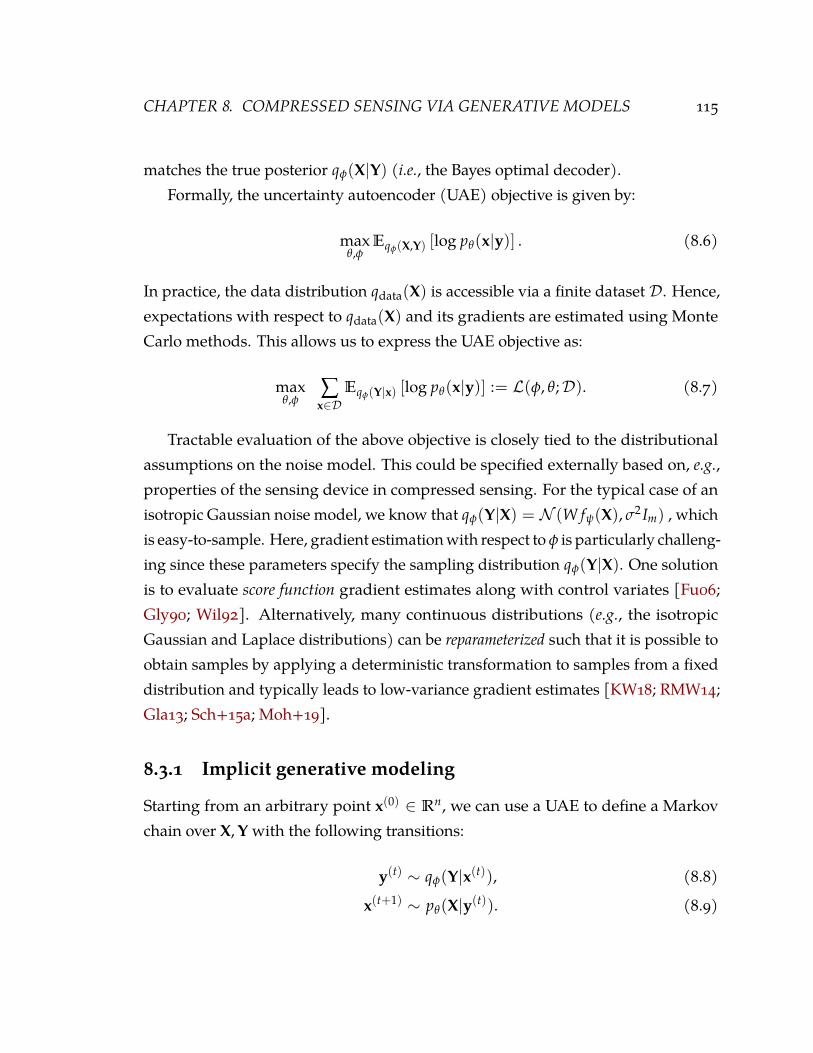
CHAPTER 8. COMPRESSED SENSING VIA GENERATIVE MODELS 115
matches the true posterior qφ(X|Y) (i.e., the Bayes optimal decoder).Formally, the uncertainty autoencoder (UAE) objective is given by:
maxθ,φ
Eqφ(X,Y) [log pθ(x|y)] . (8.6)
In practice, the data distribution qdata(X) is accessible via a finite dataset D. Hence,expectations with respect to qdata(X) and its gradients are estimated using MonteCarlo methods. This allows us to express the UAE objective as:
maxθ,φ
∑x∈D
Eqφ(Y|x) [log pθ(x|y)] := L(φ, θ;D). (8.7)
Tractable evaluation of the above objective is closely tied to the distributionalassumptions on the noise model. This could be specified externally based on, e.g.,properties of the sensing device in compressed sensing. For the typical case of anisotropic Gaussian noise model, we know that qφ(Y|X) = N (W fψ(X), σ2 Im) , whichis easy-to-sample. Here, gradient estimationwith respect to φ is particularly challeng-ing since these parameters specify the sampling distribution qφ(Y|X). One solutionis to evaluate score function gradient estimates along with control variates [Fu06;Gly90; Wil92]. Alternatively, many continuous distributions (e.g., the isotropicGaussian and Laplace distributions) can be reparameterized such that it is possible toobtain samples by applying a deterministic transformation to samples from a fixeddistribution and typically leads to low-variance gradient estimates [KW18; RMW14;Gla13; Sch+15a; Moh+19].
8.3.1 Implicit generative modeling
Starting from an arbitrary point x(0) ∈ Rn, we can use a UAE to define a Markovchain over X, Y with the following transitions:
y(t) ∼ qφ(Y|x(t)), (8.8)
x(t+1) ∼ pθ(X|y(t)). (8.9)

CHAPTER 8. COMPRESSED SENSING VIA GENERATIVE MODELS 116
Theorem 8.1. Let θ∗, φ∗ denote an optimal solution to the UAE objective in Eq. (8.6). Ifthere exists a φ such that qφ(x|y) = pθ∗(x|y) and the Markov chain defined in Eqs. (8.8,8.9) is ergodic, then the stationary distribution of the chain for the parameters φ∗ and θ∗ isgiven by qφ∗(X, Y).
Proof. See Appendix A.2.
The above theorem suggests an interesting insight into the behavior of UAEs.Under idealized conditions, the learnedmodel specifies an implicit generativemodelfor qφ∗(X, Y). Further, ergodicity can be shown to hold for the isotropic Gaussiannoise model.
Corollary 8.1. Let θ∗, φ∗ denote an optimal solution to the UAE objective in Eq. (8.6). Ifthere exists a φ such that qφ(x|y) = pθ∗(x|y) and the noise model is Gaussian, then thestationary distribution of the chain for the parameters φ∗ and θ∗ is given by qφ∗(X, Y).
Proof. See Appendix A.3.
The marginal of the joint distribution qφ(X, Y) with respect to X corresponds tothe data distribution. A UAE hence seeks to learn an implicit generative model ofthe data distribution [DG84; ML16], i.e., even though we do not have a tractableestimate for the likelihood of the model, we can generate samples using the Markovchain transitions defined in Eqs. (8.8, 8.9).
8.3.2 Comparison with Principal Component Analysis
AUAE can also be viewed as a dimensionality reduction technique. While in generalthe encoding performing this reduction can be nonlinear, the case of a linear encodingis one where the projection vectors are given as the rows of the measurement matrixW. In such a setting, a closely related objective for linear dimensionality reduction isPrincipal Component Analysis (PCA) [Pea01]. The objective for PCA is to find thedirections that explain the most variance in the data. As noted in prior work [BA03;WCF07], the principal components however may not be the the most informativelow-dimensional projections for recovering the original high-dimensional data back

CHAPTER 8. COMPRESSED SENSING VIA GENERATIVE MODELS 117
10.0 7.5 5.0 2.5 0.0 2.5 5.0 7.5 10.0
6
4
2
0
2
4
6
0.0020.004
0.006
0.00
8
0.010
0.010
0.01
2
0.012
0.014
0.014
0.016
0.016
0.018
0.018
0.020
0.020
PCA projectionUAE projectiondataPCA projected dataUAE projected data
Figure 8.1: Dimensionality reduction using PCA vs. UAE. Projections of the data(black points) on the UAE direction (green line) maximize the likelihood of de-coding unlike the PCA projection axis (magenta line) which collapses many pointsin a narrow region.
from its projections. A UAE, on the other hand, is explicitly designed to preserve asmuch information as possible (see Eq. (8.4)).
We illustrate the differences in a synthetic experiment in Figure 8.1. The truedata distribution is an equiweighted mixture of two Gaussians stretched alongorthogonal directions. We sample 100 points (black) from this mixture and considertwo dimensionality reductions. In the first case, we project the data on the firstprincipal component (blue points on magenta line). This axis captures a largefraction of the variance in the data but collapses data sampled from the bottomright Gaussian in a narrow region. The projections of the data on the UAE axis (redpoints on green line) are more spread out. This suggest that recovery is easier, evenif doing so increases the total variance in the projected space compared to PCA.

CHAPTER 8. COMPRESSED SENSING VIA GENERATIVE MODELS 118
8.4 Empirical Evaluation
8.4.1 Statistical compressed sensing
We perform compressed sensing on three high-dimensional datasets with a setof low number of measurements: m ∈ {2, 5, 10, 25, 50, 100} measurements forMNIST [LCB10] and Omniglot [LST15] with 28 × 28 = 784 dimensions, andm = {20, 50, 100, 200, 500} for CelebA dataset [Liu+15] with 64× 64× 3 = 12288
dimensions. We first discuss the MNIST and Omniglot datasets here since theyhave a similar setup. Every image in MNIST and Omniglot has a dimensionality of28× 28. In all our experiments, we assume a Gaussian noise model with σ = 0.1.We evaluated UAE against the following baselines:
• LASSO decoding with random Gaussian matrices. The MNIST and Omniglotdatasets are reasonably sparse in the canonical pixel basis, and hence, we did notobserve any gains after applying Discrete Cosine Transform and Daubechies-1Wavelet Transform.
• CS-VAE. This approach to compressed sensing was proposed by [Bor+17] andlearns a latent variable generative model over the observed variables X and thelatent variables Z. Such a model defines a mapping Gθ : Rk → Rn from Z toX, which is given by either the mean function of the observation model for aVAE or the forward deterministic mapping to generate samples for a GAN. Weuse VAEs in our experiments. Thereafter, using a random Gaussian or Bernoulliacquisition matrix (say W), the reconstruction x for any data point is given asx = Gθ(arg minz∈Rk ‖y−WGθ(z)‖2). Intuitively, this procedure seeks the latentvector z such that the corresponding point on the range of G can best approximatethe measurements y under the mapping W. We used the default parametersettings and architectures proposed in [Bor+17].
• RP-UAE. This ablation baseline encodes the data using Gaussian random pro-jections (RP) and trains the decoder based on the UAE objective in order toindependently evaluate the effect of variational decoding. Since LASSO and
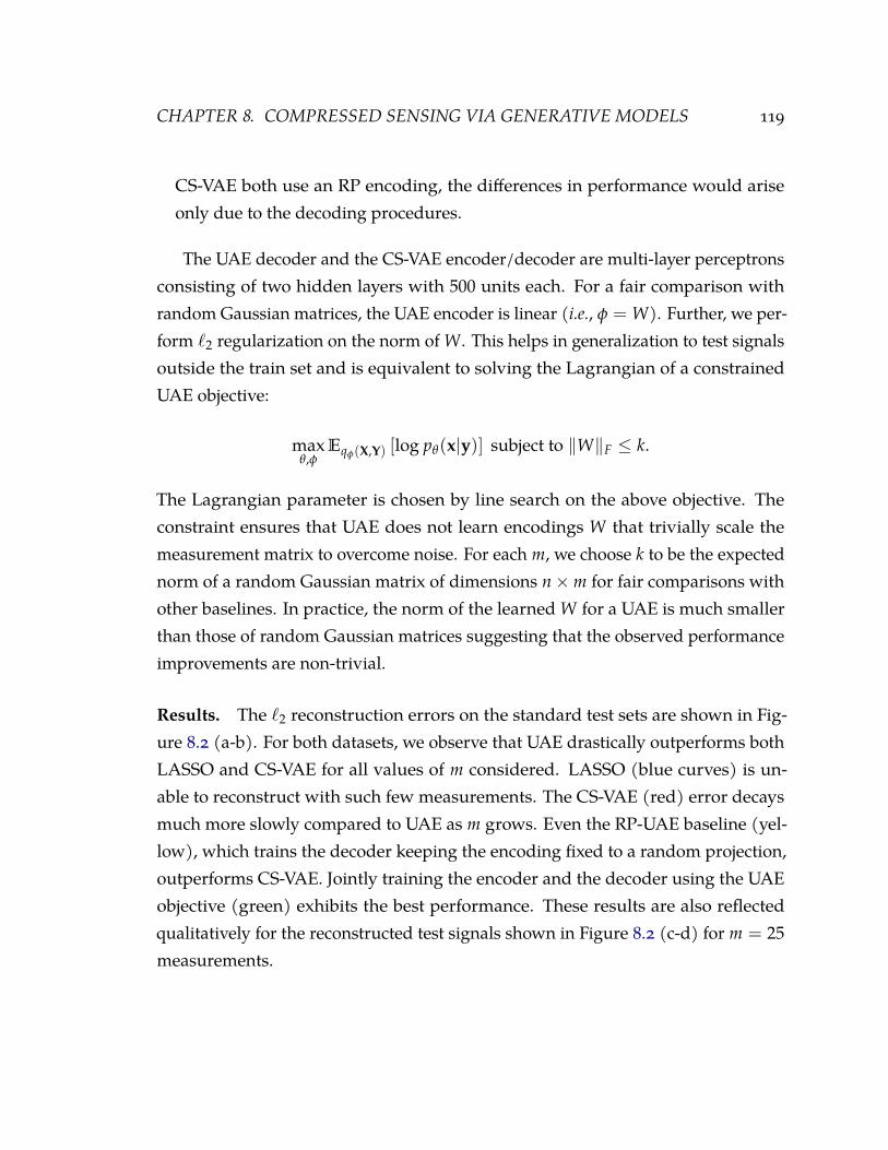
CHAPTER 8. COMPRESSED SENSING VIA GENERATIVE MODELS 119
CS-VAE both use an RP encoding, the differences in performance would ariseonly due to the decoding procedures.
The UAE decoder and the CS-VAE encoder/decoder are multi-layer perceptronsconsisting of two hidden layers with 500 units each. For a fair comparison withrandom Gaussian matrices, the UAE encoder is linear (i.e., φ = W). Further, we per-form `2 regularization on the norm of W. This helps in generalization to test signalsoutside the train set and is equivalent to solving the Lagrangian of a constrainedUAE objective:
maxθ,φ
Eqφ(X,Y) [log pθ(x|y)] subject to ‖W‖F ≤ k.
The Lagrangian parameter is chosen by line search on the above objective. Theconstraint ensures that UAE does not learn encodings W that trivially scale themeasurement matrix to overcome noise. For each m, we choose k to be the expectednorm of a random Gaussian matrix of dimensions n×m for fair comparisons withother baselines. In practice, the norm of the learned W for a UAE is much smallerthan those of random Gaussian matrices suggesting that the observed performanceimprovements are non-trivial.
Results. The `2 reconstruction errors on the standard test sets are shown in Fig-ure 8.2 (a-b). For both datasets, we observe that UAE drastically outperforms bothLASSO and CS-VAE for all values of m considered. LASSO (blue curves) is un-able to reconstruct with such few measurements. The CS-VAE (red) error decaysmuch more slowly compared to UAE as m grows. Even the RP-UAE baseline (yel-low), which trains the decoder keeping the encoding fixed to a random projection,outperforms CS-VAE. Jointly training the encoder and the decoder using the UAEobjective (green) exhibits the best performance. These results are also reflectedqualitatively for the reconstructed test signals shown in Figure 8.2 (c-d) for m = 25
measurements.

CHAPTER 8. COMPRESSED SENSING VIA GENERATIVE MODELS 120
0 20 40 60 80 100num measurements
2
3
4
5
6
7
8
9
l 2re
cons
truc
tion
erro
r
LASSO
CS-VAE
RP-UAE
UAE
(a) MNIST
0 20 40 60 80 100num measurements
3
4
5
6
7
l 2re
cons
truc
tion
erro
r
(b) Omniglot
Orig
inal
LASS
OCS
-VAE
UAE
(c) MNIST
Orig
inal
LASS
OCS
-VAE
UAE
(d) Omniglot
Figure 8.2: (a-b) Test `2 reconstruction error (per image) for compressed sensing.(c-d) Reconstructions for m = 25. First: Original. Second: LASSO. Third: CS-VAE.Last: UAE. 25 projections of the data are sufficient for UAE to reconstruct the originalimage with high accuracy.
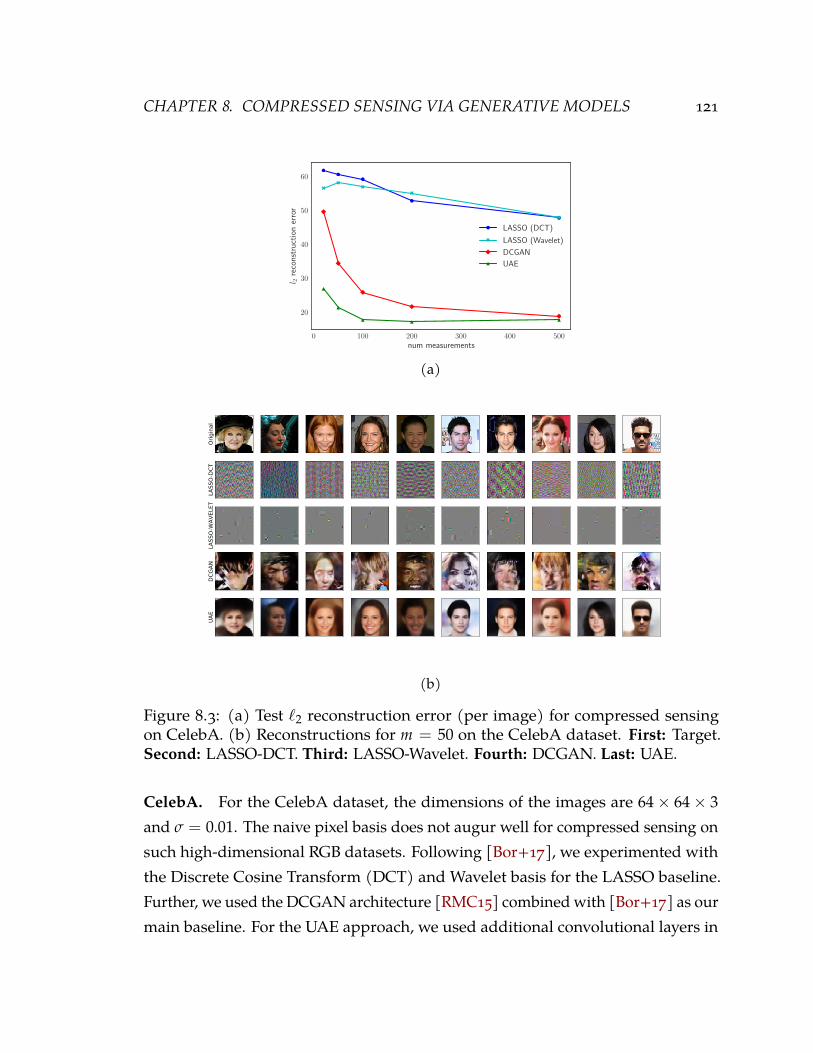
CHAPTER 8. COMPRESSED SENSING VIA GENERATIVE MODELS 121
0 100 200 300 400 500num measurements
20
30
40
50
60
l 2re
cons
truc
tion
erro
r
LASSO (DCT)
LASSO (Wavelet)
DCGAN
UAE
(a)
Orig
inal
LASS
O-DC
TLA
SSO-
WAV
ELET
DCGA
NUA
E
(b)
Figure 8.3: (a) Test `2 reconstruction error (per image) for compressed sensingon CelebA. (b) Reconstructions for m = 50 on the CelebA dataset. First: Target.Second: LASSO-DCT. Third: LASSO-Wavelet. Fourth: DCGAN. Last: UAE.
CelebA. For the CelebA dataset, the dimensions of the images are 64× 64× 3
and σ = 0.01. The naive pixel basis does not augur well for compressed sensing onsuch high-dimensional RGB datasets. Following [Bor+17], we experimented withthe Discrete Cosine Transform (DCT) and Wavelet basis for the LASSO baseline.Further, we used the DCGAN architecture [RMC15] combined with [Bor+17] as ourmain baseline. For the UAE approach, we used additional convolutional layers in

CHAPTER 8. COMPRESSED SENSING VIA GENERATIVE MODELS 122
the encoder to learn a 256 dimensional feature space for the image before projectingit down to m dimensions.
The results are shown in Figure 8.3 (a). While the performance of DCGAN iscomparable with that of UAE for m = 500, UAE outperforms DCGAN significantlywhen m is low. The LASSO baselines do not perform well, consistent with the obser-vations made for the experiments on the MNIST and Omniglot datasets. Qualitativeevaluations are shown in Figure 8.3 (b) for m = 50 measurements.
8.4.2 Transfer compressed sensing
To test the generalization of the learned models to similar, unseen datasets, weconsider the task of transfer compressed sensing task introduced in [DGE18].
Experimental setup. We train the models on a source domain that is related toa target domain. Since the dimensions of MNIST and Omniglot images match,transferring from one domain to another requires no additional processing. ForUAE, we consider two variants. In UAE-SE, we used the encodings from the sourcedomain and retrain the decoder on the target domain. For UAE-SD, we use sourcedecoder and retrain the encoder on the target domain.
Results. The `2 reconstruction errors are shown in Figure 8.4 (a-b). LASSO (bluecurves) does not involve any learning, and hence its performance is same as Fig-ure 8.2 (a-b). The CS-VAE (red) performance degrades significantly in comparison,even performing worse than LASSO in some cases. The UAE based methods out-perform these approaches and UAE-SE (green) fares better than UAE-SD (yellow).Qualitative differences are highlighted in Figure 8.4 (c-d) for m = 25 measurements.
8.4.3 Dimensionality reduction
Dimensionality reduction is a common preprocessing technique for specifying fea-tures for classification. We compare PCA and UAE on this task. For UAE decodings,

CHAPTER 8. COMPRESSED SENSING VIA GENERATIVE MODELS 123
0 20 40 60 80 100num measurements
2
3
4
5
6
7
8
9
l 2re
cons
truc
tion
erro
r
LASSO
CS-VAE
UAE-SD
UAE-SE
(a) Source: MNIST, Target: Omniglot
0 20 40 60 80 100num measurements
2
3
4
5
6
7
8
9
l 2re
cons
truc
tion
erro
r
(b) Source: Omniglot, Target: MNIST
Orig
inal
CS-V
AEUA
E-SD
UAE-
SE
(c) Source: MNIST, Target: Omniglot
Orig
inal
CS-V
AEUA
E-SD
UAE-
SE
(d) Source: Omniglot, Target: MNIST
Figure 8.4: (a-b) Test `2 reconstruction error (per image) for transfer compressedsensing. (c-d) Reconstructions for m = 25. Top: Target. Second: CS-VAE. Third:UAE-SD. Last: UAE-SE.

CHAPTER 8. COMPRESSED SENSING VIA GENERATIVE MODELS 124
we set the noise as a hyperparameter based on a validation set to enable out-of-sample generalization.
Setup. We learn the principal components and UAE projections on the MNISTtraining set for varying number of dimensions. We then learn classifiers basedon the these projections. Again, we use a linear encoder for the UAE for a fairevaluation. Since the inductive biases vary across different classifiers, we considered8 commonly used classifiers: k-Nearest Neighbors (kNN), Decision Trees (DT),Random Forests (RF), Multilayer Perceptron (MLP), AdaBoost (AdaB), GaussianNaive Bayes (NB), Quadratic Discriminant Analysis (QDA), and Support VectorMachines (SVM) with a linear kernel.
Table 8.1: PCA vs. UAE. Average test classification accuracy for the MNIST dataset.
Dimensions Method kNN DT RF MLP AdaB NB QDA SVM
2 PCA 0.4078 0.4283 0.4484 0.4695 0.4002 0.4455 0.4576 0.4503UAE 0.4644 0.5085 0.5341 0.5437 0.4248 0.5226 0.5316 0.5256
5 PCA 0.7291 0.5640 0.6257 0.7475 0.5570 0.6587 0.7321 0.7102UAE 0.8115 0.6331 0.7094 0.8262 0.6164 0.7286 0.7961 0.7873
10 PCA 0.9257 0.6354 0.6956 0.9006 0.7025 0.7789 0.8918 0.8440UAE 0.9323 0.5583 0.7362 0.9258 0.7165 0.7895 0.9098 0.8753
25 PCA 0.9734 0.6382 0.6889 0.9521 0.7234 0.8635 0.9572 0.9194UAE 0.9730 0.5407 0.7022 0.9614 0.7398 0.8306 0.9580 0.9218
50 PCA 0.9751 0.6381 0.6059 0.9580 0.7390 0.8786 0.9632 0.9376UAE 0.9754 0.5424 0.6765 0.9597 0.7330 0.8579 0.9638 0.9384
100 PCA 0.9734 0.6380 0.4040 0.9584 0.7136 0.8763 0.9570 0.9428UAE 0.9731 0.6446 0.6241 0.9597 0.7170 0.8809 0.9595 0.9431
Results. The performance of the PCAandUAE feature representations for differentnumber of dimensions is shown in Table 8.1. We find that UAE outperforms PCA ina majority of the cases. Further, this trend is largely consistent across classifiers. Theimprovements are especially highwhen the number of dimensions is low, suggestingthe benefits of UAE as a dimensionality reduction technique for classification.
CHAPTER 8. COMPRESSED SENSING VIA GENERATIVE MODELS 125
8.5 Discussion & Related Work
In this section, we contrast uncertainty autoencoders with related works in autoen-coding, compressed sensing, and mutual information maximization.
Autoencoders. To contrast uncertainty autoencoders with other commonly usedautoencoding schemes, consider a UAE with a Gaussian observation model andfixed isotropic covariance for the decoder. The UAE objective can be simplified as:
minθ,φ
Ex,y∼qφ(X,Y)
[‖x− gθ(y)‖2
2
]If we assume no measurement noise (i.e., ε = 0) and assume the observation
model pθ(X|Y) to be a Gaussian with mean gθ(Y) and a fixed isotropic Σ, then theUAE objective reduces to minimizing the mean squared error between the true andrecovered data point:
minθ,W,ψ
Ex∼qdata(X)
[‖x− gθ(W fψ(x))‖2
2
]This special case of a UAE corresponds to a standard autoencoder [Ben+09] wherethe measurements Y signify a hidden representation for X. However, this caselacks the interpretation of an implicit generative model since the assumptions ofTheorem 8.1 do not hold.
Denoising autoencoders. A DAE [Vin+08] adds noise at the level of the inputdata point X to learn robust representations. For a UAE, the noise model is definedat the level of the compressed measurements. Again, with the assumptions of aGaussian decoder, the DAE objective can be expressed as:
minθ,W,ψ
Ex∼qdata(X),x∼C(X|x)
[‖x− gθ(W fψ(x))‖2
2
]where C(·|X) is some predefined noise corruption model. Similar to Theorem 8.1, aDAE also learns an implicit model of the data distribution [Ben+13; AB14].

CHAPTER 8. COMPRESSED SENSING VIA GENERATIVE MODELS 126
Variational autoencoders. A VAE [KW18; RMW14] explicitly learns a latent vari-able model pθ(X, Y) for the dataset. The learning objective is a variational lowerbound to the marginal log-likelihood assigned by the model to the data X, whichnotationally corresponds to Eqdata(X)[log pθ(x)]. The variational objective that maxi-mizes this quantity can be simplified as:
minθ,φ
Ex,y∼qφ(X,Y)
[‖x− gθ(y)‖2
2
]+ Ex∼qdata(X)
[DKL(qφ(y|x), pθ(y))
]The learning objective includes a reconstruction error term, akin to the UAE
objective. Crucially, it also includes a regularization term to minimize the KLdivergence between the variational posterior and the prior over the latents. Onthe other hand, a UAE does not explicitly need to model the prior distribution overthe latents. On the downside, a VAE can perform efficient ancestral sampling whilea UAE requires running relatively expensive Markov Chains to obtain samples.
Recent works have attempted to unify the variants of variational autoencodersthrough the lens of mutual information [Ale+18; ZSE18; Che+17b]. These worksalso highlight scenarios where the VAE can learn to ignore the latent code in thepresence of a strong decoder thereby affecting the reconstructions to attain a lowerKL loss. One particular variant, the β-VAE, weighs the additional KL regularizationterm with a positive factor β and can effectively learn disentangled representa-tions [Hig+16; ZSE19]. Although [Hig+16] does not consider this case, the UAEcan be seen as a β-VAE with β = 0.
To summarize, our UAE formulation provides a combination of unique desirableproperties for representation learning that are absent in prior autoencoders. Asdiscussed, a UAE defines an implicit generative model without specifying a prior(Theorem 8.1) even under realistic conditions (Corollary 8.1; unlike DAEs).
Generative modeling and compressed sensing. The related work of [Bor+17]first propose to use generative models for compressed sensing. As described inSection 8.4, the goal here is to recover signals that lie on the range of a pretrainedgenerative model. [DGE18] further extend this approach to allow for recovery of
CHAPTER 8. COMPRESSED SENSING VIA GENERATIVE MODELS 127
signals which lie on or close to the range of the generative model, thereby gurantee-ing exact recovery in the limit of the number of measurements matching the datadimensionality. Similar to [Bor+17], a UAE learns a data distribution. However,in doing so, it additionally learns an acquisition/encoding function and a recov-ery/decoding function, unlike [Bor+17; DGE18] which rely on generic randommatrices and `2 decoding. The cost of implicit learning in a UAE is that some of itsinference capabilities, such as likelihood evaluation and sampling, are intractable orrequire running Markov chains. However, these inference queries are orthogonal tocompressed sensing. Finally, our decoding is amortized and scales to large datasets,unlike [Bor+17; DGE18] which solve an independent optimization problem for eachtest data point.
Mutual information maximization. The principle of mutual information maxi-mization, often referred to as InfoMax in prior work, was first proposed for learningencodings for communication over a noisy channel [Lin89]. The InfoMax objectivehas also been applied for statistical compressed sensing for learning both linearand non-linear encodings [WCF07; Car+12; Wan+14]. Our work differs from theseexisting frameworks in two fundamental ways. First, we optimize for a tractablevariational lower bound to the MI that which allows our method to scale to high-dimensional data. Second, we learn an amortized [GG14; Shu+18] decoder inaddition to the encoder that sidesteps expensive, per-example optimization for thetest data points.
Further, we improve upon the IM algorithm proposed originally for variationalinformationmaximization [BA03]. While the IM algorithm proposes to optimize thelower bound on the mutual information in alternating ‘‘wake-sleep’’ phases for op-timizing the encoder (‘‘wake”) and decoder (‘‘sleep”) analogous to the expectation-maximization procedure used in [WCF07], we optimize the encoder and decoderjointly using a single consistent objective leveraging recent advancements in gradientbased variational stochastic optimization.

CHAPTER 8. COMPRESSED SENSING VIA GENERATIVE MODELS 128
8.6 Conclusion
We presented uncertainty autoencoders (UAE), a framework for unsupervised rep-resentation learning via variational maximization of mutual information betweenan input signal and its latent representation. We showed formally that UAE learnsan implicit generative model of the underlying data distribution. Empirically, weshowed that UAEs are a natural candidate for statistical and transfer compressedsensing and outperforms competing approaches for sensing high-dimensional im-ages in practice. In a recent follow-up work, we extend the UAE framework forlearning discrete latent representations [Cho+19].
In the future, it would be interesting to incorporate advancements in compressedsensing based on complex neural network architectures [MPB15; Kul+16; Ric+17;Lu+18; Van+18] within the UAE framework. Unlike the rich theory surroundingthe compressed sensing of sparse signals, a similar theory surrounding generativemodel-based priors on the signal distribution is lacking. Recent works have madepromising progress in developing a theory of SGD based recovery methods fornonconvex inverse problems [Bor+17; HV18; DGE18; Liu+18b], which continues tobe an exciting direction for future work.

9 Multi-FidelityOptimal ExperimentalDe-sign: ACase Study in Battery Fast Charg-ing
9.1 Introduction
Simultaneously optimizing many design parameters for time-consuming experi-ments bottlenecks a broad range of scientific and engineering disciplines [Tab+18;But+18]. One such example is process and control optimization for lithium-ionbatteries during materials selection, cell manufacturing, and operation. A com-mon objective is to maximize lifetime, but conducting even a single experiment toevaluate the lifetime of a battery can take months to years [Bau+14; KJ16; Sev+19]and requires many replicate samples due to the large parameter spaces and highsampling variability [Bau+14; Sch+15b; HHL17]. Hence, the key challenge is toreduce both the number and the duration of required experiments.
Optimal experimental design (OED) approaches are widely used to reduce thecost of experimental optimization. These approaches often involve a closed-looppipeline where feedback from completed experiments informs subsequent exper-imental decisions, balancing the competing demands of exploration, i.e., testingregions of the experimental parameter space with high uncertainty, and exploitation,i.e., testing promising regions based on the results of the completed experiments.
129
CHAPTER 9. MULTI-FIDELITY OPTIMAL EXPERIMENTAL DESIGN 130
OED algorithms have been successfully applied to physical science domains such asmaterials science [Tab+18; But+18; Nik+16; Lin+17], chemistry [Béd+18; Gra+18],biology [Kin+09], and drug discovery [Sch18], as well as to computer science do-mains such as hyperparameter optimization for machine learning [DSH15; Kle+17].However, while a closed-loop approach is designed to minimize the number ofexperiments required for optimizing across a multidimensional parameter space,the time (and/or cost) per experimentmay remain high, as is the case for lithium-ionbatteries (LIB). Therefore, an OED approach should account for both the number ofexperiments and the cost per experiment.
Multi-fidelity OED approaches have been developed to learn from both inex-pensive, noisy signals and expensive, accurate signals in certain domains. Forexample, in hyperparameter optimization for machine learning algorithms, sev-eral domain-specific low-fidelity signals for predicting the final performance of analgorithmic configuration are used in tandem with more complete configurationevaluations [HHL11], e.g., extrapolated learning curves [DSH15; Kle+17], rapidtesting on a subset of the full training dataset [Pet00; Li+17]. For LIBs, classicalmethods such as factorial design that use predetermined heuristics to select ex-periments have been applied [LLW09; LHL11; Sch+18], but the design and use oflow-fidelity signals is challenging and unexplored.
In this chapter, we develop a multi-fidelity closed-loop optimization (CLO)methodology for efficient optimization over large parameter spaces with expensiveexperiments and high sampling variability. We experimentally employ this system tooptimize fast charging protocols for LIBs; reducing charging time to approach gaso-line refueling time is critical to reduce range anxiety for electric vehicles [Ahm+17;LZC19] but often comes at the expense of battery lifetime. Specifically, we optimizeover a parameter space consisting of 224 unique six-step, 10-minute fast-chargingprotocols (i.e., how current and voltage are controlled during charging) to findcharging protocols with high cycle life, defined as the battery capacity falling to 80%of its nominal value. Our system uses two key elements to reduce the optimizationcost. First, we reduce the time per experiment by using a probabilistic model to

CHAPTER 9. MULTI-FIDELITY OPTIMAL EXPERIMENTAL DESIGN 131
predict the outcome of the experiment based on data from early cycles, well be-fore the batteries reach the end of life [Sev+19]. Second, we reduce the numberof experiments by using a Bayesian optimization (BO) algorithm to balance theexploration-exploitation trade-off in choosing the next round of experiments [HSF14;Gro+18b].
Testing a single battery to failure under our fast-charging conditions requires ap-proximately 40 days. For example, when 48 experiments are performed in parallel,assessing all 224 charging protocols with triplicate measurements takes approxi-mately 560 days. Here, using CLO with early outcome prediction, only 16 days wererequired to confidently identify protocols with high cycle lives (48 parallel experi-ments). In a subsequent validation study, we find that CLO ranks these protocolsby lifetime accurately (Kendall rank correlation coefficient = 0.83) and efficiently(15x less time than a baseline brute-force approach). Furthermore, we find that thecharging protocols identified as optimal by CLO with early prediction outperformexisting fast-charging protocols designed to avoid lithium plating, the approachsuggested by conventional battery wisdom [KJ16; Ahm+17; LZC19; Sch+18].
9.2 Preliminaries
Let X denote the space of fast charging protocols and f : X → R denote the(unknown) function that relates a charging protocol x ∈ X to the observed lifetimeof a battery y as:
y = f (x) + ε (9.1)
where ε is some measurement noise, e.g., due to manufacturing variability. Wedo not know f but we can query its noisy lifetime value y by conducting batterycharging experiments. Our goal is to find the protocol x∗ ∈ X with the highestexpected lifetime:
x∗ = arg maxx∈X
f (x) (9.2)

CHAPTER 9. MULTI-FIDELITY OPTIMAL EXPERIMENTAL DESIGN 132
There are two primary challenges in inferring x∗ via ‘‘black-box” optimization thatonly allows query access to f : (a) the protocol space X could be very large topermit systematic exploration, and (b) measurement noise can be very high whichwould require repeated querying (exploitation) to estimate expected lifetime of anycandidate protocol. In addition, a third challenge for battery optimization is thatevaluating the function f for any protocol x involves time-consuming real-worldexperimentation.
The first two challenges involve a trade-off in exploration and exploitation. Apopular class of techniques for navigating this trade-off is based on Bayesian opti-mization [Sha+15]. Bayesian optimization can be seen as a wrapper around any baseprobabilistic regression model, e.g., Gaussian processes, Bayesian neural networks,etc. The key idea in Bayesian optimization is to query the black-box function atpoints that best optimize an acquisition function derived from the predictions of thebase regression model. For example, we use upper-confidence bounds (UCB) asthe choice of the acquisition function in this chapter, which is given as:
UCB(x) = µ(x)± σ(x) (9.3)
where µ(x) and σ(x) are the mean and uncertainty (std) prediction for x given bythe base regression model. Other acquisition functions are also possible and ourkey contributions in this chapter are agnostic to this choice; we refer the interestedreader to [Fra18] for a recent survey. Intuitively, the UCB score is high for pointswith high uncertainty (i.e., high σ) and high mean (i.e., high µ). Initially, the basemodel is random (or trained on offline data). Thereafter, we select the point x withthe highest UCB scores for experimentation. The results of those experiment givesanother training point (x, y), which is then used to retrain the base regression model.The whole process is repeated until the experimentation budget is exhausted.
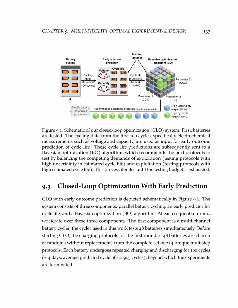
CHAPTER 9. MULTI-FIDELITY OPTIMAL EXPERIMENTAL DESIGN 133
High cycle life(exploitation)
High uncertainty(exploration)
Trainingdataset
950
540
780
670
970
590
730 980
Voltage
Capacity
Cycle life
+-
+-
+-
+-
+-
+-
+- +-
Batterycycling
Cycle lifepredictions(from MLmodel)
Parameter 1(CC1)
Parameter 2(CC2)
Parameter 3(CC3)
Early outcomepredictor
Recommended charging protocols (CC1, CC2, CC3)
Cyclingdata
(from first100 cycles)
Bayesian optimizationalgorithm (BO)
Modify batterymaterials &processes
Figure 9.1: Schematic of our closed-loop optimization (CLO) system. First, batteriesare tested. The cycling data from the first 100 cycles, specifically electrochemicalmeasurements such as voltage and capacity, are used as input for early outcomeprediction of cycle life. These cycle life predictions are subsequently sent to aBayesian optimization (BO) algorithm, which recommends the next protocols totest by balancing the competing demands of exploration (testing protocols withhigh uncertainty in estimated cycle life) and exploitation (testing protocols withhigh estimated cycle life). This process iterates until the testing budget is exhausted.
9.3 Closed-Loop Optimization With Early Prediction
CLO with early outcome prediction is depicted schematically in Figure 9.1. Thesystem consists of three components: parallel battery cycling, an early predictor forcycle life, and a Bayesian optimization (BO) algorithm. At each sequential round,we iterate over these three components. The first component is a multi-channelbattery cycler; the cycler used in this work tests 48 batteries simultaneously. Beforestarting CLO, the charging protocols for the first round of 48 batteries are chosenat random (without replacement) from the complete set of 224 unique multistepprotocols. Each battery undergoes repeated charging and discharging for 100 cycles(∼4 days; average predicted cycle life = 905 cycles), beyond which the experimentsare terminated.

CHAPTER 9. MULTI-FIDELITY OPTIMAL EXPERIMENTAL DESIGN 134
This cycling data is then fed as input to the early outcome predictor, whichestimates the final cycle lives of the batteries given data from the first 100 cycles.The early predictor is a linear model trained via elastic net regression on featuresextracted from the charging data of the first 100 cycles, similar to that presented in[Sev+19]. Predictive features include transformations of both differences betweenvoltage curves and discharge capacity fade trends. To train the early predictor, werequire a training dataset of batteries cycled to failure. Here, we used a pre-existingdataset of 41 batteries cycled to failure (cross-validation root mean squared error= 80.4 cycles). While obtaining this dataset itself requires running full cyclingexperiments for a small training set of batteries (the cost we are trying to offset),this one-time cost could be avoided if pretrained predictors or previously collecteddatasets are available. If unavailable, we pay an upfront cost in collecting thisdataset; this dataset could also be used for warm-starting the BO algorithm. Thesize of the dataset collected should best trade-off the upfront cost in acquiring thedataset to train an accurate model with the anticipated reduction in experimentationrequirements for CLO.
Finally, these predicted cycle lives from early-cycle data are fed into the BOalgorithm, which recommends the next round of 48 charging protocols that bestbalance the exploration-exploitation trade-off. This algorithm is presented in detailin the full version of the companion paper [Att+20] and builds on the prior work of[HA15] and [Gro+18b]. The algorithm maintains an estimate of both the averagecycle life and the uncertainty bounds for each protocol; these estimates are initiallyequal for all protocols and are refined as additional data are collected. Crucially,to reduce the total optimization cost, our algorithm performs these updates usingestimates from the early outcome predictor instead of using the actual cycle lives.The mean and uncertainty estimates for the cycle lives are obtained via a GaussianProcess, which has a smoothing effect and allows for updating the cycle life estimatesof untested protocols with the predictions from related protocols. The closed-loopprocess repeats until the optimization budget, in our case 192 batteries tested (100cycles each), is exhausted.
Our objective is to find the charging protocol which maximizes the expected

CHAPTER 9. MULTI-FIDELITY OPTIMAL EXPERIMENTAL DESIGN 135
0 20 40 60 80 100State of charge (%)
0
2
4
6
8
10
Cur
rent
(C ra
te)
CC1 CC2 CC3 CC4 CC5-CV1
Charging time to 80% SOC = 10 minutes
Max voltage = 3.6 V
(a)
CC13
45
67
8CC2
34
56
78
CC3
3
4
5
6
7
8
2.75
3.00
3.25
3.50
3.75
4.00
4.25
4.50
4.75CC4
(b)
Figure 9.2: Structure of our 10-minute, six-step fast-charging protocols. (a) Currentvs. SOC for an example charging protocol, 7.0C–4.8C–5.2C–3.45C (bold lines).Each charging protocol is defined by five constant current (“CC”) steps followed byone constant voltage (“CV”) step. The last two steps (CC5 and CV1) are identicalfor all charging protocols. We optimize over the first four constant-current steps,denoted CC1, CC2, CC3, and CC4. Each of these steps comprises a 20% SOCwindow, such that CC1 ranges from 0–20% SOC, CC2 ranges from 20–40% SOC,etc. CC4 is constrained by specifying that all protocols charge in the same total time(10 minutes) from 0% to 80% SOC. Thus, our parameter space consists of uniquecombinations of the three free parameters CC1, CC2, and CC3. For each step, wespecify a range of acceptable values; the upper limit is monotonically decreasingwith increasing SOC to avoid the upper cutoff potential (3.6 V for all steps). (b)CC4 (color) as a function of CC1, CC2, and CC3 (x, y, and z axes, respectively).Each point represents a unique charging protocol.

CHAPTER 9. MULTI-FIDELITY OPTIMAL EXPERIMENTAL DESIGN 136
battery cycle life for a fixed charging time (10 minutes) and state-of-charge (SOC)range (0 to 80%). The design space of our 224 six-step extreme fast-charging proto-cols is presented in Figure 9.2a. Multistep charging protocols, in which a series ofdifferent constant-current steps are applied within a single charge, are consideredadvantageous over single-step charging for maximizing cycle life during fast charg-ing [KJ16; Ahm+17] though the optimal combination remains unclear. As shownin Figure 9.2b, each protocol is specified by three independent parameters (CC1,CC2, and CC3); each parameter is a current applied over a fixed SOC range (0-20,20-40 and 40-60%, respectively). A fourth parameter, CC4, is dependent on CC1,CC2, CC3, and the charging time. Given constraints on the current values, a total of224 charging protocols are permitted.
We test commercial lithium iron phosphate (LFP)/graphite cylindrical batteries(A123 Systems) in a convective environmental chamber (30°C ambient temperature).A maximum voltage of 3.6 V is imposed. These batteries are designed to fast-chargein 17 minutes. The cycle life decreases dramatically with faster charging time. Sincethe LFP positive electrode is generally considered stable under fast charging [KJ16;Sev+19], we select this battery chemistry to isolate the effects of extreme fast chargingon graphite, which is universally employed in LIBs.
9.4 Empirical Evaluation
In all, we ran four CLO rounds sequentially, consisting of 185 batteries in total (ex-cluding seven batteries, Methods). Using early prediction, each CLO round requiresfour days to complete 100 cycles, resulting in a total testing time of sixteen days—asignificant reduction from the 560 days required to test each charging protocol tofailure three times. Figure 9.3presents the predictions and selected protocols as wellas the evolution of cycle life estimates over the parameter space as the optimizationprogresses (Figure 9.4). Initially, the estimated cycle lives for all protocols are equal.After two rounds, the overall structure of the parameter space (i.e., the dependenceof cycle life on charging protocol parameters CC1, CC2, and CC3) emerges, and a

CHAPTER 9. MULTI-FIDELITY OPTIMAL EXPERIMENTAL DESIGN 137
Figure 9.3: Early cycle life predictions per round. The tested charging protocolsand the resulting predictions are plotted for rounds 1–4. Each point represents acharging protocol, defined by CC1, CC2, and CC3 (x, y, and z axes, respectively).The color represents cycle life predictions from the early outcome prediction model.The charging protocols in the first round of testing are randomly selected. As BOshifts from exploration to exploitation, the charging protocols selected for testing bythe closed loop in subsequent rounds are primarily in the high-performing region.
Figure 9.4: Evolution of the parameter space per round. The color represents cyclelife as estimated by BO. The initial cycle life estimates are equivalent for all protocols;as more predictions are generated, BO updates its cycle life estimates.

CHAPTER 9. MULTI-FIDELITY OPTIMAL EXPERIMENTAL DESIGN 138
prominent region with high cycle life protocols has been identified. CLO’s confi-dence in this high-performing region is further improved from round 2 to round 4,but overall the cycle life estimates do not change significantly.
0 1 2 3 4Repetitions per protocol
0
20
40
60
80
100
120
Cou
nt
117
61
1726
3
(a)
0 20 40 60 80 100State of charge (%)
0
2
4
6
8
10
Cur
rent
(C ra
te)
CLO 1: 4.8C-5.2C-5.2C-4.160CCLO 2: 5.2C-5.2C-4.8C-4.160CCLO 3: 4.4C-5.6C-5.2C-4.252C
(b)
Figure 9.5: (a) Distribution of the number of repetitions for each charging pro-tocol. Only 46 of 224 protocols (21%) are tested multiple times. (b) Current vs.SOC for the top three fast-charging protocols as estimated by CLO. CC1–CC4 aredisplayed in the legend. All three protocols have relatively uniform charging (i.e.,CC1≈CC2≈CC3≈CC4).
By learning and exploiting the structure of the parameter space, we avoid evaluat-ing charging protocols with low estimated cycle life and concentrate more resourceson the high-performing region. Specifically, 117 of 224 protocols are never tested(Figure 9.5a); we spend 67% of the batteries testing 21% of the protocols (0.83batteries per protocol on average). CLO repeatedly tests several protocols with highestimated cycle life to decrease uncertainties due to manufacturing variability andthe error introduced by early outcome prediction. The uncertainty is expressed asthe prediction intervals of the posterior predictive distribution over cycle life.
To the best of the our knowledge, this work presents the largest known map ofcycle life as a function of charging conditions. This dataset can be used to validatephysics-based models of battery degradation. Most fast-charging protocols pro-posed in the battery literature suggest that current steps decreasingmonotonically asa function of SOC are optimal to avoid lithium plating on graphite, a well-accepted

CHAPTER 9. MULTI-FIDELITY OPTIMAL EXPERIMENTAL DESIGN 139
degradation mode during fast charging [KJ16; Ahm+17; LZC19; Sch+18]. In con-trast, the protocols identified as optimal by CLO (e.g., Figure 9.5b) are generallysimilar to single-step constant-current charging (i.e., CC1≈CC2≈CC3≈CC4). Specif-ically, of the 75 protocols with the highest estimated cycle lives, only ten aremonoton-ically decreasing (i.e., CC(i) ≥ CC(i+1) for all i) and two are strictly decreasing (i.e.,CC(i) > CC(i+1)). We speculate that minimizing parasitic reactions caused by heatgeneration may be the operative optimization strategy for these cells, as opposedto minimizing the propensity for lithium plating. While the optimal protocol for anew scenario would depend on the selected charge time, SOC window, temperaturecontrol conditions, and battery chemistry, this unexpected result highlights the needfor data-driven approaches for optimizing fast charging.
0 200 400 600 800 1000 1200 1400Cycle number
0.90
0.95
1.00
1.05
1.10
Dis
char
ge c
apac
ity (A
h)
Figure 9.6: Discharge capacity vs. cycle number for all batteries in the validationexperiment. See Figure 9.7 for the color scheme legend.
We validate the performance of CLO with early prediction on a subset of nineextreme fast-charging protocols. For each of these protocols, we cycle five batterieseach to failure and use the sample average of the final cycle lives as an estimateof the true lifetimes. We use this validation study to (a) confirm that CLO is ableto correctly rank protocols based on cycle life, and (b) compare the cycle lives ofprotocols recommended by CLO to protocols inspired by the battery literature.

CHAPTER 9. MULTI-FIDELITY OPTIMAL EXPERIMENTAL DESIGN 140
0 250 500 750 1000 1250 1500Mean early-predicted cycle life
(validation)
0
250
500
750
1000
1250
1500C
LO-e
stim
ated
cyc
le li
fe
r = 0.93
CLO top 3Lit-inspiredOther
(a)
0 250 500 750 1000 1250 1500Early-predicted cycle life
(validation)
0
250
500
750
1000
1250
1500
Fina
l cyc
le li
fe (v
alid
atio
n)
r = 0.86
CLO top 3Lit-inspiredOther
(b)
0 200 400 600 800 1000 1200Final cycle life (validation)
Val
idat
ion
prot
ocol
(sor
ted
by C
LO ra
nkin
g)
3.6C-6.0C-5.6C-4.755C: 755
4.4C-5.6C-5.2C-4.252C: 884
4.8C-5.2C-5.2C-4.160C: 890 cycles
5.2C-5.2C-4.8C-4.160C: 912
6.0C-5.6C-4.4C-3.834C: 880
7.0C-4.8C-4.8C-3.652C: 870
8.0C-4.4C-4.4C-3.940C: 702
8.0C-6.0C-4.8C-3.000C: 584
8.0C-7.0C-5.2C-2.680C: 496
CLO top 3Lit-inspiredOther
(c)
Figure 9.7: (a) Comparison of early-predicted cycle lives from validation to closed-loop estimates, averaged on a protocol basis. Each 10-minute charging protocol istested with five batteries. Error bars represent the 95% confidence intervals. (b)Observed vs. early-predicted cycle life for the validation experiment. While ourearly predictor appears biased, likely due to calendar aging effects, the trend iscorrectly captured (Pearson correlation coefficient r = 0.86). (c) Final cycle livesfrom validation, sorted by CLO ranking. The length of each bar and the annotationsrepresents themean final cycle life from validation per protocol. Error bars representthe 95% confidence intervals.

CHAPTER 9. MULTI-FIDELITY OPTIMAL EXPERIMENTAL DESIGN 141
The charging protocols used in validation, some of which are inspired by existingbattery fast charging literature, span the range of estimated cycle lives. We adjustthe voltage limits and charging times of these literature protocols to match ourprotocols, while maintaining similar current ratios as a function of SOC. While theliterature protocols used in these validation experiments are generally designed forbatterieswith high-voltage positive electrode chemistries, fast-charging optimizationstrategies generally focus on the graphitic negative electrode [KJ16; Ahm+17]. Forthese nine protocols, we validate the ‘‘CLO-estimated” cycle lives against the sampleaverage of the five final cycle lives. The discharge capacity fade curves (Figure 9.6)exhibit the nonlinear decay typical of fast charging [Sev+19; HHL17].
Next, we discuss the results for the validation study. If we apply our earlypredictionmodel to the batteries in the validation experiment, these early predictions(averaged over each protocol) match the CLO-estimated mean cycle lives well(Pearson correlation coefficient r = 0.93; Figure 9.7a). This result validates theperformance of the BO component of CLO in particular, since the CLO-estimatedcycle lives were inferred from early predictions.
However, our early prediction model exhibits some bias (Figure 9.7b), likelydue to calendar aging effects from different battery storage times [Kei+16]. Despitethis bias in our predictive model, we generally capture the ranking well (Kendallrank correlation coefficient = 0.83, Figure 9.7c). At the same time, we note that thefinal cycle lives for the top-ranked protocols are similar. Furthermore, the optimalprotocols identified by CLO outperform protocols inspired by previously publishedfast-charging protocols (895 vs. 728 cycles on average). This result suggests that theefficiency of our approach does not come at the expense of accuracy. A procedurethat does not use early outcome prediction and simply selects protocols to randomlytest begins to saturate to a competitive performance level after ∼7,700 battery-hours of testing. To achieve a similar level of performance, CLO requires only 500battery-hours of testing.

CHAPTER 9. MULTI-FIDELITY OPTIMAL EXPERIMENTAL DESIGN 142
9.5 Discussion & Related Work
The underlying optimal experimental design problem we seek to address is aninstance of multi-fidelity black-box optimization. These methods are especiallyuseful when a single function evaluation can itself be very expensive (in terms oftime or resources) but it is easy to obtain noisy, low-fidelity signals.
The canonical use case considered in prior work is that of hyperparameter op-timization for machine learning algorithms. Here, the goal is to find the optimalconfiguration of hyperparameters for learning a model on a target dataset. Promi-nent examples of low-fidelity signals include (a) early prediction of learning curves(e.g., [DSH15]) and (b) testing a hyperparameter configuration on a subset of thedata (e.g., [Pet00]). Multi-fidelity approaches (e.g., [Van04; KPB15; SST15; Spa+15])use one or more of these low-fidelity signals for dynamically selecting which hyper-parameter configuration to test next, e.g., successive halving routines [KKS13] suchas Hyperband [Li+17], which periodically removes half of the worst performingconfigurations. We provide details on methods that predict learning curves, sincethat form of fidelity signal is similar to the one we consider. We further refer thereader to Section 1.4 in [HKV19] for an excellent and comprehensive survey onmulti-fidelity black box optimization.
A learning curve tracks the performance of a machine learning algorithm (asmeasured via a suitablemetric such as classification accuracy on a validation dataset)as a function of training time (as measured via number of iterations, gradientupdates, etc.). These curves are typically increasing functions, and the performancemetric saturates over time. Since observing the asymptote of a learning curve for anysingle hyperparameter configuration can be expensive, [DSH15] proposed to predicta learning curve after training the model only for a small number of iterations. Thegoal is to terminate the training procedure early if the asymptotic performance ona validation set is unlikely to beat the validation performance of the best knownhyperparameter configuration so far.
The predictor is parameterized using a mixture of functional forms (e.g., Weibull,

CHAPTER 9. MULTI-FIDELITY OPTIMAL EXPERIMENTAL DESIGN 143
vapor pressure, etc.) that have similar characteristics as learning curves (i.e., increas-ing and saturatingwith respect to the performancemetric). Using standard Bayesianinference over the unknown parameters, the probability that the performance ofthe algorithm at a future iteration will exceed the best known performance so farcan be estimated. Such estimates are then used within a downstream black-boxoptimization routine such as SMAC [HHL11] or Tree Parzen Estimator [Hut+14]for the purpose of deciding whether to terminate training of a given hyperparam-eter configuration and utilize the remaining budget for testing other candidatehyperparameter configurations. [Kle+17] extend this approach via Bayesian neuralnetworks to utilize additional data from past runs of related hyperparameter config-urations. This permits learning more accurate predictors without having to observea substantial portion of the learning curve.
To draw an analogy with the current case study, we were interested in predictingthe cycle life at which the capacity of a charging protocol drops to a predefinedvalue (80% of initial capacity, or 0.88 Ah), see e.g., Figure 9.6. In contrast to typicalshapes of learning curves, (a) the capacity is decreasing as a function of cycle lifeand (b) the cycle life saturates with respect to the capacity. That is, the capacitydecreases slowly in the beginning until it hits a transition point. Beyond this point,the capacity quickly drops to 0.88 Ah. This transition point is unknown and occursclose to the final cycle life. As a result, predicting the final cycle life is challengingwithout having substantially cycled the battery to observe the transition point. Doingso however will defeat the purpose of terminating experiments early for efficientclosed-loop optimization.
We overcome this challenge by training our early predictor to use both informa-tion from prior capacity curves as well as additional features at every time step (e.g.,voltage and capacity). This method allows for highly accurate predictions only afterthe first 100 cycles. In the future, it would be interesting to deploy CLO pipelineswhere the time instant for termination is dynamically decided based on the uncer-tainty of the early predictor. If the uncertainty is relatively high, the experiment isrun longer whereas the low uncertainty experiments can potentially be terminatedmuch before even 100 cycles of charging.

CHAPTER 9. MULTI-FIDELITY OPTIMAL EXPERIMENTAL DESIGN 144
9.6 Conclusion
In summary, we have successfully accelerated the optimization of extreme fast charg-ing for lithium-ion batteries using closed-loop optimization with early outcomeprediction. This method could extend to other fast-charging design spaces, such aspulsed [Sch+18; Kei+16] and constant-power [Ahm+17] charging, as well as otherobjectives, such as slower charging and calendar aging. Additionally, this workopens up new applications for battery optimization, such as formation [WLD15],adaptive cycling [ZQ01], and parameter estimation for battery management systemmodels [Par12]. Furthermore, provided that a suitable early outcome predictorexists, this method could also be applied to optimize other aspects of battery devel-opment, such as electrode materials and electrolyte chemistries. For an extensiveanalysis of this case-study, we refer the reader to the methods and other supplemen-tary materials in the original work [Att+20].
Beyond batteries, our CLO approach combining black-box optimization withearly outcomeprediction can be extended to efficiently optimize other physical [Tab+18;But+18; Sch18] and computational [Li+17; Smi+18] multidimensional parameterspaces that involve time-intensive experimentation, illustrating the power of data-driven methods to accelerate the pace of scientific discovery.

10 Conclusions
10.1 Summary of Contributions
The motivating theme for this dissertation was to develop artificial intelligence (AI)agents that can effectively reason in complex, high-dimensional real world envi-ronments. The AI enterprise is broad and our focus was particularly on machinelearning (ML)-based AI systems that combine data and computation for reasoning.We identified supervision as the key bottleneck in developing ML systems that candraw inferences and make decisions in high-dimensions. To offset the high supervi-sion requirements of current ML systems, we discussed the theory and practice ofprobabilistic generative modeling across the three parts of this dissertation. Next,we summarize the contributions within each of these parts.
In Part 1, we setup the learning problem for generative modeling in Chapter 2as well as discussed some prominent existing frameworks for deep generative mod-eling for high-dimensional data. We followed this setup with a discussion on thefundamental trade-offs in the two main learning paradigms of generative modelingin Chapter 3. In particular, we discussed the trade-offs in the context of learningobjectives based on maximum likelihood and adversarial learning under a uniformset of modeling assumptions (flow models) and evaluation metrics (likelihoods andsample quality). Next, in Chapters 4 and 5, we turned our attention to opportunitiesand challenges in training expressive generative models.
Specifically, in Chapter 4, we discussed the model bias in current state-of-the-art
145
CHAPTER 10. CONCLUSIONS 146
models. We introduced a model-agnostic boosting procedure that uses importanceweighting to mitigate the bias of any existing generative model and consequently,induces an energy-basedmodel that surpasses the performance of the basemodel. InChapter 5, we followed this up with the related problem of dataset bias in generativemodels. This bias is especially common when generative models are learned onlarge uncurated and unlabelled datasets and gets further amplified at test time whenthe learned model is used for data generation. We presented a model-agnostic,label-free algorithm to mitigate this bias by reweighting (unlabelled) data pointsfrom the biased datasets based on their relative likelihoods with respect to a smallbut curated reference (unlabelled) dataset.
In Part 2, we considered generative models for relational data. Relational data,represented as graphs of entities connected via relations, are discrete and combina-torial objects. The key use case of generative model for relational data is to learngood representations of the entities. We presented corresponding representationlearning algorithms for nodes in graph networks (Chapter 6) and agent policiesin an interactive multiagent systems (Chapter 7). For learning representations, weused latent variable generative models as well as new objectives based on contrastivelosses for representation learning. We benchmarked the performance of these meth-ods for several downstream tasks, including semi-supervised node classificationand link prediction in graph networks as well as game outcome prediction andreinforcement learning in multiagent systems.
Finally, in Part 3 of this dissertation, we considered two real-world applicationsof probabilistic models for accelerating scientific discovery. First, in Chapter 8, wepresented a latent variable generative model for statistical compressive sensing. Thelatent variables in the model represent compressed measurements and inferred bymaximizing a tractable lower bound to the mutual information between the inputand the measurements. Second and last, in Chapter 9, we discussed a real worldcase study in battery charging that uses probabilistic generative models for optimalexperimental design. We showed that a model of battery lifetimes learned on offlinedata can be used to terminate suboptimal experiments much before their completion,thus saving significantly on time and resources.

CHAPTER 10. CONCLUSIONS 147
10.2 Future Work
There is enormous potential for using AI to enhance science and society, e.g., auto-mated screening of drugs and materials, real-time weather and crop forecasting,predict socioeconomic outcomes such as poverty, health, and education. For suchapplications, ML models can potentially aid the design of experiments, characterizethe uncertainty in making predictions, and guide decisions for planning over longhorizons. In practice however, we are limited by budget constraints for acquiringdata as well as the high complexity and noise in real world systems. This dissertationpresented advancements in probabilistic generative modeling and other forms ofunsupervised learning to tackle some of these challenges. The contributions of thisdissertation suggest new opportunities and challenges for future work, some ofwhich we highlight below.
Causality & Generative Modeling. One of the key goals of any ML model is togeneralize from past experiences. For a generative model, this implies that the modelshould be able to generate data beyond the training set, ideally in a controllablemanner via disentanglement. We believe that effective generalization requires atighter integration of causal prior knowledge into generative modeling (e.g., viaa causal graph [Koc+17]). This will better aid principled generalization of thesemodels beyond the observed data and permit a richer range of inference queriesinvolving interventions and counterfactuals required for downstream applicationssuch as off-policy policy evaluation (Chapter 4.5).
Unsupervised Reinforcement Learning. A key challenge with current reinforce-ment learning (RL) is the excessive reliance on explicit goal-specific reward signalsor demonstrations of expert behavior. Natural agents, such as humans, often learn bysimply interacting with the environment and developing their own intrinsic rewardsand dynamic models of how the world works. Learning such task-agnostic, unsuper-vised models can vastly reduce the reliance of RL on expensive supervision [Jad+16;Gup+18; Nai+18]. The learning objective for current models in this space shuttles

CHAPTER 10. CONCLUSIONS 148
between several contrastive and generative methods. A careful combination, asin Chapter 4.4, could be mutually beneficial and more broadly, a theoretical andempirical investigation of the trade-offs and synergies of these class of approachesfor unsupervised RL is a promising research direction.
Societal Impacts of Unsupervised Learning. As with any advanced emergingtechnology, there are both risks and opportunities with real-world deploymentsof unsupervised learning. For instance, in Chapter 5, we demonstrated the latentdataset bias that gets amplified by state-of-the-art generative models. There areother pressing concerns as well which merit future research, such as the rise inautomatically generated fake content or “deep-fakes” [CC18; KM18]. At the sametime, there are also positive outcomes in using thesemodels for fair, privacy-preservingrepresentation learning, as we show in [Son+19] and hope to extend to relationalsettings (Chapters 6-7) in future research.
Generative Modeling for Automated Design in Science and Engineering. De-sign thinking is a critical component of science and engineering that requires creativ-ity and knowledge. In scientific discovery, design thinking is involved in generatinga hypothesis space (e.g., candidate drugs and materials with target properties) andselecting which experiments to perform for hypothesis testing (e.g., battery chargingin Chapter 9). Designs are also omnipresent in engineering, ranging from structuresand prototype drawings in civil and mechanical engineering to circuit and chipdesign in electrical and computer engineering. With the growing availability ofvarious kinds of large design datasets [Gau+12; Sef+20], generative models offera promising approach to automate design [Kad+17; Góm+18; SA18; Seg+18] andfuture research should focus on the discreteness, symmetries, combinatorial scaling,and hard constraints inherent in the target domains [Ana+16; Gro+19b].
In summary, we believe advancements in computation and supervision-constrainedmachine learning will have a profound impact in accelerating scientific discoveryand addressing key challenges in the road to sustainable development.

A Additional Proofs
A.1 Proof of Theorem 5.1
Proof. Since pbias(x|z = k) and pbias(x|z = k′) have disjoint supports for k 6= k′,we know that for all x, there exists a deterministic mapping f : X → Z such thatpbias(x|z = f (x)) > 0.
Further, for all x 6∈ f−1(z):
pbias(x|z = f (x)) = 0, (A.1)
pref(x|z = f (x)) = 0. (A.2)
Combining Eqs. A.1,A.2 above with the assumption in Eq. (5.6), we can simplifythe density ratios as:
pbias(x)pref(x)
=
∫z pbias(x|z)pbias(z)dz∫
z pref(x|z)pref(z)dz(A.3)
=pbias(x| f (x))pbias( f (x))pref(x| f (x))pref( f (x))
(using Eqs. (A.1, A.2)) (A.4)
=pbias( f (x))pref( f (x))
(using Eq. (5.6)) (A.5)
= b( f (x)). (A.6)
From Eq. (5.4) and Eq. (A.3), the Bayes optimal classifier c∗ can hence be expressed
149
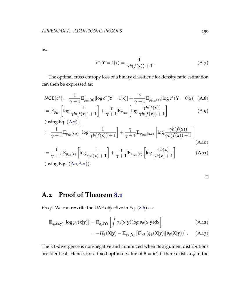
APPENDIX A. ADDITIONAL PROOFS 150
as:
c∗(Y = 1|x) = 1γb( f (x)) + 1
. (A.7)
The optimal cross-entropy loss of a binary classifier c for density ratio estimationcan then be expressed as:
NCE(c∗) =1
γ + 1Epref(x)[log c∗(Y = 1|x)] + γ
γ + 1Epbias(x)[log c∗(Y = 0|x)] (A.8)
= Epref
[log
1γb( f (x)) + 1
]+
γ
γ + 1Epbias
[log
γb( f (x))γb( f (x)) + 1
](A.9)
(using Eq. (A.7))
=1
γ + 1Epref(x,z)
[log
1γb( f (x)) + 1
]+
γ
γ + 1Epbias(x,z)
[log
γb( f (x))γb( f (x)) + 1
](A.10)
=1
γ + 1Epref(z)
[log
1γb(z) + 1
]+
γ
γ + 1Epbias(z)
[log
γb(z)γb(z) + 1
](A.11)
(using Eqs. (A.1,A.2)).
A.2 Proof of Theorem 8.1
Proof. We can rewrite the UAE objective in Eq. (8.6) as:
Eqφ(x,y) [log pθ(x|y)] = Eqφ(Y)
[∫qφ(x|y) log pθ(x|y)dx
](A.12)
= −Hφ(X|y)−Eqφ(Y)[DKL(qφ(X|y)‖pθ(X|y))
]. (A.13)
The KL-divergence is non-negative and minimized when its argument distributionsare identical. Hence, for a fixed optimal value of θ = θ∗, if there exists a φ in the

APPENDIX A. ADDITIONAL PROOFS 151
space of encoders being optimized that satisfies:
pθ∗(X|y) = qφ(X|y) (A.14)
for all x, y with p∗θ(Y) 6= 0, then it corresponds to the optimal encoder, i.e.,
φ = φ∗. (A.15)
For any value of φ, we know the following Gibbs chain converges to qφ(x, y) ifthe chain is ergodic:
y(t) ∼ qφ(Y|x(t)), (A.16)
x(t+1) ∼ qφ(X|y(t)). (A.17)
Substituting the results from Eqs. (A.14-A.17) in the Markov chain transitions inEqs. (8.8, 8.9) finishes the proof.
A.3 Proof of Corollary 8.1
Proof. By using earlier results (Proposition 2 in [RR06]), we need to show that theMarkov chain defined in Eqs. (8.8)-(8.9) is Φ-irreducible with a Gaussian noisemodel.1 That is, there exists a measure such that there is a non-zero probability oftransitioning from every set of non-zero measure to every other such set defined onthe same measure using this Markov chain.
Consider the Lebesgue measure. Formally, given any (x, y) and (x′, y′) such thatthe density q(x, y) > 0 and q(x′, y′) > 0 for the Lebesgue measure, we need to showthat the probability density of transitioning q(x′, y′|x, y) > 0.
(1) Since q(y|x) > 0 for all x ∈ Rn, y ∈ Rm (by Gaussian noise model as-sumption), we can use Eq. (8.8) to transition from (x, y) to (x, y′) with non-zeroprobability.
1Note that the symbol Φ here is different from the parameters denoted by little φ used in Chapter 8.

APPENDIX A. ADDITIONAL PROOFS 152
(2) Next, we claim that the transition probability q(x′|y) is non-negative for allx′, y. By Bayes rule, we have:
q(x′|y) = q(y|x′)q(x′)q(y)
. (A.18)
Since q(x, y) > 0 and q(x′, y′) > 0, the marginals q(y) and q(x′) are positive.Again, q(y|x′) > 0 for all x′ ∈ Rn, y ∈ Rm by the Gaussian noise model assumption.Hence, q(x′|y) is positive. Finally, using the optimality assumption for the posteriorsp(x′|y) matching q(x′|y) for all x′, y′, we can use Eq. (8.9) to transition from (x, y′)
to (x′, y′) with non-zero probability.From (1) and (2), we see that there is a non-zero probability of transitioning
from (x, y) to (x′, y′). Hence, under the assumptions of the corollary the Markovchain in Eqs. (8.8, 8.9) is ergodic.

B Additional Experimental Details & Re-sults
B.1 Chapter 3
Datasets. The MNIST dataset [LCB10] contains 50, 000 train, 10, 000 validation,and 10, 000 test images of dimensions 28× 28. The CIFAR-10 dataset [KH09] con-tains 50, 000 train and 10, 000 test images of dimensions 32× 32× 3 by default. Werandomly hold out 5, 000 training set images as validation set. Since we aremodelingdensities for discrete datasets (pixels can take a finite set of values ranging from1 to 255), the model can assign arbitrarily high log-likelihoods to these discretepoints. Following [UML13], we avoid this scenario by dequantizing the data whereuniform noise between 0 and 1 is added to every pixel. Finally, we scale the pixelsto lie between 0 and 1.
Model architectures. We used the NICE [DKB14] and Real-NVP [DSB17] archi-tectures as the normalizing flow generators for the MNIST and CIFAR-10 datasetsrespectively. For adversarial training, we consider the improved WGAN objectivewhich enforces the Lipschitz constraint over the critic by penalizing the norm of thegradient with respect to the input [Gul+17]. The critic architecture for the MNISTdataset is the same as the one used in the DCGAN [RMC15]. The batch normaliza-tion layer is removed as recommended [Gul+17]. For the CIFAR-10 experimentswe again use the DCGAN architecture with an extra convolutional layer. Batchnormalization [IS15] here was substituted by layer normalization [BKH16].
153

APPENDIX B. ADDITIONAL EXPERIMENTAL DETAILS & RESULTS 154
Hyperparameters. The hyperaparmeters specific to adversarial training with theWasserstein distance were fixed as per [Gul+17]. For all models trained on MNIST,we used a logistic prior distribution for the NICE architecture. The weights wereinitialized using the truncated normal distribution. For the models trained usingMLE, batch size was set to 200, learning rate was 0.001 with a decay of 0.9995 and theoptimizer usedwas Adamwith β1 = 0.9, β2 = 0.999. For the othermodels, the batchsize was set to 100, and the optimizer used was Adam with β1 = 0.5, β2 = 0.999
and a learning rate was 0.0001.In the case of models trained on CIFAR-10, an isotropic Gaussian prior was
used. We also used weight normalization [SK16] and Xavier initialization for all themodels. The models trained with MLE used a batch size of 100, a learning rate of0.0001 with a decay of 0.999995 and the Adam optimizer with β1 = 0.9, β2 = 0.999.The other models used a batch size of 64, a learning rate of 0.0001 and the Adamoptimizer with β1 = 0.5, β2 = 0.999.

APPENDIX B. ADDITIONAL EXPERIMENTAL DETAILS & RESULTS 155
B.2 Chapter 4
B.2.1 Bias-Variance of Different LFIW estimators
As discussed in Section 4.3, bias reduction using LFIW can suffer from issues wherethe importance weights are too small due to highly confident predictions of thebinary classifier. Across a batch of Monte Carlo samples, this can increase thecorresponding variance. Inspired from the importance sampling literature, weproposed additional mechanisms to mitigate this additional variance at the cost ofreduced debiasing in Eqs. (4.7-4.9). We now look at the empirical bias-variancetrade-off of these different estimators via a simple experiment below.
Our setup follows the goodness-of-fit testing experiments in Section 4.5. Thestatistics we choose to estimate is simply are the 2048 activations of the prefinallayer of the Inception Network, averaged across the test set of 10,000 samples ofCIFAR-10.
That is, the true statistics s = {s1, s2, · · · , s2048} are given by:
sj =1
|Dtest| ∑x∈Dtest
aj(x) (B.1)
where aj is the j-th prefinal layer activation of the Inception Network. Note that setof statistics s is fixed (computed once on the test set). To estimate these statistics,we will use different estimators. For example, the default estimator involving noreweighting is given as:
sj =1T
T
∑i=1
aj(x) (B.2)
where x ∼ pθ.Note that sj is a random variable since it depends on the T samples drawn
from pθ. Similar to Eq. (B.2), other variants of the LFIW estimators proposed inSection 4.3 can be derived using Eqs. (4.7-4.9). For any LFIW estimate sj, we canuse the standard decomposition of the expected mean-squared error into terms
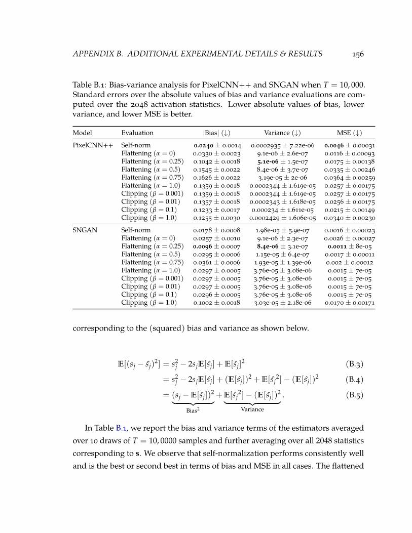
APPENDIX B. ADDITIONAL EXPERIMENTAL DETAILS & RESULTS 156
Table B.1: Bias-variance analysis for PixelCNN++ and SNGAN when T = 10, 000.Standard errors over the absolute values of bias and variance evaluations are com-puted over the 2048 activation statistics. Lower absolute values of bias, lowervariance, and lower MSE is better.
Model Evaluation |Bias| (↓) Variance (↓) MSE (↓)
PixelCNN++ Self-norm 0.0240 ± 0.0014 0.0002935 ± 7.22e-06 0.0046 ± 0.00031Flattening (α = 0) 0.0330 ± 0.0023 9.1e-06 ± 2.6e-07 0.0116 ± 0.00093Flattening (α = 0.25) 0.1042 ± 0.0018 5.1e-06 ± 1.5e-07 0.0175 ± 0.00138Flattening (α = 0.5) 0.1545 ± 0.0022 8.4e-06 ± 3.7e-07 0.0335 ± 0.00246Flattening (α = 0.75) 0.1626 ± 0.0022 3.19e-05 ± 2e-06 0.0364 ± 0.00259Flattening (α = 1.0) 0.1359 ± 0.0018 0.0002344 ± 1.619e-05 0.0257 ± 0.00175Clipping (β = 0.001) 0.1359 ± 0.0018 0.0002344 ± 1.619e-05 0.0257 ± 0.00175Clipping (β = 0.01) 0.1357 ± 0.0018 0.0002343 ± 1.618e-05 0.0256 ± 0.00175Clipping (β = 0.1) 0.1233 ± 0.0017 0.000234 ± 1.611e-05 0.0215 ± 0.00149Clipping (β = 1.0) 0.1255 ± 0.0030 0.0002429 ± 1.606e-05 0.0340 ± 0.00230
SNGAN Self-norm 0.0178 ± 0.0008 1.98e-05 ± 5.9e-07 0.0016 ± 0.00023Flattening (α = 0) 0.0257 ± 0.0010 9.1e-06 ± 2.3e-07 0.0026 ± 0.00027Flattening (α = 0.25) 0.0096 ± 0.0007 8.4e-06 ± 3.1e-07 0.0011 ± 8e-05Flattening (α = 0.5) 0.0295 ± 0.0006 1.15e-05 ± 6.4e-07 0.0017 ± 0.00011Flattening (α = 0.75) 0.0361 ± 0.0006 1.93e-05 ± 1.39e-06 0.002 ± 0.00012Flattening (α = 1.0) 0.0297 ± 0.0005 3.76e-05 ± 3.08e-06 0.0015 ± 7e-05Clipping (β = 0.001) 0.0297 ± 0.0005 3.76e-05 ± 3.08e-06 0.0015 ± 7e-05Clipping (β = 0.01) 0.0297 ± 0.0005 3.76e-05 ± 3.08e-06 0.0015 ± 7e-05Clipping (β = 0.1) 0.0296 ± 0.0005 3.76e-05 ± 3.08e-06 0.0015 ± 7e-05Clipping (β = 1.0) 0.1002 ± 0.0018 3.03e-05 ± 2.18e-06 0.0170 ± 0.00171
corresponding to the (squared) bias and variance as shown below.
E[(sj − sj)2] = s2
j − 2sjE[sj] + E[sj]2 (B.3)
= s2j − 2sjE[sj] + (E[sj])
2 + E[sj2]− (E[sj])
2 (B.4)
= (sj −E[sj])2︸ ︷︷ ︸
Bias2
+E[sj2]− (E[sj])
2︸ ︷︷ ︸Variance
. (B.5)
In Table B.1, we report the bias and variance terms of the estimators averagedover 10 draws of T = 10, 0000 samples and further averaging over all 2048 statisticscorresponding to s. We observe that self-normalization performs consistently welland is the best or second best in terms of bias and MSE in all cases. The flattened

APPENDIX B. ADDITIONAL EXPERIMENTAL DETAILS & RESULTS 157
Table B.2: Bias-variance analysis for PixelCNN++ and SNGAN when T = 5, 000.Standard errors over the absolute values of bias and variance evaluations are com-puted over the 2048 activation statistics. Lower absolute values of bias, lowervariance, and lower MSE is better.
Model Evaluation |Bias| (↓) Variance (↓) MSE (↓)
PixelCNN++ Self-norm 0.023 ± 0.0014 0.0005086 ± 1.317e-05 0.0049 ± 0.00033Flattening (α = 0) 0.0330 ± 0.0023 1.65e-05 ± 4.6e-07 0.0116 ± 0.00093Flattening (α = 0.25) 0.1038 ± 0.0018 9.5e-06 ± 3e-07 0.0174 ± 0.00137Flattening (α = 0.5) 0.1539 ± 0.0022 1.74e-05 ± 8e-07 0.0332 ± 0.00244Flattening (α = 0.75) 0.1620 ± 0.0022 6.24e-05 ± 3.83e-06 0.0362 ± 0.00256Flattening (α = 1.0) 0.1360 ± 0.0018 0.0003856 ± 2.615e-05 0.0258 ± 0.00174Clipping (β = 0.001) 0.1360 ± 0.0018 0.0003856 ± 2.615e-05 0.0258 ± 0.00174Clipping (β = 0.01) 0.1358 ± 0.0018 0.0003856 ± 2.615e-05 0.0257 ± 0.00173Clipping (β = 0.1) 0.1234 ± 0.0017 0.0003851 ± 2.599e-05 0.0217 ± 0.00148Clipping (β = 1.0) 0.1250 ± 0.0030 0.0003821 ± 2.376e-05 0.0341 ± 0.00232
SNGAN Self-norm 0.0176 ± 0.0008 3.88e-05 ± 9.6e-07 0.0016 ± 0.00022Flattening (α = 0) 0.0256 ± 0.0010 1.71e-05 ± 4.3e-07 0.0027 ± 0.00027Flattening (α = 0.25) 0.0099 ± 0.0007 1.44e-05 ± 3.7e-07 0.0011 ± 8e-05Flattening (α = 0.5) 0.0298 ± 0.0006 1.62e-05 ± 5.3e-07 0.0017 ± 0.00012Flattening (α = 0.75) 0.0366 ± 0.0006 2.38e-05 ± 1.11e-06 0.0021 ± 0.00012Flattening (α = 1.0) 0.0302 ± 0.0005 4.56e-05 ± 2.8e-06 0.0015 ± 7e-05Clipping (β = 0.001) 0.0302 ± 0.0005 4.56e-05 ± 2.8e-06 0.0015 ± 7e-05Clipping (β = 0.01) 0.0302 ± 0.0005 4.56e-05 ± 2.8e-06 0.0015 ± 7e-05Clipping (β = 0.1) 0.0302 ± 0.0005 4.56e-05 ± 2.81e-06 0.0015 ± 7e-05Clipping (β = 1.0) 0.1001 ± 0.0018 5.19e-05 ± 2.81e-06 0.0170 ± 0.0017
estimator with no debiasing (corresponding to α = 0) has lower bias and highervariance than the self-normalized estimator. Amongst the flattening estimators,lower values of α seem to provide the best bias-variance trade-off. The clipped esti-mators do not perform well in this setting, with lower values of β slightly preferableover larger values. We repeat the same experiment with T = 5, 000 samples andreport the results in Table B.2. While the variance increases as expected (by almostan order of magnitude), the estimator bias remains roughly the same.
B.2.2 Calibration
We found in all our cases that the binary classifiers used for training the model werehighly calibrated by default and did not require any further recalibration. See for
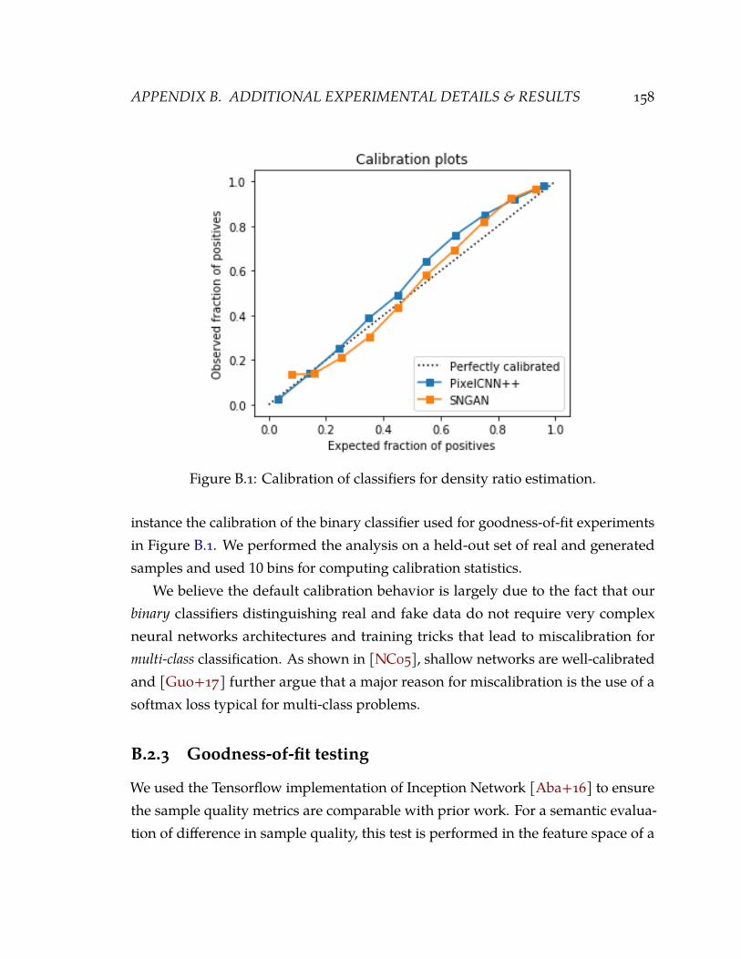
APPENDIX B. ADDITIONAL EXPERIMENTAL DETAILS & RESULTS 158
Figure B.1: Calibration of classifiers for density ratio estimation.
instance the calibration of the binary classifier used for goodness-of-fit experimentsin Figure B.1. We performed the analysis on a held-out set of real and generatedsamples and used 10 bins for computing calibration statistics.
We believe the default calibration behavior is largely due to the fact that ourbinary classifiers distinguishing real and fake data do not require very complexneural networks architectures and training tricks that lead to miscalibration formulti-class classification. As shown in [NC05], shallow networks are well-calibratedand [Guo+17] further argue that a major reason for miscalibration is the use of asoftmax loss typical for multi-class problems.
B.2.3 Goodness-of-fit testing
We used the Tensorflow implementation of Inception Network [Aba+16] to ensurethe sample quality metrics are comparable with prior work. For a semantic evalua-tion of difference in sample quality, this test is performed in the feature space of a

APPENDIX B. ADDITIONAL EXPERIMENTAL DETAILS & RESULTS 159
pretrained classifier, such as the prefinal activations of the Inception Net [Sze+16].For example, the Inception score for a generative model pθ given a classifier d(·) canbe expressed as:
IS = exp(Ex∼pθ[KL(d(y|x), d(y))]).
The FID score is another metric which unlike the Inception score also takes intoaccount real data from pdata. Mathematically, the FID between sets S and R sampledfrom distributions pθ and pdata respectively, is defined as:
FID(S, R) = ‖µS − µR‖22 + Tr(ΣS + ΣR − 2
√ΣSΣR)
where (µS, ΣS) and (µR, ΣR) are the empirical means and covariances computedbased on S and R respectively. Here, S and R are sets of datapoints from pθ andpdata. In a similar vein, KID compares statistics between samples in a feature spacedefined via a combination of kernels and a pretrained classifier. The standard kernelused is a radial-basis function kernel with a fixed bandwidth of 1. As desired, thescore is optimized when the data and model distributions match.
We used the open-sourced model implementations of PixelCNN++ [Sal+16]and SNGAN [Miy+18]. Following the observation by [LO16], we found that traininga binary classifier on top of the feature space of any pretrained image classifier wasuseful for removing the low-level artifacts in the generated images in classifyingan image as real or fake. We hence learned a multi-layer perceptron (with a singlehidden layer of 1000 units) on top of the 2048 dimensional feature space of theInception Network. Learning was done using the Adam optimizer with the defaulthyperparameters with a learning rate of 0.001 and a batch size of 64. We observedrelatively fast convergence for training the binary classifier (in less than 20 epochs) onboth PixelCNN++ and SNGAN generated data and the best validation set accuracyacross the first 20 epochs was used for final model selection.

APPENDIX B. ADDITIONAL EXPERIMENTAL DETAILS & RESULTS 160
Table B.3: Statistics for the environments.
Environment State dimensionality Action dimensionality
Swimmer 8 2HalfCheetah 17 6
HumanoidStandup 376 17
B.2.4 Data Augmentation
We used the open-source implementation of DAGAN1 [ASE17] as the base gen-erative model. Given a DAGAN model, we additionally require training a binaryclassifier for estimating importance weights and a multi-class classifier for subse-quent classification. The architecture for both these use cases follows prior workin meta learning on Omniglot [Vin+16]. We train the DAGAN on the 1200 classesreserved for training in prior works. For each class, we consider a 15/5/5 split of the20 examples for training, validation, and testing. Except for the final output layer,the architecture consists of 4 blocks of 3x3 convolutions and 64 filters, followed bybatch normalization [Sze+16], a ReLU non-linearity and 2x2 max pooling. Learningwas done for 100 epochs using the Adam optimizer with default parameters and alearning rate of 0.001 with a batch size of 32.
B.2.5 Model-based Off-policy Policy Evaluation
We used Tensorflow [Aba+16] and OpenAI baselines2 [Dha+17]. We evaluate overthree environments: Swimmer, HalfCheetah, and HumanoidStandup (Figure B.2.Both HalfCheetah and Swimmer rewards the agent for gaining higher horizontalvelocity; HumanoidStandup rewards the agent for gaining more height via standingup. In all three environments, the initial state distributions are obtained via addingsmall random perturbation around a certain state. The dimensions for state andaction spaces are shown in Table B.3.
Our policy network has two fully connected layers with 64 neurons and tanh1https://github.com/AntreasAntoniou/DAGAN.git2https://github.com/openai/baselines.git
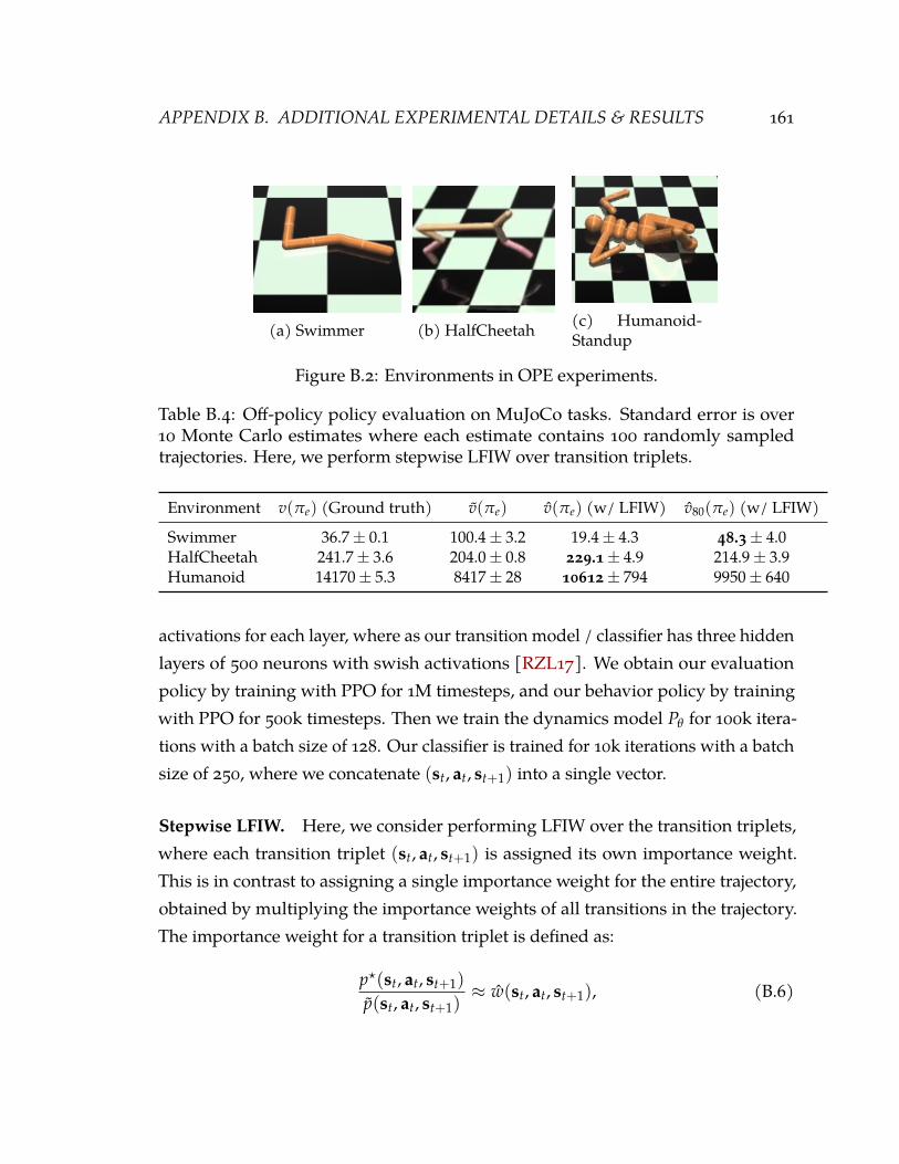
APPENDIX B. ADDITIONAL EXPERIMENTAL DETAILS & RESULTS 161
(a) Swimmer (b) HalfCheetah (c) Humanoid-Standup
Figure B.2: Environments in OPE experiments.
Table B.4: Off-policy policy evaluation on MuJoCo tasks. Standard error is over10 Monte Carlo estimates where each estimate contains 100 randomly sampledtrajectories. Here, we perform stepwise LFIW over transition triplets.
Environment v(πe) (Ground truth) v(πe) v(πe) (w/ LFIW) v80(πe) (w/ LFIW)
Swimmer 36.7± 0.1 100.4± 3.2 19.4± 4.3 48.3± 4.0HalfCheetah 241.7± 3.6 204.0± 0.8 229.1± 4.9 214.9± 3.9Humanoid 14170± 5.3 8417± 28 10612± 794 9950± 640
activations for each layer, where as our transition model / classifier has three hiddenlayers of 500 neurons with swish activations [RZL17]. We obtain our evaluationpolicy by training with PPO for 1M timesteps, and our behavior policy by trainingwith PPO for 500k timesteps. Then we train the dynamics model Pθ for 100k itera-tions with a batch size of 128. Our classifier is trained for 10k iterations with a batchsize of 250, where we concatenate (st, at, st+1) into a single vector.
Stepwise LFIW. Here, we consider performing LFIW over the transition triplets,where each transition triplet (st, at, st+1) is assigned its own importance weight.This is in contrast to assigning a single importance weight for the entire trajectory,obtained by multiplying the importance weights of all transitions in the trajectory.The importance weight for a transition triplet is defined as:
p?(st, at, st+1)
p(st, at, st+1)≈ w(st, at, st+1), (B.6)

APPENDIX B. ADDITIONAL EXPERIMENTAL DETAILS & RESULTS 162
0 20 40 60 80 100H
20
40
60|
(v)|
Swimmer
0 20 40 60 80 100H
20
40
|(v
)|
HalfCheetah
0 20 40 60 80 100H
4000
6000
|(v
)|
HumanoidStandup
Figure B.3: Estimation error δ(v) = v(πe)− vH(πe) for different values of H (mini-mum 0, maximum 100). Shaded area denotes standard error over different randomseeds; each seed uses 100 sampled trajectories. Here, we perform stepwise LFIWover transition triplets.
so the corresponding LFIW estimator is given as
v(πe) = Ep
[T−1
∑t=0
w(st, at, st+1) · r(st, at)
]. (B.7)
We describe this as the ‘‘stepwise” LFIW approach for off-policy policy evaluation.We perform self-normalization over the weights of each triplet.
From the results in Table B.4 and Figure B.3, stepwise LFIW also reduces biasfor OPE compared to without LFIW. Compared to the ‘‘trajectory based” LFIWdescribed in Eq. (4.20), the stepwise estimator has slightly higher variance andweaker performance for H = 20, 40, but outperforms the trajectory level estimatorswhen H = 100 on HalfCheetah and HumanoidStandup environments.

APPENDIX B. ADDITIONAL EXPERIMENTAL DETAILS & RESULTS 163
B.3 Chapter 5
B.3.1 Dataset Construction Procedure
We construct such dataset splits from the full CelebA training set using the followingprocedure. We initially fix our dataset size to be roughly 135K out of the total 162Kbased on the total number of females present in the data. Then for each level ofbias, we partition 1/4 of males and 1/4 of females into Dref to achieve the 50-50ratio. The remaining number of examples are used for Dbias, where the number ofmales and females are adjusted to match the desired level of bias (e.g., 0.9). Finallyat each level of reference dataset size perc, we discard the appropriate fraction ofdatapoints from both the male and female category in Dref. For example, for perc =0.5, we discard half the number of females and half the number of males from Dref.
B.3.2 FID Calculation
The FIDmetricmay exhibit a relative preference formodels trained on larger datasetsin order to maximize perceptual sample quality, at the expense of propagating oramplifying existing dataset bias. In order to obtain an estimate of sample qualitythat would also incorporate a notion of fairness across sensitive attribute classes,we pre-computed the relevant FID statistics on a ”balanced” construction of theCelebA dataset that matches our reference dataset pref. That is, we used all train/val-idation/test splits of the data such that: (1) for single-attribute, there were 50-50portions of males and females; and (2) for multi-attribute, there were even propor-tions of examples across all 4 classes (females with black hair, females without blackhair, males with black hair, males without black hair). We report ”balanced” FIDnumbers on these pre-computed statistics throughout the chapter.
B.3.3 Attribute Classifier
We use the same architecture and hyperparameters for both the single- and multi-attribute classifiers. Both are variants of ResNet-18 where the output number of

APPENDIX B. ADDITIONAL EXPERIMENTAL DETAILS & RESULTS 164
classes correspond to the dataset split (e.g., 2 classes for single-attribute, 4 classesfor the multi-attribute experiment).
Model architecture. We provide the architectural details in Table B.5 below:
Name Componentconv1 7× 7 conv, 64 filters. stride 2
Residual Block 1 3× 3 max pool, stride 2
Residual Block 2[
3× 3 conv, 128 filters3× 3 conv, 128 filters
]× 2
Residual Block 3[
3× 3 conv, 256 filters3× 3 conv, 256 filters
]× 2
Residual Block 4[
3× 3 conv, 512 filters3× 3 conv, 512 filters
]× 2
Output Layer 7× 7 average pool stride 1, fully-connected, softmax
Table B.5: ResNet-18 architecture adapted for attribute classifier.
Hyperparameters. During training, we use a batch size of 64 and the Adam op-timizer with learning rate = 0.001. The classifiers learn relatively quickly for bothsingle and multi attribute scenarios and we only needed to train for 10 epochs. Weused a validation set for model selection.
B.3.4 Density Ratio Classifier
Model architecture. We provide the same architectural details as in Table B.5.
Hyperparameters. We also use a batch size of 64, the Adam optimizer with learn-ing rate = 0.0001, and a total of 15 epochs to train the classifier for density ratioestimation.
B.3.5 BigGAN
Model architecture. The architectural details for the BigGAN are provided inTable B.6.
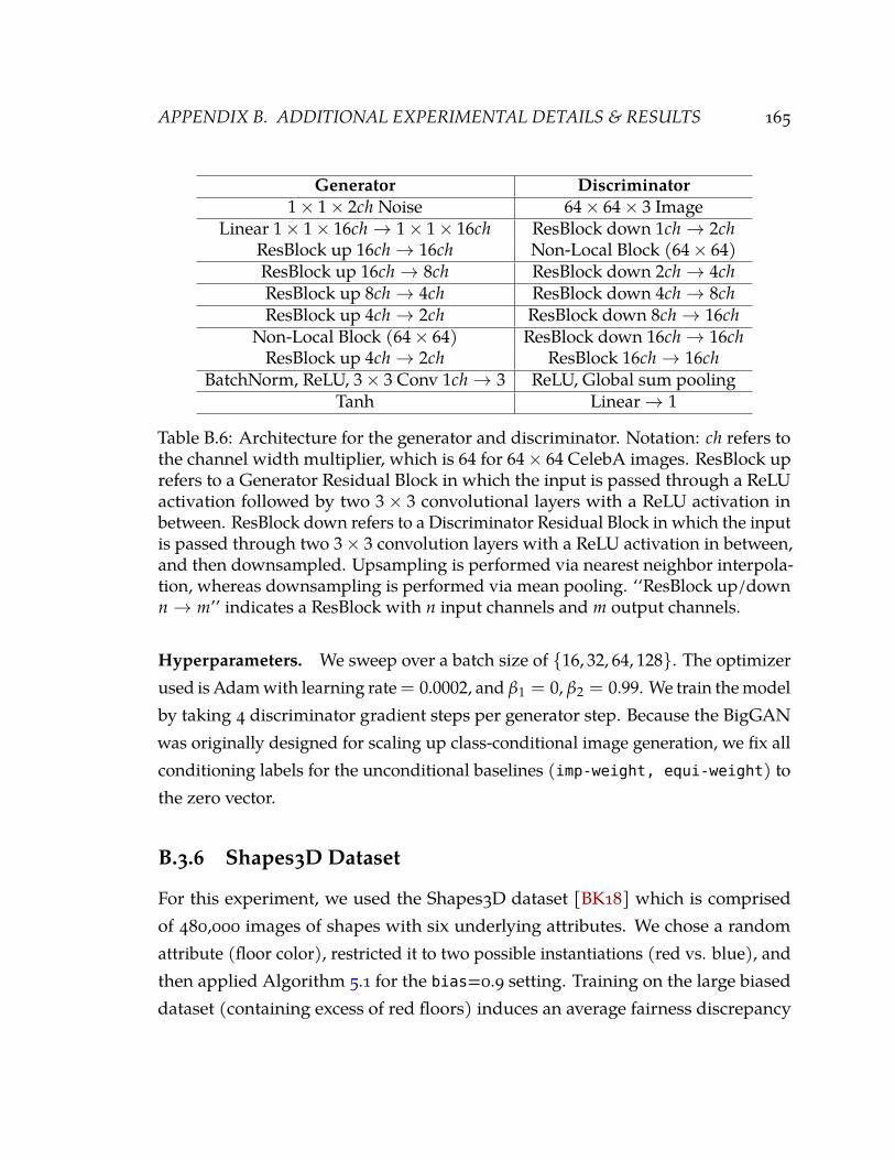
APPENDIX B. ADDITIONAL EXPERIMENTAL DETAILS & RESULTS 165
Generator Discriminator1× 1× 2ch Noise 64× 64× 3 Image
Linear 1× 1× 16ch→ 1× 1× 16ch ResBlock down 1ch→ 2chResBlock up 16ch→ 16ch Non-Local Block (64× 64)ResBlock up 16ch→ 8ch ResBlock down 2ch→ 4chResBlock up 8ch→ 4ch ResBlock down 4ch→ 8chResBlock up 4ch→ 2ch ResBlock down 8ch→ 16ch
Non-Local Block (64× 64) ResBlock down 16ch→ 16chResBlock up 4ch→ 2ch ResBlock 16ch→ 16ch
BatchNorm, ReLU, 3× 3 Conv 1ch→ 3 ReLU, Global sum poolingTanh Linear→ 1
Table B.6: Architecture for the generator and discriminator. Notation: ch refers tothe channel width multiplier, which is 64 for 64× 64 CelebA images. ResBlock uprefers to a Generator Residual Block in which the input is passed through a ReLUactivation followed by two 3× 3 convolutional layers with a ReLU activation inbetween. ResBlock down refers to a Discriminator Residual Block in which the inputis passed through two 3× 3 convolution layers with a ReLU activation in between,and then downsampled. Upsampling is performed via nearest neighbor interpola-tion, whereas downsampling is performed via mean pooling. ‘‘ResBlock up/downn→ m’’ indicates a ResBlock with n input channels and m output channels.
Hyperparameters. We sweep over a batch size of {16, 32, 64, 128}. The optimizerused is Adamwith learning rate= 0.0002, and β1 = 0, β2 = 0.99. We train themodelby taking 4 discriminator gradient steps per generator step. Because the BigGANwas originally designed for scaling up class-conditional image generation, we fix allconditioning labels for the unconditional baselines (imp-weight, equi-weight) tothe zero vector.
B.3.6 Shapes3D Dataset
For this experiment, we used the Shapes3D dataset [BK18] which is comprisedof 480,000 images of shapes with six underlying attributes. We chose a randomattribute (floor color), restricted it to two possible instantiations (red vs. blue), andthen applied Algorithm 5.1 for the bias=0.9 setting. Training on the large biaseddataset (containing excess of red floors) induces an average fairness discrepancy

APPENDIX B. ADDITIONAL EXPERIMENTAL DETAILS & RESULTS 166
(a) Baseline samples
(b) Samples after reweighting
Figure B.4: Results from the Shapes3D dataset. After restricting the possible floorcolors to red or blue and using a biased dataset of bias=0.9, we find that the samplesobtained after importance reweighting (b) are considerably more balanced thanthose without reweighting (a), as desired.
of 0.468 as shown in Figure B.4a. In contrast, applying the importance-weightingcorrection on the large biased dataset enabled us to train models that yielded anaverage fairness discrepancy of 0.002 as shown in Figure B.4b.

APPENDIX B. ADDITIONAL EXPERIMENTAL DETAILS & RESULTS 167
B.4 Chapter 6
B.4.1 Link prediction
We used the Spectral Clustering (SC) implementation from [Ped+11] and publicimplementations for others made available by the authors. For SC, we used adimension size of 128. For DeepWalk and node2vec which uses a skipgram likeobjective on random walks from the graph, we used the same dimension size anddefault settings used in [PAS14] and [GL16] respectively of 10 random walks oflength 80 per node and a context size of 10. For node2vec, we searched over therandom walk bias parameters using a grid search in {0.25, 0.5, 1, 2, 4} as prescribedin the original work. For GAE and VGAE, we used the same architecture as VGAEand Adam optimizer with learning rate of 0.01.
For Graphite-AE andGraphite-VAE,we used an architecture of 32-32 units for theencoder and 16-32-16 units for the decoder (two rounds of iterative decoding beforea final inner product). The model is trained using the Adam optimizer [KW18]with a learning rate of 0.01. All activations were RELUs.The dropout rate (foredges) and λ were tuned as hyperparameters on the validation set to optimize theAUC, whereas traditional dropout was set to 0 for all datasets. Additionally, wetrained every model for 500 iterations and used the model checkpoint with the bestvalidation loss for testing. Scores are reported as an average of 50 runs with differenttrain/validation/test splits, with the requirement that the training graph necessarilybe connected.
For Graphite, we observed that using a form of skip connections to define a linearcombination of the initial embedding Z and the final embedding Z∗ is particularlyuseful. The skip connection consists of a tunable hyperparameter λ controlling therelative weights of the embeddings. The final embedding of Graphite is a functionof the initial embedding Z and the last induced embedding Z∗. We consider twofunctions to aggregate them into a final embedding. That is, (1− λ)Z + λZ∗ and Z +
λZ∗/ ‖Z∗‖, which correspond to a convex combination of two embeddings, and anincremental update to the initial embedding in a given direction, respectively. Note

APPENDIX B. ADDITIONAL EXPERIMENTAL DETAILS & RESULTS 168
Table B.7: AUC scores for link prediction with Monte Carlo subsampling duringtraining. Higher is better.
Cora Citeseer Pubmed
VGAE 89.6 92.2 92.3Graphite 90.5 92.5 93.1
Figure B.5: AUC score of VGAE and Graphite with subsampled edges on the Coradataset.
that in either case, GAE and VGAE reduce to a special case of Graphite, using only asingle inner-product decoder (i.e., λ = 0). On Cora and Pubmed final embeddingswere derived through convex combination, on Citeseer through incremental update.
Scalability. We experimented with learning VGAE and Graphite models by sub-sampling |E| random entries for Monte Carlo evaluation of the objective at eachiteration. The corresponding AUC scores are shown in Table B.7. The results suggestthat Graphite can effectively scale to large graphs without significant loss in accu-racy. The AUC results trained with edge subsampling as we vary the subsamplingcoefficient c are shown in Figure B.5.

APPENDIX B. ADDITIONAL EXPERIMENTAL DETAILS & RESULTS 169
B.4.2 Semi-supervised node classification
Wereport the baseline results for SemiEmb [WRC08], DeepWalk [PAS14], ICA [LG03]and Planetoid [YCS16] as specified in [KW17]. GCN uses a 32-16 architecture withReLu activations and early stopping after 10 epochs without increasing validationaccuracy. The Graphite model uses the same architecture as in link prediction (withno edge dropout). The parameters of the posterior distributions are concatenatedwith node features to predict the final output. The parameters are learned using theAdam optimizer [KW18] with a learning rate of 0.01. All accuracies are taken as anaverage of 100 runs.
B.4.3 Density estimation
We learn a model architecture specified for the maximum possible nodes (i.e., 20
in this case) to accommodate for input graphs of different sizes. While feeding insmaller graphs, we add dummy nodes disconnected from the rest of the graph. The dummy nodes have no influence on the gradient updates for the parametersaffecting the latent or observed variables involving nodes in the true graph. Fordensity estimation, we pick a graph family, then train and validate on graphs sampledexclusively from that family. We consider graphs with 10 to 20 nodes belonging tothe following graph families :
• Erdos-Renyi [ER59]: each edge independently sampled with probability p =
0.5
• Ego Network: a random Erdos-Renyi graph with all nodes neighbors of onerandomly chosen node
• Random Regular: uniformly random regular graph with degree d = 4
• RandomGeometric: graph induced by uniformly randompoints in unit squarewith edges between points at euclidean distance less than r = 0.5
• Random Power Tree: Tree generated by randomly swapping elements from adegree distribution to satisfy a power law distribution for γ = 3

APPENDIX B. ADDITIONAL EXPERIMENTAL DETAILS & RESULTS 170
• Barabasi-Albert [BA99]: Preferential attachment graph generation with attach-ment edge count m = 4
Weuse convex combinations over three successively induced embeddings. Scoresare reported over an average of 50 runs. Additionally, a two-layer neural net isapplied to the initially sampled embedding Z before being fed to the inner productdecoder for GAE and VGAE, or being fed to the iterations of Eqs. (6.8) and (6.9) forboth Graphite-AE and Graphite-VAE.
APPENDIX B. ADDITIONAL EXPERIMENTAL DETAILS & RESULTS 171
B.5 Chapter 7
B.5.1 RoboSumo Environment
To limit the scope of our study, we restrict agent morphologies to only 4-leg robots.During the game, observations of each agent were represented by a 120-dimensionalvector comprised of positions and velocities of its own body and positions of the op-ponent’s body; agent’s actions were 8-dimensional vectors that represented torquesapplied to the corresponding joints.
Model architectures. Agent policies are parameterized as multi-layer perceptrons(MLPs) with 2 hidden layers of 90 units each. For the embedding network, we usedanother MLP network with 2 hidden layers of 100 units each to give an embeddingof size 100. For the conditioned policy network we also reduce the hidden layer sizeto 64 units each.
Policy optimization. For learning the population of agents, we use the distributedversion of PPO algorithm as described in [Al-+18] with 2 × 10⁻³ learning rate,ε = 0.2, 16,000 time steps per update with 6 epochs 4,000 time steps per batch.
Training agents. For our analysis, we train a diverse collection of 25 agents, some ofwhich are trained via self-play and others are trained in pairs concurrently, forminga clique agent-interaction graph (Figure B.6a).
B.5.2 ParticleWorld Environment
The overall continuous observation and discrete action space for the speaker agentsare 3 and 7 dimensions respectively. For the listener agents, the observation andaction spaces are 15 and 5 dimensions respectively.
Model architectures. Agent policies and shared critic (i.e., a value function) areparameterized as multi-layer perceptrons (MLPs) with 2 hidden layers of 64 units

APPENDIX B. ADDITIONAL EXPERIMENTAL DETAILS & RESULTS 172
12
3
4
56
7
8
9
10
(a)
1
2
3
4
5
1
2
3
4
5
Speaker Listener
(b)
Figure B.6: (a) An example clique agent interaction graph with 10 agents. (b) Anexample bipartite agent interaction graph with 5 speakers and 5 listeners.
each. The observation space for the speaker is small (3 dimensions), and a small em-bedding of size 5 for the listener policy gives good performance. For the embeddingnetwork, we again used an MLP with 2 hidden layers of 100 units each.
Policy optimization. For learning the initial population of listener and agent poli-cies, we use multiagent deep deterministic policy gradients (MADDPG) as the basealgorithm [Low+17]. Adam optimizer [KB15] with a learning rate of 4× 10⁻³ wasused for optimization. Replay buffer size was set to 106 timesteps.
Training agents. We first train 28 speaker-listener pairs using the MADDPG algo-rithm. From this collection of 28 speakers, we train another set of 28 listeners, eachtrained to work with a speaker pair, forming a bipartite agent-interaction graph(Figure B.6b). We choose the best 14 listeners for later experiments.

APPENDIX B. ADDITIONAL EXPERIMENTAL DETAILS & RESULTS 173
B.6 Chapter 8
Datasets. For MNIST, we use the train/valid/test split of 50, 000/10, 000/10, 000
images. For Omniglot, we use train/valid/test split of 23, 845/500/8, 070 images.For CelebA, we used the splits as provided by [Liu+15] on the dataset website.All images were scaled such that pixel values are between 0 and 1. We used theAdam optimizer with a learning rate of 0.001 for all the learned models. For MNISTand Omniglot, we used a batch size of 100. For CelebA, we used a batch size of 64.Further, we implemented early stopping based on the best validation bounds after200 epochs for MNIST, 500 epochs for Omniglot, and 200 epochs for CelebA.
Model architectures. For both MNIST and Omniglot, the UAE decoder used 2
hidden layers of 500 units each with ReLU activations. The encoder was a singlelinear layer with only weight parameters and no bias parameters. The encoder anddecoder architectures for the VAE baseline are symmetrical with 2 hidden layers of500 units each and 20 latent units. We used the LASSO baseline implementation fromsklearn and tuned the Lagrange parameter on the validation sets. For the baselines,we do 10 random restarts with 1, 000 steps per restart and pick the reconstructionwith best measurement error as prescribed in [Bor+17].
Table B.8: Frobenius norms of the encoding matrices for MNIST and Omniglot.
m Random Gaussian Matrices MNIST-UAE Omniglot-UAE
2 39.57 6.42 2.175 63.15 5.98 2.6610 88.98 7.24 3.5025 139.56 8.53 4.7150 198.28 9.44 5.45100 280.25 10.62 6.02
Table B.8 shows the average norms for the randomGaussian matrices used in thebaselines and the learned UAE encodings. The low norms for the UAE encodingssuggest that UAE is not trivially overcoming noise by increasing the norm of W.

APPENDIX B. ADDITIONAL EXPERIMENTAL DETAILS & RESULTS 174
For CelebA dataset, we used the following architectures for UAE.
Encoder
Signal
→ Conv[Kernel: 4x4, Stride: 2, Filters: 32, Padding: Same, Activation: Relu]
→ Conv[Kernel: 4x4, Stride: 2, Filters: 32, Padding: Same, Activation: Relu]
→ Conv[Kernel: 4x4, Stride: 2, Filters: 64, Padding: Same, Activation: Relu]
→ Conv[Kernel: 4x4, Stride: 2, Filters: 64, Padding: Same, Activation: Relu]
→ Conv[Kernel: 4x4, Stride: 1, Filters: 256, Padding: Valid, Activation: Relu]
→ Fully_Connected[Units: m, Activation: None]
Decoder
Measurements
→ Fully_Connected[Units: 256, Activation: Relu]
→ Conv_transpose[Kernel: 4x4, Stride: 1, Filters: 256, Padding: Valid, Activation: Relu]
→ Conv_transpose[Kernel: 4x4, Stride: 2, Filters: 64, Padding: Same, Activation: Relu]
→ Conv_transpose[Kernel: 4x4, Stride: 2, Filters: 64, Padding: Same, Activation: Relu]
→ Conv_transpose[Kernel: 4x4, Stride: 2, Filters: 32, Padding: Same, Activation: Relu]
→ Conv_transpose[Kernel: 4x4, Stride: 2, Filters: 3, Padding: Valid, Activation: Sigmoid]
C Code & Data
The following links provide open-source implementations and custom datasets (ifapplicable) for the various learning frameworks presented in this dissertation.
• Chapter 3
https://github.com/ermongroup/flow-gan
• Chapter 4
https://github.com/aditya-grover/bias-correction-generative
• Chapter 5
https://github.com/ermongroup/fairgen
• Chapter 6
https://github.com/ermongroup/graphite
• Chapter 8
https://github.com/aditya-grover/uae
• Chapter 9
https://github.com/chueh-ermon/battery-fast-charging-optimization
175

Bibliography
[23m16] 23&me. ‘‘The Real Issue: Diversity in Genetics Research.’’ In: Re-trieved from https://blog.23andme.com/ancestry/the-real-issue-diversity-in-genetics-research/ (2016) (cit. on p. 56).
[AB14] GuillaumeAlain andYoshuaBengio. ‘‘What regularized auto-encoderslearn from the data-generating distribution.’’ In: Journal of MachineLearning Research 15.1 (2014), pp. 3563–3593 (cit. on p. 125).
[Aba+16] Martın Abadi, Paul Barham, JianminChen, ZhifengChen, AndyDavis,Jeffrey Dean, Matthieu Devin, Sanjay Ghemawat, Geoffrey Irving,Michael Isard, et al. ‘‘Tensorflow: a system for large-scale machinelearning.’’ In: Operating Systems Design and Implementation. 2016 (cit.on pp. 158, 160).
[Abe+20] Rediet Abebe, Solon Barocas, Jon Kleinberg, Karen Levy, ManishRaghavan, and David G Robinson. ‘‘Roles for computing in socialchange.’’ In: Proceedings of the Conference on Fairness, Accountability, andTransparency. 2020 (cit. on p. 73).
[ACB17] Martin Arjovsky, Soumith Chintala, and Léon Bottou. ‘‘Wassersteingan.’’ In: arXiv preprint arXiv:1701.07875 (2017) (cit. on pp. 20, 26, 28,33).
[Ade+19] Tameem Adel, Isabel Valera, Zoubin Ghahramani, and Adrian Weller.‘‘One-network adversarial fairness.’’ In: Proceedings of the AAAI Con-ference on Artificial Intelligence. Vol. 33. 2019 (cit. on p. 71).
176

BIBLIOGRAPHY 177
[Ahm+17] Shabbir Ahmed, Ira Bloom, Andrew N Jansen, Tanvir Tanim, Eric JDufek, Ahmad Pesaran, Andrew Burnham, Richard B Carlson, Fer-nando Dias, Keith Hardy, et al. ‘‘Enabling fast charging–A batterytechnology gap assessment.’’ In: Journal of Power Sources 367 (2017),pp. 250–262 (cit. on pp. 130, 131, 136, 139, 141, 144).
[Al-+18] Maruan Al-Shedivat, Trapit Bansal, Yuri Burda, Ilya Sutskever, IgorMordatch, and Pieter Abbeel. ‘‘Continuous Adaptation via Meta-Learning in Nonstationary and Competitive Environments.’’ In: Inter-national Conference on Learning Representations. 2018 (cit. on pp. 90, 99,103, 171).
[Ale+17] Alexander A Alemi, Ian Fischer, Joshua V Dillon, and Kevin Murphy.‘‘Deep variational information bottleneck.’’ In: International Conferenceon Learning Representations. 2017 (cit. on p. 111).
[Ale+18] Alexander A Alemi, Ben Poole, Ian Fischer, Joshua V Dillon, Rif ASaurous, and KevinMurphy. ‘‘Fixing a Broken ELBO.’’ In: InternationalConference on Machine Learning. 2018 (cit. on p. 126).
[Ami+19] Alexander Amini, Ava P Soleimany, Wilko Schwarting, Sangeeta NBhatia, and Daniela Rus. ‘‘Uncovering and mitigating algorithmicbias through learned latent structure.’’ In: Proceedings of the 2019AAAI/ACM Conference on AI, Ethics, and Society. 2019 (cit. on p. 72).
[Ana+16] Ankit Anand, Aditya Grover, Mausam, and Parag Singla. ‘‘ContextualSymmetries in Probabilistic Graphical Models.’’ In: International JointConference on Artificial Intelligence. 2016 (cit. on p. 148).
[Ant+15] Stanislaw Antol, Aishwarya Agrawal, Jiasen Lu, Margaret Mitchell,Dhruv Batra, C Lawrence Zitnick, and Devi Parikh. ‘‘Vqa: Visualquestion answering.’’ In: Proceedings of the IEEE International Conferenceon Computer Vision. 2015 (cit. on p. 4).

BIBLIOGRAPHY 178
[ARZ18] Sanjeev Arora, Andrej Risteski, and Yi Zhang. ‘‘Do GANs learn thedistribution? Some Theory and Empirics.’’ In: International Conferenceon Learning Representations. 2018 (cit. on pp. 35, 58).
[AS17] Stefano V Albrecht and Peter Stone. ‘‘Autonomous Agents ModelingOther Agents: A Comprehensive Survey and Open Problems.’’ In:arXiv preprint arXiv: 1709.08071 (2017) (cit. on p. 107).
[ASE17] Antreas Antoniou, Amos Storkey, and Harrison Edwards. ‘‘Data aug-mentation generative adversarial networks.’’ In: arXiv preprint arXiv:1711.04340(2017) (cit. on pp. 35–37, 47, 160).
[Att+20] PeterAttia, AdityaGrover,Norman Jin, Kristen Severson, BryanCheong,Jerry Liao,MichaelHChen,Nicholas Perkins, Zi Yang, PatrickHerring,Muratahan Aykol, Stephen Harris, Richard Braatz, Stefano Ermon,and William Chueh. ‘‘Closed-loop optimization of extreme fast charg-ing for batteries using machine learning.’’ In: Nature 578.7795 (2020),pp. 397–402 (cit. on pp. 5, 6, 8, 134, 144).
[AZ17] Sanjeev Arora and Yi Zhang. ‘‘Do GANs actually learn the distribu-tion? An empirical study.’’ In: arXiv preprint arXiv:1706.08224 (2017)(cit. on p. 33).
[Aza+18] Samaneh Azadi, Catherine Olsson, Trevor Darrell, Ian Goodfellow,and Augustus Odena. ‘‘Discriminator rejection sampling.’’ In: arXivpreprint arXiv:1810.06758 (2018) (cit. on pp. 53, 72).
[AZG20] MichaelArbel, LiangZhou, andArthurGretton. ‘‘KALE:WhenEnergy-BasedLearningMeetsAdversarial Training.’’ In: arXiv preprint arXiv:2003.05033(2020) (cit. on p. 54).
[BA03] David Barber and Felix Agakov. ‘‘The IM algorithm: A variationalapproach to information maximization.’’ In: Advances in Neural Infor-mation Processing Systems. 2003 (cit. on pp. 111, 114, 116, 127).

BIBLIOGRAPHY 179
[BA99] Albert-Laszlo Barabasi and Reka Albert. ‘‘Emergence of Scaling inRandom Networks.’’ In: Science 286.5439 (1999), pp. 509–512 (cit. onpp. 87, 170).
[Bac+19] Arturs Backurs, Piotr Indyk, Krzysztof Onak, Baruch Schieber, AliVakilian, and Tal Wagner. ‘‘Scalable fair clustering.’’ In: arXiv preprintarXiv:1902.03519 (2019) (cit. on p. 72).
[Bar89] Horace B Barlow. ‘‘Unsupervised learning.’’ In: Neural Computation1.3 (1989), pp. 295–311 (cit. on p. 1).
[Bau+14] Thorsten Baumhöfer, Manuel Brühl, Susanne Rothgang, and DirkUwe Sauer. ‘‘Production caused variation in capacity aging trend andcorrelation to initial cell performance.’’ In: Journal of Power Sources 247(2014), pp. 332–338 (cit. on p. 129).
[BCM11] Smriti Bhagat, Graham Cormode, and S Muthukrishnan. ‘‘Node clas-sification in social networks.’’ In: Social network data analytics. Springer,2011, pp. 115–148 (cit. on p. 75).
[BCN19] Suman K Bera, Deeparnab Chakrabarty, and Maryam Negahbani.‘‘Fair algorithms for clustering.’’ In: arXiv preprint arXiv:1901.02393(2019) (cit. on p. 72).
[BCV13] Yoshua Bengio, Aaron Courville, and Pascal Vincent. ‘‘Representationlearning: A review and new perspectives.’’ In: IEEE transactions onpattern analysis and machine intelligence 35.8 (2013), pp. 1798–1828 (cit.on pp. 7, 17, 75).
[BDS18] Andrew Brock, Jeff Donahue, and Karen Simonyan. ‘‘Large scale gantraining for high fidelity natural image synthesis.’’ In: arXiv preprintarXiv:1809.11096 (2018) (cit. on p. 64).
[Béd+18] Anne-Catherine Bédard, Andrea Adamo, Kosi C Aroh, M Grace Rus-sell, Aaron A Bedermann, Jeremy Torosian, Brian Yue, Klavs F Jensen,

BIBLIOGRAPHY 180
and Timothy F Jamison. ‘‘Reconfigurable system for automated opti-mization of diverse chemical reactions.’’ In: Science 361.6408 (2018),pp. 1220–1225 (cit. on p. 130).
[Bel+17] Marc G Bellemare, Ivo Danihelka, Will Dabney, Shakir Mohamed,Balaji Lakshminarayanan, Stephan Hoyer, and Rémi Munos. ‘‘TheCramer Distance as a Solution to Biased Wasserstein Gradients.’’ In:arXiv preprint arXiv:1705.10743 (2017) (cit. on p. 33).
[Ben+09] Yoshua Bengio et al. ‘‘Learning deep architectures for AI.’’ In: Foun-dations and trends® in Machine Learning 2.1 (2009), pp. 1–127 (cit. onp. 125).
[Ben+13] Yoshua Bengio, Li Yao, Guillaume Alain, and Pascal Vincent. ‘‘Gener-alized denoising auto-encoders as generative models.’’ In: Advancesin Neural Information Processing Systems. 2013 (cit. on p. 125).
[Beu+17] Alex Beutel, Jilin Chen, Zhe Zhao, and Ed H Chi. ‘‘Data decisions andtheoretical implications when adversarially learning fair representa-tions.’’ In: arXiv preprint arXiv:1707.00075 (2017) (cit. on p. 71).
[BG18] Joy Buolamwini and Timnit Gebru. ‘‘Gender shades: Intersectional ac-curacy disparities in commercial gender classification.’’ In: Conferenceon fairness, accountability and transparency. 2018 (cit. on p. 73).
[BGS15] Yuri Burda, Roger Grosse, and Ruslan Salakhutdinov. ‘‘Importanceweighted autoencoders.’’ In: arXiv preprint arXiv:1509.00519 (2015)(cit. on p. 54).
[BHN18] Solon Barocas, Moritz Hardt, and Arvind Narayanan. Fairness andMachine Learning. http://www.fairmlbook.org. fairmlbook.org, 2018(cit. on pp. 55, 71).
[Biń+18] Mikołaj Bińkowski, Dougal J Sutherland, Michael Arbel, and ArthurGretton. ‘‘DemystifyingMMDGANs.’’ In: arXiv preprint arXiv:1801.01401(2018) (cit. on p. 46).

BIBLIOGRAPHY 181
[BK18] Chris Burgess andHyunjikKim. 3DShapesDataset. https://github.com/deep-mind/3dshapes-dataset/. 2018 (cit. on p. 165).
[BK96] Dorrit Billman and James Knutson. ‘‘Unsupervised concept learningand value systematicitiy: A complex whole aids learning the parts.’’In: Journal of Experimental Psychology: Learning, Memory, and Cognition22.2 (1996), p. 458 (cit. on p. 1).
[BKH16] Jimmy Lei Ba, Jamie Ryan Kiros, and Geoffrey E Hinton. ‘‘Layer nor-malization.’’ In: arXiv preprint arXiv:1607.06450 (2016) (cit. on p. 153).
[BKM17] David M Blei, Alp Kucukelbir, and Jon D McAuliffe. ‘‘Variational in-ference: A review for statisticians.’’ In: Journal of the American StatisticalAssociation 112.518 (2017), pp. 859–877 (cit. on p. 80).
[BL11] Lars Backstrom and Jure Leskovec. ‘‘Supervised random walks: pre-dicting and recommending links in social networks.’’ In: ACM Inter-national Conference on Web Search and Data Mining. 2011 (cit. on p. 75).
[BL18] Jonathon Byrd and Zachary C Lipton. ‘‘What is the effect of Impor-tanceWeighting in Deep Learning?’’ In: arXiv preprint arXiv:1812.03372(2018) (cit. on pp. 53, 72).
[BN02] Mikhail Belkin and Partha Niyogi. ‘‘Laplacian eigenmaps and spectraltechniques for embedding and clustering.’’ In: Advances in NeuralInformation Processing Systems. 2002 (cit. on p. 75).
[Boj+18] Aleksandar Bojchevski, Oleksandr Shchur,Daniel Zügner, and StephanGünnemann. ‘‘NetGAN: Generating Graphs via Random Walks.’’ In:International Conference on Machine Learning. 2018 (cit. on pp. 83, 88).
[Bor+17] Ashish Bora, Ajil Jalal, Eric Price, and Alexandros G Dimakis. ‘‘Com-pressed sensing using generativemodels.’’ In: arXiv preprint arXiv:1703.03208(2017) (cit. on pp. 118, 121, 126–128, 173).

BIBLIOGRAPHY 182
[Bow+15] Samuel R Bowman, Luke Vilnis, Oriol Vinyals, Andrew M Dai, RafalJozefowicz, and Samy Bengio. ‘‘Generating sentences from a continu-ous space.’’ In: arXiv preprint arXiv:1511.06349 (2015) (cit. on pp. 53,72).
[Bro+16] Greg Brockman, Vicki Cheung, Ludwig Pettersson, Jonas Schneider,John Schulman, Jie Tang, and Wojciech Zaremba. ‘‘Openai gym.’’ In:arXiv preprint arXiv:1606.01540 (2016) (cit. on p. 50).
[Bro+18] Marc Brockschmidt, Miltiadis Allamanis, Alexander L Gaunt, andOleksandr Polozov. ‘‘Generative code modeling with graphs.’’ In:arXiv preprint arXiv:1805.08490 (2018) (cit. on p. 4).
[Bro+20] TomBBrown, BenjaminMann,NickRyder,Melanie Subbiah, JaredKa-plan, Prafulla Dhariwal, Arvind Neelakantan, Pranav Shyam, GirishSastry, Amanda Askell, et al. ‘‘Language models are few-shot learn-ers.’’ In: arXiv preprint arXiv:2005.14165 (2020) (cit. on p. 55).
[BRT09] Peter J Bickel, Ya’acov Ritov, and Alexandre B Tsybakov. ‘‘Simultane-ous analysis of lasso and Dantzig selector.’’ In: The Annals of Statistics(2009), pp. 1705–1732 (cit. on p. 110).
[BS16] Solon Barocas and Andrew D Selbst. ‘‘Big data’s disparate impact.’’In: Calif. L. Rev. 104 (2016), p. 671 (cit. on p. 55).
[BSM17] David Berthelot, Tom Schumm, and Luke Metz. ‘‘Began: Boundaryequilibriumgenerative adversarial networks.’’ In: arXiv preprint arXiv:1703.10717(2017) (cit. on p. 33).
[But+18] Keith T Butler, Daniel W Davies, Hugh Cartwright, Olexandr Isayev,and Aron Walsh. ‘‘Machine learning for molecular and materialsscience.’’ In: Nature 559.7715 (2018), pp. 547–555 (cit. on pp. 129, 130,144).
[Car+12] WilliamRCarson,MinhuaChen,Miguel RDRodrigues, Robert Calder-bank, and Lawrence Carin. ‘‘Communications-inspired projection

BIBLIOGRAPHY 183
design with application to compressive sensing.’’ In: SIAM Journal onImaging Sciences 5.4 (2012), pp. 1185–1212 (cit. on p. 127).
[CC18] Danielle KCitron andRobert Chesney. ‘‘Deep Fakes: A LoomingCrisisfor National Security, Democracy and Privacy?’’ In: Lawfare (2018)(cit. on p. 148).
[CF06] Deepayan Chakrabarti and Christos Faloutsos. ‘‘Graph mining: Laws,generators, and algorithms.’’ In: ACM Computing Surveys 38.1 (2006),p. 2 (cit. on p. 87).
[Che+17a] Tong Che, Yanran Li, Athul Paul Jacob, Yoshua Bengio, and Wenjie Li.‘‘Mode Regularized Generative Adversarial Networks.’’ In: Interna-tional Conference on Learning Representations. 2017 (cit. on pp. 22, 28,33).
[Che+17b] Xi Chen, Diederik P Kingma, Tim Salimans, Yan Duan, Prafulla Dhari-wal, John Schulman, Ilya Sutskever, and Pieter Abbeel. ‘‘Variationallossy autoencoder.’’ In: International Conference on Learning Representa-tions. 2017 (cit. on pp. 111, 126).
[Chi+17] Flavio Chierichetti, Ravi Kumar, Silvio Lattanzi, and Sergei Vassilvit-skii. ‘‘Fair clustering through fairlets.’’ In: Advances in Neural Informa-tion Processing Systems. 2017 (cit. on p. 72).
[Cho+19] Kristy Choi, Kedar Tatwawadi, Aditya Grover, Tsachy Weissman, andStefano Ermon. ‘‘Neural Joint Source-Channel Coding.’’ In: Interna-tional Conference on Machine Learning. 2019 (cit. on p. 128).
[Cho+20] Kristy Choi, Aditya Grover, Trisha Singh, Rui Shu, and Stefano Ermon.‘‘Fair Generative Modeling via Weak Supervision.’’ In: InternationalConference on Machine Learning. 2020 (cit. on pp. 3, 4, 8, 53).
[CJA18] Hyunsun Choi, Eric Jang, and Alexander A Alemi. ‘‘Waic, but why?generative ensembles for robust anomaly detection.’’ In: arXiv preprintarXiv:1810.01392 (2018) (cit. on p. 23).

BIBLIOGRAPHY 184
[CKP09] Toon Calders, Faisal Kamiran, and Mykola Pechenizkiy. ‘‘Buildingclassifiers with independency constraints.’’ In: 2009 IEEE InternationalConference on Data Mining Workshops. 2009 (cit. on p. 72).
[CRT06] Emmanuel J Candès, Justin Romberg, and Terence Tao. ‘‘Robust uncer-tainty principles: Exact signal reconstruction from highly incompletefrequency information.’’ In: IEEE Transactions on information theory52.2 (2006), pp. 489–509 (cit. on pp. 6, 110, 112).
[CT05] Emmanuel J Candès and Terence Tao. ‘‘Decoding by linear program-ming.’’ In: IEEETransactions on Information Theory 51.12 (2005), pp. 4203–4215 (cit. on pp. 6, 110, 112).
[Dan+17] IvoDanihelka, Balaji Lakshminarayanan, BenignoUria, DaanWierstra,and Peter Dayan. ‘‘Comparison of Maximum Likelihood and GAN-based training of RealNVPs.’’ In: arXiv preprint arXiv:1705.05263 (2017)(cit. on pp. 33, 53, 72).
[Den+09] Jia Deng, Wei Dong, Richard Socher, Li-Jia Li, Kai Li, and Li Fei-Fei. ‘‘Imagenet: A large-scale hierarchical image database.’’ In: IEEEConference on Computer Vision and Pattern Recognition. 2009 (cit. onp. 2).
[Dev+18] Jacob Devlin, Ming-Wei Chang, Kenton Lee, and Kristina Toutanova.‘‘Bert: Pre-training of deep bidirectional transformers for languageunderstanding.’’ In: arXiv preprint arXiv:1810.04805 (2018) (cit. onp. 55).
[DG84] Peter J Diggle and Richard J Gratton. ‘‘Monte Carlo methods of infer-ence for implicit statistical models.’’ In: Journal of the Royal StatisticalSociety. (1984), pp. 193–227 (cit. on pp. 22, 116).
[DGA00] Arnaud Doucet, Simon Godsill, and Christophe Andrieu. ‘‘On se-quential Monte Carlo sampling methods for Bayesian filtering.’’ In:Statistics and Computing 10.3 (2000), pp. 197–208 (cit. on p. 44).

BIBLIOGRAPHY 185
[DGE18] Manik Dhar, Aditya Grover, and Stefano Ermon. ‘‘Modeling SparseDeviations for Compressed Sensing using Generative Models.’’ In:International Conference on Machine Learning. 2018 (cit. on pp. 122, 126–128).
[Dha+17] Prafulla Dhariwal, Christopher Hesse, Oleg Klimov, Alex Nichol,Matthias Plappert, Alec Radford, John Schulman, Szymon Sidor, andYuhuai Wu. ‘‘Openai baselines.’’ In: GitHub, GitHub repository (2017)(cit. on p. 160).
[Die+18] Maurice Diesendruck, Ethan R Elenberg, Rajat Sen, Guy W Cole,Sanjay Shakkottai, and Sinead A Williamson. ‘‘Importance weightedgenerative networks.’’ In: arXiv preprint arXiv:1806.02512 (2018) (cit.on pp. 53, 72).
[DKB14] Laurent Dinh, David Krueger, and Yoshua Bengio. ‘‘NICE: Non-linearindependent components estimation.’’ In: arXiv preprint arXiv:1410.8516(2014) (cit. on pp. 19, 20, 24, 25, 153).
[DM19] Yilun Du and Igor Mordatch. ‘‘Implicit generation and generalizationin energy-based models.’’ In: arXiv preprint arXiv:1903.08689 (2019)(cit. on p. 15).
[Don06] David L Donoho. ‘‘Compressed sensing.’’ In: IEEE Transactions oninformation theory 52.4 (2006), pp. 1289–1306 (cit. on pp. 6, 110, 112).
[Dou11] Brendan L Douglas. ‘‘The Weisfeiler-Lehman method and graph iso-morphism testing.’’ In: arXiv preprint arXiv:1101.5211 (2011) (cit. onp. 77).
[DSB17] Laurent Dinh, Jascha Sohl-Dickstein, and Samy Bengio. ‘‘Density es-timation using Real NVP.’’ In: International Conference on LearningRepresentations. 2017 (cit. on pp. 20, 24, 25, 153).
BIBLIOGRAPHY 186
[DSH15] Tobias Domhan, Jost Tobias Springenberg, and Frank Hutter. ‘‘Speed-ing up automatic hyperparameter optimization of deep neural net-works by extrapolation of learning curves.’’ In: International Joint Con-ference on Artificial Intelligence. 2015 (cit. on pp. 130, 142).
[DTB17] Shayan Doroudi, Philip S Thomas, and Emma Brunskill. ‘‘ImportanceSampling for Fair Policy Selection.’’ In: Grantee Submission (2017) (cit.on p. 72).
[Duv+15] David Duvenaud, Dougal Maclaurin, Jorge Iparraguirre, Rafael Bom-barell, Timothy Hirzel, Alan Aspuru-Guzik, and Ryan Adams. ‘‘Con-volutional Networks on Graphs for LearningMolecular Fingerprints.’’In: Advances in Neural Information Processing Systems. 2015 (cit. onp. 88).
[Dwo+12] Cynthia Dwork, Moritz Hardt, Toniann Pitassi, Omer Reingold, andRichard Zemel. ‘‘Fairness through awareness.’’ In: Proceedings of the3rd Conference in Innovations in Theoretical Computer Science. 2012 (cit.on p. 71).
[ER59] Paul Erdös and Alfréd Rényi. ‘‘On random graphs.’’ In: PublicationesMathematicae (Debrecen) 6 (1959), pp. 290–297 (cit. on pp. 87, 169).
[ES15] Harrison Edwards and Amos Storkey. ‘‘Censoring representationswith an adversary.’’ In: arXiv preprint arXiv:1511.05897 (2015) (cit. onp. 71).
[ET94] Bradley Efron and Robert J Tibshirani. An introduction to the bootstrap.CRC press, 1994 (cit. on p. 41).
[FCG18] Mehrdad Farajtabar, Yinlam Chow, and Mohammad Ghavamzadeh.‘‘More robust doubly robust off-policy evaluation.’’ In: InternationalConference on Machine Learning. 2018 (cit. on p. 51).
[Fer99] Jacques Ferber. Multi-agent systems: An introduction to distributed artifi-cial intelligence. Vol. 1. Addison-Wesley Reading, 1999 (cit. on p. 89).

BIBLIOGRAPHY 187
[FHT01] Jerome Friedman, Trevor Hastie, and Robert Tibshirani. The elementsof statistical learning. Vol. 1. Springer series in statistics New York, NY,USA: 2001 (cit. on pp. 53, 60).
[Fra18] Peter I Frazier. ‘‘A tutorial on bayesian optimization.’’ In: arXiv preprintarXiv:1807.02811 (2018) (cit. on p. 132).
[Fu06] Michael C Fu. ‘‘Gradient estimation.’’ In: Handbooks in operations re-search and management science 13 (2006), pp. 575–616 (cit. on p. 115).
[Gau+12] Anna Gaulton, Louisa J Bellis, A Patricia Bento, Jon Chambers, MarkDavies, AnneHersey, YvonneLight, ShaunMcGlinchey,DavidMichalovich,Bissan Al-Lazikani, et al. ‘‘ChEMBL: a large-scale bioactivity databasefor drug discovery.’’ In: Nucleic acids research 40.D1 (2012), pp. D1100–D1107 (cit. on p. 148).
[GDE18] Aditya Grover, Manik Dhar, and Stefano Ermon. ‘‘Flow-GAN: Com-bining maximum likelihood and adversarial learning in generativemodels.’’ In: AAAI Conference on Artificial Intelligence. 2018 (cit. onpp. 3, 8, 23).
[GE18] Aditya Grover and Stefano Ermon. ‘‘Boosted generative models.’’ In:AAAI Conference on Artificial Intelligence. 2018 (cit. on pp. 3, 8, 40, 43,72).
[GE19] Aditya Grover and Stefano Ermon. ‘‘Uncertainty Autoencoders: Learn-ing Compressed Representations via Variational Information Maxi-mization.’’ In: International Conference on Artificial Intelligence and Statis-tics. 2019 (cit. on pp. 6, 8).
[Geb+18] Timnit Gebru, Jamie Morgenstern, Briana Vecchione, Jennifer Wort-man Vaughan, Hanna Wallach, Hal Daumeé III, and Kate Crawford.‘‘Datasheets for datasets.’’ In: arXiv preprint arXiv:1803.09010 (2018)(cit. on pp. 56, 73).

BIBLIOGRAPHY 188
[Ger+15] Mathieu Germain, Karol Gregor, Iain Murray, and Hugo Larochelle.‘‘Made: Masked autoencoder for distribution estimation.’’ In: Interna-tional Conference on Machine Learning. 2015 (cit. on p. 16).
[GG14] Samuel Gershman and Noah Goodman. ‘‘Amortized inference inprobabilistic reasoning.’’ In: Proceedings of the annual meeting of thecognitive science society. Vol. 36. 36. 2014 (cit. on pp. 111, 113, 127).
[GH12] Michael U Gutmann and Aapo Hyvärinen. ‘‘Noise-contrastive estima-tion of unnormalized statistical models, with applications to naturalimage statistics.’’ In: Journal of Machine Learning Research 13.Feb (2012),pp. 307–361 (cit. on p. 53).
[Gil+17] Justin Gilmer, Samuel Schoenholz, Patrick Riley, Oriol Vinyals, andGeorge Dahl. ‘‘Neural message passing for quantum chemistry.’’ In:International Conference on Machine Learning. 2017 (cit. on p. 88).
[GL16] Aditya Grover and Jure Leskovec. ‘‘node2vec: Scalable Feature Learn-ing for Networks.’’ In: International Conference on Knowledge Discoveryand Data Mining. 2016 (cit. on pp. 4, 8, 85, 107, 167).
[Gla13] Paul Glasserman. Monte Carlo methods in financial engineering. Vol. 53.Springer Science & Business Media, 2013 (cit. on p. 115).
[Gly90] Peter W Glynn. ‘‘Likelihood ratio gradient estimation for stochasticsystems.’’ In: Communications of the ACM 33.10 (1990), pp. 75–84 (cit.on p. 115).
[Góm+18] Rafael Gómez-Bombarelli, Jennifer N Wei, David Duvenaud, JoséMiguel Hernández-Lobato, Benjamın Sánchez-Lengeling, Dennis She-berla, Jorge Aguilera-Iparraguirre, Timothy D Hirzel, Ryan P Adams,and Alán Aspuru-Guzik. ‘‘Automatic chemical design using a data-driven continuous representation of molecules.’’ In: ACS Central Sci-ence 4.2 (2018), pp. 268–276 (cit. on p. 148).

BIBLIOGRAPHY 189
[Gom+19] Carla Gomes, Thomas Dietterich, Christopher Barrett, Jon Conrad,Bistra Dilkina, Stefano Ermon, Fei Fang, Andrew Farnsworth, AlanFern, Xiaoli Fern, et al. ‘‘Computational sustainability: Computingfor a better world and a sustainable future.’’ In: Communications of theACM 62.9 (2019), pp. 56–65 (cit. on p. 5).
[Goo+14] Ian Goodfellow, Jean Pouget-Abadie, Mehdi Mirza, Bing Xu, DavidWarde-Farley, Sherjil Ozair, Aaron Courville, and Yoshua Bengio.‘‘Generative adversarial nets.’’ In: Advances in Neural Information Pro-cessing Systems. 2014 (cit. on pp. 21–23, 36, 53).
[Goo16] IanGoodfellow. ‘‘NIPS 2016 tutorial: Generative adversarial networks.’’In: arXiv preprint arXiv:1701.00160 (2016) (cit. on pp. 3, 33).
[Gop10] Alison Gopnik. ‘‘How babies think.’’ In: Scientific American 303.1(2010), pp. 76–81 (cit. on p. 1).
[Gra+18] Jarosław M Granda, Liva Donina, Vincenza Dragone, De-Liang Long,and Leroy Cronin. ‘‘Controlling an organic synthesis robot with ma-chine learning to search for new reactivity.’’ In:Nature 559.7714 (2018),pp. 377–381 (cit. on p. 130).
[Gre+07] ArthurGretton, KarstenMBorgwardt,Malte Rasch, Bernhard Schölkopf,and Alex J Smola. ‘‘A kernel method for the two-sample-problem.’’ In:Advances in Neural Information Processing Systems. 2007 (cit. on pp. 53,72).
[Grg+18] NinaGrgic-Hlaca, ElissaMRedmiles, Krishna PGummadi, andAdrianWeller. ‘‘Human perceptions of fairness in algorithmic decision mak-ing: A case study of criminal risk prediction.’’ In: International WorldWide Web Conference. 2018 (cit. on p. 71).
[GRM19] Ishaan Gulrajani, Colin Raffel, and Luke Metz. ‘‘Towards GAN Bench-marks Which Require Generalization.’’ In: International Conference onLearning Representations. 2019 (cit. on pp. 53, 72).

BIBLIOGRAPHY 190
[Gro+18a] Aditya Grover, Ramki Gummadi, Miguel Lazaro-Gredilla, Dale Schu-urmans, and Stefano Ermon. ‘‘Variational Rejection Sampling.’’ In:International Conference on Artificial Intelligence and Statistics. 2018 (cit.on p. 54).
[Gro+18b] AdityaGrover, TodorMarkov, PeterAttia,Norman Jin,Nicholas Perkins,BryanCheong,Michael Chen, Zi Yang, StephenHarris,WilliamChueh,and Stefano Ermon. ‘‘Best arm identification in multi-armed banditswith delayed feedback.’’ In: International Conference on Artificial Intelli-gence and Statistics. 2018 (cit. on pp. 8, 131, 134).
[Gro+18c] Aditya Grover, Maruan Al-Shedivat, Jayesh K Gupta, Yura Burda, andHarrison Edwards. ‘‘Learning Policy Representations in MultiagentSystems.’’ In: International Conference on Machine Learning. 2018 (cit. onpp. 5, 8).
[Gro+18d] Aditya Grover, Maruan Al-Shedivat, Jayesh K Gupta, Yuri Burda,and Harrison Edwards. ‘‘Evaluating Generalization in MultiagentSystems using Agent-Interaction Graphs.’’ In: International Conferenceon Autonomous Agents and Multiagent Systems. 2018 (cit. on pp. 5, 8,96).
[Gro+19a] Aditya Grover, Jiaming Song, Alekh Agarwal, Kenneth Tran, AshishKapoor, Eric Horvitz, and Stefano Ermon. ‘‘Bias Correction of LearnedGenerative Models using Likelihood-Free Importance Weighting.’’ In:Advances in Neural Information Processing Systems. 2019 (cit. on pp. 3, 4,8, 72).
[Gro+19b] Aditya Grover, EricWang, Aaron Zweig, and Stefano Ermon. ‘‘Stochas-tic Optimization of Sorting Networks via Continuous Relaxations.’’In: International Conference on Learning Representations (InternationalConference on Learning Representations). 2019 (cit. on p. 148).
[Gro+20] Aditya Grover, Christopher Chute, Rui Shu, Zhangjie Cao, and Ste-fano Ermon. ‘‘AlignFlow: Cycle Consistent Learning from Multiple

BIBLIOGRAPHY 191
Domains via Normalizing Flows.’’ In: AAAI Conference on ArtificialIntelligence. 2020 (cit. on pp. 4, 34).
[Gul+17] Ishaan Gulrajani, Faruk Ahmed, Martin Arjovsky, Vincent Dumoulin,and Aaron Courville. ‘‘Improved Training of Wasserstein GANs.’’ In:arXiv preprint arXiv:1704.00028 (2017) (cit. on pp. 26, 153, 154).
[Guo+17] Chuan Guo, Geoff Pleiss, Yu Sun, and Kilian Q Weinberger. ‘‘Oncalibration of modern neural networks.’’ In: International Conferenceon Machine Learning. 2017 (cit. on p. 158).
[Gup+18] Abhishek Gupta, Benjamin Eysenbach, Chelsea Finn, and SergeyLevine. ‘‘Unsupervised meta-learning for reinforcement learning.’’In: arXiv preprint arXiv:1806.04640 (2018) (cit. on p. 147).
[GZE19] Aditya Grover, Aaron Zweig, and Stefano Ermon. ‘‘Graphite: Iterativegenerative modeling of graphs.’’ In: International Conference onMachineLearning. 2019 (cit. on pp. 4, 8).
[HA15] Elad Hoffer and Nir Ailon. ‘‘Deep metric learning using triplet net-work.’’ In: International Workshop on Similarity-Based Pattern Recognition.2015 (cit. on pp. 4, 94, 107, 134).
[Has+18] Tatsunori B Hashimoto, Megha Srivastava, Hongseok Namkoong, andPercy Liang. ‘‘Fairness without demographics in repeated loss mini-mization.’’ In: arXiv preprint arXiv:1806.08010 (2018) (cit. on p. 73).
[He+16] Kaiming He, Xiangyu Zhang, Shaoqing Ren, and Jian Sun. ‘‘Deepresidual learning for image recognition.’’ In: Proceedings of the IEEEConference on Computer Vision and Pattern Recognition. 2016 (cit. onpp. 1, 64).
[HE16] Jonathan Ho and Stefano Ermon. ‘‘Generative adversarial imitationlearning.’’ In: Advances in Neural Information Processing Systems. 2016(cit. on p. 91).

BIBLIOGRAPHY 192
[Hei+18] Hoda Heidari, Claudio Ferrari, Krishna Gummadi, and AndreasKrause. ‘‘Fairness behind a veil of ignorance: A welfare analysis forautomated decision making.’’ In: Advances in Neural Information Pro-cessing Systems. 2018 (cit. on p. 71).
[Heu+17] Martin Heusel, Hubert Ramsauer, Thomas Unterthiner, BernhardNessler, and Sepp Hochreiter. ‘‘Gans trained by a two time-scale up-date rule converge to a local nash equilibrium.’’ In: Advances in NeuralInformation Processing Systems. 2017 (cit. on pp. 46, 64, 69).
[HHL11] Frank Hutter, Holger H Hoos, and Kevin Leyton-Brown. ‘‘Sequentialmodel-based optimization for general algorithm configuration.’’ In:International Conference on Learning and Intelligent Optimization. 2011(cit. on pp. 130, 143).
[HHL17] Stephen J Harris, David J Harris, and Chen Li. ‘‘Failure statistics forcommercial lithium ion batteries: A study of 24 pouch cells.’’ In: Jour-nal of Power Sources 342 (2017), pp. 589–597 (cit. on pp. 129, 141).
[Hig+16] Irina Higgins, Loic Matthey, Arka Pal, Christopher Burgess, XavierGlorot, Matthew Botvinick, Shakir Mohamed, and Alexander Lerch-ner. ‘‘beta-VAE: Learning basic visual concepts with a constrainedvariational framework.’’ In: International Conference on Learning Repre-sentations. 2016 (cit. on p. 126).
[Hin02] Geoffrey E Hinton. ‘‘Training products of experts by minimizing con-trastive divergence.’’ In:Neural Computation 14.8 (2002), pp. 1771–1800(cit. on p. 15).
[Hin12] Geoffrey E Hinton. ‘‘A practical guide to training restricted Boltz-mann machines.’’ In: Neural networks: Tricks of the trade. Springer, 2012,pp. 599–619 (cit. on p. 14).
[Hin99] Geoffrey E Hinton. ‘‘Products of experts.’’ In: (1999) (cit. on p. 43).

BIBLIOGRAPHY 193
[HKV19] Frank Hutter, Lars Kotthoff, and Joaquin Vanschoren. Automated ma-chine learning: methods, systems, challenges. Springer Nature, 2019 (cit.on pp. 5, 142).
[HLL83] Paul W Holland, Kathryn Blackmond Laskey, and Samuel Leinhardt.‘‘Stochastic blockmodels: First steps.’’ In: Social networks 5.2 (1983),pp. 109–137 (cit. on p. 87).
[Hon16] Euny Hong. ‘‘23andMe has a problem when it comes to ancestry re-ports for people of color.’’ In:Quartz. Retrieved from https://qz. com/765879/23andme-has-a-race-problem-when-it-comes-to-ancestryreports-for-non-whites (2016)(cit. on p. 56).
[Hos17] Yedid Hoshen. ‘‘VAIN: Attentional Multi-agent Predictive Modeling.’’In: Advances in Neural Information Processing Systems. 2017 (cit. onp. 107).
[HPS16] Moritz Hardt, Eric Price, and Nati Srebro. ‘‘Equality of opportunityin supervised learning.’’ In: Advances in Neural Information ProcessingSystems. 2016 (cit. on p. 73).
[HSF14] Matthew Hoffman, Bobak Shahriari, and Nando Freitas. ‘‘On corre-lation and budget constraints in model-based bandit optimizationwith application to automatic machine learning.’’ In: InternationalConference on Artificial Intelligence and Statistics. 2014 (cit. on p. 131).
[HT52] Daniel G Horvitz and Donovan J Thompson. ‘‘A generalization ofsampling without replacement from a finite universe.’’ In: Journal ofthe American Statistical Association (1952) (cit. on pp. 36, 39, 59).
[Hua+17] Cheng-ZhiAnnaHuang, TimCooijmnas,AdamRoberts, AaronCourville,and Douglas Eck. ‘‘Counterpoint by Convolution.’’ In: InternationalSociety for Music Information Retrieval Conference (2017) (cit. on p. 55).
[Hut+14] Frank Hutter, Lin Xu, Holger H Hoos, and Kevin Leyton-Brown. ‘‘Al-gorithm runtime prediction: Methods & evaluation.’’ In: ArtificialIntelligence 206 (2014), pp. 79–111 (cit. on p. 143).

BIBLIOGRAPHY 194
[HV18] Paul Hand and Vladislav Voroninski. ‘‘Global Guarantees for En-forcing Deep Generative Priors by Empirical Risk.’’ In: Conference onLearning Theory. 2018 (cit. on p. 128).
[HYL17a] Will Hamilton, Zhitao Ying, and Jure Leskovec. ‘‘Inductive represen-tation learning on large graphs.’’ In: Advances in Neural InformationProcessing Systems. 2017 (cit. on p. 88).
[HYL17b] William L Hamilton, Rex Ying, and Jure Leskovec. ‘‘RepresentationLearning on Graphs: Methods and Applications.’’ In: arXiv preprintarXiv:1709.05584 (2017) (cit. on p. 87).
[Im+18] Daniel Jiwoong Im, He Ma, Graham Taylor, and Kristin Branson.‘‘Quantitatively evaluatingGANswith divergences proposed for train-ing.’’ In: arXiv preprint arXiv:1803.01045 (2018) (cit. on pp. 53, 72).
[IS15] Sergey Ioffe and Christian Szegedy. ‘‘Batch normalization: Accelerat-ing deep network training by reducing internal covariate shift.’’ In:arXiv preprint arXiv:1502.03167 (2015) (cit. on p. 153).
[Jad+16] Max Jaderberg, Volodymyr Mnih, Wojciech Marian Czarnecki, TomSchaul, Joel Z Leibo, David Silver, andKorayKavukcuoglu. ‘‘Reinforce-ment learning with unsupervised auxiliary tasks.’’ In: arXiv preprintarXiv:1611.05397 (2016) (cit. on p. 147).
[JBJ18] Wengong Jin, Regina Barzilay, and Tommi Jaakkola. ‘‘Junction TreeVariational Autoencoder for Molecular Graph Generation.’’ In: Inter-natiional Conference on Machine Learning. 2018 (cit. on p. 88).
[JG20] Eun Seo Jo and Timnit Gebru. ‘‘Lessons from archives: strategies forcollecting sociocultural data in machine learning.’’ In: Proceedings ofthe Conference on Fairness, Accountability, and Transparency. 2020 (cit. onp. 73).
[Kad+17] Artur Kadurin, Sergey Nikolenko, Kuzma Khrabrov, Alex Aliper, andAlex Zhavoronkov. ‘‘druGAN: an advanced generative adversarialautoencoder model for de novo generation of new molecules with

BIBLIOGRAPHY 195
desired molecular properties in silico.’’ In: Molecular pharmaceutics14.9 (2017), pp. 3098–3104 (cit. on p. 148).
[KB15] Diederik P Kingma and Jimmy Ba. ‘‘Adam: A method for stochasticoptimization.’’ In: International Conference on Learning Representations.2015 (cit. on p. 172).
[KC12] Faisal Kamiran and Toon Calders. ‘‘Data preprocessing techniques forclassification without discrimination.’’ In: Knowledge and InformationSystems 33.1 (2012), pp. 1–33 (cit. on p. 72).
[Kea+16] Steven Kearnes, Kevin McCloskey, Marc Berndl, Vijay Pande, andPatrick Riley. ‘‘Molecular graph convolutions: moving beyond fin-gerprints.’’ In: Journal of Computer-aided Molecular Design 30.8 (2016),pp. 595–608 (cit. on p. 88).
[Kei+16] Peter Keil, Simon F Schuster, Jörn Wilhelm, Julian Travi, AndreasHauser, RalphCKarl, andAndreas Jossen. ‘‘Calendar aging of lithium-ion batteries.’’ In: Journal of The Electrochemical Society 163.9 (2016),A1872 (cit. on pp. 141, 144).
[KF09] Daphne Koller and Nir Friedman. Probabilistic graphical models: princi-ples and techniques. MIT press, 2009 (cit. on p. 6).
[KH09] Alex Krizhevsky and Geoffrey Hinton. ‘‘Learning multiple layers offeatures from tiny images.’’ In: https://www.cs.toronto.edu/ kriz/learning-features-2009-TR.pdf (2009) (cit. on pp. 25, 153).
[Kim+18] Been Kim,MartinWattenberg, Justin Gilmer, Carrie Cai, JamesWexler,Fernanda Viegas, et al. ‘‘Interpretability beyond feature attribution:Quantitative testing with concept activation vectors (tcav).’’ In: Inter-national conference on machine learning. 2018 (cit. on p. 73).
[Kin+09] Ross D King, Jem Rowland, Stephen G Oliver, Michael Young, WayneAubrey, Emma Byrne, Maria Liakata, Magdalena Markham, Pinar Pir,Larisa N Soldatova, et al. ‘‘The automation of science.’’ In: Science324.5923 (2009), pp. 85–89 (cit. on p. 130).

BIBLIOGRAPHY 196
[KJ16] Peter Keil and Andreas Jossen. ‘‘Charging protocols for lithium-ionbatteries and their impact on cycle life—An experimental study withdifferent 18650 high-power cells.’’ In: Journal of Energy Storage 6 (2016),pp. 125–141 (cit. on pp. 129, 131, 136, 139, 141).
[KKS13] Zohar Karnin, Tomer Koren, and Oren Somekh. ‘‘Almost optimalexploration in multi-armed bandits.’’ In: International Conference onMachine Learning. 2013 (cit. on p. 142).
[Kle+17] Aaron Klein, Stefan Falkner, Jost Tobias Springenberg, and FrankHutter. ‘‘Learning curve prediction with Bayesian neural networks.’’In: International Conference on Learning Representations. 2017 (cit. onpp. 130, 143).
[KM18] Pavel Korshunov and Sébastien Marcel. ‘‘Deepfakes: a new threatto face recognition? assessment and detection.’’ In: arXiv preprintarXiv:1812.08685 (2018) (cit. on p. 148).
[Koc+17] Murat Kocaoglu, Christopher Snyder, Alexandros G Dimakis, andSriram Vishwanath. ‘‘Causalgan: Learning causal implicit generativemodels with adversarial training.’’ In: arXiv preprint arXiv:1709.02023(2017) (cit. on p. 147).
[KPB15] Tammo Krueger, Danny Panknin, and Mikio L Braun. ‘‘Fast cross-validation via sequential testing.’’ In: Journal of Machine Learning Re-search 16.1 (2015), pp. 1103–1155 (cit. on p. 142).
[Kul+16] Kuldeep Kulkarni, Suhas Lohit, Pavan Turaga, Ronan Kerviche, andAmit Ashok. ‘‘Reconnet: Non-iterative reconstruction of images fromcompressively sensedmeasurements.’’ In: IEEEConference on ComputerVision and Pattern Recognition. 2016 (cit. on p. 128).
[KW16] ThomasNKipf andMaxWelling. ‘‘VariationalGraphAuto-Encoders.’’In: arXiv preprint arXiv:1611.07308 (2016) (cit. on pp. 84, 85, 88).

BIBLIOGRAPHY 197
[KW17] Thomas N Kipf and Max Welling. ‘‘Semi-supervised classificationwith graph convolutional networks.’’ In: International Conference onLearning Representations. 2017 (cit. on pp. 78, 86, 88, 169).
[KW18] Diederik P Kingma and Max Welling. ‘‘Auto-encoding variationalbayes.’’ In: arXiv preprint arXiv:1312.6114 (2018) (cit. on pp. 7, 17, 18,36, 76, 80, 111, 115, 126, 167, 169).
[KW19] Diederik P Kingma and Max Welling. ‘‘An introduction to variationalautoencoders.’’ In: arXiv preprint arXiv:1906.02691 (2019) (cit. on pp. 3,18).
[Lar+15] Anders Boesen LindboLarsen, SørenKaae Sønderby,HugoLarochelle,and Ole Winther. ‘‘Autoencoding beyond pixels using a learned simi-larity metric.’’ In: arXiv preprint arXiv:1512.09300 (2015) (cit. on p. 32).
[LBH15] Yann LeCun, Yoshua Bengio, and Geoffrey Hinton. ‘‘Deep learning.’’In: Nature 521.7553 (2015), pp. 436–444 (cit. on pp. 7, 13).
[LC98] Jun S Liu and Rong Chen. ‘‘Sequential Monte Carlo methods fordynamic systems.’’ In: Journal of the American Statistical Association93.443 (1998), pp. 1032–1044 (cit. on p. 44).
[LCB10] Yann LeCun, Corinna Cortes, and Christopher JC Burges. ‘‘MNISThandwritten digit database.’’ In: http://yann.lecun.com/exdb/mnist(2010) (cit. on pp. 25, 118, 153).
[LeC+06] Yann LeCun, Sumit Chopra, Raia Hadsell, M Ranzato, and F Huang.‘‘A tutorial on energy-based learning.’’ In: Predicting Structured Data1.0 (2006) (cit. on p. 14).
[LG03] Qing Lu and Lise Getoor. ‘‘Link-based Classification.’’ In: InternationalConference on Machine Learning. 2003 (cit. on p. 169).
[LHL11] Yi-Hwa Liu, Ching-Hsing Hsieh, and Yi-Feng Luo. ‘‘Search for an op-timal five-step charging pattern for Li-ion batteries using consecutiveorthogonal arrays.’’ In: IEEE Transactions on Energy Conversion 26.2(2011), pp. 654–661 (cit. on p. 130).

BIBLIOGRAPHY 198
[Li+15] Jiwei Li, Michel Galley, Chris Brockett, Jianfeng Gao, and Bill Dolan.‘‘A diversity-promoting objective function for neural conversationmodels.’’ In: arXiv preprint arXiv:1510.03055 (2015) (cit. on p. 35).
[Li+16] Yujia Li, Daniel Tarlow,Marc Brockschmidt, andRichardZemel. ‘‘Gatedgraph sequence neural networks.’’ In: International Conference on Learn-ing Representations. 2016 (cit. on p. 88).
[Li+17] Lisha Li, Kevin Jamieson, Giulia DeSalvo, Afshin Rostamizadeh, andAmeet Talwalkar. ‘‘Hyperband: A novel bandit-based approach tohyperparameter optimization.’’ In: Journal of Machine Learning Research18.1 (2017), pp. 6765–6816 (cit. on pp. 130, 142, 144).
[Li+18] Yujia Li, Oriol Vinyals, ChrisDyer, RazvanPascanu, andPeter Battaglia.‘‘Learningdeep generativemodels of graphs.’’ In: arXiv preprint arXiv:1803.03324(2018) (cit. on p. 88).
[Lin+17] Julia Ling, Maxwell Hutchinson, Erin Antono, Sean Paradiso, andBryce Meredig. ‘‘High-dimensional materials and process optimiza-tion using data-driven experimental designwithwell-calibrated uncer-tainty estimates.’’ In: IntegratingMaterials andManufacturing Innovation6.3 (2017), pp. 207–217 (cit. on p. 130).
[Lin89] Ralph Linsker. ‘‘How to generate ordered maps by maximizing themutual information between input and output signals.’’ In: NeuralComputation 1.3 (1989), pp. 402–411 (cit. on pp. 111, 127).
[Lit94] Michael L Littman. ‘‘Markov games as a framework for multi-agent re-inforcement learning.’’ In: International Conference on Machine Learning.1994 (cit. on p. 90).
[Liu+15] Ziwei Liu, Ping Luo, Xiaogang Wang, and Xiaoou Tang. ‘‘Deep learn-ing face attributes in the wild.’’ In: Proceedings of the IEEE InternationalConference on Computer Vision. 2015 (cit. on pp. 57, 63, 118, 173).

BIBLIOGRAPHY 199
[Liu+18a] Lydia T Liu, Sarah Dean, Esther Rolf, Max Simchowitz, and MoritzHardt. ‘‘Delayed impact of fair machine learning.’’ In: arXiv preprintarXiv:1803.04383 (2018) (cit. on p. 73).
[Liu+18b] Risheng Liu, Shichao Cheng, Yi He, Xin Fan, Zhouchen Lin, andZhongxuan Luo. ‘‘On the Convergence of Learning-based IterativeMethods forNonconvex Inverse Problems.’’ In: arXiv preprint arXiv:1808.05331(2018) (cit. on p. 128).
[LK07] David Liben-Nowell and Jon Kleinberg. ‘‘The link-prediction problemfor social networks.’’ In: Journal of the American Society for InformationScience and Technology 58.7 (2007), pp. 1019–1031 (cit. on p. 75).
[LLW09] Yi-Feng Luo, Yi-Hwa Liu, and Shun-Chung Wang. ‘‘Search for anoptimal multistage charging pattern for lithium-ion batteries usingthe Taguchi approach.’’ In: TENCON Region 10 conference. 2009 (cit. onp. 130).
[LO16] DavidLopez-Paz andMaximeOquab. ‘‘Revisiting classifier two-sampletests.’’ In: arXiv preprint arXiv:1610.06545 (2016) (cit. on pp. 53, 72,159).
[Loe98] John C Loehlin. Latent variable models: An introduction to factor, path,and structural analysis. Lawrence Erlbaum Associates Publishers, 1998(cit. on p. 84).
[Lou+16] Christos Louizos, Kevin Swersky, Yujia Li, Max Welling, and RichardZemel. ‘‘The variational fair autoencoder.’’ In: International Conferenceon Learning Representations. 2016 (cit. on p. 71).
[Low+17] Ryan Lowe, Yi Wu, Aviv Tamar, Jean Harb, Pieter Abbeel, and IgorMordatch. ‘‘Multi-AgentActor-Critic forMixedCooperative-CompetitiveEnvironments.’’ In: Advances in Neural Information Processing Systems.2017 (cit. on pp. 104, 105, 172).
BIBLIOGRAPHY 200
[LST15] Brenden M Lake, Ruslan Salakhutdinov, and Joshua B Tenenbaum.‘‘Human-level concept learning through probabilistic program induc-tion.’’ In: Science 350.6266 (2015), pp. 1332–1338 (cit. on pp. 36, 47,118).
[Lu+18] Xiaotong Lu, Weisheng Dong, PeiyaoWang, Guangming Shi, and Xue-mei Xie. ‘‘ConvCSNet: A Convolutional Compressive Sensing Frame-work Based on Deep Learning.’’ In: arXiv preprint arXiv:1801.10342(2018) (cit. on p. 128).
[LY17] Jae Hyun Lim and Jong Chul Ye. ‘‘Geometric gan.’’ In: arXiv preprintarXiv:1705.02894 (2017) (cit. on p. 64).
[LYC17] Hoang M Le, Yisong Yue, and Peter Carr. ‘‘Coordinated Multi-AgentImitation Learning.’’ In: International Conference on Machine Learning.2017 (cit. on p. 107).
[LZC19] Yayuan Liu, Yangying Zhu, and Yi Cui. ‘‘Challenges and opportunitiestowards fast-charging battery materials.’’ In: Nature Energy 4.7 (2019),pp. 540–550 (cit. on pp. 130, 131, 139).
[MA18] Igor Mordatch and Pieter Abbeel. ‘‘Emergence of Grounded Compo-sitional Language in Multi-Agent Populations.’’ In: AAAI Conferenceon Artificial Intelligence. 2018 (cit. on pp. 90, 104).
[Man+07] Shie Mannor, Duncan Simester, Peng Sun, and John N Tsitsiklis. ‘‘Biasand variance approximation in value function estimates.’’ In: Manage-ment Science 53.2 (2007), pp. 308–322 (cit. on pp. 35, 37).
[McC+00] Gordon McCalla, Julita Vassileva, Jim Greer, and Susan Bull. ‘‘Ac-tive learner modelling.’’ In: Intelligent Tutoring Systems. 2000 (cit. onp. 107).
[McD18] Kyle McDonald. How to recognize fake AI-generated images. 2018. url:https : / / medium . com / @kcimc / how - to - recognize - fake - ai -
generated-images-4d1f6f9a2842 (cit. on p. 35).

BIBLIOGRAPHY 201
[Met+16] Luke Metz, Ben Poole, David Pfau, and Jascha Sohl-Dickstein. ‘‘Un-rolled generative adversarial networks.’’ In: arXiv preprint arXiv:1611.02163(2016) (cit. on p. 33).
[MH08] Laurens van derMaaten andGeoffreyHinton. ‘‘Visualizing data usingt-SNE.’’ In: Journal ofMachine Learning Research 9.Nov (2008), pp. 2579–2605 (cit. on p. 86).
[Mik+13] Tomas Mikolov, Ilya Sutskever, Kai Chen, Greg S Corrado, and JeffDean. ‘‘Distributed representations of words and phrases and theircompositionality.’’ In:Advances in Neural Information Processing Systems.2013 (cit. on pp. 4, 107).
[Mit+19] Margaret Mitchell, SimoneWu, Andrew Zaldivar, Parker Barnes, LucyVasserman, Ben Hutchinson, Elena Spitzer, Inioluwa Deborah Raji,and Timnit Gebru. ‘‘Model cards for model reporting.’’ In: Proceedingsof the Conference on Fairness, Accountability, and Transparency. 2019 (cit.on p. 71).
[Mit04] Michael Mitzenmacher. ‘‘A brief history of generative models forpower law and lognormal distributions.’’ In: Internet mathematics 1.2(2004), pp. 226–251 (cit. on p. 87).
[Miy+18] TakeruMiyato, Toshiki Kataoka,Masanori Koyama, andYuichi Yoshida.‘‘Spectral normalization for generative adversarial networks.’’ In:arXiv preprint arXiv:1802.05957 (2018) (cit. on pp. 36, 46, 159).
[ML16] Shakir Mohamed and Balaji Lakshminarayanan. ‘‘Learning in implicitgenerative models.’’ In: arXiv preprint arXiv:1610.03483 (2016) (cit. onpp. 19, 22, 53, 57, 72, 111, 116).
[MNG17a] Lars Mescheder, Sebastian Nowozin, and Andreas Geiger. ‘‘Adversar-ial Variational Bayes: Unifying Variational Autoencoders and Genera-tive Adversarial Networks.’’ In: arXiv preprint arXiv:1701.04722 (2017)(cit. on p. 32).
BIBLIOGRAPHY 202
[MNG17b] Lars Mescheder, Sebastian Nowozin, and Andreas Geiger. ‘‘The Nu-merics of GANs.’’ In: arXiv preprint arXiv:1705.10461 (2017) (cit. onpp. 21, 33).
[Mni+15] Volodymyr Mnih, Koray Kavukcuoglu, David Silver, Andrei A Rusu,Joel Veness, Marc G Bellemare, Alex Graves, Martin Riedmiller, An-dreasKFidjeland,GeorgOstrovski, et al. ‘‘Human-level control throughdeep reinforcement learning.’’ In:Nature 518.7540 (2015), pp. 529–533(cit. on p. 107).
[Moh+19] ShakirMohamed,Mihaela Rosca,Michael Figurnov, andAndriyMnih.‘‘Monte carlo gradient estimation in machine learning.’’ In: arXivpreprint arXiv:1906.10652 (2019) (cit. on pp. 7, 18, 115).
[MPB15] Ali Mousavi, Ankit B Patel, and Richard G Baraniuk. ‘‘A deep learningapproach to structured signal recovery.’’ In: Annual Allerton Conferenceon Communication, Control, and Computing. 2015 (cit. on p. 128).
[Nae+17] Christian A Naesseth, Scott W Linderman, Rajesh Ranganath, andDavid M Blei. ‘‘Variational sequential monte carlo.’’ In: arXiv preprintarXiv:1705.11140 (2017) (cit. on p. 54).
[Nai+18] Ashvin V Nair, Vitchyr Pong, Murtaza Dalal, Shikhar Bahl, Steven Lin,and Sergey Levine. ‘‘Visual reinforcement learning with imaginedgoals.’’ In: Advances in Neural Information Processing Systems. 2018 (cit.on p. 147).
[NC05] AlexandruNiculescu-Mizil and Rich Caruana. ‘‘Predicting good prob-abilities with supervised learning.’’ In: International Conference on Ma-chine learning. 2005 (cit. on p. 158).
[NCT16] Sebastian Nowozin, Botond Cseke, and Ryota Tomioka. ‘‘f-gan: Train-ing generative neural samplers using variational divergence mini-mization.’’ In: Advances in Neural Information Processing Systems. 2016(cit. on pp. 21, 53, 72).

BIBLIOGRAPHY 203
[Nea01] Radford M Neal. ‘‘Annealed importance sampling.’’ In: Statistics andComputing 11.2 (2001), pp. 125–139 (cit. on p. 23).
[New03] Mark EJ Newman. ‘‘The structure and function of complex networks.’’In: SIAM review 45.2 (2003), pp. 167–256 (cit. on p. 87).
[Nik+16] Pavel Nikolaev, Daylond Hooper, FrederickWebber, Rahul Rao, KevinDecker, Michael Krein, Jason Poleski, Rick Barto, and Benji Maruyama.‘‘Autonomy in materials research: a case study in carbon nanotubegrowth.’’ In: NPJ Computational Materials 2.1 (2016), pp. 1–6 (cit. onp. 130).
[NJ02] Andrew YNg andMichael I Jordan. ‘‘On discriminative vs. generativeclassifiers: A comparison of logistic regression and naive bayes.’’ In:Advances in Neural Information Processing Systems. 2002 (cit. on p. 2).
[Ode+18] Augustus Odena, Jacob Buckman, Catherine Olsson, Tom B Brown,Christopher Olah, Colin Raffel, and Ian Goodfellow. ‘‘Is generatorconditioning causally related to gan performance?’’ In: arXiv preprintarXiv:1802.08768 (2018) (cit. on p. 34).
[Ode19] Augustus Odena. ‘‘Open Questions about Generative AdversarialNetworks.’’ In: Distill 4.4 (2019) (cit. on p. 40).
[ODO16] Augustus Odena, Vincent Dumoulin, and Chris Olah. ‘‘Deconvolutionand Checkerboard Artifacts.’’ In: Distill (2016) (cit. on p. 40).
[OKK16] Aaron van den Oord, Nal Kalchbrenner, and Koray Kavukcuoglu.‘‘Pixel recurrent neural networks.’’ In: International Conference on Ma-chine Learning. 2016 (cit. on p. 16).
[OLV18] Aaron van den Oord, Yazhe Li, and Oriol Vinyals. ‘‘Representationlearningwith contrastive predictive coding.’’ In: arXiv preprint arXiv:1807.03748(2018) (cit. on p. 107).
BIBLIOGRAPHY 204
[Oor+16] Aaron van den Oord, Sander Dieleman, Heiga Zen, Karen Simonyan,Oriol Vinyals, Alex Graves, Nal Kalchbrenner, Andrew Senior, andKoray Kavukcuoglu. ‘‘Wavenet: A generative model for raw audio.’’In: arXiv preprint arXiv:1609.03499 (2016) (cit. on p. 16).
[Oor+17] Aaron van den Oord, Yazhe Li, Igor Babuschkin, Karen Simonyan,Oriol Vinyals, KorayKavukcuoglu, George van denDriessche, EdwardLockhart, Luis C Cobo, Florian Stimberg, et al. ‘‘Parallel wavenet: Fasthigh-fidelity speech synthesis.’’ In: arXiv preprint arXiv:1711.10433(2017) (cit. on p. 55).
[Osa+18] Takayuki Osa, Joni Pajarinen, Gerhard Neumann, J Andrew Bagnell,PieterAbbeel, and Jan Peters. ‘‘An algorithmic perspective on imitationlearning.’’ In: arXiv preprint arXiv:1811.06711 (2018) (cit. on p. 107).
[Ost+17] Georg Ostrovski, Marc G Bellemare, Aaron van den Oord, and RémiMunos. ‘‘Count-based exploration with neural density models.’’ In:International Conference on Machine Learning. 2017 (cit. on p. 23).
[Pan+18] Shirui Pan, RuiqiHu,GuodongLong, Jing Jiang, LinaYao, andChengqiZhang. ‘‘Adversarially regularized graph autoencoder for graph em-bedding.’’ In: International Joint Conference on Artificial Intelligence. 2018(cit. on p. 88).
[Pap+19] George Papamakarios, Eric Nalisnick, Danilo Jimenez Rezende, ShakirMohamed, and Balaji Lakshminarayanan. ‘‘Normalizing flows forprobabilisticmodeling and inference.’’ In: arXiv preprint arXiv:1912.02762(2019) (cit. on pp. 3, 20).
[Par12] Alan Park. Battery Charging Method and Battery Pack Using the Same. USPatent App. 13/309,993. 2012 (cit. on p. 144).
[Par62] Emanuel Parzen. ‘‘On estimation of a probability density function andmode.’’ In: The Annals of Mathematical Statistics 33.3 (1962), pp. 1065–1076 (cit. on p. 23).

BIBLIOGRAPHY 205
[PAS14] Bryan Perozzi, Rami Al-Rfou, and Steven Skiena. ‘‘Deepwalk: On-line learning of social representations.’’ In: International Conference onKnowledge Discovery and Data Mining. 2014 (cit. on pp. 85, 107, 167,169).
[Pea01] Karl Pearson. ‘‘On lines and planes of closest fit to systems of pointsin space.’’ In: The London, Edinburgh, and Dublin Philosophical Magazineand Journal of Science 2.11 (1901), pp. 559–572 (cit. on pp. 7, 116).
[Ped+11] Fabian Pedregosa, Gaël Varoquaux, Alexandre Gramfort, VincentMichel, Bertrand Thirion, Olivier Grisel, Mathieu Blondel, Peter Pret-tenhofer, Ron Weiss, Vincent Dubourg, et al. ‘‘Scikit-learn: Machinelearning in Python.’’ In: Journal of Machine Learning Research 12.Oct(2011), pp. 2825–2830 (cit. on p. 167).
[Pet00] Johann Petrak. ‘‘Fast subsampling performance estimates for classifi-cation algorithm selection.’’ In: Proceedings of the ECML-00Workshop onMeta-Learning: Building Automatic Advice Strategies for Model Selectionand Method Combination. 2000 (cit. on pp. 130, 142).
[Pin+18] Flavio duPinCalmon,DennisWei, BhanukiranVinzamuri, KarthikeyanNatesan Ramamurthy, and Kush R Varshney. ‘‘Data Pre-Processingfor Discrimination Prevention: Information-Theoretic Optimizationand Analysis.’’ In: IEEE Journal of Selected Topics in Signal Processing12.5 (2018), pp. 1106–1119 (cit. on p. 71).
[Pod+14] J Podesta, P Pritzker, EJ Moniz, J Holdren, and J Zients. ‘‘Big data:seizing opportunities, preserving values.’’ In: Executive Office of thePresident, The White House (2014) (cit. on p. 55).
[Pom91] Dean A Pomerleau. ‘‘Efficient training of artificial neural networks forautonomous navigation.’’ In: Neural Computation 3.1 (1991), pp. 88–97(cit. on p. 91).

BIBLIOGRAPHY 206
[PSS00] Doina Precup, Richard S. Sutton, and Satinder P. Singh. ‘‘EligibilityTraces for Off-Policy Policy Evaluation.’’ In: International Conference onMachine Learning. 2000 (cit. on p. 37).
[Rad+13] Predrag Radivojac, Wyatt T Clark, Tal Ronnen Oron, Alexandra MSchnoes, Tobias Wittkop, Artem Sokolov, Kiley Graim, ChristopherFunk, Karin Verspoor, Asa Ben-Hur, et al. ‘‘A large-scale evaluation ofcomputational protein function prediction.’’ In: Nature Methods 10.3(2013), pp. 221–227 (cit. on p. 75).
[Rad+19] Alec Radford, Jeffrey Wu, Rewon Child, David Luan, Dario Amodei,and Ilya Sutskever. ‘‘Language models are unsupervised multitasklearners.’’ In: OpenAI Blog 1.8 (2019), p. 9 (cit. on p. 55).
[RAM17] Hee Jung Ryu, Hartwig Adam, and Margaret Mitchell. ‘‘Inclusive-facenet: Improving face attribute detection with race and gender di-versity.’’ In: arXiv preprint arXiv:1712.00193 (2017) (cit. on p. 71).
[Rat+17] Alexander J Ratner, Henry Ehrenberg, Zeshan Hussain, Jared Dun-nmon, and Christopher Ré. ‘‘Learning to compose domain-specifictransformations for data augmentation.’’ In: Advances in Neural Infor-mation Processing Systems. 2017 (cit. on p. 37).
[RB10] Stéphane Ross and Drew Bagnell. ‘‘Efficient reductions for imitationlearning.’’ In: International Conference on Artificial Intelligence and Statis-tics. 2010 (cit. on p. 50).
[RD15] Daniel AReed and JackDongarra. ‘‘Exascale computing and big data.’’In: Communications of the ACM 58.7 (2015), pp. 56–68 (cit. on p. 1).
[Ric+17] JH Rick Chang, Chun-Liang Li, Barnabas Poczos, BVK Vijaya Kumar,and Aswin C Sankaranarayanan. ‘‘One Network to Solve Them All–Solving Linear Inverse Problems Using Deep Projection Models.’’ In:Proceedings of the IEEE International Conference on Computer Vision. 2017(cit. on p. 128).

BIBLIOGRAPHY 207
[RMC15] Alec Radford, Luke Metz, and Soumith Chintala. ‘‘Unsupervised rep-resentation learning with deep convolutional generative adversarialnetworks.’’ In: arXiv preprint arXiv:1511.06434 (2015) (cit. on pp. 16,26, 121, 153).
[RMW14] Danilo JimenezRezende, ShakirMohamed, andDaanWierstra. ‘‘Stochas-tic backpropagation and approximate inference in deep generativemodels.’’ In: arXiv preprint arXiv:1401.4082 (2014) (cit. on pp. 17, 115,126).
[Ros+17] Mihaela Rosca, Balaji Lakshminarayanan, David Warde-Farley, andShakir Mohamed. ‘‘Variational approaches for auto-encoding genera-tive adversarial networks.’’ In: arXiv preprint arXiv:1706.04987 (2017)(cit. on pp. 53, 72).
[Ros56] Murray Rosenblatt. ‘‘Remarks on some nonparametric estimates ofa density function.’’ In: The Annals of Mathematical Statistics (1956),pp. 832–837 (cit. on p. 35).
[RR06] Gareth O Roberts and Jeffrey S Rosenthal. ‘‘Harris recurrence ofMetropolis-within-Gibbs and trans-dimensional Markov chains.’’ In:The Annals of Applied Probability (2006), pp. 2123–2139 (cit. on p. 151).
[RS00] Sam T Roweis and Lawrence K Saul. ‘‘Nonlinear dimensionality re-duction by locally linear embedding.’’ In: Science 290.5500 (2000),pp. 2323–2326 (cit. on p. 75).
[RW11] Jonathan Rubin and Ian Watson. ‘‘Computer poker: A review.’’ In:Artificial Intelligence 175.5-6 (2011), pp. 958–987 (cit. on p. 107).
[RZL17] Prajit Ramachandran, Barret Zoph, and Quoc V Le. ‘‘Searching foractivation functions.’’ In: arXiv preprint arXiv:1710.05941 (2017) (cit.on p. 161).
[SA18] Benjamin Sanchez-Lengeling andAlánAspuru-Guzik. ‘‘Inversemolec-ular design using machine learning: Generative models for matterengineering.’’ In: Science 361.6400 (2018), pp. 360–365 (cit. on p. 148).

BIBLIOGRAPHY 208
[Sal+16] Tim Salimans, Ian Goodfellow,Wojciech Zaremba, Vicki Cheung, AlecRadford, and Xi Chen. ‘‘Improved techniques for training gans.’’ In:Advances in Neural Information Processing Systems. 2016 (cit. on pp. 22,28, 46, 159).
[Sal+17] Tim Salimans, Andrej Karpathy, Xi Chen, and Diederik P Kingma.‘‘Pixelcnn++: Improving the pixelcnn with discretized logistic mix-ture likelihood and othermodifications.’’ In: arXiv preprint arXiv:1701.05517(2017) (cit. on pp. 16, 36, 46).
[Sam+18] Bidisha Samanta,AbirDe,NiloyGanguly, andManuelGomez-Rodriguez.‘‘Designing random graph models using variational autoencoderswith applications to chemical design.’’ In: arXiv preprint arXiv:1802.05283(2018) (cit. on p. 88).
[Sat+19] Prasanna Sattigeri, Samuel C Hoffman, Vijil Chenthamarakshan, andKush R Varshney. ‘‘Fairness GAN: Generating datasets with fairnessproperties using a generative adversarial network.’’ In: Proc. Interna-tional Conference on Learning Representations Workshop on Safe MachineLearning. Vol. 2. 2019 (cit. on p. 71).
[Sch+15a] John Schulman, Nicolas Heess, Theophane Weber, and Pieter Abbeel.‘‘Gradient estimation using stochastic computation graphs.’’ In: Ad-vances in Neural Information Processing Systems. 2015 (cit. on p. 115).
[Sch+15b] SimonF Schuster,Martin J Brand, PhilippBerg,MarkusGleissenberger,and Andreas Jossen. ‘‘Lithium-ion cell-to-cell variation during batteryelectric vehicle operation.’’ In: Journal of Power Sources 297 (2015),pp. 242–251 (cit. on p. 129).
[Sch+17a] John Schulman, Filip Wolski, Prafulla Dhariwal, Alec Radford, andOleg Klimov. ‘‘Proximal policy optimization algorithms.’’ In: arXivpreprint arXiv:1707.06347 (2017) (cit. on p. 50).

BIBLIOGRAPHY 209
[Sch+17b] John Schulman, Filip Wolski, Prafulla Dhariwal, Alec Radford, andOleg Klimov. ‘‘Proximal policy optimization algorithms.’’ In: arXivpreprint arXiv:1707.06347 (2017) (cit. on p. 99).
[Sch+18] Stefan Schindler, Marius Bauer, Hansley Cheetamun, and Michael ADanzer. ‘‘Fast charging of lithium-ion cells: identification of aging-minimal current profiles using a design of experiment approach anda mechanistic degradation analysis.’’ In: Journal of Energy Storage 19(2018), pp. 364–378 (cit. on pp. 130, 131, 139, 144).
[Sch18] Gisbert Schneider. ‘‘Automating drug discovery.’’ In: Nature ReviewsDrug Discovery 17.2 (2018), p. 97 (cit. on pp. 130, 144).
[Sef+20] Ari Seff, Yaniv Ovadia, Wenda Zhou, and Ryan P Adams. ‘‘Sketch-Graphs: A Large-Scale Dataset for Modeling Relational Geometry inComputer-Aided Design.’’ In: arXiv preprint arXiv:2007.08506 (2020)(cit. on p. 148).
[Seg+18] Marwin HS Segler, Thierry Kogej, Christian Tyrchan, and Mark PWaller. ‘‘Generating focused molecule libraries for drug discoverywith recurrent neural networks.’’ In: ACS Central Science 4.1 (2018),pp. 120–131 (cit. on p. 148).
[Sen+08] P. Sen, G. M. Namata, M. Bilgic, L. Getoor, B. Gallagher, and T. Eliassi-Rad. ‘‘Collective classification in network data.’’ In: AI Magazine 29.3(2008), pp. 93–106 (cit. on p. 84).
[Sev+19] Kristen A Severson, Peter M Attia, Norman Jin, Nicholas Perkins,Benben Jiang, Zi Yang, Michael H Chen, Muratahan Aykol, PatrickK Herring, Dimitrios Fraggedakis, et al. ‘‘Data-driven prediction ofbattery cycle life before capacity degradation.’’ In: Nature Energy 4.5(2019), pp. 383–391 (cit. on pp. 129, 131, 134, 136, 141).
[Sha+15] Bobak Shahriari, Kevin Swersky, Ziyu Wang, Ryan P Adams, andNando De Freitas. ‘‘Taking the human out of the loop: A review

BIBLIOGRAPHY 210
of Bayesian optimization.’’ In: Proceedings of the IEEE 104.1 (2015),pp. 148–175 (cit. on pp. 5, 132).
[She+11] Nino Shervashidze, Pascal Schweitzer, Erik Jan van Leeuwen, KurtMehlhorn, and Karsten M Borgwardt. ‘‘Weisfeiler-Lehman graph ker-nels.’’ In: Journal of Machine Learning Research 12.Sep (2011), pp. 2539–2561 (cit. on p. 77).
[She+19] Emily Sheng, Kai-Wei Chang, Premkumar Natarajan, and NanyunPeng. ‘‘The woman worked as a babysitter: On biases in languagegeneration.’’ In: arXiv preprint arXiv:1909.01326 (2019) (cit. on pp. 55,73).
[Shu+18] Rui Shu, Hung H Bui, Shengjia Zhao, Mykel J Kochenderfer, andStefano Ermon. ‘‘Amortized Inference Regularization.’’ In: Advancesin Neural Information Processing Systems. 2018 (cit. on pp. 111, 113, 127).
[Sil+17] David Silver, Julian Schrittwieser, Karen Simonyan, IoannisAntonoglou,Aja Huang, Arthur Guez, Thomas Hubert, Lucas Baker, Matthew Lai,Adrian Bolton, et al. ‘‘Mastering the game of gowithout human knowl-edge.’’ In: Nature 550.7676 (2017), pp. 354–359 (cit. on p. 1).
[SK16] Tim Salimans and Durk P Kingma. ‘‘Weight normalization: A simplereparameterization to accelerate training of deep neural networks.’’ In:Advances in Neural Information Processing Systems. 2016 (cit. on p. 154).
[SK18] Martin Simonovsky and Nikos Komodakis. ‘‘GraphVAE: TowardsGeneration of Small Graphs Using Variational Autoencoders.’’ In:arXiv preprint arXiv:1802.03480 (2018) (cit. on p. 88).
[SKW15] Tim Salimans, Diederik Kingma, and Max Welling. ‘‘Markov chainmonte carlo and variational inference: Bridging the gap.’’ In: Interna-tional Conference on Machine Learning. 2015 (cit. on p. 54).
[SMH11] Ilya Sutskever, James Martens, and Geoffrey E Hinton. ‘‘Generatingtext with recurrent neural networks.’’ In: International Conference onMachine Learning. 2011 (cit. on p. 16).

BIBLIOGRAPHY 211
[Smi+18] Justin S Smith, Ben Nebgen, Nicholas Lubbers, Olexandr Isayev, andAdrian E Roitberg. ‘‘Less is more: Sampling chemical spacewith activelearning.’’ In: Journal of Chemical Physics 148.24 (2018), p. 241733 (cit.on p. 144).
[Son+19] Jiaming Song, Pratyusha Kalluri, Aditya Grover, Shengjia Zhao, andStefano Ermon. ‘‘Learning Controllable Fair Representations.’’ In:International Conference on Artificial Intelligence and Statistics. 2019 (cit.on pp. 71, 148).
[Spa+15] Evan R Sparks, Ameet Talwalkar, Daniel Haas, Michael J Franklin,Michael I Jordan, and Tim Kraska. ‘‘Automating model search forlarge scale machine learning.’’ In: Proceedings of the ACM Symposiumon Cloud Computing. 2015 (cit. on p. 142).
[SSK12] Masashi Sugiyama, Taiji Suzuki, and Takafumi Kanamori. Densityratio estimation in machine learning. Cambridge University Press, 2012(cit. on pp. 36, 40, 53, 57, 60, 62, 72).
[SSS18] Melanie Schmidt, Chris Schwiegelshohn, and Christian Sohler. ‘‘Faircoresets and streaming algorithms for fair k-means clustering.’’ In:arXiv preprint arXiv:1812.10854 (2018) (cit. on p. 72).
[SST15] Ashish Sabharwal, Horst Samulowitz, and Gerald Tesauro. ‘‘Select-ing near-optimal learners via incremental data allocation.’’ In: arXivpreprint arXiv:1601.00024 (2015) (cit. on p. 142).
[SV00] Peter Stone and Manuela Veloso. ‘‘Multiagent systems: A survey froma machine learning perspective.’’ In: Autonomous Robots 8.3 (2000),pp. 345–383 (cit. on p. 107).
[Sze+16] Christian Szegedy, Vincent Vanhoucke, Sergey Ioffe, Jon Shlens, andZbigniew Wojna. ‘‘Rethinking the inception architecture for computervision.’’ In: IEEE conference on Computer Vision and Pattern Recognition.2016 (cit. on pp. 159, 160).

BIBLIOGRAPHY 212
[Tab+18] Daniel P Tabor, Loıc M Roch, Semion K Saikin, Christoph Kreisbeck,Dennis Sheberla, Joseph H Montoya, Shyam Dwaraknath, MuratahanAykol, Carlos Ortiz, Hermann Tribukait, et al. ‘‘Accelerating the dis-covery of materials for clean energy in the era of smart automation.’’In: Nature Reviews Materials 3.5 (2018), pp. 5–20 (cit. on pp. 129, 130,144).
[Tao+18] ChenyangTao, LiqunChen, RicardoHenao, Jianfeng Feng, andLawrenceCarin. ‘‘Chi-square generative adversarial network.’’ In: InternationalConference on Machine Learning. 2018 (cit. on pp. 53, 72).
[TB16] Philip Thomas and Emma Brunskill. ‘‘Data-efficient off-policy policyevaluation for reinforcement learning.’’ In: International Conference onMachine Learning. 2016 (cit. on pp. 37, 51).
[TDL00] Joshua B Tenenbaum, Vin De Silva, and John C Langford. ‘‘A globalgeometric framework for nonlinear dimensionality reduction.’’ In:Science 290.5500 (2000), pp. 2319–2323 (cit. on p. 75).
[TE+11] Antonio Torralba, Alexei A Efros, et al. ‘‘Unbiased look at datasetbias.’’ In: IEEE Conference on Computer Vision and Pattern Recognition.Vol. 1. 2011 (cit. on p. 55).
[TET12] Emanuel Todorov, Tom Erez, and Yuval Tassa. ‘‘MuJoCo: A physics en-gine for model-based control.’’ In: International Conference on IntelligentRobots and Systems. 2012 (cit. on pp. 37, 50, 99).
[Tho15] Philip S Thomas. ‘‘Safe reinforcement learning.’’ PhD thesis. Univer-sity of Massachusetts Libraries, 2015 (cit. on p. 35).
[Tib96] Robert Tibshirani. ‘‘Regression shrinkage and selection via the lasso.’’In: Journal of the Royal Statistical Society. Series B (Methodological) (1996),pp. 267–288 (cit. on p. 110).
[TL11] Lei Tang and Huan Liu. ‘‘Leveraging social media networks for classi-fication.’’ In:DataMining and Knowledge Discovery 23.3 (2011), pp. 447–478 (cit. on p. 85).

BIBLIOGRAPHY 213
[TOB16] Lucas Theis, Aäron van den Oord, and Matthias Bethge. ‘‘A note onthe evaluation of generative models.’’ In: International Conference onLearning Representations. 2016 (cit. on p. 22).
[Tom+17] Tatiana Tommasi, Novi Patricia, Barbara Caputo, and Tinne Tuytelaars.‘‘A deeper look at dataset bias.’’ In: Domain Adaptation in ComputerVision Applications. Springer, 2017, pp. 37–55 (cit. on p. 55).
[TRB17] Dustin Tran, Rajesh Ranganath, and David Blei. ‘‘Hierarchical implicitmodels and likelihood-free variational inference.’’ In: Advances inNeural Information Processing Systems. 2017 (cit. on p. 64).
[Tur+18] RyanTurner, JaneHung, Yunus Saatci, and JasonYosinski. ‘‘Metropolis-HastingsGenerativeAdversarialNetworks.’’ In: arXiv preprint arXiv:1811.11357(2018) (cit. on pp. 53, 72).
[UML13] Benigno Uria, Iain Murray, and Hugo Larochelle. ‘‘RNADE: The real-valued neural autoregressive density-estimator.’’ In: Advances in Neu-ral Information Processing Systems. 2013 (cit. on p. 153).
[Uri+16] Benigno Uria, Marc-Alexandre Côté, Karol Gregor, Iain Murray, andHugo Larochelle. ‘‘Neural autoregressive distribution estimation.’’ In:Journal of Machine Learning Research 17.1 (2016), pp. 7184–7220 (cit. onpp. 6, 16).
[Van+16] Aaron Van den Oord, Nal Kalchbrenner, Lasse Espeholt, Oriol Vinyals,Alex Graves, et al. ‘‘Conditional image generation with PixelCNNdecoders.’’ In: Advances in Neural Information Processing Systems. 2016(cit. on p. 16).
[Van+18] David Van Veen, Ajil Jalal, Eric Price, Sriram Vishwanath, and Alexan-dros G Dimakis. ‘‘Compressed Sensing with Deep Image Prior andLearned Regularization.’’ In: arXiv preprint arXiv:1806.06438 (2018)(cit. on p. 128).

BIBLIOGRAPHY 214
[Van04] Antal Van den Bosch. ‘‘Wrapped progressive sampling search for opti-mizing learning algorithm parameters.’’ In: Proceedings of the 1Belgian-Dutch Conference on Artificial Intelligence. 2004 (cit. on p. 142).
[Vap99] Vladimir N Vapnik. ‘‘An overview of statistical learning theory.’’ In:IEEE Transactions on Neural Networks 10.5 (1999), pp. 988–999 (cit. onp. 12).
[Vas+17] Ashish Vaswani, Noam Shazeer, Niki Parmar, Jakob Uszkoreit, LlionJones, AidanNGomez, ŁukaszKaiser, and Illia Polosukhin. ‘‘Attentionis all you need.’’ In: Advances in Neural Information Processing Systems.2017 (cit. on pp. 16, 55).
[Vaz+03] Alexei Vazquez, Alessandro Flammini, Amos Maritan, and Alessan-dro Vespignani. ‘‘Global protein function prediction from protein-protein interaction networks.’’ In: Nature Biotechnology 21.6 (2003),pp. 697–700 (cit. on p. 75).
[Vin+08] Pascal Vincent, Hugo Larochelle, Yoshua Bengio, and Pierre-AntoineManzagol. ‘‘Extracting and composing robust features with denoisingautoencoders.’’ In: Proceedings of the International Conference onMachineLearning. 2008 (cit. on pp. 7, 125).
[Vin+16] Oriol Vinyals, Charles Blundell, Timothy Lillicrap, Daan Wierstra, etal. ‘‘Matching networks for one shot learning.’’ In: Advances in NeuralInformation Processing Systems. 2016 (cit. on p. 160).
[Wan+14] Liming Wang, Abolfazl Razi, Miguel Rodrigues, Robert Calderbank,and Lawrence Carin. ‘‘Nonlinear information-theoretic compressivemeasurement design.’’ In: International Conference on Machine Learning.2014 (cit. on p. 127).
[Wan+17a] Quan Wang, Zhendong Mao, Bin Wang, and Li Guo. ‘‘Knowledgegraph embedding: A survey of approaches and applications.’’ In: IEEETransactions on Knowledge and Data Engineering 29.12 (2017), pp. 2724–2743 (cit. on p. 4).

BIBLIOGRAPHY 215
[Wan+17b] ZiyuWang, JoshMerel, Scott Reed,GregWayne,Nandode Freitas, andNicolas Heess. ‘‘Robust Imitation of Diverse Behaviors.’’ In: Advancesin Neural Information Processing Systems. 2017 (cit. on p. 107).
[Wan+18] Hongwei Wang, Jia Wang, Jialin Wang, Miao Zhao, Weinan Zhang,Fuzheng Zhang, Xing Xie, andMinyi Guo. ‘‘GraphGAN: Graph Repre-sentation LearningwithGenerativeAdversarialNets.’’ In: InternationalWorld Wide Web Conference. 2018 (cit. on p. 88).
[WCF07] Yair Weiss, Hyun Sung Chang, and William T Freeman. ‘‘Learningcompressed sensing.’’ In: Snowbird Learning Workshop. 2007 (cit. onpp. 116, 127).
[WF+94] Stanley Wasserman, Katherine Faust, et al. Social network analysis:Methods and applications. Vol. 8. Cambridge university press, 1994 (cit.on p. 4).
[Whi82] HalbertWhite. ‘‘Maximum likelihood estimation of misspecifiedmod-els.’’ In: Econometrica: Journal of the Econometric Society (1982), pp. 1–25(cit. on p. 25).
[Wil92] Ronald J Williams. ‘‘Simple statistical gradient-following algorithmsfor connectionist reinforcement learning.’’ In: Machine Learning 8.3-4(1992), pp. 229–256 (cit. on p. 115).
[WL68] Boris Weisfeiler and AA Lehman. ‘‘A reduction of a graph to a canon-ical form and an algebra arising during this reduction.’’ In: Nauchno-Technicheskaya Informatsia 2.9 (1968), pp. 12–16 (cit. on p. 77).
[WLD15] David LWood III, Jianlin Li, andClausDaniel. ‘‘Prospects for reducingthe processing cost of lithium ion batteries.’’ In: Journal of Power Sources275 (2015), pp. 234–242 (cit. on p. 144).
[Woo09] Michael Wooldridge. An introduction to multiagent systems. John Wiley& Sons, 2009 (cit. on pp. 4, 89).

BIBLIOGRAPHY 216
[WRC08] Jason Weston, Frédéric Ratle, and Ronan Collobert. ‘‘Deep Learn-ing via Semi-supervised Embedding.’’ In: International Conference onMachine Learning. 2008 (cit. on p. 169).
[WS98] Duncan JWatts and StevenH Strogatz. ‘‘Collective dynamics of ‘small-world’ networks.’’ In: Nature 393.6684 (1998), p. 440 (cit. on p. 87).
[WSW19] Zhengwei Wang, Qi She, and Tomas E Ward. ‘‘Generative adversarialnetworks in computer vision: A survey and taxonomy.’’ In: arXivpreprint arXiv:1906.01529 (2019) (cit. on p. 21).
[Wu+17] YuhuaiWu, Yuri Burda, Ruslan Salakhutdinov, and Roger Grosse. ‘‘Onthe Quantitative Analysis of Decoder-Based Generative Models.’’ In:International Conference on Learning Representations. 2017 (cit. on p. 23).
[Xu+18] DepengXu, ShuhanYuan, LuZhang, andXintaoWu. ‘‘Fairgan: Fairness-aware generative adversarial networks.’’ In: IEEE International Confer-ence on Big Data. 2018 (cit. on p. 71).
[Yan+06] Shuicheng Yan, Dong Xu, Benyu Zhang, Hong-Jiang Zhang, QiangYang, and Stephen Lin. ‘‘Graph embedding and extensions: A generalframework for dimensionality reduction.’’ In: Transactions on PatternAnalysis and Machine Intelligence 29.1 (2006), pp. 40–51 (cit. on p. 75).
[Yan+11] Shuang-Hong Yang, Bo Long, Alex Smola, Narayanan Sadagopan,Zhaohui Zheng, and Hongyuan Zha. ‘‘Like like alike: joint friend-ship and interest propagation in social networks.’’ In: InternationalConference on World Wide Web. 2011 (cit. on p. 75).
[YCS16] Zhilin Yang,WilliamWCohen, and Ruslan Salakhutdinov. ‘‘Revisitingsemi-supervised learning with graph embeddings.’’ In: arXiv preprintarXiv:1603.08861 (2016) (cit. on p. 169).
[You+18] Jiaxuan You, Rex Ying, Xiang Ren, William L Hamilton, and JureLeskovec. ‘‘GraphRNN: A Deep Generative Model for Graphs.’’ In:International Conference on Machine Learning. 2018 (cit. on p. 88).

BIBLIOGRAPHY 217
[YS11] Guoshen Yu and Guillermo Sapiro. ‘‘Statistical compressed sensing ofGaussian mixture models.’’ In: IEEE Transactions on Signal Processing59.12 (2011), pp. 5842–5858 (cit. on p. 112).
[Zem+13] Rich Zemel, Yu Wu, Kevin Swersky, Toni Pitassi, and Cynthia Dwork.‘‘Learning fair representations.’’ In: International Conference onMachineLearning. 2013 (cit. on p. 71).
[Zha+18] Shengjia Zhao,HongyuRen,AriannaYuan, Jiaming Song,NoahGood-man, and Stefano Ermon. ‘‘Bias and Generalization in Deep Genera-tive Models: An Empirical Study.’’ In: Advances in Neural InformationProcessing Systems. 2018 (cit. on p. 38).
[Zho18] Zhi-Hua Zhou. ‘‘A brief introduction to weakly supervised learning.’’In: National Science Review 5.1 (2018), pp. 44–53 (cit. on p. 1).
[Zhu+17] Jun-Yan Zhu, Taesung Park, Phillip Isola, and Alexei A Efros. ‘‘Un-paired image-to-image translation using cycle-consistent adversarialnetworks.’’ In: Proceedings of the IEEE international Conference on Com-puter Vision. 2017 (cit. on p. 34).
[ZQ01] AlbertHZimmerman andMichael VQuinzio.Adaptive chargingmethodfor lithium-ion battery cells. US Patent 6,204,634. 2001 (cit. on p. 144).
[ZSE18] Shengjia Zhao, Jiaming Song, and Stefano Ermon. ‘‘The InformationAutoencoding Family: A Lagrangian Perspective on Latent VariableGenerative Models.’’ In: Conference on Uncertainty in Artificial Intelli-gence. 2018 (cit. on p. 126).
[ZSE19] Shengjia Zhao, Jiaming Song, and Stefano Ermon. ‘‘Infovae: Informa-tion maximizing variational autoencoders.’’ In: AAAI Conference onArtificial Intelligence. 2019 (cit. on p. 126).