Zum Verhältnis von Dichtung und Mathematik - Ansätze und Reflexionen
Upload
khangminh22Category
view
4download
0
ETH Zurich
Departement Informatik
DiskreteMathematik
Ueli Maurer
Herbstsemester 2021

Vorwort
Viele Disziplinen der Wissenschaft, insbesondere der Natur- und Ingenieurwis-senschaften, beruhen in einer zentralen Weise auf der Mathematik. Einerseitserlaubt die Mathematik, Sachverhalte zu modellieren und damit den Diskursvon einer intuitiven auf eine prazise und formale Stufe zu heben. Andererseitserlaubt die Mathematik, wenn Sachverhalte einmal prazise modelliert sind (z.B.die Statik als Teil der Physik), konkrete Probleme zu losen (z.B. eine Brucke zudimensionieren).
Welche mathematischen Disziplinen sind fur die Computerwissenschaften(Informatik, Computer Science) speziell relevant? Was muss in der Informatikmodelliert werden? Welche Art von Problemen mochte man verstehen undlosen konnen? Der gemeinsame Nenner der vielen moglichen Antworten ist,dass es in der Informatik um diskrete, meist endliche Strukturen geht. Digi-tale Computer haben einen endlichen Zustandsraum, d.h. der Zustand ist exaktbeschreibbar als eine von endlich vielen Moglichkeiten. Zwei Zustande konnennicht, wie in der Physik, beliebig ahnlich sein. Es gibt nicht das Problem, dassreellwertige Parameter (z.B. die Temperatur) nur approximativ gemessen wer-den konnen. In der Informatik im engeren Sinn gibt es keine kontinuierlichenGrossen.1
Das heisst naturlich nicht, dass sich die Informatik nicht mit Themen be-fasst, bei denen kontinuierliche Grossen wichtig sind. Die Informatik ist ja aucheine Hilfswissenschaft, z.B. fur die Naturwissenschaften, wobei die Grenzenzwischen der eigentlichen Wissenschaft und der Hilfswissenschaft in einigenBereichen verschwommener werden. In Bereichen wie Computational Biologyoder Computational Chemistry werden wesentliche Beitrage direkt von der In-formatik beigesteuert. In diesen Bereichen der Informatik spielen reellwertigparametrisierte Systeme eine wichtige Rolle.2
1Die Mathematik der Informatik sollte demnach einfacher verstandlich sein als die kontinuier-liche Mathematik (z.B. Analysis). Sollte dies dem Leser ab und zu nicht so erscheinen, so ist esvermutlich lediglich eine Frage der Gewohnung.
2Die Numerik befasst sich unter anderem mit dem Thema der (in einem Computer unvermeid-baren) diskreten Approximation reeller Grossen und den daraus resultierenden Problemen wie z.B.numerische Instabilitaten.
Das Teilgebiet der Mathematik, das sich mit diskreten Strukturen befasst,heisst diskrete Mathematik. Der Begriff “diskret” ist zu verstehen als endlich oderabzahlbar unendlich. Viele Teilbereiche der diskreten Mathematik sind so wichtig,dass sie vertieft in einer eigenen Vorlesung behandelt werden. Dazu gehorendie Theorie der Berechnung, also die Formalisierung der Begriffe Berechnungund Algorithmus, welche in der Vorlesung “Theoretische Informatik” behan-delt wird, sowie die diskrete Wahrscheinlichkeitstheorie. Eine inhaltliche Ver-wandtschaft besteht auch zur Vorlesung uber Algorithmen und Datenstruk-turen.
In dieser Lehrveranstaltung werden die wichtigsten Begriffe, Techniken undResultate der diskreten Mathematik eingefuhrt. Hauptziele der Vorlesung sindnebst der Behandlung der konkreten Themen ebenso die adaquate Model-lierung von Sachverhalten, sowie das Verstandnis fur die Wichtigkeit von Ab-straktion, von Beweisen und generell der mathematisch-prazisen Denkweise,die auch beim Entwurf von Softwaresystemen enorm wichtig ist. Zudem wer-den einige Anwendungen diskutiert, z.B. aus der Kryptografie, der Codierungs-theorie oder der Algorithmentheorie. Diskrete Mathematik ist ein sehr bre-ites Gebiet. Entsprechend unterschiedliche Ansatze gibt es auch fur den Auf-bau einer Vorlesung uber das Thema. Mein Ziel bei der Konzipierung dieserLehrveranstaltung war es, speziell auf Themen einzugehen, die in der Infor-matik wichtig sind, sowie dem Anspruch zu genugen, keine zentralen Themender diskreten Mathematik auszulassen. Ausnahmen sind die Kombinatorik unddie Graphentheorie, die fruher als Kapitel 4 und 5 dieses Skriptes erschienen, inder letzten Studienplanrevision aber in andere Vorlesungen verschoben wur-den.
Die sechs Kapitel sind
1. Introduction and Motivation
2. Mathematical Reasoning and Proofs
3. Sets, Relations, and Functions
4. Number Theory
5. Algebra
6. Logic
Viele Beispiele werden nur an der Tafel oder in den Ubungen behandelt. DieVorlesung und die Ubungen bilden einen integralen Bestandteil der Lehrver-anstaltung und des Prufungsstoffes. Es gibt kein einzelnes Buch, das denganzen Stoff der Lehrveranstaltung behandelt. Aber unten folgt eine Liste guterBucher, die als Erganzung dienen konnen. Sie decken aber jeweils nur Teile derVorlesung ab, gehen zum Teil zu wenig tief, oder sind zu fortgeschritten im Ver-gleich zur Vorlesung.
• N. L. Biggs, Discrete Mathematics, Clarendon Press.
iv

• K. H. Rosen, Discrete Mathematics and its Applications, fourth edition,McGraw-Hill.
• A. Steger, Diskrete Strukturen, Band 1, Springer Verlag.
• M. Aigner, Diskrete Mathematik, Vieweg.
• J. Matousek, J. Nesetril, Discrete Mathematics, Clarendon Press.
• I. Anderson, A First Course in Discrete Mathematics, Springer Verlag.
• U. Schoning, Logik fur Informatiker, Spektrum Verlag, 5. Auflage, 2000.
• M. Kreuzer and S. Kuhling, Logik fur Informatiker, Pearson Studium,2006.
Das Skript ist aus verschiedenen Grunden englischsprachig verfasst, unteranderem, weil daraus eventuell einmal ein Buch entstehen soll. Wichtige Be-griffe sind auf deutsch in Fussnoten angegeben. Das Skript behandelt mehrStoff als die Vorlesung. Abschnitte, die nicht Prufungsstoff sind und vermut-lich in der Vorlesung auch nicht behandelt werden, sind mit einem Stern (∗)markiert und in einem kleineren Font gedruckt. Im Verlauf der Vorlesung werdeich eventuell einzelne weitere Teile als nicht prufungsrelevant deklarieren.
Zum Schluss einige Uberlegungen und Empfehlungen fur die Arbeitsweisebeim Besuch dieser Lehrveranstaltung. Die Lehrveranstaltung besteht ausder Vorlesung, dem Skript, den Ubungsblattern, den Musterlosungen, denUbungsstunden, und dem Selbststudium. Die verschiedenen Elemente sindaufeinander abgestimmt. Insbesondere ist die Vorlesung unter der Annahmekonzipiert, dass die Studierenden das Skript zu den behandelten Teilen nachjeder Vorlesung lesen, allenfalls auch vorher als Vorbereitung. Es ist unabd-ingbar, dass Sie das Skript regelmassig und detailiert erarbeiten, da dies demKonzept der Vorlesung entspricht. Ebenso ist es unabdingbar, zusatzlich zurUbungsstunde mehrere Stunden pro Woche eigenstandig oder in Teamarbeitfur das Losen der Ubungen aufzuwenden; ein Teil dieser Zeit soll vor derUbungsstunde investiert werden.
Ich danke David Lanzenberger fur viele konstruktive Kommentare und diekritische Durchsicht des Manuskripts.
Zurich, im September 2021 Ueli Maurer
v

Contents
Vorwort iii
1 Introduction and Motivation 1
1.1 Discrete Mathematics and Computer Science . . . . . . . . . . . . 1
1.2 Discrete Mathematics: A Selection of Teasers . . . . . . . . . . . . 2
1.3 Abstraction: Simplicity and Generality . . . . . . . . . . . . . . . . 4
2 Math. Reasoning, Proofs, and a First Approach to Logic 7
2.1 Mathematical Statements . . . . . . . . . . . . . . . . . . . . . . . . 7
2.1.1 The Concept of a Mathematical Statement . . . . . . . . . . 7
2.1.2 Composition of Mathematical Statements . . . . . . . . . . 8
2.1.3 Mathematical Statements in Computer Science . . . . . . . 9
2.2 The Concept of a Proof . . . . . . . . . . . . . . . . . . . . . . . . . 10
2.2.1 Examples of Proofs . . . . . . . . . . . . . . . . . . . . . . . 10
2.2.2 Examples of False Proofs . . . . . . . . . . . . . . . . . . . 11
2.2.3 Two Meanings of the Symbol =⇒ . . . . . . . . . . . . . . . 12
2.2.4 Proofs Using Several Implications . . . . . . . . . . . . . . 12
2.2.5 An Informal Understanding of the Proof Concept . . . . . 13
2.2.6 Informal vs. Formal Proofs . . . . . . . . . . . . . . . . . . 13
2.2.7 The Role of Logic . . . . . . . . . . . . . . . . . . . . . . . . 14
2.2.8 Proofs in this Course . . . . . . . . . . . . . . . . . . . . . . 15
2.3 A First Introduction to Propositional Logic . . . . . . . . . . . . . 15
2.3.1 Logical Constants, Operators, and Formulas . . . . . . . . 16
2.3.2 Formulas as Functions . . . . . . . . . . . . . . . . . . . . . 18
2.3.3 Logical Equivalence and some Basic Laws . . . . . . . . . 18
2.3.4 Logical Consequence (for Propositional Logic) . . . . . . . 20
2.3.5 Lifting Equivalences and Consequences to Formulas . . . 21
vii
2.3.6 Tautologies and Satisfiability . . . . . . . . . . . . . . . . . 21
2.3.7 Logical Circuits * . . . . . . . . . . . . . . . . . . . . . . . . 22
2.4 A First Introduction to Predicate Logic . . . . . . . . . . . . . . . . 23
2.4.1 Predicates . . . . . . . . . . . . . . . . . . . . . . . . . . . . 23
2.4.2 Functions . . . . . . . . . . . . . . . . . . . . . . . . . . . . 24
2.4.3 The Quantifiers ∃ and ∀ . . . . . . . . . . . . . . . . . . . . 24
2.4.4 Nested Quantifiers . . . . . . . . . . . . . . . . . . . . . . . 25
2.4.5 Interpretation of Formulas . . . . . . . . . . . . . . . . . . . 26
2.4.6 Tautologies and Satisfiability . . . . . . . . . . . . . . . . . 26
2.4.7 Equivalence and Logical Consequence . . . . . . . . . . . . 26
2.4.8 Some Useful Rules . . . . . . . . . . . . . . . . . . . . . . . 27
2.5 Logical Formulas vs. Mathematical Statements . . . . . . . . . . . 28
2.5.1 Fixed Interpretations and Formulas as Statements . . . . . 28
2.5.2 Mathematical Statements about Formulas . . . . . . . . . . 28
2.6 Some Proof Patterns . . . . . . . . . . . . . . . . . . . . . . . . . . 29
2.6.1 Composition of Implications . . . . . . . . . . . . . . . . . 29
2.6.2 Direct Proof of an Implication . . . . . . . . . . . . . . . . . 29
2.6.3 Indirect Proof of an Implication . . . . . . . . . . . . . . . . 30
2.6.4 Modus Ponens . . . . . . . . . . . . . . . . . . . . . . . . . 30
2.6.5 Case Distinction . . . . . . . . . . . . . . . . . . . . . . . . . 31
2.6.6 Proofs by Contradiction . . . . . . . . . . . . . . . . . . . . 32
2.6.7 Existence Proofs . . . . . . . . . . . . . . . . . . . . . . . . . 33
2.6.8 Existence Proofs via the Pigeonhole Principle . . . . . . . . 34
2.6.9 Proofs by Counterexample . . . . . . . . . . . . . . . . . . 36
2.6.10 Proofs by Induction . . . . . . . . . . . . . . . . . . . . . . 36
3 Sets, Relations, and Functions 38
3.1 Sets and Operations on Sets . . . . . . . . . . . . . . . . . . . . . . 38
3.1.1 The Set Concept . . . . . . . . . . . . . . . . . . . . . . . . . 38
3.1.2 Set Description . . . . . . . . . . . . . . . . . . . . . . . . . 39
3.1.3 Set Equality . . . . . . . . . . . . . . . . . . . . . . . . . . . 40
3.1.4 Sets as Elements . . . . . . . . . . . . . . . . . . . . . . . . 40
3.1.5 Subsets . . . . . . . . . . . . . . . . . . . . . . . . . . . . . . 41
3.1.6 The Empty Set . . . . . . . . . . . . . . . . . . . . . . . . . . 42
3.1.7 Constructing Sets from the Empty Set . . . . . . . . . . . . 43
3.1.8 A Construction of the Natural Numbers . . . . . . . . . . . 43
viii

3.1.9 The Power Set . . . . . . . . . . . . . . . . . . . . . . . . . . 44
3.1.10 Union, Intersection, Difference, and Complement . . . . . 44
3.1.11 The Cartesian Product of Sets . . . . . . . . . . . . . . . . . 46
3.1.12 Russell’s Paradox . . . . . . . . . . . . . . . . . . . . . . . . 47
3.2 Relations . . . . . . . . . . . . . . . . . . . . . . . . . . . . . . . . . 48
3.2.1 The Relation Concept . . . . . . . . . . . . . . . . . . . . . 48
3.2.2 Representations of Relations . . . . . . . . . . . . . . . . . 49
3.2.3 Set Operations on Relations . . . . . . . . . . . . . . . . . . 50
3.2.4 The Inverse of a Relation . . . . . . . . . . . . . . . . . . . . 50
3.2.5 Composition of Relations . . . . . . . . . . . . . . . . . . . 51
3.2.6 Special Properties of Relations . . . . . . . . . . . . . . . . 52
3.2.7 Transitive Closure . . . . . . . . . . . . . . . . . . . . . . . 54
3.3 Equivalence Relations . . . . . . . . . . . . . . . . . . . . . . . . . 54
3.3.1 Definition of Equivalence Relations . . . . . . . . . . . . . 54
3.3.2 Equivalence Classes Form a Partition . . . . . . . . . . . . 55
3.3.3 Example: Definition of the Rational Numbers . . . . . . . 56
3.4 Partial Order Relations . . . . . . . . . . . . . . . . . . . . . . . . . 57
3.4.1 Definition . . . . . . . . . . . . . . . . . . . . . . . . . . . . 57
3.4.2 Hasse Diagrams . . . . . . . . . . . . . . . . . . . . . . . . . 58
3.4.3 Combinations of Posets and the Lexicographic Order . . . 59
3.4.4 Special Elements in Posets . . . . . . . . . . . . . . . . . . . 60
3.4.5 Meet, Join, and Lattices . . . . . . . . . . . . . . . . . . . . 61
3.5 Functions . . . . . . . . . . . . . . . . . . . . . . . . . . . . . . . . . 61
3.6 Countable and Uncountable Sets . . . . . . . . . . . . . . . . . . . 64
3.6.1 Countability of Sets . . . . . . . . . . . . . . . . . . . . . . . 64
3.6.2 Between Finite and Countably Infinite . . . . . . . . . . . . 64
3.6.3 Important Countable Sets . . . . . . . . . . . . . . . . . . . 65
3.6.4 Uncountability of 0, 1∞ . . . . . . . . . . . . . . . . . . . 67
3.6.5 Existence of Uncomputable Functions . . . . . . . . . . . . 68
4 Number Theory 70
4.1 Introduction . . . . . . . . . . . . . . . . . . . . . . . . . . . . . . . 70
4.1.1 Number Theory as a Mathematical Discipline . . . . . . . 70
4.1.2 What are the Integers? . . . . . . . . . . . . . . . . . . . . . 71
4.2 Divisors and Division . . . . . . . . . . . . . . . . . . . . . . . . . . 72
4.2.1 Divisors . . . . . . . . . . . . . . . . . . . . . . . . . . . . . 72
ix
4.2.2 Division with Remainders . . . . . . . . . . . . . . . . . . . 72
4.2.3 Greatest Common Divisors . . . . . . . . . . . . . . . . . . 73
4.2.4 Least Common Multiples . . . . . . . . . . . . . . . . . . . 75
4.3 Factorization into Primes . . . . . . . . . . . . . . . . . . . . . . . . 75
4.3.1 Primes and the Fundamental Theorem of Arithmetic . . . 75
4.3.2 Proof of the Fundamental Theorem of Arithmetic * . . . . 76
4.3.3 Expressing gcd and lcm . . . . . . . . . . . . . . . . . . . . 77
4.3.4 Non-triviality of Unique Factorization * . . . . . . . . . . . 77
4.3.5 Irrationality of Roots * . . . . . . . . . . . . . . . . . . . . . 78
4.3.6 A Digression to Music Theory * . . . . . . . . . . . . . . . . 78
4.4 Some Basic Facts About Primes * . . . . . . . . . . . . . . . . . . . 79
4.4.1 The Density of Primes . . . . . . . . . . . . . . . . . . . . . 79
4.4.2 Remarks on Primality Testing . . . . . . . . . . . . . . . . . 80
4.5 Congruences and Modular Arithmetic . . . . . . . . . . . . . . . . 81
4.5.1 Modular Congruences . . . . . . . . . . . . . . . . . . . . . 81
4.5.2 Modular Arithmetic . . . . . . . . . . . . . . . . . . . . . . 82
4.5.3 Multiplicative Inverses . . . . . . . . . . . . . . . . . . . . . 84
4.5.4 The Chinese Remainder Theorem . . . . . . . . . . . . . . 85
4.6 Application: Diffie-Hellman Key-Agreement . . . . . . . . . . . . 86
5 Algebra 89
5.1 Introduction . . . . . . . . . . . . . . . . . . . . . . . . . . . . . . . 89
5.1.1 What Algebra is About . . . . . . . . . . . . . . . . . . . . . 89
5.1.2 Algebraic Structures . . . . . . . . . . . . . . . . . . . . . . 89
5.1.3 Some Examples of Algebras . . . . . . . . . . . . . . . . . . 90
5.2 Monoids and Groups . . . . . . . . . . . . . . . . . . . . . . . . . . 90
5.2.1 Neutral Elements . . . . . . . . . . . . . . . . . . . . . . . . 91
5.2.2 Associativity and Monoids . . . . . . . . . . . . . . . . . . 91
5.2.3 Inverses and Groups . . . . . . . . . . . . . . . . . . . . . . 92
5.2.4 (Non-)minimality of the Group Axioms . . . . . . . . . . . 93
5.2.5 Some Examples of Groups . . . . . . . . . . . . . . . . . . . 94
5.3 The Structure of Groups . . . . . . . . . . . . . . . . . . . . . . . . 95
5.3.1 Direct Products of Groups . . . . . . . . . . . . . . . . . . . 95
5.3.2 Group Homomorphisms . . . . . . . . . . . . . . . . . . . . 96
5.3.3 Subgroups . . . . . . . . . . . . . . . . . . . . . . . . . . . . 97
5.3.4 The Order of Group Elements and of a Group . . . . . . . 97
x

5.3.5 Cyclic Groups . . . . . . . . . . . . . . . . . . . . . . . . . . 98
5.3.6 Application: Diffie-Hellman for General Groups . . . . . 99
5.3.7 The Order of Subgroups . . . . . . . . . . . . . . . . . . . . 99
5.3.8 The Group Z∗m and Euler’s Function . . . . . . . . . . . . . 100
5.4 Application: RSA Public-Key Encryption . . . . . . . . . . . . . . 102
5.4.1 e-th Roots in a Group . . . . . . . . . . . . . . . . . . . . . . 103
5.4.2 Description of RSA . . . . . . . . . . . . . . . . . . . . . . . 103
5.4.3 On the Security of RSA * . . . . . . . . . . . . . . . . . . . . 105
5.4.4 Digital Signatures * . . . . . . . . . . . . . . . . . . . . . . . 105
5.5 Rings and Fields . . . . . . . . . . . . . . . . . . . . . . . . . . . . . 106
5.5.1 Definition of a Ring . . . . . . . . . . . . . . . . . . . . . . . 106
5.5.2 Divisors . . . . . . . . . . . . . . . . . . . . . . . . . . . . . 107
5.5.3 Units and the Multiplicative Group of a Ring . . . . . . . . 108
5.5.4 Zerodivisors and Integral Domains . . . . . . . . . . . . . 108
5.5.5 Polynomial Rings . . . . . . . . . . . . . . . . . . . . . . . . 109
5.5.6 Fields . . . . . . . . . . . . . . . . . . . . . . . . . . . . . . . 111
5.6 Polynomials over a Field . . . . . . . . . . . . . . . . . . . . . . . . 113
5.6.1 Factorization and Irreducible Polynomials . . . . . . . . . 113
5.6.2 The Division Property in F [x] . . . . . . . . . . . . . . . . . 115
5.6.3 Analogies Between Z and F [x], Euclidean Domains * . . . 116
5.7 Polynomials as Functions . . . . . . . . . . . . . . . . . . . . . . . 117
5.7.1 Polynomial Evaluation . . . . . . . . . . . . . . . . . . . . . 117
5.7.2 Roots . . . . . . . . . . . . . . . . . . . . . . . . . . . . . . . 117
5.7.3 Polynomial Interpolation . . . . . . . . . . . . . . . . . . . 119
5.8 Finite Fields . . . . . . . . . . . . . . . . . . . . . . . . . . . . . . . 119
5.8.1 The Ring F [x]m(x) . . . . . . . . . . . . . . . . . . . . . . . 119
5.8.2 Constructing Extension Fields . . . . . . . . . . . . . . . . 121
5.8.3 Some Facts About Finite Fields * . . . . . . . . . . . . . . . 124
5.9 Application: Error-Correcting Codes . . . . . . . . . . . . . . . . . 124
5.9.1 Definition of Error-Correcting Codes . . . . . . . . . . . . . 124
5.9.2 Decoding . . . . . . . . . . . . . . . . . . . . . . . . . . . . 126
5.9.3 Codes based on Polynomial Evaluation . . . . . . . . . . . 127
6 Logic 128
6.1 Introduction . . . . . . . . . . . . . . . . . . . . . . . . . . . . . . . 128
6.2 Proof Systems . . . . . . . . . . . . . . . . . . . . . . . . . . . . . . 129
xi
xii
6.2.1 Definition . . . . . . . . . . . . . . . . . . . . . . . . . . . . 129
6.2.2 Examples . . . . . . . . . . . . . . . . . . . . . . . . . . . . 131
6.2.3 Discussion . . . . . . . . . . . . . . . . . . . . . . . . . . . . 133
6.2.4 Proof Systems in Theoretical Computer Science * . . . . . . 134
6.3 Elementary General Concepts in Logic . . . . . . . . . . . . . . . . 134
6.3.1 The General Goal of Logic . . . . . . . . . . . . . . . . . . . 135
6.3.2 Syntax, Semantics, Interpretation, Model . . . . . . . . . . 135
6.3.3 Connection to Proof Systems * . . . . . . . . . . . . . . . . 137
6.3.4 Satisfiability, Tautology, Consequence, Equivalence . . . . 137
6.3.5 The Logical Operators ∧, ∨, and ¬ . . . . . . . . . . . . . . 138
6.3.6 Logical Consequence vs. Unsatisfiability . . . . . . . . . . 140
6.3.7 Theorems and Theories . . . . . . . . . . . . . . . . . . . . 140
6.4 Logical Calculi . . . . . . . . . . . . . . . . . . . . . . . . . . . . . . 141
6.4.1 Introduction . . . . . . . . . . . . . . . . . . . . . . . . . . . 141
6.4.2 Hilbert-Style Calculi . . . . . . . . . . . . . . . . . . . . . . 142
6.4.3 Soundness and Completeness of a Calculus . . . . . . . . . 143
6.4.4 Derivations from Assumptions . . . . . . . . . . . . . . . . 144
6.4.5 Connection to Proof Systems * . . . . . . . . . . . . . . . . 145
6.5 Propositional Logic . . . . . . . . . . . . . . . . . . . . . . . . . . . 145
6.5.1 Syntax . . . . . . . . . . . . . . . . . . . . . . . . . . . . . . 145
6.5.2 Semantics . . . . . . . . . . . . . . . . . . . . . . . . . . . . 145
6.5.3 Brief Discussion of General Logic Concepts . . . . . . . . . 146
6.5.4 Normal Forms . . . . . . . . . . . . . . . . . . . . . . . . . 147
6.5.5 Some Derivation Rules . . . . . . . . . . . . . . . . . . . . . 149
6.5.6 The Resolution Calculus for Propositional Logic . . . . . . 150
6.6 Predicate Logic (First-order Logic) . . . . . . . . . . . . . . . . . . 154
6.6.1 Syntax . . . . . . . . . . . . . . . . . . . . . . . . . . . . . . 154
6.6.2 Free Variables and Variable Substitution . . . . . . . . . . . 154
6.6.3 Semantics . . . . . . . . . . . . . . . . . . . . . . . . . . . . 155
6.6.4 Predicate Logic with Equality . . . . . . . . . . . . . . . . . 157
6.6.5 Some Basic Equivalences Involving Quantifiers . . . . . . 157
6.6.6 Substitution of Bound Variables . . . . . . . . . . . . . . . 158
6.6.7 Universal Instantiation . . . . . . . . . . . . . . . . . . . . . 159
6.6.8 Normal Forms . . . . . . . . . . . . . . . . . . . . . . . . . 159
6.6.9 An Example Theorem and its Interpretations . . . . . . . . 160
6.7 Beyond Predicate Logic * . . . . . . . . . . . . . . . . . . . . . . . . 163
Chapter 1
Introduction and Motivation
1.1 Discrete Mathematics and Computer Science
Discrete mathematics is concerned with finite and countably infinite mathemati-cal structures. Most areas within Computer Science make heavy use of conceptsfrom discrete mathematics. The applications range from algorithms (design andanalysis) to databases, from security to graphics, and from operating systems toprogram verification.1
There are (at least) three major reasons why discrete mathematics is of cen-tral importance in Computer Science:
1. Discrete structures. Many objects studied in Computer Science are dis-crete mathematical objects, for example a graph modeling a computer net-work or an algebraic group used in cryptography or coding theory. Manyapplications exploit sophisticated properties of the involved structures.
2. Abstraction. Abstraction is of paramount importance in Computer Sci-ence. A computer system can only be understood by considering a num-ber of layers of abstraction, from application programs via the operatingsystem layer down to the physical hardware. Discrete mathematics, espe-cially the way we present it, can teach us the art of abstraction. We refer toSection 1.3 for a discussion.
3. Mathematical derivations. Mathematical reasoning is essential in any en-gineering discipline, and especially in Computer Science. In many disci-plines (e.g.2 mechanical engineering), mathematical reasoning happens in
1We also refer to the preface to these lecture notes where the special role of mathematics forComputer Science is mentioned.
2“e.g.”, the abbreviation of the Latin “exempli gratia” should be read as “for example”.
1
1.2. Discrete Mathematics: A Selection of Teasers 2
the form of calculations (e.g. calculating the wing profile for an airplane).In contrast, in Computer Science, mathematical reasoning often happensin the form of a derivation (or, more mathematically stated, a proof). Forexample, understanding a computer program means to understand it asa well-defined discrete mathematical object, and making a desirable state-ment about the program (e.g. that it terminates within a certain numberof steps) means to prove (or derive) this statement. Similarly, the state-ment that a system (e.g. a block-chain system) is secure is a mathematicalstatement that requires a proof.
1.2 Discrete Mathematics: A Selection of Teasers
We present a number of examples as teasers for this course. Each example isrepresentative for one or several of the topics treated in this course.3
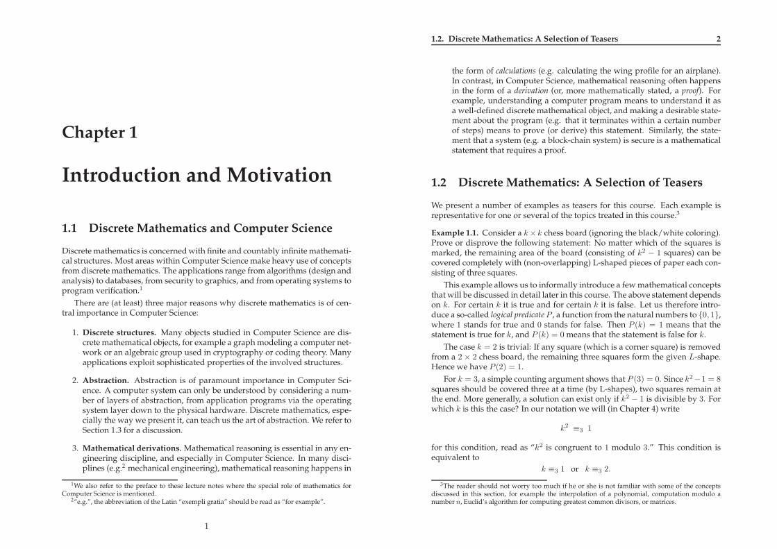
Example 1.1. Consider a k× k chess board (ignoring the black/white coloring).Prove or disprove the following statement: No matter which of the squares ismarked, the remaining area of the board (consisting of k2 − 1 squares) can becovered completely with (non-overlapping) L-shaped pieces of paper each con-sisting of three squares.
This example allows us to informally introduce a few mathematical conceptsthat will be discussed in detail later in this course. The above statement dependson k. For certain k it is true and for certain k it is false. Let us therefore intro-duce a so-called logical predicateP , a function from the natural numbers to 0, 1,where 1 stands for true and 0 stands for false. Then P (k) = 1 means that thestatement is true for k, and P (k) = 0 means that the statement is false for k.
The case k = 2 is trivial: If any square (which is a corner square) is removedfrom a 2 × 2 chess board, the remaining three squares form the given L-shape.Hence we have P (2) = 1.
For k = 3, a simple counting argument shows that P (3) = 0. Since k2−1 = 8squares should be covered three at a time (by L-shapes), two squares remain atthe end. More generally, a solution can exist only if k2 − 1 is divisible by 3. Forwhich k is this the case? In our notation we will (in Chapter 4) write
k2 ≡3 1
for this condition, read as “k2 is congruent to 1 modulo 3.” This condition isequivalent to
k ≡3 1 or k ≡3 2.
3The reader should not worry too much if he or she is not familiar with some of the conceptsdiscussed in this section, for example the interpolation of a polynomial, computation modulo anumber n, Euclid’s algorithm for computing greatest common divisors, or matrices.

3 Chapter 1. Introduction and Motivation
Hence we have P (k) = 0 for all k with k ≡3 0 (i.e.,4 the k divisible by 3).5
The case k = 4 can be solved easily by finding a solution for each of the threetypes of squares (corner, edge, interior of board) that could be marked. Hencewe have proved P (4) = 1. This proof type will later be called a proof by casedistinction.
For the case k = 5 one can prove that P (5) = 0 by showing that there is (atleast) a square which, when marked, leaves an area not coverable by L-shapes.Namely, if one marks a square next to the center square, then it is impossible tocover the remaining area by L-shapes. This proof type will later be called a proofby counterexample.
We have P (6) = 0 because 6 is divisible by 3, and hence the next interestingcase is k = 7. The reader can prove as an exercise that P (7) = 1. (How manycases do you have to check?)
The question of interest is, for a general k, whether P (k) = 1 or P (k) = 0.But one can prove (explained in the lecture) that
P (k) = 1 =⇒ P (2k) = 1,
i.e., that if the statement is true for some k, then it is also true for two times k.This implies that P (2i) = 1 for any i and also that P (7 · 2i) = 1 for any i. Hencewe have P (8) = 1, and P (9) = 0, leaving P (10) and P (11) as the next opencases. One can also prove the following generalization of the above-stated fact:
P (k) = 1 and P (ℓ) = 1 =⇒ P (kℓ) = 1.
We point out that, already in this first example, we understand the reasoningleading to the conclusion P (k) = 0 or P (k) = 1 as a proof.
Example 1.2. Consider the following simple method for testing primality. Proveor disprove that an odd number n is a prime if and only if 2n−1 divided by nyields remainder 1, i.e., if
2n−1 ≡n 1.
One can easily check that 2n−1 ≡n 1 holds for the primes n = 3, 5, 7, 11, 13 (andmany more). Moreover, one can also easily check that 2n−1 6≡n 1 for the first oddcomposite numbers n = 9, 15, 21, 25, etc. But is the formula a general primalitytest? The solution to this problem will be given in Chapter 4.
Example 1.3. The well-known cancellation law for real numbers states that ifab = ac and a 6= 0, then b = c. In other words, one can divide both sides bya. How general is this law? Does it hold for the polynomials over R, i.e., does
4“i.e.”, the abbreviation of the Latin “id est”, should be read as “that is” (German: “das heisst”).5The fact that the equation k2 ≡p 1 has two solutions modulo p, for any prime p, not just for
p = 3, will be obvious once we understand that computing modulo p is a field (see Chapter 5) andthat every element of a field has either two square roots or none.
1.3. Abstraction: Simplicity and Generality 4
a(x)b(x) = a(x)c(x) imply b(x) = c(x) if a(x) 6= 0? Does it hold for the integersmodulo m, i.e., does ab ≡m ac imply b ≡m c if a 6= 0? Does it hold for thepermutations, when multiplication is defined as composition of permutations?What does the condition a 6= 0 mean in this case? Which abstraction lies behindthe cancellation law? This is a typical algebraic question (see Chapter 5).
Example 1.4. It is well-known that one can interpolate a polynomial a(x) =adx
d + ad−1xd−1 + · · · a1x+ a0 of degree d with real coefficients from any d+ 1
values a(αi), for distinct α1, . . . , αd+1. Can we also construct polynomials over afinite domain (which is of more interest and use in Computer Science), keepingthis interpolation property?
For example, consider computation modulo 5. There are 53 = 125 polyno-mials a2x
2+a1x+a0 of degree 2 because we can freely choose three coefficientsfrom 0, 1, 2, 3, 4. It is straight-forward (though cumbersome) to verify that ifwe fix any three evaluation points (for example 0, 2, and 3), then the polyno-mial is determined by the values at these points. In other words, two differentpolynomials p and q result in distinct lists (p(0), p(2), p(3)) and (q(0), q(2), q(3))of polynomial values. What is the general principle explaining this? For theanswer and applications, see Chapter 5.
1.3 Abstraction: Simplicity and Generality
A main theme of this course is abstraction. In everyday life, the term “abstract”has a negative meaning. It stands for non-intuitive and difficult-to-understand.For us, abstraction will have precisely the opposite meaning. It will stand forsimplicity and generality. I hope to be able to convey the joy and importance ofsimplification and generalization by abstraction.
Indeed, abstraction is probably the most important principle in program-ming and the design of information systems. Computers and computer pro-grams are highly (perhaps unimaginably) complex systems. For a computer sys-tem with only 1000 bits of storage, the number 21000 of system states is greaterthan the number of atoms in the known universe. The immense complexityof software systems is usually grossly underestimated, resulting in potentiallycatastrophic software failures. For typical commercial software, failures are therule rather than the exception.
In order to manage the complexity, software systems are divided into com-ponents (called modules, layers, objects, or abstract data types) that interactwith each other and with the environment in a well-defined manner. For ex-ample, the Internet communication software is divided into a number of lay-ers, each with a dedicated set of tasks. The IP layer transports packets betweencomputers, and the TCP layer manages reliable connections. The potential com-plexity of the interaction between subsystems is channeled into clearly specifiedinterfaces. The behavior of a subsystem is described by a manageable number

5 Chapter 1. Introduction and Motivation
of rules. This is abstraction. Without abstraction, writing good software is im-possible.
Abstraction means simplification. By an abstraction one ignores all aspectsof a system that are not relevant for the problem at hand, concentrating on theproperties that matter.
Abstraction also means generalization. If one proves a property of a systemdescribed at an abstract level, then this property holds for any system with thesame abstraction, independently of any details.
Example 1.5. A standard Swiss chocolate consists of 6 rows of 4 pieces each.We would like to break it into its 24 pieces using the least number of breakingoperations. The first breaking operation can break the chocolate in any of the5 ways parallel to the short side, or in any of the 3 ways parallel to the longside. Afterwards, a breaking operation consists of taking an arbitrary piece ofchocolate and breaking it along one of the marked lines. What is the minimalnumber of breaking operations needed to break the chocolate into its 24 pieces?Is it better to first break the chocolate into two equal pieces or to break off onerow? Is it better to first break along a short or a long line? Which abstractionexplains the answer? Find a similar problem with the same abstraction.
Example 1.6. Can the shape in Figure 1.1 be cut into 9 identical pieces? If not,why? If yes, what is the abstraction that explains this? What would more gen-eral examples with the same abstraction look like? Why would it be easier tosee the answer in such generalized examples?
a a
a
a
Figure 1.1: A shape to be cut into identical pieces.
Example 1.7. Extend the following sequence of numbers: 0, 1, 1, 3, 5,11, 21, 43, 85, . . .. It is a natural human behavior to find a simple explanationconsistent with a given observation, i.e., to abstract.6 Which is the simplest rulethat defines the sequence? There may be several answers that make sense.
Example 1.8. Euclid’s well-known algorithm for computing the greatest com-mon divisor of two positive integers a and b works as follows: In each step,the larger integer is divided by the smaller integer, and the pair of integers is
6Unfortunately, this also leads to over-simplifications and inappropriate generalizations.
1.3. Abstraction: Simplicity and Generality 6
replaced by the pair consisting of the smaller integer and the remainder of thedivision. This step is repeated until the remainder is 0. The greatest commondivisor is the last non-zero remainder.
Essentially the same algorithm works for two polynomials a(x) and b(x), saywith integer (or real) coefficients, where the size of a polynomial is defined tobe its degree. In which sense are integer numbers and polynomials similar? Atwhich level of abstraction can they be seen as instantiations of the same abstractconcept? As we will see in Chapter 5, the answer is that they are both so-calledEuclidean domains, which is a special type of a so-called integral domain, which inturn is a special case of a ring.

Chapter 2
Mathematical Reasoning,Proofs, and a First Approachto Logic
2.1 Mathematical Statements
2.1.1 The Concept of a Mathematical Statement
People make many statements in life, like “I love you”, “tomorrow it will rain”,“birds can fly”, or “Roger Federer is the best tennis player”. By making thestatement, the person making it intends to claim that it is true. However, mostsuch statements are not sufficiently precise to be considered true or false, andoften they are subjective. In contrast, mathematical statements are statements thatare true or false in an absolute, indisputable sense, according to the laws ofmathematics.
Definition 2.1. A mathematical statement that is either true or false is also calleda proposition.
Alternative terms are assertion1, claim, or simply (mathematical) statement. Ex-amples of propositions are
• 71 is a prime number.
• If p is a prime number, then 2p − 1 is also a prime number.
• Every natural number is the sum of at most four square numbers. (Exam-ple: 22 = 42 + 22 + 12 + 12 and 74 = 62 + 52 + 32 + 22.)
1German: Behauptung
7
2.1. Mathematical Statements 8
• Every even natural number greater than 2 can be expressed as the sum oftwo primes.2 For example, 108 = 37 + 71 and 162 = 73 + 89.
• Any n lines ℓ1, . . . , ℓn in the plane, no two of which are parallel, intersectin one point (see Example 2.4).
• For the chess game there exists a winning strategy for the player makingthe first move (playing “white”).
The first proposition is easily shown to be true. The second proposition isfalse, and this can be proved by giving a counter-example: 11 is prime but211 − 1 = 2047 = 23 · 89 is not prime.3 The third proposition is true but byno means obvious (and requires a sophisticated proof). The fourth propositionis not known to be true (or false). The fifth proposition is false. The sixth propo-sition is not known to be true (or false).
Example 2.1. Consider the following statement which sounds like a statementas it could appear in Computer Science: “There is no algorithm for factoring anyn-bit integer in n3 steps”. This is not a precise mathematical statement becauseits truth (namely the complexity of the best algorithm) generally depends on theparticular computational model one is considering.
Definition 2.2. A true proposition is often called a theorem, a lemma, or a corol-lary.4 A proposition not known to be true or false is often called a conjecture oran assumption.
If one makes a statement, say S, for example in the context of these lecturenotes, there can be two different meanings. The first meaning is that by statingit one claims that S is true, and the second meaning is simply to discuss thestatement itself (for example as an assumption), independently of whether it istrue or not. We should try to distinguish clearly between these two meanings.
2.1.2 Composition of Mathematical Statements
A mathematical statement can be composed of several mathematical statements.Consider the following examples:
• 4 is an even number and 71 is a prime number.
• 5 is an even number and 71 is a prime number.
• 5 is an even number or 71 is a prime number.
2This statement is called the Goldbach conjecture and is one of the oldest unproven conjecturesin mathematics.
32p − 1 is prime for most primes p (e.g. for 2, 3, 5, 7, 13 and many more), but not all.4The term “theorem” is usually used for an important result, whereas a lemma is an interme-
diate, often technical result, possibly used in several subsequent proofs. A corollary is a simpleconsequence (e.g. a special case) of a theorem or lemma.

9 Chapter 2. Math. Reasoning, Proofs, and a First Approach to Logic
The first statement is true because both statements “4 is an even number” and“71 is a prime number” are true. In contrast, the second statement is false be-cause the statement “5 is an even number” is false. However, the third statementis again true because “71 is a prime number” is true and hence it is irrelevantwhether “5 is an even number” is true or false.
A slightly more involved combination of two statements S and T is implica-tion, where in mathematics one usually writes
S =⇒ T.
It stands for “If S is true, then T is true”. One also says “S implies T ”. Thestatement S =⇒ T is false if S is true and T is false, and in all other three casesit is true. In other words, the first three statements below are true while the lastone is false.
• 4 is an even number =⇒ 71 is a prime number.
• 5 is an even number =⇒ 71 is a prime number.
• 5 is an even number =⇒ 70 is a prime number.
• 4 is an even number =⇒ 70 is a prime number.
We point out that S =⇒ T does not express any kind of causality like “because Sis true, T is also true”.
Similarly, S ⇐⇒ T means that S is true if and only if T is true. This canequivalently be stated as “S implies T and T implies S.”
2.1.3 Mathematical Statements in Computer Science
Many statements relevant in Computer Science are mathematical statementswhich one would like to prove. We give a few examples of such statements:
• Program P terminates (i.e., does not enter an infinite loop) for all inputs.
• Program P terminates within k computation steps for all inputs.
• Program P computes f(x) for every input x, where f is a function of in-terest.
• Algorithm A solves problem S within accuracy ǫ.
• The error probability of file transmission system F in a file transmission isat most p (where p can be a function of the file length).
• The computer network C has the property that if any t links are deleted,every node is still connected with every other node.
• Encryption scheme E is secure (for a suitable definition of security).
• Cryptocurrency system C operates correctly as long as a majority of theinvolved nodes behave honestly, even if all the other nodes behave arbi-trarily maliciously.
2.2. The Concept of a Proof 10
• Database system D provides data privacy (for a suitable definition of pri-vacy).
Programs, algorithms, encryption schemes, etc., are (complex) discretemathematical objects, and proving statements like those mentioned above ishighly non-trivial. This course is not about programs or algorithms, let aloneencryption schemes, but it provides the foundations so that later courses canreason mathematically about these objects.
2.2 The Concept of a Proof
The purpose of a proof is to demonstrate (or prove) a mathematical statement S.In this section we informally discuss the notion of a proof. We also discussseveral proof strategies. In Chapter 6 about logic, the notion of a proof in aproof calculus will be formalized.
2.2.1 Examples of Proofs
We already gave examples of proofs in Chapter 1. We give one more simpleexample.
Example 2.2. Claim: The number n = 2143 − 1 is not a prime.
Proof: n is divisible by 2047, as one can check by a (for a computer) simplecalculation.
That this is true can even be easily seen without doing a calculation, by prov-ing a more general claim of which the above one is a special case:
Claim: n is not prime =⇒ 2n − 1 is not prime.5
Proof: If n is not a prime, then (by definition of prime numbers) n = ab witha > 1 and a < n. Now we observe that 2a − 1 divides 2ab − 1:
2ab − 1 = (2a − 1)
b−1∑
i=0
2ia = (2a − 1)(2(b−1)a + 2(b−2)a + · · ·+ 2a + 1
)
as can easily be verified by a simple calculation. Since 2a − 1 > 1 and 2a − 1 <2ab− 1, i.e., 2a− 1 is a non-trivial divisor of 2ab− 1, this means that 2ab− 1 is nota prime, concluding the proof of the claim.
Let us state a warning. Recall from the previous section that
n is prime =⇒ 2n − 1 is prime
5It is understood that this statement is meant to hold for an arbitrary n.

11 Chapter 2. Math. Reasoning, Proofs, and a First Approach to Logic
is a false statement, even though it may appear at first sight to follow from theabove claim. However, we observe that if S =⇒ T is true, then generally it doesnot follow that if S is false, then T is false.
Example 2.3. An integer n is called a square if n = m · m for some integer m.Prove that if a and b are squares, then so is a · b.
a and b are squares.
=⇒ a = u · u and b = v · v for some u and v (def. of squares).
=⇒ a · b = (u · u) · (v · v) (replace a by u · u and b by v · v).
=⇒ a · b = (u · v) · (u · v). (commutative and associative laws).
=⇒ a · b is a square (def. of squares)
The above proof follows a standard pattern of proofs as a sequence of im-plications, each step using the symbol
.=⇒. Such a proof step requires that the
justification for doing the step is clear. Often one justifies the proof step either inthe accompanying text or as a remark on the same line as the implication state-ment (as in the above proof). But even more often the justification for the stepis simply assumed to be understood from the context and not explicitly stated,which can sometimes make proofs hard to follow or even ambiguous.
2.2.2 Examples of False Proofs
As a next motivating example, let us prove a quite surprising assertion.6
Example 2.4. Claim: Any n lines ℓ1, . . . , ℓn in the plane, no two of which areparallel, intersect in one point (i.e., have one point in common).
Proof: The proof proceeds by induction.7 The induction basis is the case n = 2:Any two non-parallel lines intersect in one point. The induction hypothesis isthat any n lines intersect in one point. The induction step states that then thismust be true for any n+1 lines. The proof goes as follows. By the hypothesis, then lines ℓ1, . . . , ℓn intersect in a point P . Similarly, the n lines ℓ1, . . . , ℓn−1, ℓn+1
intersect in a point Q. The line ℓ1 lies in both groups, so it contains both P andQ. The same is true for line ℓn−1. But ℓ1 and ℓn−1 intersect at a single point,hence P = Q. This is the common point of all lines ℓ1, . . . , ℓn+1.
Something must be wrong! (What?) This example illustrates that proofsmust be designed with care. Heuristics and intuition, though essential in anyengineering discipline as well as in mathematics, can sometimes be wrong.
Example 2.5. In the lecture we present a “proof” for the statement 2 = 1.
6This example is taken from the book by Matousek and Nesetril.7Here we assume some familiarity with proofs by induction; in Section 2.6.10 we discuss them
in depth.
2.2. The Concept of a Proof 12
2.2.3 Two Meanings of the Symbol =⇒It is important to note that the symbol =⇒ is used in the mathematical literaturefor two different (but related) things:
• to express composed statements of the form S =⇒ T (see Section 2.1.2),
• to express a derivation step in a proof, as above.
To make this explicit and avoid confusion, we use a slightly different symbol.
=⇒for the second meaning.8 Hence S
.=⇒ T means that T can be obtained from S
by a proof step, and in this case we also know that the statement S =⇒ T is true.However, conversely, if S =⇒ T is true for some statements S and T , there maynot exist a proof step demonstrating this, i.e. S
.=⇒ T may not hold.
An analogous comment applies to the symbol ⇐⇒, i.e., S.⇐⇒ T can be used
express that T follows from S by a simply proof step, and also S follows from Tby a simply proof step.
2.2.4 Proofs Using Several Implications
Example 2.3 showed a proof of a statement of the form S =⇒ T using a se-quence of several implications of the form S
.=⇒ S2, S2
.=⇒ S3, S3
.=⇒ S4, and
S4.
=⇒ T .
A proof based on several implications often has a more general form: Theimplications do not form a linear sequence but a more general configuration,where each implication can assume several of the already proved statements.For example, one can imagine that in order to prove a given statement T , onestarts with two (known to be) true statements S1 and S2 and then, for somestatements S3, . . . , S7, proves the following six implications:
• S1.
=⇒ S3,
• S1.
=⇒ S4,
• S2.
=⇒ S5,
• S3 and S5.
=⇒ S6,
• S1 and S4.
=⇒ S7, as well as
• S6 and S7.
=⇒ T .
Example 2.6. In the lecture we demonstrate the proof of Example 2.2 in theabove format, making every intermediate statement explicit.
8This notation is not standard and only used in these lecture notes. The symbol.
=⇒ is intention-ally chosen very close to the symbol =⇒ to allow someonw not used to this to easlily overlook thedifference.

13 Chapter 2. Math. Reasoning, Proofs, and a First Approach to Logic
2.2.5 An Informal Understanding of the Proof Concept
There is a common informal understanding of what constitutes a proof of amathematical statement S. Informally, we could define a proof as follows:
Definition 2.3. (Informal.) A proof of a statement S is a sequence of simple, eas-ily verifiable, consecutive steps. The proof starts from a set of axioms (thingspostulated to be true) and known (previously proved) facts. Each step corre-sponds to the application of a derivation rule to a few already proven state-ments, resulting in a newly proved statement, until the final step results in S.
Concrete proofs vary in length and style according to
• which axioms and known facts one is assuming,
• what is considered to be easy to verify,
• how much is made explicit and how much is only implicit in theproof text, and
• to what extent one uses mathematical symbols (like.
=⇒) as opposed tojust writing text.
2.2.6 Informal vs. Formal Proofs
Most proofs taught in school, in textbooks, or in the scientific literature are in-tuitive but quite informal, often not making the axioms and the proof rules ex-plicit. They are usually formulated in common language rather than in a rigor-ous mathematical language. Such proofs can be considered completely correctif the reasoning is clear. An informal proof is often easier to read than a pedanticformal proof.
However, a proof, like every mathematical object, can be made rigorous andformally precise. This is a major goal of logic (see Section 2.2.7 and Chapter 6).There are at least three (related) reasons for using a more rigorous and formaltype of proof.
• Prevention of errors. Errors are quite frequently found in the scientific lit-erature. Most errors can be fixed, but some can not. In contrast, a com-pletely formal proof leaves no room for interpretation and hence allows toexclude errors.
• Proof complexity and automatic verification. Certain proofs in Computer Sci-ence, like proving the correctness of a safety-critical program or the se-curity of an information system, are too complex to be carried out andverified “by hand”. A computer is required for the verification. A com-
2.2. The Concept of a Proof 14
puter can only deal with rigorously formalized statements, not with semi-precise common language, hence a formal proof is required.9
• Precision and deeper understanding. Informal proofs often hide subtle steps.A formal proof requires the formalization of the arguments and can leadto a deeper understanding (also for the author of the proof).
There is a trade-off between mathematical rigor and an intuitive, easy-to-read (for humans) treatment. In this course, our goal is to do precise mathemat-ical reasoning, but at the same time we will try to strike a reasonable balancebetween formal rigor and intuition. In Chapters 3 to 5, our proofs will be in-formal, and the Chapter 6 on logic is devoted to understanding the notion of aformal proof.
A main problem in teaching mathematical proofs (for example in this course)is that it is hard to define exactly when an informal proof is actually a validproof. In most scientific communities there is a quite clear understanding ofwhat constitutes a valid proof, but this understanding can vary from commu-nity to community (e.g. from physics to Computer Science). A student mustlearn this culture over the years, starting in high school where proof strategieslike proofs by induction have probably been discussed. There is no quick andeasy path to understanding exactly what constitutes a proof.
The alternative to a relatively informal treatment would be to do everythingrigorously, in a formal system as discussed in Chapter 6, but this would proba-bly turn away most students and would for the most parts simply not be man-ageable. A book that tries to teach discrete mathematics very rigorously is Alogical approach to discrete math by Gries and Schneider.
2.2.7 The Role of Logic
Logic is the mathematical discipline laying the foundations for rigorous mathe-matical reasoning. Using logic, every mathematical statement as well as a prooffor it (if a proof exists) can, in principle, be formalized rigorously. As mentionedabove, rigorous formalization, and hence logic, is especially important in Com-puter Science where one sometimes wants to automate the process of provingor verifying certain statements like the correctness of a program.
Some principle tasks of logic (see Chapter 6) are to answer the followingthree questions:
1. What is a mathematical statement, i.e., in which language do we writestatements?
2. What does it mean for a statement to be true?
9A crucial issue is that the translation of an informal statement to a formal statement can beerror-prone.

15 Chapter 2. Math. Reasoning, Proofs, and a First Approach to Logic
3. What constitutes a proof for a statement from a given set of axioms?
Logic (see Chapter 6) defines the syntax of a language for expressing statementsand the semantics of such a language, defining which statements are true andwhich are false. A logical calculus allows to express and verify proofs in a purelysyntactic fashion, for example by a computer.
2.2.8 Proofs in this Course
As mentioned above, in the literature and also in this course we will see proofsat different levels of detail. This may be a bit confusing for the reader, especiallyin the context of an exam question asking for a proof. We will try to be alwaysclear about the level of detail that is expected in an exercise or in the exam. Forthis purpose, we distinguish between the following three levels:
• Proof sketch or proof idea: The non-obvious ideas used in the proof aredescribed, but the proof is not spelled out in detail with explicit referenceto all definitions that are used.
• Complete proof: The use of every definition is made explicit. Every proofstep is justified by stating the rule or the definition that is applied.
• Formal proof: The proof is entirely phrased is a given proof calculus.
Proof sketches are often used when the proof requires some clever ideas andthe main point of a task or example is to describe these ideas and how they fittogether. Complete proofs are usually used when one systematically applies thedefinitions and certain logical proof patterns, for example in our treatments ofrelations and of algebra. Proofs in the resolution calculus in Chapter 6 can beconsidered to be formal proofs.
2.3 A First Introduction to Propositional Logic
We give a brief introduction to some elementary concepts of logic. We point outthat this section is somewhat informal and that in the chapter on logic (Chap-ter 6) we will be more rigorous. In particular, we will there distinguish betweenthe syntax of the language for describing mathematical statements (called for-mulas) and the semantics, i.e., the definition of the meaning (or validity) of aformula. In this section, the boundary between syntax and semantics is (inten-tionally) not made explicit.
2.3. A First Introduction to Propositional Logic 16
2.3.1 Logical Constants, Operators, and Formulas
Definition 2.4. The logical values (constants) “true” and “false” are usually de-noted as 1 and 0, respectively.10
One can define operations on logical values:
Definition 2.5.
(i) The negation (logical NOT) of a proposition A, denoted as ¬A, is true ifand only if A is false.
(ii) The conjunction (logical AND) of two propositionsA andB, denotedA∧B,is true if and only if both A and B are true.
(iii) The disjunction (logical OR) of two propositions A and B, denoted A ∨ B,is true if and only if A or B (or both) are true.11
The logical operators are functions, where ¬ is a function 0, 1 → 0, 1 and∧ and ∨ are functions 0, 1× 0, 1 → 0, 1. These functions can be describedby function tables, as follows:
A ¬A0 11 0
A B A ∧B0 0 00 1 01 0 01 1 1
A B A ∨B0 0 00 1 11 0 11 1 1
Logical operators can also be combined, in the usual way of combining func-tions. For example, the formula
A ∨ (B ∧ C)
has function tableA B C A ∨ (B ∧C)0 0 0 00 0 1 00 1 0 00 1 1 11 0 0 11 0 1 11 1 0 11 1 1 1
10These values 1 and 0 are not meant to be the corresponding numbers, even though the samesymbols are used.
11Sometimes ¬A, A∧B, and A∨B are also denoted as NOT(A), A AND B, and A OR B, respec-tively, or a similar notation.
17 Chapter 2. Math. Reasoning, Proofs, and a First Approach to Logic
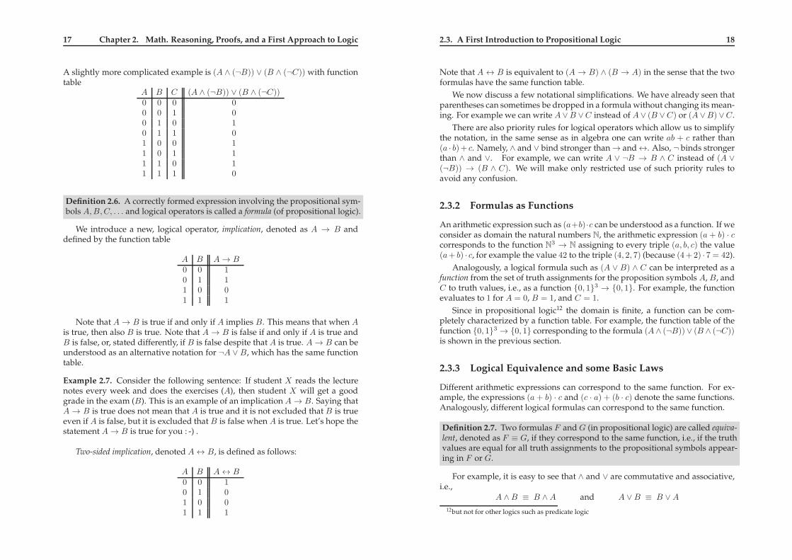
A slightly more complicated example is (A ∧ (¬B)) ∨ (B ∧ (¬C)) with functiontable
A B C (A ∧ (¬B)) ∨ (B ∧ (¬C))0 0 0 00 0 1 00 1 0 10 1 1 01 0 0 11 0 1 11 1 0 11 1 1 0
Definition 2.6. A correctly formed expression involving the propositional sym-bols A,B,C, . . . and logical operators is called a formula (of propositional logic).
We introduce a new, logical operator, implication, denoted as A → B anddefined by the function table
A B A→ B0 0 10 1 11 0 01 1 1
Note that A→ B is true if and only if A implies B. This means that when Ais true, then also B is true. Note that A → B is false if and only if A is true andB is false, or, stated differently, if B is false despite that A is true. A→ B can beunderstood as an alternative notation for ¬A ∨ B, which has the same functiontable.
Example 2.7. Consider the following sentence: If student X reads the lecturenotes every week and does the exercises (A), then student X will get a goodgrade in the exam (B). This is an example of an implication A→ B. Saying thatA → B is true does not mean that A is true and it is not excluded that B is trueeven if A is false, but it is excluded that B is false when A is true. Let’s hope thestatement A→ B is true for you : -) .
Two-sided implication, denoted A↔ B, is defined as follows:
A B A↔ B0 0 10 1 01 0 01 1 1
2.3. A First Introduction to Propositional Logic 18
Note that A ↔ B is equivalent to (A → B) ∧ (B → A) in the sense that the twoformulas have the same function table.
We now discuss a few notational simplifications. We have already seen thatparentheses can sometimes be dropped in a formula without changing its mean-ing. For example we can write A∨B ∨C instead of A∨ (B ∨C) or (A ∨B)∨C.
There are also priority rules for logical operators which allow us to simplifythe notation, in the same sense as in algebra one can write ab + c rather than(a · b)+ c. Namely, ∧ and ∨ bind stronger than → and ↔. Also, ¬ binds strongerthan ∧ and ∨. For example, we can write A ∨ ¬B → B ∧ C instead of (A ∨(¬B)) → (B ∧ C). We will make only restricted use of such priority rules toavoid any confusion.
2.3.2 Formulas as Functions
An arithmetic expression such as (a+b)·c can be understood as a function. If weconsider as domain the natural numbers N, the arithmetic expression (a+ b) · ccorresponds to the function N3 → N assigning to every triple (a, b, c) the value(a+ b) · c, for example the value 42 to the triple (4, 2, 7) (because (4+2) · 7 = 42).
Analogously, a logical formula such as (A ∨ B) ∧ C can be interpreted as afunction from the set of truth assignments for the proposition symbols A, B, andC to truth values, i.e., as a function 0, 13 → 0, 1. For example, the functionevaluates to 1 for A = 0, B = 1, and C = 1.
Since in propositional logic12 the domain is finite, a function can be com-pletely characterized by a function table. For example, the function table of thefunction 0, 13 → 0, 1 corresponding to the formula (A∧ (¬B))∨ (B ∧ (¬C))is shown in the previous section.
2.3.3 Logical Equivalence and some Basic Laws
Different arithmetic expressions can correspond to the same function. For ex-ample, the expressions (a+ b) · c and (c · a) + (b · c) denote the same functions.Analogously, different logical formulas can correspond to the same function.
Definition 2.7. Two formulas F and G (in propositional logic) are called equiva-lent, denoted as F ≡ G, if they correspond to the same function, i.e., if the truthvalues are equal for all truth assignments to the propositional symbols appear-ing in F or G.
For example, it is easy to see that ∧ and ∨ are commutative and associative,i.e.,
A ∧B ≡ B ∧ A and A ∨B ≡ B ∨ A12but not for other logics such as predicate logic

19 Chapter 2. Math. Reasoning, Proofs, and a First Approach to Logic
as well as
A ∧ (B ∧ C) ≡ (A ∧B) ∧ C.
Because of this equivalence, we introduce the notational convention that suchunnecessary parentheses can be dropped:.
A ∧B ∧ C ≡ A ∧ (B ∧C).
Similarly we have
A ∨ (B ∨C) ≡ (A ∨B) ∨ C
and can write A ∨B ∨C instead, and we also have
¬(¬A) ≡ A.
Let us look at some equivalences involving more than one operation, whichare easy to check. The operator ∨ can be expressed in terms of ¬ and ∧, asfollows:
¬(A ∨B) ≡ ¬A ∧ ¬B,
which also means that A ∨B ≡ ¬(¬A ∧ ¬B).13 In fact, ¬ and ∧ are sufficient toexpress every logical function (of propositional logic). Similarly we have
¬(A ∧B) ≡ ¬A ∨ ¬B.
Example 2.8. A↔ B ≡ (A→ B) ∧ (B → A) ≡ (A ∧B) ∨ (¬A ∧ ¬B).
Example 2.9. Here is a more complicated example which the reader can verifyas an exercise:
(A ∧ (¬B)) ∨ (B ∧ (¬C)) ≡ (A ∨B) ∧ ¬(B ∧ C).
The following example shows a distributive law for ∧ and ∨. Such laws willbe discussed more systematically in Chapter 6.
Example 2.10. (A ∧B) ∨ C ≡ (A ∨C) ∧ (B ∨ C).
We summarize the basic equivalences of propositional logic:
13Here we have used the convention that ¬ binds stronger than ∧ and ∨, which allow us to write¬(¬A ∧ ¬B) instead of ¬((¬A) ∧ (¬B)).
2.3. A First Introduction to Propositional Logic 20
Lemma 2.1.
1) A ∧A ≡ A and A ∨ A ≡ A (idempotence);
2) A ∧B ≡ B ∧ A and A ∨B ≡ B ∨ A (commutativity of ∧ and ∨);
3) (A∧B)∧C ≡ A∧ (B ∧C) and (A∨B)∨C ≡ A∨ (B ∨C) (associativity);
4) A ∧ (A ∨B) ≡ A and A ∨ (A ∧B) ≡ A (absorption);
5) A ∧ (B ∨ C) ≡ (A ∧B) ∨ (A ∧ C) (first distributive law);
6) A ∨ (B ∧ C) ≡ (A ∨B) ∧ (A ∨ C) (second distributive law);
7) ¬¬A ≡ A (double negation);
8) ¬(A ∧B) ≡ ¬A ∨ ¬B and ¬(A ∨B) ≡ ¬A ∧ ¬B (de Morgan’s rules).
2.3.4 Logical Consequence (for Propositional Logic)
For arithmetic expressions one can state relations between them that are moregeneral than equivalence. For example the relation a+ b ≤ a+ b+(c · c) betweenthe expressions a+ b and a+ b+ (c · c). What is meant by the relation is that forall values that a, b, and c can take on, the inequality holds, i.e., it holds for thefunctions corresponding to the expressions.
Analogously, one can state relations between formulas. The perhaps mostimportant relation is logical consequence which is analogous to the relation ≤between arithmetic expressions.
Definition 2.8. A formula G is a logical consequence14 of a formula F , denoted
F |= G,
if for all truth assignments to the propositional symbols appearing in F or G,the truth value of G is 1 if the truth value of F is 1.
Intuitively, if we would interpret the truth values 0 and 1 as the numbers 0and 1 (which we don’t!), then F |= G would mean F ≤ G.
Example 2.11. A ∧B |= A ∨B.
Example 2.12. Comparing the truth tables of the two formulas (A∧B)∨ (A∧C)and ¬B → (A ∨ C) one can verify that
(A ∧B) ∨ (A ∧ C) |= ¬B → (A ∨ C).
Note that the two formulas are not equivalent.
14German: (logische) Folgerung, logische Konsequenz

21 Chapter 2. Math. Reasoning, Proofs, and a First Approach to Logic
Example 2.13. The following logical consequence, which the reader can proveas an exercise, captures a fact intuitively known to us, namely that implicationis transitive:15
(A→ B) ∧ (B → C) |= A→ C.
We point out (see also Chapter 6) that two formulas F and G are equivalentif and only if each one is a logical consequence of the other, i.e.,16
F ≡ G ⇐⇒ F |= G and G |= F.
2.3.5 Lifting Equivalences and Consequences to Formulas
Logical equivalences and consequences continue to hold if the propositionalsymbols A,B,C . . . are replaced by other propositional symbols or by formulasF,G,H . . .. At this point, we do not provide a proof of this intuitive fact. Forexample, because of the logical consequences stated in the previous section wehave
F ∧G ≡ G ∧ F and F ∨G ≡ G ∨ Fas well as
F ∧ (G ∧H) ≡ (F ∧G) ∧Hfor any formulas F , G, and H .
The described lifting is analogous to the case of arithmetic expressions. Forexample, we have
(a+ b) · c = (c · a) + (b · c)for any real numbers a, b, and c. Therefore, for any arithmetic expressions f , g,and h, we have
(f + g) · h = (h · f) + (g · h).Example 2.14. We give a more complex example of such a lifting. Because ofthe logical consequence stated in Example 2.13, we have
(F → G) ∧ (G→ H) |= F → H
for any formulas F , G, and H .
2.3.6 Tautologies and Satisfiability
Definition 2.9. A formula F (in propositional logic) is called a tautology17 orvalid18 if it is true for all truth assignments of the involved propositional sym-bols. One often writes |= F to say that F is a tautology.
15The term “transitive” will be discussed in Chapter 3.16Note that we DO NOT write F |= G ∧ G |= F because the symbol ∧ is used only between two
formulas in order to form a new (combined) formula, and F |= G and G |= F are not formulas.17German: Tautologie
2.3. A First Introduction to Propositional Logic 22
Example 2.15. The formulas A∨(¬A) and (A∧(A → B)) → B are tautologies.
One often wants to make statements of the form that some formula F is atautology. As stated in Definition 2.9, one also says “F is valid” instead of “F isa tautology”.
Definition 2.10. A formula F (in propositional logic) is called satisfiable19 if itis true for at least one truth assignment of the involved propositional symbols,and it is called unsatisfiable otherwise.
The symbol ⊤ is sometimes used to denote a tautology, and the symbol ⊥is sometimes used to denote an unsatisfiable formula. One sometimes writesF ≡ ⊤ to say that F is a tautology, and F ≡ ⊥ to say that F is unsatisfiable. Forexample, for any formula F we have
F ∨ ¬F ≡ ⊤ and F ∧ ¬F ≡ ⊥.
Example 2.16. The formula (A∧¬A)∧ (B ∨C) is unsatisfiable, and the formulaA ∧B is satisfiable.
The following lemmas state two simple facts that follow immediately fromthe definitions. We only prove the second one.
Lemma 2.2. A formula F is a tautology if and only if ¬F is unsatisfiable.
Lemma 2.3. For any formulas F and G, F → G is a tautology if and only if F |= G.
Proof. The lemma has two directions which we need to prove. To prove thefirst direction (=⇒), assume that F → G is a tautology. Then, for any truthassignment to the propositional symbols, the truth values of F and G are eitherboth 0, or 0 and 1, or both 1 (but not 1 and 0). In each of the three cases itholds that G is true if F is true, i.e., F |= G. To prove the other direction (⇐=),assume F |= G. This means that for any truth assignment to the propositionalsymbols, the truth values of G is 1 if it is 1 for F . In other words, there is notruth assignment such that the truth value of F is 1 and that of G is 0. Thismeans that the truth value of F → G is always 1, which means that F → G is atautology.
2.3.7 Logical Circuits *
A logical formula as discussed above can be represented as a tree where the leaves cor-
respond to the propositions and each node corresponds to a logical operator. Such a tree
18German: allgemeingultig19German: erfullbar
23 Chapter 2. Math. Reasoning, Proofs, and a First Approach to Logic
can be implemented as a digital circuit where the operators correspond to the logical
gates. This topic will be discussed in a course on the design of digital circuits20. The two
main components of digital circuits in computers are such logical circuits and memory
cells.
2.4 A First Introduction to Predicate Logic
The elements of logic we have discussed so far belong to the realm of so-calledpropositional logic21. Propositional logic is not sufficiently expressive to capturemost statements of interest in mathematics in terms of a formula. For example,the statement “There are infinitely many prime numbers” cannot be expressed asa formula in propositional logic (though it can of course be expressed as a sen-tence in common language). We need quantifiers22, predicates, and functions. Thecorresponding extension of propositional logic is called predicate logic23 and issubstantially more involved than propositional logic. Again, we refer to Chap-ter 6 for a more thorough discussion.
2.4.1 Predicates
Let us consider a non-empty set U as the universe in which we want to reason.For example, U could be the set N of natural numbers, the set R of real numbers,the set 0, 1∗ of finite-length bit-strings, or a finite set like 0, 1, 2, 3, 4, 5, 6.
Definition 2.11. A k-ary predicate24 P on U is a function Uk → 0, 1.
A k-ary predicate P assigns to each list (x1, . . . , xk) of k elements of U thevalue P (x1, . . . , xk) which is either true (1) or false (0).
For example, for U = N we can consider the unary (k = 1) predicateprime(x) defined by
prime(x) =
1 if x is prime0 else.
Similarly, one can naturally define the unary predicates even(x) and odd(x).
For any universe U with an order relation ≤ (e.g. U = N or U = R), thebinary (i.e., k = 2) predicate less(x, y) can be defined as
less(x, y) =
1 if x < y0 else.
20German: Digitaltechnik21German: Aussagenlogik22German: Quantoren23German: Pradikatenlogik24German: Pradikat
2.4. A First Introduction to Predicate Logic 24
However, in many cases we write binary predicates in a so-called “infix” nota-tion, i.e., we simply write x < y instead of less(x, y).
2.4.2 Functions
In predicate logic one can also use functions on U , for example addition andmultiplication. For example, if the universe is U = N, then we can writeless(x+ 3, x+ 5), which is a true statement for every value x in U .
2.4.3 The Quantifiers ∃ and ∀
Definition 2.12. For a universe U and predicate P (x) we define the followinglogical statements:25
∀x P (x) stands for: P (x) is true for all x in U .
∃x P (x) stands for: P (x) is true for some x in U , i.e.,there exists an x ∈ U for which P (x) is true.
More generally, for a formula F with a variable x, which for each value x ∈ U iseither true or false, the formula ∀x F is true if and only if F is true for all x inU , and the formula ∃x F is true if and only if F is true for some x in U .
Example 2.17. Consider the universe U = N. Then ∀x (x ≥ 0) is true.26 Also,∀x (x ≥ 2) is false, and ∃x (x+ 5 = 3) is false.
The name of the variable x is irrelevant. For example, the formula ∃x (x+5 =3) is equivalent to the formula ∃y (y + 5 = 3). The formula could be stated inwords as: “There exists a natural number (let us call it y) which, if 5 is addedto it, the result is 3.” How the number is called, x or y or z, is irrelevant for thetruth or falsity of the statement. (Of course the statement is false; it would betrue if the universe were the integers Z.)
Sometimes one wants to state only that a certain formula containing x istrue for all x that satisfy a certain condition. For example, to state that x2 ≥ 25whenever x ≥ 5, one can write
∀x((x ≥ 5) → (x2 ≥ 25)
).
A different notation sometimes used to express the same statement is to state
25In the literature one also finds the notations ∀x: P (x) and ∀x. P (x) instead of ∀x P (x), andsimilarly for ∃.
26But note that ∀x (x ≥ 0) is false for the universe U = R.

25 Chapter 2. Math. Reasoning, Proofs, and a First Approach to Logic
the condition on x directly after the quantifier, followed by “:”27
∀x ≥ 5 : (x2 ≥ 25).
2.4.4 Nested Quantifiers
Quantifiers can also be nested28. For example, if P (x) andQ(x, y) are predicates,then
∀x(P (x) ∨ ∃y Q(x, y)
)
is a logical formula.
Example 2.18. The formula∀x ∃y (y < x)
states that for every x there is a smaller y. In other words, it states that there isno smallest x (in the universe under consideration). This formula is true for theuniverse of the integers or the universe of the real numbers, but it is false for theuniverse U = N.
Example 2.19. For the universe of the natural numbers, U = N, the predicateprime(x) can be defined as follows:29
prime(x)def⇐⇒ x > 1 ∧ ∀y ∀z
((yz = x) → ((y = 1) ∨ (z = 1))
).
For sequences of quantifiers of the same type one sometimes omits paren-theses or even multiple copies of the quantifier. For example one writes ∃xyzinstead of ∃x∃y ∃z.
Example 2.20. Fermat’s last theorem can be stated as follows: For universeN \ 0,
¬(∃ x ∃y ∃z ∃n (n ≥ 3 ∧ xn+yn=zn)
).
Example 2.21. The statement “for every natural number there is a larger prime”can be phrased as
∀x ∃y(y > x ∧ prime(y)
)
and means that there is no largest prime and hence that there are infinitely manyprimes.
If the universe is N, then one often uses m, n, or k instead of x and y. Theabove formula could hence equivalently be written as
∀m ∃n(n > m ∧ prime(n)
).
27We don’t do this.28German: verschachtelt
29We use the symbol “def⇐⇒” if the object on the left side is defined as being equivalent to the object
on the right side.
2.4. A First Introduction to Predicate Logic 26
Example 2.22. Let U = R. What is the meaning of the following statement, andis it true?
∀x(x = 0 ∨ ∃y (xy = 1)
)
2.4.5 Interpretation of Formulas
A formula generally has some “free parts” that are left open for interpretation.To begin with, the universe is often not fixed, but it is also quite common towrite formulas when the universe is understood and fixed. Next, we observethat the formula
∀x(P (x) → Q(x)
)
contains the predicate symbols P and Q which can be interpreted in differentways. Depending on the choice of universe and on the interpretation of P andQ, the formula can either be true or false. For example let the universe be N andlet P (x) mean that “x is divisible by 4”. Now, ifQ(x) is interpreted as “x is odd”,then ∀x (P (x) → Q(x)) is false, but if Q(x) is interpreted as “x is even”, then∀x (P (x) → Q(x)) is true. However, the precise definition of an interpretationis quite involved and deferred to Chapter 6.
2.4.6 Tautologies and Satisfiability
The concepts interpretation, tautology, and satisfiability for predicate logic willbe defined in Chapter 6.
Informally, a formula is satisfiable if there is an interpretation of the involvedsymbols that makes the formula true. Hence ∀x (P (x) → Q(x)) is satisfiableas shown above. Moreover, a formula is a tautology (or valid) if it is true for allinterpretations, i.e., for all choices of the universe and for all interpretations ofthe predicates.30
We will use the terms “tautology” and “valid” interchangeably. For example,
∀x((P (x) ∧Q(x)) → (P (x) ∨Q(x))
)
is a tautology, or valid.
2.4.7 Equivalence and Logical Consequence
One can define the equivalence of formulas and logical consequence for predi-cate logic analogously to propositional logic, but again the precise definition isquite involved and deferred to Chapter 6. Intuitively, two formulas are equiva-lent if they evaluate to the same truth value for any interpretation of the symbolsin the formula.
30We will see in Chapter 6 that predicate logic also involves function symbols, and an interpreta-tion also instantiates the function symbols by concrete functions.

27 Chapter 2. Math. Reasoning, Proofs, and a First Approach to Logic
Example 2.23. Recall Example 2.22. The formula can be written in an equivalentform, as:
∀x(x = 0 ∨ ∃y (xy = 1)
)≡ ∀x
(¬(x = 0) → ∃y (xy = 1)
).
The order of identical quantifiers does not matter, i.e., we have for example:
∃x∃y P (x, y) ≡ ∃y∃x P (x, y) and ∀x∀y P (x, y) ≡ ∀y∀x P (x, y).
A simple example of a logical consequence is
∀x P (x) |= ∃x P (x).It holds because if P (x) is true for all x in the universe, then it is also true forsome (actually an arbitrary) x. (Recall that the universe is non-empty.)
Some more involved examples of equivalences and logical consequences arestated in the next section.
2.4.8 Some Useful Rules
We list a few useful rules for predicate logic. This will be discussed in moredetail in Chapter 6. We have
∀x P (x) ∧ ∀x Q(x) ≡ ∀x(P (x) ∧Q(x)
)
since if P (x) is true for all x and also Q(x) is true for all x, then P (x) ∧ Q(x) istrue for all x, and vice versa. Also,31
∃x(P (x) ∧Q(x)
)|= ∃x P (x) ∧ ∃x Q(x)
since, no matter what P andQ actually mean, any x that makes P (x)∧Q(x) true(according to the left side) also makes P (x) and Q(x) individually true. But, incontrast, ∃x (P (x)∧Q(x)) is not a logical consequence of ∃x P (x) ∧ ∃x Q(x), asthe reader can verify. We can write
∃x P (x) ∧ ∃x Q(x) 6|= ∃x (P (x) ∧Q(x)).
We also have:¬∀x P (x) ≡ ∃x ¬P (x)
and¬∃x P (x) ≡ ∀x ¬P (x).
The reader can prove as an exercise that
∃y ∀x P (x, y) |= ∀x ∃y P (x, y)but that
∀x ∃y P (x, y) 6|= ∃y ∀x P (x, y).31We point out that defining logical consequence for predicate logic is quite involved (see Chap-
ter 6), but intuitively it should be quite clear.
2.5. Logical Formulas vs. Mathematical Statements 28
2.5 Logical Formulas vs. Mathematical Statements
A logical formula is generally not a mathematical statement because the symbolsin it can be interpreted differently, and depending on the interpretation, theformula is true or false. Without fixing an interpretation, the formula is not amathematical statement.
2.5.1 Fixed Interpretations and Formulas as Statements
If for a formula F the interpretation (including the universe and the meaning ofthe predicate and function symbols) is fixed, then this is a mathematical state-ment that is either true or false in the sense of Definition 2.1, i.e., it correspondsto a proposition. Therefore, if an interpretation is understood, we can use for-mulas as statements, for example in a proof with implication steps. In this case(but only if a fixed interpretation is understood) it is also meaningful to say thata formula is true or that it is false.
Example 2.24. For the universe N and the usual interpretation of < and >, theformula ∃n (n < 4 ∧ n > 5) is false and the formula ∀n (n > 0 → (∃m m < n))is true.
2.5.2 Mathematical Statements about Formulas
As mentioned, logical formulas are often not mathematical statements them-selves, but one makes mathematical statements about formulas. Examples ofsuch mathematical statements are:
• F is valid (i.e., a tautology, also written as |= F ),
• F is unsatisfiable,
• F |= G,
• F,G |= H .
The statement “F is valid” is a mathematical statement (about the for-mula F ). Therefore we may for example write
F is valid =⇒ G is valid, (2.1)
as a mathematical statement about the formulas F and G. This statement isdifferent from the statement F |= G. In fact, for any formulas F and G, thestatement F |= G implies statement (2.1), but the converse is generally false:
Lemma 2.4. For any two formulas F and G, if F |= G, then (2.1) is true.

29 Chapter 2. Math. Reasoning, Proofs, and a First Approach to Logic
Proof. F |= G states that for every interpretation, if F is true (for that interpre-tation), then also G is true (for that interpretation). Therefore, if F is true forevery interpretation, then also G is true for every interpretation, which is state-ment (2.1).
2.6 Some Proof Patterns
In this section we discuss a few important proof patterns (which we could alsocall proof methods or proof techniques). Such a proof pattern can be used toprove one step within a longer proof, or sometimes also to directly prove a the-orem of interest. Many proof patterns correspond to logical deduction rules.One can define a logical calculus consisting of such deduction rules, but we willdefer the discussion of this topic to Chapter 6. Often, a given statement can beproved in different ways, i.e., by using different proof patterns.
2.6.1 Composition of Implications
We first explain why the composition of implications, as occurring in manyproofs, is sound.
Definition 2.13. The proof step of composing implications is as follows: If S =⇒ Tand T =⇒ U are both true, then one concludes that S =⇒ U is also true.
The soundness of this principle is explained by the following lemma ofpropositional logic which was already stated in Example 2.13.
Lemma 2.5. (A→ B) ∧ (B → C) |= A→ C.
Proof. One writes down the truth tables of the formulas (A → B) ∧ (B → C)and A → C and checks that whenever the first evaluates to true, then also thesecond evaluates to true.
2.6.2 Direct Proof of an Implication
Many statements of interest (as intermediate steps or as the final statement ofinterest) are implications of the form S =⇒ T for some statements S and T .32
Definition 2.14. A direct proof of an implication S =⇒ T works by assuming Sand then proving T under this assumption.
32Recall Section 2.1.2.
2.6. Some Proof Patterns 30
2.6.3 Indirect Proof of an Implication
Definition 2.15. An indirect proof of an implication S =⇒ T proceeds by assum-ing that T is false and proving that S is false, under this assumption.
The soundness of this principle is explained by the following simple lemmaof propositional logic, where A stands for “statement S is true” and B standsfor “statement T is true”.
Lemma 2.6. ¬B → ¬A |= A→ B.
Proof. One can actually prove the stronger statement, namely that ¬B → ¬A ≡A → B, simply by examination of the truth table which is identical for bothformulas ¬B → ¬A and A→ B.
Example 2.25. Prove the following claim: If x > 0 is irrational, then also√x is
irrational. The indirect proof proceeds by assuming that√x is not irrational and
showing that then x is also not irrational. Here “not irrational” means rational,i.e., we prove
√x is rational =⇒ x is rational
Assume hence that√x is rational, i.e., that
√x = m/n for m,n ∈ N. This means
that x = m2/n2, i.e., x is the quotient of two natural numbers (namely m2 andn2) and thus is rational. This completes the proof of the claim.
2.6.4 Modus Ponens
Definition 2.16. A proof of a statement S by use of the so-called modus ponensproceeds in three steps:
1. Find a suitable mathematical statement R.
2. Prove R.
3. Prove R =⇒ S.
The soundness of this principle is explained by the following lemma ofpropositional logic. Again, the proof is by a simple comparison of truth tables.
Lemma 2.7. A ∧ (A→ B) |= B.
Examples will be discussed in the lecture and the exercises.
31 Chapter 2. Math. Reasoning, Proofs, and a First Approach to Logic
2.6.5 Case Distinction
Definition 2.17. A proof of a statement S by case distinction proceeds in threesteps:
1. Find a finite list R1, . . . , Rk of mathematical statements (the cases).
2. Prove that one of the Ri is true (one case occurs).
3. Prove Ri =⇒ S for i = 1, . . . , k.
More informally, one proves for a complete list of cases that the statement Sholds in all the cases.
The soundness of this principle is explained by the following lemma ofpropositional logic.
Lemma 2.8. For every k we have
(A1 ∨ · · · ∨Ak) ∧ (A1 → B) ∧ · · · ∧ (Ak → B) |= B.
Proof. For a fixed k (say k = 2) one can verify the statement by examinationof the truth table. The statement for general k can be proved by induction (seeSection 2.6.10).
Note that for k = 1 (i.e., there is only one case), case distinction correspondsto the modus ponens discussed above.
Example 2.26. Prove the following statement S: The 4th power of every naturalnumber n, which is not divisible by 5, is one more than a multiple of 5.
To prove the statement, let n = 5k + c, where 1 ≤ c ≤ 4. Using the usualbinomial formula (a+ b)4 = a4 + 4a3b+ 6a2b2 + 4ab3 + b4 we obtain:
n4 = (5k + c)4 = 54k4 + 4 · 53k3c+ 6 · 52k2c2 + 4 · 5kc3 + c4.
Each summand is divisible by 5, except for the last term c4. The statement S ishence equivalent to the statement that c4 is one more than a multiple of 5, for1 ≤ c ≤ 4.
This statement S can be proved by case distinction, i.e., by considering allfour choices for c. For c = 1 we have c4 = 1, which is trivially one more than amultiple of 5. For c = 2 we have c4 = 16, which is also one more than a multipleof 5. The same is true for c = 3 where c4 = 81 and for c = 4 where c4 = 256.This concludes the proof.
With a few insights from number theory and algebra we will see later thatthe above statement holds when 5 is replaced by any odd prime number.
2.6. Some Proof Patterns 32
2.6.6 Proofs by Contradiction
Definition 2.18. A proof by contradiction of a statement S proceeds in three steps:
1. Find a suitable mathematical statement T .
2. Prove that T is false.
3. Assume that S is false and prove (from this assumption) that T is true (acontradiction).
In many cases, the proof steps appear in a different order: One starts fromassuming that S is false, derives statements from it until one observes that oneof these statements is false (i.e., is the statement T in the above description). Inthis case, the fact that T is false (step 2) is obvious and requires no proof.
The soundness of this principle is explained by the following lemma ofpropositional logic which can again be proved by comparing the truth tablesof the involved formulas.
Lemma 2.9. (¬A→ B) ∧ ¬B |= A.
Since ¬A → B is equivalent to A ∨ B, the principle of a proof by contradic-tion can alternatively be described as follows: To prove S, one proves for somestatement T that either S or T is true (or both) and that T is false. This is justifiedbecause we have
(A ∨B) ∧ ¬B |= A.
Example 2.27. We discuss the classical proof that√2 is irrational. Recall (from
basic number theory) that a number a is rational if and only if a = m/n, i.e.,m = an, for two relatively prime33 integers m and n, i.e., with gcd(m,n) = 1:34
We first describe the proof informally, as it typically appears in a mathe-matical text, and afterwards we demonstrate in more detail the logical patternbehind the informal proof.
In order to prove that√2 is irrational, assume that
√2 is rational, i.e.,
√2 =
m/n for some relatively prime integers m and n. To arrive at a contradiction, weprove that m and n cannot be relatively prime. Namely, (m/n)2 = (
√2)2 = 2
implies m2 = 2n2, and therefore m2 is even, and hence also m is even, i.e.,m = 2k for some k. Thus m2 = 2n2 = 4k2, which implies n2 = 2k2, and hencen is also even. Thus m and n have a common factor > 1 (namely 2), whichcontradicts the assumption that they are relatively prime.
We now review the same proof in the language of logic, making explicit howthe pattern of a proof by contradiction is invoked. The statement S to be proven,
33German: teilerfremd34gcd(m,n) denotes the greatest common divisor of m and n (see Section 4.2.3).
33 Chapter 2. Math. Reasoning, Proofs, and a First Approach to Logic
namely “√2 is irrational” is the statement that the following formula F is true.35
F = ¬(∃m ∃n
(m2 = 2n2 ∧ gcd(m,n) = 1
)).
The proof by contradiction proceeds by assuming that S is false, i.e., that ¬Fis true, where
¬F ≡ ∃m ∃n(m2 = 2n2 ∧ gcd(m,n) = 1
), (2.2)
and showing that ¬F implies a false statement T (discussed below). For anyfixed m and n we have
m2 = 2n2 .=⇒ ∃k
(m = 2k ∧ m2 = 2n2
).
=⇒ ∃k(m = 2k ∧ 2n2 = 4k2
).
=⇒ ∃k(m = 2k ∧ n2 = 2k2
).
=⇒ ∃k (m = 2k) ∧ ∃ℓ (n = 2ℓ).
=⇒ gcd(m,n) ≥ 2.
=⇒ m2 = 2n2 ∧ gcd(m,n) ≥ 2,
where the last step captures that m2 = 2n2 trivially follows from m2 = 2n2 andtherefore also the AND of m2 = 2n2 and gcd(m,n) ≥ 2 follows from m2 = 2n2.Therefore we can replace m2 = 2n2 in (2.2) by m2 = 2n2 ∧ gcd(m,n) ≥ 2, andwe obtain:
¬F ≡ ∃m ∃n(m2 = 2n2 ∧ gcd(m,n) ≥ 2 ∧ gcd(m,n) = 1︸ ︷︷ ︸
false
)
︸ ︷︷ ︸def= G
.
Referring to Definition 2.18, the statement T is the statement that G is true(step 1). We note thatG (and hence T ) is false since gcd(m,n) ≥ 2 ∧ gcd(m,n) =1 is false (step 2). Of course, ¬F ≡ G also means that ¬F |= G, i.e., that the(false) statement T follows from the assumption that S is false (step 3 in Defini-tion 2.18). This hence concludes the proof by contradiction.
2.6.7 Existence Proofs
Definition 2.19. Consider a set X of parameters and for each x ∈ X a statement,denoted Sx. An existence proof is a proof of the statement that Sx is true for atleast one x ∈ X . An existence proof is constructive if it exhibits an a for which Sa
is true, and otherwise it is non-constructive.
35Note that the interpretation is fixed.
2.6. Some Proof Patterns 34
Example 2.28. Prove that there exists a prime36 number n such that n− 10 andn+ 10 are also primes, i.e., prove
∃n(prime(n) ∧ prime(n− 10) ∧ prime(n+ 10)︸ ︷︷ ︸
Sn
).
A constructive proof is obtained by giving the example n = 13 and verifyingthat S13 is true.
Example 2.29. We prove that there are infinitely many primes by involving anon-constructive existence proof.37 This statement can be rephrased as follows:For every number m there exists a prime p greater than m; as a formula:
∀m ∃p(prime(p) ∧ p > m︸ ︷︷ ︸
Sp
).
To prove this, consider an arbitrary but fixed number m and consider the state-ments Sp parameterized by p: There exists a prime p greater than m, i.e., suchthat prime(p) ∧ p > m is true.
To prove this, we use the known fact (which has been proved) that everynatural number n ≥ 2 has at least one prime divisor. We consider the specificnumber m! + 1 (where m! = 2 · 3 · · · (m − 1) · m). We observe that for all k inthe range 2 ≤ k ≤ m, k does not divide m! + 1. In particular, no prime smallerthanm divides m!+1. Becausem!+1 has at least one prime divisor, there existsa prime p greater than m which divides m! + 1. Hence there exists a prime pgreater than m.38
2.6.8 Existence Proofs via the Pigeonhole Principle
The following simple but powerful fact is known as the pigeonhole principle39.This principle is used as a proof technique for certain existence proofs.40
Theorem 2.10. If a set of n objects is partitioned into k < n sets, then at least one ofthese sets contains at least ⌈n
k ⌉ objects.41
36Recall that prime(n) is the predicate that is true if and only if n is a prime number.37See also Example 2.21, where different variable names are used.38Note that p is not known explicitly, it is only known to exist. In particular, p is generally not
equal to m! + 1.39German: Schubfachprinzip40This principle is often described as follows: If there are more pigeons than pigeon holes, then
there must be at least one pigeon hole with more than one pigeon in it. Hence the name of theprinciple.
41In the literature, the pigeon hole principle often states only that there must be a set containingat least two elements.

35 Chapter 2. Math. Reasoning, Proofs, and a First Approach to Logic
Proof. The proof is by contradiction. Suppose that all sets in the partition haveat most ⌈n
k ⌉ − 1 objects. Then the total number of objects is at most k(⌈nk ⌉ − 1
),
which is smaller than n because
k(⌈nk
⌉− 1)< k
((nk+ 1)− 1)
= k(nk
)= n.
Example 2.30. Claim: Among 100 people, there are at least nine who were bornin the same month. The claim can be equivalently stated as an existence claim:Considering any 100 people, there exists a month in which at least nine of themhave their birthday.
Proof: Set n = 100 and k = 12, and observe that ⌈100/12⌉ = 9.
Example 2.31. Claim: In any subset A of 1, 2, . . . , 2n of size |A| = n+ 1, thereexist a, b ∈ A such that a | b (a divides b).42
For example, in the set 2, 3, 5, 7, 9, 10we see that 3 | 9.
Proof: We write every ai ∈ A as 2eiui with ui odd. There are only n possiblevalues 1, 3, 5, . . . , 2n− 1 for ui. Thus there must exist two numbers ai and ajwith the same odd part (ui = uj). Therefore one of them has fewer factors 2than the other and must hence divide it.
Example 2.32. Let a1, a2, . . . , an be a sequence of numbers (real or inte-ger). A subsequence of length k of this sequence is a sequence of the formai1 , ai2 , . . . , aik , where 1 ≤ i1 < i2 < · · · < ik ≤ n. A sequence is called strictlyincreasing (decreasing) if each term is strictly greater (smaller) than the preced-ing one. For example, the sequence 3, 8, 2, 11, 1, 5, 7, 4, 14, 9 contains the increas-ing subsequences 3, 5, 7, 9 and 2, 5, 7, 14 and the decreasing subsequences 3, 2, 1and 8, 5, 4.
Claim: Every sequence of m2 + 1 distinct numbers (real or integer) contains ei-ther an increasing or a decreasing subsequence of length m + 1. (Note that inthe above example, m = 3 and m2 + 1 = 10, and there is indeed an increasingsubsequence of length 4.)
Proof: We can associate with every position (1 ≤ ℓ ≤ m2 + 1) a pair (iℓ, dℓ),where iℓ (dℓ) is the length of the longest increasing (decreasing) subsequencebeginning at position ℓ. The proof is by contradiction. Suppose the claim isfalse, i.e., 1 ≤ iℓ ≤ m and 1 ≤ dℓ ≤ m for all ℓ. Then there are at most m2 pairs(iℓ, dℓ) that can occur. Thus the pigeonhole principle guarantees that there mustbe two indices s < t with (is, ds) = (it, dt). But this leads to a contradiction.Because the numbers are distinct, either as < at or as > at. If as < at, then,since is = it, an increasing subsequence of length it + 1 can be built startingat position s, taking as followed by the increasing subsequence beginning at at.This is a contradiction. A similar contradiction is obtained if as > at.
42Note that this is tight. If we lower |A| from n+ 1 to n, then the set A = n, n+ 1, . . . , 2n− 1contains no a, b ∈ A such that a | b.
2.6. Some Proof Patterns 36
2.6.9 Proofs by Counterexample
Proofs by counterexample are a specific type of constructive existence proof,namely the proof that a counterexample exists.
Definition 2.20. Consider a set X of parameters and for each x ∈ X a statement,denoted Sx. A proof by counterexample is a proof of the statement that Sx is nottrue for all x ∈ X , by exhibiting an a (called counterexample) such that Sa is false.
Note that a proof by counterexample corresponds to an existence proof.
Example 2.33. Prove or disprove that for every integer n, the number n2−n+41is prime, i.e., prove
∀n prime(n2 − n+ 41).
One can verify the quite surprising fact that prime(n2 − n + 41) is true forn = 1, 2, 3, 4, 5, 6, . . ., for as long as the reader has the patience to continue to dothe calculation. But is it true for all n? To prove that the assertion ∀n prime(n2−n+ 41) is false, i.e., to prove
¬∀n prime(n2 − n+ 41),
it suffices to exhibit a counterexample, i.e., an a such that ¬prime(a2 − a+ 41).The smallest such a is a = 41; note that 412 − 41 + 41 = 412 is not a prime.
Example 2.34. Prove or disprove that every positive integer ≥ 10 can be writtenas the sum of at most three squares (e.g. 10 = 32 + 12, 11 = 32 + 12 + 12,12 = 22 + 22 + 22, 13 = 32 + 22, and 14 = 32 + 22 + 12.). The statement can bewritten as
∀n(n ≥ 10 → ∃ x ∃y ∃z (n = x2 + y2 + z2)
).
The statement is false because n = 15 is a counterexample.
2.6.10 Proofs by Induction
One of the most important proof technique in discrete mathematics are proofsby induction, which are used to prove statements of the form ∀n P (n), wherethe universe U is the set N = 0, 1, 2, 3, . . . of natural numbers. Alternatively,it can also be the set 1, 2, 3, . . . of positive integers, in which case P (0) belowmust be replaced by P (1). More generally, it can be the set k, k + 1, k + 2, . . .for some k.
A proof by induction consists of two steps:
Proof by induction:
1. Basis step.43 Prove P (0).
2. Induction step. Prove that for any arbitrary nwe have P (n) =⇒ P (n+1).
43German: Verankerung

37 Chapter 2. Math. Reasoning, Proofs, and a First Approach to Logic
The induction step is performed by assuming P (n) (for an arbitrary n) andderiving P (n+1). This proof technique is justified by the following theorem.44
Theorem 2.11. For the universe N and an arbitrary unary predicate P we have
P (0) ∧ ∀n (P (n) → P (n+1)) =⇒ ∀n P (n).
Let us discuss a few examples of proofs by induction.
Example 2.35. Prove that∑n
i=0 2i = 2n+1 − 1 holds for all n. To do a proof by
induction, let P (n) be defined as true if and only if∑n
i=0 2i = 2n+1 − 1. Step 1
is to prove P (0); this holds trivially because the sum consists of the single term20 = 1 and we also have 20+1 − 1 = 2 − 1 = 1. Step 2 is to prove that for anarbitrary n, under the assumption P (n), i.e.,
∑ni=0 2
i = 2n+1 − 1, also P (n + 1)is true:
n+1∑
i=0
2i =n∑
i=0
2i + 2n+1 = (2n+1 − 1) + 2n+1 = 2(n+1)+1 − 1.
This concludes the proof of ∀n P (n).
Example 2.36. Determine the set of postages you can generate using only 4-centstamps and 5-cent stamps!
Obviously 1, 2, 3, 6, 7, and 11 cents cannot be obtained, while 4, 5, 8 = 4 + 4,9 = 4 + 5, 10 = 5 + 5, 12 = 4 + 4 + 4, 13 = 4 + 4 + 5, 14 = 4 + 5 + 5, and15 = 5+ 5+ 5, can be obtained. One can prove by induction that all amounts of15 or more cents can indeed be obtained.
Let P (n) be the predicate that is true if and only if there exists a decompositionof n+ 15 into summands 4 and 5. We have just seen that P (0) is true. To provethe induction step, i.e., ∀n(P (n) → P (n + 1)), assume that P (n) is true for anarbitrary n. We distinguish two cases,45 namely whether or not the decompo-sition of n + 15 contains a 4. If this is the case, then one can replace the 4 inthe decomposition by a 5, resulting in the sum n + 16. If the decomposition ofn+ 15 contains no 4, then it contains at least three times the 5. We can thereforeobtain a decomposition of n + 16 by replacing the three 5 by four 4. In bothcases, P (n + 1) is true, hence we have proved P (n) → P (n + 1) and can applyTheorem 2.11.
44This theorem is actually one of the Peano axioms used to axiomatize the natural numbers. Inthis view, it is an axiom and not a theorem. However, one can also define the natural numbers fromaxiomatic set theory and then prove the Peano axioms as theorems. This topic is beyond the scopeof this course.
45Note that this proof step is a proof by case distinction.
Chapter 3
Sets, Relations, and Functions
There seems to be no simpler mathematical concept than a set1, a collectionof objects. Although intuitively used for a long time, the set as a mathema-tical concept was introduced by Cantor as late as 1895, using the followingwords: “Unter einer ‘Menge’ verstehen wir jede Zusammenfassung M vonbestimmten wohlunterschiedenen Objekten unserer Anschauung oder unseresDenkens (welche die ‘Elemente’ vonM genannt werden) zu einem Ganzen”. Infact, almost all of mathematics is based on the notion of sets.
In this chapter we give a standard treatment of the set concept and use it,for example, to define relations and functions. But the set concept is actuallymuch more involved than one might think. In Section 3.1.12 we discuss Rus-sell’s classical paradox proposed in 1903, which came as a shock to the math-ematics community. This paradox forced the mathematical concept of a set tobe defined much more rigorously than by Cantor. Axiomatic set theory bases settheory on a small list of axioms. It is a highly non-trivial theory on which onecan base essentially all of mathematics. For examples, the natural numbers canbe defined as special sets. Indeed, mathematicians are still working on funda-mental questions regarding the theory of sets (but not questions relevant to us).
3.1 Sets and Operations on Sets
This section is mostly a repetition of elementary facts about sets.
3.1.1 The Set Concept
We take for granted that there is some universe of possible sets and some uni-verse of objects which can be elements of sets. (Nothing prevents us from think-
1German: Menge
38

39 Chapter 3. Sets, Relations, and Functions
ing that the two universes are the same.) We use an intuitive understanding thata set can be composed of arbitrary objects.
We assume that for every object x and set A it is defined whether x is anelement of A, denoted x ∈ A, or whether it is not an element of A, denoted x /∈ A(as a short-hand for ¬(x ∈ A)). In other words, x ∈ A is a proposition.
Example 3.1. If Z denotes the set of integers, then 5 ∈ Z, but 12 /∈ Z.
Definition 3.1. The number of elements of a finite set A is called its cardinalityand is denoted |A|.
The cardinality of infinite sets will be discussed later.
3.1.2 Set Description
A natural way to specify a finite set is by listing its elements. We use the stan-dard notation A = a, b, c to say that the set A contains the three elements a, b,and c, and no other element. It is silently understood that the listed items arenames of objects in some universe of objects. The order in which elements arelisted is irrelevant, and so are multiple occurrences of the same element. In otherwords, if two elements in the list are equal, then one of them can be dropped.2
Example 3.2. 1, 2, 3 = 1, 2, 3, 1, 3 = 3, 1, 2 = 2, 1 + 2, 4− 3, 1.
A set can also be described by a defining property of its elements. If A is aset and P is a predicate defined on A, then
x ∈ A| P (x)
(or alternatively x ∈ A : P (x)) denotes the set of elements of A having prop-erty P .
Example 3.3. For A = n ∈ Z| 1 ≤ n ≤ 10 we have n ∈ A| prime(n) =2, 3, 5, 7.
Example 3.4. If we consider the integers, then n ∈ Z| ∃k ∈ Z n = 2k denotesthe set of even integers, and n ∈ Z| ∃k ∈ Z (n = k2 ∧ prime(k)) denotes theset of squares of primes.
A set can have many different descriptions.
Example 3.5. The following sets, though quite differently described, describethe same set:
2Note that we allow that an object is referred to by different names and assume there is a commonunderstanding of when two names refer to the same object. For example, in the context of numbers,357
, 35/7, and 5 would generally be understood as referring to the same object.
3.1. Sets and Operations on Sets 40
d ∈ Z
∣∣ d divides 6
n ∈ Z
∣∣ |n| ≤ 6 ∧ n 6= 0 ∧ |n| /∈ 4, 5
−6,−3,−2,−1, 1, 2, 3, 6
Example 3.6. x ∈ Z| x2 − 8x + 15 = 0 and x ∈ Z| (x odd) ∧ (2 ≤ x < 7)describe the same set.
3.1.3 Set Equality
A set is completely specified by its elements, regardless of how it is described.There is no other relevant information about a set than what its elements are. Inother words, two sets A and B are equal (A = B) if and only if they contain thesame elements, independently of how A and B are described. We state this as adefinition.3
Definition 3.2. A = Bdef⇐⇒ ∀x (x ∈ A ↔ x ∈ B).
Since a set is specified by its elements, we can conclude that if two sets, eachcontaining a single element, are equal, then the elements are equal:
Lemma 3.1. For any a and b, a = b =⇒ a = b.
Proof. Consider any fixed a and b. The statement is an implication, which weprove indirectly. Assume that a 6= b. Then a 6= b because there exists anelement, namely a, that is contained in the first set, but not in the second. Thuswe have proved that a 6= b =⇒ a 6= b. According to Definition 2.15, thisproves a = b =⇒ a = b.
Note that, in contrast, a, b = c, d neither implies that a = c nor that b = d.
3.1.4 Sets as Elements
Sets can themselves be elements of a set, and this can be very useful. For ex-ample, the set 3, 4, 5 is a set with two elements, the number 3 and the set4, 5.
Example 3.7. Here are four sets:A = 5, 4, 3, 7,B = 3, 4, 5, 7,
3It is assumed here that the universe of values x is understood, hence we can write ∀x. In anaxiomatic treatment of set theory, this definition is adopted as an axiom, called the axiom of exten-sionality.

41 Chapter 3. Sets, Relations, and Functions
C = 3, 4, 5, 7, andD = 3, 4, 5, 7.
Which sets are equal? Only the sets A and D are equal.
In a set, say a, b, there is no order of the elements: a, b = b, a. Butanother important concept is an (ordered) list of objects. For the operation offorming an ordered pair of two objects a and b, denoted (a, b), we have
(a, b) = (c, d)def⇐⇒ a = c ∧ b = d.
Example 3.8. This example shows that one can model ordered pairs by usingonly (unordered) sets?4 This means that the sets corresponding to two orderedpairs must be equal if and only if the ordered pairs are equal. A first approach is
to define (a, b)def= a, b. However, this definition of an ordered pair fails be-
cause one could not distinguish whether the set b, c denotes the orderedpair (b, c) or the ordered pair (c, b). The reader can verify as an exercise thatthe following definition is correct:
(a, b)def= a, a, b.
3.1.5 Subsets
An important relation between sets is the subset (or inclusion) relation.
Definition 3.3. The set A is a subset of the set B, denoted A ⊆ B, if everyelement of A is also an element of B, i.e.,
A ⊆ Bdef⇐⇒ ∀x (x ∈ A→ x ∈ B).
Example 3.9. The set Z of integers is a subset of the set Q of rational numbers,which is a subset of the set R of real numbers, which in turn is a subset of theset C of complex numbers. In short: Z ⊆ Q ⊆ R ⊆ C.
It follows directly from Definitions 3.2 and 3.3 that
A = B ⇐⇒ (A ⊆ B) ∧ (B ⊆ A).
In fact, this is generally the best way to prove that two sets are equal.
If A is a proper subset of B, i.e., A ⊆ B and A 6= B, this is typically denotedas A ⊂ B.5 Also, these symbols can be used in both directions (e.g. A ⊆ B isequivalent to B ⊇ A).
4We briefly address this question, although we will not make use of this later and will continueto think about ordered pairs and lists in a conventional sense and with conventional notation.
5The symbol ⊂ is in some contexts also used instead of ⊆, in particular in axiomatic set theory.
3.1. Sets and Operations on Sets 42
The subset relation is transitive, i.e., for any sets A, B, and C,
A ⊆ B ∧ B ⊆ C =⇒ A ⊆ C.
(Prove this as an exercise!)
3.1.6 The Empty Set
Definition 3.4. A set is called empty if it contains no elements and is often de-noted as ∅ or . In other words, ∀x (x 6∈ ∅).6
Lemma 3.2. There is only one empty set.
Proof. Let ∅ and ∅′ both be arbitrary empty sets. Since both are empty, everyelement that is in ∅ (namely none) is also in ∅′, and vice versa. This meansaccording to Definition 3.2 that ∅ = ∅′, which means that there is only oneempty set.
Lemma 3.3. The empty set is a subset of every set, i.e., ∀A (∅ ⊆ A)
Proof. The proof is by contradiction: Assume that there is a set A for which∅ 6⊆ A. This means that there exists an x for which x ∈ ∅ but x /∈ A. But suchan x cannot exist because ∅ contains no element, which is a contradiction.
The above is a valid proof. Just to illustrate (as an example) that the same proofcould be made more formal and more precise we can write the proof as follows,making use of logical transformation rules for formulas with quantifiers. Let Abe an arbitrary (but fixed) set. The proof is by contradiction (see Definition 2.18),where the statement S to be proved is ∅ ⊆ A and as the statement T we choose¬∀x (x /∈ ∅), which is false because it is the negation of the definition of ∅. Theproof that the negation of S implies T (step 3 in Definition 2.18) is as follows:
¬(∅ ⊆ A).⇐⇒ ¬∀x (x ∈ ∅ → x ∈ A) (def. of ∅ ⊆ A).⇐⇒ ∃x ¬(x ∈ ∅ → x ∈ A) (¬∀x F ≡ ∃x ¬F ).⇐⇒ ∃x (x ∈ ∅ ∧ x 6∈ A) (def. of → and de Morgan’s rules).
=⇒ ∃x (x ∈ ∅) ∧ ∃x (x 6∈ A) (∃x (F ∧G) |= (∃xF ) ∧ (∃xG)).
=⇒ ∃x (x ∈ ∅) (F ∧G implies F ).⇐⇒ ¬∀x (x /∈ ∅). (¬∀x F ≡ ∃x ¬F ).⇐⇒ ∅ is not the empty set,
6We take it for granted that ∅ is actually a set. In an axiomatic treatment of set theory, this mustbe stated as an axiom.

43 Chapter 3. Sets, Relations, and Functions
3.1.7 Constructing Sets from the Empty Set
The empty set can be used to construct new sets, without using any other prede-fined objects as elements. The set ∅ is a set with a single element, the emptyset ∅. It is important not to confuse ∅ with ∅. Note that |∅| = 1 while|∅| = 0. Sets with different (finite) cardinality are different. (Prove this!) Onecan define a whole sequence of such sets:
∅, ∅, ∅, ∅, . . . .
Note that, except for the empty set, all these sets have cardinality 1.
Example 3.10. A few other sets constructed from the empty set are:A = ∅, ∅,B = ∅, ∅, andC = ∅, ∅, ∅, ∅.
Their cardinalities are |A| = 2, |B| = 1, and |C| = 3. Also, A ⊆ C and B ⊆ C.
Example 3.11. We have defined three relations between sets: =, ⊆, and ∈ (notcounting derived relations like ⊂, 6⊂, and /∈). Which of these relations hold forthe following sets?
A = ∅,B = ∅, ∅,∅,C = ∅, ∅, andD = ∅, ∅, ∅.
The answer is: B = A ⊆ C ∈ D.
3.1.8 A Construction of the Natural Numbers
We briefly discuss a way to define the natural numbers from basic set theory.We use bold-face font to denote objects that we define here as special sets, andthen can observe that they can be seen as corresponding to the natural numberswith the same symbol (but written in non-bold font). We define the sets
0def= ∅, 1
def= ∅, 2
def= ∅, ∅, 3
def= ∅, ∅, ∅, ∅, . . . ,
where the successor of a set n, which we can denote by s(n), is defined as
s(n)def= n ∪ n.
For example, we have 1 = s(0) and 2 = s(1). We note that |0| = 0, |1| = 1,|2| = 2, |3| = 3, . . ., and, more generally, that |s(n)| = |n|+ 1.
An operation + on these sets 0,1,2,3, . . ., which corresponds to addition ofnumbers, can defined recursively as follows:
m+0def= m and m+s(n)
def= s(m+n).
3.1. Sets and Operations on Sets 44
One can also define a multiplication operation and prove that these operationssatisfy the usual laws of the natural numbers (commutative, associative, anddistributive laws).
3.1.9 The Power Set
Definition 3.5. The power set of a set A, denoted P(A), is the set of all subsetsof A:
P(A)def= S| S ⊆ A.
For a finite set with cardinality k, the power set has cardinality 2k (hence thename ‘power set’ and the alternative notation 2A).
Example 3.12. P(a, b, c) = ∅, a, b, c, a, b, a, c, b, c, a, b, c and|P(a, b, c)| = 8.
Example 3.13. We haveP(∅) = ∅,P(∅) = ∅, ∅,P(∅, ∅) = ∅, ∅, ∅, ∅, ∅,1, 7, 9 ∈ P(N).
3.1.10 Union, Intersection, Difference, and Complement
Let us discuss a few well-known operations on sets and the laws for these oper-ations.
Definition 3.6. The union of two sets A and B is defined as
A ∪B def= x| x ∈ A ∨ x ∈ B,
and their intersection is defined as
A ∩B def= x| x ∈ A ∧ x ∈ B.
Example 3.14. For given positive integers a and b, let
A = n ≥ 1| n divides a and
B = n ≥ 1| n divides b.Then A ∩ B = n| n divides gcd(a, b). In contrast, A ∪ B does not have asimilarly simple interpretation. For a = 12 and b = 21 we have A ∩ B = 1, 3and A ∪B = 1, 2, 3, 4, 6, 7, 12, 21.
The above definition can be extended from two to several sets, i.e., to a set(or collection) of sets. Let A be a set of sets, with finite or infinite cardinality.

45 Chapter 3. Sets, Relations, and Functions
The only restriction on A is that its elements must be sets. Then we define theunion of all sets in A as the set of all x that are an element of at least one of thesets in A:
⋃A def
= x| x ∈ A for some A ∈ A.
Similarly, we define the intersection of all sets in A as the set of all x that are anelement of every set in A:
⋂A def
= x| x ∈ A for all A ∈ A.
Example 3.15. Consider the set of sets
A =a, b, c, d, a, c, e, a, b, c, f, a, c, d
.
Then we have⋃A = a, b, c, d, e, f and
⋂A = a, c.
Typically, the sets (elements) in a set A of sets are indexed by some indexset I : A = Ai| i ∈ I. In this case, one also writes Aii∈I , and for the intersec-tion and union one writes
⋂i∈I Ai and
⋃i∈I Ai, respectively.
Definition 3.7. For a given universe U , the complement of a set A ⊆ U , denotedA, is
Adef= x ∈ U | x /∈ A
or simply A = x| x /∈ A.7
If union and intersection are understood as logical OR and AND, respec-tively, then the complement can be understood as the logical negation.
Definition 3.8. The difference of setsB andA, denotedB\A is the set of elementsof B without those that are elements of A:
B \A def= x ∈ B| x /∈ A.
Since union, intersection, and complement are defined by logical operationson set membership expressions (e.g. a ∈ A), that these set operations satisfy thecorresponding statements of Lemma 2.1, stated as a theorem.
7The complement of A is sometimes also denoted as Ac.
3.1. Sets and Operations on Sets 46
Theorem 3.4. For any sets A,B, and C, the following laws hold:
Idempotence: A ∩A = A;A ∪ A = A;
Commutativity: A ∩B = B ∩ A;A ∪B = B ∪A;
Associativity: A ∩ (B ∩ C) = (A ∩B) ∩ C;A ∪ (B ∪ C) = (A ∪B) ∪ C;
Absorption: A ∩ (A ∪B) = A;A ∪ (A ∩B) = A;
Distributivity: A ∩ (B ∪ C) = (A ∩B) ∪ (A ∩ C);A ∪ (B ∩ C) = (A ∪B) ∩ (A ∪C);
Consistency: A ⊆ B ⇐⇒ A ∩B = A ⇐⇒ A ∪B = B.
Proof. The proof is straight-forward and exploits the related laws for logical op-erations. For example, the two associative laws are implied by the associativityof the logical AND and OR, respectively. The proof is left as an exercise.
3.1.11 The Cartesian Product of Sets
Recall that two ordered pairs are equal if and only if both components agree,i.e.,
(a, b) = (c, d)def⇐⇒ a = c ∧ b = d.
More generally, we denote an (ordered) list of k objects a1, . . . , ak as (a1, . . . , ak).Two lists of the same length are equal if they agree in every component.
Definition 3.9. The Cartesian product A × B of two sets A and B is the set ofall ordered pairs with the first component from A and the second componentfrom B:
A× B =(a, b)
∣∣ a ∈ A ∧ b ∈ B.
For finite sets, the cardinality of the Cartesian product of some sets is theproduct of their cardinalities: |A×B| = |A| · |B|.
Example 3.16. Prove or disprove the following statements:
(i) ∅×A = ∅ .
(ii) A×B = B ×A .
More generally, the Cartesian product of k setsA1, . . . , Ak is the set of all listsof length k (also called k-tuples) with the i-th component from Ai:
×k
i=1Ai = (a1, . . . , ak)| ai ∈ Ai for 1 ≤ i ≤ k

47 Chapter 3. Sets, Relations, and Functions
We point out that the Cartesian product is not associative, and in particular
×3
i=1Ai 6= (A1 ×A2)×A3.
3.1.12 Russell’s Paradox
The set concept introduced by Cantor and axiomatized further by Frege seemedvery innocent and safe to work with. We have not encountered any problemsin the above discussion of set theory. But in 1903, Bertrand Russell8 (1872-1970)showed that set theory as discussed is inherently contradictory. This came as ashock to the mathematics community. As a consequence, set theory had to bebased on much more rigorous grounds, on an axiomatic foundation, a processstarted by Ernst Zermelo. It is still an active area of research in mathematicswhich axioms can and should be used as the foundation of set theory. The mostwidely considered set of axioms is called Zermelo-Fraenkel (ZF) set theory. Ax-iomatic set theory is beyond the scope of this course.
The problem with Cantor’s intuitive set theory is that, because it was notclearly axiomatized, it makes the following apparently innocent (yet false) as-sumption. Whenever one specifies a precise condition (i.e., a logical predicateP ), allowing to distinguish between objects that satisfy the condition and ob-jects that don’t, then x | P (x), the set of objects satisfying the definition, iswell-defined. Russell proposed the set
R = A | A /∈ A
of sets that are not elements of themselves. Note that there seems to be nothingwrong with a set being an element of itself. For example, the set of sets contain-ing at least 10 elements seems to be an element of itself, as it contains more than10 elements. Similarly, the set of sets containing at most 10 elements is not anelement of itself.
Either R ∈ R or R /∈ R. If R ∈ R, then by the definition of R, this impliesR /∈ R, a contradiction. Thus the only alternative is R /∈ R. But again, by thedefinition of R, this implies R ∈ R, again a contradiction. In other words,R ∈ Rif and only if R /∈ R, a paradox that requires an explanation.
The problem, subsequently addressed by Zermelo’s axiomatization, is thefollowing: While for any set B and predicate P , x ∈ B | P (x) is actually awell-defined set, x | P (x) is not. We must have a set to begin with before beingable to create new sets by selecting the elements satisfying a certain condition. In
8Russell was a very remarkable person. He was not only an outstanding philosopher and math-ematician, but also politically active as a pacifist. Because of his protests against World War I hewas dismissed from his position at Trinity College in Cambridge and imprisoned for 6 months. In1961, at the age of 89, he was arrested again for his protests against nuclear armament. In 1950 hereceived the Nobel Prize for literature.
3.2. Relations 48
other words, the universe U of objects one has in mind when writing x | P (x)is not itself a set.9
3.2 Relations
Relations are a fundamental concept in discrete mathematics and Computer Sci-ence. Many special types of relations, (e.g., equivalence relations, order rela-tions, and lattices) capture concepts naturally arising in applications. Functionsare also a special type of relation.
3.2.1 The Relation Concept
Definition 3.10. A (binary) relation ρ from a set A to a set B (also called an (A,B)-relation) is a subset of A×B. If A = B, then ρ is called a relation on A.
Instead of (a, b) ∈ ρ one usually writes
a ρ b,
and sometimes we write a 6ρ b if (a, b) /∈ ρ.
Example 3.17. IfM is the set of men andW the set of women, then “married to”is a relation from M to W , and it is also a relation from W to M . One can alsoconsider the marriage relation as a relation on the set H =M ∪W of all humanbeings. There are other natural relations on H : parenthood, brotherhood, etc.
Example 3.18. On the integers Z we already know a number of very naturalrelations: =, 6=, ≤, ≥, <, >, | (the ‘divides’ relation), and 6 | (does not divide).
Example 3.19. The relation ≡m on Z is defined as follows:
a ≡m bdef⇐⇒ a− b = km for some k,
i.e., a ≡m b if and only if a and b have the same remainder when divided by m.(See Section 4.2.)
Example 3.20. The relation (x, y)| x2 + y2 = 1 on R is the set of points on theunit circle, which is a subset of R× R.
Example 3.21. For any set S, the subset relation (⊆) is a relation on P(S).
Example 3.22. Two special relations from A to B are the empty relation (i.e., theempty set ∅) and the complete relation A×B consisting of all pairs (a, b).
9In fact, in Zermelo-Fraenkel (ZF) set theory, the axioms exclude that a set can be an element ofitself.

49 Chapter 3. Sets, Relations, and Functions
Definition 3.11. For any set A, the identity relation on A, denoted idA (or simplyid), is the relation idA = (a, a)| a ∈ A.
Relations on a finite set are of special interest. There are 2n2
different rela-tions on a set of cardinality n. (Why?)
The relation concept can be generalized from binary to k-ary relations forgiven setsA1, . . . , Ak. A k-ary relation is a subset ofA1×· · ·×Ak. Such relationsplay an important role in modeling relational databases. Here we only considerbinary relations.
3.2.2 Representations of Relations
For finite sets A and B, a (binary) relation ρ from A to B can be represented as aBoolean |A|×|B| matrixMρ with the rows and columns labeled by the elementsof A and B, respectively. For a ∈ A and b ∈ B, the matrix entry Mρ
a,b is 1 if a ρ b,and 0 otherwise.
Example 3.23. Let A = a, b, c, d and B = q, r, s, t, u, and consider the re-lation ρ = (a, r), (a, s), (a, u), (b, q), (b, s), (c, r), (c, t), (c, u), (d, s), (d, u). Thematrix representation is
q r s t u
Mρ =
abcd
0 1 1 0 11 0 1 0 00 1 0 1 10 0 1 0 1
where the rows and columns are labeled by the elements of A and B, respec-tively.
For relations on a set A, the matrix is an |A| × |A| square matrix.
Example 3.24. For the setA = 1, 2, 3, 4, 5, the relations =, ≥, and ≤ correspondto the identity matrix,10 the lower triangular matrix, and the upper triangularmatrix, respectively.
An alternative representation of a relation ρ from A to B is by a directedgraph with |A| + |B| vertices11 labeled by the elements of A and B. The graphcontains the edge12 from a to b if and only if a ρ b. For a relation on a set A, thegraph contains only |A| vertices, but it can contain loops (edges from a vertex toitself).
10The identity relation (=) on any finite set corresponds to the identity matrix.11German: Knoten12German: Kante
3.2. Relations 50
3.2.3 Set Operations on Relations
Relations fromA toB are sets, and therefore we can apply any operation definedon sets: union, intersection, and complement. In the matrix representation ofrelations, these operations correspond to the position-wise logical OR, AND,and negation, respectively. A relation can also be a subset of another relation.
Example 3.25. On the set Z, the relation ≤ ∪ ≥ is the complete relation,≤ ∩ ≥ is the identity relation, and the complement of ≤ is the relation >.Moreover, we have < ⊆ ≤ and = ⊆ ≥.
Example 3.26. For any relatively prime integers m and n, the relation ≡m ∩ ≡n
is ≡mn, as will be shown in Chapter 4. More generally, For general m and n,the relation ≡m ∩ ≡n is ≡lcm(m,n), where lcm(m,n) denotes the least commonmultiple of m and n.
3.2.4 The Inverse of a Relation
Definition 3.12. The inverse of a relation ρ from A to B is the relation ρ from Bto A defined by
ρdef=
(a, b)
∣∣ (b, a) ∈ ρ.
Note that for all a and b we have a ρ b ⇐⇒ b ρ a. An alternative notationfor the inverse of ρ is ρ−1.
Example 3.27. Let H be the set of people, O the set of objects, and π the owner-ship relation fromH toO. The inverse π is the “owned by” relation determiningwho owns an object.
Example 3.28. If φ is the parenthood relation on the set H of humans (i.e., a φ b
if a is a parent of b), then the inverse relation φ is the childhood relation.
Example 3.29. On the set Z, the inverse of the relation ≤ is the relation ≥. Theinverse of id is again id.
In the matrix representation, taking the inverse of a relation corresponds tothe transposition of the matrix. In the graph representation, taking the inversecorresponds to inverting the direction of all edges.

51 Chapter 3. Sets, Relations, and Functions
3.2.5 Composition of Relations
Definition 3.13. Let ρ be a relation from A to B and let σ be a relation from Bto C. Then the composition of ρ and σ, denoted ρ σ (or also ρσ), is the relationfrom A to C defined by
ρ σ def=
(a, c)
∣∣ ∃b((a, b) ∈ ρ ∧ (b, c) ∈ σ
).
The n-fold composition of a relation ρ on a set A with itself is denoted ρn.
Lemma 3.5. The composition of relations is associative, i.e., we have ρ (σ φ) =(ρ σ) φ.
Proof. We use the short notation ρσ instead of ρ σ. The claim of the lemma,ρ(σφ) = (ρσ)φ, states an equality of sets, which can be proved by proving thateach set is contained in the other (see Section 3.1.5). We prove ρ(σφ) ⊆ (ρσ)φ;the other inclusion is proved analogously. Suppose that (a, d) ∈ ρ(σφ). Weneed to prove that (a, d) ∈ (ρσ)φ. For illustrative purposes, We provide twoformulations of this proof, first as a text and then in logical formulas.
Because (a, d) ∈ ρ(σφ), there exists b such that (a, b) ∈ ρ and (b, d) ∈ σφ.The latter implies that there exists c such that (b, c) ∈ σ and (c, d) ∈ φ. Now,(a, b) ∈ ρ and (b, c) ∈ σ imply that (a, c) ∈ ρσ, which together with (c, d) ∈ φimplies (a, d) ∈ (ρσ)φ.
Now comes the more formal version of the same proof, where the justifica-tion for each step is omitted but should be obvious:
(a, d) ∈ ρ(σφ).
=⇒ ∃b((a, b) ∈ ρ ∧ (b, d) ∈ σφ
).
=⇒ ∃b((a, b) ∈ ρ ∧ ∃c
((b, c) ∈ σ ∧ (c, d) ∈ φ
)).
=⇒ ∃b∃c((a, b) ∈ ρ ∧
((b, c) ∈ σ ∧ (c, d) ∈ φ
)).
=⇒ ∃b∃c(((a, b) ∈ ρ ∧ (b, c) ∈ σ
)∧ (c, d) ∈ φ
).
=⇒ ∃c∃b(((a, b) ∈ ρ ∧ (b, c) ∈ σ
)∧ (c, d) ∈ φ
).
=⇒ ∃c(∃b((a, b) ∈ ρ ∧ (b, c) ∈ σ
)∧ (c, d) ∈ φ
).
=⇒ ∃c((a, c) ∈ ρσ ∧ (c, d) ∈ φ
).
=⇒ (a, d) ∈ (ρσ)φ.
Example 3.30. Consider the ownership relation π and the parenthood relation φas above. Then the relation φπ fromH toO can be interpreted as follows: a φπ bif and only if person a has a child who owns object b.
3.2. Relations 52
Example 3.31. If φ is the parenthood relation on the set H of humans, then therelation φ2 is the grand-parenthood relation.13
In the matrix representation, composing two relations corresponds to a spe-cial type of matrix multiplication. If the matrices are considered as integer ma-trices (with 0 and 1 entries), then after the multiplication all entries > 1 are setto 1.14 In the graph representation the composition corresponds to the naturalcomposition of the graphs, where a ρσ c if and only if there is a path from a(over some b) to c.
The proof of the following lemma is left as an exercise.
Lemma 3.6. Let ρ be a relation from A to B and let σ be a relation from B to C. Thenthe inverse ρσ of ρσ is the relation σρ.
3.2.6 Special Properties of Relations
Definition 3.14. A relation ρ on a set A is called reflexive if
a ρ a
is true for all a ∈ A, i.e., ifid ⊆ ρ.
In other words, a relation is reflexive if it contains the identity relation id. Inthe matrix representation of relations, reflexive means that the diagonal is all 1.In a graph representation, reflexive means that every vertex has a loop (an edgefrom the vertex to itself).
Example 3.32. The relations ≤, ≥, and | (divides) on Z \ 0 are reflexive, butthe relations < and > are not.
Definition 3.15. A relation ρ on a set A is called irreflexive if a 6ρ a for all a ∈ A,i.e., if ρ ∩ id = ∅.15
Definition 3.16. A relation ρ on a set A is called symmetric if
a ρ b ⇐⇒ b ρ a
is true for all a, b ∈ A, i.e., ifρ = ρ.
13Note that the notation φ2 is actually ambiguous; it could also denote the Cartesian productφ× φ. But in these lecture notes no ambiguity will arise.
14If the matrices are considered as Boolean matrices, then for multiplying two matrices one takesthe OR of all product terms contributing to an entry in the product matrix.
15Note that irreflexive is not the negation of reflexive, i.e., a relation that is not reflexive is notnecessarily irreflexive.

53 Chapter 3. Sets, Relations, and Functions
In the matrix representation of relations, symmetric means that the matrix issymmetric (with respect to the diagonal).
A symmetric relation ρ on a setA can be represented as an undirected graph,possibly with loops from a node to itself.
Example 3.33. The relation ≡m on Z is symmetric.
Example 3.34. The “married to” relation on the set H of humans is symmetric.
Definition 3.17. A relation ρ on a set A is called antisymmetric if
a ρ b ∧ b ρ a =⇒ a = b
is true for all a, b ∈ A, i.e., ifρ ∩ ρ ⊆ id.
In a graph representation, antisymmetric means that there is no cycle oflength 2, i.e., no distinct vertices a and b with edges both from a to b and from bto a. Note that antisymmetric is not the negation of symmetric.
Example 3.35. The relations ≤ and ≥ are antisymmetric, and so is the divisionrelation | on N: If a | b and b | a, then a = b. But note that the division relation| on Z is not antisymmetric. Why?
Definition 3.18. A relation ρ on a set A is called transitive if
a ρ b ∧ b ρ c =⇒ a ρ c
is true for all a, b, c ∈ A.
Example 3.36. The relations ≤, ≥, <, >, |, and ≡m on Z are transitive.
Example 3.37. Let ρ be the ancestor relation on the set H of humans, i.e., a ρ b ifa is an ancestor of b. This relation is transitive.
Lemma 3.7. A relation ρ is transitive if and only if ρ2 ⊆ ρ.
Proof. The “if” part of the theorem (⇐=) follows from the definition of compo-sition: If a ρ b and b ρ c, then a ρ2 c. Therefore also a ρ c since ρ2 ⊆ ρ.16 Thismeans transitivity.
Proof of the “only if” part (=⇒): Assume that ρ is transitive. To show that ρ2 ⊆ ρ,assume that a ρ2 b for some a and b. We must prove that a ρ b. The definitionof a ρ2 b states that there exists c such that a ρ c and c ρ b. Transitivity of ρthus implies that a ρ b, which concludes the proof.
16In set-theoretic notation: (a, c) ∈ ρ2 ∧ ρ2 ⊆ ρ =⇒ (a, c) ∈ ρ.
3.3. Equivalence Relations 54
3.2.7 Transitive Closure
The reader can verify as an exercise that for a transitive relation ρwe have ρn ⊆ ρfor all n > 1.
Definition 3.19. The transitive closure of a relation ρ on a set A, denoted ρ∗, is
ρ∗ =⋃
n∈N\0
ρn.
In the graph representation of a relation ρ on A, we have a ρk b if and onlyif there is a walk of length k from a to b in the graph, where a walk may visit anode multiple times. The transitive closure is the reachability relation, i.e., a ρ∗ bif and only if there is a path (of arbitrary finite length) from a to b.
Example 3.38. Consider the set P of all convex polygons. We can think of themas being given as pieces of paper. By cutting a piece into two pieces with astraight cut one can obtain new polygons. Let be the relation defined as fol-lows: a b if and only if with a single straight-line cut (or no cut) one can ob-tain b from a. Moreover, consider the covering relation ⊒, where a ⊒ b if andonly if a can completely cover b (if appropriately positioned). It is easy to seethat ⊒ is reflexive, anti-symmetric, and transitive17 whereas is only reflexiveand antisymmetric. Note that ⊒ is the transitive closure of .
3.3 Equivalence Relations
3.3.1 Definition of Equivalence Relations
Definition 3.20. An equivalence relation is a relation on a set A that is reflexive,symmetric, and transitive.
Example 3.39. The relation ≡m is an equivalence relation on Z.
Definition 3.21. For an equivalence relation θ on a set A and for a ∈ A, the setof elements of A that are equivalent to a is called the equivalence class of a and isdenoted as [a]θ:18
[a]θdef= b ∈ A| b θ a.
Two trivial equivalence relations on a set A are the complete relation A×A,for which there is only one equivalence class A, and the identity relation forwhich the equivalence classes are all singletons19 a for a ∈ A.
17Such a relation will be defined below as a partial order relation.18When the relation θ is understood, we can drop the subscript θ.19A singleton is a set with one element.

55 Chapter 3. Sets, Relations, and Functions
Example 3.40. The equivalence classes of the relation ≡3 are the sets
[0] = . . . ,−6,−3, 0, 3, 6, . . .,
[1] = . . . ,−5,−2, 1, 4, 7, . . .,
[2] = . . . ,−4,−1, 2, 5, 8, . . ..
Example 3.41. Consider the set R2 of points (x, y) in the plane, and consider therelation ρ defined by (x, y) ρ (x′, y′) ⇐⇒ x+ y = x′+ y′. Clearly, this relation isreflexive, symmetric, and transitive. The equivalence classes are the set of linesin the plane parallel to the diagonal of the second quadrant.
The proof of the following theorem is left as an exercise.
Lemma 3.8. The intersection of two equivalence relations is an equivalence relation.
Example 3.42. The intersection of ≡5 and ≡3 is ≡15.
3.3.2 Equivalence Classes Form a Partition
Definition 3.22. A partition of a set A is a set of mutually disjoint subsets of Athat cover A, i.e., a set Si|i ∈ I of sets Si (for some index set I) satisfying
Si ∩ Sj = ∅ for i 6= j and⋃
i∈I
Si = A.
Consider any partition of a set A and define the relation ≡ such that twoelements are ≡-related if and only if they are in the same set of the partition. Itis easy to see that this relation is an equivalence relation. The following theoremstates that the converse also holds. In other words, partitions and equivalencerelations capture the same (simple) abstraction.
Definition 3.23. The set of equivalence classes of an equivalence relation θ, de-noted by
A/θdef=
[a]θ
∣∣ a ∈ A,
is called the quotient set of A by θ, or simply A modulo θ, or Amod θ.
Theorem 3.9. The set A/θ of equivalence classes of an equivalence relation θ on A is apartition of A.
Proof. Since a ∈ [a] for all a ∈ A (reflexivity of θ), the union of all equivalenceclasses is equal to A. It remains to prove that equivalence classes are disjoint.This is proved by proving, for any fixed a and b, that
a θ b =⇒ [a] = [b]
3.3. Equivalence Relations 56
and
a 6 θ b =⇒ [a] ∩ [b] = ∅.
To prove the first statement we consider an arbitrary c ∈ [a] and observe that
c ∈ [a].⇐⇒ c θ a (def. of [a]).
=⇒ c θ b (use a θ b and transitivity).⇐⇒ c ∈ [b] (def. of [b].)
Note that c ∈ [a] =⇒ c ∈ [b] (for all c ∈ A) is the definition of [a] ⊆ [b]. The state-ment [b] ⊆ [a] is proved analogously but additionally requires the application ofsymmetry. (This is an exercise.) Together this implies [a] = [b].
The second statement is proved by contradiction. Suppose it is false20, i.e.,a 6 θ b and [a]∩ [b] 6= ∅, i.e., there exists some c ∈ [a]∩ [b], which means that c θ aand c θ b. By symmetry we have a θ c and thus, by transitivity, we have a θ b,a contradiction. (As an exercise, the reader can write this proof as a sequence ofimplications.)
3.3.3 Example: Definition of the Rational Numbers
We consider the set A = Z × (Z\0) and define the equivalence relation ∼ onA as follows:
(a, b) ∼ (c, d)def⇐⇒ ad = bc.
This relation is reflexive ((a, b) ∼ (a, b) since ab = ba), symmetric (since ad =bc =⇒ cb = da), and transitive. For the latter, assume (a, b) ∼ (c, d) and(c, d) ∼ (e, f). Then ad = bc and cf = de, and thus adcf = bcde. Canceling d(which is 6= 0) gives
acf = bce.
We have to consider the cases c 6= 0 and c = 0 separately. If c 6= 0, then c can becanceled, giving af = be. If c = 0, then a = 0 since d 6= 0 but ad = bc. Similarly,e = 0, and thus we also have af = be. Therefore ∼ is transitive and hence anequivalence relation.
To every equivalence class [(a, b)] we can associate the rational number a/b(b 6= 0). It is easy to see that all pairs (u, v) ∈ [(a, b)] correspond to the same ra-tional number, and two distinct rational numbers correspond to distinct equiv-alence classes. Thus21
Qdef=
(Z× (Z\0)
)/∼ .
20Recall that ¬(A → B) ≡ A ∧ ¬B.21This is a more fancy way of saying that two rational numbers a/b and c/d are the same number
if and only if the ratio is the same. But actually, this is the definition of the rational numbers. If thereader is surprised, he or she is challenged to come up with a simpler definition.

57 Chapter 3. Sets, Relations, and Functions
3.4 Partial Order Relations
3.4.1 Definition
Taking the definition of an equivalence relation and simply replacing the sym-metry condition by the anti-symmetry condition results in a completely differ-ent, but even more interesting type of relation.
Definition 3.24. A partial order (or simply an order relation22) on a set A is arelation that is reflexive, antisymmetric, and transitive. A set A together witha partial order on A is called a partially ordered set (or simply poset) and isdenoted as (A;).23
In a graph representation of relations, a partial order has no cycles (but thisis of course not a complete characterization).
Example 3.43. The relations ≤ and ≥ are partial orders on Z, Q, or R. Therelations < and > are not partial orders because they are not reflexive (thoughthey are both transitive and, in fact, also antisymmetric because a < b ∧ b < ais never true, i.e., < ∩ < = ∅).
Example 3.44. The division relation (|) is a partial order on N\0 or any subsetof N \ 0.
Example 3.45. The subset relation on the power set of a set A is a partial order.In other words, for any set A, (P(A);⊆) is a poset.
Example 3.46. The covering relation on convex polygons (see Example 3.38) isa partial order.
For a partial order relation we can define the relation a ≺ b similar to howthe relation < is obtained from ≤:
a ≺ bdef⇐⇒ a b ∧ a 6= b.
Definition 3.25. For a poset (A;), two elements a and b are called comparable24
if a b or b a; otherwise they are called incomparable.
Definition 3.26. If any two elements of a poset (A;) are comparable, then A iscalled totally ordered (or linearly ordered) by .
22German: Ordnungsrelation23Partial orders are often denoted by ≤ or by a similar symbol like or ⊑.24German: vergleichbar
3.4. Partial Order Relations 58
Example 3.47. (Z;≤) and (Z;≥) are totally ordered posets (or simply totallyordered sets), and so is any subset of Z with respect to ≤ or ≥. For instance,(2, 5, 7, 10;≤) is a totally ordered set.
Example 3.48. The poset (P(A);⊆) is not totally ordered if |A| ≥ 2, nor is theposet (N; |).
3.4.2 Hasse Diagrams
Definition 3.27. In a poset (A;) an element b is said to cover25 an element a ifa ≺ b and there exists no c with a ≺ c and c ≺ b (i.e., between a and b).
Example 3.49. In a hierarchy (say of a company), if a ≺ bmeans that b is superiorto a, then b covers a means that b is the direct superior of a.
Definition 3.28. The Hasse diagram of a (finite) poset (A;) is the directed graphwhose vertices are labeled with the elements of A and where there is an edgefrom a to b if and only if b covers a.
The Hasse diagram is a graph with directed edges. It is usually drawn suchthat whenever a ≺ b, then b is placed higher than a. This means that all arrowsare directed upwards and therefore can be omitted.
Example 3.50. The Hasse diagram of the poset (2, 3, 4, 5, 6, 7, 8, 9; |) is shownin Figure 3.1 on the left.
Example 3.51. A nicer diagram is obtained when A is the set of all divisors ofan integer n. The Hasse diagram of the poset (1, 2, 3, 4, 6, 8, 12, 24; |) is shownin Figure 3.1 in the middle.
Example 3.52. The Hasse diagram of the poset (P(a, b, c);⊆) is shown in Fig-ure 3.1 on the right.
Example 3.53. For the two Hasse diagrams in Figure 3.2, give a realization asthe divisibility poset of a set of integers.
Example 3.54. Consider the covering26 relation on the convex polygons dis-cussed in Example 3.38. A polygon a is covered by a polygon b if b can beplaced on top of a such that a disappears completely. Are there sets of six poly-gons resulting in a poset with the left (or right) Hasse diagram in Figure 3.2?
25German: uberdecken26The term “cover” is used here in a physical sense, not in the sense of Definition 3.27.

59 Chapter 3. Sets, Relations, and Functions
7
6 9
8
4
52 3 1
2
8
24
3
6
12
4a
a,b,c
a,b
b c
b,ca,c
Figure 3.1: The Hasse diagrams of the posets (2, 3, 4, 5, 6, 7, 8, 9; |),(1, 2, 3, 4, 6, 8, 12, 24; |), and (P(a, b, c);⊆).
Figure 3.2: Two Hasse diagrams.
3.4.3 Combinations of Posets and the Lexicographic Order
Definition 3.29. For given posets (A;) and (B;⊑), their direct product, de-noted (A;) × (B;⊑), is the set A × B with the relation ≤ (on A × B) definedby
(a1, b1) ≤ (a2, b2)def⇐⇒ a1 a2 ∧ b1 ⊑ b2.
Theorem 3.10. (A;) × (B;⊑) is a partial order relation.
The proof is left as an exercise. The reader can verify that when replacing ∧by ∨, the resulting relation is in general not a partial order relation.
A more interesting order relation on A× B is defined in the following theo-rem, whose proof is left as an exercise.
Theorem 3.11. For given posets (A;) and (B;⊑), the relation ≤lex defined onA×Bby
(a1, b1) ≤lex (a2, b2)def⇐⇒ a1 ≺ a2 ∨ (a1 = a2 ∧ b1 ⊑ b2)
is a partial order relation.27
27Recall that for a partial order we can define the relation ≺ as a ≺ bdef⇐⇒ a b ∧ a 6= b.
3.4. Partial Order Relations 60
The relation ≤lex is the well-known lexicographic order of pairs, usually con-sidered when both posets are identical. The lexicographic order ≤lex is usefulbecause if both (A;) and (B;⊑) are totally ordered (e.g. the alphabetical orderof the letters), then so is the lexicographic order on A×B (prove this!).
The lexicographic order can easily be generalized to the k-tuples over somealphabet Σ (denoted Σk) and more generally to the set Σ∗ of finite-length stringsover Σ. The fact that a total order on the alphabet results in a total order on Σ∗
is well-known: The telephone book has a total order on all entries.
3.4.4 Special Elements in Posets
We define a few types of special elements that a poset can have.
Definition 3.30. Let (A;) be a poset, and let S ⊆ A be some subset of A. Then
1. a ∈ A is a minimal (maximal) element of A if there exists no b ∈ A with b ≺ a(b ≻ a).28
2. a ∈ A is the least (greatest) element of A if a b (a b) for all b ∈ A.29
3. a ∈ A is a lower (upper) bound30 of S if a b (a b) for all b ∈ S.31
4. a ∈ A is the greatest lower bound (least upper bound) of S if a is the greatest(least) element of the set of all lower (upper) bounds of S.32
Minimal, maximal, least, and greatest elements are easily identified in aHasse diagram.
The greatest lower bound and the least upper bound of a set S are sometimesdenoted as glb(S) and lub(S), respectively.
Example 3.55. Consider the poset (2, 3, 4, 5, 6, 7, 8, 9; |) shown in Figure 3.1. Ithas no least or greatest elements, but 2, 3, 5, and 7 are minimal elements, and 5,6, 7, 8 and 9 are maximal elements. The number 2 is a lower bound (actually thegreatest lower bound) of the subset 4, 6, 8, and the subset 4, 9 has no lower(nor upper) bound.
Example 3.56. The poset (1, 2, 3, 4, 6, 8, 12, 24; |) shown in Figure 3.1 has botha least (1) and a greatest (24) element. The subset 8, 12 has the three lowerbounds 1, 2, and 4, and 4 is the greatest lower bound of 8, 12. Actually, this
28The relations and ≻ are defined naturally by a bdef⇐⇒ b a and a ≻ b
def⇐⇒ b ≺ a.
29Note that a least or a greatest element need not exist. However, there can be at most one leastelement, as suggested by the word “the” in the definition. This follows directly from the antisym-metry of . If there were two least elements, they would be mutually comparable, and hence mustbe equal.
30German: untere (obere) Schranke31Note that the definitions of the least element and of a lower bound differ only in that a lower
bound can be outside of the considered subset S (and therefore need not be unique).32Note that for a poset (A;) and a subset S ⊆ A, restricting to S results in a poset (S;).

61 Chapter 3. Sets, Relations, and Functions
poset is special in that any set of elements has a greatest lower bound and a leastupper bound. How can glb(S) and lub(S) be defined?
Example 3.57. The poset (P(a, b, c);⊆) shown in Figure 3.1 has both a leastelement, namely ∅, and a greatest element, namely a, b, c.
Example 3.58. In the poset (Z+; |), 1 is a least element but there is no greatestelement.
Definition 3.31. A poset (A;) is well-ordered33 if it is totally ordered and ifevery non-empty subset of A has a least element.34
Note that every totally ordered finite poset is well-ordered. The property ofbeing well-ordered is of interest only for infinite posets. The natural numbers Nare well-ordered by ≤. Any subset of the natural numbers is also well-ordered.More generally, any subset of a well-ordered set is well-ordered (by the sameorder relation).
3.4.5 Meet, Join, and Lattices
Definition 3.32. Let (A;) be a poset. If a and b (i.e., the set a, b ⊆ A) have agreatest lower bound, then it is called the meet of a and b, often denoted a ∧ b.If a and b have a least upper bound, then it is called the join of a and b, oftendenoted a ∨ b.
Definition 3.33. A poset (A;) in which every pair of elements has a meet anda join is called a lattice35.
Example 3.59. The posets (N;≤), (N \ 0; | ), and (P(S);⊆) are lattices, as thereader can verify.
Example 3.60. The poset (1, 2, 3, 4, 6, 8, 12, 24; |) shown in Figure 3.1 is a lat-tice. The meet of two elements is their greatest common divisor, and their joinis the least common multiple. For example, 6∧ 8 = 2, 6∨ 8 = 24, 3∧ 4 = 1, and3 ∨ 4 = 12. In contrast, the poset (2, 3, 4, 5, 6, 7, 8, 9; |) is not a lattice.
3.5 Functions
The concept of a function is perhaps the second most fundamental concept inmathematics (after the concept of a set). We discuss functions only now, after
33German: wohlgeordnet34The least element is defined naturally (see Definition 3.30).35German: Verband
3.5. Functions 62
having introduced relations, because functions are a special type of relation, andseveral concepts defined for relations (e.g. inversion and composition) apply tofunctions as well.
Definition 3.34. A function f : A → B from a domain36 A to a codomain37 B isa relation from A to B with the special properties (using the relation notationa f b):
1. ∀a ∈ A ∃b ∈ B a f b (f is totally defined),
2. ∀a ∈ A ∀b, b′ ∈ B(a f b ∧ a f b′ → b = b′
)(f is well-defined).
As the reader certainly knows, a function f can be understood as a mappingfrom A to B, assigning to every a ∈ A a unique element in B, usually denotedas f(a). One writes f : A→ B to indicate the domain and codomain of f , and
f : a 7→ “expression in a”
(e.g. f : a 7→ a2 or, equivalently, f : x 7→ x2) to define the function.
Definition 3.35. The set of all functions A→ B is denoted as BA. 38
One can generalize the function concept by dropping the first condition (to-tally defined), i.e., allowing that there can exist elements a ∈ A for which f(a) isnot defined.
Definition 3.36. A partial function A → B is a relation from A to B such thatcondition 2. above holds.
Two (partial) functions with common domain A and codomain B are equalif they are equal as relations (i.e., as sets). f = g is equivalent to saying that thefunction values of f and g agree for all arguments (including, in case of partialfunctions, whether or not it is defined).
Definition 3.37. For a function f : A → B and a subset S of A, the image39 of Sunder f , denoted f(S), is the set
f(S)def= f(a) | a ∈ S.
Definition 3.38. The subset f(A) of B is called the image (or range) of f and isalso denoted Im(f).
36German: Definitionsbereich37German: Bildbereich, Wertebereich38This notation is motivated by the fact that if A and B are finite, then there are |B||A| such
functions.39German: Bild

63 Chapter 3. Sets, Relations, and Functions
Example 3.61. Consider the function f : R → R defined by f(x) = x2. Theimage of the interval [2, 3] is the interval [4, 9]. The range of f is the set R≥0 ofnon-negative real numbers.
Definition 3.39. For a subset T of B, the preimage40 of T , denoted f−1(T ), is theset of values in A that map into T :
f−1(T )def= a ∈ A| f(a) ∈ T .
Example 3.62. Consider again the function f(x) = x2. The preimage of theinterval [4, 9] is [−3,−2] ∪ [2, 3].
Definition 3.40. A function f : A→ B is called
1. injective (or one-to-one or an injection) if for a 6= b we have f(a) 6= f(b), i.e.,no two distinct values are mapped to the same function value (there areno “collisions”).
2. surjective (or onto) if f(A) = B, i.e., if for every b ∈ B, b = f(a) for somea ∈ A (every value in the codomain is taken on for some argument).
3. bijective (or a bijection) if it is both injective and surjective.
Definition 3.41. For a bijective function f , the inverse (as a relation, see Defini-tion 3.12) is called the inverse function41 of f , usually denoted as f−1.
Definition 3.42. The composition of a function f : A→ B and a function g : B →C, denoted by gf or simply gf , is defined by (gf)(a) = g(f(a)).42
Example 3.63. Consider again the function f(x) = x3 + 3 and g(x) = 2x2 + x.Then g f(x) = 2(f(x))2 + f(x) = 2x6 + 13x3 + 21.
Lemma 3.12. Function composition is associative, i.e., (h g) f = h (g f).
Proof. This is a direct consequence of the fact that relation composition is asso-ciative (see Lemma 3.5).
40German: Urbild41It is easy to see that this is a function42Note that the composition of functions is the same as the composition of relations. However,
unfortunately, different notation is used: The composition of relations f and g is denoted f g while,if considered as functions, the same resulting composition is denoted as g f . (The reason is thatone thinks of functions as mapping “from right to left”.) Because of this ambiguity one must makeexplicit whether the symbol refers to function or relation composition.
3.6. Countable and Uncountable Sets 64
3.6 Countable and Uncountable Sets
3.6.1 Countability of Sets
Countability is an important concept in Computer Science. A set that is count-able can be enumerated by a program (even though this would take unboundedtime), while an uncountable set can, in principle, not be enumerated.
Definition 3.43.
(i) Two setsA andB equinumerous43, denotedA ∼ B, if there exists a bijectionA→ B.
(ii) The set B dominates the set A, denoted A B, if A ∼ C for some subsetC ⊆ B or, equivalently, if there exists an injective function A→ B.
(iii) A set A is called countable44 if A N, and uncountable45 otherwise.46
Example 3.64. The set Z = . . . ,−2,−1, 0, 1, 2, . . . of integers is countable, andZ ∼ N. A bijection f : N → Z is given by f(n) = (−1)n⌈n/2⌉.
Lemma 3.13.
(i) The relation is transitive: A B ∧ B C =⇒ A C.
(ii) A ⊆ B =⇒ A B.
Proof. Proof of (i). If there is an injection from A to B and also an injection fromB to C, then their composition is an injection from A to C.
Proof of (ii). If A ⊆ B, then the identity function on A is an injection from Ato B.
A non-trivial theorem, called the Bernstein-Schroder theorem, is stated with-out proof.47 It is not needed in this course.
Theorem 3.14. A B ∧ B A =⇒ A ∼ B.
3.6.2 Between Finite and Countably Infinite
For finite sets A and B, we have A ∼ B if and only if |A| = |B|. A finite set hasnever the same cardinality as one of its proper subsets. Somewhat surprisingly,for infinite sets this is possible.
43German: gleich machtig44German: abzahlbar45German: uberabzahlbar46Recall that N = 0, 1, 2, 3, . . ..47An elegant proof of this theorem is given in Proofs from THE BOOK by M. Aigner and G. Ziegler.

65 Chapter 3. Sets, Relations, and Functions
Example 3.65. Let O = 1, 3, 5, . . . be the set of odd natural numbers. Ofcourse, O is countable since the identity function is a (trivial) injection fromO to N. Actually, there is even a bijection f : N → O, namely f(n) = 2n + 1.Indeed, Theorem 3.15 below states a more general fact.
Theorem 3.15. A set A is countable if and only if it is finite or if A ∼ N.
The theorem can be restated as follows: There is no cardinality level betweenfinite and countably infinite.
Proof. A statement of the form “if and only if” has two directions. To prove thedirection ⇐=, note that if A is finite, then it is countable, and also if A ∼ N, thenA is countable.
To prove the other direction (=⇒), we prove that if A is countable and infinite,then A ∼ N. According to the definition, A N means that there is a bijectionf : A → C for a set C ⊆ N. For any infinite subset of N, say C, one can define abijection g : C → N as follows. According to the well-ordering principle, thereexists a least element of C, say c0. Define g(c0) = 0. Define C1 = C \ c0.Again, according to the well-ordering principle, there exists a least element ofC1, say c1. Define g(c1) = 1. This process can be continued, defining inductivelya bijection g : C → N. Now g f is a bijection A→ N, which proves A ∼ N.
3.6.3 Important Countable Sets
Theorem 3.16. The set 0, 1∗ def= ǫ, 0, 1, 00, 01, 10, 11, 000, 001, . . . of finite binary
sequences is countable.48
Proof. We could give an enumeration of the set 0, 1∗, i.e., a bijection be-tween 0, 1∗ and N, but to prove the theorem it suffices to provide an injection0, 1∗ → N, which we define as follows. We put a “1” at the beginning of thestring and then interpret it as an integer using the usual binary representationof the natural numbers. For example, the string 0010 is mapped to the integer18.49
Theorem 3.17. The set N×N (= N2) of ordered pairs of natural numbers is countable.
Proof. A possible bijection f : N → N2 is given by f(n) = (k,m), where kand m are determined using the following equations: k + m = t − 1 and
48Here ǫ denotes the empty string.49Note that without prepending a 1, different strings (e.g. 0010 and 00010) would result in the
same integer and hence the mapping would not be an injection.
3.6. Countable and Uncountable Sets 66
m = n −(t2
), where t > 0 is the smallest integer such that
(t+12
)> n. This cor-
responds to the enumeration of the pairs (k,m) along diagonals with constantsum k + m. More concretely, we enumerate the pairs as follows: (0, 0), (1, 0),(0, 1), (2, 0), (1, 1), (0, 2), (3, 0), (2, 1), (1, 2), (0, 3), (4, 0), (3, 1), · · ·. It is easy tosee that this is a bijection N → N2, hence N2 is countable.
An alternative proof works as follows. We have N ∼ 0, 1∗ and hence N ×N ∼ 0, 1∗ × 0, 1∗. Hence it suffices to show a bijection 0, 1∗ × 0, 1∗ →0, 1∗. Such a bijection is quite easy to define.
Corollary 3.18. The Cartesian productA×B of two countable sets A and B is count-able, i.e., A N ∧B N =⇒ A×B N.
Proof. According to Definition3.43, we need to exhibit an injection A × B → N.Let f1 : A → N and f2 : B → N be the injections that exist because A and Bare countable. Then the function g : A × B → N × N defined by g(a, b) =(f1(a), f2(b)) is an injection, as is easy to verify. Moreover, let h : N2 → N bethe bijection guaranteed to exist according to Theorem 3.17. Then, because thecomposition of two injections is an injection, hg is an injection A× B → N, aswas to be proved.
Corollary 3.19. The rational numbers Q are countable.
Proof. Every rational number can be represented uniquely as a pair (m,n) wherem ∈ Z, n ∈ N \ 0, and where m and n are relatively prime. Hence Q Z× N.According to Example 3.64, Z is countable, i.e., Z N. Thus, according toCorollary 3.18, Z × N N. Hence, using transitivity of , we have Q N (i.e.,Q is countable).
The next theorem provides some other important sets that are countable.
Theorem 3.20. Let A and Ai for i ∈ N be countable sets.
(i) For any n ∈ N, the set An of n-tuples over A is countable.
(ii) The union ∪i∈NAi of a countable list A0, A1, A2, . . . of countable sets is count-able.
(iii) The set A∗ of finite sequences of elements from A is countable.
Proof. Statement (i) can be proved by induction. The (trivial) induction basis isthat A1 = A is countable. The induction step shows that if An is countable, thenalsoAn+1 ∼ An×A is countable. This follows from Corollary 3.18 because bothAn and A are countable.
We omit the proof of (ii).

67 Chapter 3. Sets, Relations, and Functions
We now prove (iii), which implies (i), and hence gives an alternative prooffor (i). We define an injection A∗ → 0, 1∗. This is achieved by using an ar-bitrary injection f : A → 0, 1∗ and defining the natural injection g : A∗ →(0, 1∗)∗ as follows: For a sequence of length n in A∗, say (a1, . . . , an), we let
g(a1, . . . , an) =(f(a1), . . . , f(an)
),
i.e., each element in the sequence is mapped separately using f . Now it onlyremains to demonstrate an injection (0, 1∗)∗ → 0, 1∗, which can be achievedas follows.50 We replace every 0-bit in a sequence by 00 and every 1-bit by 01,which defines a (length-doubling) injection 0, 1∗ → 0, 1∗. Then we con-catenate all obtained expanded sequences, always separated by 11. This is aninjection because the separator symbols 11 can be detected and removed andthe extra 0’s can also be removed. Hence a given sequence can be uniquely de-composed into the component sequences, and hence no two sequences of binary(component) sequences can result in the same concatenated sequence.
Example 3.66. We illustrate the above injection (0, 1∗)∗ → 0, 1∗ by an ex-ample. Consider the sequence (0100, 10111, 01, 1) of bit-sequences. Now 0100is mapped to 00010000, 10111 is mapped to 0100010101, etc. and the final con-catenated sequence is 000100001101000101011100011101, which can uniquely bedecomposed into the original four sequences.
3.6.4 Uncountability of 0, 1∞
One can interpret a binary sequence as specifying a subset of N. If the ith bit is1, then i is in the set, otherwise it is not. The set 0, 1∗ corresponds to the finitesubsets of N. In the previous section we have hence seen that the finite subsetsof N are countable. What about all subsets of N (including the infinite ones)?They correspond to the semi-infinite binary sequences s0, s1, s2, s3, . . ..
Definition 3.44. Let 0, 1∞ denote the set of semi-infinite binary sequences.
Theorem 3.21. The set 0, 1∞ is uncountable.
Proof. This is a proof by contradiction. To arrive at a contradiction, assume thata bijection f : N → 0, 1∞ exists.51 Let βi,j be the jth bit in the i-th sequencef(i), where for convenience we begin numbering the bits with j = 0:
f(i)def= βi,0, βi,1, βi,2, βi,3, . . . .
50Note that a simple concatenation of the sequences does not work because the concatenatedsequences can not uniquely be decomposed into the original sequences, i.e., this is not an injection.
51Here we make use of Theorem 3.15 which implies that 0, 1∞ is countable if and only if sucha bijection exists.
3.6. Countable and Uncountable Sets 68
Let b be the complement of a bit b ∈ 0, 1. We define a new semi-infinite binarysequence α as follows:
αdef= β0,0, β1,1, β2,2, β3,3, . . . .
Obviously, α ∈ 0, 1∞, but there is no n ∈ N such that α = f(n) since αis constructed so as to disagree in at least one bit (actually the nth bit) withevery sequence f(n) for n ∈ N. This shows that f cannot be a bijection, whichconcludes the proof.
This proof technique is known as Cantor’s diagonalization argument; it hasalso other applications.
By interpreting the elements of 0, 1∞ as the binary expansion of a realnumber in the interval [0, 1], and vice versa, one can show that the interval [0, 1](and hence R itself), is uncountable.52
3.6.5 Existence of Uncomputable Functions
A semi-infinite sequence can be interpreted as a function N → 0, 1. For exam-ple the sequence 001101010001010001010001000001010000001 . . .corresponds tothe primality predicate. The above theorem states that there are uncountablymany functions N → 0, 1. On the other hand, every computer program, re-gardless of the programming language it is written in, corresponds to a finitestring of symbols. Without loss of generality, one can think of a program asa finite binary sequence p ∈ 0, 1∗). Hence the set of programs is countable,whereas the set of functions N → 0, 1 is uncountable. If every program com-putes at most one function, there must be functions not computed by a program.This for Computer Science fundamental consequence of Theorem 3.21 is statedbelow.
Definition 3.45. A function f : N → 0, 1 is called computable if there is aprogram that, for every n ∈ N, when given n as input, outputs f(n).
Corollary 3.22. There are uncomputable functions N → 0, 1.
In fact, essentially all such functions are uncomputable. Those that are com-putable are rare exceptions. For example, the function prime : N → 0, 1(where prime(n) = 1 if and only if n is prime) is computable.
Is there a specific uncomputable function? A prominent example is the so-called Halting problem defined as follows: Given as input a program (encoded asa natural number) together with an input (to the program), determine whether
52A subtlety, which is not a problem in the proof, is that some real numbers have two representa-tions as bit-strings. For example, the number 0.5 has representations 10000000 · · · and 0111111 · · ·.

69 Chapter 3. Sets, Relations, and Functions
the program will eventually stop (function value 1) or loop forever (functionvalue 0). This function is uncomputable. This is usually stated as: The Haltingproblem is undecidable.
This theorem can also be proved by a diagonalization argument similar tothe one above. The theorem has far-reaching consequences in theoretical andpractical Computer Science. It implies, for example, that it is impossible to writea program that can verify (in the most general case) whether a given programsatisfies its specification, or whether a given program contains malicious parts.
Chapter 4
Number Theory
4.1 Introduction
Number theory is one of the most intriguing branches of mathematics. For along time, number theory was considered one of the purest areas of mathemat-ics, in the sense of being most remote from having applications. However, sincethe 1970’s number theory has turned out to have intriguing and unexpectedapplications, primarily in cryptography.
In this course we discuss only some basic number-theoretic topics that haveapplications in Computer Science. In addition to the rich applications, a sec-ond reason for discussing the basics of number theory in a course in ComputerScience is as a preparation for the chapter on algebra (Chapter 5).
4.1.1 Number Theory as a Mathematical Discipline
Number theory (in a strict sense1) is the mathematical theory of the naturalnumbers N = 0, 1, 2, . . . or, more generally, of the integers, Z. The laws ofthe integers are so natural, simple, and well-known to us that it is amazing howapparently simple questions about the integers turn out to be extremely difficultand have resisted all attacks by the brightest mathematicians.
Example 4.1. A simple conjecture unproven to date is that there are infinitelymany prime pairs, i.e., primes p such that p + 2 is also prime. The first primepairs are (3, 5), (5, 7), (11, 13), and (17, 19).
Example 4.2. Can one find a triangle with a 90 angle whose three sides a, b, andc have integer lengths? An equivalent question is whether there exist positive
1In a more comprehensive understanding, number theory refers to a richer mathematical theorywhich also includes topics like, for instance, algebraic extensions of the rational numbers.
70

71 Chapter 4. Number Theory
integers a, b, and c such that a2 + b2 = c2. The answer is yes. Examples are32 + 42 = 52 and 122 + 52 = 132. A straight-forward generalization of thisquestion is whether there exist positive integers a, b, c, and n ≥ 3 such that an +bn = cn. The answer (no such integers exist) is known as Fermat’s last theorem,which remained one of the most famous open conjectures until Andrew Wilessettled the question some years ago, using highly sophisticated mathematics.
Example 4.3. The recent proof of the Catalan conjecture by Preda Mihailescu,who worked at ETH Zurich, is another break-through in number theory. Thistheorem states that the equation am − bn = 1 has no other integer solutions but32 − 23 = 1 (for m,n ≥ 2).
4.1.2 What are the Integers?
In this course we are trying to present a rigorous mathematical treatment of thematerial. Consequently, in order to present number theory, it appears that wewould first have to define the integers, so we know what we are talking about,in contrast to the intuitive understanding of numbers acquired since the earlyyears at school. However, such a formal, axiomatic treatment of the integers isbeyond the scope of the course.
In this chapter we take the usual approach where we assume that we knowwhat numbers and operations on numbers are and that we also know the basicfacts about numbers (e.g. the commutative, associative and distributive laws,etc.) which we can use to prove statements. But we should point out that in suchan informal approach it is difficult (if not impossible) to draw the dividing linebetween facts that are well-known and facts that require a proof. For example,why is there no integer between 0 and 1, why is −0 = 0, and why is a2 ≥ 0for all a ∈ Z? What is the complete list of facts we consider known, and whichfacts require a proof? The answer is not clear unless one states a list of axioms.For example, we will show an interesting proof of the fact that every numbercan be factored uniquely into primes. This is definitely a theorem that requiresa proof, even though, after many years of mathematical education, the readermay consider it a well-known basic fact.
The integers are a special case of a mathematical structure called a ring,which will be discussed in Chapter 5. In this chapter we mention in a few placesthat concepts like divisors, greatest common divisors, ideals, etc. can be definedfor any ring, not just for the integers.
4.2. Divisors and Division 72
4.2 Divisors and Division
4.2.1 Divisors
Definition 4.1. For integers a and b we say that a divides b, denoted a | b, if thereexists an integer c such that b = ac. In this case, a is called a divisor2 of b, and bis called a multiple3 of a. If a 6= 0 and a divisor c exists it is called the4 quotientwhen b is divided by a, and we write c = b
a or c = b/a. We write a 6 | b if a doesnot divide b.
Note that every non-zero integer is a divisor of 0. Moreover, 1 and −1 aredivisors of every integer.
4.2.2 Division with Remainders
In the previous section we defined division of a by d for any divisor d of a.In this section we generalize division to the case where d is not a divisor of aand hence division yields a remainder5. The following theorem was proved byEuclid around 300 B.C.
Theorem 4.1 (Euclid). For all integers a and d 6= 0 there exist unique integers q andr satisfying
a = dq + r and 0 ≤ r < |d|.
Here a is called the dividend, d is called the divisor, q is called the quotient, andr is called the remainder. The remainder r is often denoted asRd(a) or sometimesas a mod d.
Proof. We carry out this proof in a detailed manner, also to serve as an exampleof a systematic proof.
We define S to be the set of possible nonnegative remainders:
Sdef= s| s ≥ 0 and a = dt+ s for some t ∈ Z.
We prove the following three claims by first proving 1), then proving that 1)implies 2), and then proving that 2) implies 3).
1) S is not empty.
2) S contains an r < |d|.3) The r of claim 2) is unique.
2German: Teiler3German: Vielfaches4One can prove that it is unique.5German: Rest

73 Chapter 4. Number Theory
Proof of 1): We use case distinction and prove the statement for three cases (oneof which is always satisfied):Case 1: a ≥ 0. Then a = d0 + a and hence a ∈ S.Case 2: a < 0 and d > 0. Then a = da + (1 − d)a and thus (1 − d)a ∈ S since(1− d)a ≥ 0 because both (1− d) and a are ≤ 0.Case 3: a < 0 and d < 0. Then a = d(−a) + (1 + d)a and thus (1 + d)a ∈ S since(1 + d)a ≥ 0 because both (1 + d) and a are ≤ 0.
Proof that 1) implies 2): Because S is not empty, it has a smallest element(due to the well-ordering principle), which we denote by r. We now prove thatr < |d|, by contradiction, i.e., assuming r ≥ |d|. By definition of S we havea = dq + r for some q. We make a case distinction: d > 0 and d < 0. If d > 0,then
a = d(q + 1) + (r − |d|),hence r−|d| ≥ 0 and therefore r−|d| ∈ S, which means that r is not the smallestelement of S, a contradiction. If d < 0, then a = d(q−1)+(r−|d|), and the sameargument as above shows that r − |d| ∈ S, a contradiction.
Proof that 2) implies 3): It remains to prove that r is unique. We give a proofonly for d > 0; the case d < 0 is analogous and is left as an exercise. The proofis by contradiction. Suppose that there also exist r′ 6= r with 0 ≤ r′ < |d| andsuch that a = dq′ + r′ for some q′. We distinguish the three cases q′ = q, q′ < q,and q′ > q. If q′ = q, then r′ = a − dq′ = a − dq = r, a contradiction since weassumed r′ 6= r. If q′ < q, then q − q′ ≥ 1, so
r′ = a− dq′ = (a− dq) + d(q − q′) ≥ r + d.
Since r′ ≥ r + d ≥ d, the condition 0 ≤ r′ < |d| is violated, which is a contra-diction. A symmetric argument shows that q′ > q also results in a contradic-tion,
4.2.3 Greatest Common Divisors
Definition 4.2. For integers a and b (not both 0), an integer d is called a greatestcommon divisor6 of a and b if d divides both a and b and if every common divisorof a and b divides d, i.e., if
d | a ∧ d | b ∧ ∀c((c | a ∧ c | b) → c | d
).
The concept of a greatest common divisor applies not only to Z, but to moregeneral structures (e.g. polynomial rings). If d and d′ are both greatest commondivisors of a and b, then d | d′ and d′ | d. For the integers Z, this means thatd′ = ±d, i.e., there are two greatest common divisors. (But for more generalstructures there can be more than two greatest common divisors.)
6Note that the term “greatest” does not refer to the order relation ≤ but to the divisibility relation.
4.2. Divisors and Division 74
Definition 4.3. For a, b ∈ Z (not both 0) one denotes the unique positive greatestcommon divisor by gcd(a, b) and usually calls it the greatest common divisor. Ifgcd(a, b) = 1, then a and b are called relatively prime7.
Lemma 4.2. For any integers m,n and q, we have
gcd(m,n− qm) = gcd(m,n).
Proof. It is easy to prove (as an exercise) that every common divisor of m andn − qm (and therefore also the greatest) is also a common divisor of m and n,and vice versa.
This lemma implies in particular that
gcd(m,Rm(n)) = gcd(m,n),
which is the basis for Euclid’s well-known gcd-algorithm: Start with m < n andrepeatedly replace the pair (m,n) by the pair (Rm(n),m) until the remainderis 0, at which point the last non-zero number is equal to gcd(m,n).
Definition 4.4. For a, b ∈ Z, the ideal generated by a and b8, denoted (a, b), is theset
(a, b) := ua+ vb | u, v ∈ Z.
Similarly, the ideal generated by a single integer a is
(a) := ua | u ∈ Z.
The following lemma implies that every ideal in Z can be generated by asingle integer.
Lemma 4.3. For a, b ∈ Z there exists d ∈ Z such that (a, b) = (d).
Proof. If a = b = 0, then d = 0. Assume now that at least one of the numbers isnon-zero. Then (a, b) contains some positive numbers, so (by the well-orderingprinciple) let d be the smallest positive element in (a, b). Clearly (d) ⊆ (a, b)since every multiple of d is also in (a, b). It remains to prove (a, b) ⊆ (d). For anyc ∈ (a, b) there exist q and r with 0 ≤ r < d such that c = qd + r. Since both cand d are in (a, b), so is r = c− qd. Since 0 ≤ r < d and d is (by assumption) thesmallest positive element in (a, b), we must have r = 0. Thus c = qd ∈ (d).
Lemma 4.4. Let a, b ∈ Z (not both 0). If (a, b) = (d), then d is a greatest commondivisor of a and b.
7German: teilerfremd8German: durch a und b erzeugtes Ideal

75 Chapter 4. Number Theory
Proof. d is a common divisor of a and b since a ∈ (d) and b ∈ (d). To show that dis a greatest common divisor, i.e., that every common divisor c of a and b dividesd, note that c divides every integer of the form ua+ vb, in particular d.
The following corollary follows from Lemmas 4.3 and 4.4.
Corollary 4.5. For a, b ∈ Z (not both 0), there exist u, v ∈ Z such that
gcd(a, b) = ua+ vb.
Example 4.4. For a = 26 and b = 18 we have
gcd(26, 18) = 2 = (−2) · 26 + 3 · 18.
Also, for a = 17 and b = 13 we have
gcd(17, 13) = 1 = (−3) · 17 + 4 · 13.
An extension of Euclid’s well-known gcd-algorithm allows to efficientlycompute not only gcd(a, b), but also u and v such that gcd(a, b) = ua+ vb.
4.2.4 Least Common Multiples
The least common multiple is a dual concept of the greatest common divisor.
Definition 4.5. The least common multiple l of two positive integers a and b, de-noted l = lcm(a, b), is the common multiple of a and b which divides everycommon multiple of a and b, i.e.,
a | l ∧ b | l ∧ ∀m((a | m ∧ b | m) → l | m
).
4.3 Factorization into Primes
4.3.1 Primes and the Fundamental Theorem of Arithmetic
In this section we prove the well-known fact that prime factorization of integersis unique. This statement is true more generally for certain types of rings (seeChapter 5), for example for the ring of polynomials over a field. Even thoughrings were not introduced so far, we give hints as to how a formulation can begeneralized from the integers to more general rings.
Definition 4.6. A positive integer p > 1 is called prime if the only positive di-visors of p are 1 and p. An integer greater than 1 that is not a prime is calledcomposite9.10
9German: zusammengesetzt10Note that 1 is neither prime nor composite.
4.3. Factorization into Primes 76
This notion of having only trivial divisors extends to other rings, for examplethe ring of polynomials over R. In such a general context, the property is calledirreducible rather than prime. The term prime is in general used for the propertythat if p divides a product of elements, then it divides at least one of them (seeLemma 4.7 below). For the integers, these two concepts are equivalent. The nextlemma states one direction of this equivalence.
The following theorem is called the fundamental theorem of arithmetic.
Theorem 4.6. Every positive integer can be written uniquely (up to the order in whichfactors are listed) as the product of primes.11
4.3.2 Proof of the Fundamental Theorem of Arithmetic *
Lemma 4.7. If p is a prime which divides the product x1x2 · · · xn of some integers x1, . . . , xn,then p divides one of them, i.e., p | xi for some i ∈ 1, . . . , n.
Proof. The proof is by induction on n. The claim is trivially true for n = 1 (inductionbasis). Suppose it is true for some general n (induction hypothesis). To prove the claimfor n+ 1 (induction step), suppose that p | x1 · · ·xn+1. We let y := x1 · · ·xn (and hencep | yxn+1) and look at the two cases p | y and p 6 | y separately. If p | y, then p | xi forsome 1 ≤ i ≤ n, due to the induction hypothesis, and we are done. If p 6 | y, then, since phas no positive divisor except 1 and p, we have gcd(p, y) = 1. By Corollary 4.5 there areintegers u and v such that up+ vy = 1. Hence we have
xn+1 = (up+ vy)xn+1 = (uxn+1)p+ v(yxn+1).
Because p divides both terms (uxn+1)p and v(yxn+1) in the sum on the right side, itfollows that it also divides the sum, i.e., p | xn+1, which concludes the proof.
We now prove Theorem 4.6:
Proof. We first need to prove that a factorization into primes exists and then that it isunique.
The existence is proved by contradiction. Every prime can obviously be factored intoprimes. Let n be the smallest positive integer which has no prime factorization. Sinceit can not be a prime, we have n = km with 1 < k,m < n. Since both k and m can befactored into primes, so can km = n, a contradiction. Hence there is no smallest n thatcannot be factored into primes, and therefore every n ≥ 1 can be factored into primes.
To prove the uniqueness of the prime factorization, suppose towards a contradictionthat an integer n can be factored in two (possibly different) ways as a product of primes,
n = pa11 pa2
2 · · · parr = qb11 qb22 · · · qbss ,
where the primes p1, . . . , pr and also the primes q1, . . . , qs are put in an increasing orderand where we have written products of identical primes as powers (here ai > 0 and
11Note that 1 has zero prime factors, which is allowed.

77 Chapter 4. Number Theory
bi > 0). Then for every i, pi | n and thus pi | qb11 qb22 · · · qbss . Hence, by Lemma 4.7,pi | qj for some j and, because qj is a prime and pi > 1, we have pi = qj . Similarly forevery j, qj = pi for some i. Thus the set of primes are identical, i.e., r = s and pi = qifor 1 ≤ i ≤ r. To show that the corresponding exponents ai and bi are also identical,suppose that ai < bi for some i. We can divide both expressions by pai
i , which resultsin two numbers that are equal, yet one is divisible by pi while the other is not. This isimpossible since if two numbers are equal, then they have the same divisors.
4.3.3 Expressing gcd and lcm
The fundamental theorem of arithmetic assures that integers a and b can be writ-ten as
a =∏
i
peii and b =∏
i
pfii .
This product can be understood in two different ways. Either it is over allprimes, where all but finitely many of the ei are 0, or it is over a fixed agreed setof primes. Either view is correct. Now we have
gcd(a, b) =∏
i
pmin(ei,fi)i
andlcm(a, b) =
∏
i
pmax(ei,fi)i .
It is easy to see thatgcd(a, b) · lcm(a, b) = ab
because for all i we have
min(ei, fi) + max(ei, fi) = ei + fi.
4.3.4 Non-triviality of Unique Factorization *
It is worth-while pointing out that this theorem is not self-evident, as it may appear tothe reader completely familiar with it. There are in fact examples of rings in which theunique factorization into irreducible elements does not hold. We give two examples, onewith unique factorization into irreducible elements, and one without.
Example 4.5. Let i =√−1 denote the complex imaginary unit. The Gaussian integers
Z[i] = Z[√−1] = a+ bi | a, b ∈ Z
are the complex numbers whose real and imaginary parts are both integers. Since thenorm (as complex numbers) is multiplied when two elements of Z[i] are multiplied, theunits (actually four) are the elements with norm 1, namely 1, i,−1, and −i. Units areelements that divide every other element. An irreducible element p in Z[i] is an elementwhose only divisors are units and associates of p (i.e., elements up where u is a unit).By a generalization of the arguments given for Z one can show that factorization intoirreducible elements is unique in Z[i]. (This is not obvious.)
4.3. Factorization into Primes 78
Example 4.6. Consider now a slightly twisted version of the Gaussian integers:
Z[√−5] = a+ b
√5i | a, b ∈ Z.
Like the Gaussian integers, this set is closed with respect to addition and multiplication(of complex numbers). For example,
(a+ b√5i)(c+ d
√5i) = ac− 5bd+ (bc+ ad)
√5i.
The only units in Z[√−5] are 1 and −1. One can check easily, by ruling out all possible
divisors with smaller norm, that the elements 2, 3, 1 +√5i, and 1−
√5i are irreducible.
The element 6 can be factored in two different ways into irreducible elements:
6 = 2 · 3 = (1 +√5i)(1−
√5i).
4.3.5 Irrationality of Roots *
As a consequence of the unique prime factorization we can prove:
Theorem 4.8.√n is irrational unless n is a square (n = c2 for some c ∈ Z).
Proof. Suppose√n = a/b for two integers a and b. Then a2 = nb2. If n is not a square,
it contains at least one prime factor p with an odd power. Since the number of primefactors p in any square is even, we have a contradiction: a2 contains an even number offactors p while nb2 contains an odd number of factors p. This is impossible according toTheorem 4.6.
Note that this proof is simpler and more general than the proof given in Example 2.27because there we have not made use of the unique prime factorization of the integers.
4.3.6 A Digression to Music Theory *
An octave in music corresponds to the doubling of the frequency of a tone. Similarly, afifth12 corresponds to a ratio 3 : 2, a musical fourth13 corresponds to a ratio 4 : 3, and amajor and minor third14 correspond to the ratios 5 : 4 and 6 : 5, respectively.
No multiple of fifths (or fourths) yields a multiple of octaves, since otherwise wewould have ( 3
2)n = 2m for some n and m, which is equivalent to 3n = 2m+n. This
implies that one cannot tune a piano so that all intervals are correct since on the piano(considered to be extended to many octaves), one hits a higher octave after a certainnumber (namely 12) of fifths. It can be viewed as a number-theoretic miracle that tuninga piano is nevertheless possible with only very small inaccuracies. If one divides theoctave into 12 equal (half-tone) intervals, a half-tone corresponds to a frequency ratio of12√2 ≈ 1.05946. Three, four, five, and seven half-tones yield frequency ratios of
21/4 = 1.1892 ≈ 6/5,
12German: Quinte13German: Quarte14German: Terz

79 Chapter 4. Number Theory
21/3 = 1.2599 ≈ 5/4,
25/12 = 1.33482 ≈ 4/3, and
27/12 = 1.49828 ≈ 3/2,
approximating the minor third, major third, fourth, and fifth astonishingly well.
One can view these relations also as integer approximations. For example, we have531′441 = 312 ≈ 219 = 524′288, which implies that ( 3
2)12 ≈ 27, i.e., 12 fifths are approxi-
mately seven octaves.
A piano for which every half-tone has the same frequency ratio, namely 12√2, is called
a well-tempered15 piano. The reason why music is a pleasure, despite its theoreticallyunavoidable inaccuracy, is that our ear is trained to “round tones up or down” as needed.
4.4 Some Basic Facts About Primes *
4.4.1 The Density of Primes
The following fact was known already to Euclid.
Theorem 4.9. There are infinitely many primes.
Proof. To arrive at a contradiction, suppose that the set of primes is finite, say P =p1, . . . , pm. Then the number n =
∏mi=1 pi + 1 is not divisible by any of the primes
p1, . . . , pm and hence n is either itself a prime, or divisible by a prime not in p1, . . . , pm.In either case, this contradicts the assumption that p1, . . . , pm are the only primes.
This is a non-constructive existence proof. We now give a constructive existenceproof for another number-theoretic fact.
Theorem 4.10. Gaps between primes can be arbitrarily large, i.e., for every k ∈ N there existsn ∈ N such that the set n, n+ 1, · · · , n+ k − 1 contains no prime.
Proof. Let n = (k + 1)! + 2. Then for any l with 2 ≤ l ≤ k + 1, l divides (k + 1)! = n− 2and hence l also divides (k + 1)! + l = n − 2 + l, ruling out n, n + 1, . . . , n + k − 1 aspossible primes.
Example 4.7. The largest gap between two primes below 100 is 8. Which are theseprimes?
There exists a huge body of literature on the density and distribution of primes. Weonly state the most important one of them.
Definition 4.7. The prime counting function π : R → N is defined as follows: For any realx, π(x) is the number of primes ≤ x.
15German: wohltemperiert
4.4. Some Basic Facts About Primes * 80
The following theorem proved by Hadamard and de la Vallee Poussin in the 19thcentury states that the density of primes ≤ x is approximately 1/ ln(x). This shows thatif one tries to find a large (say 1024 bit) prime, for instance for cryptographic purposes,then a randomly selected odd integer has reasonable chances of being prime. Much moreprecise estimates for π(x) are known today.
Theorem 4.11. limx→∞
π(x) ln(x)
x= 1.
Two of the main open conjectures on prime numbers are the following:
Conjecture 4.1. There exist infinitely many twin primes, i.e., primes p for which alsop+ 2 is prime.
Conjecture 4.2 (Goldbach). Every even number greater than 2 is the sum of two primes.
4.4.2 Remarks on Primality Testing
How can we test whether a given integer n is a prime? We can test whether any smallerprime is a divisor of n. The following lemma provides a well-known short-cut. In apractical implementation, one might not have a list of primes up to
√n and can instead
simply try all odd numbers as possible divisors.
Lemma 4.12. Every composite integer n has a prime divisor ≤ √n.
Proof. If n is composite, it has a divisor a with 1 < a < n. Hence n = ab for b > 1. Eithera ≤ √
n or b ≤ √n since otherwise ab >
√n · √n = n. Hence n has a divisor c with
1 < c ≤ √n. Either c is prime or, by Theorem 4.6, has a prime divisor d < c ≤ √
n.
For large integers, trial-division up to the square root is hopelessly inefficient. Let usbriefly discuss the algorithmic problem of testing primality.
Primes are of great importance in cryptography. In many applications, one needs togenerate very large primes, with 1024 or even 2048 bits. In many cases, the primes mustremain secret and it must be infeasible to guess them. They should therefore be selecteduniformly at random from the set of primes in a certain interval, possibly satisfying somefurther restrictions for security or operational reasons.
Such primes can be generated in three different ways. The first approach is to selecta random (odd) integer from the given interval (e.g. [101023 , 101024 − 1]) and to applya general primality test. Primality testing is a very active research area. The recordin general primality testing is around 8.000 decimal digits and required sophisticatedtechniques and very massive computing power. As a celebrated theoretical breakthrough(with probably little practical relevance), it was proved in 2002 that primality testing isin P, i.e., there is a worst-case polynomial-time algorithm for deciding primality of aninteger.16
The second approach is like the first, but instead of a primality test one performs aprobabilistic compositeness test. Such a test has two outcomes, “composite” and “pos-sibly prime”. In the first case, one is certain that the number is composite, while in the
16M. Agrawal, N. Kayal, and N. Saxena, PRIMES is in P, Annals of Mathematics vol. 160, pp. 781–793.

81 Chapter 4. Number Theory
other case one has good chances that the number is a prime, without being certain. Moreprecisely, one can fix a (very small) probability ǫ (e.g. ǫ = 10−100) and then performa test such that for any composite integer, the probability that the test does not output“composite” is bounded by ǫ.
A third approach is to construct a prime together with a proof of primality. As wemight see later, the primality of an integer n can be proved if one knows part of thefactorization of n− 1.
4.5 Congruences and Modular Arithmetic
4.5.1 Modular Congruences
We consider the following motivating example:
Example 4.8. Fermat’s famous “last theorem”, proved recently by Wiles, statesthat the equation xn + yn = zn has no solution in positive integers x, y, z forn ≥ 3. Here we consider a similar question. Does x3 + x2 = y4 + y + 1 have asolution in integers x and y?
The answer is “no”, and the proof is surprisingly simple: Obviously, x must beeither even or odd. In both cases, x3 + x2 is even. On the other hand, y4 + y + 1is odd no matter whether y is even or odd. But an even number cannot be equalto an odd number.
Here is another example whose solution requires a generalization of theabove trick.
Example 4.9. Prove that x3 − x = y2 + 1 has no integer solutions.
Definition 4.8. For a, b,m ∈ Z with m ≥ 1, we say that a is congruent to b modulom if m divides a− b. We write a ≡ b (modm) or simply a ≡m b, i.e.,
a ≡m bdef⇐⇒ m | (a− b).
Example 4.10. We have 23 ≡7 44 and 54321 ≡10 1. Note that a ≡2 b means thata and b are either both even or both odd.
Example 4.11. If a ≡2 b and a ≡3 b, then a ≡6 b. The general principle underly-ing this example will be discussed later.
The above examples 4.8 and 4.9 make use of the fact that if an equality holdsover the integers, then it must also hold modulo 2 or, more generally, moduloany modulus m. In other words, for any a and b,
a = b =⇒ a ≡m b (4.1)
4.5. Congruences and Modular Arithmetic 82
for all m, i.e., the relation ≡m is reflexive (a ≡m a for all a). It is easy to verifythat this relation is also symmetric and transitive, which was already stated inChapter 3:
Lemma 4.13. For any m ≥ 1, ≡m is an equivalence relation on Z.
The implication (4.1) can be turned around and can be used to prove theinequality of two numbers a and b:
a 6≡m b =⇒ a 6= b.
The following lemma shows that modular congruences are compatible withthe arithmetic operations on Z.
Lemma 4.14. If a ≡m b and c ≡m d, then
a+ c ≡m b+ d and ac ≡m bd.
Proof. We only prove the first statement and leave the other proof as an exercise.We have m | (a − b) and m | (c − d). Hence m also divides (a − b) + (c − d) =(a+ c)− (b + d), which is the definition of a+ c ≡m b+ d.
Corollary 4.15. Let f(x1, . . . , xk) be a multi-variate polynomial in k variables withinteger coefficients, and let m ≥ 1. If ai ≡m bi for 1 ≤ i ≤ k, then
f(a1, . . . , ak) ≡m f(b1, . . . , bk).
Proof. Evaluating a polynomial corresponds to a sequence of additions and mul-tiplications. In each such step the congruence modulo m is maintained, accord-ing to Lemma 4.14. Hence the corollary follows from a proof by induction.
4.5.2 Modular Arithmetic
There are m equivalence classes of the equivalence relation ≡m, namely[0], [1], . . . , [m − 1]. Each equivalence class [a] has a natural representativeRm(a) ∈ [a] in the set
Zm := 0, . . . ,m− 1of remainders modulo m.17
In the following we are often interested only in the remainder of an integer(e.g. the result of a computation) modulo some modulus m. Addition and mul-tiplication modulo m can be considered as operations on the set Zm. We will beinterested in this structure in Chapter 5 where we will see that it is an importantexample of a so-called ring.
17Recall that Rm(a) denotes the remainder when a is divided by m.
83 Chapter 4. Number Theory
Example 4.12. Is n = 84877 · 79683 − 28674 · 43879 even or odd? The answeris trivial and does not require the computation of n. The product of two oddnumbers is odd, the product of an even and an odd numbers is even, and thedifference of an odd and an even number is odd. Thus n is odd.
The following lemma establishes the simple connection between congruencemodulo m and remainders modulo m. The proof is easy and left as an exercise.
Lemma 4.16. For any a, b,m ∈ Z with m ≥ 1,
(i) a ≡m Rm(a).
(ii) a ≡m b ⇐⇒ Rm(a) = Rm(b).
The above lemma together with Lemma 4.14 implies that if in a computationinvolving addition and multiplication one is interested only in the remainder ofthe result modulo m, then one can compute remainders modulo m at any in-termediate step (thus keeping the numbers small), without changing the result.This is referred to as modular arithmetic.
Corollary 4.17. Let f(x1, . . . , xk) be a multi-variate polynomial in k variables withinteger coefficients, and let m ≥ 1. Then
Rm
(f(a1, . . . , ak)
)= Rm
(f(Rm(a1), . . . , Rm(ak))
).
Proof. By Lemma 4.16 (i) we have ai ≡m Rm(ai) for all i. Therefore, usingCorollary 4.15 we have f(a1, . . . , ak) ≡m f(Rm(a1), . . . , Rm(ak)). Thus, usingLemma 4.16 (ii) we obtain the statement to be proved.
Example 4.13. Compute 7100 modulo 24. We make use of the fact that 72 =49 ≡24 1. Thus R24(7
100) = R24((72)50) = R24(R24(7
2)50) = R24(150) =
R24(1) = 1.
Example 4.14. Remainders can be used to check the correctness of calculations(which were, for instance, carried out by hand). If an error occurred duringthe computation, it is likely that this error also occurs when the computationis considered modulo some m. To check the result n of a computation onecan compare Rm(n) with the remainder modulo m obtained by continuouslyreducing intermediate results of the computation. The modulus m = 9 is es-pecially suited because R9(n) can be easily computed by adding the decimaldigits of n (prove this!), and computing the remainder modulo 9 of this sum.For instance, to check whether 247 · 3158 = 780026 is correct one can computeR9(247) = R9(2 + 4 + 7) = 4 and R9(3158) = R9(3 + 1 + 5 + 8) = 8 to ob-tain R9(247 · 3158) = R9(4 · 8) = 5. On the other hand we have R9(780026) =R9(7 + 8 + 2 + 6) = 5. Hence the result can be correct.
4.5. Congruences and Modular Arithmetic 84
Example 4.15. A similar test can be performed for m = 11. R11(n) can be com-puted by adding the decimal digits of n with alternating sign modulo 11. Thistest, unlike that for m = 9, detects the swapping of digits.
Example 4.16. The larger m, the more likely it is that a calculation error is de-tected. How could one implement a similar test for m = 99, how for m = 101?
4.5.3 Multiplicative Inverses
Consider the problem of finding the solutions x for the congruence equation
ax ≡m b.
Obviously, if x is a solution, then so is x + km for any k ∈ Z. Hence we canrestrict the consideration to solutions in Zm. Of special interest is the case wheregcd(a,m) = 1 and b = 1.
Lemma 4.18. The congruence equation
ax ≡m 1
has a solution x ∈ Zm if and only if gcd(a,m) = 1. The solution is unique.
Proof. (=⇒) If x satisfies ax ≡m 1, then ax = km + 1 for some k. Note thatgcd(a,m) divides both a andm, hence also ax−km, which is 1. Thus gcd(a,m) =1. Therefore, if gcd(a,m) > 1, then no solution x exists.
(⇐=) Assume now that gcd(a,m) = 1. According to Corollary 4.5 thereexist integers u and v such that ua + vm = gcd(a,m) = 1. Since vm ≡m 0 wehave ua ≡m 1. Hence x = u is a solution in Z, and thus x = Rm(u) is a solutionin Zm.
To prove uniqueness of x in Zm, suppose there is another solution x′ ∈ Zm.Then ax − ax′ ≡m 0, thus a(x − x′) ≡m 0 and hence m divides a(x − x′). Sincegcd(a,m) = 1, m must divide (x − x′).18 Therefore Rm(x) = Rm(x′) and henceRm(x) is the unique solution in Zm.
Definition 4.9. If gcd(a,m) = 1, the unique solution x ∈ Zm to the congruenceequation ax ≡m 1 is called the multiplicative inverse of a modulo m. One also usesthe notation x ≡m a−1 or x ≡m 1/a.
Example 4.17. The multiplicative inverse of 5 modulo 13 is 8 since5 · 8 = 40 ≡13 1.
18If k divides mn and gcd(k, n) = 1, then k divides m. (Prove this!)

85 Chapter 4. Number Theory
The multiplicative inverse of a modulo m can efficiently be computed usingthe so-called extended Euclidean algorithm. Note that if gcd(a,m) 6= 1, then ahas no multiplicative inverse modulo m.
4.5.4 The Chinese Remainder Theorem
We now consider a system of congruences for an integer x.
Example 4.18. Find an integer x for which x ≡3 1, x ≡4 2, and x ≡5 4. Asolution is x = 34 as one can easily verify. This is the only solution in Z60, butby adding multiples of 60 to x one obtains further solutions.
The following theorem, known as the Chinese Remainder Theorem (CRT),states this for general systems of congruences. The proof of the theorem is con-structive: it shows how a solution x can be constructed efficiently.
Theorem 4.19. Let m1,m2, . . . ,mr be pairwise relatively prime integers and let M =∏ri=1mi. For every list a1, . . . , ar with 0 ≤ ai < mi for 1 ≤ i ≤ r, the system of
congruence equations
x ≡m1 a1
x ≡m2 a2
...
x ≡mrar
for x has a unique solution x satisfying 0 ≤ x < M .
Proof. Let Mi =M/mi. Hence gcd(Mi,mi) = 1 because every factor mk (wherek 6= i) of Mi is relatively prime to mi, and thus so is Mi. Thus there exists an Ni
satisfyingMiNi ≡mi
1.
Note that for all k 6= i we have Mi ≡mk0 and thus
MiNi ≡mk0.
Thereforer∑
i=1
aiMiNi ≡mkak
for all k. Hence the integer x defined by
x = RM
(r∑
i=1
aiMiNi
)
4.6. Application: Diffie-Hellman Key-Agreement 86
satisfies all the congruences. In order to prove uniqueness, observe that for twosolutions x′ and x′′, x′ − x′′ ≡mi
0 for all i, i.e., x′ − x′′ is a multiple of all the mi
and hence of lcm(m1, . . . ,mr) =M . Thus x′ ≡M x′′.
The Chinese Remainder Theorem has several applications. When one is in-terested in a computation modulo M , then the moduli mi can be viewed as acoordinate system. One can project the numbers of interest modulo the mi, andperform the computation in the r projections (which may be more efficient thancomputing directly modulo M ). If needed at the end, one can reconstruct theresult from the projections.
Example 4.19. Compute R35(21000). We can do this computation modulo 5 and
modulo 7 separately. Since 24 ≡5 1 we have 21000 ≡5 1. Since 23 ≡7 1 we have21000 ≡7 2. This yields 21000 ≡35 16 since 16 is the (unique) integer x ∈ [0, 34]with x ≡5 1 and x ≡7 2.
4.6 Application: Diffie-Hellman Key-Agreement
Until the 1970’s, number theory was considered one of the purest of all math-ematical disciplines in the sense of being furthest away from any useful ap-plications. However, this has changed dramatically in the 1970’s when crucialapplications of number theory in cryptography were discovered.
In a seminal 1976 paper19, Diffie and Hellman proposed the revolutionaryconcept of public-key cryptography. Most security protocols, and essentially allthose used on the Internet, are based on public-key cryptography. Without thisamazing and paradoxical invention, security on the Internet would be unthink-able.
Consider the key distribution problem. In order to encrypt the communica-tion between two parties, say Alice and Bob, they need a secret key known onlyto them. How can they obtain such a key in a setting, like the Internet, wherethey initially share no secret information and where they are connected onlyby an insecure communication channel to which a potential adversary has ac-cess? We describe the famous Diffie-Hellman protocol which allows to solvethis seemingly paradoxical problem.
The Diffie-Hellman protocol (see Figure 4.2), as originally proposed20, makesuse of exponentiation modulo a large prime p, for instance with 2048 bits. Whiley = Rp(g
x) can be computed efficiently (how?), even if p, g and x are numbersof several hundred or thousands of digits, computing x when given p, g and yis generally (believed to be) computationally infeasible. This problem is known
19W. Diffie and M.E. Hellman, New directions in cryptography, IEEE Transactions on InformationTheory, vol. 22, no. 6, pp. 644-654, 1976.
20Since then, other versions, for instance based on elliptic curves, have been proposed.
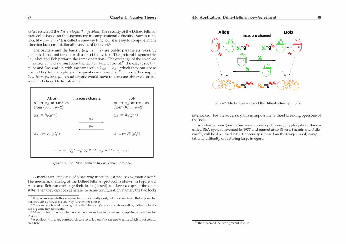
87 Chapter 4. Number Theory
as (a version of) the discrete logarithm problem. The security of the Diffie-Hellmanprotocol is based on this asymmetry in computational difficulty. Such a func-tion, like x 7→ Rp(g
x), is called a one-way function: it is easy to compute in onedirection but computationally very hard to invert.21
The prime p and the basis g (e.g. g = 2) are public parameters, possiblygenerated once and for all for all users of the system. The protocol is symmetric,i.e., Alice and Bob perform the same operations. The exchange of the so-calledpublic keys yA and yB must be authenticated, but not secret.22 It is easy to see thatAlice and Bob end up with the same value kAB = kBA which they can use asa secret key for encrypting subsequent communication.23 In order to computekAB from yA and yB , an adversary would have to compute either xA or xB ,which is believed to be infeasible.
Alice insecure channel Bobselect xA at randomfrom 0, . . . , p−2
yA := Rp(gxA)
select xB at randomfrom 0, . . . , p−2
yB := Rp(gxB)
yA
yB
kAB := Rp(yxA
B ) kBA := Rp(yxB
A )
kAB ≡p yxA
B ≡p (gxB)xA ≡p gxAxB ≡p kBA
Figure 4.1: The Diffie-Hellman key agreement protocol.
A mechanical analogue of a one-way function is a padlock without a key.24
The mechanical analog of the Diffie-Hellman protocol is shown in Figure 4.2.Alice and Bob can exchange their locks (closed) and keep a copy in the openstate. Then they can both generate the same configuration, namely the two locks
21It is not known whether one-way functions actually exist, but it is conjectured that exponentia-tion modulo a prime p is a one-way function for most p.
22This can be achieved by recognizing the other party’s voice in a phone call or, indirectly, by theuse of public-key certificates.
23More precisely, they can derive a common secret key, for example by applying a hash functionto KAB .
24A padlock with a key corresponds to a so-called trapdoor one-way function which is not consid-ered here.
4.6. Application: Diffie-Hellman Key-Agreement 88
Alice Bobinsecure channel
yAxA=g
xBxA
yB
yA
yBxB=g
kAB=g kBA=gxBxA xAxB
A A
A
B B
A
B
B
A
B
Figure 4.2: Mechanical analog of the Diffie-Hellman protocol.
interlocked. For the adversary, this is impossible without breaking open one ofthe locks.
Another famous (and more widely used) public-key cryptosystem, the so-called RSA-system invented in 1977 and named after Rivest, Shamir and Adle-man25, will be discussed later. Its security is based on the (conjectured) compu-tational difficulty of factoring large integers.
25They received the Turing award in 2003.

Chapter 5
Algebra
5.1 Introduction
5.1.1 What Algebra is About
In a nutshell, algebra is the mathematical study of structures consisting of a setand certain operations on the set. Examples are the integers Z, the rational num-bers Q, and the set of polynomials with coefficients from some domain, with therespective addition and multiplication operations. A main goal in algebra is tounderstand the properties of such algebraic systems at the highest level of gen-erality and abstraction. For us, an equally important goal is to understand thealgebraic systems that have applications in Computer Science.
For instance, one is interested in investigating which properties of the inte-gers are responsible for the unique factorization theorem. What do the integers,the polynomials with rational or real coefficients, and several other structureshave in common so that the unique factorization theorem holds? Why does itnot hold for certain other structures?
The benefit of identifying the highest level of generality and abstraction isthat things often become simpler when unnecessary details are eliminated fromconsideration, and that a proof must be carried out only once and applies to allstructures captured at the given level of generality.
5.1.2 Algebraic Structures
Definition 5.1. An operation on a set S is a function1 Sn → S, where n ≥ 0 iscalled the “arity”2 of the operation.
1In some cases, the function is only partial.2German: Stelligkeit
89
5.2. Monoids and Groups 90
Operations with arity 1 and 2 are called unary and binary operations, respec-tively. An operation with arity 0 is called a constant; it is a fixed element fromthe set S, for instance the special element 1 in Z. In many cases, only binaryoperations are actually listed explicitly,
Definition 5.2. An algebra (or algebraic structure or Ω-algebra) is a pair 〈S; Ω〉where S is a set (the carrier3 of the algebra) and Ω = (ω1, . . . , ωn) is a list ofoperations on S.4
5.1.3 Some Examples of Algebras
We give a few examples of algebras, some of which we will discuss in moredetail later.
Example 5.1. 〈Z; +,−, 0, ·, 1〉 denotes the integers with the two binary opera-tions + and ·, the unary operation − (taking the negative) and the two constants0 and 1, the neutral elements of addition and multiplication.
We sometimes omit some details and write simply 〈Z; +, ·〉 instead of〈Z; +,−, 0, ·, 1〉 when the negation operation and the special elements 0 and 1are understood. More generally, we sometimes drop unary and nullary opera-tions. This notation is actually more common in the literature (but less precise).This is a purely notational issue.
Example 5.2. 〈Zm;⊕〉 (and 〈Zm;⊙〉) denote the integers modulo m with addi-tion modulo m (and multiplication modulo m) as the only binary operation.
Example 5.3. 〈P(A);∪,∩, 〉 is the power set of a set A with union, intersection,and complement operations.
5.2 Monoids and Groups
In this section we look at algebras 〈S; ∗〉 with one binary operation and possiblyone unary and one nullary operation. The binary operation can be denotedarbitrarily, for instance by ∗. It is often denoted +, in which case it is calledaddition, or ·, in which case it is called multiplication. But it is important to notethat the name of the operation is not of mathematical relevance.
We discuss three special properties that 〈S; ∗〉 can have, (1) neutral elements,(2) associativity, and (3) inverse elements, as well as combinations of these.
3German: Tragermenge4This definition, though very general, does not capture all algebraic systems one might be inter-
ested in. A more general type of algebraic system, called heterogeneous algebraic systems, can haveseveral carrier sets.

91 Chapter 5. Algebra
5.2.1 Neutral Elements
Definition 5.3. A left [right] neutral element (or identity element) of an algebra〈S; ∗〉 is an element e ∈ S such that e ∗ a = a [a ∗ e = a] for all a ∈ S. Ife ∗ a = a ∗ e = a for all a ∈ S, then e is simply called neutral element.
If the operation is called addition, then e is usually denoted as 0, and if it iscalled multiplication, then e is usually denoted as 1.
Lemma 5.1. If 〈S; ∗〉 has both a left and a right neutral element, then they are equal.In particular 〈S; ∗〉 can have at most one neutral element.
Proof. Suppose that e and e′ are left and right neutral elements, respectively.Then, by definition, e ∗ e′ = e′ (considering e as a left neutral element), but alsoe ∗ e′ = e (considering e′ as a right neutral element). Thus e′ = e.
Example 5.4. The empty sequence ǫ is the neutral element of 〈Σ∗; |〉, where Σ∗
is the set of sequences over the alphabet Σ and | denotes concatenation of se-quences.
5.2.2 Associativity and Monoids
The operation in the previous example, sequence concatenation, has a very use-ful property: When all sequences are written one after the other, with spacesbetween sequences, it does not matter in which order one performs the concate-nation operations. In short, sequence concatenation is associative.
Definition 5.4. A binary operation ∗ on a set S is associative if a∗(b∗c) = (a∗b)∗cfor all a, b, c ∈ S.
Not all operations are associative:
Example 5.5. An example of a non-associative operation on the integers is ex-ponentiation: (ab)c 6= a(b
c) in general.
Associativity is a very special property of an operation, but it is of crucialimportance in algebra. Associativity of ∗ means that the element a1 ∗a2 ∗ · · · ∗an(for any a1, . . . , an ∈ S) is uniquely defined and independent of the order inwhich elements are combined. For example,
(((a ∗ b) ∗ c) ∗ d) = ((a ∗ b) ∗ (c ∗ d)) = (a ∗ ((b ∗ c) ∗ d)).
This justifies the use of the notation∑n
i=1 ai if the operation ∗ is called addition,and
∏ni=1 ai if the operation ∗ is called multiplication.
5.2. Monoids and Groups 92
Note that up to now, and also in the next section, we do not yet pay attentionto the fact that some operations are commutative. In a sense, commutativity isless important than associativity.
Some standard examples of associate operations are addition and multipli-cation in various structures: Z, N, Q, R, and Zm.
Definition 5.5. A monoid is an algebra 〈M ; ∗, e〉 where ∗ is associative and e isthe neutral element.
Some standard examples of monoids are 〈Z; +, 0〉, 〈Z; ·, 1〉, 〈Q; +, 0〉, 〈Q; ·, 1〉,〈R; +, 0〉, 〈R; ·, 1〉, 〈Zm;⊕, 0〉, and 〈Zm;⊙, 1〉.
Example 5.6. 〈Σ∗; || , ǫ〉 is a monoid since, as mentioned above, concatenationof sequences is associative.
Example 5.7. For a set A, the set AA of functions A→ A form a monoid with re-spect to function composition. The identity function id (defined by id(a) = a forall a ∈ A) is the neutral element. According to Lemma 3.5, relation composition,and therefore also function composition, is associative. The algebra 〈AA; , id〉 isthus a monoid.
5.2.3 Inverses and Groups
Definition 5.6. A left [right] inverse element5 of an element a in an algebra 〈S; ∗, e〉with neutral element e is an element b ∈ S such that b ∗ a = e [a ∗ b = e]. Ifb ∗ a = a ∗ b = e, then b is simply called an inverse of a.
To prove the uniqueness of the inverse (if it exists), we need ∗ to be associa-tive:
Lemma 5.2. In a monoid 〈M ; ∗, e〉, if a ∈ M has a left and a right inverse, then theyare equal. In particular, a has at most one inverse.
Proof. Let b and c be left and right inverses of a, respectively, i.e., we have b∗a =e and a ∗ c = e, Then
b = b ∗ e = b ∗ (a ∗ c) = (b ∗ a) ∗ c = e ∗ c = c,
where we have omitted the justifications for the steps.
Example 5.8. Consider again 〈AA; , id〉. A function f ∈ AA has a left inverseonly if it is injective, and it has a right inverse only if it is surjective. Hence f hasan inverse f−1 if and only if f is bijective. In this case, f f−1 = f−1 f = id.
5or simply left [right] inverse.

93 Chapter 5. Algebra
Now follows one of the most fundamental definitions of algebra.
Definition 5.7. A group is an algebra 〈G; ∗, , e〉 satisfying the following axioms:
G1 ∗ is associative.
G2 e is a neutral element: a ∗ e = e ∗ a = a for all a ∈ G.
G3 Every a ∈ G has an inverse element a, i.e., a ∗ a = a ∗ a = e.
We can write 〈G; ∗〉 (or simply G if ∗ is understood) instead of 〈G; ∗, , e〉. Ifthe operation ∗ is called addition (+) [multiplication (·)], then the inverse of a isdenoted −a [a−1 or 1/a] and the neutral element is denoted 0 [1].
Some standard examples of groups are 〈Z; +,−, 0〉, 〈Q; +,−, 0〉, 〈Q \0; ·,−1 , 1〉, 〈R; +,−, 0〉, 〈R \ 0; ·,−1 , 1〉, and 〈Zm;⊕,⊖, 0〉.
Definition 5.8. A group 〈G; ∗〉 (or monoid) is called commutative or abelian6 ifa ∗ b = b ∗ a for all a, b ∈ G.
We summarize a few facts we encountered already earlier for the special caseof the integers Z. The group is the right level of abstraction for describing thesefacts. The proofs are left as exercises.
Lemma 5.3. For a group 〈G; ∗, , e〉, we have for all a, b, c ∈ G:
(i) (a) = a.
(ii) a ∗ b = b ∗ a.
(iii) Left cancellation law: a ∗ b = a ∗ c =⇒ b = c.
(iv) Right cancellation law: b ∗ a = c ∗ a =⇒ b = c.
(v) The equation a ∗ x = b has a unique solution x for any a and b.So does the equation x ∗ a = b.
5.2.4 (Non-)minimality of the Group Axioms
In mathematics, one generally wants the axioms of a theory to be minimal. Onecan show that the group axioms as stated are not minimal. One can simplifyaxiom G2 by only requesting that a ∗ e = a; call this new axiom G2’. The equa-tion e ∗ a = a is then implied (by all axioms). The proof of this fact is left as anexercise. Similarly, one can simplify G3 by only requesting that a ∗ a = e; callthis new axiom G2’. The equation a ∗ a = e is then implied. The proof for this isas follows:
a ∗ a = (a ∗ a) ∗ e (G2’ )
= (a ∗ a) ∗ (a ∗ a) (G3’, i.e., def. of right inverse of a)
6Named after the Norwegian mathematician Niels Henrik Abel.
5.2. Monoids and Groups 94
= a ∗ (a ∗ (a ∗ a)) (G1)
= a ∗ ((a ∗ a) ∗ a) (G1)
= a ∗ (e ∗ a) (G3)
= (a ∗ e) ∗ a (G1)
= a ∗ a (G2’)
= e (G3’, i.e., def. of right inverse of a)
5.2.5 Some Examples of Groups
Example 5.9. The set of invertible (non-singular) n × n matrices over the realnumbers with matrix multiplication form a group, with the identity matrix asthe neutral element. This group is not commutative for n ≥ 2.
Example 5.10. Recall that the sequences with concatenation and the empty se-quence as the neutral element form a non-commutative monoid. This is not agroup because inverses cannot be defined (except for the empty sequence).
Example 5.11. For a given structure R supporting addition and multiplication(to be called a ring later), let R[x] denote the set of polynomials with coefficientsin R. 〈Z[x]; +〉, 〈Q[x]; +〉, and 〈R[x]; +〉 are abelian groups, where + denotespolynomial addition. 〈Z[x]; ·〉, 〈Q[x]; ·〉, and 〈R[x]; ·〉 are commutative monoids,where · denotes polynomial multiplication. The neutral element is the polyno-mial 1. Like 〈Z; ·〉, 〈R[x]; ·〉 is not a group, for any R.
Example 5.12. Let Sn be the set of n! permutations of n elements, i.e., the setof bijections 1, . . . , n → 1, . . . , n. A bijection f has an inverse f−1. Sn is asubset of the set of functions 1, . . . , n → 1, . . . , n. It follows from the asso-ciativity of function composition that the composition of permutations is alsoassociative. The group 〈Sn; ,−1 , id〉 is called the symmetric group on n elements.Sn is non-abelian for n ≥ 3.
Another important source of (usually non-abelian) groups are symmetriesand rotations of a geometric figure, mapping the figure to itself (but permut-ing the vertices). The neutral element is the identity mapping and the inverseelement is, for an axial or point symmetry, the element itself. For a rotation,the inverse element is the inverse rotation. To form a group, the closure undercomposition must be considered. For example, the composition of two axialsymmetries corresponds to a rotation by twice the angle between the axes. Sucha group is a subset (a subgroup) of the set of permutations of the vertices.
Example 5.13. Consider a square in the plane, with nodes labeled A,B,C,D.Now consider operations which map the square to itself, but with the vertices

95 Chapter 5. Algebra
permuted. Consider the four reflections with respect to one of the two mid-dle parallels or one of the two diagonals. The closure under composition ofthese four elements also includes the four rotations by 0 (the neutral element),by 90, 180, and by 270. These 8 elements (reflections and rotations) form agroup, which we denote by S. It is called the symmetry group of the square. Ifthe vertices of the square are labeled A,B,C,D, then these eight geometric op-erations each corresponds to a permutation of the set A,B,C,D. For example,the rotation by 90 corresponds to the permutation (A,B,C,D) → (B,C,D,A).Note that the set of four rotations also form a group, actually a subgroup of theabove described group and also a subgroup of the group of permutations onA,B,C,D.7
Example 5.14. It is left as an exercise to figure out the symmetry group of thethree-dimensional cube.
5.3 The Structure of Groups
5.3.1 Direct Products of Groups
Definition 5.9. The direct product of n groups 〈G1; ∗1〉 , . . . , 〈Gn; ∗n〉 is the alge-bra
〈G1 × · · · ×Gn; ⋆〉,where the operation ⋆ is component-wise:
(a1, . . . , an) ⋆ (b1, . . . , bn) = (a1 ∗1 b1, . . . , an ∗n bn).
Lemma 5.4. 〈G1×· · ·×Gn; ⋆〉 is a group, where the neutral element and the inversionoperation are component-wise in the respective groups.
Proof. Left as an exercise.
Example 5.15. Consider the group 〈Z5;⊕〉× 〈Z7;⊕〉. The carrier of the group isZ5 × Z7. The neutral element is (0, 0). If we denote the group operation by ⋆,
then we have (2, 6) ⋆ (4, 3) = (1, 2). Also, (2, 6) = (3, 1). It follows from theChinese remainder theorem that 〈Z5;⊕〉 × 〈Z7;⊕〉 is isomorphic to 〈Z35;⊕〉, aconcept introduced in the following subsection.
7We point out that one can consider the described operations also as bijections of the real plane,i.e., as functions R2 → R2.
5.3. The Structure of Groups 96
5.3.2 Group Homomorphisms
Homomorphisms are a central concept in mathematics and also in ComputerScience. A homomorphism is a structure-preserving function from an algebraicstructure into another algebraic structure. Here we only introduce homomor-phisms of groups.
Definition 5.10. For two groups 〈G; ∗, , e〉 and 〈H ; ⋆, , e′〉, a function ψ : G→ His called a group homomorphism if, for all a and b,
ψ(a ∗ b) = ψ(a) ⋆ ψ(b).
If ψ is a bijection from G to H , then it is called an isomorphism, and we say thatG and H are isomorphic and write G ≃ H .
We use the symbol˜ for the inverse operation in the group H . The proof ofthe following lemma is left as an exercise:
Lemma 5.5. A group homomorphism ψ from 〈G; ∗, , e〉 to 〈H ; ⋆, , e′〉 satisfies
(i) ψ(e) = e′,
(ii) ψ(a) = ψ(a) for all a.
The concept of an isomorphism is more general than for algebraic systems inthe strict sense, and it applies to more general algebraic structures, for instancealso to relations and hence to graphs.
Example 5.16. The group 〈Z6;⊕〉× 〈Z10;⊕〉 is isomorphic to 〈Z2;⊕〉× 〈Z30;⊕〉.The isomorphism ψ : Z6 × Z10 → Z2 × Z30 is easily checked to be given byψ((a, b)) = (a′, b′) where a′ ≡2 a (i.e., a′ = R2(a)) and b′ is given by b′ ≡3 a andb′ ≡10 b (where the Chinese remainder theorem can be applied).
Example 5.17. The logarithm function is a group homomorphism from 〈R>0, ·〉to 〈R,+〉 since log(a · b) = log a+ log b.
We give two familiar examples of relevant homomorphisms that are not iso-morphisms.
Example 5.18. If one considers the three-dimensional space R3 with vector ad-dition, then any projection on a plane through the origin or a line through theorigin are homomorphic images of R3. A special case is the projection onto anaxis of the coordinate system, which abstracts away all but one coordinate.
Example 5.19. Consider the set of real-valued n× n matrices. The determinantis a homomorphism (with respect to multiplication) from the set of matrices toR. We have det(AB) = det(A) det(B).

97 Chapter 5. Algebra
5.3.3 Subgroups
For a given algebra, for example a group or a ring (see Section 5.5), a subalgebrais a subset that is by itself an algebra of the same type, i.e., a subalgebra is a sub-set of an algebra closed under all operations. For groups we have specifically:
Definition 5.11. A subset H ⊆ G of a group 〈G; ∗, , e〉 is called a subgroup of Gif 〈H ; ∗, , e〉 is a group, i.e., if H is closed with respect to all operations:
(1) a ∗ b ∈ H for all a, b ∈ H ,
(2) e ∈ H , and
(3) a ∈ H for all a ∈ H .
Example 5.20. For any group 〈G; ∗, , e〉, there exist two trivial subgroups: thesubset e and G itself.
Example 5.21. Consider the group Z12 (more precisely 〈Z12;⊕,⊖, 0〉). Thefollowing subsets are all the subgroups: 0, 0, 6, 0, 4, 8, 0, 3, 6, 9,0, 2, 4, 6, 8, 10, and Z12.
Example 5.22. The set of symmetries and rotations discussed in example 5.13,denoted S, constitutes a subgroup (with 8 elements) of the set of 24 permuta-tions on 4 elements.
5.3.4 The Order of Group Elements and of a Group
In the remainder of Section 5.3 we will use a multiplicative notation for groups,i.e., we denote the group operation as “·” (which can also be omitted) and usethe corresponding multiplicative notation. But it is important to point out thatthis is only a notational convention that entails no loss of generality of the kindof group operation. In many cases (but not always) we denote the neutral ele-ment of a multiplicatively written group as 1. The inverse of a is denoted a−1
or 1/a, and a/b stands for ab−1. Furthermore, we use the common notation forpowers of elements: For n ∈ Z, an is defined recursively:
• a0 = e,
• an = a · an−1 for n ≥ 1, and
• an = (a−1)|n| for n ≤ −1.
It is easy to see that for all m,n ∈ Z
am · an = am+n and (am)n = amn.
5.3. The Structure of Groups 98
Definition 5.12. Let G be a group and let a be an element of G. The order8 ofa, denoted ord(a), is the least m ≥ 1 such that am = e, if such an m exists, andord(a) is said to be infinite otherwise, written ord(a) = ∞.
By definition, ord(e) = 1. If ord(a) = 2 for some a, then a−1 = a; such an a iscalled self-inverse.
Example 5.23. The order of 6 in 〈Z20;⊕,⊖, 0〉 is 10. This can be seen easily since60 = 10 · 6 is the least common multiple of 6 and 20. The order of 10 is 2, and wenote that 10 is self-inverse.
Example 5.24. The order of any axial symmetry in the group S (see exam-ple 5.13) is 2, while the order of the 90-rotation (and also of the 270-rotation)is 4.
Example 5.25. The order of any integer a 6= 0 in 〈Z; +〉 is ∞.
Example 5.26. Consider the group S5 of permutations on the set 1, 2, 3, 4, 5.What is the order of the permutations described by (1, 2, 3, 4, 5) → (3, 1, 2, 4, 5),by (1, 2, 3, 4, 5)→ (1, 2, 3, 5, 4), and by (1, 2, 3, 4, 5) → (2, 3, 1, 5, 4)?
The following lemma implies that the sequence of powers of an element of afinite group is periodic. It does not hold in every monoid (why?).
Lemma 5.6. In a finite group G, every element has a finite order.
Proof. Since G is finite, we must have ar = as = b for some r and s with r < s(and some b). Then as−r = as · a−r = b · b−1 = e.
Definition 5.13. For a finite group G, |G| is called the order of G.9
5.3.5 Cyclic Groups
If G is a group and a ∈ G has finite order, then for any m ∈ Z we have
am = aRord(a)(m).
Definition 5.14. For a group G and a ∈ G, the group generated by a, denoted 〈a〉,is defined as
〈a〉 def= an| n ∈ Z.
8German: Ordnung9Note that the term “order” has two different (but related) meanings.

99 Chapter 5. Algebra
It is easy to see that 〈a〉 is a group, actually the smallest subgroup of a groupG containing the element a ∈ G. For finite groups we have
〈a〉 def= e, a, a2, . . . , aord(a)−1.
Definition 5.15. A groupG = 〈g〉 generated by an element g ∈ G is called cyclic,and g is called a generator of G.
Being cyclic is a special property of a group. Not all groups are cyclic! Acyclic group can have many generators. In particular, if g is a generator, then sois g−1.
Example 5.27. The group 〈Zn;⊕〉 is cyclic for every n, where 1 is a generator.The generators of 〈Zn;⊕〉 are all g ∈ Zn for which gcd(g, n) = 1, as the readercan prove as an exercise.
Example 5.28. The additive group of the integers, 〈Z; +,−, 0〉, is an infinitecyclic group generated by 1. The only other generator is −1.
Theorem 5.7. A cyclic group of order n is isomorphic to 〈Zn;⊕〉 (and hence abelian).
In fact, we use 〈Zn;⊕〉 as our standard notation of a cyclic group of order n.
Proof. Let G = 〈g〉 be a cyclic group of order n (with neutral element e). Thebijection Zn → G : i 7→ gi is a group isomorphism since i ⊕ j 7→ gi+j =gi ∗ gj .
5.3.6 Application: Diffie-Hellman for General Groups
The Diffie-Hellman protocol was described in Section 4.6 for the group Z∗p (this
notation is defined below), but the concept of a group was not yet introducedthere. As an application of general cyclic groups we mention that the Diffie-Hellman protocol works just as well in any cyclic group G = 〈g〉 for which com-puting x from gx (i.e., the discrete logarithm problem) is computationally infeasi-ble. Of course, one needs to apply a suitable mapping from G to a reasonablekey space.
Elliptic curves (not discussed here) are an important class of cyclic groupsused in cryptography.
5.3.7 The Order of Subgroups
The following theorem is one of the fundamental results in group theory. Westate it without proof.
5.3. The Structure of Groups 100
Theorem 5.8 (Lagrange). Let G be a finite group and let H be a subgroup of G. Thenthe order of H divides the order of G, i.e., |H | divides |G|.
The following corollaries are direct applications of Lagrange’s theorem.
Corollary 5.9. For a finite groupG, the order of every elements divides the group order,i.e., ord(a) divides |G| for every a ∈ G.
Proof. 〈a〉 is a subgroup of G of order ord(a), which according to Theorem 5.8must divide |G|.
Corollary 5.10. Let G be a finite group. Then a|G| = e for every a ∈ G.
Proof. We have |G| = k · ord(a) for some k. Hence
a|G| = ak·ord(a) =(aord(a)
)k= ek = e.
Corollary 5.11. Every group of prime order10 is cyclic, and in such a group everyelement except the neutral element is a generator.
Proof. Let |G| = pwith p prime. For any a, the order of the subgroup 〈a〉 dividesp. Thus either ord(a) = 1 or ord(a) = p. In the first case, a = e and in the lattercase G = 〈a〉.
Groups of prime order play a very important role in cryptography.
5.3.8 The Group Z∗m and Euler’s Function
We noted earlier that the set Zm = 0, . . . ,m − 1 is a group with respect toaddition modulo m, denoted ⊕. We also noted that multiplication modulo m,denoted ⊙ (where the modulusm is usually clear from the context), is of interestas well. However, Zm is not a group with respect to multiplication modulo m.For example, in Z12, 8 has no inverse. We remember (see Section 4.5.3) thata ∈ Zm has a multiplicative inverse if and only if gcd(a,m) = 1. In order toobtain a group, we must exclude those a from Zm for which gcd(a,m) 6= 1.Thus we define
Definition 5.16. Z∗m
def= a ∈ Zm | gcd(a,m) = 1.
10i.e., |G| = p for some prime p.

101 Chapter 5. Algebra
Definition 5.17. The Euler function ϕ : Z+ → Z+ is defined as the cardinality ofZ∗m:
ϕ(m) = |Z∗m|.
Example 5.29. Z∗18 = 1, 5, 7, 11, 13, 17. Hence ϕ(18) = 6.
If p is a prime, then Z∗p = 1, . . . , p− 1 = Zp \ 0, and ϕ(p) = p− 1.
Lemma 5.12. If the prime factorization of m is m =∏r
i=1 peii , then11
ϕ(m) =
r∏
i=1
(pi − 1)pei−1i .
Proof. For a prime p and e ≥ 1 we have
ϕ(pe) = pe−1(p− 1)
since exactly every pth integer in Zpe contains a factor p and hence ϕ(pe) =pe−1(p − 1) elements contain no factor p. For a ∈ Zm we have gcd(a,m) = 1 ifand only if gcd(a, peii ) = 1 for i = 1, . . . , r. Since the numbers peii are relativelyprime, the Chinese remainder theorem implies that there is a one-to-one corre-spondence between elements of Zm and lists (a1, . . . , ar) with ai ∈ Zp
eii
. Hence,
using the above, there is also a one-to-one correspondence between elementsof Z∗
m and lists (a1, . . . , ar) with ai ∈ Z∗peii
. There are∏r
i=1(pi − 1)pei−1i such
lists.
Theorem 5.13. 〈Z∗m;⊙,−1 , 1〉 is a group.
Proof. Z∗m is closed under ⊙ because if gcd(a,m) = 1 and gcd(b,m) = 1, then
gcd(ab,m) = 1. This is true since if ab and m have a common divisor > 1, thenthey also have a common prime divisor > 1, which would be a divisor of eithera or b, and hence a common divisor of a and m or of b and m, contradicting thatgcd(a,m) = 1 and gcd(b,m) = 1.
The associativity of ⊙ is inherited from the associativity of multiplication inZ. Moreover, 1 is a neutral element and inverses exist (see Section 4.5.3). Thus〈Z∗
m;⊙,−1 , 1〉 is a group.
Example 5.30. In Z∗18 = 1, 5, 7, 11, 13, 17 we have 5 ⊙ 13 = 11 and 11−1 = 5
since 11⊙ 5 = 1 (i.e., R18(11 · 5) = 1).
11Alternatively, ϕ(m) could be defined as ϕ(m) = m ·∏
p|mp prime
(
1−1
p
)
.
5.4. Application: RSA Public-Key Encryption 102
Example 5.31. In Z∗11 = 1, 2, 3, 4, 5, 6, 7, 8, 9, 10we have 4⊙ 6 = 2 and 7−1 = 8
since 7⊙ 8 = 1.
Now we obtain the following simple but powerful corollary to Theorem 5.8.
Corollary 5.14 (Fermat, Euler). For all m ≥ 2 and all a with gcd(a,m) = 1,
aϕ(m) ≡m 1.
In particular, for every prime p and every a not divisible by p,
ap−1 ≡p 1.
Proof. This follows from Corollary 5.10 for the group Z∗m of order ϕ(m).
The special case for primes was known already to Fermat.12 The generalcase was proved by Euler, actually before the concept of a group was explicitlyintroduced in mathematics.
We state the following theorem about the structure of Z∗m without proof. Of
particular importance and interest is the fact that Z∗p is cyclic for every prime p.
Theorem 5.15. The group Z∗m is cyclic if and only if m = 2, m = 4, m = pe, or
m = 2pe, where p is an odd prime and e ≥ 1.
Example 5.32. The group Z∗19 is cyclic, and 2 is a generator. The powers of 2
are 2, 4, 8, 16, 13, 7, 14, 9, 18, 17, 15, 11, 3, 6, 12, 5, 10, 1. The other generators are3, 10, 13, 14, and 15.
5.4 Application: RSA Public-Key Encryption
The RSA public-key cryptosystem, invented in 1977 by Rivest, Shamir, andAdleman13, is used in many security protocols on the Internet, for instance inTLS/SSL. Like the Diffie-Hellman protocol it allows two parties to communi-cate securely, even if the communication channel is insecure, provided only that
12This result can be used as a primality test. Actually, the term “compositeness test” is more ap-propriate. To test whether a numbern is prime one chooses a base a and checks whether an−1 ≡n 1.If the condition is violated, thenn is clearly composite, otherwise n could be a prime. Unfortunately,it is not guaranteed to be a prime. In fact, there are composite integers n for which an−1 ≡n 1 forall a with gcd(a, n) = 1. (Can you find such an n?) For more sophisticated versions of such aprobabilistic test one can prove that for every composite n, the fraction of test values for which thecorresponding condition is satisfied is at most 1/4. Thus, by repeating the test sufficiently manytimes, the confidence that n is prime can be increased beyond any doubt. This is useful in practice,but it does not provide a proof that n is prime.
13R. L. Rivest, A. Shamir, and L. Adleman, A method for obtaining digital signatures and public-key cryptosystems, Communications of the ACM, Vol. 21, No. 2, pp. 120–126, 1978.

103 Chapter 5. Algebra
they can authenticate each other’s public keys (respectively the Diffie-Hellmanvalues). Moreover, the RSA system can be used as a digital signature scheme(see below). RSA was the first cryptographic system offering this importantfunctionality.
5.4.1 e-th Roots in a Group
To understand the RSA system, all we need is the following simple theoremwhich is a consequence of Lagrange’s theorem (Theorem 5.8).
Theorem 5.16. Let G be some finite group (multiplicatively written), and let e ∈ Z berelatively prime to |G| (i.e. gcd(e, |G|) = 1). The function x 7→ xe is a bijection andthe (unique) e-th root of y ∈ G, namely x ∈ G satisfying xe = y, is
x = yd,
where d is the multiplicative inverse of e modulo |G|, i.e.,
ed ≡|G| 1.
Proof. We have ed = k · |G|+ 1 for some k. Thus, for any x ∈ G we have
(xe)d = xed = xk·|G|+1 = (x|G|)︸ ︷︷ ︸=1
k · x = x,
which means that the function y 7→ yd is the inverse function of the functionx 7→ xe (which is hence a bijection). The under-braced term is equal to 1 becauseof Corollary 5.10.
When |G| is known, then d can be computed from ed ≡|G| 1 by using theextended Euclidean algorithm No general method is known for computing e-throots in a group G without knowing its order. This can be exploited to define apublic-key cryptosystem.
5.4.2 Description of RSA
Motivated by the Diffie-Hellman protocol also based on modular exponentia-tion, Rivest, Shamir and Adleman suggested as a possible class of groups thegroups Z∗
n, where n = pq is the product of two sufficiently large secret primes,p and q. The order of Z∗
n,
|Z∗n| = ϕ(n) = (p− 1)(q − 1),
5.4. Application: RSA Public-Key Encryption 104
Alice insecure channel Bob
Generateprimes p and qn = p · qf = (p−1)(q−1)
select ed ≡f e
−1
n, e plaintextm ∈ 1, . . . , n−1
ciphertexty = Rn(m
e)
ym = Rn(y
d)
Figure 5.1: The naıve RSA public-key cryptosystem. Alice’s public key is thepair (n, e) and her secret key is d. The public key must be sent toBob via an authenticated channel. Bob can encrypt a message, rep-resented as a number in Zn, by raising it to the eth power modulo n.Alice decrypts a ciphertext by raising it to the dth power modulo n.
can be computed only if the prime factors p and q of n are known.14 The (public)encryption transformation is defined by
m 7→ y = Rn(me),
and the (secret) decryption transformation is defined by
y 7→ m = Rn(yd),
where d can be computed according to
ed ≡(p−1)(q−1) 1.
The naıve15 RSA public-key cryptosystem16 is summarized in Figure 5.1.
The RSA system is usually (for instance in the TLS/SSL protocol) used onlyfor key management, not for encrypting actual application data. The message
14One can show that one can efficiently compute p and q when given (p − 1)(q − 1). (How?)15The described version of using RSA is not secure, for several reasons. One reason is that it is
deterministic and therefore an attacker can check potential messages by encrypting them himselfand comparing the result with the ciphertext.
16The RSA encryption was defined above as a permutation on Z∗n. But one can show that encryp-
tion and decryption work for all m ∈ Zn. Thus the condition gcd(m,n) = 1 need not be checked.

105 Chapter 5. Algebra
m is an encryption key (typically a short-term session key) for a conventionalcryptosystem which is used to encrypt the actual application data (e.g. of a TLSsession).
5.4.3 On the Security of RSA *
Let us have a brief look at the security of the RSA public-key system.17 It is not knownwhether computing e-th roots modulo n (when gcd(e,ϕ(n)) = 1) is easier than factoringn, but it is widely believed that the two problems are computationally equivalent.18 Fac-toring large integers is believed to be computationally infeasible. If no significant break-through in factoring is achieved and if processor speeds keep improving at the same rateas they are now (using the so-called Moore’s law), a modulus with 2048 bits appears tobe secure for the next 15 years, and larger moduli (e.g. 8192 bits) are secure for a verylong time.
Obviously, the system is insecure unless Bob can make sure he obtains the correctpublic key from Alice rather than a public key generated by an adversary and posted inthe name of Alice. In other words, the public key must be sent from Alice to Bob via anauthenticated channel. This is usually achieved (indirectly) using a so-called public-keycertificate signed by a trusted certification authority. One also uses the term public-keyinfrastructure (PKI). Explaining these concepts is beyond the scope of this course.
It is important to point out that for a public-key system to be secure, the messagemust be randomized in an appropriate manner. Otherwise, when given an encryptedmessage, an adversary can check plaintext messages by encrypting them and comparingthem with the given encrypted message. If the message space is small (e.g. a bit), thenthis would allow to efficiently break the system.
5.4.4 Digital Signatures *
The RSA system can also be used for generating digital signatures. A digitalsignature can only be generated by the entity knowing the secret key, but it canbe verified by anyone, e.g. by a judge, knowing the public key. Alice’s signatures for a message m is
s = Rn(zd) for z = m||h(m),
where || denotes concatenation and h is a suitable function introducing redun-dancy into the message and the string z is naturally understood as an elementof Zn.19 A signature can be verified by raising it to the e-th power modulo n andchecking that it is of the correct form m||h(m). The message is recovered fromthe signature.
17But note that a cryptographic security analysis is much more involved.18In fact, for a generic model of computation, this equivalence was proved in: D. Aggarwal and U.
Maurer, Breaking RSA generically is equivalent to factoring, IEEE Transactions on Information Theory,vol. 62, pp. 6251–6259, 2016.
19This can be a so-called cryptographic hash function. Without such additional redundancy, everys ∈ Z
∗n would be a legitimate signature, and hence forging a signature would be trivial.
5.5. Rings and Fields 106
5.5 Rings and Fields
We now consider algebraic systems with two binary operations, usually calledaddition and multiplication.
5.5.1 Definition of a Ring
Definition 5.18. A ring 〈R; +,−, 0, ·, 1〉 is an algebra for which
(i) 〈R; +,−, 0〉 is a commutative group.
(ii) 〈R; ·, 1〉 is a monoid.
(iii) a(b + c) = (ab) + (ac) and (b+ c)a = (ba) + (ca) for all a, b, c ∈ R(left and right distributive laws).
A ring is called commutative if multiplication is commutative (ab = ba).20
Example 5.33. Z,Q,R, and C are (commutative) rings.
Example 5.34. 〈Zm;⊕,⊖, 0,⊙, 1〉 is a commutative ring. Since 〈Zm;⊕,⊖, 0〉 isan abelian group and 〈Zm;⊙, 1〉 is a monoid, it only remains to check the dis-tributive law, which is inherited from the distributive law for the integers.
We list some simple facts about rings.
Lemma 5.17. For any ring 〈R; +,−, 0, ·, 1〉, and for all a, b ∈ R,
(i) 0a = a0 = 0.
(ii) (−a)b = −(ab).
(iii) (−a)(−b) = ab.
(iv) If R is non-trivial (i.e., if it has more than one element), then 1 6= 0.
Proof. Proof of (i): We have
0 = −(a0) + a0 (0 = −b+ b for all b ∈ R, e.g. for b = a0)
= −(a0) + a(0 + 0) (0 + 0 = 0)
= −(a0) + (a0 + a0) (distributive law)
= (−(a0) + a0) + a0 (associativity of +)
= 0 + a0 (−b+ b = 0 for all b ∈ R )
= a0 (0 + b = b for all b ∈ R)
20One can show (as an exercise) that ring addition must be commutative, i.e., commutativity ofaddition follows from the remaining ring axioms. The stated ring axioms are hence not minimal.The word “commutative” in (i) could be dropped.
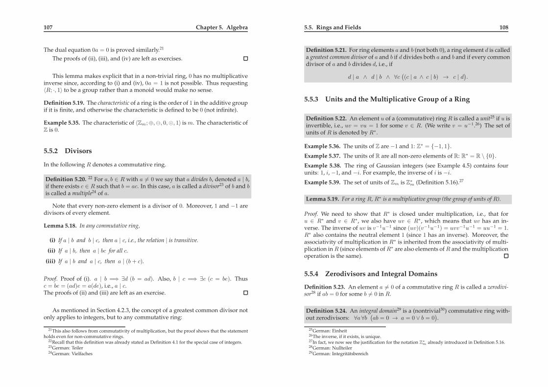
107 Chapter 5. Algebra
The dual equation 0a = 0 is proved similarly.21
The proofs of (ii), (iii), and (iv) are left as exercises.
This lemma makes explicit that in a non-trivial ring, 0 has no multiplicativeinverse since, according to (i) and (iv), 0a = 1 is not possible. Thus requesting〈R; ·, 1〉 to be a group rather than a monoid would make no sense.
Definition 5.19. The characteristic of a ring is the order of 1 in the additive groupif it is finite, and otherwise the characteristic is defined to be 0 (not infinite).
Example 5.35. The characteristic of 〈Zm;⊕,⊖, 0,⊙, 1〉 is m. The characteristic ofZ is 0.
5.5.2 Divisors
In the following R denotes a commutative ring.
Definition 5.20. 22 For a, b ∈ R with a 6= 0 we say that a divides b, denoted a | b,if there exists c ∈ R such that b = ac. In this case, a is called a divisor23 of b and bis called a multiple24 of a.
Note that every non-zero element is a divisor of 0. Moreover, 1 and −1 aredivisors of every element.
Lemma 5.18. In any commutative ring,
(i) If a | b and b | c, then a | c, i.e., the relation | is transitive.
(ii) If a | b, then a | bc for all c.
(iii) If a | b and a | c, then a | (b + c).
Proof. Proof of (i). a | b =⇒ ∃d (b = ad). Also, b | c =⇒ ∃e (c = be). Thusc = be = (ad)e = a(de), i.e., a | c.The proofs of (ii) and (iii) are left as an exercise.
As mentioned in Section 4.2.3, the concept of a greatest common divisor notonly applies to integers, but to any commutative ring:
21This also follows from commutativity of multiplication, but the proof shows that the statementholds even for non-commutative rings.
22Recall that this definition was already stated as Definition 4.1 for the special case of integers.23German: Teiler24German: Vielfaches
5.5. Rings and Fields 108
Definition 5.21. For ring elements a and b (not both 0), a ring element d is calleda greatest common divisor of a and b if d divides both a and b and if every commondivisor of a and b divides d, i.e., if
d | a ∧ d | b ∧ ∀c((c | a ∧ c | b) → c | d
).
5.5.3 Units and the Multiplicative Group of a Ring
Definition 5.22. An element u of a (commutative) ring R is called a unit25 if u isinvertible, i.e., uv = vu = 1 for some v ∈ R. (We write v = u−1.26) The set ofunits of R is denoted by R∗.
Example 5.36. The units of Z are −1 and 1: Z∗ = −1, 1.
Example 5.37. The units of R are all non-zero elements of R: R∗ = R \ 0.
Example 5.38. The ring of Gaussian integers (see Example 4.5) contains fourunits: 1, i, −1, and −i. For example, the inverse of i is −i.Example 5.39. The set of units of Zm is Z∗
m (Definition 5.16).27
Lemma 5.19. For a ring R, R∗ is a multiplicative group (the group of units of R).
Proof. We need to show that R∗ is closed under multiplication, i.e., that foru ∈ R∗ and v ∈ R∗, we also have uv ∈ R∗, which means that uv has an in-verse. The inverse of uv is v−1u−1 since (uv)(v−1u−1) = uvv−1u−1 = uu−1 = 1.R∗ also contains the neutral element 1 (since 1 has an inverse). Moreover, theassociativity of multiplication in R∗ is inherited from the associativity of multi-plication inR (since elements ofR∗ are also elements ofR and the multiplicationoperation is the same).
5.5.4 Zerodivisors and Integral Domains
Definition 5.23. An element a 6= 0 of a commutative ring R is called a zerodivi-sor28 if ab = 0 for some b 6= 0 in R.
Definition 5.24. An integral domain29 is a (nontrivial30) commutative ring with-out zerodivisors: ∀a ∀b
(ab = 0 → a = 0 ∨ b = 0
).
25German: Einheit26The inverse, if it exists, is unique.27In fact, we now see the justification for the notation Z∗
m already introduced in Definition 5.16.28German: Nullteiler29German: Integritatsbereich

109 Chapter 5. Algebra
Example 5.40. Z,Q,R, and C are integral domains.
Example 5.41. Zm is not an integral domain if m is not a prime. Any element ofZm not relatively prime to m is a zerodivisor.
Lemma 5.20. In an integral domain, if a | b, then c with b = ac is unique (and isdenoted by c = b
a or c = b/a and called quotient).31
Proof. Suppose that b = ac = ac′ for some c and c′. Then
0 = ac+ (−(ac′)) = a(c+ (−c′))
and thus, because a 6= 0 and there are no zero-divisors, we must have c+(−c′) =0 and hence c = c′.
5.5.5 Polynomial Rings
Definition 5.25. A polynomial a(x) over a ring R in the indeterminate x is aformal expression of the form
a(x) = adxd + ad−1x
d−1 + · · ·+ a1x+ a0 =
d∑
i=0
aixi.
for some non-negative integer d, with ai ∈ R. The degree of a(x), denoteddeg(a(x)), is the greatest i for which ai 6= 0. The special polynomial 0 (i.e.,all the ai are 0) is defined to have degree “minus infinity”.32 Let R[x] denote theset of polynomials (in x) over R.
Actually, it is mathematically better (but less common) to think of a poly-nomial simply as a finite list (a0, a1, . . . , ad−1, ad) of elements of R. There is noneed to think of a variable x which suggests that it can be understood as a func-tion R → R. A polynomial can, but need not, be considered as such a function(see Section 5.7).
Addition and multiplication in R[x] are defined as usual. Consider polyno-
mials a(x) =∑d
i=0 aixi of degree d and b(x) =
∑d′
i=0 bixi of degree d′. The sum
of a(x) and b(x) is a polynomial of degree at most max(d, d′) and is defined as
a(x) + b(x) =
max(d,d′)∑
i=0
(ai + bi) xi,
30i.e., 1 6= 031Note that the terms b
a(or b/a) are defined only if a | b.
32The interpretation of “minus infinity” is that it is a quantity which remains unchanged when anarbitrary integer is added to it.
5.5. Rings and Fields 110
where here and in the following coefficients with index greater than the degreeare understood to be 0. The product of a(x) and b(x) is defined as33
a(x)b(x) =
d+d′∑
i=0
(i∑
k=0
akbi−k
)xi =
d+d′∑
i=0
( ∑
u+v=i
aubv
)xi
= adbd′xd+d′
+ · · ·+ (a0b2 + a1b1 + a2b0)x2 + (a0b1 + a1b0)x+ a0b0.
The i-th coefficient of a(x)b(x) is∑i
k=0 akbi−k =∑
u+v=i aubv, where the sumis over all pairs (u, v) for which u+ v = i as well as u ≥ 0 and v ≥ 0.
The degree of the product of polynomials over a ring R is, by definition, atmost the sum of the degrees. It is equal to the sum if R is an integral domain,which implies that the highest coefficient is non-zero: adbd′ 6= 0 if ad 6= 0 andbd′ 6= 0.
Example 5.42. Consider the ring Z7 and let a(x) = 2x2+3x+1 and b(x) = 5x+6.Then
a(x) + b(x) = 2x2 + (3 + 5)x+ (1 + 6) = 2x2 + x
and
a(x)b(x) = (2 ·5)x3+(3 ·5+2 ·6)x2+(1 ·5+3 ·6)x+1 ·6 = 3x3+6x2+2x+6.
Theorem 5.21. For any ring R, R[x] is a ring.
Proof. We need to prove that the conditions of Definition 5.18 (i.e., the ring ax-ioms) are satisfied for R[x], assuming they are satisfied for R. We first observethat since multiplication in R is commutative, so is multiplication in R[x].
Condition (i) requires that R[x] is an abelian group with respect to (poly-nomial) addition. This is obvious from the definition of addition. Associativ-ity and commutativity of (polynomial) addition are inherited from associativ-ity and commutativity of addition in R (because R is a ring). The neutral el-ement is the polynomial 0, and the inverse in the group (i.e., the negative) of
a(x) =∑d
i=0 aixi is −a(x) =∑d
i=0(−ai)xi.Condition (ii) requires that R[x] is a monoid with respect to (polynomial)
multiplication. The polynomial 1 is the neutral element, which is easy to see.That multiplication is associative can be seen as follows. Let a(x) and b(x) as
above, and c(x) =∑d′′
i=0 cixi. Using the above definition of a(x)b(x), we have
(a(x)b(x)
)c(x) =
d+d′+d′′∑
i=0
i∑
j=0
∑
u+v=j
aubv
ci−j
xi
33Note that, for example, the highest coefficient∑d+d′
k=0 akbi−k is in the formula defined as a sumof d+ d′ + 1 terms, but all but one of them (namely for k = d) are zero.

111 Chapter 5. Algebra
=
d+d′+d′′∑
i=0
( ∑
u+v+w=i
(aubv)cw
)xi.
If one computes a(x)(b(x)c(x)
), one arrives at the same expression, by mak-
ing use of associativity of multiplication in R, i.e., the fact that (aubv)cw =au(bvcw) = aubvcw.
Condition (iii), the distributive law, can also be shown to follow from thedistributive law holding for R.
Lemma 5.22.
(i) If D is an integral domain, then so is D[x].
(ii) The units ofD[x] are the constant polynomials that are units ofD: D[x]∗ = D∗.
Proof. Left as an exercise.
Example 5.43. Lemma 5.22 implies that for an integral domainD, the setD[x][y]of polynomials in y with coefficients inD[x], is also an integral domain. One canalso view the elements ofD[x][y] as polynomials in two indeterminates, denotedD[x, y].
5.5.6 Fields
Definition 5.26. A field34 is a nontrivial commutative ring F in which everynonzero element is a unit, i.e., F ∗ = F \ 0.
In other words, a ring F is a field if and only if 〈F \ 0; ·,−1 , 1〉 is an abeliangroup.
Example 5.44. Q,R, and C are fields, but Z and R[x] (for any ring R) are notfields.
Theorem 5.23. Zp is a field if and only if p is prime.
Proof. This follows from our earlier analysis of Z∗p, namely that Zp \ 0 is a
multiplicative group if and only if p is prime.
In the following we denote the field with p elements by GF(p) rather thanZp. As explained later, “GF” stands for Galois field. Galois discovered finitefields around 1830.
34German: Korper
5.5. Rings and Fields 112
Fields are of crucial importance because in a field one can not only add,subtract, and multiply, but one can also divide by any nonzero element. Thisis the abstraction underlying many algorithms like those for solving systems oflinear equations (e.g. by Gaussian elimination) or for polynomial interpolation.Also, a vector space, a crucial concept in mathematics, is defined over a field,the so-called base field. Vector spaces over R are just a special case.
Example 5.45. Solve the following system of linear equations over Z11:
5x⊕ 2y = 4
2x⊕ 7y = 9
Solution: Eliminate x by adding 2 times the first and ⊖5 = 6 times the secondequation, resulting in
(2⊙ 5⊕ 6⊙ 2)︸ ︷︷ ︸=0
x+ (2 ⊙ 2⊕ 6⊙ 7)︸ ︷︷ ︸=2
y = 2⊙ 4⊕ 6⊙ 9︸ ︷︷ ︸=7
,
which is equivalent to 2y = 7. Thus y = 2−1 ⊙ 7 = 6⊙ 7 = 9. This yields
x = 2−1 ⊙ (9⊖ 7⊙ y) = 6⊙ (9⊕ 4⊙ 9) = 6⊙ 1 = 6.
Later we will describe a few applications of finite fields. Here we give an-other example of a finite field.
Example 5.46. We describe a field with 4 elements, F = 0, 1, A,B, by givingthe function tables of addition and multiplication:
+ 0 1 A B0 0 1 A B1 1 0 B AA A B 0 1B B A 1 0
· 0 1 A B0 0 0 0 01 0 1 A BA 0 A B 1B 0 B 1 A
This field is not isomorphic to the ring Z4, which is not a field. We explain theconstruction of this 4-element field in Section 5.8.2.
Theorem 5.24. A field is an integral domain.
Proof. In a field, every non-zero element is a unit, and in an integral domain,every non-zero element must not be a zero-divisor. It hence suffices to showthat in any commutative ring, a unit u ∈ R is not a zerodivisor. To arrive at acontradiction, assume that uv = 0 for some v. Then we must have v = 0 since
v = 1v = u−1uv = u−10 = 0,
and hence u is not a zerodivisor.

113 Chapter 5. Algebra
5.6 Polynomials over a Field
Recall Definition 5.25 of a polynomial over a ring R. As mentioned severaltimes, the set R[x] of polynomials over R is a ring with respect to the standardpolynomial addition and multiplication. The neutral elements of addition andmultiplication are the polynomials 0 and 1, respectively.
Polynomials over a field F are of special interest, for reasons to become clear.Namely, they have properties in common with the integers, Z.
5.6.1 Factorization and Irreducible Polynomials
For a, b ∈ Z, if b divides a, then also −b divides a. The analogy for polynomialsis as follows. If b(x) divides a(x), then so does v · b(x) for any nonzero v ∈ F be-cause if a(x) = b(x) ·c(x), then a(x) = vb(x) ·
(v−1c(x)
). Among the polynomials
vb(x) (for v ∈ F ), which are in a certain sense associated to each other, there isa distinguished one, namely that with leading coefficient 1. This is analogousto b and −b being associated in Z (see Section 5.6.3) and the positive one beingdistinguished.
Definition 5.27. A polynomial a(x) ∈ F [x] is called monic35 if the leading coef-ficient is 1.
Example 5.47. In GF(5)[x], x + 2 divides x2 + 1 since x2 + 1 = (x + 2)(x + 3).Also, 2x + 4 divides x2 + 1 since x2 + 1 = (2x + 4)(3x + 4). More generally,v · (x+2) divides x2+1 for any v ∈ GF(5) because x2+1 = v(x+2) ·v−1(x+3).
One can factor polynomials, similarly to the factorization of integers.
Example 5.48. In GF(7)[x] we have
x3 + 2x2 + 5x+ 2 = (x+ 5)(x2 + 4x+ 6).
In GF(2)[x] we have
x6 + x5 + x4 + x3 + 1 = (x2 + x+ 1)(x4 + x+ 1).
Definition 5.28. A polynomial a(x) ∈ F [x] with degree at least 1 is called irre-ducible if it is divisible only by constant polynomials and by constant multiplesof a(x).
The notion of irreducibility in F [x] corresponds to the notion of primality inZ, in a sense to be made more precise in Section 5.6.3.
35German: monisch, normiert
5.6. Polynomials over a Field 114
It follows immediately from the definition (and from the fact that the degreesare added when polynomials are multiplied) that every polynomial of degree 1is irreducible. Moreover, a polynomial of degree 2 is either irreducible or theproduct of two polynomials of degree 1. A polynomial of degree 3 is eitherirreducible or it has at least one factor of degree 1. Similarly, a polynomial ofdegree 4 is either irreducible, has a factor of degree 1, or has an irreduciblefactor of degree 2.
Irreducibility of a polynomial of degree d can be checked by testing all irre-ducible polynomials of degree ≤ d/2 as possible divisors. Actually, it suffices totest only the monic polynomials because one could always multiply a divisor bya constant, for example the inverse of the highest coefficient. This irreducibil-ity test is very similar to the primality test which checks all divisors up to thesquare root of the number to be tested.
Example 5.49. In GF(5)[x], x2 + 2 is irreducible since (as one can check) x + αdoes not divide x2 + 2, for all α ∈ GF(5).
Example 5.50. In GF(7)[x], x2 +4x+6 is irreducible since x+α does not dividex2 + 4x+ 6, for all α ∈ GF(7).
Example 5.51. In GF(2)[x], x2 + x+ 1 is irreducible because neither x nor x+ 1divides x2 + x + 1. It is easy to see that this is the only irreducible polynomialof degree 2 over GF(2). There are two irreducible polynomials of degree 3 overGF(2), namely x3 + x+ 1 and x3 + x2 + 1. Moreover, there are three irreduciblepolynomials of degree 4 over GF(2), which the reader can find as an exercise.
Not only the concepts of divisors and division with remainders (see below)carries over from Z to F [x], also the concept of the greatest common divisor canbe carried over. Recall that F [x] is a ring and hence the notion of a greatestcommon divisor is defined. For the special type of ring F [x], as for Z, one cansingle out one of them.
Definition 5.29. The monic polynomial g(x) of largest degree such that g(x) |a(x) and g(x) | b(x) is called the greatest common divisor of a(x) and b(x), de-noted gcd(a(x), b(x)).
Example 5.52. Consider GF(7)[x]. Let a(x) = x3 + 4x2 + 5x + 2 and b(x) =x3 + 6x2 + 4x + 6. One can easily check that a(x) = (x + 1)(x2 + 3x + 2) andb(x) = (x+ 3)(x2 + 3x+ 2). Thus gcd(a(x), b(x)) = x2 + 3x+ 2.
Example 5.53. Consider GF(2)[x]. Let a(x) = x3+x2+x+1 and b(x) = x2+x+1.Then gcd(a(x), b(x)) = 1.

115 Chapter 5. Algebra
5.6.2 The Division Property in F [x]
Let F be a field. The ring F [x] has strong similarities with the integers Z (seeSection 5.6.3). Both these integral domains have the special property that onecan divide one element a by another element b 6= 0, resulting in a quotient qand a remainder r which are unique when r is required to be “smaller” thanthe divisor. In case of the integers, the “size” of b ∈ Z is given by the absolutevalue |b|, and the “size” of a polynomial b(x) ∈ F [x] can be defined as its degreedeg(b(x)).
Theorem 5.25. Let F be a field. For any a(x) and b(x) 6= 0 in F [x] there exist aunique q(x) (the quotient) and a unique r(x) (the remainder) such that
a(x) = b(x) · q(x) + r(x) and deg(r(x)) < deg(b(x)).
Proof sketch. We first prove the existence of q(x) and r(x) and then the unique-ness. If deg(b(x)) > deg(a(x)), then q(x) = 0 and r(x) = a(x). We thus assumethat deg(b(x)) ≤ deg(a(x)). Let a(x) = amx
m + · · · and b(x) = bnxn + · · · with
n ≤ m, where “· · ·” stands for lower order terms. The first step of polynomialdivision consists of subtracting amb
−1n b(x)xm−n from a(x), resulting in a poly-
nomial of degree at most m−1.36 Continuing polynomial division finally yieldsq(x) and r(x), where deg(r(x)) < deg(b(x)) since otherwise one could still sub-tract a multiple of b(x).
To prove the uniqueness, suppose that
a(x) = b(x)q(x) + r(x) = b(x)q′(x) + r′(x),
where deg(r(x)) < deg(b(x)) and deg(r′(x)) < deg(b(x)). Then
b(x)[q(x) − q′(x)] = r′(x)− r(x).
Since deg(r′(x) − r(x)) < deg(b(x)), this is possible only if q(x) − q′(x) = 0, i.e.,q(x) = q′(x), which also implies r′(x) = r(x).37
In analogy to the notation Rm(a), we will denote the remainder r(x) of theabove theorem by Rb(x)(a(x)).
Example 5.54. Let F be the field GF(7) and let a(x) = x3 + 2x2 + 5x + 4 andb(x) = 2x2 + x+ 1. Then q(x) = 4x+ 6 and r(x) = 2x+ 5 since
(x3 + 2x2 + 5x+ 4) = (2x2 + x+ 1) · (4x+ 6) + (2x+ 5),
36Note that here it is important that F is a field since otherwise the existence of b−1n is not guar-
anteed.37Note that here we have made use of the fact that deg(u(x)v(x)) = deg(u(x)) + deg(v(x)). We
point out that this only holds in an integral domain. (Why?) Recall that a field is an integral domain(Theorem 5.24).
5.6. Polynomials over a Field 116
Example 5.55. In GF(2)[x] we have
(x4 + x3 + x2 + 1) : (x2 + 1) = x2 + x with remainder x+ 1.
Note that in GF(2), −1 = 1. For example, −x = x and −x2 = x2
5.6.3 Analogies Between Z and F [x], Euclidean Domains *
In this section we describe the abstraction underlying both Z and F [x].
Definition 5.30. In an integral domain, a and b are called associates, denoted a ∼ b, ifa = ub for some unit u.
Definition 5.31. In an integral domain, a non-unit p ∈ D \ 0 is irreducible if, wheneverp = ab, then either a or b is a unit.38
The units in Z are 1 and −1 and the units in F [x] are the non-zero constant polyno-mials (of degree 0). In Z, a and −a are associates.
Example 5.56. In Z, 6 and −6 are associates. In GF(5)[x], x2 + 2x + 3, 2x2 + 4x + 1,3x2 + x+ 4, and 4x2 + 3x+ 2 are associates.
For a ∈ D one can define one associate to be distinguished. For Z the distinguishedassociate of a is |a|, and for a(x) ∈ F [x] the distinguished associate of a(x) is the monicpolynomial associated with a(x). If we consider only the distinguished associates ofirreducible elements, then for Z we arrive at the usual notion of prime numbers.39
We point out that the association relation is closely related to divisibility. The proofof the following lemma is left as an exercise.
Lemma 5.26. a ∼ b ⇐⇒ a | b ∧ b | a.
There is one more crucial property shared by both integral domains Z and F [x] (forany field F ), described in the following abstract definition.
Definition 5.32. A Euclidean domain is an integral domain D together with a so-calleddegree function d : D \ 0 → N such that
(i) For every a and b 6= 0 in D there exist q and r such that a = bq+ r and d(r) < d(b)or r = 0.
(ii) For all nonzero a and b in D, d(a) ≤ d(ab).
Example 5.57. The Gaussian integers Z[√−1] discussed earlier are a Euclidean domain
where the degree of a+ bi is√a2 + b2, i.e., the absolute value (of complex numbers).
One can prove that in a Euclidean domain, the greatest (according to the degree func-tion) common divisor is well-defined, up to taking associates, i.e., up to multiplication
38In other words, p is divisible only by units and associates of p.39There is a notion of a prime element of a ring, which is different from the notion of an irreducible
element, but for the integers Z the two concepts coincide.

117 Chapter 5. Algebra
by a unit. The condition d(r) < d(b) guarantees that the gcd can be computed in thewell-known manner by continuous division. This procedure terminates because d(r)decreases monotonically in each division step.
The following theorem can be proved in a manner analogous to the proof of theunique factorization theorem for Z. One step is to show that a Euclidean domain is aprinciple ideal domain.
Theorem 5.27. In a Euclidean domain every element can be factored uniquely (up to takingassociates) into irreducible elements.
5.7 Polynomials as Functions
5.7.1 Polynomial Evaluation
For a ring R, a polynomial a(x) ∈ R[x] can be interpreted as a function R → Rby defining evaluation of a(x) at α ∈ R in the usual manner. This defines afunction R → R : α 7→ a(α).
Example 5.58. Consider the fieldGF (5) and the polynomial a(x) = 2x3+3x+1.Then a(0) = 1, a(1) = 1, a(2) = 3, a(3) = 4, and a(4) = 1.
If c(x) = a(x) · b(x), then c(α) = a(α) · b(α) for any α. Similarly, if c(x) =a(x) + b(x), then c(α) = a(α) + b(α) for any α.
5.7.2 Roots
Definition 5.33. Let a(x) ∈ R[x]. An element α ∈ R for which a(α) = 0 is calleda root40 of a(x).
Example 5.59. The polynomial x3 − 7x+ 6 in R[x] has 3 roots: −3, 1, and 2. Thepolynomial x2 + 1 in R[x] has no root. The polynomial (x3 + 2x2 + 5x + 2) inGF(7)[x] has 2 as its only root. The polynomial (x4 + x3 + x+1) in GF(2)[x] hasthe root 1.
Lemma 5.28. For a field F , α ∈ F is a root of a(x) if and only if x− α divides a(x).
Proof. (=⇒) Assume that α is a root, i.e., a(α) = 0. Then, according to Theo-rem 5.25, we can write a(x) as
a(x) = (x− α)q(x) + r(x),
40German: Nullstelle oder Wurzel
5.7. Polynomials as Functions 118
where deg(r(x)) < deg(x − α) = 1, i.e., r(x) is a constant r, where
r = a(x) − (x− α)q(x).
Setting x = α in the above equation gives
r = a(α)− (α− α)q(α) = 0− 0 · q(α) = 0.
Hence x− α divides a(x).(⇐=) To prove the other direction, assume that x − α divides a(x), i.e., a(x) =(x − α)q(x) for some q(x). Then a(α) = (α − α)q(α) = 0, i.e., α is a root ofa(x).
Lemma 5.28 implies that an irreducible polynomial of degree ≥ 2 has noroots.
Corollary 5.29. A polynomial a(x) of degree 2 or 3 over a field F is irreducible if andonly if it has no root.41
Proof. A reducible polynomial of degree 2 or 3 has a factor of degree 1 and hencea root. An irreducible polynomial has no root because according to Lemma 5.28,such a root would correspond to a (linear) factor.
Definition 5.34. If α is a root of a(x), then its multiplicity is the highest power ofx− α dividing a(x).
Example 5.60. Consider GF(2)[x]. The polynomial x5 + x has root 1 with mul-tiplicity 4 because (x + 1)4 divides x5 + x.
Theorem 5.30. For a field F , a nonzero42 polynomial a(x) ∈ F [x] of degree d has atmost d roots, counting multiplicities.
Proof. To arrive at a contradiction, suppose that a(x) has degree d but e > droots, say α1, . . . , αe (with possibly multiple occurrences). Then the polynomial∏e
i=1(x−αi) divides a(x). Since this is a polynomial of degree e, a(x) has degreeat least e, and hence more than d, which is a contradiction.
41Note that this statement is not true for polynomials of degree ≥ 4.42Note that every α ∈ F is a root of the polynomial 0.

119 Chapter 5. Algebra
5.7.3 Polynomial Interpolation
It is well-known that a polynomial of degree d over R can be interpolated fromany d + 1 values. Since the proof requires only the properties of a field (ratherthan the special properties of R), this interpolation property holds for polyno-mials over any field F . This fact is of crucial importance in many applications.
Lemma 5.31. A polynomial a(x) ∈ F [x] of degree at most d is uniquely determined byany d+1 values of a(x), i.e., by a(α1), . . . , a(αd+1) for any distinct α1, . . . , αd+1 ∈ F .
Proof. Let βi = a(αi) for i = 1, . . . , d + 1. Then a(x) is given by Lagrange’sinterpolation formula:
a(x) =
d+1∑
i=1
βiui(x),
where the polynomial ui(x) is given by
ui(x) =(x − α1) · · · (x− αi−1)(x− αi+1) · · · (x− αd+1)
(αi − α1) · · · (αi − αi−1)(αi − αi+1) · · · (αi − αd+1).
Note that for ui(x) to be well-defined, all constant terms αi − αj in the denomi-nator must be invertible. This is guaranteed if F is a field since αi − αj 6= 0 fori 6= j. Note also that the denominator is simply a constant and hence ui(x) is in-deed a polynomial of degree d. It is easy to verify that ui(αi) = 1 and ui(αj) = 0
for j 6= i. Thus the polynomials a(x) and∑d+1
i=1 βiui(x) agree when evaluated atany αi, for all i. We note that a(x) has degree at most d.43
It remains to prove the uniqueness. Suppose there is another polynomiala′(x) of degree at most d such that βi = a′(αi) for i = 1, . . . , d + 1. Then a(x) −a′(x) is also a polynomial of degree at most d, which (according to Theorem 5.30)can have at most d roots, unless it is 0. But a(x)−a′(x) has indeed the d+1 rootsα1, . . . , αd+1. Thus it must be 0, which implies a(x) = a′(x).
5.8 Finite Fields
So far we have seen the finite field GF (p), where p is prime. In this section wediscuss all other finite fields.
5.8.1 The Ring F [x]m(x)
We continue to explore the analogies between the rings Z and F [x]. In the sameway as we can compute in the integers Z modulo an integerm, yielding the ring
43The degree can be smaller than d if some βi are 0.
5.8. Finite Fields 120
〈Zm;⊕,⊖, 0,⊙, 1〉, we can also compute in F [x] modulo a polynomial m(x). LetRm(x)(a(x)) denote the (unique) remainder when a(x) is divided by m(x). Theconcept of congruence modulo m(x) is defined like congruence modulo m. Fora(x), b(x) ∈ F [x],
a(x) ≡m(x) b(x)def⇐⇒ m(x) |
(a(x)− b(x)
).
The proof of the following lemma is analogous to the proof that congruencemodulo m is an equivalence relation on Z.
Lemma 5.32. Congruence modulo m(x) is an equivalence relation on F [x], and eachequivalence class has a unique representative of degree less than deg(m(x)).
Example 5.61. Consider R[x] or Q[x]. We have, for example,
5x3 − 2x+ 1 ≡3x2+2 8x3 + 1 ≡3x2+2 − 163 x+ 1
as one can easily check. Actually, the remainder when 5x3 − 2x + 1 is dividedby 3x2 + 2 is − 16
3 x+ 1.
Example 5.62. Consider GF(2)[x]. Example 5.55 can be rephrased asRx2+1(x4+
x3 + x2 + 1) = x+ 1.
Definition 5.35. Let m(x) be a polynomial of degree d over F . Then
F [x]m(x)def=a(x) ∈ F [x]
∣∣ deg(a(x)) < d.
We state a simple fact about the cardinality of F [x]m(x) when F is finite.
Lemma 5.33. Let F be a finite field with q elements and let m(x) be a polynomial ofdegree d over F . Then |F [x]m(x)| = qd.
Proof. We have
F [x]m(x) =ad−1x
d−1 + · · ·+ a1x+ a0∣∣ a0, . . . , ad−1 ∈ F
.
There are qd choices for a0, . . . , ad−1.
F [x]m(x) is derived from F [x] in close analogy to how the ring Zm is derivedfrom the ring Z.
Lemma 5.34. F [x]m(x) is a ring with respect to addition and multiplication mod-
ulo m(x).44
44It is important to point out that we are considering three algebraic systems, namely F , F [x],and F [x]m(x). Each system has an addition and a multiplication operation, and we use the samesymbols “+” and “·” in each case, letting the context decide which one we mean. This should causeno confusion. The alternative would have been to always use different symbols, but this wouldbe too cumbersome. Note that, as mentioned above, addition (but not multiplication) in F [x] andF [x]m(x) are identical.

121 Chapter 5. Algebra
Proof. F [x]m(x) is a group with respect to polynomial addition.45 The neutralelement is the polynomial 0 and the negative of a(x) ∈ F [x]m(x) is −a(x). Asso-ciativity is inherited from F [x].
F [x]m(x) is a monoid with respect to polynomial multiplication. The neutralelement is the polynomial 1. Associativity of multiplication is inherited fromF [x], as is the distributive law.
The following lemma can be proved in analogy to Lemma 4.18.
Lemma 5.35. The congruence equation
a(x)b(x) ≡m(x) 1
(for a given a(x)) has a solution b(x) ∈ F [x]m(x) if and only if gcd(a(x),m(x)) = 1.
The solution is unique.46 In other words,
F [x]∗m(x) =a(x) ∈ F [x]m(x)
∣∣ gcd(a(x),m(x)) = 1.
Inverses in F [x]∗m(x) can be computed efficiently by a generalized version of
Euclid’s gcd-algorithm, which we do not discuss here.
5.8.2 Constructing Extension Fields
The following theorem is analogous to Theorem 5.23 stating that Zm is a field ifand only if m is prime.
Theorem 5.36. The ring F [x]m(x) is a field if and only if m(x) is irreducible.47
Proof. For an irreducible polynomial m(x), we have gcd(a(x),m(x)) = 1 for alla(x) 6= 0 with deg(a(x)) < deg(m(x)) and therefore, according to Lemma 5.35,a(x) is invertible in F [x]m(x). In other words, F [x]∗m(x) = F [x]m(x) \ 0. If m(x)
is not irreducible, then F [x]m(x) is not a field because nontrivial factors of m(x)have no multiplicative inverse.
In Computer Science, the fields of most interest are finite fields, i.e., F [x]m(x)
where F itself is a finite field. But before we discuss finite fields, we illustratethis new type of field based on polynomial arithmetic using a well-known ex-ample of an infinite field.
45Note that the sum of two polynomials is never reduced modulo m(x) because the degree of thesum is at most the maximum of the two degrees. In other words, a(x)+b(x) in F [x] and a(x)+b(x)in F [x]m(x) are the same operation when restricted to polynomials of degree less than deg(m(x)).
46This b(x) (if it exists) is called the inverse of a(x) modulo m(x).47F [x]m(x) is called an extension field of F .
5.8. Finite Fields 122
Example 5.63. The polynomial x2+1 is irreducible in R[x] because x2+1 has noroot in R. Hence, according to Theorem 5.36, R[x]x2+1 is a field. The elementsof R[x]x2+1 are the polynomials of degree at most 1, i.e., of the form ax + b.Addition and multiplication are defined by
(ax+ b) + (cx+ d) = (a+ c)x+ (b+ d)
and
(ax+ b) · (cx+ d) = Rx2+1((ax+ b) · (cx+ d))
= Rx2+1(acx2 + (bc+ ad)x+ bd)
= (bc+ ad)x+ (bd− ac).
The last step follows from the fact that Rx2+1(x2) = −1. The reader may have
noticed already that these addition and multiplication laws correspond to thoseof the complex numbers C when ax + b is interpreted as the complex numberb+ ai. Indeed, R[x]x2+1 is simply C or, more precisely, R[x]x2+1 is isomorphic toC. In fact, this appears to be the most natural way of defining C.
This example raises a natural question: Can we define other extension fieldsof R, or, what is special about C? There are many other irreducible polynomialsof degree 2, namely all those corresponding to a parabola not intersecting withthe x-axis. What is, for example, the field R[x]2x2+x+1? One can show thatR[x]m(x) is isomorphic to C for every irreducible polynomial of degree 2 overR. Are there irreducible polynomials of higher degree over R? The answer, aswe know, is negative. Every polynomial in R[x] can be factored into a productof polynomials of degree 1 (corresponding to real roots) and polynomials ofdegree 2 (corresponding to pairs of conjugate complex roots). The field C hasthe special property that a polynomial of degree d has exactly d roots in C. Forthe field R, this is not true. There are no irreducible polynomials of degree > 1over C.
Example 5.64. The polynomial x2 + x + 1 is irreducible in GF(2)[x] because ithas no roots. Hence, according to Theorem 5.36, GF(2)[x]x2+x+1 is a field. Theelements of GF(2)[x]x2+x+1 are the polynomials of degree at most 1, i.e., of theform ax+ b. Addition is defined by
(ax+ b) + (cx+ d) = (a+ c)x+ (b + d).
Note that the “+” in ax + b is in GF(2) (i.e., in Z2), and the middle “+” in(ax + b) + (cx + d) is to be understood in GF(2)[x]x2+x+1, i.e., as polynomialaddition. Multiplication is defined by
(ax+ b) · (cx+ d) = Rx2+x+1((ax + b) · (cx+ d))
= Rx2+x+1(acx2 + (bc+ ad)x+ bd)
= (bc+ ad+ ac)x+ (bd+ ac).

123 Chapter 5. Algebra
+ 0 1 x x+ 1 x2 x2 + 1 x2 + x x2 + x+ 1
0 0 1 x x+ 1 x2 x2 + 1 x2 + x x2 + x+ 1
1 0 x+ 1 x x2 + 1 x2 x2 + x+ 1 x2 + x
x 0 1 x2 + x x2 + x+ 1 x2 x2 + 1
x+ 1 0 x2 + x+ 1 x2 + x x2 + 1 x2
x2 0 1 x x+ 1
x2 + 1 0 x+ 1 x
x2 + x 0 1
x2 + x+ 1 0
Figure 5.2: The addition table for GF(8) constructed with the irreducible poly-nomial x3 + x+ 1.
· 0 1 x x+ 1 x2 x2 + 1 x2 + x x2 + x+ 1
0 0 0 0 0 0 0 0 0
1 1 x x+ 1 x2 x2 + 1 x2 + x x2 + x+ 1
x x2 x2 + x x+ 1 1 x2 + x+ 1 x2 + 1
x+ 1 x2 + 1 x2 + x+ 1 x2 1 x
x2 x2 + x x x2 + 1 1
x2 + 1 x2 + x+ 1 x+ 1 x2 + x
x2 + x x x2
x2 + x+ 1 x+ 1
Figure 5.3: The multiplication table for GF(8) constructed with the irreduciblepolynomial x3 + x+ 1.
The last step follows from the fact that Rx2+x+1(x2) = −x − 1 = x + 1 (since
−1 = 1 in GF(2)). It now becomes clear that this field with 4 elements is that ofExample 5.46. The reader can check that A = x andB = x+1 works just as wellas A = x+ 1 and B = x.
Example 5.65. The polynomial x3 + x+ 1 over GF(2) is irreducible since it hasno roots (it evaluates to 1 for both 0 and 1). The field GF(8) (also written GF(23))consists of the 8 polynomials of degree ≤ 2 over GF(2). The tables for additionand multiplication are shown in Figures 5.2 and 5.3. In this field we have, forexample,
(x+ 1)/(x2 + 1) = (x+ 1)(x2 + 1)−1 = (x+ 1)x = x2 + x.
5.9. Application: Error-Correcting Codes 124
5.8.3 Some Facts About Finite Fields *
Theorem 5.36 gives us a method for constructing a new field from an existing field F ,provided we can find an irreducible polynomial m(x) in F [x]. When F is a finite field,then so is F [x]m(x). The proofs of most facts stated in this section are beyond the scopeof this course.
The theory of finite fields was founded by the French mathematician Evariste Galois(1811–1832).48 In his honor, finite fields are called Galois fields. A field with q elements isusually denoted by GF(q) (independently of how it is constructed).
Theorem 5.37. For every prime p and every d ≥ 1 there exists an irreducible polynomial ofdegree d in GF(p)[x]. In particular, there exists a finite field with pd elements.
The following theorem states that the finite fields we have seen so far, Zp for primep and GF(p)[x]m(x) for an irreducible m(x), are all finite fields. There are no other finitefields. Moreover, one obtains no new finite fields by taking an irreducible polynomial,
say of degree d′, over some extension field GF(pd), resulting in the field GF(pdd′
). Sucha field can always be constructed directly using an irreducible polynomial of degree dd′
over GF(p).
Theorem 5.38. There exists a finite field with q elements if and only if q is a power of a prime.Moreover, any two finite fields of the same size q are isomorphic.
The last claim justifies the use of the notation GF(q) without making explicit how thefield is constructed. Different constructions yield different representations (naming) ofthe field elements, but not different fields. However, it is possible that some representa-tions are better suited than others for the efficient hardware or software implementationof the field arithmetic.
Theorem 5.39. The multiplicative group of every finite field GF(q) is cyclic.
Note that the multiplicative group of GF(q) has order q− 1 and has ϕ(q− 1) genera-tors.
Example 5.66. One can check that the fields GF(22) and GF(23) have multiplicativegroups of orders 3 and 7, which are both prime. Therefore all elements except 1 (and0 of course) are generators of the multiplicative group.
5.9 Application: Error-Correcting Codes
5.9.1 Definition of Error-Correcting Codes
Finite fields are of great importance in Computer Science and have many appli-cations, one of which is discussed in this section.
48His interest was in proving that polynomial equations over R of fifth or higher degree have ingeneral no closed form solution in radicals (while equations of up to fourth degree do). His majorcontributions to mathematics were recognized by the leading mathematicians only many years afterhis death. He died in a duel at the age of 21. The story goes that he wrote down major parts of histheory during the last night before the duel.

125 Chapter 5. Algebra
Error-correcting codes are used in many communication protocols and otherapplications. For example, the digital information on a CD is stored in such amanner that even if some of the information is lost (e.g. because of a scratch ordirt on the disc), the entire information can still be reconstructed without qualitydegradation, as long as sufficiently much of the data is still available.
There are two types of problems that can occur in data transmission or whenreading data from a storage medium. First, data can be erased, meaning thatwhen reading (or receiving) it one realizes that it is missing. Second, data cancontain errors. The second type of problem is more severe because it is not evenknown where in a data stream the errors occurred. A good error-correctingscheme can handle both problems.
Definition 5.36. A (n, k)-encoding function E for some alphabet A is an injectivefunction that maps a list (a0, . . . , ak−1) ∈ Ak of k (information) symbols to a list(c0, . . . , cn−1) ∈ An of n > k (encoded) symbols in A, called codeword:
E : Ak → An : (a0, . . . , ak−1) 7→ E((a0, . . . , ak−1)) = (c0, . . . , cn−1).
For an encoding function E one often consider the set
C = Im(E) = E((a0, . . . , ak−1)) | a0, . . . , ak−1 ∈ A
of codewords, which is called an error-correcting code.
Definition 5.37. An (n, k)-error-correcting code over the alphabet A with |A| = qis a subset of An of cardinality qk.
It is natural to use as the alphabet A = 0, 1, i.e., to take bits as the basic unitof information. However, for several reasons (one being the efficiency of encod-ing and in particular decoding), one often considers larger units of information,for example bytes (i.e., A = 0, 18).
Definition 5.38. The Hamming distance between two strings of equal length overa finite alphabet A is the number of positions at which the two strings differ.
Definition 5.39. The minimum distance of an error-correcting code C, denoteddmin(C), is the minimum of the Hamming distance between any two codewords.
Example 5.67. The following code is a (5, 2)-code over the alphabet 0, 1:
(0, 0, 0, 0, 0), (1, 1, 1, 0, 0), (0, 0, 1, 1, 1), (1, 1, 0, 1, 1).
The minimum distance is 3.
5.9. Application: Error-Correcting Codes 126
5.9.2 Decoding
Definition 5.40. A decoding function D for an (n, k)-encoding function is a func-tion D : An → Ak.
The idea is that a good decoding function takes an arbitrary list(r0, . . . , rn−1) ∈ An of symbols49 and decodes it to the most plausible (in somesense) information vector (a0, . . . , ak−1). Moreover, a good decoding functionshould be efficiently computable.
The error-correcting capability of a code C can be characterized in terms ofthe number t of errors that can be corrected. More precisely:
Definition 5.41. A decoding function D is t-error correcting for encoding func-tion E if for any (a0, . . . , ak−1)
D((r0, . . . , rn−1)
)= (a0, . . . , ak−1)
for any (r0, . . . , rn−1) with Hamming distance at most t from E((a0, . . . , ak−1)
).
A code C is t-error correcting if there exists E and D with C = Im(E) where D ist-error correcting.
Theorem 5.40. A code C with minimum distance d is t-error correcting if and only ifd ≥ 2t+ 1.
Proof. (⇐=) If any two codewords have Hamming distance at least 2t+ 1 (i.e.,differ in at least 2t+1 positions), then it is impossible that a word (r0, . . . , rn−1) ∈An could result from two different codewords by changing t positions. Thus if(r0, . . . , rn−1) has distance at most t from a codeword (c0, . . . , cn−1), then thiscodeword is uniquely determined. The decoding function D can be defined todecode to (one of) the nearest codeword(s) (more precisely, to the informationresulting (by E) in that codeword).(=⇒) If there are two codewords that differ in at most 2t positions, then thereexists a word (r0, . . . , rn−1) which differs from both codewords in at most t po-sitions; hence it is possible that t errors can not be corrected.
Example 5.68. A code with minimum distance d = 5 can correct t = 2 errors.The code in Example 5.67 can correct a single error (t = 1).
49For example the list of symbols received after transmission of a codeword over a noisy channelor read from a storage medium like a CD.

127 Chapter 5. Algebra
5.9.3 Codes based on Polynomial Evaluation
A very powerful class of codes is obtained by polynomial interpolation if A hasa field structure, i.e., A = GF(q) for some q:
Theorem 5.41. Let A = GF(q) and let α0, . . . , αn−1 be arbitrary distinct elements ofGF(q). Consider the encoding function
E((a0, . . . , ak−1)) =(a(α0), . . . , a(αn−1)
),
where a(x) is the polynomial
a(x) = ak−1xk−1 + · · ·+ a1x+ a0.
This code has minimum distance n− k + 1.
Proof. The polynomial a(x) of degree k−1 can be interpolated from any k values,i.e., from any k codeword symbols. If two polynomials agree for k arguments(or, equivalently, if two codewords agree at k positions), then they are equal.This means that two different codewords cannot agree at k positions. Hence anytwo codewords disagree in at least n− k + 1 positions.
An (n, k)-code over the field GF(2d) can be interpreted as a binary (dn, dk)-code (over GF(2)). The minimum distance of this binary code is at least that ofthe original code because two different GF(2d)-symbols must differ in at leastone bit (but can of course differ in more than one bit).
Example 5.69. Polynomial codes as described are used for storing informationon Compact Discs. In fact, the coding scheme of CD’s makes use of two differentsuch codes, but explaining the complete scheme is beyond the scope of thiscourse on discrete mathematics. The field is GF(28) defined by an irreduciblepolynomial of degree 8 over GF(2) and the two codes are a (32, 28)-code overGF(28) and a (28, 24)-code over GF(28), both with minimum distance 5.
Chapter 6
Logic
6.1 Introduction
In Chapter 2 we have introduced some basic concepts of logic, but the treat-ment was quite informal. In this chapter we discuss the foundations of logicin a mathematically rigorous manner. In particular, we clearly distinguish be-tween the syntax and the semantics of a logic and between syntactic derivationsof formulas and logical consequences they imply. We also introduce the con-cept of a logical calculus and define soundness and completeness of a calculus.Moreover, we discuss in detail a concrete calculus for propositional logic, theso-called resolution calculus.
At a very general level, the goal of logic is to provide a framework for ex-pressing mathematical statements and for expressing and verifying proofs forsuch statements. A more ambitious, secondary goal can be to provide tools forautomatically or semi-automatically generating a proof for a given statement.
A treatment of logic usually begins with a chapter on propositional logic1
(see Section 6.5), followed by a chapter on predicate (or first-order) logic2 (seeSection 6.6), which can be seen as an extension of propositional logic. There areseveral other logics which are useful in Computer Science and in mathematics,including temporal logic, modal logic, intuitionistic logic, and logics for rea-soning about knowledge and about uncertainty. Most if not all relevant logicscontain the logical operators from propositional logic, i.e., ∧,∨,¬ (and the de-rived operators → and ↔), as well as the quantifiers (∀ and ∃) from predicatelogic.
Our goal is to present the general concepts that apply to all types of log-ics in a unified manner, and then to discuss the specific instantiations of these
1German: Aussagenlogik2German: Pradikatenlogik
128

129 Chapter 6. Logic
concepts for each logic individually. Therefore we begin with such a generaltreatment (see Sections 6.2, 6.3, and 6.4) before discussing propositional andpredicate logic. From a didactic viewpoint, however, it will be useful to switchback and forth between the generic concepts of Sections 6.2, 6.3, and 6.4 and theconcrete instantiations of Sections 6.5 and 6.6.
We give a general warning: Different treatments of logic often use slightly orsometimes substantially different notation.3 Even at the conceptual level thereare significant differences. One needs to be prepared to adopt a particular no-tation used in a particular application context. However, the general principlesexplained here are essentially standard.
We also refer to the book by Kreuzer and Kuhling and that by Schoningmentioned in the preface of these lecture notes.
6.2 Proof Systems
6.2.1 Definition
In a formal treatment of mathematics, all objects of study must be described ina well-defined syntax. Typically, syntactic objects are finite strings over somealphabet Σ, for example the symbols allowed by the syntax of a logic or simplythe alphabet 0, 1, in which case syntactic objects are bit-strings. Recall that Σ∗
denotes the set of finite strings of symbols from Σ.
In this section, the two types of mathematical objects we study are
• mathematical statements of a certain type and
• proofs for this type of statements.
By a statement type we mean for example the class of statements of the formthat a given number n is prime, or the class of statements of the form that agiven graphG has a Hamiltonian cycle (see below), or the class of statements ofthe form that a given formula F in propositional logic is satisfiable.
Consider a fixed type of statements. Let S ⊆ Σ∗ be the set of (syntacticrepresentations of) mathematical statements of this type, and let P ⊆ Σ∗ be theset of (syntactic representations of) proof strings.4
Every statement s ∈ S is either true or false. The truth function
τ : S → 0, 1
3For example, in some treatments the symbol ⇒ is used for →, which can be confusing.4Membership in S and also in P is assumed to be efficiently checkable (for some notion of effi-
ciency).
6.2. Proof Systems 130
assigns to each s ∈ S its truth value τ(s). This function τ defines the meaning,called the semantics, of objects in S.5
An element p ∈ P is either a (valid) proof for a statement s ∈ S, or it is not.This can be defined via a verification function
φ : S × P → 0, 1,
where φ(s, p) = 1 means that p is a valid proof for statement s.
Without strong loss of generality we can in this section consider
S = P = 0, 1∗,
with the understanding that any string in 0, 1∗ can be interpreted as a state-ment by defining syntactically wrong statements as being false statements.
Definition 6.1. A proof system6 is a quadruple Π = (S,P , τ, φ), as above.
We now discuss the two fundamental requirements for proof systems.
Definition 6.2. A proof system Π = (S,P , τ, φ) is sound7 if no false statementhas a proof, i.e., if for all s ∈ S for which there exists p ∈ P with φ(s, p) = 1, wehave τ(s) = 1.
Definition 6.3. A proof system Π = (S,P , τ, φ) is complete8 if every true state-ment has a proof, i.e., if for all s ∈ S with τ(s) = 1, there exists p ∈ P withφ(s, p) = 1.
In addition to soundness and completeness, one requires that the functionφ be efficiently computable (for some notion of efficiency).9 We will not makethis formal, but it is obvious that a proof system is useless if proof verification iscomputationally infeasible. Since the verification has to generally examine theentire proof, the length of the proof cannot be infeasibly long.10
5In the context of logic discussed from the next section onwards, the term semantics is used in aspecific restricted manner that is compatible with its use here.
6The term proof system is also used in different ways in the mathematical literature.7German: korrekt8German: vollstandig9The usual efficiency notion in Computer Science is so-called polynomial-time computable which
we do not discuss further.10An interesting notion introduced in 1998 by Arora et al. is that of a probabilistically checkable proof
(PCP). The idea is that the proof can be very long (i.e., exponentially long), but that the verificationonly examines a very small random selection of the bits of the proof and nevertheless can decidecorrectness, except with very small error probability.

131 Chapter 6. Logic
6.2.2 Examples
Example 6.1. An undirected graph consists of a set V of nodes and a set E ofedges between nodes. Suppose that V = 0, . . . , n − 1. A graph can then bedescribed by the so-called adjacency matrix, an n×n-matrixM with 0, 1-entries,where Mi,j = 1 if and only if there is an edge between nodes i and j. A graphwith n nodes can hence be represented by a bit-string of length n2, by readingout the entries of the matrix row by row.
We are now interested in proving that a given graph has a so-called Hamilto-nian cycle, i.e., that there is a closed path from node 1 back to node 1, followingedges between nodes, and visiting every node exactly once. We are also inter-ested in the problem of proving the negation of this statement, i.e., that a givengraph has no Hamiltonian cycle. Deciding whether or not a given graph has aHamiltonian cycle is considered a computationally very hard decision problem(for large graphs).11
To prove that a graph has a Hamiltonian cycle, one can simply provide thesequence of nodes visited by the cycle. A value in V = 0, . . . , n − 1 can berepresented by a bit-string of length ⌈log2 n⌉, and a sequence of n such numberscan hence be represented by a bit-string of length n⌈log2 n⌉. We can hence defineS = P = 0, 1∗.
Now we can let τ be the function defined by τ(s) = 1 if and only if |s| = n2
for some n and the n2 bits of s encode the adjacency matrix of a graph containinga Hamiltonian cycle. If |s| is not a square or if s encodes a graph without aHamiltonian cycle, then τ(s) = 0.12 Moreover, we can let φ be the functiondefined by φ(s, p) = 1 if and only if, when s is interpreted as an n × n-matrixM and when p is interpreted as a sequence of n different numbers (a1, . . . , an)with ai ∈ 0, . . . , n − 1 (each encoded by a bit-string of length ⌈log2 n⌉), thenthe following is true:
Mai,ai+1 = 1
for i = 1, . . . , n− 1 andMan,a1 = 1.
This function φ is efficiently computable. The proof system is sound because agraph without Hamiltonian cycle has no proof, and it is complete because everygraph with a Hamiltonian cycle has a proof. Note that each s with τ(s) = 1 hasat least n different proofs because the starting point in the cycle is arbitrary.
Example 6.2. Let us now consider the opposite problem of proving the inex-istence of a Hamiltonian cycle in a given graph. In other words, in the aboveexample we define τ(s) = 1 if and only if |s| = n2 for some n and the n2 bits
11The best known algorithm has running time exponential in n. The problem is actually NP-complete, a concept that will be discussed in a later course on theoretical Computer Science.
12Note that τ defines the meaning of the strings in S , namely that they are meant to encode graphsand that we are interested in whether a given graph has a Hamiltonian cycle.
6.2. Proof Systems 132
of s encode the adjacency matrix of a graph not containing Hamiltonian cycle.In this case, no sound and complete proof system (with reasonably short andefficiently verifiable proofs) is known. It is believed that no such proof systemexists.
Example 6.3. Let again S = P = 0, 1∗, and for s ∈ 0, 1∗ let n(s) de-note the natural number whose (standard) binary representation is s, with theconvention that leading 0’s are ignored. (For example, n(101011) = 43 andn(00101) = 5.) Now, let τ be the function defined as follows: τ(s) = 1 if andonly if n(s) is not a prime number. Moreover, let φ be the function definedby φ(s, p) = 1 if and only if n(s) = 0, or if n(s) = 1, or if n(p) divides n(s) and1 < n(p) < n(s). This function φ is efficiently computable. This is a proof systemfor the non-primality (i.e., compositeness) of natural numbers. It is sound be-cause every s corresponding to a prime number n(s) has no proof since n(s) 6= 0and n(s) 6= 1 and n(s) has no divisor d satisfying 1 < d < n(s). The proof sys-tem is complete because every natural number n greater than 1 is either primeor has a prime factor q satisfying 1 < q < n (whose binary representation canserve as a proof).
Example 6.4. Let us consider the opposite problem, i.e., proving primality ofa number n(s) represented by s. In other words, in the previous example wereplace “not a prime” by “a prime”. It is far from clear how one can define averification function φ such that the proof system is sound and complete. How-ever, such an efficiently computable function φ indeed exists. Very briefly, theproof that a number n(s) (henceforth we simply write n) is prime consists of(adequate representations of):
1) the list p1, . . . , pk of distinct prime factors of n− 1,
2) a (recursive) proof of primality for each of p1, . . . , pk13
3) a generator g of the group Z∗n.
The exact representation of these three parts of the proof would have to be madeprecise, but we omit this here as it is obvious how this could be done.
The verification of a proof (i.e., the computation of the function φ) works asfollows.
• If n = 2 or n = 3, then the verification stops and returns 1.14
• It is tested whether p1, . . . , pk all divide n − 1 and whether n − 1 can bewritten as a product of powers of p1, . . . , pk (i.e., whether n − 1 containsno other prime factor).
13recursive means that the same principle is applied to prove the primality of every pi, and againfor every prime factor of pi − 1, etc.
14One could also consider a longer list of small primes for which no recursive primality proof isrequired.

133 Chapter 6. Logic
• It is verified thatgn−1 ≡n 1
and, for all i ∈ 1, . . . , k, that
g(n−1)/pi 6≡n 1.
(This means that g has order n− 1 in Z∗n).
• For every pi, an analogous proof of its primality is verified (recursively).
This proof system for primality is sound because if n is not a prime, then thereis no element of Z∗
n of order n− 1 since the order of any element is at most ϕ(n),which is smaller than n− 1. The proof system is complete because if n is prime,then GF (n) is a finite field and the multiplicative group of any finite field, i.e.,Z∗n, is cyclic and has a generator g. (We did not prove this statement in this
course.)15
6.2.3 Discussion
The examples demonstrate the following important points:
• While proof verification must be efficient (in some sense not defined here),proof generation is generally not (or at least not known to be) efficient. Forexample, finding a proof for the Hamiltonian cycle example requires tofind such a cycle, a problem that, as mentioned, is believed to be veryhard. Similarly, finding a primality proof as discussed would require thefactorization of n − 1, and the factoring problem is believed to be hard.In general, finding a proof (if it exists) is a process requiring insight andingenuity, and it cannot be efficiently automated.
• A proof system is always restricted to a certain type of mathematical state-ment. For example, the proof system of Example 6.1 is very limited in thesense that it only allows to prove statements of the form “graph G has aHamiltonian cycle”.
• Proof verification can in principle proceed in very different ways. Theproof verification method of logic, based on checking a sequence of ruleapplications, is (only) a special case.
• Asymmetry of statements and their negation: Even if a proof system existsfor a certain type of statements, it is quite possible that for the negation ofthe statements, no proof system (with efficient verification) exists.
15Actually, a quite efficient deterministic primality test was recently discovered by Agrawal et al.,and this means that primality can be checked without a proof. In other words, there exists a trivialproof system for primality with empty proofs. However, this fact is mathematically considerablymore involved than the arguments presented here for the soundness and completeness of the proofsystem for primality.
6.3. Elementary General Concepts in Logic 134
6.2.4 Proof Systems in Theoretical Computer Science *
The concept of a proof system appears in a more concrete form in theoretical computerscience (TCS), as follows. Statements and proofs are bit-strings, i.e., S = P = 0, 1∗.The predicate τ defines the set L ⊆ 0, 1∗ of strings that correspond to true statements:
L = s | τ (s) = 1.Conversely, every subset L ⊆ 0, 1∗ defines a predicate τ . In TCS, such a set L of stringsis called a formal language, and one considers the problem of proving that a given strings is in the language, i.e., s ∈ L. A proof for s ∈ L is called a witness of s, often denoted asw, and the verification function φ(s,w) defines whether a string w is a witness for s ∈ L.
One then considers the special case where the length of w is bounded by a polynomialof the length of s and where the function φ must be computable in polynomial time, i.e.,by a program with worst-case running time polynomial in the length of s. Then, theimportant class NP of languages is the set of languages for which such a polynomial-time computable verification function exists.
As mentioned in a footnote, a type of proof system of special interest are so-calledprobabilistically checkable proofs (PCP).
An important extension of the concept of proof systems are so-called interactiveproofs.16 In such a system, the proof is not a bit-string, but it consists of an interaction(a protocol) between the prover and the verifier, where one tolerates an immensely small(e.g. exponentially small) probability that a verifier accepts a “proof” for a false state-ment. The reason for considering such interactive proofs are:
• Such interactive proofs can exist for statements for which a classical (non-interactive) proof does not exist. For example, there exists an interactive proofsystem for the non-Hamiltonicity of graphs.
• Such interactive proofs can have a special property, called zero-knowledge, whichmeans that the verifier learns absolutely nothing (in a well-defined sense) duringthe protocol, except that the statement is true. In particular, the verifier cannotprove the statement to somebody else.
• Interactive proofs are of crucial importance in a large number of applications, es-pecially if they have the zero-knowledge property, for example in sophisticatedblock-chain systems.
6.3 Elementary General Concepts in Logic
The purpose of this section is to introduce the most basic concepts in logic in ageneral manner, not specific to a particular logic. However, this section is bestappreciated by considering concrete examples of logics, in particular proposi-tional logic and predicate logic. Without discussing such examples in parallel tointroducing the concepts, this section will be hard to appreciate. We will discussthe general concepts and the concrete examples in parallel, going back and forthbetween Section 6.3 and Sections 6.5 and 6.6.
16This topic is discussed in detail in the Master-level course Cryptographic Protocols taught byMartin Hirt and Ueli Maurer.

135 Chapter 6. Logic
6.3.1 The General Goal of Logic
A goal of logic is to provide a specific proof system Π = (S,P , τ, φ) for whicha very large class of mathematical statements can be expressed as an elementof S.
However, such a proof system Π = (S,P , τ, φ) can never capture all possiblemathematical statements. For example, it usually does not allow to capture(self-referential) statements about Π, such as “Π is complete”, as an element ofS. The use of common language is therefore unavoidable in mathematics andlogic (see also Section 6.7).
In logic, an element s ∈ S consists of one or more formulas (e.g. a formula,or a set of formulas, or a set of formulas and a formula), and a proof consists ofapplying a certain sequence of syntactic steps, called a derivation or a deduction.Each step consists of applying one of a set of allowed syntactic rules, and theset of allowed rules is called a calculus. A rule generally has some place-holdersthat must be instantiated by concrete values.
In standard treatments of logic, the syntax of S and the semantics (the func-tion τ ) are carefully defined. In contrast, the function φ, which consists of ver-ifying the correctness of each rule application step, is not completely explicitlydefined. One only defines rules, but for example one generally does not definea syntax for expressing how the place-holders of the rules are instantiated.17
6.3.2 Syntax, Semantics, Interpretation, Model
A logic is defined by the syntax and the semantics. The basic concept in any logicis that of a formula18.
Definition 6.4. The syntax of a logic defines an alphabet Λ (of allowed symbols)and specifies which strings in Λ∗ are formulas (i.e., are syntactically correct).
The semantics (see below) defines under which “conditions” a formula istrue (denoted as 1) or false (denoted as 0).19 What we mean by “conditions”needs to be made more precise and requires a few definitions.
Some of the symbols in Λ (e.g. the symbols A and B in propositional logicor the symbols P and Q in predicate logic) are understood as variables, each ofwhich can take on a value in a certain domain associated to the symbol.
17In a fully computerized system, this must of course be (and indeed is) defined.18German: Formel19There are logics (not considered here) with more than two truth values, for example a logic with
confidence or belief values indicating the degree of confidence in the truth of a statement.
6.3. Elementary General Concepts in Logic 136
Definition 6.5. The semantics of a logic defines (among other things, see below)a function free which assigns to each formula F = (f1, f2, . . . , fk) ∈ Λ∗ a subsetfree(F ) ⊆ 1, . . . , k of the indices. If i ∈ free(F ), then the symbol fi is said tooccur free in F .20
The same symbol β ∈ Λ can occur free in one place of F (say f3 = β where3 ∈ free(F )) and not free in another place (say f5 = β where 5 6∈ free(F )).
The free symbols of a formula denote kind of variables which need to beassigned fixed values in their respective associated domains before the formulahas a truth value. This assignment of values is called an interpretation:
Definition 6.6. An interpretation consists of a set Z ⊆ Λ of symbols of Λ, a do-main (a set of possible values) for each symbol in Z , and a function that assignsto each symbol in Z a value in its associated domain.21
Often (but not in propositional logic), the domains are defined in terms of aso-called universe U , and the domain for a symbol in Λ can for example be U , ora function Uk → U (for some k), or a function Uk → 0, 1 (for some k).
Definition 6.7. An interpretation is suitable22 for a formula F if it assigns a valueto all symbols β ∈ Λ occurring free in F .23
Definition 6.8. The semantics of a logic also defines a function24 σ assigning toeach formula F , and each interpretation A suitable for F , a truth value σ(F,A)in 0, 1.25 In treatments of logic one often writes A(F ) instead of σ(F,A) andcalls A(F ) the truth value of F under interpretation A.26
20The term “free” is not standard in the literature which instead uses special terms for each specificlogic, but as we see later it coincides for the notion of free variables in predicate logic.
21There may be restrictions for what is an allowed interpretation.22German: passend23A suitable interpretation can also assign values to symbols β ∈ Λ not occurring free in F .24We assume that the set of formulas and the set of interpretations are well-defined.25Note that different free occurrences of a symbol β ∈ Λ in F are assigned the same value, namely
that determined by the interpretation.26This notation in the literature is unfortunately a bit ambiguous since A is used for two differ-
ent things, namely for an interpretation as well as for the function induced by the interpretationwhich assigns to every formula the truth value (under that interpretation). We nevertheless use thenotation A(F ) instead of σ(F,A) in order to be compatible with most of the literature.

137 Chapter 6. Logic
Definition 6.9. A (suitable) interpretation A for which a formula F is true, (i.e.,A(F ) = 1) is called a model for F , and one also writes
A |= F.
More generally, for a set M of formulas, a (suitable) interpretation for which allformulas in M are true is called a model for M , denoted as
A |=M.
If A is not a model for M one writes A 6|=M.
6.3.3 Connection to Proof Systems *
We now explain how the semantics of a logic (the function σ in Definition 6.8) is con-nected to the semantics of a proof systems (the function τ in Definition 6.1).
First we should remark that one can treat logic in a similarly informal manner asone treats other fields of mathematics. There can be variations on how much is formal-ized in the sense of proof systems. Concretely, there are the following two options forformalizing a logic:
• In addition to formulas, also interpretations are considered to be formal objects,i.e., there is a syntax for writing (at least certain types of) interpretations. In thiscase, statements can correspond to pairs (F,A), and the function σ corresponds tothe function τ (in the sense of proof systems).
• Only formulas are formal objects and interpretations are treated informally, e.g. inwords or some other informal notation. This is the typical approach in treatmentsof logic (also in this course). This makes perfect sense if the formal statements onewants to prove only refer to formulas, and not to specific interpretations. Indeed,many statements about formulas are of this form, for example the statement that aformula F is a tautology, the statement that F is satisfiable (or unsatisfiable), or thestatement that a formula G is a logical consequence of a formula F , i.e., F |= G.Note that to prove such statements it is not necessary to formalize interpretations.
6.3.4 Satisfiability, Tautology, Consequence, Equivalence
Definition 6.10. A formula F (or set M of formulas) is called satisfiable27 if thereexists a model for F (or M ),28 and unsatisfiable otherwise. The symbol ⊥ is usedfor an unsatisfiable formula.29
27German: erfullbar28Note that the statement that M is satisfiable is not equivalent to the statement that every formula
in M is satisfiable.29The symbol ⊥ is not a formula itself, i.e., it is not part of the syntax of a logic, but if used in
expressions like F ≡ ⊥ it is to be understood as standing for an arbitrary unsatisfiable formula. Forexample, F ≡ ⊥ means that F is unsatisfiable.
6.3. Elementary General Concepts in Logic 138
Definition 6.11. A formula F is called a tautology30 or valid31 if it is true for everysuitable interpretation. The symbol ⊤ is used for a tautology.
The symbol ⊥ is sometimes called falsum, and ⊤ is sometimes called verum.The following lemma follows directly from the above definitions.
Definition 6.12. A formula G is a logical consequence32 of a formula F (or a setM of formulas), denoted
F |= G (or M |= G ),
if every interpretation suitable for both F (or M ) and G, which is a model for F(for M ), is also a model for G.33
Definition 6.13. Two formulas F and G are equivalent, denoted F ≡ G, if everyinterpretation suitable for both F and G yields the same truth value for F andG, i.e., if each one is a logical consequence of the other:
F ≡ Gdef⇐⇒ F |= G and G |= F.
A set M of formulas can be interpreted as the conjunction (AND) of all for-mulas in M since an interpretation is a model for M if and only if it is a modelfor all formulas in M .34 If M is the empty set, then, by definition, every in-terpretation is a model for M , i.e., the empty set of formulas corresponds to atautology.
Definition 6.14. If F is a tautology, one also writes |= F .
6.3.5 The Logical Operators ∧, ∨, and ¬
Essentially all logics contain the following recursive definitions as part of thesyntax definition.
Definition 6.15. If F and G are formulas, then also ¬F , (F ∧G), and (F ∨G)are formulas.
30German: Tautologie31German: gultig, allgemeingultig32German: (logische) Folgerung, logische Konsequenz33The symbol |= is used in two slightly different ways: with a formula (or set of formulas), and
also with an interpretation on the left side. This makes sense because one can consider a set M offormulas as defining a set of interpretations, namely the set of models for M .
34More formally, let G be any formula (one of the many equivalent ones) that corresponds to theconjunction of all formulas in M . Then M |= F if and only if G |= F .

139 Chapter 6. Logic
A formula of the form (F ∧ G) is called a conjunction, and a formula of theform (F ∨G) is called a disjunction.
We introduce some notational conventions for the use of parentheses. Theoutermost parentheses of a formula can be dropped, i.e., we can write F ∧ Ginstead of (F ∧ G). Moreover, parentheses not needed because of associativityof ∧ or ∨ (which is actually a consequence of the semantics defined below) canalso be dropped.
The implication introduced in Section 2.3 can be understood simply as anotational convention: F → G stands for ¬F ∨G.35 Similarly, the symbol F ↔ Gstands for (F ∧G) ∨ (¬F ∧ ¬G).
The semantics of the logical operators ∧, ∨, and ¬ is defined as follows (inany logic where these operators exist):
Definition 6.16.
A((F ∧G)) = 1 if and only if A(F ) = 1 and A(G) = 1.
A((F ∨G)) = 1 if and only if A(F ) = 1 or A(G) = 1.
A(¬F ) = 1 if and only if A(F ) = 0.
Some basic equivalences were already discussed in Section 2.3.2 and are nowstated for any logic that includes the logical operators ∧, ∨, and ¬ :
Lemma 6.1. For any formulas F , G, and H we have
1) F ∧ F ≡ F and F ∨ F ≡ F (idempotence);
2) F ∧G ≡ G ∧ F and F ∨G ≡ G ∨ F (commutativity);
3) (F ∧G)∧H ≡ F ∧ (G∧H) and (F ∨G)∨H ≡ F ∨ (G∨H) (associativity);
4) F ∧ (F ∨G) ≡ F and F ∨ (F ∧G) ≡ F (absorption);
5) F ∧ (G ∨H) ≡ (F ∧G) ∨ (F ∧H) (distributive law);
6) F ∨ (G ∧H) ≡ (F ∨G) ∧ (F ∨H) (distributive law);
7) ¬¬F ≡ F (double negation);
8) ¬(F ∧G) ≡ ¬F ∨ ¬G and ¬(F ∨G) ≡ ¬F ∧ ¬G (de Morgan’s rules);
9) F ∨ ⊤ ≡ ⊤ and F ∧ ⊤ ≡ F (tautology rules);
10) F ∨ ⊥ ≡ F and F ∧ ⊥ ≡ ⊥ (unsatisfiability rules).
11) F ∨ ¬F ≡ ⊤ and F ∧ ¬F ≡ ⊥.
Proof. The proofs follow directly from Definition 6.16. For example, the claim
35Alternatively, one could also define → to be a symbol of the syntax, in which case one wouldalso need to extend the semantics to provide an interpretation for →. This subtle distinction be-tween notational convention or syntax extension is not really relevant for us. We can simply use thesymbol →.
6.3. Elementary General Concepts in Logic 140
¬(F ∧G) ≡ ¬F ∨ ¬G follows from the fact that for any suitable interpretation,we have A(¬(F ∧ G)) = 1 if and only if A(F ∧ G) = 0, and hence if and only ifeither A(F ) = 0 or A(G) = 0, i.e., if and only if either A(¬F ) = 1 or A(¬G) = 1,and hence if and only if A(¬F ∨ ¬G) = 1.
6.3.6 Logical Consequence vs. Unsatisfiability
We state the following facts without proofs, which are rather obvious. Theselemmas are needed for example to make use of the resolution calculus (see Sec-tion 6.5.6), which allows to prove the unsatisfiability of a set of formulas, to alsobe able to prove that a formula F is a tautology, or to prove that a formula G islogical consequence of a given set F1, F2, . . . , Fk of formulas.
Lemma 6.2. A formula F is a tautology if and only if ¬F is unsatisfiable.
Lemma 6.3. The following three statements are equivalent:
1. F1, F2, . . . , Fk |= G,
2. (F1 ∧ F2 ∧ · · · ∧ Fk) → G is a tautology,
3. F1, F2, . . . , Fk,¬G is unsatisfiable.
6.3.7 Theorems and Theories
We can consider at least four types of statements one may want to prove in thecontext of using a logic:
1. Theorems in an axiomatically defined theory (see below),
2. Statements about a formula or a set of formulas, for example that F issatisfiable or that a set M of formulas is unsatisfiable.
3. The statement A |= F for a given interpretation A and a formula F ,
4. Statements about the logic, for example that a certain calculus for the logicis sound.
To describe the first type of statements, consider a fixed logic, for instancepredicate logic discussed in Section 6.6, and consider a set T of formulas,, wherethe formulas in T are called the axioms of the theory. Any formula F for which
T |= F

141 Chapter 6. Logic
is called a theorem in theory T . For example, the axioms of group theory are threeformulas in predicate logic, and any theorem in group theory (e.g. Lagrange’stheorem) is a logical consequence of the axioms.
Consider two theories T and T ′ satisfying T ⊂ T ′, T ′ contains all the axiomsof T plus one or more additional axioms. Then every theorem in T is also atheorem in T ′ (but not vice versa). In the special case where T = ∅, a theoremin T = ∅ is a tautology in the logic. Tautologies are useful because they aretheorems in any theory, i.e., for any set of axioms.
Example 6.5. The formula ¬∃x∀y(P (y, x) ↔ ¬P (y, y)
)is a tautology in predi-
cate logic, as proved in Section 6.6.9.
6.4 Logical Calculi
6.4.1 Introduction
As mentioned in Section 6.3.1, the goal of logic is to provide a framework for ex-pressing and verifying proofs of mathematical statements. A proof of a theoremshould be a purely syntactic derivation consisting of simple and easily verifiablesteps. In each step, a new syntactic object (typically a formula, but it can also bea more general object involving formulas) is derived by application of a deriva-tion rule, and at the end of the derivation, the desired theorem appears. Thesyntactic verification of a proof does not require any intelligence or “reasoningbetween the lines”, and it can in particular be performed by a computer.
Checking a proof hence simply means to execute a program. Like in com-puter programming, where the execution of a program is a dumb process whilethe design of a program is generally an intelligent, sometimes ingenious pro-cess, the verification of a proof should be a dumb process while devising a proofis an intelligent, creative, and sometimes ingenious process.
A well-defined set of rules for manipulating formulas (the syntactic objects)is called a calculus. Many such calculi have been proposed, and they differ invarious ways, for example in the syntax, the semantics, the expressiveness, howeasy or involved it is to write a proof, and how long a proof will be.
When defining a calculus, there is a trade-off between simplicity (e.g. a smallnumber of rules) and versatility. For a small set of rules, proving even sim-ple logical steps (like the substitution of a sub-formula by an equivalent sub-formula) can take a very large number of steps in the calculus.
It is beyond the scope of this course to provide an extensive treatment ofvarious logical calculi.
6.4. Logical Calculi 142
6.4.2 Hilbert-Style Calculi
As mentioned, there are different types of logical calculi. For the perhaps mostintuitive type of calculus, the syntactic objects that are manipulated are formu-las. This is sometimes called a Hilbert-style calculus. There is also another typeof calculi, often called sequent calculi (which we will not discuss in this course),where the syntactic objects are more complex objects than just formulas. Thefollowing refers to Hilbert-style calculi.
Definition 6.17. A derivation rule36 is a rule for deriving a formula from a set offormulas (called the precondition). We write
F1, . . . , Fk ⊢R G
if G can be derived from the set F1, . . . , Fk by rule R.37
The derivation rule F1, . . . , Fk ⊢R G is often also written as
F1 F2 · · · Fk
G(R),
where spaces separate the formulas above the bar.
Derivation is a purely syntactic concept. Derivation rules apply to syntac-tically correct (sets of) formulas. Some derivation rules (e.g. resolution, seeSection 6.5.6) require the formulas to be in a specific format.
Typically such a derivation rule is defined as a rule that involves place-holdersfor formulas (such as F and G), which can be instantiated with any concreteformulas. In order to apply such a rule one must instantiate each place-holderwith a concrete formula.
Definition 6.18. (Informal.) The application of a derivation rule R to a set M offormulas means
1. Select a subset N of M .
2. For the place-holders in R: specify formulas that appear in N such thatN ⊢R G for a formula G.
3. Add G to the set M (i.e., replace M by M ∪ G).
Example 6.6. Two derivation rules for propositional and predicate logic are
F ∧G ⊢ F and F,G ⊢ F ∧G36German: Schlussregel37Formally, a derivation rule is a relation from the power set of the set of formulas to the set of
formulas.

143 Chapter 6. Logic
The left rule states that if one has already derived a formula of the form F ∧ G,where F and G are arbitrary formulas, then one can derive F . The second rulestates that for any two formulas F and G that have been derived, one can alsoderive the formula F ∧G. For example, an application of the right rule yields
A ∨B, C ∨D ⊢ (A ∨B) ∧ (C ∨D),
where F is instantiated as A ∨B and G is instantiated as C ∨D. More rules arediscussed in Section 6.5.5.
Definition 6.19. A (logical) calculus38 K is a finite set of derivation rules: K =R1, . . . , Rm.
Definition 6.20. A derivation39 of a formula G from a set M of formulas in acalculus K is a finite sequence (of some length n) of applications of rules in K ,leading to G. More precisely, we have
• M0 :=M ,
• Mi := Mi−1 ∪ Gi for 1 ≤ i ≤ n, where N ⊢RjGi for some N ⊆ Mi−1
and for some Rj ∈ K , and where
• Gn = G.
We writeM ⊢K G
if there is a derivation of G from M in the calculus K .
The above treatment of syntactic derivation is not completely general. Insome contexts (e.g. in so-called Natural Deduction for predicate logic, which isa so-called sequent calculus), one needs to keep track not only of the derivedformulas, but also of the history of the derivation, i.e., the derivation steps thathave led to a given formula.
6.4.3 Soundness and Completeness of a Calculus
A main goal of logic is to formalize reasoning and proofs. One wants to per-form purely syntactic manipulations on given formulas, defined by a calculus,to arrive at a new formula which is a logical consequence. In other words, if weuse a calculus, the syntactic concept of derivation (using the calculus) should berelated to the semantic concept of logical consequence.
38German: Kalkul39German: Herleitung
6.4. Logical Calculi 144
Definition 6.21. A derivation rule R is correct if for every set M of formulas andevery formula F , M ⊢R F implies M |= F :
M ⊢R F =⇒ M |= F.
Example 6.7. The two rules of Example 6.6 are correct, but the rule
F → G, G→ F ⊢ F ∧G
is not correct. To see this, note that if F and G are both false, then F → G andG→ F are true while F ∧G is false.
Definition 6.22. A calculus K is sound40 or correct if for every set M of formu-las and every formula F , if F can be derived from M then F is also a logicalconsequence of M :
M ⊢K F =⇒ M |= F,
and K is complete41 if for every M and F , if F is a logical consequence of M ,then F can also be derived from M :
M |= F =⇒ M ⊢K F.
A calculus is hence sound and complete if
M ⊢K F ⇐⇒ M |= F,
i.e., if logical consequence and derivability are identical. Clearly, a calculus issound if and only if every derivation rule is correct. One writes ⊢K F if F canbe derived in K from the empty set of formulas. Note that if ⊢K F for a soundcalculus, then |= F , i.e., F is a tautology.
6.4.4 Derivations from Assumptions
A natural way to prove an implication F → G is to assume F and to derive G(using a calculus).
Lemma 6.4. If F1, . . . , Fk ⊢K G holds for a sound calculus, then
|=((F1 ∧ · · · ∧ Fk) → G
).
For a given calculus one can also prove new derivation rules. A proof pat-tern (i.e., a sequence of rule applications) can be captured as a new rule whichfrom then on can be used directly in a proof.42 More precisely, if for a sound
40German: widerspruchsfrei41German: vollstandig42This is analogous to a procedure that can be invoked several times in a program.

145 Chapter 6. Logic
calculus K and for formulas F1, . . . , Fk, G containing place-holders we haveF1, . . . , Fk ⊢K G, then one could extend K by the rule F1, . . . , Fk ⊢ G.This does not change the soundness or the completeness of the calculus.
6.4.5 Connection to Proof Systems *
Let us briefly explain the connection between logical calculi and the general concept ofproof systems (Definition 6.2).
In a proof system allowing to prove that a formula F is a tautology, one can let the setS of statement be the set of formulas. One further needs a precise syntax for expressingderivations. Such a syntax would, for example, have to include a way to express howplace-holders in rules are instantiated. This aspect of a calculus is usually not madeprecise and therefore a logical calculus (alone) does not completely constitute a proofsystem in the sense of Definition 6.2. However, in a computerized system this needs tobe made precise, in a language specific to that system, and such computerized system ishence a proof system in the strict sense of Section 6.2.
6.5 Propositional Logic
We also refer to Section 2.3 where some basics of propositional logic were intro-duced informally and many examples were already given. This section concen-trates on the formal aspects and the connection to Section 6.3.
6.5.1 Syntax
Definition 6.23. (Syntax.) An atomic formula is of the form Ai with i ∈ N.43
A formula is defined as follows, where the second point is a restatement (forconvenience) of Definition 6.15:
• An atomic formula is a formula.
• If F andG are formulas, then also ¬F , (F ∧G), and (F ∨G) are formulas.
A formula built according to this inductive definition corresponds naturallyto a tree where the leaves correspond to atomic formulas and the inner nodescorrespond to the logical operators.
6.5.2 Semantics
Recall Definitions 6.5 and 6.6. In propositional logic, the free symbols of a formulaare all the atomic formulas. For example, the truth value of the formula A ∧ B isdetermined only after we specify the truth values of A and B. In propositionallogic, an interpretation is called a truth assignment (see below).
43A0 is usually not used. This definition guarantees an unbounded supply of atomic formulas,but as a notational convention we can also write A,B, C, . . . instead of A1, A2, A3, . . ..
6.5. Propositional Logic 146
Definition 6.24. (Semantics.) For a set Z of atomic formulas, an interpretationA, called truth assignment44, is a function A : Z → 0, 1. A truth assignment Ais suitable for a formula F if Z contains all atomic formulas appearing in F (seeDefinition 6.7). The semantics (i.e., the truth value A(F ) of a formula F underinterpretation A) is defined by A(F ) = A(Ai) for any atomic formula F = Ai,and by Definition 6.16 (restated here for convenience):
A((F ∧G)) = 1 if and only if A(F ) = 1 and A(G) = 1.
A((F ∨G)) = 1 if and only if A(F ) = 1 or A(G) = 1.
A(¬F ) = 1 if and only if A(F ) = 0.
Example 6.8. Consider the formula
F = (A ∧ ¬B) ∨ (B ∧ ¬C)
already discussed in Section 2.3. The truth assignment A : M → 0, 1 forM = A,B that assigns A(A) = 0 and A(B) = 1 is not suitable for F becauseno truth value is assigned to C, and the truth assignment A : M → 0, 1 forM = A,B,C,D that assigns A(A) = 0, A(B) = 1, A(C) = 0, and A(D) = 1 issuitable and also a model for F . F is satisfiable but not a tautology.
6.5.3 Brief Discussion of General Logic Concepts
We briefly discuss the basic concepts from Section 6.3.4 in the context of propo-sitional logic.
Specializing Definition 6.13 to the case of propositional logic, we confirmDefinition 2.7: Two formulas F and G are equivalent if, when both formulasare considered as functions M → 0, 1, where M is the union of the atomicformulas of F and G, then the two functions are identical (i.e., have the samefunction table).
Specializing Definition 6.12 to the case of propositional logic, we see that Gis a logical consequence of F , i.e., F |= G, if the function table of G contains a 1for at least all argument for which the function table of F contains a 1.45
Example 6.9. F = (A ∧ ¬B) ∨ (B ∧ ¬C) is a logical consequence of A and ¬C,i.e., A,¬C |= F . In contrast, F is not a logical consequence of A and B, i.e.,A,B 6|= F .
The basic equivalences of Lemma 6.1 apply in particular to propositionallogic.
44German: (Wahrheits-)Belegung45If the truth values 0 and 1 were interpreted as numbers, then F |= G means that G is greater or
equal to F for all arguments. This also explains why F |= G and G |= H together imply F |= H .

147 Chapter 6. Logic
6.5.4 Normal Forms
Definition 6.25. A literal is an atomic formula or the negation of an atomic for-mula.
Definition 6.26. A formula F is in conjunctive normal form (CNF) if it is a con-junction of disjunctions of literals, i.e., if it is of the form
F = (L11 ∨ · · · ∨ L1m1) ∧ · · · ∧ (Ln1 ∨ · · · ∨ Lnmn)
for some literals Lij .
Example 6.10. The formula (A ∨ ¬B) ∧ (¬A ∨B ∨ ¬D) ∧ ¬C is in CNF.
Definition 6.27. A formula F is in disjunctive normal form (DNF) if it is a disjunc-tion of conjunctions of literals, i.e., if it is of the form
F = (L11 ∧ · · · ∧ L1m1) ∨ · · · ∨ (Ln1 ∧ · · · ∧ Lnmn)
for some literals Lij .
Example 6.11. The formula (B ∧ C) ∨ (¬A ∧B ∧ ¬C) is in DNF.
Theorem 6.5. Every formula is equivalent to a formula in CNF and also to a formulain DNF.
Proof. Consider a formula F with atomic formulas A1, . . . , An with a truth tableof size 2n.
Given such a formula F , one can use the truth table of F to derive an equiv-alent formula in DNF, as follows. For every row of the function table evaluatingto 1 one takes the conjunction of the n literals defined as follows: If Ai = 0 inthe row, one takes the literal ¬Ai, otherwise the literal Ai. This conjunction is aformula whose function table is 1 exactly for the row under consideration (and0 for all other rows). Then one takes the disjunction of all these conjunctions. Fis true if and only if one of the conjunctions is true, i.e., the truth table of thisformula in DNF is identical to that of F .
Given such a formula F , one can also use the truth table of F to derive anequivalent formula in CNF, as follows. For every row of the function table eval-uating to 0 one takes the disjunction of the n literals defined as follows: IfAi = 0in the row, one takes the literal Ai, otherwise the literal ¬Ai. This disjunctionis a formula whose function table is 0 exactly for the row under consideration(and 1 for all other rows). Then one takes the conjunction of all these (row-wise)
6.5. Propositional Logic 148
disjunctions. F is false if and only if all the disjunctions are false, i.e., the truthtable of this formula in CNF is identical to that of F .
Example 6.12. Consider the formula F = (A ∧ ¬B) ∨ (B ∧ ¬C) from above.The function table is
A B C (A ∧ ¬B) ∨ (B ∧ ¬C)0 0 0 00 0 1 00 1 0 10 1 1 01 0 0 11 0 1 11 1 0 11 1 1 0
We therefore obtain the following DNF
F ≡ (¬A ∧B ∧ ¬C) ∨ (A ∧ ¬B ∧ ¬C) ∨ (A ∧ ¬B ∧C) ∨ (A ∧B ∧ ¬C)
as the disjunction of 4 conjunctions. And we obtain the following CNF
F ≡ (A ∨B ∨ C) ∧ (A ∨B ∨ ¬C) ∧ (A ∨ ¬B ∨ ¬C) ∧ (¬A ∨ ¬B ∨ ¬C).
as the conjunction of 4 disjunctions.
It is often useful to transform a given formula into an equivalent formula ina certain normal form, but the CNF and the DNF resulting from the truth tableas described in the proof of Theorem 6.5 are generally exponentially long. Infact, in the above example F is already given in disjunctive normal form, andthe procedure has resulted in a much longer (equivalent) formula in DNF.
A transformation to CNF or DNF can also be carried out by making use ofthe basic equivalences of propositional logic.
Example 6.13. For the formula ¬((A∧¬B)∨(B∧C)
)∨D we derive an equivalent
formula in CNF, using the basic equivalences of Lemma 6.1:
¬((A ∧ ¬B) ∨ (B ∧ C)
)∨D ≡
(¬(A ∧ ¬B) ∧ ¬(B ∧ C)
)∨D
≡((¬A ∨ ¬¬B) ∧ (¬B ∨ ¬C)
)∨D
≡((¬A ∨B) ∧ (¬B ∨ ¬C)
)∨D
≡ ((¬A ∨B) ∨D) ∧ ((¬B ∨ ¬C) ∨D)
≡ (¬A ∨B ∨D) ∧ (¬B ∨ ¬C ∨D).
In the first step we have used F ∧ G ≡ ¬(¬F ∨ ¬G), which is a direct con-sequence of rule 8) of Lemma 6.1. In the second step we have applied rule 8)twice, etc.

149 Chapter 6. Logic
6.5.5 Some Derivation Rules
In this section we discuss a few derivation rules for propositional logic and anylogic which contains propositional logic. We do not provide a complete andcompactly defined calculus, just a few rules. For singleton sets of formulas weomit the brackets “” and “”.
All equivalences, including the basic equivalences of Lemma 6.1, can be usedas derivation rules. For example, the following derivation rules are correct:
¬¬F ⊢ F F ∧G ⊢ G ∧ F ¬(F ∨G) ⊢ ¬F ∧ ¬G
Other natural and correct rules, which capture logical consequences, not equiv-alences, are:
F ∧G ⊢ F F ∧G ⊢ G F,G ⊢ F ∧G
F ⊢ F ∨G F ⊢ G ∨ FF, F → G ⊢ G F ∨G, F → H, G→ H ⊢ H.
Such rules are not necessarily independent. For example, the rule F ∧ G ⊢G ∧ F could be derived from the above three rules as follows: F can be derivedfrom F ∧ G and G can also be derived from F ∧ G, resulting in the set F ∧G, F, G. G,F is a subset of F ∧G, F, G and hence one of the above rulesyields G,F ⊢ G ∧ F .
The last rule discussed above captures case distinction (two cases). It statesthat if one knows that F or G is true and that each of them implies H , then wecan conclude H . Such a proof step is in a sense non-constructive because it maynot be known which of F or G is true.
To begin a derivation from the empty set of formulas, one can use any ruleof the form ⊢ F , where F is a tautology. The best-known such rule is
⊢ F ∨ ¬F
called “tertium non datur (TND)” (in English: “there is no third [alternative]”),which captures the fact that a formula F can only be true or false (in whichcase ¬F is true); there is no option in between.46 Another rule for deriving atautology is
⊢ ¬(F ↔ ¬F ).Example 6.14. The following rule can be understood as capturing the principleof proof by contradiction. (Why?)
F ∨G, ¬G ⊢ F.
The reader can prove the correctness as an exercise.
46However, in so-called constructive or intuitionistic logic, this rule is not considered correct be-cause its application does not require explicit knowledge of whether F or ¬F is true.
6.5. Propositional Logic 150
Which set of rules constitutes an adequate calculus is generally not clear, butsome calculi have received special attention. One could argue both for a smallset of rules (which are considered the fundamental ones from which everythingelse is derived) or for a large library of rules (so there is a large degree of freedomin finding a short derivation).
6.5.6 The Resolution Calculus for Propositional Logic
Resolution is an important logical calculus that is used in certain computer al-gorithms for automated reasoning. The calculus is very simple in that it consistsof a single derivation rule. The purpose of a derivation is to prove that a givenset M of formulas (or, equivalently, their conjunction) is unsatisfiable.
As mentioned earlier (see Lemma 6.2), this also allows to prove that a for-mula F is a tautology, which is the case if and only if ¬F is unsatisfiable. It alsoallows to prove that a formula F is a logical consequence of a set M of formulas(i.e., M |= F ), as this is the case if and only if the set M ∪ ¬F is unsatisfiable(see Lemma 6.3).
The resolution calculus assumes that all formulas of M are given in conjunc-tive normal form (CNF, see Definition 6.26). This is usually not the case, andtherefore the formulas of M must first be transformed into equivalent formulasin CNF, as explained earlier. Moreover, instead of working with CNF-formulas(as the syntactic objects), one works with an equivalent object, namely sets ofclauses.
Recall (Definition 6.25) that a literal is an atomic formula or the negation ofan atomic formula. For example A and ¬B are literals.
Definition 6.28. A clause is a set of literals.
Example 6.15. A,¬B,¬D and B,C,¬C,¬D,E are clauses, and the emptyset ∅ is also a clause.
Definition 6.29. The set of clauses associated to a formula
F = (L11 ∨ · · · ∨ L1m1) ∧ · · · ∧ (Ln1 ∨ · · · ∨ Lnmn)
in CNF, denoted as K(F ), is the set
K(F )def=L11, . . . , L1m1 , . . . , Ln1, . . . , Lnmn
.
The set of clauses associated with a set M = F1, . . . , Fk of formulas is theunion of their clause sets:
K(M)def=
k⋃
i=1
K(Fi).

151 Chapter 6. Logic
The idea behind this definition is that a clause is satisfied by a truth assign-ment if and only if it contains some literal that evaluates to true. In other words,a clause stands for the disjunction (OR) of its literals. Likewise, a set K(M) ofclauses is satisfied by a truth assignment if every clause in K(M) is satisfied by it.In other words, a set of clauses stands for the conjunction (AND) of the clauses.
The set M = F1, . . . , Fk is satisfied if and only if∧k
i=1 Fi is satisfied, i.e., if andonly if all clauses in K(M) are satisfied. Note that the empty clause corresponds toan unsatisfiable formula and the empty set of clauses corresponds to a tautology.
Note that for a given formula (not necessarily in CNF) there are many equiv-alent formulas in CNF and hence many equivalent sets of clauses. Conversely,to a given set K of clauses one can associate many formulas which are, how-ever, all equivalent. Therefore, one can naturally think of a set of clauses as a(canonical) formula, and the notions of satisfiability, equivalence, and logicalconsequence carry over immediately from formulas to clause sets.
Definition 6.30. A clauseK is a resolvent of clausesK1 andK2 if there is a literalL such that L ∈ K1, ¬L ∈ K2, and47
K =(K1 \ L
)∪(K2 \ ¬L
). (6.1)
Example 6.16. The clauses A,¬B,¬C and ¬A,C,D,¬E have two resol-vents: If A is eliminated, we obtain the clause ¬B,¬C,C,D,¬E, and if Cis eliminated, we obtain the clause A,¬B,¬A,D,¬E. Note that clauses aresets and we can write the elements in arbitrary order. In particular, we couldwrite the latter clause as A,¬A,¬B,D,¬E.
It is important to point out that resolution steps must be carried out one byone; one cannot perform two steps at once. For instance, in the above exam-ple, ¬B,D,¬E is not a resolvent and can also not be obtained by two res-olution steps, even though ¬B,D,¬E would result from A,¬B,¬C and¬A,C,D,¬E by eliminating A and ¬C from the first clause and ¬A and Cfrom the second clause.48
Given a set K of clauses, a resolution step takes two clauses K1 ∈ K andK2 ∈ K, computes a resolvent K , and adds K to K. To be consistent withSection 6.4.2, one can write the resolution rule (6.1) as follows:49
K1,K2 ⊢res K,
where equation (6.1) must be satisfied. The resolution calculus, denoted Res,consists of a single rule:
Res = res.47For a literal L, ¬L is the negation of L, for example if L = ¬A, then ¬L = A.48A simpler example illustrating this is that A,B, ¬A,¬B is satisfiable, but a “double”
resolution step would falsely yield ∅, indicating that A,B, ¬A,¬B is unsatisfiable.49In the literature, one usually does not use the symbol ⊢ in the context of resolution.
6.5. Propositional Logic 152
Recall that we write K ⊢Res K if K can be derived from K using a finite num-ber of resolution steps.50
Lemma 6.6. The resolution calculus is sound, i.e., if K ⊢Res K then K |= K .51
Proof. We only need to show that the resolution rule is correct, i.e., that if K is aresolvent of clauses K1,K2 ∈ K, then K is logical consequence of K1,K2, i.e.,
K1,K2 ⊢res K =⇒ K1,K2 |= K.
Let A be an arbitrary truth assignment suitable for K1,K2 (and hence also forK). Recall that A is a model for K1,K2 if and only if A makes at least oneliteral in K1 true and also makes at least one literal in K2 true.
We refer to Definition 6.30 and distinguish two cases. If A(L) = 1, thenA makes at least one literal in K2 \ ¬L true (since ¬L is false). Similarly, ifA(L) = 0, then A makes at least one literal in K1 \ L true (since L is false).Because one of the two cases occurs, A makes at least one literal in K = (K1 \L) ∪ (K2 \ ¬L) true, which means that A is a model for K .
The goal of a derivation in the resolution calculus is to derive the emptyclause ∅ by an appropriate sequence of resolution steps. The following theoremstates that the resolution calculus is complete with respect to the task of provingunsatisfiability.
Theorem 6.7. A set M of formulas is unsatisfiable if and only if K(M) ⊢Res ∅.
Proof. The “if” part (soundness) follows from Lemma 6.6: If K(M) ⊢Res ∅,then K(M) |= ∅, i.e., every model for K(M) is a model for ∅. Since ∅ has nomodel, K(M) also does not have a model. This means that K(M) is unsatisfiable.
It remains to prove the “only if” part (completeness with respect to unsatis-fiability). We need to show that if a clause set K is unsatisfiable, then ∅ can bederived by some sequence of resolution steps. The proof is by induction overthe number n of atomic formulas appearing in K. The induction basis (for n = 1)is as follows. A clause set K involving only literals A1 and ¬A1 is unsatisfiableif and only if it contains the clauses A1 and ¬A1. One can derive ∅ exactlyif this is the case.
For the induction step, suppose that for every clause set K′ with n atomicformulas, K′ is unsatisfiable if and only if K′ ⊢Res ∅. Given an arbitrary
50In the lecture we introduce a natural graphical notation for writing a sequence of resolutionsteps.
51For convenience, the clause K is understood to mean the singleton clause set K. In otherwords, the truth value of a clause K is understood to be the same the truth value of K.

153 Chapter 6. Logic
clause set K for the atomic formulas A1, . . . , An+1, define the two clause sets K0
and K1 as follows. K0 is the clause set for atomic formulas A1, . . . , An obtainedfrom K by setting An+1 = 0, i.e.,
• by eliminating all clauses from K containing ¬An+1 (which are satisfiedsince ¬An+1 = 1), and
• by eliminating from each remaining clause the literal An+1 if it appears init (since having An+1 in it can not contribute to the clause being satisfied).
K is satisfiable under the constraint An+1 = 0 if and only if K0 is satisfiable.
Analogously, K1 is obtained from K by eliminating all clauses containingAn+1 and by eliminating from each remaining clause the literal ¬An+1 if it ap-pears in it. K is satisfiable under the constraint An+1 = 1 if and only if K1 issatisfiable.
If K is unsatisfiable, it is unsatisfiable both for An+1 = 0 and for An+1 = 1,i.e., both K0 and K1 are unsatisfiable. Therefore, by the induction hypothesis,we have K0 ⊢Res ∅ and K1 ⊢Res ∅. Now imagine that the same resolutionsteps leading from K0 to ∅ are carried out on K, i.e., with An+1. This derivationmay or may not involve clauses (of K) that contain An+1. In the latter case (i.e.,An+1 not contained), the derivation of ∅ from K0 is also a derivation of ∅ fromK, and in the other case it corresponds to a derivation of An+1 from K.
Analogously, the derivation of ∅ from K1 corresponds to a derivation of ∅from K or to a derivation of ¬An+1 from K.
If in any of the two cases we have a derivation of ∅ from K, we are done(since ∅ can be derived from K, i.e., K ⊢Res ∅). If this is not the case, thenwe have a derivation of An+1 from K, i.e., K ⊢Res An+1 as well as aderivation of ¬An+1 from K, i.e., K ⊢Res ¬An+1. From these two clausesone can derive ∅ by a final resolution step. This completes the proof.
6.6. Predicate Logic (First-order Logic) 154
6.6 Predicate Logic (First-order Logic)
We also refer to Section 2.4 where some basics of predicate logic were introducedinformally. Predicate logic is an extension of propositional logic, i.e., proposi-tional logic is embedded in predicate logic as a special case.
6.6.1 Syntax
Definition 6.31. (Syntax of predicate logic.)
• A variable symbol is of the form xi with i ∈ N.52
• A function symbol is of the form f(k)i with i, k ∈ N, where k denotes the
number of arguments of the function. Function symbols for k = 0 arecalled constants.
• A predicate symbol is of the form P(k)i with i, k ∈ N, where k denotes the
number of arguments of the predicate.
• A term is defined inductively: A variable is a term, and if t1, . . . , tk are
terms, then f(k)i (t1, . . . , tk) is a term. For k = 0 one writes no parentheses.
• A formula is defined inductively:
– For any i and k, if t1, . . . , tk are terms, then P(k)i (t1, . . . , tk) is a for-
mula, called an atomic formula.
– If F and G are formulas, then ¬F , (F ∧G), and (F ∨G) are formulas.
– If F is a formula, then, for any i, ∀xi F and ∃xi F are formulas.
∀ is called the universal quantifier, and ∃ is called the existential quantifier.
A formula constructed according to this inductive definition correspondsnaturally to a tree where the leaves correspond to terms and the inner nodescorrespond to the logical operators and the quantifiers.
To simplify notation, one usually uses function symbols f, g, h, where thenumber of arguments is implicit, and for constants one uses the symbols a, b, c.Similarly, one uses predicate symbols P,Q,R, where the number of arguments isimplicit. Moreover, one uses variable names x, y, z instead of xi, and sometimesalso u, v, w or k,m, n. To avoid confusion one can also use (∀x F ) and (∃x F )instead of ∀x F and ∃x F . Quantifiers bind stronger than ∧ and ∨.
6.6.2 Free Variables and Variable Substitution
Definition 6.32. Every occurrence of a variable in a formula is either bound orfree. If a variable x occurs in a (sub-)formula of the form ∀x G or ∃x G, then it isbound, otherwise it is free.53 A formula is closed54 if it contains no free variables.
52x0 is usually not used.53The occurrence of a variable x immediately following a quantifier is also bound.

155 Chapter 6. Logic
Note that the same variable can occur bound and free in a formula. One candraw the construction tree (see lecture) of a formula showing how a formula isconstructed according to the rules of Definition 6.31. Within the subtree corre-sponding to ∀x or ∃x, all occurrences of x are bound.
Example 6.17. In the formula
F = Q(x) ∨(∀y P (f(x, y)) ∧ ∃x R(x, y)
),
the first two occurrences of x are free, the other occurrences are bound. The lastoccurrence of y is free, the other occurrences are bound.
Definition 6.33. For a formula F , a variable x and a term t, F [x/t] denotes theformula obtained from F by substituting every free occurrence of x by t.
Example 6.18. For the formula F of Example 6.17 we have
F [x/g(a, z)] = Q(g(a, z)) ∨(∀y P (f(g(a, z), y)) ∧ ∃x R(x, y)
).
6.6.3 Semantics
Recall Definitions 6.5 and 6.6. In predicate logic, the free symbols of a formula are allpredicate symbols, all function symbols, and all occurrences of free variables. An inter-pretation, called structure in the context of predicate logic, must hence define auniverse and the meaning of all these free symbols.
Definition 6.34. An interpretation or structure is a tuple A = (U, φ, ψ, ξ) where
• U is a non-empty set, the so-called universe,
• φ is a function assigning to each function symbol (in a certain subset of allfunction symbols) a function, where for a k-ary function symbol f , φ(f)is a function Uk → U .
• ψ is a function assigning to each predicate symbol (in a certain subset ofall predicate symbols) a function, where for a k-ary predicate symbol P ,ψ(P ) is a function Uk → 0, 1, and where
• ξ is a function assigning to each variable symbol (in a certain subset of allvariable symbols) a value in U .
For notational convenience, for a structure A = (U, φ, ψ, ξ) and a functionsymbol f one usually writes fA instead of φ(f). Similarly, one writesPA insteadof ψ(P ) and xA instead of ξ(x). One also writes UA rather than U to make Aexplicit.
54German: geschlossen
6.6. Predicate Logic (First-order Logic) 156
We instantiate Definition 6.7 for predicate logic:
Definition 6.35. A interpretation (structure) A is suitable for a formula F if itdefines all function symbols, predicate symbols, and freely occurring variablesof F .
Example 6.19. For the formula
F = ∀x(P (x) ∨ P (f(x, a))
),
a suitable structure A is given by UA = N, by aA = 3 and fA(x, y) = x + y,and by letting PA be the “evenness” predicate (i.e., PA(x) = 1 if and only if x iseven). For obvious reasons, we will say (see below) that the formula evaluatesto true for this structure.
Another suitable structure A for F is defined by UA = R, aA = 2, fA(x, y) =xy and by PA(x) = 1 if and only if x ≥ 0 (i.e., PA is the “positiveness” predi-cate). For this structure, F evaluates to false (since, for example, x = −2 makesP (x) and P (f(x, a)) = P (2x) false).
The semantics of a formula is now defined in the natural way as alreadyimplicitly discussed in Section 2.4.
Definition 6.36. (Semantics.) For an interpretation (structure) A = (U, φ, ψ, ξ),we define the value (in U ) of terms and the truth value of formulas under thatstructure.
• The value A(t) of a term t is defined recursively as follows:
– If t is a variable, i.e., t = xi, then A(t) = ξ(xi).
– If t is of the form f(t1, . . . , tk) for terms t1, . . . , tk and a k-ary functionsymbol f , then A(t) = φ(f)(A(t1), . . . ,A(tk)).
• The truth value of a formula F is defined recursively by Definition 6.16and
– If F is of the form F = P (t1, . . . , tk) for terms t1, . . . , tk and a k-arypredicate symbol P , then A(F ) = ψ(P )(A(t1), . . . ,A(tk)).
– If F is of the form ∀x G or ∃x G, then let A[x→u] for u ∈ U be the samestructure as A except that ξ(x) is overwritten by u (i.e., ξ(x) = u):
A(∀x G) =
1 if A[x→u](G) = 1 for all u ∈ U0 else
A(∃x G) =
1 if A[x→u](G) = 1 for some u ∈ U0 else.
This definition defines the function σ(F,A) of Definition 6.8. Note that thedefinition is recursive not only on formulas (see the second bullet of the defini-

157 Chapter 6. Logic
tion), but also on structures. Namely, A(∀x G) and A(∃x G) are defined in termsof all structures A[x→u](G) for u ∈ U . To evaluate the truth value of a formulaF = ∀x G one needs to apply Definition 6.36 recursively, for formula G and allstructures A[x→u].
The basic concepts discussed in Section 6.3 such as satisfiable, tautology,model, logical consequence, and equivalence, are now immediately instantiatedfor predicate logic.
Note that the syntax of predicate logic does not require nested quantifiedvariables in a formula to be distinct, but we will avoid such overload of variablenames to avoid any confusion. For example, the formula ∀x (P (x) ∨ ∃y Q(y)) isequivalent to ∀x (P (x) ∨ ∃x Q(x)).
6.6.4 Predicate Logic with Equality
Reexamining the syntax of predicate logic it may surprise that the equality sym-bol “=” is not allowed. For example, ∃x f(x) = g(x) is not a formula. However,one can extend the syntax and the semantics of predicate logic to include theequality symbol “=” with its usual meaning. This is left as an exercise.
6.6.5 Some Basic Equivalences Involving Quantifiers
In addition to the equivalences stated in Lemma 6.1), we have:
Lemma 6.8. For any formulas F , G, andH , where x does not occur free in H , we have
1) ¬(∀x F ) ≡ ∃x ¬F ;
2) ¬(∃x F ) ≡ ∀x ¬F ;
3) (∀x F ) ∧ (∀x G) ≡ ∀x (F ∧G);4) (∃x F ) ∨ (∃x G) ≡ ∃x (F ∨G);5) ∀x ∀y F ≡ ∀y ∀x F ;
6) ∃x ∃y F ≡ ∃y ∃x F ;
7) (∀x F ) ∧H ≡ ∀x (F ∧H);
8) (∀x F ) ∨H ≡ ∀x (F ∨H);
9) (∃x F ) ∧H ≡ ∃x (F ∧H);
10) (∃x F ) ∨H ≡ ∃x (F ∨H).
Proof. We only prove statement 7). The other proofs are analogous.
We have to show that every structure A that is a model for (∀x F ) ∧ H isalso a model for ∀x (F ∧H), and vice versa.
6.6. Predicate Logic (First-order Logic) 158
Recall that the definition of the semantics of a formula ∀x G for a structureA is that, for all u ∈ U , A[x→u](G) = 1.
To prove the first direction, i.e., (∀x F ) ∧ H |= ∀x (F ∧ H), suppose thatA((∀x F ) ∧ H
)= 1 and hence55 that (i) A(∀x F ) = 1 and that (ii) A(H) = 1.
Recall that (i) means that A[x→u](F ) = 1 for all u ∈ U , and (ii) means thatA[x→u](H) = 1 for all u ∈ U (since x does not occur free in H and henceA[x→u](H) = A(H)). Therefore A[x→u](F ∧ H) = 1 for all u ∈ U , which meansthat A(∀x (F ∧H)) = 1, which was to be proved.
To prove the other direction, i.e. ∀x (F ∧H) |= (∀x F ) ∧H , suppose thatA(∀x (F ∧H)
)= 1, i.e., for all u ∈ U , A[x→u](F ∧H) = 1, which means that (i)
A[x→u](F ) = 1 for all u ∈ U and (ii) A[x→u](H) = 1 for all u ∈ U . By definition,(i) means that A(∀x F ) = 1. Moreover, because x does not occur free inH , by (ii)we have A[x→u](H) = A(H) = 1 for all u, which by definition means A |= H .Hence A |= (∀x F ) ∧H .
The following natural lemma is stated without proof.
Lemma 6.9. If one replaces a sub-formula G of a formula F by an equivalent (to G)formula H , then the resulting formula is equivalent to F .
Example 6.20. ∀y Q(x, y) is a sub-formula of ∃x (P (x) ∨ ∀y Q(x, y)). Therefore
∃x (P (x) ∨ ∀y Q(x, y)) ≡ ∃x (P (x) ∨ ¬∃y ¬Q(x, y))
because ∀y Q(x, y) ≡ ¬∃y ¬Q(x, y).
6.6.6 Substitution of Bound Variables
The following lemma states that the name of a bound variable carries no seman-tic meaning and can therefore be replaced by any other variable name that doesnot occur elsewhere. This is called bound substitution.
Lemma 6.10. For a formula G in which y does not occur, we have
• ∀x G ≡ ∀y G[x/y],• ∃x G ≡ ∃y G[x/y].
Proof. For any structure A = (U, φ, ψ, ξ) and u ∈ U we have
A[x→u](G) = A[y→u](G[x/y]).
Therefore ∀xG is true for exactly the same structures for which ∀y G[x/y] istrue.
55according to the semantics of ∧, see Definition 6.36
159 Chapter 6. Logic
Example 6.21. The formula ∀x ∃y (P (x, f(y)) ∨ Q(g(x), a)) is equivalent to theformula ∀u ∃v (P (u, f(v)) ∨ Q(g(u), a)) obtained by substituting x by u and yby v.
Definition 6.37. A formula in which no variable occurs both as a bound andas a free variable and in which all variables appearing after the quantifiers aredistinct is said to be in rectified56 form.
By appropriately renaming quantified variables one can transform any for-mula into an equivalent formula in rectified form.
6.6.7 Universal Instantiation
The rule of universal instantiation, also called universal elimination, states that forany formula F and any term t, one can derive from the formula ∀xF the formulaF [x/t], thus eliminating the quantifier ∀.57 This rule is justified by the followinglemma.
Lemma 6.11. For any formula F and any term t we have
∀xF |= F [x/t].
There is also a rule called existential instantiation, but it is more complicatedto explain.
6.6.8 Normal Forms
It is often useful to transform a formula into an equivalent formula of a specificform, called a normal form. This is analogous to the conjunctive and disjunctivenormal forms for formulas in propositional logic.
Definition 6.38. A formula of the form
Q1x1 Q2x2 · · ·Qnxn G,
where the Qi are arbitrary quantifiers (∀ or ∃) and G is a formula free of quanti-fiers, is said to be in prenex form58.
Theorem 6.12. For every formula there is an equivalent formula in prenex form.
56German: bereinigt57Note that if x does not occur free in F , the statement still holds but in this case is trivial.58German: Pranexform
6.6. Predicate Logic (First-order Logic) 160
Proof. One first transforms the formula into an equivalent formula in rectifiedform and then applies the equivalences of Lemma 6.8 move up all quantifiers inthe formula tree, resulting in a prenex form of the formula.
Example 6.22.
¬(∀x P (x, y) ∧ ∃y Q(x, y, z)
)≡ ¬
(∀u P (u, y) ∧ ∃v Q(x, v, z)
)
≡ ¬∀u P (u, y) ∨ ¬∃v Q(x, v, z)
(1)≡ ∃u ¬P (u, y) ∨ ¬∃v Q(x, v, z)
(2)≡ ∃u ¬P (u, y) ∨ ∀v ¬ Q(x, v, z)
(10)≡ ∃u
(¬P (u, y) ∨ ∀v ¬ Q(x, v, z)
)
≡ ∃u(∀v ¬ Q(x, v, z) ∨ ¬P (u, y)
)
(8)≡ ∃u(∀v(¬Q(x, v, z) ∨ ¬P (u, y)
))
≡ ∃u ∀v(¬Q(x, v, z) ∨ ¬P (u, y)
)
≡ ∃u ∀v(¬P (u, y) ∨ ¬ Q(x, v, z)
).
In the first step we have renamed the bound variables, in the second step wemade use of the equivalence ¬(F ∧G) ≡ ¬F ∨¬G (Lemma 6.1 8)), and then wehave applied the rules of Lemma 6.8, as indicated. We have also made explicitthe use of the commutative law for ∨ (Lemma 6.1 2)). In the second last step,the removal of parentheses is made explicit. The last step, again making useof Lemma 6.1 2), is included (only) to arrive at a form with the same order ofoccurrence of P and Q.
One can also transform every formula F into a formulaG in prenex form thatonly contains universal quantifiers (∀). However, such a formula is in generalnot equivalent to F , but only equivalent with respect to satisfiability. In otherwords, F is satisfiable if and only ifG is satisfiable. Such a normal form is calledSkolem normal form. This topic is beyond the scope of this course.
6.6.9 An Example Theorem and its Interpretations
The following apparently innocent theorem is a powerful statement from whichseveral important corollaries follow as special cases. The example illustratesthat one can prove a general theorem in predicate logic and, because it is a tau-tology, it can then be instantiated for different structures (i.e., interpretations),for each of which it is true.
Theorem 6.13. ¬∃x∀y(P (y, x) ↔ ¬P (y, y)
).

161 Chapter 6. Logic
Recall that the statement of the theorem means that the formula¬∃x∀y
(P (y, x) ↔ ¬P (y, y)
)is a tautology, i.e., true for any suitable structure,
i.e., for any universe and any choice of the predicate P .
Proof. We can transform the formula by equivalence transformations:
¬∃x ∀y(P (y, x) ↔ ¬P (y, y)
)≡ ∀x ¬∀y
(P (y, x) ↔ ¬P (y, y)
)
≡ ∀x ∃y ¬(P (y, x) ↔ ¬P (y, y)
)
≡ ∀x ∃y(P (y, x) ↔ P (y, y)
),
where we have made use of ¬(F ↔ ¬G) ≡ (F ↔ G), which is easily checkedto hold by comparing the truth tables of ¬(A↔ ¬B) and (A↔ B)
To see that the latter formula (i.e., ∀x ∃y(P (y, x) ↔ P (y, y)
)) is a tautology,
let A be an arbitrary suitable interpretation, which defines the universe UA andthe predicate PA. Below we omit the superscripts A and write simply U and P .Since A is arbitrary, it suffices to show that
A(∀x ∃y(P (y, x) ↔ P (y, y)
)) = 1.
This can be shown as follows: For every u ∈ U we have
A(P (u, u) ↔ P (u, u)) = 1.
Hence for every u ∈ U we have
A[x→u][y→u](P (y, x) ↔ P (y, y)) = 1,
and therefore for every fixed u ∈ U we have
A[x→u](∃y P (y, x) ↔ P (y, y)) = 1,
and therefore we have
A(∀x ∃y P (y, x) ↔ P (y, y)) = 1,
as was to be shown.
Let us now interpret Theorem 6.13. We can instantiate it for different uni-verses and predicates. The first interpretation is Russel’s paradox:
Corollary 6.14. There exists no set that contains all sets S that do not contain them-selves, i.e., S| S 6∈ S is not a set.
Proof. We consider the universe of all sets59 and, to be consistent with the chap-ter on set theory, use the variable names R instead of x and S instead of y.60
59The universe of all sets is not a set itself. Formally, the universe in predicate logic need not be aset (in the sense of set theory), it can be a “collection” of objects.
60The particular variable names (R and S) are not relevant and are chosen simply to be compatiblewith the chapter on set theory where sets were denoted by capital letters and Russel’s proposed setwas called R. Here we have deviated from the convention to use only small letters for variables.
6.6. Predicate Logic (First-order Logic) 162
Moreover, we consider the specific predicate P defined as P (S,R) = 1 if andonly if S ∈ R. Then Theorem 6.13 specializes to
¬∃R ∀S(S ∈ R ↔ S 6∈ S
).
This formula states that there is no set R such that for a set (say S) to be in R isequivalent to not being contained in itself (S 6∈ S).
It is interesting to observe that Russell’s paradox is a fact that holds moregenerally than in the universe of sets and where P (x, y) is defined as x ∈ y. Westate another corollary:
Example 6.23. The reader can investigate as an exercise that Theorem 6.13 alsoexplains the so-called barber paradox (e.g. see Wikipedia) which considers atown with a single barber as well as the set of men that do not shave themselves.
The following corollary was already stated as Theorem 3.21.
Corollary 6.15. The set 0, 1∞ is uncountable.
We prove the equivalent statement: Every enumeration of elements of0, 1∞ does not contain all elements of 0, 1∞.
Proof. We consider the universe N and a fixed enumeration of elements of0, 1∞, and we interpret P (y, x) as the yth bit of the xth sequence of the enu-meration. Then Theorem 6.13, ¬∃x∀y
(P (y, x) ↔ ¬P (y, y)
), states that there
exists no index x, i.e., no sequence in the enumeration, such that for all y, the ythbit on that sequence is equal to the negation of the yth bit on the yth sequence.But the sequence given by y 7→ ¬P (y, y) is a well-defined sequence in 0, 1∞,and we just proved that it does not occur in the enumeration.
Note that the proof of this corollary contains Cantor’s diagonalization argu-ment, which is hence implicite in Theorem 6.13.
We discuss a further use of the theorem. If we understand a program as de-scribable by a finite bit-string, or, equivalently, a natural number (since there isa bijection between finite bit-strings and natural numbers), and if we considerprograms that take a natural number as input and output 0 or 1, then we ob-tain the following theorem. (Here we ignore programs that do not halt (i.e.,loop forever), or, equivalently, we interpret looping as output 0.) The followingcorollary was already stated as Corollary 3.22.61
Corollary 6.16. There are uncomputable functions N → 0, 1.
61Explaining the so-called Halting problem, namely to decide whether a given program halts fora given input, would require a more general theorem than Theorem 6.13, but it could be explainedin the same spirit.

163 Chapter 6. Logic
Proof. We consider the universe N, and a program is thought of as representedby a natural number. LetP (y, x) = 1 if and only if the bit that program x outputsfor input y is 1. Theorem 6.13, ¬∃x∀y
(P (y, x) ↔ ¬P (y, y)
), states that there
exists no program x that (for all inputs y) computes the function y 7→ ¬P (y, y),i.e., this function is uncomputable.
The above corollary was already discussed as Corollary 3.22, as a directconsequence of Corollary 6.15 (i.e., of Theorem 3.21). The proof given here isstronger in the sense that it provides a concrete function, namely the functiony 7→ ¬P (y, y), that is not computable.62 We state this as a corollary:
Corollary 6.17. The function N → 0, 1 assigning to each y ∈ N the complement ofwhat program y outputs on input y, is uncomputable.
6.7 Beyond Predicate Logic *
The expressiveness of every logic is limited. For example, one can not express meta-theorems about the logic as formulas within the logic. It is therefore no surprise that theexpressiveness of predicate logic is also limited.
The formula F = ∀x∃y P (x, y) can equivalently be stated as follows: There exists a(unary) function f : U → U such that ∀x P (x, f(x)). The function f assigns to every xone of the y for which P (x, y). Such a y must exist according to F .
In other words, the pair of quantifiers ∀x∃y is equivalent to the existence of a func-tion. However, we can not write this as a formula since function symbols are not vari-ables and can not be used with a quantifier. The formula ∃f P (x, f(x)) is not a formulain predicate (or first-order) logic. Such formulas exist only in second-order logic, whichis substantially more involved and not discussed here.
Predicate logic is actually more limited than one might think. As an example, con-sider the formula
∀w ∀x ∃y ∃z P (w, x, y, z).
In this formula, y and z can depend on both w and x. It is not possible to express, as aformula in predicate logic, that in the above formula, y must only depend on w and zmust only depend on x. This appears to be an artificial restriction that is not desirable.
62This function of course depends on the concrete programming language which determines theexact meaning of a program and hence determines P .
Copyright © 2022 FDOKUMEN